© 2006 Pearson Addison-Wesley. All rights reserved10 B-1 Chapter 10 Sorting

© 2006 Pearson Addison-Wesley. All rights reserved 10 B-1

Chapter 10

Sorting

http://www-fp.aw.com/bigcovers/0321304284.jpg


Sorting

• Fundamental problem in computing science– putting a collection of items in order

• Often used as part of another algorithm– e.g. sort a list, then do many binary searches– e.g. looking for identical items in an array:

• unsorted: do O(n2) comparisons

• sort O(??), then do O(n) comparisons

• There is a sort function in java.util.Arrays


Sorting Example

12, 2, 23, -3, 21, 14

Easy….

but think about a systematic approach….


Sorting Example

4, 3, 5435, 23, -324, 432, 23, 22, 29, 11, 31, 21, 21, 17, -5, -79, -19, 312, 213, 432, 321, 11, 1243, 12, 15, 1, -1, 214, 342, 76, 78, 765, 756, -465, -2, 453, 534, 45265, 65, 23, 89, 87684, 2, 234, 6657, 7, 65, -42 ,432, 876, 97, 0, -11, -65, -87, 645, 74, 645

How well does your intuition generalize to big examples?


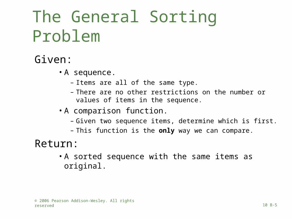
The General Sorting Problem

Given:• A sequence.

– Items are all of the same type.

– There are no other restrictions on the number or values of items in the sequence.

• A comparison function.– Given two sequence items, determine which is first.

– This function is the only way we can compare.

Return:• A sorted sequence with the same items as original.


Sorting

• There are many algorithms for sorting

• Each has different properties:– easy/hard to understand– fast/slow for large lists– fast/slow for short lists– fast in all cases/on average


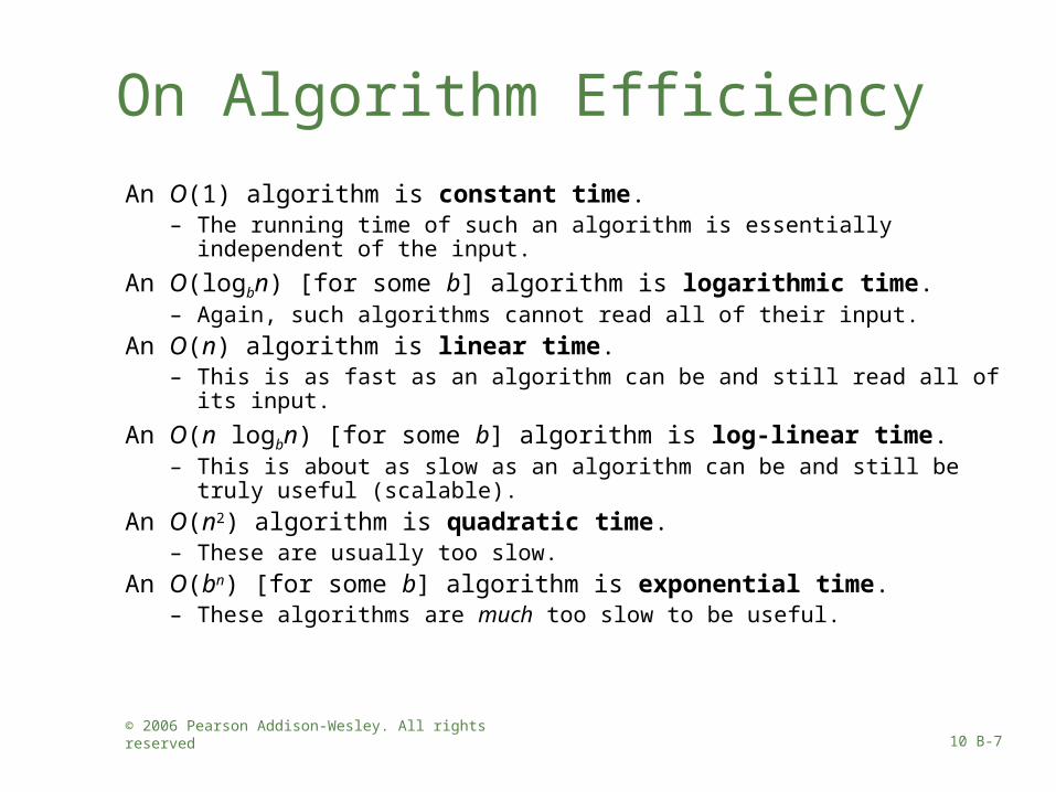
On Algorithm Efficiency

An O(1) algorithm is constant time.– The running time of such an algorithm is essentially independent of the input.

An O(logbn) [for some b] algorithm is logarithmic time.– Again, such algorithms cannot read all of their input.

An O(n) algorithm is linear time.– This is as fast as an algorithm can be and still read all of its input.

An O(n logbn) [for some b] algorithm is log-linear time.– This is about as slow as an algorithm can be and still be truly useful (scalable).

An O(n2) algorithm is quadratic time.– These are usually too slow.

An O(bn) [for some b] algorithm is exponential time.– These algorithms are much too slow to be useful.


Selection Sort

• Find the smallest item in the list

• Switch it with the first position

• Find the next smallest item

• Switch it with the second position

• Repeat until you reach the last element


Selection Sort: Example

17 8 75 23 14

Original list:

8 17 75 23 14

Smallest is 8:

8 14 75 23 17

Smallest is 14:

8 14 17 23 75

Smallest is 17:

8 14 17 23 75

Smallest is 23:

DONE!


Selection Search: Running Time

• Scan entire list (n steps)

• Scan rest of the list (n-1 steps)….

• Total steps:

n + (n -1) + (n-2) + … + 1

= n(n+1)/2 [Gauss]

= n2/2 +n/2

• So, selection sort is O(n2)


Selection Sort in Javapublic void selectionSort(int[] arr){

int i,j,min,temp;for(j=0; j < arr.length-1; j++){

min=j;for(i=j+1; i < arr.length; i++)

if(arr[i] < arr[min]) min=i;if(j!=min){

temp=arr[j];arr[j]=arr[min];arr[min]=temp;

}}


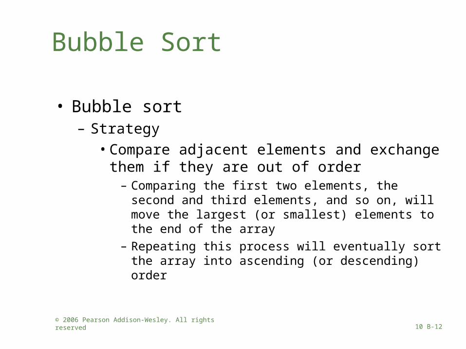
Bubble Sort

• Bubble sort– Strategy

• Compare adjacent elements and exchange them if they are out of order

– Comparing the first two elements, the second and third elements, and so on, will move the largest (or smallest) elements to the end of the array

– Repeating this process will eventually sort the array into ascending (or descending) order


Bubble Sort

Figure 10-5Figure 10-5The first two passes of a bubble sort of an array of five integers: a) pass 1;

b) pass 2


Bubble Sort

• Analysis– Worst case: O(n2)

– Best case: O(n2)

• Beyond Big-O: bubble sort generally performs worse than the other O(n2) sorts– ... you generally don’t see bubble sort outside a

university classroom


Insertion Sort

• Consider the first item to be a sorted sublist (of one item)

• Insert the second item into the sublist, shifting the first item as needed to make space

• Insert item into the sorted sublist (of two items) shifting as needed

• Repeat until all items have been inserted


Insertion Sort: Example

8 17 2 14 23

Original list:

8 17 2 14 23

Start with sorted list {8}:

8 17 2 14 23

Insert 17, nothing to shift:

2 8 17 14 23

Insert 2, shift the rest:

8 14 17 23 75

Insert 14, shift {17,23}:

8 14 17 23 75

Insert 75, nothing to shift:


Insertion Sort: Pseudocode

for pos from 1 to (n-1):

val = array[pos] // get element pos into place

i = pos – 1

while i >= 0 and array[i] > val:

array[i+1] = array[i]

i--

array[i+1] = val


Insertion Sort: Running Time

• Requires n-1 passes through the array– pass i must compare and shift up to i elements– total maximum number of comparisons/moves:

• 1 + 2 + … + n = n(n-1)/2

• So insertion sort is also O(n2)– not bad… but there are faster algorithms– it turns out insertion sort is generally faster than

other algorithms for “small” arrays (n<10??)


Insertion Sort in Java

public void insertionSort(int[] arr){

int i,k,temp;for(k=1; k < arr.length; k++){

temp=arr[k];i=k;while(i > 0 && temp < arr[i-1]){

arr[i]=arr[i-1];i--;

}arr[i]=temp;

}}


Selection and Insertion

• Same running time– Choice between is largely up to you

• Think about combining search/sort– Sorting list is O(n2)– Then binary search O(log n)– But just doing linear search is faster O(n)– Sorting first doesn’t pay off with these

algorithms


Mergesort

• Important divide-and-conquer sorting algorithms– Mergesort– Quicksort

• Mergesort– A recursive sorting algorithm– Gives the same performance, regardless of the initial

order of the array items


Merge Sort: Basics

• Idea:– Split list into two halves [looks familiar]– Recursively sort each half– “merge” the two halves into a single list


Merge Sort: Example

17 8 75 23 14 95 29 87 74 -1 -2 37 81

Split:

Recursively sort:

17 8 75 23 14 95 29 87 74 -1 -2 37 81

Original list:

8 14 17 23 29 75 95 -2 -1 37 74 81 87

Merge?


Example merge

-2 -1 8 14 17 23 29 37 74 75 81 87 95

• Must put the next-smallest element into the merged list at each point

• Each next-smallest could come from either list

8 14 17 23 29 75 95 -2 -1 37 74 81 87


Remarks

• Note that merging just requires checking the smallest element of each half– Just one comparison step– This is where the recursive call saves time

• We need to give a formal specification of the algorithm to really check running time


Merge Sort Algorithm

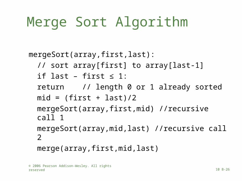
mergeSort(array,first,last):

// sort array[first] to array[last-1]

if last – first ≤ 1:

return // length 0 or 1 already sorted

mid = (first + last)/2

mergeSort(array,first,mid) //recursive call 1

mergeSort(array,mid,last) //recursive call 2

merge(array,first,mid,last)


Merge Algorithm (incorrect)

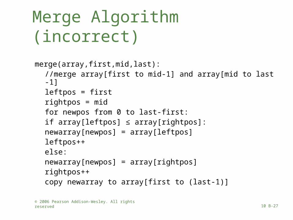
merge(array,first,mid,last)://merge array[first to mid-1] and array[mid to last -1]leftpos = firstrightpos = midfor newpos from 0 to last-first:

if array[leftpos] ≤ array[rightpos]:newarray[newpos] = array[leftpos]leftpos++

else:newarray[newpos] = array[rightpos]rightpos++

copy newarray to array[first to (last-1)]


Problem?

• The algorithm starts correctly, but has an error as it finishes

– Eventually one of the halves will empty

• Then the “if” will compare against ??

– the element past one of the halves… one of:

38 43 ??

?? 52

leftpos rightpos

leftpos rightpos


Solution

• Must prevent this: we can only look at the correct parts of the array

• So: compare only until we reach the end of one half

• Then, just copy the rest over


Merge Algorithm (1)

merge(array,first,mid,last)://merge array[first to mid-1] and array[mid to last -1]leftpos = firstrightpos = midnewpos = 0while leftpos<mid and rightpos≤last-1:

if array[leftpos] ≤ array[rightpos]:newarray[newpos] = array[leftpos]leftpos++; newpos++

else:newarray[newpos] = array[rightpos]rightpos++; newpos++

(continues)


Merge Algorithm (2)

merge(array,first,mid,last):

… //code from last slide

while leftpos<mid: // copy the rest left half (if any)

newarray[newpos] = array[leftpos]

leftpos++; newpos++

while rightpos≤last-1 // copy the rest of right half (if any)

newarray[newpos] = array[rightpos]

rightpos++; newpos++

copy newarray to array[first to (last-1)]


Example 1

10 20 40 50 30 40 60 70array:

3 4 5 6 7 8 9 10

10newarray:

0 1 2 3 4 5 6 7

leftpos:

rightpos:

newpos:

3 4 5 6

7 8 9 10 11

3 4 5 6 7 8210

merge(array,3,7,11):

compare loop fill

20 30 40 40 50 60 70

7


Example 2

50 60 70 80 10 20 30 40

array:

8 9 10 11 12 13 14 15

10newarray:

0 1 2 3 4 5 6 7

leftpos:

rightpos:

newpos:

8 9 10 11

12 13 14 15 16

3 4 5 6 7 8210

merge(array,8,12,16):

compare loop fill

20 30 40 50 60 70 80

12


Running Time

• What is the running time for merge sort?

• recursive calls * work per call?– yes, but overly simplified– work per call changes

• We know: the merge algorithm takes O(n) steps to merge a total of n elements


Merge Sort Recursive Calls

• Each level has a total of n elements

n elements

n/2 n/2

n/4 n/4 n/4 n/4

1 1 1 1 1 1


Merge Sort: Running Time

• Steps to merge each level: O(n)• Number of levels: O(log n)• Total time: O(n log n)

– Much faster than selection/insertion which both take O(n2)

• In general, no sorting algorithm can do better than O(n log n)– except maybe for restricted cases


In Place Sorting

• Merging requires extra storage

– an extra array with n elements

(can be re-used by all merges)

– insertion sort only requires a few storage variables

• An algorithm that uses at most O(1) extra storage is called “in-place”

– insertion sort/selection sort are both in-place

– merge sort is not


Mergesort - Summary

• Analysis– Worst case: O(n * log2n)– Average case: O(n * log2n)– Advantage

• It is an extremely efficient algorithm with respect to time

– Drawback• It requires a second array as large as the original

array


Quicksort• Quicksort

– A divide-and-conquer algorithm– Strategy

• Partition an array into items that are less than the pivot and those that are greater than or equal to the pivot

• Sort the left section• Sort the right section

Figure 10-12Figure 10-12

A partition about a pivot


Quicksort

• Using an invariant to develop a partition algorithm– Invariant for the partition algorithm

The items in region S1 are all less than the pivot, and those in S2 are all greater than or equal to the pivot


Invariant for the partition algorithm


Quicksort• Analysis

– Worst case• quicksort is O(n2) when the array is already sorted and the

smallest item is chosen as the pivot


A worst-case partitioning

with quicksort


Quicksort• Analysis

– Average case• quicksort is O(n * log2n) when S1 and S2 contain the same – or

nearly the same – number of items arranged at random


A average-case partitioning with

quicksort


Quicksort

• Analysis– quicksort is usually extremely fast in practice

– Even if the worst case occurs, quicksort’s performance is acceptable for moderately large arrays


Radix Sort

• Radix sort– Treats each data element as a character string

– Strategy

• Repeatedly organize the data into groups according to the ith character in each element


Radix Sort


A radix sort of eight integers


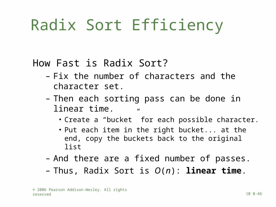
Radix Sort Efficiency

How Fast is Radix Sort?– Fix the number of characters and the character set.

– Then each sorting pass can be done in linear time.• Create a “bucket” for each possible character.

• Put each item in the right bucket... at the end, copy the buckets back to the original list

– And there are a fixed number of passes.

– Thus, Radix Sort is O(n): linear time.



How is this possible?– Radix Sort places a list of values in order. However, it

does not solve the General Sorting Problem.• In the General Sorting Problem, the only way we can get

information about our data is by applying a given comparison function to two items.

• Radix Sort does not fit within these restrictions.

– O(n log n) is best possible for a general sorting algorithm... but Radix is not general



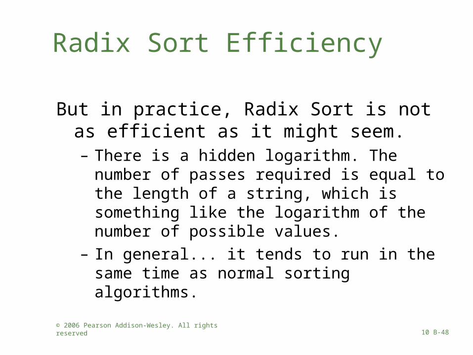
But in practice, Radix Sort is not as efficient as it might seem.– There is a hidden logarithm. The number of passes

required is equal to the length of a string, which is something like the logarithm of the number of possible values.

– In general... it tends to run in the same time as normal sorting algorithms.


However, in certain special cases (e.g., big lists of small numbers) Radix Sort can be a useful technique.

Ten million records to sort by ZIP code?

Use Radix Sort.


A Comparison of Sorting Algorithms


Approximate growth rates of time required for eight sorting algorithms


Summary• Worst-case and average-case analyses

– Worst-case analysis considers the maximum amount of work an algorithm requires on a problem of a given size

– Average-case analysis considers the expected amount of work an algorithm requires on a problem of a given size

• Order-of-magnitude analysis can be used to choose an implementation for an abstract data type

• Selection sort, bubble sort, and insertion sort are all O(n2) algorithms

• Quicksort and mergesort are two very efficient sorting algorithms


Exercise

• In the discussion of selection sort, we ignored operations that control loops or manipulate array indices. Revise the analysis to account for all operations – and show that the algorithm is still O(n2).


Solution

• Any operations outside of loops contribute a constant amount of time and would not affect the overall behavior of the selection sort for a large n.

Documents

© 2006 Pearson Addison-Wesley. All rights reserved10 B-1 Chapter 10 Sorting