© 2002 Thomson / South-Western Slide 5-1 Chapter 5 Discrete Probability Distributions

© 2002 Thomson / South-Western Slide 5-1

Chapter 5

Discrete Probability

Distributions


Learning ObjectivesLearning Objectives

• Distinguish between discrete random variables and continuous random variables.

• Identify the type of statistical experiments that can be described by the binomial distribution, and know how to work such problems.


Learning Objectives, continuedLearning Objectives, continued

• Decide when to use the Poisson distribution in analyzing statistical experiments, and know how to work such problems.

• Decide when to use the hypergeometric distribution, and know how to work such problems.


Discrete vs Continuous DistributionsDiscrete vs Continuous Distributions

• Random Variable -- a variable which contains the outcomes of a chance experiment

• Discrete Random Variable -- the set of all possible values is at most a finite or a countable infinite number of possible values

• Continuous Random Variable -- takes on values at every point over a given interval


Some Special DistributionsSome Special Distributions

• Discrete distributions are constructed from discrete ransom variables.

• The binomial, Poisson, and hypergeometric distributions are discrete distributions

• Continuous distributions are based on continuous random variables.

• The normal, uniform, exponential, t, chi-square, and F distributions are continuous distributions


Binomial Distribution

A widely known discrete distribution constructed by determining the probabilities of X successes in n trials.


Assumptions of the Binomial DistributionAssumptions of the Binomial Distribution

• The experiment involves n identical trials• Each trial has only two possible outcomes:

success and failure• Each trial is independent of the previous

trials• The terms p and q remain constant

throughout the experiment–p is the probability of a success on any one trial –q = (1-p) is the probability of a failure on any one

trial


Assumptions of the Binomial Distribution, continued

• In the n trials X is the number of successes possible where X is a whole number between 0 and n.

• Applications– Sampling with replacement – Sampling without replacement causes p

to change but if the sample size n < 5% N, the independence assumption is not a great concern.


Binomial Distribution: DevelopmentBinomial Distribution: Development

• Experiment: randomly select, with replacement, two families from the residents of the four-family town

• Success is ‘Children in Household:’ p = 0.75

• Failure is ‘No Children in Household:’ q = 1- p = 0.25

• X is the number of families in the sample with ‘Children in Household’


Binomial Distribution: Development continued (2)

Family Children in Household

Number of Automobiles

ABCD

YesYesNo

Yes

3212

Listing of Sample Space

(A,B), (A,C), (A,D), (D,D),(B,A), (B,B), (B,C), (B,D),(C,A), (C,B), (C,C), (C,D),(D,A), (D,B), (D,C), (D,D)




• Families A, B, and D have children in the household; family C does not

• Success is ‘Children in Household:’ p = 0.75

• Failure is ‘No Children in Household:’ q = 1- p = 0.25

• X is the number of families in the sample with ‘Children in Household’

(A,B), (A,C), (A,D), (D,D),(B,A), (B,B), (B,C), (B,D),(C,A), (C,B), (C,C), (C,D),(D,A), (D,B), (D,C), (D,D)

Listing of Sample Space

2122221211012212

X

1/161/161/161/161/161/161/161/161/161/161/161/161/161/161/161/16

P(outcome)




(A,B),(A,C),(A,D),(D,D),(B,A),(B,B),(B,C),(B,D),(C,A),(C,B),(C,C),(C,D),(D,A),(D,B),(D,C),(D,D)

Listing ofSampleSpace

2122221211012212

X

1/161/161/161/161/161/161/161/161/161/161/161/161/161/161/161/16

P(outcome) X

012

1/166/169/16

1

P(X)

P Xn

X n X

x n xp q( )!

! !

P X( )!

!.. .

02

0! 2 00 0625

1

160 2 075 25

P X( )!

! !.. .

12

1 2 10 375

3

161 2 175 25

P X( )!

! !.. .

22

2 2 20 5625

9

162 2 275 25




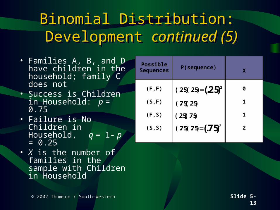
• Families A, B, and D have children in the household; family C does not

• Success is Children in Household: p = 0.75

• Failure is No Children in Household, q = 1- p = 0.25

• X is the number of families in the sample with Children in Household

XPossible

Sequences

0

1

1

2

(F,F)

(S,F)

(F,S)

(S,S)

P(sequence)

(. )(. ) (. )25 25 225

(. )(. )25 75

(. )(. )75 25

(. )(. ) (. )75 75 275




XPossible

Sequences

0

1

1

2

(F,F)

(S,F)

(F,S)

(S,S)

P(sequence)

(. )(. ) (. )25 25 225

(. )(. )25 75

(. )(. )75 25

(. )(. ) (. )75 75 275

X

0

1

2

P(X)

(. )(. )25 752 =0.375

(. )(. ) (. )75 75 275 =0.5625

(. )(. ) (. )25 25 225 =0.0625

P Xn

X n X

x n xp q( )!

! !

P X( )!

!.. .

02

0! 2 00 0625

0 2 075 25 P X( )!

! !.. .

12

1 2 10 375

1 2 175 25

P X( )!

! !.. .

22

2 2 205625

2 2 275 25


Binomial Distribution: Demonstration Problem 5.2

Binomial Distribution: Demonstration Problem 5.2

n

p

q

P X P X P X P X

20

06

94

2 0 1 2

2901 3703 2246 8850

.

.

( ) ( ) ( ) ( )

. . . .

P X( ))!

( )( )(. ) .. .

020!

0!(20 01 1 2901 2901

0 20 0

06 94

P X( )!( )!

( )(. )(. ) .. .

120!

1 20 120 06 3086 3703

1 20 1

06 94

P X( )!( )!

( )(. )(. ) .. .

220!

2 20 2190 0036 3283 2246

2 20 2

06 94


Binomial TableBinomial Table

n = 20 PROBABILITY

X 0.1 0.2 0.3 0.4 0.5 0.6 0.7 0.8 0.9

0 0.122 0.012 0.001 0.000 0.000 0.000 0.000 0.000 0.0001 0.270 0.058 0.007 0.000 0.000 0.000 0.000 0.000 0.0002 0.285 0.137 0.028 0.003 0.000 0.000 0.000 0.000 0.0003 0.190 0.205 0.072 0.012 0.001 0.000 0.000 0.000 0.0004 0.090 0.218 0.130 0.035 0.005 0.000 0.000 0.000 0.0005 0.032 0.175 0.179 0.075 0.015 0.001 0.000 0.000 0.0006 0.009 0.109 0.192 0.124 0.037 0.005 0.000 0.000 0.0007 0.002 0.055 0.164 0.166 0.074 0.015 0.001 0.000 0.0008 0.000 0.022 0.114 0.180 0.120 0.035 0.004 0.000 0.0009 0.000 0.007 0.065 0.160 0.160 0.071 0.012 0.000 0.000

10 0.000 0.002 0.031 0.117 0.176 0.117 0.031 0.002 0.00011 0.000 0.000 0.012 0.071 0.160 0.160 0.065 0.007 0.00012 0.000 0.000 0.004 0.035 0.120 0.180 0.114 0.022 0.00013 0.000 0.000 0.001 0.015 0.074 0.166 0.164 0.055 0.00214 0.000 0.000 0.000 0.005 0.037 0.124 0.192 0.109 0.00915 0.000 0.000 0.000 0.001 0.015 0.075 0.179 0.175 0.03216 0.000 0.000 0.000 0.000 0.005 0.035 0.130 0.218 0.09017 0.000 0.000 0.000 0.000 0.001 0.012 0.072 0.205 0.19018 0.000 0.000 0.000 0.000 0.000 0.003 0.028 0.137 0.28519 0.000 0.000 0.000 0.000 0.000 0.000 0.007 0.058 0.27020 0.000 0.000 0.000 0.000 0.000 0.000 0.001 0.012 0.122


Using the Binomial Table: Demonstration Problem 5.3

Using the Binomial Table: Demonstration Problem 5.3

n = 20 PROBABILITY

X 0.1 0.2 0.3 0.4

0 0.122 0.012 0.001 0.0001 0.270 0.058 0.007 0.0002 0.285 0.137 0.028 0.0033 0.190 0.205 0.072 0.0124 0.090 0.218 0.130 0.0355 0.032 0.175 0.179 0.0756 0.009 0.109 0.192 0.1247 0.002 0.055 0.164 0.1668 0.000 0.022 0.114 0.1809 0.000 0.007 0.065 0.160

10 0.000 0.002 0.031 0.11711 0.000 0.000 0.012 0.07112 0.000 0.000 0.004 0.03513 0.000 0.000 0.001 0.01514 0.000 0.000 0.000 0.00515 0.000 0.000 0.000 0.00116 0.000 0.000 0.000 0.00017 0.000 0.000 0.000 0.00018 0.000 0.000 0.000 0.00019 0.000 0.000 0.000 0.00020 0.000 0.000 0.000 0.000

n

p

P X C

20

40

10 0117120 1010 10

40 60

.

( ) .. .


Binomial DistributionBinomial Distribution

• Probability function

• Mean value

• Variance and standard deviation

P Xn

X n XX n

X n Xp q( )!

! !

for 0

n p2

2

n p q

n p q


Graphs of Selected Binomial DistributionsGraphs of Selected

Binomial Distributionsn = 4 PROBABILITY

X 0.1 0.5 0.90 0.656 0.063 0.0001 0.292 0.250 0.0042 0.049 0.375 0.0493 0.004 0.250 0.2924 0.000 0.063 0.656

P = 0.1

0.0000.1000.2000.3000.4000.5000.6000.7000.8000.9001.000

0 1 2 3 4X

P(X

)

P = 0.5

0.0000.1000.2000.3000.4000.5000.6000.7000.8000.9001.000

0 1 2 3 4X

P(X

)

P = 0.9

0.0000.1000.2000.3000.4000.5000.6000.7000.8000.9001.000

0 1 2 3 4X

P(X

)


Assumptions of the Poisson DistributionAssumptions of the Poisson Distribution

• Describes discrete occurrences over a continuum or interval

• A discrete distribution• Describes rare events• Each occurrence is independent any other

occurrences.• The number of occurrences in each

interval can vary from zero to infinity.• The expected number of occurrences must

hold constant throughout the experiment.


Poisson DistributionPoisson Distribution

• Probability function

P XX

X

where

long run average

e

Xe( )!

, , , ,...

:

. ...

for

(the base of natural logarithms )

0 1 2 3

2 718282

Mean valueMean value

Standard deviationStandard deviation VarianceVariance


Poisson Distribution: Demonstration Problem 5.7

Poisson Distribution: Demonstration Problem 5.7

3 2

6 4

1010

0 05286 4

.

!

!.

.

customers / 4 minutes

X = 10 customers / 8 minutes

Adjusted

= . customers / 8 minutes

P(X) =

( = ) =

X

106.4

e

eX

P X

3 2

6 4

66

0 15866 4

.

!

!.

.

customers / 4 minutes

X = 6 customers / 8 minutes

Adjusted

= . customers / 8 minutes

P(X) =

( = ) =

X

66.4

e

eX

P X


Poisson Distribution: Probability TablePoisson Distribution: Probability Table

X 0.5 1.5 1.6 3.0 3.2 6.4 6.5 7.0 8.00 0.6065 0.2231 0.2019 0.0498 0.0408 0.0017 0.0015 0.0009 0.00031 0.3033 0.3347 0.3230 0.1494 0.1304 0.0106 0.0098 0.0064 0.00272 0.0758 0.2510 0.2584 0.2240 0.2087 0.0340 0.0318 0.0223 0.01073 0.0126 0.1255 0.1378 0.2240 0.2226 0.0726 0.0688 0.0521 0.02864 0.0016 0.0471 0.0551 0.1680 0.1781 0.1162 0.1118 0.0912 0.05735 0.0002 0.0141 0.0176 0.1008 0.1140 0.1487 0.1454 0.1277 0.09166 0.0000 0.0035 0.0047 0.0504 0.0608 0.1586 0.1575 0.1490 0.12217 0.0000 0.0008 0.0011 0.0216 0.0278 0.1450 0.1462 0.1490 0.13968 0.0000 0.0001 0.0002 0.0081 0.0111 0.1160 0.1188 0.1304 0.13969 0.0000 0.0000 0.0000 0.0027 0.0040 0.0825 0.0858 0.1014 0.1241

10 0.0000 0.0000 0.0000 0.0008 0.0013 0.0528 0.0558 0.0710 0.099311 0.0000 0.0000 0.0000 0.0002 0.0004 0.0307 0.0330 0.0452 0.072212 0.0000 0.0000 0.0000 0.0001 0.0001 0.0164 0.0179 0.0263 0.048113 0.0000 0.0000 0.0000 0.0000 0.0000 0.0081 0.0089 0.0142 0.029614 0.0000 0.0000 0.0000 0.0000 0.0000 0.0037 0.0041 0.0071 0.016915 0.0000 0.0000 0.0000 0.0000 0.0000 0.0016 0.0018 0.0033 0.009016 0.0000 0.0000 0.0000 0.0000 0.0000 0.0006 0.0007 0.0014 0.004517 0.0000 0.0000 0.0000 0.0000 0.0000 0.0002 0.0003 0.0006 0.002118 0.0000 0.0000 0.0000 0.0000 0.0000 0.0001 0.0001 0.0002 0.0009


Using the Poisson Tables:Demonstration Problem 5.7Using the Poisson Tables:Demonstration Problem 5.7

X 0.5 1.5 1.6 3.00 0.6065 0.2231 0.2019 0.04981 0.3033 0.3347 0.3230 0.14942 0.0758 0.2510 0.2584 0.22403 0.0126 0.1255 0.1378 0.22404 0.0016 0.0471 0.0551 0.16805 0.0002 0.0141 0.0176 0.10086 0.0000 0.0035 0.0047 0.05047 0.0000 0.0008 0.0011 0.02168 0.0000 0.0001 0.0002 0.00819 0.0000 0.0000 0.0000 0.002710 0.0000 0.0000 0.0000 0.000811 0.0000 0.0000 0.0000 0.000212 0.0000 0.0000 0.0000 0.0001

1 6

4 0 0551

.

( ) .P X


Poisson Distribution: GraphsPoisson Distribution: Graphs

0.00

0.05

0.10

0.15

0.20

0.25

0.30

0.35

0 1 2 3 4 5 6 7 8

1 6.

0.00

0.02

0.04

0.06

0.08

0.10

0.12

0.14

0.16

0 2 4 6 8 10 12 14 16

6 5.


Assumptions of the Hypergeometric Distribution

Assumptions of the Hypergeometric Distribution

• It is a discrete distribution.• Sampling is done without replacement. • The number of objects in the population, N, is

finite and known.• Each trial has exactly two possible outcomes:

success and failure.• Trials are not independent• X is the number of successes in the n trials


Hypergeometric DistributionHypergeometric Distribution

• Probability function– N is population size– n is sample size– A is number of successes in

population– x is number of successes in sample

A nN

2

2

2

1

A N A n N n

NN( ) ( )

( )

P x

C C

C

A x N A n x

N n( )

• Mean value

• Variance and standard deviation


Hypergeometric Distribution:Probability Computations

Hypergeometric Distribution:Probability Computations

N = 24

X = 8

n = 5

x

0 0.1028

1 0.3426

2 0.3689

3 0.1581

4 0.0264

5 0.0013

P(x)

P xC C

CC C

C

A x N A n x

N n( )

,

.

3

56 120

42 504

1581

8 3 24 8 5 3

24 5


Hypergeometric Distribution: GraphHypergeometric Distribution: Graph

N = 24

X = 8

n = 5

x

0 0.1028

1 0.3426

2 0.3689

3 0.1581

4 0.0264

5 0.0013

P(x)

0.00

0.05

0.10

0.15

0.20

0.25

0.30

0.35

0.40

0 1 2 3 4 5


Hypergeometric Distributio:Demonstration Problem 5.8Hypergeometric Distributio:Demonstration Problem 5.8

X P(X)0 0.02451 0.22062 0.48533 0.2696

N = 18n = 3A = 12

P x P x P x P x

C C

C

C C

C

C C

C

( ) ( ) ( ) ( )

. . .

.

1 1 2 3

2206 4853 2696

9755

12 1 18 12 3 1

18 3

12 2 18 12 3 2

18 3

12 3 18 12 3 3

18 3


The Hypergeometric Distribution and the Binomial Distribution

• Because the hypergeometric distribution is described by three parameters N, A and n, it is practically impossible to create tables for easy use.

• The binomial (which has tables) is an acceptable approximation, if n < 5% N. Otherwise it is not.

• Excel has eliminated all the tedious calculations and allows the user to compute the exact probabilities for the hypergeometric.

Documents

© 2002 Thomson / South-Western Slide 5-1 Chapter 5 Discrete Probability Distributions