arX

iv:1

205.

4707

v1 [

quan

t-ph

] 2

1 M

ay 2

012

Zitterbewegung of Klein-Gordon particles and its simulation by classical systems

Tomasz M. Rusin1∗ and Wlodek Zawadzki21Orange Customer Service sp. z o. o., ul. Twarda 18, 00-105 Warsaw, Poland

2 Institute of Physics, Polish Academy of Sciences, Al. Lotnikow 32/46, 02-688 Warsaw, Poland(Dated: May 22, 2012)

The Klein-Gordon equation is used to calculate the Zitterbewegung (ZB, trembling motion) ofspin-zero particles in absence of fields and in the presence of an external magnetic field. BothHamiltonian and wave formalisms are employed to describe ZB and their results are compared. Itis demonstrated that, if one uses wave packets to represent particles, the ZB motion has a decayingbehavior. It is also shown that the trembling motion is caused by an interference of two sub-packets composed of positive and negative energy states which propagate with different velocities.In the presence of a magnetic field the quantization of energy spectrum results in many interbandfrequencies contributing to ZB oscillations and the motion follows a collapse-revival pattern. In thelimit of non-relativistic velocities the interband ZB components vanish and the motion is reduced tocyclotron oscillations. The exact dynamics of a charged Klein-Gordon particle in the presence of amagnetic field is described on an operator level. The trembling motion of a KG particle in absenceof fields is simulated using a classical model proposed by Morse and Feshbach – it is shown that avariance of a Gaussian wave packet exhibits ZB oscillations.

PACS numbers: 03.65.Pm, 11.40.-q, 03.65.-w

I. INTRODUCTION

The phenomenon of Zitterbewegung (ZB, tremblingmotion) goes back to Schrodinger who proposed it in 1930for free relativistic electrons in a vacuum [1]. Schrodingerobserved that, due to non-commutativity of the velocityoperators with the Dirac Hamiltonian, relativistic elec-trons experience a trembling motion in absence of ex-ternal fields. It was later recognized that ZB is due toan interference of electron states with positive and neg-ative electron energies. A very high frequency of ZBin a vacuum, corresponding to ~ωZ = 2mec

2, and itsvery small amplitude on the order of the Compton wave-length λc = ~/mec ≃ 3.86×10−3 A made it impossible toobserve this effect in its original form with the currentlyavailable experimental methods. However, in a recentwork Gerritsma et al. [2] simulated the 1+1 Dirac equa-tion and the resulting Zitterbewegung with the use oftrapped ions excited by laser beams. The important ad-vantage of this method is that one can simulate also thebasic parameters of the Dirac equation and tailor theirdesired values. The result of Gerritsma et al. allows oneto expect that observable effects for relativistic particlesin a vacuum can be convincingly reproduced with more“user friendly” parameters. In general, there has beenrecently a revival of interest in the relativistic-type equa-tions related to “the rise of graphene” [3], topologicalinsulators and similar systems in narrow-gap semicon-ductors [4].

The purpose of our paper is to describe the phe-nomenon of Zitterbewegung for charged Klein-Gordon(KG) spin-zero particles in absence of fields and in the

∗Electronic address: Tomasz.Rusin@orange.com

presence of a magnetic field [5–7]. The Zitterbewegungof KG particles in absence of fields was described be-fore, see [8–10]. However, in our treatment we introducea number of additional elements. First, we describe theparticles by wave packets and show that this feature leadsto a transient character of the resulting ZB motion. Sec-ond, we use both the Hamiltonian and wave forms ofKlein-Gordon equation (KGE) and show the equivalenceof the two approaches. Third, we point out that ZBis a result of interference between positive and negativeenergy sub-packets propagating with different velocities.Fourth, we simulate classically the ZB motion using asimple mechanical system proposed by Morse and Fesh-bach [11]. Still, our main objective is to consider in detailthe dynamics of a charged KG particle in the presenceof an external uniform magnetic field and describe thephenomenon of ZB in this situation. To the best of ourknowledge this problem has not been treated before.

The one-particle Klein-Gordon equation for spin-zeroparticles leads to some well known difficulties [10, 12].The KG equation involves second time derivative, theprobability density is not positively definite, there areproblems with the position operator or vanishing squareof the velocity operator. For this reason in the presentwork we calculate ZB of average current which has welldefined meaning in the theory of KG equation. Forcharged particles the average current is proportional toaverage particle velocity, so in our work we calculate oneof these two quantities. In previous treatments of ZBfor Dirac equation, simulation by trapped ions or solid-state systems, the authors usually calculated ZB of theposition operator.

In our considerations we encounter another interestinganomaly of KG equation, namely, that particle velocitiescan exceed the speed of light for sufficiently large mo-menta. In other words it appears that, in contrast to

2

the Dirac equation for electrons, KGE does not possesan automatic “safety brake” for velocities to keep thembelow c. To our knowledge this feature has not beenremarked before, so we mention it throughout our work.Our paper is organized as follows. In Section II we cal-

culate ZB of a wave packet using the Hamiltonian formal-ism, in Section III we obtain similar results with the useof KG waves and discuss explicitly physical backgroundfor the transient behavior of ZB motion. Section IV con-tains a description of ZB for a charged KG particle in amagnetic field. In Section V we simulate classically theZB phenomenon using a system proposed by Morse andFeshbach. In Section VI we discuss our results, the pa-per is concluded by a summary. Appendix A contains aderivation of particle dynamics in the presence of a mag-netic field, Appendix B discusses the problem of highparticle velocities, in Appendices C and D we give somemathematical details.

II. ZITTERBEWEGUNG IN VACUUM

We begin by considering a Klein-Gordon particle inabsence of external fields. The Klein-Gordon equation inthe Hamiltonian form is [13]

i~∂Ψ

∂t= HΨ. (1)

Here the Hamiltonian is

H =τ3 + iτ22m

p2 + τ3mc2, (2)

where m is particle mass, p is particle momentumand τj (j = 1, 2, 3) are the Pauli matrices σj , respec-tively. The wave function Ψ is a two-component vector

Ψ =

(

ϕχ

)

. (3)

In the Hamiltonian form one can introduce the Heisen-berg picture [13]. The z-th component of the time-dependent velocity operator is

vz(t) = eiHt/~vz(0)e−iHt/~, (4)

where vz(0) = ∂H/∂pz. In this representation vz(t) is

a 2 × 2 matrix operator. Expanding eiHt/~ = 1 + Ht +(1/2!)H2 + . . . and noting that H2 = E2, where the en-ergy is E = ±cp0 with

p0 = +√

m2c2 + p2, (5)

we obtain

eiHt/~ = cos(Et/~) +iH

Esin(Et/~). (6)

The velocity operator in Eq. (4) is a product of threematrices. Its (1, 1) component is

(vz)11(t) =pzm

+p2pz2mp20

[cos(2Et/~)− 1] . (7)

The remaining elements of vz(t) are calculated similarly.The vx and vy components of the velocity operator areobtained from vz(t) by the replacement pz → px, py, re-spectively. In the non-relativistic limit p≪ mc we obtainin Eq. (7) the classical motion (vz)11(t) ≃ pz/m. In ab-sence of external fields pi are good quantum numbers.We introduce p = ~k and q = λck, where the effectiveCompton wavelength is λc = ~/mc. Also, we introducea useful frequency ω0 = (mc2)/~. Both λc and ω0 referto particles of mass m. In the above notation Eq. (7)becomes

(vz)11(t) = cqz +c

2

q2qz(1 + q2)

[

cos(2ω0t√

1 + q2)− 1]

.

(8)

The first term in Eq. (8) corresponds to the classi-cal motion of a particle while the second term describesrapid oscillations of the velocity. The velocity oscillatesfrom vmax = cqz to vmin = cqz/(1 + q2). Since the max-imum velocity of the particle is c, there must be |q| ≤ 1.We notice that, in principle, Eq. (8) admits velocitiesabove the speed of light. We discuss this issue in moredetail in Appendix B. The frequency of oscillations variesfrom ω = 2ω0 for low q to ω = 2

√2ω0 for |q| = 1. The

velocity oscillations taking place in absence of externalfields are called Zitterbewegung.

Integrating (vz)11(t) in Eq. (8) over time we have

z11(t) = z11(0) + cqzt−c

2

q2qz1 + q2

t+

λc4

q2qz(1 + q2)3/2

sin(2ω0t√

1 + q2). (9)

The amplitude of ZB oscillations of the position operatoris on the order of λc. The operator z11(t) is obtainedin the formal way, physical limitations to the positionoperator will be discussed below.

In order to obtain physical observables one needs to av-erage the operator quantities over the wave packet. Theaverage velocity 〈vz(t)〉 of the wave packet |W 〉 is

〈vz(t)〉 = 〈W |τ3vz(t)|W 〉 =∑

pp′

〈W |p〉〈p|τ3vz(t)|p′〉〈p′|W 〉.

(10)For KGE in the Hamiltonian form the matrix elementsof operators include an additional τ3 factor [13]. We takethe wave packet in the form of a two-component vec-tor 〈r|W 〉 = (1, 0)T 〈r|w〉 with one non-vanishing compo-nent. Here 〈r|w〉 ≡ w(r) is a Gaussian function with anonzero momentum ~k0

w(r) =1

(d√π)3/2

exp[−r2/(2d2) + ik0r]. (11)

There is w(k) =∫

e−ikr/~w(r)d3r and we have

〈k|w〉 = (2d√π)3/2 exp[−d2(k − k0)

2/2]. (12)

3

1 2 3

0.2

0.4

0.6

0.8

d=0.5λc

v/

c

2 4 6 8

0.4

0.5

0.6

0.7

0.8 t/tc

d=2λcv

/c

0 4 8 12 16

0.5

0.6

0.7

0.8 t/tc

t/tc

d=5λc

v/

c

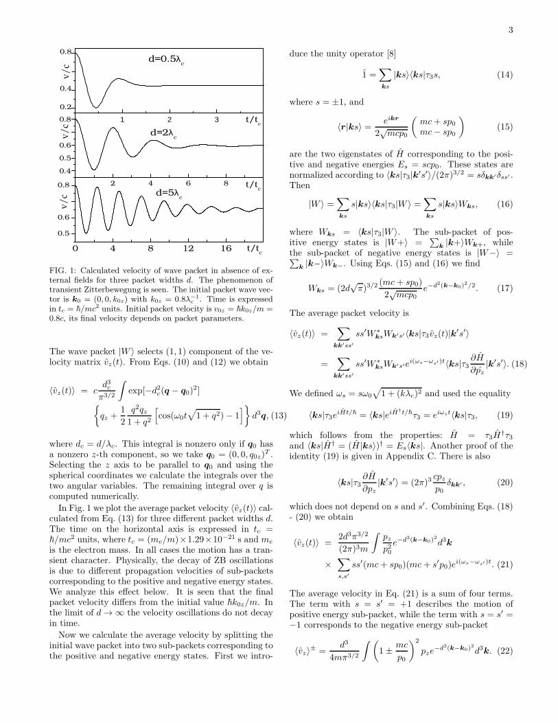
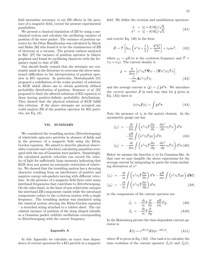
FIG. 1: Calculated velocity of wave packet in absence of ex-ternal fields for three packet widths d. The phenomenon oftransient Zitterbewegung is seen. The initial packet wave vec-tor is k0 = (0, 0, k0z) with k0z = 0.8λ−1

c . Time is expressedin tc = ~/mc2 units. Initial packet velocity is v0z = ~k0z/m =0.8c, its final velocity depends on packet parameters.

The wave packet |W 〉 selects (1, 1) component of the ve-locity matrix vz(t). From Eqs. (10) and (12) we obtain

〈vz(t)〉 = cd3cπ3/2

∫

exp[−d2c(q − q0)2]

qz +1

2

q2qz1 + q2

[

cos(ω0t√

1 + q2)− 1]

d3q, (13)

where dc = d/λc. This integral is nonzero only if q0 hasa nonzero z-th component, so we take q0 = (0, 0, q0z)

T .Selecting the z axis to be parallel to q0 and using thespherical coordinates we calculate the integrals over thetwo angular variables. The remaining integral over q iscomputed numerically.

In Fig. 1 we plot the average packet velocity 〈vz(t)〉 cal-culated from Eq. (13) for three different packet widths d.The time on the horizontal axis is expressed in tc =~/mc2 units, where tc = (me/m)×1.29×10−21 s and me

is the electron mass. In all cases the motion has a tran-sient character. Physically, the decay of ZB oscillationsis due to different propagation velocities of sub-packetscorresponding to the positive and negative energy states.We analyze this effect below. It is seen that the finalpacket velocity differs from the initial value ~k0z/m. Inthe limit of d→∞ the velocity oscillations do not decayin time.

Now we calculate the average velocity by splitting theinitial wave packet into two sub-packets corresponding tothe positive and negative energy states. First we intro-

duce the unity operator [8]

1 =∑

ks

|ks〉〈ks|τ3s, (14)

where s = ±1, and

〈r|ks〉 = eikr

2√mcp0

(

mc+ sp0mc− sp0

)

(15)

are the two eigenstates of H corresponding to the posi-tive and negative energies Es = scp0. These states arenormalized according to 〈ks|τ3|k′s′〉/(2π)3/2 = sδkk′δss′ .Then

|W 〉 =∑

ks

s|ks〉〈ks|τ3|W 〉 =∑

ks

s|ks〉Wks, (16)

where Wks = 〈ks|τ3|W 〉. The sub-packet of pos-itive energy states is |W+〉 =

∑

k |k+〉Wk+, whilethe sub-packet of negative energy states is |W−〉 =∑

k |k−〉Wk−. Using Eqs. (15) and (16) we find

Wks = (2d√π)3/2

(mc+ sp0)

2√mcp0

e−d2(k−k0)2/2. (17)

The average packet velocity is

〈vz(t)〉 =∑

kk′ss′

ss′W ∗ksWk′s′〈ks|τ3vz(t)|k′s′〉

=∑

kk′ss′

ss′W ∗ksWk′s′e

i(ωs−ωs′)t〈ks|τ3∂H

∂pz|k′s′〉. (18)

We defined ωs = sω0

√

1 + (kλc)2 and used the equality

〈ks|τ3eiHt/~ = 〈ks|eiH†t/~τ3 = eiωst〈ks|τ3, (19)

which follows from the properties: H = τ3H†τ3

and 〈ks|H† = (H |ks〉)† = Es〈ks|. Another proof of theidentity (19) is given in Appendix C. There is also

〈ks|τ3∂H

∂pz|k′s′〉 = (2π)3

cpzp0δkk′ , (20)

which does not depend on s and s′. Combining Eqs. (18)- (20) we obtain

〈vz(t)〉 =2d3π3/2

(2π)3m

∫

pzp20e−d2(k−k0)

2

d3k

×∑

s,s′

ss′(mc+ sp0)(mc+ s′p0)ei(ωs−ωs′)t. (21)

The average velocity in Eq. (21) is a sum of four terms.The term with s = s′ = +1 describes the motion ofpositive energy sub-packet, while the term with s = s′ =−1 corresponds to the negative energy sub-packet

〈vz〉± =d3

4mπ3/2

∫(

1± mc

p0

)2

pze−d2(k−k0)

2

d3k. (22)

4

Thus the two sub-packets move with different velocities.Their relative velocity is

〈vz〉rel =cd3

π3/2

∫

pzp0e−d2(k−k0)

2

d3k. (23)

Two terms in Eq. (21) with s 6= s′, corresponding to aninterference of the two packets, give rise to an oscillatoryterm

〈vz(t)〉osc =d3

4mπ3/2

∫(

1− m2c2

p20

)

pz

× cos(2ωkt)e−d2(k−k0)

2

d3k, (24)

where ωk =√

1 + (kλc)2. According to the Riemann-Lesbegues theorem this term has a transient charac-ter [14]. Performing integrations in Eqs. (22) and (24), weobtain again Eq. (13). Thus we showed that the ZB oscil-lations arise from the interference of positive and negativeenergy states. After a certain time the two sub-packetsare sufficiently far away from each other and the overlapbetween them vanishes, which results in the disappear-ance of ZB oscillations. This explains the behavior ofvelocity shown in Fig. 1.To evaluate the decay of ZB oscillations, we estimate

the time after which the two sub-packets will be sep-arated from each other by the distance 2d. Assumingthat k0λc ≃ 1, the relative velocity between the twosub-packets is 〈vz〉rel ≃ c(k0λc). The time interval afterwhich the distance between the sub-packets exceeds 2d is

td ≃2d

ck0λc. (25)

It is seen in Fig. 1 that the ZB oscillations nearly disap-pear after td. For example there is td = 5tc for d = 2λc.Since the ZB frequency is 2ω0 = 2mc2/~, a number ofnon-vanishing oscillations is approximately

Nosc ≃2ω0td2π

=2

π

(

d

λc

)(

1

k0λc

)

. (26)

The above estimation correctly evaluates the number ofZB oscillations seen in Fig. 1. The optimal conditions foran appearance of ZB are: wide packets and small valuesof |k0|. On the other hand, for too small values of |k0|one of the two sub-packets disappears, see Eq. (22), whichreduces amplitude of ZB oscillations.

III. WAVE FORM OF KGE

Now we intend to demonstrate a relation between theZB oscillations of the average packet velocity calculatedabove with the use of the Hamiltonian form of KGE andan average current obtained from the wave form of KGE.In absence of external fields the Klein-Gordon equationhas the wave equation form

1

c2∂2

∂t2φ(x) −∇

2φ(x) +m2c2

~2φ(x) = 0, (27)

where x = (ct, r) is the position four-vector [10]. Thesolution of this equation is

φ(x) =1

(2π)3

∫ √

mc

p0

[

a(k)e−ik·x + b∗(k)eik·x]

d3k,

(28)

where k = (ωk/c,k), ωk = ω0

√

1 + (kλc)2,and a(k), b∗(k) are complex coefficients. Function φ isnormalized to

i~

2mc2

∫[

φ∗∂ψ

∂t−(

∂φ∗

∂t

)

ψ

]

d3r = Q, (29)

whereQ = ±1 for charged particles andQ = 0 for neutralparticles. In the following we select Q = +1, which leadsto

∫

d3k [a∗(k)a(k)− b∗(k)b(k)] = 1. (30)

To determine the coefficients a(k) and b∗(k) we need twoboundary conditions for φ and ∂φ/∂t at x = (0, r). Hav-ing specified a(k) and b∗(k) one can calculate the currentdensity j(x)

j(x) =~

2im[φ∗(∇φ)− (∇φ∗)φ] , (31)

and the average current 〈j(t)〉 =∫

j(x)d3r.Our aim is to find a correspondence between the aver-

age packet velocity calculated in Eq. (13) and the averagecurrent 〈j(t)〉 given in Eq. (31). To this end we select thecoefficients a(k) and b∗(k) in such a way that the func-tion φ in the wave form of KGE corresponds to the wavepacket (w(r), 0)T in the Hamiltonian form of KGE. Re-lations between φ, ∂φ/∂t and the two-component wavefunction Ψ = (ϕ, χ)T in the Hamiltonian form of KGEare [10]

φ = ϕ+ χ, (32)

i∂φ/∂t = mc2(ϕ− χ)/~. (33)

Since (ϕ, χ)T = (w(r), 0)T we find the coefficients a(k)and b∗(k) from Eqs. (32) - (33) by setting ϕ(t = 0, r) =w(r) and χ = 0. From Eq. (32) we have

∫ √

mc

p0

[

a(k)e+ik·r + b∗(k)e−ik·r]

d3k

= (2d√π)3/2

∫

e−(k−k0)2d2/2+ik·rd3k, (34)

while from Eq. (33) we have∫ √

mc

p0

[

a(k)e+ik·r − b∗(k)e−ik·r]

p0d3k

= (2d√π)3/2mc

∫

e−(k−k0)2d2/2+ik·rd3k. (35)

In terms including b∗(k) we replace k → −k, solve equa-tions (34) and (35) for a(k) and b∗(−k), and obtain

φ(r, t) =(2d√π)3/2

2(2π)3

∫

d3ke−d2(k−k0)2/2+ik·r

×[(

1 +mc

p0

)

e−iωkt +

(

1− mc

p0

)

e+iωkt

]

.(36)

5

-30 -20 -10 0 10 20 300.0

0.1

0.2

0.3

d=2λc

k0=0.8/λ

c

|φ(z,t=30tc)|

|φ(z,t=30tc)|

z/λc

|φ(z,t=0)||

φ| (arb

. u

n.)

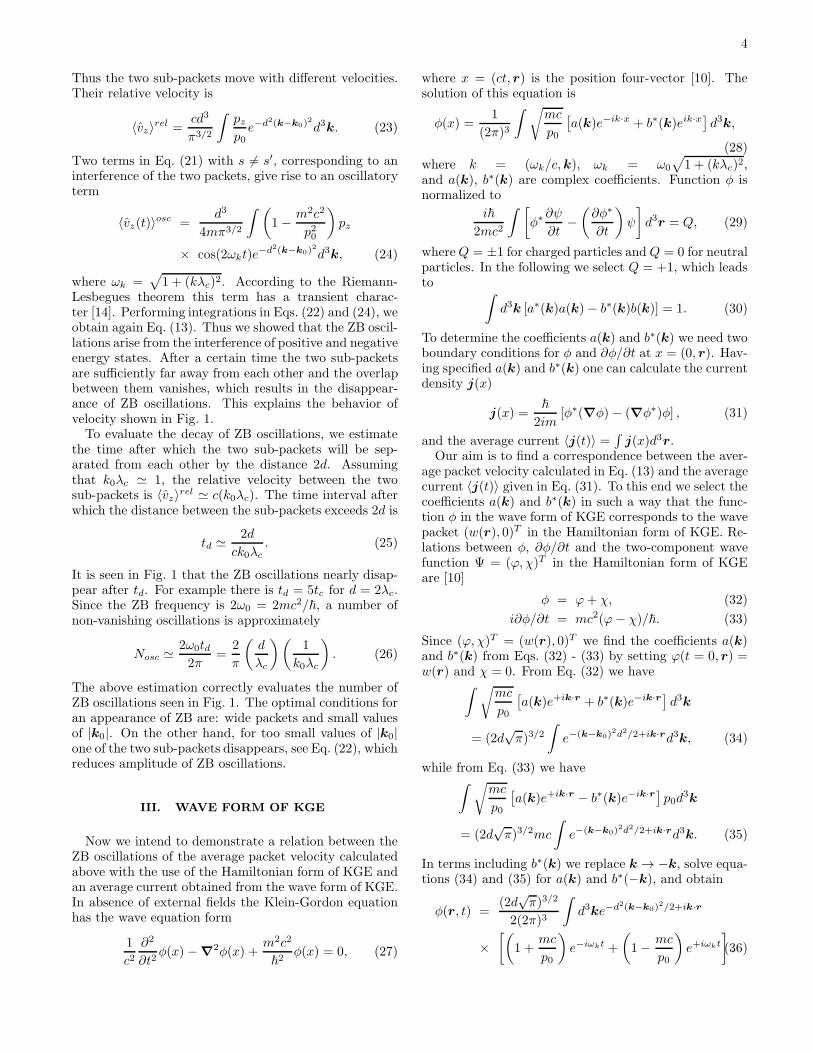
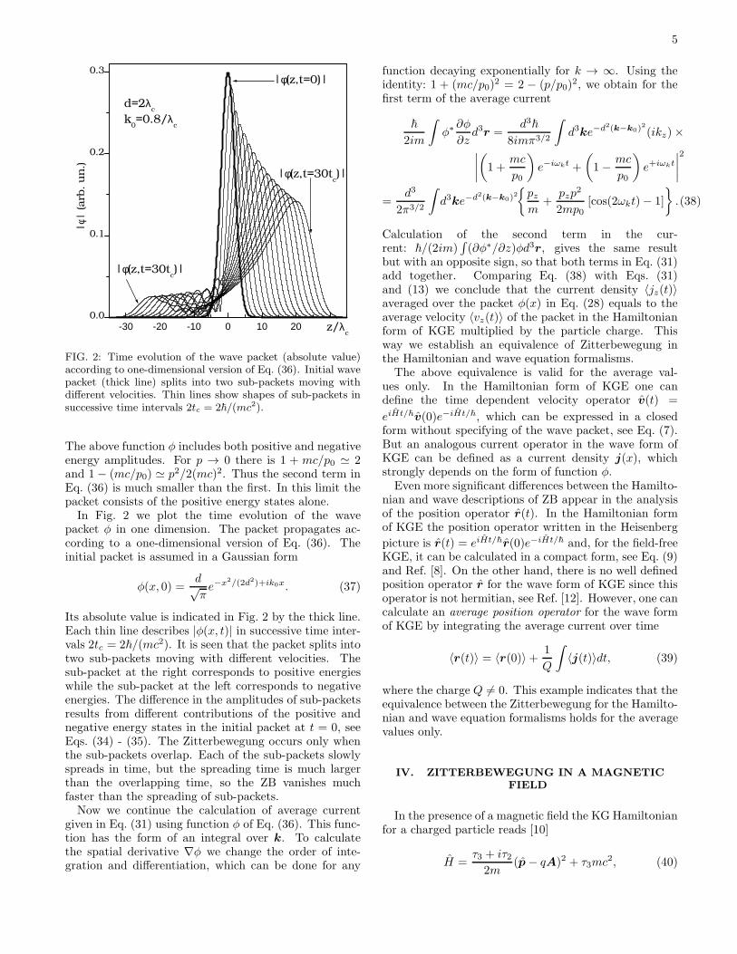
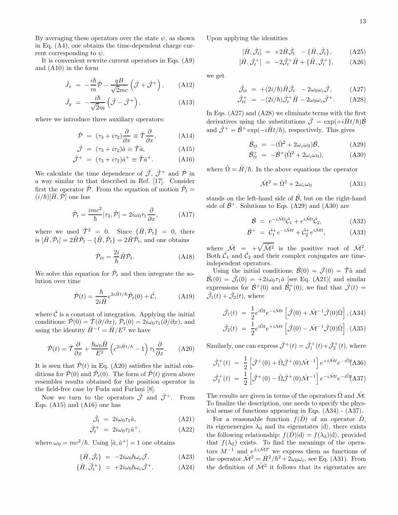
FIG. 2: Time evolution of the wave packet (absolute value)according to one-dimensional version of Eq. (36). Initial wavepacket (thick line) splits into two sub-packets moving withdifferent velocities. Thin lines show shapes of sub-packets insuccessive time intervals 2tc = 2~/(mc2).

The above function φ includes both positive and negativeenergy amplitudes. For p → 0 there is 1 + mc/p0 ≃ 2and 1 − (mc/p0) ≃ p2/2(mc)2. Thus the second term inEq. (36) is much smaller than the first. In this limit thepacket consists of the positive energy states alone.In Fig. 2 we plot the time evolution of the wave

packet φ in one dimension. The packet propagates ac-cording to a one-dimensional version of Eq. (36). Theinitial packet is assumed in a Gaussian form

φ(x, 0) =d√πe−x2/(2d2)+ik0x. (37)

Its absolute value is indicated in Fig. 2 by the thick line.Each thin line describes |φ(x, t)| in successive time inter-vals 2tc = 2~/(mc2). It is seen that the packet splits intotwo sub-packets moving with different velocities. Thesub-packet at the right corresponds to positive energieswhile the sub-packet at the left corresponds to negativeenergies. The difference in the amplitudes of sub-packetsresults from different contributions of the positive andnegative energy states in the initial packet at t = 0, seeEqs. (34) - (35). The Zitterbewegung occurs only whenthe sub-packets overlap. Each of the sub-packets slowlyspreads in time, but the spreading time is much largerthan the overlapping time, so the ZB vanishes muchfaster than the spreading of sub-packets.Now we continue the calculation of average current

given in Eq. (31) using function φ of Eq. (36). This func-tion has the form of an integral over k. To calculatethe spatial derivative ∇φ we change the order of inte-gration and differentiation, which can be done for any

function decaying exponentially for k → ∞. Using theidentity: 1 + (mc/p0)

2 = 2 − (p/p0)2, we obtain for the

first term of the average current

~

2im

∫

φ∗∂φ

∂zd3r =

d3~

8imπ3/2

∫

d3ke−d2(k−k0)2

(ikz)×∣

∣

∣

∣

(

1 +mc

p0

)

e−iωkt +

(

1− mc

p0

)

e+iωkt

∣

∣

∣

∣

2

=d3

2π3/2

∫

d3ke−d2(k−k0)2

pzm

+pzp

2

2mp0[cos(2ωkt)− 1]

.(38)

Calculation of the second term in the cur-rent: ~/(2im)

∫

(∂φ∗/∂z)φd3r, gives the same resultbut with an opposite sign, so that both terms in Eq. (31)add together. Comparing Eq. (38) with Eqs. (31)and (13) we conclude that the current density 〈jz(t)〉averaged over the packet φ(x) in Eq. (28) equals to theaverage velocity 〈vz(t)〉 of the packet in the Hamiltonianform of KGE multiplied by the particle charge. Thisway we establish an equivalence of Zitterbewegung inthe Hamiltonian and wave equation formalisms.The above equivalence is valid for the average val-

ues only. In the Hamiltonian form of KGE one candefine the time dependent velocity operator v(t) =

eiHt/~v(0)e−iHt/~, which can be expressed in a closedform without specifying of the wave packet, see Eq. (7).But an analogous current operator in the wave form ofKGE can be defined as a current density j(x), whichstrongly depends on the form of function φ.Even more significant differences between the Hamilto-

nian and wave descriptions of ZB appear in the analysisof the position operator r(t). In the Hamiltonian formof KGE the position operator written in the Heisenberg

picture is r(t) = eiHt/~r(0)e−iHt/~ and, for the field-freeKGE, it can be calculated in a compact form, see Eq. (9)and Ref. [8]. On the other hand, there is no well definedposition operator r for the wave form of KGE since thisoperator is not hermitian, see Ref. [12]. However, one cancalculate an average position operator for the wave formof KGE by integrating the average current over time

〈r(t)〉 = 〈r(0)〉+ 1

Q

∫

〈j(t)〉dt, (39)

where the charge Q 6= 0. This example indicates that theequivalence between the Zitterbewegung for the Hamilto-nian and wave equation formalisms holds for the averagevalues only.

IV. ZITTERBEWEGUNG IN A MAGNETIC

FIELD

In the presence of a magnetic field the KG Hamiltonianfor a charged particle reads [10]

H =τ3 + iτ22m

(p− qA)2 + τ3mc2, (40)

6

where q is the particle charge and A is the vector poten-tial of a magnetic field. We assume the magnetic field B

to be parallel to the z axis and describe it by the asym-metric gauge A = B(−y, 0, 0). Eigenstates of the Hamil-tonian are of the form

Ψ(r) = eikxx+ikzzΦ(y), (41)

and the resulting eigenenergy equation is HΨ = EΨ with

H = (τ3+iτ2)1

2m

[

(~kx + qBy)2 + ~2k2y + ~

2k2z]

+τ3mc2.

(42)

We introduce the magnetic radius L =√

~/|q|B and de-fine ξ = kxL + ηqy/L, where ηq = ±1 is the sign of q.Then there is ηqy = ξL − kxL2 and ∂/∂y = (1/L)∂/∂ξ.The eigenenergies are En = sEn,kz , where [15]

En,kz =√

m2c4 + 2mc2~ωc(n+ 1/2) + (c~kz)2. (43)

The corresponding eigenstates |n〉 are characterized byfour quantum numbers: |n〉 = |n, kx, kz, s〉, where n labelsthe Landau levels, kx and kz are wave vector componentsand s = ±1 label positive and negative energy branches.The wave functions are [16]

Ψn(r) ≡ 〈r|n〉 =eikxx+ikzz

4πφn(ξ)

(

µ+n,kx,s

µ−n,kx,s

)

, (44)

where φn(ξ) are the harmonic oscillator functions

φn(ξ) =1√LCn

Hn(ξ)e−1/2ξ2 , (45)

in which Hn(ξ) are the Hermite polynomials and Cn =√

2nn!√π. We defined µ±

n,kx,s= νn,kx ± s/νn,kx ,

where νn,kx =√

mc2/En,kz .We want to calculate an average packet velocity in a

magnetic field. We can, as before, introduce the Heisen-berg picture for the time-dependent velocity operator.Then the j-th component of the average velocity is, seeEq. (18),

〈vj(t)〉 = 〈W |τ3eiHt/~vje−iHt/~|W 〉, (46)

where vj = ∂H/∂pj. For the Hamiltonian (40) in theasymmetric gauge we find

vx = (τ3 + iτ2)

(

px − qBym

)

, (47)

vy = (τ3 + iτ2)pym, (48)

vz = (τ3 + iτ2)pzm. (49)

The unity operator is now

1 =∑

n

|n〉〈n|snτ3, (50)

where the states 〈r|n〉 are given in Eq. (44) and sn = ±1are the quantum numbers associated with the states |n〉.The proof of the above identity is given in Appendix C.Using the unity operator we expand the packet |W 〉 interm of the eigenstates of H [see Eq. (16)]

|W 〉 =∑

n

sn|n〉〈n|τ3|W 〉 ≡∑

n

sn|n〉Wn, (51)

where Wn = 〈n|τ3|W 〉. Inserting |W 〉 into Eq. (46) oneobtains [see Eq. (18)]

〈vj(t)〉 =∑

nm

snsmW∗nWm〈n|τ3eiHt/~vje

−iHt/~|m〉.

(52)

There is e−iHt/~|n〉 = e−iωnt|n〉, where ωn = snEn,kx/~.Proceeding the same way as in Section II we have

〈n|τ3eiHt/~ = 〈n|eiH†t/~τ3 = eiωnt〈n|τ3, (53)

which finally gives

〈vj(t)〉 =∑

nm

snsmW∗nWme

i(ωn−ωm)t〈n|τ3vj |m〉. (54)

The matrix elements of velocity operators calculated be-tween the states |n〉, |m〉 are

〈n|τ3vy|m〉 = cλc

i√2Lνn,kzνm,kzδkx,k′

xδkz ,k′

z×

(√n+ 1δm,n+1 −

√nδm,n−1), (55)

〈n|τ3vx|m〉 = cλc√2Lνn,kzνm,kzδkx,k′

xδkz ,k′

z×

(√n+ 1δm,n+1 +

√nδm,n−1), (56)

〈n|τ3vz|m〉 =pzmνn,kzνm,kzδkx,k′

xδkz ,k′

zδm,n. (57)

The matrix elements of vy and vx are nonzero for thestates with m = n± 1 and arbitrary indexes sn and sm.The matrix elements of vz are nonzero for m = n andarbitrary indexes sn and sm. To simplify the furtheranalysis we assume the initial wave packetW (r) to be ina separable form

W (r) =Wxy(x, y)Wz(z). (58)

Then there is

Wn = 〈n|τ3|W 〉 = µ+n,kz

gz(kz)Fn(kz), (59)

where

Fn(kx) =1√

2LCn

∫ ∞

−∞

gxy(kx, y)e− 1

2ξ2Hn(ξ)dy, (60)

in which

gxy(kx, y) =1√2π

∫ ∞

−∞

wxy(x, y)eikxxdx, (61)

7

and

gz(kz) =1√2π

∫ ∞

−∞

wz(z)eikzzdz. (62)

For 〈vy(t)〉 we obtain

〈vy(t)〉 = cλc

2√2iL

∞∑

n,m=0

∫ ∞

−∞

dkz ×

|gz(kz)|2(√n+ 1δm,n+1 −

√nδm,n−1

)

Un,m ×

(1 + ν2mν2n) cos(ωmt− ωnt) + (ν2mν

2n − 1) cos(ωmt+ ωnt)

+i(ν2m + ν2n) sin(ωmt− ωnt) + i(ν2m − ν2n) sin(ωmt+ ωnt)

.

In the above expressions we use the notation νn ≡ νn,kzand ωn = En,kz/~, and

Un,m =

∫ ∞

−∞

F ∗n(kx)Fm(kx)dkx. (63)

For a Gaussian packet of Eq. (11) one can obtain ana-lytical expressions for Un,m, see Appendix D. After per-forming the summation over m and changing n→ n+ 1in δm,n−1 terms we finally obtain

〈vy(t)〉 = −cλc

2√2L

∞∑

n=0

√n+ 1(Un+1,n + Un,n+1)

∫ ∞

−∞

|gz(kz)|2

(ν2n+1 + ν2n) sin(ωn+1t− ωnt)

+(ν2n+1 − ν2n) sin(ωn+1t+ ωnt)

dkz , (64)

〈vx(t)〉 = −cλc

2√2L

∞∑

n=0

√n+ 1(Un+1,n + Un,n+1)

∫ ∞

−∞

|gz(kz)|2

(1 + ν2n+1ν2n) cos(ωn+1t− ωnt)

+(1− ν2n+1ν2n) cos(ωn+1t+ ωnt)

dkz , (65)

〈vz(t)〉 =cλc2

∞∑

n=0

Un,n

∫ ∞

−∞

kz |gz(kz)|2 ×

(1 + ν4n) + (1− ν4n) cos(2ωnt)

dkz. (66)

Equations (64) - (66) are our final results for the aver-age velocity of wave packet in a magnetic field. Boththe arguments of sine and cosine functions as well ascoefficients νn and νn+1 depend on kz , so all the inte-grals vanish in the limit t → ∞ as a consequence of theRiemann-Lebegues theorem and the resulting oscillationshave a transient character. The velocity of the packet os-cillates with many frequencies ωn+1±ωn (or 2ωn for vz),but in practice the spectrum is limited to a few frequen-cies related to the largest coefficients Un+1,n and Un,n.The frequencies ωn+1 − ωn correspond to the intrabandtransitions and they can be interpreted as the cyclotron

resonances. These frequencies do not appear in vz veloc-ity. On the other hand, the frequencies ωn+1+ωn and 2ωn

(for vz) correspond to interband transitions and they canbe interpreted as the Zittebewegung components of themotion in analogy to the situation at zero field. The mo-tion in the x− y directions requires that k0x 6= 0 becausefor k0x = 0 all the coefficients Un+1,n and Un,n+1 van-ish [17]. For the motion in the z direction one needs onlythat k0z 6= 0, because the coefficients Un,n are nonzerofor any k0x vector [17].Considering the non-relativistic limit in Eqs. (64) -

(66), there is ~ωc ≪ mc2 and ~kz ≪ mc, so that ωn+1 −ωn ≃ ~ωc and ωn+1 + ωn ≃ 2mc2/~. In this limit thereis νn+1 ≃ νn ≃ 1, and the ZB part of velocity is nearlyzero. In this case we may decouple in Eqs. (64) - (66) thesummation over n and integration over kz . This gives [17]

∞∑

n=0

√n+ 1Un+1,n = −k0xL√

2(67)

∞∑

n=0

Un,n = 1. (68)

Integrating over kz one gets

〈vy(t)〉 ≃~k0xm

sin(ωct), (69)

〈vx(t)〉 ≃~k0xm

cos(ωct), (70)

〈vz(t)〉 ≃~k0zm

. (71)

Thus in the non-relativistic limit the particle moves ona circular orbit with the cyclotron frequency in the x− yplane and a constant velocity in the z direction. Let usintroduce a measure of intensity of a magnetic field byits relation to an effective Schwinger field ~eBs/m = mc2

or, equivalently, by Ls = ~/mc. There is Bs = 4.41 ×109(m/me)

2 T, where me is the electron mass. Below weperform calculations for pions π+ having the mass m ≃273.1 me, so the effective Schwinger field is Bs = 3.29×1014 T.In Fig. 3 we plot the average packet velocity for three

values of magnetic field. The ellipsoidal packet is se-lected with a nonzero initial momentum k0x. We as-sume that the five parameters: dx, dy, dz, L and k−1

0x

have similar orders of the magnitude which are the op-timal conditions for the appearance of Zitterbewegungphenomenon. In Fig. 3 we selected parameters: dx =0.91(Bs/B)λc, dy = 0.82(Bs/B)λc, dz = 0.68(Bs/B)λc,k0x = 0.7(B/Bs)λ

−1c and k0z = 0, where Bs is the effec-

tive Schwinger field. For B = 4.5Bs we set k0x = λ−1c .

For low fields (B = 0.0045Bs) the packet moves on a cir-cular orbit, see Eqs. (69) and (70). For such fields theZB components of the motion are negligible. For higherfields the packet motion includes both the intraband andinterband (ZB) components so that several frequenciesgive significant contributions to the motion. In all cases

8

1000 2000 3000

-1.0

-0.5

0.0

0.5

1.0

B=0.0045Bs

<vx(t)>

<vy(t)>

velo

cit

y (10

7m

/s) (a)

100 200 300

-6.0

-3.0

0.0

3.0

6.0

B=0.45Bs

t (tc)<v

y(t)>

<vx(t)>v

elo

cit

y (10

7m

/s)

(b)

0 20 40 60 80

-10

0

10

B=4.5Bs

t (tc)

<vy(t)>

<vx(t)>

t (tc)

velo

cit

y (10

7m

/s)

(c)

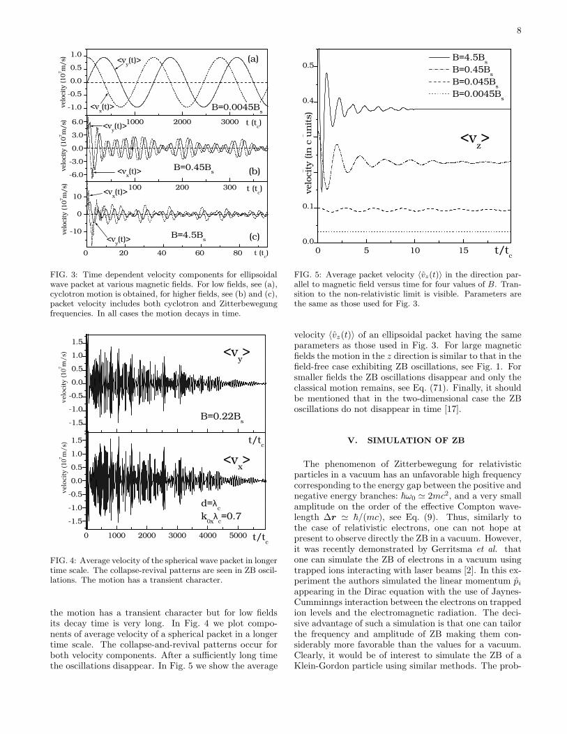
FIG. 3: Time dependent velocity components for ellipsoidalwave packet at various magnetic fields. For low fields, see (a),cyclotron motion is obtained, for higher fields, see (b) and (c),packet velocity includes both cyclotron and Zitterbewegungfrequencies. In all cases the motion decays in time.

-1.5

-1.0

-0.5

0.0

0.5

1.0

1.5

B=0.22Bs

<vy>

vel

oci

ty (

10

7 m/

s)

0 1000 2000 3000 4000 5000

-1.5

-1.0

-0.5

0.0

0.5

1.0

1.5

d=λc

k0x

λc=0.7

t/tc

vel

oci

ty (

10

7 m/

s)

t/tc

<vx>

FIG. 4: Average velocity of the spherical wave packet in longertime scale. The collapse-revival patterns are seen in ZB oscil-lations. The motion has a transient character.

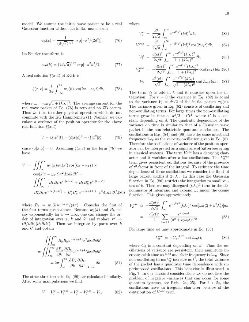
the motion has a transient character but for low fieldsits decay time is very long. In Fig. 4 we plot compo-nents of average velocity of a spherical packet in a longertime scale. The collapse-and-revival patterns occur forboth velocity components. After a sufficiently long timethe oscillations disappear. In Fig. 5 we show the average

0 5 10 150.0

0.1

0.2

0.3

0.4

0.5

<vz>

B=4.5Bs

B=0.45Bs

B=0.045Bs

B=0.0045Bs

t/tc

velo

cit

y (in

c u

nit

s)

FIG. 5: Average packet velocity 〈vz(t)〉 in the direction par-allel to magnetic field versus time for four values of B. Tran-sition to the non-relativistic limit is visible. Parameters arethe same as those used for Fig. 3.

velocity 〈vz(t)〉 of an ellipsoidal packet having the sameparameters as those used in Fig. 3. For large magneticfields the motion in the z direction is similar to that in thefield-free case exhibiting ZB oscillations, see Fig. 1. Forsmaller fields the ZB oscillations disappear and only theclassical motion remains, see Eq. (71). Finally, it shouldbe mentioned that in the two-dimensional case the ZBoscillations do not disappear in time [17].

V. SIMULATION OF ZB

The phenomenon of Zitterbewegung for relativisticparticles in a vacuum has an unfavorable high frequencycorresponding to the energy gap between the positive andnegative energy branches: ~ω0 ≃ 2mc2, and a very smallamplitude on the order of the effective Compton wave-length ∆r ≃ ~/(mc), see Eq. (9). Thus, similarly tothe case of relativistic electrons, one can not hope atpresent to observe directly the ZB in a vacuum. However,it was recently demonstrated by Gerritsma et al. thatone can simulate the ZB of electrons in a vacuum usingtrapped ions interacting with laser beams [2]. In this ex-periment the authors simulated the linear momentum piappearing in the Dirac equation with the use of Jaynes-Cumminngs interaction between the electrons on trappedion levels and the electromagnetic radiation. The deci-sive advantage of such a simulation is that one can tailorthe frequency and amplitude of ZB making them con-siderably more favorable than the values for a vacuum.Clearly, it would be of interest to simulate the ZB of aKlein-Gordon particle using similar methods. The prob-

9

y(x,t)

element dx

y

xstring's equilibrium position

string at

instant t

rubber sheet

TT

FT + F

K

FIG. 6: Classical simulation of KGE according to Morse andFeshbach [11]. Flexible string is anchored at two points andtension T is applied to each end. The string is also attached toa thin rubber sheet. At instant t the shape of string is givenby y(x, t). There are two forces acting on each element dxof the string: restoring force FT due to applied tension andelastic force FK of stretched rubber.

lem is that in KGE one deals with squares of momentumcomponents p2, which are more difficult to simulate withthe Jaynes-Cumminngs interaction. For this reason wechoose a different route.

The Klein-Gordon equation appears in several classi-cal systems, usually as a modification of the wave equa-tion φ = 0. Under some conditions KGE is used todescribe sound waves in ducts [18, 19], electromagneticwaves in the ionosphere [20, 21], transverse modes of waveguides [22] and oceanic waves [23]. Below we examine inmore detail a model proposed by Morse and Feshbachin which one can simulate KGE with the use of a pianostring and a thin rubber sheet [11]. Employing this exam-ple we demonstrate similarities and differences betweenZB in the relativistic KGE and its classical analogues.

Let us consider flexible one dimensional string in the xdirection, see Fig. 6. We assume that the string is uni-form with a linear density ρ. A uniform tension T isapplied to each element dx of the string. We neglect allother forces acting on the string (e.g. gravity) and thestiffness of the string. Let y(x, t) be a displacement ofthe element dx of the string from its equilibrium positionat an instant t. We assume that y(x, t) is small com-pared to the length of the string and to the distances toeach end of the string. The restoring force acting on eachelement dx of the string is FT = Tdx(∂2y/∂x2) and dis-placement y(x, t) of the released string changes according

to the wave equation [11]

1

u2∂2y

∂t2=∂2y

∂x2, (72)

where u2 = T/ρ. Now we attache the string to an elas-tic substrate, e.g. to a thin sheet of rubber which canshrink or expand in the y direction. Then, in additionto the restoring force due to the tension, there will beanother restoring force due to the elastic rubber actingon each element of the string. If the element dx is dis-placed to y(x, t) and the rubber sheet obeys the Hooklaw, the restoring force acting on the element dx of thestring is FK(x, t) = −Ky(x, t)dx, where K is the elasticconstant of the rubber sheet. The second Newton lawfor the element dx of the string having mass dm = dxρis dxρ(∂2y/∂t2) = FT + FK , so the equation of motionof the released string is

1

u2∂2y

∂t2=∂2y

∂x2− ν2y, (73)

where ν2 = K/T . Equation (73) has the form of waveKGE with the light speed replaced by u and the massterm m2c2/~2 replaced by ν2. Comparing Eq. (73) withEq. (27) we find the following correspondence betweenparameters of the two systems

T

ρ↔ c2, (74)

K

T↔ m2c2

~2= λ−2

c . (75)

Thus one can simulate values of c and λc by changingmaterial parameters ρ, K and T .However, there exist also limitations of such a simu-

lation and they affect a possibility of observation of ZBmotion in classical analogues of KGE. The first differencebetween the relativistic KGE and its classical counterpartis that the wave function φ in the relativistic KGE is notan observable. On the other hand, all classical analoguesof φ (such as a displacement of the string, the pressure ofsound or the oceanic waves, the intensity of electromag-netic field etc.) are observable quantities. The seconddifference is that the relativistic function φ is a functionof complex variable, while its classical counterpart is afunction of real variable. A direct consequence of theselimitations for observation of ZB in classical systems isthat, for any real function ξ(r, t) being the solution ofKGE, the current density associated with this functionis always zero: j ∝ [ξ∗∇ξ − (∇ξ∗)ξ] = 0. Therefore weare not able to simulate directly the current or velocityoscillations calculated in the previous sections.To overcome this problem let us consider the motion

of a neutral particle described by a real field ξ. For sim-plicity we assume a one-dimensional KGE that can besimulated by a flexible string attached to an elastic sub-strate described above. In our calculations we use therelativistic form of KGE but the final results will be pre-sented for parameters corresponding to the flexible string

10

model. We assume the initial wave packet to be a realGaussian function without an initial momentum

w0(x) =1

(d√π)1/2

exp[−x2/(2d2)]. (76)

Its Fourier transform is

w0(k) = (2d√π)1/2 exp[−d2k2/2]. (77)

A real solution ξ(x, t) of KGE is

ξ(x, t) =1

2π

∫ ∞

−∞

w0(k) cos(kx− ωkt)dk, (78)

where ωk = ω0

√

1 + (kλc)2. The average current for thereal wave packet of Eq. (76) is zero and no ZB occurs.Thus we turn to other physical operators which do notcommute with the KG Hamiltonian (1). Namely, we cal-culate a variance of the position operator for the abovereal function ξ(x, t)

V = 〈ξ|x2|ξ〉 − 〈φ|x|φ〉2 = 〈ξ|x2|ξ〉, (79)

since 〈φ|x|φ〉 = 0. Assuming ξ(x, t) in the form (78) wehave

V =

∫∫∫ ∞

∞

w0(k)w0(k′) cos(kx− ωkt)×

cos(k′x− ωk′t)x2dxdkdk′ =∫∫∫ ∞

∞

[

BkBk′eix(k+k) +BkB∗k′eix(k−k′)

B∗kBk′e−ix(k−k′) +B∗

kB∗k′e−ix(k+k′)

]

x2dxdkdk′,(80)

where Bk = w0(k)e−iωkt/(4π). Consider the first of

the four terms given above. Because w0(k) and Bk de-cay exponentially for k → ±∞, one can change the or-der of integration over x, k and k′ and replace x2 →(∂/∂ik)(∂/∂ik′). Then we integrate by parts over kand k′ and obtain

∫∫∫ ∞

∞

BkBk′eix(k+k)x2dxdkdk′

=

∫∫∫ ∞

∞

∂Bk

∂k

∂Bk′

∂k′eix(k+k)dxdkdk′

= 2π

∫ ∞

∞

∂Bk

∂k

∂Bk′

∂k′

∣

∣

∣

∣

k′=k

dk. (81)

The other three terms in Eq. (80) are calculated similarly.After some manipulations we find

V = V c1 + V osc

1 + V c2 + V osc

2 + V3, (82)

where

V c1 =

d3

2√π

∫ ∞

∞

e−d2k2

(kd)2dk, (83)

V osc1 =

d3

2√π

∫ ∞

∞

e−d2k2

(kd)2 cos(2ωkt)dk, (84)

V c2 =

d(ct)2

2√π

∫ ∞

∞

e−d2k2

(kλc)2

1 + (kλc)2dk, (85)

V osc2 = −d(ct)

2

2√π

∫ ∞

∞

e−d2k2

(kλc)2

1 + (kλc)2cos(2ωkt)dk,(86)

V3 =d2(ct)√

π

∫ ∞

∞

e−d2k2

(kλc)√

1 + (kλc)2sin(2ωkt)dk. (87)

The term V3 is odd in k and it vanishes upon the in-tegration. For t = 0 the variance in Eq. (82) is equalto the variance V0 = d2/2 of the initial packet w0(x).The variance given in Eq. (82) consists of oscillating andnon-oscillating terms. For large times the non-oscillatingterms grow in time as d2/2 + Ct2, where C is a con-stant depending on d. The quadratic dependence of thevariance on time is similar to that of a Gaussian wavepacket in the non-relativistic quantum mechanics. Theoscillations in Eqs. (84) and (86) have the same interbandfrequency 2ωk as the velocity oscillation given in Eq. (8).Therefore the oscillations of variance of the position oper-ator can be interpreted as a signature of Zitterbewegungin classical systems. The term V osc

1 has a decaying char-acter and it vanishes after a few oscillations. The V osc

2

term gives persistent oscillations because of the presenceof t2 factor in front of the integral. To estimate the timedependence of these oscillations we consider the limit oflarge packet widths d ≫ λc. In this case the Gaussianfunction in Eq. (86) restricts the integration to small val-ues of k. Then we may disregard (kλc)

2 term in the de-nominator of integrand and expand ωk under the cosinefunction. This gives approximately

V osc2 ≃ −d(ct)

2

2√π

∫ ∞

∞

e−d2k2

(kλc)2 cos[ω0t(2 + k2λ2c)]dk

= −d(ct)2

4

∑

η=±1

e2iηω0t

(d2 + iηω0t)3/2. (88)

For large time we may approximate in Eq. (88)

V osc2 ≃ −Cdt

1/2 cos(2ω0t), (89)

where Cd is a constant depending on d. Thus the os-cillations of variance are persistent, their amplitude in-creases with time as t1/2 and their frequency is 2ω0. Sincenon-oscillating terms V c

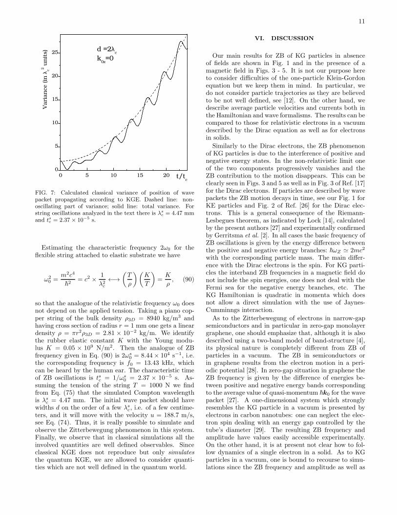
2 increase as t2, the total varianceof the packet has a quadratic time dependence with su-perimposed oscillations. This behavior is illustrated inFig. 7. In our classical considerations we do not face theproblem of negative variances that can occur for somequantum systems, see Refs. [24, 25]. For t < 5tc theoscillations have an irregular character because of thecontribution of V osc

1 term.

11

0 5 10 15 200

5

10

15

20

25d =2λ

c

k0z=0

t/tc

Vari

an

ce (in

λc2 u

nit

s)

FIG. 7: Calculated classical variance of position of wavepacket propagating according to KGE. Dashed line: non-oscillating part of variance; solid line: total variance. Forstring oscillations analyzed in the text there is λs

c = 4.47 mmand tsc = 2.37× 10−5 s.

Estimating the characteristic frequency 2ω0 for theflexible string attached to elastic substrate we have

ω20 =

m2c4

~2= c2 × 1

λ2c←→

(

T

ρ

)(

K

T

)

=K

ρ, (90)

so that the analogue of the relativistic frequency ω0 doesnot depend on the applied tension. Taking a piano cop-per string of the bulk density ρ3D = 8940 kg/m3 andhaving cross section of radius r = 1 mm one gets a lineardensity ρ = πr2ρ3D = 2.81 × 10−2 kg/m. We identifythe rubber elastic constant K with the Young modu-lus K = 0.05 × 109 N/m2. Then the analogue of ZBfrequency given in Eq. (90) is 2ωs

0 = 8.44× 104 s−1, i.e.the corresponding frequency is f0 = 13.43 kHz, whichcan be heard by the human ear. The characteristic timeof ZB oscillations is tsc = 1/ωs

0 = 2.37 × 10−5 s. As-suming the tension of the string T = 1000 N we findfrom Eq. (75) that the simulated Compton wavelengthis λsc = 4.47 mm. The initial wave packet should havewidths d on the order of a few λsc, i.e. of a few centime-ters, and it will move with the velocity u = 188.7 m/s,see Eq. (74). Thus, it is really possible to simulate andobserve the Zitterbewegung phenomenon in this system.Finally, we observe that in classical simulations all theinvolved quantities are well defined observables. Sinceclassical KGE does not reproduce but only simulates

the quantum KGE, we are allowed to consider quanti-ties which are not well defined in the quantum world.

VI. DISCUSSION

Our main results for ZB of KG particles in absenceof fields are shown in Fig. 1 and in the presence of amagnetic field in Figs. 3 - 5. It is not our purpose hereto consider difficulties of the one-particle Klein-Gordonequation but we keep them in mind. In particular, wedo not consider particle trajectories as they are believedto be not well defined, see [12]. On the other hand, wedescribe average particle velocities and currents both inthe Hamiltonian and wave formalisms. The results can becompared to those for relativistic electrons in a vacuumdescribed by the Dirac equation as well as for electronsin solids.

Similarly to the Dirac electrons, the ZB phenomenonof KG particles is due to the interference of positive andnegative energy states. In the non-relativistic limit oneof the two components progressively vanishes and theZB contribution to the motion disappears. This can beclearly seen in Figs. 3 and 5 as well as in Fig. 3 of Ref. [17]for the Dirac electrons. If particles are described by wavepackets the ZB motion decays in time, see our Fig. 1 forKE particles and Fig. 2 of Ref. [26] for the Dirac elec-trons. This is a general consequence of the Riemann-Lesbegues theorem, as indicated by Lock [14], calculatedby the present authors [27] and experimentally confirmedby Gerritsma et al. [2]. In all cases the basic frequency ofZB oscillations is given by the energy difference betweenthe positive and negative energy branches: ~ωZ ≃ 2mc2

with the corresponding particle mass. The main differ-ence with the Dirac electrons is the spin. For KG parti-cles the interband ZB frequencies in a magnetic field donot include the spin energies, one does not deal with theFermi sea for the negative energy branches, etc. TheKG Hamiltonian is quadratic in momenta which doesnot allow a direct simulation with the use of Jaynes-Cumminngs interaction.

As to the Zitterbewegung of electrons in narrow-gapsemiconductors and in particular in zero-gap monolayergraphene, one should emphasize that, although it is alsodescribed using a two-band model of band-structure [4],its physical nature is completely different from ZB ofparticles in a vacuum. The ZB in semiconductors orin graphene results from the electron motion in a peri-odic potential [28]. In zero-gap situation in graphene theZB frequency is given by the difference of energies be-tween positive and negative energy bands correspondingto the average value of quasi-momentum ~k0 for the wavepacket [27]. A one-dimensional system which stronglyresembles the KG particle in a vacuum is presented byelectrons in carbon nanotubes: one can neglect the elec-tron spin dealing with an energy gap controlled by thetube’s diameter [29]. The resulting ZB frequency andamplitude have values easily accessible experimentally.On the other hand, it is at present not clear how to fol-low dynamics of a single electron in a solid. As to KGparticles in a vacuum, one is bound to recourse to simu-lations since the ZB frequency and amplitude as well as

12

field intensities necessary to see ZB effects in the pres-ence of a magnetic field, exceed the present experimentalpossibilities.We present a classical simulation of ZB by using a me-

chanical system and calculate the oscillating variance ofposition of the wave packet. The variance of position op-erator for the Dirac Hamiltonian was calculated by Barutand Malin [30] who found it to be the reminiscence of ZBof electrons in a vacuum. The present authors analyzedin Ref. [27] the variance of position operator in bilayergraphene and found its oscillating character with the fre-quency equal to that of ZB.One should finally remark that the attempts are con-

stantly made in the literature to overcome the above men-tioned difficulties in the interpretation of position oper-ator in KG equation. In particular, Mostafazadeh [31]proposed a redefinition of the scalar product of solutionsto KGE which allows one to obtain positively definedprobability distribution of position. Semenov et al. [25]proposed to limit the allowed solutions of KG equation tothose having positive-definite probability distributions.They showed that the physical solutions of KGE fulfillthis criterion. If the above attempts are accepted onecould analyze ZB of the position operator for KG parti-cles, see Eq. (9).

VII. SUMMARY

We considered the trembling motion (Zitterbewegung)of relativistic spin-zero particles in absence of fields andin the presence of a magnetic field using the Klein-Gordon equation. We aimed to describe physical observ-ables (currents and velocities) calculating quantities aver-aged with the use of Gaussian wave packets. Surprisingly,the calculated particle velocities can exceed the veloc-ity of light for sufficiently large momenta indicating thatKGE does not posses an automatic restriction of relativ-ity. We showed that the trembling motion has a decayingcharacter resulting from an interference of positive andnegative energy sub-packets moving with different veloc-ities. In the presence of a magnetic field there exist manyinterband frequencies that contribute to Zitterbewegung.On the other hand, in the limit of non-relativistic energiesthe interband ZB components vanish while the intrabandcomponents reduce to the cyclotron motion with a singlefrequency. The trembling motion was simulated usingthe classical system obeying the Klein-Gordon equation– a stretched string attached to a rubber sheet. The cal-culated variance of position of the sting shaped initiallyas a Gaussian packet exhibits oscillations correspondingto Zitterbewegung with the correct frequency.

Appendix A

In this Appendix we calculate an exact time depen-dence of current operators for a KG particle in a magnetic

field. We define the creation and annihilation operators

a = (ξ + ∂/∂ξ)/√2,

a+ = (ξ − ∂/∂ξ)/√2,

(A1)

and rewrite Eq. (40) in the form

H = T[

~ωc

(

a+a+1

2

)

+~2k2z2m

]

+ τ3mc2, (A2)

where ωc = qB/m is the cyclotron frequency and T =(τ3 + iτ2). The current density is

j =~

2im

[

ψ†τ3T∇ψ − (∇ψ†)τ3T ψ]

− e

mcAψ†τ3T ψ, (A3)

and the average current is 〈j〉 =∫

jd3r. We introduce

the current operator J in such way that for j given inEq. (A3) there is

〈ψ|τ3J |ψ〉 =∫

jd3r. (A4)

Note the presence of τ3 in the matrix element. In theasymmetric gauge one has

〈jx〉 = − i~

2m

∫(

ψ†τ3T∂ψ

∂x− ∂ψ†

∂xτ3T ψ

)

d3r

− qBmc

∫

(

ψ†τ3T yψ)

d3r, (A5)

〈jy〉 = − i~

2m

∫(

ψ†τ3T∂ψ

∂y− ∂ψ†

∂yτ3T ψ

)

d3r.(A6)

Below we assume the function ψ to be Gaussian-like. Inthat case we may simplify the above expressions for theaverage current by integrating by parts the terms includ-ing derivatives of ψ†

〈jx〉 = − i~m

∫(

ψ†τ3T∂ψ

∂x

)

d3r − qB

mc

∫

(

ψ†τ3T yψ)

d3r,(A7)

〈jy〉 = − i~m

∫(

ψ†τ3T∂ψ

∂y

)

d3r, (A8)

so the components of the current operator are

Jx = − i~mT ∂

∂x− qB

mcT y, (A9)

Jy = − i~mT ∂

∂y. (A10)

In the Heisenberg picture the time-dependent current op-erator is

J(t) = eiHt/~J(0)e−iHt/~, (A11)

where H is given in Eq. (A2). Our task is to calculate the

time evolution of the current operator Jx(t) and Jy(t).

13

By averaging these operators over the state ψ, as shownin Eq. (A4), one obtains the time-dependent charge cur-rent corresponding to ψ.It is convenient rewrite current operators in Eqs. (A9)

and (A10) in the form

Jx = − i~mP − qB√

2mc

(

J + J+)

, (A12)

Jy = − i~√2m

(

J − J +)

, (A13)

where we introduce three auxiliary operators:

P = (τ3 + iτ2)∂

∂x≡ T ∂

∂x, (A14)

J = (τ3 + iτ2)a ≡ T a, (A15)

J+ = (τ3 + iτ2)a+ ≡ T a+. (A16)

We calculate the time dependence of J , J + and P ina way similar to that described in Ref. [17]. Consider

first the operator P . From the equation of motion Pt =(i/~)[H, P ] one has

Pt =imc2

~[τ3, P ] = 2iω0τ1

∂

∂x, (A17)

where we used T 2 = 0. Since H, Pt = 0, there

is [H, Pt] = 2HPt − H, Pt = 2HPt, and one obtains

Ptt =2i

~HPt. (A18)

We solve this equation for Pt and then integrate the so-lution over time

P(t) = ~

2iHe2iHt/~Pt(0) + C, (A19)

where C is a constant of integration. Applying the initialconditions: P(0) = T (∂/∂x), Pt(0) = 2iω0τ1(∂/∂x), and

using the identity H−1 = H/E2 we have

P(t) = T ∂

∂x+

~ω0H

E2

(

e2iHt/~ − 1)

τ1∂

∂x. (A20)

It is seen that P(t) in Eq. (A20) satisfies the initial con-

ditions for P(0) and Pt(0). The form of P(t) given aboveresembles results obtained for the position operator inthe field-free case by Fuda and Furlani [8].

Now we turn to the operators J and J +. FromEqs. (A15) and (A16) one has

Jt = 2iω0τ1a, (A21)

J +t = 2iω0τ1a

+, (A22)

where ω0 = mc2/~. Using [a, a+] = 1 one obtains

H, Jt = −2iω0~ωcJ , (A23)

H, J +t = +2iω0~ωcJ+. (A24)

Upon applying the identities

[H, Jt] = +2HJt − H, Jt, (A25)

[H, J +t ] = −2J+

t H + H, J +t , (A26)

we get

Jtt = +(2i/~)HJt − 2ω0ωcJ , (A27)

J+tt = −(2i/~)J+

t H − 2ω0ωcJ +. (A28)

In Eqs. (A27) and (A28) we eliminate terms with the first

derivatives using the substitutions J = exp(+iHt/~)Band J + = B+ exp(−iHt/~), respectively. This gives

Btt = −(Ω2 + 2ωcω0)B, (A29)

B+tt = −B+(Ω2 + 2ωcω0), (A30)

where Ω = H/~. In the above equations the operator

M2 = Ω2 + 2ωcω0 (A31)

stands on the left-hand side of B, but on the right-handside of B+. Solutions to Eqs. (A29) and (A30) are

B = e−iMtC1 + eiMtC2, (A32)

B+ = C+1 e−iMt + C+2 eiMt, (A33)

where M = +√

M2 is the positive root of M2.Both C1 and C2 and their complex conjugates are time-independent operators.Using the initial conditions: B(0) = J (0) = T a and

Bt(0) = Jt(0) = +2iω0τ1a [see Eq. (A21)] and similar

expressions for B+(0) and B+t (0), we find that J (t) =

J1(t) + J2(t), where

J1(t) =1

2eiΩte−iMt

[

J (0) + M−1J (0)Ω]

, (A34)

J2(t) =1

2eiΩte+iMt

[

J (0)− M−1J (0)Ω]

. (A35)

Similarly, one can express J +(t) = J +1 (t)+J+

2 (t), where

J+1 (t) =

1

2

[

J+(0) + ΩJ +(0)M−1]

e+iMte−iΩt,(A36)

J+2 (t) =

1

2

[

J+(0)− ΩJ +(0)M−1]

e−iMte−iΩt.(A37)

The results are given in terms of the operators Ω and M.To finalize the description, one needs to specify the phys-ical sense of functions appearing in Eqs. (A34) - (A37).

For a reasonable function f(D) of an operator D,its eigenenergies λd and its eigenstates |d〉, there exists

the following relationship: f(D)|d〉 = f(λd)|d〉, providedthat f(λd) exists. To find the meanings of the opera-

tors M−1 and e±iMT we express them as functions ofthe operator M2 = H2/~2+2ω0ωc, see Eq. (A31). From

the definition of M2 it follows that its eigenstates are

14

equal to the eigenstates |n〉 of H . The eigenvalues λ2n of

the operator M2 are λ2n,kz= E2

n+1,kzand we obtain

M±1|n〉 = (M2)±1/2|n〉 = ηE±1n+1,kz

|n〉, (A38)

e±iMt|n〉 = e±i(M2)1/2t|n〉 = e±iηEn+1,kz |n〉,(A39)

where η = +1 or η = −1. As seen from Eqs. (A34) -

(A37), the sums J1(t)+ J2(t) and J +1 (t)+ J+

2 (t) do notdepend on the sign of η, so we select η = +1.Finally we show that the matrix elements of the op-

erator J (t) = J1(t) + J2(t) are equal to the matrix el-

ements of the current operator JH(t) = eiΩtJ (0)e−iΩt

in the Heisenberg picture. The operator J is propor-tional to the annihilation operator a whose non-vanishingmatrix elements are 〈n′|a|n〉 =

√n+ 1δn′,n+1, so we

select two eigenstates of KG Hamiltonian |n〉 = |n, s〉and |n′〉 = |n + 1, z〉, see Eq. (44). Here we omitted

quantum numbers kx and kz. For JH(t) one has

〈n|τ3JH(t)|n′〉 = eisωnte−izωn+1tJ (0)nn′ , (A40)

where we define J (0)nn′ = 〈n|τ3J (0)|n′〉. To calculate

the matrix elements of J1(t) we use Eqs. (A38) - (A39)and obtain

〈n|M−1J (0)Ω|n′〉 = ~

En+1J (0)nn′

zEn+1

~= zJ (0)nn′

(A41)which finally gives

〈n|J1(t)|n′〉 =1 + z

2J (0)nn′eisωnte−iωn+1t, (A42)

〈n|J2(t)|n′〉 =1− z2J (0)nn′eisωnte+iωn+1t. (A43)

The matrix elements of J1(t) are nonzero for z = +1 only,

while the matrix elements of J2(t) are nonzero for z = −1only. Comparing Eqs. (A42) and (A43) with Eq. (A40)we see that for each of four combinations of s = ±1and z = ±1 the matrix elements of JH(t) are equal to

the matrix elements of J (t) = J1(t) + J2(t), which is

what we wanted to show. Calculations for J +(t) are

similar to those for J (t). The compact equations (A34)- (A37) are our final results for the time dependence

of J (t) and J +(t) operators. These equations are ex-act and they are quite fundamental for relativistic spin-0 particles in a magnetic field. If we calculate averagecurrents of Eqs. (A12) and (A13) with the use of ex-pressions (A42) - (A43) and the wave packet (11), oneobtains results corresponding to the velocities given inSection IV.

Appendix B

In this Appendix we analyze in more detail the rela-tion of the particle velocity to the speed of light. We

consider (1, 1) component of the velocity operator for aKG particle given in Eq. (7). For the wave packet 〈r|w〉 =w(r)(1, 0)T with one nonzero component the average ve-locity is given by the average of (vz)11(t) over the func-tion w(r). The unexpected feature of operator (vz)11(t)is that for large p this velocity can exceed the speed oflight c.There are two possible ways to overcome this problem.

We can additionally assume that |p| ≤ mc, which ensuresthat the velocity (vz)11(t) does not exceed c. This con-dition is equivalent to |q| ≤ 1 in the text, see Eq. (7).Alternatively, one can take the initial wave packet w(r)which does not contain components with |p| > mc. Thenthe Gaussian packet in Eq. (12) must be replaced by anon-Gaussian packet w′(r) of the form

〈k|w′〉 = (2d√π)3/2 exp[−d2(k − k0)

2/2]Θ(λc − |k|),(B1)

where Θ(ξ) is the step function.

For the Dirac Hamiltonian HD = c∑

j αj pj + mc2β,

the situation is different. Expanding eiHDt/~ in a power

series one obtains an expression analogous to eiHt/~ givenin Eq. (6). After some algebra we find

(vz)D11(t) =

mc2pzm2c2 + p2

[1− cos(2Et/~)] . (B2)

In contrast to the KG case, the velocity operator givenin Eq. (B2) has correct relativistic behavior for all val-ues of p. In Eq. (B2) the expression in square brack-ets oscillates between zero and two. The factor vD(p) =mc2pz/(m

2c2+p2) tends to zero for both large and smallvalues of p. Its maximum is at pmax = (0, 0,mc) forwhich one obtains

(vz)D11(t) =

c

2

[

1− cos(2√2ω0)

]

. (B3)

The above velocity never exceeds the speed of light.Therefore, when calculating the average velocity of thewave packet for the Dirac Hamiltonian, there is no needfor an artificial truncation of the high momentum com-ponents of the wave packet, as proposed in Eq. (B1) fora KG particle.

Appendix C

We prove here some identities appearing in the pre-vious sections. We begin with the identity in Eq. (50).Closing Eq. (50) with the use of states 〈r| and |r′〉, em-ploying Eq. (44) and writing explicitly the summationsand integrations over the quantum numbers we obtain

δr,r′ =∑

n

〈r|n〉〈n|r′〉snτ3 =1

16π2

∞∑

n=0

φn(ξ)φn(ξ′)

×∫ ∞

−∞

eikx(x−x′)dkx

∫ ∞

−∞

eikz(z−z′)dkz

×∑

s=±1

(

µ+

µ−

)

(

µ+, µ−)

sτ3, (C1)

15

where µ± ≡ µ±n,kz ,s

In the above equation the sum-mation over n gives δξ,ξ′ , the product of the two inte-grals is 4π2δx,x′δz,z′ , so the product of the three termsequals 4π2δr,r′ . Taking the explicit form of µ± = ν±s/νwhere ν =

√

mc2/En,kz , we obtain for the last line ofEq. (C1)

∑

s=±1

(

s(ν + s/ν)2 s(ν2 − 1/ν2)s(ν2 − 1/ν2) s(ν − s/ν)2

)(

1 00 −1

)

= 4.

(C2)Collecting all numerical factors we see that the right handside of Eq. (C1) equals δr,r′ .Next we prove the identity used in the derivation of

Eqs. (19) and (53). Let O be any operator for which O =

τ3O†τ3, where dagger signifies the Hermitian conjugate.We want to show that

τ3eO = eO

†

τ3. (C3)

To this end we expand the exponents and get

τ3

[

1 +O1!

+O2

2!. . .

]

=

[

1 +O†

1!+O†2

2!. . .

]

τ3. (C4)

Since O = τ3O†τ3, there is O† = τ3Oτ3. Then for n ≥ 0there is O†n = τ3Onτ3 and we obtain for the RHS ofEq. (C4)

[

1 +O†

1!+O†2

2!. . .

]

τ3 =

[

1 + τ3O1!τ3 + τ3

O2

2!τ3 . . .

]

τ3

= τ3

[

1 +O1!

+O2

2!. . .

]

= τ3eO,

which is the desired result.

Appendix D

In this appendix we quote for completeness all for-mulas necessary for a calculation of coefficients Um,n in

Eqs. (64) - (66). Here we assume the initial wave vec-tor in the form k0 = (k0x, 0, k0z). Using the definitionsof gxy(kx, y), Fn(kx) and Um,n, we obtain (see Ref. [17])

gxy(kx, y) =

√

dxπdy

e−12d2x(kx−k0x)

2

e− y2

2d2y , (D1)

and

Fn(kx) =An

√Ldx

√

2πdyCn

e−12d2x(kx−k0x)

2

e−12k2xD

2

Hn(−kxc),

(D2)

where D = L2/√

L2 + d2y, c = L3/√

L4 − d4y, and

An =

√2πdy

√

L2 + d2y

(

L2 − d2yL2 + d2y

)n/2

, (D3)

Um,n =A∗

mAnLQdx√π e−W 2

πCmCndy

minm,n∑

l=0

2ll!

(

ml

)(

nl

)

×((

1− (cQ)2)(m+n−2l)/2

Hm+n−2l

(

−cQY√

1− (cQ)2

)

, (D4)

in which Q = 1/√

d2x +D2, W = dxDQk0x, and Y =d2xk0xQ. For the special case of dy = L, the formulafor Um,n is much simpler:

Um,n = 2

√π (−i)m+n dxCmCnL

(

L

2P

)m+n+1

×

exp

(

−d2xk

20xL

2

2P 2

)

Hm+n

(−id2xk0xP

)

, (D5)

where P =√

d2x + 12L

2. In the above expressions the

coefficients Um,n are real numbers and they are symmet-ric in m,n indices. For further discussion of of Um,n seeRefs. [17, 32]

[1] E. Schrodinger, Sitzungsber. Preuss. Akad. Wiss. Phys.Math. Kl. 24, 418 (1930). Schrodinger’s derivation is re-produced in A. O. Barut and A. J. Bracken, Phys. Rev.D 23, 2454 (1981).

[2] R. Gerritsma, G. Kirchmair, F. Zahringer, E. Solano, R.Blatt, and C. F. Roos, Nature 463, 68 (2010).

[3] K. S. Novoselov, A. K. Geim, S. V. Morozov, D. Jiang,Y. Zhang, S. V. Dubonos, I. V. Grigorieva, and A. A.Firsov, Science 306, 666 (2004).

[4] W. Zawadzki and T. M. Rusin, J. Phys. Cond. Matt. 23,143201 (2011).

[5] O. Klein, Z. Physik 37, 895 (1926).[6] W. Gordon, Z. Physik 40, 117 (1926).

[7] V. Fock, Z. Physik 38, 242 (1926) and 39, 226 (1926).[8] M. G. Fuda and E. Furlani, Am. J. Phys. 50, 545 (1982).[9] W. Greiner Relativistic Quantum Mechanics (Springer,

Berlin, 1994).[10] A. Wachter Relativistic Quantum Mechanics (Springer,

Berlin, 2010).[11] P. M. Morse and H. Feshbach Methods of Theoretical

Physics (McGraw-Hill, New York, 1953).[12] S. S. Schweber An Introduction to Relativistic Quantum

Field Theory (Row, Peterson and Co., Evanston, 1961).[13] H. Feshbach and F. Villars, Rev. Mod. Phys. 30, 24

(1958).[14] J. A. Lock, Am. J. Phys. 47, 797 (1979).

16

[15] V. Radovanovic Problem Book in Quantum Field Theory(Springer, Berlin, 2008).

[16] N. S. Witte, R. L. Dawe, and K. C. Hines, J. Math. Phys.28, 1864 (1987).

[17] T. M. Rusin and W Zawadzki, Phys. Rev. D 82, 125031(2010).

[18] B. J. Forbes, E. R. Pike and D. B. Sharp, J. Acoust. Soc.Am. 114, 1291 (2003).

[19] B. J. Forbes and E. R. Pike, Phys. Rev. Lett. 93, 054301(2004).

[20] J. D. Jackson Classical Electrodynamics (Wiley, NewYork, 1999).

[21] S. V. Tsynkov, SIAM J. Imaging Sciences 2, 140 (2009).[22] W. Geyi Foundations of Applied Electrodynamics (Wiley,

New York, 2010).[23] D. Wurmser, G. J. Orris and R. Dashena, J. Acoust. Soc.

Am. 101, 1309 (1997).

[24] B. I. Lev, A. A. Semenov, C. V. Usenko, and J. R.Klauder, Phys. Rev. A 66, 022115 (2002).

[25] A. A. Semenov, C. V. Usenko and B. I. Lev, Phys. Lett.A 372, 4180 (2008).

[26] M. Merkl, F. E. Zimmer, G. Juzeliunas, and P. Ohberg,EPL 83, 54002 (2008).

[27] T. M. Rusin and W. Zawadzki, Phys. Rev. B 76, 195439(2007).

[28] W. Zawadzki and T. M. Rusin, Phys. Lett. A 374, 3533(2010).

[29] W. Zawadzki, Phys. Rev. B 74, 205439 (2006).[30] A. O. Barut and S. Malin, Rev. Mod. Phys. 40, 632

(1968).[31] A. Mostafazadeh, Ann. Phys. (N.Y.) 309, 1 (2004).[32] T. M. Rusin and W. Zawadzki, Phys. Rev. B 78, 125419

(2008).