EUNITED NATIONS

WORKING PAPER NO 12 Economic and Social

Council 8 May 2006 ENGLISH ONLY

ECONOMIC COMMISSION FOR EUROPE STATISTICAL COMMISSION CONFERENCE OF EUROPEAN STATISTICIANS Group of Experts on Consumer Price Indices Eighth Meeting Geneva, 10-12 May 2006 Item 11 of the provisional agenda

A PROBABILITY SAMPLE STRATEGY FOR IMPROVING THE QUALITY OF THE CONSUMER PRICE INDEX SURVEY USING THE INFORMATION

OF THE BUSINESS REGISTER*

Invited paper submitted by ISTAT, Italy

The meeting is organised jointly with the International Labour Office (ILO) * This paper has been prepared by L.Biggeri and P.D. Falorsi, Istat, at the invitation of the Secretariat. Paper posted on Internet as received from the authors.

A Probability Sample Strategy for improving the quality of the Consumer Price Index Survey using the Information of the Business Register

L.Biggeri and P.D. Falorsi, Istat1

(Provisional draft)

1. Introduction Traditionally, most of the National Statistical Institutes (NSIs) mainly use non-probability sampling in the production of a Consumer Price Index (CPI), which often can be better viewed as composed of different separate surveys, each covering different aspects of the index (outlets, products, prices, quantities and weights). As stated in ILO (2004), many reasons may justify the choice of a non-probability sampling strategy in the production of a CPI. An usual motivation is that a sampling frame is not available; this is often true for the product dimension, but less frequent for the outlet dimension. Another rationale is the negligibility of bias resulting from non probability sampling stated in some empirical studies conducted on scanner data of supermarkets: Dalen (1998) noted large biases for the sub-indices of many items groups, which however almost cancelled out after aggregation; De Haan et al. (1999) has found bias in sub-indices, but noted that non probability sampling gives rise to a smaller MSE than pps sampling; even if the large bias for large groups could be disturbing. As general statement, the use of non-probability sampling may be valid but controversial in some situations and, in any case, the opportunity to implement a probability sampling for the production of the CPI should be studied by the NSIs. Italian National Institute of Statistics (Istat) compiles CPIs using different separate surveys, conducted with both non-probability sampling (for the outlets and products) and probability sampling, at least partially (for the weights). In order to improve the quality of the CPI, Istat is studying a possible extensive revision of the production of the CPIs aiming at redesigning different aspects of data collection procedures and estimation methods, taking into account the recent availability of a business archive referred to the local units (outlets) of the distribution channels. In this paper, we present a first proposal for a general sampling strategy for the production of the Italian CPI applying some recent developments in the theory of sampling from finite populations, that could be possible to extend and implement in other different contexts and countries. We hope that the discussion will provide us observations and suggestions to validate and improve the proposed strategy. The paper is articulated as it follows. In section 2, the present procedure of compilation of Italian CPI is presented, and in the section 3 some issues that could affect its reliability are recalled, showing the aspects which quality estimation should be improved. Sections 4 and 5 describe a possible general sampling strategy for the sampling frame construction (using the data of the business register), the collection of data and the estimation of CPIs at different aggregation levels. Some recent developments in the theory of sampling from finite populations, such as balanced sampling (Chauvet G., Tillé Y. ,2006; Deville J.-C., Tillé Y., 2004), coordinated sampling using permanent random numbers (Holsson, 1995) and order sampling schemes (Rosen, 1997, 1997b) allow to face some issues that in the past have represented a serious obstacle to the adoption of a probability sampling scheme with a rigorous approach. Finally, Section 6 is devoted to some concluding remarks.

1 National Statistical Institute of Italy

2. The procedures for the construction of the Italian CPI 2.1. General description: the framework Istat, as many other NSIs, computes the CPI2 using, at a higher-level, an Annual Chain Index of the Laspeyres type (for details cf. Istat, 2005 and Istat, 2006a), that is based on the following general formulas:

∑∑ −−−

−− ==j

ymyj

yjj y

j

ymjy

jymy rw

PP

wI ,;1121,121,12

,1,12,;112 , ∑ =−

jy

j w 11,12 (2.1)

where: ymyI ,;112 − denotes the overall CPI, or any higher-level index, from period 12,y-1 to period m,y; m represents the generic month (m= 1,…12) and y the year; j represents a given good or service, denoted as elementary item, purchased for consumption by the households in a given outlet for which the prices are collected and are the price of item j in time m,y and 12,y-1 ;

ymj P , 1,12 −y

j Pymy

j r,;112 − is the elementary price index for the j for the elementary expenditure aggregate; and 1,12 −y

j w the weight attached to each of the elementary price indices, that should be based on the consumer expenditure share for the item j (defined as the relative importance of the item in terms of expenditure for consumption made by households). Therefore, the elementary items chosen and the weights are revised at the beginning of each year with reference to December of previous year, in order to approximate as closely as possible the consumption patterns, and they remain fixed for a sequence of 12 months. In order to obtain the indexes referred to the base period 0, a calculus is performed for each level of aggregation of the indexes; specifically, the chained general price index referred to the base period 0 and the current period m,y is obtained as: (2.2) ymyymt III ,;1,121,12;0;0 −−=

Taking into account the objectives of the CPI, the characteristics of the variability of the prices’ movements and the operational and administrative reasons, the framework for the construction of the CPI is referred to a kind of multistage purposive stratified sampling design.

The population of items is considered as structured by different hierarchical levels. For operational and administrative reasons, the territory of the country may be partitioned into geographical areas, as regions and provinces, and into Local Districts (LD) - i.e. municipalities- which may be grouped into different geographic regions and constitute the first stage of hierarchical structure of the population, while the outlets are the elements of the second level of the hierarchical structure.

In the product dimension, the elementary aggregates (considered as product strata in the sampling) are aggregates at different levels, following the COICOP hierarchical classification (Classification of Individual Consumption by Purpose), up to twelve groups; above the elementary aggregate there is the Type of Product (TP), which identifies a subset of elementary items for which the Consumer Price Indices have to be computed, and defines an element of the partition of the population of items, at level of the four digit categories of the COICOP classification3.

2 Currently Istat computes three different CPIs: ( i) a National CPI for the all the households, (ii) a National CPI for the workers and employees households, (iii) the European Harmonised Indices of Consumer Prices (HICP). However, for the purpose of this paper the three indices can be considered equal because they have common territorial base, price collection and procedures of computation. 3 The TPs are 106 in the international COICOP; but they are further disaggregated into 205 modalities for the Italian classification for CPI.

2

In such a context, let us denote with: a (a=1,…,A) the geographic area, in this case region, subscript; c the local district (in this case municipality) subscript; v the outlet subscript; j the elementary item subscript.

In general terms, the Laspeyres overall CPI may be obtained by successive aggregations of the elementary indices following different ‘paths’.

With reference to the item j purchased (or sold) in the outlet v of the district c (c,v) let

and denote respectively the price index and the associated weight. The Laysperes overall CPI can be written, therefore, as

ymyvcj r

,;1,12,

−

1,12,

−yvcj w

∑ ∑ ∑∑ −−∈∈

− =j a

ymyvcj

yvcjcvac

ymy rwI ,;1,12,

1,12,

,;1,12 , (2.2)

being . 11,12, =∑ ∑ ∑∑ −

∈∈j ay

vcjcvacw

Following a similar approach, other indexes can be calculated at different levels of aggregation, such as territorial areas or type of products. The calculation of the CPI proceeds in two general stages. In the first stage, elementary indices (or price relatives) are estimated for each of the elementary aggregates. Elementary indices are constructed by (a) collecting a sample of representative prices for each elementary aggregate, and then (b) calculating an average price changes for the sample. In the second stage, a weighted average is taken of the elementary indices to compute the higher-level indices. Theoretically, the weights to be used in the aggregation of the indices should be the households’ consumer expenditures share, but up to now the lack of adequate data has required the use of ‘substitute’ indicators as we show, in summary, later on. In any case the final results for the indices depend on the choices made for price collection and for the estimation of the weights, that in Italy are obtained with different separate non-probability sample surveys. 2.2. Price collection In Italy, the local districts in which the consumer price to compute the CPI must be collected are established by two laws (n. 2421/1927 and 621/1975). They stated that the price collection must be carried out in the chief towns of the provinces (103 municipalities) and in the cities with more than 30,000 inhabitants (roughly 127 municipalities), that have a working Municipal Statistical Office (MSO). Because of the lack of adequate MSOs, in 2006 only 86 of the 103 chief towns of the Italian provinces participate in the price survey and in the computation of the of the CPIs on a monthly basis (they represent about the 90% of the population of the chief towns). At the beginning of this year, Istat defined, relying on the purposive selection, 562 representative elementary items (products or services) that consist of groups of products that are as similar as possible and relatively homogeneous also in terms of price movements, chosen according a lot of specific information4, to be included in the fixed basket (actually the products included are more than 1,000, because there are some composite items). The items selected should be ones for which price movements are believed to be representative of all the products within the elementary aggregate, that is considered a product stratum.

4 Each elementary item is identified by the mix of three main elements: (a) variety, that is the type within the same product; different types of pants, different types of cheese, different types of towels, ecc. are available and each type often shows its own level of price that is different from the price of another type of the same product; (b) brand, that allows to identify the producer of each products (for example Levi's for jeans or Lavazza for coffee); (c) the package that can be specified in terms of weight (as in the case of many food products), of volume (as in the case of water or gas supply), of piece or unit (as in the case of many clothes).

3

The collection of prices is carried out in two different ways: (a) centrally, by the staff of Istat through specific sample procedures, for products and services where there are national pricing policies and show a unique price throughout the whole country, and for prices that are difficult to observe directly also because of continuous speed technological changes, etc. (the elementary items so collected are 58 and represent about the 20% in terms of the weight of the products in the CPI); (b) locally, directly by staff of MSOs, from individual outlets at territorial level. Therefore, the population U, constituted by J items, is partitioned in two sub-population of items centrally and locally observed, for which to compute the elementary indices with different procedures. The MSOs select the outlets for each product using a non-probability stratified sample, according to the size and the demographic importance of the municipality, the characteristics of the area (urban and non-urban and so on) inside the municipality, the types of distribution channel and products sold; the size of the outlet; the variability of the product’s price. The selection is made, through a kind of quota sampling, to be representative of the consumer behaviour in the municipality, using various sources of information. Therefore, in each product stratum, observations are taken from several different outlets and the same outlet is represented in many product strata. In each outlet selected for a specific product of the basket, the most sold elementary item of the product is selected; the prices of these items are collected throughout the year. Altogether, in 2006 nearly 40,000 outlets and about 400,000 elementary prices are collected, mostly on monthly basis, partly twice a month (for fresh vegetables and fruits, fresh fish and automotive fuels), and partly on quarterly basis. 2.3. The computation of CPIs and the information used for the weights Two different kind of CPIs are produced and disseminated, at national and municipal level. The calculation of the national CPI is developed by the following steps:

(i) elementary indices are calculated for each elementary item observed at central level, adopting the price of December of the previous year as the base of computation; in most cases, the elementary indices are calculated as unweighted geometric mean of the price relatives of the specific products and services, but whenever possible weighted arithmetic means are used taking into account of the expenditure share;

(ii) elementary (micro) indices are calculated for each elementary item observed in each outlet;

(iii) then, for each elementary items included in the basket which prices are collected at local level, Municipal Single Product Elementary Indices (MSPEIs) are calculated, using geometric mean of the micro indices; i.e. the elementary price index is calculated as follows:

ymycj r

,;1,12 −

McMc

v

ymyvcj

ymycj rr

1

1

,;1,12,

,;1,12 ⎟⎠⎞⎜

⎝⎛∏=

=

−−

where Mc denote the number of outlets (number of observations) of the elementary item j collected in the district c.

(iv) Regional Single Product Elementary Indices (RSPIs) are then computed as weighted arithmetic averages of MSPEIs, following the formula 2.3, but using as weights the population of the province to which belong the Municipality;

(v) National Single Product Elementary Indices (NSPIs), are calculated as Laspeyres indices that group RSPIs at national level (again following formula 2.3), adopting households’ consumer expenditures share as weights (i.e. the ratios of regional household consumer

4

expenditure for each product with respect to the national household consumer expenditure for each product);

(vi) the last step toward the CPI , i.e. the National All Products Index, is the aggregation of NSPIs, by Laspeyres index formulas, to arrive by means of successive aggregations at CPIs for different level of COICOP classification (main groups, groups and sub-groups) adopting again as weights the households’ consumer expenditures share for each product or group of products.

The Municipal CPI, i.e. All Products Index, for the 86 municipalities is computed by grouping MSPEIs by Laspeyres indices using as weights the households’ consumer expenditures share for each product or group of products at regional level (that is, the weighting system is the same for each region belonging to a region, however sometimes the weights are modified to take into account the specificity of municipality product basket). It is important to underline that the households’ consumer expenditures shares are computed using two main sources of data: the HES (the households expenditures probability sample survey) and the National Accounts estimates for households’ final consumption expenditures (additional information are also obtained from production and trade statistics, scanner data obtained from cash registered data, and so on. The weights must be referred to the period 12,y-1, but because the available data from HES and National Accounts are referred to the year y-2, the price-updated weights are computed by multiplying the weights referred to the year y-2 by elementary price indices measuring the price changes between year y-2 and the December of the year y-1, and rescaling to sum to unity, following the expression

∑ −−−−−−− =j

yyj

yj

yyj

yj

yj IwIww 1,12;221,12;221,12 .

3. The accuracy and precision of the CPI: some issues and the need for experimental analysis It is obvious that the computed CPIs are different from the desired CPIs and some sampling errors and biases may be encountered in estimating a CPI in relation to the complexity of its method of construction. A summary general classification of possible CPI errors is reported in Biggeri and Giommi, 1987 and the description of the different sampling errors and biases can be find in ILO. Taking into account the procedures followed for the computation of the Italian CPI, the main issues and possible sources of errors that it is necessary to analyses and put under control are the following:

(i) in general, the use of purposive sampling strategy and of different non linked surveys for the price collection and estimation of weights, prevents from the exact computation of the sampling precision (the standard error) of the current estimates of the CPIs; however, some attempts to obtain an evaluation of the variance have been conducted in the past based on re-sampling methods (Biggeri and Giommi, 1987), while recently some papers suggest to follow a model based approach for variance estimation using variance component models (Valliant, 1999; D’Alò et al. 2006); in any case, studies on error in CPIs show that biases are generally a much greater problem than sampling error.

(ii) the price collection and the computation of elementary indices at municipality level is very complex and could lead to some biases, so the field operations must be taken under strict control, as Istat is doing; but continuous improvements of quality control and checks of consistency have to be implemented.

(iii) the selection of the municipalities included in the computation of the CPI, also if becomes from the law and from the lack of adequate MSOs, is a kind of cut-off

5

sampling, and could cause biases if the not included municipalities display price movements which systematically differ from those of the included municipalities; this could be true also for the non inclusion of the small municipalities and especially for the distinction between the urban and rural area location of them; Istat have already carried out some experiments for the construction of CPIs for some small municipalities that show some differences from the CPIs for big municipalities, but without any evidence for systematic biases; more experiments are necessary.

(iv) the selection criterion of the “most sold” elementary item of the product for each outlet under-represents the smaller brands and products, that could have different systematic price movements form the item included.

(v) the lack of adequate detailed information on the households’ consumer expenditures, prevents, as it has been showed, the use of the weights at the elementary aggregate level (to take into account of the importance of each outlet) and at municipality level to compute the MSPEIs, the Municipal CPI and the RSPIs; the difference from the weighting system used from the desired one could cause biases, but in general they are of small entities; anyway adequate experiments and analyses have to be implemented.

The eventual biases in the CPIs coming from the issue (v) can be evaluated and analysed using the decomposition of the divergence between two CPIs that are due only to the difference in the weighting system. As showed in Biggeri and Giommi, 1987 (cf. formula 4) the divergence between the two indices can be obtained as multiplication of the standard deviation of elementary indices, the standard deviation of the differences between weights, the linear correlation coefficient between the elementary price indices and the difference in the corresponding weights, and the number of the elementary indices. Therefore it is impossible to state “a priori” the existence of a bias. In fact, it is important to have in mind that in practice the difference between the two indices vanishes when there is no relationship between the price variations of commodities and the differences between the weights attributed to them, and when one of the standard deviations of elementary indices or of the differences between weights is equal to zero. As for the possible biases coming from the issues (iii) and (iv) it easy to show (cf. Biggeri and Giommi, 1987 and Biggeri and Leoni, 2004) that the difference between a theoretical complete CPI and the CPI computed including only a part of population or items (not chosen by probability sampling methods) depends on the difference between the two indices (that is on the different movements of the set of elementary indices included in the computed index and of the set of elementary indices excluded from the computation) multiplied for the weights of the excluded items. And, obviously, the difference between the two indices can be evaluated as said above and, therefore, no “priori” statement can be make on the eventual size of the bias. From the above remarks it is evident the importance of the analyses of variability of the elementary indices and of the weights and of the relationship between indices and weights, in order to get information on the possible entity of the biases. For this studies it is necessary to have information more analytical than that normally used for the computation of the indices, that can get with specific experiments or on the occasion of the so called “benchmark” surveys. Usually Istat is implementing many experiments and now is considering also the use of new data sources for the selection of the outlets and for a possible use of the data turnover for the estimation of the weighting systems (instead of the households ‘expenditures). In fact the data contained in the local unit archive of active enterprises, recently available, could be used at this end. Anyway, in order to check and improve the quality of the Italian CPIs, last year Istat established a Scientific Committee, composed by university professors and ISTAT and various Institutions (e.g. Ministry of Finance and Economy) researchers, that is asked to review the different aspects of the indices construction process: from data collection procedures to estimation formulas and methods. Among other suggestions, the Committee has stressed the need to study and verify the construction of a probabilistic sample strategy and design which be possible to implement in a cost-efficient way.

6

A sub-group of committee members (most of them researchers of Istat) has elaborated a first proposal for a general sampling strategy for the production of the Italian CPI applying some recent developments in the theory of sampling from finite populations, that is presented, in summary, in the following sections. 4. A Proposal for a Probability Sampling Strategy and Design 4.1. General description of the sampling design The proposed sampling strategy and design is intended (tailored) for the survey of products the prices of which are collected locally in the outlets spread over the Italian municipalities. Therefore is not applicable for surveying the prices of products that are collected directly by Istat.

The sampling design herein proposed is strongly based on the hypothesis that turnover is a good proxy of the household consumer expenditure and on the availability of a sampling frame consisting in a list of outlets or points of purchase, suitably defined on the basis of the information collected in the business register. The construction of a good quality frame is a central topic for assuring the overall quality of the proposed sampling strategy. Another central issue is that this sampling strategy allows to collect the base information useful for the construction of the weights , directly from the frame and during the data collection phase.

1,12,

−yvcj w

Relying on the frame availability, the following complex sampling design is proposed. The selection units are the local districts, the outlets and the items. The local district is a geographical entity, but from the point of view considered in this proposal it can be viewed as a cluster of outlets. As described later, the outlets are selected taking into account the Type of Products (TPs) sold by them. Consequently, each outlet in the frame has to be assigned the information about the corresponding local district and the TPs sold.

When feasible, the inclusion probabilities at the different sampling stages are proportional to the turnover. In such a way, it is possible to select the sampling units using inclusion probabilities that approximate the optimal inclusion probabilities (Särndal, 1992, cap.12), defined under a simple super-population working model (ISTAT, 2006b).

The sampling design is defined aiming at assuring a given level of precision for the general population index (see section 4.2), considering for the presentation the simple case in which the time dimension assumes only two modalities: 0 for the base period and 1 for the current period, and for the lower level sub-indices defined by different aggregations of the geographic area and TP; in particular the sampling design assures a prefixed accuracy for the sub-indices (see section 4.2) referred to the generic cell obtained by the cross-classification of geographical area (a=1,…,A) and TP (d=1,…,D).

1,0Ipop

1,0)(, adpop I

The local districts, which represent the primary sampling units, are stratified by geographic area. In each stratum a prefixed number, , of local districts are selected without replacement with inclusion probability proportional to the total turnover of the outlets belonging to the local district. With a standard selection technique, in one ore more local areas could happen to select a sample of local districts having no outlets selling a given TP d; in a such a way no sample data should be available for the estimates of some of the indices . In order to overcome this problem, a

balanced sampling scheme (Deville e Tillè, 2004) is adopted, guaranteeing that the set of local districts selected in the sample include outlets covering the whole set of the D TPs.

)(an

1,0)(, adpop I

)(an

7

In the a-th geographic area, D separate samples of outlets are selected for each TP. The sample of the d-th TP (d=1,…,D) consists of outlets selected from the population of the outlets belonging to the sampled local districts selling the d-th TP. If these samples were selected independently of each other, the number of sample outlets involved in the sample could result very large increasing consequently the survey costs. In order to limit the sample size, a coordinated sample scheme is proposed (Ohlsonn, 1995), based on a permanent random number technique, aiming to guarantee the maximum overlap of the selected outlets and so a minimum number of sample outlets. Note that, in this way, if the outlet (c,v) sells TPs, it can be included in the sample for one or more of the TPs.

)(ad m

vcD ,

vcD ,

The number of prices of elementary items to be observed in each sampled outlet in the geographic area a for the d-th TP, denoted as )(ad j , is fixed to be constant for each cell obtained by the cross-classification of geographical area and type of TPs.

)(ad U

The phase of item selection from sampled outlets is the most delicate and complex issue of the entire sampling plan. A feasible probability item selection procedure is here proposed, based on the construction of a hierarchical classification of the universe of products within each TP and on a multi-phase sampling scheme5. The main operational difficulty to define a probability selection scheme is the construction of the list of all the items sold in the outlet with regard to the types of products for which the outlet is included in the sample. The construction of an exhaustive list is not feasible, especially for complex types of products or for large outlets which have a very large list of items for each TP. To overcome this difficulty a solution is proposed, in which all the products of each TP are a priori classified using hierarchical tree structure with an assigned number of levels.

The overall sample size of item/outlet prices to be observed for the sub-population is given by

)(ad U

)()( adad jm × . The sample sizes , and )(an )(ad m )(ad j are fixed in advance on the basis of various considerations involving survey costs and the planned precision of survey estimates. In this paper we focus on the topics related to the selection schemes of the sampling units, while the definition of the sample sizes for the different sampling stages will not be dealt with. In D’Alo et al. (2006) is exposed a strategy for the definition of sample sizes - , and )(an )(ad m )(ad j - based on the principle of minimising survey costs, bounding the precision of the sampling estimates. The variance of the estimates is evaluated, under a mixed model, following the Anticipated Variance approach (Särndal, 1992, ch. 12); other suggestions may be found, among others, in ILO (2004, cap. 5), in Valliant (1999) and in Leaver et al. (1996).

Before concluding this summary description, it is worthwhile to note that the definition of the A geographic areas depends on the specific survey objectives. The proposed new survey could produce estimates referred to the whole set of Italian municipalities (chief towns and medium-small municipalities, and rural municipalities). If the law constraint or if this estimation goal remain unchanged, in the new sampling design each chief town will be a separate geographic area, constituted by a single local district included in the sample with certainty. In this context it should be necessary to define some geographic areas consisting of the remaining set of medium-small and rural municipalities. As a consequence, the number of local districts in the sample will necessarily be larger than the actual size. If the above law constraints will be removed, the geographic areas could be the regions; in this case the number of local districts in the sample could decrease.

5 The proposed scheme could also overcome the drawbacks of the solution adopted for the current survey, based on the use a fixed basket of products, easy to implement, but which may introduce an unknown bias in estimates if the purposive sample is not representative enough. But it is obvious that in this case the CPI should be defined in a different way.

8

The section is articulated as it follows. Section 4.2 illustrates the population parameter which represents the CPI if all the elementary items of the population were observed in the survey. The main aspects concerning the frame construction are presented in section 4.3. Sections 4.4, 4.5 and 4.6 illustrate the selection schemes respectively for local districts, outlets and items. Appendix A.1 contains further formal details about the sampling design. 4.2. Parameters of interest In a probability sampling context, the preliminary step is the definition of the population parameter, which is defined aiming at obtaining, through the proposed sampling strategy, unbiased estimates. In order to provide a simplified expression of the parameter, let us consider the simple case in which the time dimension assumes only two modalities: 0 for the base period and 1 for the current period. With reference to the base period, let U denote the target population, referred to the base period, constituted by J units, on which the parameters of interest are defined. In order to highline the above definition, the elementary population unit will be denoted as item/outlet.

With reference to the item (d,j) sold in the outlet (c,v), let us denote respectively with: ,

and the price, the sold quantity and the monetary value of the

sold quantity (turnover) referred to the base period and denote with the price referred to the current period. In order to simplify the notation, in the following we will omit the exponents referred to the time period from the elementary price index and from the associated weight; consequently, the target parameter is the Laysperes CPI defined by

0,, vcjd P

0,, vcjd Q 0

,,0,,

0,, vcjdvcjdvcjd QPF =

1,, vcjd P

∑ ∑ ∑ ∑∑ ∑ ∑ ∑= = = == = = =

==N

c

M

v

D

d

J

jvcjdvcjd

N

c

M

v

D

d

J

j vcjd

vcjdvcjdpop

c vc vcdc vc vcd

rwP

P

F

FI

1 1 1 1,,,,

1 1 1 10,,

1,,

0.,..,.

0,,1,0

, ,, ,

where: ; ; N is the population number of local

districts; is the population number of outlets in local district c, being ; is the

number of types of products sold by the (c,v)-th outlet; the number of items of the type of

products d, sold by the (c,v)-th outlet. Moreover, denote with .

0,,

1,,,, / vcjdvcjdvcjd PPr = 0

.,..,.0,,,, / FFw vcjdvcjd =

cM ∑=

=N

ccMM

1vcD ,

vcd J ,

∑ ∑ ∑ ∑= = = =

=N

c

M

v

D

d

J

jvcjd

c vc vcd

FF1 1 1 1

0,,

0.,..,.

, ,

The parameters of interest may be defined for the whole population U or for specific subpopulations. The CPI index for the subpopulation is defined as )(ad U

∑ ∑ ∑= = =

−=)( ,

1 1 1,,,,

1)(

1,0)(,

ad cd vcdN

c

M

v

J

jvcjdvcjdadadpop rwWI

being 0.,..,.

0)(,.

)( F

FW ad

ad = and . ∑ ∑ ∑= = =

=)( ,

1 1 1

0,,.

0)(,.

ad cd vcdN

c

M

v

J

jvcdad FF

4.3. Sampling frame construction The preliminary action, to be exploited to make the sampling selection possible, is the preparation of the sampling frame (SF). The basis for this operation is the availability of a Local Unit Archive

9

(LUA) containing, in addition to the data useful for the unit identification (such as address, telephone, ecc.), also data referring to the economic activity, selling surface, number of employees of the local units. Moreover, the information about the enterprise to which the local unit belongs, such as turnover, has to be linked to the local unit data. As noted above the Italian local unit archive of active enterprise, yearly updated with administrative sources, represents the basis of this construction. In order to produce a suitable sampling frame, the information currently collected in the LUA has to be enriched appropriately. The main steps of this phase are listed in the following.

Step (1) Defining a table linking the economic activity classification to the TPs.

Step (2) Defining a proper LUA subset of the outlets selling good or services of interest for the CPI construction.

Step (3) Defining the link between each outlet and one or more TPs.

Step (4) Imputing the turnover to each outlet.

Step (5) Subdividing the outlet turnover among all the TPs sold by the outlet.

Step (1)

In order to identify the TPs sold by each outlet, a correspondence between the economic activity codes and the classification of products has to be established. For this purpose, a correspondence table has been constructed at ISTAT containing the (B×D) dummy variables (d=1,.., D ; b=1,…, B) set equal to 1 if the outlets belonging to the 5 digits NACE code b sell items of the d-th TP and 0 otherwise. It should be noted that in some particular cases the current COICOP classification of the TPs is not always appropriate to be linked to the NACE codes. In some cases it is not even possible to define an exact correspondence between the TPs and the NACE codes. This difficulty suggests the need to review the classification of product, taking into account the compatibility with the NACE codes.

bd δ

Finally, it is important to stress that while fixing the correspondence between TPs and NACE codes, the variables have to be set to 1 if and only if the outlets with NACE code b are likely to sell goods or services to households. This operation is quite immediate for TP related to goods, while it implies some uncertainty when treating with services.

bd δ

Step (2)

The subset of the LUA containing the outlets selling good or services of interest for the CPI is defined by selecting all the outlets characterised by a 5 digit NACE code b (b=1,…, B) for which at least one assumes value 1 for some d (d=1,…, D) . The output of this step is the identification of all the units belonging to the SF.

bd δ

Step (3)

From a formal point of view, the link between outlets and types of products corresponds to assigning a value to a dummy variable that have to be set equal to 1 if the (c,v)-th outlet sells items of the d-th TP and 0 otherwise. This has to be exploited for all outlets of the SF.

vcd ,δ

10

Step (4)

The business register is yearly updated and contains information on turnover of each enterprise. However, as most of the Italian enterprises are constituted by a single local unit, the turnover of the local unit coincides with the turnover of the enterprise. On the contrary, for the enterprises constituted by two or more local units, the turnover of each local unit has to be properly imputed, using models relating the turnover to some auxiliary information such as the economic activity, the number of employees and the selling surface.

For some particular economic activities, especially those related to the services, it should be important to distinguish the proportion of the total outlet turnover derived from selling to households. This action can be exploited through the use of external information, such us sampling survey data, allowing estimating such a proportion for specific subpopulations of local units.

The output of this step is the imputed value of turnover of the local unit deriving from selling goods or services to households; this quantity will be denoted in the following as 0

,.,.~

vcF .

Step (5)

Once constructed the list of outlets with the indication of the TPs sold by each one and of the total turnover, it is necessary to subdivide the whole turnover among all TPs sold by the outlet. The aim is to obtain an estimate of the outlet turnover for each product type, say 0

,,.~

vcd F (being

). For this purpose it is necessary that some source of external information

about the structure of sales is available. In Italy administrative data collected for taxation purpose gives very useful information on this topic for small and medium enterprises. Presently, some studies are being carried out on this administrative data source. Other information may be derived by the scanner data of supermarkets; a research project, jointly conducted by ISTAT and by some university institutions has been launched recently. Another solution may be exploited, using data collected by the Italian Household Budget Survey (IHBS). As for example, with reference to the base period, let’s denote with a reliable IHBS estimate of the total households expenditure for the d-th TP in outlets of g category (distinguishing, for example, traditional distribution and supermarkets) in geographic area a. The unknown value for the outlet (c,v) belonging to the

category g, could be imputed as

∑ =D

dvcvcdvcd FF 0

,.,.0,,.,

~~δ

0)(agd F&&

0,,. vcd F

⎟⎟⎠

⎞⎜⎜⎝

⎛= ∑

=′′′

D

dvcdagdagdvcvcd FFFF

1,

0)(

0)(

0,.,.

0,,.

~~ δ&&&& , being an

indicator variable which equals 1 if the outlet (c,v) sells products of the d-th Tp and equals 0 otherwise. If the estimates are not adequately reliable, data collected over two or more survey occasions may be used (Vaillant, 1995; Kish, 1987) or alternatively small area estimation techniques could be exploited (Rao, 2004) .

vcd ,δ

0)(agd F&&

Once calculated the 0,,.

~vcd F values (d=1,…, D; c=1,…,N; v=1,…, ) for all the outlets in SF, the

following quantities may be obtained by simply aggregating over the SF data cM

∑=

=cd M

vvcdcd FF

1

0,,.

0,.,.

~~ ; ; ; . ∑=

=)(

1

0,.,.

0)(,.

~~ aN

ccdad FF ∑ ∑

= =

=D

d

M

vvcdvcdc

cd

FF1 1

0,,.,

0,..,.

~~ δ ∑=

=)(

1

0,..,.

0)(.,.

~~ aN

cca FF

11

4.4. First stage: Sampling design for the local district selection

The Local Districts (LD) are stratified by geographical areas; LD are drawn in stratum a (a=1,…, A), without replacement and with inclusion probabilities proportional to the total turnover. As previously stated, a balanced sampling scheme is adopted in order to guarantee that the set of LD selected in the stratum include outlets covering the whole set of the D TPs. The definition of a balanced sample depends on the assumed inferential framework. In the model based approach, a sample is defined as balanced on a set of auxiliary variables if there is the equality between the sample and the known population means of the auxiliary variables (Royall and Herson, 1973; Valliant et al., 2000). Following the design based approach considered in this paper, a sample is balanced when the Horvitz-Thompson estimates of the auxiliary variables totals are equal to their known population totals (Deville and Tillé, 2004).

)(an

A family of algorithms is available for selecting a balanced random samples, the most familiar of these algorithm is denoted as the cube method. It is thus possible to select a sample, so that the identities

∑∑==

=)()(

11

aa N

cc

n

c c

c xxπ

(a=1,…, A) (4.1)

hold exactly or near exactly, where denote the inclusion probability for c-th LD is defined proportional to the overall turnover of the outlets belonging to it, that is

cπ

0)(.,.

0,..,.

)( ~

~

a

cac

F

Fn=π ,

and ( )ccDcdcc FFF π,~,...,~,...,~ 0,.,.

0,.,.

0,.,.1=′x is the LD vector of D+1 auxiliary variables. Note that the

balanced sampling may be defined at different level of partition of population. In the proposed sampling strategy the design is balanced at geographic area level, aiming the survey to produce planned estimates at geographic area level.

If the first D balancing equations are exactly satisfied, then in each geographical area the Horvitz-Thompson estimates of the turnover total by TP, are equal to the known population totals for each geographic area a:

0)(,.

1

0,.,.

1

0,.,.0

).(,.~~

~~̂ )()(

ad

N

ccd

n

c c

cdad FF

FF

aa

∑∑==

===π

(d=1,…, D; a=1,…,A). (4.2)

The last balancing equation of (4.1), defined on the cπ values, is expressed by

)(11

)()(

a

N

cc

n

c c

c naa

∑∑==

== πππ , (4.3)

guaranteeing that sample size in each geographic area is equal to the planned one.

The cube method satisfies exactly the constraint on sample sizes (4.3), while the balancing equations (4.2) are in general, only approximated. Even if the equations (4.2) do not exactly hold, the selected sample assures that the local district sample in each geographic area contains at least one outlet selling the generic TP d, for all d=1, …, D , thus guaranteeing the coverage of TPs.

12

4.5. Second stage: Sampling design for the outlet selection

The sample selection of the outlets from the sampled local districts is performed by a two stage sample scheme, carrying out the selection of D separate samples each one drawn from the frame of the outlets selling a particular type of product. A coordinated sampling scheme is implemented to increase the overlap between samples in order to contain survey costs. A way to handle with this issue is using an order sampling scheme (Rosen, 1997, 1997b) based on Permanent Random Number (PRN) selection technique (Ohlsson, 1995), described in detail in Appendix A.1.1.

In each selected LD the population of outlets is stratified considering a basic stratification splitting the outlets in large and small ones. This stratification may be easily exploited on the basis of the SF information. Let denote the number of outlets in c-th LD belonging to stratum g selling items of the d-th TP. The sample size, , of outlets to be selected over the population units is defined as (see appendix A.1.2)

gcd M

cgd m gcd M

0)(,.

0,.

)( ~

~

adc

cgdadcgd

F

Fmm

π≈ (4.4)

On the basis of (4.4) and taking into account the sample for the d-th TP, if the c-th LD is included in the sample, the second stage inclusion probability for the LD (c,v), selling the TP d, , is given by

0,.

0,,.

|, ~

~

cgd

vcdcgdcvcd F

Fm=π . (4.5)

Therefore, after some algebra, it may be derived that the final inclusion probability of the outlet (c,v) for the d-th sample of outlets is

vcd π , 0)(,.

0,,.

)(|, ~

~

ad

vcdadcvcdc

F

Fm≅= ππ . (4.6)

The (4.6) shows a relevant property of the proposed sampling design: the final inclusion probability of unit (c,v) for the d-th sample of outlets is proportional to the outlet turnover for the d-th TP; furthermore, it is independent from the LD and from the stratum of the outlet.

The sample units are selected by an order sampling scheme, as described in appendix A.1.1, that allows to obtain a good approximation of the

cgd m

cvcd |,π probabilities as defined in (4.5) and guarantee an high degree of overlap of the samples selected for the D TPs.

It is worthwhile to note that with the proposed two stage design, the pre-fixed outlets sampling size, represents only an expected value over repeated sampling. Therefore, it could happen that in

the realised sample selection the effective sample may differ from the planned one. In order to overcome this drawback it is possible to implement a different sampling scheme, based on a two phase sampling design, described in detail in Appendix A.1.1. This method allows to respect the constraints on the sampling sizes for each selected sample, but the computational aspect related to the definition of the sampling sizes, apt to guarantee a prefixed precision of survey estimates, is more complex using a two phase than a two stage scheme.

)(ad m

4.6. Third Stage: Sampling design for the selection of items

Once defined the sample scheme for the first two stages, for the selection of items it is necessary to construct a sampling scheme which could be translated into a selection procedure implemented in a

13

proper software for the interviewers’ laptops and performed just once at each sample outlet at the beginning of each year.

For each TP, an a-priori classification of all the products belonging to it is defined using a hierarchical tree structure with an assigned number of levels. Each node of the tree represents a specific Aggregate of Products (AP). Each parent node is split at a lower level into a maximum tractable (e.g. 10) number of child nodes. An AP of the final level identifies a very small subset of homogeneous items.

A probabilistic selection tree procedure is defined. Starting from the selection of one AP of initial level, in the subsequent step, one AP is selected among the child nodes of the selected AP of the previous level. The procedure is repeated until one AP of final level is selected.

Suppose that )(ad j items must be selected in each sample outlet for a given TP d in the area a; this parameter )(ad j (assuming generally a small value such as 1, 2 or 3) is previously defined on the basis of precision and survey costs requirements. The item selection procedure is a two step multiple phase sampling. In the first step the selection tree procedure is repeated )(ad j times independently. Each time a multiple phase sampling is applied. In this way it is possible to individuate )(ad j different final level APs or, at the extreme opposite situation, the same final level AP may be selected )(ad j times. Let’s not that the independence of the )(ad j selections determines that the event of selecting the same final AP more than once has a very low probability. The selection of )(ad j distinct final level AP in each sample outlet could be relevant in order to cover in the sample the largest number of different price dynamics. To take into account this issue, as a further development of the procedure herein proposed, a solution may be studied based on coordinated sampling using a permanent random number technique.

The number of items to be selected in a given sample final level AP is defined by the number of times the AP is selected in the )(ad j replications of the selection tree procedure. In the second step, the interviewer constructs the list of the items belonging to the sample final level APs selected in the first step and then selects one or more items (depending from the first step outcomes) from the list defined for each final level sample AP with a Pareto procedure (Rosen, 1997). The analytic details of the described sampling procedure are in Appendix 1.2.

The item selection procedure makes use, at every selection step, of selection probabilities - for the AP and for the items (the notation of which is explained in

the Appendix 1.2) - the values of which have to be defined in an appropriate way on the basis of the information available at the sample outlet. The optimal situation would occur if these probabilities were equal to the proportion of the sold value relative to the unit to the total sold value of the outlet for the set of units among which the selection has to be carried out at the specific level. In practice, it is possible to define these probabilities in different ways: (i) if the outlet has an informative system that records all the sales of each item (identified by a specific bar code), the probabilities may be directly calculated; (ii) in small outlets the proportions may be directly collected by a proper interview to the person in charge of the outlet; (iii) the probabilities may be determined by proxy variables, as for example the surface of the shelves occupied by the unit; (iv) if no information is available at the sampled outlet, some other information, available in the interviewer’s laptop, can be used; it can be based on external information, previously collected by means of proper surveys (or collected by the same survey in similar outlets), or, as an extreme solution, the proportion can be set as equal.

v,ci,...,i|i,d Ψ11 −λλ v,ci,...,i|j,d Ψ

dΛ1

In the procedure for the estimation of CPI, the survey data must be weighted by a sample weight vcjd ,, ω expressed as product of factors each referred to a different sampling stage. The factor at

14

outlet level may be obtained using the theory of the *π estimator for multiphase sampling (Särndal, 1992, sec. 9.3). It is easy to demonstrate that if the probabilities are

proportional to the turnover, the

vciiid ΨdΛdΛ ,,...,|, 11 −

v,cj,d ω factor is expressed as

( ))(,,,,.,, advcjdvcdvcjd jFF=ω

being and respectively the total turnover of the TPs d and the turnover of item j in the outlet (c,v) .

v,c,.d F v,cj,d F

Finally we add that the selection at each step is carried out by means of Permanent Random Numbers (PRNs) (drawn from an uniform [0,1] distribution), assigned for the yearly selection to each AP of every level of the classification. The PRNs remain unchanged for the consecutive years in which the outlet is included in the sample, guaranteeing the maximum overlapping between the samples of consecutive years.

5. Estimation method

The estimation method proposed in the following is based on the well known Generalised REGression (GREG) estimator (Särndal et al., 1992; Valliant, 1999) guaranteeing the condition that the sampling estimates of the totals of auxiliary variables (generally defined as households total expenditure values for the base period) agree with the known values (or with suitable estimates) of the corresponding total.

First, we assume that for each sampled item/outlet unit, in addition to the elementary price

index, a proxy, vcjd r ,,

vcjd w ,,( , of the weight is observable (or estimable) as described in detail in

appendix A.2.1. vcjd w ,,

Denote with ),...,,...,( ,,,,,,1,,,,, ′= Pvcjdpvcjdvcjdvcjd xxxx a vector of P auxiliary indicator variables available for the item/outlet (d,j,c,v), and indicate with

∑ ∑ ∑ ∑= = = =

=N

c

M

v

D

d

J

jvcjdvcjd

c vc vcd

w1 1 1 1

,,,,W

, ,

xX

the weighted overall total of the auxiliary variables . Let us assume that is known or

that a reliable estimate, , is available deriving, as for example, from National Account Data or from Household Budget Survey (Biggeri e Giommi, 1987; Leaver e Valliant, 1995).

vcjd ,, x WX

WX&&

Let us consider the following superpopulation working model

vcjdvcjdvcjd r ,,,,,, η+′= xβ

described in detail in appendix A.2.2.

Following Valliant (1999), the GREG estimator of the national index 1,0~I , may be obtained as

+= 1,01,0 ˆ~ II ∑ ∑ ∑∑∑∑= = === =

=′−)( )(

1 1 1,,,,,,,,

2

11 1WW

ˆ)ˆ(ad cgd adn

c

m

v

j

jvcjdvcjdvcjdvcjd

g

A

a

D

drwa (&& γβXX , (5.1)

where denotes the number of sample LDs in area (a) in which a sample of outlets for the d-th TP is selected and

)(ad n

cvcdcvcjdvcjd a |,,,,, / ππω= indicates the direct sampling weight expressed,

15

WX̂ and denote the direct estimates of and β , being further the GREG correction factor expressed in appendix A.2.2.

β̂ WX&& vcjd ,, γ

The estimates of the subpopulation indices, 1,0)(

~ad I , may be obtained as

∑ ∑ ∑∑= = =

−

=

=)( )(

1 1 1,,,,,,,,

1)(

2

1

1,0)(

~~ ad cgd adn

c

m

v

j

jvcjdvcjdvcjdvcjdad

gad rwaWI (γ

being

∑ ∑ ∑∑= = ==

=)( )(

1

2

1 1,,,,,,

2

1

~ ad adn

c v

j

jvcjdvcjdvcjd

gad waW (γ .

The formal expressions of the estimates for the other subpopulation indices are given in the Appendix A.2.3. Herein it is worthwhile to note that the proposed estimation method is consistent, in the sense that the national CPI estimate can be obtained as a weighted sum of the estimates of the subpopulation indices:

. ∑∑= =

=A

a

D

dadad IWI

1 1

1,0)()(

1,0 ~~~

6. Concluding remarks

The present paper describes a proposal of a sampling strategy for the CPI survey aiming to identify a solution that may work out some of the problems of the actual strategy based on purposive sampling that sometimes could cause bias in the estimates. A complex random multiple stage pps sampling schema is proposed where the inclusion (or selection) probabilities at the different stages are proportional to the turnover.

The sampling strategy is based on the availability of an outlet register, that has to be suitably worked out in order to have an useful sampling frame. The information collected on sampling frame allows the definition of methods statistically well founded for the sample selection and for the calculus of the sampling estimates.

A relevant innovation herein proposed is related to the procedure for the selection of elementary items. The proposed procedure is feasible and allows facing the problems related to actual strategy based on a a-priori definition of a fixed baskets of products. However the proposed procedure implies a consistent work for the definition of a classification of products to be implemented in the laptops’ interviewers.

Another important innovation is related to the estimation procedure, based on an observational strategy allowing: (i) to calculate proxy values of the unknown weights w; (ii) to define a consistent estimation method by means of which the national CPI estimate can be obtained as a weighted sum of the estimates of the subpopulation indices.

Finally, we note that the proposed strategy is developed under the hypothesis that the sample of elementary items and outlets has to be updated each year to take into account the rapid changes in the products and in outlet universes. The sampling selection of outlets and items developed with permanent random numbers techniques allows implementing in a simple way a yearly updating of the samples guaranteeing, at the same time, to realize a prefixed rotation rate (Ohlsson, 1995). Meanwhile, the sample of Local Districts, once selected, has to remain unchanged for several years. This is justified by cost consideration, connected with the high cost of training the interviewers for the local districts, and by the fact that the structure of local districts changes over time very slowly.

16

Willing a yearly rotation rate of the local districts, it should be better to select the local districts with a Pareto sampling with PRN technique or alternatively the algorithms illustrated in the recent paper of Tillé e Favre (2004) may be implemented that allows the coordination of balanced samples.

In order to verify the feasibility of the proposed probability sampling design, the group of researchers has carried out an experimental version of the frame useful for testing various aspects of the sampling strategy. An experimentation of the selection of local districts (correspond to municipalities) and outlets for the Italian survey has been carried out. A Monte Carlo simulation study focused on the comparison of different schemes for the selection of municipalities, based on pps and balanced sampling design, having the aim of making the most of the auxiliary variables known from the Outlet Register in order to obtain unbiased and accurate estimates and a good coverage of the types of product at geographical area level. The outlet selection from a set of sampled municipalities has been conducted, furthermore, to verify the reduction of the outlet sample size determined by the coordination of the samples. The outcomes of these experimentation have been encouraging and are reported in Cibella et al. (2006).

However many other experiments have to be carried out to check the feasibility and the cost-efficient implementation of the proposed probability sampling strategy, but also to verify the quality improvements in the current CPIs that can be obtained using only partially the probability sampling selection of the outlets/items or using only the new weightings system based on turnover applied to the current elementary items and outlets selected. Our aim is to complete the experiments in one year. In any case, in finalising the proposal it will be necessary to consider that many users are strongly asking to construct CPIs also for sub-groups of households.

References

Biggeri L., Leoni L. (2003). Family of Consumer Price Indices for different purposes. The CPIs for sub-groups of population. Joint ECE/ILO Meeting on CPI, Geneva 4-5 December 2003.

Biggeri L., Giommi A. (1987). On the Accuracy and Precision of the Consumer Price Indices: Methods and Applications to Evaluate the Influence of the Sampling of Households. Bulletin of the International Statistical Institute, LII, Book 3, 137-154.

Chauvet G., Tillé Y. (2006). A Fast Algorithm of Balanced Sampling, to appear in Journal of Computational Statistics.

Cibella N., De Vitiis C., Righi P., Scavalli E. Tuoto. T. (2006). Comparing Probability Sample Designs for the Selection of Municipalities in the Consumer Price Survey, to appear in Proocedings of the Scientific Meeting of the Italian Statistical Society.

Cibella N., De Vitiis C., Righi P., Scavalli E. Tuoto. T. (2006). A Method of Probability Selection of Points of Purchase for the Consumer Price Survey, to appear in Proocedings of the Scientific Meeting of the Italian Statistical Society.

Citro C., Hernandez D., Moorman J., (1986). Longitudinal households concepts in SIPP, Proocendings of the Social Statistical Section, American Statistical Association. 532-537.

D’Alo (2006), D’Alò M., Di Consiglio L., Falorsi S., Solari F. (2006), Estimation of variance for Consumer price index, Proocedings of the Scientific Meeting of the Italian Statistical Society.

Deville J-. C., Tillé Y. (2004). Efficient Balanced Sampling: The Cube Method. Biometrika, 91, 893-912.

EUROSTAT (2000). Classification of Individual Consumption by Purpose Adapted to the Needs of Harmonized Indices of Consumer Prices. Sito Internet

17

http://europa.eu.int/comm/eurostat/ramon/nomenclatures/index.cfm?TargetUrl=LST_NOM_DTL&StrNom=HICP_2000&StrLanguageCode=EN&IntPcKey=.

Falorsi P. D., Falorsi S., Russo A. (2002). Stimatori Corretti di Parametri Longitudinali inerenti alle Famiglie. Rivista di Statistica Ufficiale, 2, 51-73.

Falorsi S., Righi P. (2004). Il Parametro di Stima. In Documentazione della Rilevazione sui Prezzi al Consumo. Rapporto Tecnico. ISTAT.

Hansen M. H., Hurwitz W. N. (1943). On the Theory of Sampling from Finite Populations. Annals of Mathematical Statistics, 14, 333-362.

International Labour Office - ILO (2004). Consumer Price Index Manual: Theory and Practice.

ISTAT (2005) www.istat.it/prezzi/precon/aproposito/metodologia.pdf Come si rilevano i prezzi al consumo, Marzo 2005.

ISTAT (2006a), Gli indici dei prezzi al consumo per l’anno 2006: aggiornamento del paniere e della ponderazione, Febbraio 2006. ISTAT (2006b), Proposta di un piano di campionamento probabilistico per la rilevazione territoriale dei prezzi al consumo, Technical Report.

Kish L. (1987), Statistical Design For Research, Wiley, New York.

Leaver S., Valliant R. (1995). Statistical Problems in Estimating the U.S. Consumer Price Index. In Business Survey Methods. A Cura di Cox B. G., Binder D. A., Chinnappa B. N., Christianson A., Colledge M. J., Kott P. S., 543-566. New York, Wiley.

Ohlsson E. (1995). Coordination of Samples Using Permanent Random Number. In Business Survey Methods. A Cura di Cox B. G., Binder D. A., Chinnappa B. N., Christianson A., Colledge M. J., Kott P. S., 153-170. New York, Wiley.

Rao J. N. K. (2004). Small Area Estimation. New York, Wiley.

Rosen B. (1997a). Asymptotic Theory of Order Sampling. Journal of Statistical Planning and Inference, 62, 135-158.

Rosen B. (1997b). On Sampling with Probability Proportional to Size. Journal of Statistical Planning and Inference, 62, 159-191.

Royall R., Herson J. (1973) Robust Estimation in Finite Population, Journal of the American Statistical Association, 68: 880-889.

Särndal C. E., Swensson B., Wretman J. (1992). Model Assisted Survey Sampling. New York, Springer.

Tillé Y., Favre A.C. (2004). Coordination, combination and extension of balanced samples. Biometrika, 91, 4, 913-927.

Valliant R. (1999). Uses of Models in the Estimation of Price Indexes: a Review. In Proceedings of the Survey Research Methods Section, American Statistical Association.

Valliant R., Dorfman A. H., Royall R. M. (2000) Finite Population Sampling and Inference: A Prediction Approach, Wiley, New York.

18

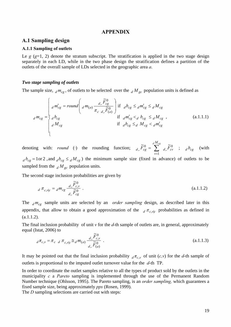
APPENDIX A.1 Sampling design A.1.1 Sampling of outlets

Le g (g=1, 2) denote the stratum subscript. The stratification is applied in the two stage design separately in each LD, while in the two phase design the stratification defines a partition of the outlets of the overall sample of LDs selected in the geographic area a.

Two stage sampling of outlets

The sample size, , of outlets to be selected over the population units is defined as cgd m gcd M

⎪⎪⎪

⎩

⎪⎪⎪

⎨

⎧

′<≤≤<′

≤′≤⎟⎟

⎠

⎞

⎜⎜

⎝

⎛=′

=

cgdcgdcgdcgd

cgdcgdcgdcgd

cgdcgdcgdadc

cgdadcgd

cgd

mMbMMbmb

MmbF

Fmroundm

m if if

if~

~

0)(,.

0,.

)(π

, (a.1.1.1)

denoting with: round (.) the rounding function; ; (with

) the minimum sample size (fixed in advance) of outlets to be sampled from the population units.

0,.

1

0,.

~~cvd

M

vcgd FF

cgd

∑=

= cgd b

cgdcgdcgd Mbb ≤= and,2or1

gcd M

The second stage inclusion probabilities are given by

0,.

0,,.

|, ~

~

cgd

vcdcgdcvcd

F

Fm=π . (a.1.1.2)

The sample units are selected by an order sampling design, as described later in this appendix, that allow to obtain a good approximation of the

cgd m

cvcd |,π probabilities as defined in (a.1.1.2).

The final inclusion probability of unit v for the d-th sample of outlets are, in general, approximately equal (Istat, 2006) to

vcd π , 0)(,.

0,,.

)(|, ~

~

ad

vcdadcvcdc

F

Fm≅= ππ . (a.1.1.3)

It may be pointed out that the final inclusion probability of unit (c,v) for the d-th sample of outlets is proportional to the imputed outlet turnover value for the d-th TP.

vcd π ,

In order to coordinate the outlet samples relative to all the types of product sold by the outlets in the municipality c a Pareto sampling is implemented through the use of the Permanent Random Number technique (Ohlsson, 1995). The Pareto sampling, is an order sampling, which guarantees a fixed sample size, being approximately pps (Rosen, 1999). The D sampling selections are carried out with steps:

19

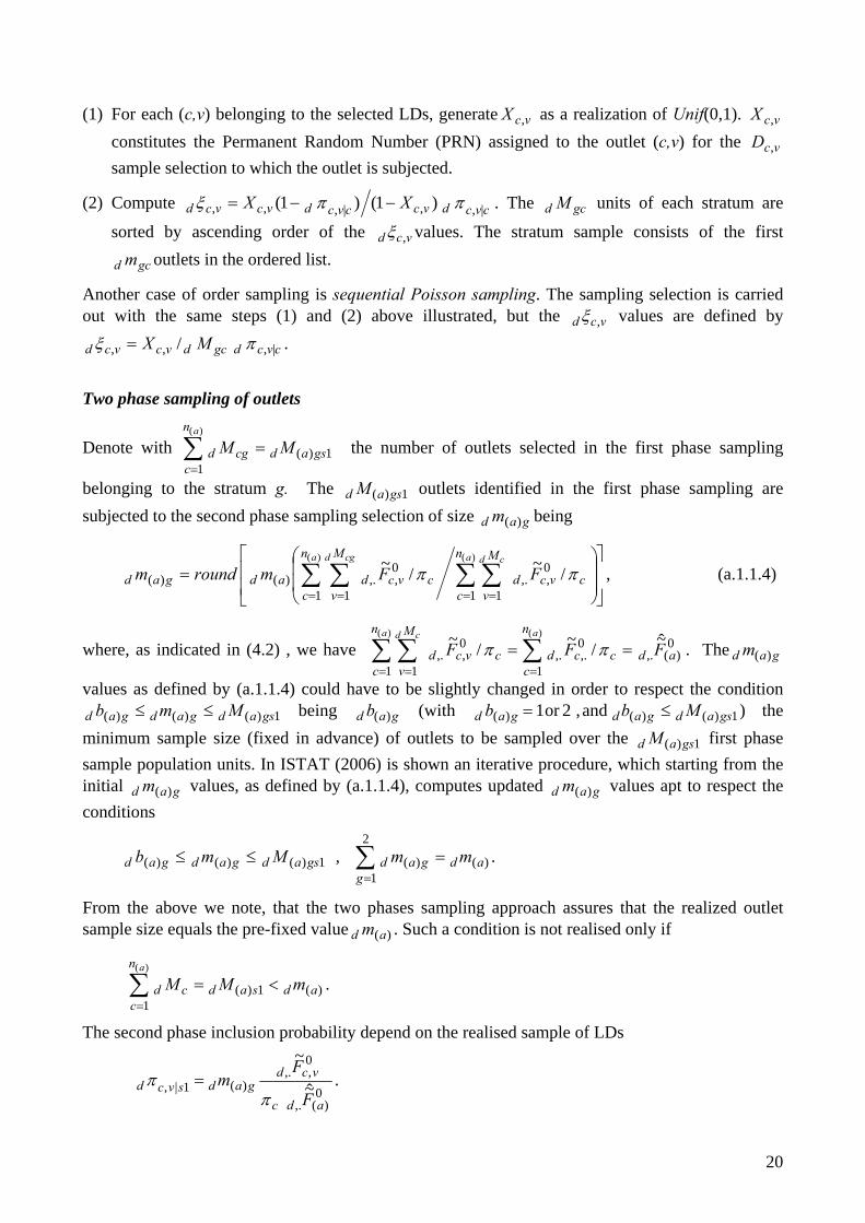
(1) For each (c,v) belonging to the selected LDs, generate as a realization of Unif(0,1). constitutes the Permanent Random Number (PRN) assigned to the outlet (c,v) for the sample selection to which the outlet is subjected.

vcX , vcX ,

vcD ,

(2) Compute cvcdvccvcdvcvcd XX |,,|,,, )1()1( ππξ −−= . The units of each stratum are

sorted by ascending order of the gcd M

vcd ,ξ values. The stratum sample consists of the first outlets in the ordered list. gcd m

Another case of order sampling is sequential Poisson sampling. The sampling selection is carried out with the same steps (1) and (2) above illustrated, but the vcd ,ξ values are defined by

cvcdgcdvcvcd MX |,,, / πξ = .

Two phase sampling of outlets

Denote with the number of outlets selected in the first phase sampling

belonging to the stratum g. The outlets identified in the first phase sampling are subjected to the second phase sampling selection of size being

1)(1

)(

gsad

n

ccgd MM

a

=∑=

1)( gsad M

gad m )(

⎥⎥

⎦

⎤

⎢⎢

⎣

⎡

⎟⎟

⎠

⎞

⎜⎜

⎝

⎛= ∑ ∑∑ ∑

= == =c

n

cvcd

M

vc

n

cvcd

M

vadgad

a cda cgd

FFmroundm ππ /~/~ )()(

1

0,,.

11

0,,.

1)()( , (a.1.1.4)

where, as indicated in (4.2) , we have . The

values as defined by (a.1.1.4) could have to be slightly changed in order to respect the condition being (with

∑∑ ∑== =

==)()(

1

0)(,.

0,.,.

1

0,,.

1

~̂/~/~ aa cd n

cadccdc

n

cvcd

M

vFFF ππ gad m )(

1)()()( gsadgadgad Mmb ≤≤ gad b )( 1)()()( and,2or1 gsadgadgad Mbb ≤= ) the minimum sample size (fixed in advance) of outlets to be sampled over the first phase sample population units. In ISTAT (2006) is shown an iterative procedure, which starting from the initial values, as defined by (a.1.1.4), computes updated values apt to respect the conditions

1)( gsad M

gad m )( gad m )(

, . 1)()()( gsadgadgad Mmb ≤≤ )(

2

1)( ad

ggad mm =∑

=

From the above we note, that the two phases sampling approach assures that the realized outlet sample size equals the pre-fixed value . Such a condition is not realised only if )(ad m

. )(1)(1

)(

adsad

n

ccd mMM

a

<=∑=

The second phase inclusion probability depend on the realised sample of LDs

0

)(,.

0,,.

)(1|, ~̂

~

adc

vcdgadsvcd

F

Fm

ππ = .

20

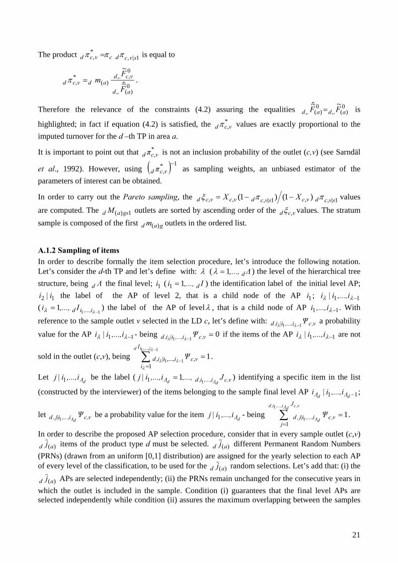
The product is equal to 1|,*, svcdcvcd πππ =

0

)(,.

0,,.

)(*, ~̂

~

ad

vcdadvcd

F

Fm=π .

Therefore the relevance of the constraints (4.2) assuring the equalities 0)(,.

0)(,.

~~̂adad FF = is

highlighted; in fact if equation (4.2) is satisfied, the values are exactly proportional to the imputed turnover for the d –th TP in area a.

*,vcdπ

It is important to point out that is not an inclusion probability of the outlet (c,v) (see Sarndäl

et al., 1992). However, using as sampling weights, an unbiased estimator of the parameters of interest can be obtained.

*,vcd π

( ) 1*,

−vcd π

In order to carry out the Pareto sampling, the 1|,,1|,,, )1()1( svcdvcsvcdvcvcd XX ππξ −−= values

are computed. The outlets are sorted by ascending order of the 1)( gsad M vcd ,ξ values. The stratum sample is composed of the first outlets in the ordered list. gad m )(

A.1.2 Sampling of items In order to describe formally the item selection procedure, let’s introduce the following notation. Let’s consider the d-th TP and let’s define with: λ ( Λ,..., d1=λ ) the level of the hierarchical tree structure, being the final level; (Λd 1i I,...,i d11 = ) the identification label of the initial level AP;

the label of the AP of level 2, that is a child node of the AP ; ( ) the label of the AP of level

12 i|i 1i 11 −λλ i,...,i|i

111

−=

λλ i,...,id I,...,i λ , that is a child node of AP . With

reference to the sample outlet v selected in the LD c, let’s define with: a probability

value for the AP - being

11 −λi,...,i

v,ci,...,i|i,d Ψ11 −λλ

11 −λλ i,...,i|i 011

=− v,ci,...,i|i,d Ψ

λλ if the items of the AP are not

sold in the outlet (c,v), being .

11 −λλ i,...,i|i

11,...,1

111

,,...,|, =∑−

−=

λ

λλλ

iid I

ivciiid Ψ

Let be the label (dΛi,...,i|j 1 v,ci,...,i,dΛ J,...,i,...,i|j

dΛd 111 = ) identifying a specific item in the list

(constructed by the interviewer) of the items belonging to the sample final level AP ;

let be a probability value for the item - being .

11 −dd ΛΛ i,...,i|i

v,ci,...,i|j,d ΨdΛ1 dΛi,...,i|j 1 1

1

11

=∑=

v,cdΛi,...,i,d

dΛ

J

jv,ci,...,i|j,d Ψ

In order to describe the proposed AP selection procedure, consider that in every sample outlet (c,v) )(ad j items of the product type d must be selected. )(ad j different Permanent Random Numbers

(PRNs) (drawn from an uniform [0,1] distribution) are assigned for the yearly selection to each AP of every level of the classification, to be used for the )(ad j random selections. Let’s add that: (i) the

)(ad j APs are selected independently; (ii) the PRNs remain unchanged for the consecutive years in which the outlet is included in the sample. Condition (i) guarantees that the final level APs are selected independently while condition (ii) assures the maximum overlapping between the samples

21

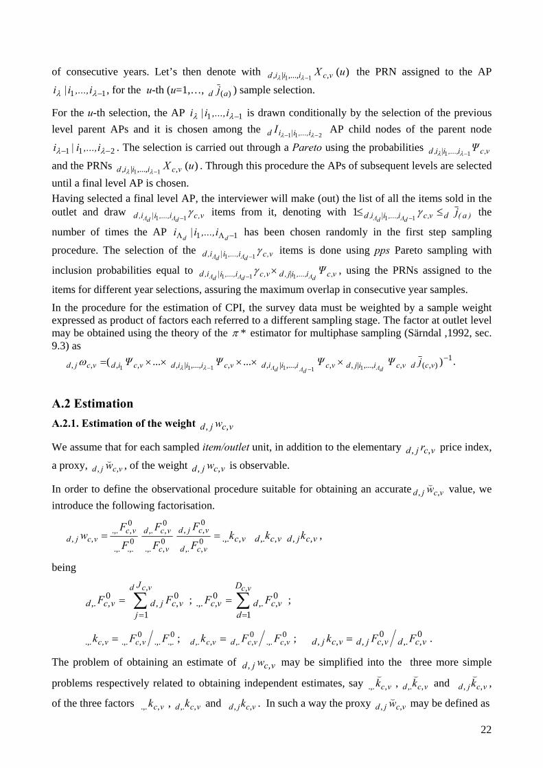
of consecutive years. Let’s then denote with the PRN assigned to the AP

, for the u-th (u=1,…,

)(,,...,|, 11uX vciiid −λλ

11 −λλ i,...,i|i )(ad j ) sample selection.

For the u-th selection, the AP is drawn conditionally by the selection of the previous level parent APs and it is chosen among the AP child nodes of the parent node

. The selection is carried out through a Pareto using the probabilities

and the PRNs . Through this procedure the APs of subsequent levels are selected until a final level AP is chosen.

11 −λλ i,...,i|i

211 −− λλ i,...,i|id I

211 −− λλ i,...,i|i v,ci,...,i|i,d Ψ11 −λλ

)(,,...,|, 11uX vciiid −λλ

Having selected a final level AP, the interviewer will make (out) the list of all the items sold in the outlet and draw v,ci,...,i|i,d dΛdΛ

γ11 −

items from it, denoting with )a(dv,ci,...,i|i,d jdΛdΛ

≤≤−γ

111 the

number of times the AP has been chosen randomly in the first step sampling

procedure. The selection of the 11 −ΛΛ dd

i,...,i|i

v,ci,...,i|i,d dΛdΛγ

11 − items is done using pps Pareto sampling with

inclusion probabilities equal to v,ci,...,i|i,d dΛdΛγ

11 −× , using the PRNs assigned to the

items for different year selections, assuring the maximum overlap in consecutive year samples. v,ci,...,i|j,d Ψ

dΛ1

In the procedure for the estimation of CPI, the survey data must be weighted by a sample weight expressed as product of factors each referred to a different sampling stage. The factor at outlet level may be obtained using the theory of the *π estimator for multiphase sampling (Särndal ,1992, sec. 9.3) as 1

),(,,...,|,,,...,|,,,...,|,,,,, )......(111111

−×××××=−− vcdvciijdvciiidvciiidvcidvcjd jΨΨΨΨ

dΛdΛdΛλλω .

A.2 Estimation A.2.1. Estimation of the weight vcjd w ,,

We assume that for each sampled item/outlet unit, in addition to the elementary price index,

a proxy, vcjd r ,,

vcjd w ,,( , of the weight is observable. vcjd w ,,

In order to define the observational procedure suitable for obtaining an accurate vcjd w ,,( value, we

introduce the following factorisation.

0,,.

0,,

0,.,.

0,,.

0.,..,.

0,.,.

,,vcd

vcjd

vc

vcdvcvcjd

F

F

F

F

F

Fw = vcjdvcdvc kkk ,,,,.,.,.= ,

being

; ; ∑=

=vcd J

jvcjdvcd FF

,

1

0,,

0,,. ∑

=

=vcD

dvcdvc FF

,

1

0,,.

0,.,.

0.,..,.

0,.,.,.,. FFk vcvc = ; 0

,.,.0,,.,,. vcvcdvcd FFk = ; 0

,,.0,,,, vcdvcjdvcjd FFk = .

The problem of obtaining an estimate of may be simplified into the three more simple

problems respectively related to obtaining independent estimates, say

vcjd w ,,

vcdvc kk ,,.,.,. ,((

and vcjd k ,,(

,

of the three factors and . In such a way the proxy vcdvc kk ,,.,.,. , vcjd k ,, vcjd w ,,( may be defined as

22

vcjdvcdvcvcjd kkkw ,,,,.,.,.,,(((( = .

The first factor representing the quota part of the turnover of the outlet (c,v) over the total

turnover may be simply estimated with the SF data as vck ,.,.

0.,..,.

0,.,.,.,.

~~ FFk vcvc =(

.

The other two factors ( ) - that represent respectively (i) the quota part of the d-th TP turnover of the (c,v)-th outlet over the total turnover of the (c,v)-th outlet and (ii) the quota part of the turnover of the item/outlet (d,j,c,v) over the d-th TP turnover of the (c,v)-th outlet - have to be estimated only for the sample outlets. The accuracy of the estimates of the two factors is strictly dependent by the informative context characterising the sample outlet. For example in the case of a supermarket, with an informative system recording the turnover of each bar-code, the factors

may be known by a proper software implementation. In a small outlet case, the person in charge of the outlet could be able to furnish accurate proxies. As a general statement, the accuracy of the information collected via a proper interview should be greater for the second factor than that attainable for the third one, which requires a more detailed acquaintance.

vcjdvcd kk ,,,,. and

vcjdvcd kk ,,,,. e

If no other information is available, the second factor may be estimated by means of the imputed SF data as 0

,.,.0,,.,,.

~~vcvcdvcd FFk =

(. The third factor may be determined by the information collected

during the phase of item selection; in general it may be defined as vcjdadvcjd jk ,,)(,, / ω=(

.

A.2.2. Estimation of the national index

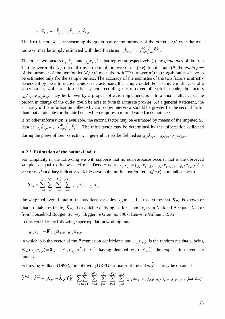
For simplicity in the following we will suppose that no non-response occurs, that is the observed sample is equal to the selected one. Denote with ),...,,...,( ,,,,,,1,,,,, ′= Pvcjdpvcjdvcjdvcjd xxxx a vector of P auxiliary indicator variables available for the item/outlet (d,j,c,v), and indicate with

∑ ∑ ∑ ∑= = = =

=N

c

M

v

D

d

J

jvcjdvcjd

c vc vcd

w1 1 1 1

,,,,W

, ,

xX

the weighted overall total of the auxiliary variables . Let us assume that is known or

that a reliable estimate, , is available deriving, as for example, from National Account Data or from Household Budget Survey (Biggeri e Giommi, 1987; Leaver e Valliant, 1995).

vcjd w ,, WX

WX&&

Let us consider the following superpopulation working model

vcjdvcjdvcjd r ,,,,,, η+′= xβ

in which β is the vector of the P regression coefficients and vcjd ,, η is the random residuals, being

0)(E ,vc,m =jd η ; having denoted with 22,,m )(E ση ≅vcjd ( )⋅mE the expectation over the

model.

Following Valliant (1999), the following GREG estimator of the index 1,0~I , may be obtained

+= 1,01,0 ˆ~ II ∑ ∑ ∑∑∑∑= = === =

=′−)( )(

1 1 1,,,,,,,,

2

11 1WW

ˆ)ˆ(ad cgd adn

c

m

v

j

jvcjdvcjdvcjdvcjd

g

A

a

D

drwa (&& γβXX , (a.2.2.1)

23

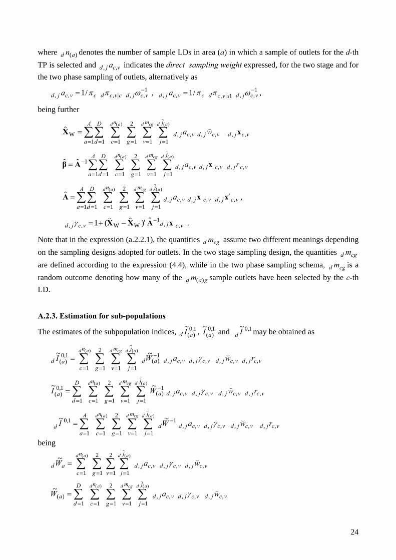
where denotes the number of sample LDs in area (a) in which a sample of outlets for the d-th TP is selected and indicates the direct sampling weight expressed, for the two stage and for the two phase sampling of outlets, alternatively as

)(ad n

vcjd a ,,

, , 1,,|,,, /1 −= vcjdcvcdcvcjd a ωππ 1

,,1|,,, /1 −= vcjdsvcdcvcjd a ωππ

being further

∑ ∑ ∑∑∑∑= = === =

=)( )(

1 1 1,,,,,,

2

11 1W

ˆad cgd adn

c

m

v

j

jvcjdvcjdvcjd

g

A

a

D

dwa xX (

∑ ∑ ∑∑∑∑= = === =

−=)( )(

1 1 1,,,,,,

2

11 1

1ˆˆad cgd adn

c

m

v

j

jvcjdvcjdvcjd

g

A

a

D

dra xAβ

∑ ∑ ∑∑∑∑= = === =

′=)( )(

1 1 1,,,,,,

2

11 1

ˆad cgd adn

c

m

v

j

jvcjdvcjdvcjd

g

A

a

D

da xxA ,

. vcjdvcjd ,,1

WW,,ˆ)ˆ(1 xAXX −′−+= &&γ

Note that in the expression (a.2.2.1), the quantities assume two different meanings depending on the sampling designs adopted for outlets. In the two stage sampling design, the quantities are defined according to the expression (4.4), while in the two phase sampling schema, is a random outcome denoting how many of the sample outlets have been selected by the c-th LD.

cgd m

cgd m

cgd m

gad m )(

A.2.3. Estimation for sub-populations

The estimates of the subpopulation indices, 1,0)(

~ad I , 1,0

)(~

aI and 1,0~Id may be obtained as

∑ ∑ ∑∑= = =

−

=

=)( )(

1 1 1,,,,,,,,

1)(

2

1

1,0)(

~~ ad cgd adn

c

m

v

j

jvcjdvcjdvcjdvcjdad

gad rwaWI (γ

∑ ∑ ∑∑∑= = =

−

==

=)( )(

1 1 1,,,,,,,,

1)(

2

11

1,0)(

~~ ad cgd adn

c

m

v

j

jvcjdvcjdvcjdvcjda

g

D

da rwaWI (γ

∑ ∑ ∑∑∑= = =

−

==

=)( )(

1 1 1,,,,,,,,

12

11

1,0 ~~ ad cgd adn

c

m

v

j

jvcjdvcjdvcjdvcjdd

g

A

ad rwaWI (γ

being

∑ ∑ ∑∑= = ==

=)( )(

1

2

1 1,,,,,,

2

1

~ ad adn

c v

j

jvcjdvcjdvcjd

gad waW (γ

∑ ∑ ∑∑∑= = ===

=)( )(

1 1 1,,,,,,

2

11)(

~ ad cgd adn

c

m

v

j

jvcjdvcjdvcjd

g

D

da waW (γ

24

∑ ∑ ∑∑∑= = ===

=)( )(

1 1 1,,,,,,

2

11

~ ad cgd adn

c

m

v

j

jvcjdvcjdvcjd

g

A

ad waW (γ .

25