Embed Size (px)
Citation preview
13/3/2013
1
Topic 2 Introduction to RF
Fundamentals 1 hour
Definition of RF
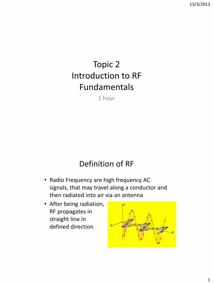
• Radio Frequency are high frequency AC signals, that may travel along a conductor and then radiated into air via an antenna
• After being radiation, RF propagates in straight line in defined direction
13/3/2013
2
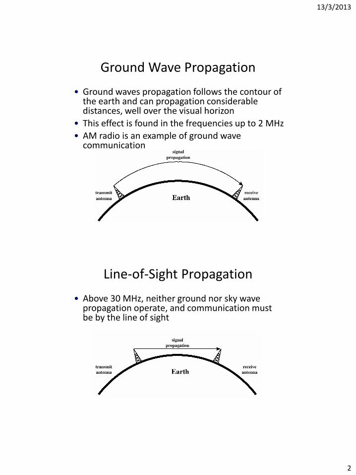
Ground Wave Propagation
• Ground waves propagation follows the contour of the earth and can propagation considerable distances, well over the visual horizon
• This effect is found in the frequencies up to 2 MHz
• AM radio is an example of ground wave communication
Line-of-Sight Propagation
• Above 30 MHz, neither ground nor sky wave propagation operate, and communication must be by the line of sight
13/3/2013
3
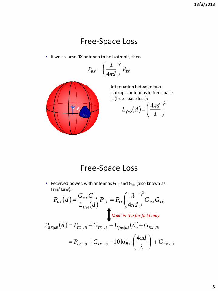
Free-Space Loss
• If we assume RX antenna to be isotropic, then
TXRX Pd
P
2
4
Attenuation between two isotropic antennas in free space is (free-space loss):
2
4
ddL free
Free-Space Loss
• Received power, with antennas GTX and GRX (also known as Friis’ Law):
TXRXTXTX
free
TXRXRX GG
dPP
dL
GGdP
2
4
dBRXdBTXdBTX
dBRXdBfreedBTXdBTXdBRX
Gd
GP
GdLGPdP
2
10
4log10
Valid in the far field only
13/3/2013
4
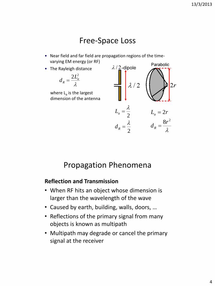
Free-Space Loss
• Near field and far field are propagation regions of the time-varying EM energy (or RF)
• The Rayleigh distance
22 aR
Ld
where La is the largest dimension of the antenna
2
2
R
a
d
L
28
2
rd
rL
R
a
Propagation Phenomena
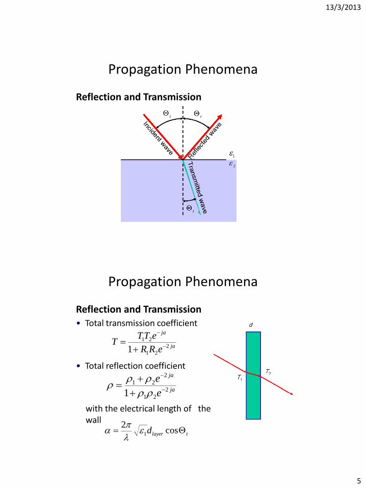
Reflection and Transmission
• When RF hits an object whose dimension is larger than the wavelength of the wave
• Caused by earth, building, walls, doors, …
• Reflections of the primary signal from many objects is known as multipath
• Multipath may degrade or cancel the primary signal at the receiver
13/3/2013
5
Propagation Phenomena
Reflection and Transmission
Propagation Phenomena
Reflection and Transmission • Total transmission coefficient
• Total reflection coefficient
with the electrical length of the wall
ja
ja
eRR
eTTT
2
21
21
1
ja
ja
e
e2
21
2
21
1
tlayerd cos2
1
13/3/2013
6
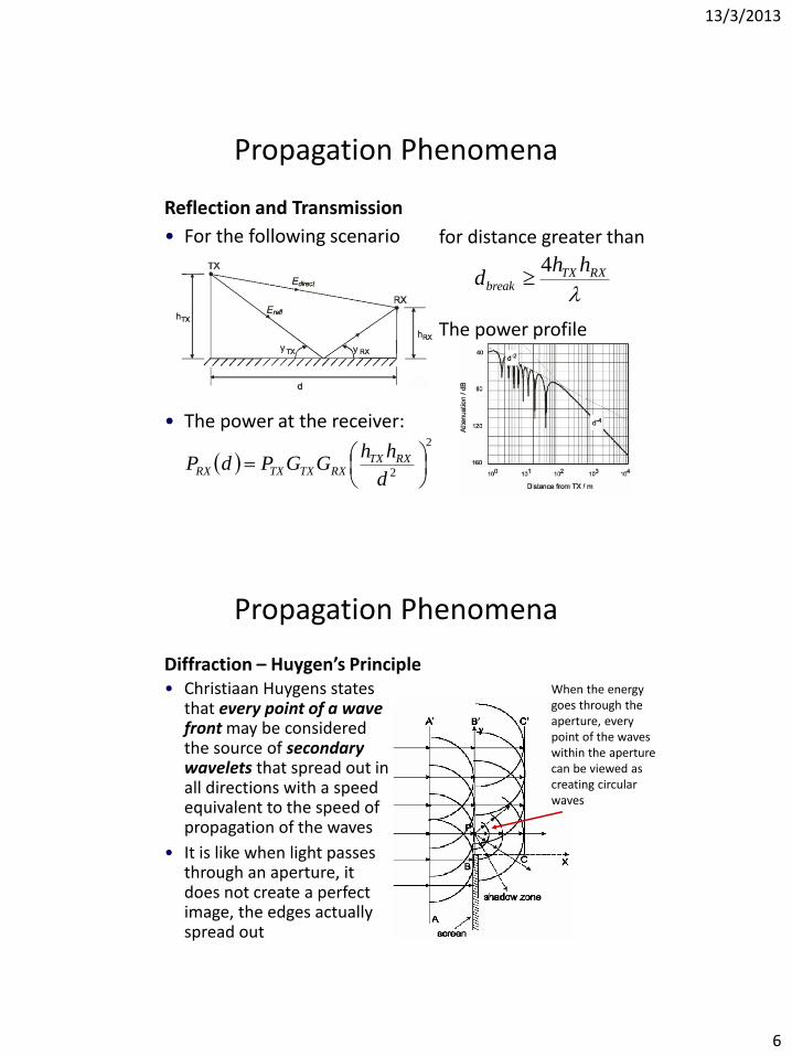
for distance greater than
The power profile
Propagation Phenomena
Reflection and Transmission
• For the following scenario
• The power at the receiver:
2
2
d
hhGGPdP RXTX
RXTXTXRX
RXTX
break
hhd
4
Propagation Phenomena
• Christiaan Huygens states
that every point of a wave front may be considered the source of secondary wavelets that spread out in all directions with a speed equivalent to the speed of propagation of the waves
• It is like when light passes through an aperture, it does not create a perfect image, the edges actually spread out
Diffraction – Huygen’s Principle When the energy goes through the aperture, every point of the waves within the aperture can be viewed as creating circular waves
13/3/2013
7
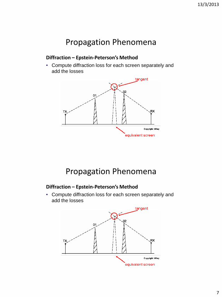
Propagation Phenomena
• Compute diffraction loss for each screen separately and
add the losses
Diffraction – Epstein-Peterson’s Method
Propagation Phenomena
• Compute diffraction loss for each screen separately and
add the losses
Diffraction – Epstein-Peterson’s Method
13/3/2013
8
Propagation Phenomena
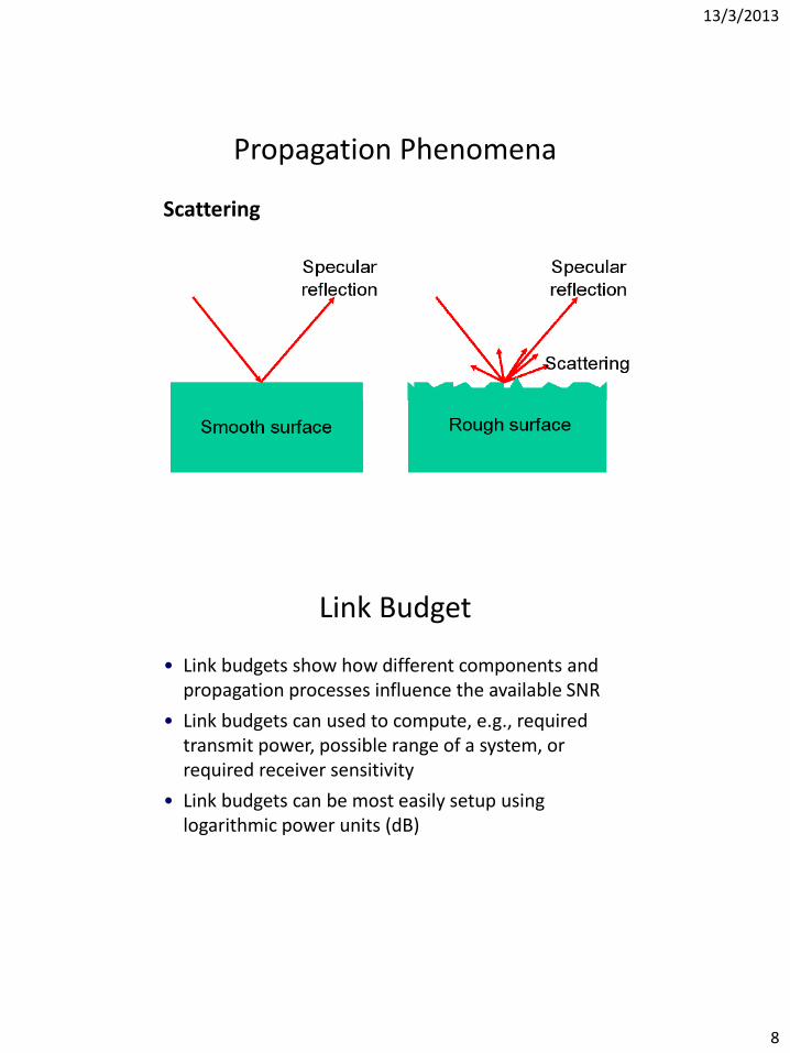
Scattering
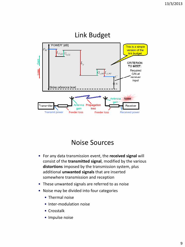
Link Budget
• Link budgets show how different components and propagation processes influence the available SNR
• Link budgets can used to compute, e.g., required transmit power, possible range of a system, or required receiver sensitivity
• Link budgets can be most easily setup using logarithmic power units (dB)
13/3/2013
9
Link Budget
Transmit power Received power Feeder loss Feeder loss
Noise Sources
• For any data transmission event, the received signal will consist of the transmitted signal, modified by the various distortions imposed by the transmission system, plus additional unwanted signals that are inserted somewhere transmission and reception
• These unwanted signals are referred to as noise
• Noise may be divided into four categories
• Thermal noise
• Inter-modulation noise
• Crosstalk
• Impulse noise
13/3/2013
10
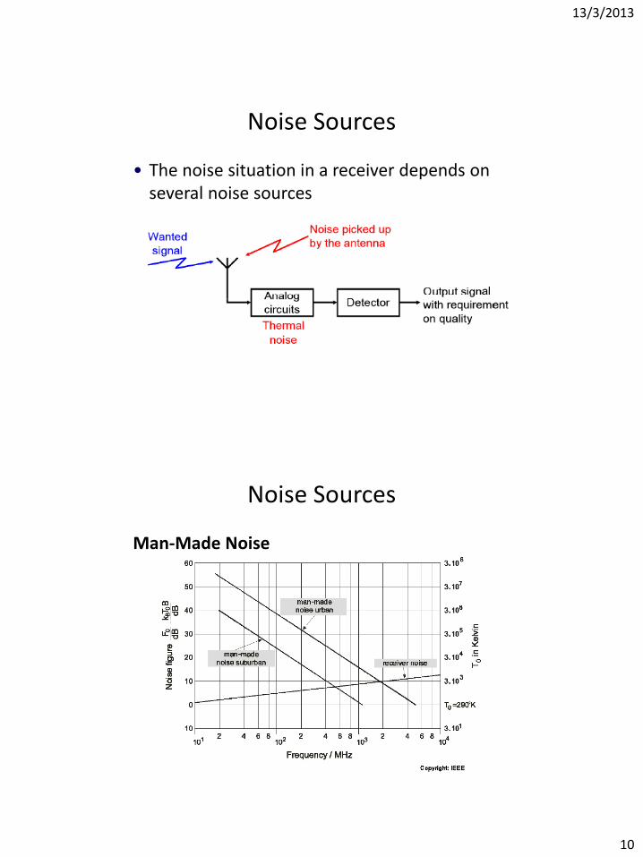
Noise Sources
• The noise situation in a receiver depends on several noise sources
Noise Sources
Man-Made Noise

13/3/2013
11
Noise Sources
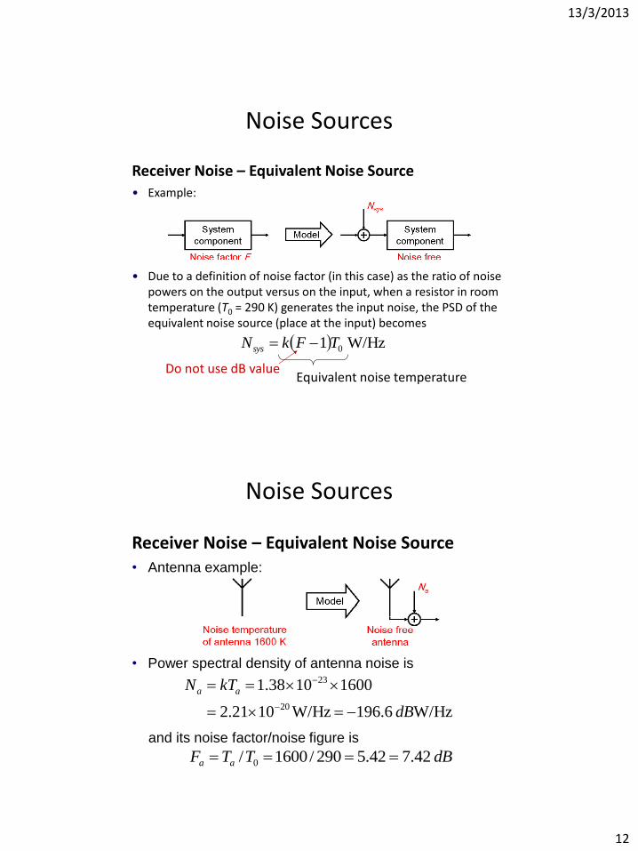
Receiver Noise – Equivalent Noise Source
• The noise situation in a receiver depends on several noise sources
Noise Sources
Receiver Noise – Equivalent Noise Source • The power spectral density of a noise source is usually given
in one of the following three ways
• Directly [W/Hz] Ns
• Noise temperature [Kelvin] Ts
• Noise factor Fs
• The relation between the three is
where k is the Boltzmann’s constant (1.38 10–23 W/Hz) and T0 is the room temperature (290 K or 17C)
0TkFkTN sss
Noise factor is sometimes given in dB which is known as noise figure
13/3/2013
12
Receiver Noise – Equivalent Noise Source
• Example:
• Due to a definition of noise factor (in this case) as the ratio of noise powers on the output versus on the input, when a resistor in room temperature (T0 = 290 K) generates the input noise, the PSD of the equivalent noise source (place at the input) becomes
Noise Sources
W/Hz1 0TFkNsys
Do not use dB value Equivalent noise temperature
Noise Sources
Receiver Noise – Equivalent Noise Source • Antenna example:
• Power spectral density of antenna noise is
and its noise factor/noise figure is
W/Hz 6.196W/Hz1021.2
16001038.1
20
23
dB
kTN aa
dBTTF aa 42.742.5290/1600/ 0
13/3/2013
13
Noise Sources
W/Hz1 0TFkNsys
Do not use dB value Equivalent noise temperature
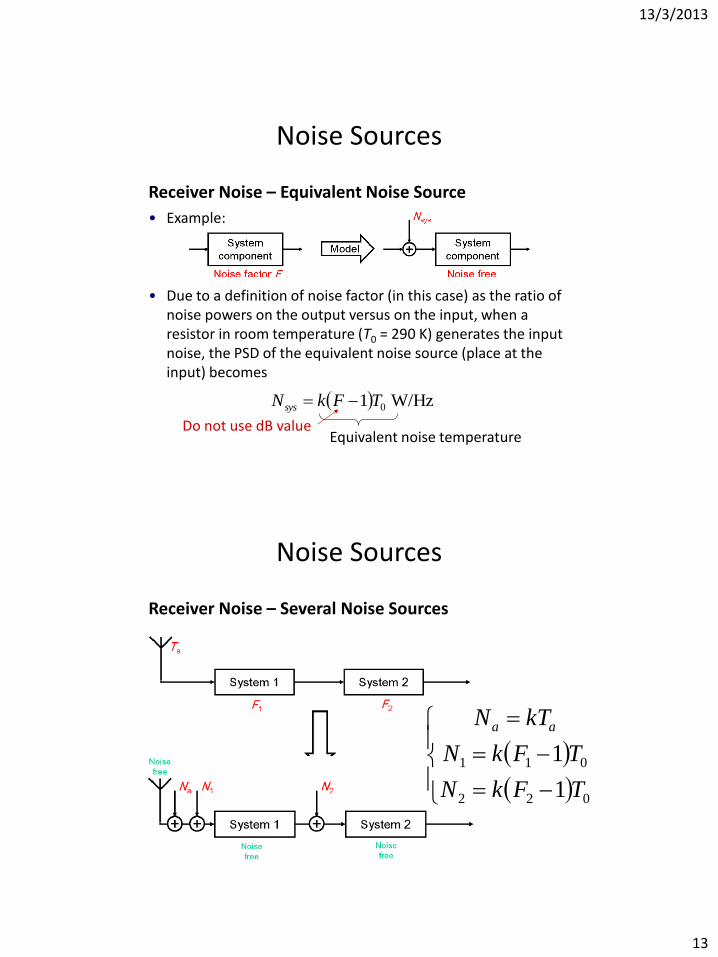
Receiver Noise – Equivalent Noise Source
• Example:
• Due to a definition of noise factor (in this case) as the ratio of noise powers on the output versus on the input, when a resistor in room temperature (T0 = 290 K) generates the input noise, the PSD of the equivalent noise source (place at the input) becomes
Receiver Noise – Several Noise Sources
Noise Sources
022
011
1
1
TFkN
TFkN
kTN aa