Embed Size (px)
Citation preview
arX
iv:1
707.
0741
2v1
[cs
.IT
] 2
4 Ju
l 201
71
Wireless Powered Cooperative Jamming for Secure
OFDM SystemGuangchi Zhang, Jie Xu, Qingqing Wu, Miao Cui, Xueyi Li, and Fan Lin
Abstract—This paper studies the secrecy communication inan orthogonal frequency division multiplexing (OFDM) system,where a source sends confidential information to a destinationin the presence of a potential eavesdropper. We employ wirelesspowered cooperative jamming to improve the secrecy rate ofthis system with the assistance of a cooperative jammer, whichworks in the harvest-then-jam protocol over two time-slots. In thefirst slot, the source sends dedicated energy signals to power thejammer; in the second slot, the jammer uses the harvested energyto jam the eavesdropper, in order to protect the simultaneoussecrecy communication from the source to the destination. Inparticular, we consider two types of receivers at the destination,namely Type-I and Type-II receivers, which do not have andhave the capability of canceling the (a-priori known) jammingsignals, respectively. For both types of receivers, we maximizethe secrecy rate at the destination by jointly optimizing thetransmit power allocation at the source and the jammer oversub-carriers, as well as the time allocation between the twotime-slots. First, we present the globally optimal solution to thisproblem via the Lagrange dual method, which, however, is of highimplementation complexity. Next, to balance tradeoff between thealgorithm complexity and performance, we propose alternativelow-complexity solutions based on minorization maximizationand heuristic successive optimization, respectively. Simulationresults show that the proposed approaches significantly improvethe secrecy rate, as compared to benchmark schemes withoutjoint power and time allocation.
Index Terms—Physical layer security, wireless powered coop-erative jamming, OFDM system, joint power and time allocation.
I. INTRODUCTION
With recent technical advancements in Internet of things
(IoT), future wireless networks are envisioned to incorporate
billions of low-power wireless devices to enable various
industrial and commercial applications [1]. How to ensure
the confidentiality of these devices’ wireless communication
against illegitimate eavesdropping attacks is becoming an in-
creasingly important task for cyber-physical security. However,
this task is particularly challenging, as conventional key-based
cryptographic techniques are difficult to be implemented due to
the broadcast nature of wireless communications. To overcome
this issue, physical layer security has emerged as a viable anti-
eavesdropping solution at the physical layer [2]–[4]. The key
design objective in physical-layer security is to maximize the
G. Zhang, J. Xu, M. Cui, and X. Li are with the School of InformationEngineering, Guangdong University of Technology, Guangzhou, China (e-mail: [email protected], [email protected], [email protected], [email protected]). J. Xu is the corresponding author.
Q. Wu is with the Department of Electrical and Computer Engineering,National University of Singapore (e-mail: [email protected]).
F. Lin is with Guangzhou GCI Science & Technology Co., Ltd., Guangzhou,China (e-mail: [email protected]).
so-called secrecy rate, which is defined as the communication
rate of a wireless channel, provided that eavesdroppers cannot
overhear any information from this channel.
In the literature, there have been various approaches pro-
posed to improve the secrecy rate. For example, one widely
adopted approach is based on the idea of artificial noise (AN)
(see, e.g., [5], [6]). In this approach, wireless transmitters send
a combined version of both confidential information signals
and AN, where the AN acts as jamming signals to interfere
with eavesdroppers, thus avoiding the information leakage.
Another celebrated approach is called cooperative jamming
(see, e.g., [7]–[9]), where external network nodes coopera-
tively send jamming signals to disrupt the eavesdropping, thus
helping protect the confidential information communication.
As compared to the AN-based approach, cooperative jamming
is able to further improve the secrecy rate by exploiting
the cooperation diversity among different nodes. Cooperative
jamming is also expected to have more abundant applications
in the IoT era, where massive low-power wireless devices
can cooperate in jamming to improve the network security.
For instance, some idle devices in wireless networks can
act as cooperative jammers to help ensuring the secrecy
communication of other actively communicating devices.
Nevertheless, the practical implementation of cooperative
jamming in IoT networks is hindered by the low-power nature
of wireless devices, since cooperative jamming will consume
energy on these devices and thus they may prefer keeping
idle to save energy instead of involving in the cooperation. To
overcome this issue, a new efficient method, namely wireless
powered cooperative jamming, has been proposed in [10]–
[13] motivated by the recent success of wireless information
and power transfer via radio frequency (RF) signals [14]–
[26].1 In this method, the cooperative jamming is powered
by the wireless energy transferred from external wireless
transmitters, and does not require cooperative jammers to
consume their own energy. Therefore, wireless powered co-
operative jamming is a promising solution to inspire low-
power IoT devices to cooperate in the jamming. In [10],
[11], wireless powered cooperative jamming was employed to
secure a point-to-point communication system in the presence
1It is worth noting that in addition to the far-field RF-based wireless powertransfer, magnetic induction is a widely used near-field wireless power transfertechnique for charging electronic devices [22], [26]. However, the magneticinduction has a limited operating range of less than one meter in general,which is much shorter than that of the RF-based wireless power transferin the order of several meters. Therefore, RF-based wireless power transferis expected to have more abundant applications to charge low-power IoTdevices in a wide range, and thus is considered here in the wireless poweredcooperative jamming systems.
2
of an eavesdropper, where a cooperative jammer operates in an
accumulate-and-jam protocol by first harvesting the wireless
energy and storing in the battery over multiple blocks and
then using the accumulated energy for cooperative jamming.
The long-term secrecy performance is optimized by adjusting
jamming parameters while taking into account the channel and
battery dynamics over time. In [12], [13], wireless powered
cooperative jamming was used in a secrecy two-way relaying
communication system, where an eavesdropper aims to inter-
cept the communicated information at the second hop, and
more than one cooperative jammers operate in a harvest-then-
jam protocol for cooperative jamming: in the first slot, the
jammers harvest the wireless energy from the source, while in
the second slot, they use the harvested energy to cooperatively
jam the eavesdroppers. As the harvested energy is immediately
used in the following slot, the harvest-then-jam protocol does
not require large-capacity energy storages nor sophisticated
energy management at cooperative jammers. For this reason,
it is generally much easier to be implemented in practice than
the accumulate-and-jam protocol.
In this paper, we consider wireless powered cooperative
jamming to secure a point-to-point communication system
from a source to a destination with the presence of a potential
eavesdropper. Different from prior works considering single-
carrier systems, we focus on the multi-carrier orthogonal
frequency division multiplexing (OFDM) system, which of-
fers the following advantages. First, note that the wireless
transmission must meet the transmit power spectrum density
constraints imposed by regulatory authorities. In this case,
the transferred power over a narrow-band system is often
limited. By contrast, using OFDM over a wideband wireless
power transfer system and exploiting the channel diversity
over frequency can help deliver more power to intended
receivers. On the other hand, as OFDM has been widely
adopted in major existing and future wireless communication
networks, using it here can also help better integrate wireless
power transfer and wireless communication for future wireless
networks (see, e.g., [26]–[30] and references therein). The
cooperative jammer works in a harvest-then-jam protocol to
help the secrecy communication by dividing each transmission
block into two time-slots: in the first slot, the source sends
dedicated energy signals to power the jammer; while in the
second slot, the jammer uses the harvested energy to interfere
with the eavesdropper to protect the confidential information
transmission.
In general, there exists a tradeoff in the time allocation
between the two slots to optimize the performance of secrecy
communication, i.e., while a longer WPT time in the first
slot can transfer more energy to increase the jamming power
for better confusing the eavesdropper, it can also reduce
the efficient wireless information transmission (WIT) time in
the second slot for delivering confidential data. Therefore,
in order to improve the secrecy rate at the destination by
maximally exploring the benefit of wireless power cooperative
jamming, it is important to jointly design the time allocation,
together with the transmit power allocation at the source
and the jammer over sub-carriers, by taking into account the
energy harvesting constraint at the jammer. We maximize the
secrecy rate via joint time and power allocation by particularly
considering two types of receivers at the destination, namely
Type-I and Type-II receivers, which do not have and have
the capability of canceling the (a-priori known) jamming
signals, respectively (see Section II for the details). Under
both receiver types, however, the two joint time and power
allocation problems are non-convex and usually difficult to
be solved. To tackle such challenges, we propose to recast
each problem into a two-layer form, in which the outer layer
corresponds to a single-variable time allocation problem and
the inner layer is a sub-carrier transmit power allocation
problem under given time allocation. The outer layer time
allocation problem is solved via a one-dimension search. As
for the inner-layer power allocation problem, we first present
the globally optimal solution via the Lagrange dual method,
which, however, is of high implementation complexity. Next,
to balance the tradeoff between the implementation complexity
and the performance, we further develop two suboptimal
solutions based on minorization maximization and heuristic
successive optimization, respectively. Simulation results show
that the proposed approaches achieve significantly higher
secrecy rate than benchmark schemes without joint time and
power allocation, and the minorization maximization based
suboptimal solution achieves a near optimal performance as
compared to the optimal solution.
It is worth noting that in the literature, there have been
several existing works [28]–[30] investigating the physical
layer security over OFDM systems. For example, the secrecy
rate of OFDM systems was investigated in [28] under a
Rayleigh fading channel setup without using AN or coopera-
tive jamming. In [29] and [30], the AN-based approach and
cooperative jamming were considered to improve the secrecy
rate of OFDM systems, respectively. Different from these prior
studies, in this paper the cooperative jamming is powered by
WPT, and thus requires a more sophisticated design with joint
time and power allocation for both WPT and jamming. This
is new and has not been addressed.
The remainder of the paper is organized as follows. Section
II presents the system model and problem formulation. Sec-
tions III and IV propose three efficient approaches to obtain
solutions to the two joint time and power allocation problems
with Type-I and Type-II destination receivers, respectively.
Section V presents simulation results to validate the perfor-
mance of our proposed joint design as compared to other
benchmark schemes. Finally, Section VI concludes this paper.
II. SYSTEM MODEL AND PROBLEM FORMULATION
A. System Model
As shown in Fig. 1, we consider secrecy communication
in an OFDM system with a source communicating with a
destination in the presence of a potential eavesdropper. We
employ wireless powered cooperative jamming to secure this
system, where a cooperative jammer uses the transferred
energy from the source to help jam the eavesdropper against
its eavesdropping. Suppose that the OFDM system consists
of a total of N orthogonal sub-carriers, and denote the set of
sub-carriers as N , {1, 2, . . . , N}. We consider a block-based
3
!"#$% &%'()*+()!*
,+-%'.#!//%#0+11%#
0
&
,
!,
!&
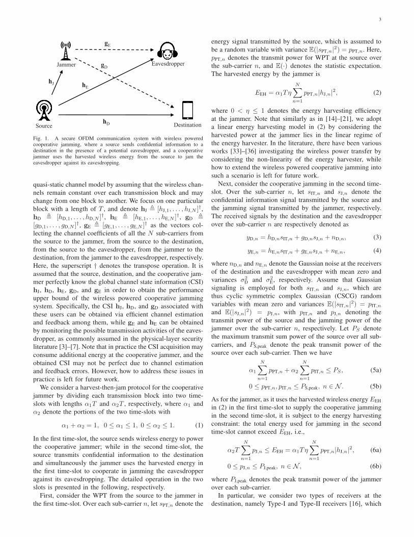
Fig. 1. A secure OFDM communication system with wireless poweredcooperative jamming, where a source sends confidential information to adestination in the presence of a potential eavesdropper, and a cooperativejammer uses the harvested wireless energy from the source to jam theeavesdropper against its eavesdropping.
quasi-static channel model by assuming that the wireless chan-
nels remain constant over each transmission block and may
change from one block to another. We focus on one particular
block with a length of T , and denote hJ , [hJ,1, . . . , hJ,N ]†,
hD , [hD,1, . . . , hD,N ]†, hE , [hE,1, . . . , hE,N ]†, gD ,
[gD,1, . . . , gD,N ]†, gE , [gE,1, . . . , gE,N ]† as the vectors col-
lecting the channel coefficients of all the N sub-carriers from
the source to the jammer, from the source to the destination,
from the source to the eavesdropper, from the jammer to the
destination, from the jammer to the eavesdropper, respectively.
Here, the superscript † denotes the transpose operation. It is
assumed that the source, destination, and the cooperative jam-
mer perfectly know the global channel state information (CSI)
hJ, hD, hE, gD, and gE in order to obtain the performance
upper bound of the wireless powered cooperative jamming
system. Specifically, the CSI hJ, hD, and gD associated with
these users can be obtained via efficient channel estimation
and feedback among them, while gE and hE can be obtained
by monitoring the possible transmission activities of the eaves-
dropper, as commonly assumed in the physical-layer security
literature [3]–[7]. Note that in practice the CSI acquisition may
consume additional energy at the cooperative jammer, and the
obtained CSI may not be perfect due to channel estimation
and feedback errors. However, how to address these issues in
practice is left for future work.
We consider a harvest-then-jam protocol for the cooperative
jammer by dividing each transmission block into two time-
slots with lengths α1T and α2T , respectively, where α1 and
α2 denote the portions of the two time-slots with
α1 + α2 = 1, 0 ≤ α1 ≤ 1, 0 ≤ α2 ≤ 1. (1)
In the first time-slot, the source sends wireless energy to power
the cooperative jammer; while in the second time-slot, the
source transmits confidential information to the destination
and simultaneously the jammer uses the harvested energy in
the first time-slot to cooperate in jamming the eavesdropper
against its eavesdropping. The detailed operation in the two
slots is presented in the following, respectively.
First, consider the WPT from the source to the jammer in
the first time-slot. Over each sub-carrier n, let sPT,n denote the
energy signal transmitted by the source, which is assumed to
be a random variable with variance E(|sPT,n|2) = pPT,n. Here,
pPT,n denotes the transmit power for WPT at the source over
the sub-carrier n, and E(·) denotes the statistic expectation.
The harvested energy by the jammer is
EEH = α1Tη
N∑
n=1
pPT,n|hJ,n|2, (2)
where 0 < η ≤ 1 denotes the energy harvesting efficiency
at the jammer. Note that similarly as in [14]–[21], we adopt
a linear energy harvesting model in (2) by considering the
harvested power at the jammer lies in the linear regime of
the energy harvester. In the literature, there have been various
works [33]–[36] investigating the wireless power transfer by
considering the non-linearity of the energy harvester, while
how to extend the wireless powered cooperative jamming into
such a scenario is left for future work.
Next, consider the cooperative jamming in the second time-
slot. Over the sub-carrier n, let sIT,n and sJ,n denote the
confidential information signal transmitted by the source and
the jamming signal transmitted by the jammer, respectively.
The received signals by the destination and the eavesdropper
over the sub-carrier n are respectively denoted as
yD,n = hD,nsIT,n + gD,nsJ,n + nD,n, (3)
yE,n = hE,nsIT,n + gE,nsJ,n + nE,n, (4)
where nD,n and nE,n denote the Gaussian noise at the receivers
of the destination and the eavesdropper with mean zero and
variances σ2D and σ2
E, respectively. Assume that Gaussian
signaling is employed for both sIT,n and sJ,n, which are
thus cyclic symmetric complex Gaussian (CSCG) random
variables with mean zero and variances E(|sIT,n|2) = pIT,n
and E(|sJ,n|2) = pJ,n, with pIT,n and pJ,n denoting the
transmit power of the source and the jamming power of the
jammer over the sub-carrier n, respectively. Let PS denote
the maximum transmit sum power of the source over all sub-
carriers, and PS,peak denote the peak transmit power of the
source over each sub-carrier. Then we have
α1
N∑
n=1
pPT,n + α2
N∑
n=1
pIT,n ≤ PS , (5a)
0 ≤ pPT,n, pIT,n ≤ PS,peak, n ∈ N . (5b)
As for the jammer, as it uses the harvested wireless energy EEH
in (2) in the first time-slot to supply the cooperative jamming
in the second time-slot, it is subject to the energy harvesting
constraint: the total energy used for jamming in the second
time-slot cannot exceed EEH, i.e.,
α2TN∑
n=1
pJ,n ≤ EEH = α1TηN∑
n=1
pPT,n|hJ,n|2, (6a)
0 ≤ pJ,n ≤ PJ,peak, n ∈ N , (6b)
where PJ,peak denotes the peak transmit power of the jammer
over each sub-carrier.
In particular, we consider two types of receivers at the
destination, namely Type-I and Type-II receivers [16], which
4
do not have and have the capability of canceling the jamming
signals sJ,n’s from the jammer, respectively. In order for a
Type-II receiver to successfully cancel the jamming signals,
such signals should be securely shared between the jammer
and the destination before the cooperative jamming [16], [29],
[31], [32]. This can be practically implemented as follows [32].
First, the same jamming signal generators and seed tables
are pre-stored at both the jammer and destination (but not
available at the eavesdropper). Next, before each transmission
phase, one seed is randomly chosen from the seed table and
the index of this seed is shared between the jammer and
destination. In particular, the two-step phase-shift modulation-
based method in [32] can be applied for the seed index sharing
as follows. In the first step, the destination sends a pilot
signal for the jammer to estimate the channel phase between
the destination and jammer. In the second step, the jammer
randomly chooses a seed index, and modulates it over the
phase of the transmitted signal after pre-compensating the
channel phase that it estimated in the previous step. The
destination is able to decode the seed index sent by the jammer
from the phases of the received signal. Since the length of this
seed index sharing procedure is very short and the channel
phase between the destination and jammer is different from
that between the destination/jammer and the eavesdropper, the
eavesdropper does not know the channel phase between the
destination and jammer, and thus is not able to decode the
signal containing the seed index in such a short time period.
For Type-I and Type-II receivers, the secrecy rates of the
secure OFDM system over the N sub-carriers are respectively
given by
R(I)sec =
N∑
n=1
[
R(I)SD,n −RSE,n
]+
, (7)
R(II)sec =
N∑
n=1
[
R(II)SD,n −RSE,n
]+
, (8)
where [x]+ , max(x, 0). Here, R(I)SD,n and R
(II)SD,n are the
achievable rates over the sub-carrier n from the source to
the destination for Type-I and Type-II receivers, respectively,
and RSE,n denotes the achievable rate from the source to the
eavesdropper over the sub-carrier n, given by
R(I)SD,n = α2 log2
(
1 +pIT,n|hD,n|2
pJ,n|gD,n|2 + σ2D
)
, (9)
R(II)SD,n = α2 log2
(
1 +pIT,n|hD,n|2
σ2D
)
, (10)
RSE,n = α2 log2
(
1 +pIT,n|hE,n|2
pJ,n|gE,n|2 + σ2E
)
. (11)
B. Problem Formulation
Our objective is to maximize the secrecy rates R(I)sec in (7)
and R(II)sec in (8) for both types of destination receivers, subject
to the transmit power constraint in (5) at the source, the
energy harvesting constraint in (6) at the jammer, and the time
constraint in (1). The decision variables include the transmit
power allocation pPT,n’s (for WPT) and pIT,n’s (for WIT) at the
source, and the jamming power allocation pJ,n’s at the jammer,
as well as the time allocation α1 and α2. For Type-I receiver,
we mathematically formulate the secrecy rate maximization
problem as
(P1) : maxα1,α2,
pPT,pIT,pJ
α2
N∑
n=1
[
log2
(
1 +pIT,n|hD,n|2
pJ,n|gD,n|2 + σ2D
)
− log2
(
1 +pIT,n|hE,n|
2
pJ,n|gE,n|2 + σ2E
)]
(12)
s.t. (1), (5), (6),
where pPT , [pPT,1, . . . , pPT,N ]†, pIT , [pIT,1, . . . , pIT,N ]†,
and pJ , [pJ,1, . . . , pJ,N ]†. Note that in the objective function
of problem (P1) we have omitted the positive operation [·]+,
which is due to the fact that the optimal value of each summa-
tion term of the objective of problem (P1), i.e. R(I)SD,n−RSE,n,
must be non-negative, and thus the problems with and without
the positive operation have the same optimal value and the
same optimal solution.2
Similarly, for Type-II receiver, the secrecy rate maximiza-
tion problem is formulated as
(P2) : maxα1,α2,
pPT,pIT,pJ
α2
N∑
n=1
[
log2
(
1 +pIT,n|hD,n|2
σ2D
)
− log2
(
1 +pIT,n|hE,n|2
pJ,n|gE,n|2 + σ2E
)]
(13)
s.t. (1), (5), (6).
Note that problems (P1) and (P2) are non-convex as their
objective functions are non-concave. As a result, they are
difficult to solve in general. In the following two sections,
we tackle such difficulties for (P1) and (P2), respectively.
III. SOLUTION TO PROBLEM (P1) WITH TYPE-I
DESTINATION RECEIVER
First, consider problem (P1) with Type-I destination re-
ceiver. We solve this problem by formulating it in a nested
form:
maxα2
α2R(I)(α2), s.t. 0 ≤ α2 ≤ 1, (14)
2This fact can be proved by contradiction. If R(I)SD,n
− RSE,n < 0, we
can increase its value to zero by setting pIT,n = 0 without violating theconstraints.
5
where
R(I)(α2) = maxpPT,pIT,pJ
N∑
n=1
[
log2
(
1 +pIT,n|hD,n|2
pJ,n|gD,n|2 + σ2D
)
− log2
(
1 +pIT,n|hE,n|2
pJ,n|gE,n|2 + σ2E
)]
(15a)
s.t. (1− α2)
N∑
n=1
pPT,n + α2
N∑
n=1
pIT,n ≤ PS ,
(15b)
0 ≤ pPT,n, pIT,n ≤ PS,peak, n ∈ N , (15c)
α2
N∑
n=1
pJ,n ≤ (1− α2)ηN∑
n=1
pPT,n|hJ,n|2,
(15d)
0 ≤ pJ,n ≤ PJ,peak, n ∈ N . (15e)
Here, the outer layer problem (14) corresponds to the time
allocation via optimizing α2, while the inner layer problem
(15) corresponds to the joint power allocation optimization
under given time allocation. We solve problem (P1) by first
solving (15) under any given α2 ∈ [0, 1], and then adopting
a one-dimensional search over the interval [0, 1] to find the
optimal α2 to solve (14). In the following, we focus on solving
the non-convex inner layer problem (15) under given α2 ∈[0, 1].
A. Optimal Solution to Problem (15) Via The Lagrange Dual
Method
First, we present the optimal solution to problem (15).
Despite the non-convexity, problem (15) can be shown to
satisfy the “time-sharing” condition defined in [37] as the
number of sub-carriers N tends to infinity, and the duality
gap is zero in this case.3 Hence, we apply the Lagrange dual
method [39] to find its optimal solution.
The partial Lagrangian of problem (15) is
L(I)(pPT,pIT,pJ, λ, µ)
=
N∑
n=1
[
log2
(
1 +pIT,n|hD,n|2
pJ,n|gD,n|2 + σ2D
)
− log2
(
1 +pIT,n|hE,n|2
pJ,n|gE,n|2 + σ2E
)]
+ λ
[
PS − (1− α2)
N∑
n=1
pPT,n − α2
N∑
n=1
pIT,n
]
+ µ
[
(1 − α2)ηN∑
n=1
pPT,n|hJ,n|2 − α2
N∑
n=1
pJ,n
]
, (16)
where λ ≥ 0 and µ ≥ 0 are the dual variables associated with
the constraints (15b) and (15d), respectively. The dual function
3It is observed in our simulations that when N = 32, the duality gap forproblem (15) is negligibly small and thus can be ignored.
is defined as
g(λ, µ) = maxpPT,pIT,pJ
L(I)(pPT,pIT,pJ, λ, µ)
s.t. 0 ≤ pPT,n ≤ PS,peak, ∀n,
0 ≤ pIT,n ≤ PS,peak, ∀n,
0 ≤ pJ,n ≤ PJ,peak, ∀n. (17)
Then, the dual problem of (15) is
minλ,µ
g(λ, µ) s.t. λ ≥ 0, µ ≥ 0. (18)
Due to the strong duality between problem (15) and the dual
problem (18), in the following we solve problem (15) by first
obtaining g(λ, µ) under given λ ≥ 0 and µ ≥ 0 via solving
problem (17), and then find the optimal λ and µ to minimize
g(λ, µ) for solving (18).
First, consider problem (17) under any given λ ≥ 0 and
µ ≥ 0. In this case, problem (17) can be decomposed into 2Nsubproblems as follows by removing irrelevant terms, where
each subproblems in (19) and (20) are for one sub-carrier n.
maxpPT,n
− λ(1− α2)pPT,n + µ(1− α2)η|hJ,n|2pPT,n
s.t. 0 ≤ pPT,n ≤ PS,peak, (19)
maxpIT,n,pJ,n
log2
(
1 +pIT,n|hD,n|2
pJ,n|gD,n|2 + σ2D
)
− log2
(
1 +pIT,n|hE,n|2
pJ,n|gE,n|2 + σ2E
)
− λα2pIT,n − µα2pJ,n
s.t. 0 ≤ pIT,n ≤ PS,peak,
0 ≤ pJ,n ≤ PJ,peak. (20)
As for subproblem (19), as the objective function is linear
over pPT,n, it is evident that the optimal solution is
p∗PT,n =
{
PS,peak, −λ(1− α2) + µ(1− α2)η|hJ,n|2 > 0,
0, −λ(1− α2) + µ(1− α2)η|hJ,n|2 ≤ 0.
(21)
Note that if −λ(1−α2)+µ(1−α2)η|hJ,n|2 = 0, p∗PT,n is not
unique, and can take any arbitrary value within [0, PS,peak]. In
this case, we set p∗PT,n = 0 only for solving problem (17),
which may not be the optimal solution of pPT,n to problem
(15) in general.
As for subproblem (20), the optimization variables pJ,n and
pIT,n couple together, thus making (20) difficult to solve. To
handle this issue, we first obtain the optimal pIT,n under any
given pJ,n ∈ [0, PJ,peak], and then apply a one-dimension search
to find the optimal pJ,n within [0, PJ,peak]. To find the optimal
pIT,n to solve problem (20) under given pJ,n, we define
an ,|hD,n|2
pJ,n|gD,n|2 + σ2D
, (22)
bn ,|hE,n|2
pJ,n|gE,n|2 + σ2E
. (23)
When an ≤ bn, the objective function of (20) is non-increasing
with respect to pIT,n, and the optimal solution of pIT,n should
be zero. When an > bn, the objective function of (20) is
concave with respect to pIT,n, and the optimal solution can be
6
obtained by checking its first-order derivative. Therefore, the
optimal pIT,n for problem (20) under given pJ,n is
p∗IT,n(pJ,n) =
{
0, an ≤ bn,
min(
[p∗n]+, PS,peak
)
, an > bn,(24)
where
p∗n =
√
(
1
2bn−
1
2an
)2
+1
λα2 ln 2
(
1
bn−
1
an
)
−1
2bn−
1
2an. (25)
In addition, let p∗J,n denote the optimal pJ,n to problem (20),
obtained via the one-dimensional search. Then p∗IT,n(p∗J,n)
becomes the optimal solution of pIT,n for (20), denoted by
p∗IT,n. By combining them with p∗PT,n for (19), the optimal
solution to (17) under given (λ, µ) is found.
Next, we solve the dual problem (18). As this problem
is convex but may not be differentiable in general, we find
the optimal (λ, µ) by applying the ellipsoid method [39]. The
required subgradients of g(λ, µ) with respect to λ and µ are
respectively given by
PS − (1 − α2)
N∑
n=1
p∗PT,n − α2
N∑
n=1
p∗IT,n, (26)
(1− α2)η
N∑
n=1
p∗PT,n|hJ,n|2 − α2
N∑
n=1
p∗J,n. (27)
Therefore, the optimal solution of (18) can be obtained as
(λ∗, µ∗).With the optimal dual variable (λ∗, µ∗) at hand, the cor-
responding p∗IT,n’s and p∗J,n’s, which are obtained by solving
problem (20), become the optimal solution to problem (15).
Now, it remains to obtain the optimal solution of pPT,n’s
for problem (15). In general, the optimal solution of pPT,n’s,
denoted as p∗PT,n’s, cannot be obtained from (21), since the
solution is not unique if −λ∗(1−α2)+µ∗(1−α2)η|hJ,n|2 = 0.
Fortunately, it can be shown that, given λ∗, µ∗, p∗IT,n’s, and
p∗J,n’s, any pPT,n’s that satisfy the constraints (15b), (15c), and
(15d) are the optimal solution to problem (15). Thus we can
find p∗PT,n’s by solving the following feasibility problem:
find pPT (28a)
s.t. (1− α2)N∑
n=1
pPT,n + α2
N∑
n=1
p∗IT,n ≤ PS , (28b)
0 ≤ pPT,n ≤ PS,peak, n ∈ N , (28c)
α2
N∑
n=1
p∗J,n ≤ (1 − α2)η
N∑
n=1
pPT,n|hJ,n|2. (28d)
The solution of problem (28) can be obtained by solving the
following problem.
maxpPT
N∑
n=1
pPT,n|hJ,n|2 (29)
s.t. (28b), (28c).
This is because any solution to problem (28) is a feasible
solution to problem (29), and thus the optimal solution to
(29) must be a solution to problem (28). Let k̂ = ⌊(PS −α2
∑Nn=1 p
∗IT,n)/[(1 − α2)PS,peak]⌋, where ⌊x⌋ denotes the
largest integer lower than x, and denote |h̃J,k̂+1| as the
(k̂ + 1)th largest value in {|hJ,n|}. The optimal solution to
problem (29) is
p∗PT,n =
PS,peak, |hJ,n| > |h̃J,k̂+1|,PS−α2
∑Nn=1
p∗
IT,n
1−α2
− k̂PS,peak, |hJ,n| = |h̃J,k̂+1|,
0, |hJ,n| < |h̃J,k̂+1|.(30)
Using (30), we obtain the closed-form optimal solution of
pPT,n’s to problem (15).
In summary, the overall algorithm is presented in Algo-
rithm 1. Denote the required accuracy for the one-dimension
search in finding pJ,n and the convergence accuracy of the
ellipsoid method as ǫJ > 0 and ǫe > 0, respectively. The
complexity of the Algorithm 1 for finding the optimal solution
is O[
N(
PJ,peak
ǫJ+ 1
)
log2RGǫe
]
, where R and G are the radius
and Lipschitz constant of the initial ellipsoid, respectively [40].
Algorithm 1 The Optimal Solution to Problem (15)
1: Initialization: Set an initial value of (λ, µ) and an initial
ellipsoid.
2: repeat
3: Under given (λ, µ), for each n, obtain p∗PT,n’s by using
(21), and obtain p∗IT,n’s and p∗J,n’s by using (24) and a
one-dimension search, respectively.
4: Update (λ, µ) by using the ellipsoid method.
5: until the volume of the ellipsoid is less than ǫe.
6: Obtain p∗PT,n’s by using (30).
B. Minorization Maximization (MM)
Although the Lagrange dual method can find the optimal
solution, it needs an exhaustive search of pJ,n to find the
optimal power p∗J,n and p∗IT,n for each sub-carrier n. As
a result, the computational complexity is rather high and
even prohibitive for large N . Here, we propose a suboptimal
approach to solve problem (15) based on the MM approach
[41] to avoid exhaustive search, which obtains the power
allocation solution iteratively. To facilitate the description, we
rewrite (15) as
maxpPT,pIT,pJ
N∑
n=1
[
ln(
pIT,n|hD,n|2 + pJ,n|gD,n|
2 + σ2D
)
− ln(
pJ,n|gD,n|2 + σ2
D
)
− ln(
pIT,n|hE,n|2 + pJ,n|gE,n|
2 + σ2E
)
+ ln(
pJ,n|gE,n|2 + σ2
E
)
]
(31)
s.t. (15b)− (15e),
where the property log2 x = lnx/ ln 2 is used. The MM
approach solves this problem iteratively as follows: in each
iteration, this approach first constructs a surrogate function
7
that is a concave lower bound of the objective function of
the original problem, then maximizes the surrogate function
within the feasible region of the original problem to obtain a
feasible solution. The iteration terminates until the series of
the obtained feasible solution converges.
Without loss of generality, we consider the (k + 1)-th
iteration with k ≥ 0. Suppose that p(k)PT = [p
(k)PT,1, . . . , p
(k)PT,N ]†,
p(k)IT = [p
(k)IT,1, . . . , p
(k)IT,N ]†, p
(k)J = [p
(k)J,1 , . . . , p
(k)J,N ]† denote
the solution obtained in the k-th iteration. We show how to
find p(k+1)PT , p
(k+1)IT and p
(k+1)J in the (k + 1)-th iteration.
Note that the first-order Taylor expansions of convex functions
− ln(pJ,n|gD,n|2+σ2
D) and − ln(pIT,n|hE,n|2+pJ,n|gE,n|
2+σ2E)
around p(k)IT and p
(k)J are their respective global under-
estimators [39]. Therefore, we have
− ln(
pJ,n|gD,n|2 + σ2
D
)
≥−|gD,n|2(pJ,n − p
(k)J,n )
p(k)J,n |gD,n|2 + σ2
D
− ln(
p(k)J,n |gD,n|
2 + σ2D
)
,(32)
− ln(
pIT,n|hE,n|2 + pJ,n|gE,n|
2 + σ2E
)
≥−|hE,n|2(pIT,n − p
(k)IT,n) + |gE,n|2(pJ,n − p
(k)J,n)
p(k)IT,n|hE,n|2 + p
(k)J,n |gE,n|2 + σ2
E
− ln(
p(k)IT,n|hE,n|
2 + p(k)J,n |gE,n|
2 + σ2E
)
.
(33)
We construct a surrogate function of the objective func-
tion in (31) by replacing − ln(pJ,n|gD,n|2 + σ2D) and
− ln(pIT,n|hE,n|2+pJ,n|gE,n|2+σ2E) with their respective first-
order Taylor expansions. Then the maximization of the surro-
gate function within the feasible region of (31) is expressed
as
maxpPT,pIT,pJ
N∑
n=1
[
ln(
pIT,n|hD,n|2 + pJ,n|gD,n|
2 + σ2D
)
+ ln(
pJ,n|gE,n|2 + σ2
E
)
−|gD,n|2pJ,n
p(k)J,n |gD,n|2 + σ2
D
−|hE,n|2pIT,n + |gE,n|2pJ,n
p(k)IT,n|hE,n|2 + p
(k)J,n |gE,n|2 + σ2
E
]
(34)
s.t. (15b)− (15e),
where the constant terms in the objective function are removed.
Since the first and second summation terms in the objective
function of (34) are concave with respect to pIT,n and pJ,n,
and the third and fourth summation terms in the objective
function are linear, the objective function of (34) is concave.
Furthermore, the constraint functions in (15b)–(15e) are all
convex, so the feasible region of (34) is convex. As a result,
problem (34) is convex. We solve it by using the Lagrange
dual method given in Appendix A, without requiring the one-
dimension exhaustive search applied in the optimal approach,
and thus the complexity is lower.
In summary, we have the MM approach as in Algorithm 2.
Since problem (34) maximizes the surrogate function which is
a lower bound of the objective function of problem (15), and
the lower bound and the objective function of (15) are equal
only at the given point (p(k)PT ,p
(k)IT ,p
(k)J ), the objective value
of problem (15) with the solution obtained by solving problem
(34) is non-decreasing over iteration. As the optimal value of
(15) is bounded from above, the MM approach is guaranteed
to converge to at least a local optimum [41]. The complexity
of the MM approach is O[
NIteN log2RGǫe
]
, where NIte is the
iteration number.
Algorithm 2 MM Approach to Solve Problem (15)
1: Initialization: Set an initial feasible solution p(0)PT , p
(0)IT
and p(0)J and k = 0.
2: repeat
3: Set k ← k + 1;
4: Solve problem (34) by using the Lagrange dual method
given in Appendix A to find p(k)PT , p
(k)IT and p
(k)J .
5: until The fractional increase of the objective value is
below a small threshold ǫM.
C. Heuristic Successive Optimization
The previous two approaches are implemented iteratively
and thus may have relatively high computation complexity.
To overcome this issue, we further propose a low-complexity
heuristic successive optimization by finding pPT, pJ, and pIT
successively without any iteration. To this end, we decouple
the variables pPT and pIT in the constraint (15b), and have the
following problem:
maxpPT,pIT,pJ
N∑
n=1
[
ln
(
1 +pIT,n|hD,n|2
pJ,n|gD,n|2 + σ2D
)
− ln
(
1 +pIT,n|hE,n|
2
pJ,n|gE,n|2 + σ2E
)]
(35a)
s.t.
N∑
n=1
pPT,n ≤ PS , 0 ≤ pPT,n ≤ PS,peak, ∀n (35b)
N∑
n=1
pIT,n ≤ PS , 0 ≤ pIT,n ≤ PS,peak, ∀n (35c)
N∑
n=1
pJ,n ≤1− α2
α2PEH, 0 ≤ pJ,n ≤ PJ,peak, ∀n.
(35d)
where PEH = η∑N
n=1 pPT,n|hJ,n|2 denotes the harvested
power at the jammer. Problem (35) is obtained based on (15)
by replacing the constraints (15b) and (15c) with (35b) and
(35c). Since any variables pPT, pIT, and pJ satisfying (35b)
and (35c) must satisfy (15b) and (15c), the feasible region of
problem (35) is a subset of that of (15). Therefore, solving
(35) will result in a feasible solution to (15) and achieve its
lower bound.
Next, we solve problem (35) by finding pPT, pJ and pIT
successively as follows.
1) Solution of pPT. Note that the optimal value of (35)
can be viewed as a function of PEH, denoted by S(PEH).It is evident that for any given PEH,1 ≥ PEH,2, we have
S(PEH,1) ≥ S(PEH,2). This is due to the fact that the larger
PEH,1 can admit a larger feasible region for pPT, pIT, and
8
pJ for problem (35), as compared to that admitted by PEH,2
(see (35d)). Therefore, S(PEH) is non-decreasing function of
PEH. As a result, although pPT is not directly involved in the
objective function (35a), increasing PEH in (35d) can increase
the objective value in (35a).
Hence, we propose to find the desirable pPT by maximizing
PEH =∑N
n=1 pPT,n|hJ,n|2. This corresponds to allocating
power over the sub-carriers with highest channel gains as fol-
lows. Sort the sequence {|hJ,n|} in the descent order and form
a new sequence {|h̃J,n|}, where |h̃J,1| ≥ |h̃J,2| ≥ . . . ≥ |h̃J,N |.Let k = ⌊PS/PS,peak⌋. Then we set
pPT,n =
PS,peak if |hJ,n| ≥ |h̃J,k|,
PS − kPS,peak if |hJ,n| = |h̃J,k+1|,
0 otherwise.
(36)
Consequently, the harvested power at the jammer is
PEH = η
[
PS,peak
k∑
n=1
|h̃J,n|2 + (PS − kPS,peak)|h̃J,k+1|
2
]
.
(37)
2) Solution of pJ. After obtaining pPT and by substituting
(36) into problem (35), the optimization over pIT and pJ
becomes
maxpIT,pJ
N∑
n=1
[
ln
(
1 +pIT,n|hD,n|
2
pJ,n|gD,n|2 + σ2D
)
− ln
(
1 +pIT,n|hE,n|2
pJ,n|gE,n|2 + σ2E
)]
(38)
s.t. (35c),N∑
n=1
pJ,n ≤ PJ,total, 0 ≤ pJ,n ≤ PJ,peak, n ∈ N ,
where PJ,total =1−α2
α2
PEH. As pIT has not been obtained at this
stage, in order to find pJ, we adopt an equal power allocation
over the sub-carriers when jamming is necessary. Considering
the sub-carrier n, we consider jamming is necessary at that
sub-carrier if increasing pJ,n at that sub-carrier will increase
the objective function in (38). Then, the jamming power is
equally allocated over such necessary sub-carriers. We have
the following lemma.
Lemma 1. If |gE,n|2/σ2E > |gD,n|2/σ2
D for sub-carrier n, then
jamming is necessary at that sub-carrier, i.e., increasing the
jamming power at sub-carrier n can increase the secrecy rate
in the objective function of (38).
Proof. See Appendix B.
Remarks: Note that |gE,n|2/σ2E and |gD,n|2/σ2
D are effective
channel gains from the jammer to the eavesdropper and the
destination, respectively. Lemma 1 shows that in order to
improve the secrecy rate of the system, jamming power should
be allocated to the sub-carriers where the effective jamming
channel gains to the eavesdropper are stronger than that to the
destination.
Denote the set of sub-carriers over which jamming is
necessary as
SJ ,
{
n∣
∣
|gE,n|2
σ2E
>|gD,n|2
σ2D
}
. (39)
Based on Lemma 1, we allocate the jamming power equally
over the sub-carriers in SJ, i.e.,
pJ,n =
{
PJ,total
|SJ|, n ∈ SJ,
0, otherwise.(40)
3) Solution of pIT. For notational convenience, we define
an and bn as in (22) and (23). By substituting (40), problem
(35) becomes
maxpIT
N∑
n=1
[ln(1 + anpIT,n)− ln(1 + bnpIT,n)] (41)
s.t. (35c).
When an ≤ bn, the objective function of (41) is non-increasing
function of pIT,n, and the optimal solution should be pIT,n = 0.
When an > bn, the objective function of (41) is concave with
respect to pIT,n, and the optimal solution can be obtained by
taking derivative of the objective function of (41) with respect
to pIT,n and setting it to zero. As a result, the optimal power
allocation solution to problem (41), is given by
pIT,n =
{
min(
[p̃n]+ , PS,peak
)
, n ∈ SIT,
0, otherwise,(42)
where
p̃n = −1
2bn−
1
2an+
√
(
1
2bn−
1
2an
)2
+1
ϑ
(
1
bn−
1
an
)
,
(43)
SIT , {n|an > bn}, (44)
and ϑ ∈ [0,maxn∈SIT(an − bn)] guarantees the power con-
straint (35c) to be satisfied with equality, and it can be
determined by bisection search. The upper bound of ϑ is found
in Appendix C. The heuristic successive optimization approach
is summarized in Algorithm 3. The complexity of it is O(N).
Algorithm 3 Heuristic Successive Optimization for Problem
(15)
1: Obtain pPT using (36), calculate PEH according to (37),
PJ,total = [(1− α2)/α2]PEH.
2: Obtain pJ using (40).
3: Obtain pIT using (42) where ϑ is found by using a
bisection search over [0,maxn∈SIT(an − bn)].
IV. SOLUTION TO PROBLEM (P2) WITH TYPE-II
DESTINATION RECEIVER
Now, we consider problem (P2) with Type-II destination
receiver. Similarly as for problem (P1) with Type-I receiver,
we reformulate this problem in the following form with outer
and inner layers.
maxα2
α2R(II)(α2), s.t. 0 ≤ α2 ≤ 1, (45)
9
where
R(II)(α2) = maxpPT,pIT,pJ
N∑
n=1
[
log2
(
1 +pIT,n|hD,n|2
σ2D
)
− log2
(
1 +pIT,n|hE,n|
2
pJ,n|gE,n|2 + σ2E
)]
(46)
s.t. (15b)− (15e).
As problem (45) can be solved by a one-dimensional search
over the interval [0, 1], we only need to focus on solving
problem (46) under given time allocation α2. In the following,
we proposed the optimal, suboptimal and heuristic approaches,
respectively, similarly as in the previous section for problem
(15).
A. Optimal Solution to Problem (46) Via The Lagrange Dual
Method
Similar to Section III-A, we apply the Lagrange dual
approach to obtain the optimal solution to problem (46). The
partial Lagrangian of (46) is
L(II)(pPT,pIT,pJ, λ, µ)
=
N∑
n=1
[
log2
(
1 +pIT,n|hD,n|2
σ2D
)
− log2
(
1 +pIT,n|hE,n|2
pJ,n|gE,n|2 + σ2E
)]
+ λ
[
PS − (1− α2)
N∑
n=1
pPT,n − α2
N∑
n=1
pIT,n
]
+ µ
[
(1 − α2)η
N∑
n=1
pPT,n|hJ,n|2 − α2
N∑
n=1
pJ,n
]
, (47)
where λ ≥ 0 and µ ≥ 0 are the dual variables associated with
the constraints (15b) and (15d). The dual function is defined
as
g(λ, µ) = maxpPT,pIT,pJ
L(II)(pPT,pIT,pJ, λ, µ)
s.t. 0 ≤ pPT,n ≤ PS,peak, ∀n,
0 ≤ pIT,n ≤ PS,peak, ∀n,
0 ≤ pJ,n ≤ PJ,peak, ∀n. (48)
Then, the dual problem of (46) is
minλ,µ
g(λ, µ) s.t. λ ≥ 0, µ ≥ 0. (49)
First, we solve problem (48) under any given λ ≥ 0 and µ ≥ 0,
which can be decomposed into 2N subproblems as follows,
each for one sub-carrier n.
maxpPT,n
− λ(1− α2)pPT,n + µ(1− α2)η|hJ,n|2pPT,n
s.t. 0 ≤ pPT,n ≤ PS,peak, (50)
maxpIT,n,pJ,n
log2
(
1 +pIT,n|hD,n|2
σ2D
)
− log2
(
1 +pIT,n|hE,n|2
pJ,n|gE,n|2 + σ2E
)
− λα2pIT,n − µα2pJ,n
s.t. 0 ≤ pIT,n ≤ PS,peak,
0 ≤ pJ,n ≤ PJ,peak. (51)
Subproblem (50) is the same with problem (19), so the solution
can be obtained by (21). Subproblem (51) can be solved by
the same method of solving problem (20). The optimal pIT,n
with given pJ,n can be obtained by (24), provided that an is
revised to be
an =|hD,n|
2
σ2D
. (52)
The optimal pJ,n is obtained by a one-dimension search within
[0, PJ,peak].To solve (49), the pair (λ, µ) is updated by the ellipsoid
method [39], and the subgradients for λ and µ are the same
with (26) and (27). With the optimal dual variables λ∗ and
µ∗, the corresponding optimal p∗IT,n’s and p∗J,n’s, which are
obtained by by solving problem (51), become optimal to
problem (46). The optimal p∗PT,n’s to problem (46) can be
obtained by using (30).
The overall algorithm is similar as Algorithm 1, and
is thus omitted here for brevity. Its complexity is
O[
N(
PJ,peak
ǫJ+ 1
)
log2RGǫe
]
[40].
B. Minorization Maximization (MM)
For the same reason expressed in Section III-B, we propose
a suboptimal approach to solve problem (46) based on the
MM approach. We rewrite (46) as
maxpPT,pIT,pJ
N∑
n=1
[
ln(
pIT,n|hD,n|2 + σ2
D
)
+ ln(
pJ,n|gE,n|2 + σ2
E
)
− ln(
pIT,n|hE,n|2 + pJ,n|gE,n|
2 + σ2E
)
]
(53)
s.t. (15b)− (15e).
This subsection adopts the MM approach to solve problem
(46) by following a similar procedure as in Section III-B.
Denote p(k)PT , p
(k)IT and p
(k)J as the solution in the k-th iteration.
Next, in the (k + 1)-th iteration, we construct the surro-
gate function of the objective function in (46) by replacing
− ln(pIT,n|hE,n|2 + pJ,n|gE,n|2 + σ2E) as its first-order Taylor
expansion around p(k)IT and p
(k)J , and then solve the following
surrogate function maximization problem within the feasible
region of (46).
maxpPT,pIT,pJ
N∑
n=1
[
ln(
pIT,n|hD,n|2 + σ2
D
)
+ ln(
pJ,n|gE,n|2 + σ2
E
)
−pIT,n|hE,n|2 + pJ,n|gE,n|2
p(k)IT,n|hE,n|2 + p
(k)J,n |gE,n|2 + σ2
E
]
(54)
s.t. (15b)− (15e).
Problem (54) is convex and thus can be solved by the Lagrange
dual method given in Appendix D. We iterate this procedure
10
until the obtained solution sequence converges. As a result,
the MM based solution is found. The algorithm description is
similar to Algorithm 2, and is omitted here for brevity. The
complexity is O[
NIteN log2RGǫe
]
.
C. Heuristic Successive Optimization
In addition, we propose a non-iterative heuristic successive
optimization with much lower implementation complexity.
Similar as in Section III-C, we obtain an efficient solution
to problem (46) by considering the following problem, where
the constraints (35b) and (35c) replace the constraints (15b)
and (15c) in (46).
maxpPT,pIT,pJ
N∑
n=1
[
log2
(
1 +pIT,n|hD,n|
2
σ2D
)
− log2
(
1 +pIT,n|hE,n|2
pJ,n|gE,n|2 + σ2E
)]
(55)
s.t. (35b), (35c), (15d), (15e).
In the following, we solve problem (55) by obtaining pPT, pJ
and pIT successively.
1) Solution of pPT. It is easy to show that the optimization
over pPT with Type-II destination receiver is indeed same as
that with Type-I receiver in Section III-C. Therefore, pPT is
obtained as in (36).
2) Solution of pJ. With pPT, the remaining optimization
over pIT and pJ is expressed as
maxpIT,pJ
N∑
n=1
[
log2
(
1 +pIT,n|hD,n|2
σ2D
)
− log2
(
1 +pIT,n|hE,n|2
pJ,n|gE,n|2 + σ2E
)]
(56)
s.t. (35c),N∑
n=1
pJ,n ≤ PJ,total, 0 ≤ pJ,n ≤ PJ,peak, n ∈ N .
Similar to the case of Type-I receiver in Section III-C, we
obtain pJ by applying an equal power allocation over sub-
carriers where jamming power is necessary to improve the
secrecy rate. From (56), it is observed that over all sub-carriers,
setting pJ,n to be positive can increase the objective function of
(56). As a result, all sub-carriers should be jammed. Therefore,
we have the equal jamming power allocation over all sub-
carriers as
pJ,n =PJ,total
N, n ∈ N . (57)
3) Solution of pIT. With pPT and pJ obtained, the optimiza-
tion over pIT is expressed as the same form in (41) , provided
that an and bn are revised to be
an =|hD,n|2
σ2D
, (58)
bn =|hE,n|2
pJ,n|gE,n|2 + σ2E
. (59)
As a result, (42) are directly applicable to obtain pIT.
By combining (36) for pPT, (57) for pJ, and (42) for pIT,
a heuristic solution to problem (46) is finally obtained. The
algorithm description is similar to Algorithm 3, and is omitted
here for brevity. The complexity is O(N).
V. SIMULATION RESULTS
In this section, we conduct computer simulations to verify
the performances of our proposed approaches, as compared to
the following benchmark schemes under fixed time allocation
α1 and α2, or without any jamming:
• MM-based approach with fixed time allocation (abbre-
viated as “MM w/ fixed TA” ): This scheme fixes the
time allocation α2 as a constant, under which the source
and jammer cooperatively allocate their power allocations
adaptively over sub-carriers to maximize the secrecy rate.
Particularly, this corresponds to solving problems (15)
and (46) by using the MM approach for Type-I and Type-
II destination receivers, respectively.
• Heuristic successive optimization with fixed time allo-
cation (abbreviated as “heuristic w/ fixed TA”): This
scheme also fixes the time allocation α2 as a constant, and
optimizes the transmit power allocation over sub-carriers
as in Sections III-C and IV-C with Type-I and Type-II
destination receivers, respectively.
• Conventional design without cooperative jamming (ab-
breviated as “conventional w/o CJ”): This scheme does
not employ any cooperative jamming by allocating all
the time and power for WIT. Under both receiver types,
the source optimizes its power allocation based on (42),
where SIT = N are set.
Note that the implementation of the MM approach for
both Type-I and Type-II destination receivers depends on the
initial power allocation solution p(0)PT , p
(0)IT and p
(0)J . In the
simulations, they are chosen based on the heuristic designs as
follows. First, the initial p(0)PT is obtained in (36). Next, the
initial p(0)J is obtained by (40) for Type-I receiver and by (57)
for Type-II receiver. Finally, the initial p(0)IT is obtained by
first finding the sub-carrier set SIT according to (44) and then
allocating the transmit power equally over all the sub-carriers
in SIT.
In the simulations, the carrier frequency is 750MHz, and
the bandwidth is 10MHz. The number of sub-carriers is set as
N = 32. The channel response vectors hJ, hD, hE, gD, and
gE are assumed to be independent and identically distributed
CSCG random variables with zero mean and propagation-
distance-dependent variances. The variances of the elements
of hJ, hD, hE, gD, and gE are ζ0(dSJ/d0)−κ, ζ0(dSD/d0)
−κ,
ζ0(dSE/d0)−κ, ζ0(dJD/d0)
−κ, and ζ0(dJE/d0)−κ, respectively,
where dSJ, dSD, dSE, dJD, and dJE denote the distances from
the source to the jammer, from the source to the destination,
from the source to the eavesdropper, from the jammer to the
destination, from the jammer to the eavesdropper, respectively.
Here, ζ0 = −30dB corresponds to the path loss at a reference
distance of d0 = 1m, and κ = 3 is the path-loss exponent. We
assume that the destination and eavesdropper are located close
to each other, and set dSD = dSE = 5m. We also assume that
the jammer is located on the straight line between the source
11
0 5 10 15
Iterations
0.5
1
1.5
2
2.5
3
Sec
recy
rat
e (b
ps/H
z)
Type-II, PS
=35dBm
Type-II, PS
=25dBm
Type-I, PS
=35dBm
Type-I, PS
=25dBm
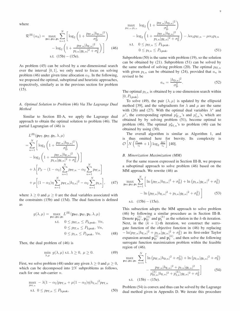
Fig. 2. Secrecy rate of the MM approach vs. iteration number when α2=0.8and dSJ = 0.5m.
and the destination (or the eavesdropper), so dJD = dSD − dSJ
and dJE = dSE − dSJ. The variances of additive Gaussian
noises over each sub-carrier are σ2D = σ2
E = σ2/N , where
σ2 = −100dBm. The energy harvesting efficiency is set as
η = 0.5. When applying the ellipsoid method, the initial dual
variables are set to λ = 100 and µ = 100, and the initial
ellipsoid is set as (λ− 100)2+(µ− 100)2 ≤ 20100. The one-
dimension search interval for finding pJ,n in Algorithm 1 is
set to ǫJ = PJ,peak/1000, the convergence accuracy of ellipsoid
method is set to ǫe = 10−4, and convergence threshold in
Algorithm 2 is set to ǫM = 10−4. Unless specified otherwise,
the following simulation results are averaged over 500 random
independent channel realizations.
First, Fig. 2 shows the convergence behavior of the proposed
MM approach for a given channel realization. The time portion
is set as α2 = 0.8, and the distance from the source to the
jammer is set as dSJ = 0.5m. The transmit power PS are
25dBm and 35dBm, respectively. In Fig. 2, it is observed
that the secrecy rates monotonically increase with the iteration
number. With Type-I destination receiver, the secrecy rates
converge within less than 10 iterations. With Type-II desti-
nation receiver, the secrecy rates converge within less than 5
iterations.
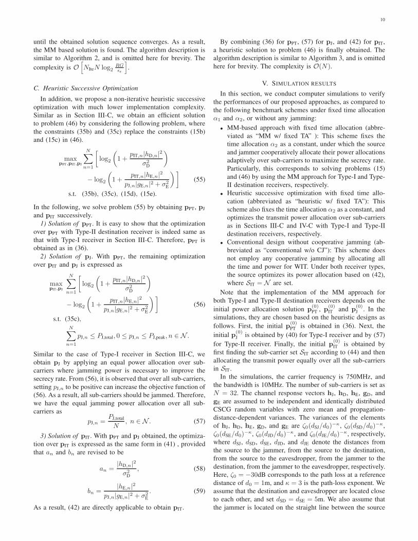
Next, Figs. 3 and 4 show the average secrecy rates versus the
transmit power PS at the source, where the distance from the
source to the jammer is set as dSJ = 0.5m. In Fig. 3 with Type-
I destination receiver, it is observed that the average secrecy
rates of all schemes increase as PS becomes large. The optimal
Lagrange dual approach achieves the highest secrecy rate. The
MM approach has a very close secrecy rate to the optimal
approach. The heuristic successive optimization is observed to
have a slightly lower secrecy rate than the optimal and MM
approaches, but outperforms the other benchmark schemes
significantly. This thus indicates the superiority of joint time
and power allocation for improving secrecy rate, and validates
the necessity of allocating time and power to wirelessly power
the cooperative jamming in order to improve the secrecy rate
of the OFDM communication.
10 15 20 25 30 35 40
PS (dBm)
0.2
0.3
0.4
0.5
0.6
0.7
0.8
0.9
1
Sec
recy
rat
e (b
ps/H
z)
OptimalMMHeuristicMM w/ fixed TAHeuristic w/ fixed TAConventional w/o CJ
Fig. 3. Secrecy rate vs. PS when dSJ = 0.5m (Type-I receiver at thedestination)
10 15 20 25 30 35 40
PS (dBm)
0
0.5
1
1.5
2
2.5
3
3.5
4
Sec
recy
rat
e (b
ps/H
z)
OptimalMMHeuristicMM w/ fixed TA, α
2=0.7
MM w/ fixed TA, α2=0.9
Heuristic w/ fixed TA, α2=0.7
Heuristic w/ fixed TA, α2=0.9
Conventional w/o CJ
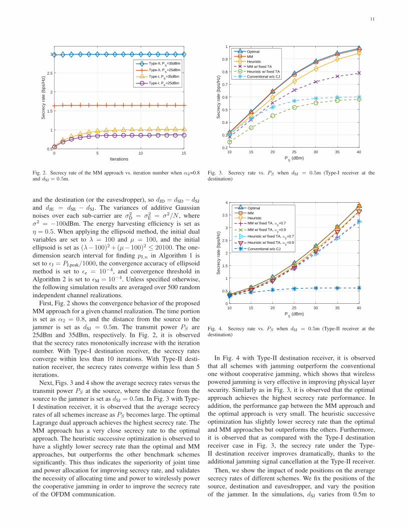
Fig. 4. Secrecy rate vs. PS when dSJ = 0.5m (Type-II receiver at thedestination)
In Fig. 4 with Type-II destination receiver, it is observed
that all schemes with jamming outperform the conventional
one without cooperative jamming, which shows that wireless
powered jamming is very effective in improving physical layer
security. Similarly as in Fig. 3, it is observed that the optimal
approach achieves the highest secrecy rate performance. In
addition, the performance gap between the MM approach and
the optimal approach is very small. The heuristic successive
optimization has slightly lower secrecy rate than the optimal
and MM approaches but outperforms the others. Furthermore,
it is observed that as compared with the Type-I destination
receiver case in Fig. 3, the secrecy rate under the Type-
II destination receiver improves dramatically, thanks to the
additional jamming signal cancellation at the Type-II receiver.
Then, we show the impact of node positions on the average
secrecy rates of different schemes. We fix the positions of the
source, destination and eavesdropper, and vary the position
of the jammer. In the simulations, dSJ varies from 0.5m to
12
0.5 1 1.5 2 2.5 3 3.5 4 4.5
dSJ
(m)
0.55
0.6
0.65
0.7
0.75
0.8
0.85
0.9
0.95S
ecre
cy r
ate
(bps
/Hz)
OptimalMMHeuristicMM w/ fixed TAHeuristic w/ fixed TAConventional w/o CJ
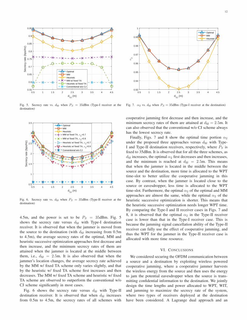
Fig. 5. Secrecy rate vs. dSJ when PS = 35dBm (Type-I receiver at thedestination)
0.5 1 1.5 2 2.5 3 3.5 4 4.5
dSJ
(m)
0.5
1
1.5
2
2.5
3
3.5
Sec
recy
rat
e (b
ps/H
z)
OptimalMMHeuristicMM w/ fixed TA, α
2=0.7
MM w/ fixed TA, α2=0.9
Heuristic w/ fixed TA, α2=0.7
Heuristic w/ fixed TA, α2=0.9
Conventional w/o CJ
Fig. 6. Secrecy rate vs. dSJ when PS = 35dBm (Type-II receiver at thedestination)
4.5m, and the power is set to be PS = 35dBm. Fig. 5
shows the secrecy rate versus dSJ with Type-I destination
receiver. It is observed that when the jammer is moved from
the source to the destination (with dSJ increasing from 0.5m
to 4.5m), the average secrecy rates of the optimal, MM and
heuristic successive optimization approaches first decrease and
then increase, and the minimum secrecy rates of them are
attained when the jammer is located at the middle between
them, i.e., dSJ = 2.5m. It is also observed that when the
jammer’s location changes, the average secrecy rate achieved
by the MM w/ fixed TA scheme only varies slightly, and that
by the heuristic w/ fixed TA scheme first increases and then
decreases. The MM w/ fixed TA scheme and heuristic w/ fixed
TA scheme are observed to outperform the conventional w/o
CJ scheme significantly in most cases.
Fig. 6 shows the secrecy rate versus dSJ with Type-II
destination receiver. It is observed that when dSJ increases
from 0.5m to 4.5m, the secrecy rates of all schemes with
0.5 1 1.5 2 2.5 3 3.5 4 4.5
dSJ
(m)
0.93
0.94
0.95
0.96
0.97
0.98
0.99
1
α2
OptimalMMHeuristic
Fig. 7. α2 vs. dSJ when PS = 35dBm (Type-I receiver at the destination)
cooperative jamming first decrease and then increase, and the
minimum secrecy rates of them are attained at dSJ = 2.5m. It
can also observed that the conventional w/o CJ scheme always
has the lowest secrecy rate.
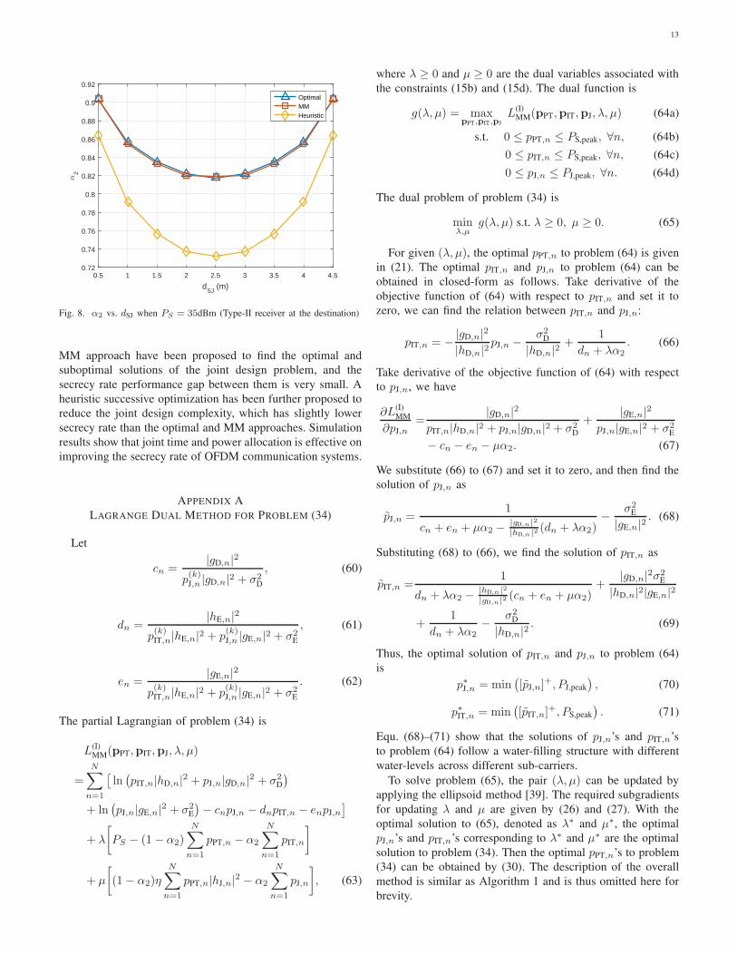
Finally, Figs. 7 and 8 show the optimal time portion α2
under the proposed three approaches versus dSJ with Type-
I and Type-II destination receivers, respectively, where PS is
fixed to 35dBm. It is observed that for all the three schemes, as
dSJ increases, the optimal α2 first decreases and then increases,
and the minimum is reached at dSJ = 2.5m. This means
that when the jammer is located in the middle between the
source and the destination, more time is allocated to the WPT
time-slot to better utilize the cooperative jamming in this
case. By contrast, when the jammer is located close to the
source or eavesdropper, less time is allocated to the WPT
time-slot. Furthermore, the optimal α2 of the optimal and MM
approaches are almost the same, while the optimal α2 of the
heuristic successive optimization is shorter. This means that
the heuristic successive optimization needs longer WPT time.
By comparing the Type-I and II receiver cases in Figs. 7 and
8, it is observed that the optimal α2 in the Type-II receiver
case is lower than that in the Type-I receiver case. This is
because the jamming signal cancellation ability of the Type-II
receiver can fully use the effect of cooperative jamming, and
thus the WPT for the jammer in the Type-II receiver case is
allocated with more time resource.
VI. CONCLUSIONS
We considered securing the OFDM communication between
a source and a destination by exploiting wireless powered
cooperative jamming, where a cooperative jammer harvests
the wireless energy from the source and then uses the energy
to jam the potential eavesdropper when the source is trans-
mitting confidential information to the destination. We jointly
design the time lengths and power allocated to WPT, WIT,
and jamming to maximize the secrecy rate of the system,
where two types of receivers deployed at the destination
have been considered. A Lagrange dual approach and an
13
0.5 1 1.5 2 2.5 3 3.5 4 4.5
dSJ
(m)
0.72
0.74
0.76
0.78
0.8
0.82
0.84
0.86
0.88
0.9
0.92
α2
OptimalMMHeuristic
Fig. 8. α2 vs. dSJ when PS = 35dBm (Type-II receiver at the destination)
MM approach have been proposed to find the optimal and
suboptimal solutions of the joint design problem, and the
secrecy rate performance gap between them is very small. A
heuristic successive optimization has been further proposed to
reduce the joint design complexity, which has slightly lower
secrecy rate than the optimal and MM approaches. Simulation
results show that joint time and power allocation is effective on
improving the secrecy rate of OFDM communication systems.
APPENDIX A
LAGRANGE DUAL METHOD FOR PROBLEM (34)
Let
cn =|gD,n|2
p(k)J,n |gD,n|2 + σ2
D
, (60)
dn =|hE,n|2
p(k)IT,n|hE,n|2 + p
(k)J,n |gE,n|2 + σ2
E
, (61)
en =|gE,n|2
p(k)IT,n|hE,n|2 + p
(k)J,n |gE,n|2 + σ2
E
. (62)
The partial Lagrangian of problem (34) is
L(I)MM(pPT,pIT,pJ, λ, µ)
=
N∑
n=1
[
ln(
pIT,n|hD,n|2 + pJ,n|gD,n|
2 + σ2D
)
+ ln(
pJ,n|gE,n|2 + σ2
E
)
− cnpJ,n − dnpIT,n − enpJ,n
]
+ λ
[
PS − (1− α2)N∑
n=1
pPT,n − α2
N∑
n=1
pIT,n
]
+ µ
[
(1 − α2)ηN∑
n=1
pPT,n|hJ,n|2 − α2
N∑
n=1
pJ,n
]
, (63)
where λ ≥ 0 and µ ≥ 0 are the dual variables associated with
the constraints (15b) and (15d). The dual function is
g(λ, µ) = maxpPT,pIT,pJ
L(I)MM(pPT,pIT,pJ, λ, µ) (64a)
s.t. 0 ≤ pPT,n ≤ PS,peak, ∀n, (64b)
0 ≤ pIT,n ≤ PS,peak, ∀n, (64c)
0 ≤ pJ,n ≤ PJ,peak, ∀n. (64d)
The dual problem of problem (34) is
minλ,µ
g(λ, µ) s.t. λ ≥ 0, µ ≥ 0. (65)
For given (λ, µ), the optimal pPT,n to problem (64) is given
in (21). The optimal pIT,n and pJ,n to problem (64) can be
obtained in closed-form as follows. Take derivative of the
objective function of (64) with respect to pIT,n and set it to
zero, we can find the relation between pIT,n and pJ,n:
pIT,n = −|gD,n|2
|hD,n|2pJ,n −
σ2D
|hD,n|2+
1
dn + λα2. (66)
Take derivative of the objective function of (64) with respect
to pJ,n, we have
∂L(I)MM
∂pJ,n
=|gD,n|2
pIT,n|hD,n|2 + pJ,n|gD,n|2 + σ2D
+|gE,n|2
pJ,n|gE,n|2 + σ2E
− cn − en − µα2. (67)
We substitute (66) to (67) and set it to zero, and then find the
solution of pJ,n as
p̃J,n =1
cn + en + µα2 −|gD,n|2
|hD,n|2(dn + λα2)
−σ2
E
|gE,n|2. (68)
Substituting (68) to (66), we find the solution of pIT,n as
p̃IT,n =1
dn + λα2 −|hD,n|2
|gD,n|2(cn + en + µα2)
+|gD,n|2σ2
E
|hD,n|2|gE,n|2
+1
dn + λα2−
σ2D
|hD,n|2. (69)
Thus, the optimal solution of pIT,n and pJ,n to problem (64)
is
p∗J,n = min(
[p̃J,n]+, PJ,peak
)
, (70)
p∗IT,n = min(
[p̃IT,n]+, PS,peak
)
. (71)
Equ. (68)–(71) show that the solutions of pJ,n’s and pIT,n’s
to problem (64) follow a water-filling structure with different
water-levels across different sub-carriers.
To solve problem (65), the pair (λ, µ) can be updated by
applying the ellipsoid method [39]. The required subgradients
for updating λ and µ are given by (26) and (27). With the
optimal solution to (65), denoted as λ∗ and µ∗, the optimal
pJ,n’s and pIT,n’s corresponding to λ∗ and µ∗ are the optimal
solution to problem (34). Then the optimal pPT,n’s to problem
(34) can be obtained by (30). The description of the overall
method is similar as Algorithm 1 and is thus omitted here for
brevity.
14
APPENDIX B
PROOF OF LEMMA 1
First, we have the following fact that for arbitrary c, d > 0,
(1+c)/(1+d) increases with c/d, which is proved as follows.
Without loss of generality, we can increase c/d by fixing dand increasing c. It is observed that (1 + c)/(1 + d) will also
increase with c, when d is fixed. So (1+ c)/(1+ d) increases
with c/d.
Then, we write the objective function of (38) into the
following form
ln1 +
(
pIT,n|hD,n|2)
/(
pJ,n|gD,n|2 + σ2
D
)
1 + (pIT,n|hE,n|2) / (pJ,n|gE,n|2 + σ2E)
. (72)
The previously proved fact tells that (72) will increase with(
pIT,n|hD,n|2)
/(
pJ,n|gD,n|2 + σ2D
)
(pIT,n|hE,n|2) / (pJ,n|gE,n|2 + σ2E)
=|hD,n|2|gE,n|2
|hE,n|2|gD,n|2
1 +
σ2
E
|gE,n|2− σ2
D
|gD,n|2
pJ,n +σ2
D
|gD,n|2
.
(73)
Note that (73) only increases with pJ,n when σ2E/|gE,n|2 −
σ2D/|gD,n|2 < 0. Hence, increasing pJ,n can increase the
objective function of (38) when |gE,n|2/σ2E > |gD,n|2/σ2
D.
APPENDIX C
THE UPPER BOUND OF ϑ
By taking derivative of the Lagrangian of problem (41) and
setting it to zero, we have the following equation
anbnp2IT,n + (an + bn)pIT,n −
an − bnϑ
+ 1 = 0, (74)
where ϑ ∈ [0, ϑmax] is the dual variable associated with the
sum power constraint∑N
n=1 pIT,n ≤ PS . The value of ϑmax
can be obtained as follows.
The p̃n in (43) is the positive root of (74). Since p̃n is
a decreasing function of ϑ, a sufficient large ϑ can make p̃nnegative for all n ∈ SIT. According to (42), negative p̃n makes
pIT,n = 0, which is obviously not the optimal solution of (41).
Hence ϑ should be bounded above to make sure at least one
p̃n, n ∈ SIT is positive.
Note that the sum of the roots of equation (74), i.e. −(an+bn)/(anbn), is negative, the condition that the equation has
positive root is equivalent to the condition that the product of
the roots is negative, i.e.
−an−bnϑ
+ 1
anbn< 0 ⇒ ϑ < an − bn, n ∈ SIT. (75)
So
ϑmax = maxn∈SIT
(an − bn). (76)
APPENDIX D
LAGRANGE DUAL METHOD FOR PROBLEM (54)
The procedure of the method is the similar with that shown
in Appendix A, and the only differences are the expressions
of the Lagrangian, the dual function, and the solution of pIT,n
and pJ,n. We only show the differences here.
The partial Lagrangian of problem (54) is
L(II)MM(pPT,pIT,pJ, λ, µ)
=
N∑
n=1
[
ln(
pIT,n|hD,n|2 + σ2
D
)
+ ln(
pJ,n|gE,n|2 + σ2
E
)
− dnpIT,n − enpJ,n
]
+ λ
[
PS − (1− α2)
N∑
n=1
pPT,n − α2
N∑
n=1
pIT,n
]
+ µ
[
(1− α2)η
N∑
n=1
pPT,n|hJ,n|2 − α2
N∑
n=1
pJ,n
]
, (77)
where dn and en are defined as (61) and (62), and λ ≥ 0 and
µ ≥ 0 are the dual variables associated with constraints (15b)
and (15d). The dual function is
g(λ, µ) = maxpPT,pIT,pJ
L(II)MM(pPT,pIT,pJ, λ, µ) (78)
s.t. (64b), (64c), (64d).
By taking derivatives of the objective value of problem (78)
with respect to pIT,n and pJ,n, respectively, and setting them
to zero, we can find the optimal pIT,n and pJ,n to problem (78)
as
p∗IT,n = min(
[p̂IT,n]+, PS,peak
)
, (79)
p∗J,n = min(
[p̂J,n]+, PJ,peak
)
, (80)
where
p̂IT,n =1
dn + λα2−
σ2D
|hD,n|2, (81)
p̂J,n =1
en + µα2−
σ2E
|gE,n|2. (82)
Equ. (79)–(82) show that the solutions of pJ,n’s and pIT,n’s
to problem (78) follow a water-filling structure with different
water-levels across different sub-carriers.
REFERENCES
[1] A. Rico-Alvarino et al., “An overview of 3GPP enhancements on machineto machine communications,” IEEE Commun. Mag., vol. 54, no. 6, pp.14-21, Jun. 2016.
[2] A. Mukherjee, S. A. A. Fakoorian, J. Huang, and A. L. Swindlehurst,“Principles of physical layer security in multiuser wireless networks: asurvey,” IEEE Commun. Surveys Tuts., vol. 16, no. 3, pp. 1550-1573,Third 2014.
[3] A. Khisti and G. W. Wornell, “Secure transmission with multiple antennasI: the MISOME wiretap channel,” IEEE Trans. Inf. Theory, vol. 56, no.7, pp. 3088-3104, Jul. 2010.
[4] J. Li, A. P. Petropulu, and S. Weber, “On cooperative relaying schemesfor wireless physical layer security,” IEEE Trans. Signal Process., vol.59, no. 10, pp. 4985-4997, Oct. 2011.
[5] S. Goel and R. Negi, “Guaranteeing secrecy using artificial noise,” IEEE
Trans. Wireless Commun., vol. 7, no. 6, pp. 2180-2189, Jun. 2008.[6] M. R. A. Khandaker and K. K. Wong, “Masked beamforming in the
presence of energy-harvesting eavesdroppers,” IEEE Trans. Inf. Forensics
Security, vol. 10, no. 1, pp. 40-54, Jan. 2015.[7] J. Huang and A. L. Swindlehurst, “Cooperative jamming for secure
communications in MIMO relay networks,” IEEE Trans. Signal Process.,vol. 59, no. 10, pp. 4871-4884, Oct. 2011.
[8] Q. Li, Y. Yang, W. K. Ma, M. Lin, J. Ge, and J. Lin, “Robust cooperativebeamforming and artificial noise design for physical-layer secrecy in AFmulti-antenna multi-relay networks,” IEEE Trans. Signal Process., vol.63, no. 1, pp. 206-220, Jan. 2015.
15
[9] S. Luo, J. Li, and A. P. Petropulu, “Uncoordinated cooperative jammingfor secret communications,” IEEE Trans. Inf. Forensics Security, vol. 8,no. 7, pp. 1081-1090, Jul. 2013.
[10] W. Liu, X. Zhou, S. Durrani, and P. Popovski, “Secure communicationwith a wireless-powered friendly jammer,” IEEE Trans. Wireless Com-
mun., vol. 15, no. 1, pp. 401-415, Jan. 2016.
[11] Y. Bi and H. Chen, “Accumulate and jam: towards secure communicationvia a wireless-powered full-duplex jammer,” IEEE J. Sel. Topics Signal
Process., vol. 10, no. 8, pp. 1538-1550, Dec. 2016.
[12] H. Xing, K. -K. Wong, Z. Chu, and A. Nallanathan, “To harvest and jam:a paradigm of self-sustaining friendly jammers for secure AF relaying,”IEEE Trans. Signal Process., vol 63, no. 24, pp. 6616-6631, Dec. 2015.
[13] H. Xing, K. -K. Wong, A. Nallanathan, and R. Zhang, “Wireless poweredcooperative jamming for secrecy multi-AF relaying networks,” IEEE
Trans. Wireless Commun., vol. 15, no. 12, pp. 7971-7984, Dec. 2016.
[14] R. Zhang and C. K. Ho, “MIMO broadcasting for simultaneous wirelessinformation and power transfer,” IEEE Trans. Wireless Commun., vol. 12,no. 5, pp. 1989-2001, May 2013.
[15] Y. Zhu, L. Wang, K. K. Wong, S. Jin, and Z. Zheng, “Wireless powertransfer in massive MIMO-aided HetNets with user association,” IEEE
Trans. Commun., vol. 64, no. 10, pp. 4181-4195, Oct. 2016.
[16] J. Xu, L. Liu, and R. Zhang, “Multiuser MISO beamforming forsimultaneous wireless information and power transfer,” IEEE Trans.
Signal Process., vol. 62, no. 18, pp. 4798-4810, Sep. 2014.
[17] J. Xu and R. Zhang, “Energy beamforming with one-bit feedback,” IEEE
Trans. Signal Process., vol. 62, no. 20, pp. 5370-5381, Oct. 2014.
[18] M. Xia and S. Aissa, “On the efficiency of far-field wireless powertransfer,” IEEE Trans. Signal Process., vol. 63, no. 11, pp. 2835-2847,Jun. 2015.
[19] D. W. K. Ng, E. S. Lo, and R. Schober, “Robust beamforming for securecommunication in systems with wireless information and power transfer,”IEEE Trans. Wireless Commun., vol. 13, no. 8, pp. 4599-4615, Aug. 2014.
[20] S. Bi, C. K. Ho, and R. Zhang, “Wireless powered communication:opportunities and challenges,” IEEE Commun. Mag., vol. 53, no. 4, pp.117-125, Apr. 2015.
[21] Y. Zeng and R. Zhang, “Optimized training design for wireless energytransfer,” IEEE Trans. Commun., vol. 63, no. 2, pp. 536-550, Feb. 2015.
[22] I. Krikidis, S. Timotheou, S. Nikolaou, G. Zheng, D. W. K. Ng, andR. Schober, “Simultaneous wireless information and power transfer inmodern communication systems,” IEEE Commun. Mag., vol. 52, no. 11,pp. 104-110, Nov. 2014.
[23] J. Xu and R. Zhang, “A general design framework for MIMO wirelessenergy transfer with limited feedback,” IEEE Trans. Signal Process., vol.64, no. 10, pp. 2475-2488, May 2016.
[24] S. Luo, J. Xu, T. J. Lim, and R. Zhang, “Capacity region of MISObroadcast channel for simultaneous wireless information and powertransfer,” IEEE Trans. Commun., vol. 63, no. 10, pp. 3856-3868, Oct.2015.
[25] Q. Wu, M. Tao, D. W. K. Ng, W. Chen, and R. Schober, “Energy-efficientresource allocation for wireless powered communication networks,” IEEE
Trans. Wireless Commun., vol. 15, no. 3, pp. 2312-2327, Mar. 2016.
[26] Q. Wu, G. Y. Li, W. Chen, D. W. K. Ng, and R. Schober, “An overviewof sustainable green 5G networks,” IEEE Wireless Commun., acceptedfor publication. Available: https://arxiv.org/abs/1609.09773
[27] X. Zhou, R. Zhang, and C. K. Ho, “Wireless information and powertransfer in multiuser OFDM systems,” IEEE Trans. Wireless Commun.,vol. 13, no. 4, pp. 2282-2294, Apr. 2014.
[28] F. Renna, N. Laurenti, and H. V. Poor, “Physical-layer secrecy forOFDM transmissions over fading channels,” IEEE Trans. Inf. Forensics
Security, vol. 7, no. 4, pp. 1354-1367, Aug. 2012.
[29] M. Zhang, Y. Liu, and R. Zhang, “Artificial noise aided secrecy infor-mation and power transfer in OFDMA systems,” IEEE Trans. Wireless
Commun., vol. 15, no. 4, pp. 3085-3096, Apr. 2016.
[30] A. Wang, Y. Cai, W. Yang, and Z. Hou, “A Stackelberg security gamewith cooperative jamming over a multiuser OFDMA network,” in Proc.
2013 WCNC, 2013, pp. 4169-4174.
[31] L. Liu, R. Zhang, and K. C. Chua, “Secrecy wireless information andpower transfer with MISO beamforming,” IEEE Trans. Signal Process.,vol. 62, no. 7, pp. 1850-1863, Apr. 2014.
[32] H. Xing, L. Liu, and R. Zhang, “Secrecy wireless information and powertransfer in fading wiretap channel,” IEEE Trans. Veh. Technol., vol. 65,no. 1, pp. 180-190, Jan. 2016.
[33] E. Boshkovska, D. Ng, N. Zlatanov, and R. Schober, “Practical non-linear energy harvesting model and resource allocation for SWIPTsystems,” IEEE Commun. Lett., vol. 19, no. 12, pp. 2082-2085, Dec.2015.
[34] M. R. V. Moghadam, Y. Zeng, and R. Zhang, “Waveform optimizationfor radio-frequency wireless power transfer,” in Proc. IEEE Conf. Signal
Process. Adv. Wireless Commun. (SPAWC), Jul. 2017.[35] Y. Zeng, B. Clerckx, and R. Zhang, “Communications and signals design
for wireless power transmission,” IEEE Trans. Commun., vol. 65, no. 5,pp. 2264-2290, May 2017.
[36] B. Clerckx and E. Bayguzina, “Waveform design for wireless powertransfer,” IEEE Trans. Signal Process., vol. 64, no. 23, pp. 6313-6328,Dec. 2016.
[37] W. Yu and R. Lui, “Dual methods for nonconvex spectrum optimizationof multicarrier systems,” IEEE Trans. Commun., vol. 54, no. 7, pp. 1310-1322, Jul. 2006.
[38] Q. Wu, W. Chen, M. Tao, J. Li, H. Tang, and J. Wu, “Resource allocationfor joint transmitter and receiver energy efficiency maximization indownlink OFDMA systems,” IEEE Trans. Commun., vol. 63, no. 2, pp.416-430, Feb. 2015.
[39] S. Boyd and L. Vandenberghe, Convex Optimization. Cambridge Uni-versity Press, 2004.
[40] S. Boyd. (2014). Ellipsoid Method [Online]. Available: https://stanford.edu/class/ee364b/lectures/ellipsoid method notes.pdf
[41] Y. Sun, P. Babu, and D. P. Palomar, “Majorization-minimization al-gorithms in signal processing, communications, and machine learning,”IEEE Trans. Signal Process., vol. 65, no. 3, pp. 794-816, Feb. 2017.


