Embed Size (px)
Citation preview
WILLINGNESS-TO-PAY FOR POMEGRANATES: IMPACT OF PRODUCT
AND HEALTH FEATURES USING NONHYPOTHETICAL PROCEDURES
A Thesis
by
CALLIE PAULINE MCADAMS
Submitted to the Office of Graduate Studies of
Texas A&M University
in partial fulfillment of the requirements for the degree of
MASTER OF SCIENCE
August 2011
Major Subject: Agricultural Economics

Willingness-to-Pay for Pomegranates: Impact of Product and Health Features Using
Nonhypothetical Procedures
Copyright 2011 Callie Pauline McAdams
WILLINGNESS-TO-PAY FOR POMEGRANATES: IMPACT OF PRODUCT
AND HEALTH FEATURES USING NONHYPOTHETICAL PROCEDURES
A Thesis
by
CALLIE PAULINE MCADAMS
Submitted to the Office of Graduate Studies of
Texas A&M University
in partial fulfillment of the requirements for the degree of
MASTER OF SCIENCE
Approved by:
Chair of Committee, Marco A. Palma
Committee Members, Charles R. Hall
Ariun Ishdorj
W. Douglass Shaw
Head of Department, John P. Nichols
August 2011
Major Subject: Agricultural Economics
iii
ABSTRACT
Willingness-to-Pay for Pomegranates: Impact of Product and Health Features Using
Nonhypothetical Procedures. (August 2011)
Callie Pauline McAdams, B.S., North Carolina State University
Chair of Advisory Committee: Dr. Marco A. Palma
The use of functional foods by individuals to address health issues is now gaining
attention. Pomegranate fruits and other pomegranate products contain phytochemicals,
including antioxidants with potential human health benefits. The production of
pomegranates in the United States is concentrated in California; yet pomegranates can be
grown in other regions. The purpose of this study was two-fold: 1) to address the market
potential and consumer preferences for pomegranate fruits and other pomegranate
products in Texas and 2) to address issues of experimental auction design and estimation
in regards to novel products and health benefits of food products. A nonhypothetical
experimental procedure was developed that combined preference rankings with a
uniform nth-price auction to elicit preferences and willingness-to-pay (WTP) for
pomegranate fruit products.
A representative sample of subjects (n=203) from the Bryan-College Station area
of Texas submitted baseline rankings and bids on six pomegranate products and a
control fruit product. Of the participants, 75.4% had never purchased a pomegranate
fruit. Three additional information treatments were imposed: tasting information, health
iv
and nutrition information, and anti-cancer information. Subjects had the greatest WTP
for the control product and the processed pomegranate products; the whole pomegranate
fruits had the lowest WTP. The preference rankings for the baseline round indicated the
same order of preferences as the bids.
Random-effects tobit models and mixed linear models on the full bids and
individual changes in bids were used to make estimates of WTP. Unengaged bidders
and bid censoring were addressed. Previous purchases of pomegranates and household
size were the most robust demographic/behavioral predictors of WTP. Tasting
information had a greater effect on WTP than health and nutrition information or anti-
cancer information. Providing a reference price also increased WTP. Preference
rankings were estimated using a rank-ordered logit and a mixed rank-ordered logit
model. There was an interaction effect of each information treatment with the product
characteristics, indicating that studies of effects of information treatments on preferences
are not generalizable across products. There was divergence in the results for the
preference rankings from the results of the experimental auction; preference rankings
and bids gave conflicting results for the same products.

v
DEDICATION
I would like to dedicate this work to my amazing family: parents, sister, aunts,
uncles, and grandparents. You have inspired my love of agriculture as well as my
dedication and work ethic. You have each played an important part in this process, and I
could not have done it without you. For that, I will never be able to sufficiently express
my gratitude. I would also like to dedicate this thesis to the memory of my late
grandfather, Howard H. McAdams Sr., who was one of the strongest, most humble men
I have ever known.

vi
ACKNOWLEDGEMENTS
I would like to thank my committee chair, Dr. Marco Palma, for the opportunity
to work on this project as well as for his guidance and support. I would like to thank
him particularly for the independence he allowed me to have throughout the entire thesis
process, as well as for the humor and diligence he used in approaching every challenge
along the way. I would also like to thank the other members of my committee for their
willingness to help throughout my time at Texas A&M University: Dr. Charlie Hall for
his advice and experience with experimental auctions and for being a voice that
reminded me of home; Dr. Ariun Ishdorj for her extensive knowledge of econometrics
and encouragement to push myself to achieve; and Dr. Douglass Shaw for his advice on
special issues in auctions related to health. I am indebted also to the faculty in the
Department of Agricultural Economics at Texas A&M University who have both taught
courses and provided advice.
To my friends and classmates throughout the master‘s program who have offered
a smile, an opinion, encouragement, or even a diversion, I say a special thank you for
making the experience I have had in College Station one that I will not soon forget. I
would also like to thank my friends and family in North Carolina who tolerated the time
I have spent away from them and for all of their support.
I owe a particular debt of gratitude to the participants of the practice auctions and
the actual study as well as all those who assisted with the auctions: Dr. Marco Palma,
Brad Roberson, Alba Collart-Dinarte, Antonio Ruiz DeKing, and Carolina Rivas. I am

vii
also indebted to the staff of the Department of Agricultural Economics and my fellow
graduate students who helped with the logistics of making the study happen. I would
like to thank the Texas A&M Horticultural Gardens and staff for the use of their
facilities as well as the Texas Pomegranate Growers Cooperative and the AgriLife
Research and Extension Station in Pecos, TX, for providing materials for the study.
Finally, I would like to express my appreciation to the Texas Department of
Agriculture for its funding of this research and the co-recipients of the grant, the Texas
Pomegranate Growers‘ Cooperative, and its members for their general enthusiasm and
knowledge of the pomegranate industry.
viii
TABLE OF CONTENTS
Page
ABSTRACT .............................................................................................................. iii
DEDICATION .......................................................................................................... v
ACKNOWLEDGEMENTS ...................................................................................... vi
TABLE OF CONTENTS .......................................................................................... viii
LIST OF FIGURES ................................................................................................... xiii
LIST OF TABLES .................................................................................................... xvi
NOMENCLATURE .................................................................................................. xxi
CHAPTER
I INTRODUCTION ................................................................................ 1
II LITERATURE REVIEW ..................................................................... 13
Experimental Economics and Value Elicitation ............................. 13
Types of Data ........................................................................ 13
Transactions Data ......................................................... 14
Survey Data .................................................................. 14
Experimental Data ........................................................ 15
Categorizing Experimental Data ......................... 16
Types of Goods ................................................... 17
Where Experiment Occurs .................................. 18
Uses for Value Elicitation Procedures................................... 19
Experimental Design ...................................................................... 22
Conjoint Analysis and Choice Experiments .......................... 23
Value Elicitation .................................................................... 25
Differences in Willingness-to-Pay and Willingness-to-
Accept…….. .......................................................................... 26
Incentive Compatibility of Auction Mechanisms ................. 30
Auction Mechanisms ............................................................. 33
Types of Auctions ........................................................ 34

ix
CHAPTER Page
Auction Mechanism Issues ........................................... 35
Which Type of Auction Is Preferred? .......................... 36
Divergence from Expectations ............................ 37
Single Round vs. Multiple Round Bidding ......... 44
Endowment Approach vs. Full Bidding
Approach ............................................................. 47
Auction Mechanism Considerations ................... 50
Internal Validity ............................................................................. 51
External Validity ............................................................................ 53
Previous Measures of Willingness-to-Pay for Food and
Horticultural Products .................................................................... 66
Functional Foods ............................................................................ 75
Scientific Basis for Functional Foods ................................... 77
Functional Food Market ........................................................ 80
Considerations for Developing Auction Procedures ...................... 83
Econometric Modeling of Preference Elicitation Procedures ........ 86
III POMEGRANATES AND THE POMEGRANATE INDUSTRY ....... 90
The Pomegranate ............................................................................ 90
Chemical Composition .......................................................... 94
Pomegranates and Antioxidants ............................................ 94
Pomegranate Production ................................................................ 101
Pre-Planting ........................................................................... 102
Cultivars ....................................................................... 102
Propagation ................................................................... 103
Soil…. .......................................................................... 104
Climate and Microclimate ............................................ 104
Soil Preparation, Irrigation System, and Weed Control 105
Planting Design ............................................................ 106
Planting ......................................................................... 107
Pruning ......................................................................... 108
Fertilization .................................................................. 108
Orchard Management ............................................................ 109
Irrigation ....................................................................... 109
Pruning ......................................................................... 110
Fertilization .................................................................. 110
Frost Protection ............................................................ 111
Pest Management .................................................................. 112
Disease ......................................................................... 112
Insects ........................................................................... 112
Weeds ........................................................................... 114

x
CHAPTER Page
Pomegranate Pest Management Issues ......................... 115
Harvest……. ......................................................................... 116
Post-Harvest .......................................................................... 117
Current State of the Industry .......................................................... 120
Products……… ..................................................................... 124
Marketing Challenges ........................................................... 125
IV METHODOLOGY ............................................................................... 127
Auction Description and Estimation Overview ............................. 127
Theoretical Framerwork for Combined Experimental
Auction and Ranking Mechanism ......................................... 131
Procedural Details and Justification ............................................... 134
Auction Procedures ............................................................... 134
Experimental Auction and Preference Ranking Design
Considerations ....................................................................... 142
Econometric Model ........................................................................ 153
Econometric Model for Experimental Auction Bids ............. 154
Ordinary Least Squares Model ..................................... 158
Tobit Model .................................................................. 159
Random Effects Tobit Model ....................................... 164
Mixed Linear Model ..................................................... 165
Models for Bid Differences across Goods and Treatments ... 166
Econometric Model for Preference Rankings ....................... 170
Rank-Ordered Logit Model .......................................... 172
Mixed Multinomial Logit Model ................................. 175
Comparison of Preferences Based on Bids and Rankings .... 184
Variation in Ranking Ability ................................................. 186
V RESULTS AND DISCUSSION .......................................................... 188
Demographics and Behavioral Characteristics .............................. 188
WTP Models for Full Experimental Auction Bids ......................... 201
Bid Censoring ........................................................................ 211
Tobit Models for Each Product and Round ........................... 213
Ordinary Least Squares Model .............................................. 218
Tobit Model for Pooled Bids ................................................. 221
Random Effects Tobit Models .............................................. 227
Mixed Linear Models ............................................................ 233
Unengaged vs. Engaged Bidders ........................................... 238
Comparison of Models for Full Bids ..................................... 249
xi
CHAPTER Page
Bid Differences across Information Treatments ............................ 251
Preference Models for Rankings .................................................... 267
Rank-Ordered Logit Model ................................................... 271
Mixed Rank-Ordered Logit Model ....................................... 276
Changes in Rankings ...................................................................... 280
Comparison of Bidding and Ranking Results ................................ 286
VI SUMMARY AND CONCLUSIONS ................................................... 298
Summary……….. .......................................................................... 298
Pomegranates and the Pomegranate Industry ........................ 298
Nonhypothetical Preference Ranking and Experimental
Auction Procedures ............................................................... 301
Analytical Procedures and Results Summary ....................... 305
Survey Procedures and Results .................................... 305
Estimation Procedures and Results .............................. 307
Conclusions………… .................................................................... 312
Key Challenges for Expansion of Pomegranate Production . 312
Novel Products and Value Elicitation Mechanisms .............. 315
Directions for Further Research ............................................ 317
REFERENCES .......................................................................................................... 320
APPENDIX A ........................................................................................................... 383
APPENDIX B ........................................................................................................... 384
APPENDIX C ........................................................................................................... 389
APPENDIX D ........................................................................................................... 407
APPENDIX E ............................................................................................................ 411
APPENDIX F ............................................................................................................ 412
APPENDIX G ........................................................................................................... 417
APPENDIX H ........................................................................................................... 425
APPENDIX I ............................................................................................................ 428
APPENDIX J ............................................................................................................. 430

xii
Page
VITA ......................................................................................................................... 453
xiii
LIST OF FIGURES
Page
Figure 1. Relationship among Types of Phytochemicals .......................................... 98
Figure 2. Examples of the Variability in Pomegranate Cultivars ............................. 103
Figure 3. Example of Insect-Damaged Pomegranate Fruits ..................................... 114
Figure 4. Example of Scald on a Pomegranate Fruit Caused by Sun Damage ......... 115
Figure 5. Total Seasonal Movements of Pomegranate Fruits within the United
States ......................................................................................................... 121
Figure 6. Season Average Shipping Point Pomegranate Fruit Prices ($/22 lb.
carton). ...................................................................................................... 122
Figure 7. Weekly Shipping Point Prices for Pomegranate Fruits ($/22 lb. carton). .. 123
Figure 8. Experimental Procedures. .......................................................................... 130
Figure 9. Familiarity with Pomegranate Products ..................................................... 195
Figure 10. Of Participants Who Previously Purchased Whole Pomegranate
Fruits, Percentages Who Purchased Pomegranate Fruits in a Particular
Month ....................................................................................................... 196
Figure 11. Conditional Mean Bids for Fruit Products by Information Treatment .... 204
Figure 12. Median Bids for All Fruit Products by Information Treatment
(Baseline, Tasting Information, Health and Nutrition Information,
Anti-Cancer Information, and Full Information) ...................................... 205
Figure 13. Distribution of Baseline Round Bids for Fruit Products in Dollars as
Estimated with a Gaussian Kernel Density Distribution .......................... 207
Figure 14. Distribution of Tasting Information Round Bids for Fruit Products in
Dollars as Estimated with a Gaussian Kernel Density Distribution ......... 208
Figure 15. Distribution of Health and Nutrition Information Round Bids for
Fruit Products in Dollars as Estimated with a Gaussian Kernel
Density Distribution ................................................................................. 209
xiv
Page
Figure 16. Distribution of Anti-Cancer Information Round Bids for Fruit
Products in Dollars as Estimated with a Gaussian Kernel Density
Distribution ............................................................................................... 210
Figure 17. Distribution of Full Information Bids for Fruit Products in Dollars as
Estimated with a Gaussian Kernel Density Distribution .......................... 211
Figure 18. Box Plot of Implied Bid Differences ....................................................... 258
Figure 19. Unengaged Implied Bids: Averages across Tasting, Health and
Nutrition, and Anti-Cancer Information Treatments ................................ 262
Figure 20. Frequency of Each Ranking for Each Product, Full Information ............ 267
Figure 21. Percentage of Subjects Who Ranked a Particular Product in the Top
Half of All Products .................................................................................. 270
Figure 22. Average Preference Ranking by Product and by Information Treatment. 271
Figure 23. Probability of a Particular Fruit Product Being Ranked Most Preferred
Based on Rank-Ordered Logit Model Estimates. ..................................... 291
Figure 24. Newspaper Advertisement for Fruit Purchasing Decisions Study ........... 383
Figure 25. Photographs of Whole Pomegranate Fruit Products. ............................... 407
Figure 26. Photographs of Ready-to-Eat (RTE) Pomegranate Fruit Products. ......... 407
Figure 27. Mixed Pomegranate Juice ........................................................................ 408
Figure 28. Pineapple .................................................................................................. 408
Figure 29. Photograph of California Wonderful Pomegranate Arils ........................ 409
Figure 30. Photograph of Texas Red Pomegranate Arils .......................................... 409
Figure 31. Photograph of Texas Salavatski Pomegranate Arils ................................ 409
Figure 32. Pomegranate Fruit Tasting Samples ........................................................ 410
Figure 33. Example Fruit Product Ranking Sheet ..................................................... 411

xv
Page
Figure 34. Example Fruit Product Bidding Sheet ..................................................... 411
xvi
LIST OF TABLES
Page
Table 1. Auction Mechanisms Summary .................................................................. 43
Table 2. Pomegranate Nutrition Information ............................................................ 93
Table 3. Demographic and Behavioral Variables ..................................................... 156
Table 4. Four Cases for Differences in Bids. ............................................................ 169
Table 5. Example of Rankings Data before "Exploding" Data ................................. 181
Table 6. Example of Rankings Data after "Exploding" Data .................................... 182
Table 7. Socioeconomic and Behavioral Characteristics of Experiment Subjects.... 189
Table 8. Sessions, Information Treatments, and Reference Price. ............................ 191
Table 9. Participant Survey Responses on Fruit and Vegetable Buying Behaviors . 192
Table 10. Subject Familiarity with Functional Foods. .............................................. 194
Table 11. Factors Cited as Important in Fruit and Vegetable Purchasing Decisions. 199
Table 12. Relative Importance of Factors in Fruit and Vegetable Purchase
Decisions Based on a Rating Scale. ......................................................... 200
Table 13. Summary Statistics: Full Bids for Pomegranate and Other Fruit Products 202
Table 14. Bids Censored at $0.00 and Bids above Reference Price, by Round ........ 212
Table 15. Tobit Models for WTP by Product, Full Information ............................... 216
Table 16. Tobit Models by Product Marginal Effects on WTP, Full Information .... 217
Table 17. Ordinary Least Squares Model Results for WTP for Fruit Products
Using Pooled Experimental Auction Bids ................................................ 220
Table 18. Standard Tobit Model Parameter Estimates for WTP for Fruit Products
Using Experimental Auction Pooled Bids ................................................ 222
xvii
Page
Table 19. Marginal Effects for Standard Tobit Model for WTP for Fruit Products
Using Pooled Experimental Auction Bids ................................................ 224
Table 20. Specification Test Values, Standard Tobit Models Using Pooled
Experimental Auction Bids ...................................................................... 227
Table 21. Random Effects Tobit Model Results for WTP for Fruit Products Using
Pooled Experimental Auction Bids ......................................................... 229
Table 22. Marginal Effects for Random Effects Tobit Model for WTP for Fruit
Products Using Pooled Experimental Auction Bids ................................. 232
Table 23. Specification Test Values, Random Effects Tobit Models for Pooled
Auction Bids ............................................................................................. 233
Table 24. Mixed Linear Model Results for WTP for Fruit Products Using
Experimental Auction Bids ...................................................................... 235
Table 25. Goodness of Fit Comparison for Specifications of Mixed Linear Models 237
Table 26. Count of Unengaged Bidders for Each Fruit Product ............................... 240
Table 27. Comparison of Random Effects Tobit Model WTP Parameter Estimates
for Levels of Bidder Engagement ............................................................. 241
Table 28. Comparison of Random Effects Tobit Model WTP Marginal Effects
Estimates for Levels of Bidder Engagement ............................................ 244
Table 29. Comparison of Mixed Linear Model WTP Parameter Estimates for
Levels of Bidder Engagement .................................................................. 246
Table 30. Test of Information Treatment Effects: Paired t-Tests ............................. 252
Table 31. Test of Information Treatment Effects: Wilcoxon Signed-Rank Tests .... 253
Table 32. Proportions of Positive, Negative, and Zero Differences for Changes in
WTP from Baseline Information Treatment, Summed for All Products .. 255
Table 33. Summary Statistics for Implied Bid Differences ..................................... 256
xviii
Page
Table 34. Jarque-Bera Test Statistics for Normality of Residuals from OLS
Estimates of Implied Differences ............................................................. 259
Table 35. Kolmogorov-Smirnov Tests for Normality of Errors for OLS
Regression of Bid Differences .................................................................. 260
Table 36. Counts of Unengaged Bids for Implied Bid Differences, by Product
and by Information Treatment .................................................................. 261
Table 37. Mixed Linear Model Results for Experimental Auction Data, Implied
Differences in WTP for Fruit Products ................................................... 263
Table 38. Percentages of Participants Who Assigned Each Ranking to Each
Product in Each Round ............................................................................. 268
Table 39. Rank-Ordered Logit Models for Explicit Preference Rankings for Fruit
Products by Information Treatment, Fully- and Partially-Ranked
Models ...................................................................................................... 273
Table 40. Mixed Rank-Ordered Logit Models for Preference Rankings, Estimated
Coefficients and Standard Deviations of Coefficients ............................ 277
Table 41. Changes in Explicit Preference Rankings by Product (Tasting
Information Rank ‒ Baseline Rank) ......................................................... 281
Table 42. Changes in Explicit Preference Rankings by Product (Health and
Nutrition Information Rank ‒ Baseline Rank) ........................................ 282
Table 43. Changes in Explicit Preference Rankings by Product (Anti-Cancer
Information Rank ‒ Baseline Rank) ......................................................... 283
Table 44. Changes in Explicit Preference Rankings by Product (Full Information
Rank ‒ Baseline Rank) ............................................................................. 285
Table 45. Count of Individuals per Round with at Least One Preference Reversal
between Explicit Rankings and Implied Ordered Bids ............................ 287
Table 46. Rank-Ordered Logit Models for Implied Preference Rankings Using
Ordered Bids for Fruit Products, by Information Treatment, Fully-
Ranked and Partially-Ranked Models ...................................................... 288
xix
Page
Table 47. Mixed Rank-Ordered Logit Models for Ordered Bids, Estimated
Coefficients and Standard Deviations of Coefficients ............................. 293
Table 48. Tobit Model Estimates, Baseline Round ................................................... 417
Table 49. Tobit Model Marginal Effects, Baseline Round ....................................... 418
Table 50. Tobit Model Estimates, Tasting Information Round ................................ 419
Table 51. Tobit Model Marginal Effects, Tasting Information Round ..................... 420
Table 52. Tobit Model Estimates of WTP, Health and Nutrition Information ........ 421
Table 53. Tobit Model Marginal Effects on WTP, Health and Nutrition
Information .............................................................................................. 422
Table 54. Tobit Model Estimates of WTP, Anti-Cancer Information Treatment ..... 423
Table 55. Tobit Model Marginal Effects on WTP, Anti-Cancer Information .......... 424
Table 56. Comparison of Random Effects Tobit Model Parameter Estimates for
WTP for Fruit Products by Engaged Bidders, One Texas Variety vs.
Two Texas Varieties ................................................................................. 425
Table 57. Comparison of Random Effects Tobit Model Marginal Effects
Estimates for WTP for Fruit Products by Engaged Bidders, One Texas
Variety vs. Two Texas Varieties .............................................................. 426
Table 58. Comparison of Mixed Linear Model Parameter Estimates for WTP for
Fruit Products by Engaged Bidders, One Texas Variety vs. Two Texas
Varieties .................................................................................................... 427
Table 59. Likelihood of a Fruit Product Option Being Ranked First, Fully-Ranked
Preferences .............................................................................................. 428
Table 60. Likelihood of a Fruit Product Option Being Ranked First, Partially-
Ranked Preferences .................................................................................. 428
Table 61. Likelihood of a Fruit Product Option Being Ranked First, Fully-Ranked
Implied Ordered Bids ............................................................................... 429

xx
Page
Table 62 . Likelihood of a Fruit Product Option Being Ranked First, Partially-
Ranked Implied Ordered Bids .................................................................. 429

xxi
NOMENCLATURE
AIC Akaike Information Criterion
BIC Bayesian Information Criterion
BDM Becker, DeGroot, and Marschak
CRRAM Constant Relative Risk Aversion Model
EPA Environmental Protection Agency
FDA Food and Drug Administration
fMRI Functional Magnetic Resonance Imaging
GM Genetically Modified
ha Hectare
HT Hydrolyzable Tannin
kg Kilogram
kPa Kilopascal
IIA Independence of Irrelevant Alternatives
lbs Pounds
MAP Modified Atmosphere Packaging
MNL Multinomial Logit
MSL Maximum Simulated Log-Likelihood
OB Ordered Bid
OLS Ordinary Least Squares
RNNE Risk Neutral Nash Equilibrium
xxii
RPL Random Parameters Logit (or Mixed Logit)
RTE Ready-to-Eat
US United States
USDA United States Department of Agriculture
WTA Willingness-to-Accept
WTP Willingness-to-Pay

1
CHAPTER I
INTRODUCTION
Marketing opportunities for new products rely on innovation and creativity, but
they also rely on the adequacy of information that is available to decision-makers. One
marketing opportunity that has seen growth in recent years is the development of foods
that address health issues; in particular, this includes foods that are plant-derived (Espín,
García-Conesa, and Tomás-Barberán 2007). The cost of traditional health care is on the
rise with total national health expenditures in the United States (US) in 2009 estimated at
$2.5 trillion, a staggering 17.3 percent of gross domestic product (GDP) (Truffer et al.
2010). The government has many incentives to reduce health care costs as well with
$1.1 trillion in public funds going towards health expenditures in 2008, and it is
projected that by 2012 half of total spending on healthcare will be from public rather
than private sources (Truffer et al. 2010). Orszag and Ellis (2007) went so far as to
suggest that the financial health of the United States will be determined by the growth
rate of per capita health care costs and to indicate that serious policy discussions of how
to slow increases in spending will be necessary to limit healthcare spending as a percent
of GDP. This is coupled with a rising life expectancy in the US; life expectancy at birth
has increased by almost 10 years in the last half century to 78.4 years in 2008 (World
Bank 2010). The combination of rising health care costs and longer life expectancies
____________
This thesis follows the style of the American Journal of Agricultural Economics.

2
affords an opportunity for businesses to market products with which consumers can take
a proactive and preventative approach to managing their own health. Epidemiological
studies have demonstrated for years the relationship between diet and disease risk, and
most scientists accept that consuming plant-derived products can have some beneficial
effect on health, particularly on age-related diseases. Diet is only one area that affects an
individual‘s health; however, each individual has a greater degree of control over his or
her own nutrition than over many of the other factors that may affect health, including
genetics or environmental hazards. This awareness of health, and the role that nutrition
can play in it, has spawned the development of so-called ―functional foods‖ (American
Dietetic Association 2004).
The term functional foods can include any food that is consumed as a part of the
regular diet and has health benefits other than direct nutrition from energy, vitamins, and
minerals. In reference to plant-derived functional foods, the compounds in plant
material that are not yet identified as essential nutrients are called phytochemicals.
Phytochemicals may have positive effects on health when consumed despite the fact that
they do not provide direct nutrition (Seeram et al. 2006a). Consumption of fruits and
vegetables, including phytochemicals, can potentially reduce the risk of a number of
chronic illnesses, including many diseases believed to be oxidation-related (Kelawala
and Ananthanarayan 2004). This includes certain cancers, inflammatory diseases,
cardiovascular diseases, and neurodegenerative diseases (Seeram et al. 2006a). Several
important plant phytochemicals are known to have antioxidant activity (Larson 1988).
Antioxidants in the body protect against oxidative stress that can damage cells. Thus,
3
the potential implication is that some of the many antioxidants in plants may be able to
defend against the development of these diseases.
Pomegranates are among the many plants that have been researched for potential
health benefits. The pomegranate fruit, along with several other components of the
plant, contain high levels of several active antioxidant species called polyphenols (e.g.,
Kelawala and Ananthanarayan 2004; Adams et al. 2010). These polyphenols, including
tannins, lignins, and flavonoids, are named due to their characteristic of having multiple
hydroxyl groups on phenolic rings. Some claim that polyphenols are the most powerful
antioxidant species in the body (Williamson and Holst 2008). This makes the
pomegranate, with its high antioxidant levels, of particular interest for future in vivo
research on the health benefits of polyphenols.
This spark of interest in functional foods and antioxidants comes at the same time
as the growth of the pomegranate industry in several parts of the world in recent years.
The pomegranate is widely cultivated in regions with the high summer temperatures
required for fruit maturation; these include the Mediterranean basin, Southern Asia, and
several areas in North and South America (Martínez et al. 2006). Despite a lack of
direct and accurate information regarding the size of the pomegranate industry, estimates
are that pomegranate fruit production worldwide has grown by a tremendous amount in
the past decade and has reached about 3.3 billion pounds per annum (Holland and Bar-
Ya‘akov 2008). USDA stopped reporting average prices and shipping amounts for
pomegranate production in 1989. However, based on the 2007 US Census of
Agriculture, 518 California farms reported a total plantings area of 24,458 acres, and the
4
remaining states with production (Arizona, Florida, Georgia, Hawaii, Louisiana,
Mississippi, Nevada, New Mexico, North Carolina, Texas, Utah, and Washington) had a
production in 2007 of a total of 59 acres across 82 farms. This gives a total U.S.
production in 2007 of 24, 517 acres of pomegranates planted, with that acreage
approximately evenly divided among bearing (12,103) and nonbearing (12,415) acres.
In the case of Texas, USDA reports indicate there were 12 acres planted on 18 farms in
2007. The total number of acres planted for the United States is a sharp increase in 2007
from the reports in the 2002 US Census of Agriculture, when there were 9,535 acres
planted across 369 farms (National Agricultural Statistics Service 2007). Based on
historical US Census of Agricultures for the state of California, acreage fluctuated from
reported levels of 524 to 1,093 acres between 1920 and 1950, with between
approximately 24,000 and 110,000 trees of bearing age during that time frame (USBC
1950). In 1992, there were over 3,000 acres and almost 430,000 trees planted in the
state of California (NASS 1992). Several producers in the pomegranate industry in
California, where the majority of the crop in the United States is grown, have mentioned
the large amount of growth in acreage and total pounds harvested that they have seen in
recent years (e.g., Bryant 2003; ―Pomegranate Acreage‖ 2009; Castellon 2010;
Kinoshita 2010).
Although pomegranate has historically survived in the southern half of the
United States (Hodgson 1917), within the US the crop has not been cultivated
extensively outside of California (Pomegranate Council 2007). For example, a 2005
report of pomegranate acreage in Texas indicates a total reported planting of only 5 acres
5
for the state (Smith and Ancisco 2005), and while there is always a chance of unreported
acreage, this report suggests with considerable certainty that the acreage grown in Texas
was small. With recent growth in the demand for pomegranate fruit, juice, and other
pomegranate products, there has been interest in other states (e.g., Florida- DuBois and
Williamson 2008) and nations (e.g., Australia- Lye 2008) in the possibility of producing
pomegranates. However, accurate estimates of the market potential for pomegranates
are needed before these efforts can be undertaken. Experimental economics offers a
novel way to analyze not only consumer interest in pomegranates, but also to look at the
effect that the provision of information has on those consumers.
Experimental economics is useful for elicitation of willingness-to-pay estimates
from consumers and has been used for such estimates of a number of horticultural
products. The methodology of experimental economics is designed to be incentive
compatible; that is, the methods are designed to induce consumers to reveal their true
preferences to researchers. Particularly in the case of pomegranates, which are not a
familiar product to US consumers in comparison to many other fruits, experimental
economics provides a useful way to gather information on market potential for a novel
product.
Further, experimental economics (including laboratory and field experiments)
affords an opportunity for control of conditions that is not available using traditional
observational or stated preference methodologies. This is one of the primary differences
between observational and experimental data. However, there can easily be unobserved
variables that are confounding results in an experimental versus an observational
6
approach; these unobserved or uncontrolled variables may be equally difficult to sort out
in either approach (Roth 1995).
However, if experimental methods are to be used for the data collection, there are
a number of considerations that must be accounted for by the researcher. These include
issues of internal and external validity, as well as a careful decision-making process for
which type of experimental technique should be used. There has been much discussion
of the benefits and drawbacks of many of these within the experimental economics
literature. The current state of research on the topic suggests that the experiment that
should be selected depends on the specific purpose of the experiment and the decisions
that are to be made using the information that is gathered.
The question of whether to use willingness-to-pay (WTP) or willingness-to-
accept (WTA) estimates is somewhat contentious, and the preference for one or the other
often depends on the specific item that is being valued. Not only has this been as a
practical concern, but also as a question of economic theory to explain the deviations (or
lack thereof) between WTP and WTA in empirical results. Learning behaviors, an
endowment effect, differences in the hypothetical vs. nonhypothetical nature of the
auction, reference relevance, and differences in experimental auctions procedures have
all been proposed as possible explanations.
There are also a range of specific auction protocols that can be utilized in
experimental methodology. These include open outcry or sealed bid types; examples of
methods are traditional English or first-price sealed bids auctions that are commonly
used in real marketplaces, or techniques that are only used in the experimental
7
environment such as the random nth-price auction. Regardless of which technique is
used, the experiment must create a direct connection between maximizing the benefits of
participation and the truthfulness of the responses made by participants.
In the case of a novel product not yet available on the market, it is nearly
impossible to determine whether the results obtained from experimental procedures are
reliable since there is no benchmark market or sales data for comparison. This makes
the justification for utilization of one auction mechanism over another even more
subjective. Another consideration is whether multiple rounds of bidding are necessary
or a single round is sufficient to do accurate value elicitation; further debate could center
around whether subjects should be given a product and asked to bid for an upgraded
product (―endowed approach‖) or be asked to bid the full-price for each product (―full
bidding approach‖). The list of possible factors influencing outcomes extends to include
whether subjects should bid for a single unit or multiple units of a good. Therefore, until
there is greater theoretical understanding of which auction mechanism is preferred, the
analogy of experimental auctions as tools may be helpful. One would not use a hammer
to sew on a button, nor would one use a needle to loosen a bolt. The appropriate tool for
the job means choosing the auction that is tailored to suit the analysis that will be
conducted, and ultimately, the economic decision that will be made as a result of
information gathered in the experiment.
Regardless of which experimental auction technique is used, there remain
fundamental experimental principles that should not be violated. Among these
principles are internal and external validity. For an experiment to be internally valid, the
8
procedure used should guarantee that conclusions can be made within the experiment
and that observed differences are a result of true differences or differences in treatment,
not differences compounded with other effects or influences (Loewenstein 1999).
Internally valid experiments test the experimenter‘s hypothesis and are generally
consistent with the predictions of economic theory. Also, any assumptions must be
applied uniformly throughout the experiment. In keeping with the traditional scientific
methodology, results that are internally valid can be replicated by other researchers or in
other locations under similar conditions.
External validity, unlike internal validity, does not describe the consistency of
results within an experiment; rather, external validity refers to the consistency of
experimental results with the real world. Any factors that are different in an
experimental setting than they are in the situation that is being analyzed could potentially
influence results from the experiment and invalidate the extrapolation of those results to
a broader context. Economic theory is a necessity in explaining results of any analytical
economic technique, from econometric modeling to experiments in a laboratory (Levitt
and List 2009). This can lead to questions of what the role of experiments should be.
Should they test economic theory, or should they provide information that will be
applied to the real world? If experimental results are applied to the real world, should
they be applied literally or in a qualitative sense? These questions have led to debate
over the external validity of almost every type of experimental auction. Differences in
experimental techniques discussed earlier have often been analyzed in terms of which
technique led to results that had greater external validity.
9
Despite the lack of clarity among experimental auction techniques and the
generalizability of such methods, many value elicitation studies have been undertaken
for food and plant-based products. The procedures used by these studies include choice-
based conjoint analysis (e.g., Darby et al. 2006), best-worst surveys (e.g., Lusk and
Parker 2009), and a range of auctions (e.g., Maynard and Franklin 2003; Yue, Alfnes,
and Jensen 2009). Many of these involve situations that are artificial but
nonhypothetical, meaning that although they would not be normally encountered in the
outside world by consumers, the experimental situation has real monetary consequences
for the participant. Some of the products analyzed range from beef (Lusk and Parker
2009) to potted plants (Hall et al. 2010) to the value of food safety (Fox et al. 1995). Of
particular interest are studies with some attribute that adds value to the underlying good.
Examples include whether consumers are willing to pay a premium for produce that is
grown locally or for food with health benefits.
This final case, foods with potential health benefits, is of particular relevance to
this study and brings us back to the previous discussion of functional foods. Although
value elicitation analysis is not necessarily generalizable from one product to another,
there have been some lessons and points of interest from earlier studies. The necessity
of scientific evidence to validate health claims, the amount of information that is
provided, how fresh a product is, how novel a product is, and the prior knowledge and
demographics of the consumer are all considerations in value elicitation procedures for
functional foods. Functional foods are relatively new to the marketplace, and much
information is needed by those wishing to enter the market and by potential consumers
10
of functional foods. This includes scientific research on what effect, if any, consumption
of functional food products may have in human subjects and what the long term effects
of functional food consumption may be; much of the initial evidence in support of the
disease prevention and treatment effects of functional foods is on the basis of in vitro or
animal studies. The size of the functional food market was estimated at $27 billion in
the United States alone in 2007, attracting a range of companies that have introduced
new functional food products (Granato et al. 2010). Research suggests that consumers
may consider the underlying attributes of the food when making a purchase decision, but
the decision on whether to purchase also depends on the underlying attributes of the
consumer. Differentiated marketing by the many companies involved in the functional
food market may be achieved if more information can be gained about demand for
functional food products and the characteristics of functional food consumers.
Specific to experimental design for this type of product, lifestyle and food culture
factors must be considered. For example, the use of a primarily college-aged subject
population could bias results when analyzing WTP for additional health benefits; college
students may not be as concerned with health issues as older age groups. Other
demographic factors, as well as food habits, may influence results. This is in addition to
the considerations mentioned previously that may affect the outcome of experiments.
Therefore, the auction must be structured in order to make the most accurate estimates of
willingness-to-pay and to also allow for the most valid conclusions to be drawn.
There are several goals of this analysis ranging from gathering applied marketing
information to an analysis of auction procedures and econometric methods. More
11
specifically, information gathered on consumers and their purchasing behaviors was
used to make inferences about the characteristics of products and information that affect
individual preferences. Information gathered on experimental economics procedures can
be analyzed to add to the discussion of which procedures are most useful for which types
of applications, and the modeling and estimation of these preference elicitation results
was further investigated. As an additional task, information on the specifics of
cultivating and marketing pomegranates is necessary for producers in order to take
advantage of any premium in WTP for pomegranates that may be found.
The overarching goals of this analysis can be further divided into the aim of
measuring specific WTP and determining preference rankings for a novel fruit product
using incentive compatible, nonhypothetical methods. Changes in preference rankings
and experimental auction due to additional information on a novel good will be studied
further. The implementation of a procedure for obtaining both rankings data and bids
from a set of participants in order to make paired comparisons of responses will also be
discussed.
This paper proceeds as follows. First is a literature review of the specifics of
value elicitation and experimental methods, along with a discussion of the most highly
contested points in the literature. Particular attention is given to previous research that
analyzed WTP for functional foods, as well as the scientific basis behind the use of
functional foods. A description of the pomegranate and its chemical composition
follows, as well as a description of cultivation practices for pomegranate and the current
state of the industry. Next is a description of the experimental procedures used in this

12
study. The results and a discussion of those results follow. The conclusion describes the
implications of this study‘s findings, as well as possible implications for expansion of
the pomegranate industry.
13
CHAPTER II
LITERATURE REVIEW
Experimental Economics and Value Elicitation
Experimental methods have been adopted in the field of agricultural economics
as a means of eliciting willingness-to-pay (WTP) in an incentive-compatible manner.
The willingness-to-pay refers to the maximum amount that a consumer will pay for a
given quantity of a good. This research has helped to develop an understanding of
consumer preferences and the influence of non-price factors in purchase decision-
making (Unnevehr et al. 2010 and references therein). An increase in consumer
affluence suggests a need for greater understanding of factors affecting consumer choice,
and there is the general need within the field to understand whether, and if so how, the
results of experiments can be applied to actual marketplace decision-making. The
methodology and results described here attempt to assist in this endeavor.
Types of Data
There are a number of methods that have been utilized in the past to both
measure willingness-to-pay and consumer attitudes towards different food attributes.
These include transactions data, survey data, and auction experiments (Werternbroch
and Skiera 2002). All of these methods seek to determine the value that the consumer
brings to the experiment for the good, sometimes termed the ―homegrown value‖ (e.g.,
Cummings, Harrison,and Rutström 1995; Lusk, Feldkamp, and Schroeder 2004), making
14
it even more of a challenge to determine which method is the most accurate way to elicit
values when compared to ―induced value‖ mechanisms. Induced values refer to the
values that experimenters induce in subjects during laboratory investigations (Smith
1976); these mechanisms have been used historically for testing economic theories of
auction equivalence and to test models of causes of deviations from the predictions of
economic theory in the real world (Rutström 1998).
Transactions Data
Transactions data, including revealed preferences from scanner data, are high in
external validity because they are based on actual purchases made by consumers in their
day-to-day lives. However, the information provided from such data indicates that the
consumers‘ WTP is at least as high as the transaction price and does not inform the
researcher on the actual level of WTP (Wertenbroch and Skiera 2002). Transactions
data is sometimes used in conjunction with other data as a measure of external validity;
hypothetical choices and nonhypothetical choices and rankings were compared to retail
shopping behavior by Chang, Lusk, and Norwood (2009), who conclude that
nonhypothetical procedures, and the nonhypothetical ranking procedure in particular,
have higher external validity (in terms of prediction of sales) than hypothetical choice
experiments.
Survey Data
Survey data can be used to elicit willingness-to-pay in the form of conjoint
15
analysis, which presents consumers with various bundles of goods and examines
rankings of those bundles or the amount of money that would make participants
indifferent among the bundles. However, there is little incentive in this approach for
consumers to reveal their true WTP, as all decisions are hypothetical in nature (Green
and Srinivasan 1978). At best, this could be termed incentive-neutral as there is no
incentive to be either truthful or dishonest about willingness-to-pay (Wertenbroch and
Skiera 2002). Fox et al. (1995) conclude that experimental auctions can be used to
complement or serve as an alternative to the more common nonmarket valuation
methods of stated preference and contingent valuation.
Experimental Data
Experimental methods that have been used in the past include choice
experiments, willingness-to-use measurements, and willingness-to-accept and
willingness-to-pay auctions. The details of each of these are discussed in the subsection
on experimental design.
Two key advantages exist for experimental methodology, both within economics
and across the sciences: replicability and control (Davis and Holt 1993). The
replicability of an experiment is the capacity to reproduce the experimental results, either
by the original researchers or by others. In contrast to experimental results,
observational data lacks replicability. Secondly, control gives researchers the ability to
manipulate conditions and test alternative theories based on observations of behavior in
the experimental setting. Control is generally lacking in observational approaches as a
16
number of assumptions are made to carry out any sort of analysis. Smith (1976)
suggests that there are also two key uses for experimentation in economics: one, that
laboratory results can be used to test economic theory, and two, that experimental results
can be useful in the understanding and interpretation of data collected in the field.
Reservations about experimentation as a means of understanding economic
phenomena include questions of external validity. This is discussed in greater detail
later. However, as a brief introduction, Davis and Holt (1993) offer examples of cases
where extrapolation of laboratory results to the marketplace could be inaccurate and
misleading. First, there is the question of whether subjects included in the experiment
possess the same knowledge and behave in the same way as actual participants in the
marketplace. Second, experiments generally greatly simplify markets and other
complicated economic institutions for the purpose of the experiment, and this leads to
questions of whether the failure of a theory in an experiment justifies its rejection in a
broader context. However, Plott (1982, 1989, 1991) suggests that the rejection of a
theory in the simplified experimental context can serve as justification for its rejection in
the more complicated world.
Categorizing Experimental Data
In general, experiments can be divided into three categories proposed by Roth
(1995) as 1) ‗speaking to theorists,‘ 2) ‗searching for facts,‘ and 3) ‗whispering in the
ears of princes.‘ These divisions are based on the intended goals of the experiment;
more specifically, whether the experiments are intended to validate (or disprove)
17
economic theory, explain real-world data not sufficiently explained by economic
models, or provide guidance for policy-making, respectively. However, these categories
are not mutually exclusive, as some experiments may seek to accomplish one or more of
these three broad goals. Experimental auctions dealing with value elicitation can be
divided by several criteria; these include divisions on the basis of the nature of goods
offered in the auction (private value vs. common value), the number of units auctioned
(single-unit vs. multiple unit), and the auction procedure used (e.g., English, first price
sealed bid, BDM mechanism).
Types of Goods
Separation based on the nature of the goods leads to two broad categories: those
experiments that deal with independent private value goods and those that deal with
common value goods (Kagel and Levin 1986). Independent private value goods are
those goods for which an individual has his own value for the good that may be different
from the values of other individuals and is assumed to be independent of those other
values. Examples in this category would be the sale of sculptures or memorabilia.
Common value goods are those which should have the same value to all individuals, but
in this case, the information that each individual has regarding the underlying value
varies. One frequent example of a good in this category is the auctioning of oil rights
(e.g., Thaler 1980; Milgrom 1989). However, many goods may fall somewhere between
these distinctions with elements of both common value and private value goods (Goeree
18
and Offerman 2003). Corrigan and Rousu (2010) suggest that almost all private value
goods have at least some common value component.
Where Experiment Occurs
Experiments can also be categorized on the basis of where they take place: in the
field or in the laboratory. Laboratory experiments occur in a more structured and limited
environment, whereas field experiments occur in the natural environment where
economic decision-making occurs. There are benefits and limitations to both; there is
also value in the description of the two as a spectrum, with intermediate values in
between. Harrison and List (2004) argue that there are characteristics of each present in
the other and that results from the field and results from the lab can offer important
intuition into further research in the opposite setting. Additionally, they suggest that
results should not be taken cumulatively from the two, but rather integrated into a single,
more thorough understanding of the question at hand. Differences between the field and
experimental environment do not necessarily influence results, but each one may impose
factors that could have a measurable outcome in terms of behavior. For example, the
lack of real monetary incentives does not by necessity bias results, but it is an
artificiality that has the potential to do so. Also, some studies have indicated that fees
paid for participation in laboratory experiments may influence estimations of WTP
(Rutström 1998). Marette, Roosen, and Blanchemanche (2008) found that decreases in
demand predicted by a lab experiment were less than those observed in a field
experiment for similar products. A criticism of the control that is frequently described as

19
an advantage of laboratory experimentation is that such control is somewhat illusory and
could create other compounding effects that are difficult to measure if the controlled
conditions are in fact artificial (Harrison and List 2004).
Uses for Value Elicitation Procedures
The relevance of all of these types of data collection lies in the way that they can
be applied to real world problems and decision-making. A number of applications have
been discussed in the literature. These include judgments on new products as well as on
the effects of public policy. In general, procedures that are used for such purposes are
based on eliciting the ―homegrown value‖ of the subjects rather than the induced value;
induced values are applied in many experiments to test the mechanisms that are being
used or some aspect of theory (e.g.; Cherry et al. 2004, Andersen et al. 2006). An
example in the literature of the application of these procedures to real problems is the
study by Lusk and Marette (2010) that analyzed the welfare effects of food labels and
bans on particular qualities. In doing so, they looked at the net effects of changes in
government policy and if those changes would have a positive or negative impact on
society based on changes in the cost of production, limits on consumer choice, or
increased availability of information to consumers. Other authors have suggested the
use of auction design theory from experimental economics as useful in designing real
world auctions, such as the sale by governments and their agencies of spectrum licenses,
(including 3G mobile phone licenses) to telecommunications companies (Klemperer
2002, 2004). Additionally, some studies have analyzed the effect that the presence of
20
genetically modified and non-genetically modified foods has on consumer surplus
(Moon, Balasubramanian, and Rimal 2007). However, there have been more recent
suggestions of limitations of WTP estimates as a sole basis for computing consumer
welfare effects; consumer demand estimations were shown to be dependent on the price
elasticity of demand for a good where information is inadequate about a characteristic
and further, that consumer demand based on laboratory results was not reflective of
time-series demand for the good (Marette, Lusk, and Roosen 2010). Based on the range
of opinions on the application of WTP to the public arena, the robustness of welfare
estimates should be thoroughly examined before they are used as the basis for public
policy decisions.
In terms of marketing decisions, several applications have been developed by
both agricultural economists and others to aid in decision-making. For example,
Umberger and Feuz (2004) suggest that experimental auctions may be useful in
determining quality factors that influence whether consumers will choose to buy the
product and if so, what premium they will be willing to pay. Guala and Mittone (2005)
suggest that for experiments in economics with the goal of informing policy,
modifications should be made to the experiment according to differences in the specific
situations where results will be applied. Hoffman et al. (1993) described the use of a
sealed bid experimental auction of beef as a test market for new products; they suggest
that this may be a cost effective way to determine the demand for a product prior to
spending large sums of money on product development only to find that consumers are
unwilling to purchase the new product. Other studies have found evidence of market
21
segmentation, which might be valuable information to marketers developing a marketing
strategy for a product, in this case bison meat (Hobbs, Sanderson, and Haghiri 2006).
Briedert, Hahsler, and Reutterer (2006) provide a review of the literature focusing on the
marketing uses of various WTP elicitation methods. These include uses for private
companies determining pricing structure for products, management of brands, and
competitive strategy.
Other studies have analyzed the use of geographical-based produce marketing
and whether consumers are willing to pay a premium for produce labeled as such (e.g.;
Hu, Woods, and Bastin 2009; Giraud, Bond, and Bond 2005). Still other researchers
have used experimental economics for elicitation of values for environmental goods
(e.g., Cummings and Taylor 1999; Hanley, Wright, and Alvarez-Farizo 2006; Shogren,
Parkhurst, and Hudson 2010).
Specific to estimates of WTP, Lusk and Hudson (2004) suggest that there is a
high degree of applicability of experimental auction procedures to agribusiness decision-
making. The WTP estimates based on individual-level data can be used to construct an
inverse demand curve for the sample marketplace. This can be used as a basis for
development of a demand curve for the larger market. However, these authors also
present several notes of caution when using auctions or other WTP elicitation
techniques. These include the degree of substitutability of the products (i.e. cross-price
effects). If such an effect is suspected, the econometric model to be used must relax the
independence of irrelevant alternatives (IIA) assumption. Further, there may be a need
to address issues of consumer heterogeneity. Variance in consumer characteristics from
22
the sample to the targeted market may influence the ability of experimental results to
accurately predict market potential. Finally, agribusiness should not rely solely on the
results of experimental economics procedures to determine potential profitability. In
addition to a number of assumptions that are made in modeling and potential biases that
may be introduced to the results by sample selection, experimental procedures, and
others, the agribusiness firm faces the possibility of reduction in sales of a current
product with the introduction of a new product or potential price-lowering by
competitors in the marketplace.
Since economically important decisions are sometimes made based on the results
of experimental economics, the auctions must be conducted carefully and methodically
in order to obtain results that are relevant. The factors mentioned later regarding
experimental design and the discussions of internal and external validity are necessary if
experimental results are to be used as a basis for decision-making. The understanding of
these must be based on consideration of the wide range, and sometimes conflicting,
results of many previous experiments within the experimental economics field.
Experimental Design
The range of experimental methods that can be utilized in value elicitation is
quite broad, with an equally broad number of considerations to be made when designing
experiments. Binmore (1999) suggests that as long as certain requirements are met in
the experimental design then the results of the experiment can be useful. The criteria
used are as follows: 1) the problem faced by subjects is not only ―simple‖ but seems
23
simple to the subjects, 2) the incentives provided are sufficient, and 3) adequate time is
allowed for adjustment following trial-and-error.
Conjoint Analysis and Choice Experiments
There are a number of conjoint analytical techniques and choice experiments that
have been conducted in order to analyze consumer WTP. In conjoint analysis, the
characteristics of the product are varied systematically, and the differences in preference
for each product are measured. These differences (―part-worths‖) are used to construct
WTP estimates for the whole product. However, one major theoretical problem with
conjoint analysis is that it frequently uses price as one of the attributes for which the
part-worth is estimated. This is in violation of neoclassical economic theory and the
premise that price does not in and of itself have a utility; rather, the price is the exchange
rate between different utility scales. Specifically, the price reflects the value of the
composite product, the budget constraint, and the utility that must be given up from not
consuming relevant substitutes (Briedert, Hahsler, and Reutterer 2006). When analyzing
the range of choice experiments, there is a range from dichotomous choice to open-
ended choice to the ranking of members of a discrete choice set. The latter of these is of
greatest relevance to the discussion that follows.
Conjoint choice analysis is a combination of the conjoint analysis and choice
techniques and has served as a means of eliciting consumer valuations for decades (e.g.,
Bohm 1972; Bishop and Heberlein 1979). However, a meta-analysis by List and Gallet
(2001) of much of the collected data indicates that the elicited values using this
24
technique are not consistent with actual decision-making if consumers do not face real
economic decisions. That is, the results of the hypothetical choice experiments are not
always statistically equivalent to results from nonhypothetical choice experiments.
Cummings, Harrison, and Rutström (1995) also tested whether hypothetical
dichotomous choice surveys were equivalent to real dichotomous choice surveys and
found that there were statistically significant differences in the two that were robust to
differences in private goods, location, and subject populations. Alfnes et al. (2006)
generated incentive compatibility in an auction of salmon filets by requiring participants
to purchase the salmon filet they had indicated as preferred in a randomly drawn round
of a dichotomous choice experiment. However, as Lusk, Fields, and Prevatt (2008)
indicate, there is an informational inefficiency of choice experiments as compared with
ranking experiments. Therefore, these authors suggest the use of an incentive
compatible profile ranking mechanism that they developed as a means of gathering more
information while still maintaining a nonhypothetical preference elicitation setting.
Chang, Lusk, and Norwood (2009) compared the nonhypothetical ranking procedure
with other experimental procedures in addition to an analysis of differences in
econometric models to analyze results. The incentive compatible ranking procedures
described by the Chang, Lusk, and Norwood (2009) and Lusk, Fields, and Prevatt (2008)
papers call for subjects in the experiment to rank their preferences for a bundle of goods.
One round was randomly selected as binding, and then the experimenters assigned
probabilities to each good based on the ranking order to determine the likelihood that
each good from the binding round would be purchased. Only one good was purchased
25
after a random draw from the goods for that round. Results suggested that the
nonhypothetical ranking procedure was the best predictor of buying behavior, but that
both nonhypothetical procedures outperformed the hypothetical choice procedure.
For choice experiments, experimental design can have a significant impact on the
results; Sándor and Franses (2009) find that presenting subjects with choice alternatives
that are similar in utility leads to choices that are inconsistent, thereby biasing estimates
of consumer preferences. They further suggest designing the experiment with the use of
an algorithm to maximize statistical efficiency while varying the choice complexity
variables (i.e. the number of options faced by subjects) within the experiment. However,
Lusk and Norwood (2005) indicate that a large sample size can compensate for poor
experimental design in choice-based conjoint analysis. Other research comparing
choice-based experiments and experimental auctions found that subjects‘ WTP values
elicited from choice experiments were greater than those from experimental auction,
with the implication of this being that people may purchase steaks in a retail setting
(where they face a choice task) for more than they would bid for them at auction (Lusk
and Schroeder 2006).
Value Elicitation
Several techniques of estimating value for a private value product are utilized in
the literature. Willingness-to-pay (WTP) is the maximum monetary amount that an
individual would give up to have a good, willingness-to-accept (WTA) is the minimum
monetary amount that an individual would have to be given in order to give up a product
26
(also known as compensation demanded), and willingness-to-use is a scale value used as
a measure of the level of desire to use a product. A more simple, but perhaps less
informative definition is that WTP is the price a buyer would pay for a good and WTA is
the price a seller would take for a good (Lusk and Shogren 2007).
Although WTP and WTA are utilized most frequently in private value elicitation
for a good, willingness-to-use a good is sometimes a preferred approach to willingness-
to-pay in the case where a good is not well-established or new to the marketplace (Urala
and Lähteenmäki 2007), although the ability to extrapolate information from this
measure is not as strong since it lacks a monetary basis.
Experimental design is of similar importance in experimental auctions, where the
accuracy of value estimates can be affected by the use of various auction procedures, the
use of within-subject or between-subject comparisons, and whether WTP or WTA is
estimated (List and Gallett 2001).
Differences in Willingness-to-Pay and Willingness-to-Accept
The differences in elicited values for willingness-to-pay and willingness-to-
accept can be large, with WTA generally exceeding WTP by a factor of two to five times
(Dubourg, Jones-Lee, and Loomes 1994). Various studies have found WTP estimates to
either diverge (e. g., Knetsch and Sinden 1984) or converge (e.g., Coursey, Hovis, and
Schulze 1987) with WTA estimates. Meta-analysis by List and Gallett (2001) suggests
that, ceteris paribus, the WTP estimates are closer to subjects‘ true valuations than WTA
estimates. Coursey, Hovis, and Schulze (1987) also theorized that the convergence in
27
their study was explained by learning behavior that occurs over the course of several
trials; this was also explicitly described by Coursey (1987) as useful for inducing
subjects to engage in demand-revealing behavior. Later results from experiments where
the opportunity for learning behavior was provided contradicted a hypothesis of learning
behavior as an explanation for a disparity between WTP and WTA (Kahneman, Knetsch,
and Thaler 1990). Kahneman, Knetsch, and Thaler (1990) found WTA estimates to
decrease over subsequent rounds of the experiment and suggested an ―endowment
effect,‖ or the increased value of a good once it is a part of an individual‘s endowment,
as a manifestation of loss aversion (Thaler 1980), is responsible for the discrepancy
between WTP and WTA. Kahneman, Knetsch, and Thaler (1991) also consider the
possibility of an endowment effect in combination with a preference to maintain the
status quo in a loss aversion effect. Tversky and Kahneman (1991) introduced a theory
of ―reference dependent preferences‖ based on the premise of loss aversion, deformation
of the indifference curve about the reference point, and a greater weight placed on losses
and disadvantages than on gains and advantages. Reference dependent preferences are
also discussed by Tversky and Kahneman (1992).
Other theories or variations on the theory of reference dependent preferences
followed. For example, a similar theory was proposed by Munro and Sugden (2003) that
did not require as many deviations from traditional expected utility theory and that also
allowed for endogenous reference points. Köszegi and Rabin (2006; 2007) follow with a
model of reference dependent preferences and loss aversion and predict that disparities
in WTP and WTA seen in the laboratory are the result of an endowment effect and that
28
their disappearance in the real market is a result of an expectation to trade; they also
apply this model to preferences over varying levels of monetary risk. These results were
in contrast to those of by Plott and Zeiler (2005), who were able to manipulate the
presence of a WTP/WTA gap by controlling several aspects of the auction mechanism.
This supported the suggestion of Shogren and Hayes (1997) that the lack of convergence
of WTP and WTA estimates in Vickrey second price versus BDM auctions may not be
due to an endowment effect but to fundamental differences in the auction types. Still,
Bateman et al. (1997) analyze eight different methods of value elicitation and cannot
disprove a WTP/WTA disparity in their analysis and indicate that the results favor an
interpretation as loss aversion under the theory of reference dependence.
In another meta-analysis of WTP and WTA estimates, Horowitz and McConnell
(2002) find that goods that are less similar to ordinary private goods have a pattern of
more divergent WTP and WTA estimates. Furthermore, they suggest that the influence
of hypothetical versus nonhypothetical elicitation procedures, student subjects versus a
broader subject base, and the opportunity for learning do not affect the disparity between
WTP and WTA. Knetsch (2007) contends that WTP should be used to measure gains
and WTA should be used to measure losses, indicating further support for the ―reference
relevance‖ in eliciting valuation. For example, Moon, Balasubramanian, and Rimal
(2007) find mean WTA a discount for genetically modified food to be greater than mean
WTP a premium for non-genetically modified food; therefore, the reference frame of
having GM or non-GM food was important to subject responses.
Even the difference between WTP and WTA has been disputed; other
29
experiments showed neither a disparity between WTP and WTA when a within-subject
design was used nor a change in WTP and WTA over repeated trials (Harless 1989).
Still others have suggested that the convergence of WTP and WTA estimates depends
heavily on the degree of substitutability of the goods (Hanemann 1991; Shogren et al.
1994). Singh (1991) found that there was less variation in median WTP values when
―bounded‖ commodities with a maximum value (such as a percentage of annual income)
were used in the experiment; this could have implications for public policy based on the
use of these techniques. Environmental and ecological applications of choice
experiments to elicit WTP and WTA are commonly used as a basis for estimating the
economic impacts of environmental policy (Hanley, Wright, and Alvarez-Farizo 2006;
White et al. 2005). Lusk and Shogren (2007) suggest that differences in WTP and WTA
may be partially a result of available information on the good up for auction, the ease of
reversing the auction transaction, the difficulty of delaying the decision, and the
availability of substitutes under conditions of imperfect information. Under conditions
of no uncertainty, they find that the disparity between WTP and WTA may depend on
price, income, and the elasticity of substitution between the auction good and any
relevant substitute or complement goods. This idea was previously introduced by Zhao
and Kling (2004), who found that the theoretical equivalence of WTP and WTA did not
hold under conditions of irreversibility, uncertainty, and learning over time. They
suggest that if such a divergence arises, the estimated WTP premiums may not be useful
for welfare analysis. Zhao and Kling (2004) further hold that under any of the three
previously mentioned conditions, the bid subjects place will include the expected value
30
of the good, along with option values for purchasing the good at present and another
option value for delaying the purchase decision.
Plott and Zeiler (2005) conducted an experimental auction using a modified
BDM mechanism and were able to eliminate the WTP/ WTA disparity by controlling for
incentive compatibility of the elicitation device, training of subjects with the auction
mechanism, paid practice with the auction mechanism, and maintained anonymity
during the experiment. These authors conclude that while it is certainly possible to
observe a WTP/WTA disparity using experimental auctions, the results of their
experiment indicate a lack of support for the endowment effect theory as the cause of
this disparity as they were able to turn the disparity on and off by modifying
experimental procedures. Further, they suggest that experimental procedures must by
necessity affect WTP/WTA gaps.
Incentive Compatibility of Auction Mechanisms
In designing the experiment, the auction mechanism to be used is a critical
decision. Individuals must have an incentive to truthfully reveal their valuations; when
the dominant strategy is to bid in order to do so, an auction mechanism is said to be
―incentive-compatible‖ (Lusk, Feldkamp, and Schroeder 2004). This term was
previously introduced into the literature and developed further by Hurwicz (1960; 1972).
Vickrey (1961) suggested the term incentive-compatible be used when a given bid
determines only that the buyer has the right to buy the good up for auction; it does not
determine the price that the buyer pays. For example, in a Vickrey second price auction,
31
a participant can never win, and the participant can lose, by not bidding exactly his true
WTP (Hoffman et al. 1993). Since the experimenter cannot force subjects to give
truthful responses, the experiment must be designed so that there is no incentive to be
dishonest in order to estimate true valuations (Myerson 1979). However, if an individual
does not believe that he is likely to win, then the incentive to bid truthfully is greatly
reduced; thus, the ability of the researcher to estimate the entire demand curve may be
limited because of inaccurate responses by low-value subjects in the experiment
(Shogren et al. 2001). Lusk, Alexander, and Rousu (2004) also point out that although
an incentive compatible mechanism should encourage bidders to submit their
homegrown values truthfully, it does not guarantee that they will do so. Rather,
incentive compatibility simply increases the cost of deviating from the dominant strategy
of submitting truthful bids.
Experimental procedures should also take saliency into account (Davis and Holt
1993). Subjects must perceive a relationship between the decisions they make and the
rewards offered by the experimenter; they must further conclude that those rewards are
substantial enough to be a motivation to provide true information. An extensive
literature describes the hypothetical bias that exists when subjects express values in a
hypothetical context lacking these motivations versus values provided in a real context
with real economic incentives, although the size of that bias varies considerably across
experiments (For extensive reviews, please see Harrison and Rutström 2008; Murphy et
al. 2005). In particular, subjects answering hypothetical questions may perceive their
answers to have an impact on their future utility and thus bias results; one suggested
32
solution to this is ‗instrument calibration‘ to measure and then account for this effect
(Cummings et al. 1997). Calibration for WTP estimates was proposed most prominently
by the National Oceanic and Atmospheric Administration (NOAA 1994, 1996) as the
use of a bias function to correct hypothetical estimates of WTP to actual WTP values.
The NOAA proposed dividing by a factor of 2 to correct for systematic bias unless WTP
estimates could be calibrated using market information. Unfortunately, this estimated
calibration factor has not been further validated to be an exact value. However,
Blackburn, Harrison, and Rutström (1994) suggest that there is indeed merit to this
approach and that there was some predictability for the hypothetical bias observed in
private value, dichotomous choice experiments. Still, the range of estimated values for
such a calibration factors can, at the very minimum, be characterized as broad with
values ranging from 0.3 to 28.2, but most values falling between 1.0 and 10.0 for the
ration of hypothetical/actual statements of value (see List and Gallett 2001). Hofler and
List (2004) describe one calibration procedure using a stochastic frontier approach that
could be used to correct for bias in previously collected estimates of willingness-to-pay.
Nevertheless, List and Shogren (1998) found treatment effects in comparisons of
hypothetical versus real auctions of baseball cards; Lusk and Shogren (2007) suggest
that the results of the baseball card study present evidence for the need for a separate
auction for each good that is to be calibrated. This would be a major problem for
hypothetical value elicitation and subsequent calibration for public or other goods that
cannot be delivered in a real auction due to time or financial constraints. This also
33
presents challenges to any intention to generalize results of experimental auctions for
one private good to other private goods.
At least two other methods are used in dichotomous choice field experiments to
control for hypothetical bias: ―cheap talk‖ and certainty adjustment. Cheap talk, as
described by Cummings and Taylor (1999), refers to an explicit discussion by
researchers of hypothetical bias, and a certainty adjustment refers to asking subjects how
certain they are about their response and removing uncertain responses from the
analysis. Blumenschein et al. (2008) suggest that the certainty approach is effective at
removing hypothetical bias from WTP estimates but that cheap talk is not. There is a
lack of consensus on this topic, with others finding effective reduction of hypothetical
bias using a cheap talk script (e. g., Lusk 2003; List 2001).
Hayes et al. (1996) used nonhypothetical experimental auctions to replicate the
decisions made by consumers in a retail setting. They contend that realism is achieved
with this procedure by using real products, real money, multiple trials, and market
discipline by not taking the highest bid as the price. An experimental auction is
nonhypothetical when subjects are given money to participate in the auction, and the
preferences that those subjects state have a monetary consequence (Jaeger and Harker
2005).
Auction Mechanisms
Several types of auction are commonly mentioned in the literature; these include
the English auction, Dutch auction, first price sealed bid auction, second price sealed bid

34
auction, random nth-price auction, and the BDM mechanism for auctions (Lusk,
Feldkamp, and Schroeder 2004). Descriptions of these mechanisms, along with
considerations for using the mechanisms, follow.
Types of Auctions
The English auction starts at a relatively low price, and participants stay in the
auction by either indicating that they want to stay in as price ascends or by offering
successively higher bids. The auction ends when only one participant is willing to pay
the current price; that participant pays the last price offered (Vickrey 1961; Coppinger,
Smith, and Titus 1980). In a first-price sealed bid auction, all participants submit sealed
bids; the winner is the participant who submits the highest bid, and he then pays the
amount he bid (the highest bid). The Vickrey second price auction is a sealed bid
analogy to the English auction but in this case, competitors concurrently submit sealed
bids. In a second price auction, the winning bidder is the one who submitted the highest
bid; however, he pays an amount equal to the second-highest bid (Vickrey 1961).
A Dutch auction is a descending bid scheme that operates in the reverse manner
of the English auction. The auctioneer starts at a relatively high price, and the price
descends until one of the participants indicates he is willing to pay that price; however, it
is not as well-established that this method gives a price that is at or very close to Pareto-
optimality (Vickrey 1961; Coppinger, Smith, and Titus 1980). If bidders are
nonhomogeneous, then the item being auctioned may go to a bidder with the lower
35
value. This is also true if there are differences in the expectations of the actions of other
bidders.
In contrast, in the BDM elicitation procedure introduced by Becker, DeGroot and
Marschak (1964), the price is randomly drawn from a predetermined uniform
distribution, and all the individuals who submitted sealed bids higher than the random
price selected must purchase a unit of the good at the random price. Shogren et al.
(2001) describe a random nth-price auction that they contend can be used to predict
consumers‘ true preferences for products. In a random nth-price auction, one bid (the
nth-bid) is selected from all of the sealed bids submitted by the participants, and all
participants who bid above that price must buy one unit at the nth-price. Thus, the
random nth-price auction is a combination of the features of the second price auction and
the BDM method. Ausubel (2004) introduces an alternative auction type for bidders
with demands for multiple units as an ascending-bid Vickrey auction which should
promote efficiency in a multiple-unit setting. Also, many consumers now face real-
world encounters with online auctions (e.g., eBay® and Amazon®) that allow them to
bid in an auction or end the auction by purchasing the item at a buy price that is preset
by the seller (e.g., Shunda 2009).
Auction Mechanism Issues
An analysis of general issues with experimental auctions leads to several points
of interest. One of these is the ―winner‘s curse‖ discussed by Capen, Clapp, and
Campbell (1971) in reference to the winning bidder for oil rights; a theoretical analysis
36
of the winner‘s curse was conducted earlier by Wilson (1969). More specifically, in a
first-price common value auction, the winner is generally the participant who over-
estimated the value of the product, and hence he experiences the ―winner‘s curse‖ (Roth
1995). Others conclude that the winner‘s curse decreases with experience and changes
in the bidding environment and that the availability of public information may increase
or decrease the role of the winner‘s curse (Kagel and Levin 1986; Kagel, Harstad, and
Levin 1987). Crawford and Iriberri (2007) describe similarities in the winner‘s curse in
common value auctions and overbidding in independent private value auctions,
explaining both with a non-equilibrium model of bidding responses based on strategic
thinking. Recent work in private value auctions has focused on regret as a means of
explaining overbidding in first-price auctions, both for the winners and losers of the
auction (e.g., Nuegebauer and Selten 2006; Filiz-Ozbay and Ozbay 2007), with
contradictory results across experiments. Further, results varied with different number
of bidders in the auctions (Nuegebauer and Selten 2006).
Which Type of Auction Is Preferred?
The preference among types of auctions is conflicting in the literature, both in
regards to which type of auction is preferred and in regards to the theoretical basis for
divergences from expected results. Other questions of experimental design that have
been addressed in detail include the use of a single round versus multiple rounds of
bidding and the use of an endowment versus full bidding approach.
37
Divergence from Expectations
Several models have been provided that give expectations for the outcomes of
experimental auctions; Nash equilibrium models include the risk-neutral Nash
equilibrium (RNNE) that was predicted in first-price auctions by Vickrey (1961) on the
assumption of identical probabilities and strategies, as well as the constant relative risk
aversion model (CRRAM) described by Cox, Smith and Walker (1982; 1983; 1988) that
allowed for generalization of Vickrey‘s hypothesis to account for heterogeneity among
bidders. The results of Cox, Smith, and Walker (1988) also indicate support for a risk
aversion hypothesis to explain divergence from RNNE. Kahneman, Knetsch and Thaler
(1990) suggest that the divergence is explained by errors in the decision-making of
inexperienced auction participants as a manifestation of the habits of standard bargaining
behavior: buyers are often rewarded for understating their true value, and sellers are
frequently rewarded for overstating their true value (Knez, Smith, and Williams 1985).
Davis and Holt (1993) conclude that the positive deviations from RNNE conditions in
first-bid auctions are consistent with risk aversion. However, Kagel and Levin (1993)
found a tendency for subjects to make errors (as consistent deviations from the dominant
strategy) by overbidding in second price auctions as well. They further report that some
subjects increased bids in response to an increase in the number of bidders, but conclude
that Nash equilibrium bidding theory is able to describe the main strategies behind the
observed behaviors of participants.
Riley and Samuelson (1981) reject a hypothesis of uniform risk aversion as an
explanation for deviations from the dominant strategy of bidding. Furthermore, Harrison
38
(1989; 1992) presented and defended an alternative hypothesis of ―payoff dominance‖ as
an explanation of deviations from dominant strategy, suggesting that the region of the
payoff curve where participants bid is flat, and therefore little incentive exists to make a
bid in accordance with the dominant strategy. If this hypothesis is true, then bids in such
auctions cannot be interpreted as true measures of maximum WTP. Kagel and Roth
(1992) suggest that risk aversion could be one factor contributing to overbidding, but
that it is not necessarily the most important factor. More recent results from Neugebauer
and Selten (2006) offer evidence that providing information on the winning bid
(information feedback) to subjects may enhance the likelihood of overbidding. Other
problems with information feedback, such as bid affiliation over rounds, are discussed in
more detail later.
In a quite different approach to this much debated topic of overbidding and the
winner‘s curse, a synergism of economics and neuroscience by Delgado et al. (2008)
utilized functional magnetic resonance imaging (fMRI) to construct a hypothesis
suggesting overbidding in auctions as a result of a fear of losing in a social setting. The
results from the single-price auctions analyzed should be distinguished from a pure risk
aversion model; subjects showed differences in bid levels even when the level of risk
was equivalent. Rather, the subjects showed a ―social loss aversion‖ that was consistent
with existing scientific knowledge of the brain‘s reward circuitry. (The application of
neuroscience to economic decision-making and understanding of economic behavior is
discussed further in Camerer 2007).
39
Vickrey‘s (1961) description of incentive compatible strategy for sealed bid
auctions was extended by Coppinger, Smith, and Titus (1980) to include that bidding a
full (true) value is a dominant strategy because ―it maximizes the probability of winning
the award while the gain obtained depends only on the bid of an independent bidder.‖
Comparisons of dominant strategies among auction types indicate English auctions and
second price auctions are isomorphic in the sense that the weakly dominant strategy in
both is to bid the value of the good regardless of risk preferences and rival bids
(Coppinger, Smith, and Titus 1980; Cox, Roberson and Smith 1982), but that this is not
the dominant strategy for Dutch and first price auctions (Cox, Roberson, and Smith
1982). An additional comparison of auction types found that of first price sealed bid,
second price sealed bid, and Dutch auctions, second price auctions were the most
efficient, followed by first price auctions, and then Dutch auctions; efficiency is
characterized as a situation where there are no unrealized gains from exchange, which is
consistent with a Pareto-optimal allocation (Cox, Roberson, and Smith 1982). Davis and
Holt (1993) point out that the incentives to bid based on value are similar for a first price
and second price auction, and that price and efficiency predictions are the same for both
of these types of auctions. Since the bidder with the highest value is predicted to bid the
highest amount, it is predicted that the outcome for English and second price auctions is
therefore efficient.
The auction mechanism can have a significant effect on the willingness-to-pay
estimates of the experiment. This is true for the random nth-price auction and later
bidding rounds of second price auctions (Lusk, Feldkamp, and Schroeder 2004).
40
Furthermore, ―the second-price auction works better on-margin, and the random nth-
price auction works better off-margin‖ in an analysis of those two types (Shogren et al.
2001). Those bidders in a second price auction who are disengaged because they
possess a WTP much lower than the second price are, conversely, engaged and have a
chance of buying the good in a random nth-price auction.
Conflicting results have been obtained from evaluations of the BDM mechanism
and the Vickrey second price auction. Some research indicates the second price auction
is a more effective WTP elicitation device than the BDM mechanism, possibly due to
differences in the shape of the payoff function (Noussair, Robin, and Ruffieux 2004).
Others (Lusk, Alexander, and Rousu 2004) suggest that of these two types of auctions,
the BDM mechanism may be preferable for elicitation of WTP for low-value (off-
margin) subjects provided that the price distribution that is chosen is close to the true
value for the individual; however, the second price auction was still preferred for high-
value (on-margin) subjects. The BDM procedure can be a means to elicit WTP in a
point-of-purchase setting and overcomes the problems of incentive-compatibility of
reverse (Dutch) auctions, but is not useful for new products not already on the market
(Wertenbroch and Skiera 2002). This has implications for the choice of mechanisms in
this study, where some of the products are available on the market, but only in a limited
geographical region. Rutström (1998) compared Vickrey, English, and BDM
mechanism auctions to look for differences in the behavior of participants. In an
analysis of auctions to elicit homegrown values of bidders, she found that when
compared to Vickrey auctions, English auctions produced lower bids, had less residual
41
variance, were more affected by the number of bidders, and were influenced by learning
over multiple rounds. Further, auctions using the BDM mechanism produced values that
had a statistically significant difference from either the English or the Vickrey auction.
The comparisons of auction mechanism also extend to differences between first-
price and second-price auctions. Kagel and Levin (1993) saw differences in the values
elicited in first-, second-, and third-price auctions. Lusk et al. (2001a) did not see
differences in bid levels for first- and second-price auctions, but indicate that a larger
sample size could have produced results with significant differences. They did,
however, find differences in the probability that participants would pay to exchange their
product for the new product (using an endowed auction approach); marginal bidders may
have been more willing to bid their true WTP values in the second-price auction. In a
theoretical analysis, Milgrom (1989) points out that when demand is inelastic, the
average price is the same in first-price and second-price auctions. Still, he suggests that
when demand is elastic, the incentives of a bidder as a price-taker in a second-price
auction are different than the incentives of a bidder as a price-setter in a first-price
auction and result in a lower average price in first price auctions than in second price
auctions. In a study by Kagel, Harstad, and Levin (1987), Nash equilibrium theory is
able to organize the outcomes of first-price (and English) auctions, but does not do a
good job of organizing the results of second-price auctions. Additionally, these authors
suggest that the increased revenues in second-price (and English) auctions over first-
price auctions predicted by Nash equilibrium are not seen empirically due to the
potential for risk-averse bidding. The effect of the level of compensation provided for
42
participation in an experimental auction can vary among auction types. Rutström (1998)
found that there was an effect on bids as a result of differences in the participation
payment given to subjects and suggested that this was an income effect, sample selection
effect, or some combination of the two in a Vickrey second price auction. No obvious
income or sample selection effects were seen in English auctions.
Even in a comparison of two Vickrey-type auctions (second price and ninth
price), the manipulation of exchange price significantly impacted the values stated by the
subjects (Knetsch, Tang, and Thaler 2001). That is, in contradiction to many other
results, the context of the valuation influenced the outcome of the Vickrey auctions.
These authors found that endowment effects remained over repeated trials in a second
price/ninth price study, suggesting that the Vickrey auction may not be robust to these
effects and thus not revealing of true consumer values. Shogren and Hayes (1997)
suggest that the lack of convergence of WTP and WTA estimates in Vickrey second
price versus BDM auctions may not be due to an endowment effect but to fundamental
differences in the auction types; the BDM market does not allow for market learning and
pricing is exogenous, whereas a second price auction enforces market discipline with an
endogenous market price to provide feedback to subjects.
A model of reference-dependence (Tversky and Kahneman 1991) for WTP
values elicited by auctions predicts that such values will vary depending on the frame of
reference of the participants; for example, the number of goods available in the auction,
aversion to loss if subjects are given one good and the opportunity to bid for an upgrade,
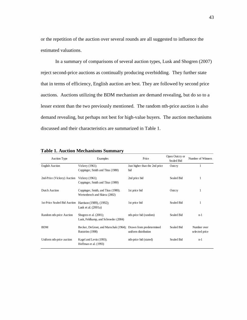
43
or the repetition of the auction over several rounds are all suggested to influence the
estimated valuations.
In a summary of comparisons of several auction types, Lusk and Shogren (2007)
reject second-price auctions as continually producing overbidding. They further state
that in terms of efficiency, English auction are best. They are followed by second price
auctions. Auctions utilizing the BDM mechanism are demand revealing, but do so to a
lesser extent than the two previously mentioned. The random nth-price auction is also
demand revealing, but perhaps not best for high-value buyers. The auction mechanisms
discussed and their characteristics are summarized in Table 1.
Table 1. Auction Mechanisms Summary
Auction Type Examples PriceOpen Outcry or
Sealed BidNumber of Winners
English Auction Vickrey (1961);
Coppinger, Smith and Titus (1980)
Just higher than the 2nd price
bid
Outcry 1
2nd-Price (Vickrey) Auction Vickrey (1961);
Coppinger, Smith and Titus (1980)
2nd price bid Sealed Bid 1
Dutch Auction Coppinger, Smith, and Titus (1980);
Wertenbroch and Skiera (2002)
1st price bid Outcry 1
1st-Price Sealed Bid Auction Harrison (1989), (1992);
Lusk et al. (2001a)
1st price bid Sealed Bid 1
Random nth-price Auction Shogren et al. (2001);
Lusk, Feldkamp, and Schroeder (2004)
nth-price bid (random) Sealed Bid n-1
BDM Becker, DeGroot, and Marschak (1964);
Rutström (1998)
Drawn from predetermined
uniform distribution
Sealed Bid Number over
selected price
Uniform nth-price auction Kagel and Levin (1993);
Hoffman et al. (1993)
nth-price bid (stated) Sealed Bid n-1
44
Single Round vs. Multiple Round Bidding
Auctions can be conducted in a single round of bidding or over several rounds.
The necessity for additional rounds has been confirmed by some and challenged by
others. Alfnes and Rickertsen (2003) suggest that using a modified Vickrey second
price auction for several goods simultaneously, one trial was sufficient to find the level
of the WTP a premium for one good over another. Corrigan and Rousu (2006b) suggest
that the practice of conducting multiple rounds of the Vickrey second price auction be
done away with completely, citing a tendency for ―bid affiliation‖ of bids in subsequent
rounds, particularly with high posted prices. Harrison (2006) further recommends that
the use of single-round auction mechanisms would elicit more accurate WTP estimates.
He says that this is for two primary reasons. The first reason suggested is that if
experimental auctions are truly designed to elicit participants‘ subjective values for the
good being auctioned, then subjects may perceive that others have more knowledge of
the attributes of the good and update their subjective values based on that information.
The second reason Harrison (2006) suggests is that knowledge of bidding behavior of
other participants may suggest a market value for the good that is below some
participants‘ value for the good, thus causing them to deviate from a strategy of bidding
their true value for the good. This would be a violation of the incentive compatibility of
the auction. Bernard (2005) tests a second-price auction for the presence of bid
affiliation over multiple rounds across three goods that differed in their novelty to
subjects. He found that differences that appeared to be based on perceptions of quality
as expressed in the first round of the auction disappeared over repeated rounds of the
45
auction and suggested that bid affiliation was a likely cause of the subsequent loss of
information about the initial values held by subjects. Corrigan and Rousu (2010)
conclude that for goods with both private and common value, bid affiliation is less of a
concern than the potential for the auction to ―overheat‖ (for bids to exceed the private
value, observed in this case in an induced value experiment).
However, others have questioned the validity of ―single-shot‖ auction
mechanisms in Vickrey single unit auctions that do not allow for a learning process; the
necessity of the learning process is suggested based on the fact that the dominant
strategy in Vickrey auctions is not immediately obvious to some participants
(Coppinger, Smith, and Titus 1980; Cox, Roberson, and Smith 1982). Kahneman and
Tversky (1979) further suggest that an ―isolation effect‖ causes people to discard the
components of all prospects that are uniform, causing differences in preferences when
the same choices are presented in different forms. In another type of sequencing effect,
Huffman et al. (2003) found that the order that different products were presented in an
auction setting also had a significant effect on results.
Shogren (2006) suggests that the use of a single round auction mechanism does
not cure the problem of bid affiliation implicitly, since other signals could be relied on to
generate affiliation in bids. Further, he suggests that the use of an auction with the
purpose of inducing a market-like experiment could be violated by using a single round
mechanism or even a multiple round mechanism with no price feedback; there is no
market learning in either of these cases. In a study of consumer valuations for several
retail beef options, Lusk and Shogren (2007) found that changes in bid levels were
46
consistent across the different qualities of beef over repeated rounds, thus raising the
question of whether the subjective views of quality of each participant influenced bids or
if the bids changed due to participant learning of the auction mechanism. Drichoutis et
al. (2009) note the differences between single shot and multiple round auctions, and
suggest an econometric procedure to test for the presence of bid affiliation. However,
this test requires at least four repeated rounds to be applied, and Drichoutis et al. (2009)
make the specific point that although their procedure has the ability to test for the
presence of bid affiliation, the authors refrain from taking a position on whether bid
affiliation is necessarily a problem that should be corrected for in an experimental
auction setting.
Bateman et al. (2008) analyze choice-based contingent valuation procedures;
however, their findings are pertinent to the discussion of single or multiple rounds in
other valuation procedures. They recommend against single-shot value elicitation and
contend that the learning process associated with unfamiliar goods and unfamiliar
institutions require the need for the opportunity for subjects to practice in order to obtain
more stable results.
There are also differences among the auction mechanism for multiple unit
auctions and auctions for products with possible negative values. Marked demand
reduction effects were seen in multiple unit uniform price auctions as compared to the
dynamic Vickrey/ Ausubel auction (Kagel and Levin 2001). In an induced value
experiment, aggregate bidding in a Vickrey second price auction was precise but biased
(high value bidders and low value bidders overstated benefits and understated costs,
47
respectively), while aggregate bidding in a random nth-price experiment was demand
revealing (unbiased) but lacking in precision (large variances) (Parkhurst, Shogren and
Dickinson 2004). Still, Menkhaus et al. (1992) point out that multiple unit Vickrey
auctions (e.g. third price auctions selling two units or fifth price auctions selling four
units) abide by the same theoretical incentive-compatibility as second price auctions.
Endowment Approach vs. Full Bidding Approach
Once an auction type has been selected, the type of bidding utilized can still have
an effect. Caution must be used at this point; auction bidding, which is a competition for
a limited quantity of goods, does not necessarily equate to the decision-making process
in point-of-purchase situations where consumers are price-takers for a practically
unlimited quantity of goods (Hoffman et al. 1993). In an endowment approach, subjects
receive a product and bid the amount that he or she would pay to exchange the
―endowed‖ product for another product; the amount bid is the WTP premium. In a full-
bidding approach, the participants in the auction bid the full price for each of the
different products and differences in bids can be used to calculate WTP premiums
(Alfnes 2009). It is important to distinguish the endowed approach described here from
the endowment effect that has been described as the cause for disparity among WTP and
WTA (Kahneman, Knetsch, and Thaler 1990).
There is disparity on whether an endowed approach is the necessary bidding set-
up (Lusk and Shogren 2007) or whether a full-bidding method is preferable (Alfnes
2009). Hoffman et al. (1993) suggested that experimental auctions are most valuable for
48
determining differences in WTP among products rather than for determining full values.
This is echoed by Hayes et al. (1996), who endow auction participants with a good and
seek the premium (or discount) that subjects have for another improved product. They
allow that the full bidding approach may be useful when the motivation for the research
is general information on the base good. A direct comparison of random nth-price,
second-price, BDM, and English auctions found differences in the significance of the
effect from the use of the endowed approach versus the full-bidding approach; a lower
value for the auctioned item was obtained using the endowed approach with the random
nth-price auction, but higher valuations of the auctioned good were obtained in the
second price auction (Lusk, Feldkamp, and Schroeder 2004). In general, the results of
Lusk, Feldkamp, and Schroeder (2004) were mixed. They found that in multiple round
auctions the endowment effect became more pronounced in later rounds. In terms of
differences in auction mechanisms, there was statistically significant evidence of loss
aversion in the random nth-price auction but not in the BDM or English auction
mechanisms. Lusk and Shogren (2007) contend that the endowment approach has the
benefits of controlling for the problem of field substitutes and outside option values,
allowing for imposition of a consumption requirement, and making a more useful
experimental outcome of estimating differences in WTP rather than actual values. In a
field experiment on WTP for steak tenderness, Lusk et al. (2001b) suggest that by asking
consumers which good they prefer and then endowing them with the opposite good,
some of the potential problems of the endowment approach will be avoided. However,
the incentive compatibility of the choice decision used here seems to be lacking in some
49
cases, as consumers would not have even a weakly dominant strategy to answer this
question in such a way that their true preferences are revealed. For example, if
consumers prefer good A over good B, they may receive good A without additional
payment by stating that they prefer good B.
On the other hand, Alfnes (2009) contends that since the effect of outside options
is similar for goods with the same outside substitutes, the Vickrey auction used with the
full-bidding approach should still provide good WTP estimates for product
characteristics. In an endowed auction, interpreting the bid for the new good as the
value placed on the trait of interest is in defiance of the reference dependence of
preferences, and the results may therefore be biased (Corrigan and Rousu 2006a).
Corrigan and Rousu (2006a) further suggest that it is impossible to predict the net
direction of the bias in the case of the endowed approach, as there is an upward bias
from reciprocal obligation and a downward bias from loss aversion, with the magnitudes
of these biases not predicted by theory. The approach they used compared bids for one
and two goods with bids to upgrade from one endowed unit of a good to another unit of
the same good; thus eliminating the possibility of a so-called ―endowment effect,‖ since
subjects never had to give up an endowed good. As an alternative means of WTP
elicitation, using a comparison of the difference in bids for two goods from the same
subject in a full-bidding approach facilitates the canceling out of the values of outside
options (including the same good and substitutes); the between-subjects comparisons of
bid differences should then provide an estimate of the distribution of willingness-to-pay
a price premium for one of the two goods over the other (Alfnes 2009). Despite Lusk
50
and Shogren‘s (2007) criticisms of the full-bidding approach, they indicate that
experimental auctions that utilize the full-bidding procedure may be appropriate if and
when few outside options exist, the endowment effect is a pervasive phenomenon, actual
consumption of the product is not an important part of the value, there is little
opportunity to learn about the value of the good in the future, and subjects will want to
―return the favor‖ of the endowment by altering their bids.
In the distinction between private value goods and common value goods, many
private value goods have a value in the outside marketplace that would be similar for all
individuals, breaking the private value condition; the usefulness of a common value
good to an individual may be enhanced by some private value (Laffont 1997). Further,
in markets for goods with both private value and common value traits, greater
inefficiency is expected in those that have higher levels of uncertainty about the common
value (Goeree and Offerman 2002; 2003).
Auction Mechanism Considerations
Unfortunately, there is a lack of formal theory to explain why, even among
incentive-compatible auction mechanisms, there is discrepancy among estimates of
willingness-to-pay. Thus, choice of auction mechanism may be based on the sort of
consumer the WTP analysis is targeting, with more emphasis given to the entire
marketplace and those consumers with low- to moderate-value with the BDM procedure
or the random nth-price auction and emphasizing higher-value consumers with the
Vickrey second price auction (Lusk, Alexander, and Rousu 2004; Shogren et al. 2001).
51
If these auctions are extended to private industry as a means of market analysis prior to
launching new products as suggested by several authors (i.e. Levitt and List 2009, Hayes
et al. 1996, Jaeger and Harker 2005), the absence of a clearly defined theoretical
understanding of the differences in auction results requires a careful consideration of
which auction type is most appropriate. Concessions are also made among the full-
bidding and endowed approaches when designing an auction, and exceptions are made to
suggest the endowed approach if 1) a consumption requirement is applied or if 2) the
two goods being compared are a novel good not available outside the experiment and a
conventional good that is available outside the experiment in order to prevent an
overestimate of the WTP premium value for the novel good (Corrigan and Rousu
2006a). Lusk and Shogren (2007) indicate that, based on the study of Lusk, Feldkamp,
and Schroder (2004), rejection of equivalence among bid mechanisms does not exclude a
conclusion that bids across mechanisms are highly correlated. The lack of unanimity in
the research on value elicitation is an indication not only that a great deal of
experimentation in this field has been carried out, but also that considerably more
experimental work is needed (Plott 1991).
Internal Validity
Internal validity refers to the ability to draw conclusions about causation from the
results of an experiment (Loewenstein 1999). An alternative definition is provided by
Samuelson (2005), who suggests that internal validity is the strength of the link between
the imposed experimental environment and the observed behavior of subjects. For an
52
experiment to be internally valid it must, therefore, be constructed in such a way as to
accurately test the hypothesis of the experimenter. The experiment might also be an
internally valid test of economic theory if it reproduces the assumptions of that theory in
order to generate results that are relevant to the predictions the theory makes (Croson
2005). Flaws in procedures that are not consistent with assumptions of the hypothesis
can lead to results that are biased. The testing of each causal hypothesis must be
conducted in isolation in order to sort out effects and either confirm or disprove the
hypotheses one by one (Guala and Mittone 2005). Economic theory is a strong tool for
testing the internal validity of experimental results (Samuelson 2005). Davis and Holt
(1993) list general methodology for controlling undesired effects within the experiment
to accurately and reproducibly test the hypotheses of the experiment. These strategies
are fairly consistent across the literature, and statistical tests can help determine the
strength of results in terms of internal validity. If results are not internally valid, then
either the researcher will fail to correctly identify the relationship between the situation
and the outcomes or he will be unable to do so because the results will be too noisy to
allow conclusions to be drawn (Samuelson 2005). Factors of internal validity that might
be of concern in experimental design include types of treatments to be applied,
elicitation method, randomization, subject pool and number of subjects, psychological
influences, learning behavior, and incentives.
Replication of results is perhaps the simplest way to test the internal validity of
an experiment (Samuelson 2005). For example, to further test a theory of bargaining,
Binmore, Shaked, and Sutton (1985) replicated previously reported results in their own
53
experiment, stating that ―under similar conditions, we obtained similar results.‖ This
replication as a control treatment in an experiment is useful in making comparisons
across time and space.
External Validity
External validity, on the other hand, refers to the generalization of experimental
results to the broader context of the world. There is generally some contradiction
between high levels of internal validity and high levels of external validity (Schram
2005). The discussion of the validity of experimental procedures within economics has
generally focused on the internal validity of experimental auctions, although discussions
of external validity are on the rise (Grebitus et al. 2010).
The ability to extrapolate the results from experimental auctions in a contained,
laboratory setting to the outside world has been questioned by those within and outside
the field of experimental economics (Umberger and Feuz 2004; Levitt and List 2007).
However, the external validity of experimental procedures and their application to the
field of economics is also extensive, with Plott (1982) arguing that experimental
methods have an important role in testing the validity of theories. This position was also
taken by Smith (1976), who extended it to include interpretation of field data as well.
As economists frequently take on normative roles in addressing policy, there are
certain strategies to improve external validity of experiments in such situations. If the
problems and exact circumstances that experimental results will be generalized to are
known, then those problems of external validity can be addressed as modifications in the

54
experimental design (Guala and Mittone 2005).
Levitt and List (2007) mention five factors that, in addition to monetary
considerations, influence the behavior of subjects in the laboratory. These are: the
presence of moral and ethical considerations, the nature and extent of scrutiny by others,
the context in which the decision is embedded (including artificial time and location
constraints), self-selection of the individuals making the decisions, and the stakes of the
game; all of these could influence the external validity of an experimental market. The
factors mentioned are generally different in a laboratory setting than in a naturally
occurring environment.
However, the generalizability of experimental results is key to their external
validity and is a question of which components of the experimental environment are
valid to use in making predictions of real-world results (Campbell and Stanley 1966).
Plott (1982) holds that the key to success in experimental design is asking questions that
can be sufficiently answered in an experimental context where a study of the simple case
can be generalized to the complex. Levitt and List (2007) also point out that the
generalizability of results based on observational data is not infallible and that caution
should be used when extending those results to real-world markets as well. Sound
economic theory is needed in both cases for data to hold value. These authors later
(2009) suggest that framed field experiments, including these types of auctions, lie on
the spectrum between laboratory experiments and econometric modeling based on
observational data. Further, they indicate that auctions avoid some of the problems of
randomization bias and attention bias on the laboratory end and identification
55
assumptions on the observational end. Roth (1995) questions the extrapolation of some
of the problems that can be commonly identified in experimental auctions to the field as
irrelevant in some cases. He suggests that for example, participants in an experimental
auction may be inexperienced and show evidence of the winner‘s curse, whereas in the
field participants in the same sort of auction may have experience and the phenomena
may not be seen. This particular distinction was disputed by Dyer, Kagel, and Levin
(1989) who found similarities in experimental results for bids of both naïve and
experienced subjects. Lange and Ratan (2010) base their criticism of the external
validity of first price and second price auctions on a theory of loss aversion; they find
that reference dependent preferences may affect the elicited valuations from a laboratory
setting versus a field setting on the basis of differences in the dimensions of the
consumption space (specifically, monetary value and actual item value).
Just and Wu (2009) hold that experimental economics can be useful in testing the
validity of a theory, particularly in the case that Binmore‘s (1999) criteria are met;
however they suggest that the greater usefulness of experimental economics as a means
of testing economic theory over making specific quantitative predictions can be a result
of the lack of practicality in implementing many proposed experiments. This view is
narrower than that taken by Guala and Mittone (2005), who advocate for the application
of experimental results to the real-world but suggest that the necessity for every
experiment to be externally valid in every situation is unrealistic. They suggest that a
more preferable approach is to categorize the results of some experiments as
―phenomena‖ and take the range of these, including various anomalies, biases, and
56
paradoxes, into consideration when making applications to particular cases. Harrison,
Lau, and Rutström (2010) emphasize that economic theory, experimental results, and
econometric techniques should be integrated for a more thorough understanding of
economics, rather than analyzing each of these as mutually exclusive. Thus,
experiments in the laboratory or in the field can be interpreted by taking the
considerations and findings of the other areas into account.
Relative WTP values obtained through experimental auction procedures appear
valid, but actual WTP values may be prejudiced by characteristics of the experimental
design. Specifically, panel size and the initial endowment were found to affect auction
prices by Umberger and Feuz (2004); the results of their auction were that market price
for a beef steak increased as the number of participants in the auction increased.
Coursey and Smith (1984) found that in a Vickrey fifth-price auction the subjects
underbid their maximum WTP, but that these underbids were consistent insomuch as the
underbids among subjects and for different objects were indicative of meaningful
differences in value. Ariely, Loewenstein, and Prelec (2003) conducted a series of six
experiments and found that in many cases, preferences measured by experimental
economics show what they term ―coherent arbitrariness.‖ That is, the preferences may
be heavily influenced by the context of the experiment; however, relative valuations
(e.g., value for more versus less of an auction good) respond in the way predicted by
economic theory. Lusk and Shogren (2007) discuss several empirical results that show
that preferences are likely not entirely arbitrary based on analysis of contingent
valuations of public policy where people are less likely to vote to implement more costly
57
policies as well as analysis of the effects of positive and negative information when
compared to a bid with no information.
Bateman et al. (2008) tested three hypotheses on the nature of preferences; these
included the a priori theory of well-formed and readily-divined preferences, the
discovered preference hypothesis introduced by Plott and Zeiler (2005), and the coherent
arbitrariness hypothesis of Ariely, Loewenstein, and Prelec (2003). Using a contingent
valuation method, Bateman et al.‘s (2008) results suggest that there are likely at least
two types of learning that occur over multiple rounds of an auction: value learning
(learning of individual preferences) and institutional learning (learning of the valuation
mechanism). They also suggest support for the discovered preference hypothesis of
preferences in which stable preferences are gained through practice and repetition with
both the good and the market institution. These are important considerations in eliciting
the homegrown value for good.
Carlsson (2010) discusses the application of theories of behavioral economics to
value elicitation procedures. He raises four areas that are all relevant to the external
validity of such studies; these include revealed versus normative preferences, learning
and construction of preferences, context dependence, and hypothetical bias. In
particular, the context dependence of preferences is pointed out, but a number of
methods (such as the use of the random-utility model and design of experiments with
different contexts as different treatments) that have been used to analyze such context-
dependence in value elicitation are suggested.
The use of experimental auctions or other experimental techniques to elicit
58
homegrown values are subject to certain issues that are not relevant for induced value
auctions. However, they are highly relevant to any results that will be extrapolated to
the real world. Many of these issues have been documented over the years; for example,
Milgrom and Weber (1982) suggested that bids may be affiliated at the beginning of an
auction or may become affiliated over the course of the auction. Others have made
pointed criticisms of the external validity of some mechanisms; the three main issues
discussed by Harrison, Harstad, and Rutström (2004) are ―field-price censoring,‖
affiliation of beliefs about field prices, and affiliation of beliefs about the quality of the
auctioned good. Experimenters must account for field-price censoring, or the curtailing
of bids at the price level for an outside substitute of the good they are auctioning in
analyzing results, as rational consumers would not bid more in an experimental auction
for a good than the price they could purchase it for outside the experimental market plus
some transaction cost, assuming they know the price of the outside good. Secondly,
institutions that reveal information to the consumer about the value of the good may
cause the estimated WTP to be biased over multiple rounds. Consumers could believe
that the bids expressed by other participants reflect knowledge of the pricing of perfect
and imperfect substitutes, as well as complements, in the outside marketplace. This
affiliation could be prevented by using simultaneous or one time value elicitation, but if
the experimenter believes that learning is a necessary part of obtaining valid results, then
the posting of bids is generally a component of that learning process. The third
methodological issue discussed by Harrison, Harstad, and Rutström (2004) is that an
affiliation of the perceived quality of goods up for auction may occur over multiple

59
rounds. If participants are unsure of the quality of the good up for auction, they may
assume that other participants have more knowledge of the quality of the good then they
do and adjust the bids they place accordingly.
Alfnes (2009) contends that if product attributes are to be valued using
experimental methods, the levels of the bids in a Vickrey second price auction are not
generally useful because they are curtailed at the market price for that good and reduced
by the value of the surplus that could be obtained by purchasing substitutes. He suggests
that products that would normally be purchased in the market place will generate bids
that are at the market price. However, for goods that would not typically be purchased
in the marketplace, participants will still seek to generate the same surplus they would
have had by purchasing substitutes in the marketplace; therefore, the bid they submit
should be less than the market price. Cherry et al. (2004) also found bid shaving
(reduced bids when homegrown value exceeds the value of the outside good) in real and
hypothetical induced-value auctions where information on outside substitute goods was
provided. Possible options to control for the effect of providing prices for substitutes are
to account for bids that are truncated (Harrison, Harstad, and Rutström (2004) or by
asking subjects what their perceptions of available substitutes and prices are for the good
being auctioned (Corrigan 2005).
Shunda (2009) found that the price set by sellers to end an online auction early
affected the valuations that consumers had for goods. He suggests that bidding behavior
more closely mirrors a reference-dependent theory than the reference-free expected
utility theory. In the case of economic development, Deaton (2009) argues that scientific

60
progress is unlikely based on uncertain experimental results and that the usefulness of
experimentation in that field may be limited. Nunes and Boatwright (2004) discuss the
effects of incidental prices on WTP, defining ―incidental prices‖ as the prices for
unrelated goods whose prices are irrelevant to the good for which WTP is being elicited.
The anchoring effect often discussed in psychology literature was observed using
incidental in three studies by Nunes and Boatwright (2004); this indicates yet another
example of the context-dependence of WTP estimates. These authors further suggest
that the effects that they observe could be strategically manipulated by marketers to
target the numerical values that consumers are exposed to near the time of purchase and
influence consumer WTP. Nevertheless, this effect remains relevant to experimental
economics in that subjects are likely to be influenced by any prices they are exposed to
during the span of an experimental session, but also in that subjects may exhibit effects
of incidental prices they were exposed to prior to the experimental session. Ariely,
Loewenstein, and Prelec (2003) also discussed the anchoring effect in their presentation
of a coherent arbitrariness hypothesis for the formation of preferences.
In a series of studies to analyze the unique complexity of price, the difficulty of
evaluating an infinite number of other uses for money, and the evidence that consumer
preferences are influenced by price, Lee, Bertini, and Ariely (2008) report evidence that
the decline in preference consistency is not an information effect. They further suggest
that preferences appeared to be more stable when price was not included as a factor in
the decision-making; however, they counter this with the fact that from a consumer
standpoint, subjects seem to be more satisfied and better able to make decisions when
61
price information is included. An important methodological consideration they find is
that there is a reduction in variability of preferences when an explicit suggestion is made
by experimenters to participants suggesting that they consider the opportunity cost of
using money to make other purchases. As a final note, there may be factors that
confound any type of data, be it experimental or observational; care must be taken to
make accurate conclusions based on the available information (Roth 1995).
Incentive compatibility is also applicable to methods of value elicitation other
than auctions, although it was traditionally lacking in hypothetical choice experiments
(see Murphy et al. 2005). Proposals have been made and utilized to develop incentive
compatibility in conjoint analysis of choice-based experiments (e.g. Alfnes et al. 2006)
and ranking experiments (Lusk, Fields, and Prevatt 2008). Analysis by others also
indicated that the preferences of an individual were not context dependent in a study to
determine whether rational decision-making by individuals was transferred from market
to non-market settings (Cherry, Crocker, and Shogren 2003).
It should be noted that comparisons of dichotomous choice surveys, open-ended
surveys, and auction procedures as methods of value elicitation indicate that
dichotomous choice questions overstate values (for both public and private goods), and
that open-ended questions also overstate the values obtained in auction results but do not
do so as severely as dichotomous choice questions (Balistreri et al. 2001). One possible
solution to this issue is to combine the use of surveys and auctions for a single analysis
of WTP and the factors that affect it in order to correct for the problems of each
approach (Yue, Alfnes, and Jensen 2009).
62
In determining whether survey methods that are hypothetical or nonhypothetical
are preferable, Chang, Lusk, and Norwood (2009) found nonhypothetical methods
(nonhypothetical choices and nonhypothetical rankings) to outperform hypothetical
choices as a means of predicting retail choices. They contend that real-world decisions,
if they are to be based on either of these two types of survey results, should be more
accurate when based on the incentive-compatible (nonhypothetical) option. However,
previous results suggested that although total WTP was sensitive to the hypothetical or
nonhypothetical nature of a choice experiment, there was no significant difference in the
estimates of marginal willingness-to-pay by either method (Lusk and Schroeder 2004).
A comparison of stated preferences from a conjoint ranking procedure and revealed
preference from scanner data for consumers of dry-cured ham in Spain used a nested
logit model and found that stated preferences could be useful for predicting general
market trends and choices, but not for predicting market shares (Resano-Ezcaray,
Sanjuán-López, and Albisu-Aguado 2010). However, Grebitus et al. (2010) found that
hypothetical nonmarket results were consistent with actual market behavior for
purchases of country-of-origin labeled meat products.
Some researchers (e.g., Shin et al. 1992; Yue, Alfnes, and Jensen 2009) include a
consumption requirement as a component of the experimental design; that is,
participants must eat the food item they bid on to ensure that true preferences are
revealed. Lusk and Shogren (2007) suggest that this is an important component of value
elicitation if a large part of the value of the good is derived from the consumption value.

63
Random lottery procedures are sometimes utilized in order to create an incentive-
compatible auction mechanism. In such an auction, several trials of the auction are
completed and one of the trials is randomly drawn to be binding for the subjects (e.g.,
Becker, DeGroot and Marschak 1964; Shin et al. 1992; Lund et al. 2006). This is
intended to control for the potential income effect as a result of a difference in the
endowment of the subjects in subsequent trials of the auction; bias could occur when
subjects experience changes in their endowment or in expectations of rewards from the
beginning to the end of the experimental procedure (Grether and Plott 1979). Holt
(1986) criticized the use of the random lottery procedure and presented results
supporting the conclusion that it is only appropriate to use the random lottery procedure
when the axioms (the independence axiom, in particular) of the von-Neumann
Morgenstern expected utility theory are not violated. If one of these axioms is violated,
the random lottery procedure may not ensure unbiased estimations of value. This
procedure has also been criticized for lack of saliency, since the expected payoff for each
task is small (Harrison 1992; 1989). Kagel and Roth (1992) agree that the payoff space
may influence subjects to deviate from the dominant bidding strategy, while Merlo and
Schotter (1992) hold that the payoff will only dominate the results of the auction
depending on when and how much subjects learn during the auction. Hey and Lee
(2005) carry out a direct test of the effectiveness of the random lottery procedure and
find no differences in expressed preferences if the questions are answered individually
versus in a series, confirming the ―separation hypothesis‖ (that rounds of an auction are
addressed separately instead of as a whole by subjects) of Starmer and Sugden (1991).

64
Corrigan and Rousu (2006a) also found results to be consistent across multiple rounds of
auctions when participants were explicitly told the dominant bidding strategy.
Placing an auction bid can be thought of as a type of lottery for the subjects.
More specifically, subjects participating in an experimental auction face a series of
uncertain outcomes. They do not know who will win the auction (and win the good if
the auction is nonhypothetical); the best estimate of the outcome would generally be
each individual‘s own subjective probability (Lusk and Shogren 2007). This leads to the
question of whether Bayesian updating occurs for participants when they are provided
with additional information.
Subjects may submit bids that reflect what they perceive as the socially preferred
option, rather than truthfully representing what their own buying decisions would be in
the marketplace (Levitt and List 2007). There has been some work to suggest that the
use of inferred valuation to address the problem of social desirability bias may reduce
this problem of external validity and produce more accurate predictions of market
purchasing behavior (Fisher 1993). This may be accomplished through the use of
indirect questioning (Lusk and Norwood 2010); for example, asking ―How much would
the average consumer pay for environmentally friendly goods?‖ instead of ―How much
would you pay for environmentally friendly goods?‖ Lusk and Norwood (2009) utilize
this strategy for both goods with a normative dimension and goods with a novel
dimension; they find that utilization of an inferred valuation method based on indirect
questioning may eliminate some of the gaps between laboratory and field behavior if the
source of the gap are the social concerns of the good. However, for a novel good with
65
minimal social concerns, Lusk and Norwood (2009) do not find significant differences
between estimates based on direct and indirect questioning for elicitation of WTP.
The prior information and beliefs held by consumers may also affect the results
of experimental auctions. Subjects who are provided with ―reference prices,‖ defined as
the price of the good in the outside world at retail markets, were shown by Drichoutis,
Lazaridis, and Nayga (2008) to raise estimates of WTP based on bids in Vickrey second
price auctions. While this finding may not hold absolutely, it does raise questions on
whether prior information on market prices or providing such information during an
experiment will affect value elicitation procedures. Grunert (2005) mentions the role of
reference prices in consumers‘ decisions on how much they are willing to pay,
particularly in the case of novel goods. In contrast, experimental results from Gil and
Soler (2006) found that the decision of Spanish consumers on whether to pay a premium
for organic olive oil was independent of whether they were provided with reference
prices.
In keeping with the discussion of reference prices, there are also possible effects
of other context aspects of an experiment. Choice heuristics and framing effects may
influence the levels of WTP that are elicited (Bateman et al. 2008). The ―focusing
illusion‖ discussed in the psychology literature is also likely a contributor to possible
problems with the external validity of WTP estimates (Schkade and Kahneman 1998).
Lancaster‘s (1966) theory of demand proposes that the utility derived from a good is not
derived from the good as a whole, but from the multiple attributes of the good.
However, valuations of goods based on the division of values for different quality based
66
on this theory of demand may be susceptible to an artificial focus that is perceived by
participants in experimental valuations procedures, causing them to inflate their
perception of the value of the good (Bateman et al. 2008).
Previous Measures of Willingness-to-Pay for Food and Horticultural Products
Previous studies have analyzed WTP using a variety of experimental techniques.
In one, a survey of best-worst questions was used to analyze differences in WTP for
different types of beef (Lusk and Parker 2009). Alternatively, real choice (RC)
experiments can be used in which numerous price scenarios are introduced for two
products at the time, and subjects must indicate which product they would purchase
(Alfnes et al. 2006). One of these scenarios is then randomly chosen to be binding to
induce incentive compatibility in estimates of WTP. These types of experiments closely
match the situations consumers face in a retail store, where they must select between
similar products with different prices.
Bougherara and Combris (2009) used experimental auctions to determine WTP
for an eco-labeled product and to determine the motivations that WTP was based on.
Subjects demonstrated an increased willingness-to-pay for both the eco-labeled and the
control products based on the availability of more information, making the level of
information provided an important consideration in the design of this analysis of
willingness-to-pay. The diversity in demographic characteristics of purchasers of
flowering potted plants was also reflected in heterogeneity of WTP for biodegradable
packaging of those products (Hall et al. 2010).
67
There is evidence from conjoint analysis procedures that consumers in Kentucky
are willing to pay more for blueberry products made from blueberries produced in
Kentucky (Hu, Woods, and Bastin 2009). These authors express caution in generalizing
this result to other products and other states, but it does indicate promise for garnering a
price premium for goods produced and marketed locally. Darby et al. (2006) find that
there is also a willingness by Ohio consumers to pay a premium for Ohio-grown
strawberries, based on the results of a choice experiment and conjoint analysis.
However, a guarantee of freshness derived a higher WTP premium than the Ohio-grown
claim, which they suggest indicates that at least the majority of the WTP premium was
as a result of this attribute. Other dichotomous choice contingent valuation procedures
have shown WTP premiums for goods produced within state in the New England region;
further, that those premiums vary with the base price of the good (Giraud, Bond, and
Bond 2005). Other WTP questions found a lower willingness-to-pay for males and
lower income respondents for locally produced foods (Adams and Adams 2008).
Experiments have also been conducted on whether consumers are willing to pay
more for health benefits by analyzing WTP for dairy products with high levels of
conjugated linoleic acid, which has been proposed as a cancer-fighting agent (Maynard
and Franklin 2003). Conclusions were that validation of claims from the medical
community is necessary for statements made regarding the health benefits of food.
Another study by Umberger, Boxall, and Lacy (2009) utilized experimental
auctions to determine the effects of credence and health information on consumers‘
WTP. More specifically, they sought to determine the product attributes and consumer
68
characteristics that influenced the purchase decisions of United States consumers for
Australian grass-fed beef. They found that providing health information had a
significant effect on consumer WTP when modeled with a two-stage Cragg model.
Variations in WTP were analyzed for consumers who were provided with production
and health information as well as an opportunity to taste the product offerings.
Several other studies also analyzed experimental auctions with the provision of
health information and the implications of such on the development of public policy.
Marette, Roosen, and Blanchemanche (2008) found that in both laboratory and field
experiments, subjects showed a decrease in consumption of some types of fish when
provided with information on possible health benefits from omega-3 fatty acids and
possible health risks from methyl-mercury. They suggest, based on differences in
response to different types of fish, that lab estimates of WTP would be more useful for
products with a large market share; they also indicate that bias may be introduced in the
laboratory because consumer choice is artificially restricted. In a study relating to the
potential gains and losses from genetically modified foods, Rousu et al. (2007) analyzed
the effects of providing consumers with positive, negative, and third-party information.
The results of their random nth-price auction indicate that in a market with a
controversial product and voluntary labeling requirements, providing verifiable third-
party information has the most impact and thus social value when activist groups (or
others) are also distributing negative information in the marketplace. They suggest that
in the case of GM food, verifiable third-party information may have a social value of up
69
to $2.6 billion annually, and that the use of experimental techniques similar to theirs may
allow policymakers to balance costs and benefits for information.
Colson, Huffman, and Rousu (2010) conducted an experimental analysis of
consumers‘ WTP for various components of GM foods (broccoli, tomatoes, and
potatoes). Of particular methodological note is that the information received by
consumers within these random nth-price auctions was randomized within each auction
session, and that consumers were presented with both biased and factual information.
They used estimates from the auctions to develop welfare estimates and compare these
to the results of welfare estimates based on a single parameter for preference for GM
products.
Poole, Martínez, and Giménez (2007) evaluated consumer demand for citrus fruit
using a Vickrey second price experimental auction and found that bidding behavior
closely reflected tasting scores of mandarin oranges; they suggest that this serves to
validate the use of auction procedures for evaluating food preferences. Consumer
valuations were elicited after visual appraisal, peeling the fruit, and tasting the fruit.
These authors also contend that industry and policymakers should not focus solely on
providing nutrition information when encouraging individuals to purchase and consume
healthful foods and that they should also focus on promoting foods that provide the most
consumption value from a pleasurable eating experience.
Nalley, Hudson, and Parkhurst (2006) used an experimental auction to test the
effects of health information and location of origin on WTP for sweet potatoes. Results
from that experiment indicate that both types of information studied affected the level of
70
bids. However, the information on the location of origin not only affected the level of
the bids, but the marginal differences in bids as well. They further suggest that attempts
to value separate attributes of food products may not be successful since the food is
purchased as a whole, rather than as a sum of individual attributes. One interesting
question raised by these authors is if there is an ordering effect when providing subjects
with an opportunity to taste a product and providing them with other information.
The use of nutrition labels on processed food products was analyzed using a
bounded dichotomous choice model by Loureiero, Gracia, and Nayga (2006). Although
this methodology may have more limitations than experimental auctions for value
elicitation (as discussed previously), the qualitative findings of the study are still of
relevance. These authors found that consumers were willing to pay more for products
with a nutrition label; further, they found that consumers suffering from diet-related
health problems were more willing to pay a premium for products with a nutrition label
than those not suffering from diet-related health problems.
Bernard and Bernard (2009) used a variation on the Vickrey second price auction
to analyze consumer WTP for various attributes of milk. They found that the valuations
for several credence attributes, including organic and no antibiotics used types, were not
additive; this suggested a diminishing marginal utility for additional attributes.
However, they also found differences in the demographic characteristics of consumers
who preferred each type of milk. They conjectured that this may allow marketers to
segment the market and target some of these consumers with other milk products that are
less expensive to produce.
71
Hayes et al. (1995) used an experimental auction to analyze WTP and WTA
responses to additional food safety information for a meat sandwich. These authors
found that marginal WTP to upgrade from a typical sandwich to a sandwich with a
guaranteed level of safety decreased as the level of risk decreased. They suggest that
subjects place a high value on their prior conceptions of illness even when new
information on the odds of illness is provided. They also observed a tendency for some
bids to cluster around the posted price of the previous round, a tendency called bid
affiliation in the literature (e.g., Corrigan and Rousu 2006b).
Willingness-to-pay for apples elicited using a second price experimental auction
procedure was influenced by both sensory (taste-testing) and emotional (opinion on
information regarding length of time since harvest) aspects of freshness (Lund et al.
2006). Multiple-round second price auctions had previously been carried out on apples
in relation to insecticide application, with WTP being income elastic (Roosen et al.
1998). Product attributes and packaging were more important than brand in WTP for
fresh-cut melon (Mayen, Marshall, and Lusk 2007). Willingness-to-pay for food safety
(specifically regarding Salmonella) was analyzed by Fox et al. (1995), with emphasis
placed on the use of real food, real incentives, and multiple rounds as components of the
auction market.
Consumers‘ level of health concern, ceteris paribus, did not generally affect their
WTP a premium for organic foods, and many consumers lacked a prior knowledge of the
National Organic Program (Batte et al. 2007). The lack of effect from recognition of the
organic seal raises questions on the usefulness of a national standard label for functional
72
foods, although Batte et al. (2007) concluded that the National Organic Program had
shown a positive effect on the market for multi-ingredient organic foods.
Gao and Schroeder (2009) used choice experiments to evaluate the effects of the
availability of additional information on WTP. They found evidence that the omission
of attribute information could influence WTP, that cue attribute information affected
WTP more than independent attribute information when provided solely but the effect
diminished when more attribute information was provided, and finally, that the relative
ranking of the importance of attributes did not vary significantly when additional
attribute information was presented regardless of changes in WTP. Gao and Schroeder
(2009) further suggest that marketers utilizing such information to release new products
should emphasize the attribute that has been shown to be most important relative to its
cost.
In an application of WTP valuations to analysis of changes in welfare, Lusk and
Marette (2010) found that estimates of effects on welfare varied across the use of
hypothetical stated preference data and nonhypothetical experimental auction data;
however, the direction of the welfare change was consistent. One solution to this
problem would be to provide a range for the estimate of effects on welfare based not
simply within a single valuation method, but across valuation methods to give a more
robust estimate. This is particularly important if estimates will be used to analyze the
effect of policy changes.
Most foods are what are known as ―experience goods.‖ That is, they are
products for which the value of consumption cannot be fully determined prior to
73
purchase (Nelson 1970). Consumption of new experience goods can provide value from
consumption as well as value from information regarding potential surplus that can be
gained in the future. In experimental results from Vickrey auctions for new experience
goods, optimal bids were higher than the expected consumption value and the difference
between the two (the information value) was affected by the purchasing frequency, the
expected future prices, and the degree of uncertainty about the consumption value
(Alfnes 2007). Alfnes (2007) also noted that the information value concept applies to
other incentive compatible methods for elicitation of WTP for novel goods. The degree
of uncertainty about consumption value may be reduced if consumers are allowed to
sample the new experience good prior to bidding.
Studies of WTP for various food products are valuable for several reasons as
discussed by Yue, Alfnes, and Jensen (2009). These include the ability to compare WTP
values for similar products, whereas a consumer would generally not purchase multiple
products in the same category (i.e. different types of apples). Further, these authors
stated an additional benefit of auctions: the ability to compare WTP for established
goods directly with WTP for goods that are not yet available in the marketplace. Choice
experiments were useful for making estimates of WTP for quality differences in a study
on beef products (Lusk and Schroeder 2004).
The willingness of consumers to pay for new varieties and types of fruit is of
particular relevance to this pomegranate study. The novelty of an unfamiliar product,
such as mango, may influence subjects to bid relatively high price premiums as a result
of ―preference learning,‖ defined as the desire to learn where a new good fits into an
74
individual‘s preference set (Shogren, List, and Hayes 2000). A premium was paid for
goods that had never been tried before, but this was reduced after trying the good. This
is consistent with a description of the product as having experience attributes. Gil and
Soler (2006) also found that the novelty of a product could bias WTP premiums upward,
and suggest that in the case of novel goods, any reference price that is provided may also
influence WTP premiums. Similarly, consumers in New Zealand were willing to pay a
premium to exchange an older variety of kiwifruit for a new, brightly-colored variety
(Jaeger and Harker 2005). This was an introduction of the use of experimental methods
for application to horticultural innovation. Moreover, if new horticultural varieties are
very different from those on the market, experimental methods could have applications
for new product development.
Urala and Lähteenmäki (2007) found the best predictor of willingness-to-use
functional foods was based on consumers‘ perceived benefits from using the functional
foods. In the same study, consumers were unwilling to sacrifice taste for additional
health benefits from the food. Participants were asked to evaluate numerous statements
regarding these so-called ―functional foods‖ as a part of a telephone survey. The
researchers elected to evaluate willingness-to-use a product, rather than willingness-to-
pay, in order to establish a more reasonable comparison between established and new-to-
the-market products.
Many functional food claims are made on the basis of compounds naturally
occurring in food products, but many other claims are on the basis of the addition of
bioactive ingredients to an existing product. The use of a new coating rich in
75
antioxidants (flavonoids and stilbenes) on apples was analyzed using a contingent
valuation technique found a positive attitude towards functional foods in general and that
WTP values varied with location (Markosyan, Wahl, and McCluskey 2007); these
antioxidant compounds have the potential be used on other whole fruit products. The
WTP of consumers in a region of Spain for a red wine product enriched with resveratrol
(a phenolic antioxidant in the stilbenes group) was analyzed using choice experiments;
researchers found a 55% premium for enrichment of the wine product over the non-
enriched product (Barreiro-Hurlé, Colombo, and Cantos-Villar 2008). However, there
are limitations to the generalizability of such exact premium values to other products or
other regions.
Functional Foods
There has been movement within some parts of the scientific community to
analyze whole foods rather than summing the individual nutrients of a food to thus better
understand the heath-nutrition interface (Jacobs and Tapsell 2007). This has been
coupled with the explosion of interest in so-called ―functional foods,‖ which include
whole or enhanced foods that provide health benefits beyond the provision of essential
nutrients (i.e. calories, fiber, vitamins, etc.) when consumed on a regular basis (Hasler
2002). Demand for functional foods appears to be driven, at least in part, by 1) a rising
average age, 2) increasing healthcare costs, 3) greater availability of information
allowing for greater individual control of health status, 4) progressing scientific evidence
76
that diet can alter disease prevalence, and 5) changes in food regulation (ADA 2004).
Similar drivers of demand are also suggested by Siro et al. (2008).
The range of functional food products is large, with over 1,700 functional food
products having been introduced in Japan alone within the span from 1988 to 1998
(Menrad 2003). The products cited as having potential to be marketed as functional
foods include everything from fruits and vegetables (Kaur and Kapoor 2001) to olive oil
(Stark and Madar 2002) to enriched custard pudding dessert (Sun et al. 2007).
The creation of marketing strategies for functional foods is complicated by the
additional credence attributes associated with the majority of food products in the
developed world beyond the experience attributes common in the less-developed world
(Barrena and Sánchez 2010). Credence attributes cannot be checked directly by the
consumer (Darby and Karni 1973), and therefore decision-making depends on
information the consumer possesses and that are provided in the market (Azzurra and
Paola 2009).
The three largest markets for functional foods are the United States, Japan, and
Europe (Bech-Larsen and Scholderer 2007). These markets have varying degrees of
regulation for the use of the ―functional food‖ terminology. In the United States there is
no regulatory definition for the term functional food, so product labelers must only abide
by existing regulations regarding health claims on food (Hasler 2002). In September
2003, the United States Food and Drug Administration (FDA) began accepting
―qualified health claims‖ based on scientific evidence; this rule was proposed with the
purpose of providing additional health information with a scientific basis to consumers

77
(FDA 2006). However, not all groups in the United States are in support of such a
labeling scheme (e.g., ADA 2004; Lupton 2009). At least 15 such claims have been
approved by the FDA to date, covering a range of health-related issues from cancer to
cardiovascular disease to cognitive function (FDA 2009). Still, some suggest that the
use of health claims in this way is in fact confusing to consumers rather than a useful
means of providing them with health information (Hasler 2008).
In Europe, however, there are much more strict qualifications for the term as laid
out by the European Council (EC), and sufficient scientific evidence of a product‘s
health benefits must be provided to the European Food Safety Agency prior to making a
claim of a beneficial effect (EC 2006). Further, these regulations enforce a uniform set
of standards for functional foods across all the European Union member nations,
possibly helping to improve the acceptability and credibility of health claims to
consumers there (Asp and Bryngelsson 2008). Japan has a series of regulations to
categorize food with health claims as either foods for specified health use (FOSHU) or
foods with nutrient function claims (FNFC) based on a relatively long (since the 1980‘s)
history of functional food use (Ohama, Ikeda, and Moriyama 2006). Several other
nations have either passed or are discussing the implementation of health claims
regulations to address some of the issues associated with making health claims about
functional foods (e.g., Tapsell 2008; Yang 2008).
Scientific Basis for Functional Foods
The chemical compounds in plants that have been shown to have positive health
78
implications but are not included in the traditional essential nutrients are broadly known
as ―phytochemicals.‖ These compounds have been shown to appear in a range of foods,
from garlic to tomatoes to citrus, and to have a range of health-improving properties
including the ability to reduce the risk of certain cancers (Rafter 2002). Polyphenols, a
class of phytochemicals characterized as having multiple hydroxyl groups on phenolic
rings, have been frequently referred to as having antioxidant properties based on results
in vitro; however, their action is much more complicated in vivo (Williamson and Holst
2008). These compounds have not been shown to be necessary for growth and
development, but have been shown to have positive effects for disease reduction,
causing them to be termed ―lifespan essential‖ by Holst and Williamson (2008). The
antioxidant effects of phenolic compounds function most frequently by free radical
scavenging and metal chelation activities (Shahidi 2009).
The activity of polyphenols is believed to be in conjunction with other
phytochemicals present in foods (Shahidi 2009). Further, the other compounds that are
bioingested at the same time as flavonoids, one of the most common classes of
polyphenols, and the complexity of the food matrix may affect bioavailability
(Williamson 2009). Bioavailability and bioefficacy vary widely across types of
polyphenols as well, as measured by changes in plasma concentration (Manach et al.
2005). Still, polyphenols have been linked to anticarginogenic activity (Duthie 2007)
and prevention of cardiovascular disease (Wilcox, Curb, and Rodriguez 2008); however,
both these papers indicate a need for further evidence before claims can be made
regarding the certainty of these effects in human populations.
79
In terms of safety, it is believed that non-nutrient antioxidants are not a cause of
health problems as they appear in the average daily diet; however, comprehensive
studies of concentrations and effects are needed, as well as more evidence that
polyphenols are absorbed by human subjects and distributed to the tissue in order to
have an antioxidant effect (Diplock et al. 1998). There is also some evidence that
whole-food sources, including the skin and hulls (i.e. total phenolic content in wheat and
barley- Shahidi 2009) have a greater level of bioactive compounds, but this is not always
the case as some processed foods have higher concentrations of phytochemicals (i.e.
lycopene in tomatoes- Rao and Ali 2007).
Another important note is the lack of in vivo research on the efficacy of
phytochemicals. A great deal of additional research is needed before sound scientific
claims can be made regarding recommended dietary levels of these compounds, and
polyphenols in particular, in order to prevent harmful effects (Williamson and Holst
2008). Westrate, van Poppel, and Verschuren (2002) list eight areas of research within
both science and economics that have potential to yield valuable information regarding
potential functional food products; the scientific questions include determination of
which molecules could have potential health benefits, if those compounds are digested
and absorbed, and if the product is effective on a human level with effects that can be
measured quantitatively. Although considerable research has been done in the
functional foods area since that time, these are still relevant questions to be answered.
The American Dietetic Association suggests that well-developed clinical trials are
needed to further establish the benefits and clinical efficacy of functional foods (ADA
80
2004).
Functional Food Market
Functional foods, as defined previously, are a market segment that has received
increased interest from both consumers desiring to protect their health and by those
involved in the food industry as a potential growth sector (Rafter 2002). For an extensive
review of the current state of the functional food market segment, please see Siró et al.
(2008). The global market for functional food generated $33 billion in 2000 and $73.5
billion in 2005 with an anticipated growth rate of 10% per annum; in the United States
alone the market size was $27 billion in 2007 (Granato et al. 2010).
Both food manufacturers and pharmaceuticals companies have become interested
in the functional foods market. Pharmaceutical companies are attracted to this market
due to much shorter development times than pharmaceutical products. Development
costs are also much lower for functional food products (Siró et al. 2008). However,
pharmaceutical companies have been met with limited success in this market (Bech-
Larsen and Scholderer 2007), possibly due to inadequate ability to develop and market a
consumer-accepted food product. Also, this market segment varies by location, with
more stringent labeling requirements in place in Europe (EC 2006) than in the United
States (Siró et al. 2008). One of the largest segments of the functional food market is for
probiotics, or living bacteria that generally promote digestion and digestive health, and
there have been some products marketed using fruits and fruit juices (Granato et al.
2010). This represents a potential market for pomegranates as a functional food with
81
multiple functional attributes.
Based on a means-end approach to analysis of consumer cognitive structure for
functional foods, Barrena and Sánchez (2010) concluded that in the case of a Bifidus
spp. dairy product, households with children would be most affected by marketing
emphasizing the overall health benefits and quality of the product, but households
without children would be more concerned with ease of consumption and time savings.
In the case of an enhanced tomato juice product, the level of demand for the functional
food was actually reduced when the product in question had multiple functional
attributes as opposed to a single functional attribute (Teratanavat and Hooker 2006). A
consumer survey in Canada found that approximately one-fourth of respondents
expressed a decreased value for a tomato product with functional properties, although
the mean change was a 67% increase in value for a functional conventional tomato
product (West et al. 2002).
Survey data indicates that as the market size and awareness for functional foods
has grown, the unconditional acceptance of such foods has decreased; consumers now
place a greater emphasis on the taste of food and surprisingly, are more reluctant to
believe that functional foods can be included as a part of a tasteful and healthy diet
(Verbeke 2006). However, over the same survey interval from 2001-2004, Verbeke
found not only an increase in perceived importance of functional foods but also a
decrease in the assumed tradeoff between healthfulness of food and taste (2005; 2006).
Foods with a strong health benefit claim may be an exception to the lack of willingness
to compromise on taste (Urala and Lähteenmäki 2007). Careful consideration should be
82
given to the taste of a functional food relative to close substitutes if experimental results
are extrapolated to the marketplace and used to develop marketing strategies.
The underlying nutrient properties of the food are a determinant of consumer
attitude towards the functional food product (Bech-Larsen and Grunert 2003).
Consumers are more willing to accept functional foods that are plant-based rather than
animal-based (Larue et al. 2004; West et al. 2002) but these general assumptions have
been contradicted by some specific products (i.e. lamb versus strawberries-Traill et al.
2008). Functional foods seem to be evaluated by consumers as foods first and as
functional foods second (Bech-Larsen and Scholderer 2007). Some results indicate that
consumers who trust innovations made in agriculture and also have a concern for the
relationship between health and food are more likely to use a functional food product
(specifically, antioxidant-enriched wine) (Barreiro-Hurlé, Colombo, and Cantos-Villar
2008). Other studies of willingness to try functional foods have found innovativeness of
the consumer to have some predictive ability of reported willingness to use new foods
(Huotilainen, Pirttilä-Backman, and Tuorila 2006). O‘Connor and White (2010) found
risk dread to be a significant negative predictor of consumers who were non-users‘
willingness to try functional foods.
Siró et al. (2008) suggest that information on the health effects of specific
products should be transmitted in a simple way through credible media in order to
increase the knowledge base of consumers, who cannot independently check the
credence attributes of functional foods. West et al. (2002) further suggest that
information on the health attributes of products should come from government officials
83
or health experts, citing a lack of trust for claims made by food manufacturers.
Introduction of genetically modified (GM) functional foods appears to be less
than promising, with household consumers generally avoiding purchasing GM products
(West et al. 2002). However, other studies found that consumers‘ attitudes on GM
products may be affected by the type of information provided (e.g. Lusk et al. 2004;
Hallman et al. 2003) and that consumers were not specifically concerned with how the
functional attributes in the food had been added (Larue et al. 2004).
Considerations for Developing Auction Procedures
Lifestyle and food culture factors have been shown to impact the fruit and
vegetable consumption of college students (Schroeter, House, and Lorence 2007), and
therefore these are important consideration for an experimental auction used to
determine whether an increase in WTP would be seen for additional health benefits in
food. A number of other factors may also influence the decisions that consumers make
regarding food purchases. Hallman et al. (2003) found consumers‘ attitudes towards
biotech foods to be influenced by their inclination to avoid risk, which was in addition to
their immediate economic interests. Based on survey data for consumers in China,
purchasing decisions for biotech foods are influenced by age (both young and old vs.
middle), income, and residence in a large city (Chen, Zhong, and Zhou 2009).
Although the health benefits of food are not equivalent to the issues of biotech food and
labeling, many of the positive health benefits of functional foods may be the opposite
end of a continuum from some consumers‘ concerns with biotech food, resulting in the
84
need to account for these factors in an experimental auction. Further, providing
information on the benefits of a product can influence the willingness-to-accept (WTA)
value of consumers, depending on the location, type of information provided, and the
previously-held beliefs of the subjects (Lusk et al. 2004). On the other hand, the
provision of positive and/or negative information can affect WTP, with negative
information generally dominating positive information regardless of the source (Fox,
Hayes, and Shogren 2002).
The randomization of treatments is a necessary component of experiments where
multiple goods are auctioned in sequence in order to prevent bias in estimates of WTP
(Huffman et al. 2003). Randomization can also have other positive effects to prevent
bias (Shogren, List, and Hayes 2000).
There is also the consideration of the ability of subjects to learn how the auction
mechanism works. Auctions that are too complex in their design may be difficult to
implement and result in valuations that take longer to converge to equilibrium (Lusk and
Shogren 2007). Milkman et al. (2008) examined a mechanism they refer to as a
―clamped second price auction mechanism‖ and compare it to a standard second price
auction. While they find that certain types of learners performed better with the
alternative mechanism, they found values to converge to equilibrium faster in the
standard mechanism. Therefore, mechanisms that seem theoretically to be more likely
to converge quickly do not always follow such a pattern, and experimenters have
numerous factors to account for in their auction design, not the least of which is clearly
communicating how the auction works.
85
Differences in WTP were found for information on the genetically modified
status and allowing tasting in the kiwifruit study mentioned previously, and there was
some tendency for differences based on an individual‘s desire to try new foods (Jaeger
and Harker 2005). In addition, the characteristics of the product being auctioned are not
the only factors that should be considered. Depending on what the goals of the
experiment are, the number of winning bids preferred by the experimenters, a desire to
maintain the interest of subjects, a minimum sample size needed, and the number and
types of treatments applied can all shape the auction mechanism and bidding approach
that are selected (Hoffman et al. 1993). For example, experimental auctions may be
selected over posted-price markets if obtaining values for price data is the goal of the
experiment (Menkhaus et al. 1992).
Difficulty arises in generalizing the data obtained for one particular product to
other types of functional foods. As demonstrated by de Jong et al. (2003), the
determinants of consumption of functional foods depend on each individual product, in
addition to gender, age, education, and vegetable intake. Barrena and Sánchez (2010)
also warn of the limited generalization potential of results for one particular functional
food to the whole category, especially when the results are based on a limited geographic
area or small sample size. One theory suggested by Teratanavat and Hooker (2006) to
explain this limited ability to generalize consumer preferences and WTP for functional
foods is that as scientific evidence in favor of the health benefit of certain foods develops
and the offering of products in the marketplace grows, more consumers are attracted to
these products as a means of enhancement of health; those consumers vary in knowledge

86
level, product familiarity, motivation, and health conditions. They find that even for a
single functional food product there can be significant heterogeneity among subjects in
WTP. However, oversimplification of characteristics of functional foods and consumers
of such is treacherous territory and may lead to inaccurate conclusions.
Econometric Modeling of Preference Elicitation Procedures
A number of econometric models have been utilized in analysis of experimental
auction results. These include linear models, tobit models, and the Cragg double-hurdle
model (1971) to name a few. Such models may be used to estimate demographic and
behavioral characteristics that influence willingness-to-pay, as well as product
characteristics that can be predictors of WTP. Depending on the nature of the data,
practitioners may need to account for bid censoring when selecting an econometric
model (Lusk and Shogren 2007). Aggregating bids for multiple products or made by the
same bidder on multiple occasions may result in a need for further modifications of the
model (Greene 2003). The selection of a particular econometric modeling procedure for
the auction results may be directed by the actual data obtained from the study.
In models for discrete choice data, multinomial logit or probit models would fail
to account for the ordered nature of the data (Greene 2003). Greene (2003) further
suggests the use of an ordered logit or probit model to account for the ordered nature of
the data, which in this case would be applicable to any rankings. However, Greene
(2003) reminds the users of such a model that the coefficients in ordered models should
be interpreted with caution.
87
Beggs, Cardell, and Hausman (1981) first introduced the rank-ordered logit
model for use in analyzing ranking data in an assessment of the potential demand for
electric cars; the derivation of the model is on the basis of the random-utility model.
Chapman and Staelin (1982) further develop the ―explosion‖ of ranking data by
decomposing rankings into a series of unranked and statistically independent choice
decisions for a multinomial logit (MNL). Such a procedure provides additional
information when compared to a single choice decision. Hausman and Ruud (1987)
developed two alternative estimators for the rank-ordered logit model. First, the rank-
ordered logit can be generalized to allow for heteroskedasticity at different levels of the
rankings; more specifically, it allows for more preciseness in the top-ranked choices than
in the bottom-ranked choices. Second, Hausman and Ruud (1987) also introduce a
consistent estimator that alleviates problems of misspecification of the distribution for
the rank-ordered logit. Train (2003) describes the use of a model to relax the
independence of irrelevant alternatives (IIA) assumption that is required by multinomial
models; this is accomplished by using a mixed logit model, also commonly called the
random parameters logit (RPL) model. For further clarification of the necessity of
relaxing this assumption, it is necessary to further investigate the implications of IIA.
The independence of irrelevant alternatives assumption, as stated by McFadden (1974;
109) says, ―The relative odds of one alternative being chosen over a second should be
independent of the presence or absence of unchosen third alternatives.‖ Train (2003)
describes further details of the IIA assumptions and gives examples of situations where
the assumption would and would not hold.
88
Srinivasan, Bhat, and Holguin-Veras (2006) describe the use of a panel rank-
ordered mixed logit model that is approximated using a quasi-Monte Carlo procedure;
parameter estimation was conducted using a maximum simulated log-likelihood (MSL)
estimation procedure.
A more specialized version of the rank-ordered logit is the latent class rank-
ordered logit (LCROL). This is a specific version of the rank-ordered logit introduced
by Van Dijk, Fok, and Paap (2007) intended to use all observed rankings while also
taking into account a lack of complete reflection of true preferences in the rankings. The
use of the latent class type of model allows a researcher to control for heterogeneity of
ranking-abilities; such a procedure increases the efficiency of the model. In discussion
of the LCROL, it is pointed out that relaxation of the IIA assumption would require the
use of rank-ordered probit or mixed logit models (Van Dijk, Fok, and Paap 2007).
Other versions of logit models have frequently been used to compensate for
certain characteristics and assumptions of the multinomial logit model. The first of these
is the random parameters logit (RPL) model, also called the ―mixed‖ logit model. The
RPL model allows for variation in preferences for product attributes within a sample
population (preference heterogeneity). Also, the RPL model relaxes the IIA assumption
mentioned previously (Abidoye et al. 2011).
In designing an experimental auction methodology for valuation of WTP, Davis
and Holt (1993) recommend consideration of possible outcomes that would either
confirm or dispute the hypotheses of interest. They recommend that the decision of
which structural test to use should be structured based on 3 factors: the data type (binary,
89
discrete, or continuous), the structure of the hypothesis (regarding a single parameter,
multiple parameters, or the entire distribution), and whether the sample contains matched
or independent observations. Davis and Holt further suggest that although both
parametric and nonparametric tests may be used, it may be useful to focus on
nonparametric tests which are less restrictive in their underlying assumptions on the
nature of the distributions tested. Experimental data may frequently have distributions
other than normal (Gaussian), and nonparametric methods may be more useful for
analysis, and finally, nonparametric methods can be particularly useful in estimation for
categorical data. Specific tests that are suggested depend on the nature of the data and of
the sample design, but include binomial tests, χ2 tests, Kolmogorov-Smirnov tests, and
Wilcoxon tests.
There is an extensive literature relevant to value elicitation for novel functional
food products. Much research has been conducted previously, but there are many
questions left to be answered regarding experimental design and interpretation of results.
90
CHAPTER III
POMEGRANATES AND THE POMEGRANATE INDUSTRY
The Pomegranate
Pomegranate (Punica granatum L.) is a fruit-bearing large shrub to small tree
that has been prized for many years for its sweet fruit; the common name ‗pomegranate‘
in English derives from ―Pomum granatum‖ (the plant‘s name in the Middle Ages) and
literally means ―seeded apple‖ (Hodgson 1917). In general, areas with hot, dry
summers and cool winters will produce the largest yields (Dubois and Williamson 2008).
Some fruiting may begin in rare cases as early as the first year, but full production
generally starts between three and five years (Glozer and Ferguson 2008). The life of an
orchard is estimated to be 25 years (Day et al. 2005).
The native range of the pomegranate is from Iran to northern India, and it was
cultivated throughout the Mediterranean region in very early times (Morton 1987); some
estimates are that Iran is the native range and that the pomegranate was spread later
(Islamic Republic of Iran 2009). Its history dates back to references in ancient Greek
and Roman literature, the Old Testament (Hodgson 1917), and the Qur‘an (Mohseni
2009). The current distribution of the pomegranate is worldwide, but mainly in the
tropics and sub-tropics; arid to semi-arid conditions are the preferred production
environment (Stover and Mercure 2007). Some varieties of pomegranate can withstand
temperatures down to 12°F, but lower temperatures cause severe damage to the plant
(Morton 1987).
91
Pomegranate has historically been categorized in the family Punicaceae, but
more recent genetic analysis provides evidence that it should be classified in the family
Lythraceae (e.g., Huang and Shi 2002; Currò et al. 2010). The plant is typically
deciduous in subtropical to temperate climates, but may be evergreen in tropical climates
(Glozer and Ferguson 2008). The plants may have more or less thorns and grow to a
mature height of 12-20 feet (Stover and Mercure 2007), although mature heights of up to
30 feet occur in rare instances (Morton 1987). Leaves are oblong-lanceolate, and stems
are short (Hodgson 1917). The plants sucker abundantly from the base and roots and
grow in a shrub form unless trained (Morton 1987).
Pomegranate fruits may be yellow to deep red in color and are generally less than
five inches in diameter (Glozer and Ferguson 2008). Each fruit is generally round and
has a prominent calyx or ―crown‖ that is maintained through maturity, giving the
pomegranate fruit its distinctive shape. Botanically, the pomegranate fruit is
characterized as a berry (Kader 2006). The pomegranate fruit consists of a tough outer
husk surrounding a cavity filled with angular sacs called arils that develop from the seed
coat. The edible parts of the fruit are the arils; they are the juicy, pulpy surroundings of
each seed. Arils may range in color from crimson to deep red in the ‗Wonderful‘
cultivar commonly grown in California to whitish pink in the ‗Mollar‘ cultivar grown in
Spain (Kader 2006). The peel of the fruit is smooth and leathery, and just inside the
outer peel is the spongy layer where the arils attach; the rind of the fruit is typically
called the husk (Morton 1987). The peel and the spongy membrane are collectively
known as the pericarp (Lansky and Newman 2007). The arils are bright red in color in
92
the most widely planted cultivars, but can range from dark red to nearly colorless (Stover
and Mercure 2007). Arils can be eaten fresh, pressed into juice, made into syrup, or
preserved in a number of other ways. The membranous divisions (septal membranes) of
the fruit that divide the cavity into sections are bitter and not recommended for fresh
consumption (Stover and Mercure 2007).
The pharmaceutical properties of the tree have also been of value, with historical
references to the medicinal properties of the pomegranate (Lansky and Newman 2007
and sources therein). Additionally, secondary products of the pomegranate tree,
including but not limited to the bark and peel, are sources of tannins and dyes
(Mirdeghan and Rahemi 2007).
Based on data in the United States Department of Agriculture (USDA) National
Nutrient Database for Standard Reference, one 4 inch diameter pomegranate (weight of
282 g, California Wonderful variety) has 234 Calories, 4.7 g of protein, and 3.3.g fat
(USDA 2009a). It also contains 28.8 mg of Vitamin C, or 48% of the recommended
daily value (FDA 2008). The nutrition information of pomegranate fruit (Wonderful
variety) is detailed in Table 2.
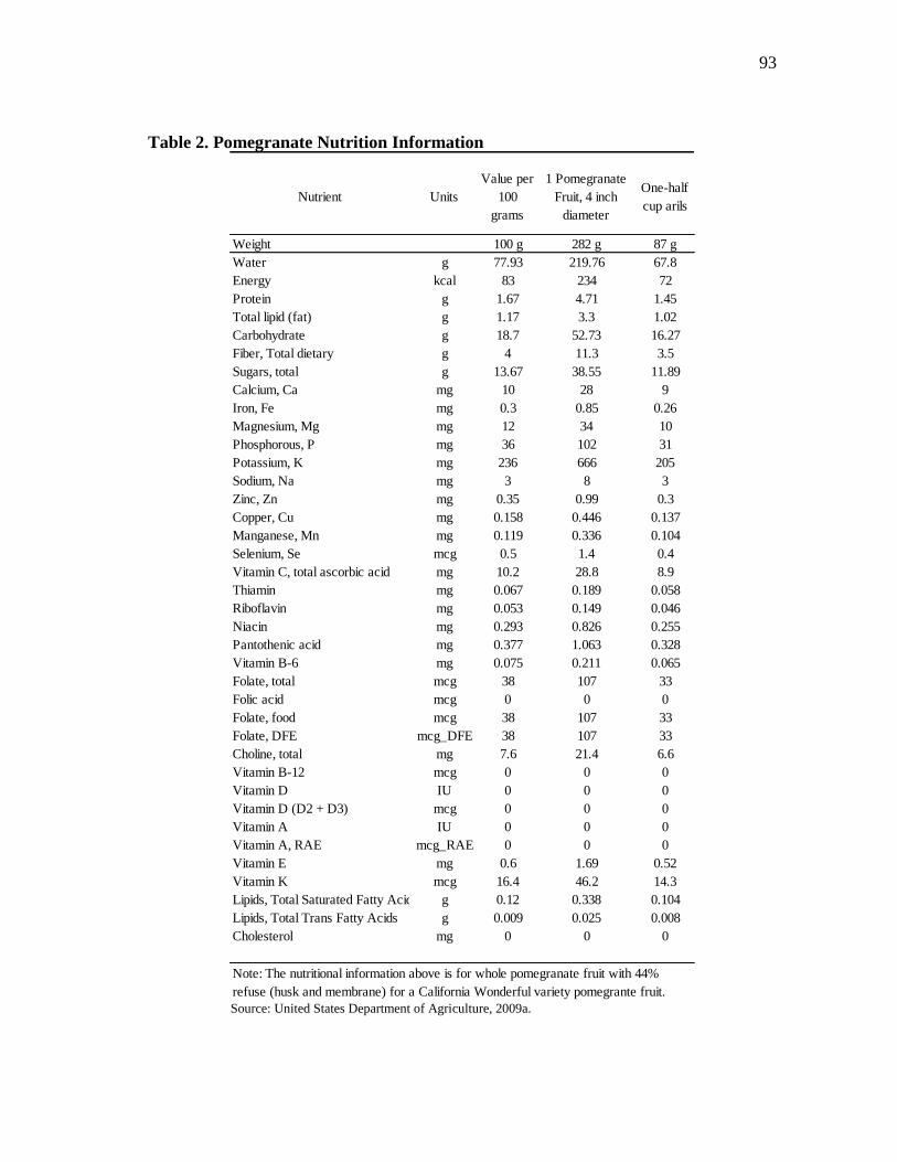
93
Table 2. Pomegranate Nutrition Information
Source: United States Department of Agriculture, 2009a.
Nutrient Units
Value per
100
grams
1 Pomegranate
Fruit, 4 inch
diameter
One-half
cup arils
Weight 100 g 282 g 87 g
Water g 77.93 219.76 67.8
Energy kcal 83 234 72
Protein g 1.67 4.71 1.45
Total lipid (fat) g 1.17 3.3 1.02
Carbohydrate g 18.7 52.73 16.27
Fiber, Total dietary g 4 11.3 3.5
Sugars, total g 13.67 38.55 11.89
Calcium, Ca mg 10 28 9
Iron, Fe mg 0.3 0.85 0.26
Magnesium, Mg mg 12 34 10
Phosphorous, P mg 36 102 31
Potassium, K mg 236 666 205
Sodium, Na mg 3 8 3
Zinc, Zn mg 0.35 0.99 0.3
Copper, Cu mg 0.158 0.446 0.137
Manganese, Mn mg 0.119 0.336 0.104
Selenium, Se mcg 0.5 1.4 0.4
Vitamin C, total ascorbic acid mg 10.2 28.8 8.9
Thiamin mg 0.067 0.189 0.058
Riboflavin mg 0.053 0.149 0.046
Niacin mg 0.293 0.826 0.255
Pantothenic acid mg 0.377 1.063 0.328
Vitamin B-6 mg 0.075 0.211 0.065
Folate, total mcg 38 107 33
Folic acid mcg 0 0 0
Folate, food mcg 38 107 33
Folate, DFE mcg_DFE 38 107 33
Choline, total mg 7.6 21.4 6.6
Vitamin B-12 mcg 0 0 0
Vitamin D IU 0 0 0
Vitamin D (D2 + D3) mcg 0 0 0
Vitamin A IU 0 0 0
Vitamin A, RAE mcg_RAE 0 0 0
Vitamin E mg 0.6 1.69 0.52
Vitamin K mcg 16.4 46.2 14.3
Lipids, Total Saturated Fatty Acids g 0.12 0.338 0.104
Lipids, Total Trans Fatty Acids g 0.009 0.025 0.008
Cholesterol mg 0 0 0
Note: The nutritional information above is for whole pomegranate fruit with 44%
refuse (husk and membrane) for a California Wonderful variety pomegrante fruit.
94
Chemical Composition
In addition to carbohydrates, fats, and proteins, pomegranate also contains many
phytochemicals; these include several classes of phenols and organic acids that may
have flavor and health implications (Mirdeghan and Rahemi 2007). Polyphenols present
include flavonoids (e.g., flavonols, flavanals, and anthocyanins), hydrolyzable tannins
(e.g., ellagitannins and gallotannins), and condensed (nonhydrolyzable) tannins (e.g.,
proanthocyanidins) (Seeram et al. 2006a). Specific compounds present in pomegranate
fruit include gallic acid, catechin, chlorogenic acid, protecatechuic acid, caffeic acid,
ferulic acid, o-coumaric acid, p-coumaric acid, phloridzin, and quercetin (Poyrazoğlu,
Gökmen, and Artɩk 2002).
There is significant variability in the chemical composition of pomegranates by
cultivar (Poyrazoğlu, Gökmen, and Artɩk 2002), as well as by growing site (e.g.;
Melgarejo, Salazar, and Artés 2000; Al-Maiman and Ahmad 2002; Poyrazoğlu,
Gökmen, and Artɩk 2002). Composition of the fruit may also be affected by maturity
and cultural practices, resulting in potential changes in the phenolic and mineral contents
(Mirdeghan and Rahemi 2007).
The chemical components of pomegranates that have been of the most interest
are the antioxidants contained both in the fruit and the rest of the plant. These properties
and the implications of such are discussed in more detail later.
Pomegranates and Antioxidants
Several major human health problems have been shown to be related to free

95
radicals and reactive oxygen species, as discussed by Kehrer (1993). He continued by
describing some of the important terminology pertinent to such a discussion: Any
molecule that contains unpaired electrons is considered a radical, and radicals are a
normal byproduct of several metabolic pathways. However, when these radicals exist in
a free form they can interact with tissue and cause dysfunction. The interaction with
tissue that alters the prooxidant-antioxidant balance towards prooxidants and potentially
leads to damage is termed ―oxidative stress.‖ ―Reactive oxygen species‖ include
chemicals with oxygen-containing functional groups that are not necessarily radicals nor
necessarily react with tissue through radical reactions; these reactive oxygen species are
not always good oxidizing agents so that terminology would be incorrect in some cases.
The list of diseases that have been implicated as having a free radical mechanism of
action is extensive and includes diseases of the lungs, brain, heart and cardiovascular
system, kidney, liver, gastrointestinal tract, blood, eye, skin, and muscle, in addition to
general inflammation and aging. Despite these links, it has been difficult to establish
some free radical interactions with tissue as a cause (versus a consequence) of disease.
Nonetheless, many studies have indicated a link between the two, suggesting further
interest in the connection between free radicals, reactive oxygen species, antioxidants,
and disease.
Antioxidants are generally described as molecules that inhibit oxidation
reactions. In more specific terms, antioxidants must meet two conditions described by
Rosenblat and Aviram (2006). One, they have the ability to neutralize (by delaying,
retarding, or preventing) autooxidation or free-radical-mediated oxidation when they are
96
present at a low concentration relative to that of the substrate to be oxidized. Two, the
resulting molecule that is formed must be stable in order to disrupt the oxidation chain
reaction. Vitamin C and Vitamin E are two commonly known antioxidants in fruits and
vegetables that play an important role in human health; however, the main antioxidant
effects of fruits and vegetables may be from other chemicals (including polyphenols)
also found in the fruits and vegetables (Wang, Cao, and Prior 1996). Cao et al. (1998)
rejected a hypothesis that increased plasma antioxidant capacity as a result of
consumption of a diet rich in fruits and vegetables could be explained by increases in α-
tocopherol (form of Vitamin E) and carotenoid (related to Vitamin A) in the plasma.
Tsao and Deng (2004) suggest that this and other evidence have led to the focus on
research on the roles of antioxidant phytochemicals. However, these authors also
indicate the difficulty in separating and detecting the large number (thousands) of such
compounds in order to elucidate specific effects.
Pomegranates have a high level of antioxidants (e. g., Kelawala and
Ananthanarayan 2004; Lansky and Newman 2007). Important polyphenols that have
been noted in pomegranate include two main types: hydrolyzable tannins and flavonoids
(McCutcheon, Udani, and Brown 2008). Hydrolyzable tannins present include
ellagitannins, gallotannins, and gallagoyl esters (Gil et al. 2000). Flavonoids found in
pomegranate include members of the classes of flavan-3-ols, anthocyanidins, flavanol
glycosides, flavonols, and anthocyanins (Lansky and Newman 2007), with the first three
of these being the most common (McCutcheon, Udani, and Brown 2008). Anthocyanins
are the most important group of water-soluble plant pigments and give red, blue, and
97
purple colors to flowers and fruits (Rosenblat and Aviram 2006). Specific flavonoids
present include catechin, quercetin, and phloridzin (Poyrazoğlu, Gökmen, and Artɩk
2002). Hydrolyzable tannins (HT) are found predominantly in the husk of the fruit. In
pomegranate juice made from pressing the whole pomegranate fruit, hydrolyzable
tannins account for 92 percent of pomegranate juice‘s antioxidant activity, with the HT
punicalagin accounting for about half the antioxidant capacity of pomegranate juice
made from the whole fruit (Seeram et al. 2006a).
The total polyphenol concentration of pomegranate juice is higher than that of
several other fruit juices, including apple, cranberry, grape, grapefruit, orange, peach,
pear, and pineapple juices (Rosenblat and Aviram 2006). Figure 1 diagrams the
relationship between the different categories of phytochemicals.
The suggested health benefits of these antioxidants range from reductions of
atherosclerosis indicators and blood pressure in humans (Aviram et al. 2004) to
improvements in prostate cancer indicators (specifically, prostate specific antigen
doubling time) in prostate cancer patients (Pantuck et al. 2006), in addition to the many
health effects on diabetes, cancer, and other diseases as shown in animal studies (e.g.,
Huang et al. 2005; Shiner, Fuhrman, and Aviram 2007). Inflammation and cancer are
the most common discussions of application of pomegranate to treat disease (Lansky and
Newman 2007). This is in addition to the recent explosion in literature on the in vitro
benefits of pomegranate-based substances as prevention or treatment techniques for
everything from breast cancer (Syed, Afaq, and Mukhtar 2007) to influenza (Haidari et
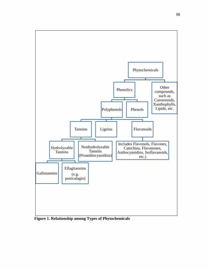
98
Figure 1. Relationship among Types of Phytochemicals
Phytochemicals
Phenolics
Polyphenols
Tannins
Hydrolyzable Tannins
Gallotannins
Ellagitannins
(e.g. punicalagin)
Nonhydrolyzable Tannins
(Proanthocyanidins)
Lignins Flavonoids
Includes Flavonols, Flavones, Catechins, Flavanones,
Anthocyanidins, Isoflavanoids, etc.)
Phenols
Other compounds,
such as Carotenoids,
Xanthophylls, Lipids, etc.
99
al. 2009). Hartman et al. (2006) suggest that the large number of compounds in
pomegranate fruit and possible synergism of these compounds may yield a preference
for dietary supplementation of the whole fruit or juice rather than with isolated
components of pomegranate. Seeram et al. (2006a) further discuss that most in vivo
research has focused on whole fruit or whole fruit products; therefore there is less
evidence for the effects of each specific pomegranate phytochemical on health.
Pomegranate juice has been effective at decreasing amyloid load and improving
behavior in mouse models of Alzheimer‘s Disease (a common cause of dementia in
humans, particularly in older populations) (Hartman et al. 2006). The consumption of
polyphenols may increase cellular signaling and neuronal communication, thus
producing anti-inflammatory activity (Joseph, Shukitt-Hale, and Casadesus 2005).
Although much work remains to be done on the biological mechanisms of
phytochemical activity in vivo, certain actions have been more commonly seen. These
include increased apoptosis, decreased metastasis and invasion, and decreased
inflammation (Lansky and Newman 2007).
The presence of polyphenols in pomegranates that have in vivo antioxidant
activity does not guarantee that consumption of pomegranate products will ensure these
effects in human subjects. These compounds must be absorbed in the digestive tract and
moved to other parts of the body for these effects to be realized. Results on the
bioavailability of ellagitannin were mixed in the detection of the free ellagic acid in
human plasma four hours after consumption (Seeram, Lee, and Heber 2004; Cerdá et al.
2004). Other studies found ellagitannin metabolites in human urine following

100
consumption of pomegranate juice (Seeram et al. 2006b). Specific work on the
bioavailability of anthocyanins and procyanidins from pomegranate products either has
not been carried out or does not offer enough evidence to draw conclusions on the
metabolic rate for these compounds; however, there have been studies of the
bioavailability of these compounds from other sources (Tomás-Barberán, Seeram, and
Espín 2006).
Although pomegranates are widely consumed and have been for thousands of
years, the focus on them as beneficial to human health may cause pomegranate and
pomegranate byproduct consumption to rise above historic levels. This leads to the
question of toxicity to humans of pomegranate. There have been some cases of allergic
reactions from eating the fruit (Hegde and Venkatesh 2004), as well as other adverse
effects, such as severe gastric inflammation and congestion of internal organs (Lansky
and Newman 2007 and sources therein). However, the reports of such adverse effects
are rare.
Most studies regarding the effects of polyphenols are in vitro or in animal
models, and a significant amount of research remains to be done in human subjects
before the benefits of polyphenols can be predicted with certainty (Hartman et al. 2006).
The precise role of antioxidants in mediating or preventing disease is still unclear, and
further biological research is needed to verify the effects of polyphenols and antioxidants
in pomegranates (Lansky and Newman 2007). Such research will be necessary to
guarantee an increase in consumer WTP. Case in point, the juice company POM
Wonderful, LLC. has launched a $34 million campaign of medical research to support its
101
pomegranate juice product, POM Wonderful® (POM 2010) and subjected such studies
to peer review (McCutcheon, Udani, and Brown 2008).
Pomegranate Production
Pomegranate production in the world is led by Iran with 63,733 hectares (ha) in
production in year 2005, followed by India, the United States, Turkey, and Spain
(Islamic Republic of Iran 2009). Other estimates place China between India and the
U.S. in area in production (Holland and Bar-Ya‘akov 2008). Iran had an export value of
$17.8 million in 2005 for approximately 27,000 metric tons of exports of pomegranates
(Islamic Republic of Iran 2009). Again, these estimates vary across sources. Holland
and Bar-Ya‘akov (2008) estimated a global production of pomegranates of 1.5 million
metric tons (1.5 billion kg); estimates for production and exports for Iran were 600,000
metric tons (600 million kg) and 60,000 metric tons (60 million kg), respectively.
The primary growing region for pomegranates in the United States is California;
production in other states is currently very limited. Pomegranates were introduced into
California by Spanish settlers in 1769 (Morton 1987), but they had previously been
grown in the United States in Florida and Georgia (Stover and Mercure 2007). In
reference to current production trends, estimates of the number of pomegranate trees in
California rose from 12,000 acres (4,856 ha) in year 2006 to 29,000 acres (11,735 ha) in
year 2009 (―Pomegranate Acreage‖ 2009).
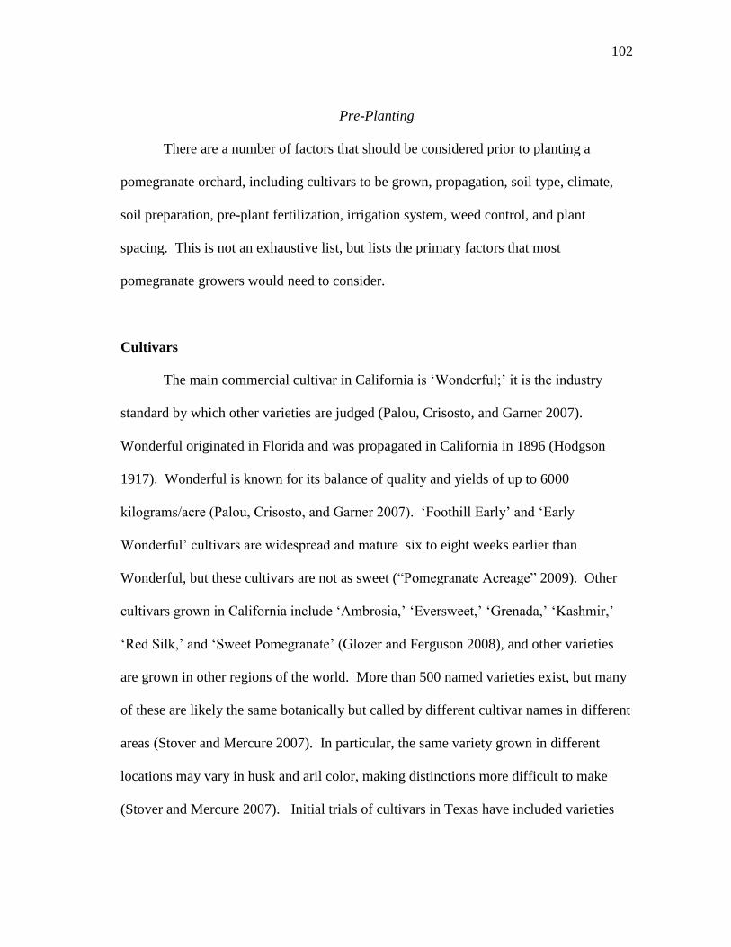
102
Pre-Planting
There are a number of factors that should be considered prior to planting a
pomegranate orchard, including cultivars to be grown, propagation, soil type, climate,
soil preparation, pre-plant fertilization, irrigation system, weed control, and plant
spacing. This is not an exhaustive list, but lists the primary factors that most
pomegranate growers would need to consider.
Cultivars
The main commercial cultivar in California is ‗Wonderful;‘ it is the industry
standard by which other varieties are judged (Palou, Crisosto, and Garner 2007).
Wonderful originated in Florida and was propagated in California in 1896 (Hodgson
1917). Wonderful is known for its balance of quality and yields of up to 6000
kilograms/acre (Palou, Crisosto, and Garner 2007). ‗Foothill Early‘ and ‗Early
Wonderful‘ cultivars are widespread and mature six to eight weeks earlier than
Wonderful, but these cultivars are not as sweet (―Pomegranate Acreage‖ 2009). Other
cultivars grown in California include ‗Ambrosia,‘ ‗Eversweet,‘ ‗Grenada,‘ ‗Kashmir,‘
‗Red Silk,‘ and ‗Sweet Pomegranate‘ (Glozer and Ferguson 2008), and other varieties
are grown in other regions of the world. More than 500 named varieties exist, but many
of these are likely the same botanically but called by different cultivar names in different
areas (Stover and Mercure 2007). In particular, the same variety grown in different
locations may vary in husk and aril color, making distinctions more difficult to make
(Stover and Mercure 2007). Initial trials of cultivars in Texas have included varieties
103
such as Kandahar, Texas Pink, Sumbar, Purple, Mridula, Salavatski, and Pecos; these
cultivars vary in their maturity, color, seed-hardness, and sweetness (Ashton 2010).
Figure 2. Examples of the Variability in Pomegranate Cultivars
The physical variability in fruit appearance among pomegranate cultivars that
can be seen in Figure 2 is matched with additional variability in other physical,
chemical, and production characteristics. Cultivars should be selected that are adapted
to the climate where the orchard is to be planted. This includes differences in cold
hardiness and salt tolerance among cultivars, as well as preferences in fruit color and
seed hardness in the target market (Stover and Mercure 2007). Possible cultivars in
Spain have been evaluated for variations in the following: seed hardness (soft preferred),
sweetness, fruit size, and yield (Martínez et al. 2006). Each of these criteria should
influence the market acceptability and potential profits from a pomegranate orchard.
Propagation
Pomegranate seeds will germinate and grow, but they do not come back true to
type (Hodgson 1917). Hardwood cuttings are best done in late winter to early spring and
104
are the preferred method of propagation for general seedling production (Larue 1977).
Cuttings of 6 to 8 inches in length and greater than ¼ inch in diameter should be placed
directly in the ground with the top node exposed and left to grow in nursery beds for one
to two years (Dubois and Williamson 2008). Glozer and Ferguson (2008) suggest that
one year is generally sufficient prior to planting in a permanent orchard. Seedlings can
also be grown using regeneration from cotlyedonary nodes (Naik, Pattnaik, and Chand
2000).
Soil
Pomegranates can adapt to a wider range of soils than many other types of fruit
trees; deep loam is preferred but suitable yields are produced on sandy or clay soils. The
tree also tolerates mildly alkali soils or mildly poor drainage; extremes of either of these
two will severely affect yields (Larue 1977). Optimal growth is on deep, fairly heavy
soils with a pH of 5.5-7.0 (Dubois and Williamson 2008).
Climate and Microclimate
Pomegranate is a drought tolerant plant, growing well in some desert regions;
however, fruit production is very limited under such conditions (Hodgson 1917).
Pomegranates grow well in full sun, and this is the preferred planting location (Glozer
and Ferguson 2008). Areas with high humidity or large amounts of rain in the late
summer to fall (during fruit development, ripening, and harvest) may be unsuitable for
production (Özgüven and Yilmaz 2000).

105
Glozer and Ferguson (2008) suggest that in general, and particularly in areas at
the northern and southern extremes of the pomegranate growing region, care should be
taken to site the orchard so that it is protected as possible from a late frost that would
damage emerging plant growth in the spring. The plants are susceptible to cold damage
from the emergence of the first leaf tissue through the bloom period. The coldest
planting locations are open areas with exposure to prevailing winds; trees planted in such
areas are more likely to be damaged by frost. Therefore, these areas should be avoided
if possible. Also, cold air settles in low-lying areas and basins; planting in these areas
should also be avoided. Siting the orchard on a north-facing hill (in the northern
hemisphere) reduces the direct sunlight exposure of the trees and will generally
encourage the plants to bloom later in the spring, thus protecting from loss due to frost
damage. Maintaining bare ground around the trees allows the soil to capture heat during
the day and can thus be useful in reducing cold damage. Proper irrigation practices can
also be valuable for limiting frost injury. Cold hardiness of the varieties to be planted
should also be considered with respect to the siting of the orchard.
Soil Preparation, Irrigation System, and Weed Control
Soil preparation generally requires plowing and harrowing of soil to ensure that
any hard pan is broken up and that soil is properly conditioned prior to planting.
Previous crop matter or residual weeds should also be removed and/or harrowed under
prior to planting (Day et al. 2005). These weeds, if allowed to grow, would compete
with young pomegranate seedlings.
106
Application and incorporation of lime (calcitic or dolomitic agricultural
limestone) to raise the soil pH or sulfur (elemental sulfur or aluminum sulfate) to lower
the soil pH to the acceptable range should be completed prior to orchard establishment.
Any pre-plant fertilization that is needed should also be completed at that time (Glozer
and Ferguson 2008).
The irrigation system should be in place prior to or immediately following
planting because seedlings generally require additional water at planting (Stover and
Mersure 2007). Irrigation may be furrow style, overhead, or drip (e.g., Day et al. 2005,
Özgüven and Yilmaz 2000). Water supply should be adequate to meet irrigation
requirements when rainfall is insufficient to meet water requirements of the
pomegranates. Although pomegranate is drought-tolerant in that it has an ability to
survive in semi-arid regions with limited rainfall, it should certainly not be considered a
drought-tolerant plant in commercial production; repeated or prolonged periods of water
stress are likely to significantly reduce yields (Still 2006).
Planting Design
Pomegranate orchards may be planted to facilitate either tree growth or bush
growth, depending on plant spacing. Spacing of 15 to 18 feet between rows and similar
spacing between trees is common in orchards (Dubois and Williamson 2008). Bush
planting spacing is a smaller distance in row, for example 14 feet by 8 feet (Cline 2008).
However, spacing varies considerably by location, and may be closer than those listed
even for the tree form (Bryant 2003). Suggested spacings for planting in Texas include a
107
14-foot in row spacing with a 17-foot between row spacing for the plants with a larger
mature size but with a 10 foot-in row spacing for the smaller cultivars (Ashton 2010).
Spacing also depends on the type and fertility of the soil (Morton 1987). The main
objective is that trees be planted where there is adequate space to meet the light,
moisture, and nutrient requirements of the specific pomegranate cultivar and allow
movement of workers and equipment through the orchard with ease.
Planting
Pomegranates are planted in late winter, after the coldest temperatures have
passed but prior to leaf emergence to allow for root growth. In California, the suggested
planting period is January (Day et al. 2005). Others suggest a late winter to early spring
planting in California to take advantage of abundant soil moisture (Stover and Mercure
2007). Pomegranates to be grown in the tree form are topped (‗headedback‘) at planting
(Day et al. 2005). This practice encourages the development of three to five main
branches and should be done at a height of 2.5-4 feet to keep fruit from touching the
ground on low hanging limbs but also prevent toppling over when the tree is heavy with
fruit (Glozer and Ferguson 2008; Hodgson 1917). Damage to the bark from sunburn or
freezing can be prevented or reduced by painting the trunk white at planting time (Larue
1977). The painting of the trunk is commonly used in production of other tree fruit
crops and is also useful in preventing insect damage.
108
Pruning
To grow in a tree form, pomegranate must be pruned; otherwise the pomegranate
will develop in a shrub form. In general, pruning of fruit trees develops stronger
branches that can hold a heavier fruit load without breaking, brings young trees into
production sooner, and allows for light and spray penetration into the canopy.
Pomegranates may be trained into a single trunk, or they may be trained into multiple
trunks if cold damage is of significant concern as this reduces the likelihood of total loss
of the tree in a freeze (Stover and Mercure 2007). In the first year, trees are pruned at
planting and suckered in early summer (Day et al. 2005). The removal of the lower
branches allows for the production of a clear main stem (Morton 1987). Different
specific pruning methods should be followed depending on the desired growth habit of
the pomegranate (Larue 1977).
Fertilization
Pomegranate should not require large amounts of nitrogen during establishment,
but recommendation range around 17 pounds N/ acre (Day et al. 2005) during the first
year. Depending on the soil composition, pre-plant fertilization may be sufficient to
meet the nutrient requirements of the pomegranate during establishment. Fertilization of
young trees should take into account the initial size and age of the tree. If applied,
fertilizer should be done in mid-spring and/or mid-summer; fertilization in the fall is
discouraged (Ashton 2010).

109
Orchard Management
Pomegranate production once the orchard is established requires regular
management. The pomegranate must be irrigated, fertilized, and pruned as needed.
Problems from disease, insects, and weeds must also be prevented when possible and
managed if problems arise.
Irrigation
Water requirements for pomegranate are similar to those for citrus trees at about
50-60 inches per year (Larue 1977). Dubois and Williamson (2008) suggest irrigating
every seven to ten days in the absence of sufficient rainfall. Pomegranates can be
irrigated with furrow, overhead, or drip irrigation; drip irrigation is the most water-
efficient but also the most expensive of these methods. Research in India found drip
irrigation to produce higher yield of both high and low grades of pomegranates (and thus
higher total yield) than basin irrigation systems (Sulochanamma, Reddy, and Reddy
2005). Cracking and splitting of the fruit may be a result of either under- or over-
watering (Özgüven and Yilmaz 2000). Another reason pomegranates may crack as they
mature is cool night-time temperatures (Ashton 2010). Larue (1977) emphasizes the
importance of irrigation in the period immediately prior to harvest, including late
summer and early fall, as a means to reduce the number of split fruit. However,
irrigation late into the fall can induce late season growth or delay the onset of dormancy,
making trees more susceptible to cold damage (Day, Klonsky, and De Moura 2010;
Glozer and Ferguson 2008). More recent descriptions of commercial pomegranate
110
production practices suggest that pomegranates need 36 acre inches of water per year,
but 80 percent efficiency for furrow irrigation requires the application of 45 acre inches
for orchards using that irrigation system (Day, Klonsky, and De Moura 2010).
Pruning
Regular pruning and suckering is done in the winter, with additional suckering in
early summer. Pomegranates sucker aggressively from the base of the plant, and these
should be removed if pomegranates are grown in the tree form (Hodgson 1917). Light
annual pruning encourages growth of fruit-bearing spurs, but heavy pruning will reduce
yield (Larue 1977). Pruning should be done with the intent of leaving strong, healthy
branches and removing dead or diseased plant material. The canopy of the tree should
be kept open for optimal fruit development (Glozer and Ferguson 2008). Some growers
prune three to six weeks prior to harvest to improve fruit color (Day, Klonsky, and De
Moura 2010).
Fertilization
Mature pomegranate trees have an annual nitrogen requirement of one-half to
one pound of actual nitrogen per tree (Larue 1977). This may be applied in a single
winter application or in a split application, depending on whether the soil is heavy or
light in texture (Larue 1977). Applications of phosphorous and potassium are not
necessary in most cases in California (Larue 1977; Day et al. 2005), although potassium
is supplemented in some other growing areas such as Israel (Blumenfield, Shaya, and
111
Hillel 2000). Zinc deficiency has been noted as a rare but possible problem; it is most
common in young trees or in pomegranates grown in alkaline soils (Glozer and Ferguson
2008), and this deficiency should be treated with foliar application of zinc only if needed
(Larue 1977; Day et al. 2005).
Management practices that encourage vegetative growth rather than fruit set,
such as excessive fertilization or irrigation, may cause fruit drop; this is true particularly
in young trees. Such practices may also delay fruit maturity and affect fruit quality
(Larue 1977).
Frost Protection
As a primary means of frost protection, pomegranate orchards should not be sited
in frost-prone areas. However, additional management techniques can reduce the danger
of late (spring) or early (fall) frost to the trees if they are not fully dormant. Dormancy
should be maintained throughout the winter; thus, there should be no late summer or fall
fertilization or pruning that would encourage plant growth (Glozer and Ferguson 2008).
Overhead irrigation is used for watering and frost-protection in some California orchards
(Morton 1987). The additional considerations mentioned previously in the description
of the microclimate should also be followed. Irrigation for frost protection may be
needed in early spring for frost protection of blooms and emerging leaves or in the
winter if temperatures drop below 23-25°F (Day, Klonsky, and De Moura 2010).
112
Pest Management
Pest management issues are not typically severe in pomegranate cultivation.
However, there are some considerations for disease, weeds, and insects. Proper attention
to these issues can prevent or greatly reduce yield reduction from pests.
Disease
Alternaria rot (also known as ‗black heart‘ or ‗heart rot‘) is caused by Alternaria
spp.; Aspergillus niger causes similar symptomology and can cause fruit loss to
pomegranate growers (D‘Aquino et al. 2009). In Alternaria rot, the interior of the fruit
is partly or completely decayed and black in color, but the husk of the fruit is unaffected;
the infection seems to take place in the bloom and progress to the central cavity of the
fruit (Larue 1977). Significant yield losses have been reported due to Alternaria rot in
Greece (Tziros, Lagopodi, and Tzavella-Klonari 2007). Botrytis cinera is also a disease
of pomegranate, although this disease is generally not of serious economic consequence
until the post-harvest stage (Day et al. 2005). However, pomegranates are not generally
threatened by serious disease in production in the United States (Day, Klonsky, and De
Moura 2010). Application of copper hydroxide is an option for control of fungal
diseases (Ashton 2010).
Insects
With limited pomegranate production in the state of Texas, most available
information on pest management is based on problems that have been reported in
113
California. Carroll et al. (2006) offer a review of some California pomegranate pests.
Aphids are one of the most commonly discussed pests, with the cotton aphid (Aphis
gossypii) and a yet unidentified species of aphid unofficially known as the ‗pomegranate
aphid‘ (Carroll et al. 2006). Biological control of these pests is generally effective.
Grape mealybug (Pseudoccus maritimus) can cause damage to the fruit, and Citricola
scale (Coccus pseudomagnoliarum) and black scale (Saissetia oleae) both occur on
pomegranate and can cause superficial damage to the fruit that results in the quality
being downgraded. The greenhouse whitefly (Trialeurodes vaporariorum) and the ash
whitefly (Siphoninus phillyreae) have also been known to cause problems. They can be
controlled biologically with parasites; Admire® (imidacloprid) and Lannate®
(methomyl) are effective means of chemical control. Other pests of pomegranates in
California include the omnivorous leaf roller (Platynota stultana), leaf-footed plant bugs
(Leptoglossus clypealis), false chinch bug (Nysius raphanus), and flat mite (Brevipalpus
lewisi). Both the flat mite and the leafroller cause checking and scarring on the fruit.
Thrips are not commonly reported as a problem in the San Joaquin Valley, California,
but they have been a cause of damage in pomegranates grown in India (Ananda, Kotikal,
and Balikai 2009).
There are a few other insects that are of particular importance in other areas of
pomegranate production. The pomegranate butterfly (Virachola livia) and the
Mediterranean fruit fly (Ceratits capitata) cause damage to pomegranate and can be
present in large numbers (Holland and Bar-Ya‘akov 2008). Good general cleanliness
practices such as removal of all fruit from trees and mowing of weeds in the orchard has

114
shown some effectiveness at managing pest populations. An example of the visual
effects of insect damage on the outer husk of the pomegranate fruit can be seen on the
pomegranate fruits in Figure 3. Such damage makes fruit less marketable as a whole
fruit product due to limited acceptability by consumers.
Figure 3. Example of Insect-Damaged Pomegranate Fruits
Weeds
Weeds can serve as a harbor for harmful insects and plant pathogens, so
management of weed populations is of economic importance. Recommendations for
California orchards are to control weeds in the orchard row with pre-emergence
herbicides in the winter and in the row middles throughout the summer with multiple
applications of a burndown chemical (e.g., glyphosate) (Day et al. 2005). Spot treatment
of in-row weeds should be completed as needed in the summer. Recommendations for
use in Texas by the Texas Pomegranate Growers Cooperative include oryzalin (e.g.,
Surflan 4 AS®) as a pre-emergent weed control, oxyfluorfen (e.g., Goal 2 XL®) to
control broadleaf weeds, and glyphosate (e.g., Roundup Ultra Max®) as a burndown
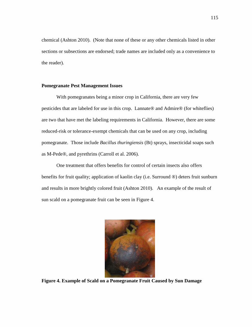
115
chemical (Ashton 2010). (Note that none of these or any other chemicals listed in other
sections or subsections are endorsed; trade names are included only as a convenience to
the reader).
Pomegranate Pest Management Issues
With pomegranates being a minor crop in California, there are very few
pesticides that are labeled for use in this crop. Lannate® and Admire® (for whiteflies)
are two that have met the labeling requirements in California. However, there are some
reduced-risk or tolerance-exempt chemicals that can be used on any crop, including
pomegranate. Those include Bacillus thuringiensis (Bt) sprays, insecticidal soaps such
as M-Pede®, and pyrethrins (Carroll et al. 2006).
One treatment that offers benefits for control of certain insects also offers
benefits for fruit quality; application of kaolin clay (i.e. Surround ®) deters fruit sunburn
and results in more brightly colored fruit (Ashton 2010). An example of the result of
sun scald on a pomegranate fruit can be seen in Figure 4.
Figure 4. Example of Scald on a Pomegranate Fruit Caused by Sun Damage
116
Harvest
On average it takes three to six months from the time of pomegranate bloom until
fruit maturity (Glozer and Ferguson 2008). The harvest period for the ‗Wonderful‘
cultivar is from September to November in California, and there has been great interest
in extending the postharvest life until at least the Christmas holiday season, when
demand is greater and prices are higher (Palou, Crisosto, and Garner 2007). Similar
concern has been shown in Israel, where there is interest in extending the time frame of
pomegranate exports to the Christmas season in Europe (Nerya et al. 2006).
Harvest of pomegranates is done by hand and should occur when the fruit is
highly colored (for Wonderful cultivar, dark red) (Glozer and Ferguson 2008). At
maturity, the fruit should also have a hollow, metallic sound when tapped (Morton
1987). A maturity index can be used to describe the readiness for harvest based on a
calculation of total suspended solids (TSS) divided by titratable acidity (TA) (Elyatem
and Kader 1984; Artés, Marín, and Martínez 1996). Pomegranate fruits should be
handled carefully to prevent scarring of the skin; the skin of the pomegranate fruit is
easily disfigured by scratches and blemishes, although such damage does not affect the
fruit inside (Glozer and Ferguson 2008). Cutting of the fruits from the trees may be
preferred to pulling the fruit off the tree (Ashton 2010) in order to prevent external
blemishing of the fruit because such damage may make the fruit more susceptible to
later infection by postharvest pathogens (Palou, Crisosto, and Garner 2007). Most
worldwide pomegranate fruit harvest is done by hand, but a mechanical harvester for
117
pomegranates has been used on a trial basis in the San Joaquin Valley of California
(Cline 2008).
Yield estimates for the cultivar Wonderful are from 6,000 kg per hectare (Palou,
Crisosto, and Garner 2007) to over 33,000 kg per hectare (Bryant 2003); yield estimates
for other cultivars vary considerably as well (Sulochanamma, Reddy, and Reddy 2005).
A moderate range of yield for Wonderful cultivar in California would be 6,200 kg/ha to
11,700 kg/ha (Day et al. 2005). The average yield for Tulare County, California (a
major area for US pomegranate production) in 2009 was 12,620 kg/ha (Kinoshita 2010).
These estimates may depend on whether only top-quality fruits suitable for fresh-market
are included in this estimate or total fruit production (suitable for juicing) is the basis.
Harvest may begin by the second or third year after propagation, but mature yields are
not attained until five to six years after propagation (Stover and Mercure 2007). Harvest
estimates for Texas varieties are in the range of 11,208 kg/ha (10,000 pounds/acre), but
this is expected to vary with growing season, location, and cultivar.
Post-Harvest
Pomegranate fruit is characterized as being nonclimacteric, meaning that the
fruits do not ripen after harvest (Artés, Marín, and Martínez 1996). Pomegranates
should therefore be harvested when color meets a minimum standard and titratable
acidity is within the appropriate range (Elyatem and Kader 1984) since ethylene
treatment is not effective at inducing ripening. The storage life of pomegranate is
similar to that of the apple; estimates range from 7 months at 80% humidity and 32 to
118
41° F (Morton 1987) to a range of 8 weeks to 20 weeks in atmosphere controlled
conditions at 45°F (Palou, Crisosto, and Garner 2007), depending on the effects of
postharvest pathogens. A review of the state of the pomegranate industry in 2008
suggested a storage period of 4 to 5 months was possible with modified storage practices
(Holland and Bar-Ya‘akov 2008). Some post-harvest issues may arise after a long
storage period as described below; still, storage has been found by some to increase the
red color of pomegranate juice (Artés, Marín, and Martínez 1996), although this change
was not observed by Palou, Crisosto, and Garner (2007).
Two of the most common post-harvest physiologic issues for pomegranate are
husk scald and chilling injury. Both of these are external to the fruit but can greatly
reduce marketability. Chilling injury is possible below temperatures of 41°F (Elyatem
and Kader 1984). Symptomology of chilling injury includes skin discoloration, surface
pitting, and accelerated fungal growth (Paull 1990). The severity of the injury due to
chilling injury is dependent on the storage temperature, duration, and whether the
pomegranate fruits are stored in air or in an atmosphere-controlled environment (Kader
2006). Husk scald is characterized by superficial browning that develops from the stem-
end of the fruit; this increases the susceptibility of the fruit to decay (Defilippi et al.
2006). Husk scald appears to be more severe on fruit harvested later in the season, but
treatment with a controlled atmosphere (CA) of 5 kPa O2 + 15 kPa CO2 (balance N2) at
7°C (44.6°F) and 90-95% relative humidity was effective at reducing the incidence of
husk scald (Defilippi et al. 2006).
119
The high environmental humidity which reduces chilling injury and weight loss
of pomegranates also creates ideal conditions for microorganism development and decay
(D‘Aquino et al. 2009). Gray mold caused by Botrytis cinera Pers.: Fr. is a considerable
economic threat to pomegranate in California (Tedford, Adaskaveg, and Ott 2005).
Other common problems include heart rot (as discussed earlier) and penicillin rot caused
by Penicillin spp. (D‘Aquino et al. 2009). Fludioxonil (trade name Scholar®) was
approved by the United States Environmental Protection Agency (EPA) in 2005 for use
as a postharvest fungicide on pomegranate (EPA 2005). Fludioxonil has shown to be a
useful tool for reducing post-harvest decay with activity against Botrytis cinera and
Penicillin spp.; there are some estimates of a large impact on profitability that
fludioxonil has had as a post-harvest treatment for pomegranate fruit (D‘Aquino et al.
2010; Tedford, Adaskaveg, and Ott 2005).
Minimally processing and using polymeric film packaging for arils to produce a
ready-to-eat product has the effect of reducing browning and allowing storage for up 14
days at 3.5-4.5°C while maintaining physical, chemical, and microbiological quality
(Sepúlveda et al. 2000). Other types of packaging resulted in a storage life of 15 days
for a low oxygen atmosphere packaging treatment and 18 days for air, nitrogen, and
enriched oxygen atmospheres (Ayhan and Eştürk 2009). Minimal processing includes
washing with sanitizing agents to reduce microbial counts, use of antioxidant agents,
control of temperature, and making pH modifications, while the semi-permeable
polymeric film serves to create a modified atmosphere packaging (MAP) that reduces
the respiratory intensity and prevents and slows the growth of contaminating
120
microorganisms (Sepúlveda et al. 2000). López-Rubira et al. (2005) found differences in
the storability of arils from pomegranate fruit harvested early in the season (14 days)
versus pomegranate fruit harvested late in the season (10 days), both in terms of
microbial counts and sensory acceptability.
Current State of the Industry
Recent developments and needed research in the pomegranate industry are
related to growing, storage, and processing practices; they include the development of
new cultivars and irrigation techniques to generate more yields of higher quality,
technologies to market a ―ready-to-eat‖ arils product, the addition of pomegranate as an
ingredient to a wide spectrum of consumer products, and modifications to storage
practices to allow longer storage times (Holland and Bar-Ya‘akov 2008). Blumenfield,
Shaya, and Hillel (2000) have also pointed out the need for a ready-to-eat aril product
that can be mass-produced in order to increase the market for fresh pomegranate fruit.
Several companies have gotten involved in the marketing of pomegranate
products. For example, POM Wonderful, LLC is a vertically integrated pomegranate
marketer with a wide range of pomegranate products that are sold fresh and used to
make juices, teas, bars, pills, and other supplements; the company is supplied with
pomegranates from over 18,000 acres of trees in the San Joaquin Valley, California
(POM Wonderful 2010). Simonian Fruit Company is also a California-based supplier of
pomegranates and a member of the Pomegranate Council (Schrak 2010). Large global
marketers have also gotten involved in pomegranate juice products, including Welch‘s®,
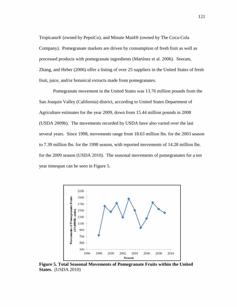
121
Tropicana® (owned by PepsiCo), and Minute Maid® (owned by The Coca-Cola
Company). Pomegranate markets are driven by consumption of fresh fruit as well as
processed products with pomegranate ingredients (Martínez et al. 2006). Seeram,
Zhang, and Heber (2006) offer a listing of over 25 suppliers in the United States of fresh
fruit, juice, and/or botanical extracts made from pomegranates.
Pomegranate movement in the United States was 13.76 million pounds from the
San Joaquin Valley (California) district, according to United States Department of
Agriculture estimates for the year 2009, down from 15.44 million pounds in 2008
(USDA 2009b). The movements recorded by USDA have also varied over the last
several years. Since 1998, movements range from 18.63 million lbs. for the 2003 season
to 7.39 million lbs. for the 1998 season, with reported movements of 14.28 million lbs.
for the 2009 season (USDA 2010). The seasonal movements of pomegranates for a ten
year timespan can be seen in Figure 5.
Figure 5. Total Seasonal Movements of Pomegranate Fruits within the United
States. (USDA 2010)
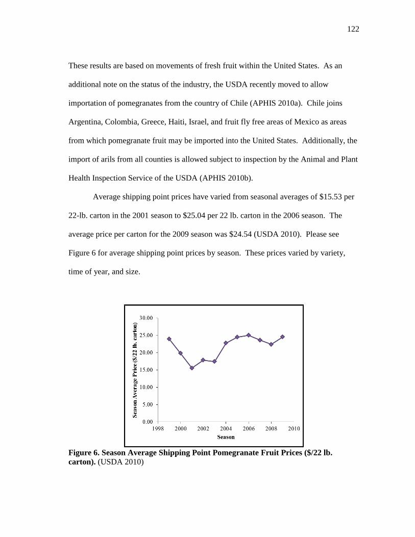
122
These results are based on movements of fresh fruit within the United States. As an
additional note on the status of the industry, the USDA recently moved to allow
importation of pomegranates from the country of Chile (APHIS 2010a). Chile joins
Argentina, Colombia, Greece, Haiti, Israel, and fruit fly free areas of Mexico as areas
from which pomegranate fruit may be imported into the United States. Additionally, the
import of arils from all counties is allowed subject to inspection by the Animal and Plant
Health Inspection Service of the USDA (APHIS 2010b).
Average shipping point prices have varied from seasonal averages of $15.53 per
22-lb. carton in the 2001 season to $25.04 per 22 lb. carton in the 2006 season. The
average price per carton for the 2009 season was $24.54 (USDA 2010). Please see
Figure 6 for average shipping point prices by season. These prices varied by variety,
time of year, and size.
Figure 6. Season Average Shipping Point Pomegranate Fruit Prices ($/22 lb.
carton). (USDA 2010)
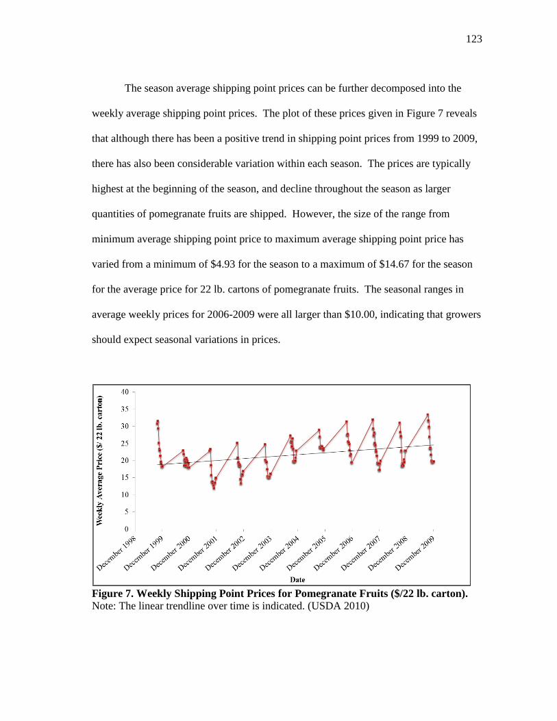
123
The season average shipping point prices can be further decomposed into the
weekly average shipping point prices. The plot of these prices given in Figure 7 reveals
that although there has been a positive trend in shipping point prices from 1999 to 2009,
there has also been considerable variation within each season. The prices are typically
highest at the beginning of the season, and decline throughout the season as larger
quantities of pomegranate fruits are shipped. However, the size of the range from
minimum average shipping point price to maximum average shipping point price has
varied from a minimum of $4.93 for the season to a maximum of $14.67 for the season
for the average price for 22 lb. cartons of pomegranate fruits. The seasonal ranges in
average weekly prices for 2006-2009 were all larger than $10.00, indicating that growers
should expect seasonal variations in prices.
Figure 7. Weekly Shipping Point Prices for Pomegranate Fruits ($/22 lb. carton).
Note: The linear trendline over time is indicated. (USDA 2010)
124
Products
Pomegranates are marketed in a number of ways, including as whole fresh fruits,
minimally processed as arils, and further processed into juice and a number of other
products.
The introduction of minimally processed arils as a ready-to-eat marketing device
in recent years has offered an opportunity to expand the market for pomegranates
(Ayhan and Eştürk 2009). These products offer greater convenience for consumers than
eating the fruit fresh, since, as pointed out in materials from the Pomegranate Council, it
is sometimes difficult to separate the arils from the membrane and husk (PC 2007).
Lopez and Rubira (2005) note that the marketing of pomegranate arils in modified
atmosphere packaging also offers the opportunity to market fruit that is cracked or
otherwise superficially blemished and that would not be acceptable for the fresh market
as a whole fruit.
The assortment of pomegranate-based products on the marketplace is astounding.
There are pomegranate husk extracts, weight-loss pills, tea, fermented wine and vinegar,
seed oil, powder, body wash, dried seeds, jelly and cattle feed, to name a few. Even
more pomegranate products are likely on the way. Examples of proposed pomegranate
products include the use of a powder made from pomegranate rind as a natural additive
to prevent oxidation of fresh ground meat (Devatkal and Naveena 2010) and
pomegranate extract as a chemotherapeutic agent (Longtin 2003).
125
Marketing Challenges
Pomegranates as a fresh fruit are generally less familiar than many other fruits to
United States consumers. Additionally, they have a tough outer husk, seeds that are
somewhat difficult to eat, and juice that readily stains clothing. The Pomegranate
Council even suggests a three step method for opening the pomegranate to minimize the
need for cleanup. The steps are as follows: 1) Remove the crown and cut the
pomegranate into sections; 2) In a bowl of water, separate the arils from the membrane
and discard everything but the arils; and 3) Strain out the water and eat the arils
(including the seeds) (PC 2007).
Further, pomegranate is a crop with a substantial acreage grown outside the
United States, as described by Holland and Bar-Ya‘akov (2008). These authors further
express several factors that could help or hinder pomegranate markets. Included are
mechanical aril separators for marketing of a ready-to-eat aril product, development of
additional high-yielding cultivars, more efficient irrigation techniques, and longer
storage periods for pomegranate fruits. Pomegranate juice concentrate can easily be
imported; therefore, some members of the industry have suggested that farmgate prices
for pomegranates will decline as more acres of pomegranates come into production
(Cline 2008). There are now multiple companies with fully-automated mechanical aril
separators on the market. Time will tell whether demand for pomegranate products will
match pomegranate production.
Pomegranates are a crop that has been cultivated by humans for thousands of
years; however, their popularity in the western world has grown tremendously in the last
126
decade. This growth has been spurred by a combination of factors, including the interest
in healthful eating in general and functional foods in particular. Pomegranate fruit and
other plant components of pomegranate are known to have high levels of antioxidants,
particularly hydrolyzable tannins and flavonoids. A number of health benefits have been
proposed for those who consume these polyphenols, particularly in the areas of reduced
cardiovascular disease and reduced risk of certain cancers. Worldwide pomegranate
production is expanding in order to meet the increasing demand for pomegranate fruits.
The primary production area in the world is Iran, where the pomegranate is believed to
have originated. Within the United States, California accounts for the overwhelming
majority of production. A number of cultural practices must be considered for
pomegranates, including fertilization and irrigation practices and management of insects
and disease. Recent innovations have led to a boom of pomegranate products in the
marketplace, including pomegranate juice, ready-to-eat fresh fruit products, and
everything from lotion to energy supplements with pomegranate as an ingredient.
Despite this, there are still a number of challenges within the pomegranate market.
These include the need for further research to verify health claims on pomegranate, the
potential for lower prices as supplies increase, further development of best production
practices, and overcoming the novelty of the pomegranate fruit for many consumers.
The pomegranate industry is poised for growth, but growth will not come without
innovation as well as scientific and crop management developments.
127
CHAPTER IV
METHODOLOGY
There are a number of important considerations when applying experimental
economics methods to elicit values for pomegranate fruits and other pomegranate
products. Many of these were outlined in the literature review chapter. However,
several of these are re-emphasized here as they apply to this experimental auction and
ranking procedure, with justification for the procedure used. In general, and in keeping
with the suggestions of Lusk and Shogren (2007), the methods and analysis were
maintained with a balance between the control and context of the experiment. This was
done with the goal of obtaining the most meaningful results that were relevant to the
questions under investigation in the study.
Auction Description and Estimation Overview
The study was designed to elicit the effects of health information on willingness-
to-pay (WTP) for pomegranate products. The study also proposes a value elicitation
mechanism that, to the author‘s knowledge, has not been previously implemented in this
specific form by combining incentive compatible and nonhypothetical mechanisms for
both discrete choice rankings and experimental auctions. A brief overview of the
procedures is included here with more detail provided later. Subjects participated in
sessions in which whole pomegranate fruits, other pomegranate products, and a control
fruit product were available for bidding. Subjects were given extensive instructions and
128
examples of auction procedures and were informed that both the ranking and auction
procedures were nonhypothetical. Following the instructions, subjects participated in
practice rounds of ranking and bidding for non-target products. After the instructions,
subjects participated in one practice ranking round and one practice auction round each
for soft drinks and for assorted snack products. Between the rounds for the two types of
products, subjects were given a brief quiz on the auction procedures and were then given
the correct answers. The winning (11th
) price for each product was posted only in the
practice rounds to ensure participants understood how winners were determined.
Subjects were also provided with an opportunity to ask questions if they were uncertain
about any of the ranking or auction procedures. Next, subjects completed a brief
demographic survey and answered preliminary questions on buying behaviors.
Subjects then participated in a series of ranking and auction rounds for fruit
products, first without any additional information and then with 3 additional information
treatments. The first round (referred to as the ―baseline round‖) was to establish a
starting point for WTP and preferences based on the information that subjects had when
they began the study. Each subsequent round involved some additional information
treatment. The order of these treatments was randomized among sessions to control for
any order effects. The three additional information treatments were: 1) an opportunity to
taste all of the products in the auctions and rankings, 2) information on the nutrition and
health value of each type of product, and 3) specific information on the anti-cancer
properties of pomegranates that are currently the focus of medical research. Also, a
portion of subjects were given a reference price; this price was based on the current
129
purchase price of the products in local retail stores.
Subjects were asked to both rank and bid on all products. For the fruit product
rounds, subjects ranked 8 options (7 fruit products and the option of no product). The
option of no product was necessary in the rankings to accommodate match the rankings
procedure to the bidding behavior and bids of $0.00. The auction used was an 11th
price
sealed-bid modified-Vickrey auction. The 11th
-price is near the median price for the
auction, and thus should elicit WTP in a way similar to that of the 2nd
price auction while
engaging a wider range of bidders. (In an 11th
price auction, the ten highest bidders all
pay the 11th
highest price for the product). Prices were not posted during the fruit
product rounds in an effort to avoid bid affiliation problems and to avoid confounding
effects with the additional information treatments.
Despite the criticisms that single-round auctions lack market feedback, if
information on the winning bids had been provided it could have been difficult to
distinguish among the effect of the auction price information and the other information
treatments (e.g., tasting information, health and nutrition information, and anti-cancer
information) that were applied between rounds. Prior to the experimental session, it was
announced that only one round of the ranking and bidding for the fruit products would
be binding, and it was explained to the subjects how the actual purchasers of the binding
products were selected. The likelihood of a product being drawn was proportional to the
subjects‘ ranking of that item; thus, there should be an incentive to truthfully rank the
most preferred product the highest and so on until the least preferred product is ranked
lowest. Subjects completed a consumer survey following the end of the rounds of
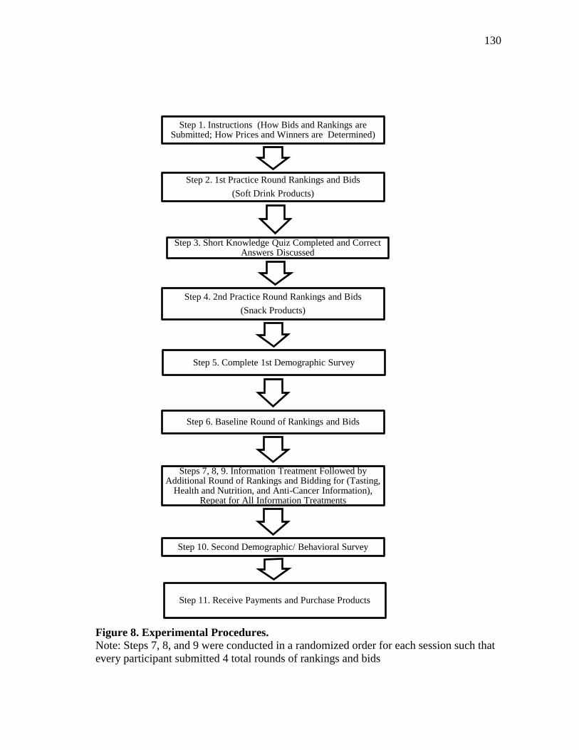
130
Figure 8. Experimental Procedures.
Note: Steps 7, 8, and 9 were conducted in a randomized order for each session such that
every participant submitted 4 total rounds of rankings and bids
Step 1. Instructions (How Bids and Rankings are Submitted; How Prices and Winners are Determined)
Step 2. 1st Practice Round Rankings and Bids
(Soft Drink Products)
Step 3. Short Knowledge Quiz Completed and Correct Answers Discussed
Step 4. 2nd Practice Round Rankings and Bids
(Snack Products)
Step 5. Complete 1st Demographic Survey
Step 6. Baseline Round of Rankings and Bids
Steps 7, 8, 9. Information Treatment Followed by Additional Round of Rankings and Bidding for (Tasting,
Health and Nutrition, and Anti-Cancer Information), Repeat for All Information Treatments
Step 10. Second Demographic/ Behavioral Survey
Step 11. Receive Payments and Purchase Products
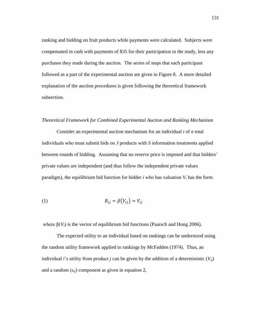
131
ranking and bidding on fruit products while payments were calculated. Subjects were
compensated in cash with payments of $35 for their participation in the study, less any
purchases they made during the auction. The series of steps that each participant
followed as a part of the experimental auction are given in Figure 8. A more detailed
explanation of the auction procedures is given following the theoretical framework
subsection.
Theoretical Framework for Combined Experimental Auction and Ranking Mechanism
Consider an experimental auction mechanism for an individual i of n total
individuals who must submit bids on J products with S information treatments applied
between rounds of bidding. Assuming that no reserve price is imposed and that bidders‘
private values are independent (and thus follow the independent private values
paradigm), the equilibrium bid function for bidder i who has valuation Vi has the form
(1) ( )
where β(Vi) is the vector of equilibrium bid functions (Paarsch and Hong 2006).
The expected utility to an individual based on rankings can be understood using
the random utility framework applied to rankings by McFadden (1974). Thus, an
individual i‘s utility from product j can be given by the addition of a deterministic (Vij)
and a random (εij) component as given in equation 2,
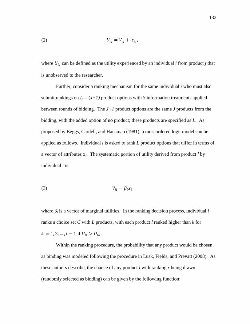
132
(2)
where can be defined as the utility experienced by an individual i from product j that
is unobserved to the researcher.
Further, consider a ranking mechanism for the same individual i who must also
submit rankings on L = (J+1) product options with S information treatments applied
between rounds of bidding. The J+1 product options are the same J products from the
bidding, with the added option of no product; these products are specified as L. As
proposed by Beggs, Cardell, and Hausman (1981), a rank-ordered logit model can be
applied as follows. Individual i is asked to rank L product options that differ in terms of
a vector of attributes xl. The systematic portion of utility derived from product l by
individual i is
(3)
where βi is a vector of marginal utilities. In the ranking decision process, individual i
ranks a choice set C with L products, with each product l ranked higher than k for
if .
Within the ranking procedure, the probability that any product would be chosen
as binding was modeled following the procedure in Lusk, Fields, and Prevatt (2008). As
these authors describe, the chance of any product l with ranking r being drawn
(randomly selected as binding) can be given by the following function:
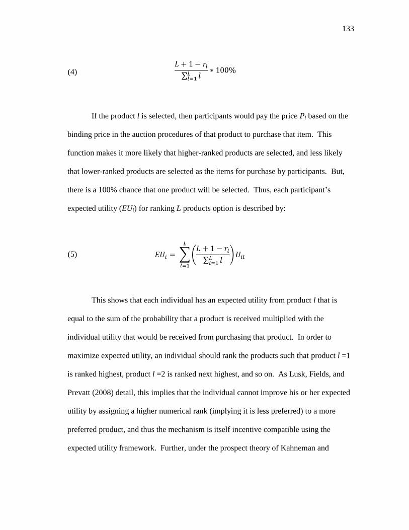
133
(4)
∑
If the product l is selected, then participants would pay the price Pl based on the
binding price in the auction procedures of that product to purchase that item. This
function makes it more likely that higher-ranked products are selected, and less likely
that lower-ranked products are selected as the items for purchase by participants. But,
there is a 100% chance that one product will be selected. Thus, each participant‘s
expected utility (EUi) for ranking L products option is described by:
(5) ∑(
∑
)
This shows that each individual has an expected utility from product l that is
equal to the sum of the probability that a product is received multiplied with the
individual utility that would be received from purchasing that product. In order to
maximize expected utility, an individual should rank the products such that product l =1
is ranked highest, product l =2 is ranked next highest, and so on. As Lusk, Fields, and
Prevatt (2008) detail, this implies that the individual cannot improve his or her expected
utility by assigning a higher numerical rank (implying it is less preferred) to a more
preferred product, and thus the mechanism is itself incentive compatible using the
expected utility framework. Further, under the prospect theory of Kahneman and

134
Tversky (1979) in which individuals misperceive probabilities such that low
probabilities are overweighted and high probabilities are underweighted, the equation
above is still maximized where the most preferred product is ranked first down to the
least preferred product ranked last, and therefore such a mechanism is indeed incentive
compatible.
The selection of which product would be purchased may seem at first glance to
be difficult to implement in a laboratory setting. However, the likelihood of any ranking
being chosen was calculated prior to the experimental sessions, and the percentages were
available if participants had further questions beyond the basic premise that an item
ranked first would be most likely to be randomly selected as binding, an item ranked
second would be next most likely to be selected, and so on until the item ranked last
would be the least likely to be selected as the item to be purchased.
Procedural Details and Justification
While an introduction to the procedures used in this study was included
previously, a number of specific details can help guarantee or bring into question the
validity of the results of an experimental auction and/or preference ranking procedure.
Therefore, more specific details of the auction procedures as well as the justification for
the procedures that were used are provided.
Auction Procedures
For the study, a total of 203 participants were recruited from the Bryan-College
135
Station area of Texas. Participants were assigned to sessions based on age and gender
demographics of U.S. grocery shoppers (please see Carpenter and Moore 2006) and the
overall Texas population. Such a subject sample was preferred over the commonly-used
participant base consisting exclusively of university students due to the nature of the
question being addressed. Information on potential long-term health benefits would be
less of a concern for a younger demographic (in general), not to mention anticipated
differences in grocery purchasing behavior within a student population versus the overall
Texas grocery-shopper demographic. The sessions were held at various times during the
day in an attempt to capture more variability in population factors such as employment.
These participants were recruited using advertisements in the local newspaper
and other local online and print media to attend one of a total of eight sessions over the
course of three days to be held at the Texas A&M University Horticultural Gardens
Classroom. The newspaper advertisement that was used to recruit participants is
included in Appendix A. Subjects were informed that they would be participating in a
study on the decision-making process for fruit purchases and were told that they would
be paid $35 for their participation in a 1.5 hour long session, less any purchases that they
made during the session. (The recruited sample was not intended to be representative of
all possible buyers, as it was expected that only individuals who were interested in such
a study would respond to the advertisement.) Individuals who agreed to participate were
emailed directions to the facility, as well as a reminder of their agreement to participate
within one week prior to the study. Individuals who did not have email addresses were
provided directions via telephone or postal mail.

136
The intent was to recruit twenty-five subjects each of eight study sessions over
three consecutive days, for a total of 200 participants in the experimental auction.
However, there was a range (n=19 to n=35) in the number of participants who were
present on the day of the auction due to last minute cancellations by participants.
However, a total of 203 participants were recruited in total to participate in the eight
sessions over three days.
Upon arrival to their designated session, participants were provided with an
instructional packet and a packet of bid and ranking sheets. They were randomly
assigned an identification number to be used throughout the experimental session to
maintain anonymity. The participants were then asked to sign a consent form as
required by the Texas A&M University Institutional Review Board (IRB). Participants
were instructed to review the procedures for the first two stages of the auction. A
session monitor read these instructions aloud, describing the auction and ranking
procedures, as well as how bids and rankings were submitted. The session monitor then
provided information on how winners were selected for the auctions and rankings. It
was made explicitly clear that both types of preference elicitation procedures were
nonhypothetical in nature and that any participant would have to pay actual money for
any good that he or she purchased during the session. It was also made clear that there
would be ten winners who actually purchased fruit items based on the results of the
auctions and ten winners who purchased fruit products based on the results of the
rankings for each session.
The instructions for the procedures were adapted from examples given in Lusk

137
and Shogren (2007); Lusk, Fields, and Prevatt (2008); Lusk and Schroeder (2006),
Umberger, Boxall, and Lacy (2009), and Rousu et al. (2007). The verbal instructions
that subjects were given included more specific details and are provided in Appendix B.
Additionally, the full written instructions that subjects received for this study can be
found in Appendix C. Subjects were provided with both verbal and numerical examples
of auctions to help them understand the 11th
-price auction mechanism and
nonhypothetical ranking procedure in which they would participate. The participants
then engaged in practice rounds, submitting rankings and bids for four common soft
drink products: Pepsi®, Coke®, Diet Coke®, and Dr. Pepper®. After one round of
ranking and one round of bidding in which the market price (the 11th
-highest price) was
posted, subjects completed a five-question quiz. The session monitor went over the
answers to the quiz and answered any questions.
Subjects then participated in another round of practice, with one ranking and one
round of bidding. The second practice round was for four snack products that varied in
their familiarity: a package of chips, a package of cheese puffs, an individually-wrapped
cookie, and a package of a less-common flavor of snack crackers. Following the
completion of the practice rounds of the auction, the participants completed a consumer
survey over their purchasing habits and demographic characteristics. The questionnaire
was broken into smaller segments to be worked on at different stages to reduce
participant fatigue. The 11th
-price for each product in the two practice rounds were
posted to ensure that participants understood how the winning price was selected.
Subjects were next given verbal and written instructions on the procedures for
138
the fruit product portion of the session. The fruit products were: California Wonderful
Pomegranate, Texas Pomegranate 1 (Variety Salavatski), Texas Pomegranate 2 (Variety
Texas Red), Ready-to-Eat California Pomegranate Arils, Ready-to-Eat Texas
Pomegranate Arils, Mixed Pomegranate Juice, and Pineapple (as a control fruit product).
A control fruit product was included because it was assumed that many individuals
would be unfamiliar with pomegranates but would be more familiar with pineapple.
Further, a product that would have a similar reference price for a single unit was
preferred for use as a reference product over a product with a dissimilar price for a single
unit. The cultivars of pomegranates were selected based on the industry standard variety
(California Wonderful) and two varieties thought to have commercial potential in Texas
(Texas Red and Texas Salavatski).
Many study designs suggest that an orthogonal approach to the different product
characteristics of the products be included as one of several important components of the
study design; however, in some cases such a comparison would lose sight of the question
of control versus context for the experiment. For example, claiming that a pineapple
product from Texas was commercially available would have been discredited by
participants, and including a California and two Texas varieties of each form of the
pomegranate products would have resulted in too large of a selection of products to
expect subjects to accurately and carefully rank them. Also, the varieties that were
included as Texas varieties are cultivars that have shown promise for commercial
cultivation in Texas, and it would have been unrealistic to separate the growing location
of Texas, the physical appearance of the product, and the flavor of the product just for
139
the purpose of estimating the specific size of these effects. These novel products were
novel because of the unique combination of these attributes that they provided. Further,
the appearance of the products was not identical across varietal cultivars; nevertheless,
the products that subjects bid on were representative of the typical appearance of that
cultivar. Images of these products can be found in Appendix D.
Subjects were given an opportunity to closely examine the fruit products and
were then asked to submit ordered rankings of the 7 products and the option of ―no
product‖ (8 total product options and to also submit a sealed bid for each of the 7
products. The option of ―no product‖ was included to allow for a comparison of the
rankings and bids, since subjects also had the option of bidding $0.00 for any of the
products. Examples of the ranking and bidding sheets provided to participants are
included in Appendix E. Five of the eight (n=138) subject sessions were provided with a
reference price of $3.50 per item as the retail price for all of the fruit products, based on
the current prices of the products in College Station retail stores. This was done in order
to control for the effects of reference prices in the magnitude of the submitted bids.
However, all participants were informed that the products available sold at retail for the
same price. Each of these sessions received three additional information treatments,
with the order of these treatments randomized among sessions.
Following the ―baseline round‖ (no information provided) of bidding, subjects
were provided with a series of three randomized information treatments. All subjects
received all three information treatments by the end of the session; in each of these they
could gain more information on the products before submitting additional rankings and

140
bids. The order of the additional information treatments were randomized across
sessions. These treatments were as follows: 1) Tasting: subjects tasted small
(approximately 2 oz.), equally-sized samples of each product and the method for
removing the husk of a whole pomegranate fruit was described, 2) Health and Nutrition
Information: subjects were provided with health and nutrition information for all fruit
products, and 3) Anti-Cancer Information: subjects were provided with specific
information on the potential anticancer properties of pomegranates. Information on how
to remove the husk of the pomegranate was included because it was assumed that in a
setting outside the experimental auction, subjects would need this minimal amount of
information in order to consume any of the whole fruit products. The full details of
these informational treatments are included in Appendix F; in general, the health and
nutrition information provided the specific nutrition facts of the products in the standard
consumer nutrition label format and gave additional background on the role that
antioxidants can play in human health. This text was written in plain language to
facilitate subject understanding.
Similarly, the anti-cancer information that was given on pomegranates was
provided on a written handout to subject participants during the appropriate round of
preference ranking and bidding. The anti-cancer information that was provided was
titled as ―Pomegranate Health Information‖ to avoid unintentionally biasing the results
with a title of ―Pomegranate Anti-Cancer Information,‖ which may have alerted
participants to what type of health information effects were being measured. The
information included some of the information from the health and nutrition information
141
treatment, but also included more specifics on potential anti-cancer properties. Clear
warnings were given on the need for further clinical research into specific anti-cancer
effects of pomegranates in human subjects.
The anti-cancer information that was provided was based on research of the
potential benefits of consuming pomegranate products as discussed in the pomegranate
chapter, and every effort was made to provide information that could potentially be
provided to consumers as point-of-purchase materials or in other types of
advertisements. All claims made were verifiable based on scientific studies.
When consumers are exposed to a new food product, there are certain types of
information that are generally gained, including both experience and credence attributes.
Consumers gain information on the basic nutrition of the products, as well as any health
claims that are made by marketers. Many attributes of food products can only be
determined when the good is consumed, and this is often valuable information to the
consumer to decide whether to purchase the item again in the future. Marketers often
make claims on other attributes of products in addition to the basic nutrition, but these
may or may not serve as valuable information to consumers.
Following the completion of all rounds of ranking and bidding, the round of the
auction bidding (baseline, tasting, health information, or anti-cancer information) that
was to be binding was drawn by a session subject with equal probability for each round
and was announced to the session participants. The product that would be binding for the
bidding rounds was randomly drawn prior to each session and placed in a sealed
envelope. The binding product from the sealed envelope was also announced to session
142
participants following the completion of all rounds of ranking and bidding. Based on the
11th
-price auction mechanism, there were ten subjects in each round who bid higher than
the 11th
-highest price and who purchased the binding product at the 11th
-price for that
product in the binding round of auction bids. Then, of subjects who did not win in the
auction, ten subjects purchased an item based on their respective rankings. These items
were purchased at the 11th
-price for that good for the binding round of the auction. All
ranks and bids were entered into a template in Microsoft Office Excel® that was
developed to sort the bids for each product, pick the 11th
price for each product, and
break any ties to randomly pick winners.
Subjects received cash compensation of $35 for their participation in the study,
less any purchases that they made based on the auction or ranking procedures. Any
subjects who purchased any of the items received those items once all results of the
auction and rankings were tabulated. The subjects signed a receipt of payment form, and
the session was complete.
Experimental Auction and Preference Ranking Design Considerations
Participants were not aware that pomegranates would be a part of the study, as
pomegranates are a novel good and the investigators wanted to ensure that the previous
level of exposure reported by participants as a part of the consumer survey was
indicative of the novelty of the product prior to the subjects‘ agreement to participate in
the experimental auction. Subjects were told only that they would be participating in a
study to evaluate fruit-purchase decision-making. Participants were also unaware that
143
there would be the opportunity to taste the products as a part of the experimental
procedures. Lusk and Shogren (2007) suggest that it is critical to make efforts to
enhance the validity and the independence of data from each phase; making participants
unaware of additional opportunities to taste and/or gather additional information on the
products was intended to assist in this effort. If participants were aware of later
information-gathering opportunities, they may have discounted bids in earlier rounds and
biased the experimental results.
The opportunity to taste the goods was important to make a more thorough
evaluation of consumers‘ WTP for pomegranates after their initial purchase. This was
also important for identifying differences in taste preference for the pomegranate
varieties. Specifically, the novelty of pomegranates meant that participants may have
been unfamiliar with the fruit, and giving them the opportunity to taste the good
increased their familiarity with the good. Since the value of food products is derived at
least in part, if not primarily, from the consumption value, then the opportunity to
consume the good was important to the external validity of the auction results. On the
opposite hand, it was just as important that participants be unaware of the opportunity to
consume the good as a part of the study. This is because, given knowledge of the
opportunity to obtain further information at a later time, it is likely that participants
would submit initially lower bids for the goods in anticipation of gaining further
information at a later time. However, since participants were previously unaware of the
requirement to consume the good, individuals who refused to taste the good were still
compensated for participation; they were not allowed to participate in further ranking
144
and bidding rounds of the study. (There were no recruited subjects who refused to
consume the fruit products.)
It was determined to be impractical to require participants to consume the
product they purchased onsite as was done in some previous WTP studies for food
products (i.e. Shin et al. 1992; Fox et al. 1995; Gimalva, Bailey, and Redfern 1997); it
requires some amount of effort to remove the husk of pomegranates and the fruits are
larger than most consumers would eat in a single sitting. However, they do not require
short-term refrigeration so no alternative pick-up requirements were made as in Lusk,
Feldkamp, and Schroeder (2004).
Only one fruit product could be purchased by any participant, and this was
emphasized to subjects. This was accomplished by randomly drawing which round of
the auction and which product within that round was binding. Winners for the ranking
procedure were then selected from non-winners in the auction. Such a procedure is
useful in avoiding demand reduction over multiple rounds of the auction, as well as
diminishing marginal utility in analysis of consumer WTP.
The effects of posting prices within experimental auctions have been debated.
One faction suggests that posting of prices causes affiliation of bids among subjects, and
they indicate that a single-shot auction mechanism is preferable. The opposite faction
indicates that repeated rounds encourage learning of the auction mechanism and that the
influence of the market effect stabilizes bids made by subjects. Further, some indicate
that the problem of bid affiliation is not necessarily solved by a single-shot auction
mechanism as there are other indicators besides a posted price that may cause bids to
145
become affiliated. Additionally, there is a lack of evidence that bids are not affiliated
before subjects begin the study and that bids are not affiliated in the outside marketplace.
Therefore, a single round auction mechanism was selected. The imposition of product
information treatments throughout the study may have been compounded with repeated
rounds, and the bidding information feedback may have made it difficult to determine if
changes in measured prices were due to bid affiliation or a result of the preference
updating of consumers that should occur when new information is received.
In terms of which auction mechanism was preferred, a uniform nth
-price auction
avoids the primary emphasis on only the highest value bidders in a standard Vickrey 2nd
-
price auction while also avoiding the emphasis on low value bidders in a random nth-
price auction. (A uniform nth-price auction selects a single nth-price for all rounds,
while a random nth-price auction selects a different random nth-price for every round of
the auction). For instance, in a 2nd
-price auction there is only one winner, so bidders
with lower individual values for the product may be ―disinterested‖ in the auction
outcome. A price in which approximately one-half of participants were winners would
eliminate some of the imbalances in the incentives to under- or over-bid for participants.
As described by Lusk and Shogren (2007), the expected monetary loss from
―misbidding‖ (where an individual‘s bid does not equal that same individual‘s WTP for
that product) varies depending on the specifics of the mechanism. However, none of
these auction mechanisms (and no others for that matter) guarantees that subjects will
bid exactly their true WTP; rather, the auction mechanisms vary in the degree to
deviation from the dominant strategy is punished and the mechanisms that do this the
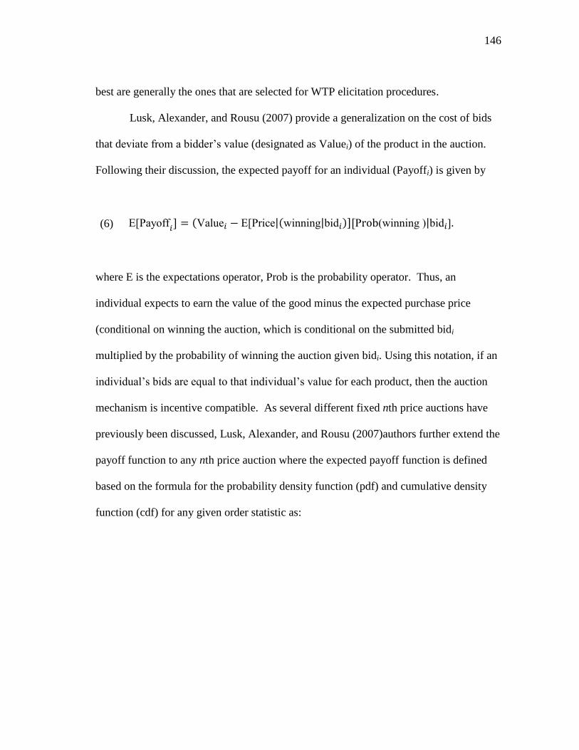
146
best are generally the ones that are selected for WTP elicitation procedures.
Lusk, Alexander, and Rousu (2007) provide a generalization on the cost of bids
that deviate from a bidder‘s value (designated as Valuei) of the product in the auction.
Following their discussion, the expected payoff for an individual (Payoffi) is given by
(6) E[Payoff (Value E[Price|(winning|bid ) P (winning )|bid
where E is the expectations operator, Prob is the probability operator. Thus, an
individual expects to earn the value of the good minus the expected purchase price
(conditional on winning the auction, which is conditional on the submitted bidi
multiplied by the probability of winning the auction given bidi. Using this notation, if an
individual‘s bids are equal to that individual‘s value for each product, then the auction
mechanism is incentive compatible. As several different fixed nth price auctions have
previously been discussed, Lusk, Alexander, and Rousu (2007)authors further extend the
payoff function to any nth price auction where the expected payoff function is defined
based on the formula for the probability density function (pdf) and cumulative density
function (cdf) for any given order statistic as:
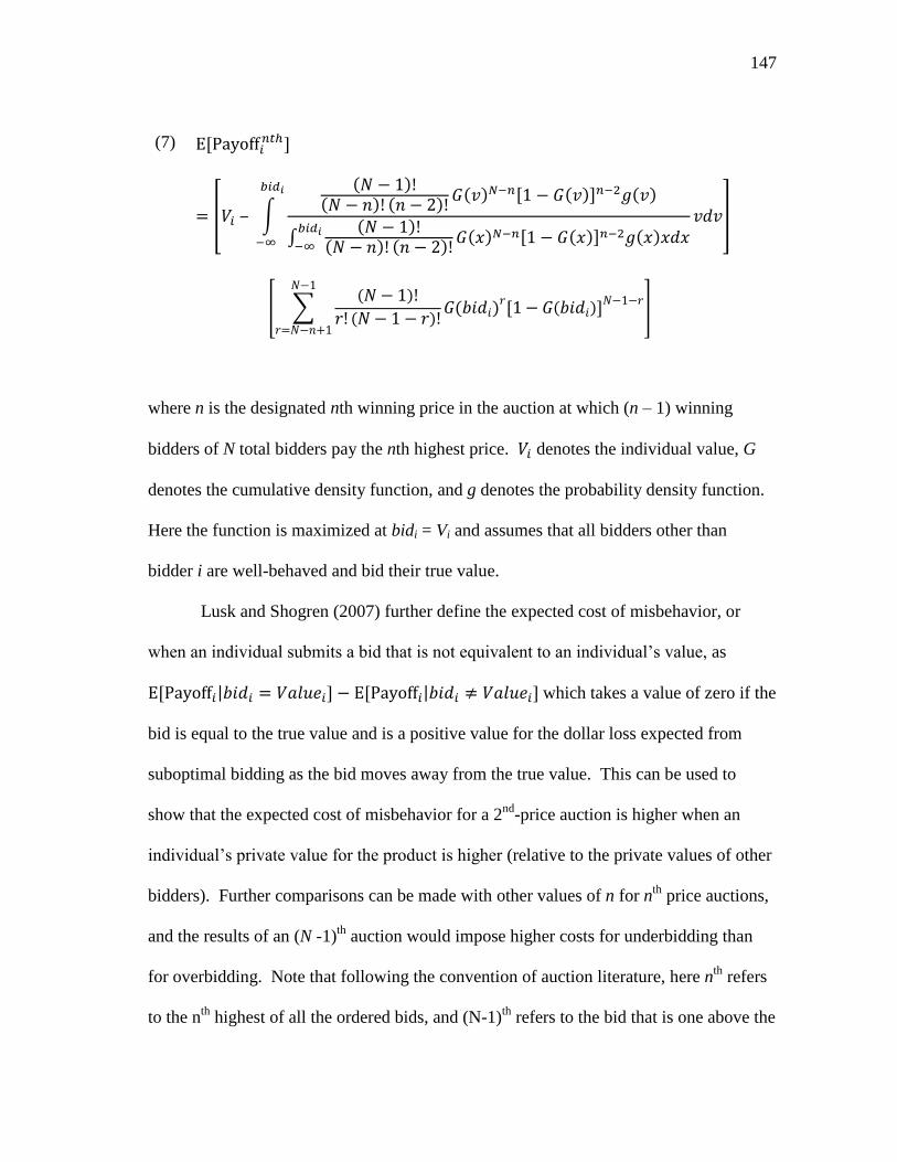
147
(7)
[ ∫
( ) ( ) ( )
( ) ( ) ( )
∫( )
( ) ( ) ( ) ( ) ( )
]
[ ∑( )
( ) ( )
( )
]
where n is the designated nth winning price in the auction at which (n – 1) winning
bidders of N total bidders pay the nth highest price. denotes the individual value, G
denotes the cumulative density function, and g denotes the probability density function.
Here the function is maximized at bidi = Vi and assumes that all bidders other than
bidder i are well-behaved and bid their true value.
Lusk and Shogren (2007) further define the expected cost of misbehavior, or
when an individual submits a bid that is not equivalent to an individual‘s value, as
| | which takes a value of zero if the
bid is equal to the true value and is a positive value for the dollar loss expected from
suboptimal bidding as the bid moves away from the true value. This can be used to
show that the expected cost of misbehavior for a 2nd
-price auction is higher when an
individual‘s private value for the product is higher (relative to the private values of other
bidders). Further comparisons can be made with other values of n for nth
price auctions,
and the results of an (N -1)th
auction would impose higher costs for underbidding than
for overbidding. Note that following the convention of auction literature, here nth
refers
to the nth
highest of all the ordered bids, and (N-1)th
refers to the bid that is one above the
148
lowest (the Nth
) bid. These conclusions are more straightforward when a uniform
distribution of private values is assumed, but can be shown to generally be similar for
other distributions of private values (i.e. normal, pseudo-normal, left-skewed, right
skewed) as well (Lusk, Alexander, and Rousu 2007). For a 5th
price auction with N=10,
these authors found results that varied depending on the distribution that was specified
and whether bidders were underbidding or overbidding. However, the main point to be
drawn from this discussion is as follows: the expected cost of deviating bids from true
values was highest when a fixed price auction was specified where n was somewhere
near the middle range of N.
A uniform nth
-price (specifically an 11th
-price) modified-Vickrey auction was
used for the experimental auction portion of this study. There have been a number of
discussions of which price should be selected as the binding price in these types of
auctions. For this study, the target products were generally novel to the participants.
There has also been discussion in the literature on the use of endowed versus full-
bidding methods for novel products. With a good that is unfamiliar to subjects, an
approach where subjects have no opportunity for further learning is preferable. This is
typically implemented as an endowed approach; however, use of the combined ranking
and bidding mechanism guaranteed that most subjects would purchase a product during
the sessions but avoided the inherent difficulty in assessing WTP based on bids to
upgrade if full bid values are not collected.
Also, a full bidding approach is generally preferred if preferences are expected to
be heterogeneous. The full-bidding approach allows for positive and negative
149
differences in values between two products. Lusk and Shogren (2007) indicate that the
endowed approach is preferable because differences in WTP are the most reliable
estimates from auction data; therefore, the implied differences in the full bidding results
for each subject were also included in the analysis. However, auction procedures that
ensured that subjects left with a good would have similar advantages to the endowed
approach of preventing future learning about the good while at the same utilizing a full-
bidding approach that allows for more realistic differences in valuation. Thus, with a
targeted study size of 20-35 participants per session, an 11th
-price auction would ensure
that ten subjects were product purchasers based on the nonhypothetical auction, and
another ten subjects were purchasers based on the nonhypothetical ranking portion of the
procedure. This was done to guarantee that most participants had no future option for
learning about the products when they made their bids and preference decisions.
Anonymity of subjects was ensured by the use of randomized identification
numbers and the use of a sealed bid auction mechanism. Envelopes were also used to
disperse payments, and care was taken not to allow other participants to see the amount
of an individual‘s payment for participation in the study.
Practice was required in order to teach the auction procedures and mechanisms to
subjects prior to the auction rounds for the target products. This was accomplished in
several ways. The subjects were provided with explicit written instructions on how the
auction mechanism worked. Further, subjects were given descriptive examples of the
auction procedures as well as explicit numerical examples. An explanation of the
dominant bidding strategy was provided and it was explicitly stated that it was in each

150
person‘s best interest to bid truthfully. Further, subjects participated in two
nonhypothetical practice rounds of auctions, one for common soft drink products and
one for snack products that varied in novelty. In between the two rounds of practice,
subjects were given a brief quiz in which they answered questions about the auction and
ranking mechanisms.
An important consideration in the experimental design is that there is a necessary
tradeoff between the external validity of the auction procedures and the degree of control
that can be obtained. The design of this experiment was undertaken giving careful
attention to these two conflicting goals. An auction setting in a classroom or laboratory
is already quite distinct from an actual purchase interaction that would occur in the day-
to-day lives of most consumers. Given this, great efforts were taken to balance these
differences and elicit the most accurate WTP estimates from the experimental procedure.
For example, consumers neither submit bids for goods they purchase in a retail
store nor submit an actual ranking for the goods they might consider purchasing.
However, consumers must implicitly answer these types of questions by selecting which
price and product combination is their most preferred option. As described in the
literature review, the use of auctions is generally thought to produce more conclusive
WTP results than choice experiments. Combining the ranking procedure with the
auction was done with the intent of providing additional information on consumer
preferences.
Separation of the imposed effects from the specific goods to be auction was
achieved in several ways. Since all of the goods up for auction during the procedure are
151
related in consumption, only one good was randomly chosen to be a binding purchase.
Further, an additional product that is somewhat novel in preparation and consumption
(fresh pineapple fruit) was included to account for specificity of health effects to a
particular product. A pineapple fruit is similarly priced to all of the pomegranate
products that were included but was anticipated to be more familiar to participants than
pomegranate products.
In order to avoid specific effects of a number of components of the experimental
procedures, randomization was utilized to avoid a systematic effect on the experimental
results. The ordering of the additional information treatments was randomized among
each of the eight sessions.
The effects of information as measured by such an experiment are subject to a
focusing effect. More specifically, there is the potential for subjects to identify the
effects of health information as one of the targets of the study and increase their bids
because they anticipate higher bids to be the expected result of the study. Another
implication of providing additional information is the potential effect of preference
learning (Shogren, List, and Hayes 2000) on the outcome of the study. If participants
believe that they will have the opportunity to gain information on the product by
purchasing it and having the opportunity to consume it (particularly for a novel product),
then this might introduce upward pressure on their bids. However, once information has
been gained on the product during the course of the experiment, then this upward
pressure from the information effect may be reduced or eliminated. Therefore, the final
WTP bids after participants have received all information treatments should reflect a

152
state of full information on the good, particularly since most participants would be
taking home a product as a result of either their rankings or bids.
Subjects were informed that they were allowed to submit zero or negative bids.
However, no subjects actually submitted negative bids. Subjects may not have felt
comfortable with submitting negative bids since they would be uncharacteristic of a
traditional retail setting. There were a high percentage of zero bids, as described by the
censoring results presented later. Allowing subjects to make zero or negative bids in the
auction rounds was mimicked in the ranking rounds by allowing a preference for the
option of ―no product.‖ Beyond allowing subjects to submit zero or negative bids, if all
submitted bids are zero or above then the econometric model must be adjusted to
account for this. These considerations are discussed further in the model estimation
subsection.
Subjects participated in one round of ranking and one round of bidding for two
sets of practice products in order to become familiar with the auction mechanism;
consequently, they participated in two total rounds of practice for each of the ranking
and bids. This was in addition to extensive descriptions of the procedures and
opportunities to answer questions. Then, subjects submitted a total of 4 additional
rankings and 4 additional rounds of bidding for the fruit products that were the target of
the auction. Further rounds would have increased subject fatigue, as well as causing the
total time for the session to be long relative to subjects‘ attention spans.
The possibility of varying the base of $35 for the participation fee was
considered; however, a variation in such an endowment would have needed to be large
153
in size to be substantial in relation to participants‘ total income. This was determined to
be unrealistic for the experimental auction setting. Also, all subjects received the same
endowment, so the premiums that each individual would pay for one product over
another should all be based relative to that endowment.
The ranking experiment included was modeled after a profile ranking procedure
introduced by Lusk, Fields, and Prevatt (2008) and a nonhypothetical ranking procedure
introduced by Chang, Lusk, and Norwood (2009). The rankings were included in the
practice rounds to give participants additional practice with the procedures. Further, the
ranking has the potential to either confirm or dispute the results of the auction
mechanism. Due to the number of questions that still surround the mechanisms of
experimental auctions, the addition of another mechanism to measure preferences may
allow a balance between some of the problems of each approach in isolation.
Prior to the actual study sessions, the experimental auction and preference
ranking procedures were tested with a group of graduate students from Texas A&M.
Based on the results of the practice study, modifications to the procedures were made to
increase the clarity of instructions and reduce the amount of time required to complete
the bidding and ranking procedures.
Econometric Model
The experimental design described above led to a need to accommodate a
number of factors in the econometric modeling of bidding and ranking behavior. The
use of rankings and biddings are generally done separately. This could either be
154
accommodated with a single model for both procedures, or it could be accommodated
with two separate models best suited for each type of data. Those types are continuous
data that is censored from below for the auction bidding and a series of choice decisions
for the ranking procedure.
The goal of modeling WTP was to gain a better understanding of which factors
may influence consumer WTP for pomegranate fruits and other pomegranate products.
If possible, such a model would also have some ability to predict consumer WTP based
on these characteristics. The models that are used should, if possible, allow for
comparisons of the two value elicitation mechanisms.
The models that have been used in the past in application to WTP are quite
diverse, and many of these are applied to this data. Considerations are given to the
benefits and drawbacks of each model in their application to this particular dataset.
Econometric Model for Experimental Auction Bids
The WTP for products in this study is modeled as a function of an individual‘s
demographic characteristics, behavioral characteristics, the reference price, the order that
information treatments are received.
Thus, each individual has a WTP that is described as the following equation:
(8)
(
)
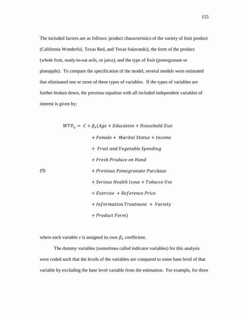
155
The included factors are as follows: product characteristics of the variety of fruit product
(California Wonderful, Texas Red, and Texas Salavatski), the form of the product
(whole fruit, ready-to-eat arils, or juice), and the type of fruit (pomegranate or
pineapple). To compare the specification of the model, several models were estimated
that eliminated one or more of these types of variables. If the types of variables are
further broken down, the previous equation with all included independent variables of
interest is given by:
(9)
(
)
where each variable v is assigned its own coefficient.
The dummy variables (sometimes called indicator variables) for this analysis
were coded such that the levels of the variables are compared to some base level of that
variable by excluding the base level variable from the estimation. For example, for three
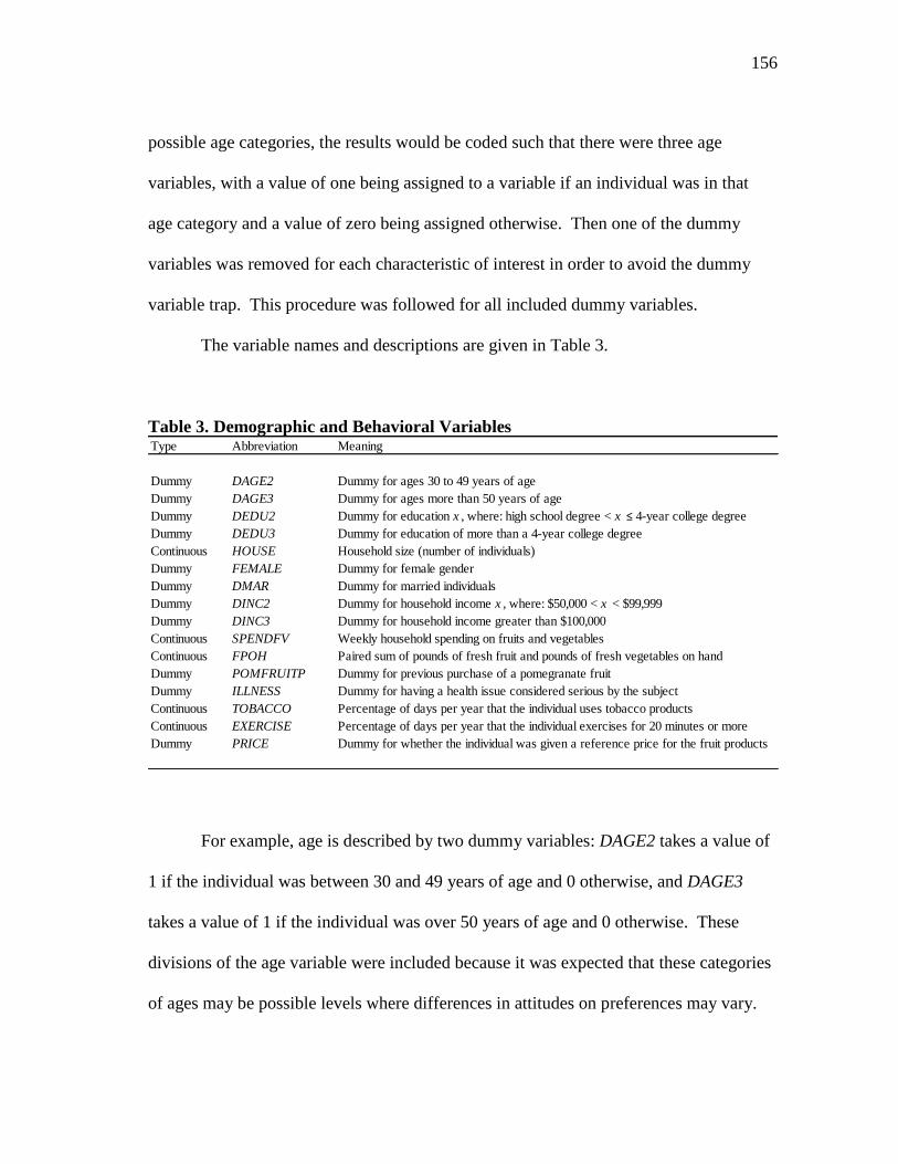
156
possible age categories, the results would be coded such that there were three age
variables, with a value of one being assigned to a variable if an individual was in that
age category and a value of zero being assigned otherwise. Then one of the dummy
variables was removed for each characteristic of interest in order to avoid the dummy
variable trap. This procedure was followed for all included dummy variables.
The variable names and descriptions are given in Table 3.
Table 3. Demographic and Behavioral Variables
For example, age is described by two dummy variables: DAGE2 takes a value of
1 if the individual was between 30 and 49 years of age and 0 otherwise, and DAGE3
takes a value of 1 if the individual was over 50 years of age and 0 otherwise. These
divisions of the age variable were included because it was expected that these categories
of ages may be possible levels where differences in attitudes on preferences may vary.
Type Abbreviation Meaning
Dummy DAGE2 Dummy for ages 30 to 49 years of age
Dummy DAGE3 Dummy for ages more than 50 years of age
Dummy DEDU2 Dummy for education x , where: high school degree < x ≤ 4-year college degree
Dummy DEDU3 Dummy for education of more than a 4-year college degree
Continuous HOUSE Household size (number of individuals)
Dummy FEMALE Dummy for female gender
Dummy DMAR Dummy for married individuals
Dummy DINC2 Dummy for household income x , where: $50,000 < x < $99,999
Dummy DINC3 Dummy for household income greater than $100,000
Continuous SPENDFV Weekly household spending on fruits and vegetables
Continuous FPOH Paired sum of pounds of fresh fruit and pounds of fresh vegetables on hand
Dummy POMFRUITP Dummy for previous purchase of a pomegranate fruit
Dummy ILLNESS Dummy for having a health issue considered serious by the subject
Continuous TOBACCO Percentage of days per year that the individual uses tobacco products
Continuous EXERCISE Percentage of days per year that the individual exercises for 20 minutes or more
Dummy PRICE Dummy for whether the individual was given a reference price for the fruit products
157
As an example of a continuous variable, fruit and vegetable spending (SPENDFV) was a
dollar amount of total weekly spending on fruits and vegetables. The variables listed in
the table above are coded similarly to these examples.
During the course of the experiment, each individual submitted a total of 28 bids
for fruit products as bids for seven products for each of four information treatments.
These bids could be treated in several ways. First, the bids could be estimated separately
for each product and each information treatment with a separate equation for each. In
this manner, the WTP was estimated for each of the seven included products. The WTP
was also estimated for the following information treatments: Baseline (BASE) - baseline
at the beginning of the study, Tasting (TASTE) - subjects were allowed to taste a small
sample of all products, Health (HEALTH) - subjects were given health and nutrition
information for all products, and Anti-Cancer (CANCER) - subjects were given
information on the anti-cancer properties of pomegranates. In addition, estimation of the
WTP for the full information set (FULL) was conducted based on an individual‘s bids
following all three information treatments. Thus, 35 equations were used to estimate
WTP based on the full bids made by subjects in the study for this technique.
The WTP for the fruit products could also be estimated in some combination of
aggregated bids (multiple bids made by an individual aggregated into one sample), either
aggregated by information treatment, product, or both. Thus, several additional models
were developed to do this. To accommodate the aggregated bids, other variables were
needed to identify the information treatments and product characteristics. The variables
for the imposed information treatments are included in parentheses above; aggregated
158
models did not include the bids for the full information set as these bids were reflected in
one of the other information rounds. The product characteristic variables that were
included are: Texas Red (TXR) took a value of 1 for Texas Red variety products and 0
otherwise; Texas Salavatski (TXS) took a value of 1 for Texas Salavatski Variety
products and 0 otherwise; RTE took a value of 1 for all ready-to-eat product forms and 0
otherwise, JUICE took a value of 1 for the juice product and 0 otherwise, and
PINEAPPLE took a value of 1 for the pineapple fruit and 0 otherwise.
There were a number of models that have been applied to auction and rankings
data. Several of these were applied and the benefits and drawbacks of each are
presented as they apply to the specific results of this study.
Ordinary Least Squares Model
A number of possible models were considered to evaluate the WTP for the
included products based on the subjects‘ bids. A basic ordinary least squares model was
first considered. Such a model can be estimated in a number of ways. An ordinary least
squares model can be estimated as above by adding a constant term and calculating the
parameters for each variable. However, given the nature of auction bidding, it was
anticipated that there would be a number of censored observations. Although
participants were informed that they had the option of bidding $0.00 or negative values,
it was anticipated that censoring would need to be accounted for in the estimation of the
parameters. Even so, an ordinary least squares model was estimated for comparison
purposes.
159
Tobit Model
The potential for bid censoring led to consideration of using a tobit model to
estimate consumer WTP for the targeted products. Although participants were informed
that they could submit zero bids, the overall distribution could still be censored at $0.00.
The tobit model was first introduced by Tobin (1958); since that time it has been
frequently used for modeling of censored and truncated dependent variables (McDonald
and Moffitt 1980). A distinction should be made between truncated and censored
variables. Truncation is seen when a researcher needs to draw conclusions about a full
population that is based on a sample that is drawn from only a restricted portion of the
population. On the other hand, censoring occurs when values in a certain range of the
distribution are reported as a single value (Greene 2003).
Greene (2003) provides a modern explanation of the tobit model (also known as
the censored regression model), which is summarized below. First, to explain the need
for a tobit model the distribution of the data of interest should first be assessed. Tobit
models are highly useful for describing censored variables. Censored variables can (but
do not have to) be understood by starting with a normal probability distribution. For
convenience, the censoring will be assumed to be at zero. When data are censored, the
distribution that applies to the censored data is described by a mixture of continuous and
discrete distributions. In order to analyze such a distribution, a new variable can be
defined such that
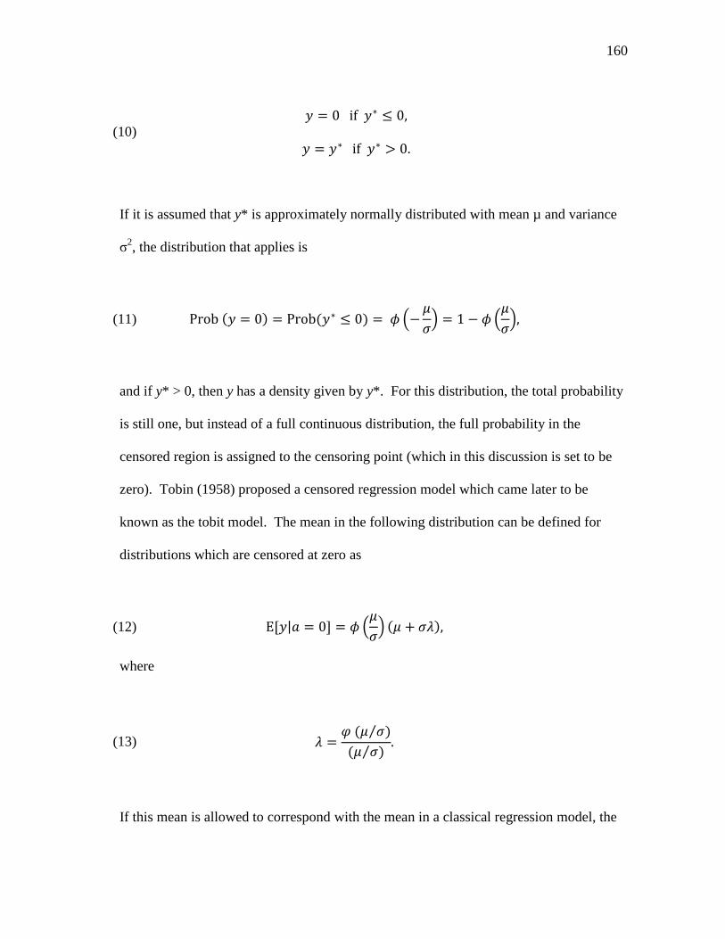
160
(10)
If it is assumed that y* is approximately normally distributed with mean µ and variance
σ2, the distribution that applies is
(11) ( ) ( ) (
) (
)
and if y* > 0, then y has a density given by y*. For this distribution, the total probability
is still one, but instead of a full continuous distribution, the full probability in the
censored region is assigned to the censoring point (which in this discussion is set to be
zero). Tobin (1958) proposed a censored regression model which came later to be
known as the tobit model. The mean in the following distribution can be defined for
distributions which are censored at zero as
(12) | (
) ( )
where
(13) ( ⁄ )
( ⁄ )
If this mean is allowed to correspond with the mean in a classical regression model, the
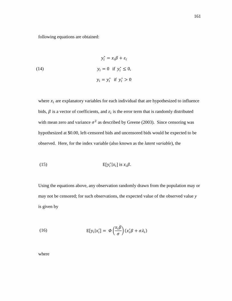
161
following equations are obtained:
(14)
where are explanatory variables for each individual that are hypothesized to influence
bids, is a vector of coefficients, and is the error term that is randomly distributed
with mean zero and variance as described by Greene (2003). Since censoring was
hypothesized at $0.00, left-censored bids and uncensored bids would be expected to be
observed. Here, for the index variable (also known as the latent variable), the
(15) |
Using the equations above, any observation randomly drawn from the population may or
may not be censored; for such observations, the expected value of the observed value y
is given by
(16) | (
) (
)
where
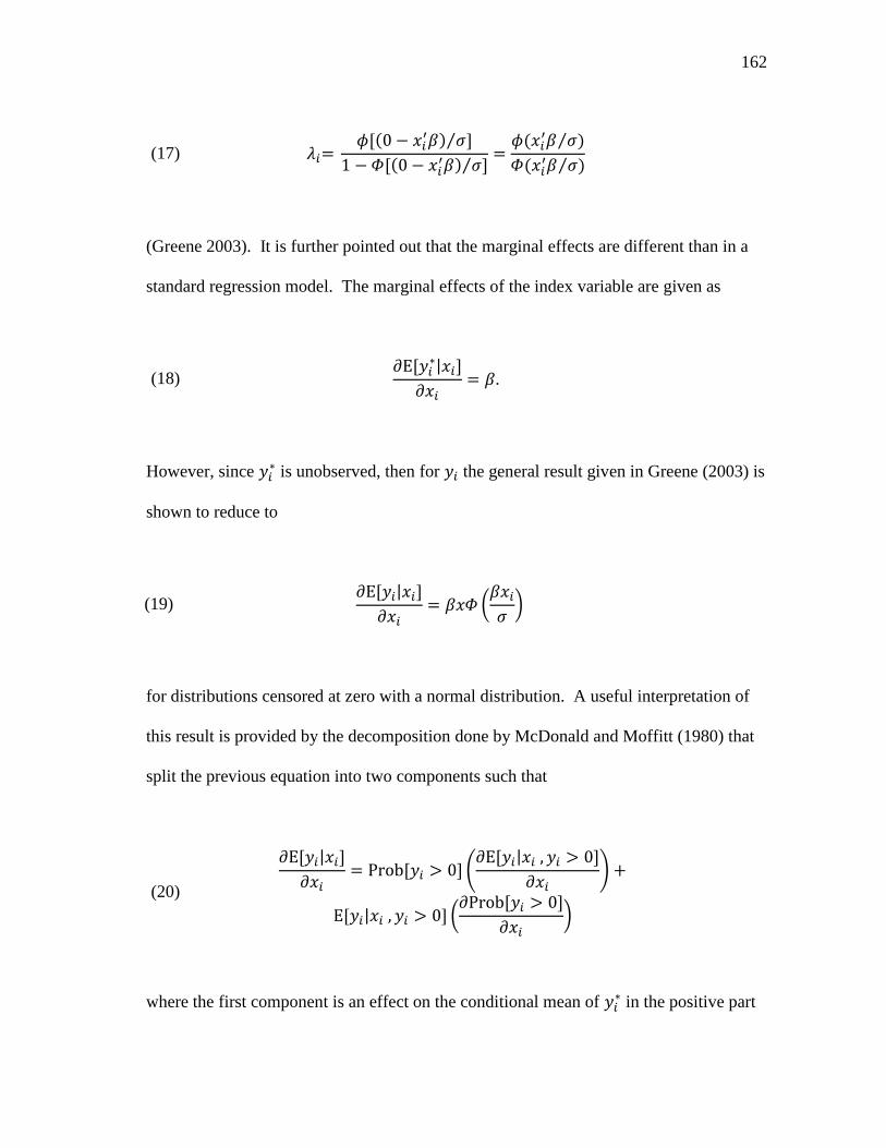
162
(17) (
) ⁄
( ) ⁄
(
⁄ )
( ⁄ )
(Greene 2003). It is further pointed out that the marginal effects are different than in a
standard regression model. The marginal effects of the index variable are given as
(18)
|
However, since is unobserved, then for the general result given in Greene (2003) is
shown to reduce to
(19) |
(
)
for distributions censored at zero with a normal distribution. A useful interpretation of
this result is provided by the decomposition done by McDonald and Moffitt (1980) that
split the previous equation into two components such that
(20)
|
(
|
)
| (
)
where the first component is an effect on the conditional mean of in the positive part
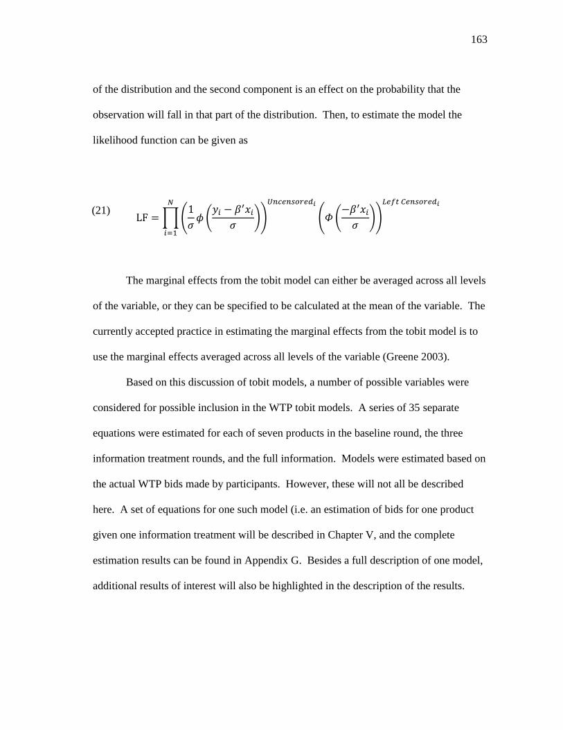
163
of the distribution and the second component is an effect on the probability that the
observation will fall in that part of the distribution. Then, to estimate the model the
likelihood function can be given as
(21)
∏(
(
))
( (
))
The marginal effects from the tobit model can either be averaged across all levels
of the variable, or they can be specified to be calculated at the mean of the variable. The
currently accepted practice in estimating the marginal effects from the tobit model is to
use the marginal effects averaged across all levels of the variable (Greene 2003).
Based on this discussion of tobit models, a number of possible variables were
considered for possible inclusion in the WTP tobit models. A series of 35 separate
equations were estimated for each of seven products in the baseline round, the three
information treatment rounds, and the full information. Models were estimated based on
the actual WTP bids made by participants. However, these will not all be described
here. A set of equations for one such model (i.e. an estimation of bids for one product
given one information treatment will be described in Chapter V, and the complete
estimation results can be found in Appendix G. Besides a full description of one model,
additional results of interest will also be highlighted in the description of the results.

164
Random Effects Tobit Model
However, individual preferences are likely to be heterogeneous, and full bids are
also likely to be censored at zero. A number of models have been developed to account
for individual heterogeneity as described by Greene (2003), including fixed effects,
random effects, random parameters models, and covariance structures. In each of these,
the underlying individual heterogeneity is addressed in the model in some way. A full
coverage of each of these is not pertinent to the topics under investigation in this study;
however, a few components of these models will be addressed. A simple pooled
regression can be assumed to be biased and inconsistent if the individual effects are
correlated with the included regressors, but such a problem can be addressed with a fixed
effects model such that there is a constant term specific to each group in the regression
(Greene 2003).
On the other hand, a random effects model assumes that the individual
heterogeneity is not correlated with the included variables but that there is a random
element specific to each group such that the differences between units are strictly
parametric shifts of the function being estimated. A random effects model can be
specified following Greene (2003) as
(22)
where is a constant term and is a group-specific random element that is similar to
the random error term except that there is only one draw from the distribution for each
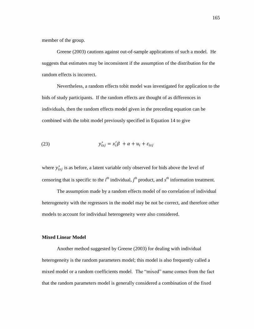
165
member of the group.
Greene (2003) cautions against out-of-sample applications of such a model. He
suggests that estimates may be inconsistent if the assumption of the distribution for the
random effects is incorrect.
Nevertheless, a random effects tobit model was investigated for application to the
bids of study participants. If the random effects are thought of as differences in
individuals, then the random effects model given in the preceding equation can be
combined with the tobit model previously specified in Equation 14 to give
(23)
where is as before, a latent variable only observed for bids above the level of
censoring that is specific to the ith
individual, jth
product, and sth
information treatment.
The assumption made by a random effects model of no correlation of individual
heterogeneity with the regressors in the model may be not be correct, and therefore other
models to account for individual heterogeneity were also considered.
Mixed Linear Model
Another method suggested by Greene (2003) for dealing with individual
heterogeneity is the random parameters model; this model is also frequently called a
mixed model or a random coefficients model. The ―mixed‖ name comes from the fact
that the random parameters model is generally considered a combination of the fixed
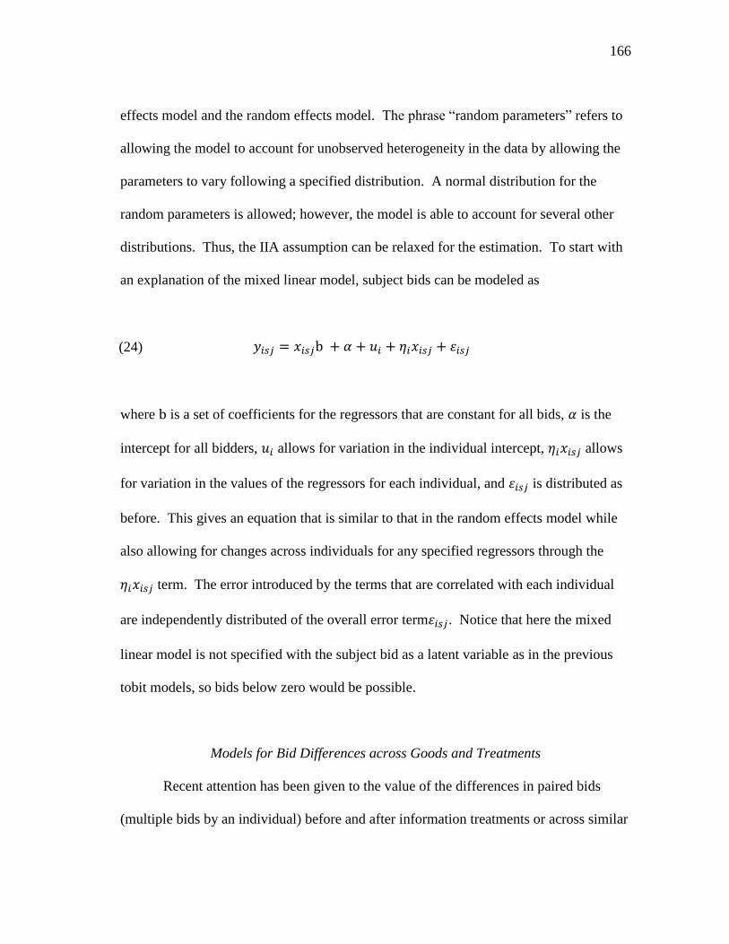
166
effects model and the random effects model. The phrase ―random parameters‖ refers to
allowing the model to account for unobserved heterogeneity in the data by allowing the
parameters to vary following a specified distribution. A normal distribution for the
random parameters is allowed; however, the model is able to account for several other
distributions. Thus, the IIA assumption can be relaxed for the estimation. To start with
an explanation of the mixed linear model, subject bids can be modeled as
(24)
where is a set of coefficients for the regressors that are constant for all bids, is the
intercept for all bidders, allows for variation in the individual intercept, allows
for variation in the values of the regressors for each individual, and is distributed as
before. This gives an equation that is similar to that in the random effects model while
also allowing for changes across individuals for any specified regressors through the
term. The error introduced by the terms that are correlated with each individual
are independently distributed of the overall error term . Notice that here the mixed
linear model is not specified with the subject bid as a latent variable as in the previous
tobit models, so bids below zero would be possible.
Models for Bid Differences across Goods and Treatments
Recent attention has been given to the value of the differences in paired bids
(multiple bids by an individual) before and after information treatments or across similar
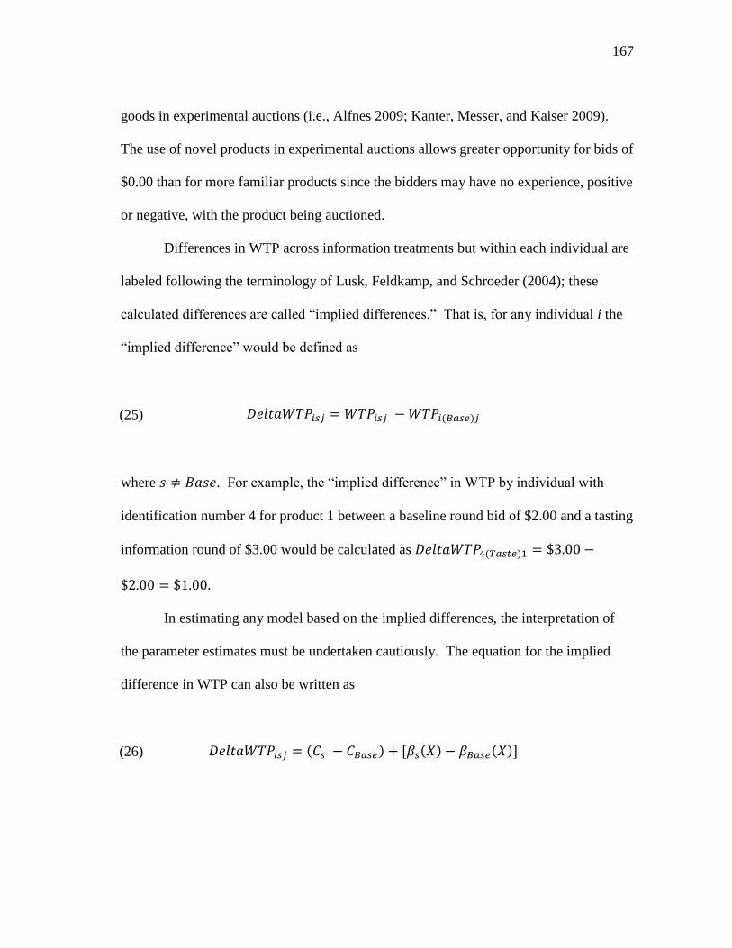
167
goods in experimental auctions (i.e., Alfnes 2009; Kanter, Messer, and Kaiser 2009).
The use of novel products in experimental auctions allows greater opportunity for bids of
$0.00 than for more familiar products since the bidders may have no experience, positive
or negative, with the product being auctioned.
Differences in WTP across information treatments but within each individual are
labeled following the terminology of Lusk, Feldkamp, and Schroeder (2004); these
calculated differences are called ―implied differences.‖ That is, for any individual i the
―implied difference‖ would be defined as
(25) ( )
where . For example, the ―implied difference‖ in WTP by individual with
identification number 4 for product 1 between a baseline round bid of $2.00 and a tasting
information round of $3.00 would be calculated as ( )
In estimating any model based on the implied differences, the interpretation of
the parameter estimates must be undertaken cautiously. The equation for the implied
difference in WTP can also be written as
(26) ( ) ( ) ( )
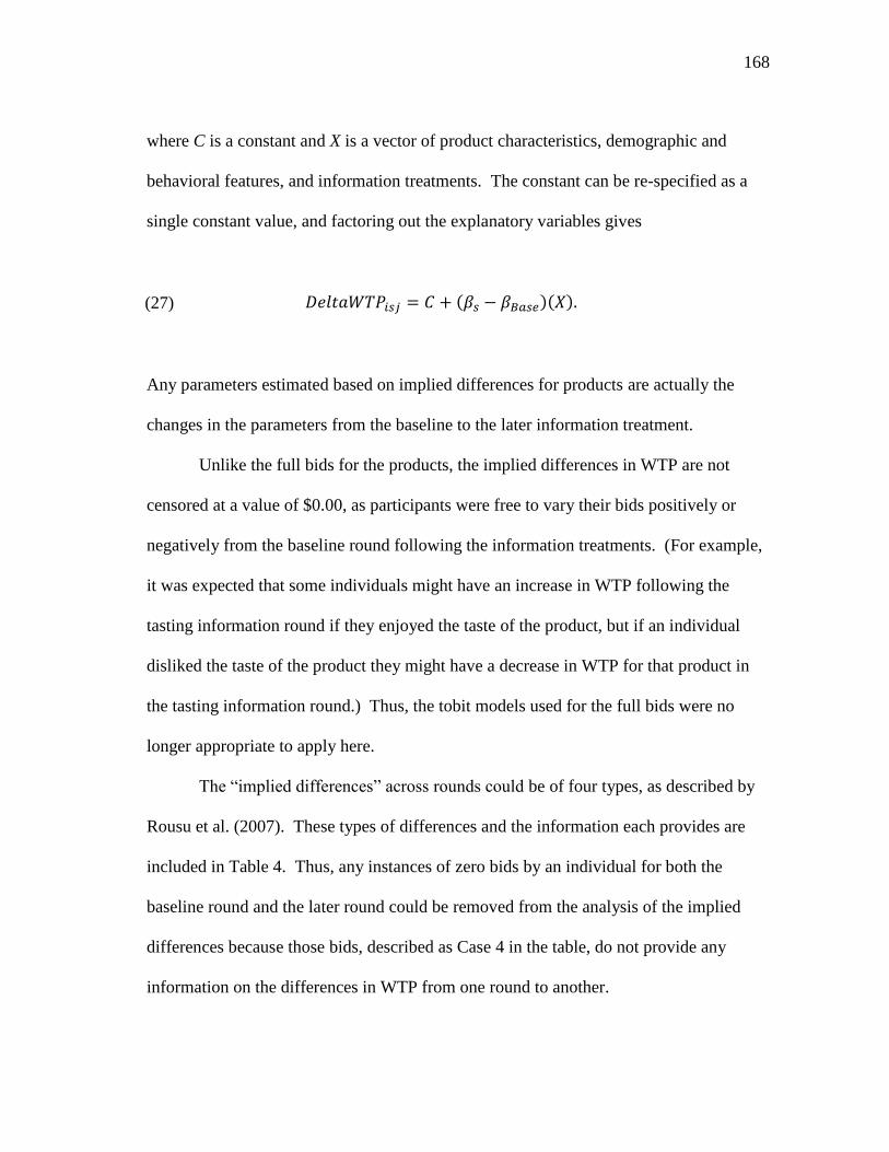
168
where C is a constant and X is a vector of product characteristics, demographic and
behavioral features, and information treatments. The constant can be re-specified as a
single constant value, and factoring out the explanatory variables gives
(27) ( )( )
Any parameters estimated based on implied differences for products are actually the
changes in the parameters from the baseline to the later information treatment.
Unlike the full bids for the products, the implied differences in WTP are not
censored at a value of $0.00, as participants were free to vary their bids positively or
negatively from the baseline round following the information treatments. (For example,
it was expected that some individuals might have an increase in WTP following the
tasting information round if they enjoyed the taste of the product, but if an individual
disliked the taste of the product they might have a decrease in WTP for that product in
the tasting information round.) Thus, the tobit models used for the full bids were no
longer appropriate to apply here.
The ―implied differences‖ across rounds could be of four types, as described by
Rousu et al. (2007). These types of differences and the information each provides are
included in Table 4. Thus, any instances of zero bids by an individual for both the
baseline round and the later round could be removed from the analysis of the implied
differences because those bids, described as Case 4 in the table, do not provide any
information on the differences in WTP from one round to another.
169
Table 4. Four Cases for Differences in Bids
Further, the analysis of models based on the implied differences in bids is of
particular value when the question to be answered involves questions of the size of those
differences. For example, and particularly in the case of a novel product where there is
likely to be individual heterogeneity not only in individual bids but also in the size of the
changes in those bids across products and information treatments, consider an individual
bidder for several products. If those products have similar outside substitutes and are
similarly valued, then these differences will cancel out when the difference of the two
bids is taken. This is true for the within-subject differences in bids for each product, as
the relevant outside substitutes are assumed to remain constant for each product across
multiple rounds. On the other hand, this is not the case for calculating differences in
overall bids for each product because the outside alternatives for a product for one
individual are not necessarily the same as those for any other individual. Alfnes (2009)
previously discussed this issue in relation to a full-bidding or endowed approach.
Bid for Baseline
(Round or
Product)
Bid for
Comparison
(Round or
Product)
Sign of Bid
DifferencePresence of Censoring Effect on Bid Difference
Case 1 Positive (+) Bid Positive (+) BidNegative (-) or
Positive (+)Uncensored
Difference in value is equal to
the difference measured
Case 2 Zero (0) Bid Positive (+) Bid Positive (+) Censored from BelowDifference is absolutely larger
than the difference measured
Case 3 Positive (+) Bid Zero (0) Bid Negative (-) Censored From AboveDifference is absolutely larger
than the difference measured
Case 4 Zero (0) Bid Zero (0) Bid Zero (0) Not DefinedDoes not provide any
information on difference
170
However, the dialogue can be extended to the value elicitation procedures for novel
products. In the case of a novel product, individuals lack familiarity with the
characteristics of the product, and there are likely to be even greater differences among
individuals in regards to which products are considered relevant outside substitutes.
These substitutes will differ in product characteristics and are likely to differ in price as
well; both of these types of information can then influence the bids that are submitted by
an individual.
However, the use of bid differences for estimation of WTP models allows the
outside substitutes for each product to cancel out when the difference in the two are
taken. Therefore, the differences in WTP should provide additional useful comparisons
because the difference in value across two consumers is not necessarily the same as the
difference in value within a single consumer due to differences in what each individual
perceives as the outside substitutes for each product.
Since the overall set of implied differences is not restricted to values that are only
positive or negative, the model for the implied differences was estimated using a mixed
linear model that was previously described.
Econometric Model for Preference Rankings
Discrete choices are often modeled using a logit model. As pointed out by Train
(2003), the functional form for the choice probabilities in a logit model has a closed
form. In addition, the interpretation of the logit model is more straightforward than that
of some alternative models. (For the purposes of clarity, we specify L products here to
171
avoid confusion with the product options presented in the models for the auction bids.)
Using , each εil is assumed to be independently and identically distributed
(IID) extreme value. Train (2003) also points out that the key assumption of the logit
model is not so much the shape of the distribution, but rather the independence of the
errors. Econometric methods to analyze choice experiments include conditional logit
and mixed logit models to estimate WTP (e.g., Teratanavat and Hooker 2006; Hu,
Woods, and Bastin 2009).
In the standard logit model, it is assumed that any unobserved utility from one
product is independent of the unobserved utility from any other product. This can be
avoided with a well specified model in which Vil is sufficient to describe the majority of
variation in the utility that the individual obtains, and the error term for one product does
not provide additional information on the error term for any other product. If this cannot
be achieved, then some other model which allows for correlated errors should be used.
A multinomial logit, which allows for more than two discrete choice outcomes, is not a
good candidate for the rankings data due to the fact that it fails to account for the ordinal
nature of the rankings data (Greene 2003). Rather, the choice decisions made by each
individual that result in ordered data provide more information to the researcher than a
single choice of the most preferred option. The rank-ordered logit model, which is in
essence a series of multinomial logit models multiplied together, can be applied to the
rankings data (Lusk, Fields, and Prevatt 2008).
172
Rank-Ordered Logit Model
In using ordered models, the model is built around a latent regression described
by Greene (2003). In this case, a general model of the form given in
(28)
where Uil is unobserved and εil are unobserved factors (alternatively interpreted as
random disturbances); this equation can be used as a starting point for building a model
that accounts for the ordered nature of the data. Following Calfee, Winston, and
Stempski (2001), let each individual i submit a response ri = {ri1, ri2, ri3,. . . ., riL}, which
is a ranking of the choice set in order of descending preference. Then, each survey
response would have a probability given by
(29) ( ) ( ) ( ) ( )
this can be further expanded to the probability expression
(30)
( ) ( ) ( )
[ ( ) ( )
] ( ) ( )
[ ( ) ( )]
173
This illustrates that a ranking response for L alternatives has an equivalent expression as
(L – 1) binary choice decisions. Thus, more preferred elements of the choice set are
censored as subsequent ranks are assigned. This application of the model is sometimes
referred to as ―exploding‖ the data, allowing the researcher to make full use of all
information by repeatedly applying whichever model is used (i.e. probit, standard logit,
mixed logit). As these authors suggest, a standard ordered probit or a rank-ordered logit
model are easier to estimate due to their closed form solutions. If the products are
indexed such that
(31) ( )
then for a rank-ordered logit, the logit probability is
(32) ( )
∑
Then, by ―exploding‖ the series of L -1 ranking decisions and assuming the error terms
are distributed type I extreme value (Gumbel) distribution (Greene 2003), the
probability for the entire ranking of L – 1 decisions is simply the product of L – 1
multinomial logit models (Lusk, Fields, and Prevatt 2008) and is given by
174
(33) ( ) ( ) ( ) ∏
∑
With N individuals in the sample where each individual‘s is independent and
identically distributed, the log-likelihood function maximized is then given by
(34)
( ) ∑ [∏
∑
]
∑∑ *
∑
+
∑∑ (
∑
)
With parameter variation across individuals (heterogeneity), the model estimated by
rank-ordered logit is subject to misspecification. Hensher and Jones (2007) suggest that
the multinomial model should be estimated first as a baseline comparison to other
models; in the case of rank-ordered data, the baseline model is simply the product of
several multinomial logit models.
More specifically, the rank-ordered logit makes an assumption of uncorrelated
stochastic components across alternatives; therefore if these errors are correlated
estimates of the parameters and WTP are inconsistent. In this case, a mixed (random
parameters) logit would be a good candidate. The mixed logit model is more flexible
than, and avoids certain limitations of, the standard logit model. A mixed logit model

175
allows for correlation in unobserved factors (an issue discussed above), has unrestricted
substitution patterns, and allows for random taste variation (Train 2003).
Mixed Multinomial Logit Model
McFadden and Train (2000) develop the properties of the mixed multinomial
logit as a model for discrete response, particularly as applied to random utility theory
and the use of maximum simulated likelihood (MSL) estimation. Train (2003) further
provides a thorough discussion of the mixed logit model and readers are referred there
for additional information. However, a brief summary is included here to describe the
model that will be used for estimation of the ranking data. When the standard logit
model is integrated over a density of parameters, a mixed logit model is obtained. More
specifically, mixed logits are any models where the choice probabilities can be described
as
(35) ∫ ( ) ( )
where Lik is the logit probability evaluated at β as given by
(36) ( ) ( )
∑ ( )
f(β) is the density function, and Vik is the observed utility which depends on the
176
parameters β for a particular product k. If utility is assumed to be linear in parameters,
then
(37) ( )
and the probability takes the form
(38) ∫
∑
( )
Thus, the mixed logit probability is based on weighting the average of the logit
formula at various parameter values β using the density f(β) to describe the weights.
Statistics literature would call f(β) the mixing distribution. In the case where a mixed
logit is specified, but none of the exclusions from the three assumptions key to a
standard logit are needed, the probability function of the mixed logit simplifies to that of
the standard logit. The mixed logit is most commonly interpreted from a random
coefficients theory, where the random coefficients refer to a vector of coefficients
representing an individual‘s taste and are allowed to vary across individuals in the
population. The mixed logit model can also be used based on an error components
theory, with a representation of the correlations among utilities for different alternatives
as the error components. Under such an interpretation, the stochastic portion of the
utility can be interpreted as a random coefficient plus the product of a vector of random

177
terms that sum to zero and the error components. Mixed logit is also free from the IIA
assumption discussed earlier in the literature review. Mixed logit models can be
estimated using simulated maximum likelihood estimation or Bayesian procedures.
Greene (2003) suggests that the mixed logit model be estimated using simulation of the
log-likelihood function rather than direct integration, as the mixture distribution based
on the error term and the random part of the coefficient is unknown to the researcher.
On this basis, a mixed logit model can be applied to the ranking decisions made
by individual participants in the study. However, the mixed logit model alone is not
equipped to handle to ordering issues presented in the description of the rank-ordered
logit model. Hence, estimation under a rank-ordered framework with a mixed logit
model allows errors to be correlated.
The preceding discussion points towards the use of a rank-ordered mixed logit
model that accounts for the ordinal nature of the data as well as avoiding the IIA
assumptions of the standard logit model. In such a model, if the stochastic terms are
used to represent deviations from the mean tastes, then the errors can be allowed to be
correlated across product alternatives. Returning to the random utility model, again let l
correspond to the alternatives to be ranked, with L – 1 choice decisions to be made. The
model can now be specified as
(39)
where . In order to allow the correlation across multiple products, the
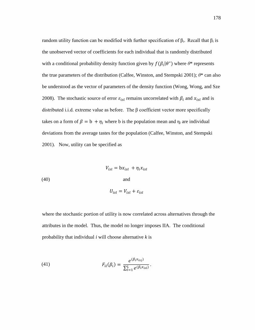
178
random utility function can be modified with further specification of βi. Recall that βi is
the unobserved vector of coefficients for each individual that is randomly distributed
with a conditional probability density function given by ( | ) where θ* represents
the true parameters of the distribution (Calfee, Winston, and Stempski 2001); θ* can also
be understood as the vector of parameters of the density function (Wong, Wong, and Sze
2008). The stochastic source of error remains uncorrelated with and and is
distributed i.i.d. extreme value as before. The β coefficient vector more specifically
takes on a form of where b is the population mean and ηi are individual
deviations from the average tastes for the population (Calfee, Winston, and Stempski
2001). Now, utility can be specified as
(40)
and
where the stochastic portion of utility is now correlated across alternatives through the
attributes in the model. Thus, the model no longer imposes IIA. The conditional
probability that individual i will choose alternative k is
(41) ( ) ( )
∑ ( )
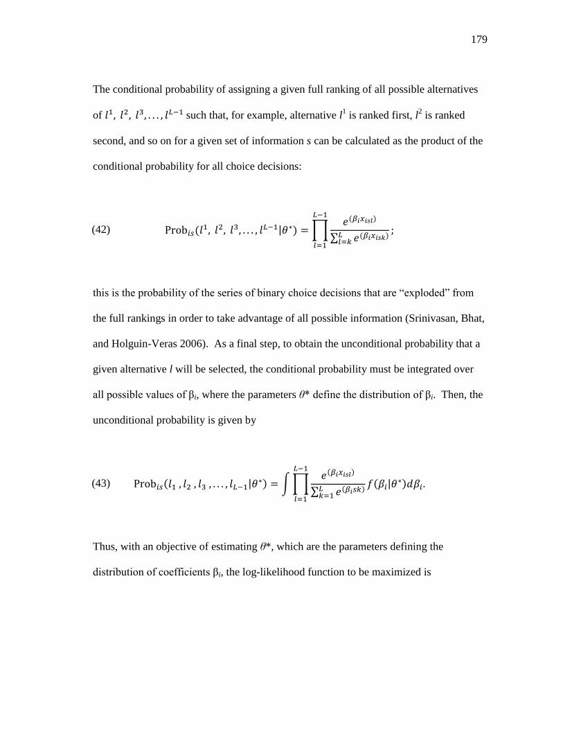
179
The conditional probability of assigning a given full ranking of all possible alternatives
of such that, for example, alternative l1 is ranked first, l
2 is ranked
second, and so on for a given set of information s can be calculated as the product of the
conditional probability for all choice decisions:
(42) ( | ) ∏
( )
∑ ( )
this is the probability of the series of binary choice decisions that are ―exploded‖ from
the full rankings in order to take advantage of all possible information (Srinivasan, Bhat,
and Holguin-Veras 2006). As a final step, to obtain the unconditional probability that a
given alternative l will be selected, the conditional probability must be integrated over
all possible values of βi, where the parameters θ* define the distribution of βi. Then, the
unconditional probability is given by
(43) ( | ) ∫∏
( )
∑ ( )
( | )
Thus, with an objective of estimating θ*, which are the parameters defining the
distribution of coefficients βi, the log-likelihood function to be maximized is
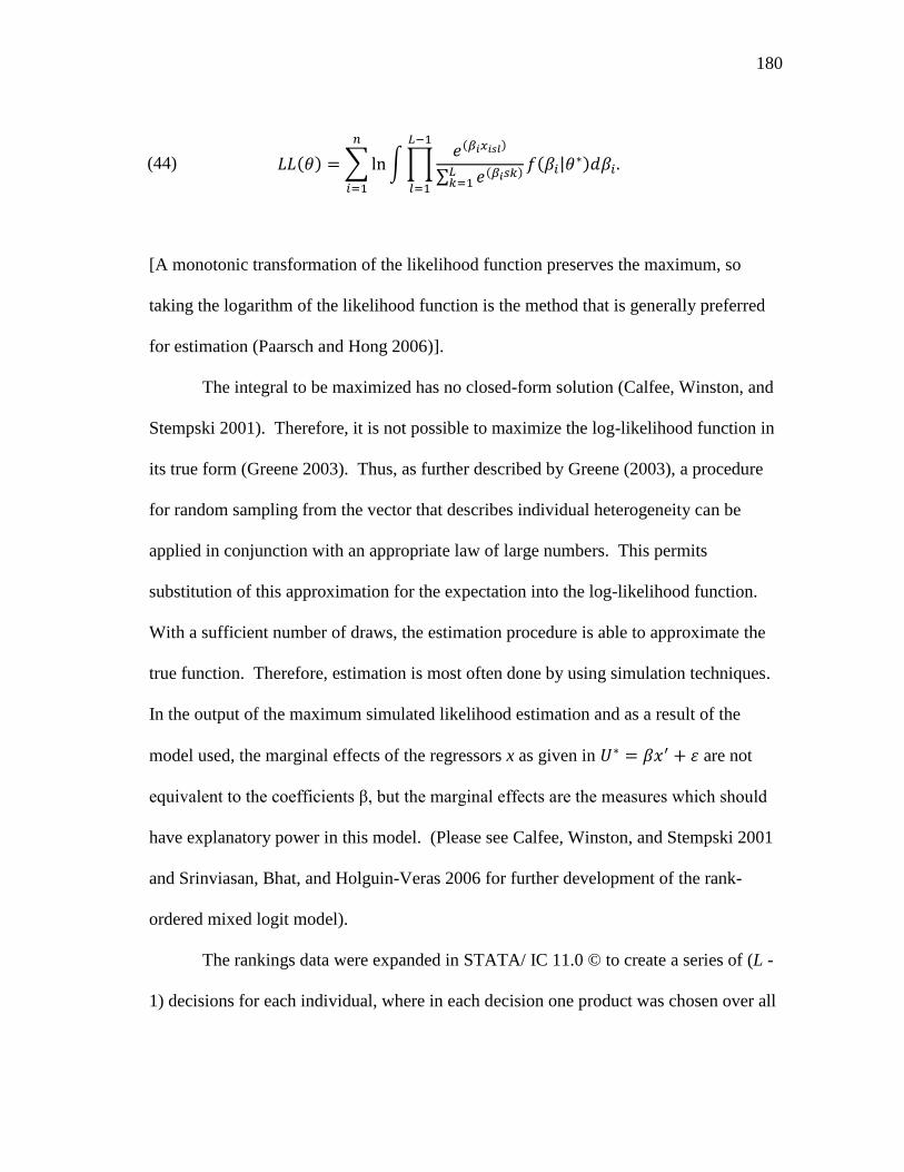
180
(44) ( ) ∑
∫∏ ( )
∑ ( )
( | )
[A monotonic transformation of the likelihood function preserves the maximum, so
taking the logarithm of the likelihood function is the method that is generally preferred
for estimation (Paarsch and Hong 2006)].
The integral to be maximized has no closed-form solution (Calfee, Winston, and
Stempski 2001). Therefore, it is not possible to maximize the log-likelihood function in
its true form (Greene 2003). Thus, as further described by Greene (2003), a procedure
for random sampling from the vector that describes individual heterogeneity can be
applied in conjunction with an appropriate law of large numbers. This permits
substitution of this approximation for the expectation into the log-likelihood function.
With a sufficient number of draws, the estimation procedure is able to approximate the
true function. Therefore, estimation is most often done by using simulation techniques.
In the output of the maximum simulated likelihood estimation and as a result of the
model used, the marginal effects of the regressors x as given in are not
equivalent to the coefficients β, but the marginal effects are the measures which should
have explanatory power in this model. (Please see Calfee, Winston, and Stempski 2001
and Srinviasan, Bhat, and Holguin-Veras 2006 for further development of the rank-
ordered mixed logit model).
The rankings data were expanded in STATA/ IC 11.0 © to create a series of (L -
1) decisions for each individual, where in each decision one product was chosen over all
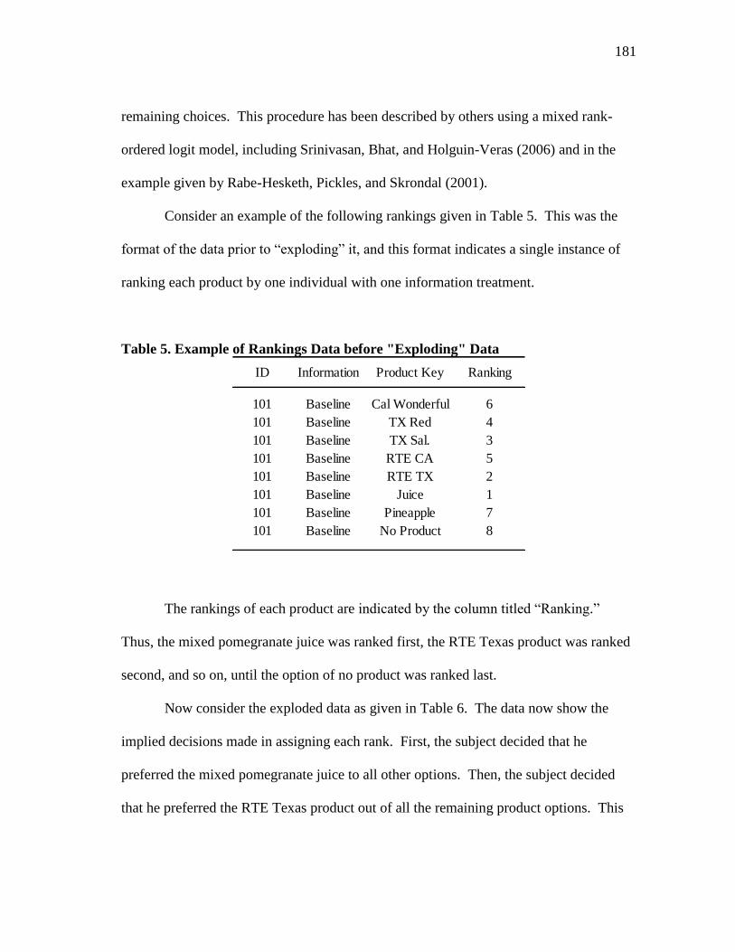
181
remaining choices. This procedure has been described by others using a mixed rank-
ordered logit model, including Srinivasan, Bhat, and Holguin-Veras (2006) and in the
example given by Rabe-Hesketh, Pickles, and Skrondal (2001).
Consider an example of the following rankings given in Table 5. This was the
format of the data prior to ―exploding‖ it, and this format indicates a single instance of
ranking each product by one individual with one information treatment.
Table 5. Example of Rankings Data before "Exploding" Data
The rankings of each product are indicated by the column titled ―Ranking.‖
Thus, the mixed pomegranate juice was ranked first, the RTE Texas product was ranked
second, and so on, until the option of no product was ranked last.
Now consider the exploded data as given in Table 6. The data now show the
implied decisions made in assigning each rank. First, the subject decided that he
preferred the mixed pomegranate juice to all other options. Then, the subject decided
that he preferred the RTE Texas product out of all the remaining product options. This
ID Information Product Key Ranking
101 Baseline Cal Wonderful 6
101 Baseline TX Red 4
101 Baseline TX Sal. 3
101 Baseline RTE CA 5
101 Baseline RTE TX 2
101 Baseline Juice 1
101 Baseline Pineapple 7
101 Baseline No Product 8
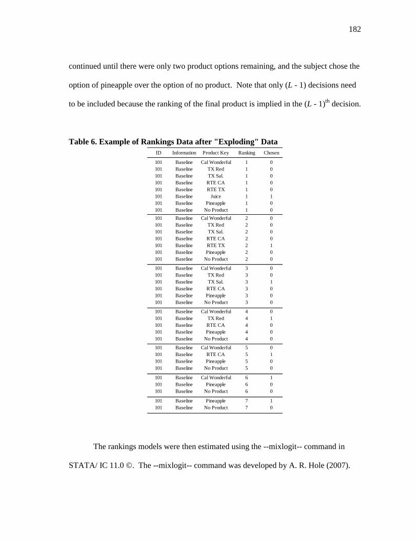
182
continued until there were only two product options remaining, and the subject chose the
option of pineapple over the option of no product. Note that only (L - 1) decisions need
to be included because the ranking of the final product is implied in the (L - 1)th
decision.
Table 6. Example of Rankings Data after "Exploding" Data
The rankings models were then estimated using the --mixlogit-- command in
STATA/ IC 11.0 ©. The --mixlogit-- command was developed by A. R. Hole (2007).
ID Information Product Key Ranking Chosen
101 Baseline Cal Wonderful 1 0
101 Baseline TX Red 1 0
101 Baseline TX Sal. 1 0
101 Baseline RTE CA 1 0
101 Baseline RTE TX 1 0
101 Baseline Juice 1 1
101 Baseline Pineapple 1 0
101 Baseline No Product 1 0
101 Baseline Cal Wonderful 2 0
101 Baseline TX Red 2 0
101 Baseline TX Sal. 2 0
101 Baseline RTE CA 2 0
101 Baseline RTE TX 2 1
101 Baseline Pineapple 2 0
101 Baseline No Product 2 0
101 Baseline Cal Wonderful 3 0
101 Baseline TX Red 3 0
101 Baseline TX Sal. 3 1
101 Baseline RTE CA 3 0
101 Baseline Pineapple 3 0
101 Baseline No Product 3 0
101 Baseline Cal Wonderful 4 0
101 Baseline TX Red 4 1
101 Baseline RTE CA 4 0
101 Baseline Pineapple 4 0
101 Baseline No Product 4 0
101 Baseline Cal Wonderful 5 0
101 Baseline RTE CA 5 1
101 Baseline Pineapple 5 0
101 Baseline No Product 5 0
101 Baseline Cal Wonderful 6 1
101 Baseline Pineapple 6 0
101 Baseline No Product 6 0
101 Baseline Pineapple 7 1
101 Baseline No Product 7 0
183
The mixed logit model is estimated using maximum simulated likelihood. Simulations
sometimes use a pseudo-random number generator as the basis for the simulation.
However, this method has relatively high discrepancy, which refers to the fact that the
draw is far from the uniform distribution. To address this and use an alternative that has
a better ―worst discrepancy‖ from a series of draws, Halton draws are used as a more
uniform alternative (Wanscher and Sørensen 2006). Henscher and Train (2003) describe
the usefulness of Halton draws as applied to mixed models, and suggest that with greater
complexity (more random parameters and treatment of preference heterogeneity)
increases the number of draws required. Train (1999) finds a lower simulated variance
in the estimated parameters when using 100 Halton numbers than when using 1,000
Halton numbers. This result is important because the estimation procedure is faster
when fewer Halton draws are used. One hundred Halton draws were used for the model
estimation.
One important note of caution is provided by Greene (2003) for discrete choice
modeling. Both logit and probit models are susceptible to two important specification
issues, which were previously described by Yatchew and Griliches (1985). First, if a
variable is omitted from the model when it should not be, even if the omitted variable is
uncorrelated with the included variables the coefficients on the included variables will
be inconsistent. Second, if the disturbances in the underlying regression are
heteroskedastic then maximum likelihood estimators will be inconsistent.
However, despite the constraints and distributional assumptions of the logit
model and its modified versions, as pointed out by Greene and Hensher (2010), the use

184
of fully nonparametric in applications is rare. While nonparametric techniques avoid the
distributional assumptions of parametric models for ordered choices, they are also
therefore less informative to the practitioner in terms of estimation results. Semi-
parametric approaches are something of a compromise between the two in which the
estimator of the probability function is done using a kernel density estimator. Greene
and Hensher (2010) further call attention to the fact that although the application of
semi-parametric methods from single choice models to ordered choice models has taken
place almost entirely in the 21st century.
Comparison of Preferences Based on Bids and Rankings
It is likely that consumers prefer to avoid instances of cognitive dissonance as
described by Alfnes, Yue, and Jensen (2010). However, a comparison of the preference
rankings and the ordered bids collected in this study lead to some questions about such
an assertion. The auction and bidding mechanisms used here are a novel combination;
however, since both were incentive compatible and nonhypothetical, it was hypothesized
that the two mechanisms would produce similar results. Olsen, Donaldson, and
Shackley (2005) addressed the issue of explicit versus implicit rankings data in terms of
public preference for health care programs. In this case, the implied rankings are the
ordered bids, and the explicit rankings are the actual preference rankings submitted by
subjects. Economic theory suggests that rational subjects would respond to either of
these ranking situations in the same way. The experimental design for this study offers a
unique opportunity to compare the two methodologies and look at the issue of
185
consistency; that is, whether the implied and explicit rankings produce convergent
results. The opportunity to analyze this issue differs in this case from that of Olsen,
Donaldson, and Shackley (2005) because subjects for this study were asked to submit
bids and rankings for a product which is typically purchased on an individual level and
has a private value unique to each individual; the Olsen, Donaldson, and Shackley
(2005) paper addressed preference ranking and partial WTP values for health care
programs that benefit the general public.
Economic theory suggests the two methodologies should produce similar results
on the basis that as a product increases in desirability to an individual from less preferred
to more preferred, that individual would be willing to give up larger and larger sums
(have a higher WTP) in exchange for that item. However, the question to be addressed
is whether this economic theory of two types of preference elicitation that are related in
their general purpose and in their theoretical underpinnings are related in practical
settings.
Two distinct methods of preference elicitation were utilized as a part of this
study, each of which lends itself to a different type of analysis. However, one primary
goal of the study was to compare the results of each of the two preference elicitation
procedures. This was done by ordering the bids (given in dollars) such that the product
with the highest bid was assigned a rank of one, the next highest bid was assigned a rank
of two, and so forth until the lowest bid was assigned a rank of 8. Two particular issues
were addressed in assigning these rankings. First, let equivalent bids (ties) be considered
participant indifference between two or more products. In the event of a tie, the products
186
with the tied bids were assigned the same ranking and the product with the next highest
bid was assigned the rank of the number of products that were above it plus one. For
example, if a subject submitted bids for four products of $2.00, $1.75, $1.75, and $1.50,
the rankings assigned to the ordered bids would be 1, 2, 2, and 4, respectively. For the
rank-ordered logit model, ties in the rankings were addressed using the exact marginal
likelihood for indifference in alternatives (StataCorp 2009). Second, as a part of the
experiment subjects submitted bids for seven fruit products during the experimental
auction rounds, but for the ranking they were asked to rank their preferences for seven
products and the option of no product, with 1 being the most preferred product and 8
being the least preferred product. Thus, there was one less product bid than there was
product option ranking. Nevertheless, while submitting bids, subjects had the option of
submitting bids of $0.00. For the ordered bids, the option of no product was assigned
the appropriate ranking based on the ordered bids (OB) as
( ) Any products that had bids of
$0.00 were assigned ordered ranks based on
The preference models for the ordered bids were then
estimated using the same model used for the preference rankings.
Variation in Ranking Ability
Both the preference rankings and the ordered bids were modeled using the full
information set for all eight product options. However, Calfee, Winston, and Stempski
(2001) follow Hausman and Ruud (1987) in considering the possibility of respondents
187
who rank more preferred alternatives more carefully than less preferred ones. If this is
the case, there should be less variance in the rankings for the most preferred alternatives
and vice versa, and the parameter estimates based on such models should be affected by
the change in the model from including all rankings to including only the top half of the
rankings. The model with only the top half of the rankings will be referred to here as the
partially-ranked model. This was done first for the preference rankings data. The
ordered bid rankings were also estimated using the partially-ranked model for the top
four rankings to check the models for heterogeneity in ranking ability.
If the preference ranking parameters are sensitive to estimation with a full-
versus partially-ranked model, then a scaling parameter can be estimated based on the
specific dataset. This procedure would be useful if there is more noise in the rankings
for the less preferred products than the more preferred products. One example of such a
technique is demonstrated by Lusk, Fields, and Prevatt (2008).
In summation, the econometric techniques applied to the dataset collected from
the experimental procedures were determined at least in part by the nature of the data
itself. This allows for accommodation of any issues which may not have been
anticipated in the experimental design.
188
CHAPTER V
RESULTS AND DISCUSSION
The study design was somewhat complex in order to allow for testing a number
of different hypotheses; still, attention to detail during the study design process yielded
results on a number of issues of interest. These results can be broadly categorized as a
discussion of the demographic and behavioral characteristics of those included in the
sample, results of the various models used to estimated WTP based on the experimental
auction, and results of the preference rankings. Further comparisons among these results
were also made, and specific characteristics of this particular data set were addressed.
Demographics and Behavioral Characteristics
A total of 203 individuals participated in the study. Of these, 198 submitted
complete and usable demographic information and auction bids. The socioeconomic
characteristics of the study sample are described in Table 7. Participants were assigned
to sessions to ensure that there was a similar demographic representation in each of the
eight sessions. It was assumed that this sample would be reflective of those who were
interested in the advertised topic of the study and who were also willing and able to
participate in the designated study sessions for the designated compensation amount.
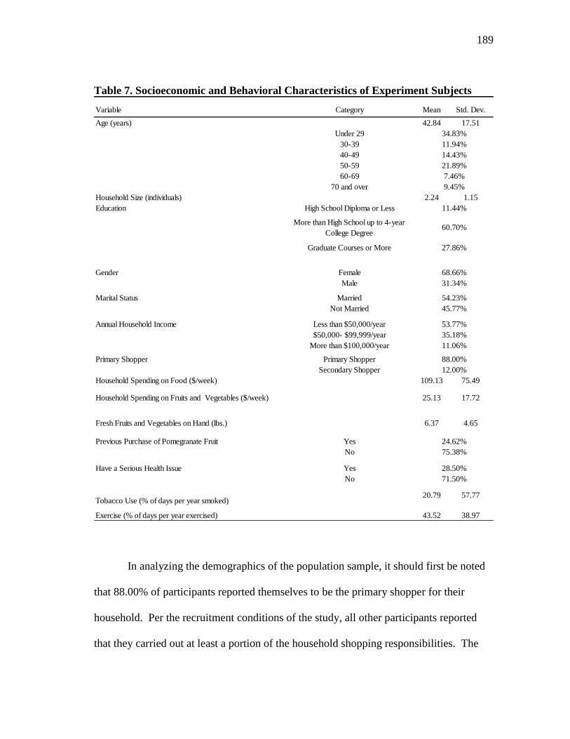
189
Table 7. Socioeconomic and Behavioral Characteristics of Experiment Subjects
In analyzing the demographics of the population sample, it should first be noted
that 88.00% of participants reported themselves to be the primary shopper for their
household. Per the recruitment conditions of the study, all other participants reported
that they carried out at least a portion of the household shopping responsibilities. The
Variable Category Mean Std. Dev.
Age (years) 42.84 17.51
Under 29
30-39
40-49
50-59
60-69
70 and over
Household Size (individuals) 2.24 1.15
Education High School Diploma or Less
More than High School up to 4-year
College Degree
Graduate Courses or More
Gender Female
Male
Marital Status Married
Not Married
Annual Household Income Less than $50,000/year
$50,000- $99,999/year
More than $100,000/year
Primary Shopper Primary Shopper
Secondary Shopper
Household Spending on Food ($/week) 109.13 75.49
Household Spending on Fruits and Vegetables ($/week) 25.13 17.72
Fresh Fruits and Vegetables on Hand (lbs.) 6.37 4.65
Previous Purchase of Pomegranate Fruit Yes
No
Have a Serious Health Issue Yes
No
Tobacco Use (% of days per year smoked)20.79 57.77
Exercise (% of days per year exercised) 43.52 38.97
24.62%
75.38%
28.50%
71.50%
34.83%
11.94%
14.43%
21.89%
7.46%
9.45%
45.77%
53.77%
35.18%
11.06%
88.00%
12.00%
54.23%
11.44%
60.70%
27.86%
68.66%
31.34%
190
mean age for the sample was 42.84 years of age, younger than the age of the average
shopper (47 years of age) in the United States (Goodman 2008). Over 68% of the
respondents were female, and participants reported an average annual household income
of $53,693. Of this income, the weekly household spending on all food purchases
(including restaurants and other purchases outside the home) was reported by
participants with a mean of $109. Of that weekly household spending on food,
participants reported a mean of $25 per week spending on all fruits and vegetables.
Also, participants reported to have an average of 6.4 pounds of fresh produce (including
fruits and vegetables) on hand at home at the time of the study. This was measured to
judge any effects that current home stocks may have had on WTP for additional fruit as
measured by the experimental auctions. As anticipated, most participants were
unaccustomed to purchasing pomegranate fruits, with just 24.5% of subjects reporting
that they had previously purchased a pomegranate fruit. This lends itself to the
interpretation of pomegranates as a novel product for the majority of participants in the
study.
A series of health questions were also posed to participants after they had
submitted all rankings and bids. Of all the study participants, 28.5% reported having a
health issue that they considered to be serious. The average tobacco use by subjects was
77 days (or 21%) of the year, while the average percentage of days exercised per year
was 161 (or 44%). These health characteristics were measured to allow for further
investigation into possible relationships between the effects of such behaviors and the
information treatments imposed throughout the course of the study.
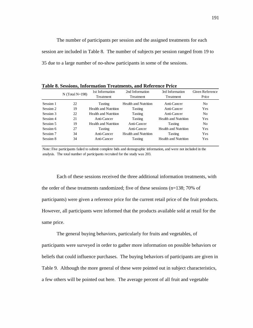
191
The number of participants per session and the assigned treatments for each
session are included in Table 8. The number of subjects per session ranged from 19 to
35 due to a large number of no-show participants in some of the sessions.
Table 8. Sessions, Information Treatments, and Reference Price
Each of these sessions received the three additional information treatments, with
the order of these treatments randomized; five of these sessions (n=138; 70% of
participants) were given a reference price for the current retail price of the fruit products.
However, all participants were informed that the products available sold at retail for the
same price.
The general buying behaviors, particularly for fruits and vegetables, of
participants were surveyed in order to gather more information on possible behaviors or
beliefs that could influence purchases. The buying behaviors of participants are given in
Table 9. Although the more general of these were pointed out in subject characteristics,
a few others will be pointed out here. The average percent of all fruit and vegetable
N (Total N=198)1st Information
Treatment
2nd Information
Treatment
3rd Information
Treatment
Given Reference
Price
Session 1 22 Tasting Health and Nutrition Anti-Cancer No
Session 2 19 Health and Nutrition Tasting Anti-Cancer Yes
Session 3 22 Health and Nutrition Tasting Anti-Cancer No
Session 4 21 Anti-Cancer Tasting Health and Nutrition Yes
Session 5 19 Health and Nutrition Anti-Cancer Tasting No
Session 6 27 Tasting Anti-Cancer Health and Nutrition Yes
Session 7 34 Anti-Cancer Health and Nutrition Tasting Yes
Session 8 34 Anti-Cancer Tasting Health and Nutrition Yes
Note: Five participants failed to submit complete bids and demographic information, and were not included in the
analysis. The total number of participants recruited for the study was 203.
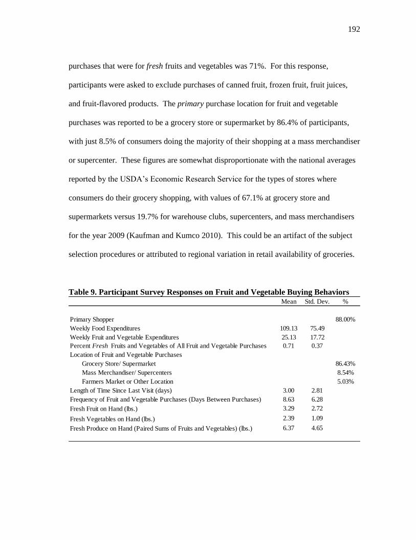
192
purchases that were for fresh fruits and vegetables was 71%. For this response,
participants were asked to exclude purchases of canned fruit, frozen fruit, fruit juices,
and fruit-flavored products. The primary purchase location for fruit and vegetable
purchases was reported to be a grocery store or supermarket by 86.4% of participants,
with just 8.5% of consumers doing the majority of their shopping at a mass merchandiser
or supercenter. These figures are somewhat disproportionate with the national averages
reported by the USDA‘s Economic Research Service for the types of stores where
consumers do their grocery shopping, with values of 67.1% at grocery store and
supermarkets versus 19.7% for warehouse clubs, supercenters, and mass merchandisers
for the year 2009 (Kaufman and Kumco 2010). This could be an artifact of the subject
selection procedures or attributed to regional variation in retail availability of groceries.
Table 9. Participant Survey Responses on Fruit and Vegetable Buying Behaviors
Mean Std. Dev. %
Primary Shopper 88.00%
Weekly Food Expenditures 109.13 75.49
Weekly Fruit and Vegetable Expenditures 25.13 17.72
Percent Fresh Fruits and Vegetables of All Fruit and Vegetable Purchases 0.71 0.37
Location of Fruit and Vegetable Purchases
Grocery Store/ Supermarket 86.43%
Mass Merchandiser/ Supercenters 8.54%
Farmers Market or Other Location 5.03%
Length of Time Since Last Visit (days) 3.00 2.81
Frequency of Fruit and Vegetable Purchases (Days Between Purchases) 8.63 6.28
Fresh Fruit on Hand (lbs.) 3.29 2.72
Fresh Vegetables on Hand (lbs.) 2.39 1.09
Fresh Produce on Hand (Paired Sums of Fruits and Vegetables) (lbs.) 6.37 4.65
193
The mean length of time since a participant‘s last visit to the retail establishment
where he or she purchased groceries was 3.00 days, with a reported typical length of
time between fruit and vegetable purchases of 8.63 days. These were both hypothesized
to influence a subject‘s bidding behavior and his or her perception of outside substitutes
and the transactions costs of delaying a purchase in the laboratory setting until the time
of their next trip to purchase groceries.
In terms of the quantity of fruits and vegetables on hand at the time of the study,
a few items are notable. First, the mean weight of fruit on hand for subjects was 3.29
pounds, and the mean pounds of vegetables on hand was somewhat lower, at 2.39
pounds. However, the paired sums of fruits and vegetables on hand for each subject
were 6.37 pounds, which is larger than the 5.67 pounds that the sum of the unpaired
means gives. This can be interpreted to mean that although there may be some outliers
in terms of either the fruit or vegetables on hand for each individual, the total fresh
produce on hand was higher than would be predicted by either of these measures alone.
These amounts were elicited from consumers in order to test whether current ―stocks‖ of
fruits and vegetables on hand would have any influence on the WTP for pomegranate
products.
The pomegranate has received a great deal of recent attention as a so-called
―functional food‖ due to the health benefits beyond basic nutritional value that the fruit
have been reported to have. One goal of the study was to gain a general understanding
of the product awareness that participants had for functional food products. Thus,
subjects were surveyed on their familiarity with functional foods, as well as their
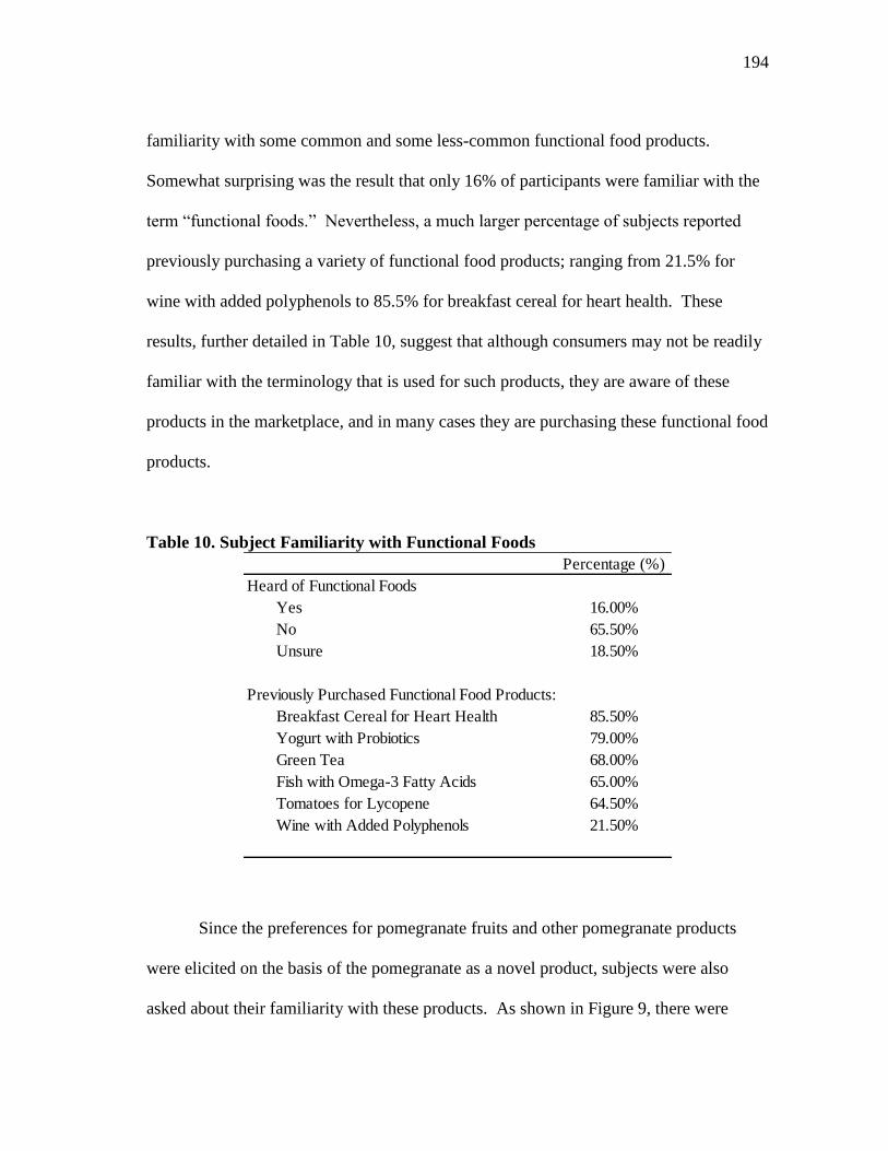
194
familiarity with some common and some less-common functional food products.
Somewhat surprising was the result that only 16% of participants were familiar with the
term ―functional foods.‖ Nevertheless, a much larger percentage of subjects reported
previously purchasing a variety of functional food products; ranging from 21.5% for
wine with added polyphenols to 85.5% for breakfast cereal for heart health. These
results, further detailed in Table 10, suggest that although consumers may not be readily
familiar with the terminology that is used for such products, they are aware of these
products in the marketplace, and in many cases they are purchasing these functional food
products.
Table 10. Subject Familiarity with Functional Foods
Since the preferences for pomegranate fruits and other pomegranate products
were elicited on the basis of the pomegranate as a novel product, subjects were also
asked about their familiarity with these products. As shown in Figure 9, there were
Percentage (%)
Heard of Functional Foods
Yes 16.00%
No 65.50%
Unsure 18.50%
Previously Purchased Functional Food Products:
Breakfast Cereal for Heart Health 85.50%
Yogurt with Probiotics 79.00%
Green Tea 68.00%
Fish with Omega-3 Fatty Acids 65.00%
Tomatoes for Lycopene 64.50%
Wine with Added Polyphenols 21.50%
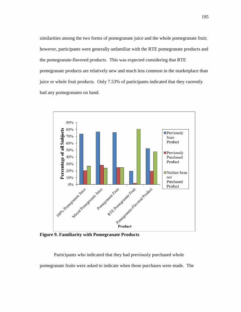
195
similarities among the two forms of pomegranate juice and the whole pomegranate fruit;
however, participants were generally unfamiliar with the RTE pomegranate products and
the pomegranate-flavored products. This was expected considering that RTE
pomegranate products are relatively new and much less common in the marketplace than
juice or whole fruit products. Only 7.53% of participants indicated that they currently
had any pomegranates on hand.
Figure 9. Familiarity with Pomegranate Products
Participants who indicated that they had previously purchased whole
pomegranate fruits were asked to indicate when those purchases were made. The
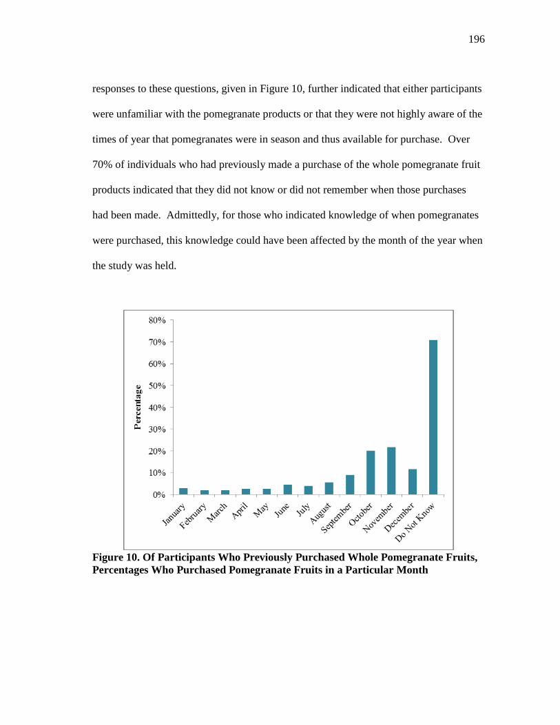
196
responses to these questions, given in Figure 10, further indicated that either participants
were unfamiliar with the pomegranate products or that they were not highly aware of the
times of year that pomegranates were in season and thus available for purchase. Over
70% of individuals who had previously made a purchase of the whole pomegranate fruit
products indicated that they did not know or did not remember when those purchases
had been made. Admittedly, for those who indicated knowledge of when pomegranates
were purchased, this knowledge could have been affected by the month of the year when
the study was held.
Figure 10. Of Participants Who Previously Purchased Whole Pomegranate Fruits,
Percentages Who Purchased Pomegranate Fruits in a Particular Month
197
The subjects in the study were also surveyed as to which of the following factors
were most important in making fruit and vegetable purchases: convenience, freshness,
growing location, nutrition, price, production practices, size, and visual appearance.
Production practices refer to any of several growing methods that are advertised at the
point-of-sale for the item, such as organic, no pesticides, or any other production
practices. These factors were measured in two separate question formats. Several items
in the responses to these questions should be noted. First, the factors that were important
in fruit and vegetable decision-making were measured in an effort to capture the
qualities that play a role in consumer decision-making in regards to fruit and vegetable
purchases. These factors were also measured to provide a comparison to the behaviors
of participants in the nonhypothetical experimental auctions and ranking procedures.
For the first measurement of these factors, subjects selected which of three factors were
the most important in their fruit and vegetable purchasing decisions. However, one
caution with this type of analysis is that a subject‘s answers could be influenced by what
he or she perceives as social norms or the socially acceptable answer; a bias of this sort
is termed as ―social desirability bias‖ by Lusk and Norwood (2009). For instance, a
subject may claim that he had a strong preference for growing location, but his bidding
and ranking behavior should indicate whether the factors he cited as important actually
had an influence on his bidding behavior.
In an effort to capture some portion of the possible social desirability bias,
subjects were asked which factors were important to them as well as which factors they
perceived to be important to the average American. An example of how this was
198
phrased in the survey questions is as follows: ―Which of these factors do you consider
most important in making fruit and vegetable purchase decisions? (Please select up to 3
options).‖ This was followed by the question, ―Which of these factors do you believe
the average American considers most important in making fruit and vegetable purchase
decisions? (Please select up to 3 options).‖ Thus, subjects were freed from an obligation
to report an answer that they saw as socially desirable by answering the second question.
Of the provided factors, the most commonly cited factor was Price for both
individuals and for the predictions for average Americans. Thus, regardless of the health
benefits or other experience attributes of a product, the cost items was confirmed to still
play an important role in purchasing decisions.
However, the results differed for the remainder of the factors between the
individual vs. average American predictions, with predictions for average Americans
being more common for visual appearance, size, convenience, and production practices.
The most striking of these was for convenience, being cited 2.75 times more often for
the prediction for average Americans than for the individual‘s reported behavior. More
individuals indicated that their own purchase decisions were based on freshness,
growing location, and nutrition than what was predicted for average Americans. This
lends support to the hypothesis by Lusk and Norwood (2009) that behaviors considered
by some to be more socially acceptable behaviors, such as choosing fresh produce based
on a growing location, freshness, or nutrition were more commonly cited for individual
behavior than for the prediction for the average American. This behavior could also be
because an individual believes he or she is more knowledgeable or has more information
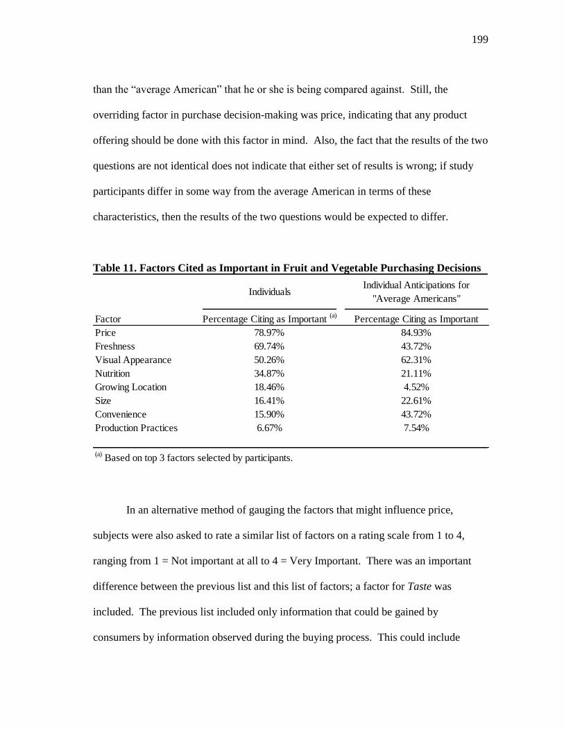
199
than the ―average American‖ that he or she is being compared against. Still, the
overriding factor in purchase decision-making was price, indicating that any product
offering should be done with this factor in mind. Also, the fact that the results of the two
questions are not identical does not indicate that either set of results is wrong; if study
participants differ in some way from the average American in terms of these
characteristics, then the results of the two questions would be expected to differ.
Table 11. Factors Cited as Important in Fruit and Vegetable Purchasing Decisions
In an alternative method of gauging the factors that might influence price,
subjects were also asked to rate a similar list of factors on a rating scale from 1 to 4,
ranging from 1 = Not important at all to 4 = Very Important. There was an important
difference between the previous list and this list of factors; a factor for Taste was
included. The previous list included only information that could be gained by
consumers by information observed during the buying process. This could include
IndividualsIndividual Anticipations for
"Average Americans"
Factor Percentage Citing as Important (a)
Percentage Citing as Important
Price 78.97% 84.93%
Freshness 69.74% 43.72%
Visual Appearance 50.26% 62.31%
Nutrition 34.87% 21.11%
Growing Location 18.46% 4.52%
Size 16.41% 22.61%
Convenience 15.90% 43.72%
Production Practices 6.67% 7.54%
(a) Based on top 3 factors selected by participants.
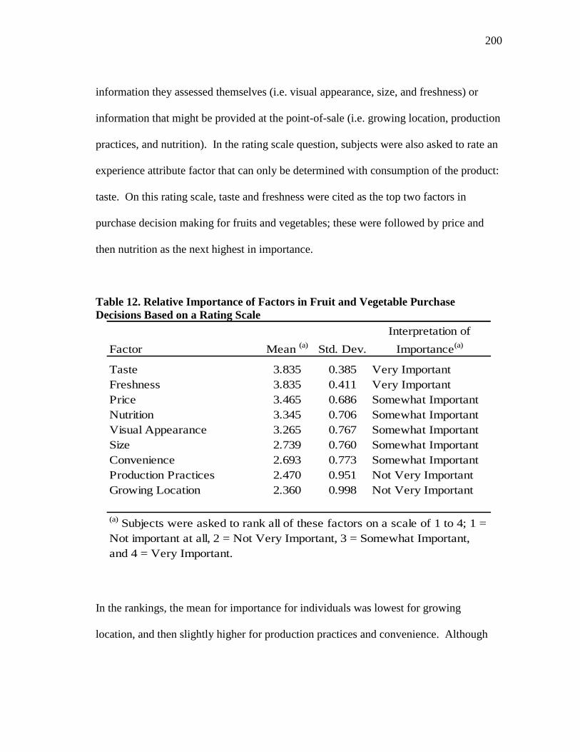
200
information they assessed themselves (i.e. visual appearance, size, and freshness) or
information that might be provided at the point-of-sale (i.e. growing location, production
practices, and nutrition). In the rating scale question, subjects were also asked to rate an
experience attribute factor that can only be determined with consumption of the product:
taste. On this rating scale, taste and freshness were cited as the top two factors in
purchase decision making for fruits and vegetables; these were followed by price and
then nutrition as the next highest in importance.
Table 12. Relative Importance of Factors in Fruit and Vegetable Purchase
Decisions Based on a Rating Scale
In the rankings, the mean for importance for individuals was lowest for growing
location, and then slightly higher for production practices and convenience. Although
Factor Mean (a)
Std. Dev.
Interpretation of
Importance(a)
Taste 3.835 0.385 Very Important
Freshness 3.835 0.411 Very Important
Price 3.465 0.686 Somewhat Important
Nutrition 3.345 0.706 Somewhat Important
Visual Appearance 3.265 0.767 Somewhat Important
Size 2.739 0.760 Somewhat Important
Convenience 2.693 0.773 Somewhat Important
Production Practices 2.470 0.951 Not Very Important
Growing Location 2.360 0.998 Not Very Important
(a) Subjects were asked to rank all of these factors on a scale of 1 to 4; 1 =
Not important at all, 2 = Not Very Important, 3 = Somewhat Important,
and 4 = Very Important.
201
these results are similar to the results measured based on selecting the top 3 factors, they
confirm that the taste value gained from consuming the food is one of the most important
factors influencing purchasing decisions for fruits and vegetables. There was also less
variability in this response than in the responses for the two lowest rated factors. The
results from the two measures of the factors involved in fruit purchasing decisions are
summarized in Table 11 and Table 12.
The responses to these survey questions can be used to make interesting
predictions about what the responses to the information treatments that are imposed
during the study will be. Also, if the results of these factor selection and ratings
responses are convergent with the results of the ranking and/or bidding model, then they
will provide confirmation of subject awareness of factors that influence their utility
maximization. If the results are divergent, then the issue of which responses are of value
in predicting economic behavior may be explored in greater detail.
WTP Models for Full Experimental Auction Bids
The full bids for the products included in the experimental auction and ranking
procedure are summarized in Table 13. Note that there were zero bids for all products in
all rounds, but that the maximum bid also exceeded the current retail price of $3.50 for
all products in all rounds, regardless of whether participants were provided with this
reference price.
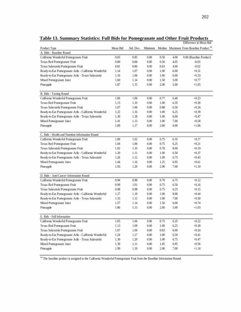
202
Table 13. Summary Statistics: Full Bids for Pomegranate and Other Fruit Products
Product Type Mean Bid Std. Dev. Minimum Median Maximum
Difference in Mean Bid
From Baseline Product (a)
A. Bids - Baseline Round
California Wonderful Pomegranate Fruit 0.83 0.85 0.00 0.50 4.00 0.00 (Baseline Product)
Texas Red Pomegranate Fruit 0.80 0.84 0.00 0.50 4.05 -0.03
Texas Salavatski Pomegranate Fruit 0.81 0.80 0.00 0.63 4.00 -0.02
Ready-to-Eat Pomegranate Arils - California Wonderful 1.14 1.07 0.00 1.00 6.00 +0.31
Ready-to-Eat Pomegranate Arils - Texas Salavatski 1.16 1.06 0.00 1.00 6.00 +0.33
Mixed Pomegranate Juice 1.60 1.14 0.00 1.50 5.00 +0.77
Pineapple 1.87 1.15 0.00 2.00 5.00 +1.05
B. Bids - Tasting Round
California Wonderful Pomegranate Fruit 1.06 1.06 0.00 0.77 6.40 +0.23
Texas Red Pomegranate Fruit 1.13 1.10 0.00 1.00 6.35 +0.30
Texas Salavatski Pomegranate Fruit 1.07 1.06 0.00 0.88 6.50 +0.24
Ready-to-Eat Pomegranate Arils - California Wonderful 1.22 1.16 0.00 1.00 6.25 +0.39
Ready-to-Eat Pomegranate Arils - Texas Salavatski 1.30 1.18 0.00 1.00 6.00 +0.47
Mixed Pomegranate Juice 1.41 1.13 0.00 1.00 7.00 +0.58
Pineapple 1.89 1.17 0.00 2.00 6.00 +1.06
C. Bids - Health and Nutrition Information Round
California Wonderful Pomegranate Fruit 1.00 1.02 0.00 0.75 6.35 +0.17
Texas Red Pomegranate Fruit 1.04 1.06 0.00 0.75 6.25 +0.21
Texas Salavatski Pomegranate Fruit 1.02 1.10 0.00 0.78 8.00 +0.19
Ready-to-Eat Pomegranate Arils - California Wonderful 1.20 1.11 0.00 1.00 6.50 +0.37
Ready-to-Eat Pomegranate Arils - Texas Salavatski 1.26 1.12 0.00 1.00 6.75 +0.43
Mixed Pomegranate Juice 1.44 1.16 0.00 1.25 6.95 +0.61
Pineapple 1.93 1.20 0.00 2.00 7.00 +1.10
D. Bids - Anti-Cancer Information Round
California Wonderful Pomegranate Fruit 0.94 0.98 0.00 0.70 6.75 +0.12
Texas Red Pomegranate Fruit 0.99 1.01 0.00 0.75 6.50 +0.16
Texas Salavatski Pomegranate Fruit 0.98 0.98 0.00 0.75 6.25 +0.15
Ready-to-Eat Pomegranate Arils - California Wonderful 1.27 1.19 0.00 1.00 8.00 +0.44
Ready-to-Eat Pomegranate Arils - Texas Salavatski 1.33 1.12 0.00 1.00 7.00 +0.50
Mixed Pomegranate Juice 1.57 1.14 0.00 1.50 6.00 +0.74
Pineapple 1.86 1.13 0.00 2.00 5.00 +1.03
E. Bids - Full Information
California Wonderful Pomegranate Fruit 1.05 1.06 0.00 0.75 6.35 +0.22
Texas Red Pomegranate Fruit 1.13 1.09 0.00 1.00 6.25 +0.30
Texas Salavatski Pomegranate Fruit 1.07 1.06 0.00 0.83 6.00 +0.24
Ready-to-Eat Pomegranate Arils - California Wonderful 1.24 1.17 0.00 1.00 6.50 +0.41
Ready-to-Eat Pomegranate Arils - Texas Salavatski 1.30 1.20 0.00 1.00 6.75 +0.47
Mixed Pomegranate Juice 1.39 1.11 0.00 1.05 6.95 +0.56
Pineapple 1.99 1.19 0.00 2.00 7.00 +1.16
(a) The baseline product is assigned to the California Wonderful Pomegranate Fruit from the Baseline Information Round.
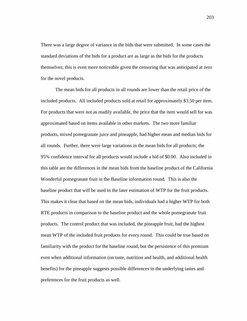
203
There was a large degree of variance in the bids that were submitted. In some cases the
standard deviations of the bids for a product are as large as the bids for the products
themselves; this is even more noticeable given the censoring that was anticipated at zero
for the novel products.
The mean bids for all products in all rounds are lower than the retail price of the
included products. All included products sold at retail for approximately $3.50 per item.
For products that were not as readily available, the price that the item would sell for was
approximated based on items available in other markets. The two more familiar
products, mixed pomegranate juice and pineapple, had higher mean and median bids for
all rounds. Further, there were large variations in the mean bids for all products; the
95% confidence interval for all products would include a bid of $0.00. Also included in
this table are the differences in the mean bids from the baseline product of the California
Wonderful pomegranate fruit in the Baseline information round. This is also the
baseline product that will be used in the later estimation of WTP for the fruit products.
This makes it clear that based on the mean bids, individuals had a higher WTP for both
RTE products in comparison to the baseline product and the whole pomegranate fruit
products. The control product that was included, the pineapple fruit, had the highest
mean WTP of the included fruit products for every round. This could be true based on
familiarity with the product for the baseline round, but the persistence of this premium
even when additional information (on taste, nutrition and health, and additional health
benefits) for the pineapple suggests possible differences in the underlying tastes and
preferences for the fruit products as well.
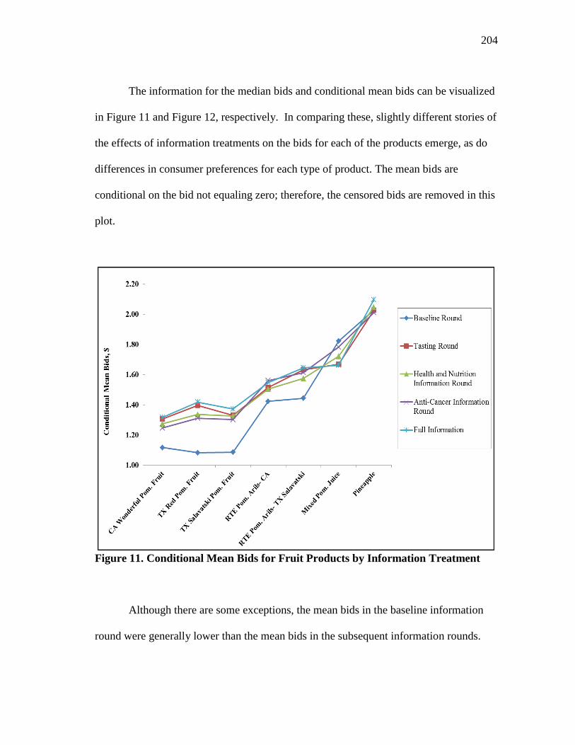
204
The information for the median bids and conditional mean bids can be visualized
in Figure 11 and Figure 12, respectively. In comparing these, slightly different stories of
the effects of information treatments on the bids for each of the products emerge, as do
differences in consumer preferences for each type of product. The mean bids are
conditional on the bid not equaling zero; therefore, the censored bids are removed in this
plot.
Figure 11. Conditional Mean Bids for Fruit Products by Information Treatment
Although there are some exceptions, the mean bids in the baseline information
round were generally lower than the mean bids in the subsequent information rounds.
205
This was true for all of the entirely pomegranate products. Secondly, the full
information mean bids closely mirror the mean bids for the tasting round for all products
except the mixed pomegranate juice and pineapple. The largest range in mean bids
across information treatments were for the three whole pomegranate fruits and the mixed
pomegranate juice. However, the direction of the change in mean bid across information
treatments was opposite for the whole pomegranate fruit products (positive change) and
the mixed pomegranate juice (negative change). This suggests that one of the biggest
hurdles in pomegranate marketing may be just getting consumers to initially try the
products.
Figure 12. Median Bids for All Fruit Products by Information Treatment (Baseline,
Tasting Information, Health and Nutrition Information, Anti-Cancer Information,
and Full Information)
206
As can be seen in Figure 12, there are differences in the median bids for the fruit
products across information treatments as well as in comparison to the mean bids
previously presented. Three things should be highlighted about this plot. First, the
median bid for the baseline round is the lowest of all information treatments for the
whole pomegranate products and the highest for the juice and pineapple; the two RTE
products have the same median bid for all rounds. Second, the bids for the full
information closely follow the tasting information as in the plot of the means. Finally,
while there was an initial price premium for the RTE products, this price premium
decreased as study participants gained information on the products.
While the summary statistics for each set of products and information treatments
are useful, it is also instructive to look at the distributions of the bids. Two ways this can
be done are with histograms or with kernel density smoothed probability density
functions. For added simplicity, the bids are plotted on separate graphs for each
information treatment, allowing for visual comparison of the distributions of bids for
each product. The probability density functions shown were estimated using a Gaussian
kernel density distribution in Simetar©.
Kernel density estimation is a nonparametric way to estimate the probability
density function. The plot of the estimated kernel density function is similar to a
histogram in that it allows the researcher to visualize the distribution of the data;
however, in an estimated kernel density distribution each observed point in the data is
assigned a specified distribution, and the sum of all of the distribution for all observed
points is used to reflect the overall distribution. By using a Gaussian (normal) kernel
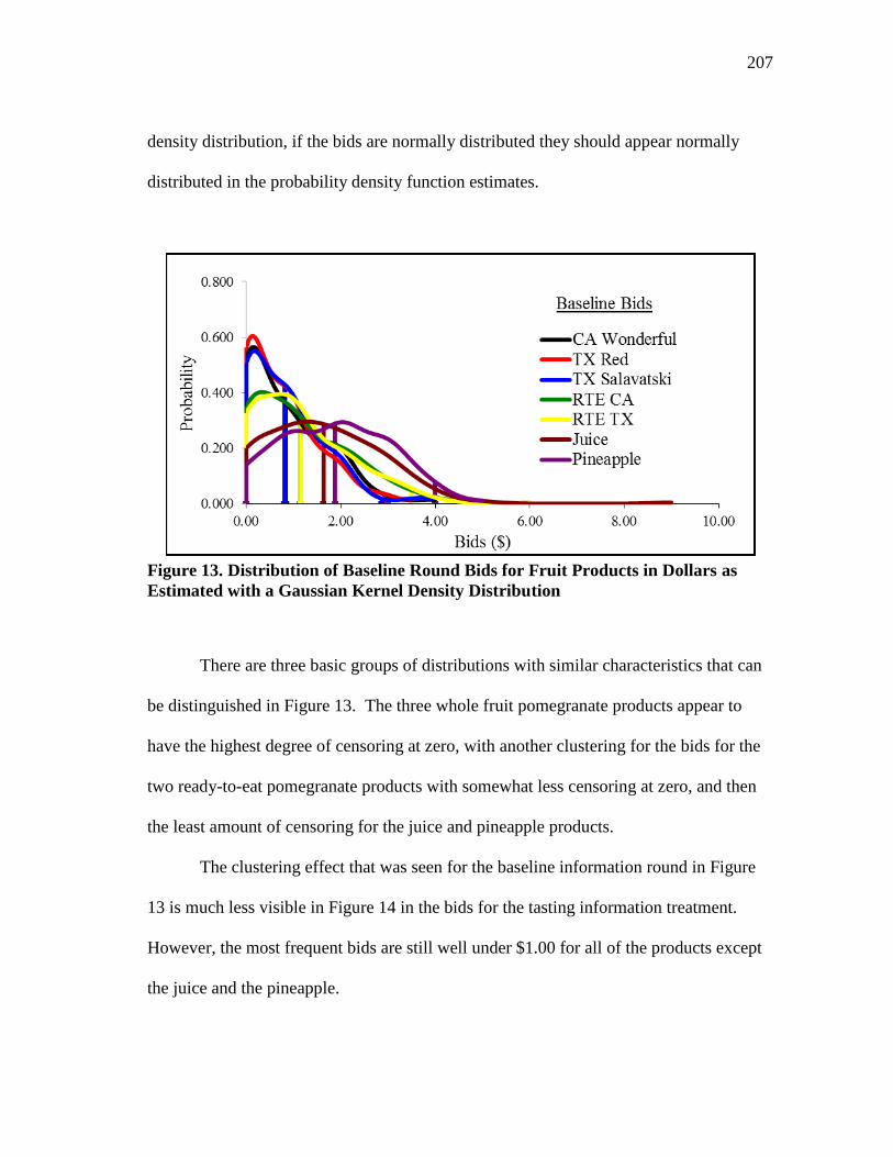
207
density distribution, if the bids are normally distributed they should appear normally
distributed in the probability density function estimates.
Figure 13. Distribution of Baseline Round Bids for Fruit Products in Dollars as
Estimated with a Gaussian Kernel Density Distribution
There are three basic groups of distributions with similar characteristics that can
be distinguished in Figure 13. The three whole fruit pomegranate products appear to
have the highest degree of censoring at zero, with another clustering for the bids for the
two ready-to-eat pomegranate products with somewhat less censoring at zero, and then
the least amount of censoring for the juice and pineapple products.
The clustering effect that was seen for the baseline information round in Figure
13 is much less visible in Figure 14 in the bids for the tasting information treatment.
However, the most frequent bids are still well under $1.00 for all of the products except
the juice and the pineapple.
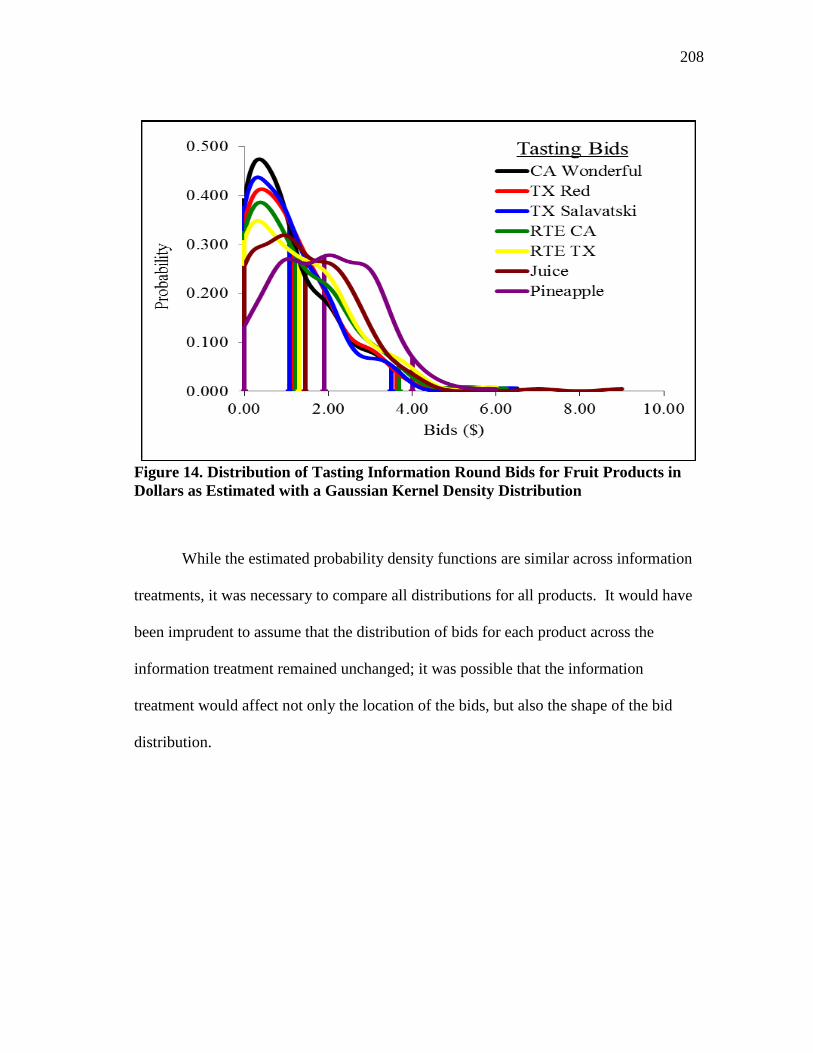
208
Figure 14. Distribution of Tasting Information Round Bids for Fruit Products in
Dollars as Estimated with a Gaussian Kernel Density Distribution
While the estimated probability density functions are similar across information
treatments, it was necessary to compare all distributions for all products. It would have
been imprudent to assume that the distribution of bids for each product across the
information treatment remained unchanged; it was possible that the information
treatment would affect not only the location of the bids, but also the shape of the bid
distribution.
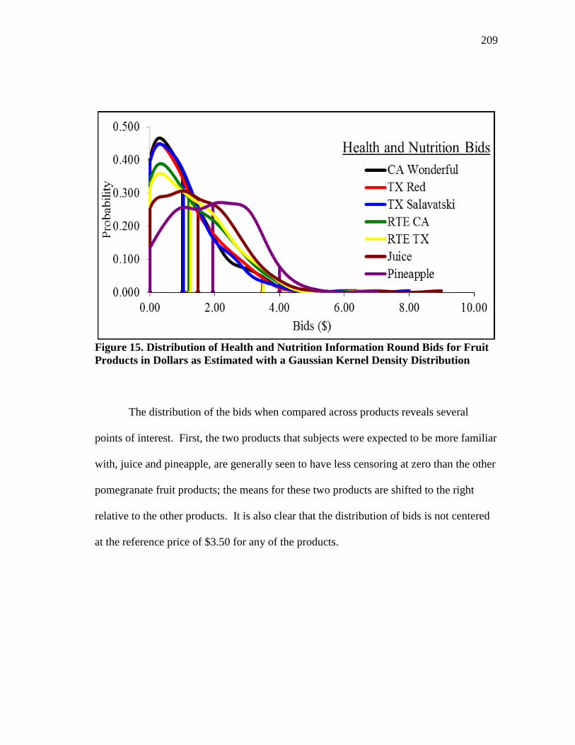
209
Figure 15. Distribution of Health and Nutrition Information Round Bids for Fruit
Products in Dollars as Estimated with a Gaussian Kernel Density Distribution
The distribution of the bids when compared across products reveals several
points of interest. First, the two products that subjects were expected to be more familiar
with, juice and pineapple, are generally seen to have less censoring at zero than the other
pomegranate fruit products; the means for these two products are shifted to the right
relative to the other products. It is also clear that the distribution of bids is not centered
at the reference price of $3.50 for any of the products.
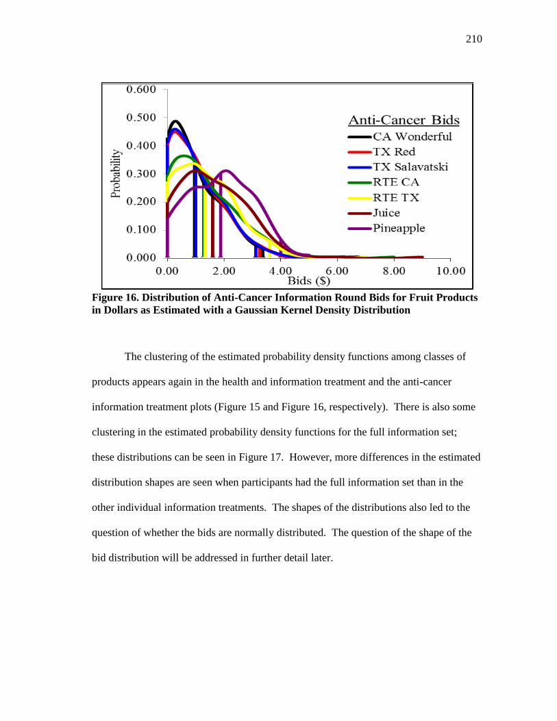
210
Figure 16. Distribution of Anti-Cancer Information Round Bids for Fruit Products
in Dollars as Estimated with a Gaussian Kernel Density Distribution
The clustering of the estimated probability density functions among classes of
products appears again in the health and information treatment and the anti-cancer
information treatment plots (Figure 15 and Figure 16, respectively). There is also some
clustering in the estimated probability density functions for the full information set;
these distributions can be seen in Figure 17. However, more differences in the estimated
distribution shapes are seen when participants had the full information set than in the
other individual information treatments. The shapes of the distributions also led to the
question of whether the bids are normally distributed. The question of the shape of the
bid distribution will be addressed in further detail later.
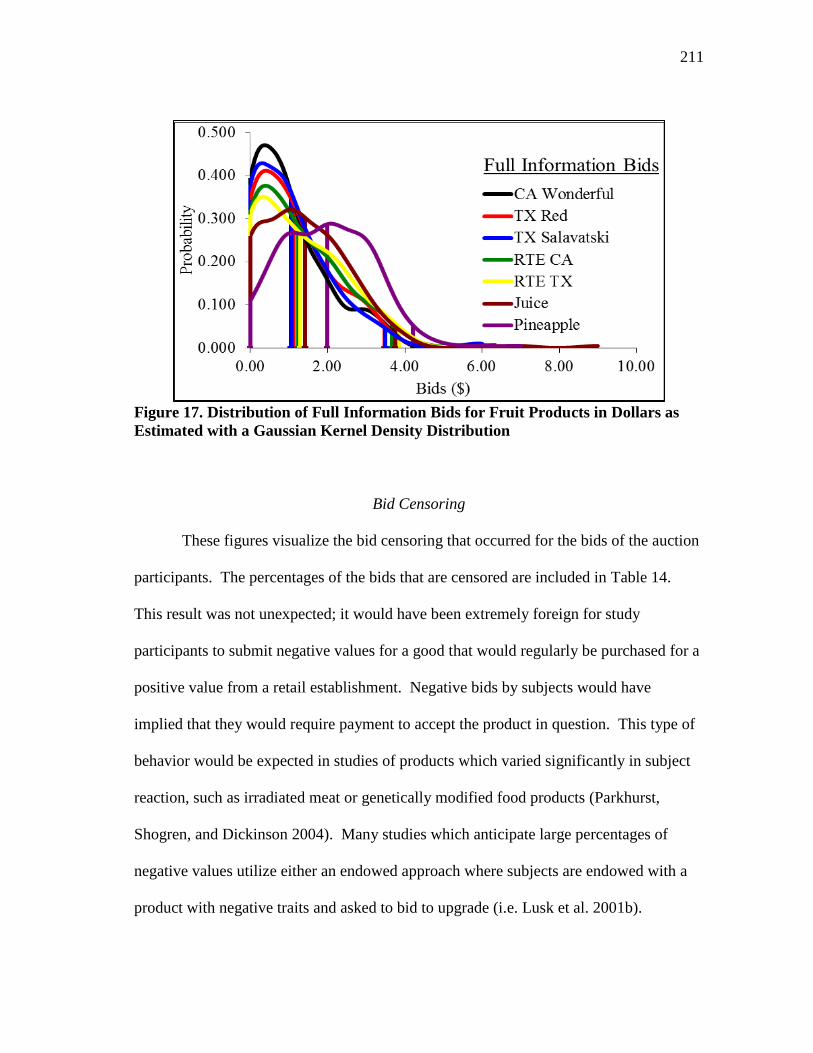
211
Figure 17. Distribution of Full Information Bids for Fruit Products in Dollars as
Estimated with a Gaussian Kernel Density Distribution
Bid Censoring
These figures visualize the bid censoring that occurred for the bids of the auction
participants. The percentages of the bids that are censored are included in Table 14.
This result was not unexpected; it would have been extremely foreign for study
participants to submit negative values for a good that would regularly be purchased for a
positive value from a retail establishment. Negative bids by subjects would have
implied that they would require payment to accept the product in question. This type of
behavior would be expected in studies of products which varied significantly in subject
reaction, such as irradiated meat or genetically modified food products (Parkhurst,
Shogren, and Dickinson 2004). Many studies which anticipate large percentages of
negative values utilize either an endowed approach where subjects are endowed with a
product with negative traits and asked to bid to upgrade (i.e. Lusk et al. 2001b).
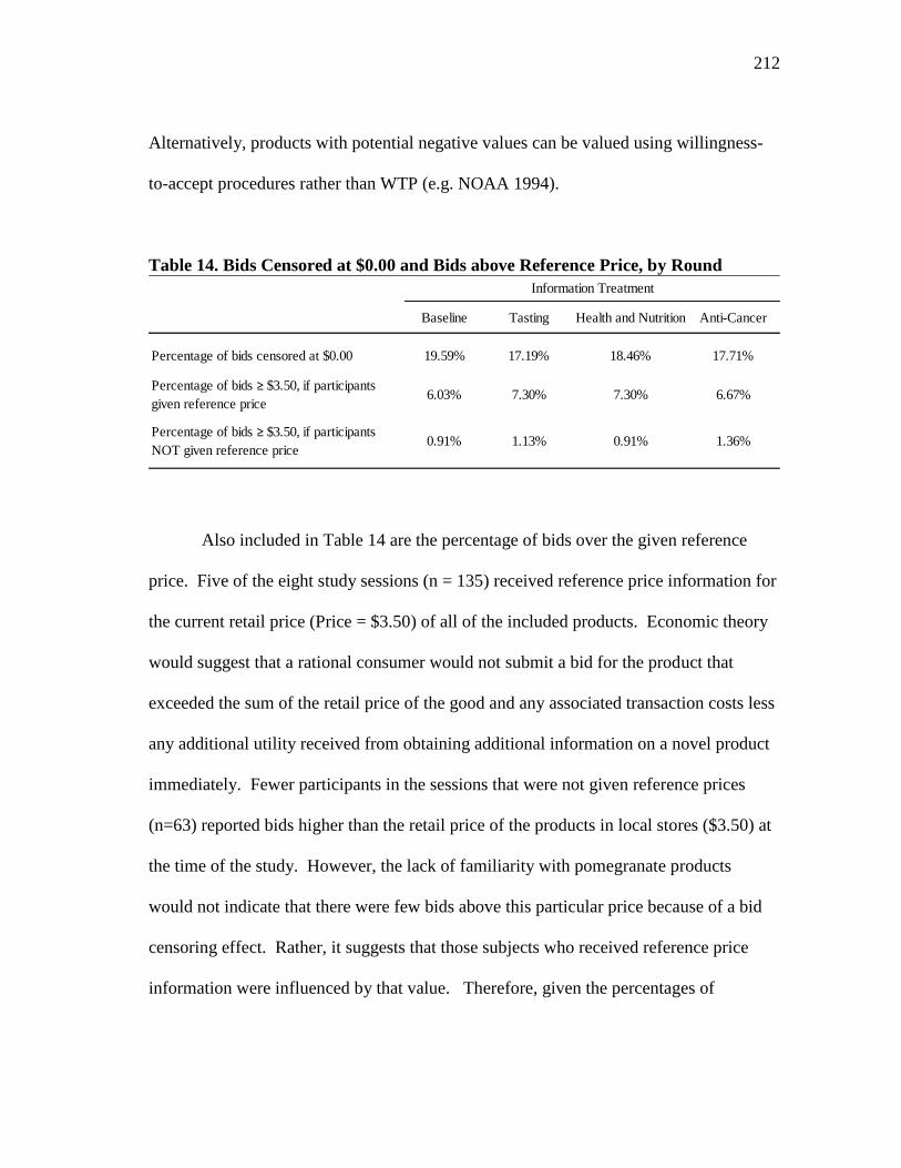
212
Alternatively, products with potential negative values can be valued using willingness-
to-accept procedures rather than WTP (e.g. NOAA 1994).
Table 14. Bids Censored at $0.00 and Bids above Reference Price, by Round
Also included in Table 14 are the percentage of bids over the given reference
price. Five of the eight study sessions (n = 135) received reference price information for
the current retail price (Price = $3.50) of all of the included products. Economic theory
would suggest that a rational consumer would not submit a bid for the product that
exceeded the sum of the retail price of the good and any associated transaction costs less
any additional utility received from obtaining additional information on a novel product
immediately. Fewer participants in the sessions that were not given reference prices
(n=63) reported bids higher than the retail price of the products in local stores ($3.50) at
the time of the study. However, the lack of familiarity with pomegranate products
would not indicate that there were few bids above this particular price because of a bid
censoring effect. Rather, it suggests that those subjects who received reference price
information were influenced by that value. Therefore, given the percentages of
Baseline Tasting Health and Nutrition Anti-Cancer
Percentage of bids censored at $0.00 19.59% 17.19% 18.46% 17.71%
Percentage of bids ≥ $3.50, if participants
given reference price6.03% 7.30% 7.30% 6.67%
Percentage of bids ≥ $3.50, if participants
NOT given reference price0.91% 1.13% 0.91% 1.36%
Information Treatment
213
participants that submitted auction bids above the given reference price, it was
concluded that an upper limit for the tobit model would not be appropriately based on
the retail price of the products. Thus, a lower-limit only tobit model was applied to the
full bids for all products and all rounds of information. Also, despite subjects being
provided with a reference price, the mean bids were much lower for the fruit products
than that reference price. This suggests that in the marketplace the average participant
would not purchase the product at the market price. However, additional estimation was
needed to determine what product, demographic, and behavioral characteristics might
influence this WTP, regardless of whether it was lower than the reference price.
Tobit Models for Each Product and Round
As discussed in the methods chapter, the WTP for pomegranates and other fruit
products was estimated using 35 tobit models, with each model being specific to a
particular product as well as to a particular information set received by subjects. For
purposes of brevity, each of these will not be fully detailed here. Rather, the results from
one set of models will be explained in detail, and the results of interest from the other
models will be noted. Full parameter estimates and marginal effects from the separate
tobit models from these models can be found in Appendix G. The results for the full
information set are presented here and only the results for one product (Texas Red
pomegranate fruit) for the full information set are interpreted here.
First, the demographic variables that were included are explained in Table 3.
These variables were introduced to account for possible differences in WTP for the

214
pomegranate and other fruit products based on differences in socioeconomic or
behavioral characteristics.
The estimates provided in Table 15 suggest that the second education level
dummy variable (education of more than high school up to and including a four-year
college degree) is significant (P < 0.05) in predicting an increase in WTP for the Texas
Red pomegranate fruit. In a similar manner, previous purchase of a pomegranate
product and being provided with a reference price also increased WTP for the Texas Red
pomegranate fruit. The estimated standard error of the regression is indicated by σ.
However, the β coefficients that are estimated in the tobit model should not be
interpreted in the same way as the β coefficients in a standard ordinary least squares
(OLS) model estimation. Rather, as pointed out by McDonald and Moffitt (1980), β
actually reflects two components: 1) the change in the dependent variable (here, yi) of
those values above the censoring limit and weighted by the probability of being above
the censoring limit, and 2) the change in the probability of being above the limit,
weighted by the expected value of yi if above the limit. A change in β is only equal to
the effect of a change in x on yi when x is equal to infinity. Therefore, the results that are
of economic interest from the tobit model are the marginal effects for each independent
variable. Estimation of marginal effects allows for comparison of the effects of the
included regressors on the observed bids.
As discussed in Chapter IV, the tobit model that is estimated is based on a
censored distribution of bids; thus, the marginal effects of interest are the expected
changes in bids given bid censoring at the specified level (here, for censoring at $0.00)
215
for a one unit change in the parameter of interest. Marginal effects were calculated
using the Delta method. Estimates for marginal effects are given in Table 16. (Note that
marginal effects for dummy variables are calculated as a change from the base level of
zero to a value of one.)
In looking at the predicted marginal effects for changes in the variables in the
tobit model for the Texas Red pomegranate, we conclude that an individual who has
more than a high school education but less than a graduate education would be willing to
pay a $0.42 premium over someone with a high school degree or less. Similarly, an
individual who had previously purchased a pomegranate fruit would pay $0.48 more for
the Texas Red pomegranate fruit, and individuals who were provided with a reference
price were willing to pay a $0.49 premium over those not given a reference price. The
results in this table for other products as well as those for other information treatments
can be interpreted similarly.
The tobit model estimations presented are useful in that they allow for
comparisons of the parameter estimates and marginal effects for each product under each
information treatment. However, this limits generalizing the results to less specific
products and to make comparisons across information treatments and products. By
pooling all of the bids made by each individual with indicator variables for the
information treatment and product that each bid was made for, further models may be
estimated to provide additional insight.
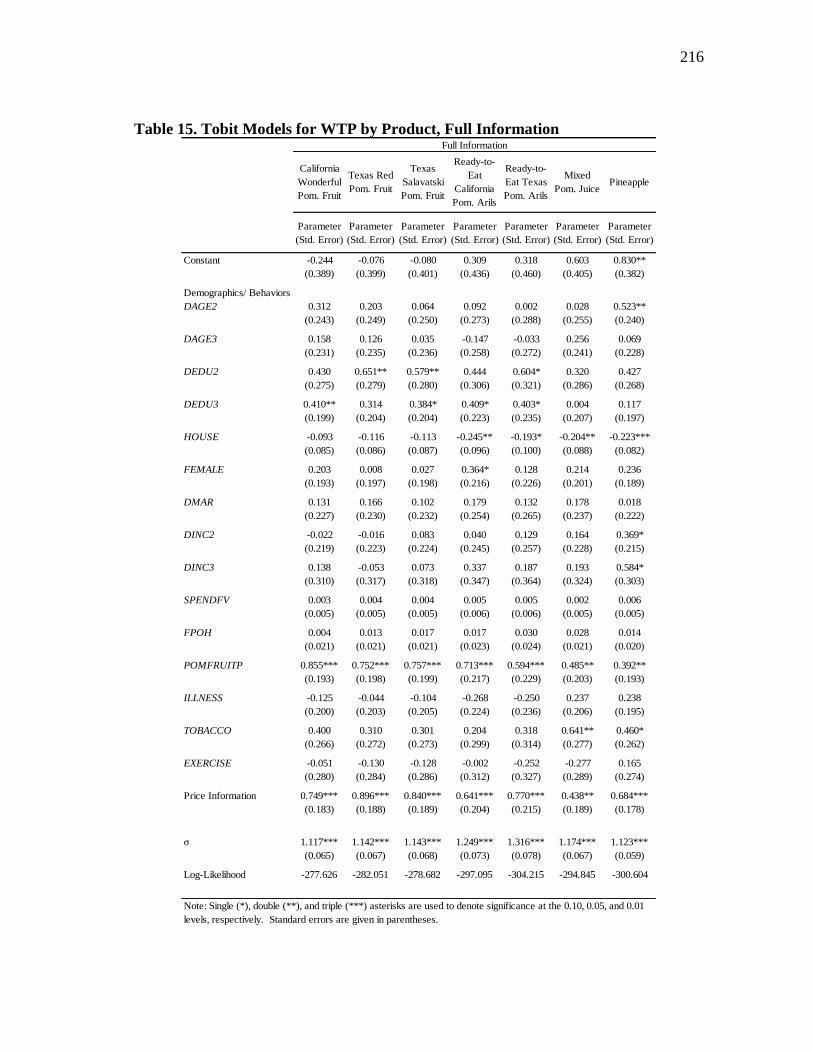
216
Table 15. Tobit Models for WTP by Product, Full Information
California
Wonderful
Pom. Fruit
Texas Red
Pom. Fruit
Texas
Salavatski
Pom. Fruit
Ready-to-
Eat
California
Pom. Arils
Ready-to-
Eat Texas
Pom. Arils
Mixed
Pom. JuicePineapple
Parameter
(Std. Error)
Parameter
(Std. Error)
Parameter
(Std. Error)
Parameter
(Std. Error)
Parameter
(Std. Error)
Parameter
(Std. Error)
Parameter
(Std. Error)
Constant -0.244
(0.389)
-0.076
(0.399)
-0.080
(0.401)
0.309
(0.436)
0.318
(0.460)
0.603
(0.405)
0.830**
(0.382)
Demographics/ Behaviors
DAGE2 0.312
(0.243)
0.203
(0.249)
0.064
(0.250)
0.092
(0.273)
0.002
(0.288)
0.028
(0.255)
0.523**
(0.240)
DAGE3 0.158
(0.231)
0.126
(0.235)
0.035
(0.236)
-0.147
(0.258)
-0.033
(0.272)
0.256
(0.241)
0.069
(0.228)
DEDU2 0.430
(0.275)
0.651**
(0.279)
0.579**
(0.280)
0.444
(0.306)
0.604*
(0.321)
0.320
(0.286)
0.427
(0.268)
DEDU3 0.410**
(0.199)
0.314
(0.204)
0.384*
(0.204)
0.409*
(0.223)
0.403*
(0.235)
0.004
(0.207)
0.117
(0.197)
HOUSE -0.093
(0.085)
-0.116
(0.086)
-0.113
(0.087)
-0.245**
(0.096)
-0.193*
(0.100)
-0.204**
(0.088)
-0.223***
(0.082)
FEMALE 0.203
(0.193)
0.008
(0.197)
0.027
(0.198)
0.364*
(0.216)
0.128
(0.226)
0.214
(0.201)
0.236
(0.189)
DMAR 0.131
(0.227)
0.166
(0.230)
0.102
(0.232)
0.179
(0.254)
0.132
(0.265)
0.178
(0.237)
0.018
(0.222)
DINC2 -0.022
(0.219)
-0.016
(0.223)
0.083
(0.224)
0.040
(0.245)
0.129
(0.257)
0.164
(0.228)
0.369*
(0.215)
DINC3 0.138
(0.310)
-0.053
(0.317)
0.073
(0.318)
0.337
(0.347)
0.187
(0.364)
0.193
(0.324)
0.584*
(0.303)
SPENDFV 0.003
(0.005)
0.004
(0.005)
0.004
(0.005)
0.005
(0.006)
0.005
(0.006)
0.002
(0.005)
0.006
(0.005)
FPOH 0.004
(0.021)
0.013
(0.021)
0.017
(0.021)
0.017
(0.023)
0.030
(0.024)
0.028
(0.021)
0.014
(0.020)
POMFRUITP 0.855***
(0.193)
0.752***
(0.198)
0.757***
(0.199)
0.713***
(0.217)
0.594***
(0.229)
0.485**
(0.203)
0.392**
(0.193)
ILLNESS -0.125
(0.200)
-0.044
(0.203)
-0.104
(0.205)
-0.268
(0.224)
-0.250
(0.236)
0.237
(0.206)
0.238
(0.195)
TOBACCO 0.400
(0.266)
0.310
(0.272)
0.301
(0.273)
0.204
(0.299)
0.318
(0.314)
0.641**
(0.277)
0.460*
(0.262)
EXERCISE -0.051
(0.280)
-0.130
(0.284)
-0.128
(0.286)
-0.002
(0.312)
-0.252
(0.327)
-0.277
(0.289)
0.165
(0.274)
Price Information 0.749***
(0.183)
0.896***
(0.188)
0.840***
(0.189)
0.641***
(0.204)
0.770***
(0.215)
0.438**
(0.189)
0.684***
(0.178)
σ 1.117***
(0.065)
1.142***
(0.067)
1.143***
(0.068)
1.249***
(0.073)
1.316***
(0.078)
1.174***
(0.067)
1.123***
(0.059)
Log-Likelihood -277.626 -282.051 -278.682 -297.095 -304.215 -294.845 -300.604
Full Information
Note: Single (*), double (**), and triple (***) asterisks are used to denote significance at the 0.10, 0.05, and 0.01
levels, respectively. Standard errors are given in parentheses.
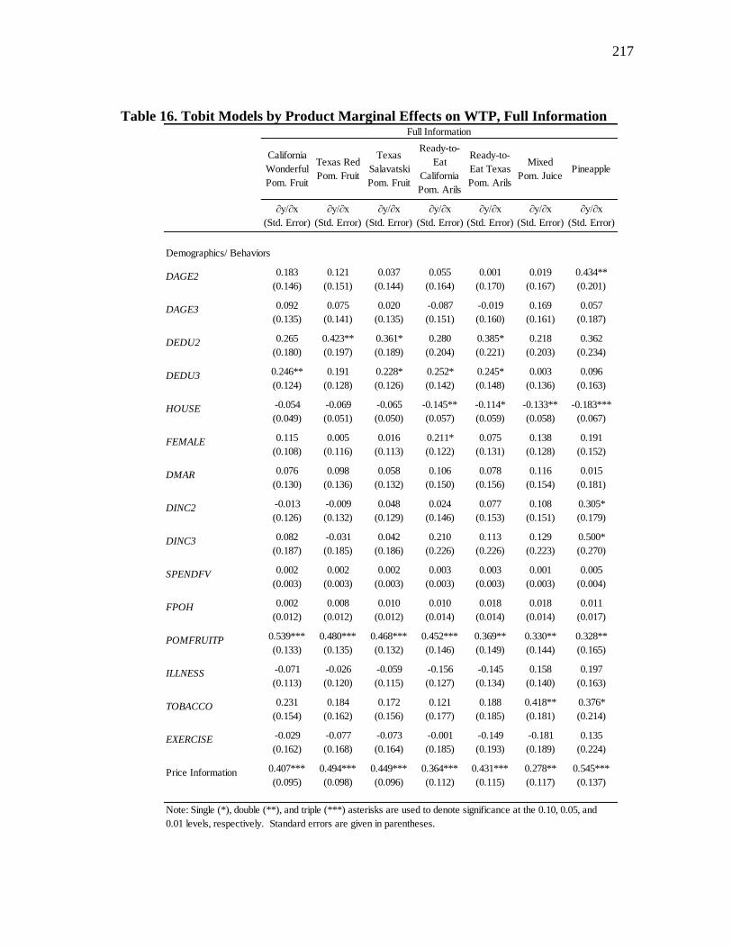
217
Table 16. Tobit Models by Product Marginal Effects on WTP, Full Information
California
Wonderful
Pom. Fruit
Texas Red
Pom. Fruit
Texas
Salavatski
Pom. Fruit
Ready-to-
Eat
California
Pom. Arils
Ready-to-
Eat Texas
Pom. Arils
Mixed
Pom. JuicePineapple
∂y/∂x
(Std. Error)
∂y/∂x
(Std. Error)
∂y/∂x
(Std. Error)
∂y/∂x
(Std. Error)
∂y/∂x
(Std. Error)
∂y/∂x
(Std. Error)
∂y/∂x
(Std. Error)
Demographics/ Behaviors
DAGE2 0.183
(0.146)
0.121
(0.151)
0.037
(0.144)
0.055
(0.164)
0.001
(0.170)
0.019
(0.167)
0.434**
(0.201)
DAGE3 0.092
(0.135)
0.075
(0.141)
0.020
(0.135)
-0.087
(0.151)
-0.019
(0.160)
0.169
(0.161)
0.057
(0.187)
DEDU2 0.265
(0.180)
0.423**
(0.197)
0.361*
(0.189)
0.280
(0.204)
0.385*
(0.221)
0.218
(0.203)
0.362
(0.234)
DEDU3 0.246**
(0.124)
0.191
(0.128)
0.228*
(0.126)
0.252*
(0.142)
0.245*
(0.148)
0.003
(0.136)
0.096
(0.163)
HOUSE -0.054
(0.049)
-0.069
(0.051)
-0.065
(0.050)
-0.145**
(0.057)
-0.114*
(0.059)
-0.133**
(0.058)
-0.183***
(0.067)
FEMALE 0.115
(0.108)
0.005
(0.116)
0.016
(0.113)
0.211*
(0.122)
0.075
(0.131)
0.138
(0.128)
0.191
(0.152)
DMAR 0.076
(0.130)
0.098
(0.136)
0.058
(0.132)
0.106
(0.150)
0.078
(0.156)
0.116
(0.154)
0.015
(0.181)
DINC2 -0.013
(0.126)
-0.009
(0.132)
0.048
(0.129)
0.024
(0.146)
0.077
(0.153)
0.108
(0.151)
0.305*
(0.179)
DINC3 0.082
(0.187)
-0.031
(0.185)
0.042
(0.186)
0.210
(0.226)
0.113
(0.226)
0.129
(0.223)
0.500*
(0.270)
SPENDFV 0.002
(0.003)
0.002
(0.003)
0.002
(0.003)
0.003
(0.003)
0.003
(0.003)
0.001
(0.003)
0.005
(0.004)
FPOH 0.002
(0.012)
0.008
(0.012)
0.010
(0.012)
0.010
(0.014)
0.018
(0.014)
0.018
(0.014)
0.011
(0.017)
POMFRUITP 0.539***
(0.133)
0.480***
(0.135)
0.468***
(0.132)
0.452***
(0.146)
0.369**
(0.149)
0.330**
(0.144)
0.328**
(0.165)
ILLNESS -0.071
(0.113)
-0.026
(0.120)
-0.059
(0.115)
-0.156
(0.127)
-0.145
(0.134)
0.158
(0.140)
0.197
(0.163)
TOBACCO 0.231
(0.154)
0.184
(0.162)
0.172
(0.156)
0.121
(0.177)
0.188
(0.185)
0.418**
(0.181)
0.376*
(0.214)
EXERCISE -0.029
(0.162)
-0.077
(0.168)
-0.073
(0.164)
-0.001
(0.185)
-0.149
(0.193)
-0.181
(0.189)
0.135
(0.224)
Price Information 0.407***
(0.095)
0.494***
(0.098)
0.449***
(0.096)
0.364***
(0.112)
0.431***
(0.115)
0.278**
(0.117)
0.545***
(0.137)
Full Information
Note: Single (*), double (**), and triple (***) asterisks are used to denote significance at the 0.10, 0.05, and
0.01 levels, respectively. Standard errors are given in parentheses.
218
However, it is noteworthy that the individual tobit models avoid some of the
issues that arise from pooling the bids made by an individual for multiple products and
under multiple information treatments. One such problem is a lack of independence
among the multiple bids submitted by an individual subject. Relationships that an
individual‘s bids have among different product characteristics in the same round (same
information treatment) or for the same product with different information treatments are
included. A model that is for a single product and a single information treatment
circumvents this by only making estimates based on one bid for each individual.
Ordinary Least Squares Model
The pooled bids for the pomegranate and other fruit products are first modeled
using an ordinary least squares (OLS) model to provide a baseline for comparison for the
other models. Using an OLS model for all of the bids by all individuals for all products
ignores the problem of censoring of bids at $0.00 that was discussed earlier. Further, it
ignores possible relationships between an individual‘s bids across products and across
information treatments. Therefore, it was hypothesized that the bids for the OLS model
would be biased and that the models discussed later would address some of the causes of
that bias. However, OLS models are frequently estimated as a baseline comparison for
the models presented later.
The results for the OLS model are presented in Table 17. The table includes the
results of five sets of variable specifications for comparison purposes. A total of 5,544
observations were included in the OLS models. The R2 values ranged from 0.08 to 0.22,
219
but each of the regressions gave an F-test value of 0.000, rejecting the null hypothesis
that all the model coefficients in a single regression equation were equal to zero.
Several points about these results are notable. First, the variety of the two Texas
pomegranate varieties was never significant in relation to the baseline variety of
California Wonderful, regardless of the other regressors that are included in the model.
Second, the product forms as well as the information treatments are significant (P <
0.01) for all the models in which they are included. The demographic results are the
same for the two models that contain them; however, not all of the demographic
variables are predicted to have a significant effect on the bids for the products included
in the experimental auctions. In including the demographic variables, an attempt was
made to create a model that would have greater explanatory power.
Many of the hypothesized factors that influence bidding behavior were not found
to be significant in the OLS regression. Those that were not significant include the older
age grouping, the middle income bracket, whether an individual had an illness that he or
she considered serious, and the frequency with which an individual exercised. However,
given the lack of familiarity with several of the products in the auction, it was surprising
that so many of the demographic factors were significant. Finally, the estimates for
Models 4 and 5 may look similar. However, the estimated parameter for the constant is
found to be negative in the final model, although it is not significant (and therefore can
be excluded); the constant value is positive for all other OLS estimations.
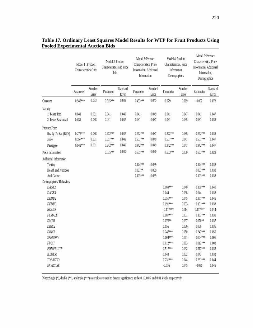
220
Table 17. Ordinary Least Squares Model Results for WTP for Fruit Products Using
Pooled Experimental Auction Bids
ParameterStandard
ErrorParameter
Standard
ErrorParameter
Standard
ErrorParameter
Standard
ErrorParameter
Standard
Error
Constant 0.948*** 0.033 0.515*** 0.038 0.433*** 0.045 0.079 0.069 -0.002 0.073
Variety
1: Texas Red 0.041 0.051 0.041 0.049 0.041 0.049 0.041 0.047 0.041 0.047
2: Texas Salavatski 0.031 0.038 0.031 0.037 0.031 0.037 0.031 0.035 0.031 0.035
Product Form
Ready-To-Eat (RTE) 0.272*** 0.038 0.272*** 0.037 0.272*** 0.037 0.272*** 0.035 0.272*** 0.035
Juice 0.557*** 0.051 0.557*** 0.049 0.557*** 0.049 0.557*** 0.047 0.557*** 0.047
Pineapple 0.942*** 0.051 0.942*** 0.049 0.942*** 0.049 0.942*** 0.047 0.942*** 0.047
Price Information 0.635*** 0.030 0.635*** 0.030 0.603*** 0.030 0.603*** 0.029
Additional Information
Tasting 0.124*** 0.039 0.124*** 0.038
Health and Nutrition 0.097** 0.039 0.097*** 0.038
Anti-Cancer 0.103*** 0.039 0.103*** 0.038
Demographics/ Behaviors
DAGE2 0.169*** 0.040 0.169*** 0.040
DAGE3 0.044 0.038 0.044 0.038
DEDU2 0.351*** 0.045 0.351*** 0.045
DEDU3 0.191*** 0.033 0.191*** 0.033
HOUSE -0.117*** 0.014 -0.117*** 0.014
FEMALE 0.187*** 0.031 0.187*** 0.031
DMAR 0.076** 0.037 0.076** 0.037
DINC2 0.056 0.036 0.056 0.036
DINC3 0.247*** 0.050 0.247*** 0.050
SPENDFV 0.004*** 0.001 0.004*** 0.001
FPOH 0.012*** 0.003 0.012*** 0.003
POMFRUITP 0.517*** 0.032 0.517*** 0.032
ILLNESS 0.043 0.032 0.043 0.032
TOBACCO 0.231*** 0.044 0.231*** 0.044
EXERCISE -0.036 0.045 -0.036 0.045
Note: Single (*), double (**), and triple (***) asterisks are used to denote significance at the 0.10, 0.05, and 0.01 levels, respectively.
Model 1 : Product
Characteristics Only
Model 2: Product
Characteristics and Price
Info
Model 3: Product
Characteristics, Price
Information, Additional
Information
Model 5: Product
Characteristics, Price
Information, Additional
Information,
Demographics
Model 4: Product
Characteristics, Price
Information,
Demographics
221
Tobit Model for Pooled Bids
The censoring that is ignored in the OLS regressions is included in the tobit
models presented in Table 18. The same five models that are estimated in the OLS
regressions are used. The estimated standard deviation of the residual is given by the σ
value indicated, and the maximized log-likelihood value is also given. The likelihood
ratio test suggests whether each model fits better than a model with no predictors.
Additionally, the marginal effects for the tobit models are presented in Table 19.
The differences between the two types of models presented thus far, OLS and
tobit, are reflected in the parameter estimations. A few contrasts are pointed out here,
and the tables can be used for further comparisons. In terms of the parameter estimates,
the constant is significant for all tobit models, even with a negative value for the two
models with demographic variables included. This may initially be a cause for concern;
still, if the characteristics of the average consumer are fit to the model then the estimated
WTP for the baseline product is given by evaluating the respective model at the means
for the demographic characteristics, then the WTP for the baseline product is positive.
This can be done using the actual mean values for each variable and using only the
variables that are significant at P < 0.05. If this is done, the estimated value is $1.10 for
both Model 4 and Model 5. The value at the means can also be evaluated by calculating
the means for each variable and then assigning values of 0 or 1 based on the means to
the dummy variables in the model.
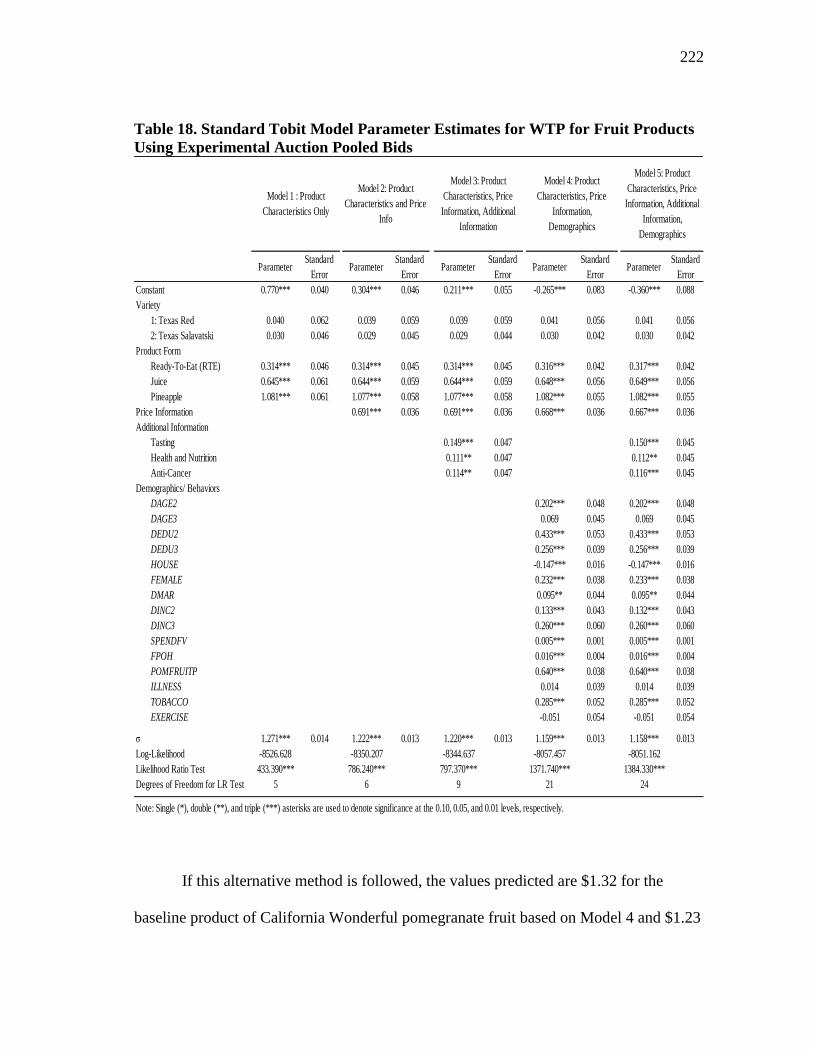
222
Table 18. Standard Tobit Model Parameter Estimates for WTP for Fruit Products
Using Experimental Auction Pooled Bids
If this alternative method is followed, the values predicted are $1.32 for the
baseline product of California Wonderful pomegranate fruit based on Model 4 and $1.23
ParameterStandard
ErrorParameter
Standard
ErrorParameter
Standard
ErrorParameter
Standard
ErrorParameter
Standard
Error
Constant 0.770*** 0.040 0.304*** 0.046 0.211*** 0.055 -0.265*** 0.083 -0.360*** 0.088
Variety
1: Texas Red 0.040 0.062 0.039 0.059 0.039 0.059 0.041 0.056 0.041 0.056
2: Texas Salavatski 0.030 0.046 0.029 0.045 0.029 0.044 0.030 0.042 0.030 0.042
Product Form
Ready-To-Eat (RTE) 0.314*** 0.046 0.314*** 0.045 0.314*** 0.045 0.316*** 0.042 0.317*** 0.042
Juice 0.645*** 0.061 0.644*** 0.059 0.644*** 0.059 0.648*** 0.056 0.649*** 0.056
Pineapple 1.081*** 0.061 1.077*** 0.058 1.077*** 0.058 1.082*** 0.055 1.082*** 0.055
Price Information 0.691*** 0.036 0.691*** 0.036 0.668*** 0.036 0.667*** 0.036
Additional Information
Tasting 0.149*** 0.047 0.150*** 0.045
Health and Nutrition 0.111** 0.047 0.112** 0.045
Anti-Cancer 0.114** 0.047 0.116*** 0.045
Demographics/ Behaviors
DAGE2 0.202*** 0.048 0.202*** 0.048
DAGE3 0.069 0.045 0.069 0.045
DEDU2 0.433*** 0.053 0.433*** 0.053
DEDU3 0.256*** 0.039 0.256*** 0.039
HOUSE -0.147*** 0.016 -0.147*** 0.016
FEMALE 0.232*** 0.038 0.233*** 0.038
DMAR 0.095** 0.044 0.095** 0.044
DINC2 0.133*** 0.043 0.132*** 0.043
DINC3 0.260*** 0.060 0.260*** 0.060
SPENDFV 0.005*** 0.001 0.005*** 0.001
FPOH 0.016*** 0.004 0.016*** 0.004
POMFRUITP 0.640*** 0.038 0.640*** 0.038
ILLNESS 0.014 0.039 0.014 0.039
TOBACCO 0.285*** 0.052 0.285*** 0.052
EXERCISE -0.051 0.054 -0.051 0.054
σ 1.271*** 0.014 1.222*** 0.013 1.220*** 0.013 1.159*** 0.013 1.158*** 0.013
Log-Likelihood -8526.628 -8350.207 -8344.637 -8057.457 -8051.162
Likelihood Ratio Test 433.390*** 786.240*** 797.370*** 1371.740*** 1384.330***
Degrees of Freedom for LR Test 5 6 9 21 24
Note: Single (*), double (**), and triple (***) asterisks are used to denote significance at the 0.10, 0.05, and 0.01 levels, respectively.
Model 1 : Product
Characteristics Only
Model 2: Product
Characteristics and Price
Info
Model 3: Product
Characteristics, Price
Information, Additional
Information
Model 4: Product
Characteristics, Price
Information,
Demographics
Model 5: Product
Characteristics, Price
Information, Additional
Information,
Demographics
223
based on Model 5. Thus, we would not generally expect the model to predict negative
WTP for products once individual demographics are included in Models 4 and 5.
However, when the lowest possible values for the demographic characteristics are
included in this model, the estimated value is negative, implying that an individual
would have to be paid to take a California Wonderful pomegranate fruit. Even so, since
the tobit model is estimated to allow for conclusions to be drawn about utility based on
willingness-to-pay, a negative value indicates that an individual with the lowest values
would have a negative utility for the baseline product (California Wonderful
pomegranate fruit). Furthermore, we are more interested in the results of the marginal
effects estimations (which do not include the constant) than in the actual parameter
estimates for the tobit model.
The demographic effects that are significant from the OLS model are also
significant for the pooled tobit models. Further, the Texas varieties are not shown to be
significant in any of the tobit models, indicating subjects were indifferent between the
California and Texas varieties on the basis of this model. There was a significant and
positive effect from the two further-processed fruit forms (RTE and juice), as well as for
the pineapple fruit and the price information. Individually each of these indicates a
positive relationship between WTP and each respective product characteristic. Taken
together, this suggests that the lack of familiarity of subjects with the pomegranate fruit
may have influenced bids for the products. For example, if a subject lacked knowledge
on how to remove the husk from a whole pomegranate fruit, he or she may have
preferred the product forms that were easier to consume. Of course, this positive
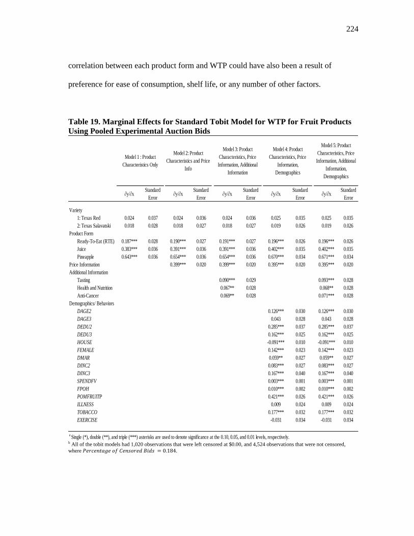
224
correlation between each product form and WTP could have also been a result of
preference for ease of consumption, shelf life, or any number of other factors.
Table 19. Marginal Effects for Standard Tobit Model for WTP for Fruit Products
Using Pooled Experimental Auction Bids
b All of the tobit models had 1,020 observations that were left censored at $0.00, and 4,524 observations that were not censored,
where .
∂y/∂xStandard
Error∂y/∂x
Standard
Error∂y/∂x
Standard
Error∂y/∂x
Standard
Error∂y/∂x
Standard
Error
Variety
1: Texas Red 0.024 0.037 0.024 0.036 0.024 0.036 0.025 0.035 0.025 0.035
2: Texas Salavatski 0.018 0.028 0.018 0.027 0.018 0.027 0.019 0.026 0.019 0.026
Product Form
Ready-To-Eat (RTE) 0.187*** 0.028 0.190*** 0.027 0.191*** 0.027 0.196*** 0.026 0.196*** 0.026
Juice 0.383*** 0.036 0.391*** 0.036 0.391*** 0.036 0.402*** 0.035 0.402*** 0.035
Pineapple 0.643*** 0.036 0.654*** 0.036 0.654*** 0.036 0.670*** 0.034 0.671*** 0.034
Price Information 0.399*** 0.020 0.399*** 0.020 0.395*** 0.020 0.395*** 0.020
Additional Information
Tasting 0.090*** 0.029 0.093*** 0.028
Health and Nutrition 0.067** 0.028 0.068** 0.028
Anti-Cancer 0.069** 0.028 0.071*** 0.028
Demographics/ Behaviors
DAGE2 0.126*** 0.030 0.126*** 0.030
DAGE3 0.043 0.028 0.043 0.028
DEDU2 0.285*** 0.037 0.285*** 0.037
DEDU3 0.162*** 0.025 0.162*** 0.025
HOUSE -0.091*** 0.010 -0.091*** 0.010
FEMALE 0.142*** 0.023 0.142*** 0.023
DMAR 0.059** 0.027 0.059** 0.027
DINC2 0.083*** 0.027 0.083*** 0.027
DINC3 0.167*** 0.040 0.167*** 0.040
SPENDFV 0.003*** 0.001 0.003*** 0.001
FPOH 0.010*** 0.002 0.010*** 0.002
POMFRUITP 0.421*** 0.026 0.421*** 0.026
ILLNESS 0.009 0.024 0.009 0.024
TOBACCO 0.177*** 0.032 0.177*** 0.032
EXERCISE -0.031 0.034 -0.031 0.034
a Single (*), double (**), and triple (***) asterisks are used to denote significance at the 0.10, 0.05, and 0.01 levels, respectively.
Model 1 : Product
Characteristics Only
Model 2: Product
Characteristics and Price
Info
Model 3: Product
Characteristics, Price
Information, Additional
Information
Model 4: Product
Characteristics, Price
Information,
Demographics
Model 5: Product
Characteristics, Price
Information, Additional
Information,
Demographics
225
Pineapple was included as a control product because it is a substitute for
pomegranates that subjects were expected to be more familiar with; the higher WTP for
the pineapple fruit could have been a result of greater product familiarity or other
differences in the products, such as flavor and size preferences. The positive marginal
effect of the price information variable (with a value of 0.40) indicates that providing a
reference price to consumers significantly influenced the bids that they submitted.
Providing a reference price would not be give valuable or significant information to
individuals who were familiar with the current retail price of the good; however, the
survey of buying behavior indicated that most subjects had not purchased a pomegranate
fruit before and therefore may have been unaware of the market price.
In comparing the marginal effects based on the tobit model estimation, the
differences between the marginal effects and the parameter estimates are indicative of
why the parameter estimates should not be used for comparisons of changes in the
values of the regressors. Only one of the demographic/ behavioral characteristics has a
negative marginal effect on bids: household size. However, this result is not necessarily
unexpected; larger households may be making purchases based on quantity and be
seeking less expensive fruit substitutes. The results across the 5 tobit models similar in
terms of the size of the effects, and are generally robust to controls for the demographic
and behavioral attributes of subjects. The only notable exception to this is the constant
term, but this was addressed previously.
In order to determine which of the specifications of the tobit model would be
preferred, three tests were considered. First, a likelihood ratio test was conducted to
226
compare Model 1 through Model 4 to Model 5. The likelihood of a function gives the
probability of the data given the parameter estimates. A likelihood ratio test is based on
the assumption that one of the models is a restricted form of the other model (the
―unrestricted‖ model). Alternatively, the test assumes that the restricted model can be
nested within the unrestricted model by assuming that the coefficients on the variables
not included in the restricted model follow a smooth constant pattern. The likelihood
ratio test statistic is calculated as
(45) (
) ( ) ( )
where LU is the likelihood function value of the unrestricted model and LR is the
likelihood function value of the restricted model. The null hypothesis of the test is that
the restrictions imposed on the model do not significantly impact the overall fit of the
model. The likelihood ratio test statistic is distributed χ2 with degrees of freedom equal
to the number of restrictions placed on the model. The results of the likelihood ratio
tests comparing each restricted model to Model 5 are given in Table 20.
The results of two additional specification tests are also provided. The Akaike
Information Criterion (AIC) and the Bayesian Information Criterion (BIC) are given for
comparison. These two measures of goodness of fit are similar except that the Bayesian
Information Criterion includes a more severe penalty for including additional variables
in order to help prevent overspecification of the model.

227
Table 20. Specification Test Values, Standard Tobit Models Using Pooled
Experimental Auction Bids
The likelihood ratio test rejects the restrictions of Models 1-4 (P < 0.01). Using
the results of the AIC and BIC, Models 4 and 5 should both be considered based on
economic theory. Combining these results indicates that both Models 1-3 should not be
used for a tobit model of the pooled bids. Finally, the comparison of the tobit model
versus the OLS model shows a high number of observations (1,020 censored
observations of 5,544 total bids) at the censoring level of $0.00, which indicates that an
OLS model is inappropriate for the bids.
Random Effects Tobit Models
The random effects tobit model is then applied to the auction bids to address
another problem with original OLS and tobit regression models. The pooled bids
contain 28 bids submitted by each individual: bids for seven fruit products across the
baseline and three additional information treatments. It is likely that these bids are
Model 1 Model 2 Model 3 Model 4 Model 5
Likelihood Ratio Test Statistic (a) 950.93 598.09 586.95 12.59 ---
P-Value 0.0000 0.0000 0.0000 0.0056 ---
Degrees of Freedom 19 18 15 3 ---
AIC 17,067.26 16,716.41 16,711.27 16,160.91 16,154.32
BIC 17,113.60 16,769.38 16,784.10 16,313.18 16,326.46
(a) Likelihood ratio test statistics are all calculated compared to Model 5.

228
related across products and across rounds. The random effects tobit model that was
discussed previously can be applied to the bids submitted by study participants in order
to account for a random effect from each individual. Thus, the model specified as
(Equation 22) in the discussion of the random effects tobit
model is fit, allowing random variation for each individual with a Gaussian (normal)
distribution. The random effects tobit model parameter estimates for each of the five
sets of explanatory variables are included in Table 21. There are several results of
interest from these models, particularly in comparison with the standard tobit model
specification.
The first is that the only model that has a significant and negative value for the
constant is the model with all of the included explanatory variables (Model 5).
However, this can be addressed as mentioned in the discussion of the tobit model, and
the linear value of the function can be calculated at the means. The estimated WTP from
the random effects tobit model at the means are less than those from the pooled tobit
model, with a value of $0.67 for Model 4 and $0.77 for Model 5 for the prediction at the
mean values. When values of 0 or 1 are assigned to the dummy variables based on the
means, the predicted WTP for the baseline product of the California Wonderful
pomegranate is $0.80 in both Model 4 and Model 5. The significance of the product
forms and the information treatments is robust to any of the presented model
specifications for regressors; however, the two Texas varieties still did not have a
significant impact on the bids that were submitted for the fruit products.
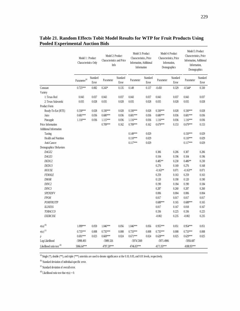
229
Table 21. Random Effects Tobit Model Results for WTP for Fruit Products Using
Pooled Experimental Auction Bids
Parameter(a)
Standard
ErrorParameter
Standard
ErrorParameter
Standard
ErrorParameter
Standard
ErrorParameter
Standard
Error
Constant 0.725*** 0.082 0.243* 0.135 0.149 0.137 -0.450 0.329 -0.544* 0.330
Variety
1: Texas Red 0.043 0.037 0.043 0.037 0.043 0.037 0.043 0.037 0.043 0.037
2: Texas Salavatski 0.035 0.028 0.035 0.028 0.035 0.028 0.035 0.028 0.035 0.028
Product Form
Ready-To-Eat (RTE) 0.330*** 0.028 0.330*** 0.028 0.330*** 0.028 0.330*** 0.028 0.330*** 0.028
Juice 0.681*** 0.036 0.680*** 0.036 0.681*** 0.036 0.680*** 0.036 0.681*** 0.036
Pineapple 1.116*** 0.036 1.115*** 0.036 1.116*** 0.036 1.116*** 0.036 1.116*** 0.036
Price Information 0.709*** 0.162 0.709*** 0.162 0.679*** 0.153 0.679*** 0.153
Additional Information
Tasting 0.149*** 0.029 0.150*** 0.029
Health and Nutrition 0.110*** 0.029 0.110*** 0.029
Anti-Cancer 0.117*** 0.029 0.117*** 0.029
Demographics/ Behaviors
DAGE2 0.306 0.206 0.307 0.206
DAGE3 0.104 0.196 0.104 0.196
DEDU2 0.485** 0.230 0.486** 0.230
DEDU3 0.276 0.169 0.276 0.168
HOUSE -0.163** 0.071 -0.163** 0.071
FEMALE 0.259 0.163 0.259 0.163
DMAR 0.120 0.190 0.120 0.190
DINC2 0.190 0.184 0.190 0.184
DINC3 0.287 0.260 0.287 0.260
SPENDFV 0.006 0.004 0.006 0.004
FPOH 0.017 0.017 0.017 0.017
POMFRUITP 0.688*** 0.165 0.688*** 0.165
ILLNESS 0.017 0.167 0.018 0.167
TOBACCO 0.336 0.225 0.336 0.225
EXERCISE -0.002 0.235 -0.002 0.235
σ(u) (b)
1.099*** 0.059 1.046*** 0.056 1.046*** 0.056 0.955*** 0.051 0.954*** 0.051
σ(e) (c)
0.735*** 0.008 0.735*** 0.008 0.733*** 0.008 0.735*** 0.008 0.733*** 0.008
ρ 0.691*** 0.023 0.669*** 0.024 0.671*** 0.024 0.628*** 0.025 0.629*** 0.025
Log-Likelihood -5998.493 -5989.326 -5974.5369 -5971.4906 -5956.687
Likelihood ratio test (d)
5066.64*** 4797.20*** 4746.83*** 4171.93*** 4188.95***
(a) Single (*), double (**), and triple (***) asterisks are used to denote significance at the 0.10, 0.05, and 0.01 levels, respectively.
(b) Standard deviation of individual-specific error.
(c) Standard deviation of overall error.
(d) Likelihood ratio test that σ(u) = 0.
Model 1 : Product
Characteristics Only
Model 2: Product
Characteristics and Price
Info
Model 3: Product
Characteristics, Price
Information, Additional
Information
Model 4: Product
Characteristics, Price
Information,
Demographics
Model 5: Product
Characteristics, Price
Information, Additional
Information,
Demographics
230
Furthermore, there were differences in the significance of the demographic
variables when the tobit model was specified to allow for random effects. When
demographic variables were included (Models 4 and 5), the random effects model only
suggests an influence on subject bids from the demographic/ behavioral characteristics
of having a 4-year college degree, household size, and previous purchase of a
pomegranate fruit. This suggests that for the novel fruit product of pomegranate there
may have been less of an influence on WTP of standard demographic characteristics
than would be expected for more familiar products.
Specification of the random effects tobit model also provides additional
regression statistics which can be useful in determining whether the model is
appropriate. The standard deviation of the individual specific error as σ(u) is provided,
and this can be tested against a standard tobit model in which σ(u) = 0 using a likelihood
ratio test. The results of the likelihood ratio test are given in the final row of Table 21.
Also provided is the value labeled ρ; this value is the percent of the overall variance that
is contributed by the individual variance. Therefore, ρ takes on values from zero to one,
with a value of zero indicating that none of the variance comes from the individual
random effects and a value of one indicating that all of the variance in the overall model
comes from the individual effects.
The likelihood ratio test rejects a specification of no individual specific error for
all five variable specifications (P < 0.001). Thus, if the assumptions of the model are
correct, the conclusion is that there are individual specific effects and that the standard
tobit model would be inappropriate.
231
As with the tobit model, the marginal effects of the random effects tobit are
useful in comparing one-unit changes for any regressor. The marginal effects are
presented in Table 22.
The random effects tobit model indicates a slightly greater increase in bids based
on the tasting information treatment when compared to the other two additional
information treatments. However, each information treatment indicates an increase of
less than $0.10 from the baseline bid. The product forms and price information had
larger marginal effects on the bid that was submitted. In looking at the demographic and
behavioral characteristics, a subject with a four-year university degree is estimated to be
willing to pay $0.31 more than an individual without a 4-year university degree.
However, this effect is still smaller than that of previous purchase of a pomegranate
fruit, which is estimated to increase the bid of a subject by $0.44 versus someone who
has not previously purchased a pomegranate fruit product. The final relevant
demographic/ behavioral marginal effect is for household size, which is estimated to
decrease bids by $0.10 for each additional member of the household. This could be
interpreted as a relationship of the tastes and preferences of individuals with larger
families, or a tradeoff in the quantity versus quality of food products that a larger
household with an income constraint must purchase.
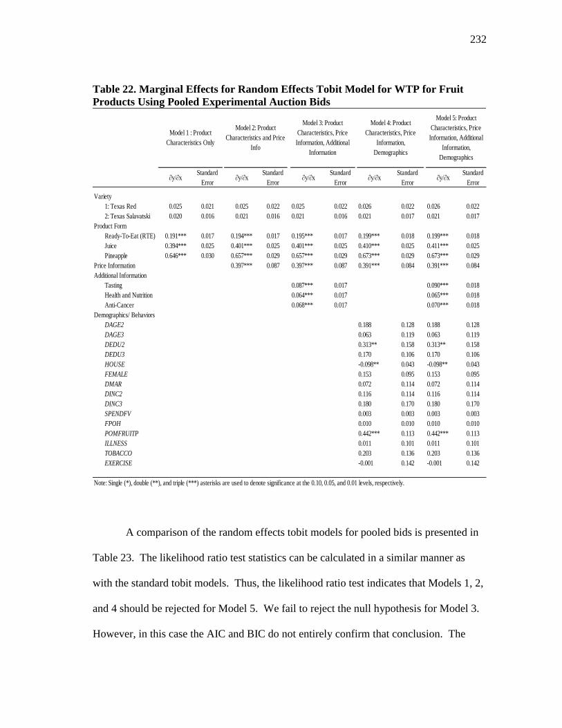
232
Table 22. Marginal Effects for Random Effects Tobit Model for WTP for Fruit
Products Using Pooled Experimental Auction Bids
A comparison of the random effects tobit models for pooled bids is presented in
Table 23. The likelihood ratio test statistics can be calculated in a similar manner as
with the standard tobit models. Thus, the likelihood ratio test indicates that Models 1, 2,
and 4 should be rejected for Model 5. We fail to reject the null hypothesis for Model 3.
However, in this case the AIC and BIC do not entirely confirm that conclusion. The
∂y/∂xStandard
Error∂y/∂x
Standard
Error∂y/∂x
Standard
Error∂y/∂x
Standard
Error∂y/∂x
Standard
Error
Variety
1: Texas Red 0.025 0.021 0.025 0.022 0.025 0.022 0.026 0.022 0.026 0.022
2: Texas Salavatski 0.020 0.016 0.021 0.016 0.021 0.016 0.021 0.017 0.021 0.017
Product Form
Ready-To-Eat (RTE) 0.191*** 0.017 0.194*** 0.017 0.195*** 0.017 0.199*** 0.018 0.199*** 0.018
Juice 0.394*** 0.025 0.401*** 0.025 0.401*** 0.025 0.410*** 0.025 0.411*** 0.025
Pineapple 0.646*** 0.030 0.657*** 0.029 0.657*** 0.029 0.673*** 0.029 0.673*** 0.029
Price Information 0.397*** 0.087 0.397*** 0.087 0.391*** 0.084 0.391*** 0.084
Additional Information
Tasting 0.087*** 0.017 0.090*** 0.018
Health and Nutrition 0.064*** 0.017 0.065*** 0.018
Anti-Cancer 0.068*** 0.017 0.070*** 0.018
Demographics/ Behaviors
DAGE2 0.188 0.128 0.188 0.128
DAGE3 0.063 0.119 0.063 0.119
DEDU2 0.313** 0.158 0.313** 0.158
DEDU3 0.170 0.106 0.170 0.106
HOUSE -0.098** 0.043 -0.098** 0.043
FEMALE 0.153 0.095 0.153 0.095
DMAR 0.072 0.114 0.072 0.114
DINC2 0.116 0.114 0.116 0.114
DINC3 0.180 0.170 0.180 0.170
SPENDFV 0.003 0.003 0.003 0.003
FPOH 0.010 0.010 0.010 0.010
POMFRUITP 0.442*** 0.113 0.442*** 0.113
ILLNESS 0.011 0.101 0.011 0.101
TOBACCO 0.203 0.136 0.203 0.136
EXERCISE -0.001 0.142 -0.001 0.142
Note: Single (*), double (**), and triple (***) asterisks are used to denote significance at the 0.10, 0.05, and 0.01 levels, respectively.
Model 1 : Product
Characteristics Only
Model 2: Product
Characteristics and Price
Info
Model 3: Product
Characteristics, Price
Information, Additional
Information
Model 4: Product
Characteristics, Price
Information,
Demographics
Model 5: Product
Characteristics, Price
Information, Additional
Information,
Demographics

233
AIC still suggests that Model 3 and 5 should both be considered, but the BIC actually
suggests that Models 1-3 would be preferred because the additional variables included in
Models 4-5 are not shown to substantially improve the fit of the model. However, this
result is not unexpected since the random effects tobit model controls for the
characteristics of each individual and the demographic and behavioral characteristics are
specific to each individual.
Table 23. Specification Test Values, Random Effects Tobit Models for Pooled
Auction Bids
Mixed Linear Models
The mixed (random parameters) linear model was applied to the participant bids
to account for possible correlations in the repeated bids of each individual (individual
heterogeneity). It is perhaps an unjustified assumption to presume that there is no
individual heterogeneity across products and across rounds. The mixed linear models
were estimated using maximum likelihood estimation.
Model 1 Model 2 Model 3 Model 4 Model 5
Likelihood Ratio Test Statistic (a) 54.01 35.67 6.09 29.61 ---
P-Value 0.0000 0.0020 0.9113 0.0000 ---
Degrees of Freedom 19 18 15 3 ---
AIC 12,012.99 11,996.65 11,973.07 11,990.98 11,967.37
BIC 12,065.95 12,056.24 12,052.52 12,149.87 12,146.13
(a) Likelihood ratio test statistics are all calculated compared to Model 5.

234
In examining the results for Models 1-5 as specified in the previous models
reported in Table 24, there are a number of points of comparison with the models
already reported. The results for the two Texas varieties are robust to this model
specification in that they are not significant in a mixed linear model. Again, the product
forms are all significant (P < 0.01) regardless of whether the demographic and/or
information variables are included in the model. While there is a tendency for an
influence of a college degree on bids, the only effects on the bids that we can expect are
a negative effect for household size and a positive effect on bids from previous
purchases of pomegranate fruit. The likelihood of this can be given by the log-
likelihood value. Also included in Table 24 are the estimated standard deviations for the
random effects specified at the individual level, reported as ̂ .
A likelihood ratio test of the null hypothesis H0 (linear regression model) versus
HA (mixed linear model) was conducted for each set of regressors. The results are listed
as the last line in Table 24. The null hypothesis of a linear regression model was
rejected for all sets of explanatory variables. This indicates that there are effects within
the model which can be accounted for by using a random parameters specification better
than can be accounted for using a standard linear regression.
For the mixed linear model, an additional specification was also estimated to
allow for further comparisons. In Model 6 given in Table 24, the model was extended to
allow for random effects on the terms for the information treatments. This can be
interpreted as variation in the effect that any particular information treatment might have
had on an individual. Thus, while an individual‘s preferences may have given him a
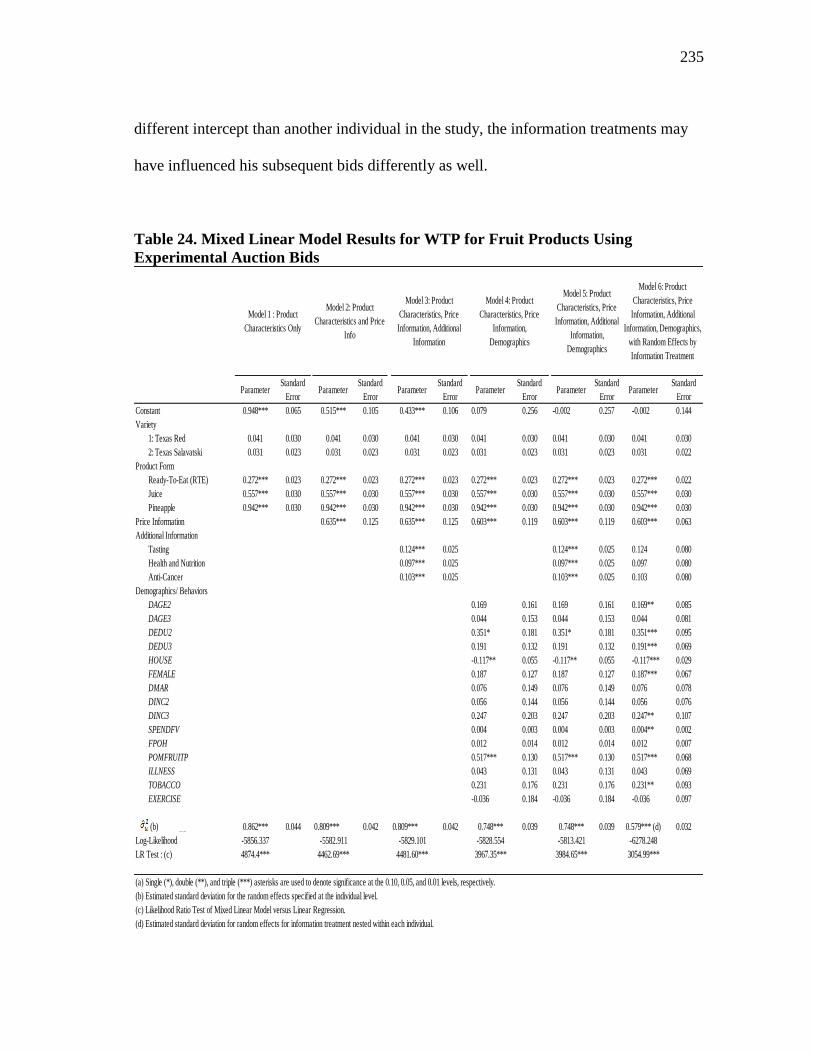
235
different intercept than another individual in the study, the information treatments may
have influenced his subsequent bids differently as well.
Table 24. Mixed Linear Model Results for WTP for Fruit Products Using
Experimental Auction Bids
ParameterStandard
ErrorParameter
Standard
ErrorParameter
Standard
ErrorParameter
Standard
ErrorParameter
Standard
ErrorParameter
Standard
Error
Constant 0.948*** 0.065 0.515*** 0.105 0.433*** 0.106 0.079 0.256 -0.002 0.257 -0.002 0.144
Variety
1: Texas Red 0.041 0.030 0.041 0.030 0.041 0.030 0.041 0.030 0.041 0.030 0.041 0.030
2: Texas Salavatski 0.031 0.023 0.031 0.023 0.031 0.023 0.031 0.023 0.031 0.023 0.031 0.022
Product Form
Ready-To-Eat (RTE) 0.272*** 0.023 0.272*** 0.023 0.272*** 0.023 0.272*** 0.023 0.272*** 0.023 0.272*** 0.022
Juice 0.557*** 0.030 0.557*** 0.030 0.557*** 0.030 0.557*** 0.030 0.557*** 0.030 0.557*** 0.030
Pineapple 0.942*** 0.030 0.942*** 0.030 0.942*** 0.030 0.942*** 0.030 0.942*** 0.030 0.942*** 0.030
Price Information 0.635*** 0.125 0.635*** 0.125 0.603*** 0.119 0.603*** 0.119 0.603*** 0.063
Additional Information
Tasting 0.124*** 0.025 0.124*** 0.025 0.124 0.080
Health and Nutrition 0.097*** 0.025 0.097*** 0.025 0.097 0.080
Anti-Cancer 0.103*** 0.025 0.103*** 0.025 0.103 0.080
Demographics/ Behaviors
DAGE2 0.169 0.161 0.169 0.161 0.169** 0.085
DAGE3 0.044 0.153 0.044 0.153 0.044 0.081
DEDU2 0.351* 0.181 0.351* 0.181 0.351*** 0.095
DEDU3 0.191 0.132 0.191 0.132 0.191*** 0.069
HOUSE -0.117** 0.055 -0.117** 0.055 -0.117*** 0.029
FEMALE 0.187 0.127 0.187 0.127 0.187*** 0.067
DMAR 0.076 0.149 0.076 0.149 0.076 0.078
DINC2 0.056 0.144 0.056 0.144 0.056 0.076
DINC3 0.247 0.203 0.247 0.203 0.247** 0.107
SPENDFV 0.004 0.003 0.004 0.003 0.004** 0.002
FPOH 0.012 0.014 0.012 0.014 0.012 0.007
POMFRUITP 0.517*** 0.130 0.517*** 0.130 0.517*** 0.068
ILLNESS 0.043 0.131 0.043 0.131 0.043 0.069
TOBACCO 0.231 0.176 0.231 0.176 0.231** 0.093
EXERCISE -0.036 0.184 -0.036 0.184 -0.036 0.097
(b) 0.862*** 0.044 0.809*** 0.042 0.809*** 0.042 0.748*** 0.039 0.748*** 0.039 0.579*** (d) 0.032
Log-Likelihood -5856.337 -5582.911 -5829.101 -5828.554 -5813.421 -6278.248
LR Test : (c) 4874.4*** 4462.69*** 4481.60*** 3967.35*** 3984.65*** 3054.99***
(a) Single (*), double (**), and triple (***) asterisks are used to denote significance at the 0.10, 0.05, and 0.01 levels, respectively.
(b) Estimated standard deviation for the random effects specified at the individual level.
(c) Likelihood Ratio Test of Mixed Linear Model versus Linear Regression.
(d) Estimated standard deviation for random effects for information treatment nested within each individual.
Model 1 : Product
Characteristics Only
Model 2: Product
Characteristics and Price
Info
Model 3: Product
Characteristics, Price
Information, Additional
Information
Model 4: Product
Characteristics, Price
Information,
Demographics
Model 5: Product
Characteristics, Price
Information, Additional
Information,
Demographics
Model 6: Product
Characteristics, Price
Information, Additional
Information, Demographics,
with Random Effects by
Information Treatment
236
For example, it was anticipated that the anti-cancer information might have a
greater effect on individuals with serious health conditions or who smoked on a regular
basis than those who did not. As another example, it was considered probable that the
tasting treatment would have a range of effects on the bids submitted, from strongly
negative to strongly positive, depending on whether that individual found the taste of
each product desirable or undesirable.
The values of the estimated parameters for the demographic model with a
random intercept only (Model 5) and the demographic model with a random intercept
and random coefficients (Model 6) for the information treatments are equal in this case.
However, looking at only the estimated parameters does not tell the full story of the
differences between these two models. The explanatory variables that would actually be
included in predictions of WTP would be very different for the two models. When the
information effect is allowed to vary for each individual, the additional information
treatments no longer has predictive ability in this model. However, the demographic
characteristics gain additional significance. Here, the 30-49 year old age group, a
college degree, completion of at least some graduate school, being a female, having a
household income greater than $100,000, having higher spending on fruits and
vegetables, and using tobacco products all increased the bids for the fruit products; only
a larger household size decreased the WTP for the fruit products.
This begs the question of which model specification for the mixed linear models
is more correct, given that either could be based on a relevant economic interpretation of
the results. First, a comparison of the Akaike Information Criterion (AIC) and the
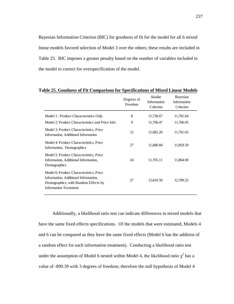
237
Bayesian Information Criterion (BIC) for goodness of fit for the model for all 6 mixed
linear models favored selection of Model 3 over the others; these results are included in
Table 25. BIC imposes a greater penalty based on the number of variables included in
the model to correct for overspecification of the model.
Table 25. Goodness of Fit Comparison for Specifications of Mixed Linear Models
Additionally, a likelihood ratio test can indicate differences in mixed models that
have the same fixed effects specifications. Of the models that were estimated, Models 4
and 6 can be compared as they have the same fixed effects (Model 6 has the addition of
a random effect for each information treatment). Conducting a likelihood ratio test
under the assumption of Model 6 nested within Model 4, the likelihood ratio χ2 has a
value of -899.39 with 3 degrees of freedom; therefore the null hypothesis of Model 4
Degrees of
Freedom
Akaike
Information
Criterion
Bayesian
Information
Criterion
Model 1 : Product Characteristics Only 8 11,728.67 11,781.64
Model 2: Product Characteristics and Price Info 9 11,706.47 11,766.05
Model 3: Product Characteristics, Price
Information, Additional Information12 11,682.20 11,761.65
Model 4: Product Characteristics, Price
Information, Demographics27 11,680.84 11,859.59
Model 5: Product Characteristics, Price
Information, Additional Information,
Demographics
24 11,705.11 11,864.00
Model 6: Product Characteristics, Price
Information, Additional Information,
Demographics, with Random Effects by
Information Treatment
27 12,610.50 12,789.25

238
(the simpler model) cannot be rejected. These two tests would indicate that using AIC,
Model 4 is preferred to Model 6. Further results of AIC indicate that Models 1, 2, and 6
are not preferred. Models 3 and 4 are close in their values and so should both be
considered. Alternatively, using the Bayesian Information Criterion suggests that the
first 3 models are all similar but that Model 6 is less desirable. Based on consideration
of the purposes of this study in describing the product characteristics, information
treatments, and demographic variables that may have a role in the WTP for pomegranate
fruit products, Model 5 allows for additional relationships with demographics to be
included and will be used for further comparisons.
If the model including all variables and all information treatments (Model 5) is
chosen based on expected differences in relevant demographic behavioral characteristics
and information treatments, then this model can be used to address other interesting
questions based on the bids submitted by study participants.
Unengaged vs. Engaged Bidders
The novelty of the fruit products investigated in this study led to the hypothesis
that there would be a number of bidders who were completely unengaged in the auction
process. That is, these ―unengaged bidders,‖ despite being recruited for a study that
expressly dealt with fruit purchase decisionmaking, were disinterested in the bidding for
one or more of the fruit products, or the entire study. These subjects were identified as
those who submitted bids of $0.00 for a particular product for all four (Baseline, Tasting,
Health and Nutrition, and Anti-Cancer) information treatment rounds. The treatment of
239
unengaged bidders has been previously described by Lusk and Fox (2003) and Roosen,
Marette, and Blanchemanche (2010), who both report results for estimations based on
both engaged and unengaged bidders.
The underlying theory for which population of bidders, engaged or unengaged,
are the ones that provide economic information of interest is of value. The results
presented thus far have referred to the entire population of bidders, both those who are
engaged and those who are unengaged. Estimates based on the entire population of
bidders may be more reflective of the general population; given the novelty of the
included fruit products, it was unlikely that all bidders actually purchase all included
products in a real world setting on a regular basis. Therefore, further comparisons of the
previous model estimates suggest that they are likely to be more representative of the
general population of shoppers.
However, the population of potential buyers of fruit products is also of economic
interest. It should be useful to review what portion of the study participants were
unengaged in each product, as well as the implications of removing the unengaged
bidders from the sample prior to estimation of the models described earlier. The counts
and percentages of unengaged bidders for each fruit product are included in Table 26.
The numbers of unengaged bidders varies considerably from ten for the control
product of pineapple to 3.5 times as many unengaged bidders for the two Texas
pomegranate fruits. This supports our hypothesis on the greater familiarity of the
pineapple, and in a secondary manner the juice product, versus the whole pomegranate
fruits. In comparing these products, the number of bidders who were unengaged for any
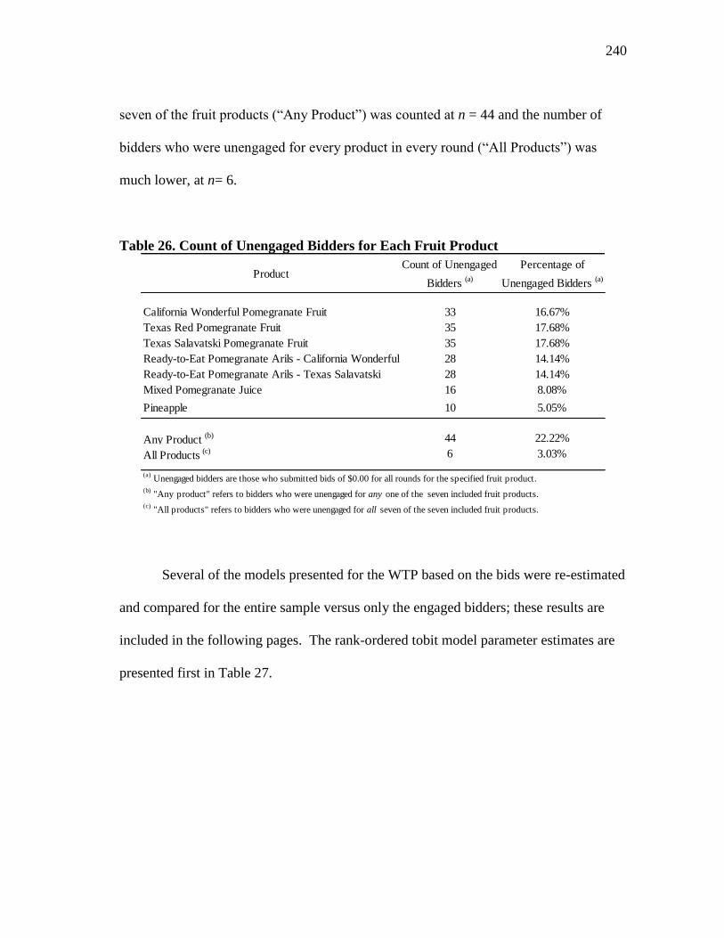
240
seven of the fruit products (―Any Product‖) was counted at n = 44 and the number of
bidders who were unengaged for every product in every round (―All Products‖) was
much lower, at n= 6.
Table 26. Count of Unengaged Bidders for Each Fruit Product
Several of the models presented for the WTP based on the bids were re-estimated
and compared for the entire sample versus only the engaged bidders; these results are
included in the following pages. The rank-ordered tobit model parameter estimates are
presented first in Table 27.
ProductCount of Unengaged
Bidders (a)
Percentage of
Unengaged Bidders (a)
California Wonderful Pomegranate Fruit 33 16.67%
Texas Red Pomegranate Fruit 35 17.68%
Texas Salavatski Pomegranate Fruit 35 17.68%
Ready-to-Eat Pomegranate Arils - California Wonderful 28 14.14%
Ready-to-Eat Pomegranate Arils - Texas Salavatski 28 14.14%
Mixed Pomegranate Juice 16 8.08%
Pineapple 10 5.05%
Any Product (b) 44 22.22%
All Products (c) 6 3.03%
(a) Unengaged bidders are those who submitted bids of $0.00 for all rounds for the specified fruit product.
(b) "Any product" refers to bidders who were unengaged for any one of the seven included fruit products.
(c) "All products" refers to bidders who were unengaged for all seven of the seven included fruit products.
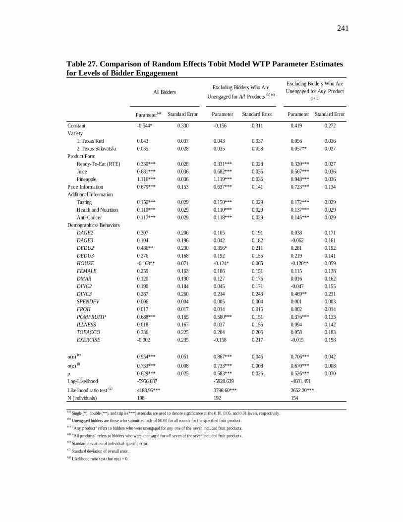
241
Table 27. Comparison of Random Effects Tobit Model WTP Parameter Estimates
for Levels of Bidder Engagement
Parameter(a) Standard Error Parameter Standard Error Parameter Standard Error
Constant -0.544* 0.330 -0.156 0.311 0.419 0.272
Variety
1: Texas Red 0.043 0.037 0.043 0.037 0.056 0.036
2: Texas Salavatski 0.035 0.028 0.035 0.028 0.057** 0.027
Product Form
Ready-To-Eat (RTE) 0.330*** 0.028 0.331*** 0.028 0.320*** 0.027
Juice 0.681*** 0.036 0.682*** 0.036 0.567*** 0.036
Pineapple 1.116*** 0.036 1.119*** 0.036 0.948*** 0.036
Price Information 0.679*** 0.153 0.637*** 0.141 0.723*** 0.134
Additional Information
Tasting 0.150*** 0.029 0.150*** 0.029 0.172*** 0.029
Health and Nutrition 0.110*** 0.029 0.110*** 0.029 0.137*** 0.029
Anti-Cancer 0.117*** 0.029 0.118*** 0.029 0.145*** 0.029
Demographics/ Behaviors
DAGE2 0.307 0.206 0.105 0.191 0.038 0.171
DAGE3 0.104 0.196 0.042 0.182 -0.062 0.161
DEDU2 0.486** 0.230 0.356* 0.211 0.281 0.192
DEDU3 0.276 0.168 0.192 0.155 0.219 0.141
HOUSE -0.163** 0.071 -0.124* 0.065 -0.120** 0.059
FEMALE 0.259 0.163 0.186 0.151 0.115 0.138
DMAR 0.120 0.190 0.127 0.176 0.016 0.162
DINC2 0.190 0.184 0.045 0.171 -0.047 0.155
DINC3 0.287 0.260 0.214 0.243 0.469** 0.231
SPENDFV 0.006 0.004 0.005 0.004 0.001 0.003
FPOH 0.017 0.017 0.014 0.016 0.002 0.014
POMFRUITP 0.688*** 0.165 0.580*** 0.151 0.376*** 0.133
ILLNESS 0.018 0.167 0.037 0.155 0.094 0.142
TOBACCO 0.336 0.225 0.204 0.206 0.058 0.183
EXERCISE -0.002 0.235 -0.158 0.217 -0.015 0.198
σ(u) (e)
0.954*** 0.051 0.867*** 0.046 0.706*** 0.042
σ(e) (f)
0.733*** 0.008 0.733*** 0.008 0.670*** 0.008
ρ 0.629*** 0.025 0.583*** 0.026 0.526*** 0.030
Log-Likelihood -5956.687 -5928.639 -4681.491
Likelihood ratio test (g)
4188.95*** 3796.60*** 2652.20***
N (individuals) 198 192 154
(b) Unengaged bidders are those who submitted bids of $0.00 for all rounds for the specified fruit product.
(c) "Any product" refers to bidders who were unengaged for any one of the seven included fruit products.
(d) "All products" refers to bidders who were unengaged for all seven of the seven included fruit products.
(e) Standard deviation of individual-specific error.
(f) Standard deviation of overall error.
(g) Likelihood ratio test that σ(u) = 0.
(a) Single (*), double (**), and triple (***) asterisks are used to denote significance at the 0.10, 0.05, and 0.01 levels, respectively.
All Bidders
Excluding Bidders Who Are
Unengaged for Any Product (b) (d)
Excluding Bidders Who Are
Unengaged for All Products (b) (c)
242
The results for ―all bidders‖ are the same as those for Model 5 in the original
rank-ordered tobit model estimates. These are compared to models where either
individuals who were unengaged for all products are removed or where individuals who
were unengaged for any product are removed. In the former case, those individuals who
were unengaged for all products indicated with their bids that they would be unwilling to
purchase any of the fruit products, regardless of the product characteristics and
regardless of the additional information that was provided. There is a lack of
information provided by these bids in terms of understanding whether the information
treatments or individual characteristics influenced their preferences for the products
since all bids were reported as zero.
On the other hand, excluding bidders who were unengaged for ―any product‖
removes a larger portion of the sample, but also removes those individuals who were
unengaged for any of the bids that are included in the regression. Thus, there should be
no bidders who were unengaged for any product included in the latter model.
In the model excluding bidders who were unengaged for all products, the only
demographic or behavioral characteristic that still has predictive power is whether or not
the individual has made previous purchases of pomegranate fruits. As a consequence,
the model including all bidders may have a suggestion as to which bidders will submit
zero bids, regardless of whether they are engaged; this may not be true of bidders that
were engaged for at least one product.
The models in which bidders who were unengaged for any product were
removed are a more interesting comparison. These models can be thought of as models
243
of those individuals who would actually purchase each product in at least one round of
the experimental auctions. There is a significant effect (P < 0.05) for the Texas
Salavatski Pomegranate variety.
This is the only model discussed so far in which there has been any effect due to
the growing location of any of the pomegranate fruit products. If individuals are willing
to buy the pomegranate products, then the random effects model that accounts for
unengaged bidders suggests there is a positive price premium for the Texas Salavatski
variety.
To determine the size of such an effect, the marginal effects are again used and
are presented in Table 28. Thus, although it is not a large sum, there is expected to be a
$0.04 premium in WTP for the Texas Salavatski pomegranate over the California
Wonderful baseline product. Also in looking at the marginal effects, the magnitude of
the effect of the information treatments is larger when unengaged bidders are removed,
as would be expected; all of the bidders whose bids were removed had no change in bids
(from $0.00) across any information treatments. Similarly, there is a larger effect from
the product characteristics on WTP because the individuals whose bids were excluded
may have been unengaged for more than one product, and thus differences in WTP
predicted by product characteristics would be masked to some extent. The effect of price
information is also larger on engaged versus unengaged bidders.
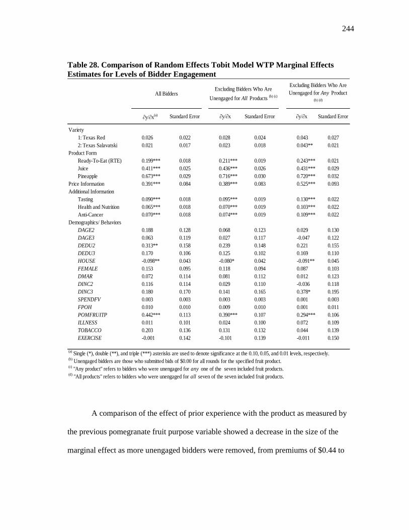
244
Table 28. Comparison of Random Effects Tobit Model WTP Marginal Effects
Estimates for Levels of Bidder Engagement
A comparison of the effect of prior experience with the product as measured by
the previous pomegranate fruit purpose variable showed a decrease in the size of the
marginal effect as more unengaged bidders were removed, from premiums of $0.44 to
∂y/∂x(a) Standard Error ∂y/∂x Standard Error ∂y/∂x Standard Error
Variety
1: Texas Red 0.026 0.022 0.028 0.024 0.043 0.027
2: Texas Salavatski 0.021 0.017 0.023 0.018 0.043** 0.021
Product Form
Ready-To-Eat (RTE) 0.199*** 0.018 0.211*** 0.019 0.243*** 0.021
Juice 0.411*** 0.025 0.436*** 0.026 0.431*** 0.029
Pineapple 0.673*** 0.029 0.716*** 0.030 0.720*** 0.032
Price Information 0.391*** 0.084 0.389*** 0.083 0.525*** 0.093
Additional Information
Tasting 0.090*** 0.018 0.095*** 0.019 0.130*** 0.022
Health and Nutrition 0.065*** 0.018 0.070*** 0.019 0.103*** 0.022
Anti-Cancer 0.070*** 0.018 0.074*** 0.019 0.109*** 0.022
Demographics/ Behaviors
DAGE2 0.188 0.128 0.068 0.123 0.029 0.130
DAGE3 0.063 0.119 0.027 0.117 -0.047 0.122
DEDU2 0.313** 0.158 0.239 0.148 0.221 0.155
DEDU3 0.170 0.106 0.125 0.102 0.169 0.110
HOUSE -0.098** 0.043 -0.080* 0.042 -0.091** 0.045
FEMALE 0.153 0.095 0.118 0.094 0.087 0.103
DMAR 0.072 0.114 0.081 0.112 0.012 0.123
DINC2 0.116 0.114 0.029 0.110 -0.036 0.118
DINC3 0.180 0.170 0.141 0.165 0.378* 0.195
SPENDFV 0.003 0.003 0.003 0.003 0.001 0.003
FPOH 0.010 0.010 0.009 0.010 0.001 0.011
POMFRUITP 0.442*** 0.113 0.390*** 0.107 0.294*** 0.106
ILLNESS 0.011 0.101 0.024 0.100 0.072 0.109
TOBACCO 0.203 0.136 0.131 0.132 0.044 0.139
EXERCISE -0.001 0.142 -0.101 0.139 -0.011 0.150
(b) Unengaged bidders are those who submitted bids of $0.00 for all rounds for the specified fruit product.
(c) "Any product" refers to bidders who were unengaged for any one of the seven included fruit products.
(d) "All products" refers to bidders who were unengaged for all seven of the seven included fruit products.
(a) Single (*), double (**), and triple (***) asterisks are used to denote significance at the 0.10, 0.05, and 0.01 levels, respectively.
All BiddersExcluding Bidders Who Are
Unengaged for All Products (b) (c)
Excluding Bidders Who Are
Unengaged for Any Product (b) (d)
245
$0.39 to $0.29. Of those bidders who were engaged, the marginal effect of the
additional information treatments was relatively larger and the marginal effect of
previous purchase of pomegranate fruit products was relatively smaller when compared
to models including all bidders. This model also suggested a tendency (P < 0.10) of a
bid premium of $0.38 for subjects who had annual household incomes of greater than
$100,000 over individuals with an annual household income of less than $50,000.
The mixed linear model including the pooled product bids was also re-estimated
to account for unengaged bidders; please see Table 29. Again, the product forms, price
information, and additional information treatments all have a significant effect (P <
0.01) on estimated WTP, with the size of these effects increasing in the model for
entirely engaged bidders for the information variables.
In a similar manner to the previously estimated models, there is an inverse
relationship between household size and observed bids for the fruit products. Further,
the influence of previous experience with the products also decreases as more unengaged
bidders are removed from the sample. Consequently, the previous experience with the
product (as indicated by POMFRUITP) should be a predictor of whether the individual
will be engaged in the experimental auction.
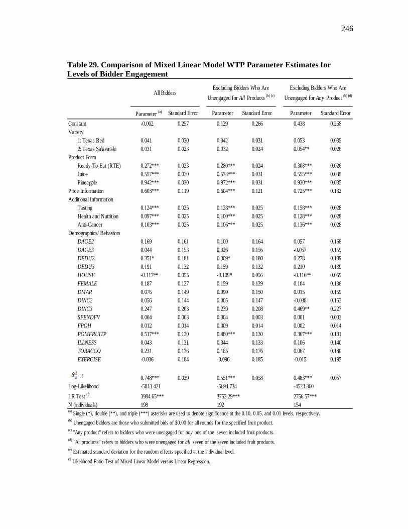
246
Table 29. Comparison of Mixed Linear Model WTP Parameter Estimates for
Levels of Bidder Engagement
Parameter (a) Standard Error Parameter Standard Error Parameter Standard Error
Constant -0.002 0.257 0.129 0.266 0.438 0.268
Variety
1: Texas Red 0.041 0.030 0.042 0.031 0.053 0.035
2: Texas Salavatski 0.031 0.023 0.032 0.024 0.054** 0.026
Product Form
Ready-To-Eat (RTE) 0.272*** 0.023 0.280*** 0.024 0.308*** 0.026
Juice 0.557*** 0.030 0.574*** 0.031 0.555*** 0.035
Pineapple 0.942*** 0.030 0.972*** 0.031 0.930*** 0.035
Price Information 0.603*** 0.119 0.604*** 0.121 0.725*** 0.132
Additional Information
Tasting 0.124*** 0.025 0.128*** 0.025 0.158*** 0.028
Health and Nutrition 0.097*** 0.025 0.100*** 0.025 0.128*** 0.028
Anti-Cancer 0.103*** 0.025 0.106*** 0.025 0.136*** 0.028
Demographics/ Behaviors
DAGE2 0.169 0.161 0.100 0.164 0.057 0.168
DAGE3 0.044 0.153 0.026 0.156 -0.057 0.159
DEDU2 0.351* 0.181 0.309* 0.180 0.278 0.189
DEDU3 0.191 0.132 0.159 0.132 0.210 0.139
HOUSE -0.117** 0.055 -0.109* 0.056 -0.116** 0.059
FEMALE 0.187 0.127 0.159 0.129 0.104 0.136
DMAR 0.076 0.149 0.090 0.150 0.015 0.159
DINC2 0.056 0.144 0.005 0.147 -0.038 0.153
DINC3 0.247 0.203 0.239 0.208 0.469** 0.227
SPENDFV 0.004 0.003 0.004 0.003 0.001 0.003
FPOH 0.012 0.014 0.009 0.014 0.002 0.014
POMFRUITP 0.517*** 0.130 0.480*** 0.130 0.367*** 0.131
ILLNESS 0.043 0.131 0.044 0.133 0.106 0.140
TOBACCO 0.231 0.176 0.185 0.176 0.067 0.180
EXERCISE -0.036 0.184 -0.096 0.185 -0.015 0.195
(e)
0.748*** 0.039 0.551*** 0.058 0.483*** 0.057
Log-Likelihood -5813.421 -5694.734 -4523.360
LR Test (f)
3984.65*** 3753.29*** 2756.57***
N (individuals) 198 192 154
(b) Unengaged bidders are those who submitted bids of $0.00 for all rounds for the specified fruit product.
(c) "Any product" refers to bidders who were unengaged for any one of the seven included fruit products.
(d) "All products" refers to bidders who were unengaged for all seven of the seven included fruit products.
(e) Estimated standard deviation for the random effects specified at the individual level.
(f) Likelihood Ratio Test of Mixed Linear Model versus Linear Regression.
(a) Single (*), double (**), and triple (***) asterisks are used to denote significance at the 0.10, 0.05, and 0.01 levels, respectively.
All BiddersExcluding Bidders Who Are
Unengaged for All Products (b) (c)
Excluding Bidders Who Are
Unengaged for Any Product (b) (d)
247
There are three additional results that are of primary interest in the mixed linear
model that includes only engaged bids by engaged bidders: those for the Texas varieties,
those for the upper income dummy variable, and those for the constant. This model
predicts a $0.05 premium for the Texas Salavatski variety as compared to the baseline
California Wonderful variety. The P-value for the Texas Red variety in the model that
excluded any individual who was unengaged was P = 0.12.
With an estimated size of the effect that is the same for either Texas variety over
California Wonderful, the difference in significance was hypothesized to likely be due to
the fact that there were two products included in the experimental auction that were the
Texas Salavatski variety and only one product that was Texas Red, so there would be
twice as many bid observations for the Texas Salavatski variety. (Some of the original
standard tobit models including all demographic and behavioral variables were estimated
using a single variable for the Texas varieties and they generally produced results that
were not significant for an effect of the Texas varieties.)
The random effects tobit and the mixed linear model that removed any
unengaged bidders were re-estimated to test such a hypothesis, and the results for those
two models are included in Appendix H in Table 56 -Table 58. The estimations of these
models give coefficients that are the same for all other included variables, excepting the
Texas varieties. However, the value for the single ―Grown in Texas‖ variable is the
same as that previously estimated for the Texas Salavatski variety, but the standard error
is smaller. This would lead us to conclude that there is an effect of the Texas variety in
general but that effect can be further divided into a specific contribution from the Texas
248
Salavatski variety in this experiment. However, this does not reject the idea that there
could be an increase in WTP for the Texas Red variety as well; rather, we fail to reject
the hypothesis that there is no change in WTP for the Texas Red variety.
The next point of interest from the comparison of engaged versus unengaged
bidders is the result for the upper income (annual household income greater than
$100,000) dummy variable. In the model for bidders who were engaged for every
product, a $0.47 increase in WTP was predicted for the included fruit products by
individuals who fit this demographic category. Thus, of individuals who were engaged
for every product, the expected positive relationship between higher income and higher
WTP was seen, but this distinction could not be made when unengaged bidders were
included.
The third result of interest is that in the estimations that include bidders who
were engaged for every product, the constant estimates (although still not significant at P
< 0.05) are now positive for the baseline product. This is expected, since engaged
bidders were those who had a positive value for the product regardless of their
demographic characteristics.
The comparisons of the models for all bidders, bidders who were engaged for at
least one product, and bidders who were engaged for all products allow for valuable
comparisons of the general population of shoppers versus bidders who would actually
make purchases of pomegranate fruit products. This is akin to the exclusion of non-
shoppers from WTP and discrete choice studies in terms of the relevance of results.
Nonetheless, a number of the included products were novel (unfamiliar) in nature and
249
excluding bidders who were not fully engaged for every product in every round could
result in reports of effects of information treatments and product characteristics that do
not account for those consumers who purchase a novel product either before or after
gaining new information on that product. This information can also be useful to
marketers of novel products who want to know the maximum that currently engaged
buyers would be willing to pay for a product. Such information can also indicate the
factors that influence the decisions of consumers who are not current purchasers of a
product but would be willing to purchase a novel product once they have gained more
information on the novel product. In effect, these differences in the models for
unengaged versus partially engaged versus fully engaged bidders suggest that there is
value in all three types of sample selection, depending on the question that is to be
addressed by researchers. Also, considering all these estimates is particularly important
for an unfamiliar product.
Comparison of Models for Full Bids
Each of the models described previously has some benefit in regards to
understanding the relative value placed on the included products by consumers.
However, each is also paired with drawbacks in terms of predicting WTP and
subsequent buying behavior. The individual tobit models are perhaps the most
straightforward in their interpretation; however, the ability to generalize them across
information treatments and products is limited in comparison to a model that includes all
bids. However, although the OLS and mixed linear models include all products and
250
information treatments, they ignore bid censoring; on the other hand, the tobit and
random effects tobit models include bid censoring in the model but do not account for
individual variation in the effects of each product characteristic and/or information
treatment.
However, even given these drawbacks there are results that are robust across
models. The product forms of RTE, juice, and the type of fruit (pineapple versus
pomegranate) were generally significant predictors of WTP. However, the Texas
varieties versus the industry standard variety were not always significant, indicating that
the product form was more important in predicting WTP than the location of origin or
the specific variety. Also, having a reference price for the products and previous
experience with the products were generally indicators of an increase in WTP for the
fruit products included in this study. The rest of the demographic and behavioral
characteristics varied in whether they were good predictors of WTP, depending on the
model that was used.
It is not entirely surprising that this analysis does not suggest a strong ability of
demographic characteristics to predict willingness-to-pay. The usefulness of
demographics in predicting consumer willingness-to-pay has been found to be limited or
insignificant by other studies, including by Umberger and Feuz (2004) in predicting
WTP for quality-differentiated beef and by Lusk et al. (2001b) in evaluating beef
tenderness. Other studies have excluded demographic attributes from the modeling of
WTP (e.g., Abidoye et al. 2011). However, overall the results on the importance of
demographic factors in predicting WTP have been mixed. For example, in a recent
251
study on WTP for grass-fed beef Xue et al. (2010) found that several demographic
factors, including household size, nutritional knowledge, consumption behavior, and
health status were all predictors of WTP. Thus, consideration of demographic
characteristics is useful, but there is no guarantee that they will be predictors of WTP for
every product.
In terms of specific model comparisons, the evaluation of which of the random
effects tobit models and the mixed linear models are preferred is not straightforward.
Comparisons of the log-likelihood values are not valid because the models are not nested
inside one another. A Hausman test could be used to compare two models; however this
test assumes that one of the models is efficient while the other model is consistent. The
choice of which model is consistent should be based on the use of whichever model is
expected to converge at the true value of the parameters. However, the Hausman test is
not necessarily appropriate for the comparison of these two types of models. This leaves
the consideration of which model is more theoretically appropriate. This can be debated
as each of the random effects tobit models and mixed linear models have their own
drawbacks.
Bid Differences across Information Treatments
One important question to be answered regarding the information treatments is
whether there was a difference in the bids subjects submitted for each product following
each information treatment. The difference in the bids across treatments were compared
using paired t-tests and two-tailed non-parametric Wilcoxon signed-rank tests on the
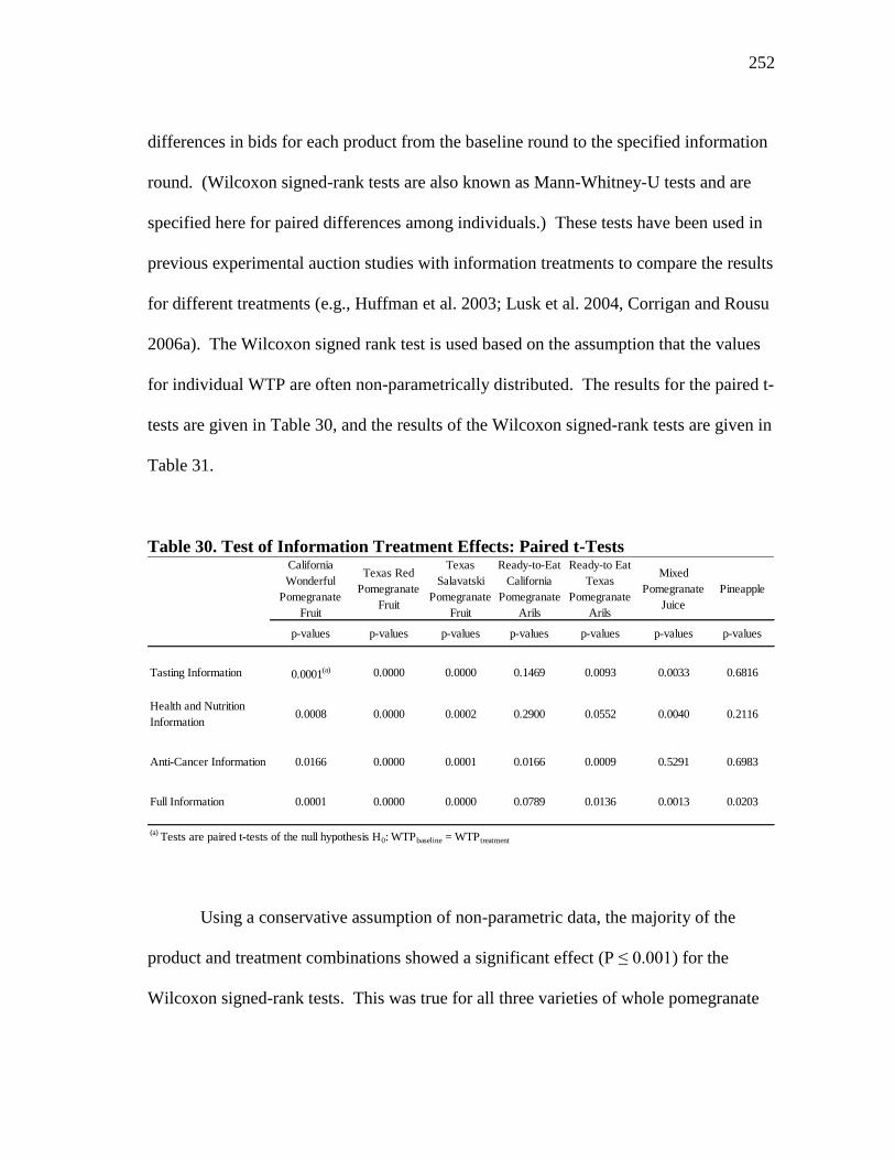
252
differences in bids for each product from the baseline round to the specified information
round. (Wilcoxon signed-rank tests are also known as Mann-Whitney-U tests and are
specified here for paired differences among individuals.) These tests have been used in
previous experimental auction studies with information treatments to compare the results
for different treatments (e.g., Huffman et al. 2003; Lusk et al. 2004, Corrigan and Rousu
2006a). The Wilcoxon signed rank test is used based on the assumption that the values
for individual WTP are often non-parametrically distributed. The results for the paired t-
tests are given in Table 30, and the results of the Wilcoxon signed-rank tests are given in
Table 31.
Table 30. Test of Information Treatment Effects: Paired t-Tests
Using a conservative assumption of non-parametric data, the majority of the
product and treatment combinations showed a significant effect (P ≤ 0.001) for the
Wilcoxon signed-rank tests. This was true for all three varieties of whole pomegranate
California
Wonderful
Pomegranate
Fruit
Texas Red
Pomegranate
Fruit
Texas
Salavatski
Pomegranate
Fruit
Ready-to-Eat
California
Pomegranate
Arils
Ready-to Eat
Texas
Pomegranate
Arils
Mixed
Pomegranate
Juice
Pineapple
p-values p-values p-values p-values p-values p-values p-values
Tasting Information 0.0001(a) 0.0000 0.0000 0.1469 0.0093 0.0033 0.6816
Health and Nutrition
Information0.0008 0.0000 0.0002 0.2900 0.0552 0.0040 0.2116
Anti-Cancer Information 0.0166 0.0000 0.0001 0.0166 0.0009 0.5291 0.6983
Full Information 0.0001 0.0000 0.0000 0.0789 0.0136 0.0013 0.0203
(a) Tests are paired t-tests of the null hypothesis H0: WTPbaseline = WTPtreatment
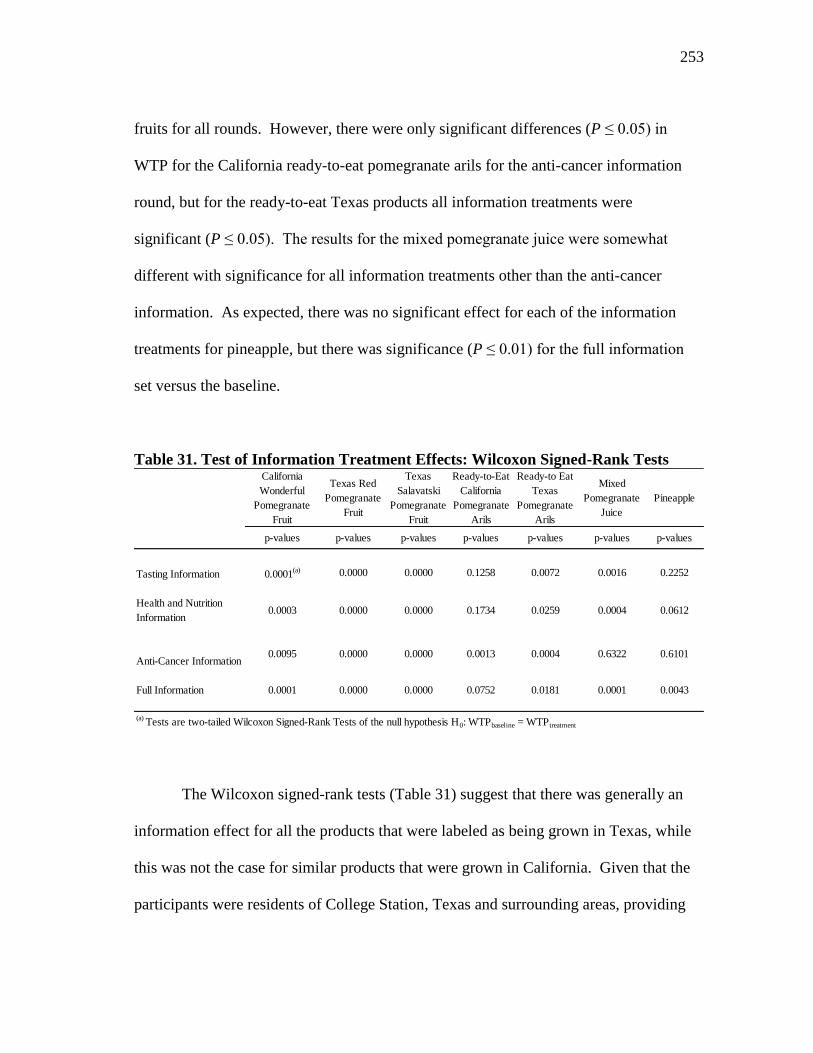
253
fruits for all rounds. However, there were only significant differences (P ≤ 0.05) in
WTP for the California ready-to-eat pomegranate arils for the anti-cancer information
round, but for the ready-to-eat Texas products all information treatments were
significant (P ≤ 0.05). The results for the mixed pomegranate juice were somewhat
different with significance for all information treatments other than the anti-cancer
information. As expected, there was no significant effect for each of the information
treatments for pineapple, but there was significance (P ≤ 0.01) for the full information
set versus the baseline.
Table 31. Test of Information Treatment Effects: Wilcoxon Signed-Rank Tests
The Wilcoxon signed-rank tests (Table 31) suggest that there was generally an
information effect for all the products that were labeled as being grown in Texas, while
this was not the case for similar products that were grown in California. Given that the
participants were residents of College Station, Texas and surrounding areas, providing
California
Wonderful
Pomegranate
Fruit
Texas Red
Pomegranate
Fruit
Texas
Salavatski
Pomegranate
Fruit
Ready-to-Eat
California
Pomegranate
Arils
Ready-to Eat
Texas
Pomegranate
Arils
Mixed
Pomegranate
Juice
Pineapple
p-values p-values p-values p-values p-values p-values p-values
Tasting Information 0.0001(a) 0.0000 0.0000 0.1258 0.0072 0.0016 0.2252
Health and Nutrition
Information0.0003 0.0000 0.0000 0.1734 0.0259 0.0004 0.0612
Anti-Cancer Information0.0095 0.0000 0.0000 0.0013 0.0004 0.6322 0.6101
Full Information 0.0001 0.0000 0.0000 0.0752 0.0181 0.0001 0.0043
(a) Tests are two-tailed Wilcoxon Signed-Rank Tests of the null hypothesis H0: WTPbaseline = WTPtreatment
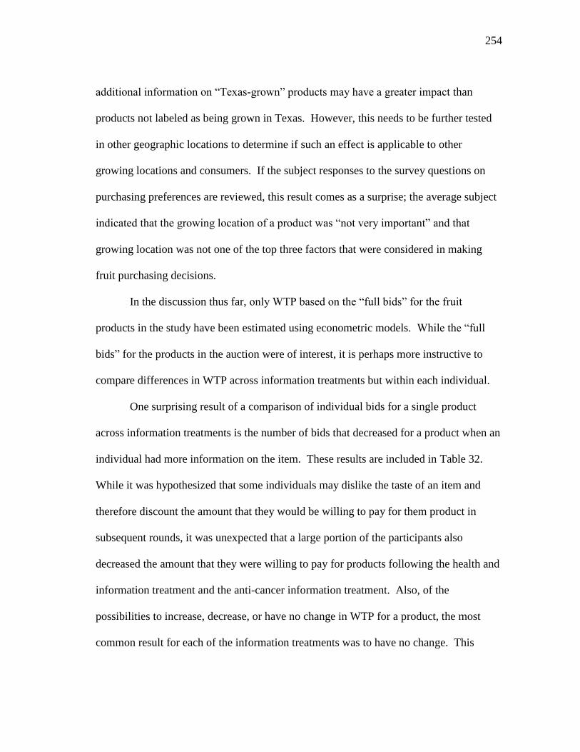
254
additional information on ―Texas-grown‖ products may have a greater impact than
products not labeled as being grown in Texas. However, this needs to be further tested
in other geographic locations to determine if such an effect is applicable to other
growing locations and consumers. If the subject responses to the survey questions on
purchasing preferences are reviewed, this result comes as a surprise; the average subject
indicated that the growing location of a product was ―not very important‖ and that
growing location was not one of the top three factors that were considered in making
fruit purchasing decisions.
In the discussion thus far, only WTP based on the ―full bids‖ for the fruit
products in the study have been estimated using econometric models. While the ―full
bids‖ for the products in the auction were of interest, it is perhaps more instructive to
compare differences in WTP across information treatments but within each individual.
One surprising result of a comparison of individual bids for a single product
across information treatments is the number of bids that decreased for a product when an
individual had more information on the item. These results are included in Table 32.
While it was hypothesized that some individuals may dislike the taste of an item and
therefore discount the amount that they would be willing to pay for them product in
subsequent rounds, it was unexpected that a large portion of the participants also
decreased the amount that they were willing to pay for products following the health and
information treatment and the anti-cancer information treatment. Also, of the
possibilities to increase, decrease, or have no change in WTP for a product, the most
common result for each of the information treatments was to have no change. This
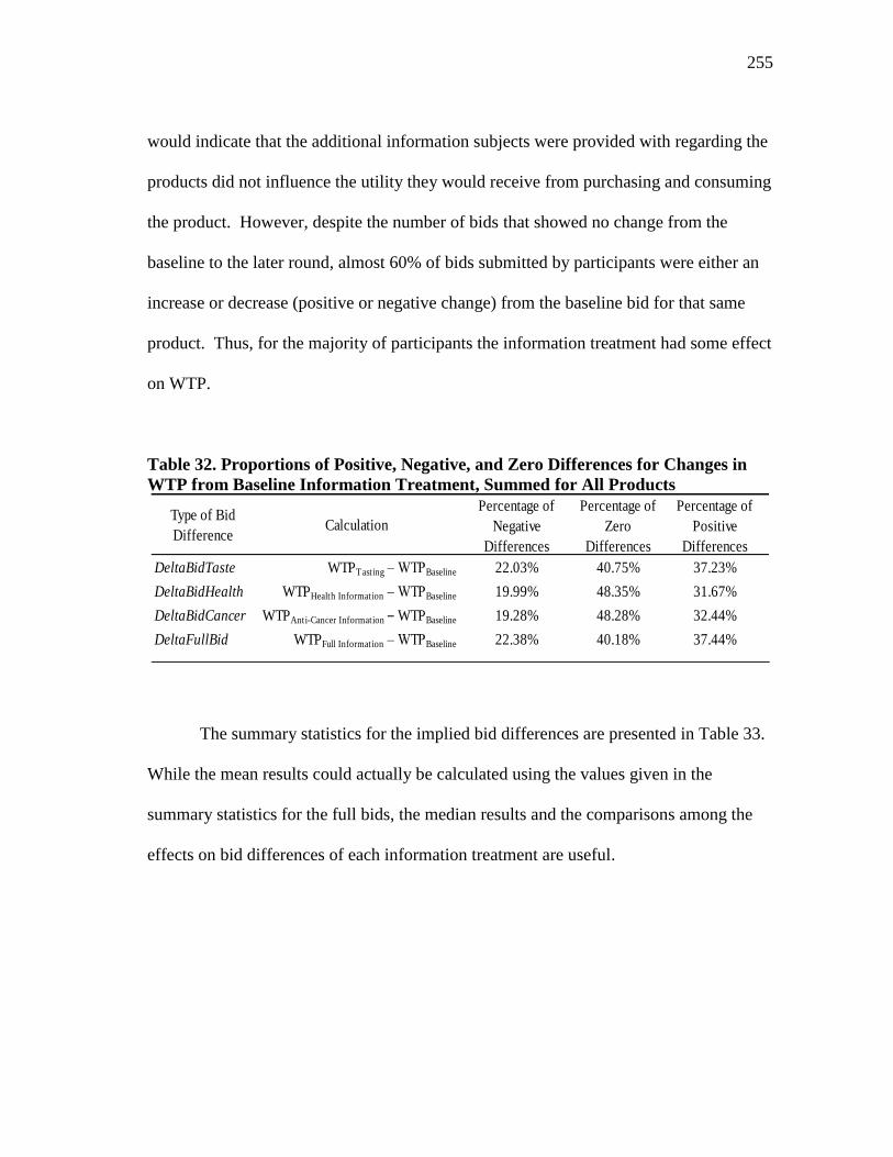
255
would indicate that the additional information subjects were provided with regarding the
products did not influence the utility they would receive from purchasing and consuming
the product. However, despite the number of bids that showed no change from the
baseline to the later round, almost 60% of bids submitted by participants were either an
increase or decrease (positive or negative change) from the baseline bid for that same
product. Thus, for the majority of participants the information treatment had some effect
on WTP.
Table 32. Proportions of Positive, Negative, and Zero Differences for Changes in
WTP from Baseline Information Treatment, Summed for All Products
The summary statistics for the implied bid differences are presented in Table 33.
While the mean results could actually be calculated using the values given in the
summary statistics for the full bids, the median results and the comparisons among the
effects on bid differences of each information treatment are useful.
Type of Bid
DifferenceCalculation
Percentage of
Negative
Differences
Percentage of
Zero
Differences
Percentage of
Positive
Differences
DeltaBidTaste WTPTasting ‒ WTPBaseline 22.03% 40.75% 37.23%
DeltaBidHealth WTPHealth Information ‒ WTPBaseline 19.99% 48.35% 31.67%
DeltaBidCancer WTPAnti-Cancer Information ‒ WTPBaseline 19.28% 48.28% 32.44%
DeltaFullBid WTPFull Information ‒ WTPBaseline 22.38% 40.18% 37.44%
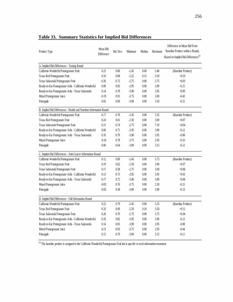
256
Table 33. Summary Statistics for Implied Bid Differences
Product TypeMean Bid
DifferenceStd. Dev. Minimum Median Maximum
Difference in Mean Bid From
Baseline Product within a Round,
Based on Implied Bid Differences(a)
A. Implied Bid Differences - Tasting Round
California Wonderful Pomegranate Fruit 0.23 0.80 -2.45 0.00 5.40 (Baseline Product)
Texas Red Pomegranate Fruit 0.33 0.68 -2.25 0.15 3.50 +0.10
Texas Salavatski Pomegranate Fruit 0.26 0.72 -2.75 0.00 3.75 +0.03
Ready-to-Eat Pomegranate Arils - California Wonderful 0.09 0.83 -3.95 0.00 3.90 -0.15
Ready-to-Eat Pomegranate Arils - Texas Salavatski 0.14 0.78 -3.90 0.00 3.95 -0.09
Mixed Pomegranate Juice -0.19 0.91 -3.75 0.00 3.00 -0.43
Pineapple 0.02 0.69 -3.00 0.00 3.10 -0.21
B. Implied Bid Differences - Health and Nutrition Information Round
California Wonderful Pomegranate Fruit 0.17 0.70 -2.45 0.00 5.35 (Baseline Product)
Texas Red Pomegranate Fruit 0.24 0.61 -2.50 0.00 3.00 +0.07
Texas Salavatski Pomegranate Fruit 0.21 0.74 -2.75 0.00 7.10 +0.04
Ready-to-Eat Pomegranate Arils - California Wonderful 0.06 0.71 -3.95 0.00 3.90 -0.12
Ready-to-Eat Pomegranate Arils - Texas Salavatski 0.10 0.70 -3.90 0.00 3.95 -0.08
Mixed Pomegranate Juice -0.16 0.78 -3.75 0.00 2.95 -0.33
Pineapple 0.06 0.64 -3.00 0.00 3.15 -0.12
C. Implied Bid Differences - Anti-Cancer Information Round
California Wonderful Pomegranate Fruit 0.12 0.69 -2.45 0.00 5.75 (Baseline Product)
Texas Red Pomegranate Fruit 0.19 0.62 -2.50 0.00 3.00 +0.07
Texas Salavatski Pomegranate Fruit 0.17 0.58 -2.75 0.00 3.00 +0.06
Ready-to-Eat Pomegranate Arils - California Wonderful 0.13 0.73 -3.95 0.00 3.95 +0.01
Ready-to-Eat Pomegranate Arils - Texas Salavatski 0.17 0.72 -3.90 0.00 3.90 +0.06
Mixed Pomegranate Juice -0.03 0.76 -3.75 0.00 2.50 -0.15
Pineapple -0.02 0.58 -3.00 0.00 3.00 -0.13
D. Implied Bid Differences - Full Information Round
California Wonderful Pomegranate Fruit 0.22 0.79 -2.45 0.00 5.35 (Baseline Product)
Texas Red Pomegranate Fruit 0.33 0.69 -2.50 0.10 3.50 +0.11
Texas Salavatski Pomegranate Fruit 0.26 0.70 -2.75 0.00 3.75 +0.04
Ready-to-Eat Pomegranate Arils - California Wonderful 0.10 0.82 -3.95 0.00 3.90 -0.12
Ready-to-Eat Pomegranate Arils - Texas Salavatski 0.14 0.81 -3.90 0.00 3.95 -0.08
Mixed Pomegranate Juice -0.21 0.93 -3.75 0.00 2.95 -0.44
Pineapple 0.12 0.70 -3.00 0.00 3.15 -0.11
(a) The baseline product is assigned to the California Wonderful Pomegranate Fruit but is specific to each information treatment.
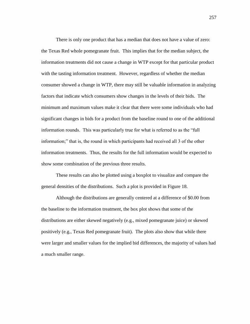
257
There is only one product that has a median that does not have a value of zero:
the Texas Red whole pomegranate fruit. This implies that for the median subject, the
information treatments did not cause a change in WTP except for that particular product
with the tasting information treatment. However, regardless of whether the median
consumer showed a change in WTP, there may still be valuable information in analyzing
factors that indicate which consumers show changes in the levels of their bids. The
minimum and maximum values make it clear that there were some individuals who had
significant changes in bids for a product from the baseline round to one of the additional
information rounds. This was particularly true for what is referred to as the ―full
information;‖ that is, the round in which participants had received all 3 of the other
information treatments. Thus, the results for the full information would be expected to
show some combination of the previous three results.
These results can also be plotted using a boxplot to visualize and compare the
general densities of the distributions. Such a plot is provided in Figure 18.
Although the distributions are generally centered at a difference of $0.00 from
the baseline to the information treatment, the box plot shows that some of the
distributions are either skewed negatively (e.g., mixed pomegranate juice) or skewed
positively (e.g., Texas Red pomegranate fruit). The plots also show that while there
were larger and smaller values for the implied bid differences, the majority of values had
a much smaller range.
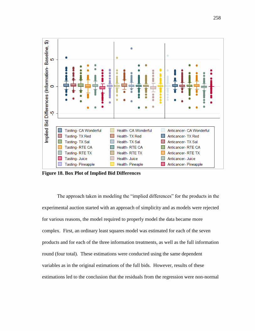
258
Figure 18. Box Plot of Implied Bid Differences
The approach taken in modeling the ―implied differences‖ for the products in the
experimental auction started with an approach of simplicity and as models were rejected
for various reasons, the model required to properly model the data became more
complex. First, an ordinary least squares model was estimated for each of the seven
products and for each of the three information treatments, as well as the full information
round (four total). These estimations were conducted using the same dependent
variables as in the original estimations of the full bids. However, results of these
estimations led to the conclusion that the residuals from the regression were non-normal
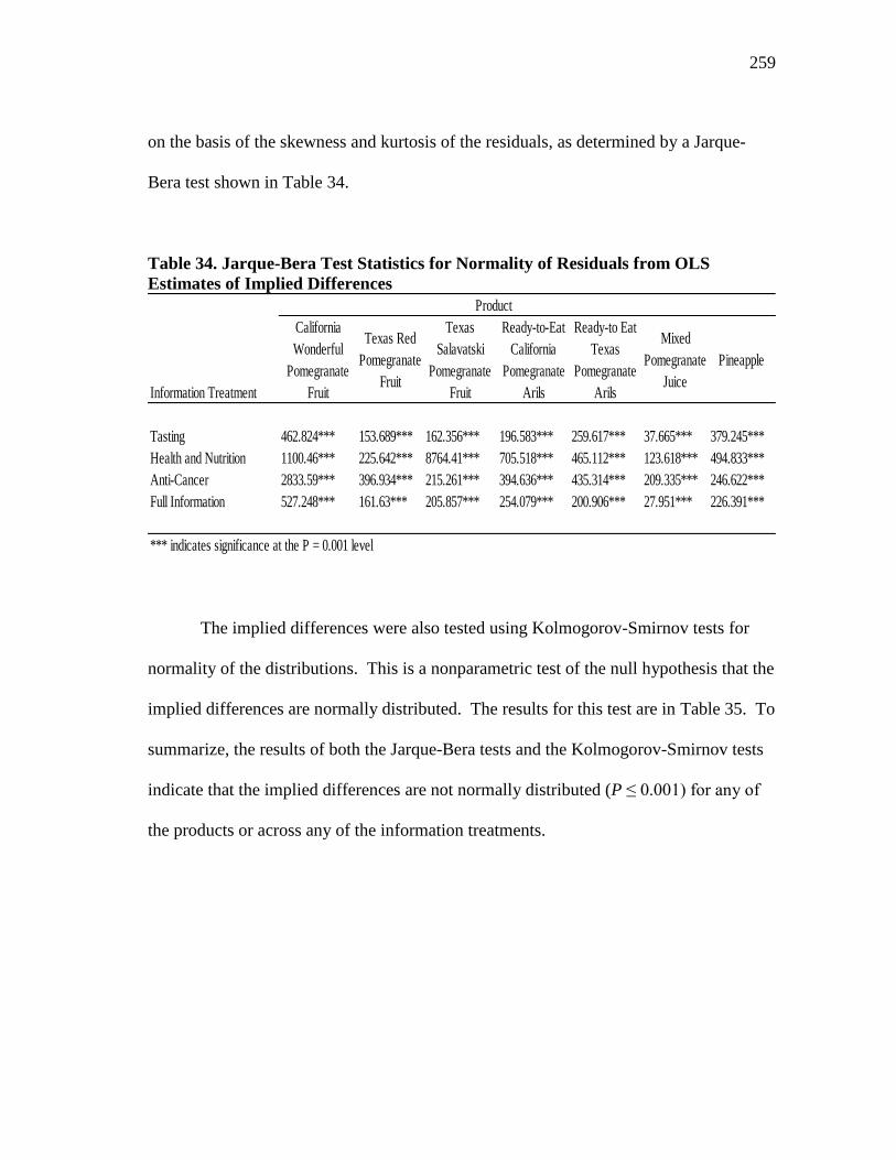
259
on the basis of the skewness and kurtosis of the residuals, as determined by a Jarque-
Bera test shown in Table 34.
Table 34. Jarque-Bera Test Statistics for Normality of Residuals from OLS
Estimates of Implied Differences
The implied differences were also tested using Kolmogorov-Smirnov tests for
normality of the distributions. This is a nonparametric test of the null hypothesis that the
implied differences are normally distributed. The results for this test are in Table 35. To
summarize, the results of both the Jarque-Bera tests and the Kolmogorov-Smirnov tests
indicate that the implied differences are not normally distributed (P ≤ 0.001) for any of
the products or across any of the information treatments.
Information Treatment
California
Wonderful
Pomegranate
Fruit
Texas Red
Pomegranate
Fruit
Texas
Salavatski
Pomegranate
Fruit
Ready-to-Eat
California
Pomegranate
Arils
Ready-to Eat
Texas
Pomegranate
Arils
Mixed
Pomegranate
Juice
Pineapple
Tasting 462.824*** 153.689*** 162.356*** 196.583*** 259.617*** 37.665*** 379.245***
Health and Nutrition 1100.46*** 225.642*** 8764.41*** 705.518*** 465.112*** 123.618*** 494.833***
Anti-Cancer 2833.59*** 396.934*** 215.261*** 394.636*** 435.314*** 209.335*** 246.622***
Full Information 527.248*** 161.63*** 205.857*** 254.079*** 200.906*** 27.951*** 226.391***
*** indicates significance at the P = 0.001 level
Product
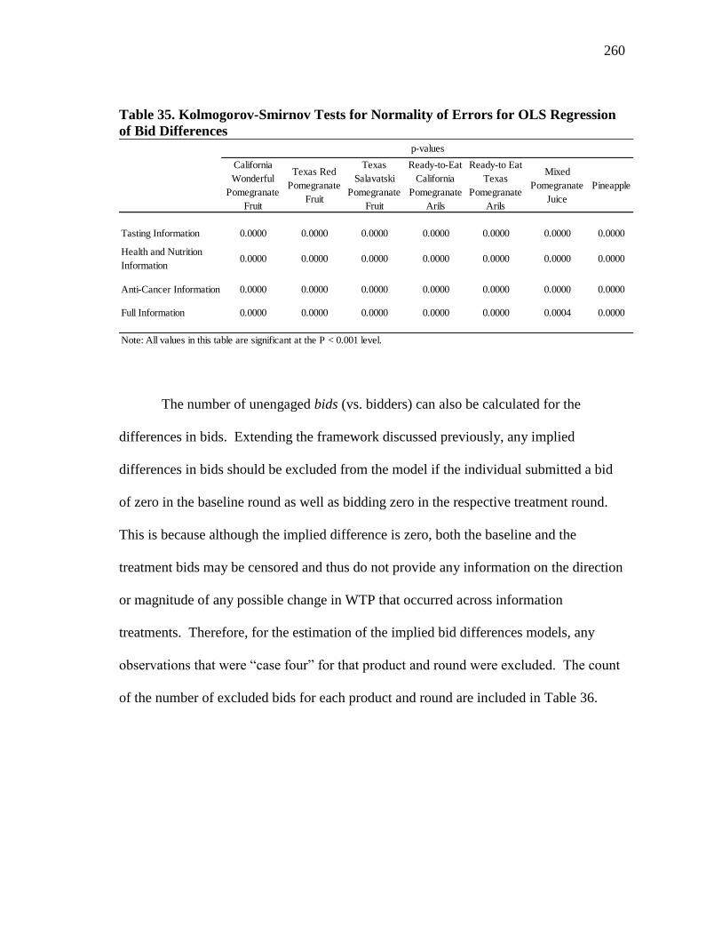
260
Table 35. Kolmogorov-Smirnov Tests for Normality of Errors for OLS Regression
of Bid Differences
The number of unengaged bids (vs. bidders) can also be calculated for the
differences in bids. Extending the framework discussed previously, any implied
differences in bids should be excluded from the model if the individual submitted a bid
of zero in the baseline round as well as bidding zero in the respective treatment round.
This is because although the implied difference is zero, both the baseline and the
treatment bids may be censored and thus do not provide any information on the direction
or magnitude of any possible change in WTP that occurred across information
treatments. Therefore, for the estimation of the implied bid differences models, any
observations that were ―case four‖ for that product and round were excluded. The count
of the number of excluded bids for each product and round are included in Table 36.
California
Wonderful
Pomegranate
Fruit
Texas Red
Pomegranate
Fruit
Texas
Salavatski
Pomegranate
Fruit
Ready-to-Eat
California
Pomegranate
Arils
Ready-to Eat
Texas
Pomegranate
Arils
Mixed
Pomegranate
Juice
Pineapple
Tasting Information 0.0000 0.0000 0.0000 0.0000 0.0000 0.0000 0.0000
Health and Nutrition
Information0.0000 0.0000 0.0000 0.0000 0.0000 0.0000 0.0000
Anti-Cancer Information 0.0000 0.0000 0.0000 0.0000 0.0000 0.0000 0.0000
Full Information 0.0000 0.0000 0.0000 0.0000 0.0000 0.0004 0.0000
Note: All values in this table are significant at the P < 0.001 level.
p-values
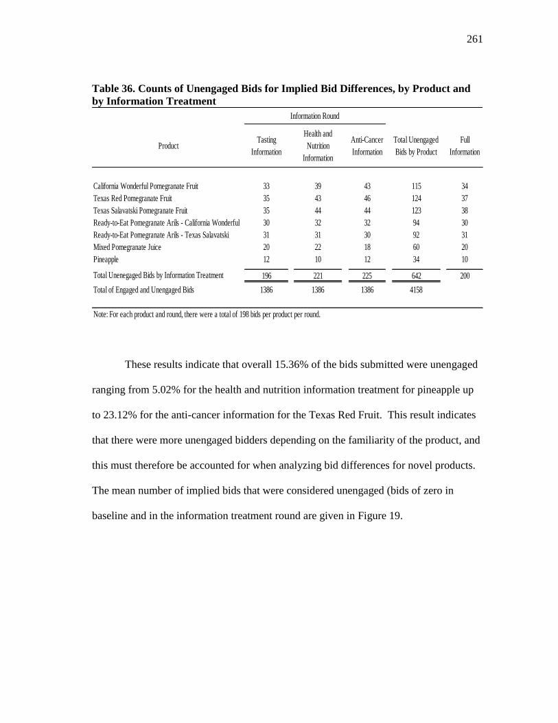
261
Table 36. Counts of Unengaged Bids for Implied Bid Differences, by Product and
by Information Treatment
These results indicate that overall 15.36% of the bids submitted were unengaged
ranging from 5.02% for the health and nutrition information treatment for pineapple up
to 23.12% for the anti-cancer information for the Texas Red Fruit. This result indicates
that there were more unengaged bidders depending on the familiarity of the product, and
this must therefore be accounted for when analyzing bid differences for novel products.
The mean number of implied bids that were considered unengaged (bids of zero in
baseline and in the information treatment round are given in Figure 19.
ProductTasting
Information
Health and
Nutrition
Information
Anti-Cancer
Information
Total Unengaged
Bids by Product
Full
Information
California Wonderful Pomegranate Fruit 33 39 43 115 34
Texas Red Pomegranate Fruit 35 43 46 124 37
Texas Salavatski Pomegranate Fruit 35 44 44 123 38
Ready-to-Eat Pomegranate Arils - California Wonderful 30 32 32 94 30
Ready-to-Eat Pomegranate Arils - Texas Salavatski 31 31 30 92 31
Mixed Pomegranate Juice 20 22 18 60 20
Pineapple 12 10 12 34 10
Total Unenegaged Bids by Information Treatment 196 221 225 642 200
Total of Engaged and Unengaged Bids 1386 1386 1386 4158
Note: For each product and round, there were a total of 198 bids per product per round.
Information Round
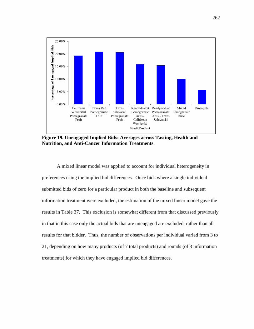
262
Figure 19. Unengaged Implied Bids: Averages across Tasting, Health and
Nutrition, and Anti-Cancer Information Treatments
A mixed linear model was applied to account for individual heterogeneity in
preferences using the implied bid differences. Once bids where a single individual
submitted bids of zero for a particular product in both the baseline and subsequent
information treatment were excluded, the estimation of the mixed linear model gave the
results in Table 37. This exclusion is somewhat different from that discussed previously
in that in this case only the actual bids that are unengaged are excluded, rather than all
results for that bidder. Thus, the number of observations per individual varied from 3 to
21, depending on how many products (of 7 total products) and rounds (of 3 information
treatments) for which they have engaged implied bid differences.
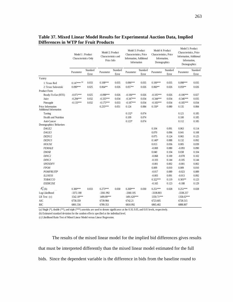
263
Table 37. Mixed Linear Model Results for Experimental Auction Data, Implied
Differences in WTP for Fruit Products
The results of the mixed linear model for the implied bid differences gives results
that must be interpreted differently than the mixed linear model estimated for the full
bids. Since the dependent variable is the difference in bids from the baseline round to
ParameterStandard
ErrorParameter
Standard
ErrorParameter
Standard
ErrorParameter
Standard
ErrorParameter
Standard
Error
Variety
1: Texas Red 0.147*** (a) 0.033 0.108*** 0.035 0.096*** 0.035 0.100*** 0.035 0.098*** 0.035
2: Texas Salavatski 0.090*** 0.025 0.064** 0.026 0.057** 0.026 0.060** 0.026 0.059** 0.026
Product Form
Ready-To-Eat (RTE) -0.071*** 0.025 -0.098*** 0.026 -0.106*** 0.026 -0.105*** 0.026 -0.106*** 0.027
Juice -0.294*** 0.032 -0.335*** 0.034 -0.347*** 0.034 -0.344*** 0.034 -0.346*** 0.035
Pineapple -0.133*** 0.032 -0.175*** 0.033 -0.187*** 0.034 -0.183*** 0.034 -0.185*** 0.034
Price Information 0.235*** 0.051 0.124 0.084 0.150* 0.080 0.135 0.084Additional Information
Tasting 0.132* 0.074 0.121 0.185
Health and Nutrition 0.109 0.074 0.100 0.185
Anti-Cancer 0.123* 0.074 0.112 0.185Demographics/ Behaviors
DAGE2 0.104 0.091 0.063 0.114
DAGE3 0.070 0.096 0.041 0.108
DEDU2 0.075 0.124 0.065 0.125
DEDU3 0.149* 0.088 0.132 0.092
HOUSE 0.013 0.036 0.005 0.039
FEMALE -0.069 0.080 -0.093 0.090
DMAR 0.040 0.104 0.038 0.104
DINC2 -0.068 0.100 -0.078 0.102
DINC3 -0.103 0.144 -0.105 0.144
SPENDFV -0.001 0.002 -0.001 0.002
FPOH 0.009 0.010 0.009 0.010
POMFRUITP -0.017 0.089 -0.023 0.089
ILLNESS -0.003 0.091 -0.013 0.092
TOBACCO 0.322*** 0.119 0.303** 0.123
EXERCISE -0.165 0.123 -0.188 0.129
(b) 0.300*** 0.033 0.273*** 0.030 0.269*** 0.030 0.251*** 0.028 0.251*** 0.028
Log-Likelihood -3372.180 -3361.992 -3360.105 -3338.803 -3338.257
LR Test : (c) 1542.18*** 1499.89*** 1491.620*** 1359.71*** 1358.02***
AIC 6758.359 6739.984 6742.21 6723.605 6728.515
BIC 6801.556 6789.353 6810.092 6865.402 6888.807
(a) Single (*), double (**), and triple (***) asterisks are used to denote significance at the 0.10, 0.05, and 0.01 levels, respectively.
(b) Estimated standard deviation for the random effects specified at the individual level.
(c) Likelihood Ratio Test of Mixed Linear Model versus Linear Regression.
Model 1 : Product
Characteristics Only
Model 2: Product
Characteristics and
Price Info
Model 3: Product
Characteristics, Price
Information, Additional
Information
Model 4: Product
Characteristics, Price
Information,
Demographics
Model 5: Product
Characteristics, Price
Information, Additional
Information,
Demographics
264
the respective information treatment round, the parameter estimates are also the
differences in the parameters for the information treatment round and the baseline round.
For example, the first estimate in Table 37 indicates that in Model 1, the estimated
difference in the effect of the Texas Red variety from the baseline to the information
treatment is an increase of 14.7¢ in value. The interpretation follows similarly for all
other dummy variables in the model; for continuous variables such as tobacco use the
estimated change in WTP for a product for any individual attributed to that variable
would be the value of that variable times the estimated parameter. Thus, the trend in
Model 4 for tobacco use would indicate a $0.14 increase in WTP for an individual who
used tobacco products every day, but only a $0.07 increase in WTP for an individual
who uses tobacco on average every other day.
Comparing the results of the mixed linear model for the implied differences in
bids to the mixed linear models for the full bids in Table 24, there are a number of
differences in the results. This would indicate that the predictors for the levels of the
actual bids for an individual under a certain information treatment are not necessarily the
same as the predictors for how an individual‘s bids will change when an information
treatment is applied. Thus, the model for the implied differences should indicate the
product and/or demographic factors that are relevant when information treatments are
applied. This type of information is economically relevant when information treatments
(i.e. advertisement, product promotional materials, etc.) are applied with the aim of
increasing WTP for a product. For the implied differences models, all product
characteristics were significant (P < 0.05), and this result was robust across all Models 1
265
to 5. However, the sign of these effects for the product form characteristics (RTE, juice,
and pineapple) was negative for the models based on implied differences. This indicates
that for any of these product form characteristics, the change in WTP attributed to that
characteristic decreased from the baseline round to the information treatment rounds,
while the positive values on the two Texas varieties variables indicates that the effect of
those product varieties on WTP increased from the baseline to the information treatment
rounds.
Depending on whether AIC or BIC is used in comparing the model
specifications, Model 2 or 4 would be preferred of these model options. In contrast to
the other models examined for predicting WTP, the price information effect was not
robust across all specifications of this model. This indicates that although price
information had an effect on the level of individual bids, it did not necessarily have an
effect on the size of the change in bids due to an information treatment. This result is of
interest for two reasons. First, reference prices and their effects on the level of bids have
been the topic of much discussion in the literature, but the application of a model based
on implied bid differences may avoid some of the problems that the presence or absence
of a reference price may cause. However, since this result was dependent on which
variables were included in the model of the change in WTP, further investigation will be
needed to confirm or disprove this result. Second, and again in contrast to the models
based on the full bids, there was generally not significance for the implied differences in
bids for the information treatment indicator variables. This is interpreted to mean there
was not a specific effect due to any one of the particular information treatments, and the
266
changes in WTP could be more correctly attributed to the product characteristics. Also,
note that in these mixed linear models a constant was not estimated in order to allow for
the calculation of differences due to all three information treatments, which were the
tasting, health and nutrition, and anti-cancer information treatments included in the
model. In the models for implied bid differences that included demographic variables,
the only effect that was significant was for tobacco-users the size of the effect due to the
information treatments was larger than for nonsmokers.
For the various test statistics for the model, based on the size and standard error
of the estimated standard deviation for the individual there were significant random
effects specified at the individual level. Note that it is less surprising that the
demographic and behavioral characteristics were not estimated to be relevant because
the random effects were specified as individual-specific effects. The likelihood ratio test
of the mixed linear model versus an ordinary least squares linear model also rejected the
null hypothesis of the OLS model.
The use of the implied bid differences instead of the full bids gives quite
different results in terms of which variables are statistically significant. If researchers
and marketers are interested in predicting what type of information on which products
will cause consumers to be willing to pay more for novel products, the use of full bids
could lead to dramatically different results than using the paired differences in bids. It
may not be sufficient to compare the differences in the means for the products and
information treatments and may therefore be preferable to utilize paired differences in
bids before and after additional information on the novel product is provided. If paired
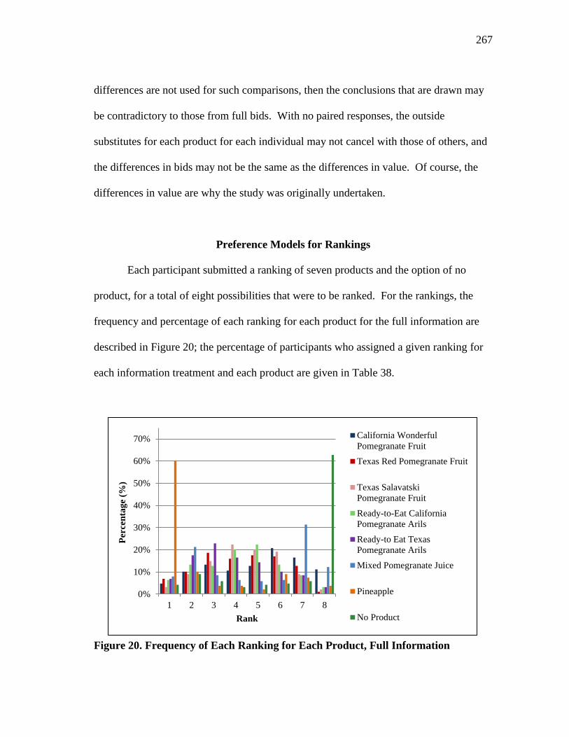
267
differences are not used for such comparisons, then the conclusions that are drawn may
be contradictory to those from full bids. With no paired responses, the outside
substitutes for each product for each individual may not cancel with those of others, and
the differences in bids may not be the same as the differences in value. Of course, the
differences in value are why the study was originally undertaken.
Preference Models for Rankings
Each participant submitted a ranking of seven products and the option of no
product, for a total of eight possibilities that were to be ranked. For the rankings, the
frequency and percentage of each ranking for each product for the full information are
described in Figure 20; the percentage of participants who assigned a given ranking for
each information treatment and each product are given in Table 38.
Figure 20. Frequency of Each Ranking for Each Product, Full Information
0%
10%
20%
30%
40%
50%
60%
70%
1 2 3 4 5 6 7 8
Per
cen
tag
e (%
)
Rank
California Wonderful
Pomegranate Fruit
Texas Red Pomegranate Fruit
Texas Salavatski
Pomegranate Fruit
Ready-to-Eat California
Pomegranate Arils
Ready-to Eat Texas
Pomegranate Arils
Mixed Pomegranate Juice
Pineapple
No Product
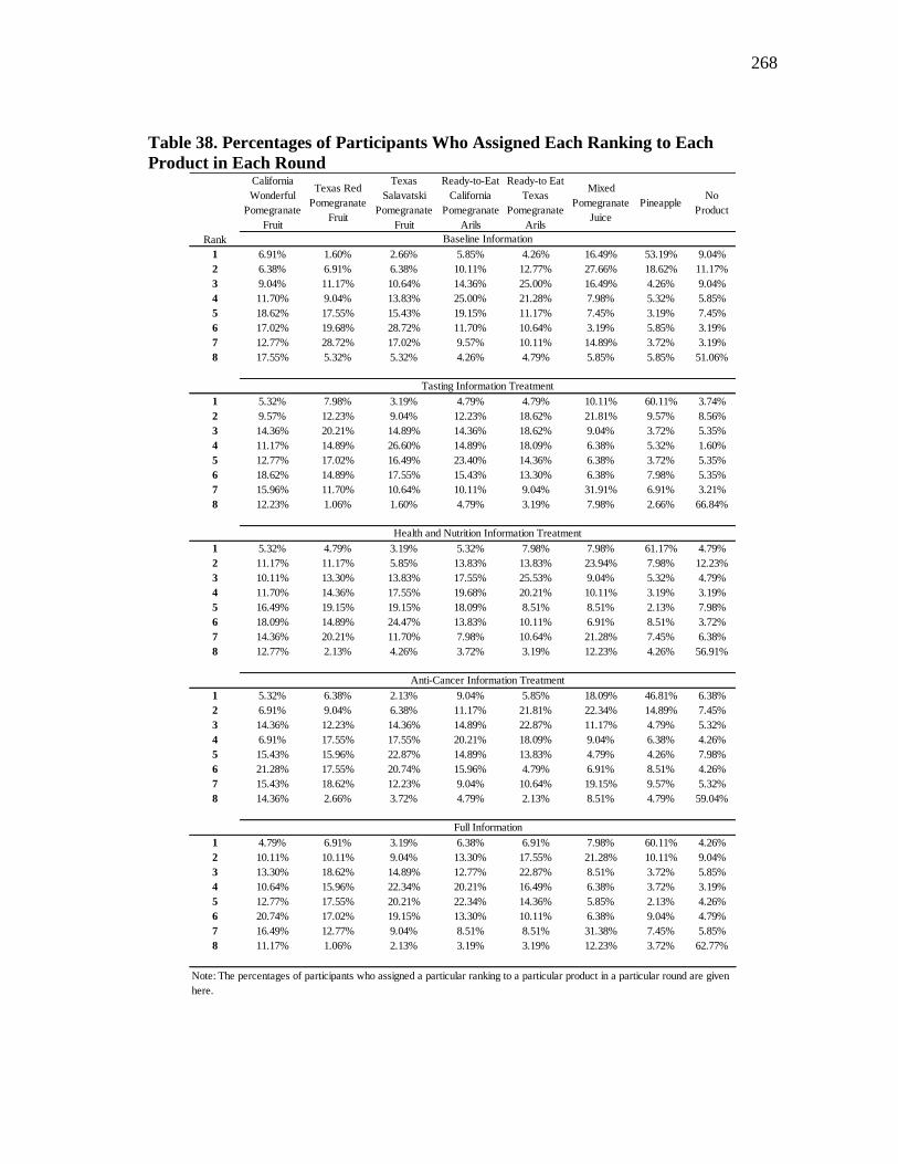
268
Table 38. Percentages of Participants Who Assigned Each Ranking to Each
Product in Each Round
California
Wonderful
Pomegranate
Fruit
Texas Red
Pomegranate
Fruit
Texas
Salavatski
Pomegranate
Fruit
Ready-to-Eat
California
Pomegranate
Arils
Ready-to Eat
Texas
Pomegranate
Arils
Mixed
Pomegranate
Juice
PineappleNo
Product
Rank
1 6.91% 1.60% 2.66% 5.85% 4.26% 16.49% 53.19% 9.04%
2 6.38% 6.91% 6.38% 10.11% 12.77% 27.66% 18.62% 11.17%
3 9.04% 11.17% 10.64% 14.36% 25.00% 16.49% 4.26% 9.04%
4 11.70% 9.04% 13.83% 25.00% 21.28% 7.98% 5.32% 5.85%
5 18.62% 17.55% 15.43% 19.15% 11.17% 7.45% 3.19% 7.45%
6 17.02% 19.68% 28.72% 11.70% 10.64% 3.19% 5.85% 3.19%
7 12.77% 28.72% 17.02% 9.57% 10.11% 14.89% 3.72% 3.19%
8 17.55% 5.32% 5.32% 4.26% 4.79% 5.85% 5.85% 51.06%
1 5.32% 7.98% 3.19% 4.79% 4.79% 10.11% 60.11% 3.74%
2 9.57% 12.23% 9.04% 12.23% 18.62% 21.81% 9.57% 8.56%
3 14.36% 20.21% 14.89% 14.36% 18.62% 9.04% 3.72% 5.35%
4 11.17% 14.89% 26.60% 14.89% 18.09% 6.38% 5.32% 1.60%
5 12.77% 17.02% 16.49% 23.40% 14.36% 6.38% 3.72% 5.35%
6 18.62% 14.89% 17.55% 15.43% 13.30% 6.38% 7.98% 5.35%
7 15.96% 11.70% 10.64% 10.11% 9.04% 31.91% 6.91% 3.21%
8 12.23% 1.06% 1.60% 4.79% 3.19% 7.98% 2.66% 66.84%
1 5.32% 4.79% 3.19% 5.32% 7.98% 7.98% 61.17% 4.79%
2 11.17% 11.17% 5.85% 13.83% 13.83% 23.94% 7.98% 12.23%
3 10.11% 13.30% 13.83% 17.55% 25.53% 9.04% 5.32% 4.79%
4 11.70% 14.36% 17.55% 19.68% 20.21% 10.11% 3.19% 3.19%
5 16.49% 19.15% 19.15% 18.09% 8.51% 8.51% 2.13% 7.98%
6 18.09% 14.89% 24.47% 13.83% 10.11% 6.91% 8.51% 3.72%
7 14.36% 20.21% 11.70% 7.98% 10.64% 21.28% 7.45% 6.38%
8 12.77% 2.13% 4.26% 3.72% 3.19% 12.23% 4.26% 56.91%
1 5.32% 6.38% 2.13% 9.04% 5.85% 18.09% 46.81% 6.38%
2 6.91% 9.04% 6.38% 11.17% 21.81% 22.34% 14.89% 7.45%
3 14.36% 12.23% 14.36% 14.89% 22.87% 11.17% 4.79% 5.32%
4 6.91% 17.55% 17.55% 20.21% 18.09% 9.04% 6.38% 4.26%
5 15.43% 15.96% 22.87% 14.89% 13.83% 4.79% 4.26% 7.98%
6 21.28% 17.55% 20.74% 15.96% 4.79% 6.91% 8.51% 4.26%
7 15.43% 18.62% 12.23% 9.04% 10.64% 19.15% 9.57% 5.32%
8 14.36% 2.66% 3.72% 4.79% 2.13% 8.51% 4.79% 59.04%
1 4.79% 6.91% 3.19% 6.38% 6.91% 7.98% 60.11% 4.26%
2 10.11% 10.11% 9.04% 13.30% 17.55% 21.28% 10.11% 9.04%
3 13.30% 18.62% 14.89% 12.77% 22.87% 8.51% 3.72% 5.85%
4 10.64% 15.96% 22.34% 20.21% 16.49% 6.38% 3.72% 3.19%
5 12.77% 17.55% 20.21% 22.34% 14.36% 5.85% 2.13% 4.26%
6 20.74% 17.02% 19.15% 13.30% 10.11% 6.38% 9.04% 4.79%
7 16.49% 12.77% 9.04% 8.51% 8.51% 31.38% 7.45% 5.85%
8 11.17% 1.06% 2.13% 3.19% 3.19% 12.23% 3.72% 62.77%
Note: The percentages of participants who assigned a particular ranking to a particular product in a particular round are given
here.
Baseline Information
Tasting Information Treatment
Health and Nutrition Information Treatment
Anti-Cancer Information Treatment
Full Information
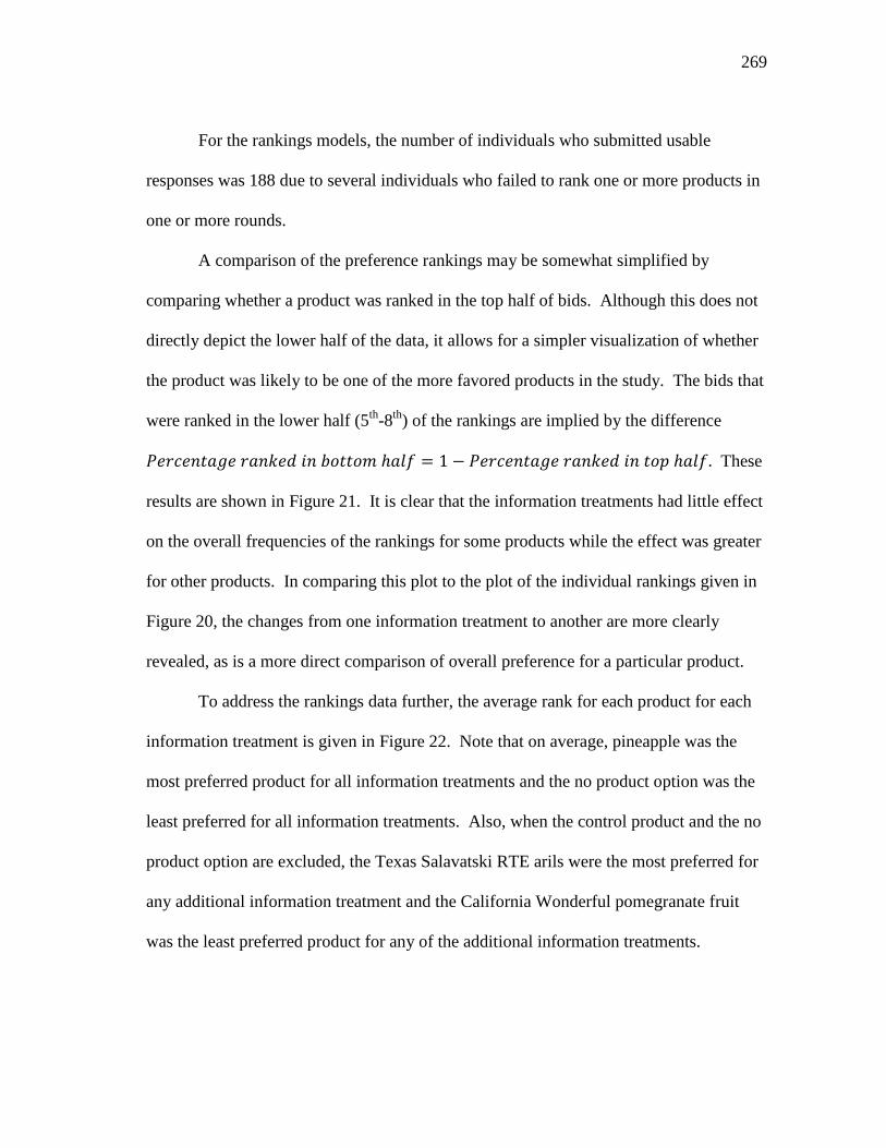
269
For the rankings models, the number of individuals who submitted usable
responses was 188 due to several individuals who failed to rank one or more products in
one or more rounds.
A comparison of the preference rankings may be somewhat simplified by
comparing whether a product was ranked in the top half of bids. Although this does not
directly depict the lower half of the data, it allows for a simpler visualization of whether
the product was likely to be one of the more favored products in the study. The bids that
were ranked in the lower half (5th
-8th
) of the rankings are implied by the difference
These
results are shown in Figure 21. It is clear that the information treatments had little effect
on the overall frequencies of the rankings for some products while the effect was greater
for other products. In comparing this plot to the plot of the individual rankings given in
Figure 20, the changes from one information treatment to another are more clearly
revealed, as is a more direct comparison of overall preference for a particular product.
To address the rankings data further, the average rank for each product for each
information treatment is given in Figure 22. Note that on average, pineapple was the
most preferred product for all information treatments and the no product option was the
least preferred for all information treatments. Also, when the control product and the no
product option are excluded, the Texas Salavatski RTE arils were the most preferred for
any additional information treatment and the California Wonderful pomegranate fruit
was the least preferred product for any of the additional information treatments.
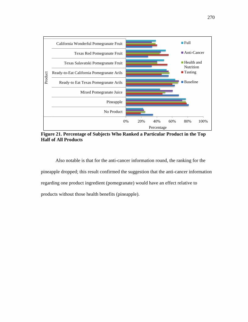
270
Figure 21. Percentage of Subjects Who Ranked a Particular Product in the Top
Half of All Products
Also notable is that for the anti-cancer information round, the ranking for the
pineapple dropped; this result confirmed the suggestion that the anti-cancer information
regarding one product ingredient (pomegranate) would have an effect relative to
products without those health benefits (pineapple).
0% 20% 40% 60% 80% 100%
No Product
Pineapple
Mixed Pomegranate Juice
Ready-to Eat Texas Pomegranate Arils
Ready-to-Eat California Pomegranate Arils
Texas Salavatski Pomegranate Fruit
Texas Red Pomegranate Fruit
California Wonderful Pomegranate FruitP
rodu
ct
Percentage
Full
Anti-Cancer
Health and
Nutrition
Tasting
Baseline
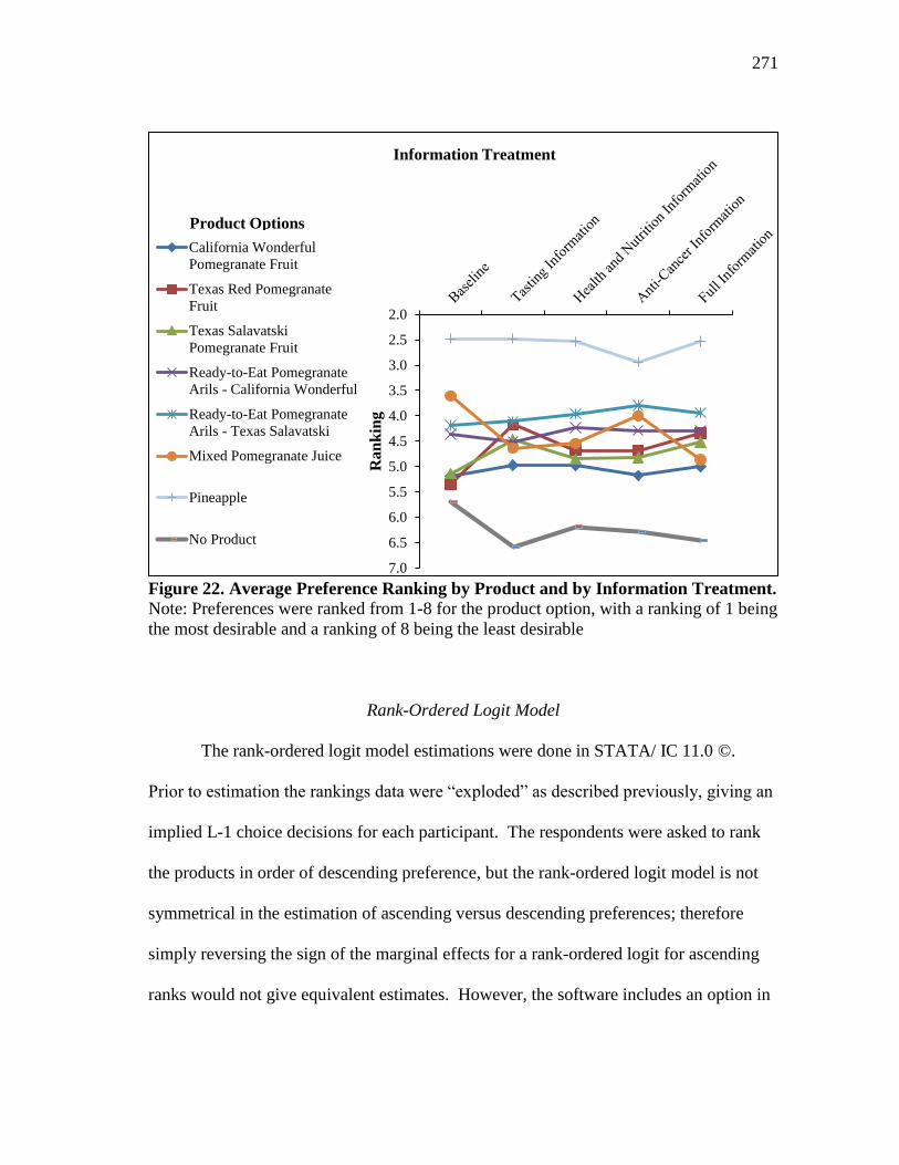
271
Figure 22. Average Preference Ranking by Product and by Information Treatment. Note: Preferences were ranked from 1-8 for the product option, with a ranking of 1 being
the most desirable and a ranking of 8 being the least desirable
Rank-Ordered Logit Model
The rank-ordered logit model estimations were done in STATA/ IC 11.0 ©.
Prior to estimation the rankings data were ―exploded‖ as described previously, giving an
implied L-1 choice decisions for each participant. The respondents were asked to rank
the products in order of descending preference, but the rank-ordered logit model is not
symmetrical in the estimation of ascending versus descending preferences; therefore
simply reversing the sign of the marginal effects for a rank-ordered logit for ascending
ranks would not give equivalent estimates. However, the software includes an option in
2.0
2.5
3.0
3.5
4.0
4.5
5.0
5.5
6.0
6.5
7.0
Ran
kin
g
Information Treatment
California Wonderful
Pomegranate Fruit
Texas Red Pomegranate
Fruit
Texas Salavatski
Pomegranate Fruit
Ready-to-Eat Pomegranate
Arils - California Wonderful
Ready-to-Eat Pomegranate
Arils - Texas Salavatski
Mixed Pomegranate Juice
Pineapple
No Product
Product Options
272
the rank-ordered logit estimation procedure to handle such ―reversed‖ ranks (StataCorp
2009). The product characteristics that were included for the rank-ordered mixed logit
models are the cultivar of the product (California Wonderful, Texas Red, and Texas
Salavatski) and the product form (RTE, juice, pineapple, and no product).
After the traditional fully-ranked models were estimated, the models were re-
estimated using partial rankings to check for possible differences in ability to rank less-
preferred versus more-preferred product options. The results of this estimation are given
in Table 39.
The first portion of the table includes estimates for the changes in ranking due to
the product characteristics. Each model was estimated separately for each information
treatment. In interpreting the parameter estimates, a product would be more preferred
due to a characteristic if it has a positive value, and less preferred due to that
characteristic if there is a negative value for the parameter estimate. Thus, in the
baseline ranking round, there was no effect on preference for a product if the product
was either of the two Texas varieties, but items were more preferred if they were RTE,
juice, or pineapple. Of these, the largest relative effect on preference was pineapple,
followed by juice, and then RTE. The option of no product was discounted in the
rankings.
The estimates of the models for tasting, health and nutrition, anti-cancer, and full
information will not be described individually. However, points of interest in each and
across models will be discussed. In the Tasting Information round, the ranking of the
juice product no longer differed significantly from the baseline. However, once subjects
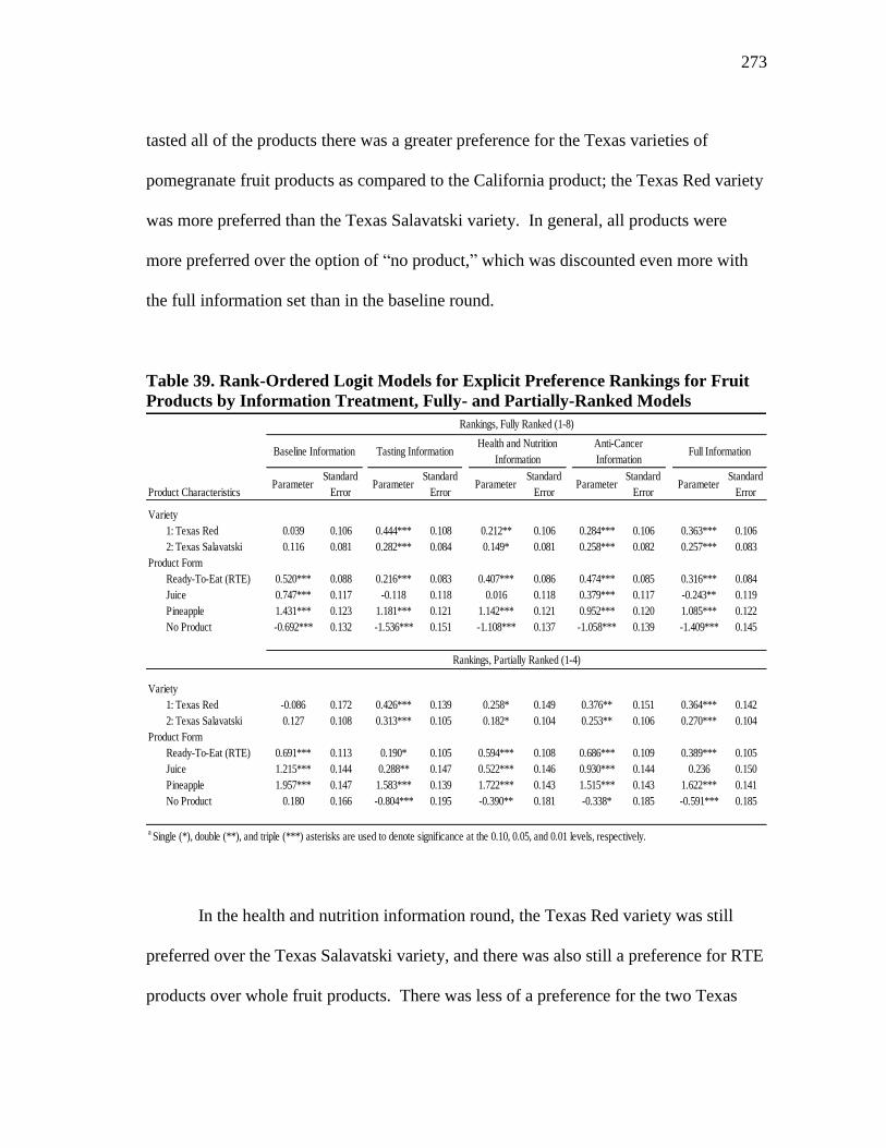
273
tasted all of the products there was a greater preference for the Texas varieties of
pomegranate fruit products as compared to the California product; the Texas Red variety
was more preferred than the Texas Salavatski variety. In general, all products were
more preferred over the option of ―no product,‖ which was discounted even more with
the full information set than in the baseline round.
Table 39. Rank-Ordered Logit Models for Explicit Preference Rankings for Fruit
Products by Information Treatment, Fully- and Partially-Ranked Models
In the health and nutrition information round, the Texas Red variety was still
preferred over the Texas Salavatski variety, and there was also still a preference for RTE
products over whole fruit products. There was less of a preference for the two Texas
Product CharacteristicsParameter
Standard
ErrorParameter
Standard
ErrorParameter
Standard
ErrorParameter
Standard
ErrorParameter
Standard
Error
Variety
1: Texas Red 0.039 0.106 0.444*** 0.108 0.212** 0.106 0.284*** 0.106 0.363*** 0.106
2: Texas Salavatski 0.116 0.081 0.282*** 0.084 0.149* 0.081 0.258*** 0.082 0.257*** 0.083
Product Form
Ready-To-Eat (RTE) 0.520*** 0.088 0.216*** 0.083 0.407*** 0.086 0.474*** 0.085 0.316*** 0.084
Juice 0.747*** 0.117 -0.118 0.118 0.016 0.118 0.379*** 0.117 -0.243** 0.119
Pineapple 1.431*** 0.123 1.181*** 0.121 1.142*** 0.121 0.952*** 0.120 1.085*** 0.122
No Product -0.692*** 0.132 -1.536*** 0.151 -1.108*** 0.137 -1.058*** 0.139 -1.409*** 0.145
Variety
1: Texas Red -0.086 0.172 0.426*** 0.139 0.258* 0.149 0.376** 0.151 0.364*** 0.142
2: Texas Salavatski 0.127 0.108 0.313*** 0.105 0.182* 0.104 0.253** 0.106 0.270*** 0.104
Product Form
Ready-To-Eat (RTE) 0.691*** 0.113 0.190* 0.105 0.594*** 0.108 0.686*** 0.109 0.389*** 0.105
Juice 1.215*** 0.144 0.288** 0.147 0.522*** 0.146 0.930*** 0.144 0.236 0.150
Pineapple 1.957*** 0.147 1.583*** 0.139 1.722*** 0.143 1.515*** 0.143 1.622*** 0.141
No Product 0.180 0.166 -0.804*** 0.195 -0.390** 0.181 -0.338* 0.185 -0.591*** 0.185
a Single (*), double (**), and triple (***) asterisks are used to denote significance at the 0.10, 0.05, and 0.01 levels, respectively.
Rankings, Fully Ranked (1-8)
Baseline Information Tasting InformationHealth and Nutrition
Information
Anti-Cancer
InformationFull Information
Rankings, Partially Ranked (1-4)
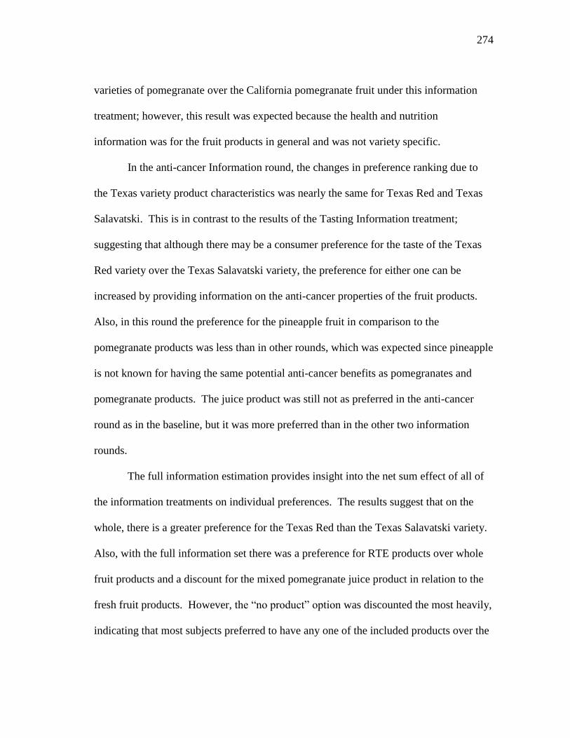
274
varieties of pomegranate over the California pomegranate fruit under this information
treatment; however, this result was expected because the health and nutrition
information was for the fruit products in general and was not variety specific.
In the anti-cancer Information round, the changes in preference ranking due to
the Texas variety product characteristics was nearly the same for Texas Red and Texas
Salavatski. This is in contrast to the results of the Tasting Information treatment;
suggesting that although there may be a consumer preference for the taste of the Texas
Red variety over the Texas Salavatski variety, the preference for either one can be
increased by providing information on the anti-cancer properties of the fruit products.
Also, in this round the preference for the pineapple fruit in comparison to the
pomegranate products was less than in other rounds, which was expected since pineapple
is not known for having the same potential anti-cancer benefits as pomegranates and
pomegranate products. The juice product was still not as preferred in the anti-cancer
round as in the baseline, but it was more preferred than in the other two information
rounds.
The full information estimation provides insight into the net sum effect of all of
the information treatments on individual preferences. The results suggest that on the
whole, there is a greater preference for the Texas Red than the Texas Salavatski variety.
Also, with the full information set there was a preference for RTE products over whole
fruit products and a discount for the mixed pomegranate juice product in relation to the
fresh fruit products. However, the ―no product‖ option was discounted the most heavily,
indicating that most subjects preferred to have any one of the included products over the
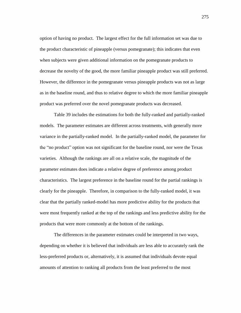
275
option of having no product. The largest effect for the full information set was due to
the product characteristic of pineapple (versus pomegranate); this indicates that even
when subjects were given additional information on the pomegranate products to
decrease the novelty of the good, the more familiar pineapple product was still preferred.
However, the difference in the pomegranate versus pineapple products was not as large
as in the baseline round, and thus to relative degree to which the more familiar pineapple
product was preferred over the novel pomegranate products was decreased.
Table 39 includes the estimations for both the fully-ranked and partially-ranked
models. The parameter estimates are different across treatments, with generally more
variance in the partially-ranked model. In the partially-ranked model, the parameter for
the ―no product‖ option was not significant for the baseline round, nor were the Texas
varieties. Although the rankings are all on a relative scale, the magnitude of the
parameter estimates does indicate a relative degree of preference among product
characteristics. The largest preference in the baseline round for the partial rankings is
clearly for the pineapple. Therefore, in comparison to the fully-ranked model, it was
clear that the partially ranked-model has more predictive ability for the products that
were most frequently ranked at the top of the rankings and less predictive ability for the
products that were more commonly at the bottom of the rankings.
The differences in the parameter estimates could be interpreted in two ways,
depending on whether it is believed that individuals are less able to accurately rank the
less-preferred products or, alternatively, it is assumed that individuals devote equal
amounts of attention to ranking all products from the least preferred to the most

276
preferred. The former situation would be interpreted as heterogeneity in an individual‘s
ability to rank the products, while the latter assumes that the rankings are done
homogeneously across all preference levels by all respondents.
Mixed Rank-Ordered Logit Model
Combining the mixed logit and rank-ordered logit framework provides the
following results. The preference data were exploded as described by Rabe-Hesketh,
Pickles, and Skrondal (2001) and Rabe-Hesketh and Skrondal (2005) and the mixed
rank-ordered logit model was then estimated using the –mixlogit– command in STATA/
IC 11.0 © developed by Hole (2007). A series of different specifications are provided
for comparison of these models. A model similar to the first rank-ordered logit model
was first estimated. As seen in Table 40, such a model provides estimated parameters
and standard errors for those parameters, but it also provides estimated standard
deviations and standard errors for the standard deviations. This is because the model
allows each individual to have their own slope for each parameter in the model. Thus, if
the standard deviation is significant then we would expect that there are differences in
each variable that depend on each individual. More precisely, the standard deviations of
the β parameters accommodate the presence of preference heterogeneity in the sample
(Hensher and Greene 2003).
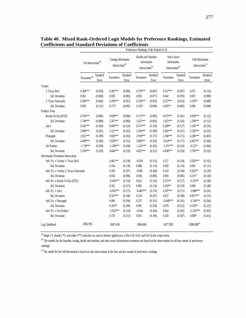
277
Table 40. Mixed Rank-Ordered Logit Models for Preference Rankings, Estimated
Coefficients and Standard Deviations of Coefficients
Parameter(a) Standard
ErrorParameter
Standard
ErrorParameter
Standard
ErrorParameter
Standard
ErrorParameter
Standard
Error
Variety
1: Texas Red 0.369*** (0.058) 0.281*** (0.066) 0.379*** (0.067) 0.337*** (0.067) 0.071 (0.114)
Std. Deviation 0.062 (0.068) 0.058 (0.082) 0.055 (0.077) 0.042 (0.076) 0.037 (0.099)
2: Texas Salavatski 0.286*** (0.046) 0.259*** (0.053) 0.318*** (0.053) 0.257*** (0.053) 0.195** (0.088)
Std. Deviation 0.059 (0.131) 0.171* (0.095) 0.163* (0.099) 0.205** (0.083) 0.060 (0.090)
Product Form
Ready-To-Eat (RTE) 0.704*** (0.096) 0.828*** (0.094) 0.715*** (0.092) 0.675*** (0.101) 0.959*** (0.132)
Std. Deviation 1.748*** (0.088) 1.567*** (0.084) 1.625*** (0.092) 1.625*** (0.126) 1.500*** (0.112)
Juice 0.542*** (0.160) 0.695*** (0.124) 0.571*** (0.126) 0.289** (0.127) 1.536*** (0.216)
Std. Deviation 2.900*** (0.201) 3.121*** (0.163) 3.100*** (0.180) 3.002*** (0.167) 3.320*** (0.235)
Pineapple 2.921*** (0.189) 3.026*** (0.182) 2.919*** (0.171) 3.166*** (0.172) 4.286*** (0.403)
Std. Deviation 4.499*** (0.206) 3.630*** (0.153) 3.606*** (0.165) 3.614*** (0.171) 4.062*** (0.266)
No Product -1.739*** (0.209) -1.198*** (0.168) -1.451*** (0.165) -1.471*** (0.162) -0.527* (0.304)
Std. Deviation 5.250*** (0.320) 4.844*** (0.218) 4.822*** (0.223) 4.838*** (0.226) 5.795*** (0.516)
Information Treatment Interactions
Info Trt. x Variety 1: Texas Red 0.461*** (0.138) -0.039 (0.133) 0.127 (0.134) 0.583*** (0.165)
Std. Deviation 0.164 (0.118) 0.088 (0.114) 0.083 (0.110) 0.061 (0.115)
Info Trt. x Variety 2: Texas Salavatski 0.169 (0.107) -0.085 (0.104) 0.143 (0.104) 0.262** (0.129)
Std. Deviation 0.054 (0.096) 0.038 (0.086) 0.093 (0.085) 0.215* (0.118)
Info Trt. x Ready-To-Eat (RTE) -0.403*** (0.114) 0.023 (0.116) 0.271** (0.117) -0.353** (0.146)
Std. Deviation 0.182 (0.115) 0.081 (0.114) 0.256** (0.119) 0.004 (0.148)
Info Trt. x Juice -0.945*** (0.175) -0.482*** (0.174) 0.587*** (0.171) -2.080*** (0.241)
Std. Deviation 0.507*** (0.160) 0.334 (0.207) 0.057 (0.188) 0.837*** (0.213)
Info Trt. x Pineapple 0.096 (0.196) 0.237 (0.191) -0.648*** (0.191) -0.746*** (0.264)
Std. Deviation 0.393** (0.200) 0.091 (0.258) 0.079 (0.213) 0.510** (0.223)
Info Trt. x No Product -1.025*** (0.216) -0.044 (0.204) 0.062 (0.202) -2.353*** (0.305)
Std. Deviation 0.159 (0.213) 0.051 (0.196) 0.250 (0.187) 0.690* (0.415)
Log Likelihood -5845.995 -5847.638 -5894.849 -5877.829 -3090.089(c)
(a) Single (*), double (**), and triple (***) asterisks are used to denote significance at the 0.10, 0.05, and 0.01 levels, respectively.
(c) The model for the full information is based on only observations in the first and last rounds of preference rankings.
(b) The models for the baseline, tasting, health and nutrition, and anti-cancer information treatments are based on the observations for all four rounds of preference
rankings.
Full Information
Interactions(c)
Preference Rankings, Fully Ranked (1-8)
No Interactions(b)
Tasting Information
Interactions(b)
Health and Nutrition
Information
Interactions(b)
Anti-Cancer
Information
Interactions(b)
278
Thus, in the first model which includes no interactions, all included product
characteristics are significant predictors of preference rankings (P < 0.001). However,
the comparison of the two Texas varieties and their standard deviations indicates that in
this model there is not a significant individual component to the prediction and these
were generally uniform across the population when differences in individual
characteristics for the other product characteristics were controlled.
These models were also estimated to include interaction effects of each
information treatment with each product characteristic. These estimations should
indicate whether receiving the additional information had an individual interaction with
the product characteristics. It would not be expected that all individuals would have the
same response to all product characteristics since it was possible that they would enjoy
the taste of one product and dislike the taste of another product. This could similarly
hold for the other information treatments. In comparing the models for each of the three
additional information treatments, the product forms and varieties were all still
significant (P <0.001) predictors of the preference rankings.
However, these models suggest that the presence of individual-level interaction
terms varied from one type of information treatment to the next. The tasting information
treatment had a positive significant effect on the Texas Red variety but a negative effect
on the RTE and juice product forms. For the juice this information interaction was also
significant on the individual level. This was not entirely surprising as the RTE form is in
comparison to the baseline of the whole fruit product, so the tasting information reduced
the premium for the RTE product in comparison to the whole fruit product. Since
279
participants were also told how to remove the husk from the whole fruit product, this is
not an unreasonable result. There was not a significant interaction effect of tasting
information on the pineapple product, which was expected since most participants were
expected to be familiar with pineapple.
For the health information, the effects were generally not a result of an
interaction of product characteristics with the information other than for the juice
product. Additionally, none of the interactions terms had a significant effect at the
individual level. For the anti-cancer information, there were effects for all of the product
forms and varieties, and all of these varied significantly with the individual except for
the Texas Red variety. There were interaction effects between the anti-cancer
information and RTE, juice, and pineapple product forms, but only the RTE form had
significant preference heterogeneity for the interaction term.
The final model presented in Table 40 was a comparison of the baseline
information treatment and the full information treatment. This model generally predicts
more individual variation in preferences and greater effects from the interaction of the
product characteristics and having the full information set. Although only the Texas
Salavatski variety was important alone, both Texas pomegranate varieties were
important when the interaction of those varieties and the full information was
considered.
280
Changes in Rankings
The rankings that were submitted by subjects following each information
treatment offer an opportunity to quantify effects of the information treatments.
Although comparisons of aggregated rankings before and after an information treatment
are useful, it is perhaps more instructive to compare the change that each individual has
in his or her preference rankings for the product, and then to compare those changes.
For example, large changes in preference by one individual may be lost in the overall
comparisons if they are offset by equally large changes in the opposite direction by
another individual. Thus, the changes for each product across each information
treatment are included in the subsequent pages.
First, in looking at Table 41, the effects of the tasting information treatment on
the relative preference rankings, more of the participants showed an improvement in the
ranking for the two Texas varieties of whole pomegranate fruits than the California
variety of pomegranate fruit. This could have been a result of less familiarity with the
Texas varieties prior to the tasting actual differences in the tastes of the three whole fruit
products. On the other hand, the changes in rankings for the ready-to-eat products were
very similar for the RTE California arils and the RTE Texas arils. Of all the products,
the mixed pomegranate juice had the most participants who ranked it worse following
the tasting round. Confirmation of the hypothesis that participants would be more
familiar with the pineapple product is seen in the much higher proportion of participants
whose ranking stayed the same relative to the other products. The means and standard
deviations for the ranking changes are provided here, but the standard deviation is large
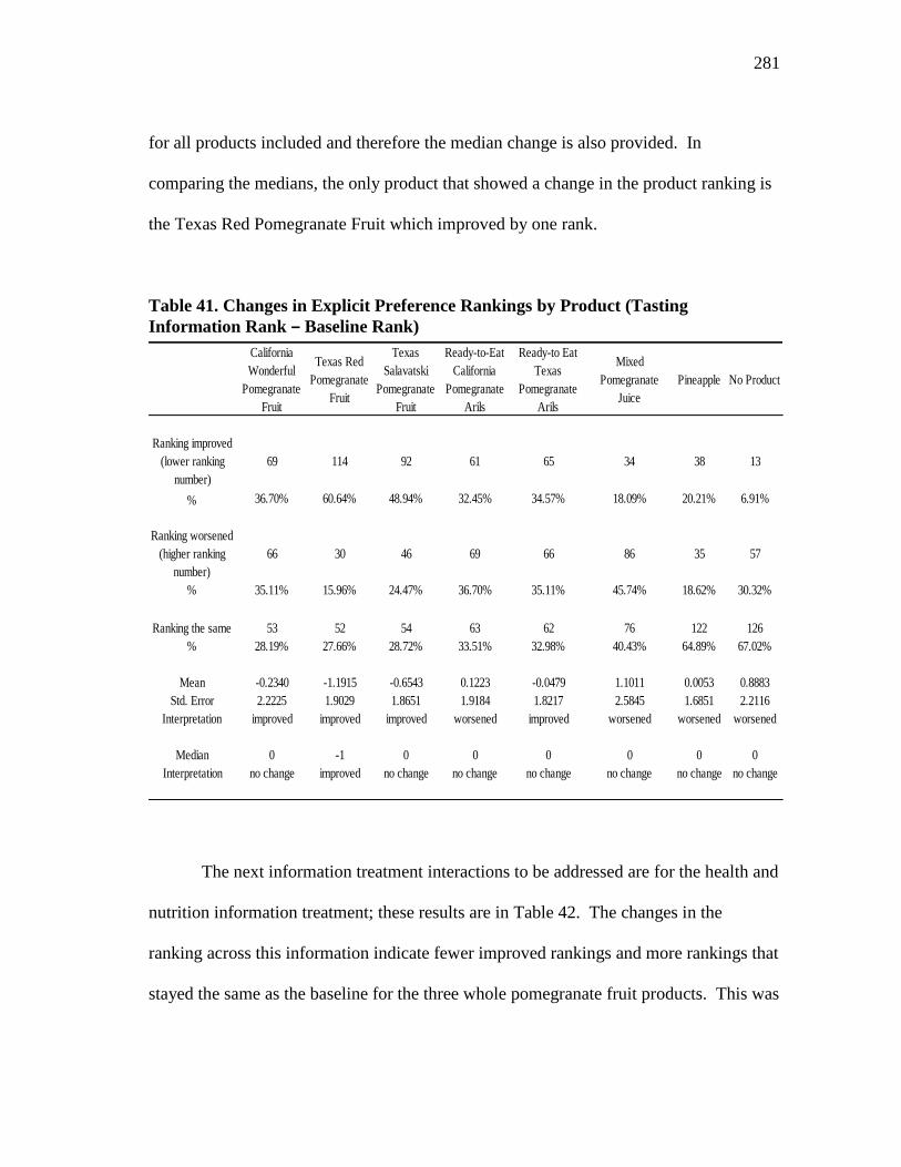
281
for all products included and therefore the median change is also provided. In
comparing the medians, the only product that showed a change in the product ranking is
the Texas Red Pomegranate Fruit which improved by one rank.
Table 41. Changes in Explicit Preference Rankings by Product (Tasting
Information Rank ‒ Baseline Rank)
The next information treatment interactions to be addressed are for the health and
nutrition information treatment; these results are in Table 42. The changes in the
ranking across this information indicate fewer improved rankings and more rankings that
stayed the same as the baseline for the three whole pomegranate fruit products. This was
California
Wonderful
Pomegranate
Fruit
Texas Red
Pomegranate
Fruit
Texas
Salavatski
Pomegranate
Fruit
Ready-to-Eat
California
Pomegranate
Arils
Ready-to Eat
Texas
Pomegranate
Arils
Mixed
Pomegranate
Juice
Pineapple No Product
Ranking improved
(lower ranking
number)
69 114 92 61 65 34 38 13
% 36.70% 60.64% 48.94% 32.45% 34.57% 18.09% 20.21% 6.91%
Ranking worsened
(higher ranking
number)
66 30 46 69 66 86 35 57
% 35.11% 15.96% 24.47% 36.70% 35.11% 45.74% 18.62% 30.32%
Ranking the same 53 52 54 63 62 76 122 126
% 28.19% 27.66% 28.72% 33.51% 32.98% 40.43% 64.89% 67.02%
Mean -0.2340 -1.1915 -0.6543 0.1223 -0.0479 1.1011 0.0053 0.8883
Std. Error 2.2225 1.9029 1.8651 1.9184 1.8217 2.5845 1.6851 2.2116
Interpretation improved improved improved worsened improved worsened worsened worsened
Median 0 -1 0 0 0 0 0 0
Interpretation no change improved no change no change no change no change no change no change
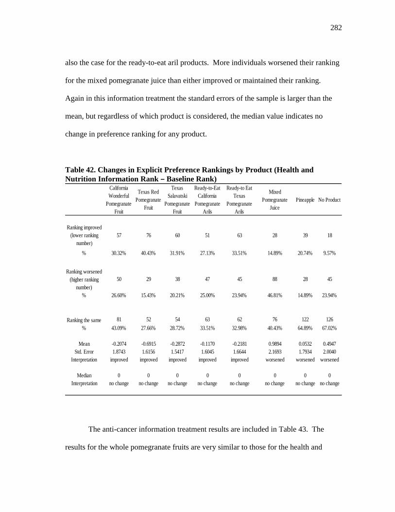
282
also the case for the ready-to-eat aril products. More individuals worsened their ranking
for the mixed pomegranate juice than either improved or maintained their ranking.
Again in this information treatment the standard errors of the sample is larger than the
mean, but regardless of which product is considered, the median value indicates no
change in preference ranking for any product.
Table 42. Changes in Explicit Preference Rankings by Product (Health and
Nutrition Information Rank ‒ Baseline Rank)
The anti-cancer information treatment results are included in Table 43. The
results for the whole pomegranate fruits are very similar to those for the health and
California
Wonderful
Pomegranate
Fruit
Texas Red
Pomegranate
Fruit
Texas
Salavatski
Pomegranate
Fruit
Ready-to-Eat
California
Pomegranate
Arils
Ready-to Eat
Texas
Pomegranate
Arils
Mixed
Pomegranate
Juice
Pineapple No Product
Ranking improved
(lower ranking
number)
57 76 60 51 63 28 39 18
% 30.32% 40.43% 31.91% 27.13% 33.51% 14.89% 20.74% 9.57%
Ranking worsened
(higher ranking
number)
50 29 38 47 45 88 28 45
% 26.60% 15.43% 20.21% 25.00% 23.94% 46.81% 14.89% 23.94%
Ranking the same 81 52 54 63 62 76 122 126
% 43.09% 27.66% 28.72% 33.51% 32.98% 40.43% 64.89% 67.02%
Mean -0.2074 -0.6915 -0.2872 -0.1170 -0.2181 0.9894 0.0532 0.4947
Std. Error 1.8743 1.6156 1.5417 1.6045 1.6644 2.1693 1.7934 2.0040
Interpretation improved improved improved improved improved worsened worsened worsened
Median 0 0 0 0 0 0 0 0
Interpretation no change no change no change no change no change no change no change no change
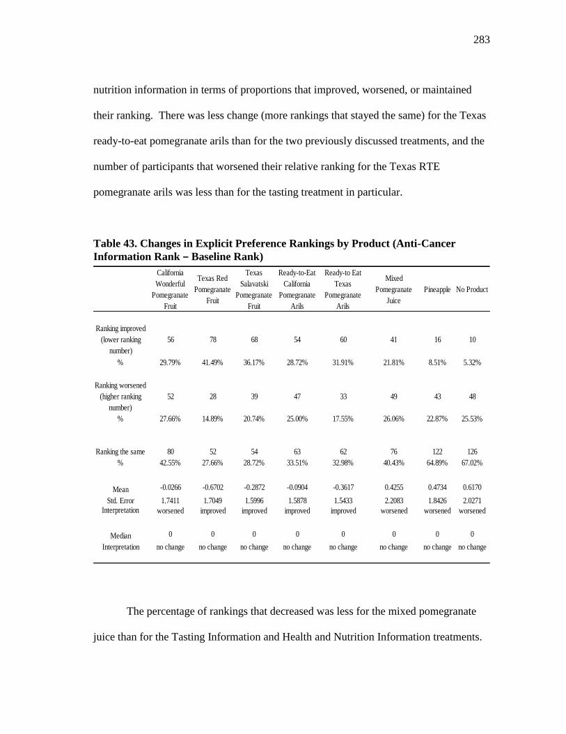
283
nutrition information in terms of proportions that improved, worsened, or maintained
their ranking. There was less change (more rankings that stayed the same) for the Texas
ready-to-eat pomegranate arils than for the two previously discussed treatments, and the
number of participants that worsened their relative ranking for the Texas RTE
pomegranate arils was less than for the tasting treatment in particular.
Table 43. Changes in Explicit Preference Rankings by Product (Anti-Cancer
Information Rank ‒ Baseline Rank)
The percentage of rankings that decreased was less for the mixed pomegranate
juice than for the Tasting Information and Health and Nutrition Information treatments.
California
Wonderful
Pomegranate
Fruit
Texas Red
Pomegranate
Fruit
Texas
Salavatski
Pomegranate
Fruit
Ready-to-Eat
California
Pomegranate
Arils
Ready-to Eat
Texas
Pomegranate
Arils
Mixed
Pomegranate
Juice
Pineapple No Product
Ranking improved
(lower ranking
number)
56 78 68 54 60 41 16 10
% 29.79% 41.49% 36.17% 28.72% 31.91% 21.81% 8.51% 5.32%
Ranking worsened
(higher ranking
number)
52 28 39 47 33 49 43 48
% 27.66% 14.89% 20.74% 25.00% 17.55% 26.06% 22.87% 25.53%
Ranking the same 80 52 54 63 62 76 122 126
% 42.55% 27.66% 28.72% 33.51% 32.98% 40.43% 64.89% 67.02%
Mean -0.0266 -0.6702 -0.2872 -0.0904 -0.3617 0.4255 0.4734 0.6170
Std. Error 1.7411 1.7049 1.5996 1.5878 1.5433 2.2083 1.8426 2.0271Interpretation worsened improved improved improved improved worsened worsened worsened
Median 0 0 0 0 0 0 0 0
Interpretation no change no change no change no change no change no change no change no change
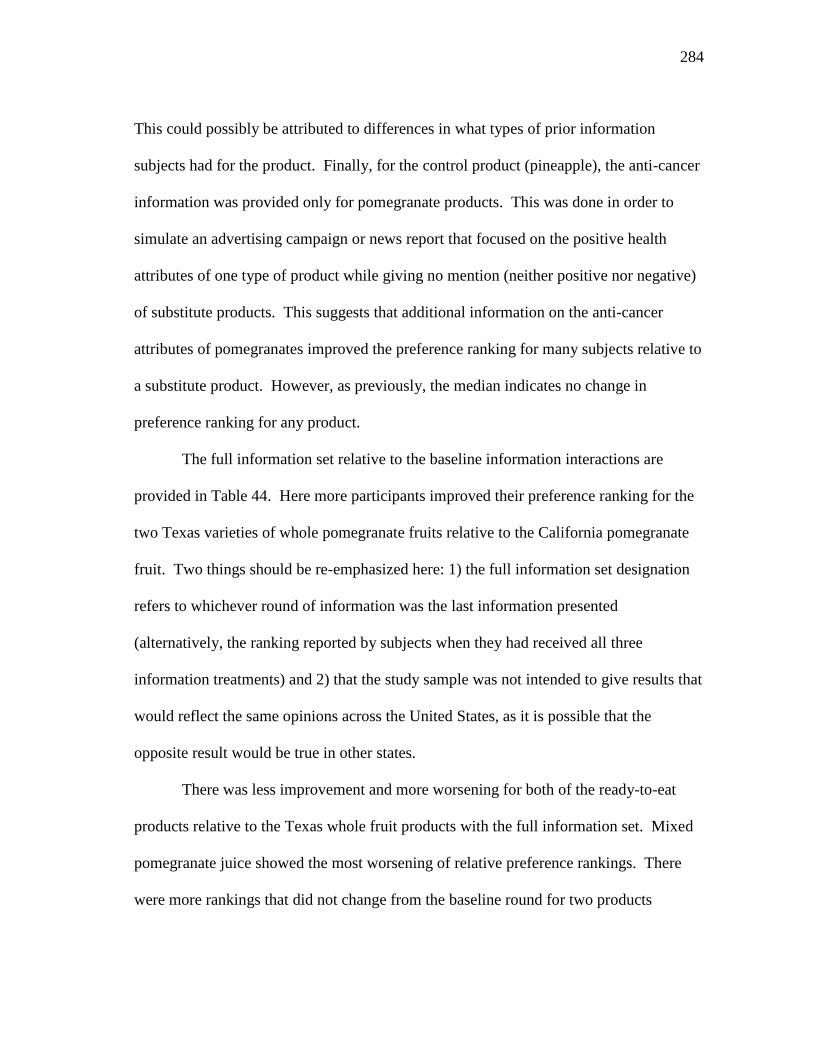
284
This could possibly be attributed to differences in what types of prior information
subjects had for the product. Finally, for the control product (pineapple), the anti-cancer
information was provided only for pomegranate products. This was done in order to
simulate an advertising campaign or news report that focused on the positive health
attributes of one type of product while giving no mention (neither positive nor negative)
of substitute products. This suggests that additional information on the anti-cancer
attributes of pomegranates improved the preference ranking for many subjects relative to
a substitute product. However, as previously, the median indicates no change in
preference ranking for any product.
The full information set relative to the baseline information interactions are
provided in Table 44. Here more participants improved their preference ranking for the
two Texas varieties of whole pomegranate fruits relative to the California pomegranate
fruit. Two things should be re-emphasized here: 1) the full information set designation
refers to whichever round of information was the last information presented
(alternatively, the ranking reported by subjects when they had received all three
information treatments) and 2) that the study sample was not intended to give results that
would reflect the same opinions across the United States, as it is possible that the
opposite result would be true in other states.
There was less improvement and more worsening for both of the ready-to-eat
products relative to the Texas whole fruit products with the full information set. Mixed
pomegranate juice showed the most worsening of relative preference rankings. There
were more rankings that did not change from the baseline round for two products
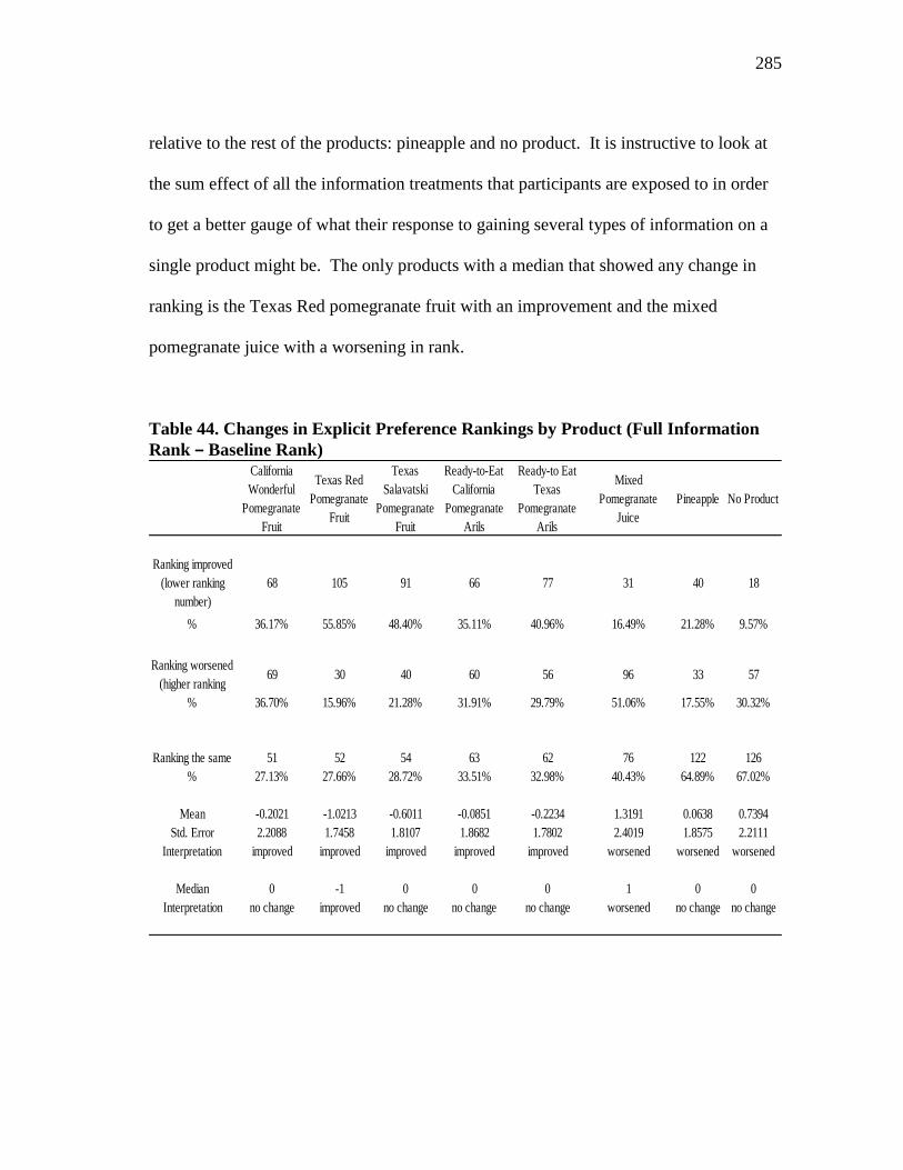
285
relative to the rest of the products: pineapple and no product. It is instructive to look at
the sum effect of all the information treatments that participants are exposed to in order
to get a better gauge of what their response to gaining several types of information on a
single product might be. The only products with a median that showed any change in
ranking is the Texas Red pomegranate fruit with an improvement and the mixed
pomegranate juice with a worsening in rank.
Table 44. Changes in Explicit Preference Rankings by Product (Full Information
Rank ‒ Baseline Rank)
California
Wonderful
Pomegranate
Fruit
Texas Red
Pomegranate
Fruit
Texas
Salavatski
Pomegranate
Fruit
Ready-to-Eat
California
Pomegranate
Arils
Ready-to Eat
Texas
Pomegranate
Arils
Mixed
Pomegranate
Juice
Pineapple No Product
Ranking improved
(lower ranking
number)
68 105 91 66 77 31 40 18
% 36.17% 55.85% 48.40% 35.11% 40.96% 16.49% 21.28% 9.57%
Ranking worsened
(higher ranking 69 30 40 60 56 96 33 57
% 36.70% 15.96% 21.28% 31.91% 29.79% 51.06% 17.55% 30.32%
Ranking the same 51 52 54 63 62 76 122 126
% 27.13% 27.66% 28.72% 33.51% 32.98% 40.43% 64.89% 67.02%
Mean -0.2021 -1.0213 -0.6011 -0.0851 -0.2234 1.3191 0.0638 0.7394
Std. Error 2.2088 1.7458 1.8107 1.8682 1.7802 2.4019 1.8575 2.2111
Interpretation improved improved improved improved improved worsened worsened worsened
Median 0 -1 0 0 0 1 0 0
Interpretation no change improved no change no change no change worsened no change no change
286
Comparison of Bidding and Ranking Results
Subjects expressed their preferences for the fruit products in two distinct yet
conceptually-related ways. Did these two methods of preference elicitation yield
compatible results, and if not, which method is preferred? It was expected that the two
methods would produce similar, yet not identical results due to inconsistencies or human
error in decision processes, failure to remember previous responses, and so on. Even so,
a rational decisionmaker would be predicted to submit rankings and bids that expressed
the same order of preferences.
However, results on the convergence of the two methods for preference
elicitation were mixed. There were a total of 142 individuals expressing at least one
preference reversal. Preference reversals have been previously discussed by Tversky
and Thaler (1990). For this description, preference reversals are defined as a difference
between rankings and ordered bids for the same round. This suggests that the
preferences expressed in the rankings indicate different preferences than the preferences
expressed by the same subjects‘ actual bids. The term preference reversal will
specifically exclude changes in rankings or biddings across rounds, as it is expected that
those could occur due to preference updating based on the additional information that
subjects received across rounds. The numbers of individuals with at least one preference
reversal among the product alternatives within any single round are listed in Table 45.
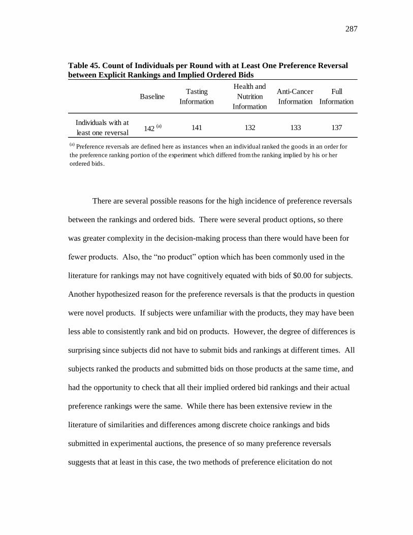
287
Table 45. Count of Individuals per Round with at Least One Preference Reversal
between Explicit Rankings and Implied Ordered Bids
There are several possible reasons for the high incidence of preference reversals
between the rankings and ordered bids. There were several product options, so there
was greater complexity in the decision-making process than there would have been for
fewer products. Also, the ―no product‖ option which has been commonly used in the
literature for rankings may not have cognitively equated with bids of $0.00 for subjects.
Another hypothesized reason for the preference reversals is that the products in question
were novel products. If subjects were unfamiliar with the products, they may have been
less able to consistently rank and bid on products. However, the degree of differences is
surprising since subjects did not have to submit bids and rankings at different times. All
subjects ranked the products and submitted bids on those products at the same time, and
had the opportunity to check that all their implied ordered bid rankings and their actual
preference rankings were the same. While there has been extensive review in the
literature of similarities and differences among discrete choice rankings and bids
submitted in experimental auctions, the presence of so many preference reversals
suggests that at least in this case, the two methods of preference elicitation do not
BaselineTasting
Information
Health and
Nutrition
Information
Anti-Cancer
Information
Full
Information
Individuals with at
least one reversal142
(a) 141 132 133 137
(a) Preference reversals are defined here as instances when an individual ranked the goods in an order for
the preference ranking portion of the experiment which differed from the ranking implied by his or her
ordered bids.
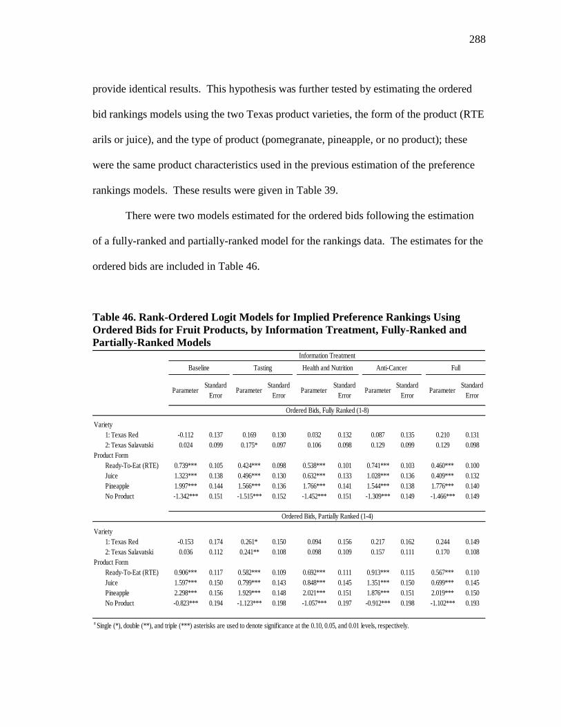
288
provide identical results. This hypothesis was further tested by estimating the ordered
bid rankings models using the two Texas product varieties, the form of the product (RTE
arils or juice), and the type of product (pomegranate, pineapple, or no product); these
were the same product characteristics used in the previous estimation of the preference
rankings models. These results were given in Table 39.
There were two models estimated for the ordered bids following the estimation
of a fully-ranked and partially-ranked model for the rankings data. The estimates for the
ordered bids are included in Table 46.
Table 46. Rank-Ordered Logit Models for Implied Preference Rankings Using
Ordered Bids for Fruit Products, by Information Treatment, Fully-Ranked and
Partially-Ranked Models
ParameterStandard
ErrorParameter
Standard
ErrorParameter
Standard
ErrorParameter
Standard
ErrorParameter
Standard
Error
Variety
1: Texas Red -0.112 0.137 0.169 0.130 0.032 0.132 0.087 0.135 0.210 0.131
2: Texas Salavatski 0.024 0.099 0.175* 0.097 0.106 0.098 0.129 0.099 0.129 0.098
Product Form
Ready-To-Eat (RTE) 0.739*** 0.105 0.424*** 0.098 0.538*** 0.101 0.741*** 0.103 0.460*** 0.100
Juice 1.323*** 0.138 0.496*** 0.130 0.632*** 0.133 1.028*** 0.136 0.409*** 0.132
Pineapple 1.997*** 0.144 1.566*** 0.136 1.766*** 0.141 1.544*** 0.138 1.776*** 0.140
No Product -1.342*** 0.151 -1.515*** 0.152 -1.452*** 0.151 -1.309*** 0.149 -1.466*** 0.149
Variety
1: Texas Red -0.153 0.174 0.261* 0.150 0.094 0.156 0.217 0.162 0.244 0.149
2: Texas Salavatski 0.036 0.112 0.241** 0.108 0.098 0.109 0.157 0.111 0.170 0.108
Product Form
Ready-To-Eat (RTE) 0.906*** 0.117 0.582*** 0.109 0.692*** 0.111 0.913*** 0.115 0.567*** 0.110
Juice 1.597*** 0.150 0.799*** 0.143 0.848*** 0.145 1.351*** 0.150 0.699*** 0.145
Pineapple 2.298*** 0.156 1.929*** 0.148 2.021*** 0.151 1.876*** 0.151 2.019*** 0.150
No Product -0.823*** 0.194 -1.123*** 0.198 -1.057*** 0.197 -0.912*** 0.198 -1.102*** 0.193
a Single (*), double (**), and triple (***) asterisks are used to denote significance at the 0.10, 0.05, and 0.01 levels, respectively.
Ordered Bids, Fully Ranked (1-8)
Ordered Bids, Partially Ranked (1-4)
Information Treatment
Baseline Tasting Health and Nutrition Anti-Cancer Full
289
For the fully ranked ordered bids, the magnitude of the estimated parameters for
the rank-ordered logit model differs from that of the estimated parameters for the
rankings model. However, for the baseline information round, in both models there was
no preference effect for either Texas variety. In order of increasing preference, there
were positive effects for RTE, juice, and pineapple. In both cases there was a negative
effect for the no product option. In the tasting round, the implied rankings from the
ordered bids indicate a tendency for a preference for the Texas Salavatski variety (P <
0.10); the Texas Red variety was preferred by the explicit rankings (Table 39) over
either Texas Salavatski or California Wonderful. Not only is this a difference in
magnitude of the parameters, this difference would lead to opposite conclusions in
selecting one variety or the other. This is a cause for concern in marketing research in
terms of which product is the one that is actually preferred and would be purchased by
consumers. The preferences for the remaining product characteristics are similar for
RTE, pineapple, and no product, but there was no significant effect in the preference
ranking for the juice while there was a preference for juice over the whole fruit products.
In fact, other than the product fruit cultivars, the ordered bids indicated increasing
preference, in order, for RTE, juice, and pineapple, with a discounted preference for no
product for the baseline and all information treatment rounds. In contrast, when subjects
had full information the RTE product was preferred to juice for the full ranked implied
rankings. For the Texas varieties, there was a trend towards a preference for the Texas
Red variety over the Texas Salavatski variety. This result is similar to the estimates of
the rank-ordered logit model for the explicit preference rankings; however, in this case
290
the result is a change from tasting round of the experimental auction bidding. It would
be unusual but not impossible for the implied preference to vary from the tasting round
to the full information set, since subjects had already tasted the product for the full
information round.
Again, although the values of the estimated parameters are not identical for the
partially-ranked implied rankings, there was a slight preference for the Texas Salavatski
variety. Overall a comparison of the implied preferences from the baseline round to the
full information set showed an increase in the relative discount for option of no product
along with less strong preferences for RTE, juice, and pineapple. This was most
noticeable for the juice, where the decrease in relative preference was approximately 1.5
times less in the full information set.
Comparing the fully ranked ordered bid model to the partially-ranked model
reveals several patterns and trends. The relative size of the effects is generally larger for
the product characteristics in the partially ranked model. However, as pointed out in the
comparison of the explicit ranking decisions, the size of the discount for no product is
much less than that in the fully ranked model. Based on the distributions of the
preference rankings, this result is not unexpected. With the majority of the ―no product‖
options ranked as the lowest rank, discarding the four lowest ranks was almost
guaranteed to underestimate the parameters for the no product option and any other
product that was consistently among the lowest ranked products; in discarding the lowest
ranks, relevant information on some of the products is discarded. Calfee, Winston, and
Stempski (2001) state that if subjects have paid less attention to the lower ranked
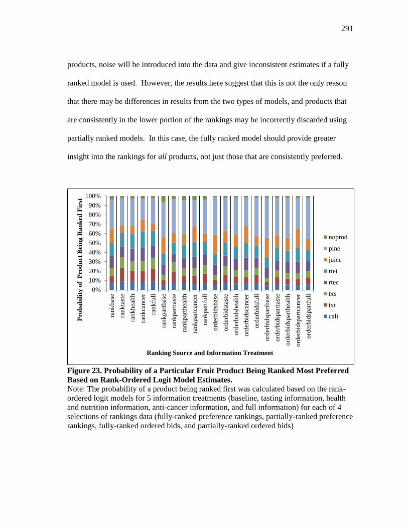
291
products, noise will be introduced into the data and give inconsistent estimates if a fully
ranked model is used. However, the results here suggest that this is not the only reason
that there may be differences in results from the two types of models, and products that
are consistently in the lower portion of the rankings may be incorrectly discarded using
partially ranked models. In this case, the fully ranked model should provide greater
insight into the rankings for all products, not just those that are consistently preferred.
Figure 23. Probability of a Particular Fruit Product Being Ranked Most Preferred
Based on Rank-Ordered Logit Model Estimates.
Note: The probability of a product being ranked first was calculated based on the rank-
ordered logit models for 5 information treatments (baseline, tasting information, health
and nutrition information, anti-cancer information, and full information) for each of 4
selections of rankings data (fully-ranked preference rankings, partially-ranked preference
rankings, fully-ranked ordered bids, and partially-ranked ordered bids)
0%
10%
20%
30%
40%
50%
60%
70%
80%
90%
100%
rank
bas
e
rank
tast
e
rank
hea
lth
rank
can
cer
rank
full
rank
par
tbas
e
rank
par
ttas
te
rank
par
thea
lth
rank
par
tcan
cer
rank
par
tfu
ll
ord
erb
idsb
ase
ord
erb
idst
aste
ord
erb
idsh
ealt
h
ord
erb
idsc
ance
r
ord
erb
idsf
ull
ord
erb
idsp
artb
ase
ord
erb
idsp
artt
aste
ord
erb
idsp
arth
ealt
h
ord
erb
idsp
artc
ance
r
ord
erb
idsp
artf
ull
Pro
ba
bil
ity
of
Pro
du
ct B
ein
g R
an
ked
Fir
st
Ranking Source and Information Treatment
noprod
pine
juice
rtet
rtec
txs
txr
cali
292
The rank-ordered logit model can also be used to predict the probabilities that a
particular product will be ranked first based on the product characteristics. These
probabilities are graphed in Figure 23, and the values of each probability are included in
Appendix I.
The general trends in these probabilities is that the probability of the California
Wonderful whole fruits was consistent across information treatments, while for the
Texas varieties of whole pomegranate fruits there was the greatest likelihood of being
ranked first in the tasting information treatment. For the baseline rounds the likelihood
of any of the fresh pomegranate products being ranked first was the lowest of all the
information levels. Also, there is a general increase in the probability of the mixed
pomegranate juice being ranked first in the anti-cancer information round. Thus, it is
useful to consider the multiple ways in which a product may be novel to a consumer. A
product may be novel in terms of its taste characteristics, its nutritional value, the
production practices that are used, and a number of other categories. Thus, these
differences indicate the potential for differences in the novelty of products in regards to
the information that was presented. Most consumers were expected to be unfamiliar
with the taste of the Texas varieties of pomegranates. Relative to the novelty of the taste
of the juice product, consumers may have been more unfamiliar with the health benefits
of the juice product. This could have led to differences in changes that were seen across
information treatments. For the fresh fruit products, there was very little difference
between the results for anti-cancer information and for health and nutrition information.
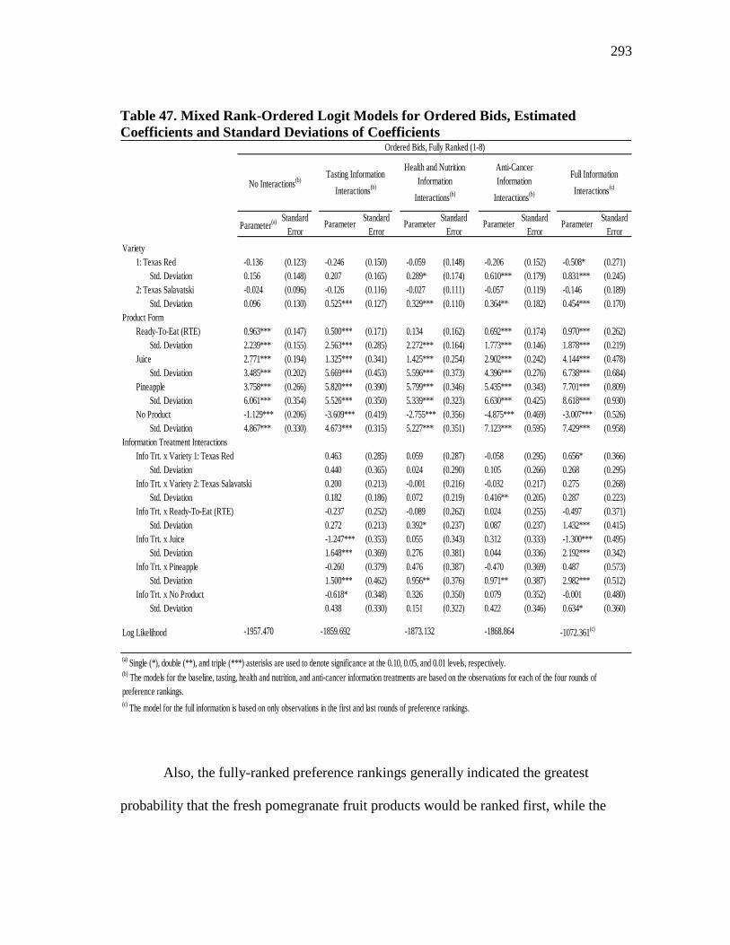
293
Table 47. Mixed Rank-Ordered Logit Models for Ordered Bids, Estimated
Coefficients and Standard Deviations of Coefficients
Also, the fully-ranked preference rankings generally indicated the greatest
probability that the fresh pomegranate fruit products would be ranked first, while the
Parameter(a) Standard
ErrorParameter
Standard
ErrorParameter
Standard
ErrorParameter
Standard
ErrorParameter
Standard
Error
Variety
1: Texas Red -0.136 (0.123) -0.246 (0.150) -0.059 (0.148) -0.206 (0.152) -0.508* (0.271)
Std. Deviation 0.156 (0.148) 0.207 (0.165) 0.289* (0.174) 0.610*** (0.179) 0.831*** (0.245)
2: Texas Salavatski -0.024 (0.096) -0.126 (0.116) -0.027 (0.111) -0.057 (0.119) -0.146 (0.189)
Std. Deviation 0.096 (0.130) 0.525*** (0.127) 0.329*** (0.110) 0.364** (0.182) 0.454*** (0.170)
Product Form
Ready-To-Eat (RTE) 0.963*** (0.147) 0.500*** (0.171) 0.134 (0.162) 0.692*** (0.174) 0.970*** (0.262)
Std. Deviation 2.239*** (0.155) 2.563*** (0.285) 2.272*** (0.164) 1.773*** (0.146) 1.878*** (0.219)
Juice 2.771*** (0.194) 1.325*** (0.341) 1.425*** (0.254) 2.902*** (0.242) 4.144*** (0.478)
Std. Deviation 3.485*** (0.202) 5.669*** (0.453) 5.596*** (0.373) 4.396*** (0.276) 6.738*** (0.684)
Pineapple 3.758*** (0.266) 5.820*** (0.390) 5.799*** (0.346) 5.435*** (0.343) 7.701*** (0.809)
Std. Deviation 6.061*** (0.354) 5.526*** (0.350) 5.339*** (0.323) 6.630*** (0.425) 8.618*** (0.930)
No Product -1.129*** (0.206) -3.609*** (0.419) -2.755*** (0.356) -4.875*** (0.469) -3.007*** (0.526)
Std. Deviation 4.867*** (0.330) 4.673*** (0.315) 5.227*** (0.351) 7.123*** (0.595) 7.429*** (0.958)
Information Treatment Interactions
Info Trt. x Variety 1: Texas Red 0.463 (0.285) 0.059 (0.287) -0.058 (0.295) 0.656* (0.366)
Std. Deviation 0.440 (0.365) 0.024 (0.290) 0.105 (0.266) 0.268 (0.295)
Info Trt. x Variety 2: Texas Salavatski 0.200 (0.213) -0.001 (0.216) -0.032 (0.217) 0.275 (0.268)
Std. Deviation 0.182 (0.186) 0.072 (0.219) 0.416** (0.205) 0.287 (0.223)
Info Trt. x Ready-To-Eat (RTE) -0.237 (0.252) -0.089 (0.262) 0.024 (0.255) -0.497 (0.371)
Std. Deviation 0.272 (0.213) 0.392* (0.237) 0.087 (0.237) 1.432*** (0.415)
Info Trt. x Juice -1.247*** (0.353) 0.055 (0.343) 0.312 (0.333) -1.300*** (0.495)
Std. Deviation 1.648*** (0.369) 0.276 (0.381) 0.044 (0.336) 2.192*** (0.342)
Info Trt. x Pineapple -0.260 (0.379) 0.476 (0.387) -0.470 (0.369) 0.487 (0.573)
Std. Deviation 1.500*** (0.462) 0.956** (0.376) 0.971** (0.387) 2.982*** (0.512)
Info Trt. x No Product -0.618* (0.348) 0.326 (0.350) 0.079 (0.352) -0.001 (0.480)
Std. Deviation 0.438 (0.330) 0.151 (0.322) 0.422 (0.346) 0.634* (0.360)
Log Likelihood -1957.470 -1859.692 -1873.132 -1868.864 -1072.361(c)
(a) Single (*), double (**), and triple (***) asterisks are used to denote significance at the 0.10, 0.05, and 0.01 levels, respectively.
(c) The model for the full information is based on only observations in the first and last rounds of preference rankings.
(b) The models for the baseline, tasting, health and nutrition, and anti-cancer information treatments are based on the observations for each of the four rounds of
preference rankings.
Ordered Bids, Fully Ranked (1-8)
No Interactions(b)
Tasting Information
Interactions(b)
Health and Nutrition
Information
Interactions(b)
Anti-Cancer
Information
Interactions(b)
Full Information
Interactions(c)
294
partially-ranked explicit preference rankings were closer to the predictions of the
estimations based on implied rankings. In all cases, the whole pomegranate fruits were
more likely to be ranked first given the full information set than for the baseline round.
This was not always true for the RTE pomegranate products. The likelihood of the juice
product being ranked first is lower in all cases from the baseline to the full information.
The rank-ordered bid models have been discussed thus far, and the focus now
shifts to the rank-ordered mixed logit models for the ordered bids. The results for the
implied preference rankings (ordered bids) are given in Table 47; the preference
rankings models were shown previously in Table 40.
The results of the application of the mixed rank-ordered logit model to the
ordered bids provide somewhat similar results to the explicit preference rankings
models. The trend is for significance of both the coefficient and the individual
preference heterogeneity for the product form attributes. For the interaction effects, in
the tasting information model there were interactions and preference heterogeneity for
the interaction of juice and tasting information, and the juice was less preferred as a
result of the tasting information. For the health and nutrition information and anti-cancer
information rounds, the interaction terms did not have predictive ability but they led to
an interesting contrast with the model in which only the baseline and full information
rounds were included, and interaction effects between those two were compared.
When the full information set was compared to the baseline by using interaction
effects of the information treatment and the product characteristics, there was trend for a
penalty on the Texas Red variety but a trend for an individual specific interaction effect
295
with the full information in which the Texas Red variety was more preferred.
Participants indicated a decreased preference for the juice product when they had
received the full information set. The signs on the product form characteristics with no
interaction terms were as expected: preferences for RTE, juice, and pineapple with a
negative preference for the no product option. One note of caution is needed in
comparing these results to the rank-ordered logit models estimated previously. The
rank-ordered logit model is equipped to handle ties in the rankings; however, in the
process that was followed for ―exploding‖ the data, ties imply that the same choice was
made at the same time when in fact there were most likely equal probabilities that the
subject would select either of the two options.
The choice of which method, discrete choice preference ranking or experimental
auctions, is more relevant for use in preference elicitation is one for which economic
theory does not provide a direct answer. Particularly since both methods were incentive
compatible in nature, the bias that those differences in hypothetical versus
nonhypothetical responses should be eliminated and subjects would be expected to
provide more convergent answers. Olsen, Donaldson, and Shackley (2005) used a
measure of ―convergent validity‖ as a percentage of respondents who equally preferred
different options over explicit and implied rankings.
For the pomegranate fruit products study, there were a few differences between
the preference rankings and WTP elicitation to be considered in a comparison of the two
results. One, although participants were informed that all of the products were currently
marketed for the same price, it is possible that subjects either chose not to believe this or
296
knew of outside options and price levels which may have influenced their rankings of all
of the products for the same price (the rankings) differently than it influenced their
preferences for the products when they could specify their own maximum price
(auctions). However, subjects did not actually pay the price they bid, and therefore
rationality would still suggest that the products be ordered in the same way, regardless of
which method was used. Secondly, although detailed explanations, quizzes, multiple
practice rounds, and question and answer sessions took place, it is impossible to rule out
the possibility that there were differences in the understandings of the two preference
elicitation mechanisms that were used; this could have subsequently produced
differences in the explicit and implied ordered results. For example, subjects may have
different preferences when the product options have a single specified price than when
those goods vary in price. However, the use of products with similar retail prices should
have eliminated this possibility in this comparison of rankings and bids.
There were a number of similarities in the trends among information levels
between the sets of ranking data that were used, and this robustness is reassuring in
terms of drawing conclusions on the direction of the effects of the information
treatments. However, the differences in the parameter estimates based on using
partially- or fully-ranked models and implied or explicit rankings is a cause for concern
in predicting the magnitude of these changes based on product characteristics. Further,
the number of preference reversals between the ordered bids and the rankings, along
with the differences in the estimated preference models, suggests that one of the two
mechanisms may not be an accurate reflection of true consumer preference. Which of

297
these is more useful should depend on the context of the research question. If
researchers are trying to determine the price that consumers would pay for a product in a
retail setting, the experimental auction procedures may provide more relevant results, but
if the question of interest is what type of product should even be offered for sale in a
retail setting, then the preference ranking procedures may be more relevant. Therefore,
caution in designing and implementing experiments is necessary to ensure that the
question of interest can accurately be addressed with the results that are obtained. To
obtain the full STATA coding for the estimates presented in this chapter, please refer to
Appendix J.
298
CHAPTER VI
SUMMARY AND CONCLUSIONS
This study provided meaningful results on many levels. First, the information
regarding pomegranates and the pomegranate industry can be used by those who are
considering growing or marketing pomegranates. Second, the procedures for a
combined nonhypothetical ranking and bidding preference elicitation mechanism
developed and used here allow for other applications of the field of experimental
economics. Third, the results of the econometric estimations provide insights into not
only the econometric differences in the models but also the implications of the
differences in product characteristics and information treatments. Each of these will be
briefly summarized, and several key conclusions based on the summation of this
information will also be presented. This discussion also leaves a number of research
questions that could be the subject of additional research, and some of these are
mentioned briefly.
Summary
Pomegranates and the Pomegranate Industry
Pomegranate (Punica granatum L.) typically grows best in warm, semiarid
environments, with most scholars attributing its location of origin to the region in and
around Iran. The large shrubs to small trees begin full production at an age of around 3
to 5 years, with an orchard lifespan of around 25 years. The pomegranate fruit are round
299
to oblate with a prominent calyx and with a color range of deep yellow to dark red,
depending on the cultivar. The tough outer husk is filled with small juice sacs called
arils that are separated into compartments within the fruit by septal membranes.
Estimates of the nutritional value of pomegranates as well as the chemical composition
of the different plant components have been made, but these characteristics have also
been shown to vary considerably with cultivar and growing location.
Pomegranates contain a number of plant-specific compounds known as
phytochemicals, and these are the compounds that give the fruits their unique flavor as
well as their potential health implications. One group of phytochemicals, the
polyphenols, is present in a number of forms including flavonoids, hydrolyzable tannins,
and condensed tannins. These compounds are more concentrated in certain parts of the
fruit and plant depending on the compound, with those that have antioxidant properties
being the most commonly cited as having potential human health implications. Diseases
that have been described to have a free radical method of action include general
inflammation and aging, along with diseases that affect the brain, heart, kidney, liver,
lungs, gastrointestinal tract, blood, eyes, skin, and muscles; antioxidants act to interfere
with destructive pathways that free radicals are involved in. Although it has been
difficult to establish causality links for these properties in humans, these properties have
been tested extensively in laboratory settings with non-human subjects. Nevertheless,
the diseases that pomegranates in particular have been linked to reducing based on
either in vitro or in the laboratory include reductions in inflammation, cancer, and
Alzheimer‘s disease symptoms. The effectiveness of pomegranate fruits as disease-
300
reducing mechanisms may also depend on the form of the fruit, as much research
remains to be done on whether the benefits of pomegranates can be obtained from the
individual chemical compounds or if greater benefits may be obtained by consuming the
whole fruit. Reports of toxicity from pomegranate fruits are rare.
The functional food market in the United States alone had a value of $27 billion
in 2007 with an anticipated growth rate of 10% per annum. This market has been
targeted by both food manufacturers and pharmaceutical companies with products that
are suggested to have additional health benefits beyond their basic nutritional value.
Much research has been conducted regarding factors that may affect consumer purchases
of these products; most results indicate differences based on the type of product, the
credibility of the information source for information on the product, the taste of the
products, and underlying consumer attitudes as important determinants of purchases.
Pomegranate production worldwide is led by Iran, followed by India and the
United States; some reports place China third worldwide in production followed by the
U.S. Within the United States, production is predominantly in the state of California,
where 29,000 acres were estimated to be grown in 2009. The typical harvest period in
the United States is October to January, depending on weather conditions and the
particular cultivar.
Pomegranates can best be grown in deep, fairly heavy soils with irrigation and
selecting a cultivar that is appropriate for the growing climate. Adequate attention
should be given to soil preparation, planting design, pruning, fertilization, and disease,
insect, and weed control. Harvest of pomegranate fruits is typically done by hand but
301
mechanical harvesters are beginning to be developed. Post-harvest, pomegranates may
be stored for a typical range of four to five months; post-harvest issues to avoid include
husk scaled and chilling injury. Ready-to-eat pomegranate arils have a much shorter
shelf life, estimated at anywhere from ten to eighteen days using modified-atmosphere
packaging.
USDA provides several estimates of the size of the pomegranate industry,
including estimated movements within the U.S. for the 2009 season of over 14 million
pounds, with a season average shipping point price of $24.54 per 22-lb. carton.
However, these prices were generally higher at the beginning of the season and dropped
as more pomegranate fruit became available; prices also varied based on fruit size,
variety, and location. However, worldwide production is growing in order to meet the
increased demand for pomegranate products and price trends that have been seen in
recent years may be altered as prices adapt to these new levels of supply and demand for
pomegranate fruits and other pomegranate products.
Nonhypothetical Preference Ranking and Experimental Auction Procedures
In this study, two common techniques in experimental economics were combined
into one nonhypothetical procedure to provide paired comparisons of the information
provided by participants. The participants in this study were asked to participate in
repeated rounds of preference rankings and uniform nth-price modified Vickrey auctions
for a baseline and three subsequent information treatments. There has been extensive
discussion in the literature for WTP estimation and preference elicitation on what type of
302
methods provide the most accurate measures of preference. Despite this discussion,
there is no overarching conclusion as to which methodology is the best; rather, there are
a number of tools available to economists in the form of different types of experiments
and these tools should be targeted at the particular question of interest. The application
of these two basic methods of preference elicitation (ranking and bidding) for a set of
products allows preferences to be gauged in two ways, and thus the results of these two
methods compared. Given that participants were informed that all of the products sold at
retail for the same price, the expectation would be that the two methods provide
equivalent measures of preference.
In particular, the application of this combined ranking and bidding preference
elicitation mechanism provided a useful means of gaining information on preferences for
novel products and the effects of information treatments. For any good that is not
currently available on the market, there will be a greater challenge in determining WTP
for products; this is particularly true for those products that derive a large portion of their
value from consumption of the item. To mimic the gain of information on a novel
product, a baseline set of preferences and bids was collected on the assumption that the
relative knowledge base on the products would vary across consumers. Seven products
were included in the study: California Wonderful whole pomegranate fruit, Texas Red
whole pomegranate fruit, Texas Salavatski pomegranate fruit, ready-to-eat California
Wonderful pomegranate arils, ready-to-eat Texas Salavatski pomegranate arils, mixed
pomegranate juice, and pineapple. Subjects were asked to submit bids on these seven
products in the experimental auction portion of the study, and to also rank the seven
303
products and the option of no product on a scale of one to eight. The preference for the
items was expected be individual-specific. Marketers of novel products must carefully
consider what types of information they target at which types of consumers if they have
the aim of increasing WTP for their products. Thus, a series of information treatments
were implemented to make comparisons about three possible types of information that
consumers might gain about the products of interest in this study. Those three
information treatments were: 1) Tasting Information, 2) Health and Nutrition
Information, and 3) Anti-Cancer Information.
Consumers who were unfamiliar with a pomegranate product were expected to
experience some effect on their WTP for that product once they have tasted the product
and/or learned how to prepare it to eat. It was also anticipated that consumers in Texas
would be generally unfamiliar with the product prior to participation in the study. This
was confirmed by the survey results on whether the products had previously been
consumed or purchased. However, particularly given the recent interest in health
benefits of food from a nutritional standpoint as well as in consideration of interest in
functional foods, marketers often make claims regarding the nutrition and health benefits
of novel food products. The question remained as to whether this information would
have any effect on WTP or indicated preferences for pomegranate and other fruit
products. To test this hypothesis, subjects were provided with the nutrition facts and a
description of potential health benefits for each type of included product. Third, recent
developments in terms of functional foods have indicated that some foods may have
specific anti-cancer properties. These effects are very difficult to trace on an individual
304
basis, and making accurate scientific conclusions typically requires expensive and
lengthy clinical trials. Thus, the relevance of such claims for these products and
estimation of the effects of such information on WTP are relevant for those considering
the time-consuming and expensive process of gathering this information and obtaining
government approval to make these claims about products. Further, the use of several
products allows for comparison of whether the effect of information treatments is the
same for all products or whether it varies by product.
The bidding procedure and ranking procedures were designed to elicit these
preferences for a novel product (as opposed to a familiar one) where individual valuation
of the product may be influenced by later opportunities to learn more about the product
characteristics. A full bidding technique was used, but each participant was informed
that most of the study participants would purchase a product, based either on being a
winning bidder or based on a weighted selection of his or her preference rankings. Thus,
it was unlikely that participants would have an opportunity to purchase the product at a
later time. By allowing the result of whether a product was purchased or not to depend
on both the experimental auction bids and preference rankings, the two main
components of the procedures were nonhypothetical in nature and participants would be
expected to express their true preferences for the products in either portion of the study.
A survey of consumer demographics and behavioral characteristics provided other
variables for comparison to the preference rankings and experimental auction bids.
305
Analytical Procedures and Results Summary
The mechanism described above was utilized to obtain results based on
behavioral and demographic characteristics reported by participants as well as make
estimates of factors that influence WTP and preferences for the included products. A
summary of these results follows.
Survey Procedures and Results
There are a few key demographics and behavioral characteristics of interest that
were measured by the survey portion of the experiment. The average weekly household
spending of participants was $109, and the average weekly household spending on fruits
and vegetables was $25. The average participant had 6.37 pounds of fruits and
vegetables on hand; this result was measured to determine if there was a potential effect
from current stocks of similar products on the WTP for the products in the study.
Subjects reported that on average 71% of their fruit and vegetable purchases were for
fresh (not frozen, dried, or canned) fruits and vegetables. Study participants were asked
about their relative position in their buying cycle in order to account for possible effects
of whether they had just gone to the store to make purchases or whether they were about
to go to make those purchases; it had been an average of 3 days since participants had
last been to the store and they indicated an average length of time between trips to buy
fruits and vegetables of 8 days.
To determine the relative novelty of the pomegranate products, participants were
surveyed as to their previous experience with the products. Only 24.6% of participants
306
had previously purchased a pomegranate, and just 7.5% of study participants had a
pomegranate fruit on hand. The portion of the subjects who had previously heard the
term functional foods was small (16%), but the proportion who had purchased a
functional food product when examples were provided was much larger (i.e. 85% for
breakfast cereal for heart health). Taste, freshness, and price were all cited as being very
important to subjects on an individual basis as factors in making fresh produce
purchasing decisions. However, when asked about the factors that they expected most
Americans to be concerned with, price and convenience became more important and
nutrition and growing location became less important. This result would be expected
since the factors that were more important when subjects were asked about their
individual behaviors were also those factors that would be expected to have a positive
social connotation (―social desirability bias‖), while that bias should have been avoided
when subjects were asked about the typical American.
Of course, caution should be used in extrapolating all of these results to the
general population, as the study sample was recruited with the explicit purpose of being
a study on fruit purchase decision-making. For example, if the individuals in the sample
differed from the average American in a way that systematically affected the factors that
influence fruit and vegetable purchasing decisions, then the result that the average of the
included individuals and ―average Americans‖ were predicted to be different would be
expected. Nevertheless, the sample should serve the purpose of providing general trends
and results for the relevant population.
However, the mean experimental auction bids for the included products ranged
307
from $0.84 to $1.99, all well below the retail price of $3.50 for all the included products.
A portion of this result could be attributed to a lack of familiarity with the products, and
perhaps more important than the absolute price levels are the relative differences in WTP
for the products, as the retail price of the products is expected to vary with the season,
geographic region, size of the individual products, and other factors.
Caution should also be exercised in extending any results for the products
included in this study to products outside the study. Even so, it would be expected that
some of the behavioral and demographic characteristics measured in this study may be
useful for other products in predicting factors that influence buying behavior,
particularly for a product that is less novel than pomegranate fruits.
Estimation Procedures and Results
Individual WTP for a product was censored at $0.00 when measured using this
experimental auction, with 18% of all submitted bids being censored. To model these
results, a number of approaches were considered. Individual models for each product
and information treatment were first applied with a tobit model to account for the bid
censoring. Using the separate tobit models, demographic and behavioral characteristics
were as a whole poor predictors of WTP for the included pomegranate and other fruit
products, with the exception of whether pomegranates had previously been purchased.
For some products there were other factors that were predicted to influence WTP,
including household size, income use, and tobacco use. Also, whether participants were
given a reference price (current retail price) for the product was generally significant.
308
The bids were then pooled across individuals, information treatments, and
products to suggest characteristics of the products that might influence WTP. The
following models were considered: ordinary least squares, standard tobit, random effects
tobit, and mixed linear. Each of these models was found to have benefits and
drawbacks. These models were each considered with several independent variable
specifications, including models with only the product characteristics, the product
characteristics along with information treatments, and both of the previous coupled with
the demographic and behavioral characteristics. While the results varied depending on
the specific model used for estimation and the variables that were included, the product
characteristics of ready-to-eat product form, juice product form, and pineapple product
often increased WTP for the products; the distinction between the California Wonderful,
Texas Red, and Texas Salavatski varieties was often not significant for the estimations
based on the full bids. Also, the random effects tobit model predicted a significant
presence of a random effect due to the individual, and the mixed linear model also
predicted an effect for each individual. The ordinary least square model and standard
tobit model were thus rejected as models for the experimental auction bids in this study;
however, both models were still included as a baseline comparison.
Although the censoring and individual effects were discussed in the model
results, there were several other effects of importance. First, there were a number of
bidders who were found to be either unengaged as individuals or unengaged for a
particular product. The models were re-estimated excluding the unengaged bidders;
excluding unengaged bidders changed the parameter estimates and resulted in a
309
prediction that the Texas Salavatski variety positively affected WTP. Second, while
comparisons using full bids across individuals are useful in predicting relative WTP for
products, they do not account for differences in product substitutes, and thus the bids
were reanalyzed by comparing the implied bid differences from one information
treatment to the next; in this way the outside substitutes for a product and individual
should cancel out. In this case it is particularly important to exclude any bids that were
unengaged (that is, where an individual submitted a bid of zero in the treatment round
and the baseline round for a product). The results from these models suggest that over
the information treatments the change in WTP for the two Texas varieties increased but
the change in WTP for RTE, juice, and pineapple decreased. Also, if demographic
variables were included, tobacco use caused an increase in the change in WTP.
Although several different models were estimated to predict WTP, the effect of
the information treatments was tested directly using two types of tests: the paired t-test,
which assumes normality of the bid distributions, and the Wilcoxon signed rank test to
compare bids with nonparametric distributions. For the three whole pomegranate fruits
and the Texas RTE arils, all the information treatments as well as the full information
set resulted in bids that were different from the baseline; results for the other products
were mixed depending on the product and information treatment.
The rankings data were also analyzed to gather information on preferences for
the included products. The preference for each product using a rank-ordered logit model
was estimated first for the products for each information treatment. Thus, product
characteristics within a given round of bids could be compared to predict which product
310
characteristics were likely to result in the product being more preferred. Using the
complete set of rankings, the relative effect of the product characteristics varied across
information treatments. In the baseline round there was no effect for the Texas variety,
items that were RTE, juice, or pineapple were more preferred, and the option of no
product was discounted. However, in considering the other information treatments and
the full information set, the two Texas varieties were preferred to the California variety,
the option of no product was discounted more severely relative to the other products, and
juice and pineapple were not as strongly preferred. The improvement in ranking for the
Texas varieties was largest in the tasting information treatment; and for all rounds where
subjects had received any information the Texas Red variety was preferred to the Texas
Salavatski variety. Due to the possibility of heterogeneity in ranking ability (more
precisely, the possibility of subjects being less careful when ranking less preferred
products than more preferred products), the rank-ordered logit model was re-estimated
using the partial rankings (ranks 1-4). The estimates of this model were not identical to
the estimations based on the complete rankings, which is indicative of possible
heterogeneity in ranking ability.
The explicit preference rankings were compared to the implied preferences based
on the ordered bids. The bids submitted by subjects were sorted from highest to lowest
and rankings were assigned for the values of 1-8. The option of no product was assigned
the next lowest rank after the last non-zero bid. Checking for reversals in preferences
(instances when the explicit orderings and implied orderings did not ―match‖) within the
same information treatment indicated that this was a concern for comparing preference
311
rankings and ordered bids. Thus, although both mechanisms were designed to be
incentive compatible in nature with weakly dominant strategies of submitting true
preferences and bids, respectively, an estimation of the rank-ordered logit models based
on the implied rankings was not expected to provide identical results for this study. For
the full information treatment relative to the baseline, the Texas varieties were neither
preferred nor discounted, the no product option was less preferred at the baseline and
became even less preferred across the information treatments, and ready-to-eat, juice,
and pineapple all had a positive relationship with preference but this became less true
across the information treatments, indicating a stronger preference for the excluded
dummy variable (whole fruit for the product form and pomegranate for the product
type).
The individual preferences for the pomegranate and other fruit product options
were also analyzed with the use of the mixed rank-ordered logit model. Such models
were estimated using both explicit preference rankings and implied rankings based on
ordered bids. These models suggest the presence of individual preference heterogeneity
for the product form characteristics, as well as for the interaction of some product
characteristics with the additional information treatments. These results varied
depending on which information treatment was considered, providing the insight that for
explicit rankings tasting information increased the preference for the Texas Red variety
over the California Wonderful variety but decreased it for RTE products relative to
whole fruit products. We would not expect the exact parameter estimates for these two
models to be equal; however, the fruit variety was generally not significant in the
312
bidding models but was significant in several of the preference ranking models. This
suggests that there may be differences in the way that subjects viewed the consequences
of misbehavior in each procedure or the individual variability that was expressed
through either rankings or bidding.
Conclusions
The summary of the pomegranate industry and experimental results based on
both the nonhypothetical auction and preference ranking procedures lead to both
conclusions and further questions. These are discussed further here.
Key Challenges for Expansion of Pomegranate Production
There are a number of challenges that must be addressed in order for
pomegranate production to expand both in terms of acreage and profitability. The
registration of fungicides, insecticides, and herbicides for application in pomegranate
production will be necessary in order to address disease, insect, and weed management
issues. As far back as 1917, Robert Hodgson, author of a text on pomegranate history
and production in California, recognized that one of the keys for the growth of the
pomegranate industry was successful education of the public about this fruit.
Several individuals involved with pomegranate production also suggest that as
global supply of pomegranates expands, prices may decrease (e.g., Cline 2008;
―Pomegranate Acreage‖ 2009). This is particularly true for storable (and thus more
easily transportable) forms of pomegranate such as concentrated juice or other
313
pomegranate by-products which may be sourced from other regions or other countries.
Thus, those considering expanding production should consider marketing opportunities
at a range of price points when determining the feasibility of expansion.
Also, expanded production plans might also take into account the seasonality of
pomegranate production and what product forms will be marketed. Fresh pomegranates
cannot be stored long enough to sustain sales from one growing season to the next with
current post-harvest technology, whereas juice or other processed products may be
stored for such a length of time. However, particularly for growers who intend to market
a product as a regionally-grown product, the price premium received may vary for each
of these different types of products. Also, there may be different cultivars of
pomegranates that are ideally suited for one of the juice, RTE, or whole fruit products
but be less than desirable for use for others.
In terms of further considerations for expansion of the pomegranate industry, the
following issues may be potential opportunities or concerns. First, considerable media
as well as research attention has been devoted to health claims about antioxidants in
general and pomegranates specifically. However, many of these claims are made based
on laboratory results and have not been verified in large, long-term studies of human
populations. As these health claims are one component of the growth in the
pomegranate industry, if these health claims cannot be verified then the projected growth
in sales of pomegranate products may not come to fruition. Until those studies can be
completed, a short-term alternative would be to emphasize the positive taste and
nutritional benefits of pomegranates.

314
Further, although health claims about functional foods are not as strictly
regulated in the United States as in some other places, the risk to producers remains that
stricter regulations may be imposed. However, such regulation may increase WTP for
any products for which regulatory approval is obtained and thereby increase consumer
confidence in the health claims that are made.
Although the acreage of pomegranates planted in the United States is growing,
the total acreage is still small relative to other commodities and more common fruit and
vegetable crops. In terms of insect, weed, and disease management, chemical products
that are available for use on other crops may not be registered for use on pomegranates
or in the state where pomegranate production may be considered. Thus, these products
may not be available for use or may be expensive if they are later registered for use.
One final issue with expansion of pomegranate production is labor considerations
for harvest. At present, use of mechanical harvesters for the crop is not widespread.
However, as with many other fruit and vegetable crops the availability and consistency
of labor for harvesting seasonal fruits and vegetables can be an uncertain component of
the process from planting to sales of pomegranates. Thus, the industry as a whole would
stand to benefit from an effective mechanical harvester that does not damage the fruit
and provides greater certainty for the supply of harvest labor.
Information provided by this study and conclusions drawn from results may not
hold absolutely; this conclusion is based on the extensive discussion of the validity of
WTP from auction mechanisms. Further, the exact levels of the WTP estimates from
this model may not be exact and should not be assumed to be easily extrapolated to exact
315
premiums in a market setting. However, there does appear to be value in the relative
importance of the factors analyzed.
Novel Products and Value Elicitation Mechanisms
The pomegranate products included in the study were generally novel to
participants, and this was an important consideration in the design of the WTP elicitation
procedures. A mechanism was needed that would limit opportunities for future learning
about the products, so that all participants would submit values that were a ―snapshot‖ of
a point-in-time valuation for all of the products and not biased by future opportunities to
gather information on the products or transaction costs of doing so. As a result, in the
estimation of WTP many of the demographic variables that may have influenced
valuations for more familiar products had little influence on the novel product,
particularly for the baseline round where participants were not given any additional
information. Prior experience with pomegranate products had a larger effect on an
individual‘s valuation of the products. This result indicates the importance of gauging
prior experience with a novel product if value elicitation procedures will be used to
estimate WTP. Also, given the lack of familiarity with the products, participant bids in
the experimental auction were affected based on whether or not a reference price was
provided as a part of the study mechanism.
Individual values varied considerably for the products, and comparisons of
within subject differences for a product across information treatments allows the
possible differences in outside substitutes to cancel out and should provide more
316
information on how the information treatments affected the change in WTP. Further,
bids and rankings on all products were collected; theory would suggest that for two
incentive compatible preference elicitation mechanisms the results would be similar.
However, the two procedures yielded results that were similar for some product
characteristics and divergent for others; the results for the two procedures were not
identical. This leads to the question of which results are more reflective of the purchases
that consumers will actually make in the future; this is the economic result of interest.
Perhaps the best way to address this would be with a paired experiment that involved
collection of both sets of results in comparison with actual sales at a retail establishment
to answer the question of which results have more external validity.
This leads to an important point: the design of the study must be done in such a
way that not only can the questions of interest outside of the experimental setting be
answered with the results, but the results would hold if the experiments were repeated.
The results of this study suggest that experimental economics may offer interesting
opportunities to evaluate new products before they are introduced to a large marketplace.
The results also suggest that outside substitutes and product attributes of the products to
be included in the study could affect the results of the preference elicitation procedures.
This study was designed to examine consumer preferences for pomegranate
products and for Texas varieties of pomegranates in particular. The results indicate that
the biggest hurdle in increasing WTP for the pomegranate products may be increasing
consumer familiarity with the product. Of the information treatments that were
provided, the one that generally had the largest effect on WTP for the Texas
317
pomegranate varieties was the tasting treatment, but this is not to say that the health and
nutrition information or the anti-cancer information did not have an effect. Producers or
retailers could increase this sort of awareness in consumers for the taste attributes of
pomegranate fruits and other pomegranate products by giving away samples of the
product, either for consumers to take home or as point-of-purchase promotions.
Directions for Further Research
While this research answered a number of questions, it has also opened up a
wealth of other questions yet to be answered. For comparing the rankings and auction
portions of the study, more research is needed into what the possible reasons for the
differences between the two preference elicitation methods are and if there is a method
that can be developed so that the results of the two are consistent.
Also, further work is needed to make the actual values obtained by the WTP
procedures more meaningful, particularly for novel products. Consumers would be
unlikely to know the suggested retail price for a product that was not currently available
in stores, yet the results of this study suggest that providing a reference price had a
significant effect on WTP for the items in this study. This is also necessary since the
standard buying environment in the United States would be one where prices are posted
on products and consumers do not have to generate their own prices for their products;
rather, they only have to decide whether they want to purchase the product at the given
price. If the results of experimental auctions could reliably be transferred to quantitative
measures of the marketplace, they would become an even more indispensible tool for
318
economists and marketers. Although results of auctions have been applied to make
welfare estimations previously, if this could be reliably done with new products or even
new government policies and regulations of those products, then policymakers could use
such results as a consideration of the costs and benefits of new regulations.
Extending the results of auctions and /or rankings procedures to make predictions
about market trends and consumption patterns would be a logical next step. If the
mechanisms and results estimations can be calibrated in order to allow marketers to
make larger assumptions about regional or national trends then they could be an
important component in new product development. Also, if marketers could compare
WTP for a new product with existing products in the marketplace they would have the
ability to gauge the effect that a new product introduction would have on the WTP for
the other products in that product sector.
The results of the auction procedure and preference ranking procedure in this
experiment were not identical. This leads to the question of whether arbitrage
procedures that have been implemented in some other auctions (e.g., Cherry and
Shogren 2007) would be an effective way to correct this problem and lead to convergent
results for the two procedures. Comparing the two procedures using induced rather than
homegrown values might provide additional insight into more specific procedural
questions.
Further research is also needed on the relationship among the size of the
endowment, the retail value of the products, and the relative income effect. Mixed
results have been obtained by other experiments, and in some experimental designs it is

319
not practical to implement a payment procedure that requires payments to vary across
subjects. In most instances the value of the endowment for participation in an
experimental auction or other preference elicitation procedure will be a small proportion
of total income. However, the endowment may be a much larger portion of a subject‘s
expenditures for that type of product or in relation to the retail value of that product.
Experiments that varied the size of the endowment as well as the values of the products
would be needed to further develop the impact that such an effect has on the
experimental results.
320
REFERENCES
Abidoye, B. O., H. Bulut, J. D. Lawrence, B. Mennecke, and A. M. Townsend. 2011.
―U.S. Consumers‘ Valuation of Quality Attributes in Beef Products.” Journal of
Agricultural and Applied Economics 43:1-12.
Adams, D. C. and A.E. Adams. 2008. ―Availability, Attitudes and Willingness to Pay for
Local Foods: Results of a Preliminary Study.‖ Selected paper presented at the
Agricultural and Applied Economics Association (AAEA) Annual Meeting, Orlando FL,
27-29 July.
Adams, L. S., Y. Zhang, N. P. Seeram, D. Heber, and S. Chen. 2010. ―Pomegranate
Ellagitannin-Derived Compounds Exhibit Antiproliferative and Antiaromatase Activity
in Breast Cancer Cells in vitro.‖ Cancer Prevention Research 3:108-110.
Al-Maiman, S. A. and D. Ahmad. 2002. ―Changes in Physical and Chemical Properties
During Pomegranate (Punica granatum L.) Fruit Maturation.‖ Food Chemistry 76:437-
441.
Alfnes, F. 2009. ―Valuing Product Attributes in Vickrey Auctions When Market
Substitutes Are Available.‖ European Review of Agricultural Economics 36:133-149.
321
—. 2007. ―Willingness to Pay versus Expected Consumption Value in Vickrey
Auctions for New Experience Goods.‖ American Journal of Agricultural Economics 89
(4): 921-931.
Alfnes, F., A. G. Guttormsen, G. Steine, and K. Kolstad. 2006. ―Consumers‘ Willingness
to Pay for the Color of Salmon: A Choice Experiment with Real Economic Incentives.‖
American Journal of Agricultural Economics 88 (4):1050-1061.
Alfnes, F. and K. Rickertson. 2003. ―European Consumers‘ Willingness to Pay for U.S.
Beef in Experimental Auction Markets.‖ American Journal of Agricultural Economics
85 (2):396-405.
Alfnes, F., C. Yue, and H. J. Jensen. 2010. ―Cognitive Dissonance as a Means of
Reducing Hypothetical Bias.‖ European Review of Agricultural Economics 37(2):147-
163.
American Dietetic Association (ADA). 2004. ―Position of the ADA—Functional
Foods.‖ Journal of the American Dietetic Association 104 (5):814-826.
Ananda, N., Y. K. Kotikal, and R. A. Balikai. 2009. ―Sucking Insect and Mite Pests of
Pomegranate and Their Natural Enemies.‖ Karnataka Journal of Agricultural Science
22:781-783.
322
Andersen, S., G. W. Harrison, M. I. Lau, and E. E. Rutström. 2006. ―Elicitation Using
Multiple Price List Formats.‖ Experimental Economics 9:383-405.
Animal and Plant Health Inspection Service (APHIS). 2010a. ―Notice of Decision to
Issue Permits for the Importation of Fresh Pomegranates and Baby Kiwi from Chile into
the United States.‖ United States Department of Agriculture (USDA). Federal Register
75:26707-26708.
—. 2010b. ―Pomegranate Commodity Summary: Approved Countries.‖ Fruits and
Vegetables Import Requirements (FAVIR). United States Department of Agriculture
(USDA). https://epermits.aphis.usda.gov/manual/index.cfm?action=commSumm
CountryP&COMCOM_ID=244.
Ariely, D., G. Loewenstein, and D. Prelec. 2003. ― ‗Coherent Arbitrariness‘: Stable
Demand Curves without Stable Preferences.‖ Quarterly Journal of Economics 118:73-
105.
Artés, F., J. G. Marín, and J. A. Martínez. 1996. ―Controlled Atmosphere Storage of
Pomegranate.‖ Zetischrift für Lebensmitteluntersuchung und –Forschung A 203:33-37.
Ashton, R. 2010. ―Texas Pomegranate Growers Cooperative Welcome Letter.‖
Unpublished, Texas Pomegranate Growers Cooperative, Inc. Brownwood TX.
323
Asp, N.-G. and S. Bryngelsson. 2008. ―Health Claims in Europe: New Legislation and
PASSCLAIM for Substantiation.‖ Journal of Nutrition 138:1210S-1215S.
Ausubel, L. M. 2004. ―An Efficient Ascending-Bid Auction for Multiple Objects.‖
American Economic Review 94 (5):1452-1475.
Aviram, M., M. Rosenblat, D. Gaitini, S. Nitecki, A. Hoffman, L. Dornfield, N.
Volkova, D. Presser, J. Attias, H. Liker, and T. Hayek. 2004. ―Pomegranate Juice
Consumption for 3 Years by Patients with Carotid Artery Stenosis Reduces Common
Carotid Intima-Media Thickness, Blood Pressure, and LDL Oxidation.‖ Clinical
Nutrition 23:423-433.
Ayhan, Z. and O. Eştürk. 2009. ―Overall Quality and Shelf Life of Minimally Processed
and Modified Atmosphere Packaged ‗Ready-to-Eat‘ Pomegranate Arils.‖ Journal of
Food Science 74:C399-C405.
Azzurra, A. and P. Paola. 2009. ―Consumers‘ Behaviours and Attitudes toward Healthy
Food Products: The Case of Organic and Functional Foods.‖ Paper presented at the
113th
EAAE Seminar ‗A Resilient European Food Industry and Food Chain in a
Challenging World‘, Chania Greece, 3-6 September.
Balistreri, E., G. McClelland, G. Poe, and W. Schulze. 2001. ―Can Hypothetical
324
Questions Reveal True Values? A Laboratory Comparison of Dichotomous Choice and
Open-Ended Contingent Values with Auction Values.‖ Environmental and Resource
Economics 18:275-292.
Barreiro-Hurlé, J., S. Colombo, and E. Cantos-Villar. 2008. ―Is There a Market for
Functional Wines? Consumer Preferences and Willingness to Pay for Resveratrol-
Enriched Red Wine.‖ Food Quality and Preference 19:360-371.
Barrena R. and M. Sánchez. 2010. ―The Link between Household Structure and the
Level of Abstraction in the Purchase Decision Process: An Analysis Using a Functional
Food.‖ Agribusiness 26 (2): 243-264.
Bateman, I. J., D. Burgess, W. G. Hutchinson, and D. I. Matthews. 2008. ―Learning
Design Contingent Valuation (LDCV): NOAA Guidelines, Preference Learning and
Coherent Arbitrariness.‖ Journal of Environmental Economics and Management 55:127-
141.
Bateman, I., A. Munro, B. Rhodes, C. Starmer, and R. Sugden. 1997. ―A Test of the
Theory of Reference-Dependent Preferences.‖ Quarterly Journal of Economics 112:479-
505.
Batte, M. T., N. H. Hooker, T. C. Haab, and J. Beaverson. 2007. ―Putting Their Money
325
Where Their Mouths Are: Consumer Willingness to Pay for Multi-Ingredient Processed
Organic Food Products.‖ Food Policy 32:145-159.
Bech-Larsen, T. and K. L Grunert. 2003. ―The Perceived Healthiness of Functional
Foods: A Conjoint Study of Danish, Finnish, and American Consumers‘ Perception on
Functional Food.‖ Appetite 40 (1):9-14.
Bech-Larsen, T. and J. Scholderer. 2007. ―Functional Foods in Europe: Consumer
Reseach, Market Experiences, and Regulatory Aspects.‖ Food Science and Technology
18:231-234.
Becker, G. M., M. H. DeGroot, and J. Marschak. 1964. ―Measuring Utility by a Single-
Response Sequential Method.‖ Behavioral Science 9 (3):226-232.
Beggs, S., S. Cardell, and J. Hausman. 1981. ―Assessing the Potential Demand for
Electric Cars.‖ Journal of Econometrics 16:1-19.
Bernard, J.C. 2005. ―Evidence of Affiliation of Values in a Repeated Trial Auction
Experiment.‖ Applied Economics Letters 12:687-691.
Bernard, J. C. and D. J. Bernard. 2009. ―What Is It about Organic Milk? An
Experimental Analysis.‖ American Journal of Agricultural Economics 91:826-836.
326
Binmore, K. 1999. ―Why Experiment in Economics?‖ The Economic Journal 109:16-24.
Binmore, K., A. Shaked, and J. Sutton. 1985. ―Testing Noncooperative Bargaining
Theory: A Preliminary Study.‖ American Economic Review 75:1178-1180.
Bishop, R. C. and T. A. Heberlein. 1979. ―Measuring Values of Extramarket Goods: Are
Indirect Measures Biased?‖ American Journal of Agricultural Economics 61:926-930.
Blackburn, M., G. W. Harrison, and E. E. Rutström. 1994. ―Statistical Bias Functions
and Informative Hypothetical Surveys.‖ American Journal of Agricultural Economics
76:1084-1088.
Blumenfield, A., F. Shaya, and R. Hillel. 2000. ―Cultivation of Pomegranate.‖
In P. Melgarejo-Moreno, J. J. Martínez-Nicolás, and T. J. Martínez-Tomé, eds. Options
Méditerranéenne: Series A, Symposium on the Production, Processing, and Marketing of
Pomegranate in the Mediterranean Region: Advances in Research and Technology.
Zaragosa Spain: CIHEAM-IAMZ, pp. 143-147.
Blumenschein, K., G. C. Blomquist, M. Johannesson, N. Horn, and P. Freeman. 2008.
―Eliciting Willingness to Pay without Bias: Evidence from a Field Experiment.‖
Economic Journal 118:114-137.
327
Bohm, P. 1972. ―Estimating Demand for Public Goods: An Experiment.‖ European
Economic Review 3:111-130.
Bougherara, D. and P. Combris. 2009. ―Eco-Labelled Food Products: What Are
Consumers Paying For?‖ European Review of Agricultural Economics 36 (3):321-341.
Briedert, C., M. Hahsler, and T. Reutterer. 2006. ―A Review of Methods for Measuring
Willingness-to-Pay.‖ Innovative Marketing 4:8-32.
Bryant, D. 2003. ―Paramount Farming Taps New Interest in Pomegranate Fresh Fruit
and Juice.‖ Western Farm Press, 2 August. http://westernfarmpress.com/news/farming_
paramount_farming_taps/.
Calfee, J., C. Winston, and R. Stempski. 2001. ―Econometric Issues in Estimating
Consumer Preference from State Preference Data: A Case Study of the Value of
Automobile Travel Time.‖ Review of Economics and Statistics 83:699-707.
Camerer, C. F. 2007. ―Neuroeconomics: Using Neuroscience to Make Economic
Predictions.‖ Economic Journal 117:C26-C42.
Campbell, D. T. and J. C. Stanley. 1966. Experimental and Quasi-Experimental Designs
for Research. Chicago IL: Rand McNally.
328
Cao, G., S. L. Booth, J. A. Sadowski, and R. L. Prior. 1998. ―Increase in Human Plasma
Antioxidant Capacity after Consumption of Controlled Diets High in Fruit and
Vegetables.‖ American Journal of Clinical Nutrition 68:1081-1087.
Capen, E. C., R. V. Clapp, and W. M. Campbell. 1971. ―Competitive Bidding in High-
Risk Situations.‖ Journal of Petroleum Technology 23:641-653.
Carlsson, F. 2010. ―Design of Stated Preference Surveys: Is There More to Learn from
Behavioral Economics?‖ Environmental and Resource Economics 46:167-177.
Carpenter, J.M., and M. Moore. 2006. ―Consumer Demographics, Store Attributes, and
Retail Format Choice in the U.S. Grocery Market.‖ International Journal of Retail and
Distribution Management 34(6):434-452.
Carroll, D., B. Puget, B. Higbee, M. Quist, O. Magellenes, N. Smith, A. Gjerde, and K.
Schneider. 2006. ―Pomegranate Pest Management in the San Joaquin Valley.‖
Association of Applied Integrated Pest Management Ecologists (AAIE).
http://www.aaie.net/IPMinfo/PomegranatePestManagement_002.pdf.
Castellon, D. 2010. ―Pomegranate Bright Spot: Tulare County Crop Report Shows
Fruit‘s Sales Doubled in ‘09 to $21m.‖ Visalia Times-Delta, 14 June.
http://www.visaliatimesdelta.com/article/20100614/NEWS01/6140311/Pomegranate-
329
bright-spot-Tulare-County-crop-report-shows-fruit-s-sales-doubled-in-09-to-21m.
Cerdá, B., J. C. Espín, S. Parra, P. Martínez, and F. A. Tomás-Barberán. 2004. ―The
Potent In Vitro Antioxidant Ellagitannins from Pomegranate Juice Are Metabolised into
Bioavailable but Poor Antioxidant Hydroxy-6H-Dibenzopyran-6-One Derivatives by the
Colonic Microflora of Healthy Humans.‖ European Journal of Nutrition 43:205-220.
Chang, J. B., J. L. Lusk, and F. B. Norwood. 2009. ―How Closely Do Hypothetical
Surveys and Laboratory Experiments Predict Field Behavior?‖ American Journal of
Agricultural Economics 91 (2):518-534.
Chapman, R. G. and R. Staelin. 1982. ―Exploiting Rank Ordered Choice Set Data
within the Stochastic Utility Model.‖ Journal of Marketing Research 19:288-301.
Chen, X., F. Zhong, and B. Zhou. 2009. ―Do Consumers Really Care about Biotech
Food Label? What Do We Know? What Else Should We Know?‖ Selected paper
presented at the Southern Agricultural Economics Association (SAEA) Annual Meeting,
Atlanta GA.
Cherry, T. L., T. D. Crocker, and J. F. Shogren. 2003. ―Rationality Spillovers.‖ Journal
of Environmental Economics and Management 45:63-84.
330
Cherry, T. L., P. Frykblom, J. F. Shogren, J. A. List, and M. B. Sullivan. 2004.
―Laboratory Testbeds and Non-Market Valuation: The Case of Bidding Behavior in a
Second-Price Auction with an Outside Option.‖ Environmental and Resource Economics
29:285-294.
Cherry, T. L. and J. F. Shogren. 2007. ―Rationality Crossovers.‖ Journal of Economic
Psychology 28:261-277.
Cline, H. 2008. ―Loquaci Ranch Site of First Mechanical Pomegranate Harvester
Demonstration.‖ Western Farm Press, 22 December. http://westernfarmpress.com/
news_archive/pomegranates-harvester-1222/.
Colson, G., W. E. Huffman, and M. Rousu. 2010. ―Estimates of the Welfare Impact of
Intragenic and Transgenic GM Labeling.‖ Selected paper presented at the Agricultural
and Applied Economics Association (AAEA) Annual Meeting, Denver CO, 25-27 July.
Coppinger, V. M., V. L. Smith, and J. A. Titus. 1980. ―Incentives and Behavior in
English, Dutch and Sealed-Bid Auctions.‖ Economic Inquiry 18 (1):1-22.
Corrigan, J. R. 2005. ―Is the Experimental Auction a Dynamic Market?‖ Environmental
and Resource Economics 31:35-45.
331
Corrigan, J. R. and M. C. Rousu. 2006a. ―The Effect of Initial Endowments in
Experimental Auctions.‖ American Journal of Agricultural Economics 88 (2):448-457.
—. 2006b. ―Posted Prices and Bid Affiliation: Evidence from Experimental Auctions.‖
American Journal of Agricultural Economics 88:1078-1090.
—. 2010. ―Are Experimental Auctions Demand Revealing When Goods Have Both
Private and Common Value?‖ Selected paper presented at the Agricultural and Applied
Economics Association (AAEA) Annual Meeting, Denver CO, 25-27 July.
Coursey, D. L. 1987. ―Markets and the Measurement of Value.‖ Public Choice 55:291-
297.
Coursey, D. L., J. L. Hovis, and W. D. Schulze. 1987. ―The Disparity between
Willingness to Accept and Willingness to Pay Measures of Value.‖ Quarterly Journal of
Economics 102:679-690.
Coursey, D. L and V. L. Smith. 1984. ―Experimental Test of an Allocation Mechanism
for Private, Public or Externality Goods.‖ Scandinavian Journal of Economics 86
(4):468-484.
Cox, J. C., B. Roberson, and V. L. Smith. 1982. ―Theory and Behavior of Single Object
332
Auctions.‖ In V. L. Smith, ed. Research in Experimental Economics, Vol. 2. Greenwich
CT: JAI Press, pp. 1-43.
Cox, J. C., V. L. Smith, and J. M. Walker. 1982. ―Auction Market Theory of
Heterogenous Bidders.‖ Economics Letters 9:319-325.
—. 1983. ―Tests of a Heterogenous Bidders Theory of First-Price Auctions.‖ Economics
Letters 12:207-212.
—. 1988. ―Theory and Individual Behavior of First-Price Auctions.‖ Journal of Risk and
Uncertainty 1 (1):61-99.
Crawford, V. P. and N. Iriberri. 2007. ―Level-k Auctions: Can a Nonequilibrium Model
of Strategic Thinking Explain the Winner‘s Curse and Overbidding in Private-Value
Auctions?‖ Econometrica 75:1721-1770.
Croson, R. 2005. ―The Method of Experimental Economics.‖ International Negotiation
10: 131-148.
Cummings, R. G., S. Elliott, G. W. Harrison, and J. Murphy. 1997. ―Are Hypothetical
Referenda Incentive Compatible?‖ Journal of Political Economy 105:609-621.
333
Cummings, R.G., G. W. Harrision, and E. E. Rutström. 1995. ―Homegrown Values and
Hypothetical Surveys: Is the Dichotomous Choice Approach Incentive-Compatible?‖
American Economic Review 85:260-266.
Cummings, R. G. and L.O. Taylor. 1999. ―Unbiased Value Estimates for Environmental
Goods: A Cheap Talk Design for the Contingent Valuation Method.‖ American
Economic Review 89:649-665.
Currò, S., M. Caruso, G. Distefano, A. Gentile, and S. La Malfa. 2010. ―New
Microsatellite Loci for Pomegranate, Punica granatum (Lythraceae).‖ American Journal
of Botany 97:e58-e60.
D‘Aquino, S., A. Palma, M. Schirra, A. Continella, E. Tribulato, and S. La Malfa. 2010.
―Influence of Film Wrapping and Fludioxonil Application on Quality of Pomegranate
Fruit.‖ Postharvest Biology and Technology 55:121-128.
D‘Aquino, S., M. Schirra, A. Palma, A. Angioni, P. Cabras, A. Gentile, and E. Tribulato.
2009. ―Effectiveness of Fluodioxonil in Control Storage Decay on Pomegranate Fruit.‖
Acta Horticulturae 818:313-318.
Darby, K., M. T. Batte, S. Ernst, and B. Roe. 2006. ―Willingness to Pay for Locally
Produced Foods: A Customer Intercept Study of Direct Market and Grocery Store
334
Shoppers.‖ Selected paper presented at the Agricultural and Applied Economics
Association (AAEA) Annual Meeting, Long Beach CA, 23-26 July.
Darby, M. R. and E. Karni. 1973. ―Free Competition and the Optimal Amount of Fraud.‖
Journal of Law and Economics 16 (1):67-88.
Davis, D. D. and C. A. Holt. 1993. Experimental Economics, Princeton NJ: Princeton
University Press.
Day, K. R., H. L. Andris, K. M. Klonsky, and R. L. De Moura. 2005. ―Sample Costs to
Establish and Produce Pomegranates, San Joaquin Valley- 2005.‖ Deptartment of
Agricultural and Resource Economics, University of California Cooperative Extension.
Tulare CA, PG-VS-05, pp. 1-20.
Day, K. R., K. M. Klonsky, and R. L. De Moura. 2010. ―Sample Costs to Establish and
Produce Pomegranates, San Joaquin Valley- 2010.‖ Department of Agricultural and
Resource Economics, University of California Cooperative Extension. Tulare CA, PG-
VS-10, pp. 1-20.
Deaton, A. 2009. ―Instruments of Development: Randomization in the Tropics, and the
Search for Elusive Keys to Economic Development.‖ Working paper, National Bureau
of Economic Research, Cambridge MA.
335
Defilippi, B. G., B. D. Whitaker, B. M. Hess-Pierce, and A. A. Kader. 2006.
―Development and Control of Scald on Wonderful Pomegranates during Long-Term
Storage.‖ Postharvest Biology and Technology 41:234-243.
Delgado, M. R., A. Schotter, E. Y. Ozbay, and E. A. Phelps. 2008. ―Understanding
Overbidding: Using the Neural Circuitry of Reward to Design Economic Auctions.‖
Science 321:1849-1852.
Devatkal, S. K. and B. M. Naveena. 2010. ―Effect of Salt, Kinnow, and Pomegranate
Fruit By-Product Powders on Color and Oxidative Stability of Raw Ground Goat Meat
During Refrigerated Storage.‖ Meat Science 85:306-311.
Diplock, A.T., J.-L. Charleux, G. Crozier-Willi, F. J. Kok, C. Rice-Evans, M.
Roberfroid, W. Stahl, and J. Viña-Ribes. 1998. ―Functional Food Science and Defence
Against Reactive Oxidative Species.‖ British Journal of Nutrition 80 (Suppl. 1):S77-
S112.
Drichoutis, A. C., P. Lazaridis, and R. M. Nayga, Jr. 2008. ―The Role of Reference
Prices in Experimental Auctions.‖ Economics Letters 99:446-448.
Drichoutis, A. C., R. M. Nayga, Jr., P. Lazaridis, and B. S. Park. 2009. ―Testing for Bid
Affiliation in Repeated Second-Price Auctions with Posted Prices.‖ Paper presented at II
336
Workshop on Valuation Methods in Agro-Food and Environmental Economics-
Experimental Auctions: Theoretical Background and Empirical Applications, Barcelona
Spain, 2-3 July.
Dubourg, W. R., M. W. Jones-Lee, and G. Loomes. 1994. ―Imprecise Preferences and
the WTP-WTA Disparity.‖ Journal of Risk and Uncertainty 9:115-133.
Duthie, S. J. 2007. ―Berry Phytochemicals, Genomic Stability and Cancer: Evidence for
Chemoprotection at Several Stages in the Carcinogenic Process.‖ Molecular Nutrition
and Food Research 51:665-674.
Dyer, D., J. H. Kagel, and D. Levin. 1989. ―A Comparison of Naive and Experienced
Bidders in Common Value Offer Auctions: A Laboratory Analysis.‖ Economic Journal
99:108-115.
Elyatem, S. M. and A. A. Kader. 1984. ―Post-Harvest Physiology and Storage Behaviour
of Pomegranate Fruits.‖ Scientia Horticulturae 24:287-298.
Environmental Protection Agency (EPA). 2005. ―Fludioxonil; Pesticide Tolerance.‖
Federal Register 70:28452-28454.
Espín, J. C., M. T. García-Conesa, and F. A. Tomás-Barberán. 2007. ―Nutraceuticals:

337
Facts and Fiction.‖ Phytochemistry 68:2986-3008.
European Council (EC). 2006. ―Regulation (EC) No. 1924|2006 of the European
Parliament and of the Council of 20 December 2006 on Nutrition and Health Claims
Made on Food.‖ Official Journal of the European Union, L 12:3-18.
Filiz-Ozbay, E. amd E. Y. Ozbay. 2007. ―Auctions with Anticipated Regret: Theory and
Experiment.‖ American Economic Review 97 (4):1407-1418.
Fisher, R. J. 1993. ―Social Desirability Bias and the Validity of Indirect Questioning.‖
Journal of Consumer Research 20:303-315.
Food and Drug Administration (FDA). 2008. ―Guidance for Industry: A Food Labeling
Guide, XIV. Appendix F: Calculate the Percent Daily Value for the Appropriate
Nutrients.‖ Food and Drug Administration, United States Department of Health and
Human Services, College Park MD.
—. 2006. ―Guidance for Industry: FDA‘s Implementation of ―Qualified Health Claim‖:
Questions and Answers; Final Guidance.‖ Center for Food Safety and Applied Nutrition
(CFSAN), Food and Drug Administration, United States Department of Health and
Human Services, Rockville MD.
338
—. 2009. ―Summary of Qualified Health Claims Subject to Enforcement Discretion.‖
Food and Drug Administration, United States Department of Health and Human
Services. http://www.fda.gov/Food/LabelingNutrition/LabelClaims/Qualified
HealthClaims/ucm007399.htm.
Fox, J. A., D. J. Hayes, and J. F. Shogren. 2002. ―Consumer Preference for Food
Irradiation: How Favorable and Unfavorable Descriptions Affect Preferences for
Irradiated Pork in Experimental Auctions.‖ Journal of Risk and Uncertainty 24 (1):75-
95.
Fox, J. A., J. F. Shogren, D. J. Hayes, and J. B. Kliebenstein. 1995. ―Experimental
Auctions to Measure Willingness to Pay for Food Safety.‖ In J. A. Caswell, ed. Valuing
Food Safety and Nutrition. Boulder CO: Westview Press, pp. 115-128.
Gao, Z. and T. C. Schroeder. 2009. ―Effects of Label Information on Consumer
Willingness-to-Pay for Food Attributes.‖ American Journal of Agricultural Economics
91:795-809.
Gil, J. M. and F. Soler. 2006. ―Knowledge and Willingness to Pay for Organic Food in
Spain: Evidence from Experimental Auctions.‖ Food Economics 3:109-124.
Gil, M. I., F. A. Tomás-Barberán, B. Hess-Pierce, D. M. Holcroft, and A. A. Kader.
339
2000. ―Antioxidant Activity of Pomegranate Juice and Its Relationship with Phenolic
Composition and Processing.‖ Journal of Agricultural and Food Chemistry 48:4581-
4589.
Gimalva, J. N., W. C. Bailey, and M. Redfern. 1997. ―An Experimental Study in
Consumers‘ Willingness-to-Pay for an Irradiated Meat Product.‖ Journal of Food Safety
17:193-202.
Giraud, K. L., C. A. Bond, and J. J. Bond. 2005. ―Consumer Preferences for Locally
Made Specialty Food Products across Northern New England.‖ Agricultural and
Resource Economics Review 34 (2):204-216.
Glozer, K. and L. Ferguson. 2008. ―Pomegranate Production in Afghanistan.‖
Department of Plant Sciences, College of Agricultural and Environmental Sciences,
University of California Davis, Davis CA.
Goeree, J. K. and T. Offerman. 2002. ―Efiiciency in Auctions with Private and Common
Values: An Experimental Study.‖ The American Economic Review 92:625-643.
—. 2003. ―Competitive Bidding in Auctions with Private Values and Common Values.‖
Economic Journal 113:598-613.
340
Goodman, J. 2008. ―Grocery Shopping: Who, Where, and When.‖ Time Use Institute.
Based on data from the American Time Use Survey, U.S. Bureau of Labor Statistics.
http://www.timeuseinstitute.org/Grocery%20White%20Paper%202008.pdf.
Granato, D., G. F. Branco, F. Nazzaro, A. G. Cruz, and J. A. F. Faria. 2010. ―Functional
Foods and Nondairy Probiotic Food Development: Trends, Concepts, and Products.‖
Comprehensive Reviews in Food Science and Food Safety 9:292-302.
Grebitus, C., G. Colson, L. Menapace, and M. Bruhn. 2010. ―Who Cares about Food
Origin? A Comparison of Hypothetical Survey Responses and Actual Market Behavior.‖
Selected paper presented at the Agricultural and Applied Economics Association
(AAEA) Annual Meeting, Denver CO, 25-27 July.
Green, P. E. and V. Srinivasan. 1978. ―Conjoint Analysis in Consumer Research: Issues
and Outlook.‖ Journal of Consumer Research 5 (2):103-123.
Greene, W. H. 2003. Econometric Analysis: Fifth Edition. Upper Saddle River, NJ:
Prentice Hall.
Greene, W. H. and D. A. Hensher. 2010. Modeling Ordered Choices: A Primer. New
York: Cambridge University Press.
341
Grether, D. M. and C. R. Plott. 1979. ―Economic Theory of Choice and the Preference
Reversal Phenomenon.‖ American Economic Review 69:623-638.
Grunert, K. G. 2005. ―Food Quality and Safety: Consumer Perception and Demand.‖
European Review of Agricultural Economics 32:369-391.
Guala, F. and L. Mittone. 2005. ―Experiments in Economics: External Validity and the
Robustness of Phenomena.‖ Journal of Economic Methodology 12:495-515.
Haidari, M., M. Ali, S. W. Casscells III, and M. Madjid. 2009. ―Pomegranate (Punica
granatum) Purified Polyphenol Extract Inhibits Influenza Virus and Has a Synergistic
Effect with Oseltamivir.‖ Phytomedicine 16:1127-1136.
Hall, C. R., B. L. Campbell, B. K. Behe, C. Yue, R. G. Lopez, and J. H. Dennis. 2010.
―The Appeal of Biodegradable Packaging to Floral Consumers.‖ HortScience 45
(4):583-591.
Hallman, W. K., W. C. Hebden, H. L. Aquino, C. L. Cuite, and J. T. Lang. 2003.
―Public Perceptions of Genetically Modified Foods: A National Study of American
Knowledge and Opinion.‖ Food Policy Institute Report. Rutgers University, New
Brunswisk NJ.
342
Hanemann, W. M. 1991. ―Willingness to Pay and Willingness to Accept: How Much
Can They Differ?‖ American Economic Review 81:635-647.
Hanley. N., R. E. Wright, and B. Alvarez-Farizo. 2006. ―Estimating the Economic Value
of Improvements in River Ecology Using Choice Experiments: An Application to the
Water Framework Directive.‖ Journal of Environmental Management 78:183-193.
Harless, D. W. 1989. ―More Laboratory Evidence on the Disparity Between Willingness
to Pay and Compensation Demanded.‖ Journal of Economic Behavior and Organization
11:359-379.
Harrison, G. W. 2006. ―Experimental Evidence on Alternative Environmental Valuation
Methods.‖ Environmental and Resource Economics 34:125-162.
—. 1989. ―Theory and Misbehavior of First-Price Auctions.‖ American Economic
Review 79:749-762.
—. 1992. ―Theory and Misbehavior of First-Price Auctions: Reply.‖ American
Economic Review 82:1426-1443.
Harrison, G. W., R. M. Harstad, and E. E Rutström. 2004. ―Experimental Methods and
Elicitation of Values.‖ Experimental Economics 7:123-140.
343
Harrison, G. W., M. Lau, and E. E. Rutström. 2010. ―Theory, Experimental Design and
Econometrics Are Complimentary (and So Are Lab and Field Experiments).‖ Working
Paper, Georgia State University, Atlanta GA.
Harrison, G. W. and J. A. List. 2004. ―Field Experiments.‖ Journal of Economic
Literature 42:1009-1055.
Harrison, G. W. and E. E. Rutström. 2008. ―Experimental Evidence on the Existence of
Hypothetical Bias in Value Elicitation Methods.‖ In C. R. Plott and V. L. Smith, eds.
Handbook of Experimental Economics Results. Amsterdam Netherlands: North Holland,
pp. 752-767.
Hartman, R. E., A. Shah, A. M. Fagan, K. E. Schwetye, M. Parsadanian, R. N.
Schulman, M. B. Finn, and D. M. Holtzman. 2006. ―Pomegranate Juice Decreases
Amyloid Load and Improves Behavior in a Mouse Model of Alzheimer‘s Disease.‖
Neurobiology of Disease 24:506-515.
Hasler, C. M. 2002. ―Functional Foods: Benefits, Concerns and Challenges- A Position
Paper from the American Council on Science and Health.‖ Journal of Nutrition 132
(12): 3772-3781.
—. 2008. ―Health Claims in the United States: An Aid to the Public of a Source of
344
Confusion?‖ Journal of Nutrition 138:1216S-1220S.
Hausman, J. A. and P. A. Ruud. 1987. ―Specifying and Testing Econometric Models for
Rank-Ordered Data.‖ Journal of Econometrics 34:83-104.
Hayes, D. J., J. F. Shogren, J. A. Fox, and J. B. Kliebenstein. 1996. ―Test Marketing
New Food Products Using a Multitrial Nonhypothetical Experimental Auction.‖
Psychology and Marketing 13 (4):365-379.
Hayes, D. J., J. F. Shogren, S. Y. Shin, and J. B. Kliebenstein. 1995. ―Valuing Food
Safety in Experimental Auction Markets.‖ American Journal of Agricultural Economics
77:40-53.
Hegde, V. L. and Y. P. Venkatesh. 2004. ―Anaphylaxis to Excipient Mannitol: Evidence
for an Immunoglobulin E-Mediated Mechanism.‖ Clinical and Experimental Allergy
34:1602-1609.
Hensher, D.A. and W. H. Greene. 2003. ―The Mixed Logit Model: The State of
Practice.‖ Transportation 30(2):33-76.
Hensher, D. A. and S. Jones. 2007. ―Forecasting Corporate Bankruptcy: Optimizing the
Performance of the Mixed Logit Model.‖ Abacus 43:241-264.
345
Hey, J. D. and J. Lee. 2005. ―Do Subjects Separate (or Are They Sophisticated?)‖
Experimental Economics 8:233-265.
Hobbs, J. E., K. Sanderson, and M. Haghiri. 2006. ―Evaluating Willingness-to-Pay for
Bison Attributes: An Experimental Auction Approach.‖ Canadian Journal of
Agricultural Economics 54:269-287.
Hodgson, R. W. 1917. ―The Pomegranate.‖ California Agricultural Experiment Station
Bulletin 276. Berkeley CA: University of California Press, pp 163-192.
Hoffman, E., D. J. Menkhaus, D. Chakravarti, R. A. Field, and G. D. Whipple. 1993.
―Using Laboratory Experimental Auctions in Marketing Research: A Case Study of New
Packaging for Fresh Beef.‖ Marketing Science 12 (3):318-338.
Hofler, R. A. and J. A. List. 2004. ―Valuation on the Frontier: Calibrating Actual and
Hypothetical Statements of Value.‖ American Journal of Agricultural Economics
86:213-221.
Hole, A. R. 2007. ―Fitting Mixed Logit Models by Using Maximum Simulated
Likelihood.‖ Stata Journal 7:388-401.
Holland, D. and I. Bar-Ya‘akov. 2008. ―The Pomegranate: New Interest in an Ancient
346
Fruit.‖ Chronica Horticulturae 48 (3):12-15.
Holst, B. and G. Williamson. 2008. ―Nutrients and Phytochemicals: From
Bioavailability to Bioefficacy beyond Antioxidants.‖ Current Opinions on
Biotechnology 19:73-82.
Holt, C. A. 1986. ―Preference Reversals and the Independence Axiom.‖ American
Economic Review 76:508-515.
Horowitz, J. K and K. E. McConnell. 2002. ―A Review of WTA/WTP Studies.‖ Journal
of Environmental Economics and Management 44:426-447.
Hu, W., T. Woods, and S. Bastin. 2009. ―Consumer Acceptance and Willingness to Pay
for Blueberry Products with Nonconventional Attributes.‖ Journal of Agricultural and
Applied Economics 41:47-60.
Huang, T. H.-W., G. Peng, B. P.Kota, G. Q. Li, J. Yamahara, B. D. Roufogalis, and Y.
Li. 2005. ―Pomegranate Flower Improves Cardiac Lipid Metabolism in a Diabetic Rat
Model: Role of Lowering Circulating Lipids.‖ British Journal of Pharmacology
145:767-774.
Huang, Y. and S. Shi. 2002. ―Phylogenetics in the Lythraceae sensu lato: A Preliminary
347
Analysis Based on Plastic rbcL and psaA-ycf3 spacer, and ITS of nrDNA Sequences.
International Journal of Plant Sciences 163:215-225.
Huffman, W. E., J. F. Shogren, M. Rousu, and A. Tegene. 2003. ―Consumer Willingness
to Pay for Genetically Modified Food Labels in a Market with Diverse Information:
Evidence from Experimental Auctions.‖ Journal of Agricultural and Resource
Economics 28:481-502.
Huotilainen, A., A.-M. Pirttilä-Backman, and H. T. Tuorila. 2006. ―How Innovativeness
Relates to Social Representation of New Foods and to the Willingness to Try and Use
Such Foods.‖ Food Quality and Preference 17:353-361.
Hurwicz, L. 1960. ―Optimality and Informational Efficiency in Resource Allocation
Processes.‖ In K. J. Arrow, S. Karlin, and P. Suppes, eds.Mathematical Methods in the
Social Sciences. Stanford CA: Stanford University Press, pp. 3-46.
—. 1972. ―On Informationally Decentralized Systems.‖ In C. B. McGuire and R.
Radner, eds. Decision and Organization. Amsterdam Netherlands: North Holland, pp.
297-336.
Islamic Republic of Iran. 2009. ―Project Document for a Regional Standard for
Pomegranate.‖ Codex Alimentarius Commission, Joint Food and Agriculture
348
Organization of the United Nations (FAO)/ World Health Organization (WHO) Food
Standards Programme, FAO/WHO Coordinating Committee for the Near East, Fifth
Session, Tunis Tunisia, 26-29 January.
Jacobs, D. R. Jr., and L. C. Tapsell. 2007. ―Food, Not Nutrients, Is the Fundamental Unit
in Nutrition.‖ Nutrition Reviews 65 (10):439-450.
Jaeger, S. R. and F. R. Harker. 2005. ―Consumer Evaluation of Novel Kiwifruit:
Willingness-to-Pay.‖ Journal of the Science of Food and Agriculture 85:2519-2526.
de Jong, N., M. C. Ocke‘, H. A. C. Branderhorst, and R. Friele. 2003. ―Demographic and
Lifestyle Characteristics of Functional Food Consumers and Dietary Supplement Users.‖
British Journal of Nutrition 89:273-281.
Joseph, J. A., B. Shukitt-Hale, and G. Casadesus. 2005. ―Reversing the Deleterious
Effects of Aging on Neuronal Communication and Behavior: Beneficial Properties of
Fruit Phenolic Compounds.” American Journal of Clinical Nutrition 81 (Suppl):313S-
316S.
Just, D. R. and S. Y. Wu. 2009. ―Experimental Economics and the Economics of
Contracts.‖ American Journal of Agricultural Economics 91 (5):1382-1388.
349
Kader, A. A. 2006. ―Postharvest Biology and Technology of Pomegranates.‖ In N. P.
Seeram, R. N. Schulman, and D. Heber, eds. Pomegranates, Ancient Roots to Modern
Medicine. Boca Raton FL: CRC Press, pp. 211-220.
Kagel, J. H. 1995. ―Auctions: A Survey of Experimental Results.‖ In J. H. Kagel and A.
E. Roth, eds. The Handbook of Experimental Economics. Princeton NJ: Princeton
University Press, pp. 501-585.
Kagel, J. H., R. M. Harstad, and D. Levin. 1987. ―Information Impact and Allocation
Rules in Auctions with Affiliated Private Values: A Laboratory Study.‖ Econometrica
55 (6):1275-1304.
Kagel, J. H. and D. Levin. 1986. ―The Winner‘s Curse and Public Information in
Common Value Auctions.‖ American Economic Review 76:894-920.
—. 1993. ―Independent Private Value Auctions: Bidder Behavior in First-, Second-, and
Third-Price Auctions with Varying Numbers of Bidders.‖ Economic Journal 103:868-
879.
—. 2001. ―Behavior in Multi-Unit Demand Auctions: Experiments with Uniform Price
and Dynamic Vickrey Auctions.‖ Econometrica 69 (2): 413-454.
350
Kagel, J. H. and A. E. Roth. 1992. ―Theory and Misbehavior of First-Price Auctions:
Comment.‖ American Economic Review 82:1379-1391.
Kahneman, D., J. L. Knetsch, and R. H. Thaler. 1990. ―Experimental Tests of the
Endowment Effect and the Coase Theorem.‖ Journal of Political Economy 98 (6):1325-
1348.
—. 1991. ―The Endowment Effect, Loss Aversion, and Status Quo Bias.‖ Journal of
Economic Perspectives 5:193-206.
Kahneman, D. and A. Tversky. 1979. ―Prospect Theory: An Analysis of Decision under
Risk.‖ Econometrica 47:263-292.
Kanter, C., K. D. Messer, and H. M. Kaiser. 2009. ―Does Production Labeling
Stigmatize Conventional Milk?‖ American Journal of Agricultural Economics 91:1097-
1109.
Kaufman, P. and A. Kumco. 2010. ―Food Marketing System in the U.S.: Food
Retailing.‖ Economic Research Service, United States Department of Agriculture,
Washington DC.
Kaur, C. and H. C. Kapoor. 2001. ―Antioxidants in Fruits and Vegetables—The
351
Millennium‘s Health.‖ International Journal of Food Science and Technology 36:703-
725.
Kehrer, J. P. 1993. ―Free Radicals as Mediators of Tissue Injury and Disease.‖ Critical
Reviews in Toxicology 23:21-48.
Kelawala, N. S. and L. Ananthanarayan. 2004. ―Antioxidant Activity of Selected
Foodstuffs.‖ International Journal of Food Sciences and Nutrition 55:511-516.
Kinoshita, M. 2010. ―Tulare County Annual Crop and Livestock Report, 2009.‖ Tulare
County Agricultural Commissioner/ Sealer of Weights and Measures, County of Tulare,
Tulare California. http://agcomm.co.tulare.ca.us/pdf/2009%20Crop%20Report.pdf.
Klemperer, P. 2004. Auctions: Theory and Practice. Princeton NJ: Princeton University
Press.
—. 2002. ―What Really Matters in Auction Design.‖ Journal of Economic Perspectives
16:169-189.
Knetsch, J. L. 2007. ―Biased Valuations, Damage Assessments, and Policy Choices: The
Choice of Measure Matters.‖ Ecological Economics 63:684-689.
352
Knetsch, J. L. and J. A. Sinden. 1984. ―Willingness to Pay and Compensation
Demanded: Experimental Evidence of an Unexpected Disparity in Measures of Value.‖
Quarterly Journal of Economics 99:507-521.
Knetsch, J. L., F.-F. Tang, and R. H. Thaler. 2001. ―The Endowment Effect and
Repeated Market Trials: Is the Vickrey Auction Demand Revealing?‖ Experimental
Economics 4 (3):257-269.
Knez, P., V. L. Smith, and A. W. Williams. 1985. ―Individual Rationality, Market
Rationality, and Value Estimation.‖ American Economic Review: Papers and
Proceedings 75:397-402.
Köszegi, B. and M. Rabin. 2006. ―A Model of Reference-Dependent Preferences.‖
Quarterly Journal of Economics 121:1133-1165.
—. 2007. ―Reference-Dependent Risk Attitudes.‖ American Economic Review 97:1047-
1073.
Laffont, J.-J. 1997. ―Game Theory and Empirical Economics: The Case of Auction
Data.‖ European Economic Review 41:1-35.
Lancaster, K. J. 1966. ―A New Approach to Consumer Theory.‖ Journal of Political
353
Economy 74 (2):132-157.
Lange, A. and A. Ratan. 2010. ―Multi-Dimensional Reference-Dependent Preferences in
Sealed-Bid Auctions- How (Most) Laboratory Experiments Differ from the Field.‖
Games and Economic Behavior 68:634-645.
Lansky, E. P. and R. A. Newman. 2007. ―Punica granatum (Pomegranate) and Its
Potential for Prevention and Treatment of Inflammation and Cancer.‖ Journal of
Ethnopharmacology 109:177-206.
Larson, R. A. 1988. ―The Antioxidants of Higher Plants.‖ Phytochemistry 27:969-978.
Larue, B., G. E. West, C. Gendron, and R. Lambert. 2004. ―Consumer Response to
Functional Foods Produced by Conventional, Organic, or Genetic Manipulation.‖
Agribusiness 20 (2):155-166.
Larue, J. H. 1977. ―Growing Pomegranates in California.‖ Tulare County Cooperative
Extension Service DANR Leaflet 2459. Reprinted by University of California Fruit and
Nut Research and Information Center. Tulare CA.
Lee, L., M. Bertini, and D. Ariely. 2008. ―Money Muddles Thinking: The Effect of Price
on Preference Consistency.‖ Working Paper, Centre for Marketing, London Business
354
School, London UK.
Levitt, S. D. and J. A. List. 2007. ―What Do Laboratory Experiments Measuring Social
Preferences Reveal about the Real World?‖ Journal of Economics Perspective 21
(2):153-174.
—. 2009. ―Field Experiments in Economics: The Past, the Present, and the Future.‖
European Economic Review 53:1-18.
List, J.A. 2001. ―Do Explicit Warnings Eliminate the Hypothetical Bias in Elicitation
Procedures? Evidence from Field Auctions for Sportscards.‖ American Economic
Review 91:1498-1507.
List, J. A, and C. A. Gallet. 2001. ―What Experimental Protocol Influence Disparities
Between Actual and Hypothetical Stated Values: Evidence from a Meta-Analysis.‖
Environmental and Resource Economics 20:241-254.
List, J. A. and J. F. Shogren. 1998. ―Calibration of the Differences between Actual and
Hypothetical Valuations in a Field Experiment.‖ Journal of Economic Behavior and
Organization 37:193-205.
Loewenstein, G. 1999. ―Experimental Economics from the Vantage-Point of
355
Behavioural Economics.‖ Economic Journal 109: F25-F34.
Longtin, R. 2003. ―The Pomegranate: Nature‘s Power Fruit?‖ Journal of the National
Cancer Institute 95:346-348.
López-Rubira, V., A. Conesa, A. Allende, and F. Artés. 2005. ―Shelf Life and Overall
Quality of Minimally Processed Pomegranate Arils Modified Atmosphere Packages and
Treated with UV-C.‖ Postharvest Biology and Technology 37:174-185.
Loureiero, M. L., A. Gracia, and R. M. Nayga, Jr. 2006. ―Do Consumers Value
Nutritional Labels?‖ European Review of Agricultural Economics 33:249-268.
Lund, C. M., S. R. Jaeger, R. L. Amos, P. Brookfield, and F. R. Harker. 2006.
―Tradeoffs between Emotional and Sensory Perceptions of Freshness Influence the Price
Consumers Will Pay for Apples: Results from an Experimental Market.‖ Postharvest
Biology and Technology 41 (2):172-180.
Lupton, J. R. 2009. ―Scientific Substantiation of Claims in the USA: Focus on
Functional Foods.‖ European Journal of Nutrition 48 (Suppl. 1):S27-S31.
Lusk, J. L. 2003. ―Effects of Cheap Talk on Consumer Willingness-to-Pay for Golden
Rice.‖ American Journal of Agricultural Economics 85:840-856.
356
Lusk, J. L., C. Alexander, and M. Rousu. 2004. ―Designing Experimental Auctions for
Marketing Research: Effect of Values, Distributions, and Mechanisms on Incentives for
Truthful Bidding.‖ Selected paper presented at the American Agricultural Economics
Association (AAEA) Annual Meeting, Denver CO, 3 August.
—. 2007. ―Designing Experimental Auctions for Marketing Research: Effect of Values,
Distributions, and Mechanisms on Incentives for Truthful Bidding.‖ Review of
Marketing Science 5(1):1-30.
Lusk, J. L., M. S. Daniel, D. R. Mark, and C. L. Lusk. 2001a. ―Alternative Calibration
and Auction Institutions for Predicting Consumer Willingness-to-Pay for Nongenetically
Modified Corn Chips.‖ Journal of Agricultural and Resource Economics 26 (1):40-57.
Lusk, J. L., T. Feldkamp, and T. C. Schroeder. 2004. ―Experimental Auction Procedure:
Impact on Valuation of Quality Differentiated Goods.‖ American Journal of Agricultural
Economics 86 (2):389-405.
Lusk, J. L., D. Fields, and W. Prevatt. 2008. ―An Incentive Compatible Conjoint
Ranking Mechanism.‖ American Journal of Agricultural Economics 90:487-498.
Lusk, J. L. and J. A. Fox. 2003. ―Value Elicitation in Retail and Laboratory
Environments.‖ Economics Letters 79:27-34.
357
Lusk, J. L., J. A. Fox, T. C. Schroeder, J. Mintert, and M. Koohmaraie. 2001b. ―In-Store
Valuation of Steak Tenderness.‖ American Journal of Agricultural Economics 83:539-
550.
Lusk, J. L., L.O. House, C. Valli, S. R. Jaeger, M. Moore, J. L. Morrow, and W. B.
Traill. 2004. ―Effect of Information about Benefits of Biotechnology on Consumer
Acceptance of Genetically Modified Food: Evidence from Experimental Auctions in the
United States, England, and France.‖ European Review of Agricultural Economics 31
(2):179-204.
Lusk, J. L. and D. Hudson. 2004. ―Willingness-to-Pay Estimates and Their Relevance to
Agribusiness Decision Making.‖ Review of Agricultural Economics 26 (2):152-169.
Lusk, J. L. and S. Marette. 2010. ―Welfare Effects of Food Labels and Bans with
Alternative Willingness to Pay Measures.‖ Applied Economic Perspectives and Policy
32:319-337.
Lusk, J. L. and B. Norwood. 2005. ―Effect of Experimental Design on Choice-Based
Conjoint Valuation Estimates.‖ American Journal of Agricultural Economics 87 (3):771-
785.
—. 2009. ―Bridging the Gap between Laboratory Experiments and Naturally Occurring
358
Markets: An Inferred Valuation Method.‖ Journal of Environmental Economics and
Management 58:236-250.
—. 2010. ―Direct versus Indirect Questioning: An Application to the Well-Being of
Farm Animals.‖ Social Indicators Research 96:551-565.
Lusk, J. L. and N. Parker. 2009. ―Consumer Preferences for Amount and Type of Fat in
Ground Beef.‖ Journal of Agricultural and Applied Economics 41 (1):75-90.
Lusk, J. L. and T. C. Schroeder. 2004. ―Are Choice Experiments Incentive Compatible?
A Test with Quality Differentiated Beef Steaks.‖ American Journal of Agricultural
Economics 86:467-482.
—. 2006. ―Auction Bids and Shopping Choices.‖ Advances in Economic Analysis and
Policy 6 (1):1-37.
Lusk, J. L. and J. F. Shogren. 2007. Experimental Auctions: Methods and Applications
in Economic and Marketing Research. Cambridge UK: Cambridge University Press.
Lye, C. 2008. ―Pomegranate: Preliminary Assessment of the Potential for an Australian
Industry.‖ Australian Government, Rural Industries Research and Development
Corporation. RIRDC Pub. No. 08/153, RIRDC Project No. GPI-1A. Goondiwindi QLD
359
Austrailia, pp. 1-17.
Manach, C., G. Williamson, C. Morand, A. Scalbert, and C. Rémésy. 2005.
―Bioavailability and Bioefficacy of Polyphenols in Humans. I. Review of 97
Bioavailability Studies.‖ American Journal of Clinical Nutrition 81 (Suppl. 1):230S-
242S.
Marette, S., J. L. Lusk, and J. Roosen. 2010. ―Welfare Impact of Information with
Experiments: The Crucial Role of the Price Elasticity of Demand.‖ Economics Bulletin
30:1585-1593.
Marette, S., J. Roosen, and S. Blanchemanche. 2008. ―Health Information and
Substitution between Fish: Lessons from Laboratory and Field Experiments.‖ Food
Policy 33:197-208.
Markosyan, A., T. I Wahl, and J. J. McCluskey. 2007. ―Functional Foods in the
Marketplace: Willingness to Pay for Apples Enriched with Antioxidants.‖ Selected paper
presented at the Agricultural and Applied Economics Association (AAEA) Annual
Meeting, Portland OR, 29 July - 1 August.
Martínez, J. J., P. Melgarejo, F. Hernández, D. M. Salazar, and R. Martínez. 2006. ―Seed
Characterization of Five New Pomegranate (Punica granatum L.) Varieties.‖ Scientia
360
Horticulturae 110:241-246.
Mayen, C., M. I. Marshall, and J. L. Lusk. 2007. ―Fresh-Cut Melon—The Money Is in
the Juice.‖ Journal of Agricultural and Applied Economics 39 (3):597-609.
Maynard, L. J. and S. T. Franklin. 2003. ―Functional Foods as a Value-Added Strategy:
The Commercial Potential of ‗Cancer-Fighting‘ Dairy Products.‖ Review of Agricultural
Economics 25 (2):316-331.
McCutcheon, A., J. Udani, and D. J. Brown. 2008. ―Scientific and Clinical Monograph
for POM Wonderful® Pomegranate Juice.‖ American Botanical Council.
http://www.wonderfulpomegranateresearch.com/media/pdf/health/POM_Full_Mono_4_
30_08.pdf.
McDonald, J. F. and R. A. Moffitt. 1980. ―The Uses of Tobit Analysis.‖ Review of
Economics and Statistics 62(2): 318-321.
McFadden, D. 1974. ―Conditional Logit Analysis of Qualitative Choice Behavior.‖ In P.
Zarembka, ed. Frontiers in Econometrics. New York NY: Academic Press, pp 105-142.
McFadden, D. and K. Train. 2000. ―Mixed MNL Models for Discrete Response.‖
Journal of Applied Econometrics 15:447-470.
361
Melgarejo, P., D. M. Salazar, and F. Artés. 2000. ―Organic Acids and Sugar
Composition of Harvested Pomegranate Fruits.‖ European Food Research and
Technology 211:185-190.
Menkhaus, D. J., G. W. Borden, G. D. Whipple, E. Hoffman, and R. A. Field. 1992. ―An
Empirical Application of Laboratory Experimental Auctions in Marketing Research.‖
Journal of Agricultural and Resource Economics 17:44-55.
Menrad, K. 2003. ―Market and Marketing of Functional Food in Europe.‖ Journal of
Food Engineering 56:181-188.
Merlo, A. and A. Schotter. 1992. ―Theory and Misbehavior of First-Price Auctions:
Comment.‖ American Economic Review 82:1413-1425.
Milgrom, P. 1989. ―Auctions and Bidding: A Primer.‖ Journal of Economic Perspectives
3:3-22.
Milgrom, P. R. and R. J. Weber. 1982. ―A Theory of Auctions and Competitive
Bidding.‖ Econometrica 50:1089-1122.
Milkman, K. L., J. Burns, D. C. Parkes, G. Barron, and K. Turner. 2008. ―Testing a
Purportedly More Learnable Auction Mechanism.‖ Applied Economics Research
362
Bulletin, Special Issue I (Auctions):106-141.
Mirdeghan S. Y. and M. Rahemi. 2007. ―Seasonal Changes of Mineral Nutrients and
Phenolics in Pomegranate (Punica granatum L.) Fruit.‖ Scientia Horticulurae 111:120-
127.
Mohseni, A. 2009. ―The Situation of Pomegranate Orchards in Iran.‖ Acta Horticulturae
818:35-42.
Moon, W., S. K. Balasubramanian, and A. Rimal. 2007. ―Willingness to Pay (WTP) for
Non-GM Foods versus Willingness to Accept (WTA) a Discount for GM Foods.‖
Journal of Agricultural and Resource Economics 32:363-382.
Morton, J. F., ed. 1987. ―Pomegranate.‖ Fruits of Warm Climates. Miami FL: Florida
Flair Books, pp. 352-355.
Munro, A. and R. Sugden. 2003. ―On the Theory of Reference-Dependent Preferences.‖
Journal of Economic Behavior and Organization 50:407-428.
Murphy, J. J., P. G. Allen, T. H. Stevens, and D. Weatherhead. 2005. ―A Meta-Analysis
of Hypothetical Bias in State Preference Valuation.‖ Environmental and Resource
Economics 30:313-325.
363
Myerson, R. B. 1979. ―Incentive Compatibility and the Bargaining Problem.‖
Econometrica 47 (1):61-73.
Naik, S. K., S. Pattnaik, and P. D. Chand. 2000. ―High Frequency Axillary Shoot
Proliferation and Plant Regeneration from Cotyledonary Nodes of Pomegranate (Punica
granatum L.).‖ Scientia Horticulturae 85:261-270.
Nalley, L.L., D. Hudson, and G. Parkhurst. 2006. ―Consistency of Consumer Valuation
under Different Information Sets: An Experimental Auction with Sweet Potatoes.‖
Journal of Food Distribution Research 37 (3):56-71.
National Agricultural Statistics Service (NASS). 1992. ―Table 31: Fruits and Nuts, 1992
and 1987.‖ The Census of Agriculture. Vol 1, Chapter 2: US Summary and State Data.
United States Department of Agriculture, Washington DC.
—. 2007. ―Table 32: Fruits and Nuts, 2007 and 2002.‖ The Census of Agriculture. Vol 1,
Chapter 2: State Level Data. United States Department of Agriculture, Washington DC.
National Oceanic and Atmospheric Administration (NOAA). 1994. ―Natural Resource
Damage Assessment: Proposed Rules.‖ United States Department of Commerce.
Federal Register 59:23098-23111.
364
—. 1996. ―Natural Resource Damage Assessment: Final Rules.‖ United States
Department of Commerce. Federal Register 61:439.
Nelson, P. 1970. ―Information and Consumer Behavior.‖ Journal of Political Economy
78 (2):311-329.
Nerya, O., A. Gizis, A. Tsvilling, D. Gemarasni, A. Sharabi-Nov, and R. Ben-Arie.
2006. ―Controlled Atmosphere Storage of Pomegranate.‖ Acta Horticulturae 712:655-
660.
Noussair, C., S. Robin, and B. Ruffieux. 2004. ―Revealing Consumers Willingness-to-
Pay: A Comparison of the BDM Mechanism and the Vickrey Auction.‖ Journal of
Economic Psychology 25:725-741.
Nuegebauer T. and R. Selten. 2006. ―Individual Behavior in First-Price Auctions: The
Importance of Information Feedback in Computerized Experimental Markets.‖ Games
and Economic Behavior 54:183-204.
Nunes, J.C. and P. Boatwright. 2004. ―Incidental Prices and Their Effect on Willingness-
to-Pay.‖ Journal of Marketing Research 41:457-466.
O‘Connor, E. L. and K. M. White. 2010. ―Willingness to Trial Functional Foods and
365
Vitamin Supplements: The Role of Attitudes, Subjective Norms, and Dread of Risks.‖
Food Quality and Preference 21:75-81.
Ohama, H., H. Ikeda, and H. Moriyama. 2006. ―Health Foods and Foods with Health
Claims in Japan.‖ Toxicology 221:95-111.
Olsen, J. A., C. Donaldson, and P. Shackley. 2005. ―Implicit versus Explicit Ranking:
On Inferring Ordinal References for Health Care Programmes Based on Differences in
Willingness-to-Pay.‖ Journal of Health Economics 24:990-996.
Orszag, P. R. and P. Ellis. 2007. ―The Challenge of Rising Health Care Costs— A View
from the Congressional Budget Office.‖ New England Journal of Medicine 357:1793-
1795.
Özgüven, A. I. and C. Yilmaz. 2000. ―Pomegranate Growing in Turkey.‖ In P.
Melgarejo-Moreno, J. J. Martínez-Nicolás, and T. J. Martínez-Tomé, eds. Options
Méditerranéenne: Series A, Symposium on the Production, Processing, and Marketing of
Pomegranate in the Mediterranean Region: Advances in Research and Technology.
Zaragosa Spain: CIHEAM-IAMZ, pp. 41-48.
Paarsch, H. J. and H. Hong. 2006. An Introduction to the Structural Econometrics of
Auction Data. Cambridge MA: MIT Press.
366
Palou, L., C. H. Crisosto, and D. Garner. 2007. ―Combination of Postharvest Antifungal
Chemical Treatments and Controlled Atmosphere Storage to Control Gray Mold and
Improve Storability of ‗Wonderful‘ Pomegranates.‖ Postharvest Biology and
Technology 43:133-142.
Pantuck, A. J., J. T. Leppert, N. Zomorodian, W. Aronson, J. Hong, R. J. Barnard, N.
Seeram, H. Liker, H. Wang, R. Elashoff, D. Heber, M. Aviram, L. Ignarro, and A.
Belldegrun. 2006. ―Phase II Study of Pomegranate Juice for Men with Rising Prostate-
Specific Antigen following Surgery or Radiation for Prostate Cancer.‖ Clinical Cancer
Research 12:4018-4026.
Parkhurst, G. M., J. F. Shogren, and D. L Dickinson. 2004. ―Negative Values in Vickrey
Auctions.‖ American Journal of Agricultural Economics 86 (1):222-235.
Paull, R. E. 1990. ―Chilling Injury of Crops of Tropical and Subtropical Origin.‖ In C.
Y. Wang, ed. Chilling Injury of Horticultural Crops. Boca Raton FL: CRC Press, pp.17-
36.
Plott, C. R. 1982. ―Industrial Organization Theory and Experimental Economics.‖
Journal of Economic Literature 20 (4):1485-1527.
—. 1989. ―An Updated Review of Industrial Organization: Applications of Experimental
367
Methods.‖ In R, Schmalansee and R. D. Willig eds., Handbook of Industrial
Organization, Vol. 2. Amsterdam Holland: Elsevier Science Publishers, 1111-1176.
—. 1991. ―Will Economics Become an Experimental Science?‖ Southern Economic
Journal 57:901-919.
Plott, C. R. and K. Zeiler. 2005. ―The Willingness to Pay-Willingness to Accept Gap, the
‗Endowmnet Effect,‘ Subject Misconceptions, and Experimental Procedures for Eliciting
Valuations.‖ American Economic Review 95:530-545.
―Pomegranate Acreage Increases in California.‖ 2009. Western Farm Press.
http://westernfarmpress.com/news/acreage-increases-0515/.
Pomegranate Council. 2007. ―3 Step- No Mess.‖ Pomegranates. http://www.
pomegranates.org/nomess.html.
POM Wonderful. 2010. ―Products.‖ POM Wonderful, LLC. http://www.
pomwonderful.com.
Poole, N. D., L. M.-C. Martínez, and F. V. Giménez. 2007. ―Quality Perceptions under
Evolving Information Conditions: Implications for Diet, Health, and Consumer
Satisfaction.‖ Food Policy 32:175-188.
368
Poyrazoğlu, E., V. Gökmen, and N. Artɩk. 2002. ―Organic Acids and Phenolic
Compounds in Pomegranates (Punica granatum L.) Grown in Turkey.‖ Journal of Food
Composition and Analysis 15:567-575.
Rabe-Hesketh, A., A. Pickles, and A. Skrondal. 2001. ―Extensions to gllamm.‖
Presentation at the 7th
UK STATA Users Meeting, London UK, 14-15 May.
Rabe-Hesketh A. and A. Skrondal. 2005. Mulitlevel and Longitudinal Modeling Using
Stata. College Station TX: Stata Press.
Rafter, J. J. 2002. ―Scientific Basis of Biomarkers and Benefits of Functional Foods for
Reduction of Disease Risk: Cancer.‖ British Journal of Nutrition 88:S219-S224.
Rao, A. V. and A. Ali. 2007. ―Biologically Active Phytochemicals in Human Health:
Lycopene.” International Journal of Food Properties 10:279-288.
Resano-Ezcaray, H., A. I. Sanjuán-López, and L. M. Albisu-Aguado. 2010. ―Combining
Stated and Revealed Preferences on Typical Food Products: The Case of Dry-Cured
Ham in Spain.‖ Journal of Agricultural Economics 61:480-498.
Riley, J. G. and W. F. Samuelson. 1981. ―Optimal Auctions.‖ American Economic
Review 71:381-392.
369
Roosen, J., J. A. Fox, D. A. Hennessy, and A. Schreiber. 1998. ―Consumers‘ Valuation
of Insecticide Use Restrictions: An Application to Apples.‖ Journal of Agricultural and
Resource Economics 23:367-384.
Roosen, J., S. Marette, and S. Blanchemanche. 2010. ―Value Elicitation Using BDM
and a Discrete Choice Mechanism.‖ Economics Bulletin 30:1554-1563.
Rosenblat, M. and M. Aviram. 2006. ―Antioxidative Properties of Pomegranate: In Vitro
Studies.‖ In N. P. Seeram, R. N. Schulman, and D. Heber, eds. Pomegranates, Ancient
Roots to Modern Medicine. Boca Raton FL: CRC Press, pp. 31-43.
Roth, A. E. 1995. ―Introduction to Experimental Economics.‖ In J. H. Kagel and A. E.
Roth, eds. The Handbook of Experimental Economics. Princeton NJ: Princeton
University Press, pp. 1-109.
Rousu, M., W. E. Huffman, J. F. Shogren, and A. Tegene. 2007. ―Effects and Value of
Verifiable Information in a Controversial Market: Evidence from Lab Auctions of
Genetically Modified Food.‖ Economic Inquiry 45:409-432.
Rutström, E. E. 1998. ―Home-Grown Values and Incentive Compatible Auction
Design.‖ International Journal of Game Theory 27:427-441.
370
Samuelson, L. 2005. ―Economic Theory and Experimental Economics.‖ Journal of
Economic Literature 43 (1):65-107.
Sándor, Z. and P. H. Franses. 2009. ―Consumer Price Evaluations through Choice
Experiments.‖ Journal of Applied Econometrics 24:517-535.
Schrak, D. 2010. ―Simonian Fruit Builds Its History Based on Deep-Rooted Loyalties.‖
The Packer. http://thepacker.com/Simonian-Fruit-builds-its-history-based-on-deep-
rooted-loyalties/Article.aspx?oid=997975&tid=&fid=PACKER-SPECIAL-SECTIONS.
Schram, A. 2005. ―Artificiality: The Tension between Internal and External Validity in
Economic Experiments.‖ Journal of Economic Methodology 12:225-237.
Schroeter, C., L. House, and A. Lorence. 2007. ―Fruit and Vegetable Consumption
among College Students in Arkansas and Florida: Food Culture vs. Health Knowledge.‖
International Food and Agribusiness Management Review 10 (3):63-89.
Seeram, N. P., S. M. Henning, Y. Zhang, M. Suchard, Z. Li, and D. Heber. 2006b.
―Pomegranate Juice Ellagitannin Metabolites Are Present in Human Plasma and Some
Persist in Urine for up to 48 Hours.‖ Journal of Nutrition 136:2481-2485.
Seeram, N. P., R. Lee, and D. Heber. 2004. ―Bioavailability of Ellagic Acid in Human
371
Plasma after Consumption of Ellagitannins from Pomegranate (Punica granatum L.)
Juice.‖ Clinica Chimica Acta 348:63-68.
Seeram, N. P., Y. Zhang, and D. Heber. 2006. ―Commercialization of Pomegranates:
Fresh Fruit, Beverages, and Botanical Extracts.‖ In N. P. Seeram, R. N. Schulman, and
D. Heber, eds. Pomegranates, Ancient Roots to Modern Medicine. Boca Raton FL: CRC
Press, pp. 187-196.
Seeram, N. P., Y. Zhang, J. D. Reed, C. G. Krueger, and J. Vaya. 2006a. ―Pomegranate
Phytochemicals.‖ In N. P. Seeram, R. N. Schulman, and D. Heber, eds. Pomegranates,
Ancient Roots to Modern Medicine. Boca Raton FL: CRC Press, pp. 3-29.
Sepúlveda, E., L. Galletti, C. Sáenz, and M. Tapia. 2000. ―Minimal Processing of
Pomegranate Var. Wonderful.‖ In P. Melgarejo-Moreno, J. J. Martínez-Nicolás, and T.
J. Martínez-Tomé, eds. Options Méditerranéennes: Series A, Symposium on the
Production, Processing, and Marketing of Pomegranate in the Mediterranean Region:
Advances in Research and Technology. Zaragosa Spain: CIHEAM-IAMZ, pp. 237-242.
Shahidi, F. 2009. ―Nutraceuticals and Functional Foods: Whole versus Processed
Foods.‖ Trends in Food Science and Technology 20:376-387.
Sheets, M. D., M. L. Dubois, and J. G. Williamson. 2008. ―HS44: The Pomegranate.‖
372
University of Florida, Institute of Food and Agricultural Sciences, Florida Cooperative
Extension Service, Horticultural Sciences Department, Gainesville FL.
Shin, S.-Y., J. Kliebenstein, D. J. Hayes, and J. F. Shogren. 1992. ―Consumer
Willingness to Pay for Safer Food Products.‖ Journal of Food Safety 13:51-59.
Shiner, M., B. Fuhrman, and M. Aviram. 2007. ―Macrophage Paraoxonase 2 (PON2)
Expression Is Up-Regulated by Pomegranate Juice Phenolic Antioxidants via PPARγ
and AP-1 Pathway Activation.‖ Atherosclerosis 195:313-321.
Shogren, J. F. 2006. ―Valuation in the Lab.‖ Environmental and Resource Economics
34:163-172.
Shogren, J. F. and D. J. Hayes. 1997. ―Resolving Differences in Willingness to Pay and
Willingness to Accept: Reply.‖ American Economic Review 87 (1): 241-244.
Shogren, J. F., J. A. List, and D. J. Hayes. 2000. ―Preference Learning in Consecutive
Experimental Auctions.‖ American Journal of Agricultural Economics 82 (4):1016-
1021.
Shogren, J. F., M. Margolis, C. Koo, and J.A. List. 2001. ―A Random nth-Price
Auction.‖ Journal of Economic Behavior & Organization 46:409-421.
373
Shogren, J. F., G. M. Parkhurst, and D. Hudson. 2010. ―Experimental Economics and the
Environment.‖ Agricultural and Resource Economics Review 39 (2):133-150.
Shogren, J. F., S. Y. Shin, D. J. Hayes, and J. B. Kliebenstein. 1994. ―Resolving
Differences in Willingness to Pay and Willingness to Accept.‖ American Economic
Review 84 (1):255-270.
Shunda, N. 2009. ―Auctions with a Buy Price: The Case of Reference-Dependent
Preferences.‖ Games and Economic Behavior 67:645-664.
Singh, H. 1991. ―The Disparity between Willingness to Pay and Compensation
Demanded: Another Look at Laboratory Evidence.‖ Economics Letters 35:263-266.
Siró, I., E. Kápolna, B. Kápolna, and A. Lugasi. 2008. ―Functional Food: Product
Development, Marketing, and Consumer Acceptance- A Review.‖ Appetite 51:456-467.
Smith, D. T. and J. L. Ancisco. 2005. The Crops of Texas. Department Technical Report
SCS-2005-01, Department of Soil and Crop Sciences, Texas A&M University, College
Station TX, pp. 1-63.
Smith, V. L. 1976. ―Experimental Economics: Induced Value Theory.‖ American
Economic Review: Papers and Proceedings of the Eighth Annual Meeting of the
American Economic Association 66:274-279.
374
Srinivasan, S., R. Bhat, and J. Holguin-Veras. 2006. ―Empirical Analysis of the Impact
of Security Perception on Intercity Mode Choice: A Panel Rank-Ordered Mixed Logit
Model.‖ Transportation Research Record: Journal of the Transportation Research
Board 1942: 9-15.
Stark, A. H. and Z. Madar. 2002. ―Olive Oil as a Functional Food: Epidemiology and
Nutritional Approaches.‖ Nutrition Reviews 60 (6):170-176.
Starmer, C. and R. Sugden. 1991. ―Does the Random-Lottery Incentive System Elicit
True Preferences? An Experimental Investigation.‖ American Economic Review 81:971-
978.
StataCorp. 2009. Stata Statistical Software: Release 11. College Station TX: StataCorp
LP.
Still, D. W. 2006. ―Pomegranates: A Botanical Perspective.‖ In N. P. Seeram, R. N.
Schulman, and D. Heber, eds. Pomegranates, Ancient Roots to Modern Medicine. Boca
Raton FL: CRC Press, pp. 199-209.
Stover, E. and E. W. Mercure. 2007. ―The Pomegranate: A New Look at the Fruit of
Paradise.‖ HortScience 42:1088-1092.
Sulochanamma, B. N., T. Y. Reddy, and G. S. Reddy. 2005. ―Effect of Basin and Drip
375
Irrigation on Growth, Yield, and Water Use Efficiency in Pomegranate cv. Ganesh.‖
Acta Horticulturae 696:277-279.
Sun, Y., S. Hayakawa, M. Ogawa, and K. Izumori. 2007. ―Antioxidant Properties of
Custard Pudding Dessert Containing Rare Hexose, D-Psicose.‖ Food Control 18:220-
227.
Syed, D. N., F. Afaq, and H. Mukhtar. 2007. ―Pomegranate Derived Products for Cancer
Chemotherapy.‖ Seminars in Cancer Biology 17:377-385.
Tapsell, L. C. 2008. ―Evidence for Health Claims: A Perspective from the Australia-
New Zealand Region.‖ Journal of Nutrition 138: 1206S-1209S.
Tedford, E. C., J. E. Adaskaveg, and A. J. Ott. 2005. ―Impact of Scholar (a New Post-
Harvest Fungicide) on the California Pomegranate Industry.‖ Plant Health Progress.
http://www.plantmanagementnetwork.org/pub/php/perspective/2005/scholar/.
Teratanavat, R., and N. H. Hooker. 2006. ―Consumer Valuations and Preference
Heterogeneity for a Novel Functional Food.‖ Journal of Food Science 71 (7):S533-S541.
Thaler, R. 1980. ―Toward a Positive Theory of Consumer Choice.‖ Journal of Economic
Behavior and Organization 1 (1):39-60.
376
Tobin, J. 1958. ―Estimation of Relationships for Limited Dependent Variables.‖
Econometrica 26(1):24-36.
Tomás-Barberán, F. A., N. P. Seeram, and J. C. Espín. 2006. ―Bioavailability of
Pomegranate Polyphenols.‖ In N. P. Seeram, R. N. Schulman, and D. Heber, eds.
Pomegranates, Ancient Roots to Modern Medicine. Boca Raton FL: CRC Press, pp. 45-
60.
Traill, B. W., M. H. P. Arnoult, S. A. Chambers, E. R. Deaville, M. H. Gordon, P. John,
P. J. Jones, K. E. Kliem, S. R. Mortimer, and J. R. Tiffin. 2008. ―Would Functional
Agricultural Foods Improve Human Health.‖ Paper prepared for the 110th
EAAE
Seminar ‗System Dynamics and Innovation in Food Networks,‘ Innsbruck-Igls Austria,
18-22 February.
Train, K. 1999. ―Halton Sequences for Mixed Logit.‖ Department of Economics,
University of California, Berkeley, Berkeley CA.
—. 2003. Discrete Choice Methods with Simulation. Cambridge UK: Cambridge
University Press.
Truffer, C. J., S. Keehan, S. Smith, J. Cylus, A. Sisko, J, A, Poisal, J. Lizonitz, and M.
K. Clemens. 2010. ―Health Spending Projections through 2019: The Recession‘s Impact
377
Continues.‖ Health Affairs 29:522-529.
Tsao, R. and Z. Deng. 2004. ―Separation Procedures for Naturally Occurring
Antioxidant Phytochemicals.‖ Journal of Chromatography B 812:85-99.
Tversky, A. and D. Kahneman. 1992. ―Advances in Prospect Theory: Cumulative
Representation of Uncertainty.‖ Journal of Risk and Uncertainty 5:297-323.
—. 1991. ―Loss Aversion in Riskless Choice: A Reference-Dependent Model.‖
Quarterly Journal of Economics 106:1039-1061.
Tversky, A. and R. Thaler. 1990. ―Preference Reversals.‖ Journal of Economic
Perspectives 4:201-211.
Tziros, G. T., A. L. Lagopodi, and K. Tzavella-Klonari. 2007. ―Alternaria alternata
Fruit Rot of Pomegranate.‖ New Disease Reports 15:14.
Umberger, W. J., P.C. Boxall, and R. C. Lacy. 2009. ―Role of Credence and Health
Information in Determining US Consumers‘ Willingness-to-Pay for Grass-Finished
Beef.‖ Australian Journal of Agricultural and Resource Economics 53:603-623.
Umberger, W. J. and D. M. Feuz. 2004. ―The Usefulness of Experimental Auctions in
378
Determining Consumers‘ Willingness-to-Pay for Quality- Differentiated Products.‖
Review of Agricultural Economics 26 (2):170-185.
United States Bureau of the Census (USBC). 1950. ―California, Chapter A: Statistics for
the State.‖ US Census of Agriculture. Vol I, Counties and State Economic Areas, Part
33. United States Department of Commerce.
United States Department of Agriculture (USDA). 2010. ―Custom Market Reports:
Pomegranate.‖ Market News Branch, Fruit and Vegetable Programs, Agricultural
Marketing Service. http://marketnews.usda.gov/portal/fv.
—. 2009b. ―Daily Market Report-Fruit Only.‖ Market News Branch, Fruit and
Vegetable Programs, Agricultural Marketing Service. http://marketnews.usda.gov/
portal/fv.
—. 2009a. ―Pomegranates, Raw.‖ USDA National Agricultural Library. National
Nutrient Database for Standard Reference, Release 22. http://www.nal.usda.gov/fnic/
foodcomp/search/.
Unnevehr, L., J. Eales, H. Jensen, J. Lusk, J. McCluskey, and J. Kinsey. 2010. ―Food
and Consumer Economics.‖ American Journal of Agricultural Economics 92:506-521.
Urala, N. and L. Lähteenmäki. 2007. ―Consumers‘ Changing Attitudes Towards
379
Functional Foods.‖ Food Quality and Preference 18:1-12.
Van Dijk, B., D. Fok, and R. Paap. 2007. ―A Rank-Ordered Logit Model with
Unobserved Heterogeneity in Ranking Capabilities.‖ Econometric Institute Report 2007-
07: Erasmus University, Rotterdam Netherlands.
Verbeke, W. 2005. ―Consumer Acceptance of Functional Foods: Socio-Demographic,
Cognitive, and Attitudinal Determinants.‖ Food Quality and Preference 16:45-57.
—. 2006. ―Functional Foods: Consumer Willingness to Compromise on Taste for
Health.‖ Food Quality and Preference 17:126-131.
Vickrey, W. 1961. ―Counterspeculation, Auctions and Competitive Sealed Tenders.‖
Journal of Finance 16:8-37.
Wang, H. G. Cao, and R. L. Prior. 1996. ―Total Antioxidant Capacity of Fruits.‖ Journal
of Agricultural and Food Chemistry 44:701-705.
Wanscher, J. B. and M. V. Sørensen. 2006. ―Drawing a Random Number.‖ Technical
Report 2006-2. Technical University of Denmark (DTU), Informatics and Mathematical
Modelling, Lyngby Denmark.

380
Wertenbroch. K. and B. Skiera. 2002. ―Measuring Consumers‘ Willingness to Pay at the
Point of Purchase.‖ Journal of Marketing Research 49:228-241.
West, G. E., C. Gendron, B. Larue, and R. Lambert. 2002. ―Consumers‘ Valuation of
Functional Properties of Foods: Results from a Canada-wide Survey.‖ Canadian Journal
of Agricultural Economics 50:541-558.
Westrate, J. A., G. van Poppel, and P. M. Verschuren. 2002. ―Functional Foods, Trends
and Future.‖ British Journal of Nutrition 88(Suppl. 2):S233-S235.
White, P. C. L., N. J. Jennings, A. R. Renwick, and N. H. L. Barker. 2005.
―Questionnaires in Ecology: A Review of Past Use and Recommendations for Best
Practice.‖ Journal of Applied Ecology 42:421-430.
Wilcox, B. J., J. D. Curb, and B. L. Rodriguez. 2008. ―Antioxidants in Cardiovascular
Health and Disease: Key Lessons from Epidemiologic Studies.‖ American Journal of
Cardiology 101(Suppl):75D-86D.
Williamson, G. 2009. ―Methodological Issues in Design and Interpretation of Studies on
Flavonoids and Health.‖ Nutrition Reviews 67:736-743.
Williamson, G. and B. Holst. 2008. ―Dietary Reference Intake (DRI) Value for Dietary
381
Polyphenols: Are We Headed in the Right Direction?‖ British Journal of Nutrition 99:
S55-S58.
Wilson, R. B. 1969. ―Competitive Bidding with Disparate Information.‖ Management
Science 15:446-448.
Wong, S. C., C. W. Wong, and N. N. Sze. 2008. ―Attitudes of Public Light Bus Drivers
to Penalties to Combat Red Light Violations in Hong Kong.‖ Transport Policy 15:43-
54.
World Bank. 2010. ―Life Expectancy at Birth, Total (Years): 2008.‖ World Development
Indicators. http://data.worldbank.org/country/united-states.
Xue, H., D. Mainville, W. You, and R. M. Nayga, Jr. 2010. ―Consumer Preferences and
Willingness to Pay for Grass-Fed Beef: Empirical Evidence from In-Store Experiments.‖
Food Quality and Preference 21:857-866.
Yang, Y. 2008. ―Scientific Substantiation of Functional Food Health Claims in China.‖
Journal of Nutrition 138:1199S-1205S.
Yatchew, A. and Z. Griliches. 1985. ―Specification Error in Probit Models.‖ Review of
Economics and Statistics 67:134-139.
382
Yue, C., F. Alfnes, and H. H. Jensen. 2009. ―Discounting Spotted Apples: Investigating
Consumers‘ Willingness to Accept Cosmetic Damage in a Organic Product.‖ Journal of
Agricultural and Applied Economics 41:29-46.
Zhao, J. and C. L. Kling. 2004. ―Willingness to Pay, Compensating Variation, and the
Cost of Commitment.‖ Economic Inquiry 42:503-517.

383
APPENDIX A
NEWSPAPER ADVERTISEMENT
Figure 24. Newspaper Advertisement for Fruit Purchasing Decisions Study

384
APPENDIX B
VERBAL AUCTION INSTRUCTIONS
A portion of the verbal instructions that subjects received are included below.
These instructions were read by the session moderator for each session of the study.
―Today‘s session will involve two types of procedures: ranking of
your preferred goods, and placing bids on goods in an auction setting. We
will now go over the information provided to you in stages 1 and 2.
Ranking Procedure. Today you will be asked to rank your
preferences for several products. You will also complete several rounds
of these rankings. The rankings will work as follows:
First, you will all be given the opportunity to carefully examine
each item. Second, you should mark your numerical ranking for each
item, with 1 being the item you would most like to purchase and the
highest number being the item you would least like to purchase. Use
each number only once. Turn in your ranking sheet when you finish your
rankings.
We have a few examples of rankings for four items. Which of
these look acceptable to you? ―1, 2, 3, 4‖- Yes; ―4, 3, 2, 1‖- Yes; 0, 2, 1,
3- No, ―1, 1, 2, 4‖- No; 1, 3, 4, blank- No. There are three keys to
remember with the rankings. No zeroes, no duplicates, and no blanks.
[Emphasis added].
The 11th-Price Auction. We will also conduct several rounds of
auctions today. The auction we conduct will likely be different from any
auction you have had experience with previously. You are probably
familiar with the traditional English auctions where the auctioneer calls
for higher and higher prices and concludes with something like ―Do I
hear $90?, Do I hear $95?, Do I hear $100?, going once, going twice,
SOLD for $95 to the bidder on my right.‖ However, the auctions we will
hold today will be sealed bid auctions where you write down your bid
rather than calling it out verbally.
The auction that you will participate in today is called an ―11th
price‖ auction. The auction will work like this: You will be given the
opportunity to re-examine the products. You will then write down your
bid for the most you would be willing to pay for each product. Your bid
sheets will be collected. After all the bids for the items have been
collected from all participants, the bids will be sorted from highest to
385
lowest. The 11th highest bid will be the market price.
Remember that the auctions are different than the rankings. You
should still submit a bid for every item, but you are allowed to bid the
same amount for more than one item and you are allowed to bid zero for
any item you would like.
How Winners are Determined. You will participate in more
than one round of auctions today. However, we will randomly choose
which one of these auctions will be binding. Only the results of that
round will be used to determine the ACTUAL WINNERS who will
purchase the items in the auction. Within that round only one product
will be the one that is binding. Therefore, you will only have a chance to
purchase one fruit product from today‘s session.
For the round that is binding, the 10 people who bid higher than
the market price (the 11th price) will be the buyers. These 10 buyers will
pay the market price for that round and will take home the product in
exchange for paying the market price.
Then, of those who did not purchase an item in the auction, 10
participants will randomly be drawn to have the ranking procedure be
binding. We will draw which rank will be the one purchased. The
likelihood of an item being drawn is proportional to the ranking. The
highest ranked product is most likely to be drawn. The lowest ranked
product is least likely to be drawn. We will draw one rank and 10
individuals who were not winners from the auction bids to purchase the
product at the market price.
The price for these winners will be the market price from the
auction for that round. Ten randomly selected individuals who did not
purchase a fruit item by winning the auction will purchase a fruit item
based on the binding ranking.
Important Reminders: For both the ranking and the auction, it is
in your best interest to be truthful about your preferences.
For the ranking portion, you should rank the items as you actually
prefer them. Put the item that you actually prefer the most as first, your
next most preferred item second, and so on. This is because it is most
likely that whichever item you select as first will be chosen as the item
you buy and least likely that the item you rank as last will be chosen.
*In the auction, it is also in your best interest to submit a bid of your
TRUE value for the good. If you submit a bid for less than you value the
item, then other bidders may win the item at a price equal to your value
and you miss out on having the item at your price. If you submit a bid for
more than you value the item, then you may win the auction for that price
and pay more than you wanted to pay for the item.
These are not hypothetical experiments. The winner will actually
pay money to obtain the item. The market price for any purchased items
will be deducted from your participation payment for today‘s session.

386
You may bid any value for the item, including $0.00.
When deciding on your bid, consider the alternatives for what
you could spend that much money on. For example, if you did not buy
the product up for auction, how many gallons of gas could you purchase
with the amount you bid? Consider your other options when deciding
what your true value is for that good.
You will not win more than one item from each of these markets.
We ensure this by randomly drawing one round and one item to be the
ones that are binding.
Many session participants will take home ONE fruit product
today. There will be 10 session participants who buy a product based on
their auction bids and 10 session participants who buy a fruit product
based on their rankings. Therefore, you should think carefully about your
ranking and bidding decisions.‖
Examples of preferences and the rankings and bids that would be submitted are given as
follows.
―I will now give you a couple of examples to help explain the
auction and the ranking procedures. Consider this general example of
ranking and auctions. Suppose that you are going to purchase a rug for
your living room. You like blue rugs the best, followed by red, followed
by green, and you like brown rugs the least. You would rank the rugs in
this order for the ranking procedure. You would also bid on the products
in the auction, bidding the maximum amount you are willing to pay for
each item. Most likely, you would bid the greatest dollar amount for the
color rug you like the best and the smallest dollar amount for the rug of
the color you like the least.
Now, consider these numerical examples of ranking and bidding.
First, suppose that your favorite soda is Pepsi®. Suppose that you are
willing to pay $2 to consume a Pepsi®. Your next favorite soda is Diet
Coke®, which you will pay $1.50 to consume. Following Diet Coke®,
you next prefer Coke®, and would pay $1 to consume Coke®. You
really do not enjoy Dr. Pepper® very much, so you would pay just $0.50
to consume it. For the ranking part of the session, you would mark a 1
beside Pepsi®, 2 beside Diet Coke®, 3 beside Coke®, and 4 beside Dr.
Pepper®. This indicates that you like Pepsi® the most and Dr. Pepper®
the least of the 4 options, with Diet Coke® and Coke® in between.
Then you will move on to the auction portion of the experiment.
387
You still prefer all of the soft drinks in the way that we just described.
However, in this portion of the session you are asked to submit a bid for
each soda. Here it is in your best interest to submit a bid for exactly your
value for the good. So, on the auction bid sheet, you would write $2.00
beside Pepsi®, $1.50 for Diet Coke®, $1.00 for Coke®, and $0.50 for Dr.
Pepper®. The winning bids will then be determined for each round. We
will then determine who the buyers of the soft drinks are based on the
bids and then based on the rankings.‖
After subjects were given an opportunity to read and answer the five questions for the
practice quiz, they were provided with answers to the quiz questions and any other
questions they had about procedures. The quiz questions and scripted answers are given
here.
―We will now review the answers to the practice quiz. The first
two questions in the quiz were about the ranking procedure.
1. The best strategy for the ranking is to rank only the first item
that you would prefer to purchase, true or false?
The correct answer to this question is FALSE. You should rank
all of the items in each round by marking a one for the item you would
most like to purchase on through to marking the highest number for the
item you would least like to purchase.
2. The results of the ranking could determine which product you
will purchase, true or false?
The correct answer to this question is TRUE. Your rankings will
be used to determine which product you buy if you are not one of the
winners of the auction, as we just saw in the case of the soft drink
practice auction.
Questions 3 and 4 were about the auction procedure.
3. In an 11th price auction, the 10 highest bidders win the
auctioned item, true or false?
The correct answer is TRUE. In an 11th
-price auction, the ten
highest bidders are the buyers, and they pay a market price equal to the
next highest bid, i.e. the 11th highest bid.
4. The people who win the auction will pay the amount they bid
for the item, true or false?
The correct answer is FALSE. You will not pay the amount that
you bid for an item; you will pay the amount that someone else bid.
Therefore, it is in your best interest to bid the exact value of the amount
of the most you are willing to pay for each product.

388
The last question was about both the auction and the ranking
procedures.
5. There will be the opportunity to purchase more than one fruit
product today, true or false?
The correct answer is FALSE. You will only purchase one fruit
product today because we will only draw one round of the auction to be
binding. If you are not a winner in the fruit product auction, we will still
only have one set of rankings as binding. Therefore, you cannot purchase
more than one fruit product from today‘s auctions.
Does anyone have any additional questions about the ranking or
auction procedures?‖
These portions of the moderator‘s script are highlighted, and the majority of the
additional instructions were very similar to those seen in the written instructions
provided to subjects.
389
APPENDIX C
WRITTEN AUCTION INSTRUCTIONS AND SURVEY
Contained in this appendix is the text of the instructions participants received during
participation in the study:
_______________________________________________________________________
DECISION-MAKING FOR FRUIT PURCHASES
INSTRUCTIONS
Please do not look at instruction pages until directed to do so.
Failure to follow the instructions outlined here may result in a session monitor asking
you to leave. If this occurs, any money you may have received and any products you
may have purchased will be forfeited.
_______________________________________________________________________
INTRODUCTORY INSTRUCTIONS
Welcome! Thank you for agreeing to participate in today‘s session.
When you entered the room you received a packet of information. You should have also
been assigned an ID number, located on the packet of information you received. You
should use this ID number to identify yourself throughout the session today. The use of
identification numbers ensures individual confidentiality.
As a reminder before we start today‘s session, your participation is completely
voluntary. At any time you may elect to end your participation in the session. Non-
participants will not be penalized. All information collected today will be kept
confidential and will not be used for any purpose other than this research.
The purpose of today‘s session is to gather some general information on the decision
making process for purchasing fruit. The first thing you should do is open your packet.
Inside you will find a packet of instructions along with several other papers. Please take
a few minutes to read the overview page and the instructions provided as stages 1 and 2.
We will now go through a series of instructions for what will happen in the remainder of
the session. These instructions will be read from a script to ensure the procedures are
accurately described. There will be an opportunity for questions once we go through
390
the instructions. Please do not read ahead in the instruction packet or you may be asked
to leave.
For the rest of today‘s session, it is very important that there be no further talking or
other communication between participants. If you have questions or comments, please
inform a session monitor. If you are not able to comply with these requests you will be
disqualified from the experiment.
If you have any questions, please direct them to a session monitor who will answer them.
_______________________________________________________________________
OVERVIEW
***Please follow all instructions presented in this booklet carefully. If you have any
questions, please ask a session monitor.
The purpose of today‘s experiment is to better understand purchasing decisions for fruit
and fruit products. To accomplish this purpose, you will be asked to complete two
surveys, rank which items you like most, and submit bids on several items. If you are
one of the winners of these auctions, you will pay the auction price and in exchange you
will receive the item. You will receive more information on the auction procedures
shortly.
The experiment will proceed in several stages as described below.
STAGE 1: Learn How Bids and Rankings Are Submitted
STAGE 2: Learn How Prices and Winners Are Determined
STAGE 3: Submit First Practice Round Rankings/Bids
STAGE 4: Complete Short Knowledge Quiz on Auction Format
STAGE 5: Submit Second Practice Round Rankings/Bids
STAGE 6: Complete the First Survey
STAGE 7: Submit Rankings/Bids for Products
STAGE 8: Complete the Second Survey
STAGE 9: Determine Auction Winners
STAGE 10: Receive Payment
However, first please review the Consent Form if you have not already done so. Once
you have read the form, you should print your name and sign and date on the second
page. Please leave the portion for the ―Signature of the Person Obtaining Consent‖
blank. You will be provided with a copy of this document.
_______________________________________________________________________

391
STAGE 1: LEARN HOW RANKINGS AND BIDS ARE SUBMITTED
Ranking What You Like: Today you will be asked to rank your preferences for several
products.
1. Examine the products that will be evaluated.
All participants will be given the opportunity to carefully examine each item.
2. Write down your numerical ranking.
You should mark your numerical ranking for each item, with 1 being the item you would
most like to purchase and the highest number being the item you would least like to
purchase.
The Auction: The auction that you will participate in today is called an ―11th price‖
auction.
1. Re-examine the products that will be auctioned.
You will be given the opportunity to re-evaluate each item if you would like to do so.
2. Write down your bid.
After you examine the items, please write down the amount that you would pay for each
one on the ―Bid Sheet.‖
IMPORTANT REMINDERS: For both the ranking and the auction, it is in your best
interest to be truthful about your preferences.
* For the ranking portion, you should rank the items as you actually prefer them. Put the
item that you actually prefer the most as first, your next most preferred item second, and
so on. This is because it is most likely that whichever item you select as first will be
chosen as the item you buy and least likely that the item you rank as last will be chosen.
* In the auction, it is also in your best interest to submit a bid of your true value for the
good. If you submit a bid for less than your value, then other bidders may win the item
at a price equal to your value and you may miss out on having the item at a price you
would be willing to pay. If you submit a bid for more than you value the item, then you
may win the auction for that price and pay more than you wanted to pay for the item.
* These are not hypothetical experiments. The winner will actually pay money to obtain
the item.
* You may bid any value for the item, including $0.00.
* When deciding on your bid, consider the alternatives for what you could spend that
much money on. For example, if you did not buy the product up for auction, how many
gallons of gas could you purchase with the amount you bid? Consider other options

392
when deciding what your true value is for that good.
* You will not win more than one item from this market. We have already selected one
product to be binding, and it is in a sealed envelope that will be opened at the conclusion
of today‘s session.
_______________________________________________________________________
STAGE 2: LEARN HOW PRICES AND WINNERS ARE DETERMINED
How The Auction Price is Determined:
Today you will be participating in an 11th-price auction.
1. Choosing the 11th Price.
After all the bids for the items have been collected from all participants, the bids will be
sorted from highest to lowest. The 11th highest bid will be the market price.
How Buyers are Determined:
1. Auction Buyers
You will participate in more than one round of auctions today. However, we will choose
only one of these rounds which will be binding. Only the results of that round will be
used to determine the actual buyers who will purchase the items in the auction. Within
that round only one product will be the one that is binding. Therefore, you will only
have a chance to purchase one fruit item from today‘s session.
For the round that is binding, the 10 people who bid higher than the market price (the
11th price) will be the buyers. These 10 buyers will pay the market price for that round.
2. Ranking Buyers
Four individuals who did not purchase an item as a result of the bidding will buy a
product based on the ranking portion of the session. Only one product will be selected.
This item will be purchased at the specified price.
IMPORTANT REMINDERS:
*Remember, in both the ranking and auction it is in your best interest to submit a bid of
EXACTLY your true value for the good. It is not in your best interest to bid more or
less than the price you would pay for the good or to rank the items differently than how
you actually prefer them.
*Many session participants will take home ONE fruit product today. There will be 10
session participants who buy a product based on their auction bids and 10 session
participants who buy a fruit product based on their rankings. Therefore, you should think
carefully about your ranking and bidding decisions.
_______________________________________________________________________

393
Please do not read any further in this booklet until instructed to do so by the session
monitor. Your cooperation is greatly appreciated.
_______________________________________________________________________
STAGE 3: FIRST PRACTICE ROUND OF RANKING/ AUCTION
INSTRUCTIONS:
In this stage you will participate in the first practice round. First you will be asked to
rank and bid on four types of soft drinks. The stage will proceed as follows.
1. When instructed by a session monitor, go to the tables with the soft drinks on
them and examine each product.
2. On the practice ranking sheet, rank each soft drink from 1 to 4, with 1 being the
one you would most like to purchase and 4 being the soft drink you would least like to
purchase. Turn in your practice ranking sheet to the session monitor.
3. On the practice bidding sheet, write down your bid for each item. Turn in your
practice bidding sheet to the session monitor.
Please take your practice ranking sheet and practice bidding sheets with you to the table
with the items on it. Please do not talk with each other during bidding. The monitor will
be happy to answer any of your questions.
Once you have completed the practice bidding and ranking on the soft drinks, please
return to your seat and wait while the price and buyers are determined. Following the
auction you will complete a short knowledge quiz on your understanding of the auction
procedures.

394
You may now take your practice ranking and bidding sheets to the table with the sodas
on it and begin the practice round.
_______________________________________________________________________
STAGE 4: SHORT KNOWLEDGE QUIZ ON RANKING AND AUCTION FORMAT
INSTRUCTIONS:
This is a brief quiz designed for you to check your understanding of how the ranking and
auctions you will participate in today will operate. Please choose the answer you feel is
correct. Once all participants have completed the quiz, we will go over the answers
together.
About the Ranking:
1. The best strategy for the ranking is to rank ONLY the first item that you would
prefer to purchase.
a. True
b. False
2. The results of the ranking could determine which product you will purchase.
a. True
b. False
About the Auction:
3. In an 11th price auction, the 10 highest bidders win the auctioned item.
a. True
b. False
4. For the binding round, the people who win the auction will pay the amount they
bid for the item.
a. True
b. False
About Both the Ranking and the Auction:
5. There will be the opportunity to actually purchase and take home more than one
fruit product today.
a. True
b. False
Please do not read any further in this booklet until instructed to do so by the session
monitor. Your cooperation is greatly appreciated.
_______________________________________________________________________

395
STAGE 5: SECOND PRACTICE ROUND OF RANKING/ AUCTION
INSTRUCTIONS:
You have completed half of the practice. Now you will be asked to rank and bid on four
types of snack products. The stage will proceed as follows.
1. When instructed by a session monitor, go to the tables with the snack products on
them and examine each product.
2. On the practice ranking sheet, rank each item from 1 to 4, with 1 being the one
you would most like to purchase and 4 being the item you would least like to purchase.
Turn in your practice ranking sheet to the session monitor.
3. On the practice bidding sheet, write down your bid for each item. Turn in your
practice bidding sheet to the session monitor.
Please take your practice ranking sheet and practice bidding sheets with you to the table
with the items on it. Please do not talk with each other during bidding. The monitor will
be happy to answer any of your questions.
After you have completed the practice bidding and ranking on the snack products, please
return to your seat. You will complete the first survey while the market price and the
buyers are determined.
You may now take your practice ranking and bidding sheets to the table with the snack
products on it and begin the second set of practice rounds.
_______________________________________________________________________
STAGE 6: SURVEY NUMBER ONE
INSTRUCTIONS: Please answer the survey questions that follow. There are no right or
wrong answers. Please think carefully about your answers, and then please mark an ―X‖
beside the letter of your response. Your survey responses are very important to the
results of today‘s sessions. Please remember that all responses will be kept confidential.
Please select only one answer by marking an ―X‖ in the blank unless otherwise
indicated.
1. AGE: Please indicate your age in years:
a. ___ 18- 19
b. ___ 20-29
c. ___ 30-39
d. ___ 40-49
e. ___ 50-59
f. ___60-69
g. ___ 70 or over

396
2. EDUCATION: Please indicate the highest level of education you have
completed:
a. ___ Some high school or less
b. ___ High School Diploma
c. ___ Some College
d. ___ 2 year/ Associates Degree
e. ___ 4 year/ Bachelors Degree
f. ___ Some Graduate School
g. ___ Graduate Degree
3. HOUSEHOLD SIZE: Including yourself, how many people live in your
household? Include yourself, your spouse, and any dependents. Please do NOT include
your roommates.
a. ___ 1
b. ___ 2
c. ___ 3
d. ___ 4
e. ___ 5
f. ___ 6
g. ___ 7
h. ___ 8
i. ___ 9
j. ___ 10 or more
4. GENDER: Please indicate your gender:
a. ___ Female
b. ___ Male
5. RACE: Please indicate your race:
a. ___ Asian/Pacific Islander
b. ___ African American
c. ___ Caucasian/White
d. ___ Native American/ Indigenous
e. ___ Hispanic
f. ___ Other (Please List: _______________________________________)
6. MARITAL STATUS: What is your current marital status?
a. ___ Single, never married
b. ___ Married
c. ___ Separated or Divorced
d. ___ Widowed

397
7. INCOME: Please indicate your household yearly income for 2009 for all the
people in your household. (Include all forms of income, including salary, interest and
dividend payments, tips, scholarship support, student loans, parental support, social
security, child support, and alimony.
a. ___ Less than $30,000
b. ___ $30,000-$39,999
c. ___ $40,000-$49,999
d. ___ $50,000-$59,999
e. ___ $60,000-$69,999
f. ___ $70,000-$79,999
g. ___ $80,000-$89,999
h. ___ $90,000-$99,999
i. ___ $100,000-$149,999
j. ___ More than $150,000
8. EMPLOYMENT: Which of these best describes your employment status?
a. ___ Student
b. ___ Stay-at-Home Parent
c. ___ Part-time Employed
d. ___ Full-time Employed
e. ___ Retired
f. ___ Disabled
g. ___ Unemployed
9. PRIMARY SHOPPER: Are you the PRIMARY grocery shopper for your
household?
a. ___ Yes
b. ___ No
10. WEEKLY FOOD EXPENDITURES: How much, on average, does your
household spend on food PER WEEK? (Include grocery, snacks, restaurants, and any
other food purchases).
a. ___ $0-$49
b. ___ $50 - $99
c. ___ $100 - $149
d. ___ $150 - $199
e. ___ $200 - $249
f. ___ $250 - $299
g. ___ $300 - $399
h. ___ $400 - $499
i. ___ $500 - $749
j. ___ $750 or more
398
11. WEEKLY FRUIT AND VEGETABLE EXPENDITURES: How much, on
average, does your household spend on fruits and vegetables PER WEEK?
a. ___ $0 - $24
b. ___ $25 - $49
c. ___ $50 - $74
d. ___ $75 - $99
e. ___ $100 or more
12. FRESH FRUIT AND VEGETABLE EXPENDITURES: Approximately what
portion of your fruit and vegetable purchases are for FRESH fruits and vegetables
(Please exclude any canned, frozen, and/or processed fruits and vegetables).
a. ___ None of the fruits and vegetables purchased are fresh.
b. ___ ¼ of the fruits and vegetables purchased are fresh.
c. ___ ½ of the fruits and vegetables purchased are fresh.
d. ___ ¾ of the fruits and vegetables purchased are fresh.
e. ___ All of the fruits and vegetables purchased are fresh.
13. LOCATION OF FRUIT AND VEGETABLE PURCHASES: Of the following
options, where does your household make the LARGEST PERCENTAGE of its fruit
and vegetable purchases?
a. ___ Mass-merchandiser (e.g., Wal-mart, Target)
b. ___ Supermarket/ Grocery Store (e.g. HEB, Kroger, Albertsons)
c. ___ Roadside Fruit and Vegetable Stand
d. ___ Farmers‘ Market
e. ___ Other (Please Indicate:_____________________________________)
14. LAST VISIT TO PURCHASE FRUIT AND VEGETABLES: When did
someone in your household last visit the establishment where you usually purchase fruits
and vegetables?
a. ___ Less than 2 days ago
b. ___ 2-4 days ago
c. ___ 4-6 days ago
d. ___ 7- 10 days ago
e. ___ 11-14 days ago
f. ___ More than 2 weeks ago
15. FREQUENCY OF FRUIT AND VEGETABLE PURCHASES: How often does
your household purchase fresh fruits and vegetables?
a. ___ Less than once a month
b. ___ Once a month
c. ___ Two to three times / month
d. ___ Once a week
e. ___ More than once a week

399
16. FRESH FRUIT ON HAND: Please estimate the amount of FRESH FRUIT that
you currently have on hand in your home.
a. ___ Less than 1 pound
b. ___ 1-2 pounds
c. ___ 2-5 pounds
d. ___ 5-10 pounds
e. ___ More than 10 pounds
17. FRESH VEGETABLES ON HAND: Please estimate the amount of FRESH
VEGETABLES that you currently have on hand in your home.
a. ___ Less than 1 pound
b. ___ 1-2 pounds
c. ___ 2-5 pounds
d. ___ 5-10 pounds
e. ___ More than 10 pounds
_______________________________________________________________________
Please do not read any further in this booklet until instructed to do so by the session
monitor. Your cooperation is greatly appreciated.
_______________________________________________________________________

400
STAGE 7: RANKING AND AUCTIONS
Thank you for participating in the practice rounds. The next rounds will be for fruit
products. They will proceed in a similar way to the practice rounds.
INSTRUCTIONS: You will be ranking and bidding on several fruit products. The stage
will proceed as follows.
1. When instructed by a session monitor, go to the tables with the fruit products on
them and examine each product.
2. On the ranking sheet, rank each item from 1 to 8, with 1 being the one you would
most like to purchase and 8 being the item you would least like to purchase. Note that
there are 7 products and one additional option of ―No Product.‖ Please turn in your
ranking sheet to the session monitor.
3. On the bidding sheet, write down your bid for each item. Turn in your practice
bidding sheet to the session monitor.
4. Return to your seat. The market price will be not be posted until the end of
today‘s session.
Please take your ranking sheet and bidding sheet with you to the table with the items on
it. Please do not talk with each other during bidding. The monitor will be happy to
answer any of your questions.
You may now take your ranking and bidding sheet to the table with the fruit products on
it and begin.
_______________________________________________________________________
STAGE 8: SURVEY NUMBER TWO
INSTRUCTIONS: Please answer the survey questions that follow. There are no right or
wrong answers. Please think carefully about your answers, and then please mark an ―X‖
beside the letter of your response. Your survey responses are very important to the
results of today‘s sessions. Please remember that all responses will be kept confidential.
Please select only one answer by marking an ―X‖ in the blank unless otherwise
indicated.
18. In the store where you purchase your fruits and vegetables, have you ever seen a
pomegranate for sale?
a. ____Yes
b. ____No
c. ____Don't Know/ Don't Remember

401
19. Have you ever eaten a pomegranate prior to today's session?
a. ____Yes
b. ____No
c. ____Don't Know/ Don't Remember
20. Have you ever purchased a pomegranate fruit prior to today's session?
a. ____Yes
b. ____No
c. ____Don't Know/ Don't Remember
21. If you answered yes to the previous question, which months of the year do you
typically purchase pomegranate fruits? (Mark all that apply)
a. ___ January
b. ___ February
c. ___ March
d. ___ April
e. ___ May
f. ___ June
g. ___ July
h. ___ August
i. ___ September
j. ___ October
k. ___ November
l. ___ December
m. ___ Don‘t Remember/ Not Applicable
22. Do you have any pomegranate fruits on hand at home? If so, how many?
a. ___ No
b. ___ Yes, 1-2 pomegranate fruit on hand
c. ___ Yes, 3 or more pomegranate fruits on hand
Which of the following pomegranate products have you seen in stores and/or purchased
within the last year? (please mark all that apply; N/A is Not Applicable)
23. 100% Pomegranate Juice:
a. ___Seen in stores b. ___ Purchased c. ___N/A
24. Mixed Pomegranate Juice
a. ___Seen in stores b. ___ Purchased c. ___N/A
25. Pomegranate Fruit:
a. ___Seen in stores b. ___ Purchased c. ___N/A

402
26. Ready-to-Eat Pomegranate Product:
a. ___Seen in stores b. ___ Purchased c. ___N/A
27. Pomegranate-Flavored Product(s):
a. ___Seen in stores b. ___ Purchased c. ___N/A
28. Which of these factors do you consider most important in making fruit and
vegetable purchasing decisions? (please select up to 3)
a. ___ Visual appearance
b. ___ Size
c. ___ Convenience
d. ___ Price
e. ___ Freshness
f. ___ Growing Location (e.g., Texas, United States)
g. ___ Production Practices (e.g., sustainable, organic)
h. ___ Nutrition
29. Which of these factors do you believe the average American considers most
important in making fruit and vegetable purchasing decisions? (please select up to 3)
a. ___ Visual appearance
b. ___ Size
c. ___ Convenience
d. ___ Price
e. ___ Freshness
f. ___ Growing Location (e.g., Texas, United States)
g. ___ Production Practices (e.g., sustainable, organic)
h. ___ Nutrition
How important are the following factors to you when making a fruit purchase decision?
(Please select only one level of importance per factor).
30. PRICE
a. ____Not Important At All
b. ____Not Very Important
c. ____Somewhat Important
d. ____Very Important
31. TASTE
a. ____Not Important At All
b. ____Not Very Important
c. ____Somewhat Important
d. ____Very Important

403
32. NUTRITION
a. ____Not Important At All
b. ____Not Very Important
c. ____Somewhat Important
d. ____Very Important
33. CONVENIENCE
a. ____Not Important At All
b. ____Not Very Important
c. ____Somewhat Important
d. ____Very Important
34. VISUAL APPEARANCE
a. ____Not Important At All
b. ____Not Very Important
c. ____Somewhat Important
d. ____Very Important
35. SIZE
a. ____Not Important At All
b. ____Not Very Important
c. ____Somewhat Important
d. ____Very Important
36. FRESHNESS
a. ____Not Important At All
b. ____Not Very Important
c. ____Somewhat Important
d. ____Very Important
37. GROWING LOCATION
a. ____Not Important At All
b. ____Not Very Important
c. ____Somewhat Important
d. ____Very Important
38. PRODUCTION PRACTICES
a. ____Not Important At All
b. ____Not Very Important
c. ____Somewhat Important
d. ____Very Important

404
39. Prior to today‘s session, had you heard the term ―functional foods‖ before?
a. ___ Yes
b. ___ No
c. ___ Don‘t Know/ Don‘t Remember
40. How important do you think the average American thinks his or her own health
is?
a. ___ Not important at all
b. ___ Not very important
c. ___ Somewhat Important
d. ___ Very Important
41. Do you currently have any serious health issues (including any conditions which
require regular doctors visits and/or prescription medication)?
a. ___ Yes
b. ___ No (If No, please also answer ―Not Applicable‖ to the next two questions)
42. If you have health issues that you would consider serious, are any of them
nutrition related?
a. ___ Yes
b. ___ No
c. ___ Not Applicable
43. If you have health issues that you would consider serious, do any of them have
specific diet requirements?
a. ___ Yes
b. ___ No
c. ___ Not Applicable
44. Have you or an immediate family member (mother, father, brother, sister and/or
child) ever been diagnosed with cancer?
a. ___ Yes
b. ___ No
45. Do you believe there to be health benefits of consuming fruits and vegetables?
a. ___ Yes
b. ___ No
c. ___ Don‘t Know/ Not Sure

405
46. On average, how often do you smoke and/or use other tobacco products?
a. ___ Never
b. ___ Less than 10 times per year
c. ___ Once a month
d. ___ Once a week
e. ___ Once a day
f. ___ More than once a day
47. How often do you exercise? (Include only periods of exercise longer than 20
minutes).
a. ___ Never
b. ___ Less than 10 times per year
c. ___ Once a month
d. ___ Once a week
e. ___ 2-3 times per week
f. ___ 4-6 times per week
g. ___ Once a day
h. ___ More than once a day
48. Do you read labels on new food products before you purchase them?
a. ___ Never
b. ___ Rarely
c. ___ Sometimes
d. ___ Most of the time
e. ___ Always
49. Do you think MOST AMERICANS read labels on new food products before
they purchase them?
a. ___ Never
b. ___ Rarely
c. ___ Sometimes
d. ___ Most of the time
e. ___ Always
50. Have you ever purchased any of the following foods? (Please check all that
apply).
a. ___ Yogurt or other dairy products with probiotics to promote digestion
b. ___ Green tea with antioxidants
c. ___ Wine with added polyphenols
d. ___ Fish high in omega-3 fatty acids
e. ___ Breakfast cereal with oat ingredients to improve heart health
f. ___ Tomato products high in lycopene

406
_______________________________________________________________________
Thank you for your participation in today‘s study over decision-making for fruit
purchases. A session monitor will collect your survey.
Please do not discuss the procedures of today‘s study with anyone who will be
participating in later rounds of the study until after they have completed their session.
This will help ensure the validity of our results.
Shortly, you will receive your payment for participation, less whatever amount you spent
on purchases in today‘s session. Please wait for further instructions.
_______________________________________________________________________
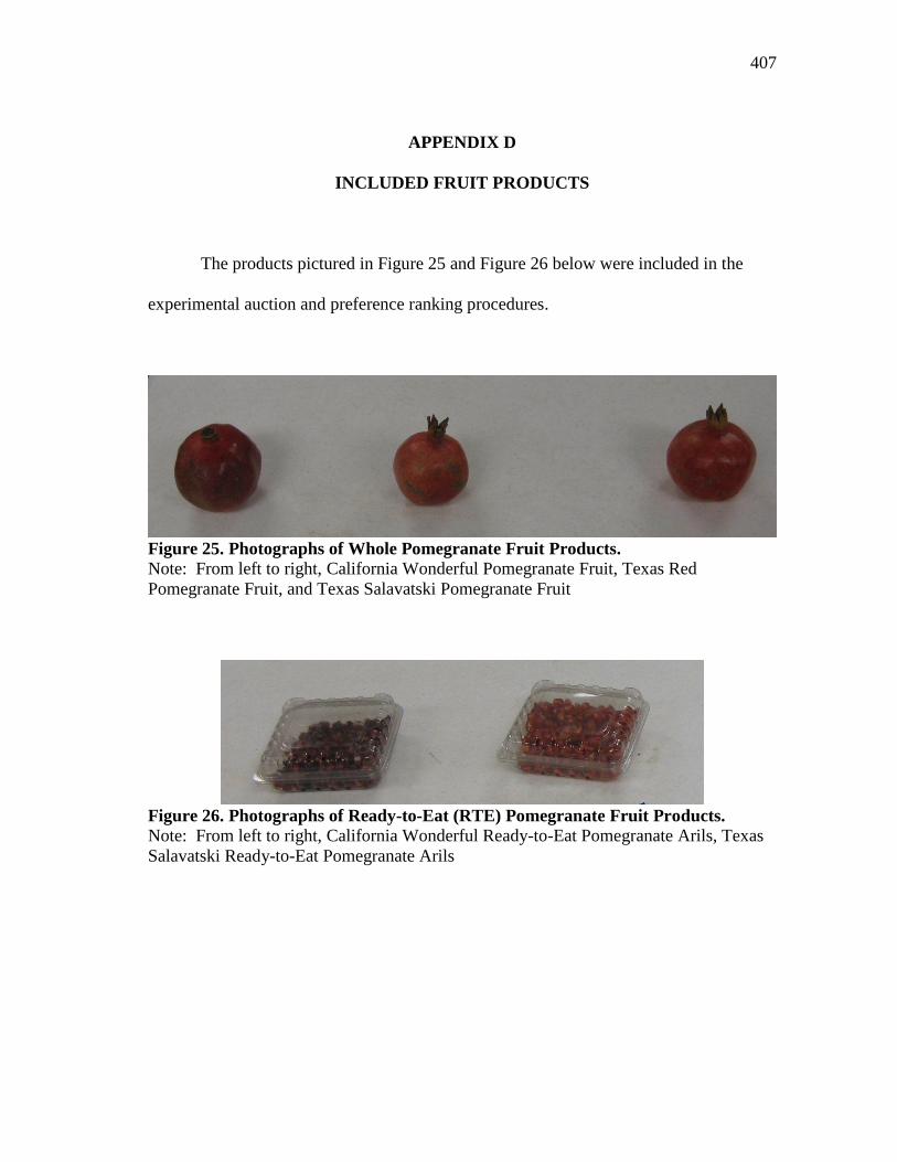
407
APPENDIX D
INCLUDED FRUIT PRODUCTS
The products pictured in Figure 25 and Figure 26 below were included in the
experimental auction and preference ranking procedures.
Figure 25. Photographs of Whole Pomegranate Fruit Products.
Note: From left to right, California Wonderful Pomegranate Fruit, Texas Red
Pomegranate Fruit, and Texas Salavatski Pomegranate Fruit
Figure 26. Photographs of Ready-to-Eat (RTE) Pomegranate Fruit Products.
Note: From left to right, California Wonderful Ready-to-Eat Pomegranate Arils, Texas
Salavatski Ready-to-Eat Pomegranate Arils
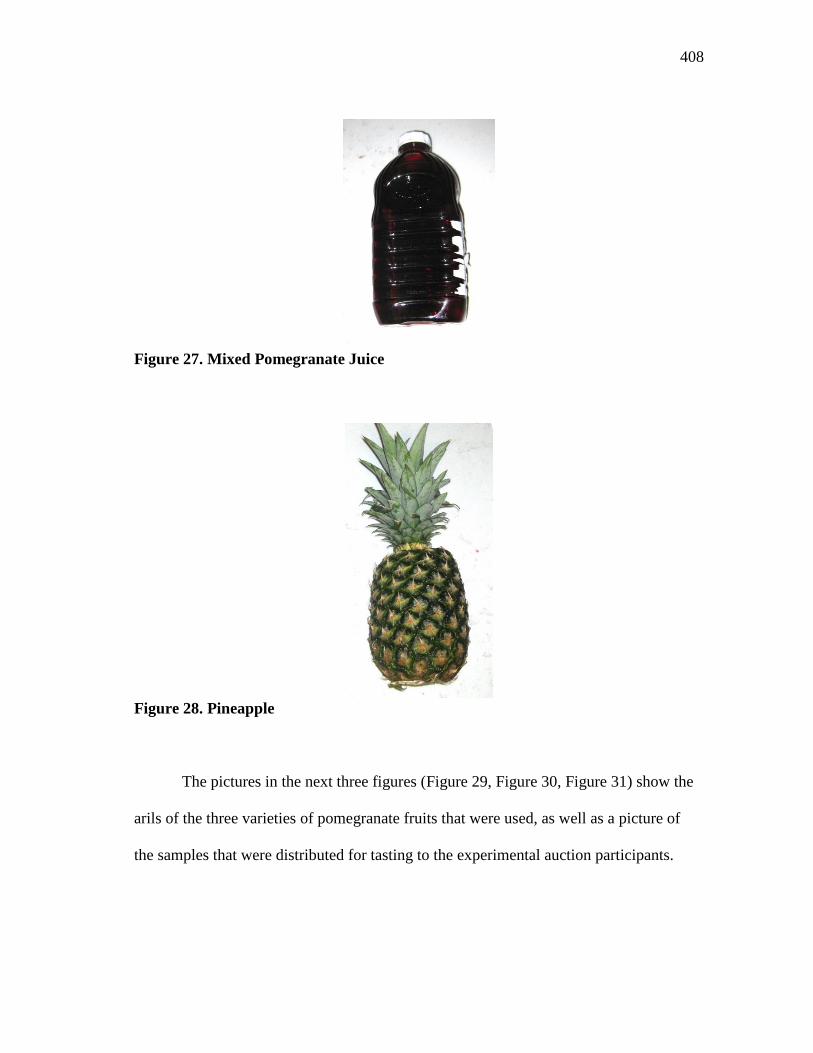
408
Figure 27. Mixed Pomegranate Juice
Figure 28. Pineapple
The pictures in the next three figures (Figure 29, Figure 30, Figure 31) show the
arils of the three varieties of pomegranate fruits that were used, as well as a picture of
the samples that were distributed for tasting to the experimental auction participants.
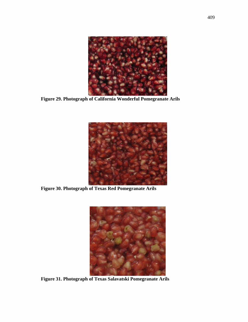
409
Figure 29. Photograph of California Wonderful Pomegranate Arils
Figure 30. Photograph of Texas Red Pomegranate Arils
Figure 31. Photograph of Texas Salavatski Pomegranate Arils
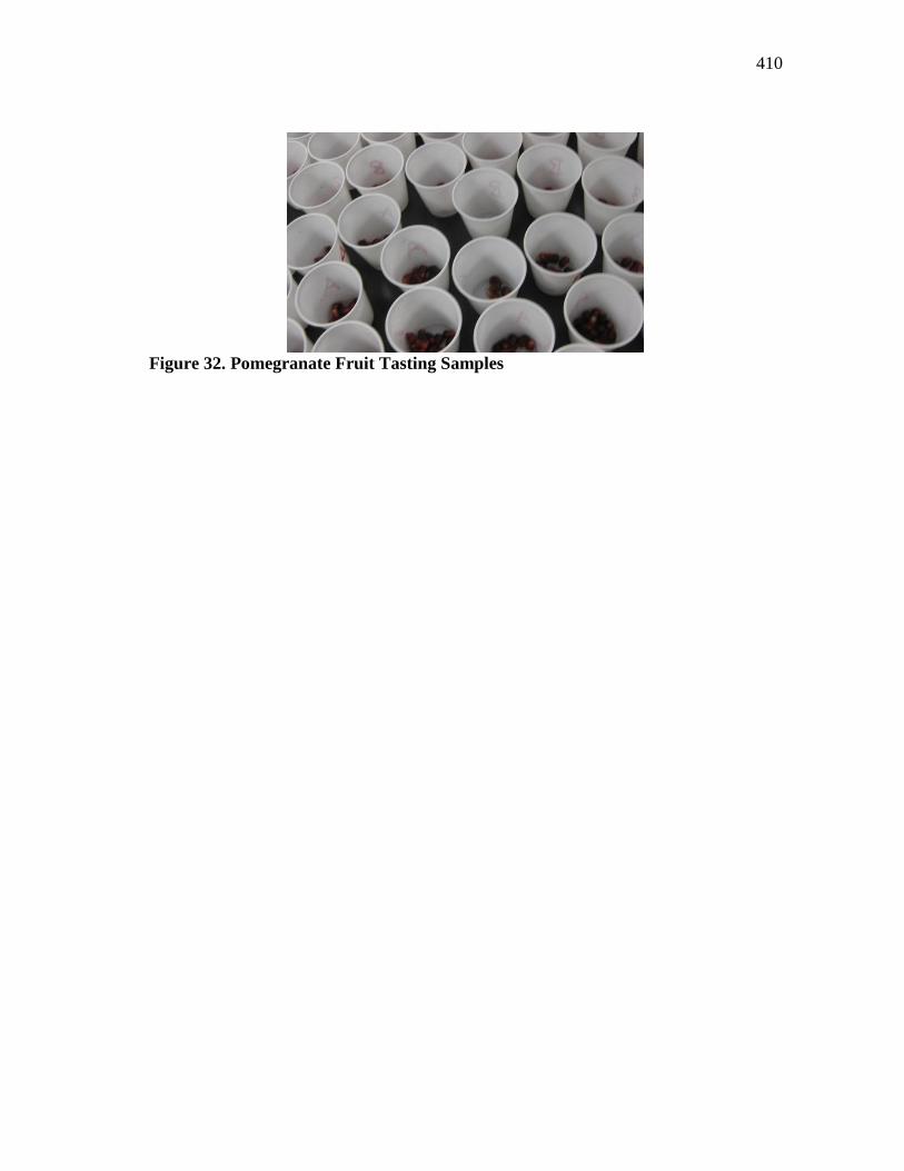
410
Figure 32. Pomegranate Fruit Tasting Samples
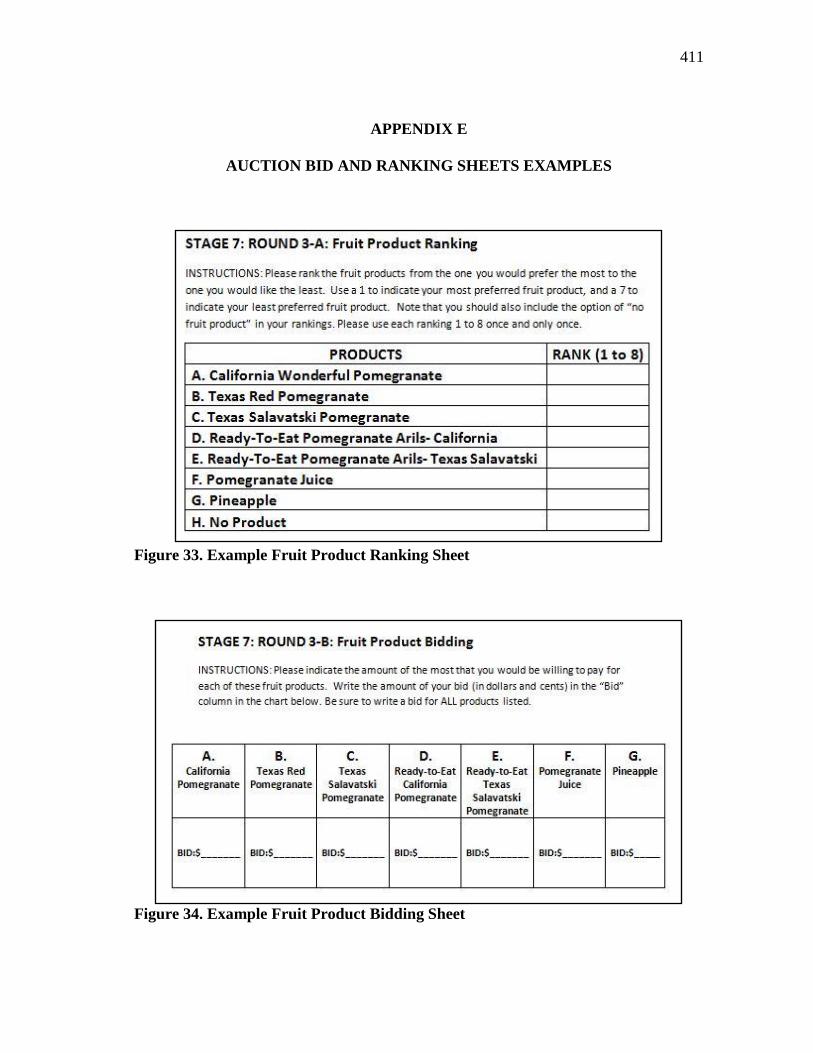
411
APPENDIX E
AUCTION BID AND RANKING SHEETS EXAMPLES
Figure 33. Example Fruit Product Ranking Sheet
Figure 34. Example Fruit Product Bidding Sheet
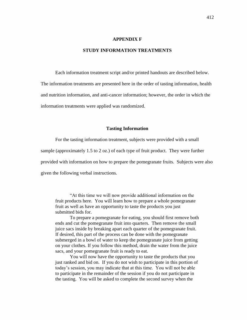
412
APPENDIX F
STUDY INFORMATION TREATMENTS
Each information treatment script and/or printed handouts are described below.
The information treatments are presented here in the order of tasting information, health
and nutrition information, and anti-cancer information; however, the order in which the
information treatments were applied was randomized.
Tasting Information
For the tasting information treatment, subjects were provided with a small
sample (approximately 1.5 to 2 oz.) of each type of fruit product. They were further
provided with information on how to prepare the pomegranate fruits. Subjects were also
given the following verbal instructions.
―At this time we will now provide additional information on the
fruit products here. You will learn how to prepare a whole pomegranate
fruit as well as have an opportunity to taste the products you just
submitted bids for.
To prepare a pomegranate for eating, you should first remove both
ends and cut the pomegranate fruit into quarters. Then remove the small
juice sacs inside by breaking apart each quarter of the pomegranate fruit.
If desired, this part of the process can be done with the pomegranate
submerged in a bowl of water to keep the pomegranate juice from getting
on your clothes. If you follow this method, drain the water from the juice
sacs, and your pomegranate fruit is ready to eat.
You will now have the opportunity to taste the products that you
just ranked and bid on. If you do not wish to participate in this portion of
today‘s session, you may indicate that at this time. You will not be able
to participate in the remainder of the session if you do not participate in
the tasting. You will be asked to complete the second survey when the

413
other participants complete that survey. However, deciding to not
participate will not affect your payment for participating in today‘s
session, provided you remain here until the other participants finish with
today‘s session.
For the tasting, please take only one sample of each product.
Once you have tasted the products, you will have the opportunity to rank
the products and bid on the products again. Does anyone have any
questions?‖
Please note that subjects were only provided with verbal instructions for the
tasting information treatment, subjects were not provided with any written information
for this round.
Health and Nutrition Information
For the health and nutrition information rounds, subjects were provided with the
nutrition facts for fresh pomegranate fruit, juice, and pineapple. Subjects were also
provided with information on the additional health benefits of pomegranates and the
additional health benefits of pineapple. Subjects were provided with the following
verbal instructions.
―You will now have an opportunity to look at some of the health
and nutrition information for the products you bid on in previous rounds.
You may also re-examine the products if you wish to do so. Once you
have reviewed all the products and information, you will have an
opportunity to resubmit your rankings and bids on these products.‖
Subjects were also provided with the written information.
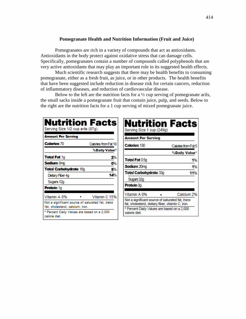
414
Pomegranate Health and Nutrition Information (Fruit and Juice)
Pomegranates are rich in a variety of compounds that act as antioxidants.
Antioxidants in the body protect against oxidative stress that can damage cells.
Specifically, pomegranates contain a number of compounds called polyphenols that are
very active antioxidants that may play an important role in its suggested health effects.
Much scientific research suggests that there may be health benefits to consuming
pomegranate, either as a fresh fruit, as juice, or in other products. The health benefits
that have been suggested include reduction in disease risk for certain cancers, reduction
of inflammatory diseases, and reduction of cardiovascular disease.
Below to the left are the nutrition facts for a ½ cup serving of pomegranate arils,
the small sacks inside a pomegranate fruit that contain juice, pulp, and seeds. Below to
the right are the nutrition facts for a 1 cup serving of mixed pomegranate juice.
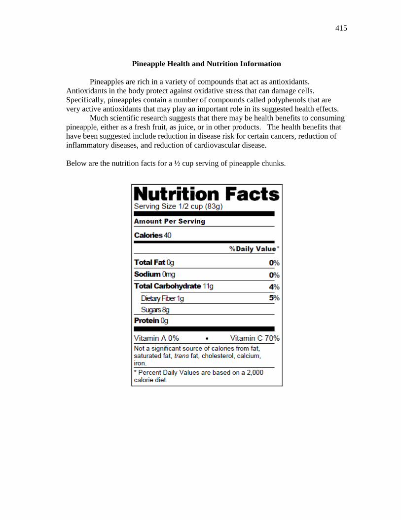
415
Pineapple Health and Nutrition Information
Pineapples are rich in a variety of compounds that act as antioxidants.
Antioxidants in the body protect against oxidative stress that can damage cells.
Specifically, pineapples contain a number of compounds called polyphenols that are
very active antioxidants that may play an important role in its suggested health effects.
Much scientific research suggests that there may be health benefits to consuming
pineapple, either as a fresh fruit, as juice, or in other products. The health benefits that
have been suggested include reduction in disease risk for certain cancers, reduction of
inflammatory diseases, and reduction of cardiovascular disease.
Below are the nutrition facts for a ½ cup serving of pineapple chunks.

416
Anti-Cancer Information
For the anti-cancer information rounds, subjects were provided with written
information on the anti-cancer properties of pomegranates. In a similar manner to the
health and nutrition information treatment, subjects were provided with the following
verbal instructions.
―You will now have an opportunity to look at some health
information for the products you bid on in previous rounds. You may also
re-examine the products if you wish to do so. Once you have reviewed
all the products and information, you will have an opportunity to resubmit
your rankings and bids on these products.‖
Subjects were also provided with the written information given below.
Pomegranate Health Information 2
Pomegranates are rich in a variety of compounds that act as antioxidants.
Antioxidants in the body protect against oxidative stress that can damage cells. Much
scientific research suggests that there may be health benefits to consuming pomegranate,
either as a fresh fruit, as juice, or in other products.
The health benefits that have been suggested include reduction in disease risk for
certain cancers, reduction of inflammatory diseases, and reduction of cardiovascular
disease. The effects of pomegranate and its components were seen in laboratory studies
on cancer cell lines; cancer cell lines where effects were seen include breast, colon,
leukemia, prostate, and skin cancer cell lines. However, these results were observed in
laboratory experiments and need to be further investigated in humans before such claims
can be fully verified.
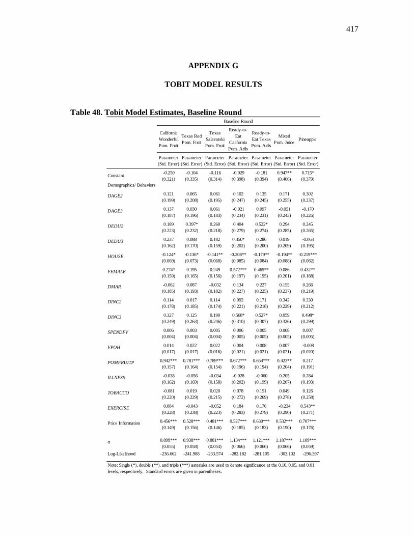
417
APPENDIX G
TOBIT MODEL RESULTS
Table 48. Tobit Model Estimates, Baseline Round
California
Wonderful
Pom. Fruit
Texas Red
Pom. Fruit
Texas
Salavatski
Pom. Fruit
Ready-to-
Eat
California
Pom. Arils
Ready-to-
Eat Texas
Pom. Arils
Mixed
Pom. JuicePineapple
Parameter
(Std. Error)
Parameter
(Std. Error)
Parameter
(Std. Error)
Parameter
(Std. Error)
Parameter
(Std. Error)
Parameter
(Std. Error)
Parameter
(Std. Error)
Constant-0.250
(0.321)
-0.104
(0.335)
-0.116
(0.314)
-0.029
(0.398)
-0.181
(0.394)
0.947**
(0.406)
0.715*
(0.379)
Demographics/ Behaviors
DAGE2 0.121
(0.199)
0.065
(0.208)
0.061
(0.195)
0.102
(0.247)
0.135
(0.245)
0.171
(0.255)
0.302
(0.237)
DAGE3 0.137
(0.187)
0.030
(0.196)
0.061
(0.183)
-0.021
(0.234)
0.097
(0.231)
-0.051
(0.243)
-0.170
(0.226)
DEDU2 0.189
(0.223)
0.397*
(0.232)
0.260
(0.218)
0.404
(0.279)
0.522*
(0.274)
0.294
(0.285)
0.245
(0.265)
DEDU3 0.237
(0.162)
0.088
(0.170)
0.182
(0.159)
0.350*
(0.202)
0.286
(0.200)
0.019
(0.209)
-0.063
(0.195)
HOUSE -0.124*
(0.069)
-0.136*
(0.073)
-0.141**
(0.068)
-0.208**
(0.085)
-0.179**
(0.084)
-0.194**
(0.088)
-0.219***
(0.082)
FEMALE 0.274*
(0.159)
0.195
(0.165)
0.249
(0.156)
0.572***
(0.197)
0.465**
(0.195)
0.086
(0.201)
0.432**
(0.188)
DMAR -0.062
(0.185)
0.087
(0.193)
-0.032
(0.182)
0.134
(0.227)
0.227
(0.225)
0.155
(0.237)
0.266
(0.219)
DINC2 0.114
(0.178)
0.017
(0.185)
0.114
(0.174)
0.092
(0.221)
0.171
(0.218)
0.342
(0.229)
0.230
(0.212)
DINC3 0.327
(0.249)
0.125
(0.263)
0.190
(0.246)
0.568*
(0.310)
0.527*
(0.307)
0.059
(0.326)
0.498*
(0.299)
SPENDFV 0.006
(0.004)
0.003
(0.004)
0.005
(0.004)
0.006
(0.005)
0.005
(0.005)
0.008
(0.005)
0.007
(0.005)
FPOH 0.014
(0.017)
0.022
(0.017)
0.022
(0.016)
0.004
(0.021)
0.008
(0.021)
0.007
(0.021)
-0.008
(0.020)
POMFRUITP 0.942***
(0.157)
0.781***
(0.164)
0.789***
(0.154)
0.672***
(0.196)
0.654***
(0.194)
0.423**
(0.204)
0.217
(0.191)
ILLNESS -0.038
(0.162)
-0.056
(0.169)
-0.034
(0.158)
-0.028
(0.202)
-0.060
(0.199)
0.205
(0.207)
0.284
(0.193)
TOBACCO -0.081
(0.220)
0.019
(0.229)
0.020
(0.215)
0.078
(0.272)
0.151
(0.269)
0.049
(0.278)
0.126
(0.258)
EXERCISE 0.084
(0.228)
-0.043
(0.238)
-0.052
(0.223)
0.184
(0.283)
0.176
(0.279)
-0.234
(0.290)
0.543**
(0.271)
Price Information 0.456***
(0.149)
0.528***
(0.156)
0.481***
(0.146)
0.527***
(0.185)
0.630***
(0.183)
0.532***
(0.190)
0.707***
(0.176)
σ 0.899***
(0.055)
0.938***
(0.058)
0.881***
(0.054)
1.134***
(0.066)
1.121***
(0.066)
1.187***
(0.066)
1.109***
(0.059)
Log-Likelihood -236.662 -241.988 -233.574 -282.182 -281.105 -303.102 -296.397
Baseline Round
Note: Single (*), double (**), and triple (***) asterisks are used to denote significance at the 0.10, 0.05, and 0.01
levels, respectively. Standard errors are given in parentheses.
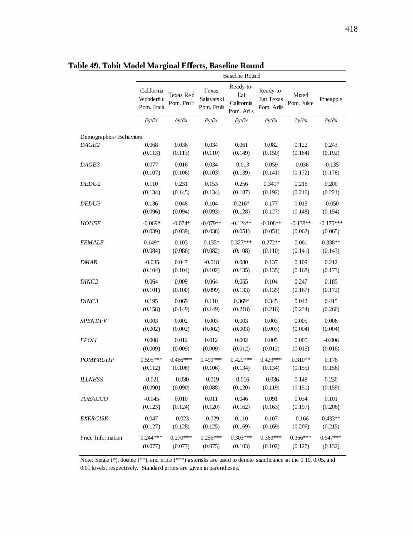
418
Table 49. Tobit Model Marginal Effects, Baseline Round
California
Wonderful
Pom. Fruit
Texas Red
Pom. Fruit
Texas
Salavatski
Pom. Fruit
Ready-to-
Eat
California
Pom. Arils
Ready-to-
Eat Texas
Pom. Arils
Mixed
Pom. JuicePineapple
∂y/∂x ∂y/∂x ∂y/∂x ∂y/∂x ∂y/∂x ∂y/∂x ∂y/∂x
Demographics/ Behaviors
DAGE2 0.068
(0.113)
0.036
(0.113)
0.034
(0.110)
0.061
(0.149)
0.082
(0.150)
0.122
(0.184)
0.243
(0.192)
DAGE3 0.077
(0.107)
0.016
(0.106)
0.034
(0.103)
-0.013
(0.139)
0.059
(0.141)
-0.036
(0.172)
-0.135
(0.178)
DEDU2 0.110
(0.134)
0.231
(0.145)
0.153
(0.134)
0.256
(0.187)
0.341*
(0.192)
0.216
(0.216)
0.200
(0.221)
DEDU3 0.136
(0.096)
0.048
(0.094)
0.104
(0.093)
0.216*
(0.128)
0.177
(0.127)
0.013
(0.148)
-0.050
(0.154)
HOUSE -0.069*
(0.039)
-0.074*
(0.039)
-0.079**
(0.038)
-0.124**
(0.051)
-0.108**
(0.051)
-0.138**
(0.062)
-0.175***
(0.065)
FEMALE 0.149*
(0.084)
0.103
(0.086)
0.135*
(0.082)
0.327***
(0.108)
0.272**
(0.110)
0.061
(0.141)
0.338**
(0.143)
DMAR -0.035
(0.104)
0.047
(0.104)
-0.018
(0.102)
0.080
(0.135)
0.137
(0.135)
0.109
(0.168)
0.212
(0.173)
DINC2 0.064
(0.101)
0.009
(0.100)
0.064
(0.099)
0.055
(0.133)
0.104
(0.135)
0.247
(0.167)
0.185
(0.172)
DINC3 0.195
(0.158)
0.069
(0.149)
0.110
(0.149)
0.369*
(0.218)
0.345
(0.216)
0.042
(0.234)
0.415
(0.260)
SPENDFV 0.003
(0.002)
0.002
(0.002)
0.003
(0.002)
0.003
(0.003)
0.003
(0.003)
0.005
(0.004)
0.006
(0.004)
FPOH 0.008
(0.009)
0.012
(0.009)
0.012
(0.009)
0.002
(0.012)
0.005
(0.012)
0.005
(0.015)
-0.006
(0.016)
POMFRUITP 0.595***
(0.112)
0.466***
(0.108)
0.490***
(0.106)
0.429***
(0.134)
0.423***
(0.134)
0.310**
(0.155)
0.176
(0.156)
ILLNESS -0.021
(0.090)
-0.030
(0.090)
-0.019
(0.088)
-0.016
(0.120)
-0.036
(0.119)
0.148
(0.151)
0.230
(0.159)
TOBACCO -0.045
(0.123)
0.010
(0.124)
0.011
(0.120)
0.046
(0.162)
0.091
(0.163)
0.034
(0.197)
0.101
(0.206)
EXERCISE 0.047
(0.127)
-0.023
(0.128)
-0.029
(0.125)
0.110
(0.169)
0.107
(0.169)
-0.166
(0.206)
0.433**
(0.215)
Price Information 0.244***
(0.077)
0.270***
(0.077)
0.256***
(0.075)
0.303***
(0.103)
0.363***
(0.102)
0.366***
(0.127)
0.547***
(0.132)
Baseline Round
Note: Single (*), double (**), and triple (***) asterisks are used to denote significance at the 0.10, 0.05, and
0.01 levels, respectively. Standard errors are given in parentheses.
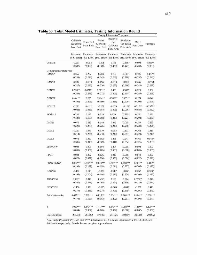
419
Table 50. Tobit Model Estimates, Tasting Information Round
California
Wonderful
Pom. Fruit
Texas Red
Pom. Fruit
Texas
Salavatski
Pom. Fruit
Ready-to-
Eat
California
Pom. Arils
Ready-to-
Eat Texas
Pom. Arils
Mixed
Pom. JuicePineapple
Parameter
(Std. Error)
Parameter
(Std. Error)
Parameter
(Std. Error)
Parameter
(Std. Error)
Parameter
(Std. Error)
Parameter
(Std. Error)
Parameter
(Std. Error)
Constant -0.251
(0.382)
-0.254
(0.399)
-0.201
(0.389)
0.151
(0.429)
0.108
(0.447)
0.604
(0.408)
0.813**
(0.383)
Demographics/ Behaviors
DAGE2 0.356
(0.239)
0.267
(0.249)
0.203
(0.243)
0.169
(0.269)
0.067
(0.280)
0.106
(0.257)
0.478**
(0.240)
DAGE3 0.285
(0.227)
-0.019
(0.236)
0.096
(0.230)
-0.013
(0.256)
-0.010
(0.266)
0.265
(0.243)
-0.138
(0.228)
DEDU2 0.559**
(0.269)
0.671**
(0.279)
0.661**
(0.272)
0.430
(0.303)
0.595*
(0.314)
0.229
(0.289)
0.092
(0.268)
DEDU3 0.461**
(0.196)
0.290
(0.205)
0.414**
(0.199)
0.509**
(0.221)
0.463**
(0.229)
0.174
(0.209)
-0.061
(0.196)
HOUSE -0.091
(0.083)
-0.112
(0.086)
-0.109
(0.084)
-0.139
(0.093)
-0.129
(0.096)
-0.216**
(0.089)
-0.237***
(0.082)
FEMALE 0.231
(0.189)
0.127
(0.197)
0.019
(0.192)
0.379*
(0.213)
0.155
(0.221)
0.151
(0.202)
0.222
(0.189)
DMAR 0.070
(0.221)
0.235
(0.230)
0.149
(0.225)
0.045
(0.248)
0.015
(0.258)
0.159
(0.239)
0.220
(0.221)
DINC2 -0.011
(0.214)
0.075
(0.224)
0.010
(0.218)
-0.053
(0.242)
0.137
(0.251)
0.262
(0.229)
0.315
(0.214)
DINC3 0.072
(0.306)
0.022
(0.316)
0.082
(0.309)
0.261
(0.341)
0.247
(0.354)
0.166
(0.326)
0.543*
(0.303)
SPENDFV 0.004
(0.005)
0.005
(0.005)
0.004
(0.005)
0.004
(0.006)
0.005
(0.006)
0.004
(0.005)
0.007
(0.005)
FPOH 0.004
(0.020)
0.002
(0.021)
0.026
(0.020)
0.016
(0.023)
0.016
(0.024)
0.019
(0.022)
0.007
(0.020)
POMFRUITP 0.819***
(0.190)
0.780***
(0.199)
0.610***
(0.193)
0.741***
(0.214)
0.658***
(0.223)
0.501**
(0.205)
0.435**
(0.192)
ILLNESS -0.162
(0.196)
0.143
(0.204)
-0.030
(0.198)
-0.287
(0.222)
-0.066
(0.229)
0.252
(0.208)
0.324*
(0.195)
TOBACCO 0.491*
(0.261)
0.342
(0.273)
0.432
(0.265)
0.199
(0.294)
0.264
(0.306)
0.579**
(0.279)
0.346
(0.261)
EXERCISE -0.156
(0.274)
0.073
(0.285)
-0.095
(0.278)
-0.063
(0.308)
-0.083
(0.319)
-0.357
(0.291)
0.413
(0.273)
Price Information 0.685***
(0.179)
0.839***
(0.188)
0.815***
(0.183)
0.604***
(0.202)
0.808***
(0.211)
0.484**
(0.190)
0.600***
(0.177)
σ 1.099***
(0.064)
1.147***
(0.067)
1.117***
(0.065)
1.240***
(0.072)
1.288***
(0.076)
1.183***
(0.067)
1.120***
(0.059)
Log-Likelihood -276.998 -284.062 -278.999 -297.326 -302.877 -297.148 -298.652
Tasting Information Treatment
Note: Single (*), double (**), and triple (***) asterisks are used to denote significance at the 0.10, 0.05, and
0.01 levels, respectively. Standard errors are given in parentheses.
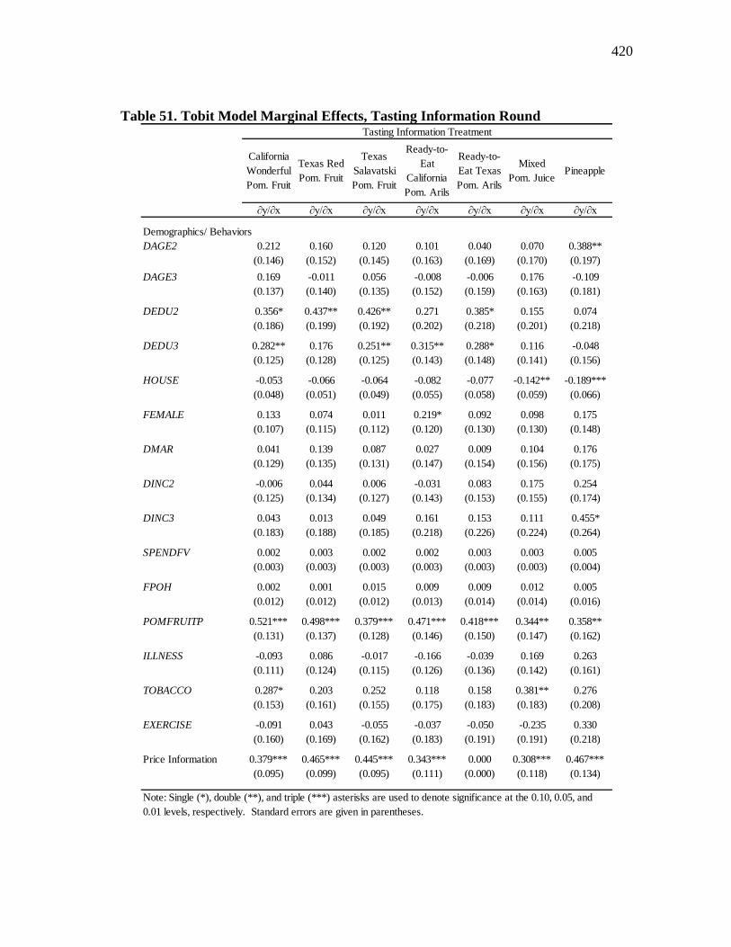
420
Table 51. Tobit Model Marginal Effects, Tasting Information Round
California
Wonderful
Pom. Fruit
Texas Red
Pom. Fruit
Texas
Salavatski
Pom. Fruit
Ready-to-
Eat
California
Pom. Arils
Ready-to-
Eat Texas
Pom. Arils
Mixed
Pom. JuicePineapple
∂y/∂x ∂y/∂x ∂y/∂x ∂y/∂x ∂y/∂x ∂y/∂x ∂y/∂x
Demographics/ Behaviors
DAGE2 0.212
(0.146)
0.160
(0.152)
0.120
(0.145)
0.101
(0.163)
0.040
(0.169)
0.070
(0.170)
0.388**
(0.197)
DAGE3 0.169
(0.137)
-0.011
(0.140)
0.056
(0.135)
-0.008
(0.152)
-0.006
(0.159)
0.176
(0.163)
-0.109
(0.181)
DEDU2 0.356*
(0.186)
0.437**
(0.199)
0.426**
(0.192)
0.271
(0.202)
0.385*
(0.218)
0.155
(0.201)
0.074
(0.218)
DEDU3 0.282**
(0.125)
0.176
(0.128)
0.251**
(0.125)
0.315**
(0.143)
0.288*
(0.148)
0.116
(0.141)
-0.048
(0.156)
HOUSE -0.053
(0.048)
-0.066
(0.051)
-0.064
(0.049)
-0.082
(0.055)
-0.077
(0.058)
-0.142**
(0.059)
-0.189***
(0.066)
FEMALE 0.133
(0.107)
0.074
(0.115)
0.011
(0.112)
0.219*
(0.120)
0.092
(0.130)
0.098
(0.130)
0.175
(0.148)
DMAR 0.041
(0.129)
0.139
(0.135)
0.087
(0.131)
0.027
(0.147)
0.009
(0.154)
0.104
(0.156)
0.176
(0.175)
DINC2 -0.006
(0.125)
0.044
(0.134)
0.006
(0.127)
-0.031
(0.143)
0.083
(0.153)
0.175
(0.155)
0.254
(0.174)
DINC3 0.043
(0.183)
0.013
(0.188)
0.049
(0.185)
0.161
(0.218)
0.153
(0.226)
0.111
(0.224)
0.455*
(0.264)
SPENDFV 0.002
(0.003)
0.003
(0.003)
0.002
(0.003)
0.002
(0.003)
0.003
(0.003)
0.003
(0.003)
0.005
(0.004)
FPOH 0.002
(0.012)
0.001
(0.012)
0.015
(0.012)
0.009
(0.013)
0.009
(0.014)
0.012
(0.014)
0.005
(0.016)
POMFRUITP 0.521***
(0.131)
0.498***
(0.137)
0.379***
(0.128)
0.471***
(0.146)
0.418***
(0.150)
0.344**
(0.147)
0.358**
(0.162)
ILLNESS -0.093
(0.111)
0.086
(0.124)
-0.017
(0.115)
-0.166
(0.126)
-0.039
(0.136)
0.169
(0.142)
0.263
(0.161)
TOBACCO 0.287*
(0.153)
0.203
(0.161)
0.252
(0.155)
0.118
(0.175)
0.158
(0.183)
0.381**
(0.183)
0.276
(0.208)
EXERCISE -0.091
(0.160)
0.043
(0.169)
-0.055
(0.162)
-0.037
(0.183)
-0.050
(0.191)
-0.235
(0.191)
0.330
(0.218)
Price Information 0.379***
(0.095)
0.465***
(0.099)
0.445***
(0.095)
0.343***
(0.111)
0.000
(0.000)
0.308***
(0.118)
0.467***
(0.134)
Tasting Information Treatment
Note: Single (*), double (**), and triple (***) asterisks are used to denote significance at the 0.10, 0.05, and
0.01 levels, respectively. Standard errors are given in parentheses.
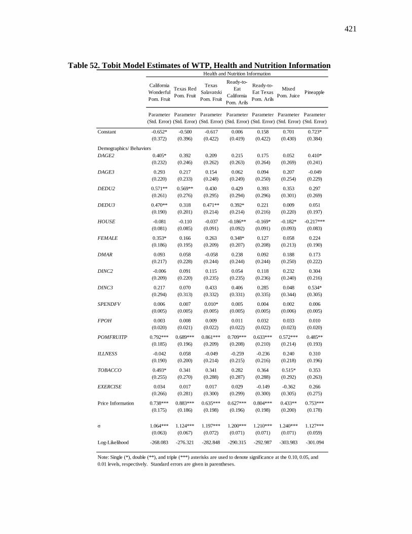
421
Table 52. Tobit Model Estimates of WTP, Health and Nutrition Information
California
Wonderful
Pom. Fruit
Texas Red
Pom. Fruit
Texas
Salavatski
Pom. Fruit
Ready-to-
Eat
California
Pom. Arils
Ready-to-
Eat Texas
Pom. Arils
Mixed
Pom. JuicePineapple
Parameter
(Std. Error)
Parameter
(Std. Error)
Parameter
(Std. Error)
Parameter
(Std. Error)
Parameter
(Std. Error)
Parameter
(Std. Error)
Parameter
(Std. Error)
Constant -0.652*
(0.372)
-0.500
(0.396)
-0.617
(0.422)
0.006
(0.419)
0.158
(0.422)
0.701
(0.430)
0.723*
(0.384)
Demographics/ Behaviors
DAGE2 0.405*
(0.232)
0.392
(0.246)
0.209
(0.262)
0.215
(0.263)
0.175
(0.264)
0.052
(0.269)
0.410*
(0.241)
DAGE3 0.293
(0.220)
0.217
(0.233)
0.154
(0.248)
0.062
(0.249)
0.094
(0.250)
0.207
(0.254)
-0.049
(0.229)
DEDU2 0.571**
(0.261)
0.569**
(0.276)
0.430
(0.295)
0.429
(0.294)
0.393
(0.296)
0.353
(0.301)
0.297
(0.269)
DEDU3 0.470**
(0.190)
0.318
(0.201)
0.471**
(0.214)
0.392*
(0.214)
0.221
(0.216)
0.009
(0.220)
0.051
(0.197)
HOUSE -0.081
(0.081)
-0.110
(0.085)
-0.037
(0.091)
-0.186**
(0.092)
-0.169*
(0.091)
-0.182*
(0.093)
-0.217***
(0.083)
FEMALE 0.353*
(0.186)
0.166
(0.195)
0.263
(0.209)
0.348*
(0.207)
0.127
(0.208)
0.058
(0.213)
0.224
(0.190)
DMAR 0.093
(0.217)
0.058
(0.228)
-0.058
(0.244)
0.238
(0.244)
0.092
(0.244)
0.188
(0.250)
0.173
(0.222)
DINC2 -0.006
(0.209)
0.091
(0.220)
0.115
(0.235)
0.054
(0.235)
0.118
(0.236)
0.232
(0.240)
0.304
(0.216)
DINC3 0.217
(0.294)
0.070
(0.313)
0.433
(0.332)
0.406
(0.331)
0.285
(0.335)
0.048
(0.344)
0.534*
(0.305)
SPENDFV 0.006
(0.005)
0.007
(0.005)
0.010*
(0.005)
0.005
(0.005)
0.004
(0.005)
0.002
(0.006)
0.006
(0.005)
FPOH 0.003
(0.020)
0.008
(0.021)
0.009
(0.022)
0.011
(0.022)
0.032
(0.022)
0.033
(0.023)
0.010
(0.020)
POMFRUITP 0.792***
(0.185)
0.689***
(0.196)
0.861***
(0.209)
0.709***
(0.208)
0.633***
(0.210)
0.572***
(0.214)
0.485**
(0.193)
ILLNESS -0.042
(0.190)
0.058
(0.200)
-0.049
(0.214)
-0.259
(0.215)
-0.236
(0.216)
0.240
(0.218)
0.310
(0.196)
TOBACCO 0.493*
(0.255)
0.341
(0.270)
0.341
(0.288)
0.282
(0.287)
0.364
(0.288)
0.515*
(0.292)
0.353
(0.263)
EXERCISE 0.034
(0.266)
0.017
(0.281)
0.017
(0.300)
0.029
(0.299)
-0.149
(0.300)
-0.362
(0.305)
0.266
(0.275)
Price Information 0.738***
(0.175)
0.883***
(0.186)
0.635***
(0.198)
0.627***
(0.196)
0.804***
(0.198)
0.433**
(0.200)
0.753***
(0.178)
σ 1.064***
(0.063)
1.124***
(0.067)
1.197***
(0.072)
1.200***
(0.071)
1.210***
(0.071)
1.240***
(0.071)
1.127***
(0.059)
Log-Likelihood -268.083 -276.321 -282.848 -290.315 -292.987 -303.983 -301.094
Health and Nutrition Information
Note: Single (*), double (**), and triple (***) asterisks are used to denote significance at the 0.10, 0.05, and
0.01 levels, respectively. Standard errors are given in parentheses.
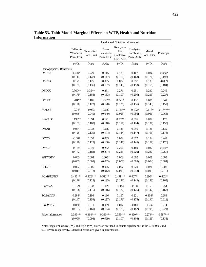
422
Table 53. Tobit Model Marginal Effects on WTP, Health and Nutrition
Information
California
Wonderful
Pom. Fruit
Texas Red
Pom. Fruit
Texas
Salavatski
Pom. Fruit
Ready-to-
Eat
California
Pom. Arils
Ready-to-
Eat Texas
Pom. Arils
Mixed
Pom. JuicePineapple
∂y/∂x ∂y/∂x ∂y/∂x ∂y/∂x ∂y/∂x ∂y/∂x ∂y/∂x
Demographics/ Behaviors
DAGE2 0.239*
(0.141)
0.229
(0.147)
0.115
(0.147)
0.129
(0.160)
0.107
(0.163)
0.034
(0.176)
0.334*
(0.198)
DAGE3 0.171
(0.131)
0.125
(0.136)
0.085
(0.137)
0.037
(0.149)
0.057
(0.153)
0.135
(0.168)
-0.039
(0.184)
DEDU2 0.360**
(0.179)
0.354*
(0.186)
0.251
(0.183)
0.271
(0.197)
0.251
(0.200)
0.240
(0.213)
0.245
(0.227)
DEDU3 0.284**
(0.120)
0.187
(0.122)
0.268**
(0.128)
0.241*
(0.136)
0.137
(0.136)
0.006
(0.143)
0.041
(0.159)
HOUSE -0.047
(0.046)
-0.063
(0.049)
-0.020
(0.049)
-0.111**
(0.055)
-0.102*
(0.056)
-0.118*
(0.061)
-0.174***
(0.066)
FEMALE 0.198**
(0.101)
0.094
(0.108)
0.141
(0.110)
0.202*
(0.117)
0.076
(0.124)
0.037
(0.137)
0.178
(0.150)
DMAR 0.054
(0.125)
0.033
(0.130)
-0.032
(0.134)
0.141
(0.144)
0.056
(0.147)
0.121
(0.161)
0.139
(0.178)
DINC2 -0.004
(0.120)
0.052
(0.127)
0.063
(0.130)
0.032
(0.141)
0.072
(0.145)
0.152
(0.159)
0.247
(0.176)
DINC3 0.129
(0.182)
0.040
(0.182)
0.252
(0.207)
0.256
(0.221)
0.180
(0.220)
0.032
(0.226)
0.450*
(0.266)
SPENDFV 0.003
(0.003)
0.004
(0.003)
0.005*
(0.003)
0.003
(0.003)
0.002
(0.003)
0.001
(0.004)
0.005
(0.004)
FPOH 0.002
(0.011)
0.005
(0.012)
0.005
(0.012)
0.007
(0.013)
0.020
(0.013)
0.021
(0.015)
0.008
(0.016)
POMFRUITP 0.496***
(0.126)
0.422***
(0.128)
0.512***
(0.135)
0.451***
(0.141)
0.407***
(0.143)
0.390**
(0.153)
0.402**
(0.165)
ILLNESS -0.024
(0.108)
0.033
(0.116)
-0.026
(0.116)
-0.150
(0.122)
-0.140
(0.126)
0.159
(0.147)
0.254
(0.163)
TOBACCO 0.284*
(0.147)
0.194
(0.154)
0.186
(0.157)
0.167
(0.171)
0.221
(0.175)
0.334*
(0.190)
0.284
(0.211)
EXERCISE 0.020
(0.153)
0.010
(0.160)
0.009
(0.164)
0.017
(0.178)
-0.090
(0.182)
-0.235
(0.198)
0.214
(0.221)
Price Information 0.399***
(0.090)
0.468***
(0.093)
0.330***
(0.099)
0.356***
(0.107)
0.460***
(0.108)
0.274**
(0.123)
0.587***
(0.135)
Note: Single (*), double (**), and triple (***) asterisks are used to denote significance at the 0.10, 0.05, and
0.01 levels, respectively. Standard errors are given in parentheses.
Health and Nutrition Information
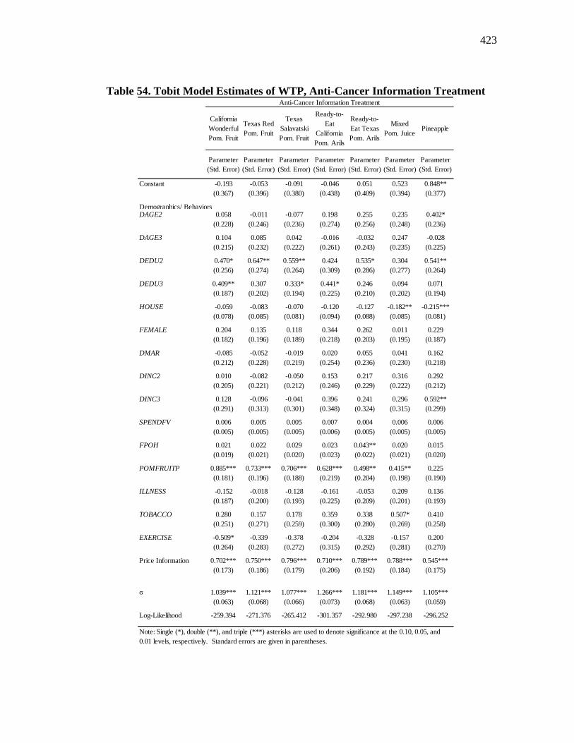
423
Table 54. Tobit Model Estimates of WTP, Anti-Cancer Information Treatment
California
Wonderful
Pom. Fruit
Texas Red
Pom. Fruit
Texas
Salavatski
Pom. Fruit
Ready-to-
Eat
California
Pom. Arils
Ready-to-
Eat Texas
Pom. Arils
Mixed
Pom. JuicePineapple
Parameter
(Std. Error)
Parameter
(Std. Error)
Parameter
(Std. Error)
Parameter
(Std. Error)
Parameter
(Std. Error)
Parameter
(Std. Error)
Parameter
(Std. Error)
Constant -0.193
(0.367)
-0.053
(0.396)
-0.091
(0.380)
-0.046
(0.438)
0.051
(0.409)
0.523
(0.394)
0.848**
(0.377)
Demographics/ BehaviorsDAGE2 0.058
(0.228)
-0.011
(0.246)
-0.077
(0.236)
0.198
(0.274)
0.255
(0.256)
0.235
(0.248)
0.402*
(0.236)
DAGE3 0.104
(0.215)
0.085
(0.232)
0.042
(0.222)
-0.016
(0.261)
-0.032
(0.243)
0.247
(0.235)
-0.028
(0.225)
DEDU2 0.470*
(0.256)
0.647**
(0.274)
0.559**
(0.264)
0.424
(0.309)
0.535*
(0.286)
0.304
(0.277)
0.541**
(0.264)
DEDU3 0.409**
(0.187)
0.307
(0.202)
0.333*
(0.194)
0.441*
(0.225)
0.246
(0.210)
0.094
(0.202)
0.071
(0.194)
HOUSE -0.059
(0.078)
-0.083
(0.085)
-0.070
(0.081)
-0.120
(0.094)
-0.127
(0.088)
-0.182**
(0.085)
-0.215***
(0.081)
FEMALE 0.204
(0.182)
0.135
(0.196)
0.118
(0.189)
0.344
(0.218)
0.262
(0.203)
0.011
(0.195)
0.229
(0.187)
DMAR -0.085
(0.212)
-0.052
(0.228)
-0.019
(0.219)
0.020
(0.254)
0.055
(0.236)
0.041
(0.230)
0.162
(0.218)
DINC2 0.010
(0.205)
-0.082
(0.221)
-0.050
(0.212)
0.153
(0.246)
0.217
(0.229)
0.316
(0.222)
0.292
(0.212)
DINC3 0.128
(0.291)
-0.096
(0.313)
-0.041
(0.301)
0.396
(0.348)
0.241
(0.324)
0.296
(0.315)
0.592**
(0.299)
SPENDFV 0.006
(0.005)
0.005
(0.005)
0.005
(0.005)
0.007
(0.006)
0.004
(0.005)
0.006
(0.005)
0.006
(0.005)
FPOH 0.021
(0.019)
0.022
(0.021)
0.029
(0.020)
0.023
(0.023)
0.043**
(0.022)
0.020
(0.021)
0.015
(0.020)
POMFRUITP 0.885***
(0.181)
0.733***
(0.196)
0.706***
(0.188)
0.628***
(0.219)
0.498**
(0.204)
0.415**
(0.198)
0.225
(0.190)
ILLNESS -0.152
(0.187)
-0.018
(0.200)
-0.128
(0.193)
-0.161
(0.225)
-0.053
(0.209)
0.209
(0.201)
0.136
(0.193)
TOBACCO 0.280
(0.251)
0.157
(0.271)
0.178
(0.259)
0.359
(0.300)
0.338
(0.280)
0.507*
(0.269)
0.410
(0.258)
EXERCISE -0.509*
(0.264)
-0.339
(0.283)
-0.378
(0.272)
-0.204
(0.315)
-0.328
(0.292)
-0.157
(0.281)
0.200
(0.270)
Price Information 0.702***
(0.173)
0.750***
(0.186)
0.796***
(0.179)
0.710***
(0.206)
0.789***
(0.192)
0.788***
(0.184)
0.545***
(0.175)
σ 1.039***
(0.063)
1.121***
(0.068)
1.077***
(0.066)
1.266***
(0.073)
1.181***
(0.068)
1.149***
(0.063)
1.105***
(0.059)
Log-Likelihood -259.394 -271.376 -265.412 -301.357 -292.980 -297.238 -296.252
Anti-Cancer Information Treatment
Note: Single (*), double (**), and triple (***) asterisks are used to denote significance at the 0.10, 0.05, and
0.01 levels, respectively. Standard errors are given in parentheses.
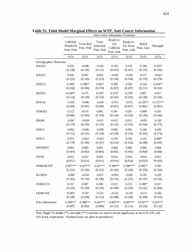
424
Table 55. Tobit Model Marginal Effects on WTP, Anti-Cancer Information
California
Wonderful
Pom. Fruit
Texas Red
Pom. Fruit
Texas
Salavatski
Pom. Fruit
Ready-to-
Eat
California
Pom. Arils
Ready-to-
Eat Texas
Pom. Arils
Mixed
Pom. JuicePineapple
∂y/∂x ∂y/∂x ∂y/∂x ∂y/∂x ∂y/∂x ∂y/∂x ∂y/∂x
Demographics/ Behaviors
DAGE2 0.033
(0.128)
-0.006
(0.136)
-0.043
(0.131)
0.120
(0.167)
0.120
(0.167)
0.168
(0.179)
0.325*
(0.193)
DAGE3 0.059
(0.122)
0.047
(0.129)
0.024
(0.125)
-0.010
(0.156)
-0.010
(0.156)
0.177
(0.170)
-0.023
(0.179)
DEDU2 0.284*
(0.166)
0.396**
(0.184)
0.343*
(0.176)
0.269
(0.207)
0.269
(0.207)
0.224
(0.211)
0.454**
(0.231)
DEDU3 0.238**
(0.114)
0.175
(0.118)
0.193*
(0.116)
0.274*
(0.145)
0.274*
(0.145)
0.067
(0.146)
0.057
(0.156)
HOUSE -0.033
(0.044)
-0.046
(0.047)
-0.039
(0.046)
-0.072
(0.057)
-0.072
(0.057)
-0.130**
(0.061)
-0.172***
(0.065)
FEMALE 0.112
(0.099)
0.074
(0.106)
0.065
(0.104)
0.201
(0.124)
0.201
(0.124)
0.008
(0.139)
0.181
(0.146)
DMAR -0.047
(0.119)
-0.029
(0.126)
-0.011
(0.123)
0.012
(0.152)
0.012
(0.152)
0.029
(0.163)
0.129
(0.173)
DINC2 0.005
(0.115)
-0.045
(0.121)
-0.028
(0.118)
0.092
(0.150)
0.092
(0.150)
0.228
(0.162)
0.236
(0.172)
DINC3 0.073
(0.170)
-0.052
(0.168)
-0.023
(0.167)
0.250
(0.232)
0.250
(0.232)
0.218
(0.240)
0.498*
(0.263)
SPENDFV 0.003
(0.003)
0.003
(0.003)
0.003
(0.003)
0.004
(0.003)
0.004
(0.003)
0.004
(0.004)
0.004
(0.004)
FPOH 0.012
(0.011)
0.012
(0.011)
0.016
(0.011)
0.014
(0.014)
0.014
(0.014)
0.014
(0.015)
0.012
(0.016)
POMFRUITP 0.547***
(0.123)
0.437***
(0.126)
0.427***
(0.122)
0.398***
(0.146)
0.398***
(0.146)
0.305**
(0.150)
0.182
(0.156)
ILLNESS -0.084
(0.102)
-0.010
(0.110)
-0.071
(0.106)
-0.095
(0.131)
-0.095
(0.131)
0.150
(0.147)
0.109
(0.156)
TOBACCO 0.157
(0.141)
0.087
(0.150)
0.100
(0.145)
0.215
(0.180)
0.215
(0.180)
0.360*
(0.191)
0.327
(0.205)
EXERCISE -0.285*
(0.148)
-0.187
(0.156)
-0.212
(0.153)
-0.122
(0.188)
-0.122
(0.188)
-0.111
(0.199)
0.160
(0.215)
Price Information 0.369***
(0.087)
0.388***
(0.092)
0.416***
(0.089)
0.405***
(0.113)
0.405***
(0.113)
0.534***
(0.120)
0.425***
(0.133)
Anti-Cancer Information Treatment
Note: Single (*), double (**), and triple (***) asterisks are used to denote significance at the 0.10, 0.05, and
0.01 levels, respectively. Standard errors are given in parentheses.
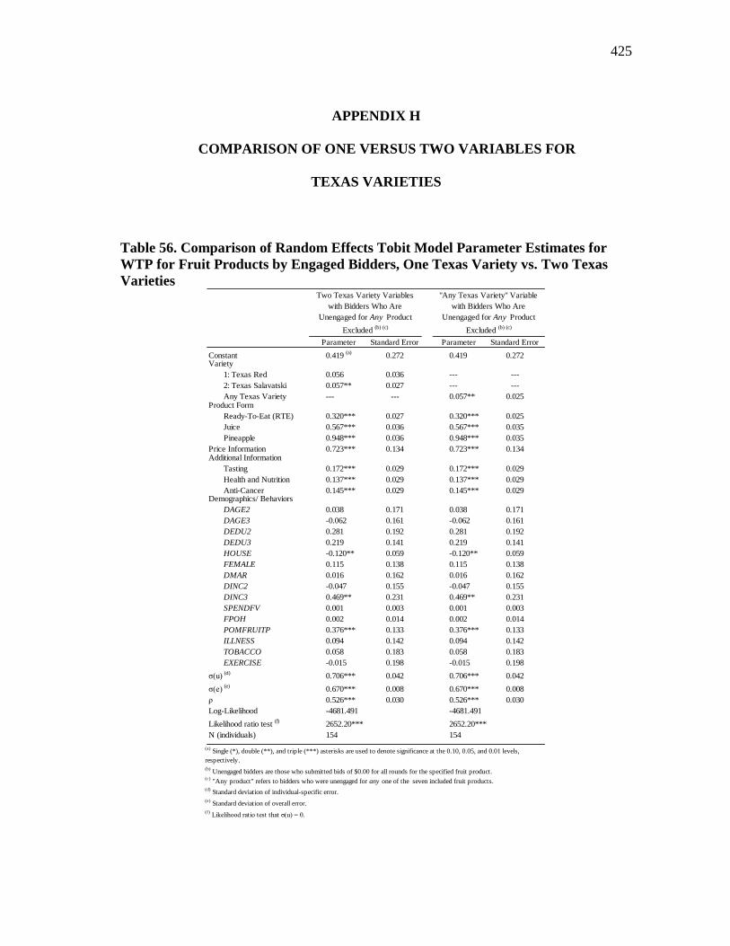
425
APPENDIX H
COMPARISON OF ONE VERSUS TWO VARIABLES FOR
TEXAS VARIETIES
Table 56. Comparison of Random Effects Tobit Model Parameter Estimates for
WTP for Fruit Products by Engaged Bidders, One Texas Variety vs. Two Texas
Varieties
Parameter Standard Error Parameter Standard Error
Constant 0.419 (a)
0.272 0.419 0.272Variety
1: Texas Red 0.056 0.036 --- ---
2: Texas Salavatski 0.057** 0.027 --- ---
Any Texas Variety --- --- 0.057** 0.025Product Form
Ready-To-Eat (RTE) 0.320*** 0.027 0.320*** 0.025
Juice 0.567*** 0.036 0.567*** 0.035
Pineapple 0.948*** 0.036 0.948*** 0.035
Price Information 0.723*** 0.134 0.723*** 0.134Additional Information
Tasting 0.172*** 0.029 0.172*** 0.029
Health and Nutrition 0.137*** 0.029 0.137*** 0.029
Anti-Cancer 0.145*** 0.029 0.145*** 0.029Demographics/ Behaviors
DAGE2 0.038 0.171 0.038 0.171
DAGE3 -0.062 0.161 -0.062 0.161
DEDU2 0.281 0.192 0.281 0.192
DEDU3 0.219 0.141 0.219 0.141
HOUSE -0.120** 0.059 -0.120** 0.059
FEMALE 0.115 0.138 0.115 0.138
DMAR 0.016 0.162 0.016 0.162
DINC2 -0.047 0.155 -0.047 0.155
DINC3 0.469** 0.231 0.469** 0.231
SPENDFV 0.001 0.003 0.001 0.003
FPOH 0.002 0.014 0.002 0.014
POMFRUITP 0.376*** 0.133 0.376*** 0.133
ILLNESS 0.094 0.142 0.094 0.142
TOBACCO 0.058 0.183 0.058 0.183
EXERCISE -0.015 0.198 -0.015 0.198
σ(u) (d)
0.706*** 0.042 0.706*** 0.042
σ(e) (e)
0.670*** 0.008 0.670*** 0.008
ρ 0.526*** 0.030 0.526*** 0.030
Log-Likelihood -4681.491 -4681.491
Likelihood ratio test (f)
2652.20*** 2652.20***
N (individuals) 154 154
"Any Texas Variety" Variable
with Bidders Who Are
Unengaged for Any Product
Excluded (b) (c)
Two Texas Variety Variables
with Bidders Who Are
Unengaged for Any Product
Excluded (b) (c)
(d) Standard deviation of individual-specific error.
(e) Standard deviation of overall error.
(f) Likelihood ratio test that σ(u) = 0.
(b) Unengaged bidders are those who submitted bids of $0.00 for all rounds for the specified fruit product.
(c) "Any product" refers to bidders who were unengaged for any one of the seven included fruit products.
(a) Single (*), double (**), and triple (***) asterisks are used to denote significance at the 0.10, 0.05, and 0.01 levels,
respectively.
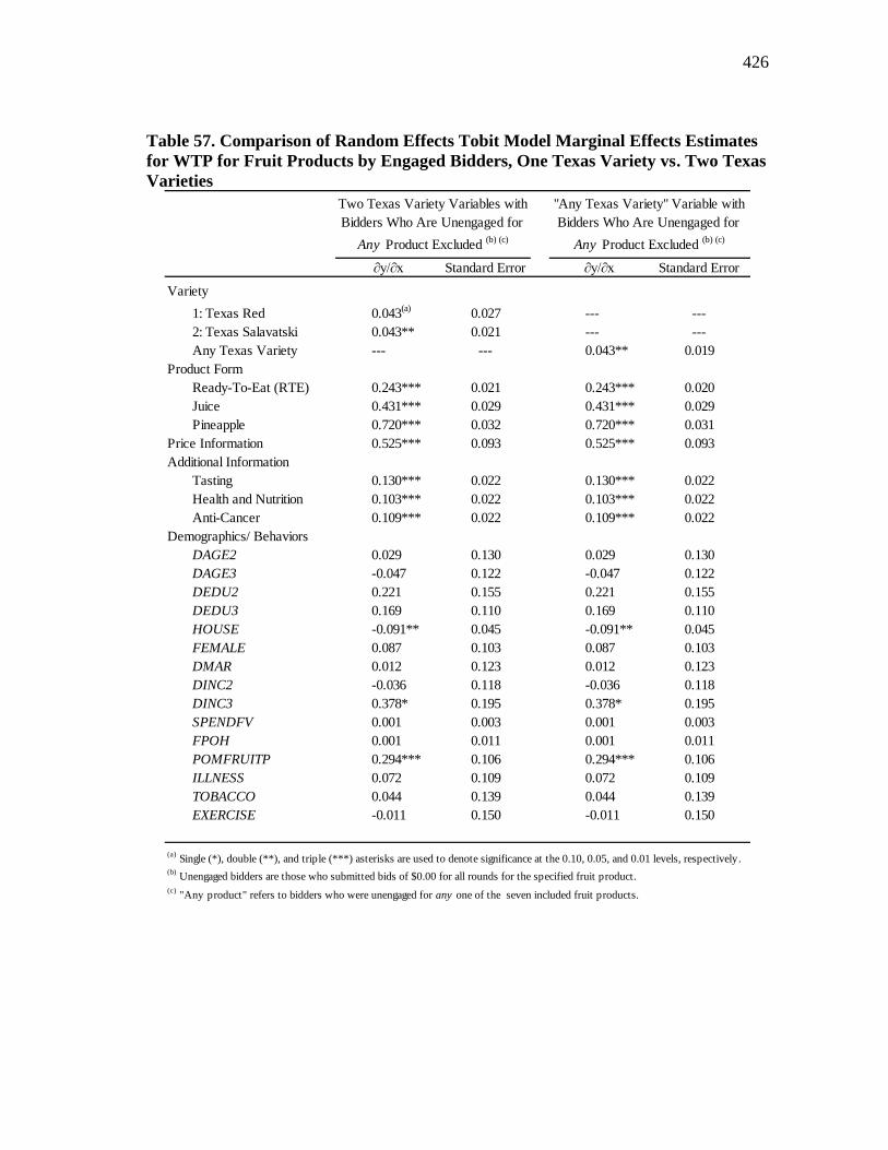
426
Table 57. Comparison of Random Effects Tobit Model Marginal Effects Estimates
for WTP for Fruit Products by Engaged Bidders, One Texas Variety vs. Two Texas
Varieties
∂y/∂x Standard Error ∂y/∂x Standard Error
Variety
1: Texas Red 0.043(a)
0.027 --- ---
2: Texas Salavatski 0.043** 0.021 --- ---
Any Texas Variety --- --- 0.043** 0.019
Product Form
Ready-To-Eat (RTE) 0.243*** 0.021 0.243*** 0.020
Juice 0.431*** 0.029 0.431*** 0.029
Pineapple 0.720*** 0.032 0.720*** 0.031
Price Information 0.525*** 0.093 0.525*** 0.093
Additional Information
Tasting 0.130*** 0.022 0.130*** 0.022
Health and Nutrition 0.103*** 0.022 0.103*** 0.022
Anti-Cancer 0.109*** 0.022 0.109*** 0.022
Demographics/ Behaviors
DAGE2 0.029 0.130 0.029 0.130
DAGE3 -0.047 0.122 -0.047 0.122
DEDU2 0.221 0.155 0.221 0.155
DEDU3 0.169 0.110 0.169 0.110
HOUSE -0.091** 0.045 -0.091** 0.045
FEMALE 0.087 0.103 0.087 0.103
DMAR 0.012 0.123 0.012 0.123
DINC2 -0.036 0.118 -0.036 0.118
DINC3 0.378* 0.195 0.378* 0.195
SPENDFV 0.001 0.003 0.001 0.003
FPOH 0.001 0.011 0.001 0.011
POMFRUITP 0.294*** 0.106 0.294*** 0.106
ILLNESS 0.072 0.109 0.072 0.109
TOBACCO 0.044 0.139 0.044 0.139
EXERCISE -0.011 0.150 -0.011 0.150
(b) Unengaged bidders are those who submitted bids of $0.00 for all rounds for the specified fruit product.
(c) "Any product" refers to bidders who were unengaged for any one of the seven included fruit products.
(a) Single (*), double (**), and triple (***) asterisks are used to denote significance at the 0.10, 0.05, and 0.01 levels, respectively.
Two Texas Variety Variables with
Bidders Who Are Unengaged for
Any Product Excluded (b) (c)
"Any Texas Variety" Variable with
Bidders Who Are Unengaged for
Any Product Excluded (b) (c)
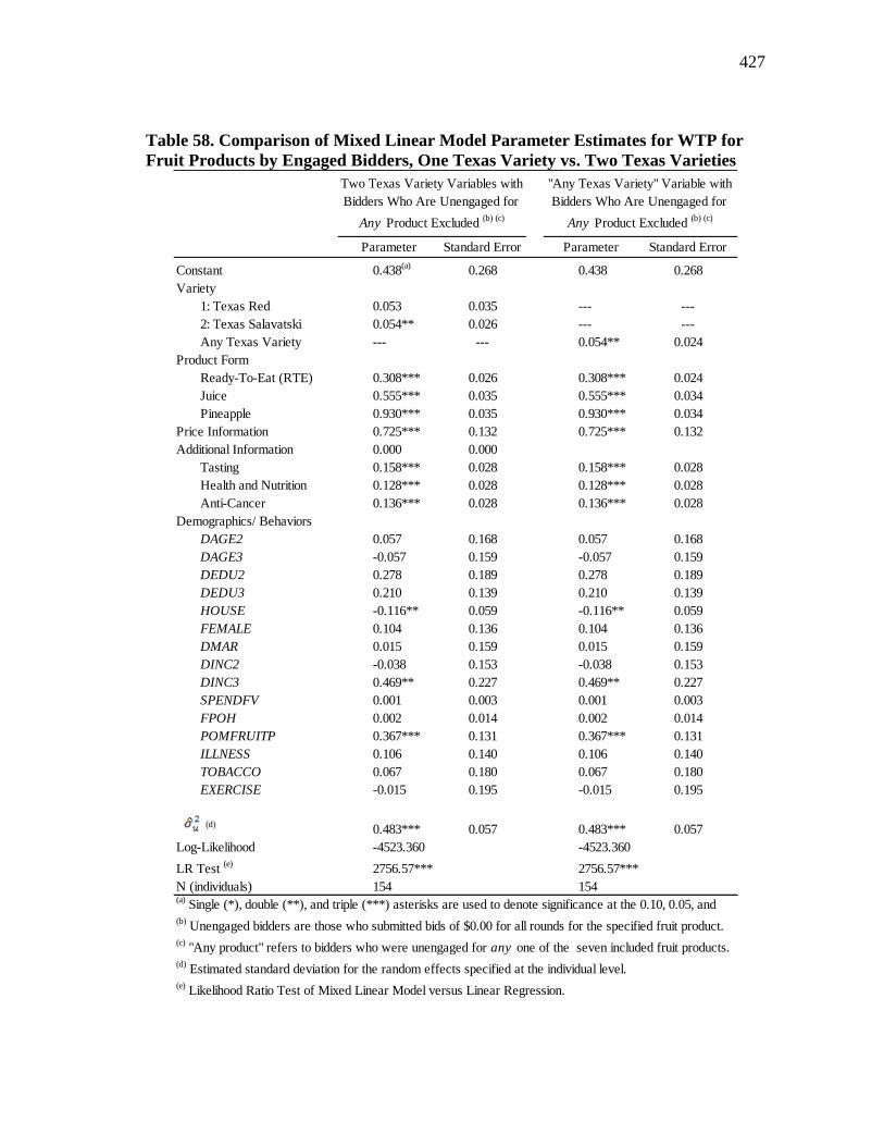
427
Table 58. Comparison of Mixed Linear Model Parameter Estimates for WTP for
Fruit Products by Engaged Bidders, One Texas Variety vs. Two Texas Varieties
Parameter Standard Error Parameter Standard Error
Constant 0.438(a)
0.268 0.438 0.268
Variety
1: Texas Red 0.053 0.035 --- ---
2: Texas Salavatski 0.054** 0.026 --- ---
Any Texas Variety --- --- 0.054** 0.024
Product Form
Ready-To-Eat (RTE) 0.308*** 0.026 0.308*** 0.024
Juice 0.555*** 0.035 0.555*** 0.034
Pineapple 0.930*** 0.035 0.930*** 0.034
Price Information 0.725*** 0.132 0.725*** 0.132
Additional Information 0.000 0.000
Tasting 0.158*** 0.028 0.158*** 0.028
Health and Nutrition 0.128*** 0.028 0.128*** 0.028
Anti-Cancer 0.136*** 0.028 0.136*** 0.028
Demographics/ Behaviors
DAGE2 0.057 0.168 0.057 0.168
DAGE3 -0.057 0.159 -0.057 0.159
DEDU2 0.278 0.189 0.278 0.189
DEDU3 0.210 0.139 0.210 0.139
HOUSE -0.116** 0.059 -0.116** 0.059
FEMALE 0.104 0.136 0.104 0.136
DMAR 0.015 0.159 0.015 0.159
DINC2 -0.038 0.153 -0.038 0.153
DINC3 0.469** 0.227 0.469** 0.227
SPENDFV 0.001 0.003 0.001 0.003
FPOH 0.002 0.014 0.002 0.014
POMFRUITP 0.367*** 0.131 0.367*** 0.131
ILLNESS 0.106 0.140 0.106 0.140
TOBACCO 0.067 0.180 0.067 0.180
EXERCISE -0.015 0.195 -0.015 0.195
(d)
0.483*** 0.057 0.483*** 0.057
Log-Likelihood -4523.360 -4523.360
LR Test (e)
2756.57*** 2756.57***
N (individuals) 154 154
(b) Unengaged bidders are those who submitted bids of $0.00 for all rounds for the specified fruit product.
(c) "Any product" refers to bidders who were unengaged for any one of the seven included fruit products.
(d) Estimated standard deviation for the random effects specified at the individual level.
(e) Likelihood Ratio Test of Mixed Linear Model versus Linear Regression.
(a) Single (*), double (**), and triple (***) asterisks are used to denote significance at the 0.10, 0.05, and
Two Texas Variety Variables with
Bidders Who Are Unengaged for
Any Product Excluded (b) (c)
"Any Texas Variety" Variable with
Bidders Who Are Unengaged for
Any Product Excluded (b) (c)
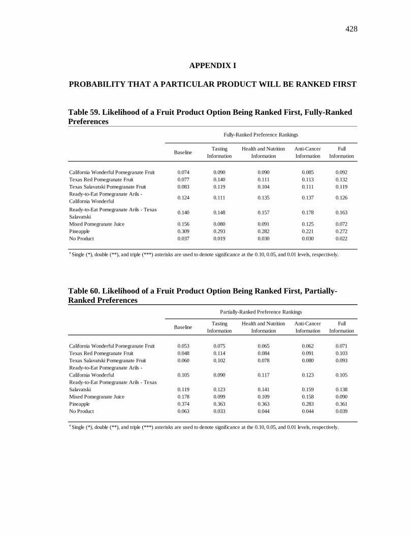
428
APPENDIX I
PROBABILITY THAT A PARTICULAR PRODUCT WILL BE RANKED FIRST
Table 59. Likelihood of a Fruit Product Option Being Ranked First, Fully-Ranked
Preferences
Table 60. Likelihood of a Fruit Product Option Being Ranked First, Partially-
Ranked Preferences
BaselineTasting
Information
Health and Nutrition
Information
Anti-Cancer
Information
Full
Information
California Wonderful Pomegranate Fruit 0.074 0.090 0.090 0.085 0.092
Texas Red Pomegranate Fruit 0.077 0.140 0.111 0.113 0.132
Texas Salavatski Pomegranate Fruit 0.083 0.119 0.104 0.111 0.119
Ready-to-Eat Pomegranate Arils -
California Wonderful0.124 0.111 0.135 0.137 0.126
Ready-to-Eat Pomegranate Arils - Texas
Salavatski0.140 0.148 0.157 0.178 0.163
Mixed Pomegranate Juice 0.156 0.080 0.091 0.125 0.072
Pineapple 0.309 0.293 0.282 0.221 0.272
No Product 0.037 0.019 0.030 0.030 0.022
a Single (*), double (**), and triple (***) asterisks are used to denote significance at the 0.10, 0.05, and 0.01 levels, respectively.
Fully-Ranked Preference Rankings
BaselineTasting
Information
Health and Nutrition
Information
Anti-Cancer
Information
Full
Information
California Wonderful Pomegranate Fruit 0.053 0.075 0.065 0.062 0.071
Texas Red Pomegranate Fruit 0.048 0.114 0.084 0.091 0.103
Texas Salavatski Pomegranate Fruit 0.060 0.102 0.078 0.080 0.093
Ready-to-Eat Pomegranate Arils -
California Wonderful 0.105 0.090 0.117 0.123 0.105
Ready-to-Eat Pomegranate Arils - Texas
Salavatski 0.119 0.123 0.141 0.159 0.138
Mixed Pomegranate Juice 0.178 0.099 0.109 0.158 0.090
Pineapple 0.374 0.363 0.363 0.283 0.361
No Product 0.063 0.033 0.044 0.044 0.039
a Single (*), double (**), and triple (***) asterisks are used to denote significance at the 0.10, 0.05, and 0.01 levels, respectively.
Partially-Ranked Preference Rankings
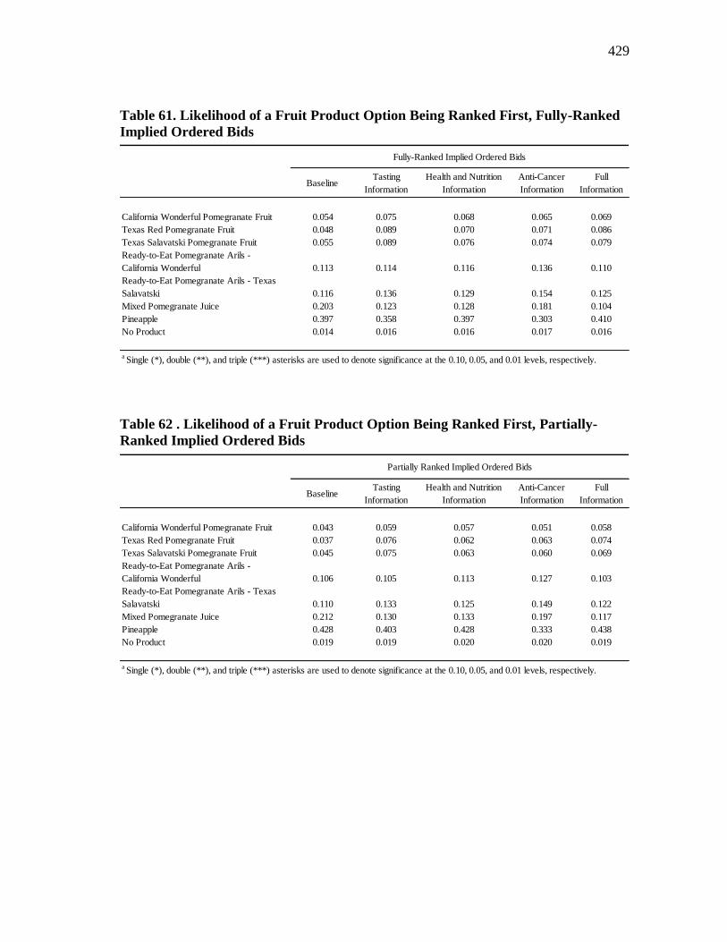
429
Table 61. Likelihood of a Fruit Product Option Being Ranked First, Fully-Ranked
Implied Ordered Bids
Table 62 . Likelihood of a Fruit Product Option Being Ranked First, Partially-
Ranked Implied Ordered Bids
BaselineTasting
Information
Health and Nutrition
Information
Anti-Cancer
Information
Full
Information
California Wonderful Pomegranate Fruit 0.054 0.075 0.068 0.065 0.069
Texas Red Pomegranate Fruit 0.048 0.089 0.070 0.071 0.086
Texas Salavatski Pomegranate Fruit 0.055 0.089 0.076 0.074 0.079
Ready-to-Eat Pomegranate Arils -
California Wonderful 0.113 0.114 0.116 0.136 0.110
Ready-to-Eat Pomegranate Arils - Texas
Salavatski 0.116 0.136 0.129 0.154 0.125
Mixed Pomegranate Juice 0.203 0.123 0.128 0.181 0.104
Pineapple 0.397 0.358 0.397 0.303 0.410
No Product 0.014 0.016 0.016 0.017 0.016
a Single (*), double (**), and triple (***) asterisks are used to denote significance at the 0.10, 0.05, and 0.01 levels, respectively.
Fully-Ranked Implied Ordered Bids
BaselineTasting
Information
Health and Nutrition
Information
Anti-Cancer
Information
Full
Information
California Wonderful Pomegranate Fruit 0.043 0.059 0.057 0.051 0.058
Texas Red Pomegranate Fruit 0.037 0.076 0.062 0.063 0.074
Texas Salavatski Pomegranate Fruit 0.045 0.075 0.063 0.060 0.069
Ready-to-Eat Pomegranate Arils -
California Wonderful 0.106 0.105 0.113 0.127 0.103
Ready-to-Eat Pomegranate Arils - Texas
Salavatski 0.110 0.133 0.125 0.149 0.122
Mixed Pomegranate Juice 0.212 0.130 0.133 0.197 0.117
Pineapple 0.428 0.403 0.428 0.333 0.438
No Product 0.019 0.019 0.020 0.020 0.019
a Single (*), double (**), and triple (***) asterisks are used to denote significance at the 0.10, 0.05, and 0.01 levels, respectively.
Partially Ranked Implied Ordered Bids
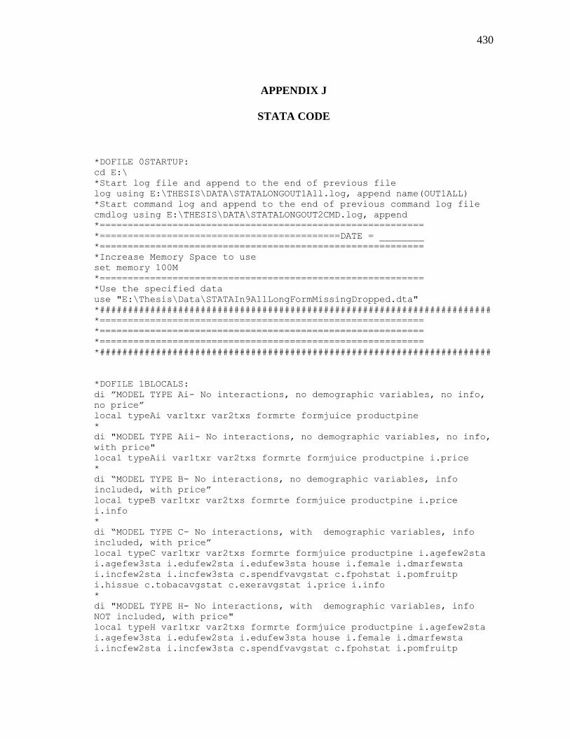
430
APPENDIX J
STATA CODE
*DOFILE 0STARTUP:
cd E:\
*Start log file and append to the end of previous file
log using E:\THESIS\DATA\STATALONGOUT1All.log, append name(OUT1ALL)
*Start command log and append to the end of previous command log file
cmdlog using E:\THESIS\DATA\STATALONGOUT2CMD.log, append
*==========================================================
*===========================================DATE = ________
*==========================================================
*Increase Memory Space to use
set memory 100M
*==========================================================
*Use the specified data
use "E:\Thesis\Data\STATAIn9AllLongFormMissingDropped.dta"
*######################################################################
*==========================================================
*==========================================================
*==========================================================
*######################################################################
*DOFILE 1BLOCALS:
di ”MODEL TYPE Ai- No interactions, no demographic variables, no info,
no price”
local typeAi var1txr var2txs formrte formjuice productpine
*
di "MODEL TYPE Aii- No interactions, no demographic variables, no info,
with price"
local typeAii var1txr var2txs formrte formjuice productpine i.price
*
di “MODEL TYPE B- No interactions, no demographic variables, info
included, with price”
local typeB var1txr var2txs formrte formjuice productpine i.price
i.info
*
di “MODEL TYPE C- No interactions, with demographic variables, info
included, with price”
local typeC var1txr var2txs formrte formjuice productpine i.agefew2sta
i.agefew3sta i.edufew2sta i.edufew3sta house i.female i.dmarfewsta
i.incfew2sta i.incfew3sta c.spendfvavgstat c.fpohstat i.pomfruitp
i.hissue c.tobacavgstat c.exeravgstat i.price i.info
*
di "MODEL TYPE H- No interactions, with demographic variables, info
NOT included, with price"
local typeH var1txr var2txs formrte formjuice productpine i.agefew2sta
i.agefew3sta i.edufew2sta i.edufew3sta house i.female i.dmarfewsta
i.incfew2sta i.incfew3sta c.spendfvavgstat c.fpohstat i.pomfruitp
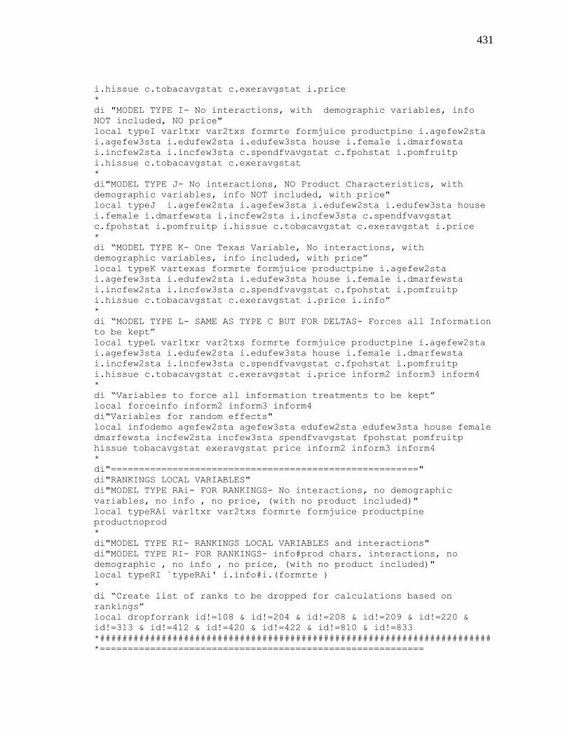
431
i.hissue c.tobacavgstat c.exeravgstat i.price
*
di "MODEL TYPE I- No interactions, with demographic variables, info
NOT included, NO price"
local typeI var1txr var2txs formrte formjuice productpine i.agefew2sta
i.agefew3sta i.edufew2sta i.edufew3sta house i.female i.dmarfewsta
i.incfew2sta i.incfew3sta c.spendfvavgstat c.fpohstat i.pomfruitp
i.hissue c.tobacavgstat c.exeravgstat
*
di"MODEL TYPE J- No interactions, NO Product Characteristics, with
demographic variables, info NOT included, with price"
local typeJ i.agefew2sta i.agefew3sta i.edufew2sta i.edufew3sta house
i.female i.dmarfewsta i.incfew2sta i.incfew3sta c.spendfvavgstat
c.fpohstat i.pomfruitp i.hissue c.tobacavgstat c.exeravgstat i.price
*
di “MODEL TYPE K- One Texas Variable, No interactions, with
demographic variables, info included, with price”
local typeK vartexas formrte formjuice productpine i.agefew2sta
i.agefew3sta i.edufew2sta i.edufew3sta house i.female i.dmarfewsta
i.incfew2sta i.incfew3sta c.spendfvavgstat c.fpohstat i.pomfruitp
i.hissue c.tobacavgstat c.exeravgstat i.price i.info”
*
di “MODEL TYPE L- SAME AS TYPE C BUT FOR DELTAS- Forces all Information
to be kept”
local typeL var1txr var2txs formrte formjuice productpine i.agefew2sta
i.agefew3sta i.edufew2sta i.edufew3sta house i.female i.dmarfewsta
i.incfew2sta i.incfew3sta c.spendfvavgstat c.fpohstat i.pomfruitp
i.hissue c.tobacavgstat c.exeravgstat i.price inform2 inform3 inform4
*
di “Variables to force all information treatments to be kept”
local forceinfo inform2 inform3 inform4
di"Variables for random effects"
local infodemo agefew2sta agefew3sta edufew2sta edufew3sta house female
dmarfewsta incfew2sta incfew3sta spendfvavgstat fpohstat pomfruitp
hissue tobacavgstat exeravgstat price inform2 inform3 inform4
*
di"======================================================="
di"RANKINGS LOCAL VARIABLES"
di"MODEL TYPE RAi- FOR RANKINGS- No interactions, no demographic
variables, no info , no price, (with no product included)"
local typeRAi var1txr var2txs formrte formjuice productpine
productnoprod
*
di"MODEL TYPE RI- RANKINGS LOCAL VARIABLES and interactions"
di"MODEL TYPE RI- FOR RANKINGS- info#prod chars. interactions, no
demographic , no info , no price, (with no product included)"
local typeRI `typeRAi' i.info#i.(formrte )
*
di “Create list of ranks to be dropped for calculations based on
rankings”
local dropforrank id!=108 & id!=204 & id!=208 & id!=209 & id!=220 &
id!=313 & id!=412 & id!=420 & id!=422 & id!=810 & id!=833
*######################################################################
*==========================================================
432
*==========================================================
*==========================================================
*######################################################################
*DOFILE 1CSUMMARY:
display "Start log file and append to the end of previous file"
log using ".\THESIS\DATA\STATALONGOUT1cSummary.log", append
name(OUT1CSUMMARY)
display "Start log file and replace previous file"
log using ".\THESIS\DATA\STATALONGOUT1cSummaryrep.log", replace
name(OUT1CSUMMARYrep)
*
*====================================================================
*==============Summary Statistics, As Needed=========================
*=== (Data are balanced, so values will be correct for all data======
*====================================================================
di”Summary Statistics for included variables”
summarize `typeC’ if key==”naivecali”
*
di"Summary Statistics for previous experience with Pomegranates"
summarize pomsee-pomflavn if key=="naivecali"
di"Detailed summary statistics for previous experience with
pomegranates"
summarize pomsee-pomflavn if key=="naivecali", detail
di “Count of individuals with any pomegranates on hand”
count if key=="naivecali" & pomhand!=1
*
di"Summarize vairables by session"
forvalues i= 1(1)8{
summarize `typeC' if info!=5&prodkey!="noprod"&s`i's==1
}
*
di "Count of individuals in each session" forvalues i=100(100)800{
list id if key=="naivecali" & `i'<=id & id<=(`i'+99)
count if key=="naivecali" & `i'<=id & id<=(`i'+99)
}
*
di"Count of total bidders included"
count if key=="naivecali"
log close OUT1CSUMMARY
log close OUT1CSUMMARYrep
*######################################################################
*==========================================================
*==========================================================
*==========================================================
*######################################################################
*DOFILE 2TOBITS:
log using E:\THESIS\DATA\STATALONGOUT2TOBITS.log, append
name(OUT2TOBITS)
*====================================================================
433
*====================================================================
*===================TOBIT MODELS, WTP===============================
*======== WTP= f(WTP= f(product characteristics, info, demographics)=
*======== 1 model for all WTP bids for all products==================
*====================================================================
*====================================================================
di"TOBIT MODEL"
di"MODEL TYPE Ai- No interactions, no demographic variables, no info ,
no price"
tobit bids `typeAi' if info!=5&prodkey!="noprod", ll(0) log
margins, dydx(*) predict(e(0,.))
estimates store tobitAi
*
di"TOBIT MODEL"
di"MODEL TYPE Aii- No interactions, no demographic variables, no info ,
with price"
tobit bids `typeAii' if info!=5&prodkey!="noprod", ll(0) log
margins, dydx(*) predict(e(0,.))
estimates store tobitAii
*
di"TOBIT MODEL"
di"MODEL TYPE B- No interactions, no demographic variables, info
included, with price"
tobit bids `typeB' if info!=5&prodkey!="noprod"&i, ll(0) log
margins, dydx(*) predict(e(0,.))
estimates store tobitB
*
di"TOBIT MODEL"
di"MODEL TYPE C- No interactions, with demographic variables, info
included, with price"
tobit bids `typeC' if info!=5&prodkey!="noprod", ll(0) log
margins, dydx(*) predict(e(0,.))
estimates store tobitC
*
di"TOBIT MODEL"
di"MODEL TYPE H- No interactions, with demographic variables, info NOT
included, with price"
tobit bids `typeH' if info!=5&prodkey!="noprod", ll(0) log
margins, dydx(*) predict(e(0,.))
estimates store tobitH
*
di"Do a likelihood ratio test on the model specifications and obtain
AIC and BIC values"
lrtest tobitH tobitAi, stats
lrtest tobitH tobitAii, stats
lrtest tobitH tobitB, stats
lrtest tobitH tobitC, stats
*
log close OUT2TOBITS
*
*######################################################################
*==========================================================
*==========================================================
*==========================================================
434
*######################################################################
*DOFILE 3ROLOGITS:
log using E:\THESIS\DATA\STATALONGOUT3rologits.log, append
name(OUT3ROLOGITS)
log using E:\THESIS\DATA\STATALONGOUT3rologitsRE.log, replace
name(OUT3ROLOGITSRE)
di"Generate variables to be used in saving estimates of rank-ordereled
logit models"
foreach ranking of varlist pref prefpart brprefer brprefpart{
forvalues i =1(1)5{
generate pRAi`ranking'info`i' =0
}
}
*
di"Create nested loops to run rank-ordered logit models for:
di"Outside Loop: fully and partially ranked explicit rankings and
implied rankings"
di"Inside Loop: Each information treatment (identified 1-5)"
foreach ranking of varlist pref prefpart brprefer brprefpart{
forvalues i =1(1)5{
di"==================================================================="
di"============RANK-ORDERED LOGIT MODELS, Rankings===================="
di"=================== Rank= f(product characteristics)==============="
di"===== 5 models (BASELINE, TASTING, HEALTH, ANTI-CANCER, FULL)======"
di"==================================================================="
di"===========rologit, Baseline Treatment (info=`i')=================="
di"================`ranking'=========================================="
rologit `ranking' `typeRAi' if info==`i' & `dropforrank' , group (id)
reverse
di"-------Probability of ranking a specific product as first----------"
drop pRAi`ranking'info`i'
predict pRAi`ranking'info`i' if e(sample)
sort id `ranking' pRAi`ranking'info`i'
gsort - pRAi`ranking'info`i'
list pRAi`ranking'info`i' prodkey `typeRAi' if id==101 & info==`i',
noobs
estimates store e`ranking'`i'
di"----------------------------------------------------------"
di"----------------------------------------------------------"
}
*
}
*
di"Make table of all estimated values based on rank-ordered logits"
estimates table epref1 epref2 epref3 epref4 epref5 eprefpart1
eprefpart2 eprefpart3 eprefpart4 eprefpart5 ebrprefer1 ebrprefer2
ebrprefer3 ebrprefer4 ebrprefer5 ebrprefpart1 ebrprefpart2 ebrprefpart3
ebrprefpart4 ebrprefpart5
*
log close OUT3ROLOGITS
log close OUT3ROLOGITSRE
*

435
*######################################################################
*==========================================================
*==========================================================
*==========================================================
*######################################################################
*DOFILE 4DELTAS:
log using E:\THESIS\DATA\STATALONGOUT4DELTAS.log, append
name(OUT4DELTAS)
log using E:\THESIS\DATA\STATALONGOUT4DELTASrep.log, replace
name(OUT4DELTASrep)
di"log using E:\THESIS\DATA\STATALONGOUT4DELTAS.log, append
name(OUT4DELTAS)"
di"log using E:\THESIS\DATA\STATALONGOUT4DELTASrep.log, replace
name(OUT4DELTASrep)"
*
di"Summary Statistics of Deltas"
summarize deltabid* if key=="naivecali", detail
summarize deltafbid* if key=="naivecali", detail
graph box deltabidtastecali deltabidtastetxr deltabidtastetxs
deltabidtastertec deltabidtastertet deltabidtastejuice
deltabidtastepine deltabidhealthcali deltabidhealthtxr
deltabidhealthtxs deltabidhealthrtec deltabidhealthrtet
deltabidhealthjuice deltabidhealthpine deltabidcancercali
deltabidcancertxr deltabidcancertxs deltabidcancerrtec
deltabidcancerrtet deltabidcancerjuice deltabidcancerpine if
key=="naivecali"
*graph save "E:\Thesis\Data\STATAOUT4boxplot.gph", replace
graph use "E:\Thesis\Data\STATAOUT4boxplot.gph"
*==============================================================
di"Count of total bids marked unengaged"
count if unengall2==1
di"Count of unique unengaged bids (taste, health, cancer)"
count if unengall2==1 & info!=5
*
di"Loop to calculate counts for each unengaged category"
forvalues i= 2(1)5{
di"========Counts for Each Category=================="
di"======================info = `i'=================="
di""
di"..................Unengaged Bids.................."
count if unengall2==1 & info==`i'
di"..............Total Bid Count....................."
count if info==`i'
}
*
foreach prod in cali txr txs rtec rtet juice pine{
forvalues i= 2(1)5{
di"========Counts for Each product in each category=================="
di"======================info = `i'========================"
di"======================Product = `prod'=================="
di""
di".............Unengaged Bids info=`i' and prod
436
=`prod'.................."
count if unengall2==1 & info==`i' & prodkey=="`prod'"
di".....Number of total bids for info=`i' and prod
=`prod'................"
count if info==`i' & prodkey=="`prod'"
}
}
*
*====================================================================
*==============DELTA BIDS ===========================================
*==============MIXED LINEAR MODELS, DELTA BIDS WTP===================
*========== WTP= f(product characteristics, demographics)============
*========================== 1 model==================================
*====================================================================
di"DELTA'S refer to the changes in bids that an individual has for a
single product across information treatments"
di"Removes full bids, naive bids, noproduct bids, and unengaged bids"
di"unengall2 identifies any individual that was a case four unengaged
bid for that particular product and round"
*
di"MIXED LINEAR MODEL- DELTAS"
di"MODEL TYPE Ai- No interactions, no demographic variables, no info ,
no price"
xtmixed deltabids `typeAi' if info!=5 & info!=1 & prodkey!="noprod" &
unengall2!=1, noconstant|| id: , mle
*xtmixed deltabids `typeAi' if info!=5 & info!=1 & prodkey!="noprod" &
unengall2!=1, noconstant|| id: , variance mle
estimates store randdeltAi
*
di"MIXED LINEAR MODEL- DELTAS"
di"MODEL TYPE Aii- No interactions, no demographic variables, no info ,
with price"
xtmixed deltabids `typeAii' if info!=5 & info!=1 & prodkey!="noprod" &
unengall2!=1, noconstant|| id: , mle
*xtmixed deltabids `typeAii' if info!=5 & info!=1 & prodkey!="noprod" &
unengall2!=1, noconstant|| id: , variance mle
estimates store randdeltAii
*
di"MIXED LINEAR MODEL- DELTAS"
di"MODEL TYPE B- No interactions, no demographic variables, info
included, with price"
xtmixed deltabids `typeAii' `forceinfo' if info!=5 & info!=1 &
prodkey!="noprod" & unengall2!=1, noconstant|| id: , mle
xtmixed deltabids `typeAii' `forceinfo' if info!=5 & info!=1 &
prodkey!="noprod" & unengall2!=1, noconstant|| id: , variance mle
estimates store randdeltB
*
di"MIXED LINEAR MODEL- DELTAS"
di"MODEL TYPE C- No interactions, with demographic variables, info
included, with price"
xtmixed deltabids `typeH' `forceinfo' if info!=5 & info!=1 &
prodkey!="noprod" & unengall2!=1, noconstant|| id: , mle
xtmixed deltabids `typeH' `forceinfo' if info!=5 & info!=1 &
prodkey!="noprod" & unengall2!=1, noconstant|| id: , variance mle
437
estimates store randdeltC
*
di"MIXED LINEAR MODEL- DELTAS"
di"MODEL TYPE H- No interactions, with demographic variables, info NOT
included, with price"
xtmixed deltabids `typeH' if info!=5 & info!=1 & prodkey!="noprod" &
unengall2!=1, noconstant|| id: , mle
*xtmixed deltabids `typeH' if info!=5 & info!=1 & prodkey!="noprod" &
unengall2!=1, noconstant|| id: , variance mle
estimates store randdeltH
*
di"Show statistics for each set of estimates"
estimates stats randdeltAi randdeltAii randdeltB randdeltC randdeltH
di"*****NOTE THAT THIS PREFERS THE MODELS WITH THE LOWEST AIC, BIC"
di"see stata reference[R] XTMIXED on page 334-335"
*====================================================================
*
*====================================================================
*==============DELTA BIDS, BASELINE TO FULL INFO=====================
*==============MIXED LINEAR MODELS, DELTA BIDS WTP===================
*========== WTP= f(product characteristics, demographics)============
*========================== 1 model==================================
*====================================================================
di"Removes full bids, naive bids, noproduct bids, and unengaged bids"
di"unengall2 identifies any individual that was a case four unengaged
for that particular product and round"
*
di"MIXED LINEAR MODEL- DELTAS"
di"MODEL TYPE Ai- No interactions, no demographic variables, no info ,
no price"
xtmixed deltabids `typeAi' if info==5 & prodkey!="noprod" &
unengall2!=1|| id: , mle
*xtmixed deltabids `typeAi' if info==5 & prodkey!="noprod" &
unengall2!=1|| id: , variance mle
estimates store randdeltFAi
*
di"MIXED LINEAR MODEL- DELTAS"
di"MODEL TYPE Aii- No interactions, no demographic variables, no info ,
with price"
xtmixed deltabids `typeAii' if info==5 & prodkey!="noprod" &
unengall2!=1|| id: , mle
*xtmixed deltabids `typeAii' if info==5 & prodkey!="noprod" &
unengall2!=1|| id: , variance mle
estimates store randdeltFAii
*
di"MIXED LINEAR MODEL- DELTAS"
di"MODEL TYPE H- No interactions, with demographic variables, info NOT
included, with price"
xtmixed deltabids `typeH' if info==5 & prodkey!="noprod" &
unengall2!=1|| id: , mle
*xtmixed deltabids `typeH' if info==5 & prodkey!="noprod" &
unengall2!=1|| id: , variance mle
estimates store randdeltFH
*
438
di"Display all stored estimates for full bids"
estimates stats randdeltFAi randdeltFAii randdeltFH
di"NOTE THAT THIS PREFERS THE MODELS WITH THE LOWEST AIC, BIC"
di"see stata reference[R] XTMIXED on page 334-335"
*========================================================
*
log close OUT4DELTAS
log close OUT4DELTASrep
*
*######################################################################
*==========================================================
*==========================================================
*==========================================================
*######################################################################
DOFILE 5MIXEDLINEAR:
log using E:\THESIS\DATA\STATALONGOUT5MIXED.log, append name(OUT5MIXED)
*====================================================================
*==============MIXED LINEAR MODELS, FULL BIDS WTP====================
*========== WTP= f(product characteristics, demographics)============
*========================== 1 model==================================
*====================================================================
di"MIXED LINEAR MODEL"
di"MODEL TYPE Ai- No interactions, no demographic variables, no info ,
no price"
xtmixed bids `typeAi' if info!=5&prodkey!="noprod"|| id: , variance mle
estimates store randAi
*
di"MIXED LINEAR MODEL"
di"MODEL TYPE Aii- No interactions, no demographic variables, no info ,
with price"
xtmixed bids `typeAii' if info!=5&prodkey!="noprod"|| id: , variance
mle
estimates store randAii
*
di"MIXED LINEAR MODEL"
di"MODEL TYPE B- No interactions, no demographic variables, info
included, with price"
xtmixed bids `typeB' if info!=5&prodkey!="noprod"|| id: , variance mle
estimates store randB
*
di"MIXED LINEAR MODEL"
di"MODEL TYPE C- No interactions, with demographic variables, info
included, with price"
xtmixed bids `typeC' if info!=5&prodkey!="noprod"|| id: , variance mle
estimates store randC
*
di"MIXED LINEAR MODEL"
di"MODEL TYPE H- No interactions, with demographic variables, info NOT
included, with price"
xtmixed bids `typeH' if info!=5&prodkey!="noprod"|| id: , variance mle
estimates store randH
*
439
di"MIXED LINEAR MODEL"
di"MODEL TYPE G- No interactions, with demographic variables, info
included, with price, nested effects"
xtmixed bids `typeC' if info!=5&prodkey!="noprod"|| id: R.info,
variance mle
estimates store randG
*
estimates stats randAi randAii randB randC randH randG
di"NOTE THAT THIS PREFERS THE MODELS WITH THE LOWEST AIC,BIC"
di"see stata reference[R] XTMIXED on page 334-335"
log close OUT5MIXED
*
*######################################################################
###
*==========================================================
*==========================================================
*==========================================================
*######################################################################
*DOFILE 6RANDOMEFFECTSTOBITS:
*====================================================================
*==============RANDOM EFFECTS TOBIT, FULL BIDS WTP===================
*========== WTP= f(product characteristics, demographics)============
*========================== 1 model==================================
*====================================================================
di"XTTOBIT- RANDOM EFFECTS TOBIT MODEL"
di"MODEL TYPE Ai- No interactions, no demographic variables, no info ,
no price"
xtset id
xttobit bids `typeAi' if info!=5&prodkey!="noprod", ll(0) log tobit
margins, dydx(*) predict(e(0,.))
estimates store xttobitAi
xtset, clear
*
di"XTTOBIT- RANDOM EFFECTS TOBIT MODEL"
di"MODEL TYPE Aii- No interactions, no demographic variables, no info ,
with price"
xtset id
xttobit bids `typeAii' if info!=5&prodkey!="noprod", ll(0) log tobit
margins, dydx(*) predict(e(0,.))
estimates store xttobitAii
xtset, clear
*
di"XTTOBIT- RANDOM EFFECTS TOBIT MODEL"
di"MODEL TYPE B- No interactions, no demographic variables, info
included, with price"
xtset id
xttobit bids `typeB' if info!=5&prodkey!="noprod", ll(0) log tobit
margins, dydx(*) predict(e(0,.))
estimates store xttobitB
xtset, clear
*
di"XTTOBIT- RANDOM EFFECTS TOBIT MODEL"
440
di"MODEL TYPE C- No interactions, with demographic variables, info
included, with price"
xtset id
xttobit bids `typeC' if info!=5&prodkey!="noprod", ll(0) log tobit
margins, dydx(*) predict(e(0,.))
estimates store xttobitC
xtset, clear
*
di"XTTOBIT- RANDOM EFFECTS TOBIT MODEL"
di"MODEL TYPE H- No interactions, with demographic variables, info NOT
included, with price"
xtset id
xttobit bids `typeH' if info!=5&prodkey!="noprod", ll(0) log tobit
margins, dydx(*) predict(e(0,.))
estimates store xttobitH
xtset, clear
*
di"Do a likelihood ratio test on the model specifications and obtain
AIC and BIC values"
lrtest xttobitH xttobitAi, stats
lrtest xttobitH xttobitAii, stats
lrtest xttobitH xttobitB, stats
lrtest xttobitH xttobitC, stats
*
*######################################################################
*==========================================================
*==========================================================
*==========================================================
*######################################################################
DOFILE 8OLS:
*====================================================================
*==============ORDINARY LEAST SQUARES, FULL BIDS WTP=================
*========== WTP= f(product characteristics, info, demographics)======
*========================== 1 model==================================
*===================(28 obsevations/ individual)=====================
*====================================================================
*
di"Ordinary Least Squares Regression"
di"MODEL TYPE Ai- No interactions, no demographic variables, no info ,
no price"
regress bids var1txr var2txs formrte formjuice productpine if
info!=5&prodkey!="noprod"
*
di"Ordinary Least Squares Regression"
di"MODEL TYPE Aii- No interactions, no demographic variables, no info ,
with price"
regress bids var1txr var2txs formrte formjuice productpine i.price if
info!=5&prodkey!="noprod"
*
di"Ordinary Least Squares Regression"
di"MODEL TYPE B- No interactions, no demographic variables, info
441
included, with price"
regress bids var1txr var2txs formrte formjuice productpine i.price
i.info if info!=5&prodkey!="noprod"
*
di"Ordinary Least Squares Regression"
di"MODEL TYPE C- No interactions, with demographic variables, info
included, with price"
regress bids var1txr var2txs formrte formjuice productpine i.agefew2sta
i.agefew3sta i.edufew2sta i.edufew3sta house i.female i.dmarfewsta
i.incfew2sta i.incfew3sta c.spendfvavgstat c.fpohstat i.pomfruitp
i.hissue c.tobacavgstat c.exeravgstat i.price i.info if
info!=5&prodkey!="noprod"
*
di"Ordinary Least Squares Regression"
di"MODEL TYPE H- No interactions, with demographic variables, info NOT
included, with price"
regress bids var1txr var2txs formrte formjuice productpine i.agefew2sta
i.agefew3sta i.edufew2sta i.edufew3sta house i.female i.dmarfewsta
i.incfew2sta i.incfew3sta c.spendfvavgstat c.fpohstat i.pomfruitp
i.hissue c.tobacavgstat c.exeravgstat i.price if
info!=5&prodkey!="noprod"
*
*######################################################################
*==========================================================
*==========================================================
*==========================================================
*######################################################################
*DOFILE 9PRODUCTTOBITS:
log using E:\THESIS\DATA\STATALONGOUT9PRODTOBITS.log, append
name(OUT9PROD)
di "==35 Tobit Models for Each Product and Each information
Treatment=="
di"==================================================================="
di"===========SEPARATE TOBIT MODELS, FULL BIDS WTP===================="
di"========== Bids= f(product characteristics, demographics)=========="
di"===5 info trtmts:(BASELINE, TASTING, HEALTH, ANTI-CANCER, FULL)===="
di"==========7 products:(cali txr txs rtec rtet juice pine)==========="
di"==================================================================="
di"==================================================================="
*
di"Create Nested Loops to Do Individual Tobit Models by Product and
Information Treatment"
forvalues i = 1(1)5{
foreach prod in cali txr txs rtec rtet juice pine{
di"==================================================================="
di"============TOBIT MODEL, INFO = `i', PRODUCT = `prod'============="
di"==================================================================="
di"MODEL TYPE H- No interactions, with demographic variables, info NOT
included, with price"
tobit bids `typeJ' if info==`i'&prodkey== "`prod'", ll(0) log
margins, dydx(*) predict(e(0,.))
442
}
}
*
log close OUT9PROD
*######################################################################
*==========================================================
*==========================================================
*==========================================================
*######################################################################
*DOFILE 10UNENGAGED:
di"Start log file and append to the end of previous file"
log using E:\THESIS\DATA\STATALONGOUTT10UNENGAGED.log, append
name(OUT10UNENGAGED)
log using E:\THESIS\DATA\STATALONGOUTT10UNENGAGEDrep.log, replace
name(OUT10UNENGAGEDrep)
di" log using E:\THESIS\DATA\STATALONGOUTT10UNENGAGED.log, append
name(OUT10UNENGAGED)"
di" log using E:\THESIS\DATA\STATALONGOUTT10UNENGAGEDrep.log, append
name(OUT10UNENGAGEDrep)"
*====================================================================
*==============ANALYSIS OF UNENGAGED BIDDERS, FULL BIDS WTP==========
*====================================================================
*====Random effects tobits, mixed linear, and separate product tobits
*====================================================================
*
*********************************************************************
*==========NO BIDDERS WHO ARE UNENGAGED FOR ANY PRODUCT==============
*********************************************************************
di"Bidders are identified as unengaged in the overall models if there
was any product for which they were unengaged"
di"Further described as 'case 4' in the text"
*
*From DOFILE 6RANDOMEFFECTSTOBITS
*====================================================================
*==============RANDOM EFFECTS TOBIT, FULL BIDS WTP====================
*========== WTP= f(product characteristics, demographics)============
*========================== 1 model==================================
*==========NO BIDDERS WHO ARE UNENGAGED FOR ANY PRODUCT==============
*====================================================================
*
di"XTTOBIT- RANDOM EFFECTS TOBIT MODEL"
di"MODEL TYPE C- No interactions, with demographic variables, info
included, with price"
xtset id
*random effects tobit model with information treatment and demographic
variables
xttobit bids `typeC' if info!=5&prodkey!="noprod"&casefourany!=1, ll(0)
log tobit
margins, dydx(*) predict(e(0,.))
xtset, clear
*
443
di"From DOFILE 5MIXEDLINEAR"
*====================================================================
*==============MIXED LINEAR MODELS, FULL BIDS WTP====================
*========== WTP= f(product characteristics, demographics)============
*========================== 1 model==================================
*==========NO BIDDERS WHO ARE UNENGAGED FOR ANY PRODUCT==============
*====================================================================
di"MIXED LINEAR MODEL"
di"REMOVE ALL UNENGAGED BIDDERS, Removes anyone unengaged for any
product"
di"MODEL TYPE C- No interactions, with demographic variables, info
included, with price"
xtmixed bids `typeC' if info!=5&prodkey!="noprod"& casefourany!=1|| id:
, variance mle
estimates store randcaseC
*
*********************************************************************
*==========NO BIDDERS WHO ARE UNENGAGED FOR ALL PRODUCTS=============
*********************************************************************
di"Bidders are identified as unengaged for all products in the overall
models if they were unengaged for all of the included products"
di"Further described as 'case 4' in the text"
*
*From DOFILE 6RANDOMEFFECTSTOBITS
*====================================================================
*==============RANDOM EFFECTS TOBIT, FULL BIDS WTP====================
*========== WTP= f(product characteristics, demographics)============
*========================== 1 model==================================
*==========NO BIDDERS WHO ARE UNENGAGED FOR ALL PRODUCTS=============
*====================================================================
di"XTTOBIT- RANDOM EFFECTS TOBIT MODEL"
di"MODEL TYPE C- No interactions, with demographic variables, info
included, with price"
xtset id
di"random effects tobit model with information treatment and
demographic variables"
xttobit bids `typeC' if info!=5&prodkey!="noprod"&casefourall!=1, ll(0)
log tobit
margins, dydx(*) predict(e(0,.))
xtset, clear
*
di"From DOFILE 5MIXEDLINEAR"
*====================================================================
*==============MIXED LINEAR MODELS, FULL BIDS WTP====================
*========== WTP= f(product characteristics, demographics)============
*========================== 1 model==================================
*==========NO BIDDERS WHO ARE UNENGAGED FOR ALL PRODUCTS=============
*====================================================================
di"MIXED LINEAR MODEL"
di"REMOVE ALL UNENGAGED BIDDERS, Removes anyone unengaged for any
product"
di"MODEL TYPE C- No interactions, with demographic variables, info
included, with price"
xtmixed bids `typeC' if info!=5&prodkey!="noprod"& casefourall!=1|| id:
444
, variance mle
estimates store randcaseC
*
*********************************************************************
*====NO BIDDERS WHO WERE UNENGAGED FOR THAT PARTICULAR PRODUCT=======
*********************************************************************
di"Bidders are identified as unengaged in the individual product and
information models"
di"if for that particular product they were unengaged"
di"Further described as 'case 4' in the text"
*
*From STATADoLong9ProdTobits
di"=35 Tobit Models, 1 for Each Product and Each information
Treatment=="
di"==================================================================="
di"===========SEPARATE TOBIT MODELS, FULL BIDS WTP===================="
di"======== Bids= f(product characteristics, demographics)============"
di"===5 info trtmts:(BASELINE, TASTING, HEALTH, ANTI-CANCER, FULL)===="
di"============7 products:(cali txr txs rtec rtet juice pine)========="
di"==================================================================="
di"====NO BIDDERS WHO WERE UNENGAGED FOR THAT PARTICULAR PRODUCT======"
di"==================================================================="
forvalues i = 1(1)5{
foreach prod in cali txr txs rtec rtec juice pine{
di"==================================================================="
di"==============TOBIT MODEL, INFO = `i', PRODUCT = `prod'==========="
di"==================================================================="
di"MODEL TYPE H- No interactions, with demographic variables, info NOT
included, with price"
di"tobit bids `typeJ' if info==`i'&prodkey==
"`prod'"&casefour`prod'!=1, ll(0) log"
di" margins, dydx(*) predict(e(0,.))"
tobit bids `typeJ' if info==`i'&prodkey== "`prod'"&casefour`prod'!=1,
ll(0) log
margins, dydx(*) predict(e(0,.))
di ""
di ""
di
"===================================================================="
di ""
}
}
*
*********************************************************************
*====NO BIDDERS WHO WERE UNENGAGED FOR THAT PARTICULAR PRODUCT ======
*---------IN THAT PARTICULAR ROUND-----------------------------------
*********************************************************************
di"Bidders are identified as unengaged in the individual product and
information models"
di"if for that particular product in that particular round they were
unengaged"
di"(Participants could be unengaged for a product in one round and not
in another"
445
di"Further described as 'case 4' in the text"
*====================================================================
*==============RANDOM EFFECTS TOBIT, FULL BIDS WTP===================
*========== WTP= f(product characteristics, demographics)============
*========================== 1 model==================================
*==========Only particular unengaged bids are removed================
*====================================================================
di"XTTOBIT- RANDOM EFFECTS TOBIT MODEL- UNENGALL Bids Removed"
di"MODEL TYPE C- No interactions, with demographic variables, info
included, with price"
xtset id
di"random effects tobit model with information treatment and
demographic variables"
xttobit bids `typeC' if info!=5&prodkey!="noprod"&unengall!=1, ll(0)
log tobit
margins, dydx(*) predict(e(0,.))
xtset, clear
*
**====================================================================
*==============MIXED LINEAR MODELS, FULL BIDS WTP====================
*========== WTP= f(product characteristics, demographics)============
*========================== 1 model==================================
*==========Only particular unengaged bids are removed================
*====================================================================
di"MIXED LINEAR MODEL"
di"REMOVE ALL UNENGAGED BIDDERS, Removes anyone unengaged for any
product"
di"MODEL TYPE C- No interactions, with demographic variables, info
included, with price"
xtmixed bids `typeC' if info!=5&prodkey!="noprod"& unengall!=1|| id: ,
variance mle
estimates store randunengC
*
log close OUT10UNENGAGED
log close OUT10UNENGAGEDrep
*
*######################################################################
*==========================================================
*==========================================================
*==========================================================
*######################################################################
*DOFILE 11ROMixedLogit:
cd E:\
*Start log file and append to the end of previous file
log using E:\THESIS\DATA\STATALONGOUT1All.log, append name(OUT1ALL)
*Start command log and append to the end of previous command log file
cmdlog using E:\THESIS\DATA\STATALONGOUT2CMD.log , append
*====================================================================
* ===================================================DATE = _________
*====================================================================
*Increase Memory Space to use
set memory 500M
446
*====================================================================
*
di"Create Mixed Rank-Ordered Logit Log"
log using .\THESIS\DATA\STATALONGOUT11ROMixed, append
name(OUT11MIXEDROLOGIT)
*
di"====================================================================
"
di"===================MIXED RANK-ORDERED LOGIT========================"
di"==================PREFERENCE RANKINGS, FULLY RANKED MODELS========="
di"==================================================================="
di"Use the specified data"
use "E:\Thesis\Data\STATAIn11MissDropGLLAMM.dta", replace
di"EXPLODE DATA"
di"Based on Rabe-Hesketh, Pickles, and Skrondal (2001)
egen maxr=max(pref), by (idinfo)
gen chosen=1
gen idx=_n
stset pref, fail(chosen) id(idx)
stsplit, at(failures) strata (idinfo) riskset (stage)
replace chosen=0 if chosen==.
drop if pref==maxr
bysort stage: generate groupcount=sum(chosen)
*
di"==================================================================="
di"==================================================================="
di"==================MIXED RANK-ORDERED LOGIT========================="
di"==================PREFERENCE RANKINGS, FULLY RANKED MODELS========="
di"==================NO INTERACTION TERMS============================="
di"==================================================================="
di"==================================================================="
di"==================================================================="
mixlogit chosen if info!=5 & `dropforrank' & stage!=. &groupcount==1 ,
group(stage) rand(`typeRAi') id(id) nrep(100)
mixlpred pRPLfull if e(sample) & info!=5 & `dropforrank' & stage!=.
&groupcount==1, nrep(100)
sort id prodkey
log using .\THESIS\DATA\STATALONGOUT11ROMixedProbs, append
name(OUT11MIXEDROLOGITprobs)
log using .\THESIS\DATA\STATALONGOUT11ROMixedProbsRep, replace
name(OUT11MIXEDROLOGITprobsRep)
list pRPLfull1 prodkey id if pref==1& info==1, noobs
list pRPLfull1 prodkey id if pref==1& info==2, noobs
list pRPLfull1 prodkey id if pref==1& info==3, noobs
list pRPLfull1 prodkey id if pref==1& info==4, noobs
log close OUT11MIXEDROLOGITprobs
log close OUT11MIXEDROLOGITprobsRep
mixlbeta `typeRAi' if info!=5 & `dropforrank' & stage!=. &groupcount==1
, saving (E:\THESIS\DATA\STATAOUT11Betas100I1) replace
save "E:\Thesis\Data\STATAIn11MissDropGLLAMMmixlogit2011_03_21.dta",
replace
*
di"==================================================================="
di"===================MIXED RANK-ORDERED LOGIT========================"
447
di"==================PREFERENCE RANKINGS, FULLY RANKED MODELS========="
di"===========WITH INTERACTION TERMS=================================="
di"==================================================================="
di"==================================================================="
*
forvalues i=2(1)4{
di"==================================================================="
di"===================MIXED RANK-ORDERED LOGIT========================"
di"==================PREFERENCE RANKINGS, FULLY RANKED MODELS========="
di"=============WITH INTERACTION TERMS================================"
di"==================================================================="
di"==================================================================="
di"=========info= `i' INTERACTION TERMS==============================="
mixlogit chosen if info!=5 & `dropforrank' & stage!=. &groupcount==1 ,
group(stage) rand(`typeRAi' interact*`i') id(id) nrep(100)
mixlpred pRPLfullI`i' if e(sample) & info!=5 & `dropforrank' & stage!=.
&groupcount==1, nrep(100)
sort id prodkey
log using .\THESIS\DATA\STATALONGOUT11ROMixedProbsI`i', append
name(OUT11MIXEDROLOGITprobsI`i')
log using .\THESIS\DATA\STATALONGOUT11ROMixedProbsI`i'Rep, replace
name(OUT11MIXEDROLOGITprobsI`i'Rep)
forvalues k=1(1)4{
di"=====================Probabilities if info= `k'==================="
list pRPLfullI`i' prodkey id if pref==1& info==`k', noobs
}
log close OUT11MIXEDROLOGITprobsI`i'
log close OUT11MIXEDROLOGITprobsI`i'Rep
mixlbeta `typeRAi' interact*`i' if info!=5 & `dropforrank' & stage!=.
&groupcount==1 , saving (E:\THESIS\DATA\STATAOUT11Betas100I`i') replace
save E:\Thesis\Data\STATAIn11MissDropGLLAMMmixlogit2011_03_21.dta,
replace
}
*
di"==================================================================="
di"===================MIXED RANK-ORDERED LOGIT========================"
di"==================PREFERENCE RANKINGS, FULLY RANKED MODELS========="
di"===========WITH INTERACTION TERMS=================================="
di"==================================================================="
di"==================================================================="
di"=========FULL INFORMATION INTERACTION TERMS========================"
mixlogit chosen if info!=2 & info!=3&info!=4 & `dropforrank' &
stage!=. &groupcount==1 , group(stage) rand(`typeRAi' interact*5)
id(id) nrep(100)
mixlpred pRPLfullI5 if e(sample) & info!=2 & info!=3&info!=4 &
`dropforrank' & stage!=. &groupcount==1, nrep(100)
sort id prodkey
log using .\THESIS\DATA\STATALONGOUT11ROMixedProbsI5, append
name(OUT11MIXEDROLOGITprobsI5)
log using .\THESIS\DATA\STATALONGOUT11ROMixedProbsI5Rep, replace
name(OUT11MIXEDROLOGITprobsI5Rep)
list pRPLfullI5 prodkey id if pref==1& info==1, noobs
list pRPLfullI5 prodkey id if pref==1& info==5, noobs
log close OUT11MIXEDROLOGITprobsI5

448
log close OUT11MIXEDROLOGITprobsI5Rep
mixlbeta `typeRAi' interact*5 if info!=2 & info!=3&info!=4 &
`dropforrank' & stage!=. &groupcount==1 , saving
(E:\THESIS\DATA\STATAOUT11Betas100I5) replace
save E:\Thesis\Data\STATAIn11MissDropGLLAMMmixlogit2011_03_21.dta,
replace
*
di"==================================================================="
di"==================================================================="
di"===========ESTIMATED BETA PARAMETERS==============================="
di"==================================================================="
di"==================================================================="
di"Do these at the end to copy and paste data"
use "E:\Thesis\Data\STATAOUT11Betas100I1.dta",
browse
pause on
pause "copy data and save and then type --pause off--"
*pause off
use "E:\Thesis\Data\STATAOUT11Betas100I2.dta",
browse
pause on
pause "copy data and save and then type --pause off--"
*pause off
use "E:\Thesis\Data\STATAOUT11Betas100I3.dta",
browse
pause on
pause "copy data and save and then type --pause off--"
*pause off
use "E:\Thesis\Data\STATAOUT11Betas100I4.dta",
browse
pause on
pause "copy data and save and then type --pause off--"
*pause off
use "E:\Thesis\Data\STATAOUT11Betas100I5.dta",
browse
pause on
pause "copy data and save and then type --pause off--"
*pause off
*#################################################################
di"==================================================================="
di"===================MIXED RANK-ORDERED LOGIT========================"
di"==============ORDERED BIDS, FULLY-RANKED MODELS===================="
di"==================================================================="
di"==================================================================="
di"==================================================================="
*
destring brpref, generate (brprefsta)
di"Use the specified data"
use "E:\Thesis\Data\STATAIn11MissDropGLLAMM.dta", replace
di"EXPLODE DATA"
egen maxr=max(brprefsta), by (idinfo)
gen chosen=1
gen idx=_n
stset brprefsta, fail(chosen) id(idx)
449
stsplit, at(failures) strata (idinfo) riskset (stage)
replace chosen=0 if chosen==.
drop if brprefsta==maxr
bysort stage: generate groupcount=sum(chosen)
di"==================MIXED RANK-ORDERED LOGIT========================="
di"==================ORDERED BIDS, FULLY RANKED MODELS================"
di"==================WITH INTERACTION TERMS==========================="
di"==================================================================="
*
mixlogit chosen if info!=5 & `dropforrank' & stage!=. &groupcount==1 ,
group(stage) rand(`typeRAi') id(id) nrep(100)
mixlpred pRPLfullBRI1 if e(sample) & info!=5 & `dropforrank' & stage!=.
&groupcount==1, nrep(100)
sort id prodkey
log using .\THESIS\DATA\STATALONGOUT11ROMixedBRProbs, append
name(OUT11MIXEDROLOGITBRprobs)
log using .\THESIS\DATA\STATALONGOUT11ROMixedBRProbsRep, replace
name(OUT11MIXEDROLOGITBRprobsRep)
forvalues k=1(1)4{
di"======Probabilities if info=`k'======================"
list pRPLfullBRI1 prodkey id if pref==1& info==`k', noobs
}
log close OUT11MIXEDROLOGITBRprobs
log close OUT11MIXEDROLOGITBRprobsRep
mixlbeta `typeRAi' if info!=5 & `dropforrank' & stage!=. &groupcount==1
, saving (E:\THESIS\DATA\STATAOUT11Betas100BRI1) replace
save "E:\Thesis\Data\STATAIn11MissDropORDEREDBIDS.dta", replace
*
di"==================================================================="
di"===================MIXED RANK-ORDERED LOGIT========================"
di"==================Ordered Bids, FULLY RANKED MODELS================"
di"===========WITH INTERACTION TERMS=================================="
di"==================================================================="
di"==================================================================="
*
forvalues i=2(1)4{
di"==================================================================="
di"===================MIXED RANK-ORDERED LOGIT========================"
di"==================ORDERED BIDS, FULLY RANKED MODELS================"
di"===========WITH INTERACTION TERMS=================================="
di"==================================================================="
di"==================================================================="
di"=========info= `i' INTERACTION TERMS==============================="
mixlogit chosen if info!=5 & `dropforrank' & stage!=. &groupcount==1 ,
group(stage) rand(`typeRAi' interact*`i') id(id) nrep(100)
mixlpred pRPLfullBRI`i' if e(sample) & info!=5 & `dropforrank' &
stage!=. &groupcount==1, nrep(100)
sort id prodkey
log using .\THESIS\DATA\STATALONGOUT11ROMixedProbsBRI`i', append
name(OUT11MIXEDROLOGITprobsBRI`i')
log using .\THESIS\DATA\STATALONGOUT11ROMixedProbsBRI`i'Rep, replace
name(OUT11MIXEDROLOGITprobsBRI`i'Rep)
forvalues k=1(1)4{
di"=====================Probabilities if info= `k'==================="
450
list pRPLfullBRI`i' prodkey id if pref==1& info==`k', noobs
}
log close OUT11MIXEDROLOGITprobsBRI`i'
log close OUT11MIXEDROLOGITprobsBRI`i'Rep
mixlbeta `typeRAi' interact*`i' if info!=5 & `dropforrank' & stage!=.
&groupcount==1 , saving (E:\THESIS\DATA\STATAOUT11Betas100BRI`i')
replace
save "E:\Thesis\Data\STATAIn11MissDropORDEREDBIDS.dta", replace
}
*
di"==================================================================="
di"=====================MIXED RANK-ORDERED LOGIT======================"
di"==================PREFERENCE RANKINGS, FULLY RANKED MODELS========="
di"=============WITH INTERACTION TERMS================================"
di"===================================================================”
di"==================================================================="
di"===========FULL INFORMATION INTERACTION TERMS======================"
mixlogit chosen if info!=2 & info!=3&info!=4 & `dropforrank' &
stage!=. &groupcount==1 , group(stage) rand(`typeRAi' interact*5)
id(id) nrep(100)
mixlpred pRPLfullBRI5 if e(sample) & info!=2 & info!=3&info!=4 &
`dropforrank' & stage!=. &groupcount==1, nrep(100)
sort id prodkey
log using .\THESIS\DATA\STATALONGOUT11ROMixedProbsBRI5, append
name(OUT11MIXEDROLOGITprobsBRI5)
log using .\THESIS\DATA\STATALONGOUT11ROMixedProbsBRI5Rep, replace
name(OUT11MIXEDROLOGITprobsBRI5Rep)
list pRPLfullBRI5 prodkey id if pref==1& info==1, noobs
list pRPLfullBRI5 prodkey id if pref==1& info==5, noobs
log close OUT11MIXEDROLOGITprobsBRI5
log close OUT11MIXEDROLOGITprobsBRI5Rep
mixlbeta `typeRAi' interact*5 if info!=2 & info!=3&info!=4 &
`dropforrank' & stage!=. &groupcount==1 , saving
(E:\THESIS\DATA\STATAOUT11Betas100BRI5) replace
save "E:\Thesis\Data\STATAIn11MissDropORDEREDBIDS.dta", replace
*
di"==================================================================="
di"==================================================================="
di"=========ESTIMATED BETA PARAMETERS================================="
di"==================================================================="
di"==================================================================="
di"Do these at the end to copy and paste data"
use "E:\Thesis\Data\STATAOUT11Betas100BRI1.dta",
browse
pause on
pause "copy data and save and then type --pause off--"
*pause off
use "E:\Thesis\Data\STATAOUT11Betas100BRI2.dta",
browse
pause on
pause "copy data and save and then type --pause off--"
*pause off
use "E:\Thesis\Data\STATAOUT11Betas100BRI3.dta",
browse
451
pause on
pause "copy data and save and then type --pause off--"
*pause off
use "E:\Thesis\Data\STATAOUT11Betas100BRI4.dta",
browse
pause on
pause "copy data and save and then type --pause off--"
*pause off
use "E:\Thesis\Data\STATAOUT11Betas100BRI5.dta",
browse
pause on
pause "copy data and save and then type --pause off--"
*pause off
*######################################################################
*==========================================================
*==========================================================
*==========================================================
*######################################################################
*DOFILE 12KSTestWilcoxonTest:
log using ".\data\KSTESTandSignedRankTest.log", append (OUT12TESTS)
codebook
di"Do a test for normality using skewness and kurtosis and correcting
for sample size"
di"Similar in design to the Jarque-Bera Tests for normality"
sktest deltabidtastecali deltabidtastetxr deltabidtastetxs
deltabidtastertec deltabidtastertet deltabidtastejuice
deltabidtastepine deltabidhealthcali deltabidhealthtxr
deltabidhealthtxs deltabidhealthrtec deltabidhealthrtet
deltabidhealthjuice deltabidhealthpine deltabidcancercali
deltabidcancertxr deltabidcancertxs deltabidcancerrtec
deltabidcancerrtet deltabidcancerjuice deltabidcancerpine deltafbidcali
deltafbidtxr deltafbidtxs deltafbidrtec deltafbidrtet deltafbidjuice
deltafbidpine
*
di"Do a Wilcoxon Signed Rank Test for differences across information
treatments"
foreach DELTAWTP in deltabidtastecali deltabidtastetxr deltabidtastetxs
deltabidtastertec deltabidtastertet deltabidtastejuice
deltabidtastepine deltabidhealthcali deltabidhealthtxr
deltabidhealthtxs deltabidhealthrtec deltabidhealthrtet
deltabidhealthjuice deltabidhealthpine deltabidcancercali
deltabidcancertxr deltabidcancertxs deltabidcancerrtec
deltabidcancerrtet deltabidcancerjuice deltabidcancerpine deltafbidcali
deltafbidtxr deltafbidtxs deltafbidrtec deltafbidrtet deltafbidjuice
deltafbidpine {
display "`DELTAWTP'"
signrank `DELTAWTP' = 0
}
*
log close OUT12TESTS

452
*######################################################################
*==========================================================
*==========================================================
*==========================================================
*######################################################################

453
VITA
Callie Pauline McAdams was raised in Efland, North Carolina as one of the fifth-
generation to work on her family‘s crop and livestock farm. She attended Orange High
School and graduated in May 2005. She then enrolled in North Carolina State
University. She was active in several agricultural organizations during her time there,
taking on leadership roles and receiving scholarships from many of them. While
enrolled, she held various positions with the university including work as a tobacco
Extension intern, work for the diversified agriculture program, and work in an animal
science nutrition lab. She received her Bachelor of Science degree from North Carolina
State University with majors in Agricultural Business Management and Animal Science
and a minor in Economics in May 2009. Her research interests include agricultural
policy, experimental economics, and horticultural marketing. She intends to pursue a
career in the agricultural field when she completes her formal education.
Ms. McAdams‘ contact information is available through the Department of
Agricultural Economics, 600 John Kimbrough Blvd., TAMU M.S. 2124, College
Station, TX 77843-2124. Her email is [email protected].


