Will the Working Poor Invest in Human Capital?: A Laboratory Experiment

Ce document a été produit dans le cadre d'uneentente de service entrele SRDC et le CIRANO.

MontréalMars 2002

Rapport de ProjetProject report

2002RP-08

Will the Working PoorInvest in Human Capital?A Laboratory Experiment

Catherine Eckel, Cathleen Johnson, ClaudeMontmarquette

CIRANO

Le CIRANO est un organisme sans but lucratif constitué en vertu de la Loi des compagnies du Québec. Lefinancement de son infrastructure et de ses activités de recherche provient des cotisations de ses organisations-membres, d’une subvention d’infrastructure du ministère de la Recherche, de la Science et de la Technologie, demême que des subventions et mandats obtenus par ses équipes de recherche.

CIRANO is a private non-profit organization incorporated under the Québec Companies Act. Its infrastructure andresearch activities are funded through fees paid by member organizations, an infrastructure grant from theMinistère de la Recherche, de la Science et de la Technologie, and grants and research mandates obtained by itsresearch teams.

Les organisations-partenaires / The Partner Organizations

•École des Hautes Études Commerciales•École Polytechnique de Montréal•Université Concordia•Université de Montréal•Université du Québec à Montréal•Université Laval•Université McGill•Ministère des Finances du Québec•MRST•Alcan inc.•AXA Canada•Banque du Canada•Banque Laurentienne du Canada•Banque Nationale du Canada•Banque Royale du Canada•Bell Canada•Bombardier•Bourse de Montréal•Développement des ressources humaines Canada (DRHC)•Fédération des caisses Desjardins du Québec•Hydro-Québec•Industrie Canada•Pratt & Whitney Canada Inc.•Raymond Chabot Grant Thornton•Ville de Montréal

© 2002 Catherine Eckel, Cathleen Johnson et Claude Montmarquette. Tous droits réservés. All rights reserved.Reproduction partielle permise avec citation du document source, incluant la notice ©.Short sections may be quoted without explicit permission, if full credit, including © notice, is given to the source.

ISSN 1499-8610

Will the Working Poor Invest in Human Capital?A Laboratory Experiment

Catherine Eckel*, Cathleen Johnson†, Claude Montmarquette‡

Résumé / Abstract

Ce rapport présente les résultats d’une expérience effectuée en laboratoireimpliquant environ 250 sujets résidant dans la région de Montréal. L’expérience tentede répondre à trois questions : 1) Les travailleurs à faible revenu investissent-ils dansdes actifs diversifiés?; 2) Les sujets sont-ils prêts à reporter leur consommation dans lefutur en échange de rendements financiers substantiels?; 3) Comment ces sujetsperçoivent-ils les choix risqués? Les réponses à ces questions vont permettre d’éclairerle sujet principal de cette recherche menée par le SRDC, à savoir : Si on leur procureles bonnes incitations, les travailleurs à faible revenu auront-ils tendance à épargnerpour investir dans du capital humain?

This paper presents the results of a laboratory experiment involving some 250subjects in the Montreal area. The experiment focused on three main questions : (1)Will the working poor invest in various assets? (2) Are these subjects willing to delayconsumption for substantial returns? (3) How do these subjects view risky choices?Answering these questions will help answering the key research question : Given theright incentive, will the working poor save to invest in human capital

Mots-clés : Travailleurs à faible revenu, expérience, incitations à l’épargne, capitalhumain, investissement

Keywords: Working poor, experiment, savings, human capital, investment

* Virginia Polytechnic Institute and State University† Social Research and Demonstration Corporation‡ Université de Montréal and CIRANO

Table of Contents Tables and Figures ii

1 Introduction 1 2 Advantages of Laboratory Experiments 3

2.1 An important addition to the economist’s toolkit 3 2.2 Particular features of this experiment 4

3 Research Design and Methods 5 3.1 Selection of subjects 5 3.2 Description of the procedure 5 3.3 Compensated questions 7 3.4 Information questionnaire (no compensation) 11

4 Revealed Behaviours 13 4.1 Some descriptive results on investing in human capital 13 4.2 Preference ordering over education, education of a family member, and retirement savings 22 4.3 Definitions and descriptive statistics on time preference and attitude towards risk 24

5 Subjects’ Preference for the Present and Attitude Toward Risk 29 5.1 Factors affecting patience 29 5.2 Factors affecting risk preference 31

6 Analysis of Investment Decisions 33 6.1 Analysis of investment in human capital 33 6.2 Analysis of investment in family member’s education 38 6.3 Analysis of investment in retirement savings 41

7 Summary and Conclusion 45 Appendices

A Materials Related to the Experiment “Will the Working Poor Invest in Human Capital? A Laboratory Experiment” 47

B Descriptive Statistics: “Will the Working Poor Invest in Human Capital? A Laboratory Experiment” 59

References 69

i

Tables and Figures

Table Page 3.1 Summary Description of Preference Questions 8

3.2 Summary Description of Time Preference Questions 9

3.3 Summary Description of the Risk-Preference Questions 10

4.1 Preference Ordering of Investment Alternatives 22

4.2 Preference Ordering — $100 Cash vs. $600 in (A) Educational Expenses, (B) Education of Family Member, and (C) Retirement Savings 23

4.3 Descriptive Statistics — Aggregate Measures of Time Preference 25

4.4 Descriptive Statistics — Aggregate Measures of Attitude Towards Risk 27

5.1 Determinants of the Number of Earliest Payoff Choices for the Time Preference Questions for Each Individual (Ordinary Least Squares, Impatient Choices) 29

5.2 Factors Affecting the Percentage of Participants Choosing the Earliest Payoff Choices for Each Time Preference Question (Logistic Specification) 30

5.3 Characteristics and Factors for Choosing the Earliest Payoff —- Preference for the Present (Random Effects Probit With Pooled Data: 9,472 Observations) 30

5.4 Determinants of Choosing the Less Risky Lotteries (Random Effects Probits With Pooled Data) 31

6.1 Determinants of Choosing Educational Expenses Over Cash (Ordered Probit, 240 Observations) 35

6.2 Simulation of the Probability of Investing in Education (240 Observations) 37

6.3 Determinants of Choosing Education of a Family Member Over Cash (Ordered Probit, 242 Observations) 39

6.4 Simulation of the Probability of Investing in Education of a Family Member (242 Observations) 40

6.5 Determinants of Choosing Retirement Savings Over Cash (Ordered Probit, 244 Observations) 42

6.6 Simulation of the Probability of Investing for Retirement 43

B.1 Survey Questions Descriptive Statistics: Mean (Standard-Deviation) or Proportion 60

B.2 Investment Preference Questions 65

B.3 Time Preference Questions 66

B.4 Risk Preference Questions 67

Figure Page

3.1 Sample Compensation Question From the Experiment 6

4.1 All Population 14

4.2 Labour Force — Those Subjects Who Declared Their Main Activity To Be Working, Unemployed, or On Leave From a Job 15

4.3 Non-labour Force — Those Subjects Who Named Their Main Activity To Be “Taking Care of Family” or Housework 16

4.4 Students — Subjects Who Were Currently Enrolled in School With No Other Main Declared Activity 17

4.5 Low-Income — Subjects Who Reported Family Income of Less Than 120 Per Cent of Statistics Canada’s Low Income Cut-Offs 18

4.6 Men 19

4.7 Women 20

4.8 All Population 22

4.9 Impatient Choices 26

iii

1 Introduction

In July 2001 the Social Research and Demonstration Corporation (SRDC) and Social and Enterprise Development Innovations (SEDI) launched a large demonstration project to test whether low-income people can be encouraged to save money to increase their human capital and, in turn, their standard of living in the long-run. Under this multi-year project, called learn$ave, participants open individual development accounts (IDAs), and for each dollar that participants put in their IDAs, program sponsors contribute matching dollars up to a predetermined limit. The matched funds must be used for post-secondary education, training, or small business start-ups. The success of this project depends on the ability of the target population (individuals with family incomes of less than 120 per cent of Statistics Canada’s low income cut-offs) to save and their willingness to save for this particular purpose.

As part of the design phase for the learn$ave demonstration project, SRDC made use of experimental economics to shed light on the behaviour and preferences of the working poor with respect to saving for learning activities. Laboratory experiments have been developing in the academic arena for some time, but they have yet to be used in conjunction with large-scale demonstration projects or social experiments conducted in real-life settings. Social experiments, using random assignment to program and control groups, remain the most powerful methodology available to isolate the impact of proposed changes in programs or policies. However, laboratory experiments can be used as a complementary approach to generate valuable information for the design of those social experiments and, perhaps, preview some their forthcoming results.

This paper presents the results of a laboratory experiment involving some 250 subjects in the Montreal area. The experiment focused on three main questions: (1) Will the working poor invest in various assets? (2) Are these subjects willing to delay consumption for substantial returns? (3) How do these subjects view risky choices? Answering these questions will inform the key research question: Given the right incentive, will the working poor save to invest in human capital?

Section 2 of the paper discusses the advantages of laboratory experiments over other approaches for learning about individuals’ behaviours and preferences. Section 3 presents the research design and operational details of the experiment. Section 4 provides descriptive observations on the subjects’ behaviours and choices as revealed through the experiment. Econometric investigation of time preference and attitude towards risk is offered in Section 5. Section 6 provides a more in-depth analysis of the investment choices and decisions on an individual basis. Section 7 concludes the paper with a look at policy implications and suggestions for further research possibilities.

1

2 Advantages of Laboratory Experiments

The effectiveness of a policy can be enhanced substantially if it is tailored to the preferences of the target population. Economists employ three different methodologies to measure these preferences: outcome-based measures, attitudinal survey questions, and experimentation. Laboratory experimental research is a relatively new addition to the economist’s toolkit, and has the potential to outperform the two traditional empirical methodologies.

2.1 An important addition to the economist’s toolkit The most commonly used empirical tool is the use of outcome-based measures of behaviour to infer the preferences of economic agents. Examples of these outcome measures include years of schooling, individual savings account balances, wages, retirement savings, and financial wealth. These measures are invaluable, but they provide only indirect information on many questions of interest. For example, an individual’s rate of time preference cannot be directly inferred from information about the balance in his or her savings account. Many socio-economic factors (such as income) and behavioural propensities (including risk aversion) jointly influence an individual’s savings behaviour. Hence, in general, outcomes data yield very noisy measures of preference parameters.

The second traditional empirical tool is attitudinal surveys. Surveys are more flexible in that they can address any topic. Social scientists can ask respondents whether they are patient by using hypothetical questions about choices over time. Survey questions can also ask respondents about their intentions with regard to human capital investment. While this approach is valuable in many cases it also has important caveats. Sceptical social scientists resist taking respondents’ self-reported statements at face value, whether they are about patience or other attitudes and behaviour. Survey questions may misrepresent the truth for several reasons. Respondents may misrepresent their attitudes or preferences because inaccurate attitudes may flatter their own self-image.1 Respondents may also misrepresent their own characteristics because they may interpret the question in their own way, which may differ from the interpretation of the researchers or of other subjects. In addition, respondents may bias their answers for “presentational” reasons, such as to look good in the eyes of the survey administrator.

In addition to economists’ two central empirical tools — behavioural measures and attitudinal survey measures — a third empirical tool has recently entered the economic mainstream: controlled laboratory experiments. In these experiments, subjects make real decisions, thereby revealing preferences that researchers are interested in. For example, instead of asking about patience, an experimentalist will give subjects 10 dollars and the opportunity to save that money with a certain return. The subjects’ willingness to give up this income in order to realize higher gains in the future is one possible measure of patience.

This approach has several advantages over the traditional empirical tools. First, these experiments control for situational variation by placing subjects in identical settings. This eliminates much of the uncontrolled variation that plagues outcome-based behavioural measures of preferences. Second, because subjects typically make decisions involving real money, it is costly to the subject to

3

1This problem occurs with “hard” data as well — self-reported income is notoriously inaccurate, and self-reported housing values regularly overstate true resale prices. See Goodman & Ittner, 1992.

4

misrepresent his true preferences. Ensuring anonymity can further minimize misrepresentation effects: if the experimenter is not able to link actions to particular individuals, then the subject has no incentive to misrepresent himself. Finally, the decisions made by subjects are real, not hypothetical. A subject makes an actual choice among alternatives, and that choice can be used to infer preferences.

Many of the original economic experiments tried to measure the overall or average behavioural propensities of entire populations of subjects. Experimentalists compared these propensities with the predictions of economic theory. Economists are just beginning a second wave of experimental research in which experiments are increasingly being used to document behavioural differences across individuals and to identify the correlates of those differences. (See for example Eckel & Grossman, 1998, in press-a, in press-b; Ansic & Powell, 1997; see also Schubert, Brown, Gyster, & Brachinger, 1999, on sex differences; Harbaugh & Krause, 2000, on children; Blondel, Lohéac, & Rinaudo, 2000, on drug users.) Results can be used to predict the response to public policies by different identifiable subgroups of the population.

2.2 Particular features of this experiment The experiment presented in this paper innovates in several ways. One big question about experiments is the extent to which behaviour in the economic laboratory predicts behaviour in the field. External (or field) validity is questionable in part because of the very general, context-free environment of most decision-making laboratory experiments. However, this study incorporates relevant contextual aspects of the decision-making process that are likely to improve the external (field) validity of the experimental results. For example, as explained below, the subjects of this experiment are making actual choices between alternatives such as (a) education for a family member, or (b) a fixed amount of cash.

Generalizing from the laboratory can also be problematic because of the necessarily small financial stakes that often characterize laboratory experiments.2 However, this study makes use of substantial economic stakes. Participants could earn as much as $400, and average earnings were $130. 3

Almost all experimental economic research is conducted with undergraduate subjects, eliminating any hope of determining the effects of age on behaviour. The range of incomes of undergraduates also tends to vary little as compared with the general population, making inferences about low-income adults problematic. This research avoids these problems by recruiting subjects who belong to the population targeted by the policy or program under study.

One last particular feature of this paper is the use of experimental economics to develop direct behavioural measures of the extent to which individual characteristics and socio-economic status influence patience and risk aversion. Very little is known about these individual characteristics. This experimental work on patience and risk adds to the literature in several ways. In this study, discount functions are measured in a wide range of subjects, enabling the identification of how discounting varies with personal characteristics. Important effects that are identified include (1) the extent to which patience appears to differ across socio-economic groups, (2) the extent to which some socio-economic groups show greater evidence of time inconsistency and, (3) the extent to which patience changes over the life cycle.

2Note that there is conflicting evidence for the importance of high stakes. Camerer and Hogarth, 1999, provide a survey on this question.

3Subjects could earn as much as $400 in cash, $600 in education expenses for the year, or $600 in a five- or seven-year fixed guaranteed investment certificate.

3 Research Design and Methods

This section describes the design and operational details of the laboratory experiment, beginning with the selection of subjects.

3.1 Selection of subjects To maximize the policy relevance of the results, the experiment was designed around the parameters of the learn$ave project. Recruitment efforts were organized through community groups whose membership included many working poor. In addition to providing experimental subjects, this recruitment was used as a pilot recruitment for the eventual demonstration project. All of the experimental sessions occurred in Montreal over a period of three weeks in November 2000.

A total of 256 subjects participated, of which 72 per cent had a family income of less than 120 per cent of Statistics Canada low income cut-offs (LICOs).1 Average total family income for the entire sample was approximately $22,500. Seventy-two per cent of the subjects were labour market participants, either employed or unemployed. Two thirds of the subjects were women. Participants were far from being uneducated: on average, they reported completing 13 to 14 years of schooling, 78 per cent of them claimed to hold a high-school diploma, and 26 per cent reported having attained a university degree. They were not completely without assets or access to capital markets: 26 per cent had a car and 54 per cent possessed a credit card. A significant fraction planned for the future: 47 per cent declared that they made regular contributions to a savings account and 27 per cent contributed to a retirement plan. Participation in lotteries was substantial but not pervasive: 27 per cent had never bought a lottery ticket.

Some participants who had not been targeted by the recruitment efforts were still able to learn about the experiment. Word of mouth about the experience and the potential for substantial sums of cash travelled fast, even in a relatively large city like Montreal. The largest group of unintended recruits was full-time students; the 31 students represent 12 per cent of the total number of subjects. Care was taken to identify this subgroup separately in the analysis.

3.2 Description of the procedure To advertise and recruit for the experiment, a brief notice was posted in low-income neighbourhoods and distributed at community group meetings. Subjects volunteered for the experiment by calling ahead and agreeing to show up at a location identified by the experimenters. Upon arrival, they were given a $12 show-up fee. The potential for additional financial compensation was explained and demonstrated to them after everyone participating in one session was assembled in one room. They were presented with two surveys (with different colours): one survey contained 64 compensated questions or choices, and another contained 43 non-compensated or information questions. They were told that at the end of the experiment

5

1Statistics Canada annually publishes a set of measures called the low income cut-offs (LICOs). Roughly speaking, the cut-offs mark income levels in which people have to spend disproportionate amounts of their incomes on food, shelter, and clothing. The LICOs vary by family size and size of community. Before-tax income cut-offs were used in view of the fact that before-tax income data was collected from the respondents.

one of the 64 compensated questions would be selected at random and they would be paid according to the answer they provided for that selected question. Instructions for the experiment are reproduced in Appendix A.

The 64 compensated questions were designed to support the three main questions to be addressed: (1) Will the working poor invest in various assets? (2) Are these subjects willing to delay consumption for substantial returns? (3) How do these subjects view risky choices? Figure 3.1 provides an example of one compensated question from the experiment that was concerned with the subjects’ preferences for investing in education. There were three versions of this type of question, with $200, $400, and $600 as the amounts being offered for an investment in education being weighted against an offer of $100 cash (one week from the day the experimental session was conducted).

Figure 3.1: Sample Compensation Question From the Experiment

You must choose A or B:

Choice A: $100 one week from today

Choice B: $400 in your own training or education These two choices are represented by the two following pictures. Please circle your choice:

$ 100 one week from

today

$400 in your own training or education

(expenses refunded)

Choice A

Or

Choice B

Once subjects had answered both surveys, the random selection of the compensated question was done with the use of a bingo cage containing 64 balls, numbered 1 to 64. Each subject was allowed to examine the numbered balls. The number on the ball drawn from the cage identified the compensation question for which they would be paid. If the compensation question selected dictated a monetary prize on the same day of the experiment, the prize was given in cash, on site. Delayed payments were mailed in the form of a cheque dated for the date indicated in the compensation question. There were many non-monetary prizes such as reimbursable educational expenses, guaranteed investment certificates (GICs), and gift certificates. A description of all prizes can be found in Appendix A. When the prize was a GIC or gift certificate, the experimenter signed an IOU and the prize was delivered to the subject by courier. All of the long-term GICs were purchased and distributed in early January 2001. All participants were required to sign a receipt. The average payoff per participant resulting from the experiment was approximately $130. Each experimental session, from instruction to payoff, took about an hour and a half.

6

Every effort was made to make the experiment accessible and non-threatening to all of the subjects. No computers were used in the administration of the experiment and simple devices like bingo balls and dice were used to generate random draws. Special attention was paid to the visual presentation and design of the compensation questions. Because the experiments were conducted in the neighbourhoods where the subjects lived, a pen-and-paper instrument was preferred over a computerized experiment. In the experimental pretest, some of the choices were found to be too challenging. To address this problem, a short set of practice compensation questions was incorporated into the instruction portion of the experiment. An example of each type of compensation question and the random draw process was illustrated in a six-question practice questionnaire. The subjects seemed to trust the experimenters to pay them as was described. In the debriefing questionnaire, 95 per cent of the subjects indicated that they were confident they would be paid in the way that was described to them in the experiment.

All experimental forms were pretested to minimize comprehension errors. However, in a few instances some subjects showed an inconsistency in their answers. In three of the questions subjects were offered the choice between $100 next week or $200, $400, or $600 in educational expenses. Some subjects made inconsistent choices within a category of questions. For example, a subject who chose the $200 investment in educational expenses over the $100 in cash, yet also chose $100 cash over the $400 or $600 choice of educational expenses, was termed “inconsistent.” Overall, very few subjects were inconsistent. Among the compensation questions concerning educational expenses (compensation questions 55, 62, and 59 summarized in Table 3.1, below) only 16 individuals or six per cent demonstrated an inconsistency. As these investment preference questions are central to the descriptive statistics in Section 4 and the analysis in Section 6, inconsistent subjects were not included.

3.3 Compensated questions Three major groupings of questions were used for the compensated questionnaire: (1) investment preference, (2) time preference, and (3) risk preference. Sections 3.3.1, 3.3.2, and 3.3.3 summarize the choices facing the participants in each category.2

Table 3.1 summarizes 13 of the 64 compensation questions that participants had to make as part of the compensated survey. The first column in the table contains the question numbers used in the compensated survey. Each row of the table represents the alternatives presented to the subject for each question. For example, Question 52 consisted of a choice between $100 that could be spent on the subject’s own education and $100 that could be spent on a durable goods item.

The first three choices in Table 3.1 (52, 53, and 54) are used to determine one measure of preference ordering between different forms of investment. Investing in one’s own education is compared with family member’s education, retirement savings, or purchase of durable goods.3 Various financial tools were used to make the compensated questions as close to these four categories in context as possible. For example, the retirement option was paid as an initial deposit into a frozen GIC redeemable in seven years. Each category of investment is described in Appendix A, as it was presented to the subjects. 2In the experiment the order of the compensation questions, by and within each major category, was randomly modified.

7

3The selection of investment categories reflects discussions that took place at the start of the learn$ave project. In the learn$ave project, participants can use matched savings accumulated in their IDAs to pay for their own educational expenses or micro-enterprise start-ups. In other IDAs schemes or demonstration projects being conducted in North America, eligible expenses may include other categories of investment, such as housing, retirement savings, and educational expenses incurred by a spouse or a child.

Table 3.1: Summary Description of Preference Questions

Question Number

Cash ($) (One Week From Today)

Own Education ($)

Education of Family Member ($)

Retirement ($)

Durable Goods ($)

52 100 100 53 500 500 54 500 500 55 100 200 56 100 600 57 100 600 58 100 200 59 100 600 60 166 500 61 250 500 62 100 400 63 250 500 64 166 500

3.3.1 Investment preference

The other 10 choices summarized in Table 3.1 address the issue of preference for investment for the four possible categories of investment. The choices were designed to simulate payroll deductions of varying amounts. For example, a choice would be: Option A: $100 a week from today or Option B: $200 for educational expenses. Or, Option A: $100 a week from today or Option B: $600 for educational expenses. These choices are designed to help pinpoint optimal match rates for the learn$ave demonstration.4

Theoretically, it would have been ideal to have subjects save their own funds in exchange for an amount earmarked for investment in their education. However, that requirement would have made the administrative cost and timing of the laboratory experiment infeasible. The learn$ave demonstration is a better tool for actually testing the savings behaviour over time. The laboratory alternative to having subjects save their own funds was to give subjects the choice between $100 in cash and $X in asset investment. In this context, high payoffs create salient decisions. For instance, in order to select the educational outcome, subjects would have to give up $100 in cash. Given the range of the subjects’ incomes, $100 represented a substantial amount of money to them.5

The nature of the alternative to cash also created the necessity for the experimenter to offer high payoffs. For instance, it is difficult to envisage situations in which educational expenses would not amount to a few hundred dollars. As an added benefit, the high payoffs were clearly salient to the subjects and they paid close attention to the procedure.

4The cash alternative was paid out one week from the day of the experiment to minimize the bias of mistrust. It was the nature of the investment alternatives that they be distributed at a later time than the experiment date. For example, a GIC was issued by the bank in the name of the subject or a selected family member after the experiment was completed. It was necessary that the subject trusted the experimenter to do this task after the completion of the experiment. If the cash alternative had been available immediately, subjects might have chosen the cash alternative rather than having to trust the experimenter.

8

5The cash alternative to investment options ranged from $100 to $250.

3.3.2 Time preference

A series of time preferences were elicited by asking subjects when they preferred to receive a certain payoff. Table 3.2 summarizes the time preference compensated questions.

Table 3.2: Summary Description of Time Preference Questions

Question Number

Today

($)

Earliest Tomorrow

($)

Payoff Next

Week ($)

Two Weeks

($)

Days Lapsed for Later Payoff

Alternative Payoff ($)

Rate of Return

(%)

6 71.50 2 71.54 10 2 71.15 3 71.21 10 17 71.20 7 71.34 10 12 71.10 14 71.37 10 4 71.00 28 71.54 10 9 72.00 2 72.20 50 3 72.15 3 72.45 50 13 72.25 7 72.94 50 10 72.10 14 73.48 50 8 72.05 28 74.81 50 19 73.25 2 74.05 200 11 73.10 3 74.30 200 14 73.00 7 75.80 200 21 73.30 14 78.92 200 18 73.15 28 84.37 200 20 73.25 2 74.05 200 22 73.10 3 74.30 200 15 73.00 7 75.80 200 24 73.30 14 78.92 200 25 73.15 28 84.37 200 26 73.25 2 74.05 200 16 73.10 3 74.30 200 5 73.00 7 75.80 200 28 73.30 14 78.92 200 23 73.15 28 84.37 200 7 72.25 2 73.75 380 29 72.10 3 74.35 380 30 72.00 7 77.25 380 32 72.50 14 83.07 380 33 72.25 2 73.75 380 35 72.10 3 74.35 380 36 72.00 7 77.25 380 1 72.50 14 83.07 380 37 26.15 2 26.69 380 27 26.05 3 26.86 380 24 26.25 7 28.16 380 31 26.10 14 29.90 380

9

Subjects were presented with the opportunity to take their payoff at some date, (say two weeks from today), or to delay payoff until some date, (say two weeks and two days from today). If the subject chose the delayed payoff, the subject was rewarded for waiting. Table 3.2 summarizes the 37 questions, varying in terms of initial payoffs and alternative payoffs with respect to days lapsed and discount rates. For example, Question 6 gave subjects the choice between $71.50 in seven days and $71.54 in nine days, rewarding the subject $0.04 for waiting two additional days. This would be equivalent to an annualized rate of return of 10 per cent. These responses can be used to measure the overall degree of patience.

tnt +

3.3.3 Risk preference

In Table 3.3, the questions with which participants’ attitudes toward risk were elicited are summarized with 14 pairs of lottery choices.

Table 3.3: Summary Description of the Risk-Preference Questions

Lotteries

Question Number Less Risky Alternative More Risky Alternative

38 ($60.00; 1.00) ($120.00; 0.50) or ($0.00; 0.50)

39 ($100.00; 1.00) ($200.00; 0.50) or ($0.00; 0.50)

40 ($60.00; 1.00) ($240.00; 0.25) or ($0.00; 0.75)

41 ($100.00; 1.00) ($400.00; 0.25) or ($0.00; 0.75)

42 ($60.00; 1.00) ($80.00; 0.75) or ($0.00; 0.25)

43 ($100.00; 1.00) ($133.33; 0.75) or ($0.00; 0.25)

44 ($100.00; 0.50) or ($0.00; 0.50) ($200.00; 0.25) or ($0.00; 0.75)

45 ($100.00; 0.40 or ($0.00; 0.60) ($400.00; 0.10) or ($0.00; 0.90)

46 ($60.00; 1.00) ($80.00; 0.50) or ($40.00; 0.50)

47 ($80.00; 1.00) ($100.00; 0.50) or ($60.00; 0.50)

48 ($120.00; 1.00) ($175.00; 0.80) or ($0.00; 0.20)

49 ($40.00; 1.00) ($90.00; 0.50) or ($0.00; 0.50)

50 ($75.00; 1.00) ($275.00; 0.30) or ($0.00; 0.70)

51 ($120.00; 0.50) or ($0.00; 0.50) ($175.00; 0.40) or ($0.00; 0.60)

Notes: The notation ($X; Y) simply means that $X dollars is offered with probability Y. For the first 10 questions, the expected value of the less risky alternative equals the expected value of the more risky alternative. For the last four questions, the expected value of the less risky alternative is less than that for the risky alternative. The three pairs of questions, 39 and 44, 41 and 45, and 48 and 51, are common-ratio lotteries.

Through these choices, subjects reported their preference for monetary gambles. For example, in Question 38, the participant is asked to choose between Option A yielding a certain $60 (that is $60 with probability of 1), and Option B yielding a 50 per cent chance of wining $120 (that is $120 with probability of 0.5).6 This series of questions with various payoffs and levels of risk can be used to explore the risk aversion of the participants.

10

6If 1 of the 14 monetary-gamble compensation questions was randomly selected for payoff, and the participant had selected an option that included a probability of winning a cash amount of less than 1, that participant was asked to simultaneously roll two 10-sided dice. The roll of the dice was used for a random selection of a number between 1 and 100. For instance, if the (cont’d)

11

3.4 Information questionnaire (no compensation) To complete the experiment, the subjects were asked to fill out an anonymous, 43-question survey. The first half of the survey contained demographic and behavioural questions (such as sex, income, education, and main activity). The second half of the survey contained attitudinal measures of subjects’ self-perceived patience, risk aversion, locus of control, and savings behaviour. Variables from this survey are used in the analysis of the compensated questions. The 43-question survey and summary statistics can be found in appendices A and B.

probability of winning the prize was 50 per cent, then a roll between 0 and 50 would be considered a winning roll. A roll between 51 and 100 would not be a winning roll.

4 Revealed Behaviours

Results of the experiment are presented in figures 4.1 to 4.6 and tables 4.1 to 6.6 in this and the next two sections. The results are presented for subgroups of subjects broken down by their main declared activity. The Labour Force subgroup was the largest subgroup in the sample and is comprised of those who declared their main activity to be working, unemployed, or on leave from a job. The Non-labour Force subgroup are those subjects who named their main activity to be “taking care of family” or housework. The Student subgroup is the smallest portion of the sample and is currently enrolled in school with no other main declared activity. The Low Income subgroup contains those subjects whose family income is less than 120 per cent of Statistics Canada’s low income cut-offs. Results are also presented by the sex of the subject. Note that these subpopulations are not mutually exclusive.

4.1 Some descriptive results on investing in human capital Figures 4.1 to 4.7 present core results of this experiment by illustrating the percentage of participants who would be prepared to save (or to forego cash) in response to various levels of incentives to invest in their own education or training. For clarity, inconsistent subjects were excluded from figures 4.1 to 4.7.1

4.1.1 Cash vs. own education

The top graph in Figure 4.1 indicates the percentage of subjects who chose $200, $400, or $600 earmarked for educational expenses over $100 cash one week from the date of the experiment. These choices represent trade-offs between cash amounts and funds for education at matching rates of 1 to 1, 1 to 3, and 1 to 5.2 At the lowest matching rate of 1 to 1, just over a fifth (22.9 per cent) of the participants chose education over cash. When subjects were presented with the opportunity analogous to the IDA learn$ave matching offer ($400 in educational expenses or $100 in cash), 43.8 per cent of subjects accepted the offer of education and training. At the highest matching rate of 1 to 5, 54.6 per cent of participants chose $600 for educational expenses when offered as an alternative to $100 cash. This indicates that about 45 per cent of the participants either did not have the ability to pay one sixth of their educational expense or did not have the desire to pay for their own education. Given that 72 per cent of subjects had family incomes below 120 per cent of Statistics Canada’s low income cut-offs it is reasonable to suspect that the cash alternative to investing in education was very attractive. Because this choice entails giving up money they would otherwise receive from participating in the experiment — i.e. “house money” — rather than their own earned income, these results most likely overstate slightly the willingness of participants to forego current income for investment in human capital under the learn$ave program. If participants had to use their own funds and give up planned consumption to do so, one would expect the take-up rate to be less than indicated in Figure 4.1. 1As stated earlier, very few subjects demonstrated an inconsistency in their choices between cash and assets: 6 per cent (16 subjects) were inconsistent concerning their own education; 5.5 per cent (14 subjects) were inconsistent concerning the choices involving a family member’s education; and 5 per cent (12 subjects) were inconsistent concerning their retirement. The student category is the only category where one individual’s inconsistency actually had a significant effect on the overall outcome of a particular category. This was simply because the student population in our sample was so small that the aberration was apparent.

13

2“1 to 5” is short form for five additional dollars for every dollar the subject contributes (or sacrifices) to the designated expense or savings option.

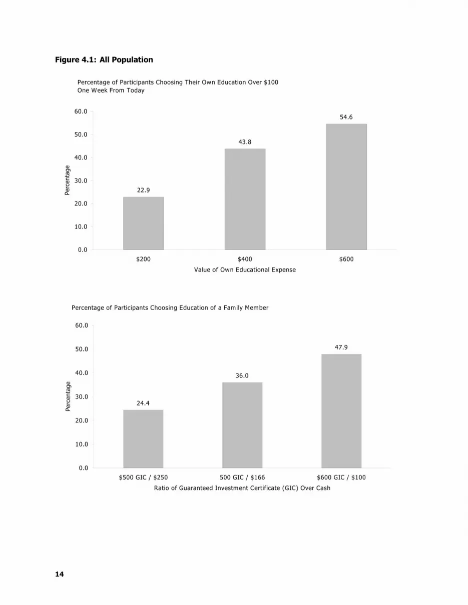
Figure 4.1: All Population

Percentage of Participants Choosing Their Own Education Over $100 One Week From Today

22.9

43.8

54.6

0.0

10.0

20.0

30.0

40.0

50.0

60.0

$200 $400 $600

Value of Own Educational Expense

Perc

enta

ge

Percentage of Participants Choosing Education of a Family Member

24.4

36.0

47.9

0.0

10.0

20.0

30.0

40.0

50.0

60.0

$500 GIC / $250 500 GIC / $166 $600 GIC / $100

Ratio of Guaranteed Investment Certificate (GIC) Over Cash

Perc

enta

ge

14

Figure 4.2: Labour Force — Those Subjects Who Declared Their Main Activity To Be Working, Unemployed, or On Leave From a Job


21.6

42.1

54.0

0.0

10.0

20.0

30.0

40.0

50.0

60.0

$200 $400 $600


Perc

enta

ge


22.4

34.5

47.1

0.0

10.0

20.0

30.0

40.0

50.0

60.0

$500 GIC / $250 $500 GIC / $166 $600 GIC / $100


Perc

enta

ge

15

Figure 4.3: Non-labour Force — Those Subjects Who Named Their Main Activity To Be “Taking Care of Family” or Housework


24.1

41.4

51.7

0.0

10.0

20.0

30.0

40.0

50.0

60.0

$200 $400 $600


Perc

enta

ge


53.3

63.3

73.3

0.0

10.0

20.0

30.0

40.0

50.0

60.0

70.0

80.0

$500 GIC / $250 $500 GIC / $166 $600 GIC / $100


Perc

enta

ge

16

Figure 4.4: Students — Subjects Who Were Currently Enrolled in School With No Other Main Declared Activity


34.6

61.5

69.2

0.0

10.0

20.0

30.0

40.0

50.0

60.0

70.0

80.0

$200 $400 $600


Perc

enta

ge


10.0

20.0

30.0

0.0

10.0

20.0

30.0

40.0

50.0

60.0

$500 GIC / $250 $500 GIC / $166 $600 GIC / $100


Perc

enta

ge

17

Figure 4.5: Low-Income — Subjects Who Reported Family Income of Less Than 120 Per Cent of Statistics Canada’s Low Income Cut-Offs


21.6

41.5

53.2

0.0

10.0

20.0

30.0

40.0

50.0

60.0

$200 $400 $600


Perc

enta

ge


28.3

38.2

49.7

0.0

10.0

20.0

30.0

40.0

50.0

60.0

$500 GIC / $250 $500 GIC / $166 $600 GIC / $100


Perc

enta

ge

18

Figure 4.6: Men


20.7

42.7

57.3

0.0

10.0

20.0

30.0

40.0

50.0

60.0

70.0

$200 $400 $600


Perc

enta

ge


23.1

37.2

46.2

0.0

10.0

20.0

30.0

40.0

50.0

60.0

$ 500 GIC / $250 $500 GIC / $166 $600 GIC / $100


Perc

enta

ge

19

Figure 4.7: Women


24.1

44.3

53.2

0.0

10.0

20.0

30.0

40.0

50.0

60.0

$200 $400 $600


Perc

enta

ge


25.0

35.4

48.8

0.0

10.0

20.0

30.0

40.0

50.0

60.0

$500 GIC / $250 $500 GIC / $166 $600 GIC / $100


Perc

enta

ge

20

Except for the Student subgroup, in which the rates of choosing education are consistently higher for all match rates, the patterns of behaviour observed in other population subgroups shown in top halves of figures 4.2 to 4.7 (Labour Force, Non-labour Force, Low Income, Men, and Women), are similar to the overall population. Comparing women and men, men appear to be more sensitive to the matching rate than the women, starting off with a lower percentage of take-up for the 1 to 1 match rate (20.7 per cent vs. 24.1 per cent) and ending with a higher take-up rate for the 1 to 5 match rate (57.3 per cent vs. 53.2 per cent).

4.1.2 Cash vs. education of a family member

The bottom halves of figures 4.1 to 4.7 represent the percentage of subjects who chose amounts earmarked for educational expenses of a family member over cash amounts one week from the date of the experiment. Although the absolute monetary amounts differ, the matching rates are equivalent to the match rates represented in the cash vs. own educational expenses: 1 to 1, 1 to 3, and 1 to 5. For example, in the lowest subsidy rate offered, participants were asked to choose between $250 cash a week from the day of the experiment and a GIC with a $500 deposit value bearing interest with a fixed maturity of five years. If this certificate of deposit was won, the winning participant had to identify the bearer (family member recipient) on the day of the experiment. It was emphasized by the experimenter that those certificates were to be used for the education of a family member.3

Figure 4.1 shows that 24.4 per cent of all participants chose the $500 in family member education over $250 in cash (1 to 1 match rate), 36.0 per cent chose the $500 in family member education over $166 in cash (1 to 3 match rate), and 47.9 per cent chose the $600 in family member education over $100 in cash (1 to 5 match rate). Similar results hold for the Low Income subpopulation.4 However, for the participants declaring their main activity to be taking care of their family (the Non-labour Force subpopulation, see Figure 4.3), these proportions are substantially higher at 53.3 per cent, 63.3 per cent, and 73.3 per cent, respectively. This observation requires a deeper look. A substantially smaller proportion of the Non-labour Force subpopulation chose education for themselves when faced with the same match rates (24.1 per cent, 41.4 per cent, and 51.7 per cent respectively). It may be that members of this subpopulation consider an investment in education to be a better investment for family members than for themselves. Further analysis of family member education is undertaken in Section 6.2.

4.1.3 Cash vs. retirement savings

The last category of investment considered is retirement savings. The experiment included three compensated questions that let the participants reveal their preferences for retirement savings. The choices varied cash and retirement savings (a fixed GIC with seven-year maturity) alternatives along the same match rates as for those of educational expenses and investment in a family member’s education. Figure 4.8 represents the percentages of all subjects who chose to forego the cash alternative for retirement savings. Further analysis of retirement savings is undertaken in Section 6.3. 3Five years from now it will be impossible to verify if the proceeds from the GICs will be invested in family members’ education. However, observation of the subjects and their reactions to the instructions and outcomes during and after the experiment leads us to believe that participants’ choices did reflect an understanding that the use of the GICs would indeed be restricted to uses related to family member education.

21

4It is interesting to compare these proportions with the results from the newly released Survey of Approaches to Educational Planning (SAEP) by Statistics Canada. In this survey, less than 20 per cent of parents reported saving for their children’s education in households where annual family income was below $30,000. See Daily, Statistics Canada, April 10, 2001.

Figure 4.8: All Population

Percentage of Participants Who Chose Retirement Savings

25

37

47

0.0

10.0

20.0

30.0

40.0

50.0

$500 GIC / $250 $500 GIC / $166 $600 GIC / $100

Ratio of GIC Over Cash

Perc

enta

ge

4.2 Preference ordering over education, education of a family member, and retirement savings

Tables 4.1 and 4.2 concern preference ordering over the three possible investment alternatives for the 256 participants. Table 4.1 summarizes the decisions of subjects in two situations, both involving direct comparisons between two of the asset alternatives valued at $500. For the first question, subjects were presented with a choice between $500 for their own educational expenses or $500 for the education of a family member (in the form of a fixed GIC, bearing interest and redeemable in five years). In the other choice pairing, the choice was between $500 in educational expenses or $500 for retirement savings (in the form of a fixed GIC, bearing interest and redeemable in seven years).

Table 4.1: Preference Ordering of Investment Alternatives

First Choice: $500 for own educational expenses (Own) vs. education of family member (Fam)

Second Choice: $500 for own educational expenses (Own) vs. retirement savings (Ret) Reference Populations Choices

Labour Force Own (60.0%) > Fam; Own (51.9%) > Ret Non-labour Force Fam (74.2%) > Own; Own (54.8%) > Ret Student Own (71.0%) > Fam; Own (67.7%) > Ret Low Income Own (54.6%) > Fam; Own (53.0%) > Ret Men Own (64.7%) > Fam; Own (63.5%) > Ret Women Own (52.6%) > Fam; Own (52.6%) > Ret All Fam (56.6%) > Own; Own (52.7%) > Ret

( ) Percentage of participants choosing this investment option.

22

Table 4.2: Preference Ordering — $100 Cash vs. $600 in Own Educational Expenses, Education of Family Member, and Retirement Savings

Reference Populations Choices

Labour Force Own (51.9%) > Fam (45.9%) > Ret (45.4%) Non-labour Force Fam (71.0%) > Ret (54.8%) > Own (51.6%) Student Own (58.1%) > Ret (32.3%) > Fam (29.0%) Low Income Own (50.3%) > Fam (48.1%) > Ret (43.2%) Men Own (55.3%) > Fam (44.7%) > Ret (32.9%) Women Ret (52.0%) > Own (50.3%) > Fam (47.4%) All Own (52.0%) > Fam (46.5%) > Ret (45.7%)

( ) Percentage of participants choosing this alternative.

Observe that with the exception of the two subgroups Non-labour Force and Women, Option A, one’s own educational expenses, is universally preferred to the other two investment choices. For the Non-labour Force subgroup, investing in a family-member’s education is preferred by a large margin to investing in one’s own education. (This result is consistent with what was observed in Section 4.1.2.) With the proportions of choices close to 50 per cent, women appear not to have a strong preference for one investment option over the other.

For each of the investment alternatives (in one’s own education, a family member’s education, and in retirement savings), the experiment included an additional way to compare the preference ordering of participants. A compensation question comparing $100 in cash and $600 in assets was asked of each participant for each investment alternative. Assuming that preferences are transitive — that is, if X is preferred to $100 and $100 is preferred to Y, it can be concluded that X is preferred to Y — subjects’ choices can be ordered, as shown below in Table 4.2. This table summarizes the findings from each of the three cash vs. $600 asset alternatives. If preferences are transitive, these results should not contradict the results presented in Table 4.1. When examining the Non-labour Force subpopulation category, there may appear to be an inconsistency. For this group, Table 4.1 suggests that B is preferred to A, and A is preferred to C (BAC), which does not match with the results summarized in Table 4.2. There, the Non-labour Force subgroup exhibits preferences of the order of B preferred to C, which is preferred to A (BCA). This inconsistency occurs because the percentages of group preference for investment in A and C over cash are so close to 50 per cent that they are not distinguishable. A better interpretation might be that indeed the Non-labour Force subgroup has a strong preference for B (education of family member) and is indifferent between choices A and C (own education and retirement savings) (BC~A).

In summary, when considering all subjects, a person’s own education is preferred to the other options, while on average subjects are indifferent in their choices between education of a family member and retirement savings. For the Non-labour Force participants, the comparison is clearer; education of a family member dominates the other two investment options. The Students participants favour their own education over retirement savings or the education of a family member. Further discussion of the investment preferences will resume with the regression analyses and policy implications in sections 6 and 7. Descriptive statistics for each investment-preference question are presented in Appendix B.

23

4.3 Definitions and descriptive statistics on time preference and attitude towards risk

It is well known that impatience and attitude toward risk influence both the decisions to invest in human capital and to save for future consumption. In this section, data from the experiment are used to construct measures of time preference and attitude towards risk. While these measures are of interest in themselves, they will also be used later in Section 6 as explanatory variables in a regression analysis of investment and savings decisions.

Existing experimental research on patience has provided economists with important stylized facts that have changed the way economists think about preferences over time. The standard economics model assumes that a person’s preferences are time-consistent. That is, a person will make the same choice no matter when he or she is asked. In contrast, experimental work discussed in Loewenstein & Thaler (1989) shows the decisions of many individuals exhibit hyperbolic discounting. Hyperbolic discounting implies that individuals are inconsistent in their time preferences in a specific way, showing little willingness to delay gratification in the short run, relative to their long-run preference to act patiently. O’Donoghue and Rabin (2000) sum this concept up nicely, “In other words, people have self-control problems caused by a tendency to pursue immediate gratification in a way that their ‘long-run selves’ do not appreciate.” (pp. 4–5) They use the term present-biased preferences to describe this type of time-inconsistency to capture the qualitative nature of the preferences without implying the specific hyperbolic functional form.

For an illustration of the concept of time-inconsistency, consider two questions from the experiment. Question 19 asked subjects to choose either A, $73.35 the day after the experiment, or B, $74.05 two days later than Choice A. Question 26 asked subjects to choose either A, $73.35 two weeks from the day of the experiment, or B, $74.05 two days later than Choice A. If subjects were time-consistent they would choose either A to both questions or B to both questions. If subjects were time-inconsistent they would choose A for one question and B for the other. Subjects would exhibit the specific type of time-inconsistency that corresponds to present-biased preferences if they chose the earliest payoff, A, for the first question and later payoff, B, for the second question. In other words, they would be willing to commit to saving $73.35 two weeks from the day of the experiment, but they would not be willing to save $73.35 immediately.

Understanding a population’s time preference is key to tailoring a savings program for them. Individuals who have present-biased preferences would like to commit themselves to save more in the future, but in the absence of a self-binding instrument they will have trouble doing so. Laibson, Repetto, and Tobacman (1998) and Angeletos, Laibson, Repetto, Tobacman, and Weinberg (2001) give many examples of the existence of such self-binding instruments, such as excess withholding as a forced saving device, Christmas clubs, vacation clubs, savings bonds, and other low interest, low liquidity goal clubs to regulate saving flows. The existence of these types of plans implies that decision-makers adopt measures to control their own impatience. These present-biased individuals need pre-commitment in order to save.

Table 4.3 defines various time preference measures and their respective values for the population of subjects and the main subgroups.

24

Table 4.3: Descriptive Statistics — Aggregate Measures of Time Preference

Reference Populations

Main Activity: Labour Force

(worker + unem-ployed + on leave)

Main Activity: Non-labour

Force (family + housework)

Main

Activity: Student

Family Income

Less Than 120% of LICOs

Men

Women

All

IMPATIENT CHOICES

23.51 (11.9)

20.03 (11.9)

18.58 (12.1)

22.96 (12.1)

24.60 (12.4)

21.14 (11.9)

22.29 (12.2)

PREFERENCE FOR TODAY

0.4541 (0.82)

0.3871 (0.76)

0.4194 (0.72)

0.4054 (0.75)

0.4118 (0.85)

0.4836 (0.76)

0.4297 (0.79)

PRESENT-BIASED CHOICES

1.95

(2.25)

2.13

(2.39)

2.10

(1.87)

2.04

(2.23)

1.64

(2.31)

2.20

(2.17)

2.01

(2.23) Note: Numbers in parentheses are standard deviations for the corresponding averages. IMPATIENT CHOICES: Number of choices of the earliest payoff from the time preference questions. Maximum is 37. (Uses all questions in Table 3.2.) PREFERENCE FOR TODAY: A measure of the extreme preference for a payoff on the day of the experiment. This measure could also be an indication for present-biased behaviour. The variable is constructed as the number of times a subject has simultaneously chosen the early choice (today) on questions 7, 29, 30, and 32 and the alternative payoff for the corresponding questions 33, 35, 36, and 1. These paired questions were identical except for the timing of the early payoffs. For questions 7, 29, 30, 32, the early payoff is today. For questions 33, 35, 36, and 1, the early payoff is tomorrow. The maximum value for this variable is 4. A value close to zero would indicate that subjects did not have an exceptional preference for payoff the day of the experiment. (See Table 3.2 for question description.) PRESENT-BIASED CHOICES: A measure of present-biased behaviour. A present-biased individual would choose the earliest payoff as it draws near and would choose the later payoff when the choices are positioned further in the future. This variable is constructed as the number of times a subject has simultaneously chosen the earliest alternative, A, for a reference set of questions and the later alternative, B, for two corresponding sequences of comparison questions (set further in the future). For comparison pairs, these questions varied only by the initial offer time. The rate of return, days lapsed, and alternative payoffs were identical. One point is contributed to this measure each time a subject simultaneously chooses the earliest alternative, A, for reference questions 19, 11,14, 21, and 18, and the later alternative, B, for corresponding sequences of questions 20, 22, 15, 24, and 25, and 26, 16, 5, 25, and 23, respectively. The maximum value for this variable is 10. A high value indicates present-biased behaviour. (See Table 3.2 for question description.)

The time preference variable, IMPATIENT CHOICES, is a simple count of the number of times the subject has chosen the earliest payoff in the time preference compensated questions described in Table 3.2. The range of this variable is from 0 to 37. A high value of IMPATIENT CHOICES suggests that under any situations with respect to payoffs, discount rates, and time delays, the subject strongly prefers the earlier consumption to a delayed consumption. PREFERENCE FOR TODAY is simply a measure of the subject’s preference for a payoff on the day of the experiment. There was a concern that subjects might exhibit inconsistent behaviour with regard to the timing of the choice when “today” was considered part of the payoff. A present-biased individual will choose the earlier time more often, as the decision is closer to the present time. As constructed, the maximum value for this variable is 4. From the mean values obtained for all groups, one can flatly reject the idea that the subjects have, on average, a strong preference for payoffs that are the day of the experiment. In addition, PRESENT-BIASED CHOICES indicates that subjects nearly always choose the early choice regardless of the timing of the choice. This supports the conclusion that on average this group does not exhibit present-biased behaviour; instead, these subjects exhibit behaviour best described by consistent exponential discounting.

Figure 4.9 shows how the IMPATIENT CHOICES index is distributed among subjects. Five per cent of participants (13 subjects) exhibited the most patient behaviour in the experiment with IMPATIENT CHOICES = 0, while fifteen per cent of the participants (43 subjects) chose the earliest payoff regardless of payoff, discount rates, or time delays. In short, 20 per cent of the subjects were not affected by the parameters of the experiment. A 380 per cent rate of return was not enough to induce 15 per cent of the sample to save, and a 10 per cent rate of return was not too

25

low to discourage 5 per cent of the sample to save. Eighty per cent of the subjects were affected by the parameters of the experiment. Their behaviours, described by a value between 0 and 37, were affected by the discount rate offered, the time delay of the alternative payoff, and the absolute dollar difference between the initial payoff and the alternative payoff. This variation is explained in Section 5.1.1 and Table 5.2.

Figure 4.9: Impatient Choices

0

5

10

15

20

25

30

35

40

45

0 1 2 3 4 5 6 7 8 9 10 11 12 13 14 15 16 17 18 19 20 21 22 23 24 25 26 27 28 29 30 31 32 33 34 35 36 37

IMPATIENT CHOICES Index (0 to 37)

Num

ber

of S

ubje

cts

The role of attitudes toward risk in decisions to invest in human capital also needs to be better understood. Attitude towards risk may be affected by income level. It seems reasonable that low-income individuals would be more risk averse than high-income individuals because of diminishing marginal utility of income, that is, diminishing marginal utility of income means that the higher the income, the less value attributed to each additional dollar of income. It is generally believed that there is a positive relationship between risk aversion and the investment in human capital (Kodde, 1986). In other words, theoretically, individuals who are risk averse are more likely to invest in education than those who are risk loving. Presumably the working poor are risk averse because of their low income, yet they invest little in human capital. A subsistence level of income leaves little for investment, regardless of risk attitudes.

Table 4.4 defines the measures of attitude towards risk and their respective values for the population of subjects and the main subgroups. LESS RISKY CHOICES is a simple count of the number of times the subject has chosen the less risky lottery in the 14 pairs of choices described in Table 3.3. There was some concern that these risk questions may have confused some subjects. Two additional measures were created using two progressively less complicated subsets of the risk questions. LESS RISKY 50/50 CHOICES and SAFE CHOICES also count, for each subject, the number of times the less risky choice was made. For LESS RISKY 50/50 CHOICES, the count used only compensation questions that had a safe (certain) choice vs. a 50/50 choice. There were five such questions. For SAFE CHOICES, the 11 compensation questions that had a safe choice (payoff with probability of 1) for the less risky alternative were the basis for the count. 26

Table 4.4: Descriptive Statistics — Aggregate Measures of Attitude Towards Risk

Reference Population

Variable


(Worker + Unemployed +

On Leave)

Main Activity:

Non-labour Force

(Family + Housework)

Main Activity: Student

Family Income Less Than 120%

of LICOs

Men

Women

All

LESS RISKY CHOICES

9.79

(3.44)

9.55

(4.21)

9.35

(3.66)

9.91

(3.64)

9.94 (3.47)

9.71

(3.62)

9.79

(3.57)

LESS RISKY 50/50 CHOICES

3.36 (1.48)

3.38 (1.89)

3.32 (1.78)

3.38 (1.58)

3.35 (1.58)

3.33 (1.56)

3.34 (1.57)

SAFE CHOICES

7.83 (2.85)

7.39 (3.59)

7.42 (3.15)

7.78 (3.03)

7.75 (2.91)

7.66 (3.02)

7.69 (2.98)

LESS RISKY CHOICES: The number of times of the less risky lottery was chosen. Maximum is 14. (See questions 38 to 51 in Table 3.3.) LESS RISKY 50/50 CHOICES: The number of times the less risky lottery was chosen. Only questions with a 50/50 trade-off for the more risky choice were used for this index. Maximum is 5. (See questions 38, 39, 46, 47, and 49 in Table 3.3.) SAFE CHOICES: The number of times of the less risky lottery was chosen. Only less risky lotteries with certain outcomes were used for this index. Maximum is 11. (See questions 38 to 43 and 46 to 50, Table 3.3)

Mean values of these variables across subgroups suggest that on average these subjects were risk averse. None of the measures suggested a difference in risk attitudes among subpopulations. Interestingly, 16 per cent of the sample always chose the least risky lottery. A smaller proportion of subjects, two per cent, always chose the risky lottery alternative.

Tables B.3 and B.4 in Appendix B summarize the overall response of participants to each compensation question relating to time preference and attitude toward risk.

27

5 Subjects’ Preference for the Present and Attitude Toward Risk

This section examines the factors that affect the subjects’ time preference and attitude towards risk. As will be shown in Section 6, both time preference and attitude towards risk variables have an effect on the investment preference decisions of the participants. It is important, therefore, to explore the factors or contextual situations that may influence one’s level of patience or tolerance of risk.

5.1 Factors affecting patience The dependent variable in the Ordinary Least Squares (OLS) regression summarized in Table 5.1 is the number of times each subject opted for the earliest payoff in responding to the 37 time preference compensation questions (IMPATIENT CHOICES). The independent variables listed in the first column are demographic characteristics that affect IMPATIENT CHOICES.

Table 5.1: Determinants of the Number of Earliest Payoff Choices for the Time Preference Questions for Each Individual (Ordinary Least Squares, Impatient Choices)

Variable Coefficient t-statistic

Constant 25.63*** 9.43

Age -0.1429* -1.96

Male 3.203* 1.98

Number of childrena 0.6548 0.822

2R = 0.023; 256 observations Bolded values indicate coefficients statistically significant on the 10 per cent level, * indicates a 5 per cent level, ** indicates a 1 per cent level, and *** indicates a 0.1 per cent level. aOther social and demographic variables, Labour force, Non-labour force, Student, Low income and Lottery, included in this regression but not summarized here were also not significant.

Younger subjects and men showed greater impatience, favouring the earliest choices more frequently. Women were more patient than the men in the sample, choosing to accept the later alternative for three more decisions on average than men. The number of children in the household did not appear to affect patience. The variation that is present in IMPATIENT CHOICES is not well explained by the socio-economic and demographic variables. The analysis now turns to an examination of the experimental parameters of each time preference question and how those question characteristics may impact behaviour.

Table 5.2 summarizes the effect the time preference experimental parameters had on the choices the subjects made. The percentage of subjects that chose the earliest payoff for the 37 time preference questions was used as the dependent variable. Delaying the alternative payoff reduced the incentive to pick the later payoff. However, increasing the rate of return induced more patient behaviour from the subjects. It is interesting to note that in addition to the relative difference, the absolute difference between payoffs encouraged the subjects to delay their reward. The variable Today was included in this regression to test whether subjects were attracted by payoffs that were offered the day of the experiment. They were not.

29

Table 5.2: Factors Affecting the Percentage of Participants Choosing the Earliest Payoff Choices for Each Time Preference Question (Logistic Specification)

Variable Coefficient t-statistic Constant 0.9678*** 8.06 Days Lapseda 0.04135*** 4.69 Todayb 0.1390 0.854 Absolute Returnc -0.1369*** -6.09 Rate of Returnd -0.002221*** -4.80

2R = 0.817; 37 observations Bolded values and *** indicate coefficients statistically significant on the 0.1 per cent level. aDays Lapsed is the number of days between the early payoff and later payoff. bToday is 1 if payoff is the day of the survey; 0 otherwise. cAbsolute Return is the absolute difference between payoffs (Later Payoff - Early Payoff). dRate of Return is the annualized rate of return for waiting for later payoff. (See Table 3.2 for a summary of the time preference questions.)

The results summarized in Table 5.3 are obtained by blending the points summarized in the two previous tables. The determinants of choosing the earliest payoff are analyzed by using a pooled probit by subjects with all the time preference questions. In a random effects model there is an error term with two components: εij and ui. The εij is the usual error term unique to each observation. ui is an error term specific to the individual constant term (an individual effect) and assumed to be randomly distributed across cross-sectional units. The significance of the coefficient Rho in Table 5.2 indicates that individual effects do exist. Among the factors included are the subpopulations and interaction variables of populations with the key parameters or contextual situations of the time preference compensation questions.

Table 5.3: Characteristics and Factors for Choosing the Earliest Payoff — Preference for the Present (Random Effects Probit With Pooled Data: 9,472 Observations*)

Variable Coefficient t-statistic

Constant 0.7257*** 3.73 Age -0.01655*** -5.86 Male 0.3159*** 5.58 Number of Children 0.01781 0.555 Labour Force 0.2708 1.90 Non-labour Force -0.3699* -2.26 Student -0.8775*** -5.33 Low Income 0.6818*** 10.50 Lotterya -0.3036*** -4.81 Days Lapsedb 0.03055*** 11.20 Todayc 0.1987** 3.20 Absolute Returnd -0.1021*** -15.19 Rho 0.6167*** 44.07 Loglikelihood -4,177.28 Restricted loglikelihood -6,106.11 * Corresponds to 37 questions by 256 participants. Bolded values indicate coefficients statistically significant on the 10 per cent level, * indicates a 5 per cent level, ** indicates a 1 per cent level, and *** indicates a 0.1 per cent level. aLottery is 1 if the subject bought lottery tickets on a regular basis; 0 otherwise. bDays Lapsed is the number of days between the earlier payoff and the alternative. cToday is 1 if payoff is the day of the survey; 0 otherwise. dAbsolute Return is the absolute difference between payoffs.

30

As in the previous regressions, older subjects and women were more likely to be patient. In general, the same can be said for the Non-labour Force subgroup and the Student subgroups. Note that the Low Income subgroup was less likely to be patient and wait for a return to savings.

5.2 Factors affecting risk preference The determinants of choosing the less risky lotteries are presented with the pooled probits in Table 5.4. The pooling is by subject across the relevant risk preference questions.

Table 5.4: Determinants of Choosing the Less Risky Lotteries (Random Effects Probits With Pooled Data)

Dependent Variable

Independent Variable Less Risky Choicesa Less Risky 50/50 Choicesa Constant 0.06487

(0.168) -0.1875 (-0.347)

Labour Force 0.3658 (1.01)

0.4822 (0.925)

Non-labour Force 0.2747 (0.714)

0.5341 (0.966)

Student 0.1843 (0.465)

0.4743 (0.855)

Low Income 0.1997 (1.26)

0.1589 (0.841)

Male 0.06153 (0.426)

-0.000245 (-0.001)

Lotteryb 0.1997 (1.26)

-0.2189 (-1.16)

Riskc 1.052 (9.34)

*** 1.5438 (6.24)

***

Rho 0.4284 (15.49)

*** 0.4994 (11.27)

***

Loglikelihood -1,881.41 -722.82 Restricted loglikelihood -2,161.29 -802.33 Number of observations 3,584, (14 x 256) 1,280, (5 x 256)

t-statistics are below each coefficient in parentheses. Bolded values and *** indicate coefficients statistically significant on the 0.1 per cent level. aA 0–1 discrete variable is constructed with the questions in LESS RISKY CHOICES and LESS RISKY 50/50 CHOICES variables (see Table 3.3).

bLottery is 1 if subject bought lottery tickets on a regular basis; 0 otherwise. cRisk is the difference in the coefficients of variation (standard error/mean) between a pair of lotteries. A higher value of Risk means a higher difference in the level of risk between a pair of lotteries.

Two measures of risk preference, LESS RISKY CHOICES and LESS RISKY 50/50 CHOICES, are retained and yield essentially the same results. The Risk variable measures the difference in the level of risk between a pair of lotteries. The positive and statistically significant coefficient estimate on this variable clearly suggests that the higher the difference in the level of risk between a pair of lotteries, the greater the probability for the subject to choose the less risky lottery. The Lottery variable, which was an indication of whether individuals purchased lottery

31

tickets on a regular basis, was included in this regression but it was not statistically significant. The behaviour of buying lottery tickets does not correlate with the behaviour of avoiding risky monetary payoffs. Recall that Table 4.4 highlighted the low variability in either of these measures of risk preference across subgroups of the population. Therefore, it is not surprising that none of the coefficients for the subpopulation variables yielded a statistically significant estimate.

32

6 Analysis of Investment Decisions

Given the right incentive, will the working poor save? In this experiment, the decision to save is represented by a choice to forego cash offered by the experimenter to invest in one’s own human capital, a family member’s education, or retirement savings. For one’s own educational expenditures, descriptive statistics shown earlier indicate that the proportion of subjects choosing the cash amount decreases from 77 per cent to 56 per cent and 45 per cent when the trade-off for a $100 cash prize increases from $200 in educational expenses to $400 and $600, respectively. These descriptive results suggest, for a proposed match rate on one type of investment, the expected behaviour from a particular part of the population.

This section continues the investigation into the components of the investment decision. Regression analysis is used to simultaneously take into account the many factors that may influence an individual’s preference for assets. Demographic, behavioural, attitudinal, and treatment variables will be considered. For instance, it is generally accepted that risk-averse persons are more likely to invest in human capital than risk lovers because schooling reduces the variance of expected income (Kodde, 1986). Such an investigation should also reveal the relationship between time preference and investment decision. On average, an impatient participant would be expected to have a smaller preference for investment of any kind than would a patient participant.

6.1 Analysis of investment in human capital This section begins with a discussion of the preference for investment in one’s own education. Consider four categories of investment preference for human capital: no preference for investment, some preference for investment, strong preference for investment, and very strong preference for investment. The latent variable captures the preference of individual i to invest in his or her own education. The following ordered probit has been estimated using a number of demographic and behavioural characteristics, listed in Table 6.1 as independent variables.

*iIE

iii XIE εβ +=*

The preference for human capital investment is not directly observed, but whether the subjects have chosen education when faced with three different trade-offs between cash and educational expenses has been observed. As a reminder, each subject made three choices during the experiment: $100 in cash vs. $200 in educational expenses, $100 in cash vs. $400 in educational expenses, and $100 in cash vs. $600 in educational expenses. Let the observed counterpart of the latent variable be defined as: if a participant never chose education for any trade-off; if education was chosen when $600 was offered in educational expenses (1 to 5 match rate); if education was chosen by the participant when at least $400 was offered in educational expenses (at least a 1 to 3 match rate); and finally, if education was always the revealed choice of the participant for any offer of educational expenses. Assuming the error

*iIE

=iIE

0=iIE1=iIE

23=iIE

33

term is standard normally distributed, and δ( 1,0~ Niε

( )βXiX

i ∫−

∞−

=−

εβX ii ≤<

βδ X i <−1

εβX ii =≤

)

)

( )

( )

)

1 and δ2 are positive values, then the probability of participant never choosing education is i

( )

≤

i*

i* )

( ) ( εεεβ

dfIEIE iii ≤=≤== Pr0Pr0Pr *

The probability of participant i choosing human capital investment only when a 1 to 5 match rate is offered is

( ) ( ) ( ) εεβδδβδ

β

dfXIEIEi

i

X

Xiii ∫

−

−

=−−=<==1

11* Pr0Pr1Pr

Similarly, the probability of choosing education only when there is at least a 1 to 3 match rate is

( ) ( ) ( ) εεβδεδδβδ

βδ

dfXIEIEi

i

X

Xiii ∫

−

−

=−≤=≤<==2

1

221 PrPr2Pr

And finally, the probability of participant i always choosing education is

( ) ( ) ( εεδδβδ

dfIEIEiX

i ∫∞

−

−=≤==2

22 PrPr(3Pr

For all probabilities to be positive, there must be 0 < δ1 < δ2.1 The δ’s are unknown parameters to be estimated with β. The estimation results for the ordered probit are reported in Table 6.1. Observe that the threshold parameters δ1 and δ2 are statistically significant and positive. This means that different match rates offered to potential learn$ave account holders will induce different response rates. On the other hand, if these coefficients were not significant, then that would imply that the target population is insensitive to differences in match rates.

Older persons are more likely to choose the cash, reflecting the smaller time period available for recouping their investment in human capital. The effects of sex, number of children, and income levels are insignificant; that is, these factors do not enter into the determination of the investment in human capital. It is important to note that many of the subjects were below or near the LICOs and this result may simply indicate that individuals near the LICOs, whether above or below, act in a similar manner.

Greater impatience results in a greater probability of choosing cash over human capital. This is consistent with the Becker-Mincer’s theory of human capital.

It is generally accepted that risk-averse persons are more likely to invest in human capital than risk lovers because schooling reduces the variance of expected income (Kodde, 1986). However, in this experiment, more risk-averse subjects show a lower probability to invest in human capital. It may be that risk attitudes in the context of human capital accumulation are not captured well by the LESS RISKY 50/50 CHOICES variable.2 If the context of the LESS RISKY 50/50 CHOICES

1The ordered probit specification is summarized in Greene’s (1993) econometric text.

34

2If attitudes toward risk are highly contextual, then the LESS RISKY 50/50 CHOICES variable may not capture attitudes towards risk relevant to the question of human capital accumulation. Another available measure of attitude toward risk is the self-described behaviour of purchasing lottery tickets. The working poor often participate in lottery games, an action that (cont’d)

variable is similar to that of the risk involved in investing in education, then perhaps an explanation for this observation is that the subjects of this experiment have endured many failures: failures in the labour market, school, and their marital situation. Investing in human capital implies a risk that they may want to avoid in order to steer clear of another possibility of failure.

Table 6.1: Determinants of Choosing Educational Expenses Over Cash (Ordered Probit, 240 Observations)

Specification

Constant 1.473(2.35)

*

1δ 0.3104(5.31)

***

2δ 0.9697(9.81)

***

Age -0.02140(-2.71)

**

Male 0.06993 (0.396)

Number of Children 0.0203 (0.236)

Low Income 0.01009 (0.056)

Student 0.1476 (0.597)

Locus of Controla -0.08468 (-1.49)

Schooling (years)b 0.05318 (1.76)

Financial Responsibilityc -0.2239 (-0.337)

IMPATIENT CHOICES -0.3082(-4.17)

***

LESS RISKY 50/50 CHOICES -0.08789 (-1.64)

Loglikelihood -280.813

Restricted loglikelihood -303.28 t-statistics are below each coefficient in parentheses. Bolded values indicate coefficients statistically significant on the 10 per cent level, * indicates a 5 per cent level, ** indicates a 1 per cent level, and *** indicates a 0.1 per cent level. aLocus of Control is the Locus of Control index (0–7). A lower value indicates that the subject has strong feelings of self-efficacy. (Internal = 0, External =7)

bSchooling (years) is the number of years of schooling. cFinancial Responsibility is the Financial Responsibility index (e.g. keeping track of expenses, maintaining a written budget, and making regular contributions to a savings account. A higher value indicates more financial responsibility.

35

is normally associated with risk-seeking attitudes. A majority of participants in this experiment (72 per cent) bought lottery tickets on at least an occasional basis. This would indicate that there is some aspect of risk-seeking behaviour among the target population. However, the purchase of a lottery ticket does not easily compare to the risks endured by seeking to increase one’s human capital. The poor might be willing to gamble small amounts for the possibility of a gain large enough to escape from poverty, yet be unwilling to invest a more substantial amount for an uncertain, more modest gain. The gambles presented in the experiment are similar to the high stakes gambles of investing in education in that the stakes are larger and the gains are more modest.

Subjects with a higher levels of schooling have a greater probability of choosing investment in education, as shown with the positive, statistically significant coefficient estimate on the number-of-school-year variable (Schooling[years]). That is, subjects who have already chosen to invest in their own human capital may be better able to assess the benefits of education. This result may also be due to selection; individuals for whom the returns to education are high may both invest in their own education and choose to invest additional amounts in education in the context of the experiment.

The other behavioural variables are not significantly related to the decision to choose cash over education, and their addition does not change the pattern of results observed in previous models.

In a probit model it is well known that the marginal effects of the regressors on the probabilities are not equal to the coefficients. Based on the subjects’ responses, we can calculate the probability to invest in education for the different subsets of the population. Table 6.2 summarizes the resulting probabilities of simulations run for different subgroups. The results were obtained in the following manner: The probability was computed for each individual to be in each of the four categories of behaviour (Never, Once, Twice, Always Chose Educational Expenses). Then, for a specific characteristic (Male, Low Income, Age), an average conditional probability with a standard deviation for each was computed. For example, on average, 45.72 per cent of men have a strong preference for cash over educational expenses, 10.78 will choose education only when the match rate is 5 to 1, 20.41 per cent will choose educational expenses only when the match rate is at least 3 to 1, and 23.09 per cent will choose educational expenses no matter what the match rate offered (as long as it is at least 1 to 1). Note that these average conditional probabilities sum to 1.

These results show that the level of impatience and the attitude towards risk both play an important role in the human capital investment decision. Note the dramatic change in the probability of investment from subjects who exhibited relatively patient behaviour (IMPATIENT CHOICES ≤ 10) to subjects who exhibited relatively impatient behaviour (30 < IMPATIENT CHOICES) for the extreme investment preference category of Never. On average, about 61 per cent of the least patient subjects never chose to invest in education compared with only about 25 per cent of the more patient subjects. A substantial reduction in the impatience level would greatly improve the probability of choosing an investment in education. To a lesser degree than impatience, attitude towards risk is also an important factor in the investment decision. On average, about 50 per cent of the more risk averse subjects have a strong preference for cash over educational expenses whereas only 35 per cent of the less risk averse subjects exhibit this tendency.

It is interesting to note that the standard deviations are low in columns 2 and 3 for each conditional characteristic. This suggests that the incentive effects of the match rates are very strong, as all participants respond to changes in the generosity of the incentive.

The results summarized in the last row of the table, “All,” compare directly to Figure 4.1 in Section 4. These average probabilities are unconditional on specific characteristics of participants and show the influence of the threshold parameters or match rates.

36

Table 6.2: Simulation of the Probability of Investing in Education (240 Observations)

Never ( )0Pr =iIE

Once ( )1Pr =iIE

Twice ( )2Pr =iIE

Always ( )3Pr =iIE

Age < 30 0.4007 (0.1687)

0.1103 (0.015)

0.2206 (0.036)

0.2683 (0.1540)

Age ≥ 30 0.4903 (0.1852)

0.1089 (0.015)

0.1994 (0.053)

0.2014 (0.1337)

Male 0.4572 (0.1930)

0.1078 (0.019)

0.2041 (0.049)

0.2309 (0.1618)

Female 0.4536 (0.1795)

0.1103 (0.013)

0.2098 (0.048)

0.2262 (0.1367)

No Children 0.4451 (0.1881)

0.1088 (0.016)

0.2090 (0.048)

0.2371 (0.1521)

With Children 0.4716 (0.1759)

0.1107 (0.014)

0.2058 (0.048)

0.2119 (0.1325)

Low Income 0.4687 (0.1822)

0.1097 (0.015)

0.2052 (0.050)

0.2163 (0.1387)

Above Low Income 0.4204 (0.1845)

0.1089 (0.016)

0.2144 (0.043)

0.2563 (0.1584)

Locus < 5 0.4288 (0.1757)

0.1105 (0.015)

0.2151 (0.044)

0.2455 (0.1452)

Locus ≥ 5 0.4826 (0.1889)

0.1084 (0.016)

0.2000 (0.052)

0.2089 (0.1440)

Schooling (years) ≤ 10 0.5667 (0.2027)

0.1021 (0.021)

0.1742 (0.066)

0.1570 (0.1301)

10 < Schooling (years) ≤ 13 0.4735 (0.1937)

0.1076 (0.015)

0.1998 (0.047)

0.2191 (0.1597)

Schooling (years) > 13 0.4225 (0.1646)

0.1120 (0.014)

0.2189 (0.041)

0.2467 (0.1360)

Most Patient Subjects (IMPATIENT CHOICES ≤ 10)

0.2544 (0.1258)

0.1004 (0.018)

0.2412 (0.024)

0.4040 (0.1361)

10 < IMPATIENT CHOICES ≤ 20 0.3558 (0.1046)

0.1158 (0.084)

0.2418 (0.022)

0.2866 (0.093)

20 < IMPATIENT CHOICES ≤ 30 0.5145 (0.1277)

0.1151 (0.013)

0.2015 (0.044)

0.1689 (0.076)

Least Patient Subjects (30 < IMPATIENT CHOICES)

0.6071 (0.1166)

0.1078 (0.015)

0.1694 (0.044)

0.1156 (0.060)

Risk Lover (LESS RISKY 50/50 CHOICES ≤ 2)

0.3529 (0.1816)

0.1060 (0.018)

0.2275 (0.046)

0.3136 (0.1555)

Risk Averse ( > 2) 0.4986 (0.1671)

0.1110 (0.014)

0.1994 (0.047)

0.1911 (0.1244)

All (Standard Error)

0.4548 (0.1838)

0.1095 (0.015)

0.2078 (0.048)

0.2278 (0.1455)

37

6.2 Analysis of investment in family member’s education This section focuses on the preference of investment in the education of a family member. Just as the investment decision was modeled in Section 6.1, the latent variable captures the preference of individual to invest in a family member’s education. The following ordered probit was estimated using a number of demographic and behavioural characteristics, listed in Table 6.3 as independent variables.

*iIF

i

iii XIF εβ +=*

The preference for investment in a family member’s education is not directly observed, but whether the subjects have chosen education when faced with the three different levels of cash and a family member’s education trade-offs has been observed. The observed counterpart of the latent variable is defined as follows: if a participant never chose education for a family member for any trade-off offered; if education was chosen when $600 was offered in educational expenses (1 to 5 match rate); if education was chosen by the participant when at least a 1 to 3 match rate was offered (that is $500 in education vs. $166 cash or $600 in education vs. $100 cash); and, finally, if education was always the revealed choice of the participant for any offer of educational expenses.

*iIF 0=iIF

1=iIF2=iIF

3=iIF

As with the previous regression, the results show again that the threshold parameters are statistically significant and positive, indicating that subjects are responsive to the “price” of investing. The number of children strongly affects this decision; people with children are substantially more likely to choose education of a family member. The interaction of Male with years of schooling (Schooling*Male) carries a negative coefficient, indicating that men with more schooling are actually more likely to choose cash over investment in a family member’s education.

Subjects with a high sense of control over their lives (Locus of Control) are more likely to take the cash alternative over investment in family education. Those with a strong preference for the present (IMPATIENT CHOICES) will again favour choosing the cash option. Contrary to the previous probit regression, attitude toward risk does not play a role in the choice to invest in a family member’s education. This is in accordance with the interpretation given earlier to this variable with respect to investing in one’s own education: the education of a family member does not create a risky situation for the subject, as such.

In Table 6.4, simulations for different subgroups are summarized.

Note the differences in probabilities for investment in family members education for subjects who exhibited relatively impatient behaviour (30< IMPATIENT CHOICES). Those individuals were far less likely to invest in family member’s education. Even when the match rate was most favourable, 1 to 5, on average close to 64 per cent of the least patient subjects would choose cash over the investment option and on average about 16 per cent would choose the investment option when the match rate was 1 to 1.

The results of the last line, “All,” are unconditional on specific characteristics of participants and show the influence of the threshold parameters or match rates. These probabilities compare directly to Figure 4.1 (bottom half) in Section 4.

38

Table 6.3: Determinants of Choosing Education of a Family Member Over Cash (Ordered Probit, 242 Observations)

Specification*

Constant 1.739 (1.40)

δ1 0.3676 (5.65)

***

δ2 0.7756 (8.35)

***

Age 0.00391 (0.460)

Malea 1.261 (1.201)

Number of Childrena 0.3863 (4.06)

***

Low Income 0.1414 (0.740)

Student -0.5537 (-2.14)

*

Locus of Controlb -0.5465 (-1.84)

Male*Locusb 0.2013 (1.320)

Schooling (years)c -0.7970 (-0.853)

Schooling c * Male -0.1438 (-2.22)

*

Schooling c * Locus 0.0313 (1.41)

Black Organizationd 0.4378 (1.67)

IMPATIENT CHOICES -0.02919 (-4.02)

***


Loglikelihood -256.28 Restricted loglikelihood -287.42

*Alternative specifications were estimated. The model presented here is the most preferred. t-statistics are below each coefficient in parentheses. Bolded values indicate coefficients statistically significant on the 10 per cent level, * indicates a 5 per cent level, ** indicates a 1 per cent level, and *** indicates a 0.1 per cent level. aThere was an alternative specification that included the independent variable “Single Parent” rather than the variables “Male” and “Number of Children.” (With the exception of two cases, female subjects head the single-parent households in the sample.)

bLocus of Control is the Locus of Control index (0–7). A lower value indicates that the subject has strong feelings of self-efficacy. (Internal = 0, External =7)

cSchooling (years) is the number of years of schooling. dFor Black Organization a value of 1 indicates participants associated with a black organization; 0 if no affiliation. This is the closest approximation to a variable of visible minority status with the existing data.

39

Table 6.4: Simulation of the Probability of Investing in Education of a Family Member (242 Observations)

Never ( )0Pr =iIF

Once ( )1Pr =iIF

Twice ( )2Pr =iIF

Always ( )3Pr =iIF

Age <30 0.5851 (0.1775)

0.1211 (0.0256)

0.1107 (0.0361)

0.1830 (0.1332)

Age ≥ 30 0.4713 (0.2280)

0.1195 (0.0297)

0.1218 (0.0377)

0.2874 (0.2100)

Male 0.5331 (0.2208)

0.1177 (0.0290)

0.1129 (0.0365)

0.2363 (0.2005)

Female 0.5107 (0.2137)

0.1213 (0.0275)

0.1194 (0.0377)

0.2487 (0.1842)

No Children 0.6152 (0.1656)

0.1189 (0.0264)

0.1059 (0.0377)

0.1601 (0.1078)

With Children 0.3476 (0.1863)

0.1224 (0.0306)

0.1373 (0.0270)

0.3928 (0.2097)

Low Income 0.4893 (0.2224)

0.1202 (0.0295)

0.1204 (0.0374)

0.2700 (0.2014)


0.1201 (0.0243)

0.1094 (0.0363)

0.1811 (0.1366)

Locus of Control < 5 0.4972 (0.2280)

0.1185 (0.0298)

0.1178 (0.0379)

0.2665 (0.2089)

Locus of Control ≥ 5 0.5393 (0.2012)

0.1219 (0.0261)

0.1167 (0.0369)

0.2221 (0.1645)

Schooling (years) ≤ 10 0.3714 (0.2706)

0.1043 (0.0403)

0.1164 (0.0407)

0.4080 (0.2846)

10 < Schooling (years) ≤ 13 0.5645 (0.2005)

0.1200 (0.0252)

0.1130 (0.0393)

0.2024 (0.1497)

Schooling (years) > 13 0.5206 (0.2007)

0.1233 (0.0257)

0.1198 (0.0356)

0.2363 (0.17)

Black Organization 0.3052 (0.2066)

0.1111 (0.0398)

0.1289 (0.0327)

0.4548 (0.2529)

Other or No Organization 0.5491 (0.1992)

0.1215 (0.0257)

0.1156 (0.0377)

0.2138 (0.1566)

IMPATIENT CHOICES ≤ 10 0.3672 (0.1709)

0.1278 (0.0249)

0.1407 (0.0216)

0.3643 (0.1861)

10 < IMPATIENT CHOICES ≤ 20

0.4305 (0.1716)

0.1303 (0.0244)

0.1346 (0.0231)

0.3046 (0.1827)


0.5473 (0.1970)

0.1218 (0.0263)

0.1152 (0.0370)

0.2156 (0.1655)

30 < IMPATIENT CHOICES 0.6397 (0.1988)

0.1086 (0.0291)

0.0946 (0.0384)

0.1571 (0.1600)

Risk Lover (LESS RISKY 0.4608 0.1218 0.1247 0.2927 50/50 CHOICES ≤ 2) (0.2187) (0.0256) (0.0318) (0.2061) Risk Averse (>2) 0.5411

(0.2109) 0.1195

(0.0290) 0.1143

(0.0390) 0.2251

(0.1790)

All (Standard Error)

0.5179 (0.2158)

0.1201 (0.0280)

0.1173 (0.0373)

0.2447 (0.1893)

40

6.3 Analysis of investment in retirement savings Under what conditions do the subjects save for their retirement? Table 6.5 reviews the determinants of the probability that subjects will choose the cash option over the alternative of saving for their retirement. As the investment decision was modeled in sections 6.1 and 6.2, the latent variable captures the preference for the propensity of individual i to invest in retirement savings. The following ordered probit was estimated using a number of demographic and behavioural characteristics listed in Table 6.5 as independent variables:

*iIR

iii XIR εβ +=*

The preference for investment in retirement is not directly observed, but whether the subjects chose retirement savings when offered the choice of three different levels of cash or retirement savings has been determined. The observed counterpart of the latent variable is defined as follows: if a participant never chooses retirement savings for any trade-off offered;

if retirement savings were chosen when $600 was offered in retirement savings (1 to 5 match rate); if retirement savings were chosen by the participant when at least a 1 to 3 match rate was offered (that is, $500 in retirement savings vs. $166 cash, or $600 in retirement savings vs. $100 cash); and finally, if retirement savings were always the revealed choice of the participant for any offer of retirement savings.

*iIR

0=iIR

iIR1=iIR

2=

3=iIR

As the matching rate increases, the choice of cash over the retirement savings instrument diminishes, as shown by the increasing coefficients on the variables δ1 and δ2. One important difference between the models in sections 5.1 and 5.2 and this model concerns the substitution of the variable Single Parent for the variables Male and Number of Children chosen in earlier specifications. With the exception of two cases, female subjects head the single-parent households in the sample. Single-parent subjects unambiguously prefer cash to retirement savings. It is also observed that students, subjects with more schooling, and those that play lotteries are more likely to take the cash option. Subjects that keep track of their expenses (Financial Responsibility) are more likely to choose the retirement savings option. This last result suggests that saving seems to be facilitated when subjects operate in a structured budgeting environment. As anticipated, subjects declaring to contribute to a retirement plan (Retirement Plan) also favour the retirement savings option. Finally, subjects reporting to have an association with a community group (Community Organization) have a higher probability of choosing the retirement savings option over the cash option.

Impatient subjects are more likely to take the cash alternative, as are more risk-averse subjects. The coefficient estimate of LESS RISKY 50/50 CHOICES suggests that more risk-averse subjects are more likely to choose the cash option. To the extent that the monetary-gamble compensation questions that construct the LESS RISKY 50/50 CHOICES variable represent an adequate evaluation of the risk attitudes of the subjects, it may be that an increased level of risk aversion keeps them from investing in their retirement savings. Perhaps they view the many different situations that can arise during the seven years of fixed deposit as too risky, leading the subjects to prefer the smaller value of certain cash in the very near future to the somewhat certain benefit seven years in the future.

41

Table 6.5: Determinants of Choosing Retirement Savings Over Cash (Ordered Probit, 244 Observations)

Specification

Constant 2.748 (2.25)

***

δ1 0.3359 (4.92)

***

δ2 0.8053 (7.26)

***

Age 0.1363 (1.52)

Single Parenta -0.2976 (-2.04)

*

Low Income 0.09260 (0.453)

Student -0.4638 (-1.71)

Locus of Controlb -0.3062 (-1.133)

Locus*Male 0.7969 (0.573)

Schooling (years)c -0.1575 (-1.71)

Schooling*Male -0.0543 (-1.24)

Schooling*Locus 0.0197 (0.956)

Financial Responsibilityd 0.1944 (2.51)

*

Retirement Plane 0.6194 (3.13)

**

Lotteryf -0.3470 (-1.76)

Community Organizationg 0.3903 (1.62)

IMPATIENT CHOICES -0.04046 (-4.97)

***


*

Loglikelihood -227.45

Restricted loglikelihood -280.60 t-statistics are below each coefficient in parentheses. Bolded values indicate coefficients statistically significant on the 10 per cent level, * indicates a 5 per cent level, ** indicates a 1 per cent level, and *** indicates a 0.1 per cent level. aSingle Parent is participants who responded that they had children and did not have marriage or common-law marital status. bLocus of Control is the Locus of Control index (0–7). A lower value indicates that the subject has strong feelings of self-efficacy. (Internal = 0, External =7)

cSchooling (years) is the number of years of schooling. dFinancial Responsibility is the Financial Responsibility index (e.g. keeping track of expenses, maintaining a written budget, and making regular contributions to a savings account. A higher value indicates more financial responsibility.

eRetirement Plan is 1 if the subject currently maintains a retirement savings; 0 otherwise. fLottery is 1 if the subject bought lottery tickets on a regular basis; 0 otherwise.

42

Table 6.6 summarizes the probabilities of preference behaviour for different subgroups.

Table 6.6: Simulation of the Probability of Investing for Retirement

Never ( )0Pr =iIE

Once ( )1Pr =iIE

Twice ( )2Pr =iIE

Always ( )3Pr =iIE

Age < 30 0.6141 (0.2527)

0.0938 (0.0341)

0.1093 (0.0550)

0.1828 (0.1898)

Age ≥ 30 0.4839 (0.2897)

0.0950 (0.0341)

0.1255 (0.0563)

0.2956 (0.2486)

No Children 0.5409 (0.2862)

0.0934 (0.0348)

0.1179 (0.0576)

0.2478 (0.2317)

Single Parent (1 to 3 children)

0.5065 (0.2696)

0.0989 (0.0313)

0.1238 (0.0494)

0.2708 (0.2481)

Single Parent (4+ children)

0.6005 (0.2530)

0.1019 (0.0288)

0.1189 (0.0615)

0.1787 (0.1670)

Low Income 0.5385 (0.2846)

0.0937 (0.0356)

0.1178 (0.0578)

0.2500 (0.2360)


0.0966 (0.0299)

0.1219 (0.0523)

0.2510 (0.2271)

Locus of Control < 5 0.5488 (0.2826)

0.0932 (0.0349)

0.1153 (0.0559)

0.2427 (0.2391)

Locus of Control ≥ 5 0.5229 (0.2824)

0.0959 (0.0331)

0.1229 (0.0566)

0.2583 (0.2273)

Schooling (years) ≤ 10 0.4071 (0.2796)

0.0968 (0.0343)

0.1343 (0.0529)

0.3618 (0.2655)

10 < Schooling (years) ≤ 13 0.5605 (0.2630)

0.0971 (0.0333)

0.1172 (0.0532)

0.2251 (0.2216)

Schooling (years) > 13 0.5479 (0.2879)

0.0927 (0.0345)

0.1170 (0.0582)

0.2424 (0.2282)

Financial Responsibility Index (≤ 1)

0.6524 (0.2517)

0.08815 (0.0374)

0.1002 (0.0583)

0.1593 (0.1798)

Financial Responsibility Index (≥ 2)

0.4265 (0.2619)

0.1014 (0.0307)

0.1371 (0.0467)

0.3350 (0.2465)

Retirement Plan 0.3188 (0.2130)

0.1028 (0.0319)

0.1508 (0.0383)

0.4276 (0.2361)

No retirement Plan 0.6202 (0.2603)

0.0913 (0.0344)

0.1067 (0.0573)

0.1818 (0.1928)

Lottery 0.5402 (0.2756)

0.0937 (0.0334)

0.1182 (0.0567)

0.2478 (0.2313)

No Lottery 0.5255 (0.2756)

0.0966 (0.0357)

0.1210 (0.0554)

0.2569 (0.2342)

Community Organization 0.4878 (0.2762)

0.0983 (0.0319)

0.1280 (0.0529)

0.2859 (0.2380)

No Community Organization 0.7288 (0.2179)

0.0795 (0.0384)

0.0830 (0.552)

0.1087 (0.1432)

IMPATIENT CHOICES ≤ 10 0.2592 (0.2011)

0.0959 (0.0321)

0.1513 (0.0402)

0.4936 (0.2245)


0.4133 (0.2201)

0.1108 (0.0230)

0.1494 (0.0360)

0.3265 (0.2099)

(continued)

43

Table 6.6: Simulation of the Probability of Investing for Retirement (Cont’d)

Never ( )0Pr =iIE

Once ( )1Pr =iIE

Twice ( )2Pr =iIE

Always ( )3Pr =iIE

30 < IMPATIENT CHOICES 0.7540 (0.1827)

0.0793 (0.0377)

0.0797 (0.0534)

0.0870 (0.0973)

Risk Lover (LESS RISKY 50/50 CHOICES ≤ 2)

0.3763

(0.2514)

0.1007

(0.0313)

0.1415

(0.0436)

0.3816

(0.2531) Risk Averse (>2) 0.6018

(0.2682) 0.0920

(0.0349) 0.1097

(0.0583) 0.1964

(0.2016) All (Standard Error)

0.5362 (0.2822)

0.0945 (0.0340)

0.1190 (0.0562)

0.2503 (0.2331)

These simulations confirm the observations from the regression that were summarized in Table 6.5. Specifically, note the probabilities associated with the participants that reported no affiliation with community groups (No Community Organization). Seventy-three per cent of those individuals, on average, have a strong preference for cash over retirement savings. Those that exhibited a high level of impatience (30 < IMPATIENT CHOICES) and risk aversion had similar probabilities of strong preference for cash of 75 per cent and 60 per cent. On the other hand, on average 50 per cent of patient subjects (IMPATIENT CHOICES ≤ 10) and 43 per cent of those that already have a retirement plan had a strong preference for retirement savings, giving up $250 in cash for a $500 GIC.

44

7 Summary and Conclusion

The laboratory experiment focused on three main questions:

(1) Will the working poor invest in various assets?

A sizable proportion of the working poor would invest in assets, one’s own education, family member’s education, and retirement savings, if the investment were subsidized. The more the investment was subsidized, the more likely individuals were to invest. When subjects were presented with the opportunity analogous to the IDA learn$ave matching offer ($400 in educational expenses or $100 in cash), 44 per cent of subjects accepted the offer of education and training. Because these results entail giving up “house money” rather than their own earned income, they are likely to slightly overstate their willingness to forego current income for an investment in education. It is worth noting that for some people, investment in any form of asset seems to have been virtually ruled out: 16 per cent of the subjects indicated no preference for any of the investment alternatives, even when the rate of return approached 500 per cent.

Not surprisingly, the subpopulation that was most responsive to the match rates for one’s own education was the student subpopulation. The non-labour force participants were the most responsive to investing in a family member’s education. With a 1 to 1 match rate, over half of them would be willing to invest in a family member’s education. Non-labour force participants preferred a family member’s education as an investment option to that of their own education or retirement savings. All other subpopulations, including the sample as a whole, preferred the option of investing in their own education to the other two investment alternatives: retirement savings and a family member’s education.

(2) Are these subjects willing to delay consumption for substantial returns?

Many subjects were willing to delay consumption for substantial returns. Subjects were asked if they preferred to receive their payment early or later. Later payments were rewarded by a higher payoff. For the subjects of the experiment, taking the later payoff is analogous to saving. The subject must forego current consumption to receive future consumption. Delaying the alternative payoff reduced the incentive to pick the later alternative even when the rate of return was held constant. In addition to the relative difference, the absolute difference between payoffs encouraged the subjects to delay their reward. More research is warranted, but as they stand these results suggest that savings programs that allow frequent withdrawals (to accelerate reward) and stress absolute difference in monetary gains as well as rate of return will fare much better than those that do not.

(3) How do these subjects view risky choices?

When the stakes were high, these subjects were risk averse. Many of the subjects participated in lottery games, an action that is normally associated with risk-seeking attitudes. The risk measures developed in this paper were not correlated to whether subjects bought lottery tickets. This mix of evidence suggests that attitudes toward risk might be more contextual than is often thought. In this experiment, the context of the monetary gambles offered as choices to the subjects had substantial stakes to be risked ($60 to $120) for uncertain modest gains. This is perhaps a better

45

indicator of one’s risk aversion to educational (or retirement) investment than the mere observation of behaviour towards lottery ticket purchases.

The answers to these questions inform the larger question: Will the working poor save to invest in human capital? The more patient participants were, the more likely they were to invest in their own education. The more risk-averse subjects were, the less likely they were to invest in their own education. These subjects viewed foregoing certain cash in exchange for a multiple of that cash in educational expenses as a risky alternative. Note that the subjects of this experiment have endured many failures: in the labour market, in school, and in their marital situation. In addition, younger subjects and those that already had invested in some post-secondary education were more likely to invest in education. Perhaps those with some post-secondary education were better able to assess the risk involved in an investment in education.

The decision to invest in a family member’s education is somewhat different than that of investing in one’s own education. Again, patient participants were more likely to invest in a family member’s education, but in contrast to investing in one’s own education, a subject’s attitude towards risk played no role. The education of a family member does not involve a risky situation for the subject, as such.

Two behavioural characteristics, patience and attitude towards risk, are key to understanding the determinants of educational investment for the low-income individuals in this experiment. More research is needed to understand the structure of the risk in investing in education and the factors that can induce one to be more patient in waiting for compensation. Perhaps if the perceived risks associated with education could be reduced, this target population would be more likely to invest in education. In addition, helping individuals to become more patient will also lead to improved investment rates for education and other investment alternatives. In the meantime, it is recommended that savings programs allow frequent withdrawals and stress the absolute level of monetary gains as well as the rate of return. Noting that those who keep track of their expenses and belong to community organizations are more likely to invest in retirement savings, it would be worthwhile to study the effect of savings groups or peer groups on the likelihood of savings success.

46

Appendix A Materials Related to the Experiment

”Will the Working Poor Invest in Human Capital? A Laboratory Experiment”

47

48

Instructions The rules: 1. You are asked to complete two questionnaires. The first questionnaire (64 questions) is made of choice

questions. The second questionnaire (43 questions) is made of information questions. All answers will be treated confidentially.

2. You win at least $12, but you can make a great deal more. 3. You must answer each question, without exception. This is the only way to win a prize. 4. If you have any questions once you have started answering the questionnaire, please raise your hand, and

someone will help you. The payment procedure: Once you have answered all the questions in the survey, you will be invited to meet with me to determine the prize you win. This prize will be determined in the following manner: 1. A ball will be drawn randomly from an urn containing 64 balls, numbered from 1 to 64 representing all the

choice questions of the survey. The urn does not include balls for the information questions. 2. The ball drawn identifies the question that determines your prize following your choice at that question. 3. Some monetary prizes will be given in cash, others will be mailed at a specific date. You will have to sign a

receipt. In the cases of non-monetary prizes, you will receive an IOU certificate and your prize will be delivered to you by a special courier in the first weeks of January.

A practice questionnaire: 1. To familiarise you with the types of choice questions of the survey, you are invited to answer 6 questions

(numbered 1 to 6) of a training questionnaire. 2. Once this is done by all participants, we will draw a few balls from the urn to illustrate the payment procedure. The whole survey should take less than 90 minutes to be completed. Please note that there is no wrong or right answer, we want to know what YOU think.

Categories of prizes Symbols Cash:

Money (in Canadian dollars) given to you now or at a later date.

Non monetary prizes:

Investment in your education and training: This category includes expenses incurred for your own education and training: admission fees at an educational institution (professional, collegial, or university), purchases of didactic material (books, software, or others). If you win this prize, we will refund your expenses made during the next year at any educational institutions.

Investment in the education of a family member: This category includes expenses incurred for your children’s (or any other family member) education: admission fees at an educational institution (professional, collegial, or university), purchases of didactic material (books, software, or others). If you win this prize, your child (or any other family member) will receive a financial asset (certificate of deposit) bearing interests with a fixed maturity of 5 years.

Investment in your retirement plan: This category is money saved for your retirement. If you win this prize, you will receive a financial asset (certificate of deposit) bearing interests with a fixed maturity of 7 years.

Purchase or maintenance of durable goods: This category includes any expenses that you are planning to do in a near future (less than a year) and which are related to the purchase of durable goods (computer, electronic good, car, etc.) or to the maintenance of these goods (home repair, car repair, etc.). If you win this prize, you will receive a RONA gift certificate.

49

Information Questions

Please take a few minutes to answer the following questions. Please remember that all information will be kept confidential and that your name will never be associated with any information from the survey.

1. In your opinion, were the survey instructions clear?

Yes No

2. In what year were you born?

19

3. Are you male or female? Male Female

4. What is your current marital status?

Married Common law Single, never married Separated Divorced Widowed

5. If you have any children under the age of 18 living with you at this time, please

indicate their year of birth below:

child 1 child 2

child 3 child 4

child 5 child 6

_____ 7 or more children

6. How many years of schooling have you completed? Circle one.

0 —1 — 2 — 3 — 4 — 5 — 6 — 7 — 8 — 9 — 10 — 11 — 12 — 13— 14—15—16+

50

7. Do you have any of the following educational credentials? (Please provide an answer for each): a. A high school diploma 1 Yes 2 No b. A college diploma 1 Yes 2 No c. A trade/vocational diploma or certificate 1 Yes 2 No d. An apprenticeship diploma 1 Yes 2 No e. A university degree 1 Yes 2 No f. Any other diplomas or degrees (please specify) :_____________________

8. Have you ever been enrolled in any other kind of school such as (include both full-

time and part-time enrolment): Mark all that apply. Community college? Business school? Technical institute/trade, vocational or other? University?

9. Are you currently enrolled in any education or training?

Yes If yes, please specify_______________________________ No

10. What do you consider to be your current main activity? Mark one only.

Caring for family Working for pay or profit Looking for paid work Going to school Household work Parental leave (from paid employment) Long-term illness/disability Retired Other, please specify______________________________________

11. Do you currently do any paid work?

Yes No If No, proceed to Question 16.

12. In this job, are you a paid worker or self-employed?

Paid worker Self-employed Does not apply

51

13. How many weeks during the year do you work at this job or business?

Weeks Does not apply

14. How many days a week do you work at this job or business?

Days Does not apply

15. What is your wage or salary at this job? Complete only one.

$______ Hourly

$______ Daily

$______ Weekly

$______ Bi-weekly

$______ Semi-monthly

$______ Monthly

$______ Yearly

16. Is there another source of income for your household? Yes

No 17. What is your best estimate of your total annual household income? Mark only one.

$0–$9,999 $10,000–$14,999 $15,000–$19,999 $20,000–$24,999 $25,000–$29,999 $30,000–$34,999 $35,000–$39,999 $40,000–$44,999 $45,000–$49,999 over $50,000

18. Do you have a budget that is written down somewhere?

Yes No

52

19. Do you have a system for keeping track of your expenses? For example, do you keep track of expenses in a notebook?

Yes No

20. Do you have a savings account that you contribute to regularly?

Yes No

21. Do you have a credit card?

Yes No

22. Do you own your home?

Yes No

23. Do you own an automobile?

Yes No 24. Generally speaking, do you feel:

most people can be trusted? you can’t be too careful when dealing with people?

25. If you lost a wallet or purse that contained $200.00, how likely is it to be returned

with the money in it if it was found by someone who lives close by? Very likely Somewhat likely Not likely at all Don’t know


with the money in it if it was found by a clerk at the grocery store where you do most of your shopping?

Very likely Somewhat likely Not likely at all Don’t know

53

27. If you lost a wallet or purse that contained $200.00, how likely is it to be returned with the money in it if it was found by a police officer?

Very likely Somewhat likely Not likely at all Don’t know


with the money in it if it was found by a complete stranger? Very likely Somewhat likely Not likely at all Don’t know

29. Do you buy lottery tickets?

Yes, every week If weekly, how many per week? ____________ Yes, occasionally Yes, very rarely Never

30. When you buy a home appliance, do you buy extended warranty coverage?

Yes No I have never bought a home appliance

31. Do you worry about having financial difficulties in your old age?

Yes, I worry quite a bit Yes, I worry somewhat No, I do not worry at all

32. Do you contribute to a retirement plan?

Yes No

33. If there is something that you are not looking forward to (for example, some people

dread going to their regular dental visit, a physical check-up, or a driving licence renewal), do you typically postpone this activity as long as you can?

Yes No

34. You have been given a prize of a wonderful meal (for two) in a very good restaurant

in Montreal, but the offer is only good for one year. Do you: use the prize as soon as possible? wait for a while before using the prize?

54

The next set of questions describes the way some people feel about how much control they have over their lives. After each statement please indicate whether you strongly disagree, disagree, agree or strongly agree.

35. You have little control over the things that happen to you.

Strongly disagree Disagree Agree Strongly agree

36. There is really no way you can solve some of the problems you have.


37. There is little you can do to change many of the important things in your life.


38. You often feel helpless in dealing with the problems of life.


39. Sometimes you feel that you are being pushed around in life.


40. What happens to you in the future mostly depends on you.


55

41. You can do just about anything you really set your mind to do. Strongly disagree Disagree Agree Strongly agree

42. Please indicate with a check mark ( ) the community groups in which you

participate: ACEM

Association culturelle Tamoul du Canada

Association Latino-Americaine de CDN

Black community association CDN

Centre communautaire CDN

Centre culturel et communautaire des Iraniens

Centre d’action socio-communautaire

Centre d’integration multi-service de l’ouest

Centre Generation Emploi

Centre Multi-ecoute

Centre Multi-Ethnique

Centre social d’aide aux immigrants

Cercles d’emprunt de Montreal

Chinese Family Services

Cloverdale Multi-Resource

Club de recherche d’emploi

Communaute Hellenique

Communaute Vietnamienne

Conseil communautaire CDN/Snowdon

Dawson College training and dev. center

Dawson community centre

English Montreal Adult Ed. Centre

Groupe conseil St-Denis

Head & Hands

Italian women’s center

Jamaica Association of Montreal

James Ling Adult Education Centre

Jewish Family Services

John Abbott College Adult Ed.

Le Trait d’union

Montreal Assoc. of Black Business Professionals

Montreal West Community Center 56

NDG Anti poverty group

NDG Black community association

NDG Community Center

NDG Community Council

Project Genesis

SACLI

SAJE Montreal Centre

SAJE Pointe Claire

South Asian Women’s Community Centre

Tyndale-St. Georges

West Island Community Resource Centre

West Island volunteer bureau

West Island women’s shelter

Women’s centre of Montreal

Youth employment services

YMCA Enterprise Center

YWCA and asociated groups

Other:_____________________________________________________________________ CDEC

Ahuntsic- Cartierville

CDEC LaSalle, Lachine, St-Pierre

CDEST

CDN-NDG

Centre Nord

Centre Sud – Plateau Mont Royal

Corporation de relance economique communautaire

RESO sud-ouest

Rosemont & Petite Patrie

SODEC RDP Pointe aux Trembles

43. After you answer this question, the survey is complete. Are you confident that you will be paid in the way described to you at the beginning of the survey?

Yes No

When you have finished, please give the two answered questionnaires. You are invited to randomly select the choice question for which you will receive compensation.

57

Appendix B Descriptive Statistics

”Will the Working Poor Invest in Human Capital? A Laboratory Experiment”

59

Table B.1: Survey Questions Descriptive Statistics: Mean (Standard-Deviation) or Proportion


Variable

Main Activity:

Labour Force (Worker +

Unemployed + On Leave)


Force (Family + Housework)


Low Income: Family

Income Less Than 120%

of LICOs

Men

Women

All Age 34.31

(10.1) 32.39 (9.00)

28.06 (8.99)

34.14 (10.26)

34.73 (11.0)

31.66 (8.78)

33.71 (10.4)

Male 0.362 0.258 0.323 0.292 0.332 Living with a partner Partner

0.297

0.484

0.226

0.286

0.388

0.269

0.309 Number of children under 18 Under18

0.524 (0.891)

1.613 (1.022)

0.419 (0.765)

0.789 (1.02)

0.447 (0.809)

0.725 (1.006)

0.633 (0.953)

Number of children under 13 Under13

0.405 (0.754)

1.516 (1.029)

0.355 (0.709)

0.649 (0.915)

0.424 (0.762)

0.573 (0.900)

0.523 (0.858)

Number of children under 5 Under5

0.178 (0.424)

0.839 (0.735)

0.194 (0.477)

0.319 (0.572)

0.224 (0.497)

0.269 (0.529)

0.254 (0.518)

Number of children

0.524 (0.891)

1.61 (1.02)

0.419 (0.765)

0.789 (1.02)

0.447 (0.809)

0.725 (1.01)

0.633 (0.952)

Single parent household Single Parent

0.157

0.452

0.161

0.243

0.00235

0.281

0.195 Number of years of schooling completed Schooling (years)

13.811 (2.765)

12.000 (3.173)

14.097 (2.071)

13.259 (3.044)

13.565 (2.962)

13.614 (2.736)

13.598 (2.807)

High school diploma Hsdeg

0.773

0.710

0.871

0.773

0.741

0.801

0.781 College diploma Coldeg

0.459

0.161

0.452

0.416

0.365

0.444

0.418 Trade/voca-tional certificate or diploma Vocdeg

0.259

0.355

0.129

0.270

0.224

0.263

0.250 Apprenticeship diploma Appdeg

0.108

0.0645

0.103

0.0941

0.0994

0.0977 (continued)

60

Table B.1: Survey Questions Descriptive Statistics: Mean (Standard-Deviation) or Proportion (Cont’d)


Variable


(Worker + Unemployed + On Leave)




Low

Income: Family


of LICOs

Men

Women

All University degree Univdeg

0.314

0.0645

0.0968

0.211

0.306

0.234

0.258 Any other degrees or diplomas Otherdeg

0.124

0.0645

0.0968

0.108

0.0941

0.123

0.113 Any community college credit Cccre

0.411

0.226

0.452

0.411

0.365

0.404

0.391 Any business school credit Buscre

0.0865

0.161

0.0645

0.0973

0.0706

0.0994

0.0898 Any technical institute, trade, or vocational school Techcre

0.265

0.258

0.226

0.292

0.271

0.275

0.273 Any university courses Unicre

0.541

0.258

0.452

0.459

0.471

0.503

0.492 Currently enrolled Enroll

0.216

0.258

0.839

0.286

0.306

0.287

0.293 Main activity is caring for family Family

0.903

0.146

0.0941

0.117

0.109 Main activity is working for pay or profit Worker

0.670

0.400

0.518

0.468

0.484 Main activity is looking for paid work Unempl

0.281

0.227

0.247

0.181

0.203 Main activity is going to school Student

1.000

0.119

0.118

0.123

0.121 Main activity is household work Hsework

0.0968

0.0162

0.0175

0.0117 (continued)

61



Variable






Low

Income: Family


of LICOs

Men

Women

All Main activity is being on parental leave (from paid employment) Onleave

0.108

0.0108

0.0117

0.0781 Main activity is being on long-term illness/ disability Disabled

0.0378

0.0235

0.0292

0.0273 Main activity is being retired Retired

0.0162

0.0175

0.0117 Main activity is something else Otheract

0.0270

0.0351

0.0234 Currently doing any paid work Anypaid

0.741

0.355

0.387

0.589

0.588

0.655

0.633 Paid worker Paidwork

0.670

0.226

0.355

0.513

0.494

0.585

0.555

Self-employed Selfemp

0.703

0.129

0.0323

0.0757

0.0941

0.0702

0.0781

Seasonal worker (<48 weeks) Seasonal

0.432

0.258

0.290

0.389

0.388

0.386

0.387 Part time (< 5 days)

0.157

0.0967

0.290

0.157

0.118

0.181

0.160

Additional sources of income Addinc

0.422

0.581

0.419

0.416

0.388

0.474

0.445 Best estimate of total annual household income Totinc

4.070 (2.648)

2.710 (1.371)

3.355 (2.751)

2.508 (1.486)

4.235 (2.562)

3.532 (2.542)

3.766 (2.565)

A written budget Budget

0.368

0.516

0.323

0.416

0.318

0.415

0.383 (continued)

62



Variable






Low

Income: Family


of LICOs

Men

Women

All Keep track of expenses Expfile

0.476

0.613

0.516

0.540

0.435

0.526

0.496 Regular contributions to a savings account Savings

0.481

0.548

0.290

0.476

0.506

0.444

0.465 Possess a credit card Credit

0.573

0.387

0.516

0.465

0.459

0.573

0.535 Own their own home Ownhome

0.114

0.0323

0.0595

0.0824

0.0877

0.0859 Own their own car Owncar

0.276

0.258

0.226

0.222

0.282

0.257

0.266 Do you feel that generally most people can be trusted? Gentrust

0.443

0.258

0.581

0.395

0.400

0.444

0.430 Wallet or purse returned by someone living close by Wallcb

0.600

0.516

0.452

0.546

0.506

0.596

0.566 Wallet or purse returned by a clerk at regular grocery store Wallsto

0.730

0.742

0.742

0.708

0.753

0.731

0.738 Wallet or purse returned by a police officer Wallpol

0.816

0.839

0.871

0.811

0.859

0.807

0.824 Wallet or purse returned by a complete stranger Wallstr

0.416

0.419

0.452

0.416

0.353

0.444

0.414 (continued)

63



Variable






Low

Income: Family


of LICOs

Men

Women

All Purchase lottery tickets Lottery

0.740

0.839

0.613

0.735

0.753

0.713

0.727 Purchase extended warranty coverage on appliances Warranty

0.443

0.548

0.355

0.465

0.424

0.462

0.449 Do NOT purchase extended warranty on appliances Nowarran

0.427

0.258

0.355

0.378

0.400

0.398

0.398 Worry about financial difficulties in old age Finworry

0.697

0.742

0.677

0.768

0.600

0.760

0.707 Contribute to retirement plan Retirement plan

0.319

0.129

0.0968

0.216

0.247

0.281

0.270 Put off unfavorable situations Dread

0.319

0.323

0.161

0.265

0.259

0.310

0.293 Do NOT delay delightful events Nosavor

0.443

0.516

0.290

0.454

0.424

0.444

0.438 Locus of control 0=external, 7=internal Locus of Control

4.15 (1.29)

3.71 (1.49)

4.19 (1.08)

3.99 (1.32)

4.22 (1.21)

4.04 (1.37)

4.10 (1.32)

Associated with a community organization Comm. Organisation

0.800

0.935

0.645??

0.816

0.741

0.836

0.805 (continued)

64



Variable






Low

Income: Family


of LICOs

Men

Women

All

Associated with a black organization Black Organiza-tion

0.119

0.290

0.0032

0.135

0.141

0.117

0.125 Number of observations

184

31

31

185

85

171

256

Table B.2: Investment Preference Questions

Percentage of Participants Choosing the First Choice


Question Number

Main Activity: Working Poor

(Worker + Unemployed +

On Leave)




Low Income:

Total Income Less Than 120%

of LICOs

Men

Women

All

52 33.5 41.9 58.1 33.0 47.1 32.2 37.1 53 51.9 54.8 67.7 54.1 63.5 47.4 52.7 54 60.0 25.8 71.0 57.2 64.7 52.6 56.6 55 77.8 71.0 64.5 77.3 78.8 74.3 75.8 56 54.1 29.0 71.0 53.1 55.3 52.6 53.5 57 54.6 45.2 67.7 56.2 67.1 48.0 54.3 58 46.5 51.6 41.9 45.9 55.3 40.9 45.7 59 48.1 48.4 41.9 48.5 44.7 49.7 48.0 60 63.8 35.5 77.4 61.9 60.0 63.2 62.1 61 75.7 61.3 87.1 73.2 82.4 69.6 73.8 62 56.8 61.3 35.5 56.7 55.3 55.0 55.1 63 75.7 48.4 90.3 72.2 74.1 74.3 74.2 64 61.1 58.1 83.9 62.9 71.8 57.9 62.5

65

Table B.3: Time Preference Questions

Percentage of Participants Choosing the Earliest Payoff


Question Number






Low Income:


of LICOs

Men

Women

All

6 82.7 83.9 71.0 80.4 83.5 79.5 80.9 2 80.5 67.7 71.0 76.3 76.5 77.8 77.3 17 83.8 71.0 77.4 79.9 87.1 77.2 80.5 12 87.6 77.4 77.4 85.1 82.4 86.0 84.8 4 89.7 77.4 83.9 86.6 87.1 87.1 87.1 9 76.8 77.4 64.5 76.3 76.5 73.7 74.6 3 76.8 71.0 64.5 75.3 71.8 75.4 74.2 13 80.0 77.4 71.0 79.4 82.4 76.0 78.1 10 81.1 77.4 61.3 80.4 77.6 77.8 77.7 8 85.9 67.7 80.6 82.5 84.7 81.9 82.8 19 56.8 41.9 38.7 53.6 58.8 49.1 52.3 11 61.1 58.1 45.2 58.8 63.5 56.1 58.6 14 56.8 45.2 41.9 54.1 61.2 48.5 52.7 21 51.4 32.3 38.7 49.5 52.9 43.3 46.5 18 51.9 38.7 48.4 50.0 58.8 45.0 49.6 20 57.3 48.4 48.4 55.7 60.0 51.5 54.3 22 58.4 64.5 45.2 59.3 65.9 53.2 57.4 15 56.2 45.2 48.4 57.2 61.2 49.1 53.1 24 61.6 38.7 38.7 55.7 67.1 49.1 55.1 25 60.5 41.9 38.7 55.7 63.5 50.9 55.1 26 55.7 35.5 48.4 51.5 61.2 46.8 51.6 16 62.7 54.8 48.4 60.3 63.5 58.5 60.2 5 62.7 51.6 48.4 59.8 67.1 55.0 59.0 28 66.5 51.6 51.6 62.4 70.6 57.9 62.1 23 61.6 51.6 45.2 59.3 65.9 54.4 58.2 7 64.3 48.4 25.8 54.1 67.1 50.3 55.9 29 54.1 41.9 41.9 52.6 60.0 45.0 50.0 30 42.7 29.0 29.0 38.7 50.6 32.7 38.7 32 44.3 38.7 32.3 44.3 52.9 36.3 41.8 33 55.7 54.8 41.9 55.7 58.8 50.9 53.5 35 48.6 35.5 29.0 47.4 51.8 41.5 44.9 36 38.9 29.0 29.0 39.2 45.9 32.2 36.7 1 43.2 41.9 19.4 41.2 49.4 35.1 39.8 37 64.3 64.5 54.8 65.5 65.9 61.4 62.9 27 71.9 67.7 58.1 71.6 76.5 64.9 68.8 34 55.1 51.6 48.4 55.7 63.5 48.5 53.5 31 61.6 51.6 51.6 60.3 67.1 54.4 58.6

66

Table B.4: Risk Preference Questions

Percentage of Participants Choosing the Less Risky Choice


Question Number






Low Income:


of LICOs

Men

Women

All

38 75.1 67.7 64.5 70.6 77.6 69.6 72.3 39 76.2 58.1 77.4 73.2 71.8 73.7 73.0 40 74.1 71.0 74.2 73.2 75.3 72.5 73.4 41 77.3 64.5 74.2 74.7 74.1 74.9 74.6 42 74.1 51.6 58.1 69.1 70.6 68.4 69.1 43 82.2 77.4 67.7 79.9 81.2 78.9 79.7 44 75.1 67.7 71.0 72.2 76.5 70.8 72.7 45 81.6 77.4 67.7 78.9 82.4 76.6 78.5 46 60.5 71.0 64.5 62.4 65.9 59.6 61.7 47 56.2 71.0 61.3 61.9 54.1 62.6 59.8 48 63.8 58.1 58.1 61.3 56.5 65.5 62.5 49 68.1 71.0 64.5 69.1 65.9 67.8 67.2 50 75.7 77.4 77.4 77.3 82.4 72.5 75.8 51 56.2 71.0 54.8 61.3 60.0 57.9 58.6

67

References

Angeletos, G. M., Laibson, D., Repetto, A., Tobacman, J., & Weinberg, S. (2001). The hyperbolic consumption model: Calibration, simulation, and empirical evaluation. Journal of Economic Perspectives, 15, 47–68.

Ansic, D., & Powell, M. (1997). Gender differences in risk behaviour in financial decision-making: An experimental analysis. Journal of Economic Psychology, 18, 605–28.

Blondel, S., Lohéac, Y., & Rinaudo, S. (2000). Rational decisions of drug users: An experimental approach, preliminary report, The 20th Arne Ryde Symposium on Experimental Economics.

Camerer, C. F., & Hogarth, R. M. (1999). The effects of financial incentives in experiments: A review and capital-labor production framework. Journal of Risk and Uncertainty, XIX, 7–42.

Eckel, C., & Grossman, P. (1998). Are women less selfish than men? Evidence from dictator experiments. Economic Journal, 108, 726–35.

Eckel, C., & Grossman, P. (in press-a). Chivalry and solidarity in ultimatum games. Economic Inquiry.

Eckel, C., & Grossman, P. (in press-b). Differences in the economic decisions of men and women: Experimental evidence. In C. Plott & V. Smith (Eds.), Handbook of experimental results. New York: Elsevier.

Goodman, J., & Ittner, J. (1992). The accuracy of home owners’ estimates of house value. Journal of Housing Economics, 2, 339–57.

Greene, W. H. (1993). Econometric analysis. Englewood Cliffs, NJ: Prentice Hall.

Harbaugh, W., & Krause, K. (2000). Children’s altruism in public good and dictator experiments. Economic Inquiry, 38, 95–109.

Kodde, D. A. (1986). Uncertainty and the demand for education. Review of Economics and Statistics, 68, 460–67.

Laibson, D. I., Repetto, A., & Tobacman, J. (1998). Self-control and saving for retirement. Brookings Papers on Economic Activity, 1, 91–196.

Loewenstein, G., & Thaler, R. (1989). Anomalies: Intertemporal choice. The Journal of Economic Perspectives, 3, 181–93.

O’Donoghue, T., & Rabin, M. (2000). Choice and procrastination. Working Paper. University of California, Berkeley.

Schubert, R., Brown, M., Gysler, M., & Brachinger, H. W. (1999). Financial decision-making: Are women really more risk-averse? American Economic Review, 89, 381–85.

Statistics Canada. (2001, April 10), Survey of approaches to educational planning. The Daily, catalogue 11-001E, pp. 2–4.

69

Liste des publications au CIRANO*

Rapport de Projet / Project Report

2002RP-08 Will the Working Poor Invest in Human Capital? A Laboratory Experiment /Catherine Eckel, Cathleen Johnson et Claude Montmarquette

2002RP-07 Bank Value and Financial Fragility / Karine Gobert, Patrick González et MichelPoitevin

2002RP-06 Innovation Strategy and Research and Development at Bell Canada Enterprise (BCE)/ Fernand Amesse, Caroline Boivin, Pierre Mohnen

2002RP-05 La Prime Associée au Diplôme d'Études Secondaires et le Décrochage Scolaire auCanada / Daniel Parent

2002RP-04 Étude Comparée sur la Réussite Universitaire Québec – Ontario pour la Période1994-1996 / Claude Montmarquette, Muriel Meunier, Jérôme Schaeffer et LaureThomas

2002RP-03 Panorama des Systèmes d’Intégration Inter-Organisationnels : AspectsTechnologiques / Muriel Mignerat et Benoit A. Aubert

2002RP-02 Les Risques Biotechnologiques : État de la Question dans l’Industrie AgroalimentaireCanadienne / Caroline Debuissy et Éric Clément

2002RP-01 Courtage en Ligne : L’Expérience de Vingt-neuf Compagnies d’Assurance / MalikaAboubekr et Suzanne Rivard

Série Scientifique / Scientific Series (ISSN 1198-8177)

2002s-24 Environmental Performance of Canadian Pulp and Paper Plants : Why Some Do Welland Others Do Not ? / Julie Doonan, Paul Lanoie et Benoit Laplante

2002s-23 A Rule-driven Approach for Defining the Behavior of Negotiating Software Agents/ Morad Benyoucef, Hakim Alj, Kim Levy et Rudolf K. Keller

2002s-22 Occupational Gender Segregation and Women’s Wages in Canada: An HistoricalPerspective / Nicole M. Fortin et Michael Huberman

2002s-21 Information Content of Volatility Forecasts at Medium-term Horizons / John W.Galbraith et Turgut Kisinbay

2002s-20 Earnings Dispersion, Risk Aversion and Education / Christian Belzil et Jörgen Hansen2002s-19 Unobserved Ability and the Return to Schooling / Christian Belzil et Jörgen Hansen2002s-18 Auditing Policies and Information Systems in Principal-Agent Analysis / Marie-

Cécile Fagart et Bernard Sinclair-Desgagné2002s-17 The Choice of Instruments for Environmental Policy: Liability or Regulation? /

Marcel Boyer, Donatella Porrini

* Consultez la liste complète des publications du CIRANO et les publications elles-mêmes sur notre site Internet :

http://www.cirano.qc.ca/publication/documents.html

2002s-16 Asymmetric Information and Product Differentiation / Marcel Boyer, PhilippeMahenc et Michel Moreaux

2002s-15 Entry Preventing Locations Under Incomplete Information / Marcel Boyer, PhilippeMahenc et Michel Moreaux

2002s-14 On the Relationship Between Financial Status and Investment in TechnologicalFlexibility / Marcel Boyer, Armel Jacques et Michel Moreaux

2002s-13 Modeling the Choice Between Regulation and Liability in Terms of Social Welfare/ Marcel Boyer et Donatella Porrini

2002s-12 Observation, Flexibilité et Structures Technologiques des Industries / Marcel Boyer,Armel Jacques et Michel Moreaux

2002s-11 Idiosyncratic Consumption Risk and the Cross-Section of Asset Returns / Kris Jacobset Kevin Q. Wang

2002s-10 The Demand for the Arts / Louis Lévy-Garboua et Claude Montmarquette2002s-09 Relative Wealth, Status Seeking, and Catching Up / Ngo Van Long, Koji Shimomura2002s-08 The Rate of Risk Aversion May Be Lower Than You Think / Kris Jacobs2002s-07 A Structural Analysis of the Correlated Random Coefficient Wage Regression Model

/ Christian Belzil et Jörgen Hansen2002s-06 Information Asymmetry, Insurance, and the Decision to Hospitalize / Åke Blomqvist

et Pierre Thomas Léger2002s-05 Coping with Stressful Decisions: Individual Differences, Appraisals and Choice /

Ann-Renée Blais2002s-04 A New Proof Of The Maximum Principle / Ngo Van Long et Koji Shimomura2002s-03 Macro Surprises And Short-Term Behaviour In Bond Futures / Eugene Durenard et

David Veredas2002s-02 Financial Asset Returns, Market Timing, and Volatility Dynamics / Peter F.

Christoffersen et Francis X. Diebold2002s-01 An Empirical Analysis of Water Supply Contracts / Serge Garcia et Alban

Thomas

Documents

Will the Working Poor Invest in Human Capital?: A Laboratory Experiment