Who Will Gain and Who Will Lose Influence Under Different Electoral Rules

The University of Chicago Press is collaborating with JSTOR to digitize, preserve and extend access to American Journal ofSociology.

http://www.jstor.org

Who Will Gain and Who Will Lose Influence Under Different Electoral Rules Author(s): Seymour Spilerman and David Dickens Source: American Journal of Sociology, Vol. 80, No. 2 (Sep., 1974), pp. 443-477Published by: The University of Chicago PressStable URL: http://www.jstor.org/stable/2777510Accessed: 11-08-2014 19:18 UTC

Your use of the JSTOR archive indicates your acceptance of the Terms & Conditions of Use, available at http://www.jstor.org/page/info/about/policies/terms.jsp

JSTOR is a not-for-profit service that helps scholars, researchers, and students discover, use, and build upon a wide range of contentin a trusted digital archive. We use information technology and tools to increase productivity and facilitate new forms of scholarship.For more information about JSTOR, please contact [email protected].

This content downloaded from 128.59.222.12 on Mon, 11 Aug 2014 19:18:49 UTCAll use subject to JSTOR Terms and Conditions

http://www.jstor.org

http://www.jstor.org/action/showPublisher?publisherCode=ucpress

http://www.jstor.org/stable/2777510

http://www.jstor.org/page/info/about/policies/terms.jsp


Who Will Gain and Who Will Lose Influence under Different Electoral Rules1

Seymour Spilerman and David Dickens University of Wisconsin

Electoral reform has periodically been an issue of immense importance, and as long as the potential for crisis remains, this issue is certain to recur. What would constitute an electoral crisis is, foremost, an indecisive contest, and, secondarily, a failure by the electoral vote winner to capture a plurality of the popular vote. A number of proposals for electoral reform have been advanced, rang- ing from simple alterations of the present Electoral College system to comprehensive reformations such as adopting a district plan, proportional division of the electoral vote, or direct popular election of the president. In this paper we investigate how the impact of various social groups on the outcome of a presidential contest would be altered under each of the reform proposals. A simulation methodology is used, with baseline data on group voting obtained from the 1960 contest between Kennedy and Nixon. Our results indicate that, in comparison with the popular vote, the Electoral College advantages the following population groups: large-state residents, metropolitan area residents, Negroes, Catholics, and possibly low-income persons. The district and proportional plans, by generally disadvantaging these populations relative to the popular vote, would build a reverse bias into the electoral system.

INTRODUCTION

A matter of perennial concern to Americans involves the operation of our electoral system. We are a society committed to the norm of selecting the most popular candidate, and dread the possibility that the electoral arrangement-the way by which popular votes are aggregated-will deny the presidency to someone who has captured a majority or a plurality of the vote. Even worse, under the present system an election may be incon- clusive, in which case the decision will be made by 43 5 men who are not bound by the popular vote.2 Indeed, such fears are not without

1 The research reported here was supported by funds granted to the Institute for Research on Poverty at the University of Wisconsin by the Office of Economic Opportunity pursuant to provisions of the Economic Opportunity Act of 1964. We also acknowledge computation funds from NICHD grant 1-PO1-HD05876. The conclusions are the sole responsibility of the authors. We wish to thank Harriet Zucker- man for her comments on an earlier draft of this paper. 2 Should no presidential candidate receive a majority of votes in the Electoral College, the House of Representatives would select a president from among the three candidates having the highest numbers of electoral votes. Each state, regardless of its size,

AJS Volume 80 Number 2 443



American Journal of Sociology

substance, since electoral crises have occurred a number of times in our history.3

Prompted by these crises, there have been several attempts during the preceding two centuries to reform the electoral process. As early as 1816, Senator Abner Lacock of Pennsylvania proposed an arrangement providing for selection of the president by the popular vote. While this and subsequent attempts to abandon the Electoral College did not reach fruition, the recent Ninety-first Congress, stimulated by the fear of an indecisive contest in 1968 due to the candidacy of George Wallace, seemed genuinely intent upon altering the electoral law. House Joint Resolution 681, calling for direct election of the president and vice-president, was passed by a vote of 339 to 70. Although this resolution did not pass in the Senate, the issue of reform remains very much a matter of national concern, certain to be raised in the course of a close contest.

Direct popular election of the president is only one of several arrangements that have been considered. Proposals have also been advanced to (a) retain the essential features of the Electoral College, introducing only minor modifications to ameliorate its worst defects, such as eliminating the hazard of the "faithless elector" by automatically validating the popular vote in a state; (b) retain the winner-take-all or unit-rule feature of the present system, but change the electoral unit from the state to the congressional district; or (c) apportion a state's electoral vote among the candidates in proportion to their popular votes. These are the main principles which have been enunciated as a basis for electoral reform; specific proposals contain many variations on these themes.

In two respects direct election of the president is the most appealing alternative. The rule would be simple to comprehend and it is consistent with the principle of selecting the most popular candidate. There are, however, some serious drawbacks to this electoral arrangement. First, the popular vote may fail to provide a decisive outcome to a presidential contest. In terms of the popular vote (though not in terms of the Electoral College tally), we have witnessed several very close elections in recent decades. With the advent of sophisticated polling techniques, which pro-

would cast one vote. In terms of 1968 figures, it is possible for 26 states with a population of 31 million to outvote 24 states with a combined population of 149 million, or for 76 representatives from 26 states to elect a president in a House of 435 representatives (U.S., Congress, House 1969, p. 475).

3 In three instances a candidate who failed to receive a plurality of the popular vote was elected president. In 1824, Andrew Jackson, while capturing a plurality of the popular and electoral vote, did not receive a majority of the electoral vote and was defeated in the House. In 1876, Samuel J. Tilden received 50.9% of the popular vote; yet Rutherford B. Hayes became president with 185 electoral votes to Tilden's 184. In 1888, Benjamin Harrison obtained 10,000 fewer votes than his opponent, Grover Cleveland, yet won an electoral majority. For additional details see Sayre and Parris (1970, pp. 29-32).

444



Changing Influence under Different Electoral Rules

vide feedback to the candidates during the course of a campaign, allowing modifications in their appeals, it is probable that future elections will be close contests with even greater regularity. This would increase the fre- quency of challenges and recounts and, at a minimum, delay validation of the outcome.4

The Electoral College has been viable in close popular contests because challenges and recounts are localized by state boundaries, and the majority of state results in any presidential campaign are not very close. Conse- quently, while a recount may be requested in New York or in Illinois, the results elsewhere may not warrant a challenge. This insulation of geographic units has meant that attention need be focused on validating only a few contests. Moreover, if a shift in outcome in these states will not alter the Electoral College result, then the recount of even these contests becomes an academic exercise. By comparison, under direct popular election, interest in a recount would not be limited to the few states with close outcomes. Wherever an additional vote were found it would contribute to the total electoral tally for a candidate, so the location of even a few votes in scattered districts could alter the decision in a tight popular contest.5 Indeed, in the 1960 election, a change of a single vote from Kennedy to Nixon in less than half the polling places would have reversed the popular mandate.

A second issue concerns the benefits which can accrue from electoral fraud. A presidential contest carries major consequence for many interest groups including the political parties. Considering that there are 160,000 polling places in the nation, it is nearly impossible to prevent all instances of electoral irregularity. If American presidential elections have been relatively clean, it is because the returns from fraud are low in most locales. Particularly in one-party states, where the opposition is poorly organized and least able to prevent vote manipulation, the motivation toward engag- ing in fraud has been weak. Localization of electoral units eliminates any benefit from piling up votes once a majority is assured. Under direct elec-

4 To illustrate the difficulty with obtaining consistent counts, Theodore H. White (U.S., Congress, Senate 1970b, p. Z9), in testimony before the Senate Judiciary Com- mittee, stated: "It may amuse you to know in all the years since [1960] I have never been able to get an official count of John F. Kennedy's margin over Richard Nixon. One count says 113,000, the Clerk of the House says 119,450; there is another count of 112,000, another count of 122,000." 5 In testimony before the Judiciary Committee, Charles Black indicated one likely adaptation in campaign strategy under direct election: "It would become the duty of the manager of anybody's campaign that might be advantaged by a recount to search very carefully in good faith for fraud, irregularity, and the sort of technical objections to voting that you refer to, so that even without those willful obstruction elements, I should think that in a close election, it would be almost inevitable that the vote everywhere would be scrutinized and contested, and every possible irregularity sought after, whereas, under the present system, it usually does not matter and people just do not bother with it" (U.S., Congress, Senate 1970c, p. 44).

445




tion, however, since the geographic origin of a vote no longer would be material, an impetus would be created in every backwater county to alter the vote tally. For these reasons, despite the intuitive appeal of a popular vote decision rule, there are difficulties with this plan.

Any alternative to direct election must permit some possibility that the electoral process will produce a different outcome from the popular vote. What can be secured at this cost, especially if electoral districts are established under a unit rule, are segregation of the results from different constituencies (thereby reducing the magnitude of the problems enumerated above) and magnification of the popular vote (which permits close popular contests to appear decisive in the electoral tally).6 The number of districts established is relevant to this trade-off: the greater this number, the more likely that the decision from aggregating the unit outcomes will be the same as the popular vote. On the other hand, increasing the number of districts reduces the magnification of the popular vote. Conversely, having few districts will mean large magnification but also a significant possibility that the electoral result will contradict the popular vote.

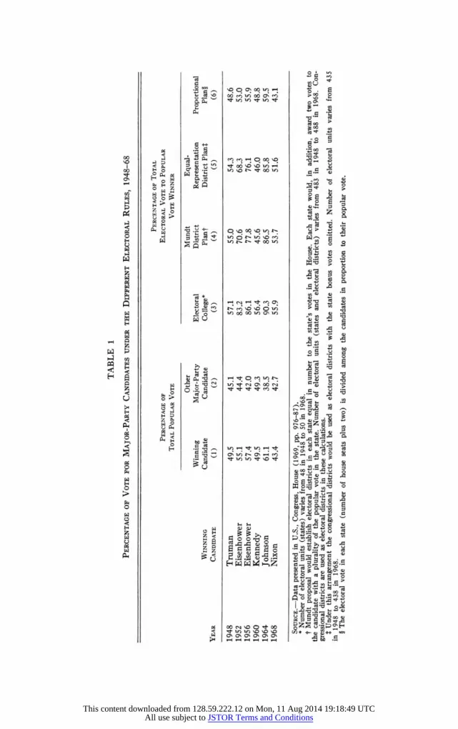
The way in which the magnification varies as a function of the number of electoral units is illustrated in table 1. Columns 1 and 2 present the proportions of the popular vote received by each major-party candidate from 1948 to 1968. In column 3 the proportion of the Electoral College tally recorded by the popular vote winner is reported, while column 5 shows the proportion of congressional districts captured by this candidate. These entries indicate that the Electoral College (containing, on average, 49 voting units) produces a greater magnification of the popular vote than the district plan (containing, on average, 437 electoral units). In- terestingly, the district plans, along with proportional division of the electoral vote, would have awarded the 1960 contest to Richard Nixon, while the Electoral College decision was consistent with the popular result. This is a fluke, however. In so close a contest there is a substantial probability that any electoral rule, other than the popular vote, would have selected a minority president.

While the above factors are central to the evaluation of any reform proposal, they ignore the Realpolitik considerations involved in changing the electoral system. The topics discussed so far derive from a voting model which conceptualizes the electorate as an undifferentiated mass of persons, rather than as urban and rural folk, Negroes and WASPS,

6 Many critics of the direct election plan are sympathetic to this exchange. For instance, Kristol and Weaver (U.S., Congress, Senate 1970b, p. 10) have written: "In a very close election, after all, any method for deciding the winner is open to criticism and doubt. Indeed, it is at least arguable that, with respect to close elections, the most important virtue of a system for deciding the winner is the clarity and decisiveness with which the verdict is rendered. And, in this respect, the Electoral College is not without its value."

446



0 ~~~tn

, < p D 4,) V7 t ~~~~~~~~~~~~~~oo >

P 4 CZ SE

o

X D i t m o t ? ~~e 0

_0 0 o O in

_ H 0*0, e 0t

0 c0e?U] 4 > _{_ o.




workers and employers. Yet, as voting studies consistently show (e.g., Berelson, Lazarsfeld, and McPhee 1954; Campbell et al. 1960), each of these groups has a characteristic propensity to prefer a particular party (although there is certainly variation from election to election reflecting the issues and personalities involved). These social groups, moreover, tend to be concentrated in particular cities and states, with the result that many geographic locales have become identified with a characteristic set of political interests and a traditional leaning toward one of the major parties. Since the alternative rules would aggregate the local propensities differently, possibly diluting or enhancing a group's impact, the concern over the specifics of electoral reform is, to a great extent, a concern over how the influence presently wielded by each population group would be altered.

These parochial issues are quite evident in congressional debates on electoral reform and in interpretative press accounts which detail the features of specific proposals. As examples, it has been argued that under direct election the influence of smaller states would be enhanced (Sayre and Parris 1970, p. 71), but also that the impact of these states would be diminished (Wides and Stotlar 1970); that "direct popular vote would give greater influence to the major urban cities" (testimony of Senator Dominick [U.S., Congress, Senate 1970a, p. 9]), yet "the metropolis would lose its most important point of leverage in the total political system" (Sayre and Parris 1970, p. 72); that "black people and other minorities would lose a distinct advantage" under direct election (Rev. Channing Phillips, quoted in Newsweek [1968, p. 23]), but also that "to compensate for their loss of big city influence, [the Negroes'] nationwide strength would be pooled instead of washed out in winner-take-all elections state by state" (Newsweek 1968, p. 24). It is our intention to elucidate this matter of electoral influence.

ASSESSING THE INFLUENCE OF A SOCIAL GROUP UNDER DIFFERENT ELECTORAL RULES

Previous Research

Despite the concern over who would obtain an electoral advantage, and the very evident confusion on this issue, few attempts have been made to estimate relative group influence under the alternative rules. One frequently cited study in which empirical estimates were derived is by Banzhaf (1968). He calculated a measure of "voter power" for residents of each state, based on a conceptualization of electoral influence as the probability of casting the decisive ballot in an election.7 Banzhaf reports

7 To motivate the computations, Banzhaf (1968, p. 306) writes: "In any voting situation it is possible to consider all of the possible ways in which the different voters

448




that citizens in small and medium-sized states are disadvantaged under the Electoral College; Longley and Braun (1972, p. 115), reviewing Banzhaf's results, conclude that the disadvantage accrues primarily to residents of medium-sized states.

Banzhaf was addressing the constitutional issue of voter representation in different states. Given this interest, it is understandable that the only information entering into his computations was state population size and number of electoral votes. In contrast, we are primarily concerned with socially defined population divisions and with the consequences of electoral reform for the influence of these groups. As we have suggested, the concerns that have been articulated reveal the salience of these divisions; they do not conform to the notion of an undifferentiated citizen which is employed by Banzhaf. Indeed, according to some investigators (e.g., Truman 1951), American politics, in its very essence, is interest-group politics.

Recently, Longley and Braun (1972), and Yunker and Longley (1972) have addressed these more partisan questions within the framework of Banzhaf's formulation. They computed a "citizen voter power" score for several social groups-Negroes, persons of foreign stock, residents of urban and rural areas. The scores were obtained by multiplying each state's relative voter power, calculated by Banzhaf, by the proportion of the group's membership residing there. Thus, subject to the assumptions of Banzhaf's model, to the extent that a group is concentrated in states with high voter-power scores, its impact on an election will be magnified.

We are critical of one of Banzhaf's fundamental assumptions. His calculations presume that every combination of votes in a state is equally likely; therefore a citizen's voter-power score, indicated by the proportion of vote combinations in which his ballot is decisive, is a function of only state population and number of electoral votes. In practice, the probability that an individual is pivotal will depend on other state characteristics besides population size. Some states consistently report a majority for a particular party, while others display little partisan loyalty. Intuitively, we expect a voter to have greater opportunity to cast a decisive ballot in a competitive state than where a one-party tradition exists.

An analogous difficulty resides in the Yunker and Longley computa-

could vote; i.e., to imagine all possible voting combinations. One then asks in how many of these voting combinations can each voter affect the outcome by changing his vote. Since, a priori, all voting combinations are equally likely and therefore equally significant, the number of combinations in which each voter can change the outcome by changing his vote serves as the measure of his voting power." In appli- cation to the Electoral College, Banzhaf takes into account the fact that casting a decisive ballot in New York means influencing more electoral votes than casting a decisive ballot in Rhode Island.

449




tions,j which utilize Banzhaf's voter-power formulation. Their analysis ignores the fact that the electoral impact of a group is a function of how other district residents tend to vote. The importance of this factor is easily illustrated. Consider a state in which blacks comprise 10% of the population. If white residents characteristically vote Republican by more than 56%, then even if all black persons were to vote Democratic, they could not affect the election outcome. Irrespective of their voter-power score under the Yunker and Longley calculation, in practice their impact would be negligible. Thus, a group's electoral influence is very much a consequence of the traditional voting patterns of other residents in the districts where it is concentrated; to have influence there must be a realistic possibility of casting a pivotal vote.

Design of This Study

The approach we propose to follow in measuring electoral influence constitutes a sensitivity analysis. As a first step, county and congressional district data on the social and economic characteristics of the population, together with election data from a particular presidential contest, are used to construct county-level estimates of how different social groups voted. These estimates provide baseline information for a simulation study in which the party preference of a group is repeatedly altered. By aggregating the resulting county voting patterns under each electoral arrangement, we can address the question of who will gain and who will lose influence.9

The election from which the baseline estimates were calculated is the 1960 contest between Richard Nixon and John F. Kennedy. Selection of this contest was dictated by several considerations. It is closest in time to the 1960 Census, which was our source of information on population characteristics; district-level data are most complete for this election, since comparatively few instances of congressional redistricting had introduced boundary changes; and the closeness of the popular vote makes a sensitivity analysis more interesting.

8 Some of Yunker and Longley's calculations are deficient in another respect. In computing voter-power scores for ethnic and racial groups under the district plan, they assume that these groups are represented at the state proportions in each congressional district. Even as a simplification, we believe that this assumption is unreasonable. 9 As used in this paper, the term "electoral influence" refers to two interrelated concepts. In the narrow sense, a group is influential to the extent that a shift in its party preference will alter the electoral vote. The sensitivity analysis reported here is based on a formalization of this interpretation. In wider usage, a group is influential if the candidates defer to its interests. Throughout the discussion we assume that a change in a group's impact in the narrow sense will produce a corresponding shift in its influence in the second usage.

450




The results from such an investigation will have to be interpreted in terms of the simplifications which were made. In the present study, since baseline information was obtained from a single presidential election, we cannot assess the extent to which our conclusions are idiosyncratic of the issues and personalities in that contest, as opposed to reflecting stable party preferences. Second, no attempt was made to incorporate "second- order effects." For example, the alleged promise by George McGovern in 1972 to appoint black persons to high office in proportion to their representation in the population may have cost him the votes of white ethnics at the same time that it attracted Negro voters. Because of the complexity of second-order assumptions, we have not simulated such processes.

A final simplification arose from neglecting local issues and the myriad of other factors which might encourage members of a group in one county to respond differently than their compatriots elsewhere. Our estimates do permit the partisan preference of a group to vary as a function of county characteristics; for instance, we expect high-income Catholics to be more Republican than low-income Catholics. We are limited, though, to making identical manipulations in every county from its initial values.

The above qualifications suggest that the findings should be viewed as providing a first approximation to the change in electoral influence which would result from adopting an alternative rule. Once data become available from the 1970 Census, this analysis could be replicated using more recent voting patterns to ascertain how stable the biases of each electoral plan are with respect to different population groups.

Voting Rules to Be Considered

We investigate five electoral rules, representing the main arrangements that have been proposed.

1. The direct election of president and vice-president.-Presently, the direct election plan appears to be the most popular alternative. Senator Birch Bayh, chairman of the Senate Subcommittee on Constitutional Amendments during the Ninety-first Congress, favors it. It has also been endorsed by the American Bar Association, the U.S. Chamber of Com- merce, and the AFL-CIO. This plan would abolish electoral voting, substituting in its place the national popular vote.

2. The current arrangement.-We assume that the Electoral College would automatically validate the state popular vote. Such a modification was suggested by Representative Hale Boggs of Louisiana to eliminate the problem of the renegade elector.

3. The Mundt district plan.-Senator Karl Mundt of South Dakota proposed that each state's electoral votes be distributed among geographic

451




districts (which we assume here to be congressional districts). 0 A unit vote decision rule would prevail in each district. In addition, the candidate receiving a plurality of the popular vote in a state would obtain a bonus of two electoral votes. Consequently, the number of electoral votes allotted to a state would remain at the present value.

4. The equal-representation district plan. Under this arrangement each congressional district would award a single electoral vote on the basis of the popular outcome. The difference between this rule and the Mundt plan is accounted for by the absence of the two-vote bonus for the state result. Here the formal advantage which the Constitution now bestows upon small states in the Electoral College would be eliminated.

5. The proportional plan. This alternative was introduced in the Ninety-first Congress by Senator Sam Ervin of North Carolina. It provides for a division of the electoral vote in each state (remaining at the current level) among the candidates in proportion to their popular votes.

Preparation of the Data

The data preparation was fairly complex and warrants some discussion. Machine-readable census information for counties was obtained from the Survey Research Center of the University of Michigan. For about 250 of the 435 congressional districts, the 1960 election results could be generated by aggregating the county votes. To obtain comparable information on the remaining districts a number of adjustments were required. In large metropolitan areas-New York City, Chicago, Philadelphia-the congressional districts are subunits of counties. For example, New York City contains 19 congressional districts located within five counties. Where complete district-level information was available, these counties were replaced by their districts as the units of observation.

This substitution was necessary for two reasons. First, the congressional district is the electoral decision unit in two of the plans under consideration. Second, the metropolitan counties contain considerable internal heterogeneity with respect to population characteristics; failure to use smaller areal units in this circumstance could lead to poor estimates of the relationship between party preference and population characteristics.

Unfortunately, district-level voting data are not uniformly available. In several states reapportionment destroyed comparability between the census enumeration unit and the electoral district. As a result, approximately one-half of the districts in multidistrict counties are reported in the Congressional District Data Book (U.S., Bureau of the Census 1963) without 1960 election data. A regression estimate of the two missing

10 In fact, Senator Hugh Scott of Pennsylvania, in Senate Joint Resolution 25, has proposed that congressional districts be used for this purpose.

452




election variables" (turnout rate and percentage Democratic12) was constructed, the predictors being percentage Negro, median income, percentage foreign stock, and median education.13 For each district lacking voting data, the estimates were calculated by substituting that district's population characteristics into the regression equation. The results were then standardized so that the Democratic vote, summed over districts within a county, would equal the reported value for the county.

With these adjustments our final data file consisted of counties when they could be aggregated into congressional districts, and county parts (congressional districts) when aggregation could not be accomplished. The following deletions were made from the data set: Massachusetts-consist- ing of 12 at-large congressional districts; Hawaii and Alaska, totaling three congressional districts, deleted because the regression predictions reflect relationships in mainland counties; Connecticut, Michigan, Texas, Maryland, Ohio-one at-large congressional district deleted in each state. This study therefore reports sensitivity analyses using the population in 416 congressional districts,'4 not the full 435.

SENSITIVITY OF THE ELECTION OUTCOME TO PREFERENCES OF DIFFERENT POPULATION GROUPS

In this section we consider the impact which different social groups would have on a presidential contest under the alternative voting rules. Specifi- cally, using 1960 Census data to specify baseline values, we examine the sensitivity of the electoral vote under each arrangement to a shift in party preference by the following groups:

States of different population size.-Much of the controversy surround- ing electoral reform has centered on the relative influence of large and small states. The central issues concern what advantage currently is enjoyed by residents in states of a particular size, and how this distribution of influence would be altered under each of the proposed plans.

11 One additional variable had to be estimated for the districts. Figures for percentage Catholic are available in the county data file but not in the Congressional District Data Book. For urban districts, the county value for Catholic populaticn was apportioned among the districts in proportion to each district's foreign-stock population originating in Catholic countries. Ireland, Italy, and the Spanish-speaking lands were used as indicators of the Catholic foreign-stock population. 12 The votes for the Liberal Party in New York State and for unpledged electors in three southern states have been grouped with the Democratic Party vote. 13 Since the missing-data problem mainly concerns urban districts, the observations in the regression were metropolitan districts for which both voting information and population characteristics are available. 14 With one exception the districts are those existing in 1962. In Alabama the 1960 boundaries were used in order to eliminate at-large districts. Alabama had nine House seats in 1960, one more than in 1962 following reapportionment.

453



American journal of Sociology

Urban and rural areas.-In part, the concern over the state-size issue derives from a recognition that different values and interests prevail in metropolitan and in rural areas, and residents in each setting are committed to perpetuating their own life styles (Wides and Stotlar 1970). Manipulating the popular vote from urban and rural locales will comple- ment the state-size analyses by providing alternate (and more direct) estimates of how the electoral impact of these populations would be affected by implementing a particular aggregation rule.

Racial and ethnic groups.-Another basis of contention involves the fear by minorities that their electoral impact would be eroded under the reform proposals. It is believed (Bickel 1970) that, as a result of being concentrated in large-population states, ethnic and racial groups currently wield influence disproportionate to their numbers in presidential politics. We present results from manipulating the partisan preferences of blacks, Catholics, and other white persons.

Different income strata.-It has also been suggested (Sayre and Parris 1970, p. 73) that a shift may occur in the relative electoral strength of different income strata. Such change could redirect executive policy on economic issues; for example, if the influence of low-income persons were diluted, support for welfare legislation might be adversely affected. While this issue is related to the preceding topics, in particular to the Negro manipulations, it involves many more persons and a different population distribution among counties than was previously the case. We investigate the electoral influence of low- and high-income persons under the alternative plans.

States of Different Population Size

The prevalent view is that the impact of large states on a presidential contest is enhanced under the Electoral College system, and therefore is greater than can be accounted for by population size alone. For instance, according to the Bar Association of the City of New York (1967, p. 4), quoted in Banzhaf (1968): "XVhile the ratio of electoral votes to population is such that it would seem that the system favors residents of . . . sparsely populated states the most, and . . . heavily populated states the least, the practice of giving all of a state's electoral votes to the winner of its popular vote, by however small a plurality, has in fact contributed to the parties' selecting their candidates and directing their campaigns with a view toward affecting the outcome in the large industrial states." Calculations performed by Banzhaf (1968), using a very different model of voter influence from our own, support the contention that residents in large states enjoy an electoral advantage.

The manipulations we report investigate the sensitivity of the electoral

454




tally to a shift in the popular vote from its 1960 values in different constituencies. To ascertain the electoral vote response we first define three state size categories: large states-the 11 largest, each having more than 12 electoral votes; small states-the 18 smallest, each having six or fewer electoral votes; intermediate-population states- 18 in number, rang- ing in size from seven to 12 electoral votes.

WVe assume in our computations that an increase or a decrease in percentage Democratic in a county from its 1960 value by an identical percentage of the opposing vote is equally difficult to produce. For instance, if a district voted 70% Democratic in 1960, we consider a 10% decrease -to 63%-as difficult to obtain as a 10o% conversion among Republican voters-which would increase the Democratic tally to 73%.

Although we speak of the relative influence of voters in states of different sizes, the manipulations must be performed on districts, since two of the reform plans would use this electoral unit. There is little reason to expect.that a change in voting behavior would occur in a uniform manner in all districts within a state; nevertheless, we will make this simplifying assumption. Lacking information about local contests, or party traditions in different communities, we alter the popular vote in each district from its 1960 value by an identical percentage amount. The state results, in turn, are derived by aggregating the effects from these local perturbations.

More precisely, the manipulations herein are described by the following equations:

Dc2 =fo%Dc + a(1 - %Dcj) (la)

9 %D, + a(%%Del), (ib)

where %Dc1 denotes percentage Democratic in a congressional district before manipulation (1960 value), %oDc2 represents the corresponding value subsequent to manipulation, and a indicates the percentage size of the induced shift in the popular vote. Equation (la) is employed to create a shift in the direction of increased Democratic voting; equation (lb) is used (with negative a) to simulate a popular vote change toward greater Republican voting. The values of a used in the simulation were a -+.04, -+.08, -.12 -+.16 +.20.

These manipulations were applied separately to congressional districts in the states in each population size category. The results for large- population states are reported in table 2. The entries in the center row, corresponding to a 0, present baseline information: the 1960 election results aggregated according to the different electoral rules. The figures in column 1 show the popular vote change produced by manipulations of various sizes on the voting preferences of large-state residents. For instance, were 20% of Democratic voters in each district in large states

455




TABLE 2

STATE-SIZE MANIPULATIONS: PERCENTAGE DEMOCRATIC VOTE UNDER DIFFERENT ELECTORAL RULES

LARGE-POPULATION STATES*

Direct Mundt Equal Election Electoral District District Proportional (Popular Colleget Plant Plant Plant Vote) (N = 510) (N = 510) (N = 416) (N = 510)

MANIPULATION (1) (2) (3) (4) (5)

a =-.20 .438 .222 .290 .283 .453 a = -.16 .451 .222 .322 .322 .464 a = -.12 .463 .222 .351 .358 .474 a = -.08 .476 .222 .380 .394 .485 a =-.04 .488 .331 .422 .435 .495 a= 0 .501 .559 .473 .474 .506 a = .04 .513 .665 .525 .529 .516 a = .08 .526 .714 .561 .567 .526 a = .12 .538 .739 .606 .618 .536 a = .16 .550 .739 .645 .666 .547 a = .20 .563 .739 .696 .728 .557

NOTE.-Alaska, Hawaii, Massachusetts, and the District of Columbia were deleted from the analysis. * Eleven states, each with more than 12 electoral votes. t A single at-large district in each of the following states was deleted: Connecticut, Michigan,

Texas, Maryland, Ohio.

to shift to the Republican column, the national percentage Democratic popular vote would change from .501 to .438. From the entries in the other columns it is apparent that this same manipulation will produce electoral vote shifts of greater magnitude under all but the proportional plan.

The effect of these manipulations under the different plans can be seen more clearly by tabulating the cumulative electoral vote change. For large states this information is presented in table 3. We see, for example, that corresponding to an increase of .062 percentage points in the percentage Democratic popular vote (produced by a 20%o reduction in Re- publican voting in large states), the electoral vote change is .223 percentage points under the Mundt plan, .254 under the equal representation district plan, and .051 under proportional division. The magnification effects of the district plans are evident from these calculations, while the proportional plan appears to reduce slightly the margin of change in the popular vote.

The response under the Electoral College rule is of a different order. The magnification produced by this arrangement is so great that all large states are already in the column of one party when a equals .12 in magnitude. Additional change, in response to larger manipulation, therefore is not possible. In passing, we note that one reason for greater magnification in the Electoral College than under the district plans is that states are more

456




TABLE 3

STATE-SIZE MANIPULATIONS: CUMULATIVE CHANGE IN PERCENTAGE DEMOCRATIC VOTE

LARGE-POPULATION STATES

Direct Mundt Equal Election Electoral District District Proportional (Popular College Plan Plan Plan Vote) (N_ 510) (N = 510) (N =416) (N= 510)

MANIPULATION (1) (2) (3) (4) (5)

aX =-.20 -.063 -.183 -.191 -.053 a =-.16 -.050 -.151 -.152 -,042 a =-.12 -.038 -.122 -.116 -.032 a =-.08 -.025 -.337 -.093 -.080 -.021 aX =-.04 -.013 -.228 -.051 -.039 -.011 a 0 a= .04 .012 .106 .052 .055 .010 a = .08 .025 .155 .088 .093 .020 a= .12 .037 .180 .133 .144 .030 a= .16 .049 .172 .192 .041 aC .20 .062 .223 .254 .051

SOURCE.-Data are from table 2.

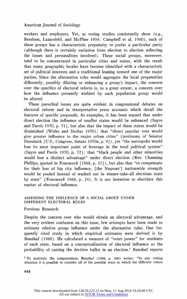
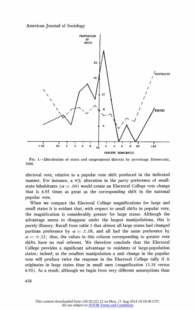
competitive electoral units than are congressional districts. Districts tend to be relatively homogeneous in their social composition and can therefore exhibit extreme partisanship; states, by contrast, especially large states, often combine districts with different political leanings, and these differences cancel each other, making for close elections and competitiveness. This situation is illustrated in figure 1, which presents the distributions of states and congressional districts by percentage Democratic in 1960. It is apparent that the districts are considerably more extreme than states in their degree of partisan support.

To obtain magnification scores the figures in table 3 were processed as follows: first, ignoring signs, the two values in each column which cor- respond to a manipulation of the same magnitude were summed; second, the resulting entries in each row were divided by the popular vote figure for the row. The reason for the first transformation is that we are un- interested in distinguishing between the effects produced by an increase or a decrease in the popular vote for a party; to a large extent such bias simply reflects the proportion of electoral units initially in its column. The second calculation standardizes the electoral vote change by the popular vote shift, enabling the magnification effects to be compared more easily.

For large-population states the results of these computations are presented in the upper panel of table 4. Analogous calculations were carried out for small and medium-sized states. The magnification scores obtained by manipulating the popular vote in those states are reported in the second and third panels of table 4. Each entry indicates the change in

457




PROPORTION OF

UNITS

20

/DISTRICTS 169/

12/

8~~~~~~ \ ~~~~ K / 8 / ~~~~~~STATES

t~ ~ ~ ~~

electoral vote, relative to a popular vote shift produced in the indicated manner. For instance, a 4% alteration in the party preference of small- state inhabitants (a - .04) would create an Electoral College vote change that is 6.95 times as great as the corresponding shift in the national popular vote.

When we compare the Electoral College magnifications for large and

small states it is evident that, with respect to small shifts in popular vote, the magnification is considerably greater for large states. Although the advantage seems to disappear under the largest manipulations, this is purely illusory. Recall from table 3 that almost all large states had changed partisan preference by 4 _ 4.08, and all had the same preference by ae i.12; thus, the values in this column corresponding to greater vote

shifts have no teas grent. We therefore conclude that the Electoral College provides a significant advantage to residents of large-population states; indeed, at the smallest manipulation a unit change in the popular vote will produce twice the response in the Electoral College tally if it originates in large states than in small ones (magnification 13.38tversus 6.95). As a result, although we begin from very different assumptions than

458




TABLE 4

STATE-SIZE MANIPULATIONS: MAGNIFICATION OF THE POPULAR VOTE

Direct Mundt Equal Election Electoral District District Proportional (Popular College Plan Plan Plan Vote) (N = 510) (N = 510) (N = 416) (N = 510)

Manipulation (1) (2) (3) (4) (5)

Large-Population States*

a= -+.20 1.0 4.15 3.26 3.63 0.83 a = +.16 1.0 5.19 3.24 3.53 0.83 a = +.12 1.0 6.92 3.41 3.58 0.83 a = +.08 1.0 9.88 3.62 3.63 0.83 a = +.04 1.0 13.38 4.17 3.76 0.83

Small-Population Statest

a = +.20 1.0 7.16 6.96 4.39 1.51 a = +.16 1.0 8.33 8.21 5.18 1.51 a? = +.12 1.0 8.29 8.46 5.49 1.51 a = +.08 1.0 6.96 7.46 4.87 1.51 a = +.04 1.0 6.95 9.94 7.31 1.51

Medium-Population States1:

a = +.20 1.0 4.95 4.67 4.43 1.19 a = +.16 1.0 5.88 5.00 4.63 1.19 a = +.12 1.0 6.73 5.09 4.52 1.19 a = +.08 1.0 9.31 6.06 5.06 1.19 a = +.04 1.0 8.96 5.27 4.30 1.19

SOURCE.-Data are froni table 3 for large states and from similar computations for the other state-size categories.

* Eleven states, each having more than 12 electoral votes. t Eighteen states, each having fewer than seven electoral votes. $ Eighteen states.

Banzhaf (1968), we also believe that the electoral impact of large states would be eroded under direct election of the president.

An even greater decrease in large-state influence would occur under the other proposed arrangements. The Mundt plan is the more detrimental of the district plans; if it were adopted small states would acquire more than twice the magnification of large states. A significant advantage would also accrue to small states under the proportional plan. This rule, incidentally, has a deflating effect for large states (magnification15 0.83) and would make close popular contests even closer in the electoral tally.16

Lending credence to the preceding analysis, the figures for states with intermediate-sized populations largely fall between the results for large

15 The magnifications do not vary because of the absence of a unit rule. The electoral vote change under this plan, in response to a popular vote shift, is linear. 16 Evidence for this feature of the proportional plan may be found in actual election data. Comparing columns 1 and 6 of table 1, we see that in every presidential contest since 1948 the winner's electoral vote under proportional division has been smaller than his popular vote percentage.

459




and small states. The fact that electoral advantage under each rule, as defined by our magnification scores, appears to vary continuously over the state-size categories suggests that it is probably a stable phenomenon, not idiosyncratic of the particular contest from which the baseline information was gathered.

Urban and Rural Areas

The concern which has been expressed regarding the different impact of votes originating in large and small states appears to derive from two distinct orientations. For some, the issue involved is that of equal representation: the extension of the one-man, one-vote principle to presidential contests (Banzhaf 1968). The other interest is more particularistic, such as the contention by Theodore H. White that large states possibly deserve to have greater impact on presidential politics to compensate for their underrepresentation in the Senate (U.S., Congress, Senate 1970b, p. 31).

In the particularistic arguments, the state-size question often serves as a proxy for a different issue, the relative representation of the opposing interests and values of metropolitan and rural communities. This issue taps a major cleavage in our society, pitting commerce, big labor, and ethnically heterogeneous populations-with an orientation to social change and liberal domestic policy-against agrarian economic interests and the traditional values of rural and small-town America.

We can investigate directly how the electoral influence of metropolitan residents and rural persons would fare under electoral reform, thereby complementing the state-size analyses. Our procedure is to apply the previous manipulations to counties which satisfy the appropriate urban or rural definitions, and then aggregate the popular vote according to each electoral rule. The difference between this study and the state-size manipulations is that formerly it was immaterial whether a voter in a state of a particular size happened to reside in an urban or a rural county, while the present formulation is sensitive to this level of detail.

A county was classified as highly urban if its population was reported in the 1960 Census to be in excess of 90%o urban.17 This definition provided the most successful delineation between major metropolitan centers and other locales. Rural and small-town places were defined as counties less than 20%o urban, or counties between 20%o and 29%0 urban with population density less than 25 persons per square mile. The rural/small- town definition served to exclude almost all counties which contain a

17 Places of 2,500 or more are defined as urban in the 1960 Census.

460




city larger than 10,000 inhabitants. We therefore have two very different types of areal units with respect to the urban-rural dimension.'8

Having eliminated all counties which are neither metropolitan centers nor primarily rural, we henceforth treated the retained counties as undifferentiated units with regard to their population characteristics. In particular, percentage Democratic in a county was used to approximate percentage Democratic in the population group of interest. Thus, all "urban" counties were considered 100% urban; all "rural" counties, 100% rural.

The manipulations described in the preceding section were repeated on the counties in each percentage-urban category. The derived popular vote was aggregated according to the alternative rules and then transformed following the steps outlined in conjunction with tables 2-4. The magnifications of the popular vote under each electoral arrangement are presented in table 5, separately for urban and rural residents.

TABLE 5

URBAN-RURAL MANIPULATIONS: MAGNIFICATION OF THE POPULAR VOTE

Direct Mundt Equal Election Electoral District District Proportional (Popular College* Plan* Plan* Plan* Vote) (N = 510) (N= 510) (N =416) (N = 510)

Manipulation (1) (2) (3) (4) (5)

Highly Urban Countiest

a = +.20 1.0 8.49 3.38 2.98 0.85 a= +.16 1.0 9.74 3.49 3.08 0.85 a=-+.12 1.0 11.54 3.77 3.25 0.85 a = +.08 1.0 12.71 3.98 3.34 0.85 a = +.04 1.0 13.27 3.91 3.42 0.85

Rural Countiest

a = +.20 1.0 11.61 6.77 5.33 1.24 a = +.16 1.0 9.98 5.59 4.26 1.24 a = +.12 1.0 6.65 5.64 4.44 1.24 a=-+.08 1.0 4.53 4.84 4.44 1.24 a=-+04 1.0 7.25 4.84 4.44 1.24

NOTE.-Alaska, Hawaii, Massachusetts, and the District of Columbia were deleted from the analysis. * A single at-large district in each of the following states was deleted: Connecticut, Michigan,

Texas, Maryland, Ohio. t Counties which are more than 90% urban. t Counties which are less than 20% urban, or between 20% and 29% urban and have population

density less than 25 persons per square mile.

18 The manipulations described below were also carried out using different definitions of urban and rural. Counties greater than 80%o urban were defined as urban; rural counties were defined alternatively as counties less than 20%S urban and as less than 10%c urban. In all instances the results were virtually identical with those presented in the text.

461




The conclusions we draw from these analyses are identical with those which were reached with the state-size manipulations: the influence of large metropolitan centers is enhanced under the Electoral College (again, the decrease in magnification above a -+? .12 in the top panel results from the majority of states with large urban populations having the same party preference by this value), while the other arrangements would advantage rural counties in the nation. Consistent with the findings from the state-size study, the district and proportional plans would favor rural areas and small towns even more than would adoption of a popular-vote rule.

Racial and Ethnic Groups

Another concern which has been articulated in the debate on electoral reform relates to a possible loss of influence by minority groups (Bickel 1970; Newsweek 1968, p. 23). It is believed that under the Electoral College, as a result of their concentration in large states and in metropolitan areas, blacks and white ethnics enjoy an electoral advantage which would be eliminated under the reform proposals. Empirical support for this contention is mixed; Longley and Braun (1972, pp. 122-24) report that persons of foreign stock do, indeed, have greater influence in presidential balloting, but blacks are below the national average on their measure of voter power.

In this section we compare the electoral influence of nonwhites, Catholics, and non-Catholic whites19 using the simulation approach. The methodology is somewhat more involved than was required by the earlier manipulations. Previously, we could identify the county or district value of percentage Democratic with the voting propensity of the group of interest in the areal unit. For example, percentage Democratic in "urban" counties provided an approximation of urban voting behavior in those counties, even though a minority of the residents were not classified as urban. However, this simplification cannot be made in the present analysis, since the ethnic groups often constitute small percentages of the population even where they are overrepresented. We must therefore employ other methods to estimate county-level voting by the minority groups in 1960.

In order to have some measure of the sensitivity of the electoral findings to our particular estimates of ethnic voting behavior, two models were used to generate the county-level figures. Both employ the techniques of ecological regression (Goodman 1959; Duncan, Cuzzort, and Duncan

19 As a simplification, we made the assumption that the population in a county can be divided among nonwhites, white Catholics, and other whites. Since our data report the county populations that are nonwhite and that are Catholic, any overlap between these categories will reduce the proportion of "other whites." That is, we define proportion "other whites" as (1 - oNW - oCath).

462




1961). We first note that for any county the percentage Democratic vote (%D) may be written as

%7D (%7oDNW) (%7NW) + (%oDcath) (% Cath) + (% Dow) (% OW)

- %Dow + (%7DNw - %Dow) (%oNW)

+ (7%DCath - %Dow) (% Cath), (2)

where the second equation is obtained using the identity (see n. 19) %OW - (1 - oNW - %Cath). The variables %oDow, %IDNw, and %IDCath (percentage Democratic for other whites, nonwhites, and Cath- olics) are unobservable in our data set; however, under suitable assumptions (see Goodman 1959 for details) estimates of them can be calculated.

Model I.-In our initial model we assume

,yDow - cl

%a DNW -C2 (3)

% DCath - C3;

that is, the party preference of each ethnic group is constant across counties. Under this specification estimates of ethnic voting can be obtained by regressing

%oD - a + bi (%oNW) + b2 (%Cath) + e (4)

over counties. The resulting estimates are

zz a G1 = a

C2 = a+ (5)

C3 -a + b2.

In practice, this model was applied in a more flexible fashion than the above description indicates. First, the regression equation (4) was esti- mated20 separately for counties from each of the geographic regions, Northeast, Midwest, Far West, and South.21 Second, state dummies were included in each regional regression to adjust for characteristic differences

20 A weighted regression procedure was employed, the weights being the voter turnout values in the counties. 21 The states were grouped as follows: Northeast-Connecticut, Delaware, Illinois, Indiana, Maine, Michigan, New Hampshire, New Jersey, New York, Ohio, Pennsyl- vania, Rhode Island, Vermont, and Wisconsin; Midwest-Arizona, Colorado, Idaho, Iowa, Kansas, Minnesota, Missouri, Montana, Nebraska, Nevada, New Mexico, North Dakota, South Dakota, Utah, and Wyoming; West-California, Oregon, and Washing- ton; South-Alabama, Arkansas, Florida, Georgia, Kentucky, Louisiana, Maryland, Mississippi, North Carolina, Oklahoma, South Carolina, Tennessee, Texas, Virginia, and West Virginia.

463




among states in voting patterns. Thus, our estimates are responsive to the different historical traditions of the regions and, within a region, permit an additive adjustment among the state voting patterns. Third, the estimates from these ecological regressions were compared with survey results on ethnic voting by region in 1960.22 Although the number of observations in the surveys is small when one is interested in tabulating ethnic voting by geographic region, the survey estimates for nonwhites appeared more reasonable than the ones from the ecological regression and were substituted for them.23 The regression estimates for the other groups were close to the survey values and were retained.24

Model II.-We know that an individual's party preference is molded by many factors besides ethnicity, by attributes such as income, occupa- tion, and educational attainment. County-level data are available for some of these variables and were used to construct estimates of ethnic voting which vary by this areal unit. For our general model we assumed the following determinants of ethnic voting:

%Dow e + f(Medlnc) + g(%YoAgric)

%DDcath - s + t(Medlnc) + u(%Agric) (6)

%0 DNW - r + q(Medlnc).

Medlnc denotes the county value of median income, and %oAgric indicates percentage of the labor force employed in agriculture. Conceptually, we would prefer that the income and industry variables were specific to the ethnic group, rather than being county figures. Lacking such data, we use the county figures, thereby implicitly assuming that the ethnic groups in a county have distributions on the income and industry variables which are identical with those of the general population, or that they respond more to the county context than to their own values on the variables.

Equations (6) were assumed for the three nonsouthern regions, where Negro employment in agriculture is negligible. For the South, our model

22 The following sources were consulted: Brink and Harris (1967), Polsby and Wildavsky (1971, pp. 21-24), and Axelrod (1972). Ethnic tabulations were also pre- pared from the post-1960 election survey conducted by the University of Michigan Survey Research Center. 23 For nonwhites the regression estimates averaged to .85, while most surveys report that Kennedy obtained approximately 75% of the Negro vote. The estimates of Negro voting by region which we substituted are from Brink and Harris (1967, p. 75). These values were adjusted to compensate for the aggregate bias introduced by the state dummies so that the state-effect terms could be utilized. 24 The regional means are: Northeast-.366, .754, .727 for %DOWx %DNW' %o?DCath) respectively; Midwest-.410, .811, .730; West-.383, .705, .725; South-.436, .746, .665. The value for a county is modified by its state dummy.

464




of the determinants of ethnic voting was modified by the inclusion of the %Agric term in the equation for nonwhites:

%7Dow e + f(Medlnc) + g(%oAgric)

%oDcath -s + t(Medlnc) + u(%o'Agric) (6')

%DNw = r + q(MedTnc) + z(%oAgric).

To estimate the coefficients in either (6) or (6'), the equations of the model are substituted into (2). Simplifying the resulting expression, we obtain, corresponding to (6), a relation of the form

%D - a + b1(%oNW) + b2(%oCath) + b3(MedInc)

+ b4( % Agric) (1 - 7oNW) + b5(% NW) (MedInc)

+ b6 (% Cath) (Medlnc) + b7 (%XCath) (%oAgric) + e. (7)

The analogous regression equation for (6') is

%oD -a ? b1(%NW) + b2(% Cath) + b3(Medlnc) + b4(%Agric)

+ b5(% NW)(MedInc) + b66(% Cath)(MedInc)

? b7( %Cath) (%Agric) + b8(%NW)(%Agric) + e. (8)

Estimates of the parameters for either model are given by

ef a .U

Equation (7) was estimated for each nonsouthern region, and (8) for the southern counties. State dummies were also included in the regressions for the reasons discussed previously. The equations for calculating Demo- cratic voting by the ethnic groups, constructed by this procedure, are presented in table 6. Examination of the entries suggests that the coefficients are at least reasonable in sign. Both median income and percentage of the labor force employed in agriculture are negatively related to Dem- ocratic voting, irrespective of the ethnic group. The reason, incidentally, why the median income figures are frequently identical is that many of the interactions involving income in equations (7) and (8) were highly correlated with one of the main effect terms and had to be removed. Each deletion eliminates one degree of freedom in estimating the coefficients, compelling terms corresponding to the same independent variable to be equated.

465




TABLE 6

REGRESSION ESTIMATES OF COEFFICIENTS FOR CALCULATING COUNTY ETHNIC VOTE

INDEPENDENT VARIABLE*

Percentage of Median Labor Force Income Employed in

DEPENDENT Constant (X 10O4) Agriculture VARIABLE (1) (2) (3)

Northeast

%DOW 0.609 -0.347 -0.724 % DNW 1.065 -0.347

%DCath 0.915 -0.347 -0.877

Midwest

%Dow 0.451 -0.038 -0.129 % DNW 0.855 -0.038

%DCath 0.757 -0.038 -0.165

West

%oDOW 0.669 -0.364 -0.312 %DNW 1.039 -0.364 %DCath 0.975 -0.364 -0.577

South

%DOW 0.523 -0.153 -0.026

%DNW 1.008 -0.711 -0.001

%DCath 0.777 -0.153 -0.026

NOTE.-A weighted regression was performned in each region, the weights being the county vote turnout values. * The regression equations from which these estimates were constructed also contained state dummies.

Using the equations in table 6, together with county values for median income and percentage employed in agriculture, we constructed an estimate of %DNWV, %Dc1ati, and %Dmw for each county.25 These estimates serve as baseline information on how the ethnics voted in the 1960 election. The vote preference for a group was then perturbed, in the manner previously described, but in accordance with the following equations:

%Dc2 % DDc, + a(l- %DEG1) (%EG) (lOa)

D,C - %D,1 + ? ( %oDEG1) ( %oEG). (1Ob)

25 The predictions from these equations were adjusted slightly to ensure that they would sum to the observed Democratic vote in a county. Using the predicted values, we constructed an estimate of county percentage Democratic: %OD = (%oDow) (%OW) + (DNw) (%oNW) + (%oDCath) (%oCath). Since %oD is known for a county, each predicted percentage Democratic figure for an ethnic group (%DEG) was adjusted by the amount (oD - 7oD).

466




The term %D,1 denotes percentage Democratic in the county before manipulation (1960 value), %D,2 represents the value after manipulation, %0 DEG1 is the regression estimate of Democratic voting by the ethnic group, and %EG equals percentage of the county population comprised by the ethnic group (nonwhites, Catholics, or other whites). Equations (10a) and (lOb) differ from their counterparts (la) and (lb) in that the group of interest no longer is assumed to be identical with the county population; the quantity %EG now explicitly appears as a variable. (If %EG 1, then %D,1 - %DEG1, and equations [10] reduce to [1].) As before, the "a" manipulation refers to change in the direction of higher percentage Democratic; the "b" manipulation refers to a vote change in the Republican direction (negative a). The values of a used in the simulation were .04, -+-.08, +.12, +.16, .20.

To ascertain the sensitivity of the electoral plans to a change in partisan preference by an ethnic group, these manipulations were applied to all counties (and county parts) and the results aggregated according to the alternative rules. This procedure was repeated for each ethnic group. Table 7 presents the magnification values, obtained from Model II's estimates of ethnic voting in a county in 1960.

Our results for the Electoral College run counter to Longley and Braun's (1972, p. 124) findings in one important respect. They report that Negroes have less than average voter power, while we find a clear advantage to nonwhites, in comparison with "other whites" (first and third panels, col. 2). Indeed, except for the very smallest manipulation, nonwhites wield greater influence in the Electoral College than do Catholics. These magnification values also mean that under direct popular election both Negroes and Catholics would relinquish the considerable influence in presidential politics which they currently enjoy.

With respect to the other rules, the magnification values indicate a slightly greater disadvantage to Catholics and Negroes under the district plans than in the popular vote. Under proportional division of the electoral vote Catholics would also experience a larger erosion in electoral impact than under direct election (magnification = 0.91), while the reverse is true for Negroes (magnification - 1.17).

How sensitive are these results to the particular estimates we have employed of ethnic voting at the county level? To address this question, the preceding manipulations were repeated using the estimates from Model I. The resulting magnifications are not presented here because they are virtually identical with the values in table 7. In no instance would a conclusion reached from an examination of table 7 be modified by the scores obtained with the cruder, regional estimates.26 The fact

26 A third set of estimates of ethnic voting was also used in the simulation. The equations in table 6 were modified so that the county estimates of percentage

467




TABLE 7

ETHNIC-GROUP MANIPULATIONS: MAGNIFICATION OF THE POPULAR VOTE

Direct Mundt Equal Election Electoral District District Proportional (Popular College* Plan* Plan* Plan* Vote) (N = 510) (N = 510) (N = 416) (N = 510)

Mlanipulation (1) (2) (3) (4) (5)

Nonwhites

a = ?.20 1.0 21.97 5.30 3.25 1.17 a = ?.16 1.0 19.74 5.10 3.21 1.17 a = ?.12 1.0 17.12 4.41 2.70 1.17 a = ?.08 1.0 24.57 5.04 3.04 1.17 a = ?.04 1.0 18.69 2.95 1.20 1.17

Catholicst

a = +.20 1.0 12.11 4.43 3.68 0.91 a = +.16 1.0 14.43 4.47 3.43 0.91 a = 4.12 1.0 12.80 4.13 3.31 0.91 a = +.08 1.0 18.84 5.01 3.80 0.91 a = +.04 1.0 21.04 4.88 3.38 0.91

Other White Personst

a = +.20 1.0 6.40 4.51 4.13 1.01 a = ?.16 1.0 7.51 4.72 4.25 1.01 a = +.12 1.0 9.23 5.06 4.45 1.01 a = +.08 1.0 11.17 5.10 4.21 1.01 a = ?.04 1.0 8.67 4.92 4.34 1.01

NOTE.-Alaska, Hawaii, Massachusetts, and the District of Columbia were deleted from the analysis. * A single at-large district in each of the following states was deleted: Connecticut, Michigan, Texas, Maryland, Ohio.

t Data on Catholic population are from Inter-University Consortium for IPolitical Research, Uni- versity of Michigan.

t Proportion "other white persons" is defined as (1 - perceptage nonwhite - percentage Catholic).

that our findings are not sensitive to alternative, reasonable calculations of the unobserved county-level ethnic voting patterns is quite important. It means that the errors which undoubtedly exist in the estimates of Democratic voting are unlikely to be responsible for the thrust of our findings.

Different Income Strata

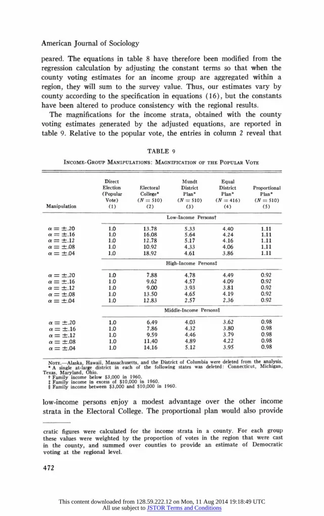
A change in relative electoral influence among income strata could have enormous consequence for the fate of class-relevant legislation. Federal support for income redistribution programs such as FAP or for full- employment policies may vary according to the perceived electoral strength of persons in different income categories.

Democratic for each ethnic group, when aggregated within a region, would sum to the regional value. This was accomplished by adjusting the constants in the equations to achieve the intended result. The magnifications obtained with the estimates from these adjusted equations hardly differ from the entries in table 7.

468




The Michigan data file on population characteristics in 1960 contains only limited information on the income distribution in a county. We are able, though, to subdivide a county's population into the proportion of families with income under $3,000, over $10,000, and between these figures, the latter to be termed the middle-income stratum. Our analysis, therefore, will examine the change in electoral influence among voters in these three earnings brackets which would arise from replacing the Elec- toral College by a different plan.

Analogous to the decomposition employed to obtain estimates of ethnic voting, we note that percentage Democratic in a county can be apportioned among the income strata:

%D =%D3-(%3-) + %D10+(%10+) + %DMI(%MI). (11)

The proportion of voters whose families had incomes below $3,000 is de- noted by %3-; % 10+ denotes the proportion with incomes in excess of $10,000; and %MJ represents the proportion in the residual category (middle-income persons). The percentage Democratic figures for the income strata are unobservable in our data set and must be estimated.

Utilizing the relation %MJ [1 - (%3-) - ) (%1o0+)], equation (11) may be rewritten

%oD %oDmI + (%oD3-- %oDMI) (%3 )

+ (%oD10+ - oDMI) (%1o0+). (12) Following the strategy in the investigation of ethnic electoral influence, we compute alternative estimates of Democratic voting by the income strata to serve as our initial conditions.

Model I.-In calculating the first set of estimates, we assume constant values of Democratic voting in a region by each income group:

7o D3_ -cl

%oDMI C2 (13)

lo D10+ c3. Substituting this specification into (12), we obtain an equation of the form

oD -a + b1(%3-) + b2(%010+) + e. (14)

By computing least-squares estimates of a, b1, and b2 from the county- level data, the parameters (13) can be recovered using the relations27

27 Analogous to the procedure in the ethnic investigation, separate regressions were carried out in each region with dummy terms for states included in the equations. The values of Democratic voting in a county therefore equal the regional estimates modified by the state terms.

469




c = + 31

C2 a (15)

C3 _a + 2

Model II.-Our second set of estimates was computed from a more complex specification of voting behavior. We assumed the following determinants of Democratic voting in a county by the income strata:

%D3 = e+f(%Cath) + g(oNW) + k(%,oUrban)

'YoD-I q + r(%oCath) + s(%oNW) + t(%oUrban) (16)

7oD,o+ =U + v(%oCath) + w(%joNW) + z(%oUrban).

This specification permits income-group voting to vary by county according to the county values of the independent variables. Substituting these relations into equation (12) and simplifying, the relevant regression for calculating the parameters of the model is

%D _ a + bl(%oCath) + b2(%NW) + b3(%oUrb) + b4(%3-)

+ b5(%oCath) (%o3-) + b6(%7NW) (%3-)

+ b7( %0Urb) (%o3-) + b&(%10+) + b9(%/oCath) (%10+)

+ blo(%oNW)(%lo0+) + bil(oUrb) (%ol0+) + e. (17)

Estimates of the coefficients in (16) are then given by28 e=g++a~~^ a ^- &+a +a^ q ~u bs a

Jzbs +bi rr v-b9+bi (18)

P 6 2 ? 2 w L) + $

i-37+ 3 ~t-3 z -ii+bs.

Both the regional and county-level estimates generated from the above two models proved unsatisfactory. The regional estimates of Democratic voting by the income strata were inconsistent with the corresponding values from the Michigan Survey Research Center's post-1960 election survey, to which they were compared. In some instances the regression estimates differed by as much as 30 percentage points. For this reason, 11 of the 12 regression estimates of regional voting were replaced by the survey values,29 although the state-effect terms were retained and the

28 Separate regressions were performed in each region with state dummies present in the equations. 29 The regression estimate for %D1o+ in the Midwest was retained. Based on N = 16 persons, the Michigan postelection survey reports Democratic voting equal to .69 in

470




survey figures adjusted accordingly to compensate for the aggregate effect of these dummy terms. Thus, our Model I estimates combine survey and regression results.

The equations for calculating the more refined county-level voting estimates (Model II) are presented in table 8. With a few exceptions

TABLE 8

REGRESSION ESTIMATES OF COEFFICIENTS FOR CALCULATING COUNTY-LEVEL VOTING BY INCOME GROUPS

INDEPENDENT VARIABLE*

Percentage Percentage Percentage DEPENDENT Constantt Catholic Nonwhite Urban VARIABLE (1) (2) (3) (4)

Northeast

%D3_ 0.212 0.169 1.114 0.217

%DMI 0.264 0.231 0.116 0.217

%OD10+ -0.497 0.231 0.116 0.758

Midwest

%D3_ 0.297 0.380 0.148 0.017

%DMI 0.503 0.237 0.497 0.017

%D10+ 0.196 0.237 0.497 0.075

West

%D3_ 0.369 0.285 0.644 0.054

%DMr 0.6 16 0.230 0.456 0.013

%D10+ -0.174 0.230 0.456 0.054

South

%D3_ 0.408 0.176 0.326 0.105 %DMI 0.496 -0.140 0.2 73 -0.206

%OD10+ 0.048 3.136 0.2 73 0.376

NOTE.-A weighted regression was performed in each region, the weights being the county vote turnout values.

* The regression equations from which these estimates were constructed also contained state dummies.

t Before adjustment the constants were (reading from top down) 0.427, 0.349, -0.727; 0.313, 0.500, 0.163; -0.165, 0.694, -0.140; 0.457, 0.667, -0.493.

the coefficients have the expected signs: percentage Catholic, percentage nonwhite, and percentage urban all have positive effects on proportion Democratic. Nevertheless, when the county estimates were checked for consistency with the Michigan survey values,30 some discrepancies ap-

this category. The regression estimate, equal to .27, is more consistent with voting by high-income persons in the other regions. The regional values of Democratic voting used in the simulation are (from low- to high-income strata): Northeast- .49, .50, .31; Midwest-.35, .54, .27; West-.60, .57, .21; South-.49, .52, .50. 30 Using the equations in table 8 (with original constant terms), percentage Demo-

471




peared. The equations in table 8 have therefore been modified from the regression calculation by adjusting the constant terms so that when the county voting estimates for an income group are aggregated within a region, they will sum to the survey value. Thus, our estimates vary by county according to the specification in equations (16), but the constants have been altered to produce consistency with the regional results.

The magnifications for the income strata, obtained with the county voting estimates generated by the adjusted equations, are reported in table 9. Relative to the popular vote, the entries in column 2 reveal that

TABLE 9

INCOME-GROUP MANIPULATIONS: MAGNIFICATION OF THE POPULAR VOTE

Direct Mundt Equal Election Electoral District District Proportional (Popular College* Plan* Plan* Plan* Vote) (N _ 510) (N = 51a) (N = 416) (N 5=1 O)

Manipulation (1) (2) (3) (4) (5)

Low-Income Personst

a = +.20 1.0 13.78 5.33 4.40 1.11 a = ?.16 1.0 16.08 5.64 4.24 1.11 a = +.12 1.0 12.78 5.17 4.16 1.11 a = +.08 1.0 10.92 4.33 4.06 1.11 a = +.04 1.0 18.92 4.61 3.86 1.11

High-Income Personst

a = +.20 1.0 7.88 4.78 4.49 0.92 a = +.16 1.0 9.62 4.57 4.09 0.92 a = +.12 1.0 9.00 3.93 3.81 0.92 a = +.08 1.0 13.50 4.65 4.19 0.92 a= +.04 1.0 12.83 2.57 2.36 0.92

Middle-Income Persons?

a = ?.20 1.0 6.49 4.03 3.62 0.98 a = +.16 1.0 7.86 4.32 3.80 0.98 a +.12 1.0 9.59 4.46 3.79 0.98 a ?.08 1.0 11.40 4.89 4.22 0.98 a =+?.04 1.0 14.16 5.12 3.95 0.98

NOTE.-Alaska, Hawaii, Massachusetts, and the District of Columbia were deleted from the analysis. * A single at-large district in each of the following states was deleted: Connecticut, Michigan,

Texas, Maryland, Ohio. t Family income below $3,000 in 1960. t Family income in excess of $10,000 in 1960. ? Family income between $3,000 and $10,000 in 1960.

low-income persons enjoy a modest advantage over the other income strata in the Electoral College. The proportional plan would also provide

cratic figures were calculated for the income strata in a county. For each group these values were weighted by the proportion of votes in the region that were cast in the county, and summed over counties to provide an estimate of Democratic voting at the regional level.

472




a small benefit to the poor (magnification - 1.11), while the district plans do not exhibit any consistent group bias.

We have less confidence in these magnification scores than in the results of the preceding investigations. One reason is because the voting estimates had to be jerry-rigged, in the manner we have described. A second reason is that the Electoral College magnifications (though not the scores for the other plans) are sensitive to the baseline estimates of income-group voting. If the unadjusted constant terms are retained in the estimating equations, the magnifications indicate a larger advantage to poor persons under the Electoral College.3' In contrast, the regional voting estimates (Model I) produce magnifications in the Electoral College which suggest little systematic advantage to any income strata.82 While we believe that table 9 was constructed using the best available calculations of voting behavior by the income strata, these results nevertheless should be viewed as exceedingly tentative.

CONCLUSIONS

Electoral reform has periodically been an issue of immense importance, and as long as the potential for crisis remains, this matter is certain to recur. What would constitute a crisis would be, foremost, the failure by any candidate to secure a majority of the Electoral College vote. In this circumstance, selection of a president would be made in the House of Representatives where the popular preference could be disregarded. Even more likely, in the period before the Electoral College formally met, the minor-party candidate would attempt to exchange his votes for policy accommodations or high administrative posts.33 In either eventuality, weeks might pass before a president were chosen,34 and the outcome would derive from a private deal. The strain on the legitimacy of the incumbent during his term of office would be enormous.

From the remarks in the introductory section it is evident that more radical reforms have been contemplated than merely removing this poten-

31 In place of the entries in col. 2 of table 9, we have (reading downward) 13, 15, 17, 12, 18; 8, 9, 9, 9, 12; 6, 7, 9, 11, 13. 32Replacing the magnifications in col. 2, we have (reading downward) 14, 14, 13, 11, 19; 9, 9, 11, 12, 21; 7, 8, 10, 12, 14. 33 A Wallace position paper from the 1968 campaign discussed this very tactic (Con- gressional Quarterly Weekly Report 1968, p. 1812). 34 According to current federal law: "The electors of President and Vice President of each state shall meet and give their votes on the first Monday after the second Wednesday in December." Also, "Congress shall be in session on the sixth day of January succeeding every meeting of the electors" (Peirce 1968, pp. 331-32). In 1960 the popular election was held on November 8, the electors voted on December 19, and the ballots were counted in Congress on January 6, 1961.

473




tial for crisis (which could be accomplished by requiring a plurality rather than a majority of the Electoral College vote for confirmation).3 In part, the impetus for comprehensive change stems from a desire to eliminate state disparities in voter influence and, as a side benefit, avert the possibility of a second kind of crisis, one in which the election is decisive but the electoral-vote winner fails to acquire a plurality of the popular vote.36 In part, support for major electoral revision has constituted an attempt to alter the distribution of influence in presidential politics in favor of one's own constituency.

We have commented briefly on some technical aspects of the electoral rules. We indicated that the direct election plan would be subject to certain abuses which are minimized when electoral constituencies are insulated and operate under a unit rule, as is presently the case. This is not to suggest that the greater problems created by fraud, vote recounts, and small victory margins under direct election outweigh the benefit from selecting the popular-vote winner (if the determination can be made in a close contest), only that there are real difficulties to be surmounted if this arrangement is adopted. On purely technical grounds we would advise against the proportional plan; this rule retains the disadvantages of direct election and, in addition, appears to deflate the margin of victory in the popular vote.

Yet, the thrust of our analysis has been to assess the change in electoral influence among population groups which would result from replacing the Electoral College by a different system. We conclude that, relative to the popular vote, the electoral clout of large states, metropolitan centers, Negroes, Catholics, and, possibly, low-income persons is enhanced under the Electoral College. Adoption of direct popular election would reduce the impact of these groups on presidential politics. With few exceptions, the district and proportional plans would produce an even greater erosion in their influence.

In the Introduction we reported that considerable disagreement exists concerning who would benefit under a particular electoral rule. While the confusion is abundant, it is not universal. There are groups which have correctly assessed the implications of each arrangement and have adopted positions consistent with their interests. For example, support for the Mundt district plan and for proportional division of the electoral vote

35 Reforms of this nature have been proposed by Representatives Henry S. Reuss of Wisconsin and Hale Boggs of Louisiana. 36 While certainly undesirable, this sort of mishap is unlikely to provoke a crisis of legitimacy. The popular election would have produced an immediate decision on the basis of established rules. Also, the winner in the Electoral College probably would not be far behind in the popular tally. Indeed, the popular vote might be a toss-up- precisely the circumstance in which the drawbacks of the direct election plan would be most prominent.

474




has come from the National Cotton Council of America, the American Farm Bureau, and the National Grange. On behalf of the proportional plan, John W. Scott of the Grange has written: "We wish the words of rural America to be heard as well as our voices. Therefore we feel that an amendment to the constitution to revise the present Electoral College procedure, as outlined in this letter, will permit our words to be heard" (U.S., Congress, House 1969, p. 231). Correspondingly, representing a highly urban constituency, the American Jewish Congress has advocated retention of the Electoral College (U.S., Congress, Senate 1970a, p. 525). In retrospect, one of the most perceptive comments concerning the operation of the Electoral College was made by Alexander M. Bickel in testimony before Congress:

I think it reasonably clear that the effect of the Electoral College system over recent generations has been that it . .. causes Presidential elections to be decided for the most part in the large, populous, heterogeneous states, where in turn block voting, as by minorities or other interest groups, is often decisive. No one, I concede, can offer mathematical proof that this is how the system has worked and will continue to work, but that is not very important. . . . Whether or not it may be in some part myth, it governs political behavior. The result has been that modern Presidents have been particularly sensitive and responsive to urban and minority interest. [U.S., Congress, Senate 1968, p. 544]

With respect to the issue of equal representation, the fact that the Electoral College weighs the votes of different populations groups un- equally need not constitute sufficient reason for altering the election procedure. The crucial question concerns what we specify as the relevant system within which equal representation is sought. If consideration is restricted to presidential politics narrowly, then large states, urban centers, and ethnic minorities do indeed have greater impact under the Electoral College. However, if we broaden the system specification to encompass the federal government, we find that the very groups advantaged in presidential politics are underrepresented in the U.S. Senate. Vhether these imbalances exactly cancel one another we cannot say, but we do believe that the distribution of influence in the legislative branch is a proper consideration, and as long as imbalances exist there, we find it difficult to justify eliminating compensatory imbalances in the executive branch.

Ultimately, if one accepts the principle of equal representation, his position on direct election must derive from a judgment as to what constitutes the relevant system. What analysis can show is how advantage currently is allocated, and how this will change if the Electoral College is replaced. In light of our findings, it would not be unreasonable for the proponents of direct election to recognize that a substantial erosion in political influence would be experienced by urban groups and, in exchange for their acquiescence, to consider offsetting adjustments such as eliminat-

475




ing seniority rules in Congress, which currently benefit rural constituencies. Related to this issue, some commentators have argued that new strategies

will become available under direct election, and they will compensate for this loss of influence. While we cannot evaluate the variety of adaptations that might occur, we are able to address one which has been frequently mentioned. To quote Neal R. Peirce (1968, pp. 282-83):

But what then of the "minority" groups-Catholics, unionists, Negroes, Jews, assorted ethnic blocs-[under direct election]? Would these groups lose a special privilege they enjoy today? The answer is clearly no. ... [T]hey would be able to transfer their voting strength to the national stage instead-and be just as effective there. . Negroes from Southern states like Georgia and Alabama would be able to combine their presidential votes with Negroes from New York, Illinois, and Michigan and thus constitute a formidable national voting bloc that the parties would ignore at their peril.

Our analysis is relevant to this contention. The manipulations performed on the vote preferences of urban residents, Negroes, and Catholics simulate precisely what would be expected from a "national voting bloc"-the tendency for individuals sharing an identity to vote together irrespective of location. What we learn from these perturbations is that even if the members of each group were to vote in concert, their impact on presidential politics would be reduced under direct election.

REFERENCES

Axelrod, Robert. 1972. "Where the Vote Comes From: An Analysis of Electoral Coalitions from 1952-1968." American Political Science Review 66 (March): 11-20.

Banzhaf, John F., III. 1968. "One Man, 3.312 Votes: A Mathematical Analysis of the Electoral College." Villanova Law Review 13 (Winter): 303-46.

Bar Association of the City of New York, Committee on Federal Legislation. 1967. Proposed Constitutional Amendment Providing for Direct Election of President and Vice President. New York: Bar Association of the City of New York.

Berelson, Bernard R., Paul F. Lazarsfeld, and William N. McPhee. 1954. Voting. Chicago: University of Chicago Press.

Bickel, Alexander M. 1970. "Direct Election of the President." New Republic, Sep- tember 26, p. 9.

Brink, William, and Louis Harris. 1967. Black and White. New York: Simon & Schuster.

Campbell, Angus, Philip E. Converse, Warren E. Miller, and Donald E. Stokes. 1960. The American Voter. New York: Wiley.

Congressional Quarterly Weekly Report. 1968. "Wallace Candidacy Raises Fear of Electoral Stalemate." July 19, 1968, pp. 1816-17.

Duncan, Otis Dudley, Ray P. Cuzzort, and Beverly Duncan. 1961. Statistical Geog- raphy. Glencoe, Ill.: Free Press.

Goodman, Leo A. 1959. "Some Alternatives to Ecological Correlation." American Journal of Sociology 64 (May): 610-25.

Longley, Lawrence D., and Alan G. Braun. 1972. The Politics of Electoral College Reform. New Haven, Conn.: Yale University Press.

Newsweek. 1968. "Archaic and Dangerous." December 30, pp. 22-24. Peirce, Neal R. 1968. The People's President. New York: Simon & Schuster.

476




Polsby, Nelson W., and Aaron B. Wildavsky. 1971. Presidential Elections. New York: Scribner's.

Sayre, Wallace S., and Judith H. Parris. 1970. Voting for President. Washington, D.C.: Brookings Institution.

Truman, David B. 1951. The Governmental Process: Political Interests and Public Opinion. New York: Knopf.

U.S., Bureau of the Census. 1963. Congressional District Data Book. Washington, D.C.: Government Printing Office.

U.S., Congress, House, Committee on the Judiciary. 1969. Electoral College Reform. 91st Cong., 1st sess.

U.S., Congress, Senate, Committee on the Judiciary. 1968. Election of the President. 89th Cong., 2d sess., and 90th Cong., 1st sess.

1970a. Electing the President. 91st Cong., 1st sess. 1970b. Electoral College Reform. 91st Cong., 2d sess. 1970c. Direct Popular Election of the President. 91st Cong., 2d sess., S. Rept.

91-1 123. Wides, Jeffrey W., and David W. Stotlar. 1970. "Urban Votes." New Republic,

June 2 7, p. 9. Yunker, John H., and Lawrence D. Longley. 1972. "The Biases of the Electoral Col-

lege: Who Is Really Advantaged?" In Democracy and Presidential Selection, edited by Donald R. Matthews. Washington, D.C.: Brookings Institution.

477



Documents

Who Will Gain and Who Will Lose Influence Under Different Electoral Rules