Embed Size (px)
Citation preview

Whither Monetary Union?
Revisiting the EMU One Year On†
Jamus Jerome Lim
Institute of Southeast Asian Studies
Address for correspondence:
Regional Economic Studies
Institute of Southeast Asian Studies
30 Heng Mui Keng Terrace
Pasir Panjang
Singapore 119614
Tel: (65) 870 2435 (Office)
(65) 778 1735 (Fax)
† Based on the author's masters thesis submitted at the London School of Economics. Acknowledgements to Professor Nobuhiro
Kiyotaki for research advice. The usual disclaimer applies. Dedicated to my father, the gentleman I never really knew.
2
Whither Monetary Union?
Revisiting the EMU One Year On
Abstract
This essay seeks to draw together the diverse range of arguments pertaining to the economics of
monetary integration and attempts to provide a formal framework for the study of monetary unions.
Where possible, models are used to flesh out the more common verbal arguments that are often found
in the literature, and where relevant, empirical work on European Monetary Union is reviewed and
critiqued. The latter part of the paper draws on recent data for the euro-zone and attempts to assess the
success of monetary integration in Europe with respect to the economic arguments already put forward.
In particular, main macroeconomic indicators such as prices, unemployment and investment are
examined and interpreted in the light of economic reasoning.
Keywords: monetary integration, European Monetary Union
JEL Classification: F33, F36

3
I. Introduction
The euro’s slump to its recent lows has provided valuable ammunition for the critics of monetary
union; whilst its proponents argue that the fledgling currency’s exchange rate has little to do with its
success in the long run. Both provide masterful arguments in support for their case; yet, all too often,
personal opinion or political bias taints the arguments.
This essay attempts to provide a modern, coherent structure for analysing the economics of monetary
union, and its associated costs and benefits. Its aim is to address the issue of monetary unification in
general and the European Monetary Union (EMU) in particular. In the section following, a review is
made of the literature concerning monetary integration, with an emphasis on formal models and
empirical research. Section III will then analyse, inter alia, monthly data for inflation, interest rates,
employment and investment, and attempt to provide some early insight on the state of the monetary
union in Europe, before a final section concludes the paper.
II. Monetary Integration
The study of monetary union necessarily requires a careful understanding of the various costs and
benefits involved in introducing a common currency. A wealth of literature exists in the field, and this
section will confine itself to a discussion of the more prominent findings, in particular research that has
relevance to the EMU. Although the literature tends to address the benefits and costs and separate
issues, it is common that a purported benefit often entails costs as well. This section will therefore
address each issue in tandem, and only highlight cases when a consensus does exist.
Optimum currency areas1
The most common approach to analysing monetary union finds its roots in the theory of optimum
currency areas (OCAs), initiated by Mundell in 1961. It attempts to determine the bounds of a region
within which a single currency would be optimal, and in so doing, identifies several structural features
that would, in principle, delineate an optimal currency area. These include factors such as the
asymmetry of shocks to the economy2, the degree of openness of the constituent economies (McKinnon
1963) and the degree of industrial diversification (Kenen 1969).
Formal models of optimum currency areas have been proposed; this section presents a simplified
version3 of the model used in Bayoumi (1994), which is a general equilibrium model with regionally
differentiated goods. The model assumes that nominal wages are rigid and are sticky downwards, and
1 The optimum currency area literature is wide-ranging and extensive. Recent reviews are provided by Masson & Taylor (1993)
and Tavlas (1993a, b).
2 The issue of asymmetric shocks has given rise to a whole strand of literature in itself, and is addressed more fully in the
following subsection.
3 Specifically, Bayoumi extends the analysis to include multiple regions as well as consider the effects of labour mobility.
4
that each region specialises in the production of one good. In a world with m regions, the production
function for region i is
Yi = Liα eε it (1)
where Yi =labour Li (0 ≤ Li ≤ 1) is the only input used in the production of output Yi for region i, with α
being a parameter which is less than 1 and εit is an independent, identically distributed disturbance of
mean zero and variance σ2. This can be normalised with respect to region 1 such that the productivity
shock ε1t is equal to zero, and the price of output Pi is set as the numeraire.
In a competitive market, the real wage (Wi/Pi ⋅ Ei) equates to the marginal product of labour
wi – pi + ei = log (αi) – (1 – α)li + εit (2)
where lowercase letters indicate logarithms, and where Wi and Ei are the nominal wages and exchange
rate, respectively. In the following discussion, sticky wages arise when, in the absence of productivity
shocks (εit = 0) with the exchange rate is normalised to 1, wages are given by ω, which is consistent
with full employment (Li = 1); yet when labour demand is below full employment level Wi remains at
ω. Bayoumi applies the ‘iceberg’ model of trade – where goods which originate from region j shrink by
a factor (1 – Tj) upon arrival in region i – in order to capture the costs of a flexible exchange rate
between two regions (ie. the ratio Ei/Ej is allowed to vary). For simplicity, the cost T is assumed to be
the same for all transactions.
Consumption is region j is based on a Cobb-Douglas utility function over all n goods,
Uj = ∑i=1n βji log (Cji) – δ (3)
where Cji is the consumption of good i in region j and δ is a constant term equal to the sum of βji log
(Cji), applied to simplify later calculation. Demand for good i from region j is given by
Yji = βji Yj Pj/Pi (4)
When two regions are not in a currency union, the volume of goods consumed in region j is less than
that consumed in region i due to transaction costs. This implies, from (4),
Cji = βji (1 – Tj)/Pi (5)
where Tj is equal to zero for regions within the union and T for regions outside of it.
In a free float, nominal wages are set at ω, and full employment implies that yi = εi. This yields
cji = log βji + log (1 – T) + εi (6)
where we have made use of the fact that Yi = ∑i βji/Pi = 1/Pi. Substituting into (3) yields
5
Uj = ∑i=1n βji εit + ∑i≠j βji log (1 – T) (7)
Consider now a hypothetical two-country currency union between regions j and k. Assuming an
average of the exchange rates of the two regions, ie. ejk = (εj + εk)/2, and a shock in region j such that an
excess demand for labour arises (and a corresponding fall in demand for labour in region k), output in
both regions will be
yj = εjt
yk = εkt – α(εjt – εkt) / [2(1 – α)] (8)
with the corresponding wages
wj = log (ω) + (εjt – εkt)/2
wk = ω (9)
Bayoumi calculates the welfare effects from the difference between the utilities for the new equilibrium
and those defined in equation (7). These are, for the two regions j and k within the union and l without,
∆Uj = βjk log (1 – T) – βjkα (εj – εk) / [2(1 – α)]
∆Uk = βkj log (1 – T) – βkkα (εj – εk) / [2(1 – α)]
∆Ul = –βlkα (εj – εk) / [2(1 – α)] (10)
In first two equations, the first term derives from the gain in the elimination of transaction costs with
the other region, whilst the second term is the loss in welfare associated with the lower output in region
k due to the lower flexibility of real wages due to the currency union. The final equation shows that the
impact of currency unions on other regions is unambiguously negative. Within a currency union, each
region has a 50 percent chance of facing excess demand for labour with another 50 percent chance of
the opposite happening. The expected value of the change in welfare for region j (and similarly for
region k) is
E(∆Uj) = βjk log (1 – T) – αβ jjE(εj – εk | εj < εk)P(εj < εk) – αβ jkE(εk – εj | εj > εk)P(εj > εk)
= βjk log (1 – T) – αβ jj2φ(0)√(σj2 – 2σjk + σk
2)½ – αβ jk2φ(0)√(σj2 – 2σjk + σk
2)½
= βjk log (1 – T) – α(βjj + βjk)φ(0)√(σj2 – 2σjk + σk
2) (11)
where φ(.) is the density function for a standard normal variate with mean 0 and standard deviation 1,
σj2 and σk
2 are the variance of the productivity shocks in regions j and k, and σjk the covariance of the
two.
The preceding equation clearly illustrates the gains and losses associated with joining a currency union.
The first term, as above, is the gain in welfare from lower transactions costs, as influenced by the
6
degree to which home consumers desire goods from the other region4. Welfare losses are incurred from
the likely size of asymmetric disturbances (the second term). The expected change in utility for the
final equation of (10) is
E(∆Uj) = –(βlj + βlk)φ(0)√(σj2 – 2σjk + σk
2) (12)
The reduction in welfare is thus largest for regions whose consumption is most closely connected with
the currency union.
The model explicitly addresses the three main criteria for an optimum currency area, that of the size
and correlation of asymmetric shocks (captured by σj2 – 2σjk + σk
2), the openness of an economy
(captured by the βs), and industrial diversification (captured by the correlation term σjk).
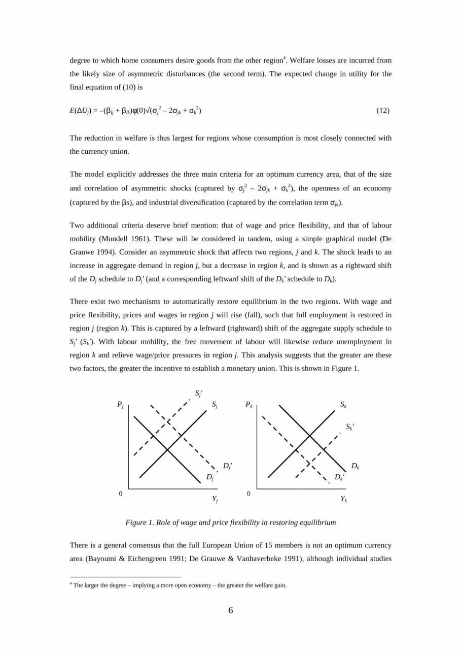
Two additional criteria deserve brief mention: that of wage and price flexibility, and that of labour
mobility (Mundell 1961). These will be considered in tandem, using a simple graphical model (De
Grauwe 1994). Consider an asymmetric shock that affects two regions, j and k. The shock leads to an
increase in aggregate demand in region j, but a decrease in region k, and is shown as a rightward shift
of the Dj schedule to Dj' (and a corresponding leftward shift of the Dk' schedule to Dk).
There exist two mechanisms to automatically restore equilibrium in the two regions. With wage and
price flexibility, prices and wages in region j will rise (fall), such that full employment is restored in
region j (region k). This is captured by a leftward (rightward) shift of the aggregate supply schedule to
Sj' (Sk'). With labour mobility, the free movement of labour will likewise reduce unemployment in
region k and relieve wage/price pressures in region j. This analysis suggests that the greater are these
two factors, the greater the incentive to establish a monetary union. This is shown in Figure 1.
Figure 1. Role of wage and price flexibility in restoring equilibrium
There is a general consensus that the full European Union of 15 members is not an optimum currency
area (Bayoumi & Eichengreen 1991; De Grauwe & Vanhaverbeke 1991), although individual studies
4 The larger the degree – implying a more open economy – the greater the welfare gain.
Dj' Dj
Sj
Dk
Dk'
Sk
Yj
Pj
Yk
Pk
Sj'
Sk'
0 0
7
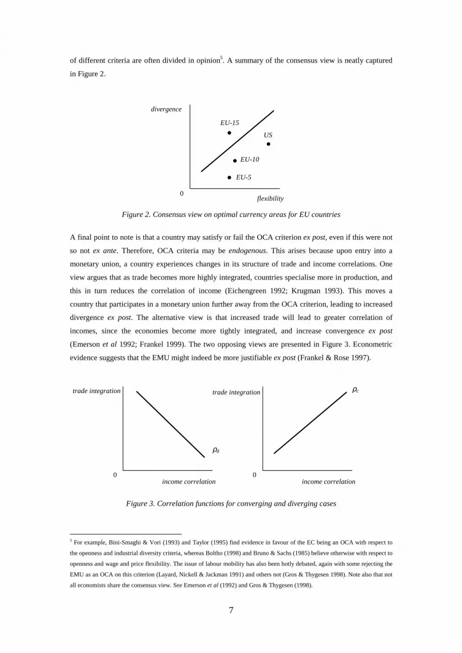
of different criteria are often divided in opinion5. A summary of the consensus view is neatly captured
in Figure 2.
Figure 2. Consensus view on optimal currency areas for EU countries
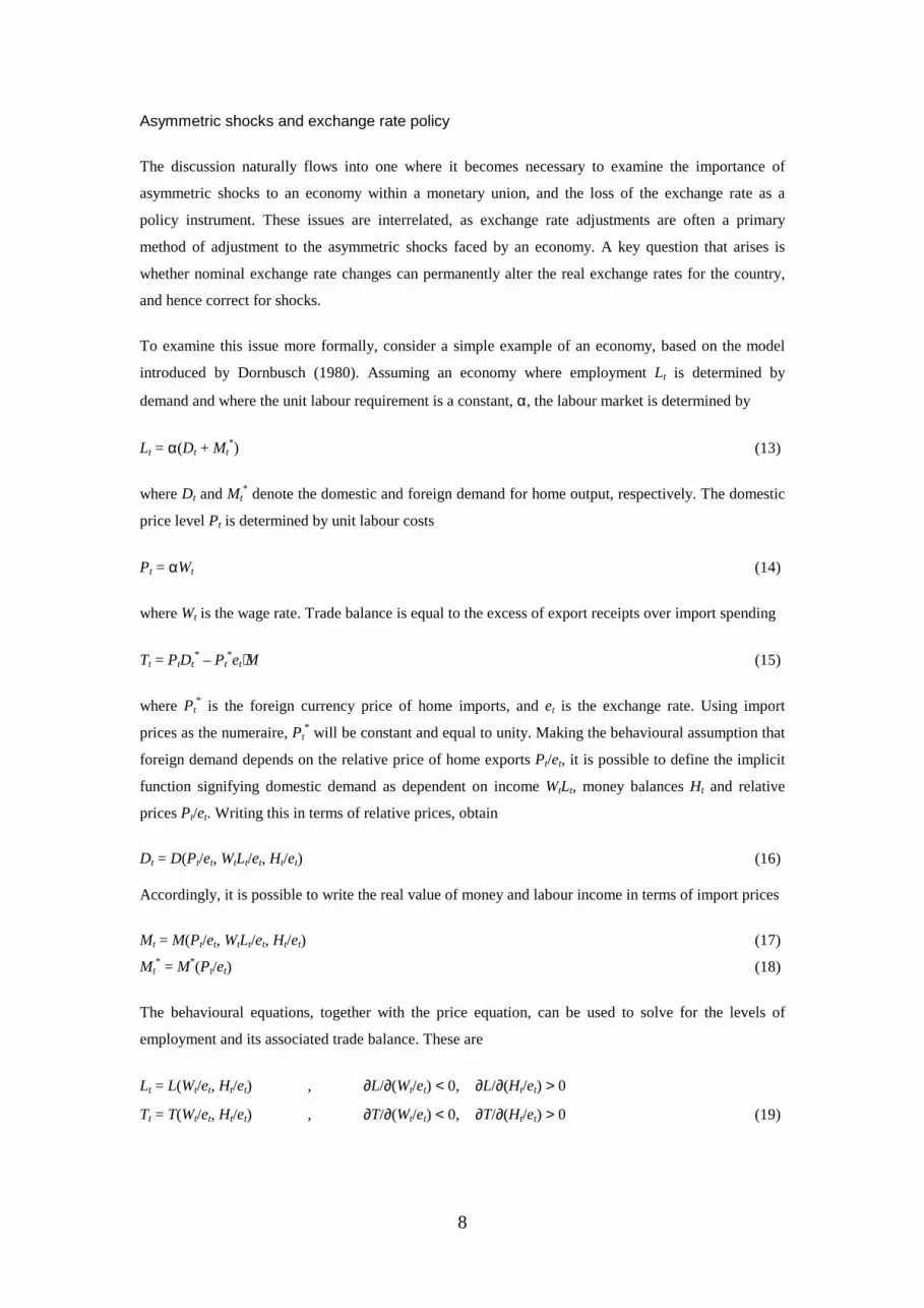
A final point to note is that a country may satisfy or fail the OCA criterion ex post, even if this were not
so not ex ante. Therefore, OCA criteria may be endogenous. This arises because upon entry into a
monetary union, a country experiences changes in its structure of trade and income correlations. One
view argues that as trade becomes more highly integrated, countries specialise more in production, and
this in turn reduces the correlation of income (Eichengreen 1992; Krugman 1993). This moves a
country that participates in a monetary union further away from the OCA criterion, leading to increased
divergence ex post. The alternative view is that increased trade will lead to greater correlation of
incomes, since the economies become more tightly integrated, and increase convergence ex post
(Emerson et al 1992; Frankel 1999). The two opposing views are presented in Figure 3. Econometric
evidence suggests that the EMU might indeed be more justifiable ex post (Frankel & Rose 1997).
Figure 3. Correlation functions for converging and diverging cases
5 For example, Bini-Smaghi & Vori (1993) and Taylor (1995) find evidence in favour of the EC being an OCA with respect to
the openness and industrial diversity criteria, whereas Boltho (1998) and Bruno & Sachs (1985) believe otherwise with respect to
openness and wage and price flexibility. The issue of labour mobility has also been hotly debated, again with some rejecting the
EMU as an OCA on this criterion (Layard, Nickell & Jackman 1991) and others not (Gros & Thygesen 1998). Note also that not
all economists share the consensus view. See Emerson et al (1992) and Gros & Thygesen (1998).
income correlation
trade integration
income correlation
trade integration
ρd
ρc
0 0
flexibility
divergence
EU-15
EU-10
EU-5
US
0
8
Asymmetric shocks and exchange rate policy
The discussion naturally flows into one where it becomes necessary to examine the importance of
asymmetric shocks to an economy within a monetary union, and the loss of the exchange rate as a
policy instrument. These issues are interrelated, as exchange rate adjustments are often a primary
method of adjustment to the asymmetric shocks faced by an economy. A key question that arises is
whether nominal exchange rate changes can permanently alter the real exchange rates for the country,
and hence correct for shocks.
To examine this issue more formally, consider a simple example of an economy, based on the model
introduced by Dornbusch (1980). Assuming an economy where employment Lt is determined by
demand and where the unit labour requirement is a constant, α, the labour market is determined by
Lt = α(Dt + Mt*) (13)
where Dt and Mt* denote the domestic and foreign demand for home output, respectively. The domestic
price level Pt is determined by unit labour costs
Pt = αWt (14)
where Wt is the wage rate. Trade balance is equal to the excess of export receipts over import spending
Tt = PtDt* – Pt
*et⋅M (15)
where Pt* is the foreign currency price of home imports, and et is the exchange rate. Using import
prices as the numeraire, Pt* will be constant and equal to unity. Making the behavioural assumption that
foreign demand depends on the relative price of home exports Pt/et, it is possible to define the implicit
function signifying domestic demand as dependent on income WtLt, money balances Ht and relative
prices Pt/et. Writing this in terms of relative prices, obtain
Dt = D(Pt/et, WtLt/et, Ht/et) (16)
Accordingly, it is possible to write the real value of money and labour income in terms of import prices
Mt = M(Pt/et, WtLt/et, Ht/et) (17)
Mt* = M*(Pt/et) (18)
The behavioural equations, together with the price equation, can be used to solve for the levels of
employment and its associated trade balance. These are
Lt = L(Wt/et, Ht/et) , ∂L/∂(Wt/et) < 0, ∂L/∂(Ht/et) > 0
Tt = T(Wt/et, Ht/et) , ∂T/∂(Wt/et) < 0, ∂T/∂(Ht/et) > 0 (19)
9
The classical adjustment process relies on money wage changes induced by unemployment and money
supply changes induced by the balance of payments. The managed system, however, attempts to attain
internal and external balance along preferred paths. Without exchange rate realignments, the system is
characterised by
∆Ht/et = T(Wt/et, Ht/et)
∆Wt/et = φ[L(Wt/et, Ht/et) – L*] (20)
where the first equation indicates how money balances rise at a rate equal to the balance of payments
surplus, and the second shows how the rate of wage change is proportional to the difference between
employment and the labour force L*. The managed system is characterised by the equations
∆Ht/et = T(Wt/et, Ht/et) + k[L* – l(Wt/et, Ht/et)]
∆Wt/et = φ[L(Wt/et, Ht/et) – L*] (21)
The additional term in equation (21a) clearly shows that depreciation supplements nominal wage
changes in moving the real wage, and so the real money stock is managed with both a view to trade
balance but also with regard to employment.
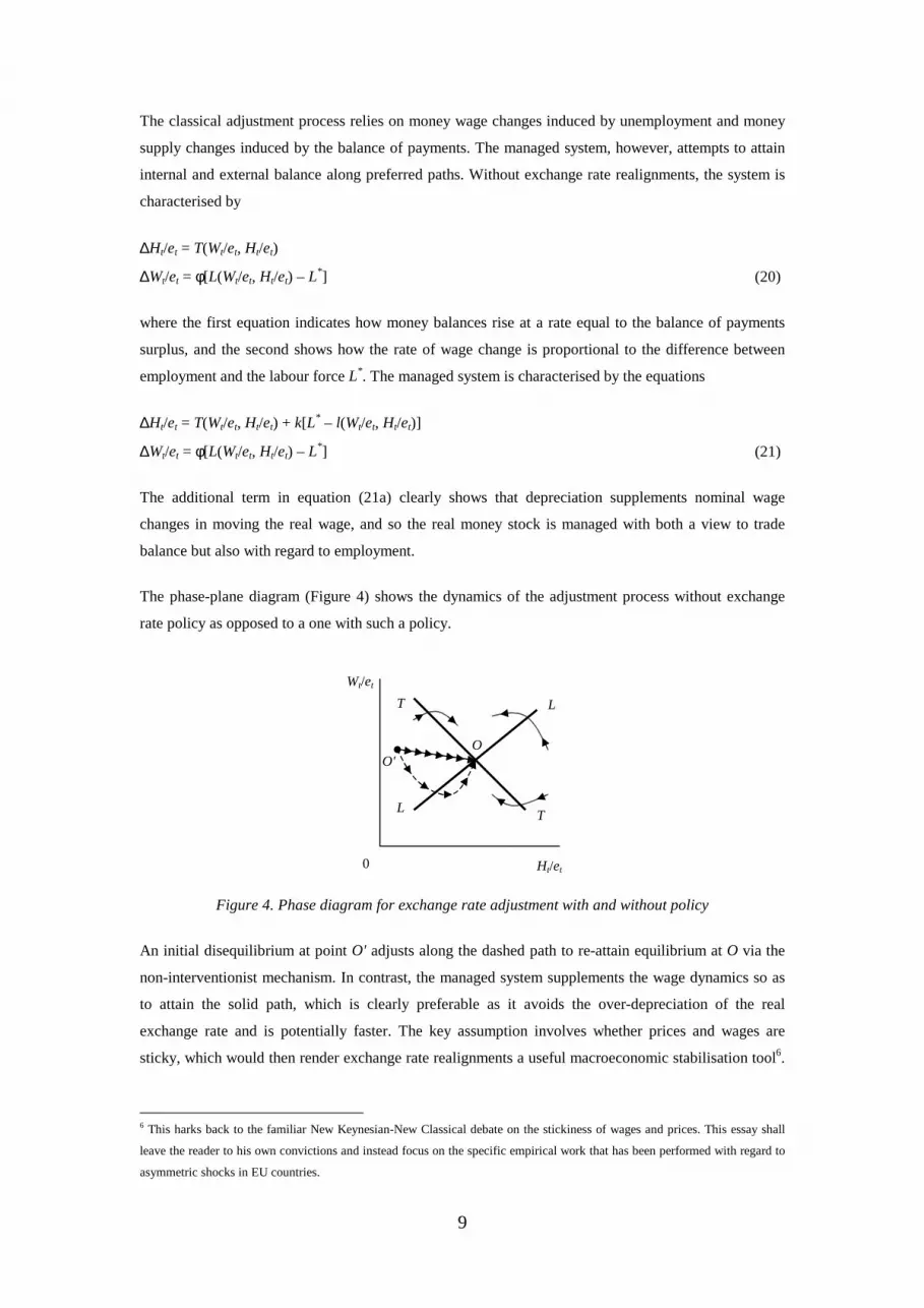
The phase-plane diagram (Figure 4) shows the dynamics of the adjustment process without exchange
rate policy as opposed to a one with such a policy.
Figure 4. Phase diagram for exchange rate adjustment with and without policy
An initial disequilibrium at point O' adjusts along the dashed path to re-attain equilibrium at O via the
non-interventionist mechanism. In contrast, the managed system supplements the wage dynamics so as
to attain the solid path, which is clearly preferable as it avoids the over-depreciation of the real
exchange rate and is potentially faster. The key assumption involves whether prices and wages are
sticky, which would then render exchange rate realignments a useful macroeconomic stabilisation tool6.
6 This harks back to the familiar New Keynesian-New Classical debate on the stickiness of wages and prices. This essay shall
leave the reader to his own convictions and instead focus on the specific empirical work that has been performed with regard to
asymmetric shocks in EU countries.
Ht/et
Wt/et
O' O
L T
L T
0

10
If so, then the loss of this instrument would mean very real costs for an economy which faced
asymmetric shocks.
Empirical studies on the issue of asymmetric shocks have adopted three main approaches: first, by that
of case studies that study the effects of exchange rate realignments on economic recovery (De Grauwe
1997; De Grauwe & Vanhaverbeke 1990; Sachs & Wyplosz 1986); second, by testing for the statistical
impact of shocks on various economies7 (Canzioneri et al 1996; Demertzis, Hallett & Rummel 1997;
Erkel-Rousse & Mélitz 1997; Schuberth & Wehinger 1999); third, by model simulations8 (Emerson et
al 1992; Masson & Symansky 1992; Minford, Rastogi & Hughes-Hallet 1992).
Policy credibility and time inconsistency
The ‘new’ view of monetary integration stresses issues of credibility (De Grauwe 1995). This is
primarily an extension of the Kydland-Prescott (1977) and Barro-Gordon (1983) model to the context
of monetary union. The discussion that follows is based on that of Alesina & Grilli (1993).
Consider a group of countries i = 1,…, n where output y is given by the expectations-adjusted Phillips
curve relation
yi = (π – πe) + εI (22)
where π is the rate of inflation, πe is the expected rate and εi is an independent, identically distributed
shock with variance σ2 that occurs after the formation of private sector expectations. The monetary
authority aims to minimise a loss function given by
Li = ½ E [π2 + γi(yi – y*)2] (23)
where y* is the target level of output. Economies are assumed two differ in two dimensions: their
preferences as reflected in γi, and the nature of the shocks, εi. The time consistent inflation policy is
thus given by
π* = γiy* – [γi/(1 + γi)]εI (24)
with the corresponding output level
yi = [1/(1 + γi)]εI (25)
7 Canzioneri et al (1996) and Erkel-Rousse & Mélitz (1997) find, in general, that the loss of the exchange rate as a policy
instrument yields minimal impact on both the core and periphery countries that they studied; in contrast, Demertzis, Hallett &
Rummel (1997) and Schuberth & Wehinger (1999), using structural vector autoregression approaches, find that there are in fact
significant costs involved in relinquishing domestic monetary policy.
8 Emerson et al (1992) ran simulations based on the IMF Multimod model and the EC Quest model; Minford, Rastogi & Hughes-
Hallet (1992) used the Liverpool world model and Masson & Symansky (1992) with the IMF Multimod model. Interestingly, the
conclusions of Emerson et al were in opposition to that of Masson & Symansky, despite the same model being used.
11
This would yield a variance of output σi2 given by
σi2 = σi
2/(1 + γi)2 (26)
However, it can be shown that were the authority be able to commit to a policy of
πc = – [γi/(1 + γi)]εI (27)
it is then possible to attain values of average inflation and output of zero, with output variance the
remaining the same as (26). The policy given by (27) is therefore superior as it improves on inflation
with no cost to output.
A monetary union leads to a situation where the inflation rate is the same across all countries (due to
the same monetary policy being adopted for all countries). The union central bank will aim to minimise
the loss function
LU = ½ E[Π t2 + Γ(Y – Y*)2] (28)
where capitalised variables indicate union values. Likewise, output is given by
Yt = (Π – Πe) + ξt (29)
Solving the optimisation problem will yield the inflation, output and output variance equations
Π = ΓY* – [Γ/(1 + Γ)]ξ
Y = [1/(1 + Γ)]ξ
σY2 = σξ
2/(1 + Γ)2 (30)
It can be shown that the net gain of joining the union is
Li – LiU = ½{ – y*2(Γ2 – γi
2) + (1 + γi){[γi/(1 + γi)]2σεi2 – Γ/(1 + Γ)]2σξ
2} + 2γi{[Γ/(1 +
Γ)]σεξ – [γi/(1 + γi)]σε}} (31)
where σεξ is the covariance between ε and ξ. Here, the difference in welfare is captured by the two
components, one representing differences in preferences (Γ and γi) and another representing economic
dissimilarities (σεi2, σξ
2 and σεξ). By assuming εi = ξ in all states of the world, such that σεi2 = σξ
2 = σεξ
= σ2, (30) simplifies to
Li – LiU = ½{ – y*2(Γ2 – γi
2) + σ2[γi/(1 + γi) – Γ/(1 + Γ)][(1 + γi)/(1 + Γ)⋅Γ – γi] } (32)
Re-expressing (31) as a ‘gain’ function,
Li – LiU = Gi(Γ, γi) (33)

12
This function takes a parabola-like shape, and Figure 5 graphs (33) for the cases y*2(1 + γi) < σε2 and
y*2(1 + γi) > σε2.
In both cases, if Γ > γi, country i is worse off with the union, since the union central bank is even less
credible than the country’s central bank. Further, if Γ < Γmin, country i also loses from the union
because the union central bank is too conservative and does not stabilise enough, leading to higher
losses from output variance than gains from reduced inflation. If Γ ∈ (Γmin, γi), then country i is strictly
better off with the union. The optimal level of γi is given by γi*.
Figure 5. Welfare gain functions for y*2(1 + γi) < σε2 and y*2(1 + γi) > σε
2
Since credibility as a concept is immeasurable, no conclusive empirical work is possible in this area. Ad
hoc data based on the comparison of inflation differentials, however, suggests that inflation-prone
countries, such as Italy, Ireland and Spain, might benefit from a monetary union that has a European
Central Bank modelled after the Bundesbank in Germany (De Grauwe 1995; Honohan 1991). The
benefits of price stability are estimated to be about 0.3% of community GDP (Emerson et al 1992).
Elimination of exchange rate variability
The introduction of a common currency would imply the elimination of variability between the
exchange rates of all countries participating in the monetary union. This has effects on the welfare of
both individuals as well as firms. Baldwin (1991) finds no less than seven different areas in which
static and dynamic efficiency gains from the elimination of exchange rate variability may be realised.
The discussion here will limit itself to the gains due to the reduction of systematic risk, whilst the
subsections that follow will address the effects of the elimination of transactions costs and the effects of
a stable exchange rate on trade.
As a preliminary, it is useful to examine the common argument that monetary unification provides a
fixed exchange rate that offers greater stability to output as compared to a regime of free floats. This
argument in general is fallacious, as can de demonstrated easily by considering modification of the
model first introduced by Poole (1970).
γi
Γmin Γ
G
Γ
G y*2(1 + γi) < σε
2
0 0
y*2(1 + γi) > σε2
Γmin γi γi* γi
*

13
Consider an economy represented by a modified IS-LM framework (Figure 6) that faces two types of
shocks, real and monetary. When a real shock occurs (a shift in the IS curve), a flexible exchange rate
would fluctuate between e1– and e1+, and output variation would vary between y1– and y1+. A fixed rate
in this case would lead to higher output variability, between y2– and y2+. When a monetary shock occurs
(a shift in the LM curve), a flexible rate would cause output variability but there is no output variation
with a fixed rate, since authorities will intervene in the money market to maintain the fixed rate. Thus,
if real shocks dominate, then a fixed exchange rate is preferable. However, if monetary shocks
dominate, then floating is preferred.
The implication of the above analysis is that elimination of exchange rate volatility does not necessarily
imply greater output stability, but instead depends on the nature of the shocks (which shift the IS or LM
curves) and the underlying structure of the economy (which determines the slope of the curves).
Figure 6. Modified IS-LM framework illustrating real and monetary shocks
At a microeconomic level, the gains from the elimination of exchange rate risk are likewise
questionable. Despite the general support of the business community (Association for the Monetary
Union of Europe 1998), economic theory does not provide a cut-and-dried case for increased profits
due to the elimination of exchange rate variability. The model here is adapted from that of Pindyck
(1982)9.
Consider a case where there exists demand uncertainty due to the possibility of exchange rate (and
hence price) fluctuations. Demand is
p = p[q, θ(t)] , ∂p/∂q ≤ 0, ∂p/∂θ > 0 (34)
with q as output determined by the quasi-concave production function q = ƒ(k, l) and θ(t) a stochastic
process of the form
dθ = σ(θ)ε(t) √dt (35)
9 Less general graphical treatments can also be found in Oi (1961) and De Grauwe (1997). Pindick’s (1982) contribution is
particularly insightful as it yields robust results as compared to earlier treatments.
y0 y1– y1+ y2– y2+ y
e
IS'' T
LM
0
IS
IS'
e0
e1–
e1+

14
where ε(t) is a serially uncorrelated normal random variable with mean zero and variance one. The
firm’s instantaneous profit is
π(t) = p(q, θ)q − wl − vi − c(i) (36)
where w are wages paid to labour L, and vi + c(i) is the cost of capital setup, v being the purchase price
of a unit of capital equipment, invested in at rate i. c(i) is the full adjustment cost of changing capital,
which is assumed to be semi-fixed10. Capital stock accumulates at a rate
∆k = i − δk (37)
where δ is the depreciation rate. The risk-neutral firm maximises the expected sum of discounted (at
rate r) profits according to
max E0 ∫0 ∞ π(t)e−rt dt (38)
subject to (35), (37) and nonzero factor inputs. In the deterministic case, θ = θ0 and
∆i = 1/c''(i) {(r + δ)[v + c'(i)] − [p + q(∂p/∂q)]⋅∂ƒ/∂k} (39)
Equations (37) and (39) describe the dynamics of k and i, and are described by the phase diagram in
Figure 7; equilibrium is attained at k* and i*.
Figure 7. Phase diagram for the deterministic solution
Consider the model in the presence of demand uncertainty. Define the value function as
J(k, θ, t) = max Et ∫t ∞ π(τ)e−rτ dτ (40)
This will lead to the fundamental equation of optimality
max [π(t)e−rt + ∂J/∂t + (i − δk)⋅∂J/∂k + ½σ2(θ)⋅∂2J/∂θ2 (41)
10 That is, changeable over time at a cost. In addition, assume c(0) = 0, c'(i) > (<) 0 ∀ i > (<) 0, c''(i) > 0.
k
i
∆k = 0
∆i = 0
0 k*
i*

15
This equation can be solved11 to yield the stochastic investment analogue to equation (39)
1/dt⋅Et di = 1/c''(i){(r + δ)[v + c'(i)] − [p + q(∂p/∂q)]⋅∂ƒ/∂k − σ2(θ)⋅(∂i/∂θ)2⋅c'''(i)} (42)
The result depends crucially on whether marginal adjustment costs are rising at an increasing (c'''(i) >
0) or decreasing (c'''(i) < 0) rate. With c'''(i) > 0, in the presence of uncertainty (σ > 0), stochastic
fluctuations create a positive expected semi-fixed cost of adjustment, which is reduced – though not
eliminated – by maintaining a larger capital stock and output level. Stochastic demand fluctuations thus
reduce the long-run marginal cost of production, but raises the average cost – profits are squeezed. The
effect is converse for the case where c'''(i) < 0. A graphical exposition of the argument is shown in
Figure 8, for the former case, with MCsr0 being the short-run marginal cost with σ = 0, MCsr
1 when σ >
0, MClr0 and MCsr
1 their long-run equivalents, and AClr0 and AClr
1 the corresponding long-run average
costs. p* is the long-run price level. Thus, the removal of exchange rate volatility could have either a
profit enhancing or eroding effect for firms12.
Figure 8. Expected output and costs for stochastic solution with C''' > 0
Empirical estimation of the effects of a removal of exchange rate volatility has proceeded by studying
the risk premia attached to securities. Ceteris paribus, this should lead to the elimination, or at least a
significant reduction, of interest rate differentials between EMU countries. Welfare gains due to the
elimination of such residual interest rates might be as small as 0.05% of EC GDP (Price Waterhouse
1988) to as much as 5-10% in the long-run due to multiplier effects (Baldwin 1991).
Elimination of transactions costs
11 The solution procedure is quite involved and the trick is the application of Ito’s lemma to the differentiated fundamental
equation of optimality. The steps are secondary to the discussion here and the interested reader is referred back to Pindyck’s
(1982) original paper.
12 Intuitively, this is easy to justify. Changes in the exchange rate not only represent a risk, but also a profit opportunity. With
variability of the exchange rate, the firm has the option to export in order to exploit the favourable exchange rate (through
demand conditions).
q
p
AClr1
MCsr1
0 q0
p*
q1
AClr1
MClr0
MClr1
MCsr0
16
The most commonly quoted13 gain from using a common currency involves the elimination of
transactions costs. Two aspects will be considered: the static gain from the elimination of costs due to
currency exchange, and the dynamic gain accruing to investment on growth.
The possibly significant economic effects that hark from seemingly small transactions costs can best be
understood by the literature on ‘menu costs’ (Akerlof and Yellen 1985). For an economy with firms
under imperfect competition, the profit function for firm i is
πi = π(Pi; P, W, Y) (43)
where Pi; P, W, Y are the prices charged by firm i, the general price level, wages and aggregate
demand, respectively. Firm i will optimise such that ∂πi/∂Pi = 0. For a change in aggregate demand we
have, via application of the Envelope Theorem,
∂πi/∂Y = ∂πi/∂Y + ∂πi/∂Pi ⋅ ∂Pi/∂Y = ∂πi/∂Y (44)
Thus the effect of a change in aggregate demand on profits will be approximately equal whether or not
a firm chooses to change its price – they are of second order. Extending this case where there are
different countries in a region, each with different aggregate demands, price rigidity might result due to
small transactions costs, which in turn induce large macroeconomic effects. An extension of this strand
of literature explores the reduced transactions costs that are involved when the single currency
introduced is a major world currency. This approach, adopted by Deveruex, Engel & Tille (1999), finds
that there are major welfare gains to be made due to the introduction of the euro.
Estimates of transactions costs for the EMU countries place the figure at between 0.25% (Emerson et al
1992) to 1% (Cukierman 1990; Dumke et al 1997) of Community GDP. This figure, although small,
implies that the deadweight loss of transactions costs might very well have significant macroeconomic
effects, if one subscribes to the New-Keynesian world view. In addition, there might be indirect
benefits such as increased transparency of prices, which effectively reduces transaction costs between
EMU nations (Thygesen 1993; De Grauwe 1997). The elimination of transactions costs together with
exchange rate volatility is thus expected to spur foreign direct investment.
The dynamic effect of the elimination of transactions costs can be understood in the context of the
basic Solow (1956) growth model. Consider a constant returns production function where per capita
output yt is determined by per capita capital stock kt, and influenced by exogenous productivity growth
At
yt = Atƒ(k/A) , ƒ' > 0, ƒ'' < 0 (45)
With accumulation of capital Kt given by
13 Indeed, the story of a tourist who went on a tour of all 15 European Union member countries, exchanging all his cash each
time, and lost more than half his money without having even bought anything, has almost attained folklore status.
17
∆Kt = τYt − δKt (46)
where τ and δ are the fraction of output Yt due to taxation and the depreciation rate, respectively, it is
straightforward to derive the long-run steady state output per capita
log yt = log ƒ(k/A)* + log A0 + ε⋅t
= g[(δ + ν + ε)−1τ] + log A0 + ε⋅t , g' > 0 (47)
where ν and ε are the population and productivity growth rates, respectively. As can be clearly seen
from equation (54), economic growth is possible only if there is technological growth, i.e. ε > 0. The
savings in transactions costs is broadly equivalent to an increase in overall productivity; indeed, the
output increase could very well exceed the productivity increase due to the presence of a multiplier
effect (Baldwin 1989).
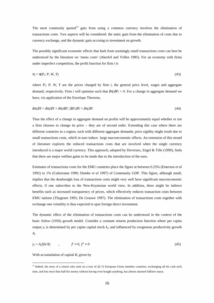
This is summarised in Figure 9. A reduction in transactions costs (an increase in productivity) shifts the
production function from AtF(k) to At+1F(k), with capital stock increasing from kt to kt+1. Output
increases more than proportionately from yt to yt+1. In addition, reductions in the interest rate from rt (as
discussed above) lead to a change in the slope of rt' to rt+1.
Figure 9. Dynamic effects of monetary integration on economic growth
As dynamic gains involve forecasting, quantitative evidence tends to be conjectural at best. Indeed, the
inability to subject dynamic gains to rigorous econometric testing ex ante is a major limitation in the
analysis. Estimates by Emerson et al (1992) and Taylor (1995) place the figure at about 5%.
International trade theory and the new economic geography
International trade theory and economic geography can be used to provide two pillars for a framework
whereby monetary integration may be analysed. A full integration would imply that impediments to
trade would disappear, and that the location of industries in space would be the only response available
to economic agents. Thus these two complementary disciplines attempt to model formally the influence
of monetary union due to changes in transportation and transaction costs, relative production costs and
advantages accruing to agglomeration.
k
y
0 kt+1 kt
yt+1
yt
AtF(k)
At+1F(k)
kt+1'
yt+1' rt
rt' rt+1
18
Studies on the effects of exchange rate uncertainty on trade yield mixed results14, although there is a
bias towards a belief that the effects are small (Hooper & Kohlhagen 1978; Kenen & Rodrick 1986).
However, in a recent paper, Rose (1999) finds robust results that suggest that the effect of a common
currency might indeed be large15. In particular, he applies a gravity approach to panel data for almost
34,000 observations and estimates
ln (Xijt) = β0 + β1ln(YiYj)t + β2 ln(YiYj/PopiPopj) + β3lnDij + β4Contij + β5Langij + β6FTAijt + β7ComNatij
+ β8ComColij + β9Colonyij + γCUijt + δV(eij)t + εijt
where i and j subscripts denote countries and t time. The dependent variable is the value of bilateral
trade and the regressors are, in the order above, a constant term, real GDP, population, distance, and
dummies for a common border, common language, existence of a trade agreement, common mother
nation, existence of colonial history by the same coloniser and colonies of each other. The final two
terms are the volatility of the nominal exchange rate and a well-behaved error term.
The main findings are that there is a strong negative effect of exchange rate volatility on trade, a large
positive effect of a common currency on trade and that this effect is much larger than the hypothetical
effect of reducing exchange rate volatility to zero.
The area of economic geography as applied to economic integration remains a largely unexplored and
exciting field. The seminal works in this area are Krugman and Venables (1990) and Krugman (1991),
who provide a rigorous theoretical framework for the study of economic integration on the location of
industries. Empirical work remains sparse; however, Nijkamp & Wang (1999) perform a neural
network analysis of industrial spatial shifts that tests whether monetary integration leads to industrial
concentration and hence unequal benefits for participating countries. They find that due to the
endogenous nature of the single currency, participating countries will tend to become more
heterogeneous, instead of homogenous, and that EMU will result in doubtful effects on the EU as a
whole. However, as Krugman (1991) himself pointed out, one should be wary of such results, which
often tend to be highly sensitive to small changes in the key parameters of the economy.
Financial market integration
A short note is in order concerning the issue of financial market integration. The introduction of a
single common currency brings to completion the process of financial market integration first begun
with the implementation of a common market (Servais 1995). This is believed to yield increased
benefits due to the complete removal of controls over foreign direct investment, improve economies of
scale due to increased market size and increase the efficiency of financing due to the increased number
of financial instruments available (Robson 1998).
14 See International Monetary Fund (1984) for a survey.
15 The closest precedents are Helliwell (1996) and McCallum (1995), although these studies focus exclusively on US-Canadian
trade and do not specifically address the effect of a monetary union on trade.

19
Studies aiming to quantify the impact of EMU on foreign direct investment estimate that gains will be
significant, and even larger than the stimulus in trade (Molle & Morsink 1990). There have also been
studies on the impact of the euro on fixed income (Nielsen 1999), equity (Biais 1999; Hardouvelis,
Priestley & Malliaropulos 1999) and derivatives markets (Steinherr 1999), usually yielding results that
indicate an improvement in financial market efficiency, at least in the medium term. However, skeptics
believe that the deepening of financial markets has little to do with the euro, attributing it instead to
other factors (Feldstein 2000).
III. Empirical Analysis
This section aims to concretise theory with fact by providing a basic empirical appraisal of the EMU. It
draws from data for the period January 1990 to December 1999, using both monthly and quarterly data,
for the 11 member countries of the EMU that have adopted the euro as of 1st January 1999 (EU-11)16 as
well as the larger European Union of 15 countries (EU-15)17. The primary aim is to use short-term
main macroeconomic indicators as assessment devices for whether the gains (or losses) to EMU are
realised.
Figure 10. Inflation convergence
Prices
16 Namely, Austria, Belgium, Finland, France, Germany, Ireland, Italy, Luxembourg, the Netherlands, Portugal and Spain.
17 The EU-11 plus Denmark, Greece, Norway, Sweden and the UK.
������������
����������������
������������������
��������������������
����������
������������������������������������
��������������������������
�������������������������
������������
����������������������������������
�������������������������������������������������
��������������������������������
������������������
��������������������������������������
���������������������������������������������������������������������������������������������������������������������������
Consumer Price Index, Year-On-Year, Selected EU-11 Countries
-2.00
0.00
2.00
4.00
6.00
8.00
10.00
Tim e
B elgium
Luxem bourg
������������������� SpainPortugal
Source: OECD Main Economic Indicators

20
Two main issues will be examined here: the ability of inflation-prone countries to ‘borrow’ credibility
from a low-inflation country such as Germany; and the success (or failure) of the ECB to maintain
price stability. Figure 10 shows that inflation did indeed converge prior to monetary union, notably for
high-inflation countries such as Portugal and Spain, supporting the thesis that credibility can be
imported by participating in a monetary union and free-riding off the reputation of a hard-nosed central
bank such as the Bundesbank.
Figure 11. Inflation performance, EU-15
Figure 12. Inflation performance, EU-11
Price stability is an essential issue that is widely debated; the main point of contention being whether
the ECB should target a price or money target (Gerlach & Svensson 1999). The inflation picture for the
larger EU-15 (Figure 11) appears to be positive, with the Harmonised Consumer Price Index (HCPI)
trending downwards since the ERM crisis in 1993. Surprisingly, this has resisted upward pressure from
energy price rises but its steep decline in recent history might be cause for a continued downward trend.
Inflation Performance, Year-On-Year, EU-15 (Disaggregated)
-4.00
-3.00
-2.00
-1.00
0.00
1.00
2.00
3.00
4.00
5.00
Time
HCPI (All Items)
HCPI (Energy)
HCPI (Food)
Source: OECD Main Economic Indicators
Inflation Performance, Year-On-Year, EU-11
-3.50
-3.00
-2.50
-2.00
-1.50
-1.00
-0.50
0.00
0.50
1.00
1.50
2.00
Time
HCPI
PPI
Source: Eurostat
21
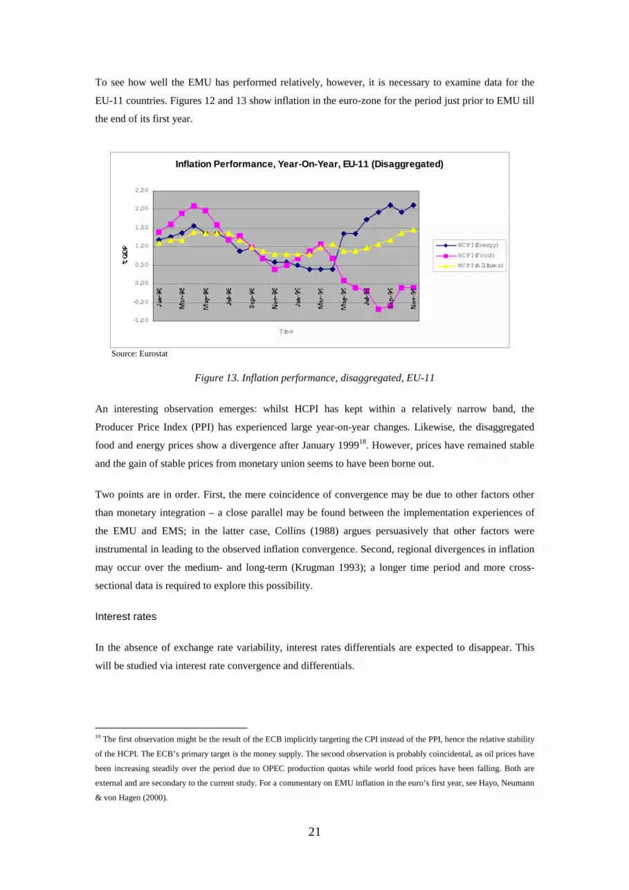
To see how well the EMU has performed relatively, however, it is necessary to examine data for the
EU-11 countries. Figures 12 and 13 show inflation in the euro-zone for the period just prior to EMU till
the end of its first year.
Figure 13. Inflation performance, disaggregated, EU-11
An interesting observation emerges: whilst HCPI has kept within a relatively narrow band, the
Producer Price Index (PPI) has experienced large year-on-year changes. Likewise, the disaggregated
food and energy prices show a divergence after January 199918. However, prices have remained stable
and the gain of stable prices from monetary union seems to have been borne out.
Two points are in order. First, the mere coincidence of convergence may be due to other factors other
than monetary integration – a close parallel may be found between the implementation experiences of
the EMU and EMS; in the latter case, Collins (1988) argues persuasively that other factors were
instrumental in leading to the observed inflation convergence. Second, regional divergences in inflation
may occur over the medium- and long-term (Krugman 1993); a longer time period and more cross-
sectional data is required to explore this possibility.
Interest rates
In the absence of exchange rate variability, interest rates differentials are expected to disappear. This
will be studied via interest rate convergence and differentials.
18 The first observation might be the result of the ECB implicitly targeting the CPI instead of the PPI, hence the relative stability
of the HCPI. The ECB’s primary target is the money supply. The second observation is probably coincidental, as oil prices have
been increasing steadily over the period due to OPEC production quotas while world food prices have been falling. Both are
external and are secondary to the current study. For a commentary on EMU inflation in the euro’s first year, see Hayo, Neumann
& von Hagen (2000).
Inflation Performance, Year-On-Year, EU-11 (Disaggregated)
-1.00
-0.50
0.00
0.50
1.00
1.50
2.00
2.50
Time
HCPI (Energy)
HCPI (Food)
HCPI (All Items)
Source: Eurostat
22
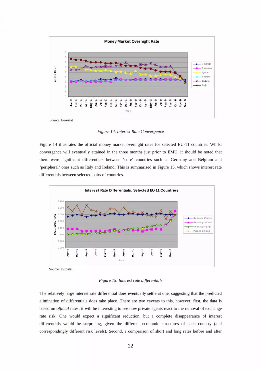
Figure 14. Interest Rate Convergence
Figure 14 illustrates the official money market overnight rates for selected EU-11 countries. Whilst
convergence will eventually attained in the three months just prior to EMU, it should be noted that
there were significant differentials between ‘core’ countries such as Germany and Belgium and
‘peripheral’ ones such as Italy and Ireland. This is summarised in Figure 15, which shows interest rate
differentials between selected pairs of countries.
Figure 15. Interest rate differentials
The relatively large interest rate differential does eventually settle at one, suggesting that the predicted
elimination of differentials does take place. There are two caveats to this, however: first, the data is
based on official rates; it will be interesting to see how private agents react to the removal of exchange
rate risk. One would expect a significant reduction, but a complete disappearance of interest
differentials would be surprising, given the different economic structures of each country (and
correspondingly different risk levels). Second, a comparison of short and long rates before and after
Money Market Overnight Rate
0
1
2
3
4
5
6
7
8
9
Time
Belguim
Germany
Spain
France
Ireland
Italy
Source: Eurostat
Interest Rate Differentials, Selected EU-11 Countries
0.000
0.200
0.400
0.600
0.800
1.000
1.200
1.400
Tim e
Germ any-France
Germ any-Ireland
Germ any-Spain
France-Finland
Source: Eurostat
23
EMU might yield yet more insights. OECD (1999) estimates that long and short nominal rates were in
fact converging in 1998.
Unemployment
Unemployment has always been a chronic problem for the euro-zone (Layard, Nickell & Jackman
1991). The loss of exchange rate policy as an instrument for macroeconomic stabilisation could
theoretically lead to an increase in unemployment due to the increased severity of asymmetric shocks.
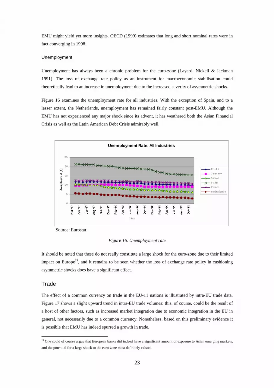
Figure 16 examines the unemployment rate for all industries. With the exception of Spain, and to a
lesser extent, the Netherlands, unemployment has remained fairly constant post-EMU. Although the
EMU has not experienced any major shock since its advent, it has weathered both the Asian Financial
Crisis as well as the Latin American Debt Crisis admirably well.
Figure 16. Unemployment rate
It should be noted that these do not really constitute a large shock for the euro-zone due to their limited
impact on Europe19, and it remains to be seen whether the loss of exchange rate policy in cushioning
asymmetric shocks does have a significant effect.
Trade
The effect of a common currency on trade in the EU-11 nations is illustrated by intra-EU trade data.
Figure 17 shows a slight upward trend in intra-EU trade volumes; this, of course, could be the result of
a host of other factors, such as increased market integration due to economic integration in the EU in
general, not necessarily due to a common currency. Nonetheless, based on this preliminary evidence it
is possible that EMU has indeed spurred a growth in trade.
19 One could of course argue that European banks did indeed have a significant amount of exposure to Asian emerging markets,
and the potential for a large shock to the euro-zone most definitely existed.
Unemployment Rate, All Industries
0
5
10
15
20
25
Time
EU-11
Germany
Ireland
Spain
France
Netherlands
Source: Eurostat

24
Figure 17. Intra-EU Trade Volumes
Investment
Investment statistics20 shed light on the static gains due to the removal of transactions cost and
exchange rate uncertainty; ceteris paribus, investment should increase due to EMU. Dynamic growth
effects should be examined in tandem with productivity; these should show up in both investment and
productivity improvements. Finally, foreign direct investment21 should also increase under EMU due to
the reasons already mentioned.
Figure 18. Investment
20 Gross fixed capital formation is used as a proxy for investment.
21 Unfortunately, due to the limited data available on FDI, an extremely small sample is utilised.
Intra-EU Trade Volumes
0
10000
20000
30000
40000
50000
60000
70000
80000
90000
Tim e
Exports
Im ports
Source: Eurostat
Investment in EU-15
1000
1050
1100
1150
1200
1250
1300
1350
Time
EU-15
Trend
Source: OECD Government Statistics
25
Figure 19. Investment in Selected EU-11
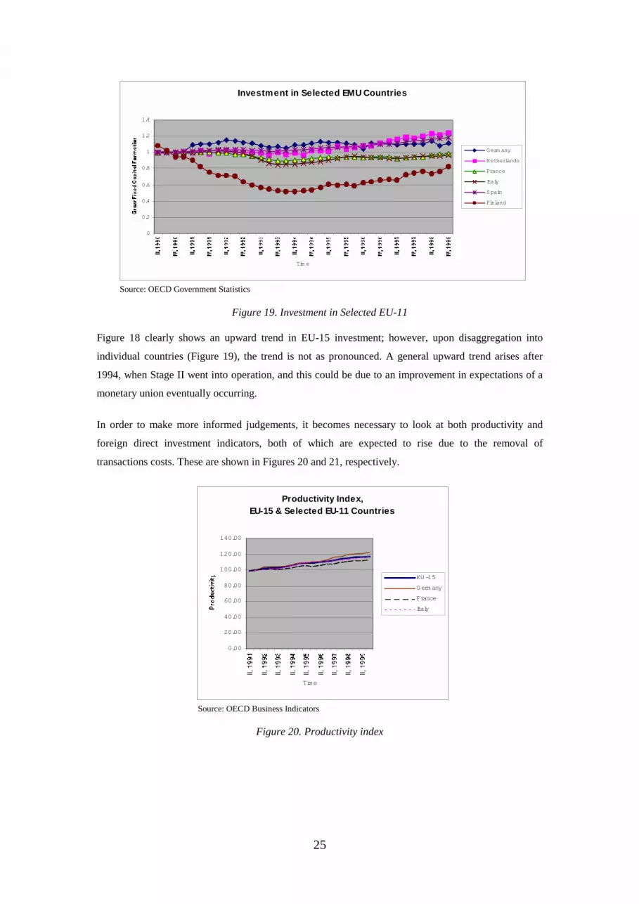
Figure 18 clearly shows an upward trend in EU-15 investment; however, upon disaggregation into
individual countries (Figure 19), the trend is not as pronounced. A general upward trend arises after
1994, when Stage II went into operation, and this could be due to an improvement in expectations of a
monetary union eventually occurring.
In order to make more informed judgements, it becomes necessary to look at both productivity and
foreign direct investment indicators, both of which are expected to rise due to the removal of
transactions costs. These are shown in Figures 20 and 21, respectively.
Figure 20. Productivity index
Source: OECD Business Indicators
Productivity Index,EU-15 & Selected EU-11 Countries
0.00
20.00
40.00
60.00
80.00
100.00
120.00
140.00
Time
EU-15
Germany
France
Italy
Investment in Selected EMU Countries
0
0.2
0.4
0.6
0.8
1
1.2
1.4
Tim e
Germ any
Netherlands
France
Italy
Spain
Finland
Source: OECD Government Statistics
26
Figure 21. Foreign Direct Investment
Productivity indices show a slow improvement up till 1994, when they begin to improve markedly.
This further strengthens the hypothesis that there has been a spur on economic growth due to improved
expectations. However, productivity growth might also be attributed to other technological
improvements as well, such as the proliferation of the Internet. Perhaps of concern is the fact that
German productivity remains above the EU-15 average. In a monetary union, it would become
necessary that German productivity growth slow in order to allow real exchange rate convergence22, so
as to prevent unsustainable asymmetries in real exchange rates across different regions of the EMU.
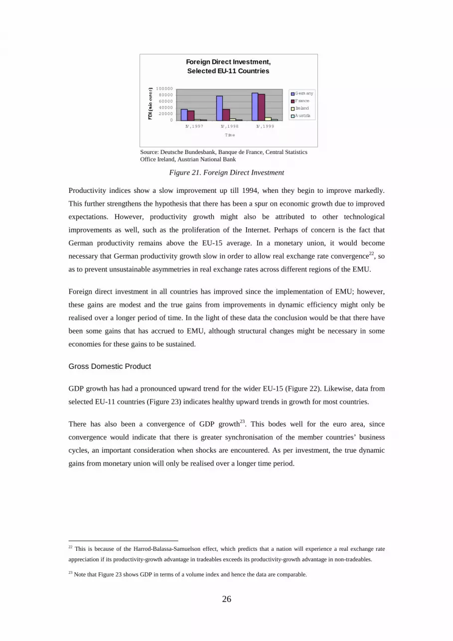
Foreign direct investment in all countries has improved since the implementation of EMU; however,
these gains are modest and the true gains from improvements in dynamic efficiency might only be
realised over a longer period of time. In the light of these data the conclusion would be that there have
been some gains that has accrued to EMU, although structural changes might be necessary in some
economies for these gains to be sustained.
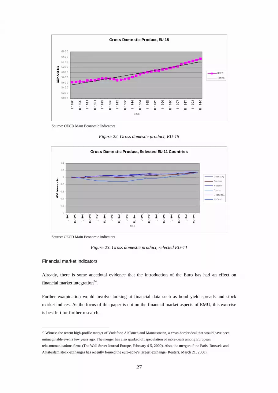
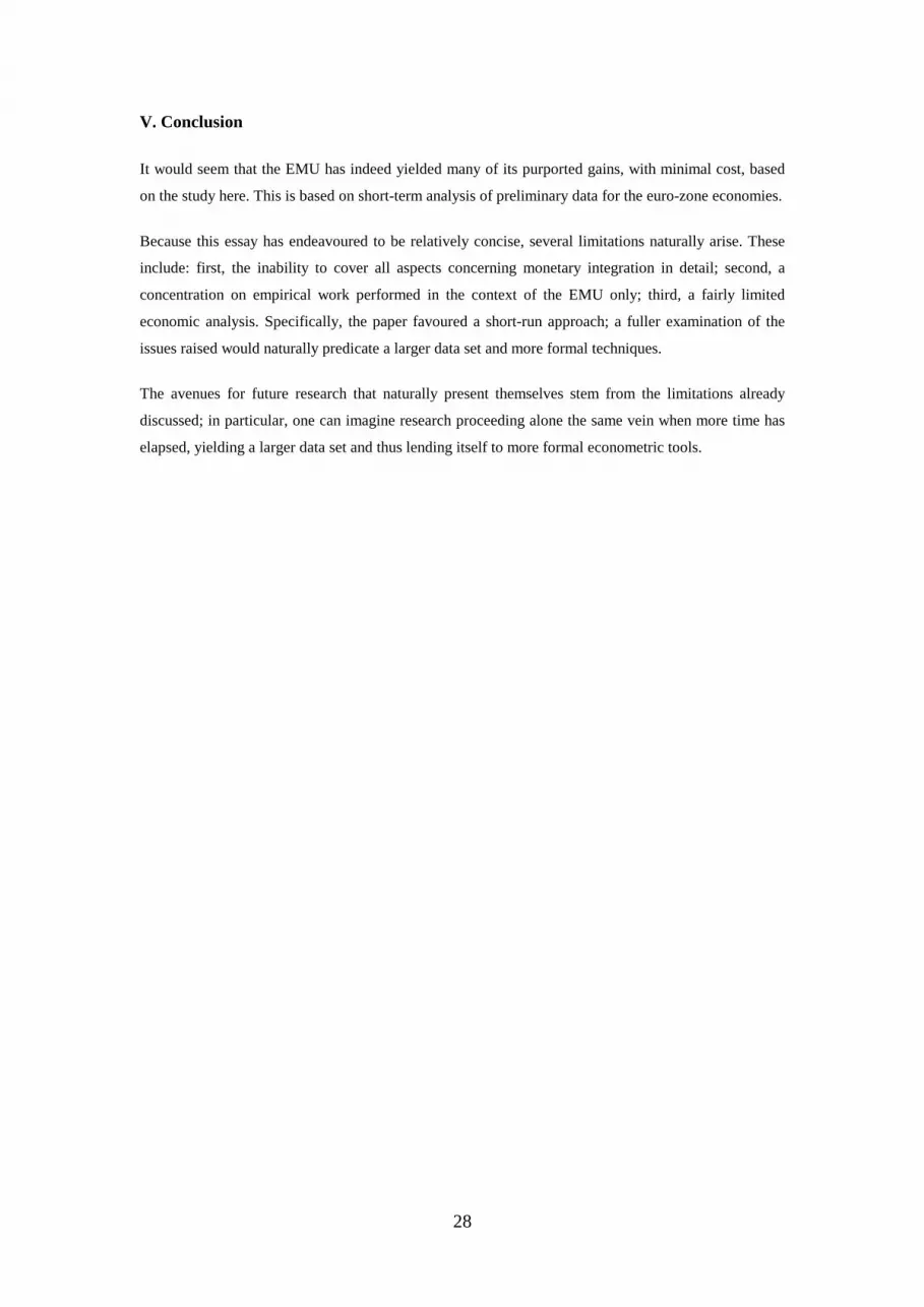
Gross Domestic Product
GDP growth has had a pronounced upward trend for the wider EU-15 (Figure 22). Likewise, data from
selected EU-11 countries (Figure 23) indicates healthy upward trends in growth for most countries.
There has also been a convergence of GDP growth23. This bodes well for the euro area, since
convergence would indicate that there is greater synchronisation of the member countries’ business
cycles, an important consideration when shocks are encountered. As per investment, the true dynamic
gains from monetary union will only be realised over a longer time period.
22 This is because of the Harrod-Balassa-Samuelson effect, which predicts that a nation will experience a real exchange rate
appreciation if its productivity-growth advantage in tradeables exceeds its productivity-growth advantage in non-tradeables.
23 Note that Figure 23 shows GDP in terms of a volume index and hence the data are comparable.
Source: Deutsche Bundesbank, Banque de France, Central Statistics Office Ireland, Austrian National Bank
Foreign Direct Investment,Selected EU-11 Countries
0
20000
40000
60000
80000
100000
IV, 1997 IV, 1998 IV, 1999
Time
Germany
France
Ireland
Austria
27
Figure 22. Gross domestic product, EU-15
Figure 23. Gross domestic product, selected EU-11
Financial market indicators
Already, there is some anecdotal evidence that the introduction of the Euro has had an effect on
financial market integration24.
Further examination would involve looking at financial data such as bond yield spreads and stock
market indices. As the focus of this paper is not on the financial market aspects of EMU, this exercise
is best left for further research.
24 Witness the recent high-profile merger of Vodafone AirTouch and Mannesmann, a cross-border deal that would have been
unimaginable even a few years ago. The merger has also sparked off speculation of more deals among European
telecommunications firms (The Wall Street Journal Europe, February 4-5, 2000). Also, the merger of the Paris, Brussels and
Amsterdam stock exchanges has recently formed the euro-zone’s largest exchange (Reuters, March 21, 2000).
Gross Domestic Product, EU-15
5000
5200
5400
5600
5800
6000
6200
6400
6600
6800
Time
GDP
Trend
Source: OECD Main Economic Indicators
Gross Domestic Product, Selected EU-11 Countries
0
0.2
0.4
0.6
0.8
1
1.2
1.4
Tim e
Germ any
France
Austria
Spain
Portugal
Finland
Source: OECD Main Economic Indicators
28
V. Conclusion
It would seem that the EMU has indeed yielded many of its purported gains, with minimal cost, based
on the study here. This is based on short-term analysis of preliminary data for the euro-zone economies.
Because this essay has endeavoured to be relatively concise, several limitations naturally arise. These
include: first, the inability to cover all aspects concerning monetary integration in detail; second, a
concentration on empirical work performed in the context of the EMU only; third, a fairly limited
economic analysis. Specifically, the paper favoured a short-run approach; a fuller examination of the
issues raised would naturally predicate a larger data set and more formal techniques.
The avenues for future research that naturally present themselves stem from the limitations already
discussed; in particular, one can imagine research proceeding alone the same vein when more time has
elapsed, yielding a larger data set and thus lending itself to more formal econometric tools.
29
References
Association for the Monetary Union of Europe 1998, The Sustainability Report, AMUE, Paris
Akerlof, G. & Yellen, J. 1985, ‘Can Small Deviations from Rationality Make Significant Differences to Economic Equilibria?’, American Economic Review, vol. 75, no. 4, pp. 708-20
Alesina, A. & Grilli, V. 1993, ‘On the Feasibility of a One or Multi-Speed European Monetary Union’, NBER Working Paper no. 4350, National Bureau of Economic Research, Cambridge, Massachusetts
Baldwin, R.E. 1989, ‘The Growth Effects of 1992’, Economic Policy, vol. 0, no. 9, pp. 248-81
Baldwin, R.E. 1991, ‘On the Microeconomics of the European Monetary Union’, in Emerson, M. and Pisani-Ferry, J. (eds.), European Economy, special edition no. 1, Commission of the European Communities, Brussels
Ball, L. & Romer, D. 1990, ‘Real Rigidities and the Non-neutrality of Money’, Review of Economic Studies, vol. 57, no. 2, pp. 183-203
Barro, R. & Gordon, D. 1983, ‘Rules, Discretion and Reputation in a Model of Monetary Policy’, Journal of Monetary Economics, vol. 12, no. 1, pp. 101-21
Bayoumi, T. 1994, ‘A Formal Model of Optimum Currency Areas’, IMF Working Paper, WP/94/42
Bayoumi, T. & Eichengreen, B. 1991, ‘Shocking Aspects of European Monetary Unification’, CEPR Discussion Paper no. 643, Centre for Economic Policy Research, London
Biais, B. 1999, ‘European Stock Markets and European Unification’, in Dermine, J. & Hillion, P. (eds.), European Capital Markets with a Single Currency, Oxford University Press, Oxford
Bini-Smaghi, L. & Vori, S. 1993, ‘Rating the EC as an Optimal Currency Area: Is it worse than the US?’, Banca d’Italia Temi di discussione no. 1987
Boltho, A. 1998, ‘Should Unemployment Convergence Precede Monetary Union?’, in Forder, J. & Menon, A. (eds.), The European Union and National Macroeconomic Policy, Routledge, London
Bruno, M. & Sachs, J. 1985, Economics of Worldwide Stagflation, National Bureau of Economic Research, Cambridge, Massachusetts
Canzoneri, M.B., Vallés, J. & Vinãls, J. 1996, ‘Do Exchange Rates Move to Address International Macroeconomic Imbalances?’, CEPR Discussion Paper no. 1498, Centre for Economic Policy Research, London
Collins, S.M. 1988, ‘Inflation and the European Monetary System’, in Giavazzi, F. & Micossi, S. (eds.), The European Monetary System, Cambridge University Press, Cambridge
Cukierman, A. 1990, ‘Fixed Parity Versus a Commonly Managed Currency and the Case Against “Stage II”’, Ministry of Finance, Paris
De Grauwe, P. 1995, ‘The Economics of Convergence towards Monetary Union in Europe’, CEPR Discussion Paper no. 1213, Centre for Economic Policy Research, London
De Grauwe, P. 1997, The Economics of Monetary Integration, 3rd revised edition, Oxford University Press, Oxford
De Grauwe, P. & Vanhaverbeke, W. 1990, ‘Exchange Rate Experiences of Small EMS Countries: The Cases of Belgium, Denmark and the Netherlands’, in Argy, V. & De Grauwe, P. (eds.), Choosing an Exchange Rate Regime, International Monetary Fund, Washington, D.C.
De Grauwe, P. & Vanhaverbeke, W. 1991, ‘Is Europe an Optimum Currency Area? Evidence from Regional Data’, CEPR Discussion Paper no. 555, Centre for Economic Policy Research, London
Demertzis, M., Hallett, A.H. & Rummel, O. 1997, ‘Does a Core-Periphery Regime Make Europe into an Optimal Currency Area?’, in Welfens, P.J.J. (ed.), European Monetary Union: Transition, International Impact and Policy Options, Springer-Verlag, Berlin
Devereux, M.B., Engel, C. & Tille, C. 1999, ‘Exchange Rate Pass-Through and the Welfare Effects of the Euro’, NBER Working Paper no. 7382, National Bureau of Economic Research, Cambridge, Massachusetts
Dornbusch, R. 1976, ‘Expectations and Exchange Rate Dynamics’, Journal of Political Economy, vol. 84, no. 6, pp. 1161-76
Dumke, R., Herrmann, A., Juchems, A. & Cherman, H. 1997, ‘Intra-EU Multi-Currency Management Costs’, Study for the European Commission, no. DG XV, IFO Schnelldienst Nr 9, pp. 3-17
Eichengreen, B. 1992, ‘Should the Maastricht Treaty be Saved?’, Princeton Studies in International Finance, no. 74, International Finance Section, Princeton University, Princeton, New Jersey
Emerson, M., Gros, D., Italianer, A., Pisani-Ferry, J. & Reichenbach, H. 1992, One Market, One Money, Oxford University Press, Oxford
Erkel-Rousse, H. & Mélitz, J. 1997, ‘New Empirical Evidence on the Costs of European Monetary Union’, in Eijffinger, S. & Huizings, H. (eds.), Positive Political Economy: Theory and Evidence, Cambridge University Press, Cambridge
Feldstein, M. 2000, ‘The European Central Bank and the Euro: The First Year’, NBER Working Paper no. 7517, National Bureau of Economic Research, Cambridge, Massachusetts
Frankel, J.A. 1999, ‘No Single Currency Regime is Right for all Countries at all Times’, NBER Working Paper 7338, National Bureau of Economic Research, Cambridge, Massachusetts
Frankel, J.A. & Rose, A.K. 1997, ‘Is EMU More Justifiable Ex Post than Ex Ante?’, European Economic Review, vol. 41, no. 3-5, pp. 753-60
30
Gerlach, S. & Svensson, L.E.O. 1999, ‘Money and Inflation in the Euro Area: A Case for Monetary Indicators?’, unpublished monograph
Gros, D. & Thygesen, N. 1998, European Monetary Integration, 2nd edition, Addison Wesley Longman, Essex
Hardouvelis, D., Priestley, R. & Malliaropulos, D. 1999, ‘EMU and European Stock Market Integration’, CEPR Discussion Paper no. 2124, Centre for Economic Policy Research, London
Hayo, B., Neumann, M.J.M. & von Hagen, J. 2000, ‘EMU Inflation’, unpublished monograph, Centre for European Integration Studies
Helliwell, J.F. 1996, ‘Do National Borders Matter for Quebec’s Trade?’, Canadian Journal of Economics, vol. 29, no. 3, pp. 507-22
Honohan, P. 1991, ‘Monetary Union’, in O’Donnell, R. (ed.), Economic and Monetary Union, Studies in European Union no. 2, Institute of European Affairs, Dublin
Hooper, P. & Kohlhagen, S. 1978, ‘The Effect of Exchange Rate Uncertainty on Prices and Volumes of International Trade’, Journal of International Economics, vol. 8, no. 4, pp. 483-511
International Monetary Fund 1984, Exchange Rate Variability and World Trade, IMF Occasional Paper no. 28, International Monetary Fund, Washington, D.C.
Kenen, P.B. 1969, ‘The Theory of Optimum Currency Areas: An Eclectic View’, in Mundell, R.I. & Swoboda, A. (eds.), Monetary Problems of the International Economy, University of Chicago Press, Chicago, Illinois
Kenen, P. & Rodrik, D. 1986, ‘Measuring and Analysing the Effects of Short-Term Volatility in Real Exchange Rates’, Review of Economics and Statistics, pp. 311-15
Krugman, P. 1991, ‘Increasing Returns and Economic Geography’, Journal of Political Economy, vol. 99, no. 3, pp. 483-99
Krugman, P. 1993, ‘Lessons of Massachusetts for EMU’, in Giavazzi, F. & Torres, F. (eds.), The Transition to Economic and Monetary Union in Europe, Cambridge University Press, Cambridge, pp. 241-61
Krugman, P. & Venables, A. 1990, ‘Integration and the Competitiveness of the Peripheral Industry’, CEPR Discussion Paper no. 363, Centre for Economic Policy Research, London
Kydland, F. & Prescott, E. 1977, ‘Rules Rather than Discretion: The Inconsistency of Optimal Plans’, Journal of Political Economy, vol. 85, no. 3, pp. 473-91
Layard, R., Nickell, S. & Jackman, R. 1991, Unemployment: Macroeconomic Performance and the Labour Market, Oxford University Press, Oxford
Masson, P.R. & Symansky, S. 1992, ‘Evaluating the EMS and EMU using Stochastic Simulations: Some Issues’, in Barrel, R. & Whitley, J. (eds.), Macroeconomic Policy Coordination in Europe: The ERM and Monetary Union, Sage Publications, London
Masson, P.R. & Taylor, M.P. 1993, ‘Currency Unions: A Survey of the Issues’, in Masson, P.R. & Taylor, M.P. (eds.), Policy Issues in the Operation of Currency Unions, Cambridge University Press, Cambridge
McCallum, J. 1995, ‘National Borders Matter: Canada-U.S. Regional Trade Patterns’, American Economic Review, vol. 85, no. 3, pp. 615-23
McKinnon, R.I. 1963, ‘Optimal Currency Areas’, American Economic Review, vol. 52, no. 4, pp. 717-25
Minford, P., Rastogi, A. & Hughes-Hallet, A. 1992, ‘ERM and EMU – Survival, Costs and Prospects’, in Barrel, R. & Whitley, J. (eds.), Macroeconomic Policy Coordination in Europe: The ERM and Monetary Union, Sage Publications, London
Molle, W. & Morsink, R. 1990, ‘Direct Investments and Monetary Integration’, in Emerson, M. and Pisani-Ferry, J. (eds.), European Economy, special edition no. 1, Commission of the European Communities, Brussels
Mundell, R.A. 1961, ‘A Theory of Optimum Currency Areas’, American Economic Review, vol. 51, no. 4, pp. 657-65
Nielsen, L. 1999, ‘Yield Spreads and Optimal Debt Management under the Single Currency’, in Dermine, J. & Hillion, P. (eds.), European Capital Markets with a Single Currency, Oxford University Press, Oxford
Nijkamp, P. & Wang, S. 1999, ‘Winners and losers in the European monetary union: a neural network analysis of industrial spatial shifts’, in Fischer, M. M. & Nijkamp, P. (eds.), Spatial Dynamics of European Integration, Springer-Verlag, Berlin, pp. 13-34
OECD 1999, EMU: Facts, Challenges and Policies, Organisation for Economic Co-operation and Development, Paris
Oi, W.Y. 1961, ‘The Desirability of Price Competition Under Perfect Competition’, Econometrica, vol. 29, no. 1, pp. 58-64
Pindyck,, R.S. 1982, ‘Adjustment Costs, Uncertainty and the Behaviour of the Firm’, American Economic Review, vol. 72, no. 3, pp. 415-27
Poole, W. 1970, ‘Optimal Choice of Monetary Policy Instruments in a Simple Stochastic Macro Model’, Quarterly Journal of Economics, vol. 84, no. 2, pp. 197-216
Price Waterhouse 1988, The Cost of ‘Non-Europe’ in Financial Services, Commission of the European Communities, Brussels
Reuters, ‘European Bourses Confirm 3-Way Merger’, March 21, 2000
Robson 1998, The Economics of International Integration 4th revised edition, Routledge, New York, New York
Rose, A.K. 1999, ‘One Money, One Market: Estimating the Effect of Common Currencies on Trade’, NBER Working Paper no. 7432
Sachs, J. & Wyplosz, C. 1986, ‘The Economic Consequences of President Mitterand’, Economic Policy, no. 2
31
Schuberth, H. & Wehinger, G.D. 1999, ‘Costs of European Monetary Union: Evidence of Monetary and Fiscal Policy Effectiveness’, in Fischer, M. M. & Nijkamp, P. (eds.), Spatial Dynamics of European Integration, Springer-Verlag, Berlin, pp. 35-62
Servais, D. 1995, A Single Financial Market, 3rd edition, Office for Official Publications of the European Communities, Luxembourg
Solow, R.M. 1956, ‘A Contribution to the Theory of Economic Growth’, Quarterly Journal of Economics, vol. 70, no. 1, pp. 65-94
Steinherr, A. 1999, ‘European Futures and Options Markets in a Single Currency Environment’, in Dermine, J. & Hillion, P. (eds.), European Capital Markets with a Single Currency, Oxford University Press, Oxford
Tavlas, G. 1993a, ‘The ‘New’ Theory of Optimum Currency Areas’, The World Economy, vol. 16, no. 6, pp. 663-85
Tavlas, G. 1993b, ‘The Theory of Monetary Integration’, Open Economies Review, vol. 5, no. 2, pp. 211-30
Taylor, C. 1995, EMU 2000? Prospects for European Monetary Union, Chatnam House Papers, Royal Institute of International Affairs, London
The Wall Street Journal Europe, ‘More Mergers Expected for Telecoms’, February 4-5, 2000
Thygesen, N. 1993, ‘European Integration and the Single Currency’, Paper for the 13th Bank of France-University Conference on Capital Movements and Foreign Exchange Markets, Paris, 24th-26th Nov
Data Sources
Most economic time series data was obtained either from Eurostat Eurostatistics (Commission of the
European Communities, Brussels), various years or from the OECD Statistical Compendium (OECD,
Paris). Where necessary, statistically comparable data were obtained, i.e. the HCPI was used to study
inflation, and constant prices, constant PPP Gross Fixed Capital Formation for investment. Data for
FDI was obtained from Deutsche Bundesbank Monthly Report, Feb 2000; Banque de France Bulletin
Digest No. 75, Mar 2000; Central Statistics Office Statistics, Ireland, 11/1/2000 and the Austrian
National Bank website. Where necessary, values given in national currencies were converted into either
US dollars or the official fixing rates of national currencies to the euro. Trendlines for data were fitted
with a linear trend for investment and an exponential trend for GDP. The full data set is available upon
request.


