10-146

Research Group: Industrial Organization March, 2010

When Is the Optimal Lending Contracts in Microfinance State

Non-Contingent?

DOH-SHIN JEON AND DOMENICO MENICUCCI

When Is the Optimal Lending Contract in

Micro�nance State Non-Contingent?�

Doh-Shin Jeony and Domenico Menicucciz

March 9, 2010

Abstract

Whether a micro�nance institution should use a state-contingent repayment or

not is very important since a state-contingent loan can provide insurance for bor-

rowers. However, the classic Grameen bank used state non-contingent repayment,

which is puzzling since it forces poor borrowers to make their payments even un-

der hard circumstances. This paper provides an explanation to this puzzle. We

consider two modes of lending, group and individual lending, and for each mode

we characterize the optimal lending and supervisory contracts when a sta¤ mem-

ber (a supervisor) can embezzle borrowers�repayments by misrepresenting realized

returns. We identify the main trade-o¤ between the insurance gain and the cost of

controlling the supervisor�s misbehavior. We also �nd that group lending dominates

individual lending either by providing more insurance or by saving audit costs.

JEL Code: O16, D82, G20Key words: Micro�nance, Repayment, Contract, Group Lending, Embezzle-

ment, Insurance.

�We thank seminar participants at Universidad Carlos III, Universitat Pompeu Fabra, Université de

Toulouse, ASSET 05 (Crete) and FEMES 06 (Beijing). We also thank Martin Besfamille, Bruno Biais,

Vicente Cuñat, Xavier Freixas, Patrick Rey, Jean-Charles Rochet, Joel Shapiro and two anonymous

referees for helpful comments. The �rst author gratefully acknowledges �nancial support from the Spanish

government under SEJ2006-09993/ECON.yToulouse School of Economics and CEPR. dohshin.jeon@gmail.comzUniversità degli Studi di Firenze, Italy. domenico.menicucci@dmd.uni�.it

1 Introduction

The remarkable success of micro�nance programs in making loans to (and recovering them

from) poor people has received world-wide attention and generated a global micro�nance

movement which has been growing rapidly. According to the report from the Microcredit

Summit Campaign, as of December 31, 2007, 3,552 microcredit institutions reported

reaching 154,825,825 clients, 106,584,679 of whom were among the poorest when they

took their �rst loan.1 The original ideas of micro�nance are from Muhammad Yunus, the

founder of the Grameen bank and Nobel peace prize laureate in 2006, who started making

small loans to groups of poor people in rural areas in Bangladesh in the 1970s. Today

the Grameen bank is a large �nancial organization: according to the monthly report of

February 2009, it disbursed a total of $ 7,776.55 million since inception to about 7.51

millions borrowers with a loan recovery rate of approximately 97.93 percent.2

There exists a large economic literature on micro�nance and most of it focuses on

how group lending a¤ects adverse selection (Ghatak, 1999, Armendáriz de Aghion and

Gollier 2000, La¤ont and N�Guessan 2000, La¤ont, 2003), moral hazard in terms of loan

repayment (Besley and Coate, 1995, Armendáriz de Aghion 1999, Sadoulet 2000, Rai and

Sjöström, 2004), and moral hazard before return realization in terms of work incentives

(Stiglitz 1990, Varian 1990, Conning 1999, Che 2002, La¤ont and Rey, 2003).3 Despite

the variety of the issues that these papers examine, most of them, with a few exceptions

mentioned later on, consider only borrowers�incentives and do not study the incentive

issues of the bank sta¤managing the loans. Furthermore, all papers studying the optimal

lending contracts �nd that state-contingent repayments are optimal, where a state refers

to a realized return of a borrower�s project. This �nding is in stark contrast with the

practice of the classic Grameen bank, which speci�es a rigid repayment schedule that

does not depend on the realization of the state of nature.4 The Grameen bank�s practice

is very puzzling since it means that poor borrowers of the Grameen bank make their

payments even under hard circumstances. This paper tries to explain the puzzle.

1See https://promujer.org/empowerment/dynamic/our_publications_5_Pdf_EN_SOCR2009%20English.pdf

accessed on Feb. 8, 2010.2See http://www.grameen-info.org/index.php?option=com_content&task=view&id=453&Itemid=5273See Ghatak and Guinnane (1999) and Morduch (1999) for surveys. The book written by Armendáriz

de Aghion and Morduch (2005) also reviews some recent papers that focus on other issues such as dynamic

incentives, competition, the use of collateral, etc.4Yunus (1998, p.110) describes the repayment mechanism of the Grameen bank as: (i) one year loan

(ii) equal weekly installments (iii) repayment starts one week after the loan etc. In section 7, we discuss

the transition from Grameen I (the classic Grameen) to Grameen II.

1

Whether a micro�nance institution should use a state-contingent loan or not is an ex-

tremely important issue since a state-contingent loan can provide insurance to borrowers

by linking repayments to the success or failure of their projects.5 However, the spectacular

growth of micro�nance institutions raises the issue of sta¤�s quality and their misbehav-

ior.6 In particular, when a loan is state-contingent, a sta¤ member managing the loan

might manipulate his7 report to the lender in order to embezzle some repayments. In this

paper, we study the optimal lending contract and the optimal supervisory contract when

a sta¤ member (called a supervisor) can embezzle repayments by misrepresenting the

realized state. More precisely, we identify the condition determining whether the optimal

repayment is state-contingent or not and analyze how the mode of lending (group versus

individual lending) a¤ects the condition.

Given that embezzlement and corruption are very frequent in most organizations in

underdeveloped countries,8 incentive schemes in micro�nance institutions should be de-

signed to reduce the scope for such misconduct of sta¤. In particular, in the case of

micro�nancing programs in poor countries, most borrowers are illiterate and means of

transportation are primitive; therefore, they get informed about the loan conditions ex-

clusively through the bank sta¤ member who visits their villages to collect repayments.

This creates signi�cant scope for the sta¤�s misconduct and embezzlement, as is docu-

mented by Bornstein (1996)9 and Mknelly and Kevane (2002).10

We consider a simple model of hierarchy: there are a lender, a supervisor and two

borrowers. The lender maximizes the borrowers�payo¤s subject to her own break-even

constraint. The supervisor must check the success or failure of the project undertaken by

each borrower and collect the repayments. We assume that the supervisor can discover the

5For instance, the Bank for Agriculture and Agricultural Cooperatives (BAAC) in Thailand uses

state-contingent repayments in that a nonrepayment can be rescheduled if it is due to force majeur, but

is penalized otherwise. (Townsend and Yaron, 2001, p.36). See also the discussion of Grameen II in

section 7.6Bazoberry (2001, p.13) describes six unauthorized activities that sta¤members of some micro�nance

organizations in Bolivia engaged in, such as creation of �ghost�loans to hide the fact that goals are not

met, utilization of inactive saving accounts to pay for outstanding debts, etc. Bond and Rai (2002) give

several examples of supervisor frauds around the world.7We use �she�for the lender, and �he�for the sta¤ member (i.e., the supervisor) and for a borrower.8For instance, Angolan o¢ cials are accused of embezzling 10 percent of the country�s GDP. (Fantaye,

2004, p.173).9Bornstein writes about embezzlement in the early period of the Grameen bank (pp. 169-174).10According to Mknelly and Kevane (2002), embezzlement occurs because illiterate borrowers cannot

maintain their account books.

2

return realization by visiting the borrowers�village and can enforce repayments.11 In other

words, we assume that a borrower is able to repay the loan even when the project fails:

although this is a signi�cant departure from the standard assumption in the micro�nance

literature, we would like to emphasize that it is consistent with the 98% repayment rate

in the Grameen bank. In addition, we suppose that a borrower�s marginal cost of paying

back one unit of money is higher when his project fails than when it succeeds. Therefore,

if the supervisor were honest, the lender would provide full insurance to the borrowers by

recovering all �nancing cost only through repayments upon success.

The lender can design either a state non-contingent lending contract in which a bor-

rower makes the same payment regardless of the realization of project returns, or a state-

contingent contract in which the repayment depends on the realization of the return(s):

in the case of individual lending, a borrower�s repayment depends only on his own return

while in the case of group lending, a borrower�s repayment can depend also on the return

of the other borrower. If the lender uses a state-contingent loan, the supervisor has some

discretion in that, for instance, when a project succeeded, he can report that the project

failed and embezzle the di¤erence between the payment upon success and the payment

upon failure. The lender can use incentive pay and/or audit to induce the supervisor

to behave well, but the supervisor is protected by limited liability: in case auditing re-

veals that embezzlement occurred, the lender can recover the stolen money and �re the

supervisor without paying any wage, but the supervisor is not liable for a further �ne.12

We �rst consider group lending. In this case, the optimal lending contract always pro-

vides some insurance by requiring that only the successful borrower pays when only one

project succeeds. Furthermore, the aggregate repayment is constant (i.e., no discretion

of the supervisor) as long as at least one project succeeds. Let the supervisor�s discre-

tion refer to the di¤erence between the aggregate repayment when there is at least one

successful project and the one when both projects fail. The optimal supervisory contract

for a given level of discretion is such that it is optimal to use incentive pay only (respec-

tively, audit only) when the amount of discretion is smaller (respectively, larger) than a

threshold level. Optimization with respect to the amount of discretion reveals that zero

11The enforcement can be done through (i) pecuniary punishment such as denial of future loan (chapter

5.2 of Armendáriz de Aghion and Morduch, 2005) and seizure of income or assets (Besley and Coate,

1995) or (ii) non-pecuniary punishment of being �hassled�by the bank (Besley and Coate, 1995).12Note that with unlimited liability, the agency problem can be solved at almost zero cost either by

imposing a �ne large enough when embezzlement is discovered or by "selling the �rm to the supervisor"

and making the supervisor a residual claimant. We do not think that any of the two is a realistic solution

to the problem.

3

discretion (respectively, maximum discretion) is optimal when the amount of discretion is

smaller (respectively, larger) than the threshold. Therefore, the optimal lending contract

involves either zero or the maximum discretion. In the latter case, each borrower makes

a payment only when his project succeeds but the lender should conduct an audit when

the supervisor reports that both projects failed. Hence, the optimal contract is state

non-contingent when the audit cost is larger than the borrowers�gain from full insurance.

Furthermore, in the case of individual lending, we �nd that the optimal lending con-

tract is also determined by a similar trade-o¤ between the insurance gain and the cost

of controlling misbehavior of the supervisor. However, conditional on that the optimal

contract is state-contingent, the lender �nds it optimal to use audit only (respectively,

a mix of audit and incentive pay) if the audit cost is lower (respectively, higher) than a

threshold.

When we compare group lending with individual lending, we �nd that the former is

strictly preferred to the latter for two reasons. First, in the case of state non-contingent

loan, group lending provides insurance when only one project fails. Second, in the case of

state-contingent loan, group lending reduces the audit cost since audit occurs only when

both projects fail in the case of group lending while audit occurs when at least a project

fails in the case of individual lending. Therefore, group lending can be regarded as an

optimal response to the embezzlement problem. However, if the borrowers can sign a

side-contract for mutual insurance before return realization, we show that the outcome

of the optimal non-contingent contract under group lending can be achieved also under

individual lending.

Our paper is closely related to the literature on collusion between a supervisor and

an agent in mechanism design theory (Tirole 1986, La¤ont and Tirole 1991, Kofman and

Lawarrée 1993 and Faure-Grimaud, La¤ont and Martimort 2003). This literature derives

the optimal collusion-proof contract when the supervisor can manipulate the information

he reports to the principal about the agent�s type in exchange for a bribe. We do not

consider collusion13 but focus on the supervisor�s incentive to unilaterally manipulate his

13Given that collection of repayments in the Grameen bank is done in a village meeting which all the

members (about 40 to 60 people) of a center should attend, a "naked" collusion at the center meeting

among a sta¤member and all the borrowers of the center seems to be unlikely. In addition, collusion with

a subset of borrowers needs to be organized and enforced without documents (since most borrowers are

illiterate) and without being noticed by other borrowers. On the contrary, embezzlement does not require

such an organization and enforcement. For these reasons, embezzlement seems like a more natural issue to

focus on than collusion. However, our model can be used to deal with collusion with minor modi�cations

and our insight is applicable to collusion issue as well (see section 5, Jeon-Menicucci, 2009).

4

report to embezzle payments.

Our paper is related to the literature on costly state veri�cation (Townsend 1979, Gale

and Hellwig 1985), in particular the one on delegated monitoring (Diamond 1984), as the

lender can conduct an audit to verify the realized returns reported by the supervisor.

However, there are three major di¤erences. First, in our model, the presence of an inter-

mediary is given, which is natural in the case of the Grameen bank, while delegation to

an intermediary endogenously arises as the optimal structure in Diamond (1984). Second,

since we assume that the two borrowers know the realized return of each other�s project,

if the lender directly deals with the borrowers without mediation of the supervisor, the

lender can achieve the �rst-best outcome by using cross-reporting even when each bor-

rower can manipulate his report.14 Third, while the literature on costly state veri�cation

assumes that a borrower cannot repay the loan in some states of nature and derives the

optimality of a state-contingent contract, we assume that a borrower is able to repay the

loan even when the project fails and study the trade-o¤ between a state-contingent loan

and a state non-contingent one.

In the micro�nance literature, only a few papers (Conning 1999 and Aubert, Janvry

and Sadoulet 2005) consider a hierarchy but none of them considers embezzlement. For

instance, Conning (1999) studies both a borrower�s incentive to divert funds and a sta¤

member�s incentive to monitor the former�s misbehavior but assumes that the realized

return is common knowledge, as many papers on micro�nance do.

The paper is organized as follows. Section 2 presents the model, section 3 analyzes

group lending, section 4 analyzes individual lending and section 5 compares the two.

Section 6 considers individual lending with mutual insurance and section 7 gives conclud-

ing remarks and discusses the transition from Grameen I to Grameen II. All proofs are

gathered in Appendix.

2 Model

We consider a hierarchy composed of a lender, a supervisor and two borrowers. The two

borrowers live in the same village. Each borrower borrows one unit of money from the

lender and invests it in a project. The lender is risk neutral and designs the contracts

to maximize the borrowers�payo¤s under her own break-even constraint. To break even,

she needs to recover the opportunity cost of the loan 2� (> 2) plus the wage bill paid

to the supervisor and the cost of audit (if there is any). For simplicity, we assume that

14The proof is available from the authors upon request.

5

the return of each project is identically and independently distributed. Let Y denote the

return from a borrower�s project: with probability p 2 (0; 1), the project succeeds andY = YS > 0; with probability 1� p, it fails and Y = YF = 0.

We distinguish a group lending contract from an individual lending contract. We as-

sume that the borrowers know the realized return of each other�s project. A group lending

contract takes the form frSS; rSF ; rFS; rFFg where, for instance, rSF is the payment thata borrower whose project succeeded has to make when the other borrower�s project failed.

An individual lending contract takes the form frS; rFg and a borrower�s repayment de-pends only on the return realization of his own project. Without loss of generality, we

assume rij � 0 for i; j = S; F and ri � 0 for i = S; F .15

The lender does not ask for any collateral. In the case of failure, however, a borrower

is still able to generate the amount of cash r > 0, but in order to do so he must reduce his

consumption (or sell his assets, or withdraw his children from school, borrow money from

local money lenders charging usurious interest rates16). This is costly in the following

sense: generating r units of money in state F costs (r) to the borrower, with (0) = 0,

0(r) > 1 and 00(r) � 0 for any r > 0; hence, (r) > r for r > 0. Let U(Y; r) denote a

borrower�s utility. We assume:

U(Y; r) = Y � r if Y � r � 0;U(Y; r) = � (r � Y ) if Y � r < 0:

Thus, a borrower�s marginal utility of one unit of money is 1 if Y � r � 0, but it is largerthan 1 if Y � r < 0. This decreasing marginal utility of money makes the borrower risk

averse. We say that the borrowers are fully insured if rF = 0 and rS � YS in the case of

individual lending (if rFj = 0 and rSj � YS for j = S; F in the case of group lending);

then, each borrower makes a payment to the lender only in state S and the marginal utility

from additional money is equal to one regardless of the realized state. When rS � YS, a

borrower�s expected payo¤ upon accepting an individual lending contract is given by:

p(YS � rS)� (1� p) (rF ): (1)

The supervisor is the intermediary between the lender and the borrowers. He has

the task to observe and report the return realization of each project to the bank, and to

collect the borrowers�repayments. We assume that the supervisor observes the realized

15We obtain the same results even though rij or ri can be negative (because negative repayments do not

provide more insurance than zero repayments), but considering this possibility makes the proofs longer.16For instance, Jain and Mansuri (2003) provide evidence of micro�nance members borrowing money

from local lenders.

6

state by visiting each borrower and can enforce the repayment. Since collecting the

repayments anyway requires him to visit the borrowers, we assume that his cost of visiting

the borrowers is zero for simplicity. A supervisory contract speci�es a wage contingent

on the states he reports: let wn represent the supervisor�s wage when he reports that

n number of projects succeeded, with n 2 f0; 1; 2g. We suppose that the supervisor�swage cannot be lower than a certain minimum wage w � 0, which is the supervisor�s

reservation utility:17 hence, his participation constraint, i.e. wn � w, is trivially satis�ed.

For simplicity, we assume w = 0.18

We focus on the moral hazard of the supervisor, who can misrepresent the realized

states to the lender. For instance, if rSS�rFF > 0, by reporting n = 0 when the true n is 2the supervisor can embezzle 2(rSS�rFF ). The lender can audit the actual payments madeby the borrowers at a cost of k(> 0): Since both borrowers live in the same village, the

cost of audit does not depend on whether the lender audits the payment of one borrower

or those of both borrowers.19 When cheating is discovered, the lender can recover the

embezzled repayment, �re the supervisor, and refuse to pay him any wage. However,

we assume that the lender cannot impose any further �ne on him since the supervisor is

protected by limited liability.20 A supervisory contract is represented by fwn; qngn=0;1;2,where qn is the probability of conducting an audit when the supervisor reports that n

number of projects succeeded. The supervisor is assumed to be risk-neutral.

A grand-contract is composed of a lending contract frSS; rSF ; rFS; rFFg or frS; rFg anda supervisory contract fwn; qngn=0;1;2. We assume that the lender makes a take-it-or-leave-it o¤er to both the supervisor and the borrowers. Let � � rS�rF , �1 � rSF +rFS�2rFFand �2 � 2rSS � rSF � rFS. We have two observations:

Observation 1: The set of individual lending contracts is a strict subset of the setof group lending contracts since the former is equal to the set of group lending contracts

that satisfy rSS = rSF = rS and rFS = rFF = rF (equivalently, �1 = �2 = �.)

Observation 2: The �rst-best outcome is such that wn = 0; qn = 0 for n = 0; 1; 2

17It is common to assume that the minimum wage is de�ned with respect to the reservation utility:

La¤ont and Martimort (2002, section 4.8.1).18Conning (1999) also assumes w = 0. See Jeon-Menicucci (2009) for the analysis of w � 0.19Since the auditor can easily �nd out the actual amount paid by a borrower as long as he visits him,

the main cost of audit is the cost of visiting the village and the marginal cost of visiting one more borrower

in the same village is negligible. Even if we assume that the cost of auditing two borrowers is 2k, our

main result would qualitatively hold.20See footnote 12 for justi�cation.

7

and each borrower makes a payment (equal to � in expectation) only when his project is

successful. If the supervisor is honest, it is possible to achieve the �rst-best with individual

lending (and, a fortiori, with group lending) by setting prS = �, rF = 0 and wn = 0; qn = 0

for n = 0; 1; 2.

For expositional facility, we de�ne two kinds of lending contracts, depending on whether

or not the contract is state-contingent, and two kinds of supervisory contracts.

De�nition 1: An individual lending contract is said to be state non-contingent (re-spectively, state-contingent) if � = 0 (respectively, otherwise). A group lending contract

is state non-contingent (respectively, state-contingent) if �1 = �2 = 0 (respectively,

otherwise).

De�nition 2: A supervisory contract with w2 = w1 = w0 and qn > 0 for some n =

0; 1; 2 is called a supervisory contract with stick. A supervisory contract with q2 = q1 = q0

and (w2 � w1)�2 > 0 and/or (w1 � w0)�1 > 021 is called a supervisory contract with

carrot.

In a state non-contingent lending contract, the supervisor has no discretion since

the total payments of the borrowers are constant and do not depend on the realized

states. When a lending contract is state-contingent, the supervisor has some discretion

(represented by �n > 0 or � > 0) and the lender can use either stick (i.e. audit) or carrot

(i.e. incentive pay) or a mix of both in order to induce the supervisor to behave well.

We make the following assumption:

A1: (i) pYS > � + (1 � p)min� (�)� �; 1+p

2kand (ii) YS � �max

1 , where �max1 is

de�ned by

�max1 =

2�+ (1� p)2k

p(2� p): (2)

Both A1(i) and A1(ii) require that YS be su¢ ciently large. Precisely, A1(i) implies

that the NPV of the project is positive at the optimal contract, for both group lending and

individual lending. A1(ii) simpli�es our analysis of the optimal group lending contract in

that rFS = 0 becomes optimal.

21Obviously, in the case of individual lending, (w2 � w1)� > 0 and/or (w1 � w0)� > 0 replaces

(w2 � w1)�2 > 0 and/or (w1 � w0)�1 > 0.

8

3 Group lending

In this section we consider group lending. By the revelation principle, there is no loss

of generality in restricting our attention to direct and truthful revelation mechanisms.

Therefore, the following incentive constraints for the supervisor to truthfully reveal the

states need to be satis�ed:

(ICnbn) wn � (1� qbn) [R(n)�R(bn) + wbn] for (n; bn) 2 f0; 1; 2g2 ; (3)

where R(2) � 2rSS, R(1) � rSF + rFS, R(0) � 2rFF are the aggregate payments of

borrowers in di¤erent states. Recall that if the embezzlement is discovered, then the

supervisor receives nothing as he loses both the embezzled money and his wage. The

lender�s break-even constraint is given by

(BE) p22rSS + 2p(1� p) (rSF + rFS) + (1� p)22rFF

� 2�+ p2(w2 + kq2) + 2p(1� p)(w1 + kq1) + (1� p)2(w0 + kq0);

where the right hand side represents the total �nancing cost of the loans. The lender�s

program, denoted by�LG�, is de�ned as follows:

max p2 (2YS � 2rSS) + 2p(1� p) (YS � rSF � (rFS))� (1� p)22 (rFF )

with respect to rSS; rSF ; rFS; rFF ; and fwn; qngn=0;1;2

subject to

(3), (BE), rij � 0 for i; j = S; F , wn � 0 for n = 0; 1; 2:

Note that in the objective function of (LG) we assume rSF � YS and rSS � YS, which

in the proof of Proposition 1 we verify to be satis�ed under A1. In what follows, we

identify the optimal contract by focusing on the case with �1 � 0 and �2 � 0, but at theend of this section, in Lemma 3, we show that the optimal contract satis�es �1 � 0 and�2 � 0.Our next lemma presents one important property of group lending:

Lemma 1 In the case of group lending, the optimal rFS is equal to zero if YS is su¢ cientlylarge.

Lemma 1 says that when only one borrower is successful, it is optimal that the un-

successful borrower pays nothing: rFS = 0. The reason is that requiring the unsuccessful

9

borrower to pay a positive amount forces him to reduce his consumption, which is more

costly than requiring the successful borrower to pay for both. Therefore, group lending

provides borrowers with insurance when only one project is successful. Clearly, the re-

sulting rSF is relatively high and this approach is viable only if the successful borrower

has enough money to pay rSF ; the proof of Proposition 1 shows that rSF � YS holds in

the optimal contract under A1.

Given �1 � 0 and �2 � 0, it is intuitive that the supervisor has no incentive to reporta state bn larger than n. Accordingly, we consider a relaxed problem �

LrG�in which the

upward incentive constraints (IC02); (IC01); (IC12) are neglected and only the following

downward incentive constraints are imposed:8><>:(IC21) w2 � (1� q1)(�2 + w1);

(IC20) w2 � (1� q0)(�2 +�1 + w0);

(IC10) w1 � (1� q0)(�1 + w0):

(4)

In the proof of Proposition 1 we show that (IC02); (IC01); (IC12) are satis�ed in the solution

of the relaxed problem, thus the solution of�LrG

�is also a solution of

�LG�.

The next lemma establishes some properties of the solution of (LrG).

Lemma 2 The solution to the relaxed problem (LrG) is such that

(i) (BE) binds, w0 = 0, q1 = q2 = 0, and �2 = 0;

(ii) all the constraints in (4) bind, hence w1 = w2 = (1� q0)�1.

The results of this lemma are quite relevant for the shape of the optimal contract, but

are also pretty intuitive. First, there is no reason to give any reward to the supervisor

when he reports n = 0: he is transferring the lowest possible amount of money to the

lender, and so w0 = 0. Second, when the supervisor reports n = 2 there is no reason

to conduct an audit: he is transferring the highest possible amount of money to the

lender, and so q2 = 0. Third, it pays to have �2 = 0 because �2 > 0 generates some

embezzlement opportunities for the supervisor, and by reducing �2, and simultaneously

increasing �1, it is possible to reduce the cost of auditing in states FS and SF and/or

the wage bill (notice that in view of Lemma 1, an increase in �1 does not increase the

payment of an unsuccessful borrower). Finally, �2 = 0 implies w1 = w2 and that no

auditing occurs in states SF and FS.

As a consequence of Lemma 2, only q0 and �1 need to be determined in order to �nd

the solution to (LrG). To this purpose, we perform a two-step analysis: we �rst �nd the

optimal q0 for any given �1 � 0, and then we identify the optimal �1.

10

Given an arbitrary value of �1 � 0, q0 a¤ects only the total �nancing cost, which is2�+ p2(1� q0)�1 + 2p(1� p)(1� q0)�1 + (1� p)2kq0. Since this cost is linear in q0, it isstraightforward to �nd q0 which minimizes the cost: After de�ning ��1 � (1�p)2

p(2�p)k, we �nd

that the minimum is achieved at q0 = 0 if �1 � ��1 (respectively, at q0 = 1 if �1 > ��1).

In the �rst case the optimal supervisory contract uses carrot only such that q0 = 0 and

w2 = w1 = �1. In the second case, �1 is large enough and this makes the carrot approach

too expensive: the optimal supervisory contract uses stick only such that q0 = 1 and

w2 = w1 = 0. Let CG(�1) denote the total �nancing cost when the supervisory contract

is chosen optimally:

CG(�1) =

(2�+ p(2� p)�1 if �1 2 [0; ��1];

2�+ (1� p)2k if �1 > ��1:

In order to derive the optimal lending contract, we recall that rFS = 0 (by Lemma

1) and �2 = 0 [by Lemma 2(i)], which implies rSF = 2rSS = �1 + 2rFF . Therefore, the

lender�s program can be written as

max�1�0;rFF�0 2pYS � p(2� p)(2rFF +�1)� (1� p)22 (rFF )

subject to (BE) 2rFF + p(2� p)�1 = CG(�1)

Consider �rst the carrot regime, that is �1 2 [0; ��1]. Then (BE) is equivalent to

rFF = �, and increasing �1 above zero has the only e¤ect of increasing the �nancing

cost (through increased wages) without improving any insurance provision. Therefore it

is optimal to choose �1 = 0 in the carrot regime; the resulting contract does not leave

any embezzlement opportunity and therefore neither carrot nor stick is necessary.

Consider now the stick regime, that is �1 � ��1. Then (BE) is equivalent to

rFF = �+1

2(1� p)2k � 1

2p(2� p)�1(� rFF (�1)): (5)

Since rFF (�1) must be non-negative and decreases in �1 with rFF (�max1 ) = 0 [�max

1 is

introduced in (2)], we need to maximize

2pYS � p(2� p)[2rFF (�1) + �1]� (1� p)22 [rFF (�1)]

with respect to �1 2 [ ��1;�max1 ]. Here an increase in �1 does not a¤ect the total �nancing

cost (which is constant) but shifts the payments of each borrower from the state FF to

other states without altering each borrower�s expected payment. Since increasing �1

11

provides more insurance without a¤ecting the �nancing cost, it is optimal to choose the

highest �1, that is �1 = �max1 , to provide full insurance (i.e. rFF = 0).

The above analysis reveals that the optimal lending contract is either a state-contingent

contract with 2rSS = rSF + rFS > 2rFF = 0 or a state non-contingent contract with

2rSS = rSF + rFS = 2rFF . Summarizing, we have:

Proposition 1 Consider group lending. Under A1,(i) the optimal grand contract is the best contract between the two following contracts:

a. A state non-contingent lending contract f2rSS = 2rFF = rSF = 2�, rFS = 0g withfq0 = q1 = q2 = 0; w0 = w1 = w2 = 0g;b. A state-contingent lending contract providing full insurance frFS = rFF = 0,

rSF = 2rSS =2�+(1�p)2kp(2�p) g combined with audit in state FF : fq0 = 1, q1 = q2 = 0;

w0 = w1 = w2 = 0g.(ii) The state non-contingent contract is optimal if and only if k � 2[ (�)� �].

A state non-contingent contract provides insurance only when at least one project

succeeds, and thus each borrower bears the cost of reducing his own consumption only

when both projects fail. On the contrary, a state-contingent contract provides insurance

for all states of the world, but auditing is necessary when both projects fail in order to

deter embezzlement. Therefore, the state-contingent contract is optimal when the audit

cost (1� p)2k is larger than the gain from providing both borrowers with full insurance,

(1� p)22[ (�)� �], as Proposition 1(ii) states.

Finally, the following lemma shows that there is no loss of generality in restricting

attention to contracts with �1 � 0 and �2 � 0 as we have done in this section.22

Lemma 3 In the case of group lending, under A1, the optimal lending contract satis�es�1 � 0 and �2 � 0:

4 Individual lending

In the case of individual lending we have rSS = rSF = rS and rFS = rFF = rF , which

implies �1 = �2 � �. In order to see the e¤ects of this restriction, we recall that undergroup lending it is optimal to set rFS = 0 (Lemma 1). Under individual lending, however,

rFS = 0 implies rFF = 0 and therefore, for instance, the state non-contingent group

22The lemma is stated here because its proof is easier to read with the knowledge of the analysis for

the case with �1 � 0 and �2 � 0.

12

lending contract described by Proposition 1(i)a is not feasible. Notice also that while it

is always optimal to set �2 = 0 under group lending [Lemma 2(i)], no similar result holds

with individual lending because �2 = 0 implies �1 = 0. In particular, we can show that

there is no loss of generality in considering only the case � � 0.

Lemma 4 The optimal contract under individual lending is such that � � 0.

The intuition for this result is that if rS < rF , then increasing the payment in state S

and decreasing the payment in state F without modifying the expected payment relaxes

the incentive constraints for the supervisor and increases the borrower�s expected utility

given that 0(r) > 1.

The lender�s problem under individual lending is de�ned as

max 2[pYS � prS � (1� p) (rF )]

with respect to rS � 0; rF � 0; and fwn; qngn=0;1;2

subject to

(ICnbn) wn � (1� qbn)[�(n� bn) + wbn] for (n; bn) 2 f0; 1; 2g2 ; (6)

(BE) 2prS + 2(1� p)rF

� 2�+ p2(w2 + kq2) + 2p(1� p)(w1 + kq1) + (1� p)2(w0 + kq0)

wn � 0 for n = 0; 1; 2

Also in this setting we consider the relaxed problem in which the upward incentive

constraints (IC02), (IC01), (IC12) are neglected, and then we verify that the solution to

the relaxed problem is the solution to the complete problem. The incentive constraints

for the relaxed problem are8><>:(IC21) w2 � (1� q1)(� + w1);

(IC20) w2 � (1� q0)(2� + w0);

(IC10) w1 � (1� q0)(� + w0);

(7)

We apply again a two-step procedure as follows: given any � � 0, �rst we �nd the

optimal supervisory contract by minimizing the total �nancing cost. Then this result is

used to �nd the optimal �. Next lemma describes the optimal supervisory contract as a

function of �.

13

Lemma 5 For any given � � 0, the optimal supervisory contract is described as followscontract �: (q0; q1; q2) = (0; 0; 0) and (w0; w1; w2) = (0;�; 2�) if � � (1�p)2

p(2�p)k;

contract �: (q0; q1; q2) = (1; 0; 0) and (w0; w1; w2) = (0; 0;�) if (1�p)2p(2�p)k < � �

2(1�p)p

k;

contract : (q0; q1; q2) = (1; 1; 0) and (w0; w1; w2) = (0; 0; 0) if 2(1�p)p

k < �.

The intuition for this lemma is quite simple. For a small � it is better to pay an

incentive pay to the supervisor, with rewards proportional to �, rather than incurring

the audit costs; then contract �, a contract which uses carrot only, is optimal. For a high

�, on the contrary, the supervisor has a large incentive to embezzle funds and therefore

auditing is the cheapest way to deter embezzlement; then contract , which uses stick

only, is optimal. For intermediate values of �, a mix of carrot and stick as described in

contract � is optimal: More precisely, the stick q0 = 1 is optimal in order to prevent the

supervisor from misrepresenting n = 2 or n = 1 as n = 0 while the carrot w2�w1 = � is

optimal in order to prevent the supervisor from misrepresenting n = 2 as n = 1.

Let CI(�) denote the minimal �nancing cost as a function of �. Lemma 5 implies

that

CI(�) =

8><>:2�+ 2p� if � � (1�p)2

p(2�p)k

2�+ (1� p)2k + p2� if (1�p)2

p(2�p)k < � �2(1�p)p

k

2�+ (1� p2)k if 2(1�p)p

k < �

(8)

(BE) is written as 2rF +2p� = CI(�), or equivalently as rF = 12CI(�)�p� � rF (�).

Direct inspection of (8) reveals that there exists a (unique) value of �, denoted by �maxI ,

such that rF (�) � 0 if and only if � 2 [0;�maxI ]. The value of �max

I depends on the sign

of 2��(1�p)(3�p)k,23 and in the following we assume 2� > (1�p)(3�p)k (the oppositecase is considered in Remark 1 below); thus �max

I = 2�+(1�p2)k2p

and �maxI > 2(1�p)

pk.

The optimal � is found by solving

max�2[0;�maxI ]

2pYS � 2p[1

2CI(�)� p�+�]� 2(1� p) [

1

2CI(�)� p�]: (9)

Let B(�) denote the objective function in (9). It turns out that B(�) is decreasing

when � belongs to the interval [0; (1�p)2

p(2�p)k], is increasing when � belongs to the inter-

val [2(1�p)p

k;�maxI ], and has a non-straightforward monotonicity (and is concave) when

� belongs to the middle interval ( (1�p)2

p(2�p)k;2(1�p)p

k] because increasing � in this interval

increases the �nancing cost but also provides some insurance by reducing rF . Because of

23Precisely, �maxI = 2�+(1�p)2kp(1�p) and (1�p)2

p(2�p)k < �maxI � 2(1�p)

p k if 2� � (1 � p)(3 � p)k, while �maxI =2�+(1�p2)k

2p and �maxI > 2(1�p)p k if 2� > (1� p)(3� p)k.

14

these features, a closed-form solution cannot be obtained without further assumptions;

thus we consider the case of linear , that is (r) = �r with � > 1. Since it turns out that

CI is concave, when is linear we obtain that B(�) is convex and so the optimal � is ei-

ther 0 or �Imax. In other terms, the optimal lending contract is either state non-contingent

(i.e., � = 0) or has the maximal �, and thus rF = 0, rS = �maxI . We have:

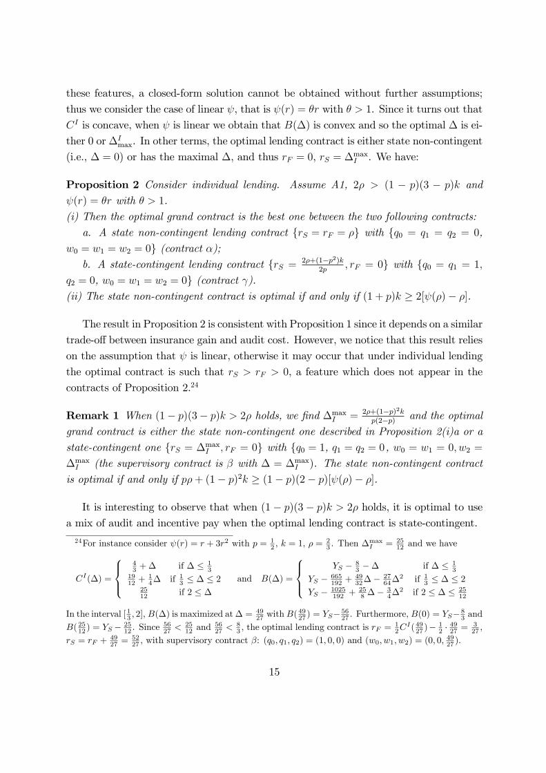
Proposition 2 Consider individual lending. Assume A1, 2� > (1 � p)(3 � p)k and

(r) = �r with � > 1.

(i) Then the optimal grand contract is the best one between the two following contracts:

a. A state non-contingent lending contract frS = rF = �g with fq0 = q1 = q2 = 0,

w0 = w1 = w2 = 0g (contract �);b. A state-contingent lending contract frS = 2�+(1�p2)k

2p; rF = 0g with fq0 = q1 = 1;

q2 = 0, w0 = w1 = w2 = 0g (contract ).(ii) The state non-contingent contract is optimal if and only if (1 + p)k � 2[ (�)� �].

The result in Proposition 2 is consistent with Proposition 1 since it depends on a similar

trade-o¤ between insurance gain and audit cost. However, we notice that this result relies

on the assumption that is linear, otherwise it may occur that under individual lending

the optimal contract is such that rS > rF > 0, a feature which does not appear in the

contracts of Proposition 2.24

Remark 1 When (1� p)(3� p)k > 2� holds, we �nd �maxI = 2�+(1�p)2k

p(2�p) and the optimal

grand contract is either the state non-contingent one described in Proposition 2(i)a or a

state-contingent one frS = �maxI ; rF = 0g with fq0 = 1, q1 = q2 = 0 , w0 = w1 = 0; w2 =

�maxI (the supervisory contract is � with � = �max

I ). The state non-contingent contract

is optimal if and only if p�+ (1� p)2k � (1� p)(2� p)[ (�)� �].

It is interesting to observe that when (1� p)(3� p)k > 2� holds, it is optimal to use

a mix of audit and incentive pay when the optimal lending contract is state-contingent.

24For instance consider (r) = r + 3r2 with p = 12 , k = 1, � =

23 . Then �

maxI = 25

12 and we have

CI(�) =

8><>:43 +� if � � 1

31912 +

14� if 13 � � � 2

2512 if 2 � �

and B(�) =

8><>:YS � 8

3 �� if � � 13

YS � 665192 +

4932��

2764�

2 if 13 � � � 2YS � 1025

192 +258 ��

34�

2 if 2 � � � 2512

In the interval [ 13 ; 2], B(�) is maximized at� =4927 withB(

4927 ) = YS� 56

27 . Furthermore, B(0) = YS� 83 and

B( 2512 ) = YS � 2512 . Since

5627 <

2512 and

5627 <

83 , the optimal lending contract is rF =

12C

I( 4927 )�12 �

4927 =

327 ,

rS = rF +4927 =

5227 , with supervisory contract �: (q0; q1; q2) = (1; 0; 0) and (w0; w1; w2) = (0; 0;

4927 ).

15

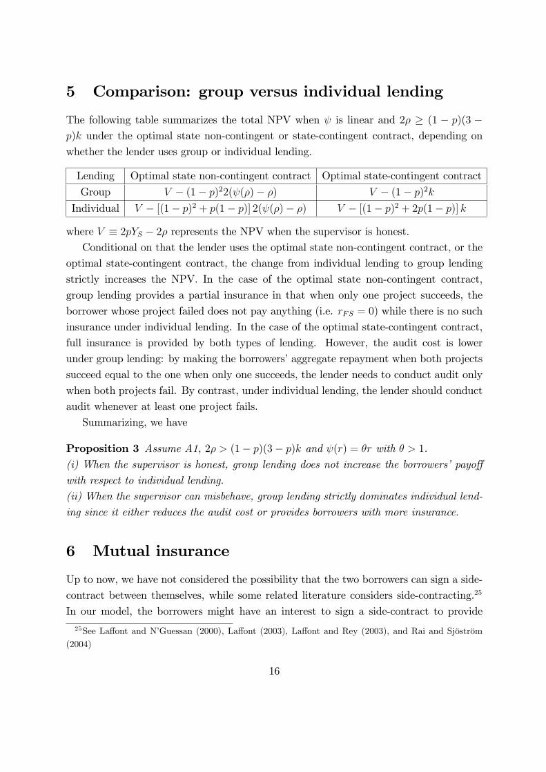
5 Comparison: group versus individual lending

The following table summarizes the total NPV when is linear and 2� � (1 � p)(3 �p)k under the optimal state non-contingent or state-contingent contract, depending on

whether the lender uses group or individual lending.

Lending Optimal state non-contingent contract Optimal state-contingent contract

Group V � (1� p)22( (�)� �) V � (1� p)2k

Individual V � [(1� p)2 + p(1� p)] 2( (�)� �) V � [(1� p)2 + 2p(1� p)] k

where V � 2pYS � 2� represents the NPV when the supervisor is honest.Conditional on that the lender uses the optimal state non-contingent contract, or the

optimal state-contingent contract, the change from individual lending to group lending

strictly increases the NPV. In the case of the optimal state non-contingent contract,

group lending provides a partial insurance in that when only one project succeeds, the

borrower whose project failed does not pay anything (i.e. rFS = 0) while there is no such

insurance under individual lending. In the case of the optimal state-contingent contract,

full insurance is provided by both types of lending. However, the audit cost is lower

under group lending: by making the borrowers�aggregate repayment when both projects

succeed equal to the one when only one succeeds, the lender needs to conduct audit only

when both projects fail. By contrast, under individual lending, the lender should conduct

audit whenever at least one project fails.

Summarizing, we have

Proposition 3 Assume A1, 2� > (1� p)(3� p)k and (r) = �r with � > 1.

(i) When the supervisor is honest, group lending does not increase the borrowers�payo¤

with respect to individual lending.

(ii) When the supervisor can misbehave, group lending strictly dominates individual lend-

ing since it either reduces the audit cost or provides borrowers with more insurance.

6 Mutual insurance

Up to now, we have not considered the possibility that the two borrowers can sign a side-

contract between themselves, while some related literature considers side-contracting.25

In our model, the borrowers might have an interest to sign a side-contract to provide

25See La¤ont and N�Guessan (2000), La¤ont (2003), La¤ont and Rey (2003), and Rai and Sjöström

(2004)

16

mutual insurance. More precisely, consider the timing in which, after accepting the lending

contract and before the realization of the state of nature, the borrowers sign a binding

side-contract which speci�es a state-contingent side-payment between themselves. Since

the lending contract and the agents are symmetric, a side-contract does not need to

specify any side-payment when both projects succeed or both fail. Hence, a side-contract

only speci�es a monetary transfer x that a borrower whose project succeeds makes to a

borrower whose project fails such that the latter uses x to make his repayment to the

lender. Note �rst that given a grand-contract, side-contracting has no impact on the

supervisor�s incentives since it does not a¤ect the borrowers�aggregate payment schedule.

Consider �rst group lending. Then, we can show that the optimal grand-contract

without side-contracting that we characterized in proposition 1 is still the optimal contract

even though the borrowers can sign a side-contract. Indeed, the only instrument of the

borrowers�coalition is x but this instrument is useless since the optimal contract speci�es

rFS = 0.

Consider now individual lending. First, we note that the outcomes that the lender

can achieve under individual lending are a subset of the outcomes achievable under group

lending regardless of whether or not the borrowers can sign a side-contract. Therefore,

the lender cannot obtain under individual lending an outcome superior to the best she can

achieve under group lending. Second, if side-contracting is possible, the lender can achieve

the outcome of the optimal state non-contingent group lending contract by o¤ering the

following individual lending contract GI� = frS = rF = �; wn = 0; qn = 0 for n = 0; 1; 2g.Under GI�, it is optimal for the borrowers to sign a side-contract specifying x� = �

because it maximizes the borrowers� ex ante expected payo¤s. Last, under individual

lending, side-contracting does not allow the lender to achieve the outcome of the optimal

state-contingent group lending contract in proposition 1(i)b. The latter contract speci�es

a repayment schedule such that 2rSS = rSF , rFS = rFF = 0. This kind of schedule cannot

be obtained under individual lending because rSS = rSF and rFS = rFF must hold. As

the table in section 5 reveals, the consequence is a higher audit cost under individual

lending. Summarizing, we have:

Proposition 4 (i) Under group lending, the optimal grand-contract is the same regard-less of whether or not the borrowers can sign a side-contract and the possibility of side-

contracting has no impact on their payo¤s.

(ii) When the borrowers can sign a side-contract,

a. the borrowers�payo¤s cannot be higher under individual lending than under group

lending.

17

b. If a state non-contingent contract is optimal under group lending, the maximal

payo¤s under group lending can be achieved also under individual lending by a grand-

contact which induces the borrowers to sign a side-contract for mutual insurance.

c. If a state-contingent contract is optimal under group lending, the borrowers�payo¤s

are strictly higher under group lending than under individual lending.

Proposition 4(ii)b implies that, conditional on that a state non-contingent contract is

optimal, our model does not necessarily predict that we should observe the use of group

lending.

7 Concluding remarks: transition from Grameen I to

Grameen II

Our paper studied the question of when it is optimal for a micro�nance institution to use

a state non-contingent repayment by focusing on the bank sta¤�s incentive to embezzle

borrowers�repayments. We found that if the optimal lending contract is state-contingent,

in the case of group lending it is optimal to induce a sta¤member to behave well by using

only audit even though a mix of audit and incentive pay can be used, whereas in the

case of individual lending a mix of both instruments become optimal for moderately large

audit cost. Therefore, a state non-contingent schedule is optimal if the cost of monitoring

the sta¤�s behavior is larger than the borrowers� gain from full insurance. When the

optimal lending contract is state non-contingent, group lending is preferred to individual

lending because the former provides borrowers with partial insurance. However, under

individual lending, the borrowers themselves have an incentive to mutually provide such

an insurance; then, individual lending is as good as group lending. When the optimal

lending contract is state-contingent, we showed that group lending is strictly preferred to

individual lending because the former allows to save audit cost.

Actually, the lending contract under Grameen I, the classic Grameen bank, speci�ed

a state non-contingent individual loan with joint liability26 but the bank discontinued the

26More generally, an individual lending contract with joint liability can be de�ned as the lending

contract in which the repayment schedule of each borrower of a group depends only on the return

realization of his own project but each borrower is responsible for the repayment of the other borrowers in

the group in case of default. Hence, joint liability can trigger a repayment game among the borrowers as

in Besley-Coate (1995). Our group lending contract is more general than the individual lending contract

with joint liability since the former includes the latter as a subset and in addition the former can specify

a repayment schedule that depends on the return realization of all group members�projects.

18

practice of joint liability after its transition to Grameen II. More precisely, Dowla and

Barua (2006) describe the transition, which was triggered by the �ood of 1998, the worst

in the history of Bangladesh, that made many borrowers unable to make repayments. This

transition is characterized by the switch from the rigid repayment schedule to �exible ones

that allow for rescheduling, the switch from joint liability to no joint liability, and new

emphasis on voluntary saving in individual account.

The Grameen bank was forced to allow for rescheduling after the �ood, otherwise there

would have been massive defaults. However, Grameen II does not distinguish common

shocks such as the �ood from individual shocks such as disease and shocks on project

return. Common shocks are observable to a third party including the lender and hence

providing insurance against common shocks does not involve any agency cost and is

desirable. For instance, rescheduling loan payments in a region severely a¤ected by the

�ood is optimal. On the contrary, providing insurance against individual shocks which

are observable only to the borrowers and the sta¤ member in charge of them, which is

the focus of our paper, can generate agency costs. Our paper suggests that the gain from

providing such an insurance should be carefully weighed against the cost of controlling

sta¤�s discretion.

Furthermore, even under Grameen II, most disbursement is made through "the basic

loan" specifying a rigid repayment schedule27. Our paper shows that in this case, joint

liability is not necessary since borrowers have an incentive to provide mutual insurance. In

addition, abandoning joint liability seems to be caused by the Grameen bank�s transfor-

mation as a saving (and lending) institution as well as its decision to introduce �exibility

to reschedule repayments. For instance, when members of a group have di¤erent saving

levels, the burden of joint liability becomes asymmetric and hence creates a tension, which

in turn reduces incentives to save.

References

Armendáriz de Aghion, B. 1999, �On the Design of a Credit Agreement with Peer

Monitoring�, Journal of Development Economics, 60:79-104

Armendáriz de Aghion, B. and C. Gollier. 2000, �Peer Group Formation in an Adverse

Selection Model�, Economic Journal, 110:632-64327According to the monthly report of February 20, 2010, among the outstand-

ing loans, the disbursement made through the basic loan is 756 million USD while

the one made through the �exible one is 27 million USD. See http://www.grameen-

info.org/index.php?option=com_content&task=view&id=453&Itemid=527 accessed on March 4,

2010.

19

Armendáriz de Aghion, B. and J. Morduch. 2005, The Economics of Micro�nance,

MIT.

Aubert, Cécile, Alain de Janvry and Elisabeth Sadoulet. 2005, �Incentives with

Non-Pro�t Objectives: Micro�ancne Agents and the Selection of Very Poor Borrowers�,

Mimeo, Université Paris Dauphine and University of California at Berkeley.

Bazoberry, Eduardo. 2001, �We Aren�t Selling Vacuum Cleaners: PRODEM�s Expe-

riences with Sta¤ Incentives�, Microbanking Bulletin, April:11-13.

Besley, T. and S. Coate. 1995, �Group Lending, Repayment, Incentives and Social

Collateral�, Journal of Development Economics, 46:1-18

Bond, P. and A. Rai. 2002, �Collateral Substitutes in Micro�nance�, Manuscript.

Bornstein, David. 1996, The Price of a Dream, University of Chicago, Chicago.

Che, Yeon-Koo. 2002, �Joint Liability and Peer Monitoring under Group Lending,�

Contributions to Theoretical Economics, 2, Article 3.

Conning, Jonathan. 1999, �Outreach, sustainability and leverage in monitored and

peer-monitored lending�, Journal of Development Economics, 60:51-77

Diamond, D. 1984, �Financial Intermediation and Delegated Monitoring,�Review of

Economic Studies, 51: 393-414.

Dowla, Asif and Dipal Barua. 2006. The Poor Always Pays Back: The Grameen II

Story. Kumarian Press, Inc.

Fantaye, Dawit Kiros. 2004, �Fighting Corruption and Embezzlement in Third World

Countries�, Journal of Criminal Law, 68(2): 170-176.

Faure-Grimaud, Antoine, Jean-Jacques La¤ont and David Martimort, 2003, �Collu-

sion, Delegation and Supervision with Soft Information�, Review of Economic Studies,

70:253-280.

Gale, D. and M. Hellwig, 1985, �Incentive-Compatible Debt Contracts: The One-

Period Problem,�Review of Economic Studies, 52: 647-663.

Ghatak, M. 1999, �Group Lending, Local Information and Peer Selection�, Journal of

Development Economics, 60:27-50

Ghatak, M. and T. W. Guinnane, 1999, �The Economics of Lending with Joint Lia-

bility: Theory and Practice�, Journal of Development Economics, 195-228

Jain, Sanjay and Ghazala Mansuri. 2003, �A Little at a time: The Use of Regularly

Scheduled Repayments in Micro�nance Programs�, Journal of Development Economics,

72:253-279

Jeon, Doh-Shin and Domenico Menicucci. 2009, �When Is the Optimal Lending Con-

tract in Micro�nance State Non-Contingent?�, Working paper, Universitat Pompeu Fabra.

20

Kofman, F. and Lawarrée, J. 1993, �Collusion in Hierarchical Agency�Econometrica,

61:629-656

La¤ont, J.-J. 2003, �Collusion and Group Lending with Adverse Selection�, Journal

of Development Economics, 70: 329-348

La¤ont, J.-J and D. Martimort. 2002. The Theory of Incentives: the Principal-Agent

Model. Princeton University Press.

La¤ont, J.-J and T. N�Guessan. 2000, �Group Lending with Adverse Selection�,

European Economic Review 44:773-784

La¤ont, J.-J. and P. Rey, 2003, �Moral Hazard, Collusion and Group Lending�,

Mimeo, University of Toulouse

La¤ont, J.-J. and J. Tirole. 1991, �The Politics of Government Decision Making: A

Theory of Regulatory Capture�, Quarterly Journal of Economics, 70: 329-348

Mknelly Barbara and Michael Kevane, 2000, �Improving Design and Performance of

Group Lending: Suggestion from Burkina Faso�, World Development 1060:1089-1127.

Morduch, Jonathan 1999, �The Micro�nance Promise�, Journal of Economic Litera-

ture, 37:1569-1614

Rai, A. and T. Sjöström. 2004, �Is Grameen Lending E¢ cient? Repayment Incentives

and Insurance in Village Economies�, Review of Economic Studies, 71:217-234.

Sadoulet, L., 2000, The Role of Mutual Insurance in Group Lending, Mimeo, ECARES.

Stiglitz, J. 1990, �Peer Monitoring and Credit Markets�, World Bank Economic Re-

view, 4(3): 351-366

Tirole, Jean, 1986, �Hierarchies and Bureaucracies: On the Role of Collusion in Or-

ganizations�, Journal of Law, Economics and Organization, 2:181-214

Townsend, R. 1979, �Optimal Contracts and Competitive Markets with Costly State

Veri�cation,�Journal of Economic Theory 21: 417-425

Townsend, R and J. Yaron. 2001, �The Credit Risk-Contingency System of An Asian

Development Bank,�Economic Perspectives Q3: 31-48

Varian, H. 1990, �Monitoring Agents With Other Agents�, Journal of Institutional

and Theoretical Economics 146: 175-176

Yunus, Muhammad, 1998, Banker to the Poor, University Press Limited.

AppendixProof of Lemma 1

Let R(1) be given, which means that rSF + rFS is given. We prove that if YS � R(1),

then it is optimal to set rFS = 0 and thus rSF = R(1). Since R(1) is given, (rSF ; rFS)

21

does not a¤ect (3) nor (BE) but a¤ects the borrowers�payo¤ only through the term

2p(1� p)[YS � rSF � (rFS)] = 2p(1� p)[YS �R(1) + rFS � (rFS)] (10)

in which the equality comes from rSF = R(1)�rFS. In writing (10), we implicitly assumedthat rSF � YS. As long as this condition holds, maximizing (10) with respect to rFS tells

us that any rFS > 0 is dominated by rFS = 0 since 0(r) > 1 for any r > 0. We prove

in Proposition 1 that the inequality rSF � YS is satis�ed in the optimal lending contract

given that A1(ii) holds.28

Proof of Lemma 2

Step 1 If G is such that (BE) is slack, then it is possible to increase the objective function;thus the solution to the relaxed problem (LrG) is such that (BE) binds. Moreover, w0 = 0

and q2 = 0.

Proof If (BE) does not bind in the solution to (LrG), then we can �nd an alternative

grand contract with reduced borrowers�payments, unchanged wages, and unchanged audit

probabilities, which yields a higher value for the objective function. Precisely, in each of

the following cases we reduce the borrowers�payments in a way that (i) satis�es (4) [given

that (4) was satis�ed initially]; (ii) leaves the right hand side of (BE) unchanged and

reduces slightly the left hand side of (BE), thus leaving (BE) satis�ed as (BE) was slack

initially; (iii) increases the borrowers�payo¤ since their payments are lower.

In case that rFF > 0, consider �rFF = �", �rSS = �" and either �rSF = �2" or�rFS = �2" (at least one between rSF and rFS is positive), for " > 0 and small: In thisway (4) is una¤ected. In case that rFF = 0, we examine two sub-cases. If rSF + rFS > 0,

consider �rSF = �2" or �rFS = �2" (at least one between rSF and rFS is positive) and�rFF = 0, �rSS = �": In this way �2 is unchanged and �1 is reduced, thus relaxing (4).

In case that rFF = 0 and rSF + rFS = 0, then consider �rSF = �rFS = �rFF = 0 and

�rSS = �": In this way �2 is reduced and �1 is unchanged, thus weakly relaxing (4).

In (LrG), (a) q2 appears only in the right hand side of (BE) and q2 = 0 relaxes (BE) most;

(b) w0 appears only in the right hand side of (BE) and in (4), and w0 = 0 relaxes these

constraints most.

Step 2 The solution to (LrG) is such that both (IC21) and (IC10) bind.

28Furthermore, if we allow for rFS < 0 then (10) becomes 2p(1 � p)[YS � R(1)] and does not depend

on rFS . However, since rSF = R(1) � rFS , a negative rFS makes rSF larger than R(1) and it is more

di¢ cult to satisfy rSF � YS .

22

Proof Constraint (IC10) binds since (a) the right hand side of (IC10) is non negative and

satisfying (IC10) implies that w1 � 0 holds; (b) reducing w1 reduces the �nancing cost

and relaxes (IC21).

Regarding (IC21), notice that if (IC21) is slack then q1 = 0, because when q1 > 0 it

is pro�table and feasible to reduce q1 in order to relax (BE) and increase the objective

function. Thus w2 > �2 + w1 needs to hold and there are two cases to consider: when

(IC20) binds and when (IC20) is slack. If (IC20) binds, then we have w2 = (1 � q0)�2 +

(1 � q0)�1 and hence w2 > �2 + w1 fails to hold because w1 = (1 � q0)�1. If (IC20) is

slack, then it is pro�table and feasible to reduce w2 in order to relax (BE) and increase

the objective function, contradicting optimality.

Step 3 The solution to (LrG) is such that �2 = 0, q1 = 0 and w2 = (1� q0)�1.

Proof Suppose that G is a solution to (LrG), so that the results in Steps 1 and 2 hold,

and moreover assume that �2 > 0. We show that there exists G0 which is strictly better

than G and satis�es �02 < �2. In this way we prove that whenever a lending contract is

such that �2 > 0, we can �nd another contract G0 with �02 < �2 which is strictly better

than G. Ultimately, this implies that the optimal contract is such that �2 = 0. We need

to distinguish the case in which (IC20) is slack from the case in which (IC20) binds.

If (IC20) is slack, then we pick G0 such that r0FS = rFS, r0SF = rSF+p2�p", r

0SS = rSS� 1�p

2�p",

r0FF = rFF for a small " > 0, thus �02 = �2�", �0

1 = �1+p2�p" and �

02+�

01 = �2+�1�

2(1�p)2�p ". Moreover, we set w

01 = w1 + (1� q0)

p2�p", w

02 = w2 + (1� q1)[�"+ (1� q0)

p2�p"]

and q0n = qn for n = 0; 1; 2. It is simple to see that the objective function has the same

value in G0 as in G since a borrower�s payment is unchanged when his project fails, and is

unchanged in expectation when his project is successful. Next we verify that G0 satis�es

(4) and that (BE) is slack in G0. Then Step 1 implies that the objective function can be

increased by reducing suitably the borrowers�payments.

In order to see that G0 satis�es (4), we notice that (IC21) and (IC10) are satis�ed in G0

given that they were satis�ed in G; (IC20) holds in G0 as it was slack in G and " > 0

is small. Regarding (BE), the left hand side is unchanged since the borrowers�expected

payment is the same as in G. On the other hand, the change in the expected wage paid

to the supervisor is

2p(1� p)(1� q0)p

2� p"+ p2(1� q1)[�"+ (1� q0)

p

2� p"] (11)

and now we prove that (11) is negative. First notice that from (IC21) binding and (IC20)

slack it follows that (1�q1)[�2+(1�q0)�1] > (1�q0)(�2+�1) and thus 1�q1 > 1�q0.Since �" + (1 � q0)

p2�p" < 0, we infer that (11) is smaller than 2p(1 � p)(1 � q0)

p2�p" +

23

p2(1� q0)[�"+ (1� q0)p2�p"] = �

p3(1�q0)q02�p " � 0; therefore (BE) is slack in G0.

If (IC20) binds, then using (IC21) we �nd

(1� q1)[�2 + (1� q0)�1] = (1� q0)(�2 +�1) (12)

Suppose that q1 = 0. Then (12) reduces to �2+(1� q0)�1 = (1� q0)(�2+�1) and thus

q0 = 0. Therefore w1 = �1, w2 = �1+�2 and since rSF = 2rFF+�1 and 2rSS = rSF+�2,

it turns out that (BE) reduces to rFF = �. Then consider G0 such that r0FF = �, r0FS = 0,

rSF = 2�, rSS = � (thus �02 = �

01 = 0) and w

0n = 0, q

0n = 0 for n = 0; 1; 2. In this way

(4) is satis�ed, (BE) holds with equality and each borrower�s payment is the same as in

G when his project fails, but is smaller in expectation when his project is successful; thus

the objective function increases.

Now we consider the case in which q1 2 (0; 1] and from (12) we �nd 1� q1 � 1� q0, whichis equivalent to q0 � q1. Consider G0 such that r0FF = rFF , r0FS = rFS, r0SF = rSF +

p2�p�2,

and r0SS = rSS� 1�p2�p�2; thus�0

1 = �1+p2�p�2, �0

2 = 0, �01+�

02 = �1+

p2�p�2. Moreover,

we set w01 = w1 + (1� q0)p2�p�2, w02 = w2 � (1� q0)

2�2p2�p �2 and q02 = 0, q

01 = q1 � " with

" > 0 and small, q00 = q0. In G0, the borrowers�payo¤ is the same as in G since the

payment of each borrower is unaltered when his project fails, and his payment in case of

success is unchanged in expectation. Next we verify that G0 satis�es (4) and that (BE) is

slack in G0. Then Step 1 implies that the objective function can be increased by reducing

suitably the borrowers�payments.

We start by noticing that (4) is satis�ed. This is immediate for (IC10) and (IC20), while

(IC21) reduces to

w2 � (1� q0)2� 2p2� p

�2 � (1� q1 + ")[w1 + (1� q0)p

2� p�2] (13)

Since (IC21) binds in G, we have that w2 = (1� q1)(�2+w1) and thus (13) boils down to

[(2� p� q1p)q0 � 2(1� p)q1]�2 � "[(2� p)w1 + (1� q0)p�2] (14)

In order to see that (14) is satis�ed, notice that if q1 2 (0; 1) then q0 � q1 implies

(2 � p � q1p)q0 � 2(1 � p)q1 � (2 � p � q1p)q1 � 2(1 � p)q1 = q1(1 � q1)p > 0, and thus

(14) holds since " > 0 is close to zero. If instead q1 = 1, then q0 = 1 by (12) and w1 = 0

given that (IC10) binds in G; then (14) is satis�ed again.

Regarding (BE), we see that (i) the borrowers�expected payment is the same as in G; (ii)

the expected wage bill is the same as in G; (iii) the cost of auditing is reduced as q01 < q1.

Finally, after �nding that �2 = 0, from (IC20) we obtain (1� q1)(1� q0)�1 � (1� q0)�1.

If (1�q0)�1 > 0, then we obtain q1 = 0; if (1�q0)�1 = 0, then q1 could be any number in

[0; 1], but q1 = 0 is optimal to minimize the �nancing cost. In either case, w2 = (1�q0)�1.

24

Proof of Proposition 1

The proof of Proposition 1(i) appears in the text. Proposition 1(ii) follows by comparing

the borrowers�payo¤s in the two contracts described in Proposition 1(i).

It is simple to verify that the neglected upward incentive constraints (IC12), (IC02), (IC01)

are satis�ed by the two contracts in Proposition 1(i).

Furthermore, we verify that YS is large enough, given A1, to make the borrowers�payo¤

positive in the optimal grand contract and to satisfy Lemma 1. First consider the state

non-contingent contract described in (i)a. The borrowers� payo¤ with this contract is

2pYS�2��2(1�p)2[ (�)��] and A1(i) implies that this payo¤ is positive.29 Furthermore,the condition rSF � YS is satis�ed since rSF = 2� < �max

1 and A1(ii) requires YS ��max1 . Regarding the state-contingent contract described in (i)b, the borrowers�payo¤

is 2pYS � p(2 � p)�max1 = 2pYS � 2� � (1 � p)2k which is positive by A1(i). Finally,

rSF = �max1 and thus rSF � YS is satis�ed because of A1(ii).

Proof of Lemma 3

We start with a preliminary result which helps prove Lemma 3.

Lemma 6 Consider a lending contract frSS; rSF ; rFS; rFFg such that rFS = 0 and rFF >0. Next, consider a lending contract fr0SS; r0SF ; r0FS; r0FFg such that r0FS = 0, r0FF < rFF

and such that the borrowers�expected payment is the same in the two contracts. Then the

borrowers�payo¤ is larger with the second contract

Proof. Let C � p22rSS+2p(1�p)rSF+(1�p)22rFF = p22r0SS+2p(1�p)r0SF+(1�p)22r0FFdenote the borrowers�expected payment under either contract. The borrowers�payo¤with

frSS; rSF ; rFS; rFFg is 2pYS � C + (1 � p)22rFF � (1 � p)22 (rFF ), and is decreasing in

r0FF since 0(r) > 1 for any r > 0. Given that r0FF < rFF , it follows that borrowers prefer

fr0SS; r0SF ; r0FS; r0FFg to frSS; rSF ; rFS; rFFg.Now we prove Lemma 3 by considering all the possible cases in which �1 < 0 and/or

�2 < 0: In any such case we prove that it is possible to increase (weakly) the borrowers�

payo¤ by satisfying �1 � 0 and �2 � 0. In particular, we need to consider four di¤erentregimes.

1. R(0) � maxfR(1); R(2)g: regime B.29Notice that A1 is more restrictive than needed for the case of group lending because we want the

same assumption to cover the case of individual lending as well.

25

Let GB denote the best grand contract within the set of grand contracts satisfying R(0) �R(1) and R(0) � R(2). We show that GB = G0, with R0(0) = R0(1) = R0(2) = 2� and

w00 = w01 = w02 = 0, q00 = q01 = q02 = 0; thus, GB satis�es �1 � 0 and �2 � 0. It is

easy to see that G0 is feasible because it satis�es (3) and (BE). The borrowers�payo¤

in G0 is 2pYS � p2R0(2) � 2p(1 � p)R0(1) � (1 � p)22 (R0(0)2) because A1(ii) implies that

YS > R0(1) = 2� and thus Lemma 1 applies. The borrowers�payo¤with a grand contract

G such that R(0) > maxfR(1); R(2)g or R(0) = maxfR(1); R(2)g > minfR(1); R(2)gis smaller than payo¤ with G0 because of the following arguments. First, suppose for

the moment that the borrowers� expected payment is the same in G as in G0. Then

G0 is better than G because of Lemma 6, given that R0(0) = R0(1) = R0(2) implies

R(0) > R0(0). Second, the expected payment in G is actually larger than in G0 because

R(0) = R(1) = R(2) fails to hold and therefore the �nancing cost is larger than 2�

since some cost must be borne to discourage embezzlement. Third, while YS � R0(1)

holds, it may be that YS < R(1) and in this case borrowers face some cost from reducing

consumption in states SF and FS and not only in state FF .

2. R(2) � R(0) � R(1): regime C.

We show that within the set of grand contracts satisfying R(2) � R(0) � R(1), the best

contract GC is such that RC(0) = RC(1) and therefore �1 � 0 and �2 � 0 are satis�ed.Let �20 � R(2) � R(0) � 0 and �01 � R(0) � R(1) � 0. We study the following

relaxed program in which we consider only (IC21), (IC20) and (IC01) among the incentive

constraints: 8><>:(IC21) w2 � (1� q1)(�20 +�01 + w1)

(IC20) w2 � (1� q0)(�20 + w0)

(IC01) w0 � (1� q1)(�01 + w1)

(15)

We prove that GC is such that�C01 = 0 by showing that starting from any feasible contract

G satisfying�01 > 0, we can �nd G0which is strictly better than G and such that�001 = 0.

Precisely, let w0n = wn, q0n = qn for n = 0; 1; 2 and R0(1) = R(1) + [p2 + (1 � p)2]�01,

R0(2) = R(2) � 2p(1 � p)�01, R0(0) = R(0) � 2p(1 � p)�01; then �001 = 0 < �01 and

�020 = �20. As a consequence, the incentive constraints in (15) are weakly relaxed and the

borrowers�expected payment is unchanged; thus G0 satis�es (BE) and (15), given that G

is feasible. Furthermore, R0(1) > R(1) and R0(0) < R(0) and thus Lemmas 1 and 6 imply

that the borrowers�payo¤ is higher in G0 than in G as long as YS � R0(1). This proves

that GC is such that�C01 = 0 as long as R

C(1) � YS. Now we characterize a few properties

of GC under the assumption that YS is large enough and then verify that YS � RC(1)

given A1(ii). When �01 = 0 and �20 � 0 it is optimal to set (i) q2 = 0, w1 = 0 (we can

26

argue like in the proof of Step 1 in the proof of Lemma 2), w0 = 0 because the right hand

side of (IC01) is 0; (ii) q1 = q0 = q because if q1 > q0 (for instance), then (IC20) binds,

(IC21) is slack and it is pro�table to reduce q1 slightly in other to reduce the audit cost

kq1 without a¤ecting w2. Then (IC21) is equivalent to (IC20) and w2 = (1� q)�20. From

(BE) binding we �nd R(1) + p2�20 = 2� + p2(1 � q)�20 + (1 � p2)kq. The right hand

side, that is the �nancing cost, is linear in q and thus is minimized with respect to q at

q = 0 or at q = 1. In either case we �nd R(1) � 2� and A1(ii) implies that 2� is smallerthan YS. Finally, given w2 = (1 � q)�20, the incentive constraints neglected in (15) are

satis�ed and we have proved that GC satis�es �01 = 0.

3. R(1) � R(2) � R(0): regime D.

We show that within the set of grand contracts satisfying R(1) � R(2) � R(0), the best

contract GD is such that RD(1) = RD(2), and therefore it satis�es �1 � 0 and �2 � 0.Let �12 � R(1)�R(2) � 0 and �20 � R(2)�R(0) � 0. We study a relaxed program in

which we consider only (IC12), (IC10) and (IC20) among the incentive constraints:8><>:(IC12) w1 � (1� q2)(�12 + w2)

(IC10) w1 � (1� q0)(�12 +�20 + w0)

(IC20) w2 � (1� q0)(�20 + w0)

(16)

By arguing as in Steps 1-2 in the proof of Lemma 2 we �nd that in any solution to

the relaxed problem w0 = 0, q1 = 0, (IC20) and (IC12) bind; thus w2 = (1 � q0)�20

and w1 = (1 � q2)[�12 + (1 � q0)�20]. Now suppose that G is a solution to the relaxed

problem and such that �12 > 0. We �nd G0 which is weakly better than G and satis�es

�012 < �12. Let R0(2) = R(2) + 2(1�p)

2�p ", R0(1) = R(1) � p

2�p" and R0(0) = R(0) with

" > 0 and small; thus �012 = �12 � ", �0

20 = �20 +2(1�p)2�p " and �

012 + �

020 = �12 +

�20 � p2�p". Furthermore, we set w

02 = w2 + (1 � q0)

2(1�p)2�p " and w

01 = w1 � (1 � q0)

p2�p"

and q0n = qn for n = 0; 1; 2. First we verify that G0 is feasible. Given that (16) holds

in G, it follows that (IC20) and (IC10) are satis�ed in G0. On the other hand, (IC12)

reduces to w1 � (1 � q0)p2�p" � (1 � q2)[�12 � " + w2 + (1 � q0)

2(1�p)2�p "] and we know

that w1 = (1 � q2)(�12 + w2) given that (IC12) binds in G. We need to prove that

(1� q2)["� (1� q0)2(1�p)2�p "] � (1� q0)

p2�p". From inserting the binding (IC12) and (IC20)

into (IC10), we obtain (1 � q2)[�12 + (1 � q0)�20] � (1 � q0)(�12 + �20), which implies

1�q2 � 1�q0. Thus (1�q2)["� (1�q0)2(1�p)2�p "] � (1�q0)["� (1�q0)2(1�p)2�p "] and it turns

out that (1� q0)["� (1� q0)2(1�p)2�p "] � (1� q0)

p2�p" holds. Regarding (BE), we �nd that

the expected wage paid to the supervisor in G0 is the same as in G and the borrowers�

expected payment is the same as in G; thus (BE) holds in G0 as it holds in G. Finally, the

27

borrowers�payo¤ is the same in G0 as in G. In this way we have proved that whenever

the lending contract is such that �12 > 0, there exists another feasible contract which is

at least as good and has a smaller �12. Therefore we can �nd a solution to the relaxed

problem by restricting our attention to contracts such that �12 = 0.

Given �12 = 0, we can argue like in the end of the proof of Step 3 in the proof of Lemma

2 to �nd that (IC10) implies q2 = 0 and w1 = (1� q0)�20. This implies that the incentive

constraints which have been neglected are satis�ed. Therefore, in regime D there is no

loss of generality in considering only the contracts such that �12 = 0.

4. R(1) � R(0) � R(2): regime E.

We show that within the set of grand contracts such that R(1) � R(0) � R(2) the

best contract GE is such that RE(0) = RE(2); therefore, it belongs to regime D. Let

�10 � R(1) � R(0) � 0 and �02 � R(0) � R(2) � 0. We study the relaxed program in

which we consider only (IC10), (IC12) and (IC02) among the incentive constraints:8><>:(IC10) w1 � (1� q0)(�10 + w0)

(IC12) w1 � (1� q2)(�10 +�02 + w2)

(IC02) w0 � (1� q2)(�02 + w2)

(17)

Suppose that G is feasible in the relaxed problem and such that �02 > 0. Then we �nd G0

which is strictly better than G and satis�es �002 = 0. Precisely, let w

0n = wn and q0n = qn

for n = 0; 1; 2 and R0(2) = R(2)+(1�p2)�02, R0(1) = R(1)�p2�02, R0(0) = R(0)�p2�02;

then �002 = 0 < �02 and �0

10 = �10. As a consequence, the incentive constraints in (17)

are weakly relaxed. Furthermore, the borrowers� expected payment and the expected

wage bill are unchanged, thus (BE) is satis�ed. Since R0(1) < R(1) and R0(0) < R(0),

Lemma 6 implies that the borrowers�payo¤ is larger in G0 than in G. Given �02 = 0

we can argue as in the proof of Step 1 in the proof of Lemma 2 and as in the analysis

of regime C in this proof of Lemma 3 to �nd that w2 = 0, q1 = 0, w0 = 0 and q0 = q2,

w1 = (1 � q0)�10; this implies that the incentive constraints which have been neglected

are satis�ed. This proves that GE satis�es �02 = 0.

Proof of Lemma 4

Suppose that a grand contract G = frS; rF ; w2; w1; w0; q2; q1; q0g is feasible and such thatrS < rF . Then we can �nd G0 = fr0S; r0F ; w02; w01; w00; q02; q01; q00g which is feasible andincreases the borrowers�payo¤ with respect to G. Precisely, let r0S = r0F = re � prS +

(1 � p)rF and w02 = w01 = w00 = 0, q02 = q01 = q00 = 0. Then (a) G0 satis�es all the

incentive constraints since � = 0; (b) the �nancing cost with G0 is equal to 2�, which is

28

the minimum feasible cost and thus it cannot be larger than the cost under G; (c) the

borrowers�expected payment [the left hand side of (BE)] with G0 is the same as the one

with G. Hence G0 is feasible and the borrowers�payo¤ is 2[pYS � pre � (1 � p) (re)].

The inequality 2[pYS � pre � (1 � p) (re)] > 2[pYS � prS � (1 � p) (rF )] is equivalent

to (rF ) � (re) > p1�p(r

e � rS) and we havep1�p(r

e � rS) = rF � re. Therefore, the

borrowers�payo¤ is higher in G0 than in G given that 0(r) > 1 for any r > 0.

Proof of Lemma 5

When � = 0, contract � satis�es (7) and is the optimal supervisory contract as

it generates a �nancing cost equal to 2�, which is the minimum feasible value. In the

following we consider the case of � > 0.

Given � > 0, we can argue like in Steps 1 and 2 of the proof of Lemma 2 to prove that

q2 = 0, w0 = 0 and (IC10) and (IC21) bind; thus w1 = (1�q0)� and w2 = (1�q1)(2�q0)�.Furthermore, (IC20) reduces to q1 � f(q0), where f(q0) � q0

2�q0 is an increasing and convex

function such that f(0) = 0 and f(1) = 1. The feasible set F for (q0; q1) is therefore

F =�(q0; q1) 2 R2+ : q0 � 1 and q1 � f(q0)

. The total �nancing cost is

Q(q0; q1) = 2�+ p2(1� q1)(2� q0)� + 2p(1� p)[(1� q0)� + kq1] + (1� p)2kq0

and no point in the interior of F minimizes Q since the Hessian matrix of Q is inde�nite

for any (q0; q1):@2Q

@q20=@2Q

@q21= 0 and

@2Q

@q0@q1= p2� > 0

This violates the second order condition for a minimum, which requires the Hessian matrix

to be positive semi-de�nite.

We can neglect any point (q̂0; 0) on the south boundary of F such that q̂0 2 (0; 1) becauseQis linear in q0 and therefore minfQ(0; 0); Q(1; 0)g � Q(q̂0; 0) for any q̂0 2 (0; 1). Likewise,we can neglect any point (1; q̂1) on the east boundary of F such that q̂1 2 (0; 1) becauseQ is linear in q1. As a consequence, only (q0; q1) = (1; 0) may be a minimum point for Q

in the subset of F in which (IC20) is slack, and that corresponds to contract �.

When also (IC20) binds, we have q1 = f(q0) and Q(q0; q1) is equal to

�Q(q0) � Q[q0; f(q0)]

= 2�+ p2[1� f(q0)](2� q0)� + 2p(1� p)[(1� q0)� + kf(q0)] + (1� p)2kq0

= 2�+ 2p(1� p)kf(q0) + (1� p)2kq0 + 2p(1� q0)�

29

Since f is convex, also �Q is so. Hence, �Q is minimized at q0 = 0 if �Q0(0) � 0 (contract�), at q0 = 1 if �Q0(1) � 0 (contract ), at some q�0 2 (0; 1) if �Q0(0) < 0 < �Q0(1). However,

q�0 is such that �Q0(q�0) = 0 which is equivalent to

@Q[q�0 ;f(q�0)]

@q0+

@Q[q�0 ;f(q�0)]

@q1f 0(q�0) = 0. Since

f 0(q�0) > 0, it must be the case that @Q[q�0 ;f(q�0)]

@q0< 0 <

@Q[q�0 ;f(q�0)]

@q1, or @Q[q�0 ;f(q

�0)]

@q0� 0 �

@Q(q�0 ;f(q�0)]

@q1. In the �rst case we do not have an optimal supervisory contract because it is

possible to reduce the cost by slightly increasing q0 above q�0 and/or by slightly decreasing

q1 below q�1 = f(q�0). The proof is completed by showing that the second case cannot

arise. Indeed, we �nd

@Q

@q0= �p2(1� q1)�� 2p(1� p)� + (1� p)2k

@Q

@q1= �p2(2� q0)� + 2p(1� p)k

Then @Q@q1

� 0 is equivalent to k � p(2�q0)2(1�p) � and this inequality implies @Q

@q0� �p2(1 �

q1)� � 2p(1 � p)� + 12p(1 � p)(2 � q0)�. The right hand side of the last inequality is

smaller than ��p(1� p) < 0 for any (q0; q1) 2 [0; 1]2.

Proof of Proposition 2

The proof of Proposition 2(i)a-b appears in the text.

It is simple to verify that the neglected upward incentive constraints (IC12), (IC02), (IC01)

are satis�ed by the two contracts described by Proposition 2(i).

Furthermore, we verify that YS is large enough to make the borrowers�payo¤ positive in

the optimal grand contract. For the state non-contingent contract described in (i)a, the

borrowers�payo¤ is 2pYS � 2� � 2(1 � p)[ (�) � �] and A1(i) implies that this payo¤ is

positive. For the state-contingent contract described in Proposition 2(i)b, the borrowers�

payo¤ is 2(pYS � p�maxI ) = 2pYS � 2�� (1� p2)k and is positive given A1(i).

30