Wave Prediction and Robust Control of Heaving Wave Energy Devices for Irregular Waves

IEEE TRANSACTIONS ON ENERGY CONVERSION, VOL. 26, NO. 2, JUNE 2011 627

Wave Prediction and Robust Control of HeavingWave Energy Devices for Irregular Waves

Marco P. Schoen, Senior Member, IEEE, Jørgen Hals, and Torgeir Moan

Abstract—This paper presents a comparison of different existingand proposed wave prediction models applicable to control waveenergy converters (WECs) in irregular waves. The objective of thecontrol is to increase the energy conversion. The power absorbedby a WEC is depending on the implemented control strategy. Un-certainties in the physical description of the system as well as in theinput from irregular waves provide challenges to the control algo-rithm. We present a hybrid robust fuzzy logic (FL) controller thataddresses the uncertainty in the model and the short-term tuningof the converter. The proposed robust controller uses the energyfrom the power take off as input, while the FL controller portionis used for short-term tuning. The FL controller action is based ona prediction of the incoming wave. Simulation results indicate thatthe proposed hybrid control yields improved energy production,while being robust to modeling errors.

Index Terms—Control systems, energy conversion, intelligentsystems, prediction methods.

I. INTRODUCTION

THE energy absorption of wave energy converters (WECs)is influenced by the use of the knowledge of future wave

data in the control loop. The prediction of future wave data is nota trivial undertaking, since real waves are irregular in nature. Anumber of contributions have been made in forecasting irregularwaves. For example, Forsberg [1] introduced an autoregressive(AR) with moving average (ARMA) model with fixed time hori-zon prediction, utilizing the maximum likelihood estimation todescribe ocean waves off the coast of Sweden. The algorithmincluded the on-line recursive form with an adaptation constantfor slowly time-varying sea condition. Results of the proposedalgorithm included prediction of waves for long time horizon,i.e., 30 s using a 0.5 s sample time, yielding predictions withadequate results. Noise considerations were given only to theextent that outliers are removed through the standard outlierdetection rule. Forsberg’s model requires an extensive modelorder in order to capture the nature of irregular waves. Hallidayet al. [2] looked at using the fast fourier transform (FFT) togenerate prediction of waves over distance. The distance factor

Manuscript received May 29, 2010; revised September 1, 2010; acceptedDecember 1, 2010. Date of publication February 4, 2011; date of current ver-sion May 18, 2011. Paper no. TEC-00239-2010.

M. P. Schoen is with Idaho State University, Pocatello, ID 83209 USA(e-mail: schomarc@ isu.edu).

J. Hals and T. Moan are with the Center for Ships and Ocean Structures(CeSOS), Norwegian University of Science and Technology (NTNU), 7491Trondheim, Norway (e-mail: [email protected]; [email protected]).

Color versions of one or more of the figures in this paper are available onlineat http://ieeexplore.ieee.org.

Digital Object Identifier 10.1109/TEC.2010.2101075

is used to avoid perturbations of the buoy to the measurements.This approach necessitates the use of directional data. The sim-ulation results presented indicate reasonable success for longdistances. One of the drawbacks of using the approach of Halli-day et al. is that the spectral estimates of the FFT-based modelsare less sensitive to sharp peaks and dips compared with ARmodels, [3]. In addition, the FFT is for strictly stationary sys-tems, and cannot handle the temporal fluctuations, which is anessential component in the characteristics of irregular waves.

WECs operating in irregular waves can be categorized intopassive- and active-tuning-based control. Relevant study hasbeen reported in the literature since the mid 1970s [4]. Tuningcan be achieved by adapting the WECs power take off’s (PTO)stiffness and damping to match the incident wave frequency andthe radiation wave damping coefficient, respectively. Extensivereview of this is given by Falnes [5], which includes the discus-sion of optimal control and phase control for WECs. Latchingcontrol attempts to achieve the same effect by halting the de-vice’s motion in order to align the phase of the system withthe wave motion. Study on latching control has been reportedby Korde [6], [7]. Optimal latching control is discussed in [8],where two analytical solutions are presented: one based on theequation of motion and the other based on optimal commandtheory. Using the future wave excitation, Babarit et al. in [9]investigated three strategies for latching control. Though the fu-ture wave excitation was not computed (assumed to be known),the study has value in terms that it showed the improvement ofthe energy absorbed using the wave excitation for the latchingtime computation. Optimality, in terms of energy, production ofWECs has been addressed in many instances in aforementionedliterature and elsewhere. Intelligent systems, such as geneticalgorithms (GAs) may present an avenue to avoid the local min-ima problem, and is to some limited extend explored in thispaper.

In this paper, we will propose a hybrid Kautz/AR predictivemodel as well as a pure predictive Kautz model and comparethem to a predictive AR and ARMA algorithm. The outcomeof our investigation into predictive models will be utilized todesign predictive fuzzy logic (FL)/robust controllers. The pre-diction models are based on local wave height measurements andassume an unperturbed wave. We also attempt to address someof the robustness aspects in designing a controller for WECs.The robustness issues are primarily focused on the uncertaintyof parameters describing the dynamics of the buoy and not onimproved performance. The performance issues are addressedby a proposed simple FL controller, which is responsible forthe short-term control of the device in order to maximize theenergy production. The proposed controllers in this paper do

0885-8969/$26.00 © 2011 IEEE

628 IEEE TRANSACTIONS ON ENERGY CONVERSION, VOL. 26, NO. 2, JUNE 2011

not employ latching control technology, rather use the resistiveforces of the PTO to improve the performance of the WEC. Thepaper is organized in two parts. First, we describe the pursuitof finding predictive models that work well in a stochastic envi-ronment are of low model order (parametric models), and havea sufficient accuracy that allows the algorithm to be used forcontrol of WECs operating in irregular waves. In the secondpart, we propose a robust controller and combine this with a FLcontroller.

II. WAVE PREDICTION MODELS

A. AR Predictive Model

Consider a simple discrete time finite impulse response (FIR)AR model to characterize irregular waves

�y(k|k − 1) =p∑

j=1

aj �y(k − j) (1)

where the output �y ∈ Rno x1 is the wave height with no = 1 and

is measured up to time t = k − 1, k is the discrete time index,p is the model order, aj ∈ R

no ×no are the influence coefficientmatrices, and ˆ denotes the predicted value. One of the mainproblems in fitting such a time series to the gathered data is thedetermination of the model order. Based on the Wold decompo-sition theorem, an AR model can fit a variety of data character-istics, if a sufficiently large model order is selected [10].

To construct a variable horizon prediction formulation on thebasis of (1) the following i-step-ahead predictor can be estab-lished (see [11])

�y(k + i|k − 1) =p∑

j=1

a(i)j �y(k − j) (2)

where we made use of the residual, which is defined by thedifference of the estimate and the true output, i.e., �ε = �y − �y.The corresponding predictive coefficient matrices are:

a(i)j = a(i−1)

1 aj + a(i−1)j+1 . (3)

One can easily argue that by any standard, the predictive modelintroduced above possesses a rather large model order. Hence,the corresponding correlation matrix utilized in the estimationalgorithm induces a large computational burden during the op-eration of the filter, in particular when repeated estimations areneeded to update to the current wave conditions. This is true tosome degree also for the recursive least squares (RLSs) method,even though no inversion of large matrices is required; the modelorder dictates the number of computations needed. This prop-erty of large model order is a general characteristic of FIR filtersdue to the missing feedback term in the filter structure. We caninvestigate the contribution of each filter weight to the predictedoutput by computing the transformed filter weights as follows:starting with the formulation for the estimated filter parametermatrices (least squares)

θAR = (ΦTARΦAR)−1ΦT

ARYAR (4)

where θAR is a vector containing the estimated parameter matri-ces, ΦAR is the information matrix, and YAR is the respective

output vector. Defining Xss = ΦTARYAR , the updated parame-

ter estimate is θAR(k + 1|k) = P (k + 1) × Xss(k + 1). Intro-ducing the modal matrix Q composed of the eigenvectors ofP = (ΦT

ARΦAR) and diagonal eigenvalue matrix Λ of the cor-relation matrix P, the transformed filter weight vector resultsinto

θ′AR(k + 1|k) = QT θAR(k + 1|k). (5)

Transforming Xss : PθAR(k + 1|k) = Xss(k + 1)

XSS(k+1) =QΛQT ×Qθ′AR(k + 1|k) =QΛθ′AR(k + 1|k)

Defining X ′ss = ΦT

ARXss , which premultiplied with QT

yields

X ′ss(k + 1) = Λθ′AR(k + 1|k). (6)

Using x′i as the elements in x′

ss and λi as the correspondingeigenvalues found on the diagonal of Λ, each individual trans-formed filter weight contribution is given by

a′(0)i =

x′i

λi, for 1 ≤ i ≤ p. (7)

B. ARMA Predictive Model

Adding to the AR formulation a MA part enhances the flex-ibility of the AR model [12]. Consider a typical ARMA modelin the output error formulation

�y(k|k − 1) =p∑

j=1

aj �y(k − j) +p∑

m=0

bm�ε(k − m) (8)

where aj and bj are the ARMA filter matrices. The MA asso-ciated with the bj matrices is nonlinear due to the predictionerror formulation. The model can be constructed through back-substitution of the output into the original filter model formula-tion. An i-step ARMA predictor thus can be given as

�y(k + i|k − 1) =p∑

j=1

a(i)j �y(k − j) +

p∑

m=1

b(i)m �ε(k − m) (9)

where the predictive parameters for the past residual terms aredefined as

a(i)j = a(i−1)

1 a(0)j + a(i−1)

j+1

for j = 1, 2, 3, . . . and ak = 0, for k > p.The predictive parameters for the MA terms are defined as

b(i)m = a(i−1)

1 b(0)m + b(i−1)

m+1

for m = 1, 2, 3, . . . and bk = 0, for k > p.The estimation of these parameters can be done, for example,

by following the Hannan–Rissanen algorithm [13].

C. Orthogonal Basis Function (OBF) Prediction Model

One of the main reasons AR and ARMA models require largemodel orders is that they are of the type FIR filter, and they donot have a structure that allows for inclusion of prior knowledgeinto the filter before the estimation occurs. AR models belong

SCHOEN et al.: WAVE PREDICTION AND ROBUST CONTROL OF HEAVING WAVE ENERGY DEVICES FOR IRREGULAR WAVES 629

to the class of orthogonal basis functions (OBFs), which are thegeneralizations of FIR models. The basis function of FIR modelsare delayed Dirac impulses expressed with the q-operator (delayoperator). In the pursuit of reducing the required model orderwhile still describing the future waveform adequately, we pro-pose to choose orthonormal filters Li (q) such that (1) becomes

�y(k + i|k − 1) =p∑

i=1

ciLi(q)�y(k). (10)

To keep the selected OBF model linear in the parameters, Li(q)are chosen before the estimation of the filter coefficient matricesci occurs. Li(q)’s are chosen with the purpose of incorporatingprior knowledge of the system to be modeled. Since the wavesexhibit an underdamped dynamical characteristic, we chooseKautz filters for the Li(q)’s. Kautz filters allow us to incorporateconjugate complex pole pairs into the model. Considering agiven conjugate complex pole pair (α ± iβ), the Kautz filtercoefficients are computed by

c =2α

1 + α2 + β2 and d = −(α2 + β2). (11)

With this, the filter Li(q) can now be computed using thefollowing orthonormalization process:

L1(q, c, d) =

√(1 − c2)(1 − d2)

q2 + c(d − 1)q − d(12)

L2(q, c, d) =

√(1 − d2)(q − c)

q2 + c(d − 1)q − d(13)

and the higher order filter parameters by using the recursiveformula as follows:

L2i−1(q, c, d) = L2(i−1)−1(q, c, d)−dq2 + c(d − 1)q + 1q2 + c(d − 1)q − d

L2i(q, c, d) = L2(i−1)(q, c, d)−dq2 + c(d − 1)q + 1q2 + c(d − 1)q − d

.

The limits on the coefficients c and d are given as

−1 < c < 1 and − 1 < d < 1.

In addition to having a purely predictive Kautz filter, one canincorporate as well some simple AR terms, resulting into hybridKautz/AR filters. The step-by-step procedure for constructingand estimating a proposed predictive Kautz or hybrid Kautz/ARfilter is given in the following. A recursive formulation can bedeveloped using the RLS approach, which is left for future work.

Step 1: Collect a sufficient amount of wave height mea-surements y(k), with a fixed sampling time. Normalize thewave height time series using y(k) = y(k)/ymax , where ymax =sup{y(k)}.

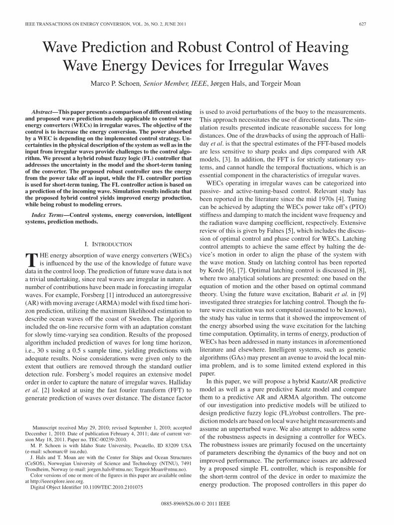
Fig. 1. Influence of Kautz parameters on prediction.

Step 2: Perform a spectral analysis and identify the frequencyω1 with the largest contribution or magnitude in the spectrum.

Step 3: Compute the Kautz filter coefficients c and d basedon the identified frequency ω1 ; also assume a damping ratio ξ.The computation of the filter coefficients c and d require thereal and imaginary parts of the dominant root location, whichare computed as follows: α = ξω1 and β = sin(cos−1 ξ)ω1 .

Step 4: Estimate the model parameter matrices ci using

Θ(i)Kautz = {ΦT

KautzΦKautz}−1ΦTKautzYKautz(M − i)

where ΦKautz is the information matrix, ΦKautz(q, c, d) asshown at the bottom of the page, where M is the data length, and

ΘKautz = [c1 , c2 , c3 , . . . , cp ]T YKautz

= [y(p + i + 1), . . . , y(M + i)]T .

Step 5: Compute the future output using (10).The aforementioned procedure for the computation of the

hybrid Kautz/AR filter involves two coefficients that need tobe selected. In the following, we clarify the reasoning for exe-cuting Step 2. For this, we use a set of simulations where theaverage correlation coefficient is computed between the pre-dicted wave height and the actual wave height. The simulationsare carried out with a hybrid model that contains four Kautzfilter terms and one AR term, i.e., the model order is five, wherep = 5 corresponds to L5 = q. The additive measurement noiseis characterized by a SNR of 1000 (0.1% noise variance), andwaves are computed based on the Pierson Moskowitz wavespectrum [14], with a corresponding wind speed of 55.5 km/h[30 knots, moderate Gale]. Fig. 1(a) gives the average and stan-dard deviation (STD) for a varying c coefficient, corresponding

ΦKautz(q, c, d) =

⎡

⎢⎢⎢⎣

L1(q, c, d)�y(p) L3(q, c, d)�y(p) . . . Lp(q, c, d)�y(p)L1(q, c, d)�y(p + 1) L3(q, c, d)�y(p + 1) . . . Lp(q, c, d)�y(p + 1)

......

. . ....

L1(q, c, d)�y(M − 1) L3(q, c, d)�y(M − 1) . . . Lp(q, c, d)�y(M − 1)

⎤

⎥⎥⎥⎦


TABLE ICORRELATION FOR DIFFERENT PREDICTIVE FILTERS UNDER VARYING

NOISE ENVIRONMENT

to the frequency of the Kautz filter. The statistics is based on aset of 50 simulation runs. First, we observe that when c = 0, theonly portions of the filter that are nonzero are corresponding tothe AR coefficients; hence, the first entry can be considered as asimple AR filter. The correlation of the AR filter is respectable,but using c �= 0, the simulations indicate that c is to be selectedaround 0.9. Using the step-by-step procedure outlined earlier,the average c value that would be selected by determining thedominant frequency in the wave spectrum is 0.9979. The re-lationship of c to the Kautz filter is that it sets its dominantfrequency to the dominant frequency of the waves.

Considering the second parameter in the proposed wave pre-diction model, the damping, we are interested in observing theinfluence of this parameter on the predicted time series. Uti-lizing the same simulation parameters as listed earlier, with aPierson–Moskowitz wave spectra corresponding to a wind speedof 46.3 km/h [25 knots, strong breeze], the statistics providedin Fig. 1(b) is generated. The parameter c is computed based onthe dominating wave frequency, which resulted in c = 0.9973.Fig. 1(b) indicates that the damping term d has little sensitivityto the quality of the prediction. Intuitively, we would imaginethat smaller damping fits the nature of the waves. This percep-tion is validated ever so slightly by Fig. 1(b). No damping resultsinto the more accurate wave prediction results.

D. Comparative Simulation-Based Analysis of AR, ARMA,Kautz/AR, and Kautz Predictive Filter Performance

Simulations with four predictive filters are carried out in orderto compare their performance. Table I was compiled using a seastate of moderate gale, i.e., 55.5 km/h wind speed, a movingprediction horizon of 20 data points corresponding to a 2-sahead prediction at every time instant, and a model order of 35for the Kautz/AR hybrid filter, the AR, and the ARMA filter.The proposed predictive Kautz filter is based on a model orderof 25 odd terms. Table I details the performance for differentadditive measurement noise conditions (N) in% noise varianceand is based on 51 simulation runs.

From the table, we recognize that for the noise-free case,all filters perform less well than when some small amount ofnoise is included. This behavior can be traced back to the usedestimation algorithm.

Comparing the performance of the hybrid Kautz/AR filterwith the pure AR filter for the cases where noise is present,one recognizes that not much improvement has been achieved

by including the Kautz elements to the AR filter. The compar-ison with the Kautz filter is to be made with caution, since ithas fewer filter weights (25) compared to the other filters (35filter weights), which corresponds to the objective to reducethe number of parameters used in a prediction model, whilemaintaining accuracy. The employed ARMA filter has a similarperformance as the proposed Kautz filter for the cases wherenoise is included. The standard deviation (STD) and average(Ave) correlation coefficient reported in Table I indicate thatthe AR and Kautz/AR filter seem to be less receptive to noisethan the ARMA and Kautz filters. Another characteristic notedin the simulations is that the Kautz filter, and to some degree,the ARMA filter offer a smoother prediction curve than theAR-based filters. Correspondingly, from observing simulationruns, the Kautz filter has a tendency to miss smaller peaks inthe forecast. A relatively simple analysis on the effectiveness toinclude additional information into the filter in order to reducethe number of filter weights is to look at the transformed filterweights, see (7). Fig. 2 depicts the transformed filter weightdistribution of four filters. Comparing all discussed filters, theproposed predictive Kautz filter requires fewer terms to describethe prediction accurately.

III. BUOY MODEL

The chosen WEC model consists of a spherical heaving buoyreacting against a fixed reference. The model includes only theheave mode with vertical excursion y, while the water depth isassumed to be infinite, and the usual linear approximation ofthe hydrodynamic forces are used. Assuming that the gravityforce is balanced by the average buoyancy force, our systemcan be modeled by the bond graph shown in Fig. 3 [15], [16].The following forces are included: the wave excitation force Fe ,the inertia forces due to buoy mass and added mass at infinitefrequency mby and m∞,b y. Furthermore, the hydrostatic stiff-ness force Fc = −Cby, the damping force due to wave radiationFr , and the load force from the power take-off machinery Fl isaccounted as well in the model.

As may be seen, the inertia force due to added mass at in-finite frequency m∞,b has been separated from the rest of theradiation force Fr , in accordance with the usual time-domainrepresentation [5]. Taking the hydrostatic stiffness force to belinear is equivalent to assuming a constant water-plane areaAω for the buoy. The buoy is modeled as a sphere with radiusr = 5[m]. The hydrostatic stiffness coefficient is then given byCb = ρgAω . As long as the incoming waves are small com-pared to the characteristic length of the buoy and the oscillationamplitude is restricted to |y| ≤ 3 [m], this approximation keepsforce errors within ±6% [17].

The bond graph has two energy-storing elements in integralcausality, which indicates that the model has two state variables:the linear momentum pb of the buoy, and its vertical position y.Also, we see that the force of the added mass is in differentialcausality, which will provide us with an implicit equation forthe inertia force.


Fig. 2. (a) Influence coefficients of the predictive ARMA filter. (b) Influence coefficients of the predictive AR filter. (c) Influence coefficients of the proposedpredictive Kautz/AR filter. (d) Transformed filter weight distribution for the proposed predictive Kautz filter.

Fig. 3. Bond graph for a heaving sphere showing the governing effects ofinertia, compliance, wave radiation, and excitation.

Deriving state equations from the bond graph yields

pb = −m∞,b

mbpb − Cby − Fl − Fr + Fe (14)

y =pb

mb. (15)

The hydrodynamic radiation force can be given as Fr =∫ t

−∞ κ(t − τ)(pb/mb)dτ , [5]. Here, the impulse response func-tion κ(t) is a memory function linking the current radiationforce to past and current values for the buoy velocity pb/mb .The convolution integral Fr may be approximated by a finite-order state-space model [18]

ψ(t) = Akψ(t) + Bkpb

mbFr (t) = Ckψ(t) (16)

which will require to find the additional state vector ψ. Rear-ranging (14), one arrives at

pb = − mb

mb + m∞,b(−Cby − Fl − Fr + Fe). (17)

Defining the new state vector x = [pb y ψT ], one can now writethe entire system, including the radiation force approximation,


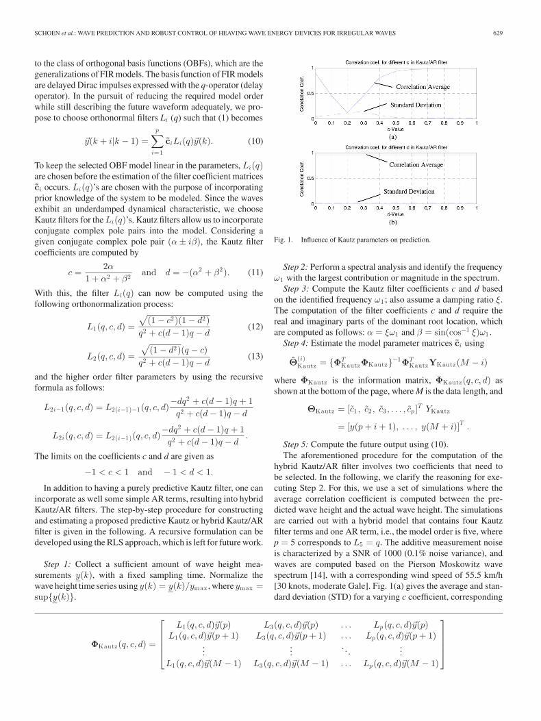
Fig. 4. Control system architecture. Dashed lines are associated with off-lineoperations.

as

x =

⎡

⎢⎣0 −mb Cb

mb +m∞, b−Ck

1mb

0 0

Bk 0 Ak

⎤

⎥⎦x

+

⎡

⎢⎣

−mb

mb +m∞, b

m b

mb +m∞, b

0 00 0

⎤

⎥⎦

[Fl

Fe

]

= Ax + B

[Fl

Fe

]. (18)

In this form, Fl is the force from the PTO machinery on thebuoy. This PTO force is the force used to control the system andis detailed in the following sections of this paper. For the studiedheaving sphere, we have used data from [19] and [20] to computethe memory function κ(t). A reasonable approximation for theconvolution term can be achieved with a state model of order sixusing Hankel singular value decomposition to reduce the modelorder [18]. This gives a total of eight states for the heaving buoymodel, taking the wave excitation force and the machinery loadforce as inputs to the system.

IV. FL CONTROL

In this section, we propose to use a FL controller with thepurpose to adapt the immediate PTO force Fl = −cy by con-trolling the damping coefficient c. The fuzzy controller includesa number of rules that allow for reducing the buoy motion, ifthe excursion becomes too large. The control output is com-puted based on the prediction of the future buoy motion, as aresult of current measured wave heights. The horizon for thiscontroller is of a rather short distance, i.e., 1 s. To accomplisha fuzzy inference system (FIS) for WEC control, the followingsystem structure is proposed (see Fig. 4). In the figure, z de-notes the wave height, y is the buoy motion, E is the energy,c∗ is the optimal damping for a given sea state, and the control

Fig. 5. FIS interaction with the WEC.

parameter is the damping generated by the PTO. For the simula-tions, the wave energy device given by block WEC is defined bythe model given in Section III [18]. The system identification SIin Fig. 4 provides a state-space model (resulting into the state-space matrices Ai , Bi , Ci , and Di) to simulate the dynamics ofthe buoy for given predicted wave motions. The SI is performedoff-line before the use of the controller. The prediction of thewave height is accomplished by a discrete time predictive ARformulation, which can be achieved by using (2).

The proposed FIS controller implementation includes as thecontrol variable the damping provided by the PTO. The Mam-dani type FIS is defined for this control action by having threeinputs and one defuzzyfied output, as depicted in Fig. 5: the threeinputs are processed using a set of different input membershipfunctions.

For the Amplitude, the membership functions are catego-rized as “‘Small Difference,” “Some Difference,” “‘Large Dif-ference,” and “‘Excessive Difference,” where Difference is de-fined as the discrepancy between |y − z| and the maximumexcursion allowed.

The selected membership function for the amplitude input aresigmoid functions for the “Small” (left) and “excessive differ-ence,” (right), while the remaining membership functions arebased on the Bell membership function. A similar set of mem-bership functions are created for the second input, the phasedifference between the buoy motion and the wave motion. Thephase is computed by establishing a time record of incomingwaves and the buoy’s motion. The “Small Phase” and “LargePhase” are characterized with left sigmoid functions and rightsigmoid functions, respectively. The “Good Phase” case is mod-eled with a Bell membership function.

The last input, the velocity, representing the buoy’s verticalvelocity, is used for the computation of the amount of damp-ing. The single membership function for the velocity is givenby a Polynomial-Z membership function. For the output, thedamping is constructed by the use of four different membership


Fig. 6. FS output surface for two inputs.

functions, i.e., “Less Damping,” “Optimal Damping,” “MoreDamping,” and “Halting.” The corresponding membershipfunctions are all Gaussian type membership function with theexception of the “Less Damping” case for which a sigmoidfunction is used, and the “Halting” case, where a Polynomial-Z membership function is employed. The output damping isthen computed as a change from the nominal value of damping.The nominal damping is equal to the optimal damping com-puted using a GA, which in turn is based on past input/outputdata, with the objective to absorb the maximum energy. Theemployed GA is based on a continuous number representation,with an elitism-based selection scheme. For more details on theused GA, see [21]. For the simulations, 100 generations areused with an initial population size of 96 chromosomes, and asteady-state population size of 48 chromosomes. The mutationrate is set to 4%. The input functions are linked to the controlleroutput by a rule base of the form as follows:

1) if (Phase is Small_Phase), then (Damping is Less_Damping);

2) if (Phase is Good_Phase), then (Damping is Optimal);3) if (Phase is Large_Phase), then (Damping is More_

Damping);4) if (Amplitude is Small_Difference), then (Damping is

More_Damping);5) if (Amplitude is Some_Difference), then (Damping is

Optimal);6) if (Amplitude is Large_Difference), then (Damping is

More_Damping);7) if (Amplitude is Excessive_Difference), then (Damping is

Halting);8) if (Velocity is zero), then (Damping is Halting).The overall resulting transfer output surface is given by Fig. 6.

We recognize that the nominal amplitude difference and thephase is normalized to 0 (desired state). The defuzzyficationis done using the centroid of the output membership func-tion. For the simulations, a Pierson–Moskowitz wave spectra of46.3 km/h [25 knots, strong breeze] wind speed is utilized, while

Fig. 7. Buoy motion and wave motion under control.

Fig. 8. Buoy motion with and without control using optimal parameters.

predicting the future wave height 10 steps (1 s) ahead. Fig. 7depicts the simulated buoy motion under the influence of the FLcontroller, which is turned ON after 65 s (k = 650).

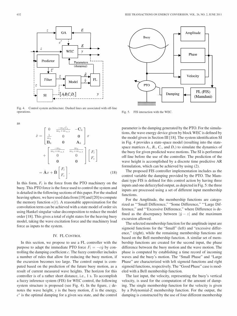
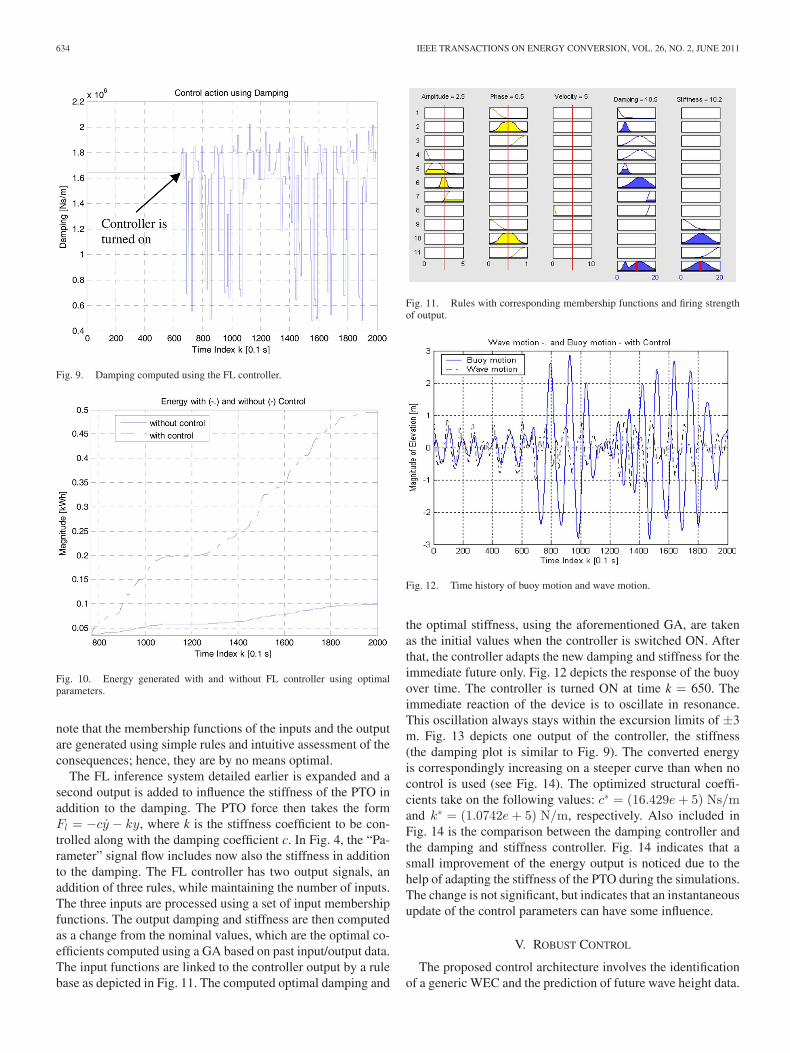
At the same time of switching the controller ON, the optimalinitial damping (and stiffness) is incorporated, which is used asthe nominal damping from which the controller deviates. Fig. 8provides a depiction of the buoy’s motion when optimal damp-ing is used without control compared to with control action. Theexcursion limits are exceeded when no control is employed,while the proposed controller keeps this excursion within thedesired limit of ±3[m]. The damping over time is depicted inFig. 9. The short-term forecast and reaction by the FL controlleris clearly manifested in the damping adaptation plot. The con-verted energy with and without the proposed FL controller isdepicted in Fig. 10 [the energy is computed according to (26)].Here in both cases, the optimal parameters are used. The energygraph indicates that the improvement is considerable. Althoughthe corresponding buoy motions as depicted in Fig. 8 showslarger excursions for the uncontrolled case, the small change inthe phase allows for a larger energy accumulation. It is also to


Fig. 9. Damping computed using the FL controller.

Fig. 10. Energy generated with and without FL controller using optimalparameters.

note that the membership functions of the inputs and the outputare generated using simple rules and intuitive assessment of theconsequences; hence, they are by no means optimal.

The FL inference system detailed earlier is expanded and asecond output is added to influence the stiffness of the PTO inaddition to the damping. The PTO force then takes the formFl = −cy − ky, where k is the stiffness coefficient to be con-trolled along with the damping coefficient c. In Fig. 4, the “Pa-rameter” signal flow includes now also the stiffness in additionto the damping. The FL controller has two output signals, anaddition of three rules, while maintaining the number of inputs.The three inputs are processed using a set of input membershipfunctions. The output damping and stiffness are then computedas a change from the nominal values, which are the optimal co-efficients computed using a GA based on past input/output data.The input functions are linked to the controller output by a rulebase as depicted in Fig. 11. The computed optimal damping and

Fig. 11. Rules with corresponding membership functions and firing strengthof output.

Fig. 12. Time history of buoy motion and wave motion.

the optimal stiffness, using the aforementioned GA, are takenas the initial values when the controller is switched ON. Afterthat, the controller adapts the new damping and stiffness for theimmediate future only. Fig. 12 depicts the response of the buoyover time. The controller is turned ON at time k = 650. Theimmediate reaction of the device is to oscillate in resonance.This oscillation always stays within the excursion limits of ±3m. Fig. 13 depicts one output of the controller, the stiffness(the damping plot is similar to Fig. 9). The converted energyis correspondingly increasing on a steeper curve than when nocontrol is used (see Fig. 14). The optimized structural coeffi-cients take on the following values: c∗ = (16.429e + 5) Ns/mand k∗ = (1.0742e + 5) N/m, respectively. Also included inFig. 14 is the comparison between the damping controller andthe damping and stiffness controller. Fig. 14 indicates that asmall improvement of the energy output is noticed due to thehelp of adapting the stiffness of the PTO during the simulations.The change is not significant, but indicates that an instantaneousupdate of the control parameters can have some influence.

V. ROBUST CONTROL

The proposed control architecture involves the identificationof a generic WEC and the prediction of future wave height data.


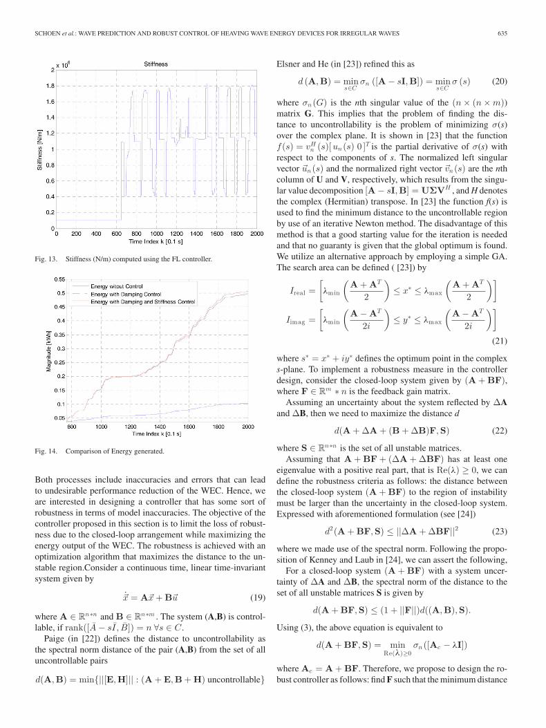
Fig. 13. Stiffness (N/m) computed using the FL controller.

Fig. 14. Comparison of Energy generated.

Both processes include inaccuracies and errors that can leadto undesirable performance reduction of the WEC. Hence, weare interested in designing a controller that has some sort ofrobustness in terms of model inaccuracies. The objective of thecontroller proposed in this section is to limit the loss of robust-ness due to the closed-loop arrangement while maximizing theenergy output of the WEC. The robustness is achieved with anoptimization algorithm that maximizes the distance to the un-stable region.Consider a continuous time, linear time-invariantsystem given by

�x = A�x + B�u (19)

where A ∈ Rn∗n and B ∈ R

n∗m . The system (A,B) is control-lable, if rank([A − sI, B]) = n ∀s ∈ C.

Paige (in [22]) defines the distance to uncontrollability asthe spectral norm distance of the pair (A,B) from the set of alluncontrollable pairs

d(A,B) = min{||[E,H]|| : (A + E,B + H) uncontrollable}

Elsner and He (in [23]) refined this as

d (A,B) = mins∈C

σn ([A − sI,B]) = mins∈C

σ (s) (20)

where σn (G) is the nth singular value of the (n × (n × m))matrix G. This implies that the problem of finding the dis-tance to uncontrollability is the problem of minimizing σ(s)over the complex plane. It is shown in [23] that the functionf(s) = vH

n (s)[un (s) 0 ]T is the partial derivative of σ(s) withrespect to the components of s. The normalized left singularvector �un (s) and the normalized right vector �vn (s) are the nthcolumn of U and V, respectively, which results from the singu-lar value decomposition [A − sI,B] = UΣVH , and H denotesthe complex (Hermitian) transpose. In [23] the function f(s) isused to find the minimum distance to the uncontrollable regionby use of an iterative Newton method. The disadvantage of thismethod is that a good starting value for the iteration is neededand that no guaranty is given that the global optimum is found.We utilize an alternative approach by employing a simple GA.The search area can be defined ( [23]) by

Ireal =[λmin

(A + AT

2

)≤ x∗ ≤ λmax

(A + AT

2

)]

Iimag =[λmin

(A − AT

2i

)≤ y∗ ≤ λmax

(A − AT

2i

)]

(21)

where s∗ = x∗ + iy∗ defines the optimum point in the complexs-plane. To implement a robustness measure in the controllerdesign, consider the closed-loop system given by (A + BF),where F ∈ R

m ∗ n is the feedback gain matrix.Assuming an uncertainty about the system reflected by ΔA

and ΔB, then we need to maximize the distance d

d(A + ΔA + (B + ΔB)F,S) (22)

where S ∈ Rn∗n is the set of all unstable matrices.

Assuming that A + BF + (ΔA + ΔBF) has at least oneeigenvalue with a positive real part, that is Re(λ) ≥ 0, we candefine the robustness criteria as follows: the distance betweenthe closed-loop system (A + BF) to the region of instabilitymust be larger than the uncertainty in the closed-loop system.Expressed with aforementioned formulation (see [24])

d2(A + BF,S) ≤ ||ΔA + ΔBF||2 (23)

where we made use of the spectral norm. Following the propo-sition of Kenney and Laub in [24], we can assert the following,

For a closed-loop system (A + BF) with a system uncer-tainty of ΔA and ΔB, the spectral norm of the distance to theset of all unstable matrices S is given by

d(A + BF,S) ≤ (1 + ||F||)d((A,B),S).

Using (3), the above equation is equivalent to

d(A + BF,S) = minRe(λ)≥0

σn ([Ac − λI])

where Ac = A + BF. Therefore, we propose to design the ro-bust controller as follows: find F such that the minimum distance


Fig. 15. Controller architecture for optimal robust FL predictive control. Dashed lines are associated with off-line operations.

to uncontrollability is maximized subjected to the constraintgiven in (21). Expressed in matrix form

Max{Min{σn ([A + BF − sI,B])}}

subjected to

Min{σn ([A + BF − λI]) } ≤ (1 + ||F||)+ Min{σn ([A − s∗I,B])}

and Irealm in ≤ x∗ ≤ Irealm a x and Iimagm in≤ y∗ ≤ Iimagm a x

.The overall controller is achieved by combining the proposed

robust controller with the proposed FL controller. In this fash-ion, we can address the short-term fluctuations of the wavesby tuning the optimal damping force of the WEC device usingthe FL controller, and the long-term fluctuations are addressedby the GA, while inaccuracies in the model and the variationsof conditions are in part compensated by the proposed robustcontroller. The resulting controller architecture/design is givenin Fig. 15. The implementation of this controller design is doneusing a simple continuous GA (see [21]) that finds the appropri-ate minima for the defined cost function. The controller designfor the robust control portion is based on a linear quadratic (LQ)controller. We have to pay special attention to the plant input,since only one input will be used to control the WEC, whileboth inputs are used to compute the control force.

Considering the input to the WEC as u = [ z Fl ]T , where FL

is the damping force, the state-space form of the system can beexpressed as follows:

x =[A − B

{K1K2

}]x and y =

[C − D

{K1K2

}]x

where we partitioned the feedback-gain matrix according to theinput u. The controller will not have any influence on the waveforce exerted onto the WEC; hence, K1 is set to zero and the

Fig. 16. Accumulated absorbed energy using robust controller and nocontroller.

TABLE IISIMULATION RESULTS FOR ACCUMULATED ABSORBED ENERGY FOR 200

SECONDS, WITH AND WITHOUT HYBRID ROBUST FL CONTROL

closed-loop system representation can be given as

x = [A − B1K2 ]xy = [C − D2K2 ]x

with B = [B1 B2 ] and D = [D1 D1 ]. Provided that u2 issufficient to reach all system states, the updated optimizationbecomes: Find K2 such that


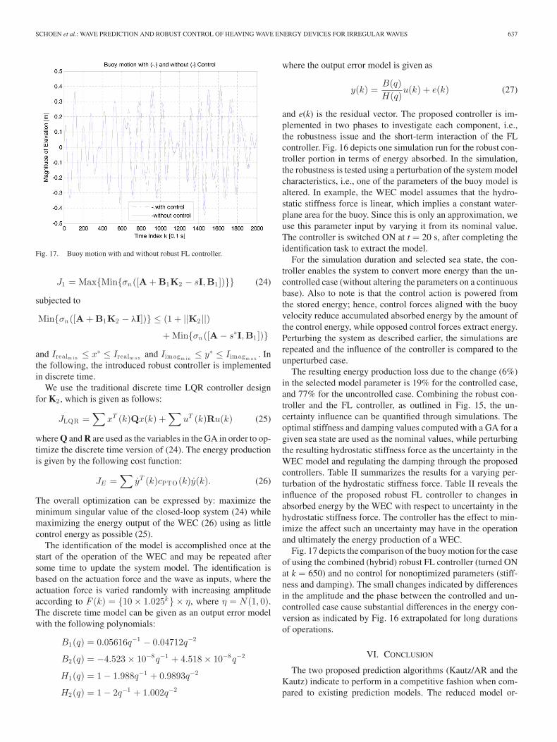
Fig. 17. Buoy motion with and without robust FL controller.

J1 = Max{Min{σn ([A + B1K2 − sI,B1 ])}} (24)

subjected to

Min{σn ([A + B1K2 − λI])} ≤ (1 + ||K2 ||)+ Min{σn ([A − s∗I,B1 ])}

and Irealm in ≤ x∗ ≤ Irealm a x and Iimagm in≤ y∗ ≤ Iimagm a x

. Inthe following, the introduced robust controller is implementedin discrete time.

We use the traditional discrete time LQR controller designfor K2 , which is given as follows:

JLQR =∑

xT (k)Qx(k) +∑

uT (k)Ru(k) (25)

where Q and R are used as the variables in the GA in order to op-timize the discrete time version of (24). The energy productionis given by the following cost function:

JE =∑

yT (k)cPTO(k)y(k). (26)

The overall optimization can be expressed by: maximize theminimum singular value of the closed-loop system (24) whilemaximizing the energy output of the WEC (26) using as littlecontrol energy as possible (25).

The identification of the model is accomplished once at thestart of the operation of the WEC and may be repeated aftersome time to update the system model. The identification isbased on the actuation force and the wave as inputs, where theactuation force is varied randomly with increasing amplitudeaccording to F (k) = {10 × 1.025k} × η, where η = N(1, 0).The discrete time model can be given as an output error modelwith the following polynomials:

B1(q) = 0.05616q−1 − 0.04712q−2

B2(q) = −4.523 × 10−8q−1 + 4.518 × 10−8q−2

H1(q) = 1 − 1.988q−1 + 0.9893q−2

H2(q) = 1 − 2q−1 + 1.002q−2

where the output error model is given as

y(k) =B(q)H(q)

u(k) + e(k) (27)

and e(k) is the residual vector. The proposed controller is im-plemented in two phases to investigate each component, i.e.,the robustness issue and the short-term interaction of the FLcontroller. Fig. 16 depicts one simulation run for the robust con-troller portion in terms of energy absorbed. In the simulation,the robustness is tested using a perturbation of the system modelcharacteristics, i.e., one of the parameters of the buoy model isaltered. In example, the WEC model assumes that the hydro-static stiffness force is linear, which implies a constant water-plane area for the buoy. Since this is only an approximation, weuse this parameter input by varying it from its nominal value.The controller is switched ON at t = 20 s, after completing theidentification task to extract the model.

For the simulation duration and selected sea state, the con-troller enables the system to convert more energy than the un-controlled case (without altering the parameters on a continuousbase). Also to note is that the control action is powered fromthe stored energy; hence, control forces aligned with the buoyvelocity reduce accumulated absorbed energy by the amount ofthe control energy, while opposed control forces extract energy.Perturbing the system as described earlier, the simulations arerepeated and the influence of the controller is compared to theunperturbed case.

The resulting energy production loss due to the change (6%)in the selected model parameter is 19% for the controlled case,and 77% for the uncontrolled case. Combining the robust con-troller and the FL controller, as outlined in Fig. 15, the un-certainty influence can be quantified through simulations. Theoptimal stiffness and damping values computed with a GA for agiven sea state are used as the nominal values, while perturbingthe resulting hydrostatic stiffness force as the uncertainty in theWEC model and regulating the damping through the proposedcontrollers. Table II summarizes the results for a varying per-turbation of the hydrostatic stiffness force. Table II reveals theinfluence of the proposed robust FL controller to changes inabsorbed energy by the WEC with respect to uncertainty in thehydrostatic stiffness force. The controller has the effect to min-imize the affect such an uncertainty may have in the operationand ultimately the energy production of a WEC.

Fig. 17 depicts the comparison of the buoy motion for the caseof using the combined (hybrid) robust FL controller (turned ONat k = 650) and no control for nonoptimized parameters (stiff-ness and damping). The small changes indicated by differencesin the amplitude and the phase between the controlled and un-controlled case cause substantial differences in the energy con-version as indicated by Fig. 16 extrapolated for long durationsof operations.

VI. CONCLUSION

The two proposed prediction algorithms (Kautz/AR and theKautz) indicate to perform in a competitive fashion when com-pared to existing prediction models. The reduced model or-


der of the proposed prediction filters will help lower the ratherhigh computational load imposed by conventional filters. Forthe operation of WECs in irregular waves, two controllers areproposed, each having a different objective. The FL controlleraddresses the short-term control, while the robust controller at-tempts to minimize the effects of the fluctuations or errors ofthe WEC model parameters on the energy absorption. The con-trol architecture proposed requires the prediction of wave heightdata as well as the optimization of the structural parameters ofthe vibrational system, which is accomplished with a simpleGA. Identification of the model is achieved off-line and may berepeated after some time when wave conditions have changed.

Simulation results for each controller are presented separatelybefore the combined robust FL controller is tested. The proposedcombined controller has the effect to limit the excursion of thebuoy motion to the predesigned limits, while maximizing theenergy output. In addition, uncertainties in the model have amore limited effect on the energy production when the proposedcontroller is used.

REFERENCES

[1] J. L. Forsberg, “On-line identification and prediction of waves,” in Hy-drodynamics of Ocean-Wave Energy Utilization, D. V Evans and A. F. deO Falcao, Eds. Berlin, Germany: Springer-Verlag, 1986, pp. 185–193.

[2] J. R. Halliday, D. G. Dorell, and A. Wood, “A Fourier approach to shortterm wave prediction,” in Proc. 16th Int. Offshore Polar Eng. Conf., SanFrancisco, CA, 2006, pp. 444–451.

[3] R. H. Jones, “Identification and autoregressive spectrum estimation,”IEEE Trans. Autom. Control, vol. AC-19, no. 6, pp. 894–897, Dec. 1974.

[4] L. Budal and J. Falnes, “A resonant point absorber of ocean-wave power,”Nature, vol. 256, pp. 478–479, 1975.

[5] J. Falnes, Ocean Waves and Oscillating Systems: Linear Interactions In-cluding Wave Energy Extraction. Cambridge, U.K.: Cambridge Univ.Press, 2002.

[6] U. A. Korde, “Efficient primary energy conversion in irregular waves,”Ocean Eng., vol. 26, pp. 625–651, 1999.

[7] U. A. Korde, “Latching control of deep water wave energy devices usingan active reference,” Ocean Eng., vol. 29, pp. 1343–1355, 2002.

[8] A. Babarit and A. H. Clement, “Optimal latching control of a wave energydevice in regular and irregular waves,” Appl. Ocean Res., vol. 28, pp. 77–91, 2006.

[9] A. Babarit, G. Cuclos, and A. H. Clement, “Benefit of latching control fora heaving wave energy device in random sea,” in Proc. 2003 Int. OffshorePolar Eng. Conf., Honolulu, Hawaii, 2003, pp. 341–348.

[10] S. M. Key and S. L. Marple, “Spectral analysis—A modern perspective,”in Proc. IEEE, Nov., 1981, vol. 69, no. 11, pp. 1380–1419.

[11] U. A. Korde, M. P. Schoen, F. Lin, “Time domain control of a single-mode wave energy device,” Presented at the Int. Soc. Offshore Polar Eng.,Stavanger, Norway, 2001.

[12] O. Nelles, Nonlinear System Identification from Classical Approaches toNeural Networks and Fuzzy Models. Berlin, Germany: Springer, 2001.

[13] P. J. Brockwell and R. A. Davis, Introduction to Time Series Analysis andForecasting. New York: Springer, 1997.

[14] W. J. Pierson and L. A. Moskowitz, “Proposed spectral form for fully de-veloped wind seas based on the similarity theory of S. A. Kitaigorodskii,”J. Geophys. Res., vol. 69, pp. 5181–5190, 1964.

[15] D. C. Karnopp, D. L. Margolis, and R. C. Rosenberg, System Dynamics:Modeling and Simulation of Mechatronic Systems, 4th ed. New York:Wiley, 2006.

[16] H. Engja and J. Hals, “Modeling and simulation of sea wave power con-version systems,” presented at the Eur. Wave Tidal Energy Conf., Porto,Portugal, 2007.

[17] J. Hals, T. Bjarte-Larsson, and J. Falnes, “Optimum reactive control andcontrol by latching of a wave-absorbing semisubmerged heaving sphere,”in Proc. Int. Conf. Offshore Mech. Arctic Eng., 2002, pp. 415–423.

[18] R. Taghipour, T. Perez, and T. Moan, “Hybrid frequency—Time domainmodels for dynamic response analysis of marine structures,” Ocean Eng.,vol. 35, pp. 685–705, 2008.

[19] T. Havelock, “Waves due to a floating sphere making periodic heavingoscillations,” in Proc. Royal Soc., vol. 231 A, pp. 1–7, 1955.

[20] A. Hulme, “The wave forces acting on a floating hemisphere undergoingforced periodic oscillations,” J. Fluid Mech., vol. 121, pp. 443–463, 1982.

[21] R. L. Haupt and S. E. Haupt, Practical Genetic Algorithms. New York:Wiley, 1998.

[22] C. C. Paige, “Properties of numerical algorithms relating to controllabil-ity,” IEEE Trans. Automat. Control, vol. AC-26, no. 1, pp. 130–138, Feb.1981.

[23] L. Elsner and C. He, “An algorithm for computing the distance to uncon-trollability,” Syst. Control Lett., vol. 17, pp. 453–464, 1991.

[24] C. Kenney and A. J. Laub, “Controllability and stability radii for compan-ion form systems,” Math. Contr. Signals Syst., vol. 1, pp. 239–256, 1988.

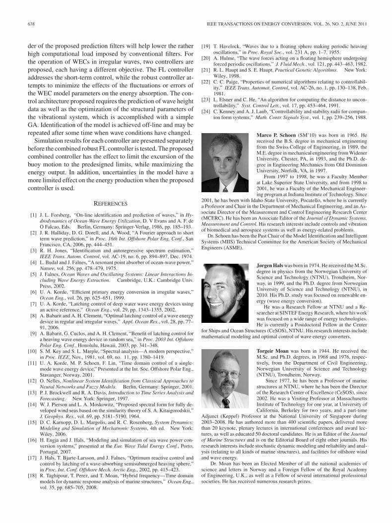
Marco P. Schoen (SM’10) was born in 1965. Hereceived the B.S. degree in mechanical engineeringfrom the Swiss College of Engineering, in 1989, theM.E. degree in mechanical engineering from WidenerUniversity, Chester, PA, in 1993, and the Ph.D. de-gree in Engineering Mechanics from Old DominionUniversity, Norfolk, VA, in 1997.

From 1997 to 1998, he was a Faculty Memberat Lake Superior State University, and from 1998 to2001, he was a Faculty of the Mechanical Engineer-ing program at Indiana Institute of Technology. Since

2001, he has been with Idaho State University, Pocatello, where he is currentlya Professor and Chair in the Department of Mechanical Engineering, and an As-sociate Director of the Measurement and Control Engineering Research Center(MCERC). He has been an Associate Editor of the Journal of Dynamic Systems,Measurement and Control. His research interests include controls and vibrationof biomedical and aerospace systems as well as energy-related problems.

Dr. Schoen has been the Past Chair of the Model Identification and IntelligentSystems (MIIS) Technical Committee for the American Society of MechanicalEngineers (ASME).

Jørgen Hals was born in 1974. He received the M.Sc.degree in physics from the Norwegian University ofScience and Technology (NTNU), Trondheim, Nor-way, in 1999, and the Ph.D. degree from NorwegianUniversity of Science and Technology (NTNU), in2010. His Ph.D. study was focused on renewable en-ergy (wave energy conversion).

He was a Research Fellow at NTNU and a Re-searcher at SINTEF Energy Research, where his workwas focused on a wide range of energy technologies.He is currently a Postdoctoral Fellow at the Center

for Ships and Ocean Structures (CeSOS), NTNU. His research interests includemathematical modeling and optimal control of wave energy converters.

Torgeir Moan was born in 1944. He received theM.Sc. and Ph.D. degrees, in 1968 and 1976, respec-tively, from the Department of Civil Engineering,Norwegian University of Science and Technology(NTNU), Trondheim, Norway.

Since 1977, he has been a Professor of marinestructures at NTNU, where he has been the Directorof the Research Center of Excellence (CeSOS), since2002. He was a Visiting Professor at MassachusettsInstitute of Technology for one year, at University ofCalifornia, Berkeley for two years, and a part-time

Adjunct (Keppel) Professor at the National University of Singapore during2003–2008. He has authored more than 400 scientific papers, delivered morethan 20 keynote, plenary lectures in international conferences and award lec-tures, as well as educated 50 doctoral candidates. He is an Editor of the Journalof Marine Structures and is on the Editorial Board of eight other journals. Hisresearch interests include stochastic dynamic modeling and reliability and anal-ysis (relating to all kinds of marine structures), and facilities for offshore windand wave energy.

Dr. Moan has been an Elected Member of all the national academies ofscience and letters in Norway and a Foreign Fellow of the Royal Academyof Engineering, U.K., as well as a Fellow of several international professionalsocieties. He has received numerous research prizes.

Documents

Wave Prediction and Robust Control of Heaving Wave Energy Devices for Irregular Waves