Water Balance in the Amazon Basin from a Land Surface Model Ensemble

Water Balance in the Amazon Basin from a Land Surface Model Ensemble

AUGUSTO C. V. GETIRANA,a EMANUEL DUTRA,b MATTHIEU GUIMBERTEAU,c JONGHUN KAM,d

HONG-YI LI,e BERTRAND DECHARME,f ZHENGQIU ZHANG,g AGNES DUCHARNE,h AARON BOONE,f

GIANPAOLO BALSAMO,b MATTHEW RODELL,a ALLY M. TOURE,a YONGKANG XUE,i

CHRISTA D. PETERS-LIDARD,a SUJAY V. KUMAR,a KRISTI ARSENAULT,a GUILLAUME DRAPEAU,j

L. RUBY LEUNG,e JOSYANE RONCHAIL,k AND JUSTIN SHEFFIELDd

aHydrological Sciences Laboratory, NASA Goddard Space Flight Center, Greenbelt, MarylandbECMWF, Reading, United Kingdom

cL’Institut Pierre-Simon Laplace/CNRS, Paris, FrancedDepartment of Civil and Environmental Engineering, Princeton University, Princeton, New Jersey

ePacific Northwest National Laboratory, Richland, WashingtonfCNRM-GAME, Météo-France, Toulouse, France

gUniversity of California, Los Angeles, Los Angeles, California, and Chinese Academy of

Meteorological Sciences, Beijing, ChinahL’Institut Pierre-Simon Laplace/CNRS, and UMR METIS,

CNRS/Université Pierre et Marie Curie, Paris, FranceiUniversity of California, Los Angeles, Los Angeles, California

jUniversité Paris Diderot, PRODIG, Paris, FrancekUniversité Paris Diderot, Universités Sorbonne Paris Cité et Sorbonne (Université Pierre et Marie Curie,

Université Paris 06), CNRS/IRD/MNHN, LOCEAN, Paris, France

(Manuscript received 25 March 2014, in final form 18 August 2014)

ABSTRACT

Despite recent advances in land surface modeling and remote sensing, estimates of the global water budget are

still fairly uncertain. This study aims to evaluate the water budget of the Amazon basin based on several state-of-

the-art land surface model (LSM) outputs. Water budget variables (terrestrial water storage TWS, evapotrans-

piration ET, surface runoff R, and base flow B) are evaluated at the basin scale using both remote sensing and in

situ data. Meteorological forcings at a 3-hourly time step and 18 spatial resolution were used to run 14 LSMs.

Precipitation datasets that have been rescaled tomatchmonthlyGlobal PrecipitationClimatology Project (GPCP)

andGlobal Precipitation Climatology Centre (GPCC) datasets and the daily Hydrologie du Bassin de l’Amazone

(HYBAM) dataset were used to perform three experiments. The Hydrological Modeling and Analysis Platform

(HyMAP) river routing scheme was forced with R and B and simulated discharges are compared against obser-

vations at 165 gauges. Simulated ET and TWS are compared against FLUXNET and MOD16A2 evapotranspi-

ration datasets andGravityRecovery andClimateExperiment (GRACE)TWSestimates in two subcatchments of

main tributaries (Madeira andNegro Rivers). At the basin scale, simulated ET ranges from 2.39 to 3.26mmday21

and a low spatial correlation between ET and precipitation indicates that evapotranspiration does not depend on

water availability over most of the basin. Results also show that other simulated water budget components vary

significantly as a function of both the LSM and precipitation dataset, but simulated TWS generally agrees with

GRACE estimates at the basin scale. The best water budget simulations resulted from experiments using

HYBAM, mostly explained by a denser rainfall gauge network and the rescaling at a finer temporal scale.

1. Introduction

Several modeling attempts have been conducted try-

ing to improve the simulation of water and energy cycles

at several temporal and spatial scales worldwide. These

attempts take into account different modeling ap-

proaches and meteorological forcings, resulting in con-

trasting water balance estimates. The accuracy of the

water budget simulated by land surface models (LSMs)

is highly dependent on data availability and quality

(meteorological forcings, soil type, and land cover),

initial conditions, and how adapted or simplified the

Corresponding author address: A.C.V. Getirana, Hydrological

Sciences Laboratory, NASA Goddard Space Flight Center, 8800

Greenbelt Rd., Greenbelt, MD 20009.

E-mail: [email protected]

2586 JOURNAL OF HYDROMETEOROLOGY VOLUME 15

DOI: 10.1175/JHM-D-14-0068.1

� 2014 American Meteorological Society

mailto:[email protected]

representation of physical processes are for a specific

location. The intercomparison of LSMs has been per-

formed through several international projects and ini-

tiatives and has guided the improvement of current

models and the development of new ones. For easier

evaluation and comparison, LSMs are often run in the

so-called offline mode, which means that these models

are run uncoupled from an atmospheric model and are

therefore driven using prescribed atmospheric forcing

derived either from in situ or satellite observations,

atmospheric model outputs, or the combination of

these three sources. Intercomparison projects such as

the Project for the Intercomparison of Land-surface

Parameterization Schemes (PILPS) and its different

phases [refer to Henderson-Sellers et al. (1995), Wood

et al. (1998), and other numerous publications],

the Global Soil Wetness Project phase 1 (GSWP-1:

Dirmeyer et al. 1999) and phase 2 (GSWP-2; Dirmeyer

et al. 2006), the Rhone aggregation LSM in-

tercomparison project (Boone et al. 2004), the African

Monsoon Multidisciplinary Analyses (AMMA) Land

Surface Model Intercomparison Project (ALMIP;

Boone et al. 2009a,b), and the Hydrological Cycle

in Mediterranean Experiment (HyMeX; Drobinski

et al. 2014), among others, have increased the un-

derstanding of LSMs and led to many model im-

provements. A comprehensive description of past LSM

intercomparison projects can be found in van den Hurk

et al. (2011).

Other studies and initiatives have shown that rout-

ing runoff simulations and comparing them against

observed streamflow can be a useful way to evaluate

the large-scale water budget simulated by LSMs

(Yamazaki et al. 2011; Decharme et al. 2012;

Guimberteau et al. 2012; Li et al. 2013; Getirana et al.

2014). The evaluation can be performed in terms of both

the timing and amount of simulated runoff. The in-

accurate representation of physical processes in LSMs

involving soil moisture, evapotranspiration, and snow-

melt may result in differences between observed and

simulated streamflows. Other sources of error in

streamflow simulations include inaccuracies in the

forcing data, involving the density of rainfall gauging

stations, when provided by in situ observations (e.g.,

Oki et al. 1999; Ducharne et al. 2003; Xavier et al. 2005),

and inaccuracies in the river routing schemes (RRSs)

themselves. Comparing simulated and observed stream-

flows can be an efficient way to assess precipitation

datasets. Such evaluations using LSMs or hydrologi-

cal models coupled with an RRS have been already

carried out at different spatial and temporal scales

(Yilmaz et al. 2005; Wilk et al. 2006; Voisin et al. 2008;

Getirana et al. 2011b).

This study builds upon the aforementioned initiatives

and efforts, and, on the basis of satellite and ground-

based data, seeks for a better understanding of the large-

scale water budget in the Amazon basin. The Amazon is

the largest basin in the world with an area of approxi-

mately 6 million km2, and it contributes to about 15%–

20%of the freshwater transported to the oceans (Richey

et al. 1986). Although the number of hydrological mo-

deling attempts in the basin has increased in past decades

(e.g., Vorosmarty et al. 1989; Costa and Foley 1997; Coe

et al. 2002; Marengo 2005; Beighley et al. 2009; Paiva

et al. 2013a; Guimberteau et al. 2014), evapotranspira-

tion and total runoff estimates are still diverging, mostly

caused by different formulations representing physical

processes. In an atmospheric modeling perspective, such

divergences at the basin scale can largely affect the re-

gional climate, exchanges at the land surface and the

ocean salinity, and temperature at the river’s mouth

(e.g., Gedney et al. 2004; Alkama et al. 2008; Durand

et al. 2011; Decharme et al. 2012).

The hydrological regime of the Amazon basin is in-

fluenced by the climatology of both the Northern and

Southern Hemispheres, with the precipitation peaks gen-

erally occurring between April and June in the Northern

Hemisphere and between December and March in the

Southern Hemisphere. In this sense, in order to better

understand the large-scale hydrological heterogeneities

within the basin, the water budgets of two main Amazon

River tributaries were also evaluated in this study: the

Negro River, draining the northern region, and the Ma-

deira River, draining the southern region. Four key hy-

drological variables (evapotranspiration ET, surface

runoff R, base flow B, and terrestrial water storage

change dS) simulated by 14 LSMs are evaluated within

the 1989–2008 period. Because of the highly heteroge-

neous formulations for representing groundwater, in-

cluding different soil depths and, in some cases, absence

of water table in the different LSMs considered in this

study, this variable is not evaluated in this study. How-

ever, a detailed description of how groundwater impacts

the water cycle modeling in the Amazon basin is de-

scribed in Miguez-Macho and Fan (2012a,b). The spatial

and temporal distributions of precipitation fields have an

important role in the water budget, and evaluating their

impacts on hydrological processes in the Amazon basin is

another objective of this study. In this sense, three

ground-based precipitation products were used to force

LSMs, totalizing 42 realizations. This paper is organized

as follows. Section 2 gives a brief description of LSMs and

meteorological forcings (including the precipitation

datasets) used in the experiments, section 3 describes the

evaluation procedure and datasets used in the evaluation,

section 4 presents and discusses the results obtained, and

DECEMBER 2014 GET IRANA ET AL . 2587

section 5 ends the paper by presenting the conclusions

from the study.

2. Land surface models, forcings, and setup

In this section, the LSMs considered in the compari-

son are listed and changes among different versions are

briefly described. Also, the meteorological forcings, in-

cluding the different precipitation datasets used in the

experiments, are presented, and the modeling setup is

defined.

a. Land surface models

LSMs compute the land surface response to the

near-surface atmospheric conditions forcing, esti-

mating the surface water and energy fluxes and the

temporal evolution of soil temperature, moisture

content, and snowpack conditions. At the interface

with the atmosphere, each grid box is divided into

fractions (tiles) to describe the land surface hetero-

geneities. In this study, some models are not using

tiles, so for them, the number of tiles is one. The

maximum number of tiles depends on the LSM and

land surface parameters used in the run. Usually, the

gridbox surface fluxes are calculated separately for

each tile, leading to a separate solution of the surface

energy balance equation and the skin temperature.

The latter represents the interface between the soil

and the atmosphere. Below the surface, the vertical

transfer of water and energy is performed using

vertical layers to represent soil temperature and

moisture.

A total of 14 LSMs were considered in the in-

tercomparison. The set is composed of three versions of

both Noah and Tiled European Centre for Medium-

Range Weather Forecasts (ECMWF) Scheme for Sur-

face Exchange over Land (TESSEL) and two versions

of both Community Land Model (CLM) and Orga-

nizing Carbon and Hydrology in Dynamic Ecosystems

(ORCHIDEE). Finally, there was one version of Mo-

saic; Interactions between Soil, Biosphere, and Atmo-

sphere (ISBA); Variable Infiltration Capacity (VIC);

and the Simplified Simple Biosphere Model, version 2

(SSiB2). Each LSMhas its own specifications that can be

found in numerous references in the literature (some of

them are listed in Table 1). Therefore, only the main

differences among versions or configurations of the

same LSM are described below, that is, Noah, TESSEL,

TABLE 1. List of LSMs and setup. The numbers associated with the models in the first column (e.g., 271, 32, and 33 following Noah)

indicate themodel version. Themodel setup used for eachmodel simulation is shown in the rightmost column. L represents the number of

vertical soil layers and SV corresponds to the soil–vegetation parameters used. The number of tiles for CLM4 is variable as a function of

SV within a grid cell.

Model Reference Institute Model setup

Noah271 Ek et al. (2003) NASA Goddard Space

Flight Center, Greenbelt,

Maryland

3L, 1 tile, 30min, 18 3 18; SV:

University of MarylandNoah32 www.ral.ucar.edu/research/

land/technology/lsm.php

Noah33 www.ral.ucar.edu/research/

land/technology/lsm.php

Mosaic Koster and Suarez (1996)

CLM2 Dai et al. (2003)

CLM4 Vertenstein et al. (2012) Pacific Northwest National

Laboratory, Richland,

Washington

15L, n tiles 30min,

0.958 3 1.258; SV: CLM

TESSEL van den Hurk and Viterbo (2003) ECMWF, Reading,

United Kingdom

4L, 6 tiles, 30min,

18 3 18; SV: ECMWFCTESSEL Boussetta et al. (2013b)

HTESSEL Balsamo et al. (2009)

ORCH-2L Krinner et al. (2005) IPSL, Paris, France 2L/11L, 13 tiles, 30min, 18 3 18;SV: International Geosphere–

Biosphere Programme

ORCH-11L D’Orgeval et al. (2008)

ISBA Noilhan and Mahfouf (1996);

Decharme and Douville (2007)

CNRM/Météo-France,Toulouse, France

3L, 12 tiles, 30min, 18 3 18;SV: ECOCLIMAP

VIC Liang et al. (1994) University of Princeton,

Princeton, USA

3L, 11 tiles, 3 h, 18 3 18;SV: University of Washington

SSiB2 Xue et al. (1991); Zhan

et al. (2003)

University of California,

Los Angeles, Los Angeles,

California

3L, 1 tile, 3 h, 18 3 18; SV: SSiB


http://www.ral.ucar.edu/research/land/technology/lsm.php






CLM, and ORCHIDEE. For all the models, Table 1

provides information about the institute where the LSM

runs were performed, recent references, and model

setup, including soil and land cover parameters used by

each one.

1) NOAH

Three Noah LSM versions were used in this study:

Noah271, Noah32, and Noah33. These versions are

currently found in the latest Land Information System

(LIS; Kumar et al. 2006) release (LIS7) and were run

within the system. The version 271 of Noah is the first

unified community version (Ek et al. 2003) as a result of

an effort promoted by the Environmental Modeling

Center (EMC) of the National Centers for Environ-

mental Prediction (NCEP) and collaborators. Im-

provements have been continuously implemented in

Noah ever since. Major improvements from 271 to 32

include modifications in the roughness length over

snow-covered surfaces, use of the Livneh scheme in the

snow albedo treatment, fairly significant changes in the

glacial ice treatment, and dependence of potential eva-

potranspiration on the Richardson number. The main

improvement from version 32 to 33 is the activation of

a time-varying roughness length.

2) CLM

The Community Land Model (Oleson et al. 2004) is

the land component of the Community Earth System

Model (CESM; Vertenstein et al. 2012; Gent et al. 2011)

hosted at the National Center for Atmospheric Re-

search (NCAR). The model consists of components that

simulate processes such as biogeophysics, the hydro-

logical cycle, biogeochemistry, and vegetation dynam-

ics. This study evaluates version 2 (CLM2; Bonan et al.

2002) and version 4 (CLM4; Lawrence et al. 2011). The

decision to include CLM2 in this comparison is based on

the fact that outputs from this LSM currently compose

the Global Land Data Assimilation System (GLDAS;

Rodell et al. 2004).

From CLM2 to CLM4, all important processes in-

cluding the parameterization of multilayer snow, frozen

water, interception, soil water limitation to latent heat,

and higher aerodynamic resistances to heat exchange

from ground are preserved, and some processes have

since been improved upon based on recent scientific

advances in the understanding and representation of

land surface processes. State-of-the-art soil hydrology

and snow process are introduced. The ground column

is extended to ;50-m depth by adding five additional

ground layers (10 soil layers and 5 bedrock layers).

Other new parameterizations involved the canopy in-

tegration, the canopy interception, the permafrost

dynamics, the soil water availability, the soil evapora-

tion, and the groundwater model for determining water

table depth (see Niu et al. 2007). A new runoff model

based on the TOPMODEL concept (Beven and Kirkby

1979) was also introduced, but Li et al. (2011) pointed

out that this new scheme tends to produce unrealistic

subsurface runoff and could be enhanced with more

generalizable implementations. All the changes added

to the portioning of the evapotranspiration into tran-

spiration; soil and canopy evaporation; the in-

corporation of snowpack heating; and metamorphism

resulting in more reasonable snow cover, cooler and

better soil temperatures in organic-rich soils, and

greater river discharge compared to the previous version

of the CLM [more details can be found in Lawrence

et al. (2011)].

3) TESSEL

Three model configurations were used in this

study: TESSEL,CTESSEL (land carbon), andHTESSEL

(hydrology). HTESSEL is the current operational

land surface scheme used at ECMWF for the medium-

to long-range forecasts differing fromTESSEL (van den

Hurk et al. 2000; Viterbo and Beljaars 1995) in several

components detailed in Balsamo et al. (2011): 1) revised

formulation for soil hydrological conductivity and dif-

fusivity (spatially variable according to a global soil

texture map) and surface runoff (based on the variable

infiltration (Balsamo et al. 2009), 2) revised snow hy-

drology (snow density and liquid water content; Dutra

et al. 2010), 3) vegetation seasonality by prescribing

a leaf area index (LAI) monthly climatology (Boussetta

et al. 2013a), and 4) revision of bare ground evaporation

(Albergel et al. 2012). CTESSEL shares the same con-

figuration as HTESSEL, but a new plant physiological

approach (photosynthesis–conductance) is used to

compute the stomatal conductance for water vapor

transpiration (Boussetta et al. 2013b), while HTESSEL

used the Jarvis formulation (Jarvis 1976). All model

configurations use the same prescribed albedo clima-

tology. As for the LAI, TESSEL uses constant values

according to the vegetation type and HTESSEL and

CTESSEL use a prescribed LAI climatology.

4) ORCHIDEE

The ORCHIDEE (Krinner et al. 2005) LSM is the

land component of L’Institut Pierre-Simon Laplace

(IPSL) coupled climate model. We compare two ver-

sions of this model, ORCH-2L and ORCH-11L, which

both describe a 2-m soil but use a different parameter-

ization of soil hydrological processes. ORCH-2L uses

a two-layer bucket-type approach (Ducoudré et al.1993), in which two soil layers are linked by an internal


diffusion flux (Ducharne et al. 1998). As in the bucket

scheme of Manabe (1969), no bottom drainage is al-

lowed, and runoff is only produced when total soil

moisture reaches the maximum capacity (300 kgm22

over all land points). This total runoff is arbitrarily

partitioned into 95% base flow and 5% surface runoff

for feeding the routing scheme (section 3a). In contrast,

ORCH-11L uses a physically based approach (De

Rosnay et al. 2002; Campoy et al. 2013). The soil column

is divided into 11 layers of increasing thickness with

depth, to solve the nonsaturated vertical soil water flow

(Richards equation), assuming gravitational drainage at

the bottom. The Mualem–van Genuchten model

(Mualem 1976; van Genuchten 1980) is used to describe

the soil hydraulic properties as a function of water

content, with parameters that depend on soil texture.

Surface runoff results from an infiltration excess mech-

anism, where infiltration follows Green and Ampt

(1911) using a time-splitting procedure (D’Orgeval et al.

2008).

b. Meteorological forcings

The meteorological dataset used as forcing for

the LSMs is provided by Princeton University on

a 3-hourly time step and at a 18 spatial resolution

(Sheffield et al. 2006) for the 1979–2008 period. This

dataset is based on the NCEP–NCAR reanalysis.

Sheffield et al. (2006) carried out corrections of the

systematic biases in the 6-hourly NCEP–NCAR re-

analysis via hybridization with global monthly gridded

observations. In addition, the precipitation was dis-

aggregated in both space and time at 18 spatial resolu-tion via statistical downscaling and at 3-hourly time

step using information from the 3-hourly Tropical

Rainfall Measuring Mission (TRMM) dataset.

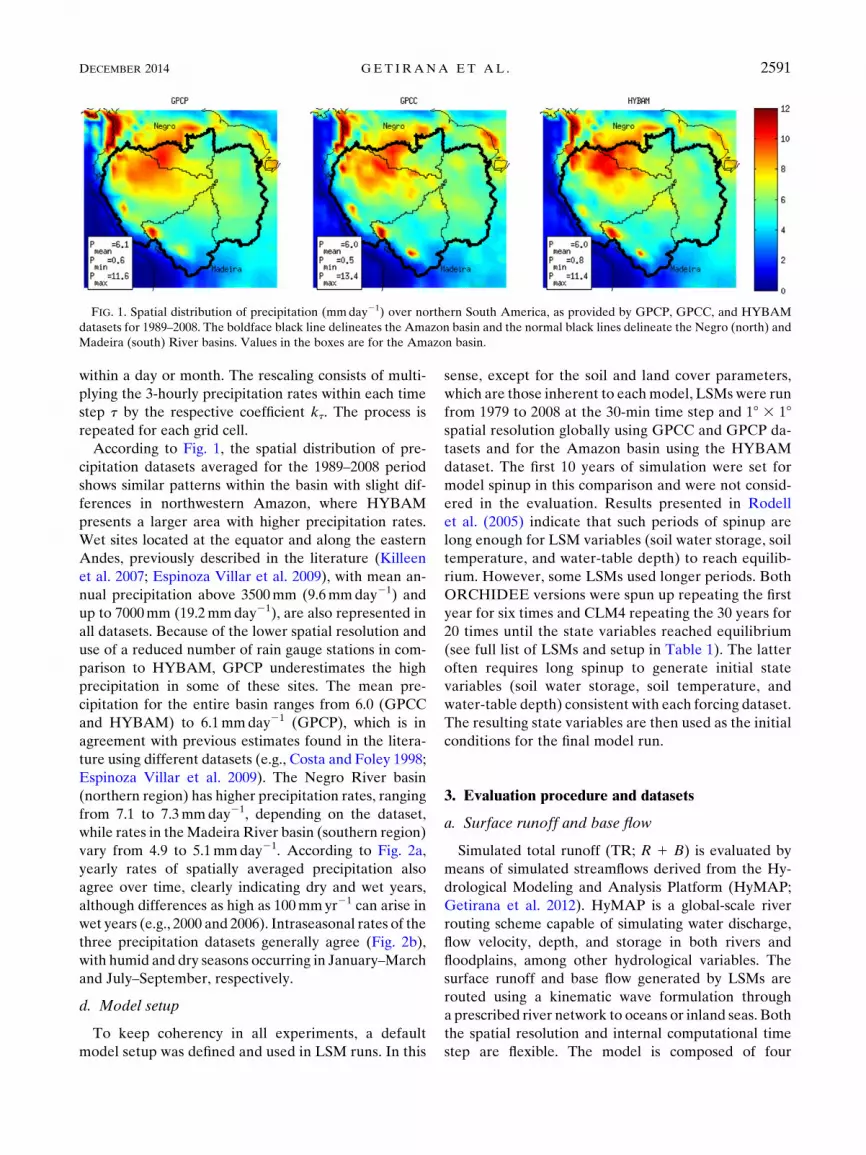
c. Precipitation

To evaluate the impacts of rainfall on water budget

simulations, the 3-hourly precipitation from Sheffield

et al. (2006) was rescaled to match the daily or monthly

precipitation values given by three datasets.

They are 1) the monthly Global Precipitation Clima-

tology Centre (GPCC) Full Data Reanalysis, version 6

(Schneider et al. 2014); 2) the monthly Global Pre-

cipitation Climatology Project (GPCP), version 2.2

(Adler et al. 2003); and 3) the daily Observatoire de

Recherche en Environnement–Hydrologie du Bassin de

l’Amazone (ORE-HYBAM; Guimberteau et al. 2012),

hereafter called HYBAM. The three precipitation

datasets are based on in situ observations over the

continents, and they were preferred over other products

because of the longer temporal availability. TheHYBAM

dataset uniquely covers theAmazon basin and is a result

of a collaboration involving all the countries composing

the region, where a large number of rain gauges has been

used to represent the precipitation field over the basin.

The first version of this dataset was presented at the

monthly time step in Espinoza Villar et al. (2009). The

daily version was firstly introduced and used in a hy-

drological modeling attempt in Guimberteau et al.

(2012). Technical information about the original pre-

cipitation datasets is listed in Table 2, and a detailed

description of how they were generated can be found in

their respective references given above.

The rescaling process, which led to three different

meteorological forcings, is classical to meteorological

hybridization techniques and follows Guo et al. (2006).

It is based on the coefficient kt, computed at each lower

temporal resolution (daily or monthly) time step t, and

defined as

kt 5Pint

�nt

i51

pti

, (1)

where Pint (mm) stands for the lower temporal resolu-

tion precipitation at t, p (mm) represents the 3-hourly

precipitation, and nt is the number of 3-h intervals

TABLE 2. List of precipitation datasets used in the modeling experiments.

Dataset

acronym Full name Reference

Format/spatial

resolution

Spatial

coverage

Series

span

Time

step

Data

source

GPCP Global Precipitation

Climatology Project,

version 2.2

Adler et al.

(2003)

Grid (2.58 3 2.58) Global 1979–present Monthly Rain

gauge,

satellite

GPCC Global Precipitation

Climatology Centre,

version 6

Schneider

et al. (2014)

Grid (1.08 3 1.08) Global 1901–2010 Monthly Rain

gauge

HYBAM ORE-HYBAM

precipitation dataset

Espinoza Villar

et al. (2009);

Guimberteau

et al. (2012)

Grid (1.08 3 1.08) Amazon

basin

1980–2009 Daily Rain

gauge


within a day or month. The rescaling consists of multi-

plying the 3-hourly precipitation rates within each time

step t by the respective coefficient kt. The process is

repeated for each grid cell.

According to Fig. 1, the spatial distribution of pre-

cipitation datasets averaged for the 1989–2008 period

shows similar patterns within the basin with slight dif-

ferences in northwestern Amazon, where HYBAM

presents a larger area with higher precipitation rates.

Wet sites located at the equator and along the eastern

Andes, previously described in the literature (Killeen

et al. 2007; Espinoza Villar et al. 2009), with mean an-

nual precipitation above 3500mm (9.6mmday21) and

up to 7000mm (19.2mmday21), are also represented in

all datasets. Because of the lower spatial resolution and

use of a reduced number of rain gauge stations in com-

parison to HYBAM, GPCP underestimates the high

precipitation in some of these sites. The mean pre-

cipitation for the entire basin ranges from 6.0 (GPCC

and HYBAM) to 6.1mmday21 (GPCP), which is in

agreement with previous estimates found in the litera-

ture using different datasets (e.g., Costa and Foley 1998;

Espinoza Villar et al. 2009). The Negro River basin

(northern region) has higher precipitation rates, ranging

from 7.1 to 7.3mmday21, depending on the dataset,

while rates in theMadeira River basin (southern region)

vary from 4.9 to 5.1mmday21. According to Fig. 2a,

yearly rates of spatially averaged precipitation also

agree over time, clearly indicating dry and wet years,

although differences as high as 100mmyr21 can arise in

wet years (e.g., 2000 and 2006). Intraseasonal rates of the

three precipitation datasets generally agree (Fig. 2b),

with humid and dry seasons occurring in January–March

and July–September, respectively.

d. Model setup

To keep coherency in all experiments, a default

model setup was defined and used in LSM runs. In this

sense, except for the soil and land cover parameters,

which are those inherent to eachmodel, LSMswere run

from 1979 to 2008 at the 30-min time step and 18 3 18spatial resolution globally using GPCC and GPCP da-

tasets and for the Amazon basin using the HYBAM

dataset. The first 10 years of simulation were set for

model spinup in this comparison and were not consid-

ered in the evaluation. Results presented in Rodell

et al. (2005) indicate that such periods of spinup are

long enough for LSM variables (soil water storage, soil

temperature, and water-table depth) to reach equilib-

rium. However, some LSMs used longer periods. Both

ORCHIDEE versions were spun up repeating the first

year for six times and CLM4 repeating the 30 years for

20 times until the state variables reached equilibrium

(see full list of LSMs and setup in Table 1). The latter

often requires long spinup to generate initial state

variables (soil water storage, soil temperature, and

water-table depth) consistent with each forcing dataset.

The resulting state variables are then used as the initial

conditions for the final model run.

3. Evaluation procedure and datasets

a. Surface runoff and base flow

Simulated total runoff (TR; R 1 B) is evaluated by

means of simulated streamflows derived from the Hy-

drological Modeling and Analysis Platform (HyMAP;

Getirana et al. 2012). HyMAP is a global-scale river

routing scheme capable of simulating water discharge,

flow velocity, depth, and storage in both rivers and

floodplains, among other hydrological variables. The

surface runoff and base flow generated by LSMs are

routed using a kinematic wave formulation through

a prescribed river network to oceans or inland seas. Both

the spatial resolution and internal computational time

step are flexible. The model is composed of four

FIG. 1. Spatial distribution of precipitation (mmday21) over northern South America, as provided by GPCP, GPCC, and HYBAM

datasets for 1989–2008. The boldface black line delineates the Amazon basin and the normal black lines delineate the Negro (north) and

Madeira (south) River basins. Values in the boxes are for the Amazon basin.


modules accounting for 1) the surface runoff and base

flow time delays, 2) flow routing in river channels,

3) flow routing in floodplains, and 4) evaporation from

open water surfaces. In this study, the spatial resolution

is 0.258, and the internal computational time step was set

as 15min and outputs provided at a daily time step.

Lowland topography and river network characteristics

such as river length and slope are prescribed on a sub-

grid-scale basis using the upscaling method described

by Yamazaki et al. (2009). The fine-resolution flow

direction map is given by the 1-km-resolution Global

Drainage Basin Database (GDBD; Masutomi et al.

2009). The flow routing in both rivers and floodplains

provides a heterogeneous spatiotemporal distribution

of flow velocities within the river floodplain network.

Since the objective is to evaluate the water budget

simulated by the LSMs, HyMAP was run without the

fourthmodule, that is, it does not account for evaporation

from open water surfaces. In this sense, the LSM water

budget was preserved. Getirana et al. (2012) have shown

that the average differential evaporation fromfloodplains

in the Amazon basin is around 0.02mmday21, corre-

sponding to less than 1% of the mean ET rate in the

basin. However, arid regions subjected to monsoon re-

gimes, such as the Parana and Niger River basins, may

benefit from the use of this module, as suggested by

Decharme et al. (2012). The latter authors showed that

considering floodplains can significantly increase the

evapotranspiration over those areas. HyMAP is fully

described and evaluated in Getirana et al. (2012) and

applications over the Amazon basin can be found in

the literature (Mouffe et al. 2012; Getirana et al. 2013;

Getirana and Peters-Lidard 2013).

To force HyMAP, R and B are used. This results in

spatially distributed streamflows over the studied area.

The evaluation of simulated streamflows is performed

for the 1989–2008 period using daily observations at 165

gauging stations provided by the Brazilian Water

Agency [Agencia Nacional de Águas (ANA)]. Selected

gauging stations have at least one year of observationswithin the studied period and drainage areas A larger

than 1000 km2.

The accuracy of streamflow simulations was de-

termined by using three performance coefficients: the

Nash–Sutcliffe coefficient (NS), the relative volume er-

ror of streamflowsRE, and the delay indexDI (days). DI

is used to measure errors related to time delay between

simulated and observed hydrographs. The coefficient is

computed using the cross-correlation function Rxy5 f(m)

from simulated x and observed y time series, where DI

equals the value of the time lagmwhen Rxy is maximum

(Paiva et al. 2013b). NS and RE are represented by the

equations below:

NS5 12

�nt

t51

( yt 2 xt)2

�nt

t51

( yt 2 y)2(2)

and

RE5

�nt

t51

xt 2 �nt

t51

yt

�nt

t51

yt

, (3)

where t is the time step and nt is the number of days with

observed data. NS ranges from 2‘ to 1, where 1 is the

optimal case and zero is when simulations represent the

mean of the observed values. RE varies from 21 to 1‘,where zero is the optimal case. One can obtain RE values

in percentage by multiplying them by 100. While NS and

DI are partially impacted by the RRS accuracy, RE for

long time series only evaluates how the total runoff pro-

duced by LSMs is under- or overestimated in comparison

to observations, outlining how mean simulated and ob-

served streamflows agree along the period studied.

FIG. 2. (a) Annual and (b) mean monthly precipitation rates from the three datasets for 1989–2008.


b. Total water storage change

Simulated dS was evaluated against data derived

from the Gravity Recovery and Climate Experiment

(GRACE) mission. Over land surfaces, GRACE data

quantify anomalies (deviations from the long-termmean)

of terrestrial water storage (TWS), including the water

stored in surface (rivers, floodplains, and lakes) and

subsurface (soil moisture and groundwater) reservoirs,

water on the leaves, and snow. When analyzing GRACE

data, there is a trade-off between spatial resolution and

accuracy, such that 150 000km2 is the approximate min-

imum area that can be resolved before errors overwhelm

the signal (Rowlands et al. 2005; Swenson et al. 2006). Its

accuracy has been estimated as about 7mm in equivalent

water height, when averaged over areas larger than about

400 000km2, and the errors increase as the area decreases

(Swenson et al. 2003). Both the Negro (;700 000km2)

and Madeira (;1 350000km2) River basins are large

enough to be evaluated with GRACE TWS estimates.

In this study, we used the latest GRACE-based TWS

dataset release 05 (RL05; Landerer and Swenson 2012)

of the Center for Space Research (CSR), Jet Propulsion

Laboratory (JPL), and GeoForschungsZentrum (GFZ)

solutions. These solutions are smoothed using a 200-km

half-width Gaussian filter and provided on a 18 globalgrid and monthly time step. The RL05 product is

available for 2003–13 (with the mean value of 2004–09

removed). TWS changes [or dS (mm)] were evaluated

for the 2003–08 period and could be estimated within

a catchment by using the continuity equation adapted

for watersheds (Getirana et al. 2011a):

dS

dt(t)5P(t)2ET(t)2Q(t) , (4)

where S (mm) stands for the total water storage in the

watershed. VariablesP (mmmonth21), ET (mmmonth21),

and Q (mmmonth21) are the precipitation, evapotrans-

piration, and river outflow (as simulated by HyMAP and

converted from m3 s21 to mm month21) at the catch-

ment outlet, respectively. Variable t is time and each

variable was cumulated to the monthly time step, fol-

lowing GRACE time intervals. Daily Q was computed

by HyMAP using R and B as forcings and averaged for

the same time intervals. GRACE-based dS is derived

from the difference between S estimates at the current

(t) and the previous (t 2 1) time step. Variable dS was

quantitatively evaluated using NS, the correlation co-

efficient r, and the ratio of standard deviations

of simulated and GRACE-based dS sx/sy. The latter al-

lows one to compare the amplitudes of simulated dS

time series against GRACE-based estimates, where

values above 1 mean that the LSM overestimates the

amplitude.

c. Evapotranspiration

Simulated ET rates were evaluated using twomonthly

global-scale products: the satellite-based MOD16 (Mu

et al. 2011) and the ground-based FLUXNET database

(http://fluxnet.ornl.gov/). MOD16 estimates evapotrans-

piration by combining observations of land use and cover

from the Moderate Resolution Imaging Spectroradi-

ometer (MODIS; Justice et al. 2002), LAI, albedo, and

fraction of photosynthetically active radiation, with air

temperatureTa, downward solar radiationRs, and actual

vapor pressure deficit ea from reanalysis data. The

MOD16 algorithm is based on the Penman–Monteith

equation, and the product used in this study is the

MOD16A2, which is available at 0.58 spatial resolutionand monthly time step from 2000 to 2012. Based on

MOD16A2 for the 13 years of available data, the mean

ET over the Amazon basin is 3.22mmday21.

The FLUXNET database is composed of regional

and global analysis of observations from over 500

FIG. 3. Spatial distribution of mean TR (mmday21) over the Amazon basin from the average of the LSMs outputs, according to the three

precipitation forcing datasets for 1989–2008.


http://fluxnet.ornl.gov/

micrometeorological tower sites using eddy covariance

methods to measure the exchanges of carbon dioxide

(CO2), water vapor, and energy between terrestrial eco-

systems and the atmosphere. In this study, we used the

latent heat flux product presented in Jung et al. (2009),

provided on a 0.58 global grid and monthly time step

from 1982 to 2008. A total of 178 tower sites passed

quality control and were used to create the global grid.

The latent heat fluxwas converted intoET (mmday21) in

order to be compared against LSMoutputs. Even if tower

sites are sparsely distributed in some regions, the ground-

based FLUXNET database is considered herein as an

alternative dataset. According to FLUXNET estimates,

the mean ET over the Amazon basin for the 27 years of

available data is 3.13mmday21. Monthly ET rates de-

rived from LSMs were averaged for three basins (Am-

azon, Madeira, and Negro River basins) from 2000 to

2008 and were evaluated against both datasets using RE

and r.

4. Results and discussion

a. Surface runoff and base flow

The spatial distribution of TR averaged for the whole

set of LSMs, as shown in Fig. 3, presents similar patterns

as those observed in the precipitation datasets. High TR

rates occur in the northwestern Amazon basin over the

equator and some wet sites along the Andes, coinciding

with the precipitation fields described above. To evalu-

ate how LSMs represent the repartition of long-term

precipitation at the large scale, Fig. 4 shows scatterplots

of TR and ET rates simulated in each experiment for the

Negro,Madeira, andAmazonRiver basins. Average TR

over the entire basin varies from 2.78 to 3.73mmday21,

as a function of the LSM and precipitation dataset used.

Overall, experiments using GPCP resulted in higher TR

rates in the Amazon basin (3.35mmday21), followed by

GPCC (3.22mmday21) and HYBAM (3.09mmday21).

In the Madeira and Negro River basins, TR rates vary

from 1.84 (Mosaic–HYBAM) to 2.85mmday21 (SSiB2–

GPCP) and from 3.74 (Noah32–HYBAM) to

4.88mmday21 (CTESSEL–GPCP), respectively.

Except for CLM2 runs, B is higher than R in all ex-

periments, suggesting that river flow at the Amazon

basin scale is mostly controlled by the groundwater slow

flow (see Fig. 5). The average B rate is 2.4mmday21

(representing 77% of TR and 39% of P) against

0.7mmday21 for R (representing 23% of TR and 12%

of P). The TR repartition shows a slight higher dissim-

ilarity over the Negro River basin, where mean B

(3.3mmday21) and R (0.8mmday21) correspond, re-

spectively, to 80% and 20% of TR. TESSEL is a partic-

ular case, generating surface runoff only when soil is

totally saturated. This is explained by the fact that this

model does not represent subgrid-scale runoff genera-

tion. In this sense, R derived from TESSEL is approxi-

mately zero.

As mentioned above, R and B were converted into

streamflow along the river network using HyMAP, al-

lowing the comparison against in situ observations at 165

gauges within the Amazon basin. Daily streamflows

were individually evaluated at three gauging stations

(Óbidos, Faz. Vista Alegre, and Serrinha stations; seelocations in Fig. 6) and then at the basin scale, using the

entire set of stations. To test how LSMs simulate the

FIG. 4. Mean ET vs TR (R 1 B) simulated by LSMs using dif-

ferent precipitation datasets in the Amazon, Negro, and Madeira

River basins for 1989–2008.


water budget at the basin scale, simulated streamflows

at the Óbidos station (the closest gauge to the mouth ofthe Amazon River, draining about 4.67 3 106 km2) are

compared against observations. Figure 7 shows 7 years

(2000–06) of daily in situ observations at Óbidos andsimulated streamflows from HyMAP forced with R

and B derived from the 14 LSMs using the three pre-

cipitation datasets (GPCC, GPCP, and HYBAM),

and their respective performance coefficients. The best

overall NSwas 0.92, obtainedwith ISBAusingHYBAM.

This experiment also had very goodDI and RE values of

3 days and 4%, respectively. These results outperform

those obtained in previous studies using ISBA coupled

with both the Total Runoff Integrating Pathways (TRIP;

Oki and Sud 1998) RRS, as presented in Decharme et al.

(2012), and HyMAP (Getirana et al. 2012). The im-

proved result in comparison to the latter study is ex-

plained by the use of the HYBAM dataset, which

provides a better spatial and temporal distribution of

precipitation over the basin because of the larger set of

rain gauge stations used to develop this product. Per-

formance coefficients atÓbidos also show improvementsin comparison to other preceding modeling attemptsusing various hydrological–hydrodynamics schemes

presented in the literature (e.g., Coe et al. 2002, 2008;

Beighley et al. 2009; Yamazaki et al. 2011; Paiva et al.

2013a). High NS values (.0.80) were obtained with

some combinations of LSMs and precipitation datasets,

such as all experiments of Noah32, Noah33, Mosaic and

VIC, Noah271, TESSEL and ISBA (GPCC and HY-

BAM), HTESSEL, and ORCH-11L (HYBAM). These

FIG. 5. Monthly climatology of selected hydrological variables (P, R, B, and ET) for the entire Amazon basin.

FIG. 6. Geographic location of streamflow gauges used in this

study and selected ones (identified by the numbers) mentioned in

the text. The numbers representÓbidos (1), Faz. Vista Alegre (5),Serrinha (21), Pimenteiras (58), and Cabixi stations (161).


FIG. 7. Daily hydrographs at Óbidos station (represented by the number 1 in Fig. 6; 103m3 s21). The NS coefficient, DI,

and RE are shown for 1989–2008.


FIG. 8. As in Fig. 7, but for Faz. Vista Alegre station (represented by the number 5 in Fig. 6).


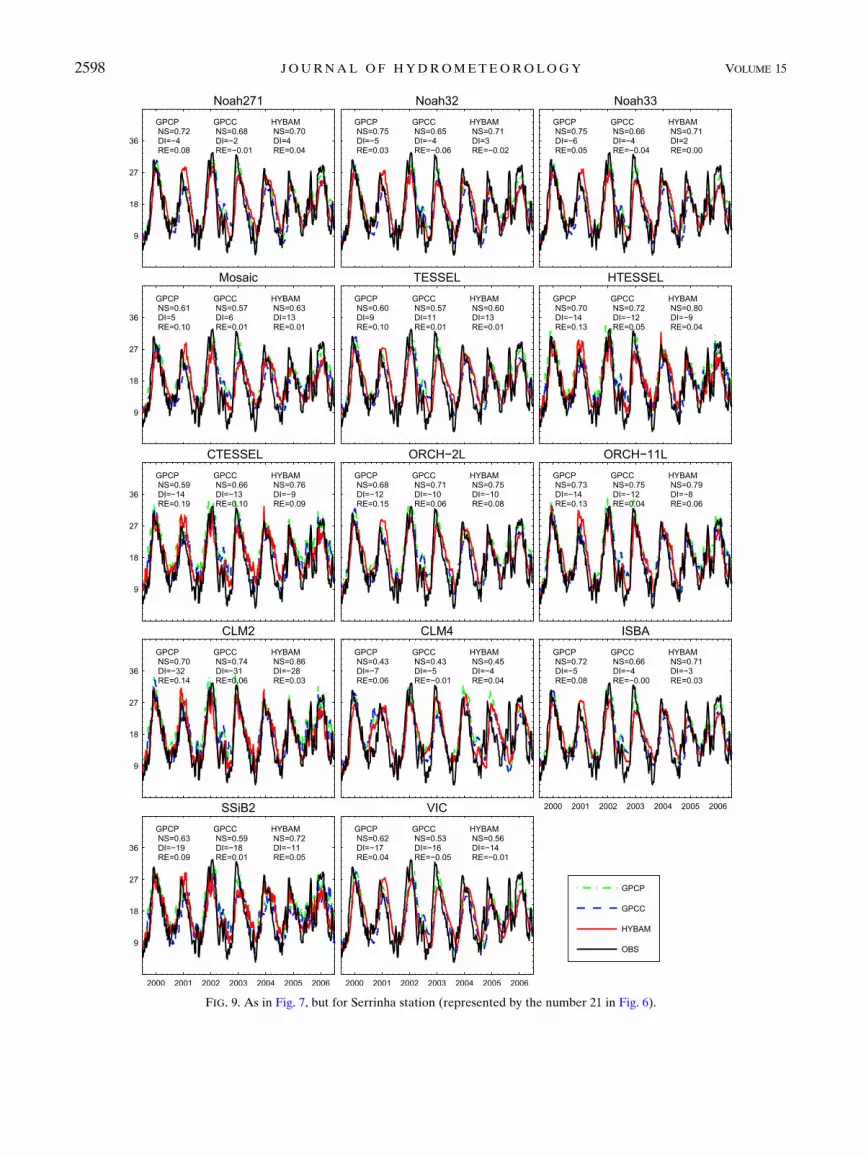
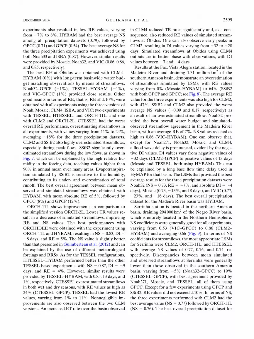
FIG. 9. As in Fig. 7, but for Serrinha station (represented by the number 21 in Fig. 6).


experiments also resulted in low RE values, varying

from 27% to 8%. HYBAM had the best average NS

among all precipitation datasets (0.79), followed by

GPCC (0.71) and GPCP (0.54). The best average NS for

the three precipitation experiments was achieved using

both Noah33 and ISBA (0.87). However, similar results

were provided by Mosaic, Noah32, and VIC (0.86, 0.86,

and 0.85, respectively).

The best RE at Óbidos was obtained with CLM4–HYBAM (0%) with long-term basinwide water bud-

get matching observations by means of streamflows.

Noah32–GPCP (21%), TESSEL–HYBAM (21%),

and VIC–GPCC (1%) provided close results. Other

good results in terms of RE, that is, RE # 610%, were

obtained with all experiments using the three versions of

Noah, Mosaic, CLM4, ISBA, and VIC; two experiments

with TESSEL, HTESSEL, and ORCH-11L; and one

with CLM2 and ORCH-2L. CTESSEL had the worst

overall RE performance, overestimating streamflows in

all experiments, with values varying from 11% to 24%,

averaging ;18% for the three precipitation datasets.

CLM2 and SSiB2 also highly overestimated streamflows,

especially during peak flows. SSiB2 significantly over-

estimated streamflows during the low flows, as shown in

Fig. 7, which can be explained by the high relative hu-

midity in the forcing data, reaching values higher than

90% in annual mean over many areas. Evapotranspira-

tion simulated by SSiB2 is sensitive to the humidity,

contributing to its under- and overestimation of total

runoff. The best overall agreement between mean ob-

served and simulated streamflows was obtained with

HYBAM, with mean absolute RE of 5%, followed by

GPCC (8%) and GPCP (12%).

ORCH-11L shows improvements in comparison to

the simplified version ORCH-2L. Lower TR values re-

sult in a decrease of simulated streamflows, improving

RE and NS values. The best performances with

ORCHIDEE were obtained with the experiment using

ORCH-11L and HYBAM, resulting in NS5 0.83, DI528 days, and RE 5 5%. The NS value is slightly better

than that presented inGuimberteau et al. (2012) and can

be explained by the use of different meteorological

forcings and RRSs. As for the TESSEL configurations,

HTESSEL–HYBAM performed better than the other

TESSEL-based experiments, with NS 5 0.87, DI 5 29

days, and RE 5 4%. However, similar results were

provided by TESSEL–HYBAM, with 0.85, 13 days, and

1%, respectively. CTESSEL overestimated streamflows

in both wet and dry seasons, with RE values as high as

24% (CTESSEL–GPCP). TESSEL had the lowest RE

values, varying from 1% to 11%. Nonnegligible im-

provements are also observed between the two CLM

versions. An increased ET rate over the basin observed

in CLM4 reduced TR rates significantly and, as a con-

sequence, also reduced RE values of simulated stream-

flows at Óbidos. One can also observe early peaks inCLM2, resulting in DI values varying from 232 to 228

days. Simulated streamflows at Óbidos using CLM4outputs are in better phase with observations, with DIvalues between 27 and 24 days.

Results at the Faz. Vista Alegre station, located in the

Madeira River and draining 1.31 million km2 of the

southern Amazon basin, demonstrate an overestimation

of streamflows simulated by LSMs, with RE values

varying from 0% (Mosaic–HYBAM) to 64% (SSiB2

with bothGPCP andGPCC; see Fig. 8). The averageRE

value for the three experiments was also high for CLM2,

with 47%. SSiB2 and CLM2 also provided the worst

average NS values (20.09 and 0.17, respectively) as

a result of an overestimated streamflow. Noah32 pro-

vided the best overall water budget and simulated–

observed streamflow agreement in the Madeira River

basin, with an average RE of 7%. NS values reached as

high as 0.86 (VIC–HYBAM). One can observe that,

except for Noah271, Noah32, Mosaic, and CLM4,

a flood wave delay is pronounced, evident by the nega-

tive DI values. DI values vary from negative values of

232 days (CLM2–GPCP) to positive values of 13 days

(Mosaic and TESSEL, both using HYBAM). This can

be explained by a long base flow time delay used in

HyMAP for that basin. The LSMs that provided the best

average results for the three precipitation datasets were

Noah32 (NS5 0.73, RE5;7%, and absolute DI5;4

days), Mosaic (0.73, ;13%, and 8 days), and VIC (0.77,

223%, and 216 days). The best overall precipitation

dataset for the Madeira River basin was HYBAM.

Serrinha station is located in the northern Amazon

basin, draining 294 000 km2 of the Negro River basin,

which is entirely located in the Northern Hemisphere.

NS coefficients were generally good for all experiments,

varying from 0.53 (VIC–GPCC) to 0.86 (CLM2–

HYBAM) and averaging 0.66 (Fig. 9). In terms of NS

coefficients for streamflows, the most appropriate LSMs

for Serrinha were CLM2, ORCH-11L, and HTESSEL

with average NS values of 0.77, 0.76, and 0.74, re-

spectively. Discrepancies between mean simulated

and observed streamflows at Serrinha were generally

lower than those observed in the southern Amazon

basin, varying from 25% (Noah32–GPCC) to 19%

(CTESSEL–GPCP), with best agreement provided by

Noah271, Mosaic, and TESSEL, all of them using

GPCC. Except for a few experiments using GPCP and

SSiB2, RE values did not exceed610%. In terms of NS,

the three experiments performed with CLM2 had the

best average value (NS5 0.77) followed by ORCH-11L

(NS 5 0.76). The best overall precipitation dataset for


that area is HYBAM, with average NS and RE values of

0.70 and 4%, respectively.

The efficiency of simulated streamflows can signifi-

cantly vary as a function of both the drainage area and

the geographical location of gauges. Figure 10 shows the

distribution of NS and RE obtained in the LSM runs

using HYBAM at the 165 gauges as a function of their

respective drainage areas and spatially distributed within

the Amazon basin. Average values of four drainage area

thresholds are also presented in the figure. Based on these

results, one can conclude that LSMs perform poorly in

small- [gauges draining 103 # A , 104 km2 (A1)] and

medium-sized [gauges draining 104 # A , 105 km2 (A2)]

basins, with worse NS and RE values. Previous studies

have reported similar conclusions that can be mainly

explained by averaging out precipitation errors and lack

of understanding and representation of finescale pro-

cesses (e.g., Getirana et al. 2012). Simulations at A1 and

A2 gauges have average NS lower than zero, with best

value of 20.82 provided by ISBA for A1 and 20.08

provided byMosaic forA2. All LSMs, except for ORCH-

2L, CLM2, SSiB2, and TESSEL, had positive NS values

FIG. 10. Performance coefficients of simulated streamflows using the HYBAM dataset for 1989–2009. (left) NS coefficients and (right)

REs as functions of the drainage area (in logarithmic scale) and spatially distributed within the Amazon basin. Values in the boxes

represent the average for each drainage area threshold.


at gauges draining large basins [105#A, 106 km2 (A3)],

with best average performances achieved by ORCH-11L

(0.37) and Mosaic (0.35). Gauges draining very large ba-

sins [A$ 106 km2 (A4)] had the best average performance,

withNS varying from 0.35 (SSiB2) to 0.72 (HTESSELand

ORCH-11L). Noah271, Noah33, CTESSEL, ISBA, and

VIC also performed well atA4 gauges with average NS.0.60. Like NS results, RE has lower performances at

gauges draining smaller areas, with best values of 25%

(Noah33), 28% (Noah32), 16% (Noah32), and 8%

(CLM4) for A1, A2, A3, and A4, respectively. Figure 11

shows scatterplots with the average NS and RE values for

the four drainage area thresholds listed in Fig. 10,

evidencing better results in larger areas and for experi-

ments using the HYBAM precipitation dataset.

Additional information can be extracted from the

spatial distribution of both coefficients. Most LSMs

highly overestimate mean streamflows (high RE values)

at gauges in the eastern side of the basin and can be

explained by overestimated total runoff caused by high

precipitation rates in that area. The same is observed in

the experiments using GPCC and GPCP.

NegativeNSvalues are observed in several gauges in the

southeastern part of the basin using any LSM and pre-

cipitation dataset. Streamflows from selected experiments

(Mosaic TESSEL and VIC forced with HYBAM) at

FIG. 10. (Continued)


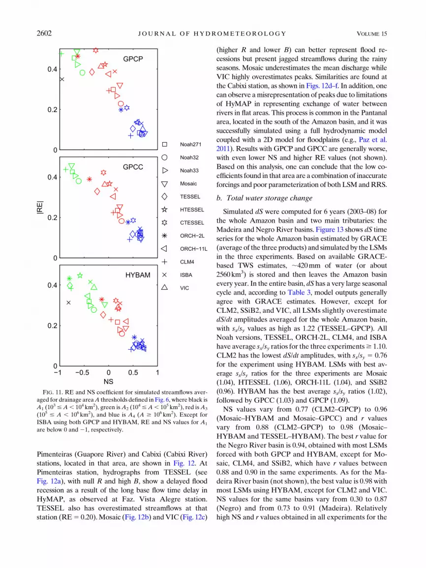
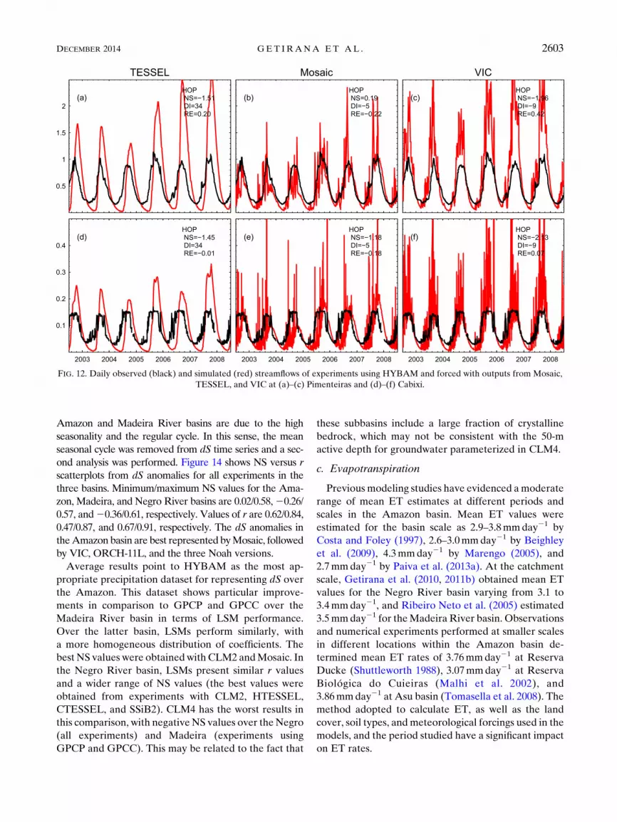
Pimenteiras (Guapore River) and Cabixi (Cabixi River)

stations, located in that area, are shown in Fig. 12. At

Pimenteiras station, hydrographs from TESSEL (see

Fig. 12a), with null R and high B, show a delayed flood

recession as a result of the long base flow time delay in

HyMAP, as observed at Faz. Vista Alegre station.

TESSEL also has overestimated streamflows at that

station (RE5 0.20).Mosaic (Fig. 12b) andVIC (Fig. 12c)

(higher R and lower B) can better represent flood re-

cessions but present jagged streamflows during the rainy

seasons. Mosaic underestimates the mean discharge while

VIC highly overestimates peaks. Similarities are found at

the Cabixi station, as shown in Figs. 12d–f. In addition, one

can observe amisrepresentation of peaks due to limitations

of HyMAP in representing exchange of water between

rivers in flat areas. This process is common in the Pantanal

area, located in the south of the Amazon basin, and it was

successfully simulated using a full hydrodynamic model

coupled with a 2D model for floodplains (e.g., Paz et al.

2011). Results with GPCP and GPCC are generally worse,

with even lower NS and higher RE values (not shown).

Based on this analysis, one can conclude that the low co-

efficients found in that area are a combination of inaccurate

forcings and poor parameterization of both LSMandRRS.

b. Total water storage change

Simulated dS were computed for 6 years (2003–08) for

the whole Amazon basin and two main tributaries: the

Madeira and Negro River basins. Figure 13 shows dS time

series for the whole Amazon basin estimated by GRACE

(average of the three products) and simulated by theLSMs

in the three experiments. Based on available GRACE-

based TWS estimates, ;420mm of water (or about

2560km3) is stored and then leaves the Amazon basin

every year. In the entire basin, dS has a very large seasonal

cycle and, according to Table 3, model outputs generally

agree with GRACE estimates. However, except for

CLM2, SSiB2, and VIC, all LSMs slightly overestimate

dS/dt amplitudes averaged for the whole Amazon basin,

with sx/sy values as high as 1.22 (TESSEL–GPCP). All

Noah versions, TESSEL, ORCH-2L, CLM4, and ISBA

have average sx/sy ratios for the three experiments$ 1.10.

CLM2 has the lowest dS/dt amplitudes, with sx/sy 5 0.76

for the experiment using HYBAM. LSMs with best av-

erage sx/sy ratios for the three experiments are Mosaic

(1.04), HTESSEL (1.06), ORCH-11L (1.04), and SSiB2

(0.96). HYBAM has the best average sx/sy ratios (1.02),

followed by GPCC (1.03) and GPCP (1.09).

NS values vary from 0.77 (CLM2–GPCP) to 0.96

(Mosaic–HYBAM and Mosaic–GPCC) and r values

vary from 0.88 (CLM2–GPCP) to 0.98 (Mosaic–

HYBAM and TESSEL–HYBAM). The best r value for

the Negro River basin is 0.94, obtained with most LSMs

forced with both GPCP and HYBAM, except for Mo-

saic, CLM4, and SSiB2, which have r values between

0.88 and 0.90 in the same experiments. As for the Ma-

deira River basin (not shown), the best value is 0.98 with

most LSMs using HYBAM, except for CLM2 and VIC.

NS values for the same basins vary from 0.30 to 0.87

(Negro) and from 0.73 to 0.91 (Madeira). Relatively

high NS and r values obtained in all experiments for the

FIG. 11. RE and NS coefficient for simulated streamflows aver-

aged for drainage areaA thresholds defined in Fig. 6, where black is

A1 (103 #A, 104 km2), green isA2 (10

4 #A, 105 km2), red isA3

(105 # A , 106 km2), and blue is A4 (A $ 106 km2). Except for

ISBA using both GPCP and HYBAM, RE and NS values for A1

are below 0 and 21, respectively.


Amazon and Madeira River basins are due to the high

seasonality and the regular cycle. In this sense, the mean

seasonal cycle was removed from dS time series and a sec-

ond analysis was performed. Figure 14 shows NS versus r

scatterplots from dS anomalies for all experiments in the

three basins. Minimum/maximum NS values for the Ama-

zon, Madeira, and Negro River basins are 0.02/0.58,20.26/

0.57, and20.36/0.61, respectively. Values of r are 0.62/0.84,

0.47/0.87, and 0.67/0.91, respectively. The dS anomalies in

theAmazon basin are best represented byMosaic, followed

by VIC, ORCH-11L, and the three Noah versions.

Average results point to HYBAM as the most ap-

propriate precipitation dataset for representing dS over

the Amazon. This dataset shows particular improve-

ments in comparison to GPCP and GPCC over the

Madeira River basin in terms of LSM performance.

Over the latter basin, LSMs perform similarly, with

a more homogeneous distribution of coefficients. The

best NS values were obtainedwith CLM2 andMosaic. In

the Negro River basin, LSMs present similar r values

and a wider range of NS values (the best values were

obtained from experiments with CLM2, HTESSEL,

CTESSEL, and SSiB2). CLM4 has the worst results in

this comparison, with negativeNS values over the Negro

(all experiments) and Madeira (experiments using

GPCP and GPCC). This may be related to the fact that

these subbasins include a large fraction of crystalline

bedrock, which may not be consistent with the 50-m

active depth for groundwater parameterized in CLM4.

c. Evapotranspiration

Previous modeling studies have evidenced amoderate

range of mean ET estimates at different periods and

scales in the Amazon basin. Mean ET values were

estimated for the basin scale as 2.9–3.8mmday21 by

Costa and Foley (1997), 2.6–3.0mmday21 by Beighley

et al. (2009), 4.3mmday21 by Marengo (2005), and

2.7mmday21 by Paiva et al. (2013a). At the catchment

scale, Getirana et al. (2010, 2011b) obtained mean ET

values for the Negro River basin varying from 3.1 to

3.4mmday21, and Ribeiro Neto et al. (2005) estimated

3.5mmday21 for theMadeira River basin. Observations

and numerical experiments performed at smaller scales

in different locations within the Amazon basin de-

termined mean ET rates of 3.76mmday21 at Reserva

Ducke (Shuttleworth 1988), 3.07mmday21 at Reserva

Biológica do Cuieiras (Malhi et al. 2002), and

3.86mmday21 at Asu basin (Tomasella et al. 2008). The

method adopted to calculate ET, as well as the land

cover, soil types, and meteorological forcings used in the

models, and the period studied have a significant impact

on ET rates.

FIG. 12. Daily observed (black) and simulated (red) streamflows of experiments using HYBAM and forced with outputs from Mosaic,

TESSEL, and VIC at (a)–(c) Pimenteiras and (d)–(f) Cabixi.


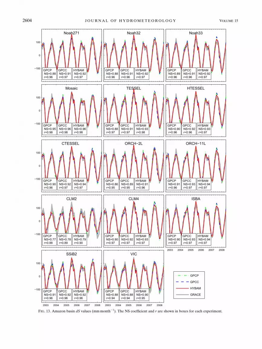
FIG. 13. Amazon basin dS values (mmmonth21). The NS coefficient and r are shown in boxes for each experiment.


As listed in Table 4, at the Amazon basin scale and for

the 1989–2008 period, we can also show a large range of

mean ET, varying from 2.39 (CTESSEL and CLM2,

both with GPCC) to 3.26mmday21 (Noah32–HYBAM),

and averaging 2.83mmday21 for the entire set of ex-

periments. These estimates correspond to 45%–49% of

the mean precipitation. Precipitation datasets had dif-

ferent impacts on ET estimates, depending on the LSM.

Simulations forcedwithGPCC resulted in the lowest ET

rates averaging 2.77mmday21, while HYBAM pro-

vided the highest ET rates, averaging 2.94mmday21,

showing consistency with the streamflow biases dis-

cussed above. Some LSMs are more sensitive to changes

in precipitation fields than others, which could be ex-

plained by the daily (in the case of HYBAM) and

monthly (GPCP and GPCC) distribution of precip-

itation, impacting the evaporation of intercepted rainfall

in the models. For example, mean ET rates provided by

CLM2 vary 17%, from 2.39 to 2.78mmday21, while

Noah271 has mean ET rates varying only 2%, from 2.93

to 3.00mmday21. Mean ET values range from 2.42

(CTESSEL–GPCC) to 3.40mmday21 (Noah32–HYBAM)

in the Negro River basin, averaging 41% of the precip-

itation. In the Madeira River basin, ET varies from 2.11

(SSiB2–GPCC) to 3.22mmday21 (Mosaic–HYBAM)

and averages 55% of the precipitation.

Spatial patterns of ET change significantly from one

LSM to another, but similar characteristics can be per-

ceived through experiments usingHYBAM, as shown in

Fig. 15.Differentmodel versions, such asNoah, TESSEL,

or ORCHIDEE, show similar spatial patterns but wide-

ranging rates. A west-to-east gradient is evidenced, with

low ET rates at high altitudes near the Andes (extreme

west and south), followed by a significant increase, and

then a slight decrease in the central Amazon. The 11-layer

ORCH-11L version (2.9mmday21) presents a ;7% in-

creaseofETwhencompared toORCH-2L (2.8mmday21).

CLM2 and VIC substantially underestimate ET in the

south, in comparison to other LSMs. The low correlation

between simulated ET and P spatial distributions [see

Fig. 16 for ET spatial distribution averaged for each ex-

periment (GPCP, GPCC, and HYBAM), MOD16, and

FLUXNET] indicates that this hydrological variable does

not depend on water availability. This has also been evi-

denced in a previous study over the Negro (Getirana et al.

2011b) and Amazon (Guimberteau et al. 2012) River

basins.

Based on the ET mean seasonal cycle computed for

the 2000–08 period, corresponding to the intersection

over time when all datasets are available (see Fig. 17),

one can observe that most models provide the lowest ET

rates in May and peak in October. Exceptions are

CLM2, SSiB2, and VIC, with later ET recessions and

peaks occurring in June–October and November–

December, respectively. The VIC version used in this

study has three soil layers in a single soil column at

a grid. The second layer is the main soil moisture storage

and the third layer provides moisture for base flow. They

were both adjusted during the calibration process to

result in routed streamflow that satisfactorily match

observations at large basin scale. Based on the time se-

ries of daily precipitation, evapotranspiration, surface

runoff, and base flow for the 2000–08 period (not

shown), VIC–GPCP shows that a large portion of P is

partitioned into surface runoff and base flow during the

dry period, which can be explained by the fact that the

second and third layers are too shallow and too thick,

respectively, leading to less soil moisture available for

evapotranspiration during the same period.

MOD16A2 evidences an earlier season, with the

lowest ET (2.91mmday21) occurring in April and peak

(3.57mmday21) in August. Except for Noah32 (3.19–

3.28mmday21) andMosaic (2.90–3.21mmday21), LSMs

underestimate mean ET rates in comparison to the

MOD16A2 product (3.22mmday21). As shown in

Fig. 18, average correlations between simulated ET and

MOD16A2 for the whole Amazon basin vary from

20.37 (VIC–GPCC) to 0.67 (ORCH-11L using GPCP).

In contrast, the same LSMs with high r values also

present high RE, with values between 230% and

210%. All Noah versions, Mosaic, CLM4, and VIC

have the best RE values in at least one of the three ex-

periments. CLM4 has the best combination of r (0.60)

and RE (28%), when compared against MOD16A2.

Nevertheless, results vary according to the region.

Noah32–HYBAM better matches MOD16A2 (r 5 0.72

TABLE 3. Std dev ratio of simulated and GRACE-based

total water storage change (i.e., sx/sy) within theAmazon basin for

2003–08.

GPCP GPCC HYBAM Avg

Noah271 1.19 1.12 1.12 1.14

Noah32 1.16 1.09 1.08 1.11

Noah33 1.15 1.09 1.08 1.11

Mosaic 1.09 1.01 1.02 1.04

TESSEL 1.22 1.15 1.13 1.16

HTESSEL 1.10 1.05 1.03 1.06

CTESSEL 1.13 1.08 1.06 1.09

ORCH-2L 1.15 1.09 1.07 1.10

ORCH-11L 1.08 1.02 1.03 1.04

CLM2 0.85 0.78 0.76 0.80

CLM4 1.14 1.08 1.08 1.10

ISBA7 1.15 1.09 1.08 1.10

SSiB2 0.99 0.93 0.96 0.96

VIC 0.92 0.87 0.86 0.88

Avg 1.09 1.03 1.02 1.05


and RE526%) in theMadeira River basin and ISBA–

GPCP (r 5 0.71 and RE 5 0) in the Negro River basin.

On the other hand, LSM outputs present a better

agreement with FLUXNET. The average recession and

peak of FLUXNET for the Amazon basin occur in June

(2.89mmday21) and in October (3.32mmday21), re-

spectively (Fig. 17). The r values are positive in all ex-

periments, varying from 0.35 (ISBA–GPCC) to 0.83

(SSiB2–GPCP; see Fig. 19). A higher number of LSMs

(all Noah versions, Mosaic, CLM4, and VIC) present

RE values lower than 10%, when compared against

FLUXNET. Based on these results, the experiment

Mosaic–HYBAM has the best performance, combining

a high r (0.78) with low RE (22%). Similar results are

obtained for the Madeira River basin. As for the Negro

River basin, a few LSM outputs resulted in negative

or near to zero r values in one or more experiments

(CTESSEL, TESSEL, CLM2, and SSiB2), indicating a

large spatial variability in the reliability of datasets.

Overall, HYBAM experiments have higher r and

lower RE.

5. Concluding remarks

This paper compares and evaluates the capability of

14 LSMs to simulate the large-scale water budget in the

Amazon basin using both remote sensing and in situ

data. To assess the impacts of precipitation on the water

budget, three experiments were performed with each

LSM using different ground-based precipitation data-

sets (GPCP, GPCC, and HYBAM), totaling 42 re-

alizations. Four water budget variables were evaluated

in this context: the total water storage change (i.e., dS),

evapotranspiration (i.e., ET), surface runoff (i.e., R),

FIG. 14. Correlation andNS coefficients of anomalies of simulated total water storage (with respect to themean seasonal cycle) change for

the Amazon, Madeira, and Negro River basins.


and base flow (i.e., B). Simulated dS was compared

against three GRACE products, ET against both the

satellite-based MOD16A2 and ground-based FLUXNET

products, and TR against observed streamflows at 165

gauging stations. TheHyMAPRRSwas used to convertR

andB into streamflow. LSMs performed differently in the

sequence of analyses. ISBA had the best performance for

streamflows at Óbidos and, except for TESSEL, ORCH-2L, CLM2, CLM4, and SSiB2, all the LSMs providedoverall good streamflows at the basin scale. In particular,CLM2 and SSiB2 presented limitations in reproducingstreamflows, which can be explained by errors with respectto the simulation of ET. Results show that streamflowssimulated at larger scales perform better than at smallerscales. This is mostly due to error compensations occurringin smaller catchments, related to scale issues, forcing er-rors, and inaccurate parameterizations. This study has alsoevidenced limitations in the representation of streamflowsin the southern Amazon basin that can be due to anoverestimation of base flow by certain LSMs and/or a poorparameterization of HyMAP, and limited representationof physical processes. These limitations should be ad-dressed in further studies. It has also been shown thatspatial distribution of simulated total runoff is correlatedto the precipitation patterns. On the other hand, the lowcorrelation between spatially distributed ET and P shows

that evapotranspiration does not depend on water avail-

ability within the basin. As for dS, at the Amazon basin

scale, most LSMs provided dS time series consistent with

GRACE estimates, with relatively high NS and r co-

efficients. When dS anomalies are evaluated for the entire

Amazon basin, Mosaic shows the best overall results,

while CLM2, CLM4, and SSiB2 present inferior perfor-

mance coefficients in comparison to other models. In

particular, the overestimated runoff from SSiB2 is mostly

TABLE 4. Mean ET (mmday21) in the Amazon basin computed

by the LSMs for 1989–2008 (except when indicated). The mean

precipitation is also provided.

GPCP GPCC HYBAM Avg

Precipitation 6.14 5.99 6.03 6.05

Noah271 2.96 2.93 3.00 2.96

Noah32 3.17 3.15 3.26 3.19

Noah33 3.09 3.07 3.15 3.10

Mosaic 2.90 2.88 3.17 2.98

TESSEL 2.76 2.72 2.94 2.81

HTESSEL 2.64 2.61 2.84 2.70

CTESSEL 2.41 2.39 2.65 2.48

ORCH-2L 2.61 2.60 2.76 2.66

ORCH-11L 2.75 2.74 2.94 2.81

CLM2 2.43 2.39 2.78 2.53

CLM4 3.00 2.98 3.01 3.00

ISBA 2.81 2.77 2.88 2.82

SSiB2 2.68 2.66 2.72 2.69

VIC 2.90 2.86 3.03 2.93

Avg 2.79 2.77 2.94 2.83

MOD16A2 (2000–11) — — — 3.22

FLUXNET (1982–2008) — — — 3.13

FIG. 15. Average ET for 1989–2008 from experiments using the HYBAM precipitation dataset.


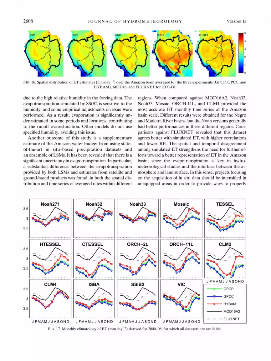
due to the high relative humidity in the forcing data. The

evapotranspiration simulated by SSiB2 is sensitive to the

humidity, and some empirical adjustments on issue were

performed. As a result, evaporation is significantly un-

derestimated in some periods and locations, contributing

to the runoff overestimation. Other models do not use

specified humidity, avoiding this issue.

Another outcome of this study is a supplementary

estimate of the Amazon water budget from using state-

of-the-art in situ–based precipitation datasets and

an ensemble of LSMs. It has been revealed that there is a

significant uncertainty in evapotranspiration. In particular,

a substantial difference between the evapotranspiration

provided by both LSMs and estimates from satellite and

ground-based products was found, in both the spatial dis-

tribution and time series of averaged rates within different

regions. When compared against MOD16A2, Noah32,

Noah33, Mosaic, ORCH-11L, and CLM4 provided the

most accurate ET monthly time series at the Amazon

basin scale. Different results were obtained for the Negro

andMadeiraRiver basins, but theNoah versions generally

had better performances in these different regions. Com-

parisons against FLUXNET revealed that this dataset

agrees better with simulated ET, with higher correlations

and lower RE. The spatial and temporal disagreement

among simulated ET strengthens the need for further ef-

forts toward a better representation of ET in the Amazon

basin, since the evapotranspiration is key in hydro-

meteorological studies and the interface between the at-

mosphere and land surface. In this sense, projects focusing

on the acquisition of in situ data should be intensified in

unequipped areas in order to provide ways to properly

FIG. 16. Spatial distribution of ET estimates (mmday21) over the Amazon basin averaged for the three experiments (GPCP, GPCC, and

HYBAM), MOD16, and FLUXNET for 2000–08.

FIG. 17. Monthly climatology of ET (mmday21) derived for 2000–08, for which all datasets are available.


evaluate and improve existing LSM parameterizations.

For example, this study suggests that CTESSEL un-

derestimates evapotranspiration, which has not been ex-

tensively evaluated. Model intercomparisons along with

different observational datasets can provide guidance to

model improvements.

Despite the differences found among LSM water

budgets, the analyses performed in this study could

show that experiments using the HYBAM pre-

cipitation dataset provided the most accurate repre-

sentation of the water budget in the Amazon basin.

Results using this dataset had the best performances

with all LSMs in most comparisons. This demonstrates

that efforts in obtaining in situ data in the framework of

international collaborations should be intensified with

the objective of providing better estimates of pre-

cipitation fields in remote and unequipped areas. It

also shows that daily distribution can play an important

role in the calculation of evapotranspiration, particu-

larly in LSMs representing rainfall interception, as

previously demonstrated in Guimberteau et al. (2012).

In this sense, a more detailed evaluation of impacts of

rainfall on evapotranspiration simulations with and

without rainfall interception is recommended for fu-

ture works.

The intercomparison performed in this study was

based on a relatively short list of LSMs, considering

the number of models being currently developed

worldwide. In this sense, the classification of most

appropriated LSMs to simulate the large-scale water

budget in theAmazon basin should be considered taking

into account that our current list is not extensive. Also,

this study focused on the evaluation of large-scale hy-

drological processes represented by LSMs rather than

FIG. 18. Performance coefficients of monthly mean ET rates for 2000–08 when compared against MOD16A2.


on the full evaluation of both water and energy budgets

at smaller spatial scales. Based on comparisons of dif-

ferent LSM versions/configurations (see the cases of

TESSEL and ORCHIDEE versions), one can conclude

that representing physical processes in a higher level of

complexity substantially improves the representation

of selected hydrological processes. This conclusion is

specially based on the results obtained for the set of

streamflow simulations where more complex versions/

configurations (HTESSEL, CTESSEL, and ORCH-11L)

derived performance coefficients at gauges higher than

simpler ones (TESSEL and ORCH-2L). A recent eval-

uation of the two ORCHIDEE versions over the Ama-

zon basin has found similar results (Guimberteau et al.

2014). Differences among the Noah versions considered

in this study resulted in minor differences of the

large-scale water budget in the Amazon basin. At the

same time, more simplified LSMs, such as Mosaic, also

had outstanding performances in comparison to the

whole set of models. This is probably because of the fact

that they have been through previous parameter cali-

brations. Other models (e.g., CLM4) essentially apply

the same set of hydrologic parameters uniformly across

the whole global domain. Further analyses considering

energetic variables at different scales can point to rea-

sons for these differences to occur. Regardless of these

limitations, this comparison provided insights of how

models simulate the spatial and temporal water avail-

ability during wet and dry seasons.

Acknowledgments. A. Getirana was funded by the

NASA Postdoctoral Program (NPP) managed by Oak

Ridge Associated Universities (ORAU). E. Dutra was fi-

nancially supportedby theFP7EUprojectEartH2Observe,

FIG. 19. Performance coefficients of monthly mean ET rates for 2000–08 when compared against FLUXNET.


and M. Guimberteau was supported by the EU-FP7

AMAZALERT project. H.-Y. Li acknowledges the sup-

port by the Office of Science of the U.S. Department of

Energy as part of the Regional and Global Climate

Modeling program. The Pacific Northwest National Lab-

oratory is operated for the DOE by Battelle Memorial

Institute under Contract DE-AC05-76RLO1830. The

study benefited from data made available by Agencia

Nacional de Águas (ANA). We thank M. Jung for pro-viding the gridded FLUXNET dataset.

REFERENCES

Adler, R. F., and Coauthors, 2003: The version 2 Global Pre-

cipitation Climatology Project (GPCP) monthly precipitation

analysis (1979–present). J. Hydrometeor., 4, 1147–1167,

doi:10.1175/1525-7541(2003)004,1147:TVGPCP.2.0.CO;2.

Albergel, C., G. Balsamo, P. de Rosnay, J. Muñoz-Sabater, andS. Boussetta, 2012: A bare ground evaporation revision in the

ECMWF land-surface scheme: Evaluation of its impact using

ground soil moisture and satellite microwave data. Hydrol.

Earth Syst. Sci., 16, 3607–3620, doi:10.5194/hess-16-3607-2012.

Alkama, M. R., M. Kageyama, G. Ramstein, O. Marti, P. Ribstein,

andD. Swingedouw, 2008: Impact of a realistic river routing in

coupled ocean–atmosphere simulations of the Last Glacial

Maximum climate. Climate Dyn., 30, 855–869, doi:10.1007/

s00382-007-0330-1.

Balsamo, G., P. Viterbo, A. Beljaars, B. van denHurk, A. K. Betts,

and K. Scipal, 2009: A revised hydrology for the ECMWF

model: Verification from field site to terrestrial water storage

and impact in the integrated forecast system. J. Hydrometeor.,

10, 623–643, doi:10.1175/2008JHM1068.1.

——, S. Boussetta, E. Dutra, A. Beljaars, P. Viterbo, and B. van

denHurk, 2011: Evolution of land surface processes in the IFS.

ECMWF Newsletter, No. 127, ECMWF, Reading, United

Kingdom, 17–22.

Beighley, R. E., K. G. Eggert, T. Dunne, Y. He, V. Gummadi, and

K. L. Verdin, 2009: Simulating hydrologic and hydraulic pro-

cesses throughout theAmazonRiver basin.Hydrol. Processes,

23, 1221–1235, doi:10.1002/hyp.7252.

Beven, K. J., and M. J. Kirkby, 1979: A physically based variable

contributing area model of basin hydrology.Hydrol. Sci. Bull.,

24, 43–69, doi:10.1080/02626667909491834.

Bonan, G. B., K. W. Oleson, M. Vertenstein, S. Levis, X. Zeng,

Y. Dai, R. E. Dickinson, and Z.-L. Yang, 2002: The land sur-

face climatology of the Community LandModel coupled to the

NCAR Community Climate Model. J. Climate, 15, 3123–3149,

doi:10.1175/1520-0442(2002)015,3123:TLSCOT.2.0.CO;2.

Boone, A., and Coauthors, 2004: The Rhone-Aggregation Land

Surface Scheme intercomparison project: An overview. J. Cli-

mate, 17, 187–208, doi:10.1175/1520-0442(2004)017,0187:

TRLSSI.2.0.CO;2.

——, and Coauthors, 2009a: The AMMA Land Surface Model

Intercomparison Project. Bull. Amer. Meteor. Soc., 90, 1865–

1880, doi:10.1175/2009BAMS2786.1.

——, and Coauthors, 2009b: AMMA Land Surface Model In-

tercomparison Project Phase 2 (ALMIP-2).Gewex News,Vol.

9, No. 4, International GEWEX Project Office, Silver Spring,

MD, 9–10. [Available online at www.gewex.org/images/

Nov2009.pdf.]

Boussetta, S., G. Balsamo, A. Beljaars, T. Kral, and L. Jarlan,

2013a: Impact of a satellite-derived leaf area index monthly

climatology in a global numerical weather prediction

model. Int. J. Remote Sens., 34, 3520–3542, doi:10.1080/

01431161.2012.716543.

——, and Coauthors, 2013b: Natural land carbon dioxide ex-

changes in the ECMWF integrated forecasting system: Im-

plementation and offline validation. J. Geophys. Res. Atmos.,

118, 5923–5946, doi:10.1002/jgrd.50488.Campoy, A., A. Ducharne, F. Chéruy, F. Hourdin, J. Polcher, and

J. C. Dupont, 2013: Response of land surface fluxes and pre-

cipitation to different soil bottom hydrological conditions in

a general circulation model. J. Geophys. Res. Atmos., 118,

10 725–10 739, doi:10.1002/jgrd.50627.

Coe, M. T., M. H. Costa, A. Botta, and C. Birkett, 2002: Long-term

simulations of discharge and floods in the Amazon basin.

J. Geophys. Res., 107, 8044, doi:10.1029/2001JD000740.

——, ——, and E. A. Howard, 2008: Simulating the surface waters

of the Amazon River basin: Impacts of new river geomorphic

and flow parameterization. Hydrol. Processes, 22, 2542–2553,

doi:10.1002/hyp.6850.

Costa, M. H., and J. A. Foley, 1997: Water balance of the Amazon

basin: Dependence on vegetation cover and canopy conduc-

tance. J. Geophys. Res., 102, 23 973–23 989, doi:10.1029/

97JD01865.

——, and ——, 1998: A comparison of precipitation datasets for

the Amazon basin. Geophys. Res. Lett., 25, 155–158,

doi:10.1029/97GL03502.

Dai, Y., andCoauthors, 2003: TheCommonLandModel.Bull. Amer.

Meteor. Soc., 84, 1013–1023, doi:10.1175/BAMS-84-8-1013.

Decharme, B., and H. Douville, 2007: Global validation of the

ISBA sub-grid hydrology. Climate Dyn., 29, 21–37,

doi:10.1007/s00382-006-0216-7.

——, R. Alkama, F. Papa, S. Faroux, H. Douville, and C. Prigent,

2012: Global off-line evaluation of the ISBA-TRIP

flood model. Climate Dyn., 38, 1389–1412, doi:10.1007/

s00382-011-1054-9.

De Rosnay, P., J. Polcher, M. Bruen, and K. Laval, 2002: Impact of

a physically based soil water flow and soil–plant interaction

representation for modeling large-scale land surface pro-

cesses. J. Geophys. Res., 107, 4118, doi:10.1029/2001JD000634.

Dirmeyer, P. A., A. Dolman, and N. Sato, 1999: The pilot phase

of the Global Soil Wetness Project. Bull. Amer. Meteor.

Soc., 80, 851–878, doi:10.1175/1520-0477(1999)080,0851:

TPPOTG.2.0.CO;2.

——, X. Gao, M. Zhao, Z. Guo, T. Oki, and N. Hanasaki, 2006:

GSWP-2: Multimodel analysis and implications for our per-

ception of the land surface.Bull. Amer.Meteor. Soc., 87, 1381–

1397, doi:10.1175/BAMS-87-10-1381.

D’Orgeval, T., J. Polcher, and P. de Rosnay, 2008: Sensitivity of the

WestAfrican hydrological cycle inORCHIDEE to infiltration

processes.Hydrol. Earth Syst. Sci., 12, 1387–1401, doi:10.5194/

hess-12-1387-2008.

Drobinski, P., and Coauthors, 2014: HyMeX: A 10-year multi-

disciplinary program on the Mediterranean water cycle.

Bull. Amer. Meteor. Soc., 95, 1063–1082, doi:10.1175/

BAMS-D-12-00242.1.

Ducharne, A., K. Laval, and J. Polcher, 1998: Sensitivity of

the hydrological cycle to the parametrization of soil hydrology

in a GCM. Climate Dyn., 14, 307–327, doi:10.1007/

s003820050226.

——, C. Golaz, E. Leblois, K. Laval, J. Polcher, E. Ledoux, and

G. de Marsily, 2003: Development of a high resolution runoff


http://dx.doi.org/10.1175/1525-7541(2003)004<1147:TVGPCP>2.0.CO;2

http://dx.doi.org/10.5194/hess-16-3607-2012

http://dx.doi.org/10.1007/s00382-007-0330-1

http://dx.doi.org/10.1007/s00382-007-0330-1

http://dx.doi.org/10.1175/2008JHM1068.1

http://dx.doi.org/10.1002/hyp.7252

http://dx.doi.org/10.1080/02626667909491834

http://dx.doi.org/10.1175/1520-0442(2002)015<3123:TLSCOT>2.0.CO;2

http://dx.doi.org/10.1175/1520-0442(2004)017<0187:TRLSSI>2.0.CO;2

http://dx.doi.org/10.1175/1520-0442(2004)017<0187:TRLSSI>2.0.CO;2

http://dx.doi.org/10.1175/2009BAMS2786.1

http://www.gewex.org/images/Nov2009.pdf

http://www.gewex.org/images/Nov2009.pdf

http://dx.doi.org/10.1080/01431161.2012.716543

http://dx.doi.org/10.1080/01431161.2012.716543

http://dx.doi.org/10.1002/jgrd.50488

http://dx.doi.org/10.1002/jgrd.50627

http://dx.doi.org/10.1029/2001JD000740


http://dx.doi.org/10.1029/97JD01865


http://dx.doi.org/10.1029/97GL03502

http://dx.doi.org/10.1175/BAMS-84-8-1013

http://dx.doi.org/10.1007/s00382-006-0216-7

http://dx.doi.org/10.1007/s00382-011-1054-9

http://dx.doi.org/10.1007/s00382-011-1054-9

http://dx.doi.org/10.1029/2001JD000634

http://dx.doi.org/10.1175/1520-0477(1999)080<0851:TPPOTG>2.0.CO;2

http://dx.doi.org/10.1175/1520-0477(1999)080<0851:TPPOTG>2.0.CO;2




http://dx.doi.org/10.1175/BAMS-D-12-00242.1


http://dx.doi.org/10.1007/s003820050226

http://dx.doi.org/10.1007/s003820050226

routing model, calibration and application to assess runoff

from the LMD GCM. J. Hydrol., 280, 207–228, doi:10.1016/

S0022-1694(03)00230-0.

Ducoudré, N., K. Laval, andA. Perrier, 1993: SECHIBA, a new set

of parameterizations of the hydrologic exchanges at the land–

atmosphere interface within the LMD atmospheric global

circulation model. J. Climate, 6, 248–273, doi:10.1175/

1520-0442(1993)006,0248:SANSOP.2.0.CO;2.

Durand, F., F. Papa, A. Rahman, and S. K. Bala, 2011: Impact of

Ganges–Brahmaputra interannual discharge variations on

Bay of Bengal salinity and temperature during the 1992–

99 period. J. Earth Syst. Sci., 120, 859–872, doi:10.1007/

s12040-011-0118-x.

Dutra, E., G. Balsamo, P. Viterbo, P. M. A. Miranda, A. Beljaars,

C. Schar, and K. Elder, 2010: An improved snow scheme for

the ECMWF land surface model: Description and offline

validation. J. Hydrometeor., 11, 899–916, doi:10.1175/

2010JHM1249.1.

Ek, M., K. Mitchell, L. Yin, P. Rogers, P. Grunmann, V. Koren,

G.Gayno, and J. Tarpley, 2003: Implementation of Noah land-

surface model advances in the NCEP operational mesoscale

Eta model. J. Geophys. Res., 108, 8851, doi:10.1029/

2002JD003296.

EspinozaVillar, J. C., andCoauthors, 2009: Spatiotemporal rainfall

variability in the Amazon basin countries (Brazil, Peru, Bo-

livia, Colombia, and Ecuador). Int. J. Climatol., 29, 1574–1594,

doi:10.1002/joc.1791.

Gedney, N., P. M. Cox, and C. Huntingford, 2004: Climate feed-

back from wetland methane emission.Geophys. Res. Lett., 31,

L20503, doi:10.1029/2004GL020919.

Gent, P. R., and Coauthors, 2011: The Community Climate System

Model version 4. J. Climate, 24, 4973–4991, doi:10.1175/

2011JCLI4083.1.

Getirana, A. C. V., and C. Peters-Lidard, 2013: Estimating water

discharge from large radar altimetry datasets. Hydrol. Earth

Syst. Sci., 17, 923–933, doi:10.5194/hess-17-923-2013.——, M.-P. Bonnet, O. C. Rotunno Filho, J.-L. Guyot, F. Seyler,

and W. J. Mansur, 2010: Hydrological modelling and water

balance of the Negro River basin: Evaluation based on in situ

and spatial altimetry data. J. Hydrol., 24, 3219–3236,

doi:10.1002/hyp.7747.

——, and Coauthors, 2011a: Calibration and validation of a hy-

drological model with in situ data, spatial altimetry and gra-

vimetry (in Portuguese).Rev. Bras. Recur. Hidricos, 16, 29–45.——, J. C. V. Espinoza, J. Ronchail, and O. C. Rotunno Filho,

2011b:Assessment of different precipitation datasets and their

impacts on the water balance of the Negro River basin.

J. Hydrol., 404, 304–322, doi:10.1016/j.jhydrol.2011.04.037.

——, A. Boone, D. Yamazaki, B. Decharme, F. Papa, and

N. Mognard, 2012: The Hydrological Modeling and Analysis

Platform (HyMAP): Evaluation in the Amazon basin.

J. Hydrometeor., 13, 1641–1665, doi:10.1175/JHM-D-12-021.1.

——, ——, ——, and N. Mognard, 2013: Automatic parameteri-

zation of a flow routing scheme driven by radar altimetry data:

Evaluation in the Amazon basin.Water Resour. Res., 49, 614–

629, doi:10.1002/wrcr.20077.

——, ——, and C. Peugeot, 2014: Evaluating LSM-based water

budgets over aWest African basin assisted with a river routing

scheme. J. Hydrometeor., doi:10.1175/JHM-D-14-0012.1, in

press.

Green, W. H., and G. Ampt, 1911: Studies on soil physics: 1. The

flow of air and water through soils. J. Agric. Sci., 4 (1), 1–24,

doi:10.1017/S0021859600001441.

Guimberteau, M., and Coauthors, 2012: Discharge simulation in

the sub-basins of the Amazon using ORCHIDEE forced by

new datasets. Hydrol. Earth Syst. Sci., 16, 911–935,

doi:10.5194/hess-16-911-2012.

——, P. Ciais, A. Ducharne, J. P. Boisier, S. Peng, M. De Weirdt,

and H. Verbeeck, 2014: Testing conceptual and physically

based soil hydrology schemes against observations for the

Amazon basin.Geosci. Model Dev., 7, 1115–1136, doi:10.5194/

gmd-7-1115-2014.

Guo, Z., P. A. Dirmeyer, Z.-Z. Hu, X. Gao, and M. Zhao, 2006:

Evaluation of the Second Global Soil Wetness Project soil

moisture simulations: 2. Sensitivity to external meteorological

forcing. J. Geophys. Res., 111, D22S03, doi:10.1029/

2006JD007845.

Henderson-Sellers, A., A. J. Pitman, P. K. Love, P. Irannejad,

and T. Chen, 1995: The Project for Intercomparison of

Land-Surface Parameterization Schemes (PILPS): Phases

2 and 3. Bull. Amer. Meteor. Soc., 76, 489–503, doi:10.1175/

1520-0477(1995)076,0489:TPFIOL.2.0.CO;2.

Jarvis, P. G., 1976: The interpretation of the variations in leaf water

potential and stomatal conductance found in canopies in the

field. Philos. Trans. Roy. Soc. London, B273, 593–610,

doi:10.1098/rstb.1976.0035.

Jung, M., M. Reichstein, and A. Bondeau, 2009: Towards global

empirical upscaling of FLUXNET eddy covariance observa-

tions: Validation of a model tree ensemble approach using

a biosphere model. Biogeosciences, 6, 2001–2013, doi:10.5194/

bg-6-2001-2009.

Justice, C. O., J. R. G. Townshend, E. F. Vermote, E. Masuoka,

R. E. Wolfe, N. Saleous, D. P. Roy, and J. T. Morisette, 2002:

An overview of MODIS Land data processing and

product status. Remote Sens. Environ., 83, 3–15, doi:10.1016/

S0034-4257(02)00084-6.

Killeen, T. J., M. Douglas, T. Consiglio, P. M. Jørgensen, and

J.Mejia, 2007:Dry spots andwet spots in theAndean hotspot. J.

Biogeogr., 34, 1357–1373, doi:10.1111/j.1365-2699.2006.01682.x.

Koster, R. D., and M. J. Suarez, 1996: Energy and water balance

calculations in the Mosaic LSM. NASA Tech. Memo. 104606,

Vol. 9, 60 pp. [Available online at http://gmao.gsfc.nasa.gov/

pubs/docs/Koster130.pdf.]

Krinner, G., and Coauthors, 2005: A dynamic global vegetation

model for studies of the coupled atmosphere–biosphere sys-

tem. Global Biogeochem. Cycles, 19, GB1015, doi:10.1029/

2003GB002199.

Kumar, S. V., and Coauthors, 2006: Land information system: An

interoperable framework for high resolution land surface

modeling. Environ. Modell. Software, 21, 1402–1415,

doi:10.1016/j.envsoft.2005.07.004.

Landerer, F. W., and S. C. Swenson, 2012: Accuracy of scaled

GRACE terrestrial water storage estimates. Water Resour.

Res., 48, W04531, doi:10.1029/2011WR011453.

Lawrence, D., and Coauthors, 2011: Parameterization improve-

ments and functional and structural advances in version 4 of

the Community Land Model. J. Adv. Model. Earth Syst., 3,

M03001, doi:10.1029/2011MS000045.

Li, H., M. Huang, M. S. Wigsmota, Y. Ke, A. M. Coleman, L. R.

Leung, A. Wang, and D. M. Ricciuto, 2011: Evaluating

runoff simulations from the Community LandModel 4.0 using

observations from flux towers and a mountainous watershed.

J. Geophys. Res., 116, D24120, doi:10.1029/2011JD016276.

——, M. S. Wigsmota, H. Wu, M. Huang, Y. Ke, A. M. Coleman,

and L. R. Leung, 2013: A physically based runoff routing


http://dx.doi.org/10.1016/S0022-1694(03)00230-0

http://dx.doi.org/10.1016/S0022-1694(03)00230-0

http://dx.doi.org/10.1175/1520-0442(1993)006<0248:SANSOP>2.0.CO;2

http://dx.doi.org/10.1175/1520-0442(1993)006<0248:SANSOP>2.0.CO;2

http://dx.doi.org/10.1007/s12040-011-0118-x

http://dx.doi.org/10.1007/s12040-011-0118-x



http://dx.doi.org/10.1029/2002JD003296

http://dx.doi.org/10.1029/2002JD003296

http://dx.doi.org/10.1002/joc.1791

http://dx.doi.org/10.1029/2004GL020919

http://dx.doi.org/10.1175/2011JCLI4083.1

http://dx.doi.org/10.1175/2011JCLI4083.1



http://dx.doi.org/10.1016/j.jhydrol.2011.04.037

http://dx.doi.org/10.1175/JHM-D-12-021.1

http://dx.doi.org/10.1002/wrcr.20077


http://dx.doi.org/10.1017/S0021859600001441


http://dx.doi.org/10.5194/gmd-7-1115-2014

http://dx.doi.org/10.5194/gmd-7-1115-2014

http://dx.doi.org/10.1029/2006JD007845

http://dx.doi.org/10.1029/2006JD007845

http://dx.doi.org/10.1175/1520-0477(1995)076<0489:TPFIOL>2.0.CO;2

http://dx.doi.org/10.1175/1520-0477(1995)076<0489:TPFIOL>2.0.CO;2

http://dx.doi.org/10.1098/rstb.1976.0035

http://dx.doi.org/10.5194/bg-6-2001-2009

http://dx.doi.org/10.5194/bg-6-2001-2009

http://dx.doi.org/10.1016/S0034-4257(02)00084-6

http://dx.doi.org/10.1016/S0034-4257(02)00084-6

http://dx.doi.org/10.1111/j.1365-2699.2006.01682.x

http://gmao.gsfc.nasa.gov/pubs/docs/Koster130.pdf

http://gmao.gsfc.nasa.gov/pubs/docs/Koster130.pdf

http://dx.doi.org/10.1029/2003GB002199

http://dx.doi.org/10.1029/2003GB002199

http://dx.doi.org/10.1016/j.envsoft.2005.07.004

http://dx.doi.org/10.1029/2011WR011453

http://dx.doi.org/10.1029/2011MS000045

http://dx.doi.org/10.1029/2011JD016276

model for land surface and Earth system models. J. Hydro-

meteor., 14, 808–828, doi:10.1175/JHM-D-12-015.1.

Liang, X., D. P. Lettenmaier, E. F.Wood, and S. J. Burges, 1994: A

simple hydrologically based model of land surface water and

energy fluxes for general circulation models. J. Geophys. Res.,

99, 14 415–14 428, doi:10.1029/94JD00483.

Malhi, Y., E. Pegoraro, A. D. Nobre, M. G. P. Pereira, J. Grace,

A. D. Culf, and R. Clement, 2002: Energy and water dynamics

of a central Amazonian rain forest. J. Geophys. Res., 107, 8061,

doi:10.1029/2001JD000623.

Manabe, S., 1969: Climate and ocean circulation: I. Atmospheric

circulation and hydrology of Earth’s surface. Mon. Wea.

Rev., 97, 739–774, doi:10.1175/1520-0493(1969)097,0739:

CATOC.2.3.CO;2.

Marengo, J. A., 2005: Characteristics and spatio-temporal vari-

ability of theAmazonRiver basin water budget.ClimateDyn.,

24, 11–22, doi:10.1007/s00382-004-0461-6.Masutomi, Y., Y. Inui, K. Takahashi, and U. Matsuoka, 2009:

Development of highly accurate global polygonal drainage

basin data. Hydrol. Processes, 23, 572–584, doi:10.1002/

hyp.7186.

Miguez-Macho, G., and Y. Fan, 2012a: The role of groundwater in

the Amazon water cycle: 1. Influence on seasonal streamflow,

flooding and wetlands. J. Geophys. Res., 117, D15113,

doi:10.1029/2012JD017539.

——, and ——, 2012b: The role of groundwater in the Amazon

water cycle: 2. Influence on seasonal soil moisture and

evapotranspiration. J. Geophys. Res., 117, D15114,

doi:10.1029/2012JD017540.

Mouffe, M., A. C. V. Getirana, S. Ricci, C. Lion, S. Biancamaria,

N. Mognard, A. Boone, and P. Rogel, 2012: Towards SWOT

data assimilation for hydrology: Automatic calibration of

global flow routing model parameters in the Amazon basin.

SimHydro 2012: Hydraulic Modeling and Uncertainty, Nice,

France, SHF/UNS/AIHR/AFM, 8 pp.

Mu, Q., M. Zhao, and S. W. Running, 2011: Improvements to

aMODIS global terrestrial evapotranspiration algorithm.Remote

Sens. Environ., 115, 1781–1800, doi:10.1016/j.rse.2011.02.019.Mualem, Y., 1976: A new model for predicting the hydraulic con-

ductivity of unsaturated porous media.Water Resour. Res., 12,

513–522, doi:10.1029/WR012i003p00513.

Niu, G.-Y., Z.-L. Yang, R. E. Dickinson, L. E. Gulden, and H. Su,

2007: Development of a simple groundwater model for use in

climate models and evaluation with Gravity Recovery and

Climate Experiment data. J. Geophys. Res., 112, D07103,

doi:10.1029/2006JD007522.

Noilhan, J., and J. F. Mahfouf, 1996: The ISBA land surface pa-

rameterisation scheme. Global Planet. Change, 13, 145–159,

doi:10.1016/0921-8181(95)00043-7.

Oki, T., and Y. C. Sud, 1998: Design of total runoff integrating

pathways (TRIP)—A global river channel network.

Earth Interact., 2, doi:10.1175/1087-3562(1998)002,0001:

DOTRIP.2.3.CO;2.

——, T. Nishimura, and P. Dirmeyer, 1999: Assessment of annual

runoff from land surface models using Total Runoff In-

tegrating Pathways (TRIP). J.Meteor. Soc. Japan, 77, 235–255.

Oleson, K. W., and Coauthors, 2004: Technical description of the

Community Land Model (CLM). NCAR Tech. Note NCAR/

TN-4611STR, 173 pp., doi:10.5065/D6N877R0.

Paiva, R. C. D., W. Collischonn, M.-P. Bonnet, D. C. Buarque,

F. Frappart, S. Calmant, and C.A. B.Mendes, 2013a: Large-scale

hydrological and hydrodynamic modelling of the Amazon

River basin. Water Resour. Res., 49, 1226–1243, doi:10.1002/

wrcr.20067.

——, ——, and D. C. Buarque, 2013b: Validation of a full hydro-

dynamic model for large-scale hydrologic modelling in the

Amazon. Hydrol. Processes, 27, 333–346, doi:10.1002/

hyp.8425.

Paz, A. R., W. Collischonn, C. E. M. Tucci, and C. R. Padovani,

2011: Large-scale modelling of channel flow and floodplain

inundation dynamics and its application to the Pantanal

(Brazil). Hydrol. Processes, 25, 1498–1516, doi:10.1002/

hyp.7926.

Ribeiro Neto, A., W. Collischonn, R. Vieira da Silva, and C. E. M.

Tucci, 2005: Hydrological modelling inAmazonia—Use of the

MGB-IPH model and alternative database. IAHS Publ., 303,

246–254.

Richey, J. E., R. H. Meade, E. Salati, A. H. Devol, C. F. Nordin,

and U. Santos, 1986: Water discharge and suspended

sediment concentrations in the Amazon River: 1982–

1984. Water Resour. Res., 22, 756–764, doi:10.1029/

WR022i005p00756.

Rodell, M., and Coauthors, 2004: The global land data assimilation

system. Bull. Amer. Meteor. Soc., 85, 381–394, doi:10.1175/

BAMS-85-3-381.

——, P. R. Houser, A. A. Berg, and J. S. Famiglietti, 2005: Eval-

uation of 10 methods for initializing a land surface model.

J. Hydrometeor., 6, 146–155, doi:10.1175/JHM414.1.

Rowlands, D. D., S. B. Luthcke, S. M. Klosko, F. G. R. Lemoine,

D. S. Chinn, J. J. McCarthy, C. M. Cox, and O. B. Anderson,

2005: Resolving mass flux at high spatial and temporal reso-

lution using GRACE intersatellite measurements. Geophys.

Res. Lett., 32, L04310, doi:10.1029/2004GL021908.

Schneider, U., A. Becker, P. Finger, A. Meyer-Christoffer,

M. Ziese, and B. Rudolf, 2014: GPCC’s new land surface

precipitation climatology based on quality-controlled in situ

data and its role in quantifying the global water cycle. Theor.

Appl. Climatol., 115, 15–40, doi:10.1007/s00704-013-0860-x.Sheffield, J., G. Goteti, and E. F. Wood, 2006: Development of

a 50-year high-resolution global dataset of meteorological

forcings for land surface modeling. J. Climate, 19, 3088–3111,

doi:10.1175/JCLI3790.1.

Shuttleworth, W. J., 1988: Evaporation from Amazonian forest.

Proc. Roy. Soc. London, 233B, 321–346, doi:10.1098/

rspb.1988.0024.

Swenson, S., J. Wahr, and P. Milly, 2003: Estimated accuracies of

regional water storage variations inferred from the Gravity

Recovery and Climate Experiment (GRACE).Water Resour.

Res., 39, 1223, doi:10.1029/2002WR001808.

——, P. J.-F. Yeh, J. Wahr, and J. S. Famiglietti, 2006: A com-

parison of terrestrial water storage variations from GRACE

with in situ measurements from Illinois. Geophys. Res. Lett.,

33, L16401, doi:10.1029/2006GL026962.

Tomasella, J., M. G. Hodnett, L. A. Cuartas, A. D. Nobre, M. J.

Oliveira, and S. M. Waterloo, 2008: The water balance of an

Amazonian micro-catchment: The effect of interannual vari-

ability of rainfall on hydrological behaviour. Hydrol. Pro-

cesses, 22, 2133–2147, doi:10.1002/hyp.6813.

van den Hurk, B., and P. Viterbo, 2003: The Torne-Kalix PILPS

2(e) experiment as a test bed formodifications to the ECMWF

land surface scheme. Global Planet. Change, 38, 165–173,

doi:10.1016/S0921-8181(03)00027-4.

——, ——, A. C. M. Beljaars, and A. K. Betts, 2000: Offline vali-

dation of the ERA40 surface scheme. ECMWF Tech. Memo.

295, 42 pp.




http://dx.doi.org/10.1029/2001JD000623

http://dx.doi.org/10.1175/1520-0493(1969)097<0739:CATOC>2.3.CO;2

http://dx.doi.org/10.1175/1520-0493(1969)097<0739:CATOC>2.3.CO;2

http://dx.doi.org/10.1007/s00382-004-0461-6



http://dx.doi.org/10.1029/2012JD017539

http://dx.doi.org/10.1029/2012JD017540

http://dx.doi.org/10.1016/j.rse.2011.02.019

http://dx.doi.org/10.1029/WR012i003p00513

http://dx.doi.org/10.1029/2006JD007522

http://dx.doi.org/10.1016/0921-8181(95)00043-7

http://dx.doi.org/10.1175/1087-3562(1998)002<0001:DOTRIP>2.3.CO;2

http://dx.doi.org/10.1175/1087-3562(1998)002<0001:DOTRIP>2.3.CO;2

http://dx.doi.org/10.5065/D6N877R0











http://dx.doi.org/10.1175/JHM414.1

http://dx.doi.org/10.1029/2004GL021908

http://dx.doi.org/10.1007/s00704-013-0860-x

http://dx.doi.org/10.1175/JCLI3790.1

http://dx.doi.org/10.1098/rspb.1988.0024

http://dx.doi.org/10.1098/rspb.1988.0024

http://dx.doi.org/10.1029/2002WR001808

http://dx.doi.org/10.1029/2006GL026962


http://dx.doi.org/10.1016/S0921-8181(03)00027-4

——, M. Best, P. Dirmeyer, A. Pitman, J. Polcher, and

J. Santanello, 2011: Acceleration of land surface model de-

velopment over a decade of GLASS.Bull. Amer.Meteor. Soc.,

92, 1593–1600, doi:10.1175/BAMS-D-11-00007.1.

vanGenuchten,M.T., 1980:Aclosed-formequation for predicting the

hydraulic conductivity of unsaturated soils. Soil Sci. Soc.Amer. J.,

44, 892–898, doi:10.2136/sssaj1980.03615995004400050002x.

Vertenstein, M., T. Craig, A. Middleton, D. Feddema, and

C. Fisher, 2012: CESM1.0.4 user’s guide. UCARDoc., 146 pp.

[Available online at www.cesm.ucar.edu/models/cesm1.0/

cesm/cesm_doc_1_0_4/ug.pdf.]

Viterbo, P., and A. C. M. Beljaars, 1995: An improved land-

surface parameterization scheme in the ECMWF model

and its validation. J. Climate, 8, 2716–2748, doi:10.1175/

1520-0442(1995)008,2716:AILSPS.2.0.CO;2.

Voisin, N., A. W. Wood, and D. P. Lettenmaier, 2008: Evaluation

of precipitation products for global hydrological prediction.

J. Hydrometeor., 9, 388–407, doi:10.1175/2007JHM938.1.

Vorosmarty, C. J., B. Moore III, A. L. Grace, and M. P. Gildea,

1989: Continental scale models of water balance and fluvial

transport: An application to South America. Global Bio-

geochem. Cycles, 3, 241–265, doi:10.1029/GB003i003p00241.

Wilk, J., D. Kniveton, L. Andersson, R. Layberry, M. C. Todd,

D. Hughes, S. Ringrose, and C. Vanderpost, 2006: Estimating

rainfall and water balance over the Okavango River basin for

hydrological applications. J. Hydrol., 331, 18–29, doi:10.1016/j.jhydrol.2006.04.049.

Wood, E. F., andCoauthors, 1998: The Project for Intercomparison

of Land-Surface Parameterization Schemes (PILPS) Phase-2c

Red–Arkansas River basin experiment: 1. Experiment de-

scription and summary intercomparisons. Global Planet.

Change, 19, 115–135, doi:10.1016/S0921-8181(98)00044-7.Xavier, L. N. R., A. A. M. Araujo, and O. C. Rotunno Filho, 2005:

Bayesian Kriging and GLUE applied to estimation of un-

certainty due to precipitation representation in hydrological

modelling. IAHS Publ., 303, 90–98.Xue, Y., P. J. Sellers, J. L. Kinter III, and J. Shukla, 1991: A

simplified biosphere model for global climate studies.

J. Climate, 4, 345–364, doi:10.1175/1520-0442(1991)004,0345:

ASBMFG.2.0.CO;2.

Yamazaki, D., T. Oki, and S. Kanae, 2009: Deriving a global river

networkmap and its sub-grid topographic characteristics from

a fine-resolution flow direction map. Hydrol. Earth Syst. Sci.,

13, 2241–2251, doi:10.5194/hess-13-2241-2009.——, S. Kanae, H. Kim, and T. Oki, 2011: A physically based de-

scription of floodplain inundation dynamics in a global river

routing model. Water Resour. Res., 47, W04501, doi:10.1029/

2010WR009726.

Yilmaz, K. K., T. S. Hogue, K.-L. Hsu, S. Sorooshian, H. V. Gupta,

and T. Wagener, 2005: Intercomparison of rain gauge, radar,

and satellite-based precipitation estimates with emphasis

on hydrologic forecasting. J. Hydrometeor., 6, 497–517,

doi:10.1175/JHM431.1.

Zhan, X., Y. Xue, and G. J. Collatz, 2003: An analytical

approach for estimating CO2 and heat fluxes over the Ama-

zonian region. Ecol. Modell., 162, 97–117, doi:10.1016/

S0304-3800(02)00405-2.



http://dx.doi.org/10.2136/sssaj1980.03615995004400050002x

http://www.cesm.ucar.edu/models/cesm1.0/cesm/cesm_doc_1_0_4/ug.pdf

http://www.cesm.ucar.edu/models/cesm1.0/cesm/cesm_doc_1_0_4/ug.pdf

http://dx.doi.org/10.1175/1520-0442(1995)008<2716:AILSPS>2.0.CO;2

http://dx.doi.org/10.1175/1520-0442(1995)008<2716:AILSPS>2.0.CO;2


http://dx.doi.org/10.1029/GB003i003p00241



http://dx.doi.org/10.1016/S0921-8181(98)00044-7

http://dx.doi.org/10.1175/1520-0442(1991)004<0345:ASBMFG>2.0.CO;2

http://dx.doi.org/10.1175/1520-0442(1991)004<0345:ASBMFG>2.0.CO;2


http://dx.doi.org/10.1029/2010WR009726

http://dx.doi.org/10.1029/2010WR009726

http://dx.doi.org/10.1175/JHM431.1

http://dx.doi.org/10.1016/S0304-3800(02)00405-2

http://dx.doi.org/10.1016/S0304-3800(02)00405-2

Documents

Water Balance in the Amazon Basin from a Land Surface Model Ensemble