Embed Size (px)
Citation preview

VU Research Portal
Empirical Studies on Financial Stability and Natural Capital
Wang, Dieter
2021
document versionPublisher's PDF, also known as Version of record
Link to publication in VU Research Portal
citation for published version (APA)Wang, D. (2021). Empirical Studies on Financial Stability and Natural Capital.
General rightsCopyright and moral rights for the publications made accessible in the public portal are retained by the authors and/or other copyright ownersand it is a condition of accessing publications that users recognise and abide by the legal requirements associated with these rights.
• Users may download and print one copy of any publication from the public portal for the purpose of private study or research. • You may not further distribute the material or use it for any profit-making activity or commercial gain • You may freely distribute the URL identifying the publication in the public portal ?
Take down policyIf you believe that this document breaches copyright please contact us providing details, and we will remove access to the work immediatelyand investigate your claim.
E-mail address:[email protected]
Download date: 12. Jul. 2022

Empirical Studies on Financial Stability
and Natural Capital
Dieter Wang
Vrije Universiteit Amsterdam and Tinbergen Institute

ISBN: 978-90-3610-655-9
Cover design: Crasborn Graphic Designers bno, Valkenburg a.d. Geul
© Dieter Wang, 2021
This book is no. 782 of the Tinbergen Institute Research Series, established through
cooperation between Rozenberg Publishers and the Tinbergen Institute. A list of books
which already appeared in the series can be found in the back.

VRIJE UNIVERSITEIT
Empirical Studies on Financial Stability and Natural Capital
ACADEMISCH PROEFSCHRIFT
ter verkrijging van de graad Doctor of Philosophy
aan de Vrije Universiteit Amsterdam,
op gezag van de rector magnificus
prof.dr. V. Subramaniam,
in het openbaar de verdedigen
ten overstaan van de promotiecommissie
van de School of Business and Economics
op maandag 3 mei 2021 om 13.45 uur
in de aula van de universiteit,
De Boelelaan 1105
door
Dieter Wang
geboren te Goslar, Duitsland

promotor: prof.dr. I.P.P. van Lelyveld
copromotor: dr. J. Schaumburg
promotiecommissie: prof.dr. P. Glasserman
prof.dr. J. de Haan
prof.dr. A. Lucas
prof.dr. F. van der Ploeg
dr. B. Schwaab

Acknowledgements
I may not have gone where I intended to go, but I think I
have ended up where I needed to be.
Douglas Adams, The Long Dark Tea-Time of the Soul
On a summer afternoon, my undergraduate microeconomics professor was sharing
stories with us in the stuffy hallways of the Tübingen economics faculty. As these
conversations tend to go, we meandered from topic to topic, until I was suddenly
asked: Do I plan to do I PhD? At that time, I was a teaching assistant and hadn’t even
started my bachelor thesis yet. Sensing that I was still undecided and hedging my
answers, the professor stepped in with the following quote: “Die Promotionszeit ist
die schönste Zeit in deinem Leben” (The PhD period is the most blissful time in your
life). Now, at the end of my own doctoral journey, I cannot agree more with him.
Even though I’m an optimist who believes that life follows an upward trend (with a
stochastic component), it’s hard to imagine a better time than the past few years. What’s
even harder to imagine is my Promotionszeitwithout the friends and colleagues around
me. More than anybody else, I thank my two incredible supervisors, Iman and Julia.
Under your guidance andmentorship I grew as a researcher andmatured as a person. I
truly appreciate the intellectual space you gave me to explore and look around, instead
of rushing towards the finish line with a tunnel vision. As you often reminded me,
the PhD is indeed a marathon. Moreover, I am grateful for your willingness to listen
to my # enthusiastic ideas, but even more grateful for saving me countless hours by
discarding " = # − & of them early on (with & > 0, but not by much). To use Iman’s
words: “Let’s save them for later!”. Knowing your doctoral student, where he excels
and where he struggles, is what turns ordinary supervisors into excellent supervisors.
Tales of how you read and even commented on my drafts – often within days – were met
with disbelief and sometimes even a tad of jealousy. I kept stories of howwe celebrated
journal submissions together mostly to myself, lest I become a show-off. And while I
v

fondly look back to the many highlights, such as sipping Julia’s superb Gin & Tonics
on her rooftop terrace or grading never-ending piles of exams on Iman’s kitchen table,
the personal support you gave me during the lowlights are episodes I will always be
deeply grateful for.
When I reminisce about “those days at the VU” many people immediately come to
mind, who I will miss meeting in the hallways. At the Finance department, I especially
thank the three department heads during my time, Ton, Remco and Utz, as well as my
senior colleagues Albert, Arjen, Leonard, Teodor, Jan, Jan, Norman, Bas, Jan Willem,
Marc, Anne, Günseli and Wilko, for your attendance at my seminars, your critical and
thoughtful feedbacks, and the many coffee chats we had at the pantry. Thank you,
Debbie, for allowingme to pick the best window seat when I first joined and the special
cupboard underneath my table. From my Econometrics colleagues, I’d like to thank
André and Siem Jan, already for their support back during my MPhil thesis, as well as
Geert, Hande, Paolo and Rutger.
I am extremely grateful for the support Charles gaveme – intellectually and technically.
I’m quite certain that I have tortured his server by hogging way too many of its cores,
crashing it due to memory overflow or completely filling up its disk space. Yet, despite
my (repeated) abusivebehavior, all I gotwere friendly emailswith subjects like “Mem...”
or “RDam filled up...”. I learned how to speed up and scale up my code, all the while
tunneling securely. My time at the VUwould have also been a lot less enjoyablewithout
Ines and Bernd, who taughtme how to teach outside the lecture hall and how to balance
work with life.
People say that the PhD time is inherently lonely and sometimes evenwarn prospective
students about the lack of social connections. I cannot disagree more. At the end of my
PhD time, I find myself with numerous friends and memories I made along the way.
From the Finance department I want to thank my immediate desk neighbors Andries,
Bouke, Justus, Driess, Shihao, Wenqian, Samet, Kirstin with whom it was always great
fun to share coffee, lunch, phone chargers and an open office space with – at least
when I was there. I’d also like to say thanks to my friends from the Econometrics
department, Mengheng, Agnieszka, Quint and Ilka, from the Economics department,
David, Casper, Elisabeth, Zichen and from outside the VU, Rob, Huyen and Vincent.
Taking you out of my PhDwould be equal to removing the color from a vivid painting.
During my Promotionszeit I had the pleasure to collaborate with and visit various
places that left their distinct marks on my journey. Thanks to Iman, I had always
been closely associated with De Nederlandsche Bank. My work on financial stability
would be unthinkable without the invaluable data and expertise of my central bank
colleagues Patty, Maurice, Martijn, Jeroen, Joris, Ronald, Bernhard and others from the
Data Science Hub. I am also incredibly thankful for Paul Glasserman, who invited me

to visit Columbia University in New York. It has been one of my few regrets that I
could not continue my stay, which was one of the most intellectually stimulating and
culturally enriching periods in my life.
My consultant position at the World Bank started as a short, one-time project, but
it turned out to be much more than that. Not only did it extend the scope of my
research to also include environmental risk and natural capital. I also made countless
friendships and personal connections that I treasure even more. Among them, I want
to thank my friend, Bo, who brought me to the Bank. Throughout many fascinating
projects and unforgettable mission trips, I was fortunate to have worked with some
truly exceptional task team leaders, Harun, Nadia, Zac, Fiona, Martijn and Katya,
across different Global Practices. I learned invaluable lessons from you, how powerful
evidence-based research is, how to get things done, how to make a difference. I’m
especially thankful to Aart Kraay, for our heated discussions and for always pushing
me to make the model just a bit simpler, just a bit more elegant. I also thank my friends
and colleagues Peter, Phoebe, Andres, Therese, Nicola, Teal, Bryan, Sam, Audrius,
Henk, Shinji, Erik and Roy, who I met during my time in Washington D.C. and hope to
meet again soon.
Last but not least, I want to thank my friends of many years, Chao and Tom, as well as
my family for their unwavering support on my journey, wherever it took me.
Amsterdam, March 2021
Contents
1 Introduction 1
2 Smooth marginalized particle filters for dynamic network effect models 52.1 Introduction . . . . . . . . . . . . . . . . . . . . . . . . . . . . . . . . . . . 5
2.2 Dynamic network effects (DNE) model . . . . . . . . . . . . . . . . . . . 8
2.3 Signal extraction . . . . . . . . . . . . . . . . . . . . . . . . . . . . . . . . 12
2.4 Model behavior . . . . . . . . . . . . . . . . . . . . . . . . . . . . . . . . . 15
2.5 Monte Carlo study . . . . . . . . . . . . . . . . . . . . . . . . . . . . . . . 20
2.6 Application: Asset pricing with peer networks . . . . . . . . . . . . . . . 27
2.7 Application: COVID-19 and travel networks . . . . . . . . . . . . . . . . 47
2.8 Conclusion . . . . . . . . . . . . . . . . . . . . . . . . . . . . . . . . . . . . 53
Appendix . . . . . . . . . . . . . . . . . . . . . . . . . . . . . . . . . . . . . . . 56
2.A Illustrative simulation . . . . . . . . . . . . . . . . . . . . . . . . . . . . . 57
2.B COVID-19 and travel networks . . . . . . . . . . . . . . . . . . . . . . . . 63
2.C Asset pricing with peer networks . . . . . . . . . . . . . . . . . . . . . . . 67
3 Do bank business model similarities explain credit risk commonalities? 713.1 Introduction . . . . . . . . . . . . . . . . . . . . . . . . . . . . . . . . . . . 71
3.2 Data . . . . . . . . . . . . . . . . . . . . . . . . . . . . . . . . . . . . . . . 76
3.3 The credit spread puzzle for Eurozone banks . . . . . . . . . . . . . . . . 78
3.4 Network of bank similarities . . . . . . . . . . . . . . . . . . . . . . . . . . 82
3.5 Analytical framework . . . . . . . . . . . . . . . . . . . . . . . . . . . . . 87
3.6 Empirical evidence for network effects . . . . . . . . . . . . . . . . . . . . 91
3.7 Empirical evidence for dynamic network effects . . . . . . . . . . . . . . 92
3.8 Conclusion . . . . . . . . . . . . . . . . . . . . . . . . . . . . . . . . . . . . 99
Appendix . . . . . . . . . . . . . . . . . . . . . . . . . . . . . . . . . . . . . . . 101
3.A Business model similarity measure . . . . . . . . . . . . . . . . . . . . . . 103
3.B Technical specification of DNE model . . . . . . . . . . . . . . . . . . . . 107
3.C Residual diagnostics . . . . . . . . . . . . . . . . . . . . . . . . . . . . . . 112
viii

4 Stochastic modeling of food insecurity 1154.1 Introduction . . . . . . . . . . . . . . . . . . . . . . . . . . . . . . . . . . . 115
4.2 Data . . . . . . . . . . . . . . . . . . . . . . . . . . . . . . . . . . . . . . . 117
4.3 Empirical framework . . . . . . . . . . . . . . . . . . . . . . . . . . . . . . 120
4.4 Variable selection . . . . . . . . . . . . . . . . . . . . . . . . . . . . . . . . 124
4.5 Forecasting . . . . . . . . . . . . . . . . . . . . . . . . . . . . . . . . . . . . 131
4.6 Expert opinion . . . . . . . . . . . . . . . . . . . . . . . . . . . . . . . . . 134
4.7 Conclusion . . . . . . . . . . . . . . . . . . . . . . . . . . . . . . . . . . . . 141
Appendix . . . . . . . . . . . . . . . . . . . . . . . . . . . . . . . . . . . . . . . 143
4.A Famine risk state transformation . . . . . . . . . . . . . . . . . . . . . . . 143
5 Natural capital and sovereign bonds 1475.1 Introduction . . . . . . . . . . . . . . . . . . . . . . . . . . . . . . . . . . . 147
5.2 Data . . . . . . . . . . . . . . . . . . . . . . . . . . . . . . . . . . . . . . . 151
5.3 Preliminary analysis . . . . . . . . . . . . . . . . . . . . . . . . . . . . . . 157
5.4 Main empirical analysis . . . . . . . . . . . . . . . . . . . . . . . . . . . . 164
5.5 Limitations . . . . . . . . . . . . . . . . . . . . . . . . . . . . . . . . . . . . 173
5.6 Summary . . . . . . . . . . . . . . . . . . . . . . . . . . . . . . . . . . . . 175
Appendix . . . . . . . . . . . . . . . . . . . . . . . . . . . . . . . . . . . . . . . 176
5.A Additional figures . . . . . . . . . . . . . . . . . . . . . . . . . . . . . . . 177
5.B Additional results . . . . . . . . . . . . . . . . . . . . . . . . . . . . . . . . 179
Summary 187
Bibliography 189

Chapter 1
Introduction
The science of political economy is essentially practical, and applicable to the common
business of human life. There are few branches of human knowledge where false views
may do more harm, or just views more good.
Thomas Malthus, Principles of Political Economy
At first glance, the reader may wonder about a unifying theme that connects the
four book chapters. While network effects and contagion may be related, how do
natural capital or food insecurity fit into the same picture? Indeed, the chapters do not
examine a single overarching topic fromdifferent angles. Instead, the chapters share the
common goal of developing econometric models with specific financial applications in
mind. Every model in this book can be traced back to a particular real-world question,
whichwas subsequently refined and sharpened through constant dialogueswith policy
makers, financial practitioners and academics. The results of these applications have
since informed policy discussions at various institutions.
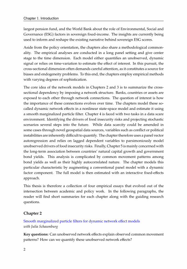
The dynamic network effects model developed in Chapter 2 and applied in Chapter
3 was originally inspired by a sudden financial market upheaval among European
banks in 2016. Could network effects explain such turmoils? Scenario analyses based
on this chapter found their way into board level meetings at De Nederlandsche Bank
to assess the vulnerabilities of Dutch banks during the COVID-19 pandemic. The
stochastic food insecurity model in Chapter 4 was specifically developed as part of
the World Bank’s Famine Action Mechanism to predict acute malnutrition. It became
the main model to assess the financial viability of a risk transfer solution and its
ability to produce stochastic forecasts has supported theWorld Bank’s budget allocation
decisions with regard to the pandemic. Chapter 5, which asks whether natural capital
is priced into sovereign bonds, finds its origins in discussions betweenGPIF, theworld’s
1
Chapter 1. Introduction
largest pension fund, and the World Bank about the role of Environmental, Social and
Governance (ESG) factors in sovereign fixed-income. The insights are currently being
used to inform and reshape the existing narrative behind sovereign ESG scores.
Aside from the policy orientation, the chapters also share a methodological common-
ality. The empirical analyses are conducted in a long panel setting and give center
stage to the time dimension. Each model either quantifies an unobserved, dynamic
signal or relies on time-variation to estimate the effect of interest. In this pursuit, the
cross-sectional dimension often demands careful attention, as it constitutes a source for
biases and endogeneity problems. To this end, the chapters employ empirical methods
with varying degrees of sophistication.
The core idea of the network models in Chapters 2 and 3 is to summarize the cross-
sectional dependency by imposing a network structure. Banks, countries or assets are
exposed to each other through network connections. The question of interest is how
the importance of these connections evolves over time. The chapters model these so-
called dynamic network effects in a nonlinear state-space model and estimate it using
a smooth marginalized particle filter. Chapter 4 is faced with two tasks in a data scare
environment. Identifying the drivers of food insecurity risks and projecting stochastic
scenarios several steps into the future. While data scarcity could be amended in
some cases through novel geospatial data sources, variables such as conflict or political
instabilities are inherently difficult to quantify. The chapter therefore uses apanel vector
autoregression and relies on lagged dependent variables to parsimoniously model
unobserveddrivers of food insecurity risks. Finally, Chapter 5 ismainly concernedwith
the long-term association between countries’ natural capital growth and government
bond yields. This analysis is complicated by common movement patterns among
bond yields as well as their highly autocorrelated nature. The chapter models this
particular characteristic by augmenting a conventional panel model with a dynamic
factor component. The full model is then estimated with an interactive fixed-effects
approach.
This thesis is therefore a collection of four empirical essays that evolved out of the
intersection between academic and policy work. In the following paragraphs, the
reader will find short summaries for each chapter along with the guiding research
questions.
Chapter 2
Smooth marginalized particle filters for dynamic network effect models
with Julia Schaumburg
Key questions: Can unobserved network effects explain observed commonmovement
patterns? How can we quantify these unobserved network effects?
2
Chapter 1. Introduction
This chapter proposes the dynamic network effect (DNE) model for the study of high-
dimensionalmultivariate time series data. Cross-sectional dependencies between units
are captured via one or multiple observed networks and a low-dimensional vector of
latent stochastic network effects. The parameter-driven, nonlinear state-space model
requires simulation-based filtering and estimation, for which we suggest to use the
smooth marginalized particle filter (SMPF). In a Monte Carlo simulation study, we
demonstrate the SMPF’s superior performance relative to benchmarks, particularly
when the cross-section dimension is large and the network is dense. The chapter pro-
vides two empirical applications to illustrate the usefulness of our method: First, we
examines the spread of the COVID-19 pandemic through international travel networks.
In particular, we analyze whether air travel or common borders served as main propa-
gation channels. Second, we apply the DNE model in an asset pricing framework and
ask whether market participants are exposed to peer risk factors.
Chapter 3
Do bank business model similarities explain credit risk commonalities?
with Iman van Lelyveld and Julia Schaumburg
Key questions: Do network effects explain contagion dynamics among Eurozone
banks? What potential biases could arise if network effects are neglected?
This paper revisits the credit spread puzzle for banks from the perspective of informa-
tion contagion. The puzzle consists of two stylized facts: Structural determinants of
credit risk not only have low explanatory power but also fail to capture common factors
in the residuals. We repro- duce the puzzle for European bank credit spreads and
hypothesize that the puzzle exists because structural models ignore contagion effects.
We therefore extend the structural approach to include information contagion through
bank business model similarities. To capture this channel, we propose an intuitive
measure for portfolio overlap and apply it to the complete asset holdings of the largest
banks in the Eurozone. Incorporating this unique network information into the struc-
tural model increases explanatory power and removes a systemic common factor from
the residuals. Furthermore, neglecting the network likely overstates the importance of
structural determinants.
Chapter 4
Stochastic modeling of food insecurity
with Bo Pieter Johannes Andree, Andres Fernando Chamorro and Phoebe Girouard Spencer
Key questions: What are the main drivers behind food insecurity risks? How can we
forecast the risk of famine and conduct scenario analyses in a data sparse environment?
3
Chapter 1. Introduction
Recent advances in food insecurity classification have made analytical approaches to
predict and inform response to food crises possible. This paper develops a predictive,
statistical framework to identify drivers of food insecurity risk with simulation capa-
bilities for scenario analyses, risk assessment and forecasting purposes. It utilizes a
panel vector-autoregression to model food insecurity distributions of 15 Sub-Saharan
African countries between October 2009 and February 2019. Statistical variable selec-
tionmethods are employed to identify themost important agronomic, weather, conflict
and economic variables. The paper finds that food insecurity dynamics are asymmet-
ric and past-dependent, with low insecurity states more likely to transition to high
insecurity states than vice versa. Conflict variables are more relevant for dynamics
in highly critical stages, while agronomic and weather variables are more important
for less critical states. Food prices are predictive for all cases. A Bayesian extension
is introduced to incorporate expert opinions through the use of priors, which lead to
significant improvements in model performance.
Chapter 5
Natural capital and sovereign bonds
single-authored
Key questions: How does 1% growth in natural capital affect a country’s borrowing
costs? Sovereign bond yields depend on global liquidity, exchange risks, inflation
expectations, among others - why should natural capital matter?
Natural capital affects governmentbonds throughmacroeconomicgrowthandsovereign
credit risks. Whether borrowing costs increase or decrease depends crucially on
whether we adopt a long-term, between-country view or short-term, within-country
view. The paper points out the dangers of the former, as results will be dominated by
the levels of income. These differences, which are the result of decades of develop-
ment, are de facto ingrained, meaning that they cannot be overcome by any short-term
policy efforts. The within-country view is unaffected by this “ingrained income bias”
and therefore leaves room for recent natural capital growth to affect bond yields. The
chapter finds that non-renewable natural capital, such as fossil fuels or mineral assets,
raise borrowing costs, possibly due to the resource curse. Renewable resources, such
as forests or agricultural wealth, lower borrowing costs because they are economically
worthwhile investments. Protected areas have an opposite effect because they aremore
likely to be luxury investments.
4
Chapter 2
Smooth marginalized particle filters fordynamic network effect models
2.1 Introduction
Multivariate time series models are important tools for studying and predicting the
dynamic interactions between key variables and/or investigation units. Depending on
the dimensionality of the data, simplifying assumptions often need to be imposed to
make estimation feasible. For example, if the cross-section is large while the time series
is short, dynamic panel-type approaches are typically employed, in which outcomes of
units at time C are functions of their own lags, but independent from contemporaneous
and lagged observations of other units. This simplification, however, can be too restric-
tive in many empirical settings. On the other end of the spectrum, we have (structural)
vector autoregression (VAR)models, which take into account the dynamic dependence
structure between the constituents, but rely on identification restrictions in order to
capture cross-sectional shock spillovers, and are only feasible for a small number of
units. Classic dynamic factor models (DFM) strike a balance by decomposing the mul-
tivariate dynamics into a constant cross-sectional part, the factor loadings, and a small
number of time-varying factors. However, they have the drawback that interpretation
of both loadings and factors is often ambiguous.
This paper discusses a class of dynamic network effect (DNE)models, which allowus to
incorporate contemporaneous network dependence between units even in large cross
sections, while capturing dynamics in the data at the same time. The method utilizes
an underlying network that is constant or slowly varying over time. The approach is
closely related to the spatial literature, but is more general as (1) network linkages are
not subject to constraints of geographic distances such as symmetry or non-negativity
(2) the intensity parameters are not constant but follow stochastic processes and (3)
5
Chapter 2. Smooth marginalized particle filters for dynamic network effect models
we allow for different transmission channels by incorporating more than one network.
Being able to incorporate these features makes our model relevant for applications in
which multivariate, cross-sectionally dependent data are observed over longer time
periods, and where networks can be observed or inferred from theory. Examples
includefinancial contagion and systemic risk (Aït-Sahalia et al., 2014; Forbes&Rigobon,
2002), comovements of business cycles (Böhm et al., 2020), and spreading of contagious
diseases via travel or social networks.
The paper contributes to the recent literature on time-varying spatial dependence, see
Blasques et al. (2016a) and Catania and Billé (2017a). However, instead of assuming
score-driven dynamics, we consider an alternative specification for the intensity pa-
rameters, in which they have their own disturbances. Allowing for this more general
parameter-driven formulation comes at the price of having to deal with a nonlin-
ear state-space model, for which no closed-form likelihood is available. The built-in
stochastic volatilities imposes additional demands on the estimation procedure. We
propose to carry out estimation and filtering using a smooth marginalized particle
filter (SMPF), which combines the smooth particle filter of Malik and Pitt (2011b) and
Doucet et al. (2001) with the marginalized particle filter of B. Y. G. Casella and Robert
(1996) and Andrieu and Doucet (2002b). This filter type is an attractive choice due to its
ability to incorporate complex nonlinearities as well as non-Gaussianities without rely-
ing on Taylor-type approximations. We can obtain arbitrarily close approximations to
the nonlinearity using sequential Monte Carlo simulations, the so-called particles, that
undergo the actual nonlinear transformation. Furthermore, the marginalization allows
us to accurately and efficiently estimate the linear parameters of the model, such as
regression coefficients with their standard errors. We illustrate the good performance
of the SMPF in Monte Carlo simulations in terms of prediction accuracy, likelihood
evaluation/estimation, signal extraction and coefficient estimation. We show that in
our setting, the SMPF clearly outperforms the widely used extended Kalman filter
(EKF), which relies on local Taylor approximations and has limited ability to handle
stochastic volatility. Within the simulations, we also investigate the impact of different
network structures on data features and filtering. In particular, we investigate network
asymmetries, different degrees of network sparsity, and incorporating both positive
and negative spillovers.
Based on these results, we apply the DNE framework in two ways. First, we show how
the DNE framework can be used in asset pricing. We argue that asset prices are not
only the result of exposure to fundamental factors, such as the market factor, the size
factor or the momentum factor. In addition, networks play a crucial role, implying that
prices also compensate investors for exposure to risky peer returns. That is, exposure
to assets with similar underlyings as the asset being priced. This application leverages
the DNE framework and measures how important such a peer network is over time,
6

Chapter 2. Smooth marginalized particle filters for dynamic network effect models
after establishing that peer networks play a statistically robust role. The SMPF allows
us to estimate constant network (or peer) effects as well as time-varying effects. In
this application, the difference between structural and error network (peer) effects
are particularly important. Structural peer effects measure the multiplier effect of the
networkwith respect to fundamental factors. Error peer effects, in contrast, capture any
unexplained correlations among the disturbances, if they follow the proposed network
structure. This application shows how the DNE can relate asset prices to each other
through a common peer network.
Second, we apply the new model and filtering method to analyze the spreading of
the new SARS-CoV2 virus across borders. Infected people either travel via airplane
(for longer distances) or via railways and roads (for shorter distances). Therefore, our
model features two candidate networks, one of which is constructed from air travel
data, while the other is an adjacency matrix where countries are connected if they
share a common border. We introduce the notion of a contagion faucet, which is a
helpful concept to understand contagion dynamics between both networks. The faucet
controls the overall contagion flow through either network and also regulates flows
between networks. We find strong time-variation in the filtered intensity parameters,
indicating several phases of international transmission of the disease. Initally, air travel
was mainly responsible for elevating the disease from an epidemic to a pandemic.
Subsequently, short-distance travel became more relevant. Our results also suggest
that towards the end of the sample, contagion occurs mainly within countries.
The paper is structured as follows. In Section 2 we describe the different dynamic
network effects models with a single network or multiple networks. Section 3 outlines
the smooth marginalized particle filter as well as the extended Kalman filter, which we
use as benchmark in the simulations. Section 4 provides an analyisis of the model’s
behavior subject to different network types. Section 5 investigates the filtering and
estimation performance of our method using simulated data. In Section 6, we illustrate
our results in an asset pricing setting and Section 7 uses the DNE model to estimate
whether the current COVID-19 disease spreads through airline routes or common
borders. Section 7 concludes.
7
Chapter 2. Smooth marginalized particle filters for dynamic network effect models
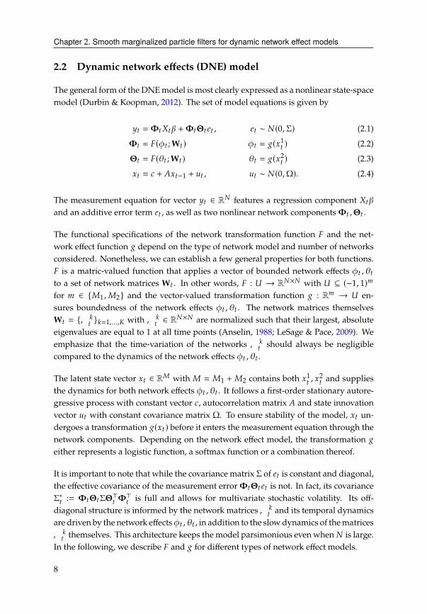
2.2 Dynamic network effects (DNE) model
The general form of the DNEmodel is most clearly expressed as a nonlinear state-space
model (Durbin & Koopman, 2012). The set of model equations is given by
HC =�C-C� +�C�C 4C , 4C ∼ #(0,Σ) (2.1)
�C = �()C ;WC ) )C = 6(G1
C ) (2.2)
�C = �(�C ;WC ) �C = 6(G2
C ) (2.3)
GC = 2 + �GC−1+ DC , DC ∼ #(0,Ω). (2.4)
The measurement equation for vector HC ∈ R# features a regression component -C�
and an additive error term 4C , as well as two nonlinear network components�C ,�C .
The functional specifications of the network transformation function � and the net-
work effect function 6 depend on the type of network model and number of networks
considered. Nonetheless, we can establish a few general properties for both functions.
� is a matric-valued function that applies a vector of bounded network effects )C , �Cto a set of network matrices WC . In other words, � : * → R#×# with * ⊆ (−1, 1)<for < ∈ {"
1, "
2} and the vector-valued transformation function 6 : R< → * en-
sures boundedness of the network effects )C , �C . The network matrices themselves
WC = {, :C}:=1,..., with, :
C∈ R#×# are normalized such that their largest, absolute
eigenvalues are equal to 1 at all time points (Anselin, 1988; LeSage & Pace, 2009). We
emphasize that the time-variation of the networks , :C
should always be negligible
compared to the dynamics of the network effects )C , �C .
The latent state vector GC ∈ R" with " = "1+"
2contains both G1
C, G2
Cand supplies
the dynamics for both network effects )C , �C . It follows a first-order stationary autore-
gressive process with constant vector 2, autocorrelation matrix � and state innovation
vector DC with constant covariance matrix Ω. To ensure stability of the model, GC un-
dergoes a transformation 6(GC ) before it enters the measurement equation through the
network components. Depending on the network effect model, the transformation 6
either represents a logistic function, a softmax function or a combination thereof.
It is important to note that while the covariance matrixΣ of 4C is constant and diagonal,
the effective covariance of the measurement error �C�C 4C is not. In fact, its covariance
Σ∗C
:= �C�C�>C �>C is full and allows for multivariate stochastic volatility. Its off-
diagonal structure is informed by the network matrices, :Cand its temporal dynamics
are driven by the network effects )C , �C , in addition to the slowdynamics of thematrices
, :Cthemselves. This architecture keeps the model parsimonious even when # is large.
In the following, we describe � and 6 for different types of network effect models.
8
Chapter 2. Smooth marginalized particle filters for dynamic network effect models
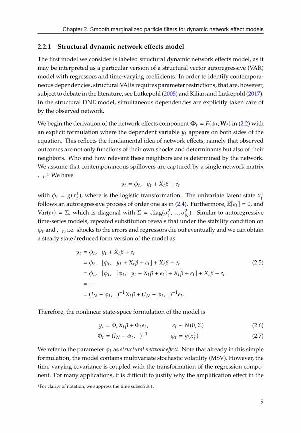
2.2.1 Structural dynamic network effects model
The first model we consider is labeled structural dynamic network effects model, as it
may be interpreted as a particular version of a structural vector autoregressive (VAR)
model with regressors and time-varying coefficients. In order to identify contempora-
neous dependencies, structural VARs requires parameter restrictions, that are, however,
subject to debate in the literature, see Lütkepohl (2005) andKilian andLütkepohl (2017).
In the structural DNE model, simultaneous dependencies are explicitly taken care of
by the observed network.
We begin the derivation of the network effects component�C = �()C ;WC ) in (2.2) with
an explicit formulation where the dependent variable HC appears on both sides of the
equation. This reflects the fundamental idea of network effects, namely that observed
outcomes are not only functions of their own shocks and determinants but also of their
neighbors. Who and how relevant these neighbors are is determined by the network.
We assume that contemporaneous spillovers are captured by a single network matrix
,C .1 We have
HC = )C,HC + -C� + 4Cwith )C = 6(G1
C), where is the logistic transformation. The univariate latent state G1
C
follows an autoregressive process of order one as in (2.4). Furthermore, E[4C] = 0, and
Var(4C ) = Σ, which is diagonal with Σ = diag(�2
1, ..., �2
#). Similar to autoregressive
time-series models, repeated substitution reveals that under the stability condition on
)C and,C , i.e. shocks to the errors and regressors die out eventually andwe can obtain
a steady state/reduced form version of the model as
HC = )C,HC + -C� + 4C= )C,[)C,HC + -C� + 4C] + -C� + 4C (2.5)
= )C,[)C,[)C,HC + -C� + 4C] + -C� + 4C] + -C� + 4C= · · ·= (�# − )C,)−1-C� + (�# − )C,)−14C .
Therefore, the nonlinear state-space formulation of the model is
HC = ΦC-C� +ΦC 4C , 4C ∼ #(0,Σ) (2.6)
ΦC = (�# − )C,)−1 )C = 6(G1
C ) (2.7)
We refer to the parameter )C as structural network effect. Note that already in this simple
formulation, the model contains multivariate stochastic volatility (MSV). However, the
time-varying covariance is coupled with the transformation of the regression compo-
nent. For many applications, it is difficult to justify why the amplification effect in the
1For clarity of notation, we suppress the time subscript C.
9

Chapter 2. Smooth marginalized particle filters for dynamic network effect models
regression component should follow the same dynamics as the error covariance. To
disentangle both effects, we model the error network effects separately.
2.2.2 Error network effects
In this specification, contemporaneous network spillovers only occur among the dis-
turbances. Therefore, we label this model error dynamic network effects model. The
conditional mean equation remains linear, corresponding to model (2.1) with�C = �# .
However, the covariance matrix has a dynamic network effect �C , which introduces
stochastic volatility. Again, we assume one network matrix , and a scalar network
effect. We have
HC = -C� + �C (2.8)
�C = �C,�C + 4C , 4C ∼ #(0,Σ), (2.9)
where Σ is diagonal as before. Equivalently, we express the model in reduced form as
HC = -C� + ΘC 4C (2.10)
ΘC = (�# − �C,)−1 , �C = 6(G2
C ). (2.11)
We refer to the parameter �C as error network effect. This linear model with multivariate
stochastic volatility is a restricted version of the model in A. Harvey et al. (1994).
Instead of a multiplicative factor ℎ8C for each error variable 48 , the temporal dynamics
are contained in �C in our case. Furthermore, A. Harvey et al. (1994) models the
variances as stochastic process, but restricts the off-diagonal covariances to zero. In our
model, the covariance structure is informed by the cross-sectional network structure in
the matrix, and, ultimately, the transformation ΘC .
2.2.3 Generalized network effects
The generalised network effects model presented here is simply a synthesis of the
structural and error network effects models introduced before. As before, we assume
that cross-sectional dependence is captured by a single network matrix , , but that
spillovers from shocks to the regressors can differ from shock spillovers among the
disturbances. In explicit form, the model is given by
HC = )C,HC + -C� + �C (2.12)
�C = �C,�C + 4C (2.13)
with )C , �C as above. In the nonlinear state-space form, the measurement equation
corresponds to
HC = ΦC-C� +ΦCΘC 4C , 4C ∼ #(0,Σ) (2.14)
10
Chapter 2. Smooth marginalized particle filters for dynamic network effect models
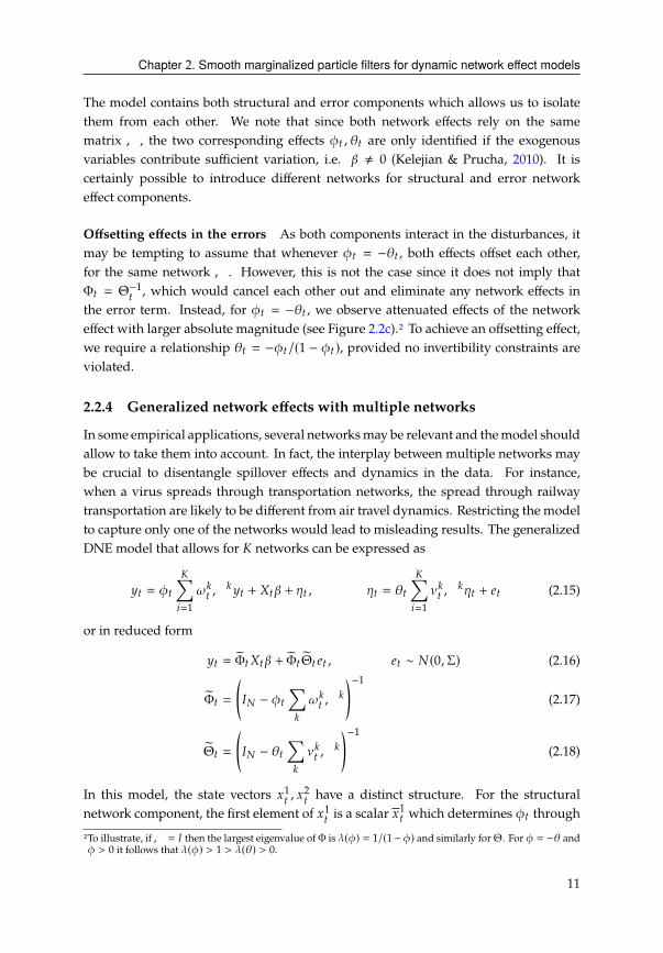
The model contains both structural and error components which allows us to isolate
them from each other. We note that since both network effects rely on the same
matrix , , the two corresponding effects )C , �C are only identified if the exogenous
variables contribute sufficient variation, i.e. � ≠ 0 (Kelejian & Prucha, 2010). It is
certainly possible to introduce different networks for structural and error network
effect components.
Offsetting effects in the errors As both components interact in the disturbances, it
may be tempting to assume that whenever )C = −�C , both effects offset each other,
for the same network , . However, this is not the case since it does not imply that
ΦC = Θ−1
C, which would cancel each other out and eliminate any network effects in
the error term. Instead, for )C = −�C , we observe attenuated effects of the network
effect with larger absolute magnitude (see Figure 2.2c).2 To achieve an offsetting effect,
we require a relationship �C = −)C/(1 − )C ), provided no invertibility constraints are
violated.
2.2.4 Generalized network effects with multiple networks
In some empirical applications, several networksmay be relevant and themodel should
allow to take them into account. In fact, the interplay between multiple networks may
be crucial to disentangle spillover effects and dynamics in the data. For instance,
when a virus spreads through transportation networks, the spread through railway
transportation are likely to be different from air travel dynamics. Restricting the model
to capture only one of the networks would lead to misleading results. The generalized
DNE model that allows for networks can be expressed as
HC = )C
∑8=1
$:C,: HC + -C� + �C , �C = �C
∑8=1
�:C,:�C + 4C (2.15)
or in reduced form
HC = ΦC-C� + ΦC ΘC 4C , 4C ∼ #(0,Σ) (2.16)
ΦC =
(�# − )C
∑:
$:C,:
)−1
(2.17)
ΘC =
(�# − �C
∑:
�:C,:
)−1
(2.18)
In this model, the state vectors G1
C, G2
Chave a distinct structure. For the structural
network component, the first element of G1
Cis a scalar G1
C which determines )C through
2To illustrate, if, = � then the largest eigenvalue ofΦ is �()) = 1/(1− )) and similarly for Θ. For ) = −� and
) > 0 it follows that �()) > 1 > �(�) > 0.
11
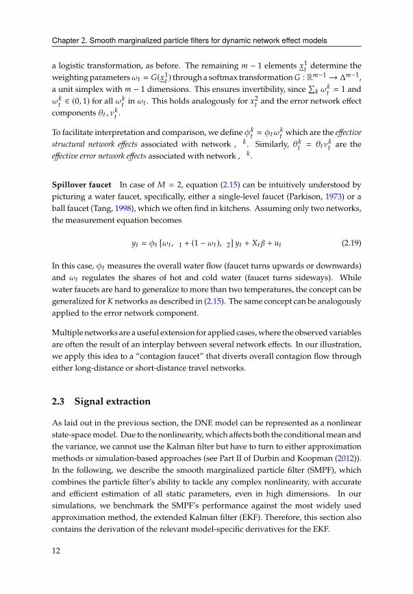
Chapter 2. Smooth marginalized particle filters for dynamic network effect models
a logistic transformation, as before. The remaining < − 1 elements G1
Cdetermine the
weightingparameters$C = �(G1
C) througha softmax transformation� : R<−1 → Δ<−1
,
a unit simplex with < − 1 dimensions. This ensures invertibility, since
∑: $
:C= 1 and
$:C∈ (0, 1) for all $:
Cin $C . This holds analogously for G2
Cand the error network effect
components �C , �:C .
To facilitate interpretation and comparison, we define ):C= )C$:C which are the effective
structural network effects associated with network , :. Similarly, �:
C= �C�:C are the
effective error network effects associated with network, :.
Spillover faucet In case of " = 2, equation (2.15) can be intuitively understood by
picturing a water faucet, specifically, either a single-level faucet (Parkison, 1973) or a
ball faucet (Tang, 1998), which we often find in kitchens. Assuming only two networks,
the measurement equation becomes
HC = )C [$C,1+ (1 − $C ),2
] HC + -C� + DC (2.19)
In this case, )C measures the overall water flow (faucet turns upwards or downwards)
and $C regulates the shares of hot and cold water (faucet turns sideways). While
water faucets are hard to generalize to more than two temperatures, the concept can be
generalized for networks as described in (2.15). The same concept can be analogously
applied to the error network component.
Multiplenetworks are auseful extension for applied cases,where theobservedvariables
are often the result of an interplay between several network effects. In our illustration,
we apply this idea to a “contagion faucet” that diverts overall contagion flow through
either long-distance or short-distance travel networks.
2.3 Signal extraction
As laid out in the previous section, the DNE model can be represented as a nonlinear
state-spacemodel. Due to the nonlinearity, which affects both the conditionalmean and
the variance, we cannot use the Kalman filter but have to turn to either approximation
methods or simulation-based approaches (see Part II of Durbin and Koopman (2012)).
In the following, we describe the smooth marginalized particle filter (SMPF), which
combines the particle filter’s ability to tackle any complex nonlinearity, with accurate
and efficient estimation of all static parameters, even in high dimensions. In our
simulations, we benchmark the SMPF’s performance against the most widely used
approximation method, the extended Kalman filter (EKF). Therefore, this section also
contains the derivation of the relevant model-specific derivatives for the EKF.
12
Chapter 2. Smooth marginalized particle filters for dynamic network effect models
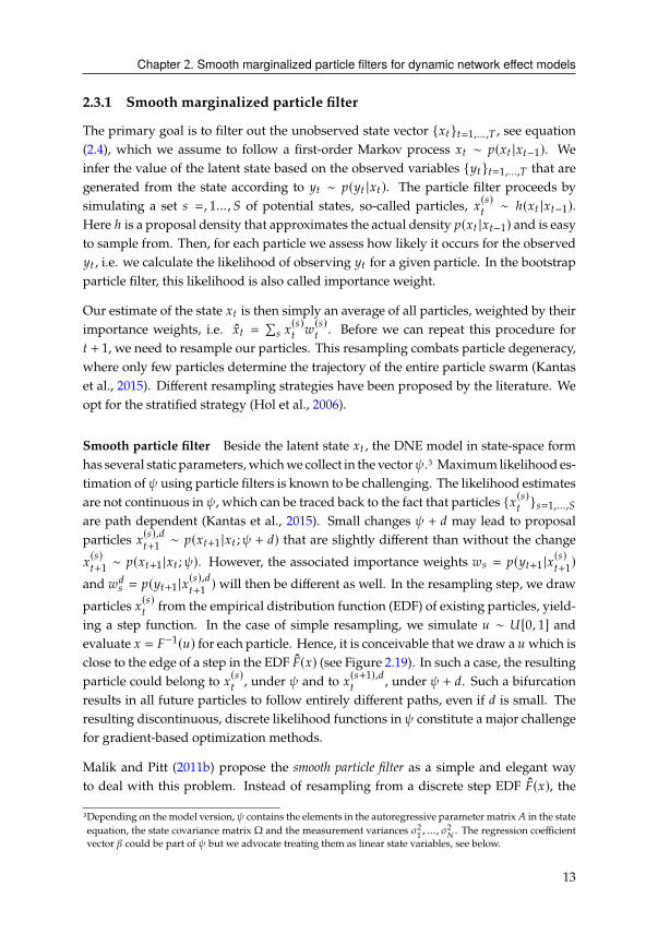
2.3.1 Smooth marginalized particle filter
The primary goal is to filter out the unobserved state vector {GC}C=1,...,) , see equation
(2.4), which we assume to follow a first-order Markov process GC ∼ ?(GC |GC−1). We
infer the value of the latent state based on the observed variables {HC}C=1,...,) that are
generated from the state according to HC ∼ ?(HC |GC ). The particle filter proceeds by
simulating a set B =, 1..., ( of potential states, so-called particles, G(B)C∼ ℎ(GC |GC−1
).Here ℎ is a proposal density that approximates the actual density ?(GC |GC−1
) and is easy
to sample from. Then, for each particle we assess how likely it occurs for the observed
HC , i.e. we calculate the likelihood of observing HC for a given particle. In the bootstrap
particle filter, this likelihood is also called importance weight.
Our estimate of the state GC is then simply an average of all particles, weighted by their
importance weights, i.e. GC =∑B G(B)CF(B)C
. Before we can repeat this procedure for
C + 1, we need to resample our particles. This resampling combats particle degeneracy,
where only few particles determine the trajectory of the entire particle swarm (Kantas
et al., 2015). Different resampling strategies have been proposed by the literature. We
opt for the stratified strategy (Hol et al., 2006).
Smooth particle filter Beside the latent state GC , the DNE model in state-space form
has several static parameters, whichwe collect in the vector#.3 Maximum likelihood es-
timation of # using particle filters is known to be challenging. The likelihood estimates
are not continuous in #, which can be traced back to the fact that particles {G(B)C}B=1,...,(
are path dependent (Kantas et al., 2015). Small changes # + 3 may lead to proposal
particles G(B),3C+1∼ ?(GC+1
|GC ;# + 3) that are slightly different than without the change
G(B)C+1∼ ?(GC+1
|GC ;#). However, the associated importance weights FB = ?(HC+1|G(B)C+1)
and F3B = ?(HC+1|G(B),3C+1) will then be different as well. In the resampling step, we draw
particles G(B)C
from the empirical distribution function (EDF) of existing particles, yield-
ing a step function. In the case of simple resampling, we simulate D ∼ *[0, 1] andevaluate G = �−1(D) for each particle. Hence, it is conceivable that we draw a D which is
close to the edge of a step in the EDF �(G) (see Figure 2.19). In such a case, the resulting
particle could belong to G(B)C
, under # and to G(B+1),3C
, under # + 3. Such a bifurcation
results in all future particles to follow entirely different paths, even if 3 is small. The
resulting discontinuous, discrete likelihood functions in # constitute a major challenge
for gradient-based optimization methods.
Malik and Pitt (2011b) propose the smooth particle filter as a simple and elegant way
to deal with this problem. Instead of resampling from a discrete step EDF �(G), the
3Depending on themodel version,# contains the elements in the autoregressive parameter matrix� in the state
equation, the state covariance matrix Ω and the measurement variances �2
1, ..., �2
#. The regression coefficient
vector � could be part of # but we advocate treating them as linear state variables, see below.
13

Chapter 2. Smooth marginalized particle filters for dynamic network effect models
authors propose a smooth EDF �(G)which is simply a linear interpolation of �(G). Thisensures that small changes � + 3 will indeed lead to small changes between resampled
G(B)C+1
and G(B),3C+1
, see Figure 2.19 for a visual representation. The resulting likelihood
estimate loses the undesirable discontinuities, as shown in Figure 2.20, and can be used
in gradient-based optimization routines. For the models studied below, we find that
only ( = 50 particles are sufficient to obtain good convergence results.
Marginalized particle filter To distinguish between nonlinear (0C ) and linear states
1C , we partition the state vector into GC = [0C , 1C]>. A conventional (smooth) particle
filter carries out the estimation of regression coefficients � by treating 1C as part of the
state vector, and filtering them in the same way as the nonlinear states 0C . That is, the
updating relies on the likelihood density ?(0C , 1C |HC ). However, this is computationally
expensive and, more importantly, statistically inefficient.4 Separating the linear from
the nonlinear state variables yields significant computational gains. This process of
marginalizing out the linear states is also known as Rao-Blackwellization. The like-
lihood density is evaluated in two parts, ?(0C , 1C |HC ) = ?(1C |0C , HC )?(0C |HC ). Using the
particle filter steps only for the nonlinear states and the Kalman filter steps for linear
states drastically reduces the computational complexity. The resulting model is known
as the marginalized particle filter or Rao-Blackwellized particle filter (Andrieu & Doucet,
2002b; Doucet et al., 2000; Schon et al., 2005; Schon et al., 2006).
2.3.2 Benchmark: Extended Kalman filter
For approximate filtering, the EKF requires the first-order derivative of the measure-
ment function �(G) = E[H |G]. For clarity, we suppress the time subscript C. We derive
the Jacobian for the general case with regression effects, such that the state vector G is
partitioned into 0 for the nonlinear and 1 for the linear state variables.
�G� = [�0�, �1�] =[%�(G)%0
,%�(G)%1
]The nonlinear state variable 0 is further subdivided into 0
1, 0
2, which correspond to
the structural and error network effects ), �. The first part of the derivative depends on
the derivative of the network transformation with respect to 0, in fact only 01, through
the logistic function 6
�0� =%�(G)
%(01, 0
2) =
[%Φ(0
1)
%01
-1, 0
]4Instead of treating them as state variables, 1C ∼ ?(1C |1C−1), one could estimate them as additional hyper-
parameters in #. However, this approach may become infeasible if the number of regression coefficients
increases.
14
Chapter 2. Smooth marginalized particle filters for dynamic network effect models
The derivative of the structural network component Φwith respect to 01is
%Φ(0)%0
1
=%�−1
%01
= −�−1%�
%01
�−1
where � = �# − 6(01), and its derivative %�/%0
1= −6′(0
1), . We use 6(G) =
4G(4G + 1)−1with the first derivative 6′(G) = 4−G(4−G + 1)−2
. The second part of the
derivative then follows immediately
�1� =%�(G)%1
=%Φ(0
1)-1
%1= Φ(0
1)-
Hence, the Jacobian matrix has dimensions # × ("0 +"1)
�G� =[6′(0
1)Φ,Φ-1, 0, Φ-
]With these derivatives we can implement the EKF using adjusted Kalman filter recur-
sions (Durbin & Koopman, 2012) and evaluate the likelihood straightforwardly using
prediction error decomposition (A. C. Harvey, 1990).
2.4 Model behavior
In this section we analyze properties of the DNE model by looking at different combi-
nations of network effects )C , �C for the following two network types. We use simplified
DNEmodels that abstract from regression components but still retain network compo-
nents of interest. The cross-section is set to # = 50.
Circular network ,� The circular network (Figure 2.1a) is a useful benchmark, al-
ready employed by Ord (1975) in the study of spatial autoregressive models, due to its
simplicity, irreducibility and scalability. The graph is strongly connected and is defined
as,� = [F8 9] ∈ R#×# where the typical element F8 9 = 1 if 8 = 9 − 1 or 8 = 9 + 1 − # ,
which ensures a closed circle. Its simplicity makes the effects of )C , �C clearly visible
and yields interesting parallels to the autoregressive time-series models.
Randomnetwork,�' Wealso considerdirectedErdős–Rényi networks,,�' (Figure
2.1b) which are closer to observed networks. Such networks have been widely studied
due to their stochastic nature and known limiting properties. The underlying graph
D(#, ?) is often referred to as a binomial random directed graph and is closely related
to the Erdős–Rényi model (A. J. Graham & Pike, 2008). The #2possible edges of the
random graph D(#, ?) are each drawn with probability ?. Similar to the Erdős–Rényi
model, the graph is almost surely strongly connected, if ? > ln(=)/=. Figure 2.1c
represents a special case where the network is partitioned into two subnetworks, that
will become relevant for the study of common factors.
15
Chapter 2. Smooth marginalized particle filters for dynamic network effect models
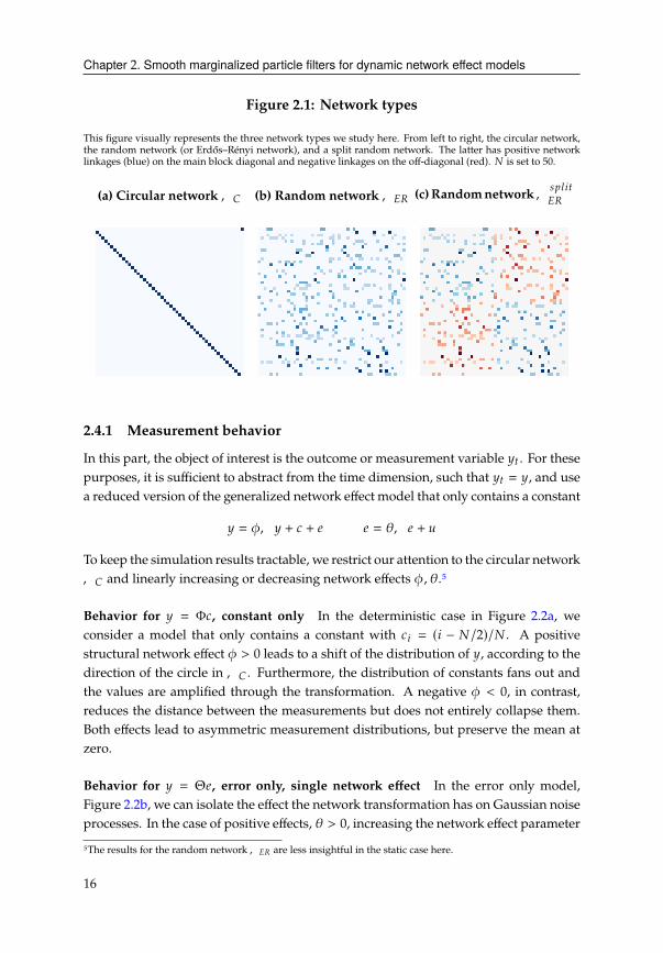
Figure 2.1: Network types
This figure visually represents the three network types we study here. From left to right, the circular network,
the random network (or Erdős–Rényi network), and a split random network. The latter has positive network
linkages (blue) on the main block diagonal and negative linkages on the off-diagonal (red). # is set to 50.
(a) Circular network,� (b) Random network,�' (c)Randomnetwork, B?;8C
�'
2.4.1 Measurement behavior
In this part, the object of interest is the outcome or measurement variable HC . For these
purposes, it is sufficient to abstract from the time dimension, such that HC = H, and use
a reduced version of the generalized network effect model that only contains a constant
H = ),H + 2 + 4 4 = �,4 + D
To keep the simulation results tractable, we restrict our attention to the circular network
,� and linearly increasing or decreasing network effects ), �.5
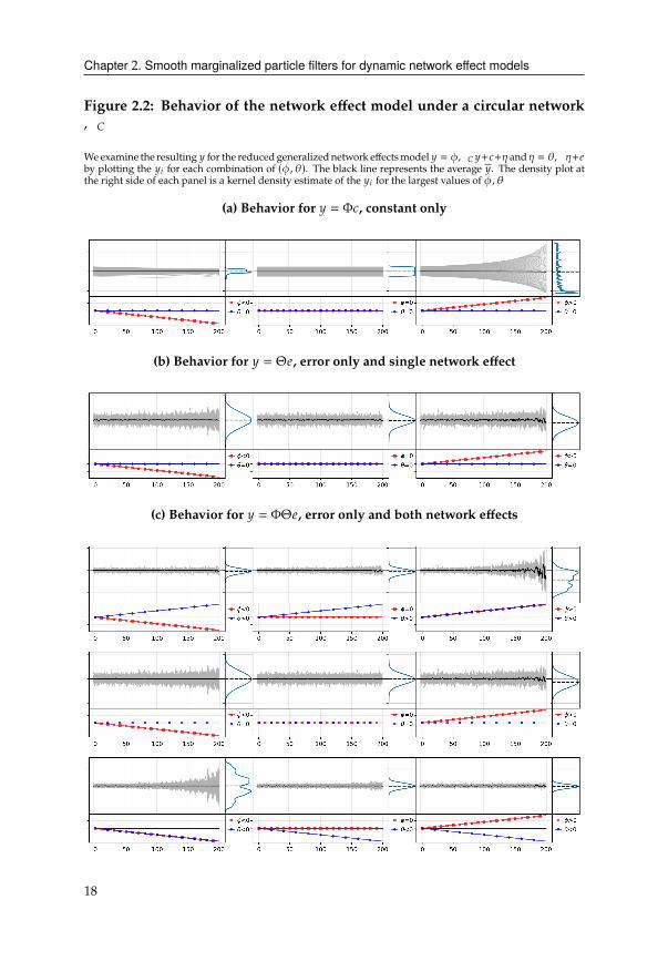
Behavior for H = Φ2, constant only In the deterministic case in Figure 2.2a, we
consider a model that only contains a constant with 28 = (8 − #/2)/# . A positive
structural network effect ) > 0 leads to a shift of the distribution of H, according to the
direction of the circle in,� . Furthermore, the distribution of constants fans out and
the values are amplified through the transformation. A negative ) < 0, in contrast,
reduces the distance between the measurements but does not entirely collapse them.
Both effects lead to asymmetric measurement distributions, but preserve the mean at
zero.
Behavior for H = Θ4, error only, single network effect In the error only model,
Figure 2.2b, we can isolate the effect the network transformation has on Gaussian noise
processes. In the case of positive effects, � > 0, increasing the network effect parameter
5The results for the random network,�' are less insightful in the static case here.
16

Chapter 2. Smooth marginalized particle filters for dynamic network effect models
leads to higher concentration and a lashing out of H. Hence, the average H oscillates
unstably. In the opposite case, � < 0, decreasing the network effect parameter leads
to lower concentration and H are fanning out symmetrically. Hence, the average H is
centered around zero. The variance increases in both cases, differing by whether or not
they are skewed.6
Behavior for H = ΦΘ4, error only, both network effects When both effects are
present, we observe compounding and offsetting effects. For ) > 0, � > 0, we can
see the combined effect of � > 0 in the single network case, with the same asymmetry
and lashing out, but stronger. Similarly, ) < 0, � < 0 has the combined effect of � < 0
in the single network case, which leads to even more dispersion but maintaining the
symmetry. The cases with opposite signs are identical to each other by construction,
) > 0, � < 0 and ) < 0, � > 0. They represent the attenuated combinations of the two
isolated cases, � < 0 and � > 0 in the single network case.
2.4.2 Common factors behavior
In this part we reintroduce the time dimension and shift our attention to common
factors contained in HC . We restrict our attention to )C ≠ 0 and set �C = 0. We
demonstrate how networks yield interesting patterns in the principal components of
HC .
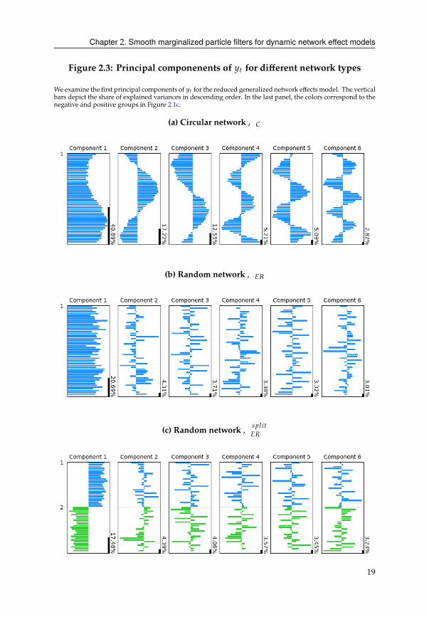
For a circular network, Figure 2.3a, we observe a curious behavior in the residuals. This
unmistakable wavelet character is the result of the spatial autoregressive dynamics we
impose on the Gaussian noise process 4C . Essentially, what we observe over the cross-
section over different components is the spectral decomposition of the ΘC 4C process
over different frequencies.
Given the random network, we can observe a common factor that affects all outcome
variables HC (Figure 2.3b). More interesting is the random network with positive and
negative quadrants (see Figure 2.1c), which can be constructed using (2.15) with the
,�' =,1 =,2
and twopositive andnegativenetwork effects)1
C, )2
C. Thepositive and
negative network linkages translate into two groups of the first principal component,
designated by the positive and negative coefficients (Figure 2.3c).7 More involved
patterns can be constructed in a similar fashion using the DNE model with multiple
networks (2.15).
6It is instructive to draw the parallel to AR(1) processes over time. The value of a particular H8C we observe for a
given � resembles the outcome of an AR(1) process, with autocorrelation coefficient � over # periods. Strong,
positive autocorrelation values lead to persistent deviations from the mean. Strong, negative autocorrelation
values lead to oscillations around the mean.
7Such a pattern can be seen in the case of credit contagion among European banks studied in D. Wang et al.
(2019).
17
Chapter 2. Smooth marginalized particle filters for dynamic network effect models
Figure 2.2: Behavior of the network effect model under a circular network,�
Weexamine the resulting H for the reduced generalized network effectsmodel H = ),� H+2+� and� = �,�+4by plotting the H8 for each combination of (), �). The black line represents the average H. The density plot at
the right side of each panel is a kernel density estimate of the H8 for the largest values of ), �
(a) Behavior for H = Φ2, constant only
(b) Behavior for H = Θ4, error only and single network effect
(c) Behavior for H = ΦΘ4, error only and both network effects
18
Chapter 2. Smooth marginalized particle filters for dynamic network effect models
Figure 2.3: Principal componenents of HC for different network types
We examine the first principal components of HC for the reduced generalized network effects model. The vertical
bars depict the share of explained variances in descending order. In the last panel, the colors correspond to the
negative and positive groups in Figure 2.1c.
(a) Circular network,�
(b) Random network,�'
(c) Random network, B?;8C
�'
19

Chapter 2. Smooth marginalized particle filters for dynamic network effect models
2.5 Monte Carlo study
In this section we investigate the performance of the smooth marginalized particle
filter (SMPF) in filtering unobserved time-varying network intensities and estimating
the vector of static coefficients. We consider all network effects introduced in Section
2.2, namely structural, error and generalised network effects. We analyze four different
network types for each network effect, circular as well as sparse, normal and dense
random networks as it is conceivable that the connectedness of a networkwill influence
an estimator’s performance.
2.5.1 Data-generating process and network inputs
The simulation study uses equation (2.12) as the data-generating process (DGP). We
simulate data for ) = 200 and # = 50, 100, 200. The measurement variance is set to
Σ = 0.1 �# . The regressor matrix -C consists of a constant -1
8C= 1 and a Gaussian noise
process -2
8C∼ #(0, 1) for all 8 , C. The associated coefficients are individual-specific
and defined as 8 = �8 = 8/# for 8 = 1, ..., # . The unrestricted state variables G1
C, G2
C
follow the stationary process described in equation (2.4) with no intercepts, 21= 2
2= 0,
autocorrelation matrix � = 0.8�2and covariance matrix variances Ω = 0.4�
2. To obtain
the structural network effects model, we set �22= 0 andΩ
22= 0. For the error network
effects model, we set �11= 0 and Ω
11= 0, accordingly.
All networks we have the property that they can be generated for different numbers
of cross-sectional units.8 As explained in the previous section, we control the density
of the random networks through the edge probability parameter ?. The network,��'
represents the threshold case where the probability of two nodes being connected is
? = � = ;=(#)/# . Erdős and Rényi (1960) show that the network is almost surely
connected for values above � and disconnected for values below it. We choose ? = 2�
for ,34=B4�'
and ? = �/2 for ,B?0AB4
�'as edge probabilities. Table 2.1 summarizes the
network properties.
2.5.2 Computer specifications and programming language
The computations for the Monte Carlo study and the subsequent illustration were
carried out on a Linux 64-bit server with Intel(R) Xeon(R) E5-2690 32-core processsor
@ 2.90GHz and 128 GB memory. The methods described here were implemented in
Python3.7 and for randomnumbergenerationweused thenumpy.random.RandomState
module (version 1.14) which employs the Mersenne Twister pseudo-random number
8This is not possible or other network types, such as the core periphery network.
20
Chapter 2. Smooth marginalized particle filters for dynamic network effect models
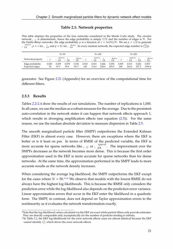
Table 2.1: Network properties
This table displays the properties of the four networks considered in the Monte Carlo study. The circular
network ,� is deterministic, hence the edge probability is simply 1/# and the number of edges is # . For
the Erdős–Rényi networks, the edge probability ? is a function of � = ;=(#)/# . We set ? = �/2 to generate
,B?0AB4
�', ? = � for,�
�'and ? = 2� for, 34=B4
�'. In every random network, the expected edge number is
(#2
)?.
N=50 N=100 N=200
Network property ,� ,B?0AB4
�',��'
,34=B4�'
,� ,B?0AB4
�',��'
,34=B4�'
,� ,B?0AB4
�',��'
,34=B4�'
Edge probability 0.020 0.039 0.078 0.156 0.010 0.023 0.046 0.092 0.005 0.013 0.026 0.053
Expected edges 50 47.9 95.8 191.7 100 114.0 228.0 455.9 200 263.6 527.2 1054.4
generator. See Figure 2.21 (Appendix) for an overview of the computational time for
different filters.
2.5.3 Results
Tables 2.2-2.4 show the results of our simulations. The number of replications is 1,000.
In all cases, we use themedian as a robustmeasure for the average. Due to the persistent
auto-correlation in the network states it can happen that network effects approach 1,
which results in diverging amplification effects (see equation (2.5)). For the same
reason, we use the median absolute deviation to measure dispersion in Table 2.5.
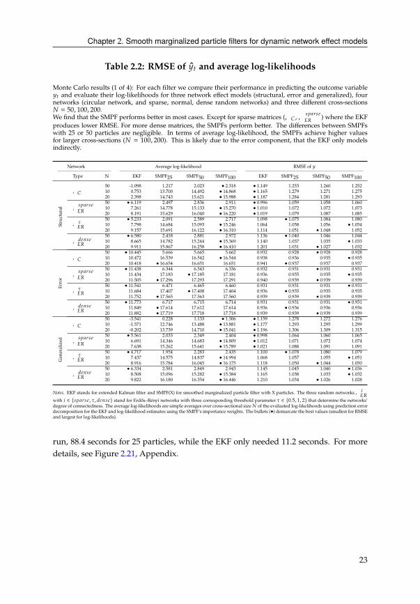
The smooth marginalized particle filter (SMPF) outperforms the Extended Kalman
Filter (EKF) in almost every case. However, there are exceptions where the EKF is
better or is it least on par. In terms of RMSE of the predicted variable, the EKF is
more accurate for sparse networks like ,� or ,B?0AB4
�'. The improvement over the
SMPFs decreases as the network becomes more dense. This is because the first order
approximation used in the EKF is more accurate for sparse networks than for dense
networks. At the same time, the approximation performed in the SMPF leads to more
accurate results as the network density increases.
When considering the average log-likelihood, the SMPF outperforms the EKF except
for the cases where # = 50.9,10 We observe that models with the lowest RMSE do not
always have the highest log-likelihoods. This is because the RMSE only considers the
prediction error while the log-likelihood also depends on the prediction error variance.
Linear approximation errors that occur in the EKF enter the likelihood in a quadratic
form. The SMPF, in contrast, does not depend on Taylor approximation errors to the
nonlinearity as it evaluates the network transformation exactly.
9Note that the log-likelihood values calculated via the EKF are exact while particle filters only provide estimates.
They are directly comparable only asymptotically for the number of particles tending to infinity.
10In Table 2.2, the EKF log-likelihoods for the error network effects cases are almost identical because the EKF
cannot identify G2
C , which drives the error network effects.
21
Chapter 2. Smooth marginalized particle filters for dynamic network effect models
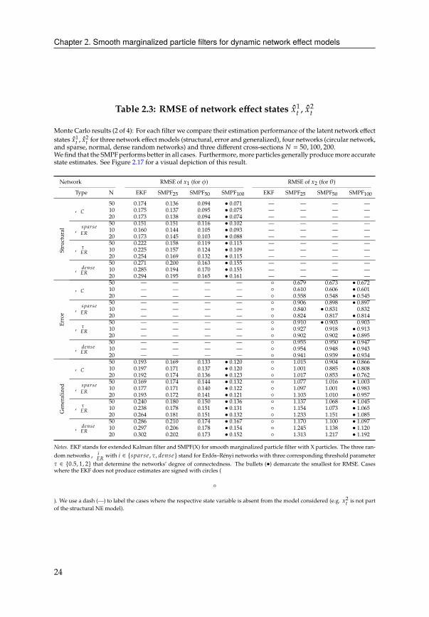
In Table 2.3, we consider the ability of the filters to accurately estimate the underlying
network effects. Different from RMSE of HC , the SMPF strictly outperforms the EKF.11
On average the SMPFwith 100 particles reduces the RMSE bymore than half compared
to the EKF. While more particles generally lead to more accurate results for both G1
C, G2
C,
the improvement ismost striking in the structural network effects. For the error network
effects, we only find slight improvements. As expected, the denser the networks are,
the more challenging it is for the filters to accurately estimate G1
C, G2
C.
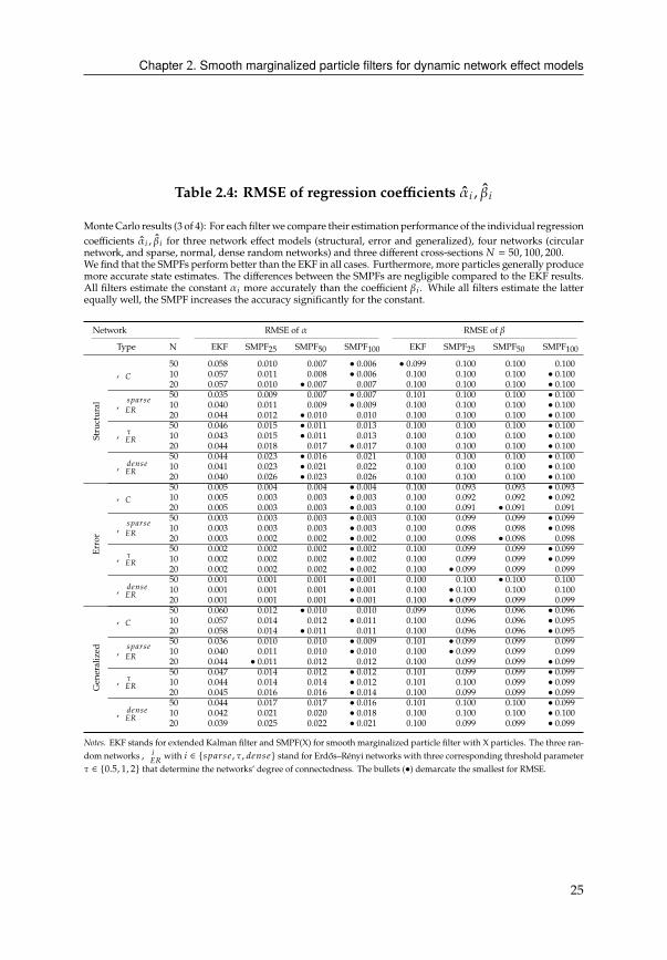
Table 2.4 also demonstrates the superior estimation performance of the SMPF. The
superiority is most notable for the structural network effects with a circular network,
where the SMPF(100) reduce the RMSE of the EKF by almost 90 percentage points.
As before, the estimation performance deteriorates with increasing network density.
For the error network effects, we do not expect any differences since the regression
coefficients are not affected by the stochastic volatility. Both filters can estimate the
constant more accurately. � estimates are almost indistinguishable across models and
filters.
Finally, Table 2.5 compares the dispersion of the log-likelihood values of each filter
across all simulations. We find that the log-likelihood values estimated with the SMPF
are less dispersed across simulations than the EKF. The error network effect model
is the exception, where for large, dense cross-sections, the EKF has lower dispersion.
However, in conjunction with the low average log-likelihoods and high RMSE for the
same cases (Table 2.2), this implies that the EKF is inaccurate in the same way across all
simulations. In contrast, the SMPF values are less dispersed than the EKF in all cases
and more particles reduce the amount of dispersion. This is relevant for parameter
estimation, particularly for gradient-based optimization procedures.
To summarize our findings, the SMPF strictly outperforms the EKF in terms of signal
extraction (G1
C, G2
C) and regression coefficient estimation ( 8 , �8). For the in-sample
prediction performance of the outcome variable H8C the results are not as clear cut.
For sparse networks and small cross-sections the linear approximation in the EKF is
it sufficiently accurate. For denser networks and larger cross-sections, the prediction
errors the approximation error in the EKF weigh down its performance, while the
SMPF yields higher likelihoods and more precise estimates. A relatively small number
of particles is sufficient to obtain good estimates of the measurement variable HC . For
signal extraction and coefficient estimation, increasing the number of particles leads
to major improvements. However, this comes at a cost of computational power. On
average, for # = 200 the SMPF with 100 particles required about 316.4 seconds per
11Since the structural and error network effects only contain one of the two network effects we remove the
corresponding segments in the table. Furthermore, since the EKF is unable to identify the error network effect
we remove these cases in the Table accordingly.
22
Chapter 2. Smooth marginalized particle filters for dynamic network effect models
Table 2.2: RMSE of HC and average log-likelihoods
Monte Carlo results (1 of 4): For each filter we compare their performance in predicting the outcome variable
HC and evaluate their log-likelihoods for three network effect models (structural, error and generalized), four
networks (circular network, and sparse, normal, dense random networks) and three different cross-sections
# = 50, 100, 200.
We find that the SMPF performs better in most cases. Except for sparse matrices (,� ,,B?0AB4
�') where the EKF
produces lower RMSE. For more dense matrices, the SMPFs perform better. The differences between SMPFs
with 25 or 50 particles are negligible. In terms of average log-likelihood, the SMPFs achieve higher values
for larger cross-sections (# = 100, 200). This is likely due to the error component, that the EKF only models
indirectly.
Network Average log-likelihood RMSE of H
Type N EKF SMPF25
SMPF50
SMPF100
EKF SMPF25
SMPF50
SMPF100
Structural
,�
50 -1.098 1.217 2.023 • 2.318 • 1.149 1.253 1.260 1.252
10 0.753 13.700 14.492 • 14.868 • 1.165 1.279 1.271 1.275
20 2.398 14.743 15.621 • 15.988 • 1.187 1.284 1.281 1.293
,B?0AB4
�'
50 • 6.119 2.497 2.836 2.911 • 0.996 1.059 1.058 1.060
10 7.261 14.778 15.133 • 15.270 • 1.010 1.072 1.072 1.073
20 8.191 15.629 16.040 • 16.220 • 1.019 1.079 1.087 1.085
,��'
50 • 5.233 2.091 2.589 2.717 1.098 • 1.075 1.084 1.080
10 7.798 14.684 15.093 • 15.246 1.064 1.058 1.056 • 1.05420 9.157 15.691 16.122 • 16.310 1.114 1.051 • 1.048 1.052
,34=B4�'
50 • 6.580 2.418 2.881 2.972 1.136 • 1.040 1.046 1.044
10 8.665 14.782 15.244 • 15.369 1.140 1.037 1.035 • 1.03320 9.911 15.867 16.258 • 16.410 1.201 1.031 • 1.027 1.032
Error
,�
50 • 10.445 5.666 5.665 5.662 0.932 0.928 • 0.928 0.928
10 10.472 16.539 16.542 • 16.544 0.938 0.936 0.935 • 0.93520 10.418 • 16.654 16.651 16.651 0.941 • 0.937 0.937 0.937
,B?0AB4
�'
50 • 11.438 6.344 6.343 6.336 0.932 0.931 • 0.931 0.931
10 11.434 17.183 • 17.185 17.181 0.936 0.935 0.935 • 0.93520 11.505 • 17.296 17.293 17.291 0.940 0.939 • 0.939 0.939
,��'
50 • 11.541 6.471 6.465 6.460 0.931 0.931 0.931 • 0.93110 11.684 17.407 • 17.408 17.404 0.936 • 0.935 0.935 0.935
20 11.752 • 17.565 17.563 17.560 0.939 0.939 • 0.939 0.939
,34=B4�'
50 • 11.773 6.717 6.715 6.714 0.931 0.931 0.931 • 0.93110 11.849 • 17.614 17.612 17.614 0.936 • 0.936 0.936 0.936
20 11.882 • 17.719 17.718 17.718 0.939 0.939 • 0.939 0.939
Generalized
,�
50 -3.541 0.228 1.133 • 1.306 • 1.159 1.278 1.272 1.276
10 -1.571 12.746 13.488 • 13.881 • 1.177 1.293 1.295 1.299
20 -0.202 13.739 14.710 • 15.041 • 1.196 1.306 1.309 1.315
,B?0AB4
�'
50 • 5.561 2.033 2.349 2.404 • 0.998 1.064 1.060 1.065
10 6.691 14.346 14.683 • 14.809 • 1.012 1.071 1.072 1.074
20 7.638 15.262 15.641 • 15.789 • 1.021 1.088 1.091 1.091
,��'
50 • 4.717 1.954 2.283 2.435 1.100 • 1.078 1.080 1.079
10 7.437 14.575 14.837 • 14.994 1.068 1.057 1.055 • 1.05120 8.916 15.784 16.045 • 16.175 1.118 1.050 • 1.044 1.050
,34=B4�'
50 • 6.334 2.581 2.849 2.943 1.145 1.045 1.040 • 1.03610 8.508 15.096 15.282 • 15.384 1.165 1.038 1.033 • 1.03220 9.822 16.180 16.354 • 16.446 1.210 1.034 • 1.026 1.028
Notes. EKF stands for extended Kalman filter and SMPF(X) for smoothed marginalized particle filter with X particles. The three random networks,8�'
with 8 ∈ {B?0AB4 , �, 34=B4} stand for Erdős–Rényi networks with three corresponding threshold parameter � ∈ {0.5, 1, 2} that determine the networks’
degree of connectedness. The average log-likelihoods are simple averages over cross-sectional size# of the evaluated log-likelihoods using prediction error
decomposition for the EKF and log-likelihood estimates using the SMPF’s importance weights. The bullets (•) demarcate the best values (smallest for RMSE
and largest for log-likelihoods).
run, 88.4 seconds for 25 particles, while the EKF only needed 11.2 seconds. For more
details, see Figure 2.21, Appendix.
23
Chapter 2. Smooth marginalized particle filters for dynamic network effect models
Table 2.3: RMSE of network effect states G1
C , G2
C
Monte Carlo results (2 of 4): For each filter we compare their estimation performance of the latent network effect
states G1
C , G2
C for three network effect models (structural, error and generalized), four networks (circular network,
and sparse, normal, dense random networks) and three different cross-sections # = 50, 100, 200.
We find that the SMPFperforms better in all cases. Furthermore, more particles generally producemore accurate
state estimates. See Figure 2.17 for a visual depiction of this result.
Network RMSE of G1(for )) RMSE of G
2(for �)
Type N EKF SMPF25
SMPF50
SMPF100
EKF SMPF25
SMPF50
SMPF100
Structural
,�
50 0.174 0.136 0.094 • 0.071 — — — —
10 0.175 0.137 0.095 • 0.075 — — — —
20 0.173 0.138 0.094 • 0.074 — — — —
,B?0AB4
�'
50 0.151 0.151 0.116 • 0.102 — — — —
10 0.160 0.144 0.105 • 0.093 — — — —
20 0.173 0.145 0.103 • 0.088 — — — —
,��'
50 0.222 0.158 0.119 • 0.115 — — — —
10 0.225 0.157 0.124 • 0.109 — — — —
20 0.254 0.169 0.132 • 0.115 — — — —
,34=B4�'
50 0.271 0.200 0.163 • 0.155 — — — —
10 0.285 0.194 0.170 • 0.155 — — — —
20 0.294 0.195 0.165 • 0.161 — — — —
Error
,�
50 — — — — ◦ 0.679 0.673 • 0.67210 — — — — ◦ 0.610 0.606 • 0.60120 — — — — ◦ 0.558 0.548 • 0.545
,B?0AB4
�'
50 — — — — ◦ 0.906 0.898 • 0.89710 — — — — ◦ 0.840 • 0.831 0.832
20 — — — — ◦ 0.824 0.817 • 0.814
,��'
50 — — — — ◦ 0.910 • 0.903 0.903
10 — — — — ◦ 0.927 0.918 • 0.91320 — — — — ◦ 0.902 0.902 • 0.895
,34=B4�'
50 — — — — ◦ 0.955 0.950 • 0.94710 — — — — ◦ 0.954 0.948 • 0.94320 — — — — ◦ 0.941 0.939 • 0.934
Generalized
,�
50 0.193 0.169 0.133 • 0.120 ◦ 1.015 0.904 • 0.86610 0.197 0.171 0.137 • 0.120 ◦ 1.001 0.885 • 0.80820 0.192 0.174 0.136 • 0.123 ◦ 1.017 0.853 • 0.762
,B?0AB4
�'
50 0.169 0.174 0.144 • 0.132 ◦ 1.077 1.016 • 1.00310 0.177 0.171 0.140 • 0.122 ◦ 1.097 1.001 • 0.98320 0.193 0.172 0.141 • 0.121 ◦ 1.103 1.010 • 0.957
,��'
50 0.240 0.180 0.150 • 0.136 ◦ 1.137 1.068 • 1.04510 0.238 0.178 0.151 • 0.131 ◦ 1.154 1.073 • 1.06520 0.264 0.181 0.151 • 0.132 ◦ 1.233 1.151 • 1.085
,34=B4�'
50 0.286 0.210 0.174 • 0.167 ◦ 1.170 1.100 • 1.09710 0.297 0.206 0.178 • 0.154 ◦ 1.245 1.138 • 1.12020 0.302 0.202 0.173 • 0.152 ◦ 1.313 1.217 • 1.192
Notes. EKF stands for extended Kalman filter and SMPF(X) for smooth marginalized particle filter with X particles. The three ran-
dom networks, 8�'
with 8 ∈ {B?0AB4 , �, 34=B4} stand for Erdős–Rényi networks with three corresponding threshold parameter
� ∈ {0.5, 1, 2} that determine the networks’ degree of connectedness. The bullets (•) demarcate the smallest for RMSE. Cases
where the EKF does not produce estimates are signed with circles (
◦
). We use a dash (—) to label the cases where the respective state variable is absent from the model considered (e.g. G2
Cis not part
of the structural NE model).
24
Chapter 2. Smooth marginalized particle filters for dynamic network effect models
Table 2.4: RMSE of regression coefficients 8 , �8
MonteCarlo results (3 of 4): For each filterwe compare their estimation performance of the individual regression
coefficients 8 , �8 for three network effect models (structural, error and generalized), four networks (circular
network, and sparse, normal, dense random networks) and three different cross-sections # = 50, 100, 200.
We find that the SMPFs perform better than the EKF in all cases. Furthermore, more particles generally produce
more accurate state estimates. The differences between the SMPFs are negligible compared to the EKF results.
All filters estimate the constant 8 more accurately than the coefficient �8 . While all filters estimate the latter
equally well, the SMPF increases the accuracy significantly for the constant.
Network RMSE of RMSE of �
Type N EKF SMPF25
SMPF50
SMPF100
EKF SMPF25
SMPF50
SMPF100
Structural
,�
50 0.058 0.010 0.007 • 0.006 • 0.099 0.100 0.100 0.100
10 0.057 0.011 0.008 • 0.006 0.100 0.100 0.100 • 0.10020 0.057 0.010 • 0.007 0.007 0.100 0.100 0.100 • 0.100
,B?0AB4
�'
50 0.035 0.009 0.007 • 0.007 0.101 0.100 0.100 • 0.10010 0.040 0.011 0.009 • 0.009 0.100 0.100 0.100 • 0.10020 0.044 0.012 • 0.010 0.010 0.100 0.100 0.100 • 0.100
,��'
50 0.046 0.015 • 0.011 0.013 0.100 0.100 0.100 • 0.10010 0.043 0.015 • 0.011 0.013 0.100 0.100 0.100 • 0.10020 0.044 0.018 0.017 • 0.017 0.100 0.100 0.100 • 0.100
,34=B4�'
50 0.044 0.023 • 0.016 0.021 0.100 0.100 0.100 • 0.10010 0.041 0.023 • 0.021 0.022 0.100 0.100 0.100 • 0.10020 0.040 0.026 • 0.023 0.026 0.100 0.100 0.100 • 0.100
Error
,�
50 0.005 0.004 0.004 • 0.004 0.100 0.093 0.093 • 0.09310 0.005 0.003 0.003 • 0.003 0.100 0.092 0.092 • 0.09220 0.005 0.003 0.003 • 0.003 0.100 0.091 • 0.091 0.091
,B?0AB4
�'
50 0.003 0.003 0.003 • 0.003 0.100 0.099 0.099 • 0.09910 0.003 0.003 0.003 • 0.003 0.100 0.098 0.098 • 0.09820 0.003 0.002 0.002 • 0.002 0.100 0.098 • 0.098 0.098
,��'
50 0.002 0.002 0.002 • 0.002 0.100 0.099 0.099 • 0.09910 0.002 0.002 0.002 • 0.002 0.100 0.099 0.099 • 0.09920 0.002 0.002 0.002 • 0.002 0.100 • 0.099 0.099 0.099
,34=B4�'
50 0.001 0.001 0.001 • 0.001 0.100 0.100 • 0.100 0.100
10 0.001 0.001 0.001 • 0.001 0.100 • 0.100 0.100 0.100
20 0.001 0.001 0.001 • 0.001 0.100 • 0.099 0.099 0.099
Generalized
,�
50 0.060 0.012 • 0.010 0.010 0.099 0.096 0.096 • 0.09610 0.057 0.014 0.012 • 0.011 0.100 0.096 0.096 • 0.09520 0.058 0.014 • 0.011 0.011 0.100 0.096 0.096 • 0.095
,B?0AB4
�'
50 0.036 0.010 0.010 • 0.009 0.101 • 0.099 0.099 0.099
10 0.040 0.011 0.010 • 0.010 0.100 • 0.099 0.099 0.099
20 0.044 • 0.011 0.012 0.012 0.100 0.099 0.099 • 0.099
,��'
50 0.047 0.014 0.012 • 0.012 0.101 0.099 0.099 • 0.09910 0.044 0.014 0.014 • 0.012 0.101 0.100 0.099 • 0.09920 0.045 0.016 0.016 • 0.014 0.100 0.099 0.099 • 0.099
,34=B4�'
50 0.044 0.017 0.017 • 0.016 0.101 0.100 0.100 • 0.09910 0.042 0.021 0.020 • 0.018 0.100 0.100 0.100 • 0.10020 0.039 0.025 0.022 • 0.021 0.100 0.099 0.099 • 0.099
Notes. EKF stands for extended Kalman filter and SMPF(X) for smooth marginalized particle filter with X particles. The three ran-
dom networks, 8�'
with 8 ∈ {B?0AB4 , �, 34=B4} stand for Erdős–Rényi networks with three corresponding threshold parameter
� ∈ {0.5, 1, 2} that determine the networks’ degree of connectedness. The bullets (•) demarcate the smallest for RMSE.
25
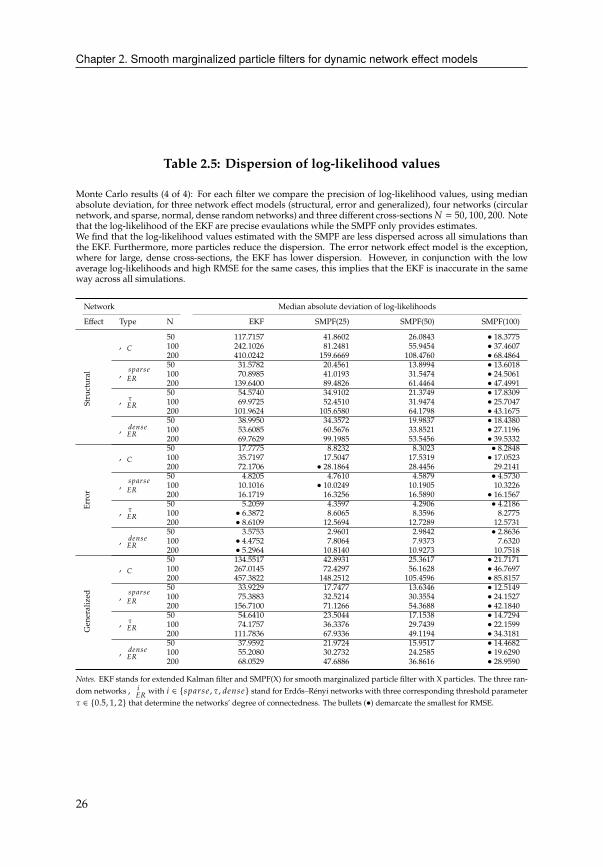
Chapter 2. Smooth marginalized particle filters for dynamic network effect models
Table 2.5: Dispersion of log-likelihood values
Monte Carlo results (4 of 4): For each filter we compare the precision of log-likelihood values, using median
absolute deviation, for three network effect models (structural, error and generalized), four networks (circular
network, and sparse, normal, dense random networks) and three different cross-sections# = 50, 100, 200. Note
that the log-likelihood of the EKF are precise evaulations while the SMPF only provides estimates.
We find that the log-likelihood values estimated with the SMPF are less dispersed across all simulations than
the EKF. Furthermore, more particles reduce the dispersion. The error network effect model is the exception,
where for large, dense cross-sections, the EKF has lower dispersion. However, in conjunction with the low
average log-likelihoods and high RMSE for the same cases, this implies that the EKF is inaccurate in the same
way across all simulations.
Network Median absolute deviation of log-likelihoods
Effect Type N EKF SMPF(25) SMPF(50) SMPF(100)
Structural
,�
50 117.7157 41.8602 26.0843 • 18.3775100 242.1026 81.2481 55.9454 • 37.4607200 410.0242 159.6669 108.4760 • 68.4864
,B?0AB4
�'
50 31.5782 20.4561 13.8994 • 13.6018100 70.8985 41.0193 31.5474 • 24.5061200 139.6400 89.4826 61.4464 • 47.4991
,��'
50 54.5740 34.9102 21.3749 • 17.8309100 69.9725 52.4510 31.9474 • 25.7047200 101.9624 105.6580 64.1798 • 43.1675
,34=B4�'
50 38.9950 34.3572 19.9837 • 18.4380100 53.6085 60.5676 33.8521 • 27.1196200 69.7629 99.1985 53.5456 • 39.5332
Error
,�
50 17.7775 8.8232 8.3023 • 8.2848100 35.7197 17.5047 17.5319 • 17.0523200 72.1706 • 28.1864 28.4456 29.2141
,B?0AB4
�'
50 4.8205 4.7610 4.5879 • 4.5730100 10.1016 • 10.0249 10.1905 10.3226
200 16.1719 16.3256 16.5890 • 16.1567
,��'
50 5.2059 4.3597 4.2906 • 4.2186100 • 6.3872 8.6065 8.3596 8.2775
200 • 8.6109 12.5694 12.7289 12.5731
,34=B4�'
50 3.5753 2.9601 2.9842 • 2.8636100 • 4.4752 7.8064 7.9373 7.6320
200 • 5.2964 10.8140 10.9273 10.7518
Generalized
,�
50 134.5517 42.8931 25.3617 • 21.7171100 267.0145 72.4297 56.1628 • 46.7697200 457.3822 148.2512 105.4596 • 85.8157
,B?0AB4
�'
50 33.9229 17.7477 13.6346 • 12.5149100 75.3883 32.5214 30.3554 • 24.1527200 156.7100 71.1266 54.3688 • 42.1840
,��'
50 54.6410 23.5044 17.1538 • 14.7294100 74.1757 36.3376 29.7439 • 22.1599200 111.7836 67.9336 49.1194 • 34.3181
,34=B4�'
50 37.9592 21.9724 15.9517 • 14.4682100 55.2080 30.2732 24.2585 • 19.6290200 68.0529 47.6886 36.8616 • 28.9590
Notes. EKF stands for extended Kalman filter and SMPF(X) for smooth marginalized particle filter with X particles. The three ran-
dom networks, 8�'
with 8 ∈ {B?0AB4 , �, 34=B4} stand for Erdős–Rényi networks with three corresponding threshold parameter
� ∈ {0.5, 1, 2} that determine the networks’ degree of connectedness. The bullets (•) demarcate the smallest for RMSE.
26
Chapter 2. Smooth marginalized particle filters for dynamic network effect models
2.6 Application: Asset pricing with peer networks
Factors used in asset pricing usually fall along a spectrum of observability. On the
one end, macroeconomic factor models relate asset returns to published economic or
financial time series. On the other end, statistical factor models extract latent factors
from asset returns as predictors. Somewhere in between are fundamental factors,
which are constructed from observable characteristics, such as Fama-French factors.
They are the returns of constructed portfolios, formed by sorting assets along certain
firm characteristics, such as size, value or profitability.
In the applicationwe show how theDNEmodel can be used to price assets with respect
to each other. Every asset is treated as a potential risk factor that could warrant a risk
premium. However, this does not mean that we aim at determining the factor loading
of every asset with respect to every other asset. Individual assets hardly possess the
systematic, non-diversifiable character that we demand of pricing factors. Instead, we
are interested in whether investors receive a premium for peer risk. We borrow the
term peer from the corporate valuation and mergers and acquisitions literature, where
it describes the set of firms that are similar enough to serve as valuation benchmarks to
the firm of interest (Foucault & Fresard, 2014). The natural application of this concept
into asset pricing is to assess stock returns with respect other, similar stocks. We call
this set of similar stocks the peers. We further introduce the notion of peer returns, which
refers to the returns of a hypothetical portfolio that consists of the peer stocks.
The financial intuition is best illustrated in the context of risk compensation. In the APT
framework, the investor is compensated for being exposed to an array of risk factors,
such as the market, size or industry factors. Every return is a linear combination of
the same fundamental factors and only differ by their loadings and the pricing errors.
We argue that similarities to other firms also constitutes a source of risk that warrants
a premium. For example, the valuation of a bank stock is naturally influenced by the
performance of other banks, which lend to the same sector, are subject to the same
regulations or comparable in their market capitalizations. Or, a tech stock might be
gravely affected due to bad news about another tech firm’s breaches in data privacy.
Several studies support this reasoning. Foucault and Fresard, 2014 specify a “learning
from peers” hypothesis where managers can learn from peer valuations about its own
firms growth opportunities. This in turn has a causal effect on their capital budgeting
decisions, as extensive CFO surveys have found (J. R. Graham & Harvey, 2001).
Thus, investors are still being compensated for their exposure to the market, size or
investment factors. But in addition, the investor also receives compensation for being
exposed to other, relevant risky assets. The question becomes which assets are deemed
27
Chapter 2. Smooth marginalized particle filters for dynamic network effect models
relevant enough. Several options are possible, ranging from common return histories,
cointegrating return relationships, similarities in the 10-K filings (Hoberg & Phillips,
2010) or common newswire occurrences (Box, 2018). We opt for a more fundamental
approach and argue that peers likely share similar cash flows, earnings per share,
leverage ratios or other characteristics and ratios – in other words, similar business
models. We rely on 45widely-used financial ratios and other accounting fundamentals,
published on an annual frequency, to determine the firm similarity.
If investors indeed account for some form of peer return factors or recognize that
firm similarities play a role in stock valuation, then neglecting these cross-sectional
commonalities will result in systematic mispricing. More concretely, suppose the peer
returns ?8C are part of the return generating process,
A8C = 8 + �8 5C + D8C (2.20)
D8C = 48C + ?8C (2.21)
where we assume that peer returns ?8C are uncorrelated with the idiosyncratic errors
48C . Then postulating a linear factor structure that omits the peer returns, A8C = 8 +�8 5C + 48C , would have two possible consequences. First, the pricing errors and
the factor loadings � will suffer from an omitted variable bias. Second, the peer risk
component ismistaken as idiosyncratic risk. Thiswould have a profound impact on any
statistical inference we can draw, based the residuals. Fortunately, such a mispricing
can be detected by scrutinizing the the residuals. The covariance matrix would be far
from diagonal and the residuals likely contain undiversifiable and persistent common
factors.
We find empirical evidence that this is indeed the case by examining the constituents
of the S&P100. After estimating a Fama-French model for all constituents’ weekly
excess returns, individually, we find that the residuals are far from idiosyncratic. The
first residual component alone accounts for 30% of residual variance. Peer effects
explain this variation and largely remove the residual common factor, which loses its
systematic character and only accounts for 15% of the residual variation. The pricing
errors are closer to zero and themarket betasdrop in coefficient size but gain in statistical
significance. As will become clear later, this is to be expected since peer returns are
simply the returns of segments of the market portfolio.
Since the proposed peer effects model leverages on the DNE framework, we are able
to extract these peer effects over time. After all, the informational value of peer stocks
may depend on the business cycle or macroeconomic conditions. We allow these inten-
sities to follow a stochastic processes and estimate them as latent states in a nonlinear
state-space model. The extracted signals shed light on the dynamics and changing
importance of peer effects. However, most of the improved pricing performance of
28
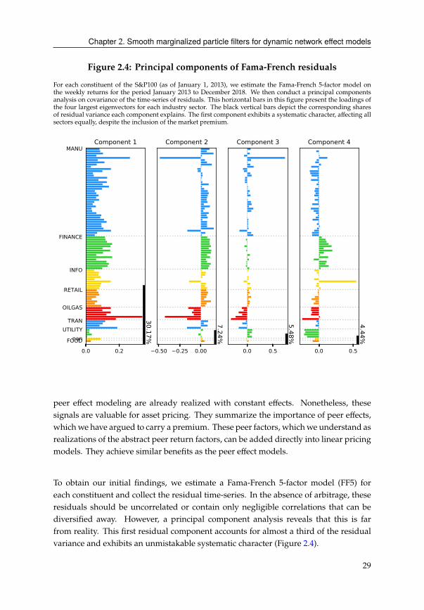
Chapter 2. Smooth marginalized particle filters for dynamic network effect models
Figure 2.4: Principal components of Fama-French residuals
For each constituent of the S&P100 (as of January 1, 2013), we estimate the Fama-French 5-factor model on
the weekly returns for the period January 2013 to December 2018. We then conduct a principal components
analysis on covariance of the time-series of residuals. This horizontal bars in this figure present the loadings of
the four largest eigenvectors for each industry sector. The black vertical bars depict the corresponding shares
of residual variance each component explains. The first component exhibits a systematic character, affecting all
sectors equally, despite the inclusion of the market premium.
0.0 0.2
30.17%
MANU
FINANCE
INFO
RETAIL
OILGAS
TRAN UTILITY
nan FOOD
Component 1
0.50 0.25 0.00
7.24%
Component 2
0.0 0.5
5.48%Component 3
0.0 0.5
4.44%
Component 4
peer effect modeling are already realized with constant effects. Nonetheless, these
signals are valuable for asset pricing. They summarize the importance of peer effects,
whichwe have argued to carry a premium. These peer factors, whichwe understand as
realizations of the abstract peer return factors, can be added directly into linear pricing
models. They achieve similar benefits as the peer effect models.
To obtain our initial findings, we estimate a Fama-French 5-factor model (FF5) for
each constituent and collect the residual time-series. In the absence of arbitrage, these
residuals should be uncorrelated or contain only negligible correlations that can be
diversified away. However, a principal component analysis reveals that this is far
from reality. This first residual component accounts for almost a third of the residual
variance and exhibits an unmistakable systematic character (Figure 2.4).
29
Chapter 2. Smooth marginalized particle filters for dynamic network effect models
2.6.1 Peer network
If equity returns are indeed priced with respect to each other, investors would have to
define a set of relevant assets for each asset they price. We measure firm similarities
through commonalities in their financial ratios and other accounting fundamentals. We
consider 45 widely-used variables, such as capital expenditure, market-to-book ratio,
R&D intensity, leverage ratio, etc. Our central assumption is that firms which report
similar numbers are most likely following similar strategies, which in turnmay contain
valuable pricing information. Furthermore, commonalities between firms are unlikely
subject to frequent changes.
We construct a peer matrix % with typical element �8 9 . Its rows represent the similarity
of firm 8 with respect to all other the firms 9 ≠ 8. The elements or weights are corre-
spondingly calculated as conditional correlations of firm 8’s fundamentals with respect
to the fundamentals of all remaining firms.12 This matrix % takes center stage in the
peer return factor model we introduce in the next section. It is important to note that
the peer weights �8 9 are not necessarily symmetric. If firm 9 is the closest peer to firm
8, in comparison to all other firms, then it does not necessarily follow, that the reverse
must also be true.
Statistical evidence for priced peer effects
Before we discuss how we operationalize the peer network %, we conduct statistical
tests to determine, first, if peer effects are present, and second, if % is a spurious
finding. We conduct a Moran’s � test for spatial dependence in the most general
sense (Anselin, 1988). The null hypothesis postulates that the dependency matrix %
does not have any predictive power. In financial terms, a peer portfolio is simply the
weighted returns of 'C , according to the rows of %. Thus, do the peer portfolios %'C
have any predictive power of 'C? More technically, we are interested in whether the
cross-sectional correlation between the excess returns, 2>AA('C , 'C ), is instead better
explained by the similarity-weighted returns of the other assets, 2>AA('C , %'C ). Hence,
a rejection of the null indicates that the returns exhibit a cross-sectional dependency
structure described by %, i.e. we find evidence for peer effects. We present the resulting
?-values of this test in Figure 2.5, upper panel. During the early-2016 stress period, we
12The term correlation here refers to the similarity of annually reported fundamentals. We treat firms as random
vectors and the annual reports are observed realizations,
5 8A<8 = [���)8 , !�+8 , �"'�)�$8 , ��%�-8 , ��(��!$,8 , ...]> .
Hence, we define firms as similar, if their vectors of reported characteristics are (partially) correlated. See
Table 2.9 for the accounting ratios used. In essence, we project each firm vector 5 8A<8 on a matrix of all other
firms [ 5 8A<9 ]9≠8 and conduct a '2decomposition. The contribution of each 5 8A<9 to the overall '2
becomes
our measure for firm similarity. If 5 8A<9 has the highest contribution in predicting 5 8A<8 , compared to all
other firms 5 8A<: with : ≠ 8 ≠ 9, then it is the closest peer of 5 8A<8 . For the details of the algorithm, we refer
to D. Wang et al., 2019, Appendix A.
30
Chapter 2. Smooth marginalized particle filters for dynamic network effect models
see increased concentration of significant peer effects and also detect clusters later on.13
The histogram on the right shows that we find these effects on the 5%-significance level
or lower for more than 40% of the observation period.
While wemotivate the choice of % with economic arguments, it is still worth examining
its robustness. Given that it is a full matrix (except for the main diagonal), one could
argue that any full matrix will produce the above results. A simple way to assess if is
the case is to shuffle the rows of %. If the tests still reject the independence assumption,
then % contains spurious peer structures. Figure 2.5, lower panel, shows that this
is not the case. Randomly reassigning peer relationships results in ?-values that are
uniformly distributed and stands in stark contrast to the proper ?matrix. This uniform
structure is what we would expect if % were randomly generated.
2.6.2 Pricing framework
In the APT framework, we assume an exact factor structure that leads to a linear pricing
model
'C = ��C + 4C (2.22)
with E(�C ) = 0, factor variance Var(�C ) = Σ 5 and E(4C ) = 0 and the errors 4C are
idiosyncratic and have negligibly small correlations, Var(4C ) = diag(�2
1, ..., �2
#). The
covariance matrix of asset returns is then
Var('C ) = �Σ 5 �> + � (2.23)
This equation stipulates that any commonalities in the asset returns are entirely due
to the factor variance as the error variance � is diagonal (Chamberlain & Rothschild,
1983). Reality rarely resonates with this assumption and the errors may exhibit non-
diversifiable components, such as we found in the previous section.
Fundamental peer effects
We augment this factor structure with peer effects. This effectively relaxes the diago-
nality assumption by imposing a predetermined covariance structure. This structure
is informed by the peer matrix %. The elements �8 9 represent how similar the firm 8 is
to firm 9, compared to all other firms. Hence, we can express the returns of asset 8 at
some point C as
A8 = �8?8 + �8 5 + 48 (2.24)
= )[�81A1 + ... + �8 9A9 ... + �8# A# ] + �8 5 + 48
13In the beginning of 2016, US equity markets found themselves amid growing pessimism and increasing
volatility. This bearish sentiment was primarily fueled by the weak oil price and slowing economic growth
figures from China. The resulting negative expectations were picked up by leading market indices.
31
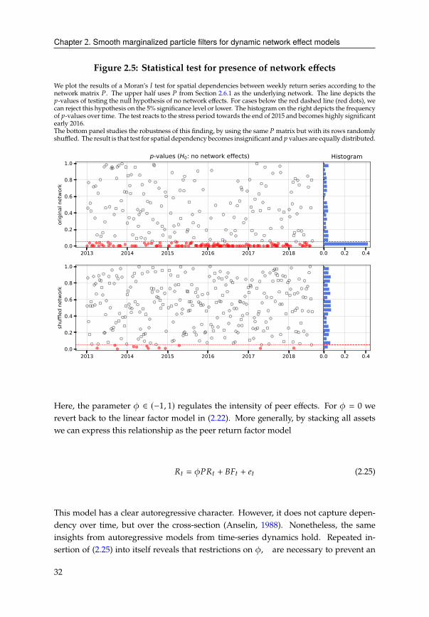
Chapter 2. Smooth marginalized particle filters for dynamic network effect models
Figure 2.5: Statistical test for presence of network effects
We plot the results of a Moran’s � test for spatial dependencies between weekly return series according to the
network matrix %. The upper half uses % from Section 2.6.1 as the underlying network. The line depicts the
?-values of testing the null hypothesis of no network effects. For cases below the red dashed line (red dots), we
can reject this hypothesis on the 5% significance level or lower. The histogram on the right depicts the frequency
of ?-values over time. The test reacts to the stress period towards the end of 2015 and becomes highly significant
early 2016.
The bottom panel studies the robustness of this finding, by using the same % matrix but with its rows randomly
shuffled. The result is that test for spatial dependency becomes insignificant and ? values are equally distributed.
0.0 0.2 0.4
Histogram
2013 2014 2015 2016 2017 20180.0
0.2
0.4
0.6
0.8
1.0
orig
inal
net
work
p-values (H0: no network effects)
0.0 0.2 0.42013 2014 2015 2016 2017 20180.0
0.2
0.4
0.6
0.8
1.0
shuf
fled
netw
ork
Here, the parameter ) ∈ (−1, 1) regulates the intensity of peer effects. For ) = 0 we
revert back to the linear factor model in (2.22). More generally, by stacking all assets
we can express this relationship as the peer return factor model
'C = )%'C + ��C + 4C (2.25)
This model has a clear autoregressive character. However, it does not capture depen-
dency over time, but over the cross-section (Anselin, 1988). Nonetheless, the same
insights from autoregressive models from time-series dynamics hold. Repeated in-
sertion of (2.25) into itself reveals that restrictions on ), are necessary to prevent an
32

Chapter 2. Smooth marginalized particle filters for dynamic network effect models
explosive process.
'C = )%'C + ��C + 4C= )%[)%'C + ��C + 4C] + ��C + 4C= )%[)%[)%'C + ��C + 4C] + ��C + 4C] + ��C + 4C= ...
Since the matrix % is row-normalized, the absolute value of its largest eigenvalue is
equal to 1. Preventing the process from exploding requires |) | < 1, which is satisfied
by assumption. Under this invertibility condition, we can write down the steady-state
formulation
'C = Φ��C +Φ4C where Φ = (�# − )%)−1(2.26)
= ��C + &C
Note that the resulting peer component Φ = Φ(), %) affects both the factor component
as well as the idiosyncratic errors. Hence, the model allows for correlations in the
errors according to Φ.
Var('C |Φ) = Φ�Σ 5 �>Φ> +Φ�Φ> (2.27)
Importantly, ourmodel distinguishes between errors &C ∼ #(0,Φ�Φ>)withpeer effects
and 4C ∼ #(0, �) adjusted for peer effects. We address both respectively as unadjusted
errors and peer-adjusted errors. The unadjusted errors still contain ‘impurities’ from
the peer component &C = Φ4C , while peer-adjusted model errors are the idiosyncratic
errors assumed in APT.
Residual peer effects
An alternative specification restricts the peer effects to the errors only. The same
rationale applies, but rather than assuming that asset returns are driven by peer asset
returns, we now isolate the peer effects to the residuals and call the corresponding
intensity parameter �.
'C = ��C + DC DC = �%DC + 4C (2.28)
In a similar fashion as for the fundamental peer effects, we can now write down the
steady-state formulation under a corresponding invertibility condition of |� | < 1
'C = ��C + Θ4C where Θ = (�# − �%)−1(2.29)
= ��C + &C
33
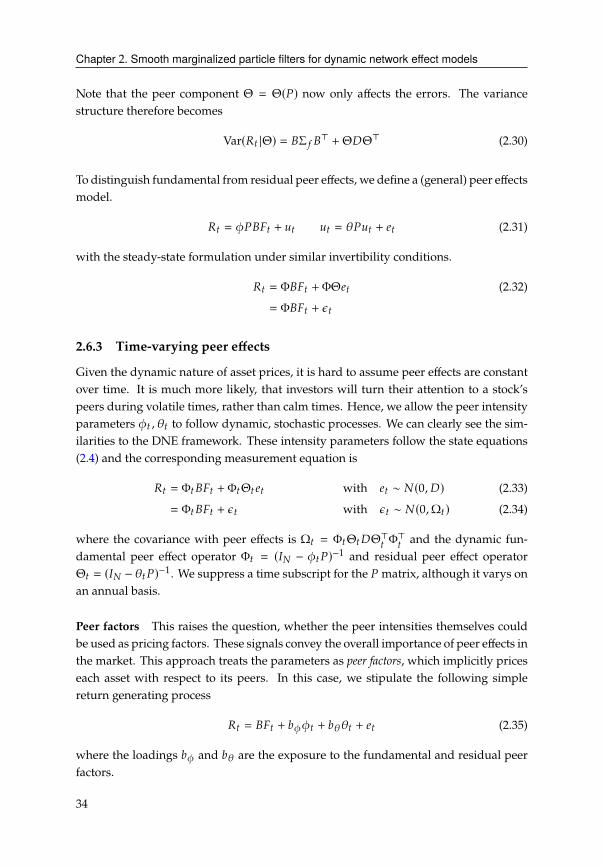
Chapter 2. Smooth marginalized particle filters for dynamic network effect models
Note that the peer component Θ = Θ(%) now only affects the errors. The variance
structure therefore becomes
Var('C |Θ) = �Σ 5 �> + Θ�Θ> (2.30)
To distinguish fundamental from residual peer effects, we define a (general) peer effects
model.
'C = )%��C + DC DC = �%DC + 4C (2.31)
with the steady-state formulation under similar invertibility conditions.
'C = Φ��C +ΦΘ4C (2.32)
= ��C + &C
2.6.3 Time-varying peer effects
Given the dynamic nature of asset prices, it is hard to assume peer effects are constant
over time. It is much more likely, that investors will turn their attention to a stock’s
peers during volatile times, rather than calm times. Hence, we allow the peer intensity
parameters )C , �C to follow dynamic, stochastic processes. We can clearly see the sim-
ilarities to the DNE framework. These intensity parameters follow the state equations
(2.4) and the corresponding measurement equation is
'C = ΦC��C +ΦCΘC 4C with 4C ∼ #(0, �) (2.33)
= ΦC��C + &C with &C ∼ #(0,ΩC ) (2.34)
where the covariance with peer effects is ΩC = ΦCΘC�Θ>CΦ>C
and the dynamic fun-
damental peer effect operator ΦC = (�# − )C%)−1and residual peer effect operator
ΘC = (�# − �C%)−1. We suppress a time subscript for the % matrix, although it varys on
an annual basis.
Peer factors This raises the question, whether the peer intensities themselves could
be used as pricing factors. These signals convey the overall importance of peer effects in
the market. This approach treats the parameters as peer factors, which implicitly prices
each asset with respect to its peers. In this case, we stipulate the following simple
return generating process
'C = ��C + 1))C + 1��C + 4C (2.35)
where the loadings 1) and 1� are the exposure to the fundamental and residual peer
factors.
34
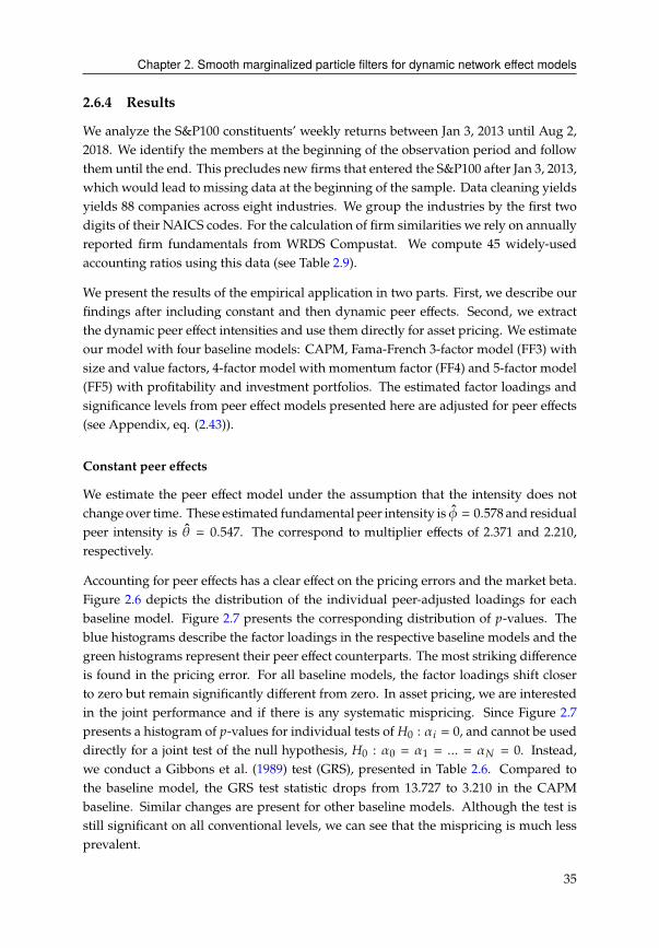
Chapter 2. Smooth marginalized particle filters for dynamic network effect models
2.6.4 Results
We analyze the S&P100 constituents’ weekly returns between Jan 3, 2013 until Aug 2,
2018. We identify the members at the beginning of the observation period and follow
them until the end. This precludes new firms that entered the S&P100 after Jan 3, 2013,
which would lead to missing data at the beginning of the sample. Data cleaning yields
yields 88 companies across eight industries. We group the industries by the first two
digits of their NAICS codes. For the calculation of firm similarities we rely on annually
reported firm fundamentals from WRDS Compustat. We compute 45 widely-used
accounting ratios using this data (see Table 2.9).
We present the results of the empirical application in two parts. First, we describe our
findings after including constant and then dynamic peer effects. Second, we extract
the dynamic peer effect intensities and use them directly for asset pricing. We estimate
our model with four baseline models: CAPM, Fama-French 3-factor model (FF3) with
size and value factors, 4-factor model with momentum factor (FF4) and 5-factor model
(FF5) with profitability and investment portfolios. The estimated factor loadings and
significance levels from peer effect models presented here are adjusted for peer effects
(see Appendix, eq. (2.43)).
Constant peer effects
We estimate the peer effect model under the assumption that the intensity does not
change over time. These estimated fundamental peer intensity is ) = 0.578 and residual
peer intensity is � = 0.547. The correspond to multiplier effects of 2.371 and 2.210,
respectively.
Accounting for peer effects has a clear effect on the pricing errors and the market beta.
Figure 2.6 depicts the distribution of the individual peer-adjusted loadings for each
baseline model. Figure 2.7 presents the corresponding distribution of ?-values. The
blue histograms describe the factor loadings in the respective baseline models and the
green histograms represent their peer effect counterparts. The most striking difference
is found in the pricing error. For all baseline models, the factor loadings shift closer
to zero but remain significantly different from zero. In asset pricing, we are interested
in the joint performance and if there is any systematic mispricing. Since Figure 2.7
presents a histogram of ?-values for individual tests of �0
: 8 = 0, and cannot be used
directly for a joint test of the null hypothesis, �0
: 0=
1= ... = # = 0. Instead,
we conduct a Gibbons et al. (1989) test (GRS), presented in Table 2.6. Compared to
the baseline model, the GRS test statistic drops from 13.727 to 3.210 in the CAPM
baseline. Similar changes are present for other baseline models. Although the test is
still significant on all conventional levels, we can see that the mispricing is much less
prevalent.
35

Chapter 2. Smooth marginalized particle filters for dynamic network effect models
We also observe that the market beta is further away from 1. In the CAPM world,
this result would be surprising. However, in the APT setting, the market factor has
no special meaning. While the baseline models have an average market beta between
0.997 and 1.058, the peer-adjusted loadings are between 0.186 and 0.204. This result
makes sense if we recall that assets are now priced with respect to peer return factors.
peer return factors can be seen as asset-specific subsets of the market portfolio. In fact,
the peer return factor represents the return of a portfolio, which consists of all assets
in the S&P100, but weighs them according to their similarity to the asset of interest.14
Hence, it is not surprising that the peer effect model affects the market factor loadings.
What is surprising, however, is that the peer-adjusted market beta also becomes much
more significant.
Finally, we conduct a principal component analysis (PCA) on the peer-adjusted resid-
uals.15 Earlier we predicted that the omittance of peer return factors not only leads to
the mispricing we just established. It also will leave the peer return factor for the resid-
uals. Hence, accounting for peer return factors should bring us closer to the diagonal
residual covariance the APT framework stipulates. The PCA reveals that this is indeed
the case. Figure 2.8 that the largest residual component loses its systematic nature
and accounts for only half of the peer-adjusted residual variance (15.10%) than in the
baseline (30.17%). We find further evidence for the better asset pricing performance in
the higher '2. While the baselinemodels range from 8.7% to 11.4%, their peer-adjusted
counterparts range from 29.5% to 32.1%. Finally, we scrutinize the residual correlation
visually in Figure 2.24a and of squared residuals in Figure 2.24b. The average absolute
correlation drops from 28.0% to 11.6% and for squared residuals, correlation drops
from 14.7% to 8.7%.
14The market factor we use is from Kenneth French’s website and is constructed using a larger universe of firms
listed on the NYSE, AMEX or NASDAQ, i.e. a superset of the S&P100.
15In the baseline model, we compute the PCA using prediction errors, 4C = 'C − 'C . In the peer effects model,
however, prediction errors contain peer effects (e.g. equation (2.25)). We refer to them as unadjusted residuals,
&C . Filtering out these effects yields peer-adjusted model residuals, 4C .
unadjusted residuals (prediction errors) &C = HC − 'C = ΦC ΘC 4Cpeer-adjusted residuals 4C = Θ
−1
C Φ−1
C &C
. Our empirical results rely on the peer-adjusted residuals.
36
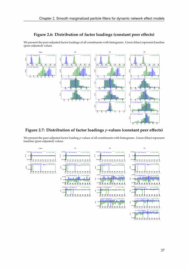
Chapter 2. Smooth marginalized particle filters for dynamic network effect models
Figure 2.6: Distribution of factor loadings (constant peer effects)
Wepresent the peer-adjusted factor loadings of all constituentswith histograms. Green (blue) represent baseline
(peer-adjusted) values.
0.03 0.02 0.01 0.00 0.01 0.02 0.03
cons
t
=-0.022 (Baseline) =-0.004 (DNE)
1.5 1.0 0.5 0.0 0.5 1.0 1.5
mkt
rf
= 0.997 (Baseline) = 0.186 (DNE)
capm
0.03 0.02 0.01 0.00 0.01 0.02 0.03
cons
t
=-0.022 (Baseline) =-0.004 (DNE)
2 1 0 1 2
mkt
rf
= 1.014 (Baseline) = 0.190 (DNE)
1.0 0.5 0.0 0.5 1.0
smb
=-0.055 (Baseline) =-0.014 (DNE)
3 2 1 0 1 2 3
hml
= 0.279 (Baseline) = 0.057 (DNE)
ff3
0.03 0.02 0.01 0.00 0.01 0.02 0.03
cons
t
=-0.022 (Baseline) =-0.004 (DNE)
2 1 0 1 2
mkt
rf
= 1.049 (Baseline) = 0.198 (DNE)
1.0 0.5 0.0 0.5 1.0
smb
=-0.070 (Baseline) =-0.017 (DNE)
2 1 0 1 2
hml
= 0.182 (Baseline) = 0.035 (DNE)
3 2 1 0 1 2 3
umd
=-0.280 (Baseline) =-0.057 (DNE)
ff4
0.03 0.02 0.01 0.00 0.01 0.02 0.03
cons
t
=-0.022 (Baseline) =-0.004 (DNE)
2 1 0 1 2
mkt
rf
= 1.058 (Baseline) = 0.204 (DNE)
1.5 1.0 0.5 0.0 0.5 1.0 1.5
smb
=-0.032 (Baseline) =-0.006 (DNE)
3 2 1 0 1 2 3
hml
= 0.195 (Baseline) = 0.027 (DNE)
2 1 0 1 2
rmw
= 0.195 (Baseline) = 0.060 (DNE)
3 2 1 0 1 2 3
cma
= 0.277 (Baseline) = 0.087 (DNE)
ff5
Figure 2.7: Distribution of factor loadings ?-values (constant peer effects)
Wepresent the peer-adjusted factor loading ?-values of all constituents with histograms. Green (blue) represent
baseline (peer-adjusted) values.
0.0 0.1 0.2 0.3 0.4 0.5 0.6 0.7 0.8 0.9 1.0100%
0%
100%
cons
t
=0.000 (Baseline) =0.001 (DNE)
0.0 0.1 0.2 0.3 0.4 0.5 0.6 0.7 0.8 0.9 1.0
50%
0%
mkt
rf
=0.398 (Baseline) =0.088 (DNE)
capm
0.0 0.1 0.2 0.3 0.4 0.5 0.6 0.7 0.8 0.9 1.0100%
0%
100%
cons
t
=0.000 (Baseline) =0.001 (DNE)
0.0 0.1 0.2 0.3 0.4 0.5 0.6 0.7 0.8 0.9 1.0
50%
0%
mkt
rf
=0.384 (Baseline) =0.091 (DNE)
0.0 0.1 0.2 0.3 0.4 0.5 0.6 0.7 0.8 0.9 1.010%
0%
10%
smb
=0.538 (Baseline) =0.444 (DNE)
0.0 0.1 0.2 0.3 0.4 0.5 0.6 0.7 0.8 0.9 1.0
25%
0%
25%
hml
=0.315 (Baseline) =0.220 (DNE)
ff3
0.0 0.1 0.2 0.3 0.4 0.5 0.6 0.7 0.8 0.9 1.0100%
0%
100%
cons
t
=0.000 (Baseline) =0.001 (DNE)
0.0 0.1 0.2 0.3 0.4 0.5 0.6 0.7 0.8 0.9 1.0
50%
0%
mkt
rf
=0.360 (Baseline) =0.108 (DNE)
0.0 0.1 0.2 0.3 0.4 0.5 0.6 0.7 0.8 0.9 1.010%
0%
10%
smb
=0.539 (Baseline) =0.447 (DNE)
0.0 0.1 0.2 0.3 0.4 0.5 0.6 0.7 0.8 0.9 1.0
25%
0%
25%
hml
=0.339 (Baseline) =0.241 (DNE)
0.0 0.1 0.2 0.3 0.4 0.5 0.6 0.7 0.8 0.9 1.010%
0%
umd
=0.424 (Baseline) =0.485 (DNE)
ff4
0.0 0.1 0.2 0.3 0.4 0.5 0.6 0.7 0.8 0.9 1.0100%
0%
100%
cons
t
=0.000 (Baseline) =0.001 (DNE)
0.0 0.1 0.2 0.3 0.4 0.5 0.6 0.7 0.8 0.9 1.0
50%
0%
mkt
rf
=0.419 (Baseline) =0.123 (DNE)
0.0 0.1 0.2 0.3 0.4 0.5 0.6 0.7 0.8 0.9 1.010%
0%
10%
smb
=0.558 (Baseline) =0.461 (DNE)
0.0 0.1 0.2 0.3 0.4 0.5 0.6 0.7 0.8 0.9 1.0
20%
0%
20%
hml
=0.399 (Baseline) =0.312 (DNE)
0.0 0.1 0.2 0.3 0.4 0.5 0.6 0.7 0.8 0.9 1.020%
0%
rmw
=0.511 (Baseline) =0.367 (DNE)
0.0 0.1 0.2 0.3 0.4 0.5 0.6 0.7 0.8 0.9 1.020%
0%
cma
=0.537 (Baseline) =0.330 (DNE)
ff5
37
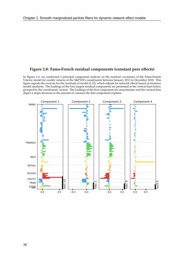
Chapter 2. Smooth marginalized particle filters for dynamic network effect models
Figure 2.8: Fama-French residual components (constant peer effects)
In Figure 2.4, we conducted a principal component analysis on the residual covariance of the Fama-French
5-factor model for weekly returns of the S&P100’s constituents between January 2013 to December 2018. This
figure repeats the exercise for the residuals of model (2.32), which adjusts for network effects based on business
model similarity. The loadings of the four largest residual components are presented in the vertical bars below,
grouped by the constituents’ sectors. The loadings of the first component are unsystematic and the vertical bars
depict a major decrease in the amount of variance the first component explains.
0.0 0.5
15.10%
MANU
FINANCE
INFO
RETAIL
OILGAS
UTILITY TRAN FOOD nan
Component 1
0.5 0.0
7.78%
Component 2
0.0 0.5
6.79%
Component 3
0.0 0.5
5.67%
Component 4
38
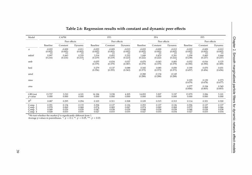
Chapter
2.Sm
oothmarginalized
particlefilters
fordynamic
networkeffectm
odels
Table 2.6: Regression results with constant and dynamic peer effects
Model CAPM FF3 FF4 FF5
Peer effects Peer effects Peer effects Peer effects
Baseline Constant Dynamic Baseline Constant Dynamic Baseline Constant Dynamic Baseline Constant Dynamic
-0.022 -0.009 -0.011 -0.022 -0.009 -0.012 -0.022 -0.009 -0.012 -0.022 -0.009 -0.012
(0.002) (0.002) (0.002) (0.002) (0.002) (0.002) (0.002) (0.002) (0.002) (0.002) (0.002) (0.002)
*** *** *** *** *** *** *** *** *** *** *** ***
mktrf 0.997 0.443 0.335 1.014 0.452 0.352 1.049 0.470 0.391 1.058 0.485 0.444
(0.216) (0.216) (0.215) (0.219) (0.219) (0.223) (0.222) (0.222) (0.222) (0.238) (0.237) (0.237)
* * *
smb -0.055 -0.034 0.037 -0.070 -0.043 0.083 -0.032 -0.016 0.125
(0.379) (0.379) (0.387) (0.379) (0.379) (0.379) (0.390) (0.390) (0.389)
hml 0.279 0.137 0.088 0.182 0.085 0.050 0.195 0.070 0.031
(0.356) (0.355) (0.363) (0.373) (0.373) (0.373) (0.457) (0.456) (0.456)
umd -0.280 -0.134 -0.145
(0.288) (0.288) (0.288)
rmw 0.195 0.139 0.373
(0.679) (0.678) (0.677)
cma 0.277 0.194 0.343
(0.806) (0.805) (0.803)
GRS test 13.727 3.210 4.101 14.184 3.238 4.205 14.093 3.207 5.197 13.979 3.206 5.101
?-value 0.000 0.000 0.000 0.000 0.000 0.000 0.000 0.000 0.000 0.000 0.000 0.000
'20.087 0.295 0.294 0.103 0.311 0.308 0.109 0.315 0.313 0.114 0.321 0.320
Comp. 1 0.291 0.134 0.133 0.294 0.127 0.126 0.293 0.127 0.126 0.296 0.127 0.127
Comp. 2 0.078 0.069 0.068 0.074 0.069 0.067 0.074 0.069 0.068 0.072 0.068 0.066
Comp. 3 0.049 0.039 0.039 0.047 0.038 0.039 0.048 0.038 0.038 0.046 0.038 0.038
Comp. 4 0.028 0.033 0.035 0.027 0.033 0.035 0.027 0.033 0.034 0.027 0.033 0.034
1We test whether the market � is significantly different from 1.
Average ?-values in parentheses. *: ? < 0.1, **: ? < 0.05, ***: ? < 0.01
39
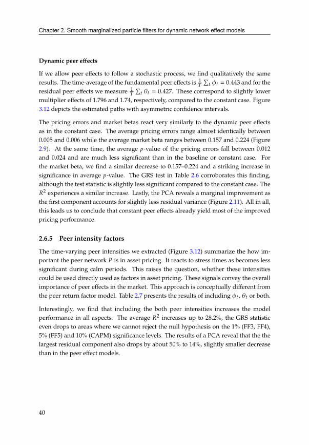
Chapter 2. Smooth marginalized particle filters for dynamic network effect models
Dynamic peer effects
If we allow peer effects to follow a stochastic process, we find qualitatively the same
results. The time-average of the fundamental peer effects is1
)
∑C )C = 0.443 and for the
residual peer effects we measure1
)
∑C �C = 0.427. These correspond to slightly lower
multiplier effects of 1.796 and 1.74, respectively, compared to the constant case. Figure
3.12 depicts the estimated paths with asymmetric confidence intervals.
The pricing errors and market betas react very similarly to the dynamic peer effects
as in the constant case. The average pricing errors range almost identically between
0.005 and 0.006 while the average market beta ranges between 0.157 and 0.224 (Figure
2.9). At the same time, the average ?-value of the pricing errors fall between 0.012
and 0.024 and are much less significant than in the baseline or constant case. For
the market beta, we find a similar decrease to 0.157–0.224 and a striking increase in
significance in average ?-value. The GRS test in Table 2.6 corroborates this finding,
although the test statistic is slightly less significant compared to the constant case. The
'2experiences a similar increase. Lastly, the PCA reveals a marginal improvement as
the first component accounts for slightly less residual variance (Figure 2.11). All in all,
this leads us to conclude that constant peer effects already yield most of the improved
pricing performance.
2.6.5 Peer intensity factors
The time-varying peer intensities we extracted (Figure 3.12) summarize the how im-
portant the peer network % is in asset pricing. It reacts to stress times as becomes less
significant during calm periods. This raises the question, whether these intensities
could be used directly used as factors in asset pricing. These signals convey the overall
importance of peer effects in the market. This approach is conceptually different from
the peer return factor model. Table 2.7 presents the results of including )C , �C or both.
Interestingly, we find that including the both peer intensities increases the model
performance in all aspects. The average '2increases up to 28.2%, the GRS statistic
even drops to areas where we cannot reject the null hypothesis on the 1% (FF3, FF4),
5% (FF5) and 10% (CAPM) significance levels. The results of a PCA reveal that the the
largest residual component also drops by about 50% to 14%, slightly smaller decrease
than in the peer effect models.
40
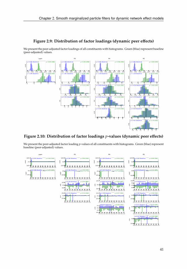
Chapter 2. Smooth marginalized particle filters for dynamic network effect models
Figure 2.9: Distribution of factor loadings (dynamic peer effects)
Wepresent the peer-adjusted factor loadings of all constituentswith histograms. Green (blue) represent baseline
(peer-adjusted) values.
0.03 0.02 0.01 0.00 0.01 0.02 0.03
cons
t
=-0.022 (Baseline) =-0.005 (DNE)
2 1 0 1 2
mkt
rf
= 1.046 (Baseline) = 0.166 (DNE)
capm
0.03 0.02 0.01 0.00 0.01 0.02 0.03
cons
t
=-0.022 (Baseline) =-0.005 (DNE)
2 1 0 1 2
mkt
rf
= 1.067 (Baseline) = 0.157 (DNE)
1.0 0.5 0.0 0.5 1.0
smb
=-0.079 (Baseline) = 0.013 (DNE)
3 2 1 0 1 2 3
hml
= 0.321 (Baseline) = 0.038 (DNE)
ff3
0.03 0.02 0.01 0.00 0.01 0.02 0.03
cons
t
=-0.022 (Baseline) =-0.006 (DNE)
2 1 0 1 2
mkt
rf
= 1.109 (Baseline) = 0.195 (DNE)
1.0 0.5 0.0 0.5 1.0sm
b
=-0.099 (Baseline) = 0.041 (DNE)
2 1 0 1 2
hml
= 0.200 (Baseline) = 0.024 (DNE)
3 2 1 0 1 2 3
umd
=-0.311 (Baseline) =-0.073 (DNE)
ff4
0.03 0.02 0.01 0.00 0.01 0.02 0.03
cons
t
=-0.022 (Baseline) =-0.006 (DNE)
2 1 0 1 2
mkt
rf
= 1.138 (Baseline) = 0.224 (DNE)
1.5 1.0 0.5 0.0 0.5 1.0 1.5
smb
=-0.039 (Baseline) = 0.066 (DNE)
3 2 1 0 1 2 3
hml
= 0.176 (Baseline) = 0.012 (DNE)
2 1 0 1 2
rmw
= 0.310 (Baseline) = 0.190 (DNE)
3 2 1 0 1 2 3cm
a
= 0.421 (Baseline) = 0.176 (DNE)
ff5
Figure 2.10: Distribution of factor loadings ?-values (dynamic peer effects)
Wepresent the peer-adjusted factor loading ?-values of all constituents with histograms. Green (blue) represent
baseline (peer-adjusted) values.
0.0 0.1 0.2 0.3 0.4 0.5 0.6 0.7 0.8 0.9 1.0100%
0%
100%
cons
t
=0.000 (Baseline) =0.000 (DNE)
0.0 0.1 0.2 0.3 0.4 0.5 0.6 0.7 0.8 0.9 1.0
50%
0%
mkt
rf
=0.398 (Baseline) =0.055 (DNE)
capm
0.0 0.1 0.2 0.3 0.4 0.5 0.6 0.7 0.8 0.9 1.0100%
0%
100%
cons
t
=0.000 (Baseline) =0.000 (DNE)
0.0 0.1 0.2 0.3 0.4 0.5 0.6 0.7 0.8 0.9 1.0
50%
0%
mkt
rf
=0.384 (Baseline) =0.059 (DNE)
0.0 0.1 0.2 0.3 0.4 0.5 0.6 0.7 0.8 0.9 1.0
10%
0%
10%
smb
=0.538 (Baseline) =0.454 (DNE)
0.0 0.1 0.2 0.3 0.4 0.5 0.6 0.7 0.8 0.9 1.0
25%
0%
25%
hml
=0.315 (Baseline) =0.210 (DNE)
ff3
0.0 0.1 0.2 0.3 0.4 0.5 0.6 0.7 0.8 0.9 1.0100%
0%
100%
cons
t
=0.000 (Baseline) =0.000 (DNE)
0.0 0.1 0.2 0.3 0.4 0.5 0.6 0.7 0.8 0.9 1.0
50%
0%
mkt
rf
=0.360 (Baseline) =0.073 (DNE)
0.0 0.1 0.2 0.3 0.4 0.5 0.6 0.7 0.8 0.9 1.010%
0%
10%
smb
=0.539 (Baseline) =0.455 (DNE)
0.0 0.1 0.2 0.3 0.4 0.5 0.6 0.7 0.8 0.9 1.0
25%
0%
25%
hml
=0.339 (Baseline) =0.227 (DNE)
0.0 0.1 0.2 0.3 0.4 0.5 0.6 0.7 0.8 0.9 1.010%
5%0%5%
umd
=0.424 (Baseline) =0.483 (DNE)
ff4
0.0 0.1 0.2 0.3 0.4 0.5 0.6 0.7 0.8 0.9 1.0100%
0%
100%
cons
t
=0.000 (Baseline) =0.000 (DNE)
0.0 0.1 0.2 0.3 0.4 0.5 0.6 0.7 0.8 0.9 1.0
50%
0%
mkt
rf
=0.419 (Baseline) =0.102 (DNE)
0.0 0.1 0.2 0.3 0.4 0.5 0.6 0.7 0.8 0.9 1.0
5%0%5%
10%
smb
=0.558 (Baseline) =0.492 (DNE)
0.0 0.1 0.2 0.3 0.4 0.5 0.6 0.7 0.8 0.9 1.0
25%
0%
hml
=0.399 (Baseline) =0.308 (DNE)
0.0 0.1 0.2 0.3 0.4 0.5 0.6 0.7 0.8 0.9 1.0
20%
0%
rmw
=0.511 (Baseline) =0.334 (DNE)
0.0 0.1 0.2 0.3 0.4 0.5 0.6 0.7 0.8 0.9 1.020%
0%
cma
=0.537 (Baseline) =0.300 (DNE)
ff5
41
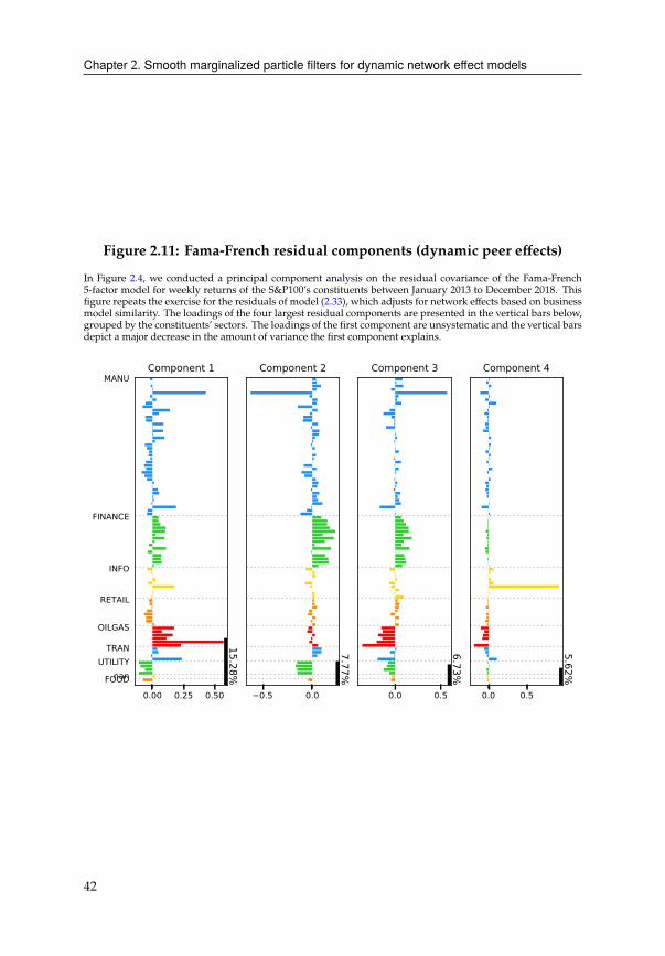
Chapter 2. Smooth marginalized particle filters for dynamic network effect models
Figure 2.11: Fama-French residual components (dynamic peer effects)
In Figure 2.4, we conducted a principal component analysis on the residual covariance of the Fama-French
5-factor model for weekly returns of the S&P100’s constituents between January 2013 to December 2018. This
figure repeats the exercise for the residuals of model (2.33), which adjusts for network effects based on business
model similarity. The loadings of the four largest residual components are presented in the vertical bars below,
grouped by the constituents’ sectors. The loadings of the first component are unsystematic and the vertical bars
depict a major decrease in the amount of variance the first component explains.
0.00 0.25 0.50
15.28%
MANU
FINANCE
INFO
RETAIL
OILGAS
TRAN UTILITY
nan FOOD
Component 1
0.5 0.0
7.77%
Component 2
0.0 0.5
6.73%
Component 3
0.0 0.5
5.62%
Component 4
42
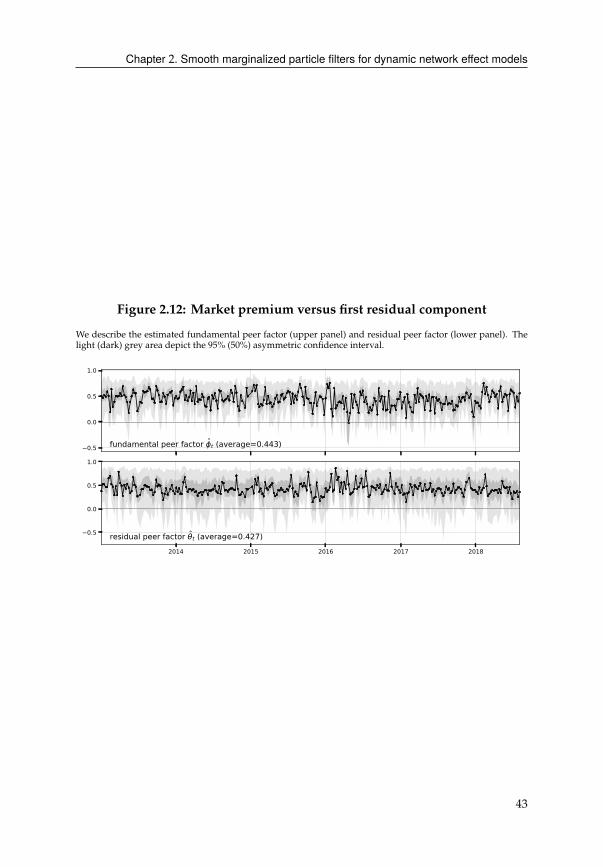
Chapter 2. Smooth marginalized particle filters for dynamic network effect models
Figure 2.12: Market premium versus first residual component
We describe the estimated fundamental peer factor (upper panel) and residual peer factor (lower panel). The
light (dark) grey area depict the 95% (50%) asymmetric confidence interval.
0.5
0.0
0.5
1.0
fundamental peer factor t (average=0.443)
2014 2015 2016 2017 2018
0.5
0.0
0.5
1.0
residual peer factor t (average=0.427)
43
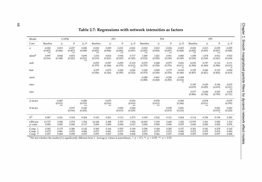
Chapter
2.Sm
oothmarginalized
particlefilters
fordynamic
networkeffectm
odels
Table 2.7: Regressions with network intensities as factors
Model CAPM FF3 FF4 FF5
Coef. Baseline ) � ), � Baseline ) � ), � Baseline ) � ), � Baseline ) � ), �
-0.022 0.019 -0.037 0.002 -0.022 0.009 -0.031 -0.001 -0.022 0.013 -0.034 -0.003 -0.022 0.013 -0.039 -0.005
(0.002) (0.006) (0.007) (0.008) (0.002) (0.004) (0.006) (0.007) (0.002) (0.005) (0.007) (0.008) (0.002) (0.005) (0.007) (0.008)
*** *** *** *** *** *** *** ***
mktrf1
0.997 0.844 0.874 0.695 1.014 0.814 0.934 0.717 1.049 1.021 0.931 0.860 1.058 1.074 0.912 0.923
(0.216) (0.198) (0.222) (0.012) (0.219) (0.201) (0.225) (0.342) (0.222) (0.205) (0.230) (0.345) (0.238) (0.218) (0.241) (0.618)
***
smb -0.055 -0.057 -0.093 -0.103 -0.070 0.048 -0.079 0.041 -0.032 0.197 -0.116 0.111
(0.379) (0.344) (0.379) (0.012) (0.379) (0.350) (0.376) (0.011) (0.390) (0.360) (0.386) (0.013)
** ** **
hml 0.279 0.073 0.242 0.026 0.182 0.009 0.175 -0.010 0.195 0.026 0.119 -0.054
(0.356) (0.324) (0.355) (0.323) (0.373) (0.345) (0.370) (0.340) (0.457) (0.421) (0.452) (0.415)
umd -0.280 -0.461 -0.206 -0.368
(0.288) (0.268) (0.290) (0.014)
**
rmw 0.195 0.629 0.196 0.633
(0.679) (0.629) (0.670) (0.011)
***
cma 0.277 0.649 0.303 0.678
(0.806) (0.744) (0.795) (0.731)
)-factor -0.087 -0.089 -0.075 -0.076 -0.078 -0.082 -0.078 -0.079
(0.012) (0.015) (0.010) (0.010) (0.012) (0.266) (0.011) (0.355)
*** *** *** *** *** ***
�-factor 0.037 0.043 0.020 0.024 0.030 0.041 0.041 0.042
(0.016) (0.202) (0.013) (0.205) (0.015) (0.210) (0.015) (0.220)
*
'20.087 0.241 0.104 0.264 0.103 0.261 0.112 0.273 0.109 0.242 0.121 0.264 0.114 0.256 0.138 0.282
GRS test 13.727 2.380 2.574 1.254 14.184 2.288 2.787 1.524 14.093 2.239 2.649 1.452 13.979 1.961 3.050 1.310
?-value 0.000 0.000 0.000 0.115 0.000 0.000 0.000 0.013 0.000 0.000 0.000 0.025 0.000 0.000 0.000 0.076
Comp. 1 0.302 0.175 0.286 0.142 0.300 0.164 0.293 0.149 0.296 0.184 0.285 0.157 0.301 0.181 0.278 0.145
Comp. 2 0.075 0.081 0.076 0.084 0.073 0.081 0.073 0.083 0.073 0.079 0.073 0.082 0.072 0.079 0.074 0.083
Comp. 3 0.057 0.068 0.058 0.070 0.055 0.067 0.056 0.068 0.056 0.066 0.057 0.068 0.055 0.065 0.057 0.068
1We test whether the market � is significantly different from 1. Average ?-values in parentheses. *: ? < 0.1, **: ? < 0.05, ***: ? < 0.01
44

Chapter 2. Smooth marginalized particle filters for dynamic network effect models
Comparing both peer factors, we find that the fundamental peer factor is statistically
highly significant for all models when it is included alone. If both factors are present,
the fundamental peer factor loses its importance for the FF4 and FF5models. Curiously,
the presence of both factors leads to the market beta to become highly significant in
the CAPM case and similarly, the size factor becomes significant for the Fama-French
models. Overall, this suggests that the peer factors contain information that is picked
up by the markets and withstands the inclusion of the Fama-French factors.
45

Chapter 2. Smooth marginalized particle filters for dynamic network effect models
Summary
In this application we examined whether the stock returns are priced with respect to
their peers. In other words, do investors price in the similarity a firm has with other
firms. This is motivated from the corporate valuation literature, where the relative
valuation model is a popular method, next to the discounted cash flow model. The
investors gauge whether a company is over- or undervalued, based on how its (price)
multiples, accounting ratios or historical averages differ from its peers. Managers
themselves rely on these methods to make capital budgeting decisions. We borrow this
suit of variables to identify peer networks.
If the return generating process indeed contain peer risk factors, then neglecting this
cross-sectional dependency structure would result in severe mispricing. The results
of pricing each constituent of the S&P100 with Fama-French type models reveal a
common factor in their residuals. This presents a case against the validity of the APT,
which assumes covariance matrices to be diagonal or only contain diversifiable risk
components. The results of mis-specification tests indicate that peer effects may indeed
be present, but neglected. As a remedy, we embed the peer network into a linear factor
structure and explicitly model these cross-sectional dependencies. Surprisingly, the
resulting GRS test statistics indicate that the pricing errors are much less prevalent
than in the baseline models. Nonetheless, they are still significantly different from
zero. Curiously, the market beta becomes more significant but less important as it
moves away from 1. This makes sense upon close inspection, since the peer risk factors
are essentially returns of peer portfolios, which consist of weighted subsets of the
market portfolio. The tailored nature of peer effects are therefore in a better position to
explain asset returns than the system-wide market portfolio.
We find further evidence that our pricing model with peer effects outperforms the
baseline model, since the average '2roughly triples to around 30% from 11%. More
over, the residual common factor is almost gone and the residual covariance becomes
more similar to thediagonal structure theAPT framework stipulates. This also holds for
squared residuals, since residual variances may still be correlated. The large residual
factor loses its systemic nature and is only left in particular industries. It accounts for
only 15% of all residual variation.
Although it seemed reasonable to assume time-varying peer intensities, we find that
almost all benefits are realized by assuming constant intensities. Nonetheless, the
extracted intensities shed light on the dynamics during particular stress times. More
interestingly, these intensities can be seen as pricing factors, which summarize the
prevalence of peer effects at a given point in time. According to our risk compensation
reasoning in deriving the peer effects model, these factors should demand a premium.
We include these peer factors into the baseline models and find that they realize most
46

Chapter 2. Smooth marginalized particle filters for dynamic network effect models
of the benefits of the dynamic peer effect models and withstand the inclusion of Fama-
French factors. For practitioners, these factors represent a convenient shortcut without
having to estimate the entire model.
The better pricing performance of the peer effects model in comparison to pure funda-
mental factor models has profound implications. It is important to realize, that it does
not propose to supersede the size, investment or momentum factors. On the contrary,
the Fama-French factors still constitute the main driving force. In fact, the peer effects
model argues that their effect reaches further than pricing single assets. The resulting
price has an impact on its peers and these in turn pass it on to their peers in a slowly
attenuating process. Our results indicate that these knock-on effects are also priced
by markets and cannot be diversified away. We propose a framework that quantifies
the magnitude of these amplification effects. Ultimately, it allows us to recover the
peer-adjusted factor loadings and residuals.
These findings highlight the dangers of disregarding peer effects and possible reme-
dies. The peer network we assumed is not unique and the structure of the remaining
residual common factor suggest other forms of knock-on effects, which are not captured
by our understanding of firm similarities. Avenues for future research may include the
examination of other peer networks, based on common occurrences in news articles
or similar descriptions in 10-K filings. It would also be interesting to determine its
relationship to characteristics-based asset pricing models, where the variables we em-
ployed to construct the peer network with are used for pricing directly. Furthermore,
this framework may present itself as an alternative to industry factors, commonly used
in pricing models.
2.7 Application: COVID-19 and travel networks
The SARS-CoV2 virus is spreading rapidly around the world. As of April 20, 211
countries reported a total of 2,520,000+ confirmed cases. Due to the long incubation
and even longer asymptomatic period (Lauer et al., 2020), research has shown that
airport screenings are of limited effectiveness (Quilty et al., 2020). It is therefore highly
probable that long-distance travel, such as commercial air travel, or short-distance
travel, such as railways or road travel, serve as propagation channels for the virus’
global reach.
In this empirical illustration we analyze the importance of networks for the spread
of COVID-19 between countries. For the number of confirmed cases we rely on the
database of Johns Hopkins University, Center For Systems Science and Engineering
(Dong et al., 2020). To capture long distance travel, we construct an airline network
47
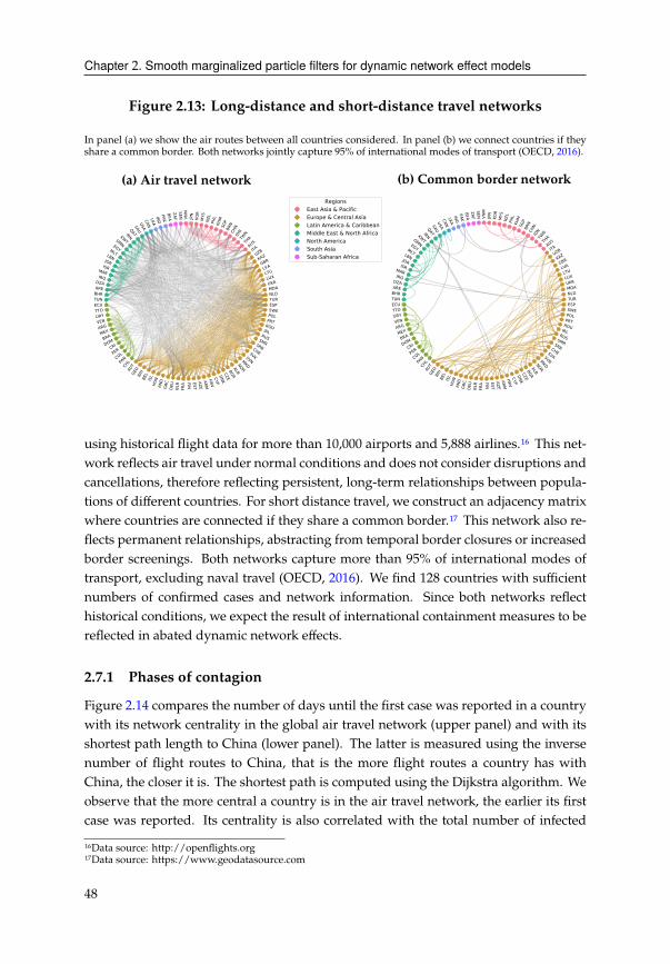
Chapter 2. Smooth marginalized particle filters for dynamic network effect models
Figure 2.13: Long-distance and short-distance travel networks
In panel (a) we show the air routes between all countries considered. In panel (b) we connect countries if they
share a common border. Both networks jointly capture 95% of international modes of transport (OECD, 2016).
(a) Air travel networkVN
M
VN
MJP
N
JPN
KOR
K
ORMY
S
MYS
NZL
N
ZLPH
L
PHL
KHM
K
HMSG
P
SGP
BRN
B
RNCH
N
CHN
IDN
ID
N
TWN
TWN
THA
THA
AUS A
US
ITA ITA
UZB UZB
KAZ KAZ
GBR GBR
LVA LVA
LTU LTU
LUX LUX
UKR UKR
MDA MDANLD NLDTUR TURESP ESPSWE SWEPOL POLPRT PRTROU ROUIRL IRLRUS RUS
SMR SMRSRB SRB
CHE CHE
SVK SVK
SVN SVN
MKD MKD
NOR NOR
ALB ALB
BGR BGR
CZE CZE
DNK DNK
CYP CYP
HRV HRV
ARM ARM
AZE AZEEST ESTFIN FIN
FRA
F
RABL
R
BLR
DEU
D
EU
GRC
G
RC
AND
A
ND
HUN
H
UN
ISL
IS
L
BEL
BE
L
BIH
BIH
GEO
G
EO
AUT
AU
T
CHL
CH
L
PAN
PAN
COL C
OL
PER PER
CRI CRI
DOM DOM
BRA BRA
MEX MEXARG ARGVEN VENURY URYTTO TTOECU ECU
TUN TUNBHR BHRARE ARE
DZA DZA
IRQ IRQ
MAR MAR
ISR ISR
JOR JOR
LBN LBN
MLT MLT
EGY EGY
OMN OMN
KWT KWT
IRN IRN
QAT QATSAU SAU
USA USACAN CAN
LKA LKAIND IND
PAK PAKBFA BFAZAF ZAFSEN SEN
RegionsEast Asia & PacificEurope & Central AsiaLatin America & CaribbeanMiddle East & North AfricaNorth AmericaSouth AsiaSub-Saharan Africa
VNM
VNM
JPN
J
PNKO
R
KOR
MYS
M
YSNZ
L
NZL
PHL
P
HLKH
M
KHM
SGP
S
GPBR
N
BRN
CHN
C
HNID
N
IDN
TWN
TWN
THA
THA
AUS A
US
ITA ITA
UZB UZB
KAZ KAZ
GBR GBR
LVA LVA
LTU LTU
LUX LUX
UKR UKR
MDA MDANLD NLDTUR TURESP ESPSWE SWEPOL POLPRT PRTROU ROUIRL IRLRUS RUS
SMR SMRSRB SRB
CHE CHE
SVK SVK
SVN SVN
MKD MKD
NOR NOR
ALB ALB
BGR BGR
CZE CZE
DNK DNK
CYP CYP
HRV HRV
ARM ARM
AZE AZEEST ESTFIN FIN
FRA
F
RABL
R
BLR
DEU
D
EU
GRC
G
RC
AND
A
ND
HUN
H
UN
ISL
IS
L
BEL
BE
L
BIH
BIH
GEO
G
EO
AUT
AU
T
CHL
CH
L
PAN
PAN
COL C
OL
PER PER
CRI CRI
DOM DOM
BRA BRA
MEX MEXARG ARGVEN VENURY URYTTO TTOECU ECU
TUN TUNBHR BHRARE ARE
DZA DZA
IRQ IRQ
MAR MAR
ISR ISR
JOR JOR
LBN LBN
MLT MLT
EGY EGY
OMN OMN
KWT KWT
IRN IRN
QAT QATSAU SAU
USA USACAN CAN
LKA LKAIND IND
PAK PAKBFA BFAZAF ZAFSEN SEN
RegionsEast Asia & PacificEurope & Central AsiaLatin America & CaribbeanMiddle East & North AfricaNorth AmericaSouth AsiaSub-Saharan Africa
(b) Common border network
VNM
VNM
JPN
J
PNKO
R
KOR
MYS
M
YSNZ
L
NZL
PHL
P
HLKH
M
KHM
SGP
S
GPBR
N
BRN
CHN
C
HNID
N
IDN
TWN
TWN
THA
THA
AUS A
US
ITA ITA
UZB UZB
KAZ KAZ
GBR GBR
LVA LVA
LTU LTU
LUX LUX
UKR UKR
MDA MDANLD NLDTUR TURESP ESPSWE SWEPOL POLPRT PRTROU ROUIRL IRLRUS RUS
SMR SMRSRB SRB
CHE CHE
SVK SVK
SVN SVN
MKD MKD
NOR NOR
ALB ALB
BGR BGR
CZE CZE
DNK DNK
CYP CYP
HRV HRV
ARM ARM
AZE AZEEST ESTFIN FIN
FRA
F
RABL
R
BLR
DEU
D
EU
GRC
G
RC
AND
A
ND
HUN
H
UN
ISL
IS
L
BEL
BE
L
BIH
BIH
GEO
G
EO
AUT
AU
T
CHL
CH
L
PAN
PAN
COL C
OL
PER PER
CRI CRI
DOM DOM
BRA BRA
MEX MEXARG ARGVEN VENURY URYTTO TTOECU ECU
TUN TUNBHR BHRARE ARE
DZA DZA
IRQ IRQ
MAR MAR
ISR ISR
JOR JOR
LBN LBN
MLT MLT
EGY EGY
OMN OMNKWT KWT
IRN IRN
QAT QATSAU SAU
USA USACAN CAN
LKA LKAIND IND
PAK PAKBFA BFAZAF ZAFSEN SEN
RegionsEast Asia & PacificEurope & Central AsiaLatin America & CaribbeanMiddle East & North AfricaNorth AmericaSouth AsiaSub-Saharan Africa
using historical flight data for more than 10,000 airports and 5,888 airlines.16 This net-
work reflects air travel under normal conditions and does not consider disruptions and
cancellations, therefore reflecting persistent, long-term relationships between popula-
tions of different countries. For short distance travel, we construct an adjacency matrix
where countries are connected if they share a common border.17 This network also re-
flects permanent relationships, abstracting from temporal border closures or increased
border screenings. Both networks capture more than 95% of international modes of
transport, excluding naval travel (OECD, 2016). We find 128 countries with sufficient
numbers of confirmed cases and network information. Since both networks reflect
historical conditions, we expect the result of international containment measures to be
reflected in abated dynamic network effects.
2.7.1 Phases of contagion
Figure 2.14 compares the number of days until the first case was reported in a country
with its network centrality in the global air travel network (upper panel) and with its
shortest path length to China (lower panel). The latter is measured using the inverse
number of flight routes to China, that is the more flight routes a country has with
China, the closer it is. The shortest path is computed using the Dijkstra algorithm. We
observe that the more central a country is in the air travel network, the earlier its first
case was reported. Its centrality is also correlated with the total number of infected
16Data source: http://openflights.org
17Data source: https://www.geodatasource.com
48

Chapter 2. Smooth marginalized particle filters for dynamic network effect models
cases. Furthermore, the lower panel shows that the closer a country is to China in
terms of how easy it is to travel to China from a certain country, the earlier a first case
is reported. Both pictures show a clear distinction between two phases around 20 days
in mid-February (red vertical line).
Phase 1 Countries were likely directly affected by China due to their proximity or
international travel hub status.
Phase 2 The spread occurs globally among all countries and is less likely fueled by
direct exposure to China.
The subsequent analysis will show that as the effects of Phase 2 abate in early April, the
world enters a Phase 3where the growing numbers are not due to international spread
but domestic contagion dynamics.
2.7.2 Contagion models
In the analysis we consider DNE models with a single network,,;>=6 or,Bℎ>AC , and
with both networks combined. The single-network DNE models in (2.37) treat the
respective networks as the only channels of contagion, which may result in overes-
timating the corresponding network effects. In contrast, the contagion faucet model
(2.38) estimates the effects of both networks together, and allows us to identify which
network dominates in different time periods.18
We first consider models without regression components. When regression compo-
nents are absent, structural and error network effects coincide. We opt for error network
effects �C to retain consistency with the subsequent extension.
HC = + �C (2.36)
Single network �C = �C,�C + 4C with , ∈ {,;>=6 ,,Bℎ>AC} (2.37)
Contagion faucet �C = �C[�C,;>=6 + (1 − �C ),Bℎ>AC
]�C + 4C (2.38)
Due to the exponentially growing case numbers, the observed variable HC is a vector
containing the log-differences of all reported cases at time C. The constant is country-
specific, = [ 1, ..., # ]>. The error 4C has a Gaussian distribution #(0, �2�# ). The
state variable GC follows a stationary process and enters the network transformation
� through the logistic transformation 6 (see Section 2.2 for details of both functions).
Since the models do not contain regression coefficients that could be marginalized out,
it suffices to use a smooth particle filter.
18See Section 2.2.4 for the explanation of the faucet.
49
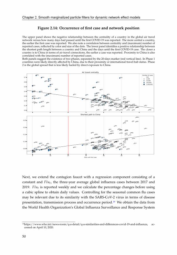
Chapter 2. Smooth marginalized particle filters for dynamic network effect models
Figure 2.14: Occurrence of first case and network position
The upper panel shows the negative relationship between the centrality of a country in the global air travel
network versus how many days had passed until the first COVID-19 was reported. The more central a country,
the earlier the first case was reported. We also note a correlation between centrality and (maximum) number of
reported cases, reflected by color and size of the dots. The lower panel identifies a positive relationship between
the shortest path length between a country and China and the days until the first COVID-19 case. The closer a
country is to China in terms of air travel connections, the earlier a case was reported. Proximity to China is also
correlated with the (maximum) number of reported cases.
Both panels suggest the existence of two phases, separated by the 20-days marker (red vertical line). In Phase 1
countries were likely directly affected by China, due to their proximity or international travel hub status. Phase
2 is the global spread that is less likely fueled by direct exposure to China.
0.0
0.1
0.2
0.3
0.4
0.5
0.6
0.7
AFG ALB
AND
ARE
ARG
ARM
AUS
AUT
AZE
BEL
BFA BGD
BGR BHR
BIH
BLR
BOL
BRA
BRN
CAN
CHE
CHL
CHN
CIV CMR
COD COG
COL
CRI
CUB
CYP
CZE
DEU
DJI
DNK
DOM
DZA
ECU
EGY
ESP
EST
ETH FIN
FRA
GAB
GBR
GEO GHA
GIN
GRC
GTM HND
HRV HUN
IDN
IND
IRL IRN
IRQ ISL
ISR
ITA
JAM
JOR JPN
KAZ
KEN
KGZ
KHM
KOR
KWT LBN
LKA LTU
LUX
LVA MAR
MDA
MDG
MEX
MKD MLI
MLT
MMR
MNE MUS
MYS
NER
NGA
NLD
NOR
NZL
OMN PAK PAN PER PHL
POL PRT
PRY
PSE
QAT
ROU
RUS
RWA
SAU
SEN
SGP
SLV
SMR SOM
SRB
SVK
SVN
SWE THA
TTO
TUN
TUR
TWN
TZA
UKR
URY
USA
UZB VEN VNM
ZAF
Air travel centralityNumber of cases
1001,00010,000100,0001,000,000
0 10 20 30 40 50 60Days until first case
0.05
0.10
0.15
0.20
0.25
KOR THA TWN JPN RUS USA CAN GBR MEX ESP FRA DEU ITA TUR UZB NLD GRC ARE MAR AUT SGP PRT BEL DZA POL IRL CHE UKR CYP TUN NOR BRA DOM IND EGY HRV KAZ MYS DNK SWE PAN CZE COL SAU QAT MLT PAK ROU FIN HUN SRB OMN ARM LKA CUB BLR AZE IRN IDN ISR LVA CRI PER ARG PHL JAM AUS SLV ETH LTU BHR KWT VNM BGR MDA BGD ZAF JOR KEN ALB LUX NZL LBN CHL VEN SEN GTM MUS IRQ GEO ECU EST ISL NGA TZA TTO MKD SVN CMR URY HND MNE AFG
SVK GHA RWA BOL CIV BIH BFA MLI KHM PRY
GIN NER DJI GAB
MDG
Shortest path to China
Next, we extend the contagion faucet with a regression component consisting of a
constant and �;DC , the three-year average global influenza cases between 2017 and
2019. �;DC is reported weekly and we calculate the percentage changes before using
a cubic spline to obtain daily values. Controlling for the seasonal common flu cases
may be relevant due to its similarity with the SARS-CoV-2 virus in terms of disease
presentation, transmission process and occurrence period.19 We obtain the data from
the World Health Organization’s Global Influenza Surveillance and Response System
19https://www.who.int/news-room/q-a-detail/q-a-similarities-and-differences-covid-19-and-influenza, ac-
cessed on April 10, 2020.
50
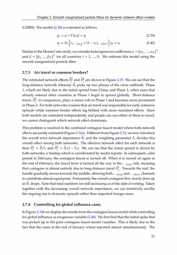
Chapter 2. Smooth marginalized particle filters for dynamic network effect models
(GISRS). The model (2.38) is extended as follows
HC = + �;DC� + �C (2.39)
�C = �C[�C,;>=6 + (1 − �C ),Bℎ>AC
]�C + 4C (2.40)
Similar to theMonteCarlo study,we considerheterogeneous coefficients = [ 1, ..., # ]>
and � = [�1, ..., �# ]> for all countries 8 = 1, ..., # . We estimate this model using the
smooth marginalized particle filter.
2.7.3 Air travel or common borders?
The estimated network effects �1
Cand �2
Care shown in Figure 2.15. We can see that the
long-distance network intensity �C picks up two phases of the virus outbreak: Phase
1, which are likely due to the initial spread from China, and Phase 2, when cases that
already entered other countries in Phase 1 begin to spread globally. Short-distance
travel, �2
C, in comparison, plays a minor role in Phase 1 and becomes more prominent
in Phase 2. For both networks it seems that air travel was responsible for early, intensive
spreads while common border effects lag behind with more sustained effects. Since
both models are estimated independently and people can use either of them to travel,
we cannot distinguish which network effect dominates.
This problem is resolved in the combined contagion faucet model where both network
effects are jointly estimated (Figure 2.16a). Different fromFigure 2.15, wenow introduce
the overall error network importance �C and the weighting parameter �C divides this
overall effect among both networks. The effective network effect for each network is
then �1
C= �C �C and �2
C= �C (1 − �C ). We can see that the initial spread is driven by
both networks, a finding which is corroborated by media reports. In subsequent, calm
period in February, the contagion faucet is turned off. When it is turned on again at
the end of February, the faucet lever is turned all the way to the,;>=6 side, meaning
that contagion is almost entirely due to long-distance travel �1
C. Towards the end, the
handle gradually moves towards the middle, allowing both,;>=6 and,Bℎ>AC channels
to contribute almost equal parts. Fortunately, the overall contagion flow slowly dries up
as �C drops. Note that total numbers are still increasing as of the date of writing. Taken
together with the decreasing overall network importance, we can tentatively ascribe
the ongoing rise to domestic spreads rather than imported foreign cases.
2.7.4 Controlling for global influenza cases
In Figure 2.16bwedisplay the results from the contagion faucetmodelwhile controlling
for global influenza as exogenous variable (2.40). We first find that the initial spike that
was picked up in the pure contagion faucet model vanishes. This is likely due to the
fact that the cases at the end of January where reported almost simultaenously. The
51

Chapter 2. Smooth marginalized particle filters for dynamic network effect models
results show that this inital, common occurrence is better captured by the observed
common factor �;DC . The second phase starting towards the end of February remains
clearly visible. The overall contagion flow is slightly lower than in the pure contagion
faucet and diminishes faster. After controlling for historical influenza cases, the overall
hump shape remains the same and the relative importances between air travel and
common borders strongly favors the former. The final peak in earlyApril also vanished.
Afterwards, it appears that the world has entered a Phase 3 where the staggering
numbers are not driven by international travel, but by domestic contagion. Table 2.8
shows the regression coefficients estimated for the constant and �;DC .
Summary
The main shortcoming lies in the COVID-19 data, which does not accurately reflect,
the long incubation period and changes in reporting standards. Furthermore, the air
travel network is assumed to be static. While a more frequently updated network is
desirable, having a network that immediately reacts to COVID-19 patterns introduces
endogeneity problems. Lastly, we have only controlled for global historical influenza
cases. Other socioeconomic control variables should be considered in future work.
52

Chapter 2. Smooth marginalized particle filters for dynamic network effect models
Figure 2.15: Spread ofCOVID-19 cases through airtravel or commonborders
We present the estimated �C for the models in (2.37). We find that the initial spike in Phase 1 is explained
by airtravel, �1(Air travel network,,;>=6 ), as well as the global spread during Phase 2. In contrast, common
borders (�2) only gain in importance in Phase 2 but their effect is more sustained until the end of the observation
period. Note that both network models are estimated independently from each other. The red line roughly
distinguishes between Phase 1 and 2 (see Figure 2.14).
(a) Single network: Air travel
(b) Single network: Common border
2.8 Conclusion
We proposed the dynamic network effects (DNE) model and put forward the smooth
marginalized particle filter (SMPF) as an appropriate estimation method. The DNE
model incorporates cross-sectional network spillovers, the intensity of which are cap-
tured by a vector of latent time-varyingparameters. Similarly to dynamic factormodels,
DNE models allow us to decompose panel data into a constant cross-sectional com-
ponent, informed by the networks, and a lower-dimensional time-varying component.
Different from the extracted factors from a dynamic factor model, the interpretation of
estimated network effects is always unambiguous as it is derived from the associated
53
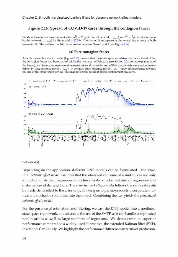
Chapter 2. Smooth marginalized particle filters for dynamic network effect models
Figure 2.16: Spread of COVID-19 cases through the contagion faucet
We show the effective error network effects �1
C = �C�C (Air travel network,,;>=6 ) and �2
C = �C (1− �C ) (Common
border network, ,Bℎ>AC ) for the model in (2.38). The dashed lines represents the overall importance of both
networks, �C . The red line roughly distinguishes between Phase 1 and 2 (see Figure 2.14).
(a) Pure contagion faucet
As with the single network model (Figure 2.15) it seems that the initial spike was driven by the air travel. After
the contagion faucet had been turned off for the most part of Feburary (see Section 2.2.4 for an explanation of
the faucet), we observe stronger overall network effects �C since the end of February, which was predominately
driven by long-distance travel (,;>=6 ). In contrast, short-distance travel (,Bℎ>AC ) grew in importance towards
the end of the observation period. This may reflect the result of global containment measures.
network(s).
Depending on the application, different DNE models can be formulated. The struc-tural network effect model assumes that the observed outcome of a unit this is not only
a function of its own regressors and idiosyncratic shocks, but also of regressors and
disturbances of its neighbors. The error network effects model follows the same rationale
but restricts its effect to the error only, allowing us to parsimoniously incorporate mul-
tivariate stochastic volatilities into the model. Combining the two yields the generalizednetwork effects model.
For the purpose of estimation and filtering, we cast the DNE model into a nonlinear
state-space framework, and advocate the use of the SMPF, as it can handle complicated
nonlinearities as well as large numbers of regressors. We demonstrate its superior
performance compared to a widely-used alternative, the extended Kalman filter (EKF),
in aMonteCarlo study. Wehighlight theperformancedifferences in termsofprediction,
54
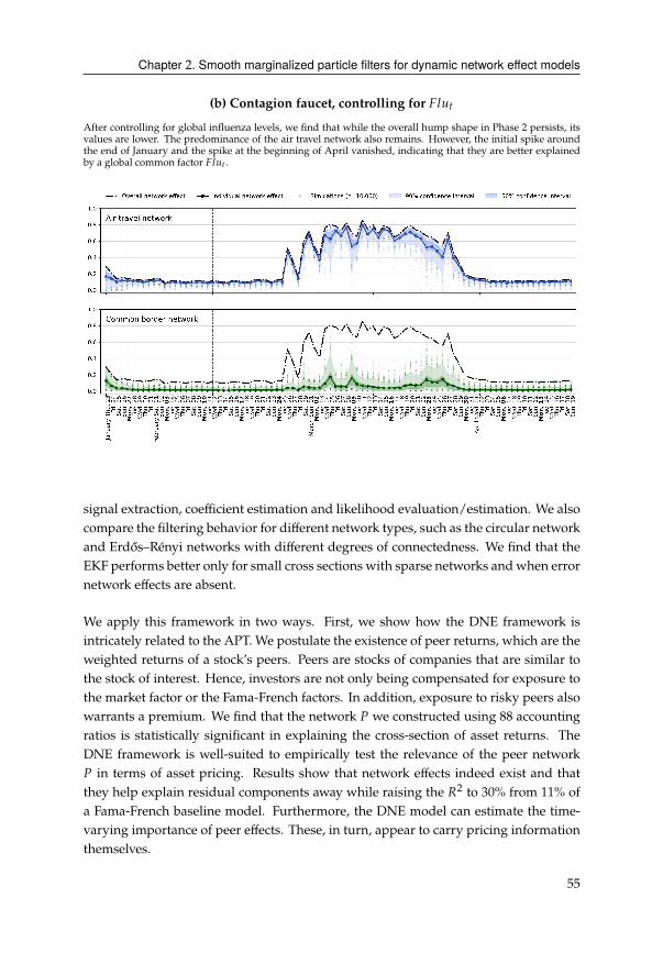
Chapter 2. Smooth marginalized particle filters for dynamic network effect models
(b) Contagion faucet, controlling for �;DCAfter controlling for global influenza levels, we find that while the overall hump shape in Phase 2 persists, its
values are lower. The predominance of the air travel network also remains. However, the initial spike around
the end of January and the spike at the beginning of April vanished, indicating that they are better explained
by a global common factor �;DC .
signal extraction, coefficient estimation and likelihood evaluation/estimation. We also
compare the filtering behavior for different network types, such as the circular network
and Erdős–Rényi networks with different degrees of connectedness. We find that the
EKF performs better only for small cross sections with sparse networks andwhen error
network effects are absent.
We apply this framework in two ways. First, we show how the DNE framework is
intricately related to the APT. We postulate the existence of peer returns, which are the
weighted returns of a stock’s peers. Peers are stocks of companies that are similar to
the stock of interest. Hence, investors are not only being compensated for exposure to
the market factor or the Fama-French factors. In addition, exposure to risky peers also
warrants a premium. We find that the network % we constructed using 88 accounting
ratios is statistically significant in explaining the cross-section of asset returns. The
DNE framework is well-suited to empirically test the relevance of the peer network
% in terms of asset pricing. Results show that network effects indeed exist and that
they help explain residual components away while raising the '2to 30% from 11% of
a Fama-French baseline model. Furthermore, the DNE model can estimate the time-
varying importance of peer effects. These, in turn, appear to carry pricing information
themselves.
55

Chapter 2. Smooth marginalized particle filters for dynamic network effect models
In a second application, we apply the DNE framework to model the contagion process
of the current COVID-19 outbreak. In this case, the model features a “contagion
faucet” that measures overall contagion flow between 128 countries through either
long-distance travel, proxied by commercial air travel routes, or short-distance travel,
proxied by a network of common borders. We find that the pandemic has spread
around the globe in two phases, at first primarily through air travel, and later through
shorter-distance travel between neighboring countries. As of the time of writing the
overall importance of networks has abated, in particular that of air travel. However,
the number of cases is still rising exponentially. This leads us to conclude that we
have a new phase where the growth of infection numbers seems to be primarily due to
domestic contagion. This is definitely an interesting subject of further research.
56
Appendix
2.A Illustrative simulation
We illustrate the performance of different candidate filters in terms of signal extraction
and regression coefficient estimation. The simulation study is set up as follows. We
simulate from a generalized DNEmodel with a regression component 8 +-8C�8 and a
circular network,� . We simulate ) = 200 periods and a cross-section of # = 50. The
measurement error variance is set to �2 = 1 for all 8. The state equation for G1
C= 6−1()C )
has no intercept, i.e., 21= 0, the autocorrelation coefficient is �
1= 0.8 and the state
variance is set to Ω1= 0.5. The state equation for G2
C= 6−1(�C ) also has 2
2= 0,
autocorrelation coefficient �2= 0.4 and the state variance Ω
2= 0.7.
We first analyze the performance of the KF, EKF and the SMPF with respect to filtering
the true state GC and thereby correctly estimating the network effects )C , �C . We then
illustrate the bias introduced to the regression coefficient estimates 8 , �8 when using
a linear filter like the KF and how the EKF and SMPF remove this bias.
2.A.1 Results: Signal extraction
We compare the results of the EKF and SMPF, as the KF does not have the capacity to
handle nonlinear latent states. The EKF is able to accurately estimate the signal )C but
has no tractability for the �C signal. This is by construction of the EKF. In the spirit
of Kalman filtering, the EKF updates the state variable based on the prediction error
EC , which relies on the derivative of the measurement function �G�(GC ). However, this
derivative is zero for G2
C, since it does not play a role in �(GC ). The derivative does
play a role in the Kalman filtering steps through the prediction error variance and the
measurement error covariance Σ∗C
:= �C�C�>C �>C . In comparison, the SMPF is able
to estimate the signal )C with a lower MSE than the EKF and, most importantly, also
provides an accurate measure for the signal �C .
57

Chapter 2. Smooth marginalized particle filters for dynamic network effect models
2.A.2 Results: Regression coefficient estimation
Regression intercept 8 We see that for increasing |)C |, the KF introduces significant
biases into the individual 8 as well as their average, The EKF largely contains the bias
and is not strongly affected by varying �1values. The SMPF has the most efficient
estimates with only small individual biases.
Regression coefficient �8 A different picture emerges for the �. We see that for
increasing |)C |, the KF introduces significant biases into the individual 8 but on
average, the estimated intercept stays around zero. As before, the EKF largely contains
the bias and is not strongly affected by varying �1values. The SMPF again yields the
most efficient estimates with negligible individual biases.
58
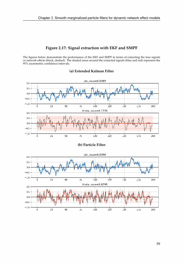
Chapter 2. Smooth marginalized particle filters for dynamic network effect models
Figure 2.17: Signal extraction with EKF and SMPF
The figures below demonstrate the performance of the EKF and SMPF in terms of extracting the true signals
or network effects (black, dashed). The shaded areas around the extracted signals (blue and red) represent the
95% asymmetric confidence intervals.
(a) Extended Kalman Filter
(b) Particle Filter
59
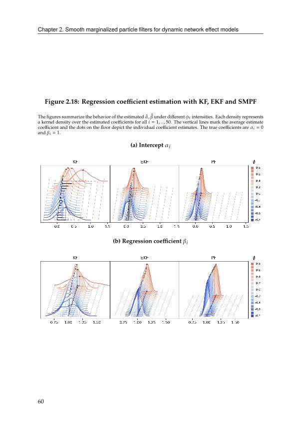
Chapter 2. Smooth marginalized particle filters for dynamic network effect models
Figure 2.18: Regression coefficient estimation with KF, EKF and SMPF
The figures summarize the behavior of the estimated , � under different )C intensities. Each density represents
a kernel density over the estimated coefficients for all 8 = 1, .., 50. The vertical lines mark the average estimate
coefficient and the dots on the floor depict the individual coefficient estimates. The true coefficients are 8 = 0
and �8 = 1.
(a) Intercept 8
(b) Regression coefficient �8
60
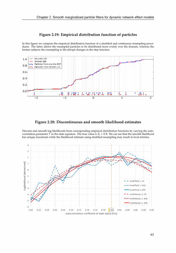
Chapter 2. Smooth marginalized particle filters for dynamic network effect models
Figure 2.19: Empirical distribution function of particles
In this figure we compare the empirical distribution function of a stratified and continuous resampling proce-
dures. The latter allows the resampled particles to be distributed more evenly over the domain, whereas the
former subjects the resampling to the abrupt changes in the step function.
Figure 2.20: Discontinuous and smooth likelihood estimates
Discrete and smooth log-likelihoods from corresponding empirical distribution functions by varying the auto-
correlation parameter ) in the state equation. The true value is )0 = 0.8. We can see that the smooth likelihood
has unique maximum while the likelihood estimate using stratified resampling may result in local minima.
61
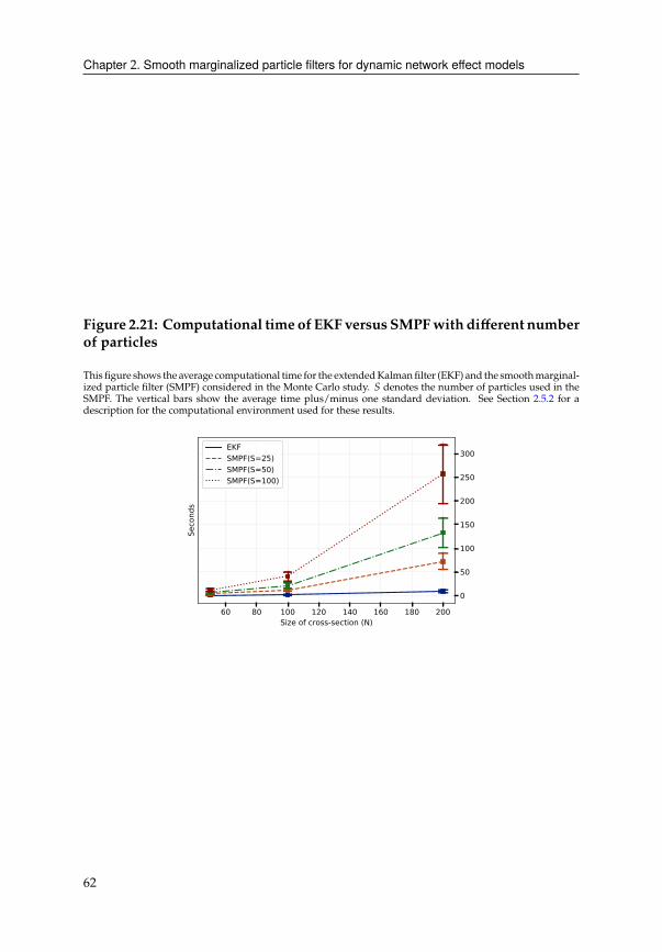
Chapter 2. Smooth marginalized particle filters for dynamic network effect models
Figure 2.21: Computational time of EKF versus SMPFwith different numberof particles
This figure shows the average computational time for the extendedKalmanfilter (EKF) and the smoothmarginal-
ized particle filter (SMPF) considered in the Monte Carlo study. ( denotes the number of particles used in the
SMPF. The vertical bars show the average time plus/minus one standard deviation. See Section 2.5.2 for a
description for the computational environment used for these results.
60 80 100 120 140 160 180 200Size of cross-section (N)
0
50
100
150
200
250
300
Seco
nds
EKFSMPF(S=25)SMPF(S=50)SMPF(S=100)
62
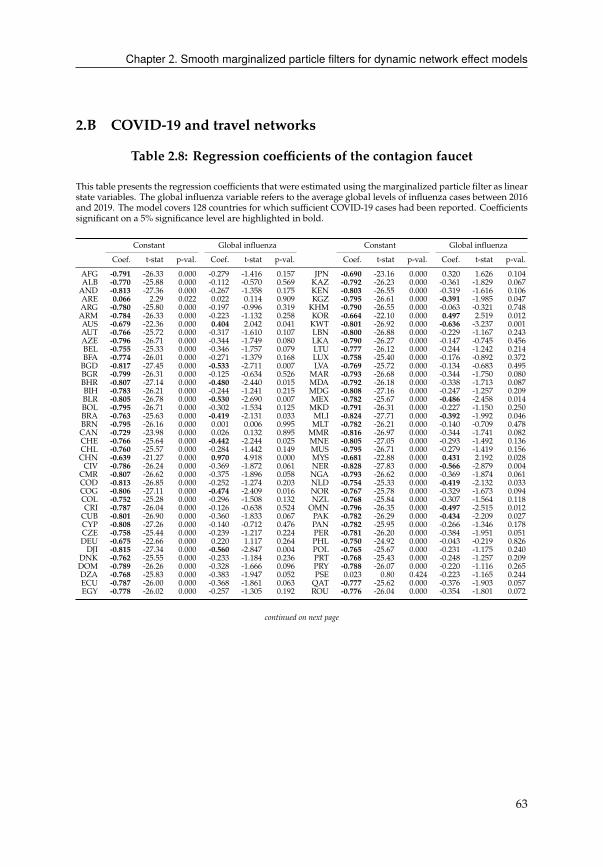
Chapter 2. Smooth marginalized particle filters for dynamic network effect models
2.B COVID-19 and travel networks
Table 2.8: Regression coefficients of the contagion faucet
This table presents the regression coefficients that were estimated using the marginalized particle filter as linear
state variables. The global influenza variable refers to the average global levels of influenza cases between 2016
and 2019. The model covers 128 countries for which sufficient COVID-19 cases had been reported. Coefficients
significant on a 5% significance level are highlighted in bold.
Constant Global influenza Constant Global influenza
Coef. t-stat p-val. Coef. t-stat p-val. Coef. t-stat p-val. Coef. t-stat p-val.
AFG -0.791 -26.33 0.000 -0.279 -1.416 0.157 JPN -0.690 -23.16 0.000 0.320 1.626 0.104
ALB -0.770 -25.88 0.000 -0.112 -0.570 0.569 KAZ -0.792 -26.23 0.000 -0.361 -1.829 0.067
AND -0.813 -27.36 0.000 -0.267 -1.358 0.175 KEN -0.803 -26.55 0.000 -0.319 -1.616 0.106
ARE 0.066 2.29 0.022 0.022 0.114 0.909 KGZ -0.795 -26.61 0.000 -0.391 -1.985 0.047
ARG -0.780 -25.80 0.000 -0.197 -0.996 0.319 KHM -0.790 -26.55 0.000 -0.063 -0.321 0.748
ARM -0.784 -26.33 0.000 -0.223 -1.132 0.258 KOR -0.664 -22.10 0.000 0.497 2.519 0.012
AUS -0.679 -22.36 0.000 0.404 2.042 0.041 KWT -0.801 -26.92 0.000 -0.636 -3.237 0.001
AUT -0.766 -25.72 0.000 -0.317 -1.610 0.107 LBN -0.800 -26.88 0.000 -0.229 -1.167 0.243
AZE -0.796 -26.71 0.000 -0.344 -1.749 0.080 LKA -0.790 -26.27 0.000 -0.147 -0.745 0.456
BEL -0.755 -25.33 0.000 -0.346 -1.757 0.079 LTU -0.777 -26.12 0.000 -0.244 -1.242 0.214
BFA -0.774 -26.01 0.000 -0.271 -1.379 0.168 LUX -0.758 -25.40 0.000 -0.176 -0.892 0.372
BGD -0.817 -27.45 0.000 -0.533 -2.711 0.007 LVA -0.769 -25.72 0.000 -0.134 -0.683 0.495
BGR -0.799 -26.31 0.000 -0.125 -0.634 0.526 MAR -0.793 -26.68 0.000 -0.344 -1.750 0.080
BHR -0.807 -27.14 0.000 -0.480 -2.440 0.015 MDA -0.792 -26.18 0.000 -0.338 -1.713 0.087
BIH -0.783 -26.21 0.000 -0.244 -1.241 0.215 MDG -0.808 -27.16 0.000 -0.247 -1.257 0.209
BLR -0.805 -26.78 0.000 -0.530 -2.690 0.007 MEX -0.782 -25.67 0.000 -0.486 -2.458 0.014
BOL -0.795 -26.71 0.000 -0.302 -1.534 0.125 MKD -0.791 -26.31 0.000 -0.227 -1.150 0.250
BRA -0.763 -25.63 0.000 -0.419 -2.131 0.033 MLI -0.824 -27.71 0.000 -0.392 -1.992 0.046
BRN -0.795 -26.16 0.000 0.001 0.006 0.995 MLT -0.782 -26.21 0.000 -0.140 -0.709 0.478
CAN -0.729 -23.98 0.000 0.026 0.132 0.895 MMR -0.816 -26.97 0.000 -0.344 -1.741 0.082
CHE -0.766 -25.64 0.000 -0.442 -2.244 0.025 MNE -0.805 -27.05 0.000 -0.293 -1.492 0.136
CHL -0.760 -25.57 0.000 -0.284 -1.442 0.149 MUS -0.795 -26.71 0.000 -0.279 -1.419 0.156
CHN -0.639 -21.27 0.000 0.970 4.918 0.000 MYS -0.681 -22.88 0.000 0.431 2.192 0.028
CIV -0.786 -26.24 0.000 -0.369 -1.872 0.061 NER -0.828 -27.83 0.000 -0.566 -2.879 0.004
CMR -0.807 -26.62 0.000 -0.375 -1.896 0.058 NGA -0.793 -26.62 0.000 -0.369 -1.874 0.061
COD -0.813 -26.85 0.000 -0.252 -1.274 0.203 NLD -0.754 -25.33 0.000 -0.419 -2.132 0.033
COG -0.806 -27.11 0.000 -0.474 -2.409 0.016 NOR -0.767 -25.78 0.000 -0.329 -1.673 0.094
COL -0.752 -25.28 0.000 -0.296 -1.508 0.132 NZL -0.768 -25.84 0.000 -0.307 -1.564 0.118
CRI -0.787 -26.04 0.000 -0.126 -0.638 0.524 OMN -0.796 -26.35 0.000 -0.497 -2.515 0.012
CUB -0.801 -26.90 0.000 -0.360 -1.833 0.067 PAK -0.782 -26.29 0.000 -0.434 -2.209 0.027
CYP -0.808 -27.26 0.000 -0.140 -0.712 0.476 PAN -0.782 -25.95 0.000 -0.266 -1.346 0.178
CZE -0.758 -25.44 0.000 -0.239 -1.217 0.224 PER -0.781 -26.20 0.000 -0.384 -1.951 0.051
DEU -0.675 -22.66 0.000 0.220 1.117 0.264 PHL -0.750 -24.92 0.000 -0.043 -0.219 0.826
DJI -0.815 -27.34 0.000 -0.560 -2.847 0.004 POL -0.765 -25.67 0.000 -0.231 -1.175 0.240
DNK -0.762 -25.55 0.000 -0.233 -1.184 0.236 PRT -0.768 -25.43 0.000 -0.248 -1.257 0.209
DOM -0.789 -26.26 0.000 -0.328 -1.666 0.096 PRY -0.788 -26.07 0.000 -0.220 -1.116 0.265
DZA -0.768 -25.83 0.000 -0.383 -1.947 0.052 PSE 0.023 0.80 0.424 -0.223 -1.165 0.244
ECU -0.787 -26.00 0.000 -0.368 -1.861 0.063 QAT -0.777 -25.62 0.000 -0.376 -1.903 0.057
EGY -0.778 -26.02 0.000 -0.257 -1.305 0.192 ROU -0.776 -26.04 0.000 -0.354 -1.801 0.072
continued on next page
63
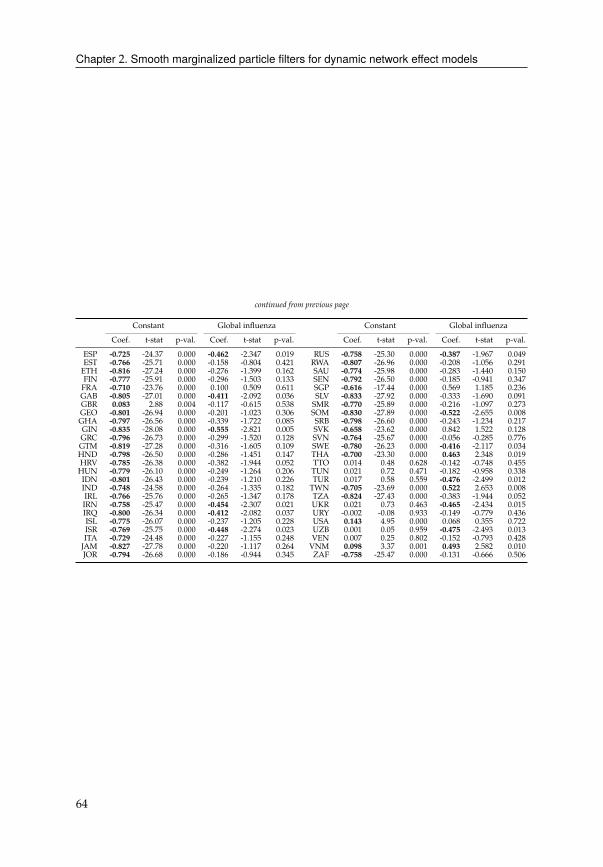
Chapter 2. Smooth marginalized particle filters for dynamic network effect models
continued from previous page
Constant Global influenza Constant Global influenza
Coef. t-stat p-val. Coef. t-stat p-val. Coef. t-stat p-val. Coef. t-stat p-val.
ESP -0.725 -24.37 0.000 -0.462 -2.347 0.019 RUS -0.758 -25.30 0.000 -0.387 -1.967 0.049
EST -0.766 -25.71 0.000 -0.158 -0.804 0.421 RWA -0.807 -26.96 0.000 -0.208 -1.056 0.291
ETH -0.816 -27.24 0.000 -0.276 -1.399 0.162 SAU -0.774 -25.98 0.000 -0.283 -1.440 0.150
FIN -0.777 -25.91 0.000 -0.296 -1.503 0.133 SEN -0.792 -26.50 0.000 -0.185 -0.941 0.347
FRA -0.710 -23.76 0.000 0.100 0.509 0.611 SGP -0.616 -17.44 0.000 0.569 1.185 0.236
GAB -0.805 -27.01 0.000 -0.411 -2.092 0.036 SLV -0.833 -27.92 0.000 -0.333 -1.690 0.091
GBR 0.083 2.88 0.004 -0.117 -0.615 0.538 SMR -0.770 -25.89 0.000 -0.216 -1.097 0.273
GEO -0.801 -26.94 0.000 -0.201 -1.023 0.306 SOM -0.830 -27.89 0.000 -0.522 -2.655 0.008
GHA -0.797 -26.56 0.000 -0.339 -1.722 0.085 SRB -0.798 -26.60 0.000 -0.243 -1.234 0.217
GIN -0.835 -28.08 0.000 -0.555 -2.821 0.005 SVK -0.658 -23.62 0.000 0.842 1.522 0.128
GRC -0.796 -26.73 0.000 -0.299 -1.520 0.128 SVN -0.764 -25.67 0.000 -0.056 -0.285 0.776
GTM -0.819 -27.28 0.000 -0.316 -1.605 0.109 SWE -0.780 -26.23 0.000 -0.416 -2.117 0.034
HND -0.798 -26.50 0.000 -0.286 -1.451 0.147 THA -0.700 -23.30 0.000 0.463 2.348 0.019
HRV -0.785 -26.38 0.000 -0.382 -1.944 0.052 TTO 0.014 0.48 0.628 -0.142 -0.748 0.455
HUN -0.779 -26.10 0.000 -0.249 -1.264 0.206 TUN 0.021 0.72 0.471 -0.182 -0.958 0.338
IDN -0.801 -26.43 0.000 -0.239 -1.210 0.226 TUR 0.017 0.58 0.559 -0.476 -2.499 0.012
IND -0.748 -24.58 0.000 -0.264 -1.335 0.182 TWN -0.705 -23.69 0.000 0.522 2.653 0.008
IRL -0.766 -25.76 0.000 -0.265 -1.347 0.178 TZA -0.824 -27.43 0.000 -0.383 -1.944 0.052
IRN -0.758 -25.47 0.000 -0.454 -2.307 0.021 UKR 0.021 0.73 0.463 -0.465 -2.434 0.015
IRQ -0.800 -26.34 0.000 -0.412 -2.082 0.037 URY -0.002 -0.08 0.933 -0.149 -0.779 0.436
ISL -0.775 -26.07 0.000 -0.237 -1.205 0.228 USA 0.143 4.95 0.000 0.068 0.355 0.722
ISR -0.769 -25.75 0.000 -0.448 -2.274 0.023 UZB 0.001 0.05 0.959 -0.475 -2.493 0.013
ITA -0.729 -24.48 0.000 -0.227 -1.155 0.248 VEN 0.007 0.25 0.802 -0.152 -0.793 0.428
JAM -0.827 -27.78 0.000 -0.220 -1.117 0.264 VNM 0.098 3.37 0.001 0.493 2.582 0.010
JOR -0.794 -26.68 0.000 -0.186 -0.944 0.345 ZAF -0.758 -25.47 0.000 -0.131 -0.666 0.506
64
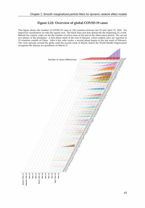
Chapter 2. Smooth marginalized particle filters for dynamic network effect models
Figure 2.22: Overview of global COVID-19 cases
This figure shows the number of COVID-19 cases in 128 countries between Jan 22 and April 19, 2020. For
improved visualization we take the square root. The black lines and dots demarcate the beginning of a week.
Behind the country codes we list the number of active cases at the end of the observation period. We can see
two phases of the pandemic: A first phase starts at the end of January, where earliest cases are reported in
33 countries outside of China. After a few calm weeks, a second phase begins in the last week of February.
The virus spreads around the globe until the second week of March, before the World Health Organization
recognizes the disease as a pandemic on March 11.
MMR, 111 MLI, 224 NER, 648 MDG, 121 SLV, 201 DJI, 846 KGZ, 554 MUS, 328 MNE, 308 SOM, 164 TZA, 170 COG, 143 UZB, 1565 URY, 517 GHA, 1042 VEN, 256 GAB, 109 TTO, 114 RWA, 147 GTM, 257 KEN, 270 GIN, 579 KAZ, 1676 ETH, 108 CUB, 1035 HND, 472 CIV, 847 JAM, 173 TUR, 86306 BOL, 520 COD, 327 PAN, 4273 BFA, 576 BRN, 138 ALB, 562 CYP, 767 BGR, 894 BGD, 2456 MDA, 2472 PRY, 206 MLT, 427 CRI, 660 SRB, 6318 CMR, 1017 PER, 15628 SVK, 1161 COL, 3792 SVN, 1330 BIH, 1285 ZAF, 3158 PSE, 437 TUN, 879 HUN, 1916 POL, 9287 JOR, 417 UKR, 5449 ARG, 2839 CHL, 10088 SAU, 9362 IDN, 6575 AND, 713 LVA, 727 PRT, 20206 SEN, 367 MAR, 2855 ECU, 9468 ARM, 1291 CZE, 6746 AZE, 1398 DOM, 4680 QAT, 5448 LUX, 3550 IRL, 15251 MEX, 7497 BLR, 4779 NGA, 627 NZL, 1431 LTU, 1298 ISL, 1771 DNK, 7580 EST, 1528 SMR, 461 NLD, 32838 NOR, 7078 ROU, 8746 PAK, 8348 BRA, 38654 GEO, 394 GRC, 2235 MKD, 1207 DZA, 2629 HRV, 1871 AUT, 14749 CHE, 27740 AFG, 996 OMN, 1266 KWT, 1915 IRQ, 1539 BHR, 1881 LBN, 673 ISR, 13491 IRN, 82211 EGY, 3144 BEL, 38496 ESP, 198674 GBR, 121172 SWE, 14385 RUS, 42853 ITA, 178972 IND, 17615 PHL, 6259 ARE, 6781 FIN, 3783 LKA, 271 DEU, 145184 KHM, 122 AUS, 6547 CAN, 35632 MYS, 5389 FRA, 154097 VNM, 268 SGP, 6588 KOR, 10661 JPN, 10797 TWN, 420 THA, 2765 CHN, 83805 USA, 759086Number of cases (differences)
- - - - - Ja
nuar
y | M
on, 2
7 - - - - - -
Febr
uary
| M
on, 0
3 - - - - - -
Mon
, 10
- - - - - - M
on, 1
7 - - - - - -
Mon
, 24
- - - - - - M
arch
| M
on, 0
2 - - - - - -
Mon
, 09
- - - - - - M
on, 1
6 - - - - - -
Mon
, 23
- - - - - - M
on, 3
0 - - - - - -
Apri
l | M
on, 0
6 - - - - - -
Mon
, 13
- - - - - -
65
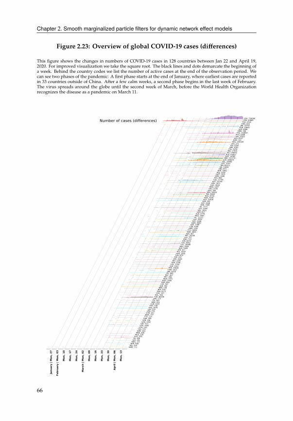
Chapter 2. Smooth marginalized particle filters for dynamic network effect models
Figure 2.23: Overview of global COVID-19 cases (differences)
This figure shows the changes in numbers of COVID-19 cases in 128 countries between Jan 22 and April 19,
2020. For improved visualization we take the square root. The black lines and dots demarcate the beginning of
a week. Behind the country codes we list the number of active cases at the end of the observation period. We
can see two phases of the pandemic: A first phase starts at the end of January, where earliest cases are reported
in 33 countries outside of China. After a few calm weeks, a second phase begins in the last week of February.
The virus spreads around the globe until the second week of March, before the World Health Organization
recognizes the disease as a pandemic on March 11.
MMR, 111 MLI, 224 NER, 648 MDG, 121 SLV, 201 DJI, 846 KGZ, 554 MUS, 328 MNE, 308 SOM, 164 TZA, 170 COG, 143 UZB, 1565 URY, 517 GHA, 1042 VEN, 256 GAB, 109 TTO, 114 RWA, 147 GTM, 257 KEN, 270 GIN, 579 KAZ, 1676 ETH, 108 CUB, 1035 HND, 472 CIV, 847 JAM, 173 TUR, 86306 BOL, 520 COD, 327 PAN, 4273 BFA, 576 BRN, 138 ALB, 562 CYP, 767 BGR, 894 BGD, 2456 MDA, 2472 PRY, 206 MLT, 427 CRI, 660 SRB, 6318 CMR, 1017 PER, 15628 SVK, 1161 COL, 3792 SVN, 1330 BIH, 1285 ZAF, 3158 PSE, 437 TUN, 879 HUN, 1916 POL, 9287 JOR, 417 UKR, 5449 ARG, 2839 CHL, 10088 SAU, 9362 IDN, 6575 AND, 713 LVA, 727 PRT, 20206 SEN, 367 MAR, 2855 ECU, 9468 ARM, 1291 CZE, 6746 AZE, 1398 DOM, 4680 QAT, 5448 LUX, 3550 IRL, 15251 MEX, 7497 BLR, 4779 NGA, 627 NZL, 1431 LTU, 1298 ISL, 1771 DNK, 7580 EST, 1528 SMR, 461 NLD, 32838 NOR, 7078 ROU, 8746 PAK, 8348 BRA, 38654 GEO, 394 GRC, 2235 MKD, 1207 DZA, 2629 HRV, 1871 AUT, 14749 CHE, 27740 AFG, 996 OMN, 1266 KWT, 1915 IRQ, 1539 BHR, 1881 LBN, 673 ISR, 13491 IRN, 82211 EGY, 3144 BEL, 38496 ESP, 198674 GBR, 121172 SWE, 14385 RUS, 42853 ITA, 178972 IND, 17615 PHL, 6259 ARE, 6781 FIN, 3783 LKA, 271 DEU, 145184 KHM, 122 AUS, 6547 CAN, 35632 MYS, 5389 FRA, 154097 VNM, 268 SGP, 6588 KOR, 10661 JPN, 10797 TWN, 420 THA, 2765 CHN, 83805 USA, 759086Number of cases (differences)
- - - - - Ja
nuar
y | M
on, 2
7 - - - - - -
Febr
uary
| M
on, 0
3 - - - - - -
Mon
, 10
- - - - - - M
on, 1
7 - - - - - -
Mon
, 24
- - - - - - M
arch
| M
on, 0
2 - - - - - -
Mon
, 09
- - - - - - M
on, 1
6 - - - - - -
Mon
, 23
- - - - - - M
on, 3
0 - - - - - -
Apri
l | M
on, 0
6 - - - - - -
Mon
, 13
- - - - - -
66

Chapter 2. Smooth marginalized particle filters for dynamic network effect models
2.C Asset pricing with peer networks
Marginal effects for fundamental factors
The estimated coefficients of the peer effects model is not directly comparable to the
coefficients of the baselinemodels. Similar to ourdistinctionbetweenpeer-adjusted and
unadjusted model errors, we also need to adjust the factor loadings correspondingly.
The factor loadings of peer effects model that are presented in the Figures and Tables
are all adjusted for peer effects. This section describes the adjustment procedure. We
rewrite (2.26) into a more detailed version and assume without loss of generality only
one factor �C
'C =
A8C...
A#C
=)
11· · · )
1#
.... . .
...
)#1· · · )##
5C�1
...
5C�#
+Φ4C (2.41)
The estimation does not yield � directly, but instead �, which is a weighted average of
other �.
A8C =
#∑9=1
)8 9 5C � 9 =
#∑9=1
)8 9 � 9
5C = �8 5C (2.42)
To retrieve �, we collect all �8 and solve the following system of linear equations
�1
= )11�
1+ · · · + )
1# �#�
2= )
21�
1+ · · · + )
2# �#...
...
�# = )#1�
1+ · · · + )## �#
or put differently,
� = Φ−1 � = (� − )%)� (2.43)
67

Chapter 2. Smooth marginalized particle filters for dynamic network effect models
Table 2.9: Firm fundamentals used in peer construction
Abbreviation Description
BOOKVEQ Book value on equity
CAPX Capital expenditure
CAPINTENSE Capital intensity
CASH Cash
CASHSTINV Cash and short-term investments
CASHFLOW Cash flow
CHEHOLD Cash holdings
CLOSEPAC Close price (end of calendar year)
CLOSEPAF Close price (end of fiscal year)
COSTCAP Cost of capital
ACT Current assets
LCT Current liabilities
DLC Debt in current liabilities
DVC Dividends (common)
DVP Dividends (preferred)
DVT Dividends (total)
EPS Earnings per share
EBIT Earnings before interest and tax
EBITDA Earnings before interest, tax, depreciation and amortization
BKVLPS Equity book value
SIZE Firm size
IB Income before extraordinary items
UXINTD Interest on long-term debt
UXINST Interest on short-term debt
LEV Leverage
LTASSET Long-term assets
LTDEBT Long-term debts
MBRATIO Market-to-book ratio
MKVALT Market value
NI Net income
PAYOUTRATIO Payout ratio
PPENT Property, plant and equipment
PRSTKC Purchase of common and preferred stocks
RDINTENSE R&D intensity
ROA Return on assets
ROE Return on equity
ROI Return on investment
SALE Sales
APC Short-term liabilities
SEQ Stockholders equity
TANG Tangibility
TOBINQ Tobin’s Q
TOTASSET Total assets
TOTEQ Total equity
TOTLIAB Total liabilities
68
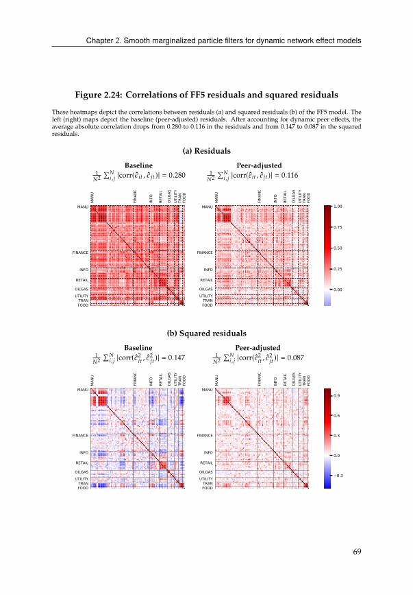
Chapter 2. Smooth marginalized particle filters for dynamic network effect models
Figure 2.24: Correlations of FF5 residuals and squared residuals
These heatmaps depict the correlations between residuals (a) and squared residuals (b) of the FF5 model. The
left (right) maps depict the baseline (peer-adjusted) residuals. After accounting for dynamic peer effects, the
average absolute correlation drops from 0.280 to 0.116 in the residuals and from 0.147 to 0.087 in the squared
residuals.
(a) Residuals
Baseline Peer-adjusted1
#2
∑#8,9 |corr(&8C , & 9C )| = 0.280
1
#2
∑#8,9 |corr(48C , 4 9C )| = 0.116
0.00
0.25
0.50
0.75
1.00MANU MAN
U
FINANCE
FIN
ANCE
INFO
INF
O
RETAIL
RET
AIL
OILGAS
OIL
GAS
UTILITY
UTI
LITY
TRAN
TRA
N
FOOD
FOO
D
MANU MAN
U
FINANCE F
INAN
CE
INFO I
NFO
RETAIL R
ETAI
LOILGAS
OIL
GAS
UTILITY U
TILI
TYTRAN
TRA
NFOOD
FOO
D
(b) Squared residuals
Baseline Peer-adjusted1
#2
∑#8,9 |corr(&2
8C, &2
9C)| = 0.147
1
#2
∑#8,9 |corr(42
8C, 42
9C)| = 0.087
0.3
0.0
0.3
0.6
0.9MANU M
ANU
FINANCE
FIN
ANCE
INFO
INF
O
RETAIL
RET
AIL
OILGAS
OIL
GAS
UTILITY
UTI
LITY
TRAN
TRA
N
FOOD
FOO
D
MANU MAN
U
FINANCE
FIN
ANCE
INFO
INF
O
RETAIL
RET
AIL
OILGAS
OIL
GAS
UTILITY
UTI
LITY
TRAN
TRA
N
FOOD
FOO
D
69

Chapter 3
Do bank business model similaritiesexplain credit risk commonalities?
3.1 Introduction
In this paper, we show that similarities between bank business models constitute an
important determinant of howmarkets value bank default risks. Given the central role
banks play in the financial system and the large costs involved in bailing out distressed
banks, accurately measuring bank riskiness is of paramount importance. There is a
rich literature estimating bank risk using, among others, publicly available accounting
information (e.g. annual accounts), ratings or confidential regulatory assessments.1
We focus on a forward looking market based indicator of banks’ default risk, namely
credit default swaps (CDS). CDS are used by market participants to adjust their credit
risk exposures. A bank’s CDS price therefore reflects its default risk as it is perceived
in the market.2
We take our cue from the empirical asset pricing literature where the credit spreads of
corporates or banks aremainlymodeled using company fundamentals and other struc-
tural determining variables, such as equity returns, the risk-free rate, market volatility,
or the slope of the yield curve. In a seminal paper by Collin-Dufresne et al. (2001)
and the subsequent empirical work of Bharath and Shumway (2008), Campbell and
Taksler (2003), Ericsson et al. (2009), and Fontana and Scheicher (2016) and B. Y. Zhang
et al. (2009) such structural models are, however, shown to have low explanatory power
and leave a systematic common factor unexplained. The lackluster performance of
variables grounded in economic theory, such as the Merton (1974) model, is commonly
1See (Petropoulos et al., 2020) and the references therein.
2CDS spreads represent a more accurate measure for credit risk than corporate bond yield spreads over a risk
free rate (Ericsson et al., 2009). Moreover, Jorion and Zhang (2007) highlight the informational advantage of
corporate CDS spreads over stock prices in studying credit contagion.
71
Chapter 3. Do bank business model similarities explain credit risk commonalities?
referred to as the credit spread puzzle. Our main contribution is an empirical framework
that suggests that for the largest European banks including information contagion into
conventional models solves part of the puzzle.
Another strand of the literature on which we build, analyzes information contagion in
bankingnetworks. Abank’s financial healthmay strongly dependon the health of other
banks as painfully demonstrated in the 2008 great financial crisis. Such interdependent
credit risks are a key topic in the financial stability literaturewith networks andfinancial
contagion occupying center stage (Glasserman & Young, 2015). This literature stresses
that banks are part of an interconnected network where risks cascade through the
system. Banks thus cannot be analyzed in isolation; rather, they must be understood in
relation to other banks.3 In their seminal contribution, Allen and Gale (2000) model the
direct lending exposure between banks wherein the lending relationships determine
relevancy. In this set-up, a bank’sdefault riskdependson thebanks it has lent todirectly.
If the borrowing banks face liquidity problems, these problems will ultimately impact
the lender. And if the lender, in turn, has borrowed money from other banks, distress
is passed on along the chain.
In contrast, when contagion is driven by fire-sales then banks with common asset
holdings become the relevant set. In the model presented by Cifuentes et al. (2005),
banks facing sudden liquidity needs sell illiquid assets to satisfy capital requirements.
The resulting downward price pressure can impact other banks with the same illiquid
asset on their books, triggering another round of asset sales, and so on. Duarte and
Eisenbach (2018) assess the vulnerability of a bank based on its share of holdings in
illiquid, systemic assets. They isolate fire-sale spillovers as the cross-sectional aspect of
aggregate vulnerability. This is consistent with the fire-sale framework of Greenwood
et al. (2015), who study the indirect vulnerability of banks following the deleveraging
of other banks.
In addition to the mechanisms discussed above, perceptions, reputations and beliefs
are key determinants of what is termed ’informational contagion’. The underlying
assumption is that signals about one bank’s financial healthmaynot only be informative
about that particular bank’s default risk; the signal may also lead to the reassessment
of other banks’ credit risk. Acharya and Yorulmazer (2008) demonstrate how, when
a systematic common factor exists in loan returns because of investments in similar
industries, bad news about one bank can be informative about the common factor and,
in turn, lead to higher borrowing costs of another bank. If the common factor is less
prevalent, then the costs can increase even more because the signal is (relatively) more
informative, incentivizing banks to hide in the herd and invest in similar industries.
3In highly interconnected financial systems, idiosyncratic shocks affecting one player’s assets may quickly spill
over to others, generating systemic risk, see, for instance, Billio et al. (2012), Demirer et al. (2018), Hautsch et al.
(2015), Betz et al. (2016) and Blasques et al. (2018).
72
Chapter 3. Do bank business model similarities explain credit risk commonalities?
This argument becomes one justification for Ahnert and Georg (2018), who also find
that bad news about one bank can be informative about another bank with common
exposures, leading to higher overall systemic risk.4
We argue that accounting for information contagion in structural credit spread models
improves our understanding of the credit risk contained in bank CDS spreads. That
is, the market’s view on a bank’s creditworthiness not only depends on its own funda-
mentals; it also depends on the creditworthiness of other banks. The common pattern
and interplay of banks’ credit risk in a turbulent period can be illustrated by the turmoil
following Deutsche Bank’s profit warnings in February 2016. Deutsche Bank reported
an unexpected net loss of EUR 2.1 billion for 2015Q4 and EUR 6.8 billion for the full
year. In the following weeks, CDS spreads of not just Deutsche Bank but also of many
other large European banks increased sharply, reflecting a growing concern of investors
over the health of European banks in general (Kiewiet et al., 2017). Since other Euro-
pean banks did not experience any structural changes during this brief period, a likely
explanation for the spread of market unrest is information contagion.
In this context, the change in a bank’s credit spread might be better explained by a
spread change of another bank, which the market deems to be similar enough to be
relevant. How relevant that other bank is, depends on how similar themarket perceives
their businesses to be. For instance, when markets price the CDS of a German savings
bank, they are more likely to factor in the spread of other German savings banks than
of, say, French investment banks. However, whenmarkets are evaluating the credit risk
of a German investment bank, the relevant set would also include investment banks
abroad. Although outsiders cannot observe a bank’s activities perfectly, there aremany
sources available to come to a realistic estimate. For example, the European Banking
Authority conducts a periodic transparency exercise releasing very detailed data on
banks’ business lines and geographic segmentation. Specialized research firms offer
bespoke sector descriptions. Thus, it is the similarity in businessmodel that determines
the potential for information spillovers which does not necessarily align with country
borders or regulatory bank type classifications.
Finally, we lean on the literature that studies bank business model similarities through
common asset holdings.Identifying bank business models and similarities therein has
been an important goal for both supervisors and academics. A study by Cernov and
Urbano (2018) highlights the importance and challenges of measuring business model
similarities for financial stability as they are crucial for assessing an institution’s riski-
4Furthermore, Slovin et al. (1999) study the externalities in the banking sector following major adverse bank
announcements. They find contagion-type effects related to the information contained in dividend reduction
announcements of money center banks. A related effect is highlighted by Morrison and White (2013) who
study reputational contagion through common regulators. The failure of a bank lowers the perceived quality
of the responsible regulator. This signal, in turn, could trigger a run on the other banks that are under the same
regulator’s umbrella.
73

Chapter 3. Do bank business model similarities explain credit risk commonalities?
ness with respect to its peers and for studying the possible impact of new regulations.
Methods to group bank business models either rely on quantitative clustering meth-
ods, such as :-nearest neighbors, or on qualitative assessments based on bank activities,
legal structures, or expert knowledge.
A bank’s business is composed ofmany different often difficult tomeasure activities. To
proxy this amalgamwe focusonasset portfolios instead. Abank’sportfolio composition
is an observable, numerical characteristic of its business model. Because they have
made similar investment, lending, or funding decisions in the past, banks that follow
similar business models usually share similar balance sheet structures (Lucas et al.,
2019; Nucera et al., 2017; Roengpitya et al., 2014; Roengpitya et al., 2017). For instance,
banks adapt their overall strategies and balance sheets to comply with new regulatory
environments (Cernov & Urbano, 2018). Similarly, the fire-sale literature studies the
implications of the link between asset holdings and business model strategies.
Most relevant to our work, Allen et al. (2012) model information contagion through
asset commonalities of banks. The portfolios of banks are the result of a network for-
mation game and the intensity of contagion is directly linked to the degree of portfolio
overlap the banks share. Coval and Stafford (2007) argue that investors following sim-
ilar strategies end up with portfolios that are concentrated in similar securities. If a
bank liquidates its assets in a fire-sale then other banks with similar asset exposures
will likely be affected. Hence, only strategy-outsiders are able to absorb these shocks
while insiders are vulnerable to each other (Shleifer & Vishny, 1992). Hence, a bank’s
misfortune is potentially relevant for another bank if their portfolios overlap. Adopt-
ing a network perspective uncovers an intricate relationship between the puzzle and
financial contagion. Taken at face value, the structural approach suggests that bank
credit risk can only be influenced by either bank-specific or system-wide common fac-
tors. Such a rigid setup is challenged by findings in the systemic risk literature, which
suggests that contagion can amplify shocks to individual banks by spreading them to
other banks. In the presence of contagion effects, it therefore comes as no surprise that
the structural model framework – which ignores contagion altogether – systematically
misprices the observed credit spreads. Once we allow the credit spread of other rele-
vant banks to inform a bank’s price as well, we find that the common factor vanishes
and the explanatory power of the structural coefficients is weakened. In other words,
the puzzle is a consequence of modeling credit risk as if it is priced only with respect
to idiosyncratic and systematic determinants.
With the purpose of modeling contagion effects in mind, we introduce a network ex-
tension to the standard model. The network’s nodes represent banks and its edges the
relevance to each other’s credit spreads. Our key assumption is that banks with similar
asset holdings likely follow similar business models and are therefore perceived to be
informative about each other. We propose an intuitive measure that establishes the
74

Chapter 3. Do bank business model similarities explain credit risk commonalities?
similarities between multiple banks. Its distinguishing feature is that it quantifies one-
to-many relationships, rather than one-to-one. More concretely, instead of measuring
the similarity of two banks in an isolated fashion, we assess their relative similarities
while considering all other banks in the system. The underlying confidential dataset
of bank holdings consists of more than 240,000 unique security identifiers, covering
holdings of around EUR 3.2 trillion (ECB, 2015). Applying our method to the com-
plete security holdings of the Eurozone’s largest banks grants us new insights into the
network structure of the European banking sector.
We start out empirical analysis by taking a structural approach without networks
and replicate the puzzle for CDS spreads of the 22 largest banks in the Eurozone. Our
results show that an extensive set of firm specific andmarket-wide are not very useful in
explaining bank risk. Surprisingly we find that, in addition to the systematic common
factor, the regression residuals also contain an uncaptured factor that distinguishes
between the Northern countries (Austria, Belgium, France, Germany and Netherlands)
and Southern countries (Italy and Spain). We then construct the network of business
model similarities based on the proposed similarity measure. Embedding it into the
structural regression reveals two novel effects: structural network effects, with one bank’s
CDS changes affecting another bank’s structural credit determinants; and error networkeffects, which allow idiosyncratic shocks to be correlated according to the network
structure. Taking these effects into account allows us to address the two stylized
facts of the credit spread puzzle. First, structural network effects increase the share
of explained variance by 13.4%, on average. Second, the residual network effects
greatly reduce the importance of the uncaptured systematic common factor including
its system-wide nature, while also removing the North-South factor. Furthermore,
most of the structural regression coefficients lose statistical and economic significance
while others, such as volatility, gain in importance. A natural extension of the constant
network is to allow network effects to be time-varying. We find, however, that most of
the estimation improvement is already achieved through including a constant network
effect. The time-varying model does help us understand the contagion mechanisms in
stress periods. Taken together, these findings indicate that neglecting network effects
likely misrepresent the relevance of structural regressors. Including network effects
improves our understanding of how risks interacts among large European banks.
The remainder of this paper is structured as follows. We first define the baseline model
and analyze the credit spread puzzle in the Eurozone. In Section 2, we construct
a measure for bank similarities. In Section 3, we derive the Network Effects (NE)
model and the Dynamic Network Effects (DNE) model as extensions to the structural
regression model. Sections 4 and 5 present the empirical results for the NE and DNE
models, respectively, before we conclude.
75
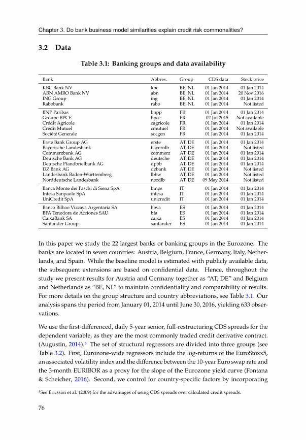
Chapter 3. Do bank business model similarities explain credit risk commonalities?
3.2 Data
Table 3.1: Banking groups and data availability
Bank Abbrev. Group CDS data Stock price
KBC Bank NV kbc BE, NL 01 Jan 2014 01 Jan 2014
ABN AMRO Bank NV abn BE, NL 01 Jan 2014 20 Nov 2016
ING Group ing BE, NL 01 Jan 2014 01 Jan 2014
Rabobank rabo BE, NL 01 Jan 2014 Not listed
BNP Paribas bnpp FR 01 Jan 2014 01 Jan 2014
Groupe BPCE bpce FR 02 Jul 2015 Not available
Crédit Agricole cagricole FR 01 Jan 2014 01 Jan 2014
Crédit Mutuel cmutuel FR 01 Jan 2014 Not available
Société Generale socgen FR 01 Jan 2014 01 Jan 2014
Erste Bank Group AG erste AT, DE 01 Jan 2014 01 Jan 2014
Bayerische Landesbank bayernlb AT, DE 01 Jan 2014 Not listed
Commerzbank AG commerz AT, DE 01 Jan 2014 01 Jan 2014
Deutsche Bank AG deutsche AT, DE 01 Jan 2014 01 Jan 2014
Deutsche Pfandbriefbank AG dpbb AT, DE 01 Jan 2014 01 Jan 2014
DZ Bank AG dzbank AT, DE 01 Jan 2014 Not listed
Landesbank Baden-Württemberg lbbw AT, DE 01 Jan 2014 Not listed
Norddeutsche Landesbank nordlb AT, DE 09 May 2014 Not listed
Banca Monte dei Paschi di Siena SpA bmps IT 01 Jan 2014 01 Jan 2014
Intesa Sanpaolo SpA intesa IT 01 Jan 2014 01 Jan 2014
UniCredit SpA unicredit IT 01 Jan 2014 01 Jan 2014
Banco Bilbao Vizcaya Argentaria SA bbva ES 01 Jan 2014 01 Jan 2014
BFA Tenedora de Acciones SAU bfa ES 01 Jan 2014 01 Jan 2014
CaixaBank SA caixa ES 01 Jan 2014 01 Jan 2014
Santander Group santander ES 01 Jan 2014 01 Jan 2014
In this paper we study the 22 largest banks or banking groups in the Eurozone. The
banks are located in seven countries: Austria, Belgium, France, Germany, Italy, Nether-
lands, and Spain. While the baseline model is estimated with publicly available data,
the subsequent extensions are based on confidential data. Hence, throughout the
study we present results for Austria and Germany together as “AT, DE” and Belgium
and Netherlands as “BE, NL” to maintain confidentiality and comparability of results.
For more details on the group structure and country abbreviations, see Table 3.1. Our
analysis spans the period from January 01, 2014 until June 30, 2016, yielding 633 obser-
vations.
We use the first-differenced, daily 5-year senior, full-restructuring CDS spreads for the
dependent variable, as they are the most commonly traded credit derivative contract.
(Augustin, 2014).5 The set of structural regressors are divided into three groups (see
Table 3.2). First, Eurozone-wide regressors include the log-returns of the EuroStoxx5,
an associated volatility index and the difference between the 10-year Euro swap rate and
the 3-month EURIBOR as a proxy for the slope of the Eurozone yield curve (Fontana
& Scheicher, 2016). Second, we control for country-specific factors by incorporating
5See Ericsson et al. (2009) for the advantages of using CDS spreads over calculated credit spreads.
76
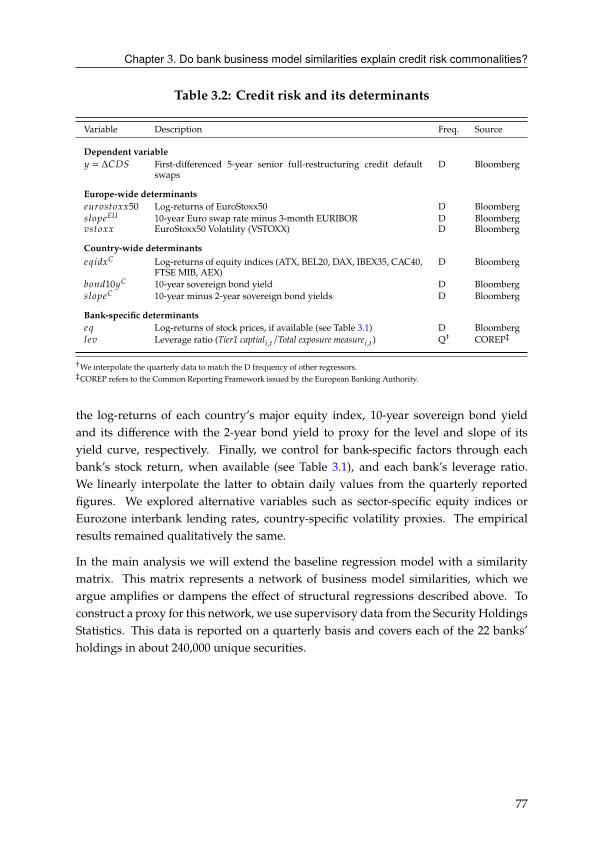
Chapter 3. Do bank business model similarities explain credit risk commonalities?
Table 3.2: Credit risk and its determinants
Variable Description Freq. Source
Dependent variableH = ��( First-differenced 5-year senior full-restructuring credit default
swaps
D Bloomberg
Europe-wide determinants4DA>BC>GG50 Log-returns of EuroStoxx50 D Bloomberg
B;>?4�* 10-year Euro swap rate minus 3-month EURIBOR D Bloomberg
EBC>GG EuroStoxx50 Volatility (VSTOXX) D Bloomberg
Country-wide determinants4@83G� Log-returns of equity indices (ATX, BEL20, DAX, IBEX35, CAC40,
FTSE MIB, AEX)
D Bloomberg
1>=310H� 10-year sovereign bond yield D Bloomberg
B;>?4� 10-year minus 2-year sovereign bond yields D Bloomberg
Bank-specific determinants4@ Log-returns of stock prices, if available (see Table 3.1) D Bloomberg
;4E Leverage ratio (Tier1 captial8 ,C/Total exposure measure8 ,C ) Q†
COREP‡
†We interpolate the quarterly data to match the D frequency of other regressors.
‡COREP refers to the Common Reporting Framework issued by the European Banking Authority.
the log-returns of each country’s major equity index, 10-year sovereign bond yield
and its difference with the 2-year bond yield to proxy for the level and slope of its
yield curve, respectively. Finally, we control for bank-specific factors through each
bank’s stock return, when available (see Table 3.1), and each bank’s leverage ratio.
We linearly interpolate the latter to obtain daily values from the quarterly reported
figures. We explored alternative variables such as sector-specific equity indices or
Eurozone interbank lending rates, country-specific volatility proxies. The empirical
results remained qualitatively the same.
In the main analysis we will extend the baseline regression model with a similarity
matrix. This matrix represents a network of business model similarities, which we
argue amplifies or dampens the effect of structural regressions described above. To
construct a proxy for this network, we use supervisory data from the Security Holdings
Statistics. This data is reported on a quarterly basis and covers each of the 22 banks’
holdings in about 240,000 unique securities.
77
Chapter 3. Do bank business model similarities explain credit risk commonalities?
3.3 The credit spread puzzle for Eurozone banks
In this section we reproduce the credit spread puzzle for banks in the Eurozone. These
results represent our baseline and set the stage for our subsequent network extension.
Our empirical strategy follows the structural approach of Collin-Dufresne2001 and
subsequent authors, who specify a reduced-form model with linear structure for CDS
spread changes. Since the puzzle was originally studied for monthly U.S. corporate
bond spreads, we use an adapted set of explanatory variables for the daily credit
spreads of European banks, as outlined in the data section.
Our baseline model stipulates that the credit spread changes are generated by the
following model
H8 ,C = �1
84DA>BC>GG50C + �2
8ΔB;>?4�*C + �3
8ΔEBC>GGC
+ �1
84@83G�C + �
2
8Δ1>=310H�C + �
3
8ΔB;>?4�C (3.1)
+ �1
84@8 ,C + �2
8;4E8 ,C + 2>=BC 8 + 48 ,C , with 48 ,C ∼ #(0, �2
8).
Note that this yields # times bank-specific regression coefficients and that the co-
variance matrix is heteroskedastic. By stacking these # equations for each bank we can
express the baseline model compactly as
HC = -C� + 4C
where HC is a # × 1 vector of CDS spread changes, -C contains the structural re-
gressors and � the # corresponding coefficients. The error component 4C follows
a multivariate normal distribution with diagonal and heteroskedastic covariance ma-
trix Σ = diag(�2
1, ..., �2
#). The empirical application also includes lagged versions of
dependent and independent variables on the right-hand side.
3.3.1 Empirical evidence
Table 3.3 presents the regression results of the linear baseline model. Due to con-
fidentiality reasons, we present the results as group averages. We also present the
anonymized regression coefficients in density plots of Figure 3.4 and the associated
?-values in the histograms of Figure 3.14 (Appendix).
For Europe-wide regressors, we find that the sign andmagnitude of the group averages
are mostly homogeneous. In line with previous research, higher equity returns and
proxy for the yield curve slope are associated with lower credit spreads while the
opposite holds for volatility indicators.6 For country-specific regressors, the group
6Note that the parentheses of Table 3.3 contain average ?-values for each group and hence cannot used directly
for the rejection of the null hypothesis.
78
Chapter 3. Do bank business model similarities explain credit risk commonalities?
averages are more heterogeneous. We discover a North-South division where Italian
and Spanish bank spreads respond similarly to their countries’ 10-year bond yields
and yield curve slopes, while the Austria, Belgium, France, Germany and Netherlands
point to the opposite direction. For the bank-specific regressors, the (lagged) equity
returns are consistently negative. The constant is insignificant for all banks. The lack
of significance for leverage is likely explained by its interpolated nature due to its low
reporting frequency.
Furthermore, we confirm the two stylized facts of the credit spread puzzle: the group
'2values range from 28.3% (Austria, Germany) to 48.5% (Italy) with an total average
of 36.5%. These values are slightly higher than what Collin-Dufresne et al. (2001)
found for U.S. corporate bonds. To determine whether this indicates a good model
performance we turn our attention to the residuals. In Figure 3.2, demonstrates that
this is not the case, sincewefinda systematic common factor across all banks. This factor
alone explains 35.63% of the residual variance, while the first four components together
makeup53.02%. Interestingly, the second component seems to capture country-specific
effects, even though the regression model already includes country-specific regressors.
Upon closer inspection, the component draws a line between Northern and Southern
Eurozonemembers. Thus, this component curiously reflects a North-South divide that
is not a feature of the country-specific regressors. Fontana and Scheicher (2016) find a
similar division for European sovereign CDS spreads.
It is worth noting that the CDS data is recorded on a daily frequency. If information
contagion takes place, particularly during stress moments as we will demonstrate in
the Deutsche Bank example (Figure 3.8, it happens within days. This is in contrast to
previous work on which consider CDS spreads over weeks or months.
Recently, several authors have argued that market microstructure frictions could also
explain residual common factors in corporate bond spread changes. Friewald and
Nagler (2019) use similar reduced form models as (3.1) and find evidence for the ex-
planatory power of inventory, search and bargaining frictions. These concerns are only
partly relevant in our analysis due to our focus on CDS contracts of banks in particular.
For instance, search frictions due to the structure of dealer networks may be less rel-
evant since European bank CDS contracts are already highly specialized. Bargaining
frictions may be a reason for co-movements CDS prices with similar underlyings. We
aim at capturing these potential commonalities through the similarity network.
3.3.2 Absence of credit contagion
These findings make intuitive sense from the perspective of credit contagion. The
linear structure of the baseline model leaves little room for contagion effects between
banks and countries. Changes in a bank’s credit risk can only be due to bank-specific,
79
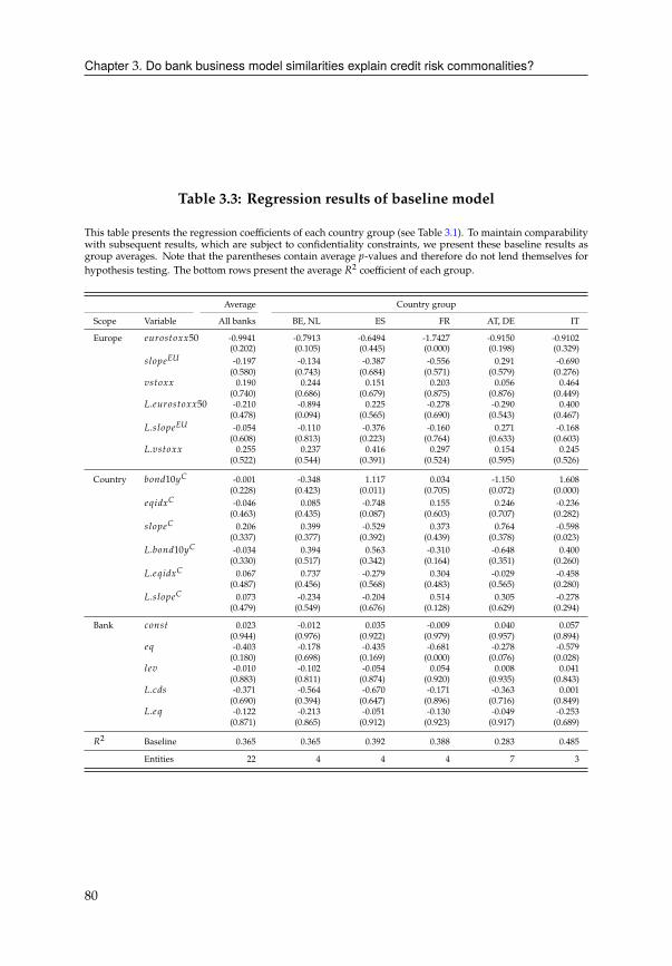
Chapter 3. Do bank business model similarities explain credit risk commonalities?
Table 3.3: Regression results of baseline model
This table presents the regression coefficients of each country group (see Table 3.1). To maintain comparability
with subsequent results, which are subject to confidentiality constraints, we present these baseline results as
group averages. Note that the parentheses contain average ?-values and therefore do not lend themselves for
hypothesis testing. The bottom rows present the average '2coefficient of each group.
Average Country group
Scope Variable All banks BE, NL ES FR AT, DE IT
Europe 4DA>BC>GG50 -0.9941 -0.7913 -0.6494 -1.7427 -0.9150 -0.9102
(0.202) (0.105) (0.445) (0.000) (0.198) (0.329)
B;>?4�* -0.197 -0.134 -0.387 -0.556 0.291 -0.690
(0.580) (0.743) (0.684) (0.571) (0.579) (0.276)
EBC>GG 0.190 0.244 0.151 0.203 0.056 0.464
(0.740) (0.686) (0.679) (0.875) (0.876) (0.449)
!.4DA>BC>GG50 -0.210 -0.894 0.225 -0.278 -0.290 0.400
(0.478) (0.094) (0.565) (0.690) (0.543) (0.467)
!.B;>?4�* -0.054 -0.110 -0.376 -0.160 0.271 -0.168
(0.608) (0.813) (0.223) (0.764) (0.633) (0.603)
!.EBC>GG 0.255 0.237 0.416 0.297 0.154 0.245
(0.522) (0.544) (0.391) (0.524) (0.595) (0.526)
Country 1>=310H� -0.001 -0.348 1.117 0.034 -1.150 1.608
(0.228) (0.423) (0.011) (0.705) (0.072) (0.000)
4@83G� -0.046 0.085 -0.748 0.155 0.246 -0.236
(0.463) (0.435) (0.087) (0.603) (0.707) (0.282)
B;>?4� 0.206 0.399 -0.529 0.373 0.764 -0.598
(0.337) (0.377) (0.392) (0.439) (0.378) (0.023)
!.1>=310H� -0.034 0.394 0.563 -0.310 -0.648 0.400
(0.330) (0.517) (0.342) (0.164) (0.351) (0.260)
!.4@83G� 0.067 0.737 -0.279 0.304 -0.029 -0.458
(0.487) (0.456) (0.568) (0.483) (0.565) (0.280)
!.B;>?4� 0.073 -0.234 -0.204 0.514 0.305 -0.278
(0.479) (0.549) (0.676) (0.128) (0.629) (0.294)
Bank 2>=BC 0.023 -0.012 0.035 -0.009 0.040 0.057
(0.944) (0.976) (0.922) (0.979) (0.957) (0.894)
4@ -0.403 -0.178 -0.435 -0.681 -0.278 -0.579
(0.180) (0.698) (0.169) (0.000) (0.076) (0.028)
;4E -0.010 -0.102 -0.054 0.054 0.008 0.041
(0.883) (0.811) (0.874) (0.920) (0.935) (0.843)
!.23B -0.371 -0.564 -0.670 -0.171 -0.363 0.001
(0.690) (0.394) (0.647) (0.896) (0.716) (0.849)
!.4@ -0.122 -0.213 -0.051 -0.130 -0.049 -0.253
(0.871) (0.865) (0.912) (0.923) (0.917) (0.689)
'2Baseline 0.365 0.365 0.392 0.388 0.283 0.485
Entities 22 4 4 4 7 3
80
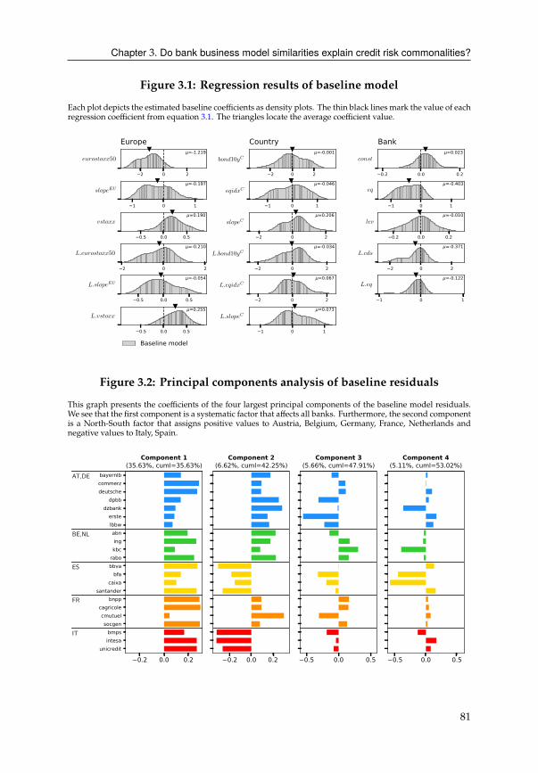
Chapter 3. Do bank business model similarities explain credit risk commonalities?
Figure 3.1: Regression results of baseline model
Each plot depicts the estimated baseline coefficients as density plots. The thin black lines mark the value of each
regression coefficient from equation 3.1. The triangles locate the average coefficient value.
2 0 2
=-1.219eurostoxx50
Europe
1 0 1
=-0.197slopeEU
0.5 0.0 0.5
=0.190vstoxx
2 0 2
=-0.210L.eurostoxx50
0.5 0.0 0.5
=-0.054L.slopeEU
0.5 0.0 0.5
=0.255L.vstoxx
2 0 2
=-0.001bond10yC
Country
1 0 1
=-0.046eqidxC
2 0 2
=0.206slopeC
2 0 2
=-0.034L.bond10yC
2 0 2
=0.067L.eqidxC
1 0 1
=0.073L.slopeC
0.2 0.0 0.2
=0.023const
Bank
1 0 1
=-0.403eq
0.2 0.0 0.2
=-0.010lev
2 0 2
=-0.371L.cds
1 0 1
=-0.122L.eq
Baseline model
Figure 3.2: Principal components analysis of baseline residuals
This graph presents the coefficients of the four largest principal components of the baseline model residuals.
We see that the first component is a systematic factor that affects all banks. Furthermore, the second component
is a North-South factor that assigns positive values to Austria, Belgium, Germany, France, Netherlands and
negative values to Italy, Spain.
0.2 0.0 0.2
bayernlbcommerzdeutsche
dpbbdzbank
erstelbbwabningkbc
rabobbva
bfacaixa
santanderbnpp
cagricolecmutuelsocgen
bmpsintesa
unicredit
AT,DE
BE,NL
ES
FR
IT
Component 1(35.63%, cuml=35.63%)
0.2 0.0 0.2
Component 2(6.62%, cuml=42.25%)
0.5 0.0 0.5
Component 3(5.66%, cuml=47.91%)
0.5 0.0 0.5
Component 4(5.11%, cuml=53.02%)
81

Chapter 3. Do bank business model similarities explain credit risk commonalities?
country-wide or Europe-wide determinants. This means, however, that commonalities
between banks within or across country borders, are left for the residuals. The North-
South factor we find belongs to this category.
The absence of contagion effects between banks also provides an explanation for the
systematic common factor. As the Collin-Dufresne2001 concluded, the systematic
factor withstands a host of explanatory variables in their “kitchen sink” approach. This
is consistent with the contagion perspective, since the additional variables still belong
to the three layers of credit determinants. In contrast, once we allow for contagion
effects, credit risk may propagate across banks and countries, which can ultimately
reach systematic proportions.
In the following sections, we propose a network extension to the structural approach.
The network reflects our assumption that banks are more likely to pass on credit risk
to institutions with similar business models. This introduces a channel for credit
contagion that lies between the three layers of structural credit spread determinants.
3.4 Network of bank similarities
The systemic risk literature has extensively studied channels of contagion, such as port-
folio overlap and common asset exposures, especially in the context of fire-sales. While
portfolio overlaps are important in our model, our main goal is to model information
contagion due to similar business model, not to capture actual fire-sales. Nonetheless,
if the market believes that a bank is vulnerable to another bank’s rapid deleveraging
efforts, then this belief would again constitute information contagion. The systemic
risk literature is therefore closely related and highly relevant. For instance, Wagener
(2010) highlights that, although portfolio diversification is desirable for individual in-
stitutions, it is dangerous on a macro level as it increases portfolio similarity among
banks and therefore exposes them to the same risks. Similarly, Caccioli et al. (2014)
study a network model with overlapping portfolios and leverage. In their model, a
system may become unstable if a critical threshold for leverage is crossed, resulting in
system-wide contagion. Cont and Schaanning (2018) use portfolio overlap to quantify
a bank’s mark-to-market losses resulting from the deleveraging decisions of another
bank. Other studies provide empirical models that can be used for stress-tests. Green-
wood et al. (2015), for example, study how banks that are seemingly unrelated can
contaminate other banks because of indirect vulnerabilities to deleveraging external-
ities. They estimate their model with balance sheet data from the European Banking
Authority. Finally, Poledna et al. (2018) propose a systemic risk measure that relies on
portfolio overlap, which they calculate using the complete security holdings of major
Mexican banks.
We develop a measure that quantifies similarities between bank business models using
82

Chapter 3. Do bank business model similarities explain credit risk commonalities?
their complete asset holdings. Themain assumption behind ourmeasure is that similar
holdings structures imply similar business models. We use the term similar in a
statistical sense and can be understood as a type of conditional correlation. Intuitively,
our measure asks howmuch the knowledge of one bank’s holdings helps in predicting
the structure of another bank’s holdings, relative to all remaining banks. To illustrate,
if the holdings structure of bank A is predictive for the holdings of bank B, ourmeasure
would assign a high degree of similarity. The highest similarity would be assigned if
the holdings of both banks are identical in terms of asset types and quantities. Next,
consider a system with three banks A,B,C. If A’s holdings structure is more predictive
for bank B’s holdings than C’s holdings are for B, we would assign a higher similarity
for A. In a more realistic setting, the measure would assign high similarity between
two German Landesbanken and low similarity between a Landesbank and a Spanish
investment bank. This reflects the notion that the holdings of one Landesbank is likely
to be much more predictive of another Landesbank’s as they follow similar business
models. In contrast, they would be less predictive of an investment bank’s holdings,
given that follow entirely different business models. Our proposed measure has three
distinct properties:
Property 1: Non-negativity. The similarity measure is either zero when banks have
no assets in common or positive if they share at least one asset. A negative similarity
has no economic interpretation.
Property 2: Relativity. The similarity measure between two banks is not absolute. It
depends on the number of other banks in the system aswell as their holding structures.
Property 3: Asymmetry. The holdings of one bank may be most similar to a second
bank of interest, relative to all other banks. However, this relationship need not be
reciprocal, as the second bank could be most similar to a third bank.
We define the similarity measure �8 , 9 between banks 8 and 9 for a systemwith # banks.
Each 10=:8 holds a vector of assets in a (-dimensional asset space. In the remainder of
this section we derive the similarity measure. We start with the similarity between two
banks and extend the concept for # banks. The 3-step algorithm and the associated
technical discussion are found in the Appendix.
83
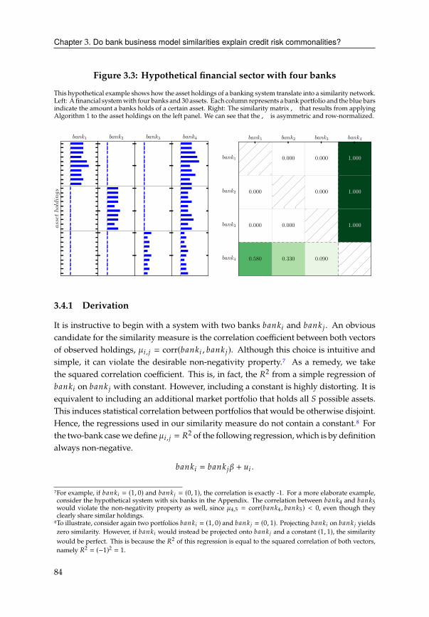
Chapter 3. Do bank business model similarities explain credit risk commonalities?
Figure 3.3: Hypothetical financial sector with four banks
This hypothetical example shows how the asset holdings of a banking system translate into a similarity network.
Left: Afinancial systemwith four banks and 30 assets. Each column represents a bankportfolio and the blue bars
indicate the amount a banks holds of a certain asset. Right: The similarity matrix, that results from applying
Algorithm 1 to the asset holdings on the left panel. We can see that the, is asymmetric and row-normalized.
assetholdings
bank1 bank2 bank3 bank4 bank1 bank2 bank3 bank4
bank1
bank2
bank3
bank4
0.000 0.000 1.000
0.000 0.000 1.000
0.000 0.000 1.000
0.580 0.330 0.090
3.4.1 Derivation
It is instructive to begin with a system with two banks 10=:8 and 10=: 9 . An obvious
candidate for the similarity measure is the correlation coefficient between both vectors
of observed holdings, �8 , 9 = corr(10=:8 , 10=: 9). Although this choice is intuitive and
simple, it can violate the desirable non-negativity property.7 As a remedy, we take
the squared correlation coefficient. This is, in fact, the '2from a simple regression of
10=:8 on 10=: 9 with constant. However, including a constant is highly distorting. It is
equivalent to including an additional market portfolio that holds all ( possible assets.
This induces statistical correlation between portfolios that would be otherwise disjoint.
Hence, the regressions used in our similarity measure do not contain a constant.8 For
the two-bank casewe define�8 , 9 = '2of the following regression, which is by definition
always non-negative.
10=:8 = 10=: 9� + D8 .
7For example, if 10=:8 = (1, 0) and 10=: 9 = (0, 1), the correlation is exactly -1. For a more elaborate example,
consider the hypothetical system with six banks in the Appendix. The correlation between 10=:4 and 10=:5
would violate the non-negativity property as well, since �4,5 = corr(10=:4 , 10=:5) < 0, even though they
clearly share similar holdings.
8To illustrate, consider again two portfolios 10=:8 = (1, 0) and 10=: 9 = (0, 1). Projecting 10=:8 on 10=: 9 yieldszero similarity. However, if 10=:8 would instead be projected onto 10=: 9 and a constant (1, 1), the similarity
would be perfect. This is because the '2of this regression is equal to the squared correlation of both vectors,
namely '2 = (−1)2 = 1.
84
Chapter 3. Do bank business model similarities explain credit risk commonalities?
In a general system with # banks, a natural extension is to calculate �8 , 9 for all 8
and 9 pairs. However, this approach results in symmetric similarity measures, that
is �8 , 9 = �9 ,8 . But symmetry is not desirable if the ultimate purpose of the measure
is to capture information contagion among banks. Moreover, it would only consider
two banks in an isolated fashion from all other banks. To illustrate, consider the
hypothetical system with four banks in Figure 3.3, left panel. We abstract from the
effects of exogenous credit spread determinants. If we observe a drop of 10=:1’s credit
spread, then this drop can only be due to information spillover from 10=:4. At the
same time, if we observe a deterioration of 10=:4’s creditworthiness, this information
spillover can be partly ascribed to each of the other three banks. Symmetry would
imply that both cases are informationally equivalent, which is not the case. For a more
concrete example for why symmetry is undesirable, recall that perceived vulnerability
to fire-sales also constitutes a type of information contagion. Clearly, 10=:4is most
central as its portfolio shares common assets with all other bankswhile the other banks’
portfolios only hold partitions of 10=:4. If 10=:
4suddenly needs to raise money, it
could be a knock-on effect from either of the other banks liquidating their assets in a
fire-sale. Conversely, if one of the other banks has to liquidate its assets, this portfolio
adjustment can only be due to deleveraging efforts of 10=:4. Asymmetry is therefore a
crucial property of the similarity measure and differs from other proposed measures,
such as Cont and Schaanning (2018) for portfolio overlaps.
Returning to the derivation, the coefficient of determination serves as a useful starting
point for constructing such an asymmetric measure. Similar to the two-bank situation,
we can calculate the '2
8from a multiple regression of each 10=:8 on all remaining
banks,
10=:8 =∑9≠8
10=: 9� 9 + D8 .
This coefficient '2
8measures how well 10=:8 ’s portfolio is jointly explained by the
portfolios of all other banks. Since we are interested in the individual contributions
of the banks on the right-hand side, we decompose the '2
8into # − 1 separate partial-
'2
8 , 9.9 These coefficients reflect the relative importance of 10=: 9 in explaining 10=:8 ,
compared to 10=:8 ’s peers. Denoting the decomposition function with 3, we have
3('2
8) := ['2
8 ,1, ..., '2
8 , 9, ..., '2
8 ,#]. Note that we define a bank’s similarity with itself as
zero, '2
8 ,8= 0. These partial-'2
capture the essence of our similarity measure. They
are, by construction, non-negative; allow the similarity measure to be asymmetric; and
depend onwhich banks and assets are considered in their calculation.10 To compute the
9This notion is conceptually related to the variance inflation factor used in regression analysis to detect multi-
collinearities between explanatory variables.
10While '2decomposition is not a trivial task, the statistical literature on relative importance and variable
selection has proposed several methods for it. We refer the reader to the Appendix for the 3-step algorithm
and accompanying technical discussion of our similarity measure.
85
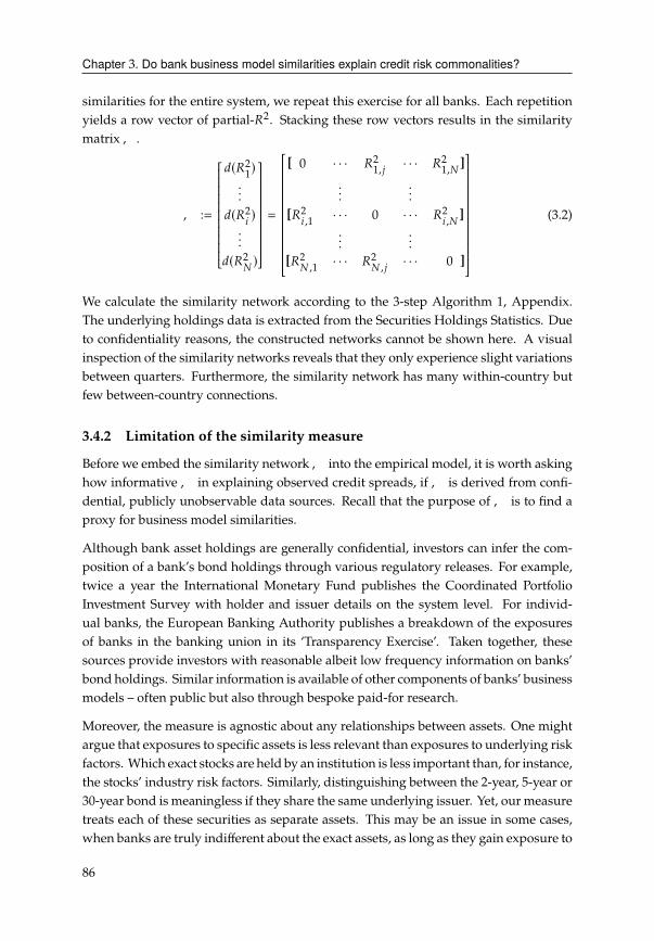
Chapter 3. Do bank business model similarities explain credit risk commonalities?
similarities for the entire system, we repeat this exercise for all banks. Each repetition
yields a row vector of partial-'2. Stacking these row vectors results in the similarity
matrix, .
, :=
3('2
1)
...
3('2
8)
...
3('2
#)
=
[ 0 · · · '2
1, 9· · · '2
1,#]
......
['2
8 ,1· · · 0 · · · '2
8 ,#]
......
['2
#,1· · · '2
#,9· · · 0 ]
(3.2)
We calculate the similarity network according to the 3-step Algorithm 1, Appendix.
The underlying holdings data is extracted from the Securities Holdings Statistics. Due
to confidentiality reasons, the constructed networks cannot be shown here. A visual
inspection of the similarity networks reveals that they only experience slight variations
between quarters. Furthermore, the similarity network has many within-country but
few between-country connections.
3.4.2 Limitation of the similarity measure
Before we embed the similarity network, into the empirical model, it is worth asking
how informative, in explaining observed credit spreads, if, is derived from confi-
dential, publicly unobservable data sources. Recall that the purpose of, is to find a
proxy for business model similarities.
Although bank asset holdings are generally confidential, investors can infer the com-
position of a bank’s bond holdings through various regulatory releases. For example,
twice a year the International Monetary Fund publishes the Coordinated Portfolio
Investment Survey with holder and issuer details on the system level. For individ-
ual banks, the European Banking Authority publishes a breakdown of the exposures
of banks in the banking union in its ‘Transparency Exercise’. Taken together, these
sources provide investors with reasonable albeit low frequency information on banks’
bond holdings. Similar information is available of other components of banks’ business
models – often public but also through bespoke paid-for research.
Moreover, the measure is agnostic about any relationships between assets. One might
argue that exposures to specific assets is less relevant than exposures to underlying risk
factors. Which exact stocks are held by an institution is less important than, for instance,
the stocks’ industry risk factors. Similarly, distinguishing between the 2-year, 5-year or
30-year bond is meaningless if they share the same underlying issuer. Yet, our measure
treats each of these securities as separate assets. This may be an issue in some cases,
when banks are truly indifferent about the exact assets, as long as they gain exposure to
86
Chapter 3. Do bank business model similarities explain credit risk commonalities?
a particular risk factor. However, we argue that banks reveal their preferences through
their holdings. Thus, a bond with a 2-year maturity may be more appropriate than a
5-year bond of the same issuer, depending on the institution’s exposure to interest rate
risk. In such a case, the 2-year bond is a conscious decision that reflects some aspect of
the bank’s business model.
A similar case can be made when dealing with derivatives. Consider a bank that holds
a certain stock. Then, consider another bank that holds a call option on that stock.
Our measure would once again treat them as completely separate assets. One might
argue that their intricate relationship would warrant a different treatment. However,
we argue that even though the underlying stock is identical, the bank that prefers the
right to an ownership position rather than the ownership itself may follow a different
investment or risk-management strategy than a bank that directly holds the stock.
If the above concerns are true, then our measure would underestimate the similarity
between institutions, compared to a measure that groups assets by risk factors or is-
suers. Consequently, a sparser similarity networkwould also lead tomore conservative
estimates of the network intensities.
3.5 Analytical framework
Now that we have established an empirical measure of the underlying similarity net-
work, we return to the original task of finding a potential answer to the credit spread
puzzle. Our econometric model extends the structural regression model of Collin-
Dufresne et al. (2001) with network effects. The main difference is that we do not only
regress a bank’s CDS changes on structural variables; we also regress on a weighted
average of CDS changes of all other banks in the system. The weights correspond to
the similarity a bank shares with all other banks, as derived in the previous section. A
scalar parameter determines the importance of these added network effects. We inter-
pret this parameter as network intensity. If the intensity is zero, the model reverts back
to the structural regression model where banks are independent. Otherwise, informa-
tion contagion takes place and CDS prices become functions of one another, depending
on their similarities. This functional dependency holds for all CDS contracts, such that
information can spillover from bank to bank. To ensure that this spillover process con-
verges, we assume that its effect attenuates with each round. The speed of convergence
is determined by the network intensity parameters.
We model these rounds as successive linear transformations with the similarity net-
work, .11 This iterative nature imitates the learning or price discovery process studied
11This transformation matrix can be understood in the same manner as the -output matrix from the Leontief
model. Instead of sectors producing goods by combining goods from other sectors, our outputs are CDS prices
resulting from the weighted combinations of other CDS prices.
87

Chapter 3. Do bank business model similarities explain credit risk commonalities?
in the financial literature, where traders act under bounded rationality and imperfect
knowledge. Most relevant to our work, Routledge (1999) shows how information dif-
fusion based on adaptive or evolutionary learning across multiple periods can lead
to a Grossman and Stiglitz (1980) type rational equilibrium. The success of this pro-
cess crucially relies on the monotonic selection dynamic, where traders imitate better
strategies more frequently than bad ones. Viewing the financial market as a complex
system, Hommes (2008) studies bounded rational traders that improve their strategies
either with adaptive learning or evolutionary selection. Using a simple cobweb model,
he shows that the market price can converge to the rational expectations equilibrium
in both cases.
In this section, we construct a framework that embeds the network, into established
credit spread models. While the baseline model (3.1) analyzes the credit spread of
each bank individually, the network approach takes a holistic view of the system. In
other words, the CDS spreads of the banks are priced jointly. We therefore stack the #
equations and collect all regressors into one regressor matrix:
HC = -C� + 4C with 4C ∼ #(0,Σ). (3.3)
In linewith the definition of the baselinemodel (3.1), the error terms are heteroskedastic
with Σ = diag(�2
1, ..., �2
#). We first introduce extensions with constant network effects
and later on, introduce time-variation in these effects.
3.5.1 Network effects model
We distinguish between two types of network effects, namely structural network effectsand error network effects. Correspondingly, we embed the same network , into the
baseline model (3.1) in two ways.12
Structural network effects13 refer to changes in one bank’s credit risk that are due to
changes in a neighboring bank’s credit risk. To incorporate this effect, we extend the
baseline model (3.1) by allowing H8 ,C to be influenced by other H9 ,C :
HC = ),C HC + -C� + 4C . (3.4)
Here, ) ∈ (−1, 1) is the structural network intensity. We distinguish between three cases
1. If ) > 0, the structural network effects amplify the credit risk associated with the
structural regression component -C�.
12Our approach is closely related to the spatial literature, but is more general as (1) network linkages are not
subject to constraints of geographic distances such as symmetry or non-negativity (2) the networksmay change
over time and (3) the intensity parameters are not constant but can follow stochastic processes
13We call this type of network effects structural for two reasons. First, because it applies the network effects to
the structural determinants of credit risk in -C . Second, the dynamic extension of this static model, as will
be discussed later, can be seen as a structural vector autoregression, where network component helps identify
the structural component. For details on the dynamic extension, we refer to D. Wang and Schaumburg (2020).
88
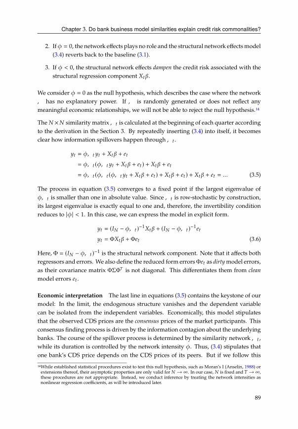
Chapter 3. Do bank business model similarities explain credit risk commonalities?
2. If ) = 0, the network effects plays no role and the structural network effectsmodel
(3.4) reverts back to the baseline (3.1).
3. If ) < 0, the structural network effects dampen the credit risk associated with the
structural regression component -C�.
We consider ) = 0 as the null hypothesis, which describes the case where the network
, has no explanatory power. If , is randomly generated or does not reflect any
meaningful economic relationships, we will not be able to reject the null hypothesis.14
The # ×# similarity matrix,C is calculated at the beginning of each quarter according
to the derivation in the Section 3. By repeatedly inserting (3.4) into itself, it becomes
clear how information spillovers happen through,C .
HC = ),C HC + -C� + 4C= ),C (),C HC + -C� + 4C ) + -C� + 4C= ),C (),C (),C HC + -C� + 4C ) + -C� + 4C ) + -C� + 4C = ... (3.5)
The process in equation (3.5) converges to a fixed point if the largest eigenvalue of
),C is smaller than one in absolute value. Since,C is row-stochastic by construction,
its largest eigenvalue is exactly equal to one and, therefore, the invertibility condition
reduces to |) | < 1. In this case, we can express the model in explicit form.
HC = (�# − ),C )−1-C� + (�# − ),C )−14C
HC = Φ-C� +Φ4C (3.6)
Here, Φ = (�# − ),C )−1is the structural network component. Note that it affects both
regressors and errors. We also define the reduced form errorsΦ4C as dirtymodel errors,
as their covariance matrix ΦΣΦ> is not diagonal. This differentiates them from cleanmodel errors 4C .
Economic interpretation The last line in equations (3.5) contains the keystone of our
model: In the limit, the endogenous structure vanishes and the dependent variable
can be isolated from the independent variables. Economically, this model stipulates
that the observed CDS prices are the consensus prices of the market participants. This
consensus finding process is driven by the information contagion about the underlying
banks. The course of the spillover process is determined by the similarity network,C ,
while its duration is controlled by the network intensity ). Thus, (3.4) stipulates that
one bank’s CDS price depends on the CDS prices of its peers. But if we follow this
14While established statistical procedures exist to test this null hypothesis, such as Moran’s I (Anselin, 1988) or
extensions thereof, their asymptotic properties are only valid for # →∞. In our case, # is fixed and ) →∞,
these procedures are not appropriate. Instead, we conduct inference by treating the network intensities as
nonlinear regression coefficients, as will be introduced later.
89

Chapter 3. Do bank business model similarities explain credit risk commonalities?
logic to the end, then the price in (3.6) ultimately depends on both the exogenous credit
determinants of its peers and their idiosyncratic errors.
This has two important implications. First, this framework establishes a channel be-
tween one bank’s credit risk and another bank’s credit determinant. Secondly, even
though the clean model errors 4C are independently distributed with diagonal covari-
ance matrix Σ, the dirty model errors &C are affected by the contagion process and have
a covariance structure ΦΣΦ>. This effectively relaxes the independence assumption of
the baseline model and introduces an additional layer of heteroskedasticity and cross-
correlations among idiosyncratic bank shocks, informed by the network structure. At
the same time, since the covariance structure is determined by the similarity matrix,C ,
we can decompose the estimated covariance matrix into a network component Φ and
the cleaned error component Σ.
Error network effects While structural network effects introduce contagion into both
regressors and errors, the error network effects model only does so for the latter. This
specification is therefore well-suited to capture contagion effects that are not driven by
structural determinants, such as during times ofmarket stress. To differentiate between
both effects, we use � to denote the error network intensity.
HC = -C� + DC with DC = �,CDC + 4C (3.7)
Under the condition that |� | < 1 we can write the model into explicit form.
HC = -C� + (�# − �,C )−14C
HC = -C� + Θ4C (3.8)
Here, Θ = (�# −�,C )−1denotes the error network component. Note that the structural
network effects and error network effects are identical if the data-generating process
does not contain any exogenous determinants.
Lastly, we define a general network effects (NE) model that contains both network
effects.
HC = ),C HC + -C� + DC with DC = �,CDC + 4C (3.9)
Under the same invertibility conditions we can reformulate (3.9) into the explicit form
HC = (�# − ),C )−1-C� + (�# − ),C )−1(�# − �,C )−14C
HC = Φ-C� +ΦΘ4C (3.10)
3.5.2 Dynamic network effects model
Since we suspect that the intensity of information contagion does not remain constant
across time, we introduce time variation in the network effects )C,C and �C,C , re-
spectively. We assume that the time dynamics are primarily driven by the intensity
90
Chapter 3. Do bank business model similarities explain credit risk commonalities?
parameters )C and �C . In fact, they vary on the same daily frequency as the credit
spreads HC , while ,C varies only on a quarterly frequency. Figure 3.11 shows an
overview of the temporal structure in the model.
This frequency is primarily dictated by the data availability. However, even if a daily
frequency were available, a lower frequency is desirable for two reasons: First, banks
are not likely to change their profiles significantly over time. Roengpitya et al. (2014)
point out that most of the 108 banks they investigate remain in the same classification.
Commercial banks switched between retail to wholesale funding before and after the
crisis, but this happened in a period of six years. In their subsequent study aboutmodel
popularity and transitions, Roengpitya et al. (2017) use the bank-year as their time unit
and find that in the period from 2006 to 2015, European banks switched business
models on average 1.25 times. Thus, even though models are not static, they certainly
do not shift from one day to the next. Second, if,C were to change daily along with )Cand �C , we would face an endogeneity problem in the estimation. The data-generating
process assumes that information contagion happens for given perceptions of the bank
similarities. If the underlying similarities were to change as a result of information
spillovers, then simultaneity will lead to biased estimates of the network effects.
For the technical specificationof thedynamicnetwork effectsmodel and the appropriate
estimation methodlogy, we refer to Section 3.B in the Appendix.
3.6 Empirical evidence for network effects
In addition to the estimation output of the baseline model, the NEmodel also produces
estimates for the latent network intensity parameters, ) = 0.458 and � = −0.093.15
These correspond to a structural multiplier effect of 1.844 and residual multiplier effect
of 0.915. Economically, this means that the structural network effects had a moderate
to strong, amplifying effect, while the residual network effects had a weak, dampening
effect on credit contagion.
Our first main result is depicted in Figure 3.5: After accounting for network effects, the
largest component in the clean residuals only accounts for 21.36% of residual variance,
representing a drop of 40% versus its baseline counterpart (35.63%). Furthermore, all
four components account jointly for 40.08%, compared to 53.02% in the baseline. Most
importantly, the first component loses its systematic nature. Its loadings are not strictly
positive for all banks anymore, and some of them are very close to zero or even change
signs. Moreover, the second component (North-South) loses its distinctive character as
its values become more erratic with no clear pattern. This means that the similarity
15The ) is statistically significant on a 1% level while the � is not significantly different from zero.
91
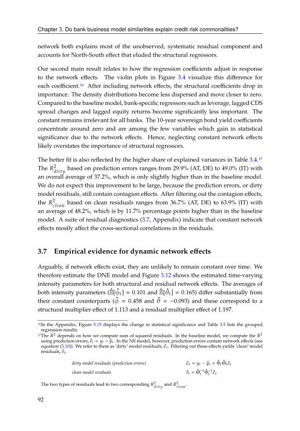
Chapter 3. Do bank business model similarities explain credit risk commonalities?
network both explains most of the unobserved, systematic residual component and
accounts for North-South effect that eluded the structural regressors.
Our second main result relates to how the regression coefficients adjust in response
to the network effects. The violin plots in Figure 3.4 visualize this difference for
each coefficient.16 After including network effects, the structural coefficients drop in
importance. The density distributions become less dispersed and move closer to zero.
Compared to the baselinemodel, bank-specific regressors such as leverage, lagged CDS
spread changes and lagged equity returns become significantly less important. The
constant remains irrelevant for all banks. The 10-year sovereign bond yield coefficients
concentrate around zero and are among the few variables which gain in statistical
significance due to the network effects. Hence, neglecting constant network effects
likely overstates the importance of structural regressors.
The better fit is also reflected by the higher share of explained variances in Table 3.4.17
The '2
38ACHbased on prediction errors ranges from 29.9% (AT, DE) to 49.0% (IT) with
an overall average of 37.2%, which is only slightly higher than in the baseline model.
We do not expect this improvement to be large, because the prediction errors, or dirty
model residuals, still contain contagion effects. After filtering out the contagion effects,
the '2
2;40=based on clean residuals ranges from 36.7% (AT, DE) to 63.9% (IT) with
an average of 48.2%, which is by 11.7% percentage points higher than in the baseline
model. A suite of residual diagnostics (3.7, Appendix) indicate that constant network
effects mostly affect the cross-sectional correlations in the residuals.
3.7 Empirical evidence for dynamic network effects
Arguably, if network effects exist, they are unlikely to remain constant over time. We
therefore estimate the DNE model and Figure 3.12 shows the estimated time-varying
intensity parameters for both structural and residual network effects. The averages of
both intensity parameters (E[)C] = 0.101 and E[�C] = 0.165) differ substantially from
their constant counterparts () = 0.458 and � = −0.093) and these correspond to a
structural multiplier effect of 1.113 and a residual multiplier effect of 1.197.
16In the Appendix, Figure 3.15 displays the change in statistical significance and Table 3.5 lists the grouped
regression results.
17The '2depends on how we compute sum of squared residuals. In the baseline model, we compute the '2
using prediction errors, 4C = HC − HC . In the NE model, however, prediction errors contain network effects (see
equation (3.10)). We refer to them as ‘dirty’ model residuals, &C . Filtering out these effects yields ‘clean’ model
residuals, 4C .
dirty model residuals (prediction errors) &C = HC − HC = ΦC ΘC 4Cclean model residuals 4C = Θ
−1
C Φ−1
C &C
The two types of residuals lead to two corresponding '2
38ACHand '2
2;40=.
92
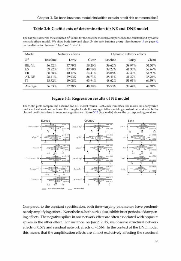
Chapter 3. Do bank business model similarities explain credit risk commonalities?
Table 3.4: Coefficients of determination for NE and DNE model
The bar plots describe the estimated'2values for the baselinemodel in comparison to the constant and dynamic
network effects model. We show both dirty and clean '2for each banking group. See footnote 17 on page 92
on the distinction between ‘clean‘ and ‘dirty‘ '2.
Model Network effects Dynamic network effects
'2Baseline Dirty Clean Baseline Dirty Clean
BE, NL 36.62% 37.79% 50.20% 36.62% 39.97% 51.53%
ES 39.22% 37.90% 48.78% 39.22% 41.38% 52.69%
FR 38.88% 40.17% 54.41% 38.88% 42.40% 54.90%
AT, DE 28.41% 29.93% 36.73% 28.41% 31.37% 38.24%
IT 48.62% 49.08% 63.94% 48.62% 51.01% 64.58%
Average 36.53% 37.28% 48.30% 36.53% 39.44% 49.91%
Figure 3.4: Regression results of NE model
The violin plots compare the baseline and NE model results. Each each thin black line marks the anonymized
coefficient value of one bank and the triangles locate the average. After modeling constant network effects, the
cleaned coefficients lose in economic significance. Figure 3.15 (Appendix) shows the corresponding ?-values.
2 0 2
eurostoxx50=-0.049
=-1.219
Europe
1 0 1
slopeEU=0.044
=-0.197
0.5 0.0 0.5
vstoxx=0.002
=0.190
2 0 2
L.eurostoxx50=-0.028
=-0.210
0.5 0.0 0.5
L.slopeEU=0.024
=-0.054
0.5 0.0 0.5
L.vstoxx=0.059
=0.255
2 0 2
bond10yC=-0.134
=-0.001
Country
1 0 1
eqidxC=-0.132
=-0.046
2 0 2
slopeC=0.099
=0.206
2 0 2
L.bond10yC=-0.084
=-0.034
2 0 2
L.eqidxC=-0.046
=0.067
1 0 1
L.slopeC=0.075
=0.073
0.2 0.0 0.2
const=0.003
=0.023
Bank
1 0 1
eq=-0.095
=-0.403
0.2 0.0 0.2
lev=0.001
=-0.010
2 0 2
L.cds=-0.192
=-0.371
1 0 1
L.eq=-0.052
=-0.122
Baseline model NE model
Compared to the constant specification, both time-varying parameters have predomi-
nantly amplifying effects. Nonetheless, both series also exhibit brief periods of dampen-
ing effects. The negative spikes in one network effect are often associatedwith opposite
spikes in the other effect. For instance, on Jan 2, 2015, we observe structural network
effects of 0.572 and residual network effects of -0.564. In the context of the DNEmodel,
this means that the amplification effects are almost exclusively affecting the structural
93
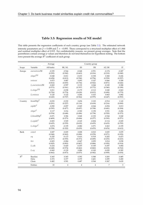
Chapter 3. Do bank business model similarities explain credit risk commonalities?
Table 3.5: Regression results of NE model
This table presents the regression coefficients of each country group (see Table 3.1). The estimated network
intensity parameters are � = 0.458 and � = −0.093. These correspond to a structural multiplier effect of 1.844
and residual multiplier effect of 0.915. For confidentiality reasons, we present group averages. Note that the
parentheses contain average ?-values and therefore do not lend themselves for hypothesis testing. The bottom
rows present the average '2coefficient of each group.
Average Country group
Scope Variable All banks BE, NL ES FR AT, DE IT
Europe 4DA>BC>GG50 -0.339 -0.544 -0.248 -0.551 -0.174 -0.287
(0.292) (0.542) (0.663) (0.016) (0.210) (0.040)
B;>?4�* -0.048 -0.011 -0.233 -0.338 0.368 -0.436
(0.658) (0.813) (0.740) (0.754) (0.539) (0.527)
EBC>GG 0.073 0.087 0.093 0.107 -0.066 0.308
(0.812) (0.835) (0.734) (0.922) (0.871) (0.626)
!.4DA>BC>GG50 -0.069 -0.597 0.132 0.044 -0.100 0.288
(0.573) (0.541) (0.767) (0.772) (0.540) (0.189)
!.B;>?4�* 0.011 -0.038 -0.179 -0.112 0.249 -0.063
(0.726) (0.774) (0.630) (0.812) (0.690) (0.779)
!.EBC>GG 0.120 0.122 0.206 0.163 0.063 0.082
(0.620) (0.727) (0.564) (0.575) (0.647) (0.593)
Country 1>=310H� -0.032 -0.232 0.694 0.102 -0.914 1.143
(0.201) (0.227) (0.116) (0.418) (0.216) (0.000)
4@83G� -0.090 -0.097 -0.269 -0.044 -0.054 0.013
(0.595) (0.477) (0.697) (0.708) (0.681) (0.304)
B;>?4� 0.117 0.216 -0.320 0.158 0.531 -0.456
(0.554) (0.648) (0.496) (0.738) (0.520) (0.372)
!.1>=310H� -0.071 0.306 0.268 -0.192 -0.544 0.240
(0.409) (0.273) (0.604) (0.277) (0.393) (0.571)
!.4@83G� -0.003 0.529 -0.169 -0.004 -0.114 -0.229
(0.625) (0.535) (0.632) (0.655) (0.633) (0.702)
!.B;>?4� 0.074 -0.195 -0.080 0.371 0.263 -0.199
(0.558) (0.322) (0.659) (0.470) (0.676) (0.612)
Bank 2>=BC 0.007 -0.029 0.008 -0.010 0.025 0.035
(0.948) (0.962) (0.898) (0.978) (0.971) (0.939)
4@ -0.320 -0.115 -0.416 -0.518 -0.202 -0.473
(0.277) (0.555) (0.373) (0.009) (0.253) (0.223)
;4E -0.003 -0.084 -0.047 0.059 0.014 0.038
(0.905) (0.893) (0.867) (0.884) (0.950) (0.914)
!.23B -0.224 -0.420 -0.255 -0.100 -0.297 0.084
(0.648) (0.574) (0.462) (0.860) (0.632) (0.762)
!.4@ -0.069 -0.120 0.086 -0.100 -0.020 -0.282
(0.862) (0.873) (0.875) (0.942) (0.909) (0.654)
'2Baseline 0.365 0.365 0.392 0.388 0.283 0.485
Dirty 0.372 0.377 0.379 0.401 0.299 0.490
Clean 0.482 0.501 0.487 0.544 0.367 0.639
Entities 22 4 4 4 7 3
94
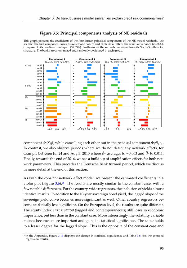
Chapter 3. Do bank business model similarities explain credit risk commonalities?
Figure 3.5: Principal components analysis of NE residuals
This graph presents the coefficients of the four largest principal components of the NE model residuals. We
see that the first component loses its systematic nature and explains a fifth of the residual variance (21.36%),
compared to its baseline counterpart (35.63%). Furthermore, the second component loses its North-South factor
structure. The banks are anonymized and randomly positioned in each group.
0.2 0.0 0.2
bank1bank2bank3bank4bank5bank6bank7bank8bank9
bank10bank11bank12bank13bank14bank15bank16bank17bank18bank19bank20bank21bank22
AT,DE
BE,NL
ES
FR
IT
Component 1(20.75%, cuml=20.75%)
0.25 0.00 0.25
Component 2(7.55%, cuml=28.30%)
0.5 0.0 0.5
Component 3(6.37%, cuml=34.67%)
0.25 0.00 0.25
Component 4(5.70%, cuml=40.36%)
component ΦC-C�, while cancelling each other out in the residual component ΦCΘC 4C .
In contrast, we also observe periods where we do not detect any network effects, for
example between Jul 24 and Aug 3, 2015 where )C averages to −0.003 and �C to 0.011.
Finally, towards the end of 2016, we see a build up of amplification effects for both net-
work parameters. This precedes the Deutsche Bank turmoil period, which we discuss
in more detail at the end of this section.
As with the constant network effect model, we present the estimated coefficients in a
violin plot (Figure 3.6).18 The results are mostly similar to the constant case, with a
few notable differences. For the country-wide regressors, the inclusion of yields almost
identical results. In addition to the 10-year sovereign bond yield, the lagged slope of the
sovereign yield curve becomes more significant as well. Other country regressors be-
come statistically less significant. On the European level, the results are quite different.
The equity index 4DA>BC>GG50 (lagged and contemporaneous) still loses in economic
importance, but less than in the constant case. More interestingly, the volatility variable
EBC>GG becomes more important and gains in statistical significance. The same holds
to a lesser degree for the lagged slope. This is the opposite of the constant case and
18In the Appendix, Figure 3.16 displays the change in statistical significance and Table 3.6 lists the grouped
regression results.
95
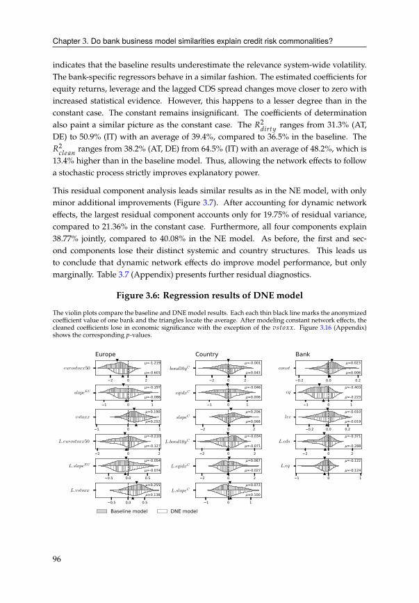
Chapter 3. Do bank business model similarities explain credit risk commonalities?
indicates that the baseline results underestimate the relevance system-wide volatility.
The bank-specific regressors behave in a similar fashion. The estimated coefficients for
equity returns, leverage and the lagged CDS spread changes move closer to zero with
increased statistical evidence. However, this happens to a lesser degree than in the
constant case. The constant remains insignificant. The coefficients of determination
also paint a similar picture as the constant case. The '2
38ACHranges from 31.3% (AT,
DE) to 50.9% (IT) with an average of 39.4%, compared to 36.5% in the baseline. The
'2
2;40=ranges from 38.2% (AT, DE) from 64.5% (IT) with an average of 48.2%, which is
13.4% higher than in the baseline model. Thus, allowing the network effects to follow
a stochastic process strictly improves explanatory power.
This residual component analysis leads similar results as in the NE model, with only
minor additional improvements (Figure 3.7). After accounting for dynamic network
effects, the largest residual component accounts only for 19.75% of residual variance,
compared to 21.36% in the constant case. Furthermore, all four components explain
38.77% jointly, compared to 40.08% in the NE model. As before, the first and sec-
ond components lose their distinct systemic and country structures. This leads us
to conclude that dynamic network effects do improve model performance, but only
marginally. Table 3.7 (Appendix) presents further residual diagnostics.
Figure 3.6: Regression results of DNE model
The violin plots compare the baseline and DNEmodel results. Each each thin black line marks the anonymized
coefficient value of one bank and the triangles locate the average. After modeling constant network effects, the
cleaned coefficients lose in economic significance with the exception of the EBC>GG. Figure 3.16 (Appendix)
shows the corresponding ?-values.
2 0 2
eurostoxx50=-0.601
=-1.219
Europe
1 0 1
slopeEU=-0.086
=-0.197
1 0 1
vstoxx=0.252
=0.190
2 0 2
L.eurostoxx50=-0.127
=-0.210
0.5 0.0 0.5
L.slopeEU=-0.074
=-0.054
0.5 0.0 0.5
L.vstoxx=0.138
=0.255
2 0 2
bond10yC=0.043
=-0.001
Country
1 0 1
eqidxC=0.006
=-0.046
2 0 2
slopeC=0.068
=0.206
2 0 2
L.bond10yC=-0.071
=-0.034
2 0 2
L.eqidxC=-0.027
=0.067
1 0 1
L.slopeC=0.100
=0.073
0.2 0.0 0.2
const=0.008
=0.023
Bank
1 0 1
eq=-0.223
=-0.403
0.2 0.0 0.2
lev=-0.019
=-0.010
2 0 2
L.cds=-0.288
=-0.371
1 0 1
L.eq=-0.124
=-0.122
Baseline model DNE model
96
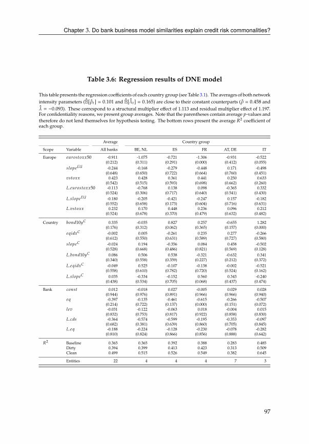
Chapter 3. Do bank business model similarities explain credit risk commonalities?
Table 3.6: Regression results of DNE model
This table presents the regression coefficients of each country group (see Table 3.1). The averages of both network
intensity parameters (E[�C ] = 0.101 and E[�C ] = 0.165) are close to their constant counterparts (� = 0.458 and
� = −0.093). These correspond to a structural multiplier effect of 1.113 and residual multiplier effect of 1.197.
For confidentiality reasons, we present group averages. Note that the parentheses contain average ?-values and
therefore do not lend themselves for hypothesis testing. The bottom rows present the average '2coefficient of
each group.
Average Country group
Scope Variable All banks BE, NL ES FR AT, DE IT
Europe 4DA>BC>GG50 -0.911 -1.075 -0.721 -1.306 -0.931 -0.522
(0.212) (0.311) (0.291) (0.000) (0.412) (0.055)
B;>?4�* -0.244 -0.168 -0.279 -0.448 0.171 -0.498
(0.648) (0.650) (0.722) (0.664) (0.760) (0.451)
EBC>GG 0.423 0.428 0.361 0.441 0.250 0.633
(0.542) (0.515) (0.593) (0.698) (0.662) (0.260)
!.4DA>BC>GG50 -0.113 -0.768 0.138 0.098 -0.365 0.332
(0.524) (0.306) (0.717) (0.640) (0.541) (0.430)
!.B;>?4�* -0.180 -0.205 -0.421 -0.247 0.157 -0.182
(0.552) (0.658) (0.173) (0.604) (0.716) (0.631)
!.EBC>GG 0.232 0.170 0.448 0.236 0.096 0.212
(0.524) (0.678) (0.370) (0.479) (0.632) (0.482)
Country 1>=310H� 0.335 -0.035 0.827 0.257 -0.655 1.282
(0.176) (0.312) (0.062) (0.365) (0.157) (0.000)
4@83G� -0.002 0.005 -0.261 0.235 0.277 -0.266
(0.612) (0.550) (0.631) (0.589) (0.727) (0.580)
B;>?4� -0.024 0.194 -0.356 0.084 0.458 -0.502
(0.528) (0.668) (0.486) (0.821) (0.569) (0.128)
!.1>=310H� 0.086 0.506 0.538 -0.321 -0.632 0.341
(0.340) (0.558) (0.359) (0.227) (0.212) (0.372)
!.4@83G� -0.049 0.525 -0.107 -0.138 -0.002 -0.521
(0.558) (0.610) (0.782) (0.720) (0.524) (0.162)
!.B;>?4� 0.035 -0.334 -0.152 0.560 0.343 -0.240
(0.438) (0.534) (0.705) (0.068) (0.437) (0.474)
Bank 2>=BC 0.012 -0.018 0.027 -0.005 0.029 0.028
(0.944) (0.976) (0.891) (0.966) (0.966) (0.940)
4@ -0.397 -0.135 -0.461 -0.615 -0.266 -0.507
(0.214) (0.722) (0.137) (0.000) (0.151) (0.072)
;4E -0.031 -0.122 -0.063 0.018 -0.004 0.015
(0.832) (0.753) (0.817) (0.922) (0.858) (0.830)
!.23B -0.364 -0.574 -0.599 -0.195 -0.353 -0.097
(0.682) (0.381) (0.639) (0.860) (0.705) (0.845)
!.4@ -0.188 -0.224 -0.128 -0.230 -0.078 -0.282
(0.810) (0.824) (0.866) (0.856) (0.888) (0.642)
'2Baseline 0.365 0.365 0.392 0.388 0.283 0.485
Dirty 0.394 0.399 0.413 0.423 0.313 0.509
Clean 0.499 0.515 0.526 0.549 0.382 0.645
Entities 22 4 4 4 7 3
97
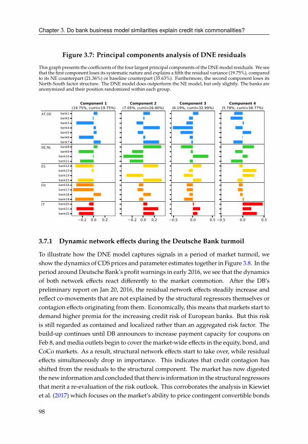
Chapter 3. Do bank business model similarities explain credit risk commonalities?
Figure 3.7: Principal components analysis of DNE residuals
This graph presents the coefficients of the four largest principal components of theDNEmodel residuals. We see
that the first component loses its systematic nature and explains a fifth the residual variance (19.75%), compared
to its NE counterpart (21.36%) or baseline counterpart (35.63%). Furthermore, the second component loses its
North-South factor structure. The DNE model does outperform the NE model, but only slightly. The banks are
anonymized and their position randomized within each group.
0.2 0.0 0.2
bank1bank2bank3bank4bank5bank6bank7bank8bank9
bank10bank11bank12bank13bank14bank15bank16bank17bank18bank19bank20bank21bank22
AT,DE
BE,NL
ES
FR
IT
Component 1(19.75%, cuml=19.75%)
0.2 0.0 0.2
Component 2(7.05%, cuml=26.80%)
0.5 0.0 0.5
Component 3(6.19%, cuml=32.99%)
0.5 0.0 0.5
Component 4(5.78%, cuml=38.77%)
3.7.1 Dynamic network effects during the Deutsche Bank turmoil
To illustrate how the DNE model captures signals in a period of market turmoil, we
show the dynamics of CDS prices and parameter estimates together in Figure 3.8. In the
period around Deutsche Bank’s profit warnings in early 2016, we see that the dynamics
of both network effects react differently to the market commotion. After the DB’s
preliminary report on Jan 20, 2016, the residual network effects steadily increase and
reflect co-movements that are not explained by the structural regressors themselves or
contagion effects originating from them. Economically, this means that markets start to
demand higher premia for the increasing credit risk of European banks. But this risk
is still regarded as contained and localized rather than an aggregated risk factor. The
build-up continues until DB announces to increase payment capacity for coupons on
Feb 8, andmedia outlets begin to cover the market-wide effects in the equity, bond, and
CoCo markets. As a result, structural network effects start to take over, while residual
effects simultaneously drop in importance. This indicates that credit contagion has
shifted from the residuals to the structural component. The market has now digested
thenew information and concluded that there is information in the structural regressors
that merit a re-evaluation of the risk outlook. This corroborates the analysis in Kiewiet
et al. (2017) which focuses on the market’s ability to price contingent convertible bonds
98
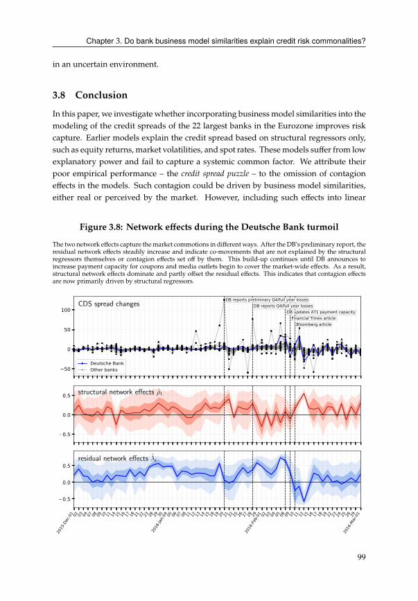
Chapter 3. Do bank business model similarities explain credit risk commonalities?
in an uncertain environment.
3.8 Conclusion
In this paper, we investigate whether incorporating business model similarities into the
modeling of the credit spreads of the 22 largest banks in the Eurozone improves risk
capture. Earlier models explain the credit spread based on structural regressors only,
such as equity returns, market volatilities, and spot rates. Thesemodels suffer from low
explanatory power and fail to capture a systemic common factor. We attribute their
poor empirical performance – the credit spread puzzle – to the omission of contagion
effects in the models. Such contagion could be driven by business model similarities,
either real or perceived by the market. However, including such effects into linear
Figure 3.8: Network effects during the Deutsche Bank turmoil
The two network effects capture themarket commotions in differentways. After theDB’s preliminary report, the
residual network effects steadily increase and indicate co-movements that are not explained by the structural
regressors themselves or contagion effects set off by them. This build-up continues until DB announces to
increase payment capacity for coupons and media outlets begin to cover the market-wide effects. As a result,
structural network effects dominate and partly offset the residual effects. This indicates that contagion effects
are now primarily driven by structural regressors.
0.5
0.0
0.5 structural network effects ρt
0.5
0.0
0.5residual network effects λt
2015
-Dec
-01 02 03 04 07 08 09 10 11 14 15 16 17 18 21 22 23 28 29 3020
16-Ja
n-04 05 06 07 08 11 12 13 14 15 18 19 20 21 22 25 26 27 28 29
2016
-Feb-0
1 02 03 04 05 08 09 10 11 12 15 16 17 18 19 22 23 24 25 26 29
2016
-Mar-
01
50
0
50
100CDS spread changes
preliminary Q4/full year lossesDB reports DB reports Q4/full year losses
DB updates AT1 payment capacityFinancial Times article
Bloomberg article
Deutsche BankOther banks
99
Chapter 3. Do bank business model similarities explain credit risk commonalities?
regressions is challenging because contagionmechanisms are self-reinforcing and non-
linear. To address this limitation, we augment the existing models with a similarity
network, positing that common asset exposures of banks are a reasonable measure of
business model similarity. We construct the network by applying an '2-decomposition
method on the banks’ complete holdings data. This leads to two extensions, the Net-
work Effects (NE)model andDynamicNetwork Effects (DNE)model. Both incorporate
the similarity network andmeasure how important it is with intensity parameters. The
difference is that theDNEmodel has time-varying intensities. If the network represents
the vehicle that credit risk uses to spread from bank to bank, then the intensity repre-
sents the fuel that determines how far the vehicle can go. We obtain several surprising
results with this modeling approach.
First, while the traditional model yields an '2for the European banks of 36.5% on
average, the NEmodel leads to a '2that is only slightly higher, averaging 37.2%. After
removing contagion effects in the residuals, the resulting average ‘clean’ '2goes up
to 48.2%, an increase of 11.7% percentage points compared to the baseline model.19
We attribute the increased explanatory power to the NE model’s structural network ef-fects. These effects include other banks as endogenous regressors, which ultimately
still depend on the structural variables through the network. In addition, we find that
the structural regressors of the NE become less important compared to the baseline.
The DNE model, which has time-varying network effects, improves these findings
even further, albeit only slightly. The average '2
2;40=amounts to 49.9%. Surprisingly,
while the regression coefficients generally become less relevant as in the NE model,
the volatility index increases in importance under the DNE model. Thus, neglecting
network effects, whether constant or dynamic, likely overstates the importance of most
structural regressors. It is interesting to note that, although banks are presumably
unaware of exactly how many assets they have in common with other banks, CDS
premia nonetheless seem to correctly price the implied contagion risk. Possibly, public
information as for instance released in the EBA transparency exercise, already provides
sufficient information for traders to come to a reasonably accurate similarity estimation.
It should therefore be in the interest of regulators to monitor this risk channel. Market
participants could benefit from these insights if they can find a reliable measure of
business sector similarity – which would seem feasible.
Second, the residuals of traditional models contain uncaptured common factors. A
principal component analysis reveals that the first component is a systematic factor
that affects all banks, responsible for 35.63% of the remaining variance. The second
component contains country-specific blocks, which is surprising since the structural
regressors already contain country-specific determinants. Upon closer inspection, this
19See footnote 17 on page 92 on the distinction between ‘clean‘ and ‘dirty‘ '2.
100
Chapter 3. Do bank business model similarities explain credit risk commonalities?
component differentiates between Northern countries (AT, BE, FR, DE, NL) and South-
ern countries (ES, IT). TheNE andDNEmodels are constructed to capture these residualnetwork effects. A subsequent residual component analysis confirms that the first com-
ponent loses its systematic nature and only explains 21.36% (NE) and 19.75% (DNE) of
the remaining variance, and the second component also loses itsNorth-South structure.
The largest four components jointly explain 40.08% (NE) and 38.77% (DNE) compared
to 53.02% in the baseline. These findings imply that the bank similarity network helps
us shed light on an aspect of credit risk that has eluded the structural regressors.
Lastly, the DNE allows us to measure the importance of the network effects over
time. The structural network intensity oscillates around a constant mean of about
E[)C] = 0.101 (corresponding to a multiplier of 1.113). At the same time, the residual
network intensity revolves around E[�C] = 0.165 (multiplier of 1.197). During the mar-
ket stress period of early 2016, these intensities reach up to 0.561 (multiplier of 2.28) for
the structural effects and 0.741 (multiplier of 3.86) for the residual effects. The time-
varying nature tells us that network effects respond to or predict periods of financial
distress. In the period following the Deutsche Bank’s negative earnings announce-
ments that spread throughout the continent, we find that there was a consistent build
up of residual correlations not captured by the structural variables. This transitioned
into a period where contagion effects were predominantly driven by structural regres-
sors. The intensities also help us understand the contagion mechanism in details, for
instance, by tracking how shocks to individual banks or Europe-wide variables find
their way through the system during calm or volatile times.
In conclusion, we find that credit contagion and the credit spread puzzle are tightly
connected. Neglecting the network component likely over- or underestimates the im-
portance of structural regressors and fails to capture important common factors. The
proposed NE/DNE framework is able to integrate these effects into established credit
spread models and helps us resolve the puzzle for the largest banks in the Eurozone.
The DNE model performs better than the NE model in every regard, as it allows for
network effects to vary over time. But the improvements are slight, indicating that
accounting for constant network effects is already sufficient to realize almost all of
the benefits. Nonetheless, the dynamic model does provide valuable insights into
the contagion mechanism during stress periods. Note that doubtlessly other conta-
gion channels, such the interbank lending channel or market liquidity conditions, play
important roles in contagion as well. Thus, our results highlight the need for more
research on the network effects in credit risk.
101

Appendix
3.A Business model similarity measure
The main premise of our similarity measure can be summarized as: Bank holdings
are predictive for each other if they follow similar business models. By treating the
holdings of eachbank as a vector of assets, we can reformulate question of similarity into
a statistical prediction exercise. To quantify which bank’s holdings is most predictive
to the holdings of a bank of interest, we regress the holdings vector of the latter onto
the holdings vectors of all remaining banks. We then examine which of the remaining
banks carries the highest explanatory power. As described in Section 3.4, this becomes
an '2decomposition exercise.
The statistical literature on relative importance and variable selection has proposed
severalmethods for'2decomposition.20 Inmultiple regression analysis, thesemethods
help us understand how much explanatory power a regressor contributes in relation
to all other regressors. Essentially, we are interested in how similar a particular bank’s
holdings are to a stressed bank’s holdings, relative to all other banks. Translated into
a variable importance problem, we are interested in the predictive power of a bank’s
portfolio regarding the stressed bank portfolio structure, compared to the remaining
portfolios.
3.A.1 Algorithm
Algorithm 1 details the steps to compute the similarity measure. The concept is similar
to the variance inflation factor used in regression analysis to detect multicollinearity.
The basic idea is best illustrated in the context of a multiple regression of H on -: If
the columns of - are mutually disjoint, then the '2of this regression is simply the
sum of the '2of regressing H on each column of -, separately. However, this does not
hold when the columns of - are not orthogonal. The idea is instead to use the nearest
20For a review of suchmethodswe refer to Grömping (2015). Ourmeasure is closest to Genizi (1993) as discussed
in Johnson (2000).
103

Chapter 3. Do bank business model similarities explain credit risk commonalities?
Algorithm 1: Portfolio similarity measure
This algorithm calculates the similarity matrix " for # portfolios with ( assets.
" has typical element �8 , 9 and we define �8 ,8 = 0. Repeat the following steps for
all 8 = 1, .., # portfolios:
1. Set the 8-th portfolio as dependent variable H and all others as regressor
matrix -.
2. Calculate pseudo-regression coefficients
1 =1√(
[->-
]−1/2 [->H
]3. Calculate the similarity measure �8 , 9 as the partial-'
2
�8 , 9 =1
(2
∑=
(->-)29 ,=12
=
Optional steps
1. Row-normalize " by divide each row by its sum.
2. When ( is small, set �8 , 9 = 0 if 1 9 = 0 to avoid spurious similaritys.
orthogonal matrix -⊥ of -.21 Since -⊥ is orthogonal, we can apply the same logic
as before and regress H on -⊥, the orthogonal counterpart of -. However, this will
give us the contributions of -⊥. Since were are interested in the contributions of -,
the algorithm involves a further projection of - onto -⊥. For more details we refer to
Johnson (2000).
To obtain the similarity matrix , , we repeat Algorithm 1 as described in equation
(3.2). The result for the hypothetical holdings is presented in Figure 3.3 and 3.9, right
panels. Note that the matrix satisfies all desired properties 1-3 and is by construction
row-stochastic, i.e. each row adds up to one and its elements are non-negative. This
system is constructed to have three distinct features. First, the holdings of 10=:1-10=:
3
and 10=:4-10=:
6form two disjoint groups. Second, the holdings of 10=:
1,10=:
2
(10=:4,10=:
5) are positively (negatively) correlated. Third, the holdings of 10=:
3and
21The closeness between twomatrices is measured using the Frobenius norm. Thematrix-⊥ can be determined
either using singular value decomposition (Fabbris, 1980) or by using the matrix square root (Genizi, 1993).
104

Chapter 3. Do bank business model similarities explain credit risk commonalities?
10=:6are randomly drawn: Their first halves follow*[0, 10]while their second halves
follow*[10, 20].
We visualize this contagion process in Figure 3.10. Panel (a) is the graphical represen-
tation of the similarity network from Figure 3.9 while panel (b) demonstrates how a
bank’s demise spreads to its neighbors in an iterative fashion, according to the portfolio
distances. With each round the network intensity decays geometrically. Panel (b) can
also be viewed as the impulse response function of the network for a given shock.
105
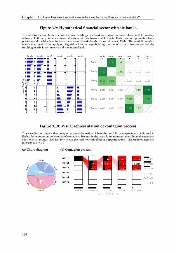
Chapter 3. Do bank business model similarities explain credit risk commonalities?
Figure 3.9: Hypothetical financial sector with six banks
This idealized example shows how the asset holdings of a banking system translate into a portfolio overlap
network. Left: A hypothetical financial system with six banks and 40 assets. Each column represents a bank
portfolio and the blue bars indicate the amount a banks holds of a certain asset. Right: The portfolio overlap
matrix that results from applying Algorithm 1 to the asset holdings on the left panel. We can see that the
resulting matrix is asymmetric and row-normalized.
assetholdings
bank1 bank2 bank3 bank4 bank5 bank6 bank1 bank2 bank3 bank4 bank5 bank6
bank1
bank2
bank3
bank4
bank5
bank6
0.755 0.245 0.000 0.000 0.000
0.765 0.235 0.000 0.000 0.000
0.517 0.482 0.000 0.000 0.000
0.000 0.000 0.000 0.150 0.850
0.000 0.000 0.000 0.391 0.609
0.000 0.000 0.000 0.798 0.202
Figure 3.10: Visual representation of contagion process
This visualization depicts the contagion process of equation (3.5) for the portfolio overlap network of Figure 3.9.
Each column represents one round of contagion. To sums in the last column represent the culminative network
effect over all rounds. The last row shows the total network effect of a specific round. The assumed network
intensity is � = 0.7.
(a) Chord diagram (b) Contagion process
bank1
bank2
bank
3ba
nk4
bank5
bank
6
106
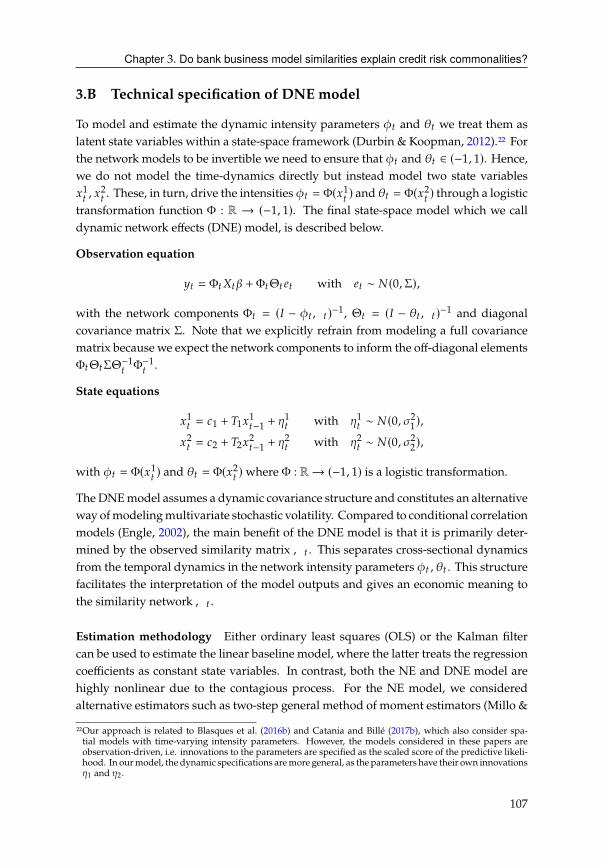
Chapter 3. Do bank business model similarities explain credit risk commonalities?
3.B Technical specification of DNE model
To model and estimate the dynamic intensity parameters )C and �C we treat them as
latent state variables within a state-space framework (Durbin & Koopman, 2012).22 For
the network models to be invertible we need to ensure that )C and �C ∈ (−1, 1). Hence,
we do not model the time-dynamics directly but instead model two state variables
G1
C, G2
C. These, in turn, drive the intensities )C = Φ(G1
C) and �C = Φ(G2
C) through a logistic
transformation function Φ : R → (−1, 1). The final state-space model which we call
dynamic network effects (DNE) model, is described below.
Observation equation
HC = ΦC-C� +ΦCΘC 4C with 4C ∼ #(0,Σ),
with the network components ΦC = (� − )C,C )−1, ΘC = (� − �C,C )−1
and diagonal
covariance matrix Σ. Note that we explicitly refrain from modeling a full covariance
matrix because we expect the network components to inform the off-diagonal elements
ΦCΘCΣΘ−1
CΦ−1
C.
State equations
G1
C = 21 + )1G1
C−1+ �1
C with �1
C ∼ #(0, �2
1),
G2
C = 22 + )2G2
C−1+ �2
C with �2
C ∼ #(0, �2
2),
with )C = Φ(G1
C) and �C = Φ(G2
C)where Φ : R→ (−1, 1) is a logistic transformation.
The DNEmodel assumes a dynamic covariance structure and constitutes an alternative
way ofmodelingmultivariate stochastic volatility. Compared to conditional correlation
models (Engle, 2002), the main benefit of the DNE model is that it is primarily deter-
mined by the observed similarity matrix,C . This separates cross-sectional dynamics
from the temporal dynamics in the network intensity parameters )C , �C . This structure
facilitates the interpretation of the model outputs and gives an economic meaning to
the similarity network,C .
Estimation methodology Either ordinary least squares (OLS) or the Kalman filter
can be used to estimate the linear baseline model, where the latter treats the regression
coefficients as constant state variables. In contrast, both the NE and DNE model are
highly nonlinear due to the contagious process. For the NE model, we considered
alternative estimators such as two-step general method of moment estimators (Millo &
22Our approach is related to Blasques et al. (2016b) and Catania and Billé (2017b), which also consider spa-
tial models with time-varying intensity parameters. However, the models considered in these papers are
observation-driven, i.e. innovations to the parameters are specified as the scaled score of the predictive likeli-
hood. In ourmodel, the dynamic specifications aremore general, as the parameters have their own innovations
�1 and �2.
107
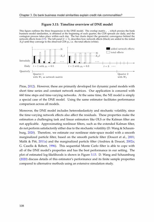
Chapter 3. Do bank business model similarities explain credit risk commonalities?
Figure 3.11: Timeline overview of DNE model
This figure outlines the three frequencies in the DNE model. The overlap matrix, , which proxies the bank
business model similarities, is obtained at the beginning of each quarter, the CDS spreads are daily, and the
contagion process takes place within each day. The bar charts depict the geometric convergence behind the
network effects from (3.5). The left panel (C = 1), describes how network effects (black) are added to the initial
-1� until they converge to the observed CDS H1, i.e. the total effects (white).
t = 1 with ρ1 = 0.5 t = 2 with ρ2 = 0.3 t = 3
X1β
y1
X2β
y2
Quarter 1with W1 as network matrix
Quarter 2with W2
Intradaily
Daily
Quarterly
added network effects
total effects
Piras, 2012). However, these are primarily developed for dynamic panel models with
short time series and constant network matrices. Our application is concered with
660 time steps and time-varying networks. At the same time, the NE model is simply
a special case of the DNE model. Using the same estimator facilitates performance
comparison across all models.
Moreover, the DNE model includes heteroskedasticty and stochastic volatility, since
the time-varying network effects also affect the residuals. These properties make the
estimation a challenging task and linear estimators like OLS or the Kalman filter are
not applicable. Approximating nonlinear filters, such as the extended Kalman filter,
do not perform satisfactorily either due to the stochastic volatility (D. Wang & Schaum-
burg, 2020). Therefore, we estimate our nonlinear state-space model with a smooth
marginalized particle filter, based on the smooth particle filter (Doucet et al., 2001;
Malik & Pitt, 2011a) and the marginalized particle filter (Andrieu & Doucet, 2002a;
G. Casella & Robert, 1996). This sequential Monte Carlo filter is able to cope with
all of the DNE model’s properties and has the best performance in our setting. The
plot of estimated log-likelihoods is shown in Figure 3.13. D. Wang and Schaumburg
(2020) discuss details of this estimator’s performance and its finite sample properties
compared to alternative methods using an extensive simulation study.
108
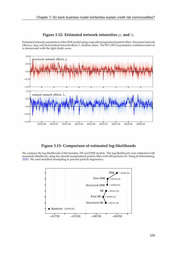
Chapter 3. Do bank business model similarities explain credit risk commonalities?
Figure 3.12: Estimated network intensities �C and �C
Estimated intensityparameters of theDNEmodel using a smoothmarginalizedparticle filter: Structural network
effects�C (top, red) and residual network effects�C (bottom, blue). The 90% (50%) asymmetric confidence interval
is demarcated with the light (dark) areas.
1.0
0.5
0.0
0.5
1.0structural network effects ρt
2014-04 2014-07 2014-10 2015-01 2015-04 2015-07 2015-10 2016-01 2016-041.0
0.5
0.0
0.5
1.0residual network effects λt
Figure 3.13: Comparison of estimated log-likelihoods
We compare the log-likelihoods of the baseline, NE and DNE models. The log-likelihoods were estimated with
maximum likelihood, using the smooth marginalized particle filter with 200 particles (D. Wang & Schaumburg,
2020). We used stratified resampling to prevent particle degeneracy.
41750 41250 40750 40250
Baseline (-41878.82)
Structural NE (-40515.78)
Error NE (-40581.41)
NE (-40510.20)
(-40482.63)Structural DNE
(-40476.44)
DNE (-40250.02)
Error DNE
109

Chapter 3. Do bank business model similarities explain credit risk commonalities?
Figure 3.14: Regression results of baseline model
Each histogram describes the ?-values of the baseline model regression coefficients. The red line demarcates
the 5% significance level. The triangles locate the average ?-value.
0.00 0.25 0.50 0.75 1.00
eurostoxx50=0.077
0
0.86Europe
0.00 0.25 0.50 0.75 1.00
slopeEU=0.362
0
0.14
0.00 0.25 0.50 0.75 1.00
vstoxx=0.580
0
0.10
0.00 0.25 0.50 0.75 1.00
L.eurostoxx50=0.270
0
0.48
0.00 0.25 0.50 0.75 1.00
L.slopeEU=0.412
0
0.19
0.00 0.25 0.50 0.75 1.00
L.vstoxx=0.282
0
0.33
0.00 0.25 0.50 0.75 1.00
bond10yC=0.125
0
0.76Country
0.00 0.25 0.50 0.75 1.00
eqidxC=0.272
0
0.43
0.00 0.25 0.50 0.75 1.00
slopeC=0.134
0
0.57
0.00 0.25 0.50 0.75 1.00
L.bond10yC=0.123
0
0.72
0.00 0.25 0.50 0.75 1.00
L.eqidxC=0.251
0
0.24
0.00 0.25 0.50 0.75 1.00
L.slopeC=0.279
0
0.48
0.00 0.25 0.50 0.75 1.00
const=0.903
0
0.43Bank
0.00 0.25 0.50 0.75 1.00
eq=0.094
0
0.86
0.00 0.25 0.50 0.75 1.00
lev=0.776
0
0.31
0.00 0.25 0.50 0.75 1.00
L.cds=0.512
0
0.29
0.00 0.25 0.50 0.75 1.00
L.eq=0.775
0
0.24
Baseline model
Figure 3.15: Regression results of NE model
Each histogram describes the ?-values of the baseline model regression coefficients. The red line demarcates
the 5% significance level. The triangles locate the average ?-value.
0.00 0.25 0.50 0.75 1.00
eurostoxx50=0.077
=0.0960.90
0.90Europe
0.00 0.25 0.50 0.75 1.00
slopeEU=0.362
=0.4460.15
0.15
0.00 0.25 0.50 0.75 1.00
vstoxx=0.580
=0.5780.10
0.10
0.00 0.25 0.50 0.75 1.00
L.eurostoxx50=0.270
=0.3160.50
0.50
0.00 0.25 0.50 0.75 1.00
L.slopeEU=0.412
=0.4660.20
0.20
0.00 0.25 0.50 0.75 1.00
L.vstoxx=0.282
=0.3400.34
0.34
0.00 0.25 0.50 0.75 1.00
bond10yC=0.125
=0.0990.80
0.80Country
0.00 0.25 0.50 0.75 1.00
eqidxC=0.272
=0.3650.44
0.44
0.00 0.25 0.50 0.75 1.00
slopeC=0.134
=0.2980.59
0.59
0.00 0.25 0.50 0.75 1.00
L.bond10yC=0.123
=0.2400.74
0.74
0.00 0.25 0.50 0.75 1.00
L.eqidxC=0.251
=0.3580.25
0.25
0.00 0.25 0.50 0.75 1.00
L.slopeC=0.279
=0.3870.49
0.49
0.00 0.25 0.50 0.75 1.00
const=0.903
=0.8980.45
0.45Bank
0.00 0.25 0.50 0.75 1.00
eq=0.094
=0.1760.89
0.89
0.00 0.25 0.50 0.75 1.00
lev=0.776
=0.7320.32
0.32
0.00 0.25 0.50 0.75 1.00
L.cds=0.512
=0.3740.30
0.30
0.00 0.25 0.50 0.75 1.00
L.eq=0.775
=0.7540.25
0.25
Baseline model NE model
110
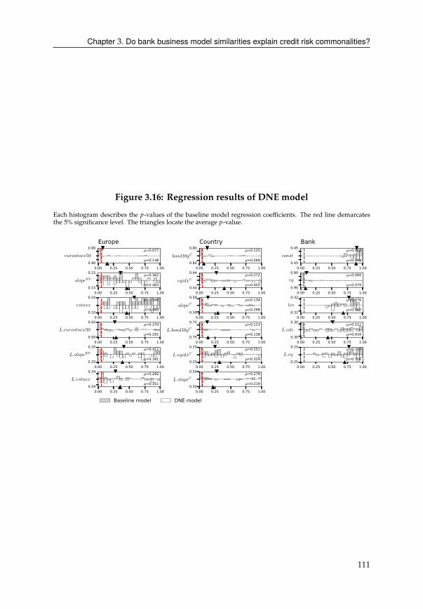
Chapter 3. Do bank business model similarities explain credit risk commonalities?
Figure 3.16: Regression results of DNE model
Each histogram describes the ?-values of the baseline model regression coefficients. The red line demarcates
the 5% significance level. The triangles locate the average ?-value.
0.00 0.25 0.50 0.75 1.00
eurostoxx50=0.077
=0.1480.90
0.90Europe
0.00 0.25 0.50 0.75 1.00
slopeEU=0.362
=0.4630.15
0.15
0.00 0.25 0.50 0.75 1.00
vstoxx=0.580
=0.4600.10
0.10
0.00 0.25 0.50 0.75 1.00
L.eurostoxx50=0.270
=0.2910.50
0.50
0.00 0.25 0.50 0.75 1.00
L.slopeEU=0.412
=0.3910.20
0.20
0.00 0.25 0.50 0.75 1.00
L.vstoxx=0.282
=0.3510.34
0.34
0.00 0.25 0.50 0.75 1.00
bond10yC=0.125
=0.0690.80
0.80Country
0.00 0.25 0.50 0.75 1.00
eqidxC=0.272
=0.4020.44
0.44
0.00 0.25 0.50 0.75 1.00
slopeC=0.134
=0.2980.59
0.59
0.00 0.25 0.50 0.75 1.00
L.bond10yC=0.123
=0.1380.75
0.75
0.00 0.25 0.50 0.75 1.00
L.eqidxC=0.251
=0.3240.25
0.25
0.00 0.25 0.50 0.75 1.00
L.slopeC=0.279
=0.2190.50
0.50
0.00 0.25 0.50 0.75 1.00
const=0.903
=0.8930.45
0.45Bank
0.00 0.25 0.50 0.75 1.00
eq=0.094
=0.0790.90
0.90
0.00 0.25 0.50 0.75 1.00
lev=0.776
=0.6820.32
0.32
0.00 0.25 0.50 0.75 1.00
L.cds=0.512
=0.4340.30
0.30
0.00 0.25 0.50 0.75 1.00
L.eq=0.775
=0.7060.25
0.25
Baseline model DNE model
111

Chapter 3. Do bank business model similarities explain credit risk commonalities?
3.C Residual diagnostics
3.C.1 Network effects model
The left panel of Table 3.7a shows how the average correlation of a bank’s residuals
with all other banks drops from 0.306 to 0.118 while also becoming less dispersed.
On the right panel of Table 3.7a we see a more similar effect for the squared residuals,
dropping from 0.177 to 0.114. In the center, Table 3.7b, we tabulate the test statistics and
?-values of a Ljung-Box test for autocorrelation. The results show that the residuals
become more autocorrelated after including network effects. When we examine the
autocorrelation structure (not shown here) we find that the autoregressive coefficients
become negative or more negative for all banks. At the bottom, Table 3.7c displays
the results of ARCH-LM tests for conditional heteroskedasticity. Different from the
increasing serial autocorrelation, we find less residual clustering for all countries, with
the exception of Spain. Nonetheless, the tests fail to find evidence for ARCH effects
in the same country groups as in the baseline (i.e. Austria, France and Germany).
This suite of tests leads us to conclude that constant network effects mostly affect the
cross-sectional correlations in the residuals.
3.C.2 Dynamic network effects model
TheDNEmodel lowers average (squared) residual correlations (Table 3.7a) further than
the NE model, but the improvements are almost indistinguishable from the constant
case. The tests for serial autocorrelation (Table 3.7b) are qualitatively similar to the NE
model, but the average ?-value indicates that we cannot reject the null hypothesis of
uncorrelated errors on the 10% significance level anymore. We also find that tests for
conditional heteroskedasticity (Table 3.7c) fail to reject the hypothesis of uncorrelat-
edness. The time-variation in the network effects therefore does remove some of the
autocorrelation introduced by the NE model.
112
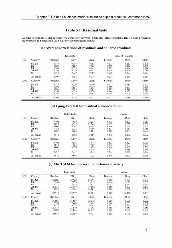
Chapter 3. Do bank business model similarities explain credit risk commonalities?
Table 3.7: Residual tests
Werefer to footnote 17 onpage 92 on the distinction between ‘clean‘ and ‘dirty‘ residuals. The ?-values presentedare averages and cannot be used directly for hypothesis testing.
(a) Average correlations of residuals and squared residuals
Residuals Squared residuals
NE Country Baseline Dirty Clean Baseline Dirty Clean
BE, NL 0.310 0.287 0.103 0.177 0.162 0.106
ES 0.304 0.287 0.122 0.188 0.173 0.131
FR 0.356 0.339 0.161 0.209 0.194 0.124
AT, DE 0.256 0.236 0.081 0.140 0.129 0.098
IT 0.354 0.339 0.160 0.208 0.192 0.123
All banks 0.306 0.288 0.118 0.177 0.163 0.114
DNE Country Baseline Dirty Clean Baseline Dirty Clean
BE, NL 0.310 0.275 0.100 0.177 0.183 0.102
ES 0.304 0.279 0.130 0.188 0.204 0.125
FR 0.356 0.325 0.161 0.209 0.221 0.120
AT, DE 0.256 0.223 0.076 0.140 0.150 0.098
IT 0.354 0.331 0.163 0.208 0.228 0.120
All banks 0.306 0.276 0.117 0.177 0.189 0.111
(b) Ljung-Box test for residual autocorrelation
Test statistic ?-value
NE Country Baseline Dirty Clean Baseline Dirty Clean
BE, NL 0.402 1.970 12.231 0.613 0.171 0.013
ES 0.813 6.910 22.566 0.612 0.015 0.000
FR 0.002 0.787 4.298 0.964 0.566 0.265
AT, DE 1.122 2.277 6.760 0.517 0.261 0.089
IT 0.267 2.268 6.081 0.607 0.233 0.095
All banks 0.614 2.792 10.088 0.645 0.252 0.092
DNE Country Baseline Dirty Clean Baseline Dirty Clean
BE, NL 0.402 0.385 6.148 0.613 0.627 0.049
ES 0.813 1.562 7.370 0.612 0.394 0.009
FR 0.002 0.174 1.475 0.964 0.787 0.360
AT, DE 1.122 1.221 4.329 0.517 0.480 0.135
IT 0.267 0.213 2.012 0.607 0.666 0.192
All banks 0.614 0.803 4.378 0.645 0.572 0.145
(c) ARCH-LM test for residual heteroskedasticty
Test statistic ?-value
NE Country Baseline Dirty Clean Baseline Dirty Clean
BE, NL 36.086 37.160 33.495 0.000 0.001 0.003
ES 17.953 17.773 29.013 0.006 0.022 0.003
FR 3.717 2.838 2.911 0.242 0.291 0.297
AT, DE 21.877 21.070 19.562 0.188 0.193 0.247
IT 40.229 42.161 36.704 0.000 0.000 0.000
All banks 22.948 22.957 23.124 0.105 0.118 0.134
DNE Country Baseline Dirty Clean Baseline Dirty Clean
BE, NL 36.086 35.887 32.742 0.000 0.000 0.002
ES 17.953 17.685 19.469 0.006 0.003 0.057
FR 3.717 6.171 3.143 0.242 0.214 0.347
AT, DE 21.877 21.549 18.787 0.188 0.184 0.289
IT 40.229 37.036 28.540 0.000 0.000 0.000
All banks 22.948 22.769 19.934 0.105 0.098 0.166
113


Chapter 4
Stochastic modeling of food insecurity
4.1 Introduction
“ZeroHunger” is the second of the seventeenUnitedNations Sustainable Development
Goals (SDGs) adopted by all Member States in 2015. Achieving this target by 2030 is
a central challenge as the UN Food and Agricultural Organization (FAO) reports more
than 2 billion people are currently estimated to suffer from hunger or food insecurity
(FAO, 2019). Globally, more than 820 million people are undernourished. About 20%
of those undernourished are located in Africa, in particular the sub-Saharan region,
which has also experienced the fastest rise of malnutrition (FAO, 2019). The topic has
gained renewed attention due to famines in Somalia in 2011-12 and the “four famines”
(Maxwell et al., 2020) that took place in Yemen in 2016 and South Sudan, Somalia, and
northeast Nigeria since 2017. In their recent report, the World Food Programme (WFP)
stresses the additional burden the COVID-19 pandemic imposes on already acutely
food-insecure populations (WFP, 2020). As of the time of writing, the FAO raised a
food crisis warning as locusts swarms are ravaging crops and pasture in east Africa
(FAO, 2020a).
In the fight to eradicate hunger, some major recent developments were made in the
measurement and classification of food insecurity. For instance, the Food Insecurity
Experience Scale (FIES) used in the SDGs distinguishes between three levels of sever-
ity: food security or mild food insecurity, moderate food insecurity, and severe food
insecurity. In the latter stage, people have typically run out of food and have not eaten
for one or more days. Different from this survey-based approach, the Integrated Food
Security Phase Classification (IPC) system was developed to support decision-making
with a clear analytical focus. The Food Security and Nutrition Analysis Unit (FSNAU)
of the FAO pioneered this system in Somalia in 2004. Since then, the IPC framework
has been adopted by various international organization and humanitarian response
115
Chapter 4. Stochastic modeling of food insecurity
agencies. In our study, we rely on IPC data published by the Famine Early Warning
Systems Network (FEWS NET).
The IPC framework is constructed to track and alert international and civil organiza-
tions to food insecurity situations, ultimately aiming to prevent the most extreme case
(famine) at all costs. The IPC scale ranges across five phases of acute food insecurity,
where Phase 1 represents none/minimal and 5 represents catastrophe/famine (see Ta-
ble 4.1). A population enters this phase if, among other criteria, the crude death rate
is at least 2 per 10,000 per day and the under-five death rate is at least 4 per 10,000
per day (IPC Global Partners, 2019). Urgent action is required to avoid populations
reaching Phase 3 or higher. The latest version of the IPC framework 3.0 introduces a
forward-looking “Famine Likely” phase in order to call for urgent action. Nonetheless,
this may already be too late as mortality has already set in and claimed many lives.
The 2011 famine that took place in parts of Somalia remains a lamentable reminder for
the consequences of inaction (Salama et al., 2012).
What distinguishes it from existing approaches is its statistical framework, forward-
looking perspective and stochastic treatment of food insecurity. The rationale behind
our work is fully aligned with that of famine prediction and prevention. The quan-
titative, empirical framework also allows us to identify the most relevant agronomic,
environmental, conflict or economic drivers behind famine dynamics among a vast
set of possible candidates, in a systematic way (Pape et al., 2018). As Lentz et al.
(2019) demonstrate, systematically incorporating such information leads to significant
improvements over existing methods.
A quantitative model also allows analyzing alternative scenarios. Once a model has
been constructed and its parameters estimated, it is possible to explore counterfactual
situations. For instance, one can construct an entire stochastic catalog that assigns
probabilities to events of interest. Quantifying such events has clear benefits fordecision
makers and contingency planners. A particularly attractive feature of a model is the
ability to trace its predictionsback to the individual drivers of famineor the assumptions
made at the outset. This keeps the model transparent and its results interpretable.
Furthermore, if the model incorporates the time-dependent characteristics of famine,
we can use it to obtain probabilistic forecasts several steps ahead. Once again the
benefits for decision makers lie in the ability to explore plausible scenarios and adjust
accordingly.
Food insecurity is a complex problem with multiple causes, several concurrent dy-
namics and catastrophic consequences. A wide range of experts such as human-
itarian organizations, agricultural specialists, geographers, conflict experts, poverty
researchers and economists are involved to tackle this multi-faceted challenge. Region-
and domain-specific knowledge are central to understand the drivers of famine and
116
Chapter 4. Stochastic modeling of food insecurity
predict its likely developments. One of the key features of our proposedmodel is that it
leaves prominent room for expert opinion. This is not only essential for policy makers
to adapt the model to situation-specific conditions. It is particularly important when
facing unprecedented scenarios that are not contained in the data, yet obvious to hu-
man decision-makers. Moreover, expert judgement is necessary to augment the short
recorded famine history. Our model therefore seeks to complement existing efforts in
food insecurity prevention by providing a statistically rigorous foundation.
The relevance of approaches to predict food insecurity and evaluate risks over multiple
timehorizons is likely going to increase in coming years as keydrivers of food insecurity
are expected to worsen into the 21st century. Historical successes in eradicating un-
dernourishment have largely occurred alongside substantial pressure on environments
(Andrée et al., 2019; Stern et al., 1996). Further degrading environments, environmental
change (Ingram et al., 2010; Myers et al., 2017), more frequent weather extremes (Diogo
et al., 2017), desertification (Grainger, 1990), at the backdrop of growing populations,
will continue to put further pressure on the ability of future agricultural systems to
produce and distribute food. These developments will be particularly felt by the rural
poor that rely on local natural assets for food consumption and income (Barbier &
Hochard, 2018; Barrett & Bevis, 2015; Duraiappah, 1998).
The remainder of this paper is structured as follows. Section 4.2 describes the data
used and introduces a convenient transformation to model famine risk distributions.
Section 4.3 introduces the single- and multi-country stochastic models that will be
used in throughout the analysis. Section 4.4 then describes howwe narrow down 1,670
possible predictors and select a relevant set of around 30 predictor variables. Section
4.5 employs the estimated model and selected variables to make expanding one-step
ahead predictions for each point in time. Section 4.6 integrates expert opinion into the
model and demonstrates significant improvements for the case of Afghanistan.
4.2 Data
In our study we rely on the Integrated Phase Classification Acute Food Insecurity (IPC)
framework for the definition of famine risk and food insecurity (see Table 4.1). We
obtain the data from FEWS NET as shown in Figure 4.1. This data is reported on the
first-level administrative country subdivisions (districts).
One of our main innovations is to model food insecurity distributions for a given
country, rather thana single indexmetric.1 Anexample for thiswouldbe the established
IPC framework, which classifies districts in a country based on the IPC stage, the worst
20th percentile of the population finds itself in. For illustration, consider the two
1Such single metrics could be calculated as (weighted) averages, specific quantiles or other index construction
methods that yield in a single metric.
117
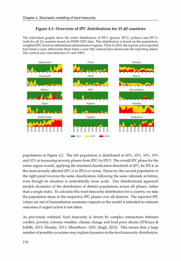
Chapter 4. Stochastic modeling of food insecurity
Figure 4.1: Overview of IPC distributions for 15 all countries
The individual graphs show the entire distribution of IPC1 (green), IPC2, (yellow) and IPC3+
(red) for all 15 countries based on FEWS NET data. This distribution is based on the population-
weighted IPC levels in subnational administrative regions. Prior to 2016, the reportswere reported
four times a year, afterwards three times a year (the vertical lines demarcate the reporting dates).
The vertical axis runs between 0% and 100%.
Afghanistan Chad Ethiopia
Guatemala Haiti Kenya
Malawi Mali Mozambique
Niger Nigeria Somalia
2010
2011
2012
2013
2014
2015
2016
2017
2018
2019
South Sudan
2010
2011
2012
2013
2014
2015
2016
2017
2018
2019
Uganda
IPC1 IPC2 IPC3+
2010
2011
2012
2013
2014
2015
2016
2017
2018
2019
Zimbabwe
populations in Figure 4.2. The left population is distributed as 60%, 10%, 10%, 10%
and 10% in increasing severity phases from IPC1 to IPC5. The overall IPC phase for the
entire region would, applying the standard classification threshold of 20%, be IPC4, as
the most severely affected 20% is in IPC4 or worse. However, the second population in
the right panel receives the same classification, following the same rationale as before,
even though its situation is undoubtedly more acute. Our distributional approach
models dynamics of the distribution of district populations across all phases, rather
than a single index. To calculate this food insecurity distribution for a country, we take
the population share in the respective IPC phases over all districts. The reported IPC
values are net of humanitarian assistance impacts as the model is intended to estimate
outcomes if urgent action is not taken.
As previously outlined, food insecurity is driven by complex interactions between
conflict, poverty, extreme weather, climate change and food price shocks (D’Souza &
Jolliffe, 2013; Headey, 2011; Misselhorn, 2005; Singh, 2012). This means that a large
number of possible covariatesmay explain dynamics in the food insecurity distribution.
118

Chapter 4. Stochastic modeling of food insecurity
Table 4.1: IPC Acute Food Insecurity Phase Descriptions
For more details we refer to IPC 3.0 Area Phase Classification (IPC Global Partners, 2019). The
left-most column describes the classification used in this article. The rationale being that IPC3+
phases are identified as requiring “urgent action” (IPC Global Partners, 2019) and individual high
IPC stages lacking sufficient historical observations.
IPC1 Phase 1 Minimal
Households are able to meet essential food and non-food needs without engaging in
atypical and unsustainable strategies to access food and income.
IPC2 Phase 2 Stressed
Households haveminimally adequate food consumption but are unable to afford some
essential non-food expenditures without engaging in stress-coping strategies.
IPC3+
Phase 3 Crisis
Households either have food consumption gaps that are reflected by high or above-
usual acute malnutrition, OR, are marginally able to meet minimum food needs but
only by depleting essential livelihood assets or through crisis-coping strategies.
Phase 4 Emergency
Households either have large food consumption gaps which are reflected in very high
acute malnutrition and excess mortality, OR, are able to mitigate large food consump-
tion gaps but only by employing emergency livelihood strategies and asset liquidation.
Phase 5 Famine
Households have an extreme lack of food and/or other basic needs even after full
employment of coping strategies. Starvation, death, destitution, and extremely critical
acute malnutrition levels are evident.
Figure 4.2: Hypothetical scenarios leading to IPC4
These two scenarios illustrate how two entirely different situations of food insecurity lead to the
same classification under the 20% rule, where a region or country is classified based on which
IPC classification the 80th-percentile of its population finds itself in. Our framework addresses
this shortcoming by using a compositional transformation and leverages the full distributional
information in the data, thereby accurately reflecting the more detrimental situation in Scenario
2.
IPC1 IPC2 IPC3 IPC4 IPC5
0.00
0.25
0.50
0.75
1.00Scenario 1
IPC1 IPC2 IPC3 IPC4 IPC5
Scenario 2
Threshold (80%)Population share(cumulated)Population share
Agronomic and weather-related variables reflect the agricultural conditions. Histori-
cally, crop failures and fluctuations in crop yields have been a key reason for worsening
food conditions. We use satellite data to calculate stress indicators and anomalies in
vegetation, humidity and soil moisture. To highlight anomalies from historical norms,
we also calculate differences with respect to long-term averages for a particular month.
Closely related are prices of staple food items, whose composition may differ between
countries. We constructed a staple food price index to capture themarket conditions for
food commodities. Volatility in food prices are seen asmajor drivers for food insecurity
(IPC Global Partners, 2019). The treatment of the raw data is discussed by (Andrée
et al., 2020). We obtain food price data from the FAO and the WFP. We additionally
119
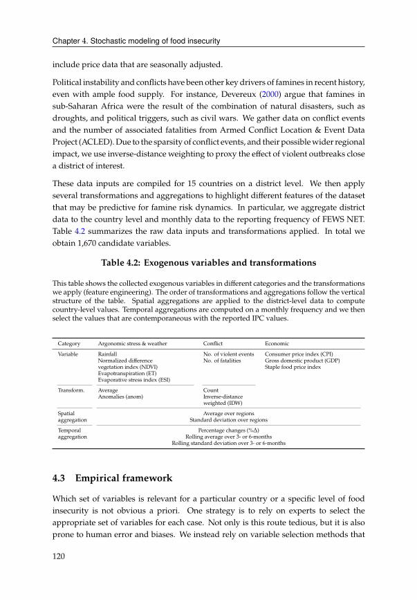
Chapter 4. Stochastic modeling of food insecurity
include price data that are seasonally adjusted.
Political instability and conflicts have been other key drivers of famines in recent history,
even with ample food supply. For instance, Devereux (2000) argue that famines in
sub-Saharan Africa were the result of the combination of natural disasters, such as
droughts, and political triggers, such as civil wars. We gather data on conflict events
and the number of associated fatalities from Armed Conflict Location & Event Data
Project (ACLED).Due to the sparsity of conflict events, and their possiblewider regional
impact, we use inverse-distance weighting to proxy the effect of violent outbreaks close
a district of interest.
These data inputs are compiled for 15 countries on a district level. We then apply
several transformations and aggregations to highlight different features of the dataset
that may be predictive for famine risk dynamics. In particular, we aggregate district
data to the country level and monthly data to the reporting frequency of FEWS NET.
Table 4.2 summarizes the raw data inputs and transformations applied. In total we
obtain 1,670 candidate variables.
Table 4.2: Exogenous variables and transformations
This table shows the collected exogenous variables in different categories and the transformations
we apply (feature engineering). The order of transformations and aggregations follow the vertical
structure of the table. Spatial aggregations are applied to the district-level data to compute
country-level values. Temporal aggregations are computed on a monthly frequency and we then
select the values that are contemporaneous with the reported IPC values.
Category Argonomic stress & weather Conflict Economic
Variable Rainfall No. of violent events Consumer price index (CPI)
Normalized difference No. of fatalities Gross domestic product (GDP)
vegetation index (NDVI) Staple food price index
Evapotranspiration (ET)
Evaporative stress index (ESI)
Transform. Average Count
Anomalies (anom) Inverse-distance
weighted (IDW)
Spatial Average over regions
aggregation Standard deviation over regions
Temporal Percentage changes (%Δ)
aggregation Rolling average over 3- or 6-months
Rolling standard deviation over 3- or 6-months
4.3 Empirical framework
Which set of variables is relevant for a particular country or a specific level of food
insecurity is not obvious a priori. One strategy is to rely on experts to select the
appropriate set of variables for each case. Not only is this route tedious, but it is also
prone to human error and biases. We instead rely on variable selection methods that
120
Chapter 4. Stochastic modeling of food insecurity
have been widely employed in the statistical, economic, medical, andmachine learning
literature. Using these methods, we select the most important drivers of famine risk
for each country and each level of famine risk. The selection process is entirely data
driven and has the explicit goal of avoiding over-fitting. That is, we aim at selecting
variables that are descriptive for historical data but also general enough to extrapolate
their effects.
It is important to emphasize that our framework was not to constructed to supersede
expert opinion. On the contrary, one of the main strengths of our model is the ability
to explicitly and transparently incorporate expert judgements. This is not only nec-
essary due to the shortness of recorded famine history. Augmenting the data with
expert knowledge is a solution that major policy institutions have chosen to over-
come their data challenges, for instance, when calculating macroeconomic forecasts.
Subjective judgements also make it possible to deviate from historical patterns when
unprecedented events are looming on the horizon. Events such as pandemic outbreaks,
conflict situations, or natural disasters have direct consequences on famine risk. These
shocks, immediately obvious to human experts as impactful, would escape a purely
data-driven model. Reserving a channel for such opinions is therefore essential for an
operational model.
4.3.1 Notation
Let -2C = [-1
2C, ..., - :
2C, ..., -
2C] denote a vector containing the population share of
country 2 in different IPC stages. For example, the Scenario 1 of Figure 4.2 would
be represented as -2C = [0.6, 0.1, 0.1, 0.1]>. In this study, we consider = 3, which
corresponds to IPC phases 1,2 and 3+. IPC3+ is the sum of populations in IPC3,4,5 and
represents the population share where urgent action is needed.
4.3.2 A convenient transformation
While modeling the entire distribution -2C provides a holistic picture, we cannot treat
it as a conventional dependent variable in a time-series model. For instance, let -C =
�-C−1+ 4C be a “naive” model with some appropriate autocorrelation matrix �. The
shortcomings of thismodel become evident oncewe consider its predictions -C . First, in
order to qualify as a distribution, the vector elements have to sum up to one,
∑: -
:C= 1.
Second, all elements of -C have to be non-negative. Or in mathematical terms, -C must
lie in a = 3 dimensional unit simplexΔ3. See Figure 4.3 for a graphical representation
of this concept for South Sudan. Neither of these requirements is guaranteed in the
naive model.
To ensure that the predicted values -C lie within the triangle of Figure 4.3, we transform
the constrained food insecurity distribution vector -C into an unconstrained famine risk
121
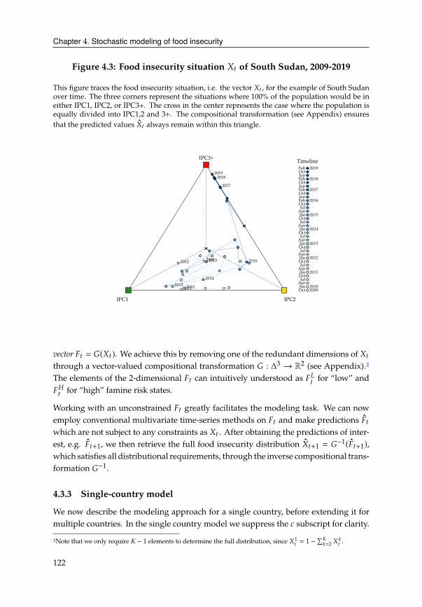
Chapter 4. Stochastic modeling of food insecurity
Figure 4.3: Food insecurity situation -C of South Sudan, 2009-2019
This figure traces the food insecurity situation, i.e. the vector -C , for the example of South Sudan
over time. The three corners represent the situations where 100% of the population would be in
either IPC1, IPC2, or IPC3+. The cross in the center represents the case where the population is
equally divided into IPC1,2 and 3+. The compositional transformation (see Appendix) ensures
that the predicted values -C always remain within this triangle.
IPC1 IPC2
IPC3+
2009
2009Oct 2010 2010Jan
Apr Jul
Oct
2011
2011Jan Apr
Jul Oct 2012
2012Jan Apr
Jul Oct
2013
2013Jan Apr
Jul Oct
2014
2014Jan Apr
Jul Oct
2015
2015Jan Apr
Jul Oct
2016
2016Feb Jun Oct
2017 2017Feb
Jun Oct
2018 2018Feb Jun Oct 2019
2019Feb Timeline
vector �C = �(-C ). We achieve this by removing one of the redundant dimensions of -C
through a vector-valued compositional transformation � : Δ3 → R2(see Appendix).2
The elements of the 2-dimensional �C can intuitively understood as �!Cfor “low” and
��C
for “high” famine risk states.
Working with an unconstrained �C greatly facilitates the modeling task. We can now
employ conventional multivariate time-series methods on �C and make predictions �C
which are not subject to any constraints as -C . After obtaining the predictions of inter-
est, e.g. �C+1, we then retrieve the full food insecurity distribution -C+1
= �−1(�C+1),
which satisfies all distributional requirements, through the inverse compositional trans-
formation �−1.
4.3.3 Single-country model
We now describe the modeling approach for a single country, before extending it for
multiple countries. In the single country model we suppress the 2 subscript for clarity.
2Note that we only require − 1 elements to determine the full distribution, since -1
C = 1 −∑ :=2
- :C .
122
Chapter 4. Stochastic modeling of food insecurity
As can be seen in Figure 4.1, food crises are a rather persistent phenomenon although
we also observe strong heterogeneity between countries. The statistical figures in Table
4.6b corroborate this finding by highlighting the predictive power of preceding data.
Thismotivates us to specify a dynamic framework, where previous values are indicative
for subsequent developments.
�!C = �1 + 0!!�!C−1+ 0!���C−1
+ /1
C �1 + D1
C (4.1)
��C = �2 + 0�!�!C−1+ 0����C−1
+ /2
C �2 + D2
C (4.2)
or in vector notation
�C = � + ��C−1+ /C� + DC (4.3)
This model is a two-dimensional vector autoregression with exogenous variables
(VARX). The autocorrelation matrix � is 2× 2. It is not diagonal, i.e. �!� ≠ 0, ��! ≠ 0,
which reflects the possibility for low famine risk states to transition to high famine
risk states, and vice versa. The errors are bivariate normal DC ∼ #(0,Σ). All exoge-
nous variables are contained in /C and as equations (4.1) and (4.2) show, the set of
relevant variables may differ between high and low food insecurity states, /1
C≠ /2
C.
Consequently, their coefficients can differ as well, �1 ≠ �2.
Ideally, we would be able to estimate the single-country model to tailor its prediction
for each country. As mentioned earlier, this is not feasible due to limitations imposed
by data availability. In Section 4.6 we will demonstrate how single-country models
become feasible once we incorporate expert opinions in a Bayesian framework.
4.3.4 Multi-country model
The single-country model conveys the dynamic framework we stipulate for each coun-
try. However, given the short time series of 34 periods and our interest of famine risk
patterns across countries, we specify a panel extension, i.e. a panel vector autoregres-
sion with exogenous variables (PVARX).
�!2C = �1 + 0!!�!2C−1+ 0!���2C−1
+ /1
C �1
2 + D1
2C (4.4)
��2C = �2 + 0�!�!2C−1+ 0����2C−1
+ /2
C �2
2 + D2
2C (4.5)
or in vector notation,
L C = �# +A# L C−1+ /C� +*C (4.6)
where �# = �# ⊗ � with ⊗ denoting the the Kronecker product and �# is a #-
dimensional vector of ones. Moreover, A# = �# ⊗ �, which implies the same auto-
correlation matrix � across all countries. The bold vector FC denotes a stacked vector
containing each countries famine risk state vector �2C for 2 = 1, ..., # . Correspond-
ingly, the disturbances*C follow amultivariate normal with block-diagonal covariance
matrix �# ⊗ Σ.
123
Chapter 4. Stochastic modeling of food insecurity
4.4 Variable selection
Based on the transformations and aggregations described in Table 4.2 we constructed
a total of 1670 candidate variables. Including all of them would certainly lead to over-
fitting and low external validity of the results. While the literature and the IPC frame-
work itself suggest certain variable types to be included, their exact transformations
remain less obvious. We therefore opt for a statistical variable selection method, also
called feature selection procedure. This is usually done using either L1-regularization
or LASSO regression (Tibshirani, 1996), L2-regularization or Ridge regression (Hoerl
& Kennard, 1970), or a combination thereof, such as the Elastic-Net regression (Zou &
Hastie, 2005), or the adaptive LASSO (Zou, 2006).
These methods all have the common goal of reducing model complexity, but differ in
what is considered complex. The LASSO regression aims at selecting as fewparameters
is possible while the Ridge regression shrinks the parameters towards zero as much
as possible. The benefit of the LASSO lies in the parsimonious nature of the resulting
model and greatly facilitates interpretation of the few resulting parameters. However,
this comes at the cost of possibly discarding variables that still may be relevant (Zou,
2006). The Ridge regression, in contrast, avoids this type of over-discarding variables as
it rarely excludes variables completely. This means the set of active variables remains
stable, but also very large which makes interpretation more ambiguous. We choose
the LASSO regression since our goal is to better understand the drivers behind famine
risk dynamics.
A key technical consideration is the choice of the regularization parameter. This is
usually done either with cross-validation or information criteria. However, the panel
setup of our model is not commonly dealt with in the machine learning or statistical
literature. The panel structure implies additional dependency structures compared to
simple cross-sectional models that are often employed to select genomic markers or
imagery features. The additional time dimension induces temporal dependency which
demands special attention (Bergmeir & Benítez, 2012). Arguably, our validation also
has to account for a spatial dependency component between countries (Roberts et al.,
2017). For instance, areas close to each other are likely to share similar agronomic
conditions and weather variables. This consideration may be relevant for district level
analyses. On the country level this is less relevant as many spatial dependencies are
aggregated out. Moreover, the 15 countries considered are rather dispersed and do not
share many common borders.
It is therefore problematic to rely on conventional best practices for cross-validation
selection (Y. Zhang & Yang, 2015). The results may be strikingly different, depending
on the method chosen. Bergmeir et al. (2018) advocate the use K-fold cross validation
for time series problems. However, their argument for the validity of these approaches
124
Chapter 4. Stochastic modeling of food insecurity
relies on a correct-specification argument which can be met more easily in their non-
parametric context, but becomes unrealistic in our application that uses only a modest
number of parameters to model the data. Moreover, our application is particularly
interested in introducing expert information through the use of priors. Such methods
introduce biases that help improve model performance for certain events, but persist
in the limit and can thus not be reconciled with a correct-specification argument in the
parametric context (Andrée, 2020; Blasques &Duplinskiy, 2018). We therefore opt for a
group K-fold cross-validation which splits the sample into train and testing folds while
accounting for the panel structure.
4.4.1 Selection results
The Tables 4.3 and 4.4 show the selected variables after employing a LASSO regression
for (4.4) and (4.5), separately. In the selection procedurewe excluded the autoregressive
components and the constant, meaningwe always select them. The results are grouped
following the same logic as they were constructed (Table 4.2) and are ordered across
the columns according to the number of monthly lags. In each cell, the vertical bar
separates the (refitted) coefficients from the relative importance of the variables.3 We
do not report standard errors due to the inferential issues following a regularized
regression (Berk et al., 2013; J. D. Lee et al., 2016). For low famine risk states, we select
29 variables and 31 variables for high famine risk states. This number is stable across
randomized subsets of candidate variables.
We can make several interesting observations. In both famine risk states we find that
the autoregressive variables are among the most top five most important features. The
weakly positive serial correlations support our time-dependent model architecture.
The “Model” components account for about a third of overall variable importance in
both cases. We also find evidence that the cross-dependency is asymmetric: Low
famine risk states are more likely to transition to high famine risk states (0�! = 0.201)than vice versa (0!� = 0.097).
For low famine risk states, in Table 4.3, conflict events tend to play a minor role with
10.74% overall importance, while (lagged) agronomic stress indicators account for
38.28%. Interestingly, the two- and six-month lags tend to bemost predictive. Economic
variables contain two of the top five most relevant variables, namely average returns
on staple food prices and the GDP dispersion across districts.
A different pattern emerges for high famine risk states, in Table 4.4. Conflict variables
gain in importance (13.81%) and contain two of the five most relevant variables. For
both conflict and economic variables, the most recent values are also most informative.
3The relative importance is calculated following the Shapely value approach as discussed in Lundberg and Lee
(2017).
125

Chapter 4. Stochastic modeling of food insecurity
Weather and agronomic variables lose in relevance but still account for a third of overall
importance and have a dispersed lag structure.
The plots of Figure 4.4 show the residuals of �!C, ��C
after estimating the PVARX with
the selected variables. We can roughly discern a bi-variate normal distribution from
the contours of the scatter plot. The marginal plots show that while the distributions
are mostly symmetric, they exhibit excess kurtosis compared to the standard normal
distribution. The higher probabilitymass around themean and fatter tails indicate that
Student C-distributions may be a better choice. Nonetheless, we choose the bi-variate
normal distribution for subsequent simulation analyses as it appears to be a reasonable
approximation.
126
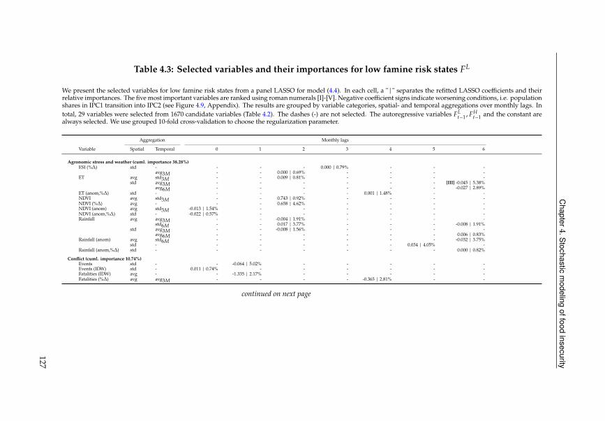
Chapter
4.Stochastic
modeling
offoodinsecurity
Table 4.3: Selected variables and their importances for low famine risk states �!
We present the selected variables for low famine risk states from a panel LASSO for model (4.4). In each cell, a "|" separates the refitted LASSO coefficients and their
relative importances. The fivemost important variables are ranked using roman numerals [I]-[V]. Negative coefficient signs indicate worsening conditions, i.e. population
shares in IPC1 transition into IPC2 (see Figure 4.9, Appendix). The results are grouped by variable categories, spatial- and temporal aggregations over monthly lags. In
total, 29 variables were selected from 1670 candidate variables (Table 4.2). The dashes (-) are not selected. The autoregressive variables �!C−1, ��
C−1and the constant are
always selected. We use grouped 10-fold cross-validation to choose the regularization parameter.
Aggregation Monthly lags
Variable Spatial Temporal 0 1 2 3 4 5 6
Agronomic stress and weather (cuml. importance 38.28%)ESI (%Δ) std - - - - 0.000 | 0.79% - - -
avg3" - - 0.000 | 0.69% - - - -
ET avg std3" - - 0.009 | 0.81% - - - -
std avg3" - - - - - - [III] -0.045 | 5.38%
avg6" - - - - - - -0.027 | 2.89%
ET (anom,%Δ) std - - - - - 0.001 | 1.48% - -
NDVI avg std3" - - 0.743 | 0.92% - - - -
NDVI (%Δ) avg - - - 0.658 | 4.62% - - - -
NDVI (anom) avg std3" -0.013 | 1.54% - - - - - -
NDVI (anom,%Δ) std - -0.022 | 0.57% - - - - - -
Rainfall avg avg3" - - -0.004 | 1.91% - - - -
std6" - - 0.017 | 3.77% - - - -0.008 | 1.91%
std avg3" - - -0.008 | 1.56% - - - -
avg6" - - - - - - 0.006 | 0.83%
Rainfall (anom) avg std6" - - - - - - -0.032 | 3.75%
std - - - - - - 0.034 | 4.05% -
Rainfall (anom,%Δ) std - - - - - - - 0.000 | 0.82%
Conflict (cuml. importance 10.74%)Events std - - -0.064 | 5.02% - - - - -
Events (IDW) std - 0.011 | 0.74% - - - - - -
Fatalities (IDW) avg - - -1.335 | 2.17% - - - - -
Fatalities (%Δ) avg avg3" - - - - -0.365 | 2.81% - -
continued on next page
127
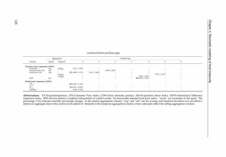
Chapter
4.Stochastic
modeling
offoodinsecurity
continued from previous page
Aggregation Monthly lags
Variable Spatial Temporal 0 1 2 3 4 5 6
Economic (cuml. importance 18.89%)Food price avg std
3" 2.111 | 1.69% - - - - - -
Food price (SA,%Δ) std - - - 4.388 | 2.82% - - - -
Food price (%Δ) avg - [V] -4.089 | 5.11% -2.161 | 2.48% - - - - -
avg3" - - - - - 0.519 | 0.51% -
avg6" - - - - 0.830 | 0.62% - -
GDP std - - - - - [II] 0.000 | 5.66% - -
Model (cuml. importance 32.08%)��C−1
[IV] 0.097 | 5.18% - - - - - -
�!C−1
[I] 0.536 | 26.90% - - - - - -
Constant 0.264 | 0.00% - - - - - -
Abbreviations. ET=Evapotranspiration, CPI=Consumer Price Index, GDP=Gross domestic product, ESI=Evaporative Stress Index, NDVI=Normalized Difference
Vegetation Index. IDW=Inverse-distance weighted interpolation of conflict events. SA=Seasonally-adjusted food price index. “anom” are anomalies to the mean. The
percentage (%Δ) indicates monthly percentage changes. In the spatial aggregation column, “avg” and “std” are the average and standard deviation over all admin-1
districts to aggregate data to the country level (admin-0). Similarly in the temporal aggregation column, where subscripts reflect the rolling aggregation window.
128
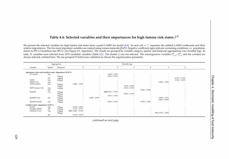
Chapter
4.Stochastic
modeling
offoodinsecurity
Table 4.4: Selected variables and their importances for high famine risk states ��
We present the selected variables for high famine risk states from a panel LASSO for model (4.4). In each cell, a "|" separates the refitted LASSO coefficients and their
relative importances. The fivemost important variables are ranked using roman numerals [I]-[V]. Negative coefficient signs indicate worsening conditions, i.e. population
shares in IPC1,2 transition into IPC3+ (see Figure 4.9, Appendix). The results are grouped by variable category, spatial- and temporal aggregations over monthly lags. In
total, 31 variables were selected from 1670 candidate variables (Table 4.2). The dashes (-) are not selected. The autoregressive variables �!C−1, ��
C−1and the constant are
always selected, omitted here. We use grouped 10-fold cross-validation to choose the regularization parameter.
Aggregation Monthly lags
Variable Spatial Temporal 0 1 2 3 4 5 6
Agronomic stress and weather (cuml. importance 33.21%)ET (anom) avg - - - 0.038 | 2.70% - - - -
avg3" - - 0.010 | 0.59% - - - -
std avg6" - - - - - - -0.107 | 3.19%
NDVI avg std6" - - - - - - -1.341 | 2.22%
NDVI (%Δ) avg - - - - - - 0.482 | 3.50% -
NDVI (anom) avg avg6" 0.006 | 1.25% - - - - - -
std6" - - - 0.015 | 2.09% - - -
NDVI (anom,%Δ) avg avg3" - - - -0.010 | 0.03% - - -
std - - - - - 0.020 | 0.54% - -
Rainfall avg avg3" - - [III] 0.013 | 7.09% - - - -
std3" - - - -0.001 | 0.15% - - -
std6" - - 0.013 | 3.44% - - - -
Rainfall (%Δ) std avg3" - -0.000 | 0.93% - - - 0.000 | 0.51% -
avg6" - - - - - 0.000 | 0.89% -
Rainfall (anom) avg avg6" - - -0.010 | 0.91% - 0.034 | 3.18% - -
Conflict (cuml. importance 13.81%)Events avg std
3" -0.214 | 2.22% - - - - - -
Fatalities (IDW) std avg3" -1.377 | 2.71% - - - - - -
Fatalities (%Δ) avg avg3" [IV] -0.481 | 4.32% - - - - - -
std6" - - - - - [V] -0.702 | 3.96% -
std - -0.162 | 0.60% - - - - - -
continued on next page
129
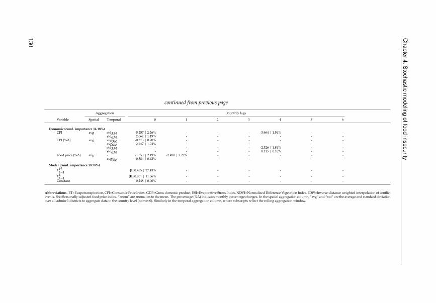
Chapter
4.Stochastic
modeling
offoodinsecurity
continued from previous page
Aggregation Monthly lags
Variable Spatial Temporal 0 1 2 3 4 5 6
Economic (cuml. importance 14.18%)CPI avg std
3" -5.257 | 2.26% - - - -3.964 | 1.54% - -
std6" 2.062 | 1.19% - - - - - -
CPI (%Δ) avg avg3" -0.313 | 0.20% - - - - - -
avg6" -2.247 | 1.24% - - - - - -
std3" - - - - -2.326 | 1.84% - -
std6" - - - - 0.115 | 0.10% - -
Food price (%Δ) avg - -1.553 | 2.19% -2.490 | 3.22% - - - - -
avg3" -0.384 | 0.42% - - - - - -
Model (cuml. importance 38.78%)��C−1
[I] 0.455 | 27.43% - - - - - -
�!C−1
[II] 0.201 | 11.36% - - - - - -
Constant 0.248 | 0.00% - - - - - -
Abbreviations. ET=Evapotranspiration, CPI=Consumer Price Index, GDP=Gross domestic product, ESI=Evaporative Stress Index, NDVI=Normalized Difference Vegetation Index. IDW=Inverse-distance weighted interpolation of conflict
events. SA=Seasonally-adjusted food price index. “anom” are anomalies to the mean. The percentage (%Δ) indicates monthly percentage changes. In the spatial aggregation column, “avg” and “std” are the average and standard deviation
over all admin-1 districts to aggregate data to the country level (admin-0). Similarly in the temporal aggregation column, where subscripts reflect the rolling aggregation window.
130
Chapter 4. Stochastic modeling of food insecurity
4.5 Forecasting
Using the selected variables and estimated model parameters we now demonstrate
the model’s prediction performance. At each point in time we calculate the one-step
ahead prediction and compare it to the famine risk distribution of the next FEWS NET
release. This imitates the situation of policy makers, who decide based on the available
information. Let I) denote all information since the beginning of recorded famine
history in October 2009 until the hypothetical decision date ). Then the one-step ahead
prediction is defined as
-)+1|) := E[-)+1|I) ]
In order to avoid incorporating future information in the one-step ahead predictions,
whichwould not have been available, we estimate themodel only using the information
until ) and then make a forecast for -)+1|) . We then re-estimate the model with
information until ) + 1 and make a forecast for -)+2|)+1. The minimal observation
period is at least ) = 15 such that there is sufficient information to fit the model.
We note, however, that the set of selected variables in Tables 4.3, 4.4 are taken as
given. Unquestionably, the selection relies on the full sample and therefore on future
information. Nonetheless, we decided against re-selecting the variables at each point
in time to avoid model instability.
The results of the rolling forecasts using 1,000 hypothetical draws are shown in Figure
4.6 and associated accuracy in Table 4.5. We can see that the model is more accurate
for higher IPC phases for almost all countries. The predictions are within the 50%
confidence interval in the majority of cases. Lower IPC stages are associated with
lower precision and broader confidence intervals. Interestingly, the model performs
well in terms of predicting the correct direction of IPC3+ dynamics, for instance, in
Afghanistan, Chad, Malawi, Mozambique, Zimbabwe.
131
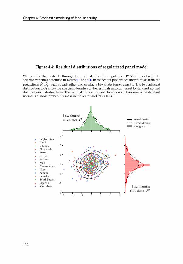
Chapter 4. Stochastic modeling of food insecurity
Figure 4.4: Residual distributions of regularized panel model
We examine the model fit through the residuals from the regularized PVARX model with the
selected variables described in Tables 4.3 and 4.4. In the scatter plot, we see the residuals from the
predictions �!C , ��C against each other and overlay a bi-variate kernel density. The two adjacent
distribution plots show the marginal densities of the residuals and compare it to standard normal
distributions in dashed lines. The residual distributions exhibit excess kurtosis versus the standard
normal, i.e. more probability mass in the center and fatter tails.
3 2 1 0 1 2 33
2
1
0
1
2
3AfghanistanChadEthiopiaGuatemalaHaitiKenyaMalawiMaliMozambiqueNigerNigeriaSomaliaSouth SudanUgandaZimbabwe
Low faminerisk states, FL
High faminerisk states, FH
Kernel densityNormal densityHistogram
132
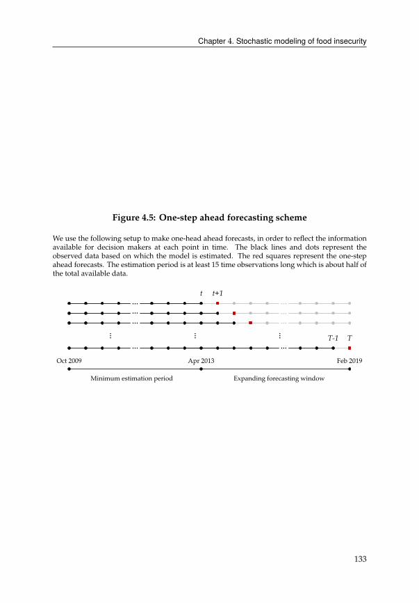
Chapter 4. Stochastic modeling of food insecurity
Figure 4.5: One-step ahead forecasting scheme
We use the following setup to make one-head ahead forecasts, in order to reflect the information
available for decision makers at each point in time. The black lines and dots represent the
observed data based on which the model is estimated. The red squares represent the one-step
ahead forecasts. The estimation period is at least 15 time observations long which is about half of
the total available data.
Apr 2013 Feb 2019
………
Oct 2009
t t+1
T-1 T
… …
Minimum estimation period Expanding forecasting window
…
………
… …
133
Chapter 4. Stochastic modeling of food insecurity
4.6 Expert opinion
One of the main challenges in this exercise lies in the scarcity of data. The short
time series imposes difficulties for the identification of model parameters, in partic-
ular for the autoregression matrix � in (4.3). Several remedy options are possible.
First, one can impose additional model structure, such as moving averages, additional
lags, nonlinear dependencies or fat-tailed distributions. However, this quickly leads to
over-parameterization and comes at the cost of tractability. Second, one can engineer
additional features and expand the set of exogenous variables. While there is merit
to this approach, we believe that the current set of 1670 explanatory variables is suf-
ficiently complete. Furthermore, more regressors only help marginally in identifying
the autocorrelation matrix �. We follow a third approach involving expert opinion.
A similar problem plagues policymakers and regulatory institutions when making
macroeconomic forecasts. GDPfigures andothermacroeconomic indicators areusually
available only on annual or quarterly frequencies. Even in advanced economies the lack
of data presents a major bottleneck for empirical analyses. Major policy institutions
such as the International Monetary Fund (Ciccarelli & Rebucci, 2003), the Federal
Reserve (Carriero et al., 2011) or the European Central Bank (Bańbura et al., 2008) have
dealt with this problem by augmenting their forecasting models with expert opinion
(Giannone et al., 2019; Litterman, 1986; Sims&Zha, 1998). Theirmodels are comparable
to our VARX model in (4.3).
Expert opinion can be used to make direct forecasts through surveys and expert panels
about the development or trend in subsequent periods. Yet, decision-makers prefer
to understand the empirical evidence leading up to a certain prediction or outcome.
Hence, we advocate a framework where expert opinion is not a substitute but a com-
plement to the statistical model. Similar to the approach of the aforementioned policy
institutions, we inject the subjective judgments into the model itself. This is different
from a purely data-driven approach which starts off agnostically and estimates its pa-
rameters entirely from the data. While this can be argued to be the most objective
way to conduct empirical investigations, we also run the risk of over-fitting to the short
dataset and are effectively handicapping ourselves, since we are not incorporating rel-
evant, prior information. Specifically, certain country groups are structurally different
from others, for instance, South Sudan, Somalia or Yemen are known to be fragile while
countries like Uganda or Mali have more stable food security situations (Figure 4.1).
Moreover, low food insecurity stages tend to be persistent while high food insecurity
stages tend to be more volatile (Table 4.6a and 4.6b). This information can ideally be
learned by the model itself but requires sufficient historical cases to learn from. Not
only is this condition not met in our case, it is also important to have representative and
134
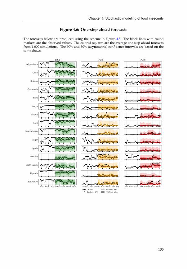
Chapter 4. Stochastic modeling of food insecurity
Figure 4.6: One-step ahead forecasts
The forecasts below are produced using the scheme in Figure 4.5. The black lines with round
markers are the observed values. The colored squares are the average one-step ahead forecasts
from 1,000 simulations. The 90% and 50% (asymmetric) confidence intervals are based on the
same draws.
Afghanistan
IPC1 IPC2 IPC3+
Chad
Ethiopia
Guatemala
Haiti
Kenya
Malawi
Mali
Mozambique
Niger
Nigeria
Somalia
South Sudan
Uganda
2010 2011 2012 2013 2014 2015 2016 2017 2018 2019
Zimbabwe
2010 2011 2012 2013 2014 2015 2016 2017 2018 2019
True IPCPredicted IPC
90% Conf. Intvl.50% Conf. Intvl.
2010 2011 2012 2013 2014 2015 2016 2017 2018 2019
135
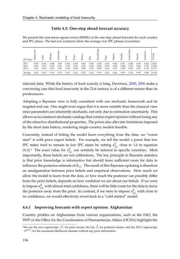
Chapter 4. Stochastic modeling of food insecurity
Table 4.5: One-step ahead forecast accuracy
We present the root-mean-square errors (RMSE) of the one-step ahead forecasts for each country
and IPC phase. The last row (column) show the average over IPC phases (countries).
IPC Phase Afghanistan
Chad
Ethiopia
Guatemala
Haiti
Kenya
Malawi
Mali
Mozambique
Niger
Nigeria
Somalia
SouthSudan
Uganda
Zimbabwe
Average
IPC1 0.307 0.294 0.188 0.247 0.256 0.203 0.269 0.238 0.229 0.321 0.366 0.241 0.258 0.278 0.224 0.261
IPC2 0.274 0.191 0.120 0.191 0.179 0.110 0.241 0.169 0.180 0.215 0.227 0.348 0.174 0.204 0.179 0.200
IPC3+ 0.107 0.125 0.123 0.073 0.108 0.109 0.249 0.079 0.085 0.126 0.147 0.188 0.258 0.079 0.198 0.137
Average 0.229 0.203 0.144 0.170 0.181 0.141 0.253 0.162 0.165 0.221 0.246 0.259 0.230 0.187 0.200 0.199
relevant data: While the history of food scarcity is long, Devereux, 2000, 2006 make a
convincing case that food insecurity in the 21st century is of a different nature than its
predecessors.
Adopting a Bayesian view is fully consistent with our stochastic framework and its
targeted end use. One might even argue that it is more suitable than the classical view
since parameters are inherently stochastic, not only due to estimation uncertainty. This
allows us to construct stochastic catalogs that contain expert opinionwithout losing any
of the attractive distributional properties. The priors also alleviate limitations imposed
by the short data history, rendering single-country models feasible.
Concretely, instead of letting the model learn everything from the data, we “warm
start” it with prior expert beliefs. For example, we tell the model a priori that low
IPC states tend to remain in low IPC states by setting 00
!!close to 1.0 in equation
(4.3).4 The exact value for 00
!!can certainly be tailored to specific countries. Most
importantly, these beliefs are not calibrations. The key principle in Bayesian statistics
is that prior knowledge is informative but should leave sufficient room for data to
influence the posterior estimate of 0!!. The result of this Bayesian updating is therefore
an amalgamation between prior beliefs and empirical observations. How much we
allow the model to learn from the data, or how much the posterior can possibly differ
from the prior beliefs, depends on how confident we are about our beliefs. If we were
to impose 00
!!with almost total confidence, therewill be little room for the data tomove
the posterior away from the prior. In contrast, if we were to impose 00
!!with close to
no confidence, we would effectively revert back to a “cold started” model.
4.6.1 Improving forecasts with expert opinion: Afghanistan
Country profiles on Afghanistan from various organizations, such as the FAO, the
WFP or the Office for the Coordination of Humanitarian Affairs (OCHA) highlight the
4We use the zero superscript, �0, for prior means, the hat, �, for posterior means, and the "!� superscript,
�"!�, for the maximum likelihood estimate without any prior information.
136
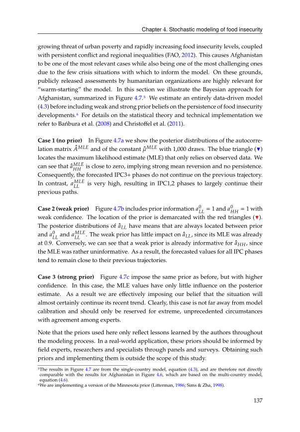
Chapter 4. Stochastic modeling of food insecurity
growing threat of urban poverty and rapidly increasing food insecurity levels, coupled
with persistent conflict and regional inequalities (FAO, 2012). This causes Afghanistan
to be one of the most relevant cases while also being one of the most challenging ones
due to the few crisis situations with which to inform the model. On these grounds,
publicly released assessments by humanitarian organizations are highly relevant for
“warm-starting” the model. In this section we illustrate the Bayesian approach for
Afghanistan, summarized in Figure 4.7.5 We estimate an entirely data-driven model
(4.3) before includingweak and strong prior beliefs on the persistence of food insecurity
developments.6 For details on the statistical theory and technical implementation we
refer to Bańbura et al. (2008) and Christoffel et al. (2011).
Case 1 (no prior) In Figure 4.7a we show the posterior distributions of the autocorre-
lation matrix �"!�and of the constant �"!�
with 1,000 draws. The blue triangle (H)
locates the maximum likelihood estimate (MLE) that only relies on observed data. We
can see that 0"!���
is close to zero, implying strong mean reversion and no persistence.
Consequently, the forecasted IPC3+ phases do not continue on the previous trajectory.
In contrast, 0"!�!!
is very high, resulting in IPC1,2 phases to largely continue their
previous paths.
Case 2 (weak prior) Figure 4.7b includes prior information 00
!!= 1 and 00
��= 1 with
weak confidence. The location of the prior is demarcated with the red triangles (H).
The posterior distributions of 0!! have means that are always located between prior
and 00
!!and 0"!�
!!. The weak prior has little impact on 0!!, since its MLE was already
at 0.9. Conversely, we can see that a weak prior is already informative for 0�� , since
theMLEwas rather uninformative. As a result, the forecasted values for all IPC phases
tend to remain close to their previous trajectories.
Case 3 (strong prior) Figure 4.7c impose the same prior as before, but with higher
confidence. In this case, the MLE values have only little influence on the posterior
estimate. As a result we are effectively imposing our belief that the situation will
almost certainly continue its recent trend. Clearly, this case is not far away from model
calibration and should only be reserved for extreme, unprecedented circumstances
with agreement among experts.
Note that the priors used here only reflect lessons learned by the authors throughout
the modeling process. In a real-world application, these priors should be informed by
field experts, researchers and specialists through panels and surveys. Obtaining such
priors and implementing them is outside the scope of this study.
5The results in Figure 4.7 are from the single-country model, equation (4.3), and are therefore not directly
comparable with the results for Afghanistan in Figure 4.6, which are based on the multi-country model,
equation (4.6).
6We are implementing a version of the Minnesota prior (Litterman, 1986; Sims & Zha, 1998).
137

Chapter 4. Stochastic modeling of food insecurity
4.6.2 Exceedance probability (EP) curves
For financial applications, particularly for risk management and cost-benefit analyses,
EP curves allow us to derive useful risk metrics. We leverage our stochastic framework
to calculate the probability of exceeding specific population (share) thresholds under
distress. Figure 4.8 illustrates this concept for total population and population share in
IPC3+ in each country. It shows the results of 10,000 simulations from the stochastic
model for 2020, 2021 and 2022.
We can see how EP curves help us distinguish between risk profiles across countries
and forecast horizons. For instance, in the short-term, Zimbabwe is at highest risk
among all countries considered. At the other end of the spectrum, Uganda and Kenya
are comparatively unaffected by food insecurity risks. For longer-term predictions,
these extreme curves tend to vanish. This is due to the uncertainty surrounding the
dynamic predictions, which increases with the forecast horizon.
138
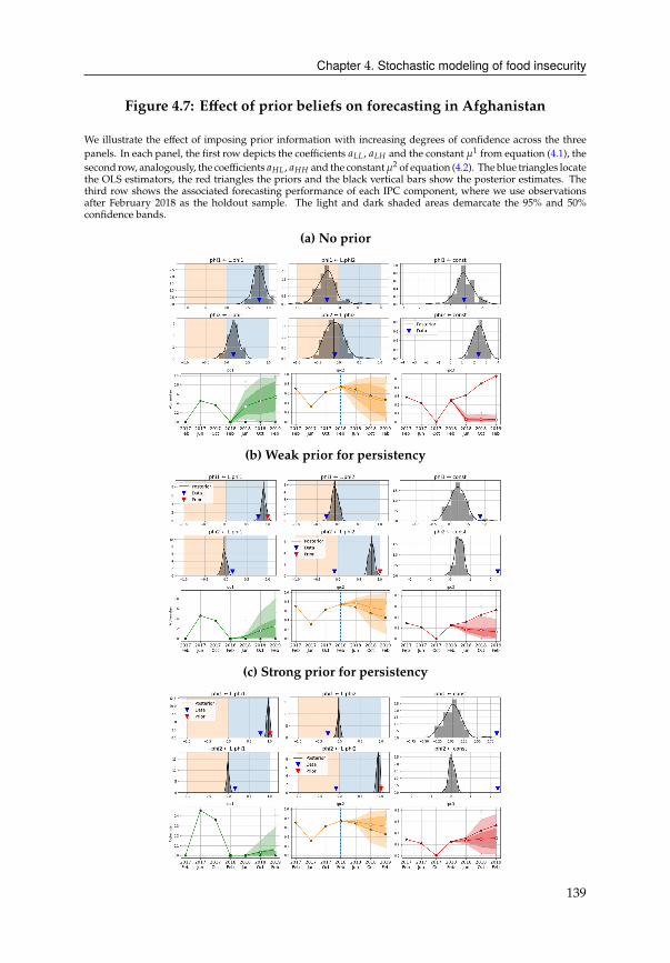
Chapter 4. Stochastic modeling of food insecurity
Figure 4.7: Effect of prior beliefs on forecasting in Afghanistan
We illustrate the effect of imposing prior information with increasing degrees of confidence across the three
panels. In each panel, the first row depicts the coefficients 0!! , 0!� and the constant �1from equation (4.1), the
second row, analogously, the coefficients 0�! , 0�� and the constant�2of equation (4.2). The blue triangles locate
the OLS estimators, the red triangles the priors and the black vertical bars show the posterior estimates. The
third row shows the associated forecasting performance of each IPC component, where we use observations
after February 2018 as the holdout sample. The light and dark shaded areas demarcate the 95% and 50%
confidence bands.
(a) No prior
(b) Weak prior for persistency
(c) Strong prior for persistency
139
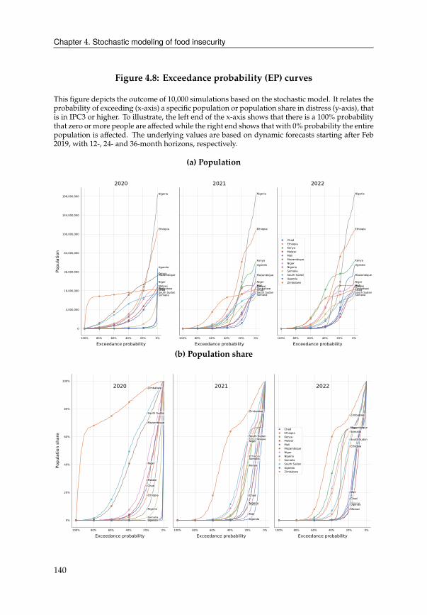
Chapter 4. Stochastic modeling of food insecurity
Figure 4.8: Exceedance probability (EP) curves
This figure depicts the outcome of 10,000 simulations based on the stochastic model. It relates the
probability of exceeding (x-axis) a specific population or population share in distress (y-axis), that
is in IPC3 or higher. To illustrate, the left end of the x-axis shows that there is a 100% probability
that zero or more people are affectedwhile the right end shows that with 0% probability the entire
population is affected. The underlying values are based on dynamic forecasts starting after Feb
2019, with 12-, 24- and 36-month horizons, respectively.
(a) Population
100% 80% 60% 40% 20% 0%
Exceedance probability
0
4,000,000
16,000,000
36,000,000
64,000,000
100,000,000
144,000,000
196,000,000
Popu
latio
n
Chad
Ethiopia
Kenya
Malawi Mali
Mozambique
Niger
Nigeria
Somalia South Sudan
Uganda
Zimbabwe
2020
100% 80% 60% 40% 20% 0%
Exceedance probability
Chad
Ethiopia
Kenya
Malawi Mali
Mozambique
Niger
Nigeria
Somalia South Sudan
Uganda
Zimbabwe
2021
100% 80% 60% 40% 20% 0%
Exceedance probability
Chad
Ethiopia
Kenya
Malawi Mali
Mozambique
Niger
Nigeria
Somalia South Sudan
Uganda
Zimbabwe
2022
ChadEthiopiaKenyaMalawiMaliMozambiqueNigerNigeriaSomaliaSouth SudanUgandaZimbabwe
(b) Population share
100% 80% 60% 40% 20% 0%
Exceedance probability
0%
20%
40%
60%
80%
100%
Popu
latio
n sh
are
Chad
Ethiopia
Kenya
Malawi
Mali
Mozambique
Niger
Nigeria
Somalia
South Sudan
Uganda
Zimbabwe2020
100% 80% 60% 40% 20% 0%
Exceedance probability
Chad
Ethiopia
Kenya
Malawi
Mali
Mozambique Niger
Nigeria
Somalia
South Sudan
Uganda
Zimbabwe
2021
100% 80% 60% 40% 20% 0%
Exceedance probability
Chad
Ethiopia
Kenya
Malawi
Mali
Mozambique Niger
Nigeria
Somalia
South Sudan
Uganda
Zimbabwe
2022
ChadEthiopiaKenyaMalawiMaliMozambiqueNigerNigeriaSomaliaSouth SudanUgandaZimbabwe
140
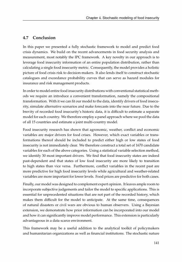
Chapter 4. Stochastic modeling of food insecurity
4.7 Conclusion
In this paper we presented a fully stochastic framework to model and predict food
crisis dynamics. We build on the recent advancements in food security analysis and
measurement, most notably the IPC framework. A key novelty in our approach is to
leverage food insecurity information of an entire population distribution, rather than
calculating a single food insecurity metric. Consequently, the model provides a holistic
picture of food crisis risk to decision-makers. It also lends itself to construct stochastic
catalogues and exceedance probability curves that can serve as hazard modules for
insurance and risk management products.
In order tomodel entire food insecurity distributionswith conventional statisticalmeth-
ods we require an introduce a convenient transformation, namely the compositional
transformation. With it we can fit ourmodel to the data, identify drivers of food insecu-
rity, simulate alternative scenarios and make forecasts into the near future. Due to the
brevity of recorded food insecurity’s historic data, it is difficult to estimate a separate
model for each country. We therefore employ a panel approachwhere we pool the data
of all 15 countries and estimate a joint multi-country model.
Food insecurity research has shown that agronomic, weather, conflict and economic
variables are major drivers for food crises. However, which exact variables or trans-
formations thereof should be included to predict either high or low states of food
insecurity is not immediately clear. We therefore construct a total set of 1670 candidate
variables for each of the above categories. Using a statistical variable selection method,
we identify 30 most important drivers. We find that food insecurity states are indeed
past-dependent and that states of low food insecurity are more likely to transition
to high states than vice versa. Furthermore, conflict variables in the recent past are
more predictive for high food insecurity levels while agricultural and weather-related
variables are more important for lower levels. Food prices are predictive for both cases.
Finally, ourmodelwas designed to complement expert opinion. It leaves ample room to
incorporate subjective judgements and tailor the model to specific applications. This is
essential for unprecedented situations that are not part of the recorded history, which
makes them difficult for the model to anticipate. At the same time, consequences
of natural disasters or civil wars are obvious to human observers. Using a Bayesian
extension, we demonstrate how prior information can be incorporated into our model
and how it can significantly improvemodel performance. This extension is particularly
advantageous in a data scarce environment.
This framework may be a useful addition to the analytical toolkit of policymakers
and humanitarian organizations as well as financial institutions. The stochastic nature
141

Chapter 4. Stochastic modeling of food insecurity
could be particularly attractive for financial triggering decisions, scenario analyses or
other risk assessments. While it is well-suited for short- to medium term predictions,
application-specific adjustments and extensions are necessary for forecasts further into
the future. We especially advise to pay careful attention to the variable selection step.
142
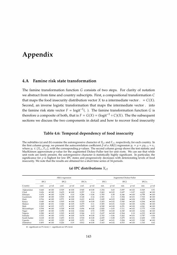
Appendix
4.A Famine risk state transformation
The famine transformation function � consists of two steps. For clarity of notation
we abstract from time and country subscripts. First, a compositional transformation �
that maps the food insecurity distribution vector - to a intermediate vector . = �(-).Second, an inverse logistic transformation that maps the intermediate vector . into
the famine risk state vector � = logit−1(.). The famine transformation function � is
therefore a composite of both, that is � = �(-) = (logit−1 ◦ �)(-). The the subsequentsections we discuss the two components in detail and how to recover food insecurity
Table 4.6: Temporal dependency of food insecurity
The subtables (a) and (b) examine the autoregressive character of -2C and �2C , respectively, for each country. In
the first column group, we present the autocorrelation coefficient � of a AR(1) regression HC = � + �HC−1 + 4C ,where HC ∈ {-2C , �2C }, with the corresponding p-values. The second column group shows the test statistic and
MacKinnon approximate p-value for the augmented Dickey-Fuller test for unit roots. We can see that while
unit roots are rarely present, the autoregressive character is statistically highly significant. In particular, the
significance for � is highest for low IPC states and progressively decreases with deteriorating levels of food
insecurity. We note that the results are obtained for a short time series of 34 periods.
(a) IPC distributions -2C
AR(1) regression Augmented Dickey-Fuller
IPC1 IPC2 IPC3+ IPC1 IPC2 IPC3+
Country coef. p-val coef. p-val coef. p-val stat. p-val stat. p-val stat. p-val
Afghanistan 0.660 • 0.00 0.529 • 0.00 0.945 • 0.00 -1.254 0.65 -3.097 • 0.02 -0.369 0.91
Chad 0.626 • 0.00 0.635 • 0.00 0.257 0.14 -3.063 • 0.02 -2.697 ◦ 0.07 -4.622 • 0.00Ethiopia 0.674 • 0.00 0.278 0.10 0.286 ◦ 0.06 -1.783 0.38 -4.346 • 0.00 -4.758 • 0.00Guatemala 0.509 • 0.00 0.503 • 0.00 0.168 0.14 -2.501 0.11 -3.304 • 0.01 -7.510 • 0.00Haiti 0.516 • 0.00 0.571 • 0.00 0.412 • 0.01 -3.045 • 0.03 -2.868 • 0.04 -3.559 • 0.00Kenya 0.640 • 0.00 0.505 • 0.00 0.520 • 0.00 -3.203 • 0.02 -3.545 • 0.00 -4.304 • 0.00Malawi 0.428 • 0.01 0.360 • 0.05 0.279 0.11 -3.305 • 0.01 -3.618 • 0.00 -4.296 • 0.00Mali 0.363 • 0.03 0.371 • 0.03 0.079 0.65 -4.549 • 0.00 -4.251 • 0.00 -4.941 • 0.00Mozambique 0.594 • 0.00 0.528 • 0.00 0.694 • 0.00 -2.820 ◦ 0.05 -3.111 • 0.02 -2.775 ◦ 0.06Niger 0.499 • 0.00 0.350 • 0.02 -0.062 0.72 -3.595 • 0.00 -4.345 • 0.00 -6.016 • 0.00Nigeria 0.280 • 0.03 0.303 • 0.02 0.264 0.13 -5.637 • 0.00 -2.564 0.10 -4.323 • 0.00Somalia 0.533 • 0.00 0.552 • 0.00 0.678 • 0.00 -2.765 ◦ 0.06 -3.262 • 0.01 -2.787 ◦ 0.06South Sudan 0.618 • 0.00 0.453 • 0.01 0.918 • 0.00 -2.655 ◦ 0.08 -3.275 • 0.01 -0.430 0.90
Uganda 0.511 • 0.00 0.523 • 0.00 0.271 ◦ 0.06 -3.407 • 0.01 -3.204 • 0.02 -5.242 • 0.00Zimbabwe 0.493 • 0.00 0.226 0.19 0.812 • 0.00 -3.163 • 0.02 -4.515 • 0.00 -1.310 0.62
• : significant on 5% level, ◦ : significant on 10% level.
143
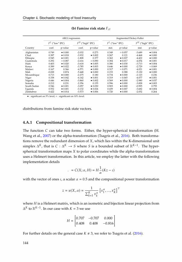
Chapter 4. Stochastic modeling of food insecurity
(b) Famine risk state �2C
AR(1) regression Augmented Dickey-Fuller
�! (“low” IPC) �� (“high” IPC) �! (“low” IPC) �� (“high” IPC)
Country coef. p-value coef. p-value stat. p-value stat. p-value
Afghanistan 0.749 • 0.000 -2.032 0.273 0.349 ◦ 0.057 -3.689 • 0.004Chad 0.387 • 0.018 -3.932 • 0.002 0.267 0.121 -4.468 • 0.000Ethiopia 0.545 • 0.001 -1.808 0.377 0.362 • 0.027 -4.422 • 0.000Guatemala 0.292 ◦ 0.087 -2.616 ◦ 0.090 0.384 • 0.017 -4.054 • 0.001Haiti 0.403 • 0.020 -3.618 • 0.005 0.380 • 0.030 -3.713 • 0.004Kenya 0.389 • 0.022 -3.785 • 0.003 0.646 • 0.000 -2.729 ◦ 0.069Malawi 0.167 0.366 -4.571 • 0.000 0.317 ◦ 0.071 -4.021 • 0.001Mali -0.028 0.874 -5.448 • 0.000 0.153 0.388 -5.130 • 0.000Mozambique 0.713 • 0.000 -2.275 0.180 0.734 • 0.000 -2.123 0.236
Niger 0.338 • 0.042 -4.142 • 0.001 0.319 ◦ 0.065 -4.077 • 0.001Nigeria 0.446 • 0.004 -3.860 • 0.002 0.569 • 0.000 -2.980 • 0.037Somalia 0.212 0.231 -2.356 0.155 0.596 • 0.000 -3.828 • 0.003South Sudan 0.546 • 0.001 -3.057 • 0.030 0.903 • 0.000 -0.995 0.755
Uganda 0.552 • 0.001 -3.132 • 0.024 0.439 • 0.007 -3.682 • 0.004Zimbabwe 0.422 • 0.014 -3.573 • 0.006 0.720 • 0.000 -2.052 0.264
• : significant on 5% level, ◦ : significant on 10% level.
distributions from famine risk state vectors.
4.A.1 Compositional transformation
The function � can take two forms. Either, the hyper-spherical transformation (H.
Wang et al., 2007) or the alpha-transformation (Tsagris et al., 2016). Both transforma-
tions remove the redundant dimension of -, which lies within the K-dimensional unit
simplex Δ , that is � : Δ → ( where ( is a bounded subset of R −1. The hyper-
spherical transformation maps - to polar coordinates while the alpha-transformation
uses a Helmert transformation. In this article, we employ the latter with the following
implementation details
. = �(-; , �) = � 1
( I − �)
with the vector of ones �, a scalar = 0.5 and the compositional power transformation
I = D(-, ) = 1∑ :=1
G :
[G
1, ..., G
]>where � is a Helmert matrix, which is an isometric and bijection linear projection from
Δ to R −1. In our case with = 3 we use
� =
[0.707 −0.707 0.000
0.408 0.408 −0.816
]For further details on the general case ≠ 3, we refer to Tsagris et al. (2016).
144
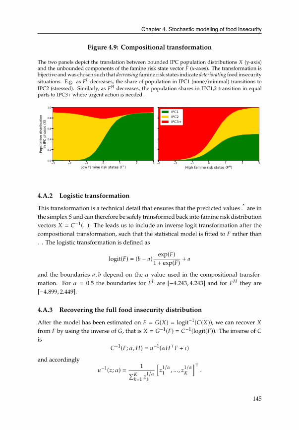
Chapter 4. Stochastic modeling of food insecurity
Figure 4.9: Compositional transformation
The two panels depict the translation between bounded IPC population distributions - (y-axis)
and the unbounded components of the famine risk state vector � (x-axes). The transformation is
bijective andwas chosen such that decreasing famine risk states indicate deteriorating food insecurity
situations. E.g. as �! decreases, the share of population in IPC1 (none/minimal) transitions to
IPC2 (stressed). Similarly, as �� decreases, the population shares in IPC1,2 transition in equal
parts to IPC3+ where urgent action is needed.
3 2 1 0 1 2 3Low famine risk states (FL)
0.0
0.2
0.4
0.6
0.8
1.0
Popu
latio
n di
strib
utio
nin
IPC
phas
es (X
)
3 2 1 0 1 2 3High famine risk states (FH)
IPC1IPC2IPC3+
4.A.2 Logistic transformation
This transformation is a technical detail that ensures that the predicted values . are in
the simplex ( and can therefore be safely transformed back into famine risk distribution
vectors - = �−1(.). The leads us to include an inverse logit transformation after the
compositional transformation, such that the statistical model is fitted to � rather than
.. The logistic transformation is defined as
logit(�) = (1 − 0)exp(�)
1 + exp(�) + 0
and the boundaries 0, 1 depend on the value used in the compositional transfor-
mation. For = 0.5 the boundaries for �! are [−4.243, 4.243] and for �� they are
[−4.899, 2.449].
4.A.3 Recovering the full food insecurity distribution
After the model has been estimated on � = �(-) = logit−1(�(-)), we can recover -
from � by using the inverse of �, that is - = �−1(�) = �−1(logit(�)). The inverse of �is
�−1(�; , �) = D−1( �>� + �)
and accordingly
D−1(I; ) = 1∑ :=1
I1/ :
[I
1/ 1
, ..., I1/
]>.
145


Chapter 5
Natural capital and sovereign bonds
5.1 Introduction
Environmental risks have become a key discussion point in the financial world. High-
profile financial and political institutions have recognized the risks posed by climate
change and the associated loss of natural capital. TheBank for International Settlements
published a report on climate change and financial stability (Bolton et al., 2020), the
Financial Stability Board’s Task Force on Climate-related Financial Disclosures and
the European Commission’s EU Taxonomy provided regulatory frameworks to bring
more transparency into reporting. Identifying the transmission channels between
environmental risks and financial stability, and quantifying the exposure of financial
institutions are the first and second items on the research priority list of Network for
Greening the Financial System (NGFS, 2020a, 2020b). In this context, it is surprising
that fixed-income instruments have received comparatively little attention (Inderst &
Stewart, 2018), despite the colossal size of global bond market of US$ 102.8 trillion
in outstanding value (SIFMA, 2019). This article studies the relationship between
environment and bonds through the lens of natural capital. It highlights the difficulties
of comparing environmental performance between countries if said countries are at
different stages of development.
Prior looking at the data or specifying any models, let us take a step back and ask:
Do markets even incorporate a natural capital into a sovereign bond prices? A direct
connection may seem far-fetched to a bond trader, who is already keeping track of a
catalogue of factors: monetary policies, central bank announcements, issuance policies,
capitalmarket depth, credit risk ratings,macroeconomic fundamentals, global liquidity
conditions, interest rate risk, currency fluctuations to name a few. Why should agricul-
tural wealth or deforestation trends be added to this series? The following paragraphs
argue that government debt already reflects the sovereign’s natural capital. The more
147
Chapter 5. Natural capital and sovereign bonds
interesting question is whether this is reflected indirectly through the macroeconomy
or directly through market perceptions. As we will see, this depends on whether we
take the long-term or the short-term view.
Natural capital and the economy
The idea that natural resources are at the foundation of the economy is old. Around
the time when the Bank of England issued the first sovereign bond, a group of French
Enlightenment economists, the Physiocrats (Greek for “rule of nature”), asserted that
all wealth of a nation is sourced from the land. In their view, every other economic
activity finds its roots in agricultural surpluses, the prime mover of the economy. This
body of thought has since lost its appeal and relevance, until policy discussions in
recent years have revitalized the importance of nature to the world economy. In this
context, natural capital is not restricted to only mean crop and livestock products,
but also encompasses forests, minerals and fossil fuels. The World Economic Forum
estimates that “$44 trillion of economic value generation –more than half of theworld’s
total GDP – is moderately or highly dependent on nature and its services [...]” (WEF,
2020b). dasgupta_dasgupta_2020 frames the loss of natural capital as part of a global
asset management problem – one that humanity has been mismanaging.
When macroeconomic textbooks discuss economic growth, however, physical and hu-
man capital take center stage. If natural capital does make a guest appearance, the role
it plays is more anecdotal or serves to explain phenomena not captured by the model.
The seminal work of Mankiw et al. (1992), which empirically assesses the celebrated
Solow (1956) long-run growth model, considers “resource endowments, climate, insti-
tutions, and so on” as part of the random technology intercept. The main attention
is paid to capital, whose marginal productivity also determines the real interest rate,
A = � ( , !).1
Since the early days ofmacroeconomics, researchers havemended this gapwithmodels
that assign a more prominent role to nature (Dasgupta & Heal, 1974; Solow, 1974;
Stiglitz, 1974). The key feature of thesemodels is that exhaustible resources are essential.Solow (1974) expresses this idea as & = �( , !)'. In words, the aggregate economic
output & is a function of (physical) capital and human labor !, but also requires an
essential resource ' > 0. Without it (' = 0), nothing can be produced (& = 0). In this
long-run growth setting, interests rates grow proportionally with the essential natural
1�( , !) denotes aggregate production function of an economywhich takes capital and labor as arguments. The
real interest rate or the returnof capital is definedas themarginal productivity of capital � ( , !) = %�/% . TheRamsey (1928) model introduces a consumer with time-preference � and intertemporal substitution elasticity
�. The equilibrium path implies that consumption growth ¤2/2 = �(A − �). Brand and Bielecki (2018) consider
this A as a way to define the natural rate of interest. For an excellent overview we refer the reader to Smulders
and Withagen (2012).
148
Chapter 5. Natural capital and sovereign bonds
resources '.2 This has clear consequences for bond yields. It is worth highlighting
that this strand of literature is primarily concerned with the optimal extraction rate of
nonrenewables, such as fossil fuels and minerals. While subsoil assets are part of the
subsequent analysis, the main emphasis of this paper lies on renewable resources.
Why government bonds?
After we have seen how natural capital influences bond returns in the (very) long-run,
we now examine their relationship in short-run. The reader might wonder, why we
are interested in bonds to begin with. The explanation is twofold. First, government
bonds are issued with maturities several decades into the future. This horizon is nec-
essary when thinking about costs of biodiversity loss or returns on sustainable farming
practices. If environmental variables do influence yields, we will likely find them on
the longer end of the yield curve.3 Second, government bonds are publicly traded
instruments. After bonds are issued, the secondary bond market shapes the prices as
the securities find their ways into the balance sheets of pension funds, insurance firms
or banks. Observed bond yields are therefore the result of a continuous price discovery
process, moving according to the valuations and expectations of market participants.
This feature differentiates bonds from forecasted growth figures published by central
banks, government ministries or think tanks.
Explaining these bond yield dynamics is a main focus of the fixed-income literature.
Different from equitymarkets, where an entire “zoo” of pricing factors help the investor
understand stock returns, fixed-income attribution is a much more opaque subject.
Bond yields can be decomposed into several factors and risk premia (Abrahams et al.,
2016; Kim & Wright, 2005; Smets & Tsatsaronis, 1997). We focus on expected inflation
and the term premium. The former is conceptually in line with the previous discussion
on growth models. An expanding economy fuels consumption growth which drives
up prices of goods and services. The resulting expected inflation pressure will cause
bond holders to demand higher real returns on their investments. At the same time,
an upwards movement of bond yields can also be explained by the term premium.4
This premium compensates the bond holder for giving up liquidity until the bond
expires. Moreover, the creditor is exposed to the risk of not being paid back. The
longer the maturity, the higher the cost of inaccessible liquidity, the higher the risk of a
default occurring. Similar to inflation expectations, the eroding creditworthiness of a
borrowing government constitutes another reason for bond holders to demand higher
yields as compensation.
2This statement becomes clear once we recall the relationship between the real interest rate and marginal
productivity A = %�( , !)'/% = � '.3The (government) yield curve traces out thebond returnsover thematurities of all bondsoutstanding. The curve
has economic importance as is used as benchmark rates. See Figure 5.12, Appendix for a visual representation.
4In the spirit of Shiller and McCulloch (1987) we use the word “term premium” synonymously with risk
premium and liquidity premium.
149

Chapter 5. Natural capital and sovereign bonds
Thus, the sameyield rise can be explained in (at least) twodifferentways. Disentangling
concurrent explanations and identifying which aspect can be attributed to natural
wealth will be the main challenge for this study. Let us illustrate this ambiguity with a
concrete example. Suppose we find evidence that carbon wealth is indeed associated
with higher long-term bond yields. From an inflation perspective, this is a positive
indicator. Countries rich in fossil fuels can collect the rents from its resources, invest
these into infrastructure, machinery and education programs, which lay the foundation
for growth in the long-run (Romer, 1986). Norway is often cited as the example for
this narrative. Its government ensured a gradual distribution of its oil rents over
several generations to prevent the sudden windfall gains from disrupting the domestic
economy (Gylfason, 2001). At the same time, highyields can also be anegative indicator.
In fact, widening bond spreads are usually taken as a sign for higher credit risk. Rating
agencies differentiate between investment grade bonds with low (or negative) yields
and speculative grade bonds, also called high yield bonds or “junk bonds”. But could
abundance in natural resources lead to higher default risk?
Natural resources bring risks
The development literature presents us with possible explanations. The natural re-
source curse, or the closely-related Dutch disease, describes the paradoxical phe-
nomenon where resource-rich countries experience lower than expected growth (van
der Ploeg, 2011; Venables, 2016). This runs entirely against the inflation channel ra-
tionale, where natural capital is supposed to give countries a leg up in climbing the
development ladder. Whether a country is affected by the curse depends on the na-
tions government effectiveness, rule of law and level of corruption. If these are not
strong enough, resource rents can be misappropriated and the country is diverted
from a long-term sustainable growth path, raising the risk of default. The Netherlands’
eponymous Dutch disease provides an alternative explanation, where newly discov-
ered gas resources disrupted the country’s export profile and exchange rate, leading to
reduced economic growth.
Looking at the Norwegian and Dutch examples, the resource curse could also be
labeled “non-renewable resource curse” as it is normally mentioned in the context of
sudden discoveries of fossil fuels or mineral deposits. Could the same explanation
also apply for renewable resources? The short-term rents from deforestation of the
Amazon rainforest or the dwindling fish populations due to overfishing come to mind.
It is not difficult to name other examples in the same, bleak flavor. In this paper,
however, we are not primarily concerned with the dismal prospects of unsustainable
resource exploitation. Nor are we concerned with the dire consequences of pollution
and carbon emissions. Instead, we are interested in the positive effects that renewable
resources have on the economy. That is, instead of asking if countries are punished
150
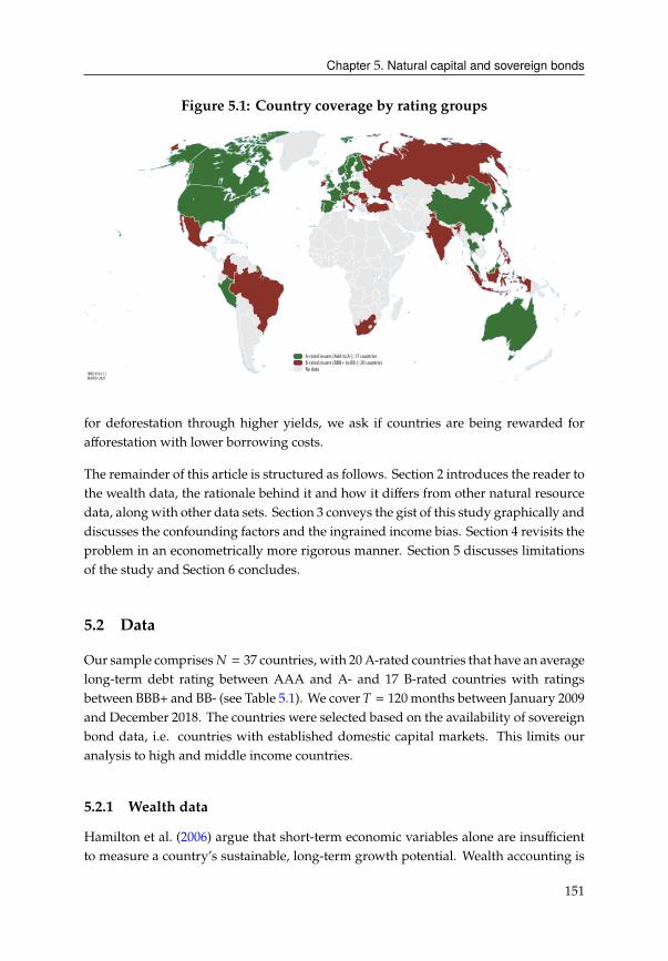
Chapter 5. Natural capital and sovereign bonds
Figure 5.1: Country coverage by rating groups
IBRD 45611 |MARCH 2021
A-rated issuers (AAA to A-); 17 countriesB-rated issuers (BBB+ to BB-); 20 countriesNo data
for deforestation through higher yields, we ask if countries are being rewarded for
afforestation with lower borrowing costs.
The remainder of this article is structured as follows. Section 2 introduces the reader to
the wealth data, the rationale behind it and how it differs from other natural resource
data, alongwith other data sets. Section 3 conveys the gist of this study graphically and
discusses the confounding factors and the ingrained income bias. Section 4 revisits the
problem in an econometrically more rigorous manner. Section 5 discusses limitations
of the study and Section 6 concludes.
5.2 Data
Our sample comprises# = 37 countries, with 20A-rated countries that have an average
long-term debt rating between AAA and A- and 17 B-rated countries with ratings
between BBB+ and BB- (see Table 5.1). We cover ) = 120 months between January 2009
and December 2018. The countries were selected based on the availability of sovereign
bond data, i.e. countries with established domestic capital markets. This limits our
analysis to high and middle income countries.
5.2.1 Wealth data
Hamilton et al. (2006) argue that short-term economic variables alone are insufficient
to measure a country’s sustainable, long-term growth potential. Wealth accounting is
151
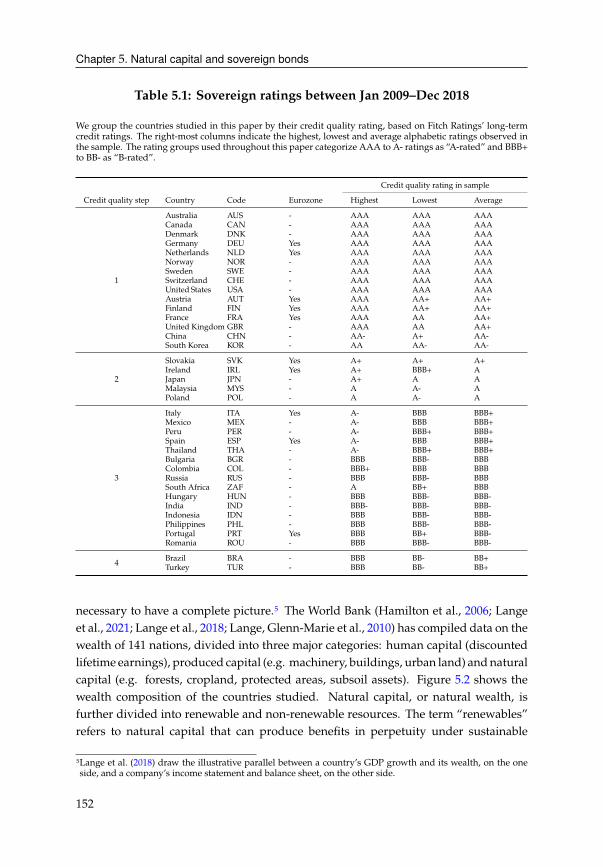
Chapter 5. Natural capital and sovereign bonds
Table 5.1: Sovereign ratings between Jan 2009–Dec 2018
We group the countries studied in this paper by their credit quality rating, based on Fitch Ratings’ long-term
credit ratings. The right-most columns indicate the highest, lowest and average alphabetic ratings observed in
the sample. The rating groups used throughout this paper categorize AAA to A- ratings as “A-rated” and BBB+
to BB- as “B-rated”.
Credit quality rating in sample
Credit quality step Country Code Eurozone Highest Lowest Average
1
Australia AUS - AAA AAA AAA
Canada CAN - AAA AAA AAA
Denmark DNK - AAA AAA AAA
Germany DEU Yes AAA AAA AAA
Netherlands NLD Yes AAA AAA AAA
Norway NOR - AAA AAA AAA
Sweden SWE - AAA AAA AAA
Switzerland CHE - AAA AAA AAA
United States USA - AAA AAA AAA
Austria AUT Yes AAA AA+ AA+
Finland FIN Yes AAA AA+ AA+
France FRA Yes AAA AA AA+
United Kingdom GBR - AAA AA AA+
China CHN - AA- A+ AA-
South Korea KOR - AA AA- AA-
2
Slovakia SVK Yes A+ A+ A+
Ireland IRL Yes A+ BBB+ A
Japan JPN - A+ A A
Malaysia MYS - A A- A
Poland POL - A A- A
3
Italy ITA Yes A- BBB BBB+
Mexico MEX - A- BBB BBB+
Peru PER - A- BBB+ BBB+
Spain ESP Yes A- BBB BBB+
Thailand THA - A- BBB+ BBB+
Bulgaria BGR - BBB BBB- BBB
Colombia COL - BBB+ BBB BBB
Russia RUS - BBB BBB- BBB
South Africa ZAF - A BB+ BBB
Hungary HUN - BBB BBB- BBB-
India IND - BBB- BBB- BBB-
Indonesia IDN - BBB BBB- BBB-
Philippines PHL - BBB BBB- BBB-
Portugal PRT Yes BBB BB+ BBB-
Romania ROU - BBB BBB- BBB-
4
Brazil BRA - BBB BB- BB+
Turkey TUR - BBB BB- BB+
necessary to have a complete picture.5 The World Bank (Hamilton et al., 2006; Lange
et al., 2021; Lange et al., 2018; Lange, Glenn-Marie et al., 2010) has compiled data on the
wealth of 141 nations, divided into three major categories: human capital (discounted
lifetime earnings), produced capital (e.g. machinery, buildings, urban land) andnatural
capital (e.g. forests, cropland, protected areas, subsoil assets). Figure 5.2 shows the
wealth composition of the countries studied. Natural capital, or natural wealth, is
further divided into renewable and non-renewable resources. The term “renewables”
refers to natural capital that can produce benefits in perpetuity under sustainable
5Lange et al. (2018) draw the illustrative parallel between a country’s GDP growth and its wealth, on the one
side, and a company’s income statement and balance sheet, on the other side.
152
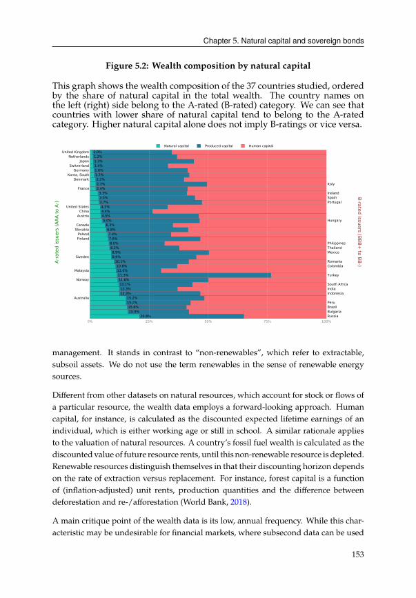
Chapter 5. Natural capital and sovereign bonds
Figure 5.2: Wealth composition by natural capital
This graph shows the wealth composition of the 37 countries studied, ordered
by the share of natural capital in the total wealth. The country names on
the left (right) side belong to the A-rated (B-rated) category. We can see that
countries with lower share of natural capital tend to belong to the A-rated
category. Higher natural capital alone does not imply B-ratings or vice versa.
15.2%Australia
4.5%Austria
6.3%Canada
2.2%Denmark
7.6%Finland
2.4%France
1.6%Germany
5.0% Hungary
3.3% Ireland
2.3% Italy
1.3%Japan
1.7%Korea, South
1.2%Netherlands
11.6%Norway
7.4%Poland
3.7% Portugal
6.8%Slovakia
3.5% Spain
8.9%Sweden
1.4%Switzerland
1.0%United Kingdom
4.3%United States
15.6% Brazil 15.9% Bulgaria
4.4%China
10.8% Colombia
12.3% India 12.3% Indonesia
11.0%Malaysia
8.9% Mexico
15.2% Peru
8.0% Philippines
10.1% Romania
20.8% Russia
12.1% South Africa
8.2% Thailand
11.3% Turkey
0% 25% 50% 75% 100%
A-ra
ted
issue
rs (A
AA to
A-)
B-rated issuers (BBB+ to BB-)
Natural capital Produced capital Human capital
management. It stands in contrast to “non-renewables”, which refer to extractable,
subsoil assets. We do not use the term renewables in the sense of renewable energy
sources.
Different from other datasets on natural resources, which account for stock or flows of
a particular resource, the wealth data employs a forward-looking approach. Human
capital, for instance, is calculated as the discounted expected lifetime earnings of an
individual, which is either working age or still in school. A similar rationale applies
to the valuation of natural resources. A country’s fossil fuel wealth is calculated as the
discountedvalue of future resource rents, until this non-renewable resource is depleted.
Renewable resources distinguish themselves in that their discounting horizon depends
on the rate of extraction versus replacement. For instance, forest capital is a function
of (inflation-adjusted) unit rents, production quantities and the difference between
deforestation and re-/afforestation (World Bank, 2018).
A main critique point of the wealth data is its low, annual frequency. While this char-
acteristic may be undesirable for financial markets, where subsecond data can be used
153
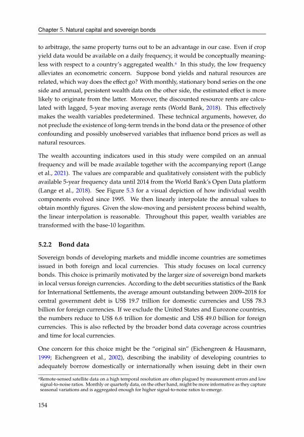
Chapter 5. Natural capital and sovereign bonds
to arbitrage, the same property turns out to be an advantage in our case. Even if crop
yield data would be available on a daily frequency, it would be conceptually meaning-
less with respect to a country’s aggregated wealth.6 In this study, the low frequency
alleviates an econometric concern. Suppose bond yields and natural resources are
related, which way does the effect go? With monthly, stationary bond series on the one
side and annual, persistent wealth data on the other side, the estimated effect is more
likely to originate from the latter. Moreover, the discounted resource rents are calcu-
lated with lagged, 5-year moving average rents (World Bank, 2018). This effectively
makes the wealth variables predetermined. These technical arguments, however, do
not preclude the existence of long-term trends in the bond data or the presence of other
confounding and possibly unobserved variables that influence bond prices as well as
natural resources.
The wealth accounting indicators used in this study were compiled on an annual
frequency and will be made available together with the accompanying report (Lange
et al., 2021). The values are comparable and qualitatively consistent with the publicly
available 5-year frequency data until 2014 from the World Bank’s Open Data platform
(Lange et al., 2018). See Figure 5.3 for a visual depiction of how individual wealth
components evolved since 1995. We then linearly interpolate the annual values to
obtain monthly figures. Given the slow-moving and persistent process behind wealth,
the linear interpolation is reasonable. Throughout this paper, wealth variables are
transformed with the base-10 logarithm.
5.2.2 Bond data
Sovereign bonds of developing markets and middle income countries are sometimes
issued in both foreign and local currencies. This study focuses on local currency
bonds. This choice is primarily motivated by the larger size of sovereign bond markets
in local versus foreign currencies. According to the debt securities statistics of the Bank
for International Settlements, the average amount outstanding between 2009–2018 for
central government debt is US$ 19.7 trillion for domestic currencies and US$ 78.3
billion for foreign currencies. If we exclude the United States and Eurozone countries,
the numbers reduce to US$ 6.6 trillion for domestic and US$ 49.0 billion for foreign
currencies. This is also reflected by the broader bond data coverage across countries
and time for local currencies.
One concern for this choice might be the “original sin” (Eichengreen & Hausmann,
1999; Eichengreen et al., 2002), describing the inability of developing countries to
adequately borrow domestically or internationally when issuing debt in their own
6Remote-sensed satellite data on a high temporal resolution are often plagued by measurement errors and low
signal-to-noise ratios. Monthly or quarterly data, on the other hand, might bemore informative as they capture
seasonal variations and is aggregated enough for higher signal-to-noise ratios to emerge.
154
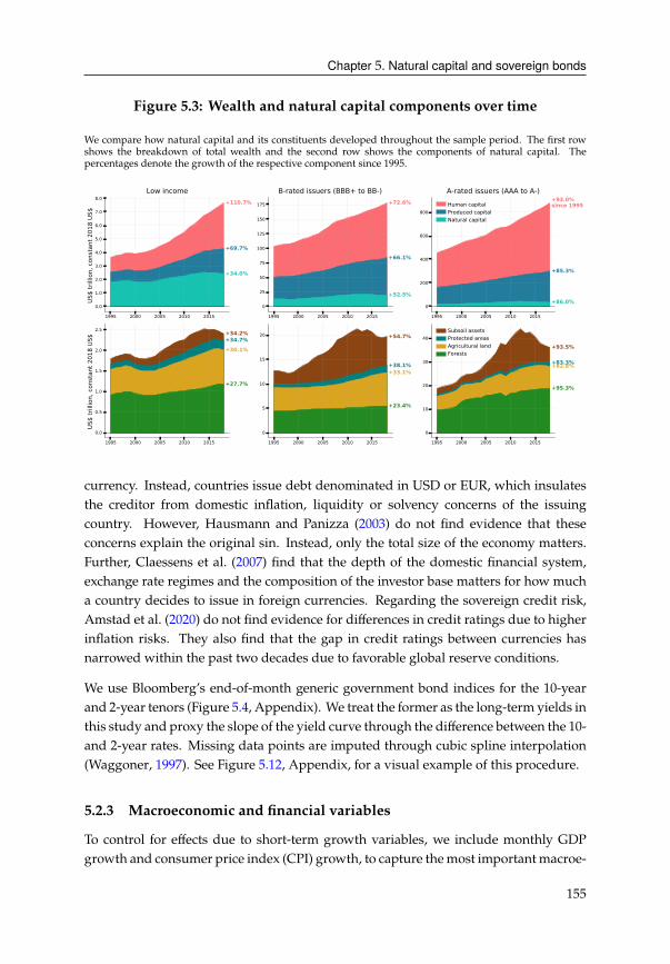
Chapter 5. Natural capital and sovereign bonds
Figure 5.3: Wealth and natural capital components over time
We compare how natural capital and its constituents developed throughout the sample period. The first row
shows the breakdown of total wealth and the second row shows the components of natural capital. The
percentages denote the growth of the respective component since 1995.
1995 2000 2005 2010 2015
0.0
1.0
2.0
3.0
4.0
5.0
6.0
7.0
8.0
US$
trillio
n, c
onst
ant 2
018
US$
+110.7%
+69.7%
+34.0%
Low income
1995 2000 2005 2010 2015
0
25
50
75
100
125
150
175 +72.6%
+66.1%
+52.5%
B-rated issuers (BBB+ to BB-)
1995 2000 2005 2010 2015
0
200
400
600
800
+93.0% since 1995
+85.3%
+86.0%
A-rated issuers (AAA to A-)Human capitalProduced capitalNatural capital
1995 2000 2005 2010 2015
0.0
0.5
1.0
1.5
2.0
2.5
US$
trillio
n, c
onst
ant 2
018
US$ +34.2%
+34.7% +30.1%
+27.7%
1995 2000 2005 2010 2015
0
5
10
15
20 +54.7%
+38.1% +33.1%
+23.4%
1995 2000 2005 2010 2015
0
10
20
30
40 +93.5%
+83.3% +82.8%
+95.3%
Subsoil assetsProtected areasAgricultural landForests
currency. Instead, countries issue debt denominated in USD or EUR, which insulates
the creditor from domestic inflation, liquidity or solvency concerns of the issuing
country. However, Hausmann and Panizza (2003) do not find evidence that these
concerns explain the original sin. Instead, only the total size of the economy matters.
Further, Claessens et al. (2007) find that the depth of the domestic financial system,
exchange rate regimes and the composition of the investor base matters for how much
a country decides to issue in foreign currencies. Regarding the sovereign credit risk,
Amstad et al. (2020) do not find evidence for differences in credit ratings due to higher
inflation risks. They also find that the gap in credit ratings between currencies has
narrowed within the past two decades due to favorable global reserve conditions.
We use Bloomberg’s end-of-month generic government bond indices for the 10-year
and 2-year tenors (Figure 5.4, Appendix). We treat the former as the long-term yields in
this study and proxy the slope of the yield curve through the difference between the 10-
and 2-year rates. Missing data points are imputed through cubic spline interpolation
(Waggoner, 1997). See Figure 5.12, Appendix, for a visual example of this procedure.
5.2.3 Macroeconomic and financial variables
To control for effects due to short-term growth variables, we include monthly GDP
growth and consumer price index (CPI) growth, to capture themost importantmacroe-
155
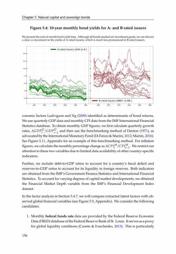
Chapter 5. Natural capital and sovereign bonds
Figure 5.4: 10-year monthly bond yields for A- and B-rated issuers
Wepresent the end-of-month bond yield data. Although all bonds studied are investment grade, we can discern
a clear co-movement in the yields of A-rated issuers, which is much less pronounced in B-rated issuers.
2010 2012 2014 2016 2018 2020
0.0
2.5
5.0
7.5
10.0
12.5
15.0
A-rated issuers (AAA to A-)
2010 2012 2014 2016 2018 2020
B-rated issuers (BBB+ to BB-)
conomic factors Ludvigson and Ng (2009) identified as determinants of bond returns.
We use quarterly GDP data andmonthly CPI data from the IMF International Financial
Statistics database. To obtain monthly GDP figures, we first calculate quarterly growth
rates, ��%&C/��%&
C−1and then use the benchmarking method of Denton (1971), as
advocated by the InternationalMonetary Fund (Di Fonzo&Marini, 2012; Marini, 2016).
See Figure 5.11, Appendix for an example of this benchmarking method. For inflation
figures, we calculate themonthly percentage change as�%�"C/�%�"
C−1. We restrict our
attention to these two variables due to limited data availability of other country-specific
indicators.
Further, we include debt-to-GDP ratios to account for a country’s fiscal deficit and
reserves-to-GDP ratios to account for its liquidity in foreign reserves. Both indicators
are obtained from the IMF’s Government Finance Statistics and International Financial
Statistics. To account for varying degrees of capital market developments, we obtained
the Financial Market Depth variable from the IMF’s Financial Development Index
dataset.
In the factor analysis in Section 5.4.7, we will compare extracted latent factors with ob-
served global financial variables (see Figure 5.9, Appendix). We consider the following
candidates.
1. Monthly federal funds rate data are provided by the Federal Reserve Economic
Data (FRED)database of the FederalReserveBankof St. Louis. It serves as aproxy
for global liquidity conditions (Csonto & Ivaschenko, 2013). This is particularly
156

Chapter 5. Natural capital and sovereign bonds
relevant for exchange rate volatilities, for instance due to the US federal reserve
large-scale asset purchase programs, which Gadanecz et al. (2018) demonstrate
to have influenced local currency bond yields.
2. We include the TED spread and the Chicago Board Options Exchange’s Volatil-
ity Index to control for global credit risk and volatility conditions (Hilscher &
Nosbusch, 2010).
3. To mirror equity market conditions in developed markets, we include end-of-
month values of theMSCI World Index.
4. For global bond market conditions, we also obtain end-of-month values of J.P.MorganGlobal Bond Index (GBI) for emergingmarkets and the Europeanmon-
etary union, which captures developments in local currencies.
5. Furthermore, we obtain end-of-month values of J.P. Morgan Emerging Mar-kets Bond Index (EMBI) suite to reflect bond market developments in foreign
currencies.
5.3 Preliminary analysis
When a country raises capital on bond markets, it needs to set the return on the
bond. This return, or yield, will determine the market appetite for this debt issuance.
To simplify and focus the subsequent discussion, we treat bond yields as price of
borrowing. Considering the importance of natural capital to the economy and thereby
to its bonds, we ask: Is it worth investing into forest expansion, sustainable agriculture
or national parks? Figure 5.5 suggests two answers.
If we follow the dashed lines, it seems that more natural capital either raises or does
not affect borrowing costs of B- and A-rated issuers, respectively. This is the between-country view or long-run view. Countries richer in natural capital, such as Brazil or
Russia, tend to have higher bond yields than countries that have less natural wealth,
such as Bulgaria or Hungary. This view effectively ignores the changes over time and
compares the average yield with the average natural capital across countries.
If we instead follow the dotted lines, we find the exact opposite. As countries grow
richer in natural wealth, the cost of borrowing drops. This is the within-countryview or short-run view. Rather than comparing countries with each other, the within
view compares the countries with themselves at different points in time. For instance,
Colombia in 2019 is wealthier in natural capital and has lower yields than it did in
2009. China or Malaysia, in contrast, moved sideways, indicating that their yields were
largely unaffected by changes in their natural capital.
157
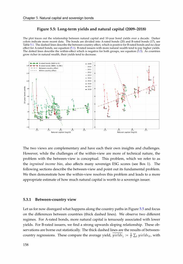
Chapter 5. Natural capital and sovereign bonds
Figure 5.5: Long-term yields and natural capital (2009–2018)
The plot traces out the relationship between natural capital and 10-year bond yields over a decade. Darker
colors indicate more recent data. The bonds are divided into A-rated bonds (20) and B-rated bonds (17), see
Table 5.1. The dashed lines describe the between-country effect, which is positive for B-rated bonds and no clear
effect for A-rated bonds, see equation (5.1). B-rated issuers with more natural wealth tend to pay higher yields.
The dotted lines describe the within-effect which is negative for both groups, see equation (5.3). As countries
grow richer in natural wealth, their yields tend to decrease.
11.0 11.5 12.0 12.5 13.0Natural capital (log10)
2
0
2
4
6
8
10
12
14
10-y
ear b
ond
yiel
ds
2009 2010 2011 2012 2013 2014 2015 2016 2017 2018
A-rated bonds (AAA to A-)B-rated bonds (BBB+ to BB-)Between-country effectWithin-country effect
11.0 11.5 12.0 12.5Natural capital (log10)
The two views are complementary and have each their own insights and challenges.
However, while the challenges of the within-view are more of technical nature, the
problem with the between-view is conceptual. This problem, which we refer to as
the ingrained income bias, also affects many sovereign ESG scores (see Box 1). The
following sections describe the between-view and point out its fundamental problem.
We then demonstrate how the within-view resolves this problem and leads to a more
appropriate estimate of how much natural capital is worth to a sovereign issuer.
5.3.1 Between-country view
Let us for now disregard what happens along the country paths in Figure 5.5 and focus
on the differences between countries (thick dashed lines). We observe two different
regimes. For A-rated bonds, more natural capital is tenuously associated with lower
yields. For B-rated issuers, we find a strong upwards sloping relationship. These ob-
servations are borne out statistically. The thick dashed lines are the results of between-
country regressions. These compare the average yield, H84;3B 8 := 1
)
∑C H84;3B8C , with
158
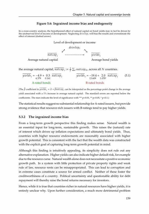
Chapter 5. Natural capital and sovereign bonds
Figure 5.6: Ingrained income bias and endogeneity
In a cross-country analysis, the hypothesized effect of natural capital on bond yields may in fact be driven by
the unobserved level of income or development. Neglecting 34E4;>?8 will bias the results and overestimate the
effect of interest (dashed arrow).
Level of development or income
34E4;>?8↗↙ ↖↘
=0C20? 8 −−−−−−−−→ H84;3B 8
Average natural capital Average bond yields
the average natural capital, =0C20? 8 := 1
)
∑C =0C20?8C , across all # countries.
H84;3B 8 = −4.94.379
+ 0.30.161
=0C20? 8 H84;3B 8 = −19.413.609
+ 2.01.078
∗=0C20? 8 (5.1)
A-rated bonds B-rated bonds
(The � coefficient in H84;3B 8 = + �=0C20? 8 can be interpreted as the percentage point change in the average
yield associated with a 1% increase in average natural capital. The standard errors are reported below the
coefficients. The stars indicate the level of significance with *** p<0.01, ** p<0.05, * p<0.1.)
The statistical results suggest no substantial relationship forA-rated issuers, but provide
strong evidence that resource-rich issuers with B-ratings tend to pay higher yields.
5.3.2 The ingrained income bias
From a long-term growth perspective this finding makes sense. Natural wealth is
an essential input for long-term, sustainable growth. This raises the (natural) rate
of interest which drives up inflation expectations and ultimately bond yields. Thus,
countries with higher resource endowments are reasonably associated with higher
growth potential. This is consistent with the fact that the wealth data was constructed
with the explicit goal of capturing long-term growth potential in mind.
Although this finding is intuitively appealing, its simplicity does not rule out any
alternative explanation. Higher yields can also indicate higher default risk, for example
due to the resource curse. Naturalwealth alone does not necessitate a positive economic
growth path. In a system with little protection of private property rights and weak
rule of law, resource rents can be misappropriated. This can lead to corruption and
in extreme cases constitute a source for armed conflict. Neither of these foster the
creditworthiness of a country. Political uncertainty and questionable ability for debt
repayment will thereby raise the bond returns necessary for investors.
Hence, while it is true that countries richer in natural resources have higher yields, it is
entirely unclear why. Upon further consideration, a much more detrimental problem
159
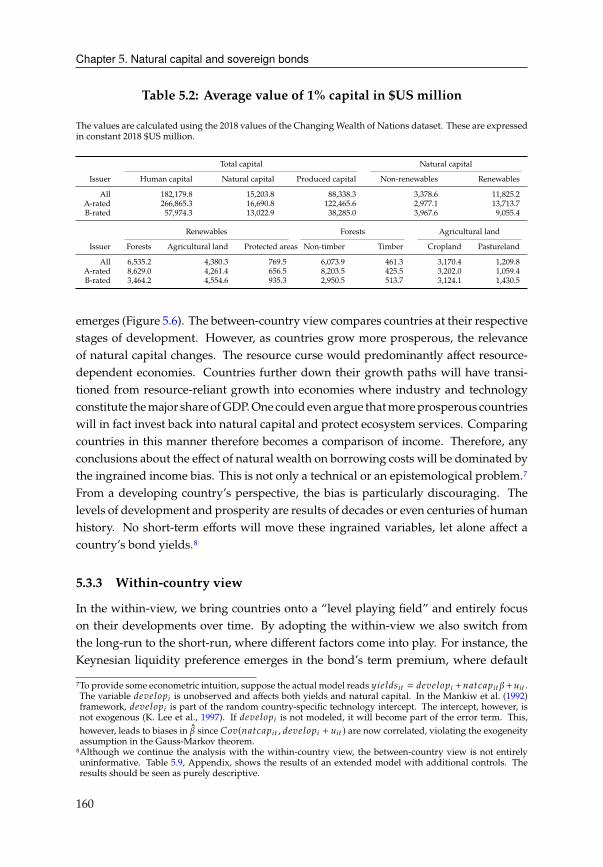
Chapter 5. Natural capital and sovereign bonds
Table 5.2: Average value of 1% capital in $US million
The values are calculated using the 2018 values of the ChangingWealth of Nations dataset. These are expressed
in constant 2018 $US million.
Total capital Natural capital
Issuer Human capital Natural capital Produced capital Non-renewables Renewables
All 182,179.8 15,203.8 88,338.3 3,378.6 11,825.2
A-rated 266,865.3 16,690.8 122,465.6 2,977.1 13,713.7
B-rated 57,974.3 13,022.9 38,285.0 3,967.6 9,055.4
Renewables Forests Agricultural land
Issuer Forests Agricultural land Protected areas Non-timber Timber Cropland Pastureland
All 6,535.2 4,380.3 769.5 6,073.9 461.3 3,170.4 1,209.8
A-rated 8,629.0 4,261.4 656.5 8,203.5 425.5 3,202.0 1,059.4
B-rated 3,464.2 4,554.6 935.3 2,950.5 513.7 3,124.1 1,430.5
emerges (Figure 5.6). The between-country view compares countries at their respective
stages of development. However, as countries grow more prosperous, the relevance
of natural capital changes. The resource curse would predominantly affect resource-
dependent economies. Countries further down their growth paths will have transi-
tioned from resource-reliant growth into economies where industry and technology
constitute themajor share ofGDP.One could evenargue thatmoreprosperous countries
will in fact invest back into natural capital and protect ecosystem services. Comparing
countries in this manner therefore becomes a comparison of income. Therefore, any
conclusions about the effect of natural wealth on borrowing costs will be dominated by
the ingrained income bias. This is not only a technical or an epistemological problem.7
From a developing country’s perspective, the bias is particularly discouraging. The
levels of development and prosperity are results of decades or even centuries of human
history. No short-term efforts will move these ingrained variables, let alone affect a
country’s bond yields.8
5.3.3 Within-country view
In the within-view, we bring countries onto a “level playing field” and entirely focus
on their developments over time. By adopting the within-view we also switch from
the long-run to the short-run, where different factors come into play. For instance, the
Keynesian liquidity preference emerges in the bond’s term premium, where default
7To provide some econometric intuition, suppose the actual model reads H84;3B8C = 34E4;>?8 +=0C20?8C�+D8C .The variable 34E4;>?8 is unobserved and affects both yields and natural capital. In the Mankiw et al. (1992)
framework, 34E4;>?8 is part of the random country-specific technology intercept. The intercept, however, is
not exogenous (K. Lee et al., 1997). If 34E4;>?8 is not modeled, it will become part of the error term. This,
however, leads to biases in � since �>E(=0C20?8C , 34E4;>?8 + D8C ) are now correlated, violating the exogeneity
assumption in the Gauss-Markov theorem.
8Although we continue the analysis with the within-country view, the between-country view is not entirely
uninformative. Table 5.9, Appendix, shows the results of an extended model with additional controls. The
results should be seen as purely descriptive.
160
Chapter 5. Natural capital and sovereign bonds
risk and foregone liquidity influence the price of money. While natural wealth can be
considered fixed in the long-run, this assumption is difficult to maintain in the short-
run. Even though natural capital follows a persistent process, Figure 5.3 shows that
it has grown by 86% since 1995. On a disaggregated level, forest wealth in A-rated
countries grew as much as 95.3% in the same period.
The main benefit of the within-view is that it eliminates the ingrained income bias.
To see how, let 34E4;>?8 be the unobserved level of income of country 8. The within
perspective removes this variable, along with other time-invariant characteristics, by
subtracting the country-average. If the original process reads
H84;3B8C = 34E4;>?8 + =0C20?8C� + D8C (5.2)
then the within model is H84;3B★8C= H84;3B8C − H84;3B 8 which implies
H84;3B★8C= (34E4;>?8 − 34E4;>? 8) + (=0C20?8C − =0C20? 8)� + (D8C − D 8)= =0C20?★
8C� + D★
8C
Box 1: The ingrained income bias and sovereign ESG scores
Sustainability has entered mainstream financial discussions. A growing share of institu-
tional investors allocate funds towards Sustainable Development Goals through Environ-
mental, Social and Governance (ESG) scores. Sovereign ESG scores, however, are often
affected by the ingrained income bias. Gratcheva, Emery, et al. (2021) document an aver-
age correlation of 85% between the sovereign ESG score and GNI per capita across seven
major ESG score providers. Cross-country comparisons, such as the between-country
model , tend to favor prosperous countries in all three ESG dimensions (Boitreaud et al.,
2020; Gratcheva, Gurhy, et al., 2021). Richer countries score higher on the Environmental
pillar given their capacity to designate and enforce national parks or put large swaths of
land under conservation. The same countries also score higher in the Social and Gover-
nance dimensions since labor force participation and strong legal rights are key drivers
of economic development.
Not accounting for the IIB may therefore have two unintended consequences. First, the
income bias in ESG scores may lead to perverse investment outcomes, since ESG-tilted
portfolios likely direct capital flows towards wealthy countries. Second, the ingrainednessmay lead to disheartening policy incentives, since short-run efforts are unlikely to affect
either a country’s income level or its ESG scores. The short-run view described in this
paper suggests an alternative approach. By studying a country’s recent performance, the
within-country model removes the ingrained income bias and assesses the relationship
of countries on a “level playing field”.
161
Chapter 5. Natural capital and sovereign bonds
since 34E4;>?8 = 34E4;>? 8 . This allows us to ask a more refined question: If overall
resource endowments and level of income were irrelevant, how much does growth
in natural resources affect the cost of borrowing? In Figure 5.5, this corresponds to
following countries along their paths from lighter to darker colors. Interestingly, the
paths do not fall straight down, which would have meant that yields fell regardless of
how natural capital develops. Instead, we observe a slight drift to the right, particularly
for A-rated issuers. This suggests, at least visually, that growth in natural capital over
time has a lowering effect on bond yields. This is depicted by the thick dotted lines in
Figure 5.5, which are the result of within-regressions, or fixed-effects (FE) regressions,
H84;3B★8C= − 5.71
1.940∗∗∗=0C20?★
8CH84;3B★
8C= − 8.24
4.949∗∗∗=0C20?★
8C(5.3)
A-rated bonds B-rated bonds
The within coefficients emerge as negative and strongly statistically significant. As a
country grows richer in natural capital, its yields drop significantly.9 This result may
be encouraging for sovereign issuers. To gain some perspective, a 1% natural capital
growth in 2018 is worth $US 15.2 billion on average. The estimated effect, however, is
likely biased due to other unobserved, confounding variables. Fortunately, these issues
can be dealt with in a straightforward manner, as we will discuss in the following
sections.
5.3.4 Unobserved common bond factors
Exploiting the time variation greatly increases the sample size, but also introduces the
problem of unobserved common factors. This is aggravated by the nature of bond
yields. First, bond yields are highly autocorrelated. For the 10-year tenor we find an
average AR(1) coefficient of � = 0.956∗∗∗
, leading to serial correlation in the residuals.
Second, the integrated nature of international bond markets leads to significant co-
movements between the bond prices, see Figure 5.5. This is a particularly severe
problem since these common factors, which reflect global liquidity conditions ormarket
turmoils such as the 2011-12 Euro crisis, affect both bond yields as well as observed
macro-financial control variables. Third, these global common factors do not affect
countries equally. If this were the case, they could be dealt with through time fixed-
effects. This strongly suggests the existence of at least one unobserved common factor
that influences some or all bonds. Since the FE estimates in (5.3) did not account for
any common factors, its estimates are likely biased.10
9A negative coefficient also implies that decreasing natural capital leads to higher yields. A glance at Figure 5.3
reveals that natural capital and its components have been growing steadily. In the subsequent analysis and
discussion we will therefore concentrate on the effect of natural capital growth.
10In the Appendix, Section 5.B.1, we demonstrate in a Monte Carlo study how a conventional within estimator,
which does not account for the factor component, will lead to biased estimates. The severity of the bias
increases with the strength of autocorrelation in (5.5). We then show how the IFE approach correctly recovers
the true coefficients, even when �C is highly autocorrelated.
162
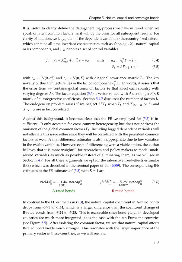
Chapter 5. Natural capital and sovereign bonds
It is useful to clearly define the data-generating process we have in mind when we
speak of latent common factors, as it will be the basis for all subsequent results. For
clarity of notation, we let H8C denote the dependent variable, 28 the country fixed-effects,
which contains all time-invariant characteristics such as 34E4;>?8 , -8C natural capital
or its components, and,8C denotes a set of control variables
H8C = 28 + ->8C � +,>8C� + D8C with D8C = �>
8�C + 48C (5.4)
�C = ��C−1+ EC (5.5)
with 48C ∼ #(0, �2
8) and EC ∼ #(0,Σ) with diagonal covariance matrix Σ. The key
novelty of this architecture lies in the factor component �>8�C . In words, it asserts that
the error term D8C contains global common factors �C that affect each country with
varying degrees �8 . The factor equation (5.5) is vector-valued with � denoting a × matrix of autoregressive coefficients. Section 5.4.7 discusses the number of factors .
The endogeneity problem arises if we neglect �>�C when �C and -8C ,,8C or �8 and
-8C ,,8C are in fact correlated.
Against this background, it becomes clear that the FE we employed for (5.3) is in-
sufficient. It only accounts for cross-country heterogeneity but does not address the
omission of the global common factors �C . Including lagged dependent variables will
not alleviate this issue either since they will be correlated with the persistent common
factors as well. A first-difference estimator is also inappropriate due to low variation
in the wealth variables. However, even if differencing were a viable option, the author
believes that it is more insightful for researchers and policy makers to model unob-
served variables as much as possible instead of eliminating them, as we will see in
Section 5.4.7. For all these arguments we opt for the interactive fixed-effects estimator
(IFE) which was described in the seminal paper of Bai (2009). The corresponding IFE
estimates to the FE estimates of (5.3) with = 1 are
H84;3B★8C= − 1.44
0.571∗∗=0C20?★
8CH84;3B★
8C= − 5.28
1.401∗∗∗=0C20?★
8C(5.6)
A-rated bonds B-rated bonds
In contrast to the FE estimates in (5.3), the natural capital coefficient in A-rated bonds
drops from -5.71 to -1.44, which is a larger difference than the coefficient change of
B-rated bonds from -8.24 to -5.28. This is reasonable since bond yields in developed
countries are much more integrated, as is the case with the ten Eurozone countries
(see Figure 5.5). After isolating the common factor, we see that natural capital affects
B-rated bond yields much stronger. This resonates with the larger importance of the
primary sector in these countries, as we will see later.
163

Chapter 5. Natural capital and sovereign bonds
5.3.5 Aggregate time effects
In addition to the common factor component, it is also possible to have aggregate time
effects. As a robustness exercise, we also include time fixed-effects 3C into (5.4), which
then reads
H8C = 28 + 3C + ->8C � +,>8C� + D8C (5.7)
Time fixed-effects assume that countries are exposed equally to 3C . This is a special
case of the common factor component. To see this, let 5C be a scalar valued factor, i.e.
�C if = 1. Then 3C = �8 5C if �8 = � for all 8.
5.3.6 Pace of development
The within-view removes the level of income effect that afflicted the cross-country
analysis. However, the pace of development is likely still different between countries.
That is, although we brought countries on a level playing field, the speed at which they
are moving will still affect the results.11 Countries higher up the development ladder
not only have lower yields, which we now account for. The yields are also decreasing
at a different pace than developing countries. We test the robustness of our results by
extending (5.4) to
H8C = 28 + ?8 C + ->8C � +,>8C� + D8C (5.8)
The term ?8 C models the different paces of development through country-specific time
trends.
5.4 Main empirical analysis
The previous models prioritized simplicity and intuition over completeness. This
sectionbuilds onmodels (5.6)-(5.8) and includes otherwealthvariables,macroeconomic
and financial control variables, and breaks natural capital down into its components.
In addition to the 10-year bond yields, which describes the overall level of the yield
curve, we will also refer to the short-term, or 2-year bond yields (see Figure 5.10). This
allows us to think about the slope of the yield curve, which is often proxied by the
difference between 10-year and 2-year yields. A positive slope is generally seen as an
indicator for optimistic economic prospects.
11In the Mankiw et al. (1992) framework, which estimates the linearized form of the exogenous technological
growth �8C = �0
84 6C , the within-transformation effectively removes the country-specific level of technology
ln�0
8but does not affect the exponential growth rate 6C.
164

Chapter 5. Natural capital and sovereign bonds
5.4.1 Model
The full model specification used for the subsequent results reads
H8C = 28 + 3C + ?8 C + ->8C � +,>8C� + D8C (5.9)
where the error term follows the dynamic factor structure
D8C = �>8�C + 48C with �C = ��C−1
+ EC (5.10)
Here, 28 is the country fixed-effect, 3C denotes the time fixed-effects, ?8 C are the country-
specific time trends, -8C are the wealth variables, ,8C are macro-financial controls.
We assume that the factors �C follow a stationary, autoregressive process. Section
5.4.7 discusses the number of factors and the rationale for our choice, = 2. The
disturbance 48C is #(0, �2
8) and the innovation EC is Gaussian with diagonal covariance
matrix. Table 5.5 introduces an interaction �8C × ->8C � where the group variable �8C is
a binary variable for the bond rating group.12
5.4.2 Estimation
In this section we discuss the various econometric challenges when estimating the
effects of natural capital and its components. It discusses how these challenges are
dealt with in the proposed framework (5.9)-(5.10), estimated with the IFE method.
The main concern is the unobserved confounding variable 34E4;>?8 . This is a well-
known issue inmicroeconometrics, such as thewhen studying the relationship between
schooling and earnings (Angrist & Krueger, 1999). Similar to how the unobserved
ability affects both sides of returns-to-schooling problems, the level of development also
affects both bond yields and natural capital. The main results will therefore include a
set of variables to control for observed confounding factors, -8C . However, this does
not entirely resolve the omitted variable bias due to 34E4;>?8 . For this purpose, we
model country fixed-effects, 28 , which contain 34E4;>?8 among other time-invariant
characteristics. Over the period of ten years, the assumption of 34E4;>?8 being time-
invariant appears justifiable.
Another source for confounding variables are country-specific time trends in bond
yields, that would have lead to falling rates irrespective of other variables. We intro-
duced this notion as the pace of development in Section 5.3.6. The endogeneity problem
arising from country-specific trends likely affects B-rated countries more, since A-rated
bonds follow similar, global trends. We therefore introduce country-specific time
trends, ?8 C.
12Since the bond rating category has only minor changes over time, it is largely absorbed by the country
fixed-effects. Hence, Table 5.5 does not include �8C by itself.
165
Chapter 5. Natural capital and sovereign bonds
Aside from these cross-sectional concerns, we also have to pay careful attention to
problems often encountered in long (dynamic) panels and multivariate time-series.
The large ), small # property of the data makes identification through time-variation
feasible. However, the persistent and co-moving nature of bond yields induces serial
correlation that cannot be fully explained by-8C or,8C . Not only could D8C be correlated
with D8C−1, but it could also be correlatedwith D9C−1
. Section 5.B.1 illustrates the severity
of the thereby induced bias. Furthermore, global financial and economic conditions are
not fully capturedby-8C and affect both bondyields andmacro-financial controls in-8C ,
such as GDP growth or inflation. Section 5.4.7 presents evidence for at least one latent
factor in D8C , which is highly correlated with global bond indices and equity indices.
Neglecting the possibility for unobserved common factors in D8C violates the strict
exogeneity assumption of E[D8C |-8B ,,8C , 28] = 0. The factor component �>8�C elegantly
resolves the above problems. The latent factors in �C allow for > 1 unobserved
global factors in D8C . This accounts for autocorrelation in the residuals and models any
cross-sectional dependency between D8C and D9C−1through the factor loadings �8 and
�9 , which load on the latent factors in �C . Different from country fixed-effects 28 , the
term �>8�C models cross-country heterogeneities that vary over time.
The interactive fixed-effects (IFE) estimator (Bai, 2009; Bai & Wang, 2016; Moon &
Weidner, 2015, 2017) employed here belongs to a strand of literature that is concerned
with inference under cross-sectional dependence and time-varying common factors
(Eberhardt & Teal, 2011). An alternative approach to the IFE is the CommonCorrelated
Effects estimator (Chudik & Pesaran, 2015; Pesaran, 2006; Pesaran & Tosetti, 2011).
These types of models generalize two-way fixed effects and are also known as models
with multi-factor error structure or linear factor models in panels. This class of models
has been applied to estimate causal treatment effects that usually rely on difference-in-
difference estimators or synthetic controls (Gobillon &Magnac, 2016; Mäkelä, 2017; Xu,
2017). This approach has also been used in non-stationary panel models (Kapetanios
et al., 2011), to identify structural breaks in panels (Li et al., 2016) or consistently
estimate panel models with errors that are serially and spatially correlated (Bertoli &
Fernández-Huertas Moraga, 2013).
Finally, it is worth emphasizing that wealth variables are predetermined. While bond
yields fluctuate on a monthly frequency, wealth is a function of resource rents, which
are computed using 5-year moving averages on an annual frequency (World Bank,
2018). It is therefore more probable for slow-moving wealth variables to steer long-
term bond prices, than monthly bond fluctuations changing the accumulation rate of
natural capital. A possible channel for reverse causality could stem from long-term
bond trends affecting the growth of natural capital. While indeed plausible, the author
deems this less of a concern since these trends are already contained in the time fixed-
effects 3C , common factor component �>8�C and the country-specific time trends ?8 C.
166
Chapter 5. Natural capital and sovereign bonds
5.4.3 Results
Table 5.3 shows the main results of (5.9)-(5.10) for the 10-year yields. In contrast to
the simple IFE model (5.6), which only allows for �8 5C with = 1, the coefficient sign
on total natural capital reverses in the full specification with = 2 and other control
variables. However, once we distinguish between non-renewables and renewables, it
becomes clear that renewables have a predominantly negative effect which is offset
by non-rewewable subsoil assets. Countries that have become richer in renewable
natural wealth between 2009-2019 have significantly lower borrowing costs, even after
controlling for an array of macro-financial variables.
This effect is strongest for forest capital and to a lesser degree agricultural land. Ta-
ble 5.4 shows the corresponding values for short-term, 2-year yields. Taking together,
renewable forest and agricultural capital lowers the entire curve but also steepens it.
Economically, this can be interpreted as a lowering of overall borrowing costs while
also improving economic prospects in the short-run. The effect is different for pro-
tected areas, which carries a positive coefficient. While sharing the same sign with
non-renewables, both effects should not be equated with each other. Table 5.4 shows
that the effect of protected areas is insignificant in the short-run. In terms of coeffi-
cient magnitudes, the long-term effect outweighs the short-term effect, indicating an
upwards tilting effect on the yield curve. In comparison, subsoil assets are significant
for both 2-year and 10-year maturities and have a depressing effect on the yield curve
slope. To give context to the positive coefficient on protected areas, it is worth men-
tioning that its value is based on opportunity cost calculations (World Bank, 2018). In
other words, it is the value of foregone rents that could have otherwise been derived
from agricultural production. This implies that growth in protected areas will have a
stronger impact in countries that rely more on the agricultural sector. We will revisit
this issue in Section 5.4.6. Albeit significant, it is important not to overemphasize this
effect, since protected areas constitute less than 5% of overall natural capital (Table 5.2)
The following paragraphs suggest and discuss two possible economic explanations
behind these findings.13
• Worthwhile investmentInvestments into natural wealth foster sustainable growth, improve the country’s
fundamentals and thereby decrease the default risk. Lower bond yields are the
result of the improving the economic foundations.
• Luxury investmentGrowth in natural capital is the result of prosperity. Lower yields are a reflection
13Theoretically, a third option is also possible, where bond proceeds are directly invested into environmental
projects. This explanation is likely to become more relevant as the number sovereign green bond issuances
grow, but is outside the scope of this study.
167
Chapter 5. Natural capital and sovereign bonds
of the higher income of the issuers. Only developed countries have the capacity
to invest into non-productive natural capital.
Todeterminewhich explanation ismost suitable, we turn to the underlyingdata sources
of natural capital. Figure 5.7 indicates that agriculture and forests lowerborrowing costs
because they are worthwhile investments, while the effect of protected areas is more
likely the result of a luxury investment.
5.4.4 Forests
Forest capital serves as a primary input for production through logging of trees, gen-
erates employment for more than 13 million people (IPBES, 2019) and is necessary for
other ecological benefits such as improved air andwater quality (Lange et al., 2018). For
instance, non-timber forest capital reflects the value of watershed protection, hunting,
fishing, along with other ecosystem services that are usually not accounted for, but
are relevant for food production, biodiversity and human health (Lange et al., 2018).
Tourism in forest-covered protected areas constitutes amajor share of the 8 billion visits
(FAO and UNEP, 2020).
In addition to the size of the forests, the diversity of tree species is also worth men-
tioning, since five of the ten countries with the most tree species are in the B-rated
category (FAO and UNEP, 2020). The FAO (2014) discusses the importance of forest
genetic resources in developing economies and economies in transition in the context
of their “actual or potential economic, environmental, scientific or societal value”.
Given the direct productive capabilities of forests and their indirect socioeconomic
benefits, investing into this renewable resource is an economicallyworthwhile decision.
We see support for this in the underlying data. Figure 5.7a shows the average annual
percentage increase in planted forest areas between 2009 and 2020. A planted forest
is a "[f]orest predominantly composed of trees established through planting and/or
deliberate seeding" (FAO, 2020b) and is to be distinguished from natural regrowth.
The fact that countries, where agriculture, forestry and fishing constitute a larger share
of GDP value-added largely coincide with the countries with the most planted forest
expansion, renders luxury investment explanation unlikely. This is further supported
by Table 5.5, Appendix, which decomposes the negative coefficient by rating category.
The same investment into forests lowers yields significantly more in B-rated countries.
Table 5.6, Appendix, shows disaggregated results where forest capital is divided into
timber and non-timber forests. Interestingly, the latter type mainly drives the yield
lowering effect of forests. Identifying whether this reflects tourism revenues based on
non-timber forest capital or in fact captures the hard-to-quantify benefits of its external
effects is left for future studies.
168
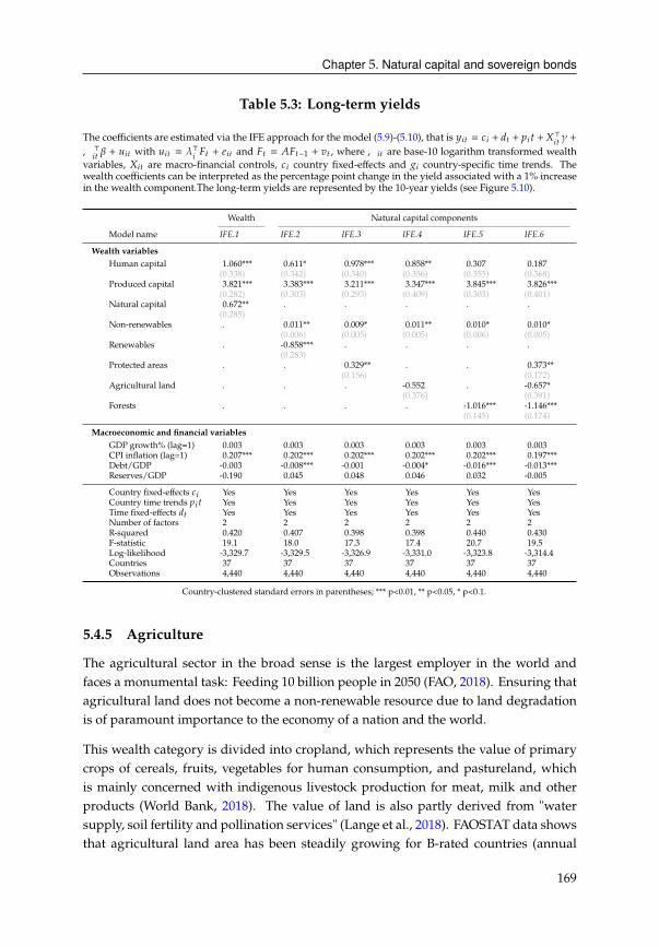
Chapter 5. Natural capital and sovereign bonds
Table 5.3: Long-term yields
The coefficients are estimated via the IFE approach for the model (5.9)-(5.10), that is H8C = 28 + 3C + ?8 C +->8C � +,>8C� + D8C with D8C = �>
8�C + 48C and �C = ��C−1 + EC , where,8C are base-10 logarithm transformed wealth
variables, -8C are macro-financial controls, 28 country fixed-effects and 68 country-specific time trends. The
wealth coefficients can be interpreted as the percentage point change in the yield associated with a 1% increase
in the wealth component.The long-term yields are represented by the 10-year yields (see Figure 5.10).
Wealth Natural capital components
Model name IFE.1 IFE.2 IFE.3 IFE.4 IFE.5 IFE.6
Wealth variablesHuman capital 1.060***
(0.338)
0.611*
(0.342)
0.978***
(0.340)
0.858**
(0.356)
0.307
(0.355)
0.187
(0.368)
Produced capital 3.821***
(0.282)
3.383***
(0.303)
3.211***
(0.293)
3.347***
(0.409)
3.845***
(0.303)
3.826***
(0.401)
Natural capital 0.672**
(0.285)
. . . . .
Non-renewables . 0.011**
(0.006)
0.009*
(0.005)
0.011**
(0.005)
0.010*
(0.006)
0.010*
(0.005)
Renewables . -0.858***
(0.283)
. . . .
Protected areas . . 0.329**
(0.156)
. . 0.373**
(0.172)
Agricultural land . . . -0.552
(0.376)
. -0.657*
(0.391)
Forests . . . . -1.016***
(0.145)
-1.146***
(0.174)
Macroeconomic and financial variablesGDP growth% (lag=1) 0.003 0.003 0.003 0.003 0.003 0.003
CPI inflation (lag=1) 0.207*** 0.202*** 0.202*** 0.202*** 0.202*** 0.197***
Debt/GDP -0.003 -0.008*** -0.001 -0.004* -0.016*** -0.013***
Reserves/GDP -0.190 0.045 0.048 0.046 0.032 -0.005
Country fixed-effects 28 Yes Yes Yes Yes Yes Yes
Country time trends ?8 C Yes Yes Yes Yes Yes Yes
Time fixed-effects 3C Yes Yes Yes Yes Yes Yes
Number of factors 2 2 2 2 2 2
R-squared 0.420 0.407 0.398 0.398 0.440 0.430
F-statistic 19.1 18.0 17.3 17.4 20.7 19.5
Log-likelihood -3,329.7 -3,329.5 -3,326.9 -3,331.0 -3,323.8 -3,314.4
Countries 37 37 37 37 37 37
Observations 4,440 4,440 4,440 4,440 4,440 4,440
Country-clustered standard errors in parentheses; *** p<0.01, ** p<0.05, * p<0.1.
5.4.5 Agriculture
The agricultural sector in the broad sense is the largest employer in the world and
faces a monumental task: Feeding 10 billion people in 2050 (FAO, 2018). Ensuring that
agricultural land does not become a non-renewable resource due to land degradation
is of paramount importance to the economy of a nation and the world.
This wealth category is divided into cropland, which represents the value of primary
crops of cereals, fruits, vegetables for human consumption, and pastureland, which
is mainly concerned with indigenous livestock production for meat, milk and other
products (World Bank, 2018). The value of land is also partly derived from "water
supply, soil fertility and pollination services" (Lange et al., 2018). FAOSTAT data shows
that agricultural land area has been steadily growing for B-rated countries (annual
169
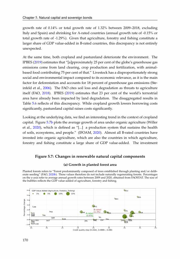
Chapter 5. Natural capital and sovereign bonds
growth rate of 0.14% or total growth rate of 1.32% between 2009–2018, excluding
Italy and Spain) and shrinking for A-rated countries (annual growth rate of -0.15% or
total growth rate of -1.29%). Given that agriculture, forestry and fishing constitute a
larger share of GDP value-added in B-rated countries, this discrepancy is not entirely
unexpected.
At the same time, both cropland and pastureland deteriorate the environment. The
IPBES (2019) estimates that “[a]pproximately 25 per cent of the globe’s greenhouse gas
emissions come from land clearing, crop production and fertilization, with animal-
based food contributing 75 per cent of that.” Livestock has a disproportionately strong
social and environmental impact compared to its economic relevance, as it is the main
factor for deforestation and accounts for 18 percent of greenhouse gas emissions (Ste-
infeld et al., 2006). The FAO cites soil loss and degradation as threats to agriculture
itself (FAO, 2018). IPBES (2019) estimates that 23 per cent of the world’s terrestrial
area have already been impacted by land degradation. The disaggregated results in
Table 5.6 reflects of this discrepancy. While cropland growth lowers borrowing costs
significantly, pastureland capital raises costs significantly.
Looking at the underlying data, we find an interesting trend in the context of cropland
capital. Figure 5.7b plots the average growth of area under organic agriculture (Willer
et al., 2020), which is defined as “[...] a production system that sustains the health
of soils, ecosystems, and people.” (IFOAM, 2020). Almost all B-rated countries have
invested into organic agriculture, which are also the countries in which agriculture,
forestry and fishing constitute a large share of GDP value-added. The investment
Figure 5.7: Changes in renewable natural capital components
(a) Growth in planted forest area
Planted forests refers to “Forest predominantly composed of trees established through planting and/or delib-
erate seeding” (FAO, 2020b). These values therefore do not include naturally regenerating forests. Percentages
on the y-axis refer to average annual growth rates between 2009 and 2020, obtained from FAOSTAT. The size of
the bubbles reflects the GDP value-added of agriculture, forestry and fishing.
0.0 0.5 1.0 1.5 2.0 2.5 3.0 3.5 4.0Credit quality step (0=AAA, 2=BBB+, 4=BB)
1%
0%
1%
2%
3%
4%
5%
6%
Perc
enta
ge c
hang
e
ROU
BRAMEX
MYSCAN
COLFRA THACHN TURPERAUS IDNSWE FINUSA PHLINDIRLGBR KOR ITA PRTSVK ESPDEU ZAFPOL HUNAUTNLD JPN RUSDNK BGRNOR CHE
B-rated(1.3%)A-rated
(0.6%)
GDP Value Added (Agriculture, Forestry, Fishing)1% 5% 10% 15%
170
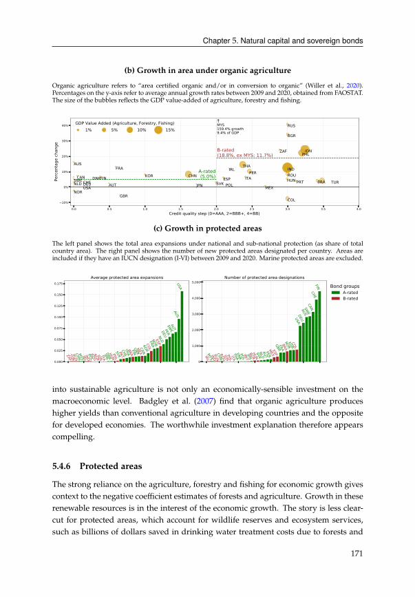
Chapter 5. Natural capital and sovereign bonds
(b) Growth in area under organic agriculture
Organic agriculture refers to “area certified organic and/or in conversion to organic” (Willer et al., 2020).
Percentages on the y-axis refer to average annual growth rates between 2009 and 2020, obtained from FAOSTAT.
The size of the bubbles reflects the GDP value-added of agriculture, forestry and fishing.
0.0 0.5 1.0 1.5 2.0 2.5 3.0 3.5 4.0Credit quality step (0=AAA, 2=BBB+, 4=BB)
10%
0%
10%
20%
30%
40%
Perc
enta
ge c
hang
e
RUS
BGR
IDNZAF PHL
AUS THAFRA INDIRLPER ROUCHNKORCAN FIN ITADNK ESP HUNSWE BRAPRT TURCHE SVKNLD DEU AUT POLJPN MEXUSA
NORGBR
COL
B-rated(18.8%, ex MYS: 11.7%)
A-rated(5.0%)
MYS159.4% growth9.4% of GDP
GDP Value Added (Agriculture, Forestry, Fishing)1% 5% 10% 15%
(c) Growth in protected areas
The left panel shows the total area expansions under national and sub-national protection (as share of total
country area). The right panel shows the number of new protected areas designated per country. Areas are
included if they have an IUCN designation (I-VI) between 2009 and 2020. Marine protected areas are excluded.
0.000
0.025
0.050
0.075
0.100
0.125
0.150
0.175
CHNMYSPOL
JPNDNK
SVKCHETHAFIN
GBRCAN
KORFRA
NORNLD
DEUPER
SWE
AUTAUS
USA
ZAFTURRUS IRLIND
ROUBGRIDN ITA
HUNPHL
PRTBRA
MEXCOL
ESP
Average protected area expansions
0
1,000
2,000
3,000
4,000
5,000
MYSCHN
THADNKPOLJPN
SVKNLDAUTPER
GBRFRA
NORKOR
USADEU
AUSSW
ECAN
CHEFIN
IRLINDRUSROUIDNPHL ITA
PRTBGRHUN
MEXESP
BRACOL
Number of protected area designations
Bond groupsA-ratedB-rated
into sustainable agriculture is not only an economically-sensible investment on the
macroeconomic level. Badgley et al. (2007) find that organic agriculture produces
higher yields than conventional agriculture in developing countries and the opposite
for developed economies. The worthwhile investment explanation therefore appears
compelling.
5.4.6 Protected areas
The strong reliance on the agriculture, forestry and fishing for economic growth gives
context to the negative coefficient estimates of forests and agriculture. Growth in these
renewable resources is in the interest of the economic growth. The story is less clear-
cut for protected areas, which account for wildlife reserves and ecosystem services,
such as billions of dollars saved in drinking water treatment costs due to forests and
171
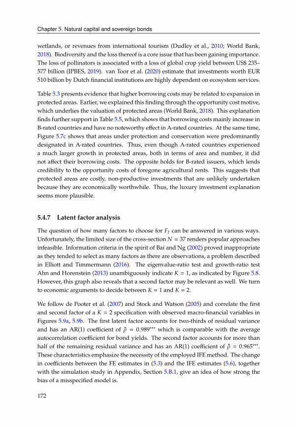
Chapter 5. Natural capital and sovereign bonds
wetlands, or revenues from international tourism (Dudley et al., 2010; World Bank,
2018). Biodiversity and the loss thereof is a core issue that has been gaining importance.
The loss of pollinators is associated with a loss of global crop yield between US$ 235–
577 billion (IPBES, 2019). van Toor et al. (2020) estimate that investments worth EUR
510 billion by Dutch financial institutions are highly dependent on ecosystem services.
Table 5.3 presents evidence that higher borrowing costs may be related to expansion in
protected areas. Earlier, we explained this finding through the opportunity costmotive,
which underlies the valuation of protected areas (World Bank, 2018). This explanation
finds further support in Table 5.5, which shows that borrowing costs mainly increase in
B-rated countries and have no noteworthy effect in A-rated countries. At the same time,
Figure 5.7c shows that areas under protection and conservation were predominantly
designated in A-rated countries. Thus, even though A-rated countries experienced
a much larger growth in protected areas, both in terms of area and number, it did
not affect their borrowing costs. The opposite holds for B-rated issuers, which lends
credibility to the opportunity costs of foregone agricultural rents. This suggests that
protected areas are costly, non-productive investments that are unlikely undertaken
because they are economically worthwhile. Thus, the luxury investment explanation
seems more plausible.
5.4.7 Latent factor analysis
The question of how many factors to choose for �C can be answered in various ways.
Unfortunately, the limited size of the cross-section # = 37 renders popular approaches
infeasible. Information criteria in the spirit of Bai and Ng (2002) proved inappropriate
as they tended to select as many factors as there are observations, a problem described
in Elliott and Timmermann (2016). The eigenvalue-ratio test and growth-ratio test
Ahn and Horenstein (2013) unambiguously indicate = 1, as indicated by Figure 5.8.
However, this graph also reveals that a second factor may be relevant as well. We turn
to economic arguments to decide between = 1 and = 2.
We follow de Pooter et al. (2007) and Stock and Watson (2005) and correlate the first
and second factor of a = 2 specification with observed macro-financial variables in
Figures 5.9a, 5.9b. The first latent factor accounts for two-thirds of residual variance
and has an AR(1) coefficient of � = 0.989∗∗∗
which is comparable with the average
autocorrelation coefficient for bond yields. The second factor accounts for more than
half of the remaining residual variance and has an AR(1) coefficient of � = 0.965∗∗∗
.
These characteristics emphasize the necessity of the employed IFEmethod. The change
in coefficients between the FE estimates in (5.3) and the IFE estimates (5.6), together
with the simulation study in Appendix, Section 5.B.1, give an idea of how strong the
bias of a misspecified model is.
172

Chapter 5. Natural capital and sovereign bonds
Figure 5.8: Shares of explained variance by latent factors
Each panel depicts the share of variance explained by fitting model (5.9)-(5.10) with = 1, 2, 3 factors, respec-
tively.
1 2 3 4 5 6 7 8 9 100%
20%
40%
60%
80%
100%
75.
6% 8
.7%
5.2
% 3
.5%
2.2
% 1
.2%
0.9
% 0
.6%
0.5
% 0
.3%
Ft with 1 factors
1 2 3 4 5 6 7 8 9 10
66.
5% 1
8.9%
4.8
% 3
.3%
2.0
% 1
.2%
0.9
% 0
.6%
0.4
% 0
.2%
Ft with 2 factors
1 2 3 4 5 6 7 8 9 10
67.
3% 1
6.9%
6.0
% 3
.3%
2.1
% 1
.2%
0.8
% 0
.6%
0.4
% 0
.2%
Ft with 3 factors
Share of explained varianceShare of explained variance (cuml.)
Figure 5.9a shows that the first latent factor is most highly correlated with the J.P. Mor-
gan Global Bond Index for the European Monetary Union (GBI-EMU) with correlation
coefficient A = 98.2%, the MSCI World Index with A = 89.2%, and the J.P. Morgan
Emerging Market Bond Index family (EMBI, EMBI-div, EMBI+) with A ≈ 87.3%. The
relevance of the GBI-EMU is sensible since our sample includes ten Eurozone coun-
tries and eight additional European Economic Area members. Figure 5.9b shows that
the second factor is most correlated with the J.P. Morgan Global Bond Index for the
EmergingMarkets (GBI-EM), which tracks local currency government bonds in emerg-
ing markets. Since the composition of the B-rated countries contains several emerging
market economies, itmakes sense to include this factor aswell. This gives us confidence
that = 2 factors are necessary to isolate the relevant global bond dynamics.
5.5 Limitations
5.5.1 Lack of biodiversity
For the sake of consistent, global coverage, thewealth datamade the deliberate decision
to calculate aggregated numbers on the country level. This prevents decompositions
beyond what Table 5.6 presents. One interesting component that affects all renewables
is biodiversity. The wealth of species diversity and ecosystem services is currently only
accounted for indirectly. These are restricted to terrestrial areas and do not include
the blue economy. Loss of biodiversity and collapse of the ecosystem is ranked as top
five global risks (WEF, 2020a). Regulators, pension funds and banks are paying more
and more attention to the effects on the financial sector (Schellekens & van Toor, 2019;
van Toor et al., 2020).
173
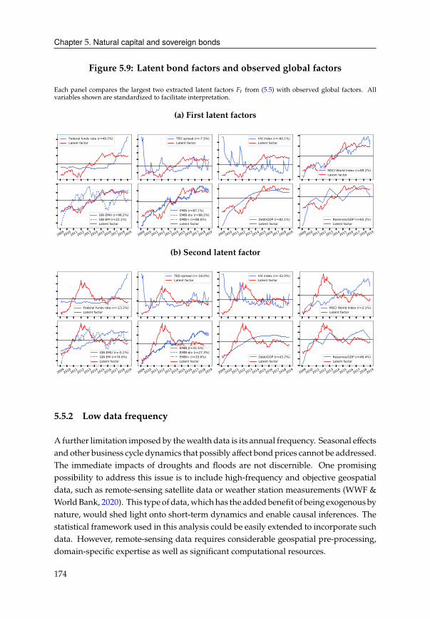
Chapter 5. Natural capital and sovereign bonds
Figure 5.9: Latent bond factors and observed global factors
Each panel compares the largest two extracted latent factors �C from (5.5) with observed global factors. All
variables shown are standardized to facilitate interpretation.
(a) First latent factors
Federal funds rate (r=49.2%)Latent factor
TED spread (r=-7.5%)Latent factor
VIX index (r=-60.1%)Latent factor
MSCI World Index (r=89.2%)Latent factor
20092010
20112012
20132014
20152016
20172018
2019
GBI-EMU (r=98.2%)GBI-EM (r=22.1%)Latent factor
20092010
20112012
20132014
20152016
20172018
2019
EMBI (r=87.1%)EMBI-div (r=88.2%)EMBI+ (r=86.6%)Latent factor
20092010
20112012
20132014
20152016
20172018
2019
Debt/GDP (r=82.1%)Latent factor
20092010
20112012
20132014
20152016
20172018
2019
Reserves/GDP (r=65.2%)Latent factor
(b) Second latent factor
Federal funds rate (r=-13.2%)Latent factor
TED spread (r=-18.0%)Latent factor
VIX index (r=-32.0%)Latent factor
MSCI World Index (r=2.1%)Latent factor
20092010
20112012
20132014
20152016
20172018
2019
GBI-EMU (r=-0.1%)GBI-EM (r=74.6%)Latent factor
20092010
20112012
20132014
20152016
20172018
2019
EMBI (r=31.5%)EMBI-div (r=27.3%)EMBI+ (r=33.6%)Latent factor
20092010
20112012
20132014
20152016
20172018
2019
Debt/GDP (r=43.2%)Latent factor
20092010
20112012
20132014
20152016
20172018
2019
Reserves/GDP (r=46.4%)Latent factor
5.5.2 Low data frequency
A further limitation imposed by thewealth data is its annual frequency. Seasonal effects
and other business cycle dynamics that possibly affect bond prices cannot be addressed.
The immediate impacts of droughts and floods are not discernible. One promising
possibility to address this issue is to include high-frequency and objective geospatial
data, such as remote-sensing satellite data or weather station measurements (WWF &
WorldBank, 2020). This typeofdata,whichhas the addedbenefit of being exogenousby
nature, would shed light onto short-term dynamics and enable causal inferences. The
statistical framework used in this analysis could be easily extended to incorporate such
data. However, remote-sensing data requires considerable geospatial pre-processing,
domain-specific expertise as well as significant computational resources.
174
Chapter 5. Natural capital and sovereign bonds
5.5.3 Lack of regional focus
At the outset of this study, we selected the largest possible set of countries to identify
general relationships between natural capital and government yields. This meant,
however, that country- or region-specific characteristics had to be abstracted from for
the sake of generality. There is little doubt that narrowing the scope to a region,
e.g. Latin America and Caribbeans or South East Asia, would allow us to account for
relevant variables such as local crop types, resource dependencies or the effect of the El
Niño–Southern Oscillation. Comparison of such regional studies with this extended
set of countries would produce interesting insights and lead to relevant takeaways for
local governments and policies makers.
5.6 Summary
This paper has explored whether natural capital is priced in sovereign bonds yields.
The data suggests two answers. Looking across countries, wealth in natural capital
seems to raise the price of government debt. This is consistent with the long-term
view of economic growth and capital accumulation. However, when looking within
countries, which compares the same country with itself at an earlier point in time, the
opposite emerges. As a country’s renewable natural wealth grew, its borrowing costs
tended to fall. This is the short-run view, where natural capital can grow and sovereign
default risk can vary.
While both approaches seems tobeviable, the long-termview is affectedby the ingrainedincome bias (see Figure 5.6). This bias refers to the problem of comparing countries at
different stages of development and levels of income. High income countries will have
transitioned into an economic system where growth is less reliant on natural capital.
Hence, explanations for higher yields due to natural wealth, such as the resource curse
or inflation expectations, will more likely affect developing economies. This presents
not only an econometric problem, but the long-run view also leads to a disheartening
conclusion. Since the level of income is the result of decades or centuries of human
history, there is nothing a country can accomplish in the short-run to affect it. This bias
also affects sovereign ESG scores (see Box 1).
Thus, there are few novel insights to be gained from cross-country comparisons, be-
cause the level of development will dominate an permeate any findings. Adopting the
within-country view resolves this problem. By bringing countries onto a “level playing
field”, cross-country differences, such as resource endowments or levels of income,
are taken out of the picture. Instead, the relationship between natural capital and
borrowing costs is estimated using changes of time, within each country. This means
that recent efforts to foster renewable natural capital, such as afforestation trends or
175
Chapter 5. Natural capital and sovereign bonds
expansion in organic agriculture, had room to impact on short-run borrowing costs of
governments.
After introducing the appropriate statistical framework, we found a significant, nega-
tive association between renewable natural capital growth and government debt costs.
Expansions in protected areas, agricultural land and forest capital affected bond yields
for two possible reasons: First, because they are worthwhile investments that improve
country fundamentals and thereby lower borrowing costs. Second, low bond yields
are in fact a reflection of wealth and therefore the capacity to invest into natural capi-
tal. Looking at the underlying data, we found that the negative effects of forests and
agricultural land are more likely explained by the worthwhile investment narrative.
Countries invest into these resources simply because they are more reliant on natural
capital for economic growth. Fostering this type of renewables is an economic worth-
while investment. The effects of protected areas, which expanded the most in A-rated
countries, are better explained by the luxury investment narrative. Designating areas
under conservation and protection is costly and incurs opportunity costs in terms of
foregone agricultural rents. High income countries can afford to expand protected
areas as they have the fiscal capabilities and rely more on produced and human capital
for growth.
In sum, this paper found evidence that government borrowing costs reflect a country’s
recent growth in natural capital. These findings emerged after accounting for various
confounding factors, such as the ingrained income bias or commonbond factors, aswell
as controlling for relevant macro-financial variables. The empirical model, however,
does not reveal the economic mechanism behind this finding. A direct channel seems
unlikely, as itwould imply thatmarkets actively prioritize natural capital considerations
in their bond purchase decisions. What seems more plausible is that natural wealth is
accounted for indirectly through its effect on the wider economy. We found support
this hypothesis. Borrowing costs of B-rated issuers, whose economies are more reliant
on natural capital, were also affected more by renewable capital growth. Formulating
and identifying the exact channel is left for future research.
176
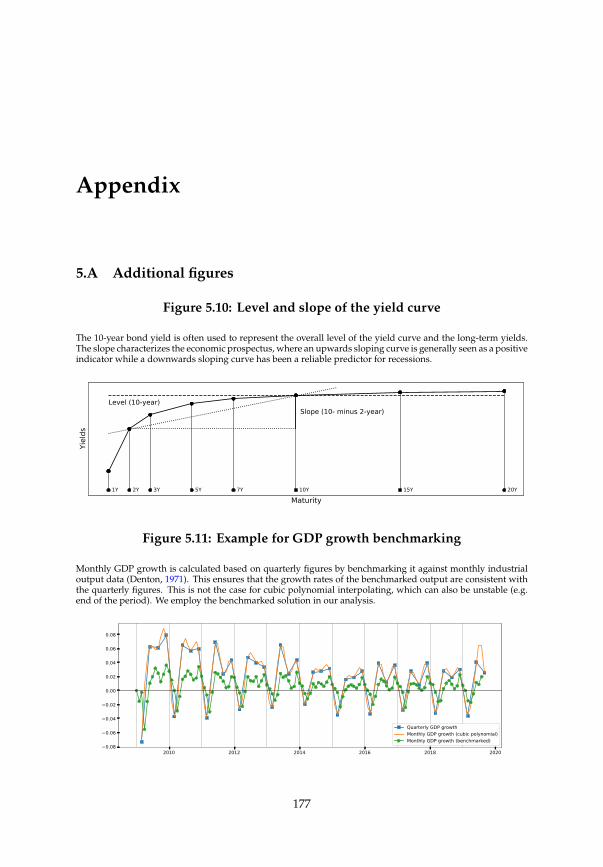
Appendix
5.A Additional figures
Figure 5.10: Level and slope of the yield curve
The 10-year bond yield is often used to represent the overall level of the yield curve and the long-term yields.
The slope characterizes the economic prospectus, where an upwards sloping curve is generally seen as a positive
indicator while a downwards sloping curve has been a reliable predictor for recessions.
Maturity
Yiel
ds
1Y 2Y 3Y 5Y 7Y 10Y 15Y 20Y
Level (10-year) Slope (10- minus 2-year)
Figure 5.11: Example for GDP growth benchmarking
Monthly GDP growth is calculated based on quarterly figures by benchmarking it against monthly industrial
output data (Denton, 1971). This ensures that the growth rates of the benchmarked output are consistent with
the quarterly figures. This is not the case for cubic polynomial interpolating, which can also be unstable (e.g.
end of the period). We employ the benchmarked solution in our analysis.
2010 2012 2014 2016 2018 20200.08
0.06
0.04
0.02
0.00
0.02
0.04
0.06
0.08
Quarterly GDP growthMonthly GDP growth (cubic polynomial)Monthly GDP growth (benchmarked)
177
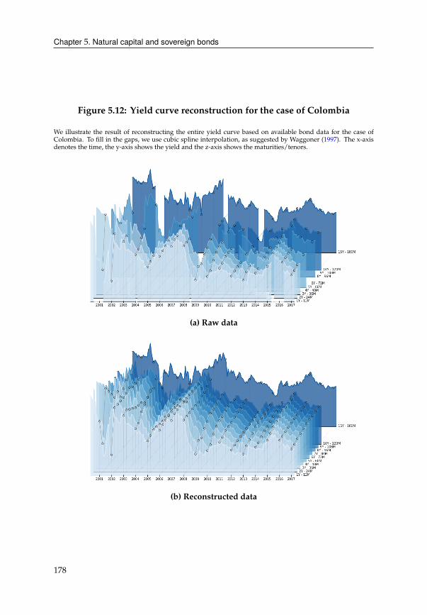
Chapter 5. Natural capital and sovereign bonds
Figure 5.12: Yield curve reconstruction for the case of Colombia
We illustrate the result of reconstructing the entire yield curve based on available bond data for the case of
Colombia. To fill in the gaps, we use cubic spline interpolation, as suggested by Waggoner (1997). The x-axis
denotes the time, the y-axis shows the yield and the z-axis shows the maturities/tenors.
(a) Raw data
(b) Reconstructed data
178
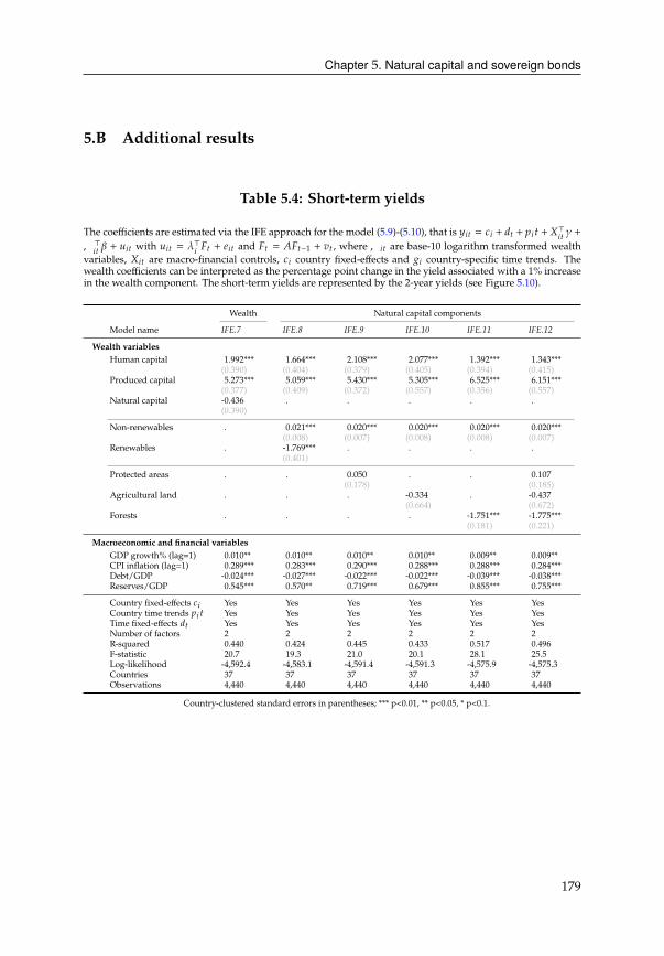
Chapter 5. Natural capital and sovereign bonds
5.B Additional results
Table 5.4: Short-term yields
The coefficients are estimated via the IFE approach for the model (5.9)-(5.10), that is H8C = 28 + 3C + ?8 C +->8C � +,>8C� + D8C with D8C = �>
8�C + 48C and �C = ��C−1 + EC , where,8C are base-10 logarithm transformed wealth
variables, -8C are macro-financial controls, 28 country fixed-effects and 68 country-specific time trends. The
wealth coefficients can be interpreted as the percentage point change in the yield associated with a 1% increase
in the wealth component. The short-term yields are represented by the 2-year yields (see Figure 5.10).
Wealth Natural capital components
Model name IFE.7 IFE.8 IFE.9 IFE.10 IFE.11 IFE.12
Wealth variablesHuman capital 1.992***
(0.390)
1.664***
(0.404)
2.108***
(0.379)
2.077***
(0.405)
1.392***
(0.394)
1.343***
(0.415)
Produced capital 5.273***
(0.377)
5.059***
(0.409)
5.430***
(0.372)
5.305***
(0.557)
6.525***
(0.356)
6.151***
(0.557)
Natural capital -0.436
(0.390)
. . . . .
Non-renewables . 0.021***
(0.008)
0.020***
(0.007)
0.020***
(0.008)
0.020***
(0.008)
0.020***
(0.007)
Renewables . -1.769***
(0.401)
. . . .
Protected areas . . 0.050
(0.178)
. . 0.107
(0.185)
Agricultural land . . . -0.334
(0.664)
. -0.437
(0.672)
Forests . . . . -1.751***
(0.181)
-1.775***
(0.221)
Macroeconomic and financial variablesGDP growth% (lag=1) 0.010** 0.010** 0.010** 0.010** 0.009** 0.009**
CPI inflation (lag=1) 0.289*** 0.283*** 0.290*** 0.288*** 0.288*** 0.284***
Debt/GDP -0.024*** -0.027*** -0.022*** -0.022*** -0.039*** -0.038***
Reserves/GDP 0.545*** 0.570** 0.719*** 0.679*** 0.855*** 0.755***
Country fixed-effects 28 Yes Yes Yes Yes Yes Yes
Country time trends ?8 C Yes Yes Yes Yes Yes Yes
Time fixed-effects 3C Yes Yes Yes Yes Yes Yes
Number of factors 2 2 2 2 2 2
R-squared 0.440 0.424 0.445 0.433 0.517 0.496
F-statistic 20.7 19.3 21.0 20.1 28.1 25.5
Log-likelihood -4,592.4 -4,583.1 -4,591.4 -4,591.3 -4,575.9 -4,575.3
Countries 37 37 37 37 37 37
Observations 4,440 4,440 4,440 4,440 4,440 4,440
Country-clustered standard errors in parentheses; *** p<0.01, ** p<0.05, * p<0.1.
179
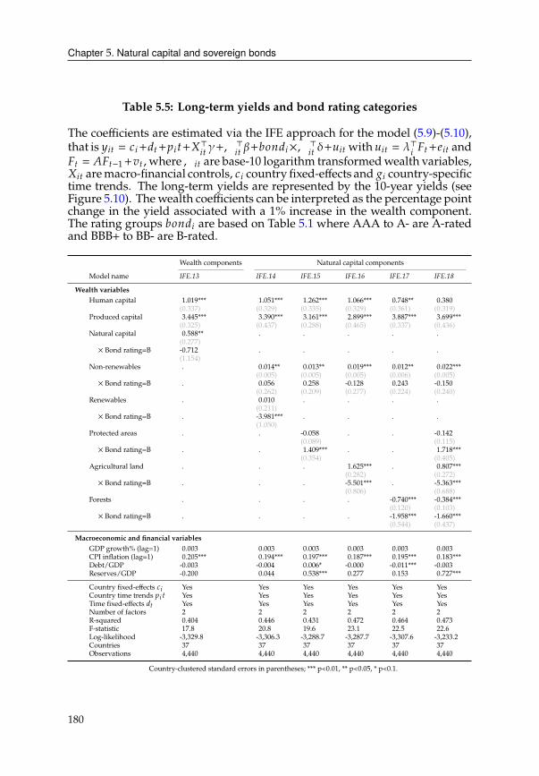
Chapter 5. Natural capital and sovereign bonds
Table 5.5: Long-term yields and bond rating categories
The coefficients are estimated via the IFE approach for the model (5.9)-(5.10),
that is H8C = 28+3C+?8C+->8C �+,>8C�+1>=38×,>8C �+D8C with D8C = �>
8�C+48C and
�C = ��C−1+EC , where,8C are base-10 logarithm transformedwealth variables,
-8C aremacro-financial controls, 28 country fixed-effects and 68 country-specifictime trends. The long-term yields are represented by the 10-year yields (see
Figure 5.10). Thewealth coefficients can be interpreted as the percentage point
change in the yield associated with a 1% increase in the wealth component.
The rating groups 1>=38 are based on Table 5.1 where AAA to A- are A-rated
and BBB+ to BB- are B-rated.
Wealth components Natural capital components
Model name IFE.13 IFE.14 IFE.15 IFE.16 IFE.17 IFE.18
Wealth variablesHuman capital 1.019***
(0.337)
1.051***
(0.329)
1.262***
(0.335)
1.066***
(0.329)
0.748**
(0.361)
0.380
(0.319)
Produced capital 3.445***
(0.325)
3.390***
(0.437)
3.161***
(0.288)
2.899***
(0.465)
3.887***
(0.337)
3.699***
(0.436)
Natural capital 0.588**
(0.277)
. . . . .
× Bond rating=B -0.712
(1.154)
. . . . .
Non-renewables . 0.014**
(0.005)
0.013**
(0.005)
0.019***
(0.005)
0.012**
(0.006)
0.022***
(0.005)
× Bond rating=B . 0.056
(0.262)
0.258
(0.209)
-0.128
(0.277)
0.243
(0.224)
-0.150
(0.240)
Renewables . 0.010
(0.211)
. . . .
× Bond rating=B . -3.981***
(1.050)
. . . .
Protected areas . . -0.058
(0.089)
. . -0.142
(0.115)
× Bond rating=B . . 1.409***
(0.354)
. . 1.718***
(0.405)
Agricultural land . . . 1.625***
(0.282)
. 0.807***
(0.272)
× Bond rating=B . . . -5.501***
(0.806)
. -5.363***
(0.688)
Forests . . . . -0.740***
(0.120)
-0.384***
(0.103)
× Bond rating=B . . . . -1.958***
(0.544)
-1.660***
(0.437)
Macroeconomic and financial variablesGDP growth% (lag=1) 0.003 0.003 0.003 0.003 0.003 0.003
CPI inflation (lag=1) 0.205*** 0.194*** 0.197*** 0.187*** 0.195*** 0.183***
Debt/GDP -0.003 -0.004 0.006* -0.000 -0.011*** -0.003
Reserves/GDP -0.200 0.044 0.538*** 0.277 0.153 0.727***
Country fixed-effects 28 Yes Yes Yes Yes Yes Yes
Country time trends ?8 C Yes Yes Yes Yes Yes Yes
Time fixed-effects 3C Yes Yes Yes Yes Yes Yes
Number of factors 2 2 2 2 2 2
R-squared 0.404 0.446 0.431 0.472 0.464 0.473
F-statistic 17.8 20.8 19.6 23.1 22.5 22.6
Log-likelihood -3,329.8 -3,306.3 -3,288.7 -3,287.7 -3,307.6 -3,233.2
Countries 37 37 37 37 37 37
Observations 4,440 4,440 4,440 4,440 4,440 4,440
Country-clustered standard errors in parentheses; *** p<0.01, ** p<0.05, * p<0.1.
180

Chapter 5. Natural capital and sovereign bonds
Table 5.6: Long-term yields and natural capital components
The coefficients are estimated via the IFE approach for the model (5.9)-(5.10), that is H8C = 28 + 3C + ?8 C +->8C� +,>
8C� + D8C with D8C = �>
8�C + 48C and �C = ��C−1 + EC , where,8C are base-10 logarithm transformed
wealth variables, -8C are macro-financial controls, 28 country fixed-effects and 68 country-specific time trends.
The long-term yields are represented by the 10-year yields (see Figure 5.10). The wealth coefficients can be
interpreted as the percentage point change in the yield associated with a 1% increase in the wealth component.
This table is an extension of Table 5.9. Cropland and pastureland constitute agricultural land, timber and
non-timber forests constitute forests.
Natural capital components
Model name IFE.19 IFE.20 IFE.21 IFE.22 IFE.23 IFE.24
Wealth variablesHuman capital 0.743**
(0.355)
1.131***
(0.342)
0.896**
(0.350)
0.925***
(0.352)
0.265
(0.351)
0.263
(0.359)
Produced capital 3.441***
(0.403)
2.457***
(0.289)
2.754***
(0.370)
3.440***
(0.321)
4.035***
(0.300)
4.254***
(0.309)
Non-renewables 0.012**
(0.005)
0.008
(0.005)
0.009*
(0.005)
0.008
(0.005)
0.009
(0.005)
0.006
(0.005)
Cropland -0.799***
(0.284)
. -1.127***
(0.290)
. . .
Pastureland . 1.344***
(0.358)
1.567***
(0.355)
. . .
Forests (timber) . . . 0.273
(0.167)
. 0.318**
(0.159)
Forests (non-timber) . . . . -0.988***
(0.142)
-1.000***
(0.140)
Macroeconomic and financial variablesGDP growth% (lag=1) 0.003 0.003 0.003 0.003 0.003 0.003
CPI inflation (lag=1) 0.202*** 0.198*** 0.197*** 0.205*** 0.204*** 0.206***
Debt/GDP -0.003 -0.001 0.001 -0.004 -0.016*** -0.016***
Reserves/GDP 0.045 0.122 0.095 0.118 0.010 0.061
Country fixed-effects 28 Yes Yes Yes Yes Yes Yes
Country time trends ?8 C Yes Yes Yes Yes Yes Yes
Time fixed-effects 3C Yes Yes Yes Yes Yes Yes
Number of factors 2 2 2 2 2 2
R-squared 0.396 0.409 0.407 0.405 0.445 0.453
F-statistic 17.2 18.2 17.9 17.9 21.0 21.6
Log-likelihood -3,327.6 -3,319.6 -3,309.6 -3,331.4 -3,324.0 -3,322.5
Countries 37 37 37 37 37 37
Observations 4,440 4,440 4,440 4,440 4,440 4,440
Country-clustered standard errors in parentheses; *** p<0.01, ** p<0.05, * p<0.1.
181
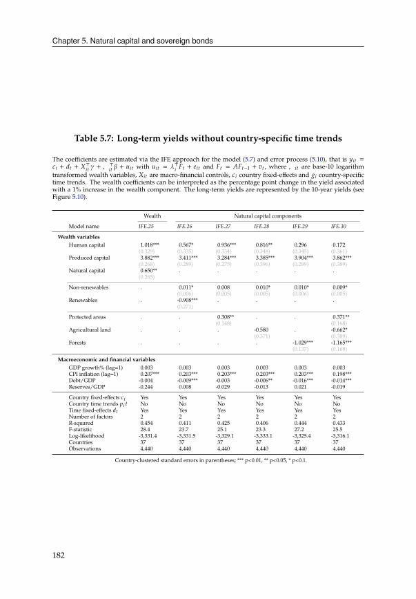
Chapter 5. Natural capital and sovereign bonds
Table 5.7: Long-term yields without country-specific time trends
The coefficients are estimated via the IFE approach for the model (5.7) and error process (5.10), that is H8C =28 + 3C + ->8C � +,
>8C� + D8C with D8C = �>
8�C + 48C and �C = ��C−1 + EC , where ,8C are base-10 logarithm
transformed wealth variables, -8C are macro-financial controls, 28 country fixed-effects and 68 country-specifictime trends. The wealth coefficients can be interpreted as the percentage point change in the yield associated
with a 1% increase in the wealth component. The long-term yields are represented by the 10-year yields (see
Figure 5.10).
Wealth Natural capital components
Model name IFE.25 IFE.26 IFE.27 IFE.28 IFE.29 IFE.30
Wealth variablesHuman capital 1.018***
(0.329)
0.567*
(0.335)
0.936***
(0.334)
0.816**
(0.348)
0.296
(0.345)
0.172
(0.361)
Produced capital 3.882***
(0.268)
3.411***
(0.289)
3.284***
(0.275)
3.385***
(0.396)
3.904***
(0.289)
3.862***
(0.389)
Natural capital 0.650**
(0.265)
. . . . .
Non-renewables . 0.011*
(0.006)
0.008
(0.005)
0.010*
(0.005)
0.010*
(0.006)
0.009*
(0.005)
Renewables . -0.908***
(0.271)
. . . .
Protected areas . . 0.308**
(0.148)
. . 0.371**
(0.168)
Agricultural land . . . -0.580
(0.371)
. -0.662*
(0.389)
Forests . . . . -1.029***
(0.137)
-1.165***
(0.168)
Macroeconomic and financial variablesGDP growth% (lag=1) 0.003 0.003 0.003 0.003 0.003 0.003
CPI inflation (lag=1) 0.207*** 0.203*** 0.203*** 0.203*** 0.203*** 0.198***
Debt/GDP -0.004 -0.009*** -0.003 -0.006** -0.016*** -0.014***
Reserves/GDP -0.244 0.008 -0.029 -0.013 0.021 -0.019
Country fixed-effects 28 Yes Yes Yes Yes Yes Yes
Country time trends ?8 C No No No No No No
Time fixed-effects 3C Yes Yes Yes Yes Yes Yes
Number of factors 2 2 2 2 2 2
R-squared 0.454 0.411 0.425 0.406 0.444 0.433
F-statistic 28.4 23.7 25.1 23.3 27.2 25.5
Log-likelihood -3,331.4 -3,331.5 -3,329.1 -3,333.1 -3,325.4 -3,316.1
Countries 37 37 37 37 37 37
Observations 4,440 4,440 4,440 4,440 4,440 4,440
Country-clustered standard errors in parentheses; *** p<0.01, ** p<0.05, * p<0.1.
182
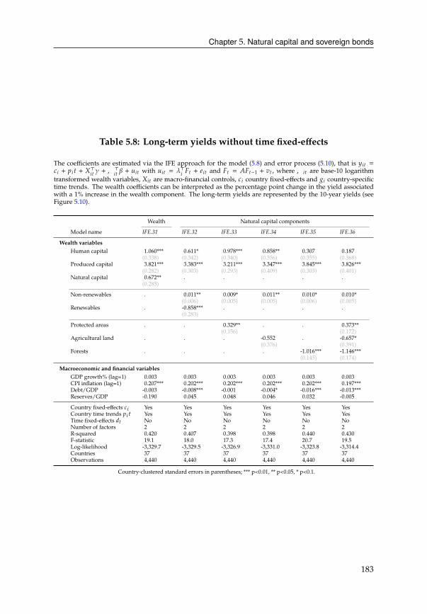
Chapter 5. Natural capital and sovereign bonds
Table 5.8: Long-term yields without time fixed-effects
The coefficients are estimated via the IFE approach for the model (5.8) and error process (5.10), that is H8C =28 + ?8 C + ->8C � +,
>8C� + D8C with D8C = �>
8�C + 48C and �C = ��C−1 + EC , where ,8C are base-10 logarithm
transformed wealth variables, -8C are macro-financial controls, 28 country fixed-effects and 68 country-specifictime trends. The wealth coefficients can be interpreted as the percentage point change in the yield associated
with a 1% increase in the wealth component. The long-term yields are represented by the 10-year yields (see
Figure 5.10).
Wealth Natural capital components
Model name IFE.31 IFE.32 IFE.33 IFE.34 IFE.35 IFE.36
Wealth variablesHuman capital 1.060***
(0.338)
0.611*
(0.342)
0.978***
(0.340)
0.858**
(0.356)
0.307
(0.355)
0.187
(0.368)
Produced capital 3.821***
(0.282)
3.383***
(0.303)
3.211***
(0.293)
3.347***
(0.409)
3.845***
(0.303)
3.826***
(0.401)
Natural capital 0.672**
(0.285)
. . . . .
Non-renewables . 0.011**
(0.006)
0.009*
(0.005)
0.011**
(0.005)
0.010*
(0.006)
0.010*
(0.005)
Renewables . -0.858***
(0.283)
. . . .
Protected areas . . 0.329**
(0.156)
. . 0.373**
(0.172)
Agricultural land . . . -0.552
(0.376)
. -0.657*
(0.391)
Forests . . . . -1.016***
(0.145)
-1.146***
(0.174)
Macroeconomic and financial variablesGDP growth% (lag=1) 0.003 0.003 0.003 0.003 0.003 0.003
CPI inflation (lag=1) 0.207*** 0.202*** 0.202*** 0.202*** 0.202*** 0.197***
Debt/GDP -0.003 -0.008*** -0.001 -0.004* -0.016*** -0.013***
Reserves/GDP -0.190 0.045 0.048 0.046 0.032 -0.005
Country fixed-effects 28 Yes Yes Yes Yes Yes Yes
Country time trends ?8 C Yes Yes Yes Yes Yes Yes
Time fixed-effects 3C No No No No No No
Number of factors 2 2 2 2 2 2
R-squared 0.420 0.407 0.398 0.398 0.440 0.430
F-statistic 19.1 18.0 17.3 17.4 20.7 19.5
Log-likelihood -3,329.7 -3,329.5 -3,326.9 -3,331.0 -3,323.8 -3,314.4
Countries 37 37 37 37 37 37
Observations 4,440 4,440 4,440 4,440 4,440 4,440
Country-clustered standard errors in parentheses; *** p<0.01, ** p<0.05, * p<0.1.
183
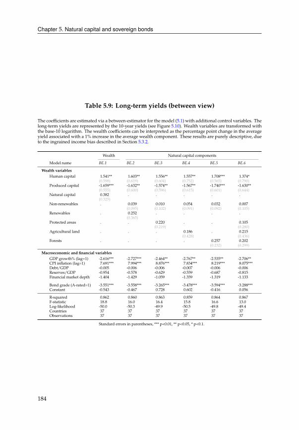
Chapter 5. Natural capital and sovereign bonds
Table 5.9: Long-term yields (between view)
The coefficients are estimated via a between-estimator for the model (5.1) with additional control variables. The
long-term yields are represented by the 10-year yields (see Figure 5.10). Wealth variables are transformed with
the base-10 logarithm. The wealth coefficients can be interpreted as the percentage point change in the average
yield associated with a 1% increase in the average wealth component. These results are purely descriptive, due
to the ingrained income bias described in Section 5.3.2.
Wealth Natural capital components
Model name BE.1 BE.2 BE.3 BE.4 BE.5 BE.6
Wealth variablesHuman capital 1.541**
(0.598)
1.603**
(0.619)
1.556**
(0.604)
1.557**
(0.752)
1.708***
(0.565)
1.374*
(0.790)
Produced capital -1.659***
(0.555)
-1.632**
(0.600)
-1.574**
(0.596)
-1.567**
(0.615)
-1.740***
(0.601)
-1.630**
(0.644)
Natural capital 0.382
(0.325)
. . . . .
Non-renewables . 0.039
(0.095)
0.010
(0.102)
0.054
(0.091)
0.032
(0.092)
0.007
(0.105)
Renewables . 0.252
(0.365)
. . . .
Protected areas . . 0.220
(0.219)
. . 0.105
(0.280)
Agricultural land . . . 0.186
(0.428)
. 0.215
(0.436)
Forests . . . . 0.257
(0.232)
0.202
(0.299)
Macroeconomic and financial variablesGDP growth% (lag=1) -2.616*** -2.727*** -2.464** -2.767** -2.535** -2.706**
CPI inflation (lag=1) 7.691*** 7.994*** 8.876*** 7.834*** 8.219*** 8.075***
Debt/GDP -0.005 -0.006 -0.006 -0.007 -0.006 -0.006
Reserves/GDP -0.954 -0.578 -0.629 -0.559 -0.687 -0.815
Financial market depth -1.404 -1.429 -1.059 -1.359 -1.319 -1.133
Bond grade (A-rated=1) -3.551*** -3.558*** -3.265*** -3.478*** -3.594*** -3.288***
Constant -0.543 -0.467 0.728 0.602 -0.416 0.056
R-squared 0.862 0.860 0.863 0.859 0.864 0.867
F-statistic 18.8 16.0 16.4 15.8 16.6 13.0
Log-likelihood -50.0 -50.3 -49.9 -50.5 -49.8 -49.4
Countries 37 37 37 37 37 37
Observations 37 37 37 37 37 37
Standard errors in parentheses, *** p<0.01, ** p<0.05, * p<0.1.
184
Chapter 5. Natural capital and sovereign bonds
5.B.1 Monte Carlo study
Setup In this simulation studywe illustratewhat problems arisewhen latent common
factors are not properly accounted for. We follow the structure of (Bai, 2009) but differ
in that we allow the factors to be autocorrelated. We then show how the interactive
fixed-effects (IFE) approach resolves this problem, even with dynamic factors. The
data-generating process reads as follows,
H8C = �0+ -8C�1
+ D8C (5.11)
-8C = � + �8 5C + �8 + 5C + F8C (5.12)
The true parameters are �0= 5, �
1= 1. The disturbances contain a latent factor,
D8C = �8 5C + 48C with randomly drawn �8 and an autoregressive latent factor process
5C = � 5C−1+ E8C . The innovations 48C , E8C are sampled from #(0, 1). We examine three
values of � ∈ {0.0, 0.3, 0.7}. The regressor -8C is constructed to induce an endogeneity
problem through the common factor, such that E[D8C |-8C] ≠ 0. The disturbances F8C
are sampled from #(0, 1) and � = 1.
Results We simulate (5.11) and (5.12) 1,000 times and use a conventional fixed-effects
model (FE) and the interactive fixed-effects (IFE) approach to estimate �0, �
1. The
results are shown in Figure 5.13. As expected, the FE estimators (red) are heavily
affected by an omitted variable bias due to the induced endogeneity. This mirrors the
case where global common factors, such as the global economy or the Eurozone crises,
affect both the bond prices and regressors, such as GDP growth or debt-to-GDP ratios.
Note that with increasing autocorrelation in the factors, the FE residuals suffer from
serial correlation, leading to increasingly less efficient estimators. The interactive fixed-
effects approach (blue) estimates the latent factor which resolves both the endogeneity
and serial correlation problems. The estimates are unbiased and more efficient.
185
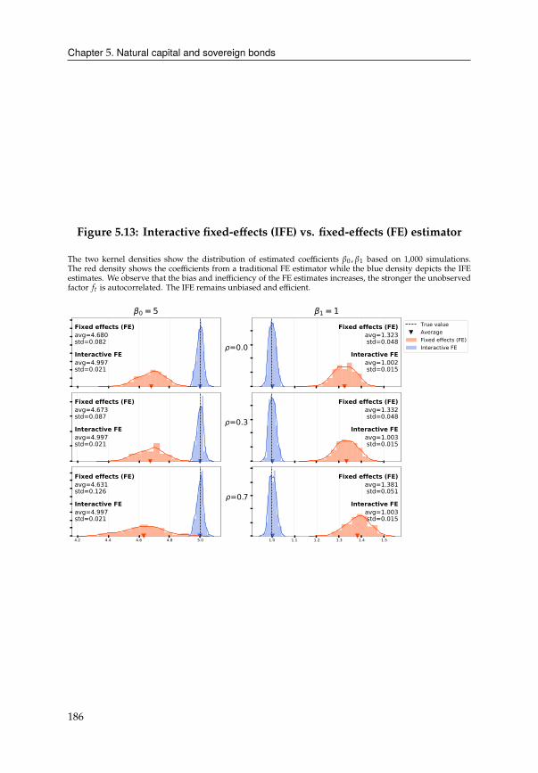
Chapter 5. Natural capital and sovereign bonds
Figure 5.13: Interactive fixed-effects (IFE) vs. fixed-effects (FE) estimator
The two kernel densities show the distribution of estimated coefficients �0 , �1 based on 1,000 simulations.
The red density shows the coefficients from a traditional FE estimator while the blue density depicts the IFE
estimates. We observe that the bias and inefficiency of the FE estimates increases, the stronger the unobserved
factor 5C is autocorrelated. The IFE remains unbiased and efficient.
Fixed effects (FE)avg=4.680std=0.082Interactive FEavg=4.997std=0.021
0 = 5
=0.0
Fixed effects (FE)avg=1.323std=0.048
Interactive FEavg=1.002std=0.015
1 = 1True valueAverageFixed effects (FE)Interactive FE
Fixed effects (FE)avg=4.673std=0.087Interactive FEavg=4.997std=0.021
=0.3
Fixed effects (FE)avg=1.332std=0.048
Interactive FEavg=1.003std=0.015
4.2 4.4 4.6 4.8 5.0
Fixed effects (FE)avg=4.631std=0.126Interactive FEavg=4.997std=0.021
1.0 1.1 1.2 1.3 1.4 1.5
=0.7
Fixed effects (FE)avg=1.381std=0.051
Interactive FEavg=1.003std=0.015
186
Summary
This thesis consists of four chapterswhich develop and apply empiricalmethods to find
policy-relevant answers regarding financial stability, contagion and network effects,
predicting food insecurity risks, and understanding environmental risk in government
bond markets. This summary gives a non-technical overview and possible future
directions for each chapter.
Chapter 2 proposes a dynamic network effect (DNE) model to study problems with a
wide cross-section (N entities) and long time series (T time periods). What makes this
type of problems interesting is that the observed behaviors of N entities, e.g. banks,
countries, firms, are not independent from each other. Network effects, which refer to
entities affecting each other depending on their (geographic or economic) proximity,
may provide an explanation for observed common behavior. These effects can quickly
become intractable for linear models since network effects can amplify initial shocks,
depending on the network structure, and thereby become nonlinear. How strong the
amplification or dampening effect is may not be constant over time. A key contribution
of this chapter is therefore the dynamic or time-varying element of the DNE model.
The chapter furthermore argues that the smooth marginalized particle filter (SMPF) is
well-suited to estimate these effects over time. Future research may combine the DNE
approach with dynamic factor models.
Chapter 3 applies the DNE model to explain contagion dynamics among Eurozone
banks. Structural determinants of credit risk (equity returns, government bond yields,
leverage ratios, etc.) alone have low explanatory power and also fail to capture un-
known common factors. That is, bank default probabilities are not fully explained
by commonly used determinants. In this chapter we argue that this so-called credit
spread puzzle is possibly explained through negligence of network effects. Banks, after
all, do not exist in isolation as (information) contagion spills over from bank to bank.
Using supervisory asset holdings information, we construct a network that measures
how similar bank business models are to each other. That rationale being that sim-
ilar asset holdings are likely the result of similar business models. The DNE results
indeed show that dynamic network effects explain the unknown common factors and
187

Chapter 5. Natural capital and sovereign bonds
increases explanatory power, particularly during turbulent times. Future work may
explore alternative network construction methods using regularization methods.
Chapter 4 is concerned with an entirely different topic and methodology, namely food
insecurity risks. The ability to predict an outbreak of acute food shortages or even
famine outbreaks just a few months ahead can prevent humanitarian disasters. Al-
thoughhumanitarianorganizations react swiftly andeffectively once a crisis is declared,
crisis declarations are made based on increased mortality which means irreversible
damage has already been done. The task is, however, not trivial due to the dearth
of data and brevity of relevant, historical records. This chapter uses a panel vector-
autoregression (PVAR) to forecast possible long-term scenarios for 21 countries. This
exhibits good performance due to two innovations. First, through variable selection
methods, the most predictive variables are selected from a large set of environmental,
economic and conflict-related predictors. Second, expert opinion can be incorporated
through Bayesian priors, which is especially useful when facing unprecedented situa-
tions. The model is stochastic and can therefore produce stochastic catalogues, based
on which one can construct insurance-like products.
Finally, Chapter 5 asks whether 1% growth in natural capital (the long-term economic
valueof forests, agriculture, protectedareas, fossil fuels andminerals) affects a country’s
borrowing costs on international markets. If countries are compared directly with each
other, that is by correlating the amount of natural capital with the countries’ 10-year
bond yields, a positive relationship emerges. This is, however, a problematic conclusion
due to the ingrained income bias (IIB). This bias is at the heart of why cross-country
comparisons often boil down to a comparison of national income. Since the latter is the
result of decades or centuries of human history, the bias is de facto ingrained, meaning
that they cannot be overcome by any short-term policy efforts. The chapter therefore
advocates focusing on each country’s recent performance. Results obtained from this
within-country analysis are unaffected by the IIB and are able to reflect recent efforts
to foster or exhaust natural capital. After accounting for relevant macro-financial
indicators and bond-specific factors, the results show that renewable natural capital
tend to lower borrowing costs. Ongoing and future work will look deeper into regional
cases and rely on remote-sensing data to examine the effects of disasters and resource
discoveries.
188

Bibliography
Abrahams, M., Adrian, T., Crump, R. K., Moench, E., & Yu, R. (2016). Decomposing real
and nominal yield curves. Journal of Monetary Economics, 84, 182–200.Acharya, V. V., & Yorulmazer, T. (2008). Information Contagion and Bank Herding.
Journal of Money, Credit and Banking, 40(1), 215–231.Ahn, S. C., & Horenstein, A. R. (2013). Eigenvalue ratio test for the number of factors.
Econometrica, 81(3), 1203–1227.Ahnert, T., & Georg, C.-P. (2018). Information Contagion and Systemic Risk. Journal of
Financial Stability, 35, 159–171.Aït-Sahalia, Y., Laeven, R. J., & Pelizzon, L. (2014). Mutual excitation in eurozone
sovereign CDS. Journal of Econometrics, 183(2), 151–167.Allen, F., Babus,A., &Carletti, E. (2012). Asset commonality, debtmaturity and systemic
risk. Journal of Financial Economics, 104(3), 519–534.Allen, F., & Gale, D. (2000). Financial Contagion. Journal of Political Economy, 108(1),
1–33.
Amstad, M., Packer, F., & Shek, J. (2020). Does sovereign risk in local and foreign
currency differ? Journal of International Money and Finance, 101, 102099.Andrée, B. P. J. (2020). Theory and Application of Dynamic Spatial Time Series Models.
Rozenberg Publishers; the Tinbergen Institute.
Andrée, B. P. J., Chamorro, A., Spencer, P., Koomen, E., &Dogo, H. (2019). Revisiting the
relation between economic growth and the environment; a global assessment
of deforestation, pollution and carbon emission. Renewable and SustainableEnergy Reviews, 114, 109221.
Andrée, B. P. J., Kraay, A., Chamorro, A., Spencer, P., & Wang, D. (2020). Predicting
Food Crisis.World Bank Policy Research Working Papers.Andrieu, C., & Doucet, A. (2002a). Particle filtering for Partially Observed Gaussian
State Space Models [Publisher: Wiley Online Library]. Journal of the RoyalStatistical Society: Series B (Statistical Methodology), 64(4), 827–836.
Andrieu, C., & Doucet, A. (2002b). Particle filtering for partially observed Gaussian
state space models. Journal of the Royal Statistical Society: Series B (StatisticalMethodology), 64(4), 827–836.
189
Chapter BIBLIOGRAPHY
Angrist, J. D., & Krueger, A. B. (1999). Empirical strategies in labor economics.Handbookof labor economics (pp. 1277–1366). Elsevier.
Anselin, L. (1988). Spatial Econometrics: Methods and Models. Springer, Dordrecht.
Augustin, P. (2014). Credit Default Swaps: A Survey. Foundations and Trends® in Finance,9(1-2), 1–196.
Badgley, C., Moghtader, J., Quintero, E., Zakem, E., Chappell, M. J., Avilés-Vázquez,
K., Samulon, A., & Perfecto, I. (2007). Organic agriculture and the global food
supply. Renewable Agriculture and Food Systems, 22(2), 86–108.Bai, J. (2009). Panel Data Models With Interactive Fixed Effects. Econometrica, 77(4),
1229–1279.
Bai, J., & Ng, S. (2002). Determining the Number of Factors in Approximate Factor
Models. Econometrica, 70(1), 191–221.Bai, J., & Wang, P. (2016). Econometric Analysis of Large Factor Models. Annual Review
of Economics, 8(1), 53–80.Bańbura, M., Giannone, D., & Reichlin, L. (2008). Large Bayesian VARs (ECB Working
Paper Series No. 966).
Barbier, E. B., & Hochard, J. P. (2018). Land degradation and poverty. Nature Sustain-ability, 1(11), 623–631.
Barrett, C. B., & Bevis, L. E. (2015). The self-reinforcing feedback between low soil
fertility and chronic poverty. Nature Geoscience, 8(12), 907–912.Bergmeir, C., & Benítez, J. M. (2012). On the use of cross-validation for time series
predictor evaluation [Publisher: Elsevier]. Information Sciences, 191, 192–213.Bergmeir, C., Hyndman, R. J., & Koo, B. (2018). A Note on the Validity of Cross-
Validation for Evaluating Autoregressive Time Series Prediction. Computa-tional Statistics and Data Analysis.
Berk, R., Brown, L., Buja, A., Zhang, K., &Zhao, L. (2013). Valid post-selection inference.
The Annals of Statistics, 41(2), 802–837.Bertoli, S., & Fernández-Huertas Moraga, J. (2013). Multilateral resistance to migration.
Journal of Development Economics, 102, 79–100.Betz, F., Hautsch, N., Peltonen, T. A., & Schienle, M. (2016). Systemic risk spillovers in
the european banking and sovereign network. Journal of Financial Stability, 25,206–224.
Bharath, S. T., & Shumway, T. (2008). Forecasting default with the Merton distance to
default model [ISBN: 08939454]. Review of Financial Studies, 21(3), 1339–1369.Billio, M., Getmansky, M., Lo, A. W., & Pelizzon, L. (2012). Econometric Measures
of Connectedness and Systemic Risk in the Finance and Insurance Sectors.
Journal of Financial Economics, 104(3), 535–559.Blasques, F., Bräuning, F., & van Lelyveld, I. (2018). A Dynamic Stochastic Network
Model of the Unsecured Interbank Lending Market. Journal of Economic Dy-namics & Control, 90, 310–342.
190

Chapter BIBLIOGRAPHY
Blasques, F., & Duplinskiy, A. (2018). Penalized indirect inference. Journal of Economet-rics, 205(1), 34–54.
Blasques, F., Koopman, S. J., Lucas, A., & Schaumburg, J. (2016a). Spillover dynamics for
systemic risk measurement using spatial financial time series models. Journalof Econometrics, 195(2), 211–223.
Blasques, F., Koopman, S. J., Lucas, A., & Schaumburg, J. (2016b). Spillover dynamics for
systemic risk measurement using spatial financial time series models. Journalof Econometrics, 195(2), 211–223.
Böhm, H., Schaumburg, J., & Tonzer, L. (2020). Financial linkages and sectoral business
cycle synchronization: Evidence from europe. Tinbergen Institute DiscussionPaper 2020-008/III.
Boitreaud, S., Gratcheva, E. M., Gurhy, B., Paladines, C., & Skarnulis, A. (2020). Ridingthe wave: Navigating the ESG landscape for sovereign debt managers (EFI Insight-Finance). World Bank. Washington, DC.
Bolton, P., Despres -Luiz, M., Pereira, A., Silva, D. A., Samama -, F., & Svartzman, R.
(2020). The green swan - Central banking and financial stability in the age of climatechange.
Box, T. (2018). Qualitative similarity and stock price comovement [Publisher: North-
Holland]. Journal of Banking & Finance, 91, 49–69.Brand, C., &Bielecki,M. (2018).The natural rate of interest: Estimates, drivers, and challenges
to monetary policy. (ECB Occasional Paper Series No. 217). European Central
Bank. LU.
Caccioli, F., Shrestha,M.,Moore,C.,&Farmer, J.D. (2014). StabilityAnalysis of Financial
Contagion due to Overlapping Portfolios. Journal of Banking and Finance, 46(1),233–245.
Campbell, J. Y., & Taksler, G. B. (2003). Equity Volatility and Corporate Bond Yields.
The Journal of Finance, 58(6).Carriero, A., Clark, T. E., & Marcellino, M. (2011). Bayesian VARs Specification Choices
and Forecast Accuracy (Federal Reserve Bank of Cleveland, Working Paper no.
11-12).
Casella, B. Y. G., & Robert, C. P. (1996). Rao-Blackwellisation of sampling schemes,
81–94.
Casella,G.,&Robert,C. P. (1996). Rao-Blackwellisationof SamplingSchemes [Publisher:
Oxford University Press]. Biometrika, 83(1), 81–94.Catania, L., & Billé, A. G. (2017a). Dynamic spatial autoregressive models with au-
toregressive and heteroskedastic disturbances. Journal of Applied Econometrics,32(6), 1178–1196.
Catania, L., & Billé, A. G. (2017b). Dynamic spatial autoregressive models with au-
toregressive and heteroskedastic disturbances. Journal of Applied Econometrics,32(6), 1178–1196.
191
Chapter BIBLIOGRAPHY
Cernov, M., & Urbano, T. (2018). Identification of EU Bank Business Models. EBA StaffPaper Series #2.
Chamberlain,G.,&Rothschild,M. (1983).Arbitrage, factor structure, andmean-variance
analysis on large asset markets. Econometrica.Christoffel, K., Coenen, G., & Warne, A. (2011). Forecasting With DSGE Models.
Chudik, A., & Pesaran,M. H. (2015). Common correlated effects estimation of heteroge-
neous dynamic panel data models with weakly exogenous regressors. Journalof Econometrics, 188(2), 393–420.
Ciccarelli,M.,&Rebucci,A. (2003).BayesianVars : A Survey of the Recent LiteraturewithAnApplication to the European Monetary System (IMFWorking Paper WP/03/102).
Cifuentes, R., Ferrucci, G., & Shin, H. S. (2005). Liquidity Risk and Contagion. Journalof the European Economic Association, 3, 556–566.
Claessens, S., Klingebiel, D., & Schmukler, S. L. (2007). Government Bonds in Domestic
and Foreign Currency: The Role of Institutional and Macroeconomic Factors.
Review of International Economics, 15(2), 370–413.Collin-Dufresne, P., Goldstein, R. S., & Martin, J. S. (2001). The Determinants of Credit
Spread Changes. The Journal of Finance, 56(6), 2177–2207.Cont, R., & Schaanning, E. (2018). Monitoring Indirect Contagion. SSRN Electronic
Journal.Coval, J., & Stafford, E. (2007). Asset Fire Sales (and Purchases) in Equity Markets.
Journal of Financial Economics, 86(2), 479–512.Csonto, B., & Ivaschenko, I. V. (2013). Determinants of Sovereign Bond Spreads in
EmergingMarkets: Local Fundamentals andGlobal Factors vs. Ever-Changing
Misalignments. IMF Working Papers, 13(164), 1.Dasgupta, P., & Heal, G. (1974). The optimal depletion of exhaustible resources. The
Review of Economic Studies, 41, 3.Demirer,M., Diebold, F. X., Liu, L., & Yilmaz, K. (2018). Estimating global bank network
connectedness. Journal of Applied Econometrics, 33(1), 1–15.Denton, F. T. (1971). Adjustment of monthly or quarterly series to annual totals: An
approach based on quadratic minimization. Journal of the American StatisticalAssociation, 66(333), 99–102.
de Pooter,M., Ravazzolo, F., & vanDijk,D. (2007,March 3).Predicting the term structure ofinterest rates: Incorporating parameter uncertainty, model uncertainty and macroeco-nomic information (Tinbergen Institute Discussion Paper TI 2007-028/4) [Num-
ber: TI 07-028/4].
Devereux, S. (2000). Famine in the Twentieth Century (IDS Working Paper No. 105).
Institute of Development Studies.
Devereux, S. (2006). The New Famines: Why Famines Persist in an Era of Globalization.Routledge.
192
Chapter BIBLIOGRAPHY
Di Fonzo, T., & Marini, M. (2012). On the Extrapolation with the Denton ProportionalBenchmarking Method (tech. rep.). IMF.
Diogo, V., Reidsma, P., Schaap, B., Andree, B. P. J., & Koomen, E. (2017). Assessing
local and regional economic impacts of climatic extremes and feasibility of
adaptation measures in Dutch arable farming systems. Agricultural Systems,157, 216–229.
Dong, E., Du, H., & Gardner, L. (2020). An interactive web-based dashboard to track
COVID-19 in real time. The Lancet Infectious Diseases.Doucet, A., de Freitas,N., &Gordon,N. (2001). SequentialMonte CarloMethods in Practice.
Springer-Verlag New York.
Doucet, A., Godsill, S., & Andrieu, C. (2000). On sequential Monte Carlo sampling
methods for Bayesian filtering. Statistics and Computing, 10(3), 197–208.D’Souza, A., & Jolliffe, D. (2013). Conflict, food price shocks, and food insecurity: The
experience of Afghan households. Food Policy.Duarte, F., & Eisenbach, T. M. (2018). Fire-Sale Spillovers and Systemic Risk. New York
Fed Staff Reports, 645.Dudley, N., Stolton, S., Belokurov, A., Krueger, L., Lopoukhine, N., MacKinnon, K.,
Sandwith, T., & Sekhran, N. (Eds.). (2010). Natural solutions: Protected areashelping people cope with climate change [OCLC: 646807821]. IUCN-WCPA, TNC,
UNDP, WCS, The World Bank; WWF.
Duraiappah, A. K. (1998). Poverty and environmental degradation: A review and anal-
ysis of the nexus. World Development, 26(12), 2169–2179.Durbin, J., & Koopman, S. J. (2012). Time series analysis by state space methods (2nd ed).
Oxford University Press.
Eberhardt,M.,&Teal, F. (2011). Econometrics for grumblers:Anew look at the literature
on cross-countrygrowthempirics [_eprint: https://onlinelibrary.wiley.com/doi/pdf/10.1111/j.1467-
6419.2010.00624.x]. Journal of Economic Surveys, 25(1), 109–155.ECB. (2015). Who holds what? new information on security holdings. ECB Economic
Bulletin, Issue 2.Eichengreen, B., & Hausmann, R. (1999). Exchange rates and financial fragility (tech. rep.).
National bureau of economic research.
Eichengreen, B., Hausmann, R., & Panizza, U. (2002). The Pain of Original Sin.
Elliott, G., & Timmermann, A. (2016, April 5). Economic forecasting. Princeton University
Press.
Engle, R. (2002). Dynamic conditional correlation: A simple class of multivariate gen-
eralized autoregressive conditional heteroskedasticity models. Journal of Busi-ness & Economic Statistics, 20(3), 339–350.
Erdős, P., & Rényi, A. (1960). On the evolution of random graphs. Publ. Math. Inst. Hung.Acad. Sci, 5(1), 17–60.
193

Chapter BIBLIOGRAPHY
Ericsson, J., Jacobs, K., & Oviedo, R. (2009). The determinants of credit default swap
premia. Journal of Financial and Quantitative Analysis, 44(1), 109–132.Fabbris, L. (1980). Measures of Predictor Variable Importance in Multiple Regression:
an Additional Suggestion. Quality and Quantity, 14(6), 787–792.FAO. (2012).Country Programming Framework (CPF) 2012-2015 forAfghanistan (tech. rep.).
Food and Agriculture Organization of the United Nations.
FAO. (2014).Global plan of action for the conservation, sustainable use and development of forestgenetic resources. Commission on Genetic Resources for Food; Agriculture,
FAO.
FAO. (2018). Transforming food and agriculture to achieve the SDGs: 20 interconnected actionsto guide decision-makers. (Technical Reference Document). Food and Agricul-
ture Organization of the United Nations. Rome.
FAO. (2019). The state of food security and nutrition in the world: Safeguarding againsteconomic slowdowns and downturns. (tech. rep.). Food and Agriculture Organi-
zation of the United Nations.
FAO. (2020a).Desert Locust Bulletin (ReportNo. 498). FoodandAgricultureOrganization
of the United Nations.
FAO. (2020b). Global forest resources assessment 2020 - terms and definitions (Forest Re-
sources Assessment Working Paper No. 188). Food and Agriculture Organi-
zation of the United Nations. Rome.
FAO and UNEP. (2020). The state of the world’s forests 2020. forests, biodiversity and people(THE STATE OF THE WORLD). Food and Agriculture Organization of the
United Nations. Rome.
Fontana, A., & Scheicher, M. (2016). An Analysis of Euro Area Sovereign CDS and their
Relation with Government Bonds. Journal of Banking and Finance, 62, 126–140NULL.
Forbes, K. J., & Rigobon, R. (2002). No Contagion, Only Interdependence: Measuring
Stock Market Comovements. The Journal of Finance, 57(5), 2223–2261.Foucault, T., & Fresard, L. (2014). Learning from peers’ stock prices and corporate
investment [Publisher: North-Holland]. Journal of Financial Economics, 111(3),554–577.
Friewald, N., & Nagler, F. (2019). Over-the-Counter Market Frictions and Yield Spread
Changes. The Journal of Finance, 74(6), 3217–3257.Gadanecz, B.,Miyajima, K., & Shu, C. (2018). Emergingmarket local currency sovereign
bond yields: The role of exchange rate risk. International Review of Economics &Finance, 57, 371–401.
Genizi, A. (1993). Decomposition of R2 in Multiple Regression with Correlated Regres-
sors. Statistica Sinica, 3, 407–420.Giannone, D., Lenza, M., & Primiceri, G. E. (2019). Priors for the Long Run. Journal of
the American Statistical Association, 114(526), 565–580.
194
Chapter BIBLIOGRAPHY
Gibbons, M. R., Ross, S. A., & Shanken, J. (1989). A test of the efficiency of a given
portfolio [Publisher: [Wiley, Econometric Society]]. Econometrica, 57(5), 1121–1152.
Glasserman, P., & Young, H. P. (2015). How Likely is Contagion in Financial Networks?
Journal of Banking and Finance, 54(642), 383–399.Gobillon, L., & Magnac, T. (2016). Regional policy evaluation: Interactive fixed effects
and synthetic controls. Review of Economics and Statistics, 98(3), 535–551.Graham, A. J., & Pike, D. A. (2008). A Note on Thresholds and Connectivity in Random
Directed Graphs. Atlantic Electronic Journal of Mathematics, 3(1), 1–5.Graham, J. R., & Harvey, C. R. (2001). The theory and practice of corporate finance: Evi-
dence from the field [Publisher: North-Holland]. Journal of Financial Economics,60(2-3), 187–243.
Grainger, A. (1990). The threatening desert: Controlling desertification. John Wiley & Sons,
Ltd.
Gratcheva, E., Emery, T., &Wang, D. (2021).Demystifying sovereign ESG scores: A practicalguide for policymakers (EFI Insight-Finance). World Bank. Washington, D.C.
Gratcheva, E., Gurhy, B., Emery, T., &Wang, D. (2021).A new dawn - the need for sovereignESG 2.0 (EFI Insight-Finance). World Bank. Washington, D.C.
Greenwood, R., Landier, A., & Thesmar, D. (2015). Vulnerable Banks. Journal of FinancialEconomics, 115(3), 471–485.
Grömping, U. (2015). Variable Importance in Regression Models.WIREs ComputationalStatistics, 7(2), 137–152.
Grossman, S. J., & Stiglitz, J. E. (1980). On the Impossibility of Informationally Efficient
Markets. The American Economic Review, 70, 393–408.Gylfason, T. (2001). Natural resources, education, and economic development. European
Economic Review, 45(4), 847–859.Hamilton, K., Ruta, Giovanni, Bolt, Katharine, Markandya, Anil, Pedroso-Galinato,
Suzette, Silva, Patricia,Ordoubadi,M. Saeed,Lange,Glenn-Marie,&Tajibaeva,
Liaila. (2006).Where is thewealth of nations?:Measuring capital for the 21st century.World Bank Group.
Harvey, A., Ruiz, E., & Shephard, N. (1994). Multivariate Stochastic Variance Models.
The Review of Economic Studies, 61(2), 247–264.Harvey, A. C. (1990). Forecasting, Structural Time Series Models and the Kalman Filter.
Cambridge University Press.
Hausmann, R., & Panizza, U. (2003). On the determinants of Original Sin: An empirical
investigation. Journal of International Money and Finance, 22(7), 957–990.Hautsch, N., Schaumburg, J., & Schienle, M. (2015). Financial Network Systemic Risk
Contributions. Review of Finance, 19(2), 685–738.Headey, D. (2011). Rethinking the global food crisis: The role of trade shocks. Food
Policy.
195
Chapter BIBLIOGRAPHY
Hilscher, J., & Nosbusch, Y. (2010). Determinants of Sovereign Risk: Macroeconomic
Fundamentals and the Pricing of Sovereign Debt. Review of Finance, 14, 235–262.
Hoberg, G., & Phillips, G. (2010). Product Market Synergies and Competition in Merg-
ers and Acquisitions: A Text-Based Analysis [Publisher: Narnia]. Review ofFinancial Studies, 23(10), 3773–3811.
Hoerl,A.E.,&Kennard,R.W. (1970). RidgeRegression: BiasedEstimation forNonorthog-
onal Problems. Technometrics, 12(1), 55–67.Hol, J. D., Schon, T. B., & Gustafsson, F. (2006). On Resampling Algorithms for Particle
Filters. 2006 IEEE Nonlinear Statistical Signal Processing Workshop, 79–82.Hommes, C. H. (2008). Bounded Rationality and Learning in Complex Markets. In
J. B. J. Rosser (Ed.), Handbook of economic complexity. Edward Elgar.
IFOAM. (2020).Definition of organic agriculture | IFOAM [Https://www.ifoam.bio/] [Re-
trieved from:https://ifoam.bio/why-organic/organic-landmarks/definition-
organic].
Inderst, G., & Stewart, F. (2018). Incorporating Environmental, Social and Governance (ESG)Factors into Fixed Income Investment (WorldBankGroupPublication). TheWorld
Bank.
Ingram, J., Ericksen, P. J., & Liverman, D. (2010). Food security and global environmentalchange. Earthscan.
IPBES. (2019). Summary for policymakers of the global assessment report on biodiversity andecosystem services of the intergovernmental science-policy platform on biodiversityand ecosystem services (IPBES Global Assessment). IPBES secretariat. Bonn,
Germany.
IPC Global Partners. (2019). Integrated Food Security Phase Classification Technical ManualVersion 3.0. Evidence and Standards for Better Food Security andNutritionDecisions.IPC Global Partners.
Johnson, J. W. (2000). A heuristic method for estimating the relative weight of predictor
variables in multiple regression.Multivariate Behavioral Research, 35(1), 1–19.Jorion, P., & Zhang, G. (2007). Good and bad credit contagion: Evidence from credit
default swaps. Journal of Financial Economics, 84(3), 860–883.Kantas, N., Doucet, A., Singh, S. S., Maciejowski, J., & Chopin, N. (2015). On Particle
Methods for Parameter Estimation in State-Space Models. Statistical Science,30(3), 328–351.
Kapetanios, G., Pesaran, M. H., & Yamagata, T. (2011). Panels with non-stationary
multifactor error structures. Journal of Econometrics, 160(2), 326–348.Kelejian,H.H., &Prucha, I. R. (2010). Specification and estimation of spatial autoregres-
sive models with autoregressive and heteroskedastic disturbances. Journal ofEconometrics, 157(1), 53–67.
196
Chapter BIBLIOGRAPHY
Kiewiet, G., van Lelyveld, I., & van Wijnbergen, S. (2017). Contingent Convertibles: Canthe Market Handle Them? (DNB Working Papers No. 572). DNB.
Kilian, L., & Lütkepohl, H. (2017). Structural vector autoregressive analysis. Cambridge
University Press.
Kim, D. H., & Wright, J. H. (2005, August 1). An arbitrage-free three-factor term struc-ture model and the recent behavior of long-term yields and distant-horizon forwardrates (SSRN Scholarly Paper ID 813267). Social Science Research Network.
Rochester, NY.
Lange, G.-M., Cust, J., Peszko, G., Garcia, L. D. H., & Naikal, E. (2021). The changingwealth of nations 2021: Managing assets for the future. World Bank Group.
Lange, G.-M., Hamilton, Kirk, Ruta, Giovanni, Chakraborti, Lopa, Desai, Deval, Edens,
Bram,Ferreira, Susana, Fraumeni, Barbara, Jarvis,Michael,Kingsmill,William,
&Li, Haizheng. (2018).The changingwealth of nations 2018: Building a sustainablefuture. World Bank Group.
Lange, Glenn-Marie, Hamilton, Kirk, Ruta, Giovanni, Chakraborti, Lopa, Desai, Deval,
Edens, Bram, Ferreira, Susana, Fraumeni, Barbara, Jarvis, Michael, Kingsmill,
William, & Li, Haizheng. (2010). The changing wealth of nations: Measuringsustainable development in the new millennium. World Bank Group.
Lauer, S. A., Grantz, K. H., Bi, Q., Jones, F. K., Zheng, Q., Meredith, H. R., Azman, A. S.,
Reich, N. G., & Lessler, J. (2020). The Incubation Period of CoronavirusDisease
2019 (COVID-19) From Publicly Reported Confirmed Cases: Estimation and
Application. Annals of Internal Medicine.Lee, J. D., Sun, D. L., Sun, Y., & Taylor, J. E. (2016). Exact post-selection inference, with
application to the lasso [arXiv: 1311.6238]. The Annals of Statistics, 44(3), 907–927.
Lee, K., Pesaran, M. H., & Smith, R. (1997). Growth and convergence in a multi-country
empirical stochastic solow model. Journal of Applied Econometrics, 12, 357–392.Lentz, E. C., Michelson, H., Baylis, K., & Zhou, Y. (2019). A data-driven approach
improves food insecurity crisis prediction.World Development, 122, 399–409.LeSage, J., & Pace, R. K. (2009). Introduction to Spatial Econometrics. Chapman; Hall/CRC
Press.
Li, D., Qian, J., & Su, L. (2016). Panel data models with interactive fixed effects and
multiple structural breaks [Publisher: Taylor & Francis]. Journal of the AmericanStatistical Association, 111(516), 1804–1819.
Litterman, R. B. (1986). Forecasting with Bayesian Vector Autoregressions: Five Years
of Experience. Journal of Business & Economic Statistics, 4(1), 25.Lucas, A., Schaumburg, J., & Schwaab, B. (2019). Bank business models at zero interest
rates. Journal of Business & Economic Statistics, 37(3), 542–555.Ludvigson, S. C., & Ng, S. (2009). Macro factors in bond risk premia. Review of Financial
Studies, 22(12), 5027–5067.
197
Chapter BIBLIOGRAPHY
Lundberg, S. M., & Lee, S.-I. (2017). A Unified Approach to Interpreting Model Pre-
dictions. In I. Guyon, U. V. Luxburg, S. Bengio, H. Wallach, R. Fergus, S.
Vishwanathan, & R. Garnett (Eds.), Advances in Neural Information ProcessingSystems 30 (pp. 4765–4774). Curran Associates, Inc.
Lütkepohl, H. (2005). New Introduction to Multiple Time Series Analysis. Springer-Verlag.Mäkelä, E. (2017). The effect of mass influx on labor markets: Portuguese 1974 evidence
revisited. European Economic Review, 98, 240–263.Malik, S., & Pitt, M. K. (2011a). Particle Filters for Continuous Likelihood Evaluation
and Maximisation. Journal of Econometrics, 165(2), 190–209.Malik, S., & Pitt, M. K. (2011b). Particle filters for continuous likelihood evaluation and
maximisation. Journal of Econometrics, 165(2), 190–209.Mankiw, N. G., Romer, D., & Weil, D. N. (1992). A contribution to the empirics of
economic growth. Quarterly Journal of Economics, 107(2), 407–437.Marini, M. (2016). Nowcasting Annual National Accounts with Quarterly Indicators: An
Assessment of Widely Used Benchmarking Methods (tech. rep.).Maxwell, D., Khalif, A., Hailey, P., &Checchi, F. (2020). Viewpoint: Determining famine:
Multi-dimensional analysis for the twenty-first century. Food Policy, 92, 101832.Merton, R. C. (1974). On the pricing of corporate debt: The risk structure of interest
rates. The Journal of Finance, 29(2), 449–470.Millo, G., & Piras, G. (2012). Splm: Spatial panel data models in r. Journal of Statistical
Software, 47(i01).Misselhorn, A. A. (2005). What drives food insecurity in southern Africa? a meta-
analysis of household economy studies. Global Environmental Change.Moon, H. R., &Weidner, M. (2015). Linear regression for panel with unknown number
of factors as interactive fixed effects. Econometrica, 83(4), 1543–1579.Moon, H. R., & Weidner, M. (2017). Dynamic linear panel regression models with
interactive fixed effects [Publisher: Cambridge University Press]. EconometricTheory, 33(1), 158–195.
Morrison, A. D., & White, L. (2013). Reputational contagion and optimal regulatory
forbearance. Journal of Financial Economics, 110(3), 642–658.Myers, S. S., Smith, M. R., Guth, S., Golden, C. D., Vaitla, B., Mueller, N. D., Dangour,
A. D., & Huybers, P. (2017). Climate Change and Global Food Systems: Po-
tential Impacts on Food Security and Undernutrition. Annual Review of PublicHealth, 38(1), 259–277.
NGFS. (2020a). The macroeconomic and financial stability impacts of climate change researchpriorities (NFGS Technical Document). Network for Greening the Financial
System.
NGFS. (2020b). Overview of environmental risk analysis by financial institutions (NFGS
Technical Document). Network for Greening the Financial System.
198
Chapter BIBLIOGRAPHY
Nucera, F., Lucas, A., Schaumburg, J., & Schwaab, B. (2017). Do negative interest rates
make banks less safe? Economics Letters, 159, 112–115.OECD. (2016). OECD tourism trends and policies 2016. OECD Publishing.
Ord, K. (1975). Estimation Methods for Models of Spatial Interaction. Journal of theAmerican Statistical Association, 70(349), 120–126.
Pape, U. J., Parisotto, L., Phipps-Ebeler, V., Mueller, A. J. M., Ralston, L. R., Nezam, T., &
Sharma, A. (2018). Impact of Conflict and Shocks on Poverty : South Sudan PovertyAssessment 2017 (tech. rep. AUS0000204). The World Bank.
Parkison, R. (1973). Single lever faucet (US3736959A).
Pesaran, M. H. (2006). Estimation and Inference in Large Heterogeneous Panels with a
Multifactor Error Structure. Econometrica, 74(4), 967–1012.Pesaran, M. H., & Tosetti, E. (2011). Large panels with common factors and spatial
correlation. Journal of Econometrics, 161(2), 182–202.Petropoulos, A., Siakoulis, V., Stavroulakis, E., & Vlachogiannakis, N. E. (2020). Predict-
ing bank insolvencies usingmachine learning techniques. International Journalof Forecasting, 36(3), 1092–1113.
Poledna, S., Martínez-Jaramillo, S., Caccioli, F., & Thurner, S. (2018). Quantification
of Systemic Risk from Overlapping Portfolios in the Financial System. arXiv,1802.00311.
Quilty, B., Clifford, S., Flasche, S., & Eggo, R. M. (2020). Effectiveness of airport screeningat detecting travellers infected with 2019-nCoV (preprint). Epidemiology.
Ramsey, F. P. (1928). A mathematical theory of saving. The Economic Journal, 38(152),543–559.
Roberts, D. R., Bahn, V., Ciuti, S., Boyce, M. S., Elith, J., Guillera-Arroita, G., Hauenstein,
S., Lahoz-Monfort, J. J., Schröder, B., Thuiller, W., Warton, D. I., Wintle, B. A.,
Hartig, F., & Dormann, C. F. (2017). Cross-validation strategies for data with
temporal, spatial, hierarchical, or phylogenetic structure.Ecography, 40(8), 913–929.
Roengpitya, R., Tarashev, N., & Tsatsaronis, K. (2014). Bank Business Models. BIS Quar-terly Review, 4, 55–65.
Roengpitya, R., Tarashev, N., Tsatsaronis, K., & Villegas, A. (2017). Bank Business Mod-
els: Popularity and Performance. BIS Working Papers, 682.Romer, P.M. (1986). Increasing returns and long-run growth. Journal of Political Economy,
94(5), 1002–1037.Routledge, B. R. (1999). Adaptive Learning in Financial Markets. The Review of Financial
Studies, 12, 1165–1202.Salama, P., Moloney, G., Bilukha, O. O., Talley, L., Maxwell, D., Hailey, P., Hillbruner, C.,
Masese-Mwirigi, L., Odundo, E., & Golden, M. H. (2012). Famine in Somalia:
Evidence for a declaration. Global Food Security, 1(1), 13–19.
199
Chapter BIBLIOGRAPHY
Schellekens, G., & van Toor, J. (2019). Values at risk? sustainability risks and goals in thedutch financial sector (DNB Report). De Nederlandsche Bank.
Schon, T., Gustafsson, F., &Nordlund, P.-J. (2005).Marginalizedparticle filters formixed
linear/nonlinear state-space models. IEEE Transactions on Signal Processing,53(7), 2279–2289.
Schon, T., Karlsson, R., & Gustafsson, F. (2006). The Marginalized Particle Filter in
Practice. 2006 IEEE Aerospace Conference, 1–11.Shiller, R. J., &McCulloch, J. H. (1987, August 1). The term structure of interest rates (NBER
Working Paper No. 2341). National Bureau of Economic Research.
Shleifer, A., & Vishny, R. W. (1992). Liquidation Values and Debt Capacity. The Journalof Finance, 47(4), 1343–1366.
SIFMA. (2019). SIFMA capital markets fact book, 2019 (SIFMAReport). Securities Industry
and Financial Markets Association.
Sims, C. A., & Zha, T. (1998). Bayesian Methods for Dynamic Multivariate Models.
International Economic Review, 39(4), 949.Singh, R. B. (2012). Climate Change and Food Security. Improving crop productivity in
sustainable agriculture.Slovin, M. B., Sushka, M. E., & Polonchek, J. A. (1999). An analysis of contagion and
competitive effects at commercial banks. Journal of Financial Economics, 54(2),197–225.
Smets, F., & Tsatsaronis, K. (1997, September). Why does the yield curve predict economicactivity?: Dissecting the evidence for germany and the united states. (BIS Working
Papers No. 49). Bank for International Settlements.
Smulders, S., & Withagen, C. (2012, October). Green growth - lessons from growth theory(World Bank Policy Research Working Papers No. 6230). The World Bank.
Solow, R. M. (1974). Intergenerational equity and exhaustible resources. The Review ofEconomic Studies, 41, 29.
Solow, R. M. (1956). A contribution to the theory of economic growth. The QuarterlyJournal of Economics, 70(1), 65.
Steinfeld, H., Gerber, P., Wassenaar, T., Castel, V., Rosales, M., & de Haan, C. (2006).
Livestock’s long shadow: Environmental issues and options. Food; Agriculture Or-
ganization of the United Nations.
Stern,D. I., Common,M. S., &Barbier, E. B. (1996). Economic growth and environmental
degradation: The environmental Kuznets curve and sustainable development.
World Development, 24(7), 1151–1160.Stiglitz, J. E. (1974). Growth with exhaustible natural resources: The competitive econ-
omy. The Review of Economic Studies, 41, 139.Stock, J., & Watson, M. (2005, July). Implications of dynamic factor models for VAR analysis
(NBER Working Paper No. 11467). National Bureau of Economic Research.
Cambridge, MA.
200
Chapter BIBLIOGRAPHY
Tang, T. (1998). Ball valve faucet (US5740836A).
Tibshirani, R. (1996). Regression Shrinkage and Selection via the Lasso [Publisher:
[Royal Statistical Society, Wiley]]. Journal of the Royal Statistical Society. Series B(Methodological), 58(1), 267–288.
Tsagris, M., Preston, S., & Wood, A. T. A. (2016). Improved Classification for Compo-
sitional Data Using the alpha-transformation. Journal of Classification, 33(2),243–261.
van der Ploeg, F. (2011). Natural resources: Curse or blessing? Journal of EconomicLiterature, 49(2), 336–420.
van Toor, J., Piljic, D., Schellekens, G., van Oorschot, M., & Kok, M. (2020, June 18).
Indebted to nature: Exploring biodiversity risks for the dutch financial sector (DNB
Report). De Nederlandsche Bank.
Venables, A. J. (2016). Using Natural Resources for Development: Why Has It Proven
So Difficult? Journal of Economic Perspectives, 30, 161–184.Wagener,W. (2010). Diversification at Financial Institutions and Systemic Crises. Journal
of Financial Intermediation, 19, 373–386.Waggoner, D. F. (1997). Spline Methods for Extracting Interest Rate Curves from Coupon
Bond Prices (Federal Reserve Bank of Atlanta Working Paper No. 97-10).
Wang, D., & Schaumburg, J. (2020). Smooth marginalized particle filters for dynamic networkeffect models (Tinbergen Institute Discussion Paper TI 2020-023/III).
Wang,D., Schaumburg, J., & van Lelyveld, I. (2019).Do information contagion and businessmodel similarities explain bank credit risk commonalities? (ESRB Working Paper
No. 94). ESRB.
Wang, H., Liu, Q., Mok, H. M., Fu, L., & Tse, W. M. (2007). A hyperspherical transfor-
mation forecasting model for compositional data [Publisher: North-Holland].
European Journal of Operational Research, 179(2), 459–468.WEF. (2020a). The global risks report 2020 (Insight Report 15th Edition). World Economic
Forum.
WEF. (2020b, January). Nature risk rising: Why the crisis engulfing nature matters forbusiness and the economy. World Economic Forum. Cologny/Geneva.
WFP. (2020). 2020 - Global Report on Food Crises (tech. rep.). World Food Programme.
Willer, H., Schlatter, B., Trávníček, J., Kemper, L., & Lernoud, J. (Eds.). (2020). The worldof organic agriculture. statistics and emerging trends 2020. Research Institute of
Organic Agriculture (FiBL); IFOAM – Organics International.
World Bank. (2018).Building the world bank’s wealth accounts:Methods and data (tech. rep.).World Bank.
WWF, & World Bank. (2020). Spatial finance: Challenges and opportunities in a changingworld (EFI Insight-Finance). World Bank Group. Washington, D.C.
201
Chapter BIBLIOGRAPHY
Xu, Y. (2017). Generalized synthetic control method: Causal inference with interactive
fixed effectsmodels [Publisher: CambridgeUniversity Press].Political Analysis,25(1), 57–76.
Zhang, B. Y., Zhou, H., & Zhu, H. (2009). Explaining Credit Default Swap Spreads with
the Equity Volatility and Jump Risks of Individual Firms. Review of FinancialStudies, 22(12), 5099–5131.
Zhang, Y., & Yang, Y. (2015). Cross-validation for selecting amodel selection procedure.
Journal of Econometrics, 187(1), 95–112.Zou, H. (2006). The Adaptive Lasso and Its Oracle Properties. Journal of the American
Statistical Association.Zou, H., & Hastie, T. (2005). Regularization and variable selection via the elastic net.
Journal of the Royal Statistical Society. Series B: Statistical Methodology, 67(2), 301–320.
202

Chapter BIBLIOGRAPHY
203

Chapter BIBLIOGRAPHY
204


