Voter Model on Signed Social Networks

Yanhua Li†∗, Wei Chen§, Yajun Wang§ and Zhi-Li Zhang†

†Dept. of Computer Science & Engineering, Univ. of Minnesota, Twin Cities

§ Microsoft Research

yanhua,zhzhang@cs.umn.edu,weic,yajunw@microsoft.com

Abstract

Online social networks (OSNs) are becoming increasingly popular in

recent years, which have generated great interest in studying the influence

diffusion and influence maximization with applications to online viral mar-

keting. Existing studies focus on social networks with only friendship re-

lations, whereas the foe or enemy relations that commonly exist in many

OSNs, e.g., Epinions and Slashdot, are completely ignored. In this paper,

we make the first attempt to investigate the influence diffusion and influ-

ence maximization in OSNs with both friend and foe relations, which are

modeled using positive and negative edges on signed networks. In partic-

ular, we extend the classic voter model to signed networks and analyze the

dynamics of influence diffusion of two opposite opinions. We first provide

systematic characterization of both short-term and long-term dynamics of

influence diffusion in this model, and illustrate that the steady state behav-

iors of the dynamics depend on three types of graph structures, which we

refer to as balanced graphs, anti-balanced graphs, and strictly unbalanced

graphs. We then apply our results to solve the influence maximization prob-

lem and develop efficient algorithms to select initial seeds of one opinion

that maximize either its short-term influence coverage or long-term steady

state influence coverage. Extensive simulation results on both synthetic and

real-world networks, such as Epinions and Slashdot, confirm our theoretical

analysis on influence diffusion dynamics, and demonstrate the efficacy of

our influence maximization algorithm over other heuristic algorithms.

Keywords: Signed networks, voter model, influence maximization, social

networks

∗A preliminary version of the results in this paper appeared in [27].

1

1 Introduction

As the popularity of online social networks (OSNs) such as Facebook and Twitter

continuously increases, OSNs have become an important platform for the dissem-

ination of news, ideas, opinions, etc. The openness of the OSN platforms and the

richness of contents and user interaction information enable intelligent online rec-

ommendation systems and viral marketing techniques. For example, if a company

wants to promote a new product, it may identify a set of influential users in the

online social network and provide them with free sample products. They hope that

these influential users could influence their friends, and friends of friends in the

network and so on, generating a large influence cascade so that many users adopt

their product as a result of such word-of-mouth effect. The question is how to se-

lect the initial users given a limited budget on free samples, so as to influence the

largest number of people to purchase the product through this “word-of-mouth”

process. Similar situations could apply to the promotion of ideas and opinions,

such as political candidates trying to find early supporters for their political pro-

posals and agendas, and government authorities or companies trying to win public

support by finding and convincing an initial set of early adopters to their ideas.

The above problem is referred to as the influence maximization problem in

the literature, which has been extensively studied in recent years [7–9, 16–18, 21,

22,26,37,38]. In these studies, several influence diffusion models are proposed to

formulate the underlying influence propagation processes, including linear thresh-

old (LT) model, independent cascade (IC) model, voter model, etc. A number of

approximation algorithms and scalable heuristics are designed under these models

to solve the influence maximization problem.

However, all existing studies only look at networks with positive (i.e., friend,

altruism, or trust) relationships, where in reality, relationships also include nega-

tive ones, such as foe, spite or distrust relationships. In Ebay, users develop trust

and distrust in agents in the network; In online review and news forums, such as

Epinions and Slashdot, readers approve or denounce reviews and articles of each

other. Some recent studies [10, 24, 25] already look into the network structures

with both positive and negative relationships. As a common sense exploited in

many existing social influence studies [7–9, 16, 21], positive relationships carry

the influence in a positive manner, i.e., you would more likely trust and adopt your

friends’ opinions. In contrast, we consider that negative relationships often carry

influence in a reverse direction — if your foe chooses one opinion or votes for one

candidate, you would more likely be influenced to do the opposite. This echoes

the principles that “the friend of my enemy is my enemy” and “the enemy of my

2

enemy is my friend”. Structural balance theory has been developed based on these

assumptions in social science (see Chapter 5 of [14] and the references therein).

We acknowledge that in real social networks, people’s reactions to the influence

from their friends or foes could be complicated, i.e., one could take the opposite

opinion of what her foe suggests for one situation or topic, but may adopt the

suggestion from the same person for a different topic, because she trusts her foe’s

expertise in that particular topic. In this study, we consider the influence diffusion

for a single topic, where one always takes the opposite opinion of what her foe

suggests. This is our first attempt to model influence diffusion in signed networks,

and such topic-dependent simplification is commonly employed in prior influence

diffusion studies on unsigned networks [7–9, 16, 18, 21]. Our work aims at pro-

viding a mathematical analysis on the influence diffusion dynamic incorporated

with negative relationship and applying our analysis to the algorithmic problem

of influence maximization.

1.1 Our contributions

In this paper, we extend the classic voter model [13, 20] to incorporate negative

relationships for modeling the diffusion of opinions in a social network. Given

an unsigned directed graph (digraph), the basic voter model works as follows. At

each step, every node in the graph randomly picks one of its outgoing neighbors

and adopts the opinion of this neighbor. Thus, the voter model is suitable to inter-

pret and model opinion diffusions where people’s opinions may switch back and

forth based on their interactions with other people in the network. To incorporate

negative relationships, we consider signed digraphs in which every directed edge

is either positive or negative, and we consider the diffusion of two opposite opin-

ions, e.g., black and white colors. We extend the voter model to signed digraphs,

such that at each step, every node randomly picks one of its outgoing neighbors,

and if the edge to this neighbor is positive, the node adopts the neighbor’s opinion,

but if the edge is negative, the node adopts the opposite of the neighbor’s opinion

(Section 2).

We provide detailed mathematical analysis on the voter model dynamics for

signed networks (Section 3). For short-term dynamics, we derive the exact for-

mula for opinion distribution at each step. For long-term dynamics, we provide

closed-form formulas for the steady state distribution of opinions. We show that

the steady state distribution depends on the graph structure: we divide signed di-

graphs into three classes of graph structures — balanced graphs, anti-balanced

graphs, and strictly unbalanced graphs, each of which leads to a different type

3

of steady state distributions of opinions. While balanced and unbalanced graphs

have been extensively studied by structural balance theory in social science [14],

the anti-balanced graphs form a new class that has not been covered before, to

the best of our knowledge. Moreover, our long-term dynamics not only cover

strongly connected and aperiodic digraphs that most of such studies focus on, but

also weakly connected and disconnected digraphs, making our study more com-

prehensive.

We then study the influence maximization problem under the voter model for

signed digraphs (Section 4). The problem here is to select at most k initial white

nodes while all others are black, so that either in short term or long term the

expected number of white nodes is maximized. This corresponds to the scenario

where one opinion is dominating the public and an alternative opinion (e.g. a

competing political agenda, or a new innovation) tries to win over supporters as

much as possible by selecting some initial seeds to influence on. We provide

efficient algorithms that find optimal solutions for both short-term and long-term

cases. In particular, for long-term influence maximization, our algorithm provides

a comprehensive solution covering weakly connected and disconnected signed

digraphs, with nontrivial computations on influence coverage of seed nodes.

Finally, we conduct extensive simulations on both real-world and synthetic

networks to verify our analysis and to show the effectiveness of our influence

maximization algorithm (Section 5). The simulation results demonstrate that our

influence maximization algorithms perform much better than other heuristic algo-

rithms.

To the best of our knowledge, we are the first to study influence diffusion and

influence maximization in signed networks, and the first to apply the voter model

to this case and provide efficient algorithms for influence maximization under

voter model for signed networks.

1.2 Related work

In this subsection, we discuss the topics that are closely related to our problem,

such as: (1) influence maximization and voter model, (2) signed networks, and (3)

competitive influence diffusion.

Influence maximization and voter model. Influence maximization has been ex-

tensively studied in the literature. The initial work [21] proposes several influence

diffusion models and provides the greedy approximation algorithm for influence

maximization. More recent works [7–9,16,18,22,26,37] study efficient optimiza-

tions and scalable heuristics for the influence maximization problem. In particular,

4

the voter model is proposed in [13,20], and is suitable for modeling opinion diffu-

sions in which people may switch opinions back and forth from time to time due

to the interactions with other people in the network. Even-Dar and Shapira [16]

study the influence maximization problem in the voter model on simple unsigned

and undirected graphs, and they show that the best seeds for long-term influence

maximization are simply the highest degree nodes. As a contrast, we show in this

paper that seed selection for signed digraphs are more sophisticated, especially for

weakly connected or disconnected signed digraphs. Chung and Tsiatas [11] con-

sider the voter models on hypergraphs as random walks on the associated weighted

directed state graphs with various restrictions, such as “memoryless” or “partial

memoryless” random walks, and provide bounds of the convergence time in var-

ious voter model settings. More voter model related research is conducted in

physics domain, where the voter model, the zero-temperature Glauber dynam-

ics for the Ising model, invasion process, and other related models of population

dynamics belong to the class of models with two absorbing states and epidemic

spreading dynamics [1,36,40]. However, none of these works study the influence

diffusion and influence maximization of voter model under signed networks.

Signed networks. The signed networks with both positive and negative links have

gained attentions recently [3,23–25]. In [24,25], the authors empirically study the

structure of real-world social networks with negative relationships based on two

social science theories, i.e., balance theory and status theory. Kunegis et al. [23]

study the spectral properties of the signed undirected graphs, with applications in

link predictions, spectral clustering, etc. Borgs et al. [3] proposes a generalized

PageRank algorithm for signed networks with application to online recommenda-

tions, where the distrust relations are considered as adversarial or arbitrary user

behaviors, thus the outgoing relations of distrusted users are ignored while rank-

ing nodes. Our algorithm can also be considered as an influence ranking algorithm

that generalizes the PageRank algorithm, but we treat distrust links as generating

negative influence rather than ignoring distrusted users’ opinions, and thus our

ranking method is different from [3]. None of the above work studies influence

diffusion and influence maximization in signed networks.

Competitive influence diffusion. A number of recent studies focus on compet-

itive influence diffusion and maximization [2, 4–6, 19, 35], in which two or more

competitive opinions or innovations are diffusing in the network. Although they

consider two or more competitive or opposing influence diffusions, they are all on

unsigned networks, different from our study here on diffusion with both positive

and negative relationships.

5

2 Voter model for signed networks

We consider a weighted directed graph (digraph) G = (V,E,A), where V is the

set of vertices, E is the set of directed edges, and A is the weighted adjacency

matrix with Aij 6= 0 if and only if (i, j) ∈ E, with Aij as the weight of edge

(i, j). The voter model was first introduced for unsigned graphs, with nonnega-

tive adjacency matrices A’s. In this model, each node holds one of two opposite

opinions, represented by black and white colors. Initially each node has either

black or white color. At each step t ≥ 1, every node i randomly picks one out-

going neighbor j with the probability proportional to the weight of (i, j), namely

Aij/∑

ℓ Aiℓ, and changes its color to j’s color. The voter model also has a random

walk interpretation. If a random walk starts from i and stops at node j at step t,then i’s color at step t is j’s color at step 0.

In this paper, we extend the voter model to signed digraphs, in which the adja-

cency matrix A may contain negative entries. A positive entry Aij represents that

i considers j as a friend or i trusts j, and a negative Aij means that i considers j as

a foe or i distrusts j. The absolute value |Aij| represents the strength of this trust

or distrust relationship. The voter model is thus extended naturally such that one

always takes the same opinion from his/her friend, and the opposite opinion of

his/her foe. Technically, at each step t ≥ 1, i randomly picks one outgoing neigh-

bor j with probability |Aij|/∑

ℓ |Aiℓ|, and if Aij > 0 (or edge (i, j) is positive)

then i changes its color to j’s color, but if Aij < 0 (or edge (i, j) is negative) then

i changes its color to the opposite of j’s color. The random walk interpretation

can also be extended for signed networks: if the t-step random walk from i to jpasses an even number of negative edges, then i’s color at step t is the same as j’s

color at step 0; while if it passes an odd number of negative edges, then i’s color

at step t is the opposite of j’s color at step 0.

Given a signed digraph G = (V,E,A), let G+ = (V,E+, A+) and G− =(V,E−, A−) denote the unsigned subgraphs consisting of all positive edges E+

and all negative edges E−, respectively, where A+ and A− are the corresponding

non-negative adjacency matrices. Thus we have A = A+ − A−. Similar to un-

signed digraphs, G is aperiodic if the greatest common divisor of the lengths of

all cycles in G is 1, and G is ergodic if it is strongly connected and aperiodic. A

sink component of a signed digraph is a strongly connected component that has

no outgoing edges to any nodes outside the component. When studying the long-

term dynamics of the voter model, we assume that all signed strongly connected

components are ergodic. We first study the case of ergodic graphs, and then ex-

tend it to the more general case of weakly connected or disconnected graphs with

6

Table 1: Notations and terminologies

G = (V,E,A),G = (V,E, A)

G is a signed digraph, with signed adjacency matrix A and G is

the unsigned version of G, with adjacency matrix A

A+, A−A+ (resp. A−) is the non-negative adjacency matrix representing

positive (resp. negative) edges of G, with A = A+ − A− and

A = A+ +A−.

1, π, x0, xt, x,

xe, xo

Vector forms. All vectors are |V |-dimensional column vectors by

default; 1 is all one vector, π is the stationary distribution of the

ergodic digraph G; x0 (resp. xt) is the white color distribution at

the beginning (resp. at step t); x is the steady state white color

distribution; xe (resp. xo) is the steady state white color distribu-

tion for even (resp. odd) steps.

d, d+, d−, Dd, d+, and d− are weighted out-degree vectors of G, where d =A1, d+ = A+1, and d− = A−1; D = diag[d] is the diagonal

degree matrix filled with entries of d.

P , PP = D−1A is the signed transition matrix of G and P = D−1A

is the transition probability matrix of G.

vZ , vS , vZ,SZ

Given a vector v, a node set Z ⊆ V , vZ is the projection of v on

Z . Given a partition S, S of V , vS is signed such that vS(i) =v(i) if i ∈ S, and vS(i) = −v(i) if i 6∈ S. Given a partition

SZ , SZ of Z , vZ,SZis taking the projection of v on Z first, then

negating the signs for entries in SZ .

I , IS , BZ

I is the identity matrix. IS = diag[1S ] is the signed identity

matrix. BZ is the projection of a matrix B to Z ⊆ V .

ergodic sink components. Table 1 provides notations and terminologies used in

the paper. Note that one basic fact we often use in studying long-term conver-

gence behavior is: If matrix P satisfies limt→∞ P t = 0, then I − P is invertible

and (I − P )−1 = limt→∞

∑t

i=0 Pi.

3 Analysis of voter model dynamics on signed di-

graphs

In this section, we study the short-term and long-term dynamics of the voter model

on signed digraphs. In particular, we answer the following two questions.

(i) Short-term dynamics: Given an initial distribution of black and white nodes,

7

what is the distribution of black and white nodes at step t > 0?

(ii) Convergence of voter model: Given an initial distribution of black and white

nodes, would the distribution converge, and what is the steady state distribution of

black and white nodes?

3.1 Short-term dynamics

To study voter model dynamics on signed digraphs, we first define the signed

transition matrix as follows.

Definition 1 (Signed transition matrix). Given a signed digraph G = (V,E,A),we define the signed transition matrix of G as P = D−1A, where D = diag[di] is

the diagonal matrix and di =∑

j∈V |Aij | is the weighted out-degree of node i.

The next proposition characterizes the dynamics of the voter model at each

step using the signed transition matrix.

Proposition 1. Let G = (V,E,A) be a signed digraph and denote the initial white

color distribution vector as x0, i.e., x0(i) represents the probability that node i is

white initially. Then, the white color distribution at step t, denoted by xt can be

computed as

xt = P tx0 + (

t−1∑

i=0

P i)g−, (1)

where g− = D−1A−1, i.e. g−(i) is the weighted fraction of outgoing negative

edges of node i.

Proof. Based on the signed digraph voter model defined in Section 2, xt can be

iteratively computed as

xt(i) =∑

j∈V

A+ij

dixt−1(j) +

∑

j∈V

A−ij

di(1− xt−1(j)). (2)

In matrix form, we have

xt = D−1Axt−1 +D−1A−1 = Pxt−1 + g−, (3)

which yields Eq.(1) by repeatedly applying Eq.(3).

8

3.2 Convergence of signed transition matrix with relation to

structural balance of signed digraphs

Eq.(1) infers that the long-term dynamics, i.e., the vector xt when t goes to in-

finity, depends critically on the limit of P t and∑t−1

i=0 Pi. We show below that

the limiting behavior of the two matrix sequences is fundamentally determined by

the structural balance of signed digraph G, which connects to the social balance

theory well studied in the social science literature (cf. [14]). We now define three

types of signed digraphs based on their balance structures.

Definition 2 (Structural balance of signed digraphs). Let G = (V,E,A) be a

signed digraph.

1. Balanced digraph. G is balanced if there exists a partition S, S of nodes in

V , such that all edges within S and S are positive and all edges across Sand S are negative.

2. Anti-balanced digraph. G is anti-balanced if there exists a partition S, Sof nodes in V , such that all edges within S and S are negative and all edges

across S and S are positive.

3. Strictly unbalanced digraph. G is strictly unbalanced if G is neither bal-

anced nor anti-balanced.

The balanced digraphs defined above correspond to the balanced graphs orig-

inally defined in social balance theory. It is known that a balanced graph can

be equivalently defined by the condition that all circles in G without considering

edge directions contain an even number of negative edges [14]. On the other hand,

the concept of anti-balanced digraphs seems not to appear in the social balance

theory. Note that balanced digraphs and anti-balanced digraphs are not mutually

exclusive. For example, a four node circle with one pair of non-adjacent edges be-

ing positive and the other pair being negative is both balanced and anti-balanced.

However, for studying long-term dynamics, we only need the above categoriza-

tion for aperiodic digraphs, for which we show below that balanced digraphs and

anti-balanced digraphs are mutually exclusive.

Proposition 2. An aperiodic digraph G cannot be both balanced and anti-

balanced.

Proof. Suppose, for a contradiction, that an aperiodic digraph G is both balanced

and anti-balanced. By the equivalent condition of balanced graphs, we know that

all cycles of G have an even number of negative edges. Since an anti-balanced

9

graph will become balanced if we negate the signs of all its edges, we know that

all cycles of G also have an even number of positive edges. Therefore, all cycles of

G must have an even number of edges, which means their lengths have a common

divisor 2, contradicting to the assumption that G is aperiodic.

With the above proposition, we know that balanced graphs, anti-balanced

graphs, and strictly unbalanced graphs indeed form a classification of aperiodic

digraphs, where anti-balanced graphs and strictly unbalanced graphs together cor-

respond to unbalanced graphs in the social balance theory. We identify anti-

balanced graphs as a special category because it has a unique long-term dynamic

behavior different from other graphs. An example of anti-balanced graphs is a

graph with only negative edges.

Case of ergodic signed digraphs. Now, we discuss the limiting behavior of

P t of ergodic signed digraphs with three balance structures. A signed digraph

G = (V,E,A) is ergodic if and only if for any node i, there always exists a signed

path to any other node in G and the common divisor of all cycle path lengths of iis 1. Here, a signed path R in a signed graph G is a sequence of nodes with the

edges being directed from each node to the following one, where the length of the

path, denoted as |R|, is the total number of directed edges in R. The sign of a path

is positive, if there is an even number of negative edges along the path; otherwise

the sign of a path is negative. Below, we first introduce Proposition 3 presenting

that the balance structures of ergodic signed digraphs can be interpreted and dis-

tinguished in terms of the path lengths and path signs in G. As a result, Lemma 1

introduces the various limiting behaviors of P t of ergodic signed digraphs with

respect to three balance structures.

Proposition 3. Let G = (V,E,A) be an ergodic strictly unbalanced digraph.

There exist two nodes i and j, and two directed paths from i to j with the same

length but different signs.

Proof. Given the following three statements, we prove Statement 1 ⇒Statement 2 ⇒ Statement 3, which in turn proves this proposition, i.e.,

¬Statement 3 ⇒ ¬Statement 1. We assume that G is a signed ergodic

digraph.

Statement 1: For any two nodes i and j, all paths from i to j with the same length

have same signs.

Statement 2: For any two nodes i and j, all paths from i to j with even length

have same signs.

Statement 3: G is either balanced or anti-balanced.

10

(1) Proof by contradiction for Statement 1 ⇒ Statement 2. We assume

that in G, there exist two even length paths Re1 and Re2 from i to j with different

signs. Since G is ergodic, by Proposition 4 in Appendix A, there must exist a

path, denoted by Ro, from j to i with odd length (no matter what sign it carries).

Denote the length of these three paths as |Re1|, |Re2| and |Ro|, respectively.

Then, Rc1 = Re1+Ro forms a cycle at node i with odd length |Re1|+ |Ro| and

Rc2 = Re2+Ro forms another cycle at i with odd length |Re2|+|Ro|. Clearly, two

cycles Rc1 and Rc2 carry different signs. Then, let R′c1 = R

|Rc2|c1 denote a cycle

of node i, by continuing Rc1 for |Rc2| times, which has the same sign with Rc1

since |Rc2| is odd. Similarly, we construct a cycle R′c2 = R

|Rc1|c2 by continuing Rc2

for |Rc1| times, which has the same sign as Rc2. Thus R′c1 and R′

c2 have the same

length of |Rc1||Rc2| but different signs, which contradicts to Statement 1.

(2) Proof for Statement 2 ⇒ Statement 3. By Proposition 4 in Ap-

pendix A, we know that between any two nodes there must exist even-length paths.

By Statement 2, we partition V into S and S, based on the signs of even length

paths originated from a particular node i ∈ V . More specifically, S contains the

nodes to which all even length paths from i have positive signs, and S contains

the other set of nodes (note that i may not be in S).

We argue that (a) within S and S, all edges have same signs; and (b) all edges

between S and S have same signs. Since G contains both negative and positive

edges, it must be either balanced or anti-balanced.

For (a), assume to the contrary that there exist two directed edges Rab = a → band Rcd = c → d, which both reside in the same set, e.g., S with different signs.

(The case for S is similar.)

We construct two even length paths from i to c and i to d as follows.

Re(i, c) = Re(i, b) +Re(b, c),

Re(i, d) = Re(i, a) +Rab +Re(b, c) +Rcd

where Re(x, y) represents the constructed even length path from node x to node

y.

Since both c, d ∈ S, by construction, then Re(i, c) and Re(i, d) have same

signs

sgn(Re(i, c)) = sgn(Re(i, d)). (4)

On the other hand, since a and b are in the same group as c and d, sgn(Re(i, a)) =

11

sgn(Re(i, b)). Then, we have

sgn(Re(i, c)) = sgn(Re(i, b))sgn(Re(b, c)), (5)

sgn(Re(i, d)) = sgn(Re(i, a))sgn(Rab)sgn(Re(b, c))sgn(Rcd)

= −sgn(Re(i, b))sgn(Re(b, c)). (6)

Eq.(6) comes from the assumption that Rab and Rcd have different signs. Eq.(4)

contradicts with Eq.(5) and Eq.(6).

For (b), assume that there exist two edges Rab and Rcd with different signs

between S and S. Still consider the two even length paths Re(i, c) and Re(i, d)constructed before. Since c and d are not in the same side, Re(i, c) and Re(i, d)have opposite signs by the construction, i.e.,

sgn(Re(i, c)) = −sgn(Re(i, d)). (7)

On the other hand, since a and b are in the different groups as well,

sgn(Re(i, a)) = −sgn(Re(i, b)). Then, we have

sgn(Re(i, c)) = sgn(Re(i, b)) · sgn(Re(b, c)), (8)

sgn(Re(i, d)) = sgn(Re(i, a))sgn(Rab)sgn(Re(b, c))sgn(Rcd)

= sgn(Re(i, b)) · sgn(Re(b, c)). (9)

However, Eq.(7) contradicts with Eq.(8) and Eq.(9). This completes the proof.

The next lemma characterizes the limiting behavior of P t of ergodic signed

digraphs with all three balance structures. Given a signed digraph G = (V,E,A),let G = (V,E, A) corresponds to its unsigned version (Aij = |Aij| for all i, j ∈V ). When G is ergodic, a random walk on G has a unique stationary distribution,

denoted as π. That is, πT = πT P , where πT is the transpose of the stationary

distribution vector π, and P = D−1A is the transition probability matrix for G.

Henceforth, we always use S, S to denote the corresponding partition for either

balanced graphs or anti-balanced graphs. We define the infinity norm of a matrix

M ∈ Rm×m as: ‖M‖∞ := max1≤i≤m

∑m

j=1 |Mij |.

Lemma 1. Given an ergodic signed digraph G = (V,E,A), when G is balanced

or strictly unbalanced, P t converges, and when G is anti-balanced, the odd and

even subsequences of P t converge, respectively.

12

Balanced G: limt→∞ P t = 1SπTS ;

Strictly unbalanced G: limt→∞ P t = 0;

Anti-balanced G: limt→∞ P 2t = 1SπTS , limt→∞ P 2t+1 = −1Sπ

TS .

Proof. (1) When G is balanced, the signed transition matrix P can be written as

P = ISP IS . Since G is ergodic, we have limt→∞ P t = 1πT . Thus,

limt→∞

P t = limt→∞

(ISP IS)t = 1Sπ

TS ,

where we use the simple facts I2S = I , IS1 = 1S , and πT IS = πTS .

(2) When G is anti-balanced, we have P = −ISP IS . Thus,

limt→∞

P 2t = limt→∞

(−ISP IS)2t = 1Sπ

TS

limt→∞

P 2t+1 = limt→∞

(−ISP IS)2t+1 = −1Sπ

TS .

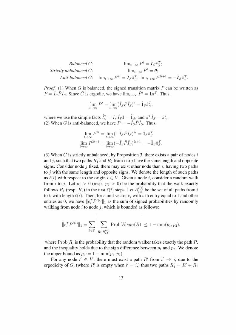
(3) When G is strictly unbalanced, by Proposition 3, there exists a pair of nodes iand j, such that two paths R1 and R2 from i to j have the same length and opposite

signs. Consider node j fixed, there may exist other node than i, having two paths

to j with the same length and opposite signs. We denote the length of such paths

as ℓ(i) with respect to the origin i ∈ V . Given a node i, consider a random walk

from i to j. Let p1 > 0 (resp. p2 > 0) be the probability that the walk exactly

follows R1 (resp. R2) in the first ℓ(i) steps. Let Rℓ(i)i,k be the set of all paths from i

to k with length ℓ(i). Then, for a unit vector ei with i-th entry equal to 1 and other

entries as 0, we have ‖eTi Pℓ(i)‖1 as the sum of signed probabilities by randomly

walking from node i to node j, which is bounded as follows:

‖eTi Pℓ(i)‖1 =

∑

k∈V

∣

∣

∣

∣

∣

∣

∣

∑

R∈Rℓ(i)i,k

Prob[R]sgn(R)

∣

∣

∣

∣

∣

∣

∣

≤ 1−min(p1, p2),

where Prob[R] is the probability that the random walker takes exactly the path P ,

and the inequality holds due to the sign difference between p1 and p2. We denote

the upper bound as ρi := 1−min(p1, p2).For any node i′ ∈ V , there must exist a path R′ from i′ → i, due to the

ergodicity of G, (where R′ is empty when i′ = i,) thus two paths R′1 = R′ + R1

13

and R′2 = R′ + R2 from i′ to j have the same length, but opposite signs. With

similar arguments as that for the node i, ‖eTi′Pℓ(i′)‖1 ≤ ρi′ holds for any i′ ∈ V .

Let ρ := maxi′∈V ρi′ < 1 and ℓ := maxi′∈V ℓ(i′), we conclude that ‖eTi′Pℓ‖1 ≤ ρ.

We can express the identity matrix I as rows of ei’s, i.e., I = [eT1 ; · · · ; eT|V |], which

infers the following inequality:

‖P ℓ‖∞ = ‖IP ℓ‖∞ = maxi′∈V

‖eTi′Pℓ‖1 ≤ max

i′∈Vρi′ = ρ < 1.

Hence, by applying the fact that ‖AB‖∞ ≤ ‖A‖∞‖B‖∞ for any square ma-

trices A and B, when t ≥ T = 2ℓ, the following inequality holds

‖P t‖∞ = ‖Ptℓℓ‖∞ ≤ ρ⌊

tℓ⌋ ≤ ρ

tT ,

which infers limt→∞ ‖P t‖∞ = 0, i.e., limt→∞ P t = 0.

The above lemma clearly shows different convergence behaviors of P t for

three types of graphs. In particular, P t of anti-balanced graphs exhibits a bounded

oscillating behavior in the long term.

Case of weakly connected signed digraphs. Now, we consider a weakly con-

nected signed digraph G = (V,E,A) with one ergodic sink component GZ with

node set Z, which only has incoming edges from the rest of the signed digraph GX

with node set X = V \ Z. Then, the signed transition matrix P has the following

block form.

P =

[

PX PY

0 PZ

]

, (10)

where PX and PZ are the block matrices for component GX and GZ , and PY

represent the one-way connections from GX to GZ . Then, the t-step transition

matrix P t can be expressed as

P t =

[

P(t)X P

(t)Y

0 P(t)Z

]

, (11)

where P(t)X = P t

X , P(t)Z = P t

Z and P(t)Y =

∑t−1i=0 P

iXPY P

t−1−iZ . When GZ is

balanced or anti-balanced, we use SZ , SZ to denote the partition of Z defining its

balance or anti-balance structure. Then, we denote column vectors

ub = (IX − PX)−1PY 1Z,SZ

, (12)

and uu = (IX + PX)−1PY 1Z,SZ

. (13)

14

The reason that IX −PX is invertible is because limt→∞ P tX = 0, which is in turn

because there is a path from any node i in GX to nodes in Z (since Z is the single

sink), and thus informally a random walk from i eventually reaches and then stays

in GZ . The same reason applies to IX + PX . Lemma 2 provides the formal proof

of the fact limt→∞ P tX = 0.

Let πZ denote the stationary distribution of nodes in GZ , and πZ,SZis signed,

with πZ,SZ(i) = πZ(i) for i ∈ SZ , and πZ,SZ

(i) = −πZ(i) for i ∈ Z \ SZ .

Lemma 2 describes the convergence of P t given various balance structures of GZ .

Lemma 2. For weakly connected signed digraph G = (V,E,A) with one ergodic

sink components, with signed transition matrix given in Eq.(11), we have

Balanced GZ: limt→∞ P t =

[

0 ubπTZ,SZ

0 1Z,SZπTZ,SZ

]

Strictly unbalanced GZ: limt→∞ P t = 0

Anti-balanced GZ: limt→∞ P 2t =

[

0 −uuπTZ,SZ

0 1Z,SZπTZ,SZ

]

,

limt→∞ P 2t+1 =

[

0 uuπTZ,SZ

0 −1Z,SZπTZ,SZ

]

Proof. We discuss the convergence of P tX , P t

Z , and P(t)Y in Eq.(11).

(1) We first prove that P tX converges to 0, i.e., limt→∞ P t

X = 0.

Since GX does not contain sink components, any node i ∈ X has a path

to component GZ . Let RiZ be the shortest path from i to some node in Z, and

Prob[RiZ ] denote the probability that a random walk starting from i takes the

path RiZ . Hence we denote

p = mini∈X

Prob[RiZ ], and m = maxi∈X

|RiZ |,

which implies that starting from any node i ∈ X , after m steps of random walk,

there is at least probability p that it reaches component GZ . Hence, we have

‖PmX ‖∞ ≤ (1− p) < 1. Let T = 2m, then for any t > T , we have

‖P tX‖∞ = ‖P

tmm

X ‖∞ ≤ (1− p)⌊tm⌋ ≤ (1− p)

tT ,

which implies limt→∞ ‖P tX‖∞ = 0, i.e., limt→∞ P t

X = 0.

15

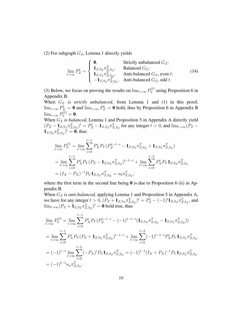
(2) For subgraph GZ , Lemma 1 directly yields

limt→∞

P tZ =

0, Strictly unbalanced GZ ;1Z,SZ

πTZ,SZ

, Balanced GZ ;1Z,SZ

πTZ,SZ

, Anti-balanced GZ , even t;−1Z,SZ

πTZ,SZ

, Anti-balanced GZ , odd t.

(14)

(3) Below, we focus on proving the results on limt→∞ P(t)Y using Proposition 6 in

Appendix B.

When GZ is strictly unbalanced, from Lemma 1 and (1) in this proof,

limt→∞ P tX = 0 and limt→∞ P t

Z = 0 hold, thus by Proposition 6 in Appendix B

limt→∞ P(t)Y = 0.

When GZ is balanced, Lemma 1 and Proposition 5 in Appendix A directly yield

(PZ − 1Z,SZπTZ,SZ

)t = P tZ − 1Z,SZ

πTZ,SZ

for any integer t > 0, and limt→∞(PZ −1Z,SZ

πTZ,SZ

)t = 0, thus

limt→∞

P(t)Y = lim

t→∞

t−1∑

i=0

P iXPY (P

t−1−iZ − 1Z,SZ

πTZ,SZ

+ 1Z,SZπTZ,SZ

)

= limt→∞

t−1∑

i=0

P iXPY (PZ − 1Z,SZ

πTZ,SZ

)t−1−i + limt→∞

t−2∑

i=0

P iXPY 1Z,SZ

πTZ,SZ

= (IX − PX)−1PY 1Z,SZ

πTZ,SZ

= ubπTZ,SZ

,

where the first term in the second line being 0 is due to Proposition 6 (ii) in Ap-

pendix B.

When GZ is anti-balanced, applying Lemma 1 and Proposition 5 in Appendix A,

we have for any integer t > 0, (PZ + 1Z,SZπTZ,SZ

)t = P tZ − (−1)t1Z,SZ

πTZ,SZ

, and

limt→∞(PZ + 1Z,SZπTZ,SZ

)t = 0 hold true, thus

limt→∞

P(t)Y = lim

t→∞

t−1∑

i=0

P iXPY (P

t−1−iZ − (−1)t−1−i(1Z,SZ

πTZ,SZ

− 1Z,SZπTZ,SZ

))

= limt→∞

t−1∑

i=0

P iXPY (PZ + 1Z,SZ

πTZ,SZ

)t−1−i + limt→∞

t−2∑

i=0

(−1)t−1−iP iXPY 1Z,SZ

πTZ,SZ

= (−1)t−1 limt→∞

t−2∑

i=0

(−PX)iPY 1Z,SZ

πTZ,SZ

= (−1)t−1(IX + PX)−1PY 1Z,SZ

πTZ,SZ

= (−1)t−1uuπTZ,SZ

.

16

Hence, we have for anti-balanced GZ : limt→∞ P(2t)Y = −uuπ

TZ,SZ

, and

limt→∞ P(2t+1)Y = uuπ

TZ,SZ

.

Multiple sink components and disconnected signed digraphs. When there exist

m > 1 ergodic sink components, i.e., GZ1, GZ2, · · · , GZm, the rest of the graph

G is considered as GX . Then the signed transition matrix P and P t can be written

as

P =

PX PY 1 · · · PYm

0 PZ1 0 0

0 0. . . 0

0 0 0 PZm

, P t =

P tX P

(t)Y 1 · · · P

(t)Y m

0 P tZ1 0 0

0 0. . . 0

0 0 0 P tZm

, (15)

where P(t)Y i =

∑t−1j=0 P

jXPY iP

t−1−jZi , 1 ≤ i ≤ m. Hence, each sink ergodic com-

ponent PZi along with PX and PY i independently follows Lemma 2. For discon-

nected signed digraph, with m ≥ 1 ergodic or weakly connected components,

each of which satisfies Lemma 1 or Lemma 2, respectively. For brevity, we omit

the details here.

3.3 Long-term dynamics

Based on the structural balance classification and the convergence of signed transi-

tion matrix discussed above, we are ready now to analyze the long-term dynamics

of the voter model on signed digraphs. Formally, we are interested in characteriz-

ing xt with t → ∞, i.e.,

x = limt→∞

xt = limt→∞

(P tx0 + (

t−1∑

i=0

P i)g−). (16)

If the even and odd subsequences of xt converge separately, we denote xe =limt→∞ x2t, xo = limt→∞ x2t+1.

Before presenting the results on long-term dynamics of voter model, we first

introduce the following useful lemma connecting a signed digraph G with another

graph G′ where all edge signs in G are negated.

Lemma 3. Given a signed digraph G = (V,E,A), let G′ = (V,E,−A) be a

signed digraph with all edge signs negated from G. Then, for any initial color

distribution x0, at any 2t steps (t > 0), the color distributions x2t(G) on G and

x2t(G′) on G′ are identical.

17

Proof. Let P ′ = −P denote the signed transition matrix of G′, and denote the

vector g− = D−1A−1 and g′− = D−1(−A)−1 = D−1A+1. Thus g′− = 1 − g−.

By Eq.(1), after two steps, we have

x2(G′) = P ′2x0 + P ′g′− + g′− = P 2x0 − P (1 − g−) + 1 − g−

= P 2x0 + Pg− + g− = x2(G),

where the last equality uses facts 1 = D−1A1 and P = D−1A. Since the lemma

holds for two steps, then clearly it holds for all even steps.

Next theorem discusses the case of ergodic signed digraphs.

Theorem 1. Let G = (V,E,A) be an ergodic signed digraph, we have

Balanced G: x = 1SπTS (x0 −

121) + 1

21 (17)

Strictly unbalanced G: x = 121 (18)

Anti-balanced G: xe = 1SπTS (x0 −

121) + 1

21 (19)

xo = −1SπTS (x0 −

121) + 1

21 (20)

Proof. We discuss the limit in Eq. (16) for three possible balance structures of G.

Balanced digraphs. From Lemma 1 and Proposition 5 in Appendix A, it is easy

to prove Pm − 1SπTS = (P − 1Sπ

TS )

m for any integer m > 0, which yields the

following result on the second part in Eq. (16).

limt→∞

t−1∑

i=0

P ig− = (I − P + 1SπTS )

−1g− + limt→∞

t−1∑

i=1

1SπTS g

− (21)

= (I − P + 1SπTS )

−1g− =1

21 −

1

21Sπ

TS 1, (22)

where the last term of Eq.(21) is canceled out due to the digraph flow circulation

law [12, 30], i.e.,

πTS g

− = πTSD

−1A−1 =∑

i∈S

π(i)∑

j∈S

Pij −∑

i∈S

π(i)∑

j∈S

Pij = 0.

The last equality in Eq.(22) holds because

1

2(I − P + 1Sπ

TS )(1 − 1Sπ

TS 1)− g− = 0.

18

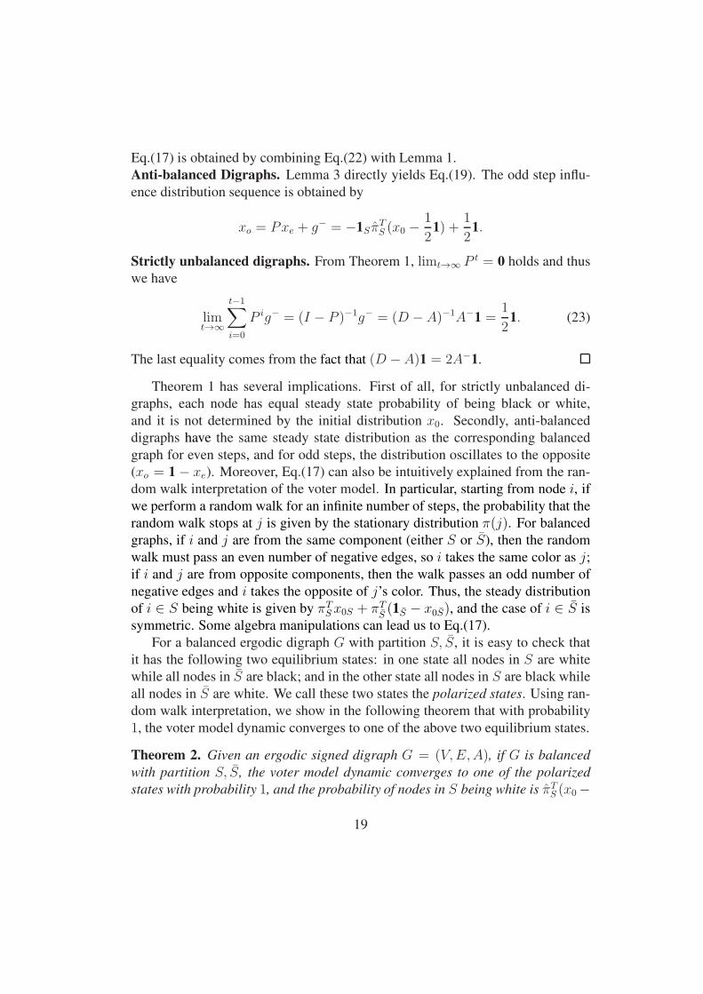
Eq.(17) is obtained by combining Eq.(22) with Lemma 1.

Anti-balanced Digraphs. Lemma 3 directly yields Eq.(19). The odd step influ-

ence distribution sequence is obtained by

xo = Pxe + g− = −1SπTS (x0 −

1

21) +

1

21.

Strictly unbalanced digraphs. From Theorem 1, limt→∞ P t = 0 holds and thus

we have

limt→∞

t−1∑

i=0

P ig− = (I − P )−1g− = (D − A)−1A−1 =1

21. (23)

The last equality comes from the fact that (D −A)1 = 2A−1.

Theorem 1 has several implications. First of all, for strictly unbalanced di-

graphs, each node has equal steady state probability of being black or white,

and it is not determined by the initial distribution x0. Secondly, anti-balanced

digraphs have the same steady state distribution as the corresponding balanced

graph for even steps, and for odd steps, the distribution oscillates to the opposite

(xo = 1 − xe). Moreover, Eq.(17) can also be intuitively explained from the ran-

dom walk interpretation of the voter model. In particular, starting from node i, if

we perform a random walk for an infinite number of steps, the probability that the

random walk stops at j is given by the stationary distribution π(j). For balanced

graphs, if i and j are from the same component (either S or S), then the random

walk must pass an even number of negative edges, so i takes the same color as j;

if i and j are from opposite components, then the walk passes an odd number of

negative edges and i takes the opposite of j’s color. Thus, the steady distribution

of i ∈ S being white is given by πTSx0S + πT

S(1S − x0S), and the case of i ∈ S is

symmetric. Some algebra manipulations can lead us to Eq.(17).

For a balanced ergodic digraph G with partition S, S, it is easy to check that

it has the following two equilibrium states: in one state all nodes in S are white

while all nodes in S are black; and in the other state all nodes in S are black while

all nodes in S are white. We call these two states the polarized states. Using ran-

dom walk interpretation, we show in the following theorem that with probability

1, the voter model dynamic converges to one of the above two equilibrium states.

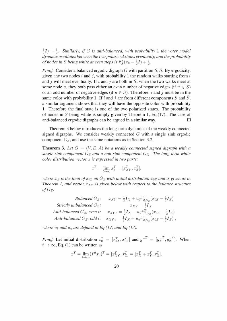
Theorem 2. Given an ergodic signed digraph G = (V,E,A), if G is balanced

with partition S, S, the voter model dynamic converges to one of the polarized

states with probability 1, and the probability of nodes in S being white is πTS (x0−

19

121) + 1

2. Similarly, if G is anti-balanced, with probability 1 the voter model

dynamic oscillates between the two polarized states eventually, and the probability

of nodes in S being white at even steps is πTS (x0 −

121) + 1

2.

Proof. Consider a balanced ergodic digraph G with partition S, S. By ergodicity,

given any two nodes i and j, with probability 1 the random walks starting from iand j will meet eventually. If i and j are both in S, when the two walks meet at

some node u, they both pass either an even number of negative edges (if u ∈ S)

or an odd number of negative edges (if u ∈ S). Therefore, i and j must be in the

same color with probability 1. If i and j are from different components S and S,

a similar argument shows that they will have the opposite color with probability

1. Therefore the final state is one of the two polarized states. The probability

of nodes in S being white is simply given by Theorem 1, Eq.(17). The case of

anti-balanced ergodic digraphs can be argued in a similar way.

Theorem 3 below introduces the long-term dynamics of the weakly connected

signed digraphs. We consider weakly connected G with a single sink ergodic

component GZ , and use the same notations as in Section 3.2.

Theorem 3. Let G = (V,E,A) be a weakly connected signed digraph with a

single sink component GZ and a non-sink component GX . The long-term white

color distribution vector x is expressed in two parts:

xT = limt→∞

xTt = [xT

XY , xTZ ].

where xZ is the limit of xtZ on GZ with initial distribution x0Z and is given as in

Theorem 1, and vector xXY is given below with respect to the balance structure

of GZ:

Balanced GZ: xXY = 121X + ubπ

TZ,SZ

(x0Z − 121Z)

Strictly unbalanced GZ: xXY = 121X

Anti-balanced GZ , even t: xXY,e =121X − uuπ

TZ,SZ

(x0Z − 121Z)

Anti-balanced GZ , odd t: xXY,o =121X + uuπ

TZ,SZ

(x0Z − 121Z) ,

where ub and uu are defined in Eq.(12) and Eq.(13).

Proof. Let initial distribution xT0 = [xT

0X , xT0Z ] and g−

T= [g−X

T, g−Z

T]. When

t → ∞, Eq. (1) can be written as

xT = limt→∞

(P tx0)T = [xT

XY , xTZ ] = [xT

X + xTY , x

TZ ],

20

where xX = limt→∞(P tXx0X +

∑t−1i=0 P

iXg

−X), xY = limt→∞(P

(t)Y x0Z +

∑t−1i=0 P

(i)Y g−Z ), and xZ = limt→∞(P t

Zx0Z +∑t−1

i=0 PiZg

−Z ).

From Lemma 2, limt→∞ P tX = 0, thus xX = (IX − PX)

−1g−X holds for any

ergodic GZ . Since GZ is ergodic, xZ follows Theorem 1. Below we will focus on

deriving xY , where the first part of xY satisfies Lemma 2, i.e.,

limt→∞

P(t)Y x0Z =

0 GZ is strictly unbalanced

ubπTZ,SZ

x0Z GZ is balanced

−uuπTZ,SZ

x0Z GZ is anti-balanced, even tuuπ

TZ,SZ

x0Z GZ is anti-balanced, odd t.

The second part of xY can be further written down as

limm→∞

m∑

t=1

P(t)Y g−Z = lim

m→∞

m−1∑

t=0

t∑

i=0

(P t−iX PY P

iZ)g

−Z

= limm→∞

m−1∑

t=0

m−t∑

i=0

(P tXPY P

iZ)g

−Z =

∞∑

t=0

(P tXPY

∞∑

i=0

P iZ)g

−Z (24)

Now we discuss Eq.(24) under different balance structures of GZ .

(1) GZ is strictly unbalanced. From Lemma 2, limt→∞ P t = 0. Then by Eq.(23)

we directly obtain that xXY = 121X . Applying Eq.(23) to

∑∞i=0 P

iZg

−Z in Eq.(24),

we have

limm→∞

m∑

t=1

P(t)Y g−Z =

1

2(IX − PX)

−1PY 1Z .

Thus, we obtain the following equation:

xXY = xX + xY = (IX − PX)−1(g−X +

1

2PY 1Z) =

1

21X .

(2) GZ is balanced. Using Eq.(22), we have

limm→∞

m∑

t=1

P(t)Y g−Z =

1

2(IX − PX)

−1PY (1Z − 1Z,SZπTZ,SZ

1Z).

Hence, we have

xXY = (IX − PX)−1(g−X +

1

2PY 1Z) + ubπ

TZ,SZ

(x0Z −1

21Z)

=1

21X + ubπ

TZ,SZ

(x0Z −1

21Z). (25)

21

(3) GZ is anti-balanced. Using Lemma 3, we can negate the signs of all edges in

G so that the sink becomes balanced. Hence, we know that at even steps in long

term,

xXY,e =1

21X − uuπ

TZ,SZ

(x0Z −1

21Z), (26)

where Eq.(26) and Eq.(25) are identical in the sense that PX’s and PY ’s in Eq.(26)

and Eq.(25) have opposite signs. Moreover, the odd step influence distribution

sequence is obtained

xXY,o = PXxXY,e + PY xZ,e + g−X =1

21X + uuπ

TZ,SZ

(x0Z −1

21Z). (27)

Theorem 3 characterizes the long-term dynamics when the underlying graph

is a weakly connected signed digraph with one ergodic sink component. We can

see that the results for balanced and anti-balanced sink components are more com-

plicated than the ergodic digraph case, since how non-sink components are con-

nected to the sink subtly affects the final outcome of the steady state behavior. In

steady state, while the sink component is still in one of the two polarized states

as stated in Theorem 2, the non-sink components exhibit more complicated color

distribution, for which we provide probability characterizations in Theorem 3. Us-

ing Eq.(15), Theorem 1 and Theorem 3 can be readily extended to the case with

more than one ergodic sink components and disconnected digraphs. When the

network only contains positive directed edges, the voter model dynamics can be

interpreted using digraph random walk theory [28–32].

4 Influence maximization

With the detailed analysis on voter model dynamics for signed digraphs, we are

ready now to solve the influence maximization problem. Intuitively, we want to

address the following question: If only at most k nodes could be selected initially

and be turned white while all other nodes are black, how should we choose seed

nodes so as to maximize the expected number of white nodes in short term and in

long term, respectively?

22

4.1 Influence maximization problem

Influence maximization objectives. We consider two types of short-term in-

fluence objectives, one is the instant influence, which counts the total number of

influenced nodes at a step t > 0; the other is the average influence, which takes the

average number of influenced nodes within the first t steps. These two objectives

have different implications and applications. For example, political campaigns try

to convince voters who may change their minds back and forth, but only the vot-

ers’ opinions on the voting day are counted, which matches the instant influence.

On the other hand, a credit card company would like to have customers keep using

its credit card service as much as possible, which is better interpreted by the av-

erage influence. When t is sufficiently large, it becomes the long-term objective,

and long-term average influence coincides with long-term instant influence when

the dynamic converges.

Formally, we define the short-term instant influence ft(x0) and the short-term

average influence ft(x0) as follows:

ft(x0) := 1Txt(x0) and ft(x0) :=

∑t

i=0 fi(x0)

t+ 1. (28)

Moreover, we define long term influence as

f(x0) := limt→∞

∑t

i=0 fi(x0)

t+ 1. (29)

Note that when the dynamic converges (e.g. ergodic balanced or ergodic strictly

unbalanced graphs), f(x0) = limt→∞ ft(x0). For ergodic anti-balanced graphs

(or sink components), it is essentially the average of even- and odd-step limit

influence.

Given a set W ⊆ V , Let eW be the vector in which eW (j) = 1 if j ∈ W and

eW (j) = 0 if j 6∈ W , which represents the initial seed distribution with only nodes

in W as white seeds. Let ei be the shorthand of ei. Unlike unsigned graphs, if

initially no white seeds are selected on a signed digraph G, i.e., x0 = 0, the instant

influence ft(0) at step t is in general non-zero, which is referred to as the ground

influence of the graph G at t. The influence contribution of a seed set W does not

count such ground influence, as shown in definition 3.

Definition 3 (Influence contribution). The instant influence contribution of a

seed set W to the t-th step instant influence objective, denoted by ct(W ), is the

difference between the instant influence at step t with only nodes in W selected

23

as seeds and the ground influence at step t: ct(W ) = ft(eW ) − ft(0). The aver-

age influence contribution ct(W ) and long-term influence contribution c(W ) are

defined in the same way: ct(W ) = ft(eW )− ft(0) and c(W ) = f(eW )− f(0).

We are now ready to formally define the influence maximization problem.

Definition 4 (Influence maximization). The influence maximization problem

for short-term instant influence is finding a seed set W of at most k seeds that

maximizes W ’s instance influence contribution at step t, i.e., finding W ∗t =

argmax|W |≤k ct(W ). Similarly, the problem for average influence and long-term

influence is finding W ∗t = argmax|W |≤k ct(W ) and W ∗ = argmax|W |≤k c(W ),

respectively.

We now provide some properties of influence contribution, which lead to the

optimal seed selection rule. By Eq.(1), we have

ct(W ) = ft(eW )− ft(0) = 1Txt(eW )− 1Txt(0) = 1TP teW . (30)

Let ct(i) be the shorthand of ct(i), and let ct = [ct(i)] denote the vector of

influence contribution of individual nodes. Then cTt = [ct(i)]T = 1TP t. When

t → ∞, the long term influence contributions of individual nodes are obtained as

a vector c:

cT = limt→∞

∑t

i=0 cTi

t+ 1= lim

t→∞

1T∑t

i=0 Pi

t+ 1. (31)

When P t converges, we simply have

cT = 1T limt→∞

P t. (32)

Lemma 4 below discloses the important property that the influence contribu-

tion is a linear set function.

Lemma 4. Given a white seed set W , ct(W ) =∑

i∈W ct(i), ct(W ) =∑

i∈W ct(i),and c(W ) =

∑

i∈W c(i).

Proof. From Eq.(30), we have

ct(W ) = 1TP teW = 1TP t∑

i∈W

ei =∑

i∈W

1TP tei =∑

i∈W

ct(i).

The linearity of ct and c can be derived from that of ct.

24

Given a vector v, let n+(v) denote the number of positive entries in v. By

applying Lemma 4, we have the optimal seed selection rule for instant influence

maximization as follows.

Optimal seed selection rule for instant influence maximization. Given a signed

digraph and a limited budget k, selecting top mink, n+(ct) seeds with the high-

est ct(i)’s, i ∈ V , leads to the maximized instant influence at step t > 0.

Note that the influence contributions of some nodes may be negative and these

nodes should not be selected as white seeds, and thus the optimal solution may

have less than k seeds. The rules for average influence maximization and long-

term influence maximization are patterned in the same way. Therefore, the central

task now becomes the computation of the influence contributions of individual

nodes. Below, we will introduce our SVIM algorithm, for Signed Voter model

Influence Maximization.

4.2 Short-term influence maximization

By applying Definition 3 and Lemma 4, we develop SVIM-S algorithm to solve

the short-term instant and average influence maximization problem, as shown in

Algorithm 1.

Algorithm 1 Short-term influence maximization SVIM-S

1: INPUT: Signed transition matrix P , short-term period t, budget k;

2: OUTPUT: White seed set W .

3: ct = 1; ct = 1;

4: for i = 1 : t do

5: cTt = cTt P ;(for instant influence maximization.)

6: ct = ct + ct; (for average influence maximization.)

7: W = top mink, n+(ct) (resp. mink, n+(ct)) nodes with the highest ct(i)(resp. ct(i)) values, for instant (resp. average) influence maximization.

SVIM-S algorithm requires t vector-matrix multiplications, each of which

takes |E| times entry-wise multiplication operations. Hence the total time com-

plexity of SVIM-S is O(t · |E|). Note that when t is sufficiently large (e.g.,

t > |V |2), the FOR loop in Algorithm 1 can be modified as follows to reduce the

number of FOR Loops to O(log t), and the total complexity to O(log t · |V | · |E|).

P0 = P ;

for i = 1 : ⌊log t⌋ do

P = P 2;(for instant influence maximization.)

25

cTt = cTt P ;(for instant influence maximization.)

ct = ct + ct; (for average influence maximization.)

for i = 2⌊log t⌋ + 1 : t do

cTt = cTt P0;(for instant influence maximization.)

ct = ct + ct; (for average influence maximization.)

P = P 2 in the first loop is performed by matrix multiplication in O(|E| · |V | +|E|) ≈ O(|E| · |V |), instead of vector-matrix multiplication in O(|E|). Thus, the

overall computation complexity is O(log t · |V | · |E|). Hence, when t > log t · |V |,the modified algorithm 1 works better; otherwise, the original algorithm1 is better.

When t > |V |2, we have t > log t · |V | for any |V | > 1, thus the modified

algorithm 1 is better.

4.3 Long-term influence maximization

We now study the long-term influence contribution c and introduce the corre-

sponding influence maximization algorithm SVIM-L. We will see that the com-

putation of influence contribution c and seed selection schemes depends on the

structural balance and connectedness of the graph. While seed selection for bal-

anced ergodic digraphs still has intuitive explanations, the computation for weakly

connected and disconnected digraphs is more involved and less intuitive.

4.3.1 Case of ergodic signed digraphs

When the signed digraph G = (V,E,A) is ergodic, Lemma 5 below characterizes

the long-term influence contributions of nodes, with respect to various balance

structures.

Lemma 5. Consider an ergodic signed digraph G = (V,E,A). If G is balanced,

with bipartition S and S, the influence contribution vector c = (|S| − |S|)πS . If

G is anti-balanced or strictly unbalanced, c = 0.

Proof. (1) When G is balanced, by Lemma 1 and Eq.(32),

cT = 1T limt→∞

P t = 1T 1SπTS = (|S| − |S|)πS.

(2) When G is strictly unbalanced, again by Lemma 1 and Eq.(32), we have cT =1T limt→∞ P t = 0.

26

(3) When G is anti-balanced, by Lemma 1 and Eq.(31), we have

cT = 1T limt→∞ P 2t + limt→∞ P 2t+1

2= 0.

Based on Lemma 5, Algorithm 2 summarizes how to compute the long-term

influence contribution c on ergodic signed digraphs.

Algorithm 2 c = ergodic(G)

1: INPUT: Signed transition matrix P .

2: OUTPUT: Long term influence contribution vector c3: Detect the structure of ergodic signed digraph G;

4: if G is balanced, with bipartition S and S then

5: Compute stationary distribution π of P ;

6: c = (|S| − |S|)πS;

7: else

8: c = 0;

Lemma 5 suggests that for ergodic balanced digraphs, we should pick the

larger component, e.g., S, if |S| > |S|, and select the top mink, |S| nodes from

S with the largest stationary distributions as white seeds. Selecting these nodes

will make the probability of the larger component being white the largest.

Theorem 1 indicates that given an anti-balanced digraph G, with bipartition

S and S, the long-term dynamic xt oscillates on odd and even steps, and their

long-term influence contribution is 0. Define the strength of the oscillation as the

difference of the long-term influence between the even vs odd steps, i.e., ∆fo,e =|fo(x0)− fe(x0)|/2. We can maximize such strength of the oscillation of the voter

model on an anti-balanced ergodic digraph by properly choosing the initial white

seeds (See Remark 1.)

Remark 1. In an anti-balanced ergodic digraph G = (V,E,A) with the bipar-

tition S and S and a budget k. Let W ′ (resp. W ′′) denote two initial seed sets,

such that mink, |S| (resp. mink, |S|) nodes are selected with highest station-

ary distribution π(i)’s in S (resp. S). Then, the optimal W ∗ that maximizes the

strength of oscillation ∆fo,e is

W ∗ := argmaxW∈W ′,W ′′

|πTS (eW −

1

21)|. (33)

27

Proof. From Theorem 1, when t becomes sufficiently large, the vector x oscillates

at two vectors on odd and even steps, respectively. Rewrite the strength of the

oscillation as

∆fo,e =|fo(x0)− fe(x0)|

2= |1T xo(x0)− xe(x0)

2| = |1T 1Sπ

TS (x0 −

1

21)|

= ||S| − |S|| · |πTS (x0 −

1

21)|.

Let W be the initial seed set, then the oscillation strength maximization is formu-

lated as

max|W |≤k

||S| − |S|| · |πTS (eW −

1

21)|

= ||S| − |S|| ·maxmax|W |≤k

πTS eW −

1

2πTS 1, max

|W |≤k−πT

S eW+1

2πTS 1, (34)

which contains two sub-problems, i.e., max|W |≤kπTS eW and

max|W |≤k−πTS eW. The first maximization problem can be rewritten as

max|W |≤k

πTS eW = max

|W |≤k

(

∑

i∈S

π(i)eW (i)−∑

j∈S

π(i)eW (j))

. (35)

Thus, let W ′ denote the optimal solution to the problem in Eq.(35), which is

obtained by choosing mink, |S| seeds with highest π(i)’s from S. Similarly,

choosing mink, |S| nodes with the highest π(i)’s from S yields the optimal so-

lution, denoted by W ′′, to the second maximization problem max|W |≤k−πTS eW.

The optimal W to the problem in eq.(34) that maximizes the oscillation strength

is the one in W ′,W ′′, with higher |πTS (eW − 1

21)|, which completes the proof of

eq.(33).

4.3.2 Case of weakly connected signed digraphs

We first consider a weakly connected signed G which has a single ergodic sink

component GZ with only incoming edges from the remaining nodes X = V \ Z.

Lemma 6. Consider a weakly connected digraph G = (V,E,A) with a single

ergodic sink component GZ . If GZ is balanced, with partition SZ and SZ , the

long term influence contribution vector cT = [cTX , cTZ ], where cX = 0X and cZ =

(1TXub + |SZ| − |SZ|)πZ,SZ

. If G is anti-balanced or strictly unbalanced, c = 0.

28

Proof. (1)When GZ is balanced, by Lemma 2, cX = 0X , and

cTZ = (1TXub + 1T

Z 1Z,SZ)πT

Z,SZ= (1T

Xub + |SZ | − |SZ|)πTZ,SZ

.

(2) When GZ is strictly unbalanced, cT = 1T limt→∞ P t = 0

(3) When GZ is anti-balanced, by Lemma 2 the limits of odd and even subse-

quences of P t cancel out, thus c = 0.

Lemma 6 indicates that influence contribution of the balanced ergodic sink

component is more complicated than that of the balanced ergodic digraph. This

is because the sink component affects the colors of the non-sink component in a

complicated way depending on how non-sink and sink components are connected.

Therefore, the optimal seed selection depends on the calculation of the influence

contributions of each sink node, and is not as intuitive as that for the ergodic

digraph case.

Theorem 3 shows that in a weakly connected signed digraph G, with single

anti-balanced sink component GZ , the long term influence f(x0) oscillates on

odd and even steps, and the average is |V |/2, which is invariant to the initial

seed selection. Similar to Remark 1, we can maximize the oscillation strength by

properly selecting initial seeds, i.e.,

W ∗ = argmax|W |≤k

|fe(eW )− fo(eW )|/2

= argmax|W |≤k

|(1TXuuπ

TZ,SZ

+ 1TZ 1Z,SZ

πTZ,SZ

)(eWZ −1

21Z)|

= |1TXuu + |SZ| − |SZ || · argmax

|W |≤k

|πTZ,SZ

(eWZ −1

21Z)| (36)

where the maximization objective is independent from x0X , thus oscillation

strength maximization problem objective in Eq.(36) for G is identical to that in

Remark 1. Hence, Remark 1 also applies here.

Using Eq.(15), Lemma 5 and Lemma 6 can be readily extended to the case

with more than one ergodic sink components and disconnected digraphs. Algo-

rithm 3 below summarizes how to compute the node influence contributions of

weakly connected signed digraphs. Note that by our assumption, we consider all

sink components to be ergodic.

4.3.3 General case and SVIM-L algorithm

Given the above systematic analysis, we are now in a position to summarize and

introduce our SVIM-L algorithm which solves the long-term voter model influ-

29

Algorithm 3 c = weakly(G)

1: INPUT: Signed transition matrix P .

2: OUTPUT: Influence contribution vector c.3: Detect the structure of the weakly connected signed digraph G, and find its

m ≥ 1 signed ergodic sink components GZ1, · · · , GZm;

4: for i = 1 : m do

5: if GZi is balanced with partition SZi, SZi then

6: Compute stationary distribution πZi of PZi;

7: ubi = (IX − PX)−1PY i1Zi,SZi

;

8: cZi = (1TXubi + |SZi| − |SZi|)π

TZi,SZi

;

9: c = [0X ; cZ1; · · · ; cZm]

ence maximization problem for general aperiodic signed digraphs.

In general, a signed digraph consists m ≥ 1 disconnected components, within

each of which the node influence contribution follows Lemma 6. The long-term

signed voter model influence maximization (SVIM-L) algorithm is constructed in

Algorithm 4.

Algorithm 4 Long-term influence maximization SVIM-L

1: INPUT: Signed transition matrix P , budget k.

2: OUTPUT: White seed set W .

3: Detect the structure of a general aperiodic signed digraph G, and find the

m ≥ 1 disconnected components G1, · · · , Gm;

4: for i = 1 : m do

5: cGi= weakly(Gi);

6: c = [cG1 ; · · · ; cGm];

7: W = top mink, n+(c) nodes with the highest c(i) values.

Complexity analysis. We consider G = (V,E,A) to be weakly connected, since

disconnected graph case can be treated independently for each connected com-

ponent for the time complexity. SVIM-L algorithm consists of two parts. The

first part extracts the connectivity and balance structure of the graph, which can

be done using depth-first search with complexity O(|E|). The second part uses

Algorithm 3 to compute influence contributions of balanced ergodic sink com-

ponents. The dominant computations are on the stationary distribution πZi’s and

(IX − PX)−1, which can be done by solving a linear equation system [41] and

matrix inverse in O(|Zi|3) and O(n3

X), respectively, where nX = |X|. Let b be

30

the number of balanced sink components in G, nZ be the number of nodes in the

largest balanced sink component. Thus SVIM-L can be done in O(bn3Z + n3

X)time. Alternatively, we can use iterative method for computing both πZi’s and

1TX(IX − PX)

−1, if the largest convergence time tC of P tZi’s and P t

X is small.

(Note that the convergence time of ergodic digraphs could be exponentially large

in general, as illustrated by an example in Appendix C). In this case, each iter-

ation step involves vector-matrix multiplication and can be done in O(mB) time,

where mB is the number of edges of the induced subgraph GB consisting of all

nodes in the balanced sink components and X . Note that mB and tC are only

related to subgraph GB, which could be significantly smaller than G, and thus

O(tCmB) could be much smaller than the time of naive iterations on the entire

graph. Overall SVIM-L can be done in O(|E|+min(bn3Z + n3

X , tCmB)) time.

5 Evaluation

In this section, we first use both synthetic datasets and real social network

datasets to demonstrate the efficacy of our short-term and long-term seed selection

schemes by comparing the performances with four baseline heuristics. Then, we

evaluate how much the short-term and long-term influence can be improved by

taking the edge signs into consideration.

5.1 Performance comparison with baseline heuristics

For different scenarios, we compare our SVIM-L and SVIM-S algorithms with

four heuristics, i.e., (1) selecting seed nodes with the highest weighted outgoing

degrees (denoted by d+ + d− in the figures), (2) highest weighted outgoing posi-

tive degrees (denoted by d+), (3) highest differences between weighted outgoing

positive and negative degrees (denoted by d+ − d−), and (4) randomly selecting

seed nodes (denoted by “Rand”), where in our evaluations, we run random seed

selection 1000 times, and compare the average number of white nodes between

our algorithm and other heuristics. Our evaluation results demonstrate that our

seed selection scheme can increase up to 72% long-term influence, and 145%short-term influence over other heuristics.

31

5.1.1 Synthetic datasets

In this part, we generate synthetic datasets with different structures to validate our

theoretical results.

Dataset generation model. We generate six types of signed digraphs, including

balanced ergodic digraphs, anti-balanced ergodic digraphs, strictly unbalanced er-

godic digraphs, weakly connected signed digraphs, disconnected signed digraphs

with ergodic components, and disconnected signed digraph with weakly con-

nected components (WCCs). All edges have unit weights. The following are

graph configuration details.

We first create an unsigned ergodic digraph G with 9500 nodes, which has

two ergodic components GA and GB , with [3000, 6500] nodes and [3000, 6500]×8random directed edges, respectively. Moreover, there are 3000×8 random directed

edges across GA and GB . Ergodicity is checked through a simple connectivity

and aperiodicity check. Given G, a balanced digraph is obtained by assigning all

edges within GA and GB with positive signs, and those across them with negative

signs. Then, an anti-balanced digraph is generated by negating all edge signs

of the balanced ergodic digraph. To generate a strictly unbalanced digraph, we

randomly assign edge signs to all edges in G and make sure that there does not

exist a balanced or anti-balanced bipartition.

Moreover, we generated a disconnected signed digraph and a weakly

connected signed digraph for our study. We first generate 5 ergodic

unsigned digraphs, G1, · · · , G5 with [500, 200, 800, 300, 2700] nodes and

[500, 200, 800, 300, 2700]×8 edges, respectively. Then, we group G23 = (G2, G3)and G45 = (G4, G5) to form two ergodic balanced digraphs, and generate a strictly

unbalanced ergodic digraph G1 by randomly assigning signs to edges in G1. Three

disconnected components G1, G23, G45 together form a disconnected signed di-

graph. To form a weakly connected signed digraph, we place in total 3000 random

direct edges from G1 to the balanced ergodic components G23 and G45, where the

nodes in subgraph G1 only have outgoing edges to G23 and G45. Moreover, we

combine the above generated balanced ergodic digraph and the weakly connected

signed digraph together forming a larger disconnected signed digraph, with the

weakly connected signed digraph as a component.

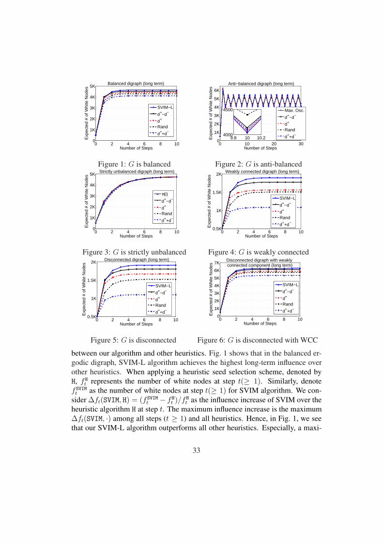
Fig. 1-Fig. 6 present the evaluation results for one set of digraphs, where we

observe that all digraphs we randomly generated exhibit consistent results. Our

tests are conducted using Matlab on a standard PC server.

Long-term influence maximization. In the evaluations, we set the influence bud-

get as k = 500, and compare the average numbers of white nodes over steps

32

0 2 4 6 8 100

1K

2K

3K

4K

5K

Number of Steps

Exp

ecte

d #

of W

hite

Nod

esBalanced digraph (long term)

SVIM−L

d+−d−

d+

Rand

d++d−

Figure 1: G is balanced

0 10 20 300

2K

4K

6K

1K

3K

5K

Number of Steps

Exp

ecte

d #

of W

hite

Nod

es

Anti−balanced digraph (long term)

9.8 10 10.24000

4500 Max. Osc.

d+−d−

d+

Rand

d++d−

Figure 2: G is anti-balanced

0 2 4 6 8 100

1K

2K

3K

4K

5K

Number of Steps

Exp

ecte

d #

of W

hite

Nod

es

Strictly unbalanced digraph (long term)

π(i)

d+−d−

d+

Rand

d++d−

Figure 3: G is strictly unbalanced

0 2 4 6 8 100.5K

1K

1.5K

2K

Number of Steps

Exp

ecte

d #

of W

hite

Nod

es

Weakly connected digraph (long term)

SVIM−L

d+−d−

d+

Rand

d++d−

Figure 4: G is weakly connected

0 2 4 6 8 100.5K

1K

1.5K

2K

Number of Steps

Exp

ecte

d #

of W

hite

Nod

es

Disconnected digraph (long term)

SVIM−L

d+−d−

d+

Rand

d++d−

Figure 5: G is disconnected

0 2 4 6 8 100

2K

4K

6K

7K

5K

1K

3K

Number of Steps

Exp

ecte

d #

of W

hite

Nod

es

Disconnected digraph with weakly connected component (long term)

SVIM−L

d+−d−

d+

Rand

d++d−

Figure 6: G is disconnected with WCC

between our algorithm and other heuristics. Fig. 1 shows that in the balanced er-

godic digraph, SVIM-L algorithm achieves the highest long-term influence over

other heuristics. When applying a heuristic seed selection scheme, denoted by

H, f H

t represents the number of white nodes at step t(≥ 1). Similarly, denote

f SVIM

t as the number of white nodes at step t(≥ 1) for SVIM algorithm. We con-

sider ∆ft(SVIM, H) = (f SVIM

t − f H

t )/fH

t as the influence increase of SVIM over the

heuristic algorithm H at step t. The maximum influence increase is the maximum

∆ft(SVIM, ·) among all steps (t ≥ 1) and all heuristics. Hence, in Fig. 1, we see

that our SVIM-L algorithm outperforms all other heuristics. Especially, a maxi-

33

0 10 20 300

1

2

3

4

5

x 104

Number of Steps

Exp

ecte

d #

of w

hite

nod

esEpinions (Short term) (at t)

in the entire dataset

(6k)SVIM−S

(6k)d+−d−

(6k)d+

(6k)d++d−

(6k)Rand

Figure 7: Instant influence in Epinions

data with k = 6k

0 10 20 300

1

2

3

4

5

x 104

Number of Steps

Exp

ecte

d #

of w

hite

nod

es

Epinions (Short term) (at t) in the entire dataset

(500)SVIM−S

(500)d+−d−

(500)d+

(500)d++d−

(500)Rand

Figure 8: Instant influence in Epinions

data with k = 500

0 10 20 30 400.5

1

1.5

2

2.5

3x 10

4

Number of Steps

Exp

ecte

d #

of w

hite

nod

es

Epinions (Short term) (at t) in the largest SCC

(6k)SVIM−S

(6k)d+−d−

(6k)d+

(6k)d++d−

(6k)Rand

Figure 9: Instant influence in SCC with

k = 6k

0 10 20 30 400

0.5

1

1.5

2

2.5x 10

4

Number of Steps

Exp

ecte

d #

of w

hite

nod

es

Epinions (Short term) (at t) in the largest SCC

(500)SVIM−S

(500)d+−d−

(500)d+

(500)d++d−

(500)Rand

Figure 10: Instant influence in SCC

with k = 500

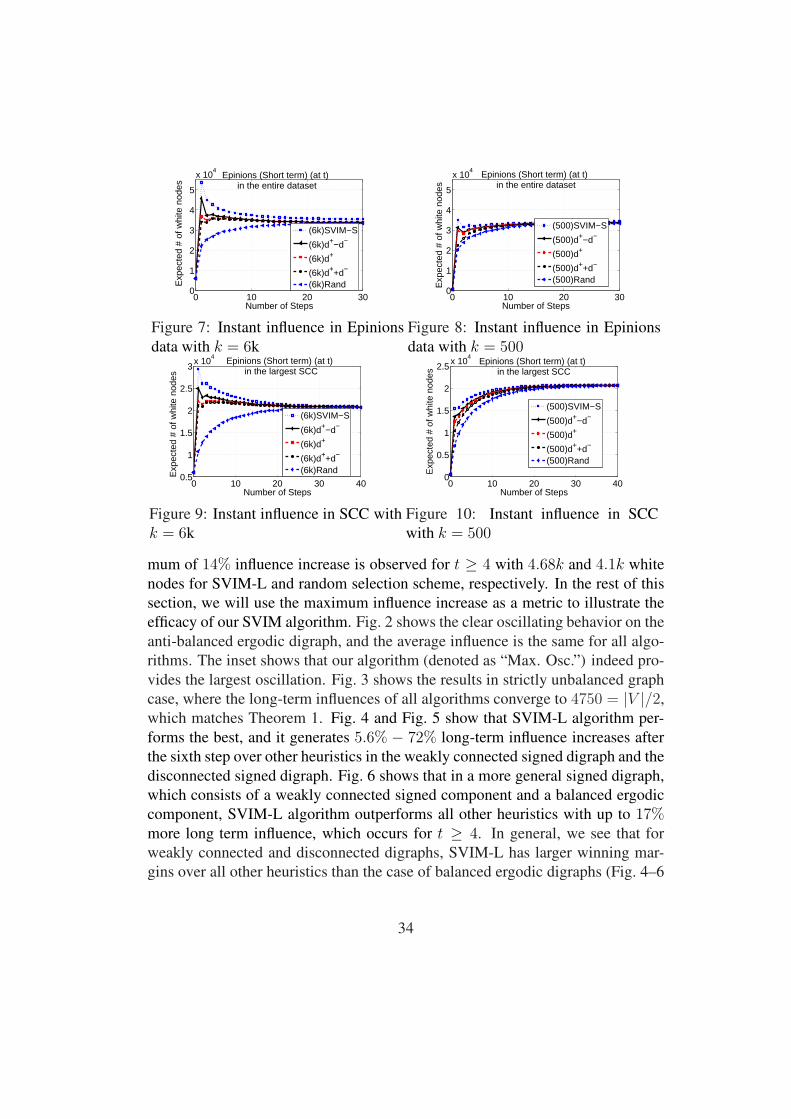
mum of 14% influence increase is observed for t ≥ 4 with 4.68k and 4.1k white

nodes for SVIM-L and random selection scheme, respectively. In the rest of this

section, we will use the maximum influence increase as a metric to illustrate the

efficacy of our SVIM algorithm. Fig. 2 shows the clear oscillating behavior on the

anti-balanced ergodic digraph, and the average influence is the same for all algo-

rithms. The inset shows that our algorithm (denoted as “Max. Osc.”) indeed pro-

vides the largest oscillation. Fig. 3 shows the results in strictly unbalanced graph

case, where the long-term influences of all algorithms converge to 4750 = |V |/2,

which matches Theorem 1. Fig. 4 and Fig. 5 show that SVIM-L algorithm per-

forms the best, and it generates 5.6% − 72% long-term influence increases after

the sixth step over other heuristics in the weakly connected signed digraph and the

disconnected signed digraph. Fig. 6 shows that in a more general signed digraph,

which consists of a weakly connected signed component and a balanced ergodic

component, SVIM-L algorithm outperforms all other heuristics with up to 17%more long term influence, which occurs for t ≥ 4. In general, we see that for

weakly connected and disconnected digraphs, SVIM-L has larger winning mar-

gins over all other heuristics than the case of balanced ergodic digraphs (Fig. 4–6

34

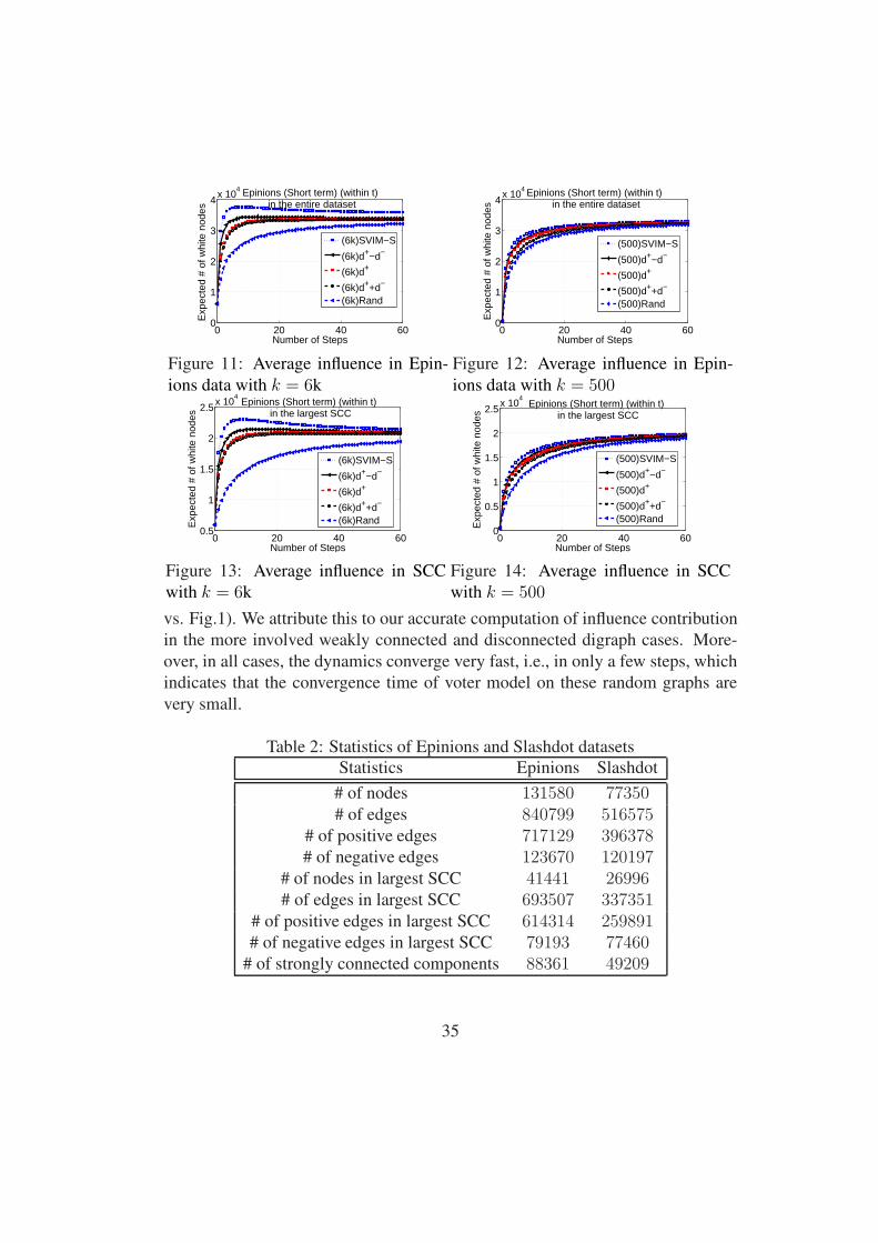
0 20 40 600

1

2

3

4x 10

4

Number of Steps

Exp

ecte

d #

of w

hite

nod

esEpinions (Short term) (within t)

in the entire dataset

(6k)SVIM−S

(6k)d+−d−

(6k)d+

(6k)d++d−

(6k)Rand

Figure 11: Average influence in Epin-

ions data with k = 6k

0 20 40 600

1

2

3

4x 10

4

Number of Steps

Exp

ecte

d #

of w

hite

nod

es

Epinions (Short term) (within t) in the entire dataset

(500)SVIM−S

(500)d+−d−

(500)d+

(500)d++d−

(500)Rand

Figure 12: Average influence in Epin-

ions data with k = 500

0 20 40 600.5

1

1.5

2

2.5x 10

4

Number of Steps

Exp

ecte

d #

of w

hite

nod

es

Epinions (Short term) (within t) in the largest SCC

(6k)SVIM−S

(6k)d+−d−

(6k)d+

(6k)d++d−

(6k)Rand

Figure 13: Average influence in SCC

with k = 6k

0 20 40 600

0.5

1

1.5

2

2.5x 10

4

Number of Steps

Exp

ecte

d #

of w

hite

nod

es

Epinions (Short term) (within t) in the largest SCC

(500)SVIM−S

(500)d+−d−

(500)d+

(500)d++d−

(500)Rand

Figure 14: Average influence in SCC

with k = 500

vs. Fig.1). We attribute this to our accurate computation of influence contribution

in the more involved weakly connected and disconnected digraph cases. More-

over, in all cases, the dynamics converge very fast, i.e., in only a few steps, which

indicates that the convergence time of voter model on these random graphs are

very small.

Table 2: Statistics of Epinions and Slashdot datasets

Statistics Epinions Slashdot

# of nodes 131580 77350# of edges 840799 516575

# of positive edges 717129 396378# of negative edges 123670 120197

# of nodes in largest SCC 41441 26996# of edges in largest SCC 693507 337351

# of positive edges in largest SCC 614314 259891# of negative edges in largest SCC 79193 77460

# of strongly connected components 88361 49209

35

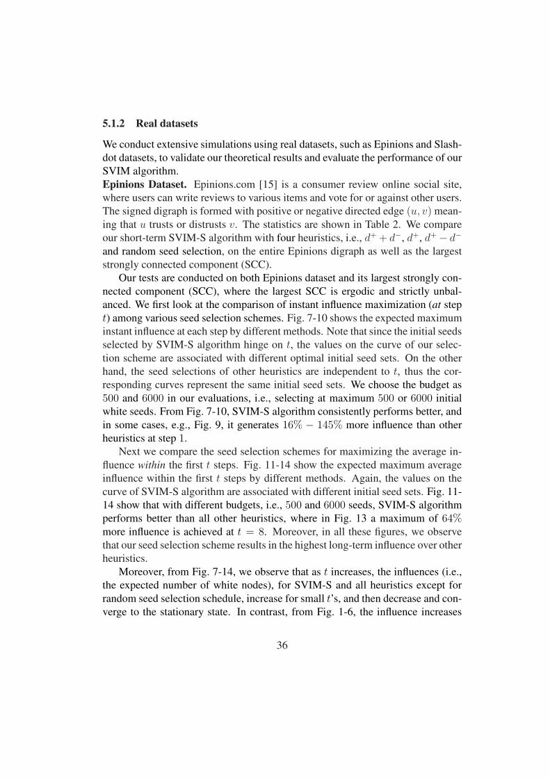
5.1.2 Real datasets

We conduct extensive simulations using real datasets, such as Epinions and Slash-

dot datasets, to validate our theoretical results and evaluate the performance of our

SVIM algorithm.

Epinions Dataset. Epinions.com [15] is a consumer review online social site,

where users can write reviews to various items and vote for or against other users.

The signed digraph is formed with positive or negative directed edge (u, v) mean-

ing that u trusts or distrusts v. The statistics are shown in Table 2. We compare

our short-term SVIM-S algorithm with four heuristics, i.e., d+ + d−, d+, d+ − d−

and random seed selection, on the entire Epinions digraph as well as the largest

strongly connected component (SCC).

Our tests are conducted on both Epinions dataset and its largest strongly con-

nected component (SCC), where the largest SCC is ergodic and strictly unbal-

anced. We first look at the comparison of instant influence maximization (at step

t) among various seed selection schemes. Fig. 7-10 shows the expected maximum

instant influence at each step by different methods. Note that since the initial seeds

selected by SVIM-S algorithm hinge on t, the values on the curve of our selec-

tion scheme are associated with different optimal initial seed sets. On the other

hand, the seed selections of other heuristics are independent to t, thus the cor-

responding curves represent the same initial seed sets. We choose the budget as

500 and 6000 in our evaluations, i.e., selecting at maximum 500 or 6000 initial

white seeds. From Fig. 7-10, SVIM-S algorithm consistently performs better, and

in some cases, e.g., Fig. 9, it generates 16% − 145% more influence than other

heuristics at step 1.

Next we compare the seed selection schemes for maximizing the average in-

fluence within the first t steps. Fig. 11-14 show the expected maximum average

influence within the first t steps by different methods. Again, the values on the

curve of SVIM-S algorithm are associated with different initial seed sets. Fig. 11-

14 show that with different budgets, i.e., 500 and 6000 seeds, SVIM-S algorithm

performs better than all other heuristics, where in Fig. 13 a maximum of 64%more influence is achieved at t = 8. Moreover, in all these figures, we observe

that our seed selection scheme results in the highest long-term influence over other

heuristics.

Moreover, from Fig. 7-14, we observe that as t increases, the influences (i.e.,

the expected number of white nodes), for SVIM-S and all heuristics except for

random seed selection schedule, increase for small t’s, and then decrease and con-

verge to the stationary state. In contrast, from Fig. 1-6, the influence increases

36

monotonically with t. This happens because Epinions dataset (as well as many

real network datasets) has large portion (around 80%) of nodes in the non-sink

components, where to maximize the long-term influence, only nodes in sink com-

ponents should be selected, which governs the long-term influence dynamics of

the whole graph, namely, sink nodes have higher long-term influence contribu-

tions. However, for short-term influence maximization, nodes with higher chances

to influence more nodes in a few steps generally have large number of incoming

links, which are able to influence a large number of nodes in either sink or non-

sink components in a short period of time. Hence, in signed digraphs with large

non-sink component, given a sufficiently large budget, the short-term influence

can definitely outnumber the long-term influence. Our evaluations confirm this

explanation. This interesting observation also leads to a problem that given a

budget k, how to find the optimal time step t that generates the largest influence

among all possible t’s. We leaves this problem as our future work.

Slashdot Dataset. Slashdot.org [39] provides a discussion forum on various

technology-related topics, where members can submit their stories, and comment

on other members’ stories. Its Slashdot Zoo feature allows members to tag each

other as friends or foes, which in turn forms a signed online social network. The

network was collected on 6-th November 2008 [25] and the statistics are shown

in Table 2.

We evaluate instant influence and average influence of our SVIM-S algorithm

on the entire slashdot dataset and its largest strongly connected component, re-

spectively. Our results for k = 6000 are presented in Fig. 15-Fig. 18, which

show that our SVIM-S algorithm performs the best among all methods tested,

especially in the early steps. When changing the budget k, similar results were

obtained, where we omitted them here for brevity.

Moreover, the convergence times for both real-world datasets are fast, in a

few tens of steps, indicating good connectivity and fast mixing property of real-

world networks. In summary, our evaluation results on both synthetic and real-

world networks validate our theoretical results and demonstrate that our SVIM

algorithms for both short term and long term are indeed the best, and often have

significant winning margins.

5.2 The impacts of signed information

Unlike Epinions and Slashdot, many online social networks such as Twitter are

simply represented by unsigned directed graphs, where friends and foe relation-

ships are not explicitly represented on edges. Without edge signs, two types of

37

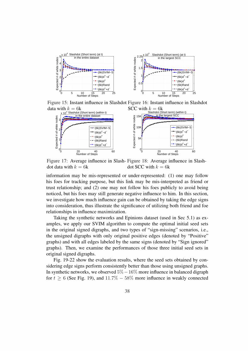
0 5 10 15 20 250

1

2

3

4

5x 10

4

Number of Steps

Exp

ecte

d #

of w

hite

nod

esSlashdot (Short term) (at t)

in the entire dataset

(6k)SVIM−S

(6k)d+−d−

(6k)d+

(6k)Rand

(6k)d++d−

Figure 15: Instant influence in Slashdot

data with k = 6k

0 5 10 15 20 250

0.5

1

1.5

22.25

x 104

Number of Steps

Exp

ecte

d #

of w

hite

nod

es

Slashdot (Short term) (at t) in the largest SCC

(6k)SVIM−S

(6k)d+−d−

(6k)d+

(6k)Rand

(6k)d++d−

Figure 16: Instant influence in Slashdot

SCC with k = 6k

0 20 40 600

1

2

3

x 104

Number of Steps

Exp

ecte

d #

of w

hite

nod

es

Slashdot (Short term) (within t) in the entire dataset

(6k)SVIM−S

(6k)d+−d−

(6k)d+

(6k)Rand

(6k)d++d−

Figure 17: Average influence in Slash-

dot data with k = 6k

0 20 40 600

5K

10K

15K

Number of Steps

Exp

ecte

d #

of w

hite

nod

es

Slashdot (Short term) (within t) in the largest SCC

(6k)SVIM−S

(6k)d+−d−

(6k)d+

(6k)Rand

(6k)d++d−

Figure 18: Average influence in Slash-

dot SCC with k = 6k

information may be mis-represented or under-represented: (1) one may follow

his foes for tracking purpose, but this link may be mis-interpreted as friend or

trust relationship; and (2) one may not follow his foes publicly to avoid being

noticed, but his foes may still generate negative influence to him. In this section,

we investigate how much influence gain can be obtained by taking the edge signs

into consideration, thus illustrate the significance of utilizing both friend and foe

relationships in influence maximization.

Taking the synthetic networks and Epinions dataset (used in Sec 5.1) as ex-

amples, we apply our SVIM algorithm to compute the optimal initial seed sets

in the original signed digraphs, and two types of “sign-missing” scenarios, i.e.,

the unsigned digraphs with only original positive edges (denoted by “Positive”

graphs) and with all edges labeled by the same signs (denoted by “Sign ignored”

graphs). Then, we examine the performances of those three initial seed sets in

original signed digraphs.

Fig. 19-22 show the evaluation results, where the seed sets obtained by con-

sidering edge signs perform consistently better than those using unsigned graphs.

In synthetic networks, we observed 5%−16% more influence in balanced digraph

for t ≥ 6 (See Fig. 19), and 11.7% − 58% more influence in weakly connected

38

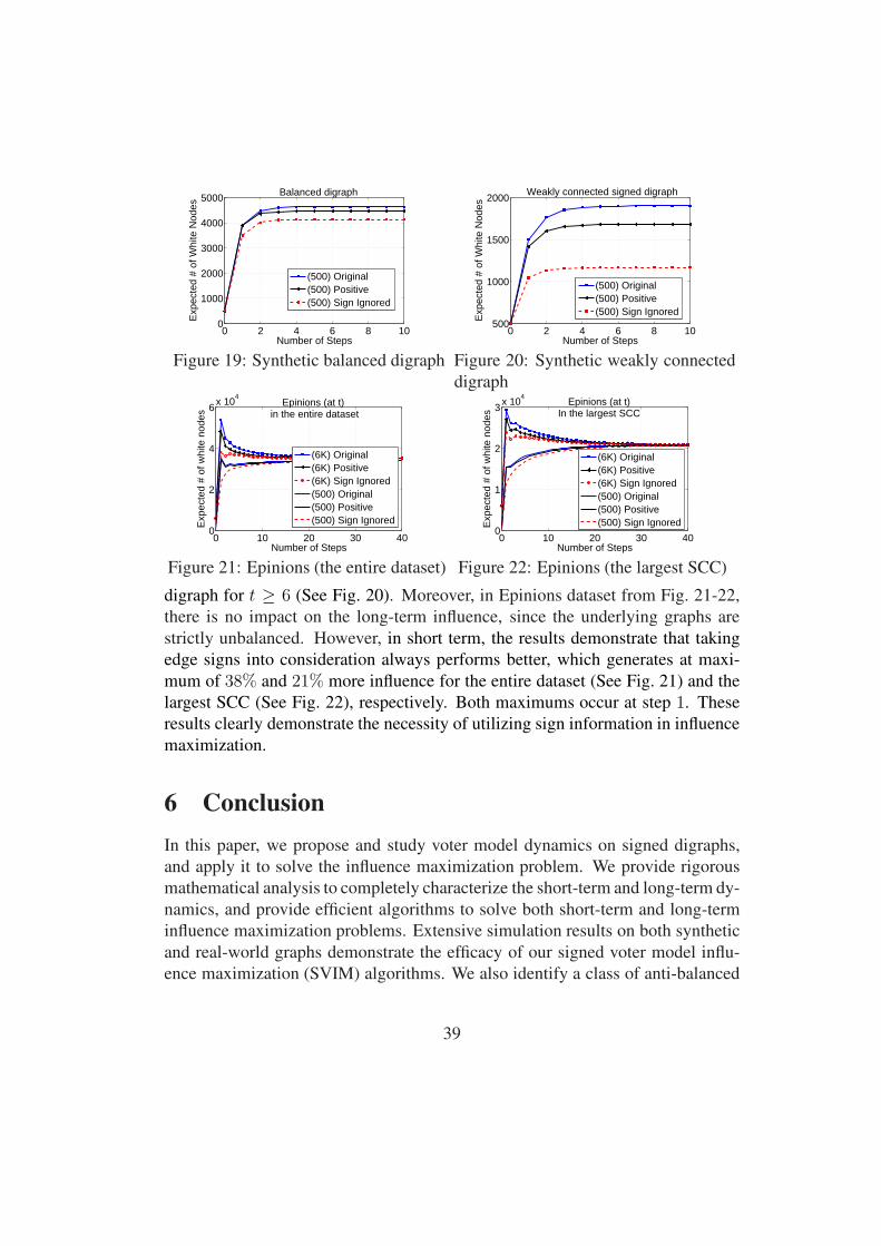
0 2 4 6 8 100

1000

2000

3000

4000

5000

Number of Steps

Exp

ecte

d #

of W

hite

Nod

esBalanced digraph

(500) Original(500) Positive(500) Sign Ignored

Figure 19: Synthetic balanced digraph

0 2 4 6 8 10500

1000

1500

2000

Number of Steps

Exp

ecte

d #

of W

hite

Nod

es

Weakly connected signed digraph

(500) Original(500) Positive(500) Sign Ignored

Figure 20: Synthetic weakly connected

digraph

0 10 20 30 400

2

4

6x 10

4

Number of Steps

Exp

ecte

d #

of w

hite

nod

es

Epinions (at t) in the entire dataset

(6K) Original(6K) Positive(6K) Sign Ignored(500) Original(500) Positive(500) Sign Ignored

Figure 21: Epinions (the entire dataset)

0 10 20 30 400

1

2

3x 10

4

Number of Steps

Exp

ecte

d #

of w

hite

nod

es

Epinions (at t)In the largest SCC

(6K) Original(6K) Positive(6K) Sign Ignored(500) Original(500) Positive(500) Sign Ignored

Figure 22: Epinions (the largest SCC)

digraph for t ≥ 6 (See Fig. 20). Moreover, in Epinions dataset from Fig. 21-22,

there is no impact on the long-term influence, since the underlying graphs are

strictly unbalanced. However, in short term, the results demonstrate that taking

edge signs into consideration always performs better, which generates at maxi-

mum of 38% and 21% more influence for the entire dataset (See Fig. 21) and the

largest SCC (See Fig. 22), respectively. Both maximums occur at step 1. These

results clearly demonstrate the necessity of utilizing sign information in influence

maximization.

6 Conclusion

In this paper, we propose and study voter model dynamics on signed digraphs,

and apply it to solve the influence maximization problem. We provide rigorous

mathematical analysis to completely characterize the short-term and long-term dy-

namics, and provide efficient algorithms to solve both short-term and long-term

influence maximization problems. Extensive simulation results on both synthetic

and real-world graphs demonstrate the efficacy of our signed voter model influ-

ence maximization (SVIM) algorithms. We also identify a class of anti-balanced

39

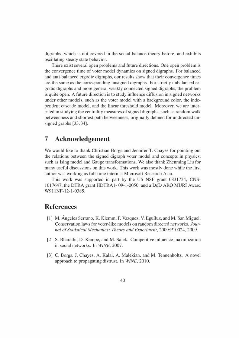
digraphs, which is not covered in the social balance theory before, and exhibits

oscillating steady state behavior.

There exist several open problems and future directions. One open problem is

the convergence time of voter model dynamics on signed digraphs. For balanced

and anti-balanced ergodic digraphs, our results show that their convergence times

are the same as the corresponding unsigned digraphs. For strictly unbalanced er-

godic digraphs and more general weakly connected signed digraphs, the problem

is quite open. A future direction is to study influence diffusion in signed networks

under other models, such as the voter model with a background color, the inde-

pendent cascade model, and the linear threshold model. Moreover, we are inter-

ested in studying the centrality measures of signed digraphs, such as random walk

betweenness and shortest path betweenness, originally defined for undirected un-

signed graphs [33, 34].

7 Acknowledgement

We would like to thank Christian Borgs and Jennifer T. Chayes for pointing out

the relations between the signed digraph voter model and concepts in physics,

such as Ising model and Gauge transformations. We also thank Zhenming Liu for

many useful discussions on this work. This work was mostly done while the first

author was working as full-time intern at Microsoft Research Asia.

This work was supported in part by the US NSF grant 0831734, CNS-

1017647, the DTRA grant HDTRA1- 09-1-0050, and a DoD ARO MURI Award

W911NF-12-1-0385.

References

[1] M. Angeles Serrano, K. Klemm, F. Vazquez, V. Eguıluz, and M. San Miguel.

Conservation laws for voter-like models on random directed networks. Jour-

nal of Statistical Mechanics: Theory and Experiment, 2009:P10024, 2009.

[2] S. Bharathi, D. Kempe, and M. Salek. Competitive influence maximization

in social networks. In WINE, 2007.

[3] C. Borgs, J. Chayes, A. Kalai, A. Malekian, and M. Tennenholtz. A novel

approach to propagating distrust. In WINE, 2010.

40

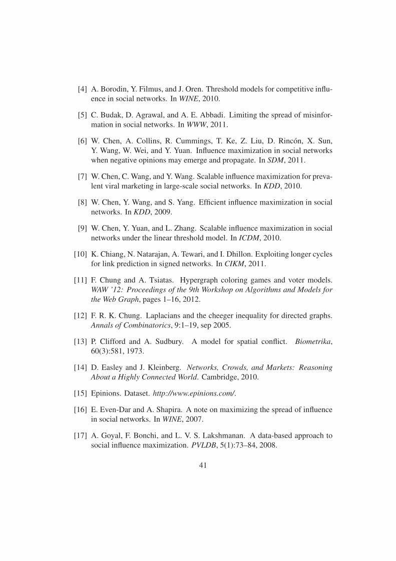
[4] A. Borodin, Y. Filmus, and J. Oren. Threshold models for competitive influ-

ence in social networks. In WINE, 2010.

[5] C. Budak, D. Agrawal, and A. E. Abbadi. Limiting the spread of misinfor-

mation in social networks. In WWW, 2011.

[6] W. Chen, A. Collins, R. Cummings, T. Ke, Z. Liu, D. Rincon, X. Sun,

Y. Wang, W. Wei, and Y. Yuan. Influence maximization in social networks

when negative opinions may emerge and propagate. In SDM, 2011.

[7] W. Chen, C. Wang, and Y. Wang. Scalable influence maximization for preva-

lent viral marketing in large-scale social networks. In KDD, 2010.

[8] W. Chen, Y. Wang, and S. Yang. Efficient influence maximization in social

networks. In KDD, 2009.

[9] W. Chen, Y. Yuan, and L. Zhang. Scalable influence maximization in social

networks under the linear threshold model. In ICDM, 2010.

[10] K. Chiang, N. Natarajan, A. Tewari, and I. Dhillon. Exploiting longer cycles

for link prediction in signed networks. In CIKM, 2011.

[11] F. Chung and A. Tsiatas. Hypergraph coloring games and voter models.

WAW ’12: Proceedings of the 9th Workshop on Algorithms and Models for

the Web Graph, pages 1–16, 2012.

[12] F. R. K. Chung. Laplacians and the cheeger inequality for directed graphs.

Annals of Combinatorics, 9:1–19, sep 2005.

[13] P. Clifford and A. Sudbury. A model for spatial conflict. Biometrika,

60(3):581, 1973.

[14] D. Easley and J. Kleinberg. Networks, Crowds, and Markets: Reasoning

About a Highly Connected World. Cambridge, 2010.

[15] Epinions. Dataset. http://www.epinions.com/.

[16] E. Even-Dar and A. Shapira. A note on maximizing the spread of influence

in social networks. In WINE, 2007.

[17] A. Goyal, F. Bonchi, and L. V. S. Lakshmanan. A data-based approach to

social influence maximization. PVLDB, 5(1):73–84, 2008.

41

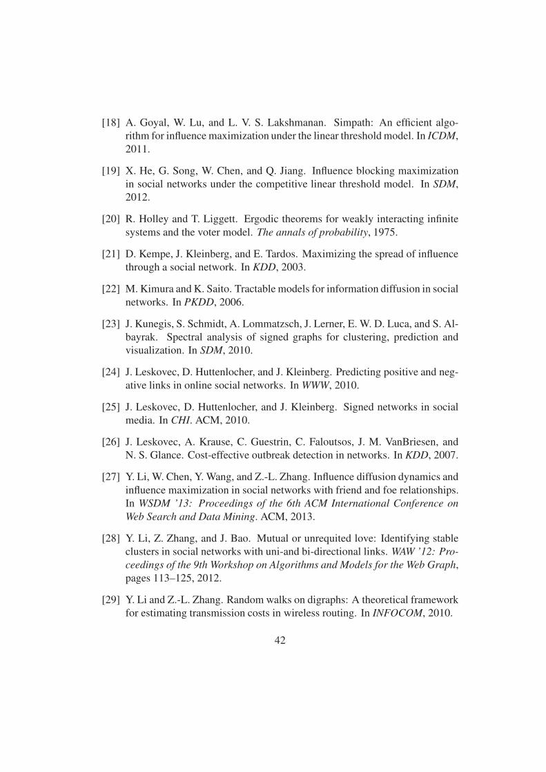
[18] A. Goyal, W. Lu, and L. V. S. Lakshmanan. Simpath: An efficient algo-

rithm for influence maximization under the linear threshold model. In ICDM,

2011.

[19] X. He, G. Song, W. Chen, and Q. Jiang. Influence blocking maximization

in social networks under the competitive linear threshold model. In SDM,

2012.

[20] R. Holley and T. Liggett. Ergodic theorems for weakly interacting infinite

systems and the voter model. The annals of probability, 1975.

[21] D. Kempe, J. Kleinberg, and E. Tardos. Maximizing the spread of influence

through a social network. In KDD, 2003.

[22] M. Kimura and K. Saito. Tractable models for information diffusion in social

networks. In PKDD, 2006.

[23] J. Kunegis, S. Schmidt, A. Lommatzsch, J. Lerner, E. W. D. Luca, and S. Al-

bayrak. Spectral analysis of signed graphs for clustering, prediction and

visualization. In SDM, 2010.

[24] J. Leskovec, D. Huttenlocher, and J. Kleinberg. Predicting positive and neg-

ative links in online social networks. In WWW, 2010.

[25] J. Leskovec, D. Huttenlocher, and J. Kleinberg. Signed networks in social

media. In CHI. ACM, 2010.

[26] J. Leskovec, A. Krause, C. Guestrin, C. Faloutsos, J. M. VanBriesen, and

N. S. Glance. Cost-effective outbreak detection in networks. In KDD, 2007.

[27] Y. Li, W. Chen, Y. Wang, and Z.-L. Zhang. Influence diffusion dynamics and

influence maximization in social networks with friend and foe relationships.

In WSDM ’13: Proceedings of the 6th ACM International Conference on

Web Search and Data Mining. ACM, 2013.

[28] Y. Li, Z. Zhang, and J. Bao. Mutual or unrequited love: Identifying stable

clusters in social networks with uni-and bi-directional links. WAW ’12: Pro-

ceedings of the 9th Workshop on Algorithms and Models for the Web Graph,

pages 113–125, 2012.

[29] Y. Li and Z.-L. Zhang. Random walks on digraphs: A theoretical framework

for estimating transmission costs in wireless routing. In INFOCOM, 2010.

42

[30] Y. Li and Z.-L. Zhang. Random walks on digraphs, the generalized digraph

laplacian and the degree of asymmetry. In LNCS WAW 2010: Proceedings of

the 7th Workshop on Algorithms and Models for the Web Graph, Stanford,

CA, 2010. LNCS.

[31] Y. Li and Z.-L. Zhang. Digraph laplacian and the degree of asymmetry.

Internet Mathematics, 8(4), 2012.

[32] Y. Li and Z.-L. Zhang. Random walks and green’s function on digraphs: A

framework for estimating wireless transmission costs. IEEE/ACM Transac-

tions on Networking, PP(99):1–14, 2012.

[33] Y. Li, Z.-L. Zhang, and D. Boley. The routing continuum from shortest-path

to all-path: A unifying theory. In ICDCS’11: 31st International Conference

on Distributed Computing Systems, pages 847–856. IEEE, 2011.

[34] Y. Li, Z.-L. Zhang, and D. Boley. From shortest-path to all-path: The routing

continuum theory and its applications. IEEE Transactions on Parallel and

Distributed Systems, PP(99):1–11, 2014.

[35] H. Ma, H. Yang, M. R. Lyu, and I. King. Mining social networks using heat

diffusion processes for marketing candidates selection. In CIKM, 2008.

[36] N. Masuda and H. Ohtsuki. Evolutionary dynamics and fixation probabilities

in directed networks. New Journal of Physics, 11:033012, 2009.

[37] R. Narayanam and Y. Narahari. Determining the top-k nodes in social net-

works using the shapley value. In AAMAS, 2008.

[38] N. Pathak, A. Banerjee, and J. Srivastava. A generalized linear threshold

model for multiple cascades. In ICDM, 2010.

[39] Slashdot. Dataset. http://slashdot.org/.

[40] V. Sood, T. Antal, and S. Redner. Voter models on heterogeneous networks.

Physical Review E, 77(4):041121, 2008.

[41] W. Stewart. Numerical methods for computing stationary distributions of

finite irreducible markov chains. Computational Probability, 2000.

43

A Properties of ergodic digraphs

Proposition 4. Let G = (V,E,A) be an ergodic digraph. For any nodes i, j ∈ V ,

there exist two paths from i to j with even and odd length, respectively.

Proof. Suppose, for a contradiction, that all paths from i to j have even lengths.

This implies that all cycles passing through i must be even length, since otherwise

we could follow node i’s odd-length cycle followed by the even length path from

i to j, making the entire path from i to j odd. Now we can consider any cycle Cr

in G, not necessarily passing i. We claim that Cr must have even length. In fact,

we can pick any node u on Cr, and construct a path from i to j with the following

segments: R1 from i to u, Cr, R2 from u back to i, and R3 from i to j. Since we

know that R1 + R2 has even length and R3 has even length, it must be the case

that Cr has even length by our assumption. However, this means that all cycles in

C has even lengths, contradicting to the aperiodicity of G.

The case of odd length paths can be proved in the same way.

Proposition 5. Let G = (V,E, A) be an ergodic unsigned digraph, with transition

probability matrix P and stationary distribution vector π. P t−1πT = (P−1πT )t

holds for any integer t > 0.

Proof. Using the facts that P1 = 1 and πT P = πT , it is easy to prove by induction

that for any integer t > 0 P t − 1πT = (P − 1πT )t holds.

B Special matrix power series

Proposition 6. Let X ∈ Rm×m, Y ∈ R

m×n and Z ∈ Rn×n. If limt→∞X t =

limt→∞ Zt = 0, the following equalities hold:

(i) limt→∞

t−1∑

i=0

X i = (I −X)−1, (37)

(ii) limt→∞

t−1∑

i=0

X iY Zt−1−i = 0, (38)

Proof. (i) Let ρ(X) be the spectral radius of matrix X , i.e., the largest absolute

value of the eigenvalues of X . Notice that limt→∞ X t = 0 if and only if ρ(X) < 1.

44

We first claim that, I − X and I − Z are invertible. Suppose I − X is not

invertible, there is a non-zero vector p such that (I − X)p = 0. Therefore, p is

the eigenvector of X with eigenvalue 1, which contradicts limt→∞X t = 0. Same

argument can be applied to I − Z. Hence, the left hand side of Eq.(37) equals to

limt→∞

t∑

i=0

X i = limt→∞

(I −X)−1(I −X t+1) = (I −X)−1.

(ii) The max-norm of X is given by ‖X‖max = maxi,j≤mXij. Let X =QXJQ−1

X be the standard Jordan form of X , where QX is an invertible matrix.

Denote J = 11T as the all-one matrix. Hence, we have

‖X i‖max = ‖QXJiQ−1

X ‖max ≤ ‖QX‖max‖Q−1X ‖max‖JJ

iJ‖max

≤ ‖QX‖max‖Q−1X ‖maxm

2‖J i‖max

J i is in form as

J i =

λi1 C1

i λi−11 C2

i λi−21 0 0

0 λi1 C1

i λi−11 0 0

0 0 λi1 0 0

0 0 0 λim0

C1i λ

i−1m0

0 0 0 0 λim0

, (39)

where Cℓi =

i!ℓ!(i−ℓ)!

≤ im and each non-zero entry in J i can be expressed as C iℓλ

i−ℓk ,

1 ≤ k ≤ m0, 1 ≤ ℓ ≤ ℓ0(k), with m0 as the number of different eigenvalues of

X and ℓ0(k) as the multiplicity of the k-th eigenvalue of X . Hence, the absolute

value of each non-zero entry in J i is upper bounded as |Cℓiλ

i−ℓk | ≤ imρ(X)i−m,

which implies that

‖X i‖max ≤ ‖QX‖max‖Q−1X ‖maxm

2imρ(X)i−m

Let ρ = max(ρ(X), ρ(Z)), we have

limt→∞

‖

t−1∑

i=0

X iY Zt−1−i‖max ≤ limt→∞

tmn‖X i‖max‖Y ‖max‖Zt−1−i‖max

≤ limt→∞

tmnTmax(m2tmρi−m)(n2tnρt−i−1−n) ≤ lim

t→∞m3n3Tmaxt

m+n+1ρt−1−n−m = 0

where Tmax = ‖Y ‖max‖QX‖max‖Q−1X ‖max‖QZ‖max‖Q

−1Z ‖max.

45

C Illustration of exponential convergence time of P t

on ergodic digraph.

Figure 23: An example digraph with exponential convergence time. All edges are

with unit weights.

Given an unsigned ergodic digraph G = (V,E, A), with transition probability

matrix P , it has fixed stationary distribution π, i.e., πT = πT P .

The convergence time (or mixing time) of a random walk Markov chain on Gis the time until the Markov chain is “close” to its stationary distribution π. To be

precise, for an initial distribution x0, let xTt = xT

0 Pt be the distribution at step t.

The variation distance mixing time is defined as the smallest t such that for any

subset W ⊆ V ,

|(xTt − πT )eW | ≤

1

4,

where eW is the vector such that eW (i) = 1 if i ∈ W , and eW (i) = 0 if i ∈ V \W .

The convergence time is said to be exponentially large if there exists x0 such

that the convergence time of the random walk starting from x0 is 2Ω(n), where

n = |V |. Lemma 7 below illustrates that the convergence time of random walk on

ergodic digraphs could be exponentially large.

Lemma 7. There exist ergodic digraphs, such that the convergence time of the

random walks on these digraphs are exponentially large.

Proof. We prove this by construction. Fig. 23 shows an example digraph G, with

|V | = 2m nodes. On the left hand side, there are m ≥ 3 nodes L1, L2, · · · , Lm

connected by m− 1 directed edges from L1 to Lm, and every node Li with i > 1has a directed connection to the leftmost node L1. The right hand side nodes

have symmetric connections as the left hand side. Moreover, node Lm and Rm

also have one more connection to R1 and L1, respectively, which connect two

components together. It is clear that the graph is strongly connected and aperiodic

(there exist cycles of length 2 and 3), and thus ergodic.

46

Let xt(Li) denote the probability that the random walk is at node Li at step

t, and x(Li) be its stationary distribution. Similarly define xt(Ri) and x(Ri) for

node Ri. The graph is symmetric, thus we have x(Li) = x(Ri) for 1 ≤ i ≤ m.

Let x(L1) = x(R1) = ρ/4, we have x(Li) = x(Ri) = ρ/2i for i = 2, 3, . . . , m.

Then, by solving∑m

i=1(x(Li) + x(Ri)) = 1, we obtain ρ = 2m−1

3·2m−2−1. It is easy to

verify that indeed the obtained x is the stationary distribution of the random walks

on the digraph.

Then, we consider the initial distribution as x0 = [1, 0, 0, . . . , 0], and the subset

W = R1, · · · , Rm including all m nodes on the right-hand side. Let xt(W ) =xTt · eW denote the total probability that the random walk is in some node in W

at step t. The only edge from the left half to the right half is the edge from Lm

to R1. Thus all additions to xt+1(W ) from xt(W ) comes from this edge, namely

xt+1(W )−xt(W ) ≤ xt(Lm)/2. We now bound xt(Lm). For t ≤ m−1, we know

that xt(Lm) = 0. For t ≥ m, we have

xt(Lm) = xt−1(Lm−1)/2 = xt−2(Lm−2)/22 = · · · = xt−m+2(L2)/2

m−2 ≤ 1/2m−2.

Hence, we have

xt(W ) =t

∑

i=1

(xi(W )− xi−1(W )) ≤ t · xt(Lm)/2 ≤ t/2m−1.

Therefore, the smallest t that satisfies |(xTt − πT )eW | = |xt(W )− 1/2| ≤ 1/4 is

such that xt(W ) ≥ 1/4, which implies that t/2m−1 ≥ 1/4 and t ≥ 2m−3. This

completes the proof.

47