Embed Size (px)
Citation preview
International Journal of Heat and Mass Transfer 47 (2004) 307–328
www.elsevier.com/locate/ijhmt
Volumetric interfacial area prediction in upward bubblytwo-phase flow
Wei Yao 1, Christophe Morel *
CEA Grenoble, DEN/DTP/SMTH/LMDS, 17 rue des Martyrs, 38054 Grenoble, C�eedex 9, France
Received 28 May 2002; received in revised form 13 June 2003
Abstract
In two-phase flow studies, a volumetric interfacial area balance equation is often used in addition to the multi-
dimensional two-fluid model to describe the geometrical structure of the two-phase flow. In the particular case of
bubbly flows, numerous works have been done by different authors on the subject. Our work concerns two main
modifications of this balance equation: (1) new time scales are proposed for turbulence induced coalescence and
breakup, (2) modeling of the nucleation of new bubbles on the volumetric interfacial area. The 3D module of the
CATHARE code is used to evaluate our new model, in comparison to three other models for interfacial area found in
the literature, on two different experiments. First, we use the DEBORA experimental data base for the comparison in
the case of boiling bubbly flow. The comparison of the different volumetric interfacial area models to the DEBORA
experimental data shows that even though the theoretical values of the coefficients are adopted in our modified model,
this model has a quite good capability to predict the local two-phase geometrical parameters in the boiling flow
conditions. Secondly, we compare the predictions obtained with the same models to the DEDALE experimental data
base, for the case of adiabatic bubbly flow. In comparison to the other models tested, our model also gives quite good
predictions of the bubble diameter in the case of adiabatic conditions.
� 2003 Elsevier Ltd. All rights reserved.
Keywords: Boiling two-phase flow; Interfacial area; Nucleation; Bubbly flow; DEBORA experiment; DEDALE experiment
1. Introduction and discussion about the volumetric
interfacial area models
The two-fluid model is currently used in many gen-
eral computational fluid dynamic codes and more
specific nuclear thermal-hydraulics analysis codes, for
two-phase flow studies. In the two-fluid model, the
volumetric interfacial area, also called the interfacial
area concentration, is a very important quantity which
determines the intensity of inter-phase mass, momentum
and energy transfers. As pointed out by Ishii [1], the
accurate modeling of the local interfacial area concen-
tration is the first step to be taken for the development
* Corresponding author. Tel.: +33-4-38-78-92-27/56-54.
E-mail addresses: [email protected] (W. Yao), morel@alpes.
cea.fr (C. Morel).1 Tel.: +33-4-38-78-56-54.
0017-9310/$ - see front matter � 2003 Elsevier Ltd. All rights reserv
doi:10.1016/j.ijheatmasstransfer.2003.06.004
of reliable two-fluid model closure relations. Recently,
more and more researchers concentrate on developing
the volumetric interfacial area transport equation to
describe the temporal and spatial evolution of the two-
phase geometrical structure.
As far as the adiabatic bubbly flow is concerned, the
effects of nucleation and interfacial heat and mass
transfers are out of consideration, thus the coalescence
and breakup effects due to the interactions among
bubbles and between bubbles and turbulent eddies have
been the subject of more attention. Wu et al. [2] have
considered five mechanisms responsible for bubbles co-
alescence and breakup: (1) coalescence due to random
collisions driven by turbulence, (2) coalescence due to
wake entrainment, (3) breakup due to the impact of
turbulent eddies, (4) shearing-off of small bubbles from
larger cap bubbles, (5) breakup of large cap bubbles due
to interfacial instabilities. In the case of low void frac-
tion conditions where no cap bubbles are present, the
ed.
Nomenclature
ai volumetric interfacial area
al thermal diffusion coefficient of liquid
A area
C constant or coefficient
Cp isobaric thermal capacity
d diameter
e internal energy
E Zuber’s factor for added mass (Eq. (85))
f frequency, pdf
g function given by Eq. (13), gravity
h thickness, heat transfer coefficient, source
term in Liouville equation
H enthalpy
I identity tensor
j local volumetric flux
J global volumetric flux (superficial velocity)
Ja Jakob number
k wave number
K constant, turbulent kinetic energy
L length, latent heat of vaporisation
m gas mass in a bubble
_mm mass flux
Mki volumetric interfacial forces
n bubble number density
ne mixture eddies number density
N active nucleation sites number density, liq-
uid eddies number density
Nu Nusselt number
P pressure
Pe P�eeclet number
Pr Prandtl number
P iK bubble induced turbulence kinetic energy
source term
P ie bubble induced turbulence dissipation rate
source term
q heat flux
q00 heat flux density
r bubble radius
Re Reynolds number
S collision area
t time
t$
stress tensor
T period, temperature
u turbulent velocity
Ur norm of the relative velocity
V volume
V*
velocity vector
We Weber number
x space coordinate
Z=D elevation to tube diameter ratio in the
DEDALE experiment
Greek symbols
a void fraction
d Dirac distribution
dt numerical time step
e turbulence dissipation rate
g coalescence/breakup efficiency
/ source/sink of bubble number density
n internal phase coordinate
w dispersed phase geometrical quantity
k thermal conductivity
q density
s time constant
r surface tension
m viscosity
D difference
C interfacial mass transfer
X variation domain for the internal phase co-
ordinates
Superscripts
BK breakup
CO coalescence
D drag
DT turbulent dispersion
i interfacial
L lift
MA added mass
NUC nucleation
RC random collision
Re Reynolds
T turbulence
TI turbulent impact
WE wake entrainment
+ non-dimensional (temperature)
� friction (velocity)
Subscripts
0 initial value
b breakup, bubble
bf free travelling of breakup
bi interaction of breakup
c coalescence, continuous phase
cf free travelling of coalescence
ci interaction of coalescence
cr critical value
d dispersed phase
D drag
DT turbulent dispersion
e eddy, evaporation
g gas or vapour
i interface
k k-phase
308 W. Yao, C. Morel / International Journal of Heat and Mass Transfer 47 (2004) 307–328
ki k-phase near the interface
K relative to the turbulent kinetic energy
l liquid
L lift
max maximum value
MA added mass
nuc nucleation
q quenching
r relative
s Sauter mean (diameter)
sat saturation
t turbulent
w wall
e relative to the turbulent dissipation rate
W. Yao, C. Morel / International Journal of Heat and Mass Transfer 47 (2004) 307–328 309
authors have simplified their model by considering only
one bubble size and the first three coalescence and
breakup mechanisms.
Some experimental results [3,4] show that the wake
entrainment results in coalescence primarily between
pairs of large cap bubbles in fluid sufficiently viscous to
keep their wake laminar; whereas small spherical or ellip-
soidal bubbles tend to repel each other. In addition, in
low viscous liquids such as water, the turbulent wake has
the tendency to break trailing bubbles because of its
intermittency and irregularity. Hibiki and Ishii [5] also
pointed out that the wake entrainment induced coales-
cence results in minor contribution to the volumetric
interfacial area variation in the bubbly flow with high
flow rate because a bubble captured in the wake region
can leave the region easily due to liquid turbulence, even
though it may play an important role in the bubbly-to-
slug flow transition. Furthermore, calculation results of
Hibiki and Ishii [5] and Ishii and Kim [6] have shown
that the gas expansion term, previously omitted by Wu
et al. [2], may contribute significantly to the total vari-
ation of volumetric interfacial area. In another hand,
although the wake entrainment effect can be omitted for
Hibiki, it appears dominant in Wu’s calculation cases. In
addition, although the coefficients are fitted from ex-
perimental data and can give reasonable one-dimen-
sional calculation results, it is surprising to notice that
the values presented by the different authors show sig-
Table 1
Comparison of volumetric interfacial area models
Models /RCn /TI
n
Tc gc Tb
Wu et al.
[2]
Free travelling time
/ d2=3s
e1=3agðaÞ
Constant Interac
/ dsut
�
Hibiki and
Ishii [5]
Free travelling time
/ d2=3s
e1=3agðaÞ
exp Kc2
ffiffiffiffiffiffiffiffiffiWeWecr
r� �Free tr
/ de1=3ð
Ishii and
Kim [6]
Free travelling time
/ d2=3s
e1=3agðaÞ
Constant Interac
/ dsut
1
�
nificant differences. Recently, Delhaye [7] gave a sys-
tematic comparison and detailed analysis of their work.
The volumetric interfacial area transport equation
written by the above authors writes:
oaiot
þr � ðaiV*
gÞ ¼2
3
aia
oaot
�þr � ðaV
*
g�
þ 36p3
aai
� �2
ð/RCn þ /WE
n þ /TIn Þ
ð1Þ
where the first term on the right-hand side (RHS) is the
gas expansion term, and /RCn , /WE
n , /TIn are the volu-
metric bubble number variations induced by the coales-
cence and breakup phenomena. Clearly, the coalescence
and breakup terms induced by turbulence can be written
in the following general forms:
/RCn ¼ 1
Tcngc; /TI
n ¼ 1
Tbngb ð2Þ
where Tc and Tb are the coalescence and breakup times
of a single bubble, gc and gb are the coalescence and
breakup efficiencies, and n is the bubble number per unit
volume. Table 1 shows a comparison of the models of
different authors [2,5,6] according to our notations in-
troduced in Eq. (2). In this table, the Weber number is
defined by the following relation:
/WEn Expansion
termgb
tion time
1 WecrWe
�1=2 exp WecrWe
� �Yes No
avelling time2=3s
1 aÞ hðaÞ
exp KB
WecrWe
� �No Yes
tion time
WecrWe
�1=2
exp WecrWe
� �Yes Yes
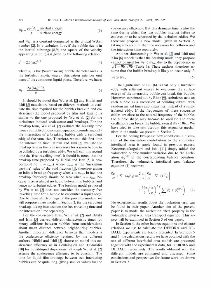
310 W. Yao, C. Morel / International Journal of Heat and Mass Transfer 47 (2004) 307–328
We ¼ qlu2ds
r¼ inertial energy
surface energyð3Þ
and Wecr is a constant designated as the critical Weber
number [2]. In a turbulent flow, if the bubble size is in
the inertial subrange [8,9], the square of the velocity
appearing in Eq. (3) is given by the following relation:
u2 ¼ 2:0ðedsÞ2=3 ð4Þ
where ds is the (Sauter mean) bubble diameter and e is
the turbulent kinetic energy dissipation rate per unit
mass of the continuous liquid phase. Therefore, we have:
We ¼ 2qlðedsÞ2=3ds
rð5Þ
It should be noted that Wu et al. [2] and Hibiki and
Ishii [5] models are based on different methods to eval-
uate the time required for the bubbles breakup and co-
alescence (the model proposed by Ishii and Kim [6] is
similar to the one proposed by Wu et al. [2] for the
turbulence induced coalescence and breakup). For the
breakup term, Wu et al. [2] evaluate the breakup time
from a simplified momentum equation, considering only
the interaction of a breaking bubble with a turbulent
eddy of the same size. Therefore, we call this first time
the �interaction time’. Hibiki and Ishii [5] evaluate the
breakup time as the time necessary for a given bubble to
be collided by a turbulent eddy. We will call this second
time the �free travelling time’. It should be noted that the
breakup time proposed by Hibiki and Ishii [5] is pro-
portional to (a amax) where amax is the �maximum
packing’ value of the void fraction [1], therefore giving
an infinite breakup frequency when a ¼ amax. In fact, the
breakup frequency should be zero when a ¼ amax be-
cause there is almost no liquid between the bubbles, and
hence no turbulent eddies. The breakup model proposed
by Wu et al. [2] does not consider the necessary free
travelling time for a bubble to encounter a liquid eddy.
Due to these shortcomings of the previous models, we
will propose a new model in Section 2, for the turbulent
breakup, taking into account the free travelling time and
the interaction time separately.
For the coalescence term, Wu et al. [2] and Hibiki
and Ishii [5] derived different characteristic times for
binary collisions between bubbles from considerations
about mean distance between neighbouring bubbles.
Another important difference between their models is
the coalescence efficiency retained by the different
authors. Hibiki and Ishii [5] choose to model this co-
alescence efficiency as in Coulaloglou and Tavlarid�ees[10] for liquid/liquid dispersions, although Wu et al. [2]
assume the coalescence efficiency to be constant. The
time for liquid film drainage between two interacting
bubbles can be quite long, giving smaller values for the
coalescence efficiency. But this drainage time is also the
time during which the two bubbles interact before to
coalesce or to be separated by the turbulent eddies. We
therefore propose a new model, given in Section 2,
taking into account the time necessary for collision and
the interaction time separately.
Another shortcoming in Wu et al. [2] and Ishii and
Kim [6] models is that the breakup model they propose
cannot be used for We < Wecr, due to the dependence inffiffiffiffiffiffiffiffiffiffiffiffiffiffiffiffiffiffiffiffiffiffiffiffiffi1 Wecr=We
p(Table 1). These authors therefore as-
sume that the bubble breakup is likely to occur only if:
WePWecr ð6Þ
The significance of Eq. (6) is that only a turbulent
eddy with sufficient energy to overcome the surface
energy of the interacting bubble can break this bubble.
However, as pointed out by Risso [9], turbulence acts on
each bubble as a succession of colliding eddies, with
random arrival times and intensities, instead of a single
isolated eddy. If the frequencies of these successive
eddies are close to the natural frequency of the bubble,
the bubble shape may become to oscillate and these
oscillations can break the bubble, even if We < Wecr. We
have tried to take into account this resonance mecha-
nism in the model we present in Section 2.
For the boiling two-phase flow conditions, a discus-
sion of the nucleation contribution to the volumetric
interfacial area is rarely found in previous papers.
Kocamustafaogullari and Ishii [11] simply added the
volumetric bubble number variation due to the nucle-
ation /NUCn in the corresponding balance equation.
Therefore, the volumetric interfacial area balance
equation (1) becomes:
oaiot
þr � ðaiV*
gÞ ¼2
3
aia
oaot
�þr � ðaV
*
g�
þ 36p3
aai
� �2 Xj
/jn
þ /NUC
n
!ð7Þ
No experimental results about the nucleation term can
be found in their paper. Another aim of the present
paper is to model the nucleation effect properly in the
volumetric interfacial area transport equation. This as-
pect will be examined in Section 3 of our paper.
In Section 4, the other balance equations and closure
relations we use to calculate the DEBORA and DE-
DALE experiments are briefly presented. In Sections 5
and 6, the calculations results we have obtained with the
use of different interfacial area models are presented
together with the experimental data, for DEBORA and
DEDALE respectively. The results obtained with the
different models are compared and discussed. Some
conclusions and perspectives for future work are drawn
in Section 7.
W. Yao, C. Morel / International Journal of Heat and Mass Transfer 47 (2004) 307–328 311
2. Modeling of the turbulence induced coalescence and
breakup
As we discussed in the previous section, two main
modifications of the turbulence induced coalescence and
breakup models will be presented here:
(1) The times for coalescence and breakup can be split
into two contributions: the free travelling time and
the interaction time.
(2) The breakup interaction time is modeled according
to the bubble-eddy resonance mechanism.
2.1. Turbulence induced coalescence
In a turbulent flow, small bubble motions are driven
randomly by turbulent eddies. In the case where ds � L,where ds is the Sauter mean bubble diameter and L is the
average distance between two neighbouring bubbles, the
probability of collision between two bubbles is larger
than the one among three or more bubbles. Assuming
only binary coalescence events, Prince and Blanch [12]
gave the following expression for the collision frequency
between two bubbles of different groups induced by
turbulence:
f Tij ¼ ninjSijðu2i þ u2j Þ1=2 ð8Þ
where the effective collision cross-sectional area is given
by:
Sij ¼p4ðri þ rjÞ2 ð9Þ
In the case of a single bubble size, given by ds, the total
collision frequency between bubbles in a unit volume
can be simplified into:
fc ¼ffiffiffi2
pp
8n2d2s u ¼
p4n2d7=3s e1=3 ¼ Cc
e1=3
d11=3s
a2 ð10Þ
where Cc ¼ 2:86. It should be noted that we have di-
vided (8) by 2 for the calculation of the total collision
frequency, in order to avoid double counting of the same
collision events between bubble pairs [12].
Accordingly the average free travelling time of one
bubble writes:
Tcfen2fc
¼ 4ffiffiffi2
ppnd2s u
¼ 1
3
d2=3s
ae1=3ð11Þ
It can be considered that when the void fraction
reaches a certain value amax, called �maximum packing
value’ [1], the bubbles touch each other and the average
free travelling time becomes zero. In the case of a single
bubble size, this limiting value of the void fraction is
given by [5]:
amax ¼p6¼ 0:52 ð12Þ
Therefore, the following modification factor:
gðaÞ ¼ ða1=3max a1=3Þ
a1=3max
ð13Þ
which considers the effect of the void fraction on the
average free travelling time, is suggested here. When the
void fraction is very small, gðaÞ ¼ 1, which corresponds
to the case of a dilute two-phase flow where no correc-
tion is needed. If the void fraction reaches its limiting
value, gðaÞ ¼ 0 and the free travelling time becomes nil.
At the end, the free travelling time can be expressed
by the following relation:
Tcf ¼1
3
gðaÞa
d2=3s
e1=3ð14Þ
In the modeling of the interaction between two in-
teracting bubbles, we adopt the film thinning model [13].
This model assumes that two bubbles will coalesce if the
contact time between them, depending on the sur-
rounding turbulent eddies, is larger than the liquid film
drainage time. Prince and Blanch [12] gave the following
expression for the film drainage time:
tc ¼qcðds=2Þ
3
16r
" #1=2lnh0hcr
ð15Þ
where the initial film thickness h0 and the critical film
thickness hcr are suggested to be 104 m [13] and 108 m
[14] (for an air–water system). Therefore, Eq. (15) can be
rewritten:
tc ¼ 0:814
ffiffiffiffiffiffiffiffiffiqcd3sr
rð16Þ
This time is used as the interaction time before coales-
cence of two bubbles:
Tci ¼ tc ð17Þ
The contact time is given by the characteristic time of
the eddies having the same size than the bubbles [12]:
sc ¼r2=3b
e1=3ð18Þ
In addition, an exponential relation is assumed [14]
to estimate the collision efficiency:
gc ¼ exp
� tc
sc
�ð19Þ
As we discussed before, the coalescence time contains
two parts: the free travelling time and the interaction
time, i.e.:
Tc ¼ Tcf þ Tci ð20Þ
312 W. Yao, C. Morel / International Journal of Heat and Mass Transfer 47 (2004) 307–328
Finally, the bubble coalescence frequency can be
expressed as:
/RCn ¼ 1
2
gcnTc
ð21Þ
where the factor one-half has been put to avoid double
counting of the same coalescence events between bubble
pairs [12].
Substituting from the above relations, the final form
writes:
/RCn ¼ Kc1
e1=3a2
d11=3s
1
gðaÞ þ Kc2affiffiffiffiffiffiffiffiffiffiffiffiffiffiffiffiffiWe=Wecr
p� exp
� Kc3
ffiffiffiffiffiffiffiffiffiWeWecr
r �ð22Þ
If we introduce the following value of the critical Weber
number [15]:
Wecr ¼ 1:24 ð23Þ
the coefficients will be Kc1 ¼ 2:86, Kc2 ¼ 1:922, Kc3 ¼1:017.
It should be noted that the ratio of the free travelling
time and the interaction time is:
TcfTci
/ gðaÞaffiffiffiffiffiffiffiffiffiffiffiffiffiffiffiffiffiWe=Wecr
p ð24Þ
This time ratio decreases when the Weber number in-
creases or the void fraction increases.
2.2. Turbulence induced breakup
For analysing the collisions between bubbles and
eddies using Eq. (8), the information of eddies number
per unit volume is needed. According to Azbel and
Athanasios [16]:
dNðkÞdk
¼ 0:1k2 ð25Þ
where NðkÞ is the number of eddies of wave number kper unit volume of the fluid (k ¼ 2=de where de is the
diameter of the eddy).
Considering the void fraction effect, the number of
eddies per unit volume in the two-phase mixture is given
by [5]:
dneðkÞdk
¼ 0:1k2ð1 aÞ ð26Þ
which can be rewritten in terms of eddy diameter:
dneðdeÞ ¼ 0:8ð1 aÞdðdeÞ
d4e
ð27Þ
Using Eqs. (4), (8), (9) and (27), the collision frequency
between bubbles characterized by their volumetric
number n and their diameter ds and eddies whose dia-
meters are comprised between two fixed values de1 and
de2 is:
fb ¼Z de2
de1
np16
ðde þ dsÞ2ffiffiffi2
pe1=3ðd2=3e þ d2=3s Þ1=2 dneðdeÞ
¼Z de2
de1
ð1 aÞn p16
ðde þ dsÞ2ffiffiffi2
pe1=3ðd2=3e þ d2=3s Þ1=2 0:8
d4edðdeÞ
ð28Þ
Assuming that only the eddies with a size comparable to
the bubble diameter can break the bubbles, and nu-
merically integrating Eq. (28) from de1 ¼ 0:65ds to
de2 ¼ ds (the value 0.65 is chosen in order to obtain a
good agreement on the bubble diameter profile in
comparison to the DEBORA experiment), we obtain:
fb ¼ C0b
ne1=3
d2=3s
ð1 aÞ ¼ Cb
e1=3
d11=3s
að1 aÞ ð29Þ
where Cb ¼ 6C0b=p ¼ 1:6 (C0
b ¼ 0:837).Therefore, the average free travelling time of bubbles
can be written as:
Tbf ¼nfb
¼ Cbt
d2=3s
e1=3ð1 aÞ ð30Þ
where Cbt ¼ 1=C0b ¼ 1:194.
As pointed out previously, the breakup mechanism is
assumed to be due to the resonance of bubble oscilla-
tions with turbulent eddies, especially in the conditions
of low Weber number. The natural frequency of the nthorder mode of the oscillating bubble is given by
[9,13,15,17]:
ð2pfnÞ2 ¼8nðn 1Þðnþ 1Þðnþ 2Þr
½ðnþ 1Þqg þ nql�d3sð31Þ
For the second mode oscillation, and if qg � ql is as-
sumed for bubbly flow, Eq. (31) gives:
f2 ¼ 1:56
ffiffiffiffiffiffiffiffiffir
qld3s
rð32Þ
The breakup characteristic time describes the increase of
the most unstable oscillation mode:
Tbi ¼1
f2¼ 0:64
ffiffiffiffiffiffiffiffiffiqld3sr
rð33Þ
This characteristic time is used as the interaction time
between a bubble and eddies. As for the coalescence, we
assume that the breakup time is the sum of the free
travelling time and the interaction time:
Tb ¼ Tbf þ Tbi ð34Þ
In addition, the breakup efficiency can be expressed
as [2]:
gb ¼ exp
� WecrWe
�ð35Þ
W. Yao, C. Morel / International Journal of Heat and Mass Transfer 47 (2004) 307–328 313
Finally, the bubble breakup frequency should be
written as:
/TIn ¼ gb
nTb
ð36Þ
Substituting from the above relations, the final form
is obtained:
/TIn ¼ Kb1
e1=3að1 aÞd11=3s
1
1þ Kb2ð1 aÞffiffiffiffiffiffiffiffiffiffiffiffiffiffiffiffiffiWe=Wecr
p� exp
� WecrWe
�ð37Þ
where Kb1 ¼ 1:6, Kb2 ¼ 0:42.The ratio of the free travelling time and the interac-
tion time is given by the following relation:
TbfTbi
/ 1
ð1 aÞffiffiffiffiffiffiffiffiffiffiffiffiffiffiffiffiffiWe=Wecr
p ð38Þ
This ratio decreases when the Weber number increases
or the void fraction decreases.
3. Modeling of the nucleation induced source term in the
volumetric interfacial area transport equation
The volumetric interfacial area transport equation
derived previously by other authors [2,5,6] is given by
Eq. (1).
The mass balance equation for the gas phase can be
written as:
o
otðaqgÞ þ r � ðaqgV
*
gÞ ¼ Cg;i þ Cg;nuc ð39Þ
where the source term due to phase change has been split
into two contributions: Cg;i and Cg;nuc are the interfacial
mass transfer terms induced by phase change without
nucleation and by nucleation respectively. Using the
above equation, Eq. (1) can be rewritten as:
oaiot
þr � ðaiV*
gÞ ¼2
3
aiaqg
Cg;i
�þ Cg;nuc a
dqg
dt
�
þ 36p3
aai
� �2
ð/RCn þ /WE
n þ /TIn Þ
ð40Þ
The first term in the RHS includes the bubble size
variations due to the mass transfer and to the gas ex-
pansion effect and the second term in the RHS repre-
sents the bubble number variations induced by
coalescence and breakup. The two kinds of phase
change, namely the nucleation part and the phase
change through the surfaces of the existing bubbles, are
considered together in Eq. (40). However, the nucleation
generates many small newborn bubbles which give quite
different contribution to the interfacial area concentra-
tion in comparison to the interfacial mass transfer
through the surface of the existing bubbles. The question
is: how to model the nucleation effect on the volumetric
interfacial area properly? This question will be addressed
in the two following subsections.
3.1. Method 1: derivation from the bubble number density
equation
Let us introduce the bubble number source term per
unit volume and time due to the nucleation /NUCn in the
following bubble number density equation:
onot
þ divðn~VVgÞ ¼ /NUCn þ /CO
n þ /BKn ð41Þ
where /COn and /BK
n are the bubble number density
variations induced by coalescence and breakup respec-
tively. Here, we have: /COn ¼ /RC
n þ /WEn and /BK
n ¼ /TIn .
Assuming a single bubble size given by the Sauter
mean diameter, we have:
ds ¼6aai
ð42Þ
n ¼ apd3s =6
¼ 1
36pa3ia2
ð43Þ
Substituting Eq. (43) into Eq. (41), we obtain:
oaiot
þr � ðaiV*
gÞ ¼2
3
aia
oaot
�þr � ðaV
*
g�
þ 36p3
aai
� �2
ð/NUCn þ /CO
n þ /BKn Þ
ð44Þ
This equation has been written by [2,5]. Using Eq. (39),
Eq. (44) can be rewritten as:
oaiot
þr � ðaiV*
gÞ ¼2
3
aiaqg
Cg;i
�þ Cg;nuc a
dqg
dt
�
þ 36p3
aai
� �2
ð/NUCn þ /CO
n þ /BKn Þ
ð45Þ
Assuming that all the nucleated bubbles appear with
the diameter ds, their total contribution to the volu-
metric interfacial area is:
pd2s /NUCn � 36p
aai
� �2
/NUCn ð46Þ
It should be noted that the nucleation term propor-
tional to /NUCn in the RHS of Eq. (45) given by:
314 W. Yao, C. Morel / International Journal of Heat and Mass Transfer 47 (2004) 307–328
36p3
aai
� �2
/NUCn ð47Þ
is only one third of the total nucleation term given by
Eq. (46). In the other hand, we can rewrite the nucle-
ation part in the first term of the RHS of Eq. (45) into
the following manner:
2
3
aiaqg
Cg;nuc ¼2
3
aiaqg
/NUCn qg
pd3s6
¼ 2
336p
aai
� �2
/NUCn ð48Þ
which gives the two other thirds of the nucleation
term.
We see that the nucleation part of the volumetric
interfacial area transport equation, as derived by several
authors on the assumption of a single bubble size [2,5,6],
is split into two terms. A first term, proportional to the
bubble number density source term, contains only one
third of the total variation of the volumetric interfacial
area due to nucleation. The two other thirds are con-
tained in the term proportional to the void fraction
variation. We prefer reunify these two terms into a single
one in order to treat the nucleation and the remaining
part of the phase change separately. This will allow us to
introduce some information about the diameter of the
newly nucleated bubbles, which is smaller than the
Sauter mean diameter ds.
3.2. Method 2: derivation from the so-called Liouville
equation
The population of the bubbles in the flow can be
described by using a probability density function (pdf).
This pdf denoted by f ðn; x; tÞ is governed by the so-
called Liouville equation. This equation writes [18]:
ofot
þ div½f _xxðn; x; tÞ� þXnj¼1
of _nnjonj
¼ hðn; x; tÞ ð49Þ
where the quantities nj are some parameters describing
the bubbles, called �internal phase coordinates’. The
third term in the left-hand side (LHS) of Eq. (49) cor-
responds to effect of the time rate of change of the
quantities nj measured along each bubble path and the
RHS of Eq. (49) represents a generalised bubble source
term.
Multiplying Eq. (49) by a given function wðn; x; tÞcharacterising the dispersed phase and integrating, we
obtain:
o
ot
ZX
wf dn þ div
ZX
w _xxf dn
¼Z
Xwhdn þ
Xnj¼1
ZX
_nnjowonj
f dn þZ
X
owot
�þ _xx � rw
�f dn
ð50Þ
where X is the domain of variations of the internal phase
coordinates nj.It can be written:
dwðn; x; tÞdt
¼ owot
þX3j¼1
owoxj
dxjdt
þXnj¼1
owonj
dnjdt
ð51Þ
which is the material derivative of the quantity w. Thismaterial derivative corresponds to the time rate of
change of w measured along each bubble path. Finally,
Eq. (50) can be rewritten as:
o
ot
ZX
wf dn þ div
ZX
w _xxf dn
¼Z
Xwhdn þ
ZX
dwdtf dn ð52Þ
3.2.1. Bubble number density equation
If we assume that the bubbles are spherical, it is
sufficient for our purpose to consider only one para-
meter n, namely the bubble diameter d. In this context,
the bubble number density is defined by:
n �Z
Xf dðdÞ ð53Þ
and the averaged velocity transporting this bubble
number density is defined by:
V*
n �R
X _xxf dðdÞRX f dðdÞ
ð54Þ
The total bubble number density source term is defined
by:
/n ¼Z
XhdðdÞ ð55Þ
Considering the three above definitions, the bubble
number density transport equation can be obtained by
making w ¼ 1 in Eq. (52). We obtain:
onot
þ divðnV*
nÞ ¼ /n ð56Þ
It must be noted that the RHS of the bubble number
density transport equation (56) represents only the
bubble number changes, and not the changes in size or
shape of the bubbles. Eq. (56) is the same as Eq. (41) if
we assume that the velocity Vn can be well approximated
by the averaged gas velocity Vg.
W. Yao, C. Morel / International Journal of Heat and Mass Transfer 47 (2004) 307–328 315
3.2.2. Volumetric interfacial area transport equation
Now we take w ¼ A ¼ pd2 which is the interfacial
area of a spherical bubble of diameter d. Let us define
the total volumetric interfacial area by:
ai �Z
Xpd2f dðdÞ ð57Þ
and the averaged velocity transporting this volumetric
interfacial area, which is the centre of area velocity, by:
V*
i �R
X _xxpd2f dðdÞRX pd2f dðdÞ ð58Þ
The volumetric interfacial area source term corre-
sponding to the bubble number density variation is de-
fined by:
Snumber ¼Z
Xpd2hdðdÞ ð59Þ
and the source term induced by the size variation of the
existing bubbles is defined by:
Ssize ¼Z
X
dAdtf dðdÞ ð60Þ
Considering the above definitions, the volumetric
interfacial area transport equation can be obtained from
Eq. (52) by taking w ¼ pd2. We obtain:
oaiot
þ divðaiV*
iÞ ¼ Snumber þ Ssize ð61Þ
In what follows, we will examine separately the two
terms Snumber and Ssize.
3.2.2.1. Source term induced by nucleation. The nucle-
ation effect is contained into the term Snumber. If we as-
sume that all the nucleated bubbles appear with the
same diameter dnuc, the function h will take the form:
h ¼ /NUCn dðd dnucÞ ð62Þ
where d is the Dirac distribution. Using Eq. (59), the
total volumetric interfacial area source term induced by
nucleation is:
Snuc ¼ pd2nuc/NUCn ð63Þ
Considering also coalescence and breakup effect, the
total contribution of the bubble number density varia-
tions to the volumetric interfacial area can be expressed
as:
Snumber ¼ pd2nuc/NUCn þ 36p
3
aai
� �2
ð/COn þ /BK
n Þ ð64Þ
3.2.2.2. Source term induced by the size variation of the
existing bubbles. Let us consider a single bubble with a
diameter d, the time variations of its volume and its
external surface area can be related to the time variation
of its diameter, due to the sphericity assumption:
dVdt
¼ pd2
2
dðdÞdt
;dAdt
¼ 2pddðdÞdt
ð65Þ
In addition, we have:
dVdt
¼ d
dtmqg
!¼ _mm
qg
Vqg
dqg
dtð66Þ
The first term in the RHS of Eq. (66) corresponds to
the mass flux through the bubble surface, and the second
term corresponds to the compressibility and thermal
inflation.
The mass flux through the bubble surface can be
expressed by:
_mm ¼ q001 þ q002L
A ð67Þ
where q001 and q002 are the heat flux densities between each
phase and the interface and L is the latent heat of va-
porisation.
Accordingly, from the above equations, we have:
dAdt
¼ 4
dqg
� q001 þ q002
LA V
dqg
dt
�ð68Þ
It should be noted from the above equation that the
contribution of the bubble to the volumetric interfacial
area depends on its diameter. Generally speaking, the
diameter pdf is needed to determine the total changes in
the volumetric interfacial area induced by the bubble
size variations for all the existing bubbles. Nevertheless,
the complete closure of the Liouville equation and the
numerical resolution of this equation is a rather difficult
task, and is beyond the scope of this paper. Instead, we
assume here a uniform bubble size for all the existing
bubbles (except for the newly nucleated bubbles which
are characterized by the diameter dnuc) given by the
Sauter mean diameter ds. This implies the following
form for the pdf:
f ¼ ndðd dsÞ ð69Þ
We obtain, from the definition (60) and using Eqs. (68)
and (69):
Ssize ¼ n4
dsqg
� q001 þ q002
LAðdsÞ V ðdsÞ
dqg
dt
�ð70Þ
Substituting n and ds from Eqs. (42) and (43), the above
equation can be rewritten into the following form:
Ssize ¼2
3
aiaqg
Cg;i
� a
dqg
dt
�ð71Þ
316 W. Yao, C. Morel / International Journal of Heat and Mass Transfer 47 (2004) 307–328
where Cg;i is the interfacial mass transfer through the
surfaces of the existing bubbles, without nucleation.
In conclusion, the volumetric interfacial area trans-
port equation is given by the following equation:
oaiot
þ divðaiV*
iÞ ¼2
3
aiaqg
Cg;i
� a
dqg
dt
�
þ 36p3
aai
� �2
ð/COn þ /BK
n Þ þ pd2nuc/NUCn
ð72Þ
where the nucleated bubble diameter and source term
will be described in the next section.
4. Presentation of the complete model we use for our
calculations
The volumetric interfacial area balance equation we
have presented in the previous sections is solved together
with the mass, momentum and energy balance equations
of the two-fluid model [1], and a K–e model for the
turbulence in the liquid phase. These equations and their
closure relations are summarised below.
The six balance equations of our two-fluid model
write [1,19]:
• Two mass balance equations:
o
otðakqkÞ þ r � ðakqkV
*
kÞ ¼ Ck ð73Þ
where Ck is the volumetric production rate of phase k
due to phase change (including nucleation).
• Two momentum balance equations:
akqk
dk~VVkdt
¼ div½akð t$
k þ t$Re
k Þ� akrP þ ~MMki
þ akqk~gg þ Ckð~VVki ~VVkÞ ð74Þ
where the first term in the RHS contains the mole-
cular stress tensor and the turbulent Reynolds stress
tensor. The closure of the Reynolds stress tensor for
the liquid phase will be described in the following,
together with the closure of the averaged interfacial
momentum transfer term Mki. It should be noted that
we neglect the Reynolds stress tensor for the dis-
persed gaseous phase.
• Two internal energy balance equations:
o
otðakqkekÞ þ r � ðakqkekV
*
kÞ
¼ r � ak kkrTk��
þ qkmtkPrt
rek��
P oak
ot
�þr � ðakV
*
kÞ�þ CkHki þ qki ð75Þ
where we have written separately the molecular
conduction and the turbulent diffusion, mtk being the
turbulent viscosity for phase k, Hki is the mean
enthalpy of phase k near interfaces, and qki is the
interfacial heat flux. The modeling of qki will be
presented in the following.
• Liquid turbulence K–e equations:
In addition to the six above balance equations, and to
Eq. (72) for the volumetric interfacial area, we also use
a K–e turbulence model for the liquid phase, which
includes the effect of the bubble induced turbulence
[19,20]. The two balance equations for the turbulent
kinetic energy and for its dissipation rate write:
o
otðalqlKlÞ þ r � ðalqlKlV
*
lÞ
¼ r � alql
mtlPrtK
rKl
� � alqlel þ al t
$Re
l : rV*
l þ P iK
rð/RCai
þ /TIaiÞ þ KliCl ð76Þ
o
otðalqlelÞ þ r � ðalqlelV
*
lÞ
¼ r � alql
mtlPrte
rel
� � Ce2alql
e2lKl
þ Ce1elKl
al t$Re
l : rV*
l 2
3alqlelr � V
*
l þ P ie þ eliCl
ð77Þ
where the fifth term in the RHS of Eq. (76) corre-
sponds to the energy exchange between the interfacial
free energy and the liquid turbulent kinetic energy
due to the bubbles coalescence and breakup. In these
equations, the liquid Reynolds stress tensor and the
liquid turbulent eddy viscosity are assumed to be
given by the following relations:
t$Re
l eql~uu0~uu0l ¼qlmtlðrV
*
lþrTV*
lÞ
2
3qlðKlþ mtlr�V
*
lÞ I$
ð78Þ
mtleClK2
l
elð79Þ
The source terms corresponding to the turbulence
produced in the wakes of bubbles are modeled ac-
cording to [20–22]:
P iK ¼ ðM
*D
g þM*MA
g ÞðV*
g V*
lÞ ð80Þ
P ie ¼ Ce3
P iK
s; s ¼ d2s
el
� �1=3
ð81Þ
where s is a characteristic time for the bubble induced
turbulence, and ~MMDg and ~MMMA
g are the averaged drag
and added mass forces exerted on the dispersed phase
in the momentum equations.
W. Yao, C. Morel / International Journal of Heat and Mass Transfer 47 (2004) 307–328 317
In the above equations, the default values of the
different coefficients are Prt ¼ 0:9, PrtK ¼ 1, Prte ¼1:3, Ce1 ¼ 1:44, Ce2 ¼ 1:92, Cl ¼ 0:09 [23]. The value
of the constant Ce3 is equal to 1 for calculations of the
DEDALE experiment and has been adjusted to 0.6
for calculations of the DEBORA experiment [24].
4.1. Interfacial momentum transfer closure laws
The interfacial momentum transfer term is assumed
to be the sum of four different contributions [19,25]:
M*
ki ¼ M*D
k þM*MA
k þM* L
k þM*DT
k ð82Þ
where the four terms in the RHS of (82) are given by the
following relations.
• Drag force:
M*D
g ¼ M*D
l ¼ 1
8aiqlCDjV
*
g V*
ljðV*
g V*
lÞ ð83Þ
where CD is the drag coefficient. This coefficient is
expressed according to Ishii [1,26].
• Added mass force:
M*MA
g ¼ M*MA
l
¼ CMAEðaÞaql
oV*
g
ot
"þ V
*
g � rV*
g
!
oV*
l
ot
þ V
*
l � rV*
l
!#ð84Þ
where the factor EðaÞ takes into account the effect of
the surrounding bubbles, it is given by [27]:
EðaÞ ¼ 1þ 2a1 a
ð85Þ
• Lift force:
M* L
g ¼ M* L
l
¼ CLaqlðV*
g V*
lÞ � ðrV*
l rTV*
lÞ ð86Þ
• Turbulent bubble dispersion force:
M*DT
g ¼ M*DT
l ¼ CDTqlKlra ð87Þ
The default values of the coefficients retained in our
calculations are CMA ¼ 0:5, CL ¼ 0:5 [28]. The coef-
ficient CDT is equal to 1 for calculations of the DE-
DALE experiment and has been adjusted to 2.5 for
calculations of the DEBORA experiment.
4.2. Interfacial heat transfer closure laws [29,30]
• For the interface to liquid heat transfer, we have:
qli ¼ hliaiðTsat TlÞ and hli ¼kl
dsNu ð88Þ
where hli is the heat transfer coefficient between the
liquid and the interface and Nu is the Nusselt number.
In the case of condensation (Ja6 0), we have for the
Nusselt number:
Nu ¼ 2þ 0:6Re0:5 Pr0:33 ð89Þ
while in the case of evaporation (JaP 0), the Nusselt
number is given by:
Nu ¼ MaxðNu1;Nu2;Nu3Þ ð90Þ
where the three Nusselt numbers in the RHS of (90)
are modeled according to [29,30]:
Nu1 ¼ffiffiffiffiffiffiffi4Pep
r; Nu2 ¼
12
pJa; Nu3 ¼ 2 ð91Þ
with the following definitions for the Jakob, Rey-
nolds and P�eeclet numbers:
Ja ¼ qlCplðTl TsatÞqgL
; Re ¼ dsUr
ml; Pe ¼ dsUr
alð92Þ
where L is the latent heat of vaporisation and Ur is the
norm of the relative velocity between phases.
• The interface to vapour heat transfer is expressed in
the following manner:
qgi ¼aqgCpg
dtðTsat TgÞ ð93Þ
where dt is the numerical time step. This expression
guarantees that the vapour temperature is very close
to the saturation temperature.
4.3. Wall heat transfer
The wall-to-liquid heat flux can be divided into three
parts [29]:
qw ¼ qc þ qq þ qe ð94Þ
• The first part is the ‘‘single phase’’ like heat transfer
through the contact area Ac between the liquid and
the duct wall:
qc ¼ AchlogðTw TlÞ ð95Þ
where the heat transfer coefficient is expressed by:
hlog ¼ qlCplu�
Tþ ð96Þ
In this expression, u� is the wall friction velocity and
Tþ is the non-dimensional temperature in the wall
318 W. Yao, C. Morel / International Journal of Heat and Mass Transfer 47 (2004) 307–328
boundary layer. Classical expressions for these two
quantities can be found in [23].
• The second part is the heat flux due to the quenching
effect:
qq ¼ Aqtqf2klðTw TlÞffiffiffiffiffiffiffiffiffiffi
paltqp ð97Þ
where Aq, tq, f and al are the fraction of the wall area
occupied by the nucleated bubbles, the time delay
between the detachment of one bubble and the ap-
parition of the following one, the detachment fre-
quency of the nucleated bubbles and the thermal
diffusivity of the liquid. The quantities Aq, tq and fare modeled as functions of the active nucleation site
density N and the bubble detachment diameter dnuc[29].
• The third part is the heat flux used for phase change
(bubbles nucleated on the wall surface):
qe ¼ fp6d3nucqgLN ð98Þ
In these relations, the bubble detachment diameter
dnuc is given by €UUnal [31] and Bor�eee et al. [32] and the
correlation for the active nucleation site density Ngiven by Kurul and Podowski [33] has been used in
our calculations. The bubble detachment diameter
dnuc has also been used as the newly nucleated bubble
diameter dnuc in the volumetric interfacial area bal-
ance equation (72).
5. Simulations of the DEBORA experiment with four
different interfacial area models
5.1. Description of the DEBORA experiment
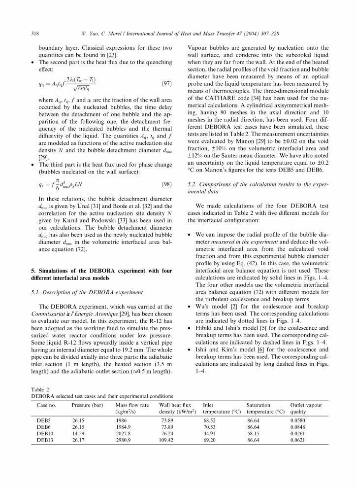
The DEBORA experiment, which was carried at the
Commissariat �aa l’Energie Atomique [29], has been chosen
to evaluate our model. In this experiment, the R-12 has
been adopted as the working fluid to simulate the pres-
surized water reactor conditions under low pressure.
Some liquid R-12 flows upwardly inside a vertical pipe
having an internal diameter equal to 19.2 mm. The whole
pipe can be divided axially into three parts: the adiabatic
inlet section (1 m length), the heated section (3.5 m
length) and the adiabatic outlet section (�0.5 m length).
Table 2
DEBORA selected test cases and their experimental conditions
Case no. Pressure (bar) Mass flow rate
(kg/m2/s)
Wall heat flu
density (kW
DEB5 26.15 1986 73.89
DEB6 26.15 1984.9 73.89
DEB10 14.59 2027.8 76.24
DEB13 26.17 2980.9 109.42
Vapour bubbles are generated by nucleation onto the
wall surface, and condense into the subcooled liquid
when they are far from the wall. At the end of the heated
section, the radial profiles of the void fraction and bubble
diameter have been measured by means of an optical
probe and the liquid temperature has been measured by
means of thermocouples. The three-dimensional module
of the CATHARE code [34] has been used for the nu-
merical calculations. A cylindrical axisymmetrical mesh-
ing, having 80 meshes in the axial direction and 10
meshes in the radial direction, has been used. Four dif-
ferent DEBORA test cases have been simulated, these
tests are listed in Table 2. The measurement uncertainties
were evaluated by Manon [29] to be ±0.02 on the void
fraction, ±10% on the volumetric interfacial area and
±12% on the Sauter mean diameter. We have also noted
an uncertainty on the liquid temperature equal to ±0.2
�C on Manon’s figures for the tests DEB5 and DEB6.
5.2. Comparisons of the calculation results to the exper-
imental data
We made calculations of the four DEBORA test
cases indicated in Table 2 with five different models for
the interfacial configuration:
• We can impose the radial profile of the bubble dia-
meter measured in the experiment and deduce the vol-
umetric interfacial area from the calculated void
fraction and from this experimental bubble diameter
profile by using Eq. (42). In this case, the volumetric
interfacial area balance equation is not used. These
calculations are indicated by solid lines in Figs. 1–4.
The four other models use the volumetric interfacial
area balance equation (72) with different models for
the turbulent coalescence and breakup terms.
• Wu’s model [2] for the coalescence and breakup
terms has been used. The corresponding calculations
are indicated by dotted lines in Figs. 1–4.
• Hibiki and Ishii’s model [5] for the coalescence and
breakup terms has been used. The corresponding cal-
culations are indicated by dashed lines in Figs. 1–4.
• Ishii and Kim’s model [6] for the coalescence and
breakup terms has been used. The corresponding cal-
culations are indicated by long dashed lines in Figs.
1–4.
x
/m2)
Inlet
temperature (�C)Saturation
temperature (�C)Outlet vapour
quality
68.52 86.64 0.0580
70.53 86.64 0.0848
34.91 58.15 0.0261
69.20 86.64 0.0621
0.000 0.002 0.004 0.006 0.008 0.010
Radial distance (m)
0.00
0.10
0.20
0.30
0.40
0.50V
oid
frac
tion
DEB 5
Fixed DsWu’s ModelHibiki and Ishii’s ModelIshii and Kim’s ModelOur Modified ModelEXP
0.000 0.002 0.004 0.006 0.008 0.010
Radial distance (m)
0.00
0.10
0.20
0.30
0.40
0.50
0.60
0.70
0.80
Voi
d fr
actio
n
DEB 6
Fixed DsWu’s ModelHibiki and Ishii’s ModelIshii and Kim’s ModelOur Modified ModelEXP
0.000 0.002 0.004 0.006 0.008 0.010
Radial distance (m)
0.00
0.10
0.20
0.30
0.40
0.50
Voi
d fr
actio
n
DEB 10
Fixed DsWu’s ModelHibiki and Ishii’s ModelIshii and Kim’s ModelOur Modified ModelEXP
0.000 0.002 0.004 0.006 0.008 0.010
Radial distance (m)
0.00
0.10
0.20
0.30
0.40
0.50
Voi
d fr
actio
n
DEB 13
Fixed DsWu’s ModelHibiki and Ishii’s ModelIshii and Kim’s ModelOur Modified ModelEXP
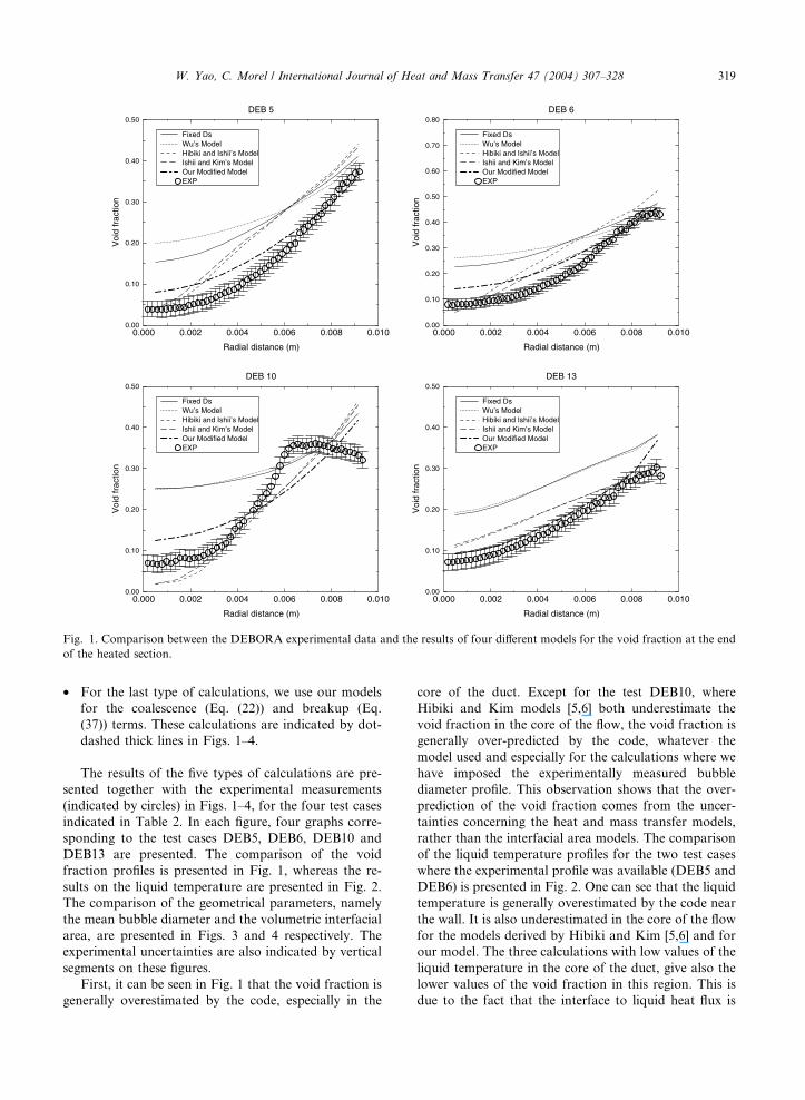
Fig. 1. Comparison between the DEBORA experimental data and the results of four different models for the void fraction at the end
of the heated section.
W. Yao, C. Morel / International Journal of Heat and Mass Transfer 47 (2004) 307–328 319
• For the last type of calculations, we use our models
for the coalescence (Eq. (22)) and breakup (Eq.
(37)) terms. These calculations are indicated by dot-
dashed thick lines in Figs. 1–4.
The results of the five types of calculations are pre-
sented together with the experimental measurements
(indicated by circles) in Figs. 1–4, for the four test cases
indicated in Table 2. In each figure, four graphs corre-
sponding to the test cases DEB5, DEB6, DEB10 and
DEB13 are presented. The comparison of the void
fraction profiles is presented in Fig. 1, whereas the re-
sults on the liquid temperature are presented in Fig. 2.
The comparison of the geometrical parameters, namely
the mean bubble diameter and the volumetric interfacial
area, are presented in Figs. 3 and 4 respectively. The
experimental uncertainties are also indicated by vertical
segments on these figures.
First, it can be seen in Fig. 1 that the void fraction is
generally overestimated by the code, especially in the
core of the duct. Except for the test DEB10, where
Hibiki and Kim models [5,6] both underestimate the
void fraction in the core of the flow, the void fraction is
generally over-predicted by the code, whatever the
model used and especially for the calculations where we
have imposed the experimentally measured bubble
diameter profile. This observation shows that the over-
prediction of the void fraction comes from the uncer-
tainties concerning the heat and mass transfer models,
rather than the interfacial area models. The comparison
of the liquid temperature profiles for the two test cases
where the experimental profile was available (DEB5 and
DEB6) is presented in Fig. 2. One can see that the liquid
temperature is generally overestimated by the code near
the wall. It is also underestimated in the core of the flow
for the models derived by Hibiki and Kim [5,6] and for
our model. The three calculations with low values of the
liquid temperature in the core of the duct, give also the
lower values of the void fraction in this region. This is
due to the fact that the interface to liquid heat flux is
0.000 0.002 0.004 0.006 0.008 0.010
Radial distance (m)
84.0
85.0
86.0
87.0
88.0Li
quid
tem
pera
ture
(C
)DEB 5
Fixed DsWu’s ModelHibiki and Ishii’s ModelIshii and Kim’s ModelOur Modified ModelEXPTsat
0.000 0.002 0.004 0.006 0.008 0.010
Radial distance (m)
84.0
85.0
86.0
87.0
88.0
Liqu
id t
empe
ratu
re (
C)
DEB 6
Fixed DsWu’s ModelHibiki and Ishii’s ModelIshii and Kim’s ModelOur Modified ModelEXPTsat
0.000 0.002 0.004 0.006 0.008 0.010
Radial distance (m)
50.0
52.0
54.0
56.0
58.0
60.0
Liqu
id t
empe
ratu
re (
C)
DEB 10
Fixed DsWu’s ModelHibiki and Ishii’s ModelIshii and Kim’s ModelOur Modified ModelTsat
0.000 0.002 0.004 0.006 0.008 0.010
Radial distance (m)
85.0
86.0
87.0
88.0
Liqu
id t
empe
ratu
re (
C)
DEB 13
Fixed DsWu’s ModelHibiki and Ishii’s ModelIshii and Kim’s ModelOur Modified ModelTsat
Fig. 2. Comparison between the DEBORA experimental data and the results of four different models for the liquid temperature at the
end of the heated section.
320 W. Yao, C. Morel / International Journal of Heat and Mass Transfer 47 (2004) 307–328
more important when the liquid temperature is lower, in
comparison to the saturation temperature, therefore
giving more phase change by condensation.
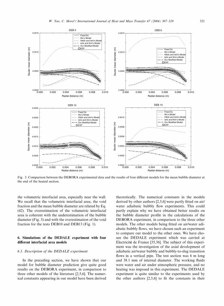
Fig. 3 shows that the best agreement on the bubble
diameter profiles is generally obtained with our model.
Wu’s model [2] gives generally a strong overestimation
of the bubble diameter. Among the four models tested,
Wu’s model has been derived the first and it appears
later that an error has been introduced in the derivation
of the wake entrainment induced bubble coalescence
[6,7]. In addition, the gas expansion term corresponding
to the first term in the RHS of Eq. (1) was not retained
in Wu’s model. As pointed out by [6,7], this term is not
negligible in upward adiabatic bubbly flow of air/water
at atmospheric pressure, and is certainly not negligible in
heated boiling flow. The two other models [5,6] give
better values for the magnitude of the bubble diameter,
but not the good shape of the radial profiles. Our model
is the only one that gives the good shape for the bubble
diameter profiles (Fig. 3). The reason of this have been
partly discussed in the previous sections. We believe that
the main advantage of our model, in comparison to the
other models tested on DEBORA, is that we have de-
composed the times necessary for breakup or coales-
cence into two contributions: free travelling time
between two collisions and interaction time between
bubbles or between a bubble and an eddy after collision.
The bubble oscillation resonance mechanism has been
considered for turbulent breakup, and the second mode
bubble oscillation period has been retained for the
bubble breaking time. In addition, the numerical con-
stants appearing in the models other than ours have
been fitted on adiabatic air/water experiments, and their
validity for boiling R-12 is questionable. Instead, the
numerical coefficients appearing in our model have been
calculated theoretically, and it seems to give quite good
results for the bubble diameter in our DEBORA calcu-
lations.
Fig. 4 shows the comparison of the volumetric inter-
facial area profiles. Our model generally overestimates
0.000 0.002 0.004 0.006 0.008 0.010
Radial distance (m)
0.0000
0.0005
0.0010
0.0015
Sau
ter
mea
n di
amet
er (
m)
DEB 5
Fixed DsWu’s ModelHibiki and Ishii’s ModelIshii and Kim’s ModelOur Modified ModelEXP
0.000 0.002 0.004 0.006 0.008 0.010
Radial distance (m)
0.0000
0.0005
0.0010
0.0015
Sau
ter
mea
n di
amet
er (
m)
DEB 6
Fixed DsWu’s ModelHibiki and Ishii’s ModelIshii and Kim’s ModelOur Modified ModelEXP
0.000 0.002 0.004 0.006 0.008 0.010Radial distance (m)
0.0000
0.0005
0.0010
0.0015
0.0020
0.0025
0.0030
Sau
ter
mea
n di
amet
er (
m)
DEB 10
Fixed DsWu’s ModelHibiki and Ishii’s ModelIshii and Kim’s ModelOur Modified ModelEXP
0.000 0.002 0.004 0.006 0.008 0.010Radial distance (m)
0.0000
0.0002
0.0004
0.0006
0.0008
0.0010S
aute
r m
ean
diam
eter
(m
)
DEB 13
Fixed DsWu’s ModelHibiki and Ishii’s ModelIshii and Kim’s ModelOur Modified ModelEXP
Fig. 3. Comparison between the DEBORA experimental data and the results of four different models for the mean bubble diameter at
the end of the heated section.
W. Yao, C. Morel / International Journal of Heat and Mass Transfer 47 (2004) 307–328 321
the volumetric interfacial area, especially near the wall.
We recall that the volumetric interfacial area, the void
fraction and the mean bubble diameter are related by Eq.
(42). The overestimation of the volumetric interfacial
area is coherent with the underestimation of the bubble
diameter (Fig. 3) and with the overestimation of the void
fraction for the tests DEB10 and DEB13 (Fig. 1).
6. Simulations of the DEDALE experiment with four
different interfacial area models
6.1. Description of the DEDALE experiment
In the preceding section, we have shown that our
model for bubble diameter prediction give quite good
results on the DEBORA experiment, in comparison to
three other models of the literature [2,5,6]. The numer-
ical constants appearing in our model have been derived
theoretically. The numerical constants in the models
derived by other authors [2,5,6] were partly fitted on air/
water adiabatic bubbly flow experiments. This could
partly explain why we have obtained better results on
the bubble diameter profile in the calculations of the
DEBORA experiment, in comparison to the three other
models. The other models being fitted on air/water adi-
abatic bubbly flows, we have chosen such an experiment
to compare our model to the other ones. We have cho-
sen the DEDALE experiment which was carried at
Electricit�ee de France [35,36]. The subject of this experi-
ment was the investigation of the axial development of
adiabatic air/water bubbly and bubbly-to-slug transition
flows in a vertical pipe. The test section was 6 m long
and 38.1 mm of internal diameter. The working fluids
were water and air under atmospheric pressure, and no
heating was imposed in this experiment. The DEDALE
experiment is quite similar to the experiments used by
the other authors [2,5,6] to fit the constants in their
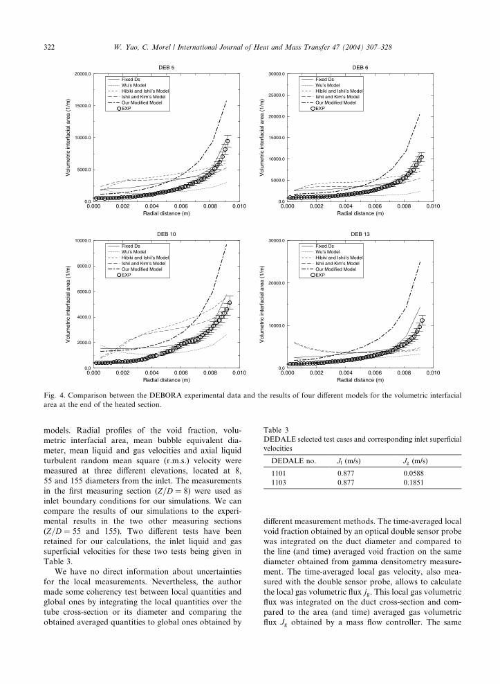
Table 3
DEDALE selected test cases and corresponding inlet superficial
velocities
DEDALE no. Jl (m/s) Jg (m/s)
1101 0.877 0.0588
1103 0.877 0.1851
0.000 0.002 0.004 0.006 0.008 0.010Radial distance (m)
0.0
5000.0
10000.0
15000.0
20000.0V
olum
etric
inte
rfac
ial a
rea
(1/m
)DEB 5
Fixed DsWu’s ModelHibiki and Ishii’s ModelIshii and Kim’s ModelOur Modified ModelEXP
0.000 0.002 0.004 0.006 0.008 0.010Radial distance (m)
0.0
5000.0
10000.0
15000.0
20000.0
25000.0
30000.0
Vol
umet
ric in
terf
acia
l are
a (1
/m)
DEB 6
Fixed DsWu’s ModelHibiki and Ishii’s ModelIshii and Kim’s ModelOur Modified ModelEXP
0.000 0.002 0.004 0.006 0.008 0.010Radial distance (m)
0.0
2000.0
4000.0
6000.0
8000.0
10000.0
Vol
umet
ric in
terf
acia
l are
a (1
/m)
DEB 10
Fixed DsWu’s ModelHibiki and Ishii’s ModelIshii and Kim’s ModelOur Modified ModelEXP
0.000 0.002 0.004 0.006 0.008 0.010Radial distance (m)
0.0
10000.0
20000.0
30000.0
Vol
umet
ric in
terf
acia
l are
a (1
/m)
DEB 13
Fixed DsWu’s ModelHibiki and Ishii’s ModelIshii and Kim’s ModelOur Modified ModelEXP
Fig. 4. Comparison between the DEBORA experimental data and the results of four different models for the volumetric interfacial
area at the end of the heated section.
322 W. Yao, C. Morel / International Journal of Heat and Mass Transfer 47 (2004) 307–328
models. Radial profiles of the void fraction, volu-
metric interfacial area, mean bubble equivalent dia-
meter, mean liquid and gas velocities and axial liquid
turbulent random mean square (r.m.s.) velocity were
measured at three different elevations, located at 8,
55 and 155 diameters from the inlet. The measurements
in the first measuring section (Z=D ¼ 8) were used as
inlet boundary conditions for our simulations. We can
compare the results of our simulations to the experi-
mental results in the two other measuring sections
(Z=D ¼ 55 and 155). Two different tests have been
retained for our calculations, the inlet liquid and gas
superficial velocities for these two tests being given in
Table 3.
We have no direct information about uncertainties
for the local measurements. Nevertheless, the author
made some coherency test between local quantities and
global ones by integrating the local quantities over the
tube cross-section or its diameter and comparing the
obtained averaged quantities to global ones obtained by
different measurement methods. The time-averaged local
void fraction obtained by an optical double sensor probe
was integrated on the duct diameter and compared to
the line (and time) averaged void fraction on the same
diameter obtained from gamma densitometry measure-
ment. The time-averaged local gas velocity, also mea-
sured with the double sensor probe, allows to calculate
the local gas volumetric flux jg. This local gas volumetric
flux was integrated on the duct cross-section and com-
pared to the area (and time) averaged gas volumetric
flux Jg obtained by a mass flow controller. The same
0.000 0.005 0.010 0.015 0.020Radial position (m)
0.000
0.002
0.004
0.006
0.008
0.010
Sau
ter
mea
n di
amet
er (
m)
DEDALE1101 (Z/D=55)
Wu’s ModelHibiki and Ishii’s ModelIshii and Kim’s ModelOur Modified ModelEXP
0.000 0.005 0.010 0.015 0.020Radial position (m)
0.000
0.002
0.004
0.006
0.008
0.010
0.012
0.014
Sau
ter
mea
n di
amet
er (
m)
DEDALE1101 (Z/D=155)
Wu’s ModelHibiki and Ishii’s ModelIshii and Kim’s ModelOur Modified ModelEXP
0.000 0.005 0.010 0.015 0.020Radial position (m)
0.00
0.02
0.04
0.06
0.08
0.10
0.12
0.14
Voi
d fr
actio
n
DEDALE1101 (Z/D=55)
Wu’s ModelHibiki and Ishii’s ModelIshii and Kim’s ModelOur Modified ModelEXP
0.000 0.005 0.010 0.015 0.020Radial position (m)
0.00
0.05
0.10
0.15
0.20
Voi
d fr
actio
n
DEDALE1101 (Z/D=155)
Wu’s ModelHibiki and Ishii’s ModelIshii and Kim’s ModelOur Modified ModelEXP
0.000 0.005 0.010 0.015 0.020Radial position (m)
0.0
100.0
200.0
300.0
400.0
Vol
umet
ric in
terf
acia
l are
a (1
/m)
DEDALE1101 (Z/D=55)
Wu’s ModelHibiki and Ishii’s ModelIshii and Kim’s ModelOur Modified ModelEXP
0.000 0.005 0.010 0.015 0.020Radial position (m)
0.0
100.0
200.0
300.0
400.0
Vol
umet
ric in
terf
acia
l are
a (1
/m)
DEDALE1101 (Z/D=155)
Wu’s ModelHibiki and Ishii’s ModelIshii and Kim’s ModelOur Modified ModelEXP
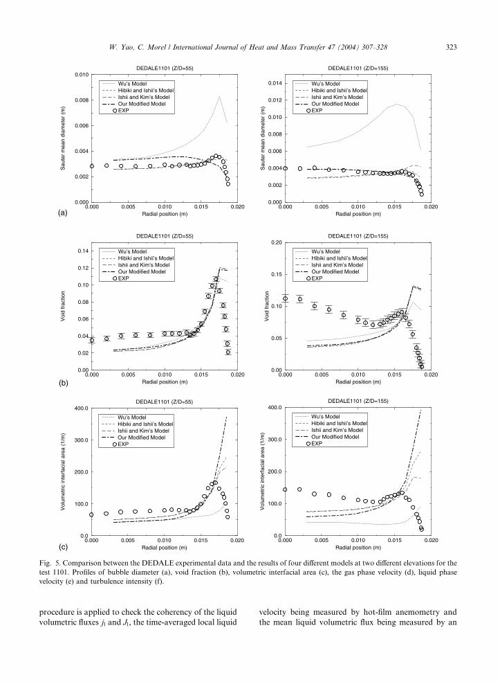
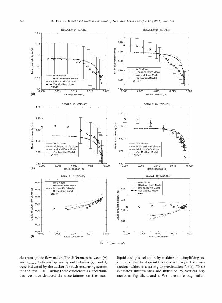
(a)
(b)
(c)
Fig. 5. Comparison between the DEDALE experimental data and the results of four different models at two different elevations for the
test 1101. Profiles of bubble diameter (a), void fraction (b), volumetric interfacial area (c), the gas phase velocity (d), liquid phase
velocity (e) and turbulence intensity (f).
W. Yao, C. Morel / International Journal of Heat and Mass Transfer 47 (2004) 307–328 323
procedure is applied to check the coherency of the liquid
volumetric fluxes jl and Jl, the time-averaged local liquid
velocity being measured by hot-film anemometry and
the mean liquid volumetric flux being measured by an
0.000 0.005 0.010 0.015 0.020Radial position (m)
1.00
1.10
1.20
1.30
1.40
1.50M
ean
gas
velo
city
(m
/s)
DEDALE1101 (Z/D=55)
Wu’s ModelHibiki and Ishii’s ModelIshii and Kim’s ModelOur Modified ModelEXP
0.000 0.005 0.010 0.015 0.020Radial position (m)
0.90
1.00
1.10
1.20
1.30
1.40
Mea
n ga
s ve
loci
ty (
m/s
)
DEDALE1101 (Z/D=155)
Wu’s ModelHibiki and Ishii’s ModelIshii and Kim’s ModelOur Modified ModelEXP
0.000 0.005 0.010 0.015 0.020Radial position (m)
0.80
0.90
1.00
1.10
1.20
1.30
Mea
n liq
uid
velo
city
(m
/s)
DEDALE1101 (Z/D=55)
Wu’s ModelHibiki and Ishii’s ModelIshii and Kim’s ModelOur Modified ModelEXP
0.000 0.005 0.010 0.015 0.020Radial position (m)
0.50
0.70
0.90
1.10
1.30M
ean
liqui
d ve
loci
ty (
m/s
)
DEDALE1101 (Z/D=155)
Wu’s ModelHibiki and Ishii’s ModelIshii and Kim’s ModelOur Modified ModelEXP
0.000 0.005 0.010 0.015 0.020Radial position (m)
0.00
0.02
0.04
0.06
0.08
0.10
0.12
0.14
Liqu
id tu
rbul
ent i
nten
sity
(m
/s)
DEDALE1101 (Z/D=55)
Wu’s ModelHibiki and Ishii’s ModelIshii and Kim’s ModelOur Modified ModelEXP
0.000 0.005 0.010 0.015 0.020Radial position (m)
0.05
0.07
0.09
0.11
0.13
Liqu
id tu
rbul
ent i
nten
sity
(m
/s)
DEDALE1101 (Z/D=155)
Wu’s ModelHibiki and Ishii’s ModelIshii and Kim’s ModelOur Modified ModelEXP
(d)
(e)
(f)
Fig. 5 (continued)
324 W. Yao, C. Morel / International Journal of Heat and Mass Transfer 47 (2004) 307–328
electromagnetic flow-meter. The differences between haiand agamma, between hjli and Jl and between hjgi and Jgwere indicated by the author for each measuring section
for the test 1101. Taking these differences as uncertain-
ties, we have deduced the uncertainties on the mean
liquid and gas velocities by making the simplifying as-
sumption that local quantities does not vary in the cross-
section (which is a strong approximation for a). Theseevaluated uncertainties are indicated by vertical seg-
ments in Fig. 5b, d and e. We have no enough infor-
0.000 0.005 0.010 0.015 0.020Radial position (m)
0.000
0.002
0.004
0.006
0.008
0.010
0.012
0.014
Sau
ter
mea
n di
amet
er (
m)
DEDALE1103 (Z/D=55)
Wu’s ModelHibiki and Ishii’s ModelIshii and Kim’s ModelOur Modified ModelEXP
0.000 0.005 0.010 0.015 0.020Radial position (m)
0.00
0.10
0.20
0.30
0.40
Voi
d fr
actio
n
DEDALE1103 (Z/D=55)
Wu’s ModelHibiki and Ishii’s ModelIshii and Kim’s ModelOur Modified ModelEXP
0.000 0.005 0.010 0.015 0.020Radial position (m)
0.0
200.0
400.0
600.0
800.0
Vol
umet
ric in
terf
acia
l are
a (1
/m)
DEDALE1103 (Z/D=55)
Wu’s ModelHibiki and Ishii’s ModelIshii and Kim’s ModelOur Modified ModelEXP
0.000 0.005 0.010 0.015 0.020Radial position (m)
1.10
1.20
1.30
1.40
Mea
n ga
s ve
loci
ty (
m/s
)
DEDALE1103 (Z/D=55)
Wu’s ModelHibiki and Ishii’s ModelIshii and Kim’s ModelOur Modified ModelEXP
0.000 0.005 0.010 0.015 0.020Radial position (m)
0.80
0.90
1.00
1.10
1.20
1.30
Mea
n liq
uid
velo
city
(m
/s)
DEDALE1103 (Z/D=55)
Wu’s ModelHibiki and Ishii’s ModelIshii and Kim’s ModelOur Modified ModelEXP
0.000 0.005 0.010 0.015 0.020Radial position (m)
0.00
0.10
0.20
Liqu
id tu
rbul
ent i
nten
sity
(m
/s)
DEDALE1103 (Z/D=55)
Wu’s ModelHibiki and Ishii’s ModelIshii and Kim’s ModelOur Modified ModelEXP
(a) (b)
(c) (d)
(e) (f)
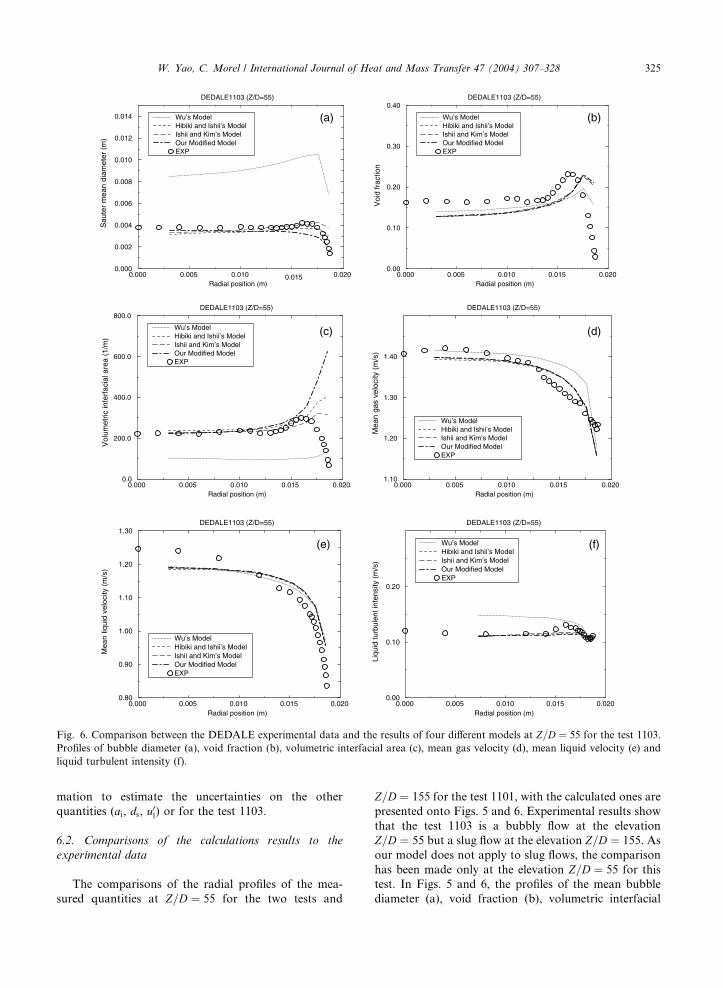
Fig. 6. Comparison between the DEDALE experimental data and the results of four different models at Z=D ¼ 55 for the test 1103.
Profiles of bubble diameter (a), void fraction (b), volumetric interfacial area (c), mean gas velocity (d), mean liquid velocity (e) and
liquid turbulent intensity (f).
W. Yao, C. Morel / International Journal of Heat and Mass Transfer 47 (2004) 307–328 325
mation to estimate the uncertainties on the other
quantities (ai, ds, u0l) or for the test 1103.
6.2. Comparisons of the calculations results to the
experimental data
The comparisons of the radial profiles of the mea-
sured quantities at Z=D ¼ 55 for the two tests and
Z=D ¼ 155 for the test 1101, with the calculated ones are
presented onto Figs. 5 and 6. Experimental results show
that the test 1103 is a bubbly flow at the elevation
Z=D ¼ 55 but a slug flow at the elevation Z=D ¼ 155. As
our model does not apply to slug flows, the comparison
has been made only at the elevation Z=D ¼ 55 for this
test. In Figs. 5 and 6, the profiles of the mean bubble
diameter (a), void fraction (b), volumetric interfacial
326 W. Yao, C. Morel / International Journal of Heat and Mass Transfer 47 (2004) 307–328
area (c), mean gas velocity (d), mean liquid velocity (e)
and liquid turbulent intensity (f ) are presented. In Fig.
5, the comparisons at the elevation Z=D ¼ 55 are shown
on the left column, and those at the elevation Z=D ¼ 155
are shown on the right. For each test, we made four
different calculations using Wu’s model [2] (indicated by
dotted lines on the figures), Hibiki’s model [5] (indicated
by dashed lines on the figures), Kim’s model [6] (indi-
cated by long dashed lines on the figures) and our model
(indicated by dot-dashed lines on the figures).
The first test we have chosen (1101) is an upward
bubbly flow up to the exit of the tube. However, due to
the coalescence and gas expansion effects, the bubble size
increases regularly along the tube as it can be seen by
comparing the experimental values of the bubble diam-
eter at the two different elevations (Fig. 5a). Due to this
bubble size variation, the shape of the void fraction
profile evolves along the tube. At the first comparing
elevation (Z=D ¼ 55), we observe a wall peaking void
fraction profile, but at the second elevation (Z=D ¼ 155),
we observe an intermediate void fraction profile (inter-
mediate between wall peaking and void coring) as it can
be seen on Fig. 5b. The code qualitatively reproduces the
wall peak of the void fraction at the first elevation, as a
result of the equilibrium between the radial components
of the lift force (Eq. (86)) and the turbulent dispersion
force (Eq. (87)), but fails to reproduce the void fraction
profile at the second elevation. The void fraction profiles
obtained with the four different models for interfacial
area prediction are quite similar, even if more important
differences are visible on the bubble diameter and in-
terfacial area profiles (Fig. 5a–c). The comparison of the
bubble diameter profiles (Fig. 5a) shows that the better
agreement is obtained with Hibiki’s model and Kim’s
model [5,6] (which give quite similar results) at the first
elevation (Z=D ¼ 55), and with our model at the second
elevation (Z=D ¼ 155). The comparison of the mean and
turbulent axial velocities (Fig. 5d–f) give quite similar
results for the four different models. When the void
fraction profile is qualitatively reproduced, as at the first
elevation, the liquid turbulent intensity profile is also
well reproduced with our K–e model (Fig. 5f).
In the second test we have simulated (1103), a flow
regime transition is observed experimentally between the
elevation Z=D ¼ 55, where a bubbly flow is observed,
and the elevation Z=D ¼ 155, where a slug flow is ob-
served. As the different models we use are not able to
describe slug flows, and the experimental measurements
conducted by Grosseteete were done by means of a
double sensor probe for the dispersed phase, assuming
spherical bubbles [35,36], we will only discuss the results
obtained at the elevation Z=D ¼ 55. As for the test 1101,
the void fraction profile is qualitatively reproduced at
the first elevation, for all the models tested. The mean
bubble diameter is also well reproduced by the different
models, except for Wu’s model [2] which strongly
overestimates the bubble diameter (Fig. 6a). The liquid
turbulent r.m.s. velocity is also well predicted at the first
elevation, as it can be seen in Fig. 6f.
7. Conclusions
In this paper, new models are proposed for the dif-
ferent source terms appearing in the RHS of the volu-
metric interfacial area balance equation for bubbly
flows. These source terms correspond to the turbulence
induced coalescence and breakup phenomena, as well as
the gas expansion and phase change terms, including the
nucleation of new bubbles on a heated wall. Our model
has been tested in comparison to three other models for
the coalescence and breakup terms found in the litera-
ture, on two different experiments. All the calculations
were done with our formulation for the gas expansion
term and for the phase change terms (Eq. (72)) because
only this formulation allows to introduce a nucleated
bubble diameter which is different from the Sauter mean
diameter. The first experiment we have investigated is
the DEBORA experiment, carried at the Commissariat �aal’Energie Atomique, France. In this experiment, initially
subcooled liquid R-12 is flowing upward in a vertical
pipe with a heated wall. Some vapour bubbles are nu-
cleated onto the wall surface, and after then migrate
towards the core of the flow where they condense in
colder liquid. The comparisons of the radial profiles of
the void fraction, liquid temperature, mean bubble dia-
meter and interfacial area at the end of the heated sec-
tion show a better agreement with our model than with
the three other models. We believe that one reason of
this is that we have separately considered the ‘‘free
travelling time’’ and the ‘‘interaction time’’ in the mode-
ling of the bubbles coalescence and breakup, as is ex-
plained in Sections 1 and 2. Another reason may be that
the numerical constants appearing in the models derived
by the other authors were fitted onto adiabatic air/water
experiments, and that their validity for boiling R-12
experiment is questionable. Instead, the numerical con-
stants appearing in our model were derived theoretically,
and therefore we hope that the range of applicability of
our model is less restricted in terms of fluids and
working conditions. In order to verify this assertion, we
have also compared the four models predictions to the
DEDALE experiment which is an adiabatic air/water
experiment. When the flow is in the bubbly regime, the
prediction of the mean bubble diameter is quite good for
Hibiki’s model [5] and Kim’s model [6], as well as for our
model. The liquid turbulent r.m.s. velocity is also well
predicted.
Because the DEBORA experimental data base is only
concerned with subcooled boiling, our model has not
been tested in the case of saturated boiling. The appli-
cation of our model to saturated boiling conditions will
W. Yao, C. Morel / International Journal of Heat and Mass Transfer 47 (2004) 307–328 327
be addressed in future work. In theory, our model
should be applicable to void fraction values as elevated
as amax given by Eq. (12). In practice, when the void
fraction is increased, a transition from bubbly-to-slug
flow may be observed, depending on the flow conditions.
The gas plugs being of the same size than the tube in-
ternal diameter, the assumptions made to derive the
turbulent coalescence and breakup terms are clearly not
valid for a slug flow. One should speak of limiting
bubble size, rather than void fraction, for our model to
be applicable.
Further research is needed for bubbly flow configu-
rations were several bubble size are present simulta-
neously in a small volume (multidispersed bubbly flow)
for a better prediction of the transition from bubbly-to-
slug flow, or for reproducing intermediate void fraction
profile, as the one observed at the higher measuring
section in DEDALE 1101 (Fig. 5b). In a recent ap-
proach, Hibiki and Ishii [37] tried to predict the transi-
tion from bubbly-to-slug flow by using a ‘‘two group
model’’ involving separate balance equations for the
void fractions and the interfacial areas of small spherical
or distorted bubbles, and for big cap bubbles or slugs.
Acknowledgements
The authors are fully indebted to the Commissariat �aal’Energie Atomique of France, to Electricit�ee de France
and also to FRAMATOME and to the French Institute
for Nuclear Safety for their financial support in the
context of the NEPTUNE project.
References
[1] M. Ishii, Two-fluid model for two-phase flow, Multiphase
Sci. Technol. 5 (1990) 1–58.
[2] Q. Wu, S. Kim, M. Ishii, S.G. Beus, One-group interfacial
area transport in vertical bubble flow, Int. J. Heat Mass
Transfer 41 (8–9) (1998) 1103–1112.
[3] C.W. Stewart, Bubble interaction in low-viscosity liquids,
Int. J. Multiphase Flow 21 (6) (1995) 1037–1046.
[4] T. Otake, S. Tone, K. Nakao, Y. Mitsuhashi, Coalescence
and breakup of bubbles in liquids, Chem. Eng. Sci. 32
(1977) 377–383.
[5] T. Hibiki, M. Ishii, One-group interfacial area transport of
bubbly flows in vertical round tubes, Int. J. Heat Mass
Transfer 43 (2000) 2711–2726.
[6] M. Ishii, S. Kim, Micro four-sensor probe measurement of
interfacial area transport for bubbly flow in round pipes,
Nucl. Eng. Des. 205 (2001) 2711–2726.
[7] J.M. Delhaye, Some issues related to the modelling of
interfacial areas in gas–liquid flows, Part II: modelling the
source terms for dispersed flows, C.R. Acad. Sci. Paris, S�eer.
IIb t. 329 (2001) 473–486.
[8] A.N. Kolmogorov, On the disintegration of drops in a
turbulent flow, Doklady Akad. Nauk., SSSR 66 (1949) 825.
[9] F. Risso, The mechanisms of deformation and breakup of
drops and bubbles, Multiphase Sci. Technol. 12 (2000) 1–
50.
[10] C.A. Coulaloglou, L.L. Tavlarid�ees, Description of inter-
action processes in agitated liquid–liquid dispersions,
Chem. Eng. Sci. 32 (1977) 1289–1297.
[11] G. Kocamustafaogullari, M. Ishii, Interfacial area and
nucleation site density in boiling systems, Int. J. Heat Mass
Transfer 26 (9) (1983) 1377–1387.
[12] M.J. Prince, H.W. Blanch, Bubble coalescence and break-
up in air-sparged bubble columns, AIChE J. 36 (10) (1990)
1485–1499.
[13] R.D. Kirkpatrick, M.J. Lockett, The influence of approach
velocity on bubble coalescence, Chem. Eng. Sci. 29 (1974)
2363.
[14] W.K. Kim, K.L. Lee, Coalescence behavior of two bubbles
in stagnant liquids, J. Chem. Eng., Jpn. 20 (1987) 449.
[15] M. Sevik, S.H. Park, The splitting of drops and bubbles by
turbulent fluid flow, J. Fluids Eng., Trans. ASME 53–60
(1973).
[16] D. Azbel, I.L. Athanasios, A mechanism of liquid entrain-
ment, in: N. Cheremisinoff (Ed.), Handbook of Fluids in
Motion, Ann Arbor Science Publishers, Ann Arbor, USA,
1983, p. 473.
[17] H. Lamb, Hydrodynamics, sixth ed., Dover Publications,
New York, 1932.
[18] J.L. Achard, Contribution �aa l’�eetude th�eeorique des �eecoul-
ements diphasiques en r�eegime transitoire, Ph.D. Thesis,
Universit�ee Scientifique et M�eedicale, Institut National
Polytechnique de Grenoble, 1978.
[19] C. Morel, Turbulence modeling and first numerical simu-
lations in turbulent two-phase flows, in: 11th Symposium
on Turbulent Shear Flows, vol. 3, Poster Session 3,
Grenoble, France, September 8–10, 1997, pp. 3-10, 3-15.
[20] C. Morel, Mod�eelisation multidimensionnelle des �eecoule-
ments diphasiques gaz–liquide, Application �aa la simulation
des �eecoulements �aa bulles ascendants en conduite verticale,
Ph.D. Thesis, Ecole Centrale Paris, 1997.
[21] M. Lance, J.L. Mari�ee, J. Bataille, Mod�eelisation de la
turbulence de la phase liquide dans un �eecoulement �aa bulles,
La Houille Blanche No. 3/4, 1984.
[22] S.E. Elgobashi, T.W. Abou-Arab, A two-equation turbu-
lence model for two-phase flows, Phys. Fluids 26 (4) (1983)
931–938.
[23] R. Schiestel, Mod�eelisation et simulation des �eecoulements
turbulents, Ed. Herm�ees, 1993.
[24] W. Yao, C. Morel, Prediction of parameters distribution of
upward boiling two-phase flow with two-fluid models, in:
10th International Conference on Nuclear Engineering,
Arlington, Virginia, USA, paper no. 22463, April 14–18,
2002.
[25] M. Lance, M. Lopez de Bertodano, Phase distribution
phenomena and wall effects in bubbly two-phase flows,
Multiphase Sci. Technol. 8 (1994) 69–123.
[26] M. Ishii, One-dimensional drift flux model and constitutive
equations for relative motion between phases in various
two-phase flow regimes, ANL Report No. 77-47, 1977.
[27] N. Zuber, On the dispersed two-phase flow in the laminar
flow regime, Chem. Eng. Sci. 19 (1964) 897.
[28] T.R. Auton, The lift force on a spherical body in a
rotational flow, J. Fluid. Mech. 183 (1987) 199–218.
328 W. Yao, C. Morel / International Journal of Heat and Mass Transfer 47 (2004) 307–328
[29] E. Manon, Contribution �aa l’analyse et �aa la mod�eelisation
locale des �eecoulements bouillants sous-satur�ees dans les
conditions des r�eeacteurs �aa eau sous pression, Ph.D. Thesis,
Ecole Centrale Paris, 2000.
[30] P. Berne, Contribution �aa la mod�eelisation du taux de
production de vapeur par auto-vaporisation dans les
�eecoulements diphasiques en conduites, Ph.D. Thesis, Ecole
des Arts et Manufactures, 1983.
[31] H.C. €UUnal, Maximum bubble diameter, maximum bubble-
growth time and bubble-growth rate during the subcooled
nucleate flow boiling, Int. J. Heat Mass Transfer 19 (1976)
643–649.
[32] J. Bor�eee, G. Charnay, J. Fabre, D. Legendre, J. Magnau-
det, Ecoulements diphasiques eau-vapeur avec changement
de phase, Rapport IMFT-Interface, 1992.
[33] N. Kurul, M.Z. Podowski, Multidimensional effects in
forced convection subcooled boiling, in: International Heat
Transfer Conference, Jerusalem, vol. 1, Paper BO-04, 1991,
pp. 31–45.
[34] F. Barr�ee, C. Sun, I. Dor, Overview of the numerical and
computational developments performed in the frame of the
CATHARE 2 code, in: International Conference on
Mathematics and Computations, Reactors Physics, and
Environmental Analyses, Portland, Oregon, 30 April–4
May, 1995.
[35] C. Grosseteete, Caract�eerisation exp�eerimentale et simulation
de l’�eevolution d’un �eecoulement diphasique �aa bulles ascen-
dant dans une conduite verticale, Ph.D. Thesis, Ecole
Centrale Paris, 1995.
[36] C. Grosseteete, Experimental investigation and prelimi-
nary numerical simulations of void profile development in
a vertical cylindrical pipe, in: A. Serizawa, T. Fukano,
J. Bataille (Eds.), 2nd International Conference on Multi-
phase Flow, Kyoto, Japan, IF1-1-10, April 3–7,
1995.
[37] T. Hibiki, M. Ishii, Two-group interfacial area transport
equations at bubbly-to-slug flow transitions, Nucl. Eng.
Des. 202 (1) (2000) 39–76.


