VISUAL AIDS VACUUM TECHNOLOGY & APPLICATIONS

INTERNATIONAL UNION FOR VACUUM SCIENCE,TECHNIQUE AND APPLICATIONS

UNION INTERNATIONALE POUR LA SCIENCE,LA TECHNIQUE ET LES APPLICATIONS DU VIDE

INTERNATIONALE UNION FÜRVAKUUM-FORSCHUNG, -TECHNIK UND -ANWENDUNG

VISUAL AIDSFOR INSTRUCTIONS IN

VACUUM TECHNOLOGY& APPLICATIONS

Series EditorJohn L Robins

Module 1:FUNDAMENTALS OF VAUUM

Second Edition

John F. O’Hanlon

Instructor’s Notes

INTERNATIONAL UNION FOR VACUUMSCIENCE, TECHNIQUE AND

APPLICATIONS

VISUAL AIDS

FOR INSTRUCTIONS INVACUUM TECHNOLOGY

& APPLICATIONS

Module 1

FUNDAMENTALS OF VACUUM

Second Edition

Presenter’s Notes

by

John F. O’Hanlon

Series EditorJohn L Robins

Module 1: Fundamentals of Vacuum IUVSTA Visual Aids Program

2

INTRODUCTION TO THE SECOND EDITION (2004)

This package of slides and associated text is intended for use in teaching short courseson vacuum fundamentals. It assumes knowledge of vacuum technique,thermodynamics and mathematics on the part of the presenter. It is assumed that theinstructor may wish to provide additional information to expand on the informationpresented here. This module has been designed to be used with an instructor and notto be used for self-study. A textbook should accompany this material.

The Microsoft PowerPoint“ slides are arranged in five sections. Gas Kinetics, GasLaws, Gas Transport, Gas Flow, and Gas Desorption from Surfaces. This material isa revision of the material written in 1983 by the Netherlands Vacuum Society. Muchof that material is used directly in this edition. However, the order of presentation hasbeen changed to accommodate the current presentation outline.

The text and slides refer to pressures in Pascal. The mbar is a popular unit in Europeand Torr remains popular in the US, because educators have been grossly negligent inmaking a transition to Système International (SI) beginning at the time of itsintroduction. The Pascal and other SI units are not commonly used today, onlybecause instructors have not insisted on introducing them to those new to the field.The comment “my students do not use Pascal” will always be true, unless instructorstake the lead in creating change.

Please read the file VA_Cond.pdf contained on this CD-ROM, which describes theIUVSTA Fair Use Policy for this material.

Corrections and comments regarding this material are best directed to John O’Hanlonat the above e-mail address.

John F. O’HanlonTucson, Arizona. USAJune 2004


3

LIST OF SLIDES

Section 1: GAS KINETICS

Slide 1.01. Gas Kinetics - Title PageSlide 1.02. A Gas in Equilibrium with its ContainerSlide 1.03. The State of the GasSlide 1.04. Maxwell-Boltzmann Velocity DistributionSlide 1.05. Maxwell-Boltzmann Velocity DistributionSlide 1.06. Mean Free PathSlide 1.07. Mean Free PathSlide 1.08. Particle FluxSlide 1.09. Particle FluxSlide 1.10. Monolayer Formation TimeSlide 1.11. PressureSlide 1.12. Dalton’s Law

Section 2: GAS LAWS

Slide 2.01. Gas Laws - Title PageSlide 2.02. The Ideal Gas at Constant Temperature and NumberSlide 2.03. The Ideal Gas at Constant Volume and NumberSlide 2.04. The Ideal Gas at Constant Pressure and NumberSlide 2.05. The Ideal Gas at Constant Temperature and VolumeSlide 2.06. The Ideal Gas: Adiabatic Change of StateSlide 2.07. The Ideal Gas: The General RelationSlide 2.08. The van der Waals Gas

Section 3: GAS TRANSPORT

Slide 3.01. Gas Transport - Title PageSlide 3.02. Diffusion–the equation and constantSlide 3.03. Diffusion–a solution in one dimensionSlide 3.04. Diffusion–low pressureSlide 3.05. Viscosity–a definitionSlide 3.06. Viscosity–the conceptSlide 3.07. Viscosity–at low pressureSlide 3.08. A Caution–graphical presentationSlide 3.09. Heat Conduction–a definitionSlide 3.10. Heat Conduction–low pressureSlide 3.11. Heat Conduction–several mechanismsSlide 3.12. Momentum and Energy Transport–a distinctionSlide 3.13. Thermal Transpiration


4

Section 4: GAS FLOW

Slide 4.01. Gas Flow - Title PageSlide 4.02. Gas Flow–its complexitySlide 4.03. Gas Flow–the nature of a gasSlide 4.04. Gas Flow–the behavior of flowing gasSlide 4.05. Flow below the choked limitSlide 4.06. Choked flow limitSlide 4.07. Turbulent flowSlide 4.08. Viscous laminar flow-its behaviorSlide 4.09. Viscous flow in short tubesSlide 4.10. Viscous flow–a short-tube exampleSlide 4.11. Molecular flow–its behaviorSlide 4.12. Molecular flow through an orificeSlide 4.13. Molecular flow through a round pipeSlide 4.14. Molecular flow through arbitrarily-shaped objectsSlide 4.15. Molecular flow–combinations of isolated componentsSlide 4.16. Molecular flow trajectoriesSlide 4.17. Molecular flow–combinations of interacting componentsSlide 4.18. Molecular flow–an example of combining interacting componentsSlide 4.19. Molecular flow–definition of volumetric pumping speedSlide 4.20. Molecular flow–the speed of an “ideal” pumpSlide 4.21. Molecular flow–the speed of a “real” pumpSlide 4.22. Molecular flow–calculating the speed of a pumping “stack”Slide 4.23. Transition FlowSlide 4.24. Gas Flow–summary of flow regions

Section 5: GAS DESORPTION FROM SURFACES

Slide 5.01. Gas Desorption from Surfaces - Title PageSlide 5.02. Scattering of helium atoms from a single-crystal metalSlide 5.03. Scattering of a reactive gas from a single-crystal metalSlide 5.04. Gas scattering from a rough surfaceSlide 5.05. Realistic surface interactionsSlide 5.06. AdsorptionSlide 5.07. Activation energiesSlide 5.08. Adsorption isotherms–LangmuirSlide 5.09. Adsorption isotherms–BETSlide 5.10. Adsorption isotherms–DRKSlide 5.11. Adsorption isotherms–TemkinSlide 5.12. Sorption materials–zeolitesSlide 5.13. Sorption exampleSlide 5.14. Fundamentals of Vacuum – Final Page


5

PRESENTER’S GUIDE

Section 1: GAS KINETICS

Slide 1.01. Gas Kinetics - Title Page

This section consists of 12 slides and presents basic gas kinetics.

Slide 1.02. A Gas in Equilibrium with its Container

A gas in equilibrium with its container exerts a pressure on its walls caused bycollisions of the gas molecules with these walls. Statistical laws or kinetic laws werederived independently by Maxwell and Boltzmann. Four assumptions were used inderiving their results.

1. The number of molecules in any reasonable volume is very large2. The molecules are spaced at distances considerably larger than their diameters3. The molecules are always in a constant state of motion4. The molecules exert no force on each other except during a collision.

Slide 1.03. The State of the Gas

The state of the gas is described by the following characteristics.

1. The kind of gas2. The mass ma of species a3. The volume V of the vessel in which the gas is contained4. The pressure P of the gas, and5. The temperature T of the gas.

In these notes, we will use SI units of cubic meters for volume, Kelvin fortemperature, the kilogram for mass, and the Pascal for pressure. One Pascal is equal to0.01 mbar, or 0.0076 Torr. It is most convenient to perform vacuum calculations in SIunits, as equations become straightforward and confusing conversion factorsunnecessary.

Slide 1.04. Maxwell-Boltzmann Velocity Distribution

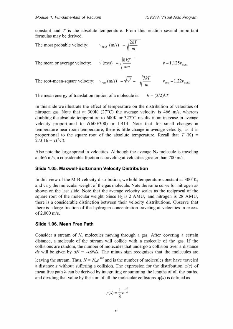
Because of the large number of collisions per unit time that a given moleculeexperiences with other molecules and/or with the walls of the vessel in which it iscontained, the velocities of its molecules are continually changing both in direction andin magnitude. For a gas that is in equilibrium and uniformly distributed in space,Maxwell and Boltzmann derived, independently, the relationship

€

1ndnvdv

=2m3

k 3T 3v 2 exp −mv

2

2kT

which gives the fraction of molecules with an absolute velocity v. In the aboverelation, n is the number of molecules per unit volume, dnv is the number of moleculeswith velocity between v and v+dv, m is the mass of the molecule, k is Boltzmann’s


6

constant and T is the absolute temperature. From this relation several importantformulas may be derived.

The most probable velocity:

€

vMAX (m/s) =2kTm

The mean or average velocity:

€

v (m/s) =8kTπm

€

v =1.125vMAX

The root-mean-square velocity:

€

vrms (m/s) = v2 = 3kTm

€

vrms =1.22vMAX

The mean energy of translation motion of a molecule is: E = (3/2)kT

In this slide we illustrate the effect of temperature on the distribution of velocities ofnitrogen gas. Note that at 300K (27°C) the average velocity is 466 m/s, whereasdoubling the absolute temperature to 600K or 327°C results in an increase in averagevelocity proportional to √(600/300) or 1.414. Note that for small changes intemperature near room temperature, there is little change in average velocity, as it isproportional to the square root of the absolute temperature. Recall that T (K) =273.16 + T(°C).

Also note the large spread in velocities. Although the average N2 molecule is travelingat 466 m/s, a considerable fraction is traveling at velocities greater than 700 m/s.

Slide 1.05. Maxwell-Boltzmann Velocity Distribution

In this view of the M-B velocity distribution, we hold temperature constant at 300°K,and vary the molecular weight of the gas molecule. Note the same curve for nitrogen asshown on the last slide. Note that the average velocity scales as the reciprocal of thesquare root of the molecular weight. Since H2 is 2 AMU, and nitrogen is 28 AMU,there is a considerable distinction between their velocity distributions. Observe thatthere is a large fraction of the hydrogen concentration traveling at velocities in excessof 2,000 m/s.

Slide 1.06. Mean Free Path

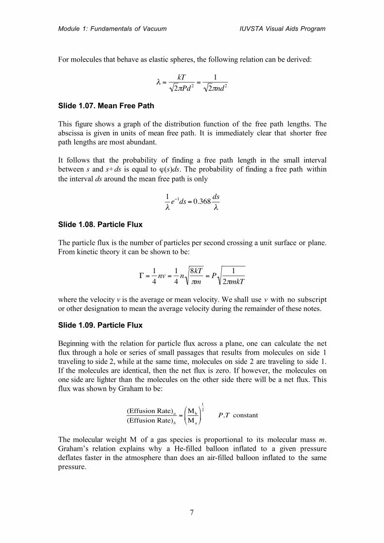
Consider a stream of No molecules moving through a gas. After covering a certaindistance, a molecule of the stream will collide with a molecule of the gas. If thecollisions are random, the number of molecules that undergo a collision over a distanceds will be given by dN = -αNds. The minus sign recognizes that the molecules are

leaving the stream. Thus, N = Noe-αs

and is the number of molecules that have traveleda distance s without suffering a collision. The expression for the distribution ϕ(s) ofmean free path λ can be derived by integrating or summing the lengths of all the paths,and dividing that value by the sum of all the molecular collisions. ϕ(s) is defined as

€

ϕ(s) =1λe−sλ


7

For molecules that behave as elastic spheres, the following relation can be derived:

€

λ =kT2πPd 2

=12πnd2

Slide 1.07. Mean Free Path

This figure shows a graph of the distribution function of the free path lengths. Theabscissa is given in units of mean free path. It is immediately clear that shorter freepath lengths are most abundant.

It follows that the probability of finding a free path length in the small intervalbetween s and s+ds is equal to ϕ(s)ds. The probability of finding a free path withinthe interval ds around the mean free path is only

€

1λe−1ds = 0.368 ds

λ

Slide 1.08. Particle Flux

The particle flux is the number of particles per second crossing a unit surface or plane.From kinetic theory it can be shown to be:

€

Γ =14nv =

14n 8kT

πm= P 1

2πmkT

where the velocity v is the average or mean velocity. We shall use v with no subscriptor other designation to mean the average velocity during the remainder of these notes.

Slide 1.09. Particle Flux

Beginning with the relation for particle flux across a plane, one can calculate the netflux through a hole or series of small passages that results from molecules on side 1traveling to side 2, while at the same time, molecules on side 2 are traveling to side 1.If the molecules are identical, then the net flux is zero. If however, the molecules onone side are lighter than the molecules on the other side there will be a net flux. Thisflux was shown by Graham to be:

€

(Effusion Rate)a(Effusion Rate)b

=Mb

Ma

12 P,T constant

The molecular weight M of a gas species is proportional to its molecular mass m.Graham’s relation explains why a He-filled balloon inflated to a given pressuredeflates faster in the atmosphere than does an air-filled balloon inflated to the samepressure.


8

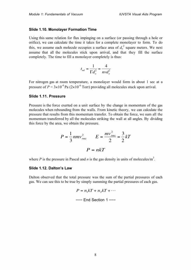
Slide 1.10. Monolayer Formation Time

Using this same relation for flux impinging on a surface (or passing through a hole ororifice), we can calculate the time it takes for a complete monolayer to form. To dothis, we assume each molecule occupies a surface area of do

2 square meters. We nextassume that all the molecules stick upon arrival, and that they fill the surfacecompletely. The time to fill a monolayer completely is thus:

€

tml =1Γdo

2 =4

nvdo2

For nitrogen gas at room temperature, a monolayer would form in about 1 sec at apressure of P = 3×10-4 Pa (2×10-6 Torr) providing all molecules stuck upon arrival.

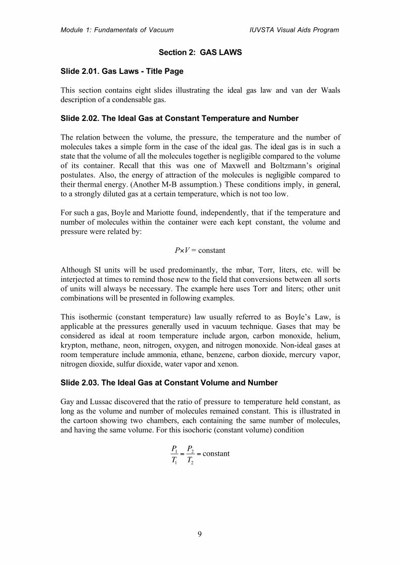
Slide 1.11. Pressure

Pressure is the force exerted on a unit surface by the change in momentum of the gasmolecules when rebounding from the walls. From kinetic theory, we can calculate thepressure that results from this momentum transfer. To obtain the force, we sum all themomentum transferred by all the molecules striking the wall at all angles. By dividingthis force by the area, we obtain the pressure.

€

P =13nmvrms

2 E =mvrms

2

2=

32kT

€

P = nkT

where P is the pressure in Pascal and n is the gas density in units of molecules/m3.

Slide 1.12. Dalton’s Law

Dalton observed that the total pressure was the sum of the partial pressures of eachgas. We can see this to be true by simply summing the partial pressures of each gas.

€

P = n1kT + n2kT +L

=== End Section 1 ===


9

Section 2: GAS LAWS

Slide 2.01. Gas Laws - Title Page

This section contains eight slides illustrating the ideal gas law and van der Waalsdescription of a condensable gas.

Slide 2.02. The Ideal Gas at Constant Temperature and Number

The relation between the volume, the pressure, the temperature and the number ofmolecules takes a simple form in the case of the ideal gas. The ideal gas is in such astate that the volume of all the molecules together is negligible compared to the volumeof its container. Recall that this was one of Maxwell and Boltzmann’s originalpostulates. Also, the energy of attraction of the molecules is negligible compared totheir thermal energy. (Another M-B assumption.) These conditions imply, in general,to a strongly diluted gas at a certain temperature, which is not too low.

For such a gas, Boyle and Mariotte found, independently, that if the temperature andnumber of molecules within the container were each kept constant, the volume andpressure were related by:

P×V = constant

Although SI units will be used predominantly, the mbar, Torr, liters, etc. will beinterjected at times to remind those new to the field that conversions between all sortsof units will always be necessary. The example here uses Torr and liters; other unitcombinations will be presented in following examples.

This isothermic (constant temperature) law usually referred to as Boyle’s Law, isapplicable at the pressures generally used in vacuum technique. Gases that may beconsidered as ideal at room temperature include argon, carbon monoxide, helium,krypton, methane, neon, nitrogen, oxygen, and nitrogen monoxide. Non-ideal gases atroom temperature include ammonia, ethane, benzene, carbon dioxide, mercury vapor,nitrogen dioxide, sulfur dioxide, water vapor and xenon.

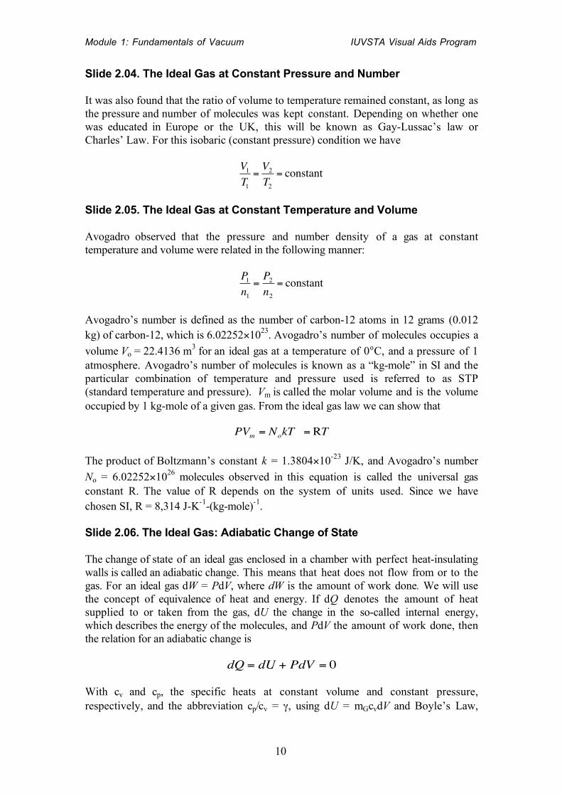
Slide 2.03. The Ideal Gas at Constant Volume and Number

Gay and Lussac discovered that the ratio of pressure to temperature held constant, aslong as the volume and number of molecules remained constant. This is illustrated inthe cartoon showing two chambers, each containing the same number of molecules,and having the same volume. For this isochoric (constant volume) condition

€

P1T1

=P2T2

= constant


10

Slide 2.04. The Ideal Gas at Constant Pressure and Number

It was also found that the ratio of volume to temperature remained constant, as long asthe pressure and number of molecules was kept constant. Depending on whether onewas educated in Europe or the UK, this will be known as Gay-Lussac’s law orCharles’ Law. For this isobaric (constant pressure) condition we have

€

V1T1

=V2T2

= constant

Slide 2.05. The Ideal Gas at Constant Temperature and Volume

Avogadro observed that the pressure and number density of a gas at constanttemperature and volume were related in the following manner:

€

P1n1

=P2n2

= constant

Avogadro’s number is defined as the number of carbon-12 atoms in 12 grams (0.012kg) of carbon-12, which is 6.02252×1023. Avogadro’s number of molecules occupies a

volume Vo = 22.4136 m3 for an ideal gas at a temperature of 0°C, and a pressure of 1atmosphere. Avogadro’s number of molecules is known as a “kg-mole” in SI and theparticular combination of temperature and pressure used is referred to as STP(standard temperature and pressure). Vm is called the molar volume and is the volumeoccupied by 1 kg-mole of a given gas. From the ideal gas law we can show that

€

PVm = NokT = RT

The product of Boltzmann’s constant k = 1.3804×10-23 J/K, and Avogadro’s number

No = 6.02252×1026 molecules observed in this equation is called the universal gasconstant R. The value of R depends on the system of units used. Since we havechosen SI, R = 8,314 J-K-1-(kg-mole)-1.

Slide 2.06. The Ideal Gas: Adiabatic Change of State

The change of state of an ideal gas enclosed in a chamber with perfect heat-insulatingwalls is called an adiabatic change. This means that heat does not flow from or to thegas. For an ideal gas dW = PdV, where dW is the amount of work done. We will usethe concept of equivalence of heat and energy. If dQ denotes the amount of heatsupplied to or taken from the gas, dU the change in the so-called internal energy,which describes the energy of the molecules, and PdV the amount of work done, thenthe relation for an adiabatic change is

€

dQ = dU + PdV = 0

With cv and cp, the specific heats at constant volume and constant pressure,respectively, and the abbreviation cp/cv = γ, using dU = mGcvdV and Boyle’s Law,


11

there remains only one independent variable. Thus, the adiabatic gas law can beexpressed in one of the following three equivalent forms.

€

T2

T1

=P2

P1

γ −1γ

or V1

V2

=P2

P1

1γ

or T2

T1

=V1

V2

γ −1

Slide 2.07. The Ideal Gas: The General Relation

The general relationship between pressure, volume, temperature, and the amount ofsubstance for an ideal gas is given by:

€

PV = nmRT

where nm is defined as the number of moles, and R is the universal gas constant. Twoindependent variables now remain for a certain amount of substance. The ideal gas lawmay also be written in the forms

€

PV = NkT or

€

P = nkT

where N is the number of molecules in volume V, and n is the density in molecules/m3.To obtain a convenient, two-dimensional, graphical representation of this law, onegenerally considers a number of discrete values for one of the independent variables. Itis instructive to take temperature as a parameter in a plot of P against V. This isdepicted in this slide.

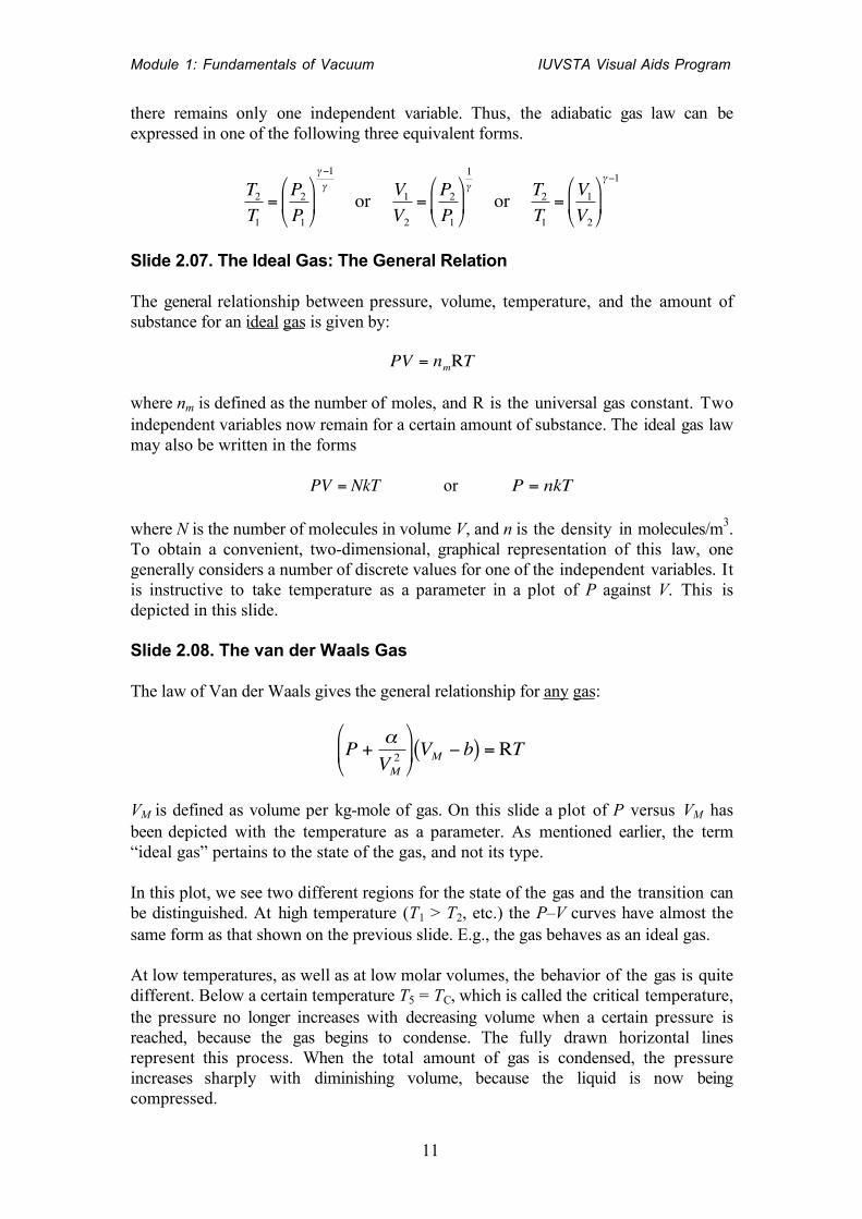
Slide 2.08. The van der Waals Gas

The law of Van der Waals gives the general relationship for any gas:

€

P +αVM2

VM − b( ) = RT

VM is defined as volume per kg-mole of gas. On this slide a plot of P versus VM hasbeen depicted with the temperature as a parameter. As mentioned earlier, the term“ideal gas” pertains to the state of the gas, and not its type.

In this plot, we see two different regions for the state of the gas and the transition canbe distinguished. At high temperature (T1 > T2, etc.) the P–V curves have almost thesame form as that shown on the previous slide. E.g., the gas behaves as an ideal gas.

At low temperatures, as well as at low molar volumes, the behavior of the gas is quitedifferent. Below a certain temperature T5 = TC, which is called the critical temperature,the pressure no longer increases with decreasing volume when a certain pressure isreached, because the gas begins to condense. The fully drawn horizontal linesrepresent this process. When the total amount of gas is condensed, the pressureincreases sharply with diminishing volume, because the liquid is now beingcompressed.


12

In addition to the horizontal lines, striated curved lines are also represented in thispart of the figure. If the experiment is performed very carefully, the portions of thesecurves close to the dotted curve can be realized under favorable conditions, but neverthe remaining portions, since this essentially represents instability. The completedstriated line is given by the van der Waals equation. The constant α in this equation is

related to the attractive potential of the molecules and the term α/VM2 represents an

extra pressure caused by mutual attraction.The constant b is associated with the total volume of the molecules, and representsapproximately the volume of the vessel containing the gas that cannot be freelyoccupied by a molecule. This volume has therefore to be subtracted from the totalvolume of the vessel.

It now becomes evident that, if a gas is contained in a certain volume, which is largecompared to b and maintained at a high temperature, so that the pressure is also high,then the constant terms α/VM

2 and b are negligible compared to P and VM. Thus,Boyle’s Law holds, e.g., we are in the upper right-hand side of the figure.

If the temperature is decreased, thereby decreasing the pressure, except for very largevalues of VM, the term α/VM

2 is no longer negligible compared to P, e.g., we are in thelower right-hand side of the figure. If the volume is now decreased, the term b alsobecomes important and the typical van der Waals plot results. If the volume is smalland the temperature rather high, the van der Waals equation remains valid (upper left-hand side of the figure.)



13

Section 3: GAS TRANSPORT

Slide 3.01. Gas Transport - Title Page

This section contains thirteen slides illustrating gas transport. The phenomena ofdiffusion, viscosity, thermal conductivity, and thermal transpiration are described.Where applicable, both the viscous and rarefied gas cases are discussed.

Slide 3.02. Diffusion–the equation and constant

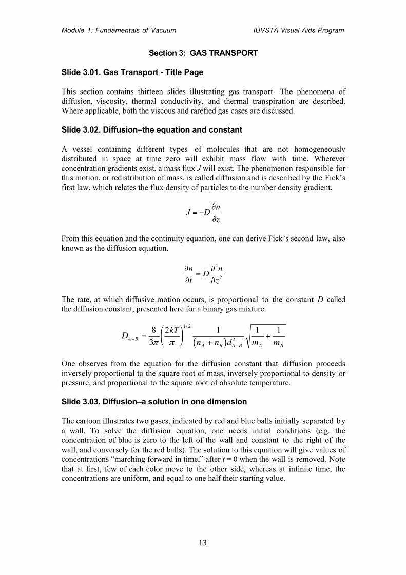
A vessel containing different types of molecules that are not homogeneouslydistributed in space at time zero will exhibit mass flow with time. Whereverconcentration gradients exist, a mass flux J will exist. The phenomenon responsible forthis motion, or redistribution of mass, is called diffusion and is described by the Fick’sfirst law, which relates the flux density of particles to the number density gradient.

€

J = −D ∂n∂z

From this equation and the continuity equation, one can derive Fick’s second law, alsoknown as the diffusion equation.

€

∂n∂t

= D ∂2n∂z2

The rate, at which diffusive motion occurs, is proportional to the constant D calledthe diffusion constant, presented here for a binary gas mixture.

€

DA−B =83π

2kTπ

1/ 2 1

nA + nB( )dA−B21mA

+1mB

One observes from the equation for the diffusion constant that diffusion proceedsinversely proportional to the square root of mass, inversely proportional to density orpressure, and proportional to the square root of absolute temperature.

Slide 3.03. Diffusion–a solution in one dimension

The cartoon illustrates two gases, indicated by red and blue balls initially separated bya wall. To solve the diffusion equation, one needs initial conditions (e.g. theconcentration of blue is zero to the left of the wall and constant to the right of thewall, and conversely for the red balls). The solution to this equation will give values ofconcentrations “marching forward in time,” after t = 0 when the wall is removed. Notethat at first, few of each color move to the other side, whereas at infinite time, theconcentrations are uniform, and equal to one half their starting value.


14

Slide 3.04. Diffusion–low pressure

At low pressure, we cannot solve the diffusion equation as it was derived. This isbecause it is the solution of a “random walk.” In a random walk, one assumes thateach molecule has equal probability to move “one space” to the left or to the right. Fora viscous gas, one assumes that gas-gas collisions predominate and a gas-gas collisiondistance represents the “one jump space”. At low pressures, the molecules do notcollide with each other, but with walls, and the diffusion constant no longer dependson pressure (or density) but only on temperature, molecular mass, and somethingadditional—the diameter of the pipe! Diffusion at low pressures is not dependent onpressure, but as Knudsen showed, is dependent on the dimension of the container.

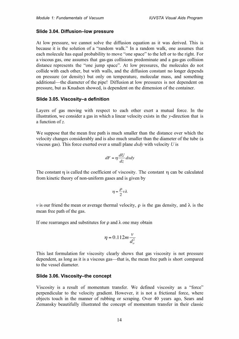
Slide 3.05. Viscosity–a definition

Layers of gas moving with respect to each other exert a mutual force. In theillustration, we consider a gas in which a linear velocity exists in the y-direction that isa function of z.

We suppose that the mean free path is much smaller than the distance over which thevelocity changes considerably and is also much smaller than the diameter of the tube (aviscous gas). This force exerted over a small plane dxdy with velocity U is

€

dF =ηdUdz

dxdy

The constant η is called the coefficient of viscosity. The constant η can be calculatedfrom kinetic theory of non-uniform gases and is given by

€

η =ρ2vλ

v is our friend the mean or average thermal velocity, ρ is the gas density, and λ is themean free path of the gas.

If one rearranges and substitutes for ρ and λ one may obtain

€

η = 0.112m vdo2

This last formulation for viscosity clearly shows that gas viscosity is not pressuredependent, as long as it is a viscous gas—that is, the mean free path is short comparedto the vessel diameter.

Slide 3.06. Viscosity–the concept

Viscosity is a result of momentum transfer. We defined viscosity as a “force”perpendicular to the velocity gradient. However, it is not a frictional force, whereobjects touch in the manner of rubbing or scraping. Over 40 years ago, Sears andZemansky beautifully illustrated the concept of momentum transfer in their classic


15

text, College Physics. They considered two coal trains traveling in the same directionwith differing velocities. On top of each coal train were an equal number of laborers.Each laborer threw the same number of equal-sized shovels of coal per minute fromtheir train to the other train. Hence the mass of each train remained the same.However, when a shovel of coal from the slow train landed on the fast train, itproduced a drag force, and slowed the fast train. In a similar manner, a shovel of coalfrom the fast train landing on the slow train increased its velocity. The “force” thataltered the speeds of both trains did not result from physical contact between the twotrains, but from momentum transfer.

Slide 3.07. Viscosity–at low pressure

We stated that the coefficient of viscosity did not depend on pressure, as long as thegas was a viscous gas. Clearly, it is also true that the coefficient of viscosity is zero atzero pressure. In the range between, the viscosity of a gas varies linearly withpressure, because the number of molecules striking the surfaces is proportional topressure when the mean free path becomes long compared to the spacing between themoving planes. The graph presented in this slide shows this behavior and assumesthat both vertical and the horizontal axes of the graph linear.

Slide 3.08. A Caution–graphical presentation

When displaying this and other phenomena over many orders of magnitude inpressure, it is convenient to display pressure on a logarithmic axis. A straight line on alinear plot becomes a “curved” line on a semi-log plot. One needs to mind thisphenomenon—plotting a linear equation on a semi-logarithmic axis. It is common anduseful to do this when plotting data over wide pressure ranges, but in the process, theunderlying physics can be obscured. For example, the equation for the low-pressurediffusion constant indicates that it is linearly proportional to pressure; this is notobvious when viewing a semi-logarithmic plot. Simply be aware that the“compression” that is observed in the horizontal axis is a natural result of thelogarithmic pressure scale.

Slide 3.09. Heat Conduction–a definition

When a temperature gradient exists, a flow of heat will occur. In the figure, considerthe heat flow dφ through a small plane dxdy, whose normal is in the direction of thetemperature gradient. The mean free path in the gas is small compared to thecharacteristic length of the situation. The coefficient of thermal conductivity is definedby

€

K =149cpcv− 5

ηcv =

149γ − 5( )ηcv

cp and cv are the specific heats at constant pressure and volume, respectively, γ = cp/cv,and η is the absolute viscosity. For heat conduction, it is not possible to derive thiscoefficient simply as can be done for viscosity. This is because in the case of unequaltemperature, the Maxwellian distribution of velocities is more seriously perturbed


16

than in the case of an additional linear velocity and our simple reasoning was based onan undisturbed velocity distribution.

The ratio of specific heats denoted by γ is determined by the relation γ = (2+f )/f. Inthis relation f is the number of degrees of freedom of the molecule. E.g., for amonatomic gas, f = 3 and γ becomes 1.667. For a diatomic gas, f = 5 (three fortranslation and two for rotation) and γ = 1.4. In a similar manner for a tri-atomic gas f= 8 and γ = 1.3333. For very high and low temperature, deviations occur due toquantum mechanical effects.

As in the case of viscosity, heat flow is independent of pressure in the range where aviscous gas exists. Note from the above relation that neither the coefficient ofviscosity η nor the specific heat at constant volume cv is dependent on pressure.

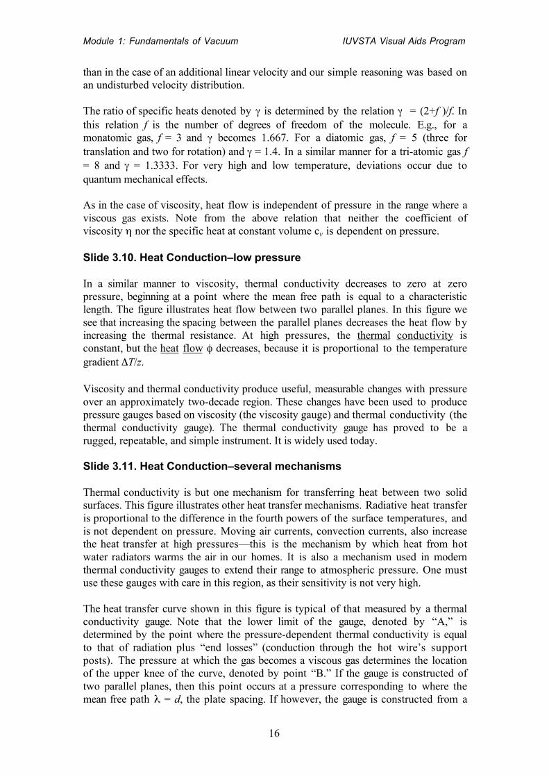
Slide 3.10. Heat Conduction–low pressure

In a similar manner to viscosity, thermal conductivity decreases to zero at zeropressure, beginning at a point where the mean free path is equal to a characteristiclength. The figure illustrates heat flow between two parallel planes. In this figure wesee that increasing the spacing between the parallel planes decreases the heat flow byincreasing the thermal resistance. At high pressures, the thermal conductivity isconstant, but the heat flow φ decreases, because it is proportional to the temperaturegradient ΔT/z.

Viscosity and thermal conductivity produce useful, measurable changes with pressureover an approximately two-decade region. These changes have been used to producepressure gauges based on viscosity (the viscosity gauge) and thermal conductivity (thethermal conductivity gauge). The thermal conductivity gauge has proved to be arugged, repeatable, and simple instrument. It is widely used today.

Slide 3.11. Heat Conduction–several mechanisms

Thermal conductivity is but one mechanism for transferring heat between two solidsurfaces. This figure illustrates other heat transfer mechanisms. Radiative heat transferis proportional to the difference in the fourth powers of the surface temperatures, andis not dependent on pressure. Moving air currents, convection currents, also increasethe heat transfer at high pressures—this is the mechanism by which heat from hotwater radiators warms the air in our homes. It is also a mechanism used in modernthermal conductivity gauges to extend their range to atmospheric pressure. One mustuse these gauges with care in this region, as their sensitivity is not very high.

The heat transfer curve shown in this figure is typical of that measured by a thermalconductivity gauge. Note that the lower limit of the gauge, denoted by “A,” isdetermined by the point where the pressure-dependent thermal conductivity is equalto that of radiation plus “end losses” (conduction through the hot wire’s supportposts). The pressure at which the gas becomes a viscous gas determines the locationof the upper knee of the curve, denoted by point “B.” If the gauge is constructed oftwo parallel planes, then this point occurs at a pressure corresponding to where themean free path λ = d, the plate spacing. If however, the gauge is constructed from a


17

fine wire located in a glass envelope, the knee occurs at a pressure corresponding tothe mean free path λ = dW, the wire diameter.

Slide 3.12. Momentum and Energy Transport–a distinction

Heat transfer by gas conduction is the result of energy transport. A gas molecule hits aheated surface, thermally accommodates, and recoils with increased energy. Successivecollisions transfer this energy to a cooler surface and permit heat to flow from the hotsurface to the cool surface.

Viscosity is the result of momentum transport. Molecules hit a rapidly movingsurface and recoil with increased momentum. Successive collisions transfer thismomentum to a more slowly moving surface and permit its momentum to increase.

The formulas given in these slides are the maximum values of momentum and heat thatcan be transferred. The correction factor for momentum factor is very close to 1.Unlike the accommodation coefficient for momentum, the accommodation coefficientfor heat may differ from 1. That is, a molecule hitting a hot surface may not reach thetemperature of the surface before it departs, and a molecule hitting the cool surfacemay not give up all its heat to the cool surface.

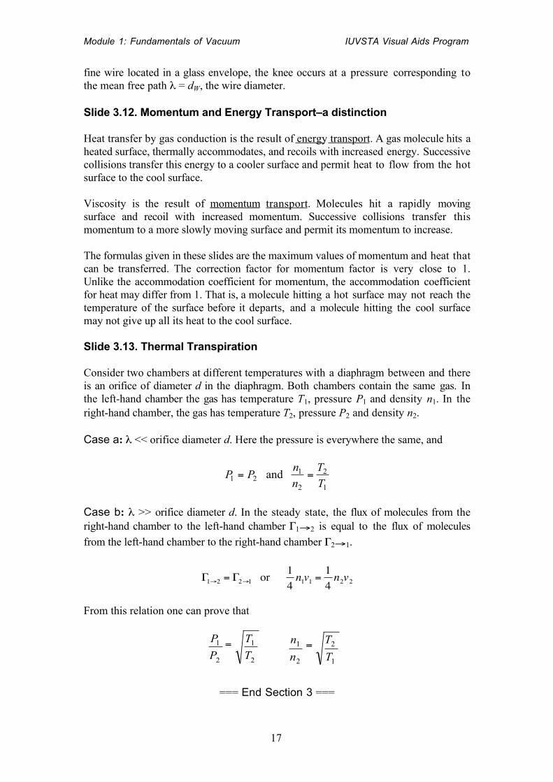
Slide 3.13. Thermal Transpiration

Consider two chambers at different temperatures with a diaphragm between and thereis an orifice of diameter d in the diaphragm. Both chambers contain the same gas. Inthe left-hand chamber the gas has temperature T1, pressure P1 and density n1. In theright-hand chamber, the gas has temperature T2, pressure P2 and density n2.

Case a: λ << orifice diameter d. Here the pressure is everywhere the same, and

1

2

2

121 and

TT

nn

PP ==

Case b: λ >> orifice diameter d. In the steady state, the flux of molecules from theright-hand chamber to the left-hand chamber Γ1→2 is equal to the flux of molecules

from the left-hand chamber to the right-hand chamber Γ2→1.

€

Γ1→2 = Γ2→1 or 14n1v1 =

14n2v2

From this relation one can prove that

2

1

2

1

T

T

P

P =

1

2

2

1

T

T

n

n =



18

Section 4: GAS FLOW

Slide 4.01. Gas Flow - Title Page

This section contains twenty-four slides illustrating gas flow in the choked, turbulent,viscous, and molecular regions. Conductance and speed are defined and calculationexamples for useful situations are presented.

Slide 4.02. Gas Flow–its complexity

The flow of gas through pipes is complex, and it cannot be described by a singlemathematical relation. Gas flow, in its many regimes has been well studied, for a longtime, and is well characterized in most of these regimes. To understand these regimeswe first define the “nature” of a gas.

Slide 4.03. Gas Flow–the nature of a gas

The “nature” of a gas as it flows in a duct or pipe is related to the size of the meanfree path as compared to a characteristic dimension of the object, such as a pipediameter. When the mean free path is short compared to the characteristic dimensionof the container, we say that the gas is a viscous gas—in this region the thermalconductivity and viscosity are constant. A viscous gas is characterized by thepredominance of gas-gas collisions. In this region, the gas behaves as a “fluid.” Whenthe mean free path is long compared to the characteristic dimension, then molecules nolonger interact with or scatter from each other. Instead, they scatter from the walls ofthe container or pipe. We say that the gas is a rarefied gas—in this region the thermalconductivity and heat flow are no longer constant but also depend on geometry. Ararefied gas is characterized by the predominance of gas-wall collisions. In this region,the gas does not behave like a fluid.

Slide 4.04. Gas Flow–the behavior of flowing gas

Gas flow is traditionally analyzed in one of four regimes: choked, turbulent, viscous,or molecular flow. Each regime can be characterized by the values of certaindimensionless variables such as the Mach number, Reynolds’ number, and Knudsen’snumber.

Slide 4.05. Flow below the choked limit

Consider two adjoining chambers whose dimensions are large compared to thediameter of the orifice in the dividing wall.

The mean free path of the gas molecules λ is much smaller than the orifice diameter d;the surface area of the orifice is denoted by A. The ratio of mean free path todimension is called Knudsen’s number, Kn.

€

Kn =λd


19

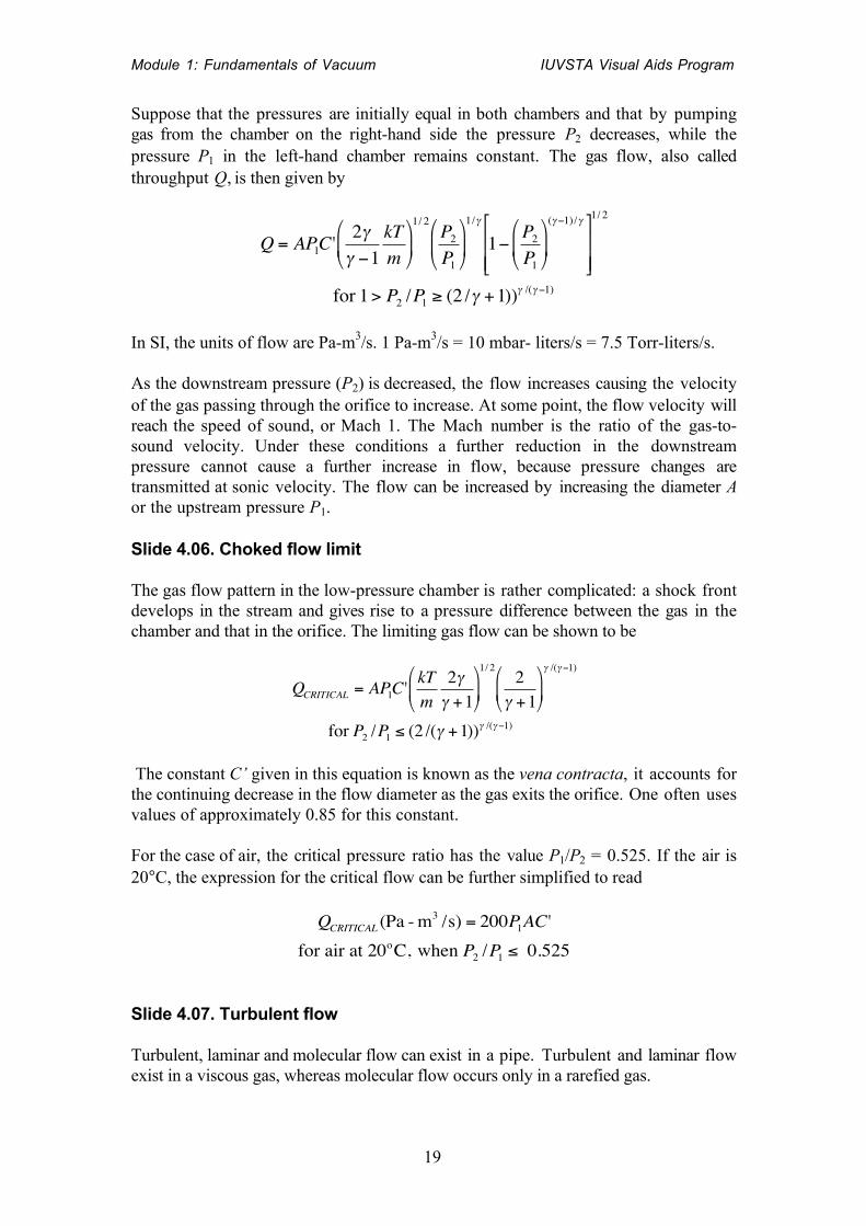
Suppose that the pressures are initially equal in both chambers and that by pumpinggas from the chamber on the right-hand side the pressure P2 decreases, while thepressure P1 in the left-hand chamber remains constant. The gas flow, also calledthroughput Q, is then given by

€

Q = AP1C' 2γγ −1

kTm

1/ 2P2

P1

1/γ

1− P2

P1

(γ −1)/γ

1/ 2

for 1 > P2 /P1 ≥ (2 /γ +1))γ /(γ −1)

In SI, the units of flow are Pa-m3/s. 1 Pa-m3/s = 10 mbar- liters/s = 7.5 Torr-liters/s.

As the downstream pressure (P2) is decreased, the flow increases causing the velocityof the gas passing through the orifice to increase. At some point, the flow velocity willreach the speed of sound, or Mach 1. The Mach number is the ratio of the gas-to-sound velocity. Under these conditions a further reduction in the downstreampressure cannot cause a further increase in flow, because pressure changes aretransmitted at sonic velocity. The flow can be increased by increasing the diameter Aor the upstream pressure P1.

Slide 4.06. Choked flow limit

The gas flow pattern in the low-pressure chamber is rather complicated: a shock frontdevelops in the stream and gives rise to a pressure difference between the gas in thechamber and that in the orifice. The limiting gas flow can be shown to be

€

QCRITICAL = AP1C' kTm

2γγ +1

1/ 22

γ +1

γ /(γ −1)

for P2 /P1 ≤ (2 /(γ +1))γ /(γ −1)

The constant C’ given in this equation is known as the vena contracta, it accounts forthe continuing decrease in the flow diameter as the gas exits the orifice. One often usesvalues of approximately 0.85 for this constant.

For the case of air, the critical pressure ratio has the value P1/P2 = 0.525. If the air is20°C, the expression for the critical flow can be further simplified to read

€

QCRITICAL (Pa - m3 /s) = 200P1AC'for air at 20oC, when P2 /P1 ≤ 0.525

Slide 4.07. Turbulent flow

Turbulent, laminar and molecular flow can exist in a pipe. Turbulent and laminar flowexist in a viscous gas, whereas molecular flow occurs only in a rarefied gas.


20

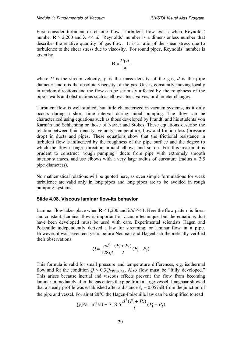
First consider turbulent or chaotic flow. Turbulent flow exists when Reynolds’number R > 2,200 and λ << d. Reynolds’ number is a dimensionless number thatdescribes the relative quantity of gas flow. It is a ratio of the shear stress due toturbulence to the shear stress due to viscosity. For round pipes, Reynolds’ number isgiven by

πρ

=dU

R

where U is the stream velocity, ρ is the mass density of the gas, d is the pipediameter, and η is the absolute viscosity of the gas. Gas is constantly moving locallyin random directions and the flow can be seriously affected by the roughness of thepipe’s walls and obstructions such as elbows, tees, valves, or diameter changes.

Turbulent flow is well studied, but little characterized in vacuum systems, as it onlyoccurs during a short time interval during initial pumping. The flow can becharacterized using equations such as those developed by Prandtl and his students vonKàrmàn and Schlichting or those of Navier and Stokes. These equations describe therelation between fluid density, velocity, temperature, flow and friction loss (pressuredrop) in ducts and pipes. These equations show that the frictional resistance inturbulent flow is influenced by the roughness of the pipe surface and the degree towhich the flow changes direction around elbows and so on. For this reason it isprudent to construct “rough pumping” ducts from pipe with extremely smoothinterior surfaces, and use elbows with a very large radius of curvature (radius ≥ 2.5pipe diameters).

No mathematical relations will be quoted here, as even simple formulations for weakturbulence are valid only in long pipes and long pipes are to be avoided in roughpumping systems.

Slide 4.08. Viscous laminar flow-its behavior

Laminar flow takes place when R < 1,200 and λ/d << 1. Here the flow pattern is linearand constant. Laminar flow is important in vacuum technique, but the equations thathave been developed must be used with care. Experimental scientists Hagen andPoiseuille independently derived a law for streaming, or laminar flow in a pipe.However, it was seventeen years before Neuman and Hagenbach theoretically verifiedtheir observations.

€

Q =πd4

128ηl(P1 + P2)2

(P1 − P2)

This formula is valid for small pressure and temperature differences, e.g. isothermalflow and for the condition Q < 0.3QCRITICAL. Also flow must be “fully developed.”This arises because inertial and viscous effects prevent the flow from becominglaminar immediately after the gas enters the pipe from a large vessel. Langhaar showedthat a steady profile was established after a distance le = 0.057dR from the junction of

the pipe and vessel. For air at 20°C the Hagen-Poiseuille law can be simplified to read

€

Q(Pa -m3/s) = 718.5 d4 (P1 + P2)

l(P1 − P2)


21

Slide 4.09. Viscous flow in short tubes

The difficulty with the Hagen-Poiseuille approach is that it is valid only in long pipes,e.g., where the length is > 100 diameters. Such designs are counter productive, as onelooses too much pumping speed when long roughing pipes are used. Santeler showedthat short pipes could be considered to be a long pipe in series with an orifice. Toformulate such a problem, one equates the laminar flow through the pipe with thechoked flow through the orifice. After solving the problem, one verifies that theartificial intermediate pressure is indeed less than 0.525P1. Santeler’s experimentaldata agreed with this model.

Slide 4.10. Viscous flow–a short-tube example

This example demonstrates Santler’s model. Imagine a fine leak, assumed to be 100µm in diameter, across a large cross-section O-ring, or through a solid wall. The slideillustrates the formulation of the problem assuming air as the gas. The left half of theequation is Poiseuille’s law, whereas the right side represents choke flow driven byunknown intermediate pressure PX. Solving for this pressure, we obtain PX = 44,550Pa, which is less than the critical pressure of 52,500 Pa. Therefore the assumption ofchoke flow is valid. If it were not valid, one would have to recast the problem usingthe equation given in Slide 4.06. The flow in such a leak is typically viscous until theexit, whereupon it expands rapidly in a manner similar to the exhaust of a rocket, as ittravels in the upper atmosphere.

Slide 4.11. Molecular flow–its behavior

Molecular flow occurs when the mean free path is greater than a critical dimension,such as a pipe diameter; in this situation, wall collisions predominate. The illustrationshows molecules arriving at a wall, and scattering in apparently random directions.Scattering is not random, but rather it follows a cosine law. In diffuse scattering,particles arrive, reside for a brief instant, and depart not knowing the direction fromwhich they came. The least energy is required to depart at an angle normal to the localsurface, and thus that is the most common angle of departure.

Slide 4.12. Molecular flow through an orifice

The relation for molecular flow through an orifice can be obtained from

€

Q =kT4vA(n1 − n2) =

v4A(P1 − P2)

where v is our old friend, the average velocity. Assuming that P2 is zero, the maximumflow can be found to be

€

Q =kT4vAn1 =

v4AP1


22

For air at room temperature, the maximum flow is Q (Pa-m3/s) = 116AP1. We defineconductance as flow divided by pressure difference and thus,

€

C =Q

P1−P2( )=v4A = 116 A

Slide 4.13. Molecular flow through a round pipe

Molecules entering an infinitely thin orifice all pass through the orifice. When a roundpipe is substituted for the infinitely thin orifice, some of the entering molecules collidewith the wall, scatter, and leave at an angle determined by the cosine distribution law.Some of the molecules will eventually pass through the pipe and depart, whereasothers will return to the entrance from whence they came. The longer the tube, inrelation to its diameter, the less will be its probability of passage. The probability ofpassage has been known variously as the Clausing factor—named after the scientistwho first formulated the solution in integral form, or more simply the transmissionprobability. The transmission probability for round pipes, as obtained from theClausing integral, is shown in this slide. Note that the absolute length is not a factor inthe transmission probability, but rather the ratio of length to diameter. Thus, a 200-mm-diameter pipe that is two meters long, has the same probability of transmittingmolecules, as does a 100-mm-diameter pipe that is one meter long.

The gas flow through a tube of arbitrary length-to-diameter ratio (L/D) can be obtainedeasily with the use of the formulas given in the previous slide, provided that they aremodified in the following manner.

€

Q =v4A(P1 − P2)a and C =

v4Aa

This is the same formula as presented on the previous slide, provided that oneconsiders a = 1 for an orifice. Indeed that is true, as there are no walls from whichparticles could scatter and return to the first chamber.

Slide 4.14. Molecular flow through arbitrarily-shaped objects

Clausing’s integral has proven too difficult to solve for even the simplest geometry—around pipe. In practice, one is required to obtain solutions for complex shapes such asvalves, chevron baffles, cold traps, elbows, frustum of a cone, annular rings, and thinparallel plates. The Monte Carlo method is used for these and other practical shapes.It is performed as the name suggests, by repeatedly projecting numerous particle“rays,” via computer—particles that scatter with cosine probability. Most vacuumtexts contain tables or graphical displays of the calculated results.

Slide 4.15. Molecular flow–combinations of isolated components

Individual components serve no purpose. They must be combined in some form to beuseful. The laws by which they are combined are straightforward. The totalconductance of elements in parallel is their linear sum. The total conductance ofelements in series depends on how the components are connected. For example, if the


23

components are connected to each other by means of a large chamber, the totalconductance is simply the reciprocal of the sum of the reciprocals. They add in thisnon-interacting, independent way, because the gas flow at the entrance to eachcomponent has relaxed to a Maxwell-Boltzmann distribution. Unfortunately, onerarely connects objects in this manner.

Slide 4.16. Molecular flow trajectories

The velocity distributions of molecules exiting or returning to the original chamber viathe pipe entrance are distinctly not Maxwellian! Shown here are the distributions fortwo cases, a thin orifice and a pipe of dimensional ratio L = 2D with the flow from leftto right. Note that the flux exiting from the thin orifice is molecular, whereas the fluxexiting the short tube is near beam-shaped. The return flux at the pipe entrance is inthe shape of a thin, annular cone. As the length-to-diameter ratio is increased, thebeam-like behavior of the forward distribution is enhanced. It is these deviations fromMaxwellian behavior that prevent us from using the simple reciprocal rule whenadding components that are NOT separated by large volumes.

Slide 4.17. Molecular flow–combinations of interacting components

Oatley was the first to derive a relation for obtaining the transmission probability oftwo components directly connected to each other. His relation is given by:

€

1a

=1a1

+1a2−1

when generalized to a number of components, it becomes:

€

1− aa

=1− a1a1

+1− a2a2

+1− a3a3

+ ...

This formalism assumes that the entrance and exit diameters of all components are thesame. Several researchers have derived formulas to account for varying diameters. Themost concise relationship was presented by Haefer and is shown in this slide.

€

1A1

1− a1→n

a1→n

=

1Ai

1− aiai

1

n

∑ +1Ai+1

−1Ai

1

n−1

∑ δi,i+1

where δi,i+1 = 1 for Ai+1 < Ai, and δi,i+1 = 0 for Ai+1 ≥ Ai

Slide 4.18. Molecular flow – an example of combining interactingcomponents

An example use of this formula is shown in this slide. Note that the Dirac deltafunctions are used to retain a term in the equation when diameter decreases, andeliminate a term when the diameter increases. To calculate the conductance of thiscombination of three objects, one first calculates the transmission probability a1→3


24

and then uses that value in the conductance formula, taking care to use the appropriateentrance area! Note that a1→3 ≠ a3→1. However, the product of the transmission

coefficient times its entrance area does not change, e.g.

A1 × a1→3 = A3 × a3→1

Slide 4.19. Molecular flow–definition of volumetric pumping speed

The next four slides present an application—calculating the net speed of a pump,pipe, and valve—that can be solved using two concepts discussed here: The conceptof adding conductance values in series and the concept of flow through an orifice.

To begin, we review the definition of conductance, and present the definition of“pumping speed,” or “volumetric speed.” In SI, speed has the same units asconductance—cubic meters per second in SI—but conductance and speed are not thesame thing. Conductance is a characteristic of a component, or a group of closelyspaced components. Speed is a characteristic that is measured at a point in a system.This is somewhat analogous to an electrical circuit. A component such as a resistorhas a unique conductance or ratio of current to voltage. Speed, the ratio of gas flow ata specific location in a system to the pressure at that location, is analogous to the ratioof current at some node in a circuit divided by the voltage between that node andground.

Slide 4.20. Molecular flow–the speed of an “ideal” pump

The flux through a thin orifice was presented in Slide 4.12. Here we take a special caseof that flow, P2 = 0. In this case, all molecules entering the hole never return. This isanalogous to a “perfect,” or “ideal” pump. Using the definition of speed presented inthe previous slide, we see that the pumping speed of this hole is given by

S

€

≡QP1

=

v4AP1P1

=v4A

This value of pumping speed, the ideal speed, is that value corresponding to thecapture of all molecules. None ever return to the upper side of the orifice plane.

Slide 4.21. Molecular flow–the speed of a “real” pump

Real pumps are not perfect. They do not capture every molecule. For example, in adiffusion pump, some molecules strike the cold cap, and recoil. In a turbopump somemolecules strike the solid parts of the stator and recoil. Using measuring “test domes”designed for the purpose, the speeds for most non-condensable gases can easily bemeasured. Such measurements are usually performed only within the companies thatmanufacture pumps, as the test domes are large and infrequently used.

However, more information than that given by the measured speed is needed, if one isto calculate properly the speed at the entrance to a series of components attached to a


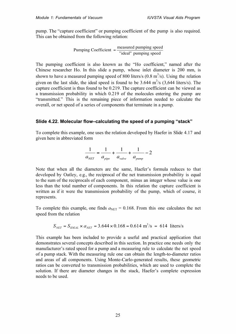
25

pump. The “capture coefficient” or pumping coefficient of the pump is also required.This can be obtained from the following relation:

€

Pumping Coefficient =measured pumping speed"ideal" pumping speed

The pumping coefficient is also known as the “Ho coefficient,” named after theChinese researcher Ho. In this slide a pump, whose inlet diameter is 200 mm, isshown to have a measured pumping speed of 800 liters/s (0.8 m3/s). Using the relationgiven on the last slide, the ideal speed is found to be 3.644 m3/s (3,644 liters/s). Thecapture coefficient is thus found to be 0.219. The capture coefficient can be viewed asa transmission probability in which 0.219 of the molecules entering the pump are“transmitted.” This is the remaining piece of information needed to calculate theoverall, or net speed of a series of components that terminate in a pump.

Slide 4.22. Molecular flow–calculating the speed of a pumping “stack”

To complete this example, one uses the relation developed by Haefer in Slide 4.17 andgiven here in abbreviated form

€

1aNET

=1apipe

+1

avalve+

1apump

− 2

Note that when all the diameters are the same, Haefer’s formula reduces to thatdeveloped by Oatley, e.g., the reciprocal of the net transmission probability is equalto the sum of the reciprocals of each component, minus an integer whose value is oneless than the total number of components. In this relation the capture coefficient iswritten as if it were the transmission probability of the pump, which of course, itrepresents.

To complete this example, one finds aNET = 0.168. From this one calculates the netspeed from the relation

€

SNET = SIDEAL × aNET = 3.644 × 0.168 = 0.614 m3/s = 614 liters/s

This example has been included to provide a useful and practical application thatdemonstrates several concepts described in this section. In practice one needs only themanufacturer’s rated speed for a pump and a measuring rule to calculate the net speedof a pump stack. With the measuring rule one can obtain the length-to-diameter ratiosand areas of all components. Using Monte-Carlo-generated results, these geometricratios can be converted to transmission probabilities, which are used to complete thesolution. If there are diameter changes in the stack, Haefer’s complete expressionneeds to be used.


26

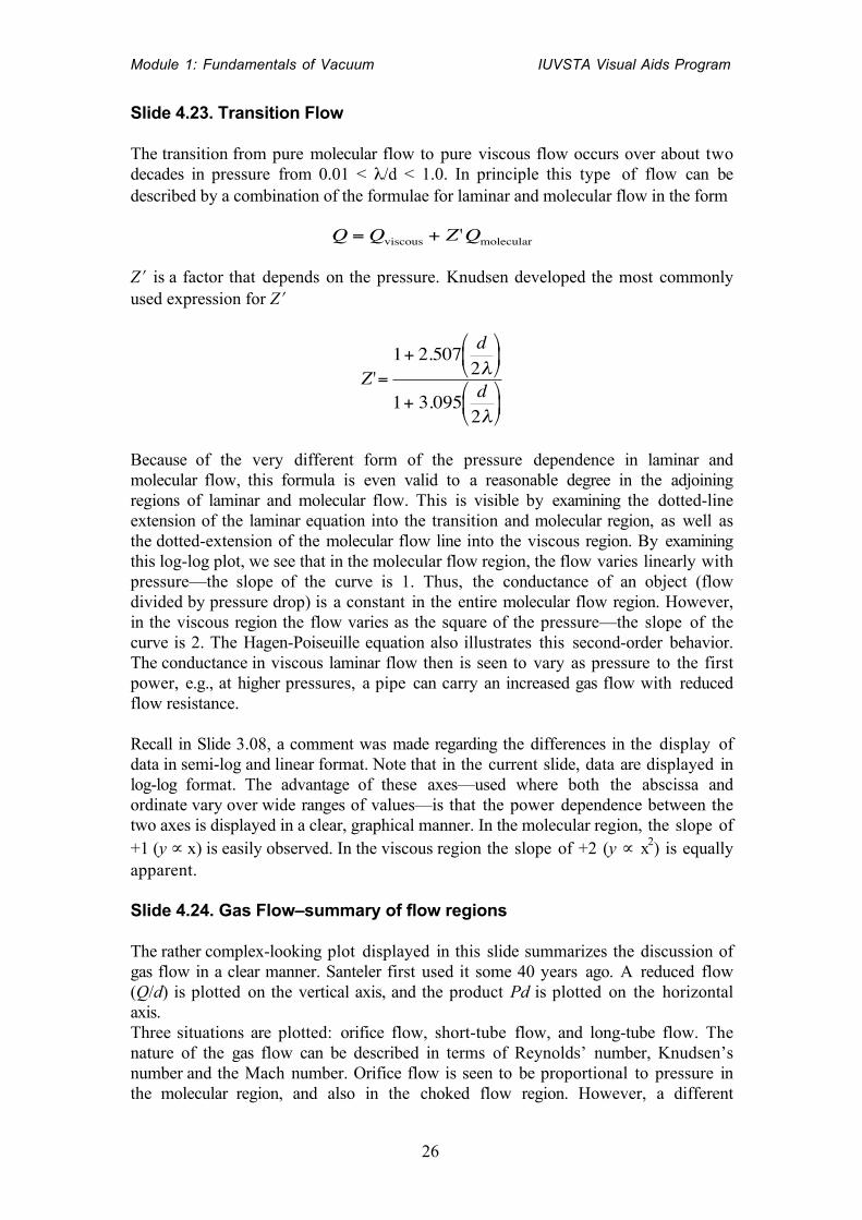
Slide 4.23. Transition Flow

The transition from pure molecular flow to pure viscous flow occurs over about twodecades in pressure from 0.01 < λ/d < 1.0. In principle this type of flow can bedescribed by a combination of the formulae for laminar and molecular flow in the form

€

Q =Qviscous + Z'Qmolecular

Z′ is a factor that depends on the pressure. Knudsen developed the most commonlyused expression for Z′

€

Z'=1+ 2.507 d

2λ

1+ 3.095 d2λ

Because of the very different form of the pressure dependence in laminar andmolecular flow, this formula is even valid to a reasonable degree in the adjoiningregions of laminar and molecular flow. This is visible by examining the dotted-lineextension of the laminar equation into the transition and molecular region, as well asthe dotted-extension of the molecular flow line into the viscous region. By examiningthis log-log plot, we see that in the molecular flow region, the flow varies linearly withpressure—the slope of the curve is 1. Thus, the conductance of an object (flowdivided by pressure drop) is a constant in the entire molecular flow region. However,in the viscous region the flow varies as the square of the pressure—the slope of thecurve is 2. The Hagen-Poiseuille equation also illustrates this second-order behavior.The conductance in viscous laminar flow then is seen to vary as pressure to the firstpower, e.g., at higher pressures, a pipe can carry an increased gas flow with reducedflow resistance.

Recall in Slide 3.08, a comment was made regarding the differences in the display ofdata in semi-log and linear format. Note that in the current slide, data are displayed inlog-log format. The advantage of these axes—used where both the abscissa andordinate vary over wide ranges of values—is that the power dependence between thetwo axes is displayed in a clear, graphical manner. In the molecular region, the slope of+1 (y ∝ x) is easily observed. In the viscous region the slope of +2 (y ∝ x2) is equallyapparent.

Slide 4.24. Gas Flow–summary of flow regions

The rather complex-looking plot displayed in this slide summarizes the discussion ofgas flow in a clear manner. Santeler first used it some 40 years ago. A reduced flow(Q/d) is plotted on the vertical axis, and the product Pd is plotted on the horizontalaxis.Three situations are plotted: orifice flow, short-tube flow, and long-tube flow. Thenature of the gas flow can be described in terms of Reynolds’ number, Knudsen’snumber and the Mach number. Orifice flow is seen to be proportional to pressure inthe molecular region, and also in the choked flow region. However, a different


27

numerical constant occurs in each range. The ranges of R and Kn are noted on thegraphical display. In a similar manner for the very long tube, the flow is seen to varydirectly with pressure in the molecular flow region. The value of flow is less than thatof an orifice, due to the reduced transmission probability. In the viscous region flowvaries as the square of the pressure, and like orifice flow, linearly with pressure in theturbulent flow regime. The intermediate case, a short tube, illustrates the commentthat Poiseuille’s law is not valid for short tubes. The flow-pressure relation is neither1st nor 2nd order, but lies between. It is for this reason that models like the onedeveloped by Santeler are used to analyze the flow in short tubes when the gas is in aviscous state.



28

Section 5: GAS DESORPTION FROM SURFACES

Slide 5.01. Gas Desorption from Surfaces - Title Page

This section contains thirteen slides which depict issues concerning desorption ofgases from solid surfaces.

Slide 5.02. Scattering of helium atoms from a single-crystal metal

The upper part of the figure shows the room temperature scattering pattern of thermalhelium atoms from a high-atomic-weight, single-crystal, metal surface. As the energyexchange between the light gas atoms and heavy metal atoms is slight, the reflection ispredominantly specular. If monoenergetic helium atoms are reflected from long rangeordered single crystal surfaces, sharp diffraction patterns will be observed.

The lower part of the figure shows the scattering of xenon atoms by the samecrystalline metal. Because of the greater exchange between the heavy xenon atoms andmetal, inelastic scattering also occurs and this causes a diffuse scattering pattern thatmasks the specular component. For a gas such as xenon the interaction energybetween gas and metal also contributes to the diffusion.

Slide 5.03. Scattering of a reactive gas from a single-crystal metal

The upper part of the figure shows the scattering of a reactive molecule by the surfaceof a single crystal of a metal in a single encounter.

The lower part of the figure shows the scattering pattern of a reactive molecule thathas been adsorbed at the surface long enough to thermally equilibrate with the crystal.In both cases, the scattering pattern is that of a cosine distribution.

Slide 5.04. Gas scattering from a rough surface

Realistic surfaces remain rough on a microscopic scale. Even after the most refinedtreatment the roughness will generally be random. In this case of random roughnessthe scattering pattern would still be diffusive because of directional effects. Thiswould be true even if the surface were random single crystals that weakly interactedwith the gas.

In the general case of comparable atomic weights of gas and metal with non-negligibleinteraction energy, the scattering will be diffuse with a cosine distribution. Regularpatterns introduced by machining can cause a minor perturbation to the cosinedistribution.

Slide 5.05. Realistic surface interactions

The left-hand surface is covered with single isolated adsorbed gas particles. Thiscorresponds to ultrahigh vacuum at a pressure less than 10-7 Pa (10-9 mbar or 7.5×10-9

Torr). The center surface is covered with a monolayer. This state corresponds to apressure of 10-6 Pa. The right-hand surface is covered with multi-layers. This


29

corresponds to all pressures greater than 10-6 Pa. At atmospheric pressure, there areup to 150 layers, and at normal high vacuum, 20–30 layers. Considering the absorbedgas particles on solid surfaces, it is easy to understand that in normal conditions gasparticles will never be reflected from surfaces. Incoming gas particles will hit, stick,and desorb after a certain amount of time. In any case, the desorption pattern has theform of a cosine distribution. Note that this is a simplified slide where time andsticking coefficients have been neglected.

The scattering of helium atoms by the single crystal surface shown in Slide 5.02 willbe an exception at extreme- and ultra-high vacuum. In normal conditions the surface ofa single crystal is covered with multi-layers of adsorbed gas. After considering theadsorbed gases on surfaces, Slides 5.03 and 5.04, one sees that all surfaces will haveidentical cosine scattering.

In general, water vapor molecules are strongly adsorbed at surfaces due to the dipoleeffect of the water molecule. The adsorption forces between the surface and the gasparticle are strong in the first layer, but become less strong with increasing distancefrom the surface. The packing density decreases with increased distance from thesurface. In the adsorbed layers different gas particles may be present, but the greatestfraction will be water vapor. This is clearly demonstrated by residual gas analysis.

In the earlier slides of this module, adsorbed surface layers were not considered. This,however, does not reduce the value of any calculations or models presented.Considerations of surface layers would not have changed the results.

Considerations of the effect of adsorption and desorption should never be dismissed.Practical pumping cycles, chamber degassing and cleaning, leak detector responsetimes, and gauge measurements from thermal conductivity through ultrahigh vacuumrepresent some of the manifold situations that will not be understandable withoutknowledge of adsorption and desorption effects.

Slide 5.06. Adsorption

Two types of adsorption of a molecule on a solid surface can be distinguished:physisorption and chemisorption.

For the case of physisorption the molecule is weakly bound to the surface and theelectronic structure of the molecule remains unimpaired, although it may be distortedby the surface forces (polarization). Chemisorption bonds are strong and theelectronic structure of the molecule is combined with that of the solid.

The figure shows the potential energy of the molecule as a function of distance fromthe surface. The curve reflects the strong influence of the force exerted by the solid onthe molecule. The potential at infinity is taken as zero. In the first potential well(coming from infinity) the molecule is physisorbed whereas in the following well,which is deeper, it is chemisorbed.

When approaching the surface from infinity, the molecule can undergo physisorption,because no extra energy is required to enter the first potential well, e.g., there is no


30

activation energy for adsorption. Therefore, in this case the activation energy fordesorption is equal to the heat of adsorption. Chemisorption requires in general anactivation energy Ea and now the activation energy for desorption is equal to the heatof desorption plus the activation energy for chemisorption, Qc + Ea. Activationenergies determine the rate of a process, whereas the heat of sorption is liberated oradsorbed during a process that occurs near equilibrium.

It often happens that molecular chemisorption is accompanied by dissociation. In thiscase a physisorbed molecule still needs an activation energy to become dissociated andchemisorbed as atoms, for example hydrogen. As the potential energy curve for theseparate atoms is very steep, strong chemisorption takes place when, by separatemeans, the hydrogen molecules are dissociated into atoms far from the surface.

Slide 5.07. Activation energies

Here the conditions are examined under which a molecule may become adsorbed in thesolid and, after diffusion through the solid, may leave the surface at the other side.This is called permeation. A molecule that is adsorbed at the surface can, after havingreceived the activation energy for absorption indicated in the slide by E, penetrate justinside the solid. For example, an increase in temperature may cause an adsorbedmolecule to become absorbed. If the molecule that is absorbed on the inner side of thesurface gains energy, which is equivalent to or greater than the activation energy ofdiffusion, it can move further into the solid. See the second line in the slide.

The next step in the process of permeation is the extraction from the solid to the outersurface, which requires the corresponding activation energy shown in line 3 of theslide. To proceed from this stage into the gaseous phase requires again the activationenergy of desorption shown in line 4 of this slide. We see that the largest activationenergy will control the permeation process. Here we have chosen some extremeexamples to demonstrate the mechanisms involved. The real form of the potentialcurve depends on the combination of molecule and solid. Some typical examplescorresponding to the curve are given here.

In the case of hydrogen permeating a smooth iron wall, the activation energy forchemisorption is the limiting energy for permeation. If, however, hydrogen atomsimpinge on the surface, they enter the iron immediately and the permeation rate ishigh. On a rough surface, places may exist where the hydrogen is absorbed in atomicform. Now the activation energy for absorption becomes the limiting factor—line 1 inthe slide.

The permeation of hydrogen through copper is controlled by the activation energy ofdiffusion—line 2 in the slide. The permeation of oxygen through zirconium is veryweak, because of the high activation energy for extraction. For the permeation ofoxygen through copper, the activation energy of desorption is the rate determiningfactor. The energy, which is set free by recombination of oxygen atoms on the surfacemake it possible to overcome this potential barrier.


31

Slide 5.08. Adsorption isotherms–Langmuir

When a gas is in equilibrium with the surface of a solid, molecules will continuouslyimpinge on the surface and either be adsorbed or reflected and molecules from theadsorbed layer on the surface will evaporate spontaneously. In equilibrium the flux ofparticles being adsorbed on the surface must be equal to the flux evaporating from thesurface. From this condition follows the relation for the surface density

€

Nα = vς sτ and τ = τ o expQ

RT

ζs is the probability of a gas molecule becoming adsorbed from the flux. τ is the meanresidence time, Q is the heat of adsorption and τo can be derived from statisticalmechanics. It represents the oscillation frequency of an atom in a potential well. Theflux to the surface can be derived from kinetic theory, whereas ζs is known in manycases and does not differ much from 1.

Langmuir calculated Nα using the following two assumptions: (1) No furtheradsorption proceeds after each adsorption site at the surface is occupied; maximumcoverage corresponds to only one monolayer of adsorbed gas. (2) The surface ishomogeneous, so that the energy of adsorption is the same over the entire surface. Inthis way Langmuir derived the density of a complete monolayer Nα∞. The followingequation gives the fractional surface coverage Nα/Nα∞

€

Nα

Nα∞

=Cp

1+ Cp

with Cp =ς sτ o exp

QRT

Nα∞ 2πmkT

Because of the first assumption, the Langmuir isotherm is most suitable forchemisorption where the force between a molecule and a surface is so strong that it isimprobable that a second molecule can be bound on the one already adsorbed. (Theforce remaining on this place will be quite weak.)

This need not be the case for physisorption. For a molecule with a dipole at one end,and no charge on the other, the probability of adsorption of a second molecule at theneutral end may be slight.

Slide 5.09. Adsorption isotherms–BET

Brunauer, Emmett and Teller made more general assumptions than did Langmuir.They considered that further molecules can be bound to an already adsorbed moleculeby the weak forces still persisting. This may happen even when the first layer is farfrom complete. See the inset in the left-hand side of the slide. Moreover, theyassumed that the mean time of adsorption for the first layer τ is greater than τ1 themean residence time for the second and subsequent layers. Now the ratio Nα/Nα∞ canbe greater than 1, and the isotherm has the form

€

Nα

Nα∞

=Kx

1− x( ) 1− x −Kx( )


32

In this equation, x is equal to P/Po where Po is the pressure of the saturated vapor andK is the constant τ/τ1. For x << 1, this form is identical to the Langmuir isotherm.

It will be clear that the BET isotherms are very suitable for physisorption where theadsorption is brought about by much weaker forces than for chemisorption, so thatthe remaining force on the place where a molecule is already adsorbed is still strongenough for physisorption.

An important application of the adsorption isotherms is the determination of thespecific surface area of a rough surface area, which can be much larger than thegeometrical surface area.

Slide 5.10. Adsorption isotherms–DRK

These investigators started their theory from the concept of the adsorption space inthe potential theory of Polyanyi. By considerations too involved to reproduce here,they derived the following formula

€

ln Nα

Nα∞

= −BR2T 2ln PPo

2

Slide 5.11. Adsorption isotherms–Temkin

The Temkin isotherm is useful for characterizing low-to-medium coverage of gaschemisorption on surfaces. The heat of adsorption decreases as the surface becomescovered

€

ΔHads = ΔHadso 1−αΘ( )

where Θ represents the fractional surface coverage and α is a fitting factor. Theequilibrium constant for adsorption is given by

€

KA = KAo exp −αΔHoads

o

RT

The dependence of surface coverage on gas pressure is then given by

€

lnP =αHads

o

RTΘ + constant

Slide 5.12. Sorption materials–zeolites

The zeolite minerals form a special type of porous material. If crystals of zeolites areslowly heated in vacuum, they lose large quantities of water without disruption oftheir basic structure. A network of AlO4 and SiO4 tetrahedrons remains containing in


33

some places, ions of the alkali and the alkaline earth metals. The empirical formula ofa zeolite crystal is

€

(MII •M2I ) - O - Al2O3 − SiO2( )n • H2O( )m

M II represents Ca, Sr or Ba ions and M I represents Na or K ions. In modern practicesynthetic zeolites are used in vacuum practice.

The slide shows the projection of two neighboring unit cells of zeolite. Only gasmolecules with a diameter smaller than 0.42 nm are able to enter the holes. Thisdiameter depends on the type of zeolite and can vary from about 0.3–1.3 nm.

Because of this property, zeolites can be used as sieves for molecules and therefore,are called molecular sieves. In vacuum technique, zeolites are used, because of the greatabsorbing surface area of their pores. For zeolite 4A, it is approximately 106 squaremeters of surface per kilogram of zeolite.

Slide 5.13. Sorption example

The left-hand side of this cartoon figure illustrates the presence of one monolayer ofnitrogen molecules that have completely covered the inside surface of a sphere. Thetemperature is imagined to be so low that there are no free molecules in the sphere.(We call this a “gedanken” experiment—it cannot be performed.)

On the right-hand side of the slide the condition is illustrated that would correspondto increasing the temperature to a value such that, ideally, no molecules remain on thewall. Assume the volume of the sphere is one liter (10-3 m3) and the temperature is300K. In this case, the distribution of molecules within the sphere corresponds to apressure of 1.25 Pa (9.4 mTorr, or 0.0125 mbar). The total number is 3×1017

molecules/m3.

Assuming that every impinging molecule is adsorbed, then the time to form amonolayer of nitrogen at a surface is about 10-4 sec at P = 1 Pa, and several hours at10-9 Pa.

======================= End Section 5 ====================

================== End Module 1================

Documents

VISUAL AIDS VACUUM TECHNOLOGY & APPLICATIONS