Embed Size (px)
Citation preview
“CONTRIBUTION TO ADVANCED HOT WIRE WIND SENSING”
Tesi doctoral presentada per a l’obtenció del títol de Doctor per la Universitat Politècnica de Catalunya, dins el Programa de Doctorat en Enginyeria Electrònica
Lukasz Kowalski
Director: Vicente Jiménez Serres
Enero 2016


... to Gabriela my daughter

Acknowledment
There are a number of people without whom this thesis and many othercontributions [1–12] might not have happen in the form they are, and towhom I am immeasurably appreciate.
I am grateful to my supervisor, Dr. Vicente Jimenez, whose expertise,generous guidance, and support made possible for me to contribute to ther-mal anemometry topic in this dissertation form.
I am hugely indebted to the Prof. Luis Castaner and Dr. ManuelDomınguez who are the persons who have recognized my possible role in theongoing project for the development of the wind sensor for Mars. Withoutyour support, counsel and valuable comments my paperwork contributionalong the Ph. D. course would not be possible.
I would like to acknowledge institutions like: Center of Astrobiology(CAB), Instituto Nacional de Tecnica Aeroespacial (INTA), Centro Nacionalde Microelectronica (CNM), Aarhus University and Oxford University, withwhom the collaboration was always kind and fruitful.
I would like to express my gratitude to the Miguel Garcia the boss ofthe clean room facility and Santiago Perez an administrator of the soft-ware servers and computer network. Without your professional skills anddedication, many from the work I have done would not be possible.
I would like to thank my colleagues Jordi Ricart, Gema Lopez, Vito deVirgilio, Arnau Coll, Sergi Gorreta and Teresa Atienza without whom mywritten contribution would not be as valuable as they are. You enriched notonly my paperwork but also me day by day life, so a big thank you for that.
Thanks also go to my fellows from the Electronic Engineering Depart-ment who made me feel like at home when I have appeared at UPC andtrough all these years of investigation when you provide me with energy andfriendship.
I would like to recognize the generous support of the Catalan Agencyfor Administration of University and Research Grants (AGAUR) for the2006FI00302 scholarship.
Finally, I would like to thank my wife, parents, and sister for their un-conditional love and support. Your encouragement and continuous love aremaking me stronger also when it goes about finishing this very importantmilestone in my educational career.
vii


Contents
1 Introduction 1
2 Mars We Know 32.1 Orbit of Mars . . . . . . . . . . . . . . . . . . . . . . . . . . . 32.2 Planet Mars . . . . . . . . . . . . . . . . . . . . . . . . . . . . 42.3 Atmosphere of Mars . . . . . . . . . . . . . . . . . . . . . . . 6
3 Thesis Background 113.1 Wind definition . . . . . . . . . . . . . . . . . . . . . . . . . . 113.2 Physical mechanism of heat transfer . . . . . . . . . . . . . . 13
3.2.1 Knudsen number . . . . . . . . . . . . . . . . . . . . . 143.2.2 Reynolds number . . . . . . . . . . . . . . . . . . . . . 153.2.3 Nusselt number . . . . . . . . . . . . . . . . . . . . . . 163.2.4 Mach number . . . . . . . . . . . . . . . . . . . . . . . 163.2.5 Grashof number . . . . . . . . . . . . . . . . . . . . . 173.2.6 Velocity boundary layer . . . . . . . . . . . . . . . . . 183.2.7 Thermal boundary layer . . . . . . . . . . . . . . . . . 183.2.8 Prandtl number . . . . . . . . . . . . . . . . . . . . . . 193.2.9 Mars atmosphere gas properties . . . . . . . . . . . . . 19
3.3 Thermal flow sensors . . . . . . . . . . . . . . . . . . . . . . . 213.3.1 Thermal anemometers . . . . . . . . . . . . . . . . . . 213.3.2 Calorimetric sensors . . . . . . . . . . . . . . . . . . . 22
3.4 Operating modes . . . . . . . . . . . . . . . . . . . . . . . . . 22
4 Thermal Anemometry in Mars Missions 254.1 Viking mission . . . . . . . . . . . . . . . . . . . . . . . . . . 26
4.1.1 Viking wind sensor unit . . . . . . . . . . . . . . . . . 274.2 Mars Pathfinder mission . . . . . . . . . . . . . . . . . . . . . 28
4.2.1 Mars Pathfinder wind sensor unit . . . . . . . . . . . . 294.3 Mars Science Laboratory mission . . . . . . . . . . . . . . . . 30
5 REMS 2-D Wind Transducer 335.1 Rover Environmental Monitoring Station (REMS) project . . 33
5.1.1 REMS objectives . . . . . . . . . . . . . . . . . . . . . 34
ix
CONTENTS
5.1.2 REMS instruments . . . . . . . . . . . . . . . . . . . . 34
5.2 Concept of the REMS 2-D wind transducer . . . . . . . . . . 39
5.2.1 REMS wind senor unit . . . . . . . . . . . . . . . . . . 41
5.2.2 Constant temperature overheat anemometer . . . . . . 43
5.3 Numerical experimentation . . . . . . . . . . . . . . . . . . . 43
5.3.1 Simulations parameters . . . . . . . . . . . . . . . . . 43
5.3.2 Different geometries . . . . . . . . . . . . . . . . . . . 45
5.4 Fluidical-thermal simulation . . . . . . . . . . . . . . . . . . . 46
5.4.1 Single unit simulation . . . . . . . . . . . . . . . . . . 47
5.4.2 Four hot dice array . . . . . . . . . . . . . . . . . . . . 50
5.4.3 Angular sensitivity . . . . . . . . . . . . . . . . . . . . 52
5.5 Fabrication and assembly . . . . . . . . . . . . . . . . . . . . 54
5.5.1 Chip mask layout . . . . . . . . . . . . . . . . . . . . . 55
5.5.2 Silicon chip fabrication . . . . . . . . . . . . . . . . . . 56
5.5.3 Fabrication process . . . . . . . . . . . . . . . . . . . . 58
5.5.4 Resistance measurements . . . . . . . . . . . . . . . . 66
5.5.5 Resistance distribution . . . . . . . . . . . . . . . . . . 68
5.5.6 Alpha coefficient . . . . . . . . . . . . . . . . . . . . . 68
5.6 2-D wind sensor assembly . . . . . . . . . . . . . . . . . . . . 71
5.6.1 Printed Circuit Board (PCB) base . . . . . . . . . . . 72
5.6.2 Pyrex support . . . . . . . . . . . . . . . . . . . . . . 72
5.6.3 Wire bonding process . . . . . . . . . . . . . . . . . . 74
5.7 Measurement circuit . . . . . . . . . . . . . . . . . . . . . . . 74
5.7.1 Electro-thermal sigma-delta modulator . . . . . . . . . 75
5.7.2 Electronic circuit . . . . . . . . . . . . . . . . . . . . . 76
5.7.3 Overheat value . . . . . . . . . . . . . . . . . . . . . . 79
5.8 Convection heat model . . . . . . . . . . . . . . . . . . . . . . 81
5.8.1 Algebraic equation model . . . . . . . . . . . . . . . . 82
5.8.2 Finite Element Method (FEM) model . . . . . . . . . 87
5.9 Measurement campaign . . . . . . . . . . . . . . . . . . . . . 89
5.9.1 Wind tunnel facilities . . . . . . . . . . . . . . . . . . 90
5.9.2 Re-circulating wind tunnel in Aarhus . . . . . . . . . . 92
5.9.3 Sensitivity to the wind speed . . . . . . . . . . . . . . 92
5.9.4 Sensitivity to the wind direction . . . . . . . . . . . . 93
5.9.5 Sensitivity to the atmospheric pressure . . . . . . . . . 95
5.9.6 Time response experiment . . . . . . . . . . . . . . . . 97
5.9.7 Open circuit wind tunnel in Oxford . . . . . . . . . . 98
5.10 REMS wind sensor in comparison to Viking and Pathfinder . 99
5.10.1 First order model . . . . . . . . . . . . . . . . . . . . . 100
5.10.2 Power efficiency . . . . . . . . . . . . . . . . . . . . . . 107
5.11 REMS 2-D wind transducer summary . . . . . . . . . . . . . 109
- x -
CONTENTS
6 3-D Hot Sphere Anemometer 115
6.1 Mars Environmental Instrumentation for Ground and Atmo-sphere (MEIGA) project . . . . . . . . . . . . . . . . . . . . . 115
6.1.1 MEIGA wind sensor . . . . . . . . . . . . . . . . . . . 116
6.2 Hot sphere anemometer concept . . . . . . . . . . . . . . . . 117
6.2.1 Hot sphere transducer . . . . . . . . . . . . . . . . . . 119
6.2.2 Hot sphere diameter . . . . . . . . . . . . . . . . . . . 120
6.3 Hot sphere convection model . . . . . . . . . . . . . . . . . . 121
6.3.1 Algebraic solution for sphere . . . . . . . . . . . . . . 122
6.3.2 Fluidic-thermal simulations . . . . . . . . . . . . . . . 124
6.3.3 Local heat flux modelling . . . . . . . . . . . . . . . . 126
6.3.4 Convection model verification . . . . . . . . . . . . . . 129
6.4 Wind magnitude and temperature issue . . . . . . . . . . . . 129
6.5 Wind direction issue . . . . . . . . . . . . . . . . . . . . . . . 131
6.5.1 Simple yaw rotation . . . . . . . . . . . . . . . . . . . 134
6.5.2 Angular sensitivity . . . . . . . . . . . . . . . . . . . . 135
6.5.3 Angle inverse algorithm . . . . . . . . . . . . . . . . . 138
6.6 Tetrahedral 3-D sensor prototype . . . . . . . . . . . . . . . . 140
6.7 Preliminary measurements . . . . . . . . . . . . . . . . . . . . 143
6.7.1 Measurements set-up . . . . . . . . . . . . . . . . . . . 143
6.7.2 Measurements sequence . . . . . . . . . . . . . . . . . 143
6.7.3 Yaw rotation experiment . . . . . . . . . . . . . . . . 145
6.7.4 Wind velocity steps . . . . . . . . . . . . . . . . . . . 147
6.7.5 3-D wind angle discrimination . . . . . . . . . . . . . . 148
6.8 3-D hot sphere anemometer summary . . . . . . . . . . . . . 149
7 Conclusions 151
7.1 Discussion . . . . . . . . . . . . . . . . . . . . . . . . . . . . . 151
7.1.1 2-D Wind Transducer . . . . . . . . . . . . . . . . . . 151
7.1.2 3-D Hot Sphere Anemometer . . . . . . . . . . . . . . 154
7.2 Suggestion for further research . . . . . . . . . . . . . . . . . 157
Appendix A 169
Metodo para la medida de la velocidad del aire y de su direccionen dos dimensiones para aplicaciones aeroespaciales . . . . . 169
Appendix B 185
A hot film anemometer for the Martian atmosphere . . . . . . . . 185
Appendix C 199
Applications of hot film anemometry to space missions . . . . . . . 199
Appendix D 207
Sensitivity analysis of the chip for REMS wind sensor . . . . . . . 207
- xi -
CONTENTS
Appendix E 211Contribution to advanced hot wire wind sensing . . . . . . . . . . 211
Appendix F 215Chip UPC para la medida del viento en Marte . . . . . . . . . . . 215
Appendix G 227Thermal modelling of the chip for the REMS wind sensor . . . . . 227
Appendix H 243Multiphysics Simulation of REMS hot-film Anemometer Under
Typical Martian Atmosphere Conditions . . . . . . . . . . . . 243
Appendix I 249Hypobaric chamber for wind sensor testing in Martian conditions . 249
Appendix J 257Congratulations & Exhibitions . . . . . . . . . . . . . . . . . . . . 257
Appendix K 261NASA Group Achievement Award . . . . . . . . . . . . . . . . . . 261
Appendix L 265Low pressure spherical thermal anemometer for space mission . . . 265
- xii -
List of Figures
2.1 Our Solar System . . . . . . . . . . . . . . . . . . . . . . . . . 4
2.2 Earth, Mars and Moon in the same scale, [13]. . . . . . . . . 5
2.3 Comparison of mean free path for Mars and Earth atmosphereaccording to the typical pressure and temperature variation. . 8
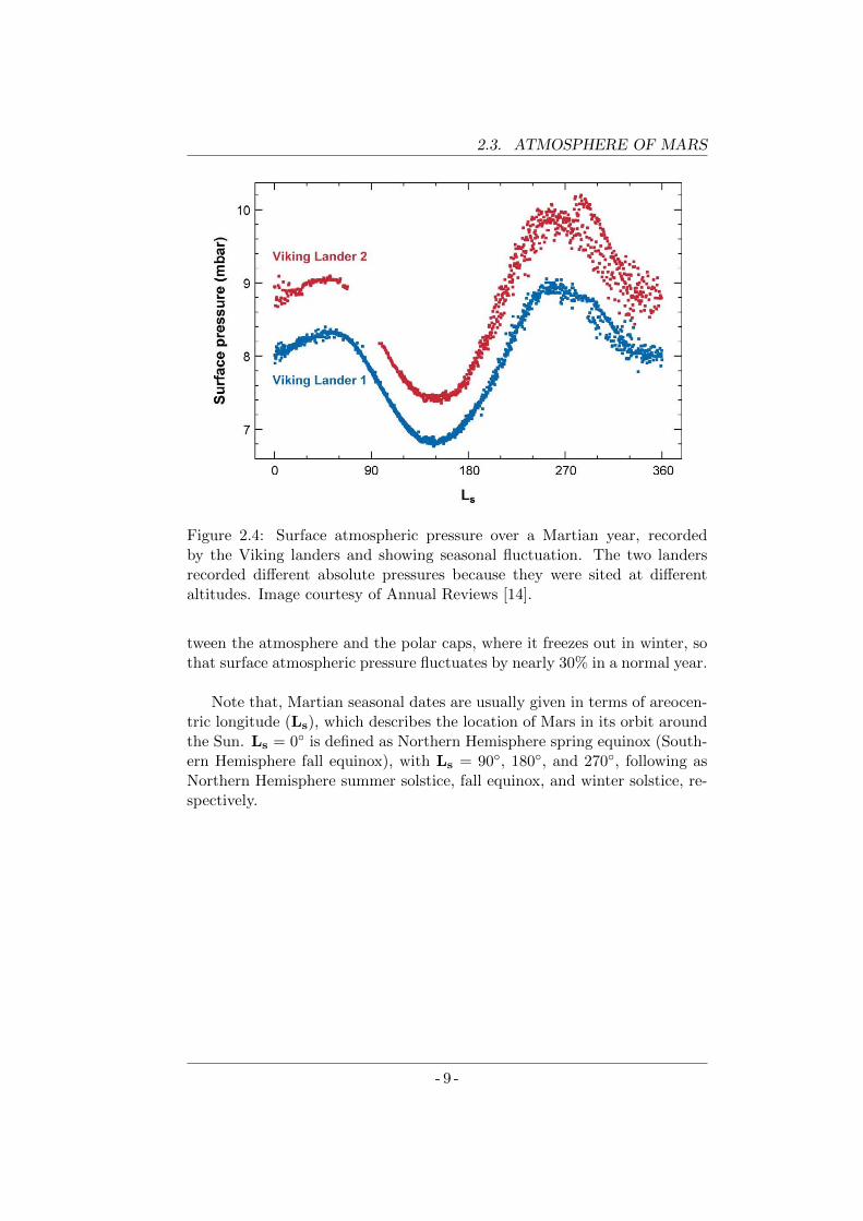
2.4 Surface atmospheric pressure over a Martian year, recordedby the Viking landers and showing seasonal fluctuation. Thetwo landers recorded different absolute pressures because theywere sited at different altitudes. Image courtesy of AnnualReviews [14]. . . . . . . . . . . . . . . . . . . . . . . . . . . . 9
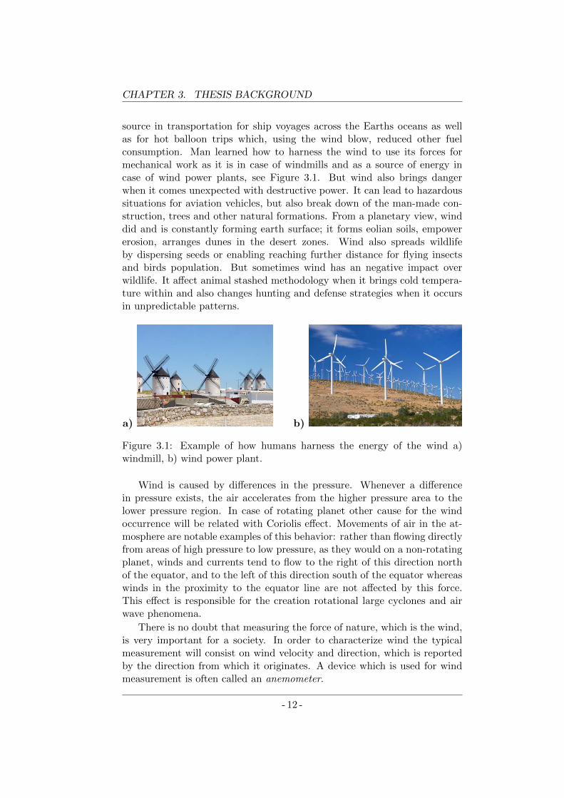
3.1 Example of how humans harness the energy of the wind a)windmill, b) wind power plant. . . . . . . . . . . . . . . . . . 12
3.2 Four different flow regimes according to the Knudsen numbervalue. . . . . . . . . . . . . . . . . . . . . . . . . . . . . . . . 14
3.3 Character of different flow regimes: a) laminar, b) turbulent. 15
3.4 Velocity boundary layer for flow medium continuum regime. . 18
4.1 Mars landing sites for planetary missions: a) Viking 1, b)Viking 2, c) Mars Pathfinder, d) Spirit, e) Opportunity, f)Phoenix, g) Mars Science Laboratory (MSL), superimposedon the topography map of the Red Planet. Courtesy NASA/JPL-Caltech. . . . . . . . . . . . . . . . . . . . . . . . . . . . . . . 26
4.2 First panoramic image of Chryse Planitia taken by camera 1on the Viking 1 Lander. The image was taken on 23 July 1976,three days after Viking 1 landed. The meteorology boom isat the center of the image and to the left is the support forthe high-gain dish antenna, [15]. Courtesy NASA/JPL-Caltech. 27
4.3 Viking wind speed sensor unit. . . . . . . . . . . . . . . . . . 28
xiii
LIST OF FIGURES
4.4 Mars Pathfinder wind sensor unit composed of platinum-iridiumwire wound 7 times fold and attached to the insulating for-mers around circumference cone. Entire 2-D wind senor wasmade out of 6 sensor units equally distributed witch 60 ra-dial step and 3 mm of separation from cylindrical cone shownhere. . . . . . . . . . . . . . . . . . . . . . . . . . . . . . . . . 30
4.5 a) Concept of the three 2-D Wind Transducer (WT) boardslocated in 120 orientation around the boom to form 3-Dwind sensor and enable reconstruction wind magnitude anddirection, b) Universitat Politecnica de Catalunya (UPC) pro-totype, c) CAB engineering model. . . . . . . . . . . . . . . . 31
5.1 The logos of cooperative institutions: a) CAB, b) NationalAeronautics and Space Administration (NASA), c) UPC, d)Finnish Meteorological Institute (FMI), e) for REMS project. 34
5.2 Curiosity rover mast with two booms pointed horizontallyin two different direction with Wind Transducer (WT) po-sition (three for each boom). Image credit: NASA/JPL-Caltech/INTA (Instituto Nacional de Tecnica Aeroespacial). . 35
5.3 Concept of the wind sensor unit with its cold point and hotpoint elements. . . . . . . . . . . . . . . . . . . . . . . . . . . 39
5.4 Sigma-delta closed loop diagram of the REMS wind trans-ducer. Only the blocks associated with one of the hot points(namely hot point C) are shown. . . . . . . . . . . . . . . . . 40
5.5 MSL - REMS wind sensor unit concept . . . . . . . . . . . . 41
5.6 Front view of silicon die with three resistances: Rsens, Rheat,Rdelta and six PADs. . . . . . . . . . . . . . . . . . . . . . . . 42
5.7 Sound of speed and incompressible flow speed limit (0.3 Ma)for Martian (CO2) atmosphere. . . . . . . . . . . . . . . . . . 44
5.8 Typical Martian atmosphere (CO2) parameters variation asa function of temperature: a) thermal conductivity, b) dy-namic viscosity and, c) specific heat, d) Prandtl number withreference to the same Earth AIR atmosphere parameters. . . 45
5.9 Several sets of geometry candidates for wind sensor to Marssurface under Finite Element Method (FEM) simulation. . . . 46
5.10 Concept of the REMS wind sensor geometry of four silicondice array fixed on the Pyrex inverted table in Analysis Sys-tem (ANSYS) finite element method simulation software. . . 47
5.11 Knudsen number calculation . . . . . . . . . . . . . . . . . . 48
5.12 REMS wind sensor unit a) boundary conditions: tempera-ture Thot = 201 K for ANSYS static FEM simulation underthe C02 wind of 10 m/s from southwest direction and ambi-ent temperature Tamb. = 200 K, b) temperature cross sectiongraph for non-compressible flow solution. . . . . . . . . . . . . 48
- xiv -
LIST OF FIGURES
5.13 a) The symmetry of the wind incidence angle in referenceto the square die geometry b) simulation of the hot die con-vection as a function of the wind direction φfor the range of<270 . . . 360>. Convection power has been measured for600 Pa CO2 flow where die temperature was set for 201 K,whereas gas temperature was set for 200 K. . . . . . . . . . . 49
5.14 a) Power convection in function of the wind flow velocity U ,b) example for wind incidence angle φ = 315, CO2 pressure600 Pa where die temperature was set for 201 K and gastemperature was set for 200 K. . . . . . . . . . . . . . . . . . 49
5.15 FEM simulation results of: a) thermal conductance of the dieA as a function of incidence angle and wind speed, b) foursilicon dice array orientation according to the wind incidenceangle directions. . . . . . . . . . . . . . . . . . . . . . . . . . 50
5.16 Thermal conductance for the four hot dice array as a functionof rotation angle for the same wind speed of 10 m/s. . . . . . 51
5.17 Average thermal conductivity for the four dice array, a) as afunction of wind incidence angle for different wind speeds, b)as a function of wind speed, having its variation for full rangeof the rotation angles. . . . . . . . . . . . . . . . . . . . . . . 51
5.18 Combination of thermal conductances a) for terms: North-South and East-West b) and what is their position in functionof the wind incidence angle. . . . . . . . . . . . . . . . . . . . 52
5.19 Angular sensitivity for the hot dice array: A, B, C, D a) asa function of the wind direction (α), b) as a function of thewind velocity (U) . . . . . . . . . . . . . . . . . . . . . . . . . 53
5.20 Angular sensitivity for the the diffential terms North-Southand East-West a) in the function of the wind direction (α),b) in function of the wind velocity (U) . . . . . . . . . . . . . 54
5.21 View of UPC-REMS wind sensor prototype, a) from the topwhere square array dimension is depicted, b) from the per-spective where dice thickness can be see. . . . . . . . . . . . . 54
5.22 Microscope photography of the silicon die of wind transducerafter fabrication: a) type L, b) type N . . . . . . . . . . . . . 55
5.23 Set of photolitograpy masks for UPC-REMS wind sensor chip:a) Mask A - Contact Windows, b) Mask B - Titanium/PlatinumPaths c) Mask C - Pads . . . . . . . . . . . . . . . . . . . . . 57
5.24 Superposition of the three layouts: A, B and C with its perfectalignment a) mask design b) photograph of the real wafer. . . 58
5.25 Silicon Wafer N-Cz 1-10 Ω·cm, thickness 400 um. . . . . . . . 595.26 Silicon oxide, thickness 120 nm. . . . . . . . . . . . . . . . . . 595.27 Thin resin spinning RPM profile. . . . . . . . . . . . . . . . . 605.28 Resin SPR-220 1.2, thickness 1 um. . . . . . . . . . . . . . . . 605.29 First photolithography . . . . . . . . . . . . . . . . . . . . . . 61
- xv -
LIST OF FIGURES
5.30 Contact window opening. . . . . . . . . . . . . . . . . . . . . 61
5.31 Second resin lift-off. . . . . . . . . . . . . . . . . . . . . . . . 61
5.32 Temperature profile of doping. . . . . . . . . . . . . . . . . . 62
5.33 Bulk doping with impurities type N. . . . . . . . . . . . . . . 62
5.34 Silicon wafer after second resin step. . . . . . . . . . . . . . . 62
5.35 Second photolithography. . . . . . . . . . . . . . . . . . . . . 62
5.36 Pattern engrave in silicon dioxide. . . . . . . . . . . . . . . . 63
5.37 Titanium sputtering, thickness 10 nm. . . . . . . . . . . . . . 63
5.38 Platinum sputtering, thickness 70 nm. . . . . . . . . . . . . . 64
5.39 Second resin lift-off. . . . . . . . . . . . . . . . . . . . . . . . 64
5.40 Thick resin spinning RPM profile. . . . . . . . . . . . . . . . 65
5.41 Resin SPR-220 7.0, thickness 7 um. . . . . . . . . . . . . . . . 65
5.42 Third photolithography. . . . . . . . . . . . . . . . . . . . . . 65
5.43 Platinum sputtering for PADs, thickness 100 nm. . . . . . . . 66
5.44 Third resin lift-off. . . . . . . . . . . . . . . . . . . . . . . . . 66
5.45 New fabricated wind sensor chips on a silicon wafer. ImageCourtesy: Dr. Jordi Ricart. . . . . . . . . . . . . . . . . . . . 67
5.46 Geometry and position of the resistances Rsens, Rheat and∆R according to the type of the dice. . . . . . . . . . . . . . 68
5.47 Example of Rheat distribution along the silicon wafer. Re-sistance has been measured in laboratory temperature con-ditions ∼25C. Circular pattern results from rotatory baseequipment during platinum raw material sputtering process. . 69
5.48 Measurement of temperature-dependent titanium/platinumthin film resistance as a function of temperature, with itsperfect match by lineal approximation function. . . . . . . . . 70
5.49 Square dice after cutting procedure with nominal size of 1675 um± 10 um. . . . . . . . . . . . . . . . . . . . . . . . . . . . . . 70
5.50 Photography of the 2-D wind sensor. . . . . . . . . . . . . . . 71
5.51 Difference in numbers of dice wire-bonding according to thea) hot point b) cold point. . . . . . . . . . . . . . . . . . . . . 71
5.52 Basic diagram of the assembled sensor with PCB, pyrex sup-port, oxidized silicon chip with Titanium/Platinum resistanceson it and gold wire bonding. . . . . . . . . . . . . . . . . . . . 72
5.53 Custom desind PCB base a) front view with visible pin-out,b) rear view. . . . . . . . . . . . . . . . . . . . . . . . . . . . 73
5.54 Pyrex support inverted table shape a) lateral view, b) dimen-sions. . . . . . . . . . . . . . . . . . . . . . . . . . . . . . . . . 73
5.55 Schematic of the 4x7 wire bonding for the hot element arrayplus 2 wires for the reference die at the bottom of the figure. 74
5.56 Block diagram of the electro-thermal sigma-delta converterfor ther REMS wind sensor die. . . . . . . . . . . . . . . . . . 75
- xvi -
LIST OF FIGURES
5.57 Close loop mode circuit to maintain constant temperatureoverheat of the hot element in reference to the ambient tem-perature, where reference die is located. . . . . . . . . . . . . 78
5.58 Electronic circuit board implemented electro-thermal sigma-delta control. . . . . . . . . . . . . . . . . . . . . . . . . . . . 80
5.59 Overheat as a function of ambient temperature for particularresistance set. . . . . . . . . . . . . . . . . . . . . . . . . . . . 81
5.60 Schematic diagram of hot volume convection model. . . . . . 82
5.61 Isothermal conductance curves in the 2-D graph as a functionof air temperature and mass flow product. . . . . . . . . . . . 85
5.62 Numerical simulation of four hot dice structure for Pamb. = 600 Pa,Tamb. = 220 K and U = 10 m/s. . . . . . . . . . . . . . . . 86
5.63 Static FEM simulation of the REMS wind sensor unit underconstant heat convection cooling, a) Temperature solution, b)Heat flow channels. . . . . . . . . . . . . . . . . . . . . . . . . 88
5.64 Close look for the FEM simulation of the REMS chip underconstant heat convection cooling, a) up the surface , b) downthe surface. . . . . . . . . . . . . . . . . . . . . . . . . . . . . 89
5.65 Wind tunnel facilities: a) rotating arm, b) re-circulating, c)open circuit, d) linear. Wind sensor under test has been sym-bolised by the red hot ball on the green support, where arrowsrepresent either movement of the flow or wind sensor unit. . . 90
5.66 REMS wind 2-D transducer set up inside Aarhus AWSTIwind tunnel facility. . . . . . . . . . . . . . . . . . . . . . . . 92
5.67 Averaged power dissipated per silicon die to the ambient tem-perature CO2 at 6 mBar a) raw data as sampled with fre-quency of 1 Hz b) as a function of the wind velocity andincidence angle (φ). . . . . . . . . . . . . . . . . . . . . . . . . 93
5.68 Visual interpretation of the data from Table 5.5. . . . . . . . 95
5.69 Averaged power delivered to the four dice structure as a func-tion of a) velocity, b) velocity by pressure product. . . . . . . 96
5.70 Power delivered to the four dice A, B, C, D as a function ofvelocity by pressure product. . . . . . . . . . . . . . . . . . . 96
5.71 Thermal conductance in result of the steep change in directionof the wind yaw angle (from -20 degree to +20 degree and thenback to the -20 degree). Measurement conditions: carbondioxide pressure 6 mBar, ambient temperature -50C , hotpoint overheat 23C, wind speed 10 m/s. . . . . . . . . . . . . 97
5.72 Prototype of the REMS wind sensor boom set-up for experi-ments inside Oxford open circuit wind tunnel chamber . . . . 98
5.73 Orientation of the REMS boom and its three Wind Trans-ducer (WT) boards for the Yaw = 0 and Pitch = 0 . . . . 99
- xvii -
LIST OF FIGURES
5.74 Longitude thermal conductance (Gth) differential term: North−South=(A+D)−(B+C) for three WT board of REMS boomprototype as a function of a) wind velocity b) wind velocityand pressure product. Experiment was run for three ambientpressure 5, 6 and 7 mBar and same temperature and overheatconditions . . . . . . . . . . . . . . . . . . . . . . . . . . . . . 100
5.75 1-D model of wind sensors from different Mars planetary mis-sions: a) Viking, b) Pathfinder, c) MSL-REMS. . . . . . . . 101
5.76 Temperature profile for 1-D thermal model solution for anemome-ters at Mars conditions (h = 80 W/(m2K) and Tamb = 300 K).The typical overheat values for Viking 100 K, for Pathfinder10 K and for REMS 30 K can also be deduced from this plot. 104
5.77 Temperature profile for the 1-D thermal model of hot sili-con REMS die according to the die boundary conditions (bc)considered. . . . . . . . . . . . . . . . . . . . . . . . . . . . . 105
5.78 Comparison of the three wind sensor: Viking, Pathfinder andREMS in a) total power and b) overheat for whole wind veloc-ity range specified for each sensor and at given atmosphericconditions (P = 670 Pa, T = 220 K). . . . . . . . . . . . . . 107
5.79 Comparison of the three wind sensor: Viking, Pathfinder andREMS in total power to overheat ratio as a function of theReynolds number for whole wind velocity range specified foreach sensor and at given atmospheric conditions. . . . . . . . 108
5.80 Space design of the three thermal anemometers used in Marsplanetary mission in comparison of the Kn regime and P∆Tratio for any possible variation of Martian conditions: pres-sure, temperature and flow velocity. Single unit and globalwind sensor are shown for clarification. . . . . . . . . . . . . . 109
5.81 Viking, Pathfinder and REMS wind sensor units in compar-ison for velocity range from 2 to 50 m/s for Martian atmo-sphere conditions adjust to: pressure 600 Pa and tempera-ture 300 K. Different working behaviour for these three ther-mal anemometers have been reflected in a) power demand, b)temperature overheat, c) power to overheat ratio. . . . . . . . 110
6.1 Spherical thermal anemometer concept of the hot point work-ing with overheat to the wind ambient temperature. . . . . . 117
6.2 Heat convection proportional to the root square of the windspeed and to the overheat value. . . . . . . . . . . . . . . . . 118
6.3 Heat delivered to the sensor surface split into three compo-nent of convection, conduction and radiation. . . . . . . . . . 119
6.4 Reynolds Number as a function of flow velocity for givensphere diameter (D). . . . . . . . . . . . . . . . . . . . . . . . 120
- xviii -
LIST OF FIGURES
6.5 Measurement maximal and minimal wind velocity limit onMars as a function of ambient temperature for hot sphereanemometer (D = 9 mm) working with constant overheat∆T = 20 K. . . . . . . . . . . . . . . . . . . . . . . . . . . . . 122
6.6 Thermal conductance of the overheated sphere as function offlow velocity for Mars-like atmospheric condition. . . . . . . . 123
6.7 Mesh geometry of the sphere skin and the cylindrical volume. 125
6.8 Local heat flux, H [W/m2K] over the 20 K overheated spheresurface with regard to the CO2 wind flow velocity of 7 m/sincoming from −~Z direction. . . . . . . . . . . . . . . . . . . 125
6.9 Spherical coordinates system. . . . . . . . . . . . . . . . . . . 126
6.10 a) Local heat flux, H approximation for sphere position as afunction of φ angle; b) function of Z coordinate forD = 15 mmPCO2 = 650 Pa, Tamb = 220 K, Tsurf = 240 K, Uf = 7 m/s . 127
6.11 Euler Rotation Angles . . . . . . . . . . . . . . . . . . . . . . 128
6.12 Thermal conductance Gth [mW/K] for different sector shapesand possible 3-D wind direction angle for wind flow Uflow = 7 m/sof PCO2 = 650 K and Tamb = 220 K, Tsurf = 240 K; a) twohemispheres, b) the eighth of the sphere. . . . . . . . . . . . . 130
6.13 Total convection heat for sphere as a function of wind mag-nitude for three ambient temperatures . . . . . . . . . . . . . 131
6.14 Thermal conductance for the whole sphere as a function ofthe wind speed. Empirical model based on Feng&Michaelides(F&M) compared to FEM simulation results . . . . . . . . . 132
6.15 Local heat flux at any point of a sphere as a function of angleΘ for wind incidence angle to be from −~Z direction . . . . . 133
6.16 a) Physical model of spherical shell division based on tetrahe-dron geometry into separated from each other four triangularsectors, b) real model has been made out in 3D printing tech-nology from ABS material with upscale 5:1 (1 cent coin addedfor size reference). Sectors: #1, #3, #4 can be seen from thepicture, whereas sector #2 is in the rear of the plot. Sectorsorientation, according to the Cartesian coordinate system, isshown as well as theoretical wind incidence point (representedby black dot) described with polar angles Θ and Φ. . . . . . . 134
6.17 Percentage of the total sphere convection heat rate trans-ferred to the ambient by the triangular sector #1 as functionof the wind direction angles (Θ, Φ). Values produced fromthe simulation data presented in Figure 6.15 according to thesector #1 orientation shown in Fig. 6.16. . . . . . . . . . . . . 135
6.18 Percentage of the total sphere convection heat rate which goesto the each of the four sectors as a function of wind angle Φ,for Θ=90. . . . . . . . . . . . . . . . . . . . . . . . . . . . . 135
- xix -
LIST OF FIGURES
6.19 Angular sensitivity plots for two type of spherical geometriesdivision into four equal sectors. Traditional biangle tessel-lation has been contrasted with a tetrahedral division. SΘ
and SΦ for both geometries and wind speed of 5m/s can beobserved for Φ rotation range 0 to 90 and for Θ=90. . . . 136
6.20 Angular sensitivity plots for tetrahedral sphere division a) SΘ
b) SΦ. Analysis was done for particular ambient conditions:Tamb = 220 K, Uflow = 5 m/s, ∆T = 20 K . . . . . . . . . . 137
6.21 Minimum angular sensitivity analysis of tetrahedral spherestructure working in CO2 600Pa atmosphere as a function ofwind speed and for different ambient temperatures scenarioat constant overheat 20C. . . . . . . . . . . . . . . . . . . . 138
6.22 Percentage heat rate solution for 3-D incidence angel example(ΘEx, ΦEx) together with other wind angle possibility thatsatisfies this particular share of each from the tetrahedral sec-tors. . . . . . . . . . . . . . . . . . . . . . . . . . . . . . . . . 139
6.23 Wind incidence angle discrimination from Computational FluidDynamics (CFD) simulation model of the power delivered tofour triangular sectors, a) the Iso-percentage curves were su-perposed in order appoint cross section zone, b) the final windincidence angle point (Θ, Φ), was determined by minimizingan error function. . . . . . . . . . . . . . . . . . . . . . . . . . 139
6.24 Models of the spherical wind sensor components, a) triangu-lar sector with its interior heat resistor mold, b) PCB withelectrical layout and central core resistor, c) union of the twoPCB’s were mechanical support and electrical wiring are pro-vided for each sector, d) four triangular sectors assembly. . . 141
6.25 Pictures of wind sensor triangular sectors, a) made out ofSilver Sterling material (alloy Au 92.5%, Cu 7.5%) in a stere-olithography 3-D printing commercial process, b) after tum-bler polishing operations with progressive grit, c) after goldthin film (100 nm) deposition on the outer surface. . . . . . . 142
6.26 Picture of the spherical ’tetrahedral’ wind sensor prototype,a) in the upside-down position for the wind tunnel chamber,b) in a perspective view after measurements in a Mars-likeconditions. . . . . . . . . . . . . . . . . . . . . . . . . . . . . . 143
6.27 a) Aarhus Mars wind tunnel facility AWTSI when opened b)3-D hot sphere wind sensor setup with yaw rotation angledegree of freedom . . . . . . . . . . . . . . . . . . . . . . . . . 144
- xx -
LIST OF FIGURES
6.28 Power delivered to the sectors, a) for different wind veloci-ties and for wind direction angle Φ sequence [45, 75, 90,105, 135], b) zoom on the section where the wind velocitywas 7m/s and only wind direction sequence is on display. CO2
atmosphere at P = 10 mBar and Tamb = -18C conditions,for Θ = 90 and overheat ∆T = 40C. . . . . . . . . . . . . . 144
6.29 Polar plot of the average power delivered to the four sectors:a) sector #1, b) sector #2, c) sector #3, d) sector #4 asfunction of the wind speed and wind direction angle Φ, forΘ = 90. . . . . . . . . . . . . . . . . . . . . . . . . . . . . . . 145
6.30 Raw measurements of total power delivered to the spherefor different wind speed blowing from direction Φ = 45 andΘ = 90 together with mean power value calculated for eachwind direction slot. . . . . . . . . . . . . . . . . . . . . . . . . 146
6.31 Mean power delivered to each sector and total sphere demandas a function of the wind speed for wind direction Θ = 90
and Φ = 45. Data selected from the Figure 6.28, whereasCFD curve was added from multi-physic numerical simulationfor the same ambient parameters . . . . . . . . . . . . . . . . 147
6.32 Wind incidence angle discrimination from the real measure-ment of the power delivered to four triangular sectors. Iso-percentage curves were superposed in order appoint cross sec-tion zone. Final wind incidence angle point (Θ, Φ) was de-termined by minimizing an error function. . . . . . . . . . . . 149
- xxi -

List of Tables
2.1 Orbital information about Mars and Earth, [16]. . . . . . . . 52.2 Planetary information about Mars in comparison to Earth, [16]. 62.3 Atmosphere’s parameters of Mars and Earth, [16] . . . . . . 72.4 Atmospheric composition of Mars and Earth, [16,17]. . . . . 7
5.1 Scientific requests for the REMS instruments, [18] . . . . . . 365.2 Measurement table of resistances Rsens, Rheat and ∆R resis-
tances for several dice type L and type N at ambient temper-ature ∼25C. . . . . . . . . . . . . . . . . . . . . . . . . . . . 67
5.3 Table of overheat value for ambient temperature at 0C, wherechip resistance parameters are as follow: Rref0 = 7000 Ω,∆RA,B,C,D = 700 Ω and α = 0.003 /C. . . . . . . . . . . . . 81
5.4 Domains and equtions . . . . . . . . . . . . . . . . . . . . . . 885.5 Averaged power of each from four hot dice array: PA, PB,
PC , PD with its differential therms: North-South (N -S) andEast-West (E-W ) for different wind flow velocity (Uflow) andyaw (φ) incidence angle. . . . . . . . . . . . . . . . . . . . . 94
5.6 Main parameters of thermal unit elements (NA - Not Appli-cable). . . . . . . . . . . . . . . . . . . . . . . . . . . . . . . . 102
5.7 Comparison of the wind sensor system for Viking [19, 20],Pathfinder [21,22] and MSL-REMS [9]. *Power consumptiondata has been calculated according to the first order modelproposed in Section (5.10.1) for CO2 atmosphere: 300K, 600Pa,50m/s. . . . . . . . . . . . . . . . . . . . . . . . . . . . . . . 112
6.1 FEM simulation conditions and geometry parameters. . . . . 1246.2 FEM simulation boundary conditions . . . . . . . . . . . . . 1246.3 Percentage heat rate share . . . . . . . . . . . . . . . . . . . . 1386.4 Measurement conditions. . . . . . . . . . . . . . . . . . . . . . 1446.5 Percentage power share from measurements. . . . . . . . . . . 148
xxiii


Glossary
ANSYS Analysis System. xiv, 43, 44, 46
ASI/MET Atmospheric Structure Instrument/Meteorology Packaged. 28
ASIC Application Specific Integrated Circuit. 79, 146, 157
ATS Air Temperature Sensor. 37
CAB Center of Astrobiology. vii, xiv, 1, 30, 33, 34, 90, 157
CCA Constant Current Anemometry. 22, 29, 87, 103, 112
CFD Computational Fluid Dynamics. xx, xxi, 33, 43, 46, 84, 85, 128, 132,137, 138, 139, 140, 147, 148, 150, 151, 153, 155, 158
CNM Centro Nacional de Microelectronica. vii, 73
COMSOL Computers and Solutions. 87, 147
CPA Constant Power Anemometry. 22, 29, 154
CRISA Computadoras, Redes e Ingenierıa , S.A.U.. 72, 90
CSIC Consejo Superior de Investigaciones Cientficas. 33, 90
CTA Constant Temperature Anemometry. 22, 23, 27, 43, 45, 103, 112,118, 146, 151, 153, 154
CTDA Constant Temperature Difference Anemometry. 23, 43, 79, 103,109, 112, 153, 154
CVA Constant Voltage Anemometry. 22
DS Dust Sensor. 115
DSMC Direct Simulation Monte Carlo. 14
FEM Finite Element Method. x, xiv, xv, xvii, xix, xxiii, 43, 44, 45, 46, 50,80, 85, 86, 87, 88, 89, 92, 118, 123, 124, 132, 152
xxv
Glossary
FMI Finnish Meteorological Institute. xiv, 33, 37, 115
GTS Ground Temperature Sensor. 36
HS Humidity Sensor. 37
ICU Instrument Control Unit. 35, 37
IKI Russian Space Research Institute. 115
INTA Instituto Nacional de Tecnica Aeroespacial. vii, 2, 33, 90, 115, 157
JPL Jet Propultion Laboratory. 1, 33, 34, 35
LA Lavochkin Association. 115
LDA Laser Doppler Anemometry. 92
MEDA Mars Environmental Dynamics Analyzer. 1, 157
MEIGA Mars Environmental Instrumentation for Ground and Atmosphere.x, xi, 2, 115, 116, 117, 149, 154
MetNet Meteorological Network. 2, 115, 154
MMPM Mars MetNet Precursor Mission. 149
MNL MetNet Lander. 115
MNT Micro and Nanotechnology. 38, 45, 55, 68, 110, 111, 115, 149, 150,151, 154, 157
MSL Mars Science Laboratory. xiii, xiv, xviii, xxiii, 1, 25, 29, 30, 33, 41,45, 68, 100, 111, 112, 151, 157
NASA National Aeronautics and Space Administration. xiv, 1, 25, 33, 38,111
PCB Printed Circuit Board. x, 37, 41, 54, 72, 73, 74, 79, 93, 146, 153, 154,157, 158
PS Pressure Sensor. 37
REMS Rover Environmental Monitoring Station. ix, x, xiv, xv, xvi, xvii,xviii, xxiii, 1, 2, 30, 33, 34, 35, 36, 37, 38, 39, 40, 41, 43, 46, 55, 56,68, 75, 76, 79, 88, 89, 90, 92, 96, 97, 98, 99, 100, 102, 103, 104, 106,107, 108, 109, 111, 112, 116, 117, 149, 151, 154, 156, 157
- xxvi -
Glossary
RSM Remote Sensing Mast. 35
SIS Solar Irradiance Sensor. 115
SWS Spherical Wind Sensor. 115
UPC Universitat Politecnica de Catalunya. xiv, xv, 30, 33, 34, 38, 45, 54,55, 56, 68, 72, 111, 112, 149, 150, 152, 157
USA United States of America. 25
USSR Union of Soviet Socialist Republics. 25
UVS Ultraviolet Sensor. 37
WS Wind Sensor. 30, 37
WT Wind Transducer. xiv, xvii, 30, 34, 37, 38, 39, 40, 72, 98, 99
- xxvii -

Chapter 1
Introduction
The thermal anemometry is a method which allows to estimate wind mag-nitude be the mean of measuring heat transfer to the ambient in a forcedconvection process. For Earth’s atmosphere condition, this method is typ-ically applied to the hot wires made of temperature dependent electricalconductor, typically platinum or tungsten, which working with overheat inreference to the ambient temperature estimate wind velocity. In the caseof the low-pressure atmospheres, like this on Mars, the mean free path formolecules, due to the rarefied ambient conditions, is much bigger. Usinghot wires designed for Earth in this conditions gives that heat exchange ata macroscopic scale which does not to obey medium continuum model butrather reveals ballistic behavior. Thus, instead of using hot wire, a struc-ture of bigger dimension like hot films are usually proposed for such a kindof application. The work included in this thesis is the contribution of theauthor Lukasz Kowalski to the goal of developing a new generation of windsensors for the atmosphere of Mars. The work consists in the conception,design, simulation, manufacture and measurement of two novel types windsensors based on thermal anemometers. Some aspects of the work duringthe development of this thesis has been reflected in author’s paperwork likepatent, articles and conference proceedings shown in references [1–12].
The first kind of concept has been developed in this thesis by using hotsilicon die made out of silicon wafer of approximate size: 1.5 x 1.5 x 0.5 mmwith platinum resistances deposited on top in order to heat it and senseits temperature. These work was been a part of the bigger undertakingunder the project CYCYT: ”Colaboracion en el desarrollo de la estacionmedioambiental denominada REMS ” (Ref. C05855). Inside the projectREMS author of the thesis was responsible for sensor shape developmentand concept validation of proposed geometry. Thermal-fluidical model ofthe device, as well as characterization and behavior, were analyzed for asimplified 2-D wind model for typical Martian atmospheric conditions. Theleader of the project Center of Astrobiology (CAB) was in charge of extrap-
1
CHAPTER 1. INTRODUCTION
olated 2-D model results into a full 3-D model by placing six 2-D sensorson two supporting booms. The use of six independent 2-D measurementsprovides enough redundancy for the use of an inverse algorithm to estimate3-D wind parameters. REMS was a Spanish contribution to the NASA mis-sion MSL which has been a great success since rover Curiosity has landedon Mars on 6th August 2012 (1:32 a.m. Eastern Standard Time) at thefoot of a layered mountain inside Gale Crater. Since then has been con-stantly running experiments on the Red Planet sending data to Earth forinterpretation. Currently, author of the thesis is participating in similarJet Propultion Laboratory (JPL) mission Mars 2020, where aboard of thenew Rover will be Spanish instrument Mars Environmental Dynamics An-alyzer (MEDA) incorporating new improved in performance and efficiencywind sensor build out of similar silicon hot die units as it was in the caseof REMS. This project is in its beginning phase and won’t be addressed inthis document.
From the experience and knowledge gained during REMS project, theauthor came out with an idea of the novel spherical sensor structure over-coming some fragility problems detected in the REMS wind sensor. Thenew 3-D wind sensor concept, besides this advantage, also provided a radi-cal simplification of data post-processing providing the comprehensive ther-mal model based on numerical simulation for any possible wind occurrence.This new device has been developed under Spanish Ministry of the Scienceand Innovation project: ”Sensor de viento para la superficie de Marte parala mission Metnet (fase inicial)” (Ref. AYA-2010-20847) and ”Sensor deviento para la superficie de Marte para la mission Meteorological Network(MetNet) (Modelo de Ingenieria)” (Ref. AYA-2011-29967-C05-04). Thisproject, denominated as MEIGA, was a join effort of many Spanish institu-tions under the leadership of INTA for the development of space technologyfor Mars-oriented application in a framework of an upcoming space mission.
To sum up, author’s work include contributions to the development oftwo wind sensor concepts:
• REMS wind sensor on board of the rover Curiosity in the surfaceof Mars since August 6th 2012, that is described in paperwork [1–9](Appendix A, Appendix B, Appendix C, Appendix D, Appendix E,Appendix F, Appendix G, Appendix H).
• Spherical wind sensor concept developed in a course of MEIGA projectand described in paperwork [10–12] (Appendix I, Appendix L).
- 2 -
Chapter 2
Mars We Know
The main objective of this chapter is to present information about planetMars, so the reader will understand the need of further in-situ exploration ofthe Red Planet. Up to date, knowledge of this land is wide and comprehen-sive, extensively published, [23–25]. Some chosen facts, related to this thesiswill be presented. In the first section I will describe Mars position insidethe Solar System. In the second section I will present the most importantdetails about geology and Mars landscape. Finally in the third section Iwill give information about Martian climate. Although Mars is one of thecloser celestial body in our terrestrial neighborhood is different to our nat-ural environment we human live in, so it is logical that in many occasionsit’s parameters will be contrasted with the Earth’s ones.
2.1 Orbit of Mars
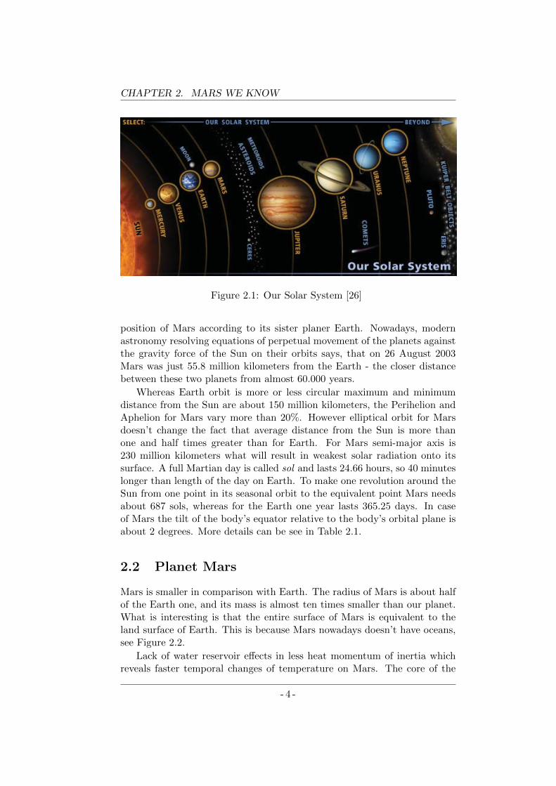
Mars is the fourth planet of our Solar System situated in between the Earthand the much bigger Jupiter, see figure 2.1.
We were aware of it existence from the prehistoric times. Ancient Greekscalled the red-bloody spot on the sky Ares, as their god of war, whereas forRomans it was Mars also named after the god of war. Status of planetcomes from Greek word planetes which means wanderer. Mars togetherwith Mercury, Jupiter and Saturn gained their migrant status as observedfrom the ground the trajectories of these shinny points on the sky were notin shape with the fixed stars on the firmament. What’s more, the disorderedmovement of Mars was identified with a chaos during times of war, [27]. Theother thing that has been noticed for Mars, as seen from Earth, was that hisbrightness is not at the constant level. These two intriguing question of Marsbehavior have been resolved not sooner as his orbit had been revealed. Whatin the past geocentric theories was believed to have mysterious character andbe assign to the over-natural phenomena today is well known and thanks tothe modern heliocentric solar system model it is easy to calculate relative
3
CHAPTER 2. MARS WE KNOW
Figure 2.1: Our Solar System [26]
position of Mars according to its sister planer Earth. Nowadays, modernastronomy resolving equations of perpetual movement of the planets againstthe gravity force of the Sun on their orbits says, that on 26 August 2003Mars was just 55.8 million kilometers from the Earth - the closer distancebetween these two planets from almost 60.000 years.
Whereas Earth orbit is more or less circular maximum and minimumdistance from the Sun are about 150 million kilometers, the Perihelion andAphelion for Mars vary more than 20%. However elliptical orbit for Marsdoesn’t change the fact that average distance from the Sun is more thanone and half times greater than for Earth. For Mars semi-major axis is230 million kilometers what will result in weakest solar radiation onto itssurface. A full Martian day is called sol and lasts 24.66 hours, so 40 minuteslonger than length of the day on Earth. To make one revolution around theSun from one point in its seasonal orbit to the equivalent point Mars needsabout 687 sols, whereas for the Earth one year lasts 365.25 days. In caseof Mars the tilt of the body’s equator relative to the body’s orbital plane isabout 2 degrees. More details can be see in Table 2.1.
2.2 Planet Mars
Mars is smaller in comparison with Earth. The radius of Mars is about halfof the Earth one, and its mass is almost ten times smaller than our planet.What is interesting is that the entire surface of Mars is equivalent to theland surface of Earth. This is because Mars nowadays doesn’t have oceans,see Figure 2.2.
Lack of water reservoir effects in less heat momentum of inertia whichreveals faster temporal changes of temperature on Mars. The core of the
- 4 -

2.2. PLANET MARS
Mars Earth Mars/Earth
Semi-major axis, 106 km 227.92 149.60 1.524Perihelion, 106 km 206.62 147.09 1.405Aphelion, 106 km 249.23 152.10 1.639Sidereal orbit period, days 686.980 365.256 1.881Tropical orbit period, days 686.973 365.242 1.881Mean orbital velocity, km/s 24.13 29.78 0.810Max. orbital velocity, km/s 26.50 30.29 0.875Min. orbital velocity, km/s 21.97 29.29 0.750Orbit inclination, deg 1.850 0.000 −Orbit eccentricity 0.0935 0.0167 0.599Sidereal rotation period, hrs 24.6229 23.9345 1.029Length of day, hrs 24.6597 24.0000 1.027Obliquity to orbit deg 25.19 23.45 1.074
Table 2.1: Orbital information about Mars and Earth, [16].
EARTH
MARS
MOON
Figure 2.2: Earth, Mars and Moon in the same scale, [13].
- 5 -
CHAPTER 2. MARS WE KNOW
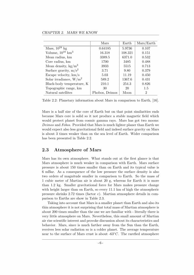
Mars Earth Mars/Earth
Mass, 1024 kg 0.64185 5.9736 0.107Volume, 1010 km3 16.318 108.321 0.151Mean radius, km 3389.5 6371.0 0.532Core radius, km 1700 3485 0.488Mean density, kg/m3 3933 5515 0.713Surface gravity, m/s2 3.71 9.80 0.379Escape velocity, km/s 5.03 11.19 0.450Solar irradiance, W/m2 589.2 1367.6 0.431Black-body temperature, K 210.1 254.3 0.826Topographic range, km 30 20 1.5Natural satellites Phobos, Deimos Moon 2
Table 2.2: Planetary information about Mars in comparison to Earth, [16].
Mars is a half size of the core of Earth but on that point similarities endsbecause Mars core is solid so it not produce a stable magnetic field whichwould protect planet from cosmic gamma rays. Mars has got two moons:Deimos and Fobos. Provided that Mars is much lighter planer than Earth wewould expect also less gravitational field and indeed surface gravity on Marsis about 3 times weaker than on the sea level of Earth. Wider comparisonhas been presented in Table 2.2.
2.3 Atmosphere of Mars
Mars has its own atmosphere. What stands out at the first glance is thatMars atmosphere is much weaker in comparison with Earth. Mars surfacepressure is about 150 times smaller than on Earth and its typical value is6 mBar. As a consequence of the low pressure the surface density is alsotwo orders of magnitude smaller in comparison to Earth. So the mass of1 cubic meter of Martian air is about 20 g, whereas for Earth it is morethan 1.2 kg. Smaller gravitational force for Mars makes pressure changewith height larger than on Earth, so every 11.1 km of high the atmosphericpressure shrinks 2.72 times (factor e). Martian atmosphere details in com-parison to Earths are show in Table 2.3.
Taking into account that Mars is a smaller planet than Earth and also itsthin atmosphere it is not surprising that total mass of Martian atmosphere isabout 200 times smaller than the one we are familiar with - literally there isvery little atmosphere on Mars. Nevertheless, this small amount of Martianair rise scientific interest and provoke discussion about its characteristics andbehavior. Mars, since is much farther away from the Sun than the Earth,receives lees solar radiation so is a colder planet. The average temperaturenear to the surface of Mars crust is about -63C. The rarefied atmosphere
- 6 -
2.3. ATMOSPHERE OF MARS
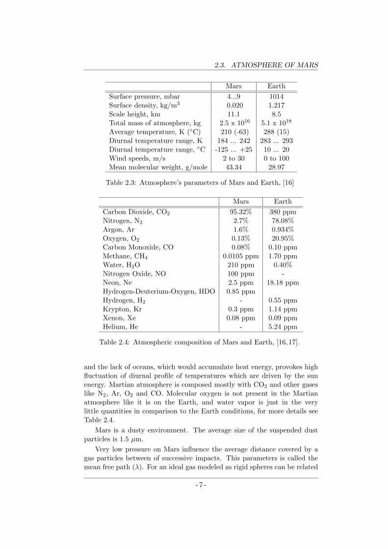
Mars Earth
Surface pressure, mbar 4...9 1014Surface density, kg/m3 0.020 1.217Scale height, km 11.1 8.5Total mass of atmosphere, kg 2.5 x 10¹⁶ 5.1 x 10¹⁸
Average temperature, K (C) 210 (-63) 288 (15)Diurnal temperature range, K 184 ... 242 283 ... 293Diurnal temperature range, C -125 ... +25 10 ... 20Wind speeds, m/s 2 to 30 0 to 100Mean molecular weight, g/mole 43.34 28.97
Table 2.3: Atmosphere’s parameters of Mars and Earth, [16]
Mars Earth
Carbon Dioxide, CO2 95.32% 380 ppmNitrogen, N2 2.7% 78.08%Argon, Ar 1.6% 0.934%Oxygen, O2 0.13% 20.95%Carbon Monoxide, CO 0.08% 0.10 ppmMethane, CH4 0.0105 ppm 1.70 ppmWater, H2O 210 ppm 0.40%Nitrogen Oxide, NO 100 ppm -Neon, Ne 2.5 ppm 18.18 ppmHydrogen-Deuterium-Oxygen, HDO 0.85 ppmHydrogen, H2 - 0.55 ppmKrypton, Kr 0.3 ppm 1.14 ppmXenon, Xe 0.08 ppm 0.09 ppmHelium, He - 5.24 ppm
Table 2.4: Atmospheric composition of Mars and Earth, [16,17].
and the lack of oceans, which would accumulate heat energy, provokes highfluctuation of diurnal profile of temperatures which are driven by the sunenergy. Martian atmosphere is composed mostly with CO2 and other gaseslike N2, Ar, O2 and CO. Molecular oxygen is not present in the Martianatmosphere like it is on the Earth, and water vapor is just in the verylittle quantities in comparison to the Earth conditions, for more details seeTable 2.4.
Mars is a dusty environment. The average size of the suspended dustparticles is 1.5 µm.
Very low pressure on Mars influence the average distance covered by agas particles between of successive impacts. This parameters is called themean free path (λ). For an ideal gas modeled as rigid spheres can be related
- 7 -
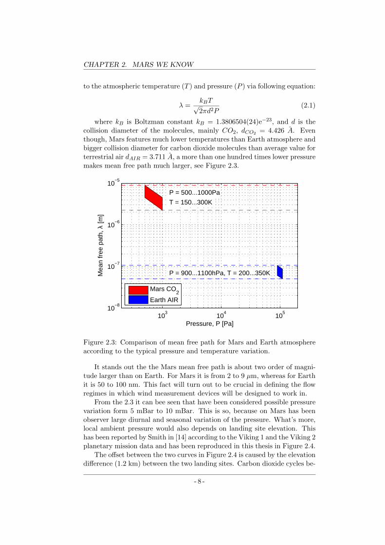
CHAPTER 2. MARS WE KNOW
to the atmospheric temperature (T ) and pressure (P ) via following equation:
λ =kBT√2πd2P
(2.1)
where kB is Boltzman constant kB = 1.3806504(24)e−23, and d is thecollision diameter of the molecules, mainly CO2, dCO2 = 4.426 A. Eventhough, Mars features much lower temperatures than Earth atmosphere andbigger collision diameter for carbon dioxide molecules than average value forterrestrial air dAIR = 3.711 A, a more than one hundred times lower pressuremakes mean free path much larger, see Figure 2.3.
103
104
105
10−8
10−7
10−6
10−5
Pressure, P [Pa]
Mea
n fr
ee p
ath,
λ [m
]
P = 500...1000Pa
T = 150...300K
P = 900...1100hPa, T = 200...350K
Mars CO2
Earth AIR
Figure 2.3: Comparison of mean free path for Mars and Earth atmosphereaccording to the typical pressure and temperature variation.
It stands out the the Mars mean free path is about two order of magni-tude larger than on Earth. For Mars it is from 2 to 9 µm, whereas for Earthit is 50 to 100 nm. This fact will turn out to be crucial in defining the flowregimes in which wind measurement devices will be designed to work in.
From the 2.3 it can bee seen that have been considered possible pressurevariation form 5 mBar to 10 mBar. This is so, because on Mars has beenobserver large diurnal and seasonal variation of the pressure. What’s more,local ambient pressure would also depends on landing site elevation. Thishas been reported by Smith in [14] according to the Viking 1 and the Viking 2planetary mission data and has been reproduced in this thesis in Figure 2.4.
The offset between the two curves in Figure 2.4 is caused by the elevationdifference (1.2 km) between the two landing sites. Carbon dioxide cycles be-
- 8 -
2.3. ATMOSPHERE OF MARS
Figure 2.4: Surface atmospheric pressure over a Martian year, recordedby the Viking landers and showing seasonal fluctuation. The two landersrecorded different absolute pressures because they were sited at differentaltitudes. Image courtesy of Annual Reviews [14].
tween the atmosphere and the polar caps, where it freezes out in winter, sothat surface atmospheric pressure fluctuates by nearly 30% in a normal year.
Note that, Martian seasonal dates are usually given in terms of areocen-tric longitude (Ls), which describes the location of Mars in its orbit aroundthe Sun. Ls = 0 is defined as Northern Hemisphere spring equinox (South-ern Hemisphere fall equinox), with Ls = 90, 180, and 270, following asNorthern Hemisphere summer solstice, fall equinox, and winter solstice, re-spectively.
- 9 -

Chapter 3
Thesis Background
In this chapter some aspects of the wind phenomena will be explained. Themeaning of the word wind will be presented. The way wind affects differ-ent matters will be shown as well as the mechanism of its creation. Thenit will be presented physical mechanism of heat transfer focusing on heatconvection phenomena as it can be forced by the wind and is the base ofthermal anemometry. Then series of the dimensionless numbers that helpsto describe the flow regime and predict its behavior will be introduced.
3.1 Wind definition
Wind is the flow of gases on a large or local scale. On a planet like Earthor Mars, wind consists of the bulk movement of air. In meteorology, windsare often referred to according to their speed, and the direction it is blow-ing from. In UXL Encyclopedia of Science, [28] wind definition is stated asfollow: ”Wind refers to any flow of air above Earth’s surface in a roughlyhorizontal direction. A wind is always named according to the directionfrom which it blows. For example, a wind blowing from west to east is awest wind. The ultimate cause of Earth’s winds is solar energy. When sun-light strikes Earth’s surface, it heats that surface differently. Newly turnedsoil, for example, absorbs more heat than does snow. Uneven heating ofEarth’s surface, in turn, causes differences in air pressure at various loca-tions. Heated air rises, creating an area of low pressure beneath. Cooler airdescends, creating an area of high pressure. Since the atmosphere constantlyseeks to restore balance, air from areas of high pressure always flow intoadjacent areas of low pressure. This flow of air is wind. The difference inair pressure between two adjacent air masses over a horizontal distance iscalled the pressure gradient force. The greater the difference in pressure, thegreater the force and the stronger the wind.”
In human civilization wind was always present. Was used as a power
11
CHAPTER 3. THESIS BACKGROUND
source in transportation for ship voyages across the Earths oceans as wellas for hot balloon trips which, using the wind blow, reduced other fuelconsumption. Man learned how to harness the wind to use its forces formechanical work as it is in case of windmills and as a source of energy incase of wind power plants, see Figure 3.1. But wind also brings dangerwhen it comes unexpected with destructive power. It can lead to hazardoussituations for aviation vehicles, but also break down of the man-made con-struction, trees and other natural formations. From a planetary view, winddid and is constantly forming earth surface; it forms eolian soils, empowererosion, arranges dunes in the desert zones. Wind also spreads wildlifeby dispersing seeds or enabling reaching further distance for flying insectsand birds population. But sometimes wind has an negative impact overwildlife. It affect animal stashed methodology when it brings cold tempera-ture within and also changes hunting and defense strategies when it occursin unpredictable patterns.
a) b)
Figure 3.1: Example of how humans harness the energy of the wind a)windmill, b) wind power plant.
Wind is caused by differences in the pressure. Whenever a differencein pressure exists, the air accelerates from the higher pressure area to thelower pressure region. In case of rotating planet other cause for the windoccurrence will be related with Coriolis effect. Movements of air in the at-mosphere are notable examples of this behavior: rather than flowing directlyfrom areas of high pressure to low pressure, as they would on a non-rotatingplanet, winds and currents tend to flow to the right of this direction northof the equator, and to the left of this direction south of the equator whereaswinds in the proximity to the equator line are not affected by this force.This effect is responsible for the creation rotational large cyclones and airwave phenomena.
There is no doubt that measuring the force of nature, which is the wind,is very important for a society. In order to characterize wind the typicalmeasurement will consist on wind velocity and direction, which is reportedby the direction from which it originates. A device which is used for windmeasurement is often called an anemometer.
- 12 -
3.2. PHYSICAL MECHANISM OF HEAT TRANSFER
The thermal anemometer is a device which is normally operated withhigher than ambient temperature what result in heat transfer to the ambientenhanced by the associated wind. This phenomena of forced cooling which ismodulated be the wind parameters (speed and direction) was a motivation toemploy physical mechanism of heat transfer in state of art wind transducerto operate on Mars.
3.2 Physical mechanism of heat transfer
Heat transfer is the mechanism that transfers heat energy to or from anobject. There are three basics mechanism of heat transfer: conduction, con-vection and radiation. When two objects interchange heat, the heat transfergoes naturally from the higher temperature object to the lower temperatureobject. However, it is possible to transfer heat from the object of the lowertemperature toward other object of higher temperature but in this processadditional energy need to be provided for the system like it is in the caseof Peltier effect. Focusing on natural heat transfer mechanism implies thatin order to occur heat transfer there must be temperature difference. Insolids heat transfer is by conduction but also radiation take place. In fluids,however, heat transfer mechanisms aren’t the same. Whenever fluid is inmotion we deal with convection, in case of no bulk fluid motion dominatesheat transfer by the conduction. Actually the higher velocity of the fluid,the higher rate of heat transfer, and this is because it brigs into contacthotter and cooler chunks of fluid increasing rate of the conduction. In gasesthe heat transport phenomena situation is even more biased to convection.Convection is the most complex mechanism of heat transfer. It depends notonly on gas properties but also on geometry of solid surface and the type ofthe fluid.
The rate of the convection heat Qconv is observed to be proportional tothe temperature difference according to Newton’s law of cooling:
Qconv = hAs(Ts − T∞) (3.1)
where h is the convection heat transfer coefficient, As is the heat transfersurface, Ts is the temperature of the surface, T∞ is the temperature ofthe fluid sufficiently far from the surface (in the infinite distance from thesurface). The heat transfer coefficient encompasses all the complexity of theconvection process and it is what makes it difficult to predict. Indeed, itcan be simply determine from the equation (3.1) as a rate of heat transferbetween a solid surface and a fluid per surface area and per temperaturedifference as follow:
h =Qconv
As(Ts − T∞)(3.2)
- 13 -
CHAPTER 3. THESIS BACKGROUND
In order to model convection heat transfer coefficient for arbitrary pro-posed shape and flow conditions additional variables are suggested for con-sideration. Common practice is to introduce dimensionless variables. Themost commonly uses are: Knudsen number (Kn), Reynolds number (Re),Prandtl number (Pr), Nusselt number (Nu), and Mach number (Ma),Grashof number (Gr).
3.2.1 Knudsen number
The Knudsen number (Kn) is a dimensionless number defined as the ratio ofthe molecular mean free path (λ) length to a representative physical lengthscale sometimes known as a characteristic length (Lc).
Kn =λ
Lc(3.3)
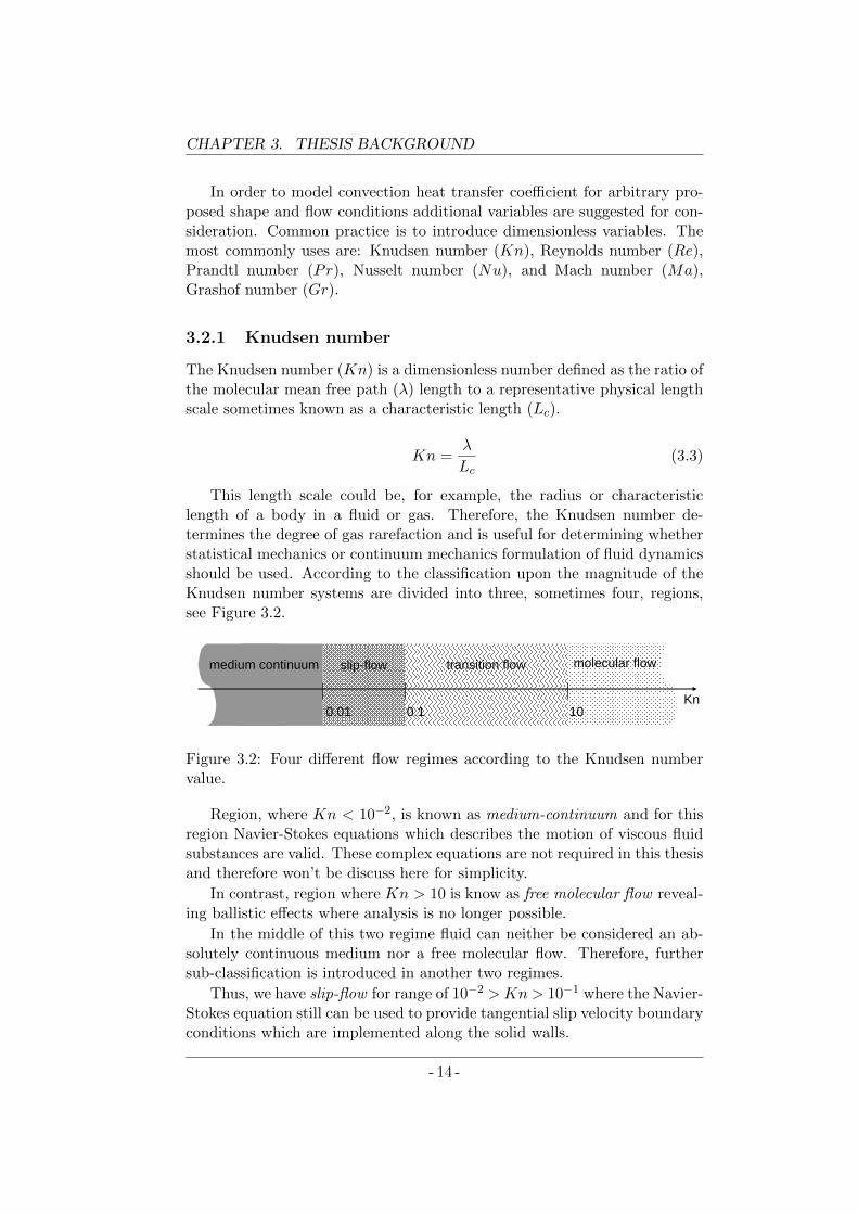
This length scale could be, for example, the radius or characteristiclength of a body in a fluid or gas. Therefore, the Knudsen number de-termines the degree of gas rarefaction and is useful for determining whetherstatistical mechanics or continuum mechanics formulation of fluid dynamicsshould be used. According to the classification upon the magnitude of theKnudsen number systems are divided into three, sometimes four, regions,see Figure 3.2.
0.01
medium continuum slip-flow molecular flowtransition flow
Kn0.1 10
Figure 3.2: Four different flow regimes according to the Knudsen numbervalue.
Region, where Kn < 10−2, is known as medium-continuum and for thisregion Navier-Stokes equations which describes the motion of viscous fluidsubstances are valid. These complex equations are not required in this thesisand therefore won’t be discuss here for simplicity.
In contrast, region where Kn > 10 is know as free molecular flow reveal-ing ballistic effects where analysis is no longer possible.
In the middle of this two regime fluid can neither be considered an ab-solutely continuous medium nor a free molecular flow. Therefore, furthersub-classification is introduced in another two regimes.
Thus, we have slip-flow for range of 10−2 >Kn > 10−1 where the Navier-Stokes equation still can be used to provide tangential slip velocity boundaryconditions which are implemented along the solid walls.
- 14 -
3.2. PHYSICAL MECHANISM OF HEAT TRANSFER
Finally, situated in between free molecular flow and slip-flow regime10−1 > Kn > 10 we have a transition flow when continuum assumptionstarts to break down but still exist alternative methods of analysis usingthe Burnett equations or particle based on Direct Simulation Monte Carlo(DSMC). Nevertheless, in this last mention region, also shortly named Mon-tecarlo, is very difficult to predict correct and recurrent solutions.
When we work in the continuum medium flow regime, the gas flowingover non-porous surface literally sticks to the surface in the close proximityso we assume a zero relative velocity to the surface. This phenomena is knowas no-slip condition and it is responsible for development of velocity profilefor flow. Because of the friction between each fluid layer, the layer thatstick to the surface slows the adjacent fluid layer, which next slows anotherlayer and this phenomena propagates. This non-slip condition is speciallyimportant when we want to provide reliable and recurrent calculation ofconvection heat transfer coefficient for the solid item immersed into fluid/gasenvironment.
3.2.2 Reynolds number
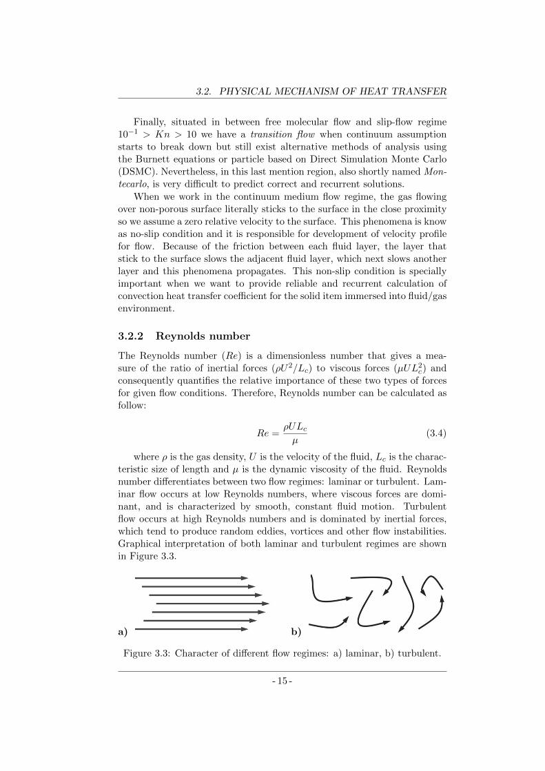
The Reynolds number (Re) is a dimensionless number that gives a mea-sure of the ratio of inertial forces (ρU2/Lc) to viscous forces (µUL2
c) andconsequently quantifies the relative importance of these two types of forcesfor given flow conditions. Therefore, Reynolds number can be calculated asfollow:
Re =ρULcµ
(3.4)
where ρ is the gas density, U is the velocity of the fluid, Lc is the charac-teristic size of length and µ is the dynamic viscosity of the fluid. Reynoldsnumber differentiates between two flow regimes: laminar or turbulent. Lam-inar flow occurs at low Reynolds numbers, where viscous forces are domi-nant, and is characterized by smooth, constant fluid motion. Turbulentflow occurs at high Reynolds numbers and is dominated by inertial forces,which tend to produce random eddies, vortices and other flow instabilities.Graphical interpretation of both laminar and turbulent regimes are shownin Figure 3.3.
a) b)
Figure 3.3: Character of different flow regimes: a) laminar, b) turbulent.
- 15 -
CHAPTER 3. THESIS BACKGROUND
Thus, for given geometry and fluid condition, for small velocities flowhas laminar character, whereas for high speed may happen that it will beturbulent. The Reynolds number at which the flow becomes turbulent iscalled the critical Reynolds number and its value is geometry dependent.
3.2.3 Nusselt number
The Nusselt number (Nu) is a dimensionless convection heat transfer coef-ficient which represents the enhancement of the heat transfer through thefluid layer as a result of convection in relation to conduction across thesame fluid layer. Having the fluid chunk of thickness Lc and temperaturedifference ∆T at each side we have heat transfer drive by two different phe-nomena. If the fluid is motionless we will have conduction heat flux rateqcond given be equation:
qcond = k∆T
Lc(3.5)
where k is the thermal conductivity of the fluid. But when fluid involvessome motion we have somehow bigger convection heat flux rate qconv whichcan be describe as:
qconv = h∆T (3.6)
Therefore, when fluid motion is present we observe the heat flux rateenhancement. The ratio between conduction heat flux against convectionheat flux is being described as a Nusselt number Nu and can be found fromboth equation(3.5) and equation (3.6) as follow:
Nu =qconvqcond
=h∆T
k∆T/Lc=hL
k(3.7)
The case, when Nu = 1, is when we deal with pure heat conductionacross the fluid layer, no motion is registered.
3.2.4 Mach number
The Mach number (Ma) is defined as the speed of an object moving throughair, or any fluid substance, divided by the speed of sound as it is in thatsubstance
Ma =U
Us(3.8)
where U is the speed object relative to the medium, Us is a speed ofsound in the medium.
Therefore, we need to define the speed of sound Us , which for the idealgas is given by the equation:
- 16 -
3.2. PHYSICAL MECHANISM OF HEAT TRANSFER
Us =
√γRT
M(3.9)
where γ is heat capacity ratio, R is a ideal gas constant, T is a gastemperature, M is a molar mass.
Six different flow regimes can be distinguish depending on the Machnumber value as a result of Equation (3.8):
• subsonic: Ma < 1
• transonic: 0.8 < Ma < 1.2
• sonic: Ma = 1
• supersonic: 1 < Ma < 5
• hypersonic: 5 < Ma < 10
• high-hypersonic: Ma > 10
Mach number, however has another implication. It has been observedthat knowing Ma value helps recognize whether gas flow can be modeled ascompressible or incompressible. It is assumed that gas flow is incompressiblewhen its density changes are less than 5% withing the analysis region. Thishappens when the flow relative velocity is less than 30% of speed of sound;what literally means the Ma < 0.3.
3.2.5 Grashof number
The Grashof number (Gr) is a dimensionless number in fluid dynamics andheat transfer which approximates the ratio of the buoyancy to viscous forceacting on a fluid. It frequently arises in the study of situations involvingnatural convection. Grashof number is described be algebraic equation:
Gr =g · β · (Ts − T∞) · L3
ν2(3.10)
where, g is acceleration due to Earth’s gravity or other celestial body con-sidered, β is the coefficient of thermal expansion (equal to approximately1/T , for ideal gases), Ts is the surface temperature Tinf is the bulk tem-perature and L is the characteristic size of the body exposed to the naturalconvection process. In case of o sphere, the characteristic size is its diameter.
- 17 -
CHAPTER 3. THESIS BACKGROUND
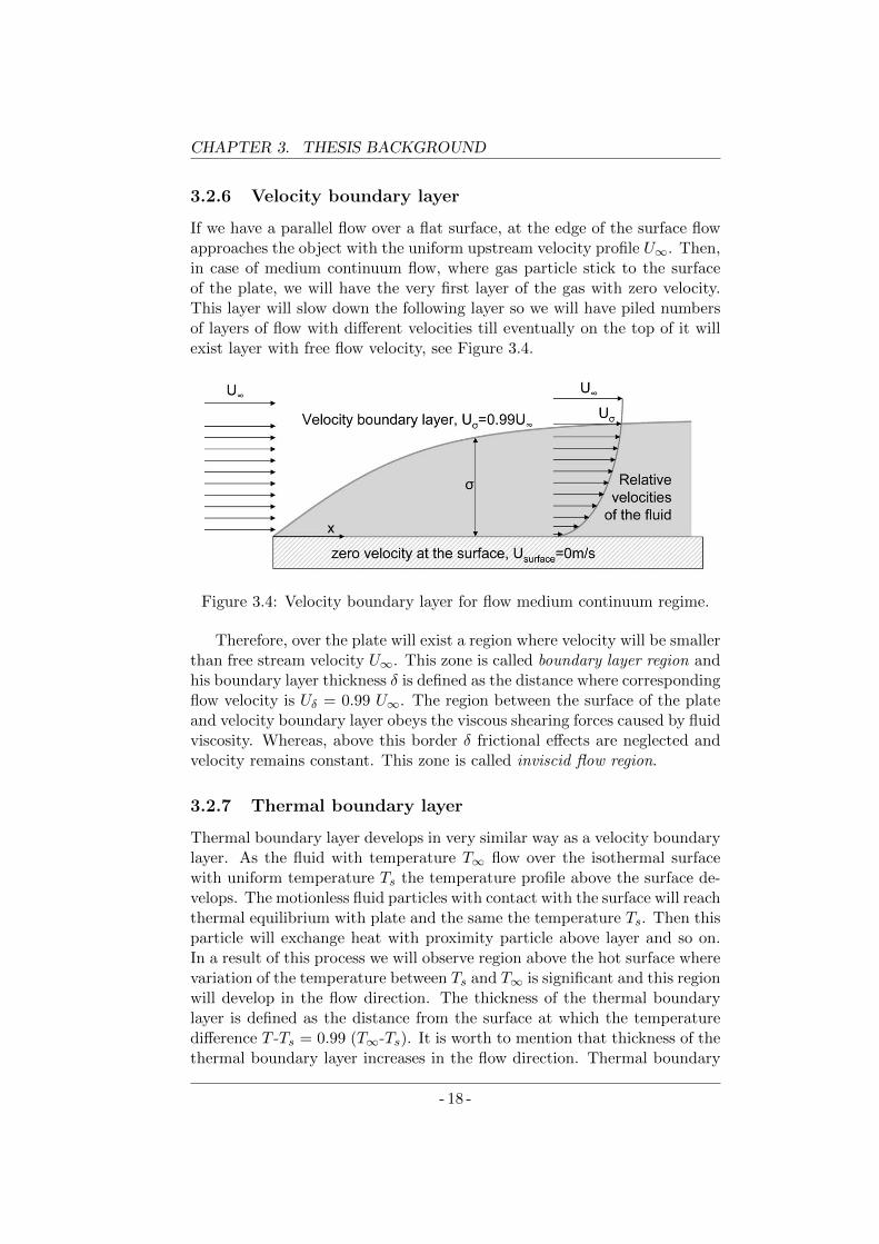
3.2.6 Velocity boundary layer
If we have a parallel flow over a flat surface, at the edge of the surface flowapproaches the object with the uniform upstream velocity profile U∞. Then,in case of medium continuum flow, where gas particle stick to the surfaceof the plate, we will have the very first layer of the gas with zero velocity.This layer will slow down the following layer so we will have piled numbersof layers of flow with different velocities till eventually on the top of it willexist layer with free flow velocity, see Figure 3.4.
Figure 3.4: Velocity boundary layer for flow medium continuum regime.
Therefore, over the plate will exist a region where velocity will be smallerthan free stream velocity U∞. This zone is called boundary layer region andhis boundary layer thickness δ is defined as the distance where correspondingflow velocity is Uδ = 0.99 U∞. The region between the surface of the plateand velocity boundary layer obeys the viscous shearing forces caused by fluidviscosity. Whereas, above this border δ frictional effects are neglected andvelocity remains constant. This zone is called inviscid flow region.
3.2.7 Thermal boundary layer
Thermal boundary layer develops in very similar way as a velocity boundarylayer. As the fluid with temperature T∞ flow over the isothermal surfacewith uniform temperature Ts the temperature profile above the surface de-velops. The motionless fluid particles with contact with the surface will reachthermal equilibrium with plate and the same the temperature Ts. Then thisparticle will exchange heat with proximity particle above layer and so on.In a result of this process we will observe region above the hot surface wherevariation of the temperature between Ts and T∞ is significant and this regionwill develop in the flow direction. The thickness of the thermal boundarylayer is defined as the distance from the surface at which the temperaturedifference T -Ts = 0.99 (T∞-Ts). It is worth to mention that thickness of thethermal boundary layer increases in the flow direction. Thermal boundary
- 18 -
3.2. PHYSICAL MECHANISM OF HEAT TRANSFER
layer has a special significance because temperature gradient at the locationis directly related to the convection heat transfer. Therefore the shape ofthe temperature profile inside thermal boundary layer governs convectionheat transfer between solid surface and the fluid flowing over it.
3.2.8 Prandtl number
The Prandtl number (Pr) is a parameter that relates the thicknesses of thevelocity and thermal boundary layers. This dimensionless parameter definedas a ratio of the viscous diffusion rate to thermal diffusion rate is given bythe following equation:
Pr =ν
α=
µ/ρ
k/(ρCp)=µCpk
(3.11)
where ν is the kinematic viscosity, α is the thermal diffusivity µ is thedynamic viscosity, ρ is the density of the fluid, k is the thermal conductivityand Cp is the specific heat at constant pressure.
Having developed both velocity boundary layer and thermal boundarylayer we can deliberate which one has bigger impact on convection heattransfer precess. But there is no doubt that this is a fluid velocity that hasa strong influence on temperature profile. Thinking that way we concludethat development of the velocity boundary layer relative to the thermalboundary layer will have significant effect on the convection heat transfer.
Different materials reveals different Prandtl number value. Liquid metalhas Prandtl number less than 0.01, when for heavy oils Pr > 100000. Forgases Prandtl number is about 1 which means that both momentum andheat dissipate through the gas at about the same rate it also means thatthickness of the velocity boundary layer will be similar to the thickness ofthe thermal boundary layer. It is worth to notice that Prandtl numberno contains length scale in its definition and dependents only on the fluidproperties and the fluid state.
3.2.9 Mars atmosphere gas properties
To calculate dimensionless numbers in all cases it is necessary to know atmo-spheric gas properties. Since Mars is composed in more that 95% of carbondioxide, the Martian atmosphere properties can be simplified to the CO2
properties. Three of them depends only on temperature: thermal conduc-tivity (k), dynamic viscosity (µ) and specific heat (Cp), whereas gas density(ρ) depends on temperature and pressure.
• Thermal conductivity, k [W/(m·K)] describes property of the gasmedium to conduct heat and depends linearly of CO2 absolute tem-perature T in Kelvin unit according to the [29] as follow:
- 19 -
CHAPTER 3. THESIS BACKGROUND
k = [9.6 + 0.072 · (T − 200)] · 10−3 (3.12)
• Dynamic viscosity, µ [Pa · s)] of a fluid expresses its resistance toshearing flows, where adjacent layers move parallel to each other withdifferent speeds. This gas parameter depends on temperature as statedin Sutherland formula [30]:
µ = µ0 ·T0 + C
T + C·(T
T0
)3/2
(3.13)
where µ0, T0, and C are constants found experimentally for givenspecific gas. In case of carbon dioxide this constant have followingvalues: µ0 = 14.8·10−6 Pa·s, T0 = 293.15 K, C = 240 K.
• Specific heat capacity, Cp [J/(kg·K))] is the ratio of the heat addedto (or removed from) an object to the resulting temperature changein relation to the unit mass. This properties depends directly to thecarbon dioxide absolute temperature , which from lineal interpolationhas been extrapolated from [31] and modeled as follow:
Cp = 530 + 1.037 · T (3.14)
• Density, ρ [kg/m3] (sometimes known as volumetric mass density) ofa substance is its mass per unit volume. This properties for gases isstrongly affected be temperature T and pressure P and for ideal gascan be described as:
ρ =M · PR · T (3.15)
where M is a molar mass and R is a ideal gas constant equal to8.3144621 J/(mol·K). Molar mass of carbon dioxide molecule MCO2
[g/mol] can be calculated as a sum of one molar weigh of atomic car-bon (MC) and two molar weight of atomic oxygen (MO):
MCO2 = MC + 2 ·MO = 12.0107 + 2 · 15.9994 = 44.0095 (3.16)
Thus, molar mass of carbon dioxide atmosphere is MCO2 ≈ 44 g/mol.
- 20 -
3.3. THERMAL FLOW SENSORS
3.3 Thermal flow sensors
Based on the phenomena of the convection cooling of the hot object im-mersed in moving flow (liquid or gas) a whole variety of the flow sensors hasbeen proposed. The rate of the heat being drained from the sensor/deviceto the ambient will depend not only on the flow parameters but sometimeswhen we got a group of hot elements also of its geometry and orientation inreference to the wind direction. It has been observed and is well known thatpart which are in upstream are refrigerated more efficient that those beingin the thermal shadow of the rear side of the group. From these two facts,the thermal flow sensors can be divided into two groups:
• thermal anemometers
• calorimetric sensors
3.3.1 Thermal anemometers
Thermal anemometer is a single unit working in overheat to the ambientwhich is capable of measuring heat loss in the process of convection. Thenthis heat drain thanks to model of convection phenomena in reference tothe achieved overheat is translated into wind speed parameter. The classicexample of the the thermal anemometer will be a hot wire wind sensor,where power P , overheat ∆T and wind speed U dependence is known todayas a King’s Law:
P =(A+B
√U)·∆T (3.17)
where A and B are the constant that depends on many parametersamong which are: gas parameters (k,Cp,µ,ρ) and wire geometrical prop-erties (d,L) as well as heat conduction losses be the boundary support com-ponents. What was surprising and reported over century ago by the Kingin [32], was that particular thin hot cylinder/wire behavior can be modeledbe simple Equation (3.17) which parameters A and B once found experi-mentally are valid for flow measurement purpose out of the lab of coursefor similar room temperature. Kings in his work has recommended alsoto work with higher overheat value making the same almost independentmeasurement of the ordinary variation of the room temperature.
Equation (3.17) is valid when wire axis is perpendicular to the flow direc-tion, otherwise if we imagine the infinite wire only the perpendicular veloc-ity component is being sense from the wire meanwhile parallel one does notmake any difference on the wire thermal behavior. Since then, the effectivecooling velocity (Ueff ) can be found from following relation:
Ueff = U · cosβ (3.18)
- 21 -
CHAPTER 3. THESIS BACKGROUND
where β is the angle between the flow vector and the normal to the axisof the sensor.
Although, single wire can be employed to found effective flow velocity,using multiple wires in different spacial orientation it is possible to expanddevice capabilities for 2D and 3-D concept of absolute velocity and anglediscrimination measurement accordingly to the number of wires used.
But thermal anemometer don’t need to be only wires [33] it can have ashape of thin-films [34] or even sphere [35] or other geometries, [36]. In caseof hot-film anemometers this is usually achieved by deposition of conductingmetal who resistance depends on temperature (like platinum for example)on the resistive substrate of quartz or oxidized silicon, [37, 38]. Bigger sizemake the sensor more sturdy and less prone for decalibration but at thesame time sensor frequency response becomes slower.
3.3.2 Calorimetric sensors
Calorimetric sensor uses the fact that heat drained from the hot element bythe flow is transported and affect surroundings or directly the other compo-nents. Therefore, we will observe a heat transfer from the one componenttoward another which will affect heat distribution in the grade that willchange either temperature or heat convection rate of that another compo-nent. The same temperature symmetry or heat dissipation conditions willdepends on the position of the particular component in reference to to ge-ometry of the structure and wind incoming angle, [39].
The way one element affect another or other way round depends notonly on wind speed but also on wind direction, so very often the calorimetricsensor are not only 1-D realization [40] but mostly 2-D [41,42] and even 3-Dsolution has been achieved [43].
Very often calorimetric sensors in which heat transfer affects symmetryof the convection coefficient of sensor units are being called for simplicitythermal anemometers.
3.4 Operating modes
One of the very important aspects of thermal flow sensor is which operatingmode it employs. For thermal anemometers this division is simple andconsist in two major modes:
• Constant Power Anemometry (CPA)
• Constant Temperature Anemometry (CTA)
Constant Power Anemometry (CPA) is a mode when Joule heat powerdelivers to the sensor does not change under changing wind parameters. As
- 22 -
3.4. OPERATING MODES
the power delivered to the sensor is to balance convection heat in Equa-tion (3.1), then the change in convection heat coefficient will result inadjustment of hot point working temperature. Constant Power Anemome-try (CPA) according to the working circuit can have another abbreviationlike: Constant Current Anemometry (CCA) and Constant Voltage Anemom-etry (CVA).
Constant Temperature Anemometry (CTA) mode has a different ap-proach for driving wind sensor. Working in this mode wind sensor hot ele-ment is kept at the same temperature level and power demand is adjustedto the necessary value to once again satisfy the Equation (3.1). Therefore,whenever wind velocity rise what will result in rise of heat convection coeffi-cient and in consequence power demand will rise to maintain overheat at thesame level. Constant Temperature Anemometry (CTA) mode sometimes isnot to set absolute value of temperature but rather is setting constant over-heat in reference to the ambient temperature conditions. In that last caseoperating mode is same times called as Constant Temperature DifferenceAnemometry (CTDA).
- 23 -

Chapter 4
Thermal Anemometry inMars Missions
Evolution of the Mars planet has always puzzled the scientific community.The understand of its magnetic filed properties as well as dynamic atmo-sphere behavior together with spectrum of solar radiation and water contentamong others would shed light on if whenever this Red Planet could havebeen able to sustain life as we know on Earth. Therefore, there is no surprisethan when technology for space mission presented its readiness the era ofMars exploration started for good. The first mission known as Marsnik 1 waslaunched in 1960 by Union of Soviet Socialist Republics (USSR) and wasan intent Mars flyby but failed and even didn’t reach the Earth orbit. Manyothers intents failed till United States of America (USA) mission Mariner 4,lunched in 1965 and flying by Mars in 1965 sent first pictures to Earth. Thismilestone was a great success and gave the leadership in Mars explorationto USA. Up to date there ahve been more than 40 missions targeting Marsmore than half of them have been declared as failure, and the great majorityof the missions that has succeeded were, as it has been in early days, fromUSA. What is even more striking is that the only successful mission thatinvolved landers or rovers on Mars were from NASA. Those are, orderedby landing dates: Viking (1976), Mars Pathfinder (1997), Spirit & Oppor-tunity (2004), Phoenix (2008) and Curiosity (2012). Each time a missionwas planed specific landing site for vehicles has been carefully assigned, seeFigure 4.1.
From the seven landers which succeed operating on Mars five of themwere equipped with wind measurement instruments in order to characterizewind near Mars surface. This shows how big scientific inters is in charac-terizing flow structures on the neighbor planet. Only Spirit & Opportunitymissed in their scientific program Martian atmosphere wind measurementgoals. Both Vikings landers were equipped with thermal hot-film anemome-ters, Pathfinder were carrying on hot-wire anemometer and a dynamic pres-
25
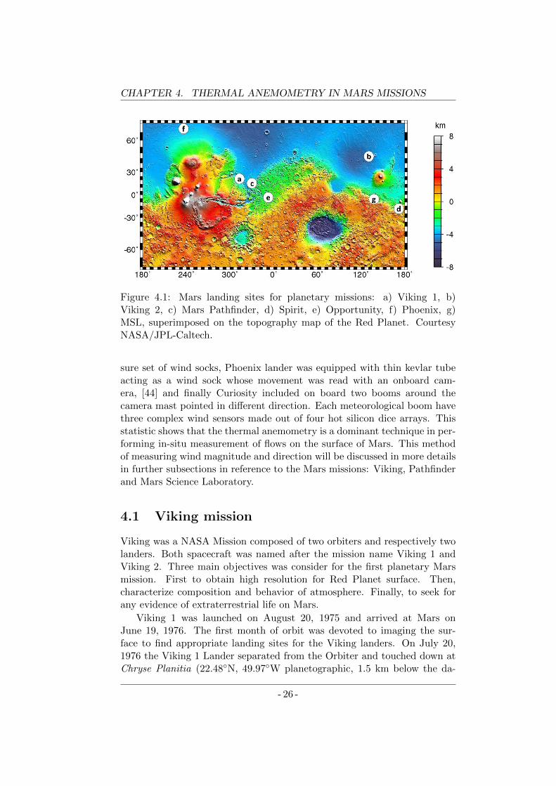
CHAPTER 4. THERMAL ANEMOMETRY IN MARS MISSIONS
Figure 4.1: Mars landing sites for planetary missions: a) Viking 1, b)Viking 2, c) Mars Pathfinder, d) Spirit, e) Opportunity, f) Phoenix, g)MSL, superimposed on the topography map of the Red Planet. CourtesyNASA/JPL-Caltech.
sure set of wind socks, Phoenix lander was equipped with thin kevlar tubeacting as a wind sock whose movement was read with an onboard cam-era, [44] and finally Curiosity included on board two booms around thecamera mast pointed in different direction. Each meteorological boom havethree complex wind sensors made out of four hot silicon dice arrays. Thisstatistic shows that the thermal anemometry is a dominant technique in per-forming in-situ measurement of flows on the surface of Mars. This methodof measuring wind magnitude and direction will be discussed in more detailsin further subsections in reference to the Mars missions: Viking, Pathfinderand Mars Science Laboratory.
4.1 Viking mission
Viking was a NASA Mission composed of two orbiters and respectively twolanders. Both spacecraft was named after the mission name Viking 1 andViking 2. Three main objectives was consider for the first planetary Marsmission. First to obtain high resolution for Red Planet surface. Then,characterize composition and behavior of atmosphere. Finally, to seek forany evidence of extraterrestrial life on Mars.
Viking 1 was launched on August 20, 1975 and arrived at Mars onJune 19, 1976. The first month of orbit was devoted to imaging the sur-face to find appropriate landing sites for the Viking landers. On July 20,1976 the Viking 1 Lander separated from the Orbiter and touched down atChryse Planitia (22.48N, 49.97W planetographic, 1.5 km below the da-
- 26 -
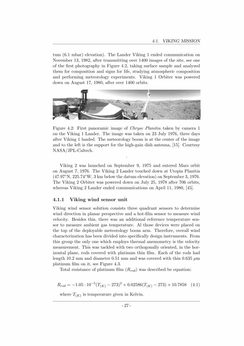
4.1. VIKING MISSION
tum (6.1 mbar) elevation). The Lander Viking 1 ended communication onNovember 13, 1982, after transmitting over 1400 images of the site, see oneof the first photography in Figure 4.2, taking surface sample and analyzedthem for composition and signs for life, studying atmospheric compositionand performing meteorology experiments. Viking 1 Orbiter was powereddown on August 17, 1980, after over 1400 orbits.
Figure 4.2: First panoramic image of Chryse Planitia taken by camera 1on the Viking 1 Lander. The image was taken on 23 July 1976, three daysafter Viking 1 landed. The meteorology boom is at the center of the imageand to the left is the support for the high-gain dish antenna, [15]. CourtesyNASA/JPL-Caltech.
.
Viking 2 was launched on September 9, 1975 and entered Mars orbiton August 7, 1976. The Viking 2 Lander touched down at Utopia Planitia(47.97N, 225.74W, 3 km below the datum elevation) on September 3, 1976.The Viking 2 Orbiter was powered down on July 25, 1978 after 706 orbits,whereas Viking 2 Lander ended communications on April 11, 1980, [45].
4.1.1 Viking wind sensor unit
Viking wind sensor solution consists three quadrant sensors to determinewind direction in planar perspective and a hot-film sensor to measure windvelocity. Besides this, there was an additional reference temperature sen-sor to measure ambient gas temperature. Al those devices were placed onthe top of the deployable meteorology boom arm. Therefore, overall windcharacterization has been divided into specifically design instruments. Fromthis group the only one which employs thermal anemometry is the velocitymeasurement. This was tackled with two orthogonally oriented, in the hor-izontal plane, rods covered with platinum thin film. Each of the rods hadlength 10.2 mm and diameter 0.51 mm and was covered with thin 0.635 µmplatinum film on it, see Figure 4.3.
Total resistance of platinum film (Rrod) was described be equation:
Rrod = −1.05 · 10−5(T(K) − 273)2 + 0.02586(T(K) − 273) + 10.7858 (4.1)
where T(K) is temperature given in Kelvin.
- 27 -
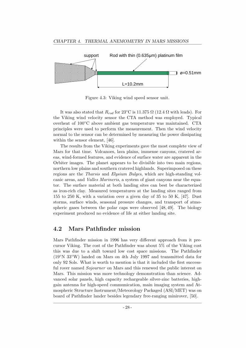
CHAPTER 4. THERMAL ANEMOMETRY IN MARS MISSIONS
L=10.2mm
ø=0.51mm
Rod
with
thin
(0.635μm) platinum
filmsupport
Figure 4.3: Viking wind speed sensor unit.
It was also stated that Rrod for 23C is 11.375 Ω (12.4 Ω with leads). Forthe Viking wind velocity sensor the CTA method was employed. Typicaloverheat of 100C above ambient gas temperature was maintained. CTAprinciples were used to perform the measurement. Then the wind velocitynormal to the sensor can be determined by measuring the power dissipatingwithin the sensor element, [46].
The results from the Viking experiments gave the most complete view ofMars for that time. Volcanoes, lava plains, immense canyons, cratered ar-eas, wind-formed features, and evidence of surface water are apparent in theOrbiter images. The planet appears to be divisible into two main regions,northern low plains and southern cratered highlands. Superimposed on theseregions are the Tharsis and Elysium Bulges, which are high-standing vol-canic areas, and Valles Marineris, a system of giant canyons near the equa-tor. The surface material at both landing sites can best be characterizedas iron-rich clay. Measured temperatures at the landing sites ranged from155 to 250 K, with a variation over a given day of 35 to 50 K, [47]. Duststorms, surface winds, seasonal pressure changes, and transport of atmo-spheric gases between the polar caps were observed [48, 49]. The biologyexperiment produced no evidence of life at either landing site.
4.2 Mars Pathfinder mission
Mars Pathfinder mission in 1996 has very different approach from it pre-cursor Viking. The cost of the Pathfinder was about 5% of the Viking costthis was due to a shift toward low cost space missions. The Pathfinder(19N 33W) landed on Mars on 4th July 1997 and transmitted data foronly 92 Sols. What is worth to mention is that it included the first success-ful rover named Sojourner on Mars and this renewed the public interest onMars. This mission was more technology demonstration than science. Ad-vanced solar panels, high capacity rechargeable silver-zinc batteries, high-gain antenna for high-speed communication, main imaging system and At-mospheric Structure Instrument/Meteorology Packaged (ASI/MET) was onboard of Pathfinder lander besides legendary free-ranging minirover, [50].
- 28 -
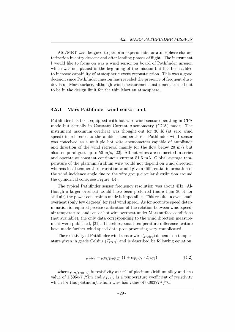
4.2. MARS PATHFINDER MISSION
ASI/MET was designed to perform experiments for atmosphere charac-terization in entry descent and after landing phases of flight. The instrumentI would like to focus on was a wind sensor on board of Pathfinder missionwhich was not planed in the beginning of the mission but has been addedto increase capability of atmospheric event reconstruction. This was a gooddecision since Pathfinder mission has revealed the presence of frequent dust-devils on Mars surface, although wind measurement instrument turned outto be in the design limit for the thin Martian atmosphere.
4.2.1 Mars Pathfinder wind sensor unit
Pathfinder has been equipped with hot-wire wind sensor operating in CPAmode but actually in Constant Current Anemometry (CCA) mode. Theinstrument maximum overheat was thought out for 30 K (at zero windspeed) in reference to the ambient temperature. Pathfinder wind sensorwas conceived as a multiple hot wire anemometers capable of amplitudeand direction of the wind retrieval mainly for the flow below 20 m/s butalso temporal gust up to 50 m/s, [22]. All hot wires are connected in seriesand operate at constant continuous current 51.5 mA. Global average tem-perature of the platinum/iridium wire would not depend on wind directionwhereas local temperature variation would give a differential information ofthe wind incidence angle due to the wire group circular distribution aroundthe cylindrical cone, see Figure 4.4.
The typical Pathfinder sensor frequency resolution was about 4Hz. Al-though a larger overheat would have been preferred (more than 30 K forstill air) the power constraints made it impossible. This results in even smalloverheat (only few degrees) for real wind speed. As for accurate speed deter-mination is required precise calibration of the relation between wind speed,air temperature, and sensor hot wire overheat under Mars surface conditions(not available), the only data corresponding to the wind direction measure-ment were published, [21]. Therefore, small temperature difference featurehave made further wind speed data post processing very complicated.
The resistivity of Pathfinder wind sensor wire (ρwire) depends on temper-ature given in grade Celsius (T(C)) and is described be following equation:
ρwire = ρPt/Ir(0C)
(1 + αPt/Ir · T(C)
)(4.2)
where ρPt/Ir(0C) is resistivity at 0C of platinum/iridium alloy and hasvalue of 1.895e-7 /Ωm and αPt/Ir is a temperature coefficient of resistivitywhich for this platinum/iridium wire has value of 0.003729 /C.
- 29 -
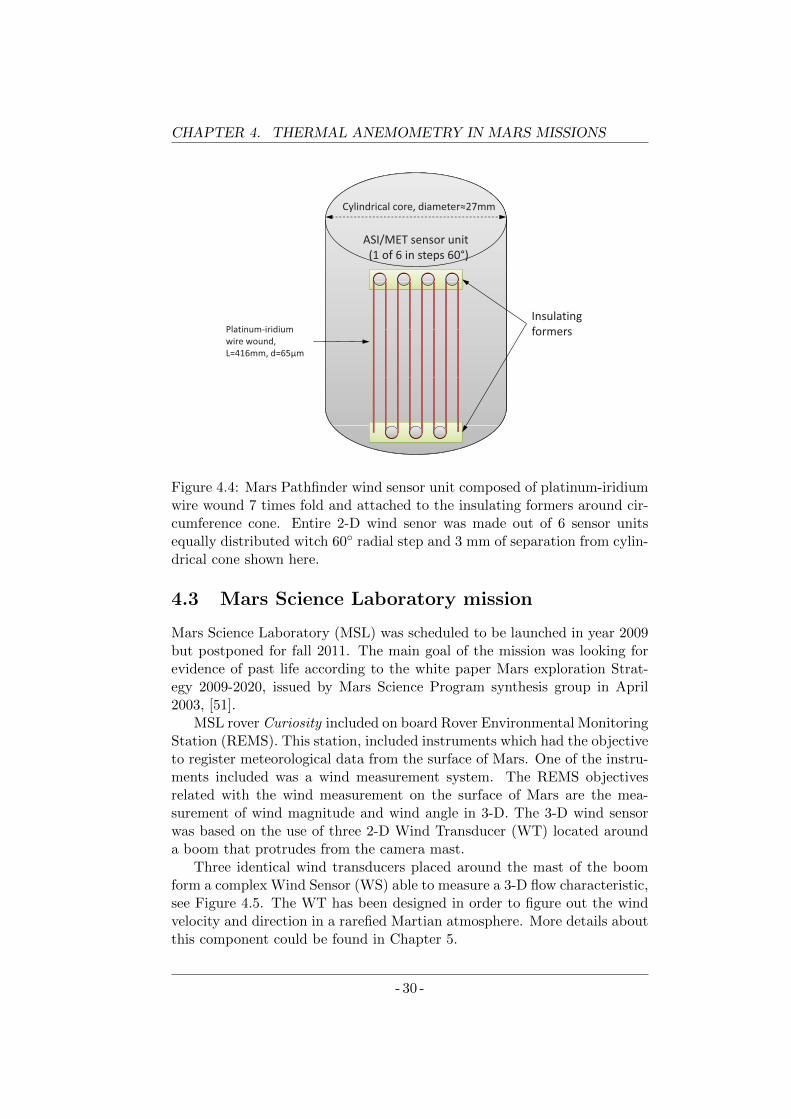
CHAPTER 4. THERMAL ANEMOMETRY IN MARS MISSIONS
Cylindricalcore,diameter27mm
ASI/METsensorunit(1of6insteps60°)
InsulatingformersPlatinumiridium formersPlatinumiridium
wirewound,L=416mm,d=65μm
Figure 4.4: Mars Pathfinder wind sensor unit composed of platinum-iridiumwire wound 7 times fold and attached to the insulating formers around cir-cumference cone. Entire 2-D wind senor was made out of 6 sensor unitsequally distributed witch 60 radial step and 3 mm of separation from cylin-drical cone shown here.
4.3 Mars Science Laboratory mission
Mars Science Laboratory (MSL) was scheduled to be launched in year 2009but postponed for fall 2011. The main goal of the mission was looking forevidence of past life according to the white paper Mars exploration Strat-egy 2009-2020, issued by Mars Science Program synthesis group in April2003, [51].
MSL rover Curiosity included on board Rover Environmental MonitoringStation (REMS). This station, included instruments which had the objectiveto register meteorological data from the surface of Mars. One of the instru-ments included was a wind measurement system. The REMS objectivesrelated with the wind measurement on the surface of Mars are the mea-surement of wind magnitude and wind angle in 3-D. The 3-D wind sensorwas based on the use of three 2-D Wind Transducer (WT) located arounda boom that protrudes from the camera mast.
Three identical wind transducers placed around the mast of the boomform a complex Wind Sensor (WS) able to measure a 3-D flow characteristic,see Figure 4.5. The WT has been designed in order to figure out the windvelocity and direction in a rarefied Martian atmosphere. More details aboutthis component could be found in Chapter 5.
- 30 -
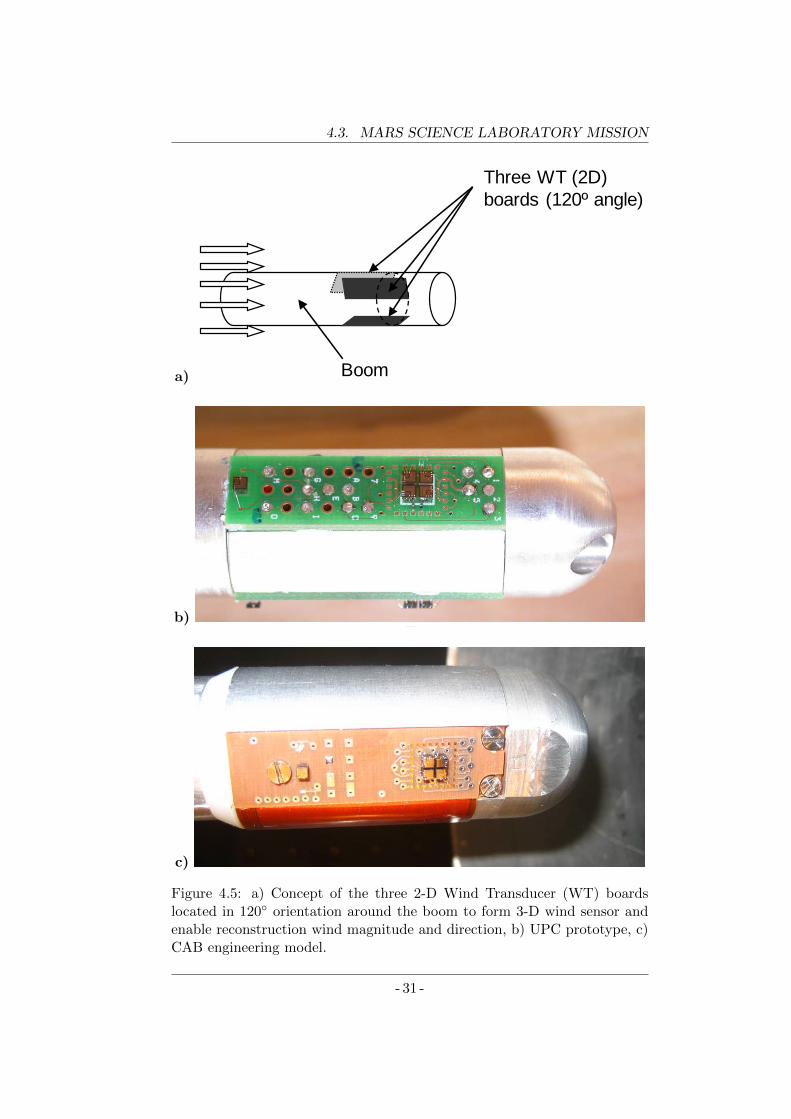
4.3. MARS SCIENCE LABORATORY MISSION
a)
Three WT (2D)
boards (120º angle)
Boom
“CONTRIBUTION TO ADVANCED HOT WIRE WIND SENSING”
Tesi doctoral presentada per a l’obtenció del títol de Doctor per la Universitat Politècnica de Catalunya, dins el Programa de Doctorat en Enginyeria Electrònica
Lukasz Kowlski
Director: Vicente Jiménez Serres
Enero 2016
b)
“CONTRIBUTION TO ADVANCED HOT WIRE WIND SENSING”
Tesi doctoral presentada per a l’obtenció del títol de Doctor per la Universitat Politècnica de Catalunya, dins el Programa de Doctorat en Enginyeria Electrònica
Lukasz Kowlski
Director: Vicente Jiménez Serres
Enero 2016
c)
Figure 4.5: a) Concept of the three 2-D Wind Transducer (WT) boardslocated in 120 orientation around the boom to form 3-D wind sensor andenable reconstruction wind magnitude and direction, b) UPC prototype, c)CAB engineering model.
- 31 -

Chapter 5
REMS 2-D Wind Transducer
This chapter contains a brief presentation of the Rover Environmental Mon-itoring Station (REMS) project. The main concept of the new 2-D windsensor being part part of the REMS will also be described. Results of thenumerical CFD simulation of the conceived structure will be shown. Step bystep fabrication process silicon chip that is central to the sensor operationwill be described. Afterwards the working circuit and measurement strat-egy will be explained. Then, thermal model of the sensor will be discussedtogether with some proof of concept measurements. Finally comparison ofthe REMS wind sensor with other thermal anemometers which has been onMars in the past will be carried out, according to a first order thermal modelfor each sensor unit element.
5.1 REMS project
Rover Environmental Monitoring Station (REMS) is a set of meteorologicscientific devices dedicated to explore weather conditions on Mars. The workoriginated as a result of the selection of the REMS station proposed by anSpanish laboratory to the NASA to be one of the instruments on board ofthe rover Curiosity of the MSL [52]. JPL mission to Mars formerly wasplanted to be launched on autumn 2009, eventually postponed to autumn2011, [53] has successfully arrived to Mars on August 2012, [54]. Underleadership of the CAB, a joint center of Consejo Superior de InvestigacionesCientficas (CSIC) - INTA. Project REMS is a Spanish Ministry of Educa-tion and Science contribution to the NASA mission, [55]. Although, undersupervision of CAB the project would not be possible without collaborationof many science and technology institutions. Basically the alliance of threecountries: Spain, USA and Finland enabled the realization of the projectREMS, see logos of the collaborators in Figure 5.1.
The leadership of the project handled by the CAB whereas NASA is re-sponsible for REMS instrument evaluation and integration with MSL rover.
33
CHAPTER 5. REMS 2-D WIND TRANSDUCER
a) b) c) d) e)
Figure 5.1: The logos of cooperative institutions: a) CAB, b) NASA, c)UPC, d) FMI, e) for REMS project.
The wind sensor design was commissioned to the Universitat Politecnica deCatalunya (UPC) and Finnish Meteorological Institute (FMI) was respon-sible for humidity sensor development.
At the UPC work for wind sensor development involved a team of 5 re-searchers: Lukasz Kowalski (author of this thesis work) , Manuel Domınguez-Pumar, Vicente Jimenez Serres, Jordi Ricart and Luis Castaner Munoz.The team interacted frequently with researchers at the CAB namely JavierGomez-Elvira, Sara Navarro, Josefina Torres and Julio Romeral, as well aswith JPL Manuel de la Torre and with MariPaz Zorzano and Luis Vazquezfrom the Universidad Complutense de Madrid.
5.1.1 REMS objectives
According to the Luis Vazquez, former personal investigator of the REMSproject and Javier Gomez-Elvira, current personal investigator and projectleader, REMS was designed to enable realization of several science objec-tives. One of the objectives it to study Martian signature of general circu-lation and the mesoscale phenomena close to the ground surface like jets,fronts and wind tides. Second objective is to characterize and understandweather system in microscale; it basically refers observation and measure-ment of heat fluxes, wind blows boundary layer turbulence or dust devils.Another objective is to learn of local hydrological cycle, for example spatialand temporal variability and diffusive transport from regolith. Following ob-jective is to estimate destructive potential of UV radiation focusing on dustoptical properties, photolysis rates and oxidant production that will providea basic link with the astrobiology studies on Mars. Finally the last objec-tive is to assess subsurface habitability according to the ground-atmosphereinteraction, [18,56].
5.1.2 REMS instruments
In order to satisfy previously established scientific objectives, the specificweather station, known as REMS, is proposed, 5.2.
The recent shape of the station is a result of the compromise betweenpayload mass and measurement ability of stat-of-art instruments. REMS
- 34 -
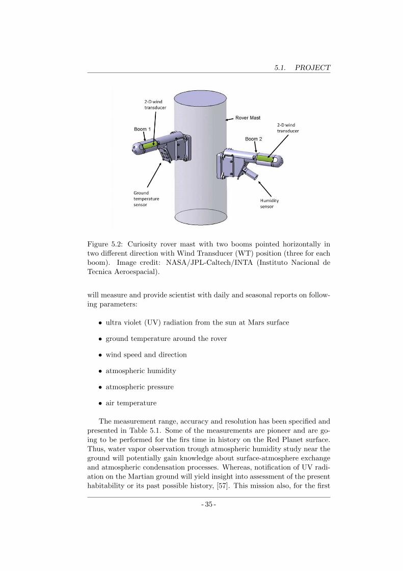
5.1. PROJECT
Figure 5.2: Curiosity rover mast with two booms pointed horizontally intwo different direction with Wind Transducer (WT) position (three for eachboom). Image credit: NASA/JPL-Caltech/INTA (Instituto Nacional deTecnica Aeroespacial).
will measure and provide scientist with daily and seasonal reports on follow-ing parameters:
• ultra violet (UV) radiation from the sun at Mars surface
• ground temperature around the rover
• wind speed and direction
• atmospheric humidity
• atmospheric pressure
• air temperature
The measurement range, accuracy and resolution has been specified andpresented in Table 5.1. Some of the measurements are pioneer and are go-ing to be performed for the firs time in history on the Red Planet surface.Thus, water vapor observation trough atmospheric humidity study near theground will potentially gain knowledge about surface-atmosphere exchangeand atmospheric condensation processes. Whereas, notification of UV radi-ation on the Martian ground will yield insight into assessment of the presenthabitability or its past possible history, [57]. This mission also, for the first
- 35 -
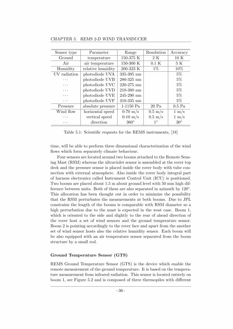
CHAPTER 5. REMS 2-D WIND TRANSDUCER
Sensor type Parameter Range Resolution Accuracy
Ground temperature 150-375 K 2 K 10 K
Air air temperature 150-300 K 0.1 K 5 K
Humidity relative humidity 200-323 K 1% 10%
UV radiation photodiode UVA 335-395 nm 5%· · · photodiode UVB 280-325 nm 5%· · · photodiode UVC 220-275 nm 5%· · · photodiode UVD 210-380 nm 5%· · · photodiode UVE 245-290 nm 5%· · · photodiode UVF 310-335 nm 5%
Pressure absolute pressure 1-1150 Pa 20 Pa 0.5 Pa
Wind flow horizontal speed 0-70 m/s 0.5 m/s 1 m/s· · · vertical speed 0-10 m/s 0.5 m/s 1 m/s· · · direction 360 1 30
Table 5.1: Scientific requests for the REMS instruments, [18]
time, will be able to perform three dimensional characterization of the windflows which form separately climate behaviour.
Four sensors are located around two booms attached to the Remote Sens-ing Mast (RSM) whereas the ultraviolet sensor is assembled at the rover topdeck and the pressure sensor is placed inside the rover body with tube con-nection with external atmosphere. Also inside the rover body integral partof harness electronics called Instrument Control Unit (ICU) is positioned.Two booms are placed about 1.5 m about ground level with 50 mm high dif-ference between units. Both of them are also separated in azimuth by 120.This allocation has been thought out in order to minimize the possibilitythat the RSM perturbates the measurements at both booms. Due to JPLconstrains the length of the booms is comparable with RSM diameter so ahigh perturbation due to the mast is expected in the wost case. Boom 1,which is oriented to the side and slightly to the rear of ahead direction ofthe rover host a set of wind sensors and the ground temperature sensor.Boom 2 is pointing accordingly to the rover face and apart from the anotherset of wind sensor hosts also the relative humidity sensor. Each boom willbe also equipped with an air temperature sensor separated from the boomstructure by a small rod.
Ground Temperature Sensor (GTS)
REMS Ground Temperature Sensor (GTS) is the device which enable theremote measurement of the ground temperature. It is based on the tempera-ture measurement from infrared radiation. This sensor is located entirely onboom 1, see Figure 5.2 and is composed of three thermopiles with different
- 36 -
5.1. PROJECT
wavelength bands; 8-14 um, 15 um, 16-20 um in order to avoid carbon diox-ide (CO2) absorption band [52]. An additional thermistor on board providessensor housing temperature to calibrate the thermopile readouts. [58].
Air Temperature Sensor (ATS)
REMS Air Temperature Sensor (ATS) has been designed as a FR4 rod withtwo standard PT1000 thermistors bonded to it. First one is glued to the rodat his middle position and another at the end of the rod, out of the boomthermal boundary layer. In this configuration knowing two temperaturesallows with the previous characterization to work out the air temperaturewith desired resolution and accuracy, [59].
Humidity Sensor (HS)
REMS Humidity Sensor (HS) is located in the boom 2 which is pointing inthe driving direction of the rover. This device has been developed by FMIin reference to the Vaisala transducer, [52]. In order to not harm the sensorby the Martian dust particles it is cloaked inside protective cylinder andinterface with atmosphere trough the dust filters, see Figure 5.2. The HSprovides REMS weather station with relative humidity readout, [18].
Ultraviolet Sensor (UVS)
REMS Ultraviolet Sensor (UVS) in difference to the previously described de-vices is located on the rover deck pointing to the Martian sky in the zenithdirection a 60 degree field of view. Device is composed of six photodiodesadjusted to the specific bands indicated on Table (5.1). For each photodi-odes a strong round magnet has been included in order to decrease dustdeposition. Furthermore, visual control of the thickness of the dust layerwill be performed in order to identify the level of dust accumulation, [52].
Pressure Sensor (PS)
PS is located inside REMS-ICU box. It is composed by two transducers lo-cated on the multi-layer Printed Circuit Board (PCB) and protected by FR4Faraday cage. Each of transducer has two Vaisala Barocap heads (single-crystal micromachined device) and two Thermocap (temperature sensors).Change in the atmospheric pressure moves the capacitor plates of the in-strument. The capacitance characterized for the Mars conditions is rangingfrom 10 to 15pF and is calibrated for different temperature scenario. Theaccuracy of the PS is 1 Pa.
- 37 -
CHAPTER 5. REMS 2-D WIND TRANSDUCER
Wind Sensor (WS)
Every boom is composed of three equal Wind Transducer (WT) . Each WTis 2-D wind sensor. WT boards are based on the wind hot film anemome-try concept and are placed on boom surface with an angular separation of120. Using a set of three independent WTs 2-D measurements inverse algo-rithm finds out the real 3-D wind parameters, [52]. This inverse algorithmpost-evaluation is possible due to the special aerodynamical simulations andcareful characterization and calibration tests performed inside the wind tun-nel.
When Micro and Nanotechnology (MNT) Group from UPC join to theREMS team we get to know about specific wind sensor requirements whichhave been indicated be NASA, [9]. As wind variations reflect the local com-ponents of the circulation, there is a strong belief that wind measurementwill provide information about surface-layer turbulence and mean verticalgradients, as well as the presence of vortices and convective plumes. There-fore, to meet the scientific community needs on Mars landing site, the windsensor requirements has been set as follow:
• The REMS shall be able to measure horizontal wind in the range of 0to 70 m/s with a resolution of 0.5 m/s and an accuracy of 1 m/s.
• The REMS shall be able to measure the direction of horizontal windwith a resolution and accuracy better than 30 degrees.
• The REMS shall be able to measure vertical wind in the range of 0 to20 m/s with a resolution of 0.5 m/s and an accuracy of 1 m/s.
• The REMS shall be able to measure over the range of air temperatures150 to 300 K.
• The REMS shall be able to operate in the Martian atmosphere (whichis nearly 96% of CO2) pressure in the range of 500 to 1000 Pa.
• The REMS shall be capable of collecting and storing sensor data at asampling rate of 1 Hz, 5 minutes each hour.
Besides this critical constraints there were others which have to be alwaystaken under consideration when developing device for space application,which are: small weight and size (so the entire volume) and low powerconsumption.
Therefore, each one of the Wind Transducer (WT) included in REMShad to be sensitive to a range of wind speeds from 1 to 60 m/s with mag-nitude precision of 0.1 m/s and angle resolution of 10 degree and operatewith a time response of 1 second. REMS wind sensor instrument needs toestimate 3-D wind direction and flow velocity and is composed of two boomsin horizontal position to the ground but pointing in two different direction
- 38 -
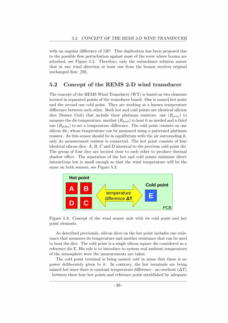
5.2. CONCEPT OF THE REMS 2-D WIND TRANSDUCER
with an angular difference of 120. This duplication has been proposed dueto the possible flow perturbation against mast of the rover where booms areattached, see Figure 5.2. Therefore, only the redundance solution assurethat at any wind direction at least one from the booms receives originalunchanged flow, [59].
5.2 Concept of the REMS 2-D wind transducer
The concept of the REMS Wind Transducer (WT) is based on two elementslocated in separated points of the transducer board. One is named hot pointand the second one cold point. They are working at a known temperaturedifference between each other. Both hot and cold points use identical siliciondice (Sensor Unit) that include three platinum resistors: one (Rsens) tomeasure the die temperature, another (Rheat) to heat it as needed and a thirdone (Rdelta) to set a temperature difference. The cold point consists on onesilicon die, whose temperature can be measured using a patterned platinumresistor. As this sensor should be in equilibrium with the air surrounding it,only its measurement resistor is connected. The hot point consists of fouridentical silicon dice: A, B, C and D identical to the previous cold point die.The group of four dice are located close to each other to produce thermalshadow effect. The separation of the hot and cold points minimize directinteractions but is small enough so that the wind temperature will be thesame on both sensors, see Figure 5.3.
A B
D CEtemperature
difference ΔT
Cold pointHot point
PCB
A B
D CEtemperature
difference ΔT
Cold pointHot point
PCB
Figure 5.3: Concept of the wind sensor unit with its cold point and hotpoint elements.
As described previously, silicon dices on the hot point includes one resis-tance that measures its temperature and another resistance that can be usedto heat the dice. The cold point is a single silicon square die considered as areference die E. His role is to introduce to system real ambient temperatureof the atmosphere were the measurements are taken.
The cold point terminal is being named cold in sense that there is nopower deliberately given to it. In contrary, the hot terminals are beingnamed hot since there is constant temperature difference - an overheat (∆T)- between these four hot points and reference point established by adequate
- 39 -
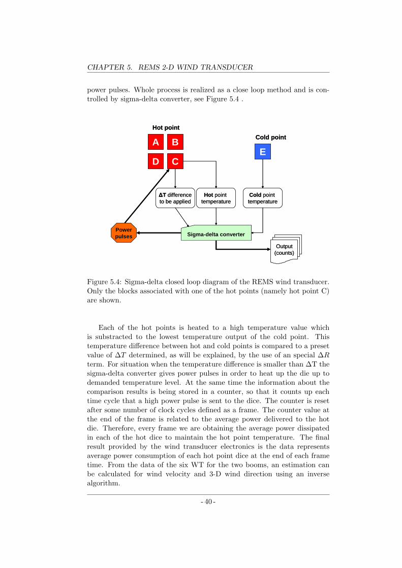
CHAPTER 5. REMS 2-D WIND TRANSDUCER
power pulses. Whole process is realized as a close loop method and is con-trolled by sigma-delta converter, see Figure 5.4 .
A B
D CE
Cold pointHot point
Sigma-delta converter
Cold point
temperature
Hot point
temperature
ΔT difference
to be applied
Output
(counts)
Powerpulses
A B
D CE
Cold pointHot point
Sigma-delta converter
Cold point
temperature
Hot point
temperature
ΔT difference
to be applied
Output
(counts)
Powerpulses
Figure 5.4: Sigma-delta closed loop diagram of the REMS wind transducer.Only the blocks associated with one of the hot points (namely hot point C)are shown.
Each of the hot points is heated to a high temperature value whichis substracted to the lowest temperature output of the cold point. Thistemperature difference between hot and cold points is compared to a presetvalue of ∆T determined, as will be explained, by the use of an special ∆Rterm. For situation when the temperature difference is smaller than ∆T thesigma-delta converter gives power pulses in order to heat up the die up todemanded temperature level. At the same time the information about thecomparison results is being stored in a counter, so that it counts up eachtime cycle that a high power pulse is sent to the dice. The counter is resetafter some number of clock cycles defined as a frame. The counter value atthe end of the frame is related to the average power delivered to the hotdie. Therefore, every frame we are obtaining the average power dissipatedin each of the hot dice to maintain the hot point temperature. The finalresult provided by the wind transducer electronics is the data representsaverage power consumption of each hot point dice at the end of each frametime. From the data of the six WT for the two booms, an estimation canbe calculated for wind velocity and 3-D wind direction using an inversealgorithm.
- 40 -
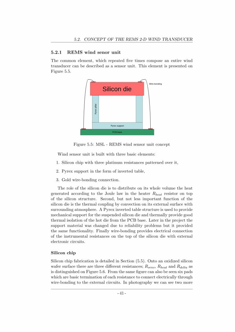
5.2. CONCEPT OF THE REMS 2-D WIND TRANSDUCER
5.2.1 REMS wind senor unit
The common element, which repeated five times compose an entire windtransducer can be described as a sensor unit. This element is presented onFigure 5.5.
Pyrex support
Pyr
ex p
illar
Silicon die
PCB base
Wire-bonding
Figure 5.5: MSL - REMS wind sensor unit concept
Wind sensor unit is built with three basic elements:
1. Silicon chip with three platinum resistances patterned over it,
2. Pyrex support in the form of inverted table,
3. Gold wire-bonding connection.
The role of the silicon die is to distribute on its whole volume the heatgenerated according to the Joule law in the heater Rheat resistor on topof the silicon structure. Second, but not less important function of thesilicon die is the thermal coupling by convection on its external surface withsurrounding atmosphere. A Pyrex inverted table structure is used to providemechanical support for the suspended silicon die and thermally provide goodthermal isolation of the hot die from the PCB base. Later in the project thesupport material was changed due to reliability problems but it providedthe same functionality. Finally wire-bonding provides electrical connectionof the instrumental resistances on the top of the silicon die with externalelectronic circuits.
Silicon chip
Silicon chip fabrication is detailed in Section (5.5). Onto an oxidized siliconwafer surface there are three different resistances; Rsens, Rheat and Rdelta asis distinguished on Figure 5.6. From the same figure can also be seen six padswhich are basic termination of each resistance to connect electrically throughwire-bonding to the external circuits. In photography we can see two more
- 41 -
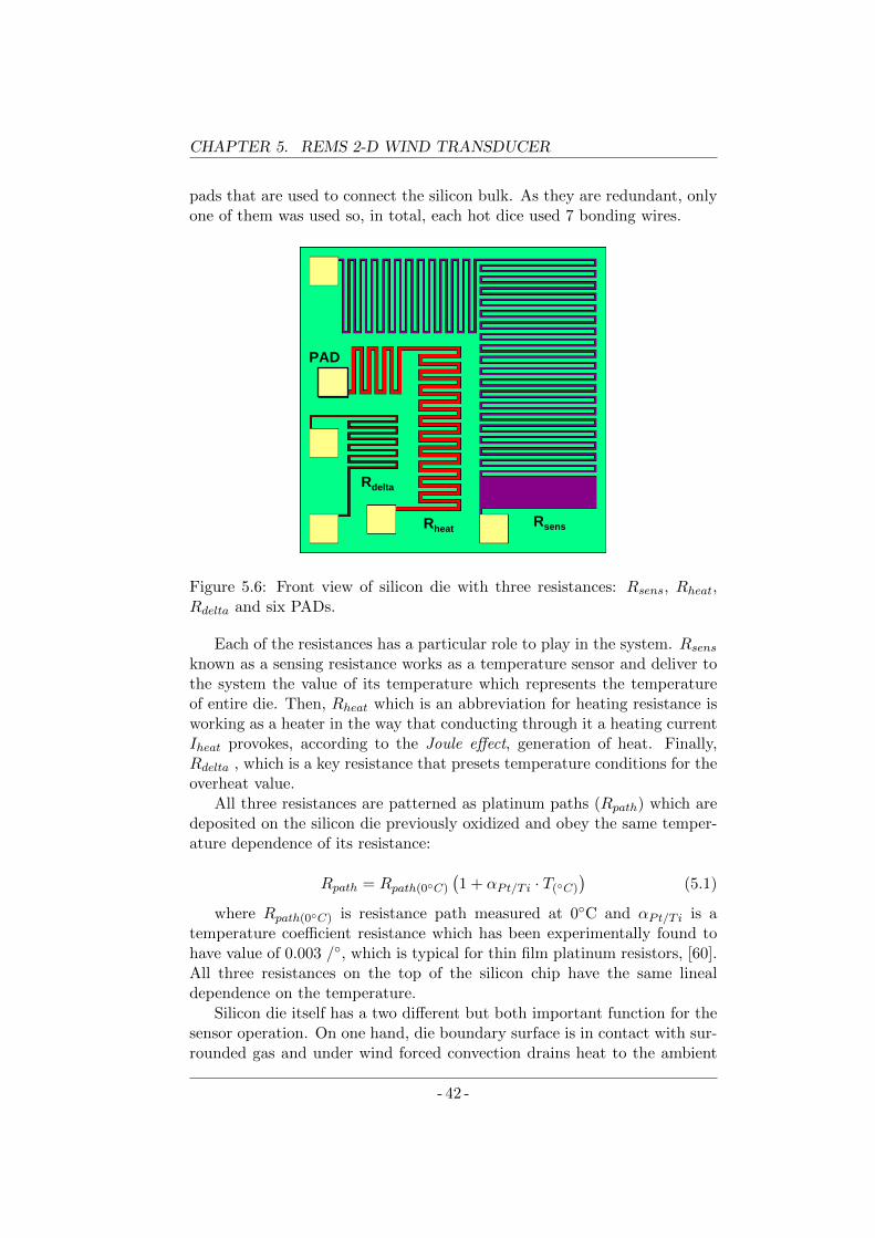
CHAPTER 5. REMS 2-D WIND TRANSDUCER
pads that are used to connect the silicon bulk. As they are redundant, onlyone of them was used so, in total, each hot dice used 7 bonding wires.
PAD
RsensRheat
Rdelta
Figure 5.6: Front view of silicon die with three resistances: Rsens, Rheat,Rdelta and six PADs.
Each of the resistances has a particular role to play in the system. Rsensknown as a sensing resistance works as a temperature sensor and deliver tothe system the value of its temperature which represents the temperatureof entire die. Then, Rheat which is an abbreviation for heating resistance isworking as a heater in the way that conducting through it a heating currentIheat provokes, according to the Joule effect, generation of heat. Finally,Rdelta , which is a key resistance that presets temperature conditions for theoverheat value.
All three resistances are patterned as platinum paths (Rpath) which aredeposited on the silicon die previously oxidized and obey the same temper-ature dependence of its resistance:
Rpath = Rpath(0C)
(1 + αPt/T i · T(C)
)(5.1)
where Rpath(0C) is resistance path measured at 0C and αPt/T i is atemperature coefficient resistance which has been experimentally found tohave value of 0.003 /, which is typical for thin film platinum resistors, [60].All three resistances on the top of the silicon chip have the same linealdependence on the temperature.
Silicon die itself has a two different but both important function for thesensor operation. On one hand, die boundary surface is in contact with sur-rounded gas and under wind forced convection drains heat to the ambient
- 42 -
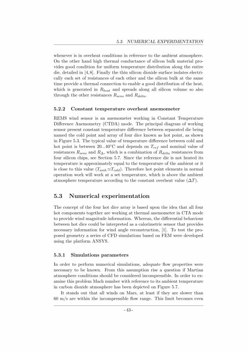
5.3. NUMERICAL EXPERIMENTATION
whenever is in overheat conditions in reference to the ambient atmosphere.On the other hand high thermal conductance of silicon bulk material pro-vides good condition for uniform temperature distribution along the entiredie, detailed in [4,8]. Finally the thin silicon dioxide surface isolates electri-cally each set of resistances of each other and the silicon bulk at the sametime provide a thermal connection to enable a good distribution of the heat,which is generated in Rheat and spreads along all silicon volume so alsothrough the other resistances Rsens and Rdelta.
5.2.2 Constant temperature overheat anemometer
REMS wind sensor is an anemometer working in Constant TemperatureDifference Anemometry (CTDA) mode. The principal diagram of workingsensor present constant temperature difference between separated die beingnamed the cold point and array of four dice known as hot point, as shownin Figure 5.3. The typical value of temperature difference between cold andhot point is between 20...40C and depends on Tref and nominal value ofresistances Rsens and R∆, which is a combination of Rdelta resistances fromfour silicon chips, see Section 5.7. Since the reference die is not heated itstemperature is approximately equal to the temperature of the ambient or itis close to this value (Tamb.'Tcold). Therefore hot point elements in normaloperation work will work at a set temperature, which is above the ambientatmosphere temperature according to the constant overheat value (∆T ).
5.3 Numerical experimentation
The concept of the four hot dice array is based upon the idea that all fourhot components together are working at thermal anemometer in CTA modeto provide wind magnitude information. Whereas, the differential behaviourbetween hot dice could be interpreted as a calorimetric sensor that providesnecessary information for wind angle reconstruction, [1]. To test the pro-posed geometry a series of CFD simulations based on FEM were developedusing the platform ANSYS.
5.3.1 Simulations parameters
In order to perform numerical simulations, adequate flow properties werenecessary to be known. From this assumption rise a question if Martianatmosphere conditions should be considered incompressible. In order to ex-amine this problem Mach number with reference to its ambient temperaturein carbon dioxide atmosphere has been depicted on Figure 5.7.
It stands out that all winds on Mars, at least if they are slower than60 m/s are within the incompressible flow range. This limit becomes even
- 43 -
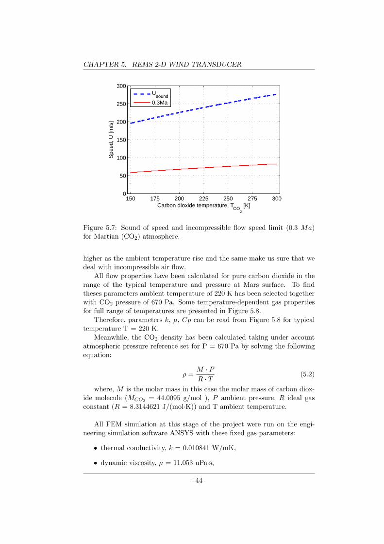
CHAPTER 5. REMS 2-D WIND TRANSDUCER
150 175 200 225 250 275 3000
50
100
150
200
250
300
Carbon dioxide temperature, TCO
2
[K]
Spe
ed, U
[m/s
]
U
sound
0.3Ma
Figure 5.7: Sound of speed and incompressible flow speed limit (0.3 Ma)for Martian (CO2) atmosphere.
higher as the ambient temperature rise and the same make us sure that wedeal with incompressible air flow.
All flow properties have been calculated for pure carbon dioxide in therange of the typical temperature and pressure at Mars surface. To findtheses parameters ambient temperature of 220 K has been selected togetherwith CO2 pressure of 670 Pa. Some temperature-dependent gas propertiesfor full range of temperatures are presented in Figure 5.8.
Therefore, parameters k, µ, Cp can be read from Figure 5.8 for typicaltemperature T = 220 K.
Meanwhile, the CO2 density has been calculated taking under accountatmospheric pressure reference set for P = 670 Pa by solving the followingequation:
ρ =M · PR · T (5.2)
where, M is the molar mass in this case the molar mass of carbon diox-ide molecule (MCO2 = 44.0095 g/mol ), P ambient pressure, R ideal gasconstant (R = 8.3144621 J/(mol·K)) and T ambient temperature.
All FEM simulation at this stage of the project were run on the engi-neering simulation software ANSYS with these fixed gas parameters:
• thermal conductivity, k = 0.010841 W/mK,
• dynamic viscosity, µ = 11.053 uPa·s,
- 44 -
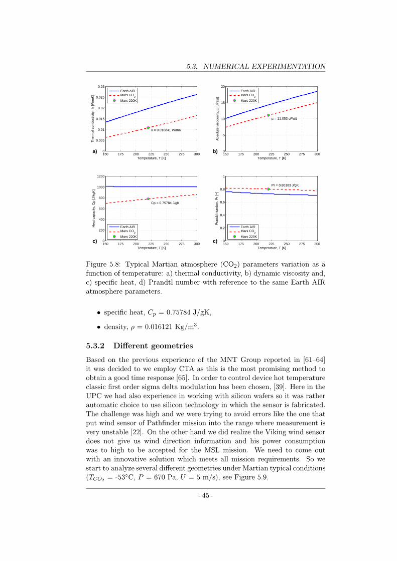
5.3. NUMERICAL EXPERIMENTATION
150 175 200 225 250 275 3000
0.005
0.01
0.015
0.02
0.025
0.03
Temperature, T [K]
The
rmal
con
duct
ivity
, k
[W/m
K]
k = 0.010841 W/mK
a)
Earth AIRMars CO
2
Mars 220K
150 175 200 225 250 275 3000
5
10
15
20
Temperature, T [K]
Abs
olut
e vi
scou
sity
, µ [u
Pa⋅
s]
µ = 11.053 uPa⋅s
b)
Earth AIRMars CO
2
Mars 220K
150 175 200 225 250 275 3000
200
400
600
800
1000
1200
Temperature, T [K]
Hea
t cap
acity
, Cp
[J/k
gK]
Cp = 0.75784 J/gK
c)
Earth AIRMars CO
2
Mars 220K
150 175 200 225 250 275 3000
0.2
0.4
0.6
0.8
1
Temperature, T [K]
Pra
ndtl
num
ber,
Pr
[−]
Pr = 0.80183 J/gK
c)
Earth AIRMars CO
2
Mars 220K
Figure 5.8: Typical Martian atmosphere (CO2) parameters variation as afunction of temperature: a) thermal conductivity, b) dynamic viscosity and,c) specific heat, d) Prandtl number with reference to the same Earth AIRatmosphere parameters.
• specific heat, Cp = 0.75784 J/gK,
• density, ρ = 0.016121 Kg/m3.
5.3.2 Different geometries
Based on the previous experience of the MNT Group reported in [61–64]it was decided to we employ CTA as this is the most promising method toobtain a good time response [65]. In order to control device hot temperatureclassic first order sigma delta modulation has been chosen, [39]. Here in theUPC we had also experience in working with silicon wafers so it was ratherautomatic choice to use silicon technology in which the sensor is fabricated.The challenge was high and we were trying to avoid errors like the one thatput wind sensor of Pathfinder mission into the range where measurement isvery unstable [22]. On the other hand we did realize the Viking wind sensordoes not give us wind direction information and his power consumptionwas to high to be accepted for the MSL mission. We need to come outwith an innovative solution which meets all mission requirements. So westart to analyze several different geometries under Martian typical conditions(TCO2 = -53C, P = 670 Pa, U = 5 m/s), see Figure 5.9.
- 45 -
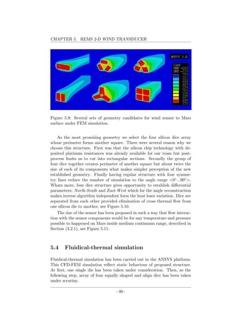
CHAPTER 5. REMS 2-D WIND TRANSDUCER
Figure 5.9: Several sets of geometry candidates for wind sensor to Marssurface under FEM simulation.
As the most promising geometry we select the four silicon dice arraywhose perimeter forms another square. There were several reason why wechoose this structure. First was that the silicon chip technology with de-posited platinum resistances was already available for our team but post-process limits us to cut into rectangular sections. Secondly the group offour dice together creates perimeter of another square but about twice thesize of each of its components what makes simpler perception of the newestablished geometry. Finally having regular structure with four symme-try lines reduce the number of simulation to the angle range <0...90>.Whats more, four dice structure gives opportunity to establish differentialparameters: North-South and East-West which for the angle reconstructionmakes inverse algorithm independent form the heat loses variation. Dice areseparated from each other provided elimination of cross thermal flow fromone silicon die to another, see Figure 5.10.
The size of the sensor has been proposed in such a way that flow interac-tion with the sensor components would be for any temperature and pressurepossible to happened on Mars inside medium continuum range, described inSection (3.2.1), see Figure 5.11.
5.4 Fluidical-thermal simulation
Fluidical-thermal simulation has been carried out in the ANSYS platform.This CFD-FEM simulation reflect static behaviour of proposed structure.At first, one single die has been taken under consideration. Then, as thefollowing step, array of four equally shaped and align dice has been takenunder scrutiny.
- 46 -
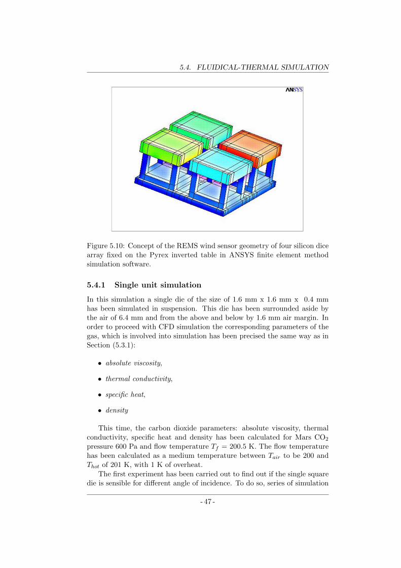
5.4. FLUIDICAL-THERMAL SIMULATION
Figure 5.10: Concept of the REMS wind sensor geometry of four silicon dicearray fixed on the Pyrex inverted table in ANSYS finite element methodsimulation software.
5.4.1 Single unit simulation
In this simulation a single die of the size of 1.6 mm x 1.6 mm x 0.4 mmhas been simulated in suspension. This die has been surrounded aside bythe air of 6.4 mm and from the above and below by 1.6 mm air margin. Inorder to proceed with CFD simulation the corresponding parameters of thegas, which is involved into simulation has been precised the same way as inSection (5.3.1):
• absolute viscosity,
• thermal conductivity,
• specific heat,
• density
This time, the carbon dioxide parameters: absolute viscosity, thermalconductivity, specific heat and density has been calculated for Mars CO2
pressure 600 Pa and flow temperature Tf = 200.5 K. The flow temperaturehas been calculated as a medium temperature between Tair to be 200 andThot of 201 K, with 1 K of overheat.
The first experiment has been carried out to find out if the single squaredie is sensible for different angle of incidence. To do so, series of simulation
- 47 -
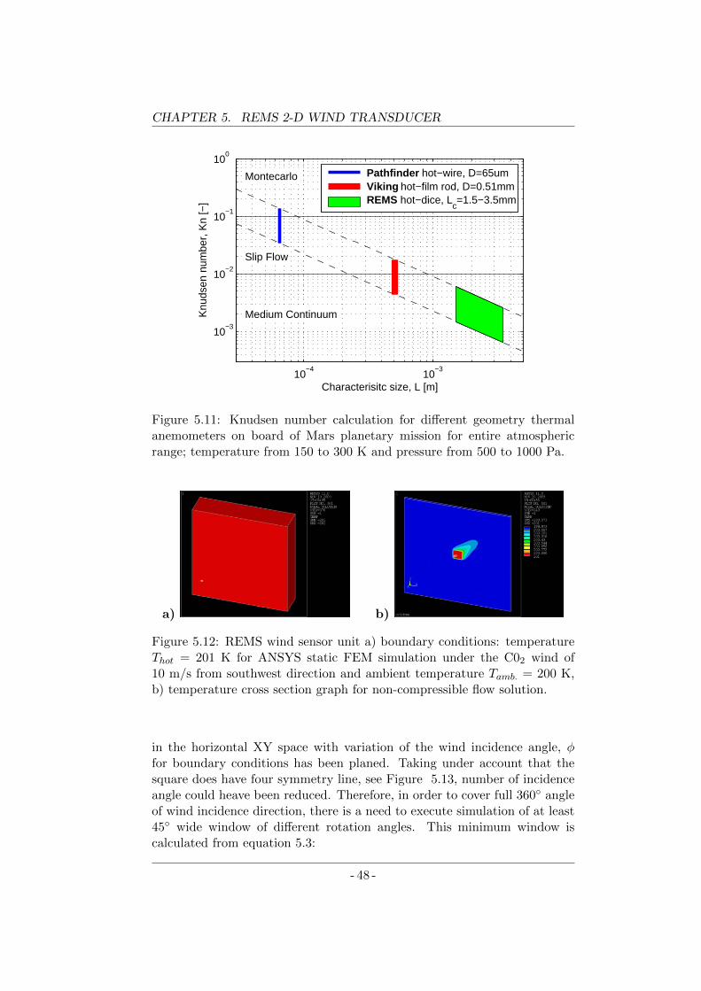
CHAPTER 5. REMS 2-D WIND TRANSDUCER
10−4
10−3
10−3
10−2
10−1
100
Montecarlo
Slip Flow
Medium Continuum
Characterisitc size, L [m]
Knu
dsen
num
ber,
Kn
[−]
Pathfinder hot−wire, D=65um Viking hot−film rod, D=0.51mm REMS hot−dice, L
c=1.5−3.5mm
Figure 5.11: Knudsen number calculation for different geometry thermalanemometers on board of Mars planetary mission for entire atmosphericrange; temperature from 150 to 300 K and pressure from 500 to 1000 Pa.
a) b)
Figure 5.12: REMS wind sensor unit a) boundary conditions: temperatureThot = 201 K for ANSYS static FEM simulation under the C02 wind of10 m/s from southwest direction and ambient temperature Tamb. = 200 K,b) temperature cross section graph for non-compressible flow solution.
in the horizontal XY space with variation of the wind incidence angle, φfor boundary conditions has been planed. Taking under account that thesquare does have four symmetry line, see Figure 5.13, number of incidenceangle could heave been reduced. Therefore, in order to cover full 360 angleof wind incidence direction, there is a need to execute simulation of at least45 wide window of different rotation angles. This minimum window iscalculated from equation 5.3:
- 48 -
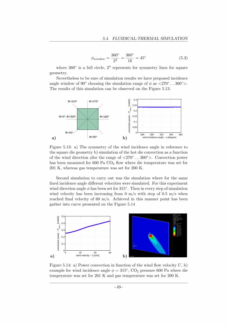
5.4. FLUIDICAL-THERMAL SIMULATION
φwindow =360
24=
360
16= 45 (5.3)
where 360 is a full circle, 24 represents for symmetry lines for squaregeometry.
Nevertheless to be sure of simulation results we have proposed incidenceangle window of 90 choosing the simulation range of φ as <270. . . 360>.The results of this simulation can be observed on the Figure 5.13.
a)
Φ=0º, Φ=360º
Φ=90ºΦ=45º
Φ=180º
Φ=270ºΦ=315º
b)280 300 320 340 360
0
0.05
0.1
0.15
0.2
0.25
0.3
wind incidance angle − φ [degree]
conv
ectio
n po
wer
− P
conv
. [mW
/K]
Figure 5.13: a) The symmetry of the wind incidence angle in reference tothe square die geometry b) simulation of the hot die convection as a functionof the wind direction φfor the range of <270 . . . 360>. Convection powerhas been measured for 600 Pa CO2 flow where die temperature was set for201 K, whereas gas temperature was set for 200 K.
Second simulation to carry out was the simulation where for the samefixed incidence angle different velocities were simulated. For this experimentwind direction angle φ has been set for 315. Then in every step of simulationwind velocity has been increasing from 0 m/s with step of 0.5 m/s whenreached final velocity of 60 m/s. Achieved in this manner point has beengather into curve presented on the Figure 5.14
a)0 20 40 60
0
0.1
0.2
0.3
0.4
0.5
wind velocity − U [m/s]
conv
ectio
n po
wer
− P
conv
. [mW
/K]
b)
Figure 5.14: a) Power convection in function of the wind flow velocity U , b)example for wind incidence angle φ = 315, CO2 pressure 600 Pa where dietemperature was set for 201 K and gas temperature was set for 200 K.
- 49 -
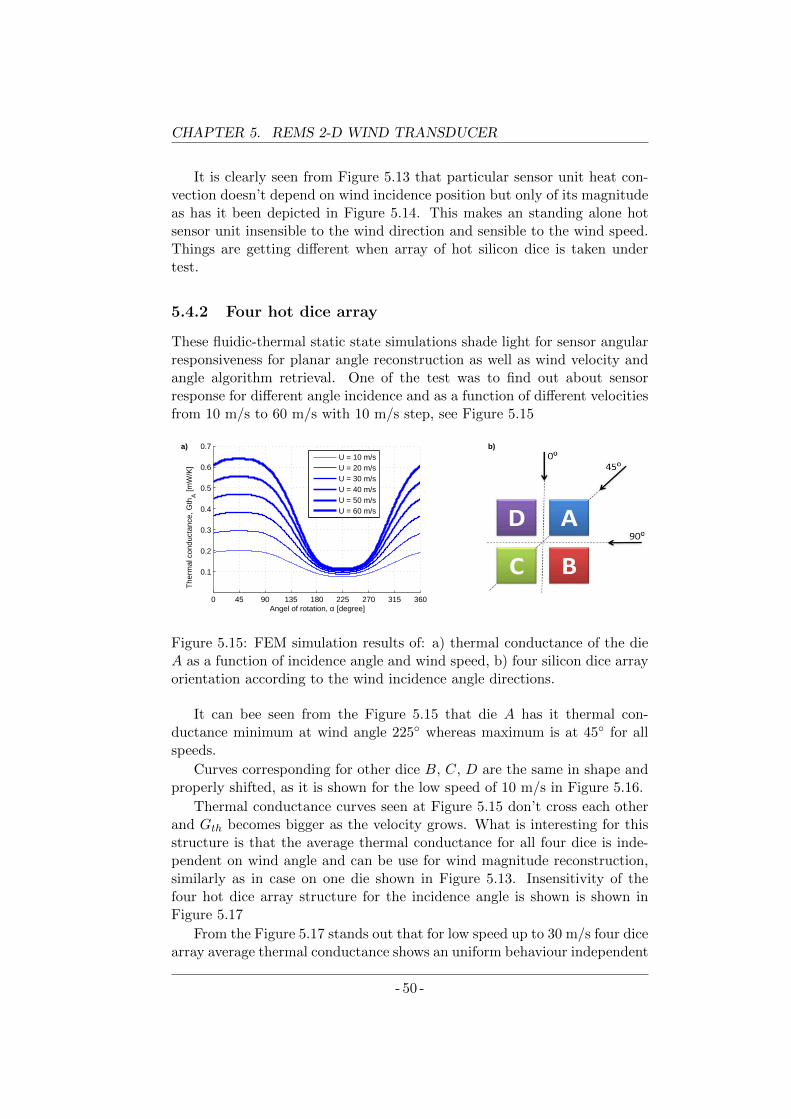
CHAPTER 5. REMS 2-D WIND TRANSDUCER
It is clearly seen from Figure 5.13 that particular sensor unit heat con-vection doesn’t depend on wind incidence position but only of its magnitudeas has it been depicted in Figure 5.14. This makes an standing alone hotsensor unit insensible to the wind direction and sensible to the wind speed.Things are getting different when array of hot silicon dice is taken undertest.
5.4.2 Four hot dice array
These fluidic-thermal static state simulations shade light for sensor angularresponsiveness for planar angle reconstruction as well as wind velocity andangle algorithm retrieval. One of the test was to find out about sensorresponse for different angle incidence and as a function of different velocitiesfrom 10 m/s to 60 m/s with 10 m/s step, see Figure 5.15
0 45 90 135 180 225 270 315 360
0.1
0.2
0.3
0.4
0.5
0.6
0.7
Angel of rotation, α [degree]
The
rmal
con
duct
ance
, Gth
A [m
W/K
]
a)
0 90 180 270 3600
0.1
0.2
0.3
0.4
0.5
Angel of rotation, α [degree]
The
amal
con
duct
ance
, Gth
avg.
[mW
/K]
a)
0 10 20 30 40 50 60 700
0.1
0.2
0.3
0.4
0.5 b)
The
amal
con
duct
ance
, Gth
avg.
[mW
/K]
Wind velocity, U [m/s]
U = 10 m/sU = 20 m/sU = 30 m/sU = 40 m/sU = 50 m/sU = 60 m/s
b)
U = 10 m/sU = 20 m/sU = 30 m/sU = 40 m/sU = 50 m/sU = 60 m/s
Figure 5.15: FEM simulation results of: a) thermal conductance of the dieA as a function of incidence angle and wind speed, b) four silicon dice arrayorientation according to the wind incidence angle directions.
It can bee seen from the Figure 5.15 that die A has it thermal con-ductance minimum at wind angle 225 whereas maximum is at 45 for allspeeds.
Curves corresponding for other dice B, C, D are the same in shape andproperly shifted, as it is shown for the low speed of 10 m/s in Figure 5.16.
Thermal conductance curves seen at Figure 5.15 don’t cross each otherand Gth becomes bigger as the velocity grows. What is interesting for thisstructure is that the average thermal conductance for all four dice is inde-pendent on wind angle and can be use for wind magnitude reconstruction,similarly as in case on one die shown in Figure 5.13. Insensitivity of thefour hot dice array structure for the incidence angle is shown is shown inFigure 5.17
From the Figure 5.17 stands out that for low speed up to 30 m/s four dicearray average thermal conductance shows an uniform behaviour independent
- 50 -
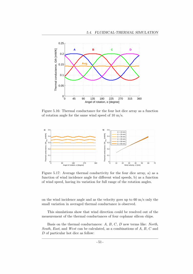
5.4. FLUIDICAL-THERMAL SIMULATION
0 45 90 135 180 225 270 315 3600
0.05
0.1
0.15
0.2
0.25
A B C D
Avg.
Angel of rotation, α [degree]
The
rmal
con
duct
ance
, Gth
[mW
/K]
Figure 5.16: Thermal conductance for the four hot dice array as a functionof rotation angle for the same wind speed of 10 m/s.
0 45 90 135 180 225 270 315 360
0.1
0.2
0.3
0.4
0.5
0.6
0.7
Angel of rotation, α [degree]
The
rmal
con
duct
ance
, Gth
A [m
W/K
]
a)
0 90 180 270 3600
0.1
0.2
0.3
0.4
0.5
Angel of rotation, α [degree]
The
amal
con
duct
ance
, Gth
avg.
[mW
/K]
a)
0 10 20 30 40 50 60 700
0.1
0.2
0.3
0.4
0.5 b)
The
amal
con
duct
ance
, Gth
avg.
[mW
/K]
Wind velocity, U [m/s]
U = 10 m/sU = 20 m/sU = 30 m/sU = 40 m/sU = 50 m/sU = 60 m/s
b)
U = 10 m/sU = 20 m/sU = 30 m/sU = 40 m/sU = 50 m/sU = 60 m/s
Figure 5.17: Average thermal conductivity for the four dice array, a) as afunction of wind incidence angle for different wind speeds, b) as a functionof wind speed, having its variation for full range of the rotation angles.
on the wind incidence angle and as the velocity goes up to 60 m/s only thesmall variation in averaged thermal conductance is observed.
This simulations show that wind direction could be resolved out of themeasurement of the thermal conductances of four coplanar silicon chips.
Basis on the thermal conductances: A, B, C, D new terms like: North,South, East, and West can be calculated, as a combinations of A, B, C andD of particular hot dice as follow:
- 51 -
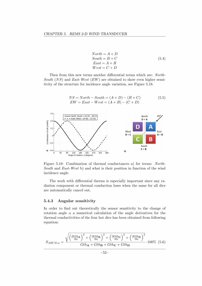
CHAPTER 5. REMS 2-D WIND TRANSDUCER
North = A+DSouth = B + CEast = A+BWest = C +D
(5.4)
Then from this new terms another differential terms which are: North-South (NS) and East-West (EW ) are obtained to show even higher sensi-tivity of the structure for incidence angle variation, see Figure 5.18.
NS = North− South = (A+D)− (B + C)EW = East−West = (A+B)− (C +D)
(5.5)
0 45 90 135 180 225 270 315 360−0.2
−0.1
0
0.1
0.2
0.3
Angel of rotation, α [degree]
Com
bina
tion
of G
th [m
W/K
]
a)
North−South = (A+D) − (B+C)East−West = (A+B) − (C+D)
b)
Figure 5.18: Combination of thermal conductances a) for terms: North-South and East-West b) and what is their position in function of the windincidence angle.
The work with differential therms is especially important since any ra-diation component or thermal conduction loses when the same for all diceare automatically cancel out.
5.4.3 Angular sensitivity
In order to find out theoretically the sensor sensitivity to the change ofrotation angle α a numerical calculation of the angle derivatives for thethermal conductivities of the four hot dice has been obtained from followingequation:
SABCD,α =
√(∂GthA∂α
)2+(∂GthB∂α
)2+(∂GthC∂α
)2+(∂GthD∂α
)2
GthA +GthB +GthC +GthD·100% (5.6)
- 52 -
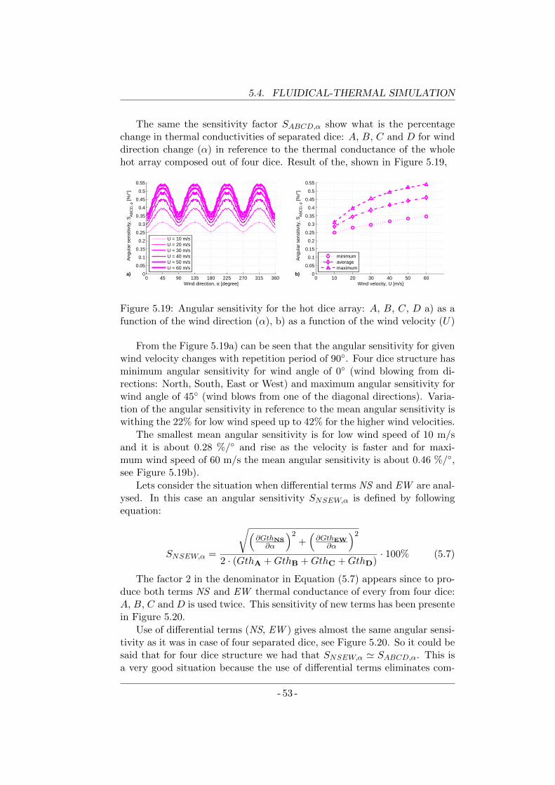
5.4. FLUIDICAL-THERMAL SIMULATION
The same the sensitivity factor SABCD,α show what is the percentagechange in thermal conductivities of separated dice: A, B, C and D for winddirection change (α) in reference to the thermal conductance of the wholehot array composed out of four dice. Result of the, shown in Figure 5.19,
0 45 90 135 180 225 270 315 3600
0.05
0.1
0.15
0.2
0.25
0.3
0.35
0.4
0.45
0.5
0.55
Wind direction, α [degree]
A
ngul
ar s
ensi
tivity
, SA
BC
D, α
[%/°
]
a)
0 45 90 135 180 225 270 315 3600
0.05
0.1
0.15
0.2
0.25
0.3
0.35
0.4
0.45
0.5
0.55
Wind direction, α [degree]
A
ngul
ar s
ensi
tivity
, SN
SE
W, α
[%/°
]
a)
U = 10 m/sU = 20 m/sU = 30 m/sU = 40 m/sU = 50 m/sU = 60 m/s
U = 10 m/sU = 20 m/sU = 30 m/sU = 40 m/sU = 50 m/sU = 60 m/s
0 10 20 30 40 50 600
0.05
0.1
0.15
0.2
0.25
0.3
0.35
0.4
0.45
0.5
0.55
Wind velocity, U [m/s]
A
ngul
ar s
ensi
tivity
, SA
BC
D, α
[%/°
]
b)
minimumaveragemaximum
10 20 30 40 50 6020
25
30
35
40
45Figure 5.19: Angular sensitivity for the hot dice array: A, B, C, D a) as afunction of the wind direction (α), b) as a function of the wind velocity (U)
From the Figure 5.19a) can be seen that the angular sensitivity for givenwind velocity changes with repetition period of 90. Four dice structure hasminimum angular sensitivity for wind angle of 0 (wind blowing from di-rections: North, South, East or West) and maximum angular sensitivity forwind angle of 45 (wind blows from one of the diagonal directions). Varia-tion of the angular sensitivity in reference to the mean angular sensitivity iswithing the 22% for low wind speed up to 42% for the higher wind velocities.
The smallest mean angular sensitivity is for low wind speed of 10 m/sand it is about 0.28 %/ and rise as the velocity is faster and for maxi-mum wind speed of 60 m/s the mean angular sensitivity is about 0.46 %/,see Figure 5.19b).
Lets consider the situation when differential terms NS and EW are anal-ysed. In this case an angular sensitivity SNSEW,α is defined by followingequation:
SNSEW,α =
√(∂GthNS∂α
)2+(∂GthEW
∂α
)2
2 · (GthA +GthB +GthC +GthD)· 100% (5.7)
The factor 2 in the denominator in Equation (5.7) appears since to pro-duce both terms NS and EW thermal conductance of every from four dice:A, B, C and D is used twice. This sensitivity of new terms has been presentein Figure 5.20.
Use of differential terms (NS, EW ) gives almost the same angular sensi-tivity as it was in case of four separated dice, see Figure 5.20. So it could besaid that for four dice structure we had that SNSEW,α ' SABCD,α. This isa very good situation because the use of differential terms eliminates com-
- 53 -
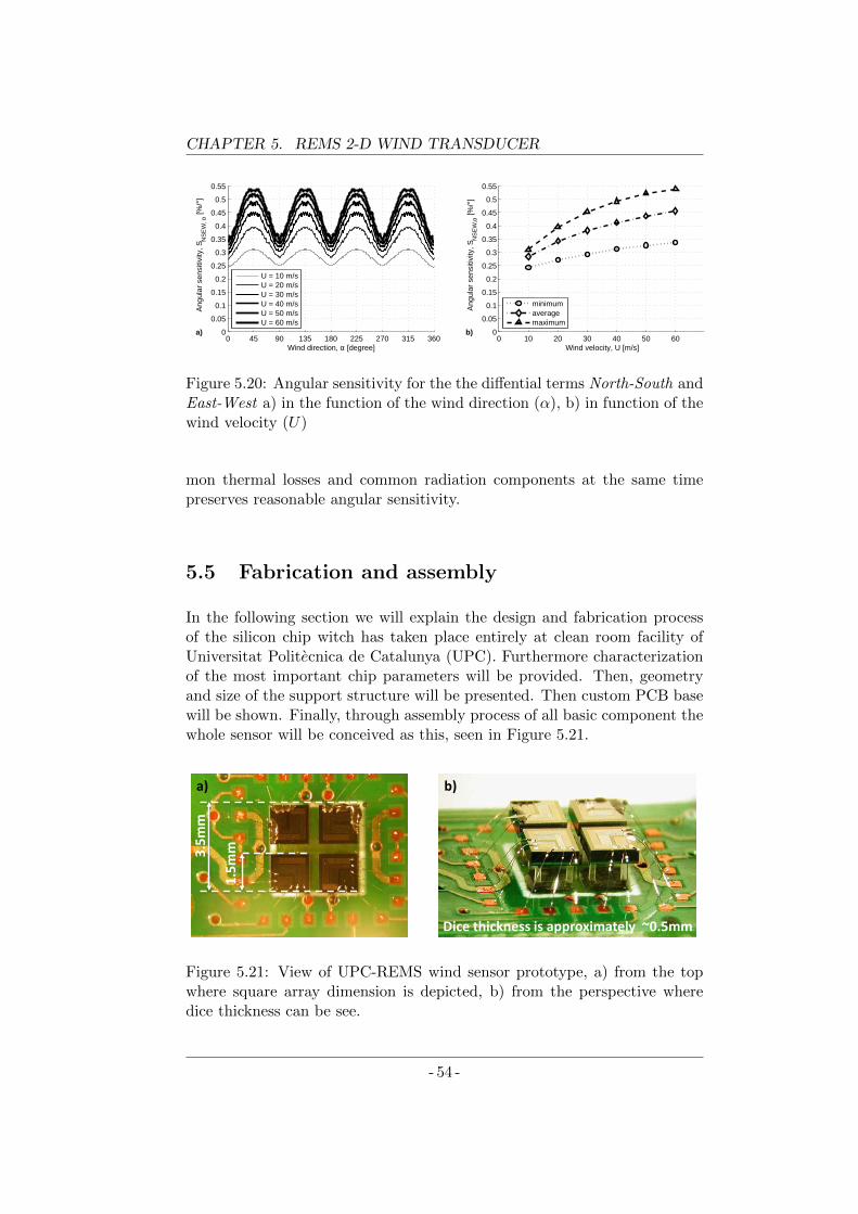
CHAPTER 5. REMS 2-D WIND TRANSDUCER0 45 90 135 180 225 270 315 360
0
0.05
0.1
0.15
0.2
0.25
0.3
0.35
0.4
0.45
0.5
0.55
Wind direction, α [degree]
A
ngul
ar s
ensi
tivity
, SA
BC
D, α
[%/°
]
a)
0 45 90 135 180 225 270 315 3600
0.05
0.1
0.15
0.2
0.25
0.3
0.35
0.4
0.45
0.5
0.55
Wind direction, α [degree]
A
ngul
ar s
ensi
tivity
, SN
SE
W, α
[%/°
]
a)
U = 10 m/sU = 20 m/sU = 30 m/sU = 40 m/sU = 50 m/sU = 60 m/s
U = 10 m/sU = 20 m/sU = 30 m/sU = 40 m/sU = 50 m/sU = 60 m/s
0 10 20 30 40 50 600
0.05
0.1
0.15
0.2
0.25
0.3
0.35
0.4
0.45
0.5
0.55
Wind velocity, U [m/s]
A
ngul
ar s
ensi
tivity
, SA
BC
D, α
[%/°
]
b)
minimumaveragemaximum
0 10 20 30 40 50 600
0.05
0.1
0.15
0.2
0.25
0.3
0.35
0.4
0.45
0.5
0.55
Wind velocity, U [m/s]
A
ngul
ar s
ensi
tivity
, SN
SE
W,α
[%/°
]
b)
minimumaveragemaximum
Figure 5.20: Angular sensitivity for the the diffential terms North-South andEast-West a) in the function of the wind direction (α), b) in function of thewind velocity (U)
mon thermal losses and common radiation components at the same timepreserves reasonable angular sensitivity.
5.5 Fabrication and assembly
In the following section we will explain the design and fabrication processof the silicon chip witch has taken place entirely at clean room facility ofUniversitat Politecnica de Catalunya (UPC). Furthermore characterizationof the most important chip parameters will be provided. Then, geometryand size of the support structure will be presented. Then custom PCB basewill be shown. Finally, through assembly process of all basic component thewhole sensor will be conceived as this, seen in Figure 5.21.
a) b)
3
.5m
m
1.5m
m
Dice thickness is approximately ~0.5mm
Figure 5.21: View of UPC-REMS wind sensor prototype, a) from the topwhere square array dimension is depicted, b) from the perspective wheredice thickness can be see.
- 54 -
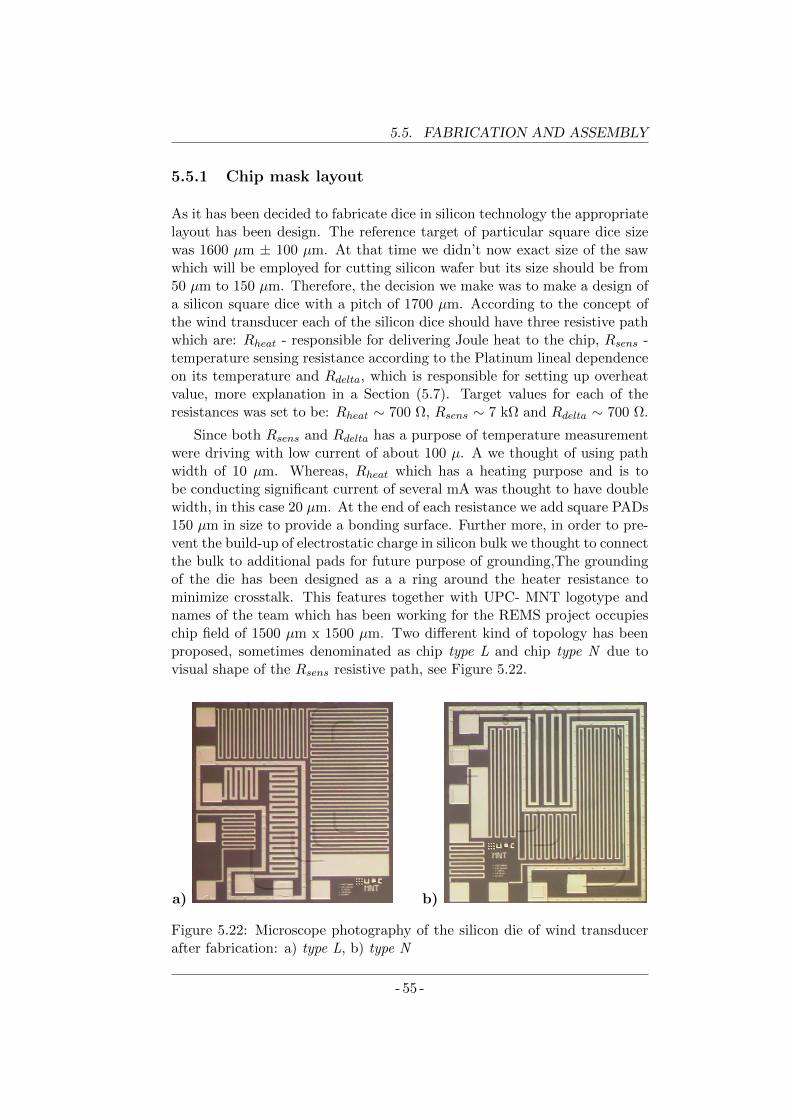
5.5. FABRICATION AND ASSEMBLY
5.5.1 Chip mask layout
As it has been decided to fabricate dice in silicon technology the appropriatelayout has been design. The reference target of particular square dice sizewas 1600 µm ± 100 µm. At that time we didn’t now exact size of the sawwhich will be employed for cutting silicon wafer but its size should be from50 µm to 150 µm. Therefore, the decision we make was to make a design ofa silicon square dice with a pitch of 1700 µm. According to the concept ofthe wind transducer each of the silicon dice should have three resistive pathwhich are: Rheat - responsible for delivering Joule heat to the chip, Rsens -temperature sensing resistance according to the Platinum lineal dependenceon its temperature and Rdelta, which is responsible for setting up overheatvalue, more explanation in a Section (5.7). Target values for each of theresistances was set to be: Rheat ∼ 700 Ω, Rsens ∼ 7 kΩ and Rdelta ∼ 700 Ω.
Since both Rsens and Rdelta has a purpose of temperature measurementwere driving with low current of about 100 µ. A we thought of using pathwidth of 10 µm. Whereas, Rheat which has a heating purpose and is tobe conducting significant current of several mA was thought to have doublewidth, in this case 20 µm. At the end of each resistance we add square PADs150 µm in size to provide a bonding surface. Further more, in order to pre-vent the build-up of electrostatic charge in silicon bulk we thought to connectthe bulk to additional pads for future purpose of grounding,The groundingof the die has been designed as a a ring around the heater resistance tominimize crosstalk. This features together with UPC- MNT logotype andnames of the team which has been working for the REMS project occupieschip field of 1500 µm x 1500 µm. Two different kind of topology has beenproposed, sometimes denominated as chip type L and chip type N due tovisual shape of the Rsens resistive path, see Figure 5.22.
a) b)
Figure 5.22: Microscope photography of the silicon die of wind transducerafter fabrication: a) type L, b) type N
- 55 -
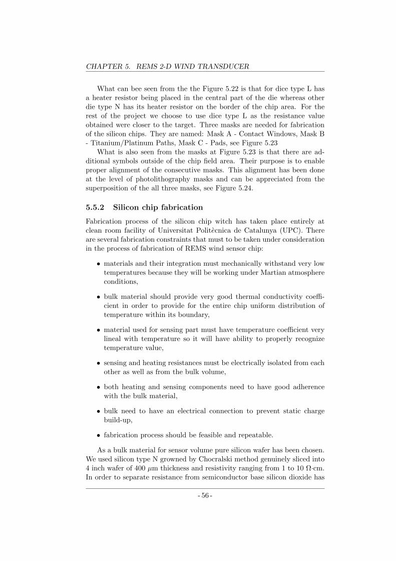
CHAPTER 5. REMS 2-D WIND TRANSDUCER
What can bee seen from the the Figure 5.22 is that for dice type L hasa heater resistor being placed in the central part of the die whereas otherdie type N has its heater resistor on the border of the chip area. For therest of the project we choose to use dice type L as the resistance valueobtained were closer to the target. Three masks are needed for fabricationof the silicon chips. They are named: Mask A - Contact Windows, Mask B- Titanium/Platinum Paths, Mask C - Pads, see Figure 5.23
What is also seen from the masks at Figure 5.23 is that there are ad-ditional symbols outside of the chip field area. Their purpose is to enableproper alignment of the consecutive masks. This alignment has been doneat the level of photolithography masks and can be appreciated from thesuperposition of the all three masks, see Figure 5.24.
5.5.2 Silicon chip fabrication
Fabrication process of the silicon chip witch has taken place entirely atclean room facility of Universitat Politecnica de Catalunya (UPC). Thereare several fabrication constraints that must to be taken under considerationin the process of fabrication of REMS wind sensor chip:
• materials and their integration must mechanically withstand very lowtemperatures because they will be working under Martian atmosphereconditions,
• bulk material should provide very good thermal conductivity coeffi-cient in order to provide for the entire chip uniform distribution oftemperature within its boundary,
• material used for sensing part must have temperature coefficient verylineal with temperature so it will have ability to properly recognizetemperature value,
• sensing and heating resistances must be electrically isolated from eachother as well as from the bulk volume,
• both heating and sensing components need to have good adherencewith the bulk material,
• bulk need to have an electrical connection to prevent static chargebuild-up,
• fabrication process should be feasible and repeatable.
As a bulk material for sensor volume pure silicon wafer has been chosen.We used silicon type N growned by Chocralski method genuinely sliced into4 inch wafer of 400 µm thickness and resistivity ranging from 1 to 10 Ω·cm.In order to separate resistance from semiconductor base silicon dioxide has
- 56 -
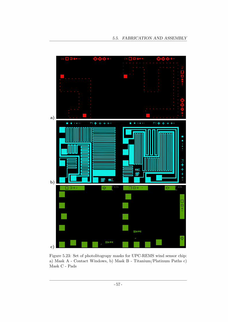
5.5. FABRICATION AND ASSEMBLY
a)
b)
c)
Figure 5.23: Set of photolitograpy masks for UPC-REMS wind sensor chip:a) Mask A - Contact Windows, b) Mask B - Titanium/Platinum Paths c)Mask C - Pads
- 57 -
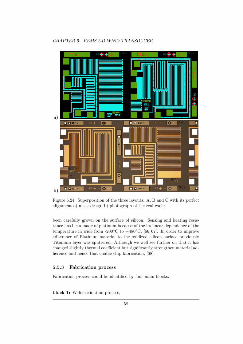
CHAPTER 5. REMS 2-D WIND TRANSDUCER
a)
b)
Figure 5.24: Superposition of the three layouts: A, B and C with its perfectalignment a) mask design b) photograph of the real wafer.
been carefully grown on the surface of silicon. Sensing and heating resis-tance has been made of platinum because of the its linear dependence of thetemperature in wide from -200C to +480C, [66, 67]. In order to improveadherence of Platinum material to the oxidized silicon surface previouslyTitanium layer was sputtered. Although we well see further on that it haschanged slightly thermal coefficient but significantly strengthen material ad-herence and hence that enable chip fabrication, [68].
5.5.3 Fabrication process
Fabrication process could be identified by four main blocks:
block 1: Wafer oxidation process,
- 58 -
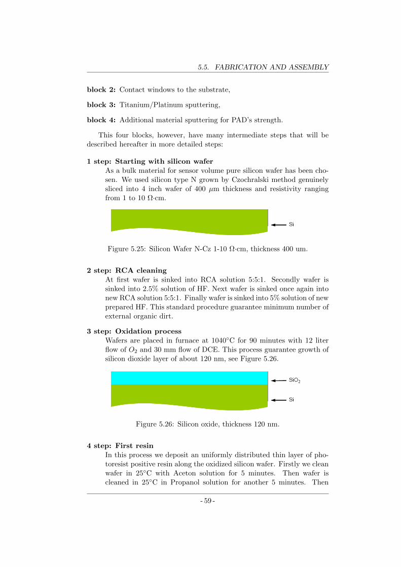
5.5. FABRICATION AND ASSEMBLY
block 2: Contact windows to the substrate,
block 3: Titanium/Platinum sputtering,
block 4: Additional material sputtering for PAD’s strength.
This four blocks, however, have many intermediate steps that will bedescribed hereafter in more detailed steps:
1 step: Starting with silicon waferAs a bulk material for sensor volume pure silicon wafer has been cho-sen. We used silicon type N grown by Czochralski method genuinelysliced into 4 inch wafer of 400 µm thickness and resistivity rangingfrom 1 to 10 Ω·cm.
Figure 5.25: Silicon Wafer N-Cz 1-10 Ω·cm, thickness 400 um.
2 step: RCA cleaningAt first wafer is sinked into RCA solution 5:5:1. Secondly wafer issinked into 2.5% solution of HF. Next wafer is sinked once again intonew RCA solution 5:5:1. Finally wafer is sinked into 5% solution of newprepared HF. This standard procedure guarantee minimum number ofexternal organic dirt.
3 step: Oxidation processWafers are placed in furnace at 1040C for 90 minutes with 12 literflow of O2 and 30 mm flow of DCE. This process guarantee growth ofsilicon dioxide layer of about 120 nm, see Figure 5.26.
Figure 5.26: Silicon oxide, thickness 120 nm.
4 step: First resinIn this process we deposit an uniformly distributed thin layer of pho-toresist positive resin along the oxidized silicon wafer. Firstly we cleanwafer in 25C with Aceton solution for 5 minutes. Then wafer iscleaned in 25C in Propanol solution for another 5 minutes. Then
- 59 -
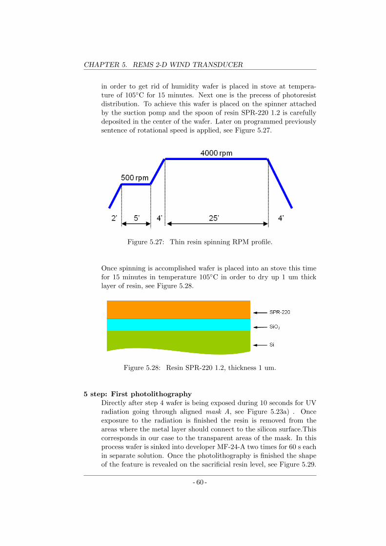
CHAPTER 5. REMS 2-D WIND TRANSDUCER
in order to get rid of humidity wafer is placed in stove at tempera-ture of 105C for 15 minutes. Next one is the precess of photoresistdistribution. To achieve this wafer is placed on the spinner attachedby the suction pomp and the spoon of resin SPR-220 1.2 is carefullydeposited in the center of the wafer. Later on programmed previouslysentence of rotational speed is applied, see Figure 5.27.
Figure 5.27: Thin resin spinning RPM profile.
Once spinning is accomplished wafer is placed into an stove this timefor 15 minutes in temperature 105C in order to dry up 1 um thicklayer of resin, see Figure 5.28.
Figure 5.28: Resin SPR-220 1.2, thickness 1 um.
5 step: First photolithographyDirectly after step 4 wafer is being exposed during 10 seconds for UVradiation going through aligned mask A, see Figure 5.23a) . Onceexposure to the radiation is finished the resin is removed from theareas where the metal layer should connect to the silicon surface.Thiscorresponds in our case to the transparent areas of the mask. In thisprocess wafer is sinked into developer MF-24-A two times for 60 s eachin separate solution. Once the photolithography is finished the shapeof the feature is revealed on the sacrificial resin level, see Figure 5.29.
- 60 -
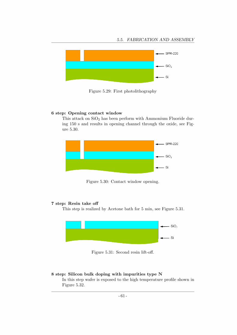
5.5. FABRICATION AND ASSEMBLY
Figure 5.29: First photolithography
6 step: Opening contact windowThis attack on SiO2 has been perform with Ammonium Fluoride dur-ing 150 s and results in opening channel through the oxide, see Fig-ure 5.30.
Figure 5.30: Contact window opening.
7 step: Resin take offThis step is realized by Acetone bath for 5 min, see Figure 5.31.
Figure 5.31: Second resin lift-off.
8 step: Silicon bulk doping with impurities type NIn this step wafer is exposed to the high temperature profile shown inFigure 5.32.
- 61 -
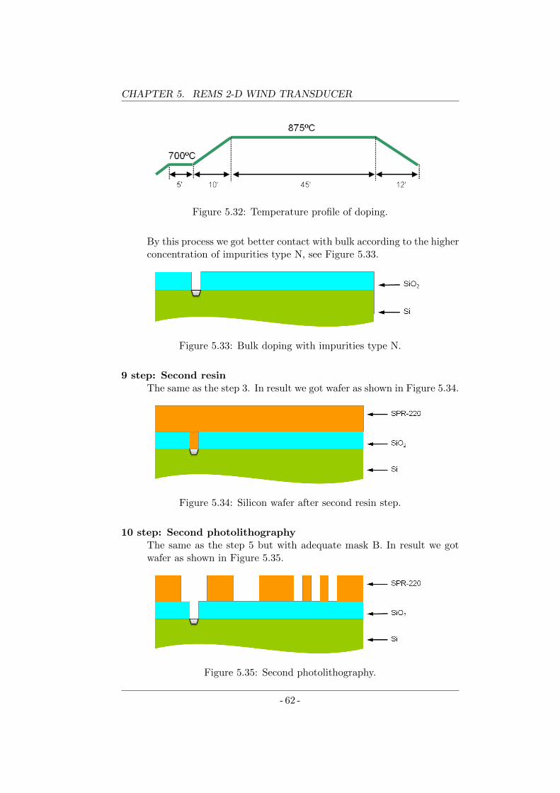
CHAPTER 5. REMS 2-D WIND TRANSDUCER
Figure 5.32: Temperature profile of doping.
By this process we got better contact with bulk according to the higherconcentration of impurities type N, see Figure 5.33.
Figure 5.33: Bulk doping with impurities type N.
9 step: Second resinThe same as the step 3. In result we got wafer as shown in Figure 5.34.
Figure 5.34: Silicon wafer after second resin step.
10 step: Second photolithographyThe same as the step 5 but with adequate mask B. In result we gotwafer as shown in Figure 5.35.
Figure 5.35: Second photolithography.
- 62 -
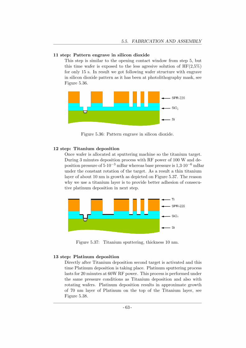
5.5. FABRICATION AND ASSEMBLY
11 step: Pattern engrave in silicon dioxideThis step is similar to the opening contact window from step 5, butthis time wafer is exposed to the less agresive solution of HF(2,5%)for only 15 s. In result we got following wafer structure with engravein silicon dioxide pattern as it has been at photolithography mask, seeFigure 5.36.
Figure 5.36: Pattern engrave in silicon dioxide.
12 step: Titanium depositionOnce wafer is allocated at sputtering machine so the titanium target.During 3 minutes deposition process with RF power of 100 W and de-position pressure of 5·10−3 mBar whereas base pressure is 1,3·10−6 mBarunder the constant rotation of the target. As a result a thin titaniumlayer of about 10 nm is growth as depicted on Figure 5.37. The reasonwhy we use a titanium layer is to provide better adhesion of consecu-tive platinum deposition in next step.
Figure 5.37: Titanium sputtering, thickness 10 nm.
13 step: Platinum depositionDirectly after Titanium deposition second target is activated and thistime Platinum deposition is taking place. Platinum sputtering processlasts for 20 minutes at 60W RF power. This process is performed underthe same pressure conditions as Titanium deposition and also withrotating wafers. Platinum deposition results in approximate growthof 70 nm layer of Platinum on the top of the Titanium layer, seeFigure 5.38.
- 63 -
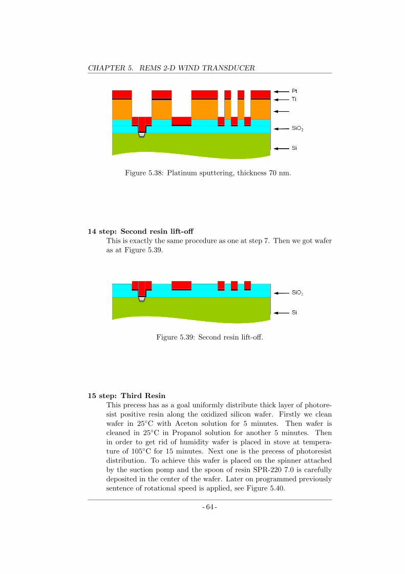
CHAPTER 5. REMS 2-D WIND TRANSDUCER
Figure 5.38: Platinum sputtering, thickness 70 nm.
14 step: Second resin lift-offThis is exactly the same procedure as one at step 7. Then we got waferas at Figure 5.39.
Figure 5.39: Second resin lift-off.
15 step: Third ResinThis precess has as a goal uniformly distribute thick layer of photore-sist positive resin along the oxidized silicon wafer. Firstly we cleanwafer in 25C with Aceton solution for 5 minutes. Then wafer iscleaned in 25C in Propanol solution for another 5 minutes. Thenin order to get rid of humidity wafer is placed in stove at tempera-ture of 105C for 15 minutes. Next one is the precess of photoresistdistribution. To achieve this wafer is placed on the spinner attachedby the suction pomp and the spoon of resin SPR-220 7.0 is carefullydeposited in the center of the wafer. Later on programmed previouslysentence of rotational speed is applied, see Figure 5.40.
- 64 -
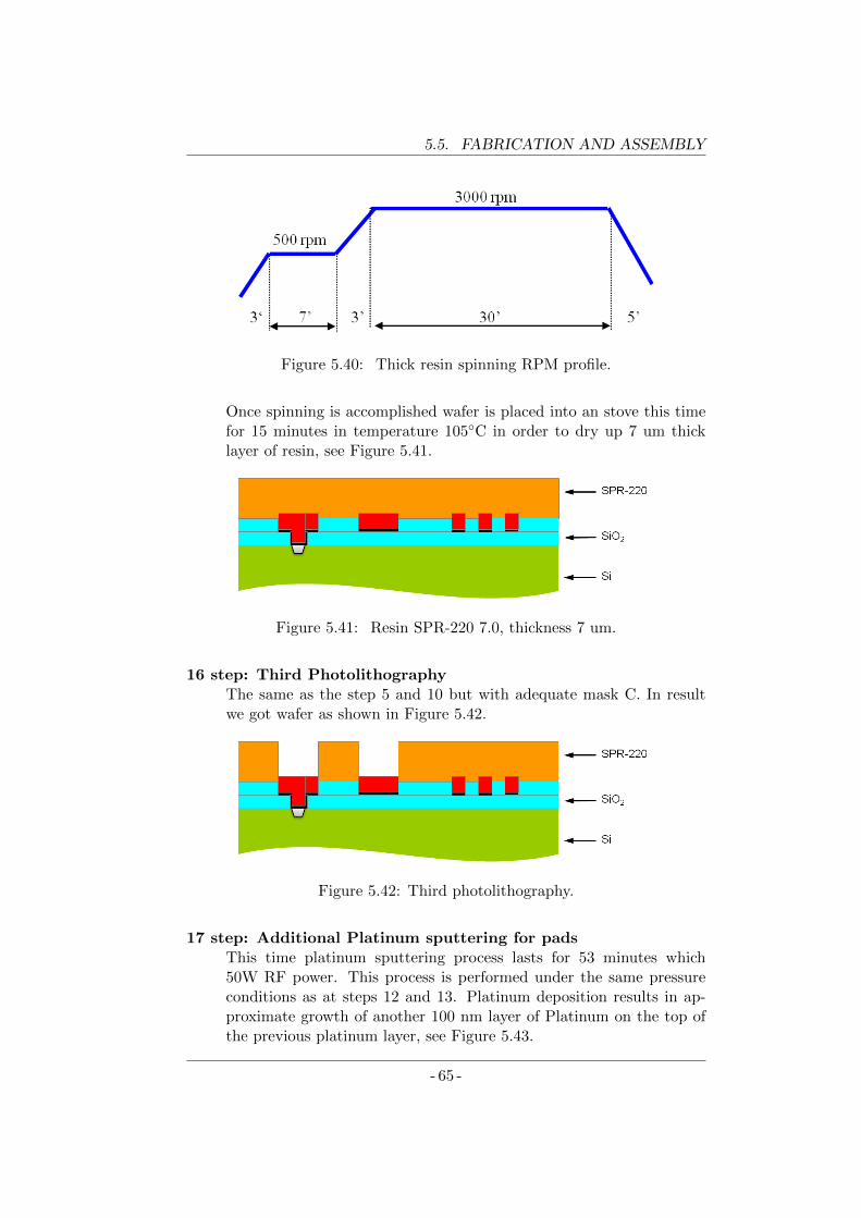
5.5. FABRICATION AND ASSEMBLY
Figure 5.40: Thick resin spinning RPM profile.
Once spinning is accomplished wafer is placed into an stove this timefor 15 minutes in temperature 105C in order to dry up 7 um thicklayer of resin, see Figure 5.41.
Figure 5.41: Resin SPR-220 7.0, thickness 7 um.
16 step: Third PhotolithographyThe same as the step 5 and 10 but with adequate mask C. In resultwe got wafer as shown in Figure 5.42.
Figure 5.42: Third photolithography.
17 step: Additional Platinum sputtering for padsThis time platinum sputtering process lasts for 53 minutes which50W RF power. This process is performed under the same pressureconditions as at steps 12 and 13. Platinum deposition results in ap-proximate growth of another 100 nm layer of Platinum on the top ofthe previous platinum layer, see Figure 5.43.
- 65 -
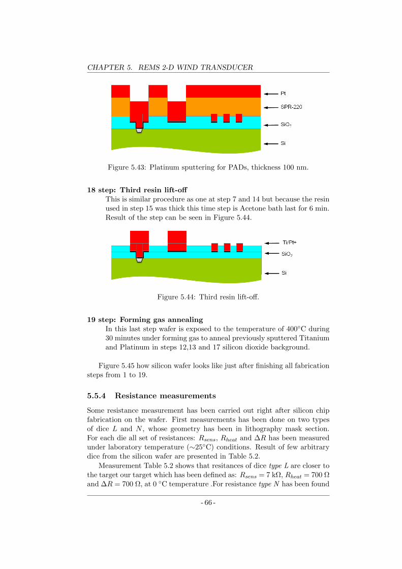
CHAPTER 5. REMS 2-D WIND TRANSDUCER
Figure 5.43: Platinum sputtering for PADs, thickness 100 nm.
18 step: Third resin lift-offThis is similar procedure as one at step 7 and 14 but because the resinused in step 15 was thick this time step is Acetone bath last for 6 min.Result of the step can be seen in Figure 5.44.
Figure 5.44: Third resin lift-off.
19 step: Forming gas annealingIn this last step wafer is exposed to the temperature of 400C during30 minutes under forming gas to anneal previously sputtered Titaniumand Platinum in steps 12,13 and 17 silicon dioxide background.
Figure 5.45 how silicon wafer looks like just after finishing all fabricationsteps from 1 to 19.
5.5.4 Resistance measurements
Some resistance measurement has been carried out right after silicon chipfabrication on the wafer. First measurements has been done on two typesof dice L and N , whose geometry has been in lithography mask section.For each die all set of resistances: Rsens, Rheat and ∆R has been measuredunder laboratory temperature (∼25C) conditions. Result of few arbitrarydice from the silicon wafer are presented in Table 5.2.
Measurement Table 5.2 shows that resitances of dice type L are closer tothe target our target which has been defined as: Rsens = 7 kΩ, Rheat = 700 Ωand ∆R = 700 Ω, at 0 C temperature .For resistance type N has been found
- 66 -
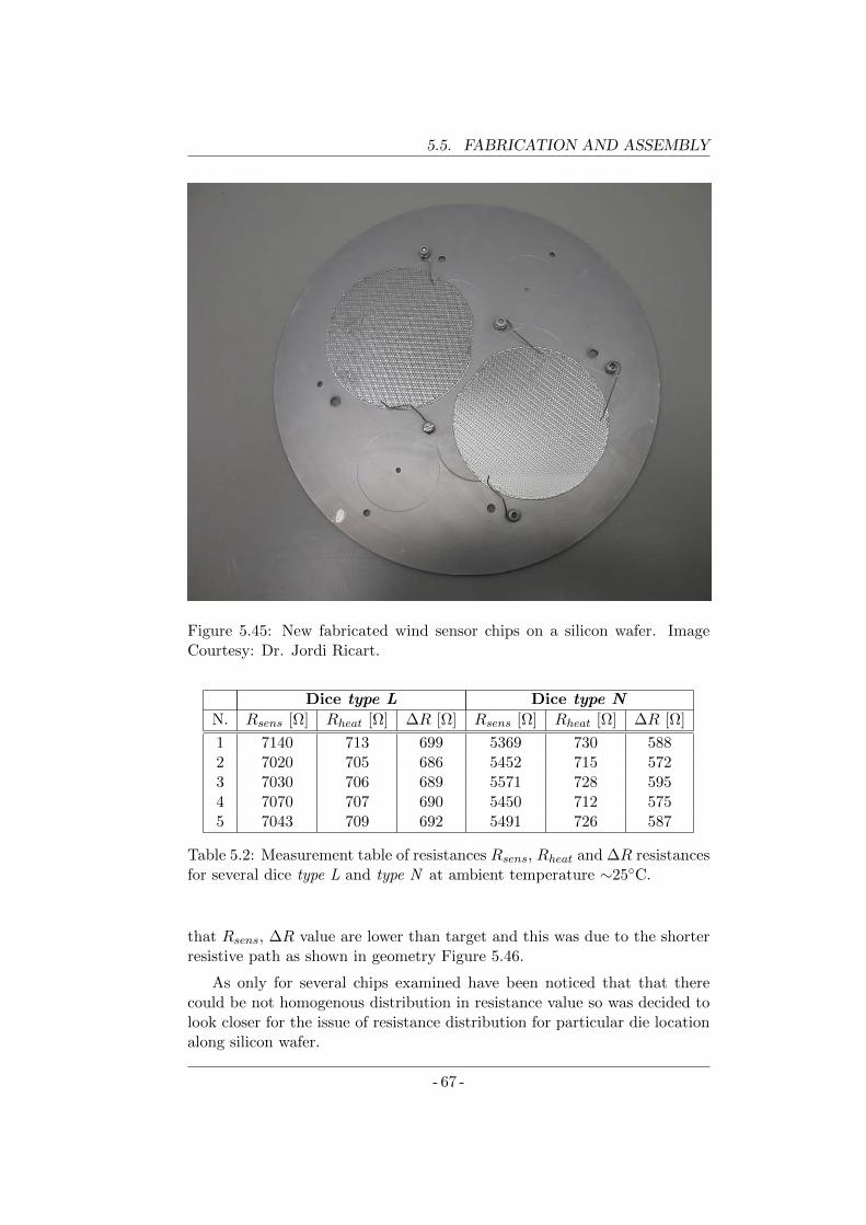
5.5. FABRICATION AND ASSEMBLY
Figure 5.45: New fabricated wind sensor chips on a silicon wafer. ImageCourtesy: Dr. Jordi Ricart.
Dice type L Dice type N
N. Rsens [Ω] Rheat [Ω] ∆R [Ω] Rsens [Ω] Rheat [Ω] ∆R [Ω]
1 7140 713 699 5369 730 5882 7020 705 686 5452 715 5723 7030 706 689 5571 728 5954 7070 707 690 5450 712 5755 7043 709 692 5491 726 587
Table 5.2: Measurement table of resistances Rsens, Rheat and ∆R resistancesfor several dice type L and type N at ambient temperature ∼25C.
that Rsens, ∆R value are lower than target and this was due to the shorterresistive path as shown in geometry Figure 5.46.
As only for several chips examined have been noticed that that therecould be not homogenous distribution in resistance value so was decided tolook closer for the issue of resistance distribution for particular die locationalong silicon wafer.
- 67 -
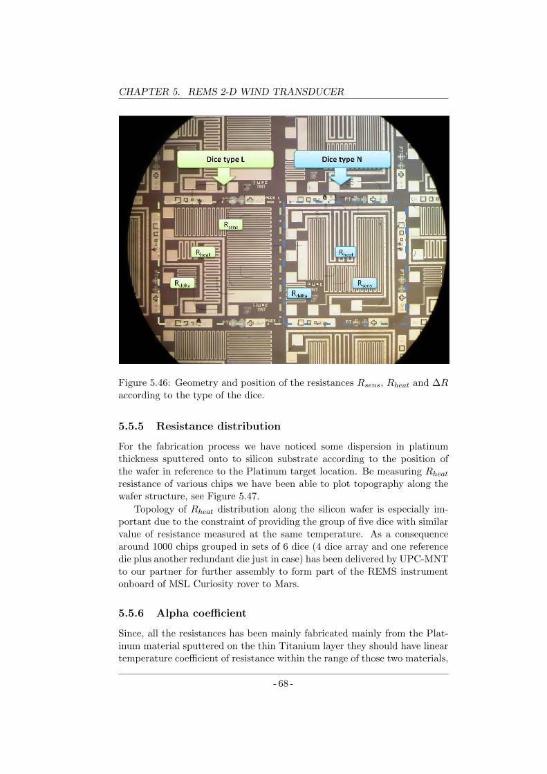
CHAPTER 5. REMS 2-D WIND TRANSDUCER
Figure 5.46: Geometry and position of the resistances Rsens, Rheat and ∆Raccording to the type of the dice.
5.5.5 Resistance distribution
For the fabrication process we have noticed some dispersion in platinumthickness sputtered onto to silicon substrate according to the position ofthe wafer in reference to the Platinum target location. Be measuring Rheatresistance of various chips we have been able to plot topography along thewafer structure, see Figure 5.47.
Topology of Rheat distribution along the silicon wafer is especially im-portant due to the constraint of providing the group of five dice with similarvalue of resistance measured at the same temperature. As a consequencearound 1000 chips grouped in sets of 6 dice (4 dice array and one referencedie plus another redundant die just in case) has been delivered by UPC-MNTto our partner for further assembly to form part of the REMS instrumentonboard of MSL Curiosity rover to Mars.
5.5.6 Alpha coefficient
Since, all the resistances has been mainly fabricated mainly from the Plat-inum material sputtered on the thin Titanium layer they should have lineartemperature coefficient of resistance within the range of those two materials,
- 68 -
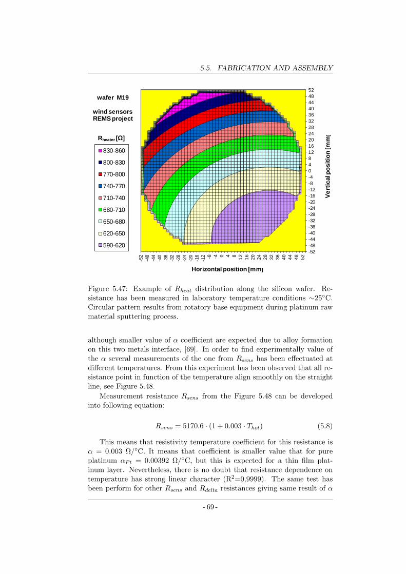
5.5. FABRICATION AND ASSEMBLY
-52
-48
-44
-40
-36
-32
-28
-24
-20
-16
-12
-8
-4
0
4
8
12
16
20
24
28
32
36
40
44
48
52
-52
-48
-44
-40
-36
-32
-28
-24
-20
-16
-12 -8 -4 0 4 8
12
16
20
24
28
32
36
40
44
48
52
Vert
ical
pos
ition
[mm
]Rheater [Ω]
Horizontal position [mm]
wafer M19
wind sensorsREMS project
830-860
800-830
770-800
740-770
710-740
680-710
650-680
620-650
590-620
Figure 5.47: Example of Rheat distribution along the silicon wafer. Re-sistance has been measured in laboratory temperature conditions ∼25C.Circular pattern results from rotatory base equipment during platinum rawmaterial sputtering process.
although smaller value of α coefficient are expected due to alloy formationon this two metals interface, [69]. In order to find experimentally value ofthe α several measurements of the one from Rsens has been effectuated atdifferent temperatures. From this experiment has been observed that all re-sistance point in function of the temperature align smoothly on the straightline, see Figure 5.48.
Measurement resistance Rsens from the Figure 5.48 can be developedinto following equation:
Rsens = 5170.6 · (1 + 0.003 · Thot) (5.8)
This means that resistivity temperature coefficient for this resistance isα = 0.003 Ω/C. It means that coefficient is smaller value that for pureplatinum αPt = 0.00392 Ω/C, but this is expected for a thin film plat-inum layer. Nevertheless, there is no doubt that resistance dependence ontemperature has strong linear character (R2=0,9999). The same test hasbeen perform for other Rsens and Rdelta resistances giving same result of α
- 69 -
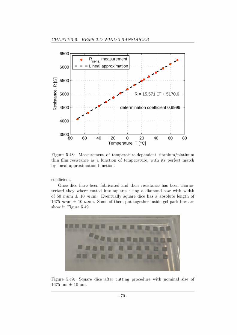
CHAPTER 5. REMS 2-D WIND TRANSDUCER
−80 −60 −40 −20 0 20 40 60 803500
4000
4500
5000
5500
6000
6500
Temperature, T [ °C]
Res
ista
nce,
R [Ω
]
R = 15,571 ⋅ T + 5170,6
determination coefficient 0,9999
Rsens.
measurement
Lineal approximation
Figure 5.48: Measurement of temperature-dependent titanium/platinumthin film resistance as a function of temperature, with its perfect matchby lineal approximation function.
coefficient.
Once dice have been fabricated and their resistance has been charac-terized they where cutted into squares using a diamond saw with widthof 50 mum ± 10 mum. Eventually square dice has a absolute length of1675 mum ± 10 mum. Some of them put together inside gel pack box areshow in Figure 5.49.
Figure 5.49: Square dice after cutting procedure with nominal size of1675 um ± 10 um.
- 70 -
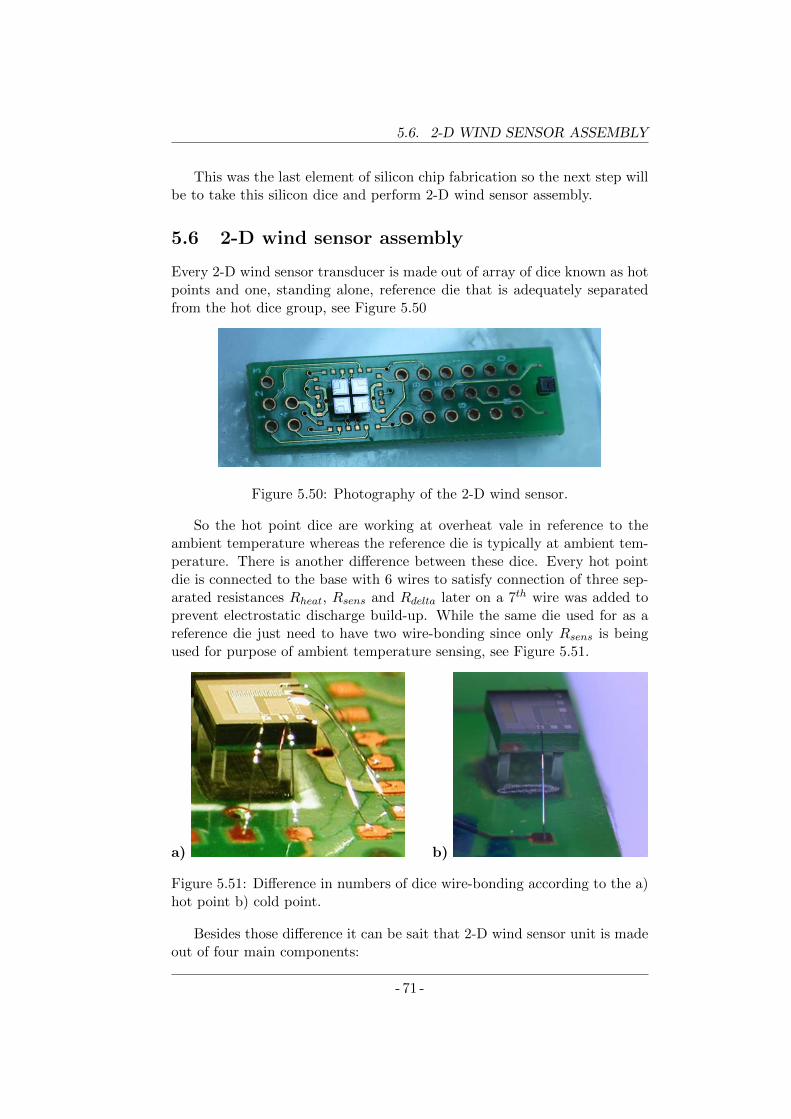
5.6. 2-D WIND SENSOR ASSEMBLY
This was the last element of silicon chip fabrication so the next step willbe to take this silicon dice and perform 2-D wind sensor assembly.
5.6 2-D wind sensor assembly
Every 2-D wind sensor transducer is made out of array of dice known as hotpoints and one, standing alone, reference die that is adequately separatedfrom the hot dice group, see Figure 5.50
Figure 5.50: Photography of the 2-D wind sensor.
So the hot point dice are working at overheat vale in reference to theambient temperature whereas the reference die is typically at ambient tem-perature. There is another difference between these dice. Every hot pointdie is connected to the base with 6 wires to satisfy connection of three sep-arated resistances Rheat, Rsens and Rdelta later on a 7th wire was added toprevent electrostatic discharge build-up. While the same die used for as areference die just need to have two wire-bonding since only Rsens is beingused for purpose of ambient temperature sensing, see Figure 5.51.
a) b)
Figure 5.51: Difference in numbers of dice wire-bonding according to the a)hot point b) cold point.
Besides those difference it can be sait that 2-D wind sensor unit is madeout of four main components:
- 71 -
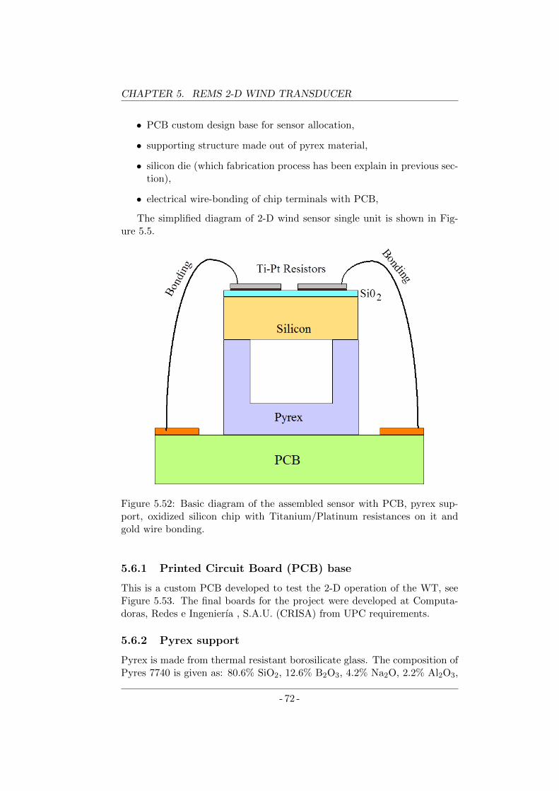
CHAPTER 5. REMS 2-D WIND TRANSDUCER
• PCB custom design base for sensor allocation,
• supporting structure made out of pyrex material,
• silicon die (which fabrication process has been explain in previous sec-tion),
• electrical wire-bonding of chip terminals with PCB,
The simplified diagram of 2-D wind sensor single unit is shown in Fig-ure 5.5.
Figure 5.52: Basic diagram of the assembled sensor with PCB, pyrex sup-port, oxidized silicon chip with Titanium/Platinum resistances on it andgold wire bonding.
5.6.1 Printed Circuit Board (PCB) base
This is a custom PCB developed to test the 2-D operation of the WT, seeFigure 5.53. The final boards for the project were developed at Computa-doras, Redes e Ingenierıa , S.A.U. (CRISA) from UPC requirements.
5.6.2 Pyrex support
Pyrex is made from thermal resistant borosilicate glass. The composition ofPyres 7740 is given as: 80.6% SiO2, 12.6% B2O3, 4.2% Na2O, 2.2% Al2O3,
- 72 -
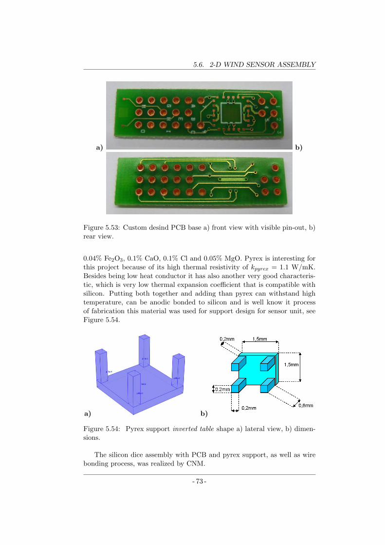
5.6. 2-D WIND SENSOR ASSEMBLY
a) b)
Figure 5.53: Custom desind PCB base a) front view with visible pin-out, b)rear view.
0.04% Fe2O3, 0.1% CaO, 0.1% Cl and 0.05% MgO. Pyrex is interesting forthis project because of its high thermal resistivity of kpyrex = 1.1 W/mK.Besides being low heat conductor it has also another very good characteris-tic, which is very low thermal expansion coefficient that is compatible withsilicon. Putting both together and adding than pyrex can withstand hightemperature, can be anodic bonded to silicon and is well know it processof fabrication this material was used for support design for sensor unit, seeFigure 5.54.
a) b)
Figure 5.54: Pyrex support inverted table shape a) lateral view, b) dimen-sions.
The silicon dice assembly with PCB and pyrex support, as well as wirebonding process, was realized by CNM.
- 73 -
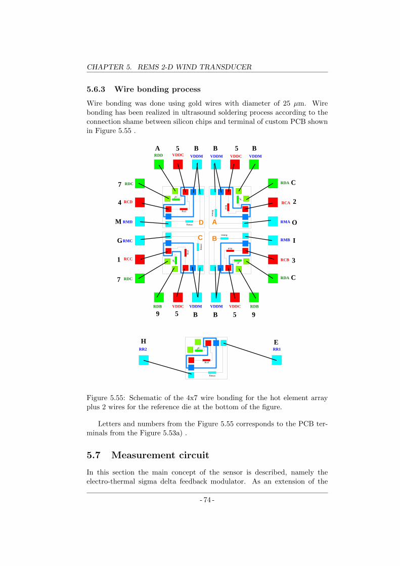
CHAPTER 5. REMS 2-D WIND TRANSDUCER
5.6.3 Wire bonding process
Wire bonding was done using gold wires with diameter of 25 µm. Wirebonding has been realized in ultrasound soldering process according to theconnection shame between silicon chips and terminal of custom PCB shownin Figure 5.55 .
∆R
Rcal
Rmeas
∆R
Rcal
Rmeas
∆R
Rcal
Rmea
s
∆ R
RcalRmeas
∆R
Rcal
Rmeas
BONDING PLACA SENSOR 2x2 Version 3
VDDC VDDC
VDDC VDDC
VDDM VDDM
VDDM VDDM
RMAA
BC
D
RMBRMC
RMD
VDDM
RDA
RDA
RDBRDB
RDC
RDC
RDD
RCA
RCBRCC
RCD
RR2 RR1
1
5 B
2
O
C
3
I
9
G
7
4
M
A
EH
B
B B
5
5 5 9
C
7
B
Figure 5.55: Schematic of the 4x7 wire bonding for the hot element arrayplus 2 wires for the reference die at the bottom of the figure.
Letters and numbers from the Figure 5.55 corresponds to the PCB ter-minals from the Figure 5.53a) .
5.7 Measurement circuit
In this section the main concept of the sensor is described, namely theelectro-thermal sigma delta feedback modulator. As an extension of the
- 74 -
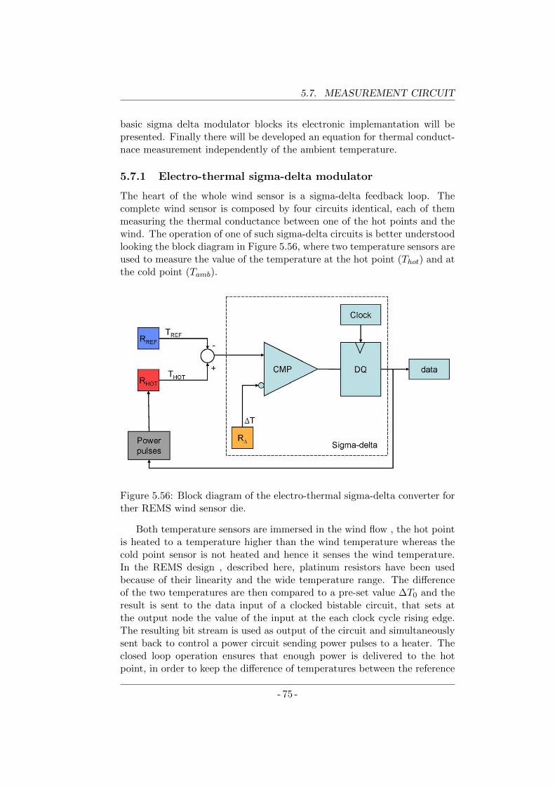
5.7. MEASUREMENT CIRCUIT
basic sigma delta modulator blocks its electronic implemantation will bepresented. Finally there will be developed an equation for thermal conduct-nace measurement independently of the ambient temperature.
5.7.1 Electro-thermal sigma-delta modulator
The heart of the whole wind sensor is a sigma-delta feedback loop. Thecomplete wind sensor is composed by four circuits identical, each of themmeasuring the thermal conductance between one of the hot points and thewind. The operation of one of such sigma-delta circuits is better understoodlooking the block diagram in Figure 5.56, where two temperature sensors areused to measure the value of the temperature at the hot point (Thot) and atthe cold point (Tamb).
Figure 5.56: Block diagram of the electro-thermal sigma-delta converter forther REMS wind sensor die.
Both temperature sensors are immersed in the wind flow , the hot pointis heated to a temperature higher than the wind temperature whereas thecold point sensor is not heated and hence it senses the wind temperature.In the REMS design , described here, platinum resistors have been usedbecause of their linearity and the wide temperature range. The differenceof the two temperatures are then compared to a pre-set value ∆T0 and theresult is sent to the data input of a clocked bistable circuit, that sets atthe output node the value of the input at the each clock cycle rising edge.The resulting bit stream is used as output of the circuit and simultaneouslysent back to control a power circuit sending power pulses to a heater. Theclosed loop operation ensures that enough power is delivered to the hotpoint, in order to keep the difference of temperatures between the reference
- 75 -
CHAPTER 5. REMS 2-D WIND TRANSDUCER
and the hot point equal to the pre-set value of ∆T0. When the wind speedis increased, there is more heat convection and the power required to keep∆T0 is larger hence, a measure of the wind speed is given by the number ofheat pulses delivered in a given window of time. The power pulses take twodiscrete values, Pmax and Pmin , if we define λ as the ratio of the number ofclock cycles in which a power Pmax is applied to the heater, divided by thetotal number of cycles in a given window of time:
λ =number of cycles with Pmaxtotal number of cycles
(5.9)
the average value of the power delivered to the hot point is given by:
P = Pmin + (Pmax − Pmin) · λ (5.10)
Defining the temperature difference between the hot point and the ref-erence point as:
∆T = Thot − Tamb. (5.11)
and If the clock frequency is high enough, the temperature of the hotpoint will have a small ripple, and hence it can be assumed that:
∆T0 = ∆T (5.12)
The thermal conductance Gth between the hot point and the ambient isgiven by
Gth =P
∆T=Pmin + (Pmax − Pmin) · λ
∆T0(5.13)
Although, average power delivered to the hot element can be easily cal-culated as a sum of Pmax and Pmin pulses per frame, in order to find outabout the thermal conductance exact value overheat need to be known. Andsince overheat is a difference between hot temperature and the ambient onethis last need to be monitored as it can vary due to well known ambienttemperature variation happening in Martian atmosphere. In order to over-come the necessity of permanent monitoring of Tamb parameter the specificelectronic circuit to drive wind sensor die has been proposed.
5.7.2 Electronic circuit
On each die of the REMS wind transducer are placed three different in shapeand length electrical resistances: Rsens, Rheat and Rdelta, see Section (5.5.1).Whereas for working circuit, shown in Figure 5.57, we have four resistancesdenominated as:RHX , Rref , ∆R and Rref but only two of them correspondto the same silicon chip working in hot. To the hot chip belong the measure-ment resistance Rx known as the Rsens and also heating purpose resistance
- 76 -
5.7. MEASUREMENT CIRCUIT
RHX which corresponds to Rheat. The third resitance that is also hot is aresistance that sets overheat value ∆R and could directly be a Rdelta butalso could be a combination of different Rdelta, which belongs to the groupof four hot chips: A, B, C, D. Finally, the reference resistance Rref which isworking in ambient temperature conditions is a Rsens of the fifth referencechip that not belongs to the hot array group.
Now it is directly shown on the Figure 5.57 that RH and ∆R and Rare working at hot temperature whereas Rref is at ambient (sometimes de-nominated as cold) temperature.We want to know the thermal conductanceGth that relates to the mean power and overheat as shown on the followingequation:
Gth =P
∆T(5.14)
This equation is true whenever we consider ideal case when thermallooses be conduction (Pcond.=0) and radiation (Prad=0) are equal to zero,so:
P = Pconv.+ 6 Pcond.+ 6 Prad. (5.15)
otherwise conduction power losses and and radiation power losses mustbe considered and characterized. Let’s now analyse ideal case where powertransfer by the convection process, in the equilibrium, equates the powerdelivered to the particular hot die by Joule heating pulses given be equation:
P =[I2min +
(I2max − I2
min
)λ]·RH (5.16)
where, Imin is a current of low energy pulse, Imax is a current of highenergy pulse, λ is a number of high energy pulses for entire frame and RHis a heater resistance at hot temperature. This last can be written as:
RH = RH0 · (1 + α · Thot) (5.17)
where RH0 is a heater resistance at the 0C temperature and α is atemperature coefficient of resistance for all resistances.
The role of the heating pulses is to achieve circuit equilibrium whichis reached when voltages on amplifier entrance Vx and Vref are equal, thishappen when
Ix ·Rx = Iref · (∆R+Rref ) (5.18)
Typically Ix=Iref and Rx0=Rref0 what simplifies equation to
Rref(hot) = ∆R(hot) +Rref(cold) (5.19)
which can be expanded as:
- 77 -
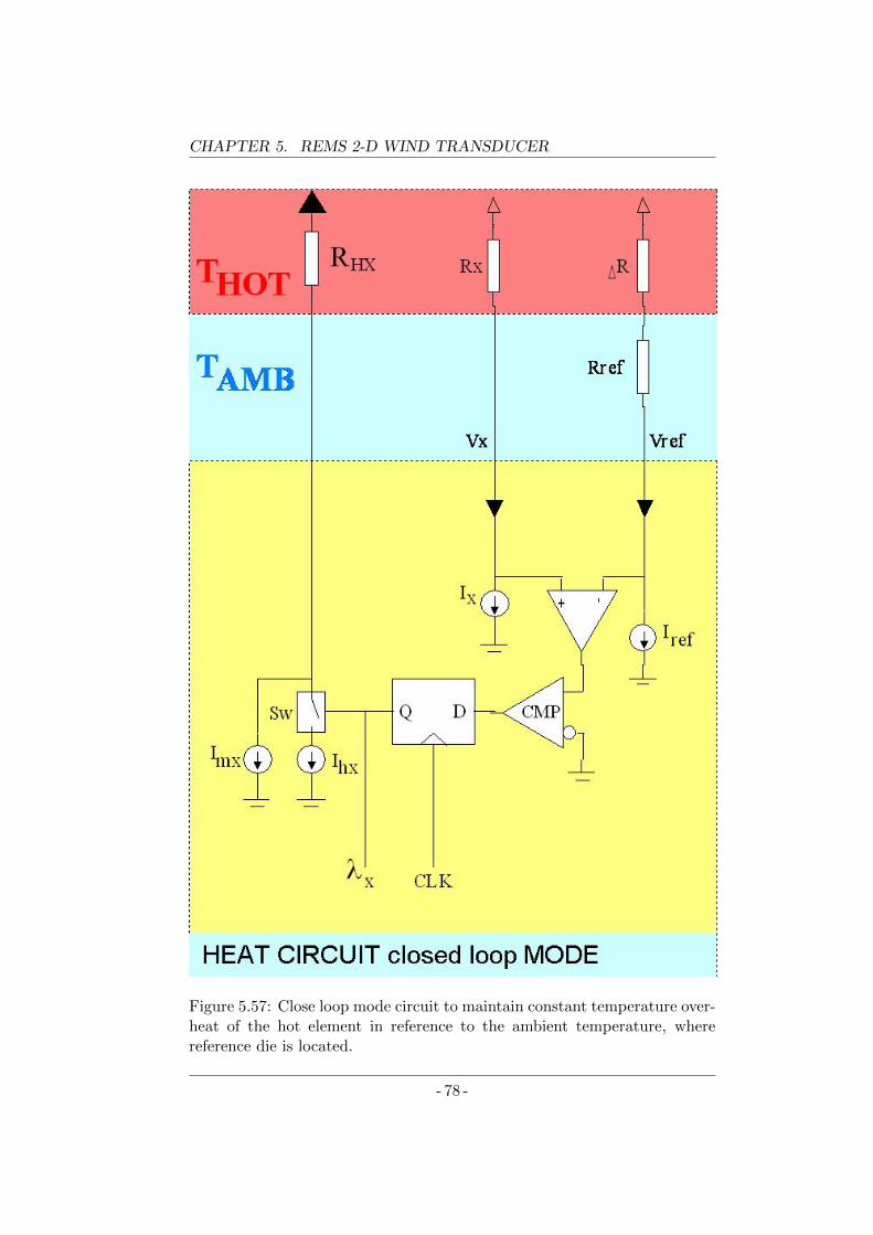
CHAPTER 5. REMS 2-D WIND TRANSDUCER
Figure 5.57: Close loop mode circuit to maintain constant temperature over-heat of the hot element in reference to the ambient temperature, wherereference die is located.
- 78 -
5.7. MEASUREMENT CIRCUIT
Rref0(1+α · (Tamb.+∆T )) = ∆R0(1+α ·Thot)+Rref0(1+α ·Tamb.) (5.20)
and, simplifies to:
Rref0 · α ·∆T = ∆R0(1 + α · Thot) (5.21)
what gives equilibrium condition as:
1 + α · Thot =Rref0 · α ·∆T
∆R0(5.22)
From that point we can combine thermal conductance equation withequilibrium conditions so we have:
Gth =
[I2min +
(I2max − I2
min
)λ]·RH0 · Rref0·α·∆T
∆R0
∆T(5.23)
what finally makes thermal conductance independent from the ambienttemperature variation:
Gth =αRref0
I2min +
(I2max − I2
min
)λRH0
∆R0(5.24)
This electronic circuit has been implemented using standard PCB tech-nology, see Figure 5.58. This test circuit was later integrated in an Appli-cation Specific Integrated Circuit (ASIC) in the final REMS flight system.
5.7.3 Overheat value
As explained, sensor chips as for thermal anemometer work with an overheatvalue that depends on the ambient temperature. As has it been mentionedsensor works in CTDA mode which means that proper shift according to theambient temperature is provided for the hot point element. This overheatvalue can be find by developing equilibrium conditions from the electroniccircuit from the Equation (5.22) into form:
∆R0 + ∆R0 · α · (Tamb. + ∆T ) = Rref0 · α ·∆T (5.25)
And this be the next step becomes:
∆R0 (1 + α · Tamb.) = ∆T · α (Rref0 −∆R0) (5.26)
to give a final equation for overheat value of:
∆T =∆R0 (1 + α · Tamb.)(Rref0 −∆R0) · α (5.27)
- 79 -
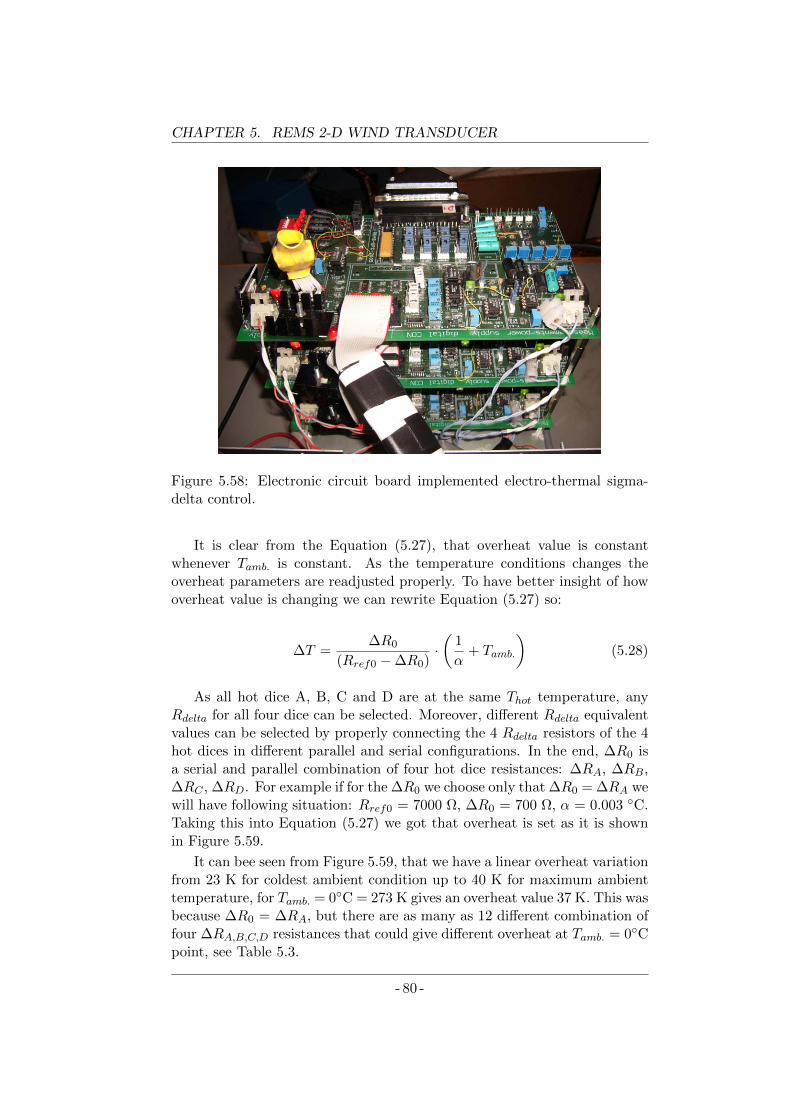
CHAPTER 5. REMS 2-D WIND TRANSDUCER
Figure 5.58: Electronic circuit board implemented electro-thermal sigma-delta control.
It is clear from the Equation (5.27), that overheat value is constantwhenever Tamb. is constant. As the temperature conditions changes theoverheat parameters are readjusted properly. To have better insight of howoverheat value is changing we can rewrite Equation (5.27) so:
∆T =∆R0
(Rref0 −∆R0)·(
1
α+ Tamb.
)(5.28)
As all hot dice A, B, C and D are at the same Thot temperature, anyRdelta for all four dice can be selected. Moreover, different Rdelta equivalentvalues can be selected by properly connecting the 4 Rdelta resistors of the 4hot dices in different parallel and serial configurations. In the end, ∆R0 isa serial and parallel combination of four hot dice resistances: ∆RA, ∆RB,∆RC , ∆RD. For example if for the ∆R0 we choose only that ∆R0 = ∆RA wewill have following situation: Rref0 = 7000 Ω, ∆R0 = 700 Ω, α = 0.003 C.Taking this into Equation (5.27) we got that overheat is set as it is shownin Figure 5.59.
It can bee seen from Figure 5.59, that we have a linear overheat variationfrom 23 K for coldest ambient condition up to 40 K for maximum ambienttemperature, for Tamb. = 0C = 273 K gives an overheat value 37 K. This wasbecause ∆R0 = ∆RA, but there are as many as 12 different combination offour ∆RA,B,C,D resistances that could give different overheat at Tamb. = 0Cpoint, see Table 5.3.
- 80 -
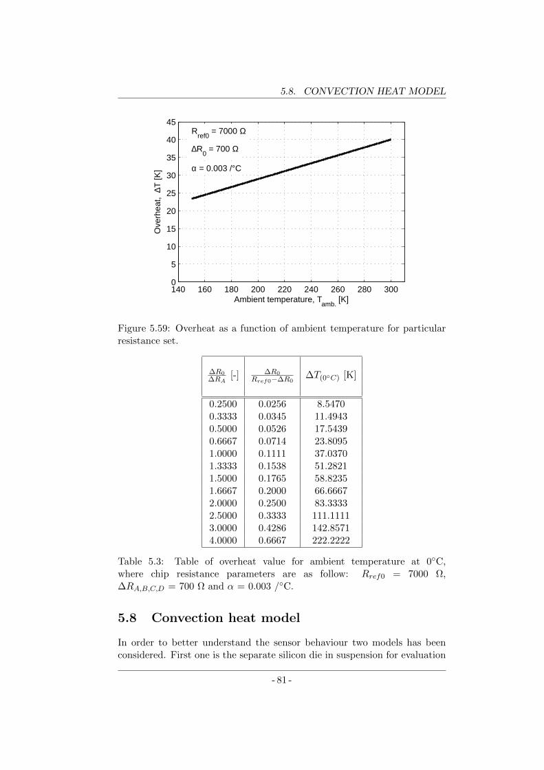
5.8. CONVECTION HEAT MODEL
140 160 180 200 220 240 260 280 3000
5
10
15
20
25
30
35
40
45
Ambient temperature, Tamb.
[K]
Ove
rhea
t, ∆
T [K
]
Rref0
= 7000 Ω
∆R0 = 700 Ω
α = 0.003 /°C
Figure 5.59: Overheat as a function of ambient temperature for particularresistance set.
∆R0∆RA
[-] ∆R0Rref0−∆R0
∆T(0C) [K]
0.2500 0.0256 8.54700.3333 0.0345 11.49430.5000 0.0526 17.54390.6667 0.0714 23.80951.0000 0.1111 37.03701.3333 0.1538 51.28211.5000 0.1765 58.82351.6667 0.2000 66.66672.0000 0.2500 83.33332.5000 0.3333 111.11113.0000 0.4286 142.85714.0000 0.6667 222.2222
Table 5.3: Table of overheat value for ambient temperature at 0C,where chip resistance parameters are as follow: Rref0 = 7000 Ω,∆RA,B,C,D = 700 Ω and α = 0.003 /C.
5.8 Convection heat model
In order to better understand the sensor behaviour two models has beenconsidered. First one is the separate silicon die in suspension for evaluation
- 81 -
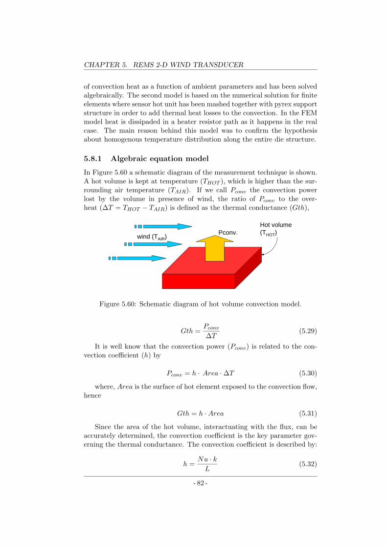
CHAPTER 5. REMS 2-D WIND TRANSDUCER
of convection heat as a function of ambient parameters and has been solvedalgebraically. The second model is based on the numerical solution for finiteelements where sensor hot unit has been mashed together with pyrex supportstructure in order to add thermal heat losses to the convection. In the FEMmodel heat is dissipaded in a heater resistor path as it happens in the realcase. The main reason behind this model was to confirm the hypothesisabout homogenous temperature distribution along the entire die structure.
5.8.1 Algebraic equation model
In Figure 5.60 a schematic diagram of the measurement technique is shown.A hot volume is kept at temperature (THOT ), which is higher than the sur-rounding air temperature (TAIR). If we call Pconv the convection powerlost by the volume in presence of wind, the ratio of Pconv to the over-heat (∆T = THOT − TAIR) is defined as the thermal conductance (Gth),
wind (TAIR)
Hot volume(THOT)Pconv.
Figure 5.60: Schematic diagram of hot volume convection model.
Gth =Pconv∆T
(5.29)
It is well know that the convection power (Pconv) is related to the con-vection coefficient (h) by
Pconv = h · Area ·∆T (5.30)
where, Area is the surface of hot element exposed to the convection flow,hence
Gth = h ·Area (5.31)
Since the area of the hot volume, interactuating with the flux, can beaccurately determined, the convection coefficient is the key parameter gov-erning the thermal conductance. The convection coefficient is described by:
h =Nu · kL
(5.32)
- 82 -
5.8. CONVECTION HEAT MODEL
where, k is the air conductivity, which depends on the temperature, L is acharacteristic length of the hot volume and Nu is the dimensionless Nusseltnumber which for a flat surface under tangential flow, see Reference [70],can be approximated by:
Nu = 0, 664 ·Re 12 · Pr 1
3 (5.33)
where, Re is the Reynolds number and Pr is the Prandtl number; bothare dimensionless numbers, [70]. The Prandtl number is defined by the ratioof the momentum diffusivity and the thermal diffusivity:
Pr =µ · Cpk
(5.34)
where, µ is the gas viscosity, Cp is the gas specific heat at constant pres-sure and k is, as mentioned above the gas conductivity. All three parametersare temperature-dependent.The Reynolds number is given by:
Re =ρ · vf · L
µ(5.35)
where, ρ is the gas density and vf stands for the wind speed. Fromthe ideal gas law, the gas density can be related to the gas pressure andtemperature as follows:
ρ =M · PR · Tf
(5.36)
where, Tf = Thot+Tair2 is the ’film’ temperature, M is the molar mass and
R is the ideal gas constant. Therefore the Reynolds number can be writtenas:
Re =M · P · vf · LR · Tf · µ
(5.37)
Finally bringing all together to equation (5.31) gives us the followingexpression:
Gth =
(0, 664 · Area ·
√M√
R · L
)·
Cp
13
(Tf ) · k23
(Tf )
ρ16
(Tf ) · T12f
·
√P · vf (5.38)
This equation can be split in three terms:
Gth = Dconst · F(Tf ) ·√P · vf (5.39)
- 83 -
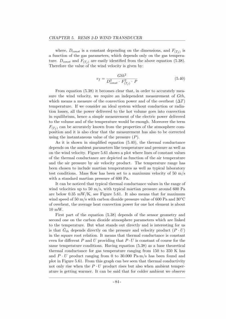
CHAPTER 5. REMS 2-D WIND TRANSDUCER
where, Dconst is a constant depending on the dimensions, and F(Tf ) isa function of the gas parameters, which depends only on the gas tempera-ture. Dconst and F(Tf ) are easily identified from the above equation (5.38).Therefore the value of the wind velocity is given by:
vf =Gth2
D2const · F 2
(Tf ) · P(5.40)
From equation (5.38) it becomes clear that, in order to accurately mea-sure the wind velocity, we require an independent measurement of Gth,which means a measure of the convection power and of the overheat (∆T )temperature. If we consider an ideal system without conduction or radia-tion losses, all the power delivered to the hot volume goes into convectionin equilibrium, hence a simple measurement of the electric power deliveredto the volume and of the temperature would be enough. Moreover the termF(Tf ) can be accurately known from the properties of the atmosphere com-position and it is also clear that the measurement has also to be correctedusing the instantaneous value of the pressure (P ).
As it is shown in simplified equation (5.40), the thermal conductancedepends on the ambient parameters like temperature and pressure as well ason the wind velocity. Figure 5.61 shows a plot where lines of constant valuesof the thermal conductance are depicted as function of the air temperatureand the air pressure by air velocity product. The temperature range hasbeen chosen to include martian temperatures as well as typical laboratorytest conditions. Mass flow has been set to a maximum velocity of 50 m/swith a standard martian pressure of 600 Pa.
It can be noticed that typical thermal conductance values in the range ofwind velocities up to 50 m/s, with typical martian pressure around 600 Paare below 0.35 mW/K, see Figure 5.61. It also means that for maximumwind speed of 50 m/s with carbon dioxide pressure value of 600 Pa and 30Cof overheat, the average heat convection power for one hot element is about10 mW.
First part of the equation (5.38) depends of the sensor geometry andsecond one on the carbon dioxide atmosphere parameters which are linkedto the temperature. But what stands out directly and is interesting for usis that Gth depends directly on the pressure and velocity product (P · U)in the square root relation. It means that thermal conductance is constanteven for different P and U providing that P ·U is constant of course for thesame temperature conditions. Having equation (5.38) as a base theoreticalthermal conductance for gas temperature ranging from 150 to 350 K hasand P · U product ranging from 0 to 30.000 Pa·m/s has been found andplot in Figure 5.61. From this graph can bee seen that thermal conductivitynot only rise when the P · U product rises but also when ambient temper-ature is getting warmer. It can be said that for colder ambient we observe
- 84 -
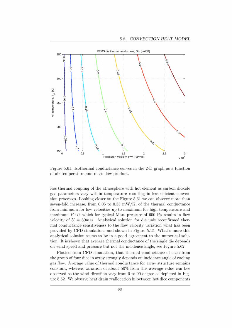
5.8. CONVECTION HEAT MODEL
0.050.05
0.05
0.10.1
0.1
0.150.15
0.150.2
0.2
0.2
0.25
0.25
0.25
0.3
0.3
0.3
0.35
Pressure * Velocity, P*V [Pa*m/s]
Air
tem
pera
ture
, Tai
r [K]
REMS die thermal conductane, Gth [mW/K]
0 0.5 1 1.5 2 2.5 3
x 104
150
200
250
300
350
Figure 5.61: Isothermal conductance curves in the 2-D graph as a functionof air temperature and mass flow product.
less thermal coupling of the atmosphere with hot element as carbon dioxidegas parameters vary within temperature resulting in less efficient convec-tion processes. Looking closer on the Figure 5.61 we can observe more thanseven-fold increase, from 0.05 to 0.35 mW/K, of the thermal conductancefrom minimum for low velocities up to maximum for high temperature andmaximum P · U which for typical Mars pressure of 600 Pa results in flowvelocity of U = 50m/s. Analytical solution for die unit reconfirmed ther-mal conductance sensitiveness to the flow velocity variation what has beenprovided by CFD simulations and shown in Figure 5.15. What’s more thisanalytical solution seems to be in a good agreement to the numerical solu-tion. It is shown that average thermal conductance of the single die dependson wind speed and pressure but not the incidence angle, see Figure 5.62.
Plotted from CFD simulation, that thermal conductance of each fromthe group of four dice in array strongly depends on incidence angle of coolinggas flow. Average value of thermal conductance for array structure remainsconstant, whereas variation of about 50% from this average value can beeobserved as the wind direction vary from 0 to 90 degree as depicted in Fig-ure 5.62. We observe heat drain reallocation in between hot dice components
- 85 -
CHAPTER 5. REMS 2-D WIND TRANSDUCER
Figure 5.62: Numerical simulation of four hot dice structure forPamb. = 600 Pa, Tamb. = 220 K and U = 10 m/s.
as die position changes from the front of the head flow (where convectionis maximum) to the side and rear position being in the thermal shadow ofother dice (where convection has its minimum). Thus, variation of all diceconvection coefficients in reaction to the wind incidence angle. Now, for theexample considered in Figure 5.62. Lets calculate average heat convectioncoefficient from FEM simulation, so we will have:
h =hA + hB + hC + hD
4=
21.2 + 10 + 26 + 16.3
4= 18.375 W/m2K
(5.41)Then assuming unit die dimensions to be 1.5 x 1.5 x 0.5 mm we have
that Aconv is:
Aconv = 2 · (1.5mm)2 + 4 · (1.5mm · 0.5mm) = 4.5mm2 + 3mm2 = 7.5mm2
(5.42)We can find the average thermal conductance from this using Equa-
tion (5.29), as follow:
Gth = h ·Aconv = 18.375 W/m2K · 7.5 mm2 = 0.137 mW/K (5.43)
As FEM simulation has been executed for atmospheric temperature200 K and pressure 600 Pa for wind velocity 10 m/s, therefore the pres-sure and velocity product will be P ·U = 6 kPa·m/s. What stands out that
- 86 -
5.8. CONVECTION HEAT MODEL
this average thermal conductivity which has been calculated for the FEMresults fits very well with the analytical solution when checked from the Fig-ure 5.61 for Tair = 200 K and for P · U = 0.6·104 Pa·m/s correspondinglyto the numerical simulation conditions.
5.8.2 Finite Element Method (FEM) model
In this section we combine in multi-physics finite element methods simula-tion two natures of the sensor behaviour: it’s electronic circuit made out ofplatinum deposited path on top of is silicon die and thermal physics which ispresent for all solid components of the sensor structure. The purpose of thisis to model in full 3-D space with support geometry and taking under con-sideration wire bonding parameters in order to find out about temperatureprofile. This work was to extend study on temperature distribution alongthe silicon sensor die. Work has been implemented in numerical platformComputers and Solutions (COMSOL). For this analysis following geometryhas been considered:
• Silicon die of particular size 1.6 x 1.6 x 0.4 mm,
• Platinum paths with 80 nm thickness of original geometry copied fromthe chip layout ended wit gold pads of 150 x 150 µm and the same asplatinum thickness,
• Support made out of for pyrex pillars of the size 0.2 x 0.2 x 0.8 mmgrowing up from pyrex base 1.4 x 1.4 x 0.2 mm respectively,
• Seven gold wire-bonding with length of 4 mm and diameter 25 µm.
Photo of the entire assembled structure can be seen in Figure 5.51 .Equation that describes physical behavior of the sensor could be dividedinto three domains: electrical, elctro-thermal and thermal. So in electricaldomain we will have path resistance equation ∆R which depends on physicaldimensions and electrical resistivity of platinum material. In electro-thermaldomain we will find formula for platinum resistivity ρPt as a function oftemperature and equation for generated power Pgen in Joule heat effect bycurrent flow through resistive way. Finally thermal domain will acomodateequation for convection power Pconv and conduction power Pcond respec-tively. Those, equation can be found in the paper [8] and has been gatheredtogether in table 5.4
For a purpose of the simulation sensor has been forced to work as CCA.Therefore, as a candidate to flow through heating resistor and generatingJoule power a current of value 5 mA has been chosen. To satisfy this anappropriate current density ±222 kA/m2 calculated for the pad area was setas a boundary conditions for both Rheat terminals. Pyrex base boundary
- 87 -
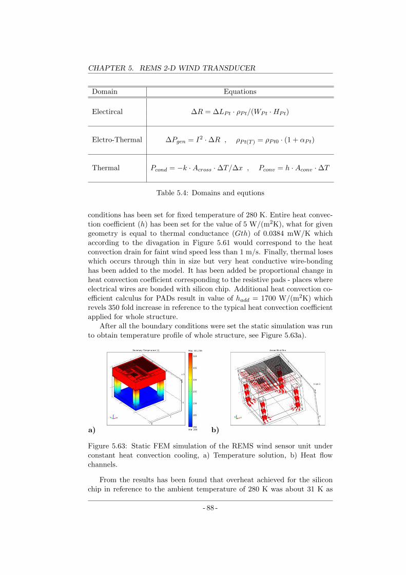
CHAPTER 5. REMS 2-D WIND TRANSDUCER
Domain Equations
Electircal ∆R = ∆LPt · ρPt/(WPt ·HPt)
Elctro-Thermal ∆Pgen = I2 ·∆R , ρPt(T ) = ρPt0 · (1 + αPt)
Thermal Pcond = −k ·Across ·∆T/∆x , Pconv = h ·Aconv ·∆T
Table 5.4: Domains and equtions
conditions has been set for fixed temperature of 280 K. Entire heat convec-tion coefficient (h) has been set for the value of 5 W/(m2K), what for givengeometry is equal to thermal conductance (Gth) of 0.0384 mW/K whichaccording to the divagation in Figure 5.61 would correspond to the heatconvection drain for faint wind speed less than 1 m/s. Finally, thermal loseswhich occurs through thin in size but very heat conductive wire-bondinghas been added to the model. It has been added be proportional change inheat convection coefficient corresponding to the resistive pads - places whereelectrical wires are bonded with silicon chip. Additional heat convection co-efficient calculus for PADs result in value of hadd = 1700 W/(m2K) whichrevels 350 fold increase in reference to the typical heat convection coefficientapplied for whole structure.
After all the boundary conditions were set the static simulation was runto obtain temperature profile of whole structure, see Figure 5.63a).
a) b)
Figure 5.63: Static FEM simulation of the REMS wind sensor unit underconstant heat convection cooling, a) Temperature solution, b) Heat flowchannels.
From the results has been found that overheat achieved for the siliconchip in reference to the ambient temperature of 280 K was about 31 K as
- 88 -
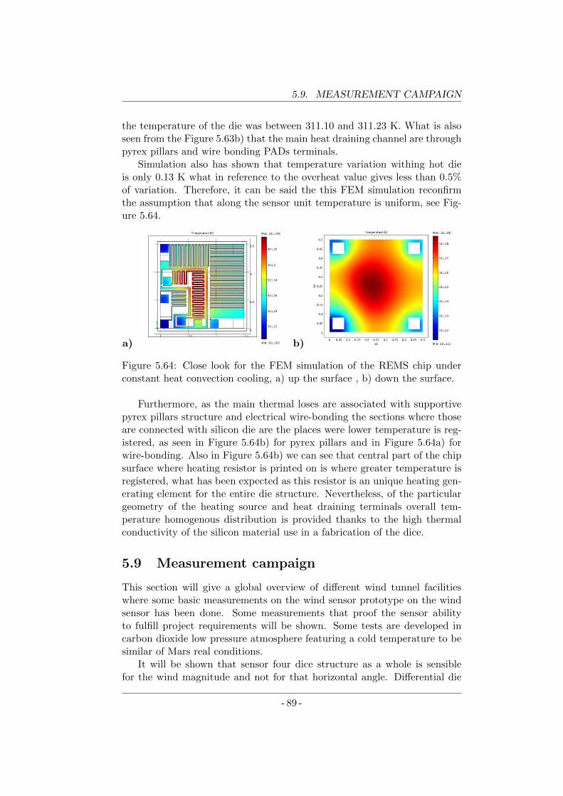
5.9. MEASUREMENT CAMPAIGN
the temperature of the die was between 311.10 and 311.23 K. What is alsoseen from the Figure 5.63b) that the main heat draining channel are throughpyrex pillars and wire bonding PADs terminals.
Simulation also has shown that temperature variation withing hot dieis only 0.13 K what in reference to the overheat value gives less than 0.5%of variation. Therefore, it can be said the this FEM simulation reconfirmthe assumption that along the sensor unit temperature is uniform, see Fig-ure 5.64.
a) b)
Figure 5.64: Close look for the FEM simulation of the REMS chip underconstant heat convection cooling, a) up the surface , b) down the surface.
Furthermore, as the main thermal loses are associated with supportivepyrex pillars structure and electrical wire-bonding the sections where thoseare connected with silicon die are the places were lower temperature is reg-istered, as seen in Figure 5.64b) for pyrex pillars and in Figure 5.64a) forwire-bonding. Also in Figure 5.64b) we can see that central part of the chipsurface where heating resistor is printed on is where greater temperature isregistered, what has been expected as this resistor is an unique heating gen-erating element for the entire die structure. Nevertheless, of the particulargeometry of the heating source and heat draining terminals overall tem-perature homogenous distribution is provided thanks to the high thermalconductivity of the silicon material use in a fabrication of the dice.
5.9 Measurement campaign
This section will give a global overview of different wind tunnel facilitieswhere some basic measurements on the wind sensor prototype on the windsensor has been done. Some measurements that proof the sensor abilityto fulfill project requirements will be shown. Some tests are developed incarbon dioxide low pressure atmosphere featuring a cold temperature to besimilar of Mars real conditions.
It will be shown that sensor four dice structure as a whole is sensiblefor the wind magnitude and not for that horizontal angle. Differential die
- 89 -
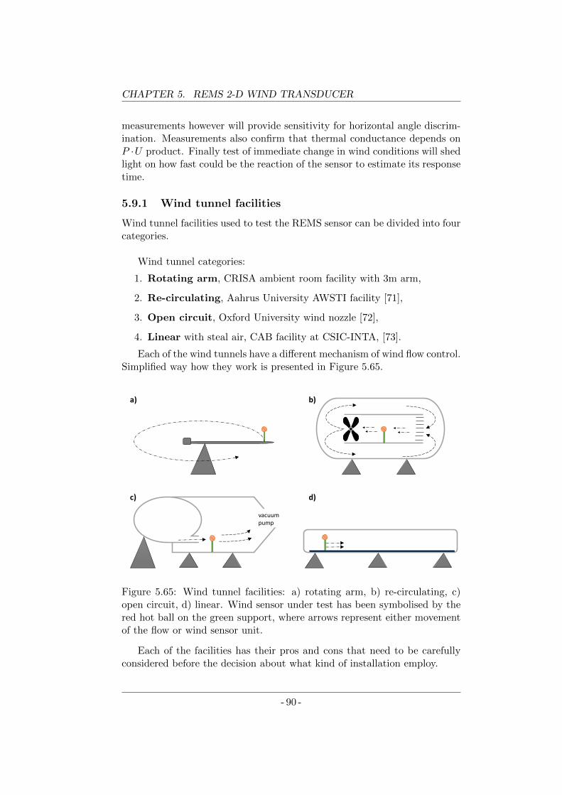
CHAPTER 5. REMS 2-D WIND TRANSDUCER
measurements however will provide sensitivity for horizontal angle discrim-ination. Measurements also confirm that thermal conductance depends onP ·U product. Finally test of immediate change in wind conditions will shedlight on how fast could be the reaction of the sensor to estimate its responsetime.
5.9.1 Wind tunnel facilities
Wind tunnel facilities used to test the REMS sensor can be divided into fourcategories.
Wind tunnel categories:
1. Rotating arm, CRISA ambient room facility with 3m arm,
2. Re-circulating, Aahrus University AWSTI facility [71],
3. Open circuit, Oxford University wind nozzle [72],
4. Linear with steal air, CAB facility at CSIC-INTA, [73].
Each of the wind tunnels have a different mechanism of wind flow control.Simplified way how they work is presented in Figure 5.65.
vacuumpump
c) d)
a) b)
Figure 5.65: Wind tunnel facilities: a) rotating arm, b) re-circulating, c)open circuit, d) linear. Wind sensor under test has been symbolised by thered hot ball on the green support, where arrows represent either movementof the flow or wind sensor unit.
Each of the facilities has their pros and cons that need to be carefullyconsidered before the decision about what kind of installation employ.
- 90 -
5.9. MEASUREMENT CAMPAIGN
Rotating arm wind tunnel need a big room to operate and its gas pa-rameter are those of the room (air at ambient temperature and pressure).The air is considered to be still and the sensor moves with lineal speed,which is a product of rotation in full turns per unit time by circumference(2πRarm). In the facility the arm was not capable to support a heavy load,so the interface circuits needed to be at the center of rotation. This solutionwas prone to generate a lot of electrical noise.
Re-circulating wind tunnel can work with any gas that can be pumped-in and its pressure can be adequately adjust. If the chamber seal is goodthis composition can stay there for a long time. Also velocity can smoothlybe tuned by the rotating fan speed. Cooling down the ambient gas to reachMartian like temperatures is difficult but some range of temperature belowthe zero could be achieved that involves cooling down entire chamber or atleast interior crust of the chamber that is thermally isolated from the mainchassis. A big disadvantage of all the re-circulating wind tunnel is that it isdifficult to introduce sudden changes in either wind temperature or velocity.
Open circuit wind tunnel is a kind of facility where gas we want to workwith is gathered in the preparation chamber at given pressure and then bethe process of expansion it reduces its pressure but gains the velocity and atthe same time cools down in adiabatic pressure. This process is driven bythe heavy duty vacuum pumps at the other end of the circuit. Sensor unitis placed just on the way out of the outflow nozzle. This tunnel enable us totune two out of three flow parameters which are Temperature (T ), Pressure(P ), Velocity (U) whereas the third one is directly driven from the ideal gasequation. In case of working with gas different from air we need to havehuge reserves of it and when working with poisoning gases like CO2 all thesafety measure at exhaust are obligatory.
Lineal wind tunnel as the recirculating tunnel it can be filled with anygas under the pressure we like and cooling down is rather difficult. Thedifference is in how its working. The air need to be static and the device ismoving with lineal velocity on the rail along the tunnel longer dimension.As the rail speed can be well known the precision in wind speed is good theinconvenience comes from the limited size of the tunnel, so when the devicesreaches the end of the rail measurement need to be finished That typicallytakes several seconds and then it is necessary to wait enough time in orderto settle all the gas particles, which have been moved by the sensor, to thestatic velocity 0 m/s. Nevertheless, the big advantage of this solution is thatthe velocity of the wind sensor device could be updated on instant so thatenables dynamic test and response time measurements.
- 91 -
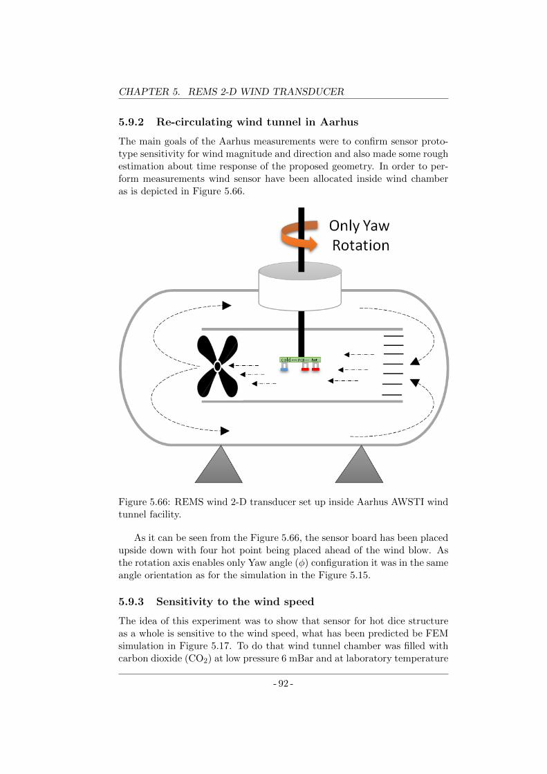
CHAPTER 5. REMS 2-D WIND TRANSDUCER
5.9.2 Re-circulating wind tunnel in Aarhus
The main goals of the Aarhus measurements were to confirm sensor proto-type sensitivity for wind magnitude and direction and also made some roughestimation about time response of the proposed geometry. In order to per-form measurements wind sensor have been allocated inside wind chamberas is depicted in Figure 5.66.
Figure 5.66: REMS wind 2-D transducer set up inside Aarhus AWSTI windtunnel facility.
As it can be seen from the Figure 5.66, the sensor board has been placedupside down with four hot point being placed ahead of the wind blow. Asthe rotation axis enables only Yaw angle (φ) configuration it was in the sameangle orientation as for the simulation in the Figure 5.15.
5.9.3 Sensitivity to the wind speed
The idea of this experiment was to show that sensor for hot dice structureas a whole is sensitive to the wind speed, what has been predicted be FEMsimulation in Figure 5.17. To do that wind tunnel chamber was filled withcarbon dioxide (CO2) at low pressure 6 mBar and at laboratory temperature
- 92 -
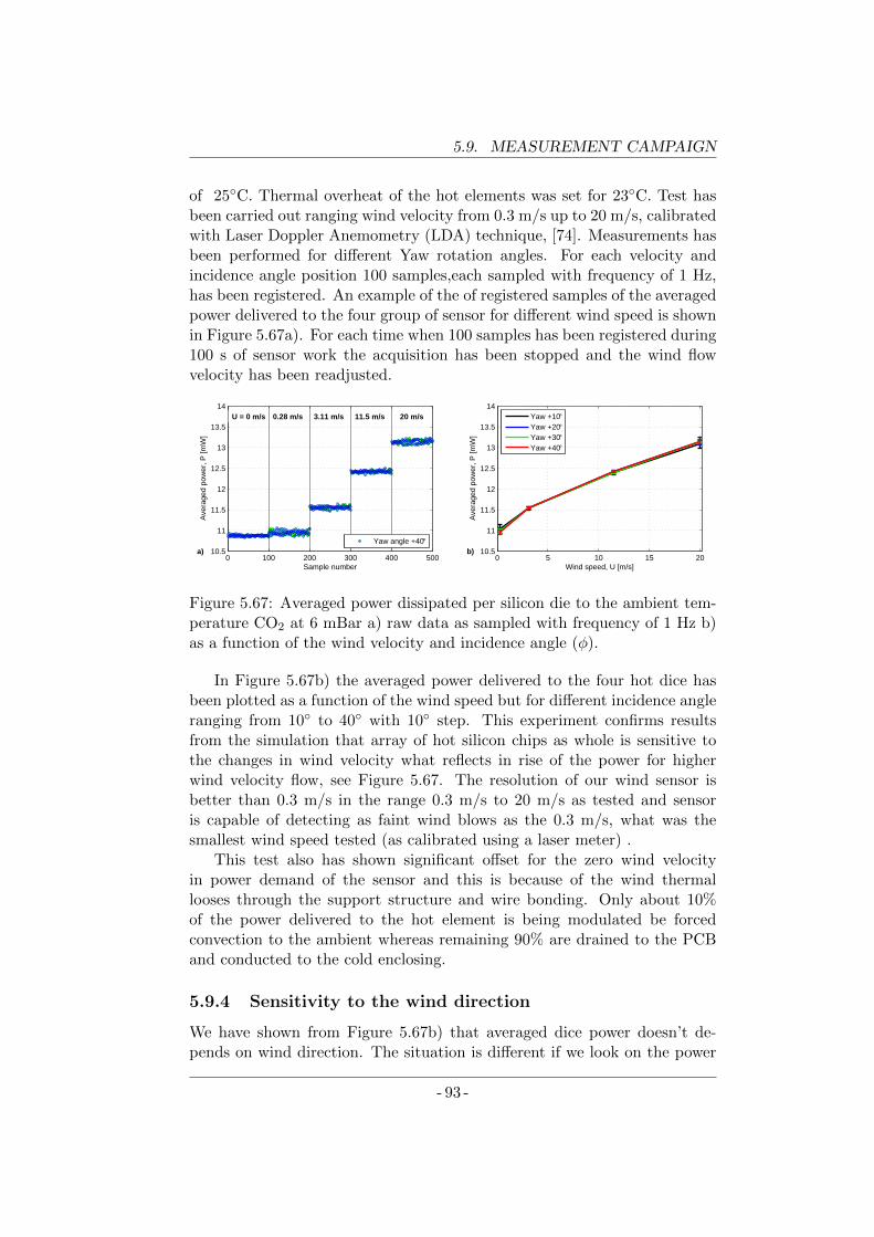
5.9. MEASUREMENT CAMPAIGN
of 25C. Thermal overheat of the hot elements was set for 23C. Test hasbeen carried out ranging wind velocity from 0.3 m/s up to 20 m/s, calibratedwith Laser Doppler Anemometry (LDA) technique, [74]. Measurements hasbeen performed for different Yaw rotation angles. For each velocity andincidence angle position 100 samples,each sampled with frequency of 1 Hz,has been registered. An example of the of registered samples of the averagedpower delivered to the four group of sensor for different wind speed is shownin Figure 5.67a). For each time when 100 samples has been registered during100 s of sensor work the acquisition has been stopped and the wind flowvelocity has been readjusted.
0 100 200 300 400 50010.5
11
11.5
12
12.5
13
13.5
14 U = 0 m/s 0.28 m/s 3.11 m/s 11.5 m/s 20 m/s
a)
Sample number
Ave
rage
d po
wer
, P [m
W]
Yaw angle +40°
0 5 10 15 2010.5
11
11.5
12
12.5
13
13.5
14
Wind speed, U [m/s]
Ave
rage
d po
wer
, P [m
W]
b)
Yaw +10°Yaw +20°Yaw +30°Yaw +40°
Figure 5.67: Averaged power dissipated per silicon die to the ambient tem-perature CO2 at 6 mBar a) raw data as sampled with frequency of 1 Hz b)as a function of the wind velocity and incidence angle (φ).
In Figure 5.67b) the averaged power delivered to the four hot dice hasbeen plotted as a function of the wind speed but for different incidence angleranging from 10 to 40 with 10 step. This experiment confirms resultsfrom the simulation that array of hot silicon chips as whole is sensitive tothe changes in wind velocity what reflects in rise of the power for higherwind velocity flow, see Figure 5.67. The resolution of our wind sensor isbetter than 0.3 m/s in the range 0.3 m/s to 20 m/s as tested and sensoris capable of detecting as faint wind blows as the 0.3 m/s, what was thesmallest wind speed tested (as calibrated using a laser meter) .
This test also has shown significant offset for the zero wind velocityin power demand of the sensor and this is because of the wind thermallooses through the support structure and wire bonding. Only about 10%of the power delivered to the hot element is being modulated be forcedconvection to the ambient whereas remaining 90% are drained to the PCBand conducted to the cold enclosing.
5.9.4 Sensitivity to the wind direction
We have shown from Figure 5.67b) that averaged dice power doesn’t de-pends on wind direction. The situation is different if we look on the power
- 93 -
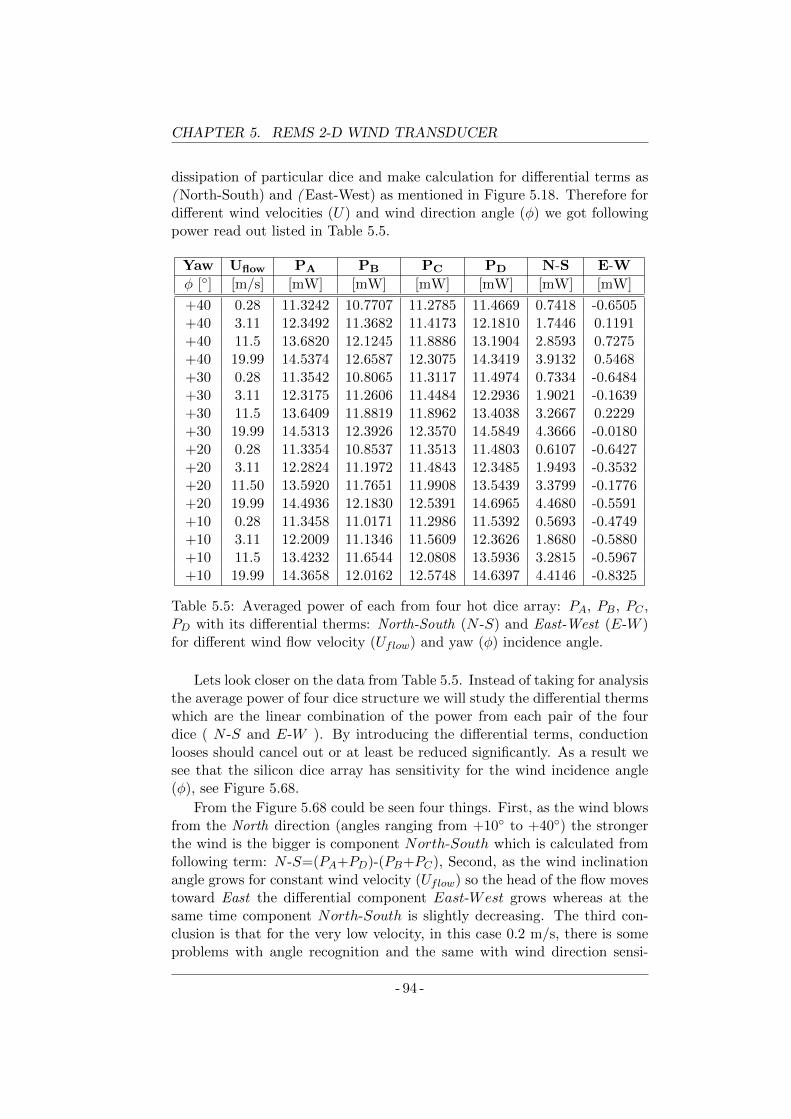
CHAPTER 5. REMS 2-D WIND TRANSDUCER
dissipation of particular dice and make calculation for differential terms as( North-South) and ( East-West) as mentioned in Figure 5.18. Therefore fordifferent wind velocities (U) and wind direction angle (φ) we got followingpower read out listed in Table 5.5.
Yaw Uflow PA PB PC PD N-S E-W
φ [] [m/s] [mW] [mW] [mW] [mW] [mW] [mW]
+40 0.28 11.3242 10.7707 11.2785 11.4669 0.7418 -0.6505+40 3.11 12.3492 11.3682 11.4173 12.1810 1.7446 0.1191+40 11.5 13.6820 12.1245 11.8886 13.1904 2.8593 0.7275+40 19.99 14.5374 12.6587 12.3075 14.3419 3.9132 0.5468+30 0.28 11.3542 10.8065 11.3117 11.4974 0.7334 -0.6484+30 3.11 12.3175 11.2606 11.4484 12.2936 1.9021 -0.1639+30 11.5 13.6409 11.8819 11.8962 13.4038 3.2667 0.2229+30 19.99 14.5313 12.3926 12.3570 14.5849 4.3666 -0.0180+20 0.28 11.3354 10.8537 11.3513 11.4803 0.6107 -0.6427+20 3.11 12.2824 11.1972 11.4843 12.3485 1.9493 -0.3532+20 11.50 13.5920 11.7651 11.9908 13.5439 3.3799 -0.1776+20 19.99 14.4936 12.1830 12.5391 14.6965 4.4680 -0.5591+10 0.28 11.3458 11.0171 11.2986 11.5392 0.5693 -0.4749+10 3.11 12.2009 11.1346 11.5609 12.3626 1.8680 -0.5880+10 11.5 13.4232 11.6544 12.0808 13.5936 3.2815 -0.5967+10 19.99 14.3658 12.0162 12.5748 14.6397 4.4146 -0.8325
Table 5.5: Averaged power of each from four hot dice array: PA, PB, PC ,PD with its differential therms: North-South (N -S) and East-West (E-W )for different wind flow velocity (Uflow) and yaw (φ) incidence angle.
Lets look closer on the data from Table 5.5. Instead of taking for analysisthe average power of four dice structure we will study the differential thermswhich are the linear combination of the power from each pair of the fourdice ( N -S and E-W ). By introducing the differential terms, conductionlooses should cancel out or at least be reduced significantly. As a result wesee that the silicon dice array has sensitivity for the wind incidence angle(φ), see Figure 5.68.
From the Figure 5.68 could be seen four things. First, as the wind blowsfrom the North direction (angles ranging from +10 to +40) the strongerthe wind is the bigger is component North-South which is calculated fromfollowing term: N -S=(PA+PD)-(PB+PC), Second, as the wind inclinationangle grows for constant wind velocity (Uflow) so the head of the flow movestoward East the differential component East-West grows whereas at thesame time component North-South is slightly decreasing. The third con-clusion is that for the very low velocity, in this case 0.2 m/s, there is someproblems with angle recognition and the same with wind direction sensi-
- 94 -
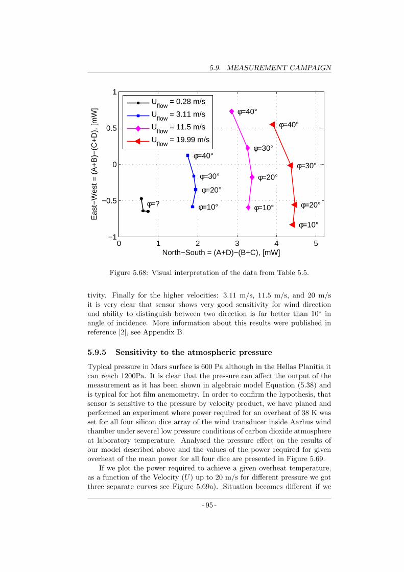
5.9. MEASUREMENT CAMPAIGN
0 1 2 3 4 5−1
−0.5
0
0.5
1
North−South = (A+D)−(B+C), [mW]
Eas
t−W
est =
(A
+B
)−(C
+D
), [m
W]
φ=40°
φ=40°
φ=40°
φ=30°
φ=30°
φ=30°
φ=20°
φ=20°
φ=20°φ=10° φ=10°
φ=10°
φ=?
Uflow
= 0.28 m/s
Uflow
= 3.11 m/s
Uflow
= 11.5 m/s
Uflow
= 19.99 m/s
Figure 5.68: Visual interpretation of the data from Table 5.5.
tivity. Finally for the higher velocities: 3.11 m/s, 11.5 m/s, and 20 m/sit is very clear that sensor shows very good sensitivity for wind directionand ability to distinguish between two direction is far better than 10 inangle of incidence. More information about this results were published inreference [2], see Appendix B.
5.9.5 Sensitivity to the atmospheric pressure
Typical pressure in Mars surface is 600 Pa although in the Hellas Planitia itcan reach 1200Pa. It is clear that the pressure can affect the output of themeasurement as it has been shown in algebraic model Equation (5.38) andis typical for hot film anemometry. In order to confirm the hypothesis, thatsensor is sensitive to the pressure by velocity product, we have planed andperformed an experiment where power required for an overheat of 38 K wasset for all four silicon dice array of the wind transducer inside Aarhus windchamber under several low pressure conditions of carbon dioxide atmosphereat laboratory temperature. Analysed the pressure effect on the results ofour model described above and the values of the power required for givenoverheat of the mean power for all four dice are presented in Figure 5.69.
If we plot the power required to achieve a given overheat temperature,as a function of the Velocity (U) up to 20 m/s for different pressure we gotthree separate curves see Figure 5.69a). Situation becomes different if we
- 95 -
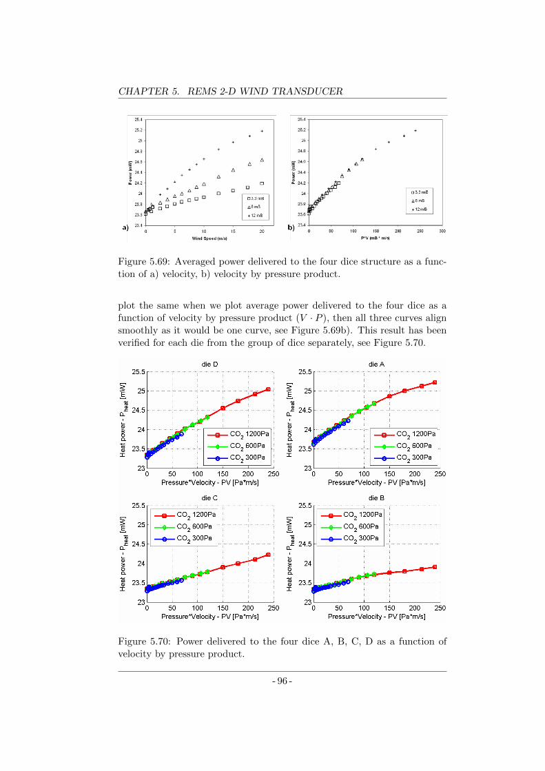
CHAPTER 5. REMS 2-D WIND TRANSDUCER
Figure 5.69: Averaged power delivered to the four dice structure as a func-tion of a) velocity, b) velocity by pressure product.
plot the same when we plot average power delivered to the four dice as afunction of velocity by pressure product (V · P ), then all three curves alignsmoothly as it would be one curve, see Figure 5.69b). This result has beenverified for each die from the group of dice separately, see Figure 5.70.
Figure 5.70: Power delivered to the four dice A, B, C, D as a function ofvelocity by pressure product.
- 96 -
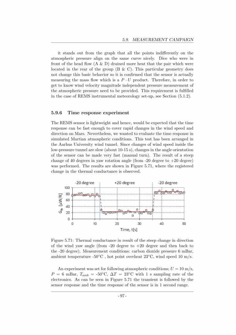
5.9. MEASUREMENT CAMPAIGN
it stands out from the graph that all the points indifferently on theatmospheric pressure align on the same curve nicely. Dice who were infront of the head flow (A & D) drained more heat that the pair which werelocated in the rear of the group (B & C). This particular geometry doesnot change this basic behavior so it is confirmed that the sensor is actuallymeasuring the mass flow which is a P · U product. Therefore, in order toget to know wind velocity magnitude independent pressure measurement ofthe atmospheric pressure need to be provided. This requirement is fulfilledin the case of REMS instrumental meteorology set-up, see Section (5.1.2).
5.9.6 Time response experiment
The REMS sensor is lightweight and hence, would be expected that the timeresponse can be fast enough to cover rapid changes in the wind speed anddirection on Mars. Nevertheless, we wanted to evaluate the time response insimulated Martian atmospheric conditions. This test has been arranged inthe Aarhus University wind tunnel. Since changes of wind speed inside thelow-pressure tunnel are slow (about 10-15 s), changes in the angle orientationof the sensor can be made very fast (manual turn). The result of a steepchange of 40 degrees in yaw rotation angle (from -20 degree to +20 degree)was performed. The results are shown in Figure 5.71, where the registeredchange in the thermal conductance is observed.
Figure 5.71: Thermal conductance in result of the steep change in directionof the wind yaw angle (from -20 degree to +20 degree and then back tothe -20 degree). Measurement conditions: carbon dioxide pressure 6 mBar,ambient temperature -50C , hot point overheat 23C, wind speed 10 m/s.
An experiment was set for following atmospheric conditions; U = 10 m/s,P = 6 mBar, Tamb = -50C, ∆T = 23C with 1 s sampling rate of theelectronics. As can be seen in Figure 5.71 the transient is followed by thesensor response and the time response of the sensor is in 1 second range.
- 97 -
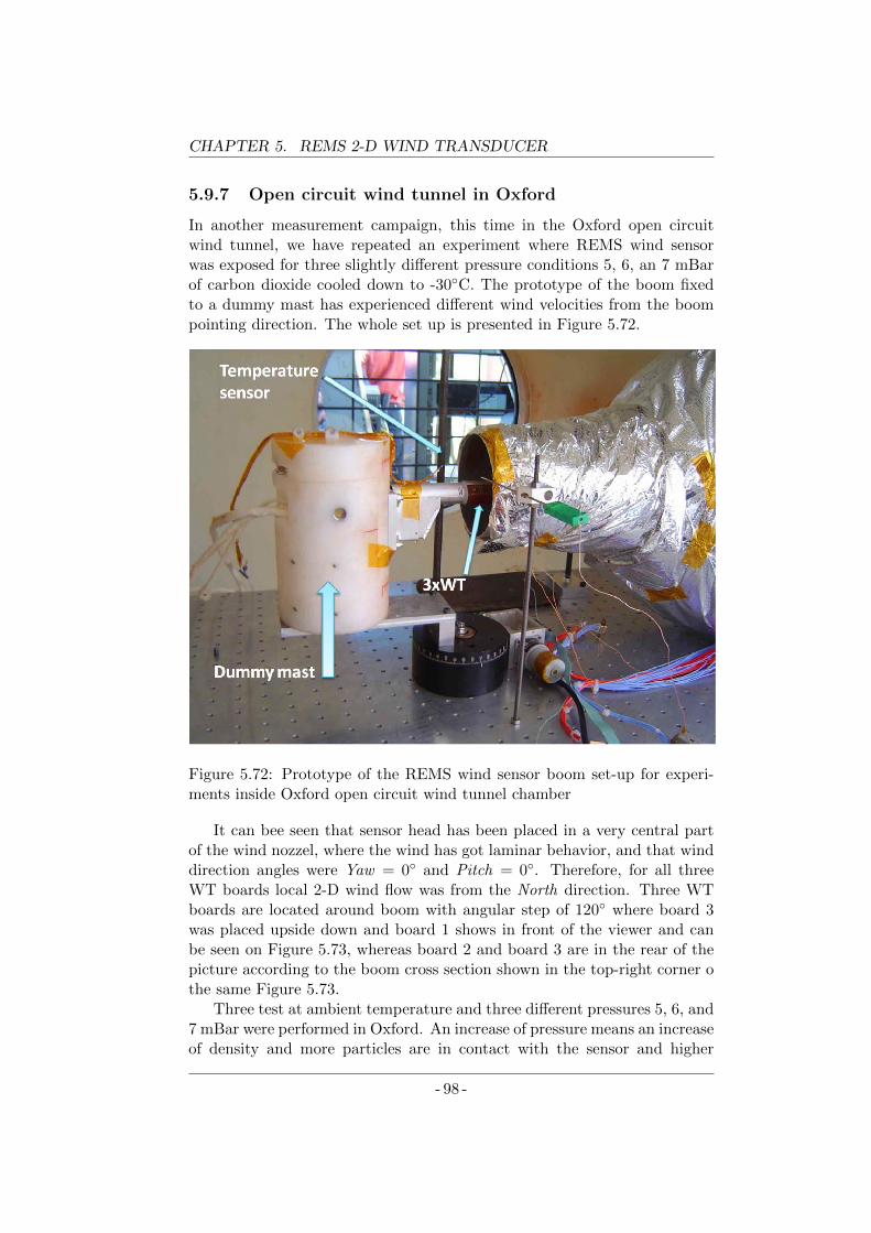
CHAPTER 5. REMS 2-D WIND TRANSDUCER
5.9.7 Open circuit wind tunnel in Oxford
In another measurement campaign, this time in the Oxford open circuitwind tunnel, we have repeated an experiment where REMS wind sensorwas exposed for three slightly different pressure conditions 5, 6, an 7 mBarof carbon dioxide cooled down to -30C. The prototype of the boom fixedto a dummy mast has experienced different wind velocities from the boompointing direction. The whole set up is presented in Figure 5.72.
Figure 5.72: Prototype of the REMS wind sensor boom set-up for experi-ments inside Oxford open circuit wind tunnel chamber
It can bee seen that sensor head has been placed in a very central partof the wind nozzel, where the wind has got laminar behavior, and that winddirection angles were Yaw = 0 and Pitch = 0. Therefore, for all threeWT boards local 2-D wind flow was from the North direction. Three WTboards are located around boom with angular step of 120 where board 3was placed upside down and board 1 shows in front of the viewer and canbe seen on Figure 5.73, whereas board 2 and board 3 are in the rear of thepicture according to the boom cross section shown in the top-right corner othe same Figure 5.73.
Three test at ambient temperature and three different pressures 5, 6, and7 mBar were performed in Oxford. An increase of pressure means an increaseof density and more particles are in contact with the sensor and higher
- 98 -
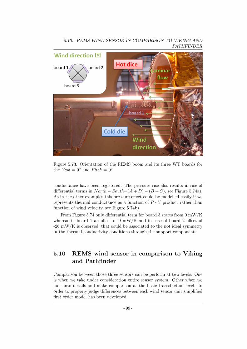
5.10. REMS WIND SENSOR IN COMPARISON TO VIKING ANDPATHFINDER
Figure 5.73: Orientation of the REMS boom and its three WT boards forthe Yaw = 0 and Pitch = 0
conductance have been registered. The pressure rise also results in rise ofdifferential terms in North− South=(A+D)− (B +C), see Figure 5.74a).As in the other examples this pressure effect could be modelled easily if werepresents thermal conductance as a function of P · U product rather thanfunction of wind velocity, see Figure 5.74b).
From Figure 5.74 only differential term for board 3 starts from 0 mW/Kwhereas in board 1 an offset of 9 mW/K and in case of board 2 offset of-26 mW/K is observed, that could be associated to the not ideal symmetryin the thermal conductivity conditions through the support components.
5.10 REMS wind sensor in comparison to Vikingand Pathfinder
Comparison between those three sensors can be perform at two levels. Oneis when we take under consideration entire sensor system. Other when welook into details and make comparison at the basic transduction level. Inorder to properly judge differences between each wind sensor unit simplifiedfirst order model has been developed.
- 99 -
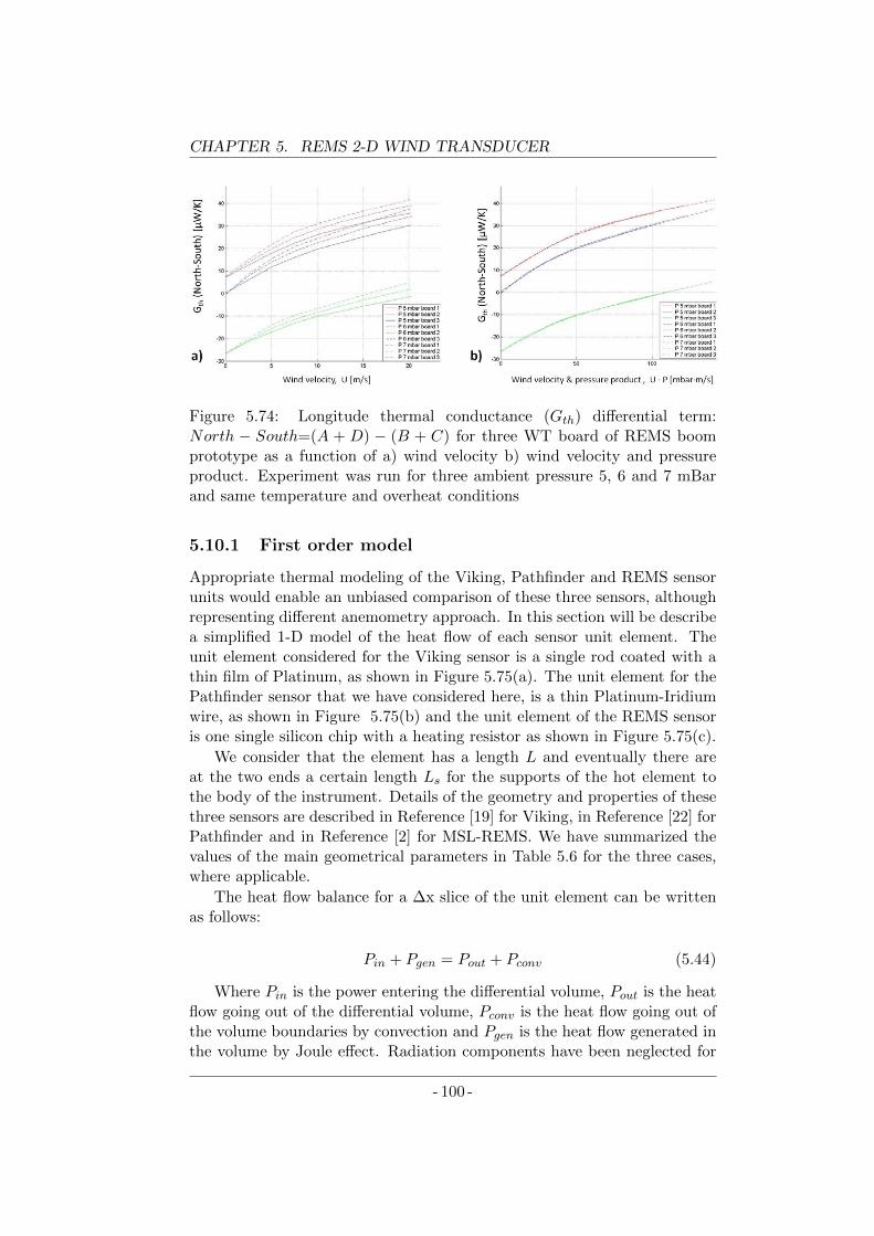
CHAPTER 5. REMS 2-D WIND TRANSDUCER
Figure 5.74: Longitude thermal conductance (Gth) differential term:North − South=(A + D) − (B + C) for three WT board of REMS boomprototype as a function of a) wind velocity b) wind velocity and pressureproduct. Experiment was run for three ambient pressure 5, 6 and 7 mBarand same temperature and overheat conditions
5.10.1 First order model
Appropriate thermal modeling of the Viking, Pathfinder and REMS sensorunits would enable an unbiased comparison of these three sensors, althoughrepresenting different anemometry approach. In this section will be describea simplified 1-D model of the heat flow of each sensor unit element. Theunit element considered for the Viking sensor is a single rod coated with athin film of Platinum, as shown in Figure 5.75(a). The unit element for thePathfinder sensor that we have considered here, is a thin Platinum-Iridiumwire, as shown in Figure 5.75(b) and the unit element of the REMS sensoris one single silicon chip with a heating resistor as shown in Figure 5.75(c).
We consider that the element has a length L and eventually there areat the two ends a certain length Ls for the supports of the hot element tothe body of the instrument. Details of the geometry and properties of thesethree sensors are described in Reference [19] for Viking, in Reference [22] forPathfinder and in Reference [2] for MSL-REMS. We have summarized thevalues of the main geometrical parameters in Table 5.6 for the three cases,where applicable.
The heat flow balance for a ∆x slice of the unit element can be writtenas follows:
Pin + Pgen = Pout + Pconv (5.44)
Where Pin is the power entering the differential volume, Pout is the heatflow going out of the differential volume, Pconv is the heat flow going out ofthe volume boundaries by convection and Pgen is the heat flow generated inthe volume by Joule effect. Radiation components have been neglected for
- 100 -
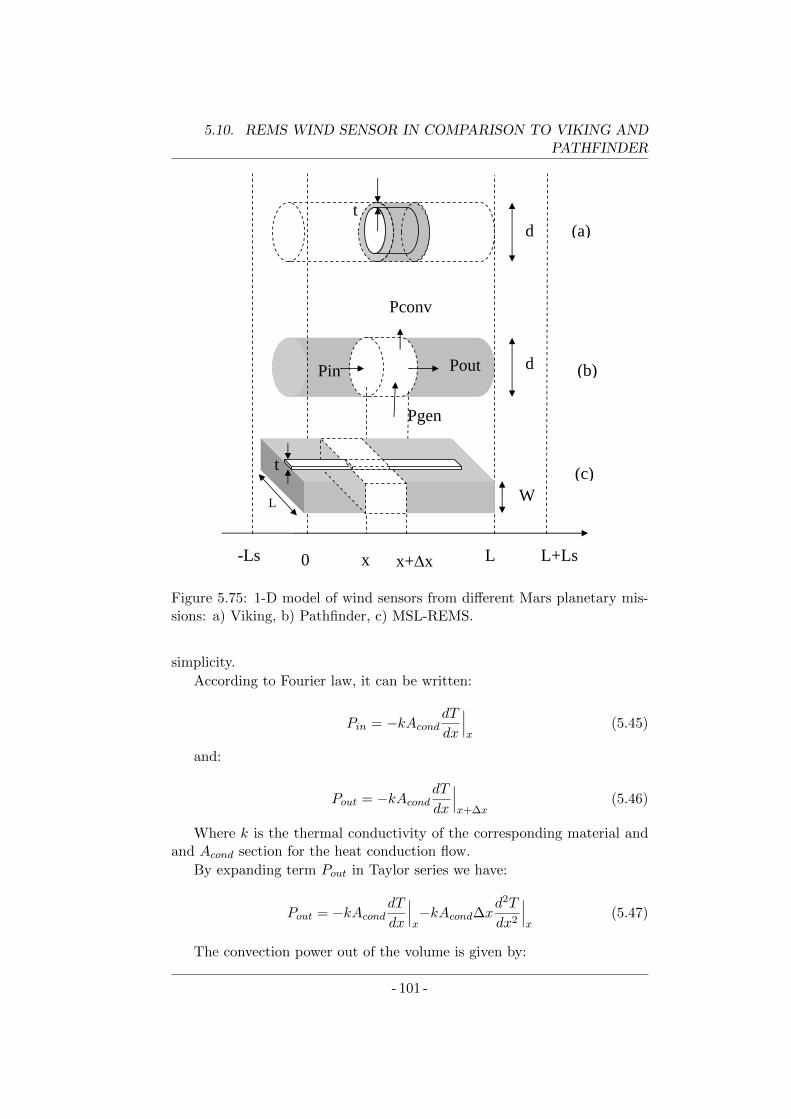
5.10. REMS WIND SENSOR IN COMPARISON TO VIKING ANDPATHFINDER
16
Figure 2
(a)
(b)
(c)
Pconv
Pout Pin
Pgen
0 L
d
d
L
Pgen
t
t
x x+x -Ls L+Ls
W
Figure 5.75: 1-D model of wind sensors from different Mars planetary mis-sions: a) Viking, b) Pathfinder, c) MSL-REMS.
simplicity.
According to Fourier law, it can be written:
Pin = −kAconddT
dx
∣∣∣x
(5.45)
and:
Pout = −kAconddT
dx
∣∣∣x+∆x
(5.46)
Where k is the thermal conductivity of the corresponding material andand Acond section for the heat conduction flow.
By expanding term Pout in Taylor series we have:
Pout = −kAconddT
dx
∣∣∣x−kAcond∆x
d2T
dx2
∣∣∣x
(5.47)
The convection power out of the volume is given by:
- 101 -
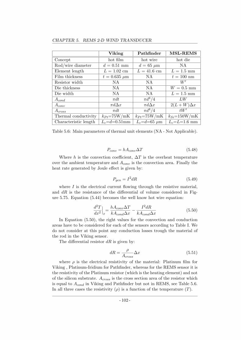
CHAPTER 5. REMS 2-D WIND TRANSDUCER
Viking Pathfinder MSL-REMS
Concept hot film hot wire hot die
Rod/wire diameter d = 0.51 mm d = 65 µm NA
Element length L = 1.02 cm L = 41.6 cm L = 1.5 mm
Film thickness t = 0.635 µm NA t = 100 nm
Resistor width NA NA W ′
Die thickness NA NA W = 0.5 mm
Die width NA NA L = 1.5 mm
Acond πdt πd4/4 LW
Aconv πd∆x πd∆x 2(L+W )∆x
Across πdt πd4/4 tW ′
Thermal conductivity kPt=75W/mK kPt=75W/mK kSi=150W/mK
Characteristic length Lc=d=0.51mm Lc=d=65 µm Lc=L=1.6 mm
Table 5.6: Main parameters of thermal unit elements (NA - Not Applicable).
Pconv = hAconv∆T (5.48)
Where h is the convection coefficient, ∆T is the overheat temperatureover the ambient temperature and Aconv is the convection area. Finally theheat rate generated by Joule effect is given by:
Pgen = I2dR (5.49)
where I is the electrical current flowing through the resistive material,and dR is the resistance of the differential of volume considered in Fig-ure 5.75. Equation (5.44) becomes the well know hot wire equation:
d2T
dx2
∣∣∣x=hAconv∆T
kAcond∆x− I2dR
kAcond∆x(5.50)
In Equation (5.50), the right values for the convection and conductionareas have to be considered for each of the sensors according to Table I. Wedo not consider at this point any conduction losses trough the material ofthe rod in the Viking sensor.
The differential resistor dR is given by:
dR =ρ
Across∆x (5.51)
where ρ is the electrical resistivity of the material: Platinum film forViking , Platinum-Iridium for Pathfinder, whereas for the REMS sensor it isthe resistivity of the Platinum resistor (which is the heating element) and notof the silicon substrate. Across is the cross section area of the resistor whichis equal to Acond in Viking and Pathfinder but not in REMS, see Table 5.6.In all three cases the resistivity (ρ) is a function of the temperature (T ).
- 102 -
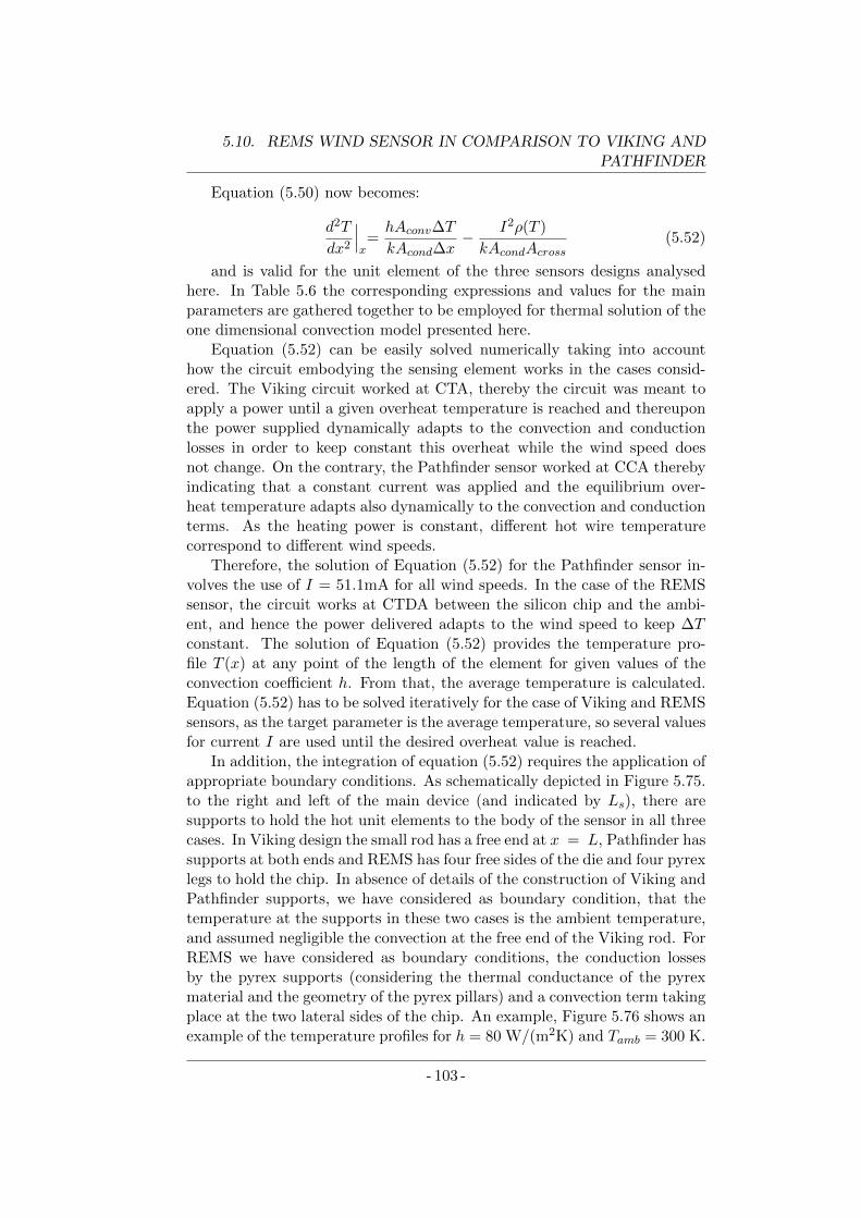
5.10. REMS WIND SENSOR IN COMPARISON TO VIKING ANDPATHFINDER
Equation (5.50) now becomes:
d2T
dx2
∣∣∣x=hAconv∆T
kAcond∆x− I2ρ(T )
kAcondAcross(5.52)
and is valid for the unit element of the three sensors designs analysedhere. In Table 5.6 the corresponding expressions and values for the mainparameters are gathered together to be employed for thermal solution of theone dimensional convection model presented here.
Equation (5.52) can be easily solved numerically taking into accounthow the circuit embodying the sensing element works in the cases consid-ered. The Viking circuit worked at CTA, thereby the circuit was meant toapply a power until a given overheat temperature is reached and thereuponthe power supplied dynamically adapts to the convection and conductionlosses in order to keep constant this overheat while the wind speed doesnot change. On the contrary, the Pathfinder sensor worked at CCA therebyindicating that a constant current was applied and the equilibrium over-heat temperature adapts also dynamically to the convection and conductionterms. As the heating power is constant, different hot wire temperaturecorrespond to different wind speeds.
Therefore, the solution of Equation (5.52) for the Pathfinder sensor in-volves the use of I = 51.1mA for all wind speeds. In the case of the REMSsensor, the circuit works at CTDA between the silicon chip and the ambi-ent, and hence the power delivered adapts to the wind speed to keep ∆Tconstant. The solution of Equation (5.52) provides the temperature pro-file T (x) at any point of the length of the element for given values of theconvection coefficient h. From that, the average temperature is calculated.Equation (5.52) has to be solved iteratively for the case of Viking and REMSsensors, as the target parameter is the average temperature, so several valuesfor current I are used until the desired overheat value is reached.
In addition, the integration of equation (5.52) requires the application ofappropriate boundary conditions. As schematically depicted in Figure 5.75.to the right and left of the main device (and indicated by Ls), there aresupports to hold the hot unit elements to the body of the sensor in all threecases. In Viking design the small rod has a free end at x = L, Pathfinder hassupports at both ends and REMS has four free sides of the die and four pyrexlegs to hold the chip. In absence of details of the construction of Viking andPathfinder supports, we have considered as boundary condition, that thetemperature at the supports in these two cases is the ambient temperature,and assumed negligible the convection at the free end of the Viking rod. ForREMS we have considered as boundary conditions, the conduction lossesby the pyrex supports (considering the thermal conductance of the pyrexmaterial and the geometry of the pyrex pillars) and a convection term takingplace at the two lateral sides of the chip. An example, Figure 5.76 shows anexample of the temperature profiles for h = 80 W/(m2K) and Tamb = 300 K.
- 103 -
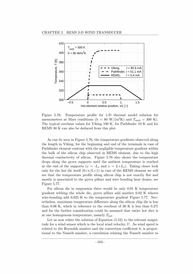
CHAPTER 5. REMS 2-D WIND TRANSDUCER
−0.5 0 0.5 1 1.5300
320
340
360
380
400
420
Hot element relative position, x/L [−]
Tem
pera
ture
, T [K
]
T
amb = 300 K
h = 80 W/m2K
Viking, I = 85.6 mA Pathfinder, I = 51.1 mA REMS, I = 5.4 mA
Figure 5.76: Temperature profile for 1-D thermal model solution foranemometers at Mars conditions (h = 80 W/(m2K) and Tamb = 300 K).The typical overheat values for Viking 100 K, for Pathfinder 10 K and forREMS 30 K can also be deduced from this plot.
As can be seen in Figure 5.76, the temperature gradients observed alongthe length in Viking, for the beginning and end of the terminals in case ofPathfinder element contrast with the negligible temperature gradient withinthe bulk of the silicon chip observed in REMS element, due to the highthermal conductivity of silicon. Figure 5.76 also shows the temperaturedrops along the pyrex supports until the ambient temperature is reachedat the end of the supports (x = -Ls and x = L+Ls). Taking closer lookonly for the hot die itself (0<x/L<1) in case of the REMS element we willsee that the temperature profile along silicon chip is not exactly flat andmostly is associated to the pyrex pillars and wire bonding heat drains, seeFigure 5.77.
For silicon die in suspension there would be only 0.01 K temperaturegradient withing the whole die, pyrex pillars add another 0.02 K whereswire-bonding add 0.025 K to the temperature gradient Figure 5.77. Nev-ertheless, maximum temperature difference along the silicon chip die is lessthan 0.06 K, which in reference to the overheat of 30 K is less than 0.2%and for the further consideration could be assumed that entire hot dice isat one homogenous temperature, namely Thot.
Let us now relate the solution of Equation (5.52) to the relevant magni-tude for a wind sensor which is the local wind velocity, U . As wind speed isrelated to the Reynolds number and the convection coefficient h, is propor-tional to the Nusselt number, a correlation relating the Nusselt number to
- 104 -
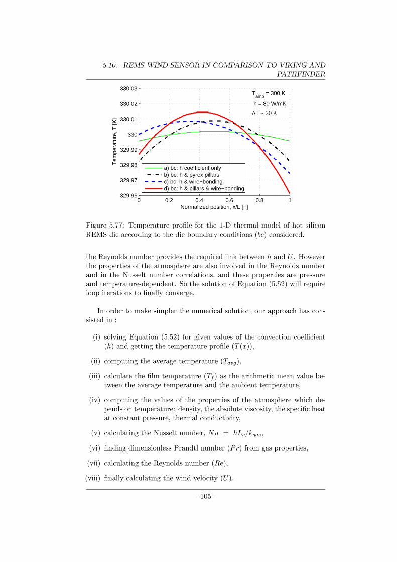
5.10. REMS WIND SENSOR IN COMPARISON TO VIKING ANDPATHFINDER
0 0.2 0.4 0.6 0.8 1329.96
329.97
329.98
329.99
330
330.01
330.02
330.03
Normalized position, x/L [−]
Tem
pera
ture
, T [K
]
T
amb = 300 K
h = 80 W/mK
∆T ~ 30 K
a) bc: h coefficient onlyb) bc: h & pyrex pillarsc) bc: h & wire−bondingd) bc: h & pillars & wire−bonding
Figure 5.77: Temperature profile for the 1-D thermal model of hot siliconREMS die according to the die boundary conditions (bc) considered.
the Reynolds number provides the required link between h and U . Howeverthe properties of the atmosphere are also involved in the Reynolds numberand in the Nusselt number correlations, and these properties are pressureand temperature-dependent. So the solution of Equation (5.52) will requireloop iterations to finally converge.
In order to make simpler the numerical solution, our approach has con-sisted in :
(i) solving Equation (5.52) for given values of the convection coefficient(h) and getting the temperature profile (T (x)),
(ii) computing the average temperature (Tavg),
(iii) calculate the film temperature (Tf ) as the arithmetic mean value be-tween the average temperature and the ambient temperature,
(iv) computing the values of the properties of the atmosphere which de-pends on temperature: density, the absolute viscosity, the specific heatat constant pressure, thermal conductivity,
(v) calculating the Nusselt number, Nu = hLc/kgas,
(vi) finding dimensionless Prandtl number (Pr) from gas properties,
(vii) calculating the Reynolds number (Re),
(viii) finally calculating the wind velocity (U).
- 105 -
CHAPTER 5. REMS 2-D WIND TRANSDUCER
The Nusselt number is related to the Prandtl and Reynolds numbers (forReynolds numbers smaller than 4000) by the Churchill and Bernstein [75],correlation for flow over a cylinder. This correlation is suitable for the Vikingand Pathfinder cases as the unit element is a cylinder:
Nu = 0.3 +0.62Re1/2Pr1/3
[1 +
(0.4Pr
)2/3]1/4(5.53)
In the case of the REMS sensor the geometry is assumed to be that of aflat surface in tangential flow. In that case the Nusselt number correlationfor Re < 5e5 is given in Reference [76] by simple equation:
Nu = 0.664Re1/2Pr1/3 (5.54)
The Churchill and Bernstein correlation in Equation (5.53) works finefor values of the Nusselt number greater than 0.3. In the cases considered inthis work and due to the low pressure of the Mars atmosphere, a correctionof the Nusselt number has been used, [77]:
1
Nuc=
1
Nu+ 2Kn (5.55)
where Nuc is the corrected number and Nu is given by Equation (5.53)and Kn is the Knudsen number, which is defined as the ratio of the meanfree path of the gas molecules divided by the characteristic length, see Sec-tion (3.2.1).
In the case of the Pathfinder model, and due to the low pressure andalso to the small value of the characteristic length, instead of the correctionshown in Equation (5.55) we have used the following correction which takesinto account the low values of the Mach number, [19,78]:
1
Nuc=
1
Nu+ 10.3
M
Re(5.56)
The procedure described above and enumerated from (a) to (h) enables,for given ambient conditions Pamb. and Tamb., to correlate following param-eters : wind velocity (U), Reynolds number (Re), Nusselt number (Nu),average temperature (Tavg), heat convection coefficient (h) and global heatconvection power (Pconv.) among others. The same, three thermal anemome-ters Viking, Pathfinder and REMS, although different in construction andfunctioning, can be contrasted according to the deliberately choose corre-lation factors. Same examples of these three sensor comparison take placein [3].
Here we compare for an hypothetical pressure (P = 670 Pa) and tem-perature (T = 220 K) how would all three sensors behave in power andoverheat aspects, see Figure 5.78.
- 106 -
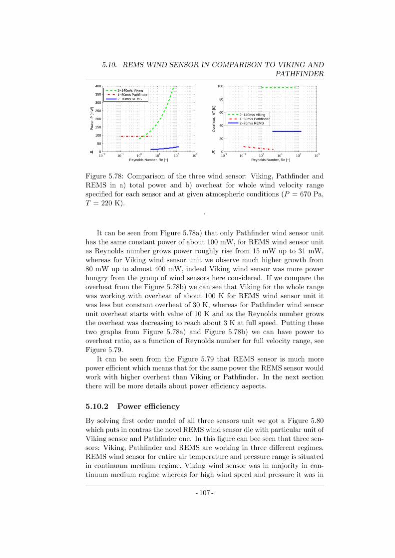
5.10. REMS WIND SENSOR IN COMPARISON TO VIKING ANDPATHFINDER
10−2
10−1
100
101
102
103
0
50
100
150
200
250
300
350
400
Reynolds Number, Re [−]
Pow
er, P
[mW
]
a)
2−140m/s Viking1−50m/s Pathfinder2−70m/s REMS
10−2
10−1
100
101
102
103
0
20
40
60
80
100
Reynolds Number, Re [−]
Ove
rhea
t, ∆
T [K
]
b)
2−140m/s Viking1−50m/s Pathfinder2−70m/s REMS
Figure 5.78: Comparison of the three wind sensor: Viking, Pathfinder andREMS in a) total power and b) overheat for whole wind velocity rangespecified for each sensor and at given atmospheric conditions (P = 670 Pa,T = 220 K).
.
It can be seen from Figure 5.78a) that only Pathfinder wind sensor unithas the same constant power of about 100 mW, for REMS wind sensor unitas Reynolds number grows power roughly rise from 15 mW up to 31 mW,whereas for Viking wind sensor unit we observe much higher growth from80 mW up to almost 400 mW, indeed Viking wind sensor was more powerhungry from the group of wind sensors here considered. If we compare theoverheat from the Figure 5.78b) we can see that Viking for the whole rangewas working with overheat of about 100 K for REMS wind sensor unit itwas less but constant overheat of 30 K, whereas for Pathfinder wind sensorunit overheat starts with value of 10 K and as the Reynolds number growsthe overheat was decreasing to reach about 3 K at full speed. Putting thesetwo graphs from Figure 5.78a) and Figure 5.78b) we can have power tooverheat ratio, as a function of Reynolds number for full velocity range, seeFigure 5.79.
It can be seen from the Figure 5.79 that REMS sensor is much morepower efficient which means that for the same power the REMS sensor wouldwork with higher overheat than Viking or Pathfinder. In the next sectionthere will be more details about power efficiency aspects.
5.10.2 Power efficiency
By solving first order model of all three sensors unit we got a Figure 5.80which puts in contras the novel REMS wind sensor die with particular unit ofViking sensor and Pathfinder one. In this figure can bee seen that three sen-sors: Viking, Pathfinder and REMS are working in three different regimes.REMS wind sensor for entire air temperature and pressure range is situatedin continuum medium regime, Viking wind sensor was in majority in con-tinuum medium regime whereas for high wind speed and pressure it was in
- 107 -
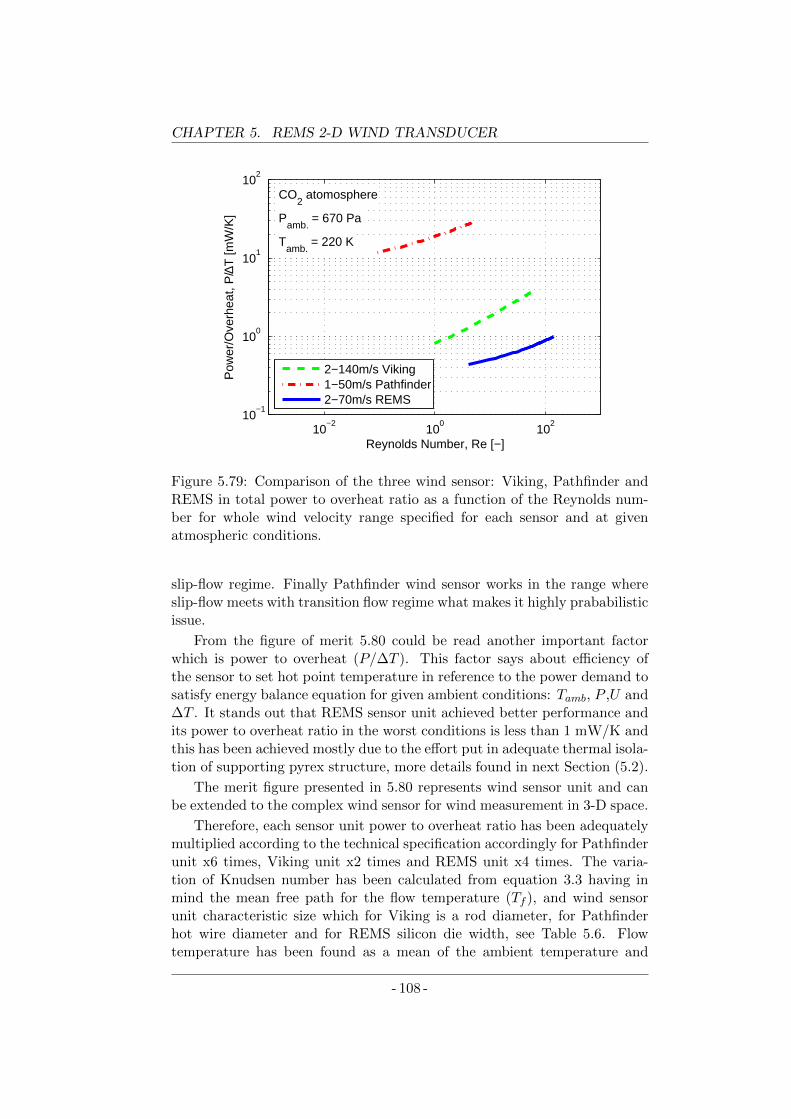
CHAPTER 5. REMS 2-D WIND TRANSDUCER
10−2
100
102
10−1
100
101
102
Reynolds Number, Re [−]
Pow
er/O
verh
eat,
P/∆
T [m
W/K
]
Pamb.
= 670 Pa
CO2 atomosphere
Tamb.
= 220 K
2−140m/s Viking1−50m/s Pathfinder2−70m/s REMS
Figure 5.79: Comparison of the three wind sensor: Viking, Pathfinder andREMS in total power to overheat ratio as a function of the Reynolds num-ber for whole wind velocity range specified for each sensor and at givenatmospheric conditions.
slip-flow regime. Finally Pathfinder wind sensor works in the range whereslip-flow meets with transition flow regime what makes it highly prababilisticissue.
From the figure of merit 5.80 could be read another important factorwhich is power to overheat (P/∆T ). This factor says about efficiency ofthe sensor to set hot point temperature in reference to the power demand tosatisfy energy balance equation for given ambient conditions: Tamb, P ,U and∆T . It stands out that REMS sensor unit achieved better performance andits power to overheat ratio in the worst conditions is less than 1 mW/K andthis has been achieved mostly due to the effort put in adequate thermal isola-tion of supporting pyrex structure, more details found in next Section (5.2).
The merit figure presented in 5.80 represents wind sensor unit and canbe extended to the complex wind sensor for wind measurement in 3-D space.
Therefore, each sensor unit power to overheat ratio has been adequatelymultiplied according to the technical specification accordingly for Pathfinderunit x6 times, Viking unit x2 times and REMS unit x4 times. The varia-tion of Knudsen number has been calculated from equation 3.3 having inmind the mean free path for the flow temperature (Tf ), and wind sensorunit characteristic size which for Viking is a rod diameter, for Pathfinderhot wire diameter and for REMS silicon die width, see Table 5.6. Flowtemperature has been found as a mean of the ambient temperature and
- 108 -
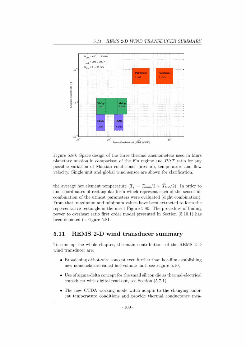
5.11. REMS 2-D WIND TRANSDUCER SUMMARY
10−1
100
101
102
10−3
10−2
10−1
Power/Overheat ratio, P/∆T [mW/K]
Knu
dsen
num
ber,
Kn
[−]
Pathfinder
1 unit
Pathfinder
6 units
Viking 1 unit
Viking 2 units
REMS
1 unit
REMS
4 units
PCO
2
= 600 ... 1200 Pa
Tamb
= 200 ... 300 K
Uflow
= 1 ... 50 m/s
Figure 5.80: Space design of the three thermal anemometers used in Marsplanetary mission in comparison of the Kn regime and P∆T ratio for anypossible variation of Martian conditions: pressure, temperature and flowvelocity. Single unit and global wind sensor are shown for clarification.
the average hot element temperature (Tf = Tamb/2 + Thot/2). In order tofind coordinates of rectangular form which represent each of the sensor allcombination of the utmost parameters were evaluated (eight combination).From that, maximum and minimum values have been extracted to form therepresentative rectangle in the merit Figure 5.80. The procedure of findingpower to overheat ratio first order model presented in Section (5.10.1) hasbeen depicted in Figure 5.81.
5.11 REMS 2-D wind transducer summary
To sum up the whole chapter, the main contributions of the REMS 2-Dwind transducer are:
• Broadening of hot-wire concept even further than hot-film establishingnew nomenclature called hot-volume unit, see Figure 5.10,
• Use of sigma-delta concept for the small silicon die as thermal-electricaltransducer with digital read out, see Section (5.7.1),
• The new CTDA working mode witch adapts to the changing ambi-ent temperature conditions and provide thermal conductance mea-
- 109 -
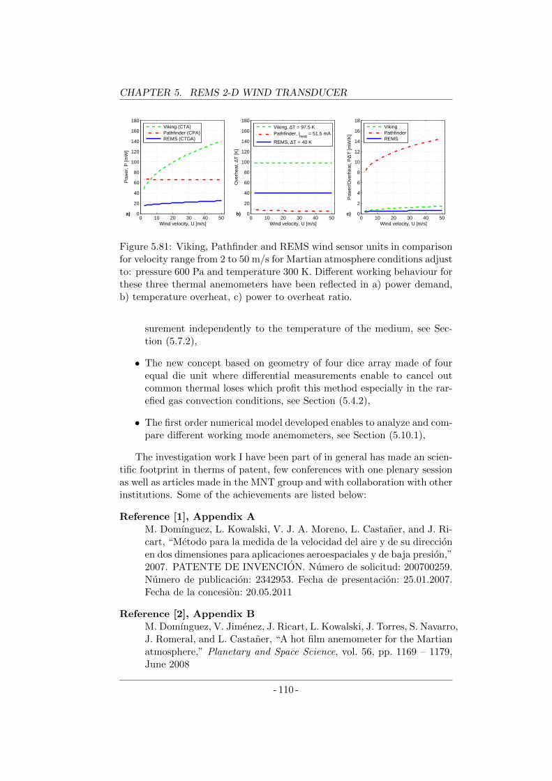
CHAPTER 5. REMS 2-D WIND TRANSDUCER
0 10 20 30 40 500
20
40
60
80
100
120
140
160
180
Wind velocity, U [m/s]
Pow
er, P
[mW
]
a)
Viking (CTA) Pathfinder (CPA) REMS (CTDA)
0 10 20 30 40 500
20
40
60
80
100
120
140
160
180
Wind velocity, U [m/s]
Ove
rhea
t, ∆T
[K]
b)
Viking, ∆T = 97.5 K Pathfinder, I
heat = 51.5 mA
REMS, ∆T = 40 K
0 10 20 30 40 500
2
4
6
8
10
12
14
16
18
Wind velocity, U [m/s]
Pow
er/O
verh
eat,
P/∆
T [m
W/K
]
c)
Viking Pathfinder REMS
Figure 5.81: Viking, Pathfinder and REMS wind sensor units in comparisonfor velocity range from 2 to 50 m/s for Martian atmosphere conditions adjustto: pressure 600 Pa and temperature 300 K. Different working behaviour forthese three thermal anemometers have been reflected in a) power demand,b) temperature overheat, c) power to overheat ratio.
surement independently to the temperature of the medium, see Sec-tion (5.7.2),
• The new concept based on geometry of four dice array made of fourequal die unit where differential measurements enable to cancel outcommon thermal loses which profit this method especially in the rar-efied gas convection conditions, see Section (5.4.2),
• The first order numerical model developed enables to analyze and com-pare different working mode anemometers, see Section (5.10.1),
The investigation work I have been part of in general has made an scien-tific footprint in therms of patent, few conferences with one plenary sessionas well as articles made in the MNT group and with collaboration with otherinstitutions. Some of the achievements are listed below:
Reference [1], Appendix AM. Domınguez, L. Kowalski, V. J. A. Moreno, L. Castaner, and J. Ri-cart, “Metodo para la medida de la velocidad del aire y de su direccionen dos dimensiones para aplicaciones aeroespaciales y de baja presion,”2007. PATENTE DE INVENCION. Numero de solicitud: 200700259.Numero de publicacion: 2342953. Fecha de presentacion: 25.01.2007.Fecha de la concesion: 20.05.2011
Reference [2], Appendix BM. Domınguez, V. Jimenez, J. Ricart, L. Kowalski, J. Torres, S. Navarro,J. Romeral, and L. Castaner, “A hot film anemometer for the Martianatmosphere,” Planetary and Space Science, vol. 56, pp. 1169 – 1179,June 2008
- 110 -
5.11. REMS 2-D WIND TRANSDUCER SUMMARY
Reference [3], Appendix CV. Jimenez, M. Domınguez-Pumar, J. Ricart, L. Kowalski, S. Navarro,J. Torres, J. Romeral, J. Merrison, and L. Castaner, “Applications ofhot film anemometry to space missions,” in Eurosensors XXII, (Dres-den, Germany), September 2008. ISBN 978-3-00-025217-4
Reference [4], Appendix DL. Kowalski, J. Ricart, V. Jimenez, M. Domınguez-Pumar, and L. Castaner,“Sensitivity analysis of the chip for REMS wind sensor,” in 7th Span-ish Conference on Electron Devices (CDE 2009), (Palma de Mallorca,Spain), pp. 289–292, February 2009
Reference [5], Appendix EL. Kowalski, “Contribution to advanced hot wire wind sensing,” in 1stBarcelona Forum on Ph.D. Research in Electronic Engineering, pp. 7–8, Universitat Politecnica de Catalunya (UPC), Centre de Publicacionsdel Campus Nord SCCL (CPET), October 2009. ISBN978-84-7653-398-7
Reference [6], Appendix GL. Kowalski, J. Ricart, V. Jimenez, M. Domınguez, and L. Castaner,“Thermal modelling of the chip for the REMS wind sensor,” Interna-tional Journal of Numerical Modelling: Electronic Networks, Devicesand Fields, vol. 23, pp. 340–353, July - October 2009. Special Issue onthe 7th Spanish Conference on Electron Devices (CDE2009)
Reference [8], Appendix HL. Kowalski, L. Castaner, M. Domınguez, and V. Jimenez, “Multi-physics simulation of REMS hot-film anemometer under typical Mar-tian atmosphere conditions,” in COMSOL Conferenece 2010, (Paris,France), October 2010
Reference [9]J. Gomez-Elvira, C. Armiens, L. Castaner, M. Domınguez-Pumar,M. Genzer, F. Gomez, R. Haberle, A.-M. Harri, V. Jimenez, H. Kahan-paa, L. Kowalski, A. Lepinette, J. Martın, J. Martınez-Frıas, I. McE-wan, L. Mora, J. Moreno, S. Navarro, M. de Pablo, V. Peinado, A. Pena,J. Polkko, M. Ramos, N. Renno, J. Ricart, M. Richardson, J. Rodrıguez-Manfredi, J. Romeral, E. Sebastian, J. Serrano, M. dela Torre Juarez,J. Torres, F. Torrero, R. Urquı, L. Vazquez, T. Velasco, J. Verdasca,M.-P. Zorzano, and J. Martın-Torres, “REMS: The environmental sen-sor suite for the Mars Science Laboratory rover,” Space Science Re-views, vol. 170, pp. 583–640, July 2012
There have been also other positive implication from participation ofUPC-MNT group in MSL-REMS mission. We have been honored with
- 111 -
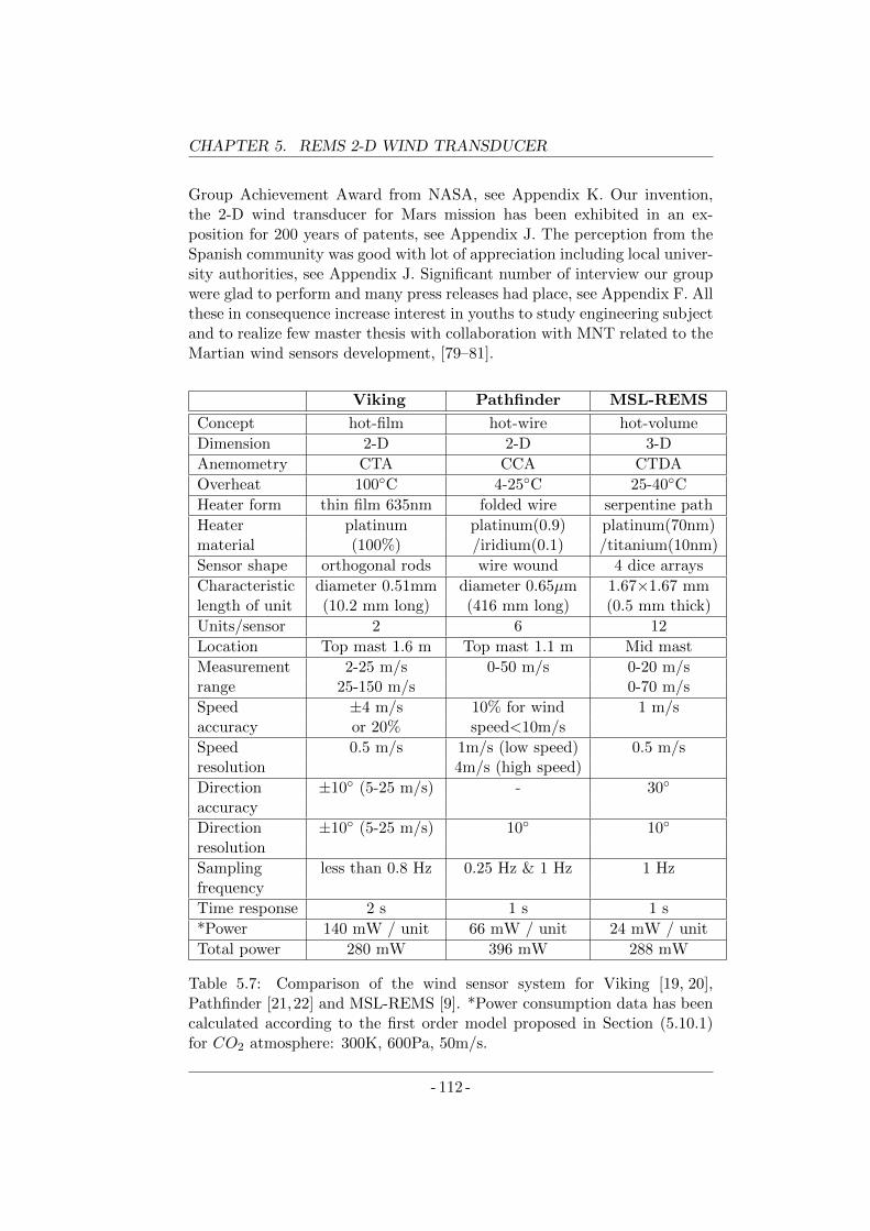
CHAPTER 5. REMS 2-D WIND TRANSDUCER
Group Achievement Award from NASA, see Appendix K. Our invention,the 2-D wind transducer for Mars mission has been exhibited in an ex-position for 200 years of patents, see Appendix J. The perception from theSpanish community was good with lot of appreciation including local univer-sity authorities, see Appendix J. Significant number of interview our groupwere glad to perform and many press releases had place, see Appendix F. Allthese in consequence increase interest in youths to study engineering subjectand to realize few master thesis with collaboration with MNT related to theMartian wind sensors development, [79–81].
Viking Pathfinder MSL-REMS
Concept hot-film hot-wire hot-volume
Dimension 2-D 2-D 3-D
Anemometry CTA CCA CTDA
Overheat 100C 4-25C 25-40C
Heater form thin film 635nm folded wire serpentine path
Heater platinum platinum(0.9) platinum(70nm)material (100%) /iridium(0.1) /titanium(10nm)
Sensor shape orthogonal rods wire wound 4 dice arrays
Characteristic diameter 0.51mm diameter 0.65µm 1.67×1.67 mmlength of unit (10.2 mm long) (416 mm long) (0.5 mm thick)
Units/sensor 2 6 12
Location Top mast 1.6 m Top mast 1.1 m Mid mast
Measurement 2-25 m/s 0-50 m/s 0-20 m/srange 25-150 m/s 0-70 m/s
Speed ±4 m/s 10% for wind 1 m/saccuracy or 20% speed<10m/s
Speed 0.5 m/s 1m/s (low speed) 0.5 m/sresolution 4m/s (high speed)
Direction ±10 (5-25 m/s) - 30
accuracy
Direction ±10 (5-25 m/s) 10 10
resolution
Sampling less than 0.8 Hz 0.25 Hz & 1 Hz 1 Hzfrequency
Time response 2 s 1 s 1 s
*Power 140 mW / unit 66 mW / unit 24 mW / unit
Total power 280 mW 396 mW 288 mW
Table 5.7: Comparison of the wind sensor system for Viking [19, 20],Pathfinder [21,22] and MSL-REMS [9]. *Power consumption data has beencalculated according to the first order model proposed in Section (5.10.1)for CO2 atmosphere: 300K, 600Pa, 50m/s.
- 112 -
5.11. REMS 2-D WIND TRANSDUCER SUMMARY
Finally, conceived and developed at UPC 2-D wind transducer ade-quately repeated is part of the REMS wind sensor instrument that is upto date operating aboard of the MSL Curiosity Rover. By performing in-situ wind measurements, REMS device has contributed to better knowledgeof Martian meteorology. Among others wind events, the whirlwind in theGale Crater has been recognized, see Appendix K. The specification of theREMS wind sensor has been put in contrast with Viking and Pathfindersensors for comparison in Table 5.7, as the REMS wind sensor has joinedthe elite group of the thermal anemometers that has an opportunity toface a challenge of Mars wind measurement. The wind sensor become thefirst three-dimensional wind sensor on the Red Planet, since the Viking andPathfinder systems were only for 2-D wind measurement within a horizontalplane. Though, the total power consumption of the REMS sensor is lowerthan for the Pathfinder one and in agreement with the Viking wind sensor.
- 113 -

Chapter 6
3-D Hot Sphere Anemometer
In this chapter, It will be said few words about MEIGA project withinwhich new 3-D spherical sensor has been developed. Then the author of thethesis will give a motivation that was upon new spherical geometry proposedfor the sensor design. The way numerical simulation has been executed tofind numerical convection model of the sensor will be presented. Rapidprototyping procedure will be described. Finally, the first measurement onthe newly conceived structure will take place in this thesis to finish with thediscussion on the new spherical sensor behavior.
6.1 MEIGA project
Mars Environmental Instrumentation for Ground and Atmosphere (MEIGA)is a project financed by Spanish Ministry of Science and Innovation (code:AYA2008-06420-C04-01/ESP) under scientific director leadership of profes-sor Luis Vazquez form Madrid Complutense University. MEIGA is a partof bigger Mars planetary mission Meteorological Network (MetNet). Met-Net is a international joint effort of many scientific institution under theleadership of FMI, where the others institutions were: Russian Space Re-search Institute (IKI), Lavochkin Association (LA) and from Spain INTA.The MetNet mission to Mars is based on a new type of semi-hard landingvehicle called MetNet Lander (MNL), [82]. As a continuation of MetNetPrecursor Mission several tens of MNLs will be deployed on the surface ofMars equipped with specialized payloads. MEIGA was about to bring newvision for Mars exploration by providing instrumentation made in Spain forthe next generation lander international mission for Martian atmosphericscience. Among instruments developed in the course of MEIGA project are:magnetometer MOURA [83], Solar Irradiance Sensor (SIS) [84], Dust Sensor(DS) [85] and Spherical Wind Sensor (SWS) [11].
115
CHAPTER 6. 3-D HOT SPHERE ANEMOMETER
6.1.1 MEIGA wind sensor
It is a general goal in all wind sensors for Mars to achieve accuracy inthe range of 0.1m/s to 0.5m/s, for wind velocity range from 0 to 15m/sand 10-30 degrees accuracy in wind direction, and doing that in a compactdesign consuming low power. For MEIGA project, the responsibility ofMNT group was to present engineering concept of 3-D wind sensor to satisfymission call for versatile robust and power efficient constraints in in-situ flowmeasurements on the surface of Mars.
Thermal flow sensors have been investigated extensively for a long time.Many of the 2-D thermal flow sensors concept have been realized [42,86–88].However to our knowledge the 3-D anemometers are built using multiple 2-Danemometers [89]. In three dimensions the wind direction can be measuredby placing several 2-D wind sensors in different planes and using an inversealgorithm to retrieve the wind direction from the values of the thermalconductances, as it is the case in the REMS wind sensor [9]. This algorithmcan be awkward depending on the specific geometry of the sensor and maynot be equally sensitive to all angles. In this case, the spherical geometrysimplifies the problem and is intrinsically 3-D.
We have in mind all advantages and inconveniences as well as huge ex-perience from participation in REMS project. The design of the wind sensorfor the Curiosity rover was to a large extent conditioned by the design of themast of the rover itself as REMS is a cylinder-like structure protruding outof the camera mast. It is the complexity of the design and of the operationis usually computationally demanding to cover all incidence angle and windspeeds. This time, the purpose was to develop a design framework to reducecomputational time and to apply the procedure to a novel geometry for windsensors in low Reynolds number environment, based on a spherical shape togain in compactness and to provide symmetry. It is intended to serve, notonly for future missions to Mars but also to other low-pressure applicationsin aeronautics or meteorologic balloons, to improve wind measurements inhigher troposphere and stratosphere, [90].
Flow over a sphere provides an ideal flow geometry and the local heat dis-sipation coefficient on the sphere skin is a function of the wind direction andof the velocity [91]. Therefore, we came with an idea of a spherical thermalanemometer with deliberately divided into sectors external shell, subject tothe wind flow. A spherical shape has been adopted because the flow aroundit is axis-symmetrical and stable for low Reynolds numbers [92]. The multi-physic simulations of convection, thermal losses problem divagation, proofof concept as well as prototype fabrication and preliminary measurementswere the main issue to address during the development of this novel device.
MEIGA project constraints according to the wind sensor specificationare:
• wind velocity measurement range 1..10 m/s,
- 116 -
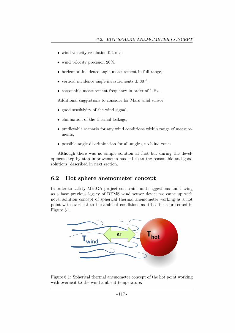
6.2. HOT SPHERE ANEMOMETER CONCEPT
• wind velocity resolution 0.2 m/s,
• wind velocity precision 20%,
• horizontal incidence angle measurement in full range,
• vertical incidence angle measurements ± 30 ,
• reasonable measurement frequency in order of 1 Hz.
Additional suggestions to consider for Mars wind sensor:
• good sensitivity of the wind signal,
• elimination of the thermal leakage,
• predictable scenario for any wind conditions within range of measure-ments,
• possible angle discrimination for all angles, no blind zones.
Although there was no simple solution at first but during the devel-opment step by step improvements has led as to the reasonable and goodsolutions, described in next section.
6.2 Hot sphere anemometer concept
In order to satisfy MEIGA project constrains and suggestions and havingas a base previous legacy of REMS wind sensor device we came up withnovel solution concept of spherical thermal anemometer working as a hotpoint with overheat to the ambient conditions as it has been presented inFigure 6.1.
∆T Twind
Thot
Figure 6.1: Spherical thermal anemometer concept of the hot point workingwith overheat to the wind ambient temperature.
- 117 -
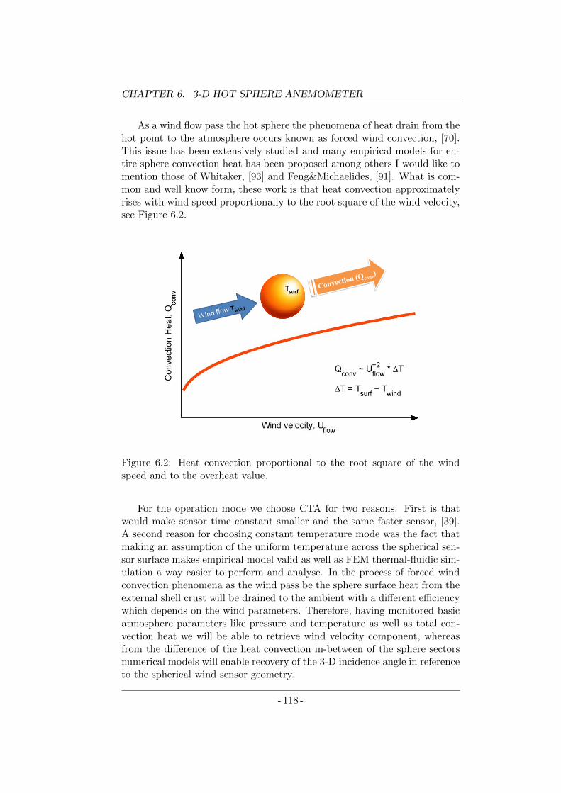
CHAPTER 6. 3-D HOT SPHERE ANEMOMETER
As a wind flow pass the hot sphere the phenomena of heat drain from thehot point to the atmosphere occurs known as forced wind convection, [70].This issue has been extensively studied and many empirical models for en-tire sphere convection heat has been proposed among others I would like tomention those of Whitaker, [93] and Feng&Michaelides, [91]. What is com-mon and well know form, these work is that heat convection approximatelyrises with wind speed proportionally to the root square of the wind velocity,see Figure 6.2.
Tsurf
Figure 6.2: Heat convection proportional to the root square of the windspeed and to the overheat value.
For the operation mode we choose CTA for two reasons. First is thatwould make sensor time constant smaller and the same faster sensor, [39].A second reason for choosing constant temperature mode was the fact thatmaking an assumption of the uniform temperature across the spherical sen-sor surface makes empirical model valid as well as FEM thermal-fluidic sim-ulation a way easier to perform and analyse. In the process of forced windconvection phenomena as the wind pass be the sphere surface heat from theexternal shell crust will be drained to the ambient with a different efficiencywhich depends on the wind parameters. Therefore, having monitored basicatmosphere parameters like pressure and temperature as well as total con-vection heat we will be able to retrieve wind velocity component, whereasfrom the difference of the heat convection in-between of the sphere sectorsnumerical models will enable recovery of the 3-D incidence angle in referenceto the spherical wind sensor geometry.
- 118 -
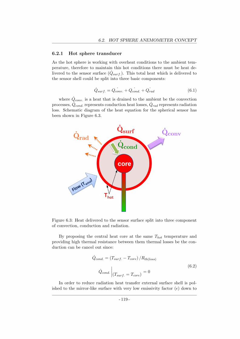
6.2. HOT SPHERE ANEMOMETER CONCEPT
6.2.1 Hot sphere transducer
As the hot sphere is working with overheat conditions to the ambient tem-perature, therefore to maintain this hot conditions there must be heat de-livered to the sensor surface (Qsurf.). This total heat which is delivered tothe sensor shell could be split into three basic components:
Qsurf. = ˙Qconv. + ˙Qcond. + ˙Qrad (6.1)
where Qconv. is a heat that is drained to the ambient be the convectionprocesses, Qcond. represents conduction heat losses, Qrad represents radiationloss. Schematic diagram of the heat equation for the spherical sensor hasbeen shown in Figure 6.3.
Figure 6.3: Heat delivered to the sensor surface split into three componentof convection, conduction and radiation.
By proposing the central heat core at the same Thot temperature andproviding high thermal resistance between them thermal losses be the con-duction can be cancel out since:
Qcond. = (Tsurf. − Tcore) /Rth(loss)
Qcond.
∣∣∣∣(Tsurf. = Tcore)= 0
(6.2)
In order to reduce radiation heat transfer external surface shell is pol-ished to the mirror-like surface with very low emissivity factor (ε) down to
- 119 -
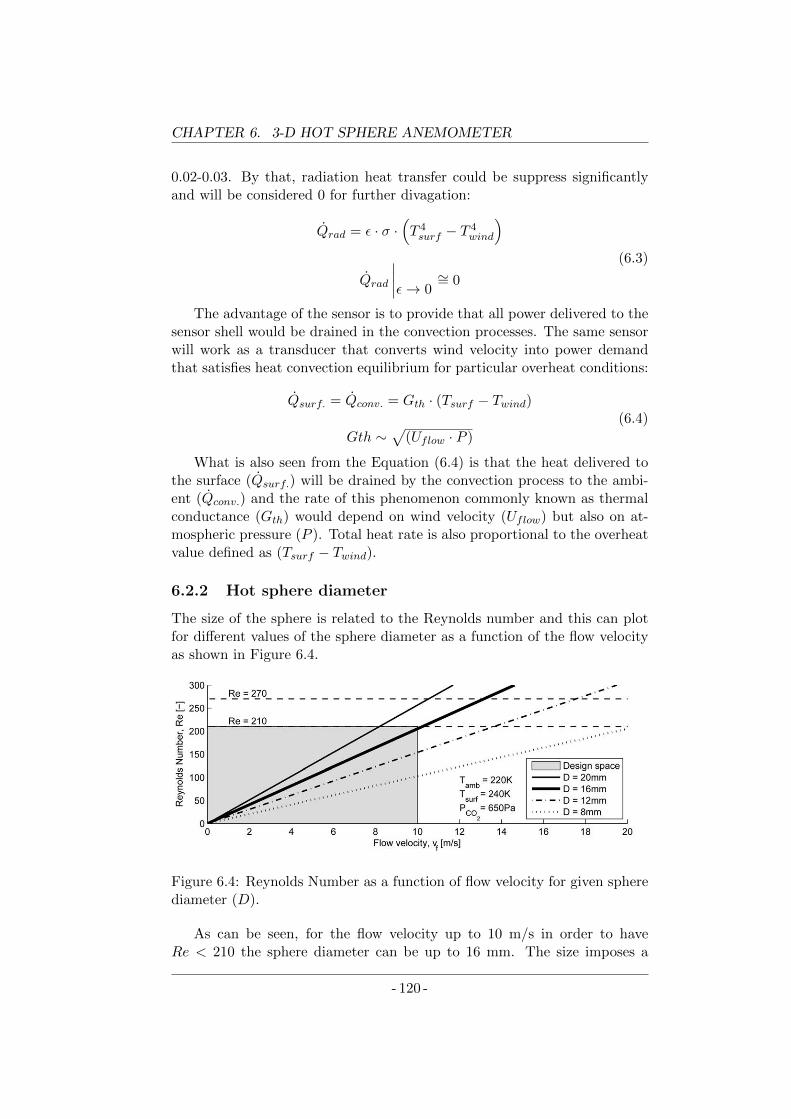
CHAPTER 6. 3-D HOT SPHERE ANEMOMETER
0.02-0.03. By that, radiation heat transfer could be suppress significantlyand will be considered 0 for further divagation:
Qrad = ε · σ ·(T 4surf − T 4
wind
)
Qrad
∣∣∣∣ε→ 0∼= 0
(6.3)
The advantage of the sensor is to provide that all power delivered to thesensor shell would be drained in the convection processes. The same sensorwill work as a transducer that converts wind velocity into power demandthat satisfies heat convection equilibrium for particular overheat conditions:
Qsurf. = Qconv. = Gth · (Tsurf − Twind)
Gth ∼√
(Uflow · P )
(6.4)
What is also seen from the Equation (6.4) is that the heat delivered tothe surface (Qsurf.) will be drained by the convection process to the ambi-ent (Qconv.) and the rate of this phenomenon commonly known as thermalconductance (Gth) would depend on wind velocity (Uflow) but also on at-mospheric pressure (P ). Total heat rate is also proportional to the overheatvalue defined as (Tsurf − Twind).
6.2.2 Hot sphere diameter
The size of the sphere is related to the Reynolds number and this can plotfor different values of the sphere diameter as a function of the flow velocityas shown in Figure 6.4.
Figure 6.4: Reynolds Number as a function of flow velocity for given spherediameter (D).
As can be seen, for the flow velocity up to 10 m/s in order to haveRe < 210 the sphere diameter can be up to 16 mm. The size imposes a
- 120 -
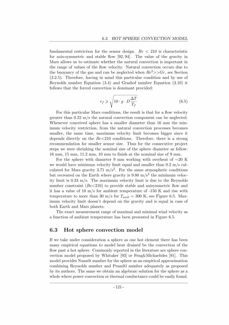
6.3. HOT SPHERE CONVECTION MODEL
fundamental restriction for the sensor design. Re < 210 is characteristicfor axis-symmetric and stable flow [92, 94]. The value of the gravity inMars allows us to estimate whether the natural convection is important inthe range of values of the flow velocity. Natural convection occurs due tothe buoyancy of the gas and can be neglected when Re2>>Gr, see Section(3.2.5). Therefore, having in mind this particular condition and by use ofReynolds number Equation (3.4) and Grashof number Equation (3.10) itfollows that the forced convection is dominant provided:
vf >√
10 · g ·D∆T
Tf(6.5)
For this particular Mars conditions, the result is that for a flow velocitygreater than 0.22 m/s the natural convection component can be neglected.Whenever conceived sphere has a smaller diameter than 16 mm the min-imum velocity restriction, from the natural convection processes becomessmaller, the same time, maximum velocity limit becomes bigger since itdepends directly on the Re<210 conditions. Therefore, there is a strongrecommendation for smaller sensor size. Thus for the consecutive projectsteps we were shrinking the nominal size of the sphere diameter as follow:16 mm, 15 mm, 11.2 mm, 10 mm to finish at the nominal size of 9 mm.
For the sphere with diameter 9 mm working with overheat of ∼20 Kwe would have minimum velocity limit equal and smaller than 0.2 m/s cal-culated for Mars gravity 3.71 m/s2. For the same atmospheric conditionsbut recreated on the Earth where gravity is 9.80 m/s2 the minimum veloc-ity limit is 0.33 m/s. The maximum velocity limit is due to the Reynoldsnumber constraint (Re<210) to provide stable and axisymmetric flow andit has a value of 10 m/s for ambient temperature of -150 K and rise withtemperature to more than 30 m/s for Tamb = 300 K, see Figure 6.5. Max-imum velocity limit doesn’t depend on the gravity and is equal in case ofboth Earth and Mars planets.
The exact measurement range of maximal and minimal wind velocity asa function of ambient temperature has been presented in Figure 6.5.
6.3 Hot sphere convection model
If we take under consideration a sphere as one hot element there has beenmany empirical equations to model heat drained be the convection of theflow past a hot sphere. Commonly reported in the literature are sphere con-vection model proposed by Whitaker [93] or Feng&Michaelides [91]. Thismodel provides Nusselt number for the sphere as an empirical approximationcombining Reynolds number and Prandtl number adequately as proposedby its authors. The same we obtain an algebraic solution for the sphere as awhole where power convection or thermal conductance could be easily found.
- 121 -
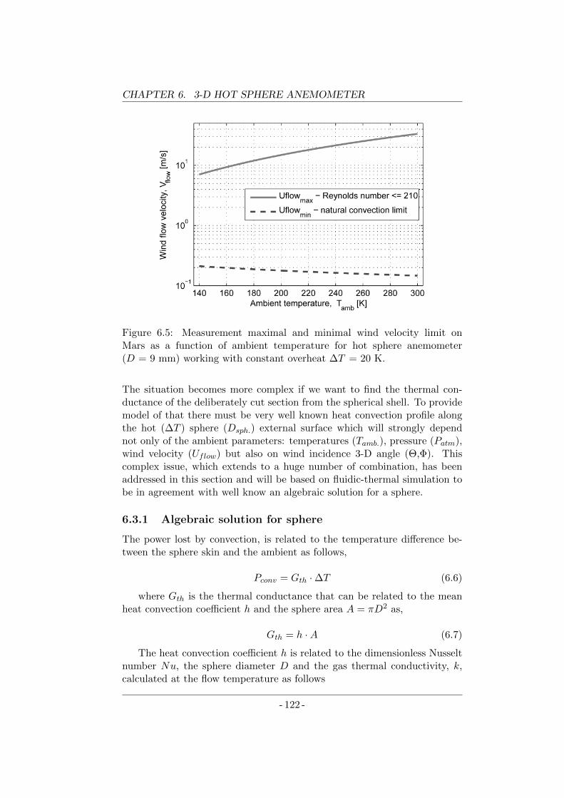
CHAPTER 6. 3-D HOT SPHERE ANEMOMETER
Figure 6.5: Measurement maximal and minimal wind velocity limit onMars as a function of ambient temperature for hot sphere anemometer(D = 9 mm) working with constant overheat ∆T = 20 K.
The situation becomes more complex if we want to find the thermal con-ductance of the deliberately cut section from the spherical shell. To providemodel of that there must be very well known heat convection profile alongthe hot (∆T ) sphere (Dsph.) external surface which will strongly dependnot only of the ambient parameters: temperatures (Tamb.), pressure (Patm),wind velocity (Uflow) but also on wind incidence 3-D angle (Θ,Φ). Thiscomplex issue, which extends to a huge number of combination, has beenaddressed in this section and will be based on fluidic-thermal simulation tobe in agreement with well know an algebraic solution for a sphere.
6.3.1 Algebraic solution for sphere
The power lost by convection, is related to the temperature difference be-tween the sphere skin and the ambient as follows,
Pconv = Gth ·∆T (6.6)
where Gth is the thermal conductance that can be related to the meanheat convection coefficient h and the sphere area A = πD2 as,
Gth = h ·A (6.7)
The heat convection coefficient h is related to the dimensionless Nusseltnumber Nu, the sphere diameter D and the gas thermal conductivity, k,calculated at the flow temperature as follows
- 122 -
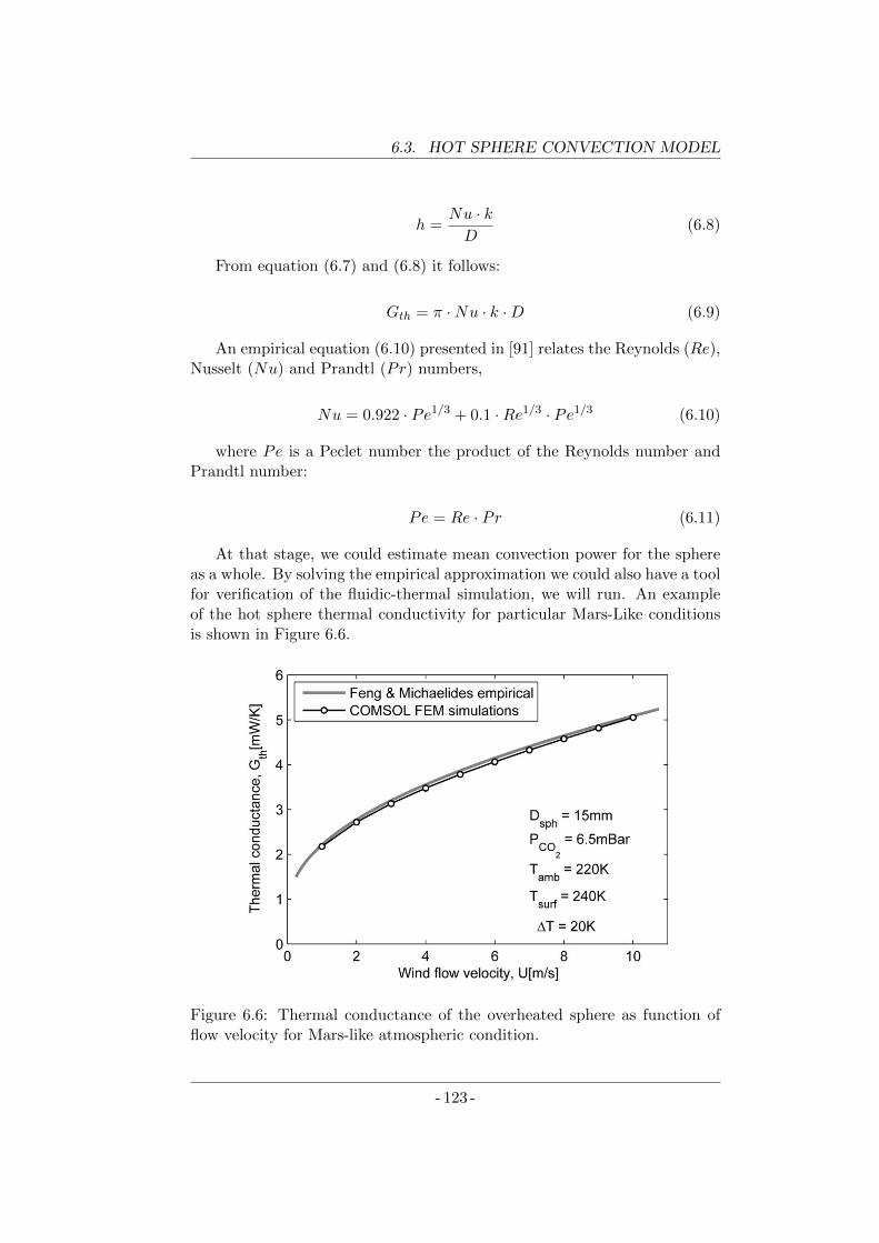
6.3. HOT SPHERE CONVECTION MODEL
h =Nu · kD
(6.8)
From equation (6.7) and (6.8) it follows:
Gth = π ·Nu · k ·D (6.9)
An empirical equation (6.10) presented in [91] relates the Reynolds (Re),Nusselt (Nu) and Prandtl (Pr) numbers,
Nu = 0.922 · Pe1/3 + 0.1 ·Re1/3 · Pe1/3 (6.10)
where Pe is a Peclet number the product of the Reynolds number andPrandtl number:
Pe = Re · Pr (6.11)
At that stage, we could estimate mean convection power for the sphereas a whole. By solving the empirical approximation we could also have a toolfor verification of the fluidic-thermal simulation, we will run. An exampleof the hot sphere thermal conductivity for particular Mars-Like conditionsis shown in Figure 6.6.
Figure 6.6: Thermal conductance of the overheated sphere as function offlow velocity for Mars-like atmospheric condition.
- 123 -
CHAPTER 6. 3-D HOT SPHERE ANEMOMETER
6.3.2 Fluidic-thermal simulations
For FEM simulation, we consider sphere immersed in a cylindrical volumeof gas as described in Table 6.1.
Atmosphere temperature, Tamb 220 K
Sphere surface temperature, Tsurf 240 K
Overheat, ∆T 20 K
Flow Temperature, Tf 230 K
Pressure, P 650 Pa
Flow speed, Uf 1,2,3,4,5,6,7,8,9,10 m/s
Sphere diameter, D 15 mm
Gas composition CO2 (100%)
Air size ahead of Sphere 10 · sphere diameter
Air size aside of Sphere 10 · sphere diameter
Air size at rear of Sphere 15 · sphere diameter
Air size of infinite lawyer 5 · sphere diameter
Table 6.1: FEM simulation conditions and geometry parameters.
Whereas boundary conditions that have been applied are gathered inTable 6.2. The IN boundary surface has an assigned normal to the sur-face inlet flow (Uf ) speed and ambient temperature (Tamb). For the OUTsurface, a zero pressure and thermal outflow with no temperature gradienthave been assigned. Finally, slip conditions have been assigned for the SIDEof the cylindrical simulation volume with thermal isolation whereas at theSPHERE surface non-slip conditions and hot surface temperature (Tsurf )have been considered.
Surface CFD Thermal
IN Uf TambSIDE slip isolation
OUT P = 0 Pa outflow
SPHERE non slip Tsurf
Table 6.2: FEM simulation boundary conditions
The geometry mesh has been set with a maximum element size of 0.4 mmfor the entire sphere thereby the sphere skin results divided in 5964 triangles.For the rest of the volume, a tetrahedral shape extra fine size element hasbeen used as can be seen in Figure 6.7.
Therefore, the complete mesh consists of 272808 elements with a totalnumber of degrees of freedom 230700. Figure 6.8 shows and example of thesimulation results where a wind speed of 1 m/s from the top surface has beenconsidered as well as overheat ∆T = 20 K. The simulation considers that
- 124 -
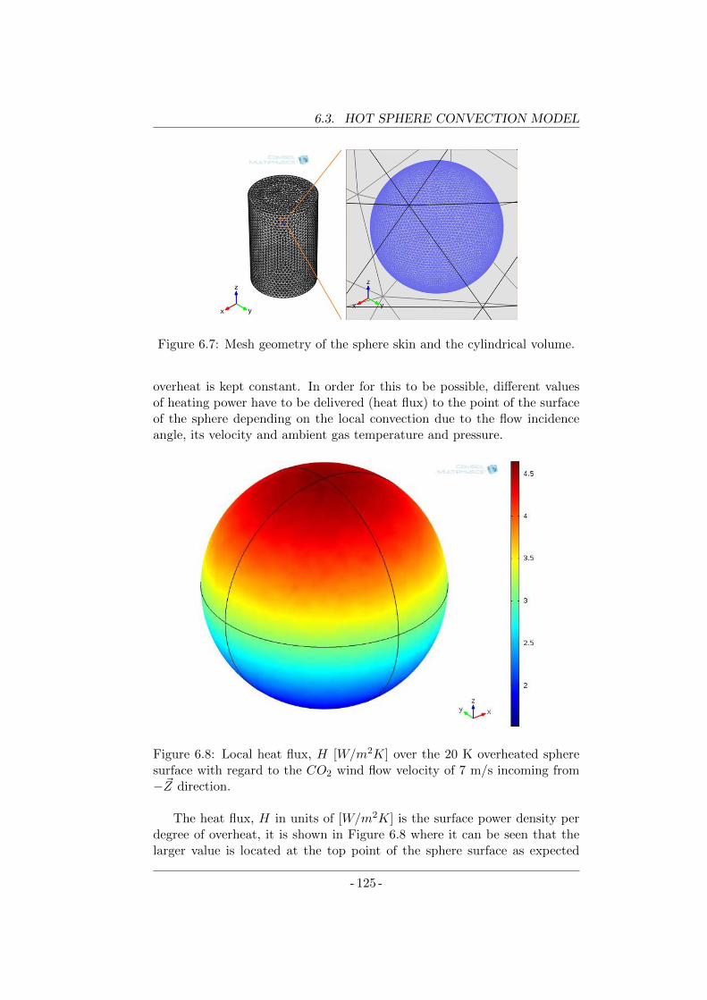
6.3. HOT SPHERE CONVECTION MODEL
Figure 6.7: Mesh geometry of the sphere skin and the cylindrical volume.
overheat is kept constant. In order for this to be possible, different valuesof heating power have to be delivered (heat flux) to the point of the surfaceof the sphere depending on the local convection due to the flow incidenceangle, its velocity and ambient gas temperature and pressure.
Figure 6.8: Local heat flux, H [W/m2K] over the 20 K overheated spheresurface with regard to the CO2 wind flow velocity of 7 m/s incoming from−~Z direction.
The heat flux, H in units of [W/m2K] is the surface power density perdegree of overheat, it is shown in Figure 6.8 where it can be seen that thelarger value is located at the top point of the sphere surface as expected
- 125 -
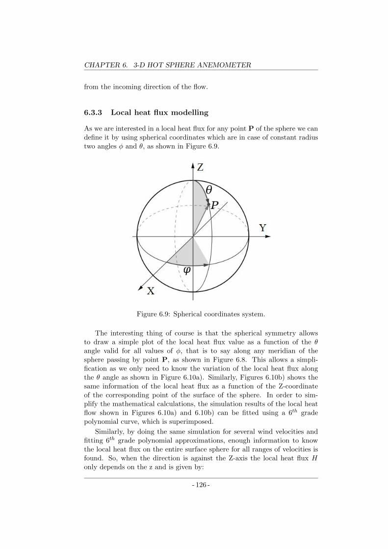
CHAPTER 6. 3-D HOT SPHERE ANEMOMETER
from the incoming direction of the flow.
6.3.3 Local heat flux modelling
As we are interested in a local heat flux for any point P of the sphere we candefine it by using spherical coordinates which are in case of constant radiustwo angles φ and θ, as shown in Figure 6.9.
Figure 6.9: Spherical coordinates system.
The interesting thing of course is that the spherical symmetry allowsto draw a simple plot of the local heat flux value as a function of the θangle valid for all values of φ, that is to say along any meridian of thesphere passing by point P, as shown in Figure 6.8. This allows a simpli-fication as we only need to know the variation of the local heat flux alongthe θ angle as shown in Figure 6.10a). Similarly, Figures 6.10b) shows thesame information of the local heat flux as a function of the Z-coordinateof the corresponding point of the surface of the sphere. In order to sim-plify the mathematical calculations, the simulation results of the local heatflow shown in Figures 6.10a) and 6.10b) can be fitted using a 6th gradepolynomial curve, which is superimposed.
Similarly, by doing the same simulation for several wind velocities andfitting 6th grade polynomial approximations, enough information to knowthe local heat flux on the entire surface sphere for all ranges of velocities isfound. So, when the direction is against the Z-axis the local heat flux Honly depends on the z and is given by:
- 126 -
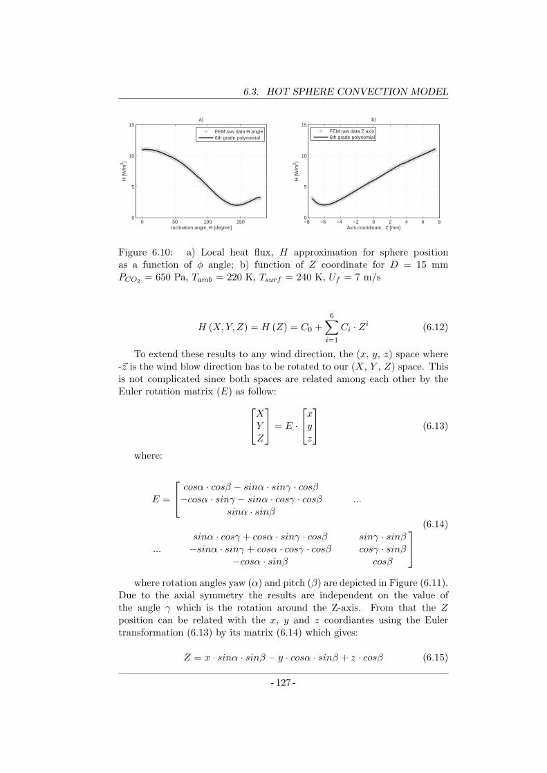
6.3. HOT SPHERE CONVECTION MODEL
0 50 100 1500
5
10
15H
[W/m
2 ]
Inclination angle, Θ [degree]
a)
−8 −6 −4 −2 0 2 4 6 80
5
10
15
H [W
/m2 ]
Axis cooridinate, Z [mm]
b)
FEM raw data Θ angle6th grade polynomial
FEM raw data Z axis6th grade polynomial
Figure 6.10: a) Local heat flux, H approximation for sphere positionas a function of φ angle; b) function of Z coordinate for D = 15 mmPCO2 = 650 Pa, Tamb = 220 K, Tsurf = 240 K, Uf = 7 m/s
H (X,Y, Z) = H (Z) = C0 +6∑
i=1
Ci · Zi (6.12)
To extend these results to any wind direction, the (x, y, z) space where-~z is the wind blow direction has to be rotated to our (X, Y , Z) space. Thisis not complicated since both spaces are related among each other by theEuler rotation matrix (E) as follow:
XYZ
= E ·
xyz
(6.13)
where:
E =
cosα · cosβ − sinα · sinγ · cosβ−cosα · sinγ − sinα · cosγ · cosβ
sinα · sinβ...
...sinα · cosγ + cosα · sinγ · cosβ sinγ · sinβ−sinα · sinγ + cosα · cosγ · cosβ cosγ · sinβ
−cosα · sinβ cosβ
(6.14)
where rotation angles yaw (α) and pitch (β) are depicted in Figure (6.11).Due to the axial symmetry the results are independent on the value ofthe angle γ which is the rotation around the Z-axis. From that the Zposition can be related with the x, y and z coordiantes using the Eulertransformation (6.13) by its matrix (6.14) which gives:
Z = x · sinα · sinβ − y · cosα · sinβ + z · cosβ (6.15)
- 127 -
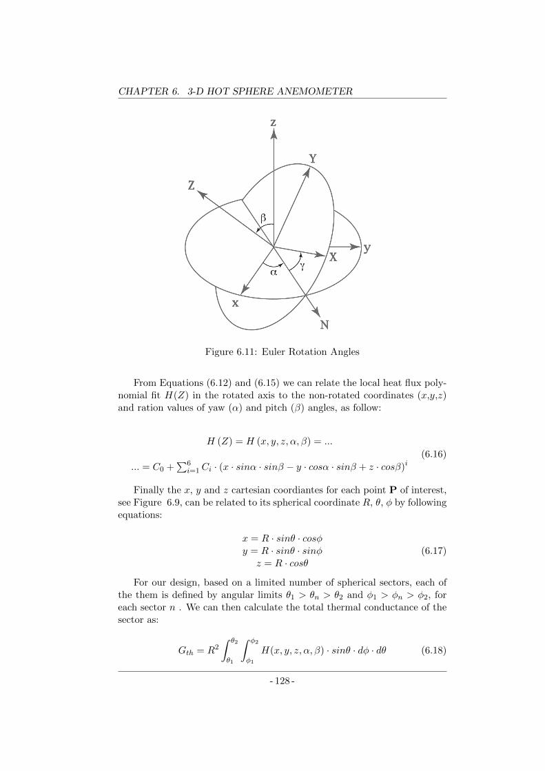
CHAPTER 6. 3-D HOT SPHERE ANEMOMETER
Figure 6.11: Euler Rotation Angles
From Equations (6.12) and (6.15) we can relate the local heat flux poly-nomial fit H(Z) in the rotated axis to the non-rotated coordinates (x,y,z)and ration values of yaw (α) and pitch (β) angles, as follow:
H (Z) = H (x, y, z, α, β) = ...
... = C0 +∑6
i=1Ci · (x · sinα · sinβ − y · cosα · sinβ + z · cosβ)i(6.16)
Finally the x, y and z cartesian coordiantes for each point P of interest,see Figure 6.9, can be related to its spherical coordinate R, θ, φ by followingequations:
x = R · sinθ · cosφy = R · sinθ · sinφ
z = R · cosθ(6.17)
For our design, based on a limited number of spherical sectors, each ofthe them is defined by angular limits θ1 > θn > θ2 and φ1 > φn > φ2, foreach sector n . We can then calculate the total thermal conductance of thesector as:
Gth = R2
∫ θ2
θ1
∫ φ2
φ1
H(x, y, z, α, β) · sinθ · dφ · dθ (6.18)
- 128 -
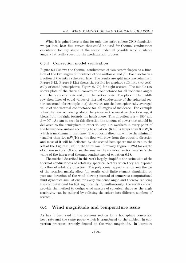
6.4. WIND MAGNITUDE AND TEMPERATURE ISSUE
What it is gained here is that for only one entire sphere CFD simulationwe got local heat flux curves that could be used for thermal conductancecalculation for any shape of the sector under all possible wind incidenceangle what really speed up the modelization process.
6.3.4 Convection model verification
Figure 6.12 shows the thermal conductance of two sector shapes as a func-tion of the two angles of incidence of the airflow α and β . Each sector is afraction of the entire sphere surface. The results are split into two columns inFigure 6.12. Figure 6.12a) shows the results for a sphere split into two verti-cally oriented hemispheres, Figure 6.12b) for eight sectors. The middle rowshows plots of the thermal convection conductance for all incidence anglesα in the horizontal axis and β in the vertical axis. The plots in the middlerow show lines of equal values of thermal conductance of the spherical sec-tor concerned, for example in a) the values are the hemispherically averagedvalue of the thermal conductance for all angles of incidence. For examplewhen the flow is blowing along the y-axis in the negative direction −~y, itblows from the right towards the hemisphere. This direction is α = 180 andβ = 90. As can be seen in this direction the amount of power that should bedelivered to the hemisphere in order to keep 1 K overheat in every point ofthe hemisphere surface according to equation (6.18) is larger than 3 mW/Kwhich is maximum in that case. The opposite direction will be the minimum(smaller than 1.4 mW/K) as the flow will blow from the opposite directionand most of it will be deflected by the second hemisphere not shown to theleft of the Figure 6.12a) in the third row. Similarly Figure 6.12b) for eighthof sphere sectors. Of course, the smaller the spherical sector, smaller is thevalue of the integrated thermal conductance of equation 6.18.
The method described in this work largely simplifies the estimation of thethermal conductances of arbitrary spherical sectors when they are exposedto a flow of arbitrary direction. The polynomial approximation and the useof the rotation matrix allow full results with finite element simulation onjust one direction of the wind blowing instead of numerous computationalfluid dynamics simulations for every incidence angle and thereby reducingthe computational budget significantly. Simultaneously, the results shownprovide the method to design wind sensors of spherical shape as the anglesensitivity can be tailored by splitting the sphere into different numbers ofsectors.
6.4 Wind magnitude and temperature issue
As has it been said in the previous section for a hot sphere convectionheat rate and the same power which is transferred to the ambient in con-vection processes strongly depend on the wind magnitude. In literature
- 129 -
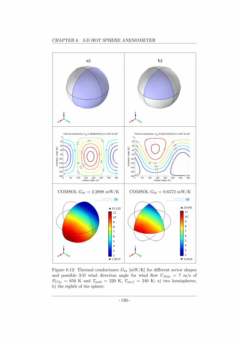
CHAPTER 6. 3-D HOT SPHERE ANEMOMETER
a) b)
0 50 100 150 200 250 300 350
0
20
40
60
80
100
120
140
160
180
1.4 1.4
1.6 1.6
1.8
1.8
1.8
1.8
2
2
2
2
2.2
2.2
2.2
2.2
2.4
2.4
2.4
2.6
2.62.6
2.8
2.8
3
rotation angle, α[°]
incl
inat
ion
ang
le, β
[°]
o
Thermal conductance, Gth
=2.2869[mW/K] for α=100° β=120°
0 50 100 150 200 250 300 350
0
20
40
60
80
100
120
140
160
180 0.3 0.30.
3
0.4
0.40.
4
0.5
0.5
0.5
0.6
0.6
0.6
0.7
0.7
0.7
0.8 0.8
0.8
0.9
rotation angle, α[°]
incl
inat
ion
ang
le, β
[°]
o
Thermal conductance, Gth
=0.65627[mW/K] for α=100° β=120°
COMSOL Gth = 2.2898 mW/K COMSOL Gth = 0.6572 mW/K
Figure 6.12: Thermal conductance Gth [mW/K] for different sector shapesand possible 3-D wind direction angle for wind flow Uflow = 7 m/s ofPCO2 = 650 K and Tamb = 220 K, Tsurf = 240 K; a) two hemispheres,b) the eighth of the sphere.
- 130 -
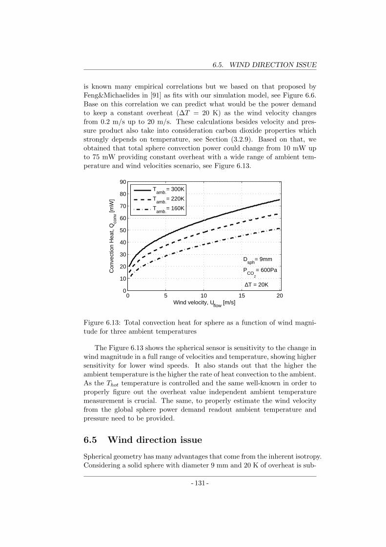
6.5. WIND DIRECTION ISSUE
is known many empirical correlations but we based on that proposed byFeng&Michaelides in [91] as fits with our simulation model, see Figure 6.6.Base on this correlation we can predict what would be the power demandto keep a constant overheat (∆T = 20 K) as the wind velocity changesfrom 0.2 m/s up to 20 m/s. These calculations besides velocity and pres-sure product also take into consideration carbon dioxide properties whichstrongly depends on temperature, see Section (3.2.9). Based on that, weobtained that total sphere convection power could change from 10 mW upto 75 mW providing constant overheat with a wide range of ambient tem-perature and wind velocities scenario, see Figure 6.13.
0 5 10 15 200
10
20
30
40
50
60
70
80
90
Wind velocity, Uflow
[m/s]
Con
vect
ion
Hea
t, Q
conv
[mW
]
Dsph
= 9mm
PCO
2
= 600Pa
∆T = 20K
Tamb.
= 300K
Tamb.
= 220K
Tamb.
= 160K
Figure 6.13: Total convection heat for sphere as a function of wind magni-tude for three ambient temperatures
The Figure 6.13 shows the spherical sensor is sensitivity to the change inwind magnitude in a full range of velocities and temperature, showing highersensitivity for lower wind speeds. It also stands out that the higher theambient temperature is the higher the rate of heat convection to the ambient.As the Thot temperature is controlled and the same well-known in order toproperly figure out the overheat value independent ambient temperaturemeasurement is crucial. The same, to properly estimate the wind velocityfrom the global sphere power demand readout ambient temperature andpressure need to be provided.
6.5 Wind direction issue
Spherical geometry has many advantages that come from the inherent isotropy.Considering a solid sphere with diameter 9 mm and 20 K of overheat is sub-
- 131 -
CHAPTER 6. 3-D HOT SPHERE ANEMOMETER
ject to a wind flow, the thermal conductance will be independent on thewind direction but will only depend on wind velocity for given atmosphericconditions(T = 220 K, P = 600 Pa), see Figure 6.14.
0 5 10 15 200
0.5
1
1.5
2
2.5
3
3.5
4
Wind speed, U [m/s]
The
rmal
con
duct
ance
, Gth
sph [m
W/K
]
D = 9mm
P = 600Pa
Tamb
= 220K
∆T = 20K
Empirical F&MFEM simulation
Figure 6.14: Thermal conductance for the whole sphere as a function of thewind speed. Empirical model based on Feng&Michaelides (F&M) comparedto FEM simulation results
Therefore, the wind magnitude will be given by the sphere thermal con-ductance (or heat transfer coefficient) of all sectors together. Furthermore,the sphere can be split into several spherical sectors that can be indepen-dently controlled. The sectors that are more exposed to the wind will loseheat more than the others and hence a measurement of the difference be-tween sectors will provide the wind direction, Figure 6.12. Variation in localheat flux coefficient is obtained for from CFD numerical simulation in thecase of a particular wind speed of 5 m/s has been presented in Figure 6.15 .
Let us now describe how the wind direction can also be measured using asbaseline the spherical geometry just described. This is achieved by breakingthe sphere surface into spherical sectors physically separated as depicted inFigure 6.16 where an example of four independent sectors is shown.
In this thesis, four sectors were used to solve for the two angles of thewind direction (Θ,Φ), extending the results where two hemispherical sec-tors were used that allow only to solve for one angle as reported in [11].We have considered not using more than four sectors for practical fabrica-tion issues and because the angle sensitivity achieved with four sectors - aswill be shown below - is currently above the typical requirements in Marsmissions. The four sectors geometry shown in Figure 6.16 are spherical tri-angles having the centers located at points with coordinates for sector #1at (Θ=54.74 and Φ=90), for sector #2 at (Θ=125.56 and Φ=180), for
- 132 -
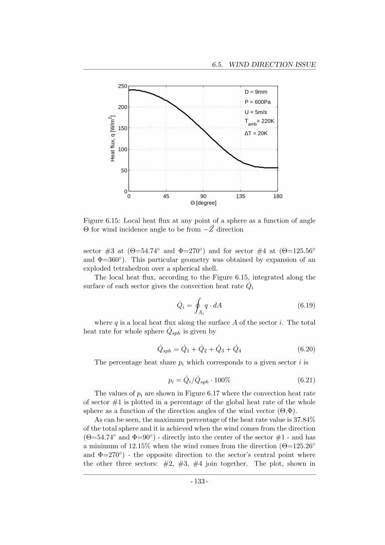
6.5. WIND DIRECTION ISSUE
0 45 90 135 1800
50
100
150
200
250
Hea
t flu
x, q
[W/m
2 ]
Θ [degree]
D = 9mm
P = 600Pa
U = 5m/s
Tamb
= 220K
∆T = 20K
Figure 6.15: Local heat flux at any point of a sphere as a function of angleΘ for wind incidence angle to be from −~Z direction
sector #3 at (Θ=54.74 and Φ=270) and for sector #4 at (Θ=125.56
and Φ=360). This particular geometry was obtained by expansion of anexploded tetrahedron over a spherical shell.
The local heat flux, according to the Figure 6.15, integrated along thesurface of each sector gives the convection heat rate Qi
Qi =
∮
Ai
q · dA (6.19)
where q is a local heat flux along the surface A of the sector i. The totalheat rate for whole sphere Qsph is given by
Qsph = Q1 + Q2 + Q3 + Q4 (6.20)
The percentage heat share pi which corresponds to a given sector i is
pi = Qi/Qsph · 100% (6.21)
The values of pi are shown in Figure 6.17 where the convection heat rateof sector #1 is plotted in a percentage of the global heat rate of the wholesphere as a function of the direction angles of the wind vector (Θ,Φ).
As can be seen, the maximum percentage of the heat rate value is 37.84%of the total sphere and it is achieved when the wind comes from the direction(Θ=54.74 and Φ=90) - directly into the center of the sector #1 - and hasa minimum of 12.15% when the wind comes from the direction (Θ=125.26
and Φ=270) - the opposite direction to the sector’s central point wherethe other three sectors: #2, #3, #4 join together. The plot, shown in
- 133 -
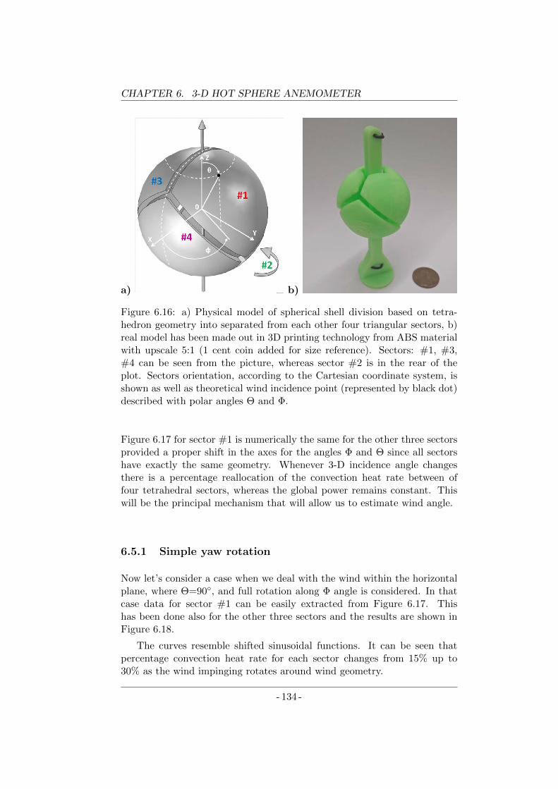
CHAPTER 6. 3-D HOT SPHERE ANEMOMETER
a) b)
Figure 6.16: a) Physical model of spherical shell division based on tetra-hedron geometry into separated from each other four triangular sectors, b)real model has been made out in 3D printing technology from ABS materialwith upscale 5:1 (1 cent coin added for size reference). Sectors: #1, #3,#4 can be seen from the picture, whereas sector #2 is in the rear of theplot. Sectors orientation, according to the Cartesian coordinate system, isshown as well as theoretical wind incidence point (represented by black dot)described with polar angles Θ and Φ.
Figure 6.17 for sector #1 is numerically the same for the other three sectorsprovided a proper shift in the axes for the angles Φ and Θ since all sectorshave exactly the same geometry. Whenever 3-D incidence angle changesthere is a percentage reallocation of the convection heat rate between offour tetrahedral sectors, whereas the global power remains constant. Thiswill be the principal mechanism that will allow us to estimate wind angle.
6.5.1 Simple yaw rotation
Now let’s consider a case when we deal with the wind within the horizontalplane, where Θ=90, and full rotation along Φ angle is considered. In thatcase data for sector #1 can be easily extracted from Figure 6.17. Thishas been done also for the other three sectors and the results are shown inFigure 6.18.
The curves resemble shifted sinusoidal functions. It can be seen thatpercentage convection heat rate for each sector changes from 15% up to30% as the wind impinging rotates around wind geometry.
- 134 -
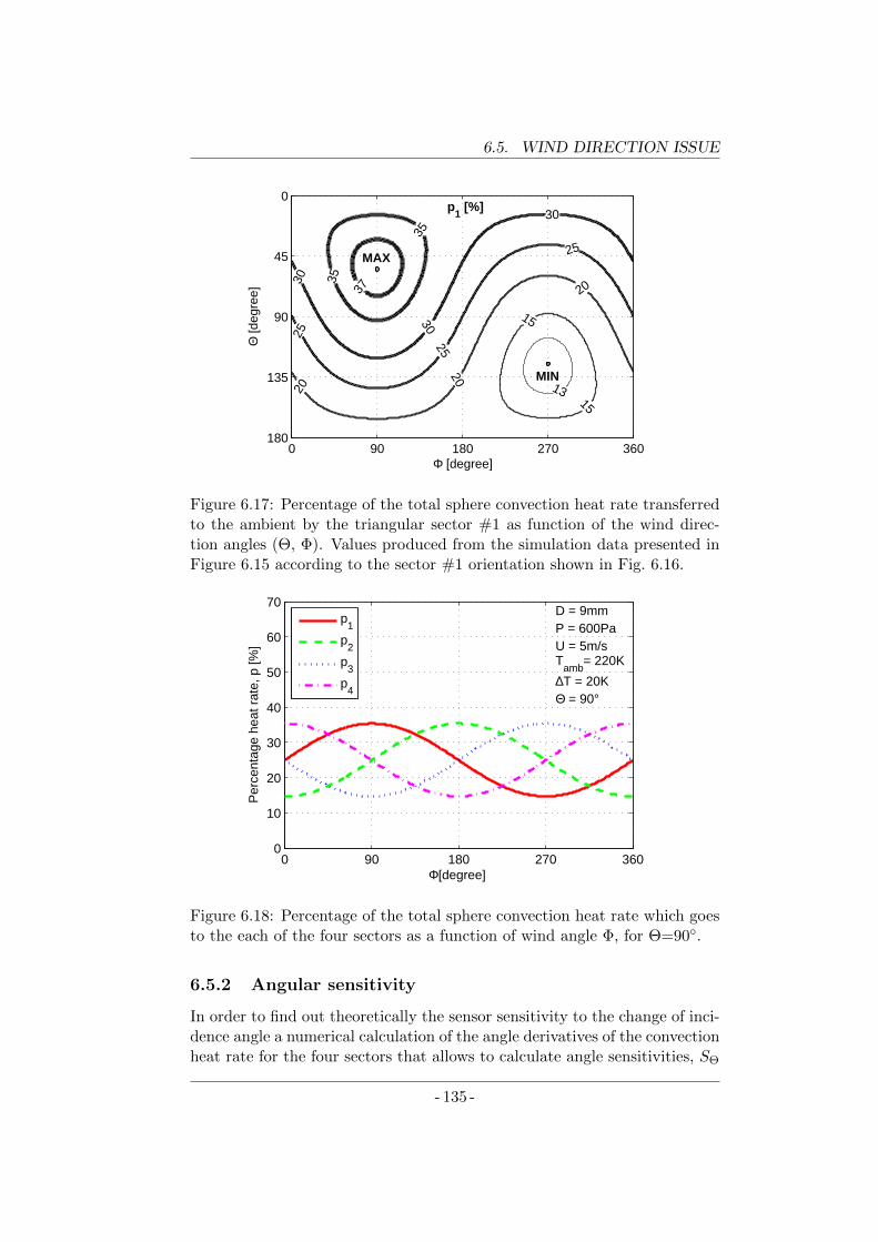
6.5. WIND DIRECTION ISSUE
37
35
35
30
30
30
25
25
25
20
20
20
15
15
13
Φ [degree]
Θ [d
egre
e] MAX
MIN
p1 [%]
0 90 180 270 360
0
45
90
135
180
Figure 6.17: Percentage of the total sphere convection heat rate transferredto the ambient by the triangular sector #1 as function of the wind direc-tion angles (Θ, Φ). Values produced from the simulation data presented inFigure 6.15 according to the sector #1 orientation shown in Fig. 6.16.
0 90 180 270 3600
10
20
30
40
50
60
70
Φ[degree]
Per
cent
age
heat
rat
e, p
[%]
D = 9mmP = 600PaU = 5m/sT
amb= 220K
∆T = 20KΘ = 90°
p1
p2
p3
p4
Figure 6.18: Percentage of the total sphere convection heat rate which goesto the each of the four sectors as a function of wind angle Φ, for Θ=90.
6.5.2 Angular sensitivity
In order to find out theoretically the sensor sensitivity to the change of inci-dence angle a numerical calculation of the angle derivatives of the convectionheat rate for the four sectors that allows to calculate angle sensitivities, SΘ
- 135 -
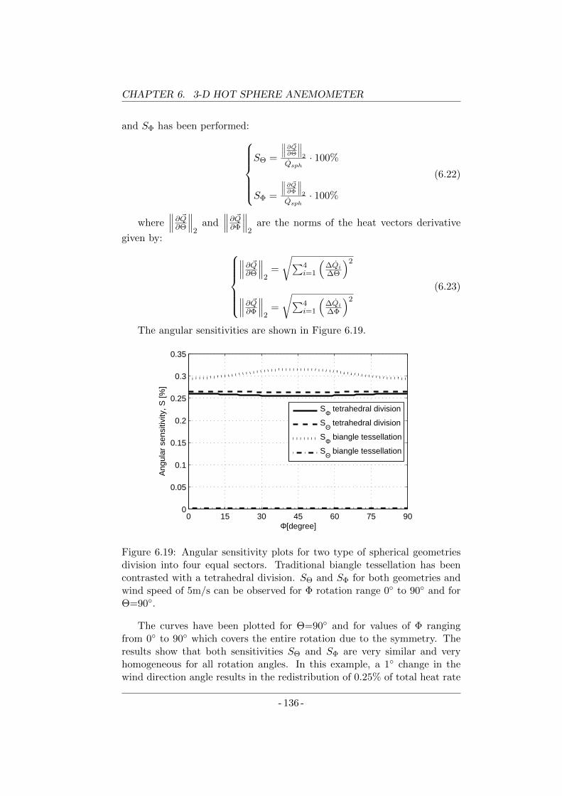
CHAPTER 6. 3-D HOT SPHERE ANEMOMETER
and SΦ has been performed:
SΘ =
∥∥∥ ∂ ~Q∂Θ
∥∥∥2
Qsph· 100%
SΦ =
∥∥∥ ∂ ~Q∂Φ
∥∥∥2
Qsph· 100%
(6.22)
where∥∥∥∂ ~Q∂Θ
∥∥∥2
and∥∥∥∂ ~Q∂Φ
∥∥∥2
are the norms of the heat vectors derivative
given by:
∥∥∥∂ ~Q∂Θ
∥∥∥2
=
√∑4
i=1
(∆Qi
∆Θ
)2
∥∥∥∂ ~Q∂Φ
∥∥∥2
=
√∑4
i=1
(∆Qi
∆Φ
)2
(6.23)
The angular sensitivities are shown in Figure 6.19.
0 15 30 45 60 75 900
0.05
0.1
0.15
0.2
0.25
0.3
0.35
Φ[degree]
Ang
ular
sen
sitiv
ity, S
[%]
SΦ tetrahedral division
SΘ tetrahedral division
SΦ biangle tessellation
SΘ biangle tessellation
Figure 6.19: Angular sensitivity plots for two type of spherical geometriesdivision into four equal sectors. Traditional biangle tessellation has beencontrasted with a tetrahedral division. SΘ and SΦ for both geometries andwind speed of 5m/s can be observed for Φ rotation range 0 to 90 and forΘ=90.
The curves have been plotted for Θ=90 and for values of Φ rangingfrom 0 to 90 which covers the entire rotation due to the symmetry. Theresults show that both sensitivities SΘ and SΦ are very similar and veryhomogeneous for all rotation angles. In this example, a 1 change in thewind direction angle results in the redistribution of 0.25% of total heat rate
- 136 -
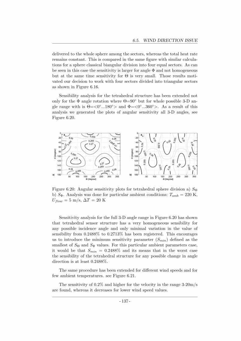
6.5. WIND DIRECTION ISSUE
delivered to the whole sphere among the sectors, whereas the total heat rateremains constant. This is compared in the same figure with similar calcula-tions for a sphere classical biangular division into four equal sectors. As canbe seen in this case the sensitivity is larger for angle Φ and not homogeneousbut at the same time sensitivity for Θ is very small. Those results moti-vated our decision to work with four sectors divided into triangular sectorsas shown in Figure 6.16.
Sensibility analysis for the tetrahedral structure has been extended notonly for the Φ angle rotation where Θ=90 but for whole possible 3-D an-gle range with is Θ=<0...180> and Φ=<0...360>. As a result of thisanalysis we generated the plots of angular sensitivity all 3-D angles, seeFigure 6.20.
Figure 6.20: Angular sensitivity plots for tetrahedral sphere division a) SΘ
b) SΦ. Analysis was done for particular ambient conditions: Tamb = 220 K,Uflow = 5 m/s, ∆T = 20 K
Sensitivity analysis for the full 3-D angle range in Figure 6.20 has shownthat tetrahedral sensor structure has a very homogeneous sensibility forany possible incidence angle and only minimal variation in the value ofsensibility from 0.2488% to 0.2713% has been registered. This encouragesus to introduce the minimum sensitivity parameter (Smin) defined as thesmallest of SΘ and SΦ values. For this particular ambient parameters case,it would be that Smin = 0.2488% and its means that in the worst casethe sensibility of the tetrahedral structure for any possible change in angledirection is at least 0.2488%.
The same procedure has been extended for different wind speeds and forfew ambient temperatures. see Figure 6.21.
The sensitivity of 0.2% and higher for the velocity in the range 3-20m/sare found, whereas it decreases for lower wind speed values.
- 137 -
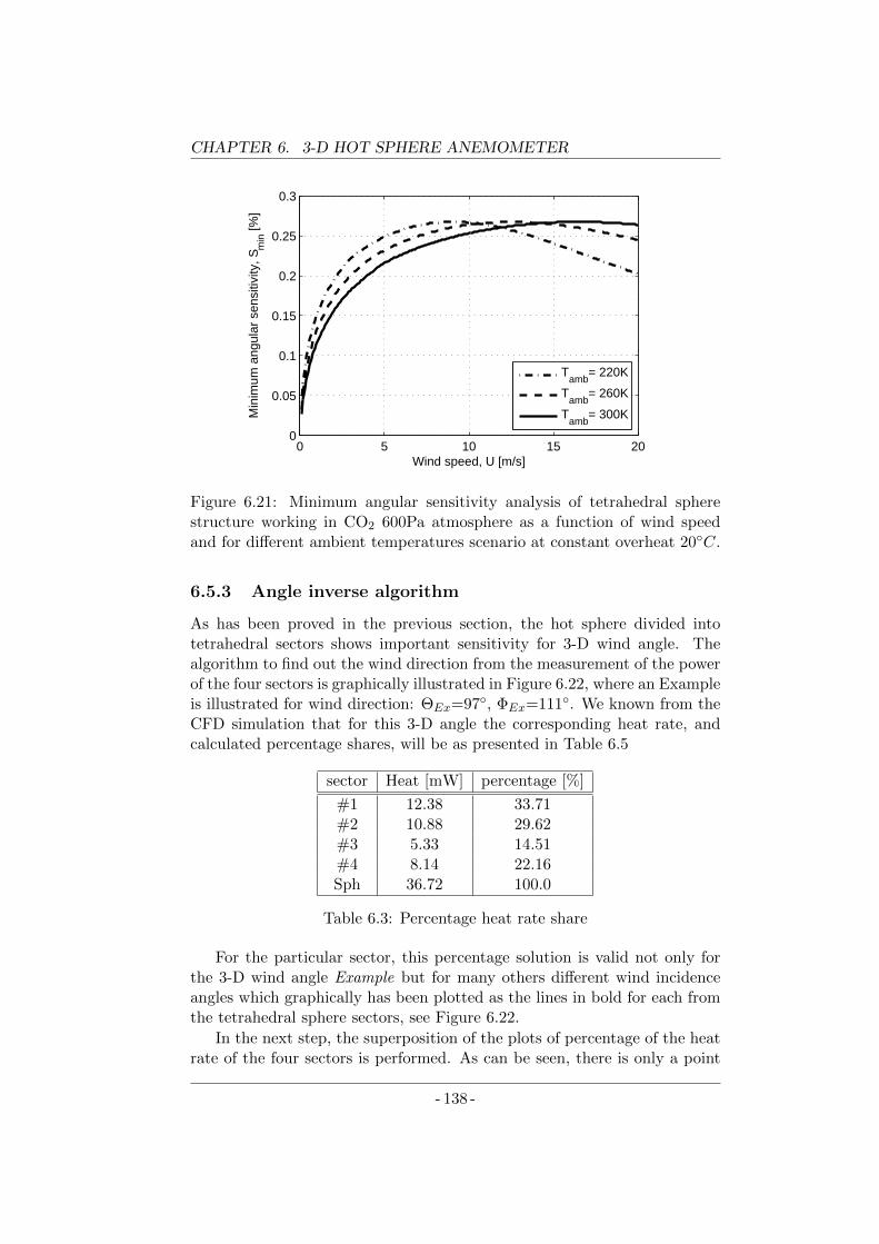
CHAPTER 6. 3-D HOT SPHERE ANEMOMETER
0 5 10 15 200
0.05
0.1
0.15
0.2
0.25
0.3
Wind speed, U [m/s]
Min
imum
ang
ular
sen
sitiv
ity, S
min
[%]
Tamb
= 220K
Tamb
= 260K
Tamb
= 300K
Figure 6.21: Minimum angular sensitivity analysis of tetrahedral spherestructure working in CO2 600Pa atmosphere as a function of wind speedand for different ambient temperatures scenario at constant overheat 20C.
6.5.3 Angle inverse algorithm
As has been proved in the previous section, the hot sphere divided intotetrahedral sectors shows important sensitivity for 3-D wind angle. Thealgorithm to find out the wind direction from the measurement of the powerof the four sectors is graphically illustrated in Figure 6.22, where an Exampleis illustrated for wind direction: ΘEx=97, ΦEx=111. We known from theCFD simulation that for this 3-D angle the corresponding heat rate, andcalculated percentage shares, will be as presented in Table 6.5
sector Heat [mW] percentage [%]
#1 12.38 33.71#2 10.88 29.62#3 5.33 14.51#4 8.14 22.16Sph 36.72 100.0
Table 6.3: Percentage heat rate share
For the particular sector, this percentage solution is valid not only forthe 3-D wind angle Example but for many others different wind incidenceangles which graphically has been plotted as the lines in bold for each fromthe tetrahedral sphere sectors, see Figure 6.22.
In the next step, the superposition of the plots of percentage of the heatrate of the four sectors is performed. As can be seen, there is only a point
- 138 -
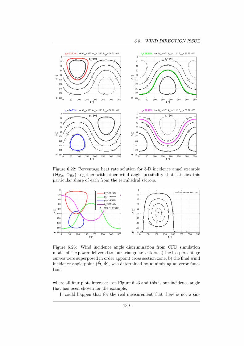
6.5. WIND DIRECTION ISSUE
35
35
30
30
30
25
25
25
20
20
20
15
15
p1= 33.71% , for: Θ
Ex= 97°, Φ
Ex= 111°, P
sph= 36.72 mW
Φ [°]
Θ [°
] p
1= [%]
a)0 50 100 150 200 250 300 350
0
20
40
60
80
100
120
140
160
180
35
35
30
30
30
25
25
25
20
20
20
15 15
p2= 29.62% , for: Θ
Ex= 97°, Φ
Ex= 111°, P
sph= 36.72 mW
Φ [°]
Θ [°
]
p2= [%]
b)0 50 100 150 200 250 300 350
0
20
40
60
80
100
120
140
160
180
35
35
30
30 30
25
25
25
20
20
20
15
15
p3= 14.51% , for: Θ
Ex= 97°, Φ
Ex= 111°, P
sph= 36.72 mW
Φ [°]
Θ [°
]
p3= [%]
c)0 50 100 150 200 250 300 350
0
20
40
60
80
100
120
140
160
180
35
35
30
30
30
25
25
25
20
20
2015
15
p4= 22.16% , for: Θ
Ex= 97°, Φ
Ex= 111°, P
sph= 36.72 mW
Φ [°]
Θ [°
]
p4= [%]
d)0 50 100 150 200 250 300 350
0
20
40
60
80
100
120
140
160
180
Figure 6.22: Percentage heat rate solution for 3-D incidence angel example(ΘEx, ΦEx) together with other wind angle possibility that satisfies thisparticular share of each from the tetrahedral sectors.
Φ [°]
Θ [°
]
a)
0 50 100 150 200 250 300 350
0
20
40
60
80
100
120
140
160
180
p1= 33.71%
p2= 29.62%
p3= 14.51%
p4= 22.16%
Θ=97°, Φ=111°
20
20
20
20
15
15
15
10
10
5
Φ [°]
Θ [°
]
b)
minimum error function
0 50 100 150 200 250 300 350
0
20
40
60
80
100
120
140
160
180
Figure 6.23: Wind incidence angle discrimination from CFD simulationmodel of the power delivered to four triangular sectors, a) the Iso-percentagecurves were superposed in order appoint cross section zone, b) the final windincidence angle point (Θ, Φ), was determined by minimizing an error func-tion.
where all four plots intersect, see Figure 6.23 and this is our incidence anglethat has been chosen for the example.
It could happen that for the real measurement that there is not a sin-
- 139 -
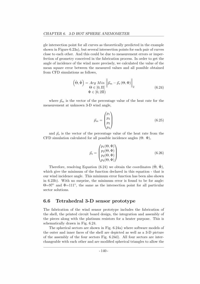
CHAPTER 6. 3-D HOT SPHERE ANEMOMETER
gle intersection point for all curves as theoretically predicted in the exampleshown in Figure 6.23a), but several intersection points for each pair of curvesclose to each other. And this could be due to measurement errors or imper-fection of geometry conceived in the fabrication process. In order to get theangle of incidence of the wind more precisely, we calculated the value of themean square error between the measured values and all possible obtainedfrom CFD simulations as follows,
(Θ, Φ
)= Arg Min
Θ ∈ [0,Π]Φ ∈ [0, 2Π)
∥∥∥∥~pm − ~ps (Θ,Φ)
∥∥∥∥2 (6.24)
where ~pm is the vector of the percentage value of the heat rate for themeasurement at unknown 3-D wind angle,
~pm =
p1
p2
p2
p4
(6.25)
and ~ps is the vector of the percentage value of the heat rate from theCFD simulation calculated for all possible incidence angles (Θ. Φ),
~ps =
p1(Θ,Φ)p2(Θ,Φ)p2(Θ,Φ)p4(Θ,Φ)
(6.26)
Therefore, resolving Equation (6.24) we obtain the coordinates (Θ, Φ),which give the minimum of the function declared in this equation - that isour wind incidence angle. This minimum error function has been also shownin 6.23b). With no surprise, the minimum error is found to be for angle:Θ=97 and Φ=111, the same as the intersection point for all particularsector solutions.
6.6 Tetrahedral 3-D sensor prototype
The fabrication of the wind sensor prototype includes the fabrication ofthe shell, the printed circuit board design, the integration and assembly ofthe pieces along with the platinum resistors for a heater purpose. This isschematically drawn in Fig. 6.24.
The spherical sectors are shown in Fig. 6.24a) where software models ofthe outer and inner faces of the shell are depicted as well as a 3-D pictureof the assembly of the four sectors Fig. 6.24d). All four sectors are inter-changeable with each other and are modified spherical triangles to allow the
- 140 -
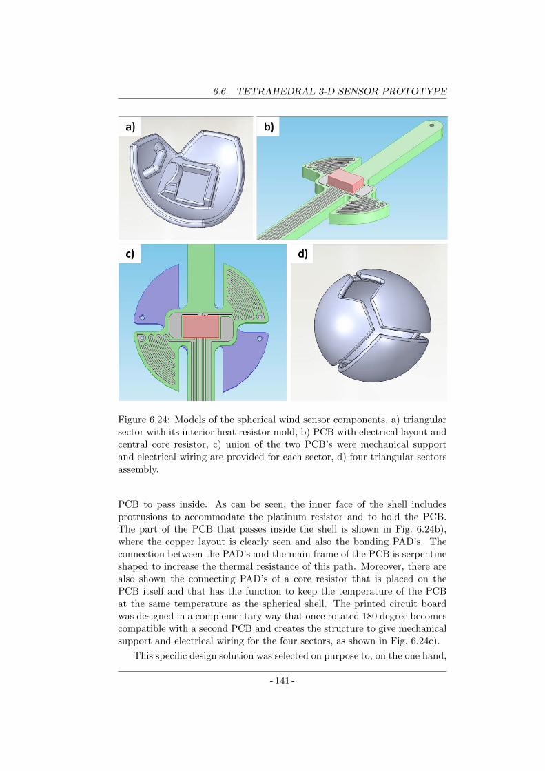
6.6. TETRAHEDRAL 3-D SENSOR PROTOTYPE
Figure 6.24: Models of the spherical wind sensor components, a) triangularsector with its interior heat resistor mold, b) PCB with electrical layout andcentral core resistor, c) union of the two PCB’s were mechanical supportand electrical wiring are provided for each sector, d) four triangular sectorsassembly.
PCB to pass inside. As can be seen, the inner face of the shell includesprotrusions to accommodate the platinum resistor and to hold the PCB.The part of the PCB that passes inside the shell is shown in Fig. 6.24b),where the copper layout is clearly seen and also the bonding PAD’s. Theconnection between the PAD’s and the main frame of the PCB is serpentineshaped to increase the thermal resistance of this path. Moreover, there arealso shown the connecting PAD’s of a core resistor that is placed on thePCB itself and that has the function to keep the temperature of the PCBat the same temperature as the spherical shell. The printed circuit boardwas designed in a complementary way that once rotated 180 degree becomescompatible with a second PCB and creates the structure to give mechanicalsupport and electrical wiring for the four sectors, as shown in Fig. 6.24c).
This specific design solution was selected on purpose to, on the one hand,
- 141 -
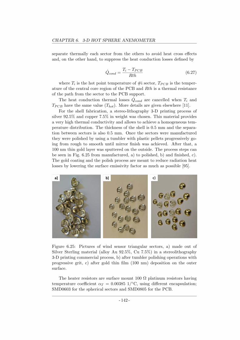
CHAPTER 6. 3-D HOT SPHERE ANEMOMETER
separate thermally each sector from the others to avoid heat cross effectsand, on the other hand, to suppress the heat conduction losses defined by
Qcond =Ti − TPCB
Rth(6.27)
where Ti is the hot point temperature of #i sector, TPCB is the temper-ature of the central core region of the PCB and Rth is a thermal resistanceof the path from the sector to the PCB support.
The heat conduction thermal losses Qcond are cancelled when Ti andTPCB have the same value (Thot). More details are given elsewhere [11].
For the shell fabrication, a stereo-lithography 3-D printing process ofsilver 92.5% and copper 7.5% in weight was chosen. This material providesa very high thermal conductivity and allows to achieve a homogeneous tem-perature distribution. The thickness of the shell is 0.5 mm and the separa-tion between sectors is also 0.5 mm. Once the sectors were manufacturedthey were polished by using a tumbler with plastic pellets progressively go-ing from rough to smooth until mirror finish was achieved. After that, a100 nm thin gold layer was sputtered on the outside. The process steps canbe seen in Fig. 6.25 from manufactured, a) to polished, b) and finished, c).The gold coating and the polish process are meant to reduce radiation heatlosses by lowering the surface emissivity factor as much as possible [95].
Figure 6.25: Pictures of wind sensor triangular sectors, a) made out ofSilver Sterling material (alloy Au 92.5%, Cu 7.5%) in a stereolithography3-D printing commercial process, b) after tumbler polishing operations withprogressive grit, c) after gold thin film (100 nm) deposition on the outersurface.
The heater resistors are surface mount 100 Ω platinum resistors havingtemperature coefficient αT = 0.00385 1/C, using different encapsulation;SMD0603 for the spherical sectors and SMD0805 for the PCB.
- 142 -
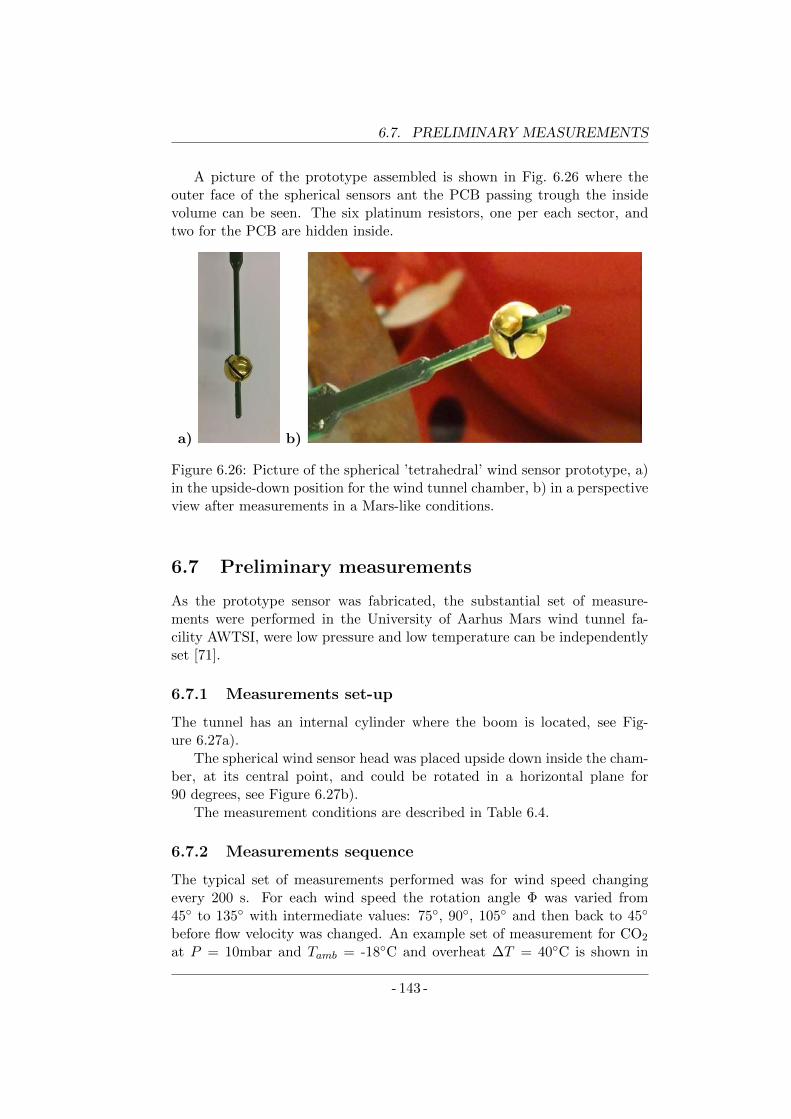
6.7. PRELIMINARY MEASUREMENTS
A picture of the prototype assembled is shown in Fig. 6.26 where theouter face of the spherical sensors ant the PCB passing trough the insidevolume can be seen. The six platinum resistors, one per each sector, andtwo for the PCB are hidden inside.
a) b)
Figure 6.26: Picture of the spherical ’tetrahedral’ wind sensor prototype, a)in the upside-down position for the wind tunnel chamber, b) in a perspectiveview after measurements in a Mars-like conditions.
6.7 Preliminary measurements
As the prototype sensor was fabricated, the substantial set of measure-ments were performed in the University of Aarhus Mars wind tunnel fa-cility AWTSI, were low pressure and low temperature can be independentlyset [71].
6.7.1 Measurements set-up
The tunnel has an internal cylinder where the boom is located, see Fig-ure 6.27a).
The spherical wind sensor head was placed upside down inside the cham-ber, at its central point, and could be rotated in a horizontal plane for90 degrees, see Figure 6.27b).
The measurement conditions are described in Table 6.4.
6.7.2 Measurements sequence
The typical set of measurements performed was for wind speed changingevery 200 s. For each wind speed the rotation angle Φ was varied from45 to 135 with intermediate values: 75, 90, 105 and then back to 45
before flow velocity was changed. An example set of measurement for CO2
at P = 10mbar and Tamb = -18C and overheat ∆T = 40C is shown in
- 143 -
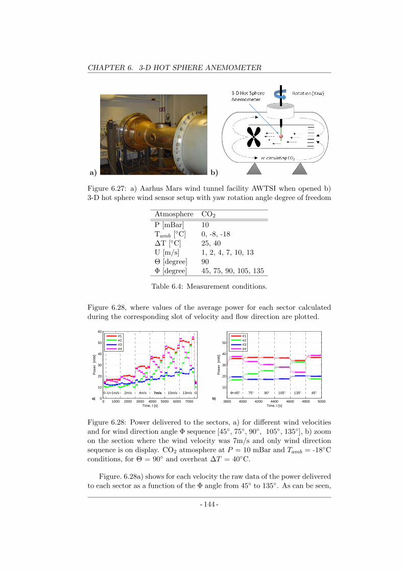
CHAPTER 6. 3-D HOT SPHERE ANEMOMETER
a) b)
Figure 6.27: a) Aarhus Mars wind tunnel facility AWTSI when opened b)3-D hot sphere wind sensor setup with yaw rotation angle degree of freedom
Atmosphere CO2
P [mBar] 10Tamb [C] 0, -8, -18∆T [C] 25, 40U [m/s] 1, 2, 4, 7, 10, 13Θ [degree] 90Φ [degree] 45, 75, 90, 105, 135
Table 6.4: Measurement conditions.
Figure 6.28, where values of the average power for each sector calculatedduring the corresponding slot of velocity and flow direction are plotted.
0 1000 2000 3000 4000 5000 6000 70000
10
20
30
40
50
60
Time, t [s]
Pow
er [
mW
]
a)
0 U=1m/s 2m/s 4m/s 7m/s 10m/s 13m/s 0
#1#2#3#4
3800 4000 4200 4400 4600 4800 5000
10
20
30
40
50
Pow
er [
mW
]
Time, t [s]
b)
Φ=45° 75° 90° 105° 135° 45°
#1#2#3#4
Figure 6.28: Power delivered to the sectors, a) for different wind velocitiesand for wind direction angle Φ sequence [45, 75, 90, 105, 135], b) zoomon the section where the wind velocity was 7m/s and only wind directionsequence is on display. CO2 atmosphere at P = 10 mBar and Tamb = -18Cconditions, for Θ = 90 and overheat ∆T = 40C.
Figure. 6.28a) shows for each velocity the raw data of the power deliveredto each sector as a function of the Φ angle from 45 to 135. As can be seen,
- 144 -
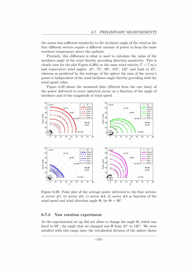
6.7. PRELIMINARY MEASUREMENTS
the sensor has sufficient sensitivity to the incidence angle of the wind as thefour different sectors require a different amount of power to keep the sameoverheat temperature above the ambient.
Precisely, this difference is what is used to calculate the value of theincidence angle of the wind thereby providing direction sensitivity. This isclearly seen for the plot Figure 6.28b) or the same wind velocity U = 7 m/sand consecutive wind angles: 45, 75, 90, 105, 135 and back to 45,whereas as predicted by the isotropy of the sphere the sum of the sector’spower is independent of the wind incidence angle thereby providing with thewind speed value.
Figure 6.29 shows the measured data (filtered from the raw data) ofthe power delivered to every spherical sector as a function of the angle ofincidence and of the magnitude of wind speed.
0 10 20 30 40 50 60 70 80
0
10
20
30
40
50
60Φ=45°
Φ=75°
Φ=90°
Φ=105°
Φ=135°
for allΘ=90°
#1
a)
Pow
er [
mW
]
0 10 20 30 40 50 60 70 80
0
10
20
30
40
50
60Φ=45°
Φ=75°
Φ=90°
Φ=105°
Φ=135°
for allΘ=90°
#2
b)
Pow
er [
mW
]
0 10 20 30 40 50 60 70 80
0
10
20
30
40
50
60Φ=45°
Φ=75°
Φ=90°
Φ=105°
Φ=135°
for allΘ=90°
#3
c)
Pow
er [
mW
]
0 10 20 30 40 50 60 70 80
0
10
20
30
40
50
60Φ=45°
Φ=75°
Φ=90°
Φ=105°
Φ=135°
for allΘ=90°
#4
d)
Pow
er [
mW
]
#113m/s10m/s7m/s4m/s2m/s1m/s
#213m/s10m/s7m/s4m/s2m/s1m/s
#313m/s10m/s7m/s4m/s2m/s1m/s
#413m/s10m/s7m/s4m/s2m/s1m/s
Figure 6.29: Polar plot of the average power delivered to the four sectors:a) sector #1, b) sector #2, c) sector #3, d) sector #4 as function of thewind speed and wind direction angle Φ, for Θ = 90.
6.7.3 Yaw rotation experiment
As the experimental set up did not allow to change the angle Θ, which wasfixed to 90, the angle that we changed was Φ from 45 to 135. We weresatisfied with this range since the tetrahedral division of the sphere shows
- 145 -
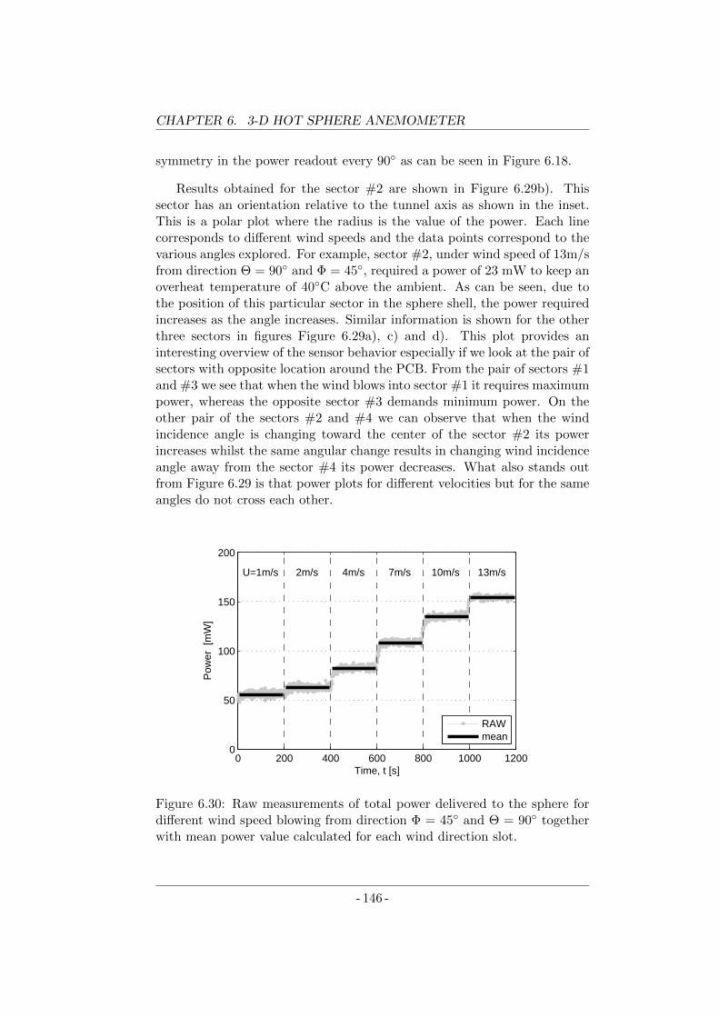
CHAPTER 6. 3-D HOT SPHERE ANEMOMETER
symmetry in the power readout every 90 as can be seen in Figure 6.18.
Results obtained for the sector #2 are shown in Figure 6.29b). Thissector has an orientation relative to the tunnel axis as shown in the inset.This is a polar plot where the radius is the value of the power. Each linecorresponds to different wind speeds and the data points correspond to thevarious angles explored. For example, sector #2, under wind speed of 13m/sfrom direction Θ = 90 and Φ = 45, required a power of 23 mW to keep anoverheat temperature of 40C above the ambient. As can be seen, due tothe position of this particular sector in the sphere shell, the power requiredincreases as the angle increases. Similar information is shown for the otherthree sectors in figures Figure 6.29a), c) and d). This plot provides aninteresting overview of the sensor behavior especially if we look at the pair ofsectors with opposite location around the PCB. From the pair of sectors #1and #3 we see that when the wind blows into sector #1 it requires maximumpower, whereas the opposite sector #3 demands minimum power. On theother pair of the sectors #2 and #4 we can observe that when the windincidence angle is changing toward the center of the sector #2 its powerincreases whilst the same angular change results in changing wind incidenceangle away from the sector #4 its power decreases. What also stands outfrom Figure 6.29 is that power plots for different velocities but for the sameangles do not cross each other.
0 200 400 600 800 1000 12000
50
100
150
200
Time, t [s]
Pow
er [
mW
]
U=1m/s 2m/s 4m/s 7m/s 10m/s 13m/s
RAWmean
Figure 6.30: Raw measurements of total power delivered to the sphere fordifferent wind speed blowing from direction Φ = 45 and Θ = 90 togetherwith mean power value calculated for each wind direction slot.
- 146 -
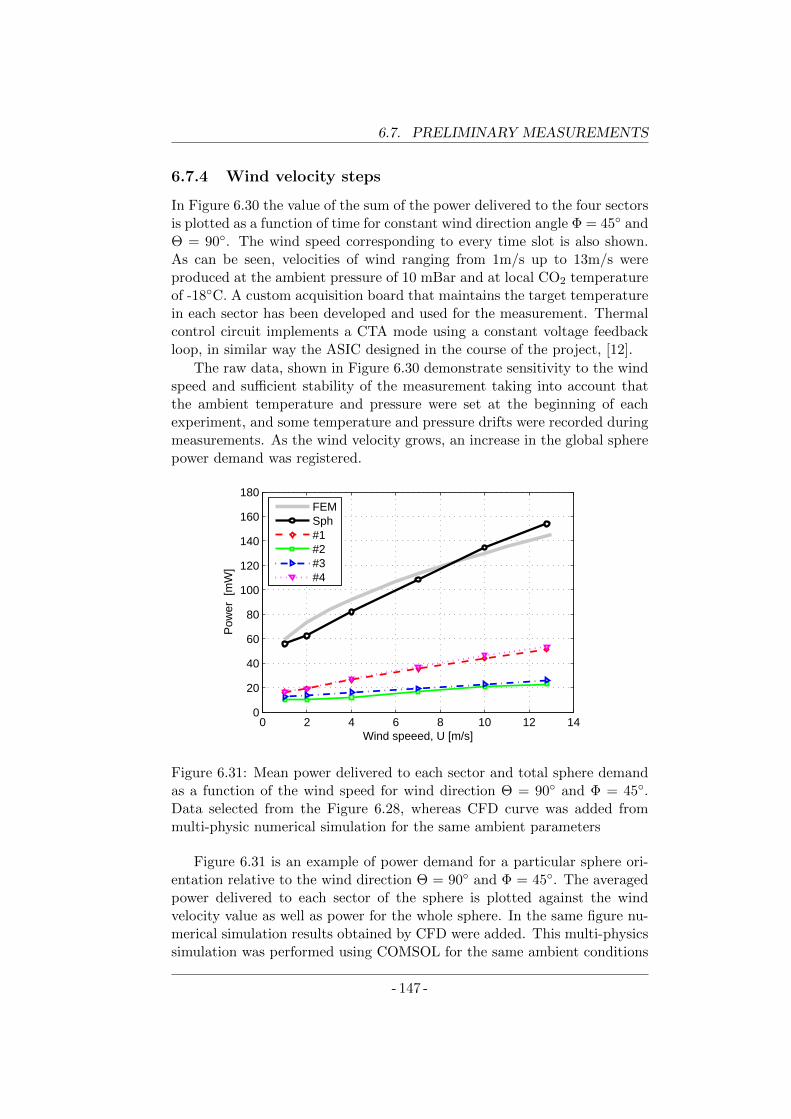
6.7. PRELIMINARY MEASUREMENTS
6.7.4 Wind velocity steps
In Figure 6.30 the value of the sum of the power delivered to the four sectorsis plotted as a function of time for constant wind direction angle Φ = 45 andΘ = 90. The wind speed corresponding to every time slot is also shown.As can be seen, velocities of wind ranging from 1m/s up to 13m/s wereproduced at the ambient pressure of 10 mBar and at local CO2 temperatureof -18C. A custom acquisition board that maintains the target temperaturein each sector has been developed and used for the measurement. Thermalcontrol circuit implements a CTA mode using a constant voltage feedbackloop, in similar way the ASIC designed in the course of the project, [12].
The raw data, shown in Figure 6.30 demonstrate sensitivity to the windspeed and sufficient stability of the measurement taking into account thatthe ambient temperature and pressure were set at the beginning of eachexperiment, and some temperature and pressure drifts were recorded duringmeasurements. As the wind velocity grows, an increase in the global spherepower demand was registered.
0 2 4 6 8 10 12 140
20
40
60
80
100
120
140
160
180
Wind speeed, U [m/s]
Pow
er [
mW
]
FEMSph#1#2#3#4
Figure 6.31: Mean power delivered to each sector and total sphere demandas a function of the wind speed for wind direction Θ = 90 and Φ = 45.Data selected from the Figure 6.28, whereas CFD curve was added frommulti-physic numerical simulation for the same ambient parameters
Figure 6.31 is an example of power demand for a particular sphere ori-entation relative to the wind direction Θ = 90 and Φ = 45. The averagedpower delivered to each sector of the sphere is plotted against the windvelocity value as well as power for the whole sphere. In the same figure nu-merical simulation results obtained by CFD were added. This multi-physicssimulation was performed using COMSOL for the same ambient conditions
- 147 -
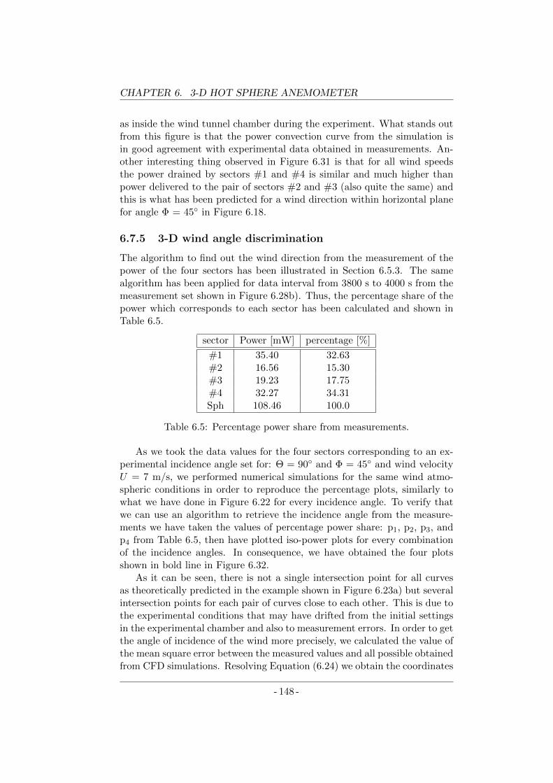
CHAPTER 6. 3-D HOT SPHERE ANEMOMETER
as inside the wind tunnel chamber during the experiment. What stands outfrom this figure is that the power convection curve from the simulation isin good agreement with experimental data obtained in measurements. An-other interesting thing observed in Figure 6.31 is that for all wind speedsthe power drained by sectors #1 and #4 is similar and much higher thanpower delivered to the pair of sectors #2 and #3 (also quite the same) andthis is what has been predicted for a wind direction within horizontal planefor angle Φ = 45 in Figure 6.18.
6.7.5 3-D wind angle discrimination
The algorithm to find out the wind direction from the measurement of thepower of the four sectors has been illustrated in Section 6.5.3. The samealgorithm has been applied for data interval from 3800 s to 4000 s from themeasurement set shown in Figure 6.28b). Thus, the percentage share of thepower which corresponds to each sector has been calculated and shown inTable 6.5.
sector Power [mW] percentage [%]
#1 35.40 32.63#2 16.56 15.30#3 19.23 17.75#4 32.27 34.31Sph 108.46 100.0
Table 6.5: Percentage power share from measurements.
As we took the data values for the four sectors corresponding to an ex-perimental incidence angle set for: Θ = 90 and Φ = 45 and wind velocityU = 7 m/s, we performed numerical simulations for the same wind atmo-spheric conditions in order to reproduce the percentage plots, similarly towhat we have done in Figure 6.22 for every incidence angle. To verify thatwe can use an algorithm to retrieve the incidence angle from the measure-ments we have taken the values of percentage power share: p1, p2, p3, andp4 from Table 6.5, then have plotted iso-power plots for every combinationof the incidence angles. In consequence, we have obtained the four plotsshown in bold line in Figure 6.32.
As it can be seen, there is not a single intersection point for all curvesas theoretically predicted in the example shown in Figure 6.23a) but severalintersection points for each pair of curves close to each other. This is due tothe experimental conditions that may have drifted from the initial settingsin the experimental chamber and also to measurement errors. In order to getthe angle of incidence of the wind more precisely, we calculated the value ofthe mean square error between the measured values and all possible obtainedfrom CFD simulations. Resolving Equation (6.24) we obtain the coordinates
- 148 -
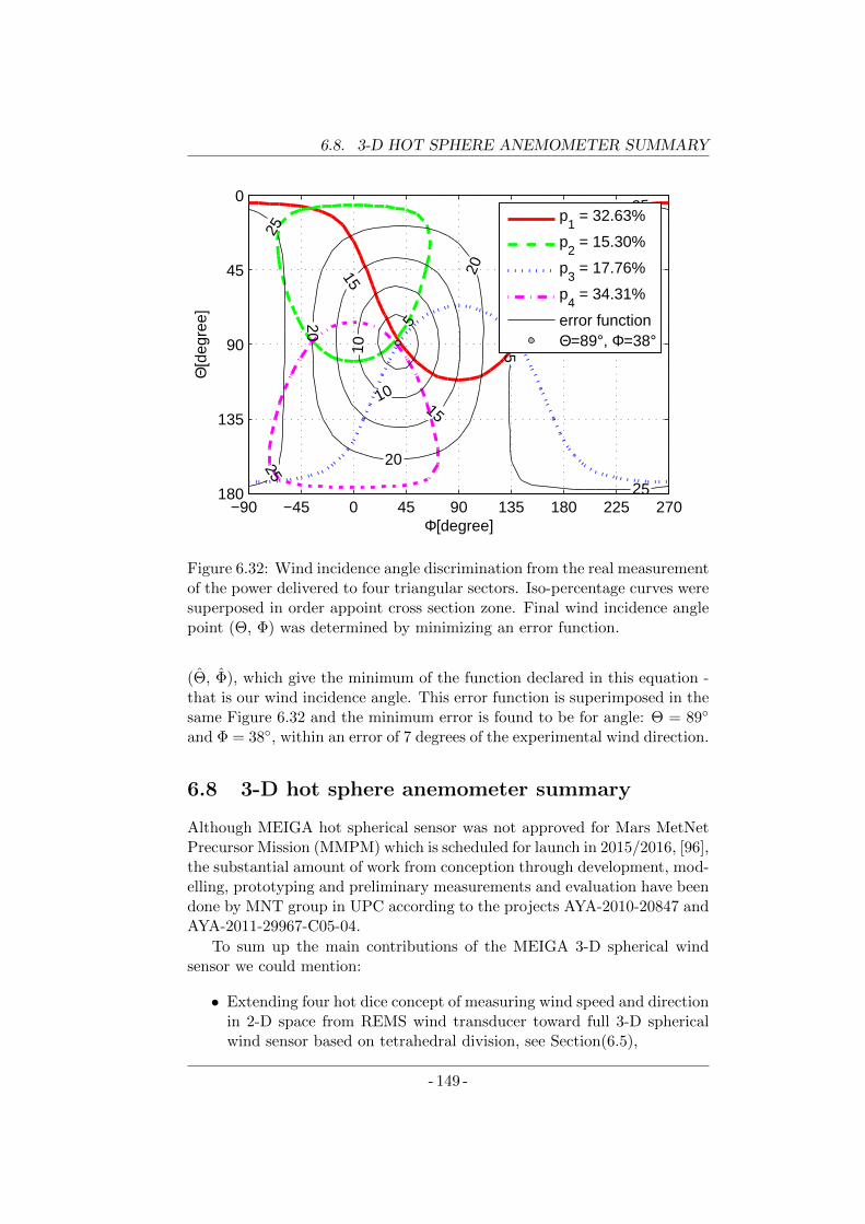
6.8. 3-D HOT SPHERE ANEMOMETER SUMMARY
−90 −45 0 45 90 135 180 225 270
0
45
90
135
180
5
10
10
15
15
20
202025
25
25
25
25
Φ[degree]
Θ[d
egre
e]
p
1 = 32.63%
p2 = 15.30%
p3 = 17.76%
p4 = 34.31%
error functionΘ=89°, Φ=38°
Figure 6.32: Wind incidence angle discrimination from the real measurementof the power delivered to four triangular sectors. Iso-percentage curves weresuperposed in order appoint cross section zone. Final wind incidence anglepoint (Θ, Φ) was determined by minimizing an error function.
(Θ, Φ), which give the minimum of the function declared in this equation -that is our wind incidence angle. This error function is superimposed in thesame Figure 6.32 and the minimum error is found to be for angle: Θ = 89
and Φ = 38, within an error of 7 degrees of the experimental wind direction.
6.8 3-D hot sphere anemometer summary
Although MEIGA hot spherical sensor was not approved for Mars MetNetPrecursor Mission (MMPM) which is scheduled for launch in 2015/2016, [96],the substantial amount of work from conception through development, mod-elling, prototyping and preliminary measurements and evaluation have beendone by MNT group in UPC according to the projects AYA-2010-20847 andAYA-2011-29967-C05-04.
To sum up the main contributions of the MEIGA 3-D spherical windsensor we could mention:
• Extending four hot dice concept of measuring wind speed and directionin 2-D space from REMS wind transducer toward full 3-D sphericalwind sensor based on tetrahedral division, see Section(6.5),
- 149 -
CHAPTER 6. 3-D HOT SPHERE ANEMOMETER
• Elimination of unwanted thermal losses (either conduction or radia-tion) be proper design and fabrication process, see Section (6.2.1),
• Providing the new efficient tool that enables to model convection heatof any arbitrary shape of the spherical sector for all possible 3-D winddirection, see Section (6.3),
• Minimalization of necessary number of CFD simulations to extend forwhole scenario of possible ambient conditions (Tamb, Pamb, U , anddirection(Θ,Φ)) to exactly predict power demand for each sector, seeSection (6.3.4),
• Design and assembly of fully operational spherical wind anemometermade out of four tetrahedral sectors to enable proof of concept tests,see Section (6.6),
• Preliminary measurement that has confirmed hypothesis for sensitivityof the wind speed and wind direction and also ability to estimate thosewind parameters based on the CFD simulation model proposed,
Besides the contributions listed below author of the thesis has been re-sponsible for building provisional UPC-MNT wind tunnel facility, and eval-uation of the simplified concept of the hot sphere anemometer made outof two hemispherical sectors. This part of the investigation work has beenreflected in following conference proceedings:
Reference [10], Appendix IL. Kowalski and M. Garcia, “Hypobaric chamber for wind sensor test-ing in Martian conditions,” in 8th Spanish Conference on Electron De-vices (CDE 2011), (Santiago de Compostela, Spain), pp. 1–4, February2011
Reference [11], Appendix LL. Kowalski, V. Jimenez, M. Domınguez-Pumar, S. Gorreta, S. Sil-vestre, and L. Castaner, “Low pressure spherical thermal anemome-ter for space missions,” in IEEE SENSORS 2013, (Baltimore, UnitedStates), pp. 1–4, November 2013
Reference [12]S. Gorreta, E. Barajas, L. Kowalski, T. Atienza, M. Domınguez-Pumar,and V. Jimenez, “A self-calibrating closed loop circuit for configurableconstant voltage thermal anemometers,” Electronics Letters, Septem-ber 2015
- 150 -
Chapter 7
Conclusions
In this chapter, author of the thesis will discuss main aspects of the two novelwind sensors he has been working on. Later author will present suggestionfor further research to carry out.
7.1 Discussion
7.1.1 2-D Wind Transducer
When the preparation to the MSL mission began so the REMS project andthe challenge to develop 2-D wind transducer was high due to demandinginstrument requirements to operate in a very thin atmosphere of Mars.
When the REMS MSLrover project began, it was clear from the startthat measuring the wind in the thin atmosphere of Mars was a challengingsubject. We were in charge of the primary transducer, the 2-D wind sensor,so we knew that it will be difficult to get a working prototype. From the firstday the MNT group, based on his experience with flow meters design, bet onthermal anemometer concept working in CTA mode, where the close-loopsigma-delta modulator provides digital power readout. In this approach weneed an electro-thermal converter that on one hand would provide fast, re-liable and stable coupling with atmosphere, and, on the other hand, mayprovide homogenous temperature distribution to run accurately CFD sim-ulations for further thermal modelling. The idea of using silicon wafer cutinto square shape chips has satisfied these requisites.
For predictable convection heat transfer rate, the sensor had to be sizedso that it works in medium continuum region. This was compatible with achip size greater than 1 mm. We knew that it was a critical subject as thePathfinder hot-wire sensor wasn’t able to perform reliable measurement dueto deep slip-flow conditions. We also knew that the only system that wasable to provide reliable wind data from Mars was the Viking hot-film sensorthat featured a characteristic size of the hot element of 0.51 mm.
151
CHAPTER 7. CONCLUSIONS
CFD simulation of one square shape die (1.6×1.6×0.4 mm) shown thatconvection heat in 2-D flow does not depend on wind direction but only onP ·U mass flow product. This concept has been expanded to the array offour coplanar silicon dice with minimum separation between them of approx-imately 0.5 mm. This separation was selected to provide thermal isolationbetween the dice, due to the very low thermal conductivity of the Martianatmosphere. At the same time, from the flow dynamics point of view, theseparation is small enough so that the group of dice would perform as a onescaled up the hot component (∼4×4×0.4 mm). Indeed, the average thermalconductance of group of four dice has shown sensitivity to the wind magni-tude preserving independent character on the wind direction, only for highervelocity range (30...60 m/s) there has been some fluctuation in thermal con-ductances. When going down to the individual thermal conductances of sep-arated dice (A, B, C, D) has been observed a significant dependence on thewind direction angle resembling sinusoidal function. For each velocity, thedifference between a maximum and a minimum of thermal conductance valueis in the range of average value (Gthmax - Gthmin ≈ Gthavg). This mecha-nism of thermal conductance reallocation between hot dice, while an averageconductance remains constant, has provided sensitivity for the wind angleidentification. Minimum angular sensitivity was for low speed (∼0.25 %/de-gree for 10 m/s) and rise for higher velocities. For the same wind velocity,angular sensitivity variation is within 22% to 42%, where maximum sensi-tivity is for winds coming from diagonal directions and minimum sensitivityis when the wind blows perpendicularly to the dice orientation. Based onthe four hot dice concept the differential terms NS (North-South) and EW(East-West) has been introduced. By using those terms there is no impor-tant variation in angular sensitivity, and, at the same time, we eliminatecommon conduction losses and external radiation component. The same,newly conceived four hot silicon dice structure becomes the state of art 2-Dwind transducer where we get the wind speed from the average power de-livered to the four dice, and we also get the wind direction from the powerdifferences between dice.
There were two main reasons why for the hot die element silicon materialhas been adapted. Silicon bulk material, thanks to its high thermal conduc-tivity provides a uniform temperature distribution within die volume. Thatwas confirmed solving 1st order thermal model and through FEM analysisthat has shown a maximum thermal gradient of 0.2% in reference to theapplied overheat. Working with silicon technology also has permitted de-position of three platinum resistances isolated by the good quality siliconthermal oxide. First of this resistances called Rsens will provide tempera-ture feedback due to its linear dependence on the temperature; indeed incharacterization has been found that α = 0.003 1/degree, which is character-istic for platinum film thinner than 100 nm. Second resistance Rheat formsa resistive circuit, which converts short electrical current pulses into heat
- 152 -
7.1. DISCUSSION
generated according to the Joule effect and dissipated into the silicon chip.Finally Rdelta is an additional resistance located at hot die element for thepurpose of setting up an appropriate overheat. For the fabrication process,which has been entirely handled by UPC clean room facility, the resistancetargets was set for Rsens = 7k Ω, Rheat = 700 Ω and Rdelta = 700 Ω. Thishas been achieved by sputtering approximately 20 nm of titanium adhesionlayer and then consecutively 80 nm of platinum resistive material amongmany steps carefully described in this thesis. The other important aspectof the fabrication is that silicon bulk has been connected through contactwindow to external potential to prevent electrical charge to be build up inthis component.
Besides the array of the four dice working as hot points that dissipateheat to the ambient by convection, there is another fifth die called a Refer-ence which estimates ambient temperature so that the system can operateat a preset overheat temperature. Each hot dice included a Rdelta resistance.A connection network gives a ∆R value from a combination of Rdelta resis-tances. The circuit was designed in the way that the hot dice overheat wasautomatically set from Rsens and ∆R values. Appropriate serial/parallelconnection of the four Rdelta resistances gives 12 combinations of differentoverheat profiles to be set-up. In the end, all four hot dice in a group followsthe same overheat profile respect to the ambient temperature. We choosethe overheat temperature profile of the hot dice so that the duty cycle read-out of the system is proportional to the thermal conductance of the dicealthough the delivered power depends on ambient temperature. To achievethis, each hot die component instead of working with CTA mode is workingin CTDA mode where the ambient temperature is constantly monitored byReference die and used to select an ambient temperature dependent over-heat. As a result, overheat temperature changes so that it adapts to thechanges in the heater resistance so that the obtained sensor responds onlyon each hot dice thermal conductance.
To understand better heat convection phenomena at the single die levelan algebraic model of the single die was analyzed for a wide range of tem-peratures, pressure and velocities taking into consideration variations of allMartian ”air” parameters (k, Cp, µ, ρ). This analysis has been contrastedwith CFD numerical simulation with good agreement.
Preliminary measurements have shown that the group of four dice hasgood sensitivity to the wind speed in the range of 0.3-20 m/s and angularsensitivity to the wind direction for the velocities higher than 0.3 m/s. Yawrotation experiment has shown that sensor has the ability to recognize windangle with higher resolution than 10. Experiments carried out in Aarhusre-circulating wind tunnel as well as in Oxford open wind tunnel has con-firmed that thermal conductances of the group of four dice as well as for thesingle die unit depends on the P ·U product, so that the velocity component(U) can be obtained providing independent ambient pressure measurement.
- 153 -
CHAPTER 7. CONCLUSIONS
Measurement campaign has also shed light on the aspects of thermal iso-lation of the hot dice component from the PCB base. It stands out thatthe heat drain through pyrex support structure is the same rate as it isthrough the wire-bonding connection. Moreover, measurements show thatonly about 10% of the power delivered to the hot element is transferred tothe ambient in the convection processes, whereas other significant 90% of thepower is classified as thermal losses. In order to reduce thermal losses andimprove the mechanical properties of the setup, the dice support materialwas changed from pyrex to glass-fiber.
Finally, elaboration of the first order heat convection model gives usa tool for comprehensive comparison of Viking (CTA), Pathfinder (CPA)and REMS (CTDA) thermal anemometers units, besides the fact that theirworking modes were different. This study has shown that only REMS hot dieelement have uniform temperature along entire hot volume, where for Vikingrod temperature gradient is observed for half of the hot-film structure andin the case of Pathfinder wire bound each end of the hot-wire experiencedtemperature drop. Compared for the same wind conditions, REMS windsensor shown better efficiency in Power/Overheat ratio and is slightly morepower efficient that Viking wind sensor unit and much more efficient thanPathfinder wind sensor unit. This result is also true for 3-D wind transducerswhen extended this analysis by multiplying power of each unit per a numberof units that compose full 3-D wind sensor.
7.1.2 3-D Hot Sphere Anemometer
Another call for the anemometer to Mars was within the course of theMEIGA project that has been a part of bigger MetNet mission undertaking.The specific requirements, assigned to MNT group, according to the windsensor development have been different from that from the REMS project.The measurement range was limited to the wind velocities from 1 m/s up to10 m/s, and the sensor had to be more resistant to a shock of about 300 gto withstand the landing procedure. But the most important thing was thatthe sensor developed in the MNT had to be a full 3-D transducer for windvelocity and wind direction. Based on the previously experience gained inREMS we thought that once again it will be a thermal anemometer workingin CTA mode. Nevertheless, this time the geometry that we came shouldgive a better-conditioned response. We came with the idea of a sphere asthe body with higher isotropy possible. Also this time we bet on the spheredivided into sectors and as it stands out from the analysis that a spheredivision into four sectors is just right to get enough information for full 3-Dangle decomposition.
The concept of the new 3-D hot sphere anemometer has been enrichedin several interesting aspects in reference to the array of four hot silicondice. Crucial was an introduction of the central core working with the same
- 154 -
7.1. DISCUSSION
temperature set point as the external shells that are in contact with sur-rounding gas. By this treatment, we have displaced all thermal losses as thecore is kept at the same temperature as the sphere surface. Therefore, therewas not need to use very high thermal resistivity materials to isolate hotspherical sectors from the cold base as this spherical sectors were physicallyconnected to the core working at the same temperature. The role of theFR4 board is to give mechanical support for the spherical sectors and alsoto provide electrical wiring. It needs to provide some thermal isolation, butthe requirements are relaxed by having a centrally heated core. It meansthat for spherical wind sensor are not required to use the thin wire-bondingconnection, and we can use a more traditional PCB technology. By that,the sensor has become more robust to physical damage like the contact withsmall pebbles when descending or landing. As we wanted to simplify tothe minimum the required wirings, we thought that it would be possibleto use just one resistance for a measure and heating purpose. Eventuallycommercial PT100 resistances were adapted for this purpose with thermalcoefficient characteristic for platinum αPt = 0.00385 1/degree.
The diameter of the sphere was optimized as a result of many factors.At first we knew that it had to be, as it was in the previous case at least1 mm or more just to be sure that we are operation in medium continuumrange. From the fabrication point of view, we knew that prototype partmust be feasible, so this shifted the size of the sensor rather into a biggersize of several millimeters. There have been many publications about theflow behaviour when passing over a hot sphere and there is a fact that tohave stable and axisymmetric flow around the sphere the Reynolds numbermust not exceed the value of 210. This in relation to the Mars atmosphericconditions situates our sphere to be not bigger than 10 mm in diameter forvery low temperatures (Tamb < 200 K). That gave our final size limitation.
There exist many empirical approximations that give average heat con-vection rate for a sphere, as Whitaker or Feng&Michaelides. This is, how-ever, true for the sphere as a whole and could give us information about theoverall sphere behaviour but not of the arbitrarily shaped sectors. To beable to separate the convection power at each sector, there have been runmany CFD simulation of a hot sphere for variations in CO2 temperature,flow velocity U , and overheat ∆T . From these simulations the local heatflux data, the simulated shell surface, has been obtained. In the next step,the simulated data has been approximated by polynomials as a function ofthe position on the wind direction axis. From this polynomial functions,we can know the local heat flux at any point on the sphere concerning theimpinging point of the wind direction without the need of all numerical rawsimulation data. This was just a step to know the thermal conductance ofarbitrary assign sector by integration of the local heat flux over correspond-ing sector’s area. All this postprocessing of the CFD simulations gives us atool that greatly speeds up the modelling of the convection of a hot sphere
- 155 -
CHAPTER 7. CONCLUSIONS
divided into sectors.As for now we have achieved the minimum size of spherical wind sensor
to be 9 mm in diameter, which is about twice the characteristic size as itwas in the case of the group of four silicon chips in REMS wind transducer.Spherical sectors were fabricated on Sterling Silver material using a commer-cial 3-D printing service. The Silver alloy was selected to provide maximumtemperature uniformity within the sector boundary. As 3-D printing givesrough surfaces before sectors assembly started, they have been polished withprogressive grit to obtain mirror finished external surface and then the thinlayer of gold (100 nm approx.) has been deposited on top of it. The polishingand gold plating procedure was selected to minimize radiation effects. Atthe same time, gold passivation protects the silver surface from oxidation.
The four piece tetrahedral geometry was selected as a result of an angularsensitivity analysis. It stands out that for tetrahedral sphere division theangular sensitivity along entire sphere is almost homogenous, this meanthat there are no blind zones where angle can not be determined or has badsensitivity. For the range of velocities from 3 m/s to 20 m/s and within theambient temperature of 220 K to 300 K the angular sensitivity for the full3-D angle is bigger than 0.2 %. The maximum angular sensitivity of 0.25 %is reached for the velocities range from 10 m/s to 15 m/s (the same value wasfor REMS at 10 m/s for 2-D angle discrimination). Hot sphere (D = 9 mm)immersed in CO2 atmosphere (P = 600 Pa) could change its global thermalconductance (Gthsph) from 0.5 mW/K for low wind 0.2 m/s at ambienttemperature 220 K up to 3.9 mW/K for a maximum wind speed of 20 m/swith ambient temperature 300 K. For the particular tetrahedral sector, itsthermal conductance (Gthsector) may vary from 10% to 40% of the globalsphere thermal conductance depending on wind incidence angle according tothe sector position. Each spherical sector dissipates maximum power whenthe wind blows directly in its center, and the minimum convection heat isobserved when the wind is coming from the opposite to its central point.
For tetrahedral sphere geometry, an algorithm for wind angle determina-tion was proposed. It is based on the numerical simulation results. It relieson iso-percentage curves in the angular space that have the same fraction ofpower being delivered. Drawing the iso-percentage curves for the four sec-tors gives a solution intersection point. The intersection point where fourcurves cross each other gives wind impinging point and if the curves don’tcross at the same point, the argument for the minimum error function con-clude the 3-D wind angle. For both, wind magnitude and wind direction,estimation the ambient temperature need to be provided. Nevertheless, asthe sphere works at constant temperature is much more resistant for ambi-ent temperature error as it operates on the relative (percentage values) ofheat power delivered to the sectors in equilibrium conditions in the case ofthe wind angle estimation.
Measurements performed in Mars-like conditions confirmed high sen-
- 156 -
7.2. SUGGESTION FOR FURTHER RESEARCH
sitivity of the spherical sensor to the wind speed and direction. In oneexperiment by changing velocity from 1 m/s up to 13 m/s it has been reg-istered a global sphere thermal conductance shift from 1.375 mW/K upto 3.875 mW/K. Also, substantial changes for each sector thermal conduc-tances to the ambient were registered when wind direction angle was changedfor all range of velocities (1, 2, 4, 7, 10, 13 m/s). Finally, an algorithm forwind angle discrimination has succeeded with 3-D angle estimation withinan error of 7 degrees of the experimental wind direction, despite the imper-fection in sensor prototype fabrication and temperature/pressure drifts inthe measurement chamber. As a result of all experiments, it has been provedthat spherical thermal anemometer build up from four identical tetrahedralsectors could be considered for a mission to Mars as a reliable 3-D windsensor alternative.
7.2 Suggestion for further research
The author of the thesis together with other researchers from the MNTgroup from UPC are currently involved in the development of the improvedversion of the REMS wind transducer to be part of the MEDA instrumenton board of the rover for Mars 2020 mission. The rover for Mars 2020mission would be based on the Mars Science Laboratory (MSL) rover con-figuration. Meteorology instruments will be provided be CAB-INTA. Theprincipal investigator of MEDA Jose Rodriguez-Manfredi has said that: ”aset of sensors will provide measurements of temperature, wind speed anddirection, pressure, relative humidity and dust size and shape”.
According to the MEDA wind sensor improvement there are few worthto mention that are under consideration for 2-D wind transducer board:
• Resistance on chip reduction to only two Rheat and Rsens that wouldreduce conduction losses to the substrate as the number of wire-bondingwill also be reduced from 7 to 4 for die (additional wire-bonding groundconnection that prevents the electrical charge to be build up will bejoined with one of the Rsens terminals),
• Further improvement of thermal isolation between hot dice elementsand PCB base by thinner wire bondings with diameter of 18 µm andhigher supporting pillars,
• Better wind signal coupling by using a higher overheat. This achieveddue to changes in ASIC performance as well as by putting hot dicedeeper in the wind according to the new support elevation,
• We want to provide hot dice group with lower resistance dispersionamong them and enumerated chips for better traceability during theentire assembly process.
- 157 -
CHAPTER 7. CONCLUSIONS
Respect to the 3-D wind spherical sensor there is also a plan for furtherimprovements and studies to carry out. We are extending sensor thermalsimulation for the dynamic behaviour to understand better what are thesensor limitations in the time response. The study is based on surface controltheory and diffusive representation that shed light on the sensor reaction inthe frequency domain. We believe that this research would indicate us whereis still a place for sensor improvement. Besides this study we are planningto:
• Perform full sensor characterization involving measurement in tem-perature and pressure control environment for entire yaw and pitchspectrum of the wind angle and entire range of velocities,
• Estimate the distortion effect of the PCB protruding-arm which pro-vides support for the spherical hot element tetrahedral shape sectorsthat are in contact with surround air,
• Improve assembling procedure and the same to lower asymmetry im-perfection that could affect convection heat profiles,
• Extend wind speed range by performing mixed natural and forced con-vection CFD simulations for the low-velocity limit as well as laminar-turbulent simulation to broaden high wind velocity limitation,
• Incorporate a silicon chip - instead of a commercial PT100 resistor - asa heating and sensing component to improve wind sensor performancein the frequency domain due to the high thermal conductivity of sil-icon compared with the typical materials used in commercial PT100components.
- 158 -
Bibliography
[1] M. Domınguez, L. Kowalski, V. J. A. Moreno, L. Castaner, and J. Ri-cart, “Metodo para la medida de la velocidad del aire y de su direccionen dos dimensiones para aplicaciones aeroespaciales y de baja presion,”2007. PATENTE DE INVENCION. Numero de solicitud: 200700259.Numero de publicacion: 2342953. Fecha de presentacion: 25.01.2007.Fecha de la concesion: 20.05.2011.
[2] M. Domınguez, V. Jimenez, J. Ricart, L. Kowalski, J. Torres,S. Navarro, J. Romeral, and L. Castaner, “A hot film anemometerfor the Martian atmosphere,” Planetary and Space Science, vol. 56,pp. 1169 – 1179, June 2008.
[3] V. Jimenez, M. Domınguez-Pumar, J. Ricart, L. Kowalski, S. Navarro,J. Torres, J. Romeral, J. Merrison, and L. Castaner, “Applications ofhot film anemometry to space missions,” in Eurosensors XXII, (Dres-den, Germany), September 2008. ISBN 978-3-00-025217-4.
[4] L. Kowalski, J. Ricart, V. Jimenez, M. Domınguez-Pumar, andL. Castaner, “Sensitivity analysis of the chip for REMS wind sensor,”in 7th Spanish Conference on Electron Devices (CDE 2009), (Palma deMallorca, Spain), pp. 289–292, February 2009.
[5] L. Kowalski, “Contribution to advanced hot wire wind sensing,” in 1stBarcelona Forum on Ph.D. Research in Electronic Engineering, pp. 7–8,Universitat Politecnica de Catalunya (UPC), Centre de Publicacions delCampus Nord SCCL (CPET), October 2009. ISBN978-84-7653-398-7.
[6] L. Kowalski, J. Ricart, V. Jimenez, M. Domınguez, and L. Castaner,“Thermal modelling of the chip for the REMS wind sensor,” Interna-tional Journal of Numerical Modelling: Electronic Networks, Devicesand Fields, vol. 23, pp. 340–353, July - October 2009. Special Issue onthe 7th Spanish Conference on Electron Devices (CDE2009).
[7] L. Castaner, M. Domınguez, V. Jimenez, J. Ricart, and L. Kowalski,“Chip UPC para la medida del viento en Marte,” tech. rep., presentedfor 7th Premio Duran Farell de Investigacion Tecnologica, Barcelona,Spain, June 2010.
159
BIBLIOGRAPHY
[8] L. Kowalski, L. Castaner, M. Domınguez, and V. Jimenez, “Multi-physics simulation of REMS hot-film anemometer under typical Mar-tian atmosphere conditions,” in COMSOL Conferenece 2010, (Paris,France), October 2010.
[9] J. Gomez-Elvira, C. Armiens, L. Castaner, M. Domınguez-Pumar,M. Genzer, F. Gomez, R. Haberle, A.-M. Harri, V. Jimenez, H. Kahan-paa, L. Kowalski, A. Lepinette, J. Martın, J. Martınez-Frıas, I. McE-wan, L. Mora, J. Moreno, S. Navarro, M. de Pablo, V. Peinado,A. Pena, J. Polkko, M. Ramos, N. Renno, J. Ricart, M. Richardson,J. Rodrıguez-Manfredi, J. Romeral, E. Sebastian, J. Serrano, M. delaTorre Juarez, J. Torres, F. Torrero, R. Urquı, L. Vazquez, T. Velasco,J. Verdasca, M.-P. Zorzano, and J. Martın-Torres, “REMS: The envi-ronmental sensor suite for the Mars Science Laboratory rover,” SpaceScience Reviews, vol. 170, pp. 583–640, July 2012.
[10] L. Kowalski and M. Garcia, “Hypobaric chamber for wind sensor testingin Martian conditions,” in 8th Spanish Conference on Electron Devices(CDE 2011), (Santiago de Compostela, Spain), pp. 1–4, February 2011.
[11] L. Kowalski, V. Jimenez, M. Domınguez-Pumar, S. Gorreta, S. Sil-vestre, and L. Castaner, “Low pressure spherical thermal anemome-ter for space missions,” in IEEE SENSORS 2013, (Baltimore, UnitedStates), pp. 1–4, November 2013.
[12] S. Gorreta, E. Barajas, L. Kowalski, T. Atienza, M. Domınguez-Pumar,and V. Jimenez, “A self-calibrating closed loop circuit for configurableconstant voltage thermal anemometers,” Electronics Letters, September2015.
[13] Wikipedia, “Earth Mars Moon celestia.” [Online], January 2010.http://commons.wikimedia.org/wiki/File:Earth mars moon celestia.jpg.
[14] M. D. Smith, “Spacecraft observations of the martian atmosphere,”Annual Review of Earth and Planetary Sciences, vol. 36, no. 1, pp. 191–219, 2008.
[15] NASA, “First camera 1 panorama of ChrysePlanitia on Mars.” [Online], February 2010.http://nssdc.gsfc.nasa.gov/planetary/viking.html.
[16] NASA, “Mars Fact Sheet.” [Online], January 2010.http://nssdc.gsfc.nasa.gov/planetary/factsheet/marsfact.html.
[17] NASA, “Earth Fact Sheet.” [Online], January 2010.http://nssdc.gsfc.nasa.gov/planetary/factsheet/earthfact.html.
- 160 -
BIBLIOGRAPHY
[18] Jet Propultion Laboratory, “MSL science corner, REMS.” [Online],January 2010. http://msl-scicorner.jpl.nasa.gov/Instruments/REMS/.
[19] L. H. R. Davey, T. Chamberlain, “Sensor design analysis report TRWreport METC-021,” tech. rep., September 1973.
[20] S. E. Larsen, H. E. Jrgensen, L. Landberg, and J. E. Tillman, “Aspectsof the atmospheric surface layers on Mars and Earth,” Boundary-LayerMeteorology, vol. 105, pp. 451–470, Dec. 2002.
[21] J. T. Schofield, J. R. Barnes, D. Crisp, R. M. Haberle, S. Larsen, J. A.Magalhes, J. R. Murphy, A. Seiff, and G. Wilson, “The Mars Pathfinderatmospheric structure investigation/meteorology (ASI/MET) experi-ment,” Science, vol. 278, no. 5344, pp. 1752–1758, 1997.
[22] A. Seiff, J. E. Tillman, J. R. Murphy, J. T. Schofield, D. Crisp, J. R.Barnes, C. LaBaw, C. Mahoney, J. D. Mihalov, G. R. Wilson, andR. Haberle, “The atmosphere structure and meteorology instrument onthe Mars Pathfinder Lander,” Journal of Geophysical Research: Plan-ets, vol. 102, no. E2, pp. 4045–4056, 1997.
[23] F. F. F. C. P. Lognonne, Planet Mars Story of Another World. Praxis,2008.
[24] C. R. John Grotzinger, Ashwin Vasavada, Mars Science Laboratory.Springer-Verlag New York, 2013. ISBN: 978-1-4614-6338-2.
[25] E. M. Marc Kaufman, MARS UP CLOSE: Inside the Curiosity Mission.August 2014.
[26] NASA, “Solar System.” [Online], January 2010.http://solarsystem.nasa.gov/planets/index.cfml.
[27] G. L. Vogt, Landscapes of Mars: A Visual Tour. Springer-Verlag NewYork, 2008.
[28] I. The Gale Group, ed., UXL Encyclopedia of Science. Encyclope-dia.com, 2002.
[29] W. M. Haynes, CRC Handbook of Chemistry and Physics, 93rd Edition.CRC Press, 2012.
[30] K. G. Herrmann Schlichting, Boundary-Layer Theory. Springer-VerlagHeidelberg New York, 2003.
[31] The Engineering ToolBox, “Carbon dioxide.” [Online], February 2011.http://www.engineeringtoolbox.com/carbon-dioxide-d 1000.html.
- 161 -
BIBLIOGRAPHY
[32] L. V. King, “On the convection of heat from small cylinders in a streamof fluid: Determination of the convection constants of small platinumwires, with applications to hot-wire anemometry,” Proceedings of theRoyal Society of London A: Mathematical, Physical and EngineeringSciences, vol. 90, no. 622, pp. 563–570, 1914.
[33] M. Laghrouche, A. Adane, J. Boussey, S. Ameur, D. Meunier, andS. Tardu, “A miniature silicon hot wire sensor for automatic wind speedmeasurements,” Renewable Energy, vol. 30, no. 12, pp. 1881 – 1896,2005.
[34] F. Mailly, A. Giani, R. Bonnot, P. Temple-Boyer, F. Pascal-Delannoy,A. Foucaran, and A. Boyer, “Anemometer with hot platinum thin film,”Sensors and Actuators A: Physical, vol. 94, no. 12, pp. 32 – 38, 2001.
[35] M. Loomans and A. v. Schijndel, “Simulation and measurement of thestationary and transient characteristics of the hot sphere anemometer,”Building and Environment, vol. 37, no. 2, pp. 153 – 163, 2002.
[36] Y. Sun and Y. Zhang, “An overview of room air motion measure-ment: Technology and application,” HVAC&R Research, vol. 13, no. 6,pp. 929–950, 2007.
[37] A. Van Putten and S. Middelhoek, “Integrated silicon anemometer,”Electronics Letters, vol. 10, pp. 425–426, October 1974.
[38] A. F. P. van Putten, M. J. A. M. van Putten, and M. H. P. M. vanPutten, “Silicon thermal anemometry: developments and applications,”Measurement Science and Technology, vol. 7, no. 10, p. 1360, 1996.
[39] K. A. A. Makinwa, Flow Sensing With Thermal Sigma-Delta Modula-tors. PhD thesis, Delft University of Technology, 2004.
[40] B. van Oudheusden, “Silicon thermal flow sensors,” Sensors and Actu-ators A: Physical, vol. 30, no. 1, pp. 5 – 26, 1992.
[41] B. W. V. Oudheusden, “Silicon thermal flow sensor with a two-dimensional direction sensitivity,” Measurement Science and Technol-ogy, vol. 1, no. 7, p. 565, 1990.
[42] J. Robadey, O. Paul, and H. Baltes, “Two-dimensional integrated gasflow sensors by CMOS IC technology,” Journal of Micromechanics andMicroengineering, vol. 5, no. 3, p. 243, 1995.
[43] L. Kowalski, T. Atienza, S. Gorreta, V. Jimenez, M. Domınguez-Pumar,S. Silvestre, and L. Castaner, “Spherical wind sensor for the atmosphereof Mars.” submitted to IEEE SENSORS JURNAL, July 2015.
- 162 -
BIBLIOGRAPHY
[44] H. P. Gunnlaugsson, C. Holstein-Rathlou, J. P. Merrison,S. Knak Jensen, C. F. Lange, S. E. Larsen, M. B. Madsen, P. Nrn-berg, H. Bechtold, E. Hald, J. J. Iversen, P. Lange, F. Lykkegaard,F. Rander, M. Lemmon, N. Renno, P. Taylor, and P. Smith, “Telltalewind indicator for the Mars Phoenix lander,” Journal of GeophysicalResearch: Planets, vol. 113, no. E3, pp. n/a–n/a, 2008. E00A04.
[45] NASA, “Viking Mission to Mars.” [Online], February 2010.http://nssdc.gsfc.nasa.gov/planetary/viking.html.
[46] T. E. Chamberlain, H. L. Cole, R. G. Dutton, G. C. Greene, and J. E.Tillman, “Atmospheric measurements on Mars - the Viking meteorol-ogy experiment,” American Meteorological Society Bulletin, vol. 57,pp. 1094–1104, Sept. 1976.
[47] O. Kemppinen, J. E. Tillman, W. Schmidt, and A.-M. Harri, “Newanalysis software for Viking Lander meteorological data,” GeoscientificInstrumentation, Methods and Data Systems, vol. 2, no. 1, pp. 61–69,2013.
[48] S. L. Hess, R. M. Henry, C. B. Leovy, J. A. Ryan, and J. E. Tillman,“Meteorological results from the surface of Mars: Viking 1 and 2,”Journal of Geophysical Research, vol. 82, no. 28, pp. 4559–4574, 1977.
[49] J. R. Murphy, C. B. Leovy, and J. E. Tillman, “Observations of Martiansurface winds at the Viking Lander 1 Site,” Journal of GeophysicalResearch: Solid Earth, vol. 95, no. B9, pp. 14555–14576, 1990.
[50] L. N. E. Jane Van Nimmen, Leonard C. Bruno, NASA Historical DataBook, NASA Launch system, Space Transportation, Human Space andSpace Science 1989-1999, vol. VII. Library of Congress, 2009.
[51] Mars Science Program Synthesis Group, “Mars Exploration Strategy2009 - 2020,” tech. rep., NASA, 2003.
[52] J. Gomez-Elvira and REMS Team, “Environmental monitoring instru-ment for Mars exploration,” in Lunar and Planetary Institute ScienceConference Abstracts, vol. 39 of Lunar and Planetary Inst. TechnicalReport, pp. 1647–+, mar 2008.
[53] NASA, “Next NASA Mars Mission Rescheduled for 2011.” [On-line], April 2008. http://www.nasa.gov/mission pages/mars/news/msl-20081204.html.
[54] W. L. S. Rob Manning, Mars Rover Curiosity: An Inside Account fromCuriosity’s Chief Engineer. Smithsonian Books, 2014.
- 163 -
BIBLIOGRAPHY
[55] Jet Propultion Laboratory, “Rover Environmental Mon-itoring Station (REMS).” [Online], January 2010.http://mars.jpl.nasa.gov/msl/mission/instruments/environsensors/rems/.
[56] J. G.-E. L. Vazquez, “The Rover Environmental Monitoring Station(REMS) of the Mars Science Laboratory (MSL,NASA/JPL 2009),”in Second workshop on Mars atmosphere modelling and observations,(Granada, Spain), p. 721, LMD, IAA, AOPP, CNES, ESA, 02 2006.held February 27 - March 3, 2006.
[57] NASA, “REMS In-Situ instrumentation.” [Online], January 2010.http://mars.nasa.gov/msl/mission/instruments/environsensors/.
[58] J. Gomez-Elvira, L. Castaner, A. Lepinette, J. Moreno, J. Polko, E. S.amd J. Torres, M. P. Zorzano, and REMS Team, “REMS, an instrumentfor Mars Science Laboratory Rover,” 40th Lunar and Planetary ScienceConference (2009), vol. 40, p. 1540, March 2009.
[59] J. Gomez-Elvira and REMS Team, “Environmental monitoring stationfor Mars Science Laboratory,” LPI Contributions, vol. 1447, pp. 9052–+, November 2008.
[60] A. Groenland, “Degradation processes of platinum thin films on a sili-con nitride surface,” June 2006.
[61] V. Jimenez, F. Masana, M. Domınguez, and L. Casta˜er, “Simulationof flow sensors for home appliances,” Microelectronics Journal, vol. 29,no. 45, pp. 283 – 289, 1998. Thermal Investigations of ICs and Mi-crostructures II.
[62] L. Castaner, V. Jimenez, M. Domınguez-Pumar, F. Masana, andA. Rodrıguez, “A conduction-convection design for liquid flow sens-ing,” Sensors and Actuators A: Physical, vol. 66, no. 13, pp. 131 – 137,1998.
[63] M. Domınguez-Pumar, M, F. Masana, V. Jimenez, S. Bermejo,J. Amirola, J. Ballester, N. Fueyo, and L. Castaner, “Low-cost thermalSigma-Delta air flow sensor,” Sensors Journal, IEEE, vol. 2, pp. 453–462, Oct 2002.
[64] M. Domınguez, J. Ricart, A. Moreno, X. Contestı, and S. Garriga, “Lowcost PCB thermal Sigma-Delta air flowmeter with improved thermalisolation,” Sensors and Actuators A: Physical, vol. 121, no. 2, pp. 388– 394, 2005.
[65] B. van Oudheusden, “Effect of operating conditions on the dynamicresponse of thermal sensors with and without analog feedback,” Sensorsand Actuators A: Physical, vol. 58, no. 2, pp. 129 – 135, 1997.
- 164 -
BIBLIOGRAPHY
[66] Z. FISK and G. WEBB, “5 - electrical resistivity of metals,” in Elec-tronic Structure and Properties (F. Y. FRADIN, ed.), vol. 21 of Treatiseon Materials Science & Technology, pp. 297 – 349, Elsevier, 1981.
[67] D. Dimitrov, A. Zahariev, J. Georgiev, G. Kolev, J. Petrinski, andT. Ivanov, “Thin film platinum resistance thermometers: calibrationand mathematical description of t(r) function,” Cryogenics, vol. 34,no. 6, pp. 487 – 489, 1994.
[68] “Chapter 6 - thin films on silicon,” in Handbook of Silicon BasedMEMSMaterials and Technologies (Second Edition) (M. Tilli, T. Mo-tooka, V.-M. Airaksinen, S. Franssila, M. Paulasto-Krckel, and V. Lin-droos, eds.), Micro and Nano Technologies, pp. 124 – 205, Boston:William Andrew Publishing, second edition ed., 2015.
[69] J. Foerster and R. Wolffenbuttel, “High-temperature accurate thermalsensing using integrated platinum resistors on silicon,” in Instrumen-tation and Measurement Technology Conference, 1995. IMTC/95. Pro-ceedings. Integrating Intelligent Instrumentation and Control., IEEE,pp. 538–, April 1995.
[70] Y. A. Cengel, Heat Transfer: A Practical Approach. Mcgraw-Hill,November 2003.
[71] J. Merrison, H. Bechtold, H. Gunnlaugsson, A. Jensen, K. Kinch,P. Nornberg, and K. Rasmussen, “An environmental simulation windtunnel for studying aeolian transport on mars,” Planetary and SpaceScience, vol. 56, no. 34, pp. 426 – 437, 2008.
[72] C. Wilson, A. Camilletti, S. Calcutt, and P. Ligrani, “A wind tunnelfor the calibration of Mars wind sensors,” Planetary and Space Science,vol. 56, no. 11, pp. 1532 – 1541, 2008.
[73] Centro de Astrobiologıa (CAB), “Linear wind tunnel.” [Online].https://cab.inta-csic.es/rems/facilities/linear-wind-tunnel/.
[74] J. Merrison, H. Gunnlaugsson, J. Jensen, K. Kinch, P. Nrnberg, andK. Rasmussen, “A miniature laser anemometer for measurement ofwind speed and dust suspension on Mars,” Planetary and Space Sci-ence, vol. 52, no. 13, pp. 1177 – 1186, 2004.
[75] B. M. A. C. Churchill SW, “Equation for forced convection from gasesand liquids to a circular cylinder in crossflow,” ASME. J. Heat Trans-fer., vol. 99, pp. 300–306, May 1977.
[76] A. S. L. Theodore L. Bergman, Frank P. Incropera, Fundamentals ofHeat and Mass Transfer. John Wiley & Sons, 2002.
- 165 -
BIBLIOGRAPHY
[77] D. C. Collis and M. J. Williams, “Two-dimensional convection fromheated wires at low Reynolds numbers,” Journal of Fluid Mechanics,vol. 6, pp. 357–384, 10 1959.
[78] L. J. C. Baldwin L. V., Sandborn V. A., “Heat transfer from transverseand yawed cylinders in continuum, slip, and free molecule air flows.,”ASME. Journal Heat Transfer., vol. 82, no. 2, pp. 77–86, 1960.
[79] S. KASSAR, “Anemometria Marciana, anemometro termico,” Master’sthesis, Universitat Politecnica de Catalunya, Escola Tecnica Superiorde Enginyeria de Telecomunicacio de Barcelona, Department of Elec-tronics, 2009.
[80] J. P. Arroyo, “Dielectric characterization for hot film anemometry inMETNET Mars mission,” Master’s thesis, Universitat Politecnica deCatalunya, Escola Tecnica Superior de Enginyeria de Telecomunicaciode Barcelona, Department of Electronics, 2010.
[81] M. Benzoni, “Wind sensor and electronic interface circuitry for spaceapplications,” Master’s thesis, UNIVERSITA DEGLI STUDI DIBRESCIA FACOLTA DI INGEGNERIA, 2010.
[82] Finnish Meteorological Institute (FMI), “MetNet.” [Online], April 2013.http://metnet.fmi.fi.
[83] M. Dıaz-Michelena, “Small magnetic sensors for space applications,”Sensors, vol. 9, no. 4, p. 2271, 2009.
[84] L. V. M-P Zorzano and S. Jimenez., “Retrieval of ultraviolet spectralirradiance from filtered photodiode measurements,” Inverse Problems,vol. 25, p. 115023, November 2009.
[85] F. Cortes, A. Gonzalez, A. Llopis, A. J. de Castro, J. Melandez, andF. Lopez, “Optimization of the dust sensor in the Mars MetNet mission;extension to in situ co2 concentration and surface temperature mea-surements by infrared multispectral sensing,” Proc. SPIE, vol. 8550,pp. 855018–855018–15, 2012.
[86] B. van Oudheusden and A. van Herwaarden, “High-sensivity 2-d flowsensor with an etched thermal isolation structure,” Sensors and Actu-ators A: Physical, vol. 22, no. 1, pp. 425 – 430, 1990.
[87] K. A. Makinwa and J. H. Huijsing, “A smart wind sensor using thermalsigma-delta modulation techniques,” Sensors and Actuators A: Phys-ical, vol. 9798, pp. 15 – 20, 2002. Selected papers from EurosenorsXV.
- 166 -
BIBLIOGRAPHY
[88] A. S. Cubukcu, E. Zernickel, U. Buerklin, and G. A. Urban, “A 2dthermal flow sensor with sub-mw power consumption,” Sensors andActuators A: Physical, vol. 163, no. 2, pp. 449 – 456, 2010.
[89] S. Sherif and R. Pletcher, “A normal sensor hot-wire/film probe methodfor the analysis of three-dimensional flows,” Flow Measurement andInstrumentation, vol. 5, no. 3, pp. 150 – 154, 1994.
[90] D. M. Riggin, E. Kudeki, and M. Sarango, “Tropospheric and strato-spheric momentum flux measurements from radar wind data collectedat Jicamarca,” Journal of Atmospheric and Solar-Terrestrial Physics,vol. 66, no. 34, pp. 277 – 283, 2004.
[91] Z.-G. Feng and E. E. Michaelides, “A numerical study on the transientheat transfer from a sphere at high Reynolds and Peclet numbers,”International Journal of Heat and Mass Transfer, vol. 43, no. 2, pp. 219– 229, 2000.
[92] S. Dhole, R. Chhabra, and V. Eswaran, “A numerical study on theforced convection heat transfer from an isothermal and isoflux spherein the steady symmetric flow regime,” International Journal of Heatand Mass Transfer, vol. 49, no. 56, pp. 984 – 994, 2006.
[93] S. Whitaker, “Forced convection heat transfer correlations for flow inpipes, past flat plates, single cylinders, single spheres, and for flow inpacked beds and tube bundles,” AIChE Journal, vol. 18, pp. 361 – 371,March 1972.
[94] K. A. A. N. M. Sadikin, N. A. Mohd Yunus, “Numerical study of flowpast a solid sphere at moderate Reynolds number,” Applied Mechanicsand Materials, vol. 660, pp. 674–678, October 2014.
[95] R. T. W. Sabuga, “Effect of roughness on the emissivity of the preciousmetals silver, gold, palladium, platinum, rhodium, and iridium,” HighTemperatures-High Pressures, vol. 33(3), pp. 261–269, 2001.
[96] A.-M. Harri, W. Schmidt, H. Guerrero, and L. Vazquez, “Future plansfor MetNet lander Mars missions,” in EGU General Assembly Confer-ence Abstracts, vol. 14, p. 8224, 2012.
- 167 -

Appendix A
Metodo para la medida de la velocidad del aire y desu direccion en dos dimensiones para aplicacionesaeroespaciales
Spanish patent number P200700259. Presentation: 25.01.2007. Requestform: 19.07.2010. Concession: 30.05.2011. Publication: 09.06.2011.
Manuel Domınguez-Pumar,Lukasz Kowalski,Vicente Jimenez Serres,Alberto Moreno,Luis Castaner Munoz,Jordi Ricart Campos.
Justificante de presentación electrónica de solicitud de patente
Este documento es un justificante de que se ha recibido una solicitud española de patente por víaelectrónica, utilizando la conexión segura de la O.E.P.M. Asimismo, se le ha asignado de formaautomática un número de solicitud y una fecha de recepción, conforme al artículo 14.3 del Reglamentopara la ejecución de la Ley 11/1986, de 20 de marzo, de Patentes. La fecha de presentación de lasolicitud de acuerdo con el art. 22 de la Ley de Patentes, le será comunicada posteriormente.
Número de solicitud: P201531421
Fecha de recepción: 02 octubre 2015, 13:16 (CEST)
Oficina receptora: OEPM Madrid
Su referencia: ControlSensor
Solicitante: Universitat Politécnica de Catalunya
Número de solicitantes: 1
País: ES
Título: Método de control para sensores químicos de gases y sistema dedetección de gases
Documentos enviados: Descripcion.pdf (16 p.)
Dibujos.pdf (7 p.)
Reivindicaciones-1.pdf (3 p.)
Resumen-1.pdf (1 p.)
OLF-ARCHIVE.zip
package-data.xml
es-request.xml
application-body.xml
es-fee-sheet.xml
feesheet.pdf
request.pdf
Enviados por: CN=CPISR-1 C ESTHER REALSALADRIGAS,serialNumber=46548596T,T=PDI,givenName=ESTHER,SN=REAL SALADRIGAS,OU=Vegeuhttps://www.catcert.cat/verCPISR-1CarrecUR (c)03,OU=Serveis Públicsde Certificació CPISR-1 amb càrrec,OU=706 ENG.DE LACONSTRUCCIÓ,O=Universitat Politècnica de Catalunya,C=ES
Fecha y hora derecepción:
02 octubre 2015, 13:16 (CEST)
Codificación del envío: 5B:17:AE:4A:30:AD:17:48:C3:28:FF:B3:1A:AD:81:09:29:FB:7F:CA
169

Appendix A
19© OFICINA ESPAÑOLA DEPATENTES Y MARCAS
ESPAÑA
11© Número de publicación: 2 342 95321© Número de solicitud: 20070025951© Int. Cl.:
G01F 1/69 (2006.01)
G01P 5/12 (2006.01)
G01W 1/17 (2006.01)
12© PATENTE DE INVENCIÓN B1
22© Fecha de presentación: 25.01.2007
43© Fecha de publicación de la solicitud: 19.07.2010
Fecha de la concesión: 30.05.2011
45© Fecha de anuncio de la concesión: 09.06.2011
45© Fecha de publicación del folleto de la patente:09.06.2011
73© Titular/es: Universitat Politècnica de Catalunyac/ Jordi Girona, 3108034 Barcelona, ES
72© Inventor/es: Domínguez Pumar, Manuel;Kowalski, Lukasz;Jiménez Serres, Vicente;Moreno, Alberto;Castañer Muñoz, Luis yRicart Campos, Jordi
74© Agente: No consta
54© Título: Método para la medida de la velocidad del aire y de su dirección en dos dimensiones para aplica-ciones aeroespaciales y de baja presión.
57© Resumen:Método para la medida de la velocidad del aire y de sudirección en dos dimensiones para aplicaciones aeroes-paciales y de baja presión.Método para la medida de la velocidad y dirección delviento en dos dimensiones, basado en anemometría tér-mica, para trabajar en aplicaciones aeroespaciales en lasuperficie de otros planetas.El método descrito utiliza dos invenciones para eliminar ladependencia de la medida con la temperatura del viento:utiliza de tres resistencias dependientes de la temperatu-ra en el elemento caliente y una estructura matricial deelementos calientes con un único elemento de referen-cia. La estructura matricial tiene simetría de rotación loque permite la obtención de la medida mediante combi-naciones diferenciales de las señales de los elementoscalientes.El segundo problema es la precisión de la medida en at-mósfera enrarecida como resultado del pequeño valor delcamino libre medio de las moléculas. El método descri-to reduce ese problema mediante el aislamiento térmicooptimizado entre los elementos calientes entre sí, y entreéstos y el sustrato y el elemento de referencia.
Aviso: Se puede realizar consulta prevista por el art. 37.3.8 LP.ES
234
295
3B
1
Venta de fascículos: Oficina Española de Patentes y Marcas. Pº de la Castellana, 75 – 28071 Madrid
- 171 -
Appendix A
5
10
15
20
25
30
35
40
45
50
55
60
65
ES 2 342 953 B1
DESCRIPCIÓN
Método para la medida de la velocidad del aire y de su dirección en dos dimensiones para aplicaciones aeroespa-ciales y de baja presión.
Sector técnico
Tecnología electrónica (sensores de viento), tecnología espacial, instrumentación de laboratorio.
Estado de la técnica
La medida de la velocidad del viento se viene haciendo tradicionalmente usando varios procedimientos, como porejemplo cazoletas giratorias, diferencia de presión, propagación de ultrasonidos, desplazamiento iónico (Ion drift),efecto doppler usando láser (LDA) y siendo el mas popular el principio de anemometría térmica que es en el que secentra esta invención.
Los anemómetros convencionales utilizan un elemento que se calienta deliberadamente de forma que se estableceuna diferencia de temperatura entre él y el entorno que lo rodea. Se establece así un equilibrio térmico medianteconducción y convección térmicas. Cuando el aire o gas que rodea al sensor se mueve, la convección térmica aumenta yel elemento caliente se refrigera reduciéndose la diferencia de temperatura entre el elemento caliente y su entorno. Estareducción está relacionada con la velocidad del viento a través de los números de Reynolds y de Prandtl, existiendonumerosas correlaciones empíricas para ellos en función de la geometría del sensor propiamente dicho y la geometríade la interacción del sensor con el ambiente, que se encuentran recogidas en los libros de texto.
El elemento caliente debe estar en intimo contacto con el fluido, la mayoría de invenciones anteriores a éstaaportan diferentes modificaciones de montaje del elemento caliente en el paso del flujo de gas (US 6,968,283), aire oliquido (US 6,971,274) para hacerlo sumergible. Las tecnologías avanzadas de microelectrónica y de micromecanizadotambién se han usado para obtener sensores anemométricos sobre soportes elevados (US 6,923,054).
El circuito mas utilizado hasta ahora para el anemómetro consiste en un puente resistivo de cuatro ramas, en una delas cuales se coloca una resistencia cuyo valor depende de la temperatura. Cuando el puente está en equilibrio, es decircuando el valor de la resistencia del elemento sensor es igual que el valor de las otras tres resistencias, la potencia quese hace circular por elemento sensor es nula. Por el contrario cuando la velocidad del viento hace que se establezcauna diferencia de temperatura en el elemento caliente respecto al ambiente, el puente se desequilibra y se aplica unapotencia hasta que se restablece el equilibrio. Este procedimiento tradicional es un procedimiento analógico cuyaprecisión y sensibilidad depende del ruido de la medida y además es de respuesta lenta por tratarse de un método apotencia constante. Se conoce que una modificación del método consistente en utilizar una estrategia diferente basadaen “diferencia de temperatura constante” es decir que se aplica la potencia necesaria hasta que se establece una ciertadiferencia de temperatura es mas rápida que la estrategia anterior.
En el pasado se ha usado el método de anemometría térmica de forma muy extendida, incorporando modificacio-nes en el numero de amplificadores del circuito mas tradicionalmente usado (US 7,013,725), así como haciendo elresultado independiente del valor de la fuente de alimentación (US 7,072,776) o usando redundancia en la medida encombinación con una medida de diferencia de presión (US 6,945,123).
Los anemómetros convencionales se basan en un hilo fino de platino o tungsteno, colocado entre dos soportesque proporcionan adecuado contacto eléctrico. Asimismo se han usado en lugar de hilos finos, películas delgadasdepositadas en un sustrato adecuado. La configuración clásica incluye al hilo o película delgada de platino o tungstenoen una de las ramas del puente de medida.
Estos anemómetros convencionales sufren de varios inconvenientes. El primero de ellos es que por tratarse de unprincipio de medida basado en el equilibrio térmico, el valor de la temperatura del fluido influye sobre el resultado dela medida de la velocidad del flujo. Si bien invenciones mas recientes han intentado reducir esta dependencia usandotécnicas de separación de sensor y sustrato bien sea mediante micromecanizado de volumen, eliminando silicio, obien sea mediante micromecanizado de superficie que al liberar las estructuras quedan separadas del sustrato, estadependencia no ha sido suficientemente cancelada hasta el presente. Este hecho tiene que ver, en parte, con el usode resistencias de calefacción realizadas mediante polisilicio o aleaciones de Níquel y Cromo cuyos coeficientes detemperatura son muy diferentes del coeficiente de temperatura del elemento sensor ya sea de platino o de tungsteno.La dependencia excesiva con la temperatura es un inconveniente más importante cuando se trata de aplicacionesaeroespaciales en las que los cambios de temperatura son muy grandes y muy rápidos, lo que puede inducir a grandeserrores en la medida.
El segundo problema que tienen estos sensores convencionales para su utilización aeroespacial es su fragilidad, asícomo la posibilidad de desajuste en las fases de prueba, ensayo y lanzamiento.
Para la medida de la dirección del viento en un plano, los anemómetros convencionales han utilizado dos elementoscalientes ortogonales entre si y un elemento que resuelve el cuadrante. Este principio ha sido utilizado por ejemplo enla medida de la dirección del viento en la superficie de Marte por la misión Viking. También se han utilizado elementos
2
- 172 -
Appendix A
5
10
15
20
25
30
35
40
45
50
55
60
65
ES 2 342 953 B1
calefactores y termopilas coplanares dispuestos en los cuatro lados de un cuadrado para medir el ángulo de ataque delviento a la estructura con el inconveniente del acoplo térmico por el propio sustrato y la perdida de sensibilidad.
Resumen de la invención
La presente invención proporciona, entre otras cosas, un sensor de velocidad y dirección de viento en un plano,incluyendo cuatro elementos independientes, sin excluir un numero distinto, denominados calientes, y dispuestos demanera que su perímetro total forma un cuadrado, sin excluir otras formas geométricas y un elemento de referenciadenominado “frío”. Cada elemento caliente incluye tres resistencias del mismo material resistivo sensible a la tem-peratura, depositadas por un método adecuado en el mismo sustrato. Una de cada tres resistencias de cada elementocaliente es una resistencia calefactora que permite subir la temperatura de todo el sustrato, la segunda resistencia esuna resistencia sensora de temperatura y la tercera es una resistencia que permite al circuito adecuado establecer y fijaruna diferencia de temperatura consigna entre el elemento caliente y el ambiente.
El sustrato puede ser de diferentes materiales, siempre que sean buenos conductores térmicos como el silicio sinexcluir otros. El material con el que se forman las resistencias es el mismo para las tres de cada mismo elementocaliente y es un material cuya resistividad es una función de la temperatura como por ejemplo el platino sin excluirotros. Esta parte de la invención es la que permite cancelar la dependencia de la conductancia térmica de conveccióncon la temperatura del medio.
El elemento de referencia o “frío” puede ser idéntico a los elementos calientes, aunque no necesariamente puestoque tanto la resistencia calefactora como la resistencia de consigna no son necesarias para su funcionamiento.
Los elementos calientes están adecuadamente aislados térmicamente y eléctricamente entre sí y respecto a una baseque puede ser un PCB, sin excluir otro tipo de base, mediante soportes de la forma y sección adecuados para reducirel acoplo térmico por convección así como las perdidas por conducción térmica. Esta reducción viene acompañada deuna estrategia de medida consistente en la medida de diferencias, dos a dos, de las conductancias térmicas de los cuatroelementos calientes, con lo que se consigue eliminar la dependencia con la temperatura del medio producida por losacoplos térmicos de los elementos calientes al sustrato. Simultáneamente el hecho de que en un entorno aeroespacialen el que la densidad del medio es baja, la cancelación de términos de pérdidas térmicas comunes a los elementoscalientes, permite mejorar la sensibilidad del sensor así como su precisión respecto a los anemómetros convencionales.
A diferencia de los anemómetros convencionales, el método descrito en esta invención incluye un circuito deadquisición de datos basado en un circuito realimentado sigma delta electrotérmico, con la ventaja de que la salida esdigital directamente y que el rango de medida puede ser ajustado dentro del rango dinámico de la salida digital.
Descripción detallada de la invención
La presente invención proporciona entre otras cosas, un sensor de velocidad y dirección del viento en dos di-mensiones incluyendo entre otras cosas, cuatro elementos, sin excluir un numero diferente, que se calientan a unatemperatura por encima del ambiente, incluyendo cada uno de ellos una primera resistencia calefactora, una sensorade temperatura formado por una segunda resistencia y una tercera resistencia para fijar la diferencia de temperaturaconsigna entre el elemento caliente y el ambiente. Cada elemento caliente esta formado por un sustrato buen conductortérmico preferentemente silicio sin excluir otros sustratos, en el que se han depositado y grabado con la tecnología y elprocedimiento adecuados, la película de material resistivo conformando las tres resistencias. El material resistivo conel que se forman las tres resistencias es un material cuya resistividad es dependiente de la temperatura, como puedeser el platino o el tungsteno sin excluir otros materiales. Las resistencias de los elementos calientes están formadas delmismo material sensible a la temperatura, Las resistencias están aisladas eléctricamente del sustrato mediante un pro-cedimiento adecuado y están en contacto térmico entre sí y con el sustrato. La invención incluye también un elementodenominado elemento de referencia o elemento frío de las mismas dimensiones que los otros elementos y que incluyeun sensor de temperatura formado por una resistencia. El elemento de referencia puede ser, aunque no tiene porqueser necesariamente, idéntico a los elementos calientes para facilitar la fabricación, pero del elemento de referenciasolamente se usa el sensor de temperatura.
Los elementos calientes y el elemento de referencia se colocan encima de un elemento de soporte, que puede serun circuito impreso sin excluir otro tipo de soporte, de forma que los cinco elementos estén separados del soporte unadistancia suficiente para que haya un mejor aislamiento térmico de los elementos calientes y del de referencia respectoal soporte. Para las aplicaciones aeroespaciales, en las que la densidad del ambiente es baja, el aislamiento térmicose ve favorecido por este hecho. La presente invención incluye un aislamiento térmico que se consigue medianteuna estructura micromecanizada que proporciona una separación entre los elementos calientes y el soporte y ademásproporciona la sujeción necesaria usando un procedimiento adecuado que puede ser un adhesivo sin excluir otrosprocedimientos.
La presente invención incluye un circuito de conversión que, para cada uno de los elementos calientes, consisteen un puente formado por dos fuentes de corriente una en cada una de dos de las ramas, la resistencia sensora enla tercera rama y la resistencia consigna en serie con la resistencia del elemento de referencia en la cuarta rama. Lasalida del puente se conduce a un amplificador cuya salida se compara con una tensión de referencia y el resultadose envía a la entrada de dato de un biestable. La salida del biestable controla un interruptor que cambia el valor de la
3
- 173 -
Appendix A
5
10
15
20
25
30
35
40
45
50
55
60
65
ES 2 342 953 B1
corriente que se hace circular por la resistencia calefactora. Este circuito de conversión tiene una parte que se denominaconvertidor sigma -delta térmico y que esta compuesto por el comparador, el biestable y un filtro paso bajo que actúaen el dominio térmico debido a las constantes de tiempo térmicas. La resistencia del elemento de referencia es comúna los circuitos de los elementos calientes. El resultado de la medida, para cada elemento caliente es el flujo de bits quesale del biestable, cuyo valor acumulado en una ventana temporal dividido por la diferencia de temperatura consignaentre el elemento caliente y el ambiente proporciona el valor de la conductancia térmica entre el elemento caliente y elambiente. El resultado de la salida de los circuitos de los elementos calientes proporciona, el valor de las conductanciastérmicas.
La invención incluye también la estrategia de proceso de los datos para la obtención de la magnitud y la direccióndel viento y consiste en el cálculo de las diferencias de los valores de las conductancias térmicas de los elementoscalientes dos a dos de manera que obtienen dos componentes ortogonales, sin excluir componentes en otras direccionesy de ellas se deducen los valores de la intensidad y dirección del viento.
En referencia a las figuras, Fig. 1 representa un esquema del elemento caliente en el que encima del sustrato 1preferentemente de silicio sin excluir otros sustratos conductores térmicos, se deposita o crece por un procedimientoadecuado, un material aislante eléctricamente 2 preferentemente óxido de silicio mediante la oxidación térmica delsilicio, sin excluir otros procedimientos de crecimiento o deposito. Encima del material aislante se deposita o creceun material, cuya resistividad es sensible a la temperatura preferentemente de platino sin excluir otros materiales, enforma de película delgada y posteriormente se graba o delinea siguiendo un procedimiento fotolitográfico, sin excluirotros procedimientos, de forma que quedan en la superficie del material aislante unas pistas en forma de U, sin excluirotras formas, de manera que quedan configuradas tres resistencias de valores distintos. 3 es la resistencia calefactora,4 es la resistencia sensora y 5 es la resistencia consigna.
El espesor del sustrato es preferentemente el mismo grosor de la oblea de silicio, sin excluir otros espesores. Ladimensión del elemento caliente es preferentemente un cuadrado del orden de un milímetro de lado sin excluir otrasdimensiones mayores o menores para poder ajustar el valor de la máxima frecuencia de respuesta del sensor que esdependiente de la masa del elemento.
Las dimensiones de las resistencias son de unas centésimas a décimas de milímetro sin excluir otras dimensionesmayores o menores para poder ajustar el valor de las resistencias eléctrica a los valores mas adecuados para el sensor.
La Fig 2 representa el elemento de referencia o elemento frió, que es básicamente de las mismas dimensiones yforma, así como esta fabricado usando el mismo procedimiento del elemento caliente. 1 es el sustrato preferentementede silicio sin excluir otros sustratos conductores térmicos, se deposita o crece por un procedimiento adecuado, un ma-terial aislante eléctricamente 2 preferentemente óxido de silicio mediante la oxidación térmica del silicio, sin excluirotros procedimientos de crecimiento o deposito. Encima del material aislante se deposita o crece un material, cuyaresistividad es sensible a la temperatura preferentemente de platino sin excluir otros materiales, en forma de películadelgada y posteriormente se graba o delinea siguiendo un procedimiento fotolitográfico, sin excluir otros procedimien-tos, de forma que quedan en la superficie del material aislante unas pistas en forma de U, sin excluir otras formas, demanera que queda configurada la resistencia sensora 4.
La Fig 3 representa la disposición de los elementos calientes 31, 32, 33 y 34 en el caso de ser cuatro y delelemento de referencia 35 cada uno de ellos encima del soporte 36 que los separa del soporte 37 una cierta distanciapreferentemente del mismo orden de magnitud que el espesor del sustrato de silicio, sin excluir distancias mayores omenores para poder reducir las pérdidas por acoplo térmico con el sustrato.
La Fig 4 es un diagrama esquemático del circuito utilizado por el sensor de viento. En la figura se muestra que elcircuito de esta invención está formado, por un puente de cuatro ramas formado por la rama 401 en la que se conectauna fuente de corriente de valor Ix 405, una rama 402 en la que se conecta una fuente de corriente de valor Iref, 406,una rama 403 en la que se conecta la resistencia sensora Rx 407, una rama 404 en la que se conecta la resistenciaconsigna ∆R, 408 en serie con la resistencia del elemento de referencia Ref., 409. Entre los nodos comunes a lasramas 401 y 403 y a las ramas 402 y 404 se conectan los terminales de entrada de un amplificador 410 cuya salida seconecta a la entrada de un comparador 411. La salida del comparador 411 se conecta a la entrada de un biestable tipoD 412 a cuya salida 413 se conecta la salida del circuito 414 y por, otro lado se conecta el control de un interruptorSW 418 que conecta o desconecta una fuente de corriente Ihx 416 a la resistencia calefactora RHX 417. Finalmente lafuente de corriente Imx 415 está siempre conectada a la resistencia calefactora 417 cerrándose de esta forma el lazo.
La invención aquí descrita incluye un número de circuitos idéntico al de la Fig 4 uno por cada elemento caliente ypor lo tanto suministra salidas digitales, cada una de ellas proporcional a la conductancia térmica entre cada elementocaliente y el ambiente. Esta conductancia térmica de convección es independiente de la temperatura por el hecho deque las tres resistencias de cada uno de los elementos calientes tienen el mismo coeficiente de temperatura al serresistencias fabricadas con el mismo material, en efecto el cálculo del circuito de la Fig 4 da el siguiente resultado:
4
- 174 -
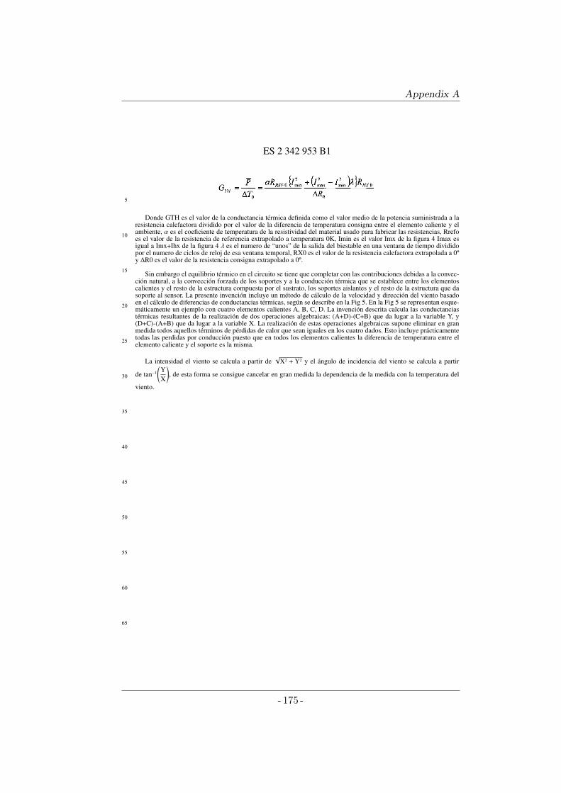
Appendix A
5
10
15
20
25
30
35
40
45
50
55
60
65
ES 2 342 953 B1
Donde GTH es el valor de la conductancia térmica definida como el valor medio de la potencia suministrada a laresistencia calefactora dividido por el valor de la diferencia de temperatura consigna entre el elemento caliente y elambiente, α es el coeficiente de temperatura de la resistividad del material usado para fabricar las resistencias, Rrefoes el valor de la resistencia de referencia extrapolado a temperatura 0K, Imin es el valor Imx de la figura 4 Imax esigual a Imx+Ihx de la figura 4 λ es el numero de “unos” de la salida del biestable en una ventana de tiempo divididopor el numero de ciclos de reloj de esa ventana temporal, RX0 es el valor de la resistencia calefactora extrapolada a 0ºy ∆R0 es el valor de la resistencia consigna extrapolado a 0º.
Sin embargo el equilibrio térmico en el circuito se tiene que completar con las contribuciones debidas a la convec-ción natural, a la convección forzada de los soportes y a la conducción térmica que se establece entre los elementoscalientes y el resto de la estructura compuesta por el sustrato, los soportes aislantes y el resto de la estructura que dasoporte al sensor. La presente invención incluye un método de cálculo de la velocidad y dirección del viento basadoen el cálculo de diferencias de conductancias térmicas, según se describe en la Fig 5. En la Fig 5 se representan esque-máticamente un ejemplo con cuatro elementos calientes A, B, C, D. La invención descrita calcula las conductanciastérmicas resultantes de la realización de dos operaciones algebraicas: (A+D)-(C+B) que da lugar a la variable Y, y(D+C)-(A+B) que da lugar a la variable X. La realización de estas operaciones algebraicas supone eliminar en granmedida todos aquellos términos de pérdidas de calor que sean iguales en los cuatro dados. Esto incluye prácticamentetodas las perdidas por conducción puesto que en todos los elementos calientes la diferencia de temperatura entre elelemento caliente y el soporte es la misma.
La intensidad el viento se calcula a partir de√
X2 + Y2 y el ángulo de incidencia del viento se calcula a partir
de tan−1
(YX
), de esta forma se consigue cancelar en gran medida la dependencia de la medida con la temperatura del
viento.
5
- 175 -
Appendix A
5
10
15
20
25
30
35
40
45
50
55
60
65
ES 2 342 953 B1
REIVINDICACIONES
1. Un sensor anemométrico de velocidad y dirección del viento que comprende:
Cuatro elementos iguales formados por un volumen de material conductor térmico recubierto de un materialaislante eléctrico,
Cada uno de los elementos antedichos comprendiendo tres resistencias situadas encima del material aislante
Una de las tres resistencias antedichas siendo una resistencia calefactora proporcionando calor al elemento
Una de las tres resistencias antedichas siendo un sensor de temperatura
Una de las tres resistencias antedichas siendo una resistencia sensible a la temperatura.
Cada una de las resistencias antedichas formadas del mismo material
El material antedicho tiene su resistividad dependiente de la temperatura.
Un elemento de la misma forma y materiales que los elementos antedichos comprendiendo una resistencia delmismo material que las resistencias de los antedichos elementos
La resistencia del quinto elemento antedicho siendo una resistencia sensora de la temperatura.
Los cinco elementos situados coplanarmente.
2. El sensor de viento de la reivindicación 1 donde cada uno de los cinco elementos antedichos, sin excluir unnúmero diferente, se encuentran separados del soporte mediante unos elementos micromecanizados hechos de materialaislante térmico que proporciona además soporte mecánico.
3. El sensor de viento de la reivindicación 1 donde los cuatro elementos iguales se encuentran a una distanciamenor que la distancia que hay entre ellos y el quinto elemento.
4. El sensor de viento de la reivindicación 1 donde las conexiones eléctricas de las resistencias de los cinco ele-mentos se realizan mediante la soldadura de hilos al sustrato.
5. El sensor de viento de la reivindicación 1 comprendiendo además un circuito idéntico para cada uno de loscuatro elementos antedichos incluyendo
a. Dos fuentes de corriente ubicadas en las dos primeras ramas de un puente de cuatro ramas
b. Donde la resistencia sensora está conectada a la tercera rama del puente
c. Donde la resistencia consigna y la resistencia del quinto elemento están situadas en la cuarta rama del puente
d. Dos fuentes de corriente suministrando potencia a las resistencias calefactoras
e. Un interruptor conmutando una de las dos fuentes de corriente que suministran potencia a las resistenciascalefactores
f. Un amplificador conectado a la salida del puente
g. Un comparador
h. Un biestable.
6. El sensor de viento de la reivindicación 1 comprendiendo un método de cálculo de la intensidad y dirección delviento incluyendo
a. El cálculo de dos magnitudes diferenciales de las cuatro salidas de los cuatro circuitos antedichos
b. Una de las dos magnitudes es la suma de las salidas de los dos elementos más cercanos a la entrada del vientocon ángulo cero menos la suma de las salidas de los dos elementos más alejados de la entrada del viento
6
- 176 -
Appendix A
5
10
15
20
25
30
35
40
45
50
55
60
65
ES 2 342 953 B1
c. La segunda de las magnitudes antedichas es la suma de las salidas de los dos elementos paralelos a la entradadel viento con ángulo cero y situados a la izquierda menos la suma de las salidas de los otros dos elementos
d. La intensidad del viento se calcula mediante la raíz cuadrada de la suma de los cuadrados de las dos magnitudesantedichas
e. La dirección del viento se calcula mediante el cálculo del arcotangente del cociente de las dos magnitudesantedichas.
7
- 177 -
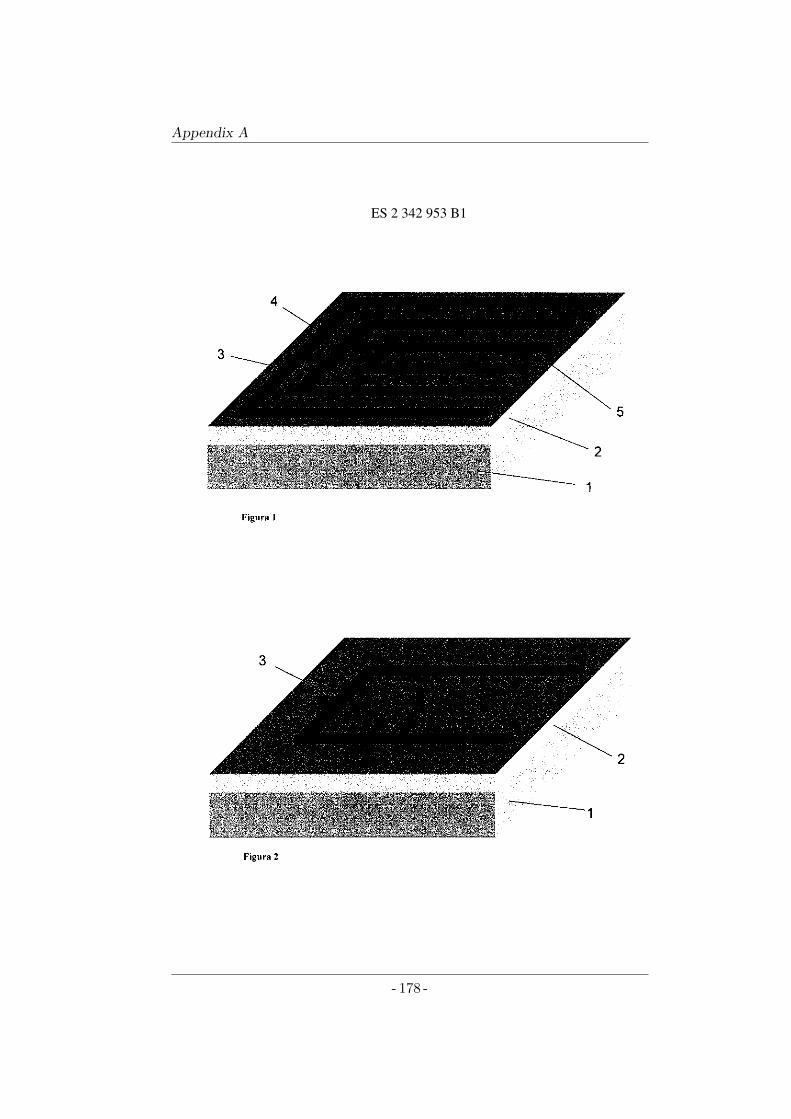
Appendix A
ES 2 342 953 B1
8
- 178 -
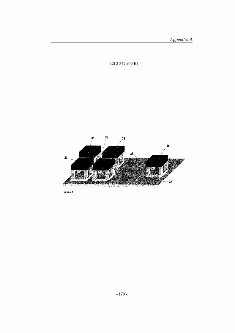
Appendix A
ES 2 342 953 B1
9
- 179 -
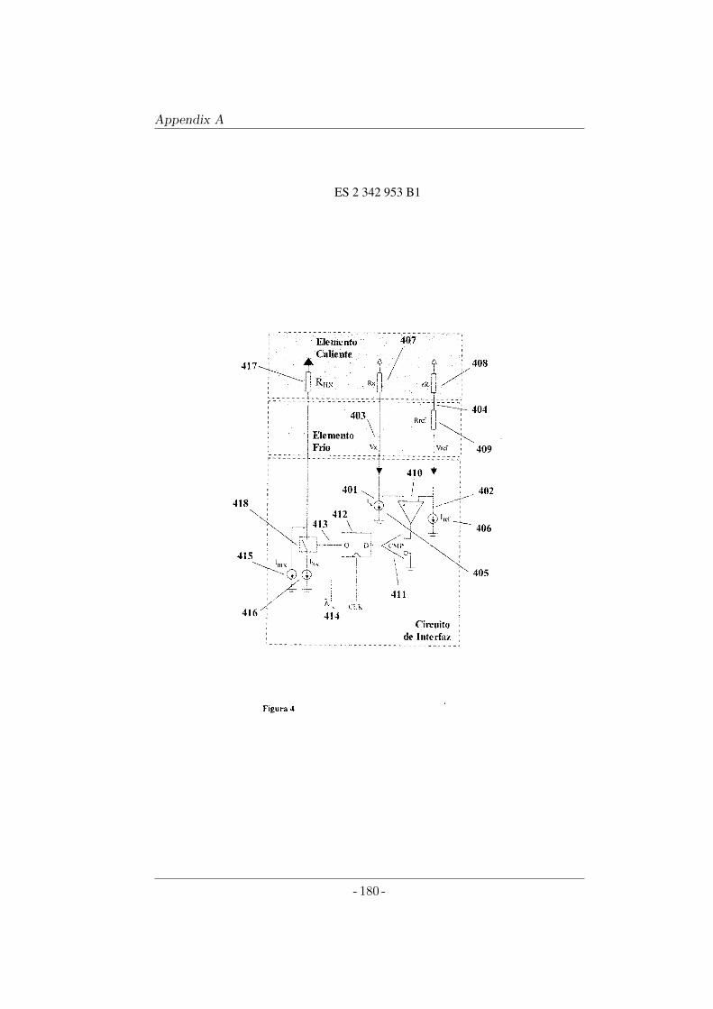
Appendix A
ES 2 342 953 B1
10
- 180 -
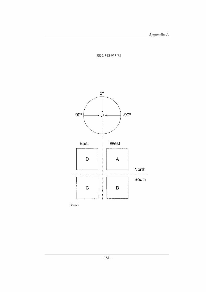
Appendix A
ES 2 342 953 B1
11
- 181 -
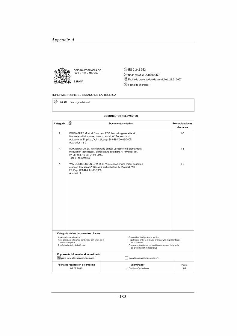
Appendix A
OFICINA ESPAÑOLA DEPATENTES Y MARCAS
ESPAÑA
11© ES 2 342 953
21© Nº de solicitud: 20070025922© Fecha de presentación de la solicitud: 25.01.2007
32© Fecha de prioridad:
INFORME SOBRE EL ESTADO DE LA TÉCNICA
51© Int. Cl.: Ver hoja adicional
DOCUMENTOS RELEVANTES
Categoría 56© Documentos citados Reivindicacionesafectadas
Categoría de los documentos citadosX: de particular relevanciaY: de particular relevancia combinado con otro/s de la
misma categoríaA: refleja el estado de la técnica
O: referido a divulgación no escritaP: publicado entre la fecha de prioridad y la de presentación
de la solicitudE: documento anterior, pero publicado después de la fecha
de presentación de la solicitud
El presente informe ha sido realizado
5 para todas las reivindicaciones para las reivindicaciones nº:
Fecha de realización del informe Examinador Página
05.07.2010 J. Cotillas Castellano 1/2
A DOMINGUEZ M. et al. "Low cost PCB thermal sigma-delta air 1-6flowmeter with improved thermal isolation". Sensors andActuators A: Physical, Vol. 121, pag. 388-394. 30-06-2005.Apartados 1 y 2.
A MAKINWA K. et al. "A smart wind sensor using thermal sigma-delta 1-6modulation techniques". Sensors and actuators A: Physical, Vol.97-98, pag. 15-20. 01-04-2002.Todo el documento.
A VAN OUDHEUSDEN B. W. et al. "An electronic wind meter based on 1-6a silicon flow sensor". Sensors and actuators A: Physical, Vol.22, Pag. 420-424. 01-06-1989.Apartado 2.
- 182 -

Appendix A
INFORME DEL ESTADO DE LA TÉCNICA Nº de solicitud: 200700259
CLASIFICACIÓN DEL OBJETO DE LA SOLICITUD
Informe del Estado de la Técnica (hoja adicional) Página 2/2
G01F 1/69 (2006.01)G01P 5/12 (2006.01)G01W 1/17 (2006.01)
- 183 -

Appendix B
A hot film anemometer for the Martian atmosphere
Journal Planetary and Space Science February 2008, Volume 56, Pages 1169-1179, DOI:10.1016 j.pss.2008.02.013
Manuel Domınguez-Pumar, Vicente Jimenez Serres, Jordi Ricart Campos, Lukasz Kowalski, Josefina Torres, Sara Navarro, Julio Romeral, Luis Castaner Munoz.
ATTENTION ¡ Pages 186 to 198 of the thesis, containing the text, are available
at the editor’s web http://www.sciencedirect.com/science/article/pii/S003206330800072X
185
Appendix C
Applications of hot film anemometry to space mis-sions
EUROSENSORS XXIII conference proceedings and opening plenary sessionDresden (Germany), 7-10 September 2008, ISBN 987-3-00-025217-4
Vicente Jimenez Serres,Manuel Domınguez-Pumar,Jordi Ricart Campos,Lukasz Kowalski,Sara Navarro,Josefina Torres,Julio Romeral,Jonathan Merrison,Luis Castaner Munoz.
199
Appendix D
Sensitivity analysis of the chip for REMS wind sen-sor
Poster for the 7th Spanish Conference on Electron Devices,Santiago de Compostela (Spain) 11-13 February 2009,* Best Poster Award.
Lukasz Kowalski,Jordi Ricart Campos,Vicente Jimenez Serres,Manuel Domınguez-Pumar,Luis Castaner Munoz.
207
Appendix D
- 208 -
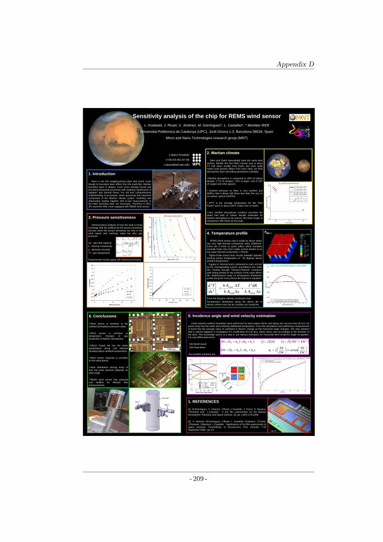
Appendix D
Sensitivity analysis of the chip for REMS wind sensorL. Kowlaski, J. Ricart, V. Jiménez, M. Domínguez*, L. Castañer*, * Member IEEE
Universitat
Politècnica
de Catalunya (UPC), Jordi
Girona
1-3, Barcelona 08034, Spain
Micro and Nano
Technologies research group (MNT)
Lukasz Kowalski
(+34) 93 401-67-66
1. Introduction
Mars is the first neighbourhood
plant with Earth. Even though its boundary layer differs from the Earth-like. Martian boundary layer is deeper, much more strongly forced and provoking dynamical processes with relatively significance of radiation and thermal fluxes. For full and comprehensive understanding of processes, which governing this important component of the Martian climate system, modeling and observation studies together with in-situ measurements in the lower boundary layer are necessary. Therefore in 2011 JPL launches MSL rover equipped with REMS wind sensor.
2. Martian climate
Mars and Earth interestingly have the same land surface. Beside this fact Mars volume size is about 7.5 half times smaller than Earth. But what really makes both planets differs from each other are their atmosphere layer describing parameters (climate):
•
Martian atmosphere is composed in: 95% of carbon dioxide, 2.7% of nitrogen, 1.6% of argon, only 0.13% of oxygen and other gasses.
•
Ambient pressure on Mars is very rarefied, just 600Pa, that is about 180 times less than the one on our planet, typical 1013hPa.
•
-87ºC is the average temperature for the “Red
Planet”
and it is about 100ºC colder than on Earth.
•
Very rarefied atmosphere condition provokes the
mean free path of carbon dioxide molecules for
Martian atmosphere to be around 100 times longer in comparison with Earth air free path.
P
Tk B
22
5. Incidence angle and wind velocity estimation
Finite element method simulation were performed for wind speed 10m/s and taking into account that all four hot points array has the same and uniformly distributed temperature.
From the simulations and preliminary measurement is found that the average value of coefficient h doesn’t change as the horizontal angle changes. The only variation that is noticed happens in revaluation of h coefficients for hot
dice, where these vary accordingly to the direction of the wind. This knowledge opens us a way to use various estimators for horizontal wind incidence angle recognition. For new differential terms :
NS=North-SouthEW=East-West
the possible solutions are:
1. REFERENCES
[1] M.Dominguez, V. Jimenez, J.Ricart, L.Kowalski, J. Torres, S. Navarro, J.Romeral
and L.Castañer
‘
A hot film anemometer for the Martian atmosphere’
Planetary and Space Science, 56, pp. 1169-1179,2008
[2] V. Jimenez, M.Dominguez, J.Ricart, L. Kowalski, S.Navarro, J.Torres, J.Romeral, J.Merrison, L.Castañer, ‘
Applications of hot film anemometry to space missions’
Proceedings of Eurosensors XXII, Dresden 7-10
September 2008 , pp.1-6
4. Temperature profile
REMS Wind sensor chip is made by silicon which has very high thermal conductivity value 150W/mK. Every die is fixed on pyrex pillars which insolates normally hotter dice from colder surface thanks to its low value thermal conductivity 1.1W/mK.
Sigma-Delta closed loop circuits maintain typically working sensor temperature on 30 degrees above ambient temperature.
Supply of thermal heat is delivered to each unit die by the corresponding current, according to the Joule law, floating through Titanium-Platinum resistance
path being printed on the surface of the each silicon die. Mathematical study on temperature distribution profile along the every silicon die lead as to equation:
From the Equation derives conclusion that:Temperature distribution along the silicon die is
almost uniform and can be consider as it would be.
6. Conclusions
•
Wind sensor is sensitive to the
rarefied atmosphere pressure value.
•
Wind sensor is sensitive to
temperature changes of gas
properties of Martian atmosphere.
•
Silicon based die has the same temperature along unit element
elevated above ambient temperature.
•
Wind sensor response is sensitive for the wind speed.
•
Heat distribution among array of four hot point element depends on
wind angle.
•
REMS wind sensor has potential
and abilities for Martian flow
measurements.
3. Pressure sensitiveness
Dimensionless analysis of how the heat is being exchange with the ambient by the forced convection process show the sensor sensitivity not only to the wind speed and overheat value but also gas
pressure:
Cp -
gas heat capacityk -
thermal conductivityμ
-
absolute
viscosityTf
–
gas temperature
Experimental results agree with dimensional theory
2
1
6
1
3
2
3
1
.
~664,0
Tf
kCpF
LR
MAreaD
TfPFDP
Tf
TfTfTf
const
Tfconstconv
xAk
dRI
xAk
TAh
dx
Td
condcond
conv
x
2
2
2
EW
NS
EW
NSfhhhhEW
EWNSfvhfvhhhhNS
vBADC
CBDA
arctan)(
)( 22
- 209 -

Appendix E
Contribution to advanced hot wire wind sensing
1st Barcelona Forum on Ph.D Research in Electronic Engineering,Barcelona (Spain), 16 October 2009, ISBN 978-84-7653-398-7.
Ph.D Student: Lukasz Kowalski,Thesis Advisor: Vicente Jimenez Serres.
211
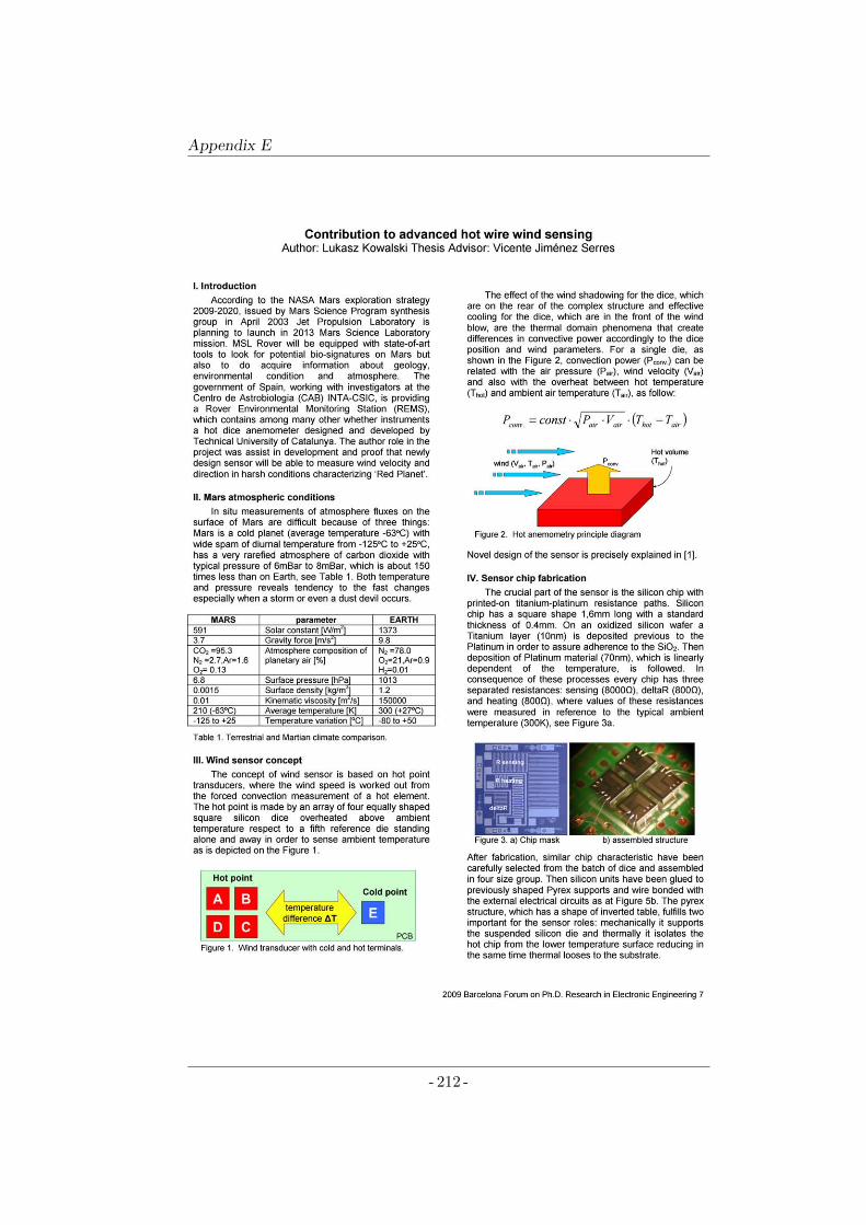
Appendix E
- 212 -
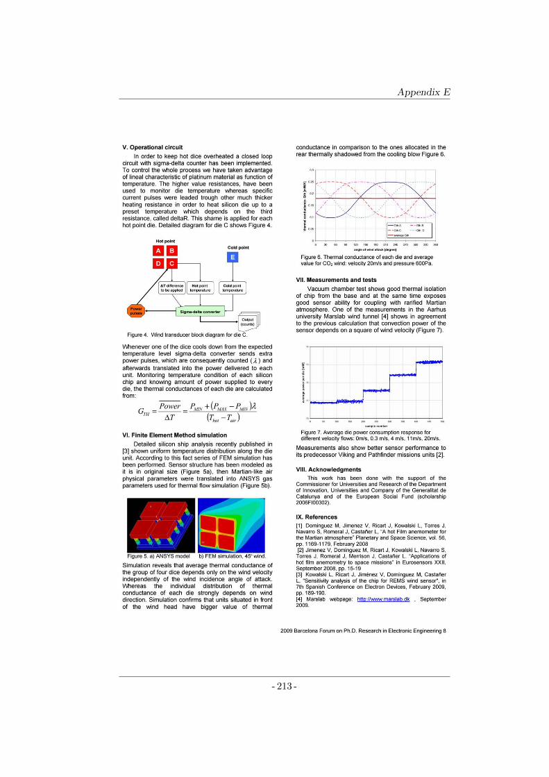
Appendix E
- 213 -

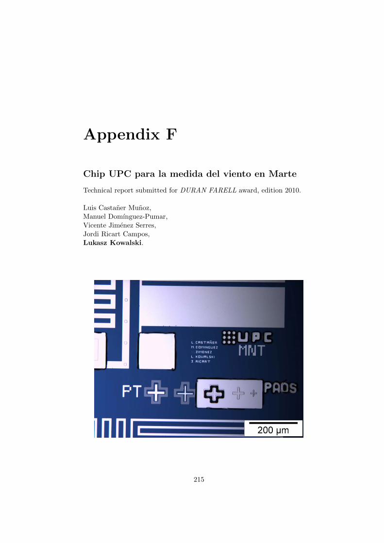
Appendix F
Chip UPC para la medida del viento en Marte
Technical report submitted for DURAN FARELL award, edition 2010.
Luis Castaner Munoz,Manuel Domınguez-Pumar,Vicente Jimenez Serres,Jordi Ricart Campos,Lukasz Kowalski.
215

Appendix F
CHIP UPC PARA LA MEDIDA DE VIENTO EN LA SUPERFICIE DE MARTE. TRABAJO PRESENTADO AL PREMI DURAN FARELL EDICIÓN 2010 1
Chip UPC para la medida del viento en MarteL. Castañer, M. Domínguez, V. Jimenez, J.Ricart y L.Kowalski
Grupo de Micro y nanotecnología (MNT),Departament d’Enginyería Electrónica, E.T.S.E.TelecomunicacióUniversitat Politècnica de Catalunya, Barcelona,e-mail: [email protected]
Abstract—Se presenta a la edición 2010 del Premi Duran Farelldel Consell Social de la Universitat Politècnica de Catalunyael trabajo de investigación desarrollado para la concepcióndiseño y fabricación de un chip que es el componentecrucial del sensor de viento para la estación meteorológicaREMS (http://msl-scicorner.jpl.nasa.gov/Instruments/REMS/)que equipa al rover de la misión MSL de laNASA MSL (http://marsprogram.jpl.nasa.gov/msl/)para la exploración de Marte para 2013(http://news.bbc.co.uk/2/hi/science/nature/8509080.stm)
REMS
I. OBJETIVOS PLANTEADOS
MARTE es el planeta mas cercano a la Tierra y seencuentra en otra fase de su evolución. Se conoce
que su atmósfera es muy ligera, con presiones atmosféricasentre 500Pa y 1000 Pa, está compuesta en su mayor partepor anhídrido carbónico (95,3%) y concentraciones pequeñasde nitrógeno, argón, oxigeno y otros gases. Al estar masalejado del Sol que la Tierra, su temperatura media es de -63oC oscilando entre 150K y 300K. Se conoce también que elcampo magnético es débil y no protege a la superficie de la laradiación. La baja densidad de la atmósfera hace que el caminolibre medio de las moléculas sea mas de cien veces mas largoque en la superficie de la Tierra y ademas las fluctuaciones decalor locales pueden producir cambios de temperatura grandesen pocossegundos.La investigación del planeta Marte tiene un interés cientí-fico extraordinario para entender su evolución, averiguar laspropiedades de su campo magnético, de la dinámica atmos-férica, los flujos de calor, la radiación solar en el visible,infrarrojo y ultravioleta y eventualmente saber si en ese planetase han dado actualmente o en el pasado condiciones parasoportar vida, tal como se entiende en la Tierra. Desde 1960en que se lanzó la misión Korabl 4 por la antigua USSR,hasta hoy se han lanzado 39 misiones a Marte, 22 de lascuales han sido declaradas fracaso. Ha habido cuatro landerscon éxito: Viking (1975), Pathfinder (1997), Mars explorationSpirit and Oportunity (2003) y Phoenix ( 2008). Las misionesa Marte han experimentado recientemente un gran impulso,al haberse descubierto la presencia de hielo de agua en susuperficie, lo que da pie a que las agencias espaciales seplanteen la programación de una misión tripulada. En esecontexto, el conocimiento de las condiciones de la atmósferadel planeta tanto en elevación como en superficie adquiere unagran relevancia. En particular, el viento es un gran desconocidotodavía porque, a pesar de que se conoce la existencia detormentas de polvo de dimensiones planetarias, existen muypocas medidas de esta variable meteorológica , prácticamente
la mayoría enviadas por la misión Viking en 1976 y otras, maslimitadas, por la misión Pathfinder en 1997.
El Proyecto REMS nació cuando la NASA invitó a Españaa participar en el proyecto MSL ( Mars Science Laboratory)aportando una estación meteorológica para ubicarla en elmástil del rover que será desplegado en la superficie de Marte.Esta participación tiene el nombre de REMS ( Remote Envi-ronmental Monitoring Station) . REMS está liderado por elCentro de Astrobiología (CAB), centro mixto entre el CSIC yel INTA, siendo su investigador principal Javier Gómez Elvira,en el que participan EADS-CRISA, el Finnish MeteorologicalInstitute y la Universitat Politécnica de Catalunya (UPC)e incorpora varios sensores: viento, infrarrojo, ultravioleta,presión, humedad, temperatura.
Como consecuencia de la experiencia del grupo investigadoren el desarrollo de sensores de caudal de aire y agua , elprimer Investigador principal del Proyecto REMS, Prof. LuisVazquez de la UCM, ofreció la participación en el desarrollode un sensor de viento para REMS.
El objetivo concreto fue la medida de intensidad y direccióndel viento en la superficie de Marte dentro de las limitacionesde tamaño, peso y consumo de potencia que impone la misión.En el proyecto REMS , la integración de la estación meteo-rológica la lidera EADS-CRISA y la fórmula de participacióndel grupo investigador fue a través de un subcontrato desuministro de los chips que se describen mas abajo para los tresmodelos contemplados: el modelo de ingeniería , el modelode calificación y el modelo de vuelo. Asímismo el trabajoasignado a la UPC consistió en el diseño conceptual y lavalidación del front-end electrónico en la fase del modelode ingeniería de manera que pudiera trasladarse a un circuitoespecífico ASIC, responsabilidad de EADS-CRISA.
II. RESULTADOS OBTENIDOS
LA misión Viking fue la primera que midió la velocidady dirección del viento en la superficie de Marte usando
un anemómetro térmico basado en una película de platinoy trabajando en modo de temperatura constante (CTA). Masde 20 años después, en 1997 el rover de Pathfinder midiódirección del viento usando un anemómetro también térmicopero usando el modo de potencia constante (CPA) y tambiénanalizando las imágenes tomadas de unas mangas anemométri-cas tomadas por una cámara. La misión Beagle2 llevaba unanemómetro térmico también pero la misión fracasó. Final-mente la misión Phoenix utilizó una veleta miniatura paraobservar también el efecto del viento mediante una cámara.Existen otros métodos de medida, a parte del térmico, pero
- 217 -
Appendix F
CHIP UPC PARA LA MEDIDA DE VIENTO EN LA SUPERFICIE DE MARTE. TRABAJO PRESENTADO AL PREMI DURAN FARELL EDICIÓN 2010 2
Fig. 1. Espacio de diseño del chip UPC comparado con Viking y Pathfinder.el eje vertical es el número de Knudsen y el horizontal es la figura de méritoPotencia/ sobretemperatura . Cuando mas abajo y a la izquierda, mejor sonlas condiciones de funcionamiento. Los datos de la Figura han sido extraidosde la publicación:
no son tan adecuados para las misiones espaciales , ya seaporque consumen mas potencia como los de ion-drift o ,porquenecesitan de partículas en suspensión como los basados enláser.
La experiencia anterior nos dice que la medida de vientoen la superficie de Marte no es un asunto trivial por la bajapresión, gran rango de variación de temperatura y la presenciade polvo en ocasión de tormentas. La baja presión es unaspecto que condiciona el diseño del sensor porque el caminolibre medio de las moléculas, que también depende de la tem-peratura, es grande. Por tanto, las dimensiones del dispositivono pueden ser muy pequeñas en comparación con él para queexista interacción suficiente. Esto se mide mediante el cono-cido número de Knudsen que es precisamente el cociente entreel camino libre medio y la longitud característica del sensor.Este número, para que se pueda considerar la aproximaciónde medio continuo, debe ser inferior a 0.01 típicamente. Estolleva a que la dimensión característica del sensor debe situarsepor encima de un milímetro. Simultáneamente, un sensor quese basa en un principio térmico no puede hacerse excesiva-mente grande porque se precisará una potencia elevada paracalentarlo superando los límites energéticos del instrumento.Otro punto muy importante en el diseño del sensor es que,debido a la poca interacción por la baja presión, las perdidas decalor por conducción hacia los soportes son comparativamentealtas y es preciso reducirlas al máximo. Reuniendo ambasrestricciones , el grupo investigador ubicó el diseño del sensordel chip UPC en el proyecto REMS en una zona operativa masfavorable que los diseños anteriores de Viking y Pathfindercomo se ve en la Figura 1.
El componente crucial en el sensor de viento es el ’chipUPC’ que ha sido desarrollado y fabricado íntegramente enel Laboratorio ’Sala Blanca’ del grupo de Micro y Nanotec-nologias (MNT) del Departament d’Enginyeria Electronica,de la ETSETB de Barcelona de la Universitat Politècnica de
Catalunya.En nuestro conocimiento, es el primer chip íntegramente dis-eñado y fabricado en España que equipa una misión científicapara la superficie del planeta Marte. El chip UPC lleva grabadoen su superficie los nombres de los miembros del equipoinvestigador y el logo del grupo de investigación.
A. Antecedentes
Este desarrollo se encuadra dentro de las actividades ini-ciadas por el grupo investigador en el año 1994 cuando,mediante financiación del Programa GAME ( Grupo Activadorde la Microelectrónica en España), desarrolló un sensor deflujo pensado para la medica de caudal de agua y de gaspara el sector del electrodoméstico en colaboración con elGrupo Mondragón Corporación Cooperativa. El concepto de-sarrollado entonces se basó en el principio de anemometríatérmica ampliamente usado hasta entonces para la medida decaudales en el sector aeroespacial, médico y meteorológico.Este principio, bien conocido, consiste en la medida indirectade la velocidad de un fluido en movimiento a partir dela medida de las pérdidas por convección de un elementocaliente.La experiencia acumulada en la aplicación al sector delelectrodoméstico, permitió al grupo investigador integrarse enel Proyecto REMS en 2006.
El presente chip UPC supone un hito en los dispositivos demedida de viento en una atmósfera rarificada como es la delPlaneta Marte. Aunque el principio de funcionamiento siguesiendo la anemometría térmica , este diseño es totalmentenuevo incorporando una serie de propiedades y característicasque lo hacen adecuado para la medida en condiciones de bajapresión ( 6-12 mbar) y baja temperatura ( 200K-300K).
B. Descripción del diseño del chip UPC
El dispositivo se compone de un chip de siliciomonocristalino de 1.6 mm de lado y 400 micras deespesor en cuya superficie se encuentran grabadas tresresistencias de película delgada de Titanio-Platino de tresvalores nominales distintos. Una de éstas resistencias, cuandoestá excitada por una corriente eléctrica, se usa para calentar,por efecto Joule, el chip. Como consecuencia del elevadovalor de la conductividad térmica del silicio, la temperaturaes prácticamente homogénea en todo el volumen. La segundaresistencia de platino se utiliza para medir la temperatura y latercera resistencia se utiliza en el circuito para introducir undesequilibrio controlado en el puente de medida diferencialque impone una diferencia de temperatura constante con elambiente.
Una peculiaridad importante que se ha utilizado en estediseño consiste en que las tres resistencias son de una películade platino y por consiguiente son fabricadas simultáneamente.El platino sirve tanto como elemento calefactor en la primeraresistencia como de elemento sensor en la segunda por que estematerial tiene una resistividad que depende de forma linealcon la temperatura en un amplio rango. En otros diseños seutiliza la misma resistencia para calentar y para medir , lo
- 218 -
Appendix F
CHIP UPC PARA LA MEDIDA DE VIENTO EN LA SUPERFICIE DE MARTE. TRABAJO PRESENTADO AL PREMI DURAN FARELL EDICIÓN 2010 3
que obliga a multiplexar la función de la resistencia. La opciónadoptada por el grupo investigador independiza los circuitos deseñal y de potencia y es viable al poder integrarse resistenciasdel orden del kilo-ohmio en superficies pequeñas como lasnecesarias en este proyecto.
En la Figura 2 se ve una fotografia del chip en su superficiefrontal donde se ven las tres resistencias y los PAD’s deconexión al exterior. Asimismo, en la parte inferior derechase ve el logo del grupo investigador MNT y los nombres delos cinco investigadores. Esta parte está ampliada en la Figura3.
Fig. 2. Fotografia de la superficie del chip donde se ven las tres resistenciasen forma de serpentines
C. Fabricación
En la Figura 4 se ve una sección transversal del chip endonde se ve que sobre un sustrato de silicio se realiza una
Fig. 3. Ampliación de la fotografia de la superficie del chip donde se venlos nombres del equipo investigador
oxidación térmica para crecer un óxido electricamente aislantede unos 200nm de espesor sobre el que se deposita una rsinafotosensible que se graba con los dibujos correspondientes ala máscara de las resistencias y se revela. A continuación sedeposita una película muy fina de titanio cuya misión es pro-porcionar adherencia a la pelicula de platino que se deposita acontinuación. Se procede a disolver la resina de forma que lasresistencias quedan grabadas mediante la técnica de lift-off.El último paso consiste en soldar los terminales eléctricos.Se han fabricado un total de 1000 de estos dispositivos y
Fig. 4. Esquema de la sección transversal
sus caracteristicas ( valor de las tres resistencias ) han sidoindividualmente medidos para proceder al apareamiento de loschips con características mas parecidas. El laboratorio dondese han fabricado se conoce con el nombre de ’Sala Blanca’porque fue la primera que se construyó en la UniversitatPolitècnica de Catalunya antes de la existencia del CampusNord. En ese Laboratorio se reunen un conjunto de equiposde fabricación de muestras incluyendo equipos de difusión yoxidación térmica, fotolitografía óptica, deposito de materialespor sputtering, plasma y evaporación térmica.
Fig. 5. Esquema de los pasos tecnológicos de fabricación
- 219 -
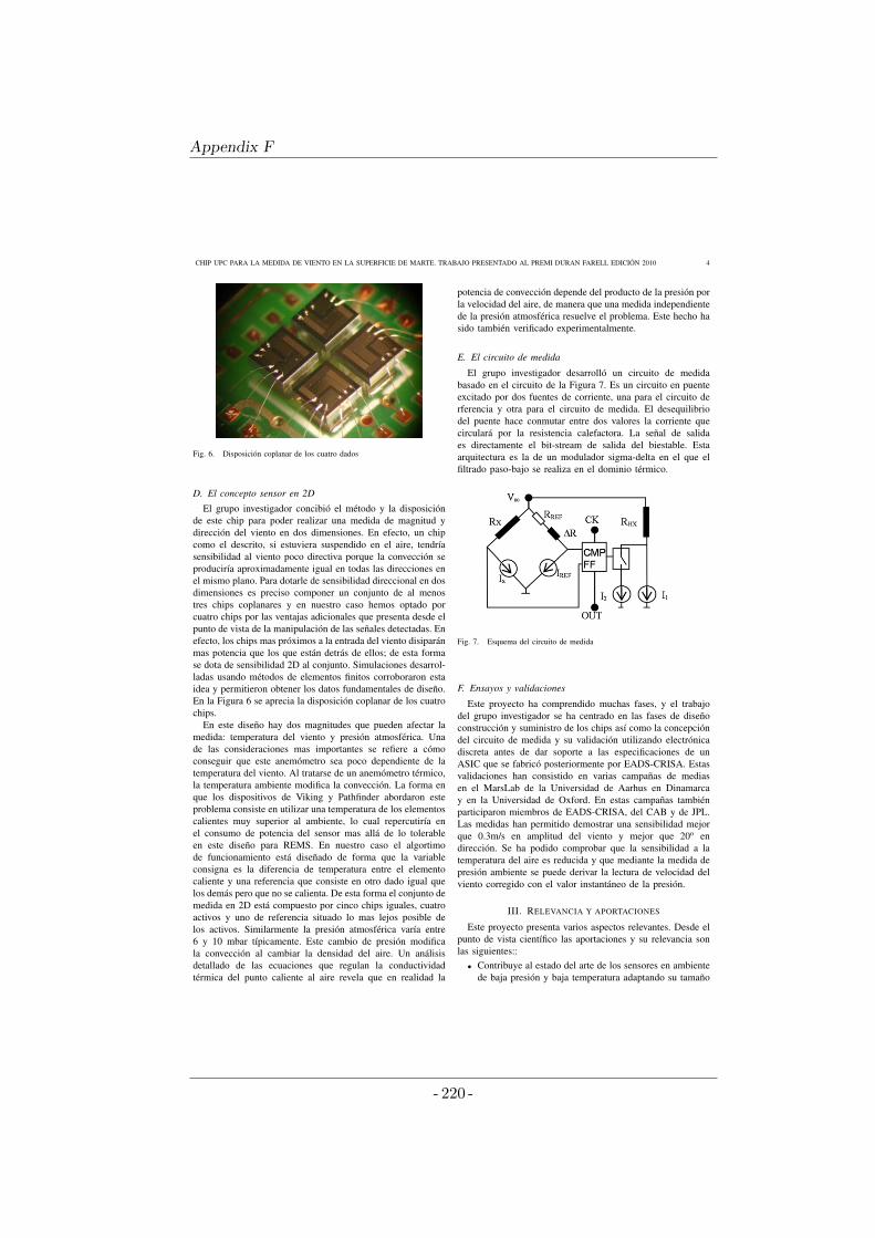
Appendix F
CHIP UPC PARA LA MEDIDA DE VIENTO EN LA SUPERFICIE DE MARTE. TRABAJO PRESENTADO AL PREMI DURAN FARELL EDICIÓN 2010 4
Fig. 6. Disposición coplanar de los cuatro dados
D. El concepto sensor en 2D
El grupo investigador concibió el método y la disposiciónde este chip para poder realizar una medida de magnitud ydirección del viento en dos dimensiones. En efecto, un chipcomo el descrito, si estuviera suspendido en el aire, tendríasensibilidad al viento poco directiva porque la convección seproduciría aproximadamente igual en todas las direcciones enel mismo plano. Para dotarle de sensibilidad direccional en dosdimensiones es preciso componer un conjunto de al menostres chips coplanares y en nuestro caso hemos optado porcuatro chips por las ventajas adicionales que presenta desde elpunto de vista de la manipulación de las señales detectadas. Enefecto, los chips mas próximos a la entrada del viento disiparánmas potencia que los que están detrás de ellos; de esta formase dota de sensibilidad 2D al conjunto. Simulaciones desarrol-ladas usando métodos de elementos finitos corroboraron estaidea y permitieron obtener los datos fundamentales de diseño.En la Figura 6 se aprecia la disposición coplanar de los cuatrochips.
En este diseño hay dos magnitudes que pueden afectar lamedida: temperatura del viento y presión atmosférica. Unade las consideraciones mas importantes se refiere a cómoconseguir que este anemómetro sea poco dependiente de latemperatura del viento. Al tratarse de un anemómetro térmico,la temperatura ambiente modifica la convección. La forma enque los dispositivos de Viking y Pathfinder abordaron esteproblema consiste en utilizar una temperatura de los elementoscalientes muy superior al ambiente, lo cual repercutiría enel consumo de potencia del sensor mas allá de lo tolerableen este diseño para REMS. En nuestro caso el algortimode funcionamiento está diseñado de forma que la variableconsigna es la diferencia de temperatura entre el elementocaliente y una referencia que consiste en otro dado igual quelos demás pero que no se calienta. De esta forma el conjunto demedida en 2D está compuesto por cinco chips iguales, cuatroactivos y uno de referencia situado lo mas lejos posible delos activos. Similarmente la presión atmosférica varía entre6 y 10 mbar típicamente. Este cambio de presión modificala convección al cambiar la densidad del aire. Un análisisdetallado de las ecuaciones que regulan la conductividadtérmica del punto caliente al aire revela que en realidad la
potencia de convección depende del producto de la presión porla velocidad del aire, de manera que una medida independientede la presión atmosférica resuelve el problema. Este hecho hasido también verificado experimentalmente.
E. El circuito de medida
El grupo investigador desarrolló un circuito de medidabasado en el circuito de la Figura 7. Es un circuito en puenteexcitado por dos fuentes de corriente, una para el circuito derferencia y otra para el circuito de medida. El desequilibriodel puente hace conmutar entre dos valores la corriente quecirculará por la resistencia calefactora. La señal de salidaes directamente el bit-stream de salida del biestable. Estaarquitectura es la de un modulador sigma-delta en el que elfiltrado paso-bajo se realiza en el dominio térmico.
Fig. 7. Esquema del circuito de medida
F. Ensayos y validaciones
Este proyecto ha comprendido muchas fases, y el trabajodel grupo investigador se ha centrado en las fases de diseñoconstrucción y suministro de los chips así como la concepcióndel circuito de medida y su validación utilizando electrónicadiscreta antes de dar soporte a las especificaciones de unASIC que se fabricó posteriormente por EADS-CRISA. Estasvalidaciones han consistido en varias campañas de mediasen el MarsLab de la Universidad de Aarhus en Dinamarcay en la Universidad de Oxford. En estas campañas tambiénparticiparon miembros de EADS-CRISA, del CAB y de JPL.Las medidas han permitido demostrar una sensibilidad mejorque 0.3m/s en amplitud del viento y mejor que 20o endirección. Se ha podido comprobar que la sensibilidad a latemperatura del aire es reducida y que mediante la medida depresión ambiente se puede derivar la lectura de velocidad delviento corregido con el valor instantáneo de la presión.
III. RELEVANCIA Y APORTACIONES
Este proyecto presenta varios aspectos relevantes. Desde elpunto de vista científico las aportaciones y su relevancia sonlas siguientes::
• Contribuye al estado del arte de los sensores en ambientede baja presión y baja temperatura adaptando su tamaño
- 220 -
Appendix F
CHIP UPC PARA LA MEDIDA DE VIENTO EN LA SUPERFICIE DE MARTE. TRABAJO PRESENTADO AL PREMI DURAN FARELL EDICIÓN 2010 5
y consumo de potencia a los requisitos de ésta y otrasmisiones espaciales.
• Modifica el concepto habitual de ’hilo caliente’ e inclusode’ pelicula fina caliente’ dando paso al concepto devolumen isotérmico, nunca usado con anterioridad en elespacio.
• Aplica el método de conversión digital de modulaciónsigma-delta a un sistema trabajando simultáneamente enel dominio térmico y en el dominio eléctrico. Tambiénaplicado por primera vez en este tipo de misiones.
• El concepto de un algoritmo que trabaje en modo dediferencia de temperatura constante (CTDA), es tambiénnuevo y mejora la respuesta estacionaria y dinámica delos modos CTA y CPA anteriormente usados.
• El concepto de sensor bidimensional, basado en cua-tro chips colocados en el mismo plano y el algoritmodiferencial de lectura de las componentes longitudinalesy transversales, es original de este proyecto y tiene larelevancia de poder cancelar errores comunes en laslecturas individuales y dar sensibilidad angular dentro delas especificaciones. Es un concepto nuevo que no ha sidousado antes.
Desde el punto de vista técnico las aportaciones y su relevanciason las siguientes:
• Primer chip totalmente diseñado y fabricado en Españaque equipa una misión espacial a Marte.
• Fabricación de mas de 1000 chips y apareamiento de suscaracterísticas. Es un logro en un medio universitario.
• Sensibilidad de lectura de velocidad de viento de 0.3 m/s• Rango de lectura de 1m/s a 70 m/s, superior a los rangos
de medida de Viking y de Pathfinder• Sensibilidad de dirección 10o y discriminación de cuad-
rante. Por ejemplo la misión Viking precisó un sensoradicional de detección de cuadrante.
• Consumo de potencia por chip de 1mW/K muy pordebajo de los de Viking y Pathfinder.
Desde el punto de vista económico y social las aportacionesy su relevancia son las siguientes:
• Las misiones espaciales tienen un gran atractivo social,las personas perciben estos proyectos como algo com-plejo, espectacular que precisa de un conocimiento téc-nico y científico sofisticado y que muchas veces permitea la humanidad entender mejor el universo. Si bien esteproyecto es una parte minúscula del esfuerzo en la ex-ploración espacial, nuestra sociedad lo acaba percibiendocomo algo mas cercano ( como cuando hay un astronautaespañol por ejemplo), y que podemos contribuir mas ymejor.
• Este proyecto contribuye a estimular el interés por laciencia y la tecnología en los mas jóvenes que están enfase de descubrir su vocación y objetivos profesionales.
• Ha tenido una amplia repercusión mediática como con-secuencia de los puntos anteriores y porque, además, elchip lleva grabados los nombres de sus inventores queserán, quizá, los primeros nombres de españoles ( y deun polaco que forma parte del equipo) que se posarán enMarte.
• El mercado espacial es muy competitivo y la presenciaespañola en el mismo puede verse incrementada.
• Estos proyectos ofrecen a los que trabajan en ellos , untrabajo de calidad, desafiante intelectual y técnicamente.
IV. CONTINUIDAD DEL TRABAJO
Como consecuencia de este desarrollo, el grupo investigadorestá desarrollando las etapas preliminares de un nuevo sensorde viento para la superficie de Marte también pero esta vez enla misión MetNet (http://europlanet.fmi.fi/MetNet/index.php,http://metnet.fmi.fi/index.php) y en la parte españolacorrespondiente que es el proyecto MEIGA (www.fdi.ucm.es/profesor/lvazquez/meiga/meigaMetNet.html)La misión MEIGA (Mars Environmental Instrumentationfor Ground and Atmosphere) es un proyecto del Ministeriode Ciencia e Innovación (AYA2008-06420-C04-01/ESP). Lamisión forma parte del proyecto MetNet (MeteorologicalNetwork) en el que participan personal científico y técnicode Finlandia (Finnish Meteorological Institute (FMI)), quelidera el proyecto, de Rusia (Lavochkin Association (LA)y Russian Space Research Institute (IKI)) y de España(Instituto Nacional de Técnica Aeroespacial (INTA)). Eldirector científico del proyecto es el profesor Luis Vázquezde la Universidad Complutense de Madrid. El objetivoconsiste en desplegar 16 estaciones meteorológicas fijas endistintos puntos del planeta que enviarían sus datos a unanave en órbita. El nuevo sensor de viento equiparía a las 16estaciones. Con anterioridad se lanzará una misión precursoraque no llevará sensor de viento pero si de radiación solar ensu lugar.
Es de destacar que este tipo de instrumentos de vuelo hansido frecuentemente desarrollados en laboratorios universitar-ios: el sensor de viento para Viking fue desarrollado en laUniversidad de Washington, el sensor de viento para Beagle2en la Universidad de Oxford (UK) y el sensor de presión yhumedad para REMS y MetNet en el Finnish MeteorologicalInstitute. Esto es posible porque se precisan pocas unidadesen general, pero calibradas y verificadas individualmente, conlo que la producción en serie queda descartada. Esto da unaventaja competitiva importante para los grupos que tienen yaexperiencia en dispositivos de vuelo en su trayectoria. En elcaso del grupo investigador los laboratorios disponibles sonflexibles y permiten adaptarse mejor a este tipo de proyectosque un centro de mayor tamaño actuando como centro deservicios.
La visibilidad que ha dado el proyecto REMS tambiénha dado frutos en otro sensor espacial, concretamente unsensor de posición del sol de alta precisión cuyo desarrolloha liderado la Universidad de Sevilla y el chip que lleva hasido fabricado también por el grupo investigador de la UPC.Este sensor equipa el Nanosat 1B del INTA y ha sido lanzadorecientemente.
V. PROCEDENCIA DE LOS FONDOS DE FINANCIACIÓN
El proyecto REMS ha sido financiado por el Ministerio deCiencia e Innovación a través del CDTI, el Plan Nacionalde I+D+i y el Ministerio de Defensa a través del Instituto
- 221 -
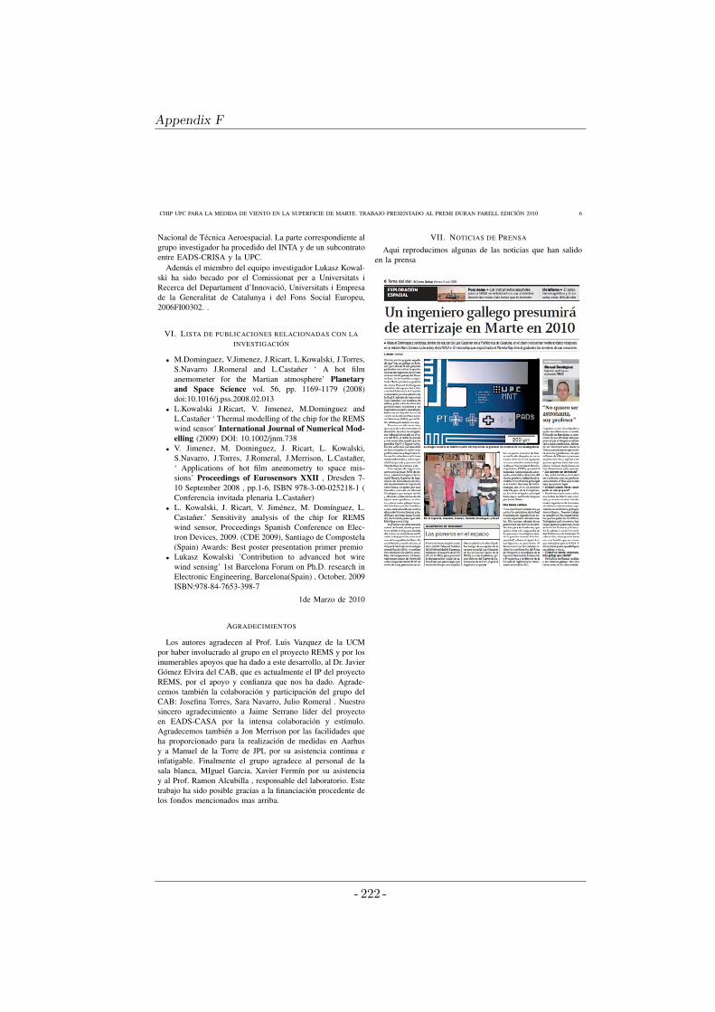
Appendix F
CHIP UPC PARA LA MEDIDA DE VIENTO EN LA SUPERFICIE DE MARTE. TRABAJO PRESENTADO AL PREMI DURAN FARELL EDICIÓN 2010 6
Nacional de Técnica Aeroespacial. La parte correspondiente algrupo investigador ha procedido del INTA y de un subcontratoentre EADS-CRISA y la UPC.
Además el miembro del equipo investigador Lukasz Kowal-ski ha sido becado por el Comissionat per a Universitats iRecerca del Departament d’Innovació, Universitats i Empresade la Generalitat de Catalunya i del Fons Social Europeu,2006FI00302. .
VI. LISTA DE PUBLICACIONES RELACIONADAS CON LAINVESTIGACIÓN
• M.Dominguez, V.Jimenez, J.Ricart, L.Kowalski, J.Torres,S.Navarro J.Romeral and L.Castañer ‘ A hot filmanemometer for the Martian atmosphere’ Planetaryand Space Science vol. 56, pp. 1169-1179 (2008)doi:10.1016/j.pss.2008.02.013
• L.Kowalski J.Ricart, V. Jimenez, M.Dominguez andL.Castañer ‘ Thermal modelling of the chip for the REMSwind sensor’ International Journal of Numerical Mod-elling (2009) DOI: 10.1002/jnm.738
• V. Jimenez, M. Dominguez, J. Ricart, L. Kowalski,S.Navarro, J.Torres, J.Romeral, J.Merrison, L.Castañer,‘ Applications of hot film anemometry to space mis-sions’ Proceedings of Eurosensors XXII , Dresden 7-10 September 2008 , pp.1-6, ISBN 978-3-00-025218-1 (Conferencia invitada plenaria L.Castañer)
• L. Kowalski, J. Ricart, V. Jiménez, M. Domínguez, L.Castañer.’ Sensitivity analysis of the chip for REMSwind sensor, Proceedings Spanish Conference on Elec-tron Devices, 2009. (CDE 2009), Santiago de Compostela(Spain) Awards: Best poster presentation primer premio
• Lukasz Kowalski ’Contribution to advanced hot wirewind sensing’ 1st Barcelona Forum on Ph.D. research inElectronic Engineering, Barcelona(Spain) , October, 2009ISBN:978-84-7653-398-7
1de Marzo de 2010
AGRADECIMIENTOS
Los autores agradecen al Prof. Luis Vazquez de la UCMpor haber involucrado al grupo en el proyecto REMS y por losinumerables apoyos que ha dado a este desarrollo, al Dr. JavierGómez Elvira del CAB, que es actualmente el IP del proyectoREMS, por el apoyo y confianza que nos ha dado. Agrade-cemos también la colaboración y participación del grupo delCAB: Josefina Torres, Sara Navarro, Julio Romeral . Nuestrosincero agradecimiento a Jaime Serrano líder del proyectoen EADS-CASA por la intensa colaboración y estímulo.Agradecemos también a Jon Merrison por las facilidades queha proporcionado para la realización de medidas en Aarhusy a Manuel de la Torre de JPL por su asistencia continua einfatigable. Finalmente el grupo agradece al personal de lasala blanca, MIguel Garcia, Xavier Fermín por su asistenciay al Prof. Ramon Alcubilla , responsable del laboratorio. Estetrabajo ha sido posible gracias a la financiación procedente delos fondos mencionados mas arriba.
VII. NOTICIAS DE PRENSA
Aqui reproducimos algunas de las noticias que han salidoen la prensa
- 222 -
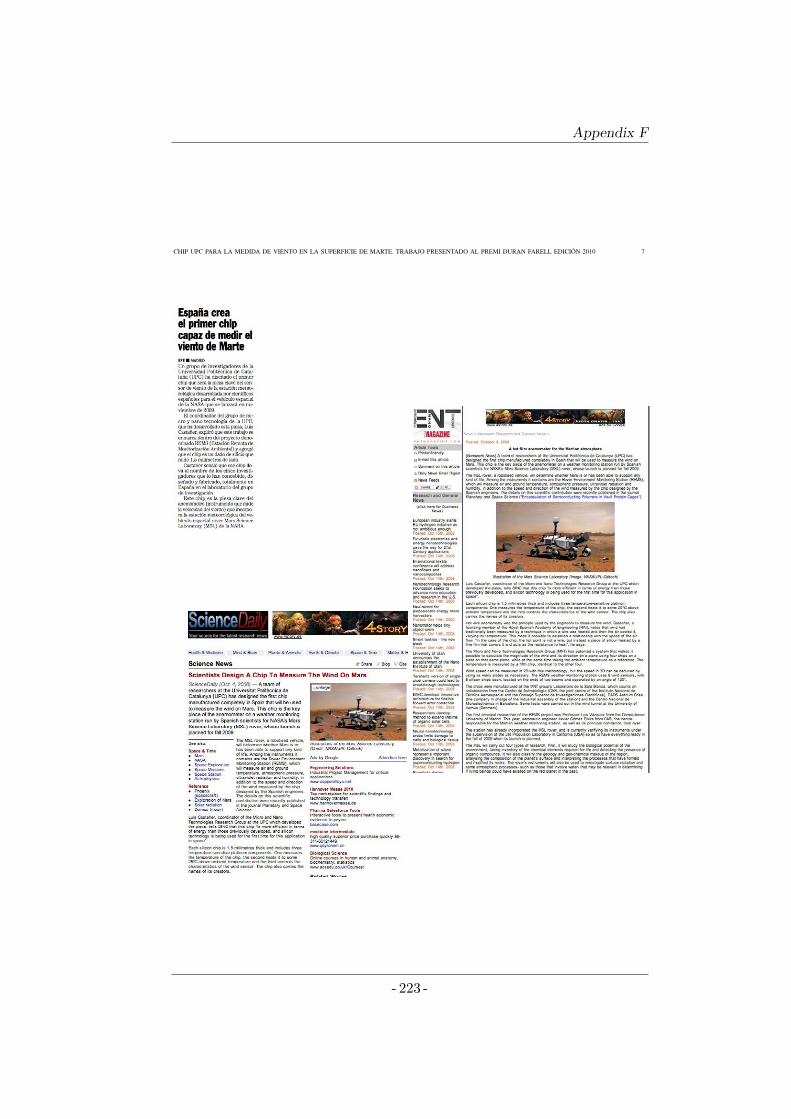
Appendix F
CHIP UPC PARA LA MEDIDA DE VIENTO EN LA SUPERFICIE DE MARTE. TRABAJO PRESENTADO AL PREMI DURAN FARELL EDICIÓN 2010 7
- 223 -
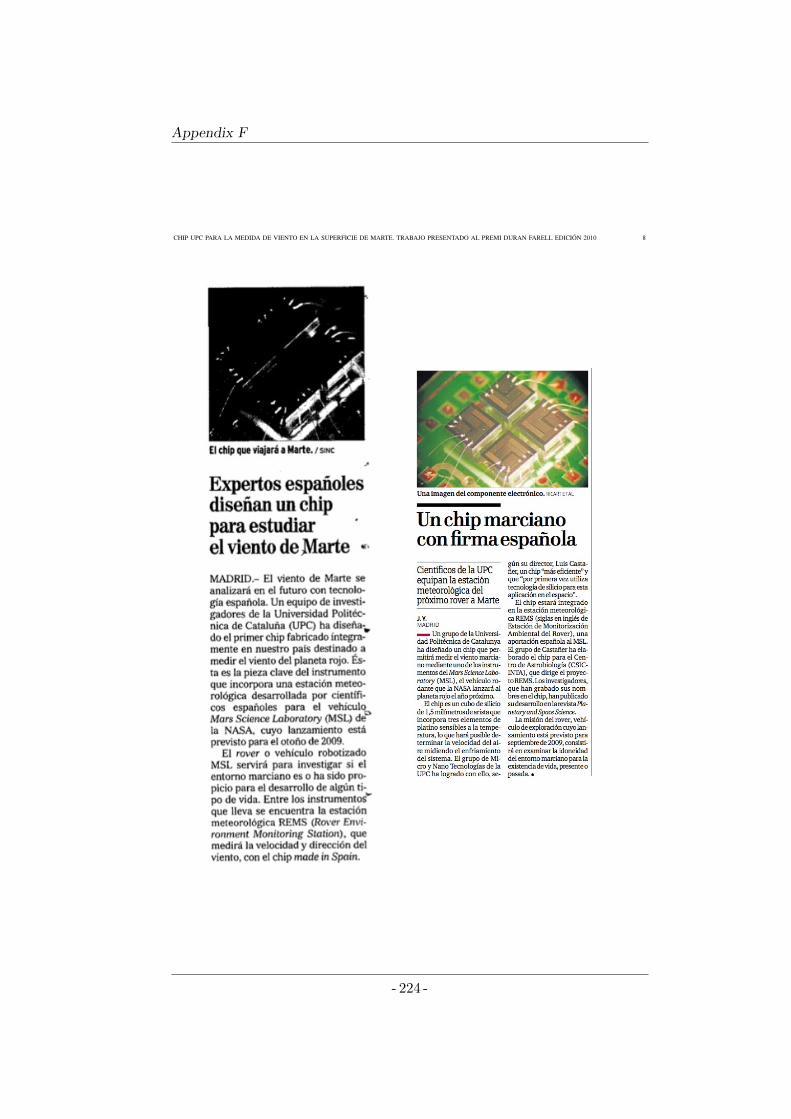
Appendix F
CHIP UPC PARA LA MEDIDA DE VIENTO EN LA SUPERFICIE DE MARTE. TRABAJO PRESENTADO AL PREMI DURAN FARELL EDICIÓN 2010 8
- 224 -
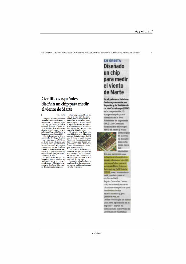
Appendix F
CHIP UPC PARA LA MEDIDA DE VIENTO EN LA SUPERFICIE DE MARTE. TRABAJO PRESENTADO AL PREMI DURAN FARELL EDICIÓN 2010 9
- 225 -

Appendix G
Thermal modelling of the chip for the REMS wind sensor
International Journal of Numerical Modelling: Electronic Networks, Devices and Fields; Special Issue on the 7th Spanish Conference on Electron Devices, July 2010, Volume 23, Issue 4-5, Pages 340-353, DOI:10.1002/jnm.v23:4/5.
Lukasz Kowalski, Jordi Ricart Campos, Vicente Jimenez Serres, Manuel Domınguez-Pumar, Luis Castaner Munoz.
ATTENTION ¡ Pages 228 to 242 of the thesis, containing the text, are available
at the editor’s web http://onlinelibrary.wiley.com/doi/10.1002/jnm.738/abstract
227
Appendix H
Multiphysics simulation of REMS hot-film anemome- ter under typical Martian atmosphere conditions
Proceeding of the COMSOL 2010 conference, Paris (France), 17-19 November 2010.
Lukasz Kowalski, Luis Castaner Munoz, Manuel Domınguez-Pumar, Vicente Jimenez Serres.
ATTENTION ¡ Pages 244 to 248 of the thesis, unpublished here by copyright, can
be found in the copy of the thesis which is preserved in the UPC Archive.
Appendix I
Hypobaric chamber for wind sensor testing in Mar- tian conditions
Proceedings and Poster of the 8th Spanish Conference on Electron Devices, Palma de Mallorca (Spain), 8-11 February 2011, DOI:10.1109/SCED.2011.5744212, *Best Poster Award.
Lukasz Kowalski, Miguel Garcia Molina.
ATTENTION ¡ Pages 250 to 253 of the thesis, containing the text, are available at
the editor’s web
http://ieeexplore.ieee.org/xpls/abs_all.jsp?arnumber=5744212&tag=1
249
Appendix I
- 254 -
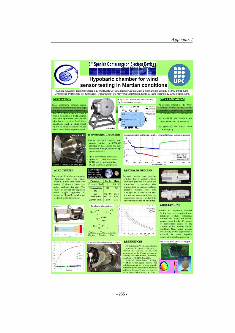
Appendix I
Hypobaric chamber for windsensor testing in Martian conditions
VACUUM SYSTEM
Appropriate exhaust of the 0,6m3
interior volume of the vacuumchamber is provided by connectedin chain two stage vacuum system:
a) Leybold TRIVAC D65BCS two-stage rotary vane vacuum pump
b) Leybold RUVAC WS-251 rootsvacuum pump
b)
a)
HYPOBARIC CHAMBER
Standard horizontal stainless steelvacuum chamber type CA3050Sprovided by K.J. Lesker has beencustomized through additional QFport manufacture.
• QF40 gas entrance and exhaust• QF100 and QF63 electrical feed• QF160 and view-port window• QF250 tapped not yet specified
Lukasz Kowalski [email protected] (+34)9340154585, Miguel Garcia Molina [email protected] (+34)9340154202
Universitat Politècnica de Catalunya, Departament d‘Enginyeria Electrònica, Micro & NanoTechnology Group, Barcelona
MOTIVATION
Space exploration program growswhat rises unprecedented challengefor appropriate sensor engineering.For MNT-UPC engineering group itwas a motivation to build simplerand more operational wind tunnelchamber to reproduce MARS-likeconditions which in future wouldenable us proof of concept for thenovel sensor in development phase.
MarsLab-UPC
CA3050S
REYNOLDS NUMBER
Reynolds number value describeswhether flow is laminar with nodisruption between the layers andstreamlines or turbulent flowcharacterized by chaotic, stochasticproperty changes flow lines.Although not as cold as on Marsand not the same atmospheric gascomposition but we reproduced thesame dimensionless Re parameter.
CONCLUSIONS
Marslab-UPC hypobaric chamberfacility has been completed withcommonly available commercialelements and refurbished vacuumsystem pumps. It takes 15 minutesto depressurize interior of thechamber for low pressure Martianconditions. Using smart pressureand velocity product adjustment weachieved the same Reynoldsnumber dimensionless parameter.
WIND TUNNEL
For our specific design we acquirededucational mini wind tunnelWTM-1000 with tube shape crosssection of diameter 10cm andhighly uniform flow-rate. Thisenable us through the adjustablepower supply regulation forsetting up desirable wind speedproduced by DC fan rotation.
Easy access and manipulation comfort by the main door entrance
µRTMPVL
=Re
µρVL
=ReRTMP
=ρ
RLPV
TM
⋅⋅=µ
Re
AIR
AIRAIR
COCO
CO
COCO
AIRAIR
MT
TM
VPVP µ
µ⋅=
22
2
22
Parameter Earth MarsPressure, [Bar] 1 6-9·10-3
Temperature, [K]
300 210
Gas composition
N2: 78% O2:21%
CO2:95%
Gravity, [m/s2] 9,80 3,71
Earth image by
Galileo orbiter,
Mars image by
Global Surveyor.
WTM-1000
REFERENCES[1] M. Dominguez, V. Jimenez, J. Ricart,L. Kowalski, J. Torres, S. Navarro, J.Romeral, L. Castaner, A hot filmanemometer for the Martian atmosphere,Planetary and Space Science, Volume 56,Issue 8, pp. 1169-1179, June 2008.[2] Robert M. Haberle, David C. Catling,A Micro-Meteorological mission forglobal network science on Mars: rationaleand measurement requirements, Planetaryand Space Science, Volume 44, Issue 11,pp 1361-1375, Intermarsnet, Nov. 1996.
Wind tunnel inside vacuum chamber UPC Mars wind sensor prototypes:
Fundamental equations:
Financial support AYA2010-20847
Depressurization and filling chamber with ambient gas in reverse process
- 255 -


Appendix J
Congratulations & Exhibitions
Antoni Giro Roca, El Rector de UPC,Barcelona (Spain), 8 May 2012.
Album y Exposicion Virtual - Oficina Espanola de Patentes200 anos de patentes 1811-2011, www.exposicionesvirtuales.oepm.es
200 años de patentes
257
Appendix J
- 258 -
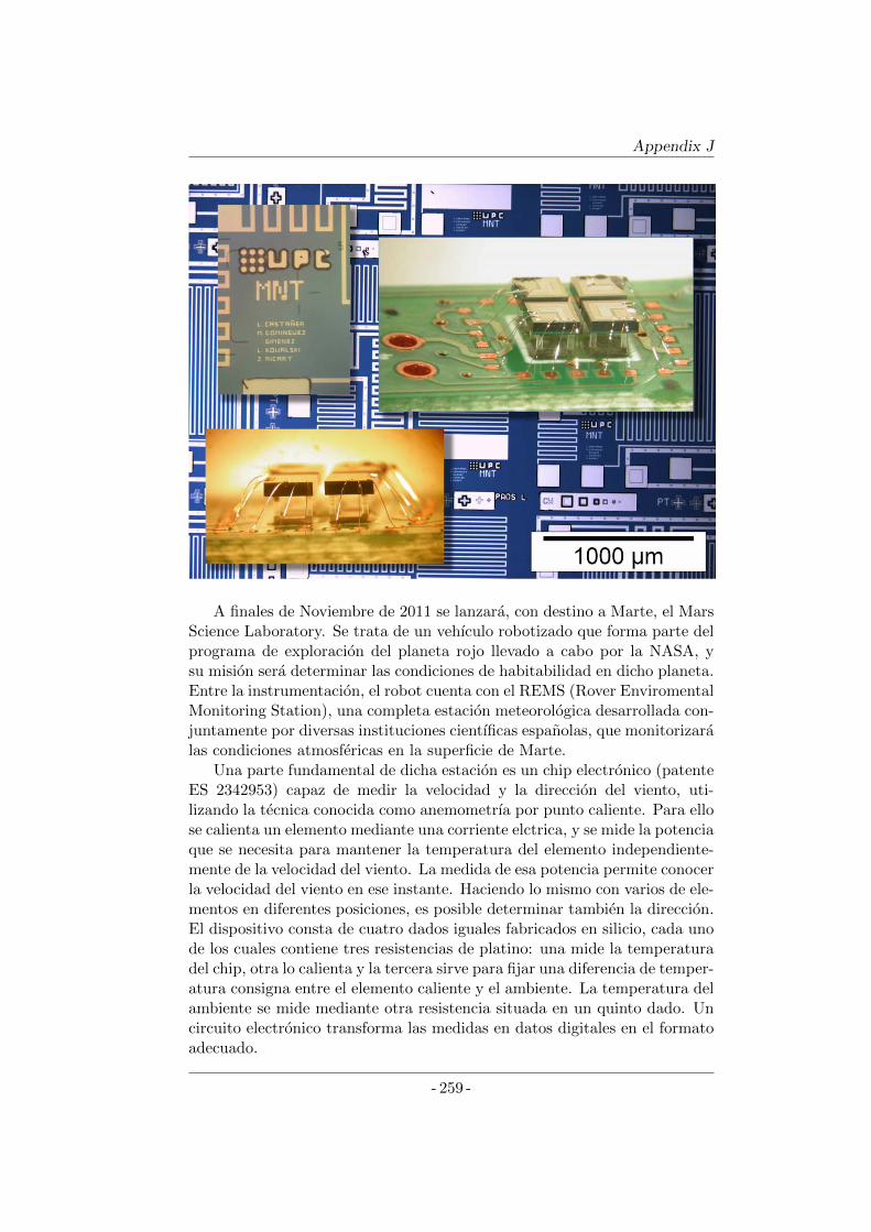
Appendix J
A finales de Noviembre de 2011 se lanzara, con destino a Marte, el MarsScience Laboratory. Se trata de un vehıculo robotizado que forma parte delprograma de exploracion del planeta rojo llevado a cabo por la NASA, ysu mision sera determinar las condiciones de habitabilidad en dicho planeta.Entre la instrumentacion, el robot cuenta con el REMS (Rover EnviromentalMonitoring Station), una completa estacion meteorologica desarrollada con-juntamente por diversas instituciones cientıficas espanolas, que monitorizaralas condiciones atmosfericas en la superficie de Marte.
Una parte fundamental de dicha estacion es un chip electronico (patenteES 2342953) capaz de medir la velocidad y la direccion del viento, uti-lizando la tecnica conocida como anemometrıa por punto caliente. Para ellose calienta un elemento mediante una corriente elctrica, y se mide la potenciaque se necesita para mantener la temperatura del elemento independiente-mente de la velocidad del viento. La medida de esa potencia permite conocerla velocidad del viento en ese instante. Haciendo lo mismo con varios de ele-mentos en diferentes posiciones, es posible determinar tambien la direccion.El dispositivo consta de cuatro dados iguales fabricados en silicio, cada unode los cuales contiene tres resistencias de platino: una mide la temperaturadel chip, otra lo calienta y la tercera sirve para fijar una diferencia de temper-atura consigna entre el elemento caliente y el ambiente. La temperatura delambiente se mide mediante otra resistencia situada en un quinto dado. Uncircuito electronico transforma las medidas en datos digitales en el formatoadecuado.
- 259 -

Appendix K
NASA Group Achievement Award
Charles F. Bolden, 12th NASA Administrator,Washington, DC (United States), 18 July 2013.
Signs of a Whirlwinds reported by REMS instrument,Gale Crater (Mars), 25 October 2012.
261
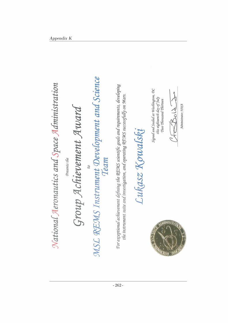
Appendix K
- 262 -
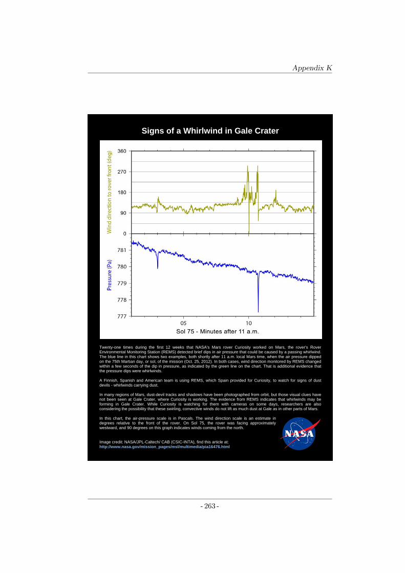
Appendix K
Signs of a Whirlwind in Gale Crater
Twenty-one times during the first 12 weeks that NASA's Mars rover Curiosity worked on Mars, the rover's Rover Environmental Monitoring Station (REMS) detected brief dips in air pressure that could be caused by a passing whirlwind. The blue line in this chart shows two examples, both shortly after 11 a.m. local Mars time, when the air pressure dipped on the 75th Martian day, or sol, of the mission (Oct. 25, 2012). In both cases, wind direction monitored by REMS changed within a few seconds of the dip in pressure, as indicated by the green line on the chart. That is additional evidence that the pressure dips were whirlwinds. A Finnish, Spanish and American team is using REMS, which Spain provided for Curiosity, to watch for signs of dust devils - whirlwinds carrying dust. In many regions of Mars, dust-devil tracks and shadows have been photographed from orbit, but those visual clues have not been seen at Gale Crater, where Curiosity is working. The evidence from REMS indicates that whirlwinds may be forming in Gale Crater. While Curiosity is watching for them with cameras on some days, researchers are also considering the possibility that these swirling, convective winds do not lift as much dust at Gale as in other parts of Mars. In this chart, the air-pressure scale is in Pascals. The wind direction scale is an estimate in degrees relative to the front of the rover. On Sol 75, the rover was facing approximately westward, and 90 degrees on this graph indicates winds coming from the north. Image credit: NASA/JPL-Caltech/ CAB (CSIC-INTA), find this article at: http://www.nasa.gov/mission_pages/msl/multimedia/pia16476.html
- 263 -

Appendix L
Low pressure spherical thermal anemometer for space mission
Proceedings and Oral presentation of the IEEE SENSORS 2013 conference, Baltimore (United States), 3-6 November 2013. * Student Best Paper Award - Track 5 (Mechanical, Magnetic, and Physical Sensors)
Lukasz Kowalski, Vicente Jimenez Serres. Manuel Domınguez-Pumar, Sergi Gorreta Marine, Santiago Silvestre, Luis Castaner Munoz.
ATTENTION ¡ Pages 266 to 269 of the thesis, containing the text, are available
at the editor’s web
http://ieeexplore.ieee.org/stamp/stamp.jsp?tp=&arnumber=6688493
265
Appendix L
- 270 -
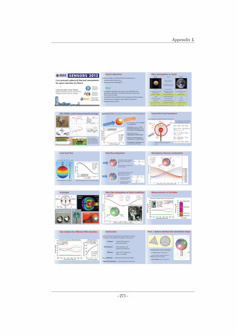
Appendix L
Low pressure spherical thermal anemometer for space missions (to Mars)
by
Lukasz Kowalski, Vicente Jiménez,Manuel Dominguez-Pumar, Sergi Gorreta,Santiago Silvestre and Luis Castañer.
Polytechnic University of
Catalonia
Electronic Engineering Department
Micro & NanoTechnologies
Research Group
Sensor objectives Compact, reliable, and efficient Mars anemometer to: • Measure wind velocity (Uflow)
•
Why? • atmosphere characterization: polar cap sublimation and
deposition, tidal flows, local blows, planetary storms, dust devils, particle charge
• Optimal NO wind condition for soil scooping and drill procedure • Planetary aerial navigation: Mars balloons and planes • Manned mission to Mars …
Mars atmosphere vs. Earth MARS Planet EARTH
Photos done by the Hubble telescope.
Mars diameter is around a half size of the Earth.
3,7 Gravity, g [m/s2] 9,8
CO2 95.32%, N2 2.7%, Ar 1.6%, O2 0.13%
Atmosphere air element composition [%]
N2 78.08%, O2 20.9%, Ar 0.93%
6-8 hPa (6-8mBar) Surface pressure [hPa] 1013 hPa (1Bar)
~ 0.020 Surface density [kg/m3] 1.2
2-10 (30 dust storms) Wind speed [m/s] 0-100
210 (-63ºC) Average temperature [K] 300 (27ºC)
from -125ºC to +25ºC Temperature variation [K] from -80ºC to +50ºC
http://nssdc.gsfc.nasa.gov/planetary/factsheet/marsfact.html , …/earthfact.html
MSL-REMS, wind measurements heritage
Image credit: NASA/JPL-Caltech/ CAB (CSIC-INTA), http://mars.nasa.gov/msl/multimedia/images/?ImageID=5207
Whirlwind Detection by Curiosity in Gale Crater
The lower right chart shows a brief disruption in wind sensed by REMS in the seconds before and after a pressure-dip event.
Spherical CTA (Constant Temperature Anemometer)
Thot • Sensor surface is kept at constant
Thot temperature
• Convection depends on wind speed at given pressure as well as on Sphere-Wind overheat:
• Spherical geometry is
independent on direction flow • Compact and robust design no
moving parts no fragile bonding
• FE simulation in agreement with common empirical models
Convection heat transducer
Joule heating process delivers power to the surface.
We estimate the wind velocityby measuring surface heat !
Power is also injected into the core!
Local heat flux
COMSOL Multiphysics simulation Local heat flux depends only on the Zenith angle!
wind
Zenith angle
Local heat flux [W/m2] for Thot const.
Heat flux integration
Wind
Full sphere heat flux integration gives total convection power loss. Total convection is independent of wind direction. If we partition the sphere surface and heat each sector with a different heater we can:
• Compute wind angle from power ratios
• Compute wind speed
from total power
Wind
Hemisphere thermal conductivity
Prototype
3D Silver Sterling shells stereolitography printed
Assemble
InfraredImage
PCB
Mars-like atmosphere at Earth conditions
desktop wind tunnel set-up
Measurements at 24.5mBar
Yaw rotation for different FAN velocities Conclusions
Spherical constant temperature anemometer is a great candidate for the Martian atmosphere wind sensor !
Compact – external shell protects from environment
Well behaved – axis-symmetric and laminar flow behavior
Efficient – about 70% of delivered power is valuable
Uflow estimation – total convection heat for sphere
Angle discrimination – sectors heat convection ratio
Tetrahedral sphere structure advantages: • Four equal triangular shape sectors,
• 4 is the minimum number of sectors to solve 3D wind direction problem
• High sensibility profile for any direction
Next -> Sphere divided into tetrahedral shape
- 271 -


