Embed Size (px)
Citation preview
UNIT 5.7Using VMD: An Introductory TutorialJen Hsin,1, 2 Anton Arkhipov,1, 2 Ying Yin,1, 2 John E. Stone,2 and Klaus
Schulten1, 2
1Department of Physics, University of Illinois at Urbana-Champaign, Urbana, Illinois2Beckman Institute, University of Illinois at Urbana-Champaign, Urbana, Illinois
ABSTRACT
VMD (Visual Molecular Dynamics) is a molecular visualization and analysis programdesigned for biological systems such as proteins, nucleic acids, lipid bilayer assem-blies, etc. This unit will serve as an introductory VMD tutorial. We will present severalstep-by-step examples of some of VMD�s most popular features, including visualizingmolecules in three dimensions with different drawing and coloring methods, renderingpublication-quality Þgures, animating and analyzing the trajectory of amolecular dynam-ics simulation, scripting in the text-based Tcl/Tk interface, and analyzing both sequenceand structure data for proteins. Curr. Protoc. Bioinform. 24:5.7.1-5.7.48. C© 2008 by JohnWiley & Sons, Inc.
Keywords: molecular modeling �molecular dynamics visualization �
interactive visualization � animation
INTRODUCTION
VMD (Visual Molecular Dynamics; Humphrey et al., 1996) is a molecular visualiza-tion and analysis program designed for biological systems such as proteins, nucleicacids, lipid bilayer assemblies, etc. It is developed by the Theoretical and Computa-tional Biophysics Group at the University of Illinois at Urbana-Champaign. Amongmolecular graphics programs, VMD is unique in its ability to efÞciently operate onmulti-gigabyte molecular dynamics trajectories, its interoperability with a large numberof molecular dynamics simulation packages, and its integration of structure and sequenceinformation.
Key features of VMD include methods: (1) general 3D molecular visualizationwith extensive drawing and coloring methods (e.g., see Fig. 5.7.1); (2) exten-sive atom selection syntax for choosing subsets of atoms for display; (3) visual-ization of dynamic molecular data; (4) visualization of volumetric data; (5) sup-port for most molecular data Þle formats; (6) no limits on the number of atoms,molecules, or trajectory frames, except available memory; (7) molecular analysiscommands; (8) rendering high-resolution, publication-quality molecule images; (9)movie making capability; (10) building and preparing systems for molecular dy-namics simulations; (11) interactive molecular dynamics simulations; (12) extensionsto the Tcl/Python scripting languages; and (13) extensible source code written inC and C++.This unitwill serve as an introductoryVMD tutorial. It is impossible to cover all ofVMD�scapabilities in one unit; instead, we will present several step-by-step examples of VMD�sbasic features. Topics covered in this tutorial include visualizing molecules in threedimensions with different drawing and coloring methods, rendering publication-qualityÞgures, animating and analyzing the trajectory of a molecular dynamics simulation,scripting in the text-based Tcl/Tk interface, and analyzing both sequence and structuredata for proteins.
Current Protocols in Bioinformatics 5.7.1-5.7.48, December 2008Published online December 2008 in Wiley Interscience (www.interscience.wiley.com).DOI: 10.1002/0471250953.bi0507s24Copyright C© 2008 John Wiley & Sons, Inc.
ModelingStructure fromSequence
5.7.1
Supplement 24
Using VMD: AnIntroductory
Tutorial
5.7.2
Supplement 24 Current Protocols in Bioinformatics
Figure 5.7.1 Example renderings made with VMD (Cruz-Chu et al., 2006; Freddolino et al., 2006; Yin et al., 2006; Yu et al.,2006; Sotomayor et al., 2007; Wang et al., 2007). For the color version of this figure go to http://www.currentprotocols.com.
DOWNLOADING VMD
Before starting, the current version of VMD needs to be downloaded. This tuto-rial was written for VMD version 1.8.6. VMD supports all major computer plat-forms and can be downloaded from the VMD homepage http://www.ks.uiuc.edu/Research/vmd. Follow the instructions online to install. Once VMD is installed, to startVMD if using Mac OS X, double-click on the VMD application icon in the Applicationsdirectory; if using Linux and SUN, type vmd in a terminal window, or if using Windows,select→ Start Programs→ VMD.
When VMD starts, by default three windows will open: the VMD Main window, theOpenGL Display window, and the VMD Console window (or a Terminal window on aMac). To end a VMD session, go to the VMD Main window, and choose File → Quit.You can also quit VMD by closing the VMDConsole window or the VMDMain window.
TOPICS AND FILES
This unit contains six sections. Each section acts as an independent tutorial for a speciÞctopic (Working with a Single Molecule, Trajectories and Movie Making, Scripting inVMD, Working with Multiple Molecules, Comparing Protein Structures and Sequenceswith the MultiSeq Plugin, and Data Analysis in VMD). For readers with no prior ex-perience with VMD, we suggest they work through the sections in the order they arepresented. Readers already familiar with the basics of VMD may selectively pursue sec-tions of their interest. Several Þles have been prepared to accompany this tutorial. Youneed to download these Þles at http://www.currentprotocols.com.
WORKING WITH A SINGLE MOLECULE
In this section, the basic functions of VMD will be introduced, starting with loading amolecule, displaying the molecule, and rendering publication-quality molecule images.This section uses the protein ubiquitin as an example molecule. Ubiquitin is a smallprotein responsible for labeling proteins for degradation, and is found in all eukaryoteswith nearly identical sequences and structures.
Necessary Resources
Hardware
Computer
Software
VMD, and an image-displaying program
Files
1ubq.pdb, which can be downloaded at http://www.currentprotocols.com
ModelingStructure fromSequence
5.7.3
Current Protocols in Bioinformatics Supplement 24
BASICPROTOCOL 1
Loading and Displaying the Molecule
A VMD session usually starts with loading structural information of a molecule intoVMD. When VMD loads a molecule, it accesses the information about the names andcoordinates of the atoms. Then, one can explore various VMD visualization features toget a nice view of the loaded molecule.
Loading a moleculeThe Þrst step is to load the molecule. The pdb Þle, 1ubq.pdb (Vijay-Kumar et al.,1987) that contains the atomic coordinates of ubiquitin will be loaded.
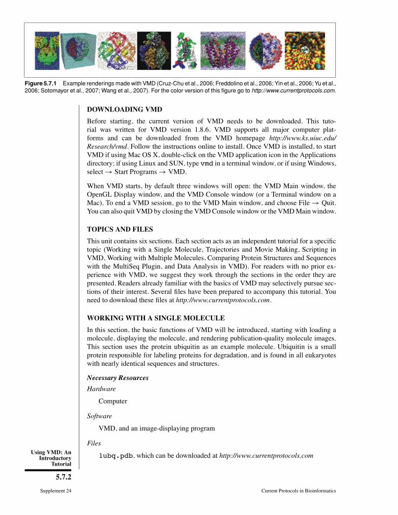
1. Start a VMD session. In the VMD Main window, choose File → New Molecule. . .(Fig. 5.7.2A). The Molecule File Browser window (Fig. 5.7.2B) will appear on thescreen.
2. Use the Browse. . . (Fig. 5.7.2C) button to Þnd the Þle 1ubq.pdb. When the Þle isselected, you will be back in the Molecule File Browser window. In order to actuallyload the Þle, press Load (Fig 5.7.2D).
3. Now, ubiquitin is shown in the OpenGL Display window. Close the Molecule FileBrowser window at any time.
VMD can download a pdb file from the Protein Data Bank (http://www.pdb.org) if anetwork connection is available. Just type the four letter code of the protein in the FileName text entry of the Molecule File Browser window and press the Load button. VMDwill download it automatically.
Displaying the moleculeIn order to see the 3D structure of our protein, the mouse will be used in multiple modesto change the viewpoint. VMD allows users to rotate, scale, and translate the viewpointof the molecule.
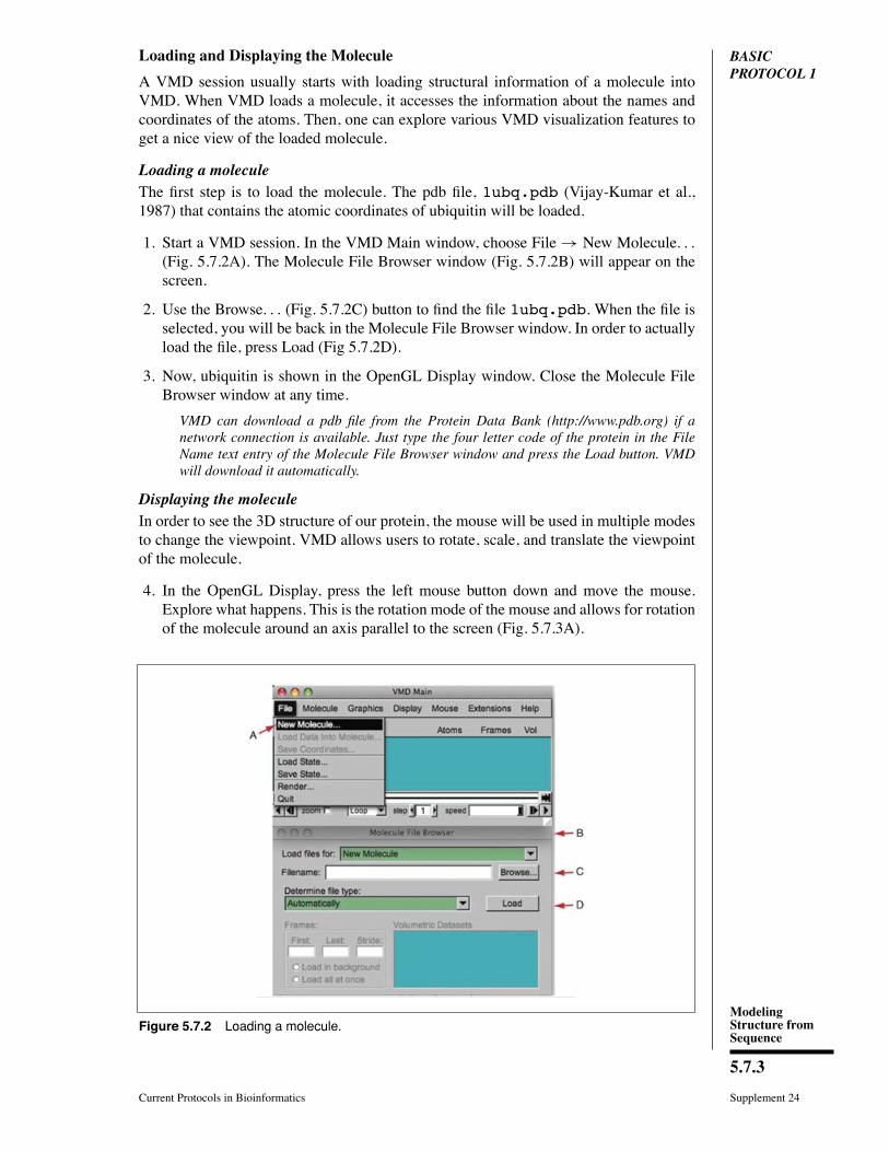
4. In the OpenGL Display, press the left mouse button down and move the mouse.Explore what happens. This is the rotation mode of the mouse and allows for rotationof the molecule around an axis parallel to the screen (Fig. 5.7.3A).
Figure 5.7.2 Loading a molecule.
Using VMD: AnIntroductory
Tutorial
5.7.4
Supplement 24 Current Protocols in Bioinformatics
BA
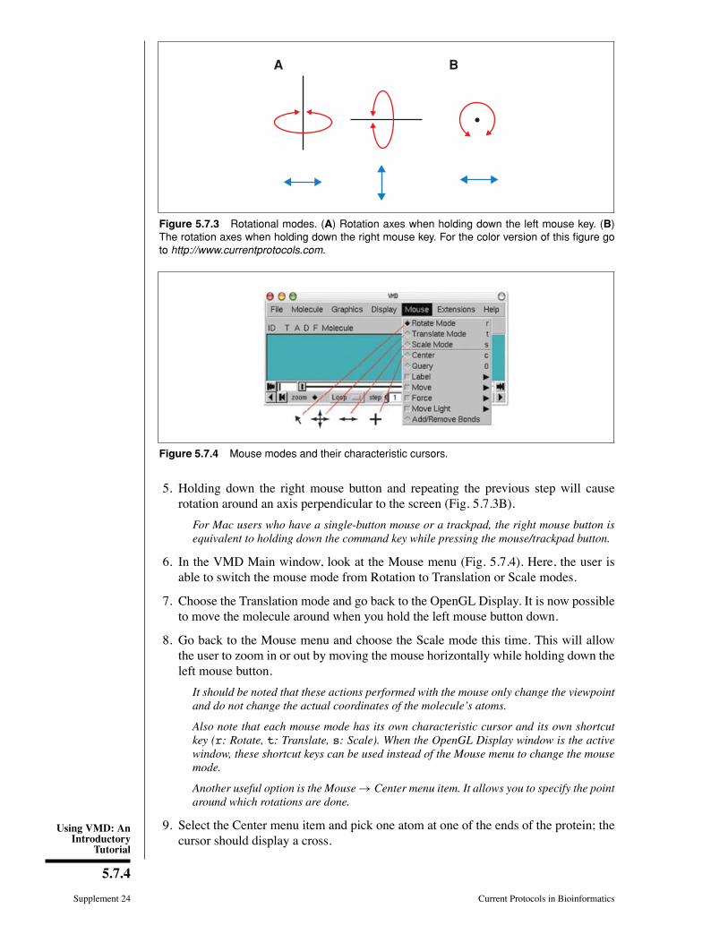
Figure 5.7.3 Rotational modes. (A) Rotation axes when holding down the left mouse key. (B)The rotation axes when holding down the right mouse key. For the color version of this figure goto http://www.currentprotocols.com.
Figure 5.7.4 Mouse modes and their characteristic cursors.
5. Holding down the right mouse button and repeating the previous step will causerotation around an axis perpendicular to the screen (Fig. 5.7.3B).
For Mac users who have a single-button mouse or a trackpad, the right mouse button isequivalent to holding down the command key while pressing the mouse/trackpad button.
6. In the VMD Main window, look at the Mouse menu (Fig. 5.7.4). Here, the user isable to switch the mouse mode from Rotation to Translation or Scale modes.
7. Choose the Translation mode and go back to the OpenGL Display. It is now possibleto move the molecule around when you hold the left mouse button down.
8. Go back to the Mouse menu and choose the Scale mode this time. This will allowthe user to zoom in or out by moving the mouse horizontally while holding down theleft mouse button.
It should be noted that these actions performed with the mouse only change the viewpointand do not change the actual coordinates of the molecule’s atoms.
Also note that each mouse mode has its own characteristic cursor and its own shortcutkey (r: Rotate, t: Translate, s: Scale). When the OpenGL Display window is the activewindow, these shortcut keys can be used instead of the Mouse menu to change the mousemode.
Another useful option is the Mouse → Center menu item. It allows you to specify the pointaround which rotations are done.
9. Select the Center menu item and pick one atom at one of the ends of the protein; thecursor should display a cross.
ModelingStructure fromSequence
5.7.5
Current Protocols in Bioinformatics Supplement 24
A
B
C
D
E
F
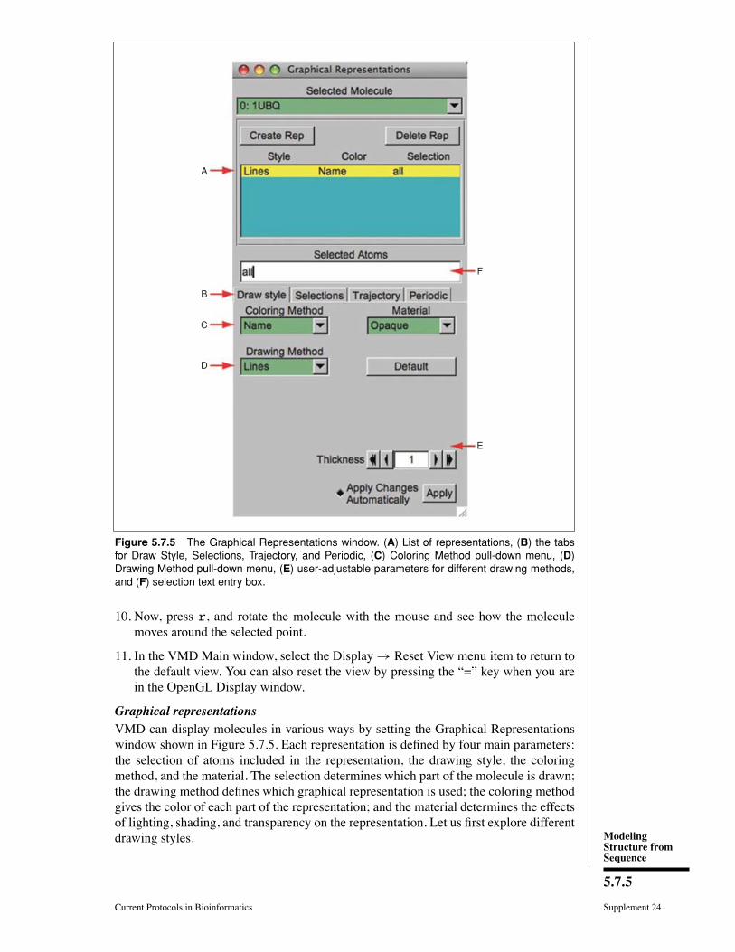
Figure 5.7.5 The Graphical Representations window. (A) List of representations, (B) the tabsfor Draw Style, Selections, Trajectory, and Periodic, (C) Coloring Method pull-down menu, (D)Drawing Method pull-down menu, (E) user-adjustable parameters for different drawing methods,and (F) selection text entry box.
10. Now, press r, and rotate the molecule with the mouse and see how the moleculemoves around the selected point.
11. In the VMD Main window, select the Display→ Reset View menu item to return tothe default view. You can also reset the view by pressing the �=� key when you arein the OpenGL Display window.
Graphical representationsVMD can display molecules in various ways by setting the Graphical Representationswindow shown in Figure 5.7.5. Each representation is deÞned by four main parameters:the selection of atoms included in the representation, the drawing style, the coloringmethod, and the material. The selection determines which part of the molecule is drawn;the drawing method deÞnes which graphical representation is used; the coloring methodgives the color of each part of the representation; and the material determines the effectsof lighting, shading, and transparency on the representation. Let us Þrst explore differentdrawing styles.
Using VMD: AnIntroductory
Tutorial
5.7.6
Supplement 24 Current Protocols in Bioinformatics
CBA
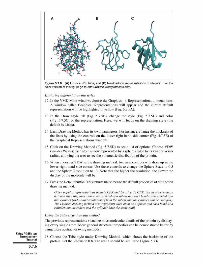
Figure 5.7.6 (A) Licorice, (B) Tube, and (C) NewCartoon representations of ubiquitin. For thecolor version of this figure go to http://www.currentprotocols.com.
Exploring different drawing styles
12. In the VMD Main window, choose the Graphics → Representations. . . menu item.A window called Graphical Representations will appear and the current defaultrepresentation will be highlighted in yellow (Fig. 5.7.5A).
13. In the Draw Style tab (Fig. 5.7.5B), change the style (Fig. 5.7.5D) and color(Fig. 5.7.5C) of the representation. Here, we will focus on the drawing style (thedefault is Lines).
14. Each Drawing Method has its own parameters. For instance, change the thickness ofthe lines by using the controls on the lower right-hand-side corner (Fig. 5.7.5E) ofthe Graphical Representations window.
15. Click on the Drawing Method (Fig. 5.7.5D) to see a list of options. Choose VDW(van der Waals); each atom is now represented by a sphere scaled to its van der Waalsradius, allowing the user to see the volumetric distribution of the protein.
16. When choosing VDW as the drawing method, two new controls will show up in thelower right-hand-side corner. Use these controls to change the Sphere Scale to 0.5and the Sphere Resolution to 13. Note that the higher the resolution, the slower thedisplay of the molecule will be.
17. Press the Default button. This returns the screen to the default properties of the chosendrawing method.
Other popular representations include CPK and Licorice. In CPK, like in old chemistryball and stick kits, each atom is represented by a sphere and each bond is represented by athin cylinder (radius and resolution of both the sphere and the cylinder can be modified).The Licorice drawing method also represents each atom as a sphere and each bond as acylinder, but the sphere and the cylinder have the same radii.
Using the Tube style drawing method
The previous representations visualize micromolecular details of the protein by display-ing every single atom. More general structural properties can be demonstrated better byusing more abstract drawing methods.
18. Choose the Tube style under Drawing Method, which shows the backbone of theprotein. Set the Radius to 0.8. The result should be similar to Figure 5.7.6.
ModelingStructure fromSequence
5.7.7
Current Protocols in Bioinformatics Supplement 24
Using the NewCartoon drawing method
The last drawing method described here is NewCartoon. It gives a simpliÞed represen-tation of a protein based on its secondary structure. Helices are drawn as coiled ribbons,β-sheets as solid, ßat arrows, and all other structures as a tube. This is probably the mostpopular drawing method to view the overall architecture of a protein.
19. In the Graphical Representations window, choose Drawing Method→ NewCartoon.The helices, β-sheets, and coils of the protein can now be easily identiÞed.
Ubiquitin has three and one half turns of α-helix (residues 23 to 34, three of themhydrophobic), one short piece of 310-helix (residues 56 to 59) and a mixed β-sheet withfive strands (residues 1 to 7, 10 to 17, 40 to 45, 48 to 50, and 64 to 72), and sevenreverse turns. VMD uses the program STRIDE (Frishman and Argos, 1995) to computethe secondary structure according to a heuristic algorithm.
Exploring different coloring methods
In this series of steps, different coloring methods are explored.
20. In the Graphical Representations window, the default coloring method is ColoringMethod → Name. In this coloring method, choose a drawing method that showsindividual atoms: each atom will have a different color, i.e., O is red, N is blue, C iscyan, and S is yellow.
21. Choose Coloring Method → ResType (Fig. 5.7.5C). This allows nonpolar residues(white) to be distinguished from basic residues (blue), acidic residues (red), and polarresidues (green).
22. Select Coloring Method→ Structure (Fig. 5.7.5C) and conÞrm that the NewCartoonrepresentation displays colors consistent with secondary structure.
Displaying different selections
To display only parts of the molecule of interest, one can specify their selection in theGraphical Representations window (Fig. 5.7.5F).
23. In the Graphical Representations window, there is a Selected Atoms text entry(Fig. 5.7.5F). Delete the word all, type helix, and press the Apply button orhit the Enter/return key (remember to do this whenever a selection is changed). VMDwill show just the helices present in the molecule.
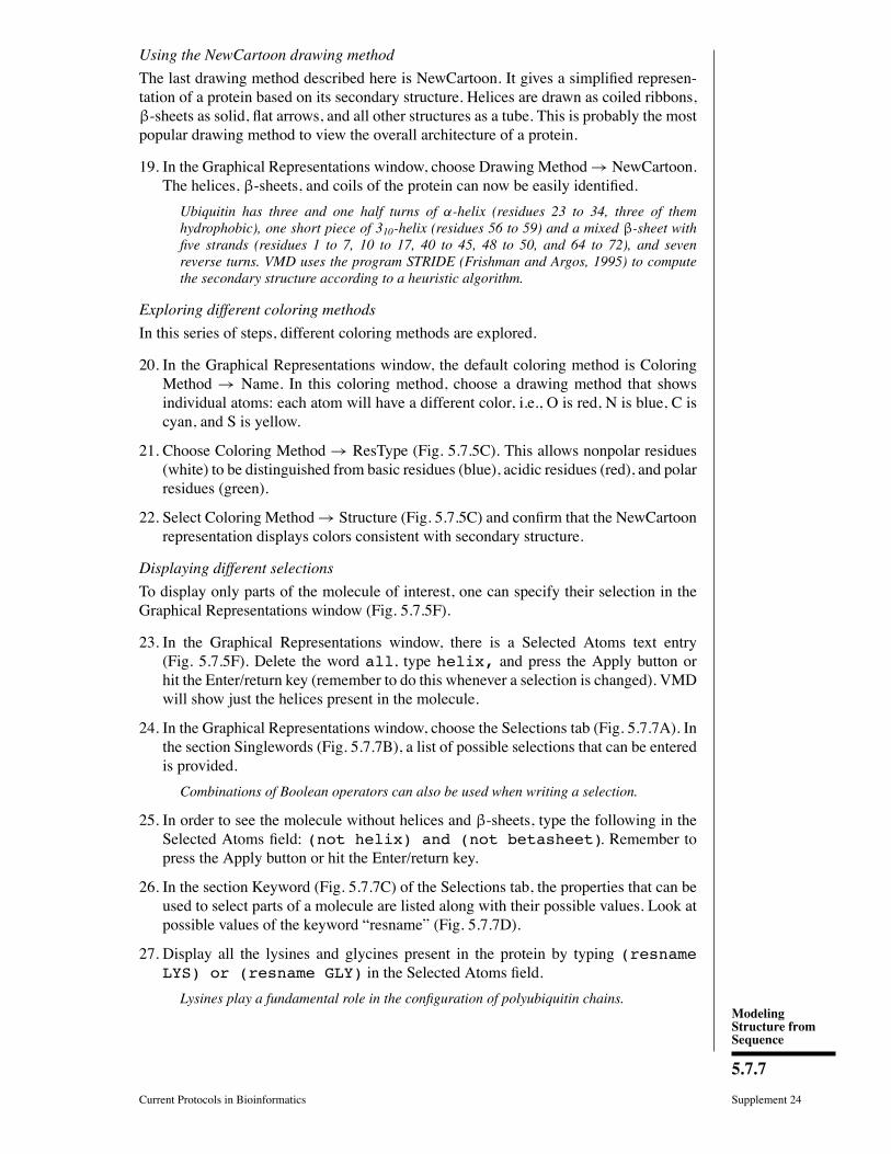
24. In the Graphical Representations window, choose the Selections tab (Fig. 5.7.7A). Inthe section Singlewords (Fig. 5.7.7B), a list of possible selections that can be enteredis provided.
Combinations of Boolean operators can also be used when writing a selection.
25. In order to see the molecule without helices and β-sheets, type the following in theSelected Atoms Þeld: (not helix) and (not betasheet). Remember topress the Apply button or hit the Enter/return key.
26. In the section Keyword (Fig. 5.7.7C) of the Selections tab, the properties that can beused to select parts of a molecule are listed along with their possible values. Look atpossible values of the keyword �resname� (Fig. 5.7.7D).
27. Display all the lysines and glycines present in the protein by typing (resnameLYS) or (resname GLY) in the Selected Atoms Þeld.
Lysines play a fundamental role in the configuration of polyubiquitin chains.
Using VMD: AnIntroductory
Tutorial
5.7.8
Supplement 24 Current Protocols in Bioinformatics
A
B
C D
Figure 5.7.7 Graphical Representations window and the (A) Selections tab, (B) list of Single-words, (C) list of Keywords, and (D) Value box that displays possible choices for a given keyword.
28. Change the current representation�s Drawing Method to CPK and the ColoringMethod to ResName in the Draw style tab. In the screen, the different lysines andglycines will be visible.
29. In the Selected Atoms text Þeld, entry type water. Choose Coloring Method →Name. The 58 water molecules present in the system now appear (in fact only theiroxygen atoms).
30. In order to see which water molecules are closer to the protein, use the commandwithin. Type water and within 3 of protein for Selected Atoms inthe text Þeld.
This selects all the water molecules that are within a distance of 3◦
A of the protein.
31. Finally, try typing in the Selected Atoms Þeld the selections shown in the Þrst columnof Table 5.7.1. Each of these selections will show the protein or part of the protein asexplained in the second column of Table 5.7.1.
ModelingStructure fromSequence
5.7.9
Current Protocols in Bioinformatics Supplement 24
Table 5.7.1 Examples of Atom Selections
Selection Action
Protein Shows the protein
resid 1 The Þrst residue
(resid 1 76) and (not water) The Þrst and last residues
(resid 23 to 34) and (protein) The α-helix
A
D
C
B
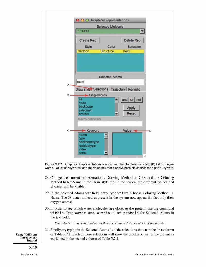
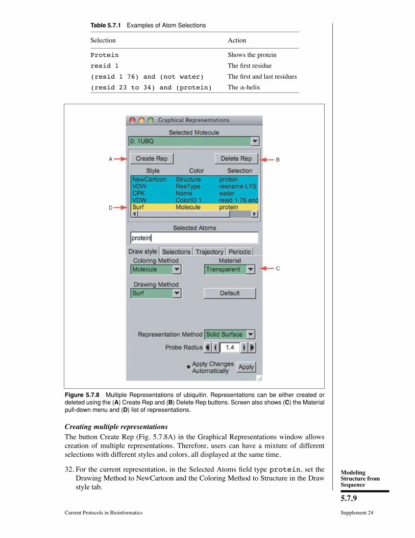
Figure 5.7.8 Multiple Representations of ubiquitin. Representations can be either created ordeleted using the (A) Create Rep and (B) Delete Rep buttons. Screen also shows (C) the Materialpull-down menu and (D) list of representations.
Creating multiple representationsThe button Create Rep (Fig. 5.7.8A) in the Graphical Representations window allowscreation of multiple representations. Therefore, users can have a mixture of differentselections with different styles and colors, all displayed at the same time.
32. For the current representation, in the Selected Atoms Þeld type protein, set theDrawing Method to NewCartoon and the Coloring Method to Structure in the Drawstyle tab.
Using VMD: AnIntroductory
Tutorial
5.7.10
Supplement 24 Current Protocols in Bioinformatics
Table 5.7.2 Examples of Representations
Selection Coloring method Drawing method
Water Name CPK
resid 1 76 and name CA ColorID 1 VDW
33. Press the Create Rep button (Fig. 5.7.8A). A new representation will be created.
34. Modify the new representation to get VDW as the Drawing Method, ResType as theColoring Method, and resname LYS as the current selection.
35. Repeating the previous procedure, create the following two new representations inTable 5.7.2. These two representations show water molecules and the Cα atoms ofthe Þrst and last residues of the protein.
36. Create the last representation by pressing the Create Rep button again. Select DrawingMethod → Surf for drawing method, Coloring Method → Molecule for coloringmethod, and type protein in the Selected Atoms Þeld. For this last representation,choose Transparent in theMaterial pull-downmenu (Fig. 5.7.8C). This representationshows the protein�s volumetric surface in transparent.
Note that you can select and modify different representations you have created by clickingon a representation to highlight it in yellow. Also, each representation can be switchedon/off by double-clicking on it. To delete a representation, highlight it and then click on theDelete Rep button (Fig. 5.7.8B). At the end of this section, the Graphical Representationswindow should look like Figure 5.7.8.
Sequence viewer extensionWhen dealing with a protein for the Þrst time, it is very useful to be able to Þnd anddisplay different amino acids quickly. The sequence viewer extension allows viewingof the protein sequence, as well as to easily pick and display one or more residues ofinterest.
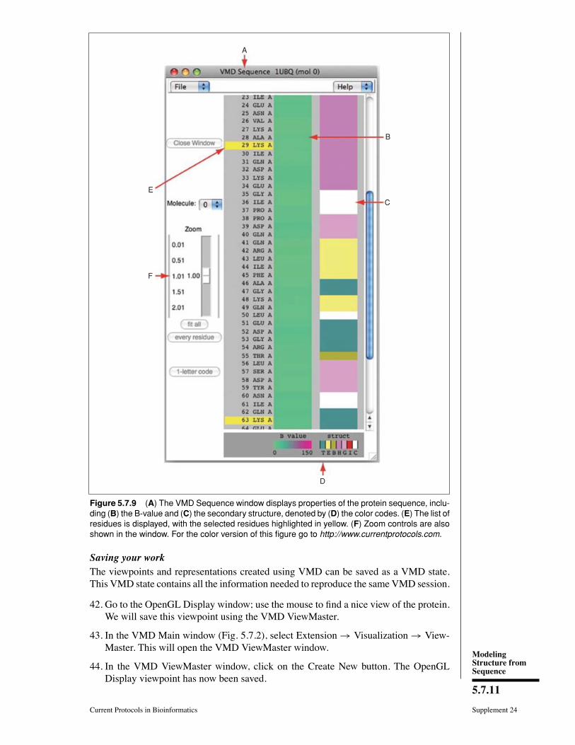
37. In the VMD Main window, choose the Extension → Analysis → Sequence Viewermenu item. A window (Fig. 5.7.9A) with a list of the amino acids (Fig. 5.7.9E) andtheir properties (Figs. 5.7.9B through 5.7.9C) will appear on the screen.
38. With the mouse, try clicking on different residues in the list (Fig. 5.7.9E) and see howthey are highlighted. In addition, the highlighted residue will appear in the OpenGLDisplay window in yellow and rendered in the bond drawing method, so its locationwithin the protein can be visualized easily.
39. Use the Zoom controls (Fig. 5.7.9F) to display the entire list of residues in thewindow.This is particularly useful for larger proteins.
40. Pick multiple residues by holding the shift key and clicking on the mouse button(Fig. 5.7.9E).
41. Look at theGraphical Representationswindow; a new representationwith the residuesthat have been selected using the Sequence Viewer Extension should be shown.Modify, hide, or delete this representation similar to the steps described above.
Information about residues is color-coded (Fig. 5.7.9D) in columns and obtained fromSTRIDE. The B-value column (Fig. 5.7.9B) shows the B-value field (temperature factor)often provided in pdb files. The “struct” column shows secondary structure (Fig. 5.7.9D),where each letter corresponds to a secondary structure, listed in Table 5.7.3.
ModelingStructure fromSequence
5.7.11
Current Protocols in Bioinformatics Supplement 24
A
E
F
C
B
D
Figure 5.7.9 (A) The VMD Sequence window displays properties of the protein sequence, inclu-ding (B) the B-value and (C) the secondary structure, denoted by (D) the color codes. (E) The list ofresidues is displayed, with the selected residues highlighted in yellow. (F) Zoom controls are alsoshown in the window. For the color version of this figure go to http://www.currentprotocols.com.
Saving your workThe viewpoints and representations created using VMD can be saved as a VMD state.This VMD state contains all the information needed to reproduce the same VMD session.
42. Go to the OpenGL Display window; use the mouse to Þnd a nice view of the protein.We will save this viewpoint using the VMD ViewMaster.
43. In the VMD Main window (Fig. 5.7.2), select Extension → Visualization → View-Master. This will open the VMD ViewMaster window.
44. In the VMD ViewMaster window, click on the Create New button. The OpenGLDisplay viewpoint has now been saved.
Using VMD: AnIntroductory
Tutorial
5.7.12
Supplement 24 Current Protocols in Bioinformatics
Table 5.7.3 Secondary Structure Codes Used by STRIDE
Letter code Secondary structure
T Turn
E Extended conformation (β-sheets)
B Isolated bridge
H Alpha helix
G 3-10 helix
I Pi helix
C Coil
45. Go back to the OpenGLDisplay window and use the mouse to Þnd another nice view.If desired, you can add/delete/modify a representation in the Graphical Representa-tions window. When a good view has been found, save it by returning to the VMDViewMaster window and clicking on the Create New button.
46. Create as many views as desired by repeating the previous step. All of the viewpointsare displayed as thumbnails in the VMD ViewMaster window. A previously savedviewpoint can be opened by clicking on its thumbnail.
47. To save the entire VMD session, in the VMDMain window, choose the File→ SaveState menu item. Type an appropriate name (e.g., myfirststate.vmd) and saveit.
The VMD state file myfirststate.vmd contains all the information needed to restorea VMD session, including the viewpoints and the representations.
To load a saved VMD state, start a new VMD session and in the VMD Main windowchoose File → Load State.
48. Quit VMD.
BASICPROTOCOL 2
The Basics of VMD Figure Rendering
One of VMD�s many strengths is its ability to render high-resolution, publication-qualitymolecule images. In this section, we will introduce some basic concepts of Þgure ren-dering in VMD.
Setting the display backgroundBefore rendering a Þgure, make sure that the OpenGL Display background is set up theway you want. Nearly all aspects of the OpenGL Display are user-adjustable, includingthe background color.
1. Start a new VMD session (Basic Protocol 1) and load the 1ubq.pdb Þle.
2. In the VMD Main window, choose Graphics → Colors. . . . The Color Controlswindow should show up. Look through the Categories list. All display colors, forexample, the colors of different atoms when colored by name, are set here.
3. In Categories, select Display. In Names, select Background. Finally, choose �8 white�in Colors. The OpenGL Display should now have a white background.
4. When making a Þgure, we often do not want to include the axes. To turn off the axes,select Display→ Axes→ Off in the VMD Main window.
ModelingStructure fromSequence
5.7.13
Current Protocols in Bioinformatics Supplement 24
Increasing geometric resolutionAll VMD objects are drawn with an adjustable resolution, allowing users to balanceÞneness of detail with drawing speed.
5. Open the Graphical Representation window via Graphics → Representations. . . inthe VMDMain menu. Modify the default representation to show just the protein, anddisplay it using the VDW drawing method.
6. Zoom in on one or two of the atoms by using Mouse Scale→Mode (shortcut s).
You might notice that as you zoom into an atom closer and closer, the atom might be cutoff by an invisible clipping plane, which makes it difficult to focus on just one atom. This isan OpenGL feature. You can move the clipping plane closer to you by doing the following:switch your mouse mode to the Translate mode, either by pressing the shortcut key “t” inthe OpenGL window or by selecting Mouse → Translate Mode, and dragging your mousein the OpenGL window while holding down the right mouse key. You can now move theclipping plane closer to you, or away from you. If this does not work, here is an alternativeway: in the VMD Main window, choose Display → Display Settings. . . ; in the DisplaySettings window that shows up you can see that many OpenGL options are adjustable;decrease the value for Near Clip, which will move the OpenGL clipping closer, allowingyou to zoom in on individual atoms without clipping them off.
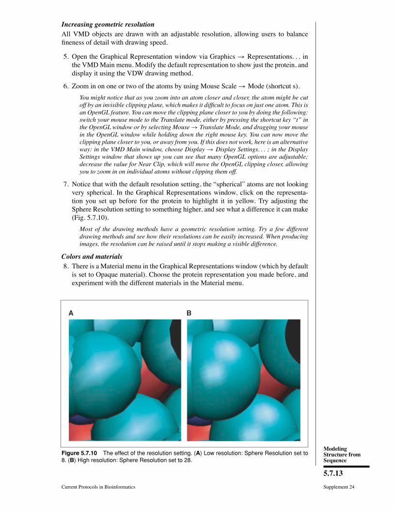
7. Notice that with the default resolution setting, the �spherical� atoms are not lookingvery spherical. In the Graphical Representations window, click on the representa-tion you set up before for the protein to highlight it in yellow. Try adjusting theSphere Resolution setting to something higher, and see what a difference it can make(Fig. 5.7.10).
Most of the drawing methods have a geometric resolution setting. Try a few differentdrawing methods and see how their resolutions can be easily increased. When producingimages, the resolution can be raised until it stops making a visible difference.
Colors and materials8. There is a Material menu in the Graphical Representations window (which by defaultis set to Opaque material). Choose the protein representation you made before, andexperiment with the different materials in the Material menu.
BA
Figure 5.7.10 The effect of the resolution setting. (A) Low resolution: Sphere Resolution set to8. (B) High resolution: Sphere Resolution set to 28.
Using VMD: AnIntroductory
Tutorial
5.7.14
Supplement 24 Current Protocols in Bioinformatics
9. Besides the predeÞned materials in the Material menu, VMD also allows users tocreate their ownmaterials. Tomake a newmaterial, in the VMDMain window chooseGraphics→Materials. . ..
10. In the Materials window that appears, you will see a list of the materials you justtried out, and their adjustable settings. Click the Create New button. A new material,Material 12, will be created. Give it the settings listed in Table 5.7.4.
11. Go back to the Graphical Representations window. In the Material menu, Material12 is now on the list. Try using Material 12 for a representation and see what it lookslike. You can also rename the materials in the Material menu.
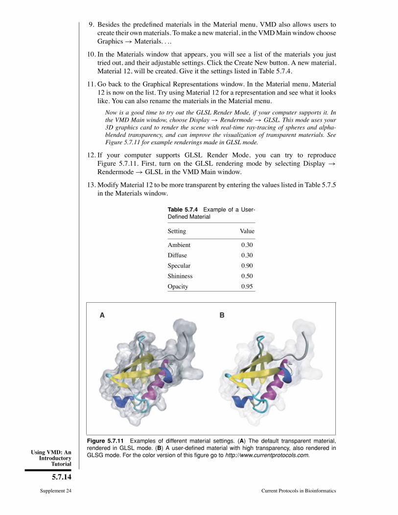
Now is a good time to try out the GLSL Render Mode, if your computer supports it. Inthe VMD Main window, choose Display → Rendermode → GLSL. This mode uses your3D graphics card to render the scene with real-time ray-tracing of spheres and alpha-blended transparency, and can improve the visualization of transparent materials. SeeFigure 5.7.11 for example renderings made in GLSL mode.
12. If your computer supports GLSL Render Mode, you can try to reproduceFigure 5.7.11. First, turn on the GLSL rendering mode by selecting Display →Rendermode→ GLSL in the VMD Main window.
13. Modify Material 12 to be more transparent by entering the values listed in Table 5.7.5in the Materials window.
Table 5.7.4 Example of a User-Defined Material
Setting Value
Ambient 0.30
Diffuse 0.30
Specular 0.90
Shininess 0.50
Opacity 0.95
BA
Figure 5.7.11 Examples of different material settings. (A) The default transparent material,rendered in GLSL mode. (B) A user-defined material with high transparency, also rendered inGLSG mode. For the color version of this figure go to http://www.currentprotocols.com.
ModelingStructure fromSequence
5.7.15
Current Protocols in Bioinformatics Supplement 24
Table 5.7.5 Example of a MoreTransparent Material
Setting Value
Ambient 0.30
Diffuse 0.50
Specular 0.87
Shininess 0.85
Opacity 0.11
Table 5.7.6 Example of Representations Drawn with Different Materials
Selection Coloring method Drawing method Material
protein Structure NewCartoon Opaque
protein ColorID→8 white Surf Material 12
14. Hide all of the current representations and create the two representations listed inTable 5.7.6.
Depth perceptionSince the molecular systems are three-dimensional, VMD has multiple ways of repre-senting the third dimension. In this section, how to use VMD to enhance or hide depthperception is discussed.
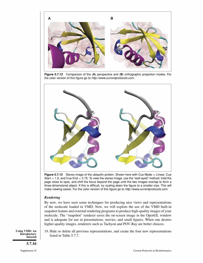
15. The Þrst thing to consider is the projection mode. In the VMDMain window, click theDisplay menu. Here, we can choose either Perspective or Orthographic in the drop-down menu. Try switching between Perspective or Orthographic projection modesand see the difference (Fig. 5.7.12).
In perspective mode, things closer to the camera appear larger. Perspective projectionprovides strong size-based visual depth cues, but the displayed image will not preservescale relationships or parallelism of lines, and objects very close to the camera mayappear distorted. Orthographic projection preserves scale and parallelism relationshipsbetween objects in the displayed image, but greatly reduces depth perception. Hence,orthographic mode tends to be more useful for analysis, because alignment is easy to see,while perspective mode is often used for producing figures and stereo images.
Another way VMD can represent depth is through so-called “depth cueing.” Depth cueingis used to enhance three-dimensional perception of molecular structures, particularly withorthographic projections.
16. Choose Display→ Depth Cueing in the VMD Main window.
When depth cueing is enabled, objects further from the camera are blended into thebackground. Depth cueing settings are found in Display → Display Settings. . . . Hereone can choose the functional dependence of the shading on distance, as well as someparameters for this function. To see the depth cueing effect better, you might want to hidethe representation with the Surf drawing method.
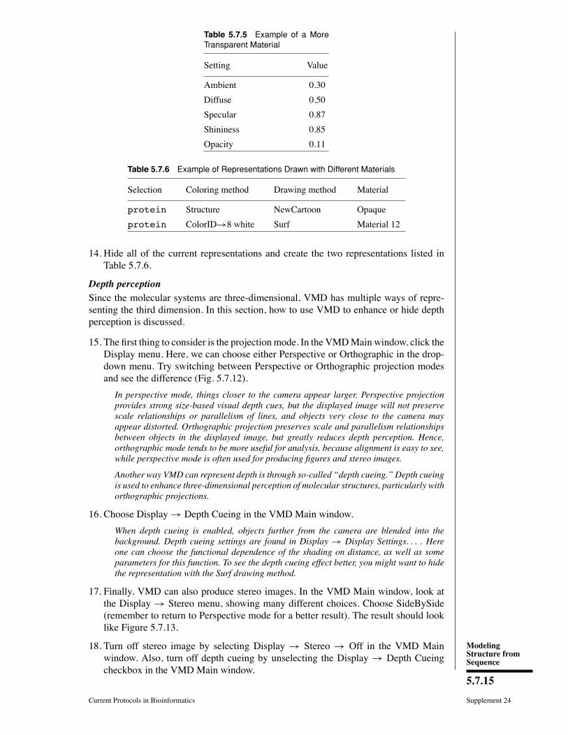
17. Finally, VMD can also produce stereo images. In the VMD Main window, look atthe Display → Stereo menu, showing many different choices. Choose SideBySide(remember to return to Perspective mode for a better result). The result should looklike Figure 5.7.13.
18. Turn off stereo image by selecting Display → Stereo → Off in the VMD Mainwindow. Also, turn off depth cueing by unselecting the Display → Depth Cueingcheckbox in the VMD Main window.
Using VMD: AnIntroductory
Tutorial
5.7.16
Supplement 24 Current Protocols in Bioinformatics
BA
Figure 5.7.12 Comparison of the (A) perspective and (B) orthographic projection modes. Forthe color version of this figure go to http://www.currentprotocols.com.
Figure 5.7.13 Stereo image of the ubiquitin protein. Shown here with Cue Mode = Linear, CueStart = 1.5, and Cue End = 2.75. To view the stereo image, use the “wall-eyed” method: hold thepage close to eyes, and shift the focus beyond the page until the two images overlap to form athree-dimensional object. If this is difficult, try scaling down the figure to a smaller size. This willmake viewing easier. For the color version of this figure go to http://www.currentprotocols.com.
RenderingBy now, we have seen some techniques for producing nice views and representationsof the molecule loaded in VMD. Now, we will explore the use of the VMD built-insnapshot feature and external rendering programs to produce high-quality images of yourmolecule. The �snapshot� renderer saves the on-screen image in the OpenGL windowand is adequate for use in presentations, movies, and small Þgures. When one desireshigher-quality images, renderers such as Tachyon and POV-Ray are better choices.
19. Hide or delete all previous representations, and create the four new representationslisted in Table 5.7.7.
ModelingStructure fromSequence
5.7.17
Current Protocols in Bioinformatics Supplement 24
Table 5.7.7 Example Representations
Selection Coloring method Drawing style Material
protein and not resid 72 to 76 Structure NewCartoon Opaque
protein and helix and name CA ColorID→8 Surf Material 12
resname GLY and not resid 72 to 76 ColorID→7 VDW Opaque
resname LYS ColorID→18 Licorice Opaque
20. Once you have the scene set the way you like it in the OpenGLwindow, simply chooseFile→ Render. . . in the VMDMain window. The File Render Controls window willappear on the screen.
21. The File Render Controls allows you to choose which renderer you want to use andthe Þle name for your image. Select �snapshot� for the rendering method, type in aÞlename of your choice, and click Start Rendering.
22. If you are using a Mac or a Linux machine, an image-processing application mightopen automatically that shows you the molecule you have just rendered using Snap-shot. If this is not the case, use any image-processing application to take a look at theimage Þle. Close the application when you are done to continue using VMD.
The snapshot renderer saves exactly what is showing in your OpenGL display window—infact, if another window overlaps the display window, it may distort the overlapped regionof the image.
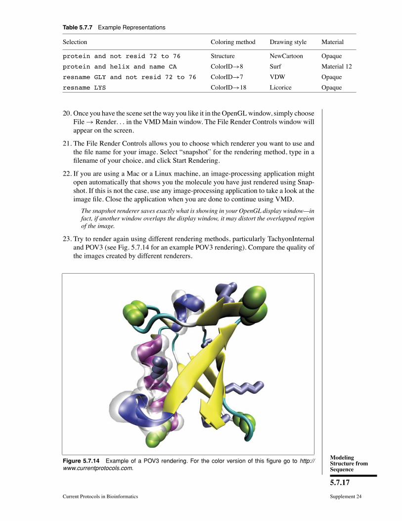
23. Try to render again using different rendering methods, particularly TachyonInternaland POV3 (see Fig. 5.7.14 for an example POV3 rendering). Compare the quality ofthe images created by different renderers.
Figure 5.7.14 Example of a POV3 rendering. For the color version of this figure go to http://www.currentprotocols.com.
Using VMD: AnIntroductory
Tutorial
5.7.18
Supplement 24 Current Protocols in Bioinformatics
The other renderers (e.g., POV3 and Tachyon) reprocess everything, so it may not lookexactly as it does in the OpenGL window. In particular, they do not “clip,” or hide, objectsvery near the camera. If you select Display → Display Settings. . . in the VMD Mainwindow, you can set Near Clip to 0.01 to get a better idea of what will appear in yourrendering.
24. Quit VMD.
WORKING WITH TRAJECTORIES AND MAKING MOVIES
Time-evolving coordinates of a system are called trajectories. They are most commonlyobtained from simulations of molecular systems, but can also be generated by othermeans and for different purposes. Upon loading a trajectory into VMD, one can see amovie of how the system evolves in time and analyze various features throughout thetrajectory. This section will introduce the basics of working with trajectory data in VMD.You will also learn how to analyze trajectory data in Basic Protocols 14, 15, and 16.
Necessary Resources
Hardware
Computer
Software
VMD, and a movie player program
Files
ubiquitin.psf and pulling.dcd, which can be downloaded fromhttp://www.currentprotocols.com
BASICPROTOCOL 3
Working with Trajectories
Trajectory Þles are commonly binary Þles that contain several sets of coordinates forthe system. Each set of coordinates corresponds to one frame in time. An example ofa trajectory Þle is a DCD Þle generated by the molecular dynamics program NAMD(Phillips et al., 2005).
Load trajectoriesTrajectory Þles do not contain information of the system contained in the protein structureÞles (PSF). Therefore, we Þrst need to load the PSF Þle, and then add the trajectory datato this Þle.
1. Start a newVMDsession. In theVMDMainwindow, select File→NewMolecule. . ..The Molecule File Browser window will appear on your screen.
2. Use the Browse. . . button to Þnd the Þle ubiquitin.psf. When you select thisÞle, you will be back in the Molecule File Browser window. Press the Load button toload the molecule.
3. In the Molecule File Browser window, make sure that ubiquitin.psf is selectedin the �Load Þles for:� pull-down menu on top, and click on the Browse button.Browse for pulling.dcd.
Note the options available in the Molecule File Browser window: one can load trajectoriesstarting and finishing at chosen frames, and adjust the stride between the loaded frames.Leave the default settings so that the whole trajectory is loaded.
4. Click on the Load button in the Molecule File Browser window.
ModelingStructure fromSequence
5.7.19
Current Protocols in Bioinformatics Supplement 24
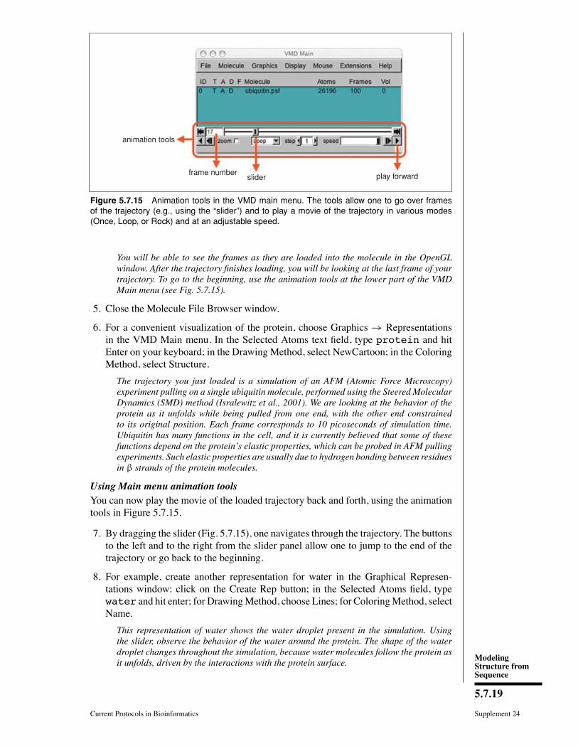
play forwardsliderframe number
animation tools
Figure 5.7.15 Animation tools in the VMD main menu. The tools allow one to go over framesof the trajectory (e.g., using the “slider”) and to play a movie of the trajectory in various modes(Once, Loop, or Rock) and at an adjustable speed.
You will be able to see the frames as they are loaded into the molecule in the OpenGLwindow. After the trajectory finishes loading, you will be looking at the last frame of yourtrajectory. To go to the beginning, use the animation tools at the lower part of the VMDMain menu (see Fig. 5.7.15).
5. Close the Molecule File Browser window.
6. For a convenient visualization of the protein, choose Graphics → Representationsin the VMD Main menu. In the Selected Atoms text Þeld, type protein and hitEnter on your keyboard; in the Drawing Method, select NewCartoon; in the ColoringMethod, select Structure.
The trajectory you just loaded is a simulation of an AFM (Atomic Force Microscopy)experiment pulling on a single ubiquitin molecule, performed using the Steered MolecularDynamics (SMD) method (Isralewitz et al., 2001). We are looking at the behavior of theprotein as it unfolds while being pulled from one end, with the other end constrainedto its original position. Each frame corresponds to 10 picoseconds of simulation time.Ubiquitin has many functions in the cell, and it is currently believed that some of thesefunctions depend on the protein’s elastic properties, which can be probed in AFM pullingexperiments. Such elastic properties are usually due to hydrogen bonding between residuesin β strands of the protein molecules.
Using Main menu animation toolsYou can now play the movie of the loaded trajectory back and forth, using the animationtools in Figure 5.7.15.
7. By dragging the slider (Fig. 5.7.15), one navigates through the trajectory. The buttonsto the left and to the right from the slider panel allow one to jump to the end of thetrajectory or go back to the beginning.
8. For example, create another representation for water in the Graphical Represen-tations window: click on the Create Rep button; in the Selected Atoms Þeld, typewater and hit enter; for DrawingMethod, choose Lines; for ColoringMethod, selectName.
This representation of water shows the water droplet present in the simulation. Usingthe slider, observe the behavior of the water around the protein. The shape of the waterdroplet changes throughout the simulation, because water molecules follow the protein asit unfolds, driven by the interactions with the protein surface.
Using VMD: AnIntroductory
Tutorial
5.7.20
Supplement 24 Current Protocols in Bioinformatics
When playing animations, you can choose between three looping styles: Once, Loop, andRock. You can also jump to a frame in the trajectory by entering the frame number in thewindow on the left of the “slider” panel.
Smoothing trajectories9. For clarity, turn off the water representation by double-clicking on it in the GraphicalRepresentations window.
As you might have noticed, when we play the animation, the protein movements are not verysmooth due to thermal fluctuations (as the simulation is performed under the conditionsthat mimic a thermal bath). VMD can smooth the animation by averaging over a givennumber of frames.
10. In the Graphical Representations window, select your protein representation andclick on the Trajectory tab. At the bottom, you should see the Trajectory SmoothingWindow Size set to zero. As your animation is playing, increase this setting. Noticethat the motion gets smoother and smoother as the size of the smoothing windowis increased. Commonly used values for this setting are 1 to 5, depending on howsmooth you want your trajectory to be.
Displaying multiple framesWe will now learn how to display many frames of the same trajectory at once.
11. In the Graphical Representations window, highlight your protein representation byclicking on it and press the Create Rep button. This creates an identical representation,but note that smoothing is set to zero. Hide the old protein representation.
12. Highlight the new protein representation and click the Trajectory tab. Above thesmoothing control, notice the Draw Multiple Frames control. It is set to now bydefault, which is simply the current frame. Enter 0:10:99, which selects everytenth frame from the range 0 to 99.
13. Go back to the Draw style tab, and change the Coloring Method to Timestep. Thiswill draw the beginning of the trajectory in red, the middle in white, and the end inblue.
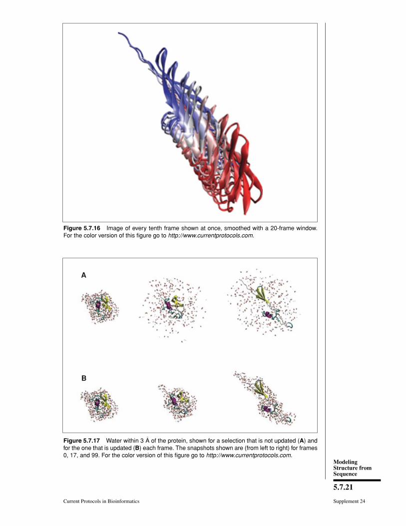
14. We can also use smoothing to make the large-scale motion of the protein moreapparent. Go back to the Trajectory tab, and set the smoothing window to 20. Theresult should look like Figure 5.7.16.
Updating selectionsNow, we will see how to make VMD update the selection each frame.
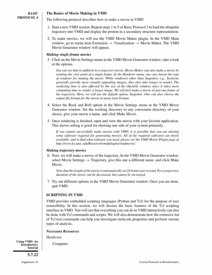
15. Hide the current representation showing all frames, and display only the water repre-sentation by double-clicking on it. Change the text in the Selected Atoms Þeld fromwater to water and within 3 of protein and hit enter. This will showall water atoms within 3
◦A of the protein.
16. Play the trajectory.
As you can see, although the displayed water atoms may be near the protein for a littlewhile, they soon wander off, and are still shown despite no longer meeting the selectioncriteria. The Update Selection Every Frame option in the Trajectory tab of the GraphicalRepresentations window remedies this. If the option box is checked, the selection is updatedevery frame. See Figure 5.7.17.
17. Quit VMD.
ModelingStructure fromSequence
5.7.21
Current Protocols in Bioinformatics Supplement 24
Figure 5.7.16 Image of every tenth frame shown at once, smoothed with a 20-frame window.For the color version of this figure go to http://www.currentprotocols.com.
A
B
Figure 5.7.17 Water within 3◦A of the protein, shown for a selection that is not updated (A) and
for the one that is updated (B) each frame. The snapshots shown are (from left to right) for frames0, 17, and 99. For the color version of this figure go to http://www.currentprotocols.com.
Using VMD: AnIntroductory
Tutorial
5.7.22
Supplement 24 Current Protocols in Bioinformatics
BASICPROTOCOL 4
The Basics of Movie Making in VMD
The following protocol describes how to make a movie in VMD.
1. Start a newVMD session. Repeat steps 1 to 5 of Basic Protocol 3 to load the ubiquitintrajectory into VMD and display the protein in a secondary structure representation.
2. To make movies, we will use the VMD Movie Maker plugin. In the VMD Mainwindow, go to menu item Extension → Visualization → Movie Maker. The VMDMovie Generator window will appear.
Making single-frame movies3. Click on the Movie Settings menu in the VMDMovie Generator window; take a lookat the options.
You can see that in addition to a trajectory movie, Movie Maker can also make a movie byrotating the view point of a single frame. In the Renderer menu, one can choose the typeof renderer for making the movie. While renderers other than Snapshot, e.g., Tachyon,generally provide more visually appealing images, they also take longer to render. Therendering time is also affected by the size of the OpenGL window, since it takes morecomputing time to render a larger image. We will first make a movie of just one frame ofthe trajectory. Here, we will use the default option, Snapshot. One can also choose theoutput file format for the movie in menu item Format.
4. Select the Rock and Roll option in the Movie Settings menu in the VMD MovieGenerator window. Set the working directory to any convenient directory of yourchoice, give your movie a name, and click Make Movie.
5. Once rendering is Þnished, open and view the movie with your favorite application.This movie setting is good for showing one side of your system primarily.
If you cannot successfully make movies with VMD, it is possible that you are missingsome software required for generating movies. All of the required softwares are freelyavailable, and to find what software you need, please see the VMD Movie Plugin page athttp://www.ks.uiuc.edu/Research/vmd/plugins/vmdmovie/.
Making trajectory movies6. Now, we will make a movie of the trajectory. In the VMDMovie Generator window,select Movie Settings → Trajectory, give this one a different name, and click MakeMovie.
Note that the length of the movie is automatically set 24 frames per second. For a trajectory,duration of the movie can be decreased, but cannot be increased.
7. Try out different options in the VMD Movie Generator window. Once you are done,quit VMD.
SCRIPTING IN VMD
VMD provides embedded scripting languages (Python and Tcl) for the purpose of userextensibility. In this section, we will discuss the basic features of the Tcl scriptinginterface in VMD. You will see that everything you can do in VMD interactively can alsobe done with Tcl commands and scripts. We will also demonstrate how the extensive listof Tcl text commands can help you investigate molecule properties and perform varioustypes of analysis.
Necessary Resources
Hardware
Computer
ModelingStructure fromSequence
5.7.23
Current Protocols in Bioinformatics Supplement 24
Software
VMD, and a text editor
Files
1ubq.pdb and beta.tcl, which can be downloaded fromhttp://www.currentprotocols.com
BASICPROTOCOL 5
The Basics of Tcl Scripting
Tcl is a rich language that contains many features and commands, in addition to thetypical conditional and looping expressions. Tk is an extension to Tcl that permits thewriting of graphical user interfaces with windows and buttons, etc. More information anddocumentations about the Tcl/Tk language can be found at http://www.tcl.tk/doc. Let usstart with the basic commands.
1. Start a new VMD session. In the VMDMain menu, select Extensions→ Tk Consoleto open the VMD TkConsole window. You can now start entering Tcl/Tk commandshere.
2. Try entering the following commands in the VMD TkConsole window. Rememberto hit enter after each line and take a look at what you get after each input.
set x 10puts ��the value of x is: $x��set text ��some text��puts ��the value of text is: $text��
As you can see, the Tcl set and put commands have the following syntax:
set variable value - sets the value of variable
puts $variable - prints out the value of variable
Also, $variable refers to the value of variable.
3. Try the expr command by entering the following lines in the VMD TkConsolewindow:
expr 3 - 8set x 10expr −3 * $x
The expr command performs mathematical operations:
expr expression - evaluates a mathematical expression.
4. Entering the following example in the VMD TkConsole window:
set result [expr −3 * $x]puts $result
By using brackets, you can embed Tcl commands into others. A bracketed expression willautomatically be substituted by the return value of the expression inside the brackets:[expression] - represents the result of the expression inside the brackets.
Using VMD: AnIntroductory
Tutorial
5.7.24
Supplement 24 Current Protocols in Bioinformatics
5. Let us calculate the values of −3*x for integers x from 0 to 10 and output the resultsinto a Þle named myoutput.dat.
set file [open ��myoutput.dat�� w]for {set x 0} {$x <= 10} {incr x} {puts $file [expr −3 * $x]}close $file
Here, you have tried the loop feature of Tcl. Tcl provides an iterated loop similar to the“for” loop in C. The for command in Tcl requires four arguments: an initialization, atest, an increment, and the block of code to evaluate. The syntax of the for command is:
for {initialization} {test} {increment} {commands}Take a look at the output file myoutput.dat, either by a text editor of your choice, orthe command less in a terminal window on a Mac or Linux Machine.
BASICPROTOCOL 6
Working with a Molecule Using Tcl Text Commands
Anything that can be done in the VMD graphical interface can also be done with textcommands. This allows scripts to be written that can automatically loadmolecules, createrepresentations, analyze data, make movies, etc. Here, we will go through some simpleexamples of what can be done using the scripting interface in VMD.
Loading molecules with text commands1. In the VMD TkConsole window, type the command mol new 1ubq.pdb and hitenter.
As you can see, this command performs the same function as described at the beginningof Basic Protocol 1, namely, loading a new molecule with file name 1ubq.pdb.
If you see the error message Unable to load file ��1ubq.pdb�� usingfile type ��pdb��, you might not be in the correct directory that contains the file1ubq.pdb. You can use the standard Unix commands in the VMD TkConsole window tonavigate to the correct directory.
When you open VMD, by default a vmd console window appears. The vmd console windowtells you what’s going on within the VMD session that you are working on. Take a look atthe vmd console window. It should tell you a molecule has been loaded, as well as someof its basic properties like number of atoms, bonds, residues etc. The Tcl commands thatyou enter in the VMD TkConsole window can also be entered in the vmd console window.If you are using a Mac, your vmd console window is the terminal window that shows upwhen you open VMD.
Working with specific parts of a molecule: the atomselect commandMany times, you might want to perform operations on only a speciÞc part a molecule.For this purpose, VMD�s atomselect command is very useful. The atomselectcommand has the following syntax:
atomselect molid “selection command” - creates a new atom selection that includesall atoms described by “selection command”.
2. Type set crystal [atomselect top ��all��] in the Tk Consolewindow.
This command allows you to select a specific part of a molecule. The first argument toatomselect is the molecule ID (shown to the very left of the VMD Main window); thesecond argument is a textual atom selection like what you have been using to describegraphical representations in Basic Protocol 1. The selection returned by atomselectis itself a command you will learn to use.
ModelingStructure fromSequence
5.7.25
Current Protocols in Bioinformatics Supplement 24
This step creates a selection, crystal, that contains all the atoms in the molecule andassigns it to the variable crystal. Instead of a molecule ID (which is a number), wehave used the shortcut top to refer to the top molecule. A top molecule means that it isthe target for scripting commands. This concept is particularly important when multiplemolecules are loaded at the same time (see Basic Protocol 9 for dealing with multiplemolecules in VMD).
The result of atomselect is a function. Thus, $crystal is now a function thatperforms actions on the contents of the ��all�� selection.
Obtaining and changing molecule properties with text commandsAfter you have deÞned an atom selection, you have many commands that you can useto operate on it. For example, you can use commands to learn about the properties ofyour atom selection (number of atoms, coordinates, total charge, etc). You can alsouse commands to change its coordinates and other properties. See VMD User�s Guide(http://www.ks.uiuc.edu/Research/vmd/vmd-1.8.6/ug/) for an extensive list of commands.
3. Type $crystal num in the Tk Console window.
Passing num to an atom selection returns the number of atoms in that selection. Checkthat this number matches the number of atoms for your molecule displayed in the VMDMain window.
4. We can also use commands to move our molecule on the screen. You can use thesecommands to change atom coordinates.
$crystal moveby {10 0 0}$crystal move [transaxis x 40 degree]
Editing properties of selected atoms5. Open the Graphical Representation window by selecting Graphics →Representations. . . in the VMD Main window. Type in protein as the atom se-lection; change its Coloring Method to Beta and its Drawing Method to VDW. Yourmolecule should now appear as a mostly red and blue assembly of spheres.
The “B” field of a PDB file typically stores the “temperature factor” for a crystal struc-ture and is read into VMD’s “Beta” field. Since we are not currently interested in thisinformation, we can use this field to store our own numerical values. VMD has a “Beta”coloring method, which colors atoms according to their β-factors. By replacing the Betavalues for various atoms, you can control the color in which they are drawn. This is veryuseful when you want to show a property of the system that you have computed.
6. Return to the Tk Console window and type $crystal set beta 0.
This resets the “beta” field (which is displayed) to zero for all atoms. As you do this, youshould observe that the atoms in your OpenGL window will suddenly change to a uniformcolor (since they all have the same beta values now).
You can obtain and set many atomic properties using atom selections, including segment,chain, residue, atom name, position (x, y and z), charge, mass, occupancy and radius, justto name a few.
7. In the Tk Console window, type set sel [atomselect top��hydrophobic��].
This creates a selection, sel, that contains all the atoms in the hydrophobic residues.
8. Let us label all hydrophobic atoms by setting their beta values to 1: type $sel setbeta 1 in the Tk Console window. If the colors in the OpenGL Display do not getupdated, go to the Graphical Representations window and click on the Apply buttonat the bottom.
Using VMD: AnIntroductory
Tutorial
5.7.26
Supplement 24 Current Protocols in Bioinformatics
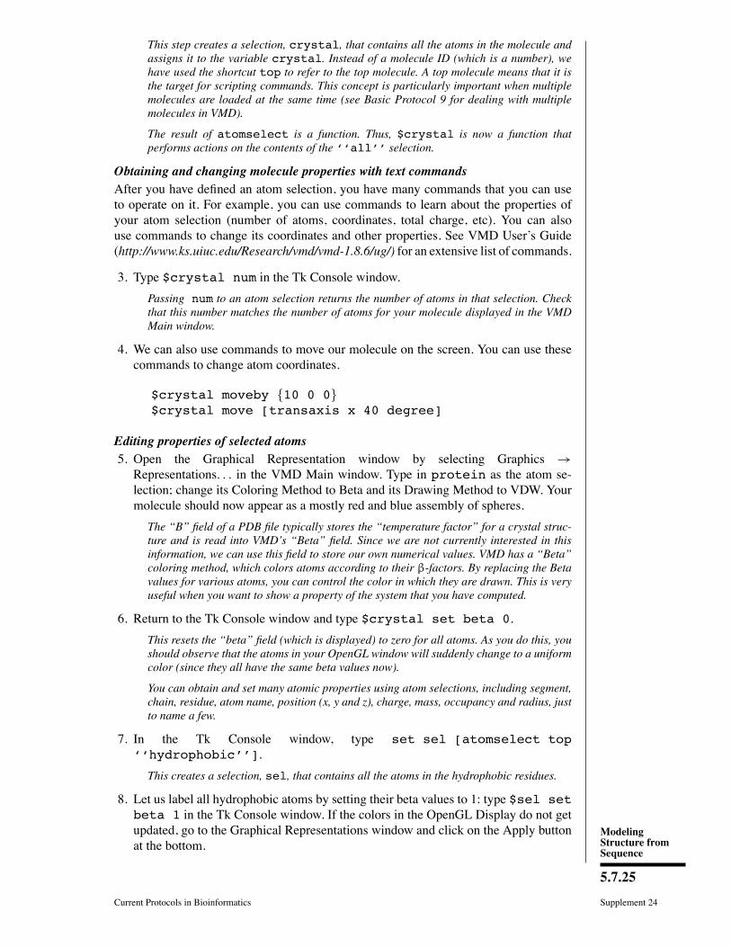
Figure 5.7.18 Ubiquitin in the VDW representation, colored according to the hydrophobicity ofits residues. For the color version of this figure go to http://www.currentprotocols.com.
9. You will now change a physical property of the atoms to further illustrate the distri-bution of hydrophobic residues. In the Tk Console window type $crystal setradius 1.0 to make all the atoms smaller and easier to see through, and then$sel set radius 1.5 to make atoms in the hydrophobic residues larger. Theradius Þeld affects the way that some representations (e.g., VDW, CPK) are drawn.
You have now created a visual state that clearly distinguishes which parts of the proteinare hydrophobic and which are hydrophilic. If you have followed the instructions correctly,your protein should resemble Figure 5.7.18.
Many times in studies of proteins, it is important to identify the locations of the hydrophobicresidues, as they often have a functional implication. The method you have just learnedis useful in this task. For example, you can easily see that in ubiquitin, the hydrophobicresidues are almost exclusively contained in the inner core of the protein. This is a typicalfeature for small water-soluble proteins. As the protein folds, the hydrophilic residues willhave a tendency to stay at the water interface, while the hydrophobic residues are pushedtogether. This helps the protein achieve proper folding and increases its stability.
The get commandAtom selections are useful not only for setting atomic data, but also for getting atomicinformation. For example, if you wish to communicate which residues are hydrophobic,all you need to do is to create a hydrophobic selection and use the get command.
10. Try to use the get command with your sel atom selection to obtain the names ofhydrophobic residues:
$sel get resname
But there is a problem; each residue contains many atoms, resulting in multiple repeatedentries. One way to circumvent this is to pick only the α-carbons in the selection.
11. Type the following in the Tk Console window (note, name CA = α-carbons):
set sel [atomselect top ��hydrophobic and name CA��]$sel get resname
This should give you the list of hydrophobic residues.
ModelingStructure fromSequence
5.7.27
Current Protocols in Bioinformatics Supplement 24
12. You can also get multiple properties simultaneously. Try the following:
$sel get resid$sel get {resname resid}$sel get {x y z}
If you want to obtain some of the structural properties, e.g., the geometric center or thesize of a selection, the command measure can do the job easily.
13. Let us try using measure with the sel selection:
measure center $selmeasure minmax $sel
The first command above returns the geometric center of atoms in sel. And the secondcommand returns two vectors, the first containing the minimum x, y, and z coordinates ofall atoms in sel, and the second containing the corresponding maxima.
Once you are done with a selection, it is always a good idea to delete it to savememory:
$sel delete
BASICPROTOCOL 7
Sourcing Scripts
When performing a task that requires many lines of commands, instead of typing eachline in the Tk Console window, it is usually more convenient to write all the lines intoa script Þle and load it into VMD. This is very easy to do. Just use any text editor towrite your script Þle, and in a VMD session, use the command source filenameto execute the Þle. You should have downloaded a simple script, beta.tcl, withthis unit. We will execute it in VMD as an example. The script beta.tcl sets thecolors of residues LYS and GLY to a different color from the rest of the protein byassigning them a different beta value, a trick you have already learned in Basic Protocol 6,steps 5 to 9.
In the Tk Console window, type source beta.tcl and observe the color change.You should see that the protein is mostly a collection of red spheres, with some residuesshown in blue. The blue residues are the LYS and GLY residues in the ubiquitin. Take aquick look at the script beta.tcl. Using any text editor of your choice, open the Þlebeta.tcl. There are six lines in this Þle, and each line represents a Tcl command linethat you have used before. Close the text editor when you are done.
The .vmd Þle you saved in Basic Protocol 1, step 47, is actually a series of commands.You are encouraged to take a look at that Þle using a text editor. Hopefully, by the end ofthis section, you�ll understand many of those commands. In fact, you can execute the Þlein the Tk Console the same way as you execute other script Þles, i.e., by typing sourcemyfirststate.vmd in the Tk Console window.
Many times when you write a script you might want to look up the commandfor an interactive VMD feature. You can either Þnd it in the VMD User�s Guide(http://www.ks.uiuc.edu/Research/vmd/vmd-1.8.6/ug/) or conveniently use the consolecommand. Try typing logfile console in your Console window. This creates alogÞle for all your actions in VMD and writes them in the Console window as commandlines. If you execute those command lines, you can repeat the exact same actions youhave performed interactively. To turn off logÞle, type logfile off.
Using VMD: AnIntroductory
Tutorial
5.7.28
Supplement 24 Current Protocols in Bioinformatics
BASICPROTOCOL 8
Drawing Shapes Using VMD Text Commands
VMD offers a way to display user-deÞned objects built from graphics primitives such aspoints, lines, cylinders, cones, spheres, triangles, and text. The command that can realizethose functions is graphics, the syntax of which is graphics molid command,where molid is a valid molecule ID and command is one of the commands shownbelow. Let us try drawing some shapes with the following examples.
1. Hide all representations in the Graphics Representations window.
2. Let us draw a point. Type the following command in your Tk Console window:
graphics top point {0 0 10}
Somewhere in your OpenGL window, there should be a small dot.
3. Let us draw a line. Type the following command in your Console window (notethe �\� in command line means the next line is a continuation of the previous line,hence do not actually type �\� when you enter the following command, and do notstart a new line):
graphics top line {-10 0 0} {0 0 0} width 5 style\solid
This will give you a solid line.
4. You can also draw a dashed line:
graphics top line {10 0 0} {0 0 0} width 5 style\dashed
All the objects so far are all drawn in blue. You can change the color of the next graphicsobject by using the command graphics top color colorid. The colorid for eachcolor can be found in Graphics → Colors. . . menu in VMD Main window. For example,the color for orange is “3.”
5. Type graphics top color 3 in the Tk Console window and the next objectyou draw will appear in orange.
6. Try the following commands to draw more shapes:
graphics top cylinder {5 0 0} {15 0 10} radius 10\resolution 60 filled no
graphics top cylinder {0 0 0} {-5 0 10} radius 5\resolution 60 filled yes
graphics top cone {40 0 0} {40 0 10} radius 10\resolution 60
graphics top triangle {80 0 0} {85 0 10} {90 0 0}graphics top text {40 0 20} ��my drawing objects��
7. In your OpenGL window, there are a lot of objects now. To Þnd the list of ob-jects you�ve drawn, use the command graphics top list. You�ll get a list ofnumbers, standing for the ID of each object.
8. The detailed information about each object can be obtained by typing graphicstop info ID. For example, type graphics top info 0 to see the informa-tion on the point you drew.
ModelingStructure fromSequence
5.7.29
Current Protocols in Bioinformatics Supplement 24
9. You can also delete some of the unwanted objects using the command graphicstop delete ID.
Using these basic shape-drawing commands, you can create geometrical objects, as wellas text, to be displayed in your OpenGL window. When you render an image (as discussedin Basic Protocol 2, steps 19 to 23), these objects will be included in the resulting imagefile. You can hence use geometric objects and texts to point or label interesting featuresin your molecule, for example, an arrow (a combination of a cylinder and a cone) can bedrawn this way to point at a region of interest of your molecule
10. Quit VMD.
WORKING WITH MULTIPLE MOLECULES
In this section, you will learn to work with multiple molecules within one VMD session.We will use the water transporting channel protein, aquaporin, as an example.
Necessary Resources
Hardware
Computer
Software
VMD
Files
1fqy.pdb and 1rc2.pdb, which can be downloaded athttp://www.currentprotocols.com
BASICPROTOCOL 9
Molecule List Browser
Aquaporins are membrane channel proteins found in a wide range of species, frombacteria to plants to human. They facilitate water transport across the cell membrane,and play an important role in the control of cell volume and transcellular water trafÞc.Many aquaporin protein structures are available in the Protein Data Bank, including ahuman aquaporin (PDB code 1FQY; Murata et al., 2000) and an E. coli aquaporin (PDBcode 1RC2; Savage et al., 2003). To practice dealing with multiple proteins in VMD, letus load both aquaporin structures.
Loading multiple molecules1. Start a new VMD session. In the VMD Main window, choose File → NewMolecule. . .. The Molecule File Browser window should appear on your screen.
2. Use the Browse. . . button to Þnd the Þle 1fqy.pdb. When you select the Þle, youwill be back in the Molecule File Browser window. Press the Load button to load themolecule. The coordinate Þle of human aquaporin AQP1 should now be loaded andcan be seen in the OpenGL window.
3. In the Molecule File Browser, make sure you choose New Molecule in the Load Þlesfor: pull-down menu on the top. Use the Browse. . . button to Þnd the Þle 1rc2.pdband press Load. Close the Molecule File Browser window.
You have just loaded two molecules. Any number of molecules can be loaded and displayedin VMD simultaneously by repeating the previous step. VMD can load as many moleculesas the memory of your computer allows.
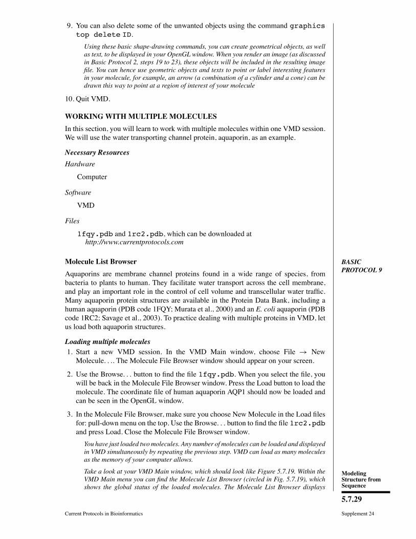
Take a look at your VMD Main window, which should look like Figure 5.7.19. Within theVMD Main menu you can find the Molecule List Browser (circled in Fig. 5.7.19), whichshows the global status of the loaded molecules. The Molecule List Browser displays
Using VMD: AnIntroductory
Tutorial
5.7.30
Supplement 24 Current Protocols in Bioinformatics
Molecule Status Flags
Molecule ListBrowser
Figure 5.7.19 The Molecule List Browser.
information about each molecule, including Molecule ID (ID), the four Molecule StatusFlags (T, A, D, and F, which stand for Top, Active, Drawn, and Fixed), name of themolecule (Molecule), number of atoms in the molecule (Atoms), number of frames loadedin the molecule (Frames), and the volumetric data loaded (Vol). Let us first start with theMolecule column. By default, the Molecule column displays file names of the moleculesloaded in VMD, but you can change the molecule names to recognize them more easily.
Changing molecule names4. In the VMD Main menu, double-click on 1fqy.pdb in the Molecule column. Awindow will pop up with the message Enter a new name for molecule0:. Type in human aquaporin, and click OK (or press enter). In the VMDMainmenu, the Þrst molecule now has the name human aquaporin.
5. Repeat the previous step for the E. coli aquaporin by double-clicking the 1rc2.pdbmolecule name, and changing it to E. coli aquaporin in the pop-up window.
Drawing different representations for different moleculesBefore we continue exploring other features in the Molecule List Browser, take a lookat your OpenGL Display window. You have two aquaporin structures, but since they areboth shown in the same default representation, it is difÞcult to distinguish them. To tellthem apart, you can assign them different representations.
6. Open the Graphical Representations window via Graphics → Representations. . .from the VMD Main menu. Make sure �0:human aquaporin� is selected in theSelected Molecule pull-down menu on top. Select NewCartoon for DrawingMethod,and ColorID→ 1 red for Coloring Method.
7. In the Graphical Representations window, select �1:E. coli aquaporin� in the SelectedMolecule pull-down menu on top. Select NewCartoon for Drawing Method, andColorID → 4 yellow for Coloring Method. Close the Graphical Representationswindow.
Now, your OpenGL Display window should show a human aquaporin colored in red andan E. coli aquaporin colored in yellow.
Molecule status flagsIn your OpenGL Display window, try moving the aquaporins around with your mousein different mouse modes (rotating, scaling, and translating). You can see that bothaquaporins move together. You can Þx any molecule by double-clicking the �F� (Þxed)ßag in the Molecule List Browser on the left of the molecule name.
ModelingStructure fromSequence
5.7.31
Current Protocols in Bioinformatics Supplement 24
8. In the Molecule List Browser, double-click on the �F� ßag on the left of �humanaquaporin� to Þx the human aquaporin molecule. Return to the OpenGL Displaywindow and toggle your mouse around. You can see that only the yellow E. coliaquaporin moves. Double-click on the �F� ßag for human aquaporin again to releaseit.
One thing to notice about the “F” flag is that, although it may seem that one moleculehas been moved relative to another when one of the molecules is fixed, the difference isonly apparent. The internal coordinates of molecules are not changed by the rotation,translation, and scaling motions. To change the coordinates of atoms in a molecule youneed to use the text command interface (discussed in Basic Protocol 6, step 4), or by usingthe atom move picking modes (by choosing Mouse→Move in the VMD Main menu).
Other features in the Molecule List Browser include the Molecule ID (ID), Top (T), Active(A), and Drawn (D). Molecule ID is a number (starting from 0) assigned to each moleculewhen it is loaded into VMD, and permits VMD to recognize each molecule internally. Youalso refer to molecules by their Molecule IDs in the text command interface. Top flag (T)indicates the default molecule in VMD operations, for example when resetting the VMDOpenGL view and when playing molecule trajectories. There can be only one top moleculeat a time. Active flag (A) indicates if the trajectory of the given molecule is updated whenusing animation tools described in Basic Protocol 3.
Finally, Drawn flag (D) indicates if the given molecule is displayed in the OpenGL window.Let us try out the Top and Drawn flags.
9. Make sure no molecule is Þxed. By default, the last molecule loaded in the VMDis the top molecule, so you can check and see that there is a �T� displayed for theE. coli aquaporin in the VMD Main menu.
10. Reset the view by pressing the �=� key on the keyboard while keeping the OpenGLDisplay window active. Note that the yellow E. coli aquaporin is now placed in thecenter of the OpenGL Display window.
11. Switch the top molecule by double-clicking on the empty �T� ßag for the humanaquaporin molecule in the VMD Main menu. A �T� should appear for the humanaquaporin, while the �T� for E. coli disappears. Go to the OpenGL Display windowand reset the view again. You can see that this time the red human aquaporin is placedin the center of the OpenGL Display window.
12. In the VMD Main menu, try hiding a molecule by double-clicking on its �D� ßag.You can display the molecule again by double-clicking its �D� ßag again.
BASICPROTOCOL 10
Aligning Molecules with the measure fit Command
When you look at your OpenGL Display window, you can see that the two aquaporinsare very similar in structure. But it is difÞcult to detect their slight structural differencesas the two proteins are placed apart. We will now try out a very useful Tcl commandmeasure fit to align two molecules.
Open the VMDTkConsole window by choosing Extension→TkConsole from the VMDMain menu, and input the following commands:
set sel0 [atomselect 0 all]set sel1 [atomselect 1 all]set M [measure fit $sel0 $sel1]$sel0 move $M
measure fit selection1 selection2 � measures the transformationmatrix that best aligns the coordinates of selection1 with the coordinates ofselection2.
Using VMD: AnIntroductory
Tutorial
5.7.32
Supplement 24 Current Protocols in Bioinformatics
Figure 5.7.20 Result of the alignment between the two aquaporins using the measure fitcommand. For the color version of this figure go to http://www.currentprotocols.com.
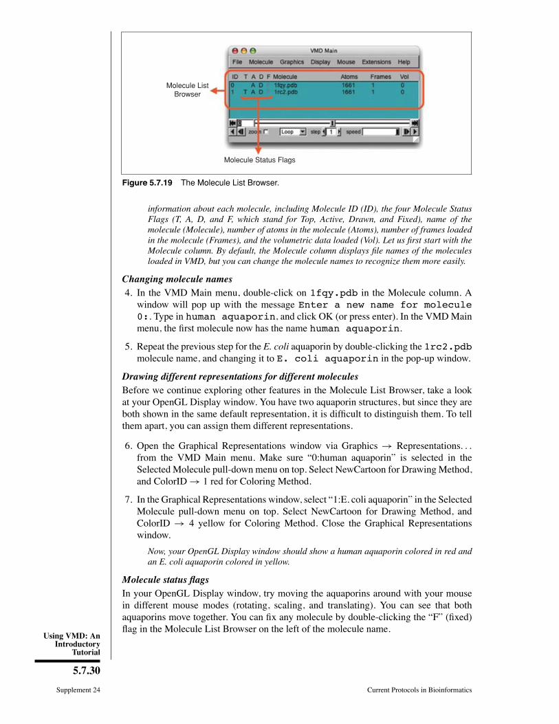
As soon as you enter the last command line, you can see that the two aquaporins arenow overlapping (Fig. 5.7.20). The α-helical regions of the aquaporins agree very well,with bigger deviations in the loop regions. Note that the measure fit command canonly work if two molecules have the same number of atoms. In this case, it is a purecoincidence that the human aquaporin and E. coli aquaporin PDB Þles have the samenumber of atoms. The measure fit command is hence most useful in aligning thesame protein in different conformations or different frames of a molecular dynamicssimulation trajectory. Generally, to compare the structures of different proteins, oneneeds to use a different method. A good tool is the VMDMultiSeq plugin, which we willdiscuss in the following section.
COMPARING PROTEIN STRUCTURES AND SEQUENCES WITH THEMultiSeq PLUGIN
MultiSeq (Roberts et al., 2006) is a bioinformatics analysis environment developed inthe Luthey-Schulten Group at the University of Illinois in Urbana-Champaign. MultiSeqallows users to organize, display, and analyze both sequence and structure data for proteinsand nucleic acids, and has been incorporated in VMD as a plugin tool starting with VMDversion 1.8.5 (MultiSeq homepage: http://www.scs.uiuc.edu/∼schulten/multiseq). In thissection, you will learn how to compare protein structures and sequences with the VMDMultiSeq plugin. We will again use the water transporting channel protein, aquaporin, asan example.
ModelingStructure fromSequence
5.7.33
Current Protocols in Bioinformatics Supplement 24
Necessary Resources
Hardware
Computer
Software
VMD, and a text editor
Files
1fqy.pdb, 1rc2.pdb, 1lda.pdb, 1j4n.pdb, and spinach aqp.fasta, which can be downloaded at http://www.currentprotocols.com
BASICPROTOCOL 11
Structure Alignment with MultiSeq
Very often comparing structures of different proteins reveals important information.For example, proteins with similar functions tend to exhibit similar structural features.MultiSeq structure alignment is useful for this reason. We will compare the structures offour aquaporin proteins listed in Table 5.7.8.
Loading aquaporin structures1. Start a new VMD session. Open the Molecule File Browser window by choosing theFile→NewMolecule. . .menu item in the VMDMain window. In the Molecule FileBrowser window, use the Browse. . . button to Þnd and select the Þle 1fqy.pdb.Press Load to load the molecule.
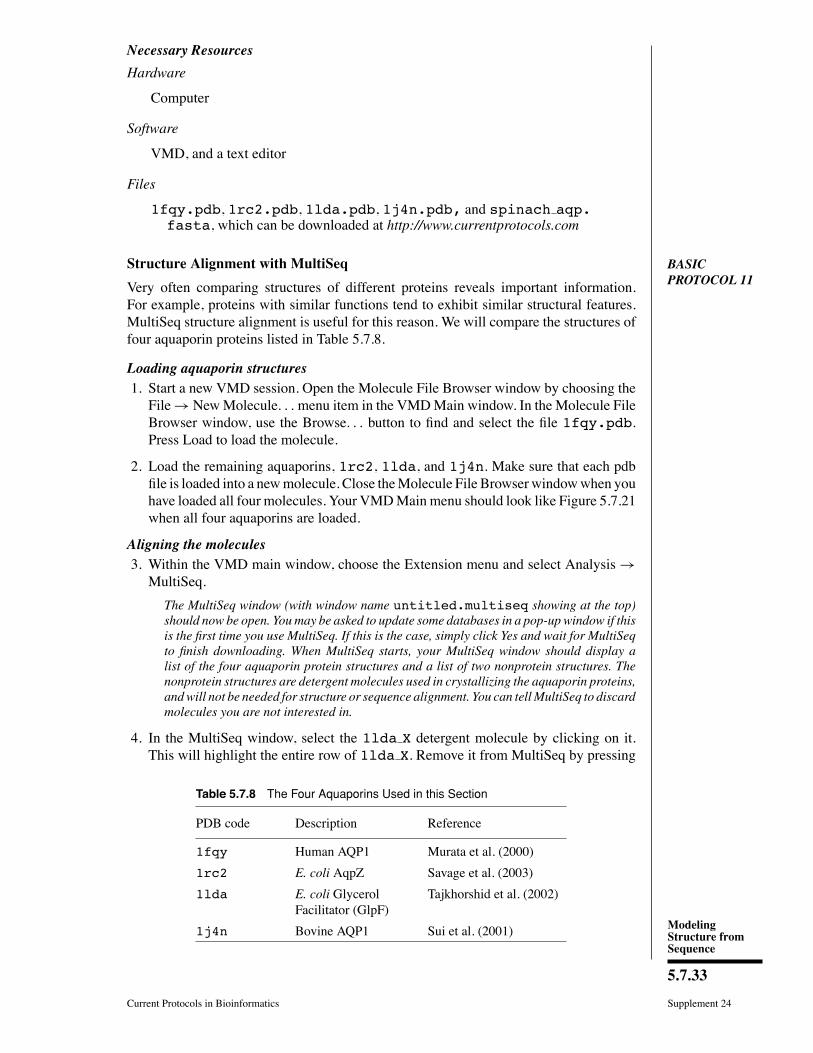
2. Load the remaining aquaporins, 1rc2, 1lda, and 1j4n. Make sure that each pdbÞle is loaded into a newmolecule. Close theMolecule File Browser windowwhen youhave loaded all four molecules. Your VMDMain menu should look like Figure 5.7.21when all four aquaporins are loaded.
Aligning the molecules3. Within the VMD main window, choose the Extension menu and select Analysis →MultiSeq.
The MultiSeq window (with window name untitled.multiseq showing at the top)should now be open. You may be asked to update some databases in a pop-up window if thisis the first time you use MultiSeq. If this is the case, simply click Yes and wait for MultiSeqto finish downloading. When MultiSeq starts, your MultiSeq window should display alist of the four aquaporin protein structures and a list of two nonprotein structures. Thenonprotein structures are detergent molecules used in crystallizing the aquaporin proteins,and will not be needed for structure or sequence alignment. You can tell MultiSeq to discardmolecules you are not interested in.
4. In the MultiSeq window, select the 1lda X detergent molecule by clicking on it.This will highlight the entire row of 1lda X. Remove it from MultiSeq by pressing
Table 5.7.8 The Four Aquaporins Used in this Section
PDB code Description Reference
1fqy Human AQP1 Murata et al. (2000)
1rc2 E. coli AqpZ Savage et al. (2003)
1lda E. coli GlycerolFacilitator (GlpF)
Tajkhorshid et al. (2002)
1j4n Bovine AQP1 Sui et al. (2001)
Using VMD: AnIntroductory
Tutorial
5.7.34
Supplement 24 Current Protocols in Bioinformatics
Figure 5.7.21 VMD Main menu after loading the four aquaporins.
the delete or Backspace key on your keyboard. Do the same to remove the 1j4n Xdetergent molecule.
MultiSeq uses the program STAMP (Russell and Barton, 1992) to align protein molecules.STAMP (Structural Alignment of Multiple Proteins) is a tool for aligning protein sequencesbased on three-dimensional structures. Its algorithm minimizes the Cα distance betweenaligned residues of each molecule by applying globally optimal rigid-body rotations andtranslations. Note that you can only perform alignments on molecules that are structurallysimilar, if you try to align proteins that have no common structures, STAMP will fail.
5. In the MultiSeq window, select Tool→ Stamp Structural Alignment. This will openthe Stamp Alignment Options window.
6. In the Stamp Alignment Options window, choose Align the following: All Structuresand go to the bottom of the menu and press OK.
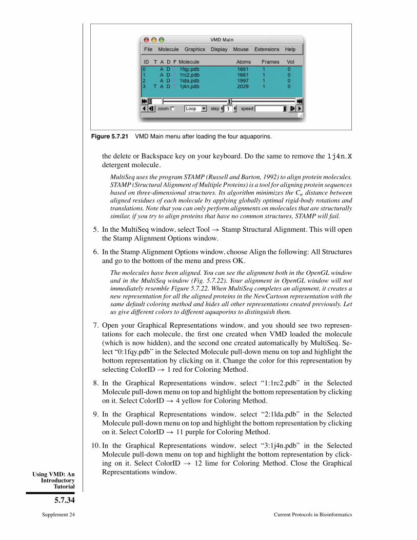
The molecules have been aligned. You can see the alignment both in the OpenGL windowand in the MultiSeq window (Fig. 5.7.22). Your alignment in OpenGL window will notimmediately resemble Figure 5.7.22. When MultiSeq completes an alignment, it creates anew representation for all the aligned proteins in the NewCartoon representation with thesame default coloring method and hides all other representations created previously. Letus give different colors to different aquaporins to distinguish them.
7. Open your Graphical Representations window, and you should see two represen-tations for each molecule, the Þrst one created when VMD loaded the molecule(which is now hidden), and the second one created automatically by MultiSeq. Se-lect �0:1fqy.pdb� in the Selected Molecule pull-down menu on top and highlight thebottom representation by clicking on it. Change the color for this representation byselecting ColorID→ 1 red for Coloring Method.
8. In the Graphical Representations window, select �1:1rc2.pdb� in the SelectedMolecule pull-down menu on top and highlight the bottom representation by clickingon it. Select ColorID→ 4 yellow for Coloring Method.
9. In the Graphical Representations window, select �2:1lda.pdb� in the SelectedMolecule pull-down menu on top and highlight the bottom representation by clickingon it. Select ColorID→ 11 purple for Coloring Method.
10. In the Graphical Representations window, select �3:1j4n.pdb� in the SelectedMolecule pull-down menu on top and highlight the bottom representation by click-ing on it. Select ColorID → 12 lime for Coloring Method. Close the GraphicalRepresentations window.
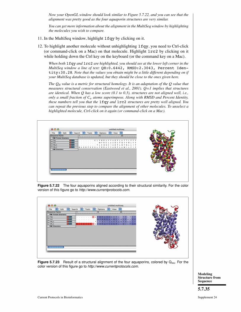
ModelingStructure fromSequence
5.7.35
Current Protocols in Bioinformatics Supplement 24
Now your OpenGL window should look similar to Figure 5.7.22, and you can see that thealignment was pretty good as the four aquaporin structures are very similar.
You can get more information about the alignment in the MultiSeq window by highlightingthe molecules you wish to compare.
11. In the MultiSeq window, highlight 1fqy by clicking on it.
12. To highlight another molecule without unhighlighting 1fqy, you need to Ctrl-click(or command-click on a Mac) on that molecule. Highlight 1rc2 by clicking on itwhile holding down the Ctrl key on the keyboard (or the command key on a Mac).
When both 1fqy and 1rc2 are highlighted, you should see at the lower left corner in theMultiSeq window a line of text: QH:0.6442, RMSD:2.3043, Percent Iden-tity:30.28. Note that the values you obtain might be a little different depending on ifyour MultiSeq database is updated, but they should be close to the ones given here.
The QH value is a metric for structural homology. It is an adaptation of the Q value thatmeasures structural conservation (Eastwood et al., 2001). Q=1 implies that structuresare identical. When Q has a low score (0.1 to 0.3), structures are not aligned well, i.e.,only a small fraction of Cα atoms superimpose. Along with RMSD and Percent Identity,these numbers tell you that the 1fqy and 1rc2 structures are pretty well aligned. Youcan repeat the previous step to compare the alignment of other molecules. To unselect ahighlighted molecule, Ctrl-click on it again (or command-click on a Mac).
Figure 5.7.22 The four aquaporins aligned according to their structural similarity. For the colorversion of this figure go to http://www.currentprotocols.com.
Figure 5.7.23 Result of a structural alignment of the four aquaporins, colored by Qres. For thecolor version of this figure go to http://www.currentprotocols.com.
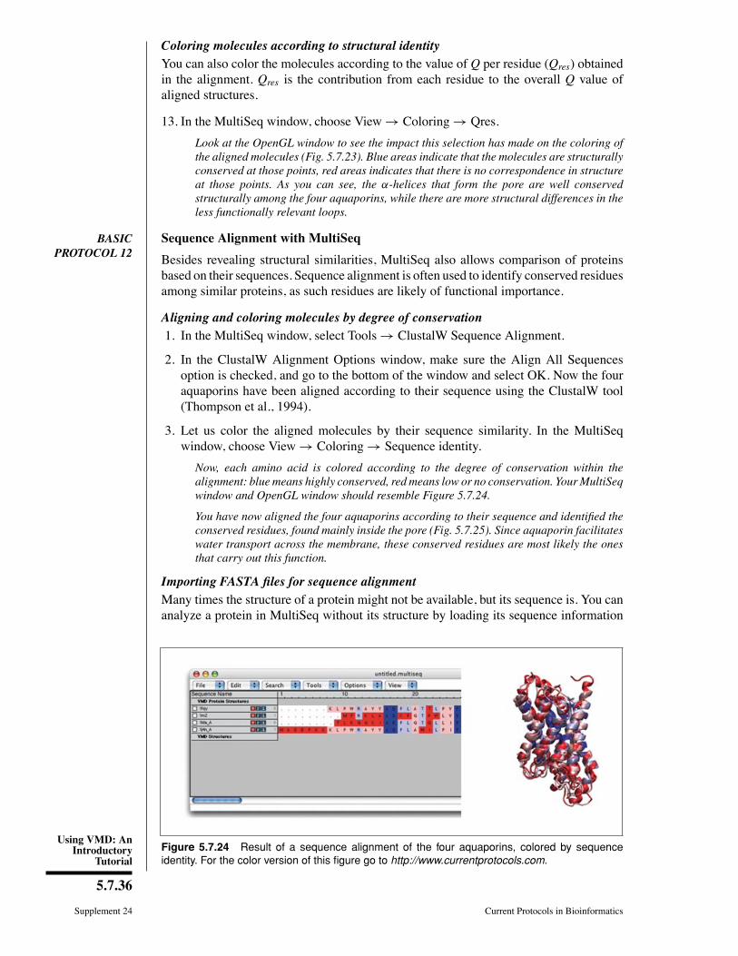
Using VMD: AnIntroductory
Tutorial
5.7.36
Supplement 24 Current Protocols in Bioinformatics
Coloring molecules according to structural identityYou can also color the molecules according to the value of Q per residue (Qres) obtainedin the alignment. Qres is the contribution from each residue to the overall Q value ofaligned structures.
13. In the MultiSeq window, choose View→ Coloring→ Qres.
Look at the OpenGL window to see the impact this selection has made on the coloring ofthe aligned molecules (Fig. 5.7.23). Blue areas indicate that the molecules are structurallyconserved at those points, red areas indicates that there is no correspondence in structureat those points. As you can see, the α-helices that form the pore are well conservedstructurally among the four aquaporins, while there are more structural differences in theless functionally relevant loops.
BASICPROTOCOL 12
Sequence Alignment with MultiSeq
Besides revealing structural similarities, MultiSeq also allows comparison of proteinsbased on their sequences. Sequence alignment is often used to identify conserved residuesamong similar proteins, as such residues are likely of functional importance.
Aligning and coloring molecules by degree of conservation1. In the MultiSeq window, select Tools→ ClustalW Sequence Alignment.
2. In the ClustalW Alignment Options window, make sure the Align All Sequencesoption is checked, and go to the bottom of the window and select OK. Now the fouraquaporins have been aligned according to their sequence using the ClustalW tool(Thompson et al., 1994).
3. Let us color the aligned molecules by their sequence similarity. In the MultiSeqwindow, choose View→ Coloring→ Sequence identity.
Now, each amino acid is colored according to the degree of conservation within thealignment: blue means highly conserved, red means low or no conservation. Your MultiSeqwindow and OpenGL window should resemble Figure 5.7.24.
You have now aligned the four aquaporins according to their sequence and identified theconserved residues, found mainly inside the pore (Fig. 5.7.25). Since aquaporin facilitateswater transport across the membrane, these conserved residues are most likely the onesthat carry out this function.
Importing FASTA files for sequence alignmentMany times the structure of a protein might not be available, but its sequence is. You cananalyze a protein in MultiSeq without its structure by loading its sequence information
Figure 5.7.24 Result of a sequence alignment of the four aquaporins, colored by sequenceidentity. For the color version of this figure go to http://www.currentprotocols.com.
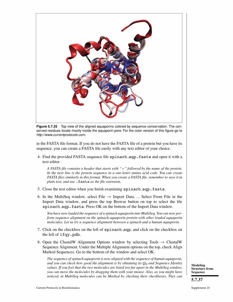
ModelingStructure fromSequence
5.7.37
Current Protocols in Bioinformatics Supplement 24
Figure 5.7.25 Top view of the aligned aquaporins colored by sequence conservation. The con-served residues locate mostly inside the aquaporin pore. For the color version of this figure go tohttp://www.currentprotocols.com.
in the FASTA Þle format. If you do not have the FASTA Þle of a protein but you have itssequence, you can create a FASTA Þle easily with any text editor of your choice.
4. Find the provided FASTA sequence Þle spinach aqp.fasta and open it with atext editor.
A FASTA file contains a header that starts with “>” followed by the name of the protein.In the next line is the protein sequence in a one-letter amino acid code. You can createFASTA files similarly in this format. When you create a FASTA file, remember to save it inplain text, and use .fasta as the file extension.
5. Close the text editor when you Þnish examining spinach aqp.fasta.
6. In the MultiSeq window, select File → Import Data. . .. Select From File in theImport Data window, and press the top Browse button on top to select the Þlespinach aqp.fasta. Press OK on the bottom of the Import Data window.
You have now loaded the sequence of a spinach aquaporin into MultiSeq. You can now per-form sequence alignment on the spinach aquaporin protein with other loaded aquaporinmolecules. Let us try a sequence alignment between a spinach and a human aquaporin.
7. Click on the checkbox on the left of spinach aqp, and click on the checkbox onthe left of 1fqy.pdb.
8. Open the ClustalW Alignment Options window by selecting Tools → ClustalWSequence Alignment. Under the Multiple Alignment options on the top, check AlignMarked Sequences. Go to the bottom of the window and select OK.
The sequence of spinach aquaporin is now aligned with the sequence of human aquaporin,and you can check how good the alignment is by obtaining its QH and Sequence Identityvalues. If you feel that the two molecules are listed too far apart in the MultiSeq window,you can move the molecules by dragging them with your mouse. Also, as you might havenoticed, in MultiSeq molecules can be Marked by checking their checkboxes. They can
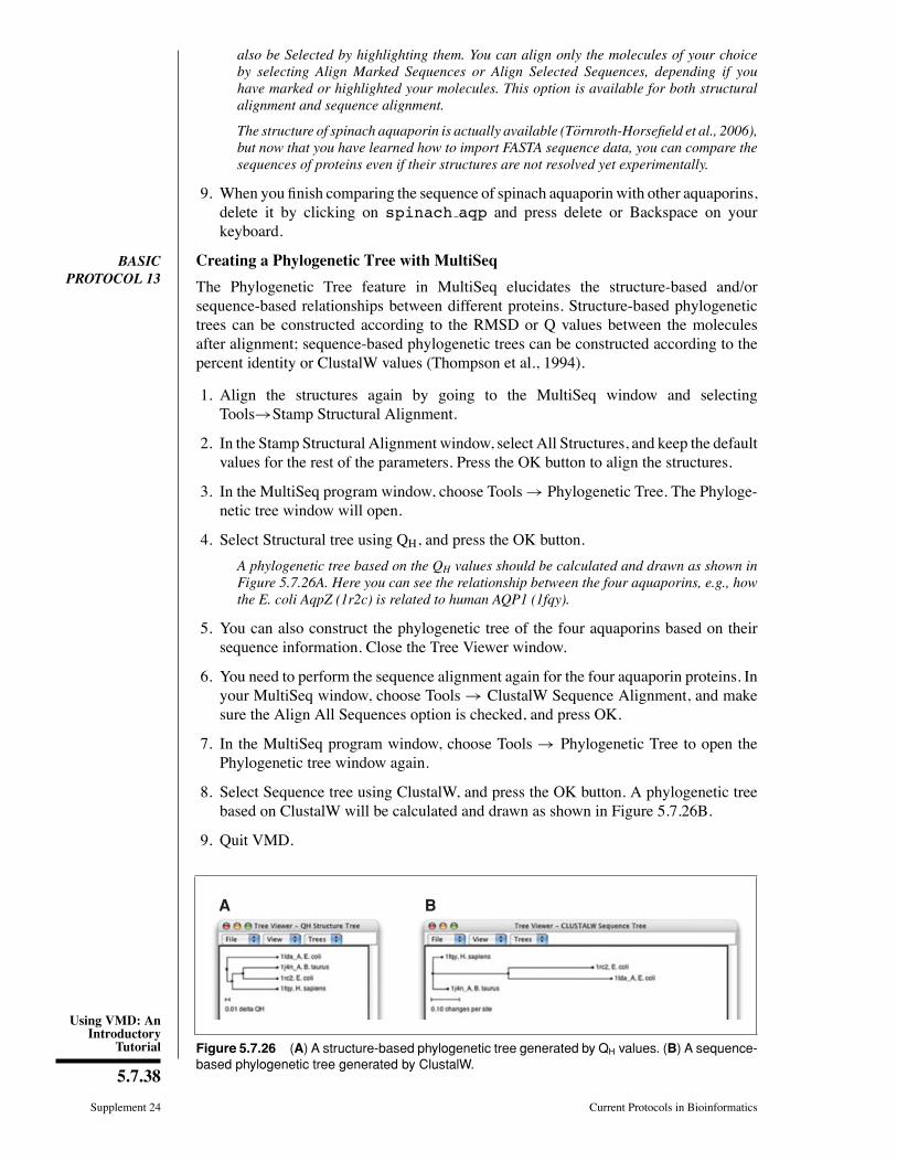
Using VMD: AnIntroductory
Tutorial
5.7.38
Supplement 24 Current Protocols in Bioinformatics
also be Selected by highlighting them. You can align only the molecules of your choiceby selecting Align Marked Sequences or Align Selected Sequences, depending if youhave marked or highlighted your molecules. This option is available for both structuralalignment and sequence alignment.
The structure of spinach aquaporin is actually available (Tornroth-Horsefield et al., 2006),but now that you have learned how to import FASTA sequence data, you can compare thesequences of proteins even if their structures are not resolved yet experimentally.
9. When you Þnish comparing the sequence of spinach aquaporin with other aquaporins,delete it by clicking on spinach aqp and press delete or Backspace on yourkeyboard.
BASICPROTOCOL 13
Creating a Phylogenetic Tree with MultiSeq
The Phylogenetic Tree feature in MultiSeq elucidates the structure-based and/orsequence-based relationships between different proteins. Structure-based phylogenetictrees can be constructed according to the RMSD or Q values between the moleculesafter alignment; sequence-based phylogenetic trees can be constructed according to thepercent identity or ClustalW values (Thompson et al., 1994).
1. Align the structures again by going to the MultiSeq window and selectingTools→Stamp Structural Alignment.
2. In the Stamp Structural Alignment window, select All Structures, and keep the defaultvalues for the rest of the parameters. Press the OK button to align the structures.
3. In the MultiSeq program window, choose Tools→ Phylogenetic Tree. The Phyloge-netic tree window will open.
4. Select Structural tree using QH, and press the OK button.
A phylogenetic tree based on the QH values should be calculated and drawn as shown inFigure 5.7.26A. Here you can see the relationship between the four aquaporins, e.g., howthe E. coli AqpZ (1r2c) is related to human AQP1 (1fqy).
5. You can also construct the phylogenetic tree of the four aquaporins based on theirsequence information. Close the Tree Viewer window.
6. You need to perform the sequence alignment again for the four aquaporin proteins. Inyour MultiSeq window, choose Tools → ClustalW Sequence Alignment, and makesure the Align All Sequences option is checked, and press OK.
7. In the MultiSeq program window, choose Tools → Phylogenetic Tree to open thePhylogenetic tree window again.
8. Select Sequence tree using ClustalW, and press the OK button. A phylogenetic treebased on ClustalW will be calculated and drawn as shown in Figure 5.7.26B.
9. Quit VMD.
BA
Figure 5.7.26 (A) A structure-based phylogenetic tree generated by QH values. (B) A sequence-based phylogenetic tree generated by ClustalW.
ModelingStructure fromSequence
5.7.39
Current Protocols in Bioinformatics Supplement 24
DATA ANALYSIS IN VMD
VMD is a powerful tool for analysis of structures and trajectories. Numerous tools foranalysis are available under theVMDMainmenu itemExtension→Analysis. In additionto these built-in tools, VMD users often use custom-written scripts to analyze desiredproperties of the simulated systems. VMD Tcl scripting capabilities are very extensive,and provide boundless opportunities for analysis. In this section, we will learn how touse built-in VMD features for standard analysis, as well as consider a simple example ofscripting.
Necessary Resources
Hardware
Computer
Software
VMD, a text editor, and a plotting application
Files
ubiquitin.psf, pulling.dcd, equilibration.dcd and distance.tcl, which can be downloaded at http://www.currentprotocols.com
BASICPROTOCOL 14
Adding Labels in VMD
Labels can be placed in VMD to get information on a particular selection, to be usedduring visualization and quantitative analysis. Labels are selected with the mouse andcan be accessed in Graphics → Labels menu. We will cover labels that can be placedon atoms and bonds, although angle and dihedral labelings are also available. In thiscontext, labels for �bonds� or �angles� actually mean distances between two atoms orangles between three atoms, the atoms do not have to be physically connected by bondsin the molecule.
1. Start a new VMD session. Load the ubiquitin trajectory into VMD (using the Þlesubiquitin.psf and pulling.dcd). For graphical representation, display pro-tein only, using NewCartoon for drawing method and Structure for coloring method.If you need help, see Basic Protocol 3, steps 1 to 6.
2. Choose the Mouse→ Labels→ Atoms menu item from the VMD Main menu. Themouse is now set to the mode for displaying atom labels. You can click on any atomon your molecule and a label will be placed for this atom. Clicking again on it willerase the label.
3. We will now try the same for bonds. Choose the Mouse → Label → Bonds menuitem from the VMD Main menu. This selects the Display Label for Bond mode.
We will consider the distance between the α carbon of Lysine 48 and of the C terminus.In the pulling simulation, the former is kept fixed, and the latter is pulled at a constantforce of 500 pN. In reality, polyubiquitin chains can be linked by a connection between theC terminus of one ubiquitin molecule and the Lysine 48 of the next. The simulation thenmimics the effect of pulling on the C terminus with this kind of linkage.
4. Open the TkConsole window by selecting Extensions → Tk Console in the VMDMain menu. We will make a VDW representation for the α carbons of Lysine 48 andof the C terminus. To Þnd out the indices of these atoms, make a selection includingthese two atoms by typing in the TkConsole window:
set sel [atomselect top ��resid 48 76 and name CA��]
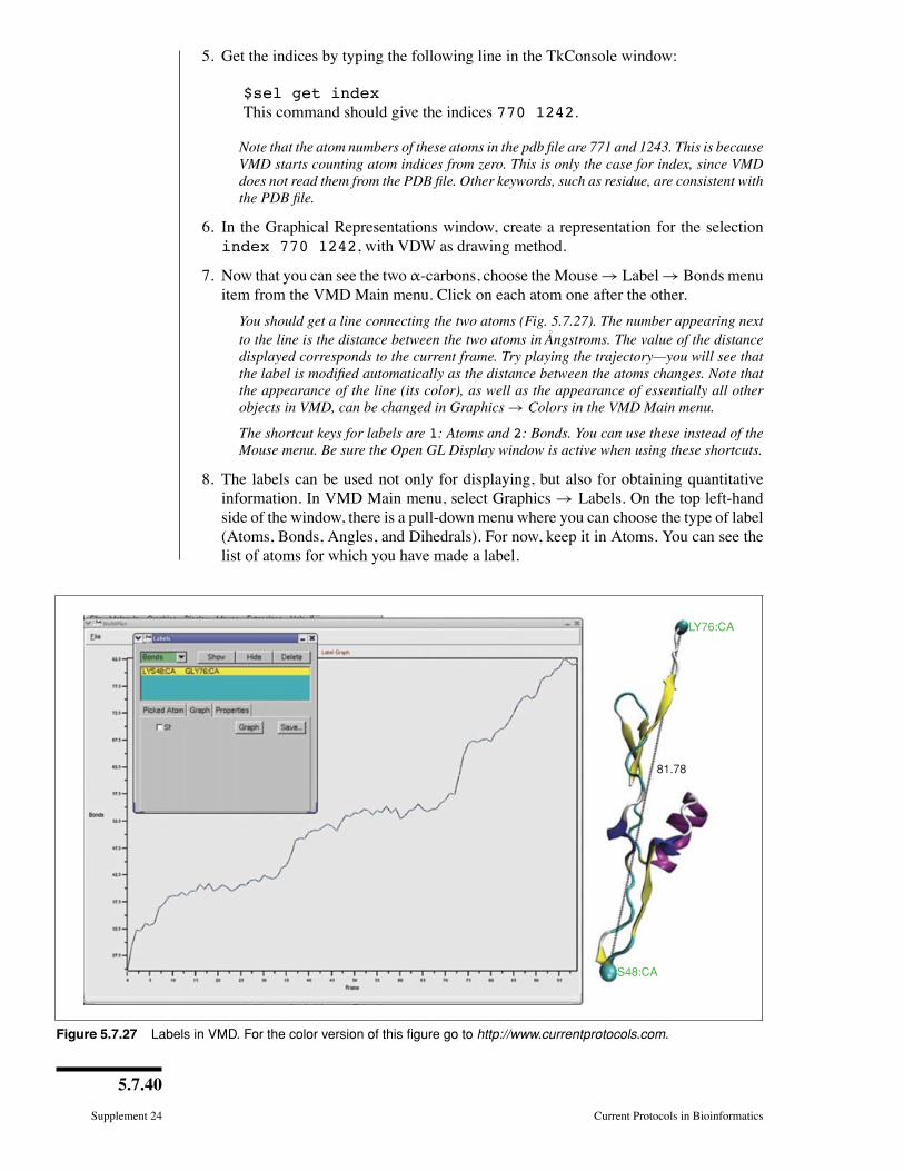
5.7.40
Supplement 24 Current Protocols in Bioinformatics
5. Get the indices by typing the following line in the TkConsole window:
$sel get indexThis command should give the indices 770 1242.
Note that the atom numbers of these atoms in the pdb file are 771 and 1243. This is becauseVMD starts counting atom indices from zero. This is only the case for index, since VMDdoes not read them from the PDB file. Other keywords, such as residue, are consistent withthe PDB file.
6. In the Graphical Representations window, create a representation for the selectionindex 770 1242, with VDW as drawing method.
7. Now that you can see the two α-carbons, choose theMouse→ Label→Bonds menuitem from the VMD Main menu. Click on each atom one after the other.
You should get a line connecting the two atoms (Fig. 5.7.27). The number appearing nextto the line is the distance between the two atoms in
◦Angstroms. The value of the distance
displayed corresponds to the current frame. Try playing the trajectory—you will see thatthe label is modified automatically as the distance between the atoms changes. Note thatthe appearance of the line (its color), as well as the appearance of essentially all otherobjects in VMD, can be changed in Graphics → Colors in the VMD Main menu.
The shortcut keys for labels are 1: Atoms and 2: Bonds. You can use these instead of theMouse menu. Be sure the Open GL Display window is active when using these shortcuts.
8. The labels can be used not only for displaying, but also for obtaining quantitativeinformation. In VMD Main menu, select Graphics → Labels. On the top left-handside of the window, there is a pull-down menu where you can choose the type of label(Atoms, Bonds, Angles, and Dihedrals). For now, keep it in Atoms. You can see thelist of atoms for which you have made a label.
LY76:CA
S48:CA
81.78
Figure 5.7.27 Labels in VMD. For the color version of this figure go to http://www.currentprotocols.com.
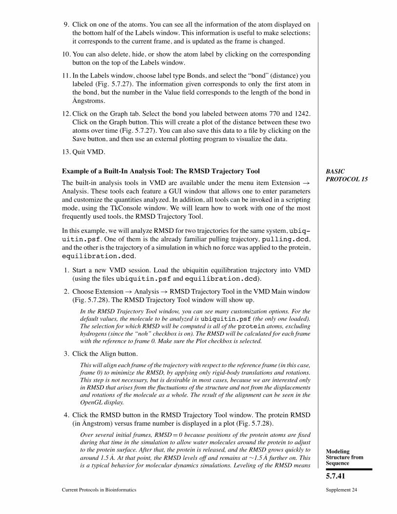
ModelingStructure fromSequence
5.7.41
Current Protocols in Bioinformatics Supplement 24
9. Click on one of the atoms. You can see all the information of the atom displayed onthe bottom half of the Labels window. This information is useful to make selections;it corresponds to the current frame, and is updated as the frame is changed.
10. You can also delete, hide, or show the atom label by clicking on the correspondingbutton on the top of the Labels window.
11. In the Labels window, choose label type Bonds, and select the �bond� (distance) youlabeled (Fig. 5.7.27). The information given corresponds to only the Þrst atom inthe bond, but the number in the Value Þeld corresponds to the length of the bond in◦Angstroms.
12. Click on the Graph tab. Select the bond you labeled between atoms 770 and 1242.Click on the Graph button. This will create a plot of the distance between these twoatoms over time (Fig. 5.7.27). You can also save this data to a Þle by clicking on theSave button, and then use an external plotting program to visualize the data.
13. Quit VMD.
BASICPROTOCOL 15
Example of a Built-In Analysis Tool: The RMSD Trajectory Tool
The built-in analysis tools in VMD are available under the menu item Extension →Analysis. These tools each feature a GUI window that allows one to enter parametersand customize the quantities analyzed. In addition, all tools can be invoked in a scriptingmode, using the TkConsole window. We will learn how to work with one of the mostfrequently used tools, the RMSD Trajectory Tool.
In this example, we will analyze RMSD for two trajectories for the same system, ubiq-uitin.psf. One of them is the already familiar pulling trajectory, pulling.dcd,and the other is the trajectory of a simulation in which no force was applied to the protein,equilibration.dcd.
1. Start a new VMD session. Load the ubiquitin equilibration trajectory into VMD(using the Þles ubiquitin.psf and equilibration.dcd).
2. Choose Extension→Analysis→ RMSD Trajectory Tool in the VMDMain window(Fig. 5.7.28). The RMSD Trajectory Tool window will show up.
In the RMSD Trajectory Tool window, you can see many customization options. For thedefault values, the molecule to be analyzed is ubiquitin.psf (the only one loaded).The selection for which RMSD will be computed is all of the protein atoms, excludinghydrogens (since the “noh” checkbox is on). The RMSD will be calculated for each framewith the reference to frame 0. Make sure the Plot checkbox is selected.
3. Click the Align button.
This will align each frame of the trajectory with respect to the reference frame (in this case,frame 0) to minimize the RMSD, by applying only rigid-body translations and rotations.This step is not necessary, but is desirable in most cases, because we are interested onlyin RMSD that arises from the fluctuations of the structure and not from the displacementsand rotations of the molecule as a whole. The result of the alignment can be seen in theOpenGL display.
4. Click the RMSD button in the RMSD Trajectory Tool window. The protein RMSD(in
◦Angstrom) versus frame number is displayed in a plot (Fig. 5.7.28).
Over several initial frames, RMSD = 0 because positions of the protein atoms are fixedduring that time in the simulation to allow water molecules around the protein to adjustto the protein surface. After that, the protein is released, and the RMSD grows quickly toaround 1.5
◦A. At that point, the RMSD levels off and remains at ∼1.5
◦A further on. This
is a typical behavior for molecular dynamics simulations. Leveling of the RMSD means
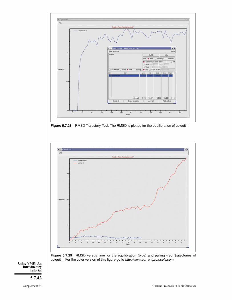
Using VMD: AnIntroductory
Tutorial
5.7.42
Supplement 24 Current Protocols in Bioinformatics
Figure 5.7.28 RMSD Trajectory Tool. The RMSD is plotted for the equilibration of ubiquitin.
Figure 5.7.29 RMSD versus time for the equilibration (blue) and pulling (red) trajectories ofubiquitin. For the color version of this figure go to http://www.currentprotocols.com.
ModelingStructure fromSequence
5.7.43
Current Protocols in Bioinformatics Supplement 24
that the protein has relaxed from its initial crystal structure (which is affected by crystalpacking and usually misses some atoms, e.g., hydrogens) to a more stable one. Productionmolecular dynamics simulations are usually preceded by such equilibration runs, wherethe protein is allowed to relax; the process is monitored by checking RMSD versus time,and equilibration is assumed to be sufficient when RMSD levels off. The RMSD of 1.5
◦A is
an acceptable value for most protein simulations. Usually, the deviations from the crystalstructure in a simulation are due to the thermal motion and to the relaxation processmentioned; imperfections of the simulation force-fields contribute as well.
5. Wewill nowworkwith the other trajectory, inwhich the ubiquitin is pulled apart. Loadthis trajectory into VMD using the Þles ubiquitin.psf and pulling.dcd.Make sure you load ubiquitin.psf as a new molecule. You can change thenames of the molecules by double-clicking on them in the VMD Main menu (seeBasic Protocol 9, steps 4 and 5).
6. In the RMSD Trajectory Tool window, hit the button Add all to update the list ofmolecules.
7. Click the Align button and then click RMSD button.
The new graph (Fig. 5.7.29) displays two RMSD plots versus time, one for the equilibrationtrajectory, and the other for the pulling trajectory. The RMSD for the pulling trajectorydoes not level off and is much higher than that in the equilibration trajectory, since theprotein is stretched in the simulation.
8. Quit VMD.
BASICPROTOCOL 16
Example of an Analysis Script
In many cases, one requires special types of trajectory analyses that are tailored forcertain needs. The Tcl scripting in VMD provides opportunities for such customtasks. Users commonly write their own scripts to analyze the features of interest. Avery extensive library of VMD scripts, contributed by many users, is available online(http://www.ks.uiuc.edu/Research/vmd/script library/). Here, we will explore a very sim-ple exemplary script, distance.tcl, which computes the distance between two atomselections vs. time and the distribution of the distances.
1. Start a new VMD session. Load the ubiquitin equilibration trajectory (Þlesubiquitin.psf and equilibration.dcd).
2. Open the TkConsole window by selecting Extension → Tk Console in the VMDMain menu.
3. In the TkConsole window, load the script into VMD by typing: sourcedistance.tcl (make sure that the Þle distance.tcl is in the current folder).This will load the procedure deÞned in distance.tcl into VMD.
4. One can now invoke the procedure by typing distance in the TkConsole window.In fact, the correct usage is
distance seltext1 seltext2 N d f r out f d out
where seltext1 and seltext2 are the selection texts for the groups of atomsbetweenwhich the distance ismeasured,N d is the number of bins for the distribution,and f r out and f d out are the Þle names to where the output distance versustime and distance distribution will be written.
5. Open the script Þle distance.tcl with a text editor. You can see that the scriptdoes the following:
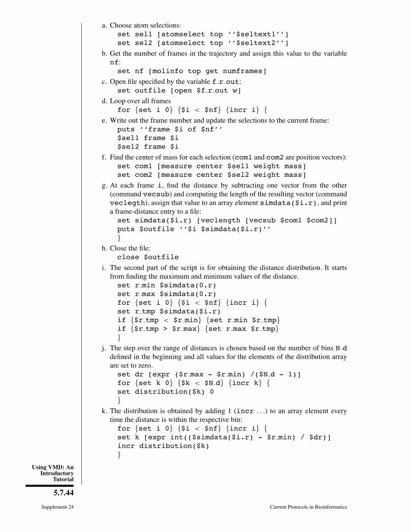
Using VMD: AnIntroductory
Tutorial
5.7.44
Supplement 24 Current Protocols in Bioinformatics
a. Choose atom selections:set sel1 [atomselect top ��$seltext1��]set sel2 [atomselect top ��$seltext2��]
b. Get the number of frames in the trajectory and assign this value to the variablenf:set nf [molinfo top get numframes]
c. Open Þle speciÞed by the variable f r out:set outfile [open $f r out w]
d. Loop over all framesfor {set i 0} {$i < $nf} {incr i} {
e. Write out the frame number and update the selections to the current frame:puts ��frame $i of $nf��$sel1 frame $i$sel2 frame $i
f. Find the center of mass for each selection (com1 and com2 are position vectors):set com1 [measure center $sel1 weight mass]set com2 [measure center $sel2 weight mass]
g. At each frame i, Þnd the distance by subtracting one vector from the other(command vecsub) and computing the length of the resulting vector (commandveclegth), assign that value to an array element simdata($i.r), and printa frame-distance entry to a Þle:set simdata($i.r) [veclength [vecsub $com1 $com2]]puts $outfile ��$i $simdata($i.r)��}
h. Close the Þle:close $outfile
i. The second part of the script is for obtaining the distance distribution. It startsfrom Þnding the maximum and minimum values of the distance.set r min $simdata(0.r)set r max $simdata(0.r)for {set i 0} {$i < $nf} {incr i} {set r tmp $simdata($i.r)if {$r tmp < $r min} {set r min $r tmp}if {$r tmp > $r max} {set r max $r tmp}}
j. The step over the range of distances is chosen based on the number of bins N ddeÞned in the beginning and all values for the elements of the distribution arrayare set to zero.set dr [expr ($r max - $r min) /($N d - 1)]for {set k 0} {$k < $N d} {incr k} {set distribution($k) 0}
k. The distribution is obtained by adding 1 (incr . . .) to an array element everytime the distance is within the respective bin:for {set i 0} {$i < $nf} {incr i} {set k [expr int(($simdata($i.r) - $r min) / $dr)]incr distribution($k)}
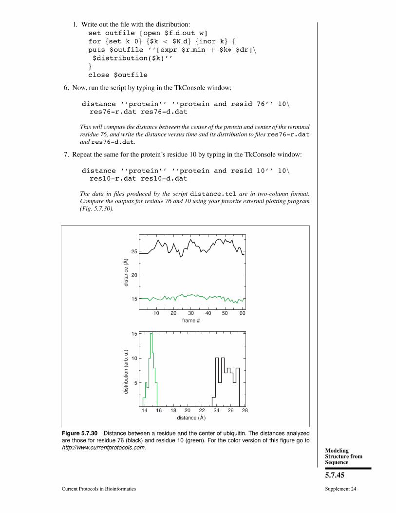
ModelingStructure fromSequence
5.7.45
Current Protocols in Bioinformatics Supplement 24
l. Write out the Þle with the distribution:set outfile [open $f d out w]for {set k 0} {$k < $N d} {incr k} {puts $outfile ��[expr $r min + $k∗ $dr]\$distribution($k)��
}close $outfile
6. Now, run the script by typing in the TkConsole window:
distance ��protein�� ��protein and resid 76�� 10\res76-r.dat res76-d.dat
This will compute the distance between the center of the protein and center of the terminalresidue 76, and write the distance versus time and its distribution to files res76-r.datand res76-d.dat.
7. Repeat the same for the protein�s residue 10 by typing in the TkConsole window:
distance ��protein�� ��protein and resid 10�� 10\res10-r.dat res10-d.dat
The data in files produced by the script distance.tcl are in two-column format.Compare the outputs for residue 76 and 10 using your favorite external plotting program(Fig. 5.7.30).
25
15
20
10 20 30
dist
ance
()
frame #40 50 60
5
15
10
14 16 18 20 22 24 26 28
dist
ribut
ion
(arb
. u.)
distance ( )
Figure 5.7.30 Distance between a residue and the center of ubiquitin. The distances analyzedare those for residue 76 (black) and residue 10 (green). For the color version of this figure go tohttp://www.currentprotocols.com.
Using VMD: AnIntroductory
Tutorial
5.7.46
Supplement 24 Current Protocols in Bioinformatics
Residue 76 is at the protein’s C-terminus, which is extended towards the solvent and isquite flexible, while residue 10 is at the surface of the globular part of ubiquitin. Thedifference in their dynamics with respect to the rest of the protein is immediately obviouswhen our newly obtained data are plotted (Fig. 5.7.30): the distance of residue 76 fromthe protein’s center is substantially greater than that of residue 10, and the distributionof the distance is noticeably wider due to the flexibility of the C-terminus. This is just asimple example of scripting for the analysis of a trajectory. Similar, but usually much morecomplex, customized scripts are routinely employed by VMD users to perform many kindsof analysis.
8. Quit VMD.
COMMENTARY
Background InformationVMD has been developed by the Theo-
retical and Computational Biophysics Groupat the University of Illinois at Urbana-Champaign. Throughout its development,many features have been added, and user-speciÞc functions can be implemented throughembedded scripting languages like Python andTcl, providing a wide spectrum of tools forthe scientiÞc community. SpeciÞcally, VMDis most suitable for high-resolution visual-ization and image rendering, preparation ofmolecular dynamics simulation systems andanalysis of simulation results, and animationof molecular dynamics trajectory. In addition,VMD can also work with volumetric data, andprovides a platform for bioinformatics analy-sis such as protein sequence alignment. Whatwe are able to present in this tutorial onlyshowcases a small part of VMD�s capabil-ity. But now that you have learned the ba-sics of VMD, you are ready to explore itsmany other features most suitable for your re-search. For this purpose, there are many tu-torials available that aim at offering a morefocused training, either on a speciÞc tool oron a scientiÞc topic. You can Þnd many usefuldocumentations, including the comprehensiveVMD User�s Guide, at the VMD homepagehttp://www.ks.uiuc.edu/Research/vmd/.
Critical Parameters andTroubleshootingMost parameters in VMD can be easily
adjusted to suit individual users� needs. Forexample, when rendering molecules using arepresentation, as described in Basic Protocol1, users can adjust the resolution of the rep-resentation in the graphical user interface, aswell as many other parameters speciÞc to thedrawing method of the representation. Newusers of VMD might Þnd default settings formost parameters are good starting points, butare also encouraged to change the parametersand test the difference. If you have any ques-
tions on using VMD, we encourage you tosubscribe to the VMDmailing list http://www.ks.uiuc.edu/Research/vmd/mailing list/.
AcknowledgmentsThis tutorial is largely based on the follow-
ing VMD tutorials, case studies, and user�sguides.We hence would like to thank these au-thors who have provided this tutorial its start-ing form:Jordi Cohen, Marcos Sotomayor, and Eliz-
abeth Villa, �VMD Molecular Graphics.�Alek Aksimentiev, John Stone, David
Wells, and Marcos Sotomayor, �VMD Imagesand Movies Tutorial.�Fatemeh Khalili, Elizabeth Villa, Yi Wang,
Emad Tajkhorshid, Brijeet Dhaliwal, ZanLuthey-Schulten, John Stone, Dan Wright,and John Eargle, �Aquaporins with the VMDMultiSeq Tool.�VMD has been developed by the Theoreti-
cal and Computational Biophysics Group atthe University of Illinois and the BeckmanInstitute, and is supported by funds from theNational Institutes of Health and the NationalScience Foundation.
Citing VMDThe development of VMD is funded by the
National Institute of Health. Proper citation isa primary way in which we demonstrate thevalue of our software to the scientiÞc commu-nity, and is essential to continued NIH fundingfor VMD. The authors request that all pub-lished work, that utilizes VMD include theprimary VMD citation at a minimum:Humphrey, W., Dalke, A. and Schulten,
K., �VMD - Visual Molecular Dynamics,� J.Molec. Graphics, 1996, vol. 14, pp. 33-38.Work that uses softwares or plugins incor-
porated into VMD should also add the propercitations for those tools. For example, workthat uses MultiSeq as introduced in Basic Pro-tocols 11 to 13 should cite:
ModelingStructure fromSequence
5.7.47
Current Protocols in Bioinformatics Supplement 24
Roberts, E., Eargle, J., Wright, D. andLuthey-Schulten Z., �MultiSeq: Unifying se-quence and structure data for evolutionaryanalysis,� BMC Bioinformatics, 2006, 7:382.Please see http://www.ks.uiuc.edu/
Research/vmd/allversions/cite.html for moreinformation on how to cite VMD and its tools.
Literature CitedCruz-Chu, E.R., Aksimentiev, A., and Schulten, K.2006.Water-silica forceÞeld for simulating nan-odevices. J. Phy. Chem. B. 110:21497-21508.
Eastwood, M.P., Hardin, C., Luthey-Schulten, Z.,and Wolynes, P.G. 2001. Evaluating proteinstructure-prediction schemes using energy land-scape theory. IBM J. Res. Dev. 45:475-497.
Freddolino, P.L., Arkhipov, A.S., Larson, S.B.,McPherson, A., and Schulten, K. 2006. Molecu-lar dynamics simulations of the complete satel-lite tobacco mosaic virus. Structure 14:437-449.
Frishman, D. and Argos, P. 1995. Knowledge-based secondary structure assignment. Proteins23:566-579.
Humphrey, W., Dalke, A., and Schulten, K. 1996.VMD�Visual Molecular Dynamics. J. Mol.Grap. 14:33-38.
Isralewitz, B., Gao, M., and Schulten, K. 2001.Steered molecular dynamics and mechanicalfunctions of proteins. Curr. Opin. Struct. Biol.11:224-230.
Murata, K., Mitsuoka, K., Hirai, T., Walz, T., Agre,P., Heymann, J.B., Engel, A., and Fujiyoshi,Y. 2000. Structural determinants of water per-meation through aquaporin-1. Nature 407:599-605.
Phillips, J.C., Braun, R., Wang, W., Gumbart, J.,Tajkhorshid, E., Villa, E., Chipot, C., Skeel,R.D., Kale, L., and Schulten, K. 2005. Scalablemolecular dynamics with NAMD. J. Comput.Chem. 26:1781-1802.
Roberts, E., Eargle, J., Wright, D., and Luthey-Schulten, Z. 2006.MultiSeq: Unifying sequenceand structure data for evolutionary analysis.BMC Bioinformatics. 7:382.
Russell, R.B. and Barton, G.J. 1992. Multiple pro-tein sequence alignment from tertiary structurecomparison: Assignment of global and resiudeconÞdence levels. Proteins 14:309-323.
Savage, D.F., Egea, P.F., Robles-Colmenares, Y.,O�Connell, J.D. III, and Stroud, R.M. 2003. Ar-chitecture and selectivity in aquaporins: 2.5
◦A
X-ray structure of aquaporin Z. PLoS Biol.1:E72.
Sotomayor, M., Vasquez, V., Perozo, E., andSchulten, K. 2007. Ion conduction throughMscS as determined by electrophysiology andsimulation. Biophys. J. 92:886-902.
Sui, H., Han, B.-G., Lee, J.K., Walian, P., and Jap,B.K. 2001. Structural basis of water-speciÞctransport through the AQP1 water channel.Nature 414:872-878.
Tajkhorshid, E., Nollert, P., Jensen, M.Ø., Miercke,L.J.W., O�Connell, J., Stroud, R.M., andSchulten, K. 2002. Control of the selectiv-ity of the aquaporin water channel family byglobal orientational tuning. Science 296:525-530.
Thompson, J.D., Higgins, D.G., and Gibson, T.J.1994. CLUSTAL W: Improving the sensitiv-ity of progressive multiple sequence alignmentthrough sequence weighting, position-speciÞcgap penalties and weight matrix choice. NucleicAcids Res. 22:4673-4680.
Tornroth-HorseÞeld, S., Wang, Y., Hedfalk, K.,Johanson, U., Karlsson, M., Tajkhorshid, E.,Neutze, R., and Kjellbom, P. 2006. Structuralmechanism of plant aquaporin gating. Nature439:688-694.
Vijay-Kumar, S., Bugg, C.E., and Cook, W.J. 1987.
Structure of ubiquitin at 1.8◦A resolution. J. Mol.
Biol. 194:531-544.
Wang, Y., Cohen, J., Boron, W.F., Schulten, K., andTajkhorshid, E. 2007. Exploring gas permeabil-ity of cellular membranes and membrane chan-nels with molecular dynamics. J. Struct. Biol.157:534-544.
Yin, Y., Jensen, M.Ø., Tajkhorshid, E., andSchulten, K. 2006. Sugar binding and proteinconformational changes in lactose permease.Biophys. J. 91:3972-3985.
Yu, J., Yool, A.J., Schulten, K., and Tajkhorshid, E.2006.Mechanism of gating and ion conductivityof a possible tetrameric pore in Aquaporin-1.Structure 14:1411-1423.
Supplemental FilesSupplemental Þles can be downloaded fromhttp://www.currentprotocols.com by clicking�Current Protocols� beneath the Bioinformaticshead and following the Sample Datasets link.
1fqy.pdbpdb coordinate file for human aquaporin (Murataet al., 2000)
1j4n.pdbpdb coordinate file for bovine aquaporin (Sui et al.,2001)
1lda.pdbpdb coordinate file for E. coli GlpF (Tajkhorshidet al., 2002)
1rc2.pdbpdb coordinate file for E. coli aquaporin (Savageet al., 2003)
1ubq.pdbpdb coordinate file for ubiquitin (Vijay-Kumar et al.,1987)
beta.tclAn example tcl script.
distance.tclAn example tcl script.
equilibration.dcddcd molecular dynamics trajectory file of an equi-libration simulation
Using VMD: AnIntroductory
Tutorial
5.7.48
Supplement 24 Current Protocols in Bioinformatics
pulling.dcddcd molecular dynamics trajectory file of a protein-pulling simulation
spinach aqp.fastaAn example fasta protein sequence file.
ubiquitin.psfpsf structure file for ubiquitin that defines connec-tivity of atoms


