Embed Size (px)
Citation preview
Using symmetry to generate solutions to the Helmholtz equation
inside an equilateral triangle
Nathaniel Stambaugh∗
Department of Computer Science and Mathematics,
Florida Southern College, Lakeland, Florida. 33801, USA
Mark Semon
Department of Physics and Astronomy,
Bates College, Lewiston, Maine. 04240, USA
(Dated: June 28, 2013)
Abstract
We prove that every solution of the Helmholtz equation ∇2ψ + k2ψ = 0 within an equilateral
triangle, which obeys the Dirichlet conditions on the boundary, is a member of one of four symmetry
classes. We then show how solutions with different symmetries, or different values of k2, can be
generated from any given solution using symmetry operators or a differential operator derived from
symmetry considerations. Our method also provides a novel way of generating the ground state
solution (that is, the solution with the lowest value of k2). Finally, we establish a correspondence
between solutions in the equilateral and 30◦ − 60◦ − 90◦ triangles.
PACS numbers:
∗Electronic address: [email protected]
1
I. INTRODUCTION.
The solutions to many important physical problems, such as electromagnetic waves in
waveguides [1], lasing modes in nanostructures [2], the electronic structure of graphene
[3] and the quantum eigenvalues and eigenfunctions for various potential energies [4] are
obtained by solving the ubiquitous Helmholtz equation
∇2ψ + k2ψ = 0. (1)
In this paper we discuss the solutions to this equation when the region of interest is an
equilateral triangle (∆) and when the solutions vanish on the boundary (i.e. when they
satisfy the Dirichlet condition ψ∣
∣
∂∆= 0). Although the explicit solutions in this case are
well-known, ([2], [4]),[5], [6]) we present an alternative method of obtaining them that does
not involve solving the differential equation directly, but rather uses only symmetry argu-
ments, or a differential operator derived from symmetry considerations alone, to generate
new solutions from any given solution. Our method is based upon first showing that each
solution within the equilateral triangle is a member of one of four symmetry classes, and
then introducing symmetry operators and a differential operator which transform solutions
in one symmetry class into those of another or from one value of k2 to another.
Obviously any method that generates one or more new solutions to the Helmholtz equa-
tion from a given solution is quite a powerful and useful tool. The fact that the new solutions
are generated from symmetry transformations alone rather than by solving the Helmholtz
equation directly makes the method even more attractive. The method also has the advan-
tage of being able to produce solutions with prescribed symmetries, which can be important
if the desired solution needs, or is known to possess, certain symmetries.
The paper is structured as follows: in Section II we establish our notation while reviewing
the results from representation theory and linear algebra which are used in the rest of the
paper. In Section III we show how that every solution to the Helmholtz equation within
an equilateral triangle, which obeys the Dirichlet conditions on the boundary, is a member
of one of four symmetry classes. In Section IV we show how to take a solution from any
one of the four classes and generate from it solutions in a different symmetry class and/or
with different values of the scalar k2. In Section V we use our approach to obtain the
explicit solution to the Helmholtz equation with the lowest value of k2, i.e. the “ground
2
FIG. 1: The generators of the symmetry group for the equilateral triangle. We let σ denote a
counter-clockwise rotation by 120◦ and µ the reflection in the x-axis.
state solution.” In Section VI we summarize our results and discuss the various ways in
which they can be applied. In particular, we discuss the correspondence between solutions
in the equilateral and (30◦, 60◦, 90◦) triangles.
II. NOTATION AND BACKGROUND
A. Representation Theory
A representation is a homomorphism ρ from the group G into the group of linear trans-
formations of a vector space (in our case, the real numbers suffice), which we denote by
ρ : G →GLn(R). The representation assigns to each group element a transformation of the
vector space that is consistent with the multiplication table of the group. For the dihe-
dral group D3, every such representation can be decomposed into a direct product of three
irreducible representations.
Before we can describe these homomorphisms we need to describe the elements of the
group D3. Let σ be a 120◦ counter-clockwise rotation about the center of an equilateral
triangle and µ be a reflection (without loss of generality) about the x−axis, as shown in
Figure (1). The defining relationship of the dihedral group says that µσ = σ−1µ. Since
these two elements generate the whole group, we need only define each homomorphism on
these generators. Listing the elements of the group, we have
3

D3 = {e, σ, σ2, µ, µσ, µσ2}.
The first irreducible representation is called the trivial representation because it maps
every group element to the identity map of R. While this may seem somewhat, well, trivial,
it actually plays an interesting role later on. Symbolically, ρ1(α) = 1 for every α ∈ D3.
The second representation is called the sign representation, though it also could be called
the orientation representation, because it shows whether a reflection has occurred. That
is, ρ2(σ) = 1 and ρ2(µ) = −1. Obviously the trivial and sign representations are one
dimensional.
The third representation is the only one that displays every nuance in the group, and it
therefore is sometimes used to define D3. Unlike the two previous representations, ρ3 is a
two dimensional representation whose elements (in GL2(R)) are
ρ3(σ) = 12
−1 −√
3√
3 −1
, ρ3(µ) =
1 0
0 −1
.
Using ρ3 we can define in a natural way the action of each group element α on a solution
f(x, y) of the Helmholtz equation . The argument of the function is the vector
x
y
in R2,
so the following action is well defined:
(α · f)(x, y) = f(
ρ3(α)−1
x
y
)
. (2)
The use of the inverse of the representation matrix is required to make this a homomorphism,
and can be thought of as a passive transformation on the coordinates. In order to simplify
the notation, we will write αf in place of α · f .
B. Inner Product Spaces
If f1 and f2 are two solutions of the Helmholtz equation then we define the inner product
of f1 and f2 as
〈f1, f2〉 =
∫ ∫
∆
f1(x, y)f2(x, y)dxdy, (3)
4

where the integral is taken over the domain ∆. The norm (or length) of a solution f is
defined as
||f || =√
〈f, f〉. (4)
This is called the L2 norm, which we will use to normalize any given solution and also to
establish when two solutions f1 and f2 are orthogonal (〈f1, f2〉 = 0 ⇐⇒ f1 ⊥ f2).
If two solutions have the same value of k and are orthogonal, we can form a two dimen-
sional space spanned by these solutions. In the same way that we use the vector
a
b
to
represent ai+ bj, in our context this column vector will represent af1 + bf2.
III. CLASSIFYING SOLUTIONS TO THE HELMHOLTZ EQUATION BY THEIR
SYMMETRIES.
If f is a solution of the Helmholtz equation within a region (denoted by ∆) whose sides
form an equilateral triangle, and which satisfies the Dirichlet conditions on the boundary,
then for each element α ∈ D3, αf (as defined by Eq. (2)) is a solution of the Helmholtz
equation with the same value of k2. In this section we prove that every such solution f
belongs to one of four sets according to its rotational and reflection symmetries. We call
these sets symmetry classes and denote them by A1, A2, E1 and E2.
We first consider the rotational symmetries of solutions of the Helmholtz equation. If a
solution f is rotated to obtain a new solution σf then, in general, the new solution can be
rotationally symmetric (σf = f), rotationally anti-symmetric (σf = −f), or rotationally
asymmetric (σf 6= ±f). We can eliminate the rotationally anti-symmetric case as follows:
Suppose that σf = −f . Then, since σ3 is the identity element,
f = σ3f = σσ(−f) = σf = −f. (5)
Thus f(x) = −f(x) for every x ∈ ∆ so f is identically zero on the domain. Therefore,
when we rotate a (non-trivial) solution f to obtain a new solution σf , the new solution σf
must be either rotationally symmetric or rotationally asymmetric. In what follows we first
consider the effect of reflections on the rotationally symmetric solutions and then the effect
of reflections on the rotationally asymmetric solutions.
5
A. Properties of rotationally symmetric solutions under reflection.
Assume that f is a rotationally symmetric solution of the Helmholtz equation, so σf =
f . In general, the solution µf can be symmetric, anti-symmetric, or asymmetric under
reflection. However, we can eliminate the asymmetric case as follows: Suppose µf 6= ±f .
Define the two functions
f+ =1
2(f + µf), (6)
f− =1
2(f − µf). (7)
The functions f+ and f− are solutions of the Helmholtz equation because each is con-
structed from a linear combination of solutions to the Helmholtz equation. Furthermore, f+
is symmetric and f− is anti-symmetric under reflections about the x−axis, and the solution
f can be written as f = f+ + f−. In addition, the boundary condition obeyed by f will also
be obeyed by f+ and f−. Consequently, any asymmetric solution f can be decomposed into
the sum of the symmetric and anti-symmetric solutions f+ and f−, and we thus need only
consider solutions to the Helmholtz equation which are symmetric or anti-symmetric under
reflection about the x-axis.
If we denote by A1 the set of solutions that are symmetric under a rotation σ and
symmetric under a reflection µ, and by A2 the set of solutions that is symmetric under a
rotation σ and anti-symmetric under reflection µ , then we can summarize the results of this
section with the following table:
TABLE I: Rotationally Symmetric Solutions
σfi µfi
f1 ∈A1 +f1 +f1
f2 ∈A2 +f2 −f2
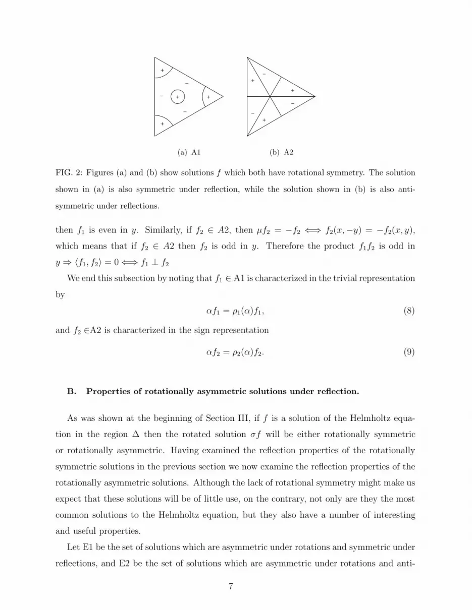
Figure (2) shows examples of solutions in the symmetry classes A1 and A2.
It’s interesting to note that all of the solutions in A1 are orthogonal to all the solutions in
A2: Suppose f1 ∈ A1, then µf1 = f1 ⇐⇒ f1(x,−y) = f1(x, y), which means that if f1 ∈ A1
6
+ +
+
+
-
-
-
(a) A1
+
+
+
-
-
-
(b) A2
FIG. 2: Figures (a) and (b) show solutions f which both have rotational symmetry. The solution
shown in (a) is also symmetric under reflection, while the solution shown in (b) is also anti-
symmetric under reflections.
then f1 is even in y. Similarly, if f2 ∈ A2, then µf2 = −f2 ⇐⇒ f2(x,−y) = −f2(x, y),
which means that if f2 ∈ A2 then f2 is odd in y. Therefore the product f1f2 is odd in
y ⇒ 〈f1, f2〉 = 0 ⇐⇒ f1 ⊥ f2
We end this subsection by noting that f1 ∈ A1 is characterized in the trivial representation
by
αf1 = ρ1(α)f1, (8)
and f2 ∈A2 is characterized in the sign representation
αf2 = ρ2(α)f2. (9)
B. Properties of rotationally asymmetric solutions under reflection.
As was shown at the beginning of Section III, if f is a solution of the Helmholtz equa-
tion in the region ∆ then the rotated solution σf will be either rotationally symmetric
or rotationally asymmetric. Having examined the reflection properties of the rotationally
symmetric solutions in the previous section we now examine the reflection properties of the
rotationally asymmetric solutions. Although the lack of rotational symmetry might make us
expect that these solutions will be of little use, on the contrary, not only are they the most
common solutions to the Helmholtz equation, but they also have a number of interesting
and useful properties.
Let E1 be the set of solutions which are asymmetric under rotations and symmetric under
reflections, and E2 be the set of solutions which are asymmetric under rotations and anti-
7
symmetric under reflections. Consider a normalized solution f1 in class E1. At this point
we do not know anything about σf1 except that it is a solution with the same value of k2
as f1. For that matter, so is σ2f1. So consider the function f2 = σf1 − σ2f1. We now show
that f2 is in symmetry class E2:
µf2 = µ(σf1 − σ2f1)
= µσf1 − µσ2f1
= σ2µf1 − σµf1
= σ2f1 − σf1
= −f2 (10)
The reason we call this new solution f2 is that it is not normalized; we will call the
normalized function f2. We also note that f1 and f2 are orthogonal since their product is
odd in y.
Since the action of the group introduces a second solution with the same value of k2, we
consider the two dimensional solution space spanned by f1 and f2. As in Section 2(a), the
vector ~f =
a
b
represents the solution f = af1+bf2. Written in this way, we can recognize
the third irreducible representation ρ3
α~f = ρ3(α)~f.
This equation actually contains a lot of information, and is strikingly similar to Eqs.(8) and
(9). We now use it to normalize f2.
Let ~f1 =
1
0
. Then σf1 can be re-expressed as a linear combination of f1 and f2 as
follows:
σf1 =1
2
−1 −√
3√
3 −1
1
0
(11)
=1
2
−1√
3
= −1
2f1 +
√3
2f2. (12)
8
+
-
-
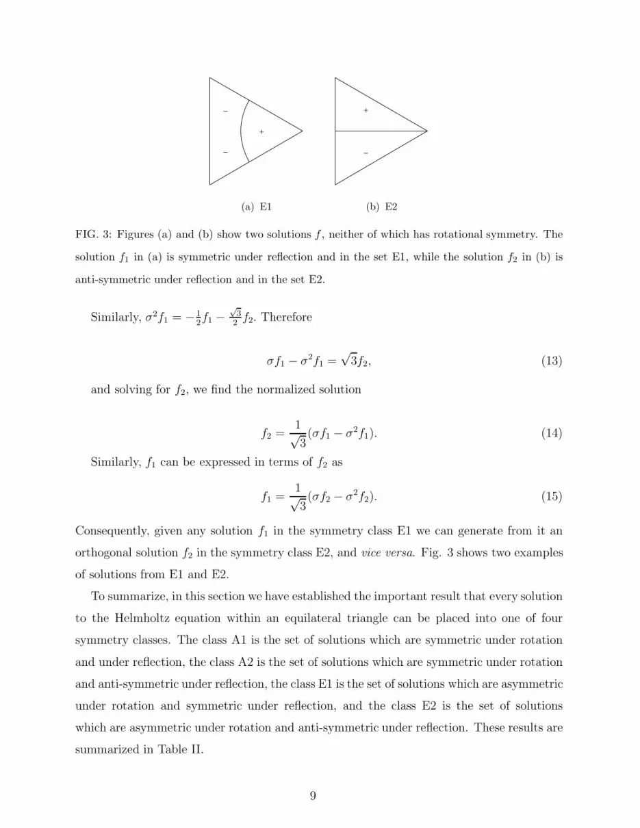
(a) E1
+
-
(b) E2
FIG. 3: Figures (a) and (b) show two solutions f , neither of which has rotational symmetry. The
solution f1 in (a) is symmetric under reflection and in the set E1, while the solution f2 in (b) is
anti-symmetric under reflection and in the set E2.
Similarly, σ2f1 = −12f1 −
√3
2f2. Therefore
σf1 − σ2f1 =√
3f2, (13)
and solving for f2, we find the normalized solution
f2 =1√3(σf1 − σ2f1). (14)
Similarly, f1 can be expressed in terms of f2 as
f1 =1√3(σf2 − σ2f2). (15)
Consequently, given any solution f1 in the symmetry class E1 we can generate from it an
orthogonal solution f2 in the symmetry class E2, and vice versa. Fig. 3 shows two examples
of solutions from E1 and E2.
To summarize, in this section we have established the important result that every solution
to the Helmholtz equation within an equilateral triangle can be placed into one of four
symmetry classes. The class A1 is the set of solutions which are symmetric under rotation
and under reflection, the class A2 is the set of solutions which are symmetric under rotation
and anti-symmetric under reflection, the class E1 is the set of solutions which are asymmetric
under rotation and symmetric under reflection, and the class E2 is the set of solutions
which are asymmetric under rotation and anti-symmetric under reflection. These results are
summarized in Table II.
9
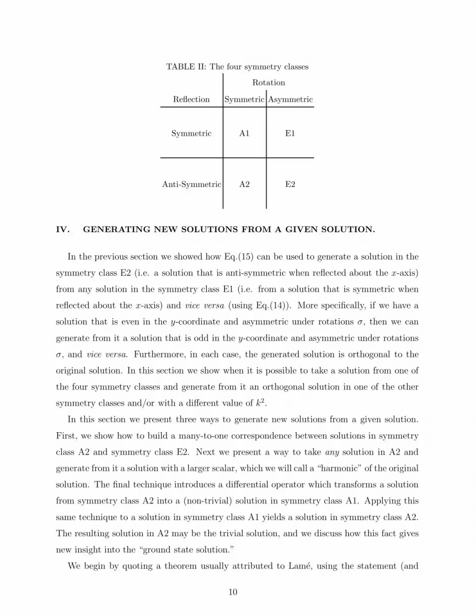
TABLE II: The four symmetry classes
Rotation
Reflection Symmetric Asymmetric
Symmetric A1 E1
Anti-Symmetric A2 E2
IV. GENERATING NEW SOLUTIONS FROM A GIVEN SOLUTION.
In the previous section we showed how Eq.(15) can be used to generate a solution in the
symmetry class E2 (i.e. a solution that is anti-symmetric when reflected about the x-axis)
from any solution in the symmetry class E1 (i.e. from a solution that is symmetric when
reflected about the x-axis) and vice versa (using Eq.(14)). More specifically, if we have a
solution that is even in the y-coordinate and asymmetric under rotations σ, then we can
generate from it a solution that is odd in the y-coordinate and asymmetric under rotations
σ, and vice versa. Furthermore, in each case, the generated solution is orthogonal to the
original solution. In this section we show when it is possible to take a solution from one of
the four symmetry classes and generate from it an orthogonal solution in one of the other
symmetry classes and/or with a different value of k2.
In this section we present three ways to generate new solutions from a given solution.
First, we show how to build a many-to-one correspondence between solutions in symmetry
class A2 and symmetry class E2. Next we present a way to take any solution in A2 and
generate from it a solution with a larger scalar, which we will call a “harmonic” of the original
solution. The final technique introduces a differential operator which transforms a solution
from symmetry class A2 into a (non-trivial) solution in symmetry class A1. Applying this
same technique to a solution in symmetry class A1 yields a solution in symmetry class A2.
The resulting solution in A2 may be the trivial solution, and we discuss how this fact gives
new insight into the “ground state solution.”
We begin by quoting a theorem usually attributed to Lame, using the statement (and
10
referring the reader to the proof) given by McCartin [6]:
Theorem 1 (Lame) Suppose that T (x, y) is a solution to the Helmholtz equation which can
be represented by the trigonometric series
T (x, y) =∑
i
(Ai sin(λix+ µiy + αi)
Bi cos(λix+ µiy + βi)) , (16)
with λ2i + µ2
i = k2. Then
1. T (x, y) is antisymmetric about any line along which it vanishes;
2. T (x, y) is symmetric about any line along which its normal derivative, ∂T∂ν
, vanishes.
Lame [6] also proves that the solutions to the Helmholtz equation in a triangular region
subject to the Dirichlet conditions can be expressed in this way and that they form a com-
plete, orthonormal set. Explicit expressions for these solutions are also given by Doncheski
et al. [4]
A. E2 ↔ A2
In order to relate solutions in the symmetry classes E2 and A2 we use a method called
“tessellating the plane,” which extends any solution within the triangular domain to the
plane. We begin the tessellation by defining the triangular region in which we are work-
ing as the “fundamental domain” and then we reflect this domain across each of its three
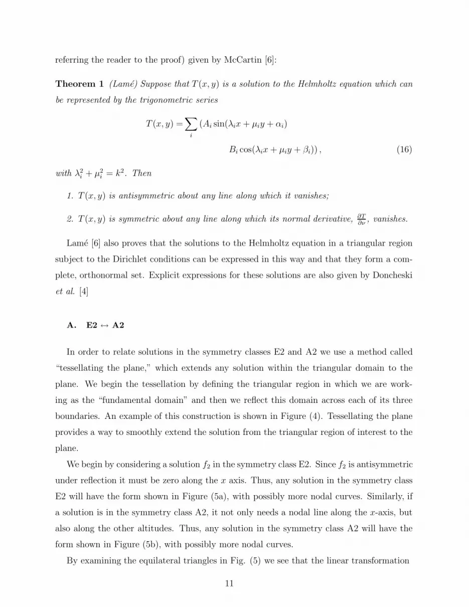
boundaries. An example of this construction is shown in Figure (4). Tessellating the plane
provides a way to smoothly extend the solution from the triangular region of interest to the
plane.
We begin by considering a solution f2 in the symmetry class E2. Since f2 is antisymmetric
under reflection it must be zero along the x axis. Thus, any solution in the symmetry class
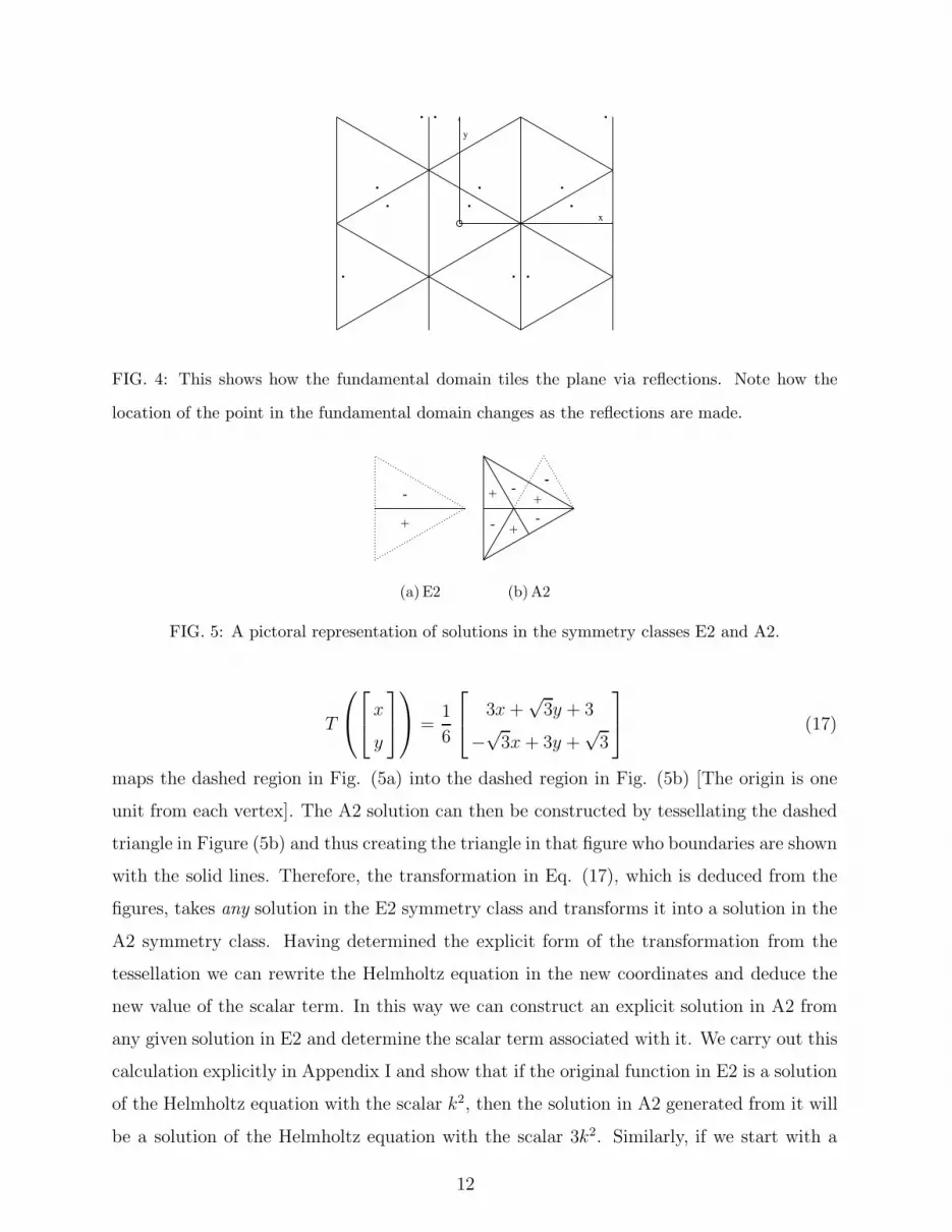
E2 will have the form shown in Figure (5a), with possibly more nodal curves. Similarly, if
a solution is in the symmetry class A2, it not only needs a nodal line along the x-axis, but
also along the other altitudes. Thus, any solution in the symmetry class A2 will have the
form shown in Figure (5b), with possibly more nodal curves.
By examining the equilateral triangles in Fig. (5) we see that the linear transformation
11
x
y
FIG. 4: This shows how the fundamental domain tiles the plane via reflections. Note how the
location of the point in the fundamental domain changes as the reflections are made.
(a) E2 (b)A2
FIG. 5: A pictoral representation of solutions in the symmetry classes E2 and A2.
T
x
y
=1
6
3x+√
3y + 3
−√
3x+ 3y +√
3
(17)
maps the dashed region in Fig. (5a) into the dashed region in Fig. (5b) [The origin is one
unit from each vertex]. The A2 solution can then be constructed by tessellating the dashed
triangle in Figure (5b) and thus creating the triangle in that figure who boundaries are shown
with the solid lines. Therefore, the transformation in Eq. (17), which is deduced from the
figures, takes any solution in the E2 symmetry class and transforms it into a solution in the
A2 symmetry class. Having determined the explicit form of the transformation from the
tessellation we can rewrite the Helmholtz equation in the new coordinates and deduce the
new value of the scalar term. In this way we can construct an explicit solution in A2 from
any given solution in E2 and determine the scalar term associated with it. We carry out this
calculation explicitly in Appendix I and show that if the original function in E2 is a solution
of the Helmholtz equation with the scalar k2, then the solution in A2 generated from it will
be a solution of the Helmholtz equation with the scalar 3k2. Similarly, if we start with a
12
(a)n = 2 (b)n = 3
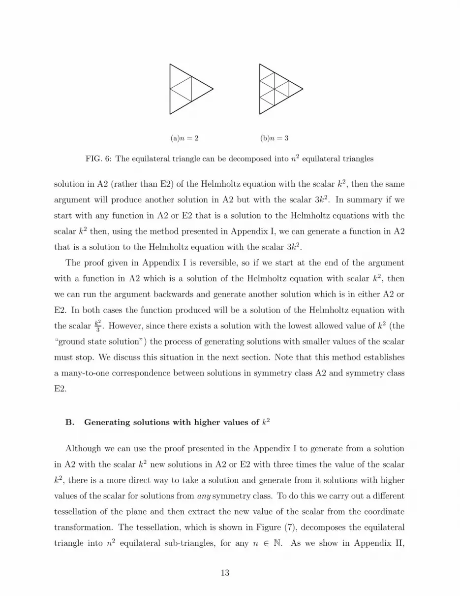
FIG. 6: The equilateral triangle can be decomposed into n2 equilateral triangles
solution in A2 (rather than E2) of the Helmholtz equation with the scalar k2, then the same
argument will produce another solution in A2 but with the scalar 3k2. In summary if we
start with any function in A2 or E2 that is a solution to the Helmholtz equations with the
scalar k2 then, using the method presented in Appendix I, we can generate a function in A2
that is a solution to the Helmholtz equation with the scalar 3k2.
The proof given in Appendix I is reversible, so if we start at the end of the argument
with a function in A2 which is a solution of the Helmholtz equation with scalar k2, then
we can run the argument backwards and generate another solution which is in either A2 or
E2. In both cases the function produced will be a solution of the Helmholtz equation with
the scalar k2
3. However, since there exists a solution with the lowest allowed value of k2 (the
“ground state solution”) the process of generating solutions with smaller values of the scalar
must stop. We discuss this situation in the next section. Note that this method establishes
a many-to-one correspondence between solutions in symmetry class A2 and symmetry class
E2.
B. Generating solutions with higher values of k2
Although we can use the proof presented in the Appendix I to generate from a solution
in A2 with the scalar k2 new solutions in A2 or E2 with three times the value of the scalar
k2, there is a more direct way to take a solution and generate from it solutions with higher
values of the scalar for solutions from any symmetry class. To do this we carry out a different
tessellation of the plane and then extract the new value of the scalar from the coordinate
transformation. The tessellation, which is shown in Figure (7), decomposes the equilateral
triangle into n2 equilateral sub-triangles, for any n ∈ N. As we show in Appendix II,
13

+-
+
-+
-
+
-
+
-
+ -
+
- +
-
+
-
(a)Two successive
constructions from
Section IVA
+-
+
-+
-
+
-
+
-
+ -
+
- +
-
+
-
(b)Harmonic with
n = 3
FIG. 7: These pictures show two redundant constructions of a higher energy state.
the explicit coordinate transformation that creates the sub-triangles is constructed from a
dilation followed by a translation along the x-axis. Carrying out this transformation we can
start with a function in any symmetry class that is a solution of the Helmholtz equation with
the scalar k2 and generate from it a family of new solutions to the Helmholtz equation with
scalar n2k2. Note that if the original solution is in the symmetry class E2 (i.e. is rotationally
asymmetric) then this approach will produce a solution in A2 (i.e. the generated solution
will become rotationally symmetric) whenever n is divisible by 3. In this case, however, we
have would have already constructed this solution by using the method from Section (IV A)
twice. See Figure 7 for a schematic proof of this fact.
Note that any solution with a vertical nodal line can be reduced using this method.
Extending the solution to the plane, we can use Theorem 1 and any vertical nodal line
to introduce a new mirror symmetry. Combining this with the mirror symmetries about
the boundaries and the rotational symmetry, there will be a fundamental domain without
vertical nodal lines. This represents a solution which can be used to generate the original
solution without any vertical nodal lines.
C. Generating even solutions from odd solutions and vice versa.
In this section we prove that there exists a differential operator that transforms a solution
f2 in A2, i.e. a solution that is symmetric under rotations and an odd function of y, into a
solution f1 in A1, that is, into a solution which is symmetric under rotations and an even
14

function of y. To show this we construct a function f1 in A1 (where f1 is the normalized
solution) by defining f1 in the following way:
f1 =
(
∂3
∂y3− 3
∂3
∂y∂x2
)
f2(x, y). (18)
The proof that f1 is in A1 goes as follows: First, it is easy to see that f1 is a solution to
the Helmholtz equation with the scalar k2 iff f2 is a solution with the same scalar k2. To
complete the proof we need to show four more things: first, that f1 is rotationally symmetric,
second, that f1 satisfies the Dirichlet conditions, third, that f1 is even in the y-coordinate,
and fourth, that f1 is not identically zero.
With single variable functions, one common way of generating an even function from an
odd function is to take the first derivative. However, the need to satisfy all of the above
conditions requires a more complicated procedure. The generalization of the first derivative
in one dimension to two dimensions is the directional derivative, and the directional deriva-
tive of a function f is ∇f · e. We can represent the directional derivative operator in the e
direction as ∇· e. Higher order directional derivatives are simply powers of this operator. As
can be easily verified, although the first directional derivative of f2 satisfies the Helmholtz
equation it would not necessarily have the correct rotational symmetry. To correct this, we
can symmetrize the solution by adding it to both of its rotates. The resulting solution will
now be even and rotationally symmetric. Additionally, the transformed solution will satisfy
the boundary (Dirichlet) condition since any nodal line parallel to a side will remain a nodal
line. This follows from Theorem 1, since every solution is antisymmetric in a nodal line.
Thus a directional derivative along the nodal line is zero, and by anti-symmetry the other
two directional derivatives will cancel out. Unfortunately, this particular method always
yields the trivial solution, so it is not very helpful. Indeed, we can imagine the directional
derivatives in the tangent plane, and by symmetry they will always add to zero.
However, this leads us to try the next odd power of the directional derivative in the
y-direction, ∂3
∂y3 . Once again, the required rotational symmetry leads us to symmetrize the
solution by adding to the third directional derivative in the y-direction the third directional
derivative in the directions parallel to the other two sides. We can describe the resulting
differential operator algebraically by rotating the directional derivative by σ:
15
(
∇ · j)3
+(
∇ · (σ · j))3
+(
∇ · (σ2 · j))3
=
(
∂
∂y
)3
+1
8
(√3∂
∂x− ∂
∂y
)3
+1
8
(
−√
3∂
∂x− ∂
∂y
)3
=3
4
(
∂3
∂y3− 3
∂3
∂y∂x2
)
(19)
This gives us our differential operator from Eq. (18), apart from a multiplicative constant
(which is unimportant since the resulting solution will still need to be normalized). With
this new understanding of Eq. (18), we can then argue as before that the new function
f1 has the correct symmetry and satisfies the Dirichlet conditions. Using the Helmholtz
relation, note that∂3
∂y∂x2= − ∂3
∂y3− k2 ∂
∂y. (20)
Combining this with our differential operator, we can rewrite it as
4∂3
∂y3+ 3k2 ∂
∂y. (21)
Written in this way, it is clear the f1 is symmetric in the x-axis. The last thing we need
to do is show that the solution is non-zero. Without loss of generality we can assume there
are no vertical nodal lines on the interior of the triangle. (This is possible using the last
paragraph from Section IV B.)
Since any solution will be analytic on the interior of the triangle, we consider the power
series of the function f2(x, y) at the origin.
f2(x, y) =∑
i,j
ci,jxiyj (22)
Let’s consider the solution along the y-axis, f2(0, y). By symmetry, we know that there
are only odd terms. Additionally, note that the directional derivative at the origin is equal
parallel to each side, also by symmetry. We have previously argued that the sum of the
three directional derivatives parallel to each side gives the zero function, thus c0,1 = 0.
f2(0, y) = f2(y) =∑
j=3, odd
c0,jyj (23)
16
By assumption, f2(0, y) is not identically zero, so there is a non-zero term with minimal
index. Now consider f1:
f1 =
(
4∂3
∂y3+ 3k2 ∂
∂y
)
f2(y)
= 4f ′′′2 (y) + 3k2f ′
2(y) (24)
Using the first non-zero term in the power series for f2, we note that its third derivative is
non-zero, and higher order terms cannot cancel it. Thus f1 is non-zero, so we can normalize
it to get a new solution f1. In addition, we can note that f1 is non-zero almost everywhere.
Indeed, if f1 is zero on an open set, then by analyticity it would be zero everywhere.
While we have only shown that this process works for functions in A2 without a node along
the y-axis, the strength of our conclusion shows that this is a local property. Combining this
with earlier methods, the requirement to be non-zero along the y-axis can be eliminated.
It should be noted that the only place we used the fact that f2 was anti-symmetric was
to prove that f1 was non-zero. Indeed, the process introduced in Eq. (18) can also be used
to transform a symmetric solution into an anti-symmetric solution, though the transformed
solution may be zero. In the next section we will show that if a solution in class A1 is
transformed by this differential operator and becomes the zero function, then it was (a
harmonic of) the “ground state.” Otherwise, the transformed solution can be normalized to
a solution in class A2, giving a one-to-one correspondence between solutions in class A2 and
those solutions in A1 which are not harmonics of the ground state.
V. THE GROUND STATE SOLUTION
In the previous section we introduced the differential operator defined in Eq. 18) that
transformed anti-symmetric solutions into symmetric solutions. One natural question is
what does this operator do to the solution of the Helmholtz equation with the minimum
value of k2, that is, to the “ground state solution”? Since the ground state solution is always
non-degenerate, the operator in Eq. (18) must transform it into the zero function. We will
now show that any solution from class A1 which transforms to zero under this differential
operator is the ground state or a harmonic of the ground state.
17
Let f be a solution in symmetry class A1 which satisfies the two equations(
∂2
∂x2+
∂2
∂y2+ k2
)
f(x, y) = 0 (25)
and(
∂3
∂y3− 3
∂3
∂y∂x2
)
f(x, y) = 0. (26)
Using the first equation we can eliminate partial derivatives with respect to x from the
second equation to obtain
0 =
(
4∂3
∂y3+ 3k2 ∂
∂y
)
f(x, y)
=⇒ 0 =∂
∂y
(
∂2
∂y2+
3k2
4
)
f(x, y).
Putting a solution of the form f(x, y) =∑
Xi(x)Yi(y) into the above equation we find
that Y1 = 1, Y2 = sin(√
3k2y) and Y3 = cos(
√3k2y). However, since solutions in class A1 are
symmetric in y, the only allowed solutions are Y1 and Y3.
Similarly, putting f(x, y) =∑
Xi(x)Yi(y) into Eq.(26), we get that X1 = A1 cos(kx) +
B1 sin(kx) and X3 = A3 cos(kx/2) + B3 sin(kx/2). Imposing the boundary condition at
x = −`/2, we find that X1(x) = sin (k(x+ `/2)) and X3(x) = sin (k/2(x + `/2)). Putting
this all together we find the solution
f(x) =A sin
(
k(
x+`
2
)
)
+B sin
(
k
2
(
x+`
2
)
)
cos
(√3k
2y
)
.
Imposing the remaining boundary condition along y = −x+`√3
, we get
0 =A sin
(
k(
x+`
2
)
)
+B sin
(
k
2
(
x+`
2
)
)
cos
(√3k
2
(−x+ `√3
)
)
A sin
(
k(
x+`
2
)
)
+B sin
(
k
2
(
x+`
2
)
)
cos
(
k
2(x− `)
)
A sin
(
kx+k`
2
)
)
+B
2
(
sin
(
3k`
4
)
+ sin
(
kx− k`
4
))
.
This equation is satisfied when B = ±2A and sin(3k`/4) = 0, so k = 4πn/3` for n > 0.
0 = sin
(
kx+k`
2
)
)
± sin
(
kx− k`
4
)
= sin
(
kx+2πn
3
)
)
± sin(
kx− πn
3
)
18

Note that these two sine waves are horizontally shifted by πn, so there is a suitable choice
of sign for B to make them cancel. Putting this all together,
fn(x) = sin
(
kn
(
x+`
2
)
)
+ 2(−1)n sin
(
kn
2
(
x+`
2
)
)
cos
(√3 kn
2y
)
, (27)
where kn = 4πn3`
. For n = 1 this agrees with the accepted solution in the literature for
the ground state solution with center-to-vertex length `.[4] To compare Eq. (27) with the
explicit solution given in McCartin, [6] note that if the inscribed circle has radius r then
k = 2π3r
, and if the side length is h then k = 4π√
33h
. For larger values of n, we simply get the
harmonics promised at the end of Section (IV C).
VI. CONCLUSION
In this paper we have examined the solutions to the Helmholtz equation ∇2ψ + k2ψ = 0
within an equilateral triangle which obey the Dirichlet conditions on the boundary. We
have shown that every solution is a member of one of four symmetry classes and that, from
symmetry considerations alone, any given solution in one symmetry class can be used to
generate solutions in another symmetry class or with other values of the scalar k2. We also
used symmetry considerations to find a novel derivation of the “ground state” solution of
the Helmholtz equation.
These results have many interesting applications. For example, in some cases we are
looking for solutions to the Helmholtz equation which possess certain specific reflection or
rotational symmetries. Referring to the chart at the end of Section III we see that if we
are looking for a solution with the symmetry properties of solutions in the symmetry class
A2, we can generate such a solution if we already have another solution in either symmetry
class A1 or symmetry class E2. Similarly, for any given value of the scalar k2, we can
generate the ground state solution using Eq. (27) and then, since the ground state solution
is in symmetry class A1, use the method presented in Section III to generate solutions
with “higher harmonics,” that is, solutions whose scalar values are n2k2. More generally,
given any solution, we can generate many different solutions in different symmetries classes
and with different values of the scalar k2 from symmetry considerations alone, and keep
generating solutions from each solution generated previously without ever having to solve
19
the Helmholtz equation directly.
We end by noting that, when collected together, the techniques in this article shed light
on the relationship between solutions within the 30◦ − 60◦ − 90◦ and equilateral triangles.
For example, solutions to the equilateral triangle which are in symmetry classes A2 and E2
vanish along the x-axis. If we restrict our domain ∆ to quadrants I and II, these solutions
become solutions to the 30◦ − 60◦ − 90◦ triangle (with the same value of k2).
Conversely, given a solution in the 30◦ − 60◦ − 90◦ triangle, we can reflect it across the
x-axis to get a solution in the equilateral triangle that is in either of the symmetry classes
A2 or E2. We can then take these solutions and construct from them solutions in A1 and E1
using the techniques from Section IV C and Section III B, respectively. Since both of these
techniques are reversible, we know that all solutions within the equilateral triangle can be
found from the solutions in the 30◦ − 60◦ − 90◦ triangle except for the ground state solution
and its harmonics. However, these solutions can be derived directly using the technique
in Section IV C, which means that knowing all of the solutions within the 30◦ − 60◦ − 90◦
triangle enables us to obtain all of the solutions within the equilateral triangle.
In summary, apart from providing a new way to generate new solutions from any given
solution to the Helmholtz equation within a triangle region, our method can also be used to
establish two interesting connections between solutions to the Helmholtz equation within the
equilateral and 30◦−60◦−90◦ triangles. First, the set of solutions within the 30◦−60◦−90◦
triangle is a subset of the set of solutions within the equilateral triangle. Second, we have
a two-to-one correspondence between the solutions in the equilateral triangle which are not
harmonics of the ground state and the solutions of the 30◦ − 60◦ − 90◦ triangle.
VII. APPENDIX I
We want to show that the solution g(x, y) = (f ◦ T−1)(x, y) = f(X(x, y), Y (x, y)) is a
solution to the differential equation
(
∂2
∂2x+
∂2
∂2y
)
g(x, y) = 3k2g(x, y)
when f is a solution to the differential equation
20
(
∂2
∂2X+
∂2
∂2Y
)
f(X, Y ) = k2f(X, Y ).
To make this a bit cleaner, we will need to write the transformation T−1(x, y) explicitly.
Solving the system of equations
x =1
6
(
3X +√
3Y + 3)
y =1
6
(√3X − 3Y +
√3)
for X and Y , we get
X(x, y) =1
4
(
6x− 2√
3y +√
3 − 3)
Y (x, y) =1
4
(
2√
3x+ 6y −√
3 − 3)
.
In order to evaluate ∂2
∂2xf(X, Y ), we use the chain rule:
∂2
∂2xf(X, Y ) =
∂
∂x
(
∂X
∂x
∂
∂Xf(X, Y ) +
∂Y
∂x
∂
∂Yf(X, Y )
)
=∂
∂x
(
6
4
∂
∂Xf(X, Y ) +
2√
3
4
∂
∂Yf(X, Y )
)
=∂
∂x
(
3
2fX(X, Y ) +
√3
2fY (X, Y )
)
=3
2
∂
∂xfX(X, Y ) +
√3
2
∂
∂xfY (X, Y )
=3
2
(
∂X
∂x
∂
∂XfX(X, Y ) +
∂Y
∂x
∂
∂YfX(X, Y )
)
+
√3
2
(
∂X
∂x
∂
∂XfY (X, Y ) +
∂Y
∂x
∂
∂YfY (X, Y )
)
=3
2
(
3
2fXX(X, Y ) +
√3
2fXY (X, Y )
)
+
√3
2
(
3
2fY X(X, Y ) +
√3
2fY Y (X, Y )
)
=9
4fXX(X, Y ) +
3√
3
2fXY (X, Y ) +
3
4fY Y (X, Y )
21
Similarly, for ∂2
∂2yf(X, Y ), we have
∂2
∂2yf(X, Y ) =
∂
∂y
(
∂X
∂y
∂
∂Xf(X, Y ) +
∂Y
∂y
∂
∂Yf(X, Y )
)
=∂
∂x
(
−2√
3
4
∂
∂Xf(X, Y ) +
6
4
∂
∂Yf(X, Y )
)
=∂
∂y
(
−√
3
2fX(X, Y ) +
3
2fY (X, Y )
)
= −√
3
2
∂
∂yfX(X, Y ) +
3
2
∂
∂yfY (X, Y )
= −√
3
2
(
∂X
∂y
∂
∂XfX(X, Y ) +
∂Y
∂y
∂
∂YfX(X, Y )
)
+
3
2
(
∂X
∂y
∂
∂XfY (X, Y ) +
∂Y
∂y
∂
∂YfY (X, Y )
)
= −√
3
2
(
−√
3
2fXX(X, Y ) +
3
2fXY (X, Y )
)
+
3
2
(
−√
3
2fY X(X, Y ) +
3
2fY Y (X, Y )
)
=3
4fXX(X, Y ) − 3
√3
2fXY (X, Y ) +
9
4fY Y (X, Y )
Combining these two equations, we get
∇2g(x, y) =∂2
∂2xf(X, Y ) +
∂2
∂2yf(X, Y )
=9
4fXX(X, Y ) +
3√
3
2fXY (X, Y ) +
3
4fY Y (X, Y )
3
4fXX(X, Y ) − 3
√3
2fXY (X, Y ) +
9
4fY Y (X, Y )
=3(fXX(X, Y ) + fY Y (X, Y ))
=3k2f(X, Y )
=3k2g(x, y)
which is the desired result.
22
VIII. APPENDIX II
In this section we examine the properties of solutions obtained by de-composing the
fundamental domain into n2 equilateral triangles. First we show that if we start with a
solution f in A2 or E2 which is a solution of the Helmholtz equation with the scalar k2
then, by decomposing the triangular domain into n2 equilateral triangles, we can generate
a solution to the Helmholtz equation with scalar n2k2.
The transformation of the plane which replaces the original triangle by n2 triangles is a
pure dilation by a factor of n, followed by a translation along the x axis. The translation
does not affect the scalar in Helmholtz’s equation, so we will just call it C . Thus our
transformation is
X(x, y) = nx+ C
Y (x, y) = ny.
An easier way to see the affect such a transformation would have on the scalar, consider
the Jacobian matrix for the transformation
J =
n 0
0 n
.
The determinant of this matrix is n2, and gives us the desired result.
Note that if the original solution has rotational symmetry (i.e. is in the symmetry class
A2), then the transformation will not change the symmetry class. This is easy to see
since, when the equilateral triangle is subdivided into n2 triangles, the resulting picture is
rotationally symmetric. Since the solution inside each of these smaller triangles is the same
rotationally symmetric symmetric solution, the resulting solution is rotationally symmetric.
However, if it started asymmetric (i.e. in the symmetry class E2) then this approach will
lead to a solution in A2 iff n is divisible by 3. As noted above, the subdivided triangle is
rotationally symmetric. However, since we are starting with a solution in E2, the resulting
picture may or may not be rotationally symmetric. To test for rotational symmetry, consider
figure VIII.
Looking at the solution inside the small triangle at the left of the subdivided triangle, we
can sketch in the solution on the large subdivided triangle by reflecting this small triangle
23
+-
+
-+
-
+
-
+
-
+ -
+
- +
-
+
-
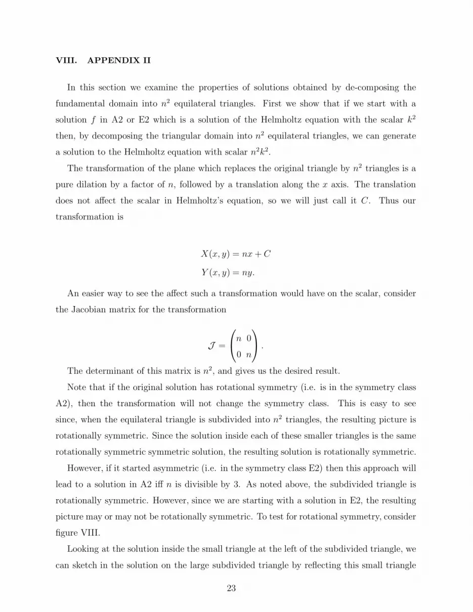
FIG. 8: Harmonics of E2/A2 solutions.
over the boundary and keep track of the nodal line. Comparing the small triangles along
the top edge, we can see that after two reflections, the solutions appears rotated by ρ−1.
Restricting ourselves to looking only at the 3 small triangles at the tips of a subdivided
triangle, note that a rotation of the large triangle induces a rotation of the small triangles.
This rotation only agrees with the reflection method if ρ = ρ−(n−1). Equivalently, ρn = 1,
which means that n must be a multiple of 3.
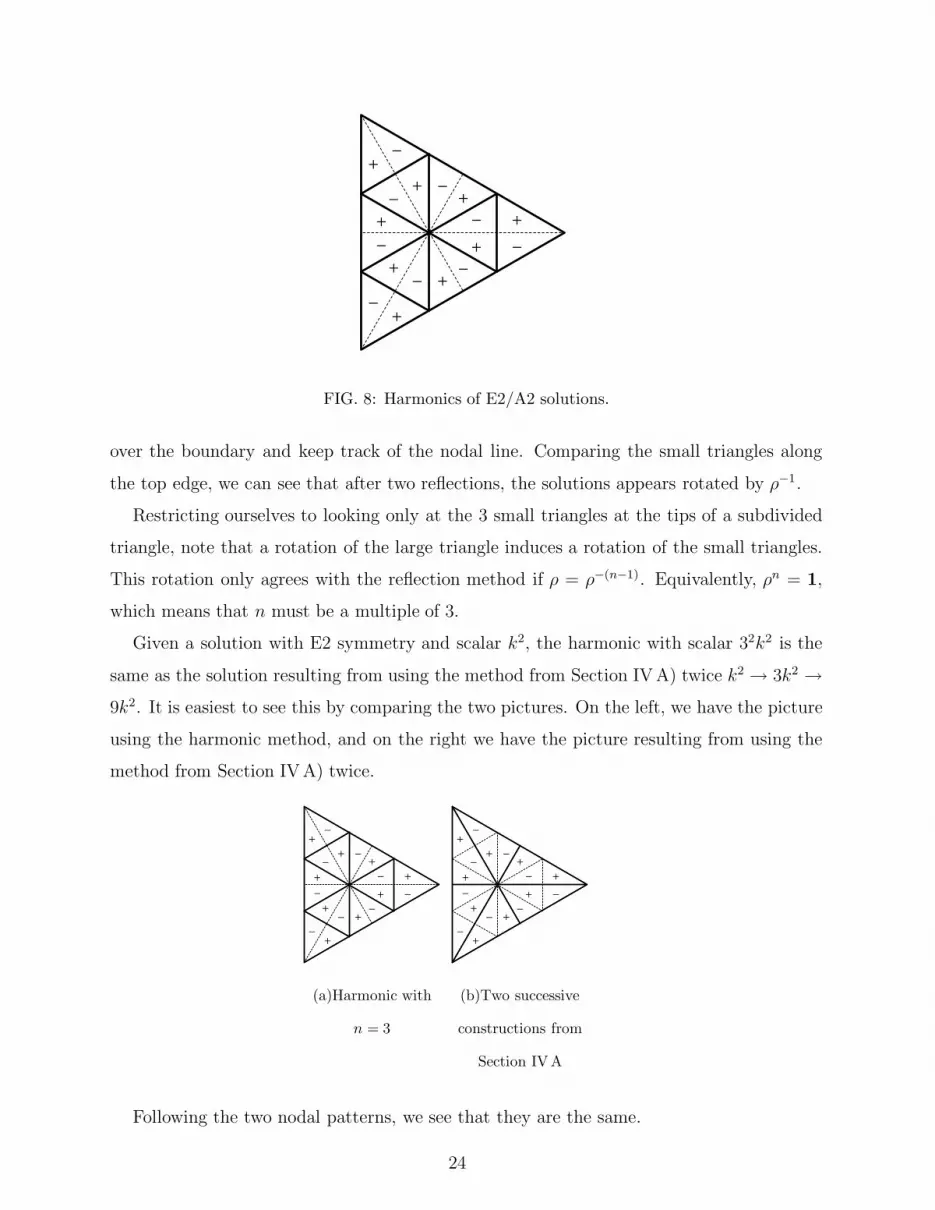
Given a solution with E2 symmetry and scalar k2, the harmonic with scalar 32k2 is the
same as the solution resulting from using the method from Section IV A) twice k2 → 3k2 →9k2. It is easiest to see this by comparing the two pictures. On the left, we have the picture
using the harmonic method, and on the right we have the picture resulting from using the
method from Section IV A) twice.
+-
+
-+
-
+
-
+
-
+ -
+
- +
-
+
-
(a)Harmonic with
n = 3
+-
+
-+
-
+
-
+
-
+ -
+
- +
-
+
-
(b)Two successive
constructions from
Section IVA
Following the two nodal patterns, we see that they are the same.
24
Acknowledgments
We would like to thank Peter Wong and Matthew Cote for many helpful discussions, and
for advising the senior thesis [7] on which much of the work presented here is based.
[1] R. L. Liboff, “The polygon quantum-billiard problem,” J. Math. Phys. 35, p. 596 (1994).
[2] C. H. Chang, G. Kioseoglou, E. H. Lee, J Haetty, M. H. Na, Y. Xuan, H. Luo, A Petrou and
A.N. Cartwright, “Lasing modes in equalateral-triangular laser cavities,” Phy. Rev. A, Vol. 62,
p. 013816-1 (2000).
[3] D. Kaufman, I. Kosztin and K. Schulten, “Electronic structure of triangular, hexagonal and
round graphene akes near the fermi level,” New J. Phys., 10, p. 103015 (2008).
[4] M. A. Doncheski, S. Heppelmann, R. W. Robinett and D. C. Tussey, “Wave packet construc-
tion in two-dimensional quantum billiards: Blueprints for the square, equilateral triangle and
circular cases,” Am. J. Phys 71, 541 - 557 (2003).
[5] C. Itzykson and J. M. Luck, “Sum Rules for Quantum Billiards,” J. Phys. A, Vol. 19, p. 211
(1986).
[6] B. McCartin, “Eigenstructure of the Equilateral Triangle, Part I: The Dirichlet Problem,”
SIAM Review, Vol 45, pp. 267-287 (2003).
[7] N. Stambaugh, A senior thesis presented to the Department of Mathematics, Bates College
(2006).
25


