á

á

Department of the Environment

COUNTRYSIDE SURVEY 1990

MAIN REPORT

C J Barr, R G H Bunce, R T Clarke, R M Fuller, M T Fume, M K Gillespie, G B Groom, C J Hallam, M Hornung,

D C Howard and M J Ness '

Cover illustration andoriginal artwork byC B Benefield

Geographical indexGreat Britain

Subject index

Ecology, land use,environment, agriculture

This Report was produced for theDepartment of the Environment.Views expressed in it do notnecessarily coincide with those ofthe Department

Countryside 1990 seriesVolume 2

0

Institute ofFreshwaterEcology

Institute of Terrestrial

1, Ecology

A Report prepared for theDepartment of the Environment bythe Institute of Terrestrial Ecologyand the Institute of FreshwaterEcology, components of the Natural

• Environment Research Council.

CI Crown copyright1993 First Reprint 1995

Applicationsfor reproductionshould be made to HMSO

Printed and publishedby theDepartmentof the Environment,London, UK

OTHER REPORTS IN THE COUNTRYSIDE 1990 SERIES

Volume 1: Ecological Consequences of Land Use Change (L10.00)Volume 2: Countryside Survey 1990: Main Report (L12.00)Volume 3: Comparison of Land Cover Definitions (L10.00)Volume 4: Development of the Countryside Information System

(L17.50)Volume 5: CORINE Land Cover Map: Pilot Study (unpriced)Volume 6: Countryside Survey 1990: Inland Water Bodies

(unpriced)

Priced DOE Publications are available from:DOE Publication Sales UnitBlock 3, Spur 7 Government BuildingsLime Grove, RuislipHA4 8SF (Tel. 0181-429-5186 Fax. 0181-429-5195)Prices include package and postage.

'FOR FURTHER /INFORMATION PLEASE CONTACT:

Research BranchWildlife and Countryside DirectorateDepartment of the EnvironmentRoom 919, Tollgate HouseHoulton StreetBristol, BS2 9DJ

Land Use GroupInstitute of Terrestrial EcologyMerlewoodWindermere RoadGrange-over-SandsCUMBRIA LA11 6JU

PREFACE

The countryside is changing - but how quickly andin what ways? This series of 'Countryside 1990'reports gives an up-to-date and comprehensivepicture of the current state of the countryside andrecent changes in it. The series is based on theprogramme of work sponsored by the Departmentof the Environment and asisociated withCountryside Survey 1990. By combining for thefirst time pioneering techniques in satellite imageanalysis and detailed ecological field survey, thestudy provides a comprehensive overview of landcover, landscape features and habitats in GreatBritain. The information from this programme willbe central to the evaluation and development ofGovernment

The EnV.ronment White Paper This CommonInheritance and the Department of theEnvironment's paper on 'Action for theCountryside' have reviewed the Government'spolicies for the countryside. These policies andrelated initiatives concentrate on action to maintama prosperous economy and thriving communitiesin the countryside. to protect and enhance thelandscape, to provide for public enjoyment of thecountryside, and to protect and conserve wildlife.They are not put forward in isolation but are firmlybased on principles presented in the White PaperTwo of these are particularly relevant here. theneed to base policies on the best evidence andanalysis available: and the need to inform publicdebate by ensuring the publication of facts. Thisseries of reports reflects the Government'scommitment to these principles.

Whilst Countryside Survey 1990 is primarily afoundation for the future, it also proV.des ananalysis of changes in the land cover andvegetation of the British countryside between in1978 and 1990. Some of the changes which thisstudy describes are a matter of public concern andthe Government has already taken action toaddress them. The causes of some of the otherchanges identified are complex and not fullyunderstood, and more work will be required toassess their significance_

'Countryside Survey 1990 - Main Report'. thesecond volume in the series, presents the mathresults of this innovative survey of the Britishcountryside. The report includes details about thestock, distribution of, and recent changes in theland cover, landscape features, vegetation, soilsand freshwater animals. The data collected form a

baseline against which future changes in thecountryside can be measured and the effect ofGovernment policies evaluated. CountrysideSurvey 1990 will make an important contribution tothe UKStrategy for Sustainable Development andthe UKBiodiversity Action Plan.

This Main Report is accompanied by a non-technical Summary Report which is available fromthe Department of the Environment.

ACKNOWLEDGEMENTS

With a project of this size, many people havecontributed to the end-product. It would be difficultto identify and thank all of those involved However,the authors are most grateful to all those who havehelped in designing this project. carrying out thefield-, desk- and computer-based operations, andchecking this and other reports. We are especiallygrateful to the Department of the Environment(DOE), the British National Space Centre/Department of Trade and Industry, the formerNature Conservancy Council and the NaturalEnvironment Research Council, who have fundedthis work.

In particular, the authors acknowledge andappreciate the pivotal role that ProfBillHeal (ITE)and MrJohnPeters (formerly DOE) played insetting up the Countryside Survey 1990 (CS1990).It was their belief, commitment and hard work in thelate 1980s that gained the support of theirrespective organisation&

Others to whom the authors are grateful for theirhelp and encouragement along the way include, inDOE. MrRobinSharp,MrPatrickLeonard,DrRichardShaw,DrSarahWebster, and especiallyDrTerryParr(now with ITE) and DrAndrewStott.Similarly, in NERC, ProfMikeRoberts(ITE), ProfAlisdairBerrie (formerly of the institute ofFreshwater Ecology (IFE)). DrBarryWyatt(ITE),DrJohnWright (IFE) have all played significantparts in providing resources and encouragement.Members of the CS1990Advisory Grouphavebeen extremely helpful and supportive both in theirofficial capacities and as friends and colleagues.

At rrE Merlewood, from where the field survey wasadministered, special thanks go to EamonnMolloy,Diane Pearson and RodPilbeam, and to all of thestaff (see below) who helped with fieldwork, datapreparation, digitising and analysis

The co-ordinators of the field survey, based at therrE research stations, were: GrahamBell,AlanBuse, Roger Cununins,Geoff Radford,andRowley Snazell.

The field surveyors. including ITEstaff andtemporary employees, were: TanyaBarden,KarenBurke,JimCampbell, JoClark,JaneClayton, MaureenCochran,MaxColeman, LizCooper, yunConroy, RuthCox, IrnogenCrawford,SimonCunning,AnitaDiaz,RebeccaDunn,Noranne Ellis,Doug Evans,KarenFindlay,Don French,WilliamGray,Nick Greatorex-

Davies, MartinHayes, JasonKerry,EwanLaurie,Gabby Levine, KevinMcGlyn,AmandaMarler,Neil Matthews,EamonnMolloy,TomMurray,Miles Nunn,Colin Pendry, KarenPollock, MikeProsser, CatherinePumphrey,RobRose, FredRamsey, Dave Scott,Owen Smith,StuartSmith,IanTaylor,HilaryWallace, MarkWatson,andGwyn Williams.

Those involved with the lengthy and often tedioustask of digitising field data included: TanyaBarden,Mike Brown,JimConroy, SimonCaning,Roger Cummins,MarkHarrison,'FanHaythorn-thwaite, EamonnMolloy,TomMunay, StuartPowling, BarbaraStrathern,Diane Pearson,RodPilbeam, and Dave Scott. Important method-ological developments, associated with analysis ofthe digitised data using Geographical InformationSystems, were undertaken by RuthCox.

At 1TE Monks Wood, ArwynJones was involved inmost of the land cover mapping on which theCS1990 remote sensing work was based NigelBrown,Andrew Mort,MarliesSanders,AndyThomson,JacquiUllyettand Sue Wallisall playedactive parts in the production of land cover andpattern data and in their integration with the CS1990field survey.

At IFE River Laboratory, the running-water samplesfrom CS1990 were collected by the field surveyteams (as above). Samples were sorted by MarcIngelrelst, Angela Matthews,KaySymes andJessica Winder Most Chironornidae andOligochaeta were mounted on slides by AngelaMatthews,preparatory to identification. Specimenswere identified by JohnBass,JohnBlackburn,RickGunnand MarcIngelrelst. The 1988 feasibilitystudy samples were collected by RickGunnandHazelJohnsonand processed by them and JohnBlackburn.

The authors are grateful to the many people whohave provided comments and suggestions relatingto the drafting of this report, to KarenThrelfallwhowas responsible for preparation of the finaldocument, and also to Penny Ward for assistingwith proof-reading.

Last, and most importantly, the authors would like totake this opportunity to thank all of the landowners.farmers and other land managers who have giventheir permission for surveyors to visit theirholdings Without such co-operation. field surveysof the type reported here would not be possible

CONTENTSPage

EXECUTIVE SUMMARY 5

Chapter 1 BACKGROUND TO COUNTRYSIDE SURVEY 19901.1 Introduction 131.2 Objectives of Countryside Survey 1990 131.3 Underlying principles 141.4 Summary of Chapter 1 16

Chapter 2 METHODS OF DATA COLLECTION AND ANALYSIS2 1 Introduction 172.2 Land cover mapping from satellite imagery 172.3 Field survey 232.4 Quality control and agsessment - field survey 282.5 Freshwater studies 292.6 Soil surveys 332.7 Summary of Chapter 2 35

Chapter 3 THE RESULTS(I): LAND COVER3.1 Interpretation of results 373.2 1990 stock figures from satellite imagery 373.3 1990 stock figures from field survey 413.4 Net change between 1978, 1984 and 1990 463.5 The matrix of change between 1984 and 1990 493.6 Relationship between satellite and field survey data 493.7 Integrated use of field survey and satellite data 513.8 Pattern analysis 523.9 Summary of Chapter 3 53

Chapter 4 THE RESULTS(II): BOUNDARY FEATURES4 1 Introduction 554 2 Boundary stock figures for 1990 564 3 Net change between 1984 and 1990 604 4 The matrix of change between 1984 and 1990 634 5 Summary of Chapter 4 64

Chapter 5 THE RESULTS(III): VEGETATION5.1 Introduction 675.2 Main plots 695.3 Habitat plots 935.4 Linear features - Hedge plots 965.5 Linear features - Verge plots 1025.6 Linear features - Streamside plots 1085.7 Conclusions and summary of Chapter 5 114

Chapter 6 THE RESULTS(IV): FRESHWATER STUDIES6 1 Introduction 1216 2 Countryside Survey 1990 field survey 1216 3 Related surveys and data bases 1266 4 Summary of Chapter 6 126

Chapter 7 THE RESULTS(V): SOIL SURVEYS7.1 Introduction 1297.2 Characterisation of the landscape types 1297.3 Countryside Survey 1990 field surveys 1307.4 Summary of Chapter 7 130

Chapter 8 CONCLUSIONS AND RECOMMENDATIONS8 1 Main conclusions 1318 3 Links to other studies 1328 4 Recommendations for further work 134

GLOSSARY OF TERMS, ABBREVIATIONS AND ACRONYMS 135

REFERENCES 143

AppendicesThe 1TELand Classification and the four landscape types 145Code lists 149

Category 1 species for analysis 1491990 Mapping code lists 1561984 Mapping code lists 157Descriptions of land cover/use categories from the field survey 158Descriptions of satellite target cover classes 161

Statistical aspects of the field surveys 1633a. Statistical formulae 170

Quality Assurance Exercise - summary 173

MCECUTIVESUMMARY

Introduction

1 Countryside Survey 1990 (CS1990) is one ofthe most comprehensive surveys of theBritish countryside that has ever beencarried out. It is also the first survey to bebased on the integration of information fromsatellite imagery and traditional field surveymethods The primary aims of the surveywere to provide information on the stock ofland cover, landscape features and habitatsin Great Britain (GB) in 1990. to identifychange in these by reference to earlier data.and to establish a new baseline for themeasurement of future change. Althoughsome aspects of the survey include urbanareas, the main focus was on the ruralenvironment

2 The survey was undertaken by the Institute ofTerrestrial Ecology (ITE) and the 'institute ofFrashwater Ecology (FE). and principalfunding was provided by the Department ofthe Environment (DOE), the Department ofTrade and Industry (DTI), the British NationalSpace Centre (BNSC). and the NaturalEnvironment Research Council (NERC).Additional funding was provided by theformer Nature Conservancy Council (NCC).

3 The British countryside is complex; CS 1990combined detailed recording of species andlandscape features, together with a census ofthe principal land cover in GB. For the firsttime, these were integrated by co-ordinatingfield survey with satellite imagery or. anational scala The former providedinformation on the quality of habitats.whereas the latter enabled information to becollected from a complete national coverageof broader land cover categories. Theprimary output of the survey was a data base.but the main obective of this report is toconvey the principal findings of initialanalyses of these data. The CountrysideInformation System (CIS), a computer-basedsystem. has been developed to enable readyaccess to more detailed results.

Methods

4 The field survey methodology wasdeveloped during previous baseline surveys

carried out by ITE in 1978 and 1984, and theIFE methodology was tested in a pilot studyin 1988. During the same period techniquesfor classifying satellite imagery to provideinformation on land cover classes were beingdeveloped in ITE. As a method of linkingthese different sorts of data. ITE developed astratification system which acts both as aframework for sample surveys, and as ameans of integrating survey results. Thisapproach, the ITELand Classification.classified all 1 Ian squares in Britain into 32relatively homogeneous 'Land Classes'. Forthe purpose of the analysis of CS1990 data.these Classes have been aggregated intofour landscape types: 'arable', 'pastural'.'marginal upland and 'upland'.

The main source of information on broad-scale land cover iriormation was obtainedfrom satellite imagery. A satellite land covermap of GB was produced from LandsatThematic Mapper Imagery using images fordates as close as possible to 1990. Landcover data were summarised in 17 coverclasses for all c 240 000 1 Ian squares in GB.Although the information is presented here interms of these 17 classes, furthersubdivisions of these main cover types havebeen identified. Similarly, information isavailable at 25 m x 25 m pixel scale, althoughit has been summarised at the 1 Ian squarelevel for CSI990 and CIS.

6 To give greater detail on components withinthe countryside. a stratified random sampleof 508 I Idn squares was drawn from the 32ITELand Classes and data recorded, throughfield survey of each 1km square, about landcover, landscape features, habitats andvegetation. Simultaneously, data werecollected on freshwater fauna (macro-invertebrates) in flowing watercourses. Soilinformation was also obtained for the 508sample squares A rigorous programme ofquality control was carried out. including aQuality Assurance Exercise, to ensure thatmethods and results were objective, reliableand repeatable.

7 Species data for over 1200 vascular plantsand a limited list of mosses and liverworts were recorded from three types of plot in

5

1978 and 1990! Mainplots were placed atrandom throughout the I km squares; linearplots were placed along hedgerows. streamsand verges; and Habitatplots were targettedto provide additional information on areas ofsemi-natural vegetation. These data wereanalysed by statistical techniques developedspecifically for vegetation data, to derivestock and change information

8 The land cover and landscape features for1984 and 1990 were recorded using aGeographical Information System (GIS) -ARC/INFO. The GIS enabled automatedmeasurement of change. but also provides abaseline digital data base for futuremonitoring. For the current report, thedescriptors of the land cover used in the fieldsurvey have been summarised into 58categories but they can be analysed at anyrequired level of detail.

9 Integration of the satellite land cover mapwith data from the field survey has beendemonstrated. In addition, subsets of the 508sample 1 km squares were used todetermine the correspondence between the17 land cover categories from the satelliteimage classification, and the field surveydata This provides a calibration betweenthe two surveys and greatly extends theirapplications.

Land cover

Satellite land cover map

10 The land cover of Great Britain was mappedfrom satellite imagery. A total of 17 keycover classes were used to compare with theCS1990 field data categories. The data havebeen summarised at a 1km square level, andincorporated into the CIS. Managed grasscovered the largest area in Britain (27%),followed by tilled land (21%) and open shrubheath moor (12%). England waspredominantly tilled land and managed grass(66%), whereas semi-natural vegetationdominated in Scotland (57%) and Wales(39%).

II Although in the arable landscapes tilled landcomprised 41% of the land cover, managedgrasslands were significant at 29%.. Thepattern was reversed in the pasturallandscapes. with 39% managed grasslandsand 22% tilled land; more land was alsocovered by semi-natural vegetationcategories. In the marginal upland

landscapes managed grasslands covered28%, with heath and moorland at 18%.indicating a mixture of contrasting land covertypes within the landscape. The uplandlandscapes were dominated by dwarf shrubheath and bog, with the combined totals foropen and dense heaths, moors and bogsbeing over 68%.

12 Pattern analysis was also carried out for thewhole of GB using the satellite data todetermine, for example, boundary lengthsbetween the 17 cover classes. Pixels whichadjoin or cross over boundaries represented44% of the total, and their distributions werecompared within landscapes.

Comparisonof field survey and satellite data

13 The results from the land cover survey of thesample 1 km squares in the field show goodgeneral agreement with the satellite-derivedland cover map for most classes. Forexample. for tilled land, both figures were21%. and managed grass covered 29% (field)compared with 27% (satellite). Somecategories. eg open shrub heath/moor (12% -satellite; 6% - field survey) differed due toinherent differences in the methods used toidentify them and in the ways they have beendefined. However, to integrate the twosources of information, the field data can bebroken down into more detailed categories.For example, the field data showed that 44%of the managed grass (satellite cover class)was actually intensively managed. Mostfigures for crops correspond to Ministry ofAgriculture. Fisheries and Food (MAFF)andDepartment of Agriculture and Fisheries forScotland (DAFS)statistics. For example, foroil-seed rape, both figures were 410 000 ha.Although the total figure for wheat and barleycombined was similar, the breakdownbetween the two crops was different betweenthe 031990 estimate and the MAFF/DAFSfigures.

14 Differences between data from field surveyand satellite imagery were quantified by inter-comparison of digital maps using GIS. Directcorrespondence was 67%. though this figureincreased to at least 71% if boundary pixelswere excluded from the comparison (and wasbetter for some cover types than others).Differences were due to the image analysisprocedures, discrepancies in field recording,and minor geometric registration enors.

15 The CIS can be used to compare summariesof regions using the two procedures. The

6

information from the field survey can also beused in conjunction with the satellite landcover map categories to estimate speciescomposition in vegetated cover categories.such as woodland or moorland.

Change in land cover 1984 to 1990

16 Figures for change in land between 1984 and1990 were obtained from 381 squares visitedin the field on both occasions. Tilled land inGB has declined by 4% of its area and withinthis category there were increases in non-traditional crops such as maize, whichincreased three fold. Within the grasslandscategory, there was a shift within themanaged grasslands towards weedygrasslands and away from less weedy types .There was a small overall gain in semi-natural cover types, though some types havedeclined. including moorland grass (byabout 3%). whereas others, such as open-canopy heath, have increased (by about 5%).Non-cropped arable land more thandoubled, perhaps due to the introduction ofset-aside schemes in 1988. Broadleavedwoodland increased by less than 1%,whereas coniferous woodland increased by5%. Built-up land, including unsurveyedurban land. increased by 4%.

17 A matrix of change shows the movementsbetween cover types as well as the overallnet change which, on its own, can mask thedegree of change taking place. Most of thelarge changes were due to the shifts betweenthe major agricultural categories. principallytilled land and managed grass The built-upcategory has expanded at the expense ofgrassland and tilled land. and much of theincrease in broadleaved woodland has comefrom managed grass. Conifer forestexpanded in area. mainly at the expense ofopen shrub heath. At this level ofaggregation, there was a high degree ofstability with little or no movement betweenmost cells in the matrix; about 87% of landhad not changed category.

Boundaries

Stock in 1990

18 Field boundaries were often composed ofdifferent elements. such as a hedge with afence and. in the present report, the data areexpressed as some 25 multiple categories, toreflect this complexity. Fences were themost widespread boundary type, occurringin over 70% of the total boundaries in GB;

they predominate in Scotland, where theyform over 60% of boundaries. Boundariescontaining hedges form 31% of the totalboundaries, and were mainly in England.Walls form 13% of boundaries in Britain, ofwhich nearly half were in Scotland.

19 Hedges and hedges-with-fences were foundmainly within the arable landscapes, but thetotal length of boundaries with a hedge washighest in pastural landscapes. Althoughwalls occurred in all landscapes, they wereconcentrated in the marginal uplands.Fences occurred in similar lengths in thearable and postural landscapes, and lessextensively in the marginal upland andupland landscapes. About 70% of allboundaries in Britain were composed ofsingle elements. with 79% in Scotland, 67% intrigland and 59°/oin Wales.

Change in boundaries 1984 to 1990

20 1TEhas previously reported to DOE onchange in hedgerows identified from CS1990data The full analysis of boundaries -presented here shows a net decrease in'thelength of hedgerows by 23% between 1984and 1990 Most of this loss was due to achange in form of the hedges. eg from amanaged hedge to a line of trees. but 10% ofhedges were removed completely.

21 ln general, the length of hedges lost wagproportional to the original stock, with no onetype being lost to a greater degree than anyother. Relict hedges showed a greaterproportional increase than any otherboundary category (over 50%), whereaswalls and walls-with-fences declined by 10%.The greatest overall lengths of wall were lostin the marginal uplands. although a highproportion were lost in the arablelandscapes. The length of single fencesincreased by 11%, of which almost half werein the pastural landscapes, with a smallerincrease in the marginal uplands.

22 Only 43% of boundaries containing hedgesremained completely unchanged in terms ofrecorded boundary elements. The majordirectional trends were from hedges-with-fencas to fences alone, and completeremoval of hedges. The major individualshift was from walls-with-fences to walls butin landscape terms the complete loss of wallswas likely to be more Important. Fenceswere the most stable boundary category.with almost two-thirds remaining as fencesover the period of time.

7

Vegetation analysis

23 Vegetation plots from surveys m 1978 and1990 were classified into types that wererelatively homogeneous. using standardstatistical techniques. These were then usedto describe the composition of vegetationand to examine changes. Botanical diversitywas considered by reference to both overallspecies numbers, and numbers of differentspecies groups (each having similarecological affinities).

Mainplots

24 The random Mainplots were classified Into29 plot classes which were then aggregatedinto six major plot groups. The plot classeswere ordered according to their relativepositions on a vegetation gradient which wasinterpreted as being from high intensity ofmanagement (arable fields) to low intensity(upland vegetation, eg bogs and moorland ).Thus, the arable landscapes contained plotsassociated with arable fields and managedgrassland. whereas pastural landscapeswere dominated by plots of managedgrassland. The marginal upland landscapesincluded both upland and lowland plotclasses, and the uplands contained highfrequencies of a limited number of uplandplot classes.

25 In Britain as a whole and considering all plotsrecorded in 1978, three of the six major plotgroups (semi-improved grass. woodland,and upland grass) showed significant lossesof species between 1978 and 1990. Only oneplot group, moorland, showed a significantincrease. These changes include plots inwhich the species composition has alteredsufficiently for that plot to have moved to adifferent plot group by 1990. For a moresensitive analysis of change, based only onplots which have remained within the sameplot group see below (section 28).

26 Within arable landscapes, most of thevegetation changes involved rotationbetween arable fields and improvedgrassland. In pastural landscapes, there wasmovement towards the plot classes withfewer species. Within the marginal uplands.there was more variation, with some plotsbecoming more intensive and others lessintensive, whereas the uplands remainedrelatively stable.

27 A total of 20 plot groups/landscapecombinations occurred and, of these, eightshowed statistically significant reductions in

species number, between 1978 and 1990.varying from two to ten species per plot, andone showed a significant increase, of fourspecies per plot. The percentage change inspecies varied both between plot class andbetween landscapes. For example. in themarginal uplands, the woodland plot groupshowed a 41% reduction in species numberbut the moorland plot group a 33% increase.

28 Examination of the species data from onlythose plots which did not change between1978 and 1990 from one broad plot group toanother provided a more sensitive test ofchanges in vegetation quality. The plots ofthe arable fields plot group. occurring in thearable landscape. showed a significant loss ofspecies (from 7 to 4) per plot. The lowlandsemi-improved grassland plot group onlyshowed a significant loss of species in thepastural landsdape. from 22 to 19 speciesper plot. The woodland plot group showedlosses of species in the pastural. marginalupland and upland landscapes. Themoorland plot group showed a significantincrease in species in both the marginaluplands and the uplands. The upland grassmosaics plot group remained stable in alllandscapes in which it occurred.

Habitatplots

29 The Habitatplots in the lowlands wereplaced mainly in agricultural grassland.unmanaged grassland, and woodland. In theuplands. the emphasis was on openvegetation. especially diverse bogs andflushes. In addition, the Habitat plots haveextended the coverage of scarce habitatssuch as marshlands and aquatic habitatscompared with the Main plots. The data willform an important baseline for monitoring thechanges in these habitats, which are ofparticular interest to the conservationagencies.

Linearplots

30 Of the Hedge plots recorded in 1978, 25%were no longer part of a hedge in 1990 (dueto removal or change in boundary category).The Hedge plots were classified on the basisof both woody and herbaceous species. Interms of woody species, hawthorn(CrataegusEnonogyna)hedges were the mostcommon. Different types of hedge showeddifferent patterns of distribution. eg elm(Ulmusspp.) hedges occurred mainly in thearable landscapes. Changes in theherbaceous species of the Hedge plots in the

8

arable landscapes, between 1978 and 1990.showed a shift towards the speciescharacteristic of arable cropland. There wasan overall loss of herbaceous species. from 15to 13 species per plot in the Hedge plots. inthe pastural landscapes. The groups ofspecies have also declined in this landscapetype, especially those from meadow.calcareous and scrub groups In the marginalupland landscapes, the herbaceousvegetation showed a pronounced trend awayfrom woodland species towards speciesassociated with intensive grassland

31 The roadside Verge plots showed a full rangeof plot classes, from the lowland landscapesthrough to the uplands; from rank tussockygrass-dominated plots in the lowlandlandscapes to dwarf heath-dominated plots inthe upland landscapes. Between 1978 and1990 there was considerable interchangebetween the verge types but with a trendtowards those typical of overgrownconditions. In terms of species number, theonly statistically significant change in roadverges was from 15 to 13species per plot inthe arable landscapes. The trend was towardsa loss of meadow species groups

32 As with the verges the Streamside plot typesshowed no distinct separation between uplandand lowland landscapes, but representationfrom across the range of plot classes. The plotclasses showed a relationship withwatercourse category: thus, reed beds werefrequent by larger rivers. In terms of theoverall balance of plot classes between 1978and 1990, there was a general decline in thelightly grazed grassland type and an increasein ungrazed grassland types Streamsidevegetation, however, was the only habitat tolose species throughout all the landscapes.although only the pastural (from 18 to 15species per plot) and upland (from 24 to 21species per plot) landscapes had significantchanges. The losses were throughout almostall specias groups, but especially meadowand wet habitats, as well as from speciesgroups from more overgrown conditions. TheQuality Assurance Exercise (see section 6)showed that there were only small differencesentirely due to annual variation, whichsuggests that these changes were not entirelydue to the drought in parts of GB in 1990.

33 The species data were also used to comparethe contribution of linear and Main plots toflonstic diversity in the British countryside.The linear plots in the lowlands containedmore species than the Man plots. even

though the linear plots had only 5% of thearea of the Main plots. Furthermore, thelinear plots contained species that wereabsent from the wide: countryside. such aswater plants. In the uplands, the vegetationof the Main plots contained high numbers ofspecies. but they were representative of fewspecies groups. Although the linear plotswere more restricted in their occurrence,they contained different species from thesurrounding countryside. Therefore, linearfeatures were important in all fourlandscapes in terms of their contribution tofloristic diversity: they also contained more ofthe total resource of meadow species. whichhad declined throughout all landscapes andplot types.

Freshwater samples

34 All 508 squares surveyed in 1990 wereconsidered for sampling for running-watermacro-invertebrate assemblages. A total of361 squares had suitable watercourses and asingle pond-net sample was taken from eachof these squares. Most watercoursessampled were small channels within 2 km oftheir source. The numbers of samples fromeach landscape varied between 66 (marginalupland) and 110 (pastural). The IFER1VPACSsystem was used to determine theenvironmental quality of each site, asindicated by their macro-invertebrateassemblages. On average, the poorestquality was recorded at sites in arablelandscapes. with successive improvementsthrough pastural and marginal upland toupland sites.

35 A total of 479 distinct taxa (mamly at specieslevel) were found in at least one of the sitesThe total numbers found in arable andpastural landscape sites were eachapproximately 50% higher than the totalnumbers found at marginal upland and atupland sites. When unpolluted sites onlywere compared, the mean number of taxaper size was highest at arable sites but onlyjust higher than pastural. Mean numbers persite showed a marked decrease betweenpastural and marginal upland and againbetween marginal upland and upland sites.

36 The data given in the present report act as abaseline against which future change may bemeasured. More detailed analysis of theresults of 051990. and other complementarydata sets. will be included in a separatethematic repon. Appropriate data will alsobe included in the CIS

9

Soils

37 Soil data derived from the data bases of theSoil Survey and Land Research Centre(SSLRC) and the Macaulay Land UseResearch Institute (MLUR1).and basedprimarily on the 1:250 000 national soil maps.have been used to determine the dominantsoils in each 1 lcmsquare in GB. and in thelandscapes used as a framework for thisreport In addition, detailed soil maps wereproduced by field survey of each of the 508field sample 1 km squares.

38 Brown soils and surface water gleysdominated the arable and pasturallandscapes. The marginal upland landscapescontained a smaller proportion of brown soilsbut a larger proportion of podzolic soils thanthe lowland landscapes, surface water gleyswere still important but are dominated bytypes which have a peaty surface. Theupland landscape was dominated by peatysurface water gleys. peats and podzolic soils.with peaty surfaced podzols beingwidespread

39 The similarities in the proportions of soilswithin the landscape types broadly agreedwith the grouping of Land Classes used toderive the landscapes. More detailedexamination of the data showed clearvariations in the proportions of different soilsbetween Land Classes and these areavailable through use of the CIS. Thecombined soil data provides a greatlyimproved characterisation of the LandClassification in terms of soils, and the datanow available provide a sound basis formodelling exercises which require soil data.

Conclusions

40 CS1990 has demonstrated that an integratedsurvey approach, based on the ITE LandClassification, can

provide information about the British countryside at one point in time.determine change from previous surveys,form a baseline for the assessment offuture change.

Thro of the major products of CS1990 are aland cover map of GB (the first producedusing satellite data) and a computer-basedCIS.

41 In overall terms, the survey has shown thatthere has been relatively little change

between the major land cover types in GBbetween 1984 and 1990. although, forexample, there has been a small reduction inthe area of tilled land and a small increase inurban land. Previously reported rates of lossof semi-natural habitat have decreasedHowever, there have been significantchanges in the detailed composition andecological quality of vegetation in thecountryside, with an overall reduction inbotanical diversity.

42 There is a need for further, more detailedexamination of the data, especially inintegrating CS1990 information to revealrelationships between different componentsof the landscape, leading to a betterunderstanding of the processes at work. Toexamine the causes of observed changes,there is also a clear need for furtherresearch. Areas which have already beenidentified include:

expansion of the data base - integrationof the CS1990 data with other nationaldata bases on agriculture. climate,pollution and biology:

availability of data - development of theCIS and its wider availability for researchand application;

spatial scales - rigorous assessment ofthe application of results at national,regional and local scales anddevelopment of analysis (or synthesis) toexpress distinct zones of influence;

causal relationships - exploration ofcorrelative relationships to assesscausality. eg by application of theory. fieldexperiments, detailed case studies or bytesting predictive models againstobserved spatial and temporal patterns;

policy targeting and analysis - use ofthe CS1990 data base to establishobjectives, to target policy in terms ofspatial locations or subject and to test theeffectiveness of policies (adoptiondynamics).

43 Meanwhile, there is already other ongoingwork which either links directly into C51990or which has resulted from it. Projectsinclude: further development of the CIS,especially the inclusion of other data sets andthe incorporation of landscape graphics; theDOE-funded 'Changes in Key Habitat' projectwhich aims to collect more information onrare habitats, not well covered in CSI990; the'Processes of Countryside Change' project

10

funded by the Economic and Social ResearchCouncil and DOE, being undertaken jointlyby Wye College and ITEto examine theunderlying socio-economic causes behindland use change.

44 While capable of further improvement anddevelopment as a methodology. CSI990 hasproved an important source of informationand thus understanding of the Britishcountryside. Outputs from the survey areespecially important in relation to currentdevelopments on issues such as biodiversityand sustainabilit.

45 The CSI990 data bases and summary arenow available for further research about theprocesses. causes and consequences ofcountryside change. I forms an importantbaseline for evaluating future changes andcurrent plans are to repeat the survey in theyear 2000.

11

12

Chapter 1 BACKGROUND TO COUNTRYSIDESURVEY 1990

1.1 Introduction 131.2 Objectives of Countryside Survey 1990 131.3 Underlying principles 141 4 Summary of Chapter 1 16

1.1 Introduction

1.1 1 In 1977 and 1978, the Institute of TerrestrialEcology (1TE)carried out an ecologicalsurvey of rural Britain (Bunce 1979). Theprimary purpose was to collect informationon vegetation and soils, and the survey useda sampling approach based on the ITE LandClassification (Bunce el al. 1983). Asecondary activity was the collection of landcover and landscape feature informationfrom each of 256 1 lcmsample squares.

1.1.2 In 1984. ITEcompleted a repeat survey of the 256 1 km squares and also surveyed afurther 128 squares, increasing the samplenumber to 384. The survey was designed toanswer questions on land use issues and soconcentrated on land cover and landscapefeature mapping. rather than da:a collectionat the detailed vegetation plot level of theprevious survey. The field methodology wasidentical to that described below, and isgiven in Barr et al. (1985)

1.1.3 During the 1980s, work in ITE (Fuller el al.I989a. b: Fuller &Parsell 1990; Jones et al.1988;Jones &Wyatt 1988. Bunce et al. 1993)demonstrated the potential of LandsatThematic Mapper CTM)imagery as a landcover mapping tool, in both lowland andupland situations.

1.1.4 Separately, staff at the Institute of FreshwaterEcology (IFE)developed a system of riverclassification based on faunal communities,which could be used to assess water qualityand pollution (RIVPACS),with obviouspotential for research links to land usestudies.

1.1.5 In 1990. the Department of the Environment(DOE) and the Natural Environment ResearchCouncil (NERC), with support from theNature Conservancy Council (NCC), fundeda major land use project called CountrysideSurvey 1990 (CS1990) (Barr 1990). Thethree-year project brought together four field

survey components: land cover and linearfeatures: vegetation plots; freshwater fauna;and soils. The inclusion of land coverinformation from satellite data was based ona foundation of funding provided by theBritish National Space Centre (BNSC) andthe Department of Trade and Industry (DTI).

1.2 Objectives of CountrysideSurvey 1990

1 2 1 The overall objectives of CS1990 were

to record the stock of countrysidefeatures in 1990. including informationon land cover, landscape features,habitats and species:to determine change by comparisonwith earlier surveys in 1978 and 1984;to provide a firm baseline, in the formof a data base of countrysideinformation, against which futurechanges could be assessed.

1 2 2 For the first time in land use research,CS1990 provided an opportunity tocombine remote sensing, field survey andecological sampling to gain an integratedGB picture of land use, land cover,landscape features, habitats. vegetation, andplant and freshwater animal species. at onetime.

1.2.3 The project was designed to collect dataand to summarise them in a way whichwould be useful to policy-makers. It isintended that detailed ecological analysisand interpretation will follow the productionof these results.

1.2 4 The data recorded during the 1990 surveyare being held, and made available tousers, in a computer-based CountrysideInformation System (CIS). This reportdescribes the survey methodology,presents the results and highlights keyfindings. Further analysis of special themes

13

in the data will be published in separaterepons (eg on hedgerows - Barr et a) 1991)

1.3 Underlying principles

1.3.1 The survey has combined two contrastingways of collecting land use information:census survey, in which a complete inventoryis made, and sample survey, where • information is collected from a representativesample of sites.

1.3.2 Analysis of satellite imagery has allowed acensus of land cover Over the entire surfaceof GB at a detailed level of spatial recording.As well as providing complete cover, the useof satellite data has potential to allow repeatsurveys at regular intervals.

1.3.3 The field survey component of CS1990 hasused a sampling approach. This has allowedmore detailed information to be collectedthan could be achieved in the satellite landcover census but, because it relies onmaking national and regional estimates froma sample of points, there are associatedstatistical errors which have been calculated(see Appendix 3).

1.3.4 The sample of field survey sites has been stratified according to the ITELandClassification: this uses combinations ofenvironmental data which are already in amapped form (such as geology, climate,topography) to allocate land to one of 32different classes. The classification unit is a1 km square and all of the approximately240 000 squares in GB have been classified.

1.3.5 The ITE Land Classes have beencharacterised. not only in terms of theirbroad environmental characteristics, but alsoby land use and ecological data obtainedfrom sample field surveys. As a way ofexpressing regional variation in the resultsfrom CS1990, the Land Classes have beenaggregated into four landscape types, eachof which is dominated by certain land covertypes:

i. arable landscapes (34% of GB) -land dominated by cereals and otherarable crops, as well as intensivelymanaged grassland - concentrated inFast Anglia and the eastern Midlands,but also in the central valley andeastern lowlands of Scotland Presentbut less widespread in north-easternEngland, the Midlands and south-eastScotland;

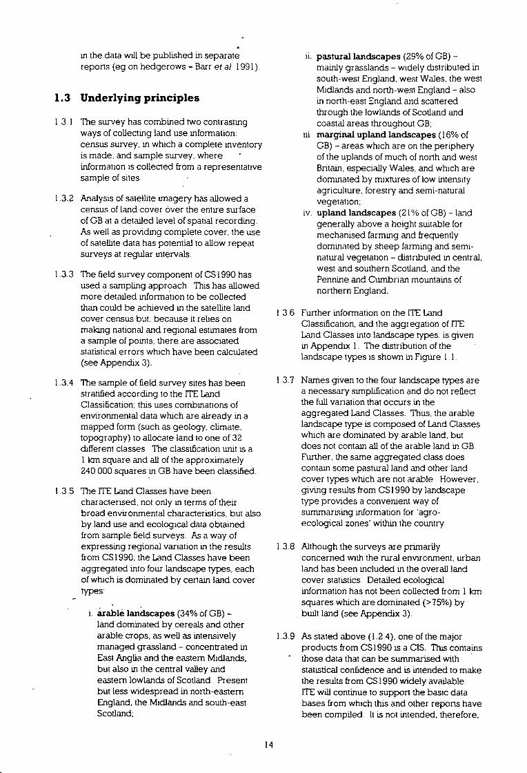
pastural landscapes (29% of GB) -mainly grasslands - widely distributed insouth-west England. west Wales, the westMidlands and north-west England - alsoin north-east England and scatteredthrough the lowlands of Scotland andcoastal areas throughout GB:marginal upland landscapes (16% ofGB) - areas which are on the peripheryof the uplands of much of north and westBritain. especially Wales, and which aredominated by mixtures of low intensityagriculture, forestry and semi-naturalvegetation;upland landscapes (21% of GB) - landgenerally above a height suitable formechanised farming and frequentlydominated by sheep farming and semi-natural vegetation - distributed in central,west and southern Scotland, and thePennine and Cumbrian mountains ofnorthern England.

1.3.6 Further information on the ITELandClassification, and the aggregation of ITELand Classes into landscape types. is givenin Appendix I . The distribution of thelandscape types is shown in Figure 1.1.

1.3.7 Names given to the four landscape types area necessary simplification and do not reflectthe full variation that occurs in theaggregated Land Classes. Thus, the arablelandscape type is composed of Land Classeswhich are dominated by arable land, butdoes not contain all of the arable land in GBFurther, the same aggregated class doescontain some pastural land and other landcover types which are not arable. However,giving results from CSI990 by landscapetype provides a convenient way ofsummarising information for 'agro-ecological zones' within the country.

1.3.8 Although the surveys are primarilyconcerned with the rural environment. urbanland has been included in the overall landcover statistics. Detailed ecologicalinformation has not been collected from 1 kmsquares which are dominated (>75%) bybuilt land (see Appendix 3).

1.3.9 As stated above (1.2.4), one of the majorproducts from CS1990 is a CIS. This containsthose data that can be summarised withstatistical confidence and is intended to makethe results from CS1990 widely available.ITEwill continue to support the basic databases from which this and other reports havebeen compiled. It is not intended, therefore,

14

Figure 1.1 The distribution of I km squares in the four landscape types

Land classes 2.3. 4. 9, 11. 12, 14. 25 Land classes 1. 5. 6. 7. 8. 10, 13, 15. 16and 26 and 27

•4

Efrs'

Marginal upland

Land classes 17. 18. 19. 20, 28 and 3 I Land classes 21, 22. 23. 24. 29. 30 and 32

15

that the present report should contain detailsof all recorded features but, rather, thereport picks out the broad patterns and keyfindings and describes examples of the sortsof data that are held and how these might beinterrogated

1.4 Sununary of Chapter 1

1.4.1 Following previous countryside surveys in1978 and 1984. and the development ofmethods of survey using remotely senseddata and field-based survey and samplingtechniques, the Institute of TerrestrialEcology and the Institute of FreshwaterEcology undertook a survey of the Britishcountryside in 1990. The work wasprincipally funded by the Department of theEnvironment. the British National SpaceCentre. the Department of Trade andIndustry, and the Natural EnvironmentResearch Council. Additional funding wasprovided by the former Nature ConservancyCouncil.

1.4.2 The primary objectives of the survey were toestablish the stock of landscape features andhabitats in GB in 1990, to identify change inthese by reference to earlier data. and tocreate a new baseline for the measurementof future change.

1.4.3 For the first time at a national scale, thesurvey integrated remotely sensed data fromsatellites with field-based survey andsampled data on a common spatial basis.While interpretation of satellite imageryyielded census information for the whole ofGB. held-based studies used the ITE LandClassification for sampling features in moredetail.

1.4.4 Regional variation in the results of the surveywas expressed using aggregations of the ITELand Classes into four landscape types.arable: pasturaL marginal upland; andupland.

16

Chapter 2 METHODS OF DATACOLLECTIONAND ANALYSIS

2.1 Introduction 172.2 Land cover mapping from satellite imagery 172.3 Field survey 232.4 Quality control and assessment - field survey 282.5 Freshwater studies 292.6 Soil surveys 332 7 Summary of Chapter 2 35

2.1 Introduction

2 1 1 Countryside Survey 1990 (031990) broughttogether researchers from a variety ofdisciplines and backgrounds, each havingspecialised in their own field for someyears. They included staff concerned withgeographical. cartographic, and remotelysensed data, botanists, freshwater biologistsand sod scientists

2.1.2 The challenge of the project was to bringthe collective skills and knowledge of thesedifferent groups together. The Integratedbasis on which the research was carried outwas the expression of results in a commonspatial framework, at the 1 lan squareresolution.

2.2 Land cover mapping fromsatellite imagery

Landsat image classification

2.2.1 This study forms an extension to a projectfunded by the British National Space Centreand the Natural Environment ResearchCouncil to map all of Britain from satellneimages. This extension is aimed atintegrating the Landsat-derived map datawith the field survey data of 051990. Itallows improved estimation of landscapestatistics by combining the detailed sample-based. field statistics with a fullspatiallyreferenced census of generahsed cover.The outputs include:

provision of land cover statistics byITELand Class, landscape type and forEngland, Scotland and Wales;provision of summary cover statisticson a 1Ian grid for inclusion in theCountryside Information System (CIS);

• analysis of elements of land cover

pattern, and summary at the 1 lansquare resolution for inclusion in theCIS:calculation of correspondencestatistics to inter-relate field surveyand Landsat data

2.2.2 Unlike the field survey data this elementrepresents the first study of its kind inBritain. It provides stock information, notchange statistics. The main outputs are inthe form of digital data bases which can beinterrogated for specific requirements.rather than forming tables which are an endin themselves.

2.2.3 This section of the report gives a briefdescription of the Landsat imageclassification, outlines the integration withthe field survey and summarises the panernanalyses. Full details of the resultingcorrespondence statistics appear in the CISand are fully described in the Final Reporton Land Cover Definitions (LCD) (Wyatt etal. in prep.). The results of pattern analysesare available through the CIS.

2 2.4 The study was based on Landsat ThematicMapper (TM) data. with its good spatialresolution and the inclusion of a middleinfrared waveband which is important inseparating a wide range of vegetation covertypes (Townshend et aL 1983). EightLandsat paths cover Britain. The orbitsoverlap very substantially in these northernlatitudes, from about 45% in southernEngland. and exceeding 50°/cfrom mid-Scotland northwards. This meant that it waspossible to use alternate paths of data innorth Scotland to achieve full cover but.elsewhere, it was necessary to use everypath.

2 2 5 The land cover mapping involved computerclassification of pared summer and winter

17

TM scenes. The baseline date for themapping was 1990 but, to accommodateany image shortages. an extended period ofplus or minus two years was allowed. Inpractice, the dates of summer images(which essentially determine the cover)ranged between 1988 and 1991.

2 2 6 Summer and winter data, in composite.helped separate the various target classes(Fuller et al 1989a. b) For example, arableareas alternated between fullplant coverand bare ground in a year. semi-naturalvegetation retained full cover, thoughperhaps of plant litter in winter. deciduoustrees were distinguished from evergreens.deciduous rough grasslands differed frompermanently green agricultural grasslands:urban areas and bare ground weredistinguished by their bare appearance inboth summer and winter (Fuller & Parsell,1990)

2.21 The appropriate definition of 'winter' and'summer' was clarified in discussion withecologists and agriculturalists familiar withthe phenology of the local vegetation invarious regions of Britain. The consensuswas that the summer period safely includedmid-May to July. that August to mid-Octoberreprasented a transition period and thatwinter covered the time from mid-Octoberto around mid-March. Late March. Apriland early May were seen as transitionPeriods which were best avoided. Inpractice, the useful periods shifted withaltitude; they also varied from north tosouth, and east to west in Britain and wereinevitably dependent on the year inquestion.

2.2.8 The search for images was based on theNational Remote Sensing Centre quick-lookphotographs of TM images acquired byLandsat within the study period Cloud-treescenes and quarter-scenes were identifiedfrom these. Image availability determinedthe timetable for image processing. In all,allowing for problems of cloud cover, about25 paired, summer/winter, scenes or part-scenes required classification to give fullcover of Britain.

2.2.9 Landsat TM data were geometricallycorrected to the British National Grid(BNG). Control points were definedinteractively on the International ImagingSystems (ES) M75 image processor. Theprocedure used 150 000 Ordnance Surveymaps mounted on a digitising table. to

derive the 'true' position of control points:dentified on the input image. Therelationship between image co-ordinatesand BNG was calculated using a polynomialmodel. The image was then resampled tofit this polynomial model (Schowengerdt1983). to produce an output image with a 25m pixel size, and a BNG map projection.Cubic convolution resampling. which bettermodelled the natural variations in radianceacross an image. was the most appropriatealgorithm (Fuller &Parsell 1990).

2 2.10 The summer/winter composite images weremade by co-registering scenes or part-scenes to give a single output image. Thisimage contained six bands of data, threeeach from the original summer and winterdata. namely TM bands 3, 4 and 5 - ie red,near and middle infrared (IR). These bandswere chosen because they representwavelengths with characteristic responsesfrom vegetation (red for chlorophyllabsorption and IRfor mesophyllreflections) They were also less affectedby haze problems than the blue-green endof the visible spectrum (Fuller et al. 1989a:Fuller & Parsell 1990).

2.2.11 An appropriate class selection was the keyto an accurate classification, consistent asfar as possible throughout Britain. and usefulto ecologists and other environmentalscientists. By reference to other surveys itwas possible to draw on a wide range ofexperience in vegetation mapping. and touse the types of classification which hadthemselves been devised for applied uses.Ultimately, of course, the classification wasdetermined by what was feasible fromsatellite images. here. the study wasstrongly influenced by the pilot exercises inCambridgeshire and Snowdonia, but withevolution of the classifications based onexperiences in the current survey, and on aconsultative exercise involving othersurveyors and end-users.

2.2.12 A final list of 25 target classes (land covertypes) was derived for mapping throughoutBritain (Figure 2.1). The classification maybe simplified, if required, by aggregatingrarer classes with related, more common,ones.

2.2.13 The procedure of classification was basedon extrapolation from sample statistics forreflectances of each class. In reality, thetarget classes were achieved by defining alarge number of spectrally unique

18

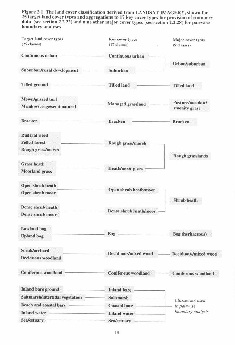
Figure 2.1 The land cover classification derived from LANDSAT IMAGERY, shown for25 target land cover types and aggregations to 17 key cover types for provision of summarydata (see section 2.2.22) and nine other major cover types (see section 2.2.28) for pairwiseboundary analyses

Target land cover types

(25 classes)

Continuous urban

Suburban/rural development

Tilled ground -

Mown/grazed turf

Meadow/verge/semi-natural

Bracken

Ruderal weed

Felled forest

Rough grass/marsh

Grass heath

Moorland grass

Open shrub heath

Open shrub moor

Dense shrub heath

Dense shrub moor

Lowland bog

Upland bog

Scrub/orchard

Deciduous woodland

Coniferous woodland

Key cover types

(17 classes)

Continuous urban

Suburban

Tilled land

Major cover types

(9 classes)

Urban/suburban

Tilled land

Bog Bog (herbaceous)

Deciduous/mixed wood Deciduous/mixed wood

Coniferous woodland Coniferous woodland

Managed grassland Pasture/meadow/amenity grass

Bracken

Rough grass/marsh

Heath/moor grass

Open shrub heath/moor

Dense shrub heath/moor

Bracken

Rough grasslands

Shrub heath

Inland bare groundInland bare

Saltmarsh/intertidal vegetation Saltmarsh

Beach and coastal bareCoastal bare

Inland waterInland water

Sea/estuarySea/estuary

Classes ma used

in pairwise

boundary analysis

19

subclasses. This was necessary becausethe maximum likelihood classifier (MLC)assumes a normal distribution in the data(Kershaw & Fuller 1992). which could onlybe achieved by subdividing multi-modaldata into component subclasses (eg talcingspecific crops as subclasses of tilled l&nd).

2.2.14 The sample are&s on which the classificationwere based were selected usingknowledge derived in the fieldreconnaissance survey. Typically, fieldreconnaissance identified the cover in about1200 land/water parcels per Landsat scene.

2.2.15 Training the image classifier involvedoutlining groups of pixels which wererepresentative of the particular classes orsubclasses intended for classification.Overall. 70-80 subclasses were typical formost scenes. Normally, there were five ormore training areas per subclass with aminimum 30 pixels in total, but, moreusually, there were 100-200 pixels persubclass.

2.2.16 Extrapolation was used to find all otherpixeLs in the scene with the same spectralcharacteristics as the subclasses used intraining. The maximum likelihood classifierallocated each pixel to its nearest subclass(in statistical terms) or rejected pixels ifdissimilar to all available subclasses. Bydefining a rejection threshold, it waspossible to reject more or less of the scene(Kershaw & Fuller 1992). In this case, all butthe very rarest of subclasses were defined.so the threshold was varied in order toclassify 98% or more of land/water parcels.

2.2.17 The process of training and classificationwas an iterative one, relying on preliminaryclassification, inspection of results. editionor addition of training subclasses, thenreclassification, working towards a fmalcover map.

2.2. I 8 Some classes could not always be reliablyseparated purely on the basis of spectraldifferences. Contextual information, eitherdrawn from outside sources or derivedfrom the data helped correct any errors.By defining a coastline, it was possible toimpose the rule that terrestrial habitats areonly found inland of the line, maritimehabitats to seaward. The definition of thecoastline was semi-automated. Maritimeclasses were extracted to form a mask, andthis was smoothed using filters to removeholes in the mask, or erroneous 'inland

maritime' areas. If necessary. the mask wasthen edited interactively on the imageprocessor. before being used forcorrection. Using a masking procedure, itwas possible to filter out small pockets ofmisclassified lowland habitat in an extensiveupland area and vice versa (there remains achoice between using these distinctions, asdescribed, or re-aggregating the upland/lowland classes. and using alternativecontextual information, such as altitude, tomake the distinction).

2 2.19 An urban mask was made from urban andsuburban pixels. and holes in the maskwere then filled using a majority filter. Theresulting mask was used to correctmisclassified urban areas, for examplewhere the change m vegetation coverbetween summer and winter images(gardens. scrub areas) resembled theseasonal changes in arable land. Any suchpatches which fell under the mask werechanged to suburban pixels. Classes suchas deciduous and coniferous woodland:water bodies or grasslands were allowed toremain, as they are normal features ofurban environments.

2 2.20 Local interactive corrections were neededsometimes odd clouds obscured a smallpan of the summer or winter image,pockets of haze might also have causedvery occasional difficulties. In such cases, itwas possible to classify that pocket usingjust the one good date, cut out the areacovered with haze. cloud or shadow. andinsert a patch from the single-date covermap. In other areas. odd cover types (egpeat cuttings), perhaps too small to train assubclasses, were misclassified; in suchcircumstances, it was possible to take out a'tile' of the cover map, renumber the covervalue in a locality to the correct value, andplace the corrected 'tile' back into the covermap.

2.2.21 In building a mosaic of full GB land cover,data have been stored as 100 km x 100 kmtiles, for convenience of access. These tileswere made as 'jigsaws' from theappropriate sections of each scene As ascene classification was completed, thesections were 'cut out' and stored in their100 krn x 100 km tile. Joins were madewithin the overlap between scenes, using asinuous outline along uniform featureswhich were classified in the same way inboth scenes. Areas where there wereImown difficulties on a scene (eg haze

20

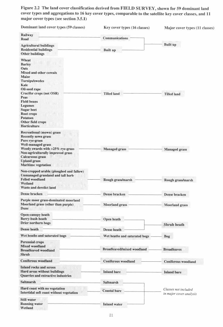
Figure 2.2 The land cover classification derived from FIELD SURVEY, shown for 59 dominant landcover types and aggregations to 16 key cover types, comparable to the satellite key cover classes, and IImajor cover types (see section 3.5.1)

Key cover types (16 classes)

Communications

Built up

Tilled land

Managed grass

Dominant land cover types (59 classes)

RailwayRoad

Agricultural buildingsResidential buildingsOther buildings

WheatBarleyOatsMixed and other cerealsMaizeTurnips/ssvedesKaleOil-seed rapeCrucifer crops (not 05R)PeasField beansLegumesSugar beetRoot cropsPotatoesOther field cropsHorticulture

Recreational (mown) grassRecently sown grassPure rye-grassWell-managed grassWeedy swards with >25% rye-grass Non-agriculturally improved grassCalcareous grassUpland grassMaritime vegetation

Non-cropped arable (ploughed and fallow)Unmanaged grassland and tall herbFelled woodlandWetlandWaste and derelict land

Dense bracken

Purple moor grass-dominated moorlandMoorland grass (other than purple)Dune

Open-canopy heathBerry-bush heathDrier northern bogs

Dense heath

Wet heaths and saturated bogs

Perennial cropsMixed woodlandBroadleaved woodlandShrub

Coniferous woodland

Inland rocks and screesHard areas without buildingsQuarries and extractive industries

Saltmarsh

Hard coast with no vegetationIntertidal soft coast without vegetation

Major cover types (11 classes)

Built up

Tilled land

Managed grass

Rough grass/marsh

Dense bracken

Moorland grass

Shrub heath

Bog

Broadleaves

Coniferous woodland

Inland bare

Classes no!! included

in major cover analysis

Rough grass/marsh

Dense bracken

Moorland grass

Open heath

Dense heath

Wet heaths and saturated bogs

Broadleaved/mixed woodland

Coniferous woodland

Inland bare

Saltmarsh

Coastal bare

Still waterRunning water Inland waterWetland

21

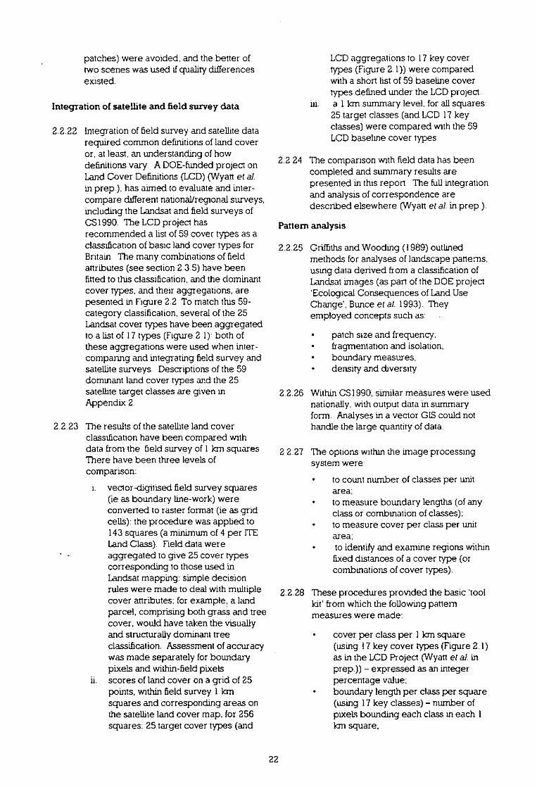
patches) were avoided and the better oftwo scenes was used ifquality differencesexisted

Integration of satellite and field survey data

2.2.22 Integration of field survey and satellite datarequired common definitions of land coveror. at least, an understanding of howdefinitions vary. A DOE-funded project onLand Cover Definitions (LCD) (Wyatt et a).in prep.). has aimed to evaluate and inter-compare different national/regional surveys,including the Landsat and field surveys ofCS1990. The LCD project hasrecommended a list of 59 cover types as aclassification of basic land cover types forBritain. The many combinations of fieldattributes (see section 2.3.5) have beenfitted to this classification, and the dominantcover types, and their aggregations. arepesented in Figure 2.2 To match this 59-category classification, several of the 25Landsat cover types have been aggregatedto a list of 17 types (Figure 2 1):both ofthese aggregations were used when inter-comparing and integrating field survey andsatellite surveys. Descriptions of the 59dominant land cover types and the 25satellite target classes are given inAppendix 2.

2 2.23 The results of the satellite land coverclassification have been compared withdata from the field survey of 1 km squares.There have been three levels ofcomparison:

i. vector-digitised field survey squares(ie as boundary line-work) wereconverted to raster format (ie as gridcells): the procedure was applied to143 squares (a minimum of 4 per ITELand Class). Field data wereaggregated to give 25 cover typescorresponding to those used inLandsat mapping. simple decisionrules were made to deal with multiplecover attributes: for example: a landparcel, comprising both grass and treecover, would have taken the visuallyand structurally dominant treeclassification. Assessment of accuracywas made separately for boundarypixels and within-field pixels.scores of land cover on a grid of 25points, within field survey 1 kmsquares and corresponding areas onthe satellite land cover map. for 256squares: 25 target cover types (and

LCD aggregations to 17 key covertypes (Figure 2.1)) were comparedwith a short list of 59 baseline covertypes defined under the LCD project.

in a 1 km summary level, for all squares:25 target classes (and LCD 17 keyclasses) were compared with the 59LCD baseline cover types.

2.2.24 The comparison with field data has beencompleted and summary results arepresented in this report. The full integrationand analysis of correspondence aredescribed elsewhere (Wyatt et a). in prep ).

Pattern analysis

2.2.25 Griffiths and Wooding (1989) outlinedmethods for analyses of landscape patterns.using data derived from a classification ofLandsat images (as pan of the DOE project'Ecological Consequences of Land UseChange'. Dunce et al. 1993). Theyemployed concepts such as: .

patch size and frequency,fragmentation and isolation;boundary measures;density and diversity.

2.2.26 Within CS1990, similar measures were usednationally, with output data in summaryform. Analyses in a vector GIS could nothandle the large quantity of data.

2 2.27 The options within the image processingsystem were:

to count number of classes per unitarea:to measure boundary lengths (of any class or combination of classes):to measure cover per class per unitarea:to identify and examine regions within

fixed distances of a cover type (orcombinations of cover types).

2.2.28 These procedures provided the basic 'toolkit' from which the following patternmeasures were made:

cover per class per 1 km square(using 17 key cover types (Figure 2.1)as in the LCD Project (Wyatt el at inprep.)) - expressed as an integerpercentage value;boundary length per class per square(using 17 key classes) - number ofpixels bounding each class in each 1km square:

22

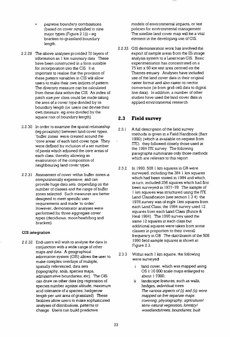
pairwise boundary combinations(based on cover simplified to ninemajor types (Figure 2 I)) - egbracken-to-grassland bowidarylength.

2.2.29 The above analyses provided 70 layers ofinformation as 1 km summary data Thesehave been constructed in a form suitablefor incorporation into the CIS. It isimportant to realise that the provision ofthese pattern variables in CIS will allowusers to make their own indices of pattern.The diversity measure can be calculatedfrom these data within the CIS. An index ofpatch size per class could be made takingthe area of a cover type divided by itsboundary length (or users can devise theirown measure. eg area divided by thesquare root of boundary length).

2.2.30 In order to examine the spatial relationship(eg proximity) between land cover types.'buffer zones- were created around the'core areas of each land cover type. Theywere defined by inclusion of a set numberof pixels which adjoined the core areas ofeach class, thereby allowing anexamination of the composition ofneighbouring land cover types

2.2.31 Assessment of cover within buffer zones iscomputationally expensive, and canprovide huge data sets, depending on thenumber of classes and the range of bufferzones selected Such measures are betterdesigned to meet specific userrequirements and made 'to order'.However, demonstrator analyses wereperformed for three aggregate covertypes (deciduous. moor/heath/bog andbracken).

GIS integration

2.2.32 End-users will wish to analyse the data inconjunction with a wide range of othermaps and data. A geographicalinformation system (GIS) allows the user tomake complex overlays of multiple,spatially referenced, data sets(topography. soils, species maps,administrative boundaries, etc). The GIScan draw on other data (eg regression ofspecies number against altitude, maximumacid tolerance of a species, hedgerowlength per unit area of grassland). Thesefacilities allow users to make sophisticatedanalyses of distributions, patterns orchange. Users can build predictive

models of environmental impacts, or testpolicies for environmental management.The satellite land cover map will be a vitalelement in the developing use of GIS.

2.2.33 GIS demonstration work has involved theexport of sample areas from the IISimageanalysis system to a Laserscan GIS. Basicexperimentation has concentrated on a75 km x 50 km test area centred on theThames estuary. Analyses have includeduse of the land cover data in their originalraster format and also raster-to-vectorconversion (ie from grid-cell data to digitalline data). In addition, a number of otherstudies have used the land cover data inapplied environmental research.

2.3 Field survey

2.3.1 A fulldescription of the field surveymethods is given in a Field Handbook (Barr1990) (which is available on request fromfrE): they followed closely those used inthe 1984 frE survey. The followingparagraphs summarise only those methodswhich are relevant to this report

2.3.2 In 1990. 508 1 km squares in GB weresurveyed, including the 384 1 km squareswhich had been visited in 1984 and which.in turn. included 256 squares which had firstbeen surveyed in 1977-78. The sample of1 km squares was structured using the ITELand Classification (see section 1.3.4): the1978 survey was of eight 1km squares fromeach Land Class: the 1984 survey used 12squares from each Land Class (Bunce &Heal 1984). The 1990 survey used thesame 12 squares in each class butadditional squares were taken from someclasses in proportion to their overallfrequency in GB. The distribution of the 5081990 field sample squares is shown inFigure 2.3.

2.3.3 Within each 1 km square. the followingwere surveyed:

i. land cover. which was mapped usingOS 1:10 000 scale maps enlarged toabout 1:7000:landscape features, such as wallshedges, individual treesThe variousaspects of (i) and (b) weremapped on live separate mapscovering: physiography; agriculture/semi-natural vegetation; forestry/woodlands/trees: boundaries; built

23

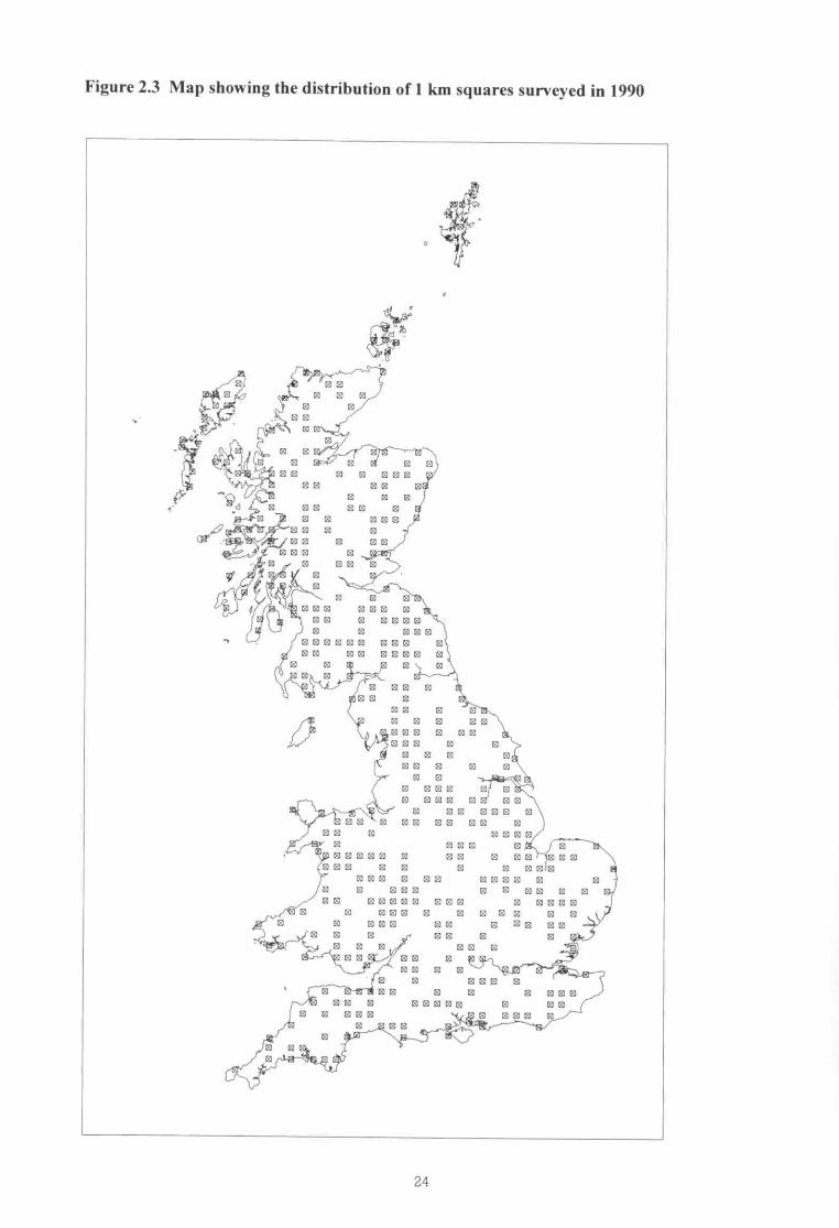
Figure 2.3 Map showing the distribution of 1 km squares surveyed in 1990

00

a 00 a 000

00 a aa a a

. o a a a a a a

a a a a a a

D 0 0 a a

ar . a 0 a 0a0 a a 0

- a 0 a a 0

V 0 •0

a a 0I Mao 2100 0

00 a 00 00a 0 000

, 0000 00 000 000 00 0000 0

0 0 0 00 a

0 0 0 0

0 0 00 0 0 0

D . . 0

000 . .0000.0 0 .

a a . 0

00 0 0 0 0 0

0 .. 00.. ... 0 .0

0 00 .00 0.0 0 00 0. .0 .

00.000 .

a ... a 0OCEI 00 a 0 0 a a a 0 0 0

000 0 0 a 0 a Cil0Oa 00 a 00 HO 0 a 0

a a 000 000000a 0 0000a 000 a a a a a

a a 0 a a a a a 0 0 0 0El a 000 a 0 a 00 Ma

a la a 0 a 0 00 0 0 a a 0

a a 0 0 000 a a

a 0 000 a. 0 00 0

00000 a0 a a a

0 0 a a 0 a

0

0 0 000 0 a 00 a

0 00 EC?

24

environment and recreation.ilL up to 27 vegetation plots, both in open

land and alongside linear features suchas hedges. roads and streams

Field mapping

2.3.4 The mapped features were described usinga predetermined list of codes as shown inAppendix 2 Where a feature could not bedeschbed using the existing codes, uniquedescriptions were used and codedseparately. Because such uniqueinformation has not necessarily beencollected in an objective and corsistentway, its use is limited

2_35 In order to give as much information aspossible about each area of land orlandscape feature, combinations of datacodes were used to annotate each categoryon the map An example of a page from afield recording booklet is given in Figure2.4. There were two types of code:primary (general descriptions of features.eg woodland) and secondary (giving moredetail about the feature, eg tree species.age. management practices, in a wood). Allfeatures were annotated with at least oneprimary code and, where more than oneprimary code has been used (eg multipleland use), then the code reflecting thedominant use was recorded first

2.3.6 The smallest area that field surveyorsrecorded (the minim= mappable area)was 0.04 ha (400 mz). No vegetation type(except bracken) was mapped as aseparate unit unless it achieved ths size.The minimum mappable length of anyboundary feature was 20 m.

2.31 The mapped area of each land coverparcel. and the length of each boundary, orboundary segment, was determined by theconstancy of a combination of codes; whereany one description differed, then a newarea or length was demarcated and a newcombination of codes was used. The samecoded descriptions were used in both 1984and 1990, except for minor amendments asshown in Appendix 2.

2.3.8 Boundary features were mapped and codedas 'single lines' on the map, even thoughthere may have been several differentelements associated with each (eg a hedgeand a fence on top of a stone bank). Foradjacent lines to be mapped individually,then a clear gap between all the elements ofthe two boundaries had to be identified

Boundaries of land associated withbuildings (curtilage) were not mapped indetail. Boundary features within woodlandwere not mapped

2.3.9 To assist in field mapping. limited aerialphotographic interpretation was carried outfor each square. Using photographs ofvarious dates. but all taken since the 1984survey, features that were no longerpresent, and those that were new to themap were marked on a 'master map' whichwas used as a base for field recording.

Vegetation recording in plots

2 3 10 Vegetation data were collected from up to27 plots in each of the 508 CS1990 fieldsquares. In 1977-78 vegetation data werealso collected from a smaller number ofplots. in 256 squares

2.3.11 The vegetation plots were of three types.

five 200 m2vegetation plots instratffied random locations - 'Mainplots'These plots were located at randomwithin five equal-sized sectors of the 1km square. If they fell on a linearfeature, they were relocated at random.five.4 m2vegetation plots placed withinsemi-natural habitats only - 'Habitatplots'These plots were placed in semi-naturalhabitats not covered by the largerrandom plots, according to a randomallocation procedure.up to 17 10 mx 1m linear plots placedalongside field boundaries (Soundaryplots). hedges ('Hedge plots).watercourses ('Streamside plots').and roads/tracks ('Verge plots').ne five Boundary plots were placed atthe nearest field boundary to each ofthe Main plots (if within 100m) - onlythose Boundary plots that occurredadjacent to hedgerows have beenincluded in the current analysis.7'woHedge plots were also placed atrandom within each 1 km squareEach of the Streamside plots wasplaced at the edge of running water,with a second, parallel, 10mxlm plotbeing recorded on the water side torecord any emergent macrophyticplants; two of the Streamside plots werelocated at random within the squareand three more were placed to sampledifferent sizes of watercourses.Verge plots were placed immediately

25

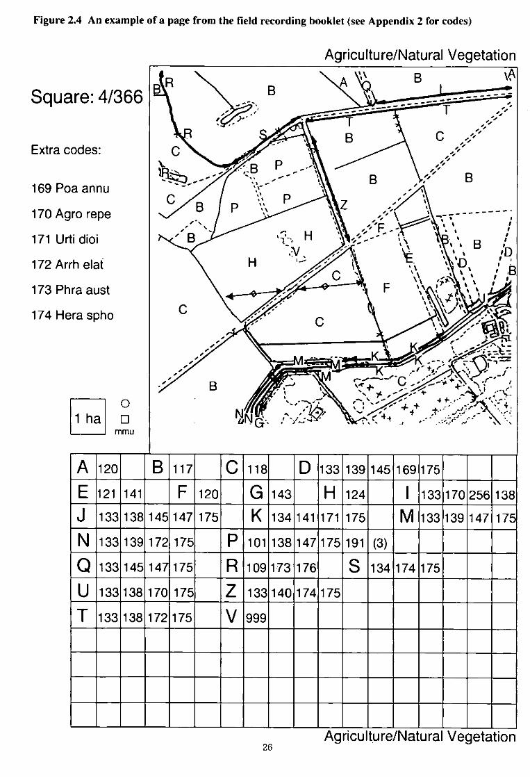
Figure 2.4 An example of a page from the field recording booklet (see Appendix 2 for codes)

Agriculture/Natural Vegetation

A----------Square:4/366

..

..

... %

IC' ‘ -------- ..° -.--:

t i

t I, . , II

G.°.••••• • I% % • B

----,I , , ,/IP%• I

'D

\ % 1 % : 13

, % , ,I,

.i

‘, 5:. , ;

F , i ,

, I 1 • \

t ‘ 11" • %I % \ II

1% •./ %• ••••

%•. -ati5S1;,

et"

it•I':11;.7-.:Ii

Extra codes:

169 Poa annu

170 Agro repe

171 Urti dioi

172 Arrh elat

173 Phra aust

174 Hera spho

C

A 120 B 117

E 121 141 F 120

J 133 138 145 147 175

133 139 172 175

Q 133 145 14 175

133 138 170 175

T 133 138 172 175

... 7 --...,----...F.."i'tf..

r------.--- C • '' .-••.1 .•i‘...r‘ts,- ,--;t

,........--,,....

ey,-,4 4-..•-• _At.Asi ., _ 4/

•• 4'4Li G...,-,/...:-4••-,,,,,•-.,...•,..:\•,

C 118 D 133 139 145 169 175

G 143

H 124 I 133 170 256 138

K 134 141 171 175 M 133 139 147 17

P 101 138 147 175 191(3)

R 109 173 176 S 134 174 175

Z 133 140 174 175

V 999

0

..I

'• B0 0

MMU

1 ha

26Agriculture/Natural Vegetation

adjacent to the road edge, in roadsideverges wider than 2 rn, a second,parallel. Verge plot was recordedimmediately adjacent to the first one(see Wide Verges in Results section):two of the Verge plots were located atrandom and three were placed tosample different road types

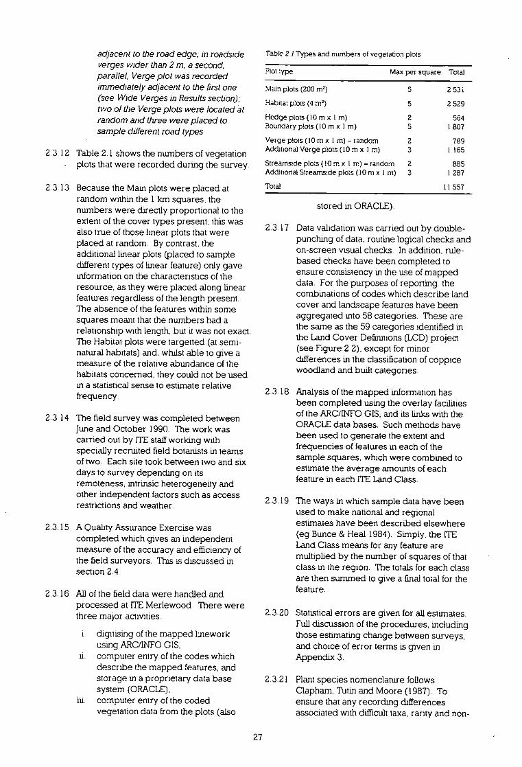
2.3.12 Table 2.1 shows the numbers of vegetation. plots that were recorded during the survey.

2.3.13 Because the Main plots were placed atrandom within the 1 km squares. thenumbers were directly proportional to theextent of the cover types present: this wasalso true of those linear plots that wereplaced at random. By contrast, theadditional linear plots (placed to sampledifferent types of linear feature) only gaveinformation on the characteristics of theresource, as they were placed along linearfeatures regardless of the length present.The absence of the features within somesquares meant that the numbers had arelationship with length. but it was not exact.The Habitat plots were targetted (at semi-natural habitats) and, whilst able to give ameasure of the relative abundance of thehabitats concerned, they could not be usedin a statistical sense to estimate relativefrequency.

2.3.14 The field survey was completed betweenJune and October 1990. The work wascarried out by ITE staff working withspecially recruited field botanists in teamsof two. Each site took between two and sixdays to survey depending on itsremoteness, intrinsic heterogeneity andother independent factors such as accessrestrictions and weather.

2.3.15 A Quality Assurance Exercise wascompleted which gives an independentmeasure of the accuracy and efficiency ofthe field surveyors. This is discussed insection 2.4.

2.3.16 All of the field data were handled andprocessed at ITE Merlewood. There werethree major activities:

i. digitising of the mapped theworkusing ARC/INFO015.computer entry of the codes whichdescribe the mapped features, andstorage in a proprietary data basesystem (ORACLE).computer entry of the codedvegetation data from the plots (also

Table 2 / Types and numbers of vegetation plots

Plot typeMax per square Total

Main plots (200 m2) 5 2 53 i

Habitat plots (4 m2) 5 2 529

Hedge plots (10 m x I m) 2 564Boundary plots (10 m x I m) 5 I 807

Verge plots (10 m x I m) - random 2 789Additional Verge plots (10 m x I nit) 3 I 165

Streamside plots (10 m x I m) - random 2 885Additional Streams:de plots (10 m x I m) 3 I 287

Total

I I 557

stored in ORACLE)

2.3.17 Data validation was carried out by double-punching of data, routine logical checks andon-screen visual checks. In addition, rule-based checks have been completed toensure consistency m the use of mappeddata. For the purposes of reporting. thecombinations of codes which describe landcover and landscape features have beenaggregated Into 58 categories. These arethe same as the 59 categories Identified inthe Land Cover Definitions (LCD) project(see Figure 2 2). except for minordifferences in the classification of coppicewoodland and built categories.

2.3.18 Analysis of the mapped information hasbeen completed using the overlay facilitiesof the ARC/INFO GIS, and its links with theORACLEdata bases. Such methods havebeen used to generate the extent andfrequencies of features in each of thesample squares, which were combined toestimate the average amounts of eachfeature in each 1TELand Class

2.3.19 The ways in which sample data have beenused to make national and regionalestimates have been described elsewhere(eg Bunce & Heal 1984). Simply. the ITELand Class means for any feature aremultiplied by the number of squares of thatclass in the region. The totals for each classare then summed to give a final total for thefeature.

2.3.20 Statistical errors are given for all estimates.Full discussion of the procedures, includingthose estimating change between surveys.and choice of error terms is given inAppendix 3.

2.3.21 Plant species nomenclature followsClapham. Tutm and Moore (1987). Toensure that any recording differencesassociated with difficult taxa. rarity and non-

27

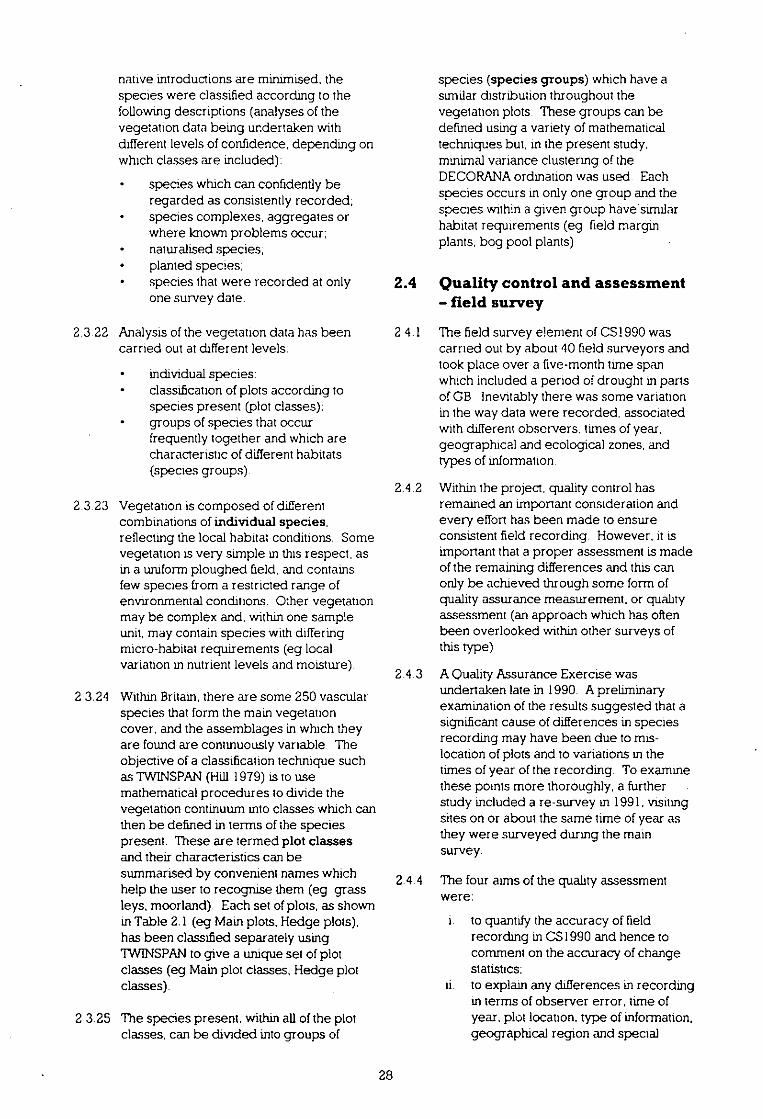
native introductions are minimised. thespecies were classified according to thefollowing descriptions (analyses of thevegetation data being undertaken withdifferent levels of confidence, depending onwhich classes are included):

species which can confidently beregarded as consistently recorded;species complexes, aggregates orwhere known problems occur;naturalised species;planted species;species that were recorded at onlyone survey data

2.3.22 Analysis of the vegetation data has beencarried out at different levels:

individual species:classification of plots according to species present (olot classes):groups of species that occurfrequently together and which arecharacteristic of different habitats(species groups).

2.3.23 Vegetation is composed of differentcombinations of individual species,reflecting the local habitat conditions. Somevegetation is very simple in this respect, asin a uniform ploughed field, and containsfew species from a restricted range ofenvironmental conditions. Other vegetationmay be complex and, within one sampleunit, may contain species with differingmicro-habitat requirements (eg localvariation in nutrient levels and moisture).

2 3.24 Within Britain, there are some 250 vascularspecies that form the main vegetationcover, and the assemblages in which theyare found are continuously variable Theobjective of a classification technique suchas TWINSPAN(Hill 1979) is to usemathematical procedures to divide thevegetation continuum into classes which canthen be defined in terms of the speciespresent. These are termed plot classesand their characteristics can besummarised by convenient names whichhelp the user to recognise them (eg grassleys, moorland). Each set of plots, as shownin Table 2.1 (eg Math plots, Hedge plots).has been classified separately usingTWINSPANto give a unique set of plotclasses (eg Main plot classes, Hedge plotclasses).

2.3.25 The species present, within all of the plotclasses, can be divided into groups of

species (species groups) which have asimilar distribution throughout thevegetation plots. These groups can bedefthed using a variety of mathematicaltechniques but. in the present study.minimal variance clustering of theDECORANAordination was used. Eachspecies occurs in only one group and thespecies within a given group havasirralarhabitat requirements (eg field marginplants. bog pool plants).

2.4 Quality control and assessment- field survey

2 4.1 The field survey element of CSI990 wascarried out by about 40 field surveyors andtook place over a five-month time spanwhich included a period of drought in partsof GB Inevitably there was some variationin the way data were recorded. associatedwith different observers. times of year,geographical and ecological zones, andtypes of information.

2.4.2 Within the project. quality control hasremained an important consideration andevery effort has been made to ensureconsistent field recording. However, it isimportant that a proper assessment is madeof the remaining differences and this canonly be achieved through some form ofquality assurance measurement, or qualityassessment (an approach which has oftenbeen overlooked within other surveys ofthis type).

2.4.3 A Quality Assurance Exercise wasundertaken late in 1990. A preliminaryexamination of the results suggested that asignificant cause of differences in speciesrecording may have been due to mis-location of plots and to variations in thetimes of year of the recording. To examinethese points more thoroughly, a further . study included a re-survey in 1991, visitingsites on or about the same time of year asthey were surveyed during the mainsurvey.

2.4.4 The four aims of the quality acsessmentwere:

to quantify the accuracy of fieldrecording in CSI990 and hence tocomment on the accuracy of changestatistics;to explain any differences in recordingin terms of observer error, time ofyear. plot location, type of information,geographical region and special

28

factors such as drought:to relate the conclusions from (i) and (ii)to previous comparative work done onITEsurvey methods

iv. to recommend modifications to surveymethodology for future surveys whichwould improve the accuracy andconfidence of the resulting statisiics.

2 4 5 The work was carried out by EcologicalSurveys (Bangor) and is summarised inAppendix 4

2.4 6 The main points to note from the quality assurance work are given below.

The permanent marldng of plots was ofsufficiently high standard to suggest thatdetailed changes in vegetation may befollowed using the present surveymethods, but that plot re-location may betime-consuming, especially in theuplands.The initial recording accuracy wasbetween 74% and 83%. depending onsuch factors as weather, seasonalvariation and relocation of plots. This levelof accuracy is close to the maximumattainable efficiency that can be expected.Estimation of species cover values as panof field mapping was variable and needsto be improved in further surveys.Trends in vegetation change have beenrelated to environmental change, usingcorrespondence analysis. The consistentdirections of change between 1990 and1991 indicated that 1990 plot data aresufficiently reliable to demonstrateenvironmental change.Land cover mapping was more reliable atthe primary code level (84% agreement)rather than at more detailed levels (78%agreement for objective qualifying codes;49% for subjective qualifiers). Recordingwas more reliable in the lowlands (95%agreement at primary code level) than inthe uplands (71%).

2.4 7 The steps that were taken to ensure reliabilityare shown in Figure 2.5. Recommendationson modifications to survey methodology havebeen made and these will be taken intoaccount in the planning of future surveys ofthis type.

2.5 Freshwater studies

2 5 1 The data bases analysed in the freshwatercomponent of this study were of aquatic

macro-invenebrate assemblages in streams.rivers, drains and canals. Complementaryenvironmental data were compiled fromcontemporary field measurements and fromcartographic sources. Separate data baseswere used to relate faunal information andwater quality to ITELand Class and landcover:

CS1990 field surveyenvironmental qualityother related stuveys and data bases

Countryside Survey 1990 - field survey

2.5.2 Where present and suitable, a single runningwatercourse was sampled in each of the 5081km squares surveyed as pan of CS1990.In this context, a suitable stream was one offirst, second or third stream order. A first-order stream is one with no tributaries, asecond-order stream is one formed by theconfluence of two first-order streams and athird-order stream results from the mergerof two second orders.

2.5 3 Fourth- and higher-order streams wereregarded as unsuitable for sampling forthree reasons.

They could be deep and silty andtherefore potentially dangerous tosample in remote locations.Deep sites would have requiredadditional, cumbersome equipment tosample adequately and this could noteasily be carried in the field.Higher-order watercourses occurredso infrequently in the survey squaresthat they were too few to allowmeaningful comparisons between ITELand Classes and might even distortany attempt to do so.

2 5.4 Higher-order streams were wellrepresented in the other data basesavailable for analysis.

2.5.5 A set of rules was established to select thewatercourse and site location in each surveysquare.

Rivers were given preference overcanals which. in turn, were preferred todrains.Third-order streams were givenpreference over second-order andsecond-order over first-order. Thisprocedure tended to equalise thenumber of sites sampled in each .categoryIn the absence of rivers, the largest canal(or drain) judged to be wadable was

29

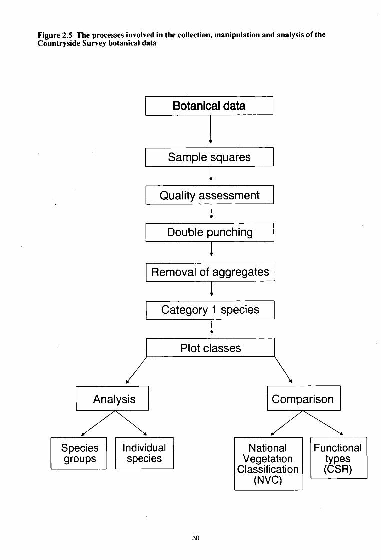
Figure 2.5 The processes involved in the collection, manipulation and analysis of theCountryside Survey botanical data

Botanicaldata

Sample squares

Quality assessment

Double punching

Removal of aggregates

Category 1 species

Plot classes

Analysis Comparison

Species Individual National Functionalgroups species Vegetation types

Classification (CSR) (NVC)

30

selectedWhere possible. the site on the chosenwatercourse was located near thepoint where it flowed out of the 1 ktrisquare. This tended to maximise theproportion of its catchment which laywithin the square and was thereforesurveyed for land cover and useReaches just downstream of possiblepoint sources of pollution or nearhuman artefacts (eg just downstreamof a sewage treatment works or closeto a weir) were avoided No othercriteria were established to ensurethat the selected stream wasnecessarily the least polluted of thoseavailable within the square. Thisstrategy ensured that, in futuresurveys, the opponunity to recordimprovements in quality, as well asdeterioration, was available within thedata set.Given the above criteria, the siteswere selected to be reasonably closeto roads and tracks in order to limit thedistance sampling equipment had tobe carried

2 5.6 Site selection was made in the laboratoryprior to sampling Field surveyors werepermitted to modify the sampling point inthe field, under certain defined conditions:

if the selected watercourse was dry:ifthe entire width of the selectedwatercourse was too deep to wadewith safety:if the chosen site was physicallyinaccessible with safety:

• ifpermission to sample was withheldby the landowner.

Field selection of a replacement site was tofollow the same criteria as had beenemployed in the original selectionprocedures (Field surveyors wereinstructed not to alter the location ofsampling sites purely for their ownconvenience.)

2 5.7 Samples were collected by use of a handnet The preferred sampling procedurewas to hold the mouth of the netdownstream of an area of streamsubstratum being vigorously disturbed bythe surveyor's foot. Where aquaticmacrophytes were present. these were alsosampled by 'sweeping' the net through thevegetation Ifthese techniques wereimpossible (eg some very shallow streams).

the surveyors were asked TO improviseusing the most appropriate strategy tocollect animals.

2.5.8 The preferred and several alternativesampling strategies were demonstrated toall surveyors during a pre-survey trainingcourse.

2.5.9 Whichever sampling strategy was used, theactive sampling duration was to be threeminutes and the underlying objective ofsampling was to collect the widest possiblevariety of species within this period.

2 5.10 In general. drains and canals were onlysampled where wadable in thigh waders,although some such watercourses wereonly sampled from the margins where thenature of the substratum rendered thempotentially dangerous to enter.

2.5.11 Samples were preserved in formalin andidentified to the best achievable level,normally species. Most identifications weremade by two highly trained staff whoworked together to identify diffIcultorcontentious specimens. Specialist help wasenlisted to identify or confirm Identificationsof difficult groups or problematicspecimens.

2.5.12 As a further safeguard against mis-identification, the lists of taxa identified ateach site were scrutinised by other.experienced 1FEstaff members. Anyunusual specimens, or specimens thoughtto be at or beyond their perceivedecological range. were re-examined in caseof error.

2.5 13 A standardised level of identification wasused in all statistical analyses andpresentation of analyses. This meant thatany small or damaged specimens whichcould not be identified to the usual detailedlevel. for their taxonomic group, weredeleted from the analytical data set.

2.5.14 At each sampling site. field surveyorsrecorded environmental data as.sociatedwith the site on a standard recording sheet.Bankside vegetation and land use. channelmanagement and pollution were recordedfor a 25 m length of watercourse either sideof the sampling site. Watercourse sizecharacteristics. current velocity andsubstratum were recorded for the sampling

-site: locational and the remaining

31

geographical and hydrological data wereread from maps Further details of howthese categories were recorded areavailable in the Field Handbook (Barr 1990).

Environmental quality

2.5.15 Each site was assigned to a biologicalquality class using procedures devised andrecommended by IFE. These wereassociated with their classification andprediction software package RIVPACS(Wright et al. 1988. 1991: Clarke et al. 1992;Sweeting et al. 1992: Furse et a! 1987; Mosset a). 1987).

2.5.16 RIVPACSassessments are based uponbiotic index values of sites derived from thetaxa present. The method used is theBiological Monitoring Worldng Party(BMWP) score system (Armitage et a).1983). Each family of invertebrate presentis allocated a score according to itstolerance of organic pollution. Intoleranttaxa are assigned high scores because theirpresence indicates a lack of pollution.Conversely, pollution-tolerant taxa have lowscores. The BMWPsite score for the site isthe sum of the scores of the individual taxapresent.

2.5.17 A criticism of the scoring system is that it iseffort- and efficiency-related. The BMWPscore is likely to increase with the durationof sampling or improved efficiency of theperson sampling. A much lessperformance-related derivative of thescoring system is the average score pertaxon (ASPT). This is the total site scoredivided by the number of taxa contributingto that score. The ASPT is thus the averagepollution tolerance of the taxa captured.

2.5.18 The ratio of the observed score or ASPT ofa sample collected from a site and thatpredicted for it by RIVPACSis termed theEnvironmental Quality Index (EQI) and is anexpression of the extent to which the faunaof a site matches that to be expected in theabsence of environmental stress (Wright eta). 1988). A perfect match provides an EQIof 1, whilst a site without taxa will have anEQI of zero. Using this procedure, sites ofentirely different environmental character indifferent parts of the country may becompared on a common basis.

2.5.19 A quality banding system has been derivedby dividing EQls into four value ranges forsingle- or multiple-season sampling (Clarke

et al. 1992). Different but complementaryvalue ranges apply to score and ASPT. A sitemay be banded according to score or ASPTalone or an overall band may be ascribedwhich is an integration of the separate bandsderived from score and ASPT (Wright et al.1991). The integration is weighted moreheavily towards the AS171'band because thisderivative of the system is least effort-dependent .

2.5.20 All sites in the CS1990 data set, for whichRIV?ACS is operative, were assigned to anASI71'quality band using this methodology.This excluded sites with National GridReferences beginning with the letter for which the requisite climatic data were notincorporated in the software package. andany other site with missing environmentaldata. A total of 339 sites remained. It shouldbe noted that, even where theoreticallyoperative. the RIVPACSpredictions arebased on comparing the sites to be bandedwith those of similar environmentalcharacteristics held in its data base. Ifnodirectly comparable sites are held, thenthose most similar to the site to be bandedare used. In this case, the system provides awarning that the prediction must be treatedwith some caution.

Related surveys and data bases

2.5.21 Prior to the incorporation of running water .studies in CS1990: DOE funded a feasibilitystudy. In 1988 a pilot study of running-watermacro-invertebrate assemblages wasundertaken in 156 of the 1 km squaresstudied by ITE in their 1978 field survey. Infour squares a second sample was alsocollected, making a total of 160 samplesavailable for analysis. The seasons andmethods of biological and environmentalsampling were the same as the full 1990survey. The same level of identification wasachieved by the same personnel and thesame methods of data validation wereapplied.

2 5.22 The IFEscientists collaborating in CS1990have also worked on a wide range of otherstudies involving the collection andidentification of running-water macro-invertebrate assemblages. Almost allsampling was undertaken at sitesbelieved to be unpolluted and in the highestchemical and biological quality class, asassessed by the standard proceduresadopted by the water industry. In addition tothe two sets of sites referred to above.

32

approximately 700 other sites wereavailable for analysis. Each had beensampled using the standard proceduresused in the CS1990 and subject to thesame identification procedures. Each wassupported by information on the samesuite of environmental variables.

2.5.23 CS1990 coincided with the most extensivebiological survey of river quality everundertaken in the United Kingdom. Thesurvey continued the cycle ofquinquennial and largely chemistry-basedsurveys of water quality undertaken on thebehalf of DOE since 1970. The 1990biological survey was organised andimplemented by the National RiversAuthority (England and Wales). RiverPurification Boards (Scotland) andDepartment of the Environment (NorthernIreland). IFE were regularly consulted bythe organisers before, during and after thesurvey The macro-invertebrate samplingprocedures were those used by IFE inaccumulating the data sets referred toabova A similar set of environmentalvariables was measured andrecorded

2.5.24 All biological and environmental dataresulting from the surveys, together withthe vast majority of the original samples,are held by IFE and available to them foranalysis. Only the results from the mathCS1990 field survey are presented indetail here. Further analysLswill be givenin a separate thematic report.

2.6 Soil surveys

2.6.1 During the CS1990 project there havebeen two important developments withrespect to the linking and integration ofsoil data with the ITE Land Classification.The first has involved the provision of soildata for each of the c 240 000 1kmsquares in GB from the data bases of theSoil Survey and Land Research Centre(SSLRC) and the Macaulay Land UseResearch Institute (MLURI). The secondhas involved the detailed mapping of thesoils of each of the 508 1 km samplesquares surveyed during CS1990. Theseadditional data present considerableopportunities for the increased andenhanced incorporation of soil informationinto studies based on the ITE LandClassification or the field survey squares.

CharaCterisation of ITE Land Classes - 1978field survey

2.6.2 At the time of the development of the initialITE Land Classification and the firstcountryside survey carried out by ITE.there was no uniform national soil data setcovering England. Wales and Scotland.Major surveys were in progress by theSoil Surveys of England and Wales, and ofScotland to fill in the gaps between theexisting, published soil maps with the aimof producing a national coverage at the1:250 000 scale.

2.6 3 In the absence of uniform soil data, it wasnot possible to incorporate soils into theinitial classification or to extract data on thesoils of the survey squares from availabledata bases. As a result, soil data werecollected from each survey square duringthe 1978 ITE field survey. A soil pit wasdug adjacent to each of the five randomvegetation quadrats recorded in each1 lcm sample square; the soil profile wasdescribed using a simple proforma andsoil samples were collected from thesurface horizons. The sods were laterallocated to one of a number of soil types.essentially soil groups, on the basis of theprofile description and field notes.

2.6.4 The resultant soil data were used todetermine the distribution of soils in theITE Land Classes and have been used in anumber of subsequent studies based onthe ITE Land Classification. However, itwas always intended that improved datawould be linked to the classification as andwhen they became available.

Characterisation of 1TELand Classes - data fromsoil maps

2.6 5 In 1983,a series of 1:250 000 scale soilmaps were published which providedcomplete coverage of GB. DuringCS1990, SSLRC and MLURI werecommissioned to develop a soil data set inmachine-readable form, based on thenational maps and providing informationon the soil subgroups occurring in each1 Ian square in GB using a uniformclassification.

2.6.6 The data were presented as the dominantand a series of subdominant soilsubgroups occurring in each 1 km squareSeparate data files were produced by the

33

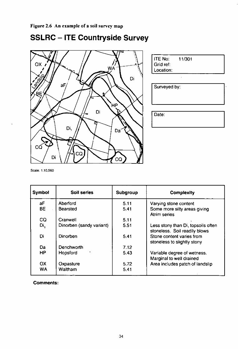
Figure 2.6 An example of a soil survey map

SSLRC - ITE Countryside Survey

Di•

• R.

WA

Di

HP

ITE No: 11/301Grid ref:Location:

Surveyed by:

Date:

Di,

CQ

' CQDi

Scale. 1.10 560

CO

Symbol Soil series Subgroup Complexity

aF Aberford 5.11 Varying stone contentBE Bearsted 5.41 Some more silty areas giving

Atrim seriesCC) Cranwell 5.11

Di, Dinorben (sandy variant) 5.51 Less stony than Di, topsoils oftenstoneless. Soil readily blows

Di Dinorben 5.41 Stone content varies from stoneless to slightly stony

Da Denchworth 7.12

HP Hopsford 5.43 Variable degree of wetness.

Marginal to well drainedOX Oxpasture 5.72 Area includes patch of landslipWA Waltham 5.41

Comments:

34

SSLRCand the MLURIbased on therespective national maps and using therespective national classifications. TheSSLRCproduced software to facilitate theconversion of the MLURIclassfficationaryunits into the equivalent units in the SSLRCclassification.

2.6 7 The merged data sets. wah all soilsclassified in terms of the SSLRCclassification have been analysed todetermine the distribution of soils betweenITE Land Classes, the most common soils ineach ITE Land Class, and the distribution ofsoils in the four landscape types. Thenumbers of 1 km squares in each iTE LandClass in which given soil subgroups occuras the dominant or subdominant soil werecalculated The numbers recorded werethen expressed as a percentage of the total1 km squares within the given ITE LandClass. the five most commonly occurringsoil units in each ITE Land Class were listed

Soil surveys in CS1990

2.6.8 During CS1990. SSLRCand MLURIwerecommissioned to carry out detailed soilsurveys of each of the 508 1 km field surveysquares The mapping was done at the1:10 000 scale and at the series level.wherever possible. Figure 2.6 provides anexample of the completed maps.

2.7 Suntmary of Chapter 2

2.7.1 One of the primary objectives of CS1990was that information on a variety of topics.related to rural land use, should beintegrated to provide a holistic view of theBritish countryside in 1990. To do this.there had to be a common frameworkwithin which the different pans of the surveycould function. This was provided by theITE Land Classification, and its use of a 1 kmsquare grid, which allowed information tobe integrated and summarised on acommon spatial basis.

2.7.2 Census land cover mapping of GB wascompleted by the interpretation andclassification of Landsat satellite imageryAlthough undertaken at a pixel size of 25 mx 25 m. the results of the classification werealso summarised at the 1 km square level.

2.7.3 Sample survey information on land cover.land use, landscape features, habitats andvegetation in quadrats was collected in 508

1km squares in GB. stratified by ITELandClass Data were summarised using the ITELand Classification.

2.7.4 Although quality control was carried out atall stages and in all pans of the project, aspecial Quality Assurance Exercise wascompleted in relation to the field survey.The results suggested that recordingaccuracy was as 'close to the maximumattainable efficiency that can be expected'.

2.7.5 Information on freshwater biota. and waterquality, was collected from a variety ofsources, including sampling the 508 1 kmsquares. Results have been expressed atthe 1 km square level and by ITELandClass

2.7 6 Soil information has been assembled fromexisting maps and, at a greater level ofspatial accuracy, by survey in 1990 of the508 1 km sample squares. Results havebeen expressed at the I km square leveland by rrE Land Class

35

Plate 1 The Land Cover Map of Great Britain

•

Chapter 3 THERESULTS(I): LAND COVER

3.1 Interpretation of results 373.2 1990 stock figures hom satellite imagery 373.3 1990 stock figures from field survey 413.4 Net change between 1978, 1984 and 1990 463.5 The matrix of change between 1984 and 1990 493.6 Relationship between satellite and field survey data 493.7 Integrated use of field survey and satellite data 513.8 Pattern analysis 523.9 Summary of Chapter 3 53

3.1 Interpretation of results

While the outputs from this study provide the mostup-to-date figures available on the stock andchange of land cover, landscape features andvegetation, caution should be used in theminterpretation, as follows.

Figures resulting from the land cover map.produced by interpretation of satellite imagery.provide census data (land cover summaries aregiven for every 1 km square in Great Britain(GB)). Because they are census data, they donot need to carry expressions of statisticalaccuracy (in contrast to sample-based systems).However, the results have been obtained usingcomputer-aided interpretation of satellite dataand there will inevitably be a proportion ofinstances where incorrect classification takesplace. Validation of the satellite data isdiscussed in section 3.6. onwards.

The field survey estimates of stock and changeare derived from a sample-based survey. Aswith any such system. there are statistical errorsassociated with extrapolation from a sample tonational estimates. These error terms are givenwhere possible and should be taken intoaccount when interpreting results, especially inconsidering change. A full account of the choiceof error terms, and how they were calculated, isgiven in Appendix 3.

Although every effort was made to standardiserecording procedures in the field (icluding anextensive training course; use of a fieldhandbook (Barr 1990), use of aerialphotographs; field supervision and checks;mixing of field teams), there are likely to besome differences in the way that the data havebeen recorded by different observers. There isno reason to expect estimates of field recording

to be biased in any particular direction and it islikely that any differences will 'balance out' overthe whole data set. (See also quality assurancein section 2.4.)

3.2 1990 stock figures from satelliteimagery

Land cover mapping

3 2.1 The land cover has been fully mapped.except where very small pockets of cloudcover obscured the land surface. The mainoutput is called the Land Cover Map ofGreat Britain, and is shown in Plate I. Out of3% which remains unclassified, perhapsone-fifth is unclassified due to cloud.Elsewhere, unusual cover types are themost likely cause. The only otherexceptions to this observation are Tiree.part of Coll and the northern and southerntips of Shetland which did not fallwithinsuitable Landsat scenes of GB. These areas,totalling perhaps 200 lan2, represent just0.1% of GB. They will be added to the landcover map after classification Ofalternativeimages. eg Landsat Multispectral Scanner.

3.2.2 In all, 46 different scenes were required tomake up full cover of GB: 88% of GB wasclassified from combined summer/winterimages. and 12% from single-date. mostlysumimer, data

3 2.3 Geometric correction was to subpixel level:this means that the polynomial model forcorrection placed ground control pointswithin 1 pixel of their Ordnance Survey(OS) mapped position. Co-registration ofvector field maps of 143 CountrysideSurvey 1990 (CS1990) squares with Landsat

37

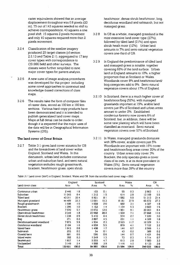
raster equivalents showed that an averagedisplacement throughout was 0.8 pixels (20m). 75 out of 143 squares needed no shift toachieve correspondence. 43 squares a onepixel shift, 15 squares 2 pixels movementand only 10 squares required more than 2pixels movement

3.2.4 Classification of the satellite imageryproduced 25 target classes (cf section2.2.13 and Table 2.1). aggregated to 17 keycover types with correspondence toCS1990 field and other surveys. Theclasses were further simplified to ninemajor cover types for pattern analysis.

3.2 5 A new suite of image analysis procedureswas developed for this project includingsome novel approaches to contextual andknowledge-based corrections of classmaps.

3.2.6 The results take the form of computer filesof raster data, stored as 100 Ian x 100 lcmsections. Various hard-copy products havebeen demonstrated and it is intended topublish generalised land cover maps.Maps at full detail can be made to order.though it is expected that the major uses ofthe data will be in Geographical InformationSystems (GIS).

The land cover of Great Britain

3.2.7 Table 3 1 gives land cover statistics for GBand the breakdown of land cover withinEngland, Scotland and Wales. In thisdiscussion, urban land includes continuousurban and suburban land, and semi-naturalvegetation includes rough grass/marsh,bracken, heath/moor grass open shrub

heath/moor, dense shrub heath/moor, bog.deciduous woodland and saltmarsh, but notmanaged grass

3.2.8 In GB as a whole, managed grassland is themost extensive land cover type (27%).followed by tilled land (21%) and openshrub heath moor (12%). Urban landamounts to 7% and semi-natural vegetationcovers one-third of GB.

3.2.9 In England the predominance of tilled landand managed grass is notable, togethercovering 66% of the land surface. Urbanland in England amounts to 10%, a higherproportion than in Scotland or Wales.Woodlands cover 8% and heath/moorland/bog categories add to 9%. Semi-naturalvegetation covers about 17% of England

3.2.10 In Scotland. there is a much higher cover ofheath/moor/bog (52%). with managedgrasslands important at 15%;arable landcovers just 8% of Scotland and urban areasamount to under 2%. Establishedconiferous forestry now covers 6% ofScotland. but, in addition, there will besome new planting which will have beenclassified as moorland. Semi-naturalvegetation covers over 57% of Scotland

3.2 11 In Wales. managed grasslands dominatewith 38% cover arable covers just 5%Woodlands are important with 16% coverand heath/moor/bog areas cover 20% of thecountry. Urban areas only cover 3%Bracken. the only species given a coverclass of its own, is at its most prevalent inWales (5%) Semi-natural vegetationcovers more than 39% of the country

Table 3 / Land cover (la-n3) m England. Scotland. Wales and CB from the swelfize land cover map -1990

Land cover classEngland

Area%Scotland

A:ea AreaWales

% ArcaCB

%

Connnuous urban 2 446 ! 8 103 0 I 55 0 3 2 603 IISuburban 11 243 8 4 I 312 1 5 614 2 8 13 169 5 5'Med land 43 311 32 4 6 921 8 I I 082 5 0 51 313 21 4Managed grassland 44 489 33 3 13 Offi 15 3 8 181 37 9 65 672 27 3Rough grass/marsh 1 988 1 5 1 659 2 0 660 3 I 4 307 I 8Bracken 1 296 1 0 1 153 1 4 1154 5 3 3 603 I 5Heath/moor grass 7 570 5 7 10 672 12 6 1961 9 1 20 203 8 4Open shrub heath/moor 2 349 1 8 23 980 28 2 I 539 7.1 27 868 11 6Dense shrub heath/mom 1 236 0 9 5 410 6 4 574 2 7 7 220 3 0Bog 271 0 2 3 807 4 5 231 I1 4 309 1 8Deciduous/mixed woodland 7 873 5 9 1 934 2 3 2 523 11.7 12 329 5 1Coniferous woodland 2 184 1 6 4 659 5 5 879 4 1 7 722 3 2Inland bare 1 013 0 8 1 408 I 7 144 0 7 2 566 1ISaltrnarsh 293 0 2 54 0 1 43 0 2 389 0 2Coastal bare 681 0 5 596 0 6 144 0 7 1 421 0 6Inland water 392 0.3 ! 249 1.3 73 0 3 1 714 0 7Sea/estuary 1 857 I 4 5 203 4 7 613 2 8 7 683 3 2Unclassified 3 149 2 4 I 868 3 9 1116 5 2 6 133 2.6Total 133 651 100.0 84 987 100.0 21 584 100.0 240 222 100.0

38

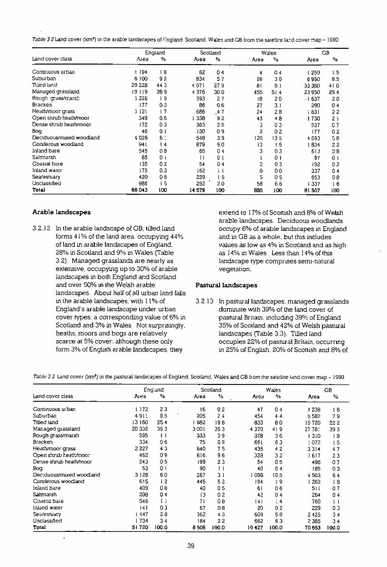
Table 3 2 Land cover pan') in the arab:e landscapes of rngland Scotland. Wales and GB from the satellre land cover map - 1990

EnglandArea%

ScotlandArea%

WalesArea% Area

GB%

1 194 1 8 62 0.4 4 0 4 I 259 1.56 100 9 2. 834 5 7 26 3 0 6 960 8.5

29 228 44 3 4 071 27.9 8! 9.1 33 380 41 019 119 28 9 4 376 30.0 455 51.4 23 950 29.4

1 226 I 9 393 2 7 18 2 0 -.1 637 2 0177 0.3 86 0 6 27 3.1 290 0 4

112! I 7 686 A 7 24 2.8 1 831 2 2349 0.5 1 338 9 2 43 4 8 1 730 2.1172 0 3 363 2 5 3 0 3 537 0.746 0.1 130 0 9 2 0 2 177 0 2

4 026 6 : 548 3.9 120 13 5 4 693 5 8941 1 4 879 5.0 13 1.5 I 834 2.2545 0 8 65 0 4 3 0 3 513 0 8

85 0 I I1 0 1 1 0 1 97 0 I135 0.2 54 0 4 2 0 3 192 0 2175 0.3 162 11 0 0 0 337 0 4420 0 6 229 1 5 5 0 5 653 0.8986 I 5 292 2 0 58 6 6 I 337 1.6

66 043 100 14 579 100 885 100 81 507 100

Land cover class

Continuous urbanSuburban/MIS landManaged grasslandRough grass/marshBrackenHeath/moor grassOpen shrub heath/moorDense shrub heath/moorBogDeciduous/mixed woodlandConiferous woodlandInland bareSalainarshCoastal bareInland waterSea/estuaryUnclassifiedTotal

Arable landscapes extend to 17% of Scottish and 8% of Welsharable landscapes. Deciduous woodlands

3.2.12 In the arable landscape of GB. tilled land occupy 6% of arable landscapes in Englandforms 41% of the land area. occupying 44% and in GB as a whole, but this includesof land in arable landscapes of England. values as low as 4% in Scotland and as high28% in Scotland and 9C/oin Wales (Table as 14% in Wales. Less than 14% of this3.2). Managed grasslands are nearly as landscape type comprises semi-naturalextensive, occupying up to 30% of arable vegetation.landscapes in both England and Scotlandand over 50% in the Welsh arable Pastural landscapeslandscapes. About half of all urban land fallsin the arable landscapes. with 11% of 3.2.13 In pastural landscapes, managed grasslandsEngland's arable landscape under urban dominate with 39% of the land cover ofcover types. a corresponding value of 6% in pastural Britain. including 39% of EnglandScotland and 3% in Wales. Not surprisingly, 35% of Scotland and 42% of Welsh pasturalheaths. moors and bogs are relatively landscapes (Table 3.3). Tilled landscarce at 5% cover: although these only occupies 22% of pastural Britain. occurringform 3% of English arable landscapes, they in 25% of English. 20% of Scottish and 8% of

Table 3 3 Land cover (ianz) in the pastural landscapes of England. Scotland. Wales and GB from the satellite land cover map - 1990

Land cover classEng:and

AreaScotland

Area% AreaWales

% AreaGB

%

Continuous urban 1172 2 3 16 0 2 47 0 4 I 238 1 8Suburban 4 91: 9 5 205 2 4 454 4 4 5 582 7 9/fIlled land 13 160 25 4 I 682 19 8 833 8 0 15 720 22 2Managed grassland 20 335 39 3 3 001 35 3 4 370 41 9 27 78: 39 3Rough grass/marsh 595 I1 333 3 9 378 3 6 1 310 1 9Bracken 334 0 6 75 0 9 661 6 3 ! 072 1 5Heath/moor grass 2 227 4 3 640 7 5 435 4 2 3 314 4 7Open shrub heathnnoor 462 0 9 816 9 6 328 3 2 1 617 2 3Dense shrub heath/moor 243 0 5 199 2 3 54 0 5 498 0 7Bog 53 0 ! 90 II 40 0 4 185 0 3Deciduous/mixed woodland 3 128 6 0 267 3 I 1 098 10 5 4 503 6 4Coniferous woodland 615 1 2 445 5 2 194 1 9 1 262 I 9Inlanc bare 409 0 8 40 0 5 61 0 6 511 0 7Saltrnarsh 208 0 4 13 0 2 42 0 4 264 0 4Coastal bare 546 1I 71 0 8 14: 1 4 760 IIInland water 141 0 3 67 0 8 20 0 2 229 0 3Sea/estuary 1 447 2 8 362 4 3 609 5 8 2 425 3 4Unclassified 1 734 3 4 184 2 2 662 6 3 2 385 3 4Total 51 720 100.0 8 506 100.0 10 427 100.0 70 653 100.0

39

Table 3 4 Land coverin the marginal upland landscapes of England. Scotland. Wales and GB from satelbte Mnd cover amp -1990

EnglandScotlandWalesGBLand cover classArea%Area%Area%Area%

Continuous urban

58 0 5 10 0 1 5 <0 0 72 0 2Suburban

208 I 8 128 0 8 133 1 3 469 1 2Tilled !and

777 6 7 714 4 4 167 1 6 I 658 4 3Managed grassland 4 464 38 7 2 874 17 6 3 353 32 8 10 691 28 CRough grass/marsh

118 1 0 335 2 0 262 2 6 715 1 9Bracken

540 4 7 238 1 5 465 4 5 1 243 3 3Heath/moor glass 2 707 23 4 2 514 15 4 1 487 14 5 6 708 17 6Open shrub heath/moo:

727 6 3 4 262 26 0 1161 11 4 6 150 16 1Dense shrub heath/moo:

522 4 5 1 020 6 2 510 5 0 2 052 5 4Bog

53 0 5 658 4 0 189 1 8 900 2 4Deciduous/waxed woodland

682 5 9 332 2 0 I3C3 12 7 2 317 6 1Coniferous woodland

275 2 4 1190 7 3 670 6 6 2 135 5 6inland bare

50 C 4 248 1 5 78 0 8 376 1 0Saltmarsh

0 0 0 6 <0 0 0 0 0 6 <0 0Coastal bare

0 0 0 120 0 7 0 0 C 120 0 3Inland water

57 0 5 145 0 9 52 0 5 254 0 7Sea/estuary

0 0 0 1 307 8 0 0 0 0 l 307 3 4Unclassified

309 2 7 265 1 6 393 3 8 968 2 5Total 11 546 100.0 16 366 100.0 10 228 100.0 38 140 100.0

Welsh pastural landscapes. In England,urban land occupies 12% of pasturallandscapes. but the corresponding figuresfor Scotland and Wales are 3% and 5%respectively, giving a GB average of 10%.Deciduous woodlands occupy 6% of GBwith figures for England. Scotland andWales showing 6%. 3% and I 1%respectively. Conifers in English pasturallandscapes cover just over 1%while inScotland cover reaches over 5% and inWales 2% Thus, tree cover in Welshpastural landscapes reaches 12%. while inEngland it is 7% and in Scotland 8%. About16% of pastural landscapes in Britaincomprise semi-natural vegetation

Marginal upland landscapes

3.2.19 In marginal landscapes, managed grassdominates at 28% of the total (Table 3.4).In England a higher proportion is managedat 39%, while in Scotland and Wales theamounts are less at 18% and 33%respectively. Tillage only covers about 4%of marginal landscapes. Heath andmoorland grass take second place in coverterms at 18% of GB. In England the heath/moor grass cover is 23%. in Scotland it is15%, and in Wales 15%. Total heath, moorand bog cover for GB is over 41%,occupying 35% of marginal landscapes inEngland. 52% in Scotland and 33% inWales. Bracken in marginal landscapesoccupies 3% of land, reaching 5% cover inEngland and Wales. Only 1-2% of Britain'smarginal landscapes are urban. The result

is a landscape comprising over 52% semi-natural vegetation.

Upland landscapes

3.2 15 The upland landscapes are dominated bydwarf shrub heath: combined totals foropen and dense shrub heaths/moors in GBshow cover to be 45% (Table 3.5). InEngland the figure is as low as 26%. inWales (where the upland landscape isrestricted mainly to Snowdonia) it reaches32%. and in Scotland it extends to 47%.Total heath, moor and bog cover in GBuplands is 68% Mature conifers cover 5%of uplands. Urban land covers just 0.4% ofuplands. The 7% cover of sea/estuaryshows that this landscape type is one thatis defined as being generallycharacteristic of the uplands, but whichextends to coastal regions in the extremenorth and west of Britain. Total semi-natural vegetation covers over 73% ofupland landscapes in GB.

Conclusions

3 2 16 The land cover mapping project hassuccessfully recorded the land cover of allGB. It is the first such survey since the1960s (Coleman 1961) and only thesecond this century (see also Stamp 1962).

3.2.17 The most important development hasbeen the provision of land cover data forGB at a single point in time. Theavailability of land cover data in digitalform greatly facilitates access to the map

40

Table 3 5 Land cover (1cm2)in the upland landscapes of England. Scotland. Wales and CB from saielbte :and cove: map - 1990

Land cover class

Continuous urbanSuburbanIlfred landManaged grasslandRough Tass/maishBrackenHeath/moor grassOpen shrub heath/moorDense shrub heath/moo:BogDeciduous/mixed woodlandConiferous woodlandInland bareSalcnarshCoastal bareInland waie:Sea/estuaryUnclassifiedTotal

England ScotlandArea % Area

2225

146571

50245

I 515812

0 50 63 4

13 21 25 6

34 918 7

2

617

300 65 3119 2 7 237 0 8

353 8 1 210 0 2 10 0 0

0 0 0

19 0 4

0 0 0 3120 2 8 1

4 342 100.0 45

15145454750 598751832564928928787145055

24351875306126536

Wales CB% Area % Area %

<0 0 0 0 0 37 0 I0 3 0 0 2 170 0 310 1 15 600 I 26 0 3 7 8 3 325 6 71 3 2 4 4 650 I 31 7 1 2 9 I 000 2 0

15 0 14 32 1 8 362 16 738 6 6 14 5 18 382 36 8

8 4 8 17 4 4 135 8 36 4 1 18 3 048 6 1I 7 1 2 9 825 1 74 7 1 1 2 2 498 5 02 3 3 6 0 1 058 2 :0 1 0 0 0 24 0 00 8 0 0 1 351 0 71 9 0 0 5 894 187 3 0 0 ! 3 386 6 62 5 3 6 5 1 248 2 5

100.0 44 100.0 49 922 100.0

information and manipulation for specificapplications.

3.2.18 The Countryside Information System (CIS)holds summary data at 1 Icrnsquareresolution Although losing the full spatialdetails of the original survey, this data setoffers an enormous quantity of informationand is suitable for most analyses where theexact spatial context of land cove: units isnot needed

3.2.19 The marriage. in CIS. of a general map oftotal land cover with the detail of a sample-based field survey offers a great potentialin terms of supplying integrated land coverinformation. Additional information ongeology, soils, terrain, climate andadministrative boundaries can increasethis potential. These data are not onlyavailable for scientific enquiry: therelatively simple access to data andanalyses within the as allows planners,policy-makers and landscape managers toaccess the data and support their decisionswith data and lailor-made' analyses.

3.2.20 The land cover data at full resolution showBritain at a field-by-field scale. This allowsthe provision of paper maps at scales up toabout 1:25 000 or overviews at perhaps1.1 000 000. Such maps can clearly helpthose concerned with wider issues of landmanagement The larger-scale productsare likely to be specially designed fining auser's requirements for scale and detailsThe small-scale product is likely to bemass-produced for general use.

32 21 The most detailed analyses of the landcover data will be in GIS. These will allowusers to explore the full resolution of theoriginal data, drawing on detailed maps oftopography, climate, terrain andadministration

3.3 1990 stock figures from fieldsurvey

3.3.1 As outlined in the earlier sections, a greatvariety of information has been collected onland cover by field survey. Each distinctparcel of land in the 508 1 km samplesquares was described and mapped usingcombinations of coded descriptora Thedescriptors were based on a suggested listof 100 primary codes which could befurther qualified w:th secondary codeseither drawn from the 250 suggested or. ifnecessary. specially created No limit wasplaced on the number of codes which couldbe used and the permutations are toonumerous to present Although the detailallows specific interrogations to followprecise and intricate questions, for thisreport the data have been aggregated into58 categories (see section 2.3.17). Furtheraggregations allow the data to besummarised in categories that correspondto those used in the land cover map (Tables3.6-3 8).

3 3.2 The predicted areas of land cover classes.with standard errors, are presented inhundreds of km squares (10 000 ha) andare calculated using the methods described

41

Table 3 6 Land cover for GB from the CS1990 deld survey, by area ( 00 Icna). standard error (SE) ('00 kTn2)and percentage (%03)( • =-presence <50 'or! or <0 5%) The subtotalssatellite land cover map

(:n bold) correspond approximately to the 17 key cover wpes obtained from the

1990GB stock 1990GB stock

Cover type Area SE % Cover type Area SE %

Communications

Rough grass/marsh

Railway 4 I • Non-cropped arable (plougheo and fallow) 35 8 2Road 44 2 2 Urmanaged grassland and tall herb 27 2 I

48 2 2 Felled woodland 4 2 +Built up

Wetland 37 5 2

Agricultural buildings 14 I I Waste and derelict land 4 1 +Residentiai buildings 58 7 3

107 9 5Other buildings 30 5 I Dense bracken 37 6 2Unstuveyed urban land 48 t 2 Moorland grass

160 10 7 Purple moor grass-dominated moorland 37 8 2

Tilled land

Mooriand grass (other than

Wheat 223 15 10 Purple moor grass) 81 II 3Barley 115 10 5 Dune 2 1 +

Oats 9 2

120 14 5Mixed and other cereals 3 2

Open heath

Maize 4 2

Open-canopy heath 82 !CI 4

Thrrips/swedes 7 1 + Berry-bush heath 12 3 I

Kale 5 2 + Dner northern bogs 52 8 2

Oil-seed rape (OSR) 41 6 2

146 13 6

Crucifer crops (other than CSR) 3 ! + Dense heath 45 8 2Peas II 3 • Wet heaths and saturated bogs 166 15 7FMId beans 10 3 • Broadleaved/mixed woodland

Legumes (not peas/field beans) - + + Perennial crops 7 3 +Sugar beet 22 4 I Mixed woodland 22 4 1Root crops (not turnips/swedes/potatoes) 1 • • Broadleaved woodland 92 7 4Potatoes 14 3 1 Shrub 9

+

Other field crops 10 2 4-

130 9 6HorncuSure 4 3

Conifers 137 16 6

481 23 21 Inland bare

Managed grass

Inland rocks and screes 2 : +Recreational (mown) grass 25 5 1 Hard areas without buildings 2 +

Recently sown grass 71 6 3 (harries and extracuve .ndustnes 3 1

Pure rye-grass 203 14 9

6 1 +Well-managed grass 93 13 8 Saltmanh 4 2 +Weedy swards with >25% rye grass 99 8 4 Coastal bare

Non-agnadturally improved grass 20 4

Intertidal soft coas: without vegetation 12 4 ICalcareous grass 7 3 4- Hard coast with no vegetation 6 1 +Upland grass 61 7 3

18 4 1

Maritime vegetabon 3 I + Inland water

682 23 29 Still water 21

Runrung water 8 I +

29 7 1

Total 2318

linsurveyed urban land is a census estimate from all 1 Ion squares not surveyed and consequently has no SE The area is includedin the built up category and percentage area but the SE :s for the built up categories without ursurveyed urban land

in Appendix 3. The surveys were of ruralland and excluded areas covered by morethan 75% built land or curtilage. The figurespresented include a total for these excludedurban areas (sunsurveyed urban lands), and aprediction for the rural part of those squares.

3 3 3 The results (which are held in the CIS) arepresented here for GB. England, Scotlandand Wales, and for the four landscape types

Great Britain in 1990

3.3.4 The results for GB are presented in Table 3.6and show general agreement with the landcover map (Table 3.1). Tilled land covers21% of the land surface and is dominated bywheat (10%) then barley (5%) and ou-seedrape (2%). These figures differ from the

1990 Ministry of Agriculture. Fisheries andFood (MAFF)June census, which shows asimilar total for wheat and barley combined.but with a different breakdown (wheat -20 100 km' from MAIT and 22 300 lan2 fromC51990. barley - 15 200 km' from MAFTand 11 500 Icrn2from CS1990)

3.3.5 The GB data are broken down by country inTable 3.7. This shows that 31% of Englandis tilled (33% if non-cropped arable isincluded), compared with only 9% of Walesand 7% of Scotland. In both Scotland andWales the barley area exceeds that forwheat. Oil-seed rape accounts for 9% of thetilled land in England, 6% in Scotland and5% in Wales, while sugar beet accounts for5% in England and less than I% in bothScotland and Wales.

42

In

Table 3.7 National land cover (rorn the 051990 Geld survey, by area COOknit). standard error (SE) (CO knit) and percentage (%0B)(4 = presence <50 Icr' or <C 5%) The subtotals (In bold) correspond approximately to the 17 key cover types obtained from thesatelhte land cover map

Stock 1990EnglandWales

Scotland

Cover ,'Area SE%AreaSE%

AreaSE. %Communications

Railway3 1-.+ 4

2. +Road32 224+2

81 135 234+2

9 I 1Built up

Agncultural buildings10 1II+!

2+ •Residenual buildings53 6484

81 1Other buildings22 423+1

52 1Unsurveyed urban land41 /3I/•

41 1126 891225

203 3Tilled land

Wheat202 14 15613

153 2Barley80 86713

295 4Oats6 241++

2I +Mixed and other cereals3 24++

-+ .Maize4 1•4++

-+ -rumps/swedes3 1•1+

3I -Kale3 14++

1I -Onseed rape (OSR)35 63I« 4

41 1Crucifer crops (otner than OSR)2 I+.++

11 •Peas10 21+++

1+ •Fleld bears9 21•++

1+ .Legumes (not peas/field beans) .«

00 0Sugar beet21 42I

• .Roo; crops (not turnips/swedes/potatoes)I -.

-+ -Potatoes11 311+

2I 4Other field crops9 2-.

.+ +Horticulture4 3-+

-+ 4403 20311929

598 7Managed grass

Recreational (mown) grass21 422+1

21 4Recently sown grass50 54713

143 2Pure rye-grass145 101125312.

345 4Well-managed grassI !2 8834534

486 6Weedy swards wuti >25% rye-grass52 5417217

304 4Non-agriculturally Improved grassII 2I313

62 ICalcareous grass4 2++-

21

Upland grass17 3I924

355 4Maritime vegetauon1 ++

+412 173197646

2I

17212 22Rough grass/marsh

Non-cropped arable (ploughed and fallow)32 82«1

21 +Urznanaged grassland and tall herb17 2I2+1

8I 1Felled woodland! +«

31 +Wetland12 2 1 512

203 2Waste and derelict land3 1+4+

!. +65 85814

343 4Dense bracken12 2I924

154 2Moorland grass

Purple moor grass.dorrunated moorland9 2110.45

194 2Moorland grass (other than purple moor grass)20 42733

547 7Dune + -

21 429

251758

758 9Open heath

Open-canopy heath19 31723

567 7Berry-bush heath2 1.•

:02 1Drier northern bogs9 21211

4 I6 530 42934

1079 13Dense heath13 31422

285 33I311

14914 19Wet heaths and saturated bogs15Broadleaved/mixed woodland

Pererthual crops7 31•+

+ 4 +Muxed woodland13 212I1

82 1Broadleaved woodland68 651015

132 2Shrub6 11+1

2+ .94 871417

234 3Coniferous woodland45 63723

8512 11Inland bare

Inland rocks and screes• +

I 4 4

Hard areas without buildings1 4

4 .4Curarnes and excacave industnes2 14

I4 .3 1++

31 +Saltmarsh3 1+I++

I+ 4.Coastal bare

Interidal sot coast without vegetacon9 4I1

2+

Hard coast with no vegetation2 I+

41 +11 4I21

61 1Inland water

Still water10 6I!4

103 1Running water5 11+

2«

15 612+1

123 1Total1311 208

790

rourveyeur an la.is a census estimate rom aI . squat es not surveyed aria consequent yas no i e area is Inc ua

the built up ca:egory and percentace area but the SE is for the buil: up categones w,thout unsurveyed urban land

43

3.3 6 Of the 31% of GB covered by managedgrass about 40% is intensively managed asshort term ley or pure rye-grass. Englandagain has the dominant share of this type ofgrassland, both in terms of area andproportion of all grassland The converse ofthis can be seen in the larger proportion ofmore natural managed grasslands inScotland and Wales.

3 31 The total area of land managed foragriculture in England is 81 500 km2 (or84 700 km2 it non-cropped arable isincluded), which compares with 84 730 lcm2from the MAFF June census for 1990. Thisarea is equivalent to 62% of the land surfaceof England; figures for Scotland and Walesare 29% and 56% respectively

3.3.8 The field survey data show that 21% of GB isoccupied by heaths. bogs and moorlandgrass, compared with the figure of 25%derived from the land cover map (Table3.1). The areas for individual countriesshow similar differences; thus, the satelliteland cover map data showed that thesecategories cover 57% of the land area ofScotland. compared to the 49% derivedfrom field survey These variations almostcertainly derive from differences in datacapture methods and definitions of covercategories (see section 3.6).

3.3.9 A more detailed examination of the data onthe heath/bog cover categories from thefield survey showed, for example. that.purple moor grass-dominated moorlandoccupied 4% of the land area of Wales. 2%in Scotland and less than 1% in England.Drier northern bogs cover 5% of Scotland.but less than 1% of England and Wales.

3.3.10 The urban area of GB (including all built-upareas and communications) covers about9% of the land area, when the non-surveyedurban land is included. Urban land ispredominantly in England (12% of landarea) and is dominated. in mral areas, byresidential building and curtilage.

3.3.11 Forest/woodland covers around 12% of GBand 11% of England. which is higher thanthe Forestry Commission (1990) estimate.but in pan may be explained by theinclusion of small woodlots, orchards(included in perennial crops) and shrub.

Arable landscapes

3.3.12 As with the satellite land cover map (Table3 2). the field data showed that the arable

landscapes are dominated by tilled land(43%) (Table 3.8). The field survey givesde:ailed estLmates of different crop types Anumber of crops are grown predominantlyin this type of landscape and this includeswheat. othseed rape. mixed and othercereals. sugar beet and peas Approx-imately 78% of the land under wheat in GBoccurred in this landscape, 60% of thebarley and 80% of the othseed rape. Thearable landscapes contain the lowestproportion of semi-natural vegetation of thefour landscape types A large proportion(45%) of the managed grass is short term orintensively managed. and may be pan of acrop rotation.

3.3.13 About 12% of the arable landscapes isurbanised and 10% forested/wooded(predominantly broadleaved).

Pastural landscapes

3.3.14 The pastural landscapes are dominated bymanaged grasslands which cover 45% ofthe area. Approximately 50% of thesegrasslands are short term or intensivelymanaged (ie recently sown or pure rye-grass) Only 18% of the area is tilled andwheat and barley are about equallydominant in cover. However, 34% of thetotal land area of GB under barley occurredin this landscape, but only 20% of the GBunder wheat. Some 5% of the area is underminor arable crops. compared with 13% ofthe arable landscapes. Forest/woodlandforms 10%. of which 70% is broadleavedwoodland. Urban land forms 14% of thepastural landscapes, a slightly higherproportion than the arable landscapes.

Marginal upland landscapes

3.3.15 Although these landscapes may beconsidered to be transitional between thepredominantly agricultural lowlandlandscapes and the more open and naturaluplands, they are more similar to the latterin character. Only 3% of the area is tilledland. which is mostly under barley and only22% of the grassland is intensivelymanaged. Heath. moorland and bogoccupied 35% of the landscapes, with 11%of this area dominated by purple moorgrass 17% by wet bogs and 15% by denseshrub heath. Some 44% of the total area ofdense bracken in GB occurs in thislandscape.

3.3 16 Forestry/woodland occupied 13% of thelandscapes and over 75% of this forest land

44

Table 3 8 Land cove: for landscape types of CB from :he CS1990 field survey by area (DO len') and standard error (SE)(DO km') (+ = presence <50 Ian' or <0 5%) The subtotals (In bold) correspond approximately to the 17 key cove: types obtainedfrom the satelire land cover map

Stock 1990ArablePasturalMarginalUpland

Cover typeAreaSEAreaSEAreaSEAreaSE

CommunicationsRailway202 ++Road201181412

221191512Built up

Agncuhurel buildings7I611+Residenual buildings28536631Ofner buldLngs154143+Unsurveyed urban land25t20IILI

*

757767514.Tilled land

Wheat175!34662100Barley67 a 40673IOats523!11Mixed and other cereaLs32•+C o+Maize3.1i0000Thrnipsfswedes3. .3111Kale2131++al-seed rape (OSR)32683-0Crucifer crops (other than OSR)21++0 ooPeas9221•0Field beans9221000Legumes (not peas /field beans)+0 ooc 0Sugar beet:6363000Root crops (not turnips/swedes/potatoes)•+•0 oPotatoes9351•+Other field crops8221•+++Horticulture43+..0000

348191211211511Managed grass

Recreatonal (mown) grass1441031*•+Recently sown grass3043246232Pure rye-grass608118922632Well-managed grass57783747853Weedy swards with >25% rye-grass23543524493Non-agriculturally improved grass935252.1Calcareous grass32I1I1. '1Upland grass62II3224224Manume vegetation•+1+1•i1

2021530514126128488Rough grass/marsh

Non-cropped arable30 a 5I• ooUnmanaged grassland and tall herb15210121FeLed woodland14•+1121Wetand31123113II2Wasie and derelict land212100

SO8294143132Dense bracken2162164124Moorland grass

Purple moor grass-dominated moorland1+42156114Moorland grass (other than purple moor grass)I+3129 a 487Dune1•1

21824610658Open heath

Open-canopy heath2162266488Berry-bush heath00++21103Drier northern bogs1I11155356

32724389210Dense heath4321196205Wet heaths and saturated bogs22-13622 e 13012 Broadleaved/mixed woodland

Perennial crops5232+++•Mixed wooriland102613132Broadleaved woodland40636410262Shrub4I4110

se 749513 z 93Coniferous woodland2052153795911Inland bare

Inland rocks and screes+ 1 •++ I IHard areas without buildings1+. + 1Quarries and extract-ve industries21+•

2+

211+1121Saltmarsh++4200+ Coastal bare

Intertdal soft coast without vegetation s 462+:+Hard coast with no vegetation++2I131

S4911+41Inland water

Still wirer862.4383Rurnng water2+3111

106515383Total807675368460

* Unsurveyed urban land is a census estimate from all : km squares not surveyed and consequently has no SE The area is included in the built up category and percentage area but the SE is for the built up categories without unsurveyed urban land

45

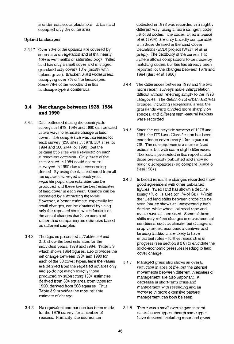
is under coniferous plantations Urban landoccupied only 3% of the area

Upland landscapes

3.3.17 Over 70% of the uplands are covered bysemi-natural vegetation and of that nearly40% is wet heaths or saturated bogs. Tilledland has only a small cover and managedgrassland only covers 10% (mostly withupland grass). Bracken Lsstillwidespread.occupying over 2% of the landscapes.Some 78% of the woodland in thislandscape type is coniferous.

3.4 Net change between 1978, 1984and 1990

3.4.1 Data collected during the countrysidesurveys in 1978. 1984 and 1990 can be usedin two ways to estimate change in landcover. The sample size was increased foreach survey (256 sites in 1978, 384 sites for1984 and 508 sites for 1990). but theoriginal 256 sites were revisited on eachsubsequent occasion. Only three of thesites visited in 1984 could not be re-surveyed in 1990 due to access beingdenied By using the data ccIlected from allthe squares surveyed in each year.separate population estimates can beproduced and these are the best estimatesof land cover in each year. Change can beestimated by subtracting the totals.However, a better estimate. especially forsmall changes. can be obtained by usingonly the repeated sites, which focuses onthe actual changes that have occurred.rather than comparing the estimates basedon different samples.

3.4.2 The figures presented in Tables 3 9 and3.10 show the best estimates for theindividual years, 1978 and 1984. Table 3 9.which shows 1984 figures. also provides thenet change between 1984 and 1990 foreach of the 58 cover types; here the valuesare derived from the repeated squares onlyand so do not match exactly thoseproduced by subtracting 1984 estimates,derived from 384 squares, from those for1990, derived from 508 squares. Thus.Table 3.9 provides the most reliableestimate of change.

3.4.3 No equivalent comparison has been made for the 1978 survey, for a number of reasons. Primarily, the information

collected in 1978 was recorded in a slightlydifferent way, using a more stringent codelist of 68 codes. The codes. listed in Bunceet al (1984), are on:), broadly comparablewith those devised in the Land CoverDefinitions (LCD) project (Wyan et al. inprep.). The flexibility of the current 1TEsystem allows comparisons to be made bymatching codes, but this has already beenreported for the changes between 1978 and1984 (Barr et a). 1986).

3.4.4 The differences between 1978 and the twomore recent surveys make interpretationdifficult without referring simply to the 1978categories. The definition of urban land wasbroader, including recreational areas, thegrasslands were divided more sharply onspecies, and different semi-natural habitatswere recorded.

3.4.5 Since the countryside surveys of 1978 and1984, the ITE Land Classification has beenextended to cover every 1km square inGB. The consequence is a more refinedestimate, but with some slight differences.The results presented in this report matchthose previously published and show nomajor discrepancies (eg compare Bunce &Heal 1984).

3.4.6 In broad terms, the changes recorded showgood agreement with other publishedfigures. Tilled land has shown a decline.losing 4% of its area (or 1% of GB). Withinthe tilled land shifts between crops can beseen: barley shows an unexpectedly highdecline, while wheat, oil-seed rape andmaize have all increased. Some of theseshifts may reflect changes in environmentalconditions, such as climate, but changes incrop varieties, economic incentives andfarming traditions are likely to haveimportant roles - further research is inprogress (see section 8.2.8) to elucidate thesocio-economic pressures leading to landcover change.

3 4 7 Managed grass also shows an overallreduction in area of 2%. but the internalmovements between different intensities ofmanagement are also important. Adecrease in short-term grasslandmanagement with reseeding and anincrease in more extensive pasturemanagement can both be seen.

3.4.8 There was a small overall gain in semi-natural cover types, though some typeshave declined, including moorland grass

46

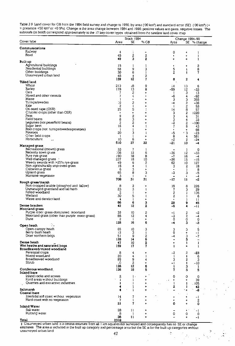
Table 19 land cover for GB from the 1984 field survey and change to 1990. by area (OO krn2) and standard error (SE) (130 km2) (4-= presence <50 lan2 or <0 5%) Change is the area change between 1984 and 1990. positive values are gams. negative losses Thesubtotals (in bold) correspond approximately to the 17 key cover types obtained from the satellite land cover map

Stock 1984 Change 1989-90Cover type AreaSE% GB AreaSE % change

Communications

Railway 4•

Road 4522

4932 1Built up

Agncultural buildings 15I1 +2Residential buildings 5693 5I8Other buildings 3061 2I7Unsurveyed urban land 4812

159127 824Tilled land

1Wheat 213i 89 14136Barley 178138 -5912-33Oats 72 1313Mixed and other cereals 74• -64-92Maize 1•+ 33355ltrnipscswedes :02 -42-36Kale 2I I253Oft-seed rape (OSR) 255 14857Crucifer crops (other than OSR) + 321220Peas 92 3431Field beans 8 3 3433lagumes (not peas/field beans) 22 -22-100Sugar beet 1641 7643Root crops (not turrups/swedes•potatoes) 11 +66Potatoes 2031 -5' 3-23&h er field crops 1,4 84581Horticulture.... 106 -22-24

5102722 -2113-4

Managed grassRecreational (mown) grass 3371 I oRecently sown grass 108125 -3612-33Pure rye-grass i 90188 -716-4Well-managed grass • 2371810 -3615-15Weedy swards vr.th >25% rye-grass 4962 6210127Non-agriculturally improved grass 1641 32I BCalcareous grass 63 I 8Upland grass 6583 -33-5Mannme vegetation 3I -4

7083131 -1711-2Rough grass/marsh

Non-cropped arable (ploughed and fallow) 82+ 188226Unmanaged grassland and tail herb 2331 7329Felled woodland 21 21135Wetland 305I 2I6Waste and derelict land 41 I11

6663 29945Dense bracken 42122 -54-11Moorland grass

Purple moor grass-dontnated moorland 39102 -I2-2Moorland grass (other than purple moor grass) 86124 -32-4Dune 2I 000

128166 -43-3Open heath

Open-canopy heath 65103 335Berry-bush heath 1231 o + -IDrier northern bogs 5192 -43-7

128146 -5-Dense heath 47102 11Wet heaths and saturated bogs 159177 I+ 1Broadleavedimixed woodland

Perennial crops 8 4+ -22-23M:xed woodland 2041 116Broadleaved woodland 8994 323Shrub :02 -11-10

128126 I31Coniferous woodland. 126185 75 5Inland bare

Inland rocks and screes 21 oo 0Hard areas wthout buildmgs -11 ++39

-Quarries and extractive Indust:nes 11 1I105

41 2I42Saltmarsh 41 - • + -9.Coastal bare

.Interndal soft coast without vegetanon 147+ -1Hard coast with no vegetation 71 +2

217 0Inland Water

Still water 2811 --1Running water 81 000

. 36I I+ --1Total 2318

r Unsurveyed urban land :s a census estimate from all 1km squares not surveyed and corsequently has no SE or changeestimates The area is included m the built up category and percentage area but the SE is for the built up categones withoutunsurveyec urban land

47 7

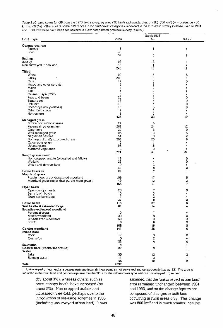
Table 3 10 Land cover for GB from the 1978 field survey, by area ('00 Ion') and standard error (Sri) ( 00 km2) N = presence <50km2 or <0 5%) (There were some differences in the land cover categones recorded in the 1978 field survey to those used in 1984and 1990. but these have been reclassified to Cow companson between survey results )

S:ock 1978

Cover type Area SE % GI3

Communications

Railway 6 1

Road 33 3 1

as 3 2Built up

Built up 198 18 9Non-surveyed urban land 48

2

246 18 11

Wheat 109 15 5Barley 206 19 9Oats 17 5

Mixed and other cereals 3 2

Maize 4 2

Kale 4 2

Oil-seed rape (OSR) s 3 -Peas and beans 20 7 oSugar beet 15 4 0Potatoes 19 4 oRoc: crops (not potatoes) 13 3 0Other field crops 2 1 •Floriculture 8 3 -

425 28 19Managed grass

Formal rem eanonai areas 24 6 1Perennial rye-grass ley 269 24 12C:her leys 20 5 0Well-managed grass 105 12 5Neglected pasture 51 a 2Non-agrcuktrally improved grass 201 20 9Calcareous grass 3 1

Upland grass 98 15 4Manume vegetation 2 c +

774 41 34Rough grass/marsh

Non-cropped arable (ploughed and fallow) 18 4 0Wetland 22 4 0Waste and deretIct !and 9 3

49 6 2Dense bracken 29 7 1Moorland grass

Pu:ple rimer grass-dominated moorland 106 17 5Moorland grass (other than purple moor grass) 49 12 2

155 17 7Open heath

Open-canopy heath 20 7

Berry-bush heath 10 3

Dner northern bogs 7 2 4

37 9 2Dense heath 115 27 5Wet heaths & saturated bogs 81 14 4Broadleaved/mixed woodland

Perennial crops 10 7 +Mixed woodland 20 8 0Broadleaved woodland 60 9 3Shrub 18 6 0

108 16 5Conifer woodland 141 2s 6Inland bare

Rock 17 3 0Ovarry/pit 5 2

22 4 0Saltmarsh 4

Coastal bare (Rocka/sand/mud) 27 9

Water

Lake 35 12 2Running water II 3

45 12 2Total 2297

$ Unsurveyed urban land is a census estimate from all I km squares not surveyed and consequently has no SE. The area isincluded in the built land and percentage area but the SE is for the urban cover type without ursurveyed urban land

(by about 3%), whereas others, such asopen-canopy heath, have increased (byabout 5%). Non-cropped arable landincreased three-fold, perhaps due to theintroduction of set-aside schemes in 1988(including unsurveyed urban land).. Itwas

assumed that the 'unsurveyed urban land'area remained unchanged between 1984and 1990, and so the change figures arecomposed of changes in built landoccurring in rural areas only. This changewas 800 krn2and is much smaller than the

48

error terms associated with the 1984 and1990 estimates (11 100 km2 and 11 200 km2respectively).

3.4 9 A small decline in the area of waterbodiesmay refieci in part, the dry summerexperienced in the south and east of GB in1990. Other physical features. such as barerocks and screes, have remained constantover the survey periods, as would beexpected.

3.4.10 Both broadleaf and coniferous woodlandhave shown increases of 1% and 5%,respectively. Within the overall broadleafcategory there was a decline in shrub andperennial crops which includes a decline inorchards.

3.5 The matrix of change between1984 and 1990

3.5.1 The matrix of change in land coverbetween 1984 and 1990 (Figure 3.1)identifies not only the quantity of change,but also what has changed into what Mostof the largest changes are between theagricultural land uses. including tilled land,managed grass and rough grass/marshSome of the changes are equally balanced.such as the tilled land to managed grasswhich equals the managed grass to tilledland, while the tilled land to rough grass/marsh may be due to introduction of set-aside schemes

3.5.2 Built-up land and communications can beseen to have increased at the expensemainly of agriculture. while forestry showsa split between agriculture (mainlybroadleaf) and more semi-natural habitatssuch as moorland grass and heath(conifers). The increase in rough grass/marsh can be seen to be mainly at theexpense of managed grass, and tilled land.

3.6 Relationship between satelliteand field survey data

3.6.1 There is broadly a good agreementbetween the estimates of area from fieldmapping and those derived from thesatelhte land cover map. as indicated inTable 3 11 and reponed in the LCD project(Wyatt et al in prep.). Differences can beexplained by different definitions andresolution of mapping.

Table 3 11 Companson of estuna;es of area (OO km2) andstandard error (SI!) ('00 AIM) of key cover types in 1990 :n G3by sa:eline and by field survey

Satellitecover map

landFeld survey

Key cover type Area % Area % SF.

Ur ban 158 7 208 9 •Med land 513 21 481 21 23Managed grass 657 27 682 29 23Rough grass/marsh 43 2 107 5 9Bracken 36 1 37 2 6Heath/moor grass 202 8 120 5 14Open shrub heatMthor 279 la 146 6 13Dense shrub heath/moor 72 3 45 2 8Bog 43 2 166 7 15Deciduous/nu:fed woodland 123 3 130 6 9Coruferous woodland 77 3 137 6 16inland ba:e 26

6 <1 1Saltma:sh 4

<I 2Coastal bare 14

18 1 4inland waler !7 1 29 1 7Sea/es:ualy 77 3

Unclassthed 61 3

Total 2402

2318

Unsurveyed urban land :s a census esumate from all 1 kmsquares not surveyed and consequently has no SE

3.6.2 Correspondence between field and satellitesurveys was quantified by inter-comparingthe maps in a GIS . Correspondence resultsare available for each of the 32 ITE LandClasses, and hence for each landscape andfor all of Britain (and for any combination ofsquares). Allowing for interpretationdifferences. overall correspondence is 67%.or 71% ifboundary pixels are excluded.

3.6.3 There are undoubtedly time-dependentdifferences between the two surveys Forexample, the field survey would have usedthe low tide line shown on OS maps. whilethe satellite survey could only depictbeaches as they appeared at the time ofimaging. The use of crop rotations isprevalent in some areas- fieldreconnaissance showed that a one-year lagmight redistribute half of the arable andgrass fields in areas of mixed farming andthat a two-year lag between imaging andfield work might mean an almost total switchin the distributions of arable and grass Thesummary of the field data for newly plantedconifers used a method which classified thecover as coniferous woodland, even if thetrees were just 0.5 m saplings with scarcely5% cover. Allowing for such likely changes,agreement between surveys is increased to81%.

3.6.4 Other reasons for differences are many andvaried. Firsi•there is straightforwardmisclassification by the image analysisprocedure. Second, there arediscrepancies in field recording: the Quality

49

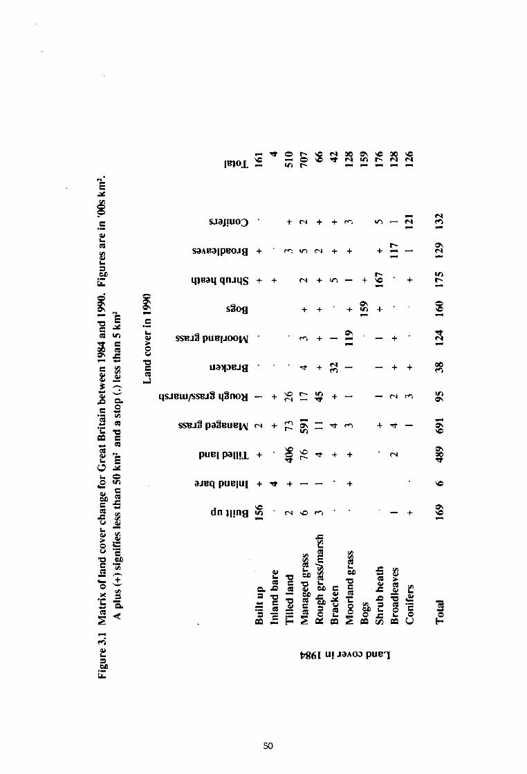
Fig

ure

3.1

Mat

rix

of

lan

dco

verc

han

ge

for

Gre

atB

rita

inb

etw

een

1984

and

1990

.F

igu

res

are

in'0

0skm

2.A

plu

s(+

)si

gn

ifie

sles

sth

an50

km2

and

ast

op

(.)

less

than

5km

2

Lan

dco

ver

in19

90

C.

=to

,od

a:E

. ._T

.o o

=co

8ac ca

7:sr

Ct

c]

coP

ice

71

E

-1.

o

t

!"'g

g 6

c.0

Eb

tC

tT

,c

.c.

cow

e

Lan

d

cove

r

in1984

Bu

iltu

pIn

lan

db

are

156

+ .

2 +

Till

edla

nd

2

406

73

Man

aged

gra

ss6

176

591

Ro

ug

hg

rass

/mar

sh3

I4

11

Bra

cken

+4

Mo

orl

and

gra

ss

++

3

Bo

gs

Sh

rub

hea

th

+

Bro

adle

aves

I

24

Co

nif

ers

+

1

To

tal

169

648

969

1

+

26

3

+

174

3+

25

2

45+

++

+2

+

+32

I

5+

+1

111

9+

I+

3

159

+

II

I+

167

+5

2+

+

117

I

3+

+1

121

9538

124

160

175

129

132

I16

1 4

510

707 66 42 128

159

176

128

126

Assurance Exercise gave an average 84%correspondence in primary coding of landcover. with 95% correspondence inlowlands and 71% in uplands There maybe minor geometric discrepancies. wherea feature is correctly classified butdisplaced in its exact map position: in adissected landscape. this can have a majorimpact on the measure of agreement (onaverage 40% of 25 m pixels fall across avector boundary).

3.6.5 A large part of the differences relate to theimpossibihty of perfectly subdividing acontinuously variable landscape intodiscrete units of uniform cover.Generalisation, hence distortion of 'thetruth', plays a necessary part, bothprocedures are forced to generaliseaccording to different rules The fieldsurvey makes considerable use of physicalboundaries (fences, walls, ditches) to mapthe land cover types The satellite studytakes no account of boundaries but simplyattempts to allocate a 25 rn square patch onthe ground to the nearest cover type.Although integration of approaches is anobjective of the project, technicalconstraints and historical precedent meanthat, for some elements, the two surveysoperate within different rules and withdifferent objectives. They can. therefore.give different results with neither beingwrong. Such complexities are discussed inthe report on the LCD project (Wyatt et al.in prep.).

3.6.6 Urban land provides an example of a coverclass that is difficult to compare betweensatellite and field survey. The satellite landcover map has two straightforward urbanclasses (continuous urban and suburban).The field survey, however, was based on asample of rural GB 1 km squares andincluded classes such as agriculturalbuildings, other buildings, roads andrailways. In addition, the field surveyestimate is supplemented by a censusfigure. from independent mappedinformation, for non-countryside areas(referred to as unsurveyed urban land. seeAppendix 3). Thus, the larger estimate ofurban land from field survey may be due tothe incorporation of more rural features.including roads, railways and curtilagearound properties.

3.6.7 With reference to reasons for differencesbetween surveys, it is perhaps sufficient tosay that. ifthe field survey correctlyrecorded 90-95% of the landscape (thus

overlapping about 85% with an equivalentquality assurance survey), and if the satellitesurvey achieved its target 80-85% success.then the overlap would be around 75%. afigure which is typical if we allow for theobvious interpretation differences, perhapswith an element of change.

3.6.8 A fuller analysis of correspondencebetween field and satellite surveys is givenin LCD project (Wyatt et al. in prep ). Thisincludes the vector analyses in fullspatialmode and the more generalised but moredetailed analyses of cover types as made inthe point-scoring and summary 1lcmsquare cover data. The latter areparticularly important as they represent thecorrespondences which are relevant to allanalyses at 1 km square level, especiallythose in the as.

3.7 Integrated use of field surveyand satellite data

3.7 I Field and satellite data have also beenintegrated into the I km square CIS database. An example helps to demonstratehow it is possible to combine the spatialinformation of the satellite-based study withthe specific details of the field survey. Thesatellite study cannot estimate theproportion of. say. oak (Quercusspp.)woodland: it makes no distinction betweendifferent deciduous tree species. The fieldsurvey 'can examine the study area in termsof the extent of the individual ITE LandClasses. By reference to Land Class meanfigures for oak woodland. it can estimate acover value for oak based on a weighting ofthe extent of the different cover types.

3.7.2 However. the field survey data cannot takesite-specific circumstances into account; forexample. in areas where woodland isparticularly extensive or perhapscompletely absent, it could not predict thecontinuous variability of woodlands across aregion, except insofar as these related toLand Class. By examining the deciduouswoodland area according to the cover map.and referring to the 1 km square pattern ofLand Classes, it is possible to estimate oakcover as aproportion of the Imowndeciduous woodland cover.

3 7.3 Wherever there is a correlation between asatellite cover type and a specific variableof interest, the land cover map can helppredict the specific details. Insofar as theextent of crops can be related to the area of

51

tilled land through the field data, so a mapof tillage can refine local crop estimates. Ifhedges are positively correlated withmanaged grasslands, the land cover mapcan be used to improve local and regionalhedgerow estimates. The procedure is notlimited to CS1990 field data: the British Trustfor Ornithology had correlated breedingbird species diversity with land coverdiversity (Gates et in press). Correlative predictions could be further improved byuse of soils, altitude and other thematic datain the CIS.

3.7.4 The CS1990 project aimed to inter-comparethe results obtained by field survey of the508 squares with the equivalent areas assurveyed by satellite automated imageclassification One stage which involved fullGIS integration compared vector field mapoverlays with the raster, satellite. map. Thevector data were simplified to theequivalent 25 cover types of the satellitemaps. for full co-registration and inter-comparison. Exact correspondence wasachieved by moving the raster back-drop,as necessary. to line up with the vectors.Results showed that more than half of allsquares registered without any shift, andthat mean displacement was 0.8 pixels.equivalent to 20 m average error.

3.8 Pattern analysis

3.8.1 Various trials were attempted in earlyassessments of the use of vector GIS forpattern analyses. Demonstration workstarted on a 75 km x 50 km iest areacentred on the Thames estuary. This areawas converted from raster data to vectorformat. Such conversion highlighted theproblems of dealing with large data bases;this relatively small area, one-sixtieth of allBritain. contained 80 000 polygons. On thisbasis, GB would probably contain fivemillion polygons in total. There is currentlyno commercial GIS which could realisticallyhandle such detailed vector information forall of Britain.

3.8.2 Basic analysis of the derived polygon datainvolved the sepafation of single land coverclasses from the main vector file: this wasnecessary because initial trials showed thatmeasuring polygon boundary length andareas was an extremely lengthy processwith such large files. For instance, the GIScounted 1908 deciduous woodlandpolygons within the Thames test area.These had a total area of 76 km2 and a total

boundary length of 1597 km. with anaverage woodland size of 0.04 km2 andaverage boundary length of 0.8 km.Further statistics can be extracted fromthese figures. such as the area/boundaryratio.

3.83 Data on cover have been summarised per1 km square for inclusion in the CIS. Thedata take the form of an array 700 x 1300pixels representing all GB x 17 layers (oneper key cover type). The 1 km squaresummary data have provided complexinformation which cannot be adequatelydisplayed in tabular form. Tabular resultsdo not give any impression of the detailswhich remain, even after simplification from25 m x 25 m data to 1 km squaresurnmanes. For these reasons, hard-copyexamples are given in the report on PatternAnalysis (Fuller et al. 1993).

3.8.4 Pattern analyses have similarly beencompleted for all of GB. Boundary lengthsper key cover type add 17 layers to the GBarray in the CIS. Pairwise combinations adda further 44 layers. .The total CIS input istherefore an array 700 x 1300 x 70 bytevalues. representing 64 Mbytes of data.

3.8.5 Raster analyses of the boundary data showvariability in proportion of boundary pixelsin different landscapes. On average, pixelswhich adjoin or cross cover boundariesrepresent 44% of all GB pixels. This figurewas confirmed by vector analyses of 1281 km squares which showed that 40% ofpixels were overlaid by field-surveyedvector boundaries. The mmor differencereflects a small proportion of 'noise' in theraster satellite data (4% out of 44% isequivalent to just 10% of boundary pixelsbeing 'noise'); in practice. the results areclose. The variability in contents ofboundary pixels has been calculated downto the individual ITELand Clags level.BecauSe the sample size is so large(thousands of squares), standard errors arevery small and significant differences arefound between many Land Classes (Fulleret al 1993).

3.8.6 The assessment of neighbouring coverwithin a fixed distance of each individualcover class generates enormous quantitiesof output data: 17 classes with 16 possible'neighbours' and buffer zones with steps of,say. 100 m. 200 m. 300 m, 500 m and1000 m, would generate 1360 extra layersof 1300 km x 700 Ian data for the CIS. Thechoice of buffer zones should depend upon

52

the objectives. Thus. in studying asongbird's feeding range a user mightrequire cover within tens of metres ofwoodland nest sites, but a study of buzzardhabitats may require buffer zones coveringmany kilometres. The processing is time-consuming (eg 100 hours of continuouscomputer-processing for 17 classes andfour different zones in a 100 km square. ienearly a year for all GB) so it is necessary tobe highly selective, and to design analysesto specific objectives.

3.8.7 The pattern analysis study thereforeinvestigated the potential for proximityanalyses. assessed the feasibility of variousanalyses. and presented preliminary resultsto demonstrate the caphbilities to users.Four 50 km squares were selected, onefrom each landscape type. The areas ofdeciduous woodland. moor and brackenwere each in turn buffered by 100 m. 200 mand 300 m.

3.9 Summary of Chapter 3

3.9.1 A land cover map of GB was produced byinterpretation and classification of LandsatThematic Mapper. satellite imagery.Although information is gathered at the25 m pixel level, it has been summarised inthis project to give the coverage of 17 keycover types in each 1 Ian square in GB.This data set has been incorporated into theCIS.

3.9.2 Satellite data showed that, in 1990. managedgrass covered the largest area in Britain(27%). followed by tilled land (21%) andopen shrub heath moor (11%). Englandwas predominantly tilled land and managedgrass (65% together). whereas in Scotlandand Wales semi-natural vegetation andmanaged grass together covered morethan two-thirds of the land.

3.9.3 Regional comparisons have been madeshowing a strong relationship between thefour landscape types and the land coverclasses present.

3.9.4 Although in the arable landscapes tilled landcomprised 41% of ihe land cover, managedgrasslands were significant at 29%. Thepattern was reversed in the pasturallandscapes. with 39% managed grasslandsand 22% tilled land, and there was moreland covered by semi-natural vegetation

categories. In the marginal uplandlandscapes, managed grasslands covered28%, with heath and moorland at 38%. Theupland landscapes were dominated bydwarf shrub heath and bog. with thecombined totals for open and dense heaths,moors and bogs being over 65%.

3.9.5 Stock information on land cover in GB hasalso been obtained by extrapolating from asample of 1 km squares which have beensurveyed in the field. The field surveyrecorded land cover in considerable detail.using combinations from a code list of over300 categories to describe the individualparcels. These have been aggregated togive 58 land cover types and these, in turn.have been summarised to more or lessmatch the 17 categories from the satelliteland cover map.

3.9.6 The results from the sample field survey of508 1 km squares show good generalagreement with the satellite-derived landcover map for most classes. For example.for tilled land. both figures were 21%, andmanaged grass covered 27% (satellite)compared with 29% (field survey) Somecategories, for example rough grass/marsh(2% - satellite; 5% - field survey) differeddue to irtherent differences in the methodsused to identify them and in the ways theyhave been defined. However, to integratethe two sources of information, the fieldsurvey data can be broken down into moredetailed categories. For example. the fieldsurvey data showed that 40% of the well-managed grass was actually intensivelymanaged. Most figures for cropscorrespond to MAFF and Department ofAgriculture and Fisheries for Scotlandstatistics: for example. for oil-seed rape,both figures were 410 000 ha

3 9.7 The exact relationship between the twoestimates of land cover stock has beenexamined from two perspectives. First, thedegree of correspondence between themhas been examined. both in terms ofcomparison of the overall estimates. and bycomparing results directly in a number ofsample squares. The correspondence isreasonable in both cases and reasons forany differences are examined. They relateto spatial arrangements. scale and featuredefmitionyand also reflect the historical andtechnical differences between theapproaches.

3 9 8 Differences between data from field survey

53

and satellite imagery were quantified byinter-comparison of digital maps using GIS.Direct correspondence was 67%, thoughthis increased to at least 71% ifboundarypixels were excluded from the comparison(and was better for some cover types thanothers). Differences were due to theimage analysis procedures. discrepanciesin field recording, and minor geometricregistration errors. The CIS can be usedto compare summaries of regions usingthe two procedures. The information fromthe field survey can also be used inconjunction with the satellite land covermap categories to estimate speciescomposition in vegetated covercategories, such as woodland ormoorland.

3.9.9 Data on land cover have been estimatedfor 1978. 1984 and 1990 using the field-based sampling approach. Figures forchange in cover types, between 1984 and1990. were obtained from 381 squaresvisited in the field on both occasions.Tilled land in GB had declined by 4% of itsarea and within this category there wereincreases in non-traditional crops such asmaize, which increased three-fold. Withinthe grasslands category, there was a shiftwithin the managed grasslands towardsweedy grasslands and away from lessweedy types. Within the semi-naturalhabitats some changes can be seen and,although there is a small overall decline.the previously reported large losses todevelopment are not evident. Reductionswere recorded for moorland grass andbracken, while bogs, tall herb and wetlandall increased albeit by small amounts Theincrease in set-aside was also recordedwithin the non-cropped arable figure.

3.9.10 A matrix of change shows the movementsbetween cover types between 1984 and1990 as well as the overall net changewhich, on its own, can mask the degree ofchange taking place. Most of the largechanges were due to the shifts betweenthe major agricultural categories,principally tilled land and managed grassThe built-up category has expanded at theexpense of managed grass and tilled land,whereas broadleaved woodlands havecome from managed grass Conifer forestexpanded in area, mainly at the expense ofopen shrub. At this level of aggregation,there was a high degree of stability withlittle or no movement between most cellsin the matrix.

3 9.1 I Using the satellite data: pattern analysis wasalso carried out for the whole of GB todetermine, for example. boundary lengthsbetween the 17 land cover classes. Pixelswhich adjoin or cross over boundariesrepresented 44% of the total, and theirdistributions were compared withinlandscapes

54

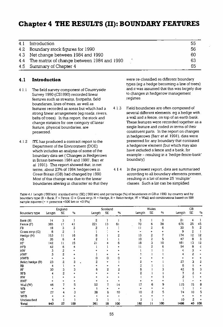
Chapter 4 THERESULTS(II): BOUNDARYFEATURES

4.1 Introduction 554.2 Boundary stock figures for 1990 564.3 Net change between 1984and 1990 604.4 The matrix of change between 1984and 1990 634.5 Summary of Chapter 4 65

4.1 Introduction

4.1.1 The field survey component of CountrysideSurvey 1990 (CS1990) recorded linearfeatures such as streams, footpaths, fieldboundaries, lines of trees. as well asfeatures recorded as areas but which had astrong linear arrangement (eg roads rivers,belts of trees). In this report. the stock andchange statistics for one category of linearfeature, physical boundaries, arepresented.

4.1 2 ITEhas produced a contract report to theDepartment of the Environment (DOE)which includes an analysis of some of theboundary data set ('Changes in Hedgerowsin Britain between 1984 and 1990', Barr etal. 1991). This report showed that. in netterms, about 23% of 1984 hedgerows inGreat Britain (GB) had changed by 1990.Most of this change was due to the linearboundaries altering in character so that they

were re-classified as different boundarytypes (eg a hedge becoming a line of trees)and it was assumed that this was largely dueto changes in hedgerow managementregimes.

4.1.3 Field boundaries are often composed ofseveral different elements. eg a hedge witha wall and a fence, on top of an earth bank.These features were recorded together as asingle feature and coded in terms of theirconstituent pans. In the report on changesin hedgerows (Barr et al. 1991). data werepresented for any boundary that containeda hedgerow element (but which may alsohave included a fence and a bank, forexample - resulting in a 'hedge-fence-bank'boundary).

4.1.4 In the present report. data are summarisedaccording to all boundary elements present.resulting in a list of some 25 'multiple'classes. Such a list can be simplified

Table 4 I length ('000 lcm) vandard error (SE) ('000 Ian) and percentage (%) of boundaries in GB in 1990. by country and byboundary type (B = Bank. F = Fence. G = Grass strip. H = Hedge. R = Relict hedge, W = Wall) and combinanons based on 508sample squares (- = presence <500 km or <0 5%)

Boundary typeEngland

LengthSE %Scotland

LengthSE

WalesLengthSE 04 Length

GB SE %

Bank (B) 14 3 I 2 1

5 1 3 21 4 1

Fence (F) 385 17 41 221 13 61 70 6 38 676 25 45

FB 18 3 2 2

11 2 6 30 5 2

Grass smp (G) 8 2 I 1

9 2 1

Hedge (H) 153 11 16 8 1 2 13 2 7 174 12 12

1113 35 6 4 2 1

10 2 5 47 8 3

Hi 142 I I 15 21 4 6 18 3 10 181 !3 12

HFB 42 6 4

• II 2 6 54 8 4

FIW 3 2 •

4 3

EWE' 3 2 + 1 • 4.

4 2 -

HWFB + + + 0 0 0

• + +

Rehr, hedge (R) 23 2 2 2 •

2

27 3 2RB 4 I +

• 4 2

6 1 +

RF 30 3 3 6 2 2 6

3 42 5 3

RFS 4 2 +

• 4 2

7 2 +

RW 1 + +

•

1

2 1 +

RWF

• + • 4 •

1

+

Wall (W) 46 7 5 52 7 14 17 6 9 115 15 8

WB

+ + 1

•

1 1

WF 27 4 3 38 6 10 10 2

74 10 5wre

+ + 4. •

+ +

Unclasstfied 5 1 1 3

2

10 2

Total 943 27 100 361 18 100 182 11 100 1486 40 100

55

according to 'dominant boundary typesbut, since there is no logical way ofprioritising these (eg determining whethera hedge-mth-a-wall should be eassined asa hedge, or a wall), the user is invited tosummarise the data according to specificrequirements It should be noted that. ifallboundaries are summarised according todominant types, there is a danger ofdouble-accounting, resulting in a totallength which is greater than 100%.

4.1.5 Boundary type was also recorded invegetation plots (see Chapter 5) and thesedata confirm results (stock and change)from the mapping exercise.

4.2 Boundary stock figuresfor 1990

4.2.1 Table 4.1 and Figure 4. I give thebreakdown of boundary types in GB. basedon analysis of all 508 squares surveyed in1990. including both single- and multiple-element categories. Relict hedges arethose elements of boundaries that wererecognised as having once been hedges.but have become, for example, rows oftrees or lines of shrubs

4.2.2 Noting comments made in section 4.1.4(above) about double-accounting, it ispossible to summarise the data in Table 4.1by dominant boundary element. In Table4.2, an arbitrary classification is used suchthat the lengths of boiindaries whichcontained a hedge are presented first then,of the remaining boundaries, the lengthcontaining a wall is presented. followed byfurther boundaries that contained fences.Last, other boundary types (banks, relicthedges and grass strips) are gwen.

4.2 3 As Table 4.2 shows, boundaries containinghedges formed 31% (464 000 lan) of thetotal length of boundaries in GB in 1990. Ofthese, 81% (378 000 km) occurred in

England. 12% (54 000 Ian) in Wales and 7%(33 000 km) in Scotland. Relict hedgeswere an element in only 6% (85 000 Ian) ofthe total boundaries (Table 4.1) and nearlythree-quarters of them (62 000 Ian) were inEngland. with 16% (13 000 Ian) in Walesand 11% (9000 km) in Scotland.

4.2.4 Boundaries within which walls weredominant formed 13% (193 000 lcm) of thetotal boundary length in GB (Table 4.2),most of which occurred in Scotland (47%91 000 Ian) and England (39% - 75 000 km).Relatively few walls were combined withother boundary elements.

4 2.5 Fences were the most widespreadboundary component. forming 45%(676 000 km) of the total length (1485 km)when considered as an individualboundary, as shown in Table 4 1 A further26% (398 000 lan) of boundaries containeda fence in conjunction with anotherboundary feature. Thus. 72% (I 074 000km) of all boundaries contained a fence.Although most fences were in England. theyformed only 41% (385 000 km) of theboundaries there, compared to 61%(221 000 lan) of the boundaries in Scotlandand 38% (70 000 Ian) in Wales.

4.2.6 Boundaries containing a bank wereinfrequent, contributing to less than 11%(167 000 Ian) of all boundanes and, ofthese, 70% (117 000 Ian) occurred inEngland and 25% (41 000 km) in Wales.

4.2 7 About 70% (1 023 000 lan) of all GBboundaries were single-elementboundaries In Scotland. 79% (286 000 Ian)of all boundaries had only one element(due, perhaps. to the scarcity ofhedgerows). compared to 67% (630 000Ian) in England and 59% (107 000 Ian) inWales. Of the boundaries in England. 24%(153 000Icm) of the single-elementboundaries were hedges, and 61%(385 000 Ian) were fences. In Scotlandthese figures were 2% (7000 km) and 77%

Table4 2 Length ('000 km), standard error (SE) ('000 krn) and percentage (%) of dominant boundary types in GB in 1990, bycounay (Hedge = any boundary thar contains a hedge element, but excluding relict hedge: Wall = any other boundary that containsa wall element. Fence = any remaining boundary tha; contains a fence element). based on 508 sample squares

England

Scotland

Wales

GB

Boundary type Length SE % Length SE 0/9 LengthSE % Length SE 0/0

Hedge 378 19 40 33 6 9 545 30 464 24 31Wall 75 9 8 91 11 25 288 15 193 21 13Fence 437 19 46 229 14 63 897 49 755 28 51Other 54 5 6 9 1 2 112 6 74 6 5Total 943 27 100 361 18 100 18211 100 1486 40 100

56

Fig

ure

4.1

Len

gth

ofbo

unda

ries

(000

km) i

nG

Bin

1990

, by

coun

try

and

bybo

unda

ryty

pe(B

=B

ank,

F=

Fen

ce, G

=G

rass

stri

p,H

=H

edge

, R=

Rel

ict h

edge

, W=

Wal

l,U

NC

=U

ncla

ssif

ied)

700

-

600

500

-

LII W

ales

Scot

land

III

Eng

land

400

300

-

200

100

-

.1-F

-J11

4-a4

_S

tt

tx5

t02

6T.

E3

MIR

Bou

ndar

yty

pe

Table 4 3 Length ('000 Ian). standard error (SE) (1300 km) and percentage (%) of boundaries in GB in 1990. by iandscape type andby boundary type (B = Bank. F = Fence. G = Grass strip. H = Fledge. R = ReLc: hedge: W Wall) and combinations. based or. 508sarnpte squares (+ = presence <500 km or <0 5%)

Boundary type LengthAlab!e

SE %Pastural

LengthSE

Marginal uplandLengthSE%

UplandLengthSE%

Bank (B) 3 2

15 4 2 2 I 1 2I2Fence (F) 253 16 47 254 14 40 107 12 47 64857FB 2 1

23 5 4 5 2 2 •Grass stop (G) 6 2

3

4

00Hedge (H) 99 8 19 58 9 11 7 2 3

I-13 5 2

38 7 6 4 2 2 000HF 89 9 17 81 9 13 I! 3 5 000HF3 7 3 1 43 8 7 4 2

000MW

3 2

4 • 000iWF 1

3 2

•

10,VFB 0 0 0

0 0 0

Relict hedge (R) 16 2 3 9 2 1 2 1 1

RB

3

2 I 1

RF 14 2 3 !7 3 3 II 3 5

RFB

4 2

2 1

RW

0 0 0

1

RWF

0 0

Wall (W) 17 4 3 35 7 5 44 12 19

WB

- 0 O 0

WF 18 5 3 17 3 3 27 6 12 1213WFB

- 0 0 0 0

0 00Unclassified I +

5

1 3

:1Total 534 22 100 628 21 100 230 22 100 9513100

(221 000 km) respectively, whilst in Walesthe figures were 12% (13 000 km) and 65%(70 000 km). Where multiple-elementboundaries occurred, the combination offences with other boundary elements issignificant as it may indicate boundaries inneed of repair or other management (eglaying of hedges).

4.2.8 Table 4.3 and Figure 4.2 show thecharacteristics of boundary lengths bylandscape type.

4.2.9 Hedges and hedges-with-fences weremainly in the arable landscapes, whereashedges-with-banks were mainly in thepastural landscapes, being typical of thewest of GB Overall, most hedgerowswere in the pastural landscapes (51% -238 000 km) but the arable landscapes stillcontained a major hedgerow resource(43% - 201 000 lcm)as pointed out byCumrnins et al. (1992). Hedges werepresent, but more restricted, in themarginal uplands and almost absent fromthe upland landscapes. Relict hedgesoccurred in similar proportions in thearable and pastural landscapes but, in thelatter, occurred more frequently inboundaries with fences.

4.2 10 There were more walls in the marginalupland landscapes than elsewhere (38% -72 000 km), a figure made more significant

by the limited extent of this landscapetype. The other three landscape types alsocontained significant lengths of wall withthe arable landscapes (19% - 36 000 Ian)having a greater length, overall, than theuplands (16% - 31 000 km) Nevertheless,in the uplands walls would be regarded ascharacteristic because they formed 310/Dofall boundaries compared to only 12% of allboundaries elsewhere.

4.2.11 Fences occurred in similar lengths in thearable (37% - 253 000 lcm)and pasturallandscapes (38% - 254 000 km) withshorter lengths overall in the marginal

'upland (16% - 107 000 lcm)and upland(9% - 64 000 lcm) landscapes. However,fences made up a higher proportion ofboundaries in marginal upland and uplandlandscapes because hedges were lesscommon.

4.2.12 A higher proportion of boundariescontaining banks were in the pasturallandscapes (76% - 127 000 km), with 11%(19 000 Ian) in the arable and 12% (18 000km) in the marginal upland landscapes.Only 2% (2000 km) of upland boundariescontained banks.

4.2.13 Upland areas had the highest percentageof single-element boundaries. with 87%(83 000 lcm) of the boundaries taking thisform, compared to 74% (394 000 km) marable landscapes. 70% (162 000 km) in

58

Figu

re4.

2L

engt

hof

boun

dary

type

s('O

Nkm

)pr

esen

tin

GB

in19

90,

byla

ndsc

ape

type

and

boun

dary

type

(B=

Ban

k,F

=Fe

nce,

G=

Gra

ssst

rip,

H=

Hed

ge,

R=

Rel

ict

hedg

e,W

=W

all,

UN

C=

Unc

lass

ifie

d)

300

Ara

ble

250

Past

ural

Mar

gina

l

al

Len

gth

('ON

km)

200

-U

plan

d

50-

0

-

22

Bou

ndar

yty

pe

marginal upland landscapes and 62%(384 000 lcrn) in pastural areas Fenceswere the most common single elementboundary in all four landscape types

4.3 Net change between 1984and 1990

4 3.1 The data for net change between 1984 and1990. by country, is given in Table 4.4 andin Figure 4.3.

4 3.2 Hedges on their own and hedges-with-fences declined more than hedgesassociated with other boundary types. interms of overall length. although, as therewas a higher mitial stock of these types in1984. the percentage change is less than forother hedge boundaries. The highpercentage loss of hedge-with-wall andhedge-with-wall-and-bank reeects theirlimited extent in GB. In general. the lengthlost was proportional to the initial stock.suggesting that no one type had been lost toa greater degree than might be expected.The same applies to the relative losses inthe three countries. This agrees with theconclusions of Cummins et al. (1992) inrelation to the species composition of thehedgerows that have been lost. The relicthedges had the greatest proportional

increase (53% - 31 000 Icrn) of anyboundary. especially in England and Wales

4.3.3 Walls had a lower percentage loss thanhedgerows. Walls-with-fences declinedmore than walls on their own, perhapsbecause the former were already indecline. Although the overall trend was fora decrease of walls throughout GB. therewas a small increase in the number of wallsin Scotland. By contrast, walls-with-fencesdeclined in England and Scotland butincreased in Wales.

4.3.4 Fences increased more in length than anyother boundary type with a 12% (75 000lan) increase overall. The increase wasmainly in England and to a lesser degree inScotland.

4.3.5 The characteristics of boundary change bylandscape type are shown in Table 4 5 andFigure 4.4.

4 3.6 The greatest length of hedges on their own was lost in the arable landscapes(27 000 Ic-n) although, proportionally.similar amounts were lost in pasturallandscapes. A higher proportion of hedge-with-banks was lost in the arablelandscapes. but. by total length. the greatestloss was in the pastural landscapes There

Table 4.4 Changes in the length ('OCOIcn) and standard error (SE) ('OCOkm) of boundaries in GB. between 1984 and I99C. bycountry and by boundary type (B - Bank: F - Fence. G = Grass strip H = Hedge. R = Relict hedge W = Wall) and combinationsbased on 381 sample squares (NB I - a gain <5130km.1 7 a loss <500 km. - - SE <500 Ion. % = percentage change of 3964)

EnglandScotlandWalesGBBoundary rypeLengthSE%LengthSE%LengthSE%LengthSE%

Bank (3) -3 3 -17 -3 1 -55 I ! 14 -6 5-20Fence (F) 38 14 1! 21 5 10 16 4 25 75 1712FB 3 5 20 -4 2 -70 1 4 7 1 9 1Crass strip (G) 7 2 >100 I 1 >100 1 4- >100 8 2>100Hedge (H) -42 10 -22

2 -33 -4 2 -20 -49 12-221il3 -10 6 -23 T I 20 -5 2 -37 -15 8-25

-36 12 -21 -7 3 -24 T 2 1 -43 14-20HEM

7 -19 -1 2 -38 -I I 4 -57 -19 10-33HW -I 1 -65 1 • -61 -1 I -81 -3 1-70HWB il + - 100 1 4 -WO 1 t -100 1 +-100HWF -I 1 -37 -I I - 66 T

27 - 2 I - 47HWFB 1 + - 7 1 • -100 1 4 -60 1 + - 33Relict hedge (R) 8 3 49 1 1 -20 -1 1 -34 'I 331RB 0 2 9 1" - >100 I I 68 2 329RF 12 5 62 3 2 >100 4 2 81 18 671RFB 4 3, >100 1 - 16 1 1 80 5 1>100RW 1 1 -7 1 + -37 -1

-I 1-46RWB 1 + -100 1

41i

1 -100RWF T 4- >100 T 44 ;11°D00 T >-1°°00 1 - >100RWFB 0

0 0

0 0

0 0 0Wall (W) -4 6 -8 4 5 7 -8 4 -35 -8 10-7WF1 I • >100 T 1 72 T , >100 I >100WF - 9 5 - 25 - 8 4 -18 2 I 31 -14 8-17WFB I 4- 83 1 + -99 1 + -82 1 -43Unclassified -9 3 -59 -2 1 -40 -1 I -24 -13 4-49Total -49 14 -5 -3 5 -I -6 3 -3 -58 16-4

60

Wal

es

II S

cotla

nd

Len

gth

('000

km)

20

,0

-JL

s

.7.-

.--

.

3€:

>_

4.z

4.-

=3

3...

.3

4.=

=4.

-20

T

-40

-60

-

Figu

re4.

3N

etch

ange

inle

ngth

ofbo

unda

ry('0

00km

)in

GB

from

1984

to19

90,

byco

untr

yan

dbo

unda

ryty

pe(B

=B

ank,

F=Fe

nce,

G=

Gra

ssst

rip,

H=

Hed

ge,

R=

Rel

ict

hedg

e,W

=W

all,

UN

C=

Unc

lass

ifie

d)

80

60

EE

ngla

nd

40-

Bou

ndar

yty

pe(*

-ch

ange

pres

ent,

but

insu

ffic

ient

tosh

owby

coun

try)

Fig

ure

4.4

Net

chan

gein

leng

thof

boun

darie

sO

Nkm

)in

GB

from

1984

to19

90,

byla

ndsc

ape

type

and

bybo

unda

ryty

pe(B

=B

ank,

F=

Fen

ce,

G=

Gra

ssst

rip,

H=

Hed

ge,

R=

Rel

ict

hedg

e,W

=W

all,

UN

C=

Unc

lass

ified

)

40•

30 211

10 0

-10

-20

-30

Len

gth

('000

km)

Crl

114

b0

)47

III

r

Ara

ble

Pas

tura

l

Mar

gina

l

Upl

and

MG

aa;la

Laa

ig

MM ad

—

Bou

ndar

yty

pe(

*-

chan

gepr

esen

t,bu

tin

suffi

cien

tto

show

byla

ndsc

ape

type

)

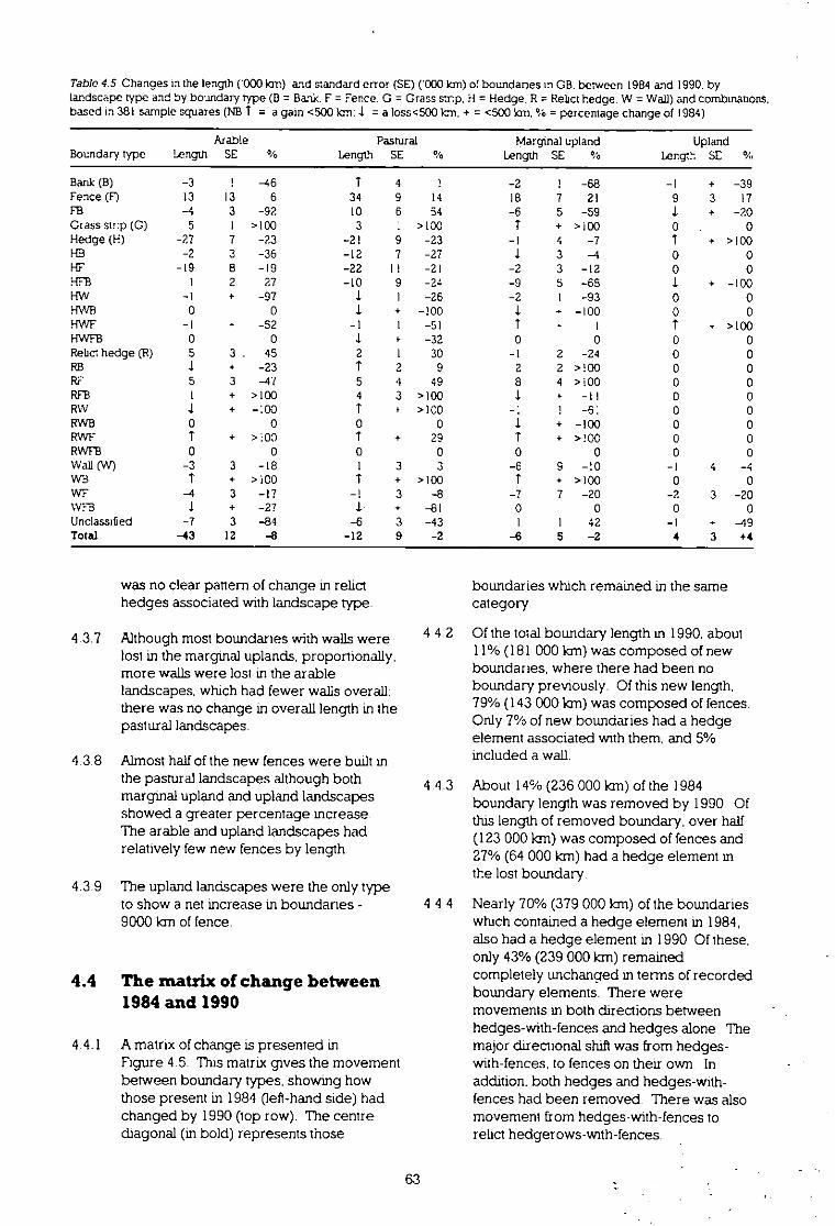
Table 9.5 Changes in the length F000 km) and standard error (SE) (000 km) of boundanes in GB. between 1984 and 1990. bylandscape type and by boundary rype (B = Bank. F = Fence. G = Grass stnp. H = Hedge. R = Relict hedge. W = Wall) and combinations.based in 381 sample squares (NB I = a gain <500 Ion: = a loss<500 km: + = <500 km. % = percentage change of 1984)

Amble Pastural

Marginal upland UplandBoundary type LengthSE% LengthSE % Length SE% LengthSE%

Bank (B) -3 !-46 T 4 1. -2 I-68 +-39Fence (F) 13 136 34 9 14 18 721

317FB -4 3-92 10 6 54 -6 5-59

+-20Grass sin() (G) 5 1>100 3 I >100 T +>100

0Hedge (FE) -27 7-23 -21 9 -23 -1 4-7

+>100FB -2 3-36 -12 7 -27 1 3-1

0

-19 8-19 -22 11 -21 -2 3-12

0FIFA 1 227 -10 9 -24 -9 5-65

+-100NW -1 +-97 1 1 -26 -z 1-93

HWF3 0 0 1 + -100 1 --100

HWF -1 4--52 -1 I -51 I 1

>I

HWFB 0 0 1 f -32 0 0

Relict hedge (R) 5 345 2 1 30 -1 2-24

RB 4 • -23 T 2 9 2 2>100

RFRFB

5 I

3 -47+>100

54

4 49 8 4

4>100

RW .1. +-:00 T 3) >>IC13130 - .

RWB 0 0 0

0 1++41>)-11I6XWY

RWF T +> M I + 29 T

RWFB 0 0 0

0 0

Wall (W) -3I

3-18+>100

I I +3

3>100

-eT

>-110

+9000-14

0

WF -4 3-I? -I 3 -8 -7 7-20 -23-2

WFB 1 +-27 1 + -81 0 0 0

Unclassified -7 3-84 -6 3 -43 1 I42 -1-4

Total -43 12-8 -12 9 -2 -6 5-2 43+

was no clear pattern of change in relicthedges associated with landscape type.

4.3.7 Although most boundarles with walls werelost in the marginal uplands, proportionally.more walls were lost in the arablelandscapes, which had fewer walls overall:there was no change in overall length in thepastural landscapes.

43.8 Almost half of the new fences were built inthe pastural landscapes although bothmarginal upland and upland landscapesshowed a greater percentage increaseThe arable and upland landscapes hadrelatively few new fences by length

4.3 9 The upland landscapes were the only typeto show a net increase in boundaries -9000 km of fence.

4.4 The matrix of change between1984 and 1990

4.4.1 A matrix of change is presented inFigure 4.5. This matrix gives the movementbetween boundary types, showing howthose present in 1984 (lefl-hand side) hadchanged by 1990 (top row). The centrediagonal (in bold) represents those

boundaries which remained in the samecategory.

4.4.2 Of the total boundary length in 1990. about11% (181 000 lcm) was composed of newboundaries, where there had been noboundary previously. Of this new length.79% (143 000 km) was composed of fences.Only 7% of new boundaries had a hedgeelement associated with them, and 5%included a wall.

4.4.3 About 14% (236 000 km) of the 1984boundary length was removed by 1990. Ofthis length of removed boundary, over half(123 000 km) was composed of fences and27% (64 000 km) had a hedge element inthe lost boundary.

4.4.4 Nearly 70% (379 000 km) of the boundarieswhich contained a hedge element in 1984,also had a hedge element in 1990. Of these.only 43% (239 000 km) remainedcompletely unchanged in terms of recordedboundary elements. There weremovements in both directions betweenhedges-with-fences and hedges alone. Themajor directional shift was from hedges-with-fences, to fences on their own. Inaddition, both hedges and hedges-with-fences had been removed. There was alsomovement from hedges-with-fences torelict hedgerows-with-fences.

63

Fig

ure

4.5

Cha

nge

inle

ngth

sof

boun

darie

s('0

00km

)in

GB

,be

twee

n19

84an

d19

90,

base

don

381

sam

ple

squa

res

F

Eft C

.

HF

HE

R

HW

HW

B

HW

F

HW

EB KB

RE

RE

D

RW

1

RW

RI

RW

E

wit

i1

1

WE

I+

i13

:Ij

WE

B

N

1431

316

UN

C+1

151

Tot

al19

9022

167

8134

10

%/

140

j21

1

BF

lE

RG

IIR

BI

HE

HE

R!

HW

HW

EI1

HW

EB

I1

10

I+1

II1

+I11

I1

143

014

+1

411

121.

1+1

114

!9

,+

I11

I+

,11

+I

II

II21

+I

108

10

134

51+

+

52

41

817

14

7;+

+

29I,

+

134

6,99

8+

++

13

711

361

II14

1+

+

+1+

+11

+

_:_

.+

1,

I+

+1

+1

I21

II

I+

++

. _.

+!6

26

111

+1

+1

8+

I

+I

5•11

5

+1

+I

1'71

143

117

6

101

310

1 1

+1

+L

L

381

I21

01

2j0

01O

i

1990

RB

IR

ER

EB

RW

RW

E

WI

Will

WE

WE

BN

IU

NC

TI9

otta

tid%

+R.

1+

+

+

II

21+

I9

+28

2

31

•

12I

516,

+'

123

360

435

+,

1

215,

+35

2

I0

14

1

45

0

15

126

7_

10

+

4

865

00

——

-

I4

181

//

52

25/

+14

+57

3

+I

ii4

0_

_ 0

+1

40 0

321

220

13

6+

583

211

218

13

+1

+1

7121

1

50

325

1

30

20

00

84 111

21

+

•

7

+I

+

281

744

18

11

120

172

0123

613

1706

100

201

310

00

710

0114

110

0

(li=

Ran

k,F

=F

ence

,G

=G

rass

stri

p,

H=

Hed

ge,

R=

Rel

ict

hed

ge,

W=

Wal

l,N

=N

ot

pre

sen

t,U

NC

=U

ncl

assi

fied

)

4.4.5 The major change in the matrix was fromwalLs-with-fences to walls but, in landscapeterms, the conversion of walls-with-fencesto fences alone, and from walls to noboundary, is more important.

4 4 6 in terms of proportions of their total length.fences were the most stable boundary typewith almost two-thirds (430 000 lan)remammg unchanged between the twosurveys Newly built fences were thelargest single contrthutor to the additionallength of fences (143 000 Ian) recorded atthe two dates, balanced to a large degreeby the removal of other fences (128 000krn) from the landscape

4.47 About half of the boundaries (837 000 Ian)retained the same characteristics (in termsof boundary element composition) between1984 and 1990

4.5 Summary of Chapter 4

4 51 Overall, boundaries with fences dominatedthe British countryside in 1990. althoughthere was still a high proportion of hedges.In GB as a whole. walls were a relativelyinfrequent type but were proportionallymore important in both Scotland and WalesEngland contained the majority ofhedgerows while most boundaries inScotland included fences and walls Waleshad the widest diversity of boundary types

4.52 The arable landscapes had the highestpercentage of fences and simple hedges.The pastural landscapes had a wider rangeof hedge types and a significant length ofwall. The marginal upland landscapescontained most walls but also had extensivefences and a minor element of hedgerowsWithin the uplands. fences occurred inalmost 80% of the boundaries and walls inover 30%. As shown elsewhere in thisreport, the upland landscapes were themost uniform type.

4.5.3 The biggest net loss in length was forboundaries containing hedges. but thelargest individual change was an increase infences. The relict hedgerows showed thebiggest percentage change, an increase of53%. In addition, the loss in walls indicatesa simplification in the landscape The majorchanges in lengths of boundary types werein England but there was a highproportional loss of hedgerows in Wales.

4 5 4 The biggest changes overall by length werein the pastural landscapes - this agrees withchanges in spec:es diversity reported inChapter S. The smallest changes were inthe uplands which were relatively stable, asis pointed out in Chapters 3 and 5 (on landcover and vegetation). The marginaluplands showed a higher percentagechange in a range of different types buttheir contribution to overall change wassmall, due to the restricted area occupiedby this typa Lastly, the arable landscapesshowed hedgerow losses on the one hand.and increases in relict hedges on the other.and a relatively small increase in fences.

65

66

Chapter 5 THERESULTS(III):VEGETATION

5.1 Introduction 675 2 Main plots 695.3 Habitat plots 935.4 Linear features - Hedge plots 965.5 - Verge plots 1025.6 - Streamside plots 1085.7 Conclusions and summary of Chapter 5 114

5.1 Intzoduction

5.1.1 This study has focused on two types ofchange which are occurring in the Britishcountryside. shifts in land cover and moresubtle changes in vegetation. The mostobvious is the step-wise shift betweenmajor land cover types. eg conversion ofheath to arable, and results on this type ofchange have been reported in previouschapters. The second type of change,discussed in this chapter. is the more subtlechange in the balance of plant specieswithin a land cover type, eg the gradualchange in a field which has been grazedand is then left unmanaged for a few years,leading to tine palatable grasses beingslowly replaced by coarse grasses and tallherbs.

5.1.2 The methods and sampling schemes usedto record the vegetation, and qualityassurance procedures are described insection 2.3, and in more detail in the FieldHandbook (Barr 1990).

5.1.3 In order to describe the wide range ofvegetation recorded in CS1990, a statisticaltechmque (TWINSPAN) has been used togroup together the vegetation plots whichare most similar into 29 classes, here called'plot classes'. This is an objective andreproducible alternative to assigning plotssubjectively to a predetermined list ofhabitat types (eg calcareous grassland.mesotrophic grassland, acid grassland).Use of this technique means that theassignment of plots to classes takes accountof allthe species in a plot rather than relyingon a few indicator species, as in key-basedsystems. Another advantage of thisapproach is that changes in vegetation canbe measured empiricay in terms of'movement' from one plot class to another.For example, the gradual transiiion of anunimproved pasture to a more Intensively

managed one may be 'measured' as thechanging species composition causes theplot to cross a statistically determined'line' from one plot class to another.

5.1.4 Within a plot class, there will be somespecies with a high frequency, whilstother species occur in only a few plots.Some plots will have more species thanothers. With such a large data set (about11 500 plots were recorded in 051990), it

is not feasible to analyse the plots m termsof the frequency and cover of eachindividual species. However, bygrouping the species which frequentlygrow together. and therefore have similarenvironmental requirements. it is possibleto describe vegetation in terms of thetype of species present. and to identifywhere there is an ecologically significantshift. eg from a group of plants typical ofwaterlogged conditions to a group typicalof drier situations. In order to producethese groups of species, a statisticaltechnique (Ward's minimum varianceclustering of DECORANA ordinationscores) has been used to group specieswhich have similar distributions within thedata set into 32 'species groups' (SG).Investigating the changes in thefrequency of these 32 species groups ismuch more manageable thanconsidering several hundred speciesindividually.

5.1.5 The way in which plot classes and speciesgroups are derived from the raw plot datais illustrated in Figure ala. Because thesame species groups have been used todescribe the Main plots (in fields.woodland and moorland) and linearplots (alongside hedges. streams androads). as shown in Figure 5.1b, it ispossible to compare the way in whichthey have changed across habitats.eg to see whether calcareous meadow

67

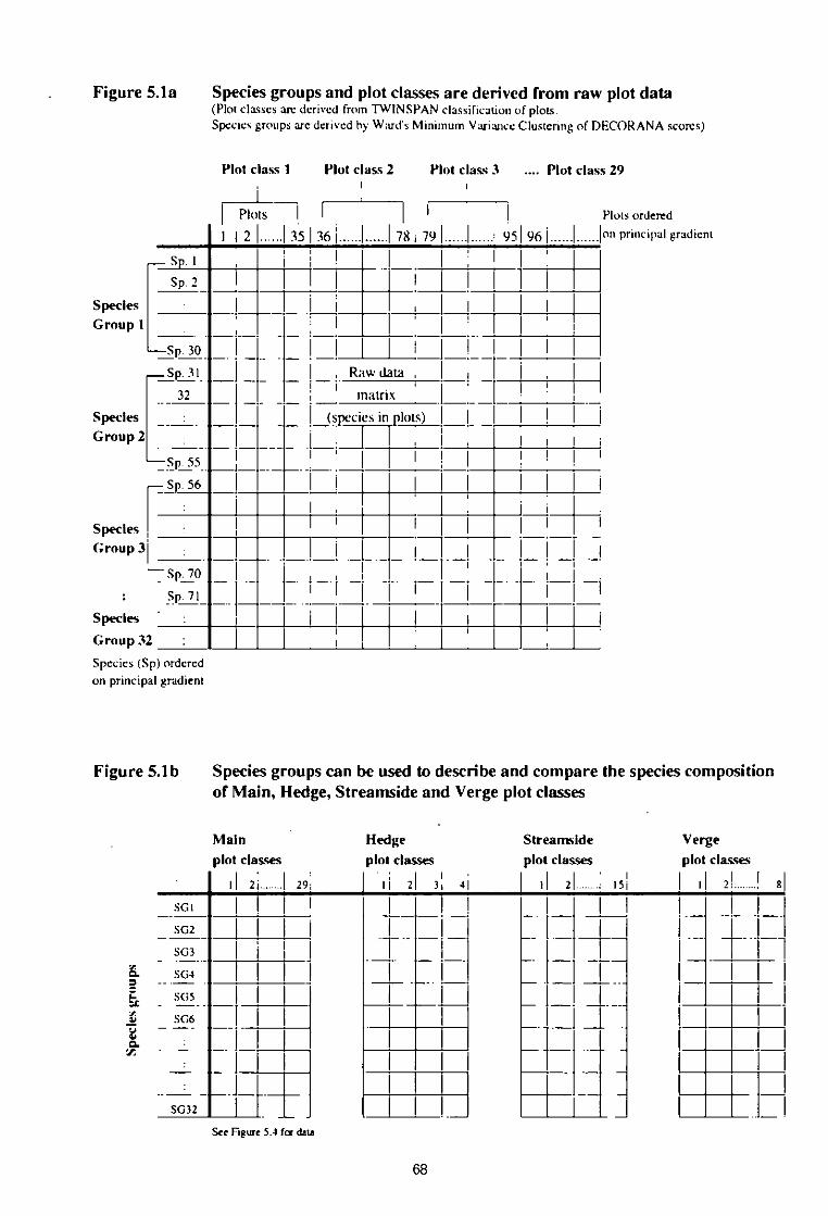
Figure 5.1a Species groups and plot classes are derived from raw plot data(Plotclasses arc derived from TWINSPAN classification of plots.

Species groups arc derived by Ward's Minimum Vari allce Clustering of DECORANA scores)

Plot class 1 Plot class 2 Plot class 3 .... Plot class 29

1Plots11.1I1I I 2 11 351361 1 178i 791 95 961

S . lI1Sp. 21 1

Plots ordered

Ion principal gradient

Figure 5.1b Species groups can be used to describe and compare the species compositionof Main, Hedge, Streamside and Verge plot classes

32 inatrix

(speciesin plots)Species

Group 2

Sp 55

Species ,

Group31

Sp. 71_

Species

Group 32 :

Species (Sp) ordered

on principal gradient

Species

Group 1

Sp. 30

—Sp. 31

I I Rawdata

6.5

tt

g.

SG32

See Figure 5.4 fordata

Main

plot classes

I 2j 29

SG I

SG2

503

SC4

SG5

SC6

Hedge

plot classes

II 21 3 al

1 1

11

68

Streamside

plot classes

Verge

plot classes

1

I

2 • 151 d 21 8

I I

I

I I

I_____,

--I I

I

I I

I

I

I_

Ii

__

plants are declining in road verges as wellas in the fields (Main plots)

5.1.6 The data have also been analysed toinvestigate change using mean number ofspecies and mean number of speciesgroups as measures of diversity. Thenumber of species in a plot may change fora number of reasons: for example.disturbance may lead to patches of bareground which allow colomsation by weedspecies. thus increasing the number ofspecies preseni A better understandingcan be gamed by considering the types ofspecies which are increasing ordecreasing. through the analysis of speciesgroups. The use of change in mean speciesnumber as a measure of diversity is alsomuch more sensitive to inaccuracies inrecording than the use of plot classes orspecies groups - for this reason, analysis ofchange in terms of species numberconsiders only those species which canconfidently be regarded as consis:ently

recorded - referred to as 'Category 1species' (see Section 2321 and Appendix 2)

5.2 Main plots

Vegetation classification

5.2.1 Plant species and cover estimates wererecorded from five randomly placed,200 m2 plots in each 1 1cmsquare Theseare referred to as 'Main plots', to distinguishthem from other randomly placed plots inparticular situations, eg roadsides. Thepurpose of the Math plots was to sample themain land cover types. ie agricultural fields.woodland, and moorland Since these plotswere located randomly they arerepresentative of the range of vegetation inthe survey squares.

5.2.2 A total of 2534 Main plots were recordedfrom 507 1km squares throughout GB (oneof the 508 survey squares was completelybuilt up in 1990). In order to describe this

Table SI Bnef descnphons of the 29 maul plot classes denved from the "IWNSPAN analysis of the Mari plots recorded in 1975 and1990. together with:he three species which show the greatest degree of preference to each class according to their frequency in thatclass, as opposed to the frequency in the other classes (Some classes had fewer than three preferential species) Plot classes (exceptsalLmarsh) are ordered on ;he princ:pal gradient (derived from DECCRANA). from I. 'Intens:ve - hugh nutrient status' to 29. 'extensive- low nutnen; status'

Warnplot class Description Characrnsnc species

MYC1 SaltrnarshARABLE FIELDSMPC2 Arable A (almost weed-free cereals)MPC3 Arable B (scattered weeds in mixed crops)MPO4 Arable C (mainly grammaceous weeds in cereals)MPC5 Arable D (broacLeaved weeds :n mixed crops;MPC6 Arable E (nuxed weeds in cereals)MDC7 Arable F (weedy leystunder-sown cereals)LOWLAND IMPROVED GRASSLANDMIPC8 LeysMPC9 Intensive grass - weedsMPCIO Rye grasslandMPC1 improved pasture?VIC 12 improved grassland + cloverLOWLAND SEMI-IMPROVED GRASSLANDMPC13 Senn-improved neutral grasslandMPC14 Neutral grasslandMPCIS Semi Improved pastureMPC16 Unimproved neutral/acid pastureWOODLANDMIPC17 Open broacLeaved secondary woodlandMPC113 Basiphilous broadleaved woodlandMDC IS Acid woodlandMPC20 Acid scrubMPC21 Suka plantahonUPLAND GRASS MOSAICSMPC22 Upland grassland diverseMPC23 Marshy upland grassMPC24 AcId grass/heath/woodMPC25 Upland grass/hea:hMOORLANDMPC26 Boggy moorlandMPC27 MoorlandMPC2E3 Dwarf shrub heathMPC29 Bog

Aster tnpolium. Suaeda manuma. Pus-melba manUma

NoneFallopia convolvulus, Polygonurn aocularc, Viola arycnsisAvena fatua. Alopecums myosuroxies BromusSeneno vulgans. Polygonum ancularc. Stellana mediaPolygonum at/mu/are, Stellana media, Poa annuaCapsclla bursa-pastons. Stellana media. Polygonum ann.:fare

Loburn perenne, Trifolium repensLolmm perenne. Plantago major. Stellana mediaLobum percnne, Rumex obtusifobus Tnfoburn repensAgrosus stolomfera. Cusiurn arverse Dactyl's glornerataLolturn perenne. nifoburn moors. Poa annua

Holcus lanatus. Loburn perenne. Tnfoburn repensCerasbum fcntanum. ?Woburn repens. Lot urn percnnePlantago lanceolata, Dactylis glomerata. Achillea malefoburnCorasburn fontanum. Holcus lanatus. Rumex acetcsa

Uruca (hoc& Arrhenathenen elauus, Crataegas monogynaCrataegus monogyna. Fraaanus excelsior, Unica dicicaOxalis acelosella, Ptendiurn aquilinurn, DigitaiispurpurcaPtendiurn aquilinum, Sorbus aucupana. Ilex agmfoliumNone

Lotus comiculatus Plantago lanceolata. Anthoxanthurn odora turnluncus ethisus. Pctentllla crecta. Anthoxanthum odoraturnGelatin saxatile. Potentilla emcta, Blechnum spicantGahum saxable, restuca onna. Deschampsia flexuosa

Nar dus stricta. Enca tetralix. Molima caerulea1/act:in:urn rnyrullus, Deschampsta IlexuosaVaccuvurn myrtillus, Deschampsia Dextiosa, Calluna vulgansErica tctralix. Tnchophorum cospnosurn. Calluna vulgans

69

vegetation. the species data from all theseMain plots (plus data from Main plotsrecorded in 1978) have been classified usingthe multivariate statistical technique,TWINSPAN,to create 29 'Main plot classes'(MPCs). These have been given shortdescriptive names to aid presentation of theresults, but it should be remembered thatthe definition of the plot classes may notcorrespond entirely with the more generalusage of these names. A total of 29 classeswas chosen as being a suitable level of detailfor the purposes of this repon: they could befurther subdivided for more detailedanalysis.

5.22 The plot classes were ordered, as shown inTable 5.1, according to their 'relativepositions on the principal gradient (derivedfrom the multivariate statistical technique.DECORANA). The order has beenmterpreted in terms of a gradient from highintensity of management (eg in arable fields)to low intensity (eg in upland vegetation).The woodlands however, occur throughoutthis gradient and they have been groupedtogether in Table 5 1 and subsequentFigures (but retaining their respective order,one to another), as an aid to interpretation.

Main plots: stock in 1990

5.2.4 Figure 52 shows how the Main plotsrecorded in 1990 were distributed betweenthese 29 Main plot classes. in the fourlandscape types.

5.2.5 In the arable landscapes. the most abundantplot clacses were those associated witharable fields and improved grass; there wasalso a small number of plots in woodlandThe more upland classes which includedmoorland and bog were mainly from landimmediately adjacent to arable areas in6cotland

5.2.6 Six classes of vegetation have beenidentified associated with arable crops. Inthe arable landscapes. classes 'Arable C'(MPC3 - mainly graminaceous weeds incereal fields) and 'Arable E' (MPC6 - mixedweeds in cereal fields) were most abundant,compared to the pastural landscapes wherethere was a more even spread over the sixclasses.

5.2.7 The pastural landscapes were dominated bygrasslands, but also included examples ofmost other plot classes. Previously themarginal upland landscapes have beenthought of as having the most diverse

landscapes, but Figure 5 2 shows that, interms of plot classes, the lowlandlandscapes have a greater variety: thepresence of upland vegetation was largelyfragments of acid grass and moorlandremaining in lowland classes

5.2 8 The vegetation of the marginal uplandlandscapes fell into two distinct groups: theupland grass/moorland and the lowlandgraSsland The spatial proximity of thesetwo habitats is important. eg in providingbird species with roosung and feedinggrounds respectively.

5 2.9 The upland landscapes were dominated bymoorland, and were least diverse in thatthey contain large areas with few plotclasses. Woodlands recorded includedboth conifer plantations and native woods.The small area of improved grassland waslargely associated with crotling townships.

Main plots: change between 1978 and 1990

5.2 10 A total of 1203 Main plots, from 248 1 lcmsquares. was recorded in the same positionin both 1978 and 1990. Data from thesepairs of plots were used here to considerhow the vegetation changed over thisperiod.

5 2 11 There are two scales of change observablefrom the plot data Fast, there is the grosschange which follows a change in land use.for instance following the ploughing of oldpasture Second, there is a more subtlechange in quality within the land cover type,as detected by a gradual loss of species

5.2.12 The extent of the gross changes is mostreliably derived from the land covermapping. as presented in Chapter 3.although vegetation plot data may provideadditional insights (as discussed brieflybelow - section 5.2.13 onwards).However, the vegetation plot data aloneprovide information on more subtlechanges in quality (as discussed in 5.2.19).

Main plots: gross change in vegetation

5 2 13 In order to consider gross change. the 29plot classes have been aggregated into sixbroad categories: 'arable fields' (classesMPC2-MPC7); 'lowland improvedgrassland' (MPC8-MPC12) ; 'lowland semi-improved grassland' (MPC13-MPC I6);'woodland' (MPCI7-MPC21); 'upland grassmosaics' (MPC22-MPC25): and 'moorland'

70

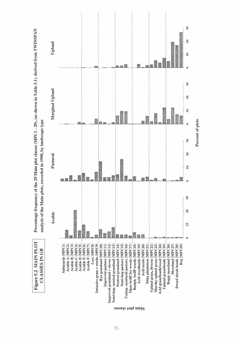
Fig

ure

5.2

MA

INP

LO

TP

erce

ntag

efr

eque

ncy

ofth

e29

Mai

npl

otcl

asse

s(M

PC

1-

29),

(as

show

nin

Tab

le5.

1),

deriv

edfr

omT

WIN

SP

AN

CL

ASS

ES

ING

Ban

alys

isof

the

Mai

npl

ots,

reco

rded

in19

90,

byla

ndsc

ape

type

Ara

bic

Pas

tora

lM

argi

nal

Upl

and

Upl

and

Sal

tmar

sh(M

PC

I)

I•

Ara

ble

A(M

PC

2)M

il•

Ara

ble

C(M

PC

4)tE

llig•

SI

IA

rabl

eB

(MP

C3)

la

Ara

ble

I)(M

PC

5)_M

I

MI

Ara

ble

E(M

PC

6)-,

-tin

7),

—1•

S

Ara

ble

F(M

PC

7)II

EN

IMLe

ys(M

KS

)1

Inte

nsiv

egr

ass

+w

eeds

(MP

C9)

•I••

•

Rye

gras

slan

d(M

PC

10)

inn

team

Imp

rov

edpa

stur

e(M

PC

II)

EN

•

Impr

oved

gras

slan

d+

clov

er(M

PC

12)

allii

cnS

emi-i

mp.

neut

ral

gras

slan

d(M

PC

13)

•z

Neu

tral

gras

slan

d(M

PC

14)

•—

OM

—A 11

3S

emi-i

mp

past

ure

(MP

C15

)•

77,

Uni

mp.

neut

/aci

dpa

stur

e(M

PC

16)

•ii•

IsO

pen

brdl

f2r

yw

oods

(MP

C17

)I

Bas

iph.

brdl

fw

oods

(MP

C18

)R

N11

Ct.

c 73A

cid

woo

dlan

ds(M

PC

19)

•

)4A

cid

scru

b(M

PC

20)

•

I

Sitk

apl

anta

tion

(MP

C21

)_

Upl

and

gras

s,di

vers

e(M

PC

22)

i

LM

arsh

yup

land

gras

s(M

PC

2.3)

II

Aci

dgr

ass/

heat

h/w

ood

(MP

C24

)i

Upl

and

gras

s/he

ath

(MP

C25

)I

11

1B

oggy

moo

rland

(MP

C26

)

Moo

rland

(MP

C27

)I

Dw

arf

shru

bhe

ath

(MP

C28

)i

Bog

(MP

C29

)I

010

2030

010

2030

010

2030

010

2030

Per

cent

ofpl

ots

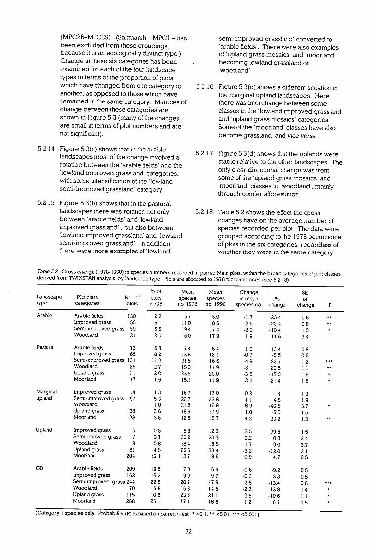
(MPC26-MPC29). (SaItmarsh - MPC1 - hasbeen excluded from these groupings,because it is an ecologically distinct type )Change in these six categories has beenexamined for each of the four landscapetypes in terms of the proportion of plotswhich have changed from one category toanother, as opposed to those which haveremained in the same category Matrices ofchange between these categories areshown in Figure 51 (many of the changesare small in terms of plot numbers and arenot significant).

5.2.14 Figure 5.3(a) shows that in the arablelandscapes most of the change involved arotation between the 'arable fields and the'lowland Improved grassland- categories.with some intensification of the 'lowlandsemi-improved grassland' category.

5215 Figure 5 3(b) shows that in the pasturallandscapes there was rotation not onlybetween 'arable fields' and 'lowlandimproved grassland' . but also between'lowland improved grassland' and 'lowlandsemi-improved grassland' In addition.there were more examples of 'lowland

semi-improved grassland' converted to'arable fields' There were also examplesof 'upland grass mosaics' and 'moorland'becoming lowland grassland orwoodland'

5 2.16 Figure 5 3(c) shows a different situation inthe marginal upland landscapes Herethere was interchange between someclasses m the lowland improved grassland'and 'upland grass mosaics' categoriesSome of the 'moorland' classes have alsobecome grassland, and vice versa.

5.2.17 Figure 5.3(d) shows that the uplands werestable relative to the other landscapes. Theonly clear directional change was fromsome of the 'upland grass mosaics- and'moorland' classes to 'woodland', mainlythrough conifer afforestation

5 2 18 Table 5 2 shows the effect the grosschanges have on the average number ofspecies recorded per plot The data weregrouped accordmg to the 1978 occurrenceof plots in the six categories, regardless ofwhether they were in the same category

Table 5 2 Cross change (1978-1990) in species nurnbers recorded in paired Main plots. within:he broad categones of plot classesdenved from TWINSPAN analysis by landscape type Plots are allocated to 1978 plot categones (see 5 2 :8)

VoofMeanMeanChangeLandscapeP:ct classNo ofb.:2sspeciesspec:esin mean%typecategonesplotsLn CBno 1978no 1990species nochange

SE of

change

AmbleArable fields13012 25 7 5 0 -I 7 -25 4 0 5 4

Improved grass555 111 0 8 5 -2 5 -22 4 0 8 ••Semiamproved grass595 519 4 17 4 -2 0 -10 4 I 0

Woodland212 016 0 17 9 I 9 11 6 3 4

PasturalArable fields736 87 4 8 4 I 0 13 4 0 9

Improved grass as 8 212.8 121 -0 7 -5 5 0.6

Semi-improved grass 12111 321 5 16 6 -4 9 -22 7 1 2 •••

Woodland292 715 0 11 9 -3 1 20 5 II let

Up:and grass212 023 5 20 0 -3 5 -15 0 1 6

Moorland171.615 1 II 9 -3 2 -21 4 1 5

Marginalimproved grassII1 316 7 17 0 0 2 I 4 I 3

uplandSemi-Improved grass575 322 7 23 8 11 4 8 I 9

Woodland11I 021 8 12 9 -8 9 -40 8 3 7

Upland grass383 618 9 !T 9 -1 0 -5 0 I 5

Moorland383 612 5 16 7 4 2 33 2 I 3 I! •

UplandImproved grass5.0 58 8 12.3 3.5 39 6 I 5

Sermamroved grass70.720 2 20.3 0.2 0 8 2.4

Woodland90 818 4 15 8 -1.7 -9 0 3.7

Upland grass514 826.6 23.4 -3.2 -12.0 2.1

Moorland20419.118.7 19 6 0 9 4.7 0.5

CBArable fields20919.67 0 6.4 -0 6 -9.2 05

Improved grass16215.29 9 9 7 -0 2 -2.3 0 5

Sernamproved grass 24422.820.7 17.9 -2.8 -13.4 0 6 11111

Woodland706 616 8 14 5 -2.3 -13 8 I 4 •Upland grassI 1510 823.6 211 -2.5 -10 6 II

Moorland26825.117 4 18 6 1.2 6.7 0.5

(Category I species onlyProbability (P) is based on paired taest <0 1. " <001. ••• <0 001)

72

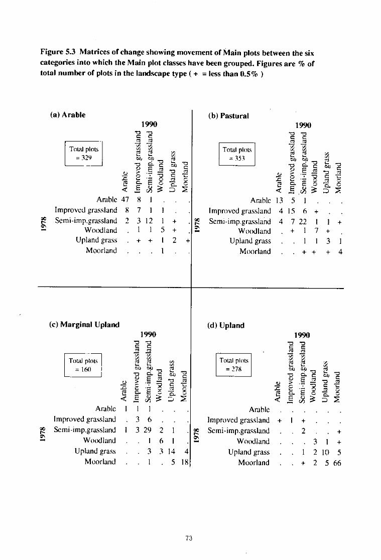
Figure 5.3 Matrices of change showing movement of Main plots between the sixcategories into which the Main plot classeshave been grouped. Figures are % oftotal number of plots in the landscape type ( + = less than 0.5% )

(a) Arable (b) Pastural

Total plots

= 329

Arable

Improved grassland

Sem i-imp.grassland Woodland

Upland grass

Moorland

1990

a a a ate: tr.;4 te

SL. I-014 S

.E .c 2 g-tt E ôD47 8 I

8 7 I I .

2 3 12 I +1 1 5 +

I 2

. 1 .

Arable

Improved grassland

Semi-imp.grasslandWoodland

Upland grass

Moorland . . +

Total plots

= 353

1990

a a

'ErbC.)

2 - C. E3

13 5 1 .

4 IS 6

4 7 22 I I + 1 7

1 1 3 I

4

.ct_

(c) Marginal Upland

[

Total ploIsi

= 160 I

- §1

Arable I

Improved grassland

Semi -imp.grassland 1

Woodland

Upland grass

Moorland

1 1

3 6 . .

3 29 2 1 OC

.161

• 3 3 14 4

. 1 . 5 18

(d) Upland

Total plots

= 278

Arable

Improved grassland

Semi-imp.grassland

Woodland

Upland grass

Moorland

1990va-aa a

ClV! V;

C.41CE>

E cE

+ . . .

2 . . +

3 I +I 2 ID 5

2 5 66

73

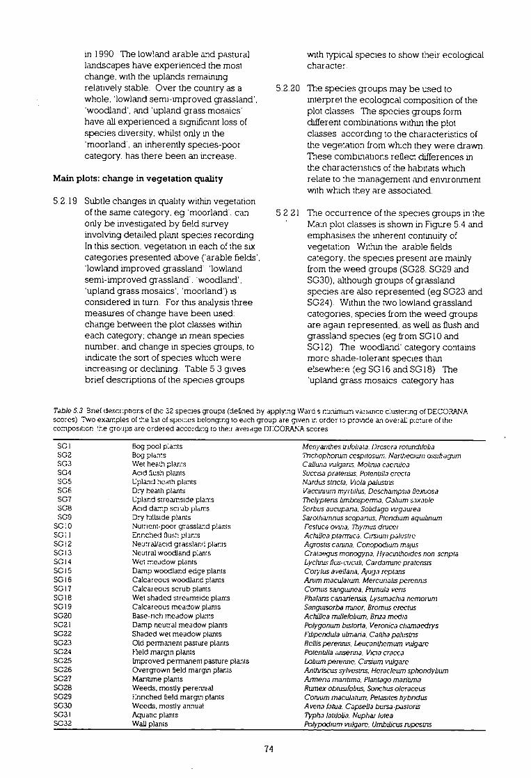
in 1990. The lowland arable and pasturallandscapes have experienced the mostchange, with the uplands remainingrelatively stable. Over the country as awhole, 'lowland semi-improved grassland'.'woodland', and 'upland grass mosaics'have all experienced a significant loss ofspecies diversity, whilst only in the'moorland-. an inherently species-poorcategory. has there been an increase.

Main plots: change in vegetation quality

5.2.19 Subtle changes in quality within vegetationof the same category. eg 'moorland. canonly be investigated by field surveyinvolving detailed plant species recording.In this section, vegetation in each of the sixcategories presented above ('arable'lowland improved grassland"lowlandsemi-improved grassland. 'woodland'.'upland grass mosaics'. 'moorland') isconsidered in turn For this analysis threemeasures of change have been used:change between the plot classes withineach category; change in mean speciesnumber: and change in species groups, toindicate the sort of species which wereincreasing or declining. Table 5.3 givesbrief descriptions of the species groups

with typical species to show their ecologicalcharacter

5.2.20 The species groups may be used tointerpret the ecological composition of theplot classes. The species groups formdifferent combinations within the plotclasses according to the characteristics ofthe vegetation from wh:ch they were drawn.These combinations reflect differences inthe characteristics of the habitats whichrelate to :he management and environmentwith which they are associated

5.2 21 The occurrence of the species groups in theMath plot classes is shown in Figure 5.4 andemphasises the inherent continuity ofvegetation Within the arable fieldscategory, the species present are mainlyfrom the weed groups (5G28. SG29 and5G30), although groups of grasslandspecies are also represented (eg 5G23 andSG24). Within the two lowland grasslandcategories, species from the weed groupsare again represented, as well as Cush andgrassland species (eg from SGIO andSG12). The woodland' category containsmore shade-tolerant species thanelsewhere (eg SGI6 and SG18). The'upland grass mosaics- category has

Table 5.3 Bnef descrpnons of the 32 species groups (defined by applying Ward s minimum variance dustering of DECORANAscores) Two examples of the tst of spedes belonging to each group are given in order to provide an overall purture of thecomposition dne groups are ordered according to their ay/alage DI:CORA-NA scores

SCI502503SG4505SG6507508SO9SCIOSGIISGI2SGI3SGI4SC155016SGI7501850195020502150225023SC24SC2550255027502850295030 &331 B332

Bog pool p'.antsBog plantsWet heath plantsAcid 5ush plantsUpland heath plantsDry heath plantsUpland streamside plantsAcid damp sclub plantsDry hillside plantsNutrient-poor grassland plantsEnriched flush plantsNeutral/acid grassland plantsNeutral woodland p:antsWe; meadow plantsDamp woodland edge plantsCalcareous woodland plantsCalcareous scrub plantsWet shaded sireamside plantsCalcareous meadow plantsBase-rich meadow plantsDamp neutral meadow plantsShaded wet meadow plantsOld permanent pasture plaixsMeld margin plainsImproved permanent pasture plantsOvergrown field margin plantsMaritme plantsWeeds, mostly perengalEnnched field margli plantsWeeds. mostly annua!Aquatic plantsWall plants

Menyanthes ulfoliata Drosera rotund ilobaThchophorurn cespnosunt Narthecium assitragumCalluna yulgarts. Moltma caendeaSuccisa pratensm. Potenulla erect'?Nardus stncta. Viola palustrzsVaccimurn myrullus. Descharnpsia flexuosaThelypteris lunbosperma, Ca/Jam saxatileSorbus aucupana Solidago VII gaureaSatothanmus scopanu.s. Ptendium aguilinumrestuca ovina, Phymts MucciAchillea ptarrivcit °maim palustreAgrostis canina Conopothurn mazusCrataegus monogyna, ilyacinthoides non seriptaLychnis Cardamum pratensisCorylus avellana, kuga reptansArum maculatum. Mercunahs percnrusComus sanguinea, Primula yensPhalans canariensis, Lysunachia nemorurnSanginsorba minor, Bromus ereausAchillea mtheloburn, Bnza mediaPolygonum bistona, Veronica chamaedrysFllipendula uimaria, Caltha palustnsRelfis perennts, Leucanthemum vulgar°Potentilla anserina, Vicia cracraLoburn perenne, CirOurn vutgareAnthhscus sylvestris. Heracleum sphondyburnArrnena manuma. Plantago maritunaRurnex obtusifobus, Sonchus oleraccusConiurn maculation, Petasites hybnclusAvena latua. Capsella bursa -pastorisTypha latilolia. Nuptial luteaPolypodium vulgare, Umbilicus nipestris

74

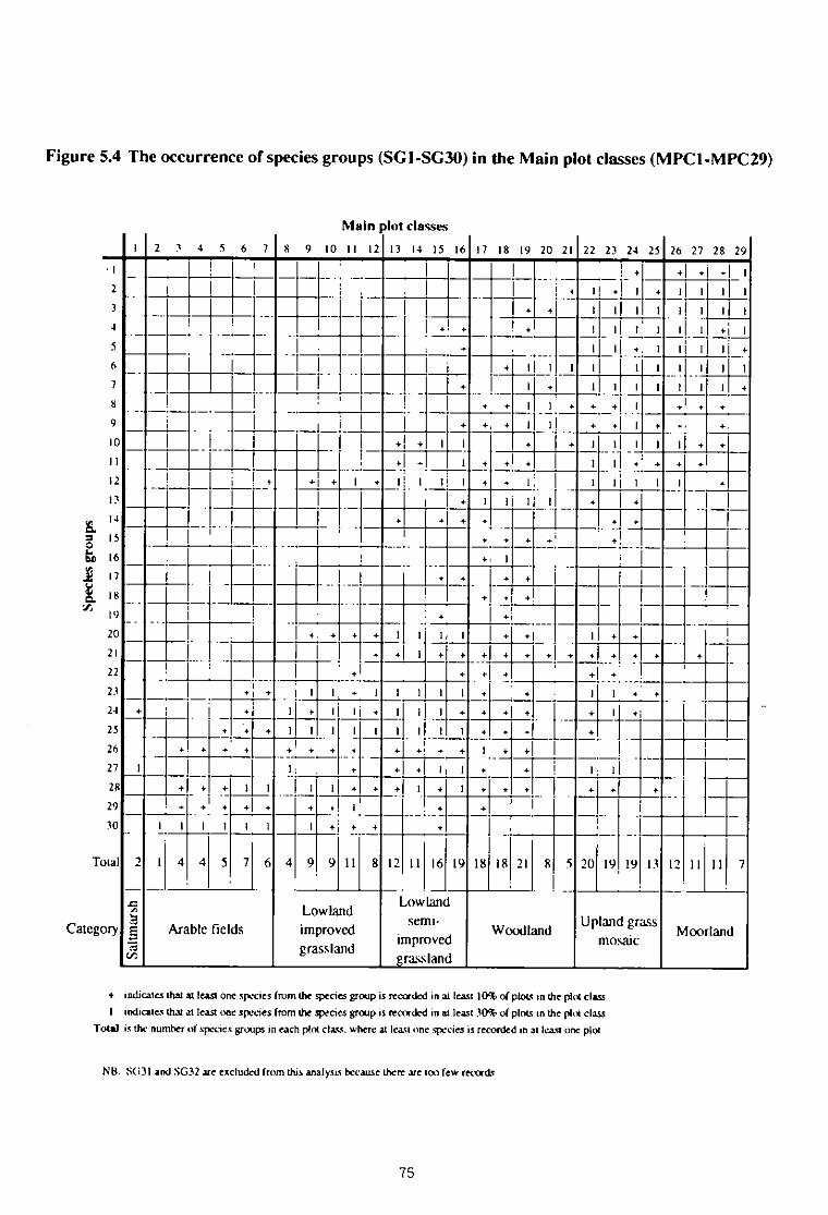
Figure 5.4 The occurrence of species groups (SCI-S630) in the Main plot classes (MPCI-MPC29)

i 2 3 45 6 7 8

2

1

3

4

5

6 _

7

8 .

9

I o

I

II

12

13

14

15

16

17

18

19

20

21

22

23

.24 •

I

25

+ I

26

•

4.

27 I

1

29

• • •

30

I I I 1 I I

Total 2 1 4 4 5 7 6 4

Category

Arable fields

18192021 22 232425 2627 2829

• + +1 1

4 1! •

1 I 11I

• •I

II III I 1 II1

•11

t 11 II ;

;

;H. I I ii ;

;

; t

11 ;

1 +1

11

1 1 I I+

+

I

+ + 1 1

• • 4-

+ I II • • 1 + •

• I • 1 I II I I • •

•_......__,• I 1 1 +

„I

1: I 1 ii 11 I

11'11 .

•

I I

Alainplot classts

9 10 II 12 13 14 15 16 17

1 •-

t + d t

•• ,

. •

• •• • • iI

1

+1 • • • • +1 •_ •••. _

I I • 1 1 1 I I I •.

I I • I I I I • •

I 1

•

•

9

Woodland

•

•

Lowland improved grassland

9 II

•

•

11

18 12 II 16 19 18 18

Lowlandsemi-

improvedrassland

1 1 II 1 I • •

+I I 1 •

11 1 • • •

+ •

11 8

1 • •

It • I I

5 20 19

ti

19 13 12 I I II 7

Upland grassMoorland

mosaic

indicates that at least one species (aim the species group is recorded in at least 10% of plots in the plot class

1 indicates that at least one species from the species group is recorded in at least 30% of plots in the plot class

Toial is the number of speciesgroups in each plot class,where at least one species is recorded in at le.1:4 one plot

NB. 5031 and 5G32 are excluded from this analysis because there age too few records

75

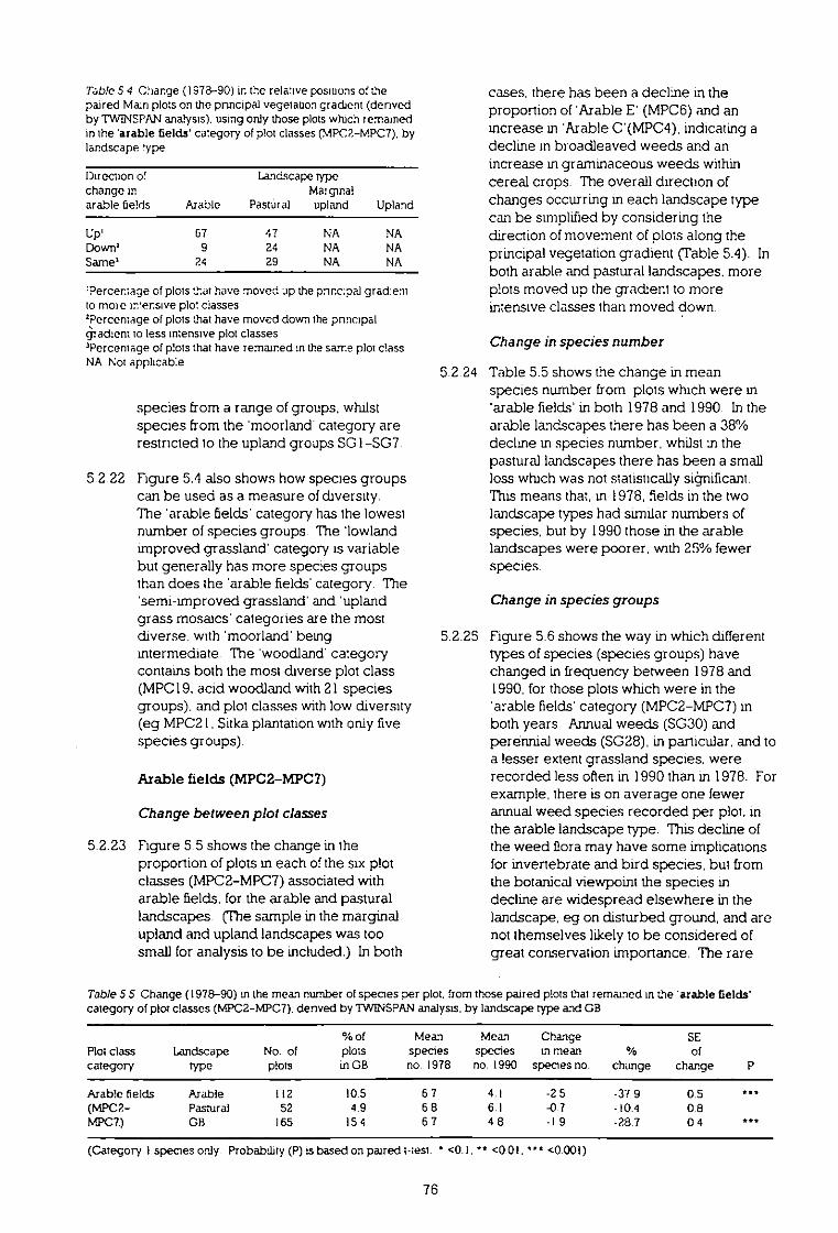
Table 5 4 Change (1978-90) in the relanve positions of thepaired Main plvs on the pnncipal vegetation gradient (derivedby TWNSPAN analysis). using only those plots which remainedin the 'arable fields category of plot classes (MPC2-MPC7). bylandscape type

Direction ofchange in

Landscape typeMargmal

arable fields Arable Postural upland Upland

Up' 67 47 NA NADown' 9 24 NA NASame' 24 29 NA NA

'Percentage of plots tug have moved up the pnnc:pal grad:entto more intensive plo: classes'Percentage of plots that have moved down the pnncipalgradient to less intensive plot classes'Percentage of plots that have remained m the same plot classNA Not applicable

species from a range of groups, whilstspecies from the 'moorland category arerestricted to the upland groups SG1-SG7.

5.2.22 Figure 5.4 also shows how species groupscan be used as a measure of diversity.The 'arable fields' category has the lowestnumber of species groups. The 'lowlandimproved grassland' category is variablebut generally has more species groupsthan does the 'arable fields' category. The'semi-improved grassland' and 'uplandgrass mosaics' categories are the mostdiverse. with 'moorland' beingintermediate. The 'woodland' ca:egorycontains both the most diverse plot class(MPC19, acid woodland with 21 speciesgroups). and plot classes with low diversity(eg MPC21. Sitka plantation wnh only fivespecies groups).

Arable fields (MPC2-MPC7)

Change between plot classes

5.2.23 Figure 5.5 shows the change in theproportion of plots in each of the six plotclasses (MPC2-MPC7) associated witharable fields, for the arable and pasturallandscapes. (The sample in the marginalupland and upland landscapes was toosmall for analysis to be included.) ln both

cases, there has been a decline in theproportion of 'Arable E' (MPC6) and anincrease in 'Arable C'(MPC4). indicating adecline in broadleaved weeds and anincrease in graminaceous weeds withincereal crops. The overall direction ofchanges occurring in each landscape typecan be simplified by considering thedirection of movement of plots along theprincipal vegetation gradient (Table 5.4). Inboth arable and pastural landscapes. moreplots moved up the gradient to moreintensive classes than moved down.

Change in species number

5.2 24 Table 5.5 shows the change in meanspecies number from plots which were in'arable fields' in both 1978 and 1990 In thearable landscapes there has been a 38%decline in species number. whilst in thepastural landscapes there has been a smallloss which was not statistically siignificant.This means that, in 1978, fields in the twolandscape types had similar numbers ofspecies, but by 1990 those in the arablelandscapes were poorer, with 25% fewerspecies.

Change in species groups

5.2.25 Figure 5.6 shows the way in which differenttypes of species (species groups) havechanged in frequency between 1978 and1990. for those plots which were in the'arable fields' category (MPC2-MPC7) inboth years. Annual weeds (SG30) andperennial weeds (SG28). in panicular, and toa lesser extent grassland species, wererecorded less often in 1990 than in 1978. Forexample, there is on average one fewerannual weed species recorded per plot, inthe arable landscape type. This decline ofthe weed fiora may have some implicationsfor invertebrate and bird species, but fromthe botanical viewpoint the species indecline are widespread elsewhere in thelandscape. eg on disturbed ground, and arenot themselves likely to be considered ofgreat conservation importance. The rare

Table 5 5 Change (1978-90) in the mean number of species per plot, from those paired plots that remained in the 'arable fields'category of plot classes (MPC2-MPC7). derived by TW1NSPAN analysis. by landscape type and GB

% of Mean MeanPlot class Landscape No. of plots species speciescategory type plots in CB no. 1978 no. 1990

Arable fields Arable 112 10.5 6.7 4.1(MPC2- Pastural 52 4.9 6 8 6.1MSC7.) GB 165 15 4 6.7 4 8

(Category I species only. Probability (P) is based on paired mest. • <0.1. " <0.01.

Change SEin mean % of

species no. change change P

-2 5 -37 9 0.5 •••

-0.7 -10.4 0.8

-1 9 -28.7 0 4 St* 2

"* <0.001)

76

Fig

ure

5.5

MA

INP

LO

TC

LA

SS

ES

IN

AR

AB

LE

FIE

LD

S

Cha

nge

Inth

efr

eque

ncy

ofth

esi

xM

ain

plo

t cla

sses

(MP

C2

-7),

(der

ived

from

TW

1NS

PA

Nan

alys

isof

the

Mai

npl

ots)

,fr

omth

e'm

able

field

s'ca

tego

ry,

usin

gon

lyth

ose

plot

sw

hich

wer

ein

the

sam

eca

tego

ryin

both

1978

and

1990

,by

land

scap

ety

peo

1978

Ca

1990

Ara

ble

Pas

tura

lM

argi

nal

Upl

and

Upl

and

Ara

ble

E(M

PC

6)

Ara

ble

F(M

PC

7)

Insu

ffici

ent

data

to

prod

uce

natio

nal

estim

ates

4060

8010

0

1. 020

4060

8010

0020

4060

8010

00

2040

6080

100

Ara

ble

A(M

PC

2)

Ara

ble

B(M

PC

3)

Ara

ble

C(M

PC

4)

a. 1A

rabl

eI)

(MP

CS

)

Num

ber

ofpl

ots

[Fig

ure

5.6

SPE

CIE

SG

RO

UPS

INA

RA

BL

EFI

EL

DS

Cha

nge

inth

em

ean

num

ber

ofsp

ecie

sfo

rea

chof

the

11sp

ecie

sgr

oups

(Tab

le53

)ch

arac

teris

ticof

'ara

ble

field

s'

(MP

C2

-7)

,by

land

scap

ety

pean

dus

ing

only

thos

epl

ots

whi

chw

ere

inth

esa

me

cate

gory

inbo

th19

78an

d19

90

Ara

ble

Pas

tura

lM

argi

nal

Upl

and

Upl

and

Neu

tral

/aci

dgr

a%la

ndpl

ants

(561

2)

Bus

e-ric

hm

eado

wpl

ants

(562

0)

Dam

pne

utra

lm

eado

wpl

ants

(5al

)

Sha

ded

wet

mea

dow

plan

ts(S

622)

EL.

Old

perm

anen

tpa

stur

epl

ants

(S(;

23)

t. et

Fie

ldm

argi

npl

ants

(562

4)

Insu

ffici

ent

data

to

prod

uce

natio

nal

estim

ates

Insu

ffici

ent

data

to

prod

uce

natio

nal

estim

ates

Impr

oved

perm

anen

tpa

stur

epl

ants

(562

5)

Ove

rgro

wn

field

mar

gin

plan

ts(5

626)

Wee

ds,

mos

tlype

renn

ial

ISC

210

Enr

iche

dfie

ldm

argi

npl

ants

(562

9)

Wee

ds,

mos

tlyan

nual

(563

0)

-1.6

-1.2

-0.8

-0.4

00.

40.

8-1

.6-1

.2-0

.8-0

.40

00.

40.

8-1

.6-1

.2-0

.8-0

.40.

00.

40.

8-1

.6-1

.2-0

.8-0

.40.

00.

40.

8

Cha

nge

Inm

ean

num

ber

ofsp

ecie

spe

rpl

ot

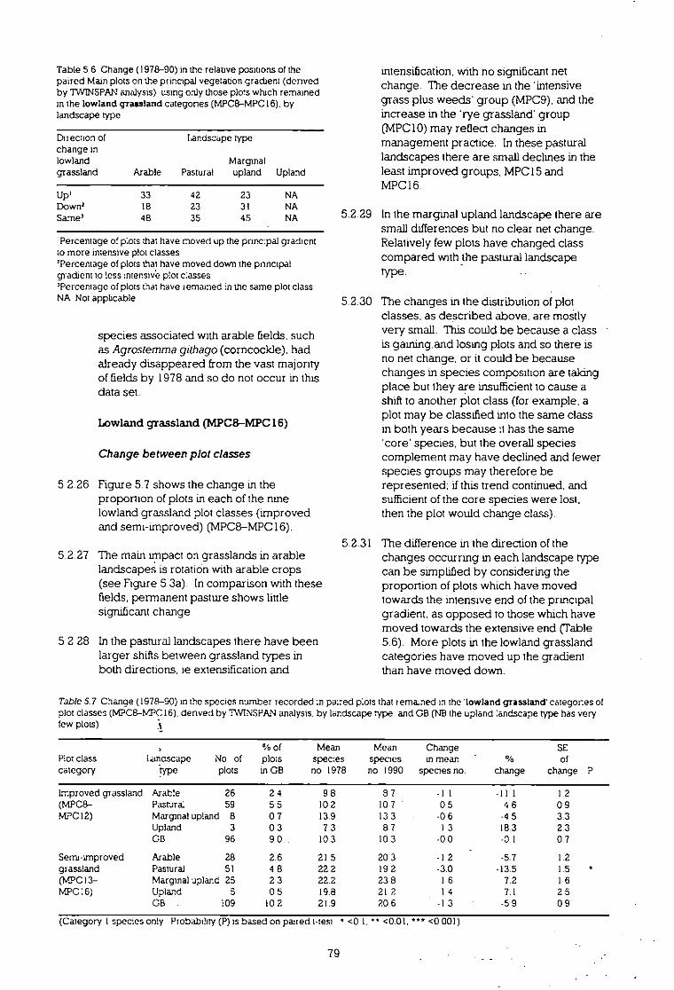
Table 5 6 Change (1978-90) in the relative positions of thepaired Main plots on the principal vegetaton gradient (derivedby TW1NSPAN analysis) using only those plots which remainedin the lowland grassland caregones (MPC8-MPC16). bylandscape type

Diiection of landscape typechange inlowland Marginalgrassland Arable Pastural upland Upland

Up' 33 42 23 NADown' 18 23 31 NASame' 48 35 45 NA

'Percentage of plots that have moved up the pnncipal gradientto more intensive plot classes'Percentage of plots that have moved down the pnncipalgradent to less mtensive plot ciasses'Percentage of plots that have remained in the same plot classNA Not applicable

species associated with arable fields, suchas Agrostemma githago (corncockle), hadalready disappeared from the vast majorityof fields by 1978 and so do not occur in thisdata set.

Lowland grassland (MPC8-MPC 16)

Change between plot classes

5 2 26 Figure 5 7 shows the change in theproportion of plots in each of the ninelowland grassland plot classes (improvedand semi-unproved) (MPC8-MPC16)

5.2.27 The main unpact on grasslands in arablelandscapes is rotatiOn with arable crops(see Figure 5.3a). In comparison with thesefields, permanent pasture shows littlesignificant change.

5.2.28 In the pastural landscapes there have beenlarger shifts between grassland types inboth directions, e extensification and

intensification, with no significant netchange. The decrease in the 'intensivegrass plus weeds group (MPC9). and theincrease in the 'rye grassland' group(MPC10) may reflect changes inmanagement practice. In these pasturallandscapes there are small declines in theleast improved groups, MPC15 andMPC16.

5.2.29 In the marginal upland landscape there aresmall differences but no clear net change.Relatively few plots have changed classcompared with the pastural landscaperYPe-

5.2.30 The changes in the distribution of plotclasses, as described above, are moStlyvery small. This could be because a class •is gaining.and losing plots and so there isno net change, or it could be becausechanges in species composition are takingplace but they are insufficient to cause ashift to another plot class (for example, aplot may be classified into the same classin both years because it has the same'core' species, but the overall speciescomplement may have declined and fewerspecies groups may therefore berepresented, if this trend continued, andsufficient of the core species were lost,then the plot would change class).

5.2.31 The difference in the direction of thechanges occurring in each landscape typecan be simplified by considering theproportion of plots which have movedtowards the intensive end of the principalgradient, as opposed to those which havemoved towards the extensive end (Table5.6). More plots in the lowland grasslandcategories have moved up the gradientthan have moved down.

Table 57 Change (1978-90) in the species number recorded :n paired p'.ots that iem&ned in the 'lowland grassland' categories ofplot classes (li4pC8-MIC16). denved by TWINSPAN analysis, by landscape Type and GB (NB the upland landscape type has veryfew plots)

% of Mean Mean Change

SEPiot class iiandscapeNo of plots spec:es species in mean

ofcategory plots in GB no 1978 no 1990 species no change changeP

Improved grassland Arable26 2 4 9 8 8 7 - II -111 I 2(MPC8- Pasrural59 5 5 10 2 10 7 0 5 4 6 0 9MPC12) Marginal uplandB 0 7 13 9 13 3 -0 6 -4 5 3 3

Upland3 0 3 7 3 8 7 I 3 18 3 2 3

GB96 9 0 10 3 10 3 -0 0 -0 1 0 7

Semuimproved Arable28 2.6 21 5 20 3 -1 2 -51 1.2grassland Pastural51 4 8 22 2 19 2 -3.0 -13.5 15•(MPC13- Marginal upland 25 2 3 222 23 8 1 6 7.2 1 6MPG :6) Upland 5 0 5 19.8 21 2 1 4 71 2 5

GB109 10 2 219 20 6 -I 3 -5 9 0 9

(Category 1 species only Probability (P) is based on paired titest • <0 I. •• <0 01. *" <0 001)

79

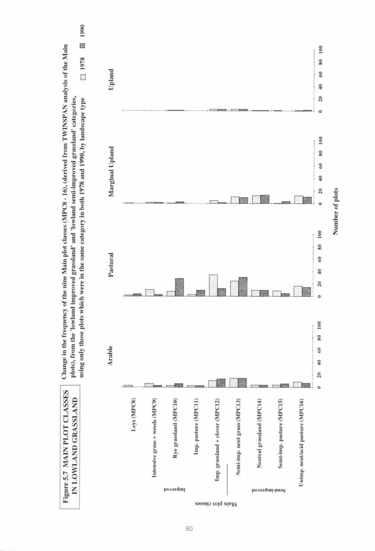
Fig

ure

5.7

MA

INP

LO

TC

LA

SSE

SC

hang

ein

the

freq

uenc

yof

the

nine

Mai

npl

otcl

asse

s(M

PC

8-

16),

(der

ived

from

TW

INS

PA

Nan

alys

isof

the

Mai

n

INL

OW

LA

ND

GR

ASS

LA

ND

plot

s),

from

the

'low

land

impr

oved

gras

slan

d'an

d'lo

wla

ndse

mi-i

mpr

oved

gras

slan

d'ca

tego

ries,

usin

gon

lyth

ose

plot

sw

hich

wer

eIn

the

sam

eca

tego

ryIn

both

1978

and

1990

,by

land

scap

ety

peE

l19

78•

1990

Ara

ble

Pas

tura

lM

argi

nal

Upl

and

Upl

and

I.

2040

6080

100

Num

ber

ofpl

ots

4060

8010

00

2040

6080

100

4060

8010

0

Leys

(MP

C8)

Inte

nsiv

egr

ass

+w

eeds

(MP

C9)

Rye

gras

slan

d(M

PC

10)

Imp.

past

ure

(MP

C11

)

Imp.

gras

slan

d+

clov

er(M

PC

12)

neut

gras

s(M

PC

I3)

k.N

eutr

algr

assl

and

(MP

C14

)

Sem

i-im

p.pa

stur

e(M

PC

I5)

Uni

mp.

neat

/aci

dpa

stur

e(M

PC

I6)

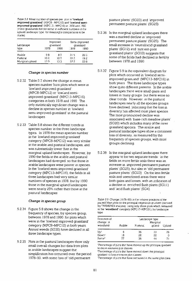
Table 58 Mean number of species per plot in lowlandimproved grassland' (MPC8 - MPCI2) and 'lowland semi-improved grassland (NTC13 - MPCI6) tr. :978 and 199C(these grasslands did not occur in sufficient numbers in theupland landscape type for mearungful comparsons to bemade)

lrnproved Semi-LmprovedLandscape grassliund grasslandtype 1978 1990 1978 1990

Arabte 9 8 8 7 21 5 20 3Pasatal 10 2 10 7 22 2 19 2Margmal upland 12 9 13 3 22 2 23 8

Change in species number

52 32 Table 5 7 shows the change in mean

species number from plots which were in'lowland improved grassland'(MPC8-MPC12) or 'lowland semi-

improved grassland' (MPC13-MPC 6)categories in both 1978 and 1990 The

only statistically significant change was adecline in species number in 'lowlandsemi-improved grassland' in the pasturallandscapes

52 33 Table 5.8 shows the differem trends in

species number in the three landscapetypes. In 1978 the mean species numberth the -lowland improved grassland'category (MPC8-MPC12) was very similarin the arable and pastural landscapes, andwas substantially lower than in themarginal upland landscapes. However, by1990 the fields in the arable and pasturallandscapes had diverged, so that those inarable landscapes were poorer in species.In the 'lowland semi-improved grassland'category (MPC13-MPC16). the fields in allthree landscapes had very similar

numbers of species in 1978. but by 1990those in the marginal upland landscapes

were nearly 25% richer than those in thepastural landscapes

Change in species group

5.2.34 Figure 5.8 shows the change in the

frequency of species. by species group,

between 1978 and 1990. for plots which

were in the 'lowland improved grassland'category (MPC8-MPC12) in both years.

Annual weeds (SG30) have declined in allthree landscape types.

5 2.35 Plots in the pastural landscapes show onlysmall overall changes but data from plotsin arable landscapes suggast tha:

simplification has occurred over the period1978-90. with some loss of 'old permanent

pasture plants' (SG23) and 'improved

permanent pasture plants' (SG25)

5.2.36 In the marginal upland landscapes there

was a marked decline in 'improvedpermanent pasture plants' (SG25). The

small increase in 'neutral/acid grassland

plants' (SGI2) and -nuthent-poorgrassland plants' (SG10) suggests that

some of the fields had declined in fertility

between 1978 and 1990.

5.2.37 Figure 5.9 is the equivalent diagram for

plots which occurred in 'lowland semi-improved grass:and' (MPCI3•MPC16) inboth years The three landscape typesshow quite different patterns. In the arablelandscapes :here were small gams andlosses in many groups but there were noclear trends However, in the pasturallandscapes nearly all the species groupshave declined: indicating that ;he loss in

diversity has affected most plant species.The most pronounced decline wasassociated with -base-rich meadow plants'(SG20) which includes many of the rarergrassland species. The arab:e and

pastural landscape types show a consistentloss of diversity. as measured by thefrequency of species groups, with mostgroups declining.

5.2.38 In the marginal upland landscapes thereappear to be two separate trends in thefields on more ferile sods there was anincrease in 'improved permanent pastureplants' (5G25), but also in 'old permanentpasture plants' (5G23) On the less fertilesoils and unenclosed areas there were

both gains and losses, with an indica:ion ofa decline in -enriched flush plants (SG 11)and 'acid flush plants' (5G4).

Table 5 9 Change (1976-90) m the relative poshons of thepazed Mam plots cr. the pnncipal vegetation trred.en: (derivedby TWLNSPANanalysis) using only those pots which remainedin :he 'woodland' category (MPC17-Na2C21). by landscapetype

Directon ofchange m

Lar.dscape typeMargit&

woodland Arable Pastural upand Upland

Up' 6 36 33 29DON712 .8 28 22 0Same' 77 36 44 71

'Percentage of plots that have moved up the pnr.cipai grarhentto more intensive pot classes'Percentage of pots that have moved down the pnncipalgradient to less intensive plot Passes'Percentage of pots that have remained ir: the same plot class

81

Fig

ure

5.8S

PE

CIE

SG

RO

UP

SIN

LOW

LAN

DIM

PR

OV

ED

GR

AS

SLA

ND

Cha

nge

inth

em

ean

num

ber

ofsp

ecie

sfo

rea

chof

the

11sp

ecie

sgr

oups

(Tab

le5.

3)ch

arac

teris

ticof

'low

land

impr

oved

gras

slan

d',

(MP

C8

-12

),by

land

scap

ety

pean

dus

ing

only

thos

epl

ots

whi

chw

ere

inth

esa

me

cate

gory

inbo

th19

78an

d19

90

Ara

ble

Pas

tura

lM

argi

nal

Upl

andU

plan

d

Insu

ffici

ent

data

to

prod

uce

natio

nal

estim

ates

Impr

oved

perm

anen

tpa

stur

epl

ants

(562

5)

Ove

rgro

wn

field

mar

gin

plan

ts(5

626)

Mar

itim

epl

ants

(562

7)

Wee

ds,

mos

tlype

renn

ial

(562

8)

Wee

ds,

mos

tlyan

nual

(563

0)

-1.6

-1.2

-0.8

-0.4

00

0.4

0.8

Nut

rient

-poo

rgr

ausl

and

plan

ts(S

C10

)

Neu

tral

/aci

dgr

assl

and

plan

ts(S

O12

)

Bus

e-ric

hm

eado

wpl

ants

(SC

20)

Dam

pne

utra

lm

eado

wpl

ants

(SW

I)

Old

perm

anen

tpa

stur

epl

ants

(562

3)

Fie

ldm

argi

npl

ants

(S62

4)

(/)

-1.6

-1.2

-0.8

-0.4

0.0

0.4

0.8

-1.6

-1.2

-0.8

-A4

0.0

0.4

0.8-

1.6

-1.2

-0.8

-0.4

OA

0.4

0.8

Cha

nge

inm

ean

num

ber

ofsp

ecie

spe

rpl

ot

Figu

re5.

9SP

EC

IES

GR

OU

PSIN

LO

WL

AN

D

SEM

I-1M

PRO

VE

DG

RA

SSL

AN

D

Cha

nge

Inth

em

ean

num

ber

ofsp

ecie

sfo

rea

chof

the

27sp

ecie

sgr

oups

(Tab

le5.

3)ch

arac

teris

ticof

'low

land

sem

i-im

prov

edgr

assl

and'

(MP

C13

-16

),by

land

scap

ety

pean

dus

ing

only

thos

epl

ots

whi

chw

ere

inth

esa

me

cate

gory

inbo

th19

78an

d19

90

Ara

ble

Aci

dflu

shpl

ants

(S64

)U

plan

dhe

ath

plan

ts(S

GS

)D

ryhe

ath

plan

ts(S

G6)

__

Upl

and

stre

amsi

depl

ants

(SG

7)A

cid

dam

psc

rub

plan

ts(S

G8)

Dry

hills

ide

plan

ts(S

C9)

Nut

rient

-poo

rgr

assl

and

plan

ts(S

GIO

)

Enr

iche

dflu

shpl

ants

(SG

11)

Neu

tral

/aci

dgr

assl

and

plan

ts(S

G12

)N

eutr

alw

oodl

and

plan

ts(S

613)

Wet

mea

dow

plan

ts(S

G14

)D

amp

woo

dlan

ded

gepl

ants

(SG

15)

Cal

care

ous

woo

dlan

dpl

ants

(SG

16)

Cal

care

ous

scru

bpl

ants

(SG

17)

Wet

shad

edst

ream

side

plan

ts(S

G18

)a.

Cal

care

ous

mea

dow

plan

ts(S

G19

)B

ase-

rich

mea

dow

plan

ts(S

G20

) D

amp

neut

ral

mea

dow

plan

ts(S

G21

) S

hade

dw

etm

eado

wpl

ants

(862

2)

Old

perm

anen

tpa

stur

epl

ants

(562

3)F

ield

mar

gin

plan

ts(5

624)

Impr

oved

perm

anen

tpa

stur

epl

ants

(562

5)O

verg

row

nfie

ldm

argi

npl

ants

(562

6)_

Mar

itim

epl

ants

(S62

7)W

eeds

,m

ostly

pere

nnia

l(S

(;28

)E

nric

hed

field

mar

gin

plan

ts(5

629)

Wee

ds,

mos

tlyan

nual

(563

0)

Pas

tora

lM

argi

nal

Upl

and

Upl

and

Insu

ffici

ent

data

to

prod

uce

natio

nal

estin

mte

s

-1.6-1.2-0.8-0.40.00.40.8

-1.6-1.2-0.8-0.40.00.40.8

-1.6-1.2-0.8-0.400

0.40.8

-1.6-1.2-0.8-0.40.00.40.8

Cha

nge

Inm

ean

num

ber

ofsp

ecie

spe

rpl

ot

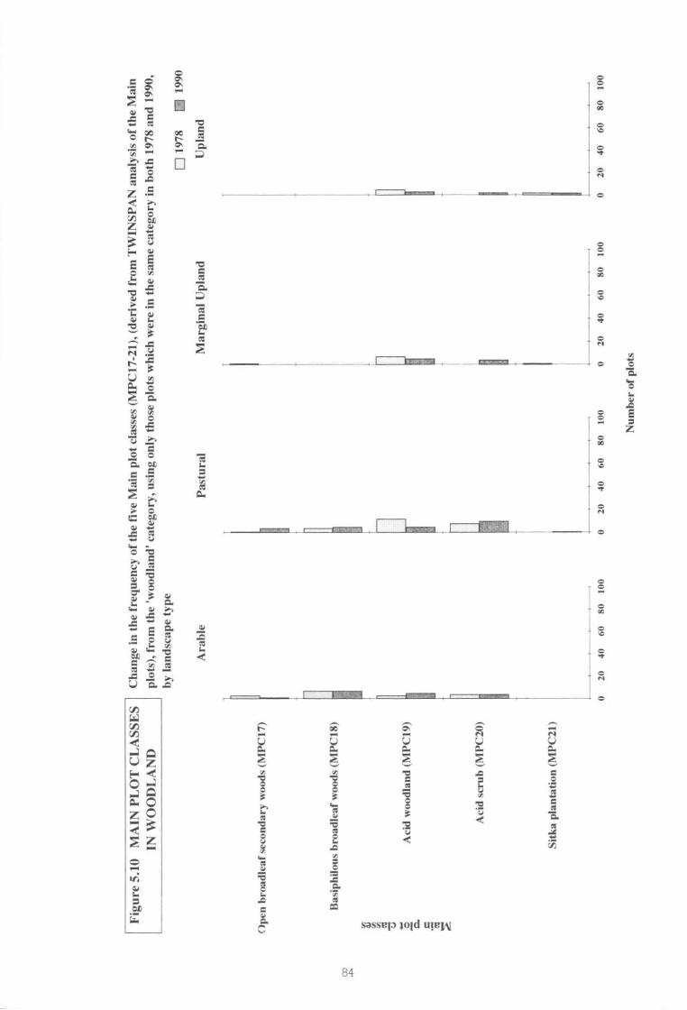
Figu

re5.

1(1

MA

INPL

OT

CL

ASS

ES

INW

OO

DL

AN

D

Cha

nge

inth

efr

eque

ncy

ofth

efi

veM

ain

plot

clas

ses

(MPC

17-2

1b(d

eriv

edfr

omT

WIN

SPA

Nan

alys

isof

the

Mai

n

plot

s),

from

the

'woo

dlan

d'ca

tego

ry,

usin

gon

lyth

ose

plot

sw

hich

wer

ein

the

sam

eca

tego

ryin

both

1978

and

1990

,

byla

ndsc

ape

type

D19

782]

1990

Ara

ble

Past

ural

Mar

gina

lU

plan

dU

plan

d

()pe

nbr

oadl

eaf

seco

ndar

yw

oods

(N11

M'1

7)

Has

iphi

lous

broa

dlea

fw

oods

(MN

:III)

Aci

dw

oodl

and

(NIP

C19

)

.707

Aci

dsc

rub

(MP

('20)

Sitk

apl

anta

tion

(NIP

C21

)

2040

60SO

100

2040

6080

100

020

4060

8010

00

2040

6080

100

Num

ber

ofpl

ots

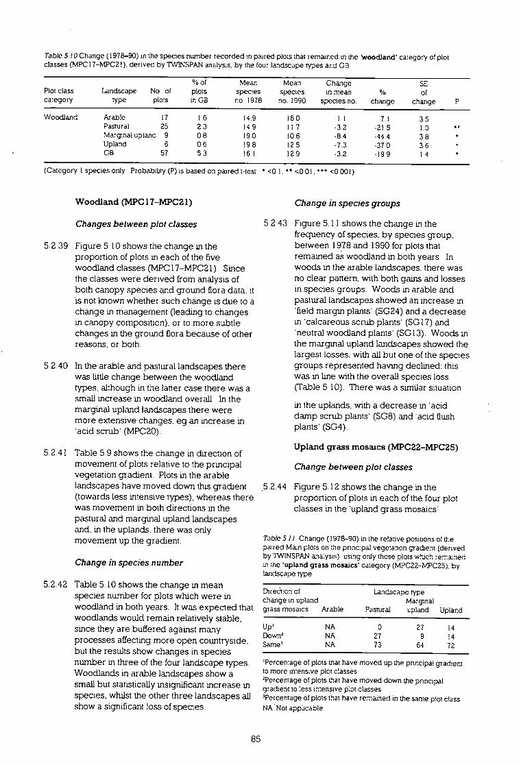
Table 5 10 Change (1978-90) in :he species number recorded in paired plots that remained in the Woodland' category of plotclasses (MPC17-IsTPC2!). derived by TWINSPAN analysis. by the four landscape types and G3

% of Mean Mean Change SEPlot class Landscape No of plots spec:es species in mean ofcategory 1YPo plots in GB no 1978 no 1990 species no change change I)

Woodland Arable 17 1 6 14 9 16 0 11 7 1 3 5

Pastural 25 2 3 14 9 II 7 -3 2 -2! 5 1 0 * •Matginai upland 9 0 8 19 0 10 6 -8 4 -44 4 3 8

Upland 6 0 6 !9 8 12 5 -7 3 -37 0 3 6

GB 57 5 3 16 I 12 9 -3 2 -19 9 I

(Category 1 species only Probability (P) is based on paired ;hest <0 I. n <0 01. ••• <0 001)

Woodland (MPC17-MPC21)

Changes between plot classes

5.2.39 Figure 5.10 shows the change in theproportion of plots in each of the fivewoodland classes (MPC17-MPC21). Sincethe classes were derived from analysis ofboth canopy species and ground flora data. nis not imown whether such change is due to achange in management (leading to changesin canopy composition). or to more subtlechanges in the ground flora because of otherreasons, or both.

5.2.40 In the arable and pastural landscapes therewas little change between the woodlandtypes, although in the latter case there was asmall increase m woodland overall In themarginal upland landscapes there weremore extensive changes. eg an increase in'acid scrub (MPC20).

5.2.41 Table 5.9 shows the change in direction ofmovement of plots relative to the principalvegetation gradient. Plots in the arablelandscapes have moved down this gradient(towards less intensive types), whereas therewas movement in both directions in thepastural and marginal upland landscapesand, in the uplands. there was onlymovement up the gradient.

Change in species number

5.2.42 Table 5.10 shows the change in meanspecies number for plots which were inwoodland in both years. It was expected thatwoodlands would remain relatively stable,since they are buffered against manyprocesses affecting more open countryside,but the results show changes in speciesnumber in three of the four landscape types.Woodlands in arable landscapes show asmall but statistically insignificant increase inspecies, whilst the other three landscapes allshow a significant loss of spec:es.

Change in species groups

5 2.43 Figure 5.11 shows the change in thefrequency of species, by species group.between 1978 and 1990 for plots thatremained as woodland in both years Inwoods in the arable landscapes. there wasno clear pattern, with both gains and lossesin species groups. Woods in arable andpastural landscapes showed an increase in'field margth plants' (5024) and a decreasein 'calcareous scrub plants' (SG17) and'neutral woodland plants' (SGI3). Woods inthe marginal upland landscapes showed thelargest losses, with all but one of the speciesgroups represented having declined: thiswas in line with the overall species loss(Table 5.10). There was a similar situation

in the uplands, with a decrease in 'aciddamp scrub plants' (SG8) and 'acid flushplants' (504).

Upland grass mosaics (MPC22-MPC25)

Change between plot classes

5 2.44 Figure 5.12 shows the change in theproportion of plots in each of the four plotclasses in the 'upland grass mosaics'

Table 5 11 Change (1978-90) in the relative positions of thepaued Math plots on the principal vegetation gradient (derivedby 'IWINSPAN analysis) using only those plots which retiredin the 'upland grass mosaics' category (MPC22-Iv5)C25). bylandscape type

Direth:on ofchange in upland

Landscape typeMarginal

grass mosaics Arable Pastural upland Upland

Up' NA

27 14Down' NA 27 9 !4Same' NA 73 64 72

'Percentage of plots that have moved up the pnncipal gradientto more in:ens:ye plot classesPercentage of plots that have moved down the pnncipalgradient to less intensive plot classesPercentage of plots that have remained in the same plot classNA 'Not appicable

85

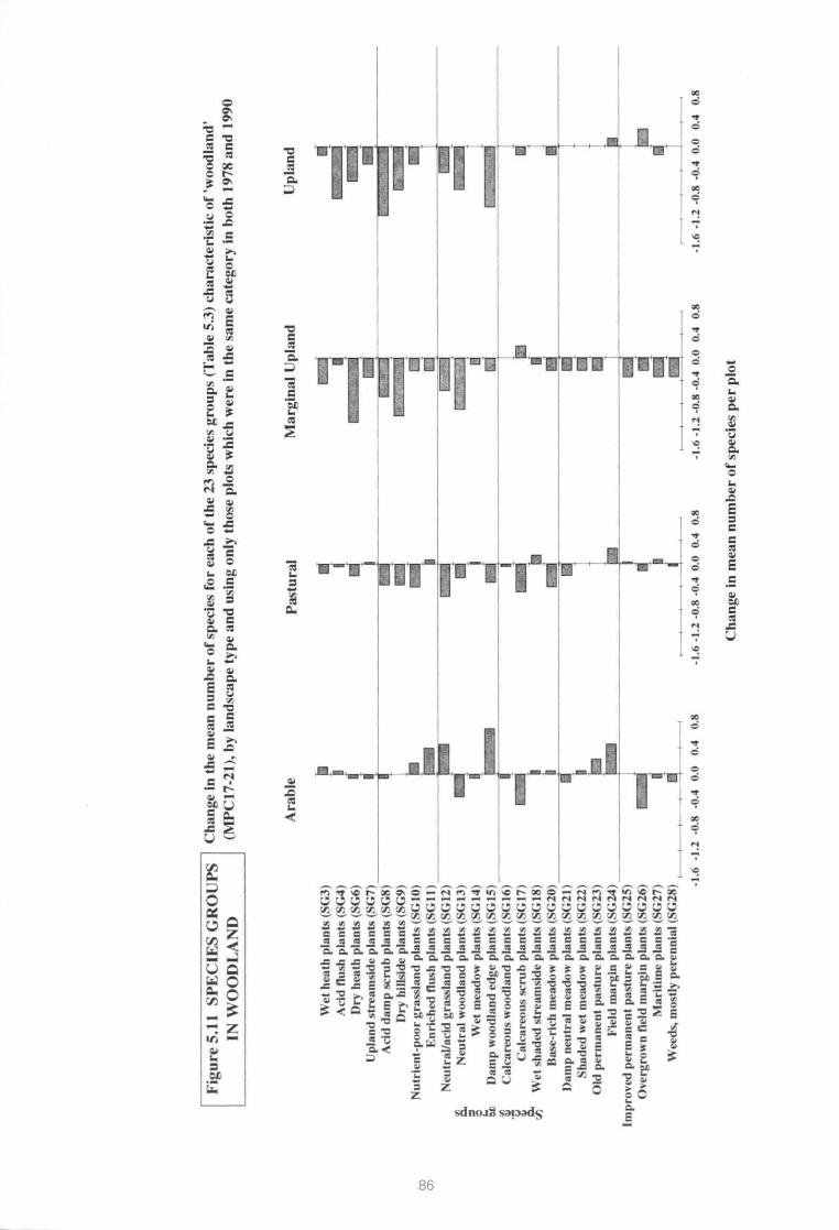
Fig

ure

5.11

SP

EC

IES

GR

OU

PS

Cha

nge

inth

em

ean

num

ber

ofsp

ecie

sfo

rea

chof

the

23sp

ecie

sgr

oups

(Tab

le5.

3)ch

arac

teris

ticof

'woo

dlan

d'

INW

OO

DLA

ND

(MP

C17

-21)

,by

land

scap

ety

pean

dus

ing

only

thos

epl

ots

whi

chw

ere

inth

esa

me

cate

gory

inbo

th19

78an

d19

90

Mar

gina

lU

plan

d

Mr;

Upl

and

Ara

ble

Wet

heat

hpl

ants

(563

)

Aci

dflu

shpl

ants

(564

)

Dry

heat

hpl

ants

(S(;

6)

tTpl

rnid

stre

amsk

lepl

ants

(567

)

Aci

dda

mp

scru

bpl

ants

(S68

)

Dry

hills

ide

plan

ts(5

69)

Nut

rient

-poo

rgr

assl

and

plan

ts(M

;101

Enr

iche

dB

ush

plan

ts(S

C11

)

Neu

tral

/aci

dgr

assl

and

plan

ts(5

612)

Neu

tral

woo

dlan

dpl

ants

(SC

1)1

Wet

mea

dow

plan

ts(5

614)

aD

amp

woo

dlan

ded

gepl

ants

(561

5)

Cal

care

ous

woo

dlan

dpl

ants

(561

6)

Cal

care

ous

scru

bpl

ants

(S61

7)

AW

etsh

aded

stre

amsi

depl

ants

(SC

18)

Bas

e-ric

hm

eado

wpl

ants

(562

0)

Dam

pne

utra

lm

eado

wpl

ants

(562

11

Sha

ded

wet

mea

dow

plan

ts(5

622)

Old

perm

anen

tpa

stur

epl

ants

(562

3)

Fie

ldm

argi

npl

ants

(562

4)

Impr

oved

perm

anen

tpa

stur

epl

ants

(562

5)

Ove

rgro

wn

field

mar

gin

plan

ts(S

626)

Mar

itim

epl

ants

(562

7)

Wee

ds,

mos

tlype

renn

ial

(562

8)

-1m

-1.2

-0.8

-0.4

0.0

0.4

0.8

Pas

tura

l

—

-1.6

-1.2

-0.8

-0.4

0.0

0.4

0.8

cate

det.

2811

8W-1

1r.

-1.6

-1.2

-0.8

-0.4

0.0

0.4

0.8

-1.6

-1.2

-0.8

-0.4

OM

0.4

0.8

Cha

nge

inm

ean

num

ber

ofsp

ecie

spe

rpl

ot

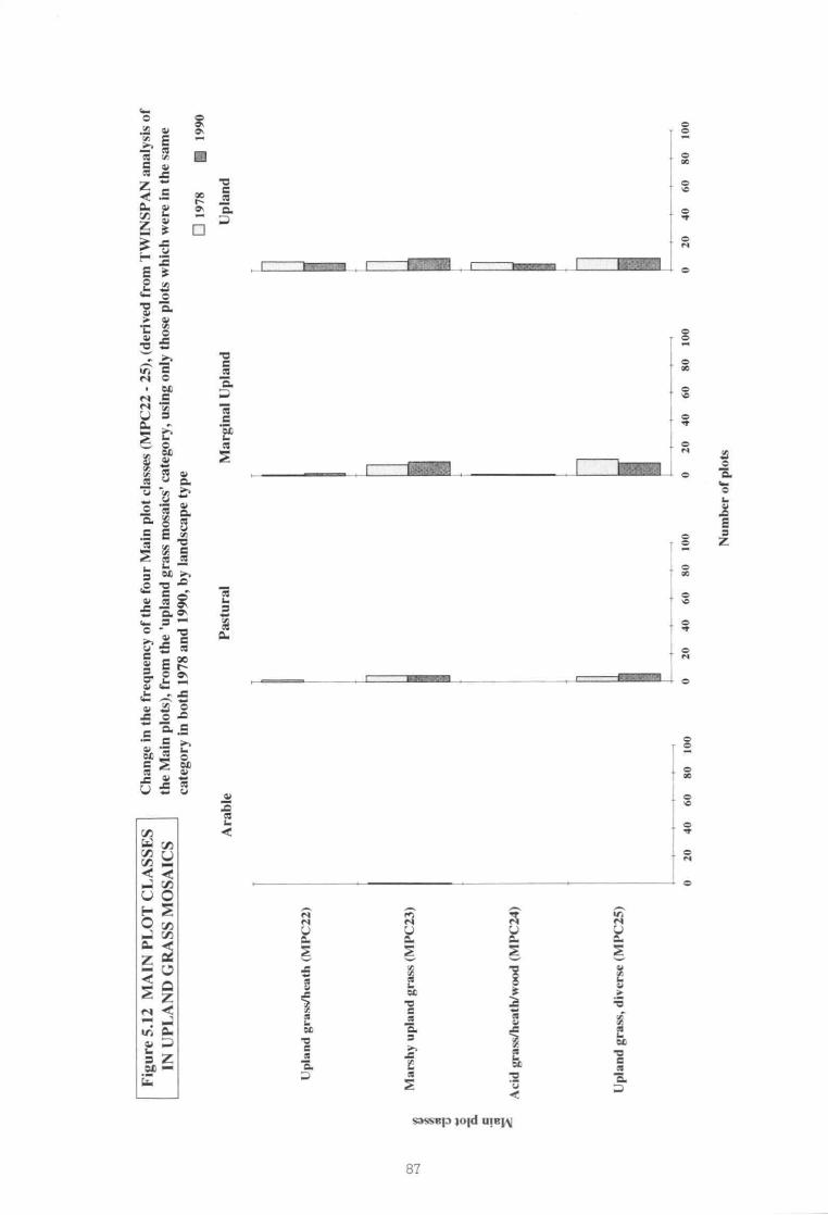
Cha

nge

inth

efr

eque

ncy

ofth

efo

urM

ain

plot

clas

ses

(N1P

C22

-25

),(d

eriv

edfr

omT

W1N

SP

AN

anal

ysis

of

the

Mai

npl

ots)

,fr

omth

e'u

plan

dgr

ass

mos

aics

'ca

tego

ry,

usin

gon

lyth

ose

plot

sw

hich

wer

ein

the

sam

e

cate

gory

inbo

th19

78an

d19

90,

byla

ndsc

ape

type

Fig

ure

5.12

MA

INP

LOT

C1A

SS

ES

INU

PIA

ND

GR

AS

SM

OS

AIC

S

1978

1990

Ara

ble

Pas

tura

lM

argi

nal

Upl

and

Upl

and

Ipla

ml

gras

s/he

ath

(MP

C22

1

Mar

shy

upla

ndgr

ass

(NIP

C23

)

Aci

dgr

as4h

eath

/w4o

d(M

PC

24)

Upl

and

gras

s,di

vers

eIM

PC

251

-

020

4060

8010

00

2040

6080

100

020

4060

8010

00

2040

6080

100

Num

ber

ofpl

ots

Table 512 Change (:978-90) in the species nunthet recorded in paired p!ots that remained in the 'upland grass mosaics categoryof plot classes (MPC22-MPC25). derived by TW845PAN analysis, by landscape type and CB

% ofMeanPlot classLandscapeNo ofspec:escategorytypeplotsplots in GBno 1978

Upland grassPasturalI I1 025 9mosaicsM.argnal upland222 I:8 4(MPC22Upland292 725 1-MPC25)G3635 923 2

(Category 1 species onlyProbablity (P) is based on paired t-test

Mean species no 1990

22 I:9 026 823 4

<0 I.** <0

Changein mean

species no

-3 80 61 70 2

0I.**• <0 001)

change

-14 73 26 7: C

SE of

charge

2 1I 92 0I 2

category (MP022-MPC25). by landscapetype. In the pastural landscapes the plotswere stable, whilst in the marginal uplandlandscapes there was a small decrease in the'upland grass diverse' class (MPC25) andsmall increases in the other three classes. Inthe upland landscapes there was little netchange.

5.2.45 The difference in the direction of changesoccurring in each landscape type can besimplified by considering the proportion bfplots which have moved towards theintensive end of the principal gradient, asopposed to those which have moved to theextensive end, this is illustrated in Table 5.11The majority of plots were stable, withpastural landscapes showing movementtowards less intensively managedvegetation, and marginal upland landscapesmoving in the opposite direction.

Change in species number

5.2.46 Table 5.12 shows the change in meanspecies number from plots which were in the'upland grass mosaics' category(MPC22-MPC25) in both 1978 and 1990.None of the landscape types show astatistically significant change in speciesnumber, although the trend was for adecrease in the pasiural landscapes and aslight increase in the marginal upland andupland landscapes.

Change in species groups

5.2.47 Figure 5.13 shows the change in thefrequency of species in species groups inplots in the 'upland grass mosaics' category.In the pastural landscapes there has beensome loss of 'old permanent pasture plants'(SG23) from the fields on neutral soils, aswell as 'upland heath plants' (SG5) and 'dryheath plants' (S06). In contrast, in themarginal upland landscapes there has beensome increase in 'neutral/acid grasslandplants' (SG12) and a loss of 'enriched flushplants' (SG11). 'acid flush plants' (SG4) and'bog plants' (SG2). In the upland landscapes,

there was an increase in 'acid flush plants'(SO4) and 'upland heath plants' (SG5)

Moorland (MPC26-MPC29)

Change between plot classes

5.2.48 Figure 5. !4 shows the change in theproportion of plots in each of the fourmoorland plot classes (MPC26-MPC29).There were only a few examples of thesetypes from the pastural landscapes, butthese were relatively stable However, inthe marginal upland landscapes there hasbeen a decline in the two most uplandcategories (MPC28 - 'dwarf shrub heath'and MPC29 - 'bog') and an increase in theleast upland category (MPC26 - 'boggymoorland'), ie a shift down the principalgradient. In the upland landscapes therewas also an increase in 'boggy moorland'(MPC26) and a decrease in 'bog' (MPC29).The majority of plots were stable, althoughmore plots in the upland landscape typemoved up the gradient than moved down,in contrast to plots in the pastural andmarginal upland landscapes, where thereverse was true (Table. 5.13).

Change in species number

5.2.49 Table 5.14 shows the change in speciesnumber for the plots which were in the

Table 5.13 Change (1978-90) :n the relanve posinors of thepaired Main plots on the pnnapal vegetation gradient (denvedby 'IWINSPAN analysts), using only Mose plots which remainedin the 'moorland' category (MPC26-MPC29). by landscapelYPe

Directon cfchange in

landscape typeMarginal

moorland Arable Pastural upland Upland

Up' NA 7 18 2:Down2 NA 14 21 13Same' NA

61 66

'Percentage of plots tha: have moved up the principal gradientto more intersive plot classes'Percentage of pats erat have moved down the pnnc:paigradient to less intensive plot classes'Percentage of plots that have remained in the same plot c:ass

NA NOTapplicable

88

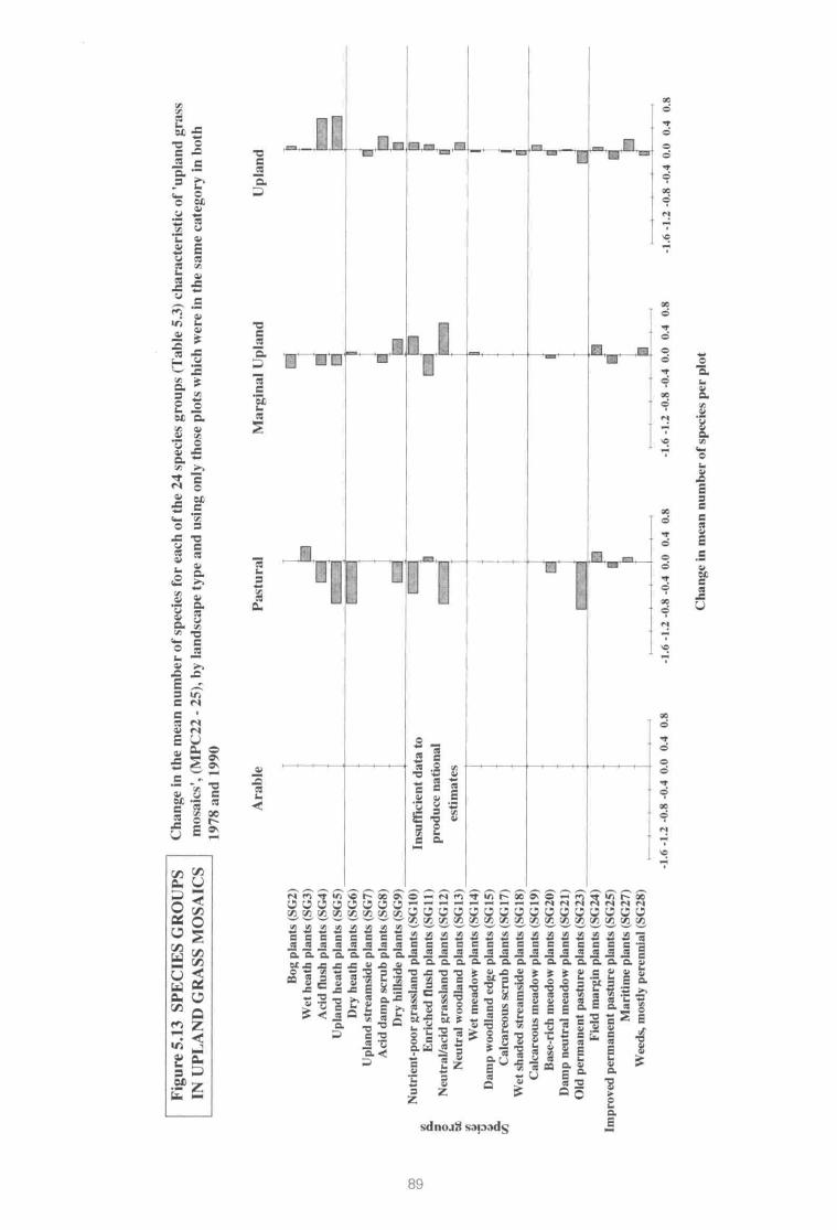
Figu

re5.

13SP

EC

IES

GR

OU

PSC

hang

ein

the

mea

nnu

mbe

rof

spec

ies

for

each

ofth

e24

spec

ies

grou

ps(T

able

5.3)

char

acte

ristic

of'u

plan

dgr

ass

INU

PLA

ND

GR

ASS

MO

SAIC

Sm

osai

cs',

(MP

C22

-25

),by

land

scap

ety

pean

dus

ing

only

thos

epl

ots

whi

chw

ere

inth

esa

me

cate

gory

inbo

th

1978

and

1990

Spe

cies

grou

ps

Bog

plan

ts(5

62)

Wet

heat

hpl

ants

(563

)

Aci

dflu

shpl

ants

(564

) U

plan

dhe

ath

plan

tsIS

(;S

)

Dry

heat

hpl

ants

(566

) U

plan

dst

ream

side

plan

ts15

67)

Aci

dda

mp

scru

bpl

ants

(568

)

Dry

hills

ide

plan

ts(5

69)

Nut

rient

-poo

rgr

assl

and

plan

ts(5

610)

Enr

iche

dflu

shpl

ants

(SG

II

) N

eutr

al/a

cid

gras

slan

dpl

ants

(561

2)

Neu

tral

woo

dlan

dpl

ants

(SG

13)

Wet

mea

dow

plan

ts(5

G14

)

Dam

pw

oodl

and

edge

plan

ts(S

GIS

)

Cal

care

ous

scru

bpl

ants

(SG

17)

Wet

shad

edst

ream

side

plan

ts(S

G18

) C

alca

reou

sm

eado

wpl

ants

(S61

9)

Bas

e-ric

hm

eado

wpl

ants

(562

0)

Dam

pne

utra

lm

eado

wpl

ants

(562

1)

Old

perm

anen

tpa

stur

epl

ants

(562

3)

Fie

ldm

argi

npl

ants

(562

4)

Impr

oved

perm

anen

tpa

stur

epl

ants

(562

5)

Mar

itim

epl

ants

(S(;

27)

Wee

ds,

mos

tlype

renn

ial

(S62

8)

Aru

ble

Insu

ffici

ent

data

to

prod

uce

natio

nal

estim

ates

-1.6-1.2-0.8-0.40.00.40.8

Pas

tura

lM

argi

nal

Upl

and

Upl

and

Eal

Ent

ci

0

4C

-k-4

ir'1

1

diau

CI

(=I

-1.6-1.2-0.8-0.40.00.40.8

-1.6-1.2-0.8-0.40.00.40.8

II 1.1

ff3

a-1.6-1.2-0.8-0.40.00.40.8

Cha

nge

inm

ean

num

ber

ofsp

ecie

spe

rpl

ot

Fig

ure

5.14

MA

INP

LO

TC

han

ge

Inth

efr

equ

ency

of

the

fou

rM

ain

plo

tcl

asse

s(M

PC

26-

29),

(der

ived

fro

mT

WIN

SP

AN

anal

ysis

of

the

CL

AS

SE

SIN

MO

OR

LA

ND

Mai

np

lots

),fr

om

the

'mo

orl

and

'ca

teg

ory

,u

sin

go

nly

tho

sep

lots

wh

ich

wer

ein

the

sam

eca

teg

ory

Inb

oth

1978

and

1990

,b

yla

nd

scap

ety

pe

LI19

78•1

990

Ara

ble

Pas

tura

lM

arg

inal

Up

lan

dU

pla

nd

Bo

ny

mo

orl

and

(MP

C26

)

Mo

orl

and

(MP

C27

)

Dw

arf

shru

bh

eath

(MP

C28

)

Bo

g(M

PC

29)

Insu

ffic

ient

data

to

prod

uce

nati

onal

es

tim

ates

020

4060

8010

00

2040

6080

100

020

4060

8010

00

2040

6080

100

Num

ber

ofpl

ots

Table 5 14 Change (1978-90) in the species r.umber recorded in paired plots that remained in the 'moorland' category of plotclasses (MPC26-MPC29). derived by TW1NSPAN analysis, by landscape type and GB

% of Mean Mean Change SF:Plot class Landscape Na of plots species species in mean ofcategory h*Pe pids in G3 no 1978 no 1990 species no change change P

Moorland Pasnual 14 I 3 15 6 12 I -3 4 -22 0 1 1 ••(MPC26- Marginal upland 28 2 6 12 4 16 3 3 9 31 7 I 3 Int

MPC29) Upland :83 17 1 18 9 20 2 I 3 6 6 0 6GB 230 21 5 17.7 19 0 I 4 7 8 0 5 ••

(Category ; spec:es only. Probability (P) :s based on paired t-zest • <0.1. ** <0 01. ••• <0 MI)

'moorland category in both 1978 and 1990.Both marginal upland and uplandlandscapes show a significant increase inspecies number. in contrast to the pasturallandscapes where the species number hasdeclined. Moorland habitats are inherentlyspecies-poor, so the increase in speciesnumber might Lndicate invasion by non-moorland species. implying a change inecological character.

Change in species groups

5.2.50 Figure 5.15 shows the change in thefrequency of species in species groups forthese 'moorland' plots. In the pastural t. landscapes there was a loss of 'bog poolplants' (SG1) and 'bog plants' (SG2). Incontrast, plots from the marginal upland andupland landscapes show increases in mostgroups; this suggests that whilst some of theincrease in species number in theselandscapes was Oftypical moorland species(SG I-SG3). in other cases it was due toinvasion by species more typical of acidgrassland (SG5-SG7). The largest increasein the upland landscapes was in speciesassociated with acid flashes (5G4). whichform an integral part of many moorlands.

Main plots: conclusions

5.2.51 Within the arable landscapes the overalltrend has been one of reduction in diversityof vegetation. except in woodland This lossin diversity was particularly marked in thearable fields, reflecting improved cropmanagement and the use of herbicides andfertilizers. The loss in diversity reflects anoverall decline in an already depletedresource; the species showing most declinewere mainly widespread weeds incultivated fields. The losses in semi-improved grassland are more significant inthat they represent a reduction in the stockof an already restricted group of species.The loss of diversity in fields means that, inmany areas. linear features provide the onlyremaining source of meadow species and.

as such, provide an important but limitedresource of plant diversity which couldexpand in response to suitablemanagement practices.

5.2.52 In the pastural landscapes, the loss ofplant diversity has been greater ingrassland than in arable fields. The loss ofquality in grassland reported heresupports the results of work by Hopkinsand Wainwright (1989). Although theoverall loss of species was higher inpastural landscapes than in arablelandscapes, the proportional loss waslower because of the higher initialcomplement. However, the speciesdeclining include those which are alreadynationally scarce, ie those associated withunimproved meadows, which areintolerant of frequent disturbance and areunable to compete successfully againstmore vigorous species. except on infertilesoils.

5.2.53 In the marginal upland landscapes thereappears to be some polarisation betweenchanges in the enclosed fields, and theunenclosed land. In the enclosed fields.losses and gains in diversity were takingplace simultaneously. More detailedanalysis of management on farms will berequired to examine the cause of thesechanges. The unenclosed areas weremore stable, although moorland shows atrend towards an increase in the numberand range of species. indicating a negativeeffect on the integrity of the moorlandhabitat.

5.2.54 In comparison with the other landscapetypes, the upland landscapes appearstable, confirming the conclusions of theanalysis of the land cover data (Chapter 3).The most obvious changes result fromafforestation. There was some indication ofa quality change in moorland with anincrease in species number and a trendaway from the most extreme types ofupland vegetation.

91

Fig

ure

515

SPE

CIE

SG

RO

UPS

INM

OO

RIA

ND

Cha

nge

inth

em

ean

num

ber

ofsp

ecie

sfo

rea

chof

the

22sp

ecie

sgr

oups

(Tab

le5.

3)ch

arac

teris

ticof

'moo

rland

'

(MP

C26

-29

),by

land

scap

ety

pean

dus

ing

only

thos

epl

ots

whi

chw

ere

inth

esa

me

cate

gory

inbo

th19

78an

d19

90

Ara

ble

Pas

tura

lM

argi

nal

Upl

and

Upl

and

Ni

Bog

pool

plan

ts(S

61)

Bog

plan

ts(5

62)

Wet

heat

hpl

ants

(S(;

3)

Aci

dflu

shpl

ants

(564

)

Upl

and

heat

hpl

ants

(565

)

Dry

heat

hpl

ants

(566

)

Upl

and

stre

amsi

depl

ants

(S11

:7)

Aci

dda

mp

scru

bpl

ants

(568

)

Dry

hills

ide

plan

ts(5

469)

IME

ER

IMin

t_

Insu

ffici

ent

data

to

prod

uce

natio

nal

estim

ates

--

-

6).

zN

utrie

nt-p

oor

gras

slan

dpl

ants

(S61

0)

Enr

iche

dB

osh

plan

ts(S

6111

Neu

tral

/acl

dgr

assl

and

plan

ts(S

C12

)

Neu

tral

woo

dlan

dpl

ants

(SC

13)

Wet

mea

dow

plan

ts(5

614)

Dam

pw

oodl

and

edge

plan

ts(S

C15

I

Wet

shad

edst

ream

side

plan

ts(S

C18

)

Bas

e-ric

hm

eado

wpl

ants

(S62

0)

Old

perm

anen

tpa

stur

epl

ants

(562

3)

Fie

ldm

argi

npl

ants

(562

4)

impr

oved

perm

anen

tpa

stur

epl

ants

(562

5)

Ove

rgro

wn

field

mar

gin

plan

ts(5

626)

Mar

itim

epl

ants

(562

7)

-1.6

-1.2

-0.8

-0.4

0.0

0.4

0.8

-1.6

-1.2

-0.8

-0.4

0.0

0.4

0.8

-1.6

-1.2

-0.8

-0.4

0A1

0.4

0.8

-1.6

-1.2

-0.8

-0.4

00

0.4

0.8

Cha

nge

inm

ean

spec

ies

num

ber

per

plot

5.2.55 These changes in moorlands may berelated to differences in grazing regimes.Grazing pressure has changed in differentways in different parts of the uplands overthe 1978-90 period: for example, stockinglevels for sheep have decreased in theOuter Isles (Watson 1988). but increasedover much of the mainland, whilst deergrazing has increased considerably in mostof Scotland (see Bunce et al. (1993) forfurther discussion). Change in moorlandvegetation may also be an indirect result ofafforestation through impact on catchmenthydrology. The identification of theprocesses involved requires further surveyand analysis.

52 56 It was expected that woodland would berelatively stable, since it is generailythought to be buffered against many of thechanges affecting farmland and moorland.However, the results show that in thepastural. marginal upland and uplandlandscapes there has been an overalldecline in species number within woodlandbut an increased proportion of speciesassociated With disturbed grasslandFurther study is required to determine theprocesses causing these changes (egnitrogen loading, as described by Pitcairnet (1991)).

5 2.57 The upland grass mosaics were the moststable category of plot classes and the onlysignificant change in land use in the uplandswas afforestation However, the increase inthe number and type of species recorded inplots on moorland and bogs is noteworthybecause. as Usher (1991) has emphasised.the diversification of inherently species-poor ecosystems represents ecologicaldegradation

5 2.58 The overall movement of plots in relation tothe principal gradient is summarised inTable 5 15. This emphasises how much

Table 5 15 Change in the re:anve posmons of the :978 and 1990paned Main plc:s on the Tufo:pal vegthanor. Tathent (derivedby rilN:NSPAN analys:s) using piths horn al: categor:es(NPC1-MPC29). by landscape type

:.er.dscape typeD:rection of Ma:einalchange Arable Pasnarai upland Upland

Up 48 49 36 27Down1 19 22 25 18Same) 34 29 36 53nercerrage a pcts t ci: ave rnoy up me thincip era ,ent

to :tore intensive p:ot classesPercentage of plots :bat :lave moved down the 2:J1c:oatTether: m less :rnenswe pal c:asses"omen:age of pacts that have:en:a:nod :n ;he same plo: class

more stable the uplands were compared tothe other landscape types. with over 50% ofplots remaining in the same plot class Allfour landscapes show a net change towardsmore intensively managed vegetation butthis varies from 8% of plots in the uplands to11% in the marginal upland landscapes. 27%in the pastural landscapes and 29% in thearable landscapes

5.3 Habitat plots

5.3.1 In 1990. Eve 4 m2 Habitat plots wererecorded in each 1 km square, within semi-natural vegetation, in order to sample thosescarce and fragmented habitats not coveredby the randomly located Main plots.Because these plots were not recorded in1978. no change data are available but theHabitat plots provide a baseline formonitoring future trends in such vegetation.Some habitats. eg lowland heath andsaltmarsh. were so restricted that the samplewas only slightly increased: in these cases.the only way to increase coverage would beto uncrease the sample size or specificallytarget these types of habitats (this is nowbeing undertaken as part of the DOE'Changes un Key Habitats' project) Whilstable to give a measure of the relativeabundance of the habitats concerned.information from Habitat plots cannot beused in a statistical sense to estimate relativefrequency of habitats.

5.3.2 Figure 5 16 shows the distribution of habitatssampled in this way. in each landscape type(these Habitat plots were groupedaccording to their dominant land cover code- as described in Chapter 3). There was aclear division between the lowland andupland landscapes In the lowlands most ofthe plots were placed in fields of agriculturaland unmanaged grassland. with quite a highproportion in woodland. In the uplands theemphasis was on unenclosed vegetation.especially diverse bogs and flu.shes, andupland grass. More information on thespecies present in the Habitat plots (asopposed to the randomly placed Main plots)will be available when these groups areanalysed in more detail

5.3.3 Comparisons of the relative occurrence ofthe five random (200 m2) Main plots with thefive (4 rn2) Habitat plots within the fourlandscape types are given in Figure 5.17.

5 3.4 in the arable landscapes the main coverageof the random Main plots was of crops andweed species in arable fields. whereas the

93

Fig

ure

5.16

HA

BIT

AT

PL

OT

CIA

SSE

SIN

CB

Per

cent

age

freq

uenc

yof

Hab

itat

plot

sin

the

twel

vepr

inci

pal

Hab

itat

type

sIn

1990

,by

land

scap

ety

pe

Ara

ble

Pas

tora

lM

argi

nal

Upl

and

Upl

and

Flus

h

Ilog

hrom

r

Moo

rlan

dgr

oss

Upl

and

gras

s

Mar

itim

e

Wom

iland

Unm

anag

edgr

ass

Mar

sh

Aqu

atic

vege

tatio

n

Low

land

heat

h

Low

land

gras

s

Ara

ble

1020

3040

010

2030

400

1020

3040

010

2030

40

Perc

ent

ofpl

ots

Fig

ure

5.17

HA

BIT

AT

AN

DC

ompa

riso

nof

the

rela

tive

freq

uenc

yof

Hab

itat

plot

san

dM

ain

plot

sin

the

twel

vepr

inci

pal

MA

INP

LO

TC

OM

PA

RIS

ON

Hab

itat

type

sin

1990

,by

land

scap

ety

peII

Mai

nD

Hab

itat

Ara

ble

Pas

tura

lM

argi

nal

Upl

and

Upl

and

Flu

sh

Bop

/moo

r

Moo

rland

gras

s

Upl

and

gras

s

Mar

itim

e

Woo

dlan

d

Unm

anag

edgr

ass

Mar

sh

Aqu

atic

vege

tatio

n

Low

land

heat

h

Low

land

gras

s

Ara

ble

010

020

030

040

00

100

200

300

400

010

020

030

040

00

100

200

300

400

Num

ber

ofpl

ots

Habitat plots are mainly in lowlandgrassland', 'unmanaged grassland and'woodland'

5.3.5 In the postural landscapes the random Mathplots cover a greater range of vegetationthan in the arable landscapes. but theHabitat plots extend the number of samplesin woodland and unmanaged grasstogether with less common habitats, such asmarshes, flushes and aquatic margins.

5 3.6 In the marginal upland landscapes semi-natural vegetation was more widespreadand was therefore well covered by therandom Main plots. The Habitat plotsextend the number of samples into some

. restricted habitats, such as marshes.unmanaged grassland and flushes.

5.31 In the upland landscapes, the random Mainplots gwe good coverage of most of themoorland vegetation, but the Habitat plotsadd more samples of flushes and the morespecies-rich pans of the upland grasslandThey also add to smaller and scarcerhabitats such as marshes and maritimevegetation.

5 3 8 The Habitat plots double the coverage ofwoodland and greatly extend the number ofplots placed in unmanaged grassland. aswell as adding many more in lowlandagricultural grassland. Further breakdownof these types may reveal that more diversetypes. eg chalk grassland, were morefrequently sampled by Habitat plots and thatmany more species were recorded, onaverage, in the Habitat plots, compared toMain plots. ln addition. the Habitat plotshave extended the coverage of otherscarce habitats. such as marshes and heath.

Table 5 16 Frequency of total Hedge plots placed alonghedgerows in 1990 horn both targened Hedge plots and thoseBoundary plots that wet e hedgerows, by landscape type

Landscape Hedge Boundary Total hedge

hrPe plots (hedge) plots plots

Arable 268 200 458Pastul al 255 158 423Marginal upland 410 18 59Upland 0 0 0Total 03 564 386 950

5.4 Linear features - Hedge plots

5.4.1 As outlined in Chapter 2, there were twotypes of plot which contributed data onhedgerows- the first of these were plotsplaced on boundaries adjacent to Main plots(Boundary plots - see section 2 3.11), some,of which were adjacent to hedgerows: thesecond type were plots targeted specificallyat hedgerows (Hedge plots - see 2.3.11).

5.4.2 Analysis of the numbers of different types ofplots enables the landscape types to becompared. Table 5.16 presents theoccurrence of Hedge plots Lnlinear featuresand those Boundary plots which wereadjacent to hedgerows. in each landscapeand in Britain as a whole. The plotstargetted on hedgerows over-samplehedges in 1 km squares where there is alimited hedgerow resource (because twoHedge plots were always placed,irrespective of the total length ofhedgerow).

5.4.3 Considering boundaries other thanhedgerows. Table 5.17 presents informationon the types of boundary sampled byBoundary plots placed (being linked to therandom 200 m2plots). and hence thefrequency of different boundary types. Theeight boundary types in Table 5.17 arebased on the dominant boundary element.These data reproduce the results from theland cover mapping reported in Chapter 4.

5.4.4 A high proportion of field boundaries in thearable landscapes were fences. hedges andwater edges In a national context. thearable landscapes contained most instanceswhere road verges and grass strips formedthe field boundary

5.4.5 Fences account for an even higherproportion of boundaries in posturallandscapes than in arable ones. Hedgesand to a lasser extent walls were alsocommon. Most of the banks occurring asboundaries were also in these areas.

5.4.6 In the marginal upland landscapes. fenceswere again the most common type of field

Table 5 17 Frequency of eight boundary types recorded in the Boundary plots placed adjacent to Main plots in 1990 by the fourIandscape types

landscape type Hedge Fence Wall Water Crass strip Bank Verge Other Total

Arable 199 268 39 130 24 IS 79 8 762Fasmral 161 331 81 41 12 43 23 16 714Marginal uplar.d 18 125 51 8 C 2 5

211Upland C 84 28 6 0 0 2

120Total GB 384 809 199 185 36 60 109 25 18C7

96

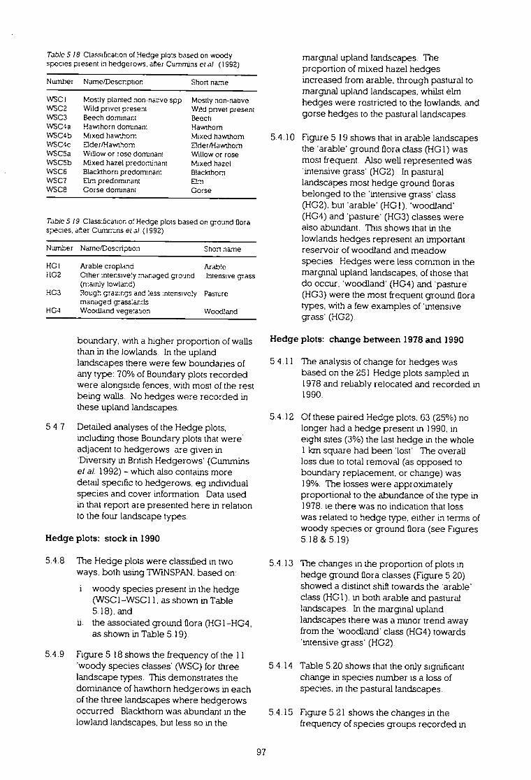
Table 5 18 Classification of Hedge plots based on woodyspecies present in hedgerows. after Cumrnins et al (1992)

Number Name/Description Shon name

WSC I Mostly planted nonnative spp Mostly non-nauveWSC2 Wild privet present Wild pnvet presentWSC3 Beech dominant BeechINSC4 a Hawthorn dominant HawthornWSC4b Mixed hawthorn Mixed hawthornWSC4c Elder/Hawthorn Eider/HawthornWSC5a Willow or lose dommant Willow or roseWSC5b Mixed hazel predominant Mixed hazelWSC6 Blackthorn predommant BlackthornWSC7 Elm predominant amWSCe Corse dominant Corse

Table 5 19 Classification of Hedge plots based or. ground floraspecies. after Cumrrths et al (1992)

Number Narne/Deschpuon Shon name

HC1 Amble cropland Arable1102

Other intensively managed ground Intensive grass (mainly lowland)

HC3 Rough grazings and less intensively Pasturemanaged grass:ands

HC4 Woodland vegetation Woodland

boundary, with a higher proportion of wallsthan in the lowlands. In the uplandlandscapes there were few boundaries ofany type: 70% of Boundary plots recordedwere alongside fences, with most of the restbeing walls. No hedges were recorded inthese upland landscapes

5 4.7 Detailed analyses of the Hedge plots,including those Boundary plots that were.adjacent to hedgerows. are given in'Diversity in British Hedgerows' (Cumminset al. 1992) - which also contains moredetail specific to hedgerows. eg indMdualspecies and cover information Data usedin that report are presented here in relationto the four landscape types.

Hedge plots: stock in 1990

5.4 8 The Hedge plots were classified in twoways. both using TW1NSPAN.based on:

woody species present in the hedge(WSC1-WSC11, as shown in Table5.18): andthe associated ground flora (HG1-HG4,as shown in Table 5.19).

5.4.9 Figure 5.18 shows the frequency of the II'woody species classes' (WSC) for threelandscape types. This demonstrates thedominance of hawthorn hedgerows in eachof the three landscapes where hedgerowsoccurred Blackthorn was abundant in thelowland landscapes. but less so in the

marginal upland landscapes The proportion of mixed hazel hedgesincreased from arable, through pastural tomarginal upland landscapes, whilst elmhedges were restricted to the lowlands, andgorse hedges to the pastural landscapes

5.4.10 Figure 5 19 shows that in arable landscapesthe 'arable ground flora class (HG1) wasmost frequent Also well represented was'intensive grass' (HG2). In pasturallandscapes most hedge ground florasbelonged to the 'intensive grass' class(HG2). but 'arable' (FIGl). 'woodland'(HG4) and 'pasture' (HG3) classes werealso abundant. This shows that in thelowlands hedges represent an importantreservoir of woodland and meadowspecies Hedges were less common in themarginal upland landscapes; of those thatdo occur. 'woodland' (HG4) and 'pasture:(HG3) were the most frequent ground floratypes, with a few examples of 'intensivegrass' (HG2).

Hedge plots: change between 1978 and 1990

5.4.11 The analysis of change for hedges wasbased on the 251 Hedge plots sampled in1978 and reliably relocated and recorded in1990.

5.4.12 Of these paired Hedge plots. 63 (25%) nolonger had a hedge present in 1990, ineight sites (3%) the last hedge in the whole1km square had been 'lost' The overallloss due to total removal (as opposed toboundary replacement, or change) was19%. The losses were approximatelyproportional to the abundance of the type in1978. le there was no indication that losswas related to hedge type, either in terms ofwoody species or ground flora (see Figures5.18 & 5.19)

5.4.13 The changes in the proportion of plots inhedge ground flora classes (Figure 5.20)showed a distinct shift towards the 'arable'class (HG1). in both arable and pasturallandscapes. In the marginal uplandlandscapes there was a minor trend awayfrom the 'woodland' class (HG4) towards'intensive grass' (HG2).

5.4.14 Table 5.20 shows that the only significantchange in species number is a loss ofspecies. in the pastural landscapes.

5 4 15 Figure 5 21 shows the changes in thefrequency of species groups recorded m

97

Figu

re5.

18H

ED

GE

PLO

TC

LA

SSE

S:

WO

OD

YSP

EC

IES

OF

LO

STH

ED

GE

S

Fre

quen

cyan

dpr

opor

tion

ofth

eH

edge

plot

sin

the

elev

enH

edge

type

s(W

SC

1-8)

,(d

eriv

edfr

omT

WIN

SP

AN

anal

ysis

ofth

ew

oody

spec

ies)

,lo

stbe

twee

n19

78an

d19

90,

byla

ndsc

ape

type

IDP

rese

ntin

1990

Lost

betw

een

1978

and

1990

Ara

ble

Pas

tura

lM

argi

nal

Upl

and

Upl

and

Mos

tlyno

n-na

tive

(WS

C1)

Wild

priv

etpr

esen

t(W

SC

2)

Bee

ch(W

SC

3)

Haw

thor

n(W

SC

4a)

Mix

edha

wth

orn

M.S

C.

41))

Eld

er/H

awth

orn

(WS

C4c

)

Will

owor

rose

(WS

C5a

)

Mix

edha

zel

(WA

:5h

)

Bla

ckth

orn

(WS

C

Elm

(WS

C7)

Gor

se(W

SC

8)

co CO

Hed

ge

type

s

-woo

dy

spec

ies

clas

ses

020

1060

80

Insu

ffici

ent

data

to

prod

uce

natio

nal

estim

ates

I

01

1

020

4060

800

2040

6080

020

4060

80

Num

ber

ofpl

ots

Figu

re5.

19H

ED

GE

PLO

TC

LA

SSE

S:

Fre

quen

cyan

dpr

opor

tion

ofH

edge

plot

sin

the

four

Hed

gety

pes

(HG

1-4)

.(d

eriv

edfr

omT

W1N

SP

AN

GR

OU

ND

FLO

RA

OF

LO

STH

ED

GE

San

alys

isof

the

grou

ndflo

ra),

lost

betw

een

1978

and

1990

,by

land

scap

ety

pe

Pre

sent

in19

90fl

Lost

betw

een

1978

and

1990

Ara

ble

Pas

tura

lM

argi

nal

Upl

and

Upl

and

Ara

ble

IHG

1)

11cr

,cc

s-In

tens

ive

gras

s(H

G2)

a+

Pas

ture

(HG

3)

X

Insu

ffici

ent

data

to

prod

uct

natio

nal

estim

ates

11W

oodl

and

(FIG

4)

020

4060

020

4060

020

4060

020

4060

Num

ber

ofpl

ots

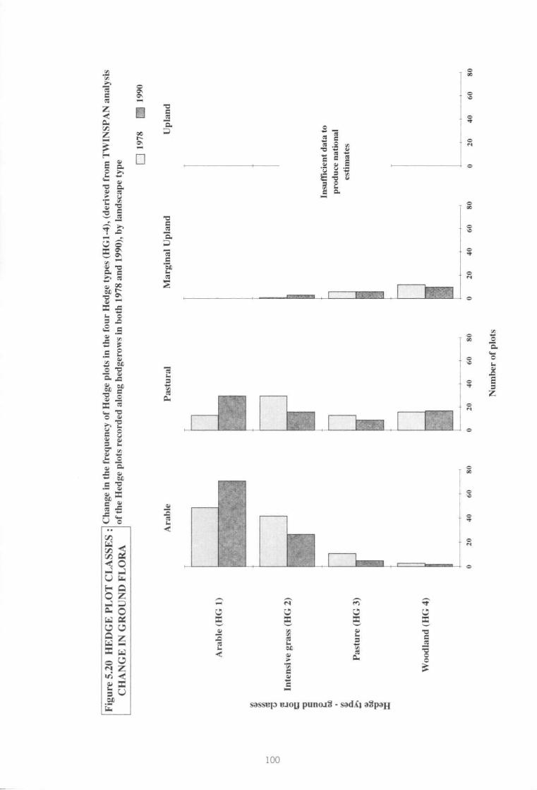
Fig

ure

5.20

HE

DG

EP

LO

TC

LA

SSE

S:

Cha

nge

inth

efr

eque

ncy

ofH

edge

plot

sin

the

four

Hed

gety

pes

(HG

I-4)

,(d

eriv

edfr

omT

WIN

SPA

Nan

alys

is

CH

AN

GE

ING

RO

UN

DF

LO

RA

ofth

eH

edge

plot

sre

cord

edal

ong

hedg

erow

sin

both

1978

and

1990

),by

land

scap

ety

pe 019

78•

1990

Ara

ble

Pas

tura

lM

argi

nal

Upl

and

Upl

and

Ara

ble

(HG

1)

Inte

nsiv

egr

ass

(HG

2)

Pas

ture

(HG

3)

Woo

dlan

d(H

G4)

Insu

ffic

ient

data

to

prod

uce

nati

onal

es

tim

ates

020

4060

800

2040

6080

020

4060

800

2040

6080

Num

ber

ofpl

ots

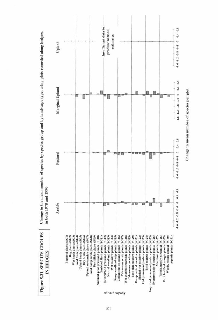
Fig

ure

5.21

SPE

CIE

SG

RO

UP

SC

hang

ein

the

mea

nnu

mbe

rof

spec

ies

bysp

ecie

sgr

oup

and

byla

ndsc

ape

type

,us

ing

plot

sre

cord

edal

ong

hedg

es,

INH

ED

GE

Sin

both

1978

and

1990

Ara

ble

l'ast

ura

lM

arg

inal

Up

lan

dU

pla

nd

Bog

pool

plan

ts(S

G1)

Bog

plan

ts(S

G2)

Wet

heat

hpl

ants

(S63

)

Add

flush

plan

ts(S

64)

Upl

and

heat

hpl

ants

(565

)

Dry

heat

hpl

ants

(566

)

Upl

and

stre

amsi

depl

ants

(SG

1)

Add

dam

psc

nih

plan

ts(5

68)

Dry

hills

ide

plan

ts(5

69)

Nut

rient

-poo

rgr

assl

and

plan

ts(S

GI

0)

Enr

iche

dM

ush

plan

ts(M

aI)

Neu

tral

/aci

dgr

assl

and

plan

ts(5

612)

7N

eutr

alw

oodl

and

plan

ts(S

G13

)

Wet

mea

dow

plan

ts(S

G14

)

6D

amp

woo

dlan

ded

gepl

ants

(561

5)

Cal

care

ous

woo

dlan

dpl

ants

(561

6)

Cal

care

ous

scru

bpl

ants

(561

7)A

Wet

shad

edst

ream

side

plan

ts(5

6I8)

Cal

care

ous

mea

dow

plan

ts(5

619)

Bas

e-ric

hm

eado

wpl

ants

(562

0)

Dam

pne

utra

lm

eado

wpl

ants

(562

I)

Sha

ded

wet

mea

dow

plan

ts(5

622)

Old

perm

anen

tpa

stur

epl

ants

(562

3)

Fie

ldm

argi

npl

ants

(S(;

24)

Impr

oved

perm

anen

tpa

stur

epl

ants

(562

5)

Ove

rgro

wn

field

mar

gin

plan

ts(5

626)

Mar

itim

epl

ants

(562

7)

Wee

ds,

mas

tlype

renn

ial

(562

8)

Enr

iche

dfie

ldm

argi

npl

ants

(562

9)

Wee

ds,

mos

tlyan

nual

(563

0)

Aqu

atic

plan

ts(5

631)

1 i ili

N

oil la

ar4

k J- MI

11

-1.6

-1.2

-a8

-0.4

00.

40.

8-1

.6-1

.2-0

.8-0

.40

0.4

0.8

Insu

ffici

ent

data

to-

prod

uce

natio

nal

estim

ates

-1.6

-1.2

-0.8

-0.4

00.

40.

8-1

.6-1

.2-0

.8-0

.40

0.4

0.8

Cha

nge

inm

ean

num

ber

ofsp

ecie

spe

rpl

ot

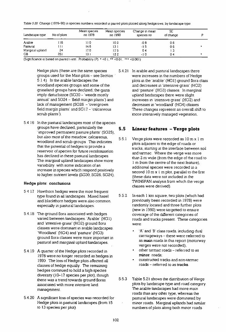
Table 5 20 Change (1978-90) in species numbers recorded in paired plots placed along hedgerows, by landscape type

Mean species Mean species Change in mean SELandscape type No of plots no 1978 no 1990 species no of change

Arable 116 11 0 10 2 -0 8 0 6Pastural III 15 6 13 I -I 5 0 6Marginal upland 24 170 17 5 0 4 1 3GB 251 13 i 12 2 -1 0 0 4

(Significance is based on paired Nest Probability (P) • <0 I • <0 01 • <0 001)

Hedge plots (these are the same speciesgroups used for the Main plots - see Section5 1.4) In the arable landscapes thewoodland species groups and some of thegrassland groups have declined; the gamsimply disturbance (S030 - 'weeds mostlyannual and 5(324 - 'field margin plants') andlack of management (5(326 - 'overgrownfield margin plants' and SG17 - 'calcareousscrub plants).

5.4 16 In the pastural landscapes most of the speciesgroups have declined, particularly the'improved permanent pasture plants' (SG25).but also most of the meadow, calcareous,woodland and scrub groups This indicatesthat the potential of hedges to provide areservoir of species for future recolonisationhas declined in these pastural landscapesThe marginal upland landscapes show morevariability, with some indication of anincrease in species which respond positively to higher nutrient levels (5G30, 5(326, SG24).

Hedge plots: conclusions

5.4 17 Hawthorn hedges were the most frequenttype found in all landscapes. Mixed hazeland blackthorn hedges were also common.especially in pastural landscapes.

5.4 18 The ground flora associated with hedgesvaried between landscapes. 'Arable' (HG1)and 'intensive grass' (HG2) ground floraclasses were dominant in arable landscapes.'Woodland' (HG4) and 'pasture' (HG3)ground flora classes were more important inpastural and marginal upland landscapes.

•5.4.19 A quarter of the Hedge plots recorded in

1978 were no longer recorded as hedges in1990. The loss of Hedge plots affected allclasses of hedge equally. The remaininghedges continued to hold a high speciesdiversity (10-17 species per plot), thoughthere was a trend towards ground florasassociated with more intensive landmanagement.

5.4.20 A significant loss of species was recorded forHedge plots in pastural landscapes (from 15to 13 species per plot).

5.4.21 In arable and pastural landscapes therewere increases in the numbers of Hedgeplots in the 'arable' (HG I) ground flora classand decreases in 'intensive grass' (HG2)and 'pasture' (HG3) classes In marginalupland landscapes there were slightincreases in -intensive grass' 0-1(32)anddecreases in 'woodland' (HG4) classes.These changes represent an overall shill tomore intensively managed vegetation.

5.5 Linear features - Verge plots

5.5.1 Verge plots were recorded as 10 mx 1 mplots adjacent to the edge of roads ortracks, starting at the interface between soiland tarmac. Where the verge was morethan 2 m wide (from the edge of the road to1 m from the centre of the next feature),additional species were recorded in asecond 10 mxlm plot, parallel to the first(these data were not included in theTW1NSPANanalysis from which the vergeclasses were derived).

5.5.2 In each I km square, two plots (which hadpreviously been recorded in 1978) wererandomly located and three further plots(new in 1990) were targetted to ensurecoverage of the different categories ofroads and tracks present. These categorieswere:

'A' and 'B' class roads, including dualcarriageways - these were referred toas main roads in this report (motorwayverges were not recorded);other tarmac roads - referred to asminor roads:constructed tracks and non-tarmac roads - referred to as tracks.

5.5.3 Table 5.21 shows the distribution of Vergeplots by landscape type and road category.The arable landscapes had more mainroads than any other type, whereas thepastural landscapes were dominated byminor roads. Marginal uplands had similarnumbers of plots along both minor roads

102

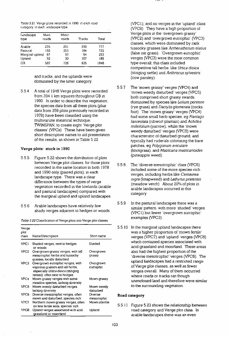
Table 521 Verge plots recorded si 1990 in each toadcategory. in each :andscape type

landscapeMain

0/Peroads

Minor roads Tracks Total

&able 276 251 250 777Pastural 192 353 184 729Marginal upland 67 92 94 253Upland 52 30 107 189

CB 587 726 635 1948

and tracks, and the uplands were dominated by the latter category.

5.5.4 A total of 1948 Verge plots were recordedfrom 394 1 lari squares throughout GB in1990. In order to describe this vegetation.the species data from all these plots (plusdata from 359 plots previously recorded in1978) have been classified using themultwariate statistical technique.TWINSPAN. to create eight 'Verge plotclasses (VPCs). These have been givenshort descriptive names to aid presentationof the results, as shown in Table 5.22.

Verge plots: stock in 1990

5 5.5 Figure 5.22 shows the distribution of plotsbetween Verge plot classes, for those plotsrecorded in the same location in both 1978and 1990 only (paired plots), in eachlandscape type. There was a cleardifference between the types of vergevegetation recorded in the lowlands (arableand pastural landscapes) compared withthe marginal upland and upland landscapes.

5 5 6 Arable landscapes have relatively fewshady verges adjacent to hedges or woods

Table 5 22 Classification of Verge plots into Verge plot classes

Vergeplotclass Name/Description Short name

VPC I Shaded verges, next to hedges Shadedor woods

VPC2 Overgrown grassy verges, with tall Overgrownmesthrophic herbs and tussocicy grassygrasses, locally disturbed

VPC3 Overgrown eutrophic verges. with Overgrownvigorous grasses and tall herbs. eutrophicespecially Unica choice (stingingnettles). often next to hedges

VPC4 Mown grassy verges with some Mown grassymeadow species. lacking diversity

VPC5 Mown weedy disturbed verges. Mown weedylacking diversity disturbed

VPCS Diverse mesorrophic verges. often Diversemown and disturbed. species-nch mesthrophic

VPC7 Northern mown grassy verges, often Mown infertileon less fertile sods, species rich

VPC8 Upland verges associated with and Uplandassland or moorland

(VPC1). and no verges in the 'upland' class(VPC8). They have a high proportion ofVerge plots in the 'overgrown grassy'(VPC2) and 'overgrown eutrophic' (VPC3)classes, which were dominated by ranktussocky grasses like Arrhenatherum eladus(false oat grass). 'Overgrown eutrophic•verges (VPC3) were the most commontype overall; this class includedcompetitive tall herbs. like Urbcadioica(stinging nettle) and Anthriscus sylvestris(cow parsley).

5.5.7 The 'mown grassy' verges (VPC4) and'mown weedy disturbed' verges (VPC5)both comprised short grassy swardsdominated by species like Lolium perenne(rye grass) and Dactylis glomerata (cocksfoot). The 'mown grassy' verges (VPC4)had some small herb species. eg Plantagolanceolata (ribwort plantain) and Achillea.mIllefolium (yarrow). whilst the 'mown •weedy clisturbed' verges (VPC5) werecharacteristic of disturbed ground, andtypically had ruderals colonising the barepatches. eg Polygonum aviculare(Imotgrass). and Matricana matricarioides(pineapple weed).

5.5.8 The 'diverse mesotrophic' class (VPC6)included some of the more species-richverges, including herbs like Centaureanigra (knapweed) and Lathyrus pratensis(meadow vetch). About 20% of plots inarable landscapes occurred in thiscategory.

5.5.9 In the pastural landscapes there was asimilar pattern, with more 'shaded' verges(VPC1) but fewer 'overgrown eutrophic'examples (VPC3).

5.5.10 In the marginal upland landscapes therewas a higher proportion of 'mown fertile'verges (VPC7) and 'upland' verges (VPC8)which contained species associated withacid grassland and moorland. These areasalso had the highest proportion of the'diverse mesotrophic' verges (VPC6). Theupland landscapes had a restricted rangeof Verge plot classes, as well as fewerverges overall. Many of them occurredwhere roads or tracks ran thoughunenclosed land and therefore were similarto the surrounding vegetation.

Road category

5.5.11 Figure 5.23 shows the relationship betweenroad category and Verge plot class. Inarable landscapes there was an even

103

Fig

ure

5.22

VE

RG

EF

requ

ency

ofpl

ots

in19

78an

d19

90in

the

eigh

tV

erge

plot

clas

ses

(VP

C1-

8),

(der

ived

from

TW

INSP

AN

PL

OT

CL

ASS

ES

anal

ysis

ofth

epl

ots

reco

rded

alon

gve

rges

Inbo

th19

78an

d19

90),

byla

ndsc

ape

type

019

78•

1990

Ara

ble

Pas

tura

lM

argi

nal

Upl

and

Upl

and

Shad

ed(V

PC

1)

Ove

rgro

wn

gras

sy(V

PC

2)

Ove

rgro

wn

eutr

ophi

c(V

PC

3)

Mow

ngr

assy

(VP

C4)

Mow

nw

eedy

dist

ubed

(VP

C5)

Div

erse

mes

otro

phic

(VP

C6)

Mow

nin

fert

ile(V

PC

7)

Upl

and

(VP

C8)

020

4060

020

4060

020

4060

020

4060

Num

ber

ofpl

ots

Fig

ure

5.23

VE

RG

EP

LO

TC

LA

SSE

SPe

rcen

tage

freq

uenc

yof

the

eigh

tV

erge

plot

clas

ses

(VPC

1-

8),

(der

ived

from

TW

INSP

AN

anal

ysis

ofth

eV

erge

AN

DR

OA

DC

AT

EG

OR

Ypl

ots

reco

rded

in19

90),

byro

adca

tego

ryan

dby

land

scap

ety

pe

•M

ain

El

Min

orT

rack

Ara

ble

Past

ural

Mar

gina

lU

plan

dU

plan

d

Shad

ed(V

PC1)

Ove

rgro

wn

gras

sy(V

PC2)

Ove

rgro

wn

eutr

ophi

c(V

PC3)

Mow

ngr

assy

(VPC

4)

Mow

nw

eedy

dist

urbe

d(V

PC5)

Div

erse

mes

otro

phic

(VPC

6)

Mow

nin

fert

ile(V

PC7)

Upl

and

(VPC

8)

o=0

2040

600

2040

600

2040

600

2040

60

Per

cent

ofpl

ots

distribution between road categories.'Mown grassy verges (VPC4). 'mownweedy disturbed' verges (VPCS) and'diverse mosotrophic' verges (VPC6) werefound more often on main roads, which mayreflect more regular management regimes.'Mown infertile' verges (V207) and 'upland'verges (VPC8) were more often found onminor roads and tracks.

5 5 12 In pastural landscapes the 'overgrowneutrophic' verges (V203) and 'shaded'verges (VPC I) were more frequent onminor roads The 'diverse mesotrophic'verges (VPC6) were less common besidetracks

5.5.13 ln marginal upland landscapes also the'diverse mesotrophic' verges (VPC6) wereless common beside tracks. Uplandlandscapes were dominated by 'mowninfertile' verges (VPC7) and 'upland' verges(VPC8) which are characteristic of lessfertile soils; they also had a limitedrepresentation of the more diverse types.

Wide verges

5.5.14 The species most oflen recorded asadditional in the second I m plot are shownin Table 5.23. In the lowland and marginalupland landscapes these were largely tall

Table 5 23 Frequency of the spec:es most often formd only inthe second 1rn of Verge plots

Aralite % ofPastura: % oflandscapes plotslandscapes plots

Unica choice

Rubus fruecosus 19Gahum apanne

Unica choica 19Anhenatherum &anus

Callum apanne 14Rubus Miticosus

Anhenatnenun elauus 13Heracleum sphondyburn

Heracleum sphondyhum IIAnihnscus sylvestns

Anthn.scus sylvestris 9RIII77CXONLIS110bLIS

Ceaum arvense

Notts lanatus

Holcus lanatus 6Lamvum album

Rumex obtustlobus 6Curium aniense

Thymus stenlis

Centaurea mgra

Festuca tubra

Marginal % ofUpland °//ooflandscapes plotslandscapes pl ts

Unica choice 14 luncus effusus

Heracleum sphondyllum 13 Rumex acetcrsa

Coburn apostle I I Blechnum spicant

Anthnscus sylvestris

Unica choice

Arrhonathemm elatius

Gahum saratile

Rubus liuticosus

Calluna vulgaris

Lathynts platens's

Cerastium lontanum

Cerastium fonlanum

Casium vulgare

Cruciata laeopes

Rift's's Miucosus

Veronica chamaedrys

Rumex obtusilblius

Rumex obtusdobus

competitive herbs, like Unicadioica(stinging nettle). Heracleum sphondyhum(hogweed) and Anthnscus sylyesths (cowparsley), but they also include tall meadowspecies, for example C'enlaurea mgra(Imapweed). The vaned structure of thewider verges is important in allowing thepersistence of species unable to tolerateregular cutting, and in allowing meadowspecies to flower. These verges provide animportant seed source for colonisation, aswell as food sources and habitat forinvertebrates, birds and small mammals.

5.5.15 In the upland landscapes the vegetation inthese plots differs in that many of them werealongside.unenclosed roads and thereforehave similar species to the surroundingupland vegetation.

Verge plots: change between 1978and 1990

5.5.16 Analysis of change for the verge data wasbased on 304 paired plots from 167 squaresthroughout GB which were recorded inboth 1978 and 1990. Data from these pairsof plots are used here to consider howverge vegetation has changed over thisperiod.

5.5 17 Figure 5.22 shows the changes in theproportion of plots in the Verge plot classes.In the arable landscapes, there was anincrease in the 'overgrown grassy' verges(VPC2) and the 'overgrown eutrophic'verges (VPC3). and a decrease in the'mown weedy disturbed' verges (VPC5)and 'diverse mesotropthe (VPC6) verges;the laner declined by 5%. In the pasturallandscapes the changes were smallincluding an increase in the 'overgrowngrassy' class (VPC2). Verges in themarginal upland landscapes showed adecline in the 'mown infertile' class (VPC7)and 'diverse mesotrophic' class (VPC6).and an increase in 'shaded' verges (VPC1)and 'overgrown eutrophic' verges (VPC3).Verges in the uplands were more stable.

5.5.18 Table 5.24 shows the change in speciesnumber for Verge plots in each landscapetype. The only statistically significantchange occurred in plots in the arablelandscape where the mean species numberhas declined from 14.5 to 13.2.

5.5.19 Figure 5.24 shows the changes in speciesgroups between 1978 and 1990. In thearable landscapes the largest changes werea loss of 'base-rich meadow plants' (SG20),

106

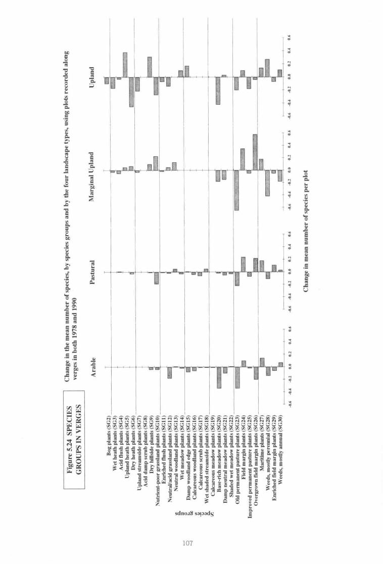
Fig

ure

5.24

SP

EC

IES

GR

OU

PS

INV

ER

GE

S

Cha

nge

inth

em

ean

num

ber

ofsp

ecie

s,by

spec

ies

grou

psan

dby

the

four

land

scap

ety

pes,

usin

gpl

ots

reco

rded

alon

g

verg

esin

both

1978

and

1990

Ara

ble

l'ast

ural

Mar

gina

lU

plan

dU

plan

d

maw

1:53

$

Bog

plan

ts(S

C2)

Wet

heat

hpl

ants

IS(;

3)

Aci

dflu

shpl

ants

(SG

4)

Upl

and

heat

hpl

ants

(565

)

Dry

heat

hpl

ants

(566

)

Upl

and

stre

amsi

depl

ants

(567

)

Aci

dda

mp

scru

bpl

ants

(SC

II)

Dry

hills

ide

plan

ts(5

69)

Nut

rient

-poo

rgr

assl

and

plan

ts(S

G10

)

Enr

iche

dflu

shpl

ants

1561

1)

Neu

tral

/aci

dgr

assl

and

plan

tsIS

Cl2

1

Neu

tral

woo

dlan

dpl

ants

(561

3)

Wet

mea

dow

plan

ts(S

614)

L.D

amp

woo

dlan

ded

gepl

ants

(St;

15)

Cal

care

ous

woo

dlan

dpl

ants

(SC

161

Cal

care

ous

scru

bpl

ants

1561

71

Wet

shad

edst

ream

side

plan

ts(S

C18

)

Cal

care

ous

mea

dow

plan

ts(S

Cl9

)

Bas

e-ric

hm

eado

wpl

ants

(562

0)

Dam

pne

utra

lm

eado

wpl

ants

ISC

2l

Sha

ded

wet

mea

dow

plan

ts(S

622)

Old

perm

anen

tpa

stur

epl

ants

(562

3)

Fie

ldm

argi

npl

ants

(562

4)

Impr

oved

perm

anen

tpa

stur

epl

ants

(562

5)

Ove

rgro

wn

field

mar

gin

plan

ts(5

626)

_

Mar

itim

epl

ants

(562

7)

Wee

ds,

mos

tlype

renn

ial

(562

8)

Enr

iche

dfie

ldm

argi

npl

ants

(562

9)

Wee

ds,

mos

tlyan

nual

(563

0)

El In

nP

AI=

111E

1F

,1

rE

l=

1

oata

rzsr

eQ

a_

.J t=

=:9

Pa

4.01

9.1&

Els 00

0.2

0.1

0.6

0.4

0.6

0.6

0.0

0.2

0.1

06

Cha

nge

inm

ean

num

ber

ofsp

ecie

spe

rpl

ot

Table 5 29 Change in species numbers recorded in paired 'plots placed along verges in :978 and 1990, by landscape typeand GB

ChangeMean Mean in mean SE

Landscape No of species species species of

lYPe plots no 1978 no 1990 no charge P

14 5 13 2 -1 3 0 715 8 15 9 0 0 0 717 0 17 2 0 2 0 919 5 18 8 -0 7 I 415 8 15 2 -0 6 C

(Significance is based on paned mest ProbabiLty (P) <0 I** <0 01. ••• <0 001)

and 'old permanent pasture plants (SG23)- similar to the groups which havedeclined in the Main plots (see52 34-5.2.38).

5.5 20 Verges in the pastural and marginalupland landscapes also showed a declinein 'old permanent pasture plants' (SG23),and an increase in 'overgrown fieldmargin plants' (SG26) and 'field marginplants' (SG24). In the uplands. the 'oldpermanent pasture plants' (SG23) and the'base-rich meadow plants' (5020) havedeclined, along with some ofthe uplandgrass classes (506. 507 and SG10). Insome plots, characteristic of more fertilesoils, there has been an increase inperennial weeds (S028), while on theunenclosed land there has been anincrease of 'dry hillside plants' (509) and'upland heath plants' (SG5).

Verge plots: conclusions

5.5.21 Verges in the lowlands (arable andpastural landscapes) were mainly in the'overgrown eutrophic' (VCP3) and'diverse mesotrophic' (VCP6) classes.These include many species groups whichare less well represented in thesurrounding agricultural fields. The'diverse mesotrophic' class (VPC6) is animportant source of plant diversity.

5 5.22 Verges in the marginal upland and uplandlandscapes are characterised by morespecies-rich upland, mown infertile anddiverse mesotrophic types, which oftenhave a similar species composition to theadjacent land.

.5.5.23 Wider verges contain more meadowspecies and more tall competitive herbs,which play an important role in providinghabitats and a food source for a widevariety of invertebrate and bird species.

5.5.24 In the lowlands there has been an increasein plots from 'overgrown grassy' verges(VPC2) and 'overgrown eutrophic' verges(VPC3), and a decrease in plots in the'diverse mesotrophic' class (VPC6). Therehas been a small but significant loss ofspecies numbers in Verge plots in arablelandscapes (from 14.5 to 13 2 species perplot)

5.5.25 Verges are susceptible to a number offactors which influence their speciescomposition. The management of vergestends to be different from that in thesurrounding countryside Verges are alsovulnerable to disturbance, eg from roadworks and car parldng. Itwas noticeable in1990 (being a year of drought in the southand east) that some verges dried outHowever, the Quality Assurance Exercise(see Appendix 4). using comparable datafrom 1990 and 1991, showed that therewere only small differences due to annualvariation.

5.6 Linen features - Streantsideplots

5.6.1 Vegetation plots were recorded adjacent toditches, streams, rivers, and canals (forconvenience referred to here asstreamsides). They were recorded as 10 mx 1 m plots adjacent to the waterside edge(as defined in the Field Handbook (Barr1990)). In addition, a further linear plot ofthe same size was recorded in the aquaticmargin, to pick up species which wererooted or floating in the water.

5.6.2 In each 1 km square, two plots (which hadpreviously been recorded in 1978) wererandomly located and three further plots(new in 1990) were recorded to ensuredifferent categories of watercourse weresampled. These categories were river orcanalised river; stream; canal; non-roadsideditch; and roadside ditch.

Table 5.25 Frequency of Streamside plots recorded along sixwatercourse categones in 1990 in the four landscape types

Watercourse categorylandscape RoadIYPe River Stream Canal Ditch ditch Other Total

Arable 78 197 10 298 41 6 630Pas:um) 98 376 4 156 19 8 661Marginal

upland337 250 0 49 6 2 344

Upland 47 438 I 42 8 I 537GB 260 1261 IS 545 74 17 2172

Arable I 24Pastural I 1IMargnal upland 40Upland 29GB 3C4

108

Table 5.26 Classification of Strearnside pIois into Stream:side plot easses

Streamsideplot class Name/Descnpnon Shon name

. SPC I Overgrown arsophic grassland with tall herbs and br ambles. mainly bylowland cinchesScrub and shade tolerant herbs. speces-poor. mainly by lowland streamsWoodland on mineral soils, by streams or nvers. lowlandWoodland with heavy shade, on mildly acid soils by streams. lowland/marginal.Reed beds, spec:es-poor mainly by rivers. lowlandOvergrown grassland with perennial weeds, mainly by ditches. :n lowlandand marginal landscapesLightly grazed grassland with Impeded drainage, by sirearns and ditches. Inlowland and marginal laedscapesGrazed improved pasture. mainly by streams, mainly lowland landscapesGrazed rem-al/acid pastures. mainly by streams. species-rich. mainlybwland iandscapes

Acid marshy pasture, mainly by streams some lowland, mainlymarginal and upland landscapes.Moo:land grass. mainly by streams. species-rich, mainly in upland landscapesMoorland shrub heath, by streams, speces-nch. manly in upland landscapesValley bog. by streams. sort :owland and margma: marnly in upland landscapesPeat bog by streams, mainly in up:and landscapesSalonarsh. species-poor. in lowland landscapes

Table 5 25 shows Streamside plotsrecorded in 1990 in terms of landscape typeand watercourse category.

5.6.4 A total of 2172 Streamside plots wererecorded from 446 squares throughout GBin 1990. In order to describe thisvegetation, the species data from all theseplots (plus data from 374 plots previouslyrecorded in 1978) have been classifiedusing the multivariate statistical technique.TWINSPAN, to create 15 'Streamside plotclasses (SPCs). These are shown in Table5.26. ordered on the principal gradient. withshort descriptive names which have beengiven to aid presentation of the results.

Streamside plots: stock in 1990

5.65 Figure 5.25 shows the distribution of thedifferent Streamside plot classes recordedin 1990. in each landscape type. Unlike theverges, there was no pronouncedseparation between the lowlands anduplands, rather a continuous distribution ofplot classes across all four landscapes.although they show different patterns.

5 6.6 In arable landscapes, most of the plots werein grassy vegetation (SPC6-SPC8). many ofthem overgrown (SPC6): these includeditches running through arable fields, andunmanaged vegetation beside rivers. Mostof the 'reed beds' (SPC5) occur in thislandscape type. Compared to otherlandscape types, only a small proportion ofplots were in grazed pastures. There werealso a small number occurring within

Ove:grown eutropluc grassand

Woodland marginWoodlandShaded woodlandReed bedsOvergrown grass:and

Rushy grassland

Improved pastureNeutral/acid pastre

Acid marshy pasture

Moorland grassDwarf shrub heathValley bogPeat bogSaamarsh

woodlands (SPC3, SPC4) or on 'woodlandmargins' (SPC2). In the pasturallandscapes most of the plots were besidestreams or ditches running through 'rushygrassland' (SPC7); others were inwoodland (SPC3. SPC4) or on moorland(SPC 11. SPC13). In the marginal uplandlandscapes more of the plots were inneutral/acid (SPC9) and marshy (SPC7)pasture. whereas in the uplands most ofthe plots were on streams draining bogs(SPC13. SPC14) or running throughmoorland (SPC11. SPC12).

Watercourse category

5.6.7 Figure 5 25 also shows the relationshipbetween watercourse category andStreamside plot class. In the arablelandscapes, the 'reed beds' plot class(SPC5) occurs mainly on rivers, whereasditches often have the overgrown plotclasses (SPC1. SPC6). In the pasturallandscape. streamsides contained all of theplot classes. whilst ditches had morerestricted vegetation confined largely tograssland types (SPC6, SPC7. SPC8). Inthe marginal upland landscapes the samepattern holds. but a higher proportion ofplots were beside streams. In the uplandlandscapes fewer plot classes wererecorded. with the majority of plots besidestreams.

Water plots (second 1 m)

5.6.8 Table 5.27 shows the species recordedmost often in the second 10 mxlm plot,adjacent to the Streamside plot (see

SPC2SPC3SPC4SPC5SPC6

SPC7

SPC8SPC9

SPC 10

SPC 11SPC 12SPC 13SPC 14SPCI5

563

109

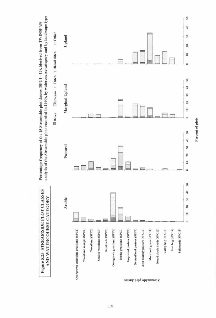
Figu

re5.

25ST

RE

AM

SID

EPL

OT

CL

ASS

ES

AN

DW

AT

ER

CO

UR

SEC

AT

EG

OR

Y

Per

cent

age

freq

uenc

yof

the

15S

trea

msi

depl

otcl

asse

s(S

PC

1-

15),

(der

ived

from

TW

INS

PA

N

anal

ysis

ofth

eS

trea

msi

depl

ots

reco

rded

in19

90),

byw

ater

coum

eca

tego

ryan

dby

land

scap

ety

pe

Riv

erE

lstr

eam

Oni

tch

CR

oad

ditc

hE

Oth

er

Mar

gina

lU

plan

dU

plan

d

Ove

rgro

wn

eutr

ophi

cgr

assl

and

(SP

CI)

Woo

dlan

dm

argi

n(S

PC

2)

Woo

dlan

d(S

PC

3)

Sha

ded

woo

dlan

d(S

PC

4)

Ree

dbe

ds(S

PC

5)

Ove

rgro

wn

gras

slan

d(S

PC

6)

Rus

hygr

assl

and

(SP

CT

)in

Impr

oved

past

ure

(SP

CS

)

T./

Neu

tral

/add

past

ure

(SP

C9)

a,A

cid

man

hypa

stur

e(S

PC

1c)

Moo

rland

gras

s(S

PC

II)

Dw

arf

shru

bhe

ath

(SP

C12

)

Val

ley

bog

(SP

C13

)

Pea

tbo

g(S

PC

I4)

Sal

tmar

sh(S

PC

15)

Ara

ble

Pas

tura

l

PT

hII

II0

010

2030

4050

1020

3040

500

1020

3040

500

1020

3040

50

Per

cent

ofpl

ots

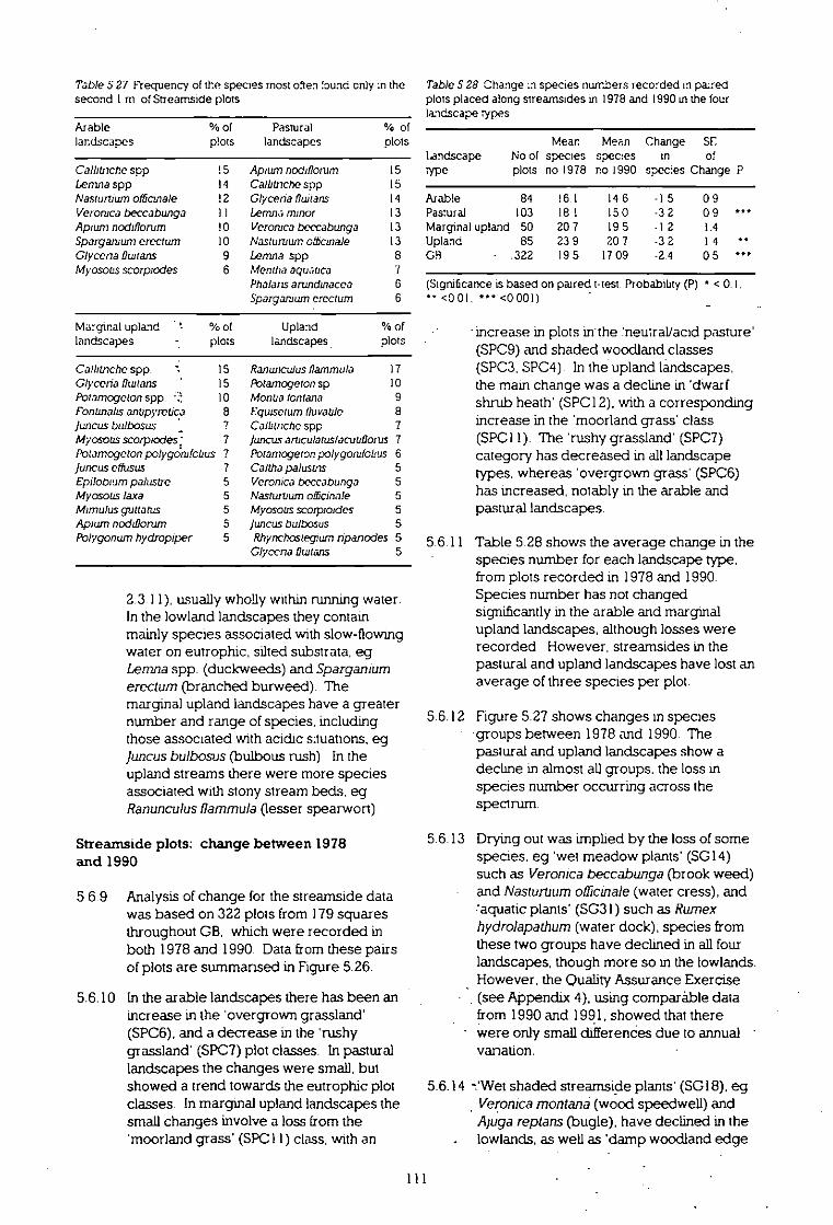
Table 5 21 Frequency of the species most often found only :n the Table 5 28 Change :n species nurnbers recorded in pazedsecond I rn of Strearrside plots plots placed along streamsides in 1978 and 1990 In the four

landscape typesArablelandscapes

Calhtnche sopLemna sppNasturtium olficinaleVeronica beccabungaApium nodiflorurnSpargamurn erecturnGlycena thutansMyosotis scorplodes

% of Pastural

plots landscapes

15 Apiurn nodiflonim

14 Callanche sgp

!2 Glycena Pagans

11 Lerma minor

!0 Veronica beccabunga

10 Nasturtium cthonale9 Lemma spp

6 Mentha aguaticaPhalans anindinacea Sparganiurn erecturn

Mean Mean Change SrLandscape No of species spec:es in oftype plots no 1978 no 1990 speaes Change P

Arable 84 16 1 14 6 -I 5 0 9Pasmral 103 18 15 0 -3 2 0 9Marginal upland 50 20 7 19 5 -1 2 I 4Upland 85 23 9 20 7 -3 2 1 4C13 • 322 19 5 1709 -2 4 0 5 •**

(Significance is based on paired t-test Probability (P) • < 0 I." <0 01. *.* <0 001)

% ofots

5543338'/66

% of plots

Marginal upland t % of Uplandlandscapes plots landscapes

Calbinche spp. 15 Ranunculus flammula 17GlyceriatIuttans • 15 Potamogetonsp 10Potamogeton spp. 10 Montia lontana 9Fontinabs anUpyretica 8 Equisecumfiuvatile 8luncus bulbosus Callanche sopMyosotis scorprodes: 7 lanais articulatuslacutifionisPotamogeton polygorvfcbus Potarnogeton polygondobus 6Juntas effusus 7 Caltha palustns 5Epilobium pa/us-tie 5 Veronica beccabunga 5Myosotis /axe 5 Nastunium officinale 5Mimulusgvnatus 5 Myosous scorploides 5Apium nochDonim 5 luncus bulbasus 5Polygonum hydropiper 5 Rhynchostegium npanccles 5

Glycena Dtatans 5

2.3.11). usually wholly within running water.In the lowland landscapes they containmainly species associated with slow-flowingwater on eutrophic, silted substrata. egLemnaspp. (duckweeds) and Sparganiumerectum (branched burweed). Themarginal upland landscapes have a greaternumber and range of species, includingthose associated with acidic sluations, egJuncusbulbosus (bulbous rush). In theupland streams there were more speciesassociated with stony stream beds, egRanunculusflammula(lesser spearwort).

Streamside plots: change between 1978and 1990

5 6.9 Analysis of change for the streamside datawas based on 322 plots from 179 squaresthroughout GB, which were recorded inboth 1978 and 1990. Data from these pairsof plots are summarised in Figure 5.26,

5.6.10 In the arable landscapes there has been anincrease in the 'overgrown grassland'(SPC6), and a decrease in the 'rushygrassland' (SPC7) plot classes. In pasturallandscapes the changes were small, butshowed a trend towards the eutrophic plotclasses. In marginal upland landscapes thesmall changes involve a loss from the'moorland grass' (SPC I I) class, with an

'increase in plots in-the :neutral/acid pasture'(SPC9) and shaded woodland classes(SPC3, SPC4). In the upland landscapes.the main change was a decline in 'dWarfshrub heath' (SPC12), with a correspondingincrease in the 'moorland grass' class(SPC I 1). The 'rushy grassland' (SPC7)category has decreased in all landscapetypes. whereas 'overgrown grass' (SPC6)has increased, notably in the arable andpastural landscapes.

5.6.11 Table 5.28 shows the average change in thespecies number for each landscape type.from plots recorded in 1978 and 1990.Species number has not changedsignificantly in the arable and marginalupland landscapes, although losses wererecorded However, streamsides in thepastural and upland landscapes have lost anaverage of three species per plot.

5.6.12 Figure 5.27 shows changes in speciesgroups between 1978 and 1990. Thepastural and upland landscapes show adecline in almost all groups. the loss inspecies number occurring across thespectrum.

5.6.13 Drying out was implied by the loss of somespecies. eg 'wet meadow plants' (SG14)such as Veronicabeccabunga (brook weed)and Nasturtiumoflicinale(water cress), and?aquatic plants' (S03 I) such as Rumexhydrolapathum(water dock); species fromthese two groups have declined in all fourlandscapes, though more so in the lowlands.However, the Quality Assurance Exercise(see Appendix 4), using comparable datafrom 1990 and 1991, showed that therewere only small differenCes due to annual •variation.

5.6.14 -.'Wet shaded streamside plants' (SG18), eg- Veronicamontana (wood speedwell) andAjugareptans (bugle), have declined in thelowlands, as well as 'damp woodland edge

111

C.)

Fig

ure

5.26

STR

EA

MSI

DE

Ch

ang

eIn

the

freq

uen

cyo

fth

e14

Str

eam

sId

ep

lot

clas

ses(

SP

C1

-14

),(d

eriv

edfr

om

TW

INS

PA

Nan

alys

iso

fth

e

PL

OT

CL

ASS

ES

Str

eam

sMe

plo

tsre

cord

edin

bo

th19

78an

d19

90),

by

lan

dsc

ape

typ

eE

l19

78•

1990

Ara

ble

Pas

tura

lM

arg

inal

Up

lan

dU

pla

nd

Ove

rgro

wn

eutr

op

hic

gra

ssla

nd

(SP

CI)

Wo

od

lan

dm

arg

in(S

PC

2)

Wo

od

lan

d(S

PC

3)

Sh

aded

wo

od

lan

d(S

PC

4)

Ree

db

eds

(SP

C5)

Ove

rgro

wn

gra

ssla

nd

(SP

C6)

Ru

shy

gra

ssla

nd

(SP

C7)

Imp

rove

dp

astu

re(S

PC

S)

Neu

tral

/aci

dp

astu

re(S

PC

9)

ten

Aci

dm

arsh

yp

astu

re(S

PC

10)

Mo

orl

and

gra

ss(S

PC

11)

Dw

arf

shru

bh

eath

(SP

CI2

)

Val

ley

bo

g(S

PC

13)

Pea

tb

og

(SP

C14

)

1

010

2030

400

1020

3040

010

2030

400

1020

3040

Nu

mb

ero

fp

lots

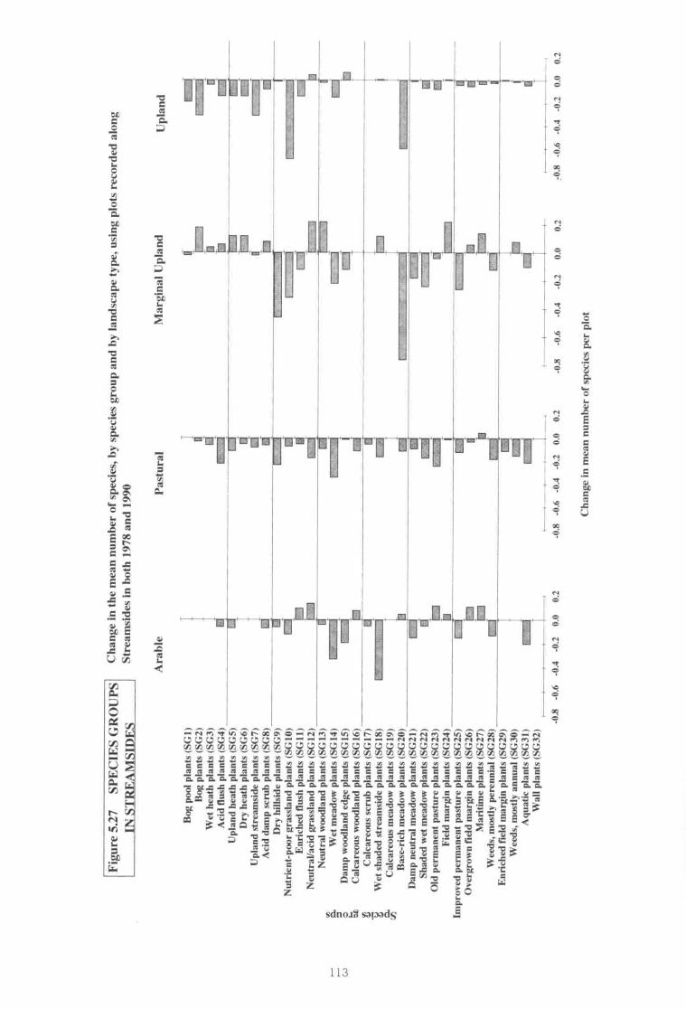
Fig

ure

5.27

SP

EC

I ES

(iR

OU

PS

Cha

nge

inth

em

ean

num

ber

ofsp

ecie

s,by

spec

ies

grou

pan

dby

land

scap

ety

pe,

usin

gpl

ots

reco

rded

alon

gS

trea

msi

des

inbo

th19

78an

d19

90

Ara

ble

l'ast

ural

Mar

gina

lU

plan

dU

plan

d

Bog

pool

plan

ts(S

C1)

Bog

plan

ts(S

C2)

Wet

heat

hpl

ants

(563

)

Aci

dflu

shpl

ants

(S64

)

Upl

and

heat

hpl

ants

(5(5

)D

ryhe

ath

plan

ts(5

66)

Upl

and

stre

amsi

depl

ants

(567

)A

cid

dam

psc

rub

plan

ts(5

68)

Dry

hills

ide

plan

ts(5

69)

Nut

rient

-poo

rgr

assl

and

plan

tstS

610)

Enr

iche

dflu

shpl

ants

(56

I1)

Neu

tral

/aci

dgr

assl

and

plan

ts(5

612)

Neu

tral

woo

dlan

dpl

ants

(SC

13)

ta.W

etm

eado

wpl

ants

(56

14)

0Dam

pw

oodl

and

edge

plan

ts(S

CIS

)tz

Cal

care

ous

woo

dlan

dpl

ants

(561

6)C

alca

reou

ssc

rub

plan

ts(S

617)

Wet

shad

edst

ream

side

plan

ts(S

618)

Cal

care

ous

mea

dow

plan

ts(S

619)

Bas

e-ric

hm

eado

wpl

ants

1562

0)D

amp

neut

ral

mea

dow

plan

ts(5

621)

Sha

ded

wet

mea

dow

plan

ts(5

622)

Old

perm

anen

tpa

stur

epl

ants

(562

3)

Fie

ldm

argi

npl

ants

(562

4)

Impr

oved

perm

anen

tpa

stur

epl

ants

(562

5)O

verg

row

nfie

ldm

argi

npl

ants

1562

6)M

ariti

me

plan

ts(5

627)

Wee

ds,

mos

tlype

renn

ial

1562

8)E

nric

hed

field

mar

gin

plan

ts(5

629)

Wee

ds,

mos

tlyan

nual

(563

0)A

quat

icpl

ants

(563

1)W

all

plan

ts(5

632)

-0.8

-0.6

-04

-0.2

0.0

0.2

-0.8

-0.6

-0.4

-0.2

000.

248

-0.6

-0.4

-0.2

0.0

0.2

-0.8

-0.6

-0.4

4E2

0.0

0.2

Cha

nge

inm

ean

num

ber

ofsp

ecie

spe

rpl

ot

plants (SG15). eg Valehana(valerian) and Angelica sylvestris (angelica)in the arable and marginal uplandlandscapes. The largest losses of anyspecies group, in any landscape type, wereof the 'base-rich meadow plants' (SG20) inthe marginal upland and upland landscapesand the 'infertile grassland plants' (SGIO)which have declined in the uplands.

Streamside plots: conclusions

5.6.15 Streamside vegetation plots in the lowlandswere dominated by-overgrown grasslandand rushy pastures. In the marginal uplandsthey were characterised by a variety of wetpasture types. whilst in the uplandsmoorland types were present.

5.6.16 The extent of grassland with Lmpededdrathage decreased in all landscape types.whilst overgrown grassland increased in thelowlands.

5 6.17 There was an overall loss in speciesnumbers in all Streamside plots, especiallyin the pastural and upland landscapes.

5.6 18 Streamsides contain a range of speciesinfrequent in other pans of lowlandlandscapes and so hold a substantialproportion of lowland plant diversity. Theloss of diversity and the contributory factorswill require further study.

5.7 Conclusions and summary ofChapter 5

5.7.1 In the above discussion, the results havebeen analysed for each component of thelandscape th turn. In concluding, it isimportant to consider the Britishcountryside as a whole.

5.7.2 Figures 5.28, 5.29, 5.30 and 5.31 compare,for each landscape type, in 1990, therelative abundance of species groups in thethree linear features (ie verges, streamsand hedges) with that in the Main plots. Ininterpreting these diagrams, it should beremembered that plots in the linear featureswere 10 rn2whilst the Main plots were 200m2.

5.7.3 In the two lowland landscape types, therewere more species in the 10 m2linear plotsthan in the 200 &Main plots, for mostspecies groups. 'Field margin plants'(SG24), 'improved permanent pastureplants' (SG25) and 'weeds, mostly

perennial' (SG28) were most frequent in theverges. 'Wet meadow plants' (SG14).'damp neutral meadow plants' (SG21) and'aquatic plants' (SG31) were most abundantin Streamside plots, whilst the hedges hadmore woodland species (SG13, SG16 andSG26). The 'base-rich meadow plants'(SG20). described (above) as being widelyin decline, were most abundant onstreamsides and verges in the arablelandscapes, and in verges and fields (ieMain plots) in the pastural landscapes.

5 7 4 In marginal upland landscapes, infesnilegrassland plants' (SG10). 'neutral/acidgrassland plants (SG12). and moorlandplants (SG] -SG5) were most frequentlyrepresented in the Math plots andstreamsides. The 'old permanent pastureplants' (SG23) and 'base-rich meadowplants' (SG20). along with most of thegrassland groups. were most abundant onverges, though also widespread elsewhere.'Wet meadow plants' (SG14) and 'ennchedflush plants' (SG11) were most commonbeside streams, whilst 'neutral woodlandplants' (SG13) and 'dry hillside plants'(SG9) were most frequently recorded inHedge plots Groups associated withupland habitats. ie 'upland streamsideplants' (SG7) . 'wet heath plants' (5G3) and'bog plants' (SG2) were best represented inthe Math plots and Streamside plots.

5.7.5 In the upland landscapes. vegetationrecorded in the Math plots was moreuniform than in the other landscape types, inthat there were more species in fewer plotclasses. Verges contained the highestproportion of 'old permanent pasture plants'(SG23) and -base-rich meadow plants'(5G20). and therefore represent a majorresource of this type. Upland vegetation inthe unenclosed land was well representedby the Main plots. Verges are important fortheir variety of 'infertile grassland plants'(SG10). and the streamside vegetation alsocontains a high proportion of species inthese categories. Overall, the linearfeatures were shown to be important in allfour landscapes, in terms of theircontribution to the diversity of plant species.This was least obvious in uplandlandscapes, where hedges were absentand there were fewer verges thanelsewhere in the country. Verges, andespecially streamsides, were lessdistinctive in their species composition inthe uplands than in other landscapes, sincethey are mainly contiguous with the

114

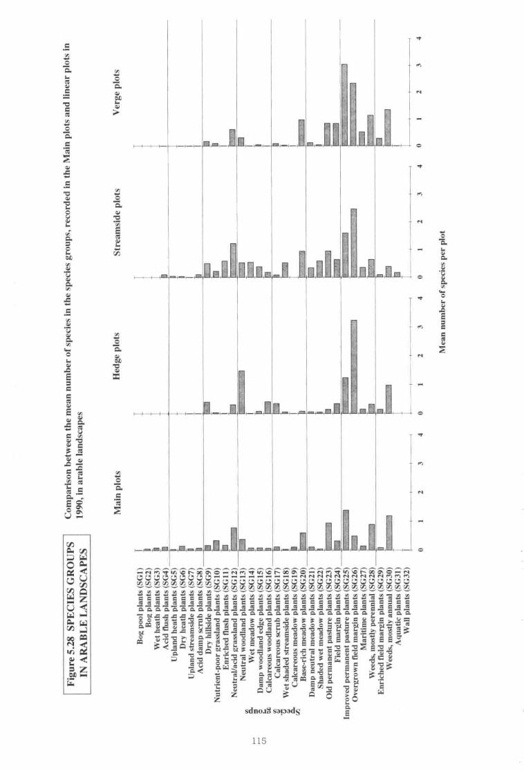
Figu

re5.

28SP

EC

IES

GR

OU

PS

INA

RA

BL

EL

AN

DSC

APE

S

Com

paris

onbe

twee

nth

em

ean

num

ber

ofsp

ecie

sin

the

spec

ies

grou

ps,

reco

rded

inth

eM

ain

plot

san

dlin

ear

plot

sin

1990

,in

arab

lela

ndsc

apes

Mai

npl

ots

Hed

gepl

ots

Str

eam

sIde

plot

sV

erge

plot

s

puz:

21

Imm

oS

.0.

4.11

t4a0

Ulle

al.

23

40

23

40

I2

34

0I

2

tmo

'Is ME

E

1..

Bog

pool

plan

ts(5

61)

Bog

plan

ts(5

62)

Wet

heat

hpl

ants

(S(;

3)

Aci

dflu

shpl

ants

(S64

) U

plan

dhe

ath

plan

ts(S

65)

Dry

heat

hpl

ants

(566

) U

plan

dst

ream

side

plan

ts(5

67)

Aci

dda

mp

scru

bpl

ants

(SG

IO

Dry

hills

ide

plan

ts(5

69)

Nut

rient

-poo

rgr

assl

and

plan

ts(5

610)

E

nric

hed

flush

plan

ts(S

G11

) N

eutr

al/a

cid

gras

slan

dpl

ants

(561

2)

Neu

tral

woo

dlan

dpl

ants

(561

3)

Wet

mea

dow

plan

ts(5

614)

C71

Dam

pw

oodl

and

edge

plan

ts(S

O15

)O

LC

alca

reou

sw

oodl

and

plan

ts(5

616)

Cal

mre

ous

scru

hpl

ants

(561

7)W

etsh

aded

stre

amai

depl

ants

(561

8)a.

Cal

care

ous

mea

dow

plan

ts(5

619)

AB

ase-

rich

mea

dow

plan

ts(5

620)

D

amp

neut

ral

mea

dow

plan

ts(5

621)

S

hade

dw

etm

eado

wpl

ants

(562

2)

Old

perm

anen

tpa

stur

epl

ants

(SO

23)

Fie

ldm

argi

npl

ants

(S62

4)

Impr

oved

perm

anen

tpa

stur

epl

ants

(562

5)

Ove

rgro

wn

field

mar

gin

plan

ts(S

626)

M

ariti

me

plan

ts(S

627)

W

eeds

,m

ostly

pere

nnia

l(S

628)

E

nric

hed

field

mar

gin

plan

ts(5

629)

W

eeds

,m

ostly

annu

al(M

OM

A

quat

icpl

ants

(563

1)

Wal

lpl

ants

(563

2)

Mea

nnu

mbe

rof

spec

ies

per

plot

Fig

ure

5.29

SP

EC

IES

GR

OU

PS

Com

paris

onbe

twee

nth

em

ean

num

ber

ofsp

ecie

sin

the

spec

ies

grou

ps,

reco

rded

inth

eM

ain

plot

san

d

INPA

STU

RA

LL

AN

DSC

APE

Slin

ear

plot

sin

1990

,in

past

oral

land

scap

es

Dog

pool

plan

ts(S

61)

Dog

plan

ts(S

(;2)

W

ethe

ath

plan

ts(S

631

Aci

dflu

shpl

ants

(S(;

4)

Upl

and

heat

hpl

ants

(565

) D

ryhe

ath

plan

ts(5

66)

Upl

and

stre

amsi

depl

ants

(S67

) A

cid

clam

psc

nib

plan

ts(S

OO

D

ryhi

llsid

epl

ants

(569

) N

utrie

nt-p

oor

gras

slan

dpl

ants

(561

0)

Enr

iche

dflu

shpl

ants

(SG

111

Neu

tral

/aci

dgr

assl

and

plan

ts(S

612)

N

eutr

alw

oodl

and

plan

ts(5

613)

W

etm

eado

wpl

ants

(S(;

14)

Dam

pw

oodl

and

edge

plan

ts(S

615)

OL

Cal

care

ous

woo

dlan

dpl

ants

(SG

16)

Cal

care

ous

scru

bpl

ants

(561

7)W

etsh

aded

stre

amsi

depl

ants

(561

8)C

alca

reou

sm

eado

wpl

ants

(561

9)

Bus

e-ric

hm

eado

wpl

ants

(562

0)_

Dam

pne

utra

lm

eado

wpl

ants

(562

1)

Sha

ded

wet

mea

dow

plan

ts(S

622)

O

ldpe

rman

ent

past

ure

plan

ts(5

623)

F

ield

mar

gin

plan

ts(5

624)

Im

prov

edpe

rman

ent

past

ure

plan

ts(5

625)

O

verg

row

nfie

ldm

argi

npl

ants

(S62

6)

Mar

itim

epl

ants

(S62

7)

Wee

ds,

mos

tlype

renn

ial

(562

8)

Enr

iche

dfie

ldm

argi

npl

ants

(S62

9)

Wee

ds,

mos

tlyan

nual

(S63

0)

Aqu

atic

plan

ts(5

631)

W

all

plan

ts(5

632)

Str

eam

side

plot

sV

erge

plot

sM

ain

plot

sH

edge

plot

s

EM I

ltwou

Min

g3r3

11

Sim

_En

__

40

123

401

234

0I

23

40

I2

:

"IM

P

IEN

Mea

nnu

mbe

rof

spec

ies

per

plot

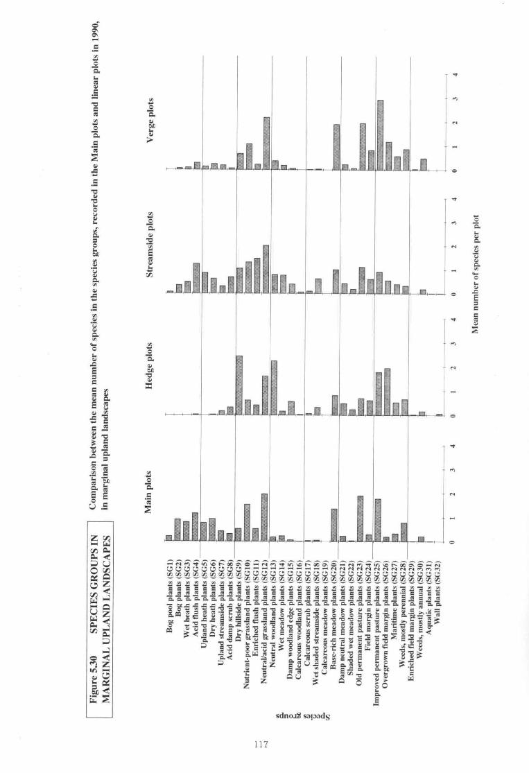
Fig

ure

530

SP

EC

IES

GR

OU

PS

INM

AR

GIN

AL

UP

LAN

DLA

ND

SC

AP

ES

Com

pari

son

betw

een

the

mea

nnu

mbe

rof

spec

ies

inth

esp

ecie

sgr

oups

,re

cord

edin

the

Mai

npl

ots

and

linea

rpl

ots

in19

90,

inm

argi

nal

upla

ndla

ndsc

apes

Stre

amsi

depl

ots

Ver

gepl

ots

Met

tite

lle'

Spec

ios

grou

ps

Mai

npl

ots

Hed

gepl

ots

Bog

pool

plan

ts(S

G!)

Bog

plan

ts(S

G2)

Wet

heat

hpl

ants

(SG

3)A

cid

flush

plan

ts(S

G4)

Upl

and

heat

hpl

ants

(SG

S)

Dry

heat

hpl

ants

(SG

6)U

plan

dst

ream

side

plan

ts(S

G7)

Aci

dda

mp

scm

hpl

ants

(SG

8)D

ryhi

llsid

epl

ants

(SG

9)N

utrie

nt-p

oor

gras

slan

dpl

ants

ISG

IO)

Enr

iche

dflu

shpl

ants

(SG

11)

Neu

tral

/aci

dgr

assl

and

plan

ts(S

G12

)N

eutr

alw

oodl

and

plan

ts(S

G13

)W

elm

eado

wpl

ants

(S(;

14)

Dam

pw

oodl

and

edge

plan

ts(S

G15

)C

alca

reou

sw

oodl

and

plan

ts(S

G16

) C

alca

reou

ssc

rub

plan

ts(S

G17

)I

Wet

shad

edst

ream

side

plan

ts(S

G18

)C

alca

reou

sm

eado

wpl

ants

(SG

19)

Bas

e-ric

hm

eado

wpl

ants

(SG

20)

Dam

pne

utra

lm

eado

wpl

ants

(SG

21)

Sha

ded

wet

mea

dow

plan

ts(S

G22

)

Old

perm

anen

tpa

stur

epl

ants

ISG

23)

1110

)041

1141

1)M

aoF

ield

mar

gMpl

ants

(5G

24)

4.S

IPP

INV

AIS

...W

KN

E.1

17;N

OZ

ON

t14

2).4

0020

1440

2

11,1

4024

1110

11

,14)

11)1

1:

18,=

1041

4)00

8,110

0

Impr

oved

perm

anen

tpa

stur

epl

ants

(SG

2S)

Ove

rgro

wn

field

mar

gin

plan

ts(5

(7.2

6)M

ariti

me

plan

ts(5

627)

Wee

ds,

mos

tlype

renn

ial

(562

8)E

nric

hed

field

mar

gin

plan

ts(S

G29

)W

eeds

,m

ostly

annu

al(5

6301

*A

quat

icpl

ants

(SG

31)

Wal

lpl

ants

(563

2)

01

23

0123

4012

3423

4

Mea

nnu

mbe

rof

spec

ies

per

plot

Fig

ure

5.31

SP

EC

IES

GR

OU

PS

INC

ompa

rison

betw

een

the

mea

nnu

mbe

rof

spec

ies

inth

esp

ecie

sgr

oups

,re

cord

edin

Mai

npl

ots

and

linea

rpl

ots

in

UP

LAN

DIA

ND

SC

AP

ES

1990

,in

upla

ndla

ndsc

apes

Ct

r33

N

Bog

pool

plan

ts(M

a)B

ogpl

ants

(862

)W

ethe

ath

plan

ts($

63)

Add

flush

plan

ts(5

64)

Upl

and

heat

hpl

ants

(565

)D

ryhe

ath

plan

ts(5

66)

Upl

and

stre

amsi

depl

ants

(567

)A

cid

dam

pse

nd)

plan

ts(S

CA

)

Dry

hills

ide

plan

ts(5

69)

Nut

rient

-poo

rgr

awda

ndpl

ants

(S61

0)

Enr

iche

dflu

shpl

ants

(SG

II)

Neu

tral

/ark

!gr

assl

and

plan

ts(5

612)

Neu

tral

woo

dlan

dpl

ants

(561

3)

Wet

mea

dow

plan

ts(5

614)

Dam

pw

oodl

and

edge

plan

ts(S

615)

Cal

care

ous

woo

dlan

dpl

ants

(S61

6)

Cal

care

ous

scru

bpl

ants

(561

7)W

etsh

aded

stre

amsi

depl

ants

(861

8)

Cal

care

ous

mea

dow

plan

ts(S

619)

Bas

e-rk

hm

eado

wpl

ants

(562

0)

Dam

pne

utra

lm

eado

wpl

ants

(562

1)S

hade

dw

etm

eado

wpl

ants

(S62

2)

Old

perm

anen

tpa

stur

epl

ants

(562

3)F

ield

mar

gin

plan

ts(S

624)

Impr

oved

perm

anen

tpa

stur

epl

ants

(S62

5)O

verg

row

nfie

ldm

argi

npl

ants

(562

6)

Mar

itim

epl

ants

(S62

7)W

eeds

,m

ostly

pere

nnia

l(8

628)

Enr

iche

dfie

ldm

argi

npl

ants

(862

9)W

eeds

,m

ostly

annu

al(5

630)

Aqu

atic

plan

ts(S

G31

)W

all

plan

ts(8

632)

L

Mai

npl

ots

Hed

gepl

ots

Insu

ffici

ent

data

to

prod

uce

natio

nal

estim

ates

Str

eam

side

plot

sV

erge

plot

s

12

34

01

23

40

12

40

12

3

Mea

nnu

mbe

rof

spec

ies

per

plot

surrounding open moorland and grassland;however, they still make a majorcontribution to the overall diversity

5.7.6 In the marginal upland and lowlandlandscapes the contribution of hedges,verges and streams to botanical diversitywas more apparent The hedges containmany woodland and shrub species, and,together with the verges, provide a refugefor many meadow and pasture species.The streamsides also contain grasslandspecies which require damp conditions andthat are absent elsewhere in thecountryside The significance of linearfeatures was most obvious in the arablelandscapes where the fields were generallyspecies-poor, and most of the remainingdiversity of native plant spec:es occurs inthe restricted areas which were covered bythe Habitat plots.

5.7.7 The extent and types of change affecting theareal habitats and linear features have beendiscussed earlier, and it is useful at thispoint to draw these together to provide asummary of the overall impact on the widercountryside.

5.7.8 in the arable landscapes, the arable fieldshave lost diversity from an already lowbase. The hedge-bottom flora wasincreasingly becoming dominated byspecies associated with cultivated land.Both verges and streamsides showincreases in vigorous species as opposed toa decline in more sensitive meadowspecies. Streamsides have lost speciesoverall, especially those associated withaquatic margins, wet meadows and moistwoodland The woodland and semi-improved grassland plot classes show littlechange.

5.7 9 In the pastural landscapes. the semi-improved grassland shows a significantdecline in species. especially those typicalof unimproved mesotrophic meadows. Thelatter have also declined in the hedgebottoms, verges and streamsides. Theverges have become more overgrown andshow an increase in coarse grasses as wellas species associated with disturbance.The streamsides also have fewer speciesindicative of aquatic margins and wetmeadows. Woodland shows a decline inspecies number and evidence ofdisturbance, with a trend towards a moregrassy ground flora. The loss of meadowspecies. which were once an important

component of the pastural landscapes, hasfurther reduced an already depletedresource. This landscape type has thehighest degree of change, in part becauseof the extent of the changes themselves, andin pan because of the range of typespresent.

5.7.10 ln the marginal upland landscapes. theresults show an interchange between thegrassland types. The hedge bottoms havemore species associated with improvedgrassland. and fewer woodland species.The woods themselves show a loss inspecies number which has affected mostspecies groups. Some semi-improvedfields show a small increase in speciesnumber and a trend towards mcreasingabundance of species associated withunimproved and infertile soils. Thesespecies have also increased in the uplandgrass mosaics, which otherwise wererelatively stable. There was a decline inwet meadow species from the streamsideswhich have also lost some speciesassociated with unimproved and infertilesoils. The verges include more plot classescharacteristic of overgrown and shadedconditions as was the case in the lowlandlandscapes. with fewer meadow speciesand more coarse grasses Moorland showsan increase in species. particularly thosefrom grassland species groups, at theexpense of heathland groups. This agreeswith the widely held view that thesemarginal upland areas are particularlysensitive to change and may be associatedwith the mixture of upland and lowlandtypes of vegetation in close proximity.

5.7.11 in the upland landscapes, woodland haslost species from most groups. The uplandgrass mosaics have also lost diversityoverall, whereas moorland shows a smallincrease in diversity. especially in speciesassociated with flushes. Overall, there wasa limited range of plot classes in theuplands, but these contain a large numberof individual species. The changes.therefore, were relatively small incomparison with this total resource.

119

120

Chapter 6 THE RESULTS(IV): FRESHWATERSTUDIES

6 1 Introduction 1216.2 CS1990 field survey 1216.3 Related surveys and data bases 1266.4 Summary of Chapter 6 126

6.1 Introduction Table 6.1171e number (and p!oportion) of I Ian squares surveyed.sampled, dry or unsstable in each of the four landscape types

6.1.1 The 1990 survey was the first of the threecountryside surveys (1978, 1984 and 1990) toincorporate the study of running-watermacro-invertebrate assemblages. Changestatistics of the type given elsewhere in thisreport are therefore not yet available forfreshwater assemblages. The datapresented here provide a baseline againstwhich future change can be assessed

6. I 2 Sites sampled in Countryside Survey 1990(CS1990) sites were mainly on small streams.as described in Chapter 2. In order to makebetween-landscape comparisons of macro-invertebrate assemblages in largerwatercourses. analyses of other appropriateInstitute of Freshwater Ecology (IFE) andwater industry data sets need to beundertaken. This is to be the subject of aseparate thematic report (Furse et al. inprep.).

6.2 CS1990 field survey

Sampling sites

6.2 I Each of the 508 1 lcm squares were surveyedfor possible freshwater sampling sites. Ofthese. only 361 squares had a suitablerunning watercourse which was sampled foraquatic macro-invertebrates. Of theremaining squares. 64 had no watercoursesmarked on OS l:10 000 maps or anyapparent in the square during survey. Afurther 66 sites had marked channels whichwere found to be dry when surveyed In 15squares the only rivers or canals presentwere not eligible for sampling (see 2 5.3) andno samples were available for the tworemaining squares.

6.22 The greatest number and proportion of drysquares were in the arable landscapes(Table 6.1), whereas there were very fewsuch squares in either the marginal upland orupland landscapes. 'In a high proportion of

Land- Dry Unsuitablescape Sur- I or un-type veyed Sampled No streams Dry streams available

Arable 162 81(5Cf%) 37 (23%) 37 (23%) 7 (4%)Pastural 158 I IC (70%) 18 (11%) 23 (15%) 7 (4%)Marginal

upland77 66 (86%) 7 (9%) 3 (4%) I (I%)

Upland III 104 (94%) 2 (2%) 3 (34/0 2 (2%)

GB 508 361(71%) 64 (13%) 66 ( ! 3O) 7 (3%)

squares in the arable landscapes, allwatercourses present were dry at the time ofsurvey; these were predominantly lowlandsquares in south-east England. the eastMidlands and East Anglia, and oftenassociated with chalk soils. In the pasturallandscapes the highest proportion of drysquares of this kind were m the south. theMidlands, and coastal areas.

6.2.3 A comparison between squares sampled inthe 1988 pilot study. and those surveyed forsampling in 1990 provides further informationon intermittently dry squares (Table 6.2).Overall, 9% of the 156 squares sampled in1988 were dry in 1990. A large majority ofthese dried squares were in the eastMidlands and East Anglia.

Environmental characteristics

6.2.4 The environmental characteristics of streamsin the four landscapes, and their dominantriparian vegetation and adjacent land use arecompared in Tables 6.3 and 6.4. Channel

Table 6 2 Tne numbers of sqbares in each :andscape type whichwere sampled in 1988 and surveyed in 1990. together with thenumber (and proportion) which had Lowmg wa:ercourses in

1988 (wet) but none in 1990 (dry)

Landscape Squares visited in Sqbares wet in :988ripe 1988 and 1990 but dry in 1990

Arable 42 8(19%)Pasairal 53 4(8%;Marginal upland 25 2(8%)Upland 36 0(0%)

GB 56 14(9%)

121

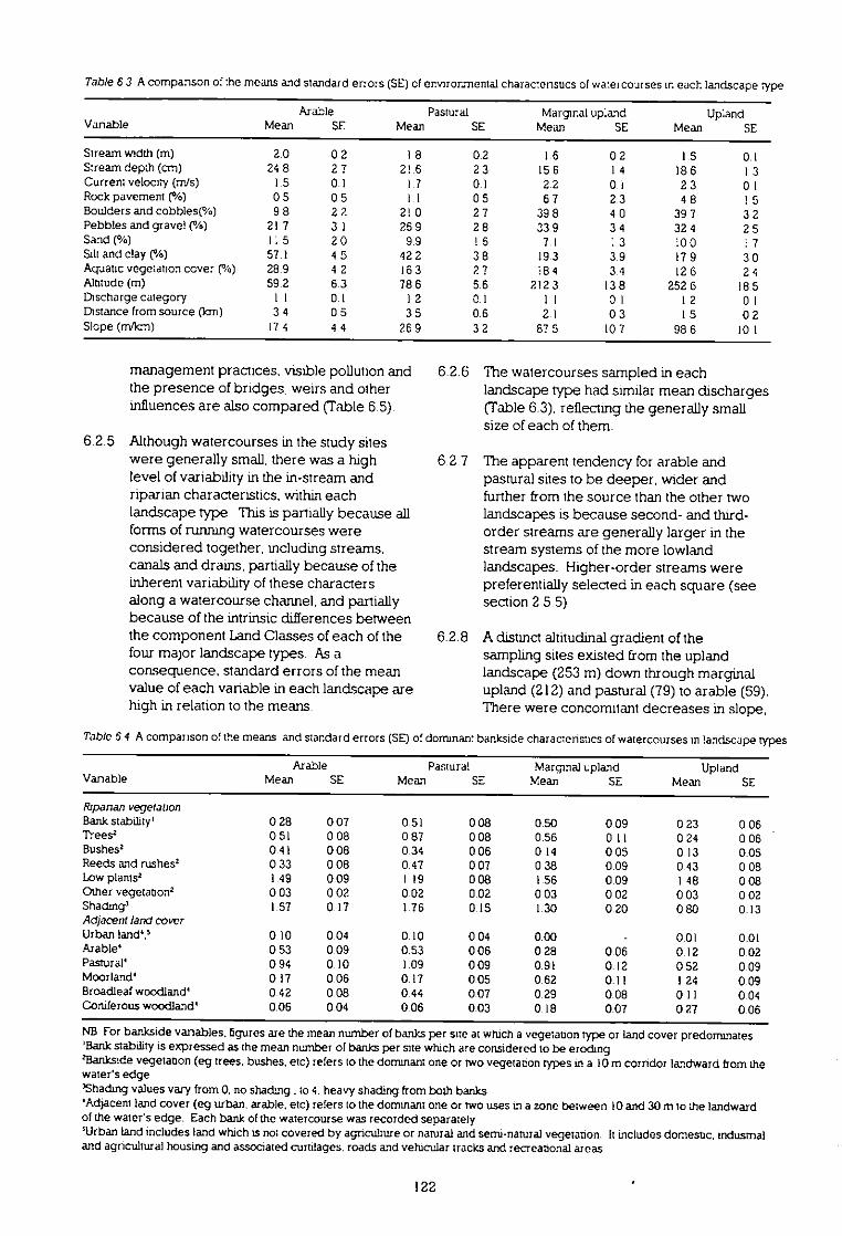
Table 6 3 A companson of :he means and standard errors (SE) of envirormental charamensucs of watet courses in each landscape type

VariableArable

MeanSEPastural

Mean SEMarginal up:and

MeanSE MeanUpland

SE

Stream width (m) 2 0 0 2 1 8 0 2 1 6 0 2 I 5 0 1S:ream depth (cm) 24 8 2 7 21 6 2 3 15 6 1 4 18 6 1 3Current velocity (rnts) I 5 0 1 I 7 0 1 2 2 0 1 2 3 0 1Rock pavement (%) 0 5 0 5 11 0 5 6 7 2 3 4 8 1 5Boulders and cobbles(%) 9 8 2 2 21 0 2 7 39 8 4 0 39 7 3 2Pebbles and grave! (%) 21 7 3 1 25 9 2 8 33 9 3 4 32 4 2 5Sand (%) 1.5 2 0 9 9 ! 5 7 1 : 3 :0 0 . 7Silt and clay (%) 57 1 4 5 42 2 3 8 19 3 3 9 17 9 3 0Agoatic vegetation cover (0/0) 28 9 4 2 16 3 2 7 18 4 3 4 12 6 2 4Altitude (m) 59 2 6 3 78 6 5 6 212 3 13 8 252 6 18 5Discharge category 11 0 1 1 2 0 1 11 0 1 1 2 0 1Distance from source (km) 3 4 0 5 3 5 0 6 2 I 0 3 I 5 0 2Slope (mich) 17 4 4 4 26 9 3 2 87 5 10 7 98 6 10 1

management practices, visible pollution andthe presence of bridges, weirs and otherinfluences are also compared (Table 6.5).

6.2.5 Although watercourses in the study siteswere generally small, there was a highlevel of variability in the in-stream andriparian characteristics, within eachlandscape type. This is partially because allforms of running watercourses wereconsidered together. including streams,canals and drains, partially because of theinherent variability of these charactersalong a watercourse channel, and partiallybecause of the intrinsic differences betweenthe component Land Classes of each of thefour major landscape types. As aconsequence, standard errors of the meanvalue of each variable in each landscape arehigh in relation to the means.

6.2.6 The watercourses sampled in eachlandscape type had similar mean discharges(Table 6.3). reflecting the generally smallsize of each of them.

6.2.7 The apparent tendency for arable andpastural sites to be deeper, wider andfurther from the source than the other twolandscapes is because second- and third-order streams are generally larger in thestream systems of the more lowlandlandscapes. Higher-order streams werepreferentially selected in each square (seesection 2.5.5)

6.2.8 A distinct altitudinal gradient of thesampling sites existed from the uplandlandscape (253 m) down through marginalupland (212) and pastural (79) to arable (59).There were concomitant decreases in slope.

Table 5.4 A comparison of the means and standard errors (SE) of dominant bankside characteristics of watercourses in landscape types

Anble

Pastural Marginal upland

UplandVanable MeanSE Mean SE Mean SE Mean SE

Ripanan vegetation

Bank stability' 0 28 0 07 0 51 0 118 0 50 0 09 0 23 0 06Trees2 0 51 0 08 0 87 0 08 0 56 0 II 0 24 0 06Bushes' 0 41 0 08 0 34 0 06 0 14 0 05 0 13 0.05Reeds and rushes2 0 33 0 08 0 47 0 07 0 38 0 09 0 43 0 08Low plants' 1 49 0 09 119 0 08 1 56 0 09 1 48 0 08Other vegetation2 0 03 0 02 0 02 0 02 0 03 0 02 0 03 0 02Shadmg" I 57 0 17 1 76 0 15 1 30 0 20 0 80 0.13Adjacent land cover

Urban land? 0.10 0.04 0.10 0 04 0.00 - 0.01 0.01Arable' 0.53 0.09 0.53 0 06 0 28 0.06 0.12 0.02Pastural' 0.94 0.10 1.09 0 09 0.91 0.12 0 52 0.09Moorland' 0 17 0.06 0.17 0.05 0.62 0.11 I 24 0.09Broadleaf woodland' 0.42 0.08 0 44 0.07 0.29 0.08 0 I I 0.04Coniferous woodland' 0.06 0.04 0 06 0.03 0.18 0.07 0 27 0.06

NB For bankside variables. figures are the mean number of banks per site at which a vegetation type or land cover predominates'Bank stability is expressed as the mean number of banks per site which are considered to be erodingSankside vegetation (eg trees, bushes, etc) refers to the dominant one or two vegetation types in a 10 m corridor landward from thewater's edge'Shading values vary from 0, no shadung . to 4. heavy shading from both banks'Adocent land cover (eg urban. arable, etc) refers to the dominant one or two uses in a zone between 10 and 30 m to the landwardof the water's edge Each bank of the watercourse was recorded separately'Urban land includes land which is no; covered by agriculture or natural and semi-natural vegetation It mcludes domestic, industrialand agricultural hounng and assmated curulages. roads and vehicular tracks and recreabonal areas

122

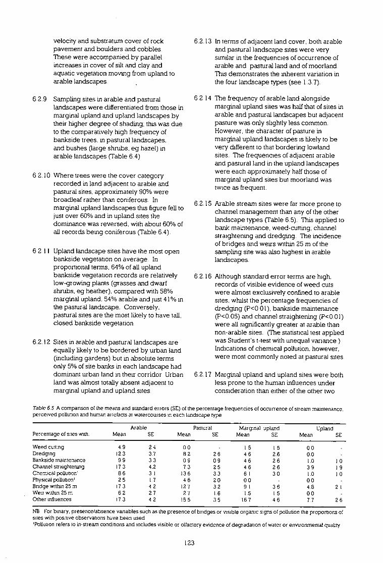
velocity and substratum cover of rockpavement and boulders and cobbles.These were accompanied by parallelincreases in cover of silt and clay andaquatic vegetation moving from upland toarable landscapes.

6.2.9 Sampling sites in arable and pasturallandscapes were differentiated from those inmarginal upland and upland landscapes bytheir higher degree of shading; this was dueto the comparatively high frequency ofbankside trees, in pastural landscapes.and bushes (large shrubs, eg hazel) inarable landscapes (Table 6.4)

6.2.10 Where trees were the cover categoryrecorded in land adjacent to arable andpastural sites. approximately 90% werebroadleaf rather than coniferous. Inmarginal upland landscapes this figure fell tojust over 60% and in upland sites thedominance was reversed, with about 60% ofall recorcLs being coniferous (Table 6.4).

6.2.11 Upland landscape sites have the most open bankside vegetation on average. Inproportional terms, 64% of all uplandbankside vegetation records are relativelylow-growing plants (grasses and dwarfshrubs, eg heather), compared with 58%marginal upland. 54% arable and just 41% inthe pastural landscape. Conversely,pastural sites are the most likely to have tall.closed bankside vegetation.

6.2.12 Sites in arable and pastural landscapes areequally likely to be bordered by urban land(including gardens) but in absolute termsonly 5% of site banks in each landscape haddominant urban land in their corridor. Urbanland was almost totally absent adjacent tomarginal upland and upland sites.

6.2.13 In terms of adjacent land cover, both arableand pastural landscape sites were verysimilar in the frequencies of occurrence ofarable and pastural land and of moorland.This demonstrates the inherent variation inthe four landscape types (see 1.3.7).

6.2.14 The frequency of arable land alongsidemarginal upland sites was half that of sites inarable and pastural landscapes but adjacentpasture was only slightly less common.However, the character of pasture inmarginal upland landscapes is likely to bevery different to that bordering lowlandsites. The frequencies of adjacent arableand pastural land in the upland landscapeswere each approximately half those ofmarginal upland sites but moorland wastwice as frequent.

6.2.15 Arable stream sites were far more prone tochannel management than any of the otherlandscape types (Table 6.5). This applied tobank maintenance. weed-cutling, channelstraightening and dredging. The incidenceof bridges and weirs within 25 m of thesampling site was also highest in arablelandscapes.

6.2.16 Although standard error terms are high.records of visible evidence of weed cutswere almost exclusively confined to arablesites. whilst the percentage frequencies ofdredging (P<0.01). bankside maintenance(P<0.05) and channel straightening (P<0.01)were all significantly greater at arable thannon-arable sites. (The statistical test appliedwas Student's t-test with unequal variance.)Indications of chemical pollution, however,were most commonly noted at postural sites.

6.2.17 Marginal upland and upland sites were bothless prone to the human influences underconsideration than either of the other two

Table 6.5 A companson of the means and standard errors (SE) of the percentage frequencies of occurrence of stream maintenance,perceived pollution and human artefacts at watercourses in each landscape type

Percentage of saes with: MeanArablePastural

SEMean SEMarginal upland

MeanSE MeanUpland

SE

Weed cuttsig 4 9 2 4 0 0

1 5 I 5 0 0

Dredging 12 3 3 7 8 2 2 6 4 6 2 6 0 0 -Bankside maintenance 9 9 3 3 0 9 0 9 4 6 2 6 1 0 1 0Channel straightening 17 3 4.2 7 3 2 5 4 6 2 6 3 9 1 9Chemical pollution 8 6 3 1 13 6 3 3 6 1 3 0 1 0 1 0Physical pollunon' 2 5 1 7 4 6 2 0 0 0 - 0 0 -Bndge within 25 m 17 3 4 2 12 7 3 2 9 1 3 6 4 8 2 IWeir within 25 m 6 2 2 7 2 'I 1 6 I 5 I 5 0 0 -Other influences 17 3 4 2 15 5 3 5 16 7 4 6 7 7 2 6

NB For binary, presence/absence vanables such as the presence of bridges or visible organ:c signs of pollution the proportions ofsites with posaive observations have been used'Pollution refers to in-stream conditions and Includes visible or olfactory evidence of degradation of water or environmental quality

123

landscape types. with upland sites especiallyfree of maintenance activities, bridges andweirs.

Freshwater environmental quality

6.2.18 The RIVPACSmethodology (see Chapter 2)was used to assess the environmental qualityof sites, as indicated by their macro-invertebrate assemblages.

6.2.19 In general terms, the higher the total oraverage score attained by a s:te the greaterits environmental quality is assessed to be(but see 6.2.23) RIVPACSuses a system ofprediction by analogy to forecast targetBiological Monitoring Working Party(BMWP)scores and Average Score PerTaxon (AS17) of sites, based on theirmeasured environmental characteristics.

6.2.20 The means of the observed and RIVPACS-predicted BMWP scores, number of scoringtaxa and ASPT for sites in each landscapetype are shown LnTable 6.6 and in Figure6.1.

6.2.21 Mean predicted BMWPindex values areconsistently higher than those observed inthe samples collected. This is simplybecause mean predictions are based uponthe idealised fauna in the absence ofpollution, whereas the mean observedvalues are derived from both clean andpolluted sites. Mean observed scores are areflection of the average degree to whichthe component sites are polluted, orotherwise stressed.

6.2.22 The most marked difference betweenlandscape types was in ASPT.which tendedto increase from sites in arable landscapes,

through pastural and marginal upland toupland. This shift was more marked inobserved than predicted values andindicated a possible environmental qualitygradient, increasing in the direction of theupland landscapes.

6.2.23 The values given in Table 6.6 can be used asa basis for monitoring future change.However, because of their underlyingenvironmental characteristics. sites differ inthe actual score they can attain, even whenunpolluted. This is shown by the between-landscape predicted values in the Table.This critical factor needs to be taken intoaccount when making spatial comparisonsbetween sites in different landscapes.

6.2.24 Comparisons were also made between theEnvironmental Quality Index (E01) values forsites in each landscape type (Table 6.6).There is little difference between landscapesin their EQI values for BMWPscore andnumber of scoring taxa. However, thebiological quality of the watercourses is bestindicated by their EQls for the ASIY1'(Wrightet al. 1988). Here the gradient of improvedquality from arable to upland, suggested insection 6.2.22, is confirmed by a pattern ofincreasing EQI values for each landscapeTYPe.

6.2.25 All 339 sites in CS1990. for which R1VPACSis operative (see 2,5.20). were assigned toan ASIYI'quality band using the methodologydescribed in Chapter 2. The distribution ofsites in four quality bands is shown in Table6 7

6.2.26 Overall, 71% of the sites were assigned tothe highest quality band. band A. whichcomprises sites sufficiently close to their

Table 6 6 A comparison of the means and standard errors (SE) of river quality charactenstics of watercourses in each landscape type

Arable

Pastaral Marginal upland Upland

Variable MeanSE Mean SE MeanSE Mean SE

Observed BMWPscore 60 53.6 71.9 4.1 68.3 5 I 61.3 3 1Observed number of taxa I 3 30.6 14.0 0 6 11.8 0 7 10 4 0 4Observed ASFT 4 20.1 4 8 0.1 5.5 0 2 5.7 0.1Predicted BMWPscore 94 41.0 104 0 1 8 110.2 2 6 96.7 0.9Predicted number of taxa 18.50.3 19.1 0 2 18 2 0 4 16 2 0.1Predicted ASPT 5 10.1 5 4 0 1 6.0 + 6.0 +EQIBMWP score 0.640.04 0 68 0.04 0.62 0.05 0 63 0 03E01 number of taxa 0 720.03 0 73 0.03 0.65 0 04 0 64 0 03EQI ASPT 0 840.02 0.88 0.02 0.91 0.03 0.96 0 02

NB The rano of the observed score or ASPTof a sample collected from a sne and that predicted for it by RIVPACSis termed theEnvironmental Quality Index (E01) and is an expression of the extent to whach the fauna of a site matches that to be expected tn theabsence of environmental stress, (Wright et a/ 1988). A perfect match provides an £01 of I, whilst a site without taxa will have anCOI of zero Using this procedure mes of entirely different environmental character, in different parts of the country, may becompared on a common basis (NB * = <0 05)

124

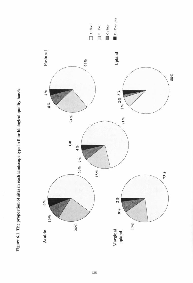
Fig

ure

6.1

The

prop

ortio

nof

site

sin

each

land

scap

ety

pein

four

biol

ogic

alqu

ality

band

s

Ara

ble

6%4%

Pas

tura

l10

%

GB

24%

24%

60%

7%4%

64%

Mar

gina

l

upla

nd2

8%%

18%

71%

7%2%

3%U

plan

d

A: G

oal

13F

air

CP

oor

DV

ery

poor

17%

73%

88%

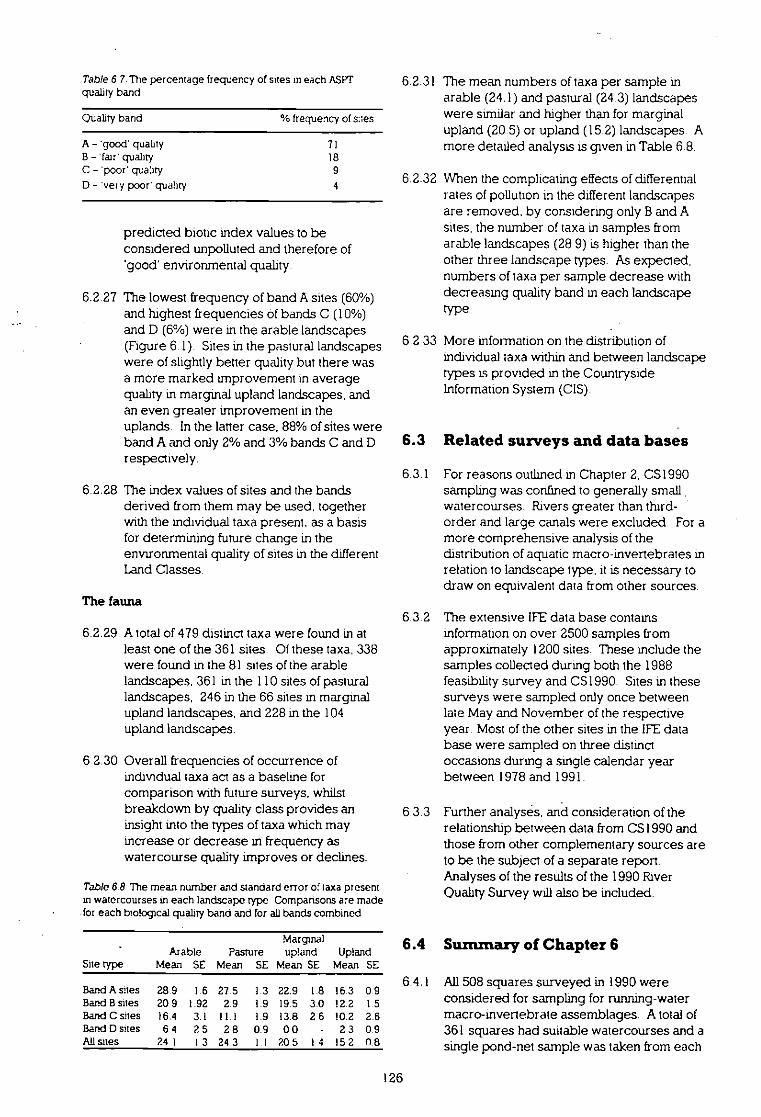
Table 6 7. The percentage frequency of saes in each ASP1'quality band

Otality band % frequency of ales

A - 'good quality 71B - 'fan' quality 18C - 'poor' quality 9

D - 'very poor' quality 4

predicted biotic index values to beconsidered unpolluted and therefore of'good' environmental quality.

6.2.27 The lowest frequency of band A sites (60%)and highest frequencies 6f bands C (10%)and D (6%) were in the arable landscapes(Figure 6.1). Sites in the pastural landscapeswere of slightly better quality but there wasa more marked improvement in averagequality in marginal upland landscapes, andan even greater improvement in theuplands. In the latter case, 88% of sites wereband A and only 2% and 3% bands C and Drespectively.

6.2.28 The index values of sites and the bandsderived from them may be used, togetherwith the individual taxa present, as a basisfor determining fumre change in theenvironmental quality of sites in the differentLand Classes.

The fauna

6.2.29 A total of 479 distinct taxa were found in atleast one of the 361 sites. Of these taxa. 338were found in the 81 sites of the arablelandscapes. 361 in the 110 sites of pasturallandscapes, 246 in the 66 sites m marginalupland landscapes, and 228 in the 104upland landscapes.

6.2.30 Overall frequencies of occurrence ofindividual taxa act as a baseline forcomparison with future surveys, whilstbreakdown by quality class provides aninsight into the types of taxa which mayincrease or decrease in frequency aswatercourse quality improves or declines.

Table 6 8 The mean number and standard error of taxa presentin watercourses in each landscape type Comparisons are madefor each btolcgical qualay band and for all bands combined

Arable PastureMarginalupland Upland

Site type Mean SE Mean SE Mean SE Mean SE

Band A sites 28.9 1.6 27.5 1.3 22.9 1.8 16.3 0 9Band B sites 20.9 1.92 2.9 1.9 19.5 3.0 12.2 1 5Band C sites 16.4 3.1 11.1 1.9 13.8 2 6 10.2 2.6Band D sites 6.4 2 5 2.8 0.9 0 0 - 2 3 0.9All sites 24.1 I 3 24.3 1.1 20 5 1 4 15 2 0.8

6.2.31 The mean numbers of taxa per sample inarable (24.1) and pastural (24.3) landscapeswere similar and higher than for marginalupland (20.5) or upland (15.2) landscapes. Amore detailed analysis is given in Table 6.8.

6.2.32 When the complicating effects of differentialrates of pollution in the different landscapesare removed, by considering only B and Asites, the number of taxa in samples fromarable landscapes (28 9) is higher than theother three landscape types. As expected.numbers of taxa per sample decrease withdecreasing quality band in each landscapetype

6.2 33 More information on the distribution ofindividual taxa within and between landscapetypes is provided in the CountrysideInformation System (CIS).

6.3 Related surveys and data bases

6.3.1 For reasons outlined in Chapter 2. CS1990sampling was confined to generally smallwatercourses. Rivers greater than third-order and large canals were excluded. For amore comprehensive analysis of thedistribution of aquatic macro-invertebrates inrelation to landscape type, it is necessary todraw on equivalent data from other sources.

6.3.2 The extensive IFE data base containsinformation on over 2500 samples fromapproximately 1200 sites. These include thesamples collected during both the 1988feasibility survey and CS1990. Sites in thesesurveys were sampled only once betweenlate May and November of the respectiveyear. Most of the other sites in the IFE database were sampled on three distinctoccasions during a single calendar yearbetween 1978 and 1991.

6 3 3 Further analyses, and comsideration of therelationship between data from CSI990 andthose from other complementary sources areto be the subject of a separate report.Analyses of the results of the 1990 River(Duality Survey will also be included.

6.4 Sununary of Chapter 6

6.4.1 All 508 squares surveyed in 1990 wereconsidered for sampling for running-watermacro-invertebrate assemblages. A total of361 squares had suitable watercourses and asingle pond-net sample was taken from each

326

of these squares. Most watercoursessampled were small channels within 2 lan oftheir source

642 Analyses were undertaken and results arepresented at the landscape level. Thenumbers of samples from each landscapevaried between 66 (marginal upland) and110 (pastural)

6 4.3 Squares lacking flowing watercourses weredivided into two types. those without runningwater channels and those in which allchanneLs were dry. Comparison betweensquares sampled for aquatic macro-invertebrates L-11988and re-surveyed in1990 showed that an average of 9% ofsquares with flowing water in 1988 were dryin 1990. In all cases, the rate of drying-upwas highest in the arable landscape andlowest in the upland landscapes.

6.4.4 Environmental characteristics of sites in eachlandscape type were compared. Adecreasing altiludinal gradient existed fromupland landscapes, through marginal uplandand pastural. to arable. Slope, velocity andcoarseness of substratum decreased alongthe same gradient, whilst degree of siltationand aquatic macrophy.e cover increased.

6 4 5 Sites in the arable and pastural landscapeswere more shaded and had more frequentadjacent urban land than marginal upland orupland sites. Bankside trees and woodswere primarily broadleaf in the lowlandlandscapes. Upland sites were more open.on average, than :hose in the marginalupland landscapes, with twice as manyrecords of adjacent moorland. Coniferouswoodland was twice as common alongsideupland sites as beside sites in the marginaluplands where broadleaf predomina:ed

6.4 6 Sites in arable landscapes mcluded moreexamples of bank maintenance, weed-cutting, channel straightening, dredging andthe presence of bridges and weirs thanthose in any other landscapes. Indications ofpollution were most frequently noted inpastural landscapes Marginal upland and.especially. upland sites were least prone tohuman influences of the type beingrecorded.

6.4.7 On average, the poorest environmentalquality (determined using the IFER1VPACSsystem) was recorded at sites in araidelandscapes. with successive improvementsthrough pastural and marginal upland toupland sizes. Overall. 71% of sites were

assigned to the highest-quality band A('good' quality). 18% to band B ( faul. 9% toband C ('poor'), and band D ( very poor')

6.4.8 A total of 479 distinct taxa (mainly at specieslevel) were found in at least one of the sites.The total numbers found in arable andpastural landscape sites were eachapproximately 50% higher than the totalnumbers found at marginal upland and atupland sites.

6 4 9 When unpolluted sites only were compared,the mean number of taxa per site washighest at arable sites, closely followed bythose in the pastural landscape Meannumbers per site showed a markeddecrease between pastural and marginalupland sites, and again between marginalupland and upland sites

6 4.10 The data given in the present report act as abaseline against which future change maybe measured. More detailed analysis of theresults of CS1990, and other complementarydata sets, will be included in a separatereport Appropriate data will also beincluded in the CIS.

127

128

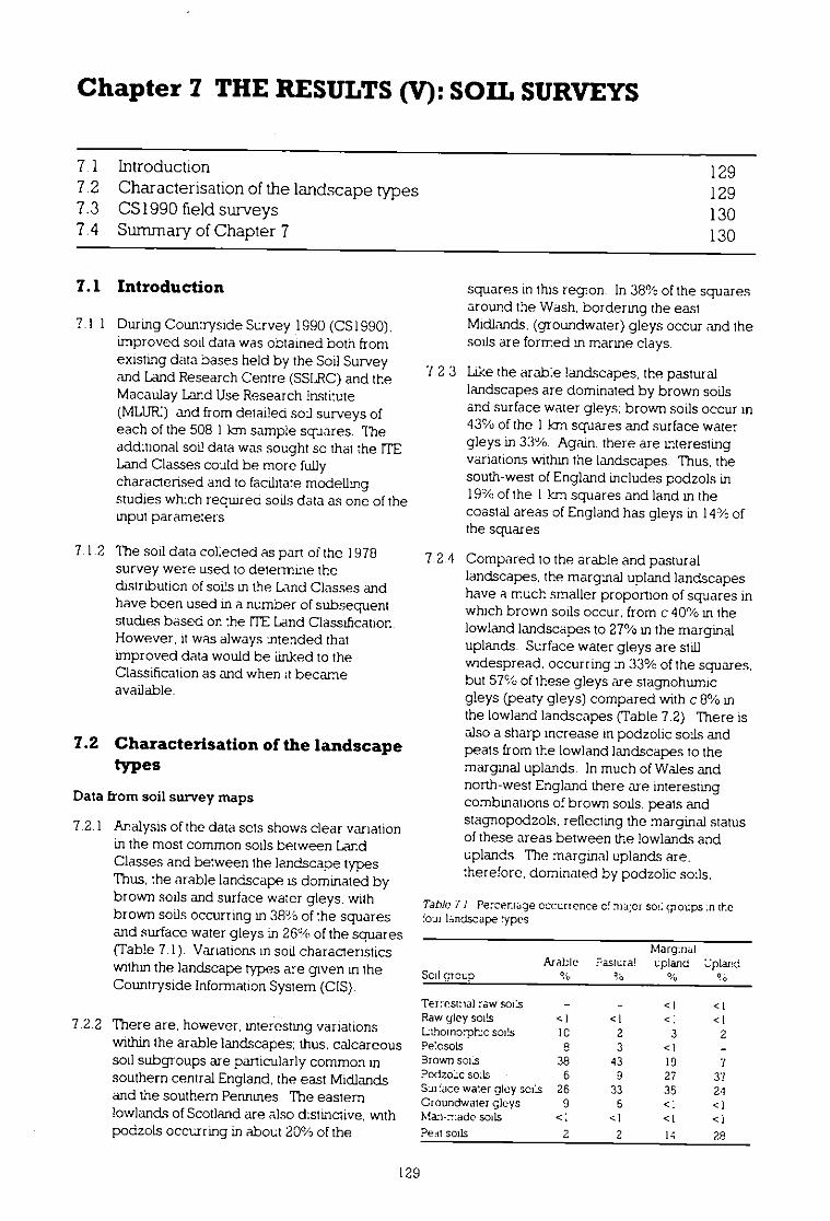
Chapter 7 THERESULTS(V):SOIL SURVEYS

7 1 Introduction 1297 2 Characterisation of the landscape types 1297.3 CS1990 field surveys 1307.4 Summary of Chapter 7 130

7.1 Introduction

7 1 1 During Countryside Survey 1990 (CS1990).improved soil data was obtained both fromexisting data bases held by the Soil Surveyand Land Research Centre (SSLRC)and theMacaulay Land Use Research institute(MLUR) and from detailed soi surveys ofeach of the 508 1Ian sample squares Theadditional soil data was sought sc that the ITELand Classes could be more fullycharacterised and to facilitate modellingstudies which required soils data as one of theinput parameters

7.1.2 The soil data coliected as pan of the 1978survey were used to determine thedistribution of soils in the Land Classes andhave been used in a number of subsequentstudiss based or. :he ITE Land Classification.However, it was always Intended thatimproved data would be linked to theClassification as and when It becameavailable.

7.2 Characterisation of the landscapetypes

Data from soil survey maps

7.2.1 Analysis of the data sets shows clear variationin the most common soils between LandClasses and between the landscape types.Thus, the arable landscape is dominated bybrown soils and surface water gleys. withbrown soils occurring in 38% of the squaresand surface water greys in 26% of the squares(Table 7 1). Variations in soil characteristicswithin the landscape types are given in theCountryside Information System (CIS).

7 2 2 There are, however, interesting variationswithin the arable landscapes. thus. calcareoussoil subgroups are particularly common insouthern central England. the east Midlandsand the southern Pennines The easternlowlands of Scotland are also distinctive, withpodzols occurring in about 20% of the

squares in this region. In 38% of the squaresaround the Wash. bordering the eastMidlands. (groundwater) gleys occur and thesoils are formed in marine clays.

7.2 3 Like the arab:e landscapes, the posturallandscapes are dominated by brown soilsand surface water greys. brown soils occur in43% of the 1 km squares and surface watergleys in 33%. Again, there are interestingvariations within the landscapes. Thus, thesouth-west of England includes podzols in19% of the 1km squares and land in thecoastal areas of England has gleys in 14% ofthe squares.

7.2.4 Compared to the arable and pasturallandscapes, the marginal upland landscapeshave a much smaller proponion of squares inwhich brown soils occur; from c 40% in thelowland landscapes to 27% in the marginaluplands. Surface water greys are stillwidespread. occurring in 33% of the squares.but 57% of these gleys are stagnohumicgleys (peaty greys) compared with c 8% inthe lowland landscapes (Table 7.2) There isalso a sharp increase in podzolic soils andpeats from the lowland landscapes to themarginal uplands. In much of Wales andnorth-west England there are interestingcombinations of brown soils. peals andstagnopodzoLs. reflecting the marginal statusof these areas between the lowlands anduplands. The marginal uplands are.therefore, dominated by podzolic sods.

Table 7 / Percentage occurrence of ma:or sot: gtoups :n thefoul landscape types

Marg:nal

Arable Pastura! upland',:plandSoil group

PO

Terrestrial raw soils _

<1< IRaw gley sol's <1 <I <1<ILthornorpbc soils IC 2 32Pe:osoLs sr 3 <I-Brown soUs 38 43 197Podzoc sals 6 9 2737Sul face water gley sois 26 33 3521Groundwater gleys 9 5 <I<1M.an--ado soils <: <I <I<1Peot soils 2 2 1428

129

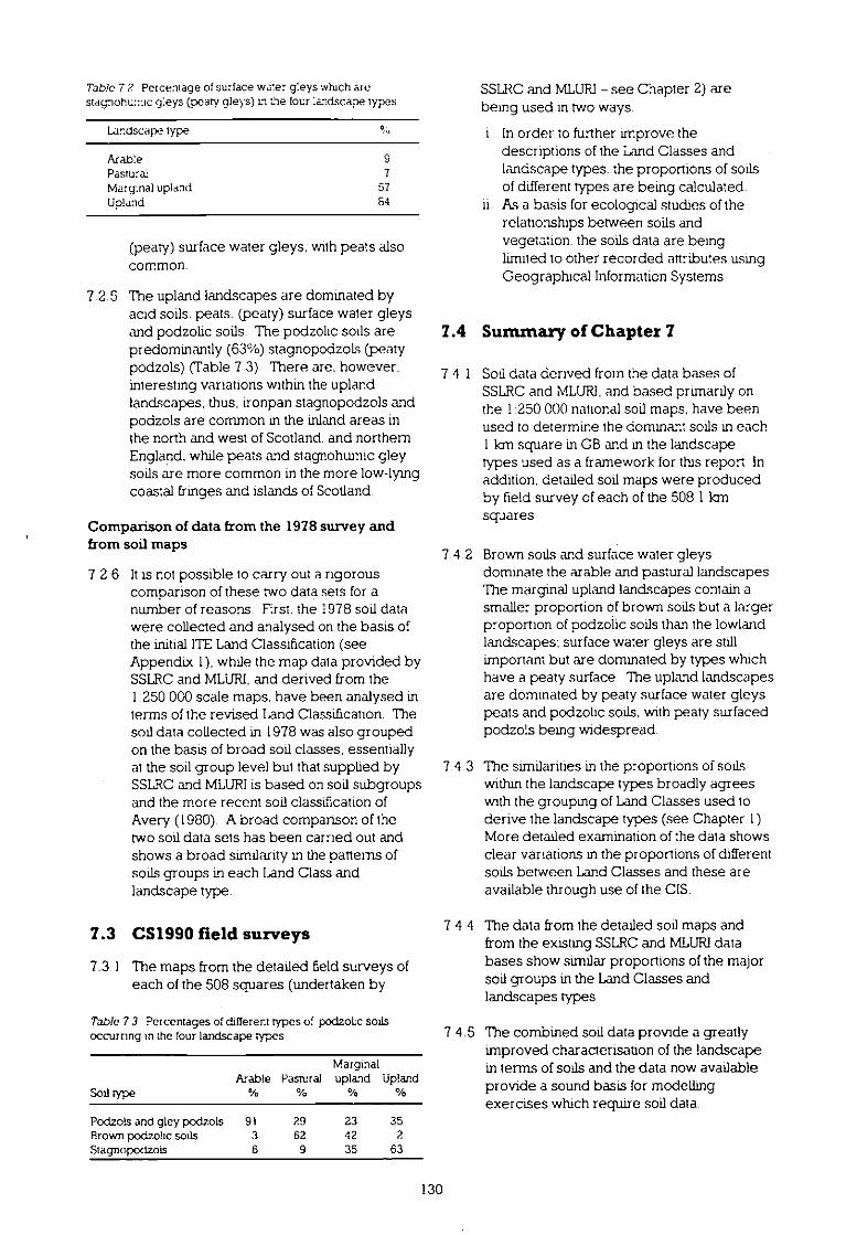
Table 7 2 Percentage of surface water g'.eys which arestagnohurnic gleys (peaty gleys) in the four landscape Types

Landscape type */tt

Arab:e 9Pastura': 7Marg:nal upland 57Upland 64

(peaty) surface water gleys. with peals alsocommon

7.2.5 The upland landscapes are dominated byacid soils. peats. (peaty) surface water gleysand podzolic soils. The podzolic soils arepredominantly (63%) stagnopodzoLs (peatypodzols) (Table 7.3). There are, however.interesting variations within the uplandlandscapes; thus. ironpan stagnopodzols andpodzols are common in the inland areas inthe north and west of Scotland. and northernEngland. while peals and stagnohumic gleysoils are more common in the more low-lyingcoastal fringes and islands of Scotland.

Comparison of data from the 1978 survey andfrom soil maps

7.2.6 It is not possible to carry out a rigorouscomparison of these two data sets for anumber of reasons. Flrst. the 1978 soil datawere collected and analysed on the basis ofthe initial ITELand Classification (seeAppendix 1). while the map data provided bySSLRC and MLURI.and derived from the1:250 OGOscale maps, have been analysed interms of the revised land Classification. Thesoil data collected in 1978 was also groupedon the basis of broad sod classes, essentiallyat the soil group level but that supplied bySSLRCand MLURIis based on soil subgroupsand the more recent soil classification ofAvery (1980). A broad comparison of thetwo soil data sets has been carried out andshows a broad similarity in the patterns ofsoiLsgroups in each Land Class andlandscape type.

7.3 CS1990 field surveys

7.3 1 The maps from the detailed field surveys ofeach of the 508 squares (undertaken by

Table 7 3 Percentages of different types of podzoLc soilsoccurnng tn the four landscape types

Arable PantralMarginaluplandUpland

Sod type

04

Podzols and gley podzols 91 29 23 35Ftrown podzoltc sotls 3 62 42 2Stagnopodzois 6 9 35 63

SSLRCand MLURI- see Chapter 2) arebeing used in two ways.

i In order to further improve thedescriptions of the Land Classes andlandscape types. the proportions of soilsof different types are being calculated.

ii As a basis for ecological studies of therelationships between soils andvegetation, the soils data are beinglimited to other recorded attributes usingGeographical Information Systems.

7.4 Summary of Chapter 7

7.4.1 Sou data derived from the data bases ofSSLRCand MLURI.and based primarily onthe 1:250 000 national soil maps. have beenused to determine the dominant soils in each1km square in GB and in the landscapetypes used as a framework for this report. Inaddition, detailed soil maps were producedby field survey cf each of the 508 1 Iansquares.

7.4.2 Brown soils and surface water gleysdominate the arable and pastural landscapesThe marginal upland landscapes contain asmaller proportion of brown soils but a largerproportion of podzolic soils than the lowlandlandscapes: surface water gleys are stillimportant but are dominated by types whichhave a peaty surface. The upland landscapesare dominated by peaty surface water gleyspeats and podzolic soils, with peaty surfacedpodzols being widespread.

7.4.3 The similarities in the proportions of soiLswithin the landscape types broadly agreeswith the grouping of Land Classes used toderive the landscape types (see Chapter 1)More detailed examination of the data showsclear variations in the proportions of differentsoils between Land Classes and these areavailable through use of the CIS.

7 4.4 The data from the detailed soil maps andfrom the existing SSLRCand MLURIdatabases show similar proportions of the majorsoil groups in the Land Classes andlandscapes types

7.4.5 The combined soil data provide a greatlyimproved characterisation of the landscapein terms of soils and the data now availableprovide a sound basis for modellingexercises which require soil data.

130

Chapter 8 CONCLUSIONSANDRECOMMENDATIONS

8.1 Main conclusions

8.2 Links to other studies8.3 Recommendations for further work

8.1 Main conclusions

Methods

8.1 1 Countryside Survey 1990 (CS1990) hasbeen the firs: fully integrated survey of thecountryside of Great Britain (GB)incorporating the detail of field survey withthe synoptic coverage of satellite imagery.In this respect it is innovative and unique.It provides a snapshot view of a widerange of information at one point in timeand sets a new baseline against whichfuture changes m land cover, vegetation.soils and freshwater biota may beassessed.

8.1 2 Much of the effort to date has beenconcerned with the collection . validationand summation of individual data sets.However, ways in which information fromthese different sources can be integrated.to give enhanced information andunderstanding of the countryside, havebeen demonstrated. Examples include theprediction of different types of woodlandand grassland using a combination of thecensus information from satellite data, withthe probabilistic but more detailed datafrom field survey (see section 3.7).Similarly, another project has used landcover, vegetation plot data and soilsinformation to examine the vegetationtypes witch were likely to be mostaffected by afforestation of moorlands

(Metx 1992).

Land cover map from satellite data

. 813 CS1990 has included the use of satellitedata to give the first complete land covermap of GB since the 1950s. Data at 25 mpixel resolution are held in machine-readable form. for each of the c 240 0001 km squares in GB These data havebeen aggregated at three different levelsfor reporting purposes, but individualusers may require the classes (and evensub-classes) to be aggregated in differentways for different purposes.

131132 134

8.1 4 The 17 key satellite :and cover types can becombined with detailed ecologicalinformation on individual species. obtainedfrom field survey, thus utilising the strengthsof both approaches.

Field survey of land cover and vegetation

8.1.5 The field survey information, collected fromonly a very small sample of 1 Ian squares(0.2% of GB). produced estimates of landcover which were close to those derivedfrom satellite imagery. This is due to theefficient dispersal of samples through use ofthe ITE Land Classification system. Reasonsfor any differences between the twoestimates ranged from the inherentstatistical error associated with using asample. to the inability of each surveyapproach to record certain featuresconsistently. For example, the satelliteinterpretation cannot distinguish betweenmoorland and newly plantedforest; the fieldsurvey camnot record accurate boundariesbetween semi-natural vegetation types..

8.1.6 One of the more precise aspects of CS1990has been the recording of plant speciesdata from plots. Statistics on change in plantspecies. within plots, have been collated forthe first time at the national level Althoughthe data summarised and presented hereare from c 1280 plots which were recordedin both 1978 and 1990, one of the majorachievements cf CS 1990 was to record andpermanently mark a to:al of c 11 SOOplots.This has formed a very valuable anddetailed baseline for monitoring•the moresubtle changes that may take place in futureyears.

Other data collected as part of CS1990

8.1.7 The collection, identification anddocumentation of freshwater biota from theCS1990 squares provide an extremelyuseful addition to the Institute of FreshwaterEcology's national data base. as well asforming an important scientific resource inits own right

131

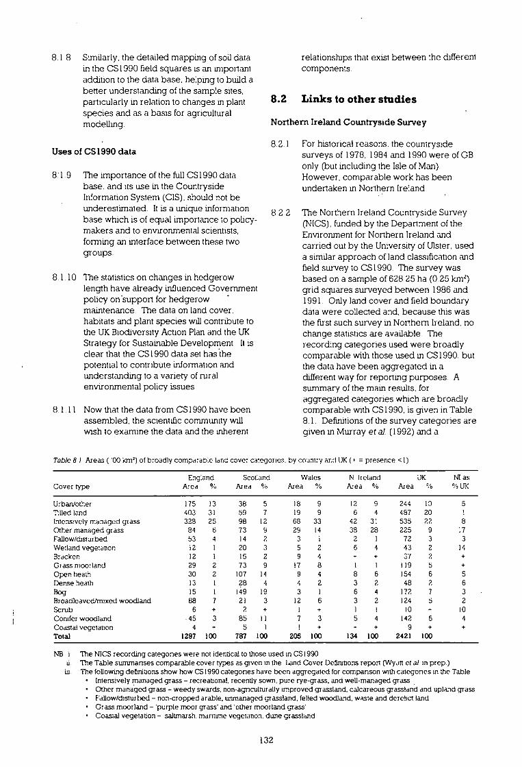
8.1 8 Similarly. the detailed mapping of soil datain the CS1990 field squares is an importantaddition to the data base. helping to build abetter understanding of the sample sites,particularly in relation to changes in plantspecies and as a basis for agriculturalmodelling.

Uses of CS1990 data

8:1.9 The importance of the fullCS1990 database. and us use in the CountrysideInformation System (CIS), should not beunderestimated. It is a unique informationbase which is of equal importance to policy-makers and to environmental scientists,forming an interface between these twogroups.

8.1 10 The statistics on changes in hedgerowlength have already influenced Governmentpolicy on'support for hedgerowmaintenance. The data on land cover.habitats and plant species willcontribute tothe UKBiodiversity Action Plan and the UKStrategy for Sustainable Development. It isclear that the CSI990 data set has thepotential to contribute information andunderstanding to a variety of ruralenvironmental policy issues

8 1 II Now that the data from CSI990 have beenassembled, the scientific community willwish to examine the data and the inherent

relationships that exist between :he differentcomponen:s

8.2 Links to other studies

Northern Ireland Countryside Survey

8.21 For historical reasons. the countrysidesurveys of 1978, 1984 and 1990 were of GBonly (but including the Isle of Man).However, comparable work has beenundertaken in Northern Ireland.

8.2.2 The Northern Ireland Countryside Survey(NICS). funded by the Department of theEnvironment for Northern Ireland andcarried out by the University of Ulster, useda similar approach of land classification andfield survey to C51990. The survey wasbased on a sample of 628 25 ha (0.25 kmi)grid squares surveyed between 1986 and1991. Only land cover and field boundarydata were collected and, because this wasthe first such survey in Northern Ireland. nochange statistics are available. Therecording categories used were broadlycomparable with those used in CS1990. butthe data have been aggregated in adifferent way for reporting purposes. Asummary of the math results, foraggregated categories which are broadlycomparable with CS1990. is given in Table8.1. Definitions of the survey categories aregiven in Murray et al. (1992) and a

Table 8 I Areas ( '00 km') of broadly comparable land Cover Categories, by coUntry and UKN = presence <1)

Cover typeEngIand

Area%Sconand

Area% AreaWales

%N Iteland

Asea% AreaUK

%NI as

% UK

LI:ban/other 175 13 38 5 18 9 12 9 244 II) 5'flied land 403 31 59 7 19 9 6 4 487 20 .lntenswely managed glass 329 25 98 12 68 33 42 3: 535 22 8Other managed grass 84 6 73 9 29 14 38 28 225 9 17Fallow/disturbed 53 4 14 2 3 I 2 1 72 3 3We:land vegeunon i2 I 20 3 5 2 6 4 43 2 14Bracken 12 1 15 2 9 4 - + 37 2

Class moo:land 29 2 73 9 17 8 1 I 119 5 +Open heath 30 2 107 II 9 4 8 6 154 6 5Derse heath 13 1 ?8 4 4 2 3 2 48 2 6Rog 15 1 !49 19 3 I 6 4 172 7 3Broadleavedirruxed woodland 88 7 21 3 12 6 3 2 124 5 2Scrub 6 + 2 + 1 + 1 1 10 - 10Conifer woodland .45 3 85 II 7 3 5 4 142 5 4Coastal vecetanon 4 . 5 1 ! + - + 9 +

Total 1297 100 787 100 205 100 134 100 2421 100

NB The N1CS recording categories were not identcal to those used in CS1990The Table summarises comparable cover types as given in the Land Cover Definitions report (Wyan et al in prep )The following definitions show how CS1990 categones have been aggregated for comparison with categones in the Table

Intensively managed grass - recreatonai recently sown, pure rye-grass, and well-managed grassOther managed grass - weedy swards. non-agnculturally improved grassland. calcareous Tassland and upland grassFallow/disturbed - non-cropped ara.ble unmanaged arassland. felled woodland, waste and derelict landGrass moorland - 'purple moor grass and 'other moorland grass'Coastal vegetation - saltmarsh, mabilrle vegetanon. dune grassland

132

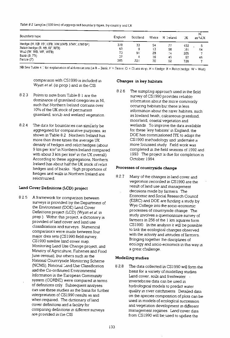
Table 8 2 liengths (000 km) of aggiegated bounda:y types, by country and UK

NIEngland Scotland Wales N lieland IJK as %UK

378 33 54 27 492 . 562 8 13 98 181 5473 91 29 !4 205 732 4 16 45 97 45

385 221 7C 52 728 7

Boundary type

Hedge (H. HB.HP. HW.HWB. HWI4.HINI3*)Relict hedge (R. 12.9.RE RF3)WaIl (W. WB. WF. VIM)Bank (B. 13)Fence (F)

NB See Table 4 for explanaccn of abbreviarons - Bank. F'= Fence! G = 0: ass snip. H = Hedge R = Relict hedge W = Wall)

comparison with CS1990 is included inWyatt et a/ (in prep ) and in the CIS

8 2.3 Points to note from Table 8.1 are thedominance of grassland categories in NI,such *ha:Northern Ireland con:ains over10% of the UKstock of permanentgrassland. scrub and wetland vegetation.

8.2.4 The data for boundaries can similarly beaggregated for comparative purposes. asshown in Table 8.2 Northern Ireland hasmore than three times the average UKdensity of hedges and relict hedges (about9 lcmper km' in Northern Ireland comparedwith about 3 km per kmi in the UKoverall)According to these aggregations. NorthernIreland has about half the UKstock of relicthedges and of banks. High proportions ofhedges and walls in Northern Ireland arerelict/ruined.

Land Cover Definitions (LCD) project

8.2.5 A framework for comparison betweensurveys is provided by the Department ofthe Environment (DOE) Land CoverDefinitions project (LCD) (Wyatt et al. inprep ). Within this project, a dictionary isprovided of land cover and land useclassifications and surveys. Numericalcomparisons were made between fourmajor data sets (CS1990 field survey:CSI990 satellite land cover map:Monitoring Land Use Change project: andMinistry of Agriculture, Fisheries and FoodJune census), but others such as theNational Countryside Monitoring Scheme(NCMS). National Land Use Classificationand the Co-ordinated Environmentalinformation Lnthe European Communitysystem (CORINE) were compared in termsof definitions only. Subsequent analysescan use these studies as the bass for furtherinterpretation of CS1990 results as andwhen required. The dictionary of landcover definitions and a facility forcomparing definitions in different surveysare provided in the CIS.

Changes in key habitats

8 2 6 The sampling approach used in the fieldsurvey of CS1990 prov:des reliableinformal:on about the more commonlyoccurtng habitats bu: there is lessinformation about the rarer habitats, suchas lowland heath, calcareous grassland.moorland, coastal vegetation andwetlands To improve the data availablefor these 'key habitats m England. theDOE has commissioned ITE to adapt theCS1990 methodology and undertake amore focussed study. Field work wascompleted in the field seasons of 1992 and1993 The project is due for completion inOctober 1994

Processes of countryside change

8.2.7 Many of the changes in land cover andvegetation recorded in CS1990 are theresult of land use and managementdecisions made by farmers TheEconomic and Social Research Council(ESRC) and DOE are fisding a study byWye College into the socio-economicprocesses of countryside change. Thestudy involves a questionnaire survey offarmers in 256 of the 1 lcmsquares formCS1990. In the analysis it will be possibleto link the ecological changes observedwith the activity and attitudes of farmers.Bringing together the disciplines ofecology and socio-ecnomics in this way isa great challenge.

Modelling studies

8.2.8 The data collected in CS1990 will form thebasis for a variety of modelling studiesLand cover, soils and freshwater -invertebrate data can be used inhydrological models to predict waterquality in river catchments. Detailed dataon the species composition of plots can beused in models of ecological successionand vegetation development in differentmanagement regimes. Land'cover datafrom CS1990 will be.used to update the

133

Land Use Allocation Model (LUAM)developed by the Centre for AgriculturalStrategy. University of Reading.

8.3 Recontmendations for furtherwork

8.3.1 In each of the component pans of the.project.opportunities for further work have beenrecognised:

The satellite land cover map has a widerange of potential applications forresource assessment and is currentlybeing developed for this purpose. Thereis a range of potential GIS developmentslinldng the map to other spatial databases. There is also a possibility ofmonitoring change from the existing mapat regional or national levels. Theapplication of mathematical proceduresfor pattern analysis has a high scientificpotential.

The digitised land cover data base, fromeach 1 lcmsquare in the field survey.could be used for spatial analysis in orderto relate the land cover to the compositionof the detailed vegetation plots. Therelationship of linear features and theirassociated vegetation also deservesfurther study. The different types ofpattern analysis, developed in theEcological Consequences of Land UseChange (ECOLUC) project (Bunce et al.1993). could reveal important informationproviding relationships between patchesof vegetation and animal distribution. Theanalytical overlaying power ofGeographical Information Systems meansthat the data base is ideal for looldng atScenarios of potential change in thelandscape.

One principal area of future work that hasbeen identified is the development of anunderstanding of the processes ofchange, since currently these can only beinferred. A range of hypotheses has beendeveloped which need to be tested inorder to develop adequate predictivemodels; these can then be used to aidland management. Further analysis isrequired of the patterns of diversity andtheir relationship with the spatialarrangement of land cover elements.

The freshwater studies form afundamental baseline for assessing futurechanges in freshwater fauna and water

quality. relating these to changes in landuse and land cover. An integratedapproach would identify importantinformation on sensitive taxa and therelationships between change andmanagement of the land

The soils information will be an importantelement of studies of vegetation andchange and could provide links to work or.critical loads and pollution leveLsat localand national scales.

8.3.2 - In addition. a number of suggestions forfuture work have arisen as a result of ameeting held in Edinburgh (organised by theLand Use Research Coordinating Committee(LUROC).March 1993). which was calledspecifically to discuss work that mightdevelop from CS1990 (LURCC 1993). Themain areas for future work. recognLsed bythe meeting. were as follows

Expansion of the data base - integrationof :he CSI990 data with other national databases on agriculture, climate pollution andbiology

Availability of data - development of theCIS and its wider availability for researchand application.

Spatial scales - rigorous assessment of theapplication of results at national..regionaland local scales and development bfanalysis (or synthes...$)to express distinctzones of influence.

Causal relationships - exploration ofcorrelative relationships to assesscausality. eg by application of theory. fieldexperiments, detailed case studies ortesting predictive models against observedspatial and temporal patterns

Policy targeting and analysis - use of theCS1990 data base to establish objectives.to target policy in terms of spatial locationsor subject, and to test the effectiveness ofpolicies (adoption dynamics).

8.3.3 The LURCC report of the meeting states: 'Itwas generally accepted that the combinationof information which had been incorporatedinto CS1990 constitutes a major benchmarkfor future biological research, for integrationwith social and economic research, and forexploration of important policy issues suchas conservation of biodiversity and theeffects of the Common Agricultural Policy.'

134

GLOSSARYOF TERMS, ABBREVIATIONSAND ACRONYMS

1990RiverQualitySurvey - chemical and biological survey of the quality of watercourses in 1990,undertaken by the Institute of Freshwater Ecology (IFE) and commissioned by the National RiversAuthority (England and Wales). the River Purification Boards (Scotland) and the Department ofEconomic Development (N. Ireland).

Aerial photographic interpretation(API)- the use of aerial photographs to update and enhance basemaps prior to field survey (see sect:on 2 3 9)

Aquaticmacrophytes - higher plants which are growmg in. or on. water

Arable landscapes - one of the four landscape types into which ITE Land Classes have beenaggregated to present results from CS1990 (see Appendix 1 - section Al /).

ARC/INFO- proprietary Geographical Information System (GIS) written by the Environmental SystemsResearch Institute. Redlands. California. and used at both the ITEMonks Wood and Merlewood sites.

ASPT- average score per taxon - the to:al site score divided by the number of taxa contributing to thatscore (see section 2 5.17).

Bioticindex values - simple numeric representations of complex biological information, normally usedto indicate some aspect of environmental quality (see BMWPscore, number of sconng taxa and ASPT)

BMWP- Biological MonitoringWorking Party- responsible for devising a scoring system relatingfreshwater biota to their tolerance of organic pollution (see section 2.5.16 and Armitage et al 1983)

BNG- BritishNationalGrid- as shown. fcr example, on Ordnance Survey maps.

BNSC- BritishNationalSpace Centre - based in London, the BNSCwas formed Ln1985 as apartnership between UKGovernment departments and the research councils (eg NERC) to form thefocus for Britain's non-military space :nterests. A contributor of funding to CS1990.

Boundaryplots - one of the linear plot types recorded during the field survey, placed alongside fieldboundaries (see section 2.3 11).

Bufferzone - used in classification of satellite Lmagery to define an area of user-selected widthsurrounding features of a defined type (see section 2.2.30).

Category 1species - plant species which were used in the analysis of botanical data. having fewtaxonomic or identification difficulties and which were consistently recorded by field surveyors (seeAppendix 2).

Census data - data collected from every unit/member of a population. eg a complete inventory of landuse information (cf sample data)

Changes in KeyHabitats- a DOE-funded project to collect data from specific habitats which have alimited representation in CS1990 and to examine the effects of designations on these.

135

CIS- CountrysideInformationSystem - a computer-based system to display and integrate CS1990data and other environmental information

CORINE- Co-ordinated Informationon the EuropeanEnvironment- a joint European initiative whichincludes the aim of mapping the land cover of all CEC countries using satellite imagery.

DAFS- Departmentof Agricultureand Fisheries forScotland - responsible for the promotion ofagriculture and the fishing Industry in Scotland (now SOAFS- ScottishOfficeAgricultureand FisheriesDepartment).

DECORANA- Detrended Correspondence Analysis - a FORTRANcomputer program whichproduces an ordination (gradient) of species and plots, using an improved version of CorrespondenceAnalysis.

Digital data base - usually referring to a data base comprised of digitised map co-ordinates (seeDigitising).

Digitising - the process of capturing information from maps in the form of points, lines or areas. andconvening these into computer-readable co-ordinates (grid references).

DOE- Departmentof the Environment- one of the principal funders of CSI990 and the commissionersof this report.

DRA- Directorateof RuralAffairs- division of DOE responsible for CSI990.

DTI- Departmentof Trade and Industry- one of the principal funders of CS1990, especially in relationto the land cover map.

ECOLUC- Ecological Consequences of LandUse Change - ITEresearch project. completed in 1989and funded by DOE (see Bunce et at 1993)..

EQI- EnvironmentalQualityIndex - an expression of the extent to which the freshwater fauna of a sitematches that to be expected in the absence of environmental stress (see section 2.5.18)

Errorterms - (eg standard error) measures of the reliability of an estimate which has been based on asample (eg when extrapolating from a sample of 1km squares to a national or regional estimate).

GIS- Geographical InformationSystem - a computer package which handles spatial information(usually as computerised maps) and which allows analysis of, for example, area, length and overlay

Habitatplots - 4 in2plot recorded within areas of semi-natural vegetation during the field surveyelement of CS1990. Up to five were recorded in each 1 lan square (see section 2 3.11).

IFE- Instituteof FreshwaterEcology - one of the research institutes of the Natural EnvironmentResearch Council.

118- InternationalImaging Systems (alsol2S) - image analysis softwareThardware for processingsatellite images.

lit - infra-red- wavelength used in satellite imagery.

ISA- IndicatorSpecies Analysis - a computer program from which TWINSPANwas developed.

ITE- Instituteof TerrestrialEcology - one of the research institutes of the Natural EnvironmentResearch Council.

136

rrE Land Classification - the system deve:oped by FIT to classify each of the c 240 000 1 km squaresin Great Britain into one of 32 Land Classes, depending on its environmental affinities Used to stratifythe CSI990 field survey (see Appendix 1).

Land Classes - 32 strata produced by the :FE Land Classification (see Appendix 1)

Land cover - the composition of the land surface, being described in terms of land cover classes (egarable crops, trees, buildings. bare rock)

Land cover map - map of GB showing the principal land cover classes and derived from interpretationof satellite imagery by staff at CE Monks Wood. as pan of CS1990

Landscape type - one of the four aggregations of the FE Land Classes ( into arable. pastural marginalupland and upland types) (see Appendix 1)

Laserscan GIS - proprietary Geographica Information System, developed by Laser-Scan LaboratoriesLtd. Cambridge.

Linear plots - 10 mx 1 m plots placed alongside field boundaries streamsides and road verges in the1 icmfield survey sites from which vegetation data were recorded (see section 2.3.11)

LUAM - Land Use Allocation Model - the product of research project carried out by :he Centre ofAgricultural Strategy, Reading Urnversity (with input by ITE). which links national agricultural statisticsto the ITE Land Classes.

LURCC - Land Use Research Coordinating Committee - a national committee under the auspices ofNERC. with membership from Departments. Agencies and academia, and a remit to encouragecollaboration and dissemination of land use research.

MAFF - Ministry of Agriculture, Fisheries and Food - responsible for administering Governmentpolicy for agriculture horticulture and fisheries in Engthnd

Main plot classes - outputs from TWINSPANclassification of all Math (vegetation) plots (29 in number).

Main plots - 200 m2 plots placed a: random in each 1 lcmfield sample square (5 in each) from whichvegetation data were recorded

Majority filter - filtering prccedure, used to smooth out 'noise' in classification of satellite data. toproduce generalised images

Marginal upland landscape - one of the feu landscape types into which ITE Land Classes have beenaggregated to present results from CS1990 (see Appendix 1 - section A1.7).

Minimum mappable area (0.04 ha) - smallest area of land to be mapped as a homogeneous unit(using a consistent coded description) within the field survey part of CS1990.

Minimum mappable length (20 m) - shortest length of any linear feature to be mapped as ahomogeneous unit (using a consistent coded description) within :he field survey part of CSl990.

MLCI - Maximum likelihood classifier - statistical prccedure used in the classification of satelliteimagery to extrapolate from sample data and to allocate pixels in a remotely sensed image to the mostappropriate classes, based on the spectral reffectances recorded by the sensor.

137

MLC2- MonitoringLandscape Change (project) - 1984 sample survey cf the countryside of Englandand Wales carried out by Huntings Technical Services on behalf of the DOE and the CountrysideCommission

MLURI- MacaulayLandUse ResearchInstitute- based in Aberdeen. MUJRIwas subcontracted tocarry out the soil survey element of CS1990 in Scotland (see section 2 6 1)

MSS- MultispectralScanner - instrument carried on all Landsat satellites. offering an 80 m spatialresolution and four wavebands

Multiple-element category - used in describing physical boundaries which have more than oneelement (eg wall with a wire fence)

Multivariatestatisticaltechnique - statistical analysis using more than one variable (characteristic) at atime to classify members of a statistical population

National RemoteSensing Centre - (now NationalRemote Sensing Centre Limited)- home of theEarth Observation Data Centre and British agents for the supply of Landsat data

NCC - NatureConservancy Council - until 1992, the Government agency with responsibility for natureconservation in Britain now undertaken by the Countryside Council for Wales, English Nature the JointNature Conservation Committee and Scottish Natural Heritage A contrabuter of funding to CS1990

NCMS- NationalCountrysideMonitoringScheme - developed by the former Nature ConservancyCouncil (NCC) to record changes in GB using aerial photography on a county-by-county basisCurrently being used in Scotland

NERC- NaturalEnvironmentResearchCouncil - responsible for planning. support andencouragement of research in those sciences that relate to man's natural environment and its resources

NorthernIrelandCountrysideSurvey (NICS)- field survey adopting similar approach to CS1990.funded by the Depanment of the Environment for Northern Ireland. carried out between 1986 and 1991(see section 8 2 2)

NRA- NationalRiversAuthority- formed in 1989 as an independent body with statutoryresponsibilities for ;he management of such things as water resources, flood defence, fisheries andpollution control for all fnland waters, estuaries, coastal waters and natural underground water inEngland and Wales

ORACLE- data base management system, widely used in C51990.

OS - Ordnance Survey - based in Southampton and responsible for the official survey and mapping ofGreat Britain

Pasturallandscape - one of the four landscape types into which ITE Land Classes have beenaggregated to present results from CS1990 (see Appendix 1 - section Al 7)

Patchsize - used in landscape ecology and pattern analysis as a measure of the area of a unit ofvegetation, habitat or land cover typE

Patternanalysis - general term to describe the measurement of elements in the landscape, such asarea of fields, lengths of boundaries and edges. and the relationships between them.

138

Pixel - area of ground surface which is the unit of classification used in satellite image interpretation (eg25 m x 25 m in C31990).

Plot classes - outputs from classification of vegetation plots and determined by the plant speciespresent in the plot - plots in the same class will generally have the same species present

Polygon data - data derived from multi-sided figures representing distinct areas on a field survey mapor satellite image

Polynomial model - mathematical expression which. in this report expresses how the geometry of theoriginal satellite image relates to that of the earth's surface and which is used to alter the imagegeometrically to match the desired map scale and projection.

Primary codes - used in the field mapping part of CS1990 to define the general nature of a feature (egwoodland, lake, field of grass) (cf secondary codes which descnbe the feature in more detail).

Principal vegetation gradient - name given to the first axis resulting from a TWINSPAN analysis of thevegetation data - generay interpreted as being from plots which are characteristic of highly managedlowland vegetation, often with high levels of nutrients, to those of unmanaged upland vegetation withlow nutrient levels

Proximity analysis - measurement of the closeness of one land cover type to another.

Quality assessment - means of measuring the quality of work. eg by repeat sampling of vegetationplots (see Appendix 4)

Quality Assurance Exercise - partial resurvey carried out in 1990 and 1991 to assess consistency andreliability of CS1990 field survey (see Appendix 4).

Raster data - data which relate to areas rather than lines (vector data) - raster maps may be made up ofa grid of cells, each having a separate value.

Refiectances - light values reflected from the earth's surface and recorded by satellites

Relict hedges - boundaries recorded in the field survey which at some point in the past have beenhedges but are something else at the time of survey (eg line of trees).

Remote sensing - a general term to include observation of the land surface from a distance. usuallyapplied to aerial photography and satellite imagery.

RIVPACS - a software package devised by lFE for assessing the biological quality of rivers.

RPB - River Purification Boards - have similar responsibilities in Scotland as the National RiversAuthority in England and Wales.

Sample data - data which have been collected from only some members of a statistical population andwhich are usually assumed to be representative of the whole population.

Satellite image - general term used to refer to data aquired by remote sensing; also used to refer to thevisual display of such data on a screen or as printed paper products

Satellite imagery - process of collecting satellite images.

139

SE - standard error - estimated standard deviation of an estunate of a parameter (see Appendix 3and 3a)

Secondary codes - used in the field mapping pan of CS1990 to define the characteristics of mappedfeatures in detail (eg tree species in woodland, size of lake, species present in grass field ) (cf primarycodes).

Semi-natural vegetation - generally. vegetation which has no: been created by human activity(management) although it may have been influenced by it.

Soil group - division of soiLsinto one of ten major groups. eg podzolic

Soil subgroups - division of major soil group into more detailed classes as supplied by SSLRCandMLUR1for CS1990

Spatial recording - recording the position of features (eg fields, trees) using a co-ordinate (gridreference) system

Spatial scales - data recorded at one scale applied at national, regional or local levels

Species cover values - estimates of the ground area covered by a plant species.

Species groups - groupings of plant species resulting from DECORANAanalysLs of the whole CS1990vegetation data set (see section 2.3.25)

Spectral characteristics - refiectances in different wavebands. from difTerent surfaces on the ground.measured at sensor. and peculiar to a particular cover type.

SSLRC - Soil Survey and Land Research Centre - based at Silsoe, Bedfordshire. SSLRCwassubcontracted to carry out the soil survey element of CSI990 in England and Wales (see section 2.6 I)

Stock - the amount of any feature present at a point in time.

Stratified sample - sample drawn from different divisions (strata) of the whole data set - intended toincrease the chances of the sample being truly representative of the whole population.

Stratified random sample - sample drawn at random from within each of the different strata of a dataset (eg the CS1990 1km field sample squares were drawn at random from each of the 32 ITE LandClasses (strata))

Stream order - classification of streams/rivers where a first-order stream is one which runs from asource to the first confluence: second-order streams run from the confluence of two first-order streamsto a confluence with another second-order stream, and so on.

Streamside plots - one of the linear plot types, placed alongside flowing watercourses (see section2.3.11).

Student's t-test - statLsticalprocedure to last for significant differences between two sets of data.

Suburban - land cover class shown on the land cover map (see Appendix 2).

Target land cover classes - one of the classifications of land cover data produced from the land covermap (being 25 in number)

140

Taxa - any group of organisms that is sufficiently distinct from any other group to be distinguished by nameat one or other level of classification

Thematic Mapper (TM) - scanner on board the Landsat satellite. which provided the reflectance data usedin mapping land cover: the scanner offers seven wavebands of data for relectances from 30 m ground cells.

TWINSPAN - Two-way Indicator Species Analysis - a FORTRANprogram used in CSI 990 to classify plotdata into vegetation classes (see Hill 1979)

Unsurveyed urban land - a census estimate of urban land from all 1 l‘m squares not surveyed (seeAppendix 3 - section A3 46)

Upland landscape- one of the four landscape types into which rrELand Classes have been aggregated to•present results from CSI990 (see )ppendix 1 - section Al .7)

Vascular plants - all plants excluding mosses. liverworts and aigae (le ferns, conifers and flowering plants).

Vector-digitising - entering the spatial co-ordinates of features (eg fields Imes of trees) from a map to aGIS using continuous lines in order to represent the feature as exactly as possible (cf raster data)

Vegetation gradient - see principal vegetation gradient

Vegetation plots - three types of plot. Main. Habitat and linear, recorded in each I km field survey squarefor vegetation analysis (see section 2 3.11).

Verge plots - one of the linear plot types. placed alongside roads/tracks (see section 2.3.11).

Ward's minimum variance clustering - statistical technique to group species which have similardistributions (see section 5.1 4)

141

142

REFERENCES

Armitage, PD., Moss, D., Wright, J.F. & Purse, M.T: 1963 Theperformance of a new Mc:log:cal water gualty score systembased on macro:nvenebrates over a wide range of un.pollutedrunrung water :ices Water Research. 17.333-347

Avery, B.W. 1980 System of soil classification for England andWales (tagher categones) ( Teohrucal Monograph no 14 )Harpenden Soil Survey

Ban, C.J. 199C Mapping the changng face of 3stainGeographical Magazine. 62(9). 44-47

Barr, C.J. 1990 Field handbook Orange-over-Sands Insame ofTeresa:a Ecology

Barr, C.J., Ball, D.F., Bunce, AGM. & Whittaker, H.A. 1935Rural land thse and landscape change. AMILLIIReport of theInstitute ol Tentstnal Ecology 1924.133- :35

Barr, C.J., Benefield, C.B., Bunce. R.aH., Ridsclale, HA. &Whittaker, M. 1985 Landscape changes in Britain AbbotsR:pton. Eunungdon Insnare of Terrestnal Ecology

Barr. CI., Howard, D.C., Bunce, R.G.H., Gillespie, M.K. &Hallam, C.J. :991 Changes in hedgerows ill Brom between1984 and 1999 NEFC contract report to :he Department of theEmcronrnent. Grance over-Sinds- Institute of TerrestrialEcology.

Bunce. R.G.H. 1979 Ecologoar survey of Britain. Annual Reportof the Institute of Terrestrial Ecology 1978. 74-75

Dunce, R.G.H. & Heal, O.W. 1984 Landscape evaluation andthe mmact of charging :arid use on the rural envn orkr.ent theproblem and au approach In. Planning and ecology. edited byR D Roberts & 7 M Roberts. :64-166 London Chapman andHa

Una:. R.G.H., Barr, C.J. & Whittaker, HA. :983. Astrathcanon system for ecological samptrig In Ecologicalmapping from ground. air and space edited by R M Euler39-46 (17Esyrnpos:um no IC ) Cambridge Insurse of7errestr.a: Ecology

Bunce, Walt, Howard, D.C.. Hallam, C.J., Barr, Cj. &Benefield, CA. :993 Ecoicgmal consequenccs al land usechange London Department of the Environment

Burnham, K.P., Anderson, DA., White. C.c., Brownie. C. &Pollock, KM. 1987 Cesign and analysis methods for fish survivalexperiments based on release-capture (Monograph no 5 )Bethsaida. Maryland: Arner:can Fisheries Society

Clapham, A.R.. rutin, T.G. & Moore, D.M. 1987 Flora of theBritish Isles 'Third edition Carnbridge- Cantiondge UniversityPress

Clarke, R.T., Flame, M.T. & Wright. J.F. :992 Testing andfurther development of RP/PACS A comparison of single. pairedand 3 season combined macro-uwertebrate samples for thebiological banding of river qualny (NERC corm ern repor to theNat:onal Raters Authority ) Wareham Institute of FreshwaterEcology

Cochran, W.a :977 Sampling techniques 3rd. ed WileyNew York

Coleman. A. 1961 7be second land use survey progress andprospect Geographical Journal. 127 168-186

Cummins, R.C., French, D., Bunce, Walt, Howard, D.C. &Barr. Cj. 1992 Diversity in British hedgerows (N:7C contractreport to the Department of the Envisonment ) Grange over-Sands Institute of Terrestnal Ecology

LM., Brown, N.J., Ullyett, J.M., Sanders, MA., Groom,G.B., Howard, D.C. & Gillespie, MA. 1993 Countryside Survey1990 mapping the land cover of Great Rntam using Landsatimagery a demonstrator project in remote sensing Final reporton pattern analysis and 015 (NERO contract report to theDeparanent of the Environment ) Abbots Ripton. Hurangdon.11-SIIILI:eof Terrestrial Ecology

Fuller, R.M. & Parsell, R.J. 1990 Classification of TM imagery in -the study of landase :n lowland Britain practcal considerahonsfor cperanonal use International Journal of Remote Sensing 11.190 :-1917.

Fuller. R.M., Parsell. R.J., Oliver, M. & Wyatt, G. 1989a Visualand computer Cassi5caoons of remotely-sensed images A casestudy of gr asslands Cambralgesthre International Journal ofRemote Sensing 10. 193-21C

Fuller, R.M., Jones, A.R. & Wyatt, B.K. i 989b Remote sensingfor ecoloTcal research problems and possible solunons InRemote sensing for Operational Applications technical contents ofthe 15ih Annual Conference of the Remote Sensing Society. 1989.compiled by E C Barrett & KA Brown, 155-: 64 ReadngRemote Sersing Socety.

Purse, M.T., Moss, D., Wright, J.F. & Armitage, P.D. 1987.Freshwater s:te assessment using mule-vanate techniques :nThe use of invertebrates in site assessment for conservation .edited by M I. Luff Newcaste-upon-Tyne Agncultur alannronment Research Group. University cf Newcastle upon

Tyne

Ruse, MT., Clarke, R.T., Blackburn, LH.. Gunn, R.J.M.,Symes, K.O., Winder, J.M. & Harrison, S.N. :n prepCountryside Survey 1990 running-water studies WarehamInstitute of Freshwater Ecology

Gates, S., Gibbons, D.W., Fuller, R.M. & Hill, DA. 1993 The:nfluence of haban diversity, measured by remote sens:ng. onavian spec:es nchness :n Eastern England Journal of AnimalEcology :n press

Griffiths GM. & Wooding, MG. 1989 Use of satellite data forthe preparation of land cover maps and statistics Final report tothe National Remote Sensing Cenrre contract report toDepartment of the Envaonrnent Volume I. main reponUnpublished

Hill, M.O. 1979 TWEIVSPAN- a FORTRANprogram for arrangingmut vanate data in an ordered two-way table by classification ofthe individuals and attributes Ithaca. N Y Section of Ecology andSysternatos. Cornell Urtversity

Hill, M. 0., Dunce, R. G. H. & Shaw, M. W. :975 Indicatorspeces analys:s. a divisive polythetc method of classi5cation. •and its application to a survey of native dnewoods a ScotlandJournal of Ecology. 63. 597-613

143

Hopkins, A. &Wainwright, J. 1999 Changes in botanicalcornposmon and agricultural managegunt in eng.osedgrasslands in England and Wales 1970-1966 and someconservation implications Biological Conservation. 47, 219-235

Watson, A. 1988 Land use. reducton of heather and nataraltree regeneration in open land Annual Report of the Institute ofTerestnal Ecology. 1988. 25-27

Jones, A.R. & Wyatt. 131. 1988 improved automatedclassificalion of opland env:rorments utiliz:nc toga resolutonsateLite data :n Ecological change in the uplands edned by MB Usher & D B A Thompson. 109-119 (BLS Special Publ:cnonno 7 Oxford Blackwell Scenofic

Jones, A.R., Settle, J. & Wyatt, BX. 1988 Use of ova: terraindata in the interpretation of SPOT-1 HIRVrnultspectral imageryInternalionallournal of Rernote Sensing. 9. 669-682

Kershaw. C.D. & Fuller R M 1992 Statistical problems in the&scrim:nation of land cover from saelli,e images a case studyin lowland 3ntain International Journal of Remote Sensing. 13.3085-3164

Land Use Research Coordinating Committee. :991Countryside sunray 1390 a preview Newcastle-upon-TyneLURCC

Moss, D., Purse, M.T.,Wright. J.F. &Armitage, P.D. 1987 Thepredicton of the mvenebrate faro of unpoLuted runruno-watersites in Great Bntain using envuonmental data FreshwaterBiology. 17. 4 l-52.

Murray, R., McCann, T. and Cooper, A. 1992 A landclassification and landscape ecological study of Northern Ireland(tirilversity of Ulster contract report to the Department of theEnvironment (NI) ) Coleraine Universay of Ulster

Nilsson, I.N. &Nilsson, S.C. 1985 ExpearnenTal estimates ofcensus efficiency and pseudo turnover on islar.ds error trendand between observer vanaoon when recording vascularplants Journa/ of Ecology 73 65-76

Pietx i Colom, J. 1992 Comfer afforestation in upland Bntain amodel of impact assessment for soil types and heather (Callunavulgans) vegetation MSc thesis. Insutute of Env:Tonnrental andBiological Sciences. Urtversny of Lancaster

Pitcairn, C.E.R., Fowler, D. & Grace, J. l99L Changes inspecies composition of semi-natural vegetation associated withthe increase in aunosphenc inputs of nitrogen (NERC contractrepoit to the Nature Conservancy Council ) Penicuik.Nuctothian Institute of Terresural Ecology

Prosser, M.V. & Wallace, H.L. 1992 1990 Countryside Survey.Quality Assurance Exerctse Report to Institute of TerrestrialEcology. Ecological Surveys. Bangor

Schowengerdt, LA. 1983 Techniques for image processing andclassification in remote sensing London Academic Press

Stamp, L.D. 1962 The land of Britain its use and misuse. 3rd edLondon !Longman

Sweeting. RA, Lowson, D., Hale, P. & Wright, J.F. 1992 1990biological assessment of nvers in the UK In River water qua/ity.edited by El Newman. M A Pwaux & R A Sweeting. 319-326Ecological acsnsment and control. Luxembourg Commissionof the European Cornrnunites

Townshend, J.R.G.. Gayler, J.R., Hardy, J.R., Jackson, M.J. &Baker, J.R. 1983 Preliminary analysts of Landsat 4 ThematicMapper products International Journal of Remote Sensing. 4.817-828

Usher, MX. 1991 &adversity - a scientific challenge forresource managers m the 1990s Ln Biological diversity. editedby F D. Pmeda et al, 33-40 Madrid Fundamen Ram6n Areces

Wright, J.F., Armitage, P.D., Purse, Mi., Moss, D. & Gunn,R.J.M. 1958 Analysis of natural and polluted nver communities inGreat Britain Report for the penod Apnl 1984 - March 1988(NERC contract report to the Department of the ay:torment )Wareham Institute of Freshwater Ecology

Wright, J.F., Furse, M.T., Clarke, R.T. &Moss, D. 199: Testingand further development of RIVPACS (NERC contract report(R&D243/1PC)to the National Rvers Author:Ty) Warehamlnstaute of Freshwater Ecology

Wyatt, B.K., Greatorex-Davies, N., Bunce, R.C.H, Fuller. R.M.& Hill, M.O. In prep Comparison of land cover definitions(NERC contract report to the Depaitment of Environment )Abbots Rpton. Huntingdon InsInute of Ter restna: Ecology

144

Appendix 1 THE ITE LAND CLASSIFICATION ANDTHE FOUR LANDSCAPE TYPES

Description of the nt LandClassification

AI.1 The term 'Land Classification has beenused to describe a range of methodsvariously concerned with splitting orgrouping land cover, land use andlandscape. The techniques are based onthe assumption that the land surface can bedivided through objective mathematicalclassification of defined environmentalparameters The function cf the :TIELandClassification is to stratify the !and so that itcan be sampled efficient}, to provideestimates of cover and distribution oflandscape elements, which cannct be easilyor cost-effectively determined by directcensus. A carefully applied stratifiedsample can provide both reliablepopulation estimates and descriptions of thepanerms of variability. The majorassumption is that the character of alandscape is determined by physicalenvironmental factors, although thesefactors may have been modified by theinfluence of man. The patterns visible todayreflect both the management history andcurrent physical conditions; analysis ofecological change relies on theidentification of the causative factors whichmust either be measured directly orreplaced by surrogate variables.

A1.2 The ITELand.Classification uses the 1Iansquares of the Ordnance Survey NationalGrid as its sampling unit. One km squaresare grouped into 32 'Land Classes' on thebasis of a wide range of environmentalparameters. Such standard, regularsampling units have the advantages ofbeing easy to handle and objective.removing some of the subjectivity involvedin attempting to define boundaries of naturalunits. The heterogeneity within the squaresis an integral pan of the approach and isused to distinguish Classes. Thedevelopment of the FIT Land Classificationsystem has been in two phases.

A1.3 initially. in 1977 the Land Classes werederived from a statistical classification of anationally distributed sample of 1228 *KM

squares, each of which was situated at theintersection of a 15 km x 15 km grid. Foreach sample square, 282 environmentalattributes were recorded from maps.covering climate. topography. geology.and man-made artefacts (such as roads andrailways). On the basis of these data, thesample squares were classified into 32Land Classes using Indicator SpeciesAnalysis (ISA- Hill et al. 1975). Thistechnique generates a subset of 'Indicator'attributes which can subsequently be usedas a key to allocate further sample squaresInto classes. The Land Classes from thisclassification were used as strata for the1978 national field survey of 256 squares(eight from each Land Class). and the 1984survey of the same squares plus anadditional four squares from each class.

AI.4 The second phase of development. in 1989,classified all 240 000 squares in GB intoLand Classes. Since 1977, advances incomputer power and the availability ofGeographical Information Systems (GIS)made it possible to automate some datacapture and to analyse collectively thisquantity of data. It was decided at theoutset to simulate the initial classification asclosely as possible Whilst in theory, theISAkey derived from the first classificationmight have been used amply to allocatesquares to Classes. in practice theacquisition of :he necessary detailed datafor the key for every G3 square waslogistically impossible within the limitationsof resources Instead, a reduced set ofsome 70 artributes, selected to representas closely as possible the variability in theinitial classification, were recorded for eachof the 240 000 GB squares and used in theclassification process. These attributes canbe grouped under seven broad headings:topography. climate, solid geology. driftgeology, man-made features, island statusand distance from coasts. The technique(logistic discrimination) used the 1228squares of the initial classification as a'training set'. so maintaining a closecorrespondence between the two .classifications. This latest classification ofall 240 000 GB squares into 32 LandClasses forms the stratification system used

145

to select sample squares for theCountryside Survey 1990

A1.5 The ITE Land Classification thus provides asystem which describes GB. and itsconstituent pans. in terms of theirunderlying environmental characteristics.Further, it provides a representativeframework for sampling features which arelikely to be acsociated with theseunderlying environmental parameters, and,together with its use of a standard spatialunit (the 1 km square). it provldes a usefulsystem for integrating information.

Table A I / Relative distnbution of mapped elements amongstthe four landscape types (% of mapped element in eachlandscape type - source Bartholomew)

ArableMargtnal

Pasturaupland Up:and

Water - sea and tidal 9 34 16 41Water - inland 18 12 14 56Woodland 29 18 26 28Built up - towns 51 46 3

Built up - villages 48 40 8 5Motorways 40 57 3

A-roads 44 41 9

B-roads 45 38 11 6Minor roads 45 41 11 3Canals 43 53 3

Railways 41 49 6 4Rivers 27 29 18 26Open countryside 34 29 16 21

Table Al 2 The average and maximum altitude (m) for thedifferent landscape types The figures are based on the meanaltitude per 1 km square drawn from a 100-point matrix basedover each square

Mean MaxLmumaltitude (m) alltrzude (m)

Arable 76 280Pastural 97 340Marginal upland 214 985Upland 313 1225

Table A I .3 Climate in the landscape types. descnbing theaverage hours of bright sunshine per day in July. the meanminimum temperature (in 'PC)in January and the averagenumber of days with snow falling in each year (source. 1941-70An Ministry data)

Sun (hrs) Temp CC) Snow (days)

Arable 5 8 0 7 26 0Pastural 5 7 1.4 22 IMarginal upland 4 9 0 9 36 9Upland 4 4 0 3 48 0

Table Al 4 Landscape composition of each county (% of countyin each landscape type)

MarginalCour.ty/Region Arable PasturauplandUpland

England

Avon 15 85

Bedford 98 2

Berkshire 51 39

Buckinghamshire 70 30

Cambndgeshire 98 2

Cheshire 12 82

Cleveland II 51

Cornwall

100

Cumbna 12 34 35

Derbyshire 22 38 39Devon 3 87 10

Dorset 61 39

Durham 20 34 123

East Sussex 88 12 0

Essex 95 5 0

Gloucestershire 46 49

Greater London 42 58

GM' Manchester 3 77 2

Hampshrre 77 23

Hereford & Wor ceste: 20 75

Hertford 90 10

Humberside 55 45

isle of Wight 67 33 0

Kent 86 14 0

Lancashire 2 67 31Leicestershire 82 18

Lincoln 95 5

Merseyside 2 98

Norfolk 95 5

North Yorkshire 18 47

Northampton 96 4

Northumberland 36 26 I I2

Notungharnshire 82 18 0

Oxfordshire 71 29 0

Shropshire 34 43 22

Somerset 23 67 10

South Yorkshire 26 55 19

Staffordshire 22 66 12

Suffolk 99 0 0

Surrey 83 17 0

Tyne & Wear 50 49 1

Warwick 37 63 0

West Midlands 58 42

West Sussex 88 12

West Yorkshire 13 53 34

Wiltshire 72 28 0

Scotland

Borders 17 20 164

Central 36 6 124

Damfhes & Galloway 20 35 232

Flfe 72 21 5

Grampian aa 10 133

Highland 6 1 177

Lothian 54 16 25

Orkney I o as I

Shetland 0 o 524

Strathclyde 17 14 264

Tayside 22 14 65

Western Isles - o 99Wales

Clwyd 7 41 51Dyfed I 74 25Gwent 9 66 25Gwynedd 0 49 49Mid Glamorgan + 48 52Powys 9 6 84South Glamorgan 3 97 oWest Glamorgan o 79 21Isle of Man 0 77 23

146

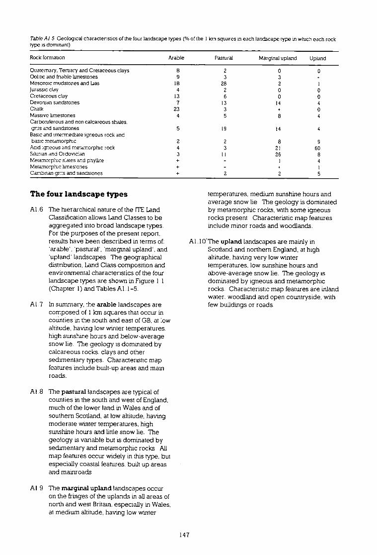
Table A l 5 Geological charactensUcs of ;he four landscape types (% of the I Ian squares in each landscape type in which each rocktype is dominant)

Rock formation Arable Pastural Marginal upland Upland

Ouaternary. Tertiary and Cretaceous clays 8 2 0 0Ooktic and friable limestones 9 3 3

Mesozoic mudstones and Las 18 28 2

Jurassic clay 4 2 0 0Cretaceous clay 13 6 0 0Devonian sandstones 7 13 14 4Chalk 23 3

0Massive hmeston.es 4 5 8 4Carboniferous and non calcareous shales.gms and sandstones 5 19 14 4Bas;c and Intermediate igneous rock andbasic metamorphic 2 2 8 9

Acid :gneous and metamorphic lock 4 3 2! 60Silurian and Ordovician 3 II 26

Metamorphic slates and phyllue

4Meta.morph:c hmestones

Carnbnan gms and sandstones

2 2 5

The four landscape types

A1.6 The hierarchical nature of the ITE LandClassification allows Land Classes to beaggregated into broad landscape types.For the purposes of the present report.results have been described in terms of:'arable'. 'pastural'. 'marginal upland'. and'upland landscapes. The geographicaldistnbution, Land Class composition andenvironmental characteristics of the fourlandscape types are shown in Figure 1 1(Chapter I) and Tables A1.1-5.

Al 3 ln summary, the arable landscapes arecomposed of 1 Ian squares that occur incounties in the south and east of GB, at lowaltitude, havLng low winter temperatures.high sunshine hours and below-averagesnow lie. The geology is dominated bycalcareous rocks. clays and othersedimentary types. Characterustic mapfeatures include built-up areas and mainroads.

ALB The pastural landscapes are typical ofcounties in the south and west of England,much of the lower land in Wales and ofsouthern Scotland, at low altitude, havingmoderate winter temperatures, highsunshine hours and little snow lie. Thegeology is variable but is dominated bysedimentary and metamorphic rocks. Allmap features occur widely in this type, butespecially coastal features. built up areasand mainroads.

AI.9 The marginal upland landscapes occuron the fringes of the uplands in all areas ofnorth and west Britain. especially in Wales,at medium altitude, having low winter

temperatures, medium sunshine hours andaverage snow lie. The geology is dominatedby metamorphic rocks, with some igneousrocks present Characteristic map featuresinclude minor roads and woodlands.

Al 1O'The upland landscapes are mainly inScotland and northern England, at highaltitude, having very low wintertemperatures, low sunshine hours andabove-average snow lie. The geology isdominated by igneous and metamorphicrocks. Characteristic map features are inlandwater, woodland and open countryside. withfew buildings or roads.

147

148

Appendix 2 CODE LISTS

Category 1 species for analysis

Plant species names which were used in the analysis of botanical data, having few taxonomical oridentification difficulties and which were consistently recorded by field surveyors.

Acer campestre (Field maple)Achillea rnillefolium (Yarrow)Achillea ptarmica (Sneezewort)Acinos arvensis (Basil thyme)Adoxa moschatellina (Moschatel)Aethusa cynapium (Fool's parsley)Agnmonia eapatona (Agrimony)Agrimoma procera (Fragrant agrimony)Agrostis capillaris (Common bent)Agrostis curtisii (Bristle bent)Agroslis gigantea (Black bent)Agrostis stolonifera (Creeping bent)Arra caryophyllea (Silver hair grass)Aira praecox (Early hair grass)Ajuga reptans (Bugle)Alchemille alpina (Alpine ladys mantle)Alisma plantago-aguatica (Water plantain)Alharia petiolata (Garlic mustard)Album ursinum (Ramsons)Album vineale (Wild onion)AMus glutinosa (Alder)Alopecums aequalis (Orange foxtail)Alopecurus geniculatus (Marsh foxtail)Alopecurus myosuroides (Black grass)Alopecurus pratensis (Meadow foxtad)Ammophila arenaha (Marram)Anacarnptis pyramidalis (Pyramidal orchid)Anagallis arvensis (Scar:et pimpernel)Anagallis minima (Chaffweed)Anagallis tenella (Bog pimpernel)Anchusa arvensis (Bugloss)Andromeda poll/Oka (Bog rosemary)Anemone nemorosa (Wood anemone)Angehca sylvestris (Wild angelica)Antennana dioica (Mountain everlasting)Anthems arvensis (Corn chamomile)Anthemis cotula (Stinkng mayweed)Anthoxanthum ocloratum (Sweet vernal grass)Anthrisc-uscaucaulis (Bur chervil)Anthnscus sylvesths (Cow parsley)Anthylhs vulneraria (Kidney vetch)Apium graveolens (Wild celery)Apiurn inundatum (Lesser marshwort)Apiurn nocliflorum (Fool's water cress)Aguilegia vulgaris (Columbine)Arabidopsis thaliana (Thale cress)Arabs hirsuta (Hairy rock cress)Arctostaphylos alpinus (Alpine bearberry)Arctostaphylos uva-ursi (Bearberry)Arenaha serpyllifolia (Thyme-leaved sandwort)Armena maritima (Thrift)

An-henathrum elatius (False oat grass)Artemisia absinthium (Wormwood)Artemisia campestris (Field southernwood)Artemisia maritima (Sea wormwood)Artemisia vulgaris (Mugwon)Arum maculatum (lords-and-ladies)Asparagus officinalis (Asparagus)Asperula cynanchica (Sguinancywort)Asplenium adiantum-nigrum (Black spleenwort)Asplenium man-num (Sea spleenwon)Asplenium ruta-muria (Wall rue)Asplenium scolopendrium (Han's tongue)Asplenium thchomanes (Maidenhair spleenwort)Asplemum viride (Green spleenwon)Aster tnpohum (Sea aster)Athyrium filix- lamina (Lady fern)Atnchum undulatum (Wavy-leaved thread moss)Atropa belladonna (Deadly nightshade)Aulacommum palustre (Bog thread moss)Avena fatua (Wild oat)Avena stngosa (Black oat)Avenula pratensis (Meadow oat grass)Avenula pubescens (Downy oat grass)Ballota nigra (Black horehound)Barbarea vulgaris (Winter cress)Belhs perennis (Daisy)Berula erecta (Lesser water parsnip)Bidens cemua (Nodding bur marigold)Bidens tnpartita (Trifid bur marigold)Blackstorna perfoliata (Yellow-wort)Blechnum spicant (Hard fern)Botrychium lunana (Moonwon)Brachypodiurn pinnalum (Tor grass)Brachypodium sylvaticum (False brome)Breutelia chrysocoma (moss)Bnza media (Quaking grass)Bromus commutalus (Meadow brome)Bromus erectus (Upright brome)Bromus hordeaceus (Softbrome)Bromus racemosus (Smooth brome)Bromus ramosus (Hairy brome)Bromus rigidus - No English nameBromus stenhs (Barren brome)Bryonia cretica (White bryony)Butomus umbellatus (Flowering rush)Calamagrostis epigejos (Wood small reed)Calamintha ascendens (Common calaminth)Calluna vulgaris (Heather)Caltha palustris (Marsh marigold)Calystegia septum (Hairy bindweed)Calystegia soldanella (Sea bindweed)

149

Campanula glornerata (Clustered bellflower)Campanula lanfolb (Giant bellflower)Campanula rotundifolia (Harebell)Carnpanula trachehum (Nettle-leaved bellflower)Capsella bursa-pastons (Sheperd's purse)Cardamine amara (Large bitter cress)Cardarnine impatiens (Narrow-leaved bitter cress)Cardarnine pratensis (Cuckoo'lower)Carduus acanthoidies (Welted thi.stle)Carduus nutans (Musk thistle)Carduus tenuiflorus (Slender thistle)Carex acutrformis (Lesser pond sedge)Carex aguatilis (Water sedge)Carex arenana (Sand sedge)Carex brgelown (Stiffsedge)Carex binervis (Green-ribbed sedge)Carex caphans (Hair sedge)Carex caryophyllea (Spring sedge)Carex curta (White sedge)Carex demissa (Common yellow sedge)Carex diandra (Lesser tussock sedge)Carex dioica (Dioecious sedge)Carex distans (Distant sedge)Carex disticha (Brown sedge)Carex divisa (Divided sedge)Carex divulsa (Grey sedge)Carex echinata (Star sedge)Carex extensa (Long braced sedge)Carex flacca (Glaucous sedge)Carex hills (Hairy sedge)Carex hostiana (Tawny sedge)Carex humilis (Dwarf sedge)Carex laevigata (Smooth-stalked sedge)Carex lepidocarpa (Long-stalked yellow sedge)Carex hmosa (Bog sedge)Carex muricata agg (Prickly sedge)Carex nigra (Common sedge)Carex otrubae (False fox sedge)Carex ovalis (Oval sedge)Carex palleseens (Pale sedge)Carex pahicea (Carnation sedge)Carex paniculata (Greater tussock sedge)Carex pauciflora (Few-flowered sedge)Carex pendula (Pendulous sedge)Carex piluhfera (Pill sedge)Carex pseudocyperus (Cyperus sedge)Carex remota (Remote sedge)Carex npaha (Great pond sedge)Carex rostrata (Bottle sedge)Carex serotina (Small-fruited yellow sedge)Carex stngosa (Thin-spiked wood sedge)Carex sylvatica (Wood sedge)Carex vesicaria (Bladder sedge)Carex vulpina (True fox sedge)Carlina vulgaris (Carline thistle)Carpinus betulus (Hornbeam)Carum venicillatum (Whorled caraway)Catabrosa aquatica (Water whorlgrass)Centaurea calcitrapa (Red star thistle)Centaurea nernoralis (Slender knapweed)

Centaurea rugra (Common knapweed)Centaurea scabiosa (Greater knapweed)Centaurium erythraea (Common centaury)Cerastrum alpinurn (Alpine mouse ear)Cerastiurn arcticurn (Arctic mouse ear)Cerastiurn arvense (Field mouse ear)Cerastiurn diffusurn (Sea mouse ear)Cerastium fontanum (Common mouse ear)Cerastium glomeraturn (Sticky mouse ear)Cerastium semidecandrurn (Little mouse ear)Ceratophyllum dernersurn (Soft hornwort)Chaenorlunurn minus (Small toadlizo)Chaerophyllurn ternulentum (Rough chervil)Charnaemelurn nobtle (Chamomile)Chamaenerion angustifohurn (Rosebay willowherb)Chelidoniurn rnajus (Greater celandine)Chrysanthemum segeturn (Corn marigold)Chrysospleniurn altennfohurn (Alternate-leavedgolden saxifrage)Chrysospleniurn oppositrfolium (Opposite-leavedgolden saxifrage)Cichonurn intybus (Chicory)Circaea alpina (Alpine echanter's nightshade)Circaea lutetiana (Enchanter's nightshade)arsium acaule (Dwarf thistle)Cirsium arvense (Creeping thistle)Cirsiurn dissecturn (Meadow thiStle)Cirsium eriophorurn (Woolly thistle)Cirsrum helenioides (Melancholy thistle)Cirsium palustre (Marsh thistle)Cirsiurn vulgare (Spear thistle)Cladiurn rnanscus (Great fen sedge)Cladoma arbuscula (lichen)Cladonia furcata (lichen)Cladonia impexa (lichen)Cladonia uncrans (lichen)Clematis vitalba (Traveller's joy)Chnopochurn vulgate (Wild basil)Cochlearia officinahs (Common scurvygrass)Coeloglossurn vinde (Frog orchid)Colchicurn autumnale (Autumn crocus)Cornurnmaculatum (Hemlock)Conopochurn majus (Pignut)Convallana majalis (Lilyof the valley)Convolvulus arvensis (Field bindweed)Comas sanguinea (Dogwood)Comus svecica (Dwarf cornel)Coronopus didyrnus (Lesser swine cress)Coronopus sguarnatus (Swine cress)Corydahs claviculata (Climbing corydalis)Corylus avellana (Hazel)Crataegus laevigata (Midland hawthorn)Crataegus laevigata x rnonogyna (Hawthorn hybrids)Crataegus monogyna (Hawthorn)Crepis biennis (Rough hawk's beard)Crepis capillahs (Smooth hawk's beard)Crepis paludosa (Marsh hawk's beard)Crepts vesicana (Beaked hawk's beard)Crithmurn maritimum (Rock samphire)Cruciata laevipes (Crosswort)

150

Crypiogramrna crispa (Parsley fern)Cuscuta epithyrnurn (Dodder)Cynoglossum officinale (Hound's tongue)Cynosurus enstalus (Crested dog's tail)Cystopteris fragilis (Brittle bladder fern)Cytisus scoparius (Broom)Dactylis glomerata (Cock's fooi)Danthonia decurnbens (Heath grass)Daphne laureola (Spurge laurel)Daphne rnezereum (Mezereon)Daucus carota (Wild carrot)Deschampsia cespitosa (Tufted hair grass)Descharnpsia Ilexuosa (Wavy hair grass)Desrnazeria ngida (Fern grass) .Dicranella heterornalla (Silky fork moss)Dicranurn majus (Greater fork moss)Dicranum scoparium (Lesser fork moss)Digitalis purpurea (Foxglove)aphasiastium alpinum (Alpine clubmoss)Diplotaxis muralis (Arnual wail rocket)Diplotaxis tenuifolia (Perennial wall Rocket)Dipsacus fullonum (Fuller s teasel)Drosera anglica (Great sundew)Drosera iniennedia (Oblong-leaved sundew)Drosera rotundifolia (Round-leaved sundew)D7as octopetala (Mountain avens)Echium vulgare ;Viper's bugloss)Eleochans malticaulis (Many-stalked spike rush)Eleochans palustris (Common spike rush)Eleochans quinguellora (Few-flowered spike rush)Eleochans uniglumis - No English nameEleoyiton fluitans (Floating clubrush)Elymus farctus (Sand couch grass)Elymuspycnanthus (Sea couch)Empetrum nig= (Crowberry)Epilobium anagathehlohum (Alpine willow herb)Epilobium hirsutum (Great willowherb)Epilobiurn palustre (Marsh willowherb)Epipactis helleborine (Broad helleborme)Equisetum aryense (Field horsetail)Equisetum fluviatile (Water horsetail)Eguisetum palustre (Marsh horsetail)Eguiseturn pratense (Shady horsetail)antiserum sylvaucum (Wood horsetail)Eguiseturn telernaleia (Great horse:ail)Erica cinerea (Bell heather)Erica tetralix (Cross-leaved heather)Engeron acer (Blue fleabane)Erlophomm anyustifolium (Common conongrass)Enophorum vagmatum (Hare's tail cottongrass)Erodium cicutarium (Common storks bill)Erophila vema (Common whitlowgrass)Erysirnurn chmianthoides (Treacle mustard)Euonymus europaeus (Spmdle)Eupatonum cannatunurn (Hemp agrimony)Euphorbia amygdaloides (Wood spurge)Fallopia convolvulus (Black bindweed)restuca allissima (Wood fescue)Festuca arundmacea (Tall fescue)Festuca gigantea (Giant fescue)

Festuca ovina (Sheep's fescue)Festuca pratensis (Meadow fescue)festuca rubra (Red fescue)Festuca tenuifolia (Fine-leaved sheep's fescue)Festuca vivipara (Vivlparous fescue)Fest/do/rum hybrid (Hybrid fescue)rilago lutescens (Common cudweed)Filayo minima (Small cudweed)Eilago vulgaris (Cudweed)lilipendula ulmaria (Meadowsweet)Filipendula vulgaris (Dropwort)Fragaria vesca (Wild stawberry)Fraxinus excelsior (Ash)Fumaria bastardh (Tall rampmg fumitory)Fumaria capreolata (White ramping fumitory)Furnaria otheinalis (Common fumitory)Galeopsis angustifolia (Red hemp nettle)Galeopsis segeturn (Downy hemp nettle)Galeopsis speciosa (Large-flowered hemp nettle)Galeopsis tetrahit (Common hemp nettle)Galium apanhe (Cleavers)Gahum boreale (Northern bedstraw)Galium mollugo (Hedge bedstraw)Gaburn odoratum (Woodruff)Callum palustre (Common marsh bedstraw)Callum purniturn (Slender bedstraw)Galiurn saxatile (Heath bedstraw)Gahurn stemeri (Limestone bedstraw)Gahurn tricomutum (Corn cleavers)Galiurn uliymosum (Fen bedstraw)Gahum verum (Lady's bedstraw)Cenista anglica (Petty whin)Cenista tinctona (Dyer's greenweed)Gentianella amarella (Autumn gentian)Genuanella campestfis (Field gentian)Geranium columbinium (Long-stalked crane's bill)Geranium dissectum (Cut-leaved crane's bill)Geranium lucidum (Shining crane's bill)Geranium molle (Dove's-foot crane's bill)Geranium pratense (Meadow crane's bill)Geranium pusillum (Small-flowered crane's bill)Geranium pyrenaicum (Hedgerow crane's bill)Geranium robenianum (Herb Robert)Geranium sanguineum (Bloody crane's bill)Geranium sylvatiann (Woody crane's bill)Geum rivale (Water avens)Ceurn urbanum (Wood avens)Geum x intermediurn (Hybrid amens)Glaucium flavum (Yellow horned poppy)Claux mahtima (Sea milkwort)Glechoma hederacea (Ground ivy)Glycena declinata (Small sweet graes)Glyceria fluitans (floating sweet grass)Glycena maxima (Reed sweet grass)Glycena phcata (Plicate swee: grass)Gnaphaburn supinum (Dwarf cudweed)Gnaphahum sylvaticum (Heath cudweed)Gnaphahum uhythosum (Marsh cudweed)Goodyera repens (Creeping lady's tresses)Gymnadema conopsea (Fragrant orchid)

151

Gyrnnocarpium dryopteris (Oak fern) Lactuca serriola (Prickly lettuce)Halimione portulacoides (Sea purslane) Lamiastrurn galeobdolon (Yellow archangel)Hedera helix (Ivy) Larruum album (White dead nettle)Helianthemum nummularium (Common rock rose) tamium amplexlcaule (Henbit dead nettle)Heracleurn sphondylium (Hogweed) Lamium hybridum (Cut-leaved dead nettle)Hieracium pilosella (Mouse ear hawkweed) Larniumpurpureum (Red dead nettle)Hippocreprs comosa (Horseshoe vetch) Lapsana communis (Nipplewort)Hippuna vulgans (Mare's tail) Lathyrus montanus (Bitter vetch)Holcus lanatus (Yorkshire fog) Lathyrus nissolia (Grass vetchling)Holcus moth's (Creeping soft grass) Lathyrus pratensis (Meadow vetchlir.g)Honkenya peploides (Sea sandwon) begousia hybrida (Venus's looking glass)Hordelymus europaeus (Wood barley) Lemnammor (Common duckweed)Hordeum munnum (Wall barley) Lepdium campestre (Field pepperwon)Hordeum secalinum (Meadow barley) Lepidium heterophyllum (Smith's cress)Humulus lupulus (Hop) Lepichum latilblium (Dittander)Huperzia selago (Fir clubmoss) Leucanthemum vulgare (0 x eye daisy)Hyacinthoides non-scnpta (Bluebell) Leucobryum glaucum (White fork moss)Hydrccharis morsus-ranae (Frogbit) Leymus arenarius (Lyrne grass)Hydrocotyle vulgahs (Marsh pennywon) Ligusticum scoacum (Scots lovage)Hylocomium splendens (Glittering feather moss) Ligustmm vulgare (Wild privet)Hypehcum androsaemum (Tutsan) Lifium martagon (Managon hly)Hypericum calycinum (Rose of Sharon) Limonium humile (Lax-flowered sea lavender)Hypericum elodes (Marsh St John's won) Limonfiun vulgare (Common sea lavender)Hypericum hirsutum (Hairy StJohn's won) Linana vulgaris (Common toadflax)Hypericum humifusum (Trailing St John's won) Linum bienne (Pale flax)Hypericum maculatum (Imperforate StJohn's won) Linum catharticum (Fairy flax)Hypericum montanum (Pale St John's won) bparis loeselii (Pen orchid)Hypencum perforaturn (Perforate St John's won) Listen cordata (Lesser twayblade)Hypericum pulchrum (Slender St John's won) Listen ovata (Common twayblade)Hypericum tetrapterum (Square-stalked St John's won) Lithospermum arvense (Corn gromwell)Hypericum undulatum (Wavy St John's won) Litorella unillora (Shore weed)flex aquifolium (Holly) Lobelia dortmanna (Water lobelia)Mula conyza (Ploughman's spilcenard) Loiseleuria procumbens (Trailing azalea)Mula crithmoides (Golden samphire) Latium perenne (Perennial rye grass)Iris foetidissima (Stinking iris) Lonicera periclymenum (Honeysuckle)Ins pseudocorus (Yellow iris) Lotus corniculatus (Common bird's foot trefoil)Isoetes lacustns (Quillwort) Lotus subbifloms (Hairy bird's foot trefoil)Isoleps cemua (Slender club rush) Lotus tenuis (Narrow-leaved bird's foot trefoil)Isolepis setacea (Bristle club rush) Lotus uliginosus (Greater bird's foot trefoil)Jasione montana (Sheep's bit) Luzula pilosa (Hairy wood rush)Juncus ambiguus - No English name Luzulaspicata (Spiked wood rush)Juncus bufonius (Toad rush) Luzula sylvatica (Great wood rush)Juncus bulbosus (Bulbous rush) Lychnis flos-cucub (Ragged Robin)Juncus castaneus (Chesnut rush) Lycopodium clavatum (Stag's-horn clubmoss)Juncus conglomeratus (Compact rush) Lycopsis arvensis (Bugloss)Juncus elfusus (Soft rush) Lycopus europaeus (Gipsywon)Juncus gerardi (Saltmarsh rush) Lysirnactua nemorurn (Yellow pimpernel)Juncus inflexus (Hard rush) Lysimachia nummularia (Creeping Jenny)Juncus maritimus (Sea rush) Lysimachia vulgaris (Yellow loosestrife)Juncus squarrosus(Heath rush) Lythrum portula (Water purslane)Juncos subnodulosus (Blunt-flowered rush) Lythrum salicaria (Purple loosestrife)Juncus tenuis (Slender rush) Malus sylvestris (Crab apple)Juncus trifidus (Three-leaved rush) Malva moschata (Musk mallow)Juncus thglumis (Three-flowered rush) Malva neglecta (Dwarf mallow)Juniperus cornmunis (Juniper) Malva sylvestris (Common mallow)Kicloaa elamine (Sharp-leaved fluellen) Marrubiurn vulgare (White horehound)Kiclocia spuria (Round-leaved fluellen) Matricana matricahoides (Pineappleweed)Knauba arvensis (Field scabious) Matricanarecutila(Scented mayweed)Koeleria macrantha (Crested hair grass) Meconopsis cambrica (Welsh poppy)Lactuca saligna (Least lettuce) Medicago arabica (Spotted medick)

152

Medicago lupulina (Black rnedick)Melatnpyrurn pratense (Common cow wheat)Melica unillora (Wood melick)Melittis mefissophyllurn (Bastard balm)Menyanthes trifoliata(Bogbean)Mercurialis perennis (Dog's mercury)Miliurneffusurn (Wood millet)Minuartia verna (Vernal sandwort)Mnium hornurn (Swan s neck thread moss)Moehringia tnnervia (-Three-nerved sandwort)Mohnia caerulea (Purple moor grass)Moneses uniflora (One-flowered wintergreen)Montia fontana (Blinks)Mycefis muralis (Wall lettuce)Myosolon aquatic-um (Water chickweed)Myrica gale (Bog myrtle)Mynophyllurn alterntfolia (Alternate-flowered water

milfoil)Mynophyllum spicata (Spiked water milfoil)Mysobs arvensis (Field forget-me-not)Nardus strk-ta (Mat grass)Narthecium ossifragurn (Bog asphodel)Nasturtium rnicrophyllurn (Winter cress)Nasturtium officinale (Water cress)Nuphar lutda (Yellow water lily)Nymphaea alba (White water lily)Odontites vema (Red bartsia)Oenanthe crocata (Hemlock water dropwort)Oenanthe fistulosa (Tubular water dropwort)Onorns repens (Common restharrow)Ononis spinosa (Spiny restharrow)Ophloglossum vulgatum (Adder's tongue)Ophrys apifera (Bee orchid)Orchis mascula (Early-purple orchid)OreoptenE limbospenna (Lemon-scented fern)Onganum vulgare (Marjoram)Ornithopus perpusillus (Bird's foot)Orobanche minor (Common broomrape)Osmunda regalis (Royal fern)OxahEacetosella (Wood sorrel)Oxyna digyna (Mountain sorrel)Papaver dubiurn (Long-headed poppy)Papaver rhoeas (Common poppy)Paraphofis singosa (Hard grass)Parentucellia viscosa (Yellow bansia)Panetaha judacia (Pellitory-cf-the-wall)Parnassiapalustns (Grass of Parnassus)Pastinaca saliva (Wild parsnip)PeclicularispalustnE (Marsh lousewort)PediculanE sylvatica (Lousewort)Peltigera canina (lichen)Petasites hybridus (Butterbur)Petracialmumsegetum (Corn parsley)Phalarisamndinacea (Reed canary grass)Phalariscanariensis (Canary grass)Phalarisminor (Lesser canary grass)Phegoptehs connectibs (Beech fern)Phragmites australis (Common reed)Phyteurna orbiculare (Round-headed rampion)Picrisechloides (Bristly ox tongue)

Picrishieraciodes (Hawkweed ox tongue)Pimpmella major (Greater burnet saxifrage)Pirnpthellasaxifraga (Burnet saxifrage)Pmguicula lusitanica (Pale bunerwort)Pinguicula vulgaris (Common butterwort)Plagiornnium undulaturn (moss)Plagothecium denticulaturn (Sharp fern-like feather moss)Plagiothecium undulatum (moss)Plantago coronopus (Buck's-horn plantain)Plantago lanceolata (Ripwort plantain)Plantago major (Greater plantain)Plantago maritirna (Sea plantain)Plantago media (Hoary plantain)Platanthera biloha (Lesser butterfly orchid)Platanthera chlorantha (Greater butterfly orchid)Pleurozium schreben (Red stemmed feather moss)Poa angustifolia (Narrow-leaved meadow grass)Poa annua (Ammal meadow grass)Poa compressa (Flattened meadow grass)Poapratensis (Smooth meadow grass)Poa subcaerulea (Spreading meadow grass)Polygala calcarea (Chalk milkwon)Polygonatum rnultiflorurn(Solomon's seal)Polygonum amphibium (Amphibious bison)Polygonum arenastrum (Small-leaved knotgrass)Polygonum aviculare (Knotgrass)Polygonum bistorta (Common bistort)Polygonurn hydropiper (Water pepper)Polygonum lapathifolium (Pale persicana)Polygonum mite (Tasteless water pepper)Polygonum persicaria (Redshank)Polygonum vivipallIM (Alpine biston)Polypodium vulgare (Polypody)Populus trernula (Aspen)Potarnogeton natans (Broad-leaved pondweed)Potarnogeton polygonifohus (Bog pondweed)Potentilla anglica (Trailing tormentil)Potentilla anserina (Silverweed)Potentilla erecta (Tormentil)Potentillapalusths (Marsh cinquefoil)Potenblla reptans (Creeping cinquefoil)Potentilla sterilis (Barren strawberry)Pnmula elauor (Oxlip)Primula yens (Cowslip)Pnrnula vulgans (Primrose)Prunella vulgaris (Selfheal)Pnmus aviurn (Wild cherry)Prunuspadus (Bird cherry)Prunus spinosa (Blackthorn)Pseudorchis albida (Small-white orchid)Pseudoscleropodium pururn (Neat meadow feather moss)Pteridium aguihnum (Bracken)Puccinellia distans (Reflexed saltmarsh grass)Puccinellia fasciculata (Borrer's saltmarsh grass)Puccinellia maribma (Common saltmarsh grass)Pulicariadysentenca (Common fleabane)Pulmonana officinalis (Lungwort)Pyrola minor (Common wintergreen)Ranunculus acnE (Meadow buttercup)Ranunculus aquatilis (Common water crowfoot)

153

Ranunculus arvensis (Corn crowfoot)Ranunculus auncomus (Wood crowfoot)Ranunculus bulbosus (Bulbousbuttercup)Ranunculus licaria (Lesser celandine)Ranunculus liammu/a (Lesser spearwon)Ranunculus fluitansRanunculus hederaceus (Ivy-leaved crowfoot)Ranunculus lingua (Great spearwort)Ranunculus omiophyllus - No EnglishnameRanuncu/uspannflorus (Small-floweredbuttercup)Ranunculus peltatus - No EnglishnameRanunculus penicillatus - No EnglishnameRanunculus repens (Creeping buttercup)Ranuncu/us sardous (Hairybuttercup)Ranunculus sceleratus (Celery-leaved buttercup)Ranunculus trichophyllus - No EnglishnameRaphanus mantimus (Sea radish)Raphanus raphanistrum (Wildradish)Reseda lutea (Wildmignonette)Rhacomitrium lanuginosum (WoollyfrIngemoss)Rhamnus catharticus (Buckthorn)Rhizomnium punctatum (moss)Rhynchospora a/ba (Whitebeak sedge)Rhytidiadelphus loreus (moss)Rhytidiadelphus sguarrosus (Drooping-leaved

feather moss)Rhytidiade/phus tnguetrus (Triangular-leaved

feather moss)Ribes uva-crispa (Gooseberry)Rorippa amphibia (Great yellowcress)Rorippa islandica (Northern marsh yellowcress)Ronppa palustns (Common marsh yellOwcress)Ronppa sylvestns (Creeping yellowcress)Rubia peregrine (Wildmadder)Rubus caesius (Dewberry)Rubus chamaemorus (Cloudberry)Rubus idaeus (Rasberry)Rubus sexatilis (Stonebramble)Rumex acetosa (Common sorel)Rumex acetosella (Sheep s sorrel)Rumex crispus (Curled dock)Rumex hydrolapathum (Water dock)Rumex longifolius (Northern dock)Rumex maritimus (Golden dock)Rumex obtusifolius (Broad-leaved dock)Rumex palustns (Marshdock)Rumex pulcher (Fiddle dock)Rumex rupestris (Shore dock)Ruscus aculeatus (Butcher's broom)Sagittane sagittifolie (Arrowhead)Sambucus nigra (Elder)Samolus valerandi (Brookweed)Sanguisorba minor (Salad burnet)Sanguisorba ollicinalis (Great burnet)Sanicula europaea (Sanicle)Sarcocomia perennis - No EnglishnameSaxitraga aizoicies (Yellowsaxifrage)Saxifrage granulate (Meadow saxifrage)Saxifrage hypnoides (Mossysaxifrage)Saxifrage oppositifolia (Purple saxifrage)

Saxifrage stellahs (Starrysaxifrage)Scabiosa columbaria (Smallscabious)Schoenoplectus lacustns (Common club rush)Schoenus nigricans (Blackbog rush)Solla autumnalis (Autumnsquill)Scilla vema (Spring squill)Sorpus rnaritimus (Sea club rush)Sorpus sylvabous (Woodclub rush)Scrophularia auricu/ata (Water figwort)Scrophulane nodose (Common figwort)Scutellane gale/wt./la/a (Skullcap)Scutellana minor (Lesser skullcap)Sedum album (Whitestonecrop)Sedum forsteranum (Rockstonecrop)Sedum rosea (Roseroot)Sedum telephinum (Orpine)Sedum villosum (Hairystonecrop)Selagmella selagmoides (Lesser clubmoss)Senecio aguaticus (Marsh ragwort)Senecio congestus (Marshfleawort).Senecio erucifolius (Hoaryragwort)Senecio integnfolius (Fieldfleawort)Senecio jecobaea (Common ragwort)Senecio sylvaticus (Woodgrounclsel)Senecto viscosvs (Stickygroundsel)Senecio vu/garis (Groundsel)Serratula tinctona (Sawwon)Seseli libanotis (Mooncarrot)Ses/ena albicans (Bluemoor grass)Sherardia arvensis (Fieldmadder)Sibthorpia europaea (Cornish rnoneywort)Silaum silaus (Pepper saxifrage)Silene dioica (Redcampion)Silene latifolia (Whitecampion)Silene mentuna (Sea campion)Silene vu/gans (Bladder campion)Sison amomum (Stoneparsley)Sisymbnum altissimum (Tallrocket)Sisymbrium oflionale (Hedge mustard)Smyanum olusatrum (Alexanders)Solidago virgaurea (Goldenrod)Sonchus arvensis (Perennialsow thistle)Sonchus asper (Pricklysow thistle)Sonchus oleraceus (Smoothsow thistle)Sonchus palustris (Marshsow thistle)Sorbus ana (Common whitebeam)Sorbus aucupana (Rowan)Sorbus torrninalis (Wildservice tree)Sparganium emersurn (Unbranched bur reed)Sparganium erectum (Branched bur reed)Spergulaha marginate (Greater sea spurrey)Spergulaha marina (Lesser sea spurrey)Spergulane rubra (Sandspurrey)Spiranthes spiralis (Autumnlady's tresses)Stachys x ambigua (hybrid, probably Hedge

woundwon)Stachys arvensis (Fieldwoundwort)Stachys officinaks (Betony)Stachys palustris (Marshwoundwort)Stachys sylvatice (Hedge woundwort)

154

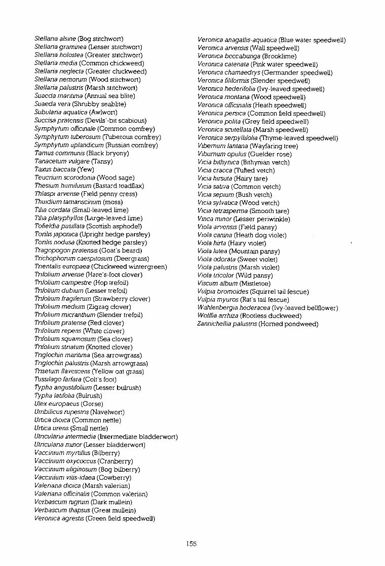
Steliana alsine (Bog stitchwon)SteIlane graminea (Lesser stitchwon)Steliana holostea (Greater stitchwort)SteIlana media (Common chickweed)SteIlana neglecta (Greater chickweed)Stellaria nemorum (Wood stitchwort)SteIlaria palustn's (Marsh stitchwon)Suacda mantima (Annual sea blite)Suaeda vera (Shrubby seablite)Subularia aquatica (Awlwort)Succisa pratensis (DeviIs'-bit scabious)Symphytum ollicinale (Common comfrey)Symphytum tuberosum (Tuberous comfrey)Syrnphytum uplandicum (Russian comfrey)Tamuscornrnunis (Black bryony)Tanacetum vulgare (Tansy)Taxus baccata (Yew)Teucnurn scorodonia (Wood sage)Thesium humilusum (Bastard toadllax)Thlaspi arvense (Field penny cress)Thindiurn tamanscinum (moss)Tilia cordate (Small-leaved lime)

lia platyphyllos (Large-leaved lime)Tolieldia pusillata (Scottish asphodel)Tonfis japonica (Upright hedge parsley)Tonlis nodusa (Knotted hedge parsley)Tragopogon pratensts (Goat's beard)Trichophorum caespitosurn (Deergrass)Tnentalis europaea (Chickweed wintergreen)Thfoliurn arvense (Hare's-foot clover)Trifollum campestre (Hop trefoil)Tnfolium duthurn (Lesser trefoil)Trifolium fragiferum (Strawberry clover)Trifolium medium (Zigzag clover)Trifolium micranthum (Slender trefoil)Tnfolium pretense (Red clover)Trifokum repens (White clover)Tntolium squamosum (Sea clover)Trifolium sthatum (Knotted clover)Tnglochin maritima (Sea arrowgrass)Thglochih palustris (Marsh arrowgrass)Trisetum Ilavescens (Yellow oat grass)7lissilago farfara (Colts foot)Typha angustifolium (Lesser bulrush)Typha latifolia (Bulrush)Ulex europaeus (Gorse)Umbilicus mpesins (Navelwort)Unica choice (Common nettle)Urtica urens (Small nettle)Utncularia intennedia (Intermediate bladderwort)Utnculana minor (Lesser bladderwort)Vaccinium myrtillus (Bilberry)Vaccinium oxycoccus (Cranberry)Vaccimum uliginosum (Bog bilberry)Vaccinium vitis-idaea (Cowberry)Valenana choice (Marsh valerian)Valeriana officinalis (Common valerian)Verbascum nigmrn (Dark mullein)Verbascurn thapsus (Great mullein)Veronica agrestis (Green field speedwell)

Veronica anagallis-aquatica (Blue water speedwell)Veronica arvensis (Wall speedwell)Veronica beccabunga (Brooklime)Veronica catenate (Pink water speedwell)Veronica chamaedrys (Germander speedwell)Veronica filiforrnis (Slender speedwell)Veronica hederifolia (Ivy-leaved speedwell)Veronica montane (Wood speedwell)Veronica ollicinalis (Heath speedwell)Veronica persica (Common field speedwell)Veronica polite (Grey field speedwell)Veronica scutellata (Marsh speedwell)Veronica serpyllifolia (Thyme-leaved speedwell)Vibernurn lantana (Wayfaring tree)Viburnum opulus (Guelder rose)Vicia bithynica (Bithynian vetch)Vicia cracca (Tufted vetch)Vicia husuta (Hairy tare)Vicia sativa (Common vetch)Vicia sepium (Bush vetch)Vicia sylvatica (Wood vetch)Vicia tetrasperma (Smooth tare)Vince minor (Lesser periwinkle)Viola an,ensis (Field pansy)Viola canina (Heath dog violet)Viola hirta (Hairy violet)Viola lutea (Mountain pansy)Viola odorata (Sweet violet)Viola palustns (Marsh violet)Viola tricolor (Wild pansy)Viscum album (Mistletoe)Vulpia bromoides (Squirrel tail fescue)Vulpia myuros (Rat's tail fescue)Wahlenbergia hederacea (Ivy-leaved bellflower)Wolflia arrhiza (Rootless duckweed)Zannichellia palustns (Homed pondweed)

155

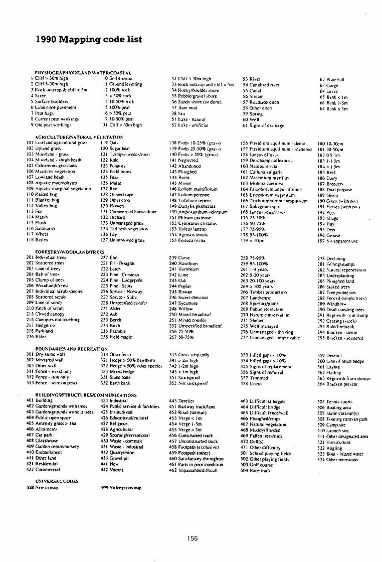
1990 Mapping code list

PlITSIOCRAPHYANLAND WATER/COASTAL1 Cliff > 30m high2 Cliff 5-30m high3 Rock uutcrop & cliff < 5m4 Scree

5 Surface boulders6 Limestone pavement7 Peat hags

8 Current peat workings9 Old peat workings

0 Soil erosionI Ground levelling2 100% rock3 >50% mck4 10-50% mck5 100% peat6 >50% peat7 10-50% peat1 Cliff > 30m high

32 Cliff 5-30m high33 Rock outcrop and cliff < 5m34 Rocky/boulder share35 Pebble/gravel share36 Sandy shore (or dune)37 Bare mud38 Sea5 I Lake - natural52 lake • artificial

53 River54 Canalised river55 Canal56 Sircam57 Roadside ditch58 Other ditch59 Spring60 Well61 Signs of drainage

62 Waterfall63 Gorge

64 Levee65 Bank < 1m66 Bank I-5m67 Bank > 5m

AGRICULTUREINATURAL VEGETATION

101 Lowland agricultural grass 19 Oars 38 Farb. 10-25% (grass) 56 Plendium aquilinum - dense 80 10-30cm102 Upland grass 20 Sugar beat 39 Forbs 25-50% (grass) 57 therichum aquilinum - scattered 81 30-50cm103 Mrsuland - grass 21 Turnips/swedevroots 40 Rubs > 50% (grass) 58 luncus ef (usu. 82 05-1m104 Maorland - shrub heath 22 Kale 41 Neglected 59 Descharripsiaflexuosu 831-1.5m105 Calcareous grassland 23 Putatoes 42 Abandoned 60 Nardus stricta 84 > I.5m106 Maritime vegetation 24 Field beans 43 Ploughed 61 Calluna sulgaris 85 Beef107 Lowland heath 25 Peas 44 Burnt 62 Vaccinium mynilus 86 DairY108 Aquatic rnacrophytes 26 Mairt 45 Mown 63 Molinia caerulea 87 Breeders109 Aquatic marginal vegetation 27 Rye 46 Latium multillorum 64 Eriaphorum angustifolium 88 Dual purpose110 Raised tog 28 Oilseed rape 47 Latium perenne 65 Eriophorum vagindum 89 SheepIII Blanket bog 29 Other crap 48 Trifolium repens 66 Tricharophomm CaespitONLIM 90 GOals (with rso.)112 Valley bog 30 Mourn 49 Dactylis glomerata 67 Sphagnum spp. 91 Hor es (with no)113 Fen 31 Commercial horticulture 50 Anthoranthum odoratum 68 /Pew, squanosus 92 Pigs114 Marsh 32 Orehard 51 Phleum pratense 75 25-50% 93 Silage115 Flush 33 Unmanaged grass 52 Cynosurus Cristalus 76 50-75% 94 Hay116 Saltmarsh 34 Tall herb vegetation 53 Marcus lanatus 77 75-95% 95 Deer117 Wheat 36 ley 54 Agromis tenuis 78 95-103% 96 Grouse118 Barley 37 Unimproved grass 55 Fescue, ovina 79 < 1(km 97 No apparent use

FORFSTRY/WOODLAND/TREES

201 Individual trees237 Elm 239 Gorse 258 75-95% 278 Declining202 Scattered trees221 Fir - Douglas 240 Hawthorn 259 95-100% 281 Felling/stumps203 Line of trees222 Larch 241 Hornbeam 2611-4 years 282 Narural regeneration204 Belt of trees223 Pine • Corsican 242 Lime 262 5-20 years 283 Uncle:planting205 Clump of trees224 Pine - Lodgepok 243 Oak 263 20-100 years 285 Plisughtd land206 Woodland/forest225 Pine • Scots 244 Poplar 264 > 100 years 286 Staked trees207 Individual scrub species226 SpruceNofway 245 Rowan 266 Timber production 287 Tree protectors208 Scattered scrub227 Spnat - Sida 244 Sweet chestnut 267 Landscape 268 Fenced (single trees)209 Line of scrub228 Unspecified conifer 247 Sycamore 268 Spurting/game 289 Windhlow210 Patch of scrub231 Alder 248 Willow 269 Public recreation 290 Dead standing trees215 Closed canopy232 Ash 250 Mixed hnsadleaf 270 Nature conservation 291 Regrowth - cut stump216 Canopies not touching233 Beech 251 Mixed conifer 271 Shelter 292 Grazing (stock)217 Hedgerow234 Birch 252 Unspecified broadleaf 275 Well managed 293 Ride/firehreak218 Parkland235 Bramble 256 25-50% 276 Unmanaged • thriving 294 Bracken - dense236 Elder238 held maple 257 50-75% 277 Unmanaged - improvable 295 Bracken - scattered

BOUNDARIES AND RECREATION

301 Dry-stone wall314 Other fence 333 Grass strip unly 353 Filled gaps <10% 359 Derelict302 Mortared wall321 Hedge > 50% hawthorn 341 >2,n high 354 Filled gaps > 10% 360 Line of relici hedge303 Other wall322 Hedge > 50% other species 342 I•2m high 355 Signs of replacement 361 Laying311 Fencewood only323 Mixed hedge 343 < Im high 356 Signs of removal 362 Mailing312 Fence - iron only331 Stone bank 351 Stockproof 357 Trimmed 363 Regrowth from stumps313 Fence - wire on posts332 Earth bank 352 Not stickpin( 358 Uncut 364 Bracken present

BUILDINGS/STRUCTURES/COMM UNICATIONS

401 Building423 Industrial 443 Derelict 463 Difficult stile/gate 505 Tennis courts402 Garden/grounds wirh trees424 Public service & facilities 451 Railway track/land 464 Difficult bridge 506 Boating area403 Garden/grounds without trees425 Institutional 452 Road (tarmac) 465 Difficult fence/wall 507 Sufic caravan(%)404 Public open space426 Exhalkmalkultural 453 Verge < 1m 466 Ploughed/crops 508 Touring caravan park405 Amenity grass > 1ha427 Religious. 454 Verge 1-5m 467 Natural vegetation 509 Camp soe406 Allotments428 Avic-ultural 455 Verge > 5m 468 Muddy/flooded 510 Launch site407 Cal park429 Sponing/rearational 456 Constructed track 469 Fallen treesnock 511 Other designated arca408 Glasshouse430 Waste - domestic 457 Unconstructed track 470 Bull(s) 521 Honiculture409 Garden centre/nursery431 Waste - industrial 458 Footpath (exclusive) 471 Other difficulty 522 Angling410 Embankment432 Quarry/mine 459 Footpath (other) 501 School playing fields 523 Boat - inland water411 Other land433 Gravel pit 460 Satisfactory throughout 502 Other playing fields 524 Other recrearion421 Residential441 New 461 Parts in poor condition 503 Golf crone

504 Race track422 Commercial442 Vacant 462 Impassable/difficult

UNIVERSAL CODES

888 New to map999 No longer on map

156

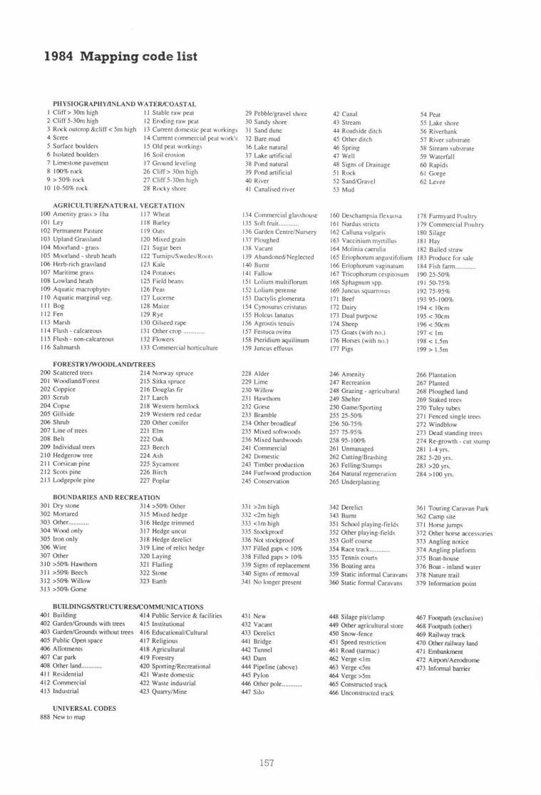
1984 Mapping code list

PHYSIOGRAPHY/INLAND WATER/COASTAL1 Cliff > 30m high I I Stable raw peal2 Cliff 5-30m high 12 Eroding raw peat3 Rock outcrop &cliff < 5m high 13 Current domestic peat workings4 Scree 14 Current commercial peat work's5 Surface boulders 15 Old peat workings6 Isolated boulders 16 Soil erosion7 Limestone pavement 17 Ground leveling8 100% rock 26 Cliff > 30m high9 > 50% rock 27 Cliff 5-30m high

10 10-50% rock 28 Rocky shore

AGRICULTURE/NATURAL VEGETATION00 Amenity grass > I ha 17 Wheat

1 Ley 18 Barley02 Permanent Pasture 19 Oats03 Upland Grassland 20 Mixed grain04 Moorland - grass 21 Sugar beet05 Moorland - shrub heath 22 Turnips/Swedes/Roots06 Herb-rich grassland 23 Kale07 Maritime grass 24 Potatoes08 Lowland heath 25 Field beans09 Aquatic macrophytes 26 Peas10 Aquatic marginal veg. 27 LucerneII Bog 28 Maize12 Fen 29 Rye13 Marsh 30 Oilseed rape14 Flush - calcareous 31 Other crop 15 Flush - non-calcareous 32 Flowers16 Saltmarsh 33 Commercial honiculture

FORESTRY/WOODLAND/TREES200 Scattered trees 214 Norway spruce201 Woodland/Forest 215 Sitka spruce202 Coppice 216 Douglas fir203 Scrub 217 Larch204 Copse 218 Western hemlock205 Gillside 219 Western red cedar206 Shrub 220 Other conifer207 Line of trees 221 Elm208 Belt 222 Oak209 Individual trees 223 Beech210 Hedgerow tree 224 Ash211 Corsican pine 225 Sycamore212 Scots pine 226 Birch213 Lodgepole pine 227 Poplar

BOUNDARIES AND RECREATION

29 Pebble/gravel shore30 Sandy shore31 5and dune32 Bare mud

36 Lake natural37 Lake artificial

38 Pond natural39 Pond artificialao River

41 Canalised river

34 Commercial glasshouse35 Soft fruit 36 Garden Centre/Nursery37 Ploughed

38 Vacant39 Abandoned/Neglectedao Bumt41 Fallow

SI Lolium multillorum52 Lolium perenne53 Dactylis glomerata54 Cynosunis cristatus55 Holcus lanatus56 Agrostis remits57 Festuca ovina58 Pteridium aquilinum59 luncus effusus

228 Alder229 Lime230 Willow231 Hawthorn232 Gorse233 Bramble

234 Other broadleaf235 Mixed softwoods236 Mixed hardwoods241 Commercial242 Domestic243 Timber production244 Fuelwood production245 Conservation

42 Canal

43 Stream44 Roadside ditch45 Other ditch46 Spring47 Well

48 Signs of Drainage51 Rock

52 Sand/Gravel53 Mud

60 Deschampsia flexuosa1 Nardus suicta

62 Calluna vulgaris63 Vacciniurn mynillus64 Molinia caerulia65 Eriophorum angustifolium66 Eriophorum vaginat um67 Tricophorum cespitosum68 Sphagnum spp.69 Juncos squarrosus71 Beef72 Dairy

73 Dual purpose74 Sheep75 Goats (with no.)76 Horses (with no.)77 Pigs

246 Amenity247 Recreation248 Grazing - agricultural249 Shelter250 Game/Sponing255 25-50%256 50-75%257 75-95%

258 95-100%261 Unmanaged262 Cutting/Bra.shing263 Felling/Stumps264 Natural regeneration265 Underplanting

54 Peat

55 Lake shore56 Riverbank57 River substrate58 Stream substrate59 Waterfall60 Rapids61 Gorge

62 Levee

78 Farmyard Poultry79 Commercial Poultry80 Silage

81 Hay

82 Bailed straw83 Produce for sale84 Fish farm 90 25-50%91 50-75%

92 75-95%93 95-100%

94 < 10cm95 < 30cm96 < 50cm97 < 1m

98 < 15m99 > 1.5m

266 Plantation267 Planted268 Ploughed land269 Staked trees270 Tuley tubes271 Fenced single trees272 Windblow273 Dead standing trees274 Re-growth - cut stump281 1-4 yrs.282 5-20 yrs.283 >20 yrs.284 >100 yrs.

61 Touring Caravan Park62 Camp site71 Horse jumps

72 Other hors& accessories373 Angling notice374 Angling platform375 Boat-house376 Boat • inland water378 Nature trail379 Information point

301 Dry stone302 Mortared303 Other 304 Wood only305 Iron only306 Wire307 Other

310 >50% Hawthorn311 >50% Beech312 >50% Willow313 >50% Gorse

314 >50% Other315 Mixed hedge316 Hedge trimmed317 Hedge uncut318 Hedge derelict319 Line of relict hedge320 Laying321 Flailing

322 Stone323 Earth

331 >2m high332 <2m high333 clm high335 Stockproof336 Not stockproof337 Filled gaps < 10%338 Filled gaps > 10%339 Signs of replacement340 Signs of removal341 No longer present

342 Derelict 3343 Burnt 3351 School playing-fields 3352 Other playing-fields 3353 Golf course354 Race track 355 Tennis coons356 Boating area359 Static informal Caravans360 Static formal Caravans

BUILDINGS/STRUCTURES/COMMUNICATIONS401 Building 414 Public Service & facilities 431 New402 Garden/Grounds with trees 415 Institutional 432 Vacant403 Garden/Grounds without trees 416 Educational/Cultural 433 Derelict405 Public Open space 417 Religious 441 Bridge406 Allotments 418 Agricultural 442 Tunnel407 Car park 419 Forestry 443 Dam408 Other land 420 Sporting/Recreational 444 Pipeline (above)411 Residential 421 Waste domestic 445 Pylon412 Commercial 422 Waste industrial 446 Other pole 413 Industrial 423 Quarry/Mine 447 Silo

UNIVERSAL CODES888 New to map

448 Silage pit/clamp449 Other agricultural store450 Snow-fence

451 Speed restriction461 Road (tarmac)462 Verge <1m463 Verge <5m

464 Verge >5m465 Constructed track466 Unconstructed track

467 Footpath (exclusive)468 Footpath (other)469 Railway track470 Other railway land471 Embankment472 Aiqxin/Aemdrome473 Informal barrier

157

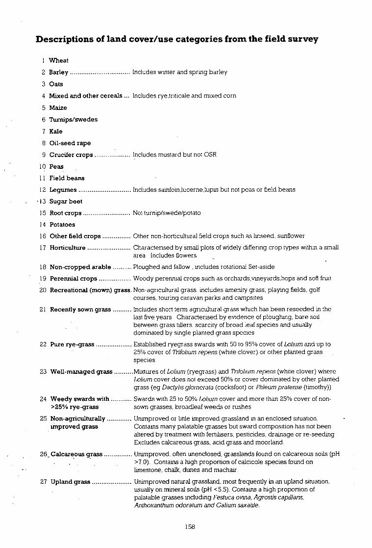
Descriptions of land cover/use categories from the field survey

1 Wheat

2 Barley Includes wmter and spring barley

3 Oats

4 Mixed and other cereals Includes rye.triticale and mixed corn

5 Maize

6 Turnips/swedes

7 Kale

Oil-seed rape

9 Crucifer crops Includes mustard but not OSR

10 Peas

11 Field beans

12 Legumes Includes sainfoin,lucernelupin but not peas or Eeld beans

13 Sugar beet

15 Root crops Not turnip/swede/potato

14 Potatoes

16 Other field crops Other non-horticultural field crops such as linseed. sunflower

17 Horticulture Characterised by small plots of widely differing crop types within a smallarea Includes flowers.

18 Non-cropped arable Ploughed and fallow includes rotational Set-aside

9 Perennial crops Woody perennial crops such as orchardsymeyards.hops and soft fruit

20 Recreational (mown) grass Non-agricultural grass includes amenity grass, playing fields, golfcourses, touring caravan parks and campsites

21 Recently sown grass Includes short term agricultural grass which has been reseeded in thelast five years. Characterised by evidence of ploughing. bare soilbetween grass tillers. scarcity of broad leaf species and usuallydominated by single planted grass species

22 Pure rye-grass Established ryegrass swards with 50 to 95% cover of bolium and up to25% cover of flifolium repens (white clover) or other planted grassspecies.

23 Well-managed grass Mixtures of tolium (ryegrass) and Thfolium repens (white clover) whereLatium cover does not exceed 50% or cover dominated by other plantedgrass (eg Dactyl's glornerata (cocksfoot) or Phleum pratense (timothy))

24 Weedy swards with Swards with 25 to 50% Loh= cover and more than 25% cover of non->25% rye-grass sown grasses, broadleaf weeds or rushes

25 Non-agriculturally Unimproved or little improved grassland in an enclosed situation.improved grass Contains many palatable grasses but sward composition has not been

altered by treatment with fertilisers. pesticides, drainage or re-seeding.Excludes calcareous grass acid grass and moorland.

26_ Calcareous grass Unimproved, often unenclosed, grasslands found on calcareous soiLs(pH>7.0). Contains a high Proportion of calcicole species found onlimestone, chalk, dunes and machair.

27 Upland grass Unimproved natural grassland, most frequently in an upland situation.usually on mineral soiLs(pH <5.5). Contains a high proportion ofpalatable grasses including lestuca ovum. Agrostis capillahs,Anthoxanthum odoraturn and Galiurnsaxatile.

158

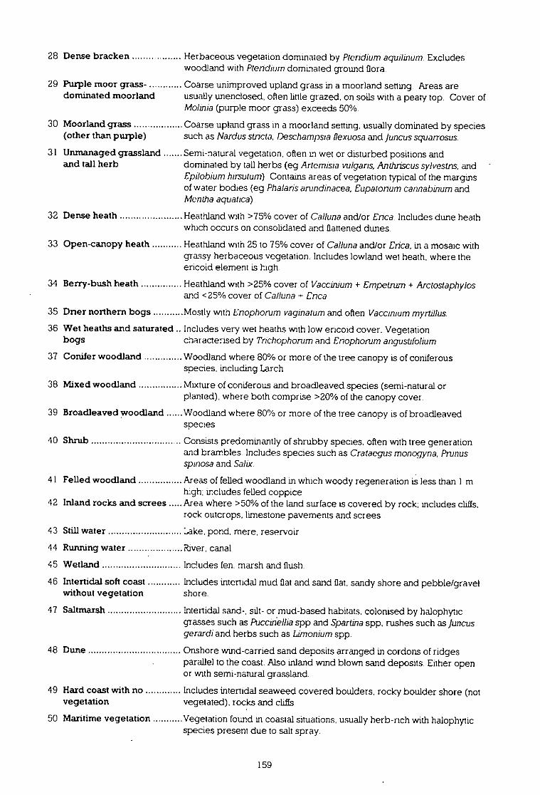
28 Dense bracken Herbaceous vegetation dominated

by Pleridium aguilinurn Excludeswoodland with Ptendiurn dominated ground flora

29 Purple moor grass- ....... ... Coarse unimproved upland grass in a moorland setting. Areas aredominated moorland usually unenclosed, often little grazed, on soils with a peaty top. Cover of

Mohnia (purple moor grass) exceeds 50%.

30 Moorland grass Coarse upland grass in a moorland senmg, usually dominated by species

(other than purple) such as Nardus stricta, Deschampsia tlexuosa and Juncus sguanbsus

31 Unmanaged grassland Semi-natural vegetation, often in wet or disturbed positions andand tall herb dominated by tall herbs (eg Artemma vulgans, Anthriscus sylvestns, and

Epilobiurn hirsuturn). Contains areas of vegetation typical of the marginsof water bodies (eg Phalaris arundinacea, Eupatoriurn cannabinum andMentha aguatica)

32 Dense heath Heathland with >75% cover of Calluna and/or Erica. Includes dune heathwhich occurs on consolidated and flattened dunes.

33 Open-canopy heath Heathland with 25 to 75% cover of Calluna and/or Erica, in a mosaic withgrassy herbaceous vegetation. Includes lowland wet heath, where theericoid element is high.

34 Berry-bush heath Heathland with >25% cover of Vaccinium + Empetrurn + Arctostaphylosand <25% cover of Calluna Enca

35 Drier northern bogs ....... ....Mostly with Enophorum vaginaturn and often Vaccirnurn myrtillus

36 Wet heaths and saturated .. Includes very wet heaths with low ericoid cover. Vegetationbogs characterised by Trichophorum and Eriophorum angustilbhurn

37 Conifer woodland Woodland where 80% or more of the tree canopy is of coniferousspecies. including Larch

38 Mixed woodland Mixture of coniferous and broadleaved species (semi-natural orplanted), where both comprise >20% of the canopy cover.

39 Broadleaved woodland Woodland where 80% or more of the tree canopy is of broadleavedspecies

40 Shrub Consists predominantly of shrubby species, often with tree generationand brambles. Includes species such as Crataegus rnonogyna, Prunusspinosa and Salix.

41 Felled woodland Areas of felled woodland in which woody regeneration is less than 1 mhIgh; Mcludes felled coppice

42 Inland rocks and screes Area where >50% of the land surface is covered by rock; includes cliffs.rock outcrops, limestone pavements and screes..

43 Still water Lake, pond, mere, reservoir

44 Running water River, canal

45 Wetland Includes fen. marsh and flush.

46 Intertidal soft coast Includes intertidal mud flat and sand flat, sandy shore and pebble/gravelwithout vegetation shore.

47 Saltmarsh Intertidal sand-, silt- or mud-based habitats, colonised by halophyticgrasses such as Pucciriellia spp and Spartina spp, rushes such as Juncusgerardi and herbs such as Limonium spp.

48 Dune Onshore wind-carried sand deposits arranged in cordons of ridgesparallel to the coast. Also inland wind blown sand deposits. Either openor with semi-natural grassland.

49 Hard coast with no Includes intertidal seaweed covered boulders, rocky boulder shore (notvegetation vegetated), rocks and cliffs

50 Maritime vegetation Vegetation found in coastal situations, usually herb-rich with halophyticspecies present due to salt spray.

159

51 Railway Includes all track and associated land

52 Road Includes any road, whether private or not, which is totally tarmac orconcrete across its width.

53 Agricultural buildings Includes sheds.barns and silos as well as commercial glasshouses.

54 Residential buildings Dwellings and associated land

55 Other buildings Includes commercial. mdustrial. public servme and other facilities

56 Waste and derelict land Includes domestic and mdustrial waste land as well as allotment land

57 Hard areas without Unvegetated derelict land, building sites, car parks. ungrassedbuildings recreational grounds and public spaces.

58 Quarries and extractive Gravel pH,quarry. opencast mineindustries

160

Descriptions of satellite target cover classes

0 Unclassified: Cover types which did not fitinto the 25 'target' classes

1 Sea/estuary: Sea, coastal waters andestuaries, inland to the first bridging point orbarrier.

2 Inland water: Inland freshwaters andestuarine waters above the first bridgingpoint or barrier.

3 Coastal bare ground (beach/mudflats/cliffs): Bare coastal mud, silt, sand, shingleand rock. including coastal accretion anderosion features above high water.

4 Saltmarsh Intertidal seaweed beds andsaltmarshes up to normal levels of high waterspring tides

5 Grass heath: Semi-natural, mostly acid.grasslands of dunes. heaths and lowland/upland margins

6 Mown/grazed turf Pastures and amenityswards. mown or grazed. to form a turfthroughout the growing season

7 Meadow/verge/semi-natural swards:Meadows. verges, low-intersity amenitygrasslands and semi-natural croppedswards. not maintained as a short turf

8 Rough grass/marsh Lowland marsh/roughgrasslands, mostly uncropped andunmanaged, forming grass and herbaceouscommunities, of mostly perennial species.with high winter-litter content

Moorland grass Montanefhill grasslands.mostly unenclosed Nardus/Mohnia moorland

10 Open shrub moor: UP:and. dwarf shrub/grass moorland

11 Dense shrub moor Upland evergreendwarf shrub-dominated moorland

12 Bracken: Bracken-dominated herbaceou-scommunities.

13 Dense shrub heath Lowland evergreenshrub-dominated heathland

14 Scrub/orchard Deaduous scrub andorchards

15 Deciduous woodland. Deciduousbroadleaved and mixed woodlands.

16 Coniferous/evergreen woodland! Coniferand broadleaved evergreen trees

17 Upland bog: Upland herbaceous wetlandswith permanent or temporary standing water.

18 Tilled land (arable crops): Arable andother seasonally or temporarily bare ground

19 Ruderal weed- Ruderal weeds colonisingnatural and man-made bare ground

20 Suburban/rural development: Suburbanand rural developed land comprisingbuildings and/ or roads but with some coverof permanent vegetation.

21 Urban development: Industrial. urban andany other developments, lacking permanentvegetation.

22 Inland bare ground: Ground bare ofvegetation, surfaced with 'natural' materials.

23 Felled forest: Felled forest, with ruderalweeds and rough grass.

24 Lowland bog: Lowland herbaceouswetlands with permanent or temporystanding water.

25 Open shrub heath Lowland. dwarf shrub/grass heathland

161

162

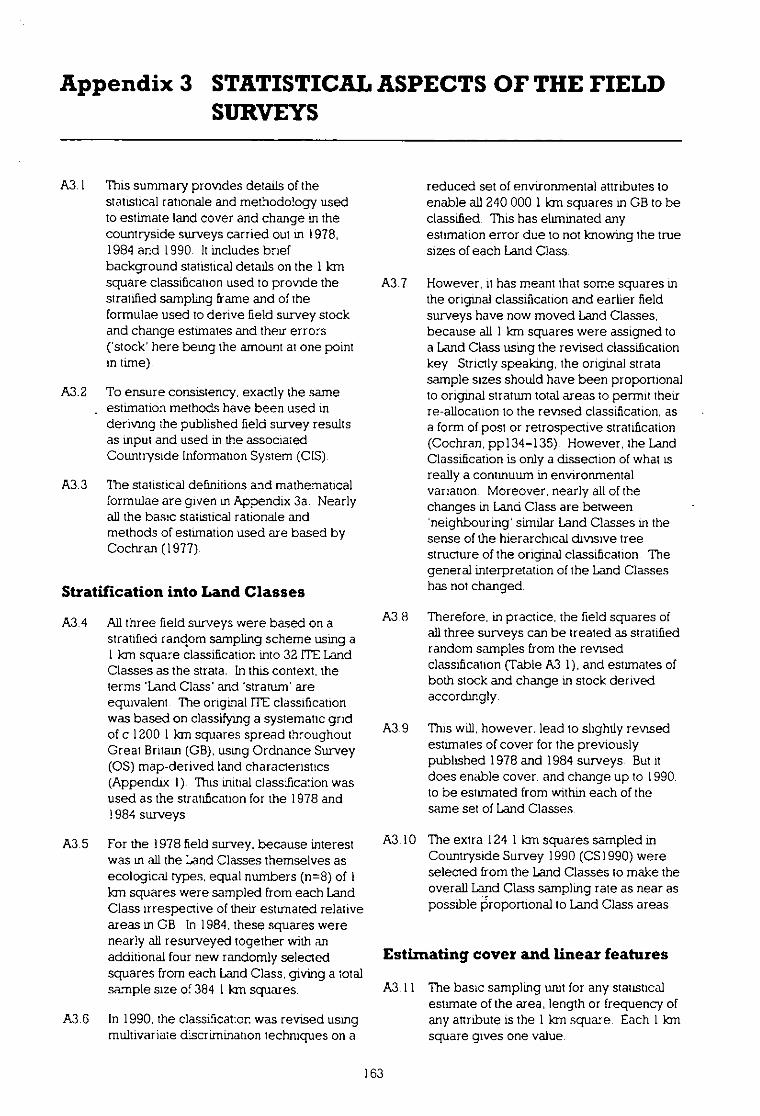
Appendix 3 STATISTICAL ASPECTS OF THE FIELDSURVEYS

A3.1 This summary provides details of thestatistical rationale and methodology usedto estimate land cover and change in thecountryside surveys carried out in 1978,1984 and 1990. It includes briefbackground statistical details on the 1 kmsquare classification used to provide thestratified sampling frame and of theformulae used to derive field survey stockand change estimates and their errors('stock here being the amount at one pointin time).

A3.2 To ensure consistency, exactly the sameestimation methods have been used inderiving the published field survey resultsas input and used in the associatedCountryside Information System (CIS).

A3.3 The statistical definitions and mathematicalformulae are given in Appendix 3a. Nearlyall the basic statistical rationale andmethods of estimation used are based byCochran (1977).

Stratification into Land Classes

A3.4 All three field surveys were based on astratified random sampling scheme using a1 km square classification into 32 ITE LandClasses as the strata. In this context, theterms 'Land Class' and 'stratum' areequivalent The origLial ITE classificationwas based on classifying a systematic gridof c 1200 1 km squares spread throughoutGreat Britain (GB), using Ordnance Survey(OS) map-derived land characteristics(Appendix I). This initial classification wasused as the stratification for the 1978 and1984 surveys

A3.5 For the 1978 field survey, because interestwas in all the Land Classes themselves asecological types, equal numbers (n=8) of 1km squares were sampled from each LandClass irrespective of their estimated relativeareas in GB. In 1984, these squares werenearly all resurveyed together with anadditional four new randomly selectedsquares from each Land Class, giving a totalsample size of 384 1km squares.

A3.6 In 1990. the classification was revised usingmultivariate discrimLnation techniques on a

reduced set of environmental attributes toenable all 240 000 I km squares in GB to beclassified This has eliminated anyestimation error due to not knowing the truesizes of each Land Class.

A3.7 However, it has meant that some squares inthe original classification and earlier fieldsurveys have now moved Land Classes.because all 1 km squares were assigned toa Land Class using the revised classificationkey Strictly speaking, the original stratasample sizes should have been proportionalto original stratum total areas to permit theirre-allocation to the revised classification, asa form of post or retrospective stratification(Cochran, pp134-135). However. the LandClassification is only a dissection of what isreally a continuum in environmentalvariation. Moreover, nearly all of thechanges in Land Class are between'neighbouring' similar Land Classes in thesense of the hierarchical divisive treestructure of the original classification. Thegeneral interpretation of the Land Classeshas not changed.

A3.8 Therefore. in practice. the field squares ofall three surveys can be treated as stratifiedrandom samples from the revisedclassification (Table A3.1), and estimates ofboth stock and change in stock derivedaccordingly.

A3.9 This will, however, lead to slightly revisedestimates of cover for the previouslypublished 1978 and 1984 surveys. But itdoes enable cover, and change up to 1990.to be estimated from within each of thesame set of Land Classes.

A3.10 The extra 124 1 km squares sampled inCountryside Survey 1990 (CS1990) wereselected from the Land Classes to make theoverall Land Class sampling rate as near aspossible proportional to Land Class areas.

Estimating cover and linear features

A3.11 The basic sampling unit for any statisticalestimate of the area, length or frequency ofany attribute is the 1 km square. Each 1kmsquare gives one value.

163

A3.12 Variation between squares within each LandClass represents the natural variation and isused to derive estimates of error for ourpopulation estimates. Inadequate samplingwould lead to estimates and the estimatedprecision of those estimates (eg theirstandard error (SE)) both being imprecise.

A3.13 There are many attributes which can bederived for each square from the detailedinformation in the field survey. These rangefrom areal estimates of single orcombinations of recorded field sheetattributes, to lengths of hedgerow types. tothe presence and richness of species in thequadrats. Different types of attribute mayrequire different methods of estimation.

A3.14 The ITELand Classification is effective as ameans of providing a stratification for thefield surveys, in that it restricts theoccurrence of any individual attribute to afraction of the Land Classes, and it is absent(or at least not found) in the other LandClasses. However, in those Land Classeswhere the attribute does occur, it is stillabsent from a proportion of the samplesquares and the statistical distribution ofvalues is skewed and highly non-normal.The median is often still zero in many LandClasses where the attribute does occur.

A3.I5 To obtain unbiased estimates of apopulation mean or total, regardless of thestatistical distribution, we first need toestimate the arithmetic mean (m) for eachLand Class, rather than, say. the median or(bias-corrected) geometric mean. This is asimple but important point

A3.16 To give some indication of the precision ofestimates, their SE will often be given. Insome cases the SE may be presented as apercentage of the estimate itself, in whichcase it is known as the percentagecoefficient of variation (%CV) of theestimate (eg an estimate of 60. with SE of15. has %CV of 25%).

A3.17 However, the skewed distribution andrelatively small sample sizes within eachLand Class mean that the sample stratummeans (m) are probably not symmetricallyor normally distributed, so that (m ± 2SE(m)) does not provide reasonableestimates of 95% confidence limits. (SE(m)= standard error of sample mean m.)Therefore, if95% confidence limits arerequired for estimates of the stratum means(or totals), it is thought that they would be

TableA3 I Symmetric and asymmetric confidence limits fordtferent coefficients of vananon

%CVSymmetric limits

LowerUpperAsymmetnc limits

LowerUpper

5 0 90 1 10 0 90 1 1110 0 80 1 20 0 82 1 2223 0 60 1 40 0 57

4930 0 40 1 60 0 56 1 8040 0 20 180 0 46 2 165C 0 00 2 00 0 39 2 57

better represented by asymmetricconfidence hmits assuming a log-normaldistribution

These multiplicative confidence limits wereestimated as follows-

lower limit = m / lc upper limit = m . k

where k = exp(I.96 V(var(logam)))

var(logern) = variance of log.m

which can be estimated by:

v2 = loge(1+[CV(m))21

where CV(rn) = SE(m) / m = coefficient ofvariation of m.

A3.18 This method of estimanng the variance oflogern is taken from Burnham et al.(1987).Table A3.1 indicates the difference betweenusing these limits and the usual symmetricallimits given by (m ± 1.96 SE(m)) (Forclarity of illustration 2.00 is used instead of1.96, and all hrmth are expressed as a ratioof the estimate m.) .

A3.19 In practical terms. this Lmplieswe are lesssure about the upper limit for the area. say,of the attribute than the lower limit It alsoensures we do not get any negative lowerconfidence limits for poorly estimatedattributes, so that. if%CV Ls50% for poorlyestimate attributes, the limits are not zero todouble the estimate, but the more plausiblerange of 0 39-2.57 x the estimate.

A3.20 The total area of an attribute in the wholepopulation (A..)and its variance Var(x.) areestimated by weighted summations overthe strata, as detailed in Appendix 3a.Because the population total estimate isbased on 32 strata and many more samples,it is more likely to be normally distributed,so (xi. ± 2 SE) may be used to givereasonable 95% confidence limits forwidespread attributes. However, for manydetailed attributes of low overall percentagecover, absent from a high proportion of allsample squares, the true limits could still be

164

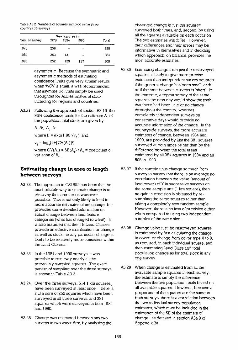
Talate A3 2 Numbers of squares samp!ed in the threecountryside surveys

New squares inYear of survey 1978 1984 1990 Tote!

1978 256

256

1984 253 131

384

1990 252 129 127 508

asymmetric. Because the symmetric andasymmetric methods of estimatingconfidencelLmits give very similar resultswhen %CV is small, it was recommendedthat asymmetric limits simply be usedthroughout for ALLestimates of stock.including for regions and countries.

A3.21 Following the approach of section A3.16. the95% confidence limits for the estimate A. ofthe populat:on total stock are given by

/k. A_ k

where k = exp(1 96 N1v3).and

v3 = loge{I+[CV(A_)]2}

where CV(Ar) = SE(A.1)/ AT= coefficient ofvariation of AT

Estimating change in area or lengthbetween surveys

A3.22 The approach in 051990 has been that themost reliable way to estimate change is toresurvey the same areas whereverpossible. This is not only likely to lead tomore accurate estimates of net change, butprovides some detailed information onactual change between land featurecategories (what has changed to what!). Itis also assumed that the ITE Land Classesprovide an effective stratification for changeas well as stock, le any particular change islikely to be relatively more consistent withinthe Land Classes.

A3.23 In the 1984 and 1990 surveys, it waspossible to resurvey nearly all thepreviously sampled squares. The exactpattern of sampling over the three surveysis shown in Table A3.2.

A3.24 Over the three surveys, 514 1km squares _have been surveyed at least once There isstill a core of 252 squares which have beensurveyed in all three surveys and 381squares which were surveyed in both 1984and 1990.

A3.25 Change was estimated between any twosurveys in two ways: first, by analysing the

observed change in just the squaressurveyed both times, and, second, by usingall the squares available on each occasionThe two estimates will differ! However,their differences and their errors may beinformative in themselves and in decidingwhich approach. on balance, provides themost accurate estimates.

A3.26 Estimating change from just the resurveyedsquares is likely to give more preciseestimates than independent survey squaresif the general change has been small, and/or if the tune between surveys is 'short' Inthe extreme, a repeat survey of the samesquares the next day would show the truththat there had been little or no changethroughout the country, whereascompletely independent surveys onconsecutive days would provide noaccurate information of the change. In thecountryside surveys, the more accurateestimates of change. between 1984 and1990. are provided by just the 381 squaressurveyed at both times rather than by thedifference between the total areasestimated by all 384 squares in 1984 and all508 in 1990

A3.27 Ifthe sample units change so much fromsurvey to survey that there is on average nocorrelation between the value (amount ofland cover) of Y in successive surveys onthe same sample unit (1 ICITIsquare), thenno gain in precision is obtained by re-sampling the same squares rather thantaking a completely new random sample.However, there is no loss of precision eitherwhen compared to using two independentsamples of the same size. •

A3.28 Change using just the resurveyed squaresis estimated by first calculating the changein cover, or change from cover type A to B.as required. in each individual square. andthen estimating Land Class and totalpopulation change as for total stock in anyone survey

A3.29 When change Lsestimated from all theavailable sample squares in each survey.the estimate is simply the differencebetween the two population totals based onall available squares. However. because aproportion of the squares are the same inboth surveys, there is a correlation betweenthe two individual survey populationestimates. which must be included in theestimation of the SE of the estimate ofchange.. as detailed in section A3a.9 ofAppendix 3a.

165

Estimates for regions of GB

A3:30 Separate estimates are provided forScotland. England. and Wales in addition toGB as a whole.

A3.31 The estimates of stock and change for anyregion or country in both the publishedreports and the Countryside informationSystem (CIS) are based on using the overallGB means for each Land Class. Ideally, theestimates for any region should be basedonly on the Land Class means estimatedfrom sample squares within the region.Although the ITE Land Classification is an'environmental', and not regional,classification, it is still possible that land useand cover within a Land Class may differbetween geographic regions for historicaland economic reasons. Therefore,estimates for England. Scotland and Walesmight also be made using just the LandClass means for the sample survey squaresin each country. These should becompared with the corresponding estimatesbased on the GB Land Class means. (Anybetween-country differences in Land Classmeans can be assessed by non-parametricstatistical tests )

A3:32 It is best not to use within-region estimatesof Land Class means for small regionsbecause the estimates will be based oninadequate numbers of sampled squares.and any gain through reduction in bias willbe outweighed by loss of precision Usingthe GB estimates of Land Class means, inany region, does assume no significantregional differences of land stock within anyLand Class.

A3.33 Standard errors and confidence limits willnot therefore be very reliable estimates ofthe accuracy of estimates for Englishcounty-size regions, and in the CIS noerrors will be given for such small regionsof less than 5000 1,3112.

Non-sampling of 'mostly sea' squares

A3.34 The sampling frame for each of the threefield surveys was the population of all 1 kmsquares, referenced to the OS NationalGrid, which contained any land in GB.However, since the surveys aim to estimatecountryside land statistics, any'1 kmsquares randomly selected from each ITELand Class which were more than 90% seaas measured from OS maps, were not

included in the sample squares and fieldsurvey. They are referred to as 'mostlysea' squares. In practice, only one initiallyselected square had over 90% sea, butseveral others were rejected because theywere mostly a combination of sea andbuilt-up land, again as measured from OSmaps.

A3.35 The small area of land in any flL LandClass that is in 1km squares with morethan 90% sea (as measured on 1:250 000OS maps) was assumed to have the sameaverage composition of land cover typesas any other part of that Land Class.

Estimating the total area of land ineach Land Class

A3.36 The simplest approach for estimating thetotal area of an attribute in a Land Class isjust to estimate the mean percentage of(the whole of) each 1 km square coveredby the attribute in the Land Class and thenmultiply by the total area (mcluding sea) ofall 1km squares in the Land Class.

A3.37 Since the basic sampling unit is the 1kmsquare referenced to the National Grid.some 'coastal' sample field survey squareswill include an area of sea, as only squareswhich were 'mostly sea' (see sectionA3.34) were excluded This mainly affectsITE Land Classes 7 and 8 (mostly SWEngland and Wales). and 14. and 29. 30and 31 (mostly Scottish islands). Derivingcover as a percentage of land removes thesample variation in attribute areas duesimply to the differing amount of land in thesampled squares. Also, since the actualarea of land. rather than the total area, in allthe 1 km squares of a Land Class has beenmeasured, it seems sensible to use this'known' land area to try to improve theprecision of cover estimates.

A3.38 Therefore. both the 1990 field surveyanalyses and the related CIS computersystem used a second approach which ismore complex. As part of the ITE LandClassification of every 1 km square in thewhole of GB, the area of sea of every 1kmsquare was measured by digitisation from1:250 000 OS maps. This means we have a'census figure for the total area of land ineach Land Class. The field survey estimateof the proportion of land m a Land Classcovered by a particular attribute was thenmultiplied by the census figure for total

166

land area in that Land Class to estimate thetotal area of the attribute in the Land Class

A3.39 The proportion of land covered by anattribute in a Land Class was estimated asthe ratio of total attribute area to total landarea from the field sample squares in thatLand Class, and hence it. and its standarderror, were calculated using standardstatistical methods for 'Ratio estimators'(Cochran 1977). The computational detailsare given in Appendix 3a Ifthe censusvalues for the total area of land in each LandClass were exact, then this second methodwould provide more precise estimates ofto:al attribute areas and provide moreaccurate spatial estimates of cover forindividual coastal squares in the CIS.

A3.40 The complication is that the field surveyestimates of sea area are based on 1:10 000scale maps which are more accurate thanthe 1:250 000 scale maps. Analysis of a setof squares for both 1:250 000 map area ofsea (SM) and 110 000 field survey area ofsea (SF) showed that there was a generaltendency for SM to overestimate SF. but thisvaried between Land Classes, being muchmore pronounced in the 'lowland LandClasses. Detailed analysis of the samplerelationships between SF and SM suggestedthat these discrepancies could beadequately allowed for by simply dividingall squares into two major Land Classgroups (Land Classes 1-16 and 17-32) andderiving one correction factor for each landClass group.

A3A1 From the set of squares from each LandClass group (1-16 or 17-32) with both SMand SF measured, the following ratioestimate conversion factor B (with SE(B))was derived, based on the ratio of mean SFto mean SM:

for Land Classes 1-16

B = 0 487 SEW) = 0.073. r=0 50. SDr=12 5

for Land Classes 17-32

B = 0.825. SE(S) = 0.056; r=0.95. SIDt= 6 0

where r measured the correlation betweenSM and SF. whde SD, indicated the averageerror (in hectares) in using B x SM toestimate the 'true' 1.10 000 field surveyarea of sea in any one 1km square. It wasseen that the estimates were not particularlyaccurate for individual 'coastal' squares(which might be selected in the CIS).especially in Land Classes 1-16 (mostly

classes 7 and 8), where estimates forindividual 1 km squares could be out by upto 20 hectares, so users of the CIS shouldbeware.)

A3 42 The following procedure was used toestimate the total area of land in each LandClass. h

Calculate the total area pc.r).includingsea, of all 1 Ian squares in the Land Class

Calculate the total area of sea (X,$)(asdefined from the 1:250 000 maps) of allsquares in the Land Class that arerecorded as having some sea (again asderived from the 1:250 000 maps).

Then, estimate the total area of land (X,) inLand Class, h. as

= Xh7- X B

and the variance of X, by

Var(Xh) = (X,s SE(B))'

A3.43 For any whole Land Class or large regioninvolving several Land Classes, thepercentage error (%CV) in estimating thetotal land area will usually be smallcompared to the %CV for the proportionalcover of attributes; and hence can usuallybe ignored.

A3.44 There were also a few squares which didhave some sea (as defined by field survey1:10 000 maps), but which were recordedas having no sea from the 1:250 000 mapdigitisation. However, analysis of thesamples squares with both SM and SF,indicated that the amount of sea missed andhence the amount of land overestimatedwas less than 0.1% of the total area of land inall the 1 km squares calculated to have nosea from the 1:250 000 maps. and henceunimportant.

A3.45 For Land Classes or regions with little (orno) sea, the above procedure produced thesame estimates as the simpler approachgiven in section A3.36.

Allowing for 'urban' 1 km squares

A3.46 Squares were only included in CS1990 ifthey were less than 75% built-up or urbanland. as measured from 1:250 000 OS maps.Such squares are termed 'rural' squares.while the built-up squares are referred to as'urban' squares. The built-up or urban land

167

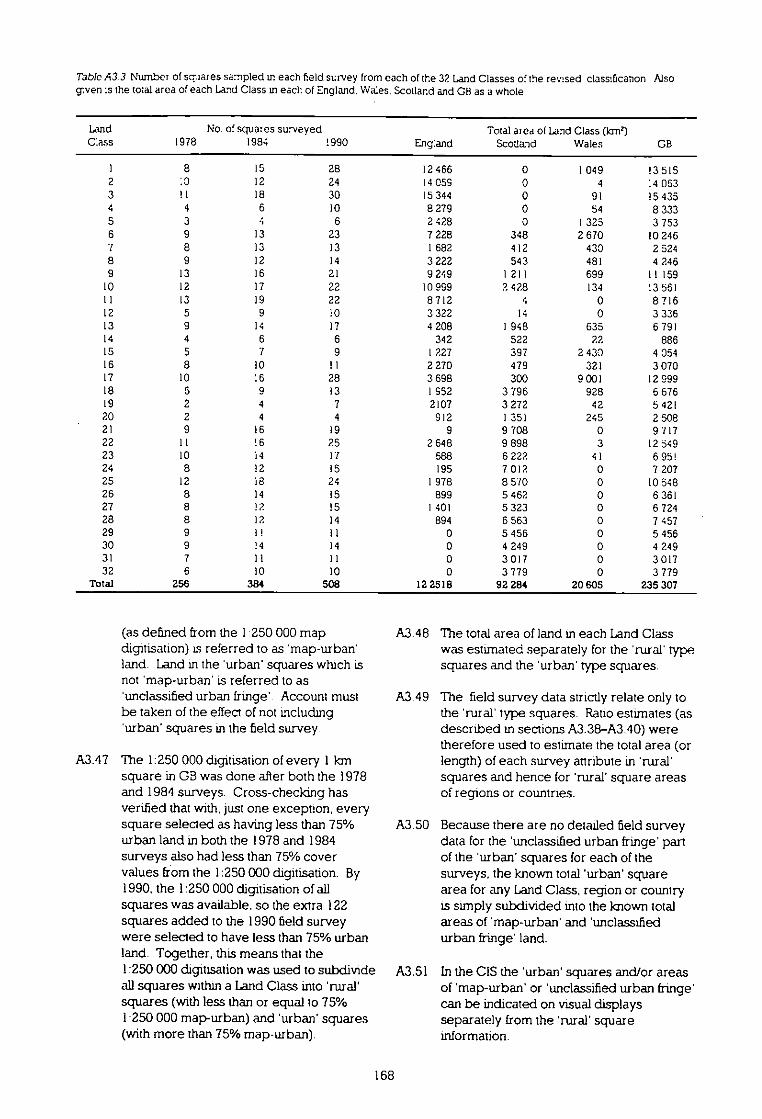
Table A33 Number of squares sampled in each field survey from each of the 32 Land Classes of the rensed class:flexion Alsogtven :s the total area of each Land Class In each of England. Wales. Scotland and CR as a whole

Land

No of squat es surveyed

Total area of Land Class (lan2)Class 19781984 1990 Eng:and Seothund Wales GB

I

a 15 28 12 466 0 1 049 l3 5152 :0 12 24 14059 0

4:4 0633 H 18 30 15344 0 91 15 4354

46 10 8 279 0 54 8 3335

34 6 2 428 0 1 325 3 7536

913 23 7 228 348 2 670 10 2467

813 13 1 682 412 430 2 5248

912 14 3 222 543 481 4 2469 13 16 21 9 249 1211 699 111590 12 17 22 10 999 2 4Z8 134 :3 551I 13 19 22 8 712 4

08 7162

59 10 3 322 14

03 3363

914 17 4 208 1 948 635 6 7914 4 6 6 342 522 22 8865

57 9 1227 397 2 430 4 0546

810 11 2 270 479 321 3 0707 10 16 28 3 698 300 9 001 12 9998

5 9 13 1 952 3 796 928 5 6769

24 7 2107 3 272 42 5 42120

24 4 912 I 351 245 2 50821

916 19

99 708

09 71722 11 16 25 2 648 9 898

312 64923 I 14 I7 588 6 222 41 6 95!24

12 15 195 7 012

7 20725 I 18 24 1 978 8 570

10 54826

14 15 899 5 462

6 36127

!2 15 1 401 5 323

6 72428

12 14 89 6 563

7 45729

11 II

5 456

5 45530

14 14

4 249

4 24931

11 11

3 017

3 01732

10 10

3 779

3 779Total 256 384 508 12 251 92 284 20 60 235 307

(as defined from the 1:250 000 mapdigffisation) is referred to as 'map-urban'land. Land in the 'urban' squares which isnot 'map-urban is referred to as'unclassified urban fringe' Account mustbe taken of the effect of not including'urban' squares in the field survey

A3.47 The 1:250 000 digitisation of every 1 kmsquare in GB was done aller both the 1978and 1984 surveys. Cross-checking hasverified that with, just one exception, everysquare selected as having less than 75%urban land in both the 1978 and 1984surveys also had less than 75% covervalues from the 1:250 000 digitisation. By1990, the 1:250 000 digitisation of allsquares was available, so the extra 122squares added to the 1990 field surveywere selected to have less than 75% urbanland. Together, this means that the1:250 000 digffisation was used to subdivideall squares within a Land Class into 'rural'squares (with less than or equal to 75%1:250 000 map-urban) and 'urban' squares(with more than 75% map-urban).

A3 48 The total area of land in each Land Classwas estimated separately for the 'rural' typesquares and the 'urban' type squares

A3.49 The field survey data strictly relate only tothe 'rural' type squares. Ratio estimates (asdescribed in sections A3.38-A3.40) weretherefore used to estimate the total area (orlength) of each survey attribute in 'rural'squares and hence for 'rural' square areasof regions or countries.

A3.50 Because there are no detailed field surveydata for the 'unclassified urban fringe' partof the 'urban' squares for each of thesurveys, the known total 'urban' squarearea for any Land Class region or countryis simply subdivided into the }mown totalareas of 'map-urban' and 'unclassifiedurban fringe' land.

A3.51 In the CIS the 'urban' squares and/or areasof 'map-urban' or 'unclassified urban fringe'can be indicated on visual displaysseparately from the 'rural' squareinformation.

168

A3 52 Although any squares with more than 75%'map-urban were classed as 'urban'squares, the total area of 'unclassified urbanfringe' is only 8% of the total area of all the'urban' squares.

A3 53 The 'urban' squares themselves form only2.3% of the total area of land in GBTherefore. in GB as a whole, the'unclassified urban fringe' is less than 0 2%of the total area of land

A3.54 Where it is required to derive field surveystock and change estimates for all land in aregion or country. including the area of'urban' squares, the following procedurewas adopted.

The 'map-urban' part of the 'urban'squares was treated as a separatecover attribute and its area identifiedfor each square, Land Cass or region.as required (By its definition, it has noerror.)

For the (usually) relatively small area of'unclassified urban fringe' in the 'urban'squares of any particular Land Class ina region, the relative proportionalcover and distribution of the 'rural' fieldsurvey attributes was assumed to bethe same as trithe 'rural' squares in thatLand Class. The total area. X. of landin the 'rural' squares and the'unclassified urban fringe' in that LandClass h was calculated for the regionconcerned. Ifq: was the estimate of theproportion of land in that Land Classcovered by thLsattribute, then theestimate of the annbute's total area inthat Land Class was calculated for theregion as (\cid. using the formulae tocalculate errors described in sectionsAl I 1-A3.2 I and given in Appendix 3a.sections A3a.I 0-A3a 12).

A3.55 The above procedure ignores the fact thatsome of the area in the 'rural' squares ismade up of attributes which probablyrepresent the 'map-urban' part of squares.Therefore, the simple approach above maytend to underestmate the areas of ruralattributes in the 'unclassified urban fringe'.However, we have no detailed informationon the true composition of the 'unclassifiedurban fringe' and it is usually only a veryminor pan of the total area concerned. Theproportional and total area of 'unclassifiedurban fringe' in a reglon should always beindicated, and a warning given that this

proportion of the total area of any attributets from 'unclassified urban fringe' in 'urban'squares, and hence must be treated withextreme caution

169

Appendix 3a STATISTICAL FORMULAE

A3a 1 The change in the mean value of apopulation attribute X between time I andtime 2 can be estimated by taking samplesat each time. There are several optionsavailable. At one extreme, independentseparate samples could be taken on the twooccasions, and, at the other extreme: thesame sample units could be used in bothsample surveys. The ITE field surveys usedan intermediate approach whereby (nearly)all of the sample 1km squares surveyed attime I were resurveyed at time 2, togetherwith a number of new randomly selectedunits. A few of the 1km squares surveyedin 1978 and/or 1984 could not beresurveyed because permission could notbe obtained. In statistical terms, this meansthe ITEsampling scheme for change iseffectively a 'partial replacement scheme.with only a proportion of the sample unitssurveyed in both of any two surveys(Cochran 1977. pp344-358).

A3a.2 The choice of resampling scheme affectsthe estimator of change and its sampthigvariance or precision. Details of how toestimate cover (or lengths) and change forthe field surveys are given below.

A3a.3 Suppose the whole population has beendivided into Lstrata, and each stratum hasbeen randomly sampled separately. Forthe ITEcountryside surveys, the L strata arethe 32 ITE Land Classes. Throughout thisAppendix, 'stratum' and Land Class' aresynonymous.

A3a.4 Then, the following section (A3a.5) must firstbe applied and calculated independentlyfor each stratum in turn, and section(A3a.10) then used to multiply up LandClass statistics to obtain populationestimates.

WITHIN ANY ONE STRATUM(LAND CLASS), h

A3a.5 Definitions

Let Y = the measured variable of interest.

A 'rural' square is defined to be a I km squarewhich when digitised from a map was less than 75%built-up land All other 1km squares are referred

to as 'urban' squares. as defined in sectionsA3.46-A3.55. The field survey only sampled -rural'squares.

j ,. nh0= number of squares sampled at time 1 and2 respectively in Land Class h

= value of attribute Y in the j" sampled square ofLand Class h at time t. 1=1. n., t=1,2

In any particular sampled square, the value of ;will usually be either the proportion of the squarecovered by the attribute. or its total length in thesquare if it is a linear attribute.

Let X = proportion of the yr'sampled square inLand Class h which is land;(as measured directly from the 1:10 000 maps forthe field survey).

Let Xj = 'census' figure of total area of land of all 1km 'rural' squares in Land Class h.including correction of 'map' sea (SM) tomore accurate field 'survey' sea (SF) - seesection A3.40 for details.

= / = proportion of land in the th sampledsquare of Land Class h which is covered byattribute Y:j=

Assume (ifnecessary after suitable re-ordering)that the first rc of these sample squares weresampled at both times 1 and 2. This means that thefirst rc sampled umts for this stratum in each surveyare the same units (but obviously not necessarilywith the same values), le:

= number of 'overlap' sample units

Phi =11,111hi proportion of the squaressampled at time 1 that were re-sampled at time 2

Phi = rlitinhz proportion of the units sampled attime 2 that were also sampled attime 1

11111.1-c<= nhij <=I,Ph2 <=n11

y =i Y /rk, = sample mean of Y in Land Class h atr

tune t, t=I.2

xj. XN/R,= sample mean of X in Land Class h at1=1 tuThet, t=1,2

(E means sum over the squares indicated)

170

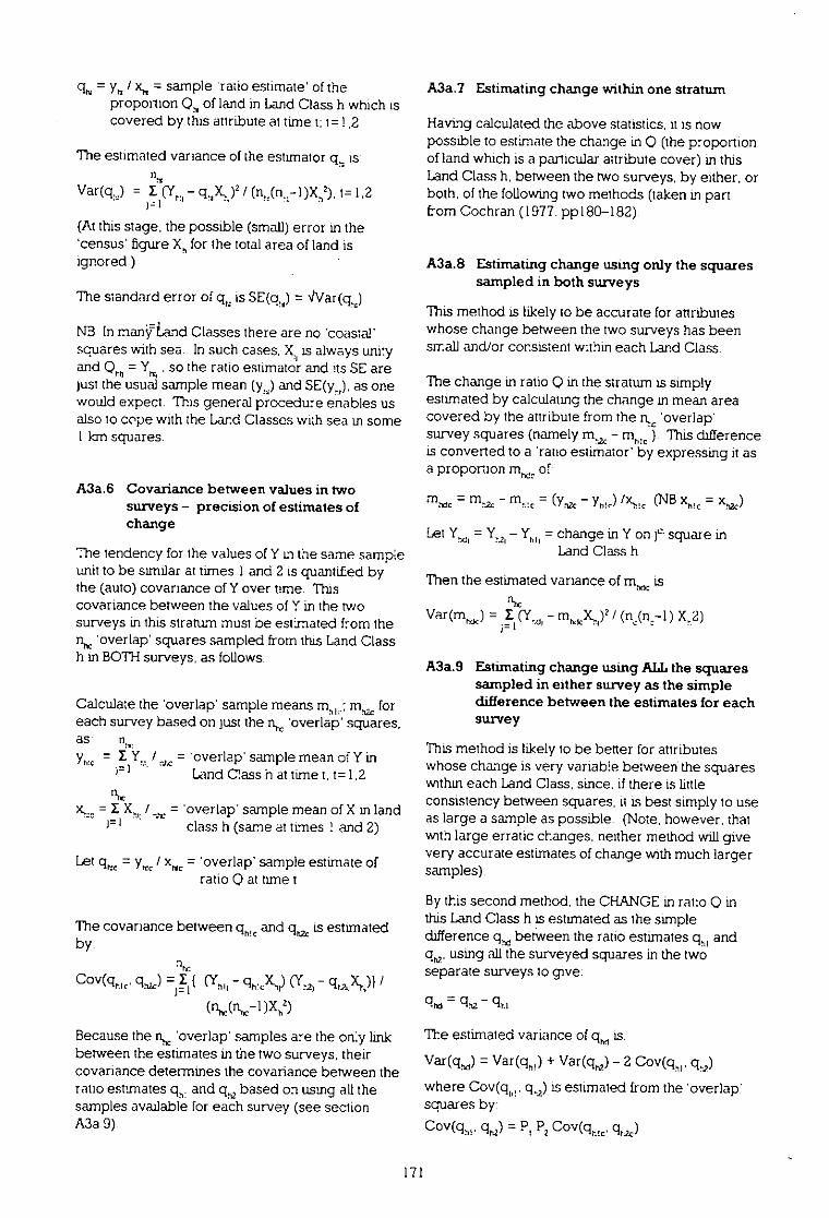
cin= yt, / xit = sample 'ratio estimate of theproportion Q1 of land in Land Class h which iscovered by this attribute at time t; t=12

The estimated variance of the estimator qt. is:n2,

Var(q.) = I - / ( „(nt-1)X,2). t=1,2F I

(At this stage, the possible (small) error in the'census' figure X„for the total area of land isignored.)

The standard error of qt. is SE(qt.) = 4Var(q.)

N3 In manVland Classes there are no 'coastal'squares with sea. In such cases. X:,is always unityand Q... = Ytti. so the ratio estimator and its SE arejust the usual sample mean ()It) and SE(yt), as onewould expect. This general procedure enables usalso to cope with the Land Classes with sea m someI km squares.

A3a.6 Covariance between values in twosurveys - precision of estimates ofchange

The tendency for the values of Y in the same sampleunit to be similar at times 1 and 2 is quantifed bythe (auto) covariance of Y over tima Thiscovariance between the values of Y in the twosurveys in this stratiLm must be estimated from theh.. 'overlap' squares sampled from this Land Classh in BOTHsurveys, as follows

Calculate the 'overlap' sample means mak: rrL.2cforeach survey based on just the ri,.c'overlap' squares,aS: nhr.

= I / = 'overlap' sample mean of Y inj=1 Land Class h at time t. t=12

"it= X / = 'overlap' sample mean of X in landi= class h (same at times I and 2)

Let qt.t.= y, / xtic= 'overlap' sample estimate ofratio Q at time t

The covariance between gm. and c42.is estimatedby:

Cov(q.1., ?if (Ym- qh:A1) - qvAtX.Ity)/

(nbc(ritc-1);')

Because the nhc'overlap' samples are the only linkbetween the estimates in the two surveys, theircovariance determines the covariance between theratio estimates qh: and q,i2based on using all thesamples available for each survey (see sectionA3a.9).

A3a.7 Estimating change within one stratum

Having calculated the above statistics, it is nowpossible to estimate the change in Q (the proportionof land which is a particular attribute cover) in thisLand Class h, between the two surveys, by either, orboth, of the following two methods (taken Lnpartfrom Cochran (1977. pp180-182).

A3a.8 Estimating change using only the squaressampled in both surveys

This method is likely to be accurate for attributeswhose change between the two surveys has beensmall and/or cor.sistent within each Land Class

The change in ratio Q in the stratum is simplyestimated by calculating the change in mean areacovered by the attribute from the n 'overlap'survey squares (namely rn - rnw. y This differenceis converted to a 'rano estimator' by expressing it asa proportion mixt,of:

m hec = 61:12c— Yldr) /X1-Ic (NB = Xh2)

bet Y = Y - Y = change in Y on j'nsquare inLand Class h

Then the estimated variance of rri..Knrc

Var(m ) = I (Y_d- mNkX,..)2/(MR,-l) Xt.2).

A3a.9 Estimating change using ALLthe squaressampled in either survey as the simpledifference between the estimates for eachsurvey

This method is likely to be better for attributeswhose change is very variable between the squareswithin each Land Class, since, if there is littleconsistency between squares, it is best simply to useas large a sample as possible. (Note, however, thatwith large erratic changes. neither method will givevery accurate estimates of change with much largersamples).

By this second method. the CHANGE in ratio Q inthis Land Class h is estimated as the simpledifference q between the ratio estimates qto and04,2,using all the surveyed squares in the twoseparate surveys to give:

grid= clha

The estimated variance of qm is.

Var(qw) = Var(qh,) + Var(q,) - 2 Cov(q,1. qt)

where Cov(qw. q,2) is estimated from the 'overlap'squares by:

Cov(qh,. = P, P2 Cov(Clittc. c211,)

171

The standard error of gho= SE(q;:o)= NtVar(q,d) wnh sea. Stwill be negligible and can be ignored

COMBINING STRATUM (LANDCLASS) ESTIMATES INTO ANESTIMATE FOR A WHOLEREGION (OR COUNTRY OR GB)

The following formulae are used to combine theestimates in each Land Class of the proportionalcover of any particular attribute, with the 'census'figures for the total area of land in each Land Classto derive estimates of totals for a whole region.where the phrase 'region could mean just one LandClass, or a whole country, or all of GB.

The formulae can be applied to estimate the totalarea of:

just the 'rural' squares. orjust the 'unclassified urban fringe'. orboth the above - to give totals for both'rural' and 'urban' squares,

simply by using the appropriate 'census' figure Xsfor the total area of land - see sections A3.40 andA3 51 for further details.

X, = appropriate 'census' figure of total area of landin Land Class h

Xs = Xi + X2+ + X32= total area of land in whole'region' of interest

As before, let qm, R.:2denote the estimators for ratioQ at times 1 and 2 for Land Class h.

Let m = the estimator for change in ratiobetween times 1and 2 for stratum h. (NBrnbacouldhere be the estimates based on all the squares ineach survey, or just the 'overlap' squares

Var(mm). Var(mh2)and Var(mo„,)denotetheir estimated variances - calculated as detailed insection A3a 5

A3a.10 Estimating total cover of an attribute in a 'region' in any single survey

The TOTAL area Aifor attribute Y. in the 'region', attime t, is estimated by:

32At =31 Xhqu , t=1,2

The estimated variance of AIis:

32Var(A1)= hli(X6)2Var(q„) +

where S: is the error variance on the 'census' figure for the total area of land Xi,in the region. Unless the 'region' includes a high proportion of 1 km squares

Ifrequired, St is calculated as follows (as in sectionA3 40)

Let kis = the total area of 'map' sea (as definedfrom the 1:250 000 maps) of all squares inLand Class in the 'region' that arerecorded as having some sea (again asderived from the 1:250 000 maps).

Because we have two sea conversion factors 13,Btand B2for Land Class groups (1-16) and (17-32)respectively, we need to calculate:

15 32A:s = I (X,s.q,,) and Ns

Then, using the standard errors SE(BI) and SE(B2)ofthe two correction factors Bfrom section A3 40. wehave.

S. = ( A:sSE(Bi) 12+ {AasSE(B2)}2

A3a.11 Estimating change in cover in a 'region'between surveys

The TOTALCHANGE Adin area of attribute Y in the'region' between times 1 and 2 can be estimatedby:

32A, = E t=1.2

- 1 •

The estimated variance of A, is:.32

Var(k) =1£.(k)2Var(qhs,) + Sd

where So Lsas S: above except q,, replaces qr, inthe formulae for A:s and A2s.

The standard error Ad = SE(Ad)= N/Var(Ady

A3a.12 Estimating lengths (in contrast to areas)

All the above principles can be used in the sameway to estimate the total lengths of linear attributes(such as hedgerows and roads).

The attribute Y will then be the total length of theattribute in each 1 km survey square. If X is still theproportion of the square which is land, then thesame ratio estimator q=y/x ,used in section A3a.5,now estimates the length of the attribute per 1 Fan2.

Therefore, multiplying by the total area of all land(in lan2) in that Land Class in the 'region' concernedand summing over the region in the same way asfor areas (see sections A3a.10-A3a11) will estimatethe total length of the attribute in the 'region'.

172

Appendix 4 QUALITY ASSURANCE EXERCISE -SUMMARY

Introduction

It is recognised that in a field investigation on thescale of the Countryside Survey 1990 the largenumbers of recorders and surveyors involved willproduce an inherent degree of variation, despitethe provision of a training course, a field handbook(Barr 1990) and on-site visits by supervisors(quality control). Whilst there is no reason toexpect any directional bias in the records made.neither was any subsequently demonstrated, it isimportant to attempt to measure the consistencyand reliability of the work done withm the majorcomponents of the field programme (QualityAssurance Exercise).

A sample comprising 37 of the 512 squaressurveyed in 1990 was selected and in each of theseone quarter was resurveyed in 1991. at the sametime of year as the original survey The resurveyincluded one of each of the six permanently markedplot types: Main (200 m2)plots; Habitat (4 mi plots;Verge plots: Hedge plots: Streamside plots: andfield boundaries (all 10 m x 1 m plots) used in themain survey

The Quality Assurance Exercise investigated

the efficiency of plot relocationthe reproducibility of species records made bythe original surveyorsthe accuracy of percentage cover estimates ofthe species presentthe effect of the level of recording on the resultsobtained when subject to the normaltechniques used to demonstrate habitat changethe accuracy of the land use mapping of the 1Ian squares.

The Quality Assurance Exercise has been fullyreported (Prosser et al. 1992) this Appendixpresents some of the key results and observations

Plot relocation

Only 23 out of the 178 plots in the sample could notbe relocated by the assessors in a brief search (5minutes). It is considered that this 'recovery rate'(87%) justified the time taken during CS 1990 topermanently mark and photograph all plots Thehigh relocation percentage suggests that detailedchanges in the vegetation can be followed using the

present survey methods. However, the relocationof plots. especially those in unenclosed land is oftentime-consuming and in future surveys additionalmanpower will be needed if all plots in a 1 lcmsquare are to be sought

Accuracy of species records

Of c 5000 species records in 178 plots drawn from asubsample comprising 35 I km squares.

63% were confirmed as species present by theassessors at the nme of the:r survey,

of the remaining 37%;11% were clearlyattributable to real differences in speciescomposition of the plots surveyed in the twoyears and a further 9% were considered likely tobe due to seasonal effects which could not beclearly demonstrated

This suggests an initial recording accuracy lyingbetween 74% at the lowest and 83% at the highestestimate. which is close to the value of 79% given asthe maximum attainable efficiency betweenstandardised searches by experienced fieldworkers in Nilsson and Nilsson (1985).

The full report includes a detailed breakdown of thenature of species mismatches between the 1990survey and the 1991 Quality Assurance Exercise(Prosser et al. 1992).

Not all plots gave equal levels of agreement.Results for Main (200 ma)and for roadside Vergeplots indicate that high levels of confidence can beattached to analyses of these sites Those forHabitat (4 m2) plots and Streamside plots are lessreproducible: improved survey techniques couldbe developed to bring these up to the samestandard Recommendations for simplemodifications of survey techniques are included inthe full report

Estimates of vegetation cover

When a comparison was made of the 20 mostfrequent species forming appreciable cover, onlytwo (both grasses) have been recorded atsignificantly different levels in plots by thesurveyors and the assessors. However. visual

173

assessments of cover made over larger areas aspart of the land cover mapping were more variable.and attention needs to be given to improving thisaspect of countryside surveys

Direction of vegetation change

When data for changes in species compositionwithin individual plots over time were subjected tocorrespondence analysis (eg DECORANA,Hill1979). the shifts in position of plots or groups ofplots could be related to changas in theenvironment acting on the vegetation in these plots.A series of such analyses have been performed inwhich the 1990 survey data and those of the 1991Quality Assurance Exercise are compared for eachindividual plot type. In all cases, axis shills havebeen demonstrated

The overall axis shift between 1990 and 1991,though insufficient to be significant at this relativelysmall sample size, parallelled that previouslydemonstrated during the Ecological Consequencesof Land Use Change project To what extent the1990-91 results reinforce the changes previouslydemonstrated or are evidence of a singular climaticshill between the two individual seasons cannot atpresent be established with certainty. Theconsistent direction of change shown since thesurveys of 1978 and 1988 nevertheless indicate thatthe plot data obtained for 1990 were sufficientlYreliable to be used with confidence to demonstrateenvironmental change.

Land cover mapping

Land cover mapping involved the use of a series ofcodes (see Appendix 2) which may. for the purposeof analysis, be subdivided into three groups: •

primary codes: major habitat and crop types,

secondary descriptive codes: related to stockand variations in land management;

• cover codes: a further characterisation of agiven parcel of land usmg a combination of themapping of the most prevalent species togetherwith a code denoting the cover of each.

The overall agreement found in primary coding was84%; there was, however, a marked differencebetween the reliability of coding between thelowlands (95%) and the uplands (71%). The greaterdiscrepancies identified in the unenclosed uplandsrelate in particular to difficulties experienced indistinctions between upland heath and bog types.Upland heath seemed to be under-recorded. This

was the only instance in which there appeared to bea directional bias in coding.

It is clear that the allocation of primary codes to thecommoner forms of managed and naturalvegetation cover is reliable. Rarer habitats were.

. inevitably, represented only by a small number ofsamples; the reliability of information derived for -these is less than for widespread habitats.

The percentage agreement found for the simplersecondary descriptive (or qualifying) codes was78%. This figure relates to the use of codes whichwere unambiguous and involved simple decision-making. eg whether a hedge was stocicproof or notstockproof. No satisfactory method was derived fordirect comparison of strings of codes whichincluded considerable elements of judgement. Themethod presented in the full report indicates thelevel of agreement for such qualifying codes to beapproximately 49%.

174

á

á