UNIVERSITY OF CALGARY

Robust Visual Servoing of a Robot Arm Using

Artificial Immune System and Adaptive Control

by

Alejandro Carrasco Elizalde

A THESIS

SUBMITTED TO THE FACULTY OF GRADUATE STUDIES

IN PARTIAL FULFILMENT OF THE REQUIREMENTS FOR THE

DEGREE OF DOCTOR OF PHILOSOPHY

DEPARTMENT OF MECHANICAL AND MANUFACTURING ENGINEERING

CALGARY, ALBERTA

JANUARY, 2012

© Alejandro Carrasco Elizalde 2012

Library and Archives Canada

Published Heritage Branch

Bibliothdque et Archives Canada

Direction du Patrimoine de l'6dition

395 Wellington Street Ottawa ON K1A 0N4 Canada

395, rue Wellington Ottawa ON K1A 0N4 Canada

Your file Votre r6f6rence

ISBN: 978-0-494-83444-2

Our file Notre r6f6rence

ISBN: 978-0494-83444-2

NOTICE:

The author has granted a non­exclusive license allowing Library and Archives Canada to reproduce, publish, archive, preserve, conserve, communicate to the public by telecommunication or on the Internet, loan, distrbute and sell theses worldwide, for commercial or non­commercial purposes, in microform, paper, electronic and/or any other formats.

AVIS:

L'auteur a accords une licence non exclusive permettant £ la Bibliothdque et Archives Canada de reproduire, publier, archiver, sauvegarder, conserver, transmettre au public par telecommunication ou par (Internet, prSter, distribuer et vendre des thdses partout dans le monde, d des fins commerciales ou autres, sur support microforme, papier, 6lectronique et/ou autres formats.

The author retains copyright ownership and moral rights in this thesis. Neither the thesis nor substantial extracts from it may be printed or otherwise reproduced without the author's permission.

L'auteur conserve la propri£t6 du droit d'auteur et des droits moraux qui protege cette th6se. Ni la th&se ni des extraits substantiels de celle-ci ne doivent 6tre imprimis ou autrement reproduits sans son autorisation.

In compliance with the Canadian Privacy Act some supporting forms may have been removed from this thesis.

While these forms may be included in the document page count, their removal does not represent any loss of content from the thesis.

Conform6ment £ la loi canadienne sur la protection de la vie priv6e, quelques formulaires secondares ont 6t6 enlev6s de cette thdse.

Bien que ces formulaires aient inclus dans la pagination, il n'y aura aucun contenu manquant.

Canada

Abstract

Vision systems greatly enhance the capabilities of robots and allow them to be applied

to complex tasks within dynamic environments. In this thesis, we explore the problem of

controlling a robotic arm using image-based servoing in a monocular eye-in-hand config­

uration. Specifically, we develop a visual servoing system capable of tracking non-planar

objects in the presence of uncertainties in both the robotic arm and the visual system.

To track selected features of a target object, we propose a feature extraction algorithm

that behaves as an immune systems. We evaluate the performance of our artificial im­

mune system for three object representations: template, histogram and contour, and we

show that the AIS can track multiple features under affine transformations and nonlinear

distortions.

We then develop an image-based visual servoing control that is robust to parametric

uncertainties in the robot model and camera calibrations. We use the LaSalle's invariance

principle to prove the stability of the system and that the tracking error approaches zero

if the uncertainty is bounded. Simulations verify the robustness of the system.

To implement the visual servoing system on an experimental robot, we design an

open-architecture controller to replace the industrial controller of a PUMA robot. We

then compare the performance and robustness of the proposed control versus that of a

proportional control and a quasi-newton adaptive control under a variety of test con­

ditions. We conclude that the proposed control has the best performance of the three

controls tested.

ii

Acknowledgements

The development of this thesis has been like a long walkthrough in the vastness of the

desert. In this time I had have good times and really personal bad times, but luckily

in the way I encountered people who have shared their wisdom and support with me

making this journey more bearable and reach fruition. To all of them I thank you for

your support, encouragement and hospitality.

I'll start by thanking my thesis supervisor, Peter Goldsmith. His enthusiasm, sup­

port and insatiable patience of this work has been greatly appreciated. I would like to

acknowledge the generous funding of this work provided by the CONACyT program, the

Mexican Scholarships program. This work would not have been possible without their

support.

I'd like to thank my Mom for believing in me and trying to understand why I left

my country to pursue this thesis, and my Dad for teaching me that with hard work and

perseverance I can achieve my goals no matter how hard they can be. I'd like to thank

the whole family for providing a great deal of support, and for their enthusiasm at the

prospect of me to finish. Finally, I'm incredibly grateful to my wife Melissa for made my

days brighter in my bad days, for her love, understanding and encourage necessary to

finish this thesis.

iii

iv

Table of Contents

Abstract ii Acknowledgements iii Table of Contents iv List of Tables ' vii List of Figures viii List of Symbols and Abbreviations xi 1 Introduction 1 1.1 Motivation 1 1.2 Problem Description 3

1.2.1 Physical Setup 4 1.2.2 Subgoals 5

1.3 Contributions 5 1.4 Outline of Thesis 6 2 Visual Servoing Introduction 8 2.1 Concepts and Definitions of Visual Servoing 8

2.1.1 Definitions 9 2.2 Classification of Visual Servoing Systems 11 2.3 Proposed Approach of Visual Control 18 3 Vision System and Feature Extraction 19 3.1 Introduction Vision System 19 3.2 Camera Model 22

3.2.1 Pinhole Camera 22 3.2.2 Perspective Projection Model and Camera Parameters 23 3.2.3 Camera Calibration 25

3.3 Feature Extraction 26 3.3.1 Object Modeling 27

3.3.1.1 Parametric Representations 28 3.3.1.2 Non-parametric Representations 29

3.3.2 Object Identification 31 3.3.2.1 Supervised Learning 32 3.3.2.2 Distribution Representation 34

3.3.3 Object Tracking 37 3.3.3.1 Deterministic Tracking 38 3.3.3.2 Probabilistic Tracking 39

3.3.4 Occlusion Handling 41 3.4 Artificial Immune System Tracking (Proposed approach) 42

3.4.1 Artificial Immune system: Clonal Selection And Somatic Mutation 42 3.4.2 Experiments 48

3.4.2.1 Comparison Between Template and Histogram as B-cells 48 3.4.2.2 Tracking a Planar Object Under Affine and Nonlinear

Transformations 51

V

3.4.2.3 Tracking a 3D Object Under Distortions 53 3.4.2.4 Tracking an Object Using a Contour Representation . . 54

3.5 Summary 55 4 Control Synthesis 56 4.1 Introduction 56 4.2 Dynamics of Mechanical Systems 57 4.3 Definition of image Jacobian matrix 58 4.4 Control Law Formulation 61 4.5 Stability Analysis 64 4.6 Simulation Results 67 4.7 Summary and Conclusions 71 5 Experimental Performance Analysis on a Puma Robot 72 5.1 Introduction 72 5.2 Experimental Visual Servo Testbed 73 5.3 Camera Calibration 75 5.4 Open Loop Test 76 5.5 Controls Tested 77

5.5.1 Proportional Control 77 5.5.2 Quasi Newton Adaptive Control 78 5.5.3 Robust Adaptive Control (Proposed) 78

5.6 Tracking a Planar Object 79 5.6.1 Planar Object in 3D Translation 80 5.6.2 Planar Target Object in Translation and Rotation 87

5.7 Tracking of a Non Planar Object 95 5.8 Robustness Testing 100

5.8.1 Effect of Jacobian Error 100 5.8.2 Effect of Initial Depth Error 102 5.8.3 Effect of Initial Rotation Error 103 5.8.4 Effect of target position 105

5.9 Tracking a Moving Target Object 107 5.9.1 Rectangle Trajectory 107 5.9.2 Elliptical Trajectory Ill

6 Conclusion 114 6.1 Summary and Conclusions 114 6.2 Limitations and Future Work 116 Bibliography 118 A Definitions 131 B Robot controller 133 C Software Functions 137 C.l Robotic Interface Functions 137 C.2 Image Processing Functions 137 C.3 Matrix Functions 139 C.4 Main Object Classes 140

C.4.1 Class Puma Interface 140

C.4.2 Class Matrix Code 141 C.4.3 Class Feature Code 148

D Integral Image 151

vi

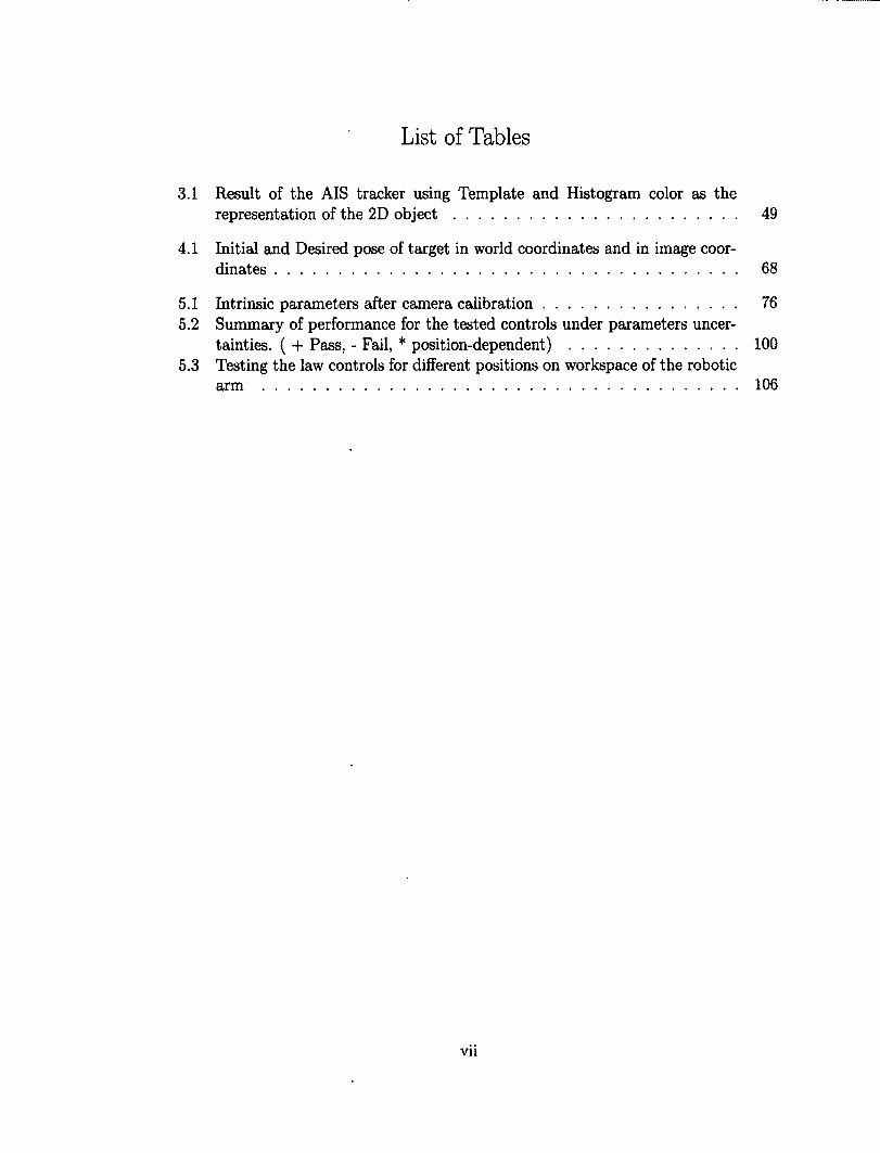
List of Tables

3.1 Result of the AIS tracker using Template and Histogram color as the representation of the 2D object 49

4.1 Initial and Desired pose of target in world coordinates and in image coor­dinates 68

5.1 Intrinsic parameters after camera calibration 76 5.2 Summary of performance for the tested controls under parameters uncer­

tainties. ( 4- Pass, - Fail, * position-dependent) 100 5.3 Testing the law controls for different positions on workspace of the robotic

arm 106

vii

viii

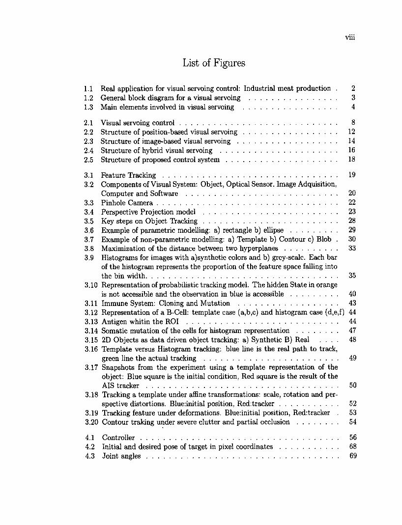
List of Figures

1.1 Real application for visual servoing control: Industrial meat production . 2 1.2 General block diagram for a visual servoing 3 1.3 Main elements involved in visual servoing 4

2.1 Visual servoing control 8 2.2 Structure of position-based visual servoing 12 2.3 Structure of image-based visual servoing 14 2.4 Structure of hybrid visual servoing 16 2.5 Structure of proposed control system 18

3.1 Feature Tracking 19 3.2 Components of Visual System: Object, Optical Sensor, Image Adquisition,

Computer and Software 20 3.3 Pinhole Camera 22 3.4 Perspective Projection model 23 3.5 Key steps on Object Tracking 28 3.6 Example of parametric modelling: a) rectangle b) ellipse 29 3.7 Example of non-parametric modelling: a) Template b) Contour c) Blob . 30 3.8 Maximization of the distance between two hyperplanes 33 3.9 Histograms for images with a)synthetic colors and b) grey-scale. Each bar

of the histogram represents the proportion of the feature space falling into the bin width 35

3.10 Representation of probabilistic tracking model. The hidden State in orange is not accessible and the observation in blue is accessible 40

3.11 Immune System: Cloning and Mutation 43 3.12 Representation of a B-Cell: template case (a,b,c) and histogram case (d,e,f) 44 3.13 Antigen whitin the ROI 44 3.14 Somatic mutation of the cells for histogram representation 47 3.15 2D Objects as data driven object tracking: a) Synthetic B) Real .... 48 3.16 Template versus Histogram tracking: blue line is the real path to track,

green line the actual tracking 49 3.17 Snapshots from the experiment using a template representation of the

object: Blue square is the initial condition, Red square is the result of the AIS tracker 50

3.18 Tracking a template under affine transformations: scale, rotation and per­spective distortions. Blue:initial position, Red:tracker 52

3.19 Tracking feature under deformations. Blue:initial position, Red:tracker . 53 3.20 Contour traking under severe clutter and partial occlusion 54

4.1 Controller 56 4.2 Initial and desired pose of target in pixel coordinates 68 4.3 Joint angles 69

ix

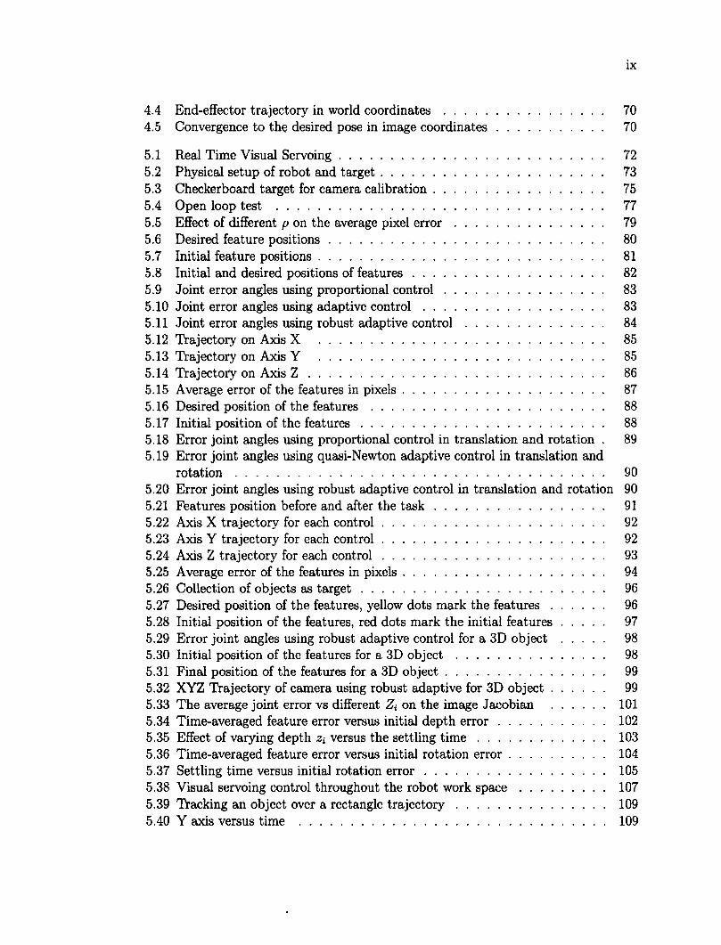
4.4 End-effector trajectory in world coordinates 70 4.5 Convergence to the desired pose in image coordinates 70

5.1 Real Time Visual Servoing 72 5.2 Physical setup of robot and target 73 5.3 Checkerboard target for camera calibration 75 5.4 Open loop test 77 5.5 Effect of different p on the average pixel error 79 5.6 Desired feature positions 80 5.7 Initial feature positions 81 5.8 Initial and desired positions of features 82 5.9 Joint error angles using proportional control 83 5.10 Joint error angles using adaptive control 83 5.11 Joint error angles using robust adaptive control 84 5.12 Trajectory on Axis X 85 5.13 Trajectory on Axis Y 85 5.14 Trajectory on Axis Z 86 5.15 Average error of the features in pixels 87 5.16 Desired position of the features 88 5.17 Initial position of the features 88 5.18 Error joint angles using proportional control in translation and rotation . 89 5.19 Error joint angles using quasi-Newton adaptive control in translation and

rotation 90 5.20 Error joint angles using robust adaptive control in translation and rotation 90 5.21 Features position before and after the task 91 5.22 Axis X trajectory for each control 92 5.23 Axis Y trajectory for each control 92 5.24 Axis Z trajectory for each control 93 5.25 Average error of the features in pixels 94 5.26 Collection of objects as target 96 5.27 Desired position of the features, yellow dots mark the features 96 5.28 Initial position of the features, red dots mark the initial features 97 5.29 Error joint angles using robust adaptive control for a 3D object 98 5.30 Initial position of the features for a 3D object 98 5.31 Final position of the features for a 3D object 99 5.32 XYZ Trajectory of camera using robust adaptive for 3D object 99 5.33 The average joint error vs different Z\ on the image Jacobian 101 5.34 Time-averaged feature error versus initial depth error 102 5.35 Effect of varying depth Zi versus the settling time 103 5.36 Time-averaged feature error versus initial rotation error 104 5.37 Settling time versus initial rotation error 105 5.38 Visual servoing control throughout the robot work space 107 5.39 Tracking an object over a rectangle trajectory 109 5.40 Y axis versus time 109

5.41 X axis versus time 110 5.42 Z axis versus time 110 5.43 Tracking an object over a ellipse trajectory 112 5.44 Z axis versus time 112 5.45 X axis versus time 113 5.46 Y axis versus time 113

B.l Electric Diagram for microcontroller 133 B.2 Electric Diagram for communication bus among microcontroller 134 B.3 Configuration of micro-controller interruptions 135 B.4 Main cycle for micro-controller 136

D.l Integral Image blocks 152 D.2 Integral Image: A particular example 152

x

xi

List of Symbols and Abbreviations

Chapter 2

P Point in three-dimensional space. R Rotation Matrix in three-dimensional space. t Vector representing a translation. r Pose of an object (positions and translations). T Task space. SE3 Special Euclidean group (3 dimensional space) n3 Real numbers (3 dimensional space). so3 Orthogonal group (3x3 Matrix). Vi Translational velocities. Wi Rotational velocities. s Error signal (image space). PBVS Position-based visual servoing. IBVS Image-based visual servoing. HVS Hibrid visual servoing. J img Image Jacobian.

Chapter 3

n Image plane. 0 Camera frame. f Focal length. X , Y , Z World coordinates of a point in space. kXy Skew coefficient. CCD Charge-coupled device. CMOS Complementary metal-oxide-semiconductor. a Scale factor. u , v Image coordinates.

Parameters for camera transformation from world coordenates to image rriij space. «(0 Spline function. K) B-Spline function. ANN Artificial neural networks. ft) Cost function. <!(•) Penalization function. R ( - ) Risk function. P ( - ) Bhattacharyya measure. H ( - ) Hellinger distance measure. NCC Normalized cross-correlation.

xii

SSD Sum of square difference. SNR Signal to noise ratio. AIS Artificial immune system. /(•) Affinity function. Xk Memory cells. Wk Weight memory cells.

Chapter 4

L Lagrangian. . T Torque vector. Q Joint displacement vector. H ( - ) Inertia matrix. CM Coriolis matrix. c(.) Gravitational force vector. no Regression matrix. e Robot parameter vector. Jim Image Jacobian. Ds Diagonal matrix of sigma-modification. K Nonimal value of robot parameter.

P Upper bound of the Jacobian uncertainty. Qu Unit vector of joint displacement. A , K p , K d Matrices of gains. V ( . ) Lyapunov function.

11-11 Vector Norm.

1

Chapter 1

Introduction

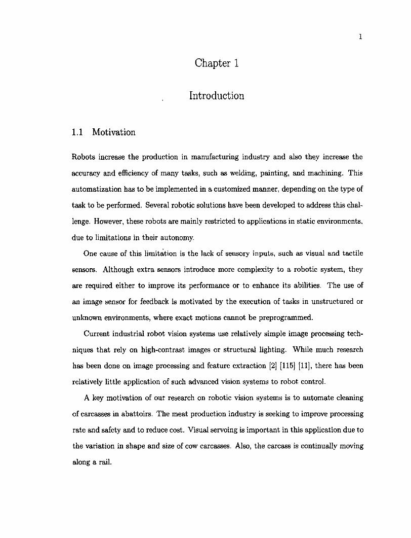
1.1 Motivation

Robots increase the production in manufacturing industry and also they increase the

accuracy and efficiency of many tasks, such as welding, painting, and machining. This

automatization has to be implemented in a customized manner, depending on the type of

task to be performed. Several robotic solutions have been developed to address this chal­

lenge. However, these robots are mainly restricted to applications in static environments,

due to limitations in their autonomy.

One cause of this limitation is the lack of sensory inputs, such as visual and tactile

sensors. Although extra sensors introduce more complexity to a robotic system, they

are required either to improve its performance or to enhance its abilities. The use of

an image sensor for feedback is motivated by the execution of tasks in unstructured or

unknown environments, where exact motions cannot be preprogrammed.

Current industrial robot vision systems use relatively simple image processing tech­

niques that rely on high-contrast images or structural lighting. While much research

has been done on image processing and feature extraction [2] [115] [11], there has been

relatively little application of such advanced vision systems to robot control.

A key motivation of our research on robotic vision systems is to automate cleaning

of carcasses in abattoirs. The meat production industry is seeking to improve processing

rate and safety and to reduce cost. Visual servoing is important in this application due to

the variation in shape and size of cow carcasses. Also, the carcass is continually moving

along a rail.

2

To help automate this cleaning operation, the author was previously involved in the

design of the hydraulic robot shown in Figure 1.1. The robot positions a vacuum cleaner

near the carcass to remove E.Coli bacteria. However, there was no vision system to

automatically detect the bacteria and to control the robot during the cleaning operation.

A robot equipped with a vision system could also be applied to horn and hoof removal

and to skinning.

Figure 1.1: Real application for visual servoing control: Industrial meat production

Early approaches to visual robot control in the literature implement the ; look-and-

move' paradigm [100] [19], in which the vision and control portions of the system are

separate. A static image is captured and processed, and then the manipulator is moved.

This approach has also been used in recent work [97],

More recent approaches use real-time visual feedback for continuous tracking con­

trol [101] [68] [43]. Unfortunately, these are susceptible to inaccuracies in the image-

3

space/task-space due to uncertain camera calibration, for example. In addition, stability

analyses of such systems are based only on the visual part.

The goal of this thesis is to develop an adaptive visual tracking system that is robust

to uncertainties in the robot model and the camera calibration. To achieve this goal, we

develop novel algorithms for feature tracking and for robot control and integrate them

on an open-architecture platform.

1.2 Problem Description

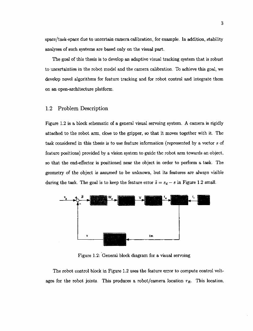
Figure 1.2 is a block schematic of a general visual servoing system. A camera is rigidly

attached to the robot arm, close to the gripper, so that it moves together with it. The

task considered in this thesis is to use feature information (represented by a vector s of

feature positions) provided by a vision system to guide the robot arm towards an object,

so that the end-effector is positioned near the object in order to perform a task. The

geometry of the object is assumed to be unknown, but its features are always visible

during the task. The goal is to keep the feature error s = s,i — s in Figure 1.2 small.

Figure 1.2: General block diagram for a visual servoing

The robot control block in Figure 1.2 uses the feature error to compute control volt­

ages for the robot joints. This produces a robot/camera location tr. This location.

4

relative to the target object location rj, results in a camera image Im. A feature extrac­

tion module then computes the feature vector s to be regulated.

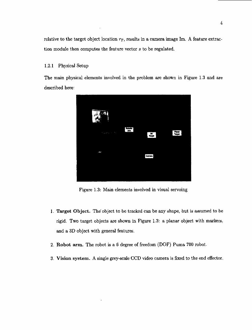
1.2.1 Physical Setup

The main physical elements involved in the problem are shown in Figure 1.3 and are

described here:

Figure 1.3: Main elements involved in visual servoing

1. Target Object. The object to be tracked can be any shape, but is assumed to be

rigid. Two target objects are shown in Figure 1.3: a planar object with markers,

and a 3D object with general features.

2. Robot arm. The robot is a 6 degree of freedom (DOF) Puma 700 robot.

3. Vision system. A single grey-scale CCD video camera is fixed to the end effector.

5

1.2.2 Subgoals

The objective of this thesis may be broken down into the following subgoals:

1. Design an algorithm for feature extraction, and select an image repre­

sentation for the features. This algorithm and image representation must be

able to track the translation, rotation, and perspective transformations of the image

features that result from 3D motion of the target object.

2. Design a control law to guide a robot arm towards the desired position.

This control law must be robust to uncertainty in the visual information and in

the robotic system. The visual servoing control law must run in real time (versus

a look-and-move approach).

3. Develop an open-architecture controller and integrate the feature ex­

traction module with the robot control module. This architecture must be

flexible so that that both modules can be easily modified or replaced, to enable

more complex capabilities and applications.

1.3 Contributions

The main contributions of this thesis are:

1. Development of a method for the tracking of selected features. This

method is based on immune systems. We evaluate the performance of our artificial

immune system (AIS) for three object representations: template, histogram and

contour. As shown by experiment, the AIS tracks multiple features under affine

transformations and nonlinear distortions.

6

2. Development of a robust visual servoing control. This control is image-

based and is robust to parametric uncertainties in the robot model and the camera

calibration.

3. Stability proof of the control law. This proof uses LaSalle's invariance princi­

ple to show that the overall the proposed control is stable and the tracking error

approaches zero subject to a bound on the parametric uncertainty.

4. Development of an open-architecture controller. This electronic hardware

and microcontroller programs were designed and built by the author to replace

the industrial controller of the PUMA robot. The proposed vision and control

algorithms were developed and implemented on this platform, along with a graphic

user interface (GUI) to facilitate testing.

5. An Experimental comparison with two alternative controls. The perfor­

mance and robustness of the proposed control is compared with that of a propor­

tional control and a quasi-newton adaptive control under a variety of test conditions.

1.4 Outline of Thesis

The rest of this thesis is organized as follows:

• Chapter 2 provides background on the visual servoing problem and introduces

some definitions and notation. It also classifies the three general approaches to the

problem and the one taken in this thesis.

• Chapter 3 focuses on the design of the feature extraction module and introduces

the artificial immune system (AIS) used to track the features. Its performance is

evaluated experimentally for various object representations (template, histogram,

and contours).

7

• Chapter 4 describes the design of the proposed robust visual servoing control law.

This chapter also presents the stability proof for our control law and simulations

to assess the effect of uncertainty on system performance.

• Chapter 5 describes the implementation and testing of the proposed control on a

Puma robot. Experiments are conducted to compare its performance and robust­

ness against that of a proportional control and a quasi-newton adaptive control.

• Chapter 6 summarizes the main conclusions from the thesis and briefly describes

some lines of future work.

8

Chapter 2

Visual Servoing Introduction

2.1 Concepts and Definitions of Visual Servoing

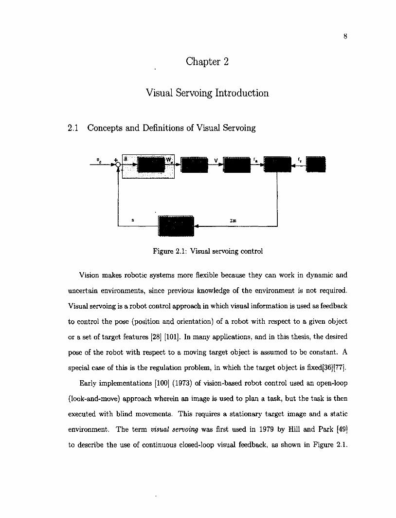
Figure 2.1: Visual servoing control

Vision makes robotic systems more flexible because they can work in dynamic and

uncertain environments, since previous knowledge of the environment is not required.

Visual servoing is a robot control approach in which visual information is used as feedback

to control the pose (position and orientation) of a robot with respect to a given object

or a set of target features [28] [101]. In many applications, and in this thesis, the desired

pose of the robot with respect to a moving target object is assumed to be constant. A

special case of this is the regulation problem, in which the target object is fixed[36] [77].

Early implementations [100] (1973) of vision-based robot control used an open-loop

(look-and-move) approach wherein an image is used to plan a task, but the task is then

executed with blind movements. This requires a stationary target image and a static

environment. The term visual servoing was first used in 1979 by Hill and Park [49]

to describe the use of continuous closed-loop visual feedback, as shown in Figure 2.1.

9

The visual servoing approach is used in this thesis. Introductions to visual servoing and

reviews on its evolution from its early years can be found in [27], [63], and [28]. This

chapter focuses on concepts, defininitions, and notation related to the visual control block

highlighted in Figure 2.1.

2.1.1 Definitions

Typically, robotic tasks are specified with respect to one or more coordinate frames. For

example, a camera may supply information about the location of an object with respect to

the camera frame, while the configuration used to grasp the object may be specified with

respect to a coordinate frame of the end-effector. Let the represention of the coordinates

of a point P with respect to frame a by the notation aP. Given the frames, a and b, the

rotation matrix that represents the orientation of frame b with respect to a is denoted by

aRb. The location of the origin of the frame b with respect to frame a is denoted by atb.

Together, the position and orientation of a frame are referred as pose, which we denote

by % = (aRb,atb).

If we are given bP and arb = (aRb,ati,), we can obtain the coordinates of aP by the

transformation

aP=a RbbP+atb. (2.1)

In visual servoing. relevant features are extracted from the image of a moving target

object, in order to track the object with a robot arm. In [101], an image feature is

defined as any structural feature that can be extracted from an image, such as an edge

or a corner. According to [7], an image feature corresponds to the projection in the

image plane of an scene feature, which can be defined as a set of 3D elements - such as

points, lines or vertices - rigidly attached to a single body. In our control approach, each

image feature is assigned a unique 2D position s4 in pixels. A set of n feature positions

s = [si,s2,-,Sn]t are used to control the robot.

10

The selection of image features depends on the task to be performed. It is best to

select features that can be quickly extracted to provide the control law with new input

data at an adequate frequency [20] [91]. The use of prediction methods to estimate

the location of the image features can help to improve the robustness and the speed of

the tracking [85] [113]. These methods can also be useful to handle the problem of the

occlusion of features. A review of feature tracking methods used in visual servoing works

can be found in [27].

The visual servoing control law uses the values of the image features to determine

the movements the robot should perform in its task space. The task space of the robot,

represented here by T = SE3 = 5R3 x SO3, is the set of poses (positions and orienta­

tions) that the robot can achieve [101] and is a smooth m-manifold [67], where m is the

dimension of the task space.

We represent the components of a pose r € T as r = [tx,ty,tx,6x,0v, 9Z}1. where the U

indicate translations and the are the rotations, for i € {x,y, z}. In some applications,

the task space can be reduced to a subset of the above, that is, T C SE3. The dimension

of the task space determines the minimum number of degrees of freedom that the robot

needs to perform a task.

In this thesis, we compute the velocity r in task space to correct the error between its

current and desired pose in the task space T = SE3. This velocity can be expressed as

r = [V, H]f = [Vx, Vy, Vz, ojx,uiy, Ug]*, where values V* correspond to translational velocities

and values to rotational velocities, for i € {x,y,zj. This vector r is known as the

velocity screw of the robot.

In other works [36] [63], the design of the control law has followed the so called task

function formalism [37] [15]. According to this approach, it is possible to express any

servoing scheme according to the regulation to zero of a function called the task function,

or control error function. When the current pose of the robot matches the target or

11

desired one, the value returned by the task function should be zero.

2.2 Classification of Visual Servoing Systems

Classification of visual servo systems is typically based on two criteria:

• Organization of the control structure. This criterion is related to the level at

which the control law computes commands for the robot. Two types of systems

have been distinguished:

- Two-stage control. The control is performed in two stages. As shown in Figure

2.1, the Visual Control uses the image error e to produce a desired task space

location Wd or velocity, which is input to the Robot Control, which sends

motor voltages V to the robot joints. Most of the reported systems in the

literature follow this approach [101] [63].

- One-stage control. A single control directly computes the motor voltages V

from the image error e. This is the approach used in this thesis.

• Space of the error signal. This criterion considers the space in which the differ­

ence or error between the current and the desired pose of the robot -and, therefore,

the task function- is computed. In all of the structures, the image features are

extracted from the image using a windowing techniques, reducing time processing,

and image feature parameters are measured. Three types of systems are distin­

guished:

- Position-based visual servo systems (PBVS). The general structure of a PBVS

is shown in Fig 2.2. A PBVS system operates in Cartesian space and allows

the direct specification of the desired camera trajectory in Cartesian space,

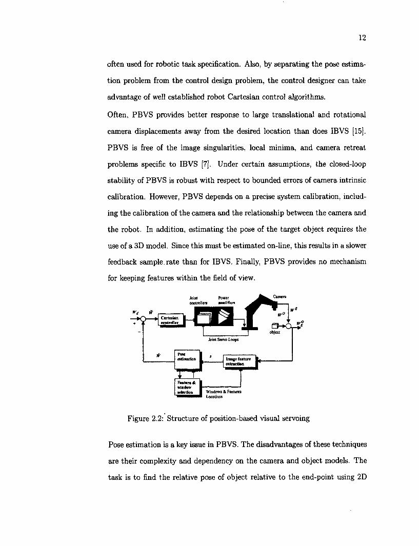
12

often used for robotic task specification. Also, by separating the pose estima­

tion problem from the control design problem, the control designer can take

advantage of well established robot Cartesian control algorithms.

Often, PBVS provides better response to large translational and rotational

camera displacements away from the desired location than does IBVS [15].

PBVS is free of the image singularities, local minima, and camera retreat

problems specific to IBVS [7], Under certain assumptions, the closed-loop

stability of PBVS is robust with respect to bounded errors of camera intrinsic

calibration. However, PBVS depends on a precise system calibration, includ­

ing the calibration of the camera and the relationship between the camera and

the robot. In addition, estimating the pose of the target object requires the

use of a 3D model. Since this must be estimated on-line, this results in a slower

feedback sample, rate than for IBVS. Finally, PBVS provides no mechanism

for keeping features within the field of view.

Power amplifiers

Cartesian controller

Joint Servo Loops

Iraage feature extractton

Feature & window selection Windows & Features

Locations

Figure 2.2: Structure of position-based visual servoing

Pose estimation is a key issue in PBVS. The disadvantages of these techniques

are their complexity and dependency on the camera and object models. The

task is to find the relative pose of object relative to the end-point using 2D

13

image coordinates of feature points and knowledge about the camera intrinsic

parameters and the relationship between the observed feature points (usually

from the CAD model of the object). It has been shown that at least three

feature points are required to solve for the 6D pose vector [118]. However, to

obtain a unique solution, at least four features will be needed. The existing

solutions for pose estimation problem can be divided into analytic and least-

squares solutions.

To reduce the noise effect in pose estimation, some sort of smoothing or averag­

ing is usually incorporated. Extended Kalman filtering (EKF) provides such

an excellent iterative solution to pose estimation. This approach has been

implemented for 6D control of the robot end effector successfully using the

observations of image coordinates of 4 or more features [114] [56]. To adapt

to the sudden motions of the object, an adaptive Kalman filter estimation

has also been formulated recently for 6D pose estimation [72], In comparison

to many techniques, Kalman filter-based solutions are less sensitive to small

measurements noise.

- Image-based visual servo systems (IBVS) is the approach used in this thesis. In

IBVS (shown in Figure 2.1), the error signal and control command is calculated

in the image space. The task of the control is to minimize the error of the

feature parameter vector, given by s = sj — s. The advantage of IBVS is

that it does not require full pose estimation and hence is computationally less

involved than PBVS. Also, it is claimed that the positioning accuracy of IBVS

is less sensitive to camera calibration errors than PBVS [101]. However. IBVS

can lead to image singularities that might cause control instabilities.

The system may use either a fixed camera or an eye-in-hand configuration.

In the case of a fixed camera, the robot moves in front of the camera until

14

Camera Joint Controllers

Power Amplifiers

*4 J Feature »Q » space

+ * k controller

Joint Servo Loops

Image feature extraction

* 1 Feature & window selection Windows & Features

Locations

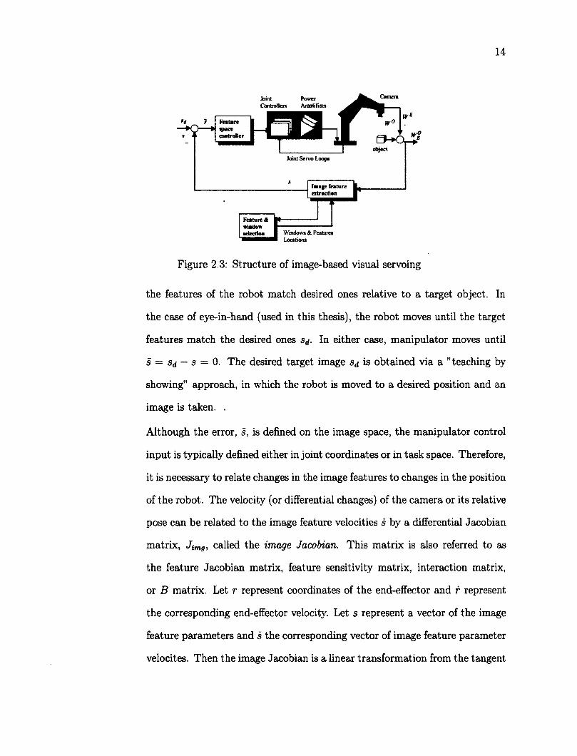
Figure 2.3: Structure of image-based visual servoing

the features of the robot match desired ones relative to a target object. In

the case of eye-in-hand (used in this thesis), the robot moves until the target

features match the desired ones s^. In either case, manipulator moves until

s = Sd — s = 0. The desired target image Sd is obtained via a "teaching by

showing" approach, in which the robot is moved to a desired position and an

image is taken. .

Although the error, s, is defined on the image space, the manipulator control

input is typically defined either in joint coordinates or in task space. Therefore,

it is necessary to relate changes in the image features to changes in the position

of the robot. The velocity (or differential changes) of the camera or its relative

pose can be related to the image feature velocities s by a differential Jacobian

matrix, Jjm9, called the image Jacobian. This matrix is also referred to as

the feature Jacobian matrix, feature sensitivity matrix, interaction matrix,

or B matrix. Let r represent coordinates of the end-effector and f represent

the corresponding end-effector velocity. Let s represent a vector of the image

feature parameters and s the corresponding vector of image feature parameter

velocites. Then the image Jacobian is a linear transformation from the tangent

15

space of T at r to the tangent space of 5 at s:

S = JimgT (2.2)

where JiTng 6 Mkxm.

In real visual servo systems, it is impossible to know perfectly in practice the

image Jacobian Jimg, so an approximation or an estimation must be realized.

One way to "adapt" the image Jacobian is to use information obtained while

performing the task, specifically the changes in visual feature values versus

the changes in motor joint angles.

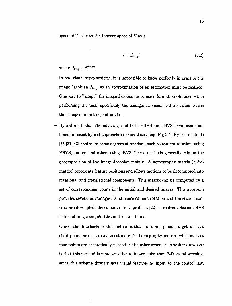
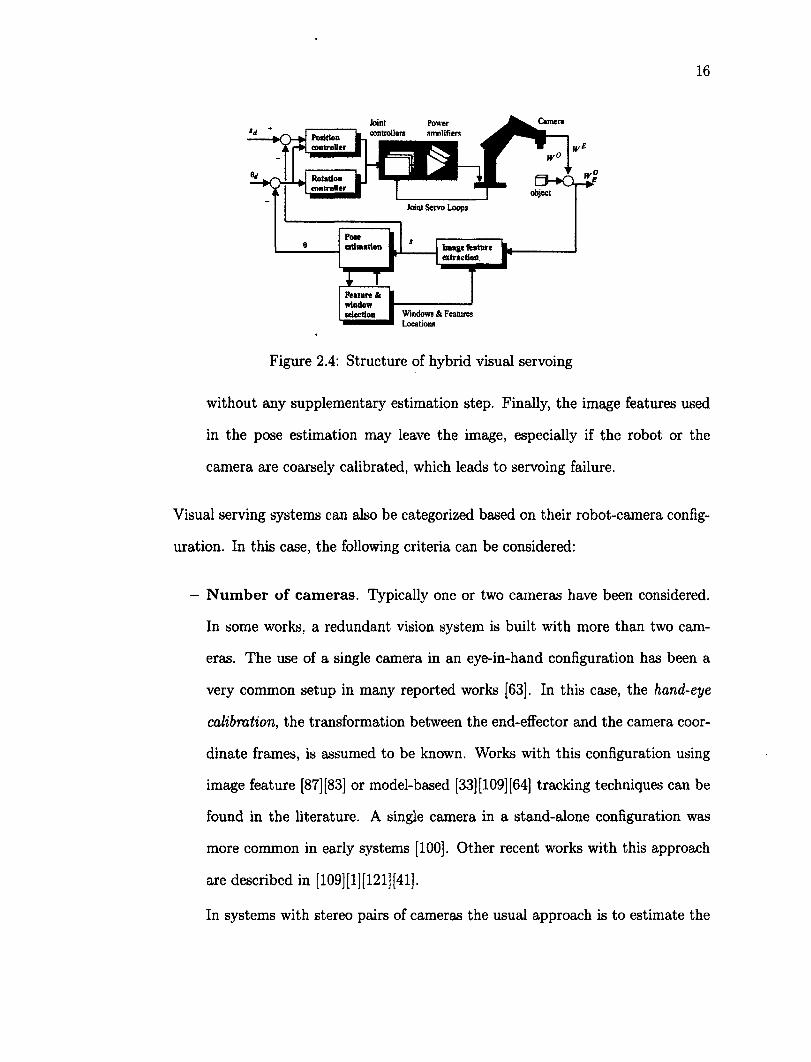
- Hybrid methods. The advantages of both PBVS and IBVS have been com­

bined in recent hybrid approaches to visual servoing, Fig 2.4. Hybrid methods

[75] [31] [43] control of some degrees of freedom, such as camera rotation, using

PBVS, and control others using IBVS. These methods generally rely on the

decomposition of the image Jacobian matrix. A homography matrix (a 3x3

matrix) represents feature positions and allows motions to be decomposed into

rotational and translational components. This matrix can be computed by a

set of corresponding points in the initial and desired images. This approach

provides several advantages. First, since camera rotation and translation con­

trols are decoupled, the camera retreat problem [22] is resolved. Second, HVS

is free of image singularities and local minima.

One of the drawbacks of this method is that, for a non planar target, at least

eight points are necessary to estimate the homography matrix, while at least

four points are theoretically needed in the other schemes. Another drawback

is that this method is more sensitive to image noise than 2-D visual servoing,

since this scheme directly uses visual features as input to the control law,

16

Joint Power ^^fc^^Camera controllers arnntifiers

sal; I | object

Rotation controller

Joint Servo Loops

Pose estimation

Windows & Features Locations

Figure 2.4: Structure of hybrid visual servoing

without any supplementary estimation step. Finally, the image features used

in the pose estimation may leave the image, especially if the robot or the

camera are coarsely calibrated, which leads to servoing failure.

Visual serving systems can also be categorized based on their robot-camera config­

uration. In this case, the following criteria can be considered:

- Number of cameras. Typically one or two cameras have been considered.

In some works, a redundant vision system is built with more than two cam­

eras. The use of a single camera in an eye-in-hand configuration has been a

very common setup in many reported works [63]. In this case, the hand-eye

calibration, the transformation between the end-effector and the camera coor­

dinate frames, is assumed to be known. Works with this configuration using

image feature [87] [83] or model-based [33] [109] [64] tracking techniques can be

found in the literature. A single camera in a stand-alone configuration was

more common in early systems [100], Other recent works with this approach

are described in [109] [1] [121] [41].

In systems with stereo pairs of cameras the usual approach is to estimate the

17

disparity and the depth of the scene [62] [76]. However one of the problems

with respect to this computation is the detection of matching features between

two or more images. The use of a stereo head mounted on the end-effector is

less common than in a stand-alone configuration, since in the latter is easier

to make the baseline, the line joining both cameras, large enough to obtain an

accurate depth estimation [63]. Some systems using a stereo head in a eye-in-

hand configuration are described in [68] [32]. Some examples of two cameras

in a stand-alone configuration can be found in [47] [51] [52].

- Camera Location. The following options are available:

* Eye-in-hand. The camera, or cameras, is mounted on the end-effector of

the robot. With this configuration, it is possible to have a more detailed

view of the object of interest.

* Stand-alone. The camera, or cameras, is fixed on the workspace of the

robot. This configuration provides a wider field of view of the scene.

A final classification of visual servo system is given in [101]:

- Endpoint open-loop (EOL) systems. These are systems in which only

the target can be observed. Systems following this approach can be found in

[84].

- Endpoint closed-loop (ECL) systems. In these systems, both the target

and end-effector of the robot can be observed. Although control is more precise

for ECL systems, the need for an end-effector image, in addition to the target

image, increases the computational cost of feature extraction. Some ECL

systems have been reported in [117].

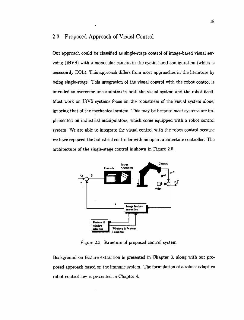
2.3 Proposed Approach of Visual Control

18

Our approach could be classified as single-stage control of image-based visual ser-

voing (IBVS) with a monocular camera in the eye-in-hand configuration (which is

necessarily EOL). This approach differs from most approaches in the literature by

being single-stage. This integration of the visual control with the robot control is

intended to overcome uncertainties in both the visual system and the robot itself.

Most work on IBVS systems focus on the robustness of the visual system alone,

ignoring that of the mechanical system. This may be because most systems are im­

plemented on industrial manipulators, which come equipped with a robot control

system. We are able to integrate the visual control with the robot control because

we have replaced the industrial controller with an open-architecture controller. The

architecture of the single-stage control is shown in Figure 2.5.

Power ^^Cimen

Controls Amolifiers

S31 object

Image feature extraction

Feature & window •election Windows & Features

Locations

Figure 2.5: Structure of proposed control system

Background on feature extraction is presented in Chapter 3, along with our pro­

posed approach based on the immune system. The formulation of a robust adaptive

robot control law is presented in Chapter 4.

19

Chapter 3

Vision System and Feature Extraction

3.1 Introduction'Vision System

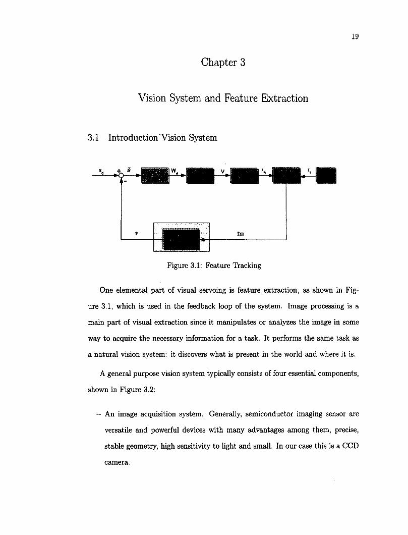
Figure 3.1: Feature Tracking

One elemental part of visual servoing is feature extraction, as shown in Fig­

ure 3.1, which is used in the feedback loop of the system. Image processing is a

main part of visual extraction since it manipulates or analyzes the image in some

way to acquire the necessary information for a task. It performs the same task as

a natural vision system: it discovers what is present in the world and where it is.

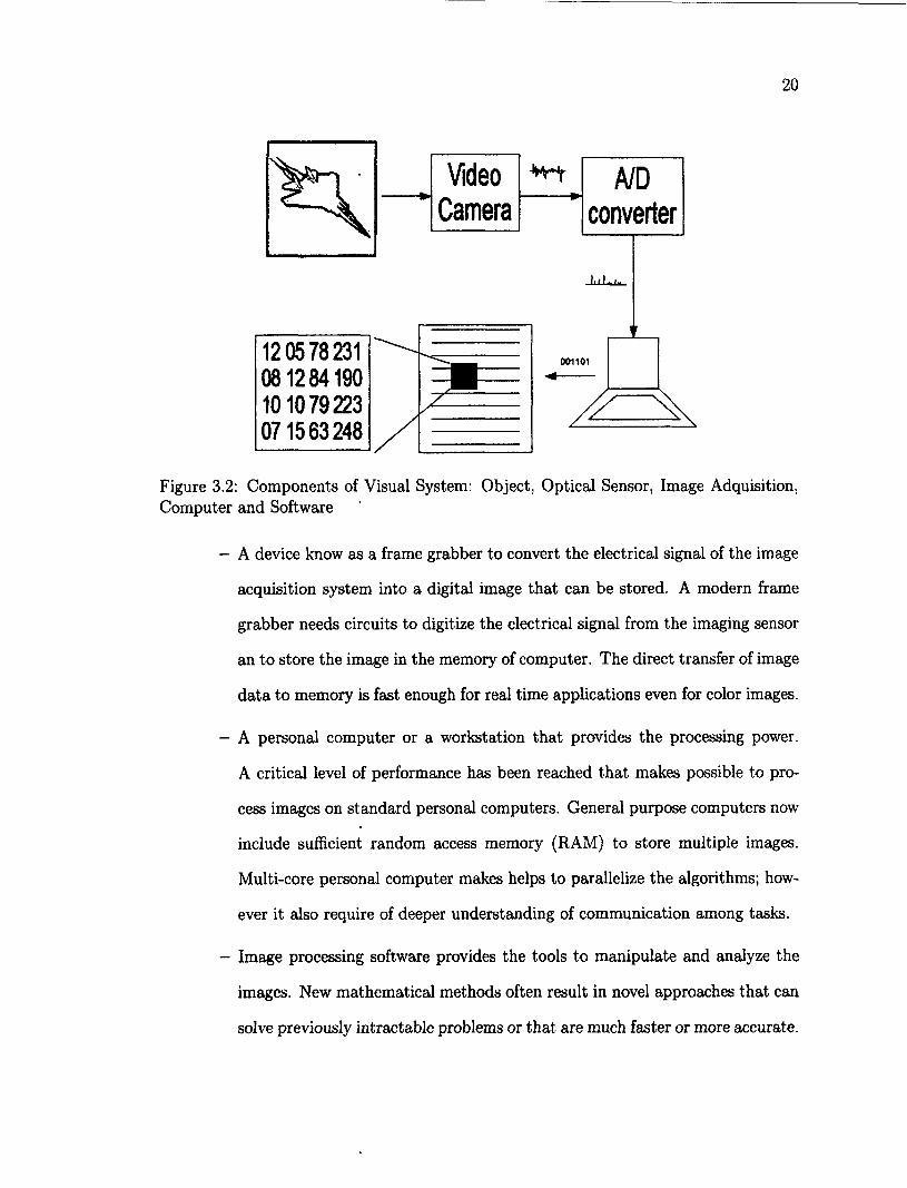
A general purpose vision system typically consists of four essential components,

shown in Figure 3.2:

- An image acquisition system. Generally, semiconductor imaging sensor are

versatile and powerful devices with many advantages among them, precise,

stable geometry, high sensitivity to light and small. In our case this is a CCD

camera.

20

Video 111 - 1 TTT A/D Camera converter

I I I l . i . l i i

12 05 78231 08 1284190 101079223 071563248

001101

Figure 3.2: Components of Visual System: Object, Optical Sensor, Image Adquisition, Computer and Software

- A device know as a frame grabber to convert the electrical signal of the image

acquisition system into a digital image that can be stored. A modern frame

grabber needs circuits to digitize the electrical signal from the imaging sensor

an to store the image in the memory of computer. The direct transfer of image

data to memory is fast enough for real time applications even for color images.

- A personal computer or a workstation that provides the processing power.

A critical level of performance has been reached that makes possible to pro­

cess images on standard personal computers. General purpose computers now

include sufficient random access memory (RAM) to store multiple images.

Multi-core personal computer makes helps to parallelize the algorithms; how­

ever it also require of deeper understanding of communication among tasks.

- Image processing software provides the tools to manipulate and analyze the

images. New mathematical methods often result in novel approaches that can

solve previously intractable problems or that are much faster or more accurate.

21

Often the speed-up that can be gained reaches several orders of magnitude.

Thus fast algorithms make many image processing techniques applicable and

reduce the hardware costs.

Image processing begins with the capture of an image with an acquisition sys­

tem. In several applications, we may select the appropriate image system and set

up the illumination, to capture best the object feature of interest. Once the image

is sensed, it must be -transformed into a form that can be treated with a digital

computer: this process is called digitization. The first steps of digital processing

may include a number of different operations. For example, if the sensor has non­

linear characteristics, such as fish-eye, these need to be corrected. Other common

operations can be applied if brightness, contrast and noise of the image are not

appropriate.

Likewise, other types of processing steps are necessary to analyze, identify and

track objects. Segmentation distinguishes the objects of interest from other objects

and the background. This is an easy task if an object is well distinguished from the

background by some local features; however this is not often the case. Therefore

more sophisticated techniques axe required. These techniques use various optimiza-

tion strategies to minimize the deviation between the image data and a given model

of the object.

But, what is an object? How can we represent it? There are no simple answers.

However, it is clear that we wish to capture the appearance of those recognizable

properties of the object, such as lumps, geometry, color and some time its motion.

This situation is easily accomplished by humans and computer vision systems only

perform elementary or well-defined fixed tasks. The human visual system is capable

to reduce the amount of received visual data to a small but relevant amount of

22

information. We could conclude that the human visual system can easily recognize

objects, but less well suited for accurate measurements of color, distances and areas.

3.2 Camera Model

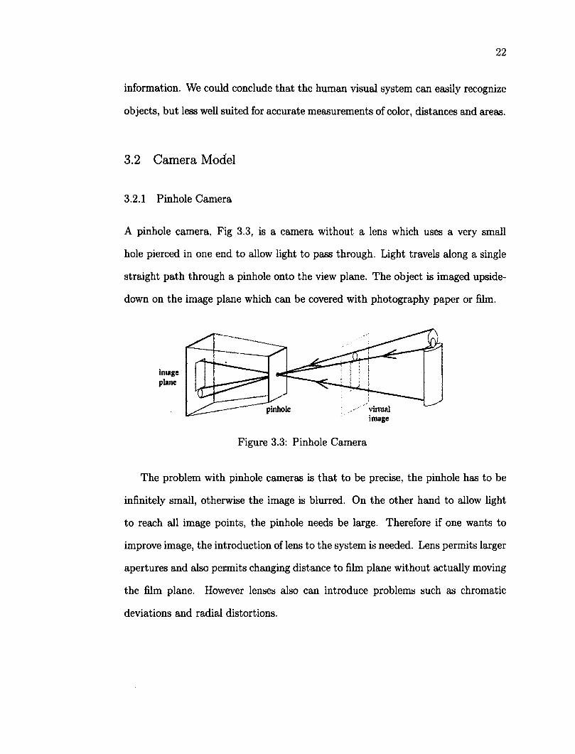
3.2.1 Pinhole Camera

A pinhole camera, Fig 3.3, is a camera without a lens which uses a very small

hole pierced in one end to allow light to pass through. Light travels along a single

straight path through a pinhole onto the view plane. The object is imaged upside-

down on the image plane which can be covered with photography paper or film.

The problem with pinhole cameras is that to be precise, the pinhole has to be

infinitely small, otherwise the image is blurred. On the other hand to allow light

to reach all image points, the pinhole needs be large. Therefore if one wants to

improve image, the introduction of lens to the system is needed. Lens permits larger

apertures and also permits changing distance to film plane without actually moving

the film plane. However lenses also can introduce problems such as chromatic

deviations and radial distortions.

irna plai

virtual image

Figure 3.3: Pinhole Camera

23

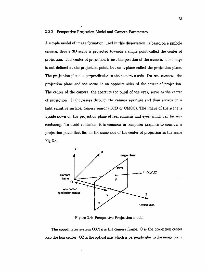
3.2.2 Perspective Projection Model and Camera Parameters

A simple model of image formation, used in this dissertation, is based on a pinhole

camera, thus a 3D scene is projected towards a single point called the center of

projection. This center of projection is just the position of the camera. The image

is not defined at the projection point, but on a plane called the projection plane.

The projection plane is perpendicular to the camera z axis. For real cameras, the

projection plane and the scene lie on opposite sides of the center of projection.

The center of the camera, the aperture (or pupil of the eye), serve as the center

of projection. Light .passes through the camera aperture and then arrives on a

light sensitive surface, camera sensor (CCD or CMOS). The image of the scene is

upside down on the projection plane of real cameras and eyes, which can be very

confusing. To avoid confusion, it is common in computer graphics to consider a

projection plane that lies on the same side of the center of projection as the scene

Fig 3.4.

Y X

Image plane

(U,V)

Camera frame

Lens center /projection center

Optical axis

Figure 3.4: Perspective Projection model

The coordinates system OXYZ is the camera frame. O is the projection center

also the lens center. OZ is the optical axis which is perpendicular to the image plane

24

7t\ Their intersection o is the principle point. The distance between projection

center O and the image plane 7r is the focal length /. P is a point in camera

frame with coordinates P(X, Y, Z) and p is its projection on the image plane. To

calculate p(u,v,z), the perspective projection of P(X,Y,Z) into the projection

plane at z = f we make use the similar triangles to write the ratios given by

u _ X

f " Z

" = f j , (3.1)

v _ y / ' z

v = f j (3.2)

The division by Z causes the perspective projection of more distant objects to

be smaller than that of closer objects. The relation between the camera and some

other world frame is a rigid motion, related to camera orientation and position. It

c a n b e r e p r e s e n t e d b y a n o r t h o g o n a l r o t a t i o n m a t r i x R , a n d a t r a n s l a t i o n v e c t o r t .

X r n ri2 f\3 £i

Y =

rai T 2 2 7*23 h

Z r n rz2 r33 h

P = RPw + t (3.3)

Measurements on the image plane are not made directly, because the image is

sampled in pixels. The relation between image plane point and pixel addresses is

modeled by an affine transformation. Aligning the pixel and the image coordinate

system so the u and x directions coincide, we obtain

25

au .

§ Sb

<

t

10 0 0

av - - 0 f y V 0 0 10 0

a 0 0 1 0 0 10

X

Y

Z

1

(3.4)

where the 5 coefficients f x , f y , k x y , uq and v 0 are the camera intrinsic parameters,

representing the focal length in horizontal pixels, focal length in vertical pixels,

skew coefficient, principle points coordinates respectively. We take the parameter

kxy to be zero because the lens distortion in our camera is minimal. Combining

(3.3) and (3.4) gives the direct linear transformation (DLT) [4] form of the camera

model:

au mn mi2 mi3 mu

av =

m21 Tfl 22 m2z m24

a m31 m3 2 m33 m34

y

1

(3.5)

This is the usual camera model for many vision system where the camera in-

trinsics and pose are not initially known. The transformation matrix is defined up

to a scale factor, thus there are 11 degrees of freedom.

3.2.3 Camera Calibration

To Calibrate the camera we need to fix the 11 unknowns in the 12 parameters

This is done by having at least 6 points of known position, not all coplanar. Each

observation generates two homogeneous equations in terms of m^,

mn X + m^Y + rtiizZ + m14 u =

v —

mz\X + m32y + m33 Z + ra34

77?21 X + TH22Y + 77123 Z ^24 m3 \X + m32y + m33Z + m34'

(3.6)

(3.7)

26

if n points are available, we can write it as a 2n x 12 matrix

X Y Z 1 0 0 0 0 -uX ~uY -uZ -u

0 0 0 0 X Y Z 1 -vX -vY -vZ -v

m i i

ml2

m u

= 0 (3.8)

Since the system is homogeneous, we can constrain m34 = 1 and solve nsing

linear least square estimation. If image positions are noisy, the results can be

improved by taking more than 6 points. As in [6], we use a special calibration

object with very accurate grids.

Since the linear method is ill-conditioned, we use a large number of reference

points (49) as in [107]. A better solution is to solve for ||m|| = 1, as in [48], then

the solution correspond to the smallest singular value of the matrix in (3.8). Then

this solution is use as starting point for a minimization of the difference between

the measured and projected point. Other calibration methods based on nonlinear

optimization and decomposition of the matrix M have yielded better results [38],

but the linear method is sufficient for our robust visual servoing system. Having

obtained the DLT form, the intrinsic and extrinsic parameters can be extracted if

required.

3.3 Feature Extraction

Three key processes are required in feature extraction, and they are defined as

modeling, identification and motion prediction of an object in the image plane

as the object moves around a scene. In other words, a "tracker" that follows

the tracked object in different frames of a video. Additionally, depending on the

tracking task, a tracker can also provide information about the object, such as

27

orientation, area, or shape of an object. Tracking objects can be challenging due

to:

- Loss of information caused by projection of the 3D world on a 2D image.

- Noise in images.

- Complex object motion.

- Partial and full object occlusions.

- Scene illumination changes.

- Complex object shapes.

- Non-rigid or articulated nature of objects.

- Real-time processing requirements.

One can simplify .tracking by imposing constraints on the motion and/or ap­

pearance of objects. For example, many tracking algorithms assume that the object

trajectory to be is smooth or the changes to be continuous. One can also restrict

the object motion to be of constant velocity or constant acceleration based on past

information. The size of objects, shape and the object appearance, can also be

used to simplify the problem.

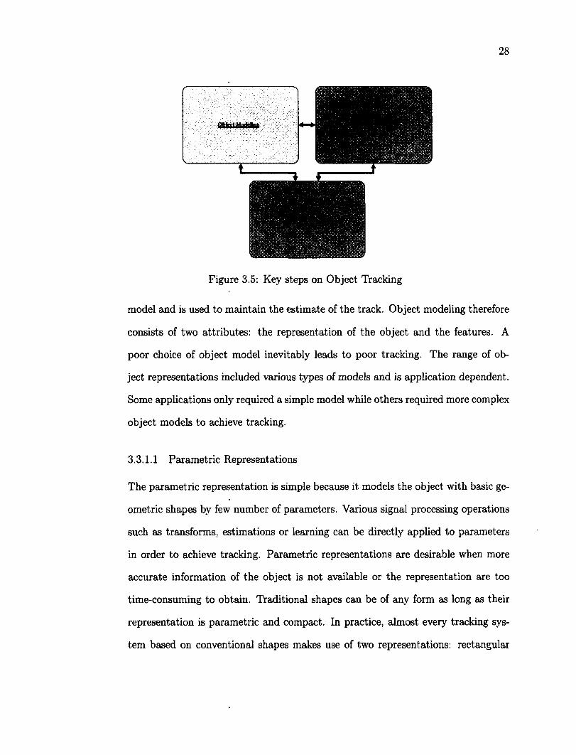
The three key steps in object tracking analysis are shown in Figure 3.5 : Object

modeling, object identification, and analysis of object tracks to recognize their

behavior.

3.3.1 Object Modeling

Object modeling plays a essential role in visual tracking because it distinguishes

an object of interest from the background. The feature is defined by the object

28

r ..

• .• • . - : - v - 1 f e

........ .. . .... . • • • .. ... . . V . ..

IMt* Mint-*11 -

'

• : . . •

•

V

.. ' •

Figure 3.5: Key steps on Object Tracking

model and is used to maintain the estimate of the track. Object modeling therefore

consists of two attributes: the representation of the object and the features. A

poor choice of object model inevitably leads to poor tracking. The range of ob­

ject representations included various types of models and is application dependent.

Some applications only required a simple model while others required more complex

object models to achieve tracking.

3.3.1.1 Parametric Representations

The parametric representation is simple because it models the object with basic ge­

ometric shapes by few number of parameters. Various signal processing operations

such as transforms, estimations or learning can be directly applied to parameters

in order to achieve tracking. Parametric representations are desirable when more

accurate information of the object is not available or the representation are too

time-consuming to obtain. Traditional shapes can be of any form as long as their

representation is parametric and compact. In practice, almost every tracking sys­

tem based on conventional shapes makes use of two representations: rectangular

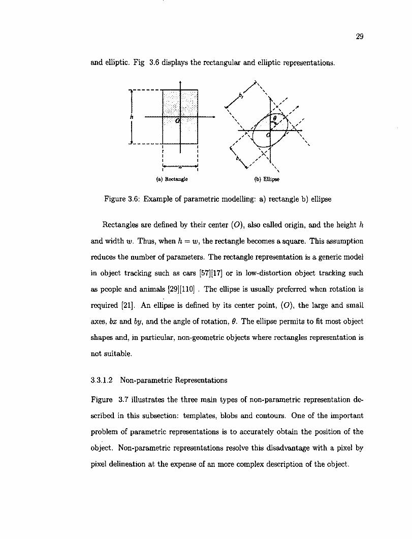
29

and elliptic. Fig 3.6 displays the rectangular and elliptic representations.

Figure 3.6: Example of parametric modelling: a) rectangle b) ellipse

Rectangles are defined by their center (O), also called origin, and the height h

and width w. Thus, when h = w, the rectangle becomes a square. This assumption

reduces the number of parameters. The rectangle representation is a generic model

in object tracking such as cars [57] [17] or in low-distortion object tracking such

as people and animals [29] [110] . The ellipse is usually preferred when rotation is

required [21]. An ellipse is defined by its center point, (O), the large and small

axes, bx and by, and the angle of rotation, 9. The ellipse permits to fit most object

shapes and, in particular, non-geometric objects where rectangles representation is

not suitable.

3.3.1.2 Non-parametric Representations

Figure 3.7 illustrates the three main types of non-parametric representation de­

scribed in this subsection: templates, blobs and contours. One of the important

problem of parametric representations is to accurately obtain the position of the

object. Non-parametric representations resolve this disadvantage with a pixel by

pixel delineation at the expense of an more complex description of the object.

h

\ \ \

(a) Rectangle (b) Ellipse

30

a)Template b)Contour C)B|0b

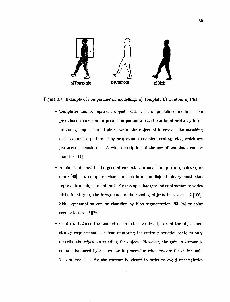
Figure 3.7: Example of non-parametric modelling: a) Template b) Contour c) Blob

- Templates aim to represent objects with a set of predefined models. The

predefined models are a priori non-parametric and can be of arbitrary form,

providing single or multiple views of the object of interest. The matching

of the model is performed by projection, distortion, scaling, etc., which are

parametric transforms. A wide description of the use of templates can be

found in [11].

- A blob is defined in the general context as a small lump, drop, splotch, or

daub [86]. In computer vision, a blob is a non-disjoint binary mask that

represents an object of interest. For example, background subtraction provides

blobs identifying the foreground or the moving objects in a scene [2] [106].

Skin segmentation can be classified by blob segmentation [93] [94] or color

segmentation [25] [26].

- Contours balance the amount of an extensive description of the object and

storage requirements. Instead of storing the entire silhouette, contours only

describe the edges surrounding the object. However, the gain in storage is

counter balanced by an increase in processing when restore the entire blob.

The preference is for the contour be closed in order to avoid uncertainties

31

in the reconstruction, although some techniques [61] [18] can handle small

breaks in the continuity of the shape. Despite these requirements, contours are

widely used because a tracking framework based on splines has been developed

[44] [115]. Splines are a piecewise function of polynomials with smoothness con­

straints. They were introduced by Schoenberg in 1946 [99]. The description of

splines below is based on [108]. A spline s modeling the contour C = k\,.., kn

is described as

where is a B-spline function and c(k) are estimated coefficients. The objec­

tive of contour tracking is the estimation of the parameters c(k) and the spline

basis. Applications of active contours for object tracking are varied, from

tracking with optical flow [44] or through severe occlusion [13] [3] to Bayesian

estimation [116].

3.3.2 Object Identification

Object identification, also called object detection, is a elemental step towards track­

ing; the object of interest needs to be identified in the frame before estimation of

its position can be performed. Object identification can either provide the ini­

tialization for a tracking algorithm only or can be integrated into the tracking

algorithm to provide object identification. Detection is based on object modeling

and it depends on the selection of the features. We investigate in this section the

different techniques employed for object identification, namely, supervised learning,

distribution representation and segmentation.

N

(3.9)

32

3.3.2.1 Supervised Learning

Supervised learning techniques learns complex patterns from a set of samples given

by a certain type of classification. Learning provides high-level decisions from the

available data based on the analysis of low-level, from simple elementary features.

Several theses, books and journal articles are entirely dedicated to supervised learn­

ing techniques [9] [46]. This subsection provides a short introduction to artificial

neural networks and support vector machines, the main algorithms used for object

detection nowadays.

- Artificial Neural Networks (ANNs) for pattern recognition started with the

invention of the perceptron in 1957 by Rosenblatt [92]. ANNs are composed

by a more simple basic elements, the neuron, and its associated activation

function. The Multi-Layer Perceptron (MLP) is the basic ANN. In object

recognition, the input vector is a set of features. The learning phase aims to

teach the desired behavior to the ANNs using a supervised learning algorithm.

Traditionally, the minimization of the empirical risk is used in the training

process. For sample n in the training dataset, let us denote the desired output

d of the linear ANN to a given input x. If the actual output is yg, the empirical

risk is expressed as

fi(y) = E^»")'<i<n)) + AnW <3'10> n=l

and

• y e ( x ) = W i X i + W 2 X 2 + \ - w n x n + b (3.11)

where is a cost function and fi(0) is regularization term to penalize large

weights w. The minimization of the empirical risk R(y) is achieved through

the adjustment of the set of weights in the neural network. Empirical risk

33

minimization has, as its objective, the convergence of the output y to the

d e s i r e d o u t p u t d v i a m i n i m i z a t i o n o f t h e c o s t f u n c t i o n R ( y ) .

Artificial neural networks are found in a wide variety of applications from

object detection, such as faces [74] and pedestrians [70], to vehicles [112] or

skin detection [66]. Also, different types of neural networks exist, depending

on the type of connections such as recurrent networks (e.g. , Hopfield networks

[53]]), the choice of activation functions (e.g. . Radial Basis Function networks)

or dimension of the input (convolutional networks).

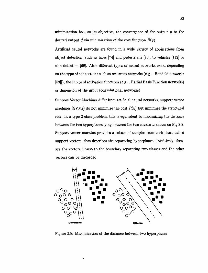
Support Vector Machines differ from artificial neural networks, support vector

machines (SVMs) do not minimize the cost R(y) but minimize the structural

risk. In a type 2-class problem, this is equivalent to maximizing the distance

between the two hyperplanes lying between the two classes as shown on Fig 3.8.

Support vector machine provides a subset of samples from each class, called

support vectors, that describes the separating hyperplanes. Intuitively, those

are the vectors closest to the boundary separating two classes and the other

vectors can be discarded.

O u O O O O

O O O \\ Q o° o\\ O o°©\«

t a)Non-Msdmum b) Maximum

Figure 3.8: Maximization of the distance between two hyperplanes

34

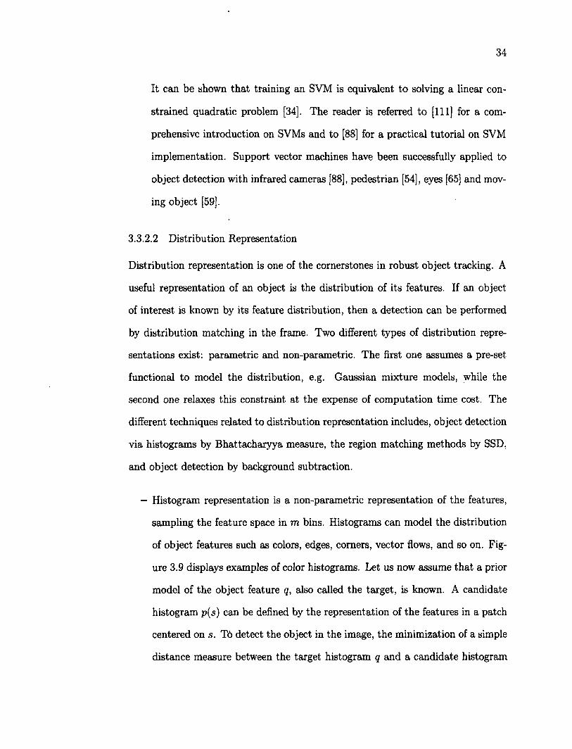
It can be shown that training an SVM is equivalent to solving a linear con­

strained quadratic problem [34]. The reader is referred to [111] for a com­

prehensive introduction on SVMs and to [88] for a practical tutorial on SVM

implementation. Support vector machines have been successfully applied to

object detection with infrared cameras [88], pedestrian [54], eyes [65] and mov­

ing object [59].

3.3.2.2 Distribution Representation

Distribution representation is one of the cornerstones in robust object tracking. A

useful representation of an object is the distribution of its features. If an object

of interest is known by its feature distribution, then a detection can be performed

by distribution matching in the frame. Two different types of distribution repre­

sentations exist: parametric and non-parametric. The first one assumes a pre-set

functional to model the distribution, e.g. Gaussian mixture models, while the

second one relaxes this constraint at the expense of computation time cost. The

different techniques related to distribution representation includes, object detection

via histograms by Bhattacharyya measure, the region matching methods by SSD,

and object detection by background subtraction.

- Histogram representation is a non-parametric representation of the features,

sampling the feature space in m bins. Histograms can model the distribution

of object features such as colors, edges, corners, vector flows, and so on. Fig­

ure 3.9 displays examples of color histograms. Let us now assume that a prior

model of the object feature q, also called the target, is known. A candidate

histogram p(s) can be defined by the representation of the features in a patch

centered on s. To detect the object in the image, the minimization of a simple

distance measure between the target histogram q and a candidate histogram

35

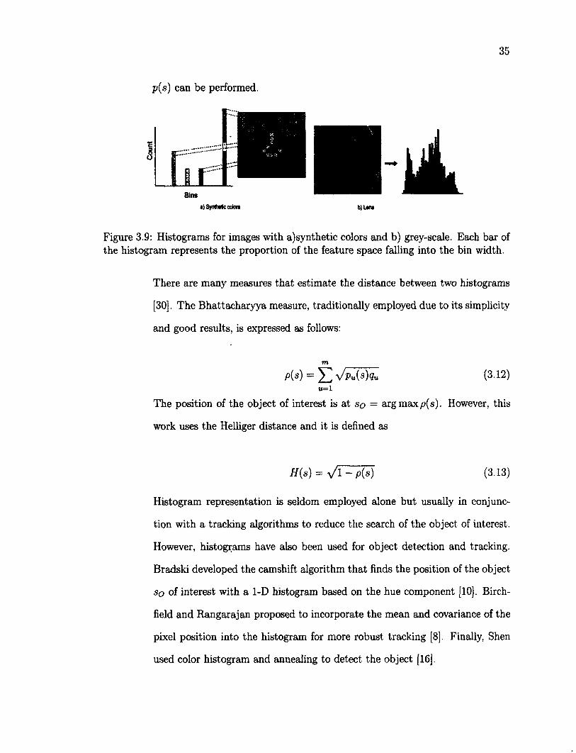
p ( s ) can be performed.

Bins

*)3ynMle colon b)Ura

Figure 3.9: Histograms for images with a)synthetic colors and b) grey-scale. Each bar of the histogram represents the proportion of the feature space falling into the bin width.

There are many measures that estimate the distance between two histograms

[30]. The Bhattacharyya measure, traditionally employed due to its simplicity

and good results, is expressed as follows:

U=1

The position of the object of interest is at s o — argmax p ( s ) . However, this

work uses the Helliger distance and it is defined as

Histogram representation is seldom employed alone but usually in conjunc­

tion with a tracking algorithms to reduce the search of the object of interest.

However, histograms have also been used for object detection and tracking.

Bradski developed the camshift algorithm that finds the position of the object

so of interest with a 1-D histogram based on the hue component [10], Birch-

field and Rangarajan proposed to incorporate the mean and covariance of the

pixel position into the histogram for more robust tracking [8], Finally, Shen

used color histogram and annealing to detect the object [16].

m

(3.12)

H ( s ) = a/WM (3.13)

36

- Sum of square difference is commonly used when the signal to noise ratio

(SNR) of an image is poor and the local computation of the spatio-temporal

derivatives can be inaccurate. Matching region methods are usually based on

the maximization of the Normalized Cross-Correlation (NCC), (3.16), or the

minimization of a distance between region. Given an image I and a feature s,

the square Euclidean distance between the image and the feature at a given

position (x, y), also referred to as SSD,

S S D ( x , y ) = ' ^ T [ I { x , y ) 2 + s ( x — d x , y — d y ) 2 - 2 1 { x , y ) s { x - d x , y - d y ) ] dx,dy

(314)

A cross-correlation measure can be calculated as:

C o r r i j ( x , y ) = ^ 2 I ( x , y ) s ( x - d x , y - d y ) (3.15) dx,dy

As this measure depends on the intensity distribution in the image and on the

size of the feature, a normalized version can be derived as,

Yljr rin U(x, y) — 71 f s (x — d x , y — d y ) — s i NCCjj(x, y) = JL^ (3.16)

\/Edx,<iy [J(x> y) - 7]2 [s(® — d x , y — d y ) - s]2

where s and 7 are the mean of the feature and the mean of the image region

on which lies the feature, respectively. These methods are in fact similar to

differential techniques in the sense that they both minimize a distance metric

but they are applied to a larger scale, and therefore relatively robust to noise.

- Background modeling is a technique used in computer vision to extract rele­

vant motion from a sequence of images. In the early days of computer vision,

[60] proposed a frame differencing algorithm subtracting two consecutive im­

ages from one another, thus canceling static areas in the scene. Since then,

37

the research effort has focused on improving the modeling of the background.

Several works have successfully combined the Gaussian mixture model with

different techniques to increase the robustness of the foreground detection. For

instance, [120] merged the foreground extracted by the mixture of Gaussians

algorithm with the optical flow to obtain better segmentation of foreground

objects. The multi-scale approach has been used to enhance the discrimina­

tion between the background and the foreground [58]. Active contours [14]

and skin detection [90] have also been combined with the Gaussian mixture

model to provide better delineation of the foreground blob.

3.3.3 Object Tracking

The relation between object representation, object identification and tracking is

very strong because tracking is performed on representative features of the object

defined by the first two tasks. The object is represented by a feature vector that

i n c l u d e s s o m e c h a r a c t e r i s t i c s t o t r a c k . T h e f e a t u r e v e c t o r a t t i m e t i s d e n o t e d x t .

If it is assumed that tracking of an object starts at time t = 1, then the feature

track X at time t — T is defined as

X = {xt\t = l...T). (3.17)

Some models assume that the feature vector x t and the track X are not accessi­

ble, but only an observation zt is. In this case, the observation track can be defined

in a similar way

Z = { z t \ t = l . . . T } . (3.18)

Finally, we denote a portion of feature track from start time t 3 to finish time t f as

xt,-tf = {xt\t = and likewise for the observation track zts:tf — {zt\t =

38

Note that X and Z can be denoted by X = x\-r and Z — z\-t. In this section, we

present deterministic and probabilistic tracking, the two main approaches in the

field. The handling of occlusions which relies upon object representation, identifi­

cation and tracking is also introduced.

3.3.3.1 Deterministic Tracking

Deterministic tracking has been commonly in the literature due to its simplicity.

The terminology deterministic means that the tracking algorithm does not inte­

grate any uncertainty in the modeling of the problem. Nevertheless, this does not

mean that problems that includes noise or other kind of uncertainty cannot be

tackled by deterministic algorithms. Simply put, the uncertainty is not taking into

account here. Deterministic algorithms are convenient because they require little

computation. They traditionally rely on simple parametric tracking for points and

contours. However, more advanced models and in particular kernel-based tracking

have also been implemented. Tracking relies on a set of samples to determine the

state of the feature vector at time t from a portion of the feature track. Without

loss of generality and because the feature vector depends at most on the entire

feature track at time t — 1, xt is written as

= /(Zl:t-1,©), (3.19)

where 0 is the vector of parameters. Normally, the problem is reduced to a

linear or locally linearized transform to simplify calculations so that the tracking

can be formulated in matrix form, i.e. , xt = Parametric techniques

were essentially employed in the early research because of the great performance

they offered for a low computational cost. [95][96] define rigid constraints to find

the optimum match of the feature vector state. Multi-scale approaches [5] and

39

direct kernel bandwidth tuning have been proposed in recent years. Multiple kernel

tracking has also been proposed to tackle the problem [42]. Finally, [82] proposed

to estimate the kernel bandwidth and initialization through the Kalman filter for

the purpose of vehicle tracking .

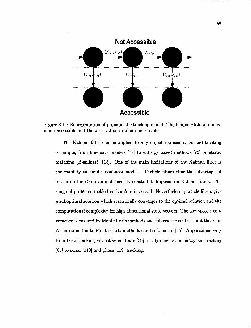
3.3.3.2 Probabilistic Tracking

Probabilistic tracking has emerged from the need to account for uncertainty in

tracking. There are several sources of uncertainties in a sequence of images. First,

the signal is degraded with noise. And secondly, the information on the object of

interest can be inaccessible due to occlusion or clutter. The probabilistic model is

composited of two layers: a hidden layer, representing the state, and an observation

layer, providing inference on the state. Figure 3.10 shows a schematic view of the

system. The equations can be expressed as follows:

where ft-i and ht are vector functions; they are assumed to be known and

possibly nonlinear and time dependent. The functions depend on the states xt~i

and xt and observation noises. vt~i and nt, respectively. The hidden Markov model

sets up the framework for recursive Bayesian filtering. The Bayesian approach

p r o v i d e s s o m e d e g r e e o f b e l i e f f o r t h e s t a t e x t f r o m t h e s e t o f o b s e r v a t i o n s Z t =

{zi,z2,..., zt} available at time t. In other words, the Bayesian recursion estimates

the posterior density p(xt\Zt) to estimate the state of an object using Bayes rule.

The Bayesian recursion is performed in two steps: prediction and update.

xt = /t-i(»t-i.Vt-i) (3.20)

Z t — h t { X t , T l t ) , (3.21)

40

Not Accessible

Accessible

Figure 3.10: Representation of probabilistic tracking model. The hidden State in orange is not accessible and the observation in blue is accessible

The Kalman filter can be applied to any object representation and tracking

technique, from kinematic models [78] to entropy based methods [73] or elastic

matching (B-splines) [115]. One of the main limitations of the Kalman filter is

the inability to handle nonlinear models. Particle filters offer the advantage of

loosen up the Gaussian and linearity constraints imposed on Kalman filters. The

range of problems tackled is therefore increased. Nevertheless, particle filters give

a suboptimal solution which statistically converges to the optimal solution and the

computational complexity for high dimensional state vectors. The asymptotic con­

vergence is ensured by Monte Carlo methods and follows the central limit theorem.

An introduction to Monte Carlo methods can be found in [45]. Applications vary

from head tracking via active contours [39] or edge and color histogram tracking

[69] to sonar [110] and phase [119] tracking.

41

3.3.4 Occlusion Handling

Occlusion is defined as the lack of visual clues either partially or totality of the

object. The ability of tracking algorithms to handle occlusion is crucial to provide

a good estimate of the object state. Occlusion handling decreases the effects of the

lack of information on an object under occlusion. There exist three different cases

of occlusion:

- Self occlusion: The object of interest is articulated and the constraints on

motion does not prevent the overlap when the object is projected on the

camera plane.

- Inter-object occlusion: The object of interest is occluded by another object in

the frame. Inter-object occlusion can occur at any time since the environment

in which the object evolves is not controlled. Inter-object occlusion can be of

any duration.

- Occlusion from a background object: The object of interest is occluded by

the background. Typically, the object passes behind a tree, a house, etc. The

background is usually static and therefore enables the learning of inference on

occlusion. However, occlusion is usually total and the observation zt does not

exist.

The testing a disrupted observation z leads to the detection of occlusion. For

instance, alterations on observations are a clue to occlusion. In other words, if

the probability of an observation drops rapidly, the object can be partial or to­

tal occlusion. Analysis of the observation, such as probability of occurrence and

thresholding provides criteria to potential occlusion. Occlusion detection is crucial

since it provides an indicator of the tracking confidence.

42

3.4 Artificial Immune System Tracking (Proposed approach)

In this section we introduce a framework to track the features of interest for the

visual servoing control. Despite feature tracking is an important requirement in

Visual servoing, many researches neglect this part of the problem. In order to

have more realistic scenarios, we have to tackle many assumptions used to make

the tracking problem tractable, for example, illumination constancy, partial occlu­

sion. clutter, high contrast with respect to background, etc. Thus, tracking and

associated problems of feature selection, object representation, dynamic shape, and

motion estimation are considered in this framework.

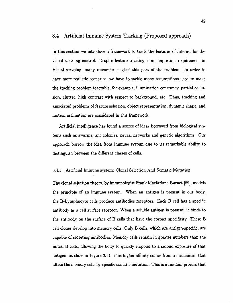
Artificial intelligence has found a source of ideas borrowed from biological sys­

tems such as swarms, ant colonies, neural networks and genetic algorithms. Our

approach borrow the idea from Immune system due to its remarkable ability to

distinguish between the different classes of cells.

3.4.1 Artificial Immune system: Clonal Selection And Somatic Mutation

The clonal selection theory, by immunologist Frank Macfarlane Burnet [89], models

the principle of an immune system. When an antigen is present in our body,

the B-Lymphocyte cells produce antibodies receptors. Each B cell has a specific

antibody as a cell surface receptor. When a soluble antigen is present, it binds to

the antibody on the surface of B cells that have the correct specificity. These B

cell clones develop into memory cells. Only B cells, which are antigen-specific, are

capable of secreting antibodies. Memory cells remain in greater numbers than the

initial B cells, allowing the body to quickly respond to a second exposure of that

antigen, as show in Figure 3.11. This higher affinity comes from a mechanism that

alters the memory cells by specific somatic mutation. This is a random process that

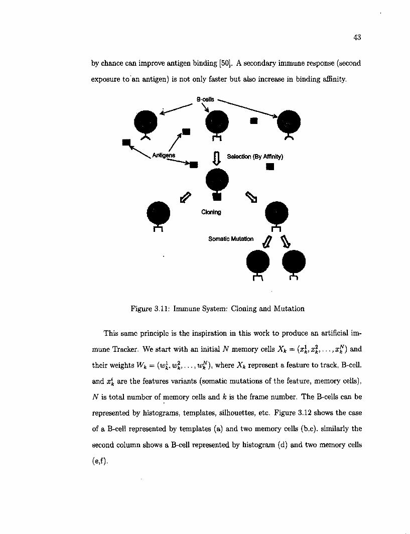
43

by chance can improve antigen binding [50]. A secondary immune response (second

exposure to an antigen) is not only faster but also increase in binding affinity.

Q amII#

Figure 3.11: Immune System: Cloning and Mutation

This same principle is the inspiration in this work to produce an artificial im­

mune Tracker. We start with an initial N memory cells Xk = {x\, x\,... ,xk) and

their weights Wk = (wk, uuk,..., wk), where Xk represent a feature to track, B-cell.

and xk are the features variants (somatic mutations of the feature, memory cells),

N is total number of memory cells and k is the frame number. The B-cells can be

represented by histograms, templates, silhouettes, etc. Figure 3.12 shows the case

of a B-cell represented by templates (a) and two memory cells (b.c). similarly the

second column shows a B-cell represented by histogram (d) and two memory cells

Selection (By Affinity)

Cloning

Somatic Mutation

(e,f).

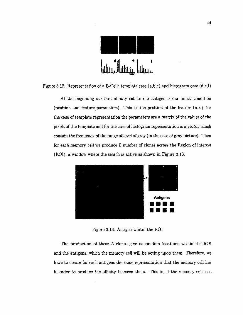
44

e

lllli. flllllll^ lillhi.

Figure 3.12: Representation of a B-Cell: template case (a,b,c) and histogram case (d,e,f)

At the beginning our best affinity cell to our antigen is our initial condition

(position and feature parameters). This is, the position of the feature (u, v), for

the case of template representation the parameters are a matrix of the values of the

pixels of the template and for the case of histogram representation is a vector which

contain the frequency of the range of level of gray (in the case of gray picture). Then

for each memory cell we produce L number of clones across the Region of interest

(ROI), a window where the search is active as shown in Figure 3.13.

Antigens

Figure 3.13: Antigen whitin the ROI

The production of these L clones give us random locations within the ROI

and the antigens, which the memory cell will be acting upon them. Therefore, we

have to create for each antigens the same representation that the memory cell has

in order to produce the affinity between them. This is, if the memory cell is a

45

histogram then the representation of the antigen is a histogram too.

After the creation of the antigen, we applied the affinity function /(.) with its

correspondence weight w, in order to calculate the total affinity A of the antigen

Y and the memory cell given by,

where / € [0,1], I = [1,..., L) and i = [1,..., N\ . The total affinity represent the

similitude among a particular antigen Yl and the memory cells xl for a particular

B-Cell X, the feature. The affinity function /(.) is related to representation but

not unique, for example the affinity function for histograms could be the Helliger

distance (3.13) or Battacharyya measure (3.12) and for template could be the SSD

(3.14) or a normalized cross-correlation (3.16).

For example for 3 memory cells (histrogram representation) and 4 clones the

total affinity will be,

and /(.) is the Helliger distance for each antigen tested Y. Then, according to

their total affinity we determine the best cell that match our antigen as Xbest =

maxf^l1, A2,..., A4},.thus it gives best position of that feature.

Other affinity functions are used to complement the affinity function, an exam­

ple is the dynamic of the feature as mention in the object tracking section 3.3.3. For

example, /(.) = fi{x, Y)f2{x(s),x(s)), where fi(x, Y) is the measure of similarity

N

(3.22)

clonel : yl1 = w 1 f ( x 1 , V1) -I- w 2 f {x 2 , V1) + w 3 f ( x 3, y1), (3.23)

clone2 : A 2 = w l f ( x l , Y 2 ) + w 2 f ( x 2 , Y 2 ) + w 3 f ( x 3 , Y 2 ) , (3.24)

clone3 : A 3 = w 1 f ( x 1 , Y 3 ) + w 2 f {x 2 , Y 3 ) + w 3 f ( x 3 , K3), (3.25)

clone4 : A 4 = w l f {x \Y 4 ) + w 2 f ( x 2 , Y 4 ) + w 3 f ( x 3 , Y 4), (3.26)

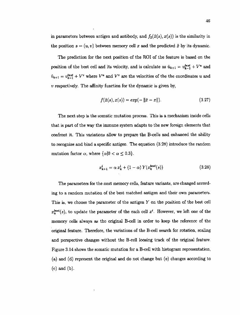
46

in parameters between antigen and antibody, and f2(x(s),x(s)) is the similarity in

the position s = (u, v) between memory cell x and the predicted x by its dynamic.

The prediction for the next position of the ROI of the feature is based on the

position of the best cell and its velocity, and is calculate as «*+! = u^{ + Vu and

Vk+1 = vj^Jf + V" where V" and Vv are the velocities of the the coordinates u and

v respectively. The affinity function for the dynamic is given by,

The next step is the somatic mutation process. This is a mechanism inside cells

that is part of the way the immune system adapts to the new foreign elements that

confront it. This variations allow to prepare the B-cells and enhanced the ability

to recognize and bind a specific antigen. The equation (3.28) introduce the random

mutation factor a, where {c*|0 < a < 0.3}.

The parameters for the next memory cells, feature variants, are changed accord­

ing to a random mutation of the best matched antigen and their own parameters.

This is, we choose the parameter of the antigen Y on the position of the best cell

x)*st{s), to update the parameter of the each cell x\ However, we left one of the

memory cells always as the original B-cell in order to keep the reference of the

original feature. Therefore, the variations of the B-cell search for rotation, scaling

and perspective changes without the B-cell loosing track of the original feature.

Figure 3.14 shows the somatic mutation for a B-cell with histogram representation,

(a) and (d) represent the original and do not change but (e) changes according to

(c) and (b).

f {x{s ) , x(s)) = exp{ - \ \ x - x||). (3.27)

4+i = a 4 + (1 - a) ^(^(s)) (3.28)

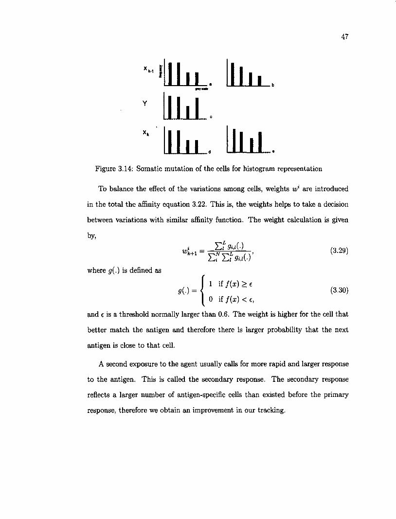
47

M 11 u m**—

ll li ill

Jill Figure 3.14: Somatic mutation of the cells for histogram representation

To balance the effect of the variations among cells, weights w l are introduced

in the total the affinity equation 3.22. This is, the weights helps to take a decision

between variations with similar affinity function. The weight calculation is given

by, n. .( \

(3.29) wk+1 -

9 ( - ) = (3.30)

EfEf *»(•)' where g( . ) is defined as

*

1 if f ( x ) > e

0 if f(x) < e,

and e is a threshold normally larger than 0.6. The weight is higher for the cell that

better match the antigen and therefore there is larger probability that the next

antigen is close to that cell.

A second exposure to the agent usually calls for more rapid and larger response

to the antigen. This is called the secondary response. The secondary response

reflects a larger number of antigen-specific cells than existed before the primary

response, therefore we obtain an improvement in our tracking.

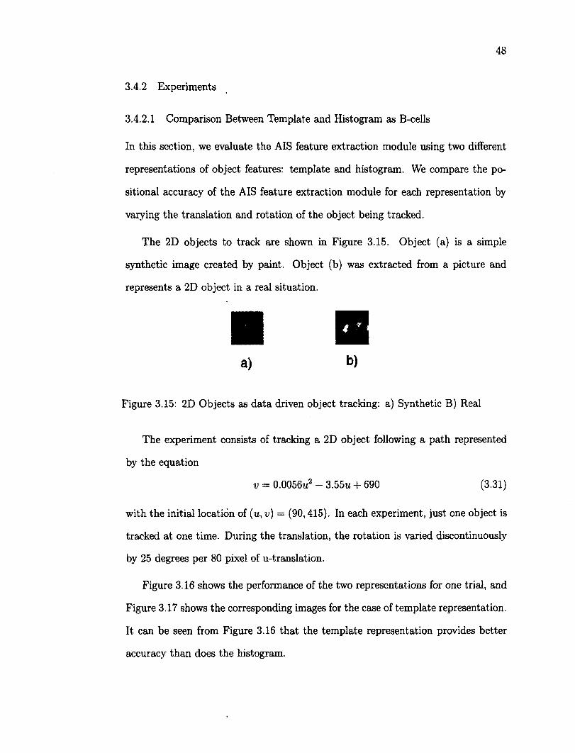
48

3.4.2 Experiments

3.4.2.1 Comparison Between Template and Histogram as B-cells

In this section, we evaluate the AIS feature extraction module using two different

representations of object features: template and histogram. We compare the po­

sitional accuracy of the AIS feature extraction module for each representation by

varying the translation and rotation of the object being tracked.

The 2D objects to track are shown in Figure 3.15. Object (a) is a simple

synthetic image created by paint. Object (b) was extracted from a picture and

represents a 2D object in a real situation.

a) b)

Figure 3.15: 2D Objects as data driven object tracking: a) Synthetic B) Real

The experiment consists of tracking a 2D object following a path represented

by the equation

v = 0.0056u2 - 3.55ti + 690 (3.31)

with the initial location of (u , v ) = (90,415). In each experiment, just one object is

tracked at one time. During the translation, the rotation is varied discontinuously

by 25 degrees per 80 pixel of u-translation.

Figure 3.16 shows the performance of the two representations for one trial, and

Figure 3.17 shows the corresponding images for the case of template representation.

It can be seen from Figure 3.16 that the template representation provides better

accuracy than does the histogram.

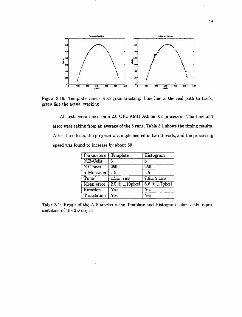
49

Tamplata Traddng Histogram Trading 400

350 350

300 300

250 2S0

200 200

ISO 150

100 100

500 100 200 300 poori u

400 600 100 200 500 400 600

Figure 3.16: Template versus Histogram tracking: blue line is the real path to track, green line the actual tracking

All tests were timed on a 2.0 GHz AMD Athlon X2 processor. The time and

error were taking from an average of the 5 runs; Table 3.1 shows the timing results.

After these tests, the program was implemented in two threads, and the processing

speed was found to increase by about 50

Parameters Template Histogram N.B-Cells 3 3 N. Clones 250 250 a Mutation .15 .15 Time 1.5± .7ms 7.6± 2.1ms Mean error 2.5 ± l.lOpixel 6.6 ± 1.7pixel Rotation Yes Yes Translation Yes Yes

Table 3.1: Result of the AIS tracker using Template and Histogram color as the repre­sentation of the 2D object

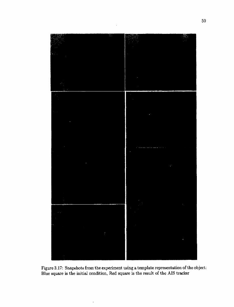
Figure 3.17: Snapshots from the experiment using a template representation of the object: Blue square is the initial condition, Red square is the result of the AIS tracker

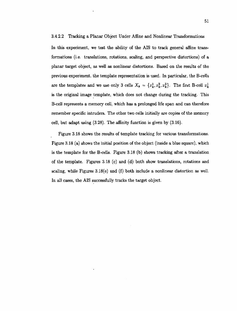
51

3.4.2.2 Tracking a Planar Object Under Affine and Nonlinear Transformations

In this experiment, we test the ability of the AIS to track general affine trans­

formations (i.e. translations, rotations, scaling, and perspective distortions) of a

planar target object, as well as nonlinear distortions. Based on the results of the

previous experiment, the template representation is used. In particular, the B-cells

are the templates and we use only 3 cells Xk = {z£, x2k, x|}. The first B-cell x|

is the original image template, which does not change during the tracking. This

B-cell represents a memory cell, which has a prolonged life span and can therefore

remember specific intruders. The other two cells initially are copies of the memory

cell, but adapt using (3.28). The affinity function is given by (3.16).

Figure 3.18 shows the results of template tracking for various transformations.

Figure 3.18 (a) shows the initial position of the object (inside a blue square), which

is the template for the B-cells. Figure 3.18 (b) shows tracking after a translation

of the template. Figures 3.18 (c) and (d) both show translations, rotations and

scaling, while Figures 3.18(e) and (f) both include a nonlinear distortion as well.

In all cases, the AIS successfully tracks the target object.

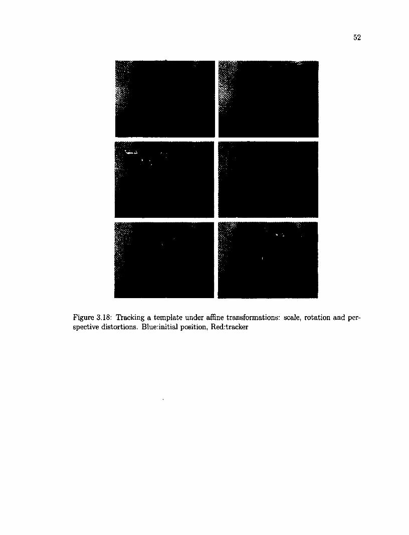
Figure 3.18: Tracking a template under affine transformations spective distortions. Blue:initial position, Red:tracker

scale, rotation and per-

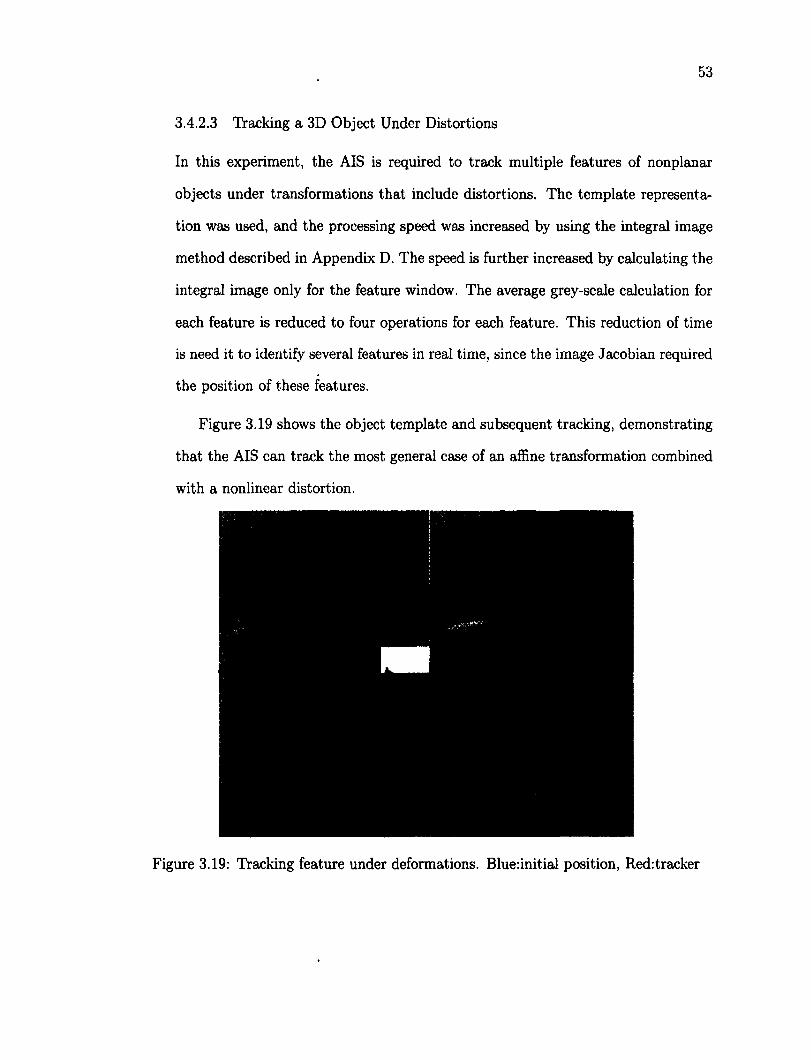
53

3.4.2.3 Tracking a 3D Object Under Distortions

In this experiment, the AIS is required to track multiple features of nonplanar

objects under transformations that include distortions. The template representa­

tion was used, and the processing speed was increased by using the integral image

method described in Appendix D. The speed is further increased by calculating the

integral image only for the feature window. The average grey-scale calculation for

each feature is reduced to four operations for each feature. This reduction of time

is need it to identify several features in real time, since the image Jacobian required

the position of these features.

Figure 3.19 shows the object template and subsequent tracking, demonstrating

that the AIS can track the most general case of an affine transformation combined

with a nonlinear distortion.

Figure 3.19: Tracking feature under deformations. Blue:initial position, Red:tracker

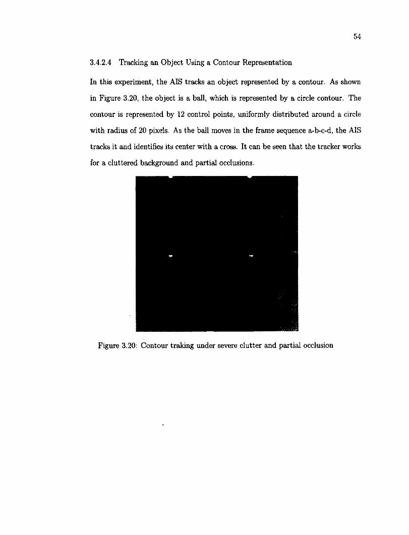
54

3.4.2.4 Tracking an Object Using a Contour Representation

In this experiment, the AIS tracks an object represented by a contour. As shown

in Figure 3.20, the object is a ball, which is represented by a circle contour. The

contour is represented by 12 control points, uniformly distributed around a circle

with radius of 20 pixels. As the ball moves in the frame sequence a-b-c-d, the AIS

tracks it and identifies its center with a cross. It can be seen that the tracker works

for a cluttered background and partial occlusions.

Figure 3.20: Contour traking under severe clutter and partial occlusion

55

3.5 Summary

In this chapter, we presented the some state-of-the-art algorithms for object track­

ing and introduced a new framework based on Artificial Immune Systems (AIS)

to meet the needs of our visual servoing system. We evaluated the performance of

the AIS using histogram and template object representations, and found that the

template representation provided the best accuracy and processing speed. Con­

sequently, the template representation will be used in the visual servo sytem of

Chapter 5.

The experiments showed that the AIS is capable of tracking objects under affine

transformation and nonlinear distortions and can track multiple features in real

time. Finally, to show the flexibility of the AIS, we also implemented it using

contour representations.

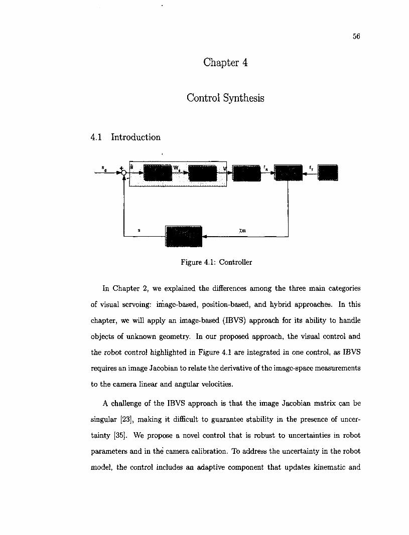
Chapter 4

56

Control Synthesis

4.1 Introduction

Figure 4.1: Controller

In Chapter 2, we explained the differences among the three main categories

of visual servoing: image-based, position-based, and hybrid approaches. In this

chapter, we will apply an image-based (IBVS) approach for its ability to handle

objects of unknown geometry. In our proposed approach, the visual control and

the robot control highlighted in Figure 4.1 are integrated in one control, as IBVS

requires an image Jacobian to relate the derivative of the image-space measurements

to the camera linear and angular velocities.

A challenge of the IBVS approach is that the image Jacobian matrix can be

singular [23], making it difficult to guarantee stability in the presence of uncer­

tainty [35]. We propose a novel control that is robust to uncertainties in robot

parameters and in the camera calibration. To address the uncertainty in the robot

model, the control includes an adaptive component that updates kinematic and

57

dynamic parameters. Robustness to uncertainty in the camera calibration is ad­

dressed by including in the control an error bound on the system Jacobian (which

is a combination of the robot and image Jacobians).

Stability of the proposed control is proved via Lasalle's invariant principle. Sim­

ulations are used to test the control before it is applied on a real robotic system in

Chapter 5.

4.2 Dynamics of Mechanical Systems

The Euler-Lagrange (EL) equations of motion are defined as

ddL 91 _ ( A U d t dq 8q T ' ^ *

where q € is the vector of joint displacements, r € is a vector of generalized

forces, and L is the Lagrangian. When applied to a robot arm, this equation gives

H{q)q + C(q ,q )q + G(q) = r, (4.2)

where H(q) € 3?nxn is a symmetric positive definite inertia matrix, C(q , q )q is a

vector of centripetal and Coriolis torques and G(q) £ is a vector of gravitational

torques, and r is a vector of joint torques.

The robot dynamic model (4.2) has the following properties [40]:

— Property 1. The dynamic equations may be expressed as a linear function of

a constant parameter vector 9 € 5?':

H(q)q + C(q , q )q + G(q) = Y{q , q , q )9 = r, (4.3)

where Y(q , q , q ) € 3fl n x l is known as the regression matrix.

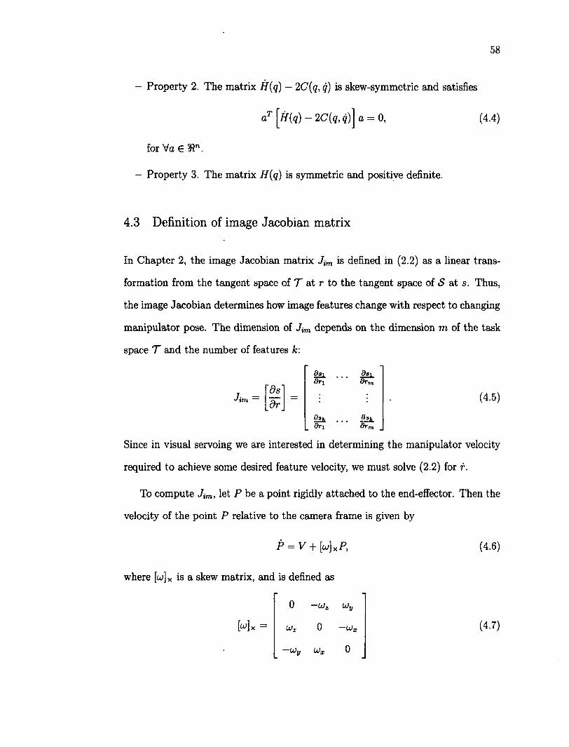
58

- Property 2. The matrix H(q) - 2C(q , q ) is skew-symmetric and satisfies

aT [&{<!) ~ 2C{q , 9)J a = 0, (4.4)

for Va € 5Rn.

- Property 3. The matrix H(q) is symmetric and positive definite.

4.3 Definition of image Jacobian matrix

In Chapter 2, the image Jacobian matrix Jim is defined in (2.2) as a linear trans­

formation from the tangent space of T at r to the tangent space of S at s. Thus,

the image Jacobian determines how image features change with respect to changing

manipulator pose. The dimension of Jim depends on the dimension m of the task

space T and the number of features k:

Jirn — ds

dr

&8\ dr\

dri

d8\

dsk drm

(4.5)

Since in visual servoing we are interested in determining the manipulator velocity

requ i red to ach ieve some des i red f ea tu re ve loc i ty , we mus t so lve (2 .2 ) fo r r .

To compute Jim, let P be a point rigidly attached to the end-effector. Then the

velocity of the point P relative to the camera frame is given by

(4.6) p = v + HxP,

is a skew matrix, and is defined as

0 ~UZ UJy

Mx = £ 0

1 £

i i £

£ O

i

(4.7)

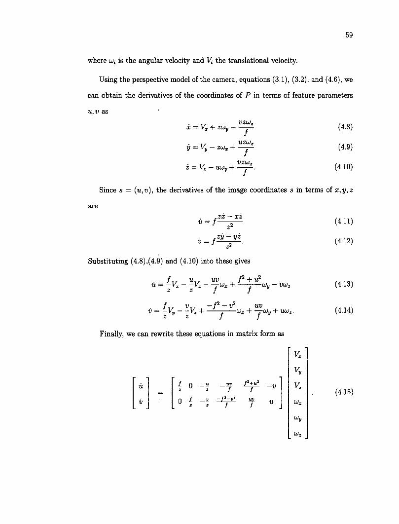
59

where u/j is the angular velocity and the translational velocity.

Using the perspective model of the camera, equations (3.1), (3.2), and (4.6), we

can obtain the derivatives of the coordinates of P in terms of feature parameters

u, v as

x = VX + zu.

y = V y - zu x +

i = Vg - UUJy +

VZU)z

V ~ ~ T UZU)z

~T vzux

(4.8)

(4.9)

(4.10)

Since s = (u ,v ), the derivatives of the image coordinates s in terms of x , y , z

are

« = / zx — x z

z y - y z v = f z2 •

Substituting (4.8),(4.9) and (4.10) into these gives

/ u uv f 2 4- u 2

u = -Vx - -Vz —t u x + 1—-—ojy - vojz u , , uv

7 U * ' f

2 „,2 f r r V T r — f 2 — V 2 U V V — —Vy Vz -\ U)x H

Z " Z f J

Finally, we can rewrite these equations in matrix form as

ii

V

* 0 z

0 I

u z

lit;

/

f UV

f u

V x

Vy

V z

Wz

Uy

Uz

(4.11)

(4.12)

(4.13)

(4.14)

(4.15)

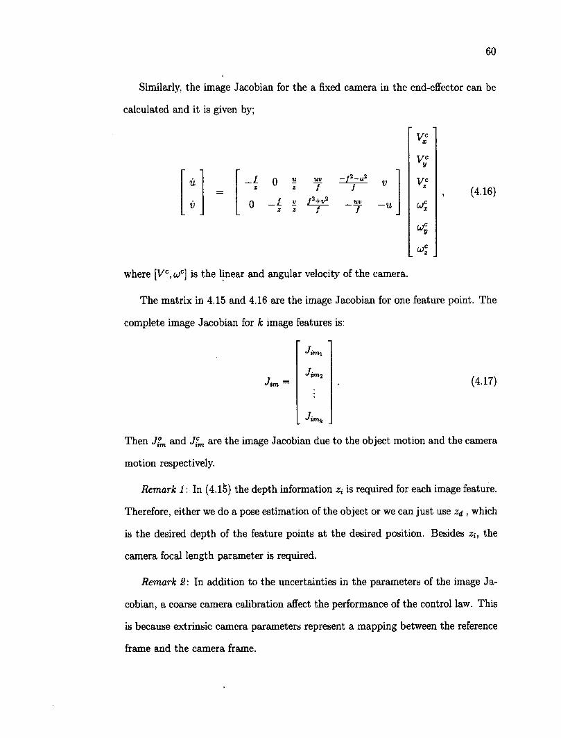
60

Similaxly, the image Jacobian for the a fixed camera in the end-effector can be

calculated and it is given by;

u

V

1 N

0 u z

uv f

-/2-u2

/

0 _z z

V

z f2+v2

f uv f

v

—u

V c X

V v

Kc

oj:

U)' \

U>'

(4.16)

where [Vc, wc] is the linear and angular velocity of the camera.

The matrix in 4.15 and 4.16 are the image Jacobian for one feature point. The

complete image Jacobian for k image features is:

Jim

Jim\

J j' 11712

'% mk

(4.17)

Then J°m and J f m are the image Jacobian due to the object motion and the camera

motion respectively.

Remark 1: In (4.15) the depth information z* is required for each image feature.

Therefore, either we do a pose estimation of the object or we can just use zj , which

is the desired depth of the feature points at the desired position. Besides ziy the

camera focal length parameter is required.

Remark 2 \ In addition to the uncertainties in the parameters of the image Ja­

cobian, a coarse camera calibration affect the performance of the control law. This

is because extrinsic camera parameters represent a mapping between the reference

frame and the camera frame.

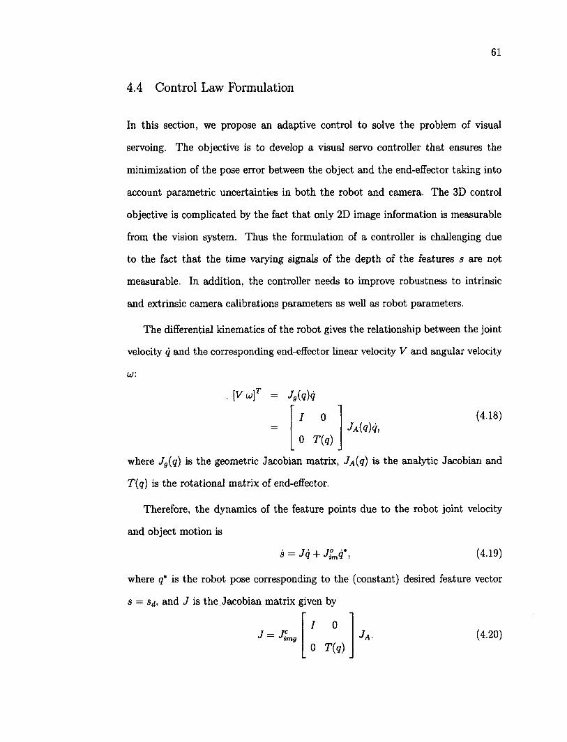
61

4.4 Control Law Formulation

In this section, we propose an adaptive control to solve the problem of visual

servoing. The objective is to develop a visual servo controller that ensures the

minimization of the pose error between the object and the end-effector taking into

account parametric uncertainties in both the robot and camera. The 3D control

objective is complicated by the fact that only 2D image information is measurable

from the vision system. Thus the formulation of a controller is challenging due

to the fact that the time varying signals of the depth of the features s are not

measurable. In addition, the controller needs to improve robustness to intrinsic

and extrinsic camera calibrations parameters as well as robot parameters.

The differential kinematics of the robot gives the relationship between the joint

velocity q and the corresponding end-effector linear velocity V and angular velocity

w:

where J g ( q ) is the geometric Jacobian matrix, J A{<I) is the analytic Jacobian and

T(q) is the rotational matrix of end-effector.

Therefore, the dynamics of the feature points due to the robot joint velocity

and object motion is

where q* is the robot pose corresponding to the (constant) desired feature vector

s = Sd, and J is the Jacobian matrix given by

. \Vu)T = J,(q)g

I 0

0 T(q) J A{Q)Q,

(4.18)

s = Jq + J°mq*, (4.19)

/ 0 J = J L %mg J A- (4.20)

0 T{q)

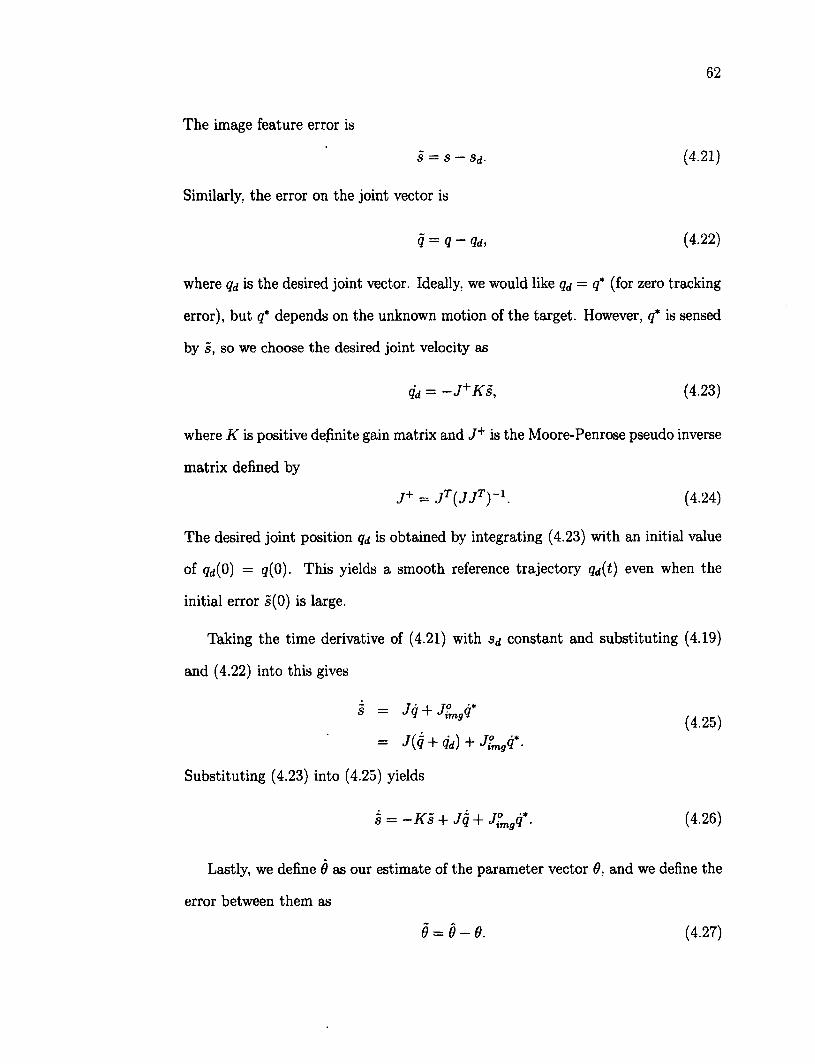
62

The image feature error is

S = S - SD- (4.21)

Similarly, the error on the joint vector is

Q = q~Qd, (4.22)

where qd is the desired joint vector. Ideally, we would like qd = q* (for zero tracking

error), but q* depends on the unknown motion of the target. However, q* is sensed

by 5, so we choose the desired joint velocity as

where K is positive definite gain matrix and J+ is the Moore-Penrose pseudo inverse

matrix defined by

The desired joint position qd is obtained by integrating (4.23) with an initial value

of <fa(0) = <7(0). This yields a smooth reference trajectory qd{t) even when the

initial error s(0) is large.

Taking the time derivative of (4.21) with Sd constant and substituting (4.19)

and (4.22) into this gives

q d = —J + Ks , (4.23)

J+ = JT(JJT)~\ (4.24)

« = JQ+JimgQ*

= J(^ + Qd) + (4.25)

Substituting (4.23) into (4.25) yields

~s = -K~s + Jq + J°mgq*. (4.26)

Lastly, we define 6 as our estimate of the parameter vector 6 , and we define the

error between them as

0 = 0 - 0 . (4.27)

63

In order to design a robust controller to compensate for uncertainties in the

parameters of the visual system as well as the uncertainties in the parameters of the

manipulator, both the properties 1-3 of the mechanical systems and the following

assumptions are taking in consideration:

Assumption 1. There exists a unique joint position vector q* such that s = Sd

(i.e. it is possible to reach the desired feature vector Sd).

Assumption 2. The uncertainty of the Jacobian matrix J is bounded as,

J - J < P, P> 0, (4.28)

where J is the estimated value of J and p is a known value.

Assumption 1 ensures that the control problem is solvable and Assumption 2 is

required in the stability analysis. The control problem is to design a control law r

and a parameter vector update 9 such that the control error in the image plane s

approaches zero as t —> oo. Our control is based in adaptive control proposed by

Slotine and Li, [102], but we include additional terms for the visual servo problem

under Jacobian uncertainties. The original Slotine and Li control is

T = YD6- Kpq - Kdq, (4.29)

where Yd = Y(q, q, qd, ijd) and the estimated parameters 9 are generated according

to the adaptive update law

$ = (4.30)

where A denotes a positive constant diagonal adaptation gain matrix.

This control was chosen because the feed-forward term Yd9 takes advantage of

the known nominal rpbot parameters [55]. Our modification of control law (4.29)

is based on the structure of the system and the following stability analysis. We

64

choose the control torque as

T = YD9 - Kpq - Kdq - JTs - p p|| qu (4.31)

Qu =

where Kp, Kd € 3?6x6 denote diagonal matrices of positive constant control gains,

and qu is a unit vector:

?/ M\ ^ 9 ^ 0 (4.32)

0 if q = 0.

The last two terms of (4.31) are added to improve the control when the exact value

of the Jacobian is not known. In contrast, the Cartesian version of Slotine and Li's

control in [102] assumes exact knowledge of the manipulator Jacobian.

4.5 Stability Analysis

Consider the system

x(t) = /(&(*)), (4.33)

which is assumed to have an equilibrium point at x = 0 (i.e. /(0) = 0). The

stability of this equilibrium point is defined in Appendix A.

Theorem 1. Lasalle's invariance principle [71}. Suppose that there exist a

positive definite function V(x) : Kn —)• 3? whose derivative along solutions of the

system (4.33) satisfies the inequality V < 0. Let M be the largest invariant set

contained in the set £? = |a:: V(z) = o|. Then the the equilibrium point x = 0 is

stable and every solution that remains bounded for t > 0 approaches M as t -> oo.

In particular, if all solutions remain bounded and M = {0}, then the system is

globally asymptotically stable.

As explained in [71], the boundedness of solutions required in Theorem 1 is

guaranteed if V (x) is radially unbounded.

65

We will use LaSalle's invariance principle to conclude stability of the origin and

asymptotic convergence of the tracking error for the case of a stationary target

object. We must first establish that the origin is an equilibrium point. Our system

corresponding to (4.33) is given by the robot(4.2), the vision system (4.19 with a

stationary target object (q* — 0), combined with our control law (4.31) and the

adaptive update law (4.30).

We choose the state as x = ( s , q , q , 6 ) T . It is easily shown that the trajectory

x(t) = 0 satisfies the above system equations if Assumption 1 holds. Hence, x = 0

is an equilibrium point.

Theorem 1 gives sufficient conditions for the stability of the system, but it

does not give instructions for determining the function V(x) with the properties

given the Theorem, therefore the task is to search for a function that satisfies the

conditions.

Theorem 2. Consider the robot and vision system given by (4.2) and (4.19), for

the case of a stationary target object (q* = 0). If the uncertainty in the Jacobian

matrix is bounded as in (4.28), then the control law (4.31) along with the adaptive

update law defined in (4.30) makes the system stable and achieves asymptotic

tracking: s —>• 0 as t -> oo.

Proof. Define the positive definite, radially unbounded function

(4.34)

The time derivative of (4.34) is

V = qTHq + ̂ qTHq + 9TA6 4- qrKpq + sTs. (4.35)

From (4.2)

Hq — T — Cq — G, (4.36)

and using (4.36) and (4.22), we may write the first term of (4.35) as

qTHq = qT (r - Cq - G - Hqd) . (4.37)

Prom Property 2, the second term of (4.35) may be written as

1 f [1(H-2C) + C],1

= fCq . (4.38)

Therefore, adding (4.37) and (4.38) and using (4.22) we have

F ( T - C q - G - H q d ) + i T C i = = f ( T - H q d - C q d - G ) . (4.39)

Prom (4.26) with q* = 0 we obtain

IPs = (-Ks + Jq)T s (4.40)

- - sT lFs + p jTs .

Substituting (4.39) and (4.40) in (4.35) and rearranging terms yields

V = F { T- Hqd - Cqd - G + K pq) + d T A § - sT K s + f j T s . (4.41)

From the control law (4.31) and (4.41), the derivative of the Lyapunov function

candidate becomes

V = qT (:Yd6 - Kji -JTs-p p|| qu) + qT {-Hqd - Cqd - G) V ' (4.42)

+6tA9 - STKS + qTJTs.

Using property 1 and (4.27) in V yields

V = qT (Yd9 - Kdq - JTs - p ||s|| qu^j + 6TA9 - sTKs 4- qTJTs. (4.43)

Substituting qrqu = ||g|| and J = J — J into (4.43) gives

V = -qTKdq + (F + Yjqj - sTKTs + qTJTs - p ||s|| ||g||. (4.44)

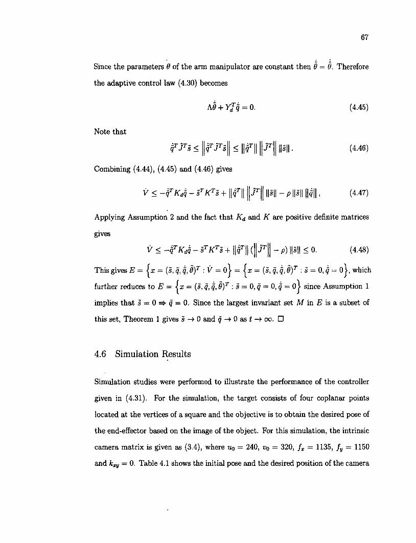
67

Since the parameters 9 of the arm manipulator are constant then 0 = 0. Therefore

the adaptive control law (4.30) becomes

A0 + Yj$ = 0.

Note that

qTjTs < fJrS ^ llf II s •

(4.45)

(4.46)

Combining (4.44), (4.45) and (4.46) gives

V < - q r K d f i - 8 1 ' K ' r 8 + \ \ q zT i sTz , I I ~T 1*1 11*11 Ml, (4.47)

Applying Assumption 2 and the fact that Kd and K are positive definite matrices

gives

V < - f K d $ - st K t s + pr|| (|| jT|| - p) p|| < 0. (4.48)

This gives E = = (s, q, q, 9)T : V = o| = = (s, q, q, 0)T : s = 0, q = o|, which

further reduces to E = = (s, q, q, 9)T : s = 0, q = 0, q = o| since Assumption 1

implies that s = 0 =>• q = 0. Since the largest invariant set M in E is a subset of

this set, Theorem 1 gives s —• 0 and q 0 as t-> oc. •

4.6 Simulation Results

Simulation studies were performed to illustrate the performance of the controller

given in (4.31). For the simulation, the target consists of four coplanar points

located at the vertices of a square and the objective is to obtain the desired pose of

the end-effector based on the image of the object. For this simulation, the intrinsic

camera matrix is given as (3.4), where u0 = 240, v0 = 320, fx = 1135, fy = 1150

and kxy = 0. Table 4.1 shows the initial pose and the desired position of the camera

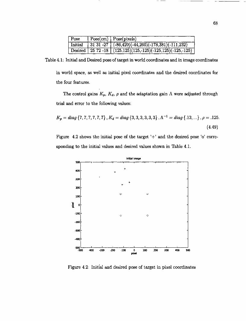
68

Pose Pose(cm) Pose(pixels) Initial 31 31 -27 (-86,420)(-44,260)(-178,381)(-l 11,232) Desired 25 72 -18 (125,125)(125,-125)(-125,125)(-125,-125)

Table 4.1: Initial and Desired pose of target in world coordinates and in image coordinates

in world space, as well as initial pixel coordinates and the desired coordinates for

the four features.

The control gains Kp, Kj., p and the adaptation gain A were adjusted through

trial and error to the following values:

Kp = diag{7,7,7,7,7,7}, K& = diag{3,3,3,3,3,3} , A-1 = diag {.13,...} ,p — .125.

(4.49)

Figure 4.2 shows the initial pose of the target and the desired pose 'o' corre­

sponding to the initial values and desired values shown in Table 4.1.

500

400

300

200

100

1 0 a

-100

-200

-300

-400

-500 -500 -400 -300 -200 -100 0 100 200 300 400 500

pixel

Figure 4.2: Initial and desired pose of target in pixel coordinates

Initial Image i i 1 r-

_j i i i i i L.

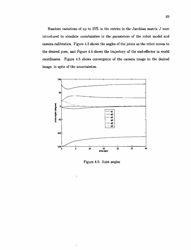
69

Random variations of up to 25% in the entries in the Jacobian matrix J were

introduced to simulate uncertainties in the parameters of the robot model and

camera calibration. Figure 4.3 shows the angles of the joints as the robot moves to

the desired pose, and Figure 4.4 shows the trajectory of the end-effector in world

coordinates. Figure 4.5 shows convergence of the camera image to the desired

image, in spite of the uncertainties.

1001 1 1 1 1 r

0 5 10 15 20 25 30 time (see)

Figure 4.3: Joint angles

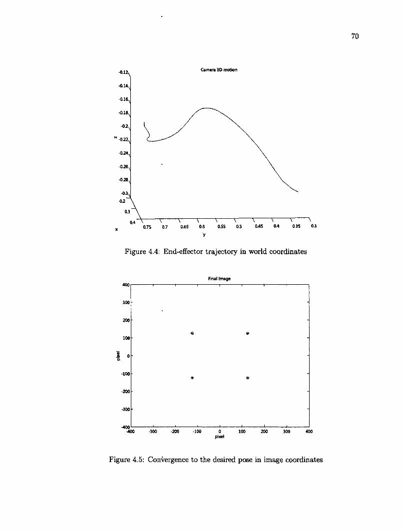
-0,12k

-0.14

-0.16.

-0.1S.

-0.2,

' -0.22,

-0.24,

-0.26,

-0.28,

Camera 3D motion

Q4 \ * * S * * * * * \ 0.75 0:7 0.65 0.6 0.55 0.5 OAS 0.4 0.35 0.3

Figure 4.4: End-effector trajectory in world coordinates

Final Image 400

400

Figure 4.5: Convergence to the desired pose in image coordinates

71

4.7 Summary and Conclusions

In this Chapter we formulated a new control based on an adaptive control proposed

by Slotine-Li. The changes made includes robustness in the visual servoing system

against parameter uncertainties in the image Jacobian. Adaptive controls use the

gradient descent to adjust the parameters of the control law. However, there are

adaptive controls based on others optimization techniques as least-squares method

[79] and conjugate gradient [103]. The parameter estimation improves the perfor­

mance of the control, for situation where the values are unknown or the values are

time-varying.

Nevertheless, adaptive controls have their own problems, [98], such as instability

by parameter drifting, high gains or fast adaption on parameters. The lack of

robustness in the adaptive control law is a problem and they can be more susceptible

to disturbance than a static control law. Macnab [24] discusses the problem and

suggests that without a robust modification in the gradient descent terms, the

parameter might drift to large values. To overcome the robustness problem of the

adaptive control different techniques have been used in literature. In [80] several

techniques are described, such as e-modification, cr-modification, dead zone and

parameter projection.

Therefore, it is important to notice that the stability proof presented for our the

controller is based in the ideal case, that is, there is not presence of disturbance.

Due to this limitation, we recommend for future work to extent the control for

robustness in the adaptive term. A possible candidate is the piecewise linear cr-

modification. Since, it does not modified the ideal adaptive law if the imposed

bound holds and in the case the bound does not hold, the robust adaptive law has

the same properties as the fixed cr-modification, as mention in [80].

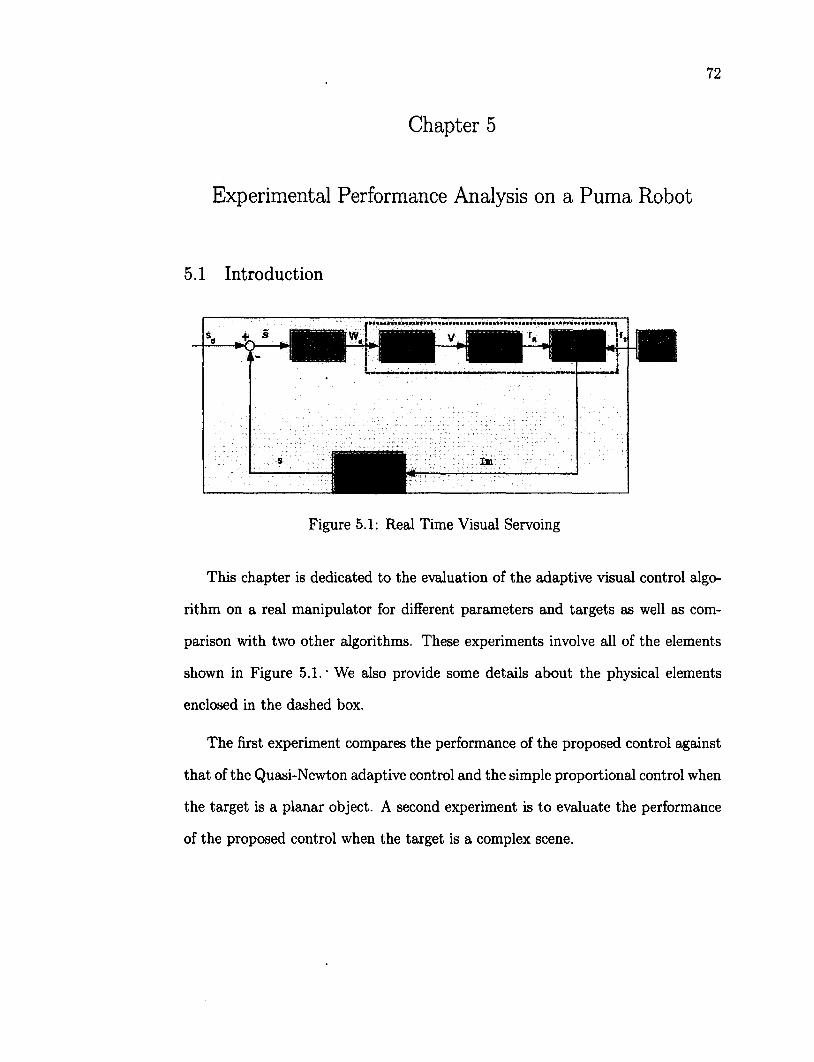
72

Chapter 5

Experimental Performance Analysis on a Puma Robot

5.1 Introduction

Figure 5.1: Real Time Visual Servoing

This chapter is dedicated to the evaluation of the adaptive visual control algo­

rithm on a real manipulator for different parameters and targets as well as com­

parison with two other algorithms. These experiments involve all of the elements

shown in Figure 5.1. • We also provide some details about the physical elements

enclosed in the dashed box.

The first experiment compares the performance of the proposed control against

that of the Quasi-Newton adaptive control and the simple proportional control when

the target is a planar object. A second experiment is to evaluate the performance

of the proposed control when the target is a complex scene.

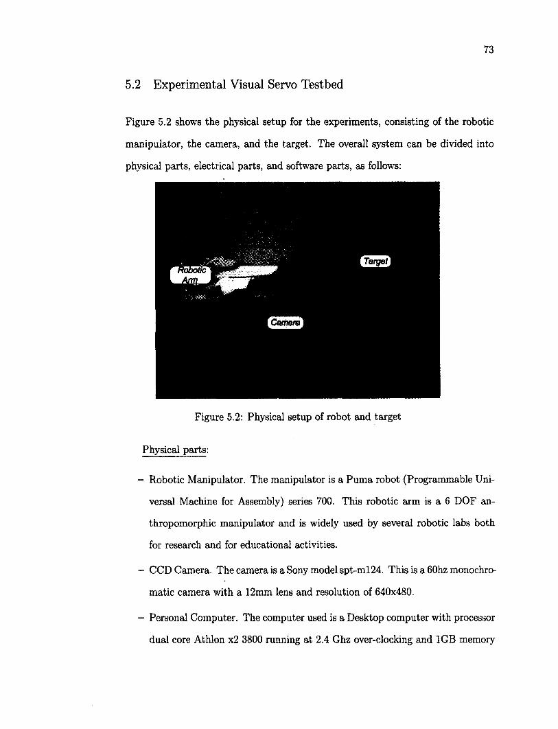
73

5.2 Experimental Visual Servo Testbed

Figure 5.2 shows the physical setup for the experiments, consisting of the robotic

manipulator, the camera, and the target. The overall system can be divided into

physical parts, electrical parts, and software parts, as follows:

Figure 5.2: Physical setup of robot and target

Physical parts:

- Robotic Manipulator. The manipulator is a Puma robot (Programmable Uni­

versal Machine for Assembly) series 700. This robotic arm is a 6 DOF an­

thropomorphic manipulator and is widely used by several robotic labs both

for research and for educational activities.

- CCD Camera. The camera is a Sony model spt-m 124. This is a 60hz monochro­

matic camera with a 12mm lens and resolution of 640x480.

- Personal Computer. The computer used is a Desktop computer with processor

dual core Athlon x2 3800 running at 2.4 Ghz over-clocking and 1GB memory

74

ram. A multi-core processor is needed to handle parallel threads in real time

systems.

Electrical Parts:

- Robot Controller. We developed an open-architecture controller to replace

the outdated interface and control system. It consists of 6 picfl220 micro­

controllers and 6 H bridges (24 volts, 8 amps) with heat-sink. The micro­

controller has an internal oscillator up to 10MHZ, 10 bit A/D, and a PWM

module. This controller is documented in Appendix B, which includes a sig­

nal flow diagram, circuit diagrams, and the assembler program of the robot

controller.

- Video Digitizer. The framegrabber used is a PCI Flashbus MV Pro from

Integral tech. It supports a 30 frames/second progressive scan camera and

includes a Software Developers Kit (SDK) and Dynamic Link Libary (DLL)

that provides programmable access to the features of the FlashBus MV Pro

hardware architecture.

Software Parts:

- Controller Interface. The software for the robot controller consist of a col­

lection of GUI programs written in C#. The main programs are listed in

Appendix C and perform the following tasks: manipulation of the robotic

arm with mouse, path planning from a txt file, control of single links, and

visual controller. The software is designed to be as modular as possible to

facilitate future work by other students.

- Image Processing. The image processing library is written in C#, and is doc­

umented in Appendix C. This library includes the main algorithms mentioned

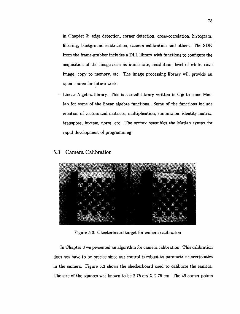
75

in Chapter 3: edge detection, corner detection, cross-correlation, histogram,

filtering, background subtraction, camera calibration and others. The SDK

from the frame-grabber includes a DLL library with functions to configure the

acquisition of the image such as frame rate, resolution, level of white, save

image, copy to memory, etc. The image processing library will provide an

open source for future work.

- Linear Algebra library. This is a small library written in C# to clone Mat-

lab for some of the linear algebra functions. Some of the functions include

creation of vectors and matrices, multiplication, summation, identity matrix,

transpose, inverse, norm, etc. The syntax resembles the Matlab syntax for

rapid development of programming.

5.3 Camera Calibration

Figure 5.3: Checkerboard target for camera calibration

In Chapter 3 we presented an algorithm for camera calibration. This calibration

does not have to be precise since our control is robust to parametric uncertainties

in the camera. Figure 5.3 shows the checkerboard used to calibrate the camera.

The size of the squares was known to be 2.75 cm X 2.75 cm. The 49 corner points

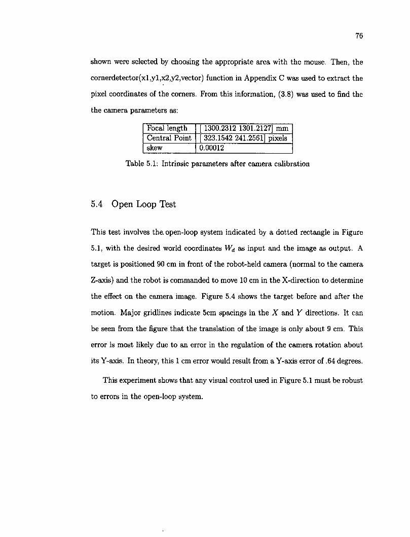
76

shown were selected by choosing the appropriate area with the mouse. Then, the

cornerdetector(xl,yl,x2,y2,vector) function in Appendix C was used to extract the

pixel coordinates of the corners. Prom this information, (3.8) was used to find the

the camera parameters as:

Focal length 1300.2312 1301.2127] mm Central Point 323.1542 241.2561] pixels skew 0.00012

Table 5.1: Intrinsic parameters after camera calibration

5.4 Open Loop Test

This test involves the. open-loop system indicated by a dotted rectangle in Figure

5.1, with the desired world coordinates as input and the image as output. A

target is positioned 90 cm in front of the robot-held camera (normal to the camera

Z-axis) and the robot is commanded to move 10 cm in the X-direction to determine

the effect on the camera image. Figure 5.4 shows the target before and after the

motion. Major gridlines indicate 5cm spacings in the X and Y directions. It can

be seen from the figure that the translation of the image is only about 9 cm. This

error is most likely due to an error in the regulation of the camera rotation about

its Y-axis. In theory, this 1 cm error would result from a Y-axis error of .64 degrees.

This experiment shows that any visual control used in Figure 5.1 must be robust

to errors in the open-loop system.

77

Figure 5.4: Open loop test

5.5 Controls Tested

5.5.1 Proportional Control

Based on (2.2), we compute a desired world velocity as

fi = -JimgkpS- (51)

Then the robot control calculated the joint torques via the PID control:

r = Kpeg + KDeg + A"/ J eq (5.2)

where KP = diag{ 10 10 10 15 15 15}, KD = dia{3 3 3 2 2 2} and A'/ =

diag{0.b 0.5 0.5 0.2 0.2 0.2}. Then, these torques are converted to joint voltages

by neglecting the inductance as

V = Kmq + RaK;\ (5.3)

where Ke = diag{0.26 0.26 0.26 0.09 0.09 0.9} V/rad, Km = Ke Nm/Amp and

Ra = diag{ 1.6 1.6 1.6 3.76 3.76 3.76} Ohms. Ke is the back EMF constant, Km is

the motor torque constant and Ra is the armature resistance, which their values are

taken from the PUMA manual. The PID gains were calculate so the controller were

critically damped, but these values in the real manipulator gave an under-damped

78

performance. Consequently, we tuned the gains by experimentation over several

trajectories.

The Jacobian Jimg used in this control is based on the depths Z{ of each feature

when the target is the desired position. The gain kp in (5.1) was tuned to 3.0 by

varying kp from 1 to 10 over 10 trials and assessing the tracking performance as the

target was moved manually to different positions. The target was slowly translated

and rotated and then stopped. The highest gain that did not produce overshoot

was 3.0. Gains close to 10 resulted in jerkiness and failure to track the features.

5.5.2 Quasi Newton Adaptive Control

One problem with the proportional control is that a constant image Jacobian Jimgis

used, whereas the actual image Jacobian varies with tracking error. Quasi-newton

adaptive (Q-N) control updates the image Jacobian according to.

sm _ a . (Ar" ~ JL,^sk){Ask)T

Jimg img + (As k ) T As k ' V '

where Ar and As is the change in camera position and the change in feature

respectively. After adapting the image Jacobian, the proportional control law given

by (5.1) and (5.2) is applied.

5.5.3 Robust Adaptive Control (Proposed)

The control law for the joint motor torques is given by (4.31). The values of Kp and

Kd were chosen the same as in the proportional control. The control (4.31) varies

the robot kinematic and dynamic parameters in 0. It could also vary the image

Jacobian, as in the adaptive control, but we used a static Jacobian for performance

comparison with the proportional control. The estimated bound on the Jacobian

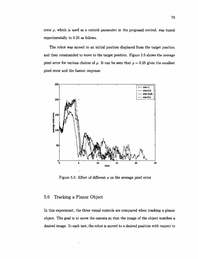
79

error p, which is used as a control parameter in the proposed control, was tuned

experimentally to 0.25 as follows.

The robot was moved to an initial position displaced from the target position

and then commanded to move to the target position. Figure 5.5 shows the average

pixel error for various choices of p. It can be seen that p = 0.25 gives the smallest

pixel error and the fastest response.

250 — rho=l

rho=0.5 — rho=0.25 — rho=0.1

200

150

15 25 0 5 10 20 time

Figure 5.5: Effect of different p on the average pixel error

5.6 Tracking a Planar Object

In this experiment, the three visual controls are compared when tracking a planar

object. The goal is to move the camera so that the image of the object matches a

desired image. In each test, the robot is moved to a desired position with respect to

80

the target, and an image is taken as reference. Then, the robot is moved to an initial

position, where the view of the target is different from that of the reference, but all

features remain within the field of view. Finally, the tested control is activated to

move the camera back to the desired position.

5.6.1 Planar Object .in 3D Translation

This experiment tests the performance of the controls when the camera is displaced

from the desired position using only translations. For this experiment, the changes

in translation with respect to the desired position are AP = [10 5 18] cm. Fig­

ures 5.6 and 5.7 show the desired and initial position for the planar test. These

positions are the same for each of the three controls tested.

Figure 5.6: Desired feature positions

81

Figure 5.7: Initial feature positions

The controls performed well when a planar object and only translation was

involved. From Figure 5.7, we infer that there are uncertainties in the parameters

of the camera position or the robotic arm, since we commanded an initial position

that is only translated from the target, but the image is slightly rotated. In spite

of this calibration error, all three controls achieve the final position as shown in

Figure 5.8.

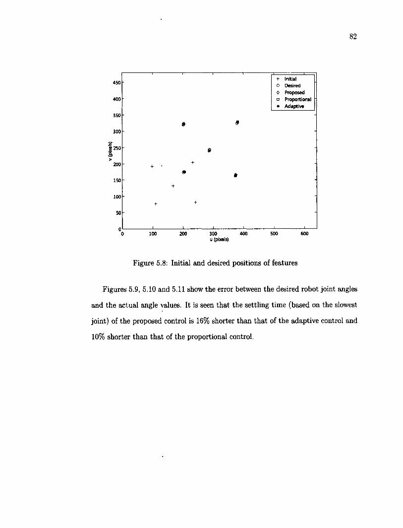
82

450

400

350

300

1250 S >

200

150

100

50

0 0 100 200 300 400 500 600

u (pixels)

Figure 5.8: Initial and desired positions of features

Figures 5.9, 5.10 and 5.11 show the error between the desired robot joint angles

and the actual angle values. It is seen that the settling time (based on the slowest

joint) of the proposed control is 16% shorter than that of the adaptive control and

10% shorter than that of the proportional control.

1 1 1 1 + Initial o Desired O Proposed

- • Proportional ' * Adaptive

& 9

$ -

+ +

• • +

+ +

i i i i

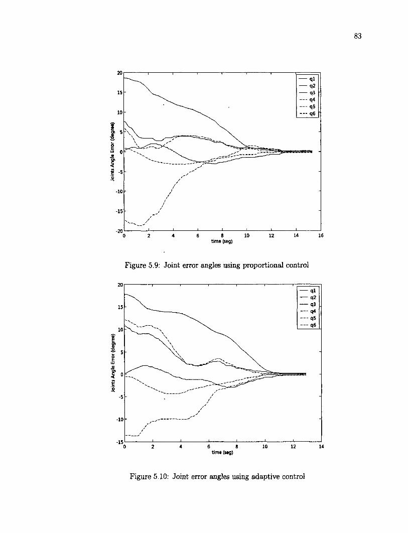
0 2 4 6 8 10 12 14 16 time (seg)

Figure 5.9: Joint error angles using proportional control

20

15 — q4

— q5 — q6

10

s 5

£ o

s

-10

-15 0 2

time (seg)

Figure 5.10: Joint error angles using adaptive control

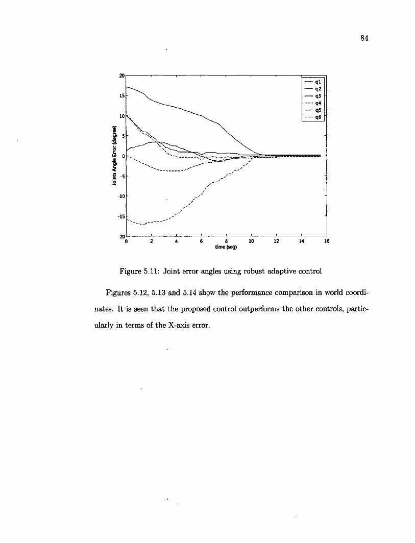
84

20 — ql

15

— q4

q5 10

5 "O

0

•5

-10

-15

-20 0

time (seg)

Figure 5.11: Joint error angles using robust adaptive control

Figures 5.12, 5.13 and 5.14 show the performance comparison in world coordi­

nates. It is seen that the proposed control outperforms the other controls, partic­

ularly in terms of the X-axis error.

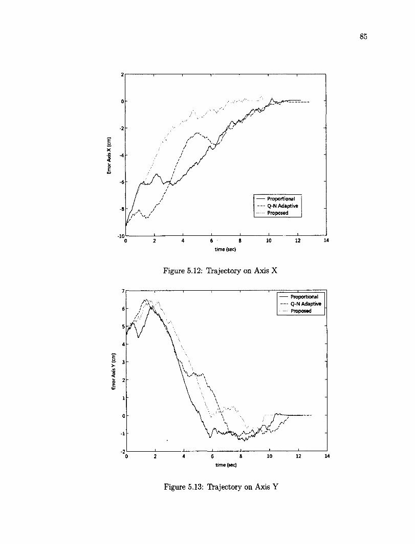
— Proportional — Q-N Adaptive

Proposed

J I L

2 4 6 8 10 12 14

time (sec)

Figure 5.12: Trajectory on Axis X

Proportional Q-N Adaptive Proposed

0 2 4 6 8 10 12 14

time (sec)

Figure 5.13: Trajectory on Axis Y

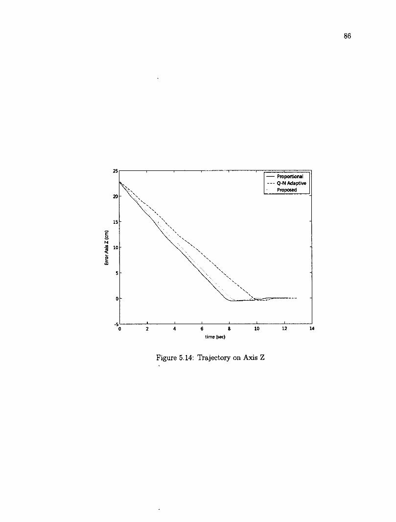
Proportional Q-N Adaptive Proposed

? «Sd> N M

I V-

g LU

time (sec)

Figure 5.14: Trajectory on Axis Z

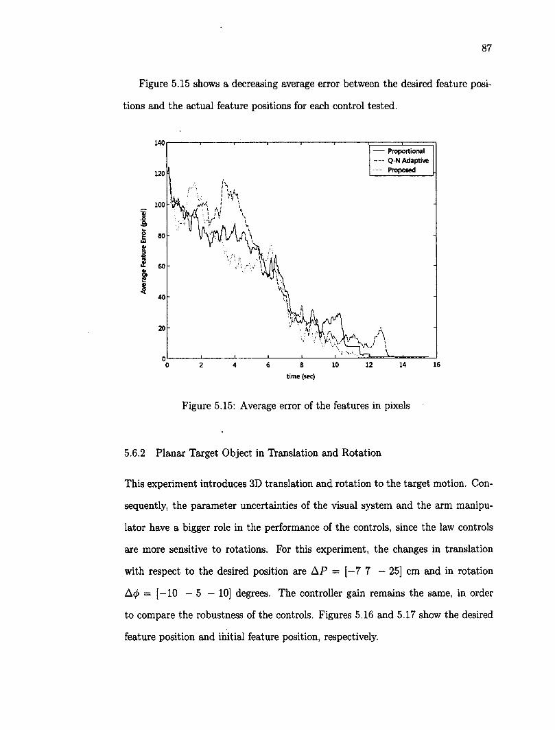
87

Figure 5.15 shows a decreasing average error between the desired feature posi­

tions and the actual feature positions for each control tested.

140 — Proportional — Q-N Adaptive

Proposed 120

100

.8 & w t ui s

£ « O) 2

I

time (sec)

Figure 5.15: Average error of the features in pixels

5.6.2 Planar Target Object in Translation and Rotation

This experiment introduces 3D translation and rotation to the target motion. Con­

sequently, the parameter uncertainties of the visual system and the arm manipu­

lator have a bigger role in the performance of the controls, since the law controls

are more sensitive to rotations. For this experiment, the changes in translation

with respect to the desired position are AP = [—7 7 — 25] cm and in rotation

A4> = [—10 — 5 — 10] degrees. The controller gain remains the same, in order

to compare the robustness of the controls. Figures 5.16 and 5.17 show the desired

feature position and initial feature position, respectively.

Figure 5.16: Desired position of the features

Figure 5.17: Initial position of the features

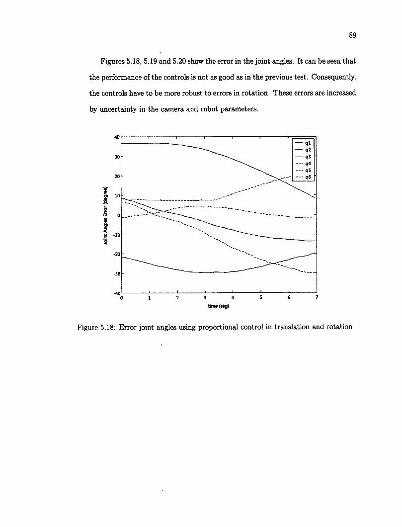
89

Figures 5.18, 5.19 and 5.20 show the error in the joint angles. It can be seen that

the performance of the controls is not as good as in the previous test. Consequently,

the controls have to be more robust to errors in rotation. These errors are increased

by uncertainty in the camera and robot parameters.

--- q5

— q6

I

1

J

-10

-20

-30

-40

Figure 5.18: Error joint angles using proportional control in translation and rotation

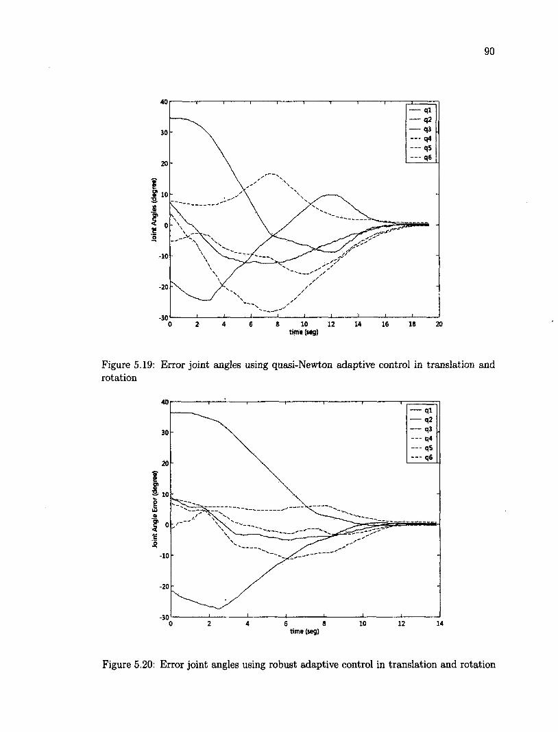
90

— q$

— q6

/ /

-20

-30 4 6 8 10 12 14 16 18 20 0 2

time (sag)

Figure 5.19: Error joint angles using quasi-Newton adaptive control in translation and rotation

— «i q2

- q4

I I LU «

I - / -

€ o

-10

-20

-30 8 10 12 14 0 2 4 6

time (seg)

Figure 5.20: Error joint angles using robust adaptive control in translation and rotation

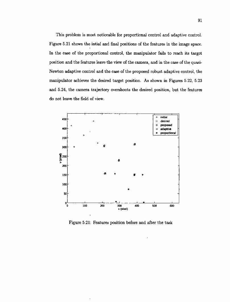
91

This problem is most noticeable for proportional control and adaptive control.

Figure 5.21 shows the intial and final positions of the features in the image space.

In the case of the proportional control, the manipulator fails to reach its target

position and the features leave the view of the camera, and in the case of the quasi-

Newton adaptive control and the case of the proposed robust adaptive control, the

manipulator achieves the desired target position. As shown in Figures 5.22, 5.23

and 5.24, the camera trajectory overshoots the desired position, but the features

do not leave the field of view.

450

400

350

300

3250 & >

200

150

100

50

0 0 100 200 300 400 500 600

u (pixel)

1 t 1 1 + initial

+ o desired

+ O proposed - • adaptive

X * proportional T

+ a

-

- + * 9

A

0 * § *

-

*

i i * i i * 1 I

Figure 5.21: Features position before and after the task

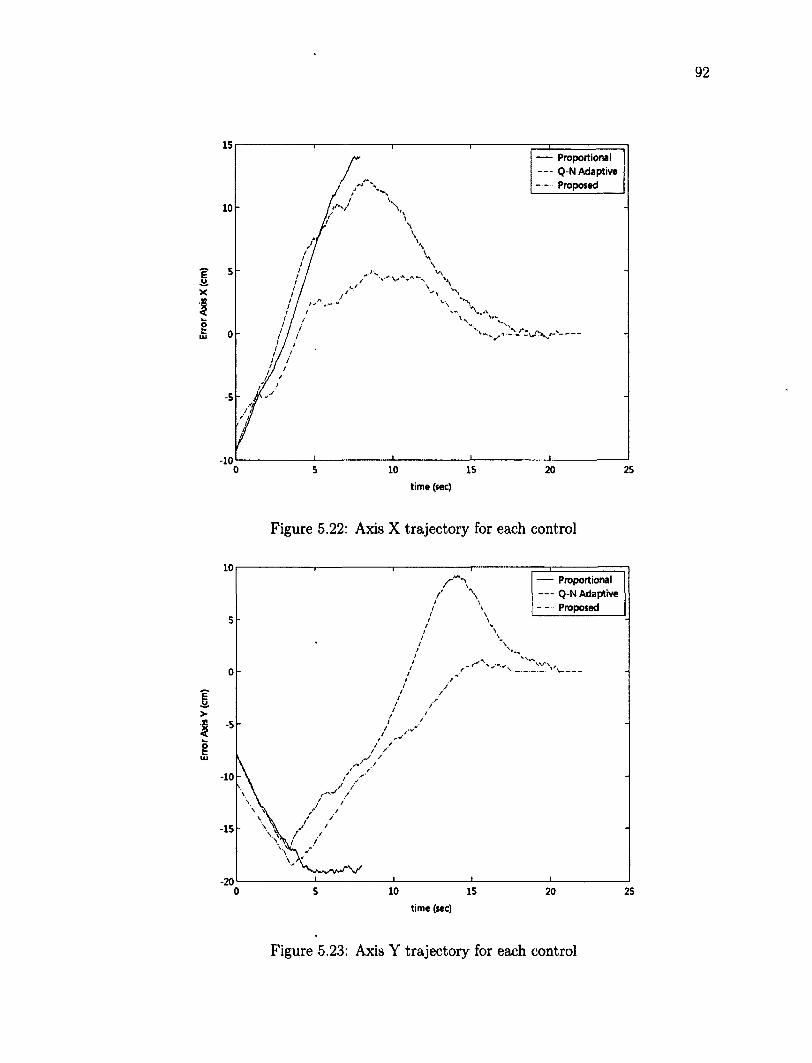
— Proportional — Q-N Adaptive

— Proposed

S

0

5

0 15 5

time (sec)

Figure 5.22: Axis X trajectory for each control

10 — Proportional — Q-N Adaptive

— Proposed 5

0

5 / v

0 15 5 20 25

time (sec)

Figure 5.23: Axis Y trajectory for each control

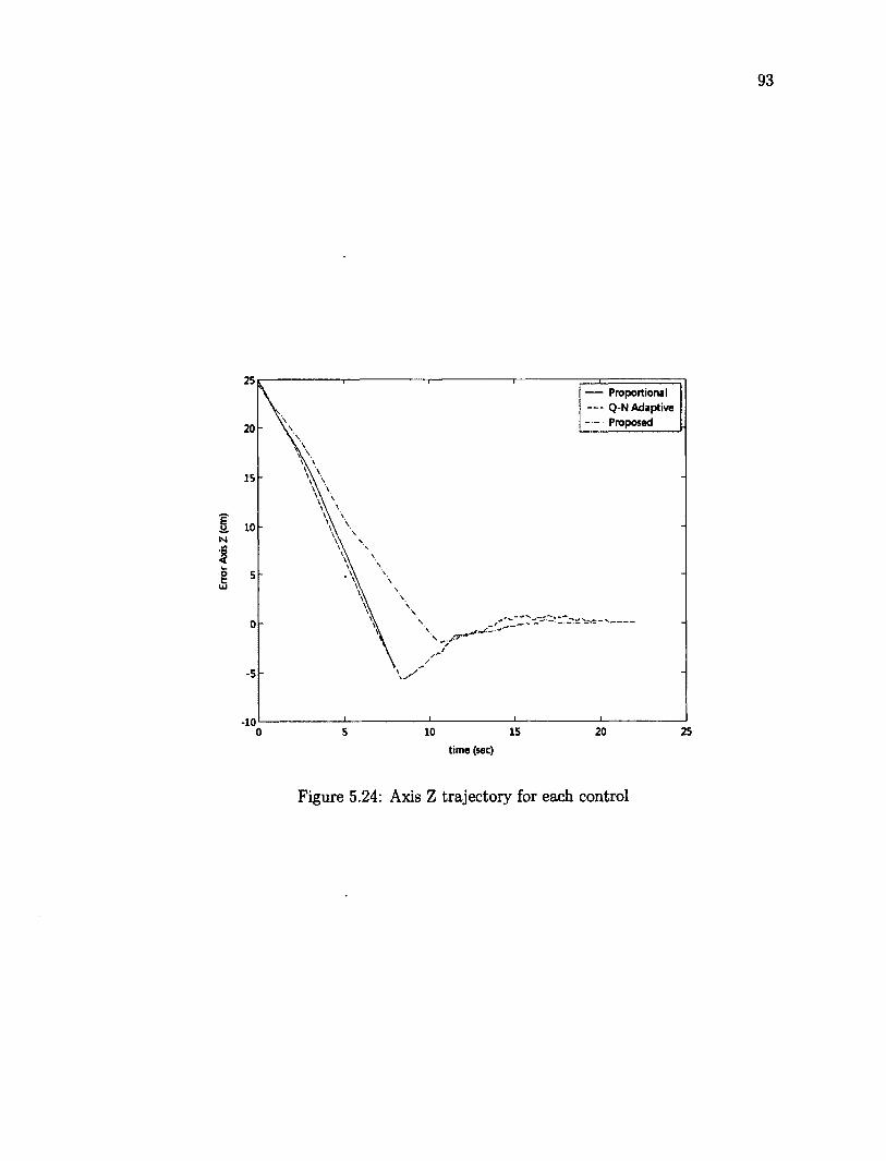
25 Proportional Q-N Adaptive Proposed 20

15

10

5

0

5

10 0

time (sec)

Figure 5.24: Axis Z trajectory for each control

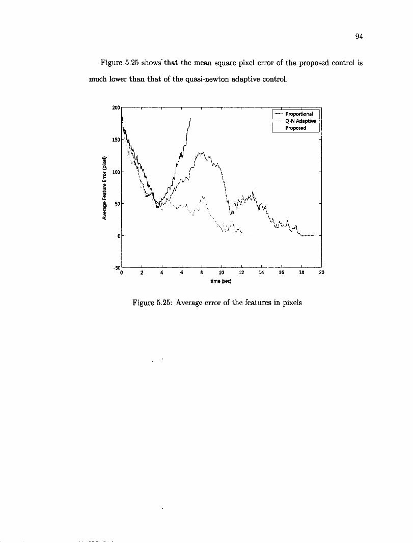
94

Figure 5.25 shows' that the mean square pixel error of the proposed control is

much lower than that of the quasi-newton adaptive control.

I

200

ISO

100

-50

— Proportional -- Q-N Adaptive

Proposed

1 u vV\ v/'v

10

time (sec)

12 14 16 18 20

Figure 5.25: Average error of the features in pixels

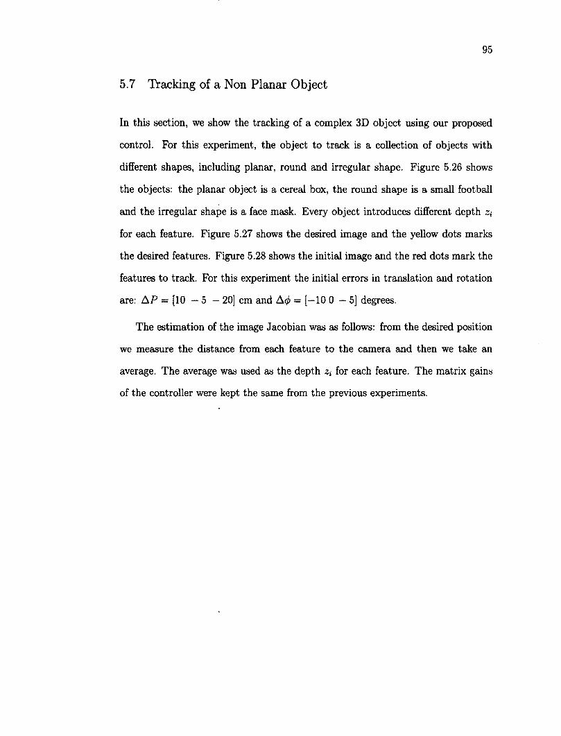
95

5.7 Tracking of a Non Planar Object

In this section, we show the tracking of a complex 3D object using our proposed

control. For this experiment, the object to track is a collection of objects with

different shapes, including planar, round and irregular shape. Figure 5.26 shows

the objects: the planar object is a cereal box, the round shape is a small football

and the irregular shape is a face mask. Every object introduces different depth Zi

for each feature. Figure 5.27 shows the desired image and the yellow dots marks

the desired features. Figure 5.28 shows the initial image and the red dots mark the

features to track. For this experiment the initial errors in translation and rotation

are: AP = [10 — 5 — 20] cm and A<j) = [—10 0 — 5] degrees.

The estimation of the image Jacobian was as follows: from the desired position

we measure the distance from each feature to the camera and then we take an

average. The average was used as the depth Zj for each feature. The matrix gains

of the controller were kept the same from the previous experiments.

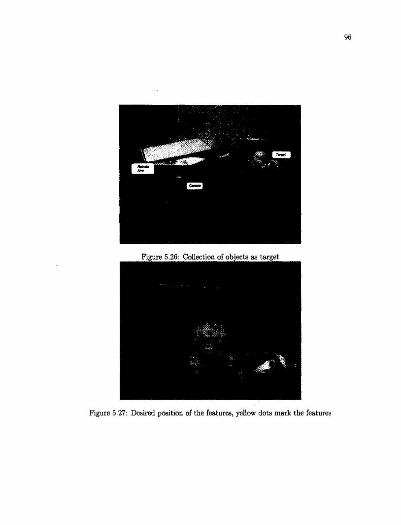
Figure 5.26: Collection of objects as target

Figure 5.27: Desired position of the features, yellow dots mark the features

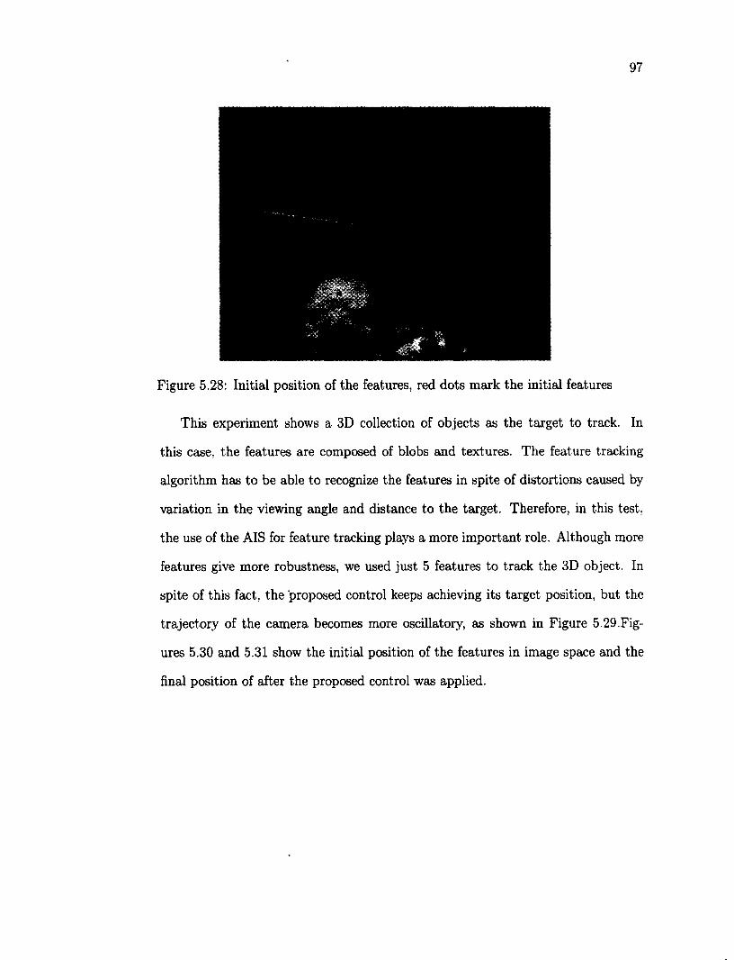
97

Figure 5.28: Initial position of the features, red dots mark the initial features

This experiment shows a 3D collection of objects as the target to track. In

this case, the features are composed of blobs and textures. The feature tracking

algorithm has to be able to recognize the features in spite of distortions caused by

variation in the viewing angle and distance to the target. Therefore, in this test,

the use of the AIS for feature tracking plays a more important role. Although more

features give more robustness, we used just 5 features to track the 3D object. In

spite of this fact, the proposed control keeps achieving its target position, but the

trajectory of the camera becomes more oscillatory, as shown in Figure 5.29.Fig-

ures 5.30 and 5.31 show the initial position of the features in image space and the

final position of after the proposed control was applied.

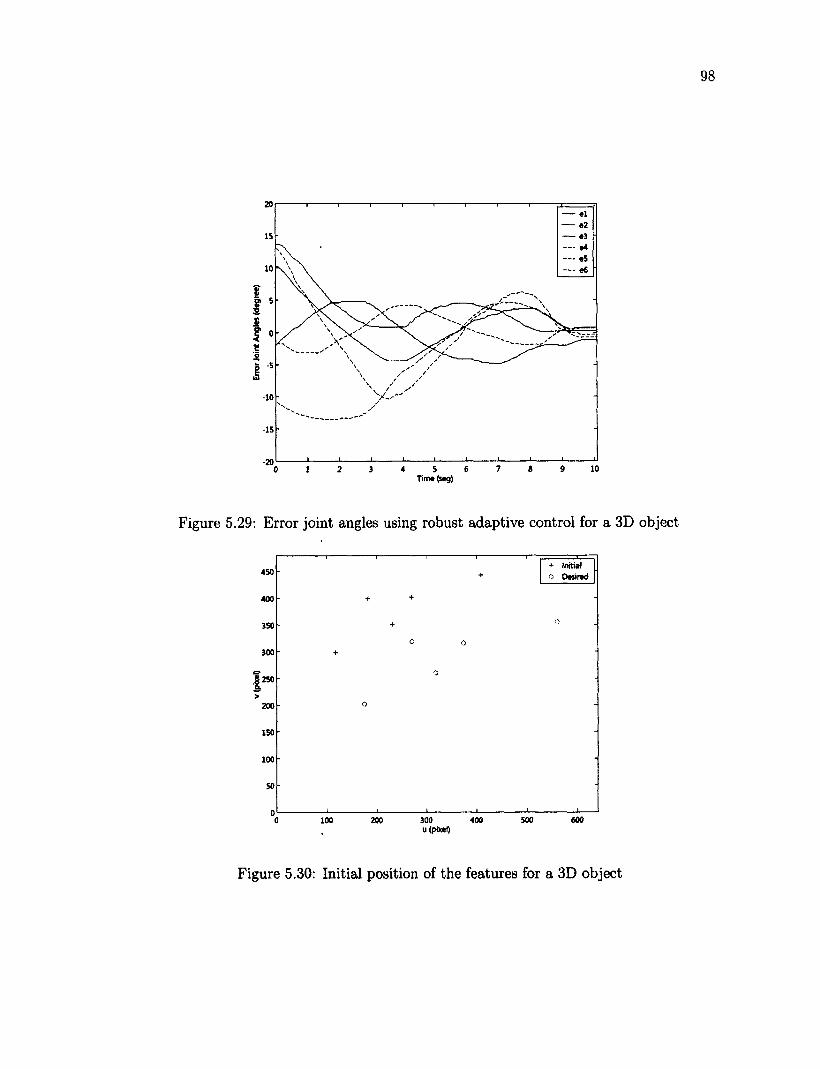
20

IS

10

5

0

-5

10

•15

-20 0 Time (seg)

Figure 5.29: Error joint angles using robust adaptive control for a 3D object

450

400

350

300

1250

200

150

100

600 100 200 300 400 500

+ initial

o Desired

100 200 300 400 u (pixel)

Figure 5.30: Initial position of the features for a 3D object

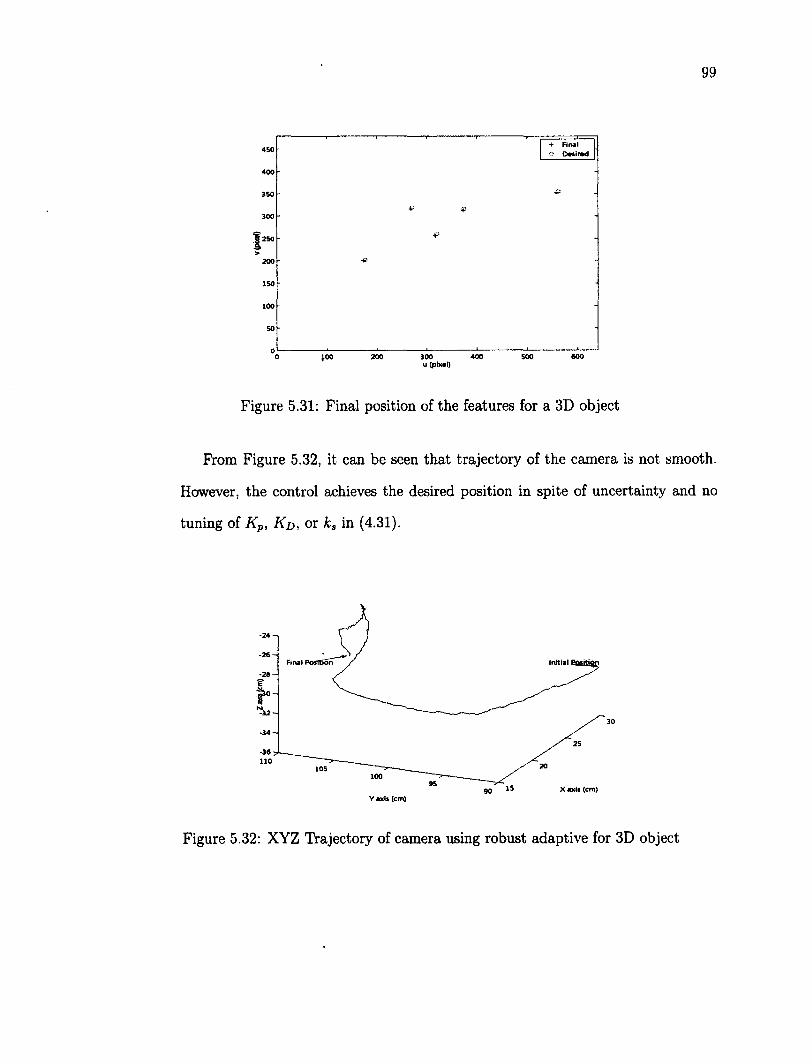
99

450

400

350

300

250

200

150

100

SO

200 300 400 500 600 *00 *00 200 300 400 500 600 u (pixftl)

Figure 5.31: Final position of the features for a 3D object

From Figure 5.32, it can be seen that trajectory of the camera is not smooth.

However, the control achieves the desired position in spite of uncertainty and no

tuning of Kp, K&, or ks in (4.31).

Initial Final

10-

30

25

20 105 100

95 X axis (em) 90

Y axis (cm)

Figure 5.32: XYZ Trajectory of camera using robust adaptive for 3D object

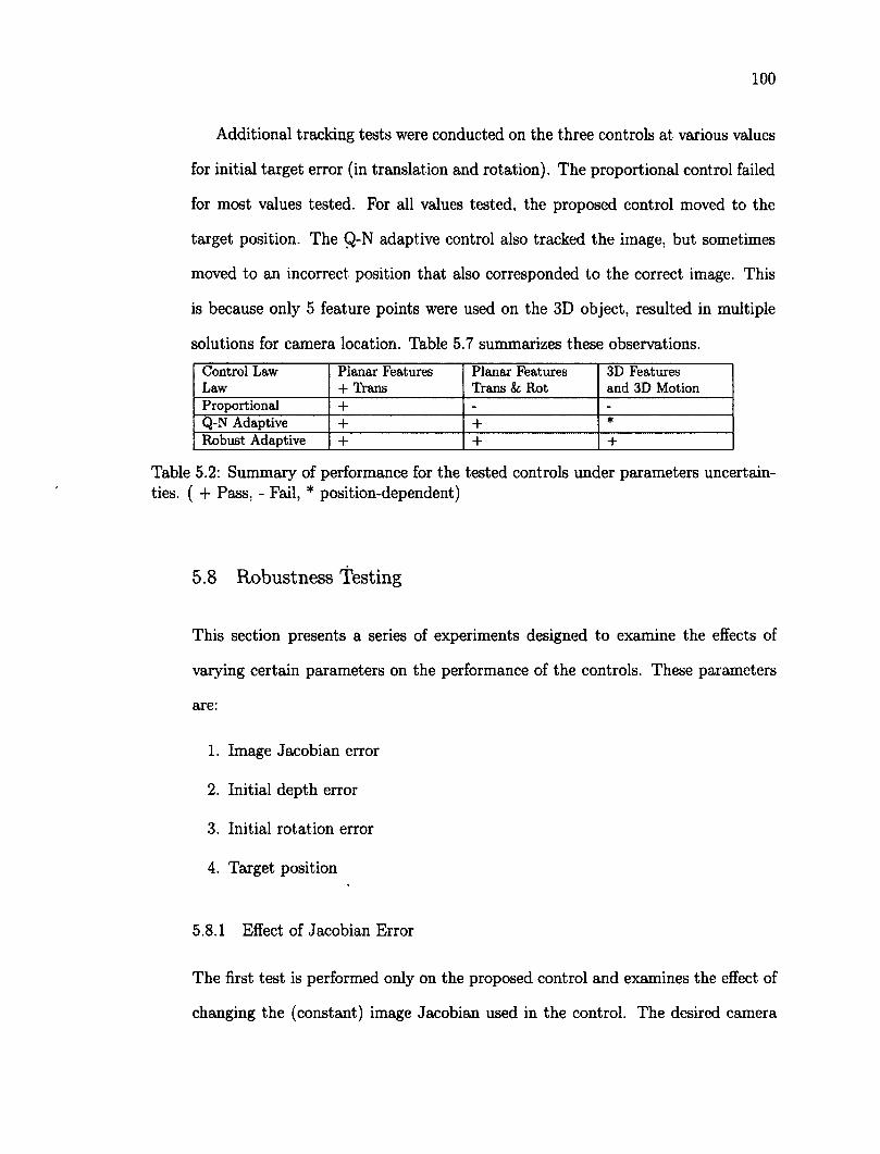
100

Additional tracking tests were conducted on the three controls at various values

for initial target error (in translation and rotation). The proportional control failed

for most values tested. For all values tested, the proposed control moved to the

target position. The Q-N adaptive control also tracked the image, but sometimes

moved to an incorrect position that also corresponded to the correct image. This

is because only 5 feature points were used on the 3D object, resulted in multiple

solutions for camera location. Table 5.7 summarizes these observations.

Control Law Planar Features Planar Features 3D Features Law + Trans Trans & Rot and 3D Motion Proportional + - -

Q-N Adaptive + + •

Robust Adaptive + + +

Table 5.2: Summary of performance for the tested controls under parameters uncertain­ties. ( + Pass, - Fail, * position-dependent)

5.8 Robustness Testing

This section presents a series of experiments designed to examine the effects of

varying certain parameters on the performance of the controls. These parameters

are:

1. Image Jacobian error

2. Initial depth error

3. Initial rotation error

4. Target position

5.8.1 Effect of Jacobian Error

The first test is performed only on the proposed control and examines the effect of

changing the (constant) image Jacobian used in the control. The desired camera

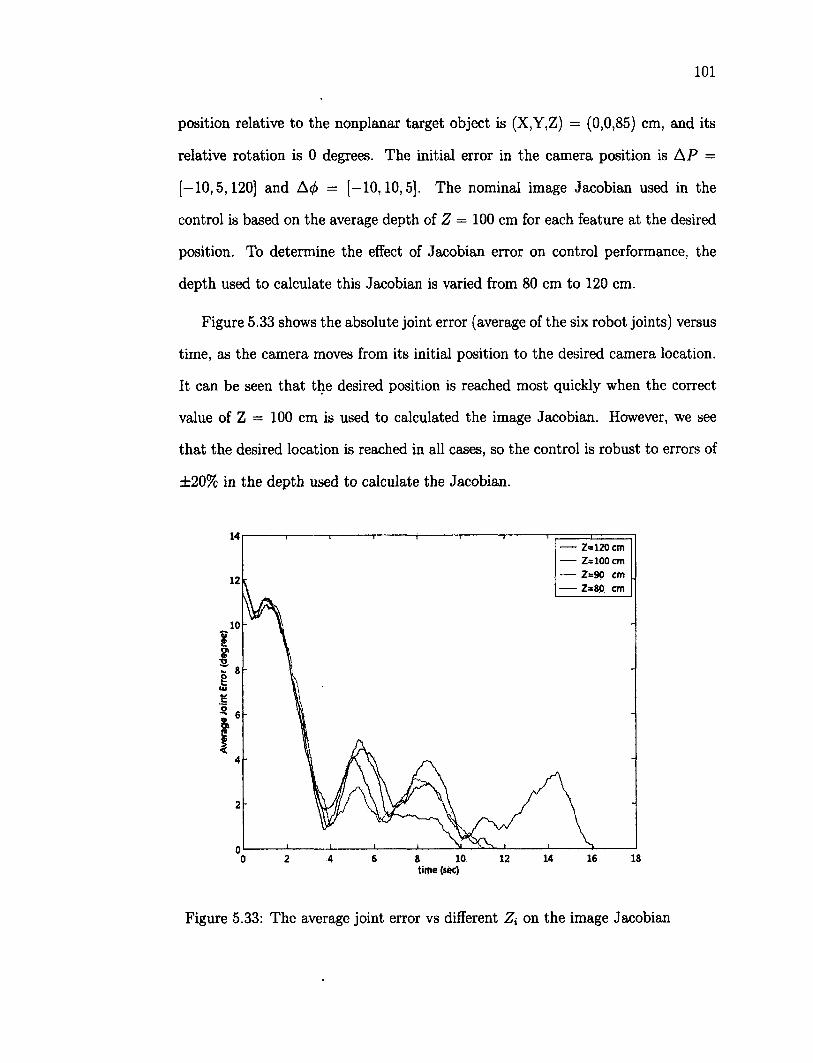
101

position relative to the nonplanar target object is (X,Y,Z) = (0,0,85) cm, and its

relative rotation is 0 degrees. The initial error in the camera position is AP =

[—10,5,120] and A(j> = [—10,10,5]. The nominal image Jacobian used in the

control is based on the average depth of Z = 100 cm for each feature at the desired

position. To determine the effect of Jacobian error on control performance, the

depth used to calculate this Jacobian is varied from 80 cm to 120 cm.

Figure 5.33 shows the absolute joint error (average of the six robot joints) versus

time, as the camera moves from its initial position to the desired camera location.

It can be seen that the desired position is reached most quickly when the correct

value of Z = 100 cm is used to calculated the image Jacobian. However, we see

that the desired location is reached in all cases, so the control is robust to errors of

±20% in the depth used to calculate the Jacobian.

14

12

— 2=120 cm — Z=100 cm — 2=90 em

Z=80 cm

0 0 2 4 6 8 10 12 14 16 18 time (tec)

Figure 5.33: The average joint error vs different on the image Jacobian

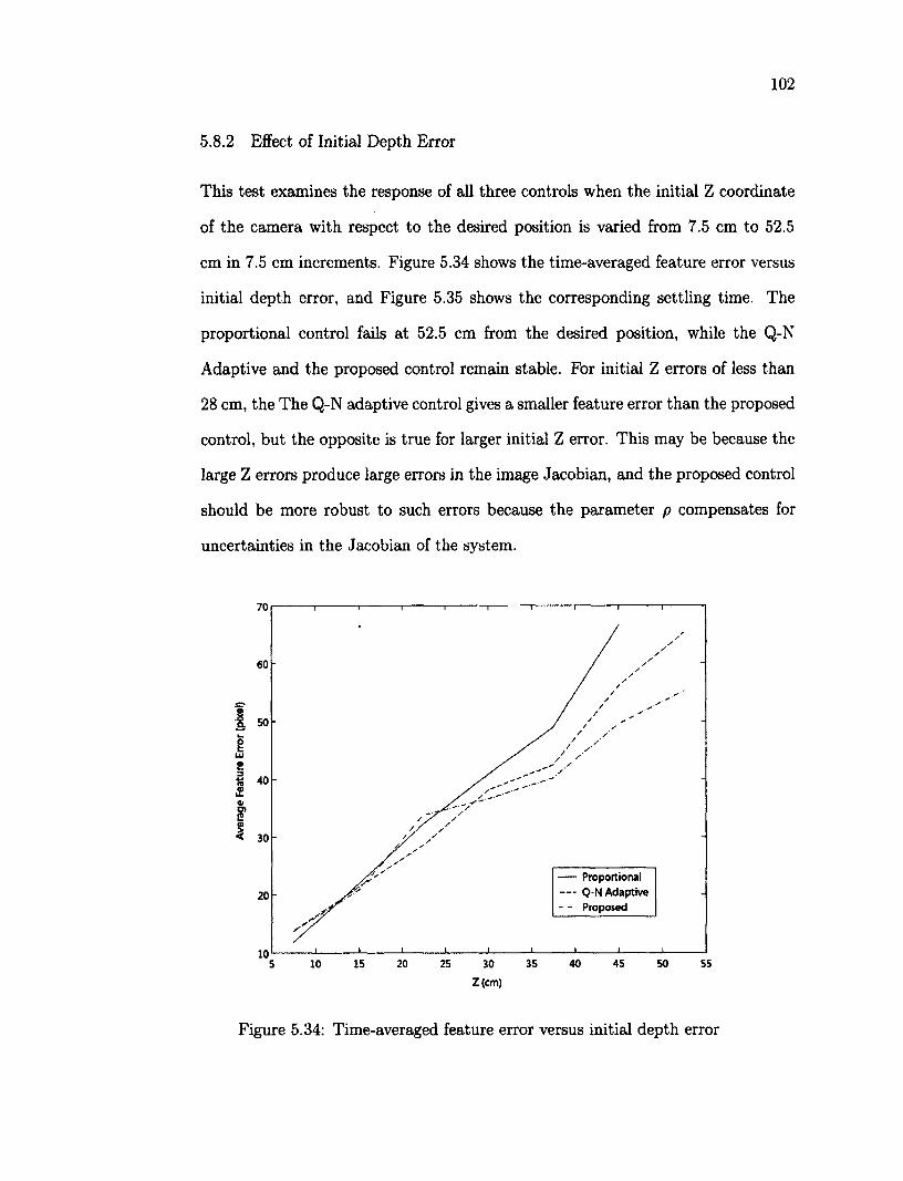
102

5.8.2 Effect of Initial Depth Error

This test examines the response of all three controls when the initial Z coordinate

of the camera with respect to the desired position is varied from 7.5 cm to 52.5

cm in 7.5 cm increments. Figure 5.34 shows the time-averaged feature error versus

initial depth error, and Figure 5.35 shows the corresponding settling time. The

proportional control fails at 52.5 cm from the desired position, while the Q-N

Adaptive and the proposed control remain stable. For initial Z errors of less than

28 cm, the The Q-N adaptive control gives a smaller feature error than the proposed

control, but the opposite is true for larger initial Z error. This may be because the

large Z errors produce large errors in the image Jacobian, and the proposed control

should be more robust to such errors because the parameter p compensates for

uncertainties in the Jacobian of the system.

70

60

40

30

— Proportional — Q-N Adaptive

Proposed 20

10 35 40 15 20 25 45 50 5 30 10

Z(cm)

Figure 5.34: Time-averaged feature error versus initial depth error

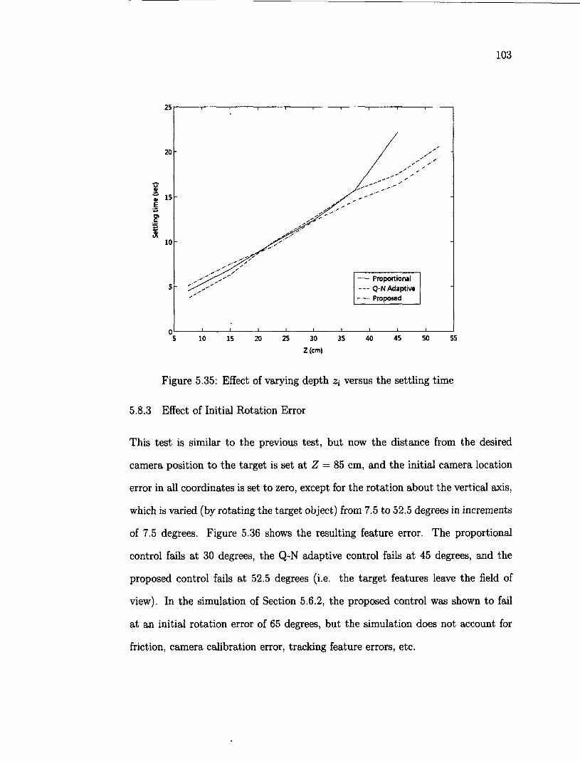
103

20

15

10

— Proportional — Q-N Adaptive

Proposed

5

Z(cm)

Figure 5.35: Effect of varying depth Zi versus the settling time

5.8.3 Effect of Initial Rotation Error

This test is similar to the previous test, but now the distance from the desired

camera position to the target is set at Z — 85 cm, and the initial camera location

error in all coordinates is set to zero, except for the rotation about the vertical axis,

which is varied (by rotating the target object) from 7.5 to 52.5 degrees in increments

of 7.5 degrees. Figure 5.36 shows the resulting feature error. The proportional

control fails at 30 degrees, the Q-N adaptive control fails at 45 degrees, and the

proposed control fails at 52.5 degrees (i.e. the target features leave the field of

view). In the simulation of Section 5.6.2, the proposed control was shown to fail

at an initial rotation error of 65 degrees, but the simulation does not account for

friction, camera calibration error, tracking feature errors, etc.

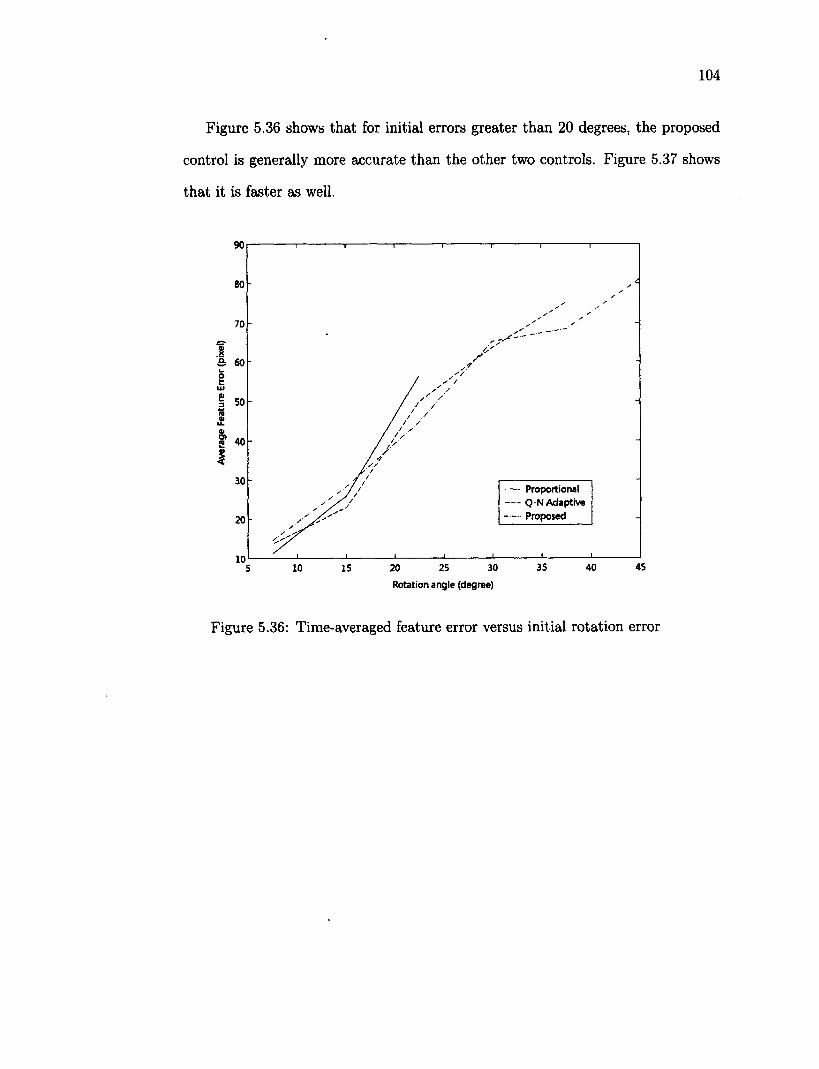
104

Figure 5.36 shows that for initial errors greater than 20 degrees, the proposed

control is generally more accurate than the other two controls. Figure 5.37 shows

that it is faster as well.

— Proportional — Q-N Adaptive

Proposed

20 25 30

Rotation angle (degree)

35 40 45

Figure 5.36: Time-averaged feature error versus initial rotation error

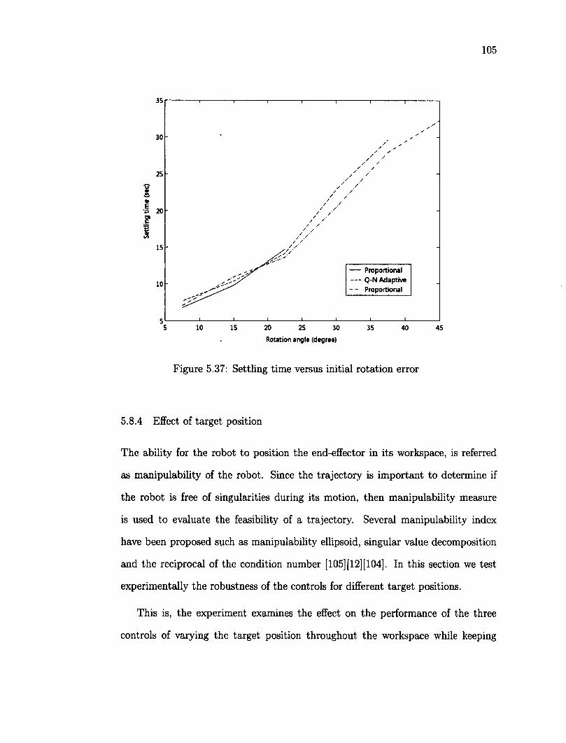
105

35

30

25

1 4>

I 20 jp

1 15

10

5 5 10 15 20 25 30 35 40 45

Rotation angle (degree)

Figure 5.37: Settling time versus initial rotation error

5.8.4 Effect of target position

The ability for the robot to position the end-effector in its workspace, is referred

as manipulability of the robot. Since the trajectory is important to determine if

the robot is free of singularities during its motion, then manipulability measure

is used to evaluate the feasibility of a trajectory. Several manipulability index

have been proposed such as manipulability ellipsoid, singular value decomposition

and the reciprocal of the condition number [105] [12] [104]. In this section we test

experimentally the robustness of the controls for different target positions.

This is, the experiment examines the effect on the performance of the three

controls of varying the target position throughout the workspace while keeping

Proportional Q-N Adaptive Proportional

1

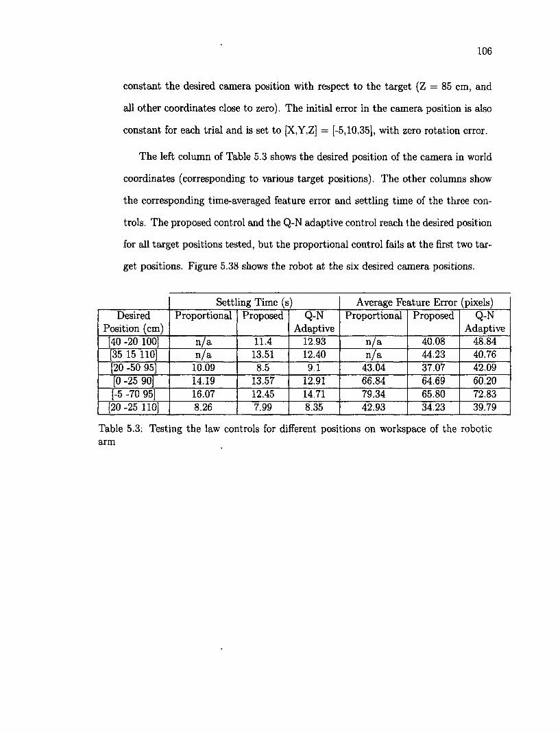
106

constant the desired camera position with respect to the target (Z = 85 cm, and

all other coordinates close to zero). The initial error in the camera position is also

constant for each trial and is set to [X,Y,Z] = [-5,10,35], with zero rotation error.

The left column of Table 5.3 shows the desired position of the camera in world

coordinates (corresponding to various target positions). The other columns show

the corresponding time-averaged feature error and settling time of the three con­

trols. The proposed control and the Q-N adaptive control reach the desired position

for all target positions tested, but the proportional control fails at the first two tar­

get positions. Figure 5.38 shows the robot at the six desired camera positions.

Settling Time (s) Average Feature Error (pixels) Desired Proportional Proposed Q-N Proportional Proposed Q-N

Position (cm) Adaptive Adaptive [40 -20 100] n/a 11.4 12.93 n/a 40.08 48.84 [35 15 110] n/a 13.51 12.40 n/a 44.23 40.76 [20 -50 95] 10.09 8.5 9.1 43.04 37.07 42.09 [0 -25 90] 14.19 13.57 12.91 66.84 64.69 60.20 [-5 -70 95 16.07 12.45 14.71 79.34 65.80 72.83

[20 -25 110] 8.26 7.99 8.35 42.93 34.23 39.79

Table 5.3: Testing the law controls for different positions on workspace of the robotic arm

107

Figure 5.38: Visual servoing control throughout the robot work space

5.9 Tracking a Moving Target Object

5.9.1 Rectangle Trajectory

The control proposed is designed for fixed object position, however we also tested

the ability of the control to track moving objects. In this experiment, the robot

tracked the target shown in Figure 5.6. The target was moved manually around

a 30 cm X 20 cm rectangle in the X-Z plane of the camera without rotating the

target. The desired camera position with respect to the target was set to Z = 80

cm. with all other coordinates set near zero. Tape guides on a table were used to

keep the edges of the reference rectangle straight, but there was some shiver in the

manual motion of the target.

Figure 5.39 shows the reference trajectory and the camera trajectory. The

camera trajectories in the Z direction are seen to be at a slight angle with respect

to the reference edges. This may be due to the target being slightly rotated about

the camera Y axis after the desired target image was taken, since X-displacements

are very sensitive to Y-rotations.

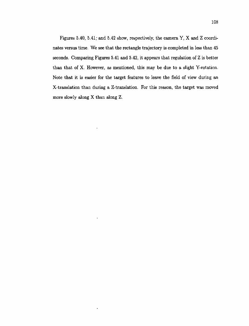
108

Figures 5.40, 5.41; and 5.42 show, respectively, the camera Y, X and Z coordi­

nates versus time. We see that the rectangle trajectory is completed in less than 45

seconds. Comparing Figures 5.41 and 5.42, it appears that regulation of Z is better

than that of X. However, as mentioned, this may be due to a slight Y-rotation.

Note that it is easier for the target features to leave the field of view during an

X-translation than during a Z-translation. For this reason, the target was moved

more slowly along X than along Z.

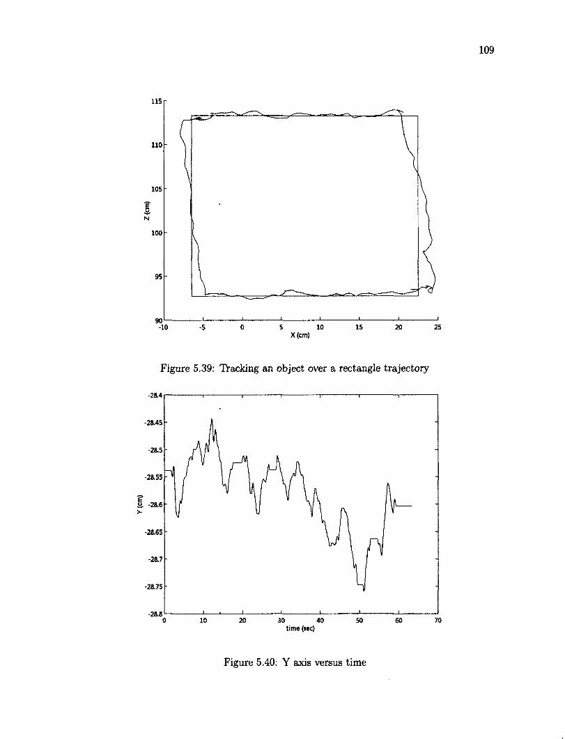
115

110

105

100

95

-10 -5 0 5 10 15 20 25 X(em)

Figure 5.39: Tracking an object over a rectangle trajectory

-28.4

-28.45

-28.5

-28.55

U. -28.6

-28.65

-28.7

-28.75

-28.8 30 50 0 10 20 40 60 70

time (sec)

Figure 5.40: Y axis versus time

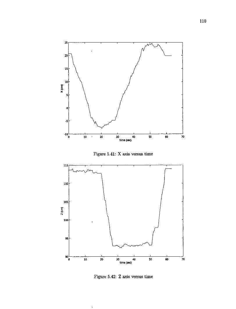
-10

time (sec)

Figure 5.41: X axis versus time

115

110

105

E

N

100

time (sec)

Figure 5.42: Z axis versus time

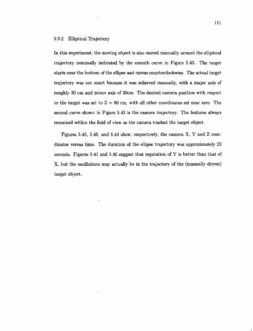
I l l

5.9.2 Elliptical Trajectory

In this experiment, the moving object is also moved manually around the elliptical

trajectory nominally indicated by the smooth curve in Figure 5.43. The target

starts near the bottom of the ellipse and moves counterclockwise. The actual target

trajectory was not exact because it was achieved manually, with a major axis of

roughly 30 cm and minor axis of 20cm. The desired camera position with respect

to the target was set to Z = 80 cm, with all other coordinates set near zero. The

second curve shown in Figure 5.43 is the camera trajectory. The features always

remained within the field of view as the camera tracked the target object.

Figures 5.45, 5.46, and 5.44 show, respectively, the camera X, Y and Z coor­

dinates versus time. The duration of the ellipse trajectory was approximately 23

seconds. Figures 5.41 and 5.40 suggest that regulation of Y is better than that of

X, but the oscillations may actually be in the trajectory of the (manually driven)

target object.

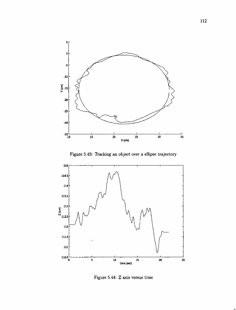
112

10 15 20 25 30 35 X (cm)

Figure 5.43; IVacking an object over a ellipse trajectory

115

114.5

114

113.5

113 -E .u

N

112

111.5

111

110.5 10 15 20 25 0 5

time (sec)

Figure 5.44: Z axis versus time

A

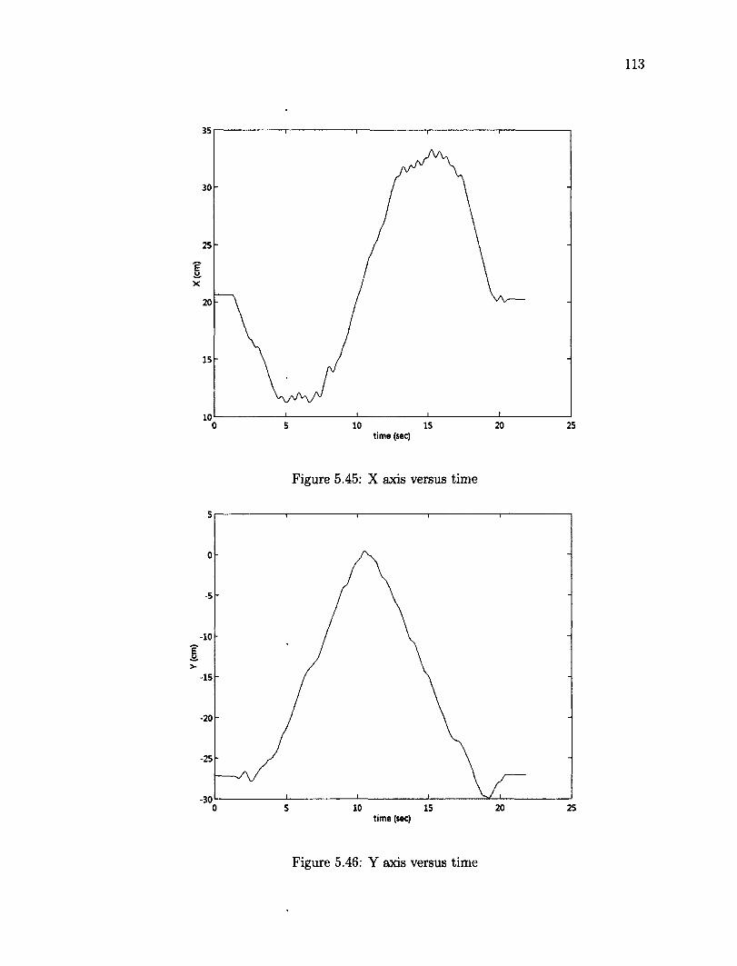
35

30

25

? v.

X

20

15

10 0

time (sec)

Figure 5.45: X axis versus time

-10

>

-15

-20

-25

-30 10 20 0 5 15 25

time (sec)

Figure 5.46: Y axis versus time

114

Chapter 6

Conclusion

6.1 Summary and Conclusions

In this dissertation, we have described the design of an adaptive visual servoing

system that is robust to uncertainties in camera and robot parameters. An im­

portant feature of this system is that the feature tracking software and the robot

control software were both developed from the bottom up and integrated on an

open-architecture platform developed in the lab. This is in contrast to most sys­

tems described in the literature, which integrate commercially-available software

components (for feature tracking, robot control, or both). The advantage of our

approach is that any component can be redesigned or tuned for a particular appli­

cation.

In Chapter 2, we described various approaches to the visual servoing problem

and classified our proposed approach as Image-based Visual Servoing (IBVS).

In Chapter 3, we considered the problem of feature extraction and proposed

a new approach that behaves as an Artificial Immune System (AIS). AIS have

been previously used for optimization, but not for feature extraction in vision sys­

tems. We evaluated the performance of the AIS using histogram and template

object representations, and found that the template representation provided the

best accuracy and processing speed. Experiments showed that the AIS is capable

of tracking objects under affine transformations and nonlinear distortions and can

track multiple features in real time.

115

In Chapter 4, we proposed a novel control that is robust to uncertainties in

robot parameters and in the camera calibration. This control includes an adaptive

component that updates kinematic and dynamic parameters. It also includes a

model of the uncertainty in the extrinsic parameters of the camera calibration,

expressed as an error bound on the system Jacobian. The proposed control was

proved to be stable and the tracking error approaches zero, via Lasalle's invariance

principle. Simulations showed that the control was robust to uncertainty in the

system Jacobian.

In Chapter 5, we presented experiments on a PUMA robot comparing the per­

formance of the proposed control versus that of two other controls (proportional

and Quasi-Newton adaptive). An open-architecture controller (described in Ap­

pendix B) was developed for this purpose.

Sections 5.6 through 5.8 reported experiments involving the tracking of a sin­

gle displacement of an object (versus a continuously-moving object). In Section

5.6, all three controls successfully tracked a planar object in translation, but the

proportional control failed when rotations were included. The proposed control out­

performed the other controls in these tests and reduced settling time in translation

tests by up-to 16 percent.

Section 5.8 presented a series of experiments investigating the robustness of the

controls to changes in four parameters. In 5.8.1, it was shown that the proposed

control was robust to errors in the system Jacobian. The effect of initial camera

depth error was investigated in Section 5.8.2. For large initial errors, the propor­

tional control failed, and the proposed control outperformed the Q-N Adaptive

Control. In Section 5.8.3, it was shown that all three controls fail for sufficiently

large initial rotation errors but that the proposed control is the most robust. Fi­

116

nally, the effect of target position in the workspace was considered in Section 5.8.4.

While the proportional control failed at two positions, the other two controls were

always stable and had similar performance. In Section 5.9, it was shown that the

proposed control can track a planar object moving in the X-Z and X-Y planes, but

at limited speed.

In conclusion, the proposed control was found to be more robust than the pro­

portional control and the Q-N adaptive control and was generally faster and more

accurate. The robustness of the proposed control to uncertainty in camera param­

eters is a useful feature because camera calibration is a slow and tedious process,

and calibration errors can cause instability. Its robustness to robot model uncer­

tainty eliminates the need to change the kinematic and dynamic parameters when

the robot switches to a different tool, for example.

6.2 Limitations and Future Work

The open architecture controller facilitates future improvements of the system to

address current limitations of the proposed control. These are:

- Need for manual tuning The control contains three gains that must be

tuned manually (e.g. by experimentation): the twelve PD gains and the un­

certainty bound p in the system Jacobian. The control would be more adaptive

if it tuned these parameters automatically.

- Improve object target tracking. A modification of the control is needed to

improve the tracking of the object in motion. The inclusion of the estimation

of the velocity of the object requires a control law for non-autonomous systems.

- Improve sample frequencies. Better results may be achieved if the sam-

117

pie frequency increases, by introducing a faster camera frame and processing

power.

- No occlusion handling. The current control requires that all of the target

features be visible. This limits the displacement of the object in the field of

view and does not allow occluding objects in the scene. Therefore, a method­

ology to handle occlusions is needed for some applications.

Bibliography

[1] A. Remazeilles A. Diosi, F. Spindler and F. Chaumette. Visual path following

using only monocular vision for urban environments. Intelligent Robots and

Systems, IROS, December, 2007.

[2] D. Harwood A. Elgammal and L. Davis. Non-parametric model for back­

ground subtraction. In Proceedings of the European Conference on Computer

Vision, pages 751-767, 2000.

[3] L. Xin A. Yilmaz and M. Shah. Contour-based object tracking with occlusion

handling in video acquired using mobile cameras. IEEE Transactions on

Pattern Analysis and Machine Intelligence, 26(11): 1531—1536, 2004.

[4] Y. Adbel-Aziz and H. Karara. Direct linear transformation from comparator

coordinates into object space coordinates in close-range photogrammetry. In

Proc. ASP/UI Symp. on Close-Range Photogrammetry, pages 1-18, Jan ,

1971.

[5] S. Avidan. Ensemble tracking. IEEE Transactions on Pattern Analysis and

Machine Intelligence, 29(2):261—271, 2007.

[6] N.J. Ayache. Artificial vision for mobile robots: Stereo vision and multisen-

sory perception. English translation by P.T. Sanders, MIT , 1991.

[7] F. Chaumette B. Espiau and P.Rives. A new approach to visual servoing

in robotics. IEEE Transactions on Robotics and Automation, 8(3):313—325,

June 1992.

[8] S. T. Birchfield and S. Rangarajan. Spatiograms versus histograms for region-

based tracking. In Proceedings of the IEEE Conference on Computer Vision

and Pattern Recognition, 2:1158-1163, 2005.

118

119

[9] C. M. Bishop. Neural networks for pattern recognition, 1995.

[10] E. Bradski. Computer vision face tracking for use in a perceptual user inter­

face. technical report, intel corporation, 1998.

[11] R. Brunelli. Template Matching Techniques in Computer Vision: Theory and

Practice. John Wiley and Sons, 2009.

[12] Gosselin C. Dexterity indices for planar and spatial robot manipulator.

Robotics and Automation Proc. Int. Conf., Vol 1, pages 650-655, 1990.

[13] O. Camps C. Gentile and M. Sznaier. Segmentation for robust tracking in

the presence of severe occlusion. IEEE Transactions on Image Processing,

13(2) :166—178, 2004.

[14] B. Z. Yuan C. K. Wan and Z. J. Miao. A new algorithm for static camera

foreground segmentation via active coutours and gmm. In Proceedings of the

IEEE International Conference on Pattern Recognition, pages 1-4, 2008.

[15] M. Le Borgne C. Samson and B. Espiau. Robot control, the task function

approach. Robotica, Oxford University Press, 1991.

[16] M. J. Brooks C. Shen and A. van den Hengel. Augmented particle filtering for

efficient visual tracking. In Proceedings of the IEEE International Conference

on Image Processing, 3:856-859, 2005.

[17] S. Peeta C. Shu-Ching, S. Mei-Ling and Z. Chengcui. Learning-based

spatio-temporal vehicle tracking and indexing for transportation multimedia

database systems. IEEE Transactions on Intelligent Transportation Systems,

4(3).154-167, 2003.

[18] R. Duraiswami C. Yang and L. Davis. Fast multiple object tracking via a hi­

erarchical particle filter. In Proceedings of the IEEE International Conference

on Computer Vision, 1:212-219, 2005.

120

[19] Gleason Carlisle and McGhie. The puma/vs-100 robot vision system. Proc.

of the fist International Conference on Robot Vision and, Sensory Controls,

pages 149-160, 1981.

[20] A. Castano and S. Hutshinson. Visual compliance: Task-directed visual servo

control. IEEE Transactions on Robotics and Automation, 10(3):334-345,

June 1994.

[21] C. Chang and R. Ansari. Kernel particle filter for visual tracking. IEEE

Signal Processing Letters, 12(3):242-245, 2005.

[22] Francois Chaumette. The confluence of vision and control. Chapter: Poten­

tial problems of stability and convergence in image-based and position-based

visual servoing. Springer-Verlag, 1999.

[23] Francois Chaumette and Ezio Malis. 2 1/2 visual servoing: a possible solution

to improve image-based and position-based visual servoings. IEEE Int. Conf

on Robotics and Automation, ICRA2000, 2000.

[24] Macnab CJB. Preventing bursting in approximate-adaptive control when

using local basis functions. Fuzzy Sets Systems, pages 439-462, 2009.

[25] D. Comaniciu and P. Meer. Robust analysis of feature spaces: color image

segmentation. In Proceedings of the IEEE Conference on Computer Vision

and Pattern Recognition, pages 750-755, 1997.

[26] D. Comaniciu and P. Meer. Mean shift: a robust approach toward feature

space analysis. IEEE Transactions on Pattern Analysis and Machine Intelli­

gence, pages 603-619, 2002.

[27] P.I. Corke. Visual servo control of manipulators -a review. In K. Hashimoto,

editor, Visual Servoing, 7:1—31, 1993.

121

[28] P.I. Corke and S.A. Hutchinson. Real-time vision, tracking and control. In

Proc. IEEE Intl. Conf. on Robotics and Automation, pages 622-629, April

2000.

[29] J. Czyz. Object detection in video via particle filters. In Proceedings of the

IEEE International Conference on Pattern Recognition, 1:820-823, 2006.

[30] M. Nachtegael D. Van der Weken and E. Kerre. Using similarity measures

for histogram comparison. In Fuzzy Sets and Systems, 56(1):1—9, 2003.

[31] K. Deguchi. Optimal motion control for image-based visual servoing by de­

coupling translation and rotation. In Proc. IEEE/RSJ Intl. Conf. on Robotics

and systems, pages 705-711. October, 1998.

[32] F. Dionnet and E. Marchand. Stereo tracking and servoing for space appli­

cations. Advanced Robotics, 23(5):579-599, April, 2009.

[33] T. Drummond and R. Cipolla. Real-time tracking of multiple articulated

structures in multiple views. In Proc. 6th European Conference on Computer

Vision, volume 2:20-36, July, 2000.

[34] R. Freund E. Osuna and F. Girosit. Training support vector machines: an

application to face detection. In Proceedings of the IEEE Conference on

Computer Vision and Pattern Recognition, pages 130-136, 1997.

[35] B. Espiau. Effect of camera calibration errors on visual servoing in robotics.

In Proc. 3th Int. Sym. Experimental Robotics, Kyoto, Oct., 1993.

[36] P.Martinet F. Berry and J. Gallice. Real time visual servoing around a com­

plex object. IEICE Transactions on Information and Systems, E83-D:1358-

1368, July 2000.

[37] P.Rives F. Chaumette and B. Espiau. Robot motion planning. In Proc. IEEE

Intl. Conf. on Robotics and Automation, 3:2248-2253, Sacramento, 1991.

122

[38] O.D. Faugeras and G. Toscani. The calibration problem for stereo. In Proc.

conf. Computer Vision and Pattern Recognition, pages 15-20, 1986.

[39] R. Feghali and A. Mitiche. Spatiotemporal motion boundary detection and

motion boundary velocity estimation for tracking moving objects with a mov­

ing camera: a level sets pdes approach with concurrent camera motion com­

pensation. IEEE Transactions on Image Processing, 13(11); 1473-1490, 2004.

[40] D. Dawson Frak Lewis and C. Abdallah. Robot maipulator control: theory

and, practice. Marcel Dekker, Englewood Cliffs, NJ, 2004.

[41] Y.Mezouar G. Blanc, O. Ait-Aider and T. Chauteau. Autonomous image-

based navigation in indoor enviroment. Symposium on Intelligent Au­

tonomous Vehicles, Portugal, July, 2004.

[42] M. Dewan G. D. Hager and C. V. Stewart. Multiple kernel tracking with ssd.

In Proceedings -of the IEEE Conference on Computer Vision and Pattern

Recognition, 1:790-797, 2004.

[43] J.Szewczyk G. Morel, T.Liebezeit and S. Boudet. Lecture notes in control

and information sciences. Experimental Robotics VI, 250:99-108, 2000.

[44] H. Krim G. Unal and A. Yezzi. Fast incorporation of optical flow into active

polygons. IEEE Transactions on Image Processing, 14(6):745-759, 2005.

[45] D. Gamerman. Markov chain monte carlo: stochastic simulation for bayesian

inference. 2006.

[46] S. Baluja H. A. Rowley and T. Kanade. Neural network-based face detection.

IEEE Transactions on Pattern Analysis and Machine Intelligence, pages 23-

38, 1998.

[47] G.D. Hager. A modular system for robust positioning using feedback stereo

123

vision. IEEE Transactions on Robotics and Automation, 13(4):582-595, Au­

gust, 1997.

[48] R. I. Hartley and A. Zisserman. Multiple View Geometry in Computer Vision.

Cambridge University Press, second edition, 2004.

[49] J. Hill and W.T. Park. Real time control of a robot with a mobile camera.

In Proc. 9th International Symposium on Industrial Robots, pages 233-246,

Washington D.C, March 1979.

[50] Steven A. Hofmeyr. An interpretation introduction to the immune system.

Dept. of Computer Science, Univ. of New Mexico, April 25, 2000.

[51] N. Hollinghurst. Uncalibrated stereo and hand-eye coordination. PhD Thesis,

Deparment of Engineering, University of Cambridge, 1997.

[52] N. Hollinghurst and R. Cipolla. Uncalibrated stereo hand-eye coordination.

Image and Vision Computing, 12(3):187—192, 1994.

[53] J. J. Hopfield. Neural networks and physical systems with emergent collective

computational abilities. Proceedings of the National Academy of Sciences of

the United States of America, 79(8):2554-2558, 1988.

[54] D. F. Llorca I. P. Alonso and M. A. Sotelo. Combination of feature extraction

methods for svm pedestrian detection. IEEE Transactions on Intelligent

Transportation Systems, 8(2):292-307, 2007.

[55] Unimation Inc. Unimate Puma 700 robot Volume 1: Technical Manual, Ver­

sion 2.0. Danbury, 1986.

[56] Wang J. Optimal estimation of 3d relative position and orientation for robot

control. M.A.Sc. dissertation, Dept. Electrical and Computer Engineering,

Univ. Waterloo, Canada, 1992.

124

[57] A. Bernardino J. Melo, A. Naftel and J. Santos-Victor. Detection and classifi­

cation of highway lanes using vehicle motion trajectories. IEEE Transactions

on Intelligent Transportation Systems, 7(2):188-200, 2006.

[58] A. Tabb J. Park and A. C. Kak. Hierarchical data structure for real-time

background subtraction. In Proceedings of the International Conference on

Image processing, pages 1849-1852, 2006.

[59] D. Gao J. Zhou and D. Zhang. Moving vehicle detection for automatic traffic

monitoring. IEEE Transactions on Vehicular Technology, 56(1):51—59, 2007.

[60] R. C. Jain and H. H. Nagel. On the analysis of accumulative difference

pictures from image sequences of real world scenes. IEEE Transactions on

Pattern Analysis and Machine Intelligence, 1(2):206—213, 1979.

[61] I. Horiba K. Suzuki and N. Sugie. Fast connected-component labeling based

on sequential local operations in the course of forward raster scan followed by

backward raster scan. In Proceedings of the IEEE International Conference

on Pattern Recognition. 2:434-437, 2000.

[62] K. Konolige. Small vision systems: hardware and implementation. The 8th

International Sysmposium on Robotics Research, pages 203-212, October,

1997.

[63] D. Kragic and H. Christensen. Survey on visual servoing for manipulation.

Technical Report ISRN, Department of Numerical Analysis and Computing

Science, Sweden, 2001.

[64] D. Kragic and H.I. Christensen. A framework for visual servoing tasks. In­

telligent Autonomous Systems, 6:835-842, Italy, 2000.

[65] I. Kukenys and B. McCane. Classifier cascades for support vector machines.

In Proceedings of the International Conference Image and Vision Computing,

125

pages 1-6, New Zealand, 2008.

[66] Z. Liu L. Chen, J. Zhou and W. Chen. A skin detector based on neural

network. In Proceedings of the IEEE International Conference on Commu­

nications, Circuits and Systems and West Sino Expositions, 1:615-619, 2002.

[67] J.C Latombe. Robots Motion Planning. Springer, 1991.

[68] H. J. Lee and M. C. Lee. Color-based visual servoing of a mobile manipulator

with stereo vision. The International Federation of Automatic Control, Korea.

July, 2008.

[69] J. Li and S. Chin-Chua. Transductive inference for color-based particle filter

tracking. In Proceedings of the IEEE International Conference on Image

Processing, 3:949-952, 2003.

[70] Z. Liang and C. E. Thorpe. Stereo and neural network-based pedestrian de­

tection. IEEE Transactions on Intelligent Transportation Systems, 1(3) :148—

154, 2000.

[71] Daniel Liberzon. Switching in systems and control. Birkhauser Boston, 2003.

[72] Ficocelli M. and Janabi-Sharifi. Adaptive filtering for pose estimation in

visual servoing. Int. Conf. On Intelligent Robots and Systems, pages 19-24,

Hawwaii, 2001.

[73] J. Denzler M. Zobel and H. Niemann. Entropy based camera control for

visual object tracking. In Proceedings of the IEEE International Conference

on Image Processing, 3:901-904, 2002.

[74] E. Makinen and R. Raisamo. Evaluation of gender classification methods

with automatically detected and aligned faces. IEEE Transactions on Pattern

Analysis and Machine Intelligence, 30(3):541-547, 2008.

126

[75] Chaumette F. Malis E. and Boudet S. 2-1/2-d visual servoing. IEEE Trans­

action Robotic and Automation, 15:238-250, October, 1999.

[76] D. Marr and T. Poggio. A cooperative computation of stereo-disparity. Sci­

ence, 194(4262):283-287, 1990.

[77] P. Martinet and E. Cervera. Real time visual servoing around a complex

object. Proc. IEEE Intl. Conf. on Robotics and Automation, pages 717-722,

Seoul,Korea, May 2001.

[78] K. Nickels and S. Hutchinson. Weighting observations: the use of kinematic

models in object tracking. In Proceedings of the IEEE International Confer­

ence on Robotics and Automation, 2:1677-1682, 1998.

[79] Ono M. Ogawa H. and MAsukake Y. Model following adaptive control based

on least squares method. Control, Automation and Systems, ICCAS, pages

638-641, 2008.

[80] Ioanou P. and J. Sun. Robust Adaptive Control. Prentice-Hall, 1996.

[81] Viola P. and Jones M. Rapid object detection using a boosted cascade of

simple features. In IEEE Computer Vision and Pattern Recognition, 1:511—

518, 2001.

[82] S. L. Phung P. Bouttefroy, A. Bouzerdoum and A. Beghdadi. Vehicle tracking

by non-drifting mean-shift using projective kalman filter. In Proceedings of

the IEEE Conference on Intelligent Transportation Systems, pages 61-66,

2008.

[83] N. Papanikolopoulos and C. Smith. Computer vision issues during eye-in-

hand robotic tasks. In Proc. IEEE Intl. Conf. on Robotics and Automation,

volume 3:2989-2994, 1995.

127

[84] A.P. del Pobil P.J. Sanz and J.M. Inesta. Vision-guided grasping of unknown

objects for service robots. In Proc. IEEE Intl. Conf. on Robotics and Au­

tomation, pages 3018-3025, 1998.

[85] B.H Yoshimi P.K. Allen, A. Timcenko and P. Michelman. Automatic tracking

and grasping of a moving object with a robotic hand-eye system. IEEE

Transactions on Robotics and Automation, 9(2):152—165, April 1993.

[86] Macmillan Publishers. The macquarie dictionary, 2005.

[87] F. Dornaika R. Horaud and B. Espiau. Visually guided grasping. IEEE

Transactions on Robotics and Automation, 14(4):525—532, August, 1998.

[88] F. Perez-Cruz R. Santiago-Mozos, J. M. Leiva-Murillo and A. Artes Ro­

driguez. Supervised-pca and svm classifiers for object detection in infrared

images. In Proceedings of the IEEE Conference on Advanced Video and Sig­

nal Based Surveillance, pages 122-127, 2003.

[89] Domenico Ribatti. Sir frank macfarlane burnet and the clonal selection theory

of antibody formation. Clinical and Experimental Medicine, 9:253-258, 2009.

[90] H. L. Ribeiro and A. Gonzaga. Hand image segmentation in video sequence

by gmm: a comparative analysis. In Proceedings of the Brazilian Symposium

on Computer Graphics and Image Processing, pages 357-364, 2006.

[91] A. Rizzi and D. Koditschek. Preliminary experiments in spatial robot

juggling. Proc. 2nd International Symposium on Experimental Robotics,

190:282-298, Toulouse, France, June 1991.

[92] F. Rosenblatt. The perceptron: A probabilistic model for information storage

and organization in the brain, 1958.

[93] M. C. Shin S. Jayaram, S. Schmugge and L. V. Tsap. Effect of colorspace

transformation, the illuminance component, and color modeling on skin de­

128

tection. In Proceedings of the IEEE Conference on Computer Vision and

Pattern Recognition, 2:813-818, 2004.

[94] A. Bouzerdoum S. L. Phung and D. Chai. Skin segmentation using color

pixel classification: analysis and comparison. IEEE Transactions on Pattern

Analysis and Machine Intelligence, 27(1): 148-154. 2005.

[95] J. W. Davis S. S. Intille and A. F. Bobick. Real-time closed-world tracking.

In Proceedings of the IEEE Conference on Computer Vision and Pattern

Recognition, pages 697-703, 1997.

[96] V. Salari and I. K. Sethi. Feature point correspondence in the presence of

occlusion. IEEE Transactions on Pattern Analysis and Machine Intelligence,

12(1):87—91, 1990.

[97] Sang-Hyun Nam Sang Shin and Hyun Geun Yu. Conveyor visual tracking us­

ing robot vision. FCRAR Florida Conference on Recent Advances in Robotics,

2006.

[98] Shankar Sastry and Marc Bodson. Adaptive Control: Stability, Converge and

Robustness. Prentice-Hall, 1994.

[99] I. J. Schoenberg. Contribution to the problem of approximation of equidistant

data by analytic function. Quarterly of Applied Mathematics, pages 45-99,

1946.

[100] Y. Shirai and H. Inoue. Guiding a robot by visual feedback in assembling

tasks. Pattern Recognition, 5:99-108, 1973.

[101] G.D. Hager S.Hutchinson and P.I. Corke. A tutorial on visual servo control.

IEEE Transactions on Robotics and Automation, 12:651-670, October 1996.

[102] Jean-Jacques Slotine and Weiping Li. On the adaptive control of robot ma­

nipulators. IEEE Int. Conf. Robotics And Automation, 1986.

129

[103] Jeffrey Spooner. Stable adaptive control and estimation for nonlinear systems.

John Wiley and Sons, 2002.

[104] Tanev T. and Stoyanov B. On performance indexes fo robot manipulators.

Problems of enfineering cybernetics and robotics, 2000.

[105] Yoshikawa T. Manipulability of robotics mechanisms. Int. Journal of

Robotics Research, Vol. 4, pages 3-9, 1985.

[106] M. Lu T. Ying-Li and A. Hampapur. Robust and efficient foreground analysis

for real-time video surveillance. In Proceedings of the IEEE Conference on

Computer Vision and Pattern Recognition, 1:1182-1187, 2005.

[107] R.Y. Tsai and R.K. Lenz. Techniques for calibration of the factor and image

center for high accuracy 3d machine vision. IEEE Trans. Pattern Analysis

and Machine Intell, 10:713-720, 1988.

[108] M. Unser. Splines: a perfect fit for signal and image processing. IEEE Signal

Processing Magazine, 16(6):22-38, 1999.

[109] B. Siciliano V. Lippiello and L. Villani. Eye-in-hand/ eye-to-hand multi-

camera visual servoing. IEEE Conference on Decision and Control, Spain,

December, 2005.

[110] P. Vadakkepat and L. Jing. Improved particle filter in sensor fusion for track­

ing randomly moving object. IEEE Transactions on Instrumentation and

Measurement, 55(5):1823-1832, 2006.

[111] N. V. Vladimir. The nature of statistical learning theory, 1995.

[112] D. M. Weber and D. P. Casasent. Quadratic gabor filters for object detection.

IEEE Transactions on Image Processing, 10(2):218-230, 2001.

[113] W. wilson. Visual servo control of robots using kalman filter estimates of

130

robot pose relative to work-pieces. In K. Hashimoto, editor, Visual Servoing,

pages 71-104, 1994.

[114] Williams Hulls Wilson W.J. and Janabi-Sharifi. Robust image processing

and position-based visual servoing. Robust Vision for Vision-Based Control

of Motion, IEEE Press, pages 163-201, 2000.

[115] L. Xingzhi and S. M. Bhandarkar. Multiple object tracking using elastic

matching. In Proceedings of the IEEE Conference on Advanced Video and

Signal Based Surveillance, pages 123-128, 2005.

[116] N. Vaswani Y. Rathi and A. Tannenbaum. A generic framework for tracking

using particle filter with dynamic shape prior. IEEE Transactions on Image

Processing, 16(5): 1370-1382, 2007.

[117] B.H. Yoshimi and P.K. Allen. Vision control grasping and manipulation

tasks. In Proc. IEEE Intl. Conf. on Multisensor Fusion and Integration of

Intelligence Systems, pages 575-582, 1994.

[118] J.S. Yuan. A general photogrammetric method for determining object posi­

tion and orientation. IEEE Trans. Robotic and Automation, 5:129-142, 1989.

[119] T. Zhao and R. Nevatia. Tracking multiple humans in complex situa­

tions. IEEE Transactions on Pattern Analysis and Machine Intelligence,

26(9): 1208-1221, 2004.

[120] D. Zhou and H. Zhang. Modified gmm background modeling and optical flow

for detection of moving objects. In Proceedings of the IEEE International

Conference on Systems, 3:2224-2229, 2005.

[121] Jun Zhou and Christopher M. Clark. Autonomous fish tracking by rov using

monocular camera. Canadian Conference on Computer and Robot Vision,

2006.

131

Appendix A

Definitions

Norm

The norm \x\ of a vector a; is a real valued function with the follow properties:

- |a;| > 0 with |a;| if and only if x = 0

- |aa;| = |a| |x| for any scalar a

- I# + y\ < M + M (triangle inequality, this shows that norms are continuous

functions).

Induced norm

The induced norm ||AJ| of a matrix A e JJmXn is define by

|| A|| = sup W and satisfies the next properties: I/O 11

- \Ax\ < P|| |x|

- \\A + f?|| < ||i4|| + ||S||

- ||AB|| < ||i4|| ||5||.

Function norm

The Cp norm for a function is define as

for p € [1, oo) and ||a;|| exists when is finite.

Equilibrium point

x * is an equilibrium point of a system x = f ( x , t ) and x ( t 0 ) = x 0 if f { x * , t ) = 0 for

all t > 0.

132

Stable point (in the Lyapunov sense)

The equilibrium point x * is stable if for arbitraty t o and e > 0 there exist a 5 ( e , t 0 )

s u c h t h a t i f | x ( t o ) | < < K M o ) , t h e n j x ( i ) | < e f o r a l l t > t o .

Attractive point

The point x = 0 is attractive if for all t o > 0 there exists 8 ( t o ) such that |x0| < S

then lim^oo |x(i)| = 0.

Asymptotic stability

The equilibrium point x = 0 is an asymptotically stable equilibrium point of the

system x = f(x, t) if

- x = 0 is a stable equilibrium point.

- x = 0 is attractive.

Lipschitz continuity

A function f ( x , t ) is Lipschitz continuous in x , if for some h > 0, there exists L > 0

such that \f(xi, t) - f(x2, t)\> L\xi~ x2\ for all xi,x2e B{0, t), where B(0, h) is

the ball of radius h centered at 0. The constant L is called the Lipschitz constant.

Uniformly continuous function

A function f ( x ) is said to be uniformly continuous if, for any e > 0, there exists

6 > 0 such that |r — s| < 6 implies |/(r) - /(s)| < e.

Positive Definite Functions

If V ( x , t ) is a positive definite function if V"(0) = 0 and there exists a continuous,

non-decreasing scalar function a(x) such that a(0) = 0 and Vx ^ 0, 0 < Q(||X'||) <

V ( x , t ) .

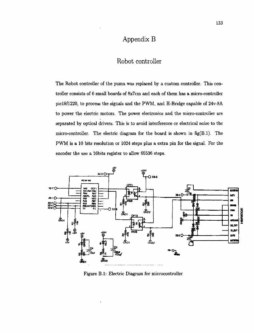
133

Appendix B

Robot controller

The Robot controller of the puma was replaced by a custom controller. This con­

troller consists of 6 small boards of 8x7cm and each of them has a micro-controller

picl8fl220, to process the signals and the PWM, and H-Bridge capable of 24v-8A

to power the electric motors. The power electronics and the micro-controller are

separated by optical drivers. This is to avoid interference or electrical noise to the

micro-controller. The electric diagram for the board is shown in fig(B.l). The

PWM is a 10 bits resolution or 1024 steps plus a extra pin for the signal. For the

encoder the use a 16bits register to allow 65536 steps.

+5V

nci«F-ae

MAC CCF1 RAt/NAtRB2

/MCRl RAS VS5 VOO

RAS RS) RBCANTOBS

GND

m

GMD2

Figure B.l: Electric Diagram for microcontroller

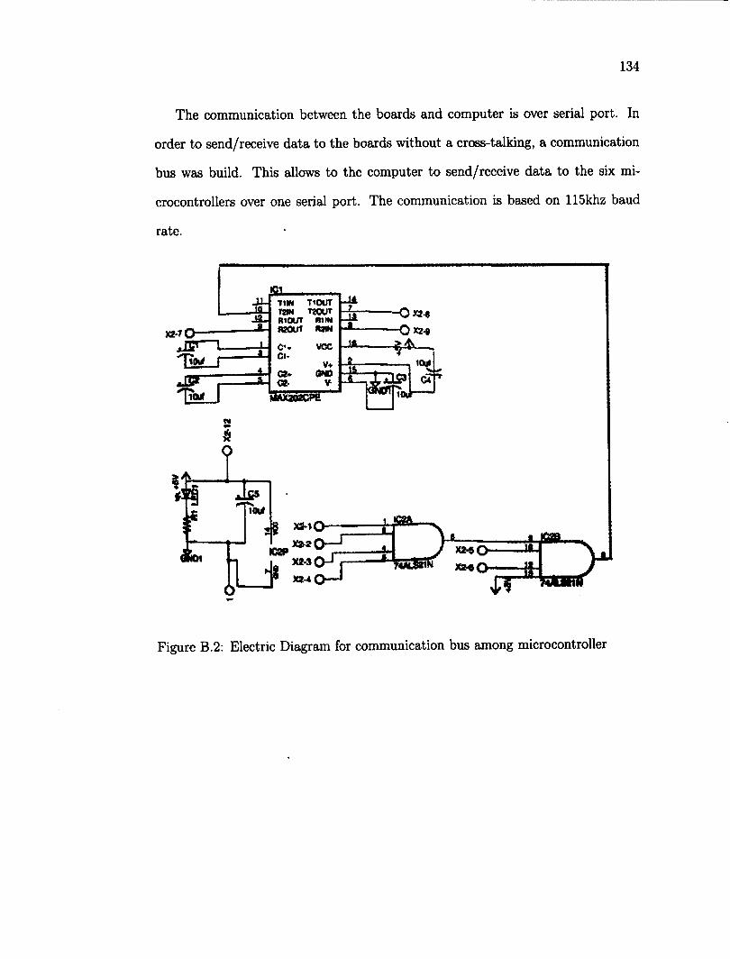
134

The communication between the boards and computer is over serial port. In

order to send/receive data to the boards without a cross-talking, a communication

bus was build. This allows to the computer to send/receive data to the six mi­

crocontrollers over one serial port. The communication is based on 115khz baud

rate.

vcc

Figure B.2: Electric Diagram for communication bus among microcontroller

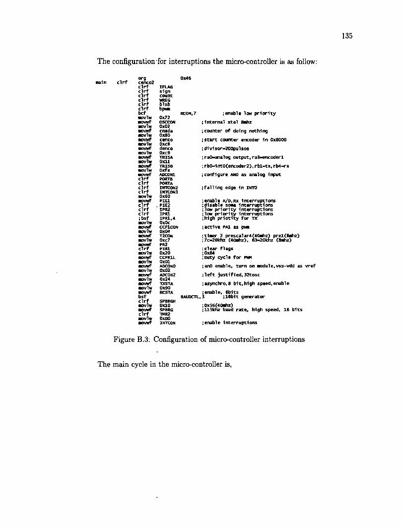
The configuration for interruptions the micro-controller is as follow:

•aln clrf org cenco2 clrf IFLAG clrf sign clrf count clrf WREG clrf blsb clrf bpwn bcf

bpwn

aovlw 0x72 •ovwf OSCCON •ovlw 0x02 •ovwf cnada •ovlw 0x80 •ovwf cenco •ovlw 0xc8 •ovwf denco •ovlw 0xc9 •ovwf TRISA •ovlw Oxll •ovwf TRISB •ovlw Oxfe •ovwf AOCON1 clrf PORTB clrf PORTA clrf XNTCON2 clrf INTCON3 •ovlw 0x60 •ovwf PIE1 clrf . PIE2 clrf IPR2 clrf IPR1 ;bsf IPRl,4 •ovlw 0x0c •ovwf CCP1CON •ovlw 0x04 •ovwf T2CON •ovlw 0xc7 •ovwf PR2 clrf PIR1 •ovlw 0x20 •ovwf CCPR1L •ovlw 0x01 •ovwf ADCONO •ovlw 0X02 •ovwf ADCON2 •ovlw 0x24 •ovwf TXSTA •ovlw 0X90 •ovwf RCSTA bsf clrf SPBRGH •ovlw 0x10 •ovwf SPBRG clrf TMR2 •ovlw OxDO •ovwf INTCON

0x46

rc0n.7

BAUDCTL

;enable low priority

; Internal xtal 8ahz

;counter of doing nothing

;start counter encoder 1n 0x8000

;d1vlsor-200pulsos

;raO»analog output,ra3-encoderl

i rbO-1ntO(encoder2), rbl-tx,rb4-rx

;configure ano as analog Input

;fal!1ng edge 1n iktO

;enable a/d, rx Interruptions ;disable sone Interruptions ;low priority Interruptions :low priority Interruptions ;h1gh prlotlty for TX

;active PA1 as pwa

;t1aer 2 prescalar4(40ahz) prel(Sahz) ;7c-20khz (40ahz), 63-20khz (Sahz)

iclear flags ;0x64 ;Duty cycle for pwm

;anO enable, turn on Module,vss-vdd as vref

;left justified,32tosc

;asynchro,8 bit,high speed,enable

;enable, 8b1ts ,3 ;16Mt generator

;0x56(40ahz) ;115khz baud rate, high speed, 16 bits

;enable Interruptions

Figure B.3: Configuration of micro-controller interruptions

The main cycle in the micro-controller is,

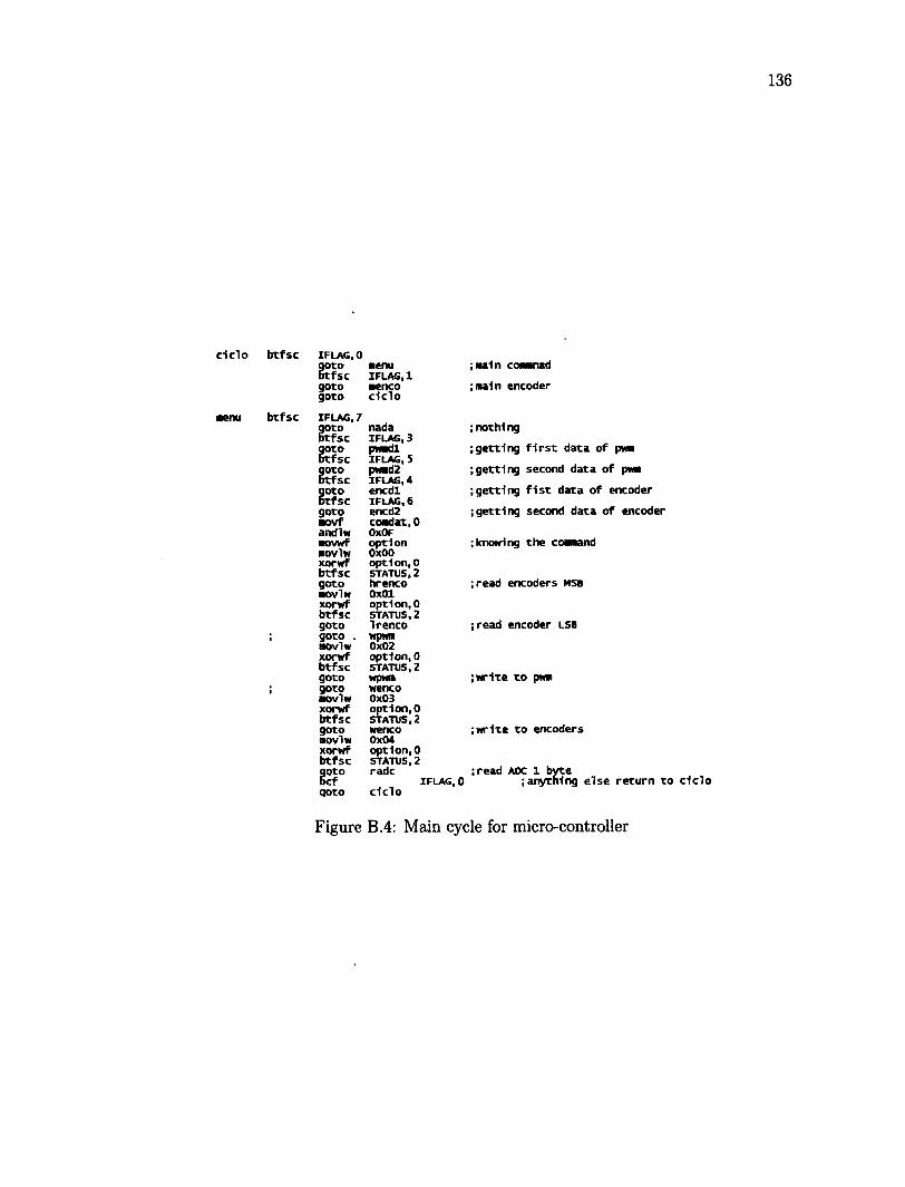
136

dclo btfsc

btfsc

iflag.o goto aenu btfsc IFLAG, 1 goto aenco goto dclo

IFLAG,7 goto Btfsc goto btfsc goto Btfsc goto Btfsc goto aovf andlw aovwf •ovlw xorwf btfsc goto •ovlw xorwf btfsc goto goto . •ovlw xorwf btfsc goto goto •ovlw xorwf btfsc goto •ovlw xorwf btfsc

goto cf

qoto

nada IFLAG,3 pwadl IFLAG, 5 |>mkI2 IFLAG, 4 encdl IFLAG, 6 ericd2 coadat,0 OxOF option 0x00 option,0 STATUS,2

hrenco 0x01 option,0 STATUS,2 Irenco

0x02 option,0 STATUS,2 wpwn wenco 0x03 option, 0 STATUS,2 wenco 0x04 option, 0 STATUS,2 radc

;aa1n coaanad

;aa1n encoder

; nothing

;getting first data of pwa

;getting second data of pwa

;getting fist data of encoder

;getting second data of encoder

;knowing the coaaand

;read encoders MSB

;read encoder LSB

;write to pwa

;write to encoders

clclo

;read ADC 1 byte IFLAG.O ;anything else return to clclo

Figure B.4: Main cycle for micro-controller

137

Appendix C

Software Functions

C.l Robotic Interface Functions

PumaOpenQ

Open a serial communication.

PumaClear()

Clear the serial Buffer communication.

PumaRead(IN nlink,OUT encoder)

Read the encoder of the link given by nlink.

Pumawrite(IN nlink, IN value)

Write a voltage (value) in the link given by nlink.

Mousecontrol(In rectangle, IN active, IN gripper)

This function receives the area (rectangle) where the mouse can be activated. The

push down the mouse send a signal to toggle the active value to 1 otherwise the

value is 0. The end effector can be maintain automatically in a 90 degrees or a 0

degrees depending of the gripper value.

C.2 Image Processing Functions

FB_Init()

Initialize the framegrabber to be ready for use.

FB_Cleanup()

138

Clean the framegrabber buffer.

FB_SetVideoConfig(int a,int al,int a2,int a3)

Configures the framegrabber: a=type, al=standard, a2=source, a3=greensync.

FB_VideoOfFscreen(int a,int b,int c,int d)

Configure camera type: a=pixel width, b=pixel height, c=pixel depth, c=start.

Corner (IN ROI)

This is a corner detection function using the Harris corner detection method. It

returns a vector of points where corners where detected over the ROI.

Edge(IN image, IN rectagle, IN flag, IN threshold, OUT matrix)

Return a matrix with 255's (black) in the edge detected in the rectangle otherwise

O's (white). The flag=l returns the edge detected in the matrix or flag=0 in over­

write the same image.

Crosscorr(IN feature a, IN featureb)

Return the normalized crosscorrelation between two templates.

bhatta(IN feature a, IN feature b)

Return the geometric Bhattacharyya distance between two histograms.

hiscoi(IN image)

Histogram receive and image returns vector with 15 bins.

Filtering(IN image, IN rectangle, IN matrixk, IN flag, OUT matrixout)

Filtering applies the matrix kernel (matrixk) to the image in the area given by the

points of the rectangle. The flag indicates to return the result in the initial image

or to return the result in the matrixout.

BackSub(IN imagel, IN image2,IN threshold, OUT image3)

Background subtraction function subtracts image2 from imagel and return the re­

sult in image3. If the pixel is within the threshold the result is 0.

IntegralImg(IN image, IN rectangle, OUT matrix)

139

Integral Image return a matrix of the summed area given by the rectangle over the

image.

CameraCal(IN vectorl, IN vector2, OUT vector3)

Camera calibration function returns a vector with intrinsic and extrinsic parame­

ters of the camera. The inputs are the vector of pixel coordinates and a vector of

their positions.

C.3 Matrix Functions

Matrix(IN c, IN r)

Creates a matrix with c columns and r rows.

! Matrix

Returns the matrix transpose.

Matrix.eye(IN v)

Create a diagonal matrix with value v.

Matrix.DetQ

Returns the determinant of the matrix.

Matrix.Inv()

Returns the inverse of the matrix.

Matrix.Norm()

Returns the Frobenius norm of the matrix

Matrix.Print()

Print the matrix elements.

Matrix.SetRow(IN r,IN vec)

Set the row r with a vector vec .

Matrix.SetCol(IN c, IN vec)

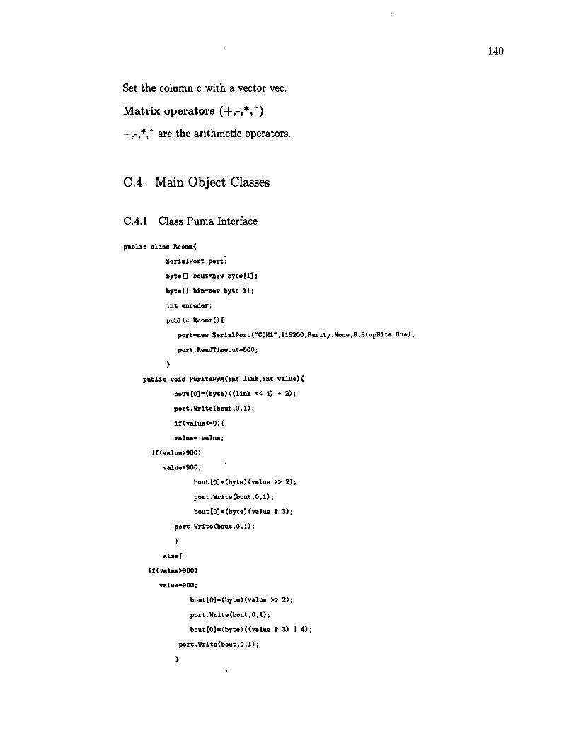
140

Set the column c with a vector vec.

Matrix operators (+,-»T)

+,->V are the arithmetic operators.

C.4 Main Object Classes

C.4.1 Class Puma Interface

public class Rcomm{

SerialPort port;

byte[] bout-new byte[l];

byte[] bin-new byte[l];

int encoder;

public Rcoon(){

port-new SerialPort("C0M1",115200.Parity.None,8.StopBits.One);

port.ReadTimeout-500;

>

public void PwritePWM(int link,int valueH

bout[0]-(byte)(Clink « 4) +2);

port.Vrite(bout,0,1);

if(value<»0){

value—value;

if(value>900)

value-900;

bout[0]-(byte)(value » 2);

port.Write(bout,0,1);

bout [0]-(byte)(value t 3);

port.Write(bout,0,1);

>

else{

if(value>900)

value-900;

bout[0]-(byte)(value » 2);

port.Write(bout,0,1);

bout[0]-(byte)((value t 3) 14);

port.Write(bout,0,1);

>

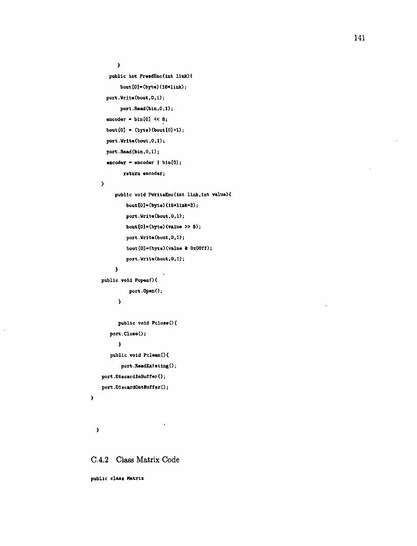
public lnt PreadEncCint llnkH

bout[0]»(bytB>(16*link);

port.Write(bout,0,1);

port.Read(bin,0,1);

encoder • bin[0] « 8;

bout[0] » (byte)(bout [0]+1);

port.Write(bout,0,1);

port.Read(bin,0,1);

encoder " encoder I binCO];

return encoder;

>

public void PvriteEncdnt link,lnt value){

bout[0]»(byte)(16*link+3);

port.Write(bout,0,1);

bout[0]"(byte)(value » 8);

port.Write(bout,0,1);

bout[0]«(byte)(value 4 0x001f);

port.Write(bout,0,1);

>

public void Popen(H

port.Open();

>

public void Pclose(){

port.Close0;

>

public void Pclean(){

port.ReadExi sting();

port .DiscardlnBufferO;

port.DiscardOutBuffer0;

>

C.4.2 Class Matrix Code

public class Hatrix

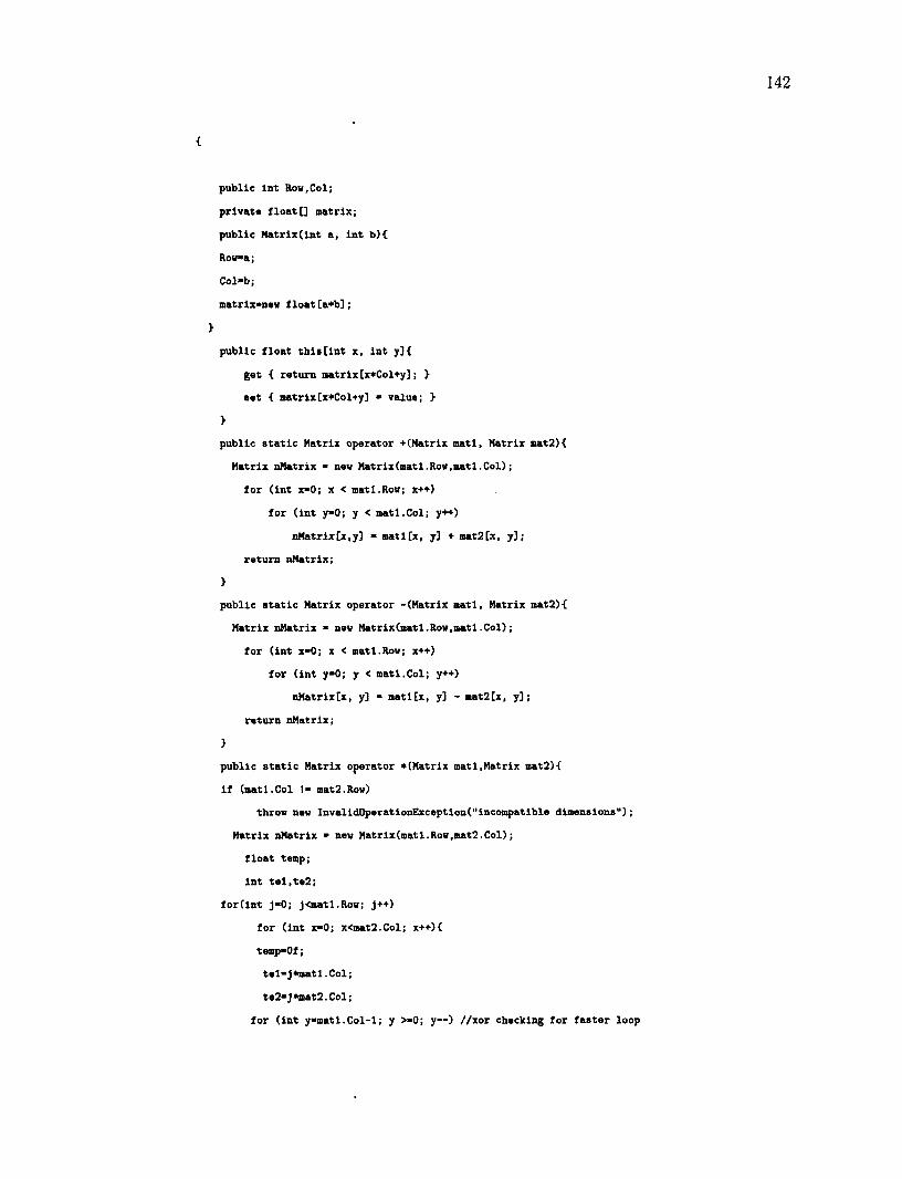
public int Row,Col;

private float[] matrix;

public Matrix(int a, int b){

Row-a;

Col-b;

matrix-new float[a*b];

public float this [int x, int y]{

get { return matrix[x»Col+y]; >

set { matrix[x*Col+y] » value; >

>

public static Matrix operator +(Matrix matl, Matrix mat2){

Matrix nMatrix • new Matrix(matl.Row,matl.Col);

for (int x«0; x < mat1.Row; x++)

for (int y»0; y < mat1.Col; y++)

nMatrix[x,y] • matl[x, y ] + mat2[x, y ] ;

return nMatrix;

>

public static Matrix operator -(Matrix matl, Matrix mat2){

Matrix nMatrix * new Matrix(matl.Row,matl.Col);

for (int x-0; x < matl.Row; x++)

for (int y"0; y < matl.Col; y++)

nMatrix[x, y] - matl[x, y] - mat2[x, y];

return nMatrix;

>

public static Matrix operator *(Matrix matl.Matrix mat2){

if (matl.Col !• mat2.Row)

throw new InvalidOperationException("incompatible dimensions");

Matrix nMatrix • new Matrix(matl.Row,mat2.Col);

float temp;

int tel,te2;

for(int j»0; J<matl.Row; j++)

for (int x«0; x<mat2.Col; x++){

temp«0f;

tel-j*matl.Col;

te2"j*mat2.Col;

for (int y«matl.Col-l; y >»0; y—) //xor checking for faster loop

temp +• matl.matrix[tel+y] • mat2[y,x];

nMatrix.matrix[te2+x]"temp;

>

return nMatrix;

>

public static Matrix operator *(float a,Matrix matl){

Matrix nMatrix « new Matrix(matl.Row,mati.Col);

for (int x»0; x < matl.Col; x++)

for (int y-matl.Row-1; y >"0; y—)

nMatrix [y, x] • a * matlCy, x];

return nMatrix;

>

public static Matrix operator *(Matrix matl,float a){

Matrix nMatrix « new Matrix(matl.Ron,matl.Col);

for (int x«0; x < matl.Col; x++)

for (int yaatl.Rov-1; y >"0 ; y—)

nMatrix[y, x] » a * matlCy, x];

return nMatrix;

>

public static Matrix operator /(Matrix matl,float a){

Matrix nMatrix - new Matrix(matl.Row,matl.Col);

a-lf/a;

for (int x»0; x < matl.Col; x++)

for (int y-matl.Rov-1; y >"0 ; y—)

nMatrix[y, x] - a * matl[y, x];

return nMatrix;

>

public static Matrix operator ! (Matrix matlH

Matrix nMatrix • new Matrix(matl.Col,matl.Row);

for (int x-0; x < matl.Row; x++)

for (int y»0; y < matl.Col; y++)

nMatrix[y,.x] • matl[x, y];

return nMatrix;

public void eye(float n){

int tel;

for (int x»0; x < Row; x++H

tel«x»Col;

for (int y»0; y < Col; y++){

lf(x--y)

matrix[tel+y]»n;

else

matrix[tel+y]"Of;

>

>

>

public void SetColdnt y,Matrix a){

for(int i"0;i<Row;i++)

thls[l,y]«a.matrix[i];

public void SetRovdnt x,Matrix a){

int tel;

tel-x*Col;

for(int i"0;i<Col;i++)

oatrix[tel+i]"a.matrix[i];

h public Matrix GetColdnt y){

Matrix nMatrix»new Matrix(RoH,l);

for(int i»0;i<Row;i++)

nMatrix.matrix[i]'this[i,y];

return nMatrix;

>

public Matrix GetRowdnt x){

Matrix nMatrix-new Matrix(1,Col);

fordnt i"0; KCol; i++)

nM&trix.matrix[1]"this[x,i];

return nMatrix;

>

int UpTriang(){

Matrix matl»new Matrix(Row,1);

int sign»l,tel,te2;

float temp;

fordnt i"0; KRow-l; i++){

if (this [i, i]•this[i,i]<-.OOOOif){

matl>GetRow(i);

SetRov(i,GetRow(i+l));

SetRov(i+i,matl);

sign *—1;

>

fordnt j»i+i; j<Rov; j++H

temp-this CJ,i]/this[i,i];

tel"i*Col;

te2»j*Col;

fordnt k«0;k<Col;k++)

matrix[te2+k] -» temp*matrix[tel+k];

>

>

return sign;

>

void Gauss(M

Matrix matl-new Matrix(Row,1);

float temp;

int tel,te2;

fordnt i«0;i<Rov;i++){

tel»i*Col;

if(matrix[tel+i]'matrix[tel+i]<-.00001f){

matl"GetRow(i);

SetRow(i,GetRow(i+l));

SetRow(i+l,matl);

>

temp»matrixd*Col+i];

tel"i*Col;

fordnt k-0;k<Col;k++)

matrix[tel+k] /« temp;

fordnt j-0;j<Row;j++){

if(J!"i){

temp*matrix[j *Col+i];

tel»j*Col;

te2"i»Col;

for(lnt k-0;k<Col;k++)

matrix[tel+k] -• temp*matrix[te2+k];

>

}

>

>

public float DetO{

Matrix matl-new Matrix(Row,Col)j

int sign;

for(lnt i»0;i<Row;i++)

mat 1.SetRow(i,GetRow(i));

sign*matl .UpTriangO;

float temp"l.Of;

for(int l-0;i<Rov;i++)

temp *» matl [1,1];

return temp*sign;

>

public static Matrix operator/(Matrix matl,Matrix mat2){

Matrix mat3-nev Matrix(matl.Row,matl.Col+1) ;

Matrix mat4"nsw MatrixOnatl.Rov.l);

//Augmented matrix

for (int i»0; Kmatl .Col; i++)

mat3 .SetCoKi ,matl .GetCol(i)) ;

mat3.SetCol(matl.Col,mat2);

//Gauss Elimination

mat3.GaussO;

for (int 1-0; Kmatl. Col ;i++)

mat4[1,0]"mat3[i,matl.Col];

return mat4;

>

public Matrix InvO

{

Matrix matl-neu Matrix(Row,Col);

matl.eye(lf);

Matrix mat2«new Matrix(Row,Col*2);

for(int i»0;i<Col;i++)

{ mat2.SetCol(i,GetCol(i));

mat2.S8tCol(i+Col,matl.GetCol(i));

>

mat2.GaussO;

//Return the last columns

for(int i-0;i<Col;i++)

matl.SetCol(i,mat2.GetCol(i+Col));

return matl;

>

public float Norm(M

float temp-Of;

if (Col—1H

for(int i-Oji<Rov;i++)

temp +» matrix[i]"matrix[i];

}

if(ftow--l){

for(int i«0;i<Col;i++)

temp +• matrix[i]"matrix[i];

>

temp"(float)Math.Sqrt(temp);

return temp;

>

public void InitMatrix(){

Random rand " new Random();

for (int x-0; x < this.Row; x++)

for (int y-0; y < this.Col; y++)

this[x,y] - (rand.Next()\%100)/100f;

>

public void PrintMatrixC(){

Console.WriteLineO;

for (int x«0; x < Row; x++H

Console.Write("[ ");

for (int y-0; y < Col; y++){

// format the output

Console.Write("{0,6:#,000}", this[x,y]);

>

Console.WriteLine(" ] " );

>

Console.WriteLine();

>

public String PrintMatrixO

{

StringBullder s - new StringBuilderO;

StringBuilder s2 • nev StringBuilderO;

for (int x»0; * < Row; x++){

s.AppendC'C ");

for (int y«0; y < Col; y++){

// format the output

s2.AppendForoat( "{0:0.0000} ",this[x,y]);

}

s.Append(s2);

s.Append(" ]\n");

s2.Length-0;

>

return s.ToStringO;

>

C.4.3 Class Feature Code

public class Feature{

public int px,py;

public float nean.std;

public float[] fnorm-new float[25*25]; //template of 25*25

public int[] hcolor-nev int[15]; //histogram with 15 bins

private int aux2,cot;

public Feature(int x.int y){

px"x;

py-y; mean"0f;

std-Of;

forUnt i-0;i<15;i++){

hcolor[i]»0;

>

>

public void paranCref byte[] tempH

int i,J;

int x,aux,ptested;

float sum;

ptested-py»640+px;

raean-Of;

for( i—12;i<13;i++M

aux«ptested+i*640;

if(aux<307188 tt aux>12)

for <j—12;j<13;j++>

mean+"temp[aux+j];

>

mean-mean/625;

x-0;

sum-Of;

for( i—12;i<13;i++M

aux"ptasted+i*640;

if(aux<307188 tt aux>12)

for (J—12;j<13;J++H

fnorm[x]"temp[aux+J]-mean j

sum+»(fnorm[x]»fnorm[x]);

x++;

>

>

std-(float)Math.Sqrt(sum);

>

public void bistcolCref byta[] tempH

int i.j;

int x,aux,ptested;

ptB8t«d»py»640+px;

for(i-0;i<15;i++)

hcolor[i]"0;

150

for( i«-12;i<13;i++){

aux"pte«ted+i»640;

if(aux<307188 tt aux>12)

for (J—12;j<i3;J++){

x-(int)(temp[aux+j]/17.05f);

hcolor[*]++j

>

>

>

public float crossc(Feature a,Feature b){

float correlation«Of;

float stda«0f,stdb»0f,teapa,tempb;

forCint i«0;i<625;i++H

tempa*a.fnorm[i]-a.mean;

tempb-b.fnorm[i]-b.mean;

corre lat i on+»tempa*tempb;

stda+«(tempa»tempa);

stdb+»(tempb*teinpb);

>

return correlation/((float)Math.Sqrt(stda*stdb));

public float bhatta(Feature a,Feature b){

float sum'Of;

for(int i«0;i<a.hcolor.Length;i++){

sum+»(float)Hath.Sqrt(a.hcolor[i]*b.hcolor[i]);

>

return (float)Math.Sqrt(lf-sum);

>

>

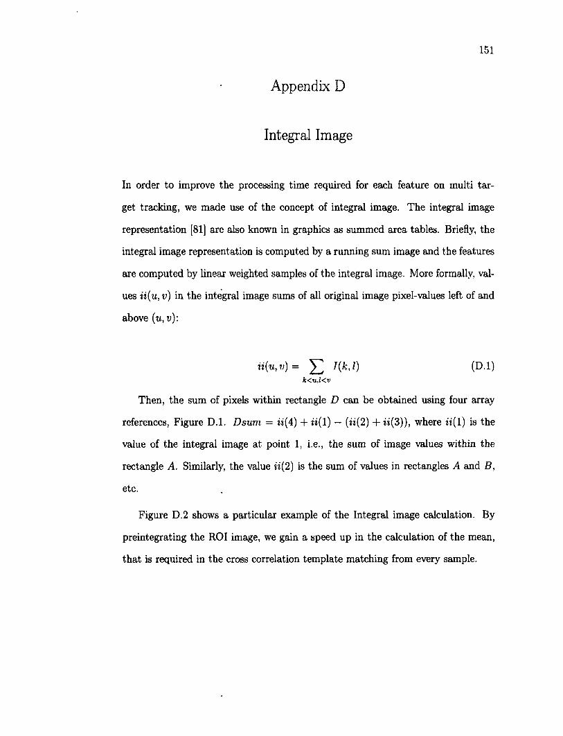
Appendix D

151

Integral Image

In order to improve the processing time required for each feature on multi tar­

get tracking, we made use of the concept of integral image. The integral image

representation [81] are also known in graphics as summed area tables. Briefly, the

integral image representation is computed by a running sum image and the features

are computed by linear weighted samples of the integral image. More formally, val­

ues ii{u, v) in the integral image sums of all original image pixel-values left of and

above (u,v):

Then, the sum of pixels within rectangle D can be obtained using four array

references, Figure D.l. Dsum = n(4) + ii( 1) — (n(2) + n(3)), where «(1) is the

value of the integral image at point 1, i.e., the sum of image values within the

rectangle A. Similarly, the value ii(2) is the sum of values in rectangles A and B,

etc.

Figure D.2 shows a particular example of the Integral image calculation. By

preintegrating the ROI image, we gain a speed up in the calculation of the mean,

that is required in the cross correlation template matching from every sample.

(D.l) k<u,l<v

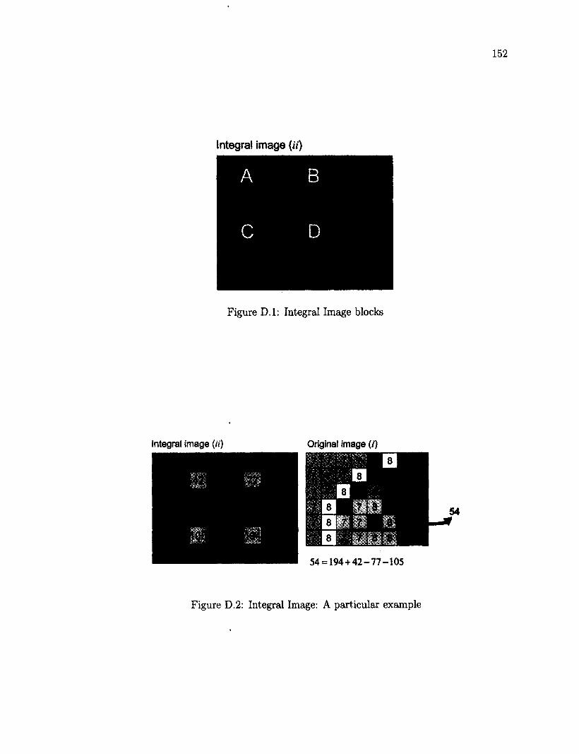
Integral image ( i i )

Figure D.l: Integral Image blocks

Integral image (ii) Original image (I)

54 = 194+42-77-105

Figure D.2: Integral Image: A particular example