UNCERTAINTY AND TAXPAYER COMPLIANCE

UNCERTAINTY AND TAXPAYER COMPLIANCE Authors: Jordi Caballé

Unitat de Fonaments de l'Anàlisi Econòmica and CODE Universitat Autònoma de Barcelona

Judith Panadés Unitat de Fonaments de l'Anàlisi Econòmica

Universitat Autònoma de Barcelona

P. T. N.o 35/03

N.B.: Las opiniones expresadas en este trabajo son de la exclusiva responsabilidad de los autores, pudiendo no coincidir con las del Instituto de Estudios Fiscales.

Desde el año 1998, la colección de Papeles de Trabajo del Instituto de Estudios Fiscales está disponible en versión electrónica, en la dirección: >http://www.minhac.es/ief/principal.htm.

http://www.minhac.es/ief/principal.htm

Edita: Instituto de Estudios Fiscales

N.I.P.O.: 111-03-006-8

I.S.S.N.: 1578-0252

Depósito Legal: M-23772-2001

INDEX

1. INTRODUCTION

2. THE MODEL

3. PROPERTIES OF THE EQUILIBRIUM

4. THE BIAS OF THE EFFECTIVE TAX SYSTEM

5. THE EFFECTS OF THE VARIANCE OF THE AUDIT COST

6. CONCLUSION

APPENDIX

REFERENCES

— 3 —

XXXXX

ABSTRACT

The complexity of both tax code provisions and tax forms could induce taxpayers to commit errors when they fill their income reports. The existence of these involuntary mistakes affects the tax enforcement policy as tax auditors will face now two sources of uncertainty, namely, the typical one associated with taxpayers' income and that associated with report errors. Moreover, the inspection policy can be exposed to some randomness due to audit cost uncertainty. The aim of this paper is to provide an unified framework to analyze the effects of all these sources of uncertainty. In this paper we provide an unified framework to analyze the effects of all these sources of uncertainty in a model of tax compliance where the interaction between auditors and taxpayers takes the form of a principal-agent relation. We show that more complexity in the tax code increases tax compliance. The effects of audit cost uncertainty are generally ambiguous. We also discuss the implications of our model for the regressive (or progressive) bias of the effective tax system.

Key words: Tax evasion, tax complexity, audit cost. JEL Classification Number: H26.

— 5 —

XXXXX

Instituto de Estudios Fiscales

1. INTRODUCTION

The complexity of both tax code provisions and tax forms could induce taxpayers to commit errors when they fill their income reports. The existence of these involuntary mistakes affects the tax enforcement policy as tax auditors will face now two sources of uncertainty, namely, the typical one associated with taxpayers' income and that associated with report errors. Moreover, the inspection policy can be exposed to some randomness due to audit cost uncertainty. The aim of this paper is to provide an unified framework to analyze the effects of all these sources of uncertainty in a model of tax compliance where the interaction between auditors and taxpayers takes the form of a principal-agent relation.

The first models that analyzed the phenomenon of tax evasion through a portfolio selection approach (like those of Allingham and Sandmo, 1972; and Yitzhaki, 1974) assumed that all taxpayers were facing a constant and identical probability of being audited by the tax enforcement agency. However, consider a tax auditor that observes the amount of income reported by a taxpayer before conducting the corresponding audit. If this auditor wants to maximize the expected revenue from each taxpayer, there is no apparent reason why he should commit to an audit policy independent of the report he observes. An auditor using optimally all the relevant information at his disposal should make both the probability of inspection and the effort applied to a taxpayer contingent on the corresponding amount of reported income. One of the first attempts to analyze those contingent policies was made by Reinganum and Wilde (1985), who considered a model where the tax enforcement agency commits to follow a cut-off audit policy. According to this policy, taxpayers reporting less income than a given level are inspected, whereas the other taxpayers are not inspected. In a very influential paper the same authors (Reinganum and Wilde, 1986) considered an alternative scenario where a revenue-maximizing tax authority does not commit to an audit rule but selects an optimal policy given the realization of the taxpayers' reports. Moreover, in this new framework the probability of inspection is allowed to take all the possible values in the interval [0, 1]. Therefore, here the relationship between taxpayers and the tax enforcement agency mimics that of the typical principal-agent relationship with no commitment. The agency plays the role of the principal and follows a rule that gives the probability which a taxpayer is audited with. This probability rule ends up being a decreasing function of the reported amount of individual income. Taking as given the audit rule of the tax agency, taxpayers play the role of agents and choose their optimal re

— 7 —

ports in order to maximize their disposable income. Optimal reports turn out to be increasing functions of the true income1 .

The interaction between taxpayers and tax auditors is usually exposed to additional sources of randomness. The fact that tax codes are complex, vague and ambiguous has been recognized by several studies2. This aspect of tax codes makes difficult for the taxpayers to apply the law even if they want to do so. Scotchmer and Slemrod (1989) consider a model were the ambiguity of tax laws gives raise to an audit policy yielding random outcomes depending on the interpretation of the law made by the auditors. Such a randomness results in more compliance by taxpayers, since they want to reduce the risk of the penalties associated with a tough inspection that could reveal a large amount of evaded income3. In fact, Alm, Jackson and McKee (1992) have conducted experiments that confirm that audit randomness induces tax compliance.

Reinganum and Wilde (1988) consider another source of uncertainty faced by taxpayers, namely, that associated with the cost of conducting an audit. In their model the cut-off level of income that triggers an inspection is a function of an unknown audit cost. Therefore, taxpayers form non-degenerate beliefs about this cut-off income from the distribution of the audit cost. These authors conclude that some degree of induced uncertainty about the audit cost improves compliance and, thus, increases the revenue collected by the agency, but excessive uncertainty could decrease compliance.

The model we present in this paper considers sources of uncertainty similar to those appearing in the previous models. We will also model the interaction between the tax enforcement agency and taxpayers as a principal-agent relation so that tax auditors investigate taxpayers with an intensity that depends on the amount of reported income. The revenue accruing from the inspection is assumed to be proportional to the effort made by the auditor and to the amount of evaded taxes. As in Reinganum and Wilde (1988), the audit cost is private information of each auditor and, thus, taxpayers do not know the exact response of auditors after reading their income reports. However, we depart from Reinga

1 The previous basic models have been enriched in several directions. For instance, Border and Sobel (1994) allow for general objective functions for the principal; Mookherjee and P'ng (1989) study the implications of having risk averse agents; Sanchez and Sobel (1983) analyze the conditions under which cut-off policies are optimal from the expected revenue viewpoint; and Erard and Feinstein (1994) introduce a fraction of honest taxpayers that always produce truthful reports. The principal-agent model has been tested by Alm, Bahl, and Murray (1993), who provide strong empirical support for this game-theoretical approach versus the alternative of random audit policies 2 See the abundant references in Section 9.1 of Andreoni, Erard and Feinstein (1998). 3 Scotchmer (1989) and Jung (1991) consider instead models where tax complexity makes taxpayers uncertain about their true taxable income. Pestieau, Possen and Slutsky (1998) analyze the welfare implications of explicit randomization in tax laws.

— 8 —


num and Wilde (1988) by considering general audit policies instead of cut-off ones. Another even more important departure is that we consider a fully rational expectations equilibrium. This means that taxpayers' beliefs about the audit costs coincide with the real distribution of these costs, whereas in the paper of Reinganum and Wilde the true distribution of these costs was degenerate and thus the confusion suffered by taxpayers about that cost was incompatible with the rational expectations equilibrium concept. In our model, the distribution of costs arises from the heterogeneous quality of tax auditors due to different natural auditing skills or non-homogeneous formal training. Moreover, in our model we assume quadratic costs structures parametrized by the value of a coefficient parameter that is private information of each auditor. We will show with the help of a couple of examples that the effects of increasing the variance of that parameter value are very sensitive to the specific distribution under consideration.

We also allow for mistakes made by taxpayers when they fill their income report forms. As we have already said, the involuntary nature of these mistakes could be a consequence of the complexity of the tax law or of the tax form itself. Like in Rubinstein (1979), even a honest taxpayer can be exposed to a penalty by the tax authority since the income he reports does not coincide necessarily with his true income. As Scotchmer and Slemrod (1989), we show that an increase in tax complexity generates more revenue for the government. However, instead of making tax complexity a source of random audits, we make it responsible for income reports containing accidental imprecisions.

Our paper analyzes also other three questions. First, we show that a larger variance of the income distribution reduces (not surprisingly) tax compliance, since auditors face more uncertainty about a variable that is private information of taxpayers. Second, we evaluate the effects of the different sources of uncertainty on taxpayers welfare under the assumption that the government revenue is not used to provide goods or services entering in the taxpayers' utility function. Our analysis shows that expected utility responds ambiguously to changes in the variances of income and of report errors. Finally, we analyze the progressive (or regressive) bias of the audit policies followed by the tax auditors of our model. We show that the sign of this bias could also be ambiguous since a tax inspection could now serve as an instrument to correct for the involuntary mistakes leading to excessive tax contribution. This ambiguity concerning the effective progressiveness of the tax system is in stark contrast to what is obtained in the standard model of tax compliance with strategic interaction between auditors and taxpayers, where the resulting effective tax system is always more regressive than the statutory one (see Reinganum and Wilde, 1986; and Scotchmer, 1992).

The paper is organized as follows. Section 2 presents the model and derives the rational expectations equilibrium. Section 3 discusses some properties of the

— 9 —

equilibrium. Section 4 contains the analysis of the potential progressive bias of the effective tax system. Section 5 discusses the implications of changes in the variance of the audit cost. Section 6 concludes the paper. All the proofs appear in the appendix.

2. THE MODEL

Let us consider an economy with a continuum of taxpayers distributed on ~the interval [0,1]. Assume that the income y of each taxpayer is a normally dis

tributed random variable with mean y and variance Vy ≥ 0 . The income of each taxpayer is independent of that of the others. Therefore, from the strong law of large numbers, the empirical average income is y . The tax law establishes a statutory tax rate τ ( )∈ 0,1 on income. After observing the realization y of his in-come, a taxpayer optimally decides the amount x of declared income4. However, individuals commit involuntary errors during the process of filling the corresponding income report forms. These errors take the form of a normally distri

~buted random variable ε having zero mean and variance Vε . Therefore, the in-come report received by the tax enforcement agency will be the realization of

~ ~ ~the random variable z = x + ε . In order to understand the nature of the discrepancy between the variables

~ ~ x and z , note that a taxpayer could mistakenly think that some sources of in-come are tax-exempt while others are taxable, so that the report on taxable income sent to the agency collects these involuntary mistakes. Obviously, the complexity of the tax code is a natural source of the aforementioned errors. An even more direct source of mistakes arises from the design of the income report form that, in many circumstances, induces taxpayer confusion. For instance, if the sources of income are diverse and, thus, the report has to contain multiple components (as in Rhoades, 1999), then the final report could easily contain some imprecisions. Therefore, even if a taxpayer wants to declare an income of x dollars, the final report z submitted to the tax enforcement agency ends up being a noisy transformation of the intended report x .

The tax enforcement agency has a pool of tax auditors and each income report is assigned randomly to one auditor. The auditor chooses the audit intensity p applied to each taxpayer in order to maximize the expected net revenue (tax and penalty revenue, less audit cost) per taxpayer. Note that, due to the strong law of large numbers, this objective implies the maximization of the aggregate net revenue collected by the tax agency. The audit intensity is contingent

4 We suppress the tilde to denote the realization of a random variable.

— 10 —


upon the report z observed by the tax auditor. We interpret the audit intensity p as a variable proportional to the effort e applied to the inspection and to the penalty rate f >1 on the amount of evaded taxes, i.e., p = ef . Moreover, the resources that can be exacted by these audits are assumed to be proportional to the audit intensity and to the amount of evaded taxes. Thus, the penalty revenue is

pτ(y − z) = efτ(y − z). Therefore, if the reported income z coincides with the true taxable income

y of a taxpayer, then no new revenues will arise from an inspection. Moreover, no additional revenues are obtained by a tax auditor when either no effort is devoted to the inspection of potential tax evaders (e = 0) or no penalties are imposed on the amount of evaded taxes (f = 0). Finally, note that a taxpayer who wanted to be honest and selects x = y could end up paying a penalty due to

~the involuntary errors summarized by the variable ε .

For the rest of the paper we will take as given the tax rate τ and the penalty rate f . Therefore, without loss of generality, we will use the audit intensity p as the choice variable of tax auditors, since this variable is entirely determined by the endogenous audit effort e applied to a given taxpayer.

We assume that audit costs are quadratic in the effort devoted to auditing, 1

ce2 with c > 0 . These costs include all the resources spent by the tax auditor 2

in the process of inspection. Note that, by making c = c f2 > 0 , the previous cost 2function becomes 1

cp . The value of the cost parameter c , and thus of c ,2

varies across auditors according to an exogenously given distribution. The value of that parameter could depend, for instance, on the natural skills and the previous training of the tax auditor. The exact value of his cost parameter c is observable by each auditor but is not observable by taxpayers, so that the cost

~parameter is a random variable c with a known distribution from the taxpayers' ~viewpoint. The relevant realization of the random variable c for a given tax

payer corresponds to the value c of the auditor assigned to him. ~~ ~Finally, we assume that the random variables y,ε and c are mutually inde

pendent. The joint distribution of these random variables is common knowledge. Let p(z;c) be the audit intensity strategy of an auditor with a value c of his

cost parameter. This strategy assigns to each report an audit intensity. Since ~taxpayers do not observe the realization of the random variable c , they are un

certain about the audit policy that auditors will apply in their respective cases. Taxpayers are risk neutral and want to maximize the expected amount of their disposable income after the inspection has taken place. The expected disposable

— 11 —

~ ~ ~ ~income of a taxpayer with initial income y will be E[y − τz − p( )z;c τ(y − z)]. Note that y − τz is the disposable income after the amount τz of taxes has been voluntarily paid and before the inspection has taken place. The amount ( ) ( y − z) isp z;c τthe additional revenue that the auditor collects through the inspection.

Taxpayers form rational expectations about the strategies followed by tax auditors. Since they observe their true income, taxpayers follow a report strategy satisfying

~~ ~ x( )y = argmaxE[y − τ(x + ε)− p(x + ~ε;c)τ(y − x − ε)]. (2.1) x

The first order condition of this problem is ~ ∂p(x + ~ε;c) ~ ~−1− E ~ y − x − ε) − p(x + ~ε;c) = 0. (2.2)

∂(x + ε) (

The second order condition is

∂ 2p(x + ~ε; ~ c) ∂p(x + ~ε; ~ c) ~− E (y − x − ε)− 2 < 0. (2.3) 2 ~ ~ ∂ (x + ε) ∂ (x + ε)

We see that, unlike the seminal papers of Allingham and Sandmo (1972) and Yitzhaki (1974), the taxpayer does not take as given the audit intensity but takes into account the effect of his report on the effort that the tax auditor will devote to enforce the tax law. Note also that we consider the audit intensity (or the audit effort) as the variable selected by auditors, whereas in previous models the choice variable used to be the probability of inspection.

Tax auditors want to maximize the net revenue from each taxpayer they audit. Therefore, an auditor with a value of the audit cost parameter equal to c chooses the audit intensity p to be applied to a taxpayer declaring the income level z , according to an audit strategy satisfying

~ 1 2( ) = argmaxE z p ( − z)− cpp z;c τ + τ y z , (2.4)

2p

~ ~ ~Where z is the realization of the random variable z = x( )+ εy . The first order condition of this problem is

~ E[τ(y − z)− cp z] = 0.

The sufficient second order condition is simply c > 0 , which is satisfied by assumption. Therefore, the audit intensity is given by

τ p = E ~[ ( )y z − z]. (2.5)

c

An equilibrium with rational expectation is thus a report strategy ( ) and an x y

audit strategy ( ) satisfying simultaneously (2.1) and (2.4). We will restrict p z;c

our attention to linear report strategies, x( )y = α + βy , and to audit strategies

— 12 —


that are linear in the observed income reports, ( ) = δ c + γ c z . Note that for p z;c ( ) ( )these linear audit strategies the sufficient second order condition (2.3) of the

~taxpayer problem becomes simply E γ( )c[ ] < 0 . The next proposition provides the unique equilibrium belonging to this class:

Proposition 2.1. Assume that Vε > Vy / 4. Then, there exists a unique equilibrium with rational expectations where ( ) is linear and p ·;·x · ( ) is linear in the amount z of reported income. This equilibrium is given by

( )= α + βyx y ,

where

1 1 Vy α = y − ~ 1+ , (2.6) 2 τE(1/ c) 4Vε

β = 1

; (2.7) 2

and

p( ) z;c ( ) ( )+ γ c z,= δ c

where

1 1 Vy Vy − 4Vε δ( )c = − τy , (2.8) c

E(1/ ~ c) 4Vε Vy + 4Vε

τ Vy − 4V γ( )c = ε . (2.9)

c Vy + 4Vε

For the rest of the paper we will maintain the assumption Vε > Vy / 4, which is necessary and sufficient for the second order condition (2.3) of the taxpayer problem. This condition requires in fact that the audit intensity be decreasing in the amount of reported income. If the previous assumption were not imposed, the audit intensity could be increasing in reported income, so that taxpayers would find optimal to report an infinite negative income level. In this respect, note that when Vε > Vy / 4, taxpayers make moderate mistakes and, thus, the reports they submit are very informative about their true income. In this case, since β = 1/ 2 , the amount of voluntarily evaded income y − x y( ) rises with the true income y and, hence, tax auditors maximize the penalty revenue by inspecting more intensively the taxpayers who submit high-income reports. On the contrary, if the variance of errors is sufficiently high relative to that of income, as assumed in Proposition 2.1, the reports are not so informative and, hence, auditors attribute high-income reports to involuntary mistakes committed by taxpayers. Moreover, since in this case the dispersion of income is small, the

— 13 —

optimal audit policy consists on inspecting more intensively the low-income reports, which are the ones that have a higher probability of being submitted by taxpayers who (involuntarily) underreport their true income.

Note that, using the equilibrium values of the coefficients α, β, δ( ) γ cc and ( ), the previous equilibrium pair of strategies can be written as

1 1 Vy ( )= y + y − 1+ (2.10)x y ~ 2 τE(1/ c) 4Vε

and

1 Vy − 4Vε 1 Vy p( ) z;c = τ (z − y)+ . (2.11) ~ c

Vy + 4Vε E(1/ c) 4Vε

We see that, on the one hand, the intended report ( ) is increasing in the x y

true individual income y and in the tax rate τ 5. Moreover, for a taxpayer with a given income level y , his report x increases with the variance Vε of involuntary errors, whereas it is decreasing in the variance Vy of income. Finally, the in

~tended report is increasing in the expectation E( )1/ c . On the other hand, the inspection intensity ( ) applied to a taxpayer is decreasing in his income re-p z;c

port z , as required by the second order condition (2.3), and decreasing in the cost parameter c . Finally, for a given report z and a given realization of the value c of the cost parameter, the inspection intensity p is increasing in the variance Vy of income, decreasing in the variance Vε of report errors, and de

~creasing in the expectation E( )1/ c .

Let us discuss the previous properties of the equilibrium strategies. Consider a taxpayer with a given income level y . Clearly, as Vε increases the taxpayer knows that the probability of committing important mistakes by accident be-comes larger. Since the audit intensity is decreasing in reported income, taxpayers know that low reports will be heavily inspected, while high reports will not be exposed to so severe inspections. This bias in the audit policy induces taxpayers to minimize the probability of a rigorous audit. Hence, when Vε rises, the intended amount x of reported income increases in order to raise the probability of generating a sufficiently large income report. The report x de-creases with the income variance Vy , which is consistent with the fact that tax auditors are facing more uncertainty about the true income of taxpayers. Finally, if taxpayers believe that the expected audit cost is high (that amounts “ceteris

5 Reported income increases with the tax rate as in the model of Yitzhaki (1974). Some authors claim that this comparative statics is at odds with empirical evidence and this has generated a strand of the literature aimed at obtaining a negative relation between reported income and tax rates (see Yaniv, 1994; Panadés, 2001; and Lee, 2001, among others).

— 14 —


~paribus”' to a low value of E( )1/ c , then they will expect a low audit intensity by ~the tax auditors. Therefore, optimal reports must be increasing in E( )1/ c .

Concerning the audit intensity for given values of z and c , we see that, as the variance Vy of income increases, tax auditors face more uncertainty about a variable that is private information of taxpayers and, thus, more resources must be devoted to audit activities. The variance Vε of report errors affects negatively the inspection intensity. This is consistent with the fact that taxpayers raise the amount of income they report when Vε increases and, hence, less effort should be devoted to audit taxpayers that underreport less income on average. Moreover, the audit intensity is obviously decreasing in the cost parameter c

~and is also decreasing in E( )1/ c . Note that, if taxpayers expect a high value of the ~ ~random variable c , then E 1/ c( ) will tend to be low. In this case they will under

report more income, since they think that the auditors will not be very aggressive in their inspection policy. The best response to this taxpayer strategy is to conduct an audit policy more aggressive than the one expected by taxpayers.

3. PROPERTIES OF THE EQUILIBRIUM

In this section we study some indicators of the performance of the tax compliance policy in equilibrium. From (2.10) we can compute first the expected reported income per capita in the economy,

1 Vy ~ E ~ ~( ) = E[x( ) + ε] = y − ~ 1+ .z y 2τE( ) 1/ c 4Vε

Note that, as occurs with the intended reports x , the expected reported in~come is increasing in both E( )1/ c and Vε , whereas is decreasing in Vy . Moreo

∂E( )~ zver, = 1, so that an increase in the average income results in an increase of ∂y

average reported income of identical amount. We can compute now the expected audit intensity to see how the different

sources of uncertainty affect the audit policy of the tax enforcement agency on average. To this end we compute the unconditional expectation of (2.11), which will give us the expected intensity before observing the realization of the cost

~parameter c of each auditor,

1 Vy ~ ~( ) [ ( ( )y + ε ) 1+ .E ~ p = E p x ~ ;c ] = 2 4Vε

It is obvious that the expected audit intensity ( ) is increasing in yE ~p V , de~creasing in Vε and independent of both c and E( )1/ c . Clearly, as Vε increases

— 15 —

the reports become less reliable signals of the true income. Recall that high values of the variance of involuntary errors induce larger amounts of reported income. In this case tax auditors should reduce the average intensity in order to lower the probability of applying to much effort in inspecting honest taxpayers. Again, more income uncertainty, parametrized by the variance Vy , requires more effort by the auditors. Finally, observe that, when computing the unconditional expectation, we are eliminating the asymmetry referred to the audit cost between the agency and the taxpayer. When both the agency and the taxpayer face the same priors about the cost parameter c , the opposite effects of the distribution

~of c on the reporting and inspection strategies cancel out on average.

We can now look at the expected revenue net of audit costs raised by the tax enforcement agency and see also how is affected by the different sources of uncertainty. The (random) net revenue per taxpayer is

~ ~ ~ ~ ~ ~ ~ ~ 1 ~ ~ ~ 2= τ( ( )+ ε)+ p x y + ε c) ( − x y − ε)− [ ( ( )y + ε cR x y ( ( ) ~ ; τ y ( ) c p x ~ ; )] . (3.1) 2

As we have already said, since there is a continuum of ex-ante identical taxpayers distributed uniformly on the interval [0,1], the expected net resources extracted from a taxpayer coincide with the aggregate net revenue raised by the agency.

~ Corollary 3.1. The expected net revenue E(R) is increasing in Vε and decrea~ ~sing in Vy . Moreover, E(R) is increasing in E( )1/ c .

A larger value of the variance Vy of income means a larger disadvantage of tax auditors with respect to taxpayers and, hence, tax auditors end up putting to much effort on low income taxpayers, who are the ones that pay less fines. When Vε increases, taxpayers commit more errors so that the agency will raise more revenues both from the penalties imposed on involuntary evaded taxes and from the taxes on the larger amount of voluntarily reported income. Therefore, the tax authority benefits from taxpayer confusion and, hence, it has no incentives to reduce the complexity of either tax laws or tax forms. Finally, a

~low value of E( )1/ c is typically associated with a large expected cost. Hence, the expected net revenue will be low since taxpayers anticipate that it is very costly for the auditors to conduct an audit.

Note that we have just looked at the unconditional expected net revenue raised by the tax agency. We could look now at the expected net revenue con

~ ditional to a given realization of the cost parameter E(R ~ c = c). The previous

conditional expectation is the expected revenue raised by a tax auditor with a value of the cost parameter equal to c . In this case, the effects of changes in Vε

~ V ( )and y are the same as in the unconditional case. However, the effects of E 1/ c

— 16 —


are generally ambiguous. To see this, consider the case where there is no in~come uncertainty, that is Vy = 0 or, equivalently, y = y . This is in fact a situation

very similar to that considered by Reinganum and Wilde (1988), where the agency knows the realization of its (homogeneous) audit cost parameter and

~taxpayers view this cost parameter as a random variable c with a given distribution. More precisely, these authors consider a cut-off policy where a taxpayer with a given income y is only inspected if his level of underreporting is so large that the penalty revenue outweighs the audit cost. They also assume a constant cost per inspection that the taxpayer views as if it were drawn from a uniform distribution. Coming back to our scenario, we can compute from (3.1) the follo-wing conditional expectation:

2~ ~ 1 1 1 τE(R ~ c = c, y = y)= τy − + + V ,~ ε~ 22E(1/ c) 8c[E(1/ c)] 2 c

which is obviously decreasing in the value of the cost parameter c and increasing in the error variance Vε . However, it is immediate to obtain that

~ ~ ∂E(R ~ c = c,y = y) > ~ < 1 ~ <0 if and only if E 1/ c >( ) . (3.2)

∂ ( )cE 1/ 2c

Therefore, if the tax authority can affect the beliefs of taxpayers through its disclosure (or secrecy) policy about its audit cost, then the expected revenue is

~maximized when taxpayers are induced to think that E(1/ c)=1/ 2c . Usually, a disclosure policy about the audit costs faced by the tax authority affects the variance

~of the distribution of c as perceived by taxpayers. In the next section we will assume that the tax enforcement agency can affect the variance of the true dis

~tribution of c and, then, we will make explicit the relation between Var ~c and ( )~ E( )1/ c through a couple of examples.

We discuss next the comparative statics concerning taxpayers' welfare. We assume that the revenue raised by the government is not spent in activities that affect the individuals' utility. Therefore, since taxpayers are risk neutral, we only have to compute the expected net income E( )~n of a taxpayer. Recall that the (random) net income of a taxpayer is

~ ~ ~ ~ ~ ~ ~~ ~− τ( ( )y + ε)− p x y + ~ε;c) (y −n = y x ( ( ) τ x( )y − ε).

( )Corollary 3.2. (a) The expected net income E ~n of a taxpayer is decreasing in ~ E( )1/ c . (b) If Vy = 0, then ( ) is decreasing in Vε . (c) The effects of changes in VεE ~n

and Vy on E( )~n are ambiguous when Vy > 0 .

Obviously, a low expected value of the parameter c [i.e., a large value of ~ E( )1/ c ] makes the expected net income small, since the tax auditor is expected

to use a quite aggressive policy to fight tax evasion. To understand part (b) of

— 17 —

the previous corollary, we just have to remind that reported income increases with the variance of errors and that the auditor does not longer have an informative disadvantage when Vy = 0 . Concerning the effects of the variances of income and of errors when Vy > 0 , the results of the comparative statics are ambiguous according to part (c). Recall that an increase in the variance of in-come (errors) triggers more (less) underreporting of income and more (less) intensive audits. These two effects on taxpayers' net income go in opposite direction and the dominating effect will thus depend on the particular parameter values of the model.

4. THE BIAS OF THE EFFECTIVE TAX SYSTEM

Another question that can be analyzed in the present context is the degree of effective progressiveness exhibited by the tax system in equilibrium. It is a well established result in the literature that the effective tax rate displays less progressiveness than the statutory one when the relationship between auditors and taxpayers is strategic (see Reinganum and Wilde, 1986; and Scotchmer, 1992). This is so because the agency will audit individuals reporting low income with more intensity than individuals producing high income reports. Therefore, even if the optimal amount of reported income is increasing in true income, highincome individuals find more attractive to underreport a larger proportion of their income. This generates a regressive bias in the effective tax structure once we take into account the penalty payments6 .

In order to analyze whether the effective tax structure of our model is progressive or regressive, we should compute the average expected tax rate faced by a taxpayer and see how this rate changes with the true income y . The expected payment (including taxes and penalties) of a taxpayer having a level y of income is

~~ ~τ x y p x y ~ ; ) y x y )g( )y = E[ ( ( ) + ε)+ ( ( ) + ε c τ( − ( )− ε ]. Note that in the previous expression we have to compute the expectation

~~just with respect to the random variables ε and c . The average expected tax rate is thus

( )g y( ) = .τ y y

Scochmer (1987) and Galmarini (1997) analyze the size of the regressive bias under cut-off audit policies when taxpayers are sorted into income classes and when taxpayers differ in terms of their risk aversion, respectively. These two modifications imply a reduction in the size of the regressive bias.

— 18 —

6


Under effective proportionality τ( )ˆ y should be independent of y , while under effective progressiveness (regressiveness) τ( )ˆ y should be increasing (decreasing). The following corollary tells that, unlike the previous papers, the function τ( )ˆ y could be non-monotonic:

Corollary 4.1. There exists an income level y such that the derivative of the average expected tax rate satisfies

ˆ ( )< 0 for all y > ˆτ′ y y .

Moreover, the function τ( )ˆ y could be either

(a) decreasing both on the interval (− ∞,0) and on the interval (0,∞); or

(b) U-shaped on the interval (− ∞,0) and inverted U-shaped on the interval (0,∞). According to the first part of the corollary, the effective tax system is always

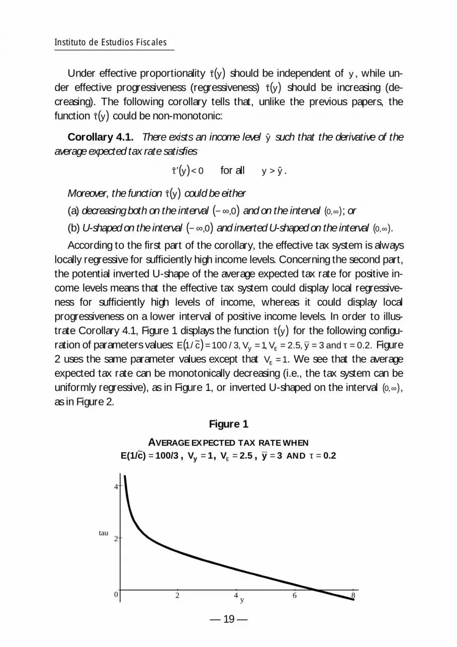
locally regressive for sufficiently high income levels. Concerning the second part, the potential inverted U-shape of the average expected tax rate for positive in-come levels means that the effective tax system could display local regressiveness for sufficiently high levels of income, whereas it could display local progressiveness on a lower interval of positive income levels. In order to illustrate Corollary 4.1, Figure 1 displays the function τ( )ˆ y for the following configu

~ E 1/ c y = 0.2. Figureration of parameters values: ( ) = 100 / 3, V = 1, Vε = 2.5, y = 3 and τ

2 uses the same parameter values except that Vε = 1. We see that the average expected tax rate can be monotonically decreasing (i.e., the tax system can be uniformly regressive), as in Figure 1, or inverted U-shaped on the interval (0,∞), as in Figure 2.

Figure 1

— 19 —

AVERAGE EXPECTED TAX RATE WHEN ~ E(1/c) = 100/3 , Vy = 1, Vε = 2.5 , y = 3 AND τ = 0.2

0

2

4

tau

2 4 6 8 y

Figure 2

AVERAGE EXPECTED TAX RATE WHEN ~ E(1/c) = 100/3 , Vy = 1, Vε = 1, y = 3 AND τ = 0.2

-0.5

0

0.5

tau

2 4 6 8y

To understand the potential non-monotonic behavior of the average expected tax rate, we should bear in mind that individuals suffering an inspection might end up receiving a tax refund. This is so because they could have declared an amount of income larger than the true one due to the involuntary mistakes made during the process of filling the tax form. Note also that the existence of these report errors makes taxpayers to declare a larger amount of income. Therefore, audits could detect accidental excessive tax contributions. Since the audit intensity is decreasing in the amount of reported income and reports are decreasing in true income, low-income individuals are more intensively inspected and, thus, they are more likely to get tax refunds. Note that this feature of the audit policy induces a progressive bias in the tax system that could outweigh the aforementioned regressive bias present in strategic models of tax compliance. The potential nonmonotonic behavior of τ( )ˆ y just captures the trade-off between these two biases.

5. THE EFFECTS OF THE VARIANCE OF THE AUDIT COST

The comparative statics exercises of the previous section have been per~formed in terms of the expectation E( )1/ c . In this section we analyze how this

~expectation could be affected by the moments of the distribution of c . In order to motivate this exercise, assume that the tax enforcement agency has a given budget to provide some training to its inspectors. Let us assume that the amount of resources available per auditor is equal to b . There is a stochastic training technology that relates the value of the cost parameter c of a tax auditor with the amount b invested in his training,

— 20 —

~ c E( )1 c = dc = ∫c−η 2η c


~~ c = h(b;ξ), ~where h is strictly decreasing in b and ξ is a random variable independent of

the amount b . As we already know, if the tax authority wants to maximize its aggregate revenue, then it has to maximize the expected revenue per taxpayer. According to Corollary 3.1, it is obvious that the agency should try to reach the

~largest possible value for E( )1/ c .

The following natural question arising in this context is whether the tax agency should give identical training to all the auditors, or should allow for some non-homogeneous training that will give rise in turn to some dispersion in the idiosyncratic values of the audit cost parameter. We are thus implicitly assuming that the tax enforcement agency can control, at some extent, some statistical

~properties of the random variable ξ at zero cost. To answer the previous ques~tion we analyze how the value of E( )1/ c is affected by the variance of the distri

~ ~bution of c in two particular cases, namely, when the random variable c is uniformly distributed and when it is log-normal. The choice of these two distributions allows us to be consistent with the second order condition of the tax auditor problem requiring that the value c of his cost parameter be strictly positive.

~Assume first that c has a uniform density. In particular, let ~ ~ˆh(b;ξ)= h( )b + ξ ,

~where ξ has a uniform density with zero mean and h b( ) is a positive valued and ~strictly decreasing mapping. Therefore, the mean of c is

( )= h( )b (5.1)E ~ c

and the variance is ~

Var( )~ c = Var(ξ). (5.2) ~The density of c can be thus written as,

1 for c ∈ (c − η,c + η)

f( )c = 2η

0 otherwise,

~with η > 0 and c − η > 0 so that c takes always on positive values. Therefore, it E ~ 2 3 . holds that ( )= c and ( )c = ηc Var ~ It is then clear that Var ~c is a strictly in( )

creasing function of η . Then,

+η 1 1 ln(c + η)− ln(c − η) .2η

After some simplification we obtain the following derivatives:

— 21 —

∂ ( )~E 1 c 1= − < 0,∂c c2 − η2

∂ ( )~ (5.3) E 1 c 1 ln(c + η)− ln(c − η)= − − < 0.∂η c 2 − η2 2η2

Hence, we have that

~ ∂E( )1/ c < . (5.4) ∂Var( )~ c

0

Since the audit cost of an auditor is strictly decreasing in the amount of resources devoted to his training, the derivative (5.3) implies that the expected

~value of c should be minimized and, thus, the agency should select b = b so that ( ) = (b), as follows from (5.1). This means that the agency should exhaust all E ~ c h ˆ

the resources for training. Moreover, according to (5.4), if the randomization device of the training technology generates a uniform distribution of the cost

~ parameter c , a tax enforcement agency aiming at the maximization of its net ~revenue should try to minimize the variance of c . Obviously, this is achieved by ~minimizing the variance of the random variable ξ [see (5.2)].

~Assume now that the cost parameter c is log-normally distributed. More precisely, assume that

~ ~( ξ)= ˆ( )ξ, (5.5) h b; h b

~ ~ where ξ is log-normal with E(ξ) = 1 and h b , has the same properties as before. ˆ( )~Therefore, the mean of the random variable c is

( )c = ( ), (5.6) E ~ h b

and its variance is 2 ~ˆ( )= ( )] Var ξ .Var ~ c [h b ( ) (5.7)

~ ~ 2 ~[ ] µ ] isLet E ln( ) = and Var [ln( ) = σ . Therefore, the mean of ξξ βξ

~ σ2 ξ = E( ) exp µ + = 1, 2

so that µ = −σ2 / 2 . Moreover,

~ ~ 2 2 2Var( ) ( )E ξ exp( )− ]= exp σ −ξ = [ ] [ σ 1 ( ) 1. (5.8) ~ ( )Since c is log-normal, the random variable ln ~ c is normally distributed.

Therefore, from (5.5), we have that 2

E[ln( )~ ] = ( ) h b + µ = ( ) h b − ,c ln ˆ( ) ln ˆ( ) σ

2 2Var[ln( )~ c ] = σ .

— 22 —


~ ~Similarly, the random variable 1/ c is log-normal as ln(1/ c) is normal. Since ~ ln( ) 1/ c = −ln( )~ c , we get

( c)] = − ( ) h b + 2

, (5.9) E[ln 1/ ~ ln ˆ( ) σ

2

and ~ Var[ln(1/ c)] = σ2 . (5.10)

Therefore, using (5.9) and (5.10), we can obtain the mean of the random ~variable 1/ c ,

~ ~ ~ Var[ln(1/ c)]

E(1/ c)= exp E ln 1/ )] + = exp[ ( ) h b + σ2 [ ( c − ln ˆ( ) ]. (5.11) 2

A revenue-maximizing tax enforcement agency should select the largest fea~sible value of E( )1/ c (see Corollary 3.1), and it is obvious from (5.11) that this is

achieved by choosing simultaneously the lowest feasible value for ln(h( )b ) and the 2largest feasible value for σ . The minimization of ln(h( )b ) is accomplished again

by selecting b = b so that ( )c = h ˆˆ E ~ ˆ(b), as follows from (5.6). Having picked optimally the value of E( )~ c , note from (5.8) that the maximization of the variance σ2

~means that the variance of ξ has to reach its largest feasible value. Moreover, the previous policy implies that, for a given value of resources per auditor b , the

~variance of c must be set as large as possible by the tax enforcement agency [see (5.7)].

~We see that the effect of the variance of the cost parameter c on the ex~pectation E( )1/ c under a log-normal distribution is the opposite to that obtained

under a uniform distribution. Thus, if the results contained in Corollaries 3.1 and ~3.2, and in expression (3.2) were written in terms of the variance of c , the

corresponding comparative statics exercises would be extremely dependent on ~the specific distribution of c under consideration.

6. CONCLUSION

In the context of a model of strategic interaction between tax auditors and taxpayers, we have analyzed the effects of different sources of uncertainty on the performance of the tax compliance policy. Besides the typical uncertainty faced by tax auditors associated with the income of taxpayers, we add two additional sources of uncertainty. The first one refers to the involuntary errors committed by taxpayers when they fill their income reports. The variance of these errors is usually increasing in the complexity of both tax laws and report

— 23 —

forms. The second source of uncertainty refers to the fact that the cost of conducting an audit is private information of the tax auditors so that the inspection policy is viewed as random by the taxpayers. Our main results can be summarized as follows:

— Larger variance of involuntary errors results in more average income reported, less average audit intensity, and more net revenue for the government.

— Larger variance of the income distribution results in less average income reported, more average audit intensity, and less net revenue for the government.

— Larger average audit costs typically result in less average income reported, less net revenue for the government, and more disposable in-come for the taxpayers on average.

— The relation between the average expected tax rate and true income could be non-monotonic. Therefore, the tax system could be locally progressive on some range of income levels and locally regressive on some other range.

— 24 —


y

E y z = y + − y . (A.1)2V + (V / β ) β y ε

APPENDIX

Proof of Proposition 2.1. The tax auditor observes the reported income z and the value c of the cost parameter and chooses the audit intensity p in order to solve (2.4). Therefore, the optimal audit intensity is given by (2.5). The auditor conjectures that taxpayers follow linear report strategies, i.e.,

( ) = α + βyx y , and thus, ~ ~~ ~ ~ z = x( )y + ε = α + βy + ε.

~Note that observing a realization of the random variable z is informationally equivalent to observing a realization of the random variable

~ ~ z − α ~ ε = y + ,β β

which has mean equal to y and variance equal to Vε / β2 . Therefore,

~ E(~ y z) = E y

z − α ~ E y = β

~ ~ ε y + .β ~ ~Since y and ε are mutually independent, we can apply the projection theo

rem for normally distributed random variables to get

V z − α (~ )

Plugging (A.1) in (2.5) and collecting terms we obtain

V y

τ V y α τ V = − ( ) − ( ) + [ (

y

p 1 y )] −1 z.c V + V / β 2 y ε V y + V ε / β 2 β c V y + V ε / β 2 β

The previous expression confirms that the audit strategy is linear in the observed report z . Therefore, letting ( ) = δ c + γ c z and equating coefficients,p z;c ( ) ( )we get

τ Vy Vy α δ c ( )= 1− y − , (A.2)2 2c Vy + (Vε / β ) Vy + (Vε / β ) β

and Vτ y ( ) = −1 . (A.3)γ c

2c [V + (V / β )]β y ε

A taxpayer observes his true income y and conjectures that the tax auditor follows an audit strategy that is linear in ( ) = δ c + γz, p z;c ( ) ( )c z. Therefore, the objective of the taxpayer is to maximize

— 25 —

~ ~~ ~ ~{ − τ( ) [ c + γ c x + ε) τ y − x − ε) .E y x + ε − δ( ) ( )( ] ( }The optimal intended report x must satisfy the following first order condi

tion [see (2.2)]: ~ ~ ~~ ~ E[ ( )( − x − ε)− δ( ) ( )c ( + ε) = 0.−1− γ c y c − γ x ]

~ ~Using the fact that c and ε are mutually independent, we can solve the previous equation for x ,

1 (1− δ) x = y + , (A.4)

2 γ ~ ~where δ = E δ( )c and γ = E γ c[ ] ( ) . The second order condition (2.3) becomes [ ]

simply γ < 0 . Note that (A.4) confirms that the report strategies used by taxpayers are linear in their income, that is, x( )y = α + βy. Therefore, equating coefficients we obtain,

1 1− δα = , (A.5) 2 γ

and

β = 1

. (A.6) 2

~We must compute now the expected values of the coefficients δ( ) and γ( )~ .c c

To this end, we compute the expectation of (A.2) and (A.3) to obtain.

~ Vy Vy α δ = τE(1/ c) 1− y − (A.7)

2 2 Vy + (Vε / β ) Vy + (Vε / β ) β

and V

~ y γ = τE( ) 1/ c −1 . (A.8) 2 [Vy + (Vε / β )]β

We can find the values of α,β,δ,and γ by solving the system of equations (A.5), (A.6), (A.7) and (A.8). After some tedious algebra we obtain the values of α and β given in (2.6) and (2.7) and

V V − 4V y ~ y εδ = − τE(1/ c)y

,

4V V + 4Vε y ε

V − 4V ~ y εγ = τE(1/ c) .

V + 4V y ε

Note that the second order condition γ < 0 is satisfied since 4Vε > Vy holds by assumption.

— 26 —


— 27 —

We can now find the coefficients δ and γ defining the audit strategy. To this end we only have to plug the values of α and β we have just obtained into (A.2) and (A.3). Some additional algebra yields the values of δ( )c and γ( )c given in(2.8) and (2.9).

Proof of Corollary 3.1. The expected net revenue raised by a tax auditor ~ before observing the realization of the cost ~c and the report z is

~ ⎧ ( (~ ) ~ ) ( ( )~ ~ ~ ~ ~ ~ ) 1 ) ( ( ) [ ( ( )~ ~ ~ E(R) = E⎨τ x y + ε + p x y + ε; c τ y − x y − ε − c p x y + ε;c)]2 ⎫⎬

⎩ 2 ⎭

⎧ ~ ~ ~ ~ ~ ~ ~ = E⎨ τ(α + βy + ε)+ [δ( )c + γ ( )c (α + βy + ε)]τ(y − α − βy − ε) ⎩

1 − ( )( ~ ~α + βy + ε)]2 ⎫c[δ( )c + γ c ⎬ . 2 ⎭

Using the equilibrium values of α β, , γ( )c and δ( )c obtained in Proposition 2.1, and after some cumbersome algebra, we obtain

~ 1 E(R) = 3 [V y y − 4V V 2 − 80 2V V ε − 3~ ε y 192V ε128Vε

2(V + 4V )E(1/ c) y ε

2 ( ~ ) 3 ( ~ ) 2 3[ ( ~+ 128τyV y E 1/ c − 128 2yVε E 1/ c + 512τ Vε τ V V y ε E 1/ c)]

+ 2 4 ~τ 2 2 2 2 ~256 2 V ε [E(1/ c )] + 16τ V V y ε [E(1/ c)] ].We can compute now the following derivative:

~ ∂E(R) 1 ⎡ = 16V V 2 2 + 364V V − V 4 − 4V V 3 ∂Vε 64V3 (V + 4V )2

ε y ε E( ~ ⎢ 1/ c) ⎣ y ε y ε y y ε

2 2 2 [ ( ~ )]2 2 4[ ( ~ - 9 1/ 2 ~ ⎤6τ V V E c + 256τ V V

E 1/ c)] +

y 512τ 2

y εV5 [E(1/ c)]2

ε ε. ⎥⎦

It can be shown that the previous derivative becomes equal to zero only when 4Vε = Vy , whereas it is positive whenever 0 < Vy < 4Vε, which holds by assumption.

Concerning the effects of Vy we compute ~ ∂E(R) 1 3 2 2 2 2 ~ = 2 2

∂V[Vy + 4V V 2 ~ ε2 ( ) ( ) y + 8τ V Vy ε [E 1/ ( c )] −16V Vy ε

y 64Vε V y + 4V ε E 1/ c (A.9)

− 384τ2 4 V ε [ ( ~E 2 − 64V 3 2 3 ~1/ c)] ε + 64τ V V 2y ε [E (1/ c )] ] .

The previous derivative becomes equal to zero whenever

Vy = 4Vε, (A.10)

⎡ ~ ~ ~ ⎤Vy = 4V 1 2 − 2

ε − τ V ε [E( 1/ c)] + τE(1/ c ) Vε (τ 2Vε [E(1/ c ⎢ )]2 − 4 , (A.11) ⎣

) ⎦⎥

or ~ ~ ~ V y = 4V ε −1− τ 2V [E(1/ c)]2

ε − τE(1/ c) V (τ 2 V [E(1/ c)]2 ε ε − 4

) . (A.12)

~ −The roots (A.11) and (A.12) are imaginary when V ∈ (0, [τE(1/ c) / 2] 2 ). In this ε

~ ]−2case, the single real root is the one given by (A.10). If Vε ≥ [τE(1/ c) / 2 , then the roots (A.11) and (A.12) are real. The root (A.12) is obviously negative. Concerning the root (A.11), it can be easily checked that it is also negative when

~ ]−2Vε ≥ [τE(1/ c) / 2 . Therefore, (A.9) does not change its sign in all the parameter region satisfying 0 < Vy < 4Vε, which holds by assumption. Then, we only have to check numerically that (A.9) is negative in that region.

~Finally, we can compute the following derivative with respect to E(1/ c) : ~

∂E(R) 1 3 2 2 2 2 2= [− V +16τ V V [E(1/ ~ c)] + 4V Vy y ε y ε2 2∂E(1/ ~ c) 128V (V + 4V )[E(1/ ~ c)]ε y ε

2 3 2 2 2 4 2 3−128τ V V [E(1/ ~ c)] y + 80V V + 256τ V [E(1/ ~ c)] +192V ].y ε y ε ε y

The previous derivative is always positive, as it can be shown by checking ~that it has only two imaginary roots for E(1/ c) , so that never changes sign for all

~positive real values of E(1/ c) .

Proof of Corollary 3.2. (a) The expected disposable income of a taxpayer is ~ ~ ~ ~ ~ ~ ~ E( ~ E[~ ( ( )+ ε)− p(x( ) y + ~ε;c) ( − x y − εn) = y − τ x y τ y ( ) )] =

~ ~ ~ ~ ~ ~ ~ ~ ~ E{~ ( y ) c + γ c y )] ( − α − βy − ε) .y − τ α + β + ε − [δ( ) ( )(α + β + ε τ y }Using the equilibrium values of , , ( ) and ( ) given in (2.6)-(2.9) and simα β δ c γ c

plifying, we obtain 1 2 2 3 2 2E( ~ n) = [64yV V [E(1/ ~ c)] + 256yV [E(1/ ~ c)]− 64τyV V [E(1/ ~ c)]− 4V Vy ε ε y ε y ε264E(1/ ~ c)V (V + 4V )ε y ε

3 2 3 3 2 3 2 2 4 2− 256τyV [E(1/ ~ c)]+16V V + 64V − V + 64τ V V [E(1/ ~ c)] − 256τ V [E(1/ ~ c)] ].ε y ε ε y y ε ε

We can compute then the following derivative: ∂E( ~ n) 1 2 2 3 3= [4V V −16V V − 64V + V~ y ε y ε ε y2 ~ 2∂E(1/ c) ( )[ ( )]64Vε Vy + 4Vε E 1/ c

2 3 ~ 2 2 4 ~ 264τ V V [ ( )] − 256τ V E 1/ c ] .+ E 1/ c [ ( ) ]y ε ε

It can be easily shown that (A.13) never becomes zero and takes always negative values whenever 0 < Vy < 4Vε, .

(b) Computing the derivative of E( ~n) with respect to Vε , we obtain

∂E( ~ n) 1 2 5 2 3 2 2= [− 512τ V [E(1/ ~ c)] + 8V V +16V Vε y ε y ε3 2∂Vε 32V (V + 4V ) E(1/ ~ c)ε y ε

4 2 2 3 2 2 4 2+ V + 32τ V V [E(1/ ~ c)] − 256τ V V [E(1/ ~ c)] ].y y ε y ε

— 28 —


For Vy = 0, the previous derivative simplifies to

∂E( ~ n) ~ = −τE(1/ c) < 0. ∂Vε

(c) Let

( 1

V V y y + 4Vε ) 2

2 ρ = ,8 τV 16V 3 + 8V 2 2 ε V V ε ε − y ε

Note that ρ > 0 whenever 0 < Vy < 4Vε, holds. Then, it can be easily checked that

( )∂ n > ~ <E ~ ( ) > ρ .< 0 for all E 1/ c

∂Vε

Similarly, for the effects of Vy on E( ~n) we can compute

∂E( ~ n) 1 3 2 2 2 4 2= [V − 8V V −16V V + 256τ V [E(1/ ~ c)] ]. y y ε y ε ε2 2∂Vy 32V (Vy + 4Vε ) E(1/ ~ c)ε

Let 1 2

θ y ( )V (V y + 4V ε )

= , 16τV2

ε

Note that θ > 0 . Then, it can be easily verified that

∂E( )~ n < ~ <( ) > θ .> 0 for all E 1/ c ∂Vy

Proof of Corollary 4.1. The average expected tax rate is ~~ ~( ) E τ(x( )y + ε)+ ( ( ) + ε c (y − ( )− ε ]g y [ p x y ~ ; )τ x y )( ) = = =τ y

y y ~ ~ ~~ ~ τ α + β + ε + δ( ) ( )( ] ( }E{ ( y ) [ c + γ c α + βy + ε) τ y − α − βy − ε)

. y

Using the equilibrium values of the parameters characterizing the audit and report strategies given in (2.6)-(2.9) and computing the expectation with respect

~ ~ to c and ε , we get an expression of the following type:

my + ny + qτ( )

2

,ˆ y = sy

where the coefficients m,n,q and s depend on the parameters of the model. In particular,

2 ~ 2 2m =16τ [ ( )] V V − 4Vε )E 1/ c ε ( ,y

— 29 —

and

s = 64yV 2 (Vy + 4V ε )E( ~ 1/ c

).ε

Note that m < 0 as Vy < 4V ε , whereas s > 0 . Therefore,

τ ( )y = −∞,lim y→∞

τlim ( )y = ∞,y→−∞

and the function τ( )y is discontinuous at y = 0 . Moreover, the equation τ ′( )y = 0

has two conjugate solutions,

± ∆ ,~ 4τVεE(1/ c)

with

8τyV V E ( ~ V2 1/ c ) ~∆ = − + 8V V − 32τyV2E (1/ c )− 64 τ 2y y V3 ~ 2y ε ε ε ε [E (1/ c )]

~ + 16V 2 + 16τ 2y 2V 2 ε ε [E(1/ c )]2 .

These two solutions are both real with opposite sign when the term ∆ is positive. Otherwise, the two solutions are imaginary. Therefore, on the one hand, when ∆ is negative, the function τ ( )y is decreasing on the interval (− ∞, 0)and is also decreasing on the interval (0,∞). On the other hand, if ∆ is positive then the function τ ( )y is U-shaped on the interval (− ∞,0) and inverted U-shaped on the interval (0,∞). Note that in both cases there exists an income level y

such that τ' ( )y < 0, for all y > y . Finally, note that ∆ can be positive or negative depending on the parameter values. For instance, let ( )~E 1 c =100 / 3 , Vy =1 ,y = 3 and τ = 0.2 . In this case, if Vε = 1, then ∆ = 2780.6. However, if Vε = 2.5,

then ∆ = −8723.4.

— 30 —

REFERENCES

ALLINGHAM, M. G., and SANDMO, A. (1972): “Income Tax Evasion: A Theoretical Analysis.” Journal of Public Economics 1, 323-38.

ALM, J.; JACKSON, B., and MCKEE, M. (1992): “Institutional Uncertainty and Taxpayer Compliance.” American Economic Review 82, 1018-1026.

ALM, J.; BAHL, R., and MURRAY, M. N. (1993): “Audit Selection and Income Tax Underreporting in the Tax Compliance Game.” Journal of Development Economics 42, 1-33.

ANDREONI, J.; ERARD, B., and FEINSTEIN, J. (1998): “Tax Compliance.” Journal of Economic Literature 36, 818-860.

BORDER, K., and SOBEL, J. (1987): “Samurai Accountant: A Theory of Auditing and Plunder.” Review of Economic Studies 54, 525-540.

ERARD, B., and FEINSTEIN, J. (1994): “Honesty and Evasion in the Tax Compliance Game.” RAND Journal of Economics 25, 1-19.

GALMARINI, U. (1997): “On the Size of the Regressive Bias in Tax Enforcement.” Economic Notes by Banca Monte dei Paschi di Siena SpA 26, 75-102.

JUNG, W. (1991): “Tax Reporting Game under Uncertain Tax Laws and Asymmetric Information.” Economics Letters 37, 323-329.

LEE, K. (2001): “Tax Evasion and Self-Insurance.” Journal of Public Economics 81, 73-81.

MOOKHERJEE, D., and P'NG, I. (1989): “Optimal Auditing, Insurance, and Redistribution.” Quartely Journal of Economics 104, 399-415.

PANADÉS, J. (2001): “Tax Evasion and Ricardian Equivalence”. European Journal of Political Economy 17, 799-815.

PESTIEAU, P.; POSSEN, U. M., and SLUTSKY, S. M. (1998): “The Value of Explicit Randomization in the Tax Code”. Journal of Public Economics 67, 87-103.

REINGANUM, J., and WILDE, L. (1985): “Income Tax Compliance in a Principal-Agent Framework.” Journal of Public Economics 26, 1-18.

– (1986): “Equilibrium Verification and Reporting Policies in a Model of Tax Compliance.” International Economic Review 27, 739-760.

– (1988): “A Note on Enforcement Uncertainty and Taxpayer Compliance.” Quarterly Journal of Economics 103, 793-798.

RHOADES, S. C. (1999): “The Impact of Multiple Component Reporting on Tax Compliance and Audit Strategies.” The Accounting Review 74, 63-85.

RUBINSTEIN, A. (1979): “An Optimal Conviction Policy for Offenses that May Have Been Committed by Accident.” Applied Game Theory, 406-413.

— 31 —

SÁNCHEZ, I., and SOBEL, J. (1993): “Hierarchical Design and Enforcement of In-come Tax Policies.” Journal of Public Economics 50, 345-369.

SCOTCHMER, S. (1987). “Audit Classes and Tax Enforcement Policy.” American Economic Review 77, 229-233.

– (1989): “Who Profits from Taxpayer Confusion.” Economics Letters 29, 49-55. SCOTCHMER, S. (1992): “The Regressive Bias in Tax Enforcement.” in PESTIEAU,

P. (ed.): Public Finance in a World of Transition, Proceedings of the 47th Congress of the IIPF, St. Petersburg, 1991, Supplement to Public Finance / Finances Publiques 47, 366-371.

SCOTCHMER, S., and SLEMROD, J. (1989): “Randomness in Tax Enforcement.” Journal of Public Economics 38, 17-32.

YANIV, G. (1994): “Tax Evasion and the Income Tax Rate a Theoretical Reexamination.” Public Finance / Finances Publiques 49, 107-112.

YITZHAKI, S. (1974): “A Note on Income Tax Evasion: A Theoretical Analysis.” Journal of Public Economics 3, 201-202.

— 32 —

NORMAS DE PUBLICACIÓN DE PAPELES DE TRABAJO DEL INSTITUTO DE ESTUDIOS FISCALES

Esta colección de Papeles de Trabajo tiene como objetivo ofrecer un vehículo de expresión a todas aquellas personas interasadas en los temas de Economía Pública. Las normas para la presentación y selección de originales son las siguientes:

1. Todos los originales que se presenten estarán sometidos a evaluación y podrán ser directamente aceptados para su publicación, aceptados sujetos a revisión, o rechazados.

2. Los trabajos deberán enviarse por duplicado a la Subdirección de Estudios Tributarios. Instituto de Estudios Fiscales. Avda. Cardenal Herrera Oria, 378. 28035 Madrid.

3. La extensión máxima de texto escrito, incluidos apéndices y referencias bibliográfícas será de 7000 palabras.

4. Los originales deberán presentarse mecanografiados a doble espacio. En la primera página deberá aparecer el título del trabajo, el nombre del autor(es) y la institución a la que pertenece, así como su dirección postal y electrónica. Además, en la primera página aparecerá también un abstract de no más de 125 palabras, los códigos JEL y las palabras clave.

5. Los epígrafes irán numerados secuencialmente siguiendo la numeración arábiga. Las notas al texto irán numeradas correlativamente y aparecerán al pie de la correspondiente página. Las fórmulas matemáticas se numerarán secuencialmente ajustadas al margen derecho de las mismas. La bibliografía aparecerá al final del trabajo, bajo la inscripción “Referencias” por orden alfabético de autores y, en cada una, ajustándose al siguiente orden: autor(es), año de publicación (distinguiendo a, b, c si hay varias correspondientes al mismo autor(es) y año), título del artículo o libro, título de la revista en cursiva, número de la revista y páginas.

6. En caso de que aparezcan tablas y gráficos, éstos podrán incorporarse directamente al texto o, alternativamente, presentarse todos juntos y debidamente numerados al final del trabajo, antes de la bibliografía.

7. En cualquier caso, se deberá adjuntar un disquete con el trabajo en formato word. Siempre que el documento presente tablas y/o gráficos, éstos deberán aparecer en ficheros independientes. Asimismo, en caso de que los gráficos procedan de tablas creadas en excel, estas deberán incorporarse en el disquete debidamente identificadas.

Junto al original del Papel de Trabajo se entregará también un resumen de un máximo de dos folios que contenga las principales implicaciones de política económica que se deriven de la investigación realizada.

— 33 —

PUBLISHING GUIDELINES OF WORKING PAPERS AT THE INSTITUTE FOR FISCAL STUDIES

This serie of Papeles de Trabajo (working papers) aims to provide those having an interest in Public Economics with a vehicle to publicize their ideas. The rules governing submission and selection of papers are the following:

1. The manuscripts submitted will all be assessed and may be directly accepted for publication, accepted with subjections for revision or rejected.

2. The papers shall be sent in duplicate to Subdirección General de Estudios Tributarios (The Deputy Direction of Tax Studies), Instituto de Estudios Fiscales (Institute for Fiscal Studies), Avenida del Cardenal Herrera Oria, nº 378, Madrid 28035.

3. The maximum length of the text including appendices and bibliography will be no more than 7000 words.

4. The originals should be double spaced. The first page of the manuscript should contain the following information: (1) the title; (2) the name and the institutional affiliation of the author(s); (3) an abstract of no more than 125 words; (4) JEL codes and keywords; (5) the postal and e-mail address of the corresponding author.

5. Sections will be numbered in sequence with arabic numerals. Footnotes will be numbered correlatively and will appear at the foot of the corresponding page. Mathematical formulae will be numbered on the right margin of the page in sequence. Bibliographical references will appear at the end of the paper under the heading “References” in alphabetical order of authors. Each reference will have to include in this order the following terms of references: author(s), publishing date (with an a, b or c in case there are several references to the same author(s) and year), title of the article or book, name of the journal in italics, number of the issue and pages.

6. If tables and graphs are necessary, they may be included directly in the text or alternatively presented altogether and duly numbered at the end of the paper, before the bibliography.

7. In any case, a floppy disk will be enclosed in Word format. Whenever the document provides tables and/or graphs, they must be contained in separate files. Furthermore, if graphs are drawn from tables within the Excell package, these must be included in the floppy disk and duly identified.

Together with the original copy of the working paper a brief two-page summary highlighting the main policy implications derived from the research is also requested.

— 34 —

1

1

1

1

1

1

1

1

1

ÚLTIMOS PAPELES DE TRABAJO EDITADOS POR EL

INSTITUTO DE ESTUDIOS FISCALES

2000

1/00 Crédito fiscal a la inversión en el impuesto de sociedades y neutralidad impositiva: Más evidencia para un viejo debate. Autor: Desiderio Romero Jordán. Páginas: 40.

2/00 Estudio del consumo familiar de bienes y servicios públicos a partir de la encuesta de presupuestos familiares. Autores: Ernesto Carrilllo y Manuel Tamayo. Páginas: 40.

3/00 Evidencia empírica de la convergencia real. Autores: Lorenzo Escot y Miguel Ángel Galindo. Páginas: 58.

Nueva Época

4/00 The effects of human capital depreciation on experience-earnings profiles: Evidence salaried spanish men. Autores: M. Arrazola, J. de Hevia, M. Risueño y J. F. Sanz. Páginas: 24.

5/00 Las ayudas fiscales a la adquisición de inmuebles residenciales en la nueva Ley del IRPF: Un análisis comparado a través del concepto de coste de uso. Autor: José Félix Sanz Sanz. Páginas: 44.

6/00 Las medidas fiscales de estímulo del ahorro contenidas en el Real Decreto-Ley 3/2000: análisis de sus efectos a través del tipo marginal efectivo. Autores: José Manuel González Páramo y Nuria Badenes Plá. Páginas: 28.

7/00 Análisis de las ganancias de bienestar asociadas a los efectos de la Reforma del IRPF sobre la oferta laboral de la familia española. Autores: Juan Prieto Rodríguez y Santiago Álvarez García. Páginas 32.

8/00 Un marco para la discusión de los efectos de la política impositiva sobre los precios y el stock de vivienda. Autor: Miguel Ángel López García. Páginas 36.

9/00 Descomposición de los efectos redistributivos de la Reforma del IRPF. Autores: Jorge Onrubia Fernández y María del Carmen Rodado Ruiz. Páginas 24.

10/00 Aspectos teóricos de la convergencia real, integración y política fiscal. Autores: Lorenzo Escot y Miguel Ángel Galindo. Páginas 28.

— 35 —

1

1

1

1

1

1

1

1

1

2001

1/01 Notas sobre desagregación temporal de series económicas. Autor: Enrique M. Quilis. Páginas 38.

2/01 Estimación y comparación de tasas de rendimiento de la educación en España. Autores: M. Arrazola, J. de Hevia, M. Risueño y J. F. Sanz. Páginas 28.

3/01 Doble imposición, “efecto clientela” y aversión al riesgo. Autores: Antonio Bustos Gisbert y Francisco Pedraja Chaparro. Páginas 34.

4/01 Non-Institutional Federalism in Spain. Autor: Joan Rosselló Villalonga. Páginas 32.

5/01 Estimating utilisation of Health care: A groupe data regression approach. Autora: Mabel Amaya Amaya. Páginas 30.

6/01 Shapley inequality descomposition by factor components. Autores: Mercedes Sastre y Alain Trannoy. Páginas 40.

7/01 An empirical analysis of the demand for physician services across the European Union. Autores: Sergi Jiménez Martín, José M. Labeaga y Maite Martínez-Granado. Páginas 40.

8/01 Demand, childbirth and the costs of babies: evidence from spanish panel data. Autores: José M.ª Labeaga, Ian Preston y Juan A. Sanchis-Llopis. Páginas 56.

9/01 Imposición marginal efectiva sobre el factor trabajo: Breve nota metodológica y comparación internacional. Autores: Desiderio Romero Jordán y José Félix Sanz Sanz. Páginas 40.

10/01 A non-parametric decomposition of redistribution into vertical and horizontal components. Autores: Irene Perrote, Juan Gabriel Rodríguez y Rafael Salas. Páginas 28.

11/01 Efectos sobre la renta disponible y el bienestar de la deducción por rentas ganadas en el IRPF. Autora: Nuria Badenes Plá. Páginas 28.

12/01 Seguros sanitarios y gasto público en España. Un modelo de microsimulación para las políticas de gastos fiscales en sanidad. Autor: Ángel López Nicolás. Páginas 40.

13/01 A complete parametrical class of redistribution and progressivity measures. Autores: Isabel Rabadán y Rafael Salas. Páginas 20.

14/01 La medición de la desigualdad económica. Autor: Rafael Salas. Páginas 40.

— 36 —

15/01 Crecimiento económico y dinámica de distribución de la renta en las regiones de la UE: un análisis no paramétrico. Autores: Julián Ramajo Hernández y María del Mar Salinas Jiménez. Páginas 32.

16/01 La descentralización territorial de las prestaciones asistenciales: efectos sobre la igualdad. Autores: Luis Ayala Cañón, Rosa Martínez López y Jesus Ruiz-Huerta. Páginas 48.

17/01 Redistribution and labour supply. Autores: Jorge Onrubia, Rafael Salas y José Félix Sanz. Páginas 24.

18/01 Medición de la eficiencia técnica en la economía española: El papel de las infraestructuras productivas. Autoras: M.a Jesús Delgado Rodríguez e Inmaculada Álvarez Ayuso. Páginas 32.

19/01 Inversión pública eficiente e impuestos distorsionantes en un contexto de equilibrio general. Autores: José Manuel González-Páramo y Diego Martínez López. Páginas 28.

20/01 La incidencia distributiva del gasto público social. Análisis general y tratamiento específico de la incidencia distributiva entre grupos sociales y entre grupos de edad. Autor: Jorge Calero Martínez. Páginas 36.

21/01 Crisis cambiarias: Teoría y evidencia. Autor: Óscar Bajo Rubio. Páginas 32.

22/01 Distributive impact and evaluation of devolution proposals in Japanese local public finance. Autores: Kazuyuki Nakamura, Minoru Kunizaki y Masanori Tahira. Páginas 36.

23/01 El funcionamiento de los sistemas de garantía en el modelo de financiación autonómica. Autor: Alfonso Utrilla de la Hoz. Páginas 48.

24/01 Rendimiento de la educación en España: Nueva evidencia de las diferencias entre Hombres y Mujeres. Autores: M. Arrazola y J. de Hevia. Páginas 36.

25/01 Fecundidad y beneficios fiscales y sociales por descendientes. Autora: Anabel Zárate Marco. Páginas 52.

26/01 Estimación de precios sombra a partir del análisis Input-Output: Aplicación a la economía española. Autora: Guadalupe Souto Nieves. Páginas 56.

27/01 Análisis empírico de la depreciación del capital humano para el caso de las Mujeres y los Hombres en España. Autores: M. Arrazola y J. de Hevia. Páginas 28.

— 37 —

1

1

1

1

1

1

1

1

1

28/01 Equivalence scales in tax and transfer policies. Autores: Luis Ayala, Rosa Martínez y Jesús Ruiz-Huerta. Páginas 44.

29/01 Un modelo de crecimiento con restricciones de demanda: el gasto público como amortiguador del desequilibrio externo. Autora: Belén Fernández Castro. Páginas 44.

30/01 A bi-stochastic nonparametric estimator. Autores: Juan G. Rodríguez y Rafael Salas. Páginas 24.

2002

1/02 Las cestas autonómicas. Autores: Alejandro Esteller, Jorge Navas y Pilar Sorribas. Páginas 72.

2/02 Evolución del endeudamiento autonómico entre 1985 y 1997: la incidencia de los Escenarios de Consolidación Presupuestaria y de los límites de la LOFCA. Autores: Julio López Laborda y Jaime Vallés Giménez. Páginas 60.

3/02 Optimal Pricing and Grant Policies for Museums. Autores: Juan Prieto Rodríguez y Víctor Fernández Blanco. Páginas 28.

4/02 El mercado financiero y el racionamiento del endeudamiento autonómico. Autores: Nuria Alcalde Fradejas y Jaime Vallés Giménez. Páginas 36.

5/02 Experimentos secuenciales en la gestión de los recursos comunes. Autores: Lluis Bru, Susana Cabrera, C. Mónica Capra y Rosario Gómez. Páginas 32.

6/02 La eficiencia de la universidad medida a través de la función de distancia: Un análisis de las relaciones entre la docencia y la investigación. Autores: Alfredo Moreno Sáez y David Trillo del Pozo. Páginas 40.

7/02 Movilidad social y desigualdad económica. Autores: Juan Prieto-Rodríguez, Rafael Salas y Santiago Álvarez-García. Páginas 32.

8/02 Modelos BVAR: Especificación, estimación e inferencia. Autor: Enrique M. Quilis. Páginas 44.

9/02 Imposición lineal sobre la renta y equivalencia distributiva: Un ejercicio de microsimulación. Autores: Juan Manuel Castañer Carrasco y José Félix Sanz Sanz. Páginas 44.

10/02 The evolution of income inequality in the European Union during the period 1993-1996. Autores: Santiago Álvarez García, Juan Prieto-Rodríguez y Rafael Salas. Páginas 36.

— 38 —

11/02 Una descomposición de la redistribución en sus componentes vertical y horizontal: Una aplicación al IRPF. Autora: Irene Perrote. Páginas 32.

12/02 Análisis de las políticas públicas de fomento de la innovación tecnológica en las regiones españolas. Autor: Antonio Fonfría Mesa. Páginas 40.

13/02 Los efectos de la política fiscal sobre el consumo privado: nueva evidencia para el caso español. Autores: Agustín García y Julián Ramajo. Páginas 52.

14/02 Micro-modelling of retirement behavior in Spain. Autores: Michele Boldrin, Sergi Jiménez-Martín y Franco Peracchi. Páginas 96.

15/02 Estado de salud y participación laboral de las personas mayores. Autores: Juan Prieto Rodríguez, Desiderio Romero Jordán y Santiago Álvarez García. Páginas 40.

16/02 Technological change, efficiency gains and capital accumulation in labour productivity growth and convergence: an application to the Spanish regions. Autora: M.ª del Mar Salinas Jiménez. Páginas 40.

17/02 Déficit público, masa monetaria e inflación. Evidencia empírica en la Unión Europea. Autor: César Pérez López. Páginas 40.

18/02 Tax evasion and relative contribution. Autora: Judith Panadés i Martí. Páginas 28.

19/02 Fiscal policy and growth revisited: the case of the Spanish regions. Autores: Óscar Bajo Rubio, Carmen Díaz Roldán y M. a Dolores Montávez Garcés. Páginas 28.

20/02 Optimal endowments of public investment: an empirical analysis for the Spanish regions. Autores: Óscar Bajo Rubio, Carmen Díaz Roldán y M.a Dolores Montávez Garcés. Páginas 28.

21/02 Régimen fiscal de la previsión social empresarial. Incentivos existentes y equidad del sistema. Autor: Félix Domínguez Barrero. Páginas 52.

22/02 Poverty statics and dynamics: does the accounting period matter?. Autores: Olga Cantó, Coral del Río y Carlos Gradín. Páginas 52.

23/02 Public employment and redistribution in Spain. Autores: José Manuel Marqués Sevillano y Joan Rosselló Villallonga. Páginas 36.

— 39 —

1

24/02 La evolución de la pobreza estática y dinámica en España en el periodo 1985-1995. Autores: Olga Cantó, Coral del Río y Carlos Gradín. Páginas: 76.

25/02 Estimación de los efectos de un "tratamiento": una aplicación a la Educación superior en España. Autores: M. Arrazola y J. de Hevia. Páginas 32.

26/02 Sensibilidad de las estimaciones del rendimiento de la educación a la elección de instrumentos y de forma funcional. Autores: M. Arrazola y J. de Hevia. Páginas 40.

27/02 Reforma fiscal verde y doble dividendo. Una revisión de la evidencia empírica. Autor: Miguel Enrique Rodríguez Méndez. Páginas 40.

28/02 Productividad y eficiencia en la gestión pública del transporte de ferrocarriles implicaciones de política económica. Autor: Marcelino Martínez Cabrera. Páginas 32.

29/02 Building stronger national movie industries: The case of Spain. Autores: Víctor Fernández Blanco y Juan Prieto Rodríguez. Páginas 52.

30/02 Análisis comparativo del gravamen efectivo sobre la renta empresarial entre países y activos en el contexto de la Unión Europea (2001). Autora: Raquel Paredes Gómez. Páginas 48.

31/02 Voting over taxes with endogenous altruism. Autor: Joan Esteban. Páginas 32.

32/02 Midiendo el coste marginal en bienestar de una reforma impositiva. Autor: José Manuel González-Páramo. Páginas 48.

33/02 Redistributive taxation with endogenous sentiments. Autores: Joan Esteban y Laurence Kranich. Páginas 40.

34/02 Una nota sobre la compensación de incentivos a la adquisición de vivienda habitual tras la reforma del IRPF de 1998. Autores: Jorge Onrubia Fernández, Desiderio Romero Jordán y José Félix Sanz Sanz. Páginas 36.

35/02 Simulación de políticas económicas: los modelos de equilibrio general aplicado. Autor: Antonio Gómez Gómez-Plana. Páginas 36.

2003

1/03 Análisis de la distribución de la renta a partir de funciones de cuantiles: robustez y sensibilidad de los resultados frente a escalas de equivalencia. Autores: Marta Pascual Sáez y José María Sarabia Alegría. Páginas 52.

— 40 —

1

1

1

1

1

1

1

1

2/03 Macroeconomic conditions, institutional factors and demographic structure: What causes welfare caseloads? Autores: Luis Ayala y César Pérez. Páginas 44.

3/03 Endeudamiento local y restricciones institucionales. De la ley reguladora de haciendas locales a la estabilidad presupuestaria. Autores: Jaime Vallés Giménez, Pedro Pascual Arzoz y Fermín Cabasés Hita. Páginas 56.

4/03 The dual tax as a flat tax with a surtax on labour income. Autor: José María Durán Cabré. Páginas 40.

5/03 La estimación de la función de producción educativa en valor añadido mediante redes neuronales: una aplicación para el caso español. Autor: Daniel Santín González. Páginas 52.

6/03 Privación relativa, imposición sobre la renta e índice de Gini generalizado. Autores: Elena Bárcena Martín, Luis Imedio Olmedo y Guillermina Martín Reyes. Páginas 36.

7/03 Fijación de precios óptimos en el sector público: una aplicación para el servicio municipal de agua. Autora: M.ª Ángeles García Valiñas. Páginas 44.

8/03 Tasas de descuento para la evaluación de inversiones públicas: Estimaciones para España. Autora: Guadalupe Souto Nieves. Páginas 40.

9/03 Una evaluación del grado de incumplimiento fiscal para las provincias españolas. Autores: Ángel Alañón Pardo y Miguel Gómez de Antonio. Páginas 44.

10/03 Extended bi-polarization and inequality measures. Autores: Juan G. Rodríguez y Rafael Salas. Páginas 32.

11/03 Fiscal decentralization, macrostability and growth. Autores: Jorge Martínez-Vázquez y Robert M. McNab. Páginas 44.

12/03 Valoración de bienes públicos en relación al patrimonio histórico cultural: aplicación comparada de métodos estadísticos de estimación. Autores: Luis César Herrero Prieto, José Ángel Sanz Lara y Ana María Bedate Centeno. Páginas 44.

13/03 Growth, convergence and public investment. A bayesian model averaging approach. Autores: Roberto León-González y Daniel Montolio. Páginas 44.

14/03 ¿Qué puede esperarse de una reducción de la imposición indirecta que recae sobre el consumo cultural?: Un análisis a partir de las técnicas de microsimulación. Autores: José Félix Sanz Sanz, Desiderio Romero Jordán y Juan Prieto Rodríguez. Páginas 40.

— 41 —

15/03 Estimaciones de la tasa de paro de equilibrio de la economía española a partir de la Ley de Okun. Autores: Inés P. Murillo y Carlos Usabiaga. Páginas 32.

16/03 La previsión social en la empresa, tras la Ley 46/2002, de reforma parcial del impuesto sobre la renta de las personas físicas. Autor: Félix Domínguez Barrero. Páginas 48.

17/03 The influence of previous labour market experiences on subsequent job tenure. Autores: José María Arranz y Carlos García-Serrano. Páginas 48.

18/03 Promoting sutdent's effort: standards versus torunaments. Autores: Pedro Landeras y J. M. Pérez de Villarreal. Páginas 44.

19/03 Non-employment and subsequent wage losses. Autores: José María Arranz y Carlos García-Serrano. Páginas 52.

20/03 La medida de los ingresos públicos en la Agencia Tributaria. Caja, derechos reconocidos y devengo económico. Autores: Rafael Frutos, Francisco Melis, M.ª Jesús Pérez de la Ossa y José Luis Ramos. Páginas 80.

21/03 Tratamiento fiscal de la vivienda y exceso de gravamen. Autor: Miguel Ángel López García. Páginas 44.

22/03 Medición del capital humano y análisis de su rendimiento. Autores: María Arrazola y José de Hevia. Páginas 36.

23/03 Vivienda, reforma impositiva y coste en bienestar. Autor: Miguel Ángel López García. Páginas 52.

24/03 Algunos comentarios sobre la medición del capital humano. Autores: María Arrazola y José de Hevia. Páginas 40.

25/03 Exploring the spanish interbank yield curve. Autores: Leandro Navarro y Enrique M. Quilis. Páginas 32.

26/03 Redes neuronales y medición de eficiencia: aplicación al servicio de recogida de basuras. Autor: Francisco J. Delgado Rivero. Páginas 60.

27/03 Equivalencia ricardiana y tipos de interés. Autoesr: Agustín García, Julián Ramajo e Inés Piedraescrita Murillo. Páginas 40.

28/03 Instrumentos y objetivos de las políticas de apoyo a las PYME en España. Autor: Antonio Fonfría Mesa. Páginas 44.

— 42 —

29/03 Análisis de incidencia del gasto público en educación superior: enfoque transversal. Autora: María Gil Izquierdo. Páginas 48.

30/03 Rentabilidad social de la inversión pública española en infraestructuras. Autores: Jaime Alonso-Carrera, María Jesús Freire-Serén y Baltasar Manzano. Páginas 44.

31/03 Las rentas de capital en Phogue: análisis de su fiabilidad y corrección mediante fusión estadística. Autor: Fidel Picos Sánchez. Páginas 44.

32/03 Efecto de los sistemas de rentas mínimas autonómicas sobre la migración interregional. Autora: María Martínez Torres. Páginas 44.

33/03 Rentas mínimas autonómicas en España. Su dimensión espacial. Autora: María Martínez Torres. Páginas 76.

34/03 Un nuevo examen de las causas del déficit autonómico. Autor: Santiago Lago Peñas. Páginas 52.

35/03 Uncertainty and taxpayer compliance. Autores: Jordi Caballé y Judith Panadés. Páginas 44.

— 43 —

Documents

UNCERTAINTY AND TAXPAYER COMPLIANCE