Embed Size (px)
Citation preview
arX
iv:h
ep-t
h/04
0425
4v2
20
May
200
4DAMTP-2004-42
hep-th/0404254
Type IIA Orientifolds on General
Supersymmetric ZN Orbifolds
Ralph Blumenhagen,1 Joseph P. Conlon 2 and Kerim Suruliz 3
DAMTP, Centre for Mathematical Sciences,
Wilberforce Road, Cambridge, CB3 0WA, UK
Abstract
We construct Type IIA orientifolds for general supersymmetric ZN orb-ifolds. In particular, we provide the methods to deal with the non-factoris-able six-dimensional tori for the cases Z7, Z8, Z
′8, Z12 and Z
′12. As an
application of these methods we explicitly construct many new orientifoldmodels.
1e-mail: [email protected]: [email protected]: [email protected]
Contents
1 Introduction 2
2 Type IIA orientifolds on non-factorisable orbifolds 42.1 Definition of ΩR orientifolds . . . . . . . . . . . . . . . . . . . . . 42.2 Dealing with non-factorisable lattices . . . . . . . . . . . . . . . . 9
3 The massless spectrum 123.1 The closed string spectrum . . . . . . . . . . . . . . . . . . . . . . 123.2 The open string spectrum . . . . . . . . . . . . . . . . . . . . . . 13
4 Examples of factorisable orientifolds revisited 14
5 Examples of non-factorisable orientifolds 155.1 Z7 Model : A7 with v = 1
7(1, 2,−3) . . . . . . . . . . . . . . . . . 15
5.2 Z′
8 Model: B2 ×B4 with v = 18(2, 1,−3) . . . . . . . . . . . . . . . 20
5.3 Z8 Model: D2 ×B4 with v = 18(−4, 1, 3) . . . . . . . . . . . . . . 25
5.4 Z12 Model: A2 × F4 with v = 112
(4, 1,−5) . . . . . . . . . . . . . . 26
5.5 Z′
12 Model: D2 × F4 with v = 112
(−6, 1, 5) . . . . . . . . . . . . . . 285.6 Z4 Model: A3 ×A3 with v = 1
4(1,−2, 1) . . . . . . . . . . . . . . . 29
6 Conclusions 34
A Oscillator Formulae 36
B Lattices 38
1 Introduction
The last years have seen some considerable effort in constructing new stringvacua with D-branes in the background. The natural set-up involves so-calledorientifold models, for which tadpole cancellation really forces us to introduceD-branes, which from the low energy point of view extends the closed stringgravity theory by gauge degrees of freedom (see [1] and refs. therein). Therefore,besides the heterotic string these orientifold models constitute a class of stringbackgrounds which exhibit interesting phenomenological properties.
It is by now well established that chirality can be implemented in Type IIAorientifold models by using intersecting D6-branes, where each topological inter-section point gives rise to a chiral fermion. Indeed, following some earlier work[2, 3, 4, 5, 6, 7, 8, 9, 10, 11] many of these so-called intersecting D-brane models
2
have been constructed so far, which feature some of the properties of the non-supersymmetric [12, 13, 14, 15, 16, 17, 18] or supersymmetric Standard Model[19, 20, 21, 22, 23, 24, 25, 26] (please consult the reviews [27, 28] for more refs.).
However, the class of closed string backgrounds studied so far is still quite lim-ited. There are two principal classes of models which are still under investigation.One is the class of toroidal orbifold backgrounds, for which only a limited num-ber of examples have been investigated so far [19, 20, 21, 22, 24, 25]. The secondclass are orientifolds of Gepner models [29, 30], for which the general structureof the one-loop amplitudes and the tadpole cancellation conditions were workedout recently in [31, 32, 33, 34, 35, 36, 37].
The aim of this paper is to extend the work on Type IIA orientifolds oftoroidal orbifolds, where so far only the cases Z2 × Z2, Z3, Z4, Z4 × Z2 and Z6
have been studied to the extent that chiral intersecting D6-brane models havebeen constructed. The main reason for focusing on these orbifolds is of technicalnature, namely that in these cases the complex structure of the six-dimensionaltorus can be chosen such that it decomposes as T 6 = T 2 ×T 2 ×T 2. All the otherZN Type IIA orientifolds, namely Z7, Z8, Z
′8 Z12 and Z
′12, are not completely
factorisable in the above sense and so far remained largely unexplored. It is theaim of this paper to resolve some of the technical problems with describing theseorientifolds properly and to provide the necessary technical tools.
Note, that Type IIB orientifolds on these non-factorisable orbifolds are tech-nically much simpler and partition functions could be computed fairly straight-forwardly [38, 39]. However, it was found there that certain Type IIB ZN ori-entifolds with N even do not allow for tadpole cancelling configurations of D9and D5 branes [40, 39, 41]. We would like to point out that first the Type IIAmodels considered here are not T-dual to the Type IIB models mentioned aboveand second that in our case we always find tadpole cancelling configurations.This is surely related to the fact that here only untwisted and almost trivial Z2
twisted sector tadpoles appear, whereas in the Type IIB case twisted tadpoles inall sectors do arise.
Of course we are finally interested in constructing chiral supersymmetric inter-secting brane models on these non-factorisable orbifolds. After determining thegeneral form of the Klein-bottle amplitudes, as a starting point we restrict our-selves to the solutions with D6-branes placed on top of the orientifold planes, thusgeneralising the work of [6, 7, 8]. As we will discuss, to construct these solutionsproperly, some new ingredients in the computation of the one-loop amplitudesneed to be employed.
This paper is organised as follows. In section 2 we first review the classificationof supersymmetric ZN orbifolds allowing for a crystallographic action of the sym-metry. Then we provide the general framework to deal with the non-factorisableorbifolds and derive general results for the various one-loop amplitudes. Section3 contains the rules for computing both the closed and the open string spectrum.In section 4 we revisit and extend the factorisable orbifolds studied already in [6].
3
In section 5 we apply our techniques to the construction of new orientifolds onnon-factorisable orientifolds, where we discuss quite a large number in detail andencounter some new technical subtleties in computing the one-loop amplitudes.As a first step, here we focus on the non-chiral solutions to the tadpole cancel-lation conditions with D6-branes right on top of the orientifold planes. Finally,section 6 contains our conclusions.
2 Type IIA orientifolds on non-factorisable orb-
ifolds
In this section we first review some facts about ΩR orientifolds and the clas-sification of supersymmetric six-dimensional orbifolds. In the second part wedevelop new methods to deal with the non-factorisable lattices and to computeone-loop partition functions from which one can extract the tadpole cancellationconditions.
2.1 Definition of ΩR orientifolds
Orientifolds are a natural method for introducing D-branes into a theory. Supposewe start with type II string theory on a background M
4 × X6, where for ourpurposes X6 will be assumed compact. An orientifold is defined by taking thequotient of this theory by H = F + ΩG, where F and G are discrete groupsof target space symmetries. If G were empty, we would have an orbifold - theorientifold is defined by the fact that the symmetry we divide out by involvesworldsheet orientation reversal Ω. We then project onto states that are invariantunder this symmetry.
The fixed points of G define an O-plane. These are non-dynamical, geometricsurfaces that carry R-R charge and have a nonzero tadpole amplitude to emitclosed strings into the bulk. Unoriented closed string theories are generally in-consistent due to this uncancelled R-R charge located on the O-planes. In thecompact space X6, the R-R flux has nowhere to escape to and it is necessary toadd D-branes to cancel the overall R-R charge. Closed strings then couple toboth D-branes and O-planes, each giving a tadpole amplitude for the emission ofclosed strings into the vacuum. The disc (D-brane) and RP2 (O-plane) tadpolesgive rise to infrared divergences due to closed string exchange in the one-loopdiagrams. This can be computed as a tree channel diagram, by constructingboundary and crosscap states and finding their overlap (for a review see [42]).However, world-sheet duality means that we can reinterpret closed string treechannel diagrams as open string or closed string one loop diagrams. In this pa-per we are not making explicit use of the tree channel approach, but instead startdirectly with the computation of the relevant loop channel amplitudes, i.e. theKlein bottle, annulus and Mobius strip amplitude.
4
Table 1: Possible orbifold actions preserving N=1 supersymmetry
Z3 (1, 1,−2)/3 Z4 (1, 1,−2)/4 Z6 (1, 1,−2)/6Z
′
6 (1, 2,−3)/6 Z7 (1, 2,−3)/7 Z8 (1, 3,−4)/8Z
′
8 (2, 1,−3)/8 Z12 (4, 1,−5)/12 Z′
12 (−6, 1, 5)/12
In this paper we will consider what are called ΩR orientifolds. The group Galways includes the element R, which acts as
R : Zi ↔ Zi i = 1, 2, 3 (1)
on the complex coordinates Z1 = x4 + ix5, Z2 = x6 + ix7, Z3 = x8 + ix9. Theaction of ΩR on R-R states is then
ΩR|s0, s1, s2, s3〉⊗ |s′0, s′1, s′2, s′3〉 = −|s′0,−s′1,−s′2,−s′3〉⊗ |s0,−s1,−s2,−s3〉 (2)
and consequently ΩR is, for four-dimensional compactifications, a symmetry oftype IIA string theory. Note that for the analogous six-dimensional case ΩR is asymmetry of type IIB 4.
The models we consider are ΩR orientifolds of type IIA orbifolds. It wasshown in the mid eighties [45, 46] that all orbifold actions Θ satisfying modularinvariance and preserving 4-dimensional N = 2 supersymmetry can be writtenas
Zi → exp(2πivi)Zi
Zi → exp(−2πivi)Zi (3)
where vi has the possible values given in table 1.The requirement that Θ act crystallographically places stringent conditions
on the compact space X6, namely X6 must be a toroidal lattice and in factthere are only 18 distinct possibilities [47]. These are listed in table 2 togetherwith the corresponding numbers of (1, 1) and (1, 2)-forms, h1,1 and h1,2. For 15of these cases, the orbifold action can be realised as the Coxeter element ω =Γ1Γ2Γ3Γ4Γ5Γ6 acting on the root lattice of an appropriate Lie algebra. For theother three, the orbifold action is instead realised as a combination of Weylreflections and outer automorphisms acting on the Lie algebra root lattice. Thisis shown in the last column of table 2. Γi is a Weyl reflection on the simple rooti and Pij exchanges roots i and j. For most of the orbifolds in this paper, and forall those we study in detail, there is no distinction between the orbifold action Θand the Coxeter element ω. However, notationally we will tend to use Θ whenreferring to an element of the orbifold group and ω when referring to its actionon the basis vectors of the lattice. We trust this will not cause confusion.
4Note, the action of ΩR on the R-R states guarantees that the orientifold is T-dual to theType IIB Ω orientifold and therefore preserves supersymmetry. Therefore, the action implicitlyincludes the (−1)FL factor found by A.Sen [43, 44].
5
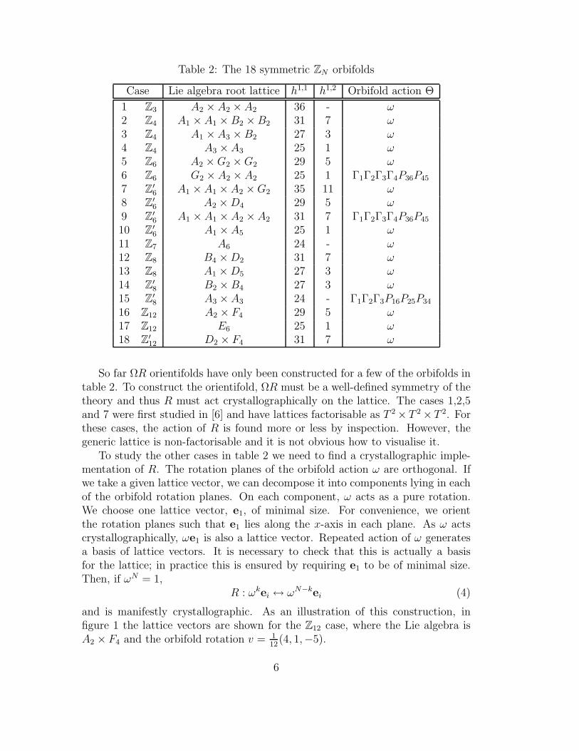
Table 2: The 18 symmetric ZN orbifolds
Case Lie algebra root lattice h1,1 h1,2 Orbifold action Θ
1 Z3 A2 × A2 × A2 36 - ω2 Z4 A1 × A1 × B2 ×B2 31 7 ω3 Z4 A1 ×A3 × B2 27 3 ω4 Z4 A3 × A3 25 1 ω5 Z6 A2 ×G2 ×G2 29 5 ω6 Z6 G2 × A2 × A2 25 1 Γ1Γ2Γ3Γ4P36P45
7 Z′6 A1 × A1 × A2 ×G2 35 11 ω
8 Z′6 A2 ×D4 29 5 ω
9 Z′6 A1 × A1 × A2 ×A2 31 7 Γ1Γ2Γ3Γ4P36P45
10 Z′6 A1 × A5 25 1 ω
11 Z7 A6 24 - ω12 Z8 B4 ×D2 31 7 ω13 Z8 A1 ×D5 27 3 ω14 Z
′8 B2 × B4 27 3 ω
15 Z′8 A3 × A3 24 - Γ1Γ2Γ3P16P25P34
16 Z12 A2 × F4 29 5 ω17 Z12 E6 25 1 ω18 Z
′12 D2 × F4 31 7 ω
So far ΩR orientifolds have only been constructed for a few of the orbifolds intable 2. To construct the orientifold, ΩR must be a well-defined symmetry of thetheory and thus R must act crystallographically on the lattice. The cases 1,2,5and 7 were first studied in [6] and have lattices factorisable as T 2 × T 2 × T 2. Forthese cases, the action of R is found more or less by inspection. However, thegeneric lattice is non-factorisable and it is not obvious how to visualise it.
To study the other cases in table 2 we need to find a crystallographic imple-mentation of R. The rotation planes of the orbifold action ω are orthogonal. Ifwe take a given lattice vector, we can decompose it into components lying in eachof the orbifold rotation planes. On each component, ω acts as a pure rotation.We choose one lattice vector, e1, of minimal size. For convenience, we orientthe rotation planes such that e1 lies along the x-axis in each plane. As ω actscrystallographically, ωe1 is also a lattice vector. Repeated action of ω generatesa basis of lattice vectors. It is necessary to check that this is actually a basisfor the lattice; in practice this is ensured by requiring e1 to be of minimal size.Then, if ωN = 1,
R : ωkei ↔ ωN−kei (4)
and is manifestly crystallographic. As an illustration of this construction, infigure 1 the lattice vectors are shown for the Z12 case, where the Lie algebra isA2 × F4 and the orbifold rotation v = 1
12(4, 1,−5).
6

4
5
e
e
A
B
6
7
e
e
ee
1
2
34
8
9
e
e
e
e
1
2
3
4
Figure 1: The Z12 lattice vectors. The arrow marked ei in each plane is not ei
itself; rather, it is the component of ei in that plane.
Table 2 lists the Lie algebras on whose root lattices the orbifold action isimplemented. However, we are not interested in the root structure of the algebraper se, but rather in the lattice derived from it. Also, the simple roots in generalare of different magnitude, but our construction generates basis vectors havingthe same size. Thus the basis we use, although a perfectly good basis for thelattice, does not generally consist of root vectors. We will see an example of thisin the Z
′8 case below.
For the factorisable T 2×T 2×T 2 case, it was found that there are two distinctways of implementing the ΩR projection in each T 2. These were called A andB type lattices, and correspond to the R fixed plane being either along the rootvectors or at a rotation of ω
12 . One effect of using more generic lattices is to
reduce this freedom - the action of R in one rotation plane determines its actionin another. For each independent torus - of whatever dimension - in the lattice,there are two possible crystallographic actions of ΩR. As was observed for thefactorisable cases in [4] [6], in certain models the tree channel amplitudes hadthe peculiar feature that the different contributions had the right prefactor tobe interpreted as a complete projector. In fact this feature served as a guidingprinciple for model building and it was even claimed that it is necessary forconsistency of the model. This claim was corrected in [48] where it was statedthat the other choices of the orientifold action also lead to consistent models.In section 4 we will reconsider this issue for the factorisable case and explicitlyconstruct all the consistent models where the complete projector does not appear.
We will implement the action of ΩR on the closed string modes as
(ΩR)ψr(ΩR)−1 = ψr
(ΩR)ψr(ΩR)−1 = ψr (5)
and likewise for the αr, αr oscillators. The loop channel amplitudes contributing
7
to R-R exchange in tree channel are then
KB = c
∫ ∞
0
dt
t3TrNSNS
(
ΩR(
1 + Θ + · · ·+ ΘN−1)
Ne−2πt(L0+L0)
)
A =c
4
∫ ∞
0
dt
t3TrNS
(
(−1)F
(
1 + Θ + · · ·+ ΘN−1)
Ne−2πtL0
)
MS = −c4
∫ ∞
0
dt
t3TrR
(
ΩR
(
1 + Θ + · · ·+ ΘN−1)
Ne−2πtL0
)
(6)
Here c ≡ V4/(8π2α′)2 arises from the integration over non-compact momenta.
These amplitudes involve combinations of ϑ functions and lattice sums. Wetransform these amplitudes to tree channel using
t =
12l
Annulus14l
Klein Bottle18l
Mobius Strip(7)
As RΘk = Θn−kR, (ΩRΘk)2 = 1 and so we expect only untwisted states topropagate in tree channel. The oscillator contributions in a given twisted sectorare straightforward. We convert these to tree channel using the modular trans-formation properties of the ϑ functions. These, together with the resulting treechannel expressions, are given in the appendix. The lattice contributions aremore involved and will be considered below.
In the Klein bottle trace, all insertions in the trace give rise to the sameoscillator contribution. However, insertions of the form ΩRΘ2k and ΩRΘ2k+1
generically give rise to different lattice contributions. For the annulus and Mobiussectors, the branes are placed at orientations related by Θ
12 . ‘Twisted sector’
open string amplitudes then correspond to strings stretching between branes atangles. The only non-vanishing insertions in the annulus amplitude are 1 and, ifN is even, Θ
N2 . The latter insertion leaves all the D6-branes invariant and hence
induces an action on the Chan-Paton factors described by a matrix γN2. The
twisted tadpole cancellation condition then implies tr(γN2) = 0. As this is the
sole effect of this insertion, when we consider particular models we will not writeout explicitly the amplitudes arising from this term.
In the Mobius amplitude, only (6i, 6i+2λ) strings can be invariant under anΩRΘk insertion and thus contribute in the Mobius strip amplitude. There aretwo insertions under which such strings are invariant, schematically ΩRΘλ andΩRΘλ+ N
2 . These contribute to the Θλ and Θλ+ N2 twisted sectors. For both the
annulus and Mobius strip amplitudes, strings starting on the 62k and 61+2k branesgenerically give different lattice contributions.
8
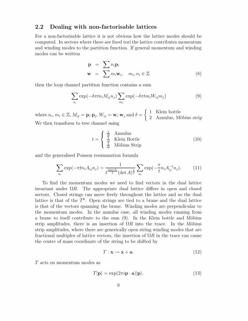
2.2 Dealing with non-factorisable lattices
For a non-factorisable lattice it is not obvious how the lattice modes should becomputed. In sectors where there are fixed tori the lattice contributes momentumand winding modes to the partition function. If general momentum and windingmodes can be written
p =∑
nipi
w =∑
miwi, mi, ni ∈ Z (8)
then the loop channel partition function contains a sum
∑
ni
exp(−δπtniMijnj)∑
mi
exp(−δπtmiWijmj) (9)
where ni,mi ∈ Z,Mij = pi·pj,Wij = wi·wj and δ =
1 Klein bottle2 Annulus, Mobius strip
We then transform to tree channel using
t =
12l
Annulus14l
Klein Bottle18l
Mobius Strip(10)
and the generalised Poisson resummation formula
∑
ni
exp(−πtniAijnj) =1
tdim(A)
2 (detA)12
∑
ni
exp(−πtniA
−1ij nj). (11)
To find the momentum modes we need to find vectors in the dual latticeinvariant under ΩR. The appropriate dual lattice differs in open and closedsectors. Closed strings can move freely throughout the lattice and so the duallattice is that of the T 6. Open strings are tied to a brane and the dual latticeis that of the vectors spanning the brane. Winding modes are perpendicular tothe momentum modes. In the annulus case, all winding modes running froma brane to itself contribute to the sum (9). In the Klein bottle and Mobiusstrip amplitudes, there is an insertion of ΩR into the trace. In the Mobiusstrip amplitudes, where there are generically open string winding modes that arefractional multiples of lattice vectors, the insertion of ΩR in the trace can causethe centre of mass coordinate of the string to be shifted by
T : x → x + a. (12)
T acts on momentum modes as
T |p〉 = exp(2πip · a)|p〉. (13)
9

In the particular case where p = nex
Rand T : x → x + R
2ex, the sum over
momentum modes in (9) is then
∑
ni
(−1)n exp(−πtniAijnj). (14)
Transformed to tree channel, this sum does not actually diverge in the l → ∞limit and so such winding modes do not contribute to the tadpoles. Latticemodes also occur when one complex plane is left invariant under the orbifoldaction, when an analogous version of the above discussion applies.
The lattice also contributes to the amplitude through fixed points and braneintersection numbers. For a non-factorisable lattice, it is difficult to find thesevisually. For the former, the Lefschetz fixed point theorem is not sufficient aswe also need to know which points are invariant under the action of ΩR. Wetherefore need to compute explicitly the location of the fixed points using theaction of ω. This is tedious but not difficult. A useful reference for this andother details of the non-factorisable lattices is [49], although the lattice basesused there differ from ours. To calculate brane intersection numbers we need tofind a spanning set of lattice vectors for each of the branes. The intersectionpoints are then given by solving a set of equations of the schematic form
∑
αivi =∑
βiwi (15)
for nontrivial (not in Z) values of αi. In the case of the Mobius strip, we alsoneed to investigate whether the intersection points are invariant under ΩRΘk forthe appropriate value of k.
Actually, for the annulus amplitude we would like to present a simple methodfor calculating the contribution of the lattice modes and the intersection numbers.Let ei be the basis vectors of the lattice and let gij = ei · ej . Let vi, i = 1, 2, 3 bethe lattice vectors that describe the 3-cycle wrapped by the brane, such that anypoint x on the brane can be uniquely written
x =∑
αivi αi ∈ [0, 1). (16)
We then define (MA)ij = vi · vj . The lattice dual to the brane is now given byv∗
i = vj(M−1A )ji, with v∗
i · v∗j = (M−1
A )ij. The contribution of momentum modesto the one-loop amplitude is then
∑
ni
exp(
−2πtni(M−1A )ijnj
)
→ ldim(MA)
2 (detMA)12
∑
ni
exp (−πlni(MA)ijnj) .
(17)Suppose a generic winding mode is written
w =∑
miwi mi ∈ Z, (18)
10
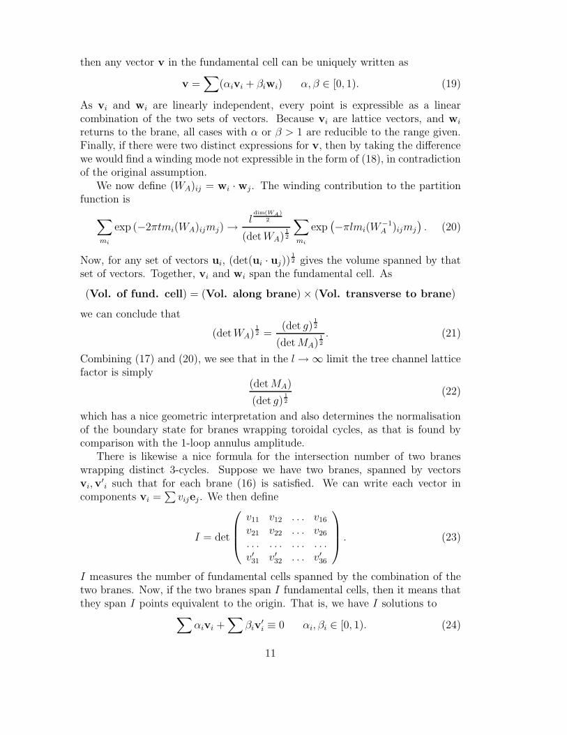
then any vector v in the fundamental cell can be uniquely written as
v =∑
(αivi + βiwi) α, β ∈ [0, 1). (19)
As vi and wi are linearly independent, every point is expressible as a linearcombination of the two sets of vectors. Because vi are lattice vectors, and wi
returns to the brane, all cases with α or β > 1 are reducible to the range given.Finally, if there were two distinct expressions for v, then by taking the differencewe would find a winding mode not expressible in the form of (18), in contradictionof the original assumption.
We now define (WA)ij = wi · wj . The winding contribution to the partitionfunction is
∑
mi
exp (−2πtmi(WA)ijmj) →ldim(WA)
2
(detWA)12
∑
mi
exp(
−πlmi(W−1A )ijmj
)
. (20)
Now, for any set of vectors ui, (det(ui · uj))12 gives the volume spanned by that
set of vectors. Together, vi and wi span the fundamental cell. As
(Vol. of fund. cell) = (Vol. along brane) × (Vol. transverse to brane)
we can conclude that
(detWA)12 =
(det g)12
(detMA)12
. (21)
Combining (17) and (20), we see that in the l → ∞ limit the tree channel latticefactor is simply
(detMA)
(det g)12
(22)
which has a nice geometric interpretation and also determines the normalisationof the boundary state for branes wrapping toroidal cycles, as that is found bycomparison with the 1-loop annulus amplitude.
There is likewise a nice formula for the intersection number of two braneswrapping distinct 3-cycles. Suppose we have two branes, spanned by vectorsvi,v
′i such that for each brane (16) is satisfied. We can write each vector in
components vi =∑
vijej . We then define
I = det
v11 v12 . . . v16
v21 v22 . . . v26
. . . . . . . . . . . .v′31 v′32 . . . v′36
. (23)
I measures the number of fundamental cells spanned by the combination of thetwo branes. Now, if the two branes span I fundamental cells, then it means thatthey span I points equivalent to the origin. That is, we have I solutions to
∑
αivi +∑
βiv′i ≡ 0 αi, βi ∈ [0, 1). (24)
11
However, (24) is equivalent to the existence of I sets of (αi, βi) such that
∑
αivi ≡ −∑
βiv′i αi, βi ∈ [0, 1), (25)
and therefore I is nothing else than the intersection number of the two branes.Formula (23) generalises the familiar case of a 2-torus, where branes with wrap-ping numbers (m1, n1), (m2, n2) have intersection number m1n2 − n1m2.
The above formulae are simple and require no detailed calculation. In thecase of the Mobius strip and Klein bottle amplitudes, it would be nice to havean equally elegant way of computing the lattice contributions and intersectionnumbers, given the action of ΩR on the lattice. Even though R will just act asa projection on the modes, such a formula has eluded us. We must thereforeexplicitly compute modes and intersection points invariant under ΩR.
Suppose we have found generators of momentum modes pi (Klein bottle) orvectors vi spanning the brane (annulus or Mobius strip), and also winding modeswi in the lattice. Then we define
(MKB)ij = pi · pj
(MMS)ij = (MA)ij = vi · vj
(WKB)ij = (WMS)ij = wi · wj. (26)
Then, if dim(M) = dim(W ) = n, the tree channel lattice mode contributions are
KB : 4n
(det MKB det WKB)12
A : (det MA)
(det g)12
MS : 4n(det MMS)12
(det WMS)12. (27)
Once we have computed the lattice modes, twisted sector fixed points, and braneintersection numbers, we can write down the tree-channel amplitudes as pre-scribed in the appendix.
3 The massless spectrum
3.1 The closed string spectrum
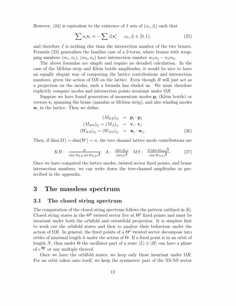
The computation of the closed string spectrum follows the pattern outlined in [6].Closed string states in the Θk twisted sector live at Θk fixed points and must beinvariant under both the orbifold and orientifold projection. It is simplest firstto work out the orbifold states and then to analyse their behaviour under theaction of ΩR. In general, the fixed points of a Θk twisted sector decompose intoorbits of maximal length k under the action of Θ. If a fixed point is in an orbit oflength N , then under Θ the oscillator part of a state |L〉 ⊗ |R〉 can have a phase
of e2πiN or any multiple thereof.
Once we have the orbifold states, we keep only those invariant under ΩR.For an orbit taken onto itself, we keep the symmetric part of the NS-NS sector
12
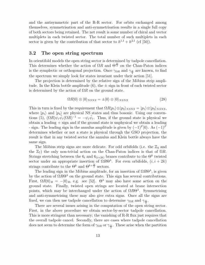
and the antisymmetric part of the R-R sector. For orbits exchanged amongthemselves, symmetrisation and anti-symmetrisation results in a single full copyof both sectors being retained. The net result is some number of chiral and vectormultiplets in each twisted sector. The total number of such multiplets in eachsector is given by the contribution of that sector to h1,1 + h2,1 (cf [50]).
3.2 The open string spectrum
In orientifold models the open string sector is determined by tadpole cancellation.This determines whether the action of ΩR and Θ
N2 on the Chan-Paton indices
is the symplectic or orthogonal projection. Once γΩR and γN2
are known, to find
the spectrum we simply look for states invariant under their action [51].The projection is determined by the relative sign of the Mobius strip ampli-
tude. In the Klein bottle amplitude (6), the ± sign in front of each twisted sectoris determined by the action of ΩR on the ground state.
ΩR|0〉 ⊗ |0〉NSNS = ±|0〉 ⊗ |0〉NSNS (28)
This in turn is fixed by the requirement that ΩR|p1〉⊗|p2〉NSNS = |p1〉⊗|p2〉NSNS,where |p1〉 and |p2〉 are physical NS states and thus bosonic. Using our conven-tions (5), (ΩR)ψrψr(ΩR)−1 = −ψrψr. Thus, if the ground state is physical weobtain a leading + sign and if the ground state is unphysical we obtain a leading- sign. The leading sign in the annulus amplitude is given by (−1)F |0〉. As (−1)F
determines whether or not a state is physical through the GSO projection, theresult is that in any twisted sector the annulus and Klein bottle always have thesame sign.
The Mobius strip signs are more delicate. For odd orbifolds (i.e. the Z3 andthe Z7) the only non-trivial action on the Chan-Paton indices is that of ΩR.Strings stretching between the 6i and 6(i+2k) branes contribute to the Θk twistedsector under an appropriate insertion of ΩRΘλ. For even orbifolds, (i, i + 2k)
strings contribute to the Θk and Θk+ N2 sectors.
The leading sign in the Mobius amplitude, for an insertion of ΩRΘλ, is givenby the action of ΩRΘλ on the ground state. This sign has several contributions.First, ΩR|0〉R = −|0〉R, e.g. see [52]. Θλ may also have some action on theground state. Finally, twisted open strings are located at brane intersectionpoints, which may be interchanged under the action of ΩRΘλ. Symmetrisingand anti-symmetrising these may also give extra signs. Once all the signs arefixed, we can then use tadpole cancellation to determine γΩR and γN
2.
There are several issues arising in the computation of the open string sector.First, in the above procedure we obtain sector-by-sector tadpole cancellation.This is more stringent than necessary; the vanishing of R-R flux just requires thatthe overall tadpole cancel. Secondly, there are cases where tadpole cancellationdoes not seem to determine the form of γΩR or γN
2. These arise when the partition
13

function in a twisted sector contains a ϑ[
1212
]
part, which vanishes. Indeed, for
Z4 orbifolds all twisted sector partition functions vanish.We take the view that these vanishing sectors in a certain sense vanish ac-
cidentally. To determine the open string spectrum, we require that we still ob-tain tadpole cancellation under a small formal deformation of the twist, e.g.(1
4, 1
4, 1
2) → (1
4, 1
4+ ǫ, 1
2+ ǫ). This procedure allows a determination of the spec-
trum and, applied to the cases studied in [4][6], results in the same spectrum asfound there.
4 Examples of factorisable orientifolds revisited
As previously explained, we can relax the requirement that the complete projectorappear in all three (Klein bottle, annulus and Mobius strip) amplitudes, yieldingmodels which generically have different gauge groups carried by 62i and 62i+1
branes. In some cases the gauge groups are the same, but the massless open stringspectrum is not invariant under the exchange of the two gauge group factors,similarly to the Z
′6 case in [6]. We found that all the various ΩR implementations
for the Z4,Z6,Z′6 models yield consistent solutions 5. Their closed and open
string spectra 6 are shown in tables 3,4 and 5. We use 10 to denote a U(2) singletuncharged under the gauge group.
Table 3: Closed string spectra
Model Θ0 Θ + Θ−1 Θ2(+Θ−2) Θ3
Z4 (AAA) 5C+1V 16C 16C absentZ4 (AAB) 5C+1V 12C+4V 16C absentZ6 (AAA) 4C+1V 2C+1V 10C+5V 10C+1VZ6 (BBB) 4C+1V 3C 15C 10C+1VZ′6 (AAA) 4C 7C+5V 14C+4V 10C+2V
Z′6 (BBB) 4C 9C+3V 18C 10C+2V
Since for the factorisable Z4 models with v = 14(1, 1,−2), ΩRΘ takes an A-type
lattice into a B-type lattice in the first two tori, and thus the AAA and BBA,AAB and BBB to be equivalent to each other. Similarly, models AAA andBBA, AAB and BBB for Z6 as well as AAA and BAB, ABA and BBB forZ′6 are equivalent.
5One can also revisit the 6-dimensional orientifolds of [4]. We again find consistent models,and the computed spectrum is anomaly free.
6We thank Gabriele Honecker for alerting us to the presence of vector multiplets in theclosed string untwisted sector.
14

Table 4: The Z4 open string spectra
Model (6i, 6i) (6i, 6i+1) (6i, 6i+2)AAA U(16) × U(4) 1C (16, 4) ⊕ (16, 4) 2C (256, 1) + 8C (1, 16)
(1V+1C) (256, 1) ⊕ (1, 16)+2C (120, 1) ⊕ (120, 1)+2C (1, 6) ⊕ (1, 6)
AAB U(8) × U(2) 2C (8, 2) ⊕ (8, 2) 2C (64, 10) + 8C (1, 4)(1V+1C) (64, 10) ⊕ (1, 4)+2C (28, 10) ⊕ (28, 10)+2C (1, 1) ⊕ (1, 1)
5 Examples of non-factorisable orientifolds
In this section we discuss in some detail a couple of completely new examples ofΩR orientifolds on non-factorisable orbifolds. Employing the general formalismdeveloped in section 2 and section 3 we consider the solutions to the tadpolecancellation conditions where we place the D6-branes parallel to the orientifoldplanes. The closed string spectrum for all models considered in this section iscomputed as in section 3 and appears in table 6.
5.1 Z7 Model : A7 with v = 17(1, 2,−3)
The SU(7) algebra has six root vectors, denoted by ei. They are of equal mag-nitude (taken to be 1), and gij = ei · ej is given by
gij =
1 −12
0 0 0 0−1
21 −1
20 0 0
0 −12
1 −12
0 00 0 −1
21 −1
20
0 0 0 −12
1 −12
0 0 0 0 −12
1
(29)
The Weyl element Γi reflects across the plane perpendicular to a root vector. Itsaction on a vector x is given by
Γix = x − 2ei · xei · ei
ei (30)
The Coxeter element ω = Γ1Γ2 . . .Γ6 acts as
ωei = ei+1 i = 1, 2, 3, 4, 5ωe6 = −e1 − e2 − e3 − e4 − e5 − e6
(31)
15
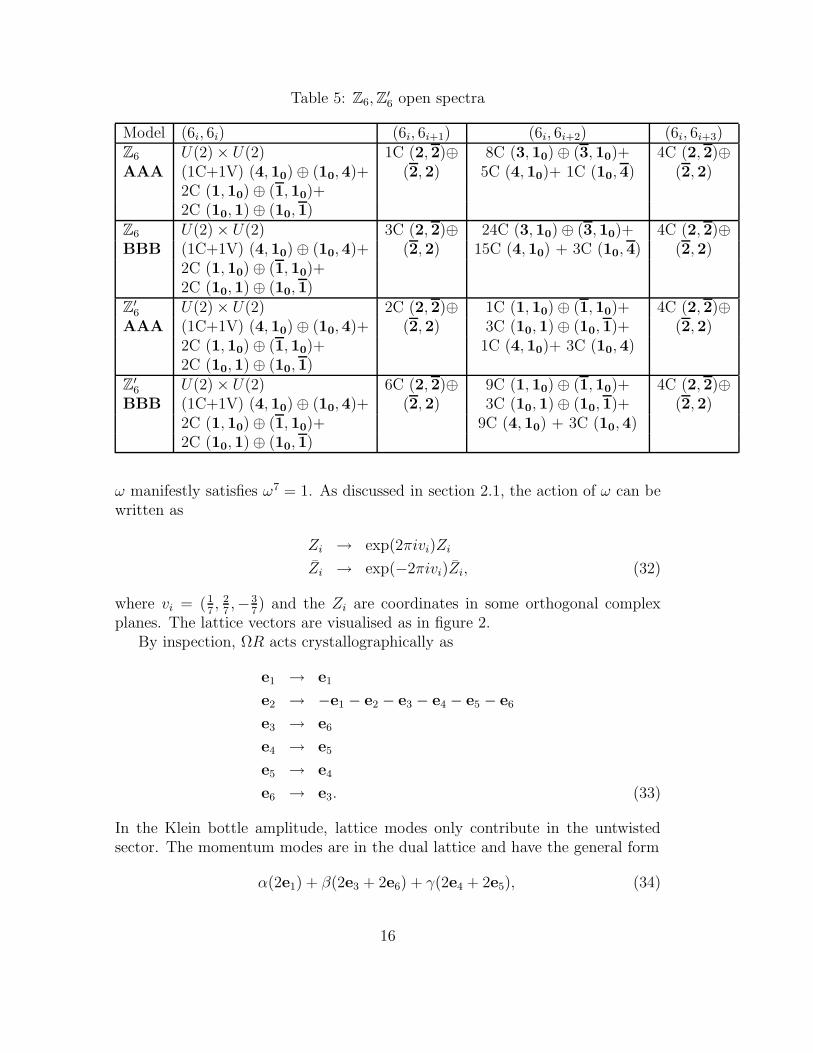
Table 5: Z6,Z′6 open spectra
Model (6i, 6i) (6i, 6i+1) (6i, 6i+2) (6i, 6i+3)Z6 U(2) × U(2) 1C (2, 2)⊕ 8C (3, 10) ⊕ (3, 10)+ 4C (2, 2)⊕AAA (1C+1V) (4, 10) ⊕ (10, 4)+ (2, 2) 5C (4, 10)+ 1C (10, 4) (2, 2)
2C (1, 10) ⊕ (1, 10)+2C (10, 1) ⊕ (10, 1)
Z6 U(2) × U(2) 3C (2, 2)⊕ 24C (3, 10) ⊕ (3, 10)+ 4C (2, 2)⊕BBB (1C+1V) (4, 10) ⊕ (10, 4)+ (2, 2) 15C (4, 10) + 3C (10, 4) (2, 2)
2C (1, 10) ⊕ (1, 10)+2C (10, 1) ⊕ (10, 1)
Z′6 U(2) × U(2) 2C (2, 2)⊕ 1C (1, 10) ⊕ (1, 10)+ 4C (2, 2)⊕
AAA (1C+1V) (4, 10) ⊕ (10, 4)+ (2, 2) 3C (10, 1) ⊕ (10, 1)+ (2, 2)2C (1, 10) ⊕ (1, 10)+ 1C (4, 10)+ 3C (10, 4)2C (10, 1) ⊕ (10, 1)
Z′6 U(2) × U(2) 6C (2, 2)⊕ 9C (1, 10) ⊕ (1, 10)+ 4C (2, 2)⊕
BBB (1C+1V) (4, 10) ⊕ (10, 4)+ (2, 2) 3C (10, 1) ⊕ (10, 1)+ (2, 2)2C (1, 10) ⊕ (1, 10)+ 9C (4, 10) + 3C (10, 4)2C (10, 1) ⊕ (10, 1)
ω manifestly satisfies ω7 = 1. As discussed in section 2.1, the action of ω can bewritten as
Zi → exp(2πivi)Zi
Zi → exp(−2πivi)Zi, (32)
where vi = (17, 2
7,−3
7) and the Zi are coordinates in some orthogonal complex
planes. The lattice vectors are visualised as in figure 2.By inspection, ΩR acts crystallographically as
e1 → e1
e2 → −e1 − e2 − e3 − e4 − e5 − e6
e3 → e6
e4 → e5
e5 → e4
e6 → e3. (33)
In the Klein bottle amplitude, lattice modes only contribute in the untwistedsector. The momentum modes are in the dual lattice and have the general form
α(2e1) + β(2e3 + 2e6) + γ(2e4 + 2e5), (34)
16

Table 6: Closed string spectra
Model Θ0 Θ + Θ−1 Θ2 + Θ−2 Θ3 + Θ−3 Θ4 (+Θ−4) Θ5 + Θ−5 Θ6
Z7(A) 3C 4C+3V 4C+3V 4C+3V absent absent absentZ7(B) 3C 7C 7C 7C absent absent absentZ8(AA) 4C 8C 8C 8C 10C absent absentZ8(BA) 4C 6C+2V 8C 6C+2V 10C absent absentZ
′
8(AA) 3C 4C 10C 4C 9C absent absentZ
′
8(BA) 3C 4C 9C + 1V 4C 9C absent absentZ12(AA) 3C 2C+1V 2C+1V 6C 6C + 3V 2C + 1V 7CZ12(BA) 3C 3C 3C 6C 9C 3C 7CZ
′
12(AA) 4C 4C 2C 8C 10C 4C 6CZ
′
12(BA) 4C 3C+1V 2C 6C + 2V 10C 3C + 1V 6C
8
9
e
ee
e
ee
1
2
3
4
5
6
4
5
e
e
e
e
1
23
4
5
6
e
e
6
7e
e
e
e
e
2
3
4
5
6
1e
Figure 2: The Z7 lattice
where α, β, γ ∈ Z. The winding modes are
α′(e1 + 2e2 + e3 + e4 + e5 + e6) + β ′(e3 − e6) + γ′(e4 − e5) (35)
with α′, β ′, γ′ ∈ Z. We then get
MKB = 4
1 0 00 2 −10 −1 1
(36)
WKB =
2 −1 0−1 2 −10 −1 3
. (37)
The untwisted lattice factor is then 64
(det MKB)12 (det WKB)
12
= 8√7. The SU(7) lattice
17
has 7 fixed points in each twisted sector. These are n7(e1 + 2e2 + 3e3 + 4e4 +
5e5 + 6e6), where n = 0, 1, . . . , 6. It is easily verified that only the n = 0 case isinvariant under ΩR.
We can now write down the tree channel Klein bottle amplitude. As the zeropoint energy in all sectors is negative, ΩR|0〉 ⊗ |0〉 = −|0〉 ⊗ |0〉, and all sectorscarry a leading minus sign
KB = c
∫ ∞
0
16ldl
( −1
16l4(Θ0)
8l3√7− 1
2l(Θ) − . . .
1
2l(Θ6)
)
= c
∫ ∞
0
dl8√7
(
−(Θ0) −√
7(Θ1) −√
7(Θ2) − . . .−√
7(Θ6))
. (38)
As sin(π7) sin(2π
7) sin(4π
7) =
√7
8, we actually have the complete projector
∏
i 2 sin(πvi)appearing here.
9
8
6
6
6666
6
1
3
572
4
6
6
6
666
6
6
5
41
2
3
45
6
7
6
7
6
6
666
6
6
1
5
263
7
4
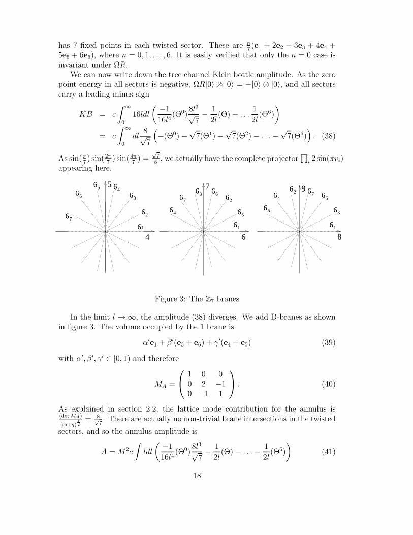
Figure 3: The Z7 branes
In the limit l → ∞, the amplitude (38) diverges. We add D-branes as shownin figure 3. The volume occupied by the 1 brane is
α′e1 + β ′(e3 + e6) + γ′(e4 + e5) (39)
with α′, β ′, γ′ ∈ [0, 1) and therefore
MA =
1 0 00 2 −10 −1 1
. (40)
As explained in section 2.2, the lattice mode contribution for the annulus is(det MA)
(det g)12
= 8√7. There are actually no non-trivial brane intersections in the twisted
sectors, and so the annulus amplitude is
A = M2c
∫
ldl
( −1
16l4(Θ0)
8l3√7− 1
2l(Θ) − . . .− 1
2l(Θ6)
)
(41)
18
which can be simplified to
A = M2c
∫
dl
2√
7
(
−(Θ0) −√
7(Θ) − . . .√
7(Θ6))
(42)
As with the Klein bottle amplitude (38), in all sectors the ground state is un-physical and so (−1)F |0〉 = −|0〉.
Finally we need to consider the Mobius strip amplitude. The twisted sectorintersection numbers remain trivial. The lattice modes must be invariant underΩR. As described in section 2.2, we have
MMS = MA =
1 0 00 2 −10 −1 1
(43)
WMS = WKB =
2 −1 0−1 2 −10 −1 3
(44)
with a resulting lattice factor for the Mobius strip amplitude of 64 (det MMS)12
(det WMS)12
= 64√7.
The Mobius amplitude reads
MS = +Mc
∫
16ldl
(
1
28l4(Θ0)
64l3√7
+1
4l(Θ) + . . .+
1
4l(Θ6)
)
(45)
giving
MS = +Mc
∫
dl4√7
(
(Θ0) +√
7(Θ) + . . .√
7(Θ6))
. (46)
We have in equation (46) fixed tr(γTΩRΘkγ
−1ΩRΘk) = +M in all sectors. Extracting
the leading divergences from equations (38), (42) and (46), the tadpole cancella-tion conditions are
(M2 − 8M + 16) = 0, (47)
implying M = 4 and the branes carrying an SO(4) gauge group.The closed string spectrum was given in table 6. For the open strings, the ΩR
projection is the SO(n) projection in all sectors. In each twisted sector, there isone massless oscillator state located at the origin. This being an odd orbifold,there is no additional Θ
N2 projection to concern us and the open string spectrum
is as in table 7.The above action of R is not the only crystallographic implementation. We
could also implement R at a rotation of Θ12 in the B orientation. If we repeat
the above analysis, we find that all amplitudes are multiplied by 7. This does notaffect the tadpole cancellation condition and we again get an SO(4) gauge group.This behaviour is exactly analogous to that encountered for the Z3 orientifold in[6].
19
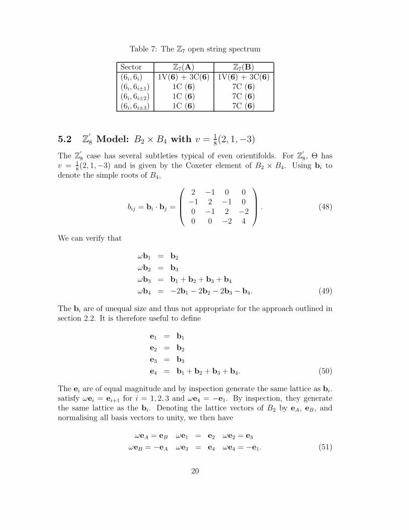
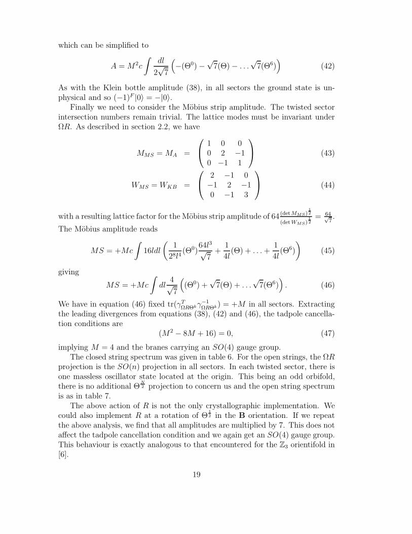
Table 7: The Z7 open string spectrum
Sector Z7(A) Z7(B)(6i, 6i) 1V(6) + 3C(6) 1V(6) + 3C(6)(6i, 6i±1) 1C (6) 7C (6)(6i, 6i±2) 1C (6) 7C (6)(6i, 6i±3) 1C (6) 7C (6)
5.2 Z′
8 Model: B2 ×B4 with v = 18(2, 1,−3)
The Z′
8 case has several subtleties typical of even orientifolds. For Z′
8, Θ hasv = 1
8(2, 1,−3) and is given by the Coxeter element of B2 × B4. Using bi to
denote the simple roots of B4,
bij = bi · bj =
2 −1 0 0−1 2 −1 00 −1 2 −20 0 −2 4
. (48)
We can verify that
ωb1 = b2
ωb2 = b3
ωb3 = b1 + b2 + b3 + b4
ωb4 = −2b1 − 2b2 − 2b3 − b4. (49)
The bi are of unequal size and thus not appropriate for the approach outlined insection 2.2. It is therefore useful to define
e1 = b1
e2 = b2
e3 = b3
e4 = b1 + b2 + b3 + b4. (50)
The ei are of equal magnitude and by inspection generate the same lattice as bi.satisfy ωei = ei+1 for i = 1, 2, 3 and ωe4 = −e1. By inspection, they generatethe same lattice as the bi. Denoting the lattice vectors of B2 by eA, eB, andnormalising all basis vectors to unity, we then have
ωeA = eB ωe1 = e2 ωe2 = e3
ωeB = −eA ωe3 = e4 ωe4 = −e1. (51)
20
gij = ei · ej =
1 0 0 0 0 00 1 0 0 0 00 0 1 −1
20 1
2
0 0 −12
1 −12
00 0 0 −1
21 −1
2
0 0 12
0 −12
1
. (52)
The lattice vectors are shown in figure 4. The action of R is given by
eA ↔ eB
e1 ↔ e1
e2 ↔ −e4
e3 ↔ −e3. (53)
e
e
4
5
B
A
6
7
e
eee
1
234
8
9
e
e
ee
1
2
3
4
Figure 4: The Z′
8 lattice
There are two independent insertions in the Klein bottle trace (6), ΩR andΩRΘ. Under ΩR, the lattice modes in the untwisted sector are
pΩR = l(eA + eB) +m(2e1) + n(e2 − e4), l,m, n ∈ Z
wΩR = l′(eA − eB) +m′e3 + n(e2 + e4), l′, m′, n′ ∈ Z (54)
and under ΩRΘ we have
pΩRΘ = leA +m(e1 − e4 + e2 − e3) + 2n(e1 − e4), l,m, n ∈ Z
wΩRΘ = l′eB +m′(e1 + e4) + n′(e2 + e3), l′, m′, n′ ∈ Z (55)
From (54) we obtain
MKB,ΩR =
2 0 00 4 −20 −2 2
(56)
WKB,ΩR =
2 0 00 1 −10 −1 2
. (57)
21
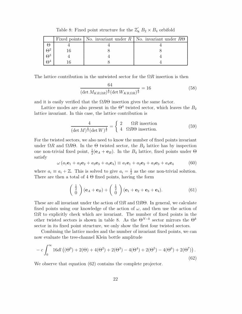
Table 8: Fixed point structure for the Z′
8 B2 × B4 orbifold
Fixed points No. invariant under R No. invariant under RΘΘ 4 4 4Θ2 16 8 8Θ3 4 4 4Θ4 16 8 4
The lattice contribution in the untwisted sector for the ΩR insertion is then
64
(detMKB,ΩR)12 (detWKB,ΩR)
12
= 16 (58)
and it is easily verified that the ΩRΘ insertion gives the same factor.Lattice modes are also present in the Θ4 twisted sector, which leaves the B2
lattice invariant. In this case, the lattice contribution is
4
(detM)12 (detW )
12
=
2 ΩR insertion4 ΩRΘ insertion.
(59)
For the twisted sectors, we also need to know the number of fixed points invariantunder ΩR and ΩRΘ. In the Θ twisted sector, the B2 lattice has by inspectionone non-trivial fixed point, 1
2(eA + eB). In the B4 lattice, fixed points under Θ
satisfyω (a1e1 + a2e2 + a3e3 + a4e4) ≡ a1e1 + a2e2 + a3e3 + a4e4 (60)
where ai ≡ ai + Z. This is solved to give ai = 12
as the one non-trivial solution.There are then a total of 4 Θ fixed points, having the form
(
12
0
)
(eA + eB) +
(
12
0
)
(e1 + e2 + e3 + e4). (61)
These are all invariant under the action of ΩR and ΩRΘ. In general, we calculatefixed points using our knowledge of the action of ω, and then use the action ofΩR to explicitly check which are invariant. The number of fixed points in theother twisted sectors is shown in table 8. As the ΘN−k sector mirrors the Θk
sector in its fixed point structure, we only show the first four twisted sectors.Combining the lattice modes and the number of invariant fixed points, we can
now evaluate the tree-channel Klein bottle amplitude
− c
∫ ∞
0
16dl(
(Θ0) + 2(Θ) + 4(Θ2) + 2(Θ3) − 4(Θ4) + 2(Θ5) − 4(Θ6) + 2(Θ7))
.
(62)We observe that equation (62) contains the complete projector.
22
56
4
6
66
5
6
1,5
2,63,7
4,8
66
6
66
66
6
6
1
3
2
45
6
7
8
86
6
66
6
6
1
6
3
8627
8
7 9
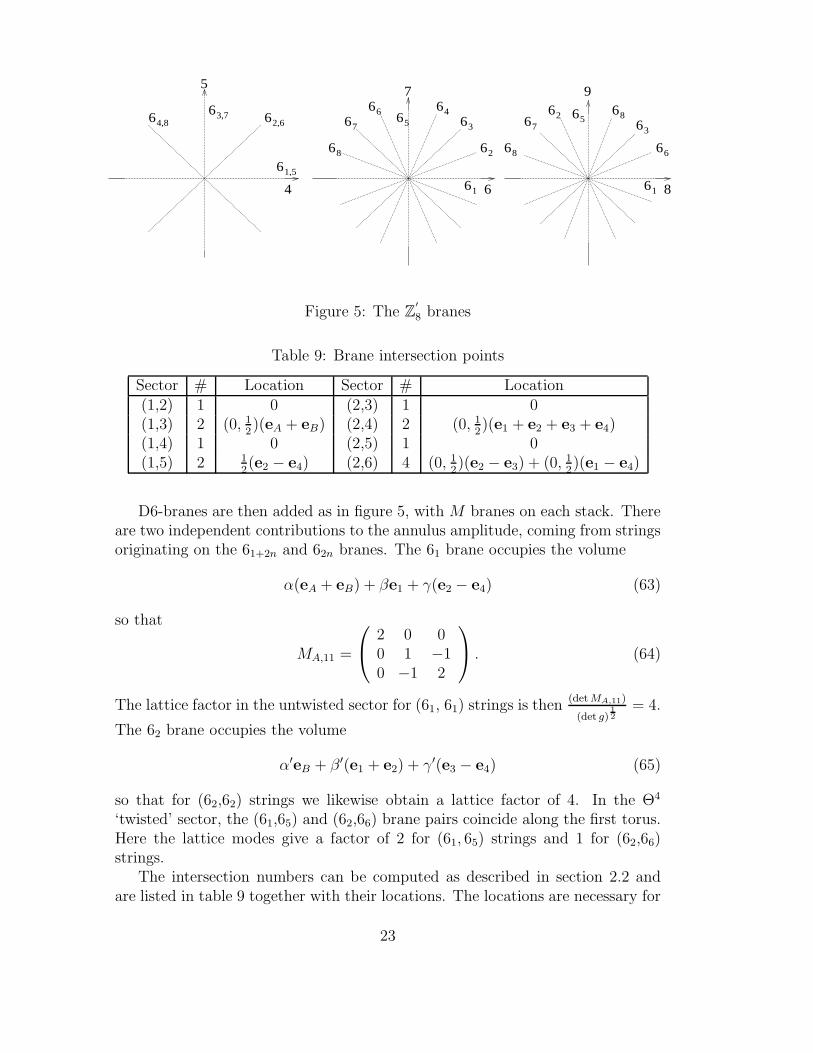
Figure 5: The Z′
8 branes
Table 9: Brane intersection points
Sector # Location Sector # Location(1,2) 1 0 (2,3) 1 0(1,3) 2 (0, 1
2)(eA + eB) (2,4) 2 (0, 1
2)(e1 + e2 + e3 + e4)
(1,4) 1 0 (2,5) 1 0(1,5) 2 1
2(e2 − e4) (2,6) 4 (0, 1
2)(e2 − e3) + (0, 1
2)(e1 − e4)
D6-branes are then added as in figure 5, with M branes on each stack. Thereare two independent contributions to the annulus amplitude, coming from stringsoriginating on the 61+2n and 62n branes. The 61 brane occupies the volume
α(eA + eB) + βe1 + γ(e2 − e4) (63)
so that
MA,11 =
2 0 00 1 −10 −1 2
. (64)
The lattice factor in the untwisted sector for (61, 61) strings is then(det MA,11)
(det g)12
= 4.
The 62 brane occupies the volume
α′eB + β ′(e1 + e2) + γ′(e3 − e4) (65)
so that for (62,62) strings we likewise obtain a lattice factor of 4. In the Θ4
‘twisted’ sector, the (61,65) and (62,66) brane pairs coincide along the first torus.Here the lattice modes give a factor of 2 for (61, 65) strings and 1 for (62,66)strings.
The intersection numbers can be computed as described in section 2.2 andare listed in table 9 together with their locations. The locations are necessary for
23
the Mobius strip amplitude and must be found by explicit computation, e.g. tofind (61, 62) intersection points we look for non-trivial solutions of
α(eA + eB) + βe1 + γ(e2 − e4) ≡ α′eB + β ′(e1 + e2) + γ′(e3 − e4). (66)
We can now write down the annulus amplitude
− cM2
∫
ldl
(
1
16l4(Θ0)4 +
1
2l(Θ) +
1
2l2(Θ2) +
1
2l(Θ3) +
l
4l24(Θ4) + . . .
)
(67)
which can be brought to the form
A = −M2c
∫
dl
4
(
(Θ0) + 2(Θ) + 4(Θ2) + 2(Θ3) − 4(Θ4) + . . .)
. (68)
This has the same form as the Klein bottle amplitude (62).For the Mobius amplitude, as discussed in section 2.2, we find
WMS,11 = WKB,ΩR =
2 0 00 1 −10 −1 2
(69)
MMS,11 = MA,11 =
2 0 00 1 −10 −1 2
. (70)
The lattice factor for (61, 61) strings is then 64(det MMS,11)
12
(det WMS,11)12
= 64 and a similar
treatment for (62, 62) strings yields 64, as well.No other lattice modes contribute to the Mobius amplitude. The 61 and 65
branes have a coincident direction and so could in principle have lattice modes.However, (61, 65) strings are invariant under an insertion of ΩRΘ2 in the trace.As this acts as a reflection on the coincident direction, there are no invariantlattice modes. Finally, all intersection points are invariant under the appropriateinsertion of ΩRΘk except those in the (62, 66) sector. Here, only two of the fourpoints are invariant.
We then obtain the following tree channel Mobius strip amplitude
Mc
∫
4dl(
(Θ0) + 2(Θ) + 4(Θ2) + 2(Θ3) − 4(Θ4) + . . .)
. (71)
To obtain (71) we have fixed the action of the various Chan-Paton matrices; thisdetermines the open string spectrum. Extracting the leading divergence from thethree amplitudes, we get
(M − 8)2 = 0 (72)
implying that we need stacks of 8 D-branes to cancel tadpoles and that the gaugegroup is U(4) × U(4).
24
The above represents a BA ΩR implementation. We can also consider theAA ΩR orientation. The tree channel Klein bottle amplitude is then
K = −c∫ ∞
0
dl(
(16 + 4)(Θ0) + 8(2 + 2)(Θ) + 8(8 + 2)(Θ2) + 8(2 + 2)(Θ3) −
8(8 + 2)(Θ4) + . . .)
(73)
Supposing that there are M 62k and N 62k+1 branes, the tree channel annulusamplitude takes the form
A = −c∫
dl
32
(
(2M2 + 8N2)(Θ0) + 16MN(Θ) + 8(M2 + 4N2)(Θ2)
+16MN(Θ3) − 8(M2 + 4N2)(Θ4) + . . .)
(74)
and the Mobius amplitude is similarly seen to be
M = c
∫
4dl
(
1
2(M +N)(Θ0) +
1
2(M + 4N)(Θ) + 2(M +N)(Θ2) +
1
2(M + 4N)(Θ3) − 2(M +N)(Θ4) + . . .
)
. (75)
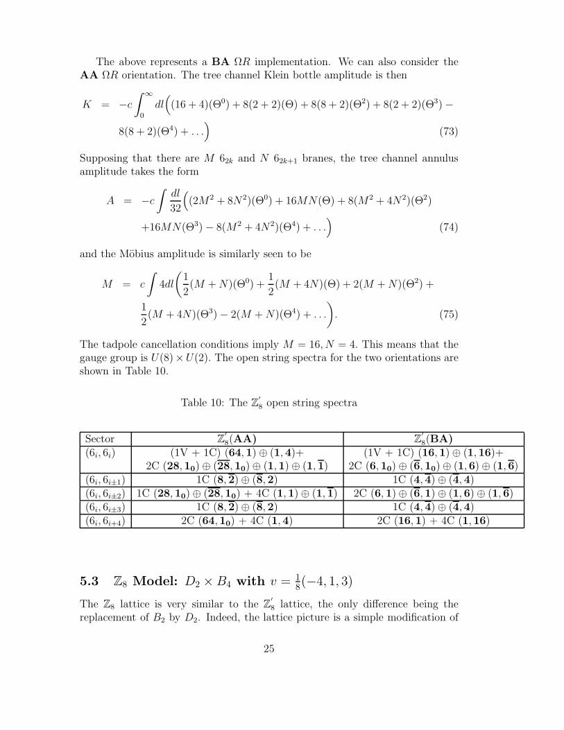
The tadpole cancellation conditions imply M = 16, N = 4. This means that thegauge group is U(8)×U(2). The open string spectra for the two orientations areshown in Table 10.
Table 10: The Z′
8 open string spectra
Sector Z′
8(AA) Z′
8(BA)(6i, 6i) (1V + 1C) (64, 1) ⊕ (1, 4)+ (1V + 1C) (16, 1) ⊕ (1, 16)+
2C (28, 10) ⊕ (28, 10) ⊕ (1, 1) ⊕ (1, 1) 2C (6, 10) ⊕ (6, 10) ⊕ (1, 6) ⊕ (1, 6)(6i, 6i±1) 1C (8, 2) ⊕ (8, 2) 1C (4, 4) ⊕ (4, 4)(6i, 6i±2) 1C (28, 10) ⊕ (28, 10) + 4C (1, 1) ⊕ (1, 1) 2C (6, 1) ⊕ (6, 1) ⊕ (1, 6) ⊕ (1, 6)(6i, 6i±3) 1C (8, 2) ⊕ (8, 2) 1C (4, 4) ⊕ (4, 4)(6i, 6i+4) 2C (64, 10) + 4C (1, 4) 2C (16, 1) + 4C (1, 16)
5.3 Z8 Model: D2 × B4 with v = 18(−4, 1, 3)
The Z8 lattice is very similar to the Z′
8 lattice, the only difference being thereplacement of B2 by D2. Indeed, the lattice picture is a simple modification of
25
4. The action of ω on the lattice basis ei is
ωeA = −eA ωe1 = e2 ωe2 = e3
ωeB = −eB ωe3 = e4 ωe4 = −e1. (76)
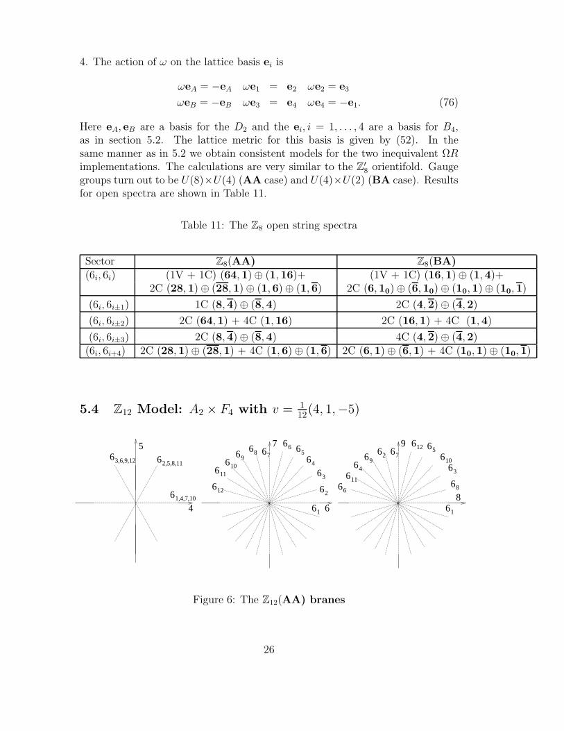
Here eA, eB are a basis for the D2 and the ei, i = 1, . . . , 4 are a basis for B4,as in section 5.2. The lattice metric for this basis is given by (52). In thesame manner as in 5.2 we obtain consistent models for the two inequivalent ΩRimplementations. The calculations are very similar to the Z
′8 orientifold. Gauge
groups turn out to be U(8)×U(4) (AA case) and U(4)×U(2) (BA case). Resultsfor open spectra are shown in Table 11.
Table 11: The Z8 open string spectra
Sector Z8(AA) Z8(BA)(6i, 6i) (1V + 1C) (64, 1) ⊕ (1, 16)+ (1V + 1C) (16, 1) ⊕ (1, 4)+
2C (28, 1) ⊕ (28, 1) ⊕ (1, 6) ⊕ (1, 6) 2C (6, 10) ⊕ (6, 10) ⊕ (10, 1) ⊕ (10, 1)
(6i, 6i±1) 1C (8, 4) ⊕ (8, 4) 2C (4, 2) ⊕ (4, 2)
(6i, 6i±2) 2C (64, 1) + 4C (1, 16) 2C (16, 1) + 4C (1, 4)
(6i, 6i±3) 2C (8, 4) ⊕ (8, 4) 4C (4, 2) ⊕ (4, 2)(6i, 6i+4) 2C (28, 1) ⊕ (28, 1) + 4C (1, 6) ⊕ (1, 6) 2C (6, 1) ⊕ (6, 1) + 4C (10, 1) ⊕ (10, 1)
5.4 Z12 Model: A2 × F4 with v = 112(4, 1,−5)
8
9
6
666
66 6
66
66
1
8
3
10
51272
94
11
6
6
4
5
6
66
1,4,7,10
2,5,8,113,6,9,12
7
66
6
66
66666
6
6
6
1
2
3
4
56
789
1011
12
Figure 6: The Z12(AA) branes
26
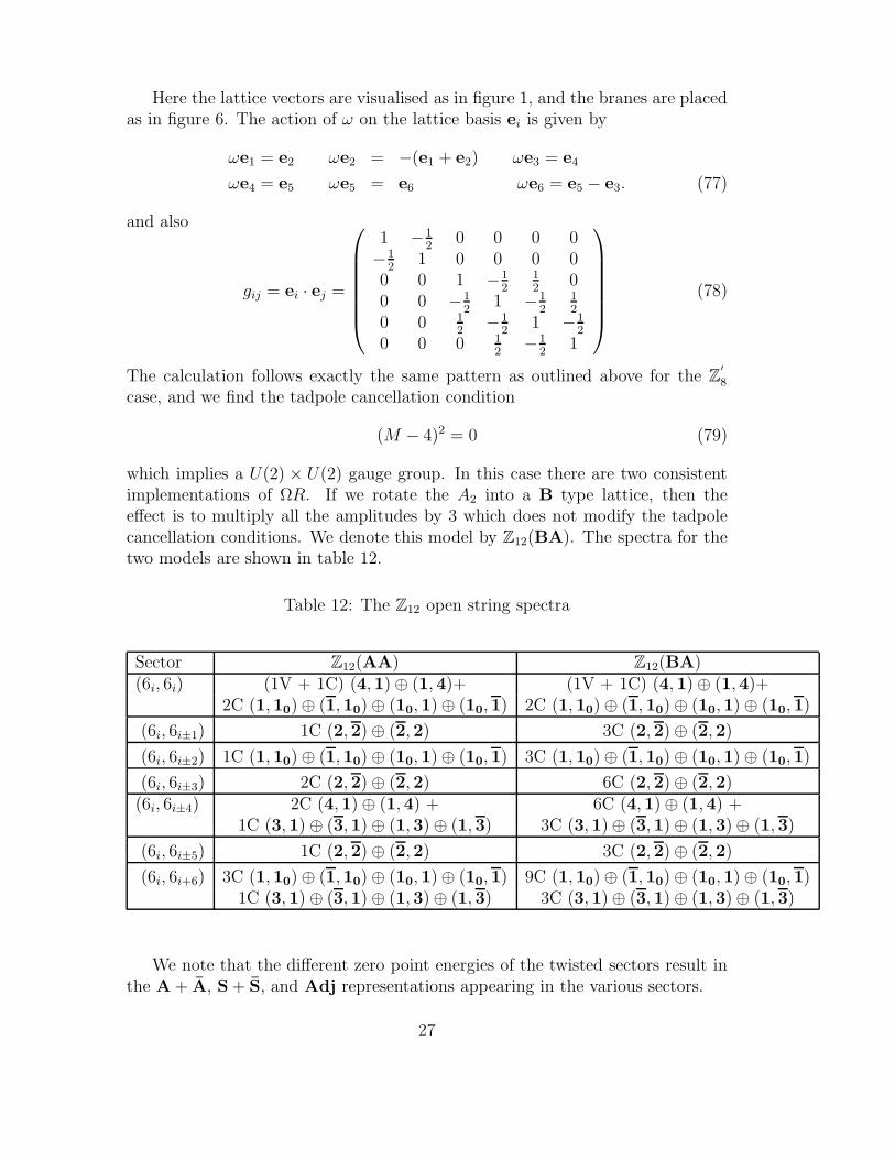
Here the lattice vectors are visualised as in figure 1, and the branes are placedas in figure 6. The action of ω on the lattice basis ei is given by
ωe1 = e2 ωe2 = −(e1 + e2) ωe3 = e4
ωe4 = e5 ωe5 = e6 ωe6 = e5 − e3. (77)
and also
gij = ei · ej =
1 −12
0 0 0 0−1
21 0 0 0 0
0 0 1 −12
12
00 0 −1
21 −1
212
0 0 12
−12
1 −12
0 0 0 12
−12
1
(78)
The calculation follows exactly the same pattern as outlined above for the Z′
8
case, and we find the tadpole cancellation condition
(M − 4)2 = 0 (79)
which implies a U(2) × U(2) gauge group. In this case there are two consistentimplementations of ΩR. If we rotate the A2 into a B type lattice, then theeffect is to multiply all the amplitudes by 3 which does not modify the tadpolecancellation conditions. We denote this model by Z12(BA). The spectra for thetwo models are shown in table 12.
Table 12: The Z12 open string spectra
Sector Z12(AA) Z12(BA)(6i, 6i) (1V + 1C) (4, 1) ⊕ (1, 4)+ (1V + 1C) (4, 1) ⊕ (1, 4)+
2C (1, 10) ⊕ (1, 10) ⊕ (10, 1) ⊕ (10, 1) 2C (1, 10) ⊕ (1, 10) ⊕ (10, 1) ⊕ (10, 1)
(6i, 6i±1) 1C (2, 2) ⊕ (2, 2) 3C (2, 2) ⊕ (2, 2)
(6i, 6i±2) 1C (1, 10) ⊕ (1, 10) ⊕ (10, 1) ⊕ (10, 1) 3C (1, 10) ⊕ (1, 10) ⊕ (10, 1) ⊕ (10, 1)
(6i, 6i±3) 2C (2, 2) ⊕ (2, 2) 6C (2, 2) ⊕ (2, 2)(6i, 6i±4) 2C (4, 1) ⊕ (1, 4) + 6C (4, 1) ⊕ (1, 4) +
1C (3, 1) ⊕ (3, 1) ⊕ (1, 3) ⊕ (1, 3) 3C (3, 1) ⊕ (3, 1) ⊕ (1, 3) ⊕ (1, 3)
(6i, 6i±5) 1C (2, 2) ⊕ (2, 2) 3C (2, 2) ⊕ (2, 2)
(6i, 6i+6) 3C (1, 10) ⊕ (1, 10) ⊕ (10, 1) ⊕ (10, 1) 9C (1, 10) ⊕ (1, 10) ⊕ (10, 1) ⊕ (10, 1)1C (3, 1) ⊕ (3, 1) ⊕ (1, 3) ⊕ (1, 3) 3C (3, 1) ⊕ (3, 1) ⊕ (1, 3) ⊕ (1, 3)
We note that the different zero point energies of the twisted sectors result inthe A + A, S + S, and Adj representations appearing in the various sectors.
27
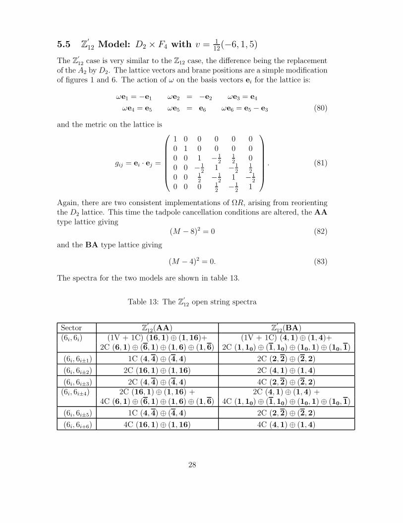
5.5 Z′
12 Model: D2 × F4 with v = 112(−6, 1, 5)
The Z′
12 case is very similar to the Z12 case, the difference being the replacementof the A2 by D2. The lattice vectors and brane positions are a simple modificationof figures 1 and 6. The action of ω on the basis vectors ei for the lattice is:
ωe1 = −e1 ωe2 = −e2 ωe3 = e4
ωe4 = e5 ωe5 = e6 ωe6 = e5 − e3 (80)
and the metric on the lattice is
gij = ei · ej =
1 0 0 0 0 00 1 0 0 0 00 0 1 −1
212
00 0 −1
21 −1
212
0 0 12
−12
1 −12
0 0 0 12
−12
1
. (81)
Again, there are two consistent implementations of ΩR, arising from reorientingthe D2 lattice. This time the tadpole cancellation conditions are altered, the AAtype lattice giving
(M − 8)2 = 0 (82)
and the BA type lattice giving
(M − 4)2 = 0. (83)
The spectra for the two models are shown in table 13.
Table 13: The Z′
12 open string spectra
Sector Z′
12(AA) Z′
12(BA)(6i, 6i) (1V + 1C) (16, 1) ⊕ (1, 16)+ (1V + 1C) (4, 1) ⊕ (1, 4)+
2C (6, 1) ⊕ (6, 1) ⊕ (1, 6) ⊕ (1, 6) 2C (1, 10) ⊕ (1, 10) ⊕ (10, 1) ⊕ (10, 1)
(6i, 6i±1) 1C (4, 4) ⊕ (4, 4) 2C (2, 2) ⊕ (2, 2)
(6i, 6i±2) 2C (16, 1) ⊕ (1, 16) 2C (4, 1) ⊕ (1, 4)
(6i, 6i±3) 2C (4, 4) ⊕ (4, 4) 4C (2, 2) ⊕ (2, 2)(6i, 6i±4) 2C (16, 1) ⊕ (1, 16) + 2C (4, 1) ⊕ (1, 4) +
4C (6, 1) ⊕ (6, 1) ⊕ (1, 6) ⊕ (1, 6) 4C (1, 10) ⊕ (1, 10) ⊕ (10, 1) ⊕ (10, 1)
(6i, 6i±5) 1C (4, 4) ⊕ (4, 4) 2C (2, 2) ⊕ (2, 2)
(6i, 6i+6) 4C (16, 1) ⊕ (1, 16) 4C (4, 1) ⊕ (1, 4)
28
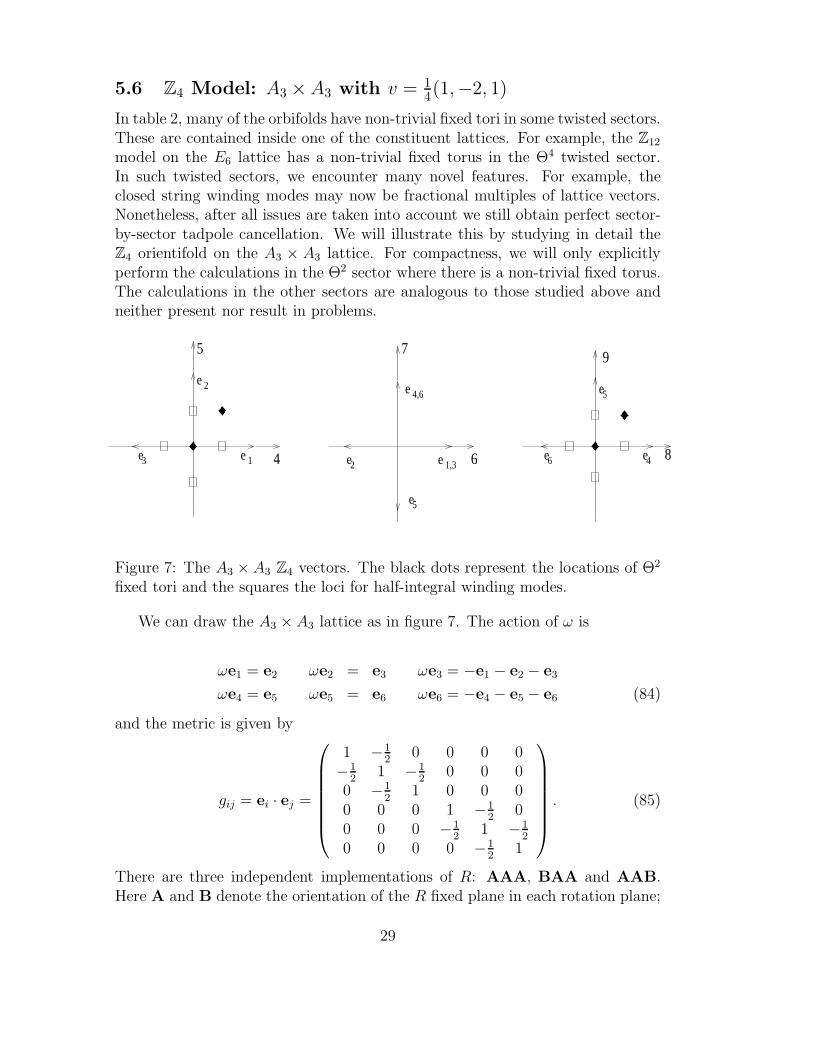
5.6 Z4 Model: A3 ×A3 with v = 14(1,−2, 1)
In table 2, many of the orbifolds have non-trivial fixed tori in some twisted sectors.These are contained inside one of the constituent lattices. For example, the Z12
model on the E6 lattice has a non-trivial fixed torus in the Θ4 twisted sector.In such twisted sectors, we encounter many novel features. For example, theclosed string winding modes may now be fractional multiples of lattice vectors.Nonetheless, after all issues are taken into account we still obtain perfect sector-by-sector tadpole cancellation. We will illustrate this by studying in detail theZ4 orientifold on the A3 × A3 lattice. For compactness, we will only explicitlyperform the calculations in the Θ2 sector where there is a non-trivial fixed torus.The calculations in the other sectors are analogous to those studied above andneither present nor result in problems.
e
e
e ee
e
e
e
e
e 4
5
61,32
5
4,6
1
2
3 4
5
6
7
8
9
Figure 7: The A3 × A3 Z4 vectors. The black dots represent the locations of Θ2
fixed tori and the squares the loci for half-integral winding modes.
We can draw the A3 × A3 lattice as in figure 7. The action of ω is
ωe1 = e2 ωe2 = e3 ωe3 = −e1 − e2 − e3
ωe4 = e5 ωe5 = e6 ωe6 = −e4 − e5 − e6 (84)
and the metric is given by
gij = ei · ej =
1 −12
0 0 0 0−1
21 −1
20 0 0
0 −12
1 0 0 00 0 0 1 −1
20
0 0 0 −12
1 −12
0 0 0 0 −12
1
. (85)
There are three independent implementations of R: AAA, BAA and AAB.Here A and B denote the orientation of the R fixed plane in each rotation plane;
29
A corresponds to aligning the fixed plane along the x-axis and B at an angle ofπ4
to this. In case AAA R acts as
e1 ↔ e1
e2 ↔ −e1 − e2 − e3
e3 ↔ e3
e4 ↔ −e6
e5 ↔ −e5 (86)
and in case BAA the action is
e1 ↔ e1 + e2 + e3
e2 ↔ −e3
e4 ↔ −e6
e5 ↔ −e5 (87)
and finally in case AAB R acts as
e1 ↔ e1
e2 ↔ −e1 − e2 − e3
e3 ↔ e3
e4 ↔ e5
e6 ↔ −e4 − e5 − e6. (88)
We will only explicitly consider the AAA ΩR orientation, as the behaviour forBAA and AAB is similar. For the Klein bottle amplitude, we need to know thestructure of fixed points and fixed tori. The Θ2 sector has 4 fixed tori
n′
2(e1 + e2) +
m′
2(e4 + e5) + α(e1 + e3) + β(e4 + e6) (89)
where n′, m′ ∈ 0, 1. From figure 7, or by explicit computation, one can see thatthe action of R on the fixed tori in general involves a shift as well as a reflection.As the lattice is non-factorisable, the different rotation planes do not decouplefrom each other.
In the Θ2 twisted sector, naively the momentum and winding modes wouldbe, for an ΩR insertion in the trace,
p =n
2(e1 + e3)
w = m(e4 + e6) (90)
with m,n ∈ Z, and for an ΩRΘ insertion in the trace,
p =n
2(e4 + e6)
w = m(e1 + e3). (91)
30
However, there are two subtle issues that render this invalid. First, since R actsas
R :1
2(e1 + e2) → 1
2(e1 + e2) +
1
2(e1 + e3)
R :1
2(e4 + e5) → 1
2(e4 + e5) +
1
2(e4 + e6), (92)
on the fixed tori labelled by (n′, m′) R acts as a shift by n′
2(e1 +e3)+ m′
2(e4 +e6).
Recall that the effect of a translation T : x → x+a on a momentum mode |p〉 is
T |p〉 = exp(2πip · a)|p〉. (93)
Therefore, for tori where n′ = 1, momentum modes having p = (1 + 2k)(e1 + e3)pick up a phase factor of eiπ under the action ofR. When the sum over momentummodes is performed, such modes have no net contribution, because they cancelagainst similar modes from tori where no such shift occurs. This results in aneffective doubling of the momentum modes. Schematically,
∑
n
(−1)n exp(−πtn2p2) +∑
n
exp(−πtn2p2) = 2∑
n
exp(−4πtn2p2). (94)
The shift along the winding direction does not have any effect on the sum in thepartition function. Moreover, as
RΘ :1
2(e1 + e2) → 1
2(e1 + e2)
RΘ :1
2(e4 + e5) → 1
2(e4 + e5) (95)
the insertion of ΩRΘ has no effect on the contributing momentum modes.There is also a subtlety at work for the winding modes. The condition that a
string state be an acceptable orbifold state in the Θ2 twisted sector is that
Xµ(σ + 2π, τ) = Θ2Xµ(σ, τ). (96)
Consider the points marked with a square in figure 7. These have the propertythat, when acted on with Θ2, they are brought back to themselves with a shiftby either 1
2(e4 + e6) or 1
2(e1 + e3). Explicitly, we have for example
Θ2 1
4(e4 − e6) =
1
4(e4 − e6) +
1
2(e4 + e6) (97)
It is this shift that allows the existence of winding modes that are half-integralmultiples of lattice vectors. Thus the winding state
X(σ, τ) =1
4(e4 − e6) +
σ
2π
(e4 + e6)
2+ (τ dependence) (98)
31
is a legitimate orbifold state in the Θ2 twisted sector.Next, we must consider whether these states are invariant under the action
of ΩR and ΩRΘ. Under the insertion of ΩRΘ, all loci for half-integral windingmodes are exchanged among themselves and there is no net contribution to thepartition function. However, under the insertion of ΩR, four such loci survive,and we have additional winding modes of the form
X(σ, τ) =
(
12
0
)
(e1 + e2) ±e4 − e6
4+
σ
2π
e4 + e6
2+ (τ dependence). (99)
The multiplicity is exactly the same as that of the number of fixed tori and thenet effect is then that the effective winding mode for the ΩR insertion is reducedfrom (e4 + e6) to 1
2(e4 + e6). For the ΩRΘ insertion, the net winding mode is
unchanged.The actual momentum and winding modes appearing in the partition function
are then, for an ΩR insertion in the trace
p = n(e1 + e3)
w =m
2(e4 + e6) (100)
with m,n ∈ Z, and for an ΩRΘ insertion in the trace,
p =n
2(e4 + e6)
w = m(e1 + e3). (101)
Performing a similar analysis for the other cases, we obtain the following Kleinbottle amplitudes
Case AAA −c∫∞0
16dl ((Θ0) + 4(Θ) − 4(Θ2) − 4(Θ3))
Case BAA −c∫∞0
32dl ((Θ0) + 4(Θ) − 4(Θ2) − 4(Θ3))
Case AAB −c∫∞0
8dl ((Θ0) + 4(Θ) − 4(Θ2) − 4(Θ3)) . (102)
Let us now consider the annulus amplitudes. We describe case AAA in detailand quote the results for the other cases. For case AAA, the branes are at
61 αe1 + βe3 + γ(e4 − e6)
62 α(e1 + e2) + β(e4 + e5) + γ(e4 + e6)
63 αe2 + β(e1 + e3) + γ(2e5 + e4 + e6)
64 α(e2 + e3) + β(e5 + e6) + γ(e4 + e6). (103)
As before, we focus on the sector arising from (61, 63) and (62, 64) strings. In eachcase there are two intersection points: 0 and 1
2(e4 + e6) for (61, 63) strings and
32
0 and 12(e5 + e6) for (62, 64) strings. For the former case, the lattice modes are
given by
p =n
2(e1 + e3)
w =m
2(e4 + e6) (104)
and for (62, 64) strings by
p =n
2(e4 + e6)
w =m
2(e1 + e3). (105)
Interestingly, the winding modes in the second case are a composite result ofstrings starting at two distinct points. The cases of m even arise from stringsstarting at 0; the cases of m odd arise from strings starting at 1
2(e1 +e2). Similar
behaviour occurs for the other two cases. Computing the annulus amplitude, weobtain
Case AAA −cM2∫∞0
dl4
((Θ0) + 4(Θ) − 4(Θ2) − 4(Θ3))
Case BAA −cM2∫∞0
dl2
((Θ0) + 4(Θ) − 4(Θ2) − 4(Θ3))
Case AAB −cM2∫∞
0dl8
((Θ0) + 4(Θ) − 4(Θ2) − 4(Θ3)) . (106)
In the computation of the Mobius strip amplitude, the Θ2 sector arises fromthe insertion of ΩRΘ2 into the trace, for (61, 61) and (62, 62) strings. This in-sertion leaves one plane invariant, which can then contribute lattice modes. Thecontributing modes are then, for case AAA,
(61, 61) p = n(e1 + e3), w =m
2(e4 + e6)
(62, 62) p = n2(e4 + e6), w = m(e1 + e3). (107)
Here, new behaviour is seen for the winding modes in the (61, 61) sector. Forthe factorisable models studied previously, half-integral winding modes did notappear in the Mobius strip amplitude. Instead, a winding mode doubling wasobserved. To see where the difference lies, consider the (61, 61) winding modestarting at 0 and ending at 1
2(e4 − e6) and having winding vector 1
2(e4 + e6).
Under ΩRΘ2, this is taken to a winding mode which starts at 12(e4 − e6) and
ends at 0, with the winding vector remaining invariant. So, the effect of ΩRΘ2
on these modes is as a translation,
T : x → x +1
2(e4 − e6). (108)
33
As in (93), this causes momentum modes to pick up a phase exp(πip · (e4 − e6)).For the case above, the momentum modes are orthogonal to the translation direc-tion and the phase factor is unity. Therefore the half-integral modes contributeto the partition function. In the factorisable case, the momentum modes layalong the translation direction. For half-integral winding modes, the sum of themomentum modes in the partition function was then
∑
n
(−1)n exp(−πtn2p2) (109)
which does not give rise to any divergence in the t → 0 limit. This can beseen straightforwardly using the Poisson resummation formula. Having takenthe above points into account, we obtain the following Mobius strip amplitudes
Case AAA cM∫∞0
4dl ((Θ0) + 4(Θ) − 4(Θ2) − 4(Θ3))
Case BAA cM∫∞0
8dl ((Θ0) + 4(Θ) − 4(Θ2) − 4(Θ3))
Case AAB cM∫∞0
2dl ((Θ0) + 4(Θ) − 4(Θ2) − 4(Θ3)) . (110)
Comparing the respective Klein bottle, annulus and Mobius strip amplitudes,we see that in all three cases the amplitudes factorise perfectly and we obtain atadpole cancellation condition
(M − 8)2 = 0 (111)
giving a gauge group of U(4) × U(4). The behaviour encountered above in theA3 × A3 is typical of those models which have a non-trivial fixed torus in oneof the twisted sectors. After taking into account the subtleties described above,and if necessary using different numbers of branes on different O-planes, onecan cancel all tadpoles sector-by-sector. Despite the many subtleties involved inthe one-loop calculation, at the end one obtains a simple answer. Indeed, forthe A3 × A3 case above the amplitudes actually take the form of the completeprojector.
As well as the models written up in detail above, we have also studied allother cases in table 2. In table 14 we give tadpole-cancelling solutions for all ΩRorientations for the models in table 2. For cases 1,2,5 and 7, some results havealready appeared in [6]. The spectra for these models can be determined exactlyas for the other cases using the methods described in section 3. However, as theywould not present any new features we have not written them out.
6 Conclusions
In this paper we have developed techniques to construct supersymmetric TypeIIA orientifolds on six-dimensional orbifolds which do not factorise into three
34
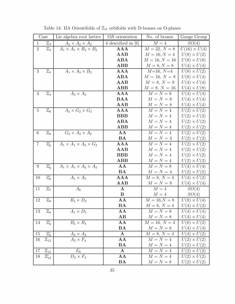
Table 14: IIA Orientifolds of ZN orbifolds with D-branes on O-planes
Case Lie algebra root lattice ΩR orientation No. of branes Gauge Group
1 Z3 A2 ×A2 × A2 4 described in [6] M = 4 SO(4)2 Z4 A1 × A1 ×B2 × B2 AAA M = 32, N = 8 U(16) × U(4)
AAB M = 16, N = 4 U(8) × U(2)ABA M = 16, N = 16 U(8) × U(8)ABB M = 8, N = 8 U(4) × U(4)
3 Z4 A1 × A3 × B2 AAA M=16, N=4 U(8) × U(2)ABA M = 16, N = 8 U(8) × U(4)AAB M = 8, N = 8 U(4) × U(4)ABB M = 8, N = 16 U(4) × U(8)
4 Z4 A3 ×A3 AAA M = N = 8 U(4) × U(4)BAA M = N = 8 U(4) × U(4)AAB M = N = 8 U(4) × U(4)
5 Z6 A2 ×G2 ×G2 AAA M = N = 4 U(2) × U(2)BBB M = N = 4 U(2) × U(2)ABA M = N = 4 U(2) × U(2)ABB M = N = 4 U(2) × U(2)
6 Z6 G2 ×A2 ×A2 AA M = N = 4 U(2) × U(2)BA M = N = 4 U(2) × U(2)
7 Z′6 A1 ×A1 ×A2 ×G2 AAA M = N = 4 U(2) × U(2)
AAB M = N = 4 U(2) × U(2)BBB M = N = 4 U(2) × U(2)ABB M = N = 4 U(2) × U(2)
9 Z′6 A1 × A1 ×A2 × A2 AA M = N = 8 U(4) × U(4)
BA M = N = 4 U(2) × U(2)10 Z
′6 A1 ×A5 AAA M = 8, N = 4 U(4) × U(2)
AAB M = N = 8 U(4) × U(4)11 Z7 A6 A M = 4 SO(4)
B M = 4 SO(4)12 Z8 B4 ×D2 AA M = 16,N = 8 U(8) × U(4)
BA M = 8, N = 4 U(4) × U(2)13 Z8 A1 ×D5 AA M = N = 8 U(4) × U(4)
AB M = N = 8 U(4) × U(4)14 Z
′8 B2 ×B4 AA M = 16, N = 4 U(8) × U(2)
BA M = N = 8 U(4) × U(4)15 Z
′8 A3 ×A3 A M = 8, N = 4 U(4) × U(2)
16 Z12 A2 × F4 AA M = N = 4 U(2) × U(2)BA M = N = 4 U(2) × U(2)
17 Z12 E6 A M = N = 4 U(2) × U(2)18 Z
′12 D2 × F4 AA M = N = 4 U(2) × U(2)
BA M = N = 8 U(2) × U(2)
35
two-dimensional tori. Using these techniques we have constructed many newexplicit orientifold models, where we placed the D6-branes parallel to the orien-tifold planes. For some of these models, in particular those containing non-trivialfixed tori, we have encountered some new technical features in the amplitudes,which nicely played together to finally yield consistent solutions to the tadpolecancellation conditions. All these supersymmetric Type IIA orientifold modelsare expected to lift up to M-theory compactifications on singular compact G2
manifolds [53, 54, 55].The next step is to move beyond these simple solutions to the tadpole cancella-
tion conditions and to study more general (supersymmetric) intersecting D-branemodels in these backgrounds. It is expected that these more general intersectingD6-branes give rise to chirality and might be interesting for building semi-realisticmodels. Once interesting models are found, employing the results of the effectivelow energy action as described in [56, 57, 58, 59, 60, 61, 62, 63], the discussion ofthe phenomenological implications would be the natural next step to perform.
Acknowledgements
RB is supported by PPARC and JC is grateful to EPSRC for a researchstudentship. KS thanks Trinity College, Cambridge for financial support. Weare grateful to Gabriele Honecker and Tassilo Ott for discussions. It is a pleasureto thank Fernando Quevedo for helpful comments and encouragement.
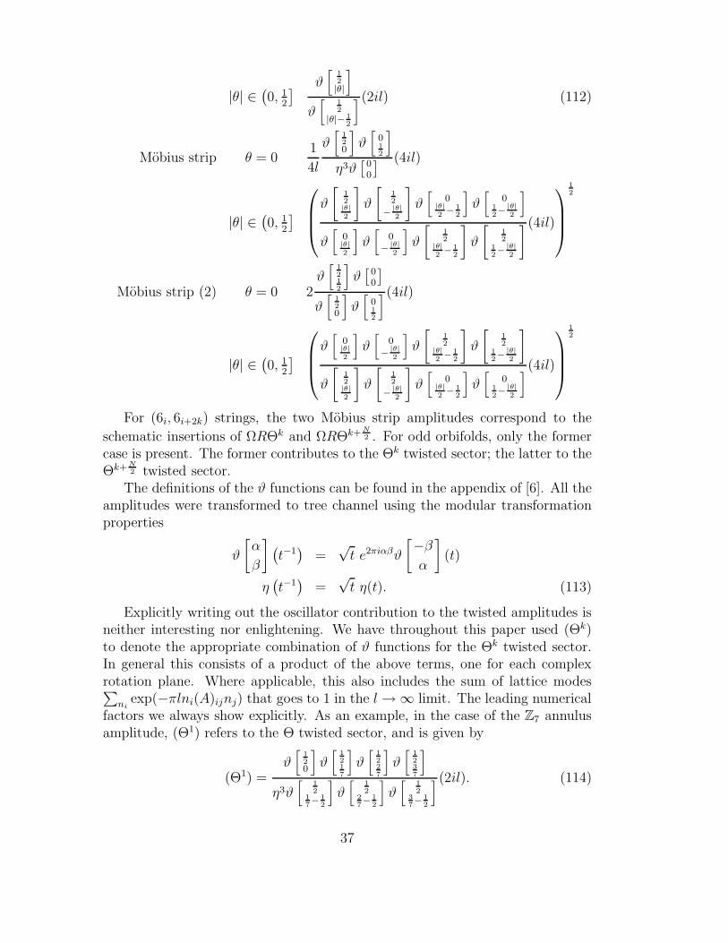
A Oscillator Formulae
Here we give the oscillator contribution to the tree channel amplitude for a com-plex plane twisted by θ. For the closed string traces, this means that pointsrelated by a rotation of 2πθ are identified. For the open string sectors, this refersto strings stretching between branes at a relative angle πθ.
Klein bottle θ = 01
2l
ϑ[
120
]
η3(2il)
|θ| ∈(
0, 12
]
ϑ[
12|θ|
]
ϑ[
12
|θ|− 12
](2il)
Annulus θ = 01
2l
ϑ[
120
]
η3(2il)
36
|θ| ∈(
0, 12
]
ϑ[
12|θ|
]
ϑ[
12
|θ|− 12
](2il) (112)
Mobius strip θ = 01
4l
ϑ[
120
]
ϑ[
012
]
η3ϑ[
00
] (4il)
|θ| ∈(
0, 12
]
ϑ
[
12|θ|2
]
ϑ
[
12
− |θ|2
]
ϑ[
0|θ|2− 1
2
]
ϑ[
012− |θ|
2
]
ϑ[
0|θ|2
]
ϑ[
0− |θ|
2
]
ϑ
[
12
|θ|2− 1
2
]
ϑ
[
12
12− |θ|
2
](4il)
12
Mobius strip (2) θ = 0 2ϑ[
1212
]
ϑ[
00
]
ϑ[
120
]
ϑ[
012
](4il)
|θ| ∈(
0, 12
]
ϑ[
0|θ|2
]
ϑ[
0− |θ|
2
]
ϑ
[
12
|θ|2− 1
2
]
ϑ
[
12
12− |θ|
2
]
ϑ
[
12|θ|2
]
ϑ
[
12
− |θ|2
]
ϑ[
0|θ|2− 1
2
]
ϑ[
012− |θ|
2
]
(4il)
12
For (6i, 6i+2k) strings, the two Mobius strip amplitudes correspond to the
schematic insertions of ΩRΘk and ΩRΘk+ N2 . For odd orbifolds, only the former
case is present. The former contributes to the Θk twisted sector; the latter to theΘk+ N
2 twisted sector.The definitions of the ϑ functions can be found in the appendix of [6]. All the
amplitudes were transformed to tree channel using the modular transformationproperties
ϑ
[
α
β
]
(
t−1)
=√t e2πiαβϑ
[−βα
]
(t)
η(
t−1)
=√t η(t). (113)
Explicitly writing out the oscillator contribution to the twisted amplitudes isneither interesting nor enlightening. We have throughout this paper used (Θk)to denote the appropriate combination of ϑ functions for the Θk twisted sector.In general this consists of a product of the above terms, one for each complexrotation plane. Where applicable, this also includes the sum of lattice modes∑
niexp(−πlni(A)ijnj) that goes to 1 in the l → ∞ limit. The leading numerical
factors we always show explicitly. As an example, in the case of the Z7 annulusamplitude, (Θ1) refers to the Θ twisted sector, and is given by
(Θ1) =ϑ[
120
]
ϑ[
1217
]
ϑ[
1227
]
ϑ[
1237
]
η3ϑ[
12
17− 1
2
]
ϑ[
12
27− 1
2
]
ϑ[
12
37− 1
2
](2il). (114)
37
B Lattices
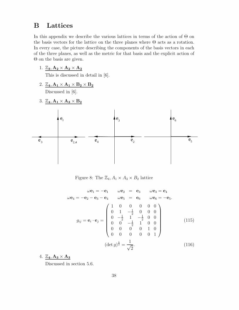
In this appendix we describe the various lattices in terms of the action of Θ onthe basis vectors for the lattice on the three planes where Θ acts as a rotation.In every case, the picture describing the components of the basis vectors in eachof the three planes, as well as the metric for that basis and the explicit action ofΘ on the basis are given.
1. Z3,A2 × A2 ×A2
This is discussed in detail in [6].
2. Z4,A1 × A1 ×B2 × B2
Discussed in [6].
3. Z4,A1 × A3 ×B2
e
ee
e
1
2,43 e e
3
4 2
e
e5
6
Figure 8: The Z4, A1 × A3 × B2 lattice
ωe1 = −e1 ωe2 = e3 ωe3 = e4
ωe4 = −e2 − e3 − e4 ωe5 = e6 ωe6 = −e5.
gij = ei · ej =
1 0 0 0 0 00 1 −1
20 0 0
0 −12
1 −12
0 00 0 −1
21 0 0
0 0 0 0 1 00 0 0 0 0 1
(115)
(det g)12 =
1√2. (116)
4. Z4,A3 × A3
Discussed in section 5.6.
38
5. Z6,A2 × G2 × G2
Discussed in [6].
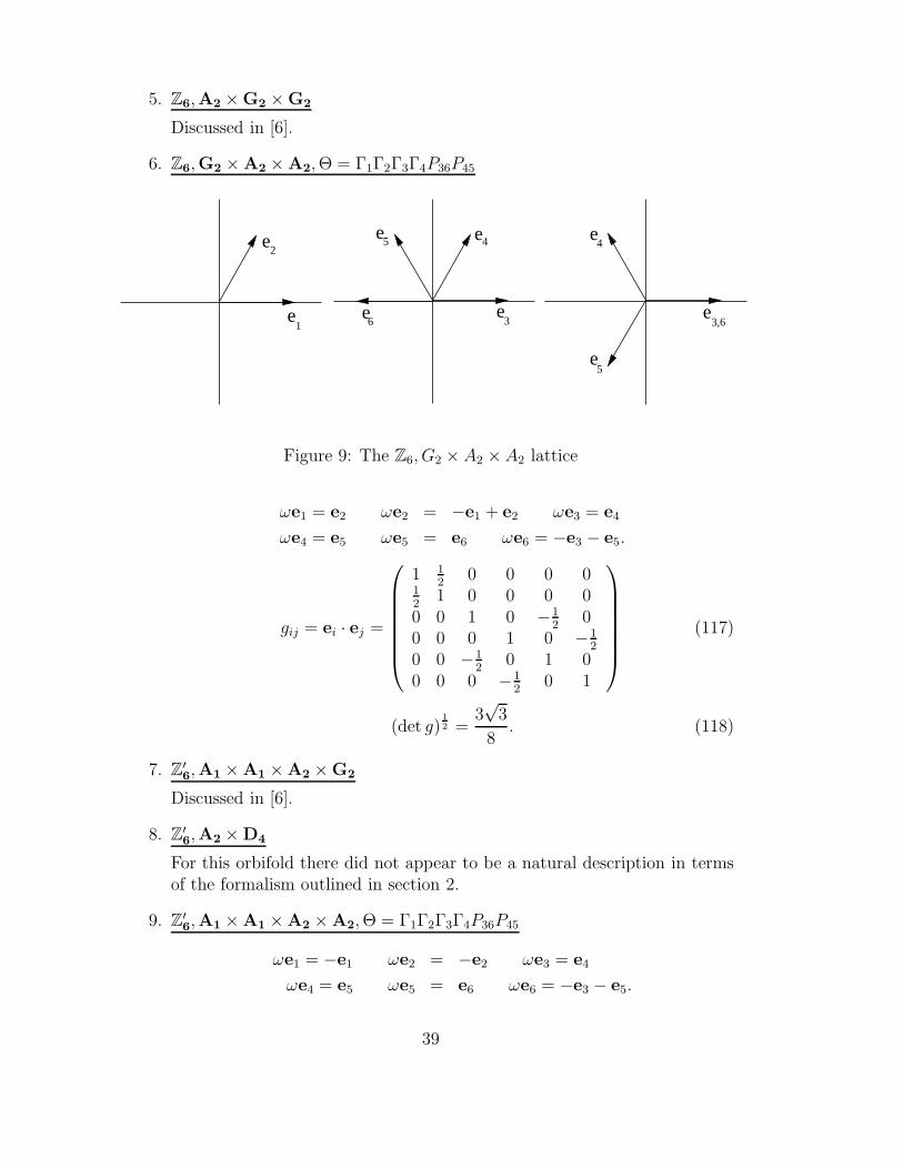
6. Z6,G2 × A2 × A2,Θ = Γ1Γ2Γ3Γ4P36P45
e e3,6e
e
1
2ee
e 3
45
6
e
e
4
5
Figure 9: The Z6, G2 × A2 ×A2 lattice
ωe1 = e2 ωe2 = −e1 + e2 ωe3 = e4
ωe4 = e5 ωe5 = e6 ωe6 = −e3 − e5.
gij = ei · ej =
1 12
0 0 0 012
1 0 0 0 00 0 1 0 −1
20
0 0 0 1 0 −12
0 0 −12
0 1 00 0 0 −1
20 1
(117)
(det g)12 =
3√
3
8. (118)
7. Z′6,A1 × A1 ×A2 × G2
Discussed in [6].
8. Z′6,A2 × D4
For this orbifold there did not appear to be a natural description in termsof the formalism outlined in section 2.
9. Z′6,A1 × A1 ×A2 × A2,Θ = Γ1Γ2Γ3Γ4P36P45
ωe1 = −e1 ωe2 = −e2 ωe3 = e4
ωe4 = e5 ωe5 = e6 ωe6 = −e3 − e5.
39
e e
5
e
e
1
2
e e
e 3
45
6
e
e
4
3,6
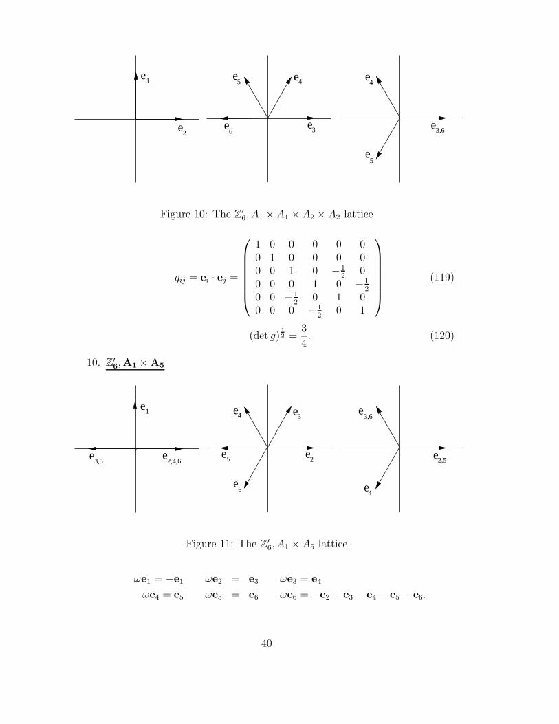
Figure 10: The Z′6, A1 ×A1 × A2 × A2 lattice
gij = ei · ej =
1 0 0 0 0 00 1 0 0 0 00 0 1 0 −1
20
0 0 0 1 0 −12
0 0 −12
0 1 00 0 0 −1
20 1
(119)
(det g)12 =
3
4. (120)
10. Z′6,A1 × A5
e
e e3,6
e2,5
e
e2,4,6
1
3,5e
e
e
e
2
34
5
6 e4
Figure 11: The Z′6, A1 × A5 lattice
ωe1 = −e1 ωe2 = e3 ωe3 = e4
ωe4 = e5 ωe5 = e6 ωe6 = −e2 − e3 − e4 − e5 − e6.
40

gij = ei · ej =
1 0 0 0 0 00 1 −1
20 0 0
0 −12
1 −12
0 00 0 −1
21 −1
20
0 0 0 −12
1 −12
0 0 0 0 −12
1
(121)
(det g)12 =
3
4. (122)
11. Z7,A6
See section 5.1.
12. Z8,B4 × D2
See section 5.3.
13. Z8,A1 × D5
e3,5 2,4,6e
e ee1 e
e
e
e2
345
6
e
ee
e
2
3
4
6
5
Figure 12: The Z8, A1 ×D5 lattice
ωe1 = −e1 ωe2 = e3 ωe3 = e4
ωe4 = e5 ωe5 = e6 ωe6 = −e2 − e3 − e6.
gij = ei · ej =
1 0 0 0 0 00 1 −1
212
−12
00 −1
21 −1
212
−12
0 12
−12
1 −12
12
0 −12
12
−12
1 −12
0 0 −12
12
−12
1
(123)
(det g)12 =
1
2√
2. (124)
41
14. Z′8,B2 × B4
See section 5.2.
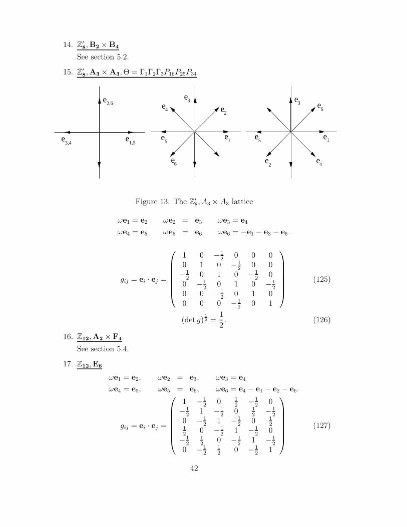
15. Z′8,A3 × A3,Θ = Γ1Γ2Γ3P16P25P34
e
e e
e5e
e2,6
3,4 1,5
e e
e
e
1
2
3
4
6
e
e
ee
e 15
42
63
Figure 13: The Z′8, A3 × A3 lattice
ωe1 = e2 ωe2 = e3 ωe3 = e4
ωe4 = e5 ωe5 = e6 ωe6 = −e1 − e3 − e5.
gij = ei · ej =
1 0 −12
0 0 00 1 0 −1
20 0
−12
0 1 0 −12
00 −1
20 1 0 −1
2
0 0 −12
0 1 00 0 0 −1
20 1
(125)
(det g)12 =
1
2. (126)
16. Z12,A2 × F4
See section 5.4.
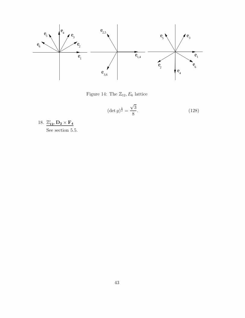
17. Z12,E6
ωe1 = e2, ωe2 = e3, ωe3 = e4
ωe4 = e5, ωe5 = e6, ωe6 = e4 − e1 − e2 − e6.
gij = ei · ej =
1 −12
0 12
−12
0−1
21 −1
20 1
2−1
2
0 −12
1 −12
0 12
12
0 −12
1 −12
0−1
212
0 −12
1 −12
0 −12
12
0 −12
1
(127)
42
e
e
e
e
ee
e
e1
2
3
45
6
e
e1,4
2,5
3,6
e
e
ee
e
1
35
2 6
4
Figure 14: The Z12, E6 lattice
(det g)12 =
√3
8. (128)
18. Z′12,D2 × F4
See section 5.5.
43
References
[1] C. Angelantonj and A. Sagnotti, “Open Strings,” Phys. Rept. 371 (2002)1–150, hep-th/0204089.
[2] C. Bachas, “A Way to Break Supersymmetry,” hep-th/9503030.
[3] M. Berkooz, M. R. Douglas, and R. G. Leigh, “Branes Intersecting atAngles,” Nucl. Phys. B480 (1996) 265–278, hep-th/9606139.
[4] R. Blumenhagen, L. Gorlich, and B. Kors, “Supersymmetric orientifolds in6D with D-branes at angles,” Nucl. Phys. B569 (2000) 209–228,hep-th/9908130.
[5] C. Angelantonj and R. Blumenhagen, “Discrete deformations in type Ivacua,” Phys. Lett. B473 (2000) 86–93, hep-th/9911190.
[6] R. Blumenhagen, L. Gorlich, and B. Kors, “Supersymmetric 4Dorientifolds of type IIA with D6-branes at angles,” JHEP 01 (2000) 040,hep-th/9912204.
[7] G. Pradisi, “Type I vacua from diagonal Z3-orbifolds,” Nucl. Phys. B575(2000) 134–150, hep-th/9912218.
[8] S. Forste, G. Honecker, and R. Schreyer, “Supersymmetric ZN × ZM
orientifolds in 4D with D-branes at angles,” Nucl. Phys. B593 (2001)127–154, hep-th/0008250.
[9] R. Blumenhagen, L. Gorlich, B. Kors, and D. Lust, “Asymmetric orbifolds,noncommutative geometry and type I string vacua,” Nucl. Phys. B582(2000) 44–64, hep-th/0003024.
[10] R. Blumenhagen, L. Gorlich, B. Kors, and D. Lust, “NoncommutativeCompactifications of Type I Strings on Tori with Magnetic BackgroundFlux,” JHEP 10 (2000) 006, hep-th/0007024.
[11] C. Angelantonj, I. Antoniadis, E. Dudas, and A. Sagnotti, “Type-I stringson magnetised orbifolds and brane transmutation,” Phys. Lett. B489(2000) 223–232, hep-th/0007090.
[12] G. Aldazabal, S. Franco, L. E. Ibanez, R. Rabadan, and A. M. Uranga,“Intersecting brane worlds,” JHEP 02 (2001) 047, hep-ph/0011132.
[13] G. Aldazabal, S. Franco, L. E. Ibanez, R. Rabadan, and A. M. Uranga, “D= 4 Chiral String Compactifications from Intersecting Branes,” J. Math.
Phys. 42 (2001) 3103–3126, hep-th/0011073.
44
[14] R. Blumenhagen, B. Kors, and D. Lust, “Type I strings with F- andB-flux,” JHEP 02 (2001) 030, hep-th/0012156.
[15] L. E. Ibanez, F. Marchesano, and R. Rabadan, “Getting just the standardmodel at intersecting branes,” JHEP 11 (2001) 002, hep-th/0105155.
[16] R. Blumenhagen, B. Kors, D. Lust, and T. Ott, “The Standard Modelfrom Stable Intersecting Brane World Orbifolds,” Nucl. Phys. B616 (2001)3–33, hep-th/0107138.
[17] D. Bailin, G. V. Kraniotis, and A. Love, “Standard-like models fromintersecting D4-branes,” Phys. Lett. B530 (2002) 202–209,hep-th/0108131.
[18] C. Kokorelis, “GUT model hierarchies from intersecting branes,” JHEP 08(2002) 018, hep-th/0203187.
[19] M. Cvetic, G. Shiu, and A. M. Uranga, “Three-family supersymmetricstandard like models from intersecting brane worlds,” Phys. Rev. Lett. 87(2001) 201801, hep-th/0107143.
[20] M. Cvetic, G. Shiu, and A. M. Uranga, “Chiral four-dimensional N = 1supersymmetric type IIA orientifolds from intersecting D6-branes,” Nucl.
Phys. B615 (2001) 3–32, hep-th/0107166.
[21] R. Blumenhagen, L. Gorlich, and T. Ott, “Supersymmetric intersectingbranes on the type IIA T 6/Z4 orientifold,” JHEP 01 (2003) 021,hep-th/0211059.
[22] G. Honecker, “Chiral supersymmetric models on an orientifold of Z4 × Z2
with intersecting D6-branes,” Nucl. Phys. B666 (2003) 175–196,hep-th/0303015.
[23] M. Cvetic and I. Papadimitriou, “More supersymmetric standard-likemodels from intersecting D6-branes on type IIA orientifolds,” Phys. Rev.
D67 (2003) 126006, hep-th/0303197.
[24] M. Larosa and G. Pradisi, “Magnetized four-dimensional Z2 × Z2
orientifolds,” Nucl. Phys. B667 (2003) 261–309, hep-th/0305224.
[25] G. Honecker and T. Ott, “Getting just the Supersymmetric StandardModel at Intersecting Branes on the Z6-orientifold,” hep-th/0404055.
[26] M. Cvetic, T. Li, and T. Liu, “Supersymmetric Pati-Salam models fromintersecting D6- branes: A road to the standard model,” hep-th/0403061.
45
[27] A. M. Uranga, “Chiral four-dimensional string compactifications withintersecting D-branes,” Class. Quant. Grav. 20 (2003) S373–S394,hep-th/0301032.
[28] D. Lust, “Intersecting Brane Worlds: A Path to the Standard Model?,”hep-th/0401156.
[29] C. Angelantonj, M. Bianchi, G. Pradisi, A. Sagnotti, and Y. S. Stanev,“Comments on Gepner models and type I vacua in string theory,” Phys.
Lett. B387 (1996) 743–749, hep-th/9607229.
[30] R. Blumenhagen and A. Wisskirchen, “Spectra of 4D, N = 1 type I stringvacua on non-toroidal CY threefolds,” Phys. Lett. B438 (1998) 52–60,hep-th/9806131.
[31] G. Aldazabal, E. C. Andres, M. Leston, and C. Nunez, “Type IIBorientifolds on Gepner points,” JHEP 09 (2003) 067, hep-th/0307183.
[32] R. Blumenhagen, “Supersymmetric orientifolds of Gepner models,” JHEP
11 (2003) 055, hep-th/0310244.
[33] I. Brunner, K. Hori, K. Hosomichi, and J. Walcher, “Orientifolds of Gepnermodels,” hep-th/0401137.
[34] R. Blumenhagen and T. Weigand, “Chiral supersymmetric Gepner modelorientifolds,” JHEP 02 (2004) 041, hep-th/0401148.
[35] T. P. T. Dijkstra, L. R. Huiszoon, and A. N. Schellekens, “Chiralsupersymmetric standard model spectra from orientifolds of Gepnermodels,” hep-th/0403196.
[36] R. Blumenhagen and T. Weigand, “A note on partition functions ofGepner model orientifolds,” hep-th/0403299.
[37] G. Aldazabal, E. C. Andres, and J. E. Juknevich, “Particle models fromorientifolds at Gepner-orbifold points,” hep-th/0403262.
[38] Z. Kakushadze and G. Shiu, “A chiral N = 1 type I vacuum in fourdimensions and its heterotic dual,” Phys. Rev. D56 (1997) 3686–3697,hep-th/9705163.
[39] G. Aldazabal, A. Font, L. E. Ibanez, and G. Violero, “D = 4, N = 1, typeIIB orientifolds,” Nucl. Phys. B536 (1998) 29–68, hep-th/9804026.
[40] G. Zwart, “Four-dimensional N = 1 Z(N) x Z(M) orientifolds,” Nucl. Phys.
B526 (1998) 378–392, hep-th/9708040.
46
[41] Z. Kakushadze, G. Shiu, and S. H. H. Tye, “Type IIB orientifolds,F-theory, type I strings on orbifolds and type I heterotic duality,” Nucl.
Phys. B533 (1998) 25–87, hep-th/9804092.
[42] M. R. Gaberdiel, “Lectures on non-BPS Dirichlet branes,” Class. Quant.
Grav. 17 (2000) 3483–3520, hep-th/0005029.
[43] A. Sen, “F-theory and Orientifolds,” Nucl. Phys. B475 (1996) 562–578,hep-th/9605150.
[44] A. Sen, “A note on enhanced gauge symmetries in M- and string theory,”JHEP 09 (1997) 001, hep-th/9707123.
[45] L. J. Dixon, J. A. Harvey, C. Vafa, and E. Witten, “Strings on Orbifolds,”Nucl. Phys. B261 (1985) 678–686.
[46] L. J. Dixon, J. A. Harvey, C. Vafa, and E. Witten, “Strings onOrbifolds(II),” Nucl. Phys. B274 (1986) 285–314.
[47] J. Erler and A. Klemm, “Comment on the Generation Number in OrbifoldCompactifications,” Commun. Math. Phys. 153 (1993) 579–604,hep-th/9207111.
[48] R. Blumenhagen, V. Braun, B. Kors, and D. Lust, “Orientifolds of K3 andCalabi-Yau manifolds with intersecting D-branes,” JHEP 07 (2002) 026,hep-th/0206038.
[49] J. A. Casas, F. Gomez, and C. Munoz, “Complete structure of Zn Yukawacouplings,” Int. J. Mod. Phys. A8 (1993) 455–506, hep-th/9110060.
[50] M. Klein and R. Rabadan, “D = 4, N = 1 orientifolds with vectorstructure,” Nucl. Phys. B596 (2001) 197–230, hep-th/0007087.
[51] E. G. Gimon and J. Polchinski, “Consistency Conditions for Orientifoldsand D-Manifolds,” Phys. Rev. D54 (1996) 1667–1676, hep-th/9601038.
[52] A. Dabholkar, “Lectures on Orientifolds and Duality,” hep-th/9804208.
[53] S. Kachru and J. McGreevy, “M-theory on manifolds of G(2) holonomyand type IIA orientifolds,” JHEP 06 (2001) 027, hep-th/0103223.
[54] M. Atiyah and E. Witten, “M-theory dynamics on a manifold of G(2)holonomy,” Adv. Theor. Math. Phys. 6 (2003) 1–106, hep-th/0107177.
[55] E. Witten, “Anomaly cancellation on G(2) manifolds,” hep-th/0108165.
[56] D. Cremades, L. E. Ibanez, and F. Marchesano, “Yukawa couplings inintersecting D-brane models,” JHEP 07 (2003) 038, hep-th/0302105.
47
[57] D. Lust and S. Stieberger, “Gauge threshold corrections in intersectingbrane world models,” hep-th/0302221.
[58] M. Cvetic and I. Papadimitriou, “Conformal field theory couplings forintersecting D-branes on orientifolds,” Phys. Rev. D68 (2003) 046001,hep-th/0303083.
[59] S. A. Abel and A. W. Owen, “Interactions in intersecting brane models,”Nucl. Phys. B663 (2003) 197–214, hep-th/0303124.
[60] S. A. Abel and A. W. Owen, “N-point amplitudes in intersecting branemodels,” hep-th/0310257.
[61] B. Kors and P. Nath, “Effective action and soft supersymmetry breakingfor intersecting D-brane models,” Nucl. Phys. B681 (2004) 77–119,hep-th/0309167.
[62] D. Lust, P. Mayr, R. Richter, and S. Stieberger, “Scattering of Gauge,Matter, and Moduli Fields from Intersecting Branes,” hep-th/0404134.
[63] D. Cremades, L. E. Ibanez, and F. Marchesano, “Computing YukawaCouplings from Magnetized Extra Dimensions,” hep-th/0404229.
48


