Embed Size (px)
Citation preview

: www.hoorijani.ir
: [email protected], [email protected]
: hamed hoorijani
: Hamed Hoorijani
Tutorial Aspen HYSIS v8.8- Dynamic mode
Dynamic process 2
Author: Hamed Hoorijani

: www.hoorijani.ir
: [email protected], [email protected]
: hamed hoorijani
: Hamed Hoorijani
Tutorial 3. Simulate the given PFD using the description and the supplementary
data for dynamic simulation.
Feed is mostly cooled Methane that is fed to a two-phase separator. The level and
pressure of this separator is controlled. To control temperature of the Liquid
product of the separator another controller is used with controlling the duty of the
cooler. In actuality, dead time of the process has a delay effect at the end of the
vessel’s pipes. The time required for the fluid to reach the measurement equipment
from the outlet of the cooler is called transfer delay which is one the most common
dead times in the fluid process industries. Second transfer function is a sinusoidal
function to model the noises in the feed flow. The noises are considered based on
the effect of the system’s capacity to damp the noises. Temperatures noises is
considered zero in this PFD. Also the dead time of the temperature is a small value
of 0.1 minute.
PFD and supplementary data:
o Stream “2” temperature : 10℃
o In the dynamic mode, for the duty stream of “Q-100” consider Min
Available and Max Available as 0 and 2000000, respectively.
o Temperature difference between the stream “5” with PV in the TIC-
100 controller is due to the transfer function
o Build a strip chart with the name of “Temperatures” to monitor the
simultaneous changes of the :
Stream “2” – Temperature
Stream “5” – Temperature
Stream “Feed” – Temperature
TIC-100-PV
TIC-100-SP

: www.hoorijani.ir
: [email protected], [email protected]
: hamed hoorijani
: Hamed Hoorijani
PFD
Controllers and transfer functions:

: www.hoorijani.ir
: [email protected], [email protected]
: hamed hoorijani
: Hamed Hoorijani
Solution.
1. Open Aspen HYSIS and create a new case.
2. At the Components Lists menu add the given components for simulation.
3. At the Fluid Packages add Peng-Robinson as the proper fluid package for calculating
pair-coefficient for obtaining thermodynamic and physical properties of the each
components and mixture.
4. At the simulation tab, define the Feed stream with given mole fraction and operating
conditions.

: www.hoorijani.ir
: [email protected], [email protected]
: hamed hoorijani
: Hamed Hoorijani
5. After defining the feed stream, place each and proper process equipment at the path of the
process stream and enter each ones proper design parameters.
6. After each process equipment were defined, place two transfer function
“TemperatureDistribution” and “DeadtimeModel” at the start and end of the PFD.
Enter each ones proper settings to have their block colors turn into light colors.
Deadtime Model

: www.hoorijani.ir
: [email protected], [email protected]
: hamed hoorijani
: Hamed Hoorijani
7. Place the controllers on the Flowsheet and enter each ones modes, parameters to act on
the process.

: www.hoorijani.ir
: [email protected], [email protected]
: hamed hoorijani
: Hamed Hoorijani
Simulation Hint:
For the TIC-100 controller the Q-100 duty stream need a maximum value for the control
valve of the controller to know its range and try to maintain the SP in the range. Try
entering a bigger value than the calculate SP value for the maxim value of the Q-100
instead of the <infinite>. In this case, it’s declared to consider 0 and 2e6 for the Min. and
Max. available value for the Q-100.

: www.hoorijani.ir
: [email protected], [email protected]
: hamed hoorijani
: Hamed Hoorijani
8. Enter Dynamic Assistant in the Dynamic tab to make the necessary changes on the
flowsheet for dynamic simulations.
9. To plot all the asking parameters in the question, in the Dynamics tab, you can use strip
charts options in the Tools section.
10. In the opened window, add a Strip Chart Name.

: www.hoorijani.ir
: [email protected], [email protected]
: hamed hoorijani
: Hamed Hoorijani
11. Then select your named Strip Chart and press the Edit button, in the opened window try
adding different variables to be probed using the chart.
12. Then by pressing Display a chart will be opened and you can observe the changes in each
variable in your simulation.

: www.hoorijani.ir
: [email protected], [email protected]
: hamed hoorijani
: Hamed Hoorijani
13. Activate the Dynamic Simulation Model and use the Integrator for setting the End time of
the simulation, start Time and time step simultaneously with the Display of the stripchart
so that you can witness the changes in the stream’s properties.
: www.hoorijani.ir
: [email protected], [email protected]
: hamed hoorijani
: Hamed Hoorijani
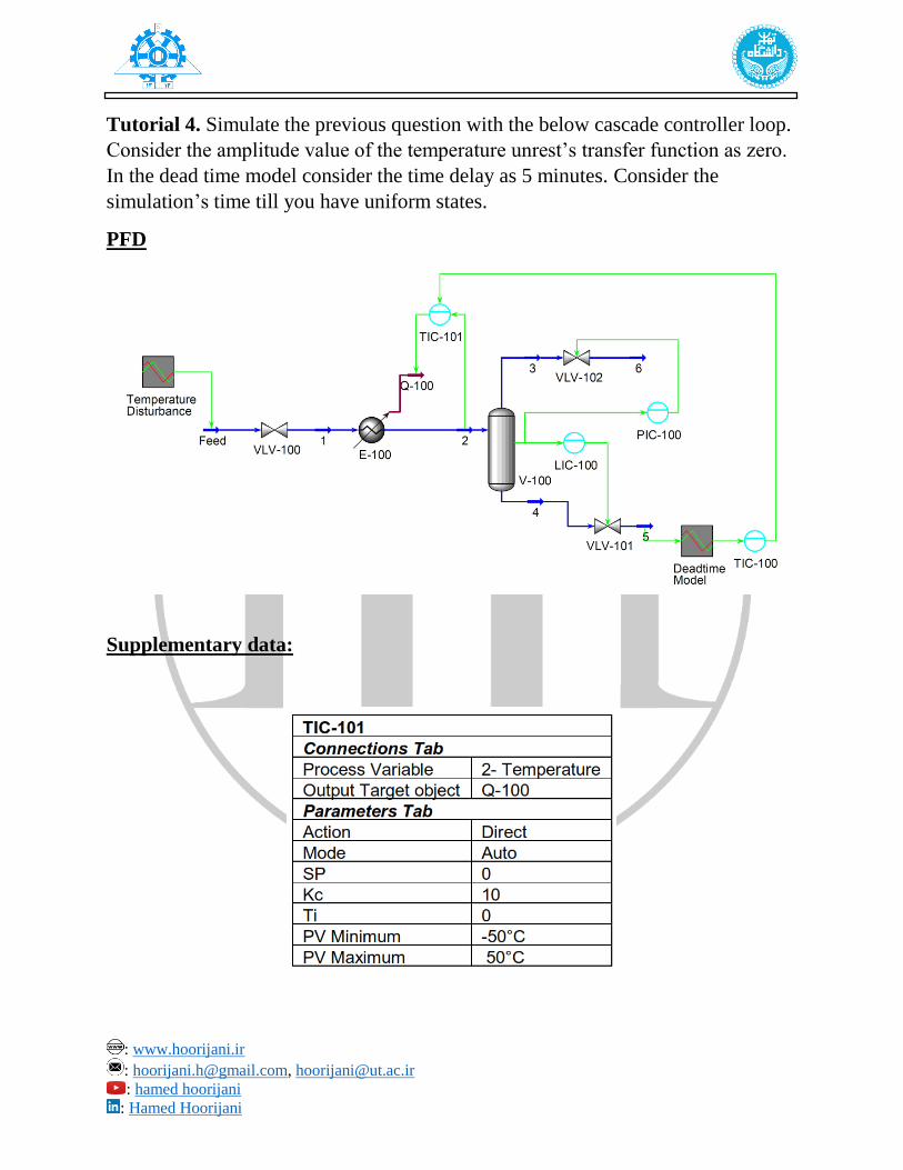
Tutorial 4. Simulate the previous question with the below cascade controller loop.
Consider the amplitude value of the temperature unrest’s transfer function as zero.
In the dead time model consider the time delay as 5 minutes. Consider the
simulation’s time till you have uniform states.
PFD
Supplementary data:

: www.hoorijani.ir
: [email protected], [email protected]
: hamed hoorijani
: Hamed Hoorijani
Solution.
1. Do the simulation steps of previous tutorial.
2. To simulate the PFD using a cascade loop controller, first for the TIC-100 disconnect the
“Output Target Object” and choose the SP of the TIC-101 ‘s controller as the Variable.
3. In the Parameters Tab of the TIC-100 choose Reverse Action since the TIC-100 is the
first controller of the cascade to measure and act. Change the mode to Manual and enter
the OP value of 50%.
Change the Kc and Ti to 2 and 10, respectively.

: www.hoorijani.ir
: [email protected], [email protected]
: hamed hoorijani
: Hamed Hoorijani
4. For the TIC-101 choose the temperature of the Stream “2” as the Process Variable Source
and the control valve of the “Q-100” stream. In the Remote Setpoint, press Select RSP
button and choose the TIC-100 as the source.
5. In the Parameters set the action of this controller as the Direct and the mode on the Auto.
6. Set the PV Minimum and Maximum as -50 and 50, respectively as stated in the question.
Enter the Kc and Ti as 10 and 0 (proportional controller), respectively.

: www.hoorijani.ir
: [email protected], [email protected]
: hamed hoorijani
: Hamed Hoorijani
7. To enter the Delay in the DeadTime model in the Parameters tab, open the Delay page
and in there you can make your desired changes to the Active transfer function. After you
enable the Delay transfer function you can enter its value in the table, Delay Parameters
below.


