Transport cost functions, network expansionand economies of scope

Sergio R. Jara-D�ııaz *, Leonardo J. Basso

Department of Civil Engineering, Universidad de Chile, Casilla 228-3, Santiago, Chile

Abstract

This paper shows technically that economies of transport network expansion should be viewed through

the concept of economies of scope rather than through the concept of economies of scale. The basictechnological dimensions that are specific to transport production are identified. The framework is used to

derive explicit cost functions for two and three nodes systems in order to show how the potential technical

advantages of network expansions (new nodes served) are transferred into transport cost functions. These

advantages are shown to translate into economies of scope that can exist even under constant returns to

scale.

� 2003 Elsevier Science Ltd. All rights reserved.

Keywords: Transport cost functions; Network effects; Industry structure

1. Introduction

The product of a transport firm is a vector of flows of persons and goods, moved during anumber of periods and among many origins and destinations (OD pairs) in space (Jara-D�ııaz,1982a). This detailed vectorial description of product has not been used in the estimation oftransport cost functions although ‘‘treating the movement of each commodity from each origin toeach destination as a separate product would be desirable. There would be so many outputs,however, that estimating a cost function would be impossible’’ (Braeutigam, 1999, p. 68). This hasmade the use of aggregate descriptions necessary, e.g. ton-kilometers, number of shipments orseat-kilometers, each one synthesizing one or more dimensions of the actual product. Other

Transportation Research Part E 39 (2003) 271–288www.elsevier.com/locate/tre

* Corresponding author. Tel.: +56-2-678-4380; fax: +56-2-689-4206.

E-mail addresses: jaradiaz@cec.uchile.cl (S.R. Jara-D�ııaz), lbasso@cec.uchile.cl (L.J. Basso).

1366-5545/03/$ - see front matter � 2003 Elsevier Science Ltd. All rights reserved.

doi:10.1016/S1366-5545(03)00002-4

attributes have been considered as well in the estimation of transport cost functions, as is the caseof average distance or load factor, which somehow try to capture output heterogeneity.Econometric cost functions estimated using aggregated output have been used mainly to an-

alyze industry structure. As stated by Oum and Waters (1996), the first purpose of the empiricalmeasurement of transportation cost functions is the study of the ‘‘cost structure of the industry,notably whether or not there are economies of scale. These are important for assessing the fea-sibility of competition between firms of different size, and the long run equilibrium industrialorganization of an industry’’ (p. 425). Thus, estimated cost functions are aimed at understandingfor example, how many transport firms will serve a certain region. Will one firm cover the wholenetwork? Would it be less costly to have a few, each one serving part of the network?When analyzing industry structure, the degree of economies of scale is probably the most

important concept that emerges as the center of this type of analysis. In transport, the use ofaggregates––that normally obviates the spatial dimension of product––has provoked the need tomake a distinction between economies of scale and economies of density, which have been as-sociated to a varying or constant network size respectively. The usual approach is based upon anestimated cost function eCCðeYY ;NÞ where eYY is a vector of aggregated product descriptions (includingthe so-called attributes) and N is a variable representing the network (factor prices are suppressedfor simplicity). Returns to density (RTD) and returns to scale (RTS) are defined as

RTD ¼ 1Pj ~ggj

ð1Þ

RTS ¼ 1Pj ~ggj þ gN

ð2Þ

where ~ggj is the elasticity of eCCðeYY ;NÞ with respect to aggregate product j and gN is the elasticity withrespect to N , fulfilling RTS < RTD since the network elasticity is positive (as obtained in allempirical studies).According to Oum and Waters (1996, p. 429), ‘‘RTD is referred to the impact on average cost

of expanding all traffic, holding network size constant, whereas RTS refers to the impact onaverage cost of equi-proportionate increases in traffic and network size’’. From this, the prevailinginterpretation on industry structure in the literature is simple. Increasing returns to scale(RTS > 1) suggest that both product and network size should be increased because serving largernetworks would diminish average cost. Constant returns to scale together with increasing returnsto density (RTD > 1) would indicate that traffic should be increased keeping network constant.This apparently straightforward analysis has an evident limitation, though: as RTS < RTD a firmthat has both optimal density and optimal network size cannot be described. Moreover, if net-work size was optimal (RTS ¼ 1) the firm must exhibit increasing returns to density. This hasgenerated ad hoc explanations for the observed trend to expand networks in some industries 1 and

1 For example in the case of air transportation, Brueckner and Spiller (1994) state that ‘‘the growth of networks can

be understood as an attempt to exploit economies of traffic density, under which the marginal cost of carrying an extra

passenger on a non-stop route falls as traffic on the route rises’’. Note that under this interpretation an optimal network

size could never be reached.

272 S.R. Jara-D�ııaz, L.J. Basso / Transportation Research Part E 39 (2003) 271–288

a growing controversy regarding what should be measured and what is measured from a costfunction in order to develop a meaningful analysis of industry structure (see for example Gagn�ee,1990; Ying, 1992; Xu et al., 1994; Jara-D�ııaz and Cort�ees, 1996; Oum and Zhang, 1997; Jara-D�ııazet al., 2001). In our opinion, more effort has been devoted to the development of sophisticatedeconometric tools than to the understanding of transport technology, which is, after all, what liesbehind the properties of a cost function. From this viewpoint, the spatial dimension of producthas been particularly neglected in the literature, in spite of the discussions and observations re-garding this aspect by authors like Spady (1985), Daughety (1985) or Antoniou (1991).The objective of this paper is to identify unambiguously the role of the spatial dimension of

product in the analysis of the transport industry structure, notably within the context of in-creasing networks. This is done by means of the analysis of the links between disaggregatedproduct, transport technology and the cost function within the context of varying network size insimple systems whose technology can be reproduced in some detail. The technical description oftransport processes in simple systems has been shown to be very useful to clarify some pointsregarding industry structure, scale and scope. For example, Jara-D�ııaz (1982b) described thetechnology and derived the corresponding cost function for a cyclical back-haul system (i.e. twoOD pairs) and was able to identify precisely the role of scale and scope within the context of a(fixed) transport network, showing the ambiguity of the most popular aggregate description ofproduct (ton-kilometers). Most important, the technical analysis of transport production for sucha simple network was enough to provide an explanation for the incentives to merge between firmsserving different portions of a network even under the presence of constant returns to scale,namely the existence of economies of spatial scope. This basic system, however, is not enough toillustrate the effects of a network expansion.In this paper we identify and define the elements that are essential to characterize the spatial

aspects of transport production (decisions of the firm). To do this, we use the two nodes system asa basis to analyze the economics of a network expansion through the examination of bothtechnology and cost function of a three nodes system (six OD pairs). This seemingly simple de-parture introduces a new dimension to the technical decisions of the firm, namely the choice of aroute structure to serve a given set of OD flows. With these tools, the analysis of proportional flowexpansions (scale) and the addition of new flows (scope) through network expansions can beperformed without ambiguity both technically (efficient frontiers) and economically (cost func-tions). On this basis, the role of the spatial dimension of product and the so-called network effectsflow unambiguously within the context of the study of the transport industry structure. Note thatthis technical analysis is not done with the intention to recommend the best way to operate suchsystems, but to understand the relations between production in a transport network and the issuesin the analysis of industry structure as viewed with the aim of transport cost functions. The maingoal is to obtain elements to estimate, interpret and use empirically estimated transport costfunctions, which obviously represent fairly complex networks.In the next section the decisions of a transport firm are identified with emphasis on the spatially

related elements. Then the analytics of production in a two nodes system is summarized in sectionthree in order to set the basis for the expansion to a three nodes system (Section 4), where thepotential of some aggregates actually used in the literature on cost functions is highlighted. Theanalytically obtained cost functions are used in Section 5 to show how the spatial decisions (i.e.how to use the network) translate into the calculation of economies of scale and scope, which are

S.R. Jara-D�ııaz, L.J. Basso / Transportation Research Part E 39 (2003) 271–288 273

the main determinants of industry structure. Finally, the challenge on what to do with estimatedcost functions for a proper study of industrial organization is synthesized.

2. Decisions of a cost minimising transport firm

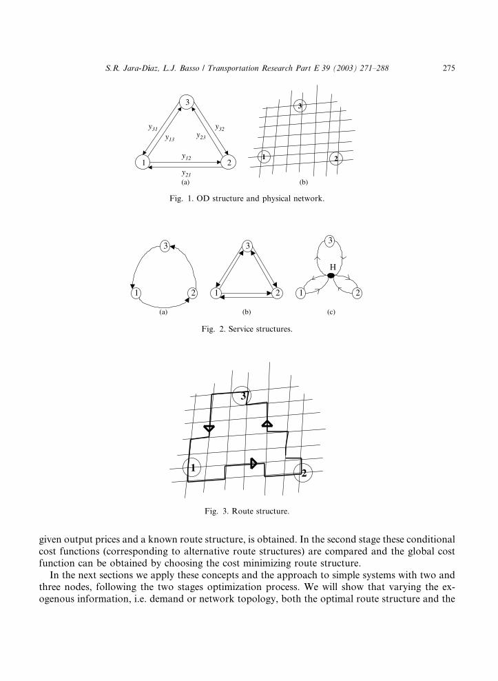
The microeconomic description of production processes rests upon the concepts of inputs,outputs and technological feasibility. In the case of transport, a firm produces flows of differentthings between different origins and destinations along different periods. Thus, transport productis a vector (Jara-D�ııaz, 1982a) Y ¼ fyktij g where yktij is the amount of flow type k (e.g. persons orgoods), between origin i and destination j, during period t. This way, movements of passengersbetween Santiago and Temuco during the last week of the year and the movement of fruit betweenSantiago and New York during a week in July, are different products (even if we said passengersinstead of fruit). In this paper we will concentrate on the spatial dimension of product, namely itsOD structure, as this is the main distinctive feature of transport processes.For a certain level of production Y , a transport firm has to make decisions regarding quantity

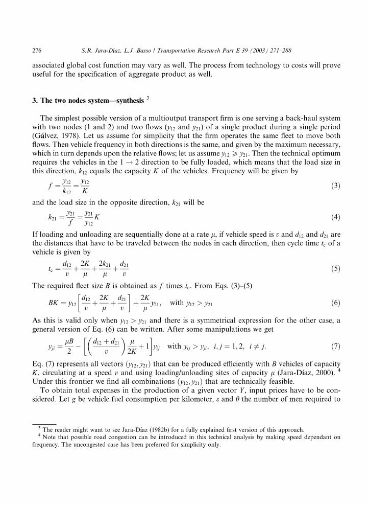
and characteristics of inputs (e.g. number of vehicles, number of loading–unloading sites and theirrespective capacities) and operating rules (e.g. speeds, frequencies, load sizes). Because transportproduction takes place on a network, a transport firm has to decide, as well, a service structure––i.e. the generic way in which vehicles will visit the nodes to produce the flows––and a link sequence.These two endogenous decisions define a route structure, which has to be chosen using exogenousspatial information, namely the OD structure of demand (defined by the vector Y ), the location ofthe nodes and the physical network. Note that the need to make a decision on a route structure is,finally, a consequence of the spatial dimension of product. Note also that this type of decision isessentially a discrete one. Let us illustrate these new important elements through an example withthree nodes and six OD pairs as shown in Fig. 1a, with a physical network as the one representedin Fig. 1b.Three possible service structures are shown in Fig. 2 (Jara-D�ııaz, 2000). Structure (a) corre-

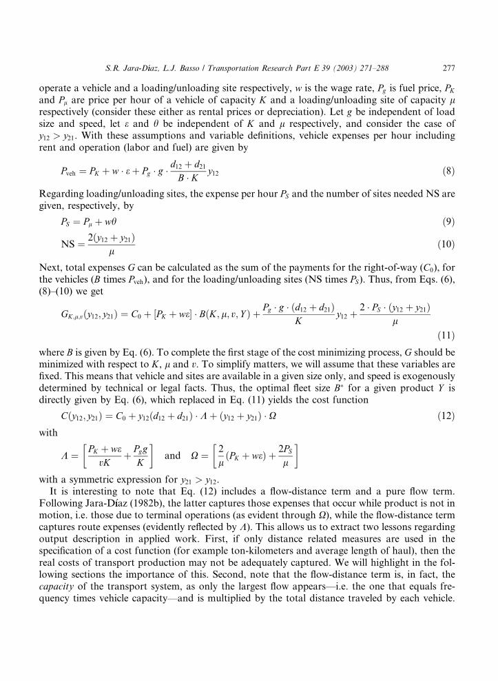
sponds to a general cyclical system (G�aalvez, 1978), 2structure (b) corresponds to three simplecyclical systems (direct service) and structure (c), where a distribution node is created, is known ashub-and-spoke and is very common in air transport (note that hub H can or cannot coincide withan origin or destination node). Regarding vehicle assignment to fleets, which is part of the servicestructure, there is no choice but one fleet (one frequency) in case (a), three fleets in case (b) andone, two (with three alternatives) or three fleets in case (c). If a cyclical system counter-clockwiselike the one in Fig. 2a was chosen, a possible route structure could be the one shown in Fig. 3.As stated earlier, the decisions of a transport firm are three: quantity and characteristics of the

inputs, operating rules and route structure. Given the discrete nature of this latter decision, theunderlying cost minimizing process can be seen as a sequence with two stages. First, for a given

route structure the firm optimizes inputs and operating rules. After establishing the productionpossibility frontier (technical optimality) input prices are considered and expenses are minimized.A conditional cost function, that gives the minimum cost necessary to produce a given output Y for

2 Obviously, vehicles could circulate clockwise as well.

274 S.R. Jara-D�ııaz, L.J. Basso / Transportation Research Part E 39 (2003) 271–288

given output prices and a known route structure, is obtained. In the second stage these conditionalcost functions (corresponding to alternative route structures) are compared and the global costfunction can be obtained by choosing the cost minimizing route structure.In the next sections we apply these concepts and the approach to simple systems with two and

three nodes, following the two stages optimization process. We will show that varying the ex-ogenous information, i.e. demand or network topology, both the optimal route structure and the

1 2y21

y31

3

y32

y12

y13y23

1 2

3

(a) (b)

Fig. 1. OD structure and physical network.

1 2

3

1 2

3

1 2

3

H

(a) (b) (c)

Fig. 2. Service structures.

1 2

3

Fig. 3. Route structure.

S.R. Jara-D�ııaz, L.J. Basso / Transportation Research Part E 39 (2003) 271–288 275

associated global cost function may vary as well. The process from technology to costs will proveuseful for the specification of aggregate product as well.

3. The two nodes system––synthesis 3

The simplest possible version of a multioutput transport firm is one serving a back-haul systemwith two nodes (1 and 2) and two flows (y12 and y21) of a single product during a single period(G�aalvez, 1978). Let us assume for simplicity that the firm operates the same fleet to move bothflows. Then vehicle frequency in both directions is the same, and given by the maximum necessary,which in turn depends upon the relative flows; let us assume y12 P y21. Then the technical optimumrequires the vehicles in the 1 ! 2 direction to be fully loaded, which means that the load size inthis direction, k12 equals the capacity K of the vehicles. Frequency will be given by

f ¼ y12k12

¼ y12K

ð3Þ

and the load size in the opposite direction, k21 will be

k21 ¼y21f

¼ y21y12

K ð4Þ

If loading and unloading are sequentially done at a rate l, if vehicle speed is v and d12 and d21 arethe distances that have to be traveled between the nodes in each direction, then cycle time tc of avehicle is given by

tc ¼d12v

þ 2Kl

þ 2k21l

þ d21v

ð5Þ

The required fleet size B is obtained as f times tc. From Eqs. (3)–(5)

BK ¼ y12d12v

�þ 2K

lþ d21

v

�þ 2K

ly21; with y12 > y21 ð6Þ

As this is valid only when y12 > y21 and there is a symmetrical expression for the other case, ageneral version of Eq. (6) can be written. After some manipulations we get

yji ¼lB2

� d12 þ d21v

� �l2K

�þ 1

�yij with yij > yji; i; j ¼ 1; 2; i 6¼ j: ð7Þ

Eq. (7) represents all vectors ðy12; y21Þ that can be produced efficiently with B vehicles of capacityK, circulating at a speed v and using loading/unloading sites of capacity l (Jara-D�ııaz, 2000). 4

Under this frontier we find all combinations ðy12; y21Þ that are technically feasible.To obtain total expenses in the production of a given vector Y , input prices have to be con-

sidered. Let g be vehicle fuel consumption per kilometer, e and h the number of men required to

3 The reader might want to see Jara-D�ııaz (1982b) for a fully explained first version of this approach.4 Note that possible road congestion can be introduced in this technical analysis by making speed dependant on

frequency. The uncongested case has been preferred for simplicity only.

276 S.R. Jara-D�ııaz, L.J. Basso / Transportation Research Part E 39 (2003) 271–288

operate a vehicle and a loading/unloading site respectively, w is the wage rate, Pg is fuel price, PKand Pl are price per hour of a vehicle of capacity K and a loading/unloading site of capacity lrespectively (consider these either as rental prices or depreciation). Let g be independent of loadsize and speed, let e and h be independent of K and l respectively, and consider the case ofy12 > y21. With these assumptions and variable definitions, vehicle expenses per hour includingrent and operation (labor and fuel) are given by

Pveh ¼ PK þ w e þ Pg g d12 þ d21B K y12 ð8Þ

Regarding loading/unloading sites, the expense per hour PS and the number of sites needed NS aregiven, respectively, by

PS ¼ Pl þ wh ð9Þ

NS ¼ 2ðy12 þ y21Þl

ð10Þ

Next, total expenses G can be calculated as the sum of the payments for the right-of-way (C0), forthe vehicles (B times Pveh), and for the loading/unloading sites (NS times PS). Thus, from Eqs. (6),(8)–(10) we get

GK;l;vðy12; y21Þ ¼ C0 þ ½PK þ we� BðK; l; v; Y Þ þ Pg g ðd12 þ d21ÞK

y12 þ2 PS ðy12 þ y21Þ

l

ð11Þwhere B is given by Eq. (6). To complete the first stage of the cost minimizing process, G should beminimized with respect to K, l and v. To simplify matters, we will assume that these variables arefixed. This means that vehicle and sites are available in a given size only, and speed is exogenouslydetermined by technical or legal facts. Thus, the optimal fleet size B for a given product Y isdirectly given by Eq. (6), which replaced in Eq. (11) yields the cost function

Cðy12; y21Þ ¼ C0 þ y12ðd12 þ d21Þ K þ ðy12 þ y21Þ X ð12Þwith

K ¼ PK þ wevK

�þ Pgg

K

�and X ¼ 2

lðPK

�þ weÞ þ 2PS

l

�with a symmetric expression for y21 > y12.It is interesting to note that Eq. (12) includes a flow-distance term and a pure flow term.

Following Jara-D�ııaz (1982b), the latter captures those expenses that occur while product is not inmotion, i.e. those due to terminal operations (as evident through X), while the flow-distance termcaptures route expenses (evidently reflected by K). This allows us to extract two lessons regardingoutput description in applied work. First, if only distance related measures are used in thespecification of a cost function (for example ton-kilometers and average length of haul), then thereal costs of transport production may not be adequately captured. We will highlight in the fol-lowing sections the importance of this. Second, note that the flow-distance term is, in fact, thecapacity of the transport system, as only the largest flow appears––i.e. the one that equals fre-quency times vehicle capacity––and is multiplied by the total distance traveled by each vehicle.

S.R. Jara-D�ııaz, L.J. Basso / Transportation Research Part E 39 (2003) 271–288 277

This means that if product is passenger flows, for example, that term will be the total seat-kilo-meters ‘‘produced’’ by the firm. This provides a justification for the use of such aggregates in theliterature on transport cost functions (see, for instance, Keeler and Formby, 1994): once the firmhas optimized operations such that the flows are served at a minimum cost, route expenses aredirectly related with total transport capacity.As explained, the two nodes system synthesized here is insufficient to show the two stages

optimization process completely. The second stage, namely the comparison between cost func-tions that are conditional on route structure, is not applicable to this single route structure case.However, this case will prove very useful for the explanation of the three nodes system, where achoice on route structure indeed exists, and for the comparison of costs after a network expan-sion.

4. The three nodes system

4.1. Conditional cost functions

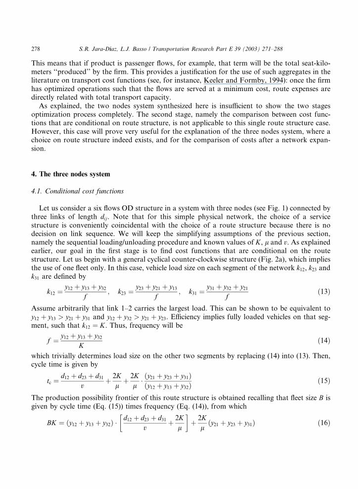
Let us consider a six flows OD structure in a system with three nodes (see Fig. 1) connected bythree links of length dij. Note that for this simple physical network, the choice of a servicestructure is conveniently coincidental with the choice of a route structure because there is nodecision on link sequence. We will keep the simplifying assumptions of the previous section,namely the sequential loading/unloading procedure and known values of K, l and v. As explainedearlier, our goal in the first stage is to find cost functions that are conditional on the routestructure. Let us begin with a general cyclical counter-clockwise structure (Fig. 2a), which impliesthe use of one fleet only. In this case, vehicle load size on each segment of the network k12, k23 andk31 are defined by

k12 ¼y12 þ y13 þ y32

f; k23 ¼

y23 þ y21 þ y13f

; k31 ¼y31 þ y32 þ y21

fð13Þ

Assume arbitrarily that link 1–2 carries the largest load. This can be shown to be equivalent toy12 þ y13 > y21 þ y31 and y12 þ y32 > y21 þ y23. Efficiency implies fully loaded vehicles on that seg-ment, such that k12 ¼ K. Thus, frequency will be

f ¼ y12 þ y13 þ y32K

ð14Þ

which trivially determines load size on the other two segments by replacing (14) into (13). Then,cycle time is given by

tc ¼d12 þ d23 þ d31

vþ 2K

lþ 2K

l ðy21 þ y23 þ y31Þðy12 þ y13 þ y32Þ

ð15Þ

The production possibility frontier of this route structure is obtained recalling that fleet size B isgiven by cycle time (Eq. (15)) times frequency (Eq. (14)), from which

BK ¼ ðy12 þ y13 þ y32Þ d12 þ d23 þ d31

v

�þ 2K

l

�þ 2K

lðy21 þ y23 þ y31Þ ð16Þ

278 S.R. Jara-D�ııaz, L.J. Basso / Transportation Research Part E 39 (2003) 271–288

with

y12 þ y13 > y21 þ y31 and y12 þ y32 > y21 þ y23

Given K, l and v, Eq. (16) is directly B ðY Þ. Just as we did with the two nodes system, theconditional cost function is obtained calculating expenses per vehicle-hour times B and addingloading/unloading sites expenses plus the right-of-way cost. Doing this and after some re-order-ing, we get

CCGðY Þ ¼ C0 þ ðy12 þ y13 þ y32Þ ðd12 þ d23 þ d31Þ K þ ðy12 þ y13 þ y32 þ y21 þ y31þ y23Þ X ð17Þ

with

y12 þ y13 > y21 þ y31 and y12 þ y32 > y21 þ y23

that is the cost function conditional on a cyclical route structure, with K and X defined as in Eq.(12).The similarity between this conditional cost function and the one obtained for the two nodes

system (Eq. (12)) is evident. First, we obtain again the distance-flow term with the same meaning,namely the capacity of the system, as the flows involved are those that define frequency. Second,the pure flow term is generated by loading/unloading activities. Finally, note that the obtainedfunction reduces to that of the two nodes system if the four new flows are set to zero and d23 þ d31is defined as d21.Let us move to a second possible route structure, the one known as hub-and-spoke, very

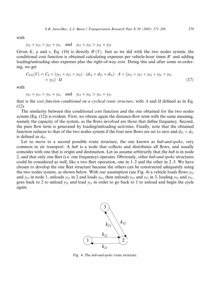
common in air transport. A hub is a node that collects and distributes all flows, and usuallycoincides with one that is origin and destination. Let us assume arbitrarily that the hub is in node2, and that only one fleet (i.e. one frequency) operates. Obviously, other hub-and-spoke structurescould be considered as well, like a two fleet operation, one in 1–2 and the other in 2–3. We havechosen to develop the one fleet structure because the others can be constructed adequately usingthe two nodes system, as shown below. With our assumption (see Fig. 4) a vehicle loads flows y12and y13 in node 1, unloads y12 in 2 and loads y23, then unloads y13 and y23 in 3, loading y32 and y31,goes back to 2 to unload y32 and load y21 in order to go back to 1 to unload and begin the cycleagain.

1 2k21

3

k32

k12

k23

Fig. 4. The hub-and-spoke route structure.

S.R. Jara-D�ııaz, L.J. Basso / Transportation Research Part E 39 (2003) 271–288 279

In this case, the four load sizes are given by

k12 ¼y12 þ y13

f; k32 ¼

y32 þ y31f

; k23 ¼y23 þ y13

f; k21 ¼

y31 þ y21f

ð18Þ

Again we will assume that total flow in link 1–2 is the largest, which makes k12 equal to K and thefrequency of the hub-and-spoke system happens to be

f ¼ y12 þ y13K

ð19Þ

Replacing (19) in (18) the other three load sizes are obtained. Cycle time and fleet capacity areobtained as usual, which yields

tc ¼d12 þ d23 þ d32 þ d21

vþ 2K

lþ 2K

l ðy21 þ y23 þ y31 þ y32Þ

ðy12 þ y13Þð20Þ

BK ¼ ðy12 þ y13Þ d12 þ d23 þ d32 þ d21

v

�þ 2K

l

�þ 2K

lðy21 þ y23 þ y31 þ y32Þ ð21Þ

For given values of K, l and v, Eq. (21) represents B ðY Þ for the hub-and-spoke structure. Fol-lowing the same procedure as in the two previous cases, we obtain the cost function conditional inthe hub-and-spoke route structure, i.e.

CHSðY Þ ¼ C0 þ ðy12 þ y13Þ ðd12 þ d23 þ d32 þ d21Þ K þ ðy12 þ y13 þ y32 þ y21 þ y31 þ y23Þ Xð22Þ

whose terms have the same interpretation as the ones in Eqs. (12) and (17). Once again, a distance-flow term representing the capacity of the system appears, as well as a pure flow term generated byloading/unloading activities.So far, we have obtained two conditional cost functions for the three nodes system. By simple

analogy, the conditional functions for other three route structures can be obtained as well: theclockwise cyclical system and the hub-and-spoke systems with the hub in nodes 1 or 3. Addi-tionally, adequately using the cost function for the two nodes system, we can derive conditionalcost functions for other cases: the direct service with three fleets, each one serving a pair of nodescyclically (1–2, 2–3 and 1–3), and the hub-and-spoke with two fleets, each one connecting a pair ofnodes (with the hub at any of the three nodes). Note that in this latter case some flows will have tobe loaded and unloaded twice (origin, destination and hub), which increases expenses unlike theother cases, but cycle times will be shorter. This is not intended to be an exhaustive list, as otheralternative route structures are possible. However, the ones developed and explained here areenough to illustrate that choosing a route structure is a key endogenous element, and to show thatthe minimum cost is associated with such choice, which is what we do next.

4.2. Global cost function and the role of flows and network

The second stage of the sequential optimization process is the search for the optimal routestructure, i.e. the one that minimizes cost in the production of Y and defines the global costfunction. This second stage requires the comparison of the conditional cost functions obtained in

280 S.R. Jara-D�ııaz, L.J. Basso / Transportation Research Part E 39 (2003) 271–288

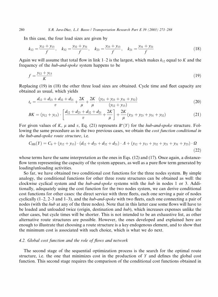
the first stage. Let us illustrate this process in the three nodes system considering yij ¼ y (equalflows) and the network shown in Fig. 5.Let us define the following notation for the alternative route structures.

CG-123: cyclic counter-clockwise.CG-132: cyclic clockwise.3F: direct service; three fleets.HS-i: hub-and-spoke with the hub in node i; one fleet.2F-i: hub-and-spoke with the hub in node i; two fleets.

Using the conditional cost functions explicitly derived earlier and the definitions of the systems,the conditional cost functions for each one can be constructed and evaluated for the equilateraltriangular network in Fig. 5 and equal flows on each OD pair. Omitting C0 for simplicity theresults are

CCG-123 ¼ CCG-132 ¼ 9 y K þ 6 y XCHS-1 ¼ CHS-2 ¼ CHS-3 ¼ 8 y K þ 6 y XC3F ¼ 6 y K þ 6 y XC2F-1 ¼ C2F-2 ¼ C2F-3 ¼ 8 y K þ 8 y X

ð23Þ

Thus, it is optimum to serve the flows directly with three fleets, each one connecting a pair ofnodes. It is worth noting that the hub-and-spoke structures with two fleets have larger costs thanthe ones with one fleet because of terminal operations, and that the cyclic systems have the largesten-route costs. As we explained in Section 2, the choice of a route structure is dependant onexogenous information, namely the OD structure of demand (the Y vector) and the networktopology. Therefore, now we want to examine the effect of a variation of this exogenous infor-mation on the choice of an optimal route structure.First, let us see the effect of changes in the OD structure of demand keeping the same physical

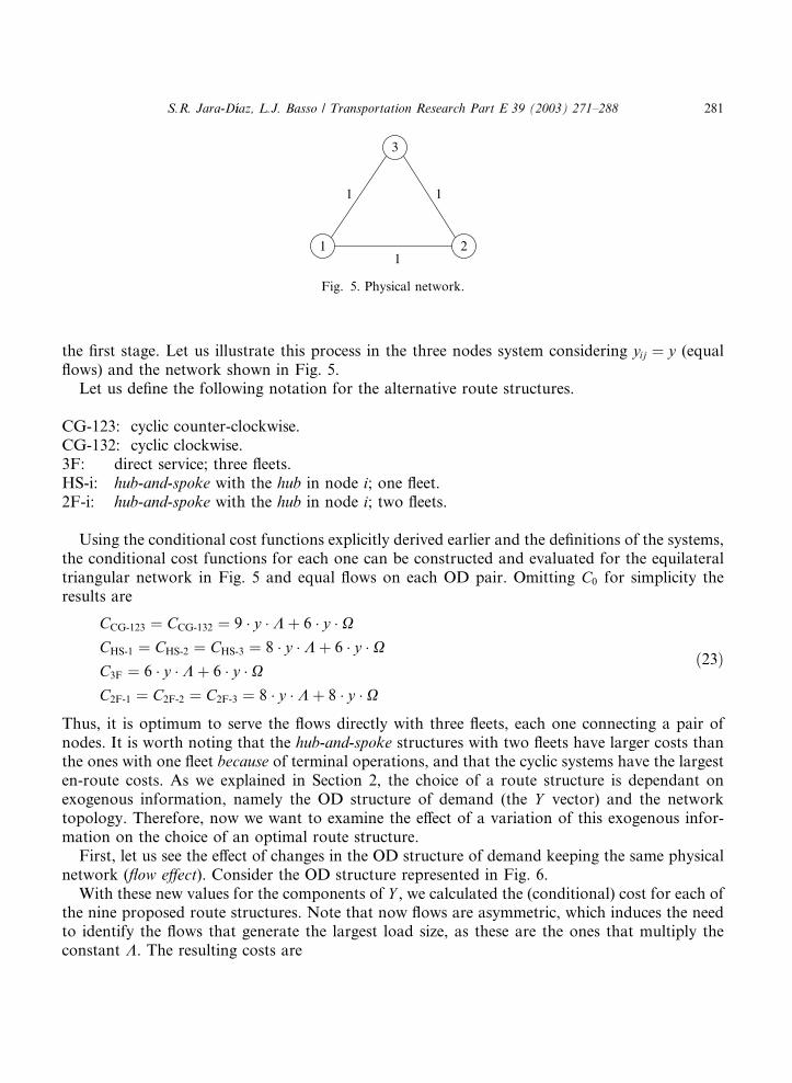
network (flow effect). Consider the OD structure represented in Fig. 6.With these new values for the components of Y , we calculated the (conditional) cost for each of

the nine proposed route structures. Note that now flows are asymmetric, which induces the needto identify the flows that generate the largest load size, as these are the ones that multiply theconstant K. The resulting costs are

1 21

1

3

1

Fig. 5. Physical network.

S.R. Jara-D�ııaz, L.J. Basso / Transportation Research Part E 39 (2003) 271–288 281

CCG-123 ¼ 195 K þ 110 X CHS-1 ¼ 200 K þ 110 XC2F-1 ¼ 170 K þ 160 X CCG-132 ¼ 165 K þ 110 XCHS-2 ¼ 200 K þ 110 X C2F-2 ¼ 170 K þ 150 XC3F ¼ 150 K þ 110 X CHS-3 ¼ 140 K þ 110 XC2F-3 ¼ 140 K þ 130 X

ð24Þ

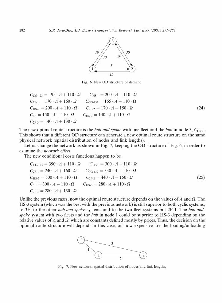
The new optimal route structure is the hub-and-spoke with one fleet and the hub in node 3, CHS-3.This shows that a different OD structure can generate a new optimal route structure on the samephysical network (spatial distribution of nodes and link lengths).Let us change the network as shown in Fig. 7, keeping the OD structure of Fig. 6, in order to

examine the network effect.The new conditional costs functions happen to be

CCG-123 ¼ 390 K þ 110 X CHS-1 ¼ 300 K þ 110 XC2F-1 ¼ 240 K þ 160 X CCG-132 ¼ 330 K þ 110 XCHS-2 ¼ 500 K þ 110 X C2F-2 ¼ 440 K þ 150 XC3F ¼ 300 K þ 110 X CHS-3 ¼ 280 K þ 110 XC2F-3 ¼ 280 K þ 130 X

ð25Þ

Unlike the previous cases, now the optimal route structure depends on the values of K and X. TheHS-3 system (which was the best with the previous network) is still superior to both cyclic systems,to 3F, to the other hub-and-spoke systems and to the two fleet systems but 2F-1. The hub-and-spoke system with two fleets and the hub in node 1 could be superior to HS-3 depending on therelative values of K and X, which are constants defined mostly by prices. Thus, the decision on theoptimal route structure will depend, in this case, on how expensive are the loading/unloading

1 2

15

10

3

30

5

30 20

Fig. 6. New OD structure of demand.

1 22

1

33

Fig. 7. New network: spatial distribution of nodes and link lengths.

282 S.R. Jara-D�ııaz, L.J. Basso / Transportation Research Part E 39 (2003) 271–288

activities relative to activities en-route, which is very reasonable. Note that a proportional growthof distances (links) would increase the difference between expenses en-route of the two structures,keeping the difference between terminal expenses constant, which would increase the attractive-ness of route structure 2F-1. This illustrates the network effect on the optimal route structure.Before closing this section, we find important to stress two points. First, when dealing with real

data it is vital to be very precise about what is exogenous and what is endogenous in order toavoid misinterpretations. Our impression is that in the literature, the concept of ‘‘network’’ hasbeen used in fairly different manners, conveying both endogenous decisions and exogenous in-formation. Just as an example, the ‘‘network’’ descriptor number of route miles has been definedeither as the total miles of the physical network (exogenous information) or the number of milesactually used (endogenously decided). Second, it is worth noting that it have been argued that inthe absence of economies of density, a monopoly airline would provide non-stop connections, i.e.direct service, while in the presence of such economies, the airline would save money by operatinga hub network (see for instance Brueckner and Spiller, 1991). Our discussion regarding the im-portance of the exogenous information in the cost minimizing behavior of firms, shows that theselection of a route structure goes beyond the existence of decreasing or constant marginal costs atthe arc level. The importance of collecting adequately the costs of loading and unloading activ-ities––which are not related to distances––in the empirical work, is now apparent.

5. Scale, scope and industry structure

Within a multioutput framework, increasing output has two meanings: increasing volume orincreasing the number of products. Scale economies are related with the behavior of cost asproducts expand proportionally (radial analysis). On the other hand, economies of scope arerelated with the impact on cost of adding new outputs to the line of production. Analytically, thedegree of economies of scale, S, can be calculated as the inverse of the sum of cost-productelasticities (Panzar and Willig, 1975), such that a value of S greater, equal or less than 1 showsincreasing, constant or decreasing returns to scale respectively, indicating the relative convenienceof proportional expansions or reductions of output. The degree of economies of scope relative to asubset R of products, SCR is calculated as (Panzar and Willig, 1981)

SCR ¼ CðY RÞ þ CðY M�RÞ þ CðY ÞCðY Þ ð26Þ

where Y R is vector Y with yi ¼ 0, 8i 62 R � M , withM being the whole product set. Then, a positivevalue for SCR indicates that it is cheaper to produce Y with one firm than to split production intotwo orthogonal subsets R and M � R. It can be easily shown that SCR lies in the interval (�1; 1).In the transport case, scale economies are related with the convenience or inconvenience of

expanding proportionally the flows in all OD pairs, while economies of scope are related with thepotential advantages or disadvantages of serving all OD pairs with one firm (for a full explanationof the concepts of spatial scale and scope, see Jara-D�ııaz, 2000). Examining the different condi-tional cost functions derived in the previous sections, we can observe that the choice of a routestructure will be invariant to proportional expansions of flows, i.e. the cost minimizing route

S.R. Jara-D�ııaz, L.J. Basso / Transportation Research Part E 39 (2003) 271–288 283

structure will be the same. 5 It is quite simple to show that for all the conditional cost functions(including that of the two nodes system) the degree of economies of scale S is given by the ratiobetween CðY Þ and CðY Þ � C0. Then C0 ¼ 0 implies constant returns and C0 > 0 generates in-creasing returns.Regarding scope analysis, the two nodes system admits only one orthogonal partition. In this

case SC examines whether it is convenient to serve the two flows with one firm or to serve y12 withone firm and y21 with other. It can be easily shown that SC is positive even if C0 ¼ 0 (Jara-D�ııaz,1982b, 2000), such that a one firm operation is convenient basically due to the avoidance of idlecapacity. Note that for nil right-of-way costs, constant returns to scale coexist with economies ofscope, which means that, from a cost viewpoint, it would be convenient to have many firmscompeting on this system, each one serving both OD pairs.The analysis of scope in the three nodes system admits various possible orthogonal partitions of

the six flows product vector (Fig. 1a). However, the main motivation for the analysis of thissystem was to study the case in which one node is added or subtracted from a firm service(network expansion or reduction). Thus, let us consider the orthogonal partitionY R ¼ fy12; y21; 0; 0; 0; 0g, Y M�R ¼ f0; 0; y13; y31; y23; y32g, which permits the comparison between onefirm serving all six flows against two firms, one serving the two flows between nodes 1 and 2 andthe other serving the rest. Note that CðY Þ � CðY RÞ is precisely the cost of adding the new node 3 tothe network {1,2}, not necessarily equal to CðY M�RÞ unless SCR was nil. As seen, the value of thedegree of economies of scope depends on the exogenous information (flows and network) becausethe global cost function does. We will analyze the case depicted in Fig. 6 with link lengths equal toone, with C0 ¼ 0 in order to get rid of the fixed cost effect that influences (increases) both scale andscope. In this case, the global cost function for the firm serving all flows corresponds to that of theHS-3 structure, which yields CðY Þ ¼ 140 K þ 110 X. On the other hand, the global cost functionfor the two flows system is given by Eq. (10), which yields CðY RÞ ¼ 30 K þ 20 X for the values offlows and distances in this case. For Y M�R the three nodes system analysis applies, with two flowsset to zero. It can be shown that the optimal route structure could be either 2F-3 or HS-3, bothwith a cost CðY M�RÞ given by 120 K þ 90 X. Now we can calculate SCR from Eq. (26), whichyields

SCR ¼ ð30K þ 20XÞ þ ð120K þ 90XÞ � ð140K þ 110XÞCðY Þ ¼ 10 K

CðY Þ > 0: ð27Þ

This means that, even if C0 ¼ 0, the six flows will be better served with one firm. Note that in thiscase savings occur due to expenses en-route, i.e. a single firm permits a better use of the fleetcapacity than two firms (vehicle load is larger in average) by means of adjustments in the routestructure. Note also that this might not happen for other values of Y or for another physicalnetwork. The same applies to loading/unloading activities; in this particular case they are neither asource of economies nor diseconomies of scope because in the three optimal route structures every

5 We must note, however, that more detailed technical considerations might have an impact on this result: the fact

that speed or fuel consumption could be dependent on load size, or that bigger vehicles and loading/unloading sites

could have scale advantages, or that congestion could be present, might change the optimal route structure after a

proportional growth of all OD flows.

284 S.R. Jara-D�ııaz, L.J. Basso / Transportation Research Part E 39 (2003) 271–288

unit is loaded and unloaded once. Under other circumstances, a hub-and-spoke structure with twofleets might be optimal in producing Y , with loading and unloading activities being a source ofdiseconomies of spatial scope.The results obtained with this example are enough to show two relevant aspects. First, route

structure is an important endogenous cost minimizing variable, which translates into a potentialsource of economies of scope. As stated by Antoniou (1991), ‘‘Networking and the route structure(. . .) is a well thought-out strategy aimed at taking full advantage of economies of scope andeconomies of vehicle size’’ (p. 171). Second, we confirm that incentives to merge might appearbecause of economies of spatial scope even under constant returns to scale (C0 ¼ 0). This showsthat the use of the concepts of economies of scale and economies of (spatial) scope as defined inthis article may help solving the problem presented by the couple RTD and RTS, namely that afirm with no incentives to increase its density over a fixed network but with incentives to increaseits network may be described. Thus, economies of network expansion should not be looked atthrough the concept of scale but through the concept of (spatial) scope.Finally, it is important to emphasize that it was necessary to study a particular case in order to

analyze spatial scope correctly, because the characteristics of the physical network and the level ofproduction described as a vector Y , play a key role. Therefore, if these elements are not adequatelycaptured in the empirical work, the analysis of industry structure could be done incorrectly orcould be simply unfeasible.

6. Final comments and conclusions

The research described in this article is intended to increase our understanding of the basictechnological dimensions that are specific to transport production, in order to improve theanalysis of industry structure based upon the estimation of transport cost functions. We feel thatthe econometrics behind the empirical approach have received much more attention than theproduction process itself; progress in this latter area is urgently needed. In our opinion, it isprecisely the lack of a rigorous view of the key technical aspects, specifically the spatial dimensionof product, what is causing difficulties when it comes to make interpretations and inferences onindustry structure from estimated cost functions.This paper shows technically that economies of transport network expansion should be viewed

through the concept of economies of scope rather than through the concept of economies of scale.The generalization of the technical approach by Jara-D�ııaz (1982b, 2000) to a three nodes systempresented here, has been instrumental to emphasize the spatial nature of product and to illustrate,in a fairly precise manner, the process that leads a cost minimizing transport firm to the opti-mization of the route structure as a key endogenous decision. We have been particularly keen onthe distinction between what is truly exogenous to the firm––the OD structure of demand, net-work topology and links description––from what is an endogenous decision as the route structure(service structure and link sequence), showing how the optimal operation of a firm changes as theexogenous variables change. This is a particularly relevant aspect, as all these network relatedconcepts have been treated in a somewhat confusing manner in the empirical work. For example,several variables have been used to describe the network (number of points served, number ofroute miles, even average length of haul), or the same network descriptor (number of route miles)

S.R. Jara-D�ııaz, L.J. Basso / Transportation Research Part E 39 (2003) 271–288 285

has been defined in different ways, either as the total miles of the physical network or the numberof miles actually used.The cost functions obtained for the two nodes system and for various cases in the three nodes

system have similar structures. They are separable into two terms: a pure flow term related withexpenses on terminal operations, and a flow-distance term directly related with en-route expenses.This latter was shown to represent the optimal transport supply (capacity) offered by the firm (e.g.seat-kilometers), a very reasonable result as en-route expenses depend on the fleet size, frequencyand distance traveled, variables that are optimized in order to minimize cost in the production of agiven vector Y . Thus, transport supply indices representing product proxies, sometimes used in theempirical work, have received here theoretical support provided the firm is operating in a tech-nically optimal way. The pure flow term was shown to be relevant in the selection of a routestructure because some structures imply additional loading and unloading. Thus, given the keyrole of the route structure in the generation of scope economies, pure flow terms are particularlyimportant for industry structure analysis using aggregated output. When only distance relatedvariables are used to describe output (as is the case in many applied studies) loading/unloadingcosts may not be adequately captured.On the other hand, the analysis of scale, scope and industry structure involving relatively simple

transport networks technically described in detail, has generated important conclusions. Forsynthesis, we have been able to show the process through which cost advantages arising from anetwork expansion (new nodes served) are realized. In essence, fleet capacity can be better used bymeans of variations in the route structure when new flows are incorporated to production afterthis type of network expansion. From a microeconomic viewpoint, this translates into economiesof scope, which have been shown to exist even under constant returns to scale (in this case, theabsence of fixed costs). This provides a new conceptual framework that might help understandingthe observed behavior in some transport industries, which is a problem that, so far, has beenanalyzed as a scale property, an inadequate approach in our view.Thus, what we can call increasing returns to (spatial) scope are influenced not only by the OD

structure of demand––which is already a difficult aspect to cope with in the empirical work––butalso by the exogenous spatial information on the network (topology). Therefore, in order toanalyze correctly the potential advantages or disadvantages of network expansions through em-

pirically estimated cost functions, these elements have to be adequately captured. We believe thatthis is mainly a problem of an adequate interpretation of ‘‘aggregate’’ cost functions eCCðeYY ;NÞ. Sofar, this has been treated through ambiguous concepts like economies of scale with variablenetwork size under constant density, a concept that should be carefully examined in order toimprove the transport industry structure analysis. The challenge that lies ahead is how to calculateeconomies of spatial scope from this type of cost function, which is exactly the work in which weare presently engaged.The two and three nodes networks technically analyzed here have been sufficient to prove the

main point, which is that network expansion should be studied through scope rather than scaleeconomies. As stated earlier, this approach was not intended to find optimal service structures fortransport firms, but to understand key issues relating cost functions, transport networks andindustrial organization. Nevertheless, it is worth asking whether further insight could be gained byexpanding this type of detailed analysis to larger networks when feasible. We believe that it mighthelp finding aggregate specifications for transport product that are adequate for the empirical

286 S.R. Jara-D�ııaz, L.J. Basso / Transportation Research Part E 39 (2003) 271–288

estimation of cost functions. It could help as well to examine how optimal frequencies and routestructures affect aggregates that are used in the literature, as average distance or average load. Itshould be stressed, though, that finding analytical cost functions for actual transport firms servingmany OD pairs over complex networks is simply unfeasible, which is precisely the reason why it isdone econometrically. The point is, however, that statistical feasibility should be no excuse toforget neither the true product nor the type of decisions made by a transport firm on a networkwhen using this empirical cost functions for industrial organization analysis.

Acknowledgements

This research has been partially funded by Fondecyt, Chile, Grant 1010687 and the MillenniumNucleus ‘‘Complex Engineering Systems’’.

References

Antoniou, A., 1991. Economies of scale in the airline industry: the evidence revisited. The Logistics and Transportation

Review 27 (2), 159–184.

Braeutigam, R.R., 1999. Learning about transport costs. In: Gomez-Iba~nnez, J., Tye, W.B., Winston, C. (Eds.), Essays

in Transportation Economics and Policy. Brookings Institution Press, Washington DC, pp. 57–97.

Brueckner, J.K., Spiller, P.T., 1991. Competition and mergers in airline networks. International Journal of Industrial

organization 9, 323–342.

Brueckner, J.K., Spiller, P.T., 1994. Economies of traffic density in the deregulated airline industry. The Journal of Law

and Economics 37 (2), 379–413.

Daughety, A.F., 1985. Transportation research on pricing and regulation: overview and suggestions for future research.

Transportation Research 19A (5/6), 471–487.

Gagn�ee, R., 1990. On the relevant elasticity estimates for cost structure analysis of the trucking industry. The Review of

Economics and Statistics 72, 160–164.

G�aalvez, T., 1978. An�aalisis de Operaciones en Sistemas de Transporte (Transport Systems Operations Analysis),

Working Paper ST/INV/04/78, Departamento de Ingenier�ııa Civil, Universidad de Chile, Santiago de Chile.

Jara-D�ııaz, S.R., 1982a. The estimation of transport cost functions: A methodological review. Transport Reviews 2,

257–278.

Jara-D�ııaz, S.R., 1982b. Transportation product, transportation function and cost functions. Transportation Science 16,522–539.

Jara-D�ııaz, S.R., 2000. Transport production and the analysis of industry structure. In: Polak, J., Heertje, A. (Eds.),

Analytical Transport Economics, An International Perspective. Elgar, Cheltenham, UK, pp. 27–50.

Jara-D�ııaz, S.R., Cort�ees, C., 1996. On the calculation of scale economies from transport cost functions. Journal of

Transport Economics and Policy 30, 157–170.

Jara-D�ııaz, S.R., Cort�ees, C., Ponce, F., 2001. Number of points served and economies of spatial scope in transport cost

functions. Journal of Transport Economics and Policy 35 (2), 327–341.

Keeler, J.P., Formby, J.P., 1994. Cost economies and consolidation in the US airline industry. International Journal of

Transport Economics 21 (1), 21–45.

Oum, T.H., Waters II, W.G., 1996. A survey of recent developments in transportation cost function research. Logistics

and Transportation Review 32 (4), 423–463.

Oum, T.H., Zhang, Y., 1997. A note on scale economies in transport. Journal of Transport Economics and Policy 31,

309–315.

Panzar, J. Willig, R., 1975. Economies of scale and economies of scope in multioutput production, Economic

Discussion paper no. 33. Bell Laboratories.

S.R. Jara-D�ııaz, L.J. Basso / Transportation Research Part E 39 (2003) 271–288 287

Panzar, J., Willig, R., 1981. Economies of scope. American Economic Review 71, 268–272.

Spady, R.H., 1985. Using indexed quadratic cost functions to model network technologies. In: Daughety, A. (Ed.),

Analytical Studies in Transport Economics. Cambridge University Press, UK, pp. 121–135.

Xu, K., Windle, C., Grimm, C., Corsi, T., 1994. Re-evaluating returns to scale in transport. Journal of Transport

Economics and Policy 28, 275–286.

Ying, J.S., 1992. On calculating cost elasticities. The Logistics and Transportation Review 28 (3), 231–235.

288 S.R. Jara-D�ııaz, L.J. Basso / Transportation Research Part E 39 (2003) 271–288