Transforming Complete Coverage Algorithms to Partial Coverage Algorithms for Wireless Sensor Networks

MANUSCRIPT TO BE SUBMITTED TO IEEE TRANSACTIONS ON PARALLEL AND DISTRIBUTED SYSTEMS 1

Transforming Complete Coverage Algorithms toPartial Coverage Algorithms

for Wireless Sensor NetworksYingshu Li, Member, IEEE, Chinh Vu, Student, IEEE, Chunyu Ai, Student, IEEE,

Guantao Chen, Member, IEEE, and Yi Zhao

Abstract—The complete area coverage problem in Wireless Sensor Networks (WSNs) has been extensively studied in the literature.However, many applications do not require complete coverage all the time. For such applications, one effective method to save energyand prolong network lifetime is to partially cover the area. This method for prolonging network lifetime recently attracts much attention.However, due to the hardness of verifying the coverage ratio, all the existing centralized or distributed but non-parallel algorithms forpartial coverage have very high time complexities. In this work, we propose a framework which can transform almost any existingcomplete coverage algorithm to a partial coverage one with any coverage ratio by running a complete coverage algorithm to find fullcoverage sets with virtual radii and converting the coverage sets to partial coverage sets via adjusting sensing radii. Our frameworkcan preserve the characteristics of the original algorithms and the conversion process has low time complexity. The framework alsoguarantees some degree of uniform partial coverage of the monitored area.

Index Terms—Partial coverage, Wireless sensor networks, Energy efficiency.

F

1 INTRODUCTION

R ESEARCHERS have spent lots of effort to design al-gorithms to completely cover an area - complete cov-

erage problem. Most of the coverage-related works con-cern how to prolong network lifetime through differenttechniques. One of the techniques which recently attractsresearchers’ attention is to reduce the coverage qualityto trade for network lifetime. In some applications, therequired coverage quality may even be different at dif-ferent points of time. For example, forest fire monitoringapplications [13], [14] and [15] may require completecoverage in dried seasons while only require 80% ofthe area to be covered in rainy seasons. Thus, to extendnetwork lifetime, we can lower the coverage quality ifit is acceptable. The problem to cover only a portionof an area is referred as the “partial coverage” problem.The requirement for the partial coverage problem is thatthe ratio of the covered area over the whole monitoredarea is no less than a pre-defined value. This value isa user-specified parameter. In this work, we use thenotation α to refer to this parameter. Consequently, thepartial coverage problem is also referred as α-coverageproblem of which the objective is to cover only α-portionof the area (the formal definition of this problem is

• Y. Li, C. Vu, and C. Ai are with the Department of Computer Science,Georgia State University, Atlanta, GA, 30303.E-mail: {yli, chinhvtr, chunyuai}@cs.gsu.edu

• G. Chen and Y. Zhao are with the Department of Mathematics andStatistics, Georgia State University, Atlanta, GA, 30303.E-mail: {matgtc,matyxz}@langate.gsu.edu

This work is supported by the NSF under grant No. CCF-0545667, theNational Grand Fundamental Research 973 Program of China under grantNo. 2006CB303000 and NSFC-RGC of China under grant No. 60831160525.

given in Definition 2). Moreover, it is always desirableto schedule the sensors such that the area is uniformlycovered. It is clearly undesired if the network only coverssome particular sub-regions of the area while uncoversthe other large and continuous sub-regions. To evaluatecoverage quality, a metric named Sensing Void Distance(SVD) [11], [18] is used (the formal definition of thismetric is given in Definition 6).

In this work, we solve the α-coverage problem bytransforming various well known complete coveragealgorithms to partial coverage algorithms. Our frame-work has four strategies, two general strategies andtwo extended strategies. The two general strategies aredesigned for networks where sensors have fixed sensingranges (fixed-sensing-range network) and the other twoare for networks where sensors can adjust their sens-ing ranges (adjustable-sensing-range network). For anyparticular α, the two general strategies also guarantee aconstant bound of SVD.

2 RELATED WORKThe problem of partial coverage is recently investigatedin the literature under many alias such as “α-lifetime”[8], [9], “p-percentage coverage” [10], [18], ”θ-coverage”[11], or ”q-portion coverage” [16]. The problem requiresthe network to cover at least ”p percent”, ”α portion” or”q portion” of an area. In other words, if α = θ = q = p

100 ,those problems are actually the same. To be consistentwith the name when this problem was first proposed[8], [9] and to make the term self-explaining, we use thename “α-coverage” (which will be formally defined laterin Definition 2) to refer to this problem and α is referredas coverage ratio.


The work in [8] shows the upper bound of networklifetime when only α-portion of the whole area is cov-ered. It shows that network lifetime may increase upto 15% for 99%-coverage and 25% for 95%-coverage.Then in [9], the authors proposed a centralized algorithmto solve the α-coverage problem of which the incre-ment of network lifetime is close to the upper boundderived in [8]. In [16], a centralized algorithm basedon the Garg-Konemann method for q-portion coverageis proposed. The algorithm has a performance ratio of(1 + ε)(1 + ln 1

1−q ), for any ε > 0.In [12], percentage coverage instead of complete cover-

age is selected as the design goal, and a location-basedPercentage Coverage Configuration Protocol (PCCP) isdeveloped to assure that the proportion of the area afterconfiguration to the original area is no less than a desiredpercentage.

Liu et. al [11] presented a centralized algorithm whichtakes both coverage and connectivity into account. Theirwork is the first one to analyze partial coverage proper-ties in order to prolong network lifetime. Initially, activesensors are randomly selected. In each iteration, nodeson a chosen candidate path with the maximum gain arechosen. The algorithm continues until the whole area isθ-covered. This method is also employed by [10]. Thework in [10] proposed two algorithms, one centralizedand one distributed, for the same problem. To providedifferent coverage qualities at different locations of themonitored area, the area is partitioned into a number ofclusters and the algorithms partially cover the clustersone by one.

For the α-coverage problem, we always want to knowhow uniformly the sub-regions are covered. To evaluatethis, adapted from [11], the work in [18] uses SensingVoid Distance (SVD) which is the distance from an un-covered point to a nearest covered point. The authorsof [18] also claimed that their CDS-based distributedalgorithm CpPCA-CDS can provide a constant-boundedSVD. However, the value of p is too small that even asubset of a CDS can provide p-percentage coverage, thuscoverage redundancy is high to guarantee a boundedSVD. In other words, in [18] the coverage redundancy isthe price paid for a bounded SVD.

To the best of our knowledge, most proposed algo-rithms for α-coverage are centralized ones. There aredistributed algorithms discussed in [10], [18]. However,those algorithms work in a distributed manner but nota parallel fashion, i.e., each sensor has to wait for thevalue of α to be calculated by its neighbors to decidewhether to be active or to sleep. So the time complexitymay be very high. In the worst case, the time complexityof a non-parallel (consequential) algorithm may be of theorder of the network size.

The rest of the paper is organized as follows: Section3 states the motivation of our work. Section 4 introducessome preliminary concepts and supporting knowledge.In Section 5, we explain our framework in details. Wethen evaluate the effectiveness of the proposed frame-

work in Section Simulation of Supplementary File. Weconclude our work in Section 6.

3 MOTIVATIONMost of the existing algorithms for the α-coverage prob-lem are greedy on a so-called contribution (or gain).Contribution of a set X of sensors is a parameter thatmainly depends on the current uncovered area that canbe covered by X . For the simplest case where sensors’sensing regions are assumed to be perfect disks, thatregion usually is the part of union of disks that is notcovered by some other overlapping disks (neighbors).However, calculating the area of this union region is nottrivial even for the case that all the sensors have thesame sensing range. The previous works usually ignoreto explain how to do that calculation. To the best of ourknowledge, there is no existing method to calculate theexact area for such region.

Besides, most of the current works directly solve thepartial coverage problem. The common method is togreedily (on contribution) add sensors until at least αportion of the area is covered. As a result, most ofthe existing algorithms are centralized. The rest, fewdistributed algorithms have high time complexity due tothe fact that they have to scan through all the sensors oneby one until α-portion of the area is covered. That meansthe sensors cannot work in a parallel manner. In a sense,we claim that the α-coverage problem is an impossible-to-directly-solve problem in a distributed and parallelmanner due to the fact that α is a global parameter whichcannot be acquired in a parallel manner.

Moreover, there are a great deal of existing algorithmsdesigned for complete coverage which motivate us tofind a way to utilize them for partial coverage. In theliterature, there do exist many fully distributed andparallel algorithms which do not depend on contributionsuch as the algorithms in [2]–[7]. It is a significant contri-bution if we somehow convert those algorithms to solvepartially (instead of completely) area cover problems.The resulting algorithms have to guarantee some levelof coverage quality as required by users. The conversionshould preserve the characteristics of the original algo-rithms. Moreover, the conversion should be simple andfast enough to not increase time-complexity too much.Importantly, the conversion process should work withmost of the existing complete-coverage algorithms.

In this work, we propose a framework that satisfies allthe requirements of an algorithm conversion frameworkwe just mentioned above. The framework consists offour strategies (two general strategies and the other twoextended strategies) which are designed for differentkinds of networks. Two (one general and one extendedstrategy) are designed for fixed-sensing-range WSNs andthe other two are for adjustable-sensing-range WSNs.Amazingly, for any certain desired coverage ratio α anda particular WSN, the resulting algorithm of two generalstrategies for partial coverage can guarantee a constant-bounded SVD for all the original algorithms for complete


coverage. In other words, the resulting algorithms of twogeneral strategies uniformly cover the area. Also, thegeneral strategies work for almost all complete-coveragealgorithms.

4 PRELIMINARY

We dedicate this section to introduce some concepts anddefinitions.

Definition 1: (α-cover) Given a real number α where0 < α < 1, a two-dimensional region A and set S of nsensors si for i = 1 . . . n. Sensor si’s sensing region isSi. ‖A‖ denotes the area of region A. A sub-set C ⊆ Sα-covers area A (C is an α-set-cover of A) if:

‖(⋃

si∈CSi)

⋂A‖ ≥ α‖A‖ (1)

By this definition, the traditional set cover is alsocalled 1-set-cover in this work. Now, we define the α-coverage problem as following:

Definition 2: (α-coverage problem) Given a real numberα where 0 < α < 1, a two-dimensional region A and setS of n sensors si for i = 1 . . . n. Find a set of α-set coversC1, .., Cl of S for region A.

Definition 3: (γ-virtual network) For a particular realnumber γ where 0 < γ and a WSN S with n sensorss1, ..., sn.• If S is a fixed sensing range WSN where sensor si

(i = 1...n) has a sensing range Ri, then the γ-virtualnetwork of S, denoted by Sγ , is the network wheresensor si has a sensing range Ri√

γ . This sensing rangeis called the virtual sensing range.

• If S is an adjustable sensing range WSN wheresensor si (i = 1...n) has the maximum sensing rangeof MaxRi, then:

– The γ-virtual network of S, denoted by Sγ ,is the adjustable-sensing-range network wheresensor si has maximum sensing range of MaxRi√

γ

for i = 1...n. This maximum sensing range iscalled virtual maximum sensing range.

– The fixed-γ-virtual network of S, denotedby Sγ

fixed, is the fixed-sensing-range networkwhere sensor si has sensing range of MaxRi√

γ .This sensing range is called the virtual sensingrange.

Because we have to deal with two types of networksin this paper (real and virtual networks), it is necessaryto distinguish two types of set covers corresponding tothe two types of networks as follows:

Definition 4: (V SCγ :γ-virtual-set-cover) Given a realnumber γ (0 < γ) and set S of n sensors si (i = 1 . . . n),the γ-virtual network of S is Sγ . A 1-set-cover of Sγ iscalled γ-virtual-set-cover, denoted by V SCγ .

Definition 5: (µ-RSC:µ-real-set-cover) Given a realnumber µ (0 < µ) and set S of n sensors si (i = 1 . . . n).The µ-real-set-cover, denoted by µ-RSC, of a virtual setcover Cj (Cj is not necessarily a V SCγ) is the set coverwhere every sensor has a sensing range of

√µ times of

its sensing range in Cj . Furthermore, a µ-RSC is feasibleif either of the following conditions is true:

• If the network is a fixed-sensing-range network,then every sensor of µ-RSC must have its pre-defined sensing range.

• If the network is an adjustable-sensing-range net-work, then every sensor of µ-RSC must have itssensing range no larger than its pre-defined maxi-mum sensing range.

5 A FRAMEWORK FOR α-COVERAGE ALGO-RITHMS

The framework requires three inputs: i) the coverageratio α, ii) a complete-coverage algorithm A (sometimesreferred as “original algorithm”), and iii) the network Sconsisting of n sensors S = {s1, .., sn}. Our frameworktransforms the input original algorithms to the ones thatcan generate a set of α-set-covers. We sometimes referthe obtained algorithms as “α-coverage algorithms”.

5.1 Assumptions and notations

We assume the sensing region of a sensor si is a diskcentered at si. If si has a sensing range of Ri, denotedby si(Ri), then that disk has a radius of Ri.

For an input algorithm A, conventionally, the resultof A to completely cover a sensor network S is a setof {Cj , tj} pairs where each Cj is a 1-set-cover and tjis its working schedule. Each set cover Cj is a set ofsensors (with their sensing ranges) that will be turnedon to provide complete coverage. The schedule tj of setcover Cj may include the starting time points and thedurations that the set cover Cj will be activated. It isworth emphasizing that an algorithm A does not alwaysexplicitly create a set of all desired set covers and returnthem as an output. For instance, the family of schedulingalgorithms that work in rounden, of which the networkworking time is divided into equal-length rounds andthe algorithms create a set cover for each round, theyjust create one set cover at a time for each round. Wemake the assumption about the result of the originalalgorithms only for clear and easier explanation of ourframework.

For an adjustable-sensing-range WSN S = {s1, .., sn},we assume that each sensor si is able to smoothlyadjust its sensing range under some upper cut-off range.This assumption is employed by most works concerningadjustable-sensing-range WSNs such as [3] and [4].

Our framework has no restriction on the type ofWSNs. In terms of sensors’ sensing ranges and initialenergy, the WSNs may be heterogeneous or homoge-neous, and the network may be fixed-sensing-range oradjustable-sensing-range networks. However, the algo-rithms generated by our framework has the same re-striction as the original algorithms.


5.2 Basic idea of the framework

Before explaining our strategies in detail, it is necessaryto emphasize the essences of our framework. Our frame-work essentially converts a complete-coverage algorithmto a resulting algorithm for the α-coverage problem.The framework first makes the original algorithm tobe executed on a virtual network. The result of thatexecution is a set of virtual set covers Cj and theirschedules tj . These set covers are for the virtual network,so the sensors of those set covers may have virtualsensing ranges which might be bigger than their realmaximum sensing ranges. The framework then modifiesthe original algorithm so that the final result is a set ofreal set covers Cj , where each set cover Cj is α-RSC ofCj . Though in Section 5.3.1, Section 5.3.2, and SectionExtended strategies of Supplementary File, our strategiesare actually the general guidelines on how to modifyan original algorithm (for complete coverage) to obtaina desired algorithm for α-coverage. When modifying anoriginal algorithm, every step does not have to be exactlythe same as shown in the pseudo-codes:• The process to modify the algorithm A is not al-

ways the same. For example, instead of creatinga new virtual network, our framework suggeststhat the original algorithm should be modified inthe way that anytime sensors’ sensing ranges arereferenced by the algorithm A, the strategies justhave to replace the original sensing ranges with thecorresponding virtual sensing ranges.

• Since there exist complete-coverage algorithms thatdo not generate all set covers at once, their resultingalgorithms for the α-coverage problem do not haveto explicitly identify all α-set-covers. Most of thetime, when the algorithm A generates a set coverfor the virtual network, the algorithm A will bemodified in the way that right before a virtual setcover is returned, it will be converted to a real setcover.

5.3 General strategies

5.3.1 General strategy for fixed-sensing-range WSNs -Strategy G-1:Assume that a sensor si (i = 1, ..., n) has a fixed sens-ing range Ri. Strategy G-1 is given in Algorithm 1 ofSupplementary File.

This strategy works for both types of original algo-rithms A:• Type 1: Algorithm A is designed for fixed-sensing-

range WSNs. Strategy G-1 first runs the originalalgorithm A on α-virtual network Sα where sensorsi has a sensing range of Ri√

αto get a set of virtual

set covers Cj and their schedules tj . For a sensorsi ∈ Cj , its virtual sensing range in Cj is Ri√

α. From

virtual set cover Cj , the set cover Cj is created ofwhich each sensor si has a sensing range of Ri,which is si’s real sensing range. It can be seen that

each set cover Cj is a V SCα and set cover Cj is anα-RSC of Cj . The final result is a set of set coversCj where sensors use their real sensing ranges Ri

and their schedule tj for j = 1...l.• Type 2: Algorithm A is designed for adjustable-

sensing-range WSNs. Strategy G-1 runs the originalalgorithm A on α-virtual network Sα where sensorsi has the maximum sensing range of Ri√

αto get a

set of {Cj , tj} pairs. Denote the sensing range of asensor si in Cj as Rj

i and Rji ≤ Ri√

α. In the final

resulting set covers Cj , sensor si ∈ Cj uses its realsensing range Ri (i.e., we intentionally ignore thevirtual sensing ranges assigned by the algorithm A)and schedule tj . Usually, it is not practical to executeType 2 algorithms on fixed-sensing-range WSNs. Wejust list this case here to illustrate the universalityof our framework. We do not recommend StrategyG-1 to be applied for adjustable-sensing-range algo-rithms on fixed-sensing-range WSNs.

Since Strategy G-1 forces sensors of the final resultingset covers Cj to use their original sensing ranges (with-out considering the sensors’ sensing ranges in the virtualset cover Cj), the following lemmas are directly derived:

Lemma 1: Given a real number α (0 < α < 1) anda fixed-sensing-range WSN, for any original (complete-coverage) algorithm as an input, the α-coverage algo-rithm derived by Strategy G-1 generates feasible setcovers whose sensors’ sensing ranges are their originalsensing ranges.

Lemma 2: The sensing range of a sensor in a finalresult’s set cover Cj is no smaller than

√α times of its

sensing range in the corresponding virtual set cover Cj .

5.3.2 General strategy for adjustable-sensing-rangeWSNs - Strategy G-2:We assume that each sensor si’s sensing range has a pre-defined upper bound MaxRi. Strategy G-2 is given inAlgorithm 2 of Supplementary File and works for bothtypes of original algorithms.• Type 1: The original algorithm A is designed for

fixed-sensing range WSNs. Strategy G-2 runs theoriginal algorithm A on fixed-β-virtual networkSβ

fixed where α ≤ β. That is, execute algorithmsA on a virtual network where a sensor si has afixed sensing range of MaxRi√

β. The result of this

execution is a set of virtual set covers Cj , andeach Cj is a V SCβ . Then adjusts each sensor’s thesensing range from MaxRi√

βin V SCβ Cj to Ri =

√α × MaxRi√

β=

√α√β× MaxRi in α-RSC Cj . Since

α ≤ β, Ri ≤ MaxRi, which makes the final resultingset covers Cj feasible. If we choose β = α, then thisstrategy is similar as Strategy G-1.

• Type 2: The original algorithm A is designed foradjustable-sensing-range WSNs. Strategy G-2 runsthe original algorithm A on β-virtual network Sβ ,where α ≤ β to decide sensors’ sensing ranges andtheir schedules. Let Rj

i be the sensing range that A


decides for sensor si in a virtual set cover Cj , clearlyRj

i ≤ MaxRi√β

. Then, each sensor’s sensing range isadjusted to

√αRj

i in the final resulting set cover Cj .Because α ≤ β,

√αRj

i ≤√

α × MaxRi√β

≤ MaxRi.Thus, the set cover Cj is a feasible set cover.

Based on the explanation above, the following lemmashold:

Lemma 3: Given a real number α where 0 < α < 1and an adjustable-sensing-range WSN, for any originalcomplete coverage algorithm, Strategy G-2 generatesfeasible set covers whose sensors’ sensing ranges are nolarger than their pre-defined upper bound.

Lemma 4: In a final resulting set cover Cj , each sen-sor’s sensing range is exactly

√α times of its sensing

range in the corresponding virtual set cover Cj .

5.3.3 Analysis

Before showing the correctness of the two general strate-gies, we first introduce a supporting lemma:

Lemma 5: Given a real number α (0 < α < 1), an infi-nite monitored area, and a WSN where sensors’ sensingregions are disks, assume the network can completelycover the monitored area. If the sensing ranges of allthe active sensors shrink down with the ratio

√α, then

the network with the new sensing range assignment canα-cover the monitored area.

Proof: Let δ =√

α, then this lemma is a direct resultof the δ-compression theorem (Theorem 11 of Section5.3.4).

Theorem 6: (Correctness) Given a real number α (0 <α < 1) and an infinite monitored area, the proposed twogeneral strategies work correctly.

Proof: To prove the correctness of the two generalstrategies, we need to prove the following:

a) The final resulting set covers are feasible: Accordingto Lemma 1 and Lemma 3, the resulting set covers ofboth strategies are feasible.

b) The final resulting set covers can α-cover the area:According to Lemma 2 and Lemma 4, the sensing rangesof sensors of final real set covers are no smaller than

√α

times of those of the corresponding virtual set covers.Since the virtual set covers can completely cover the area,according to Lemma 5, the final set covers can α-coverthe area.

The resulting set covers of α-coverage algorithms ofthe both strategies are feasible and can α-cover themonitored area, which proves the correctness of bothstrategies.

For the partial coverage problem, it is always desirableto evaluate how uniformly the network α-covers thearea. A good metric for such an evaluation is SensingVoid Distance defined in [11] and [18] as follows:

Definition 6: (Sensing Void Distance - SVD) SensingVoid Distance is the maximum distance from a point thatis not covered by any active sensor to the nearest pointthat is covered by an active sensor.

Based on the definition of SVD, the upper boundof SVD of any α-coverage derived by the two generalstrategies is given in the following theorem:

Theorem 7: Let Rmax be the maximum sensing range asensor may have. That is, for fixed-sensing-range WSNs,Rmax is the largest sensing range of all the sensors andfor adjustable-sensing-range WSNs, Rmax is the largestone among all the possible maximum sensing ranges ofall the sensors. For any original algorithm, the SVD ofα-coverage derived by the two general strategies arebounded by the following values:• SV D ≤ 1−√α√

αRmax for Strategy G-1.

• SV D ≤ 1−√α√β

Rmax for Strategy G-2.

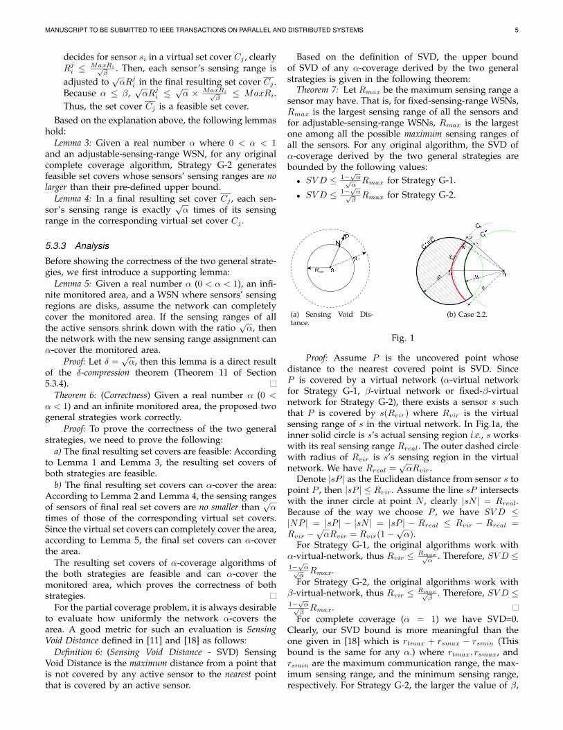
(a) Sensing Void Dis-tance.

(b) Case 2.2.

Fig. 1

Proof: Assume P is the uncovered point whosedistance to the nearest covered point is SVD. SinceP is covered by a virtual network (α-virtual networkfor Strategy G-1, β-virtual network or fixed-β-virtualnetwork for Strategy G-2), there exists a sensor s suchthat P is covered by s(Rvir) where Rvir is the virtualsensing range of s in the virtual network. In Fig.1a, theinner solid circle is s’s actual sensing region i.e., s workswith its real sensing range Rreal. The outer dashed circlewith radius of Rvir is s’s sensing region in the virtualnetwork. We have Rreal =

√αRvir.

Denote |sP | as the Euclidean distance from sensor s topoint P , then |sP | ≤ Rvir. Assume the line sP intersectswith the inner circle at point N , clearly |sN | = Rreal.Because of the way we choose P , we have SV D ≤|NP | = |sP | − |sN | = |sP | − Rreal ≤ Rvir − Rreal =Rvir −

√αRvir = Rvir(1−

√α).

For Strategy G-1, the original algorithms work withα-virtual-network, thus Rvir ≤ Rmax√

α. Therefore, SV D ≤

1−√α√α

Rmax.For Strategy G-2, the original algorithms work with

β-virtual-network, thus Rvir ≤ Rmax√β

. Therefore, SV D ≤1−√α√

βRmax.

For complete coverage (α = 1) we have SVD=0.Clearly, our SVD bound is more meaningful than theone given in [18] which is rtmax + rsmax − rsmin (Thisbound is the same for any α.) where rtmax, rsmax, andrsmin are the maximum communication range, the max-imum sensing range, and the minimum sensing range,respectively. For Strategy G-2, the larger the value of β,


the smaller the value of SVD. Thus, users may use alarge β to get a better coverage uniformity. However, ifβ is too large, the virtual network might not be able tocompletely cover the monitored area, since the sensors’sensing ranges in the virtual network are too small.

Theorem 8: The time complexity of any resulting α-coverage algorithm derived by the two general strategiesis the same as that of the original algorithm.

Proof: The proposed general strategies essentiallyadjust the source code of an original algorithm in away that the resulting algorithm can α-cover the area.Basically, the general strategies carry out two tasks:

1) Let the original algorithm work with a virtual net-work where every sensor s has its virtual sensingrange. In this step, the framework (which also in-cludes two extended strategies discussed in Section5.3) only considers any reference to s’s sensingrange and merely changes s’s real sensing range toa virtual sensing range. Thus, our framework doesnot change the time complexities of the original al-gorithms since it just conducts a simple calculationoperation (a division) to the original algorithms.

2) Convert the virtual set covers to real set covers. Es-sentially, before returning the results i.e., set coverswith schedules, the two general strategies simplymodify a piece of code in the original algorithmsuch that instead of returning the virtual sensingranges, it returns real sensing ranges which areusually

√α times of the virtual sensing ranges.

Understanding the general strategies in this way,the time complexity of an original algorithm is notchanged.

Thus, the time complexity of the resulting algorithmderived by the two proposed general strategies is thesame as that of the original algorithm.

5.3.4 δ-compression theoremWe dedicate this section to prove an important theoremshowing the correctness of our framework. We firstintroduce some notations and definitions.

A. NotationsC(O, R) denotes a circle C with radius R centered at

point O. The region enclosed by C is denoted by D(C)(D stands for disk). We use ‖A‖ to denote the area ofregion A. For a line XY , |XY | is its length.

For 2 two-dimensional regions A and B, we say A ⊆ Bif for every point P ∈ A, we also have P ∈ B. In otherwords, A is fully covered by B. We say A * B if thereexists a point P ∈ A, but P /∈ B. For example, as shownin Fig.2a, we have D(C5) ⊆ D(C4), D(C5) * D(C). A−Bincludes any point P such that P ∈ A, but P /∈ B.

B. DefinitionsDefinition 7: (Neighbors) In the plane, given a circle C

and l other circles C1, C2, . . . , Cl, a circle Ci (i = 1 . . . l)is said to be a neighbor of C if C and Ci overlap.

For example, in Fig.2a, C1, C3, C4, C5 are all the neigh-bors of C while C2 is not.

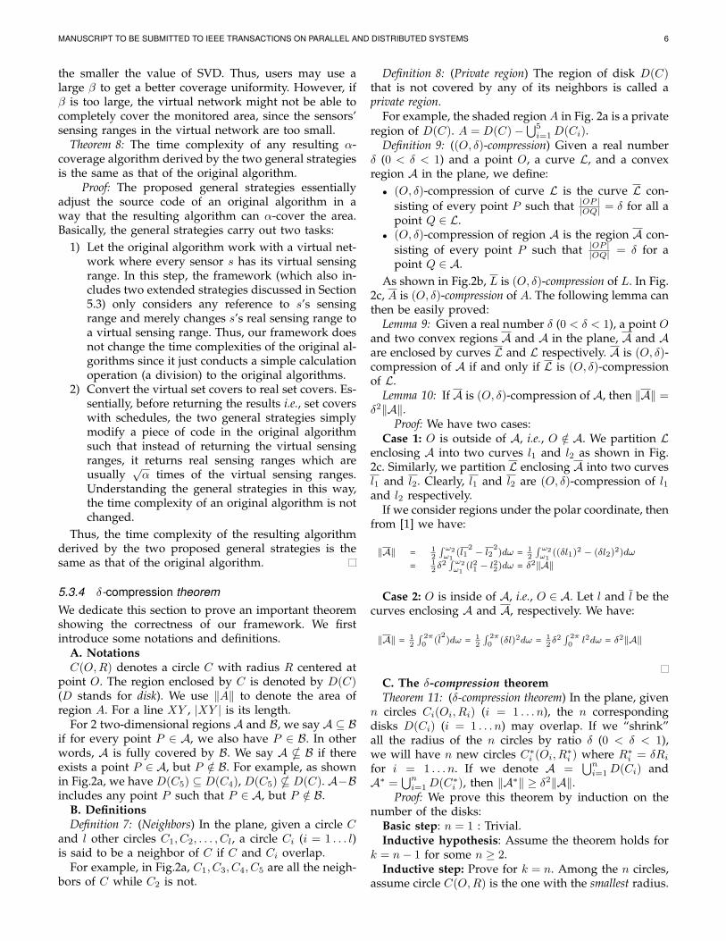
Definition 8: (Private region) The region of disk D(C)that is not covered by any of its neighbors is called aprivate region.

For example, the shaded region A in Fig. 2a is a privateregion of D(C). A = D(C)−⋃5

i=1 D(Ci).Definition 9: ((O, δ)-compression) Given a real number

δ (0 < δ < 1) and a point O, a curve L, and a convexregion A in the plane, we define:• (O, δ)-compression of curve L is the curve L con-

sisting of every point P such that |OP ||OQ| = δ for all a

point Q ∈ L.• (O, δ)-compression of region A is the region A con-

sisting of every point P such that |OP ||OQ| = δ for a

point Q ∈ A.As shown in Fig.2b, L is (O, δ)-compression of L. In Fig.

2c, A is (O, δ)-compression of A. The following lemma canthen be easily proved:

Lemma 9: Given a real number δ (0 < δ < 1), a point Oand two convex regions A and A in the plane, A and Aare enclosed by curves L and L respectively. A is (O, δ)-compression of A if and only if L is (O, δ)-compressionof L.

Lemma 10: If A is (O, δ)-compression of A, then ‖A‖ =δ2‖A‖.

Proof: We have two cases:Case 1: O is outside of A, i.e., O /∈ A. We partition L

enclosing A into two curves l1 and l2 as shown in Fig.2c. Similarly, we partition L enclosing A into two curvesl1 and l2. Clearly, l1 and l2 are (O, δ)-compression of l1and l2 respectively.

If we consider regions under the polar coordinate, thenfrom [1] we have:

‖A‖ = 12

∫ ω2ω1

(l12 − l2

2)dω = 1

2

∫ ω2ω1

((δl1)2 − (δl2)2)dω

= 12δ2

∫ ω2ω1

(l21 − l22)dω = δ2‖A‖

Case 2: O is inside of A, i.e., O ∈ A. Let l and l be thecurves enclosing A and A, respectively. We have:

‖A‖ = 12

∫ 2π0 (l

2)dω = 1

2

∫ 2π0 (δl)2dω = 1

2δ2

∫ 2π0 l2dω = δ2‖A‖

C. The δ-compression theoremTheorem 11: (δ-compression theorem) In the plane, given

n circles Ci(Oi, Ri) (i = 1 . . . n), the n correspondingdisks D(Ci) (i = 1 . . . n) may overlap. If we “shrink”all the radius of the n circles by ratio δ (0 < δ < 1),we will have n new circles C∗i (Oi, R

∗i ) where R∗i = δRi

for i = 1 . . . n. If we denote A =⋃n

i=1 D(Ci) andA∗ =

⋃ni=1 D(C∗i ), then ‖A∗‖ ≥ δ2‖A‖.

Proof: We prove this theorem by induction on thenumber of the disks:

Basic step: n = 1 : Trivial.Inductive hypothesis: Assume the theorem holds for

k = n− 1 for some n ≥ 2.Inductive step: Prove for k = n. Among the n circles,

assume circle C(O, R) is the one with the smallest radius.


(a) Private region of disk C (b) (O, δ)-compression fora curve

(c) (O, δ)-compression fora region

Fig. 2: Private region and (O, δ)-compression.

Denote other n − 1 circles as Ci(Oi, Ri) (i = 1 . . . n − 1).We have R ≤ Ri for i = 1 . . . n− 1.

LetAn−1 =

n−1⋃

i=1

D(Ci) (2)

A = [

n−1⋃

i=1

D(Ci)]⋃

D(C) = An−1

⋃D(C). (3)

Intuitively, A is the union region of n disks D(C) andD(Ci) (i = 1 . . . n−1), while An−1 is the union region ofn− 1 disks D(Ci) (i = 1 . . . n− 1) not including D(C).

After n circles shrink with ratio δ, we have n newcircles C∗i (Oi, R

∗i ) (i = 1 . . . n− 1) and C∗(O, R∗), where

R∗i = δRi and R∗ = δR.Let

A∗n−1 =

n−1⋃

i=1

D(C∗i ) (4)

A∗ = [

n−1⋃

i=1

D(C∗i )]

⋃D(C

∗) = A∗n−1

⋃D(C

∗). (5)

Intuitively, A∗ is the union region of n disks, whileA∗n−1 is the union region of n − 1 disks not includingD(C∗).

With all those notations, the inductive hypothesis canbe rewritten as ‖A∗n−1‖ ≥ δ2‖An−1‖. We need to prove‖A∗‖ ≥ δ2‖A‖. There are two cases:

Case 1. Before shrinking, if D(C) is completely cov-ered by all of its neighbors, i.e., D(C) ⊆ ⋃n−1

i=1 D(Ci) =An−1 ⇒ A = An−1

⋃D(C) = An−1, then we are done

because ‖A∗‖ ≥ ‖A∗n−1‖ ≥ δ2‖An−1‖ = δ2‖A‖.Case 2. Otherwise, D(C) is not fully covered by all of

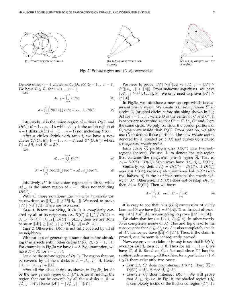
its neighbors.Without loss of generality, assume that before shrink-

ing C intersects with l other circles Ci(Oi, Ri) (i = 1 . . . l).For example, in Fig.3a we have l = 3. By assumption, wehave R ≤ Ri for i = 1 . . . l.

Let A be the private region of D(C). The region that canbe covered by all the n disks is A = An−1 + A. Hence‖A‖ = ‖An−1‖+ ‖A‖.

After all the disks shrink as shown in Fig.3b, let A∗

be the new private region of D(C∗). After shrinking, theregion that can be covered by all the n disks is A∗ =A∗n−1 + A∗. Hence ‖A∗‖ = ‖A∗n−1‖+ ‖A∗‖.

We need to prove ‖A∗‖ ≥ δ2‖A‖ ⇔ ‖A∗n−1‖+ ‖A∗‖ ≥δ2(‖An−1‖ + ‖A‖). From inductive hypotheses, we have‖A∗n−1‖ ≥ δ2‖An−1‖. So, we only need to prove ‖A∗‖ ≥δ2‖A‖.

In Fig.3c, we introduce a new concept which is com-pressed private region. We create (O, δ)-compression Ci ofcircles Ci (original circles before shrinking shown in Fig.3a) for i = 1 . . . l , where O is the center of C and C∗. Itis necessary to emphasize that C∗ ≡ C, i.e., C∗ and C arethe same circle. We only consider the border portions ofCi which are inside disk D(C). From now on, we alsouse Ci to denote those portions. The new private region,denoted by A, created by D(C) and curves Ci is calleda compressed private region.

Each curve Ci partitions disk D(C∗) into two sub-regions (halves). We use Ai to denote the sub-regionthat contains the compressed private region A. That is,Ai = D(C∗)−D(Ci). We always have A ⊆ Ai ⊆ D(C∗).

Similarly, we define A∗i = D(C∗) − D(C∗i ). If D(C∗i )overlaps D(C∗), circle C∗i also partitions disk D(C∗) intotwo halves, A∗i is the half that contains the private sub-region A∗. Otherwise, if D(C∗i ) does not overlap D(C∗),then A∗i = D(C∗). Then we have:

A =l⋂

i=1

Ai and A∗

=l⋂

i=1

A∗i (6)

It is easy to see that A is (O, δ)-compression of A. ByLemma 10, we have ‖A‖ = δ2‖A‖. Thus instead of prov-ing ‖A∗‖ ≥ δ2‖A‖, we are going to prove ‖A∗‖ ≥ ‖A‖.

We claim that for i = 1 . . . l, Ai ⊆ A∗i . In other words,Ai is completely inside of A∗i . This and Eq. 6 lead to theconsequence that A ⊆ A∗, i.e., A is also completely insideof A∗. Hence we have ‖A‖ ≤ ‖A∗‖. Thus, if the claim isproved, our theorem is consequently proved.

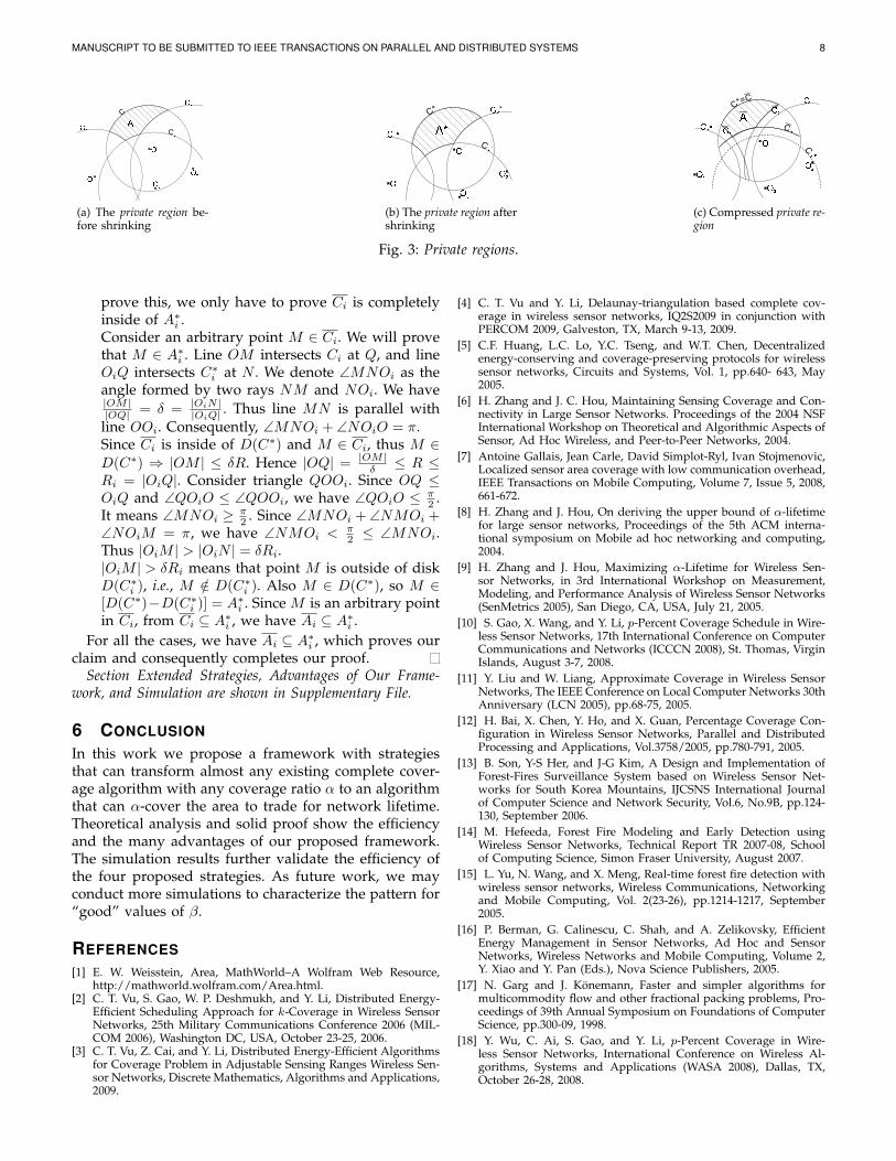
Now, we prove our claim. It is easy to see that if D(Ci)overlaps D(C), then Ci 6= ∅. Thus for all i = 1 . . . l, wehave Ci 6= ∅. Based on that fact and since C∗ has thesmallest radius among all the disks, for a particular i (1 ≤i ≤ l), there exist only two cases:• Case 2.1: C∗i does not intersect D(C∗). Then, Ai ⊆

D(C∗) = A∗i . Hence Ai ⊆ A∗i .• Case 2.2: C∗i does intersect D(C∗). We will prove

that Ai ⊆ A∗i , i.e., in Fig.1b, the shaded region (Ai)is completely inside of the thickened region (A∗i ). To


(a) The private region be-fore shrinking

(b) The private region aftershrinking

(c) Compressed private re-gion

Fig. 3: Private regions.

prove this, we only have to prove Ci is completelyinside of A∗i .Consider an arbitrary point M ∈ Ci. We will provethat M ∈ A∗i . Line OM intersects Ci at Q, and lineOiQ intersects C∗i at N . We denote ∠MNOi as theangle formed by two rays NM and NOi. We have|OM ||OQ| = δ = |OiN |

|OiQ| . Thus line MN is parallel withline OOi. Consequently, ∠MNOi + ∠NOiO = π.Since Ci is inside of D(C∗) and M ∈ Ci, thus M ∈D(C∗) ⇒ |OM | ≤ δR. Hence |OQ| = |OM |

δ ≤ R ≤Ri = |OiQ|. Consider triangle QOOi. Since OQ ≤OiQ and ∠QOiO ≤ ∠QOOi, we have ∠QOiO ≤ π

2 .It means ∠MNOi ≥ π

2 . Since ∠MNOi + ∠NMOi +∠NOiM = π, we have ∠NMOi < π

2 ≤ ∠MNOi.Thus |OiM | > |OiN | = δRi.|OiM | > δRi means that point M is outside of diskD(C∗i ), i.e., M /∈ D(C∗i ). Also M ∈ D(C∗), so M ∈[D(C∗)−D(C∗i )] = A∗i . Since M is an arbitrary pointin Ci, from Ci ⊆ A∗i , we have Ai ⊆ A∗i .

For all the cases, we have Ai ⊆ A∗i , which proves ourclaim and consequently completes our proof.

Section Extended Strategies, Advantages of Our Frame-work, and Simulation are shown in Supplementary File.

6 CONCLUSION

In this work we propose a framework with strategiesthat can transform almost any existing complete cover-age algorithm with any coverage ratio α to an algorithmthat can α-cover the area to trade for network lifetime.Theoretical analysis and solid proof show the efficiencyand the many advantages of our proposed framework.The simulation results further validate the efficiency ofthe four proposed strategies. As future work, we mayconduct more simulations to characterize the pattern for“good” values of β.

REFERENCES[1] E. W. Weisstein, Area, MathWorld–A Wolfram Web Resource,

http://mathworld.wolfram.com/Area.html.[2] C. T. Vu, S. Gao, W. P. Deshmukh, and Y. Li, Distributed Energy-

Efficient Scheduling Approach for k-Coverage in Wireless SensorNetworks, 25th Military Communications Conference 2006 (MIL-COM 2006), Washington DC, USA, October 23-25, 2006.

[3] C. T. Vu, Z. Cai, and Y. Li, Distributed Energy-Efficient Algorithmsfor Coverage Problem in Adjustable Sensing Ranges Wireless Sen-sor Networks, Discrete Mathematics, Algorithms and Applications,2009.

[4] C. T. Vu and Y. Li, Delaunay-triangulation based complete cov-erage in wireless sensor networks, IQ2S2009 in conjunction withPERCOM 2009, Galveston, TX, March 9-13, 2009.

[5] C.F. Huang, L.C. Lo, Y.C. Tseng, and W.T. Chen, Decentralizedenergy-conserving and coverage-preserving protocols for wirelesssensor networks, Circuits and Systems, Vol. 1, pp.640- 643, May2005.

[6] H. Zhang and J. C. Hou, Maintaining Sensing Coverage and Con-nectivity in Large Sensor Networks. Proceedings of the 2004 NSFInternational Workshop on Theoretical and Algorithmic Aspects ofSensor, Ad Hoc Wireless, and Peer-to-Peer Networks, 2004.

[7] Antoine Gallais, Jean Carle, David Simplot-Ryl, Ivan Stojmenovic,Localized sensor area coverage with low communication overhead,IEEE Transactions on Mobile Computing, Volume 7, Issue 5, 2008,661-672.

[8] H. Zhang and J. Hou, On deriving the upper bound of α-lifetimefor large sensor networks, Proceedings of the 5th ACM interna-tional symposium on Mobile ad hoc networking and computing,2004.

[9] H. Zhang and J. Hou, Maximizing α-Lifetime for Wireless Sen-sor Networks, in 3rd International Workshop on Measurement,Modeling, and Performance Analysis of Wireless Sensor Networks(SenMetrics 2005), San Diego, CA, USA, July 21, 2005.

[10] S. Gao, X. Wang, and Y. Li, p-Percent Coverage Schedule in Wire-less Sensor Networks, 17th International Conference on ComputerCommunications and Networks (ICCCN 2008), St. Thomas, VirginIslands, August 3-7, 2008.

[11] Y. Liu and W. Liang, Approximate Coverage in Wireless SensorNetworks, The IEEE Conference on Local Computer Networks 30thAnniversary (LCN 2005), pp.68-75, 2005.

[12] H. Bai, X. Chen, Y. Ho, and X. Guan, Percentage Coverage Con-figuration in Wireless Sensor Networks, Parallel and DistributedProcessing and Applications, Vol.3758/2005, pp.780-791, 2005.

[13] B. Son, Y-S Her, and J-G Kim, A Design and Implementation ofForest-Fires Surveillance System based on Wireless Sensor Net-works for South Korea Mountains, IJCSNS International Journalof Computer Science and Network Security, Vol.6, No.9B, pp.124-130, September 2006.

[14] M. Hefeeda, Forest Fire Modeling and Early Detection usingWireless Sensor Networks, Technical Report TR 2007-08, Schoolof Computing Science, Simon Fraser University, August 2007.

[15] L. Yu, N. Wang, and X. Meng, Real-time forest fire detection withwireless sensor networks, Wireless Communications, Networkingand Mobile Computing, Vol. 2(23-26), pp.1214-1217, September2005.

[16] P. Berman, G. Calinescu, C. Shah, and A. Zelikovsky, EfficientEnergy Management in Sensor Networks, Ad Hoc and SensorNetworks, Wireless Networks and Mobile Computing, Volume 2,Y. Xiao and Y. Pan (Eds.), Nova Science Publishers, 2005.

[17] N. Garg and J. Konemann, Faster and simpler algorithms formulticommodity flow and other fractional packing problems, Pro-ceedings of 39th Annual Symposium on Foundations of ComputerScience, pp.300-09, 1998.

[18] Y. Wu, C. Ai, S. Gao, and Y. Li, p-Percent Coverage in Wire-less Sensor Networks, International Conference on Wireless Al-gorithms, Systems and Applications (WASA 2008), Dallas, TX,October 26-28, 2008.


Yingshu Li received her BS degree in computer science from BeijingInstitute of Technology, China, and her MS and PhD degrees in com-puter science from the University of Minnesota at Twin Cities. She iscurrently an Assistant Professor in the Department of Computer Scienceat the Georgia State University. Her research interests include wirelessnetworking, wireless sensor networks, and data management in sensornetworks. She is the recipient of an NSF CAREER Award. She is amember of ACM and IEEE.

Chinh Vu received his Ph.D degree and MS degree in the Department ofComputer Science at the Georgia State University in 2009 and 2007. Hereceived the BS degrees in electronics and information technology fromHanoi University of Technology, Vietnam and Hanoi Open University,Vietnam, in 2000. His current research interests include wireless sensornetworks, approximation algorithms, and distributed systems. He is astudent member of the IEEE.

Chunyu Ai is a Ph.D. candidate in Department of Computer Scienceat Georgia State University. She received her Bachelor and Masterdegrees of Computer Science from Heilongjiang University in 2001and 2004, respectively. Her research interests include wireless sensornetworks, database, and data security.

Guantao Chen received his BS degree in mathematics and MS degreein Operations Search from the Central China Normal University in 1982and 1984, respectively. He received his PhD degree from the Universityof Memphis in 1991. He is currently a Professor in the Department ofMathematics and Statistics with an joint appointment at the Departmentof Computer Science at Georgia State University. His research areasinclude graph theory, combinatorial algorithms, and bioinformatics.

Yi Zhao received his PhD degree in mathematics from Rutgers Univer-sity in 2001. He is an Assistant Professor of mathematics at GeorgiaState University. His research interests include graph theory, combina-torics, and their applications to computer science.

Documents

Transforming Complete Coverage Algorithms to Partial Coverage Algorithms for Wireless Sensor Networks