IJCSNS International Journal of Computer Science and Network Security, VOL.6 No.1A, January 2006

153

Manuscript received January, 2006.

Towards Optimal Model Order Selection for Autoregressive Spectral Analysis of Mental Tasks Using Genetic Algorithm

Ramaswamy Palaniappan

Computer Science Dept., University of Essex, CO4 3SQ, United Kingdom

Summary Autoregressive (AR) models for spectral analysis of electroencephalogram (EEG) signals are advantageous over the classical Fourier transform methods due to their ability to deal with short segments of data, superior resolution and smoother spectra. But a problem or rather a parameter that needs to be optimised in this method is the model order of the AR equation. Currently, statistical methods like Akaike Information Criterion, Final Prediction Error, Residual Variance, Minimum Description Length, Criterion Autoregressive Transfer and Hannan-Quinn have been used for this purpose. These methods depend on the statistical properties of the data, which selects the lowest order that is optimal to represent the signal. In this paper, the use of genetic algorithm (GA) is proposed to select the order of the AR model during classifier training. This technique fuses GA with Fuzzy ARTMAP to select the appropriate AR model order for EEG signals during system training to optimise classification of test signals into their respective different mental tasks. The experimental results show that this method outperforms the other statistical methods and a fixed 6th order model although the simulations were carried out with a small number of genetic populations and generations to reduce the computational cost. Key words: Autoregressive, EEG, Genetic Algorithm, Mental tasks, Model order.

1. Introduction

Linear parametric techniques like autoregressive (AR) models have a broad spectrum of applications ranging from identification; prediction and control of dynamical systems and digital spectral analysis using these models have proven to be superior to classical Fourier transform techniques like Discrete Fourier Transform (DFT) or the computationally efficient Fast Fourier Transform (FFT). This is due to the ability of AR models to handle short segments of data while giving better frequency resolution and smoother power spectra than Fourier methods. Furthermore, AR methods need only one or more cycles of sinusoidal-type activity to be present in the segment to produce good spectral peaks and they also provide the ability to observe small shifts in peak frequencies, which are not easily observed with FFT derived spectra [16].

Specifically, AR models are even more popular than the other linear parametric models like moving average (MA) and autoregressive moving average (ARMA) due to their inherent computational efficiency [23]. The AR model coefficients can be easily estimated by solving a set of linear equations using the Yule-Walker method or solving recursively for higher orders using Levinson-Durbin [6] or Burg [7] methods. In addition, AR coefficients can be efficiently updated when new data becomes available through the use of Kalman filter equations [11]. But MA and ARMA require complicated procedures to estimate the model coefficients [23]. Successful applications of AR models are abundant in literature. It has been used in radar applications by Alkin [3], geophysical application by Landers and Lacoss [22], medical signal processing like Electroencephalogram (EEG) [4, 5, 11, 14, 16, 23, 25, 28] and Electrocardiogram (ECG) [26], ultrasonic tissue backscatter coefficient estimation [32], speech processing [29] and music understanding [28]. In the realm of EEG analysis, Ning and Bronzino [23] have analysed EEG signals with AR and bispectral methods, Pfurtscheller et al [25] have used AR parameters to separate EEG signals recorded from right and left motor imagery as a means of brain computer interface, Keirn and Aunon [21] proposed a new mode of communication using EEG signals where one of the methods used was the AR technique. Saiwaki et al [28] have studied EEG signals with AR models for understanding music and brain signal flow. Anderson et al [4] have experimented on classification of different mental tasks using AR models and neural network. Aufrichtig and Pedersen [5] and Herrera et al [14] have analysed sleep using EEG spectral analysis. Successful as they are, however, there is a problem or rather a parameter that must be selected in order to utilise an AR technique properly i.e. the model order. As one can surmise, the AR model can be any order as desired. However, it should be as accurate as possible in terms of signal representation. Intuitively, it is known that a model order, which is too small will not represent the properties

IJCSNS International Journal of Computer Science and Network Security, VOL.6 No.1A, January 2006

154

of the signal, whereas a model order which is too high will also represent noise and inaccuracies and thus, will not be a reliable representation of the true signal. Therefore, methods that will determine the appropriate model order must be used and this problem has found many published work [1-3, 5, 11, 13, 14, 19, 24, 26, 27, 30, 32]. There are many criteria in literatures for determining the AR order. Some of these are like Akaike Information Criterion (AIC) and Final Prediction Error (FPE) [1] pioneered by Akaike. Other commonly used criteria are like Minimum Description Length (MDL) suggested by Rissanen [27], Criterion Autoregressive Transfer (CAT) by Parzen [24] and Residual Variance (RV) [18, 32]. Hannan and Quinn (HQ) [13] criterion increases the penalty for large order models to counteract the overfitting tendency of AIC. Aufrichtig and Pederson [5] have studied AIC and MDL methods for AR modelling of EEG sleep recordings. Alkin [3] has investigated AR model order selection methods using AIC, FPE, MDL and CAT for radar adaptive clutter suppression. Herrera et al [14] studied AIC and HQ for modelling multichannel EEG signals during sleep. Pinna et al [26] have studied the use of AIC in AR spectral analysis of cardiovascular variability signals and Wear et al [32] used AIC, FPE, MDL and RV as model order criteria in their paper. Simpson [30] studied AIC, FPE and CAT for selecting the AR order for EEG signals. Aksasse and Radourne [2] have analysed order selection criteria for 2-D models. These publications are not complete considering the vast amount of published work in this area but serves to suffice since it covers most of the popular techniques that are currently available for solving the problem of selecting the AR model order. The goal of the work in this paper is to improve the method of selecting the AR order. A new method of using genetic algorithm (GA) to select to select the appropriate AR model order for representing EEG signals is proposed. Although EEG signals have been used in the experimental study in this paper, the proposed method is general and is applicable to other applications, which requires the selection of AR model order. The proposed method fuses GA with a Fuzzy ARTMAP (FA) network to select the appropriate model order during training phase. GA use FA classification as the fitness or objective function to select the appropriate AR model order. AR coefficients are obtained next and power spectral densities (PSD) for the EEG signals are extracted and the system classifies the EEG signals for different mental tasks. The experimental results demonstrate that this method outperforms other currently used statistical methods, namely: AIC, FPE, MDL, CAT, HQ, RV in addition to a fixed 6th order model. This is since GA selects the order, which maximises recognition performance while the performances of the

other methods depend on the statistical properties of the data and the nature of the modelling process. 2. Autoregressive systems and statistical model order selection methods

2.1 Autoregressive systems

A real valued, zero mean, stationary, non-deterministic, autoregressive process of order p is given by

= )()(1

)( neknxp

k kanx +−∑=

−= , (1)

where p is the model order, x(n) is the data of the signal at sampled point n, ak are the real valued AR coefficients and e(n) represents the error term independent of past samples. The term autoregressive implies that the process x(n) is seen to be regressed upon previous samples of itself. The error term is assumed to be a zero mean white noise with finite variance, 2

eσ . In applications, the values of ak and 2eσ have to be estimated from finite samples of data x(1),

x(2), x(3), ………., x(N). Many different techniques have been proposed to estimate ak, each with its own merits and demerits. Some of these are like autocorrelation, covariance and lattice methods [11]. The most common method is to use the autocorrelation technique of solving the Yule-Walker equations [6, 18]. The Yule-Walker equations can be solved directly directly using conventional linear equation solutions like Gaussian elimination but a shortcoming of this approach lies in its huge computational time. Thus, recursive algorithms have been developed which are based on the concept of estimating the parameters of a model of order p from the parameters of a model of order p-1. Some of these methods are like Burg’s algorithm [7] and Levinson–Durbin algorithm [6]. Burg’s method is more accurate than Levinson-Durbin since it uses the data points directly unlike the latter method, which relies on the estimation of the autocorrelation function, which is generally erroneous for small data segments. The earlier method also uses more data points simultaneously by minimising not only a forward error (as in the Levinson-Durbin case) but also a backward error. This algorithm will be discussed later.

2.2 Statistical Model Order Selection Methods

It was mentioned earlier that before an AR process could be used, there is a prerequisite of having to know the order of the model. Most order selection criteria are

IJCSNS International Journal of Computer Science and Network Security, VOL.6 No.1A, January 2006

155

transformations of the mean squared error1, 2eσ which is

computed as a function of the order in model estimation. These techniques employ a multiplication of this error and a cost function, which increases monotonically with order p. Methods pioneered by Akaike [1] are popular and two model order selection criteria developed by him i.e. AIC and FPE are based upon concepts in mathematical statistics. FPE method gives the model order, which minimises the function below

pNpNpepFPE

−+

= )(2ˆ)( σ , (2)

where p is the model order, N is the number of data points, )(ˆ 2 peσ is the estimated error variance for the model. An

‘unbiased’ estimate of this error variance is given by Parzen [24] as

pNNpp ee −

= )(ˆ)(ˆ̂ 22 σσ . (3)

An unbiased estimate attempts to estimate by assuming that the model order is correct and the parameters are known exactly, not estimated. If the mean value of the data has been subtracted, then the unbiased estimate of this error variance is given by Jones [19] as

1)(ˆ)(ˆ̂ 22

−−=

pNNpp ee σσ ,

(4)

and the FPE is now given by

11)(2ˆ)(

−−++

=pNpNpepFPE σ . (5)

The fractional portion of FPE increases with p and as such represent the inaccuracies in estimating the AR parameters. The principle behind the FPE criterion is that the unbiased estimate of the error variance is multiplied by the factor

Np /1+ , (6)where p is the number of parameters to be estimated and N is the number of points observed. This factor allows for the increase in the error variance when the estimated coefficients are used to make predictions on new, independent data. Akaike [1] then extended this model selection criterion to any maximum likelihood situation. This other criterion is called AIC and is given by

AIC(k)=-2ln(maximum likelihood) + 2k, (7)where k is the number of parameters estimated. Using this method, the order of the model is selected which minimises the following function

ppeNpAIC 2)(2ˆ̂ln)( += σ . (8)

The term 2p represents the penalty for selecting higher orders. The two criteria are asymptotically equivalent and 1 In this paper, mean squared error is used interchangeably with error variance. This is since the error is assumed to be white noise where the mean value is zero.

in the limit of large N, FPE and AIC will predict the same optimal order [20]. Residual Variance (RV) criterion is based on the fact that if an insufficient number of terms have been fitted in the AR model given by (1), the estimate of the error variance )(ˆ 2 peσ will be inflated by those terms not yet included. Only when the correct number of terms has been included will a valid estimate of )(ˆ 2 peσ be obtained. Jenkin and Watts [18] suggest that if the RV estimate

)(ˆ̂12

)( 2 ppNpNpRV eσ−−

−= , (9)

is plotted versus p, the curve will flatten out or show a minimum at the point corresponding to the correct order of the AR process. In the paper by Wear et al [32], this term is incorrectly denoted as

)(ˆ̂12

1)( 2 ppN

pRV eσ−−

= . (10)

The numerator of RV given on page 197 of reference [18] is actually the total sum of residuals and not the error variance as used in [32]. Since AIC has a tendency to overestimate the optimal order, Rissanen [27] has suggested MDL, which is given by

pNNppMDL e

)ln())(ˆ̂ln()( 2 += σ . (11)

MDL increases the penalty factor for higher orders as compared to AIC and as such favours the selection of lower orders. Another criterion which counteract the overfitting tendency of AIC is given by Hannan and Quinn [13]. HQ criterion chooses the minimum of

pN

NppHQ e)ln(ln2))(ˆ̂ln()( 2 += σ . (12)

CAT by Parzen [24] selects the order which minimize the criterion

)(ˆ̂1)

)(ˆ̂1(1)(

21

2 pkNpCAT

e

p

k e σσ−= ∑

=

. (13)

A point must be noted here. There are generally two different methods by which these criteria have been applied. The common method is to select the order, which gives the global minimum by using the specific criterion. The other method is to select the order, which gives the first minimum of the criterion. In this paper, the earlier method is used as it is more common and actually follows more closely to the original work behind these criteria.

2.3 Burg’s method

Burg’s method is common is AR literatures and as such, only a brief discussion of the algorithm is given. Proofs and further details of this algorithm can be found in [7,11]. The algorithm is as follows:

IJCSNS International Journal of Computer Science and Network Security, VOL.6 No.1A, January 2006

156

1. Calculate initial values

• Error variance, ∑−

=1

0

22 )]([1)0(ˆN

e nxN

σ

where x(n) is the nth data with mean value subtracted • Forward error, )()0( nxen =

• Backward error, )1()0(1 −=− nxbn 2. Calculate reflection coefficient and error variance • Reflection coefficient,

∑

∑−

=−

−

=−

−+−

−−−= 1

21

2

1

1

)]1()1([

)1()1(2 N

mnnn

n

N

mnn

m

mbme

membπ

• Error variance, )1(]||1[)( 222 −−= mm eme σπσ

3. Update Error and AR coefficients • AR coefficients,

11

)()1()1()(

1 =>

⎭⎬⎫

=−+−= −

mm

mamamama

m

kmmkk

ππ

• Forward Error Update, )1()1()( 1 −+−= − mbmeme nmnn π

• Backward Error Update, )1()1()( 1 −+−= − membmb nmnn π

4. Repeat steps 2 and 3 (with m incremented by one) until the selected model order p is reached.

2.4 Autoregressive Spectral Estimation

After selecting the order of the model by the any one of the discussed criterion, we can proceed with the estimation of the AR coefficients using Burg’s algorithm. These coefficients are then used to obtain the power spectral density (PSD) values by using the equation

∑=

−= p

kfkTieka

feSfS

02|2|

)()(

π,

(14)

where S(f) represents the power spectral density function, T is the sampling period and Se(f) represents the power spectrum of the error sequence. Since the term Se(f) applies to the errors or residuals which are in theory white, the resulting power spectrum should be flat and therefore Se(f) should be a constant independent of the frequency. Ideally, the value of this constant (noting that the mean of the residuals are zero) will be directly proportional to the variance of the residuals. Hence, the final expression for the conventional AR spectral estimate is obtained by replacing Se(f) with Tpe )(ˆ̂ 2σ where )(ˆ̂ 2 peσ is the

unbiased estimated variance of the residuals and the term T is included so that the true power of the corresponding analog signal will be represented digitally. The final PSD equation is given by

∑=

−= p

kfkTieka

TpfS

02|2|

2ˆ̂)(

π

σ . (15)

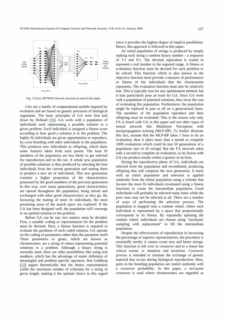
3. Fuzzy ARTMAP and Genetic Algorithm This section introduces FA and GA. FA was initially developed by Carpenter and Grossberg [8]. FA incorporates fuzzy set theory in its computation and as such it is able to learn stable responses to either analog or binary valued input patterns. It consists of two Fuzzy ART modules (Fuzzy ARTa and Fuzzy ARTb) that create stable recognition categories in response to sequence of input patterns. During supervised learning, Fuzzy ARTa receives a stream of input features representing the pattern and Fuzzy ARTb receives a stream of output features representing the target class of the pattern. An Inter ART module links these two modules, which is actually an associative controller that creates a minimal linkage of recognition categories between the two Fuzzy ART modules to meet a certain accuracy criteria. This is accomplished by realizing a learning rule that minimizes predictive error and maximizes predictive generalization. It works by increasing the vigilance parameter ρa of Fuzzy ARTa by a minimal amount needed to correct a predictive error at Fuzzy ARTb. Parameter ρa calibrates the minimum confidence that Fuzzy ARTa must have in a recognition category, or hypothesis that is activated by an input vector in order for Fuzzy ARTa to accept that category, rather than search for a better one through an automatically controlled process of hypothesis testing. Lower values of ρa enable larger categories to form and lead to a broader generalization and higher code compression. A predictive failure at Fuzzy ARTb increases the minimal confidence ρa by the least amount needed to trigger hypothesis testing at Fuzzy ARTa using a mechanism called match tracking. Match tracking sacrifices the minimum amount of generalization necessary to correct the predictive error. Match tracking leads to an increase in the confidence criterion just enough to trigger hypothesis testing which leads to a new selection of Fuzzy ARTa category. This new cluster is better able to predict the correct target class as compared to the cluster before match tracking. Fig. 1 shows the network structure of FA as used in this paper. Further details of this method can be found in [8,10].

IJCSNS International Journal of Computer Science and Network Security, VOL.6 No.1A, January 2006

157

PSDof EEGsignals

Foa F1a

F2a

Targets(mental

taskclasses)

FobF1b

F2b

InterART

Fuzzy ART a

Fuzzy ART b

Fig. 1 Fuzzy ARTMAP network structure as used in this paper.

GAs are a family of computational models inspired by evolution and are based on genetic processes of biological organisms. The basic principles of GA were first laid down by Holland [15]. GA work with a population of individuals each representing a possible solution to a given problem. Each individual is assigned a fitness score according to how good a solution is to the problem. The highly fit individuals are given opportunities to reproduce, by cross breeding with other individuals in the population. This produces new individuals as offspring, which share some features taken from each parent. The least fit members of the population are less likely to get selected for reproduction and so die out. A whole new population of possible solutions is thus produced by selecting the best individuals from the current generation and mating them to produce a new set of individuals. This new generation contains a higher proportion of the characteristics possessed by the good members of the previous generation. In this way, over many generations, good characteristics are spread throughout the population, being mixed and exchanged with other good characteristics as they go. By favouring the mating of more fit individuals, the most promising areas of the search space are explored. If the GA has been designed well, the population will converge to an optimal solution to the problem. Before GA can be run, two matters must be decided. First, a suitable coding or representation for the problem must be devised. Next, a fitness function is required to evaluate the goodness of each coded solution. GA operate on the coding of parameters rather than the parameter itself. These parameters or genes, which are known as chromosomes, are a string of values representing potential solutions to a problem. Although a binary string is normally used, there are other possibilities like using real numbers, which has the advantage of easier definition of meaningful and problem specific operators. But Goldberg [12] argues theoretically that the binary representation yields the maximum number of schemata for a string of given length, making it the optimal choice in this regard

since it provides the highest degree of implicit parallelism. Hence, this approach is followed in this paper. An initial population of strings is produced by simply making each string a random binary number - a sequence of 1’s and 0’s. The decimal equivalent is scaled to represent a real number in the required range. A fitness or evaluation function must be devised for each problem to be solved. This function which is also known as the objective function must provide a measure of performance or fitness of the individuals that the chromosome represents. The evaluation function must also be relatively fast. This is typically true for any optimisation method, but it may particularly pose an issue for GA. Since GA work with a population of potential solutions, they incur the cost of evaluating this population. Furthermore, the population might be replaced in part or all on a generational basis. The members of the population reproduce and their offspring must be evaluated. This is the reason why only FA is fused with GA in this paper and not other types of neural network like Multilayer Perceptron with backpropagation training (MLP-BP). To further illustrate this fact, assume that the MLP-BP takes 1 hour to do an evaluation, then it takes more than a month to complete 1000 evaluations which could be just 50 generations of a population size of 20 strings! But the FA network takes only a second to complete an evaluation, so its fusion with GA can produce results within a quarter of an hour. During the reproductive phase of GA, individuals are selected from the population and recombined, producing offspring that will comprise the next generation. It starts with an initial population and selection is applied randomly from the initial population using a scheme that favours the more fit individuals (evaluated using a fitness function) to create the intermediate population. Good individuals will probably be selected many times while the poor ones may not be selected at all. There are a number of ways of performing the selection process. The population is mapped onto a roulette wheel, where each individual is represented by a space that proportionally corresponds to its fitness. By repeatedly spinning the roulette wheel, individuals are chosen using “stochastic sampling with replacement” to fill the intermediate population. Despite the effectiveness of reproduction in increasing the percentage of superior representatives, the procedure is essentially sterile; it cannot create new and better strings. This function is left over to crossover and to a lesser but critical extent, to mutation and inversion. Crossover process is intended to simulate the exchange of genetic material that occurs during biological reproduction. Here, pairs in the breeding population are mated randomly with a crossover probability. In this paper, a two-point crossover is used where chromosomes are regarded as

IJCSNS International Journal of Computer Science and Network Security, VOL.6 No.1A, January 2006

158

loops formed by joining the ends together rather than linear strings as in single point crossover. To exchange a segment from one loop with that from another loop requires the selection of two cut points. A chromosome considered as a loop can contain more building blocks – since they are able to wrap around at the end of the string and this is the reason why a two-point crossover is better than a single point crossover. Mutation randomly perturbs the population’s characteristics, thereby preventing evolutionary dead ends. Most mutations are damaging rather than beneficial; mutation probability must be low to avoid the destruction of species. It works by randomly selecting a bit with a certain mutation probability in the string and reversing its value. Although inversion is not exactly a type of crossover but it is similar to crossover, only performed differently. Inversion operates by clipping out a section of a string, reversing it and putting it back. Inversion is the only way that the strings might be reordered but this operation must be applied carefully since its effects can be ruinous. 4. Genetic Fuzzy ARTMAP for AR model order selection In this section, the proposed method of using GA and FA to select the model order during the training phase will be discussed. This method will be called as Genetic Fuzzy ARTMAP or GFA in short. The explanation here will concentrate on this technique while the experimental study and results will be discussed in the next section. In general, the proposed method can be divided into 2 different phases, which uses 3 different data sets namely training, validation and test. The first phase is the training and validation stage where GA is engaged with FA to generate AR model orders for training data, which optimises the classification performance for validation data. One of the statistical model order criterion mentioned in Section 3 will be used to select the model order of the signals for the validation data. In the second phase of testing, GA is disengaged and only FA is used. Model orders for testing data are selected using one of the statistical model order criterion chosen earlier for validation data. In other words, GFA generates model orders to train the FA classifier only such that it optimises classification performance for validation data where the model orders are still selected using one of the statistical criterion. The same statistical model order criterion is also used for the test data. Initially in the first stage, a set of populations is generated as random binary strings with a certain number of bits used to represent the model order. This number of bits is chosen such as to suffice representation of the highest model order i.e. enough values to represent all the

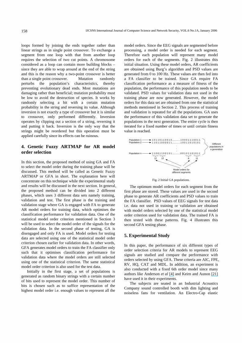
model orders. Since the EEG signals are segmented before processing, a model order is needed for each segment. Therefore each population will represent many model orders for each of the segments. Fig. 2 illustrates this initial situation. Using these model orders, AR coefficients are obtained using Burg’s algorithm and PSD values are generated from 0 to 100 Hz. These values are then fed into a FA classifier to be trained. Since GA require FA classification performance as a measure of fitness of the population, the performance of this population needs to be validated. PSD values for validation data not used in the training phase are now generated. However, the model orders for this data set are obtained from one the statistical methods mentioned in Section 2. This process of training and validation is repeated for all the populations. GA uses the performance of this validation data set to generate the populations in the next generation. The entire cycle is then iterated for a fixed number of times or until certain fitness value is reached.

1 0 1 1 0 1 1 0 0 1 0 .............1 0 0 0 1 1 1 0 0 1 11 1 0 1 1 0 0 0 0 1 1 .............1 0 0 1 1 0 1 0 1 0 1

.

.

.1 1 0 0 1 1 0 0 1 0 1 .............0 0 1 0 1 1 0 1 0 1 1

12 11612

Model orders fordifferent segments

Differentpopulations ina generation

Population 1Population 2

Population n

Fig. 2 Initial GA populations.

The optimum model orders for each segment from the first phase are stored. These values are used in the second phase to generate AR coefficients and PSD values to train the FA classifier. PSD values of EEG signals for test data i.e. data not used in training or validation are obtained with model orders selected by one of the statistical model order criterion used for validation data. The trained FA is then tested with these patterns. Fig. 4 illustrates this second GFA testing phase. 5. Experimental Study In this paper, the performance of six different types of order selection criteria for AR models to represent EEG signals are studied and compare the performance with orders selected by using GFA. These criteria are AIC, FPE, RV, HQ, CAT and MDL. In addition, an experiment is also conducted with a fixed 6th order model since many authors like Anderson et al [4] and Keirn and Aunon [21] have used it in their experiments. The subjects are seated in an Industrial Acoustics Company sound controlled booth with dim lighting and noiseless fans for ventilation. An Electro-Cap elastic

IJCSNS International Journal of Computer Science and Network Security, VOL.6 No.1A, January 2006

159

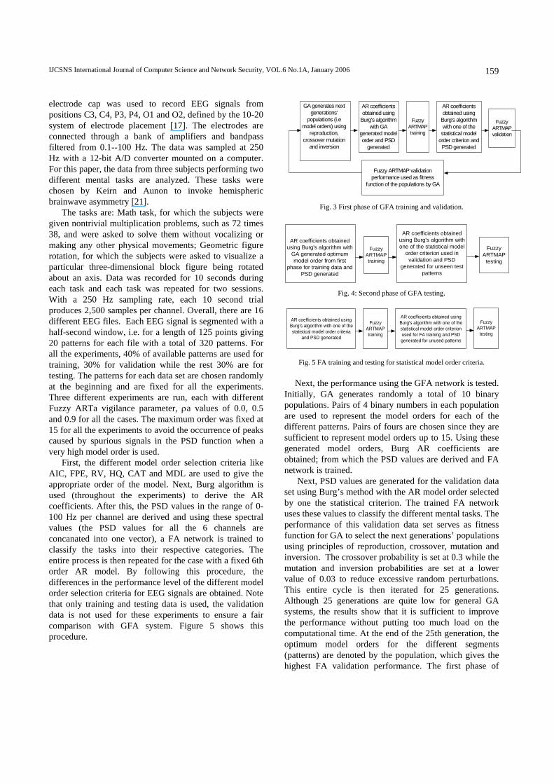
electrode cap was used to record EEG signals from positions C3, C4, P3, P4, O1 and O2, defined by the 10-20 system of electrode placement [17]. The electrodes are connected through a bank of amplifiers and bandpass filtered from 0.1--100 Hz. The data was sampled at 250 Hz with a 12-bit A/D converter mounted on a computer. For this paper, the data from three subjects performing two different mental tasks are analyzed. These tasks were chosen by Keirn and Aunon to invoke hemispheric brainwave asymmetry [21]. The tasks are: Math task, for which the subjects were given nontrivial multiplication problems, such as 72 times 38, and were asked to solve them without vocalizing or making any other physical movements; Geometric figure rotation, for which the subjects were asked to visualize a particular three-dimensional block figure being rotated about an axis. Data was recorded for 10 seconds during each task and each task was repeated for two sessions. With a 250 Hz sampling rate, each 10 second trial produces 2,500 samples per channel. Overall, there are 16 different EEG files. Each EEG signal is segmented with a half-second window, i.e. for a length of 125 points giving 20 patterns for each file with a total of 320 patterns. For all the experiments, 40% of available patterns are used for training, 30% for validation while the rest 30% are for testing. The patterns for each data set are chosen randomly at the beginning and are fixed for all the experiments. Three different experiments are run, each with different Fuzzy ARTa vigilance parameter, ρa values of 0.0, 0.5 and 0.9 for all the cases. The maximum order was fixed at 15 for all the experiments to avoid the occurrence of peaks caused by spurious signals in the PSD function when a very high model order is used. First, the different model order selection criteria like AIC, FPE, RV, HQ, CAT and MDL are used to give the appropriate order of the model. Next, Burg algorithm is used (throughout the experiments) to derive the AR coefficients. After this, the PSD values in the range of 0-100 Hz per channel are derived and using these spectral values (the PSD values for all the 6 channels are concanated into one vector), a FA network is trained to classify the tasks into their respective categories. The entire process is then repeated for the case with a fixed 6th order AR model. By following this procedure, the differences in the performance level of the different model order selection criteria for EEG signals are obtained. Note that only training and testing data is used, the validation data is not used for these experiments to ensure a fair comparison with GFA system. Figure 5 shows this procedure.

GA generates nextgenerations'

populations (i.emodel orders) using

reproduction,crossover mutation

and inversion

AR coefficientsobtained using

Burg's algorithmwith GA

generated modelorder and PSD

generated

FuzzyARTMAPtraining

Fuzzy ARTMAP validationperformance used as fitness

function of the populations by GA

AR coefficientsobtained using

Burg's algorithmwith one of thestatistical model

order criterion andPSD generated

FuzzyARTMAPvalidation

Fig. 3 First phase of GFA training and validation.

AR coefficients obtainedusing Burg's algorithm with

GA generated optimummodel order from first

phase for training data andPSD generated

FuzzyARTMAPtraining

AR coefficients obtainedusing Burg's algorithm withone of the statistical model

order criterion used invalidation and PSD

generated for unseen testpatterns

FuzzyARTMAP

testing

Fig. 4: Second phase of GFA testing.

AR coefficients obtained usingBurg's algorithm with one of thestatistical model order criteria

and PSD generated

FuzzyARTMAPtraining

AR coefficients obtained usingBurg's algorithm with one of thestatistical model order criterionused for FA training and PSDgenerated for unused patterns

FuzzyARTMAP

testing

Fig. 5 FA training and testing for statistical model order criteria. Next, the performance using the GFA network is tested. Initially, GA generates randomly a total of 10 binary populations. Pairs of 4 binary numbers in each population are used to represent the model orders for each of the different patterns. Pairs of fours are chosen since they are sufficient to represent model orders up to 15. Using these generated model orders, Burg AR coefficients are obtained; from which the PSD values are derived and FA network is trained. Next, PSD values are generated for the validation data set using Burg’s method with the AR model order selected by one the statistical criterion. The trained FA network uses these values to classify the different mental tasks. The performance of this validation data set serves as fitness function for GA to select the next generations’ populations using principles of reproduction, crossover, mutation and inversion. The crossover probability is set at 0.3 while the mutation and inversion probabilities are set at a lower value of 0.03 to reduce excessive random perturbations. This entire cycle is then iterated for 25 generations. Although 25 generations are quite low for general GA systems, the results show that it is sufficient to improve the performance without putting too much load on the computational time. At the end of the 25th generation, the optimum model orders for the different segments (patterns) are denoted by the population, which gives the highest FA validation performance. The first phase of

IJCSNS International Journal of Computer Science and Network Security, VOL.6 No.1A, January 2006

160

GFA training and validation (as shown in Fig. 3) is now completed. In the second phase, the optimum model order is used for each segment generated by GFA in the first phase and the AR coefficients are derived and PSD computed using Burg’s algorithm for training data. These PSD values are used to train FA classifier. Next, one of the statistical model order criterion is used to select the appropriate model order for test patterns i.e. data not used in training and validation. PSD for this data is generated and the trained FA is used to classify these signals into their respective mental tasks. This process is illustrated in Fig. 4. Both these phases are then repeated for all the statistical order selection criteria.

6. Results

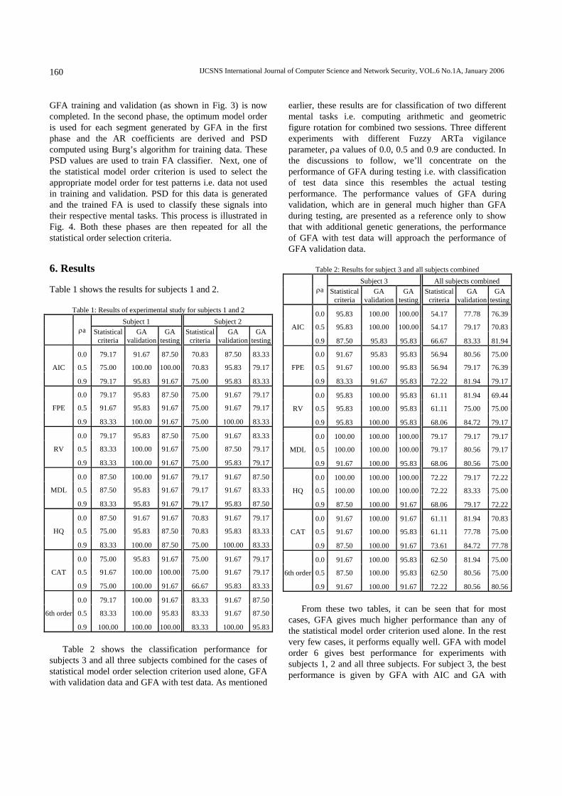
Table 1 shows the results for subjects 1 and 2.

Table 1: Results of experimental study for subjects 1 and 2 Subject 1 Subject 2

ρa

Statistical criteria

GA validation

GA testing

Statistical criteria

GA validation

GAtesting

0.0 79.17 91.67 87.50 70.83 87.50 83.33

AIC 0.5 75.00 100.00 100.00 70.83 95.83 79.17

0.9 79.17 95.83 91.67 75.00 95.83 83.33

0.0 79.17 95.83 87.50 75.00 91.67 79.17

FPE 0.5 91.67 95.83 91.67 75.00 91.67 79.17

0.9 83.33 100.00 91.67 75.00 100.00 83.33

0.0 79.17 95.83 87.50 75.00 91.67 83.33

RV 0.5 83.33 100.00 91.67 75.00 87.50 79.17

0.9 83.33 100.00 91.67 75.00 95.83 79.17

0.0 87.50 100.00 91.67 79.17 91.67 87.50

MDL 0.5 87.50 95.83 91.67 79.17 91.67 83.33

0.9 83.33 95.83 91.67 79.17 95.83 87.50

0.0 87.50 91.67 91.67 70.83 91.67 79.17

HQ 0.5 75.00 95.83 87.50 70.83 95.83 83.33

0.9 83.33 100.00 87.50 75.00 100.00 83.33

0.0 75.00 95.83 91.67 75.00 91.67 79.17

CAT 0.5 91.67 100.00 100.00 75.00 91.67 79.17

0.9 75.00 100.00 91.67 66.67 95.83 83.33

0.0 79.17 100.00 91.67 83.33 91.67 87.50

6th order 0.5 83.33 100.00 95.83 83.33 91.67 87.50

0.9 100.00 100.00 100.00

83.33 100.00 95.83 Table 2 shows the classification performance for subjects 3 and all three subjects combined for the cases of statistical model order selection criterion used alone, GFA with validation data and GFA with test data. As mentioned

earlier, these results are for classification of two different mental tasks i.e. computing arithmetic and geometric figure rotation for combined two sessions. Three different experiments with different Fuzzy ARTa vigilance parameter, ρa values of 0.0, 0.5 and 0.9 are conducted. In the discussions to follow, we’ll concentrate on the performance of GFA during testing i.e. with classification of test data since this resembles the actual testing performance. The performance values of GFA during validation, which are in general much higher than GFA during testing, are presented as a reference only to show that with additional genetic generations, the performance of GFA with test data will approach the performance of GFA validation data.

Table 2: Results for subject 3 and all subjects combined Subject 3 All subjects combined

ρa Statistical

criteriaGA

validationGA

testing Statistical

criteria GA

validationGA

testing

0.0 95.83 100.00 100.00 54.17 77.78 76.39

AIC 0.5 95.83 100.00 100.00 54.17 79.17 70.83

0.9 87.50 95.83 95.83 66.67 83.33 81.94

0.0 91.67 95.83 95.83 56.94 80.56 75.00

FPE 0.5 91.67 100.00 95.83 56.94 79.17 76.39

0.9 83.33 91.67 95.83 72.22 81.94 79.17

0.0 95.83 100.00 95.83 61.11 81.94 69.44

RV 0.5 95.83 100.00 95.83 61.11 75.00 75.00

0.9 95.83 100.00 95.83 68.06 84.72 79.17

0.0 100.00 100.00 100.00 79.17 79.17 79.17

MDL 0.5 100.00 100.00 100.00 79.17 80.56 79.17

0.9 91.67 100.00 95.83 68.06 80.56 75.00

0.0 100.00 100.00 100.00 72.22 79.17 72.22

HQ 0.5 100.00 100.00 100.00 72.22 83.33 75.00

0.9 87.50 100.00 91.67 68.06 79.17 72.22

0.0 91.67 100.00 91.67 61.11 81.94 70.83

CAT 0.5 91.67 100.00 95.83 61.11 77.78 75.00

0.9 87.50 100.00 91.67 73.61 84.72 77.78

0.0 91.67 100.00 95.83 62.50 81.94 75.00

6th order 0.5 87.50 100.00 95.83 62.50 80.56 75.00

0.9 91.67 100.00 91.67

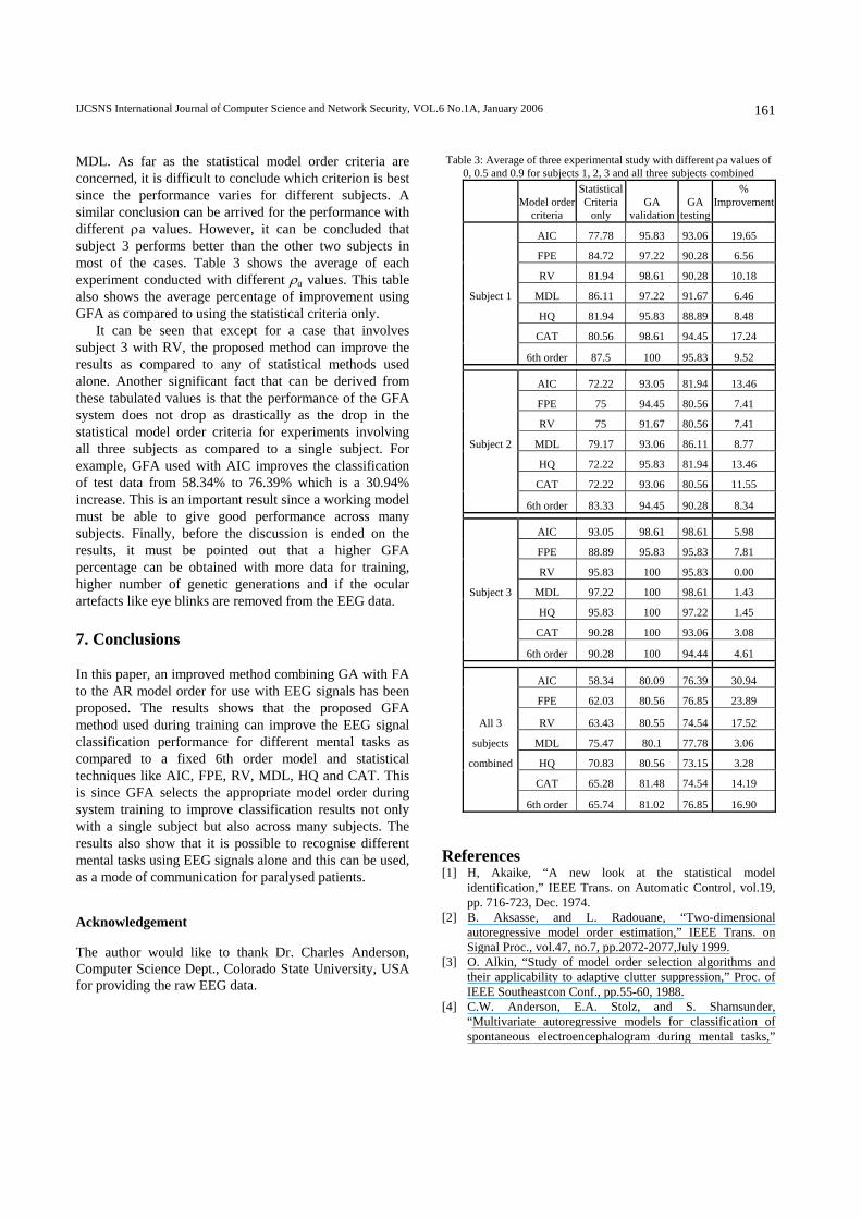
72.22 80.56 80.56 From these two tables, it can be seen that for most cases, GFA gives much higher performance than any of the statistical model order criterion used alone. In the rest very few cases, it performs equally well. GFA with model order 6 gives best performance for experiments with subjects 1, 2 and all three subjects. For subject 3, the best performance is given by GFA with AIC and GA with

IJCSNS International Journal of Computer Science and Network Security, VOL.6 No.1A, January 2006

161

MDL. As far as the statistical model order criteria are concerned, it is difficult to conclude which criterion is best since the performance varies for different subjects. A similar conclusion can be arrived for the performance with different ρa values. However, it can be concluded that subject 3 performs better than the other two subjects in most of the cases. Table 3 shows the average of each experiment conducted with different ρa values. This table also shows the average percentage of improvement using GFA as compared to using the statistical criteria only. It can be seen that except for a case that involves subject 3 with RV, the proposed method can improve the results as compared to any of statistical methods used alone. Another significant fact that can be derived from these tabulated values is that the performance of the GFA system does not drop as drastically as the drop in the statistical model order criteria for experiments involving all three subjects as compared to a single subject. For example, GFA used with AIC improves the classification of test data from 58.34% to 76.39% which is a 30.94% increase. This is an important result since a working model must be able to give good performance across many subjects. Finally, before the discussion is ended on the results, it must be pointed out that a higher GFA percentage can be obtained with more data for training, higher number of genetic generations and if the ocular artefacts like eye blinks are removed from the EEG data. 7. Conclusions In this paper, an improved method combining GA with FA to the AR model order for use with EEG signals has been proposed. The results shows that the proposed GFA method used during training can improve the EEG signal classification performance for different mental tasks as compared to a fixed 6th order model and statistical techniques like AIC, FPE, RV, MDL, HQ and CAT. This is since GFA selects the appropriate model order during system training to improve classification results not only with a single subject but also across many subjects. The results also show that it is possible to recognise different mental tasks using EEG signals alone and this can be used, as a mode of communication for paralysed patients.

Acknowledgement

The author would like to thank Dr. Charles Anderson, Computer Science Dept., Colorado State University, USA for providing the raw EEG data.

Table 3: Average of three experimental study with different ρa values of 0, 0.5 and 0.9 for subjects 1, 2, 3 and all three subjects combined

Model order

criteria

Statistical Criteria

only GA

validation GA

testing

% Improvement

AIC 77.78 95.83 93.06 19.65

FPE 84.72 97.22 90.28 6.56

RV 81.94 98.61 90.28 10.18

Subject 1 MDL 86.11 97.22 91.67 6.46

HQ 81.94 95.83 88.89 8.48

CAT 80.56 98.61 94.45 17.24

6th order 87.5 100 95.83 9.52

AIC 72.22 93.05 81.94 13.46

FPE 75 94.45 80.56 7.41

RV 75 91.67 80.56 7.41

Subject 2 MDL 79.17 93.06 86.11 8.77

HQ 72.22 95.83 81.94 13.46

CAT 72.22 93.06 80.56 11.55

6th order 83.33 94.45 90.28 8.34

AIC 93.05 98.61 98.61 5.98

FPE 88.89 95.83 95.83 7.81

RV 95.83 100 95.83 0.00

Subject 3 MDL 97.22 100 98.61 1.43

HQ 95.83 100 97.22 1.45

CAT 90.28 100 93.06 3.08

6th order 90.28 100 94.44 4.61

AIC 58.34 80.09 76.39 30.94

FPE 62.03 80.56 76.85 23.89

All 3 RV 63.43 80.55 74.54 17.52

subjects MDL 75.47 80.1 77.78 3.06

combined HQ 70.83 80.56 73.15 3.28

CAT 65.28 81.48 74.54 14.19

6th order 65.74 81.02 76.85 16.90 References [1] H, Akaike, “A new look at the statistical model

identification,” IEEE Trans. on Automatic Control, vol.19, pp. 716-723, Dec. 1974.

[2] B. Aksasse, and L. Radouane, “Two-dimensional autoregressive model order estimation,” IEEE Trans. on Signal Proc., vol.47, no.7, pp.2072-2077,July 1999.

[3] O. Alkin, “Study of model order selection algorithms and their applicability to adaptive clutter suppression,” Proc. of IEEE Southeastcon Conf., pp.55-60, 1988.

[4] C.W. Anderson, E.A. Stolz, and S. Shamsunder, “Multivariate autoregressive models for classification of spontaneous electroencephalogram during mental tasks,”

IJCSNS International Journal of Computer Science and Network Security, VOL.6 No.1A, January 2006

162

IEEE Trans. Biomedical Eng., vol.45, no.3, pp.277-286, 1998.

[5] R. Aufrichtig, and S.B. Pedersen, “Order estimation and model verification in autoregressive modeling on EEG sleep recordings,” Proc. of the Ann. Int. Conf. of the IEEE Eng. in Med. and Bio. Soc., vol. 14, pp.2653-2564, 1992.

[6] G.E.P. Box, and G.M. Jenkins, Time Series Analysis: Forecasting and Control, Holden Day, San Francisco, 1976.

[7] J.P. Burg, “A new analysis technique for time series data,” NATO Adv. Study Ins. on Signal Proc. with Emphasis on Underwater Acoustics, Netherlands, August 1968.

[8] G.A. Carpenter, and S. Grossberg, “A massively parallel architecture for a self-organizing neural pattern recognition machine,” Comp. Vision, Graphics, and Image Proc., vol. 37, pp.54-115, 1987.

[9] G.A. Carpenter, S. Grossberg, and J.J. Reynolds, “A fuzzy ARTMAP nonparametric probability estimator for nonstationary pattern recognition problems,” IEEE Trans. on Neural Networks, vol. 6, no. 6, pp. 330-1336, 1995.

[10] G.A. Carpenter, S. Grossberg, N. Markuzon, J.H. Reynolds, and D.B. Rosen, “Fuzzy ARTMAP: a neural network architecture for incremental supervised learning of analog multidimensional maps,” IEEE Trans. on Neural Networks, vol. 3, no.5, pp. 698-713, Sept. 1992.

[11] D.G. Childers (ed.), Modern Spectrum Analysis, New York, IEEE Press, 1978.

[12] D.E. Goldberg, Genetic Algorithm in Search, Optimization and Machine Learning, Reading Mass., Addison–Wesley, 1989.

[13] E.J. Hannan, and B.G. Quinn, “The determination of the order of an autoregression,” J. of the Royal Statistical Soc., vol. B41, no.2, pp. 190-195, 1979.

[14] R.E. Herrera, M. Sun, R.E. Dahl, N.D. Ryan, and R.J. Sclabassi, “Vector autoregressive model selection in multichannel EEG,” Proc. of 19th Int. Conf. of the IEEE Eng. in Med. and Bio. Soc., Chicago, vol. 3, pp.1211-1214, 1997.

[15] J.H. Holland, Adaptations in Natural and Artificial Systems, The University of Michigan Press, Ann Arbor, 1975.

[16] B.H. Jansen, J.R. Bourne, and J.W. Ward, “Autoregressive estimation of short segment spectra for computerized EEG analysis,” IEEE Trans. on Biomed. Eng., vol. 28, no. 9, pp. 630-638, Sept. 1981.

[17] H. Jasper, “The ten twenty electrode system of the international federation,” Electroencephalographic and Clinical Neurophysiology, vol. 10, pp. 371-375, 1958.

[18] G.M. Jenkins, and D.G. Watts, Spectral Analysis and Its Applications, Holden-Day, San Francisco, 1968.

[19] R.H. Jones, “Autoregression order selection,” Geophysics, vol.41, pp.771-773, Aug. 1976.

[20] R.H. Jones, “Identification and Autoregressive Spectrum Estimation,” IEEE Transactions on Automatic Control, vol. 19, pp. 894-897, Dec. 1974.

[21] Z.A. Keirn, and J.I. Aunon, “A new mode of communication between man and his surroundings,” IEEE Trans. Biomed. Eng., vol.37, no.12, pp. 1209-1214, 1990.

[22] T.E. Landers, and R.T. Lacoss, “Some geophysical applications of autoregressive spectral estimates,” IEEE Trans. on Geoscience, vol. 15, pp. 26-32, Jan. 1997.

[23] T. Ning, and J.D. Bronzino, “Autoregressive and bispectral analysis techniques: EEG applications,” IEEE Eng. in Med. and Bio. Mag., vol. 9 no.1, pp. 47-50, March 1990.

[24] E. Parzen, “Some recent advances in time series modeling,” IEEE Trans. on Automatic Control, vol. 19, pp. 723-730, Dec. 1974.

[25] G. Pfurtscheller, C. Neuper, A. Schogl, and K.Lugger, “Separability of EEG signals recorded during right and left motor imagery using adaptive autoregressive parameters,” IEEE Trans. Rehab. Eng., vol. 6 no. 3, pp. 316-325, 1998.

[26] G.D. Pinna, R. Maestri, and A.D. Cesare, “On the use of the Akaike Information Criterion in AR spectral analysis of cardiovascular variability signals: a case report study,” Proc. of Comp. in Cardiology, pp. 471-474, 1993.

[27] J. Rissanen, “Modelling by shortest data description,” Automatica, vol.14, pp.465-471, 1978.

[28] N. Saiwaki, K. Kato, and S. Inokuchi, “An approach to analysis of EEGs recorded during music listening,” J. of New Music Research, vol. 26, pp.227-243, 1997.

[29] R.W. Schafer, and J.D. Markel (eds.), Speech Analysis, New York, IEEE Press, 1979.

[30] D.M. Simpson, A.F.C. Infantosi, J.F.C. Carneiro JR., A.J. Peixoto, and L.M.S. Abrantes, “On the selection of autoregressive order for electroencephalographic signals,” Proc. of the 38th Midwest Symp. on Circuits and Systems, vol. 2, pp. 1353-1356, 1996.

[31] T.J. Ulrych, and T.N. Bishop, “Maximum entropy spectral analysis and autoregressive decomposition,” Reviews of Geophysical and Space Physics, vol. 13, pp. 183-200, 1975.

[32] K.A. Wear, R.F. Wagner, and B.S. Garra, “A comparison of autoregressive spectral estimation algorithms and order determination methods in ultrasonic tissue characterization,” IEEE Trans. on Ultrasonics, Ferroelectrics and Frequency Control, vol. 42, no. 4, pp. 709-716, July 1995.

R. Palaniappan received his first degree and MEngSc degree in electrical engineering and Phd degree in microelectronics/biomedical engineering in 1997, 1999 and 2002, respectively. He is currently a lecturer with the Dept of Computer Science, University of Essex, United Kingdom, where he is a member in the Brain-Computer Interface group. Prior to this, he was the Associate Dean and Senior Lecturer at Multimedia University, Malaysia and Research Fellow in the Biomedical Engineering Research Centre-University of Washington Alliance,

Nanyang Technological University, Singapore. He has been a consultant to the Industry Grant Scheme managed by Ministry of Science, Technology & Environment, Malaysia and helped to set-up the biomedical engineering department in University Malaya, Malaysia. His research interests include biological signal processing, brain computer interfaces, artificial neural networks, genetic algorithms, biometrics and image processing. To date, he has published over 70 papers in international journals and conference proceedings. Dr. Palaniappan is a member of the Institute of Electrical and Electronics Engineers, Institution of Electrical Engineers, Biomedical Engineering Society, and IEEE Engineering in Medicine and Biology.