Towards a rigorously justified algebraic preconditioner for high-contrast diffusion problems

Comput Visual Sci (2008) 11:319–331DOI 10.1007/s00791-008-0105-1

REGULAR ARTICLE

Towards a rigorously justified algebraic preconditionerfor high-contrast diffusion problems

Burak Aksoylu · Ivan G. Graham · Hector Klie ·Robert Scheichl

Received: 14 November 2007 / Accepted: 10 January 2008 / Published online: 27 March 2008© Springer-Verlag 2008

Abstract In this paper we present a new preconditionersuitable for solving linear systems arising from finite elementapproximations of elliptic PDEs with high-contrast coeffi-cients. The construction of the preconditioner consists oftwo phases. The first phase is an algebraic one which par-titions the degrees of freedom into “high” and “low” permea-bility regions which may be of arbitrary geometry. Thispartition yields a corresponding blocking of the stiffnessmatrix and hence a formula for the action of its inverse invol-ving the inverses of both the high permeability block and itsSchur complement in the original matrix. The structure ofthe required sub-block inverses in the high contrast case isrevealed by a singular perturbation analysis (with the con-trast playing the role of a large parameter). This shows thatfor high enough contrast each of the sub-block inverses canbe approximated well by solving only systems with constantcoefficients. The second phase of the algorithm involves theapproximation of these constant coefficient systems usingmultigrid methods. The result is a general method of algebraic

Dedicated to Wolfgang Hackbusch on the occasion of his 60th birthday.

Communicated by G. Wittum.

B. AksoyluDepartment of Mathematics and Centre for Computationand Technology, Louisiana State University,Baton Rouge, LA 70803, USA

I. G. Graham (B) · R. ScheichlDepartment of Mathematical Sciences and Bath Institutefor Complex Systems, University of Bath, Bath BA2 7AY, UKe-mail: [email protected]

H. KlieConuco Phillips Company,2042 North Sea, 600 North Dairy Ashford,Houston, TX 77079-1175, USA

character which (under suitable hypotheses) can be provedto be robust with respect to both the contrast and the meshsize. While a similar performance is also achieved in practiceby algebraic multigrid (AMG) methods, this performance isstill without theoretical justification. Since the first phase ofour method is comparable to the process of identifying weakand strong connections in conventional AMG algorithms, ourtheory provides to some extent a theoretical justification forthese successful algebraic procedures. We demonstrate theadvantageous properties of our preconditioner using experi-ments on model problems. Our numerical experiments showthat for sufficiently high contrast the performance of our newpreconditioner is almost identical to that of the Ruge andStüben AMG preconditioner, both in terms of iteration countand CPU-time.

Keywords Diffusion problem · High-contrast coefficients ·Finite element approximation · Algebraic preconditioner ·Schur complement · Multigrid

Mathematics Subject Classification (2000) 15A12 ·65F10 · 65F35 · 65N22 · 65N55

1 Introduction

Problems with high-contrast coefficients are ubiquitous inporous media flow applications; e.g. [20,24,25]. Conseq-uently, development of efficient solvers for high-contrastheterogeneous media has been an active area of research,specifically in the setting of multiscale solvers [2,10,11,22].In this paper, we are particularly concerned with the conver-gence of a family of algebraic preconditioners that exploitthe binary character of high-contrast coefficients related tothose recently proposed by Aksoylu and Klie [3].

123

320 B. Aksoylu et al.

We consider preconditioners for piecewise linear finiteelement discretisations of boundary-value problems for themodel elliptic problem

− ∇ · (α∇u) = f , (1)

in a bounded polygonal or polyhedral domain Ω ⊂ Rd ,

d = 2 or 3 with suitable boundary conditions on the bound-ary ∂Ω . The coefficient α(x) may vary over many ordersof magnitude in an unstructured way on Ω . Many exam-ples of this kind arise in groundwater flow and oil reservoirsimulation; see for example the comprehensive overviews[1,7,15,17]. For the theoretical statements in this paper, wewill assume for convenience that α in (1) is a scalar function.However all the same results hold when α(x) is replaced bya symmetric positive definite matrix A(x), with spectrumlying in the range [C−1α(x), Cα(x)] where C is moderatein size, and where the scalar function α(x) has the propertieswhich we assume below. The case when C is very large (theanisotropic case) presents additional difficulties and shouldbe the subject of future analysis.

Let T h be a conforming shape-regular simplicial mesh onΩ and let Vh denote the space of continuous piecewise linearfinite elements on T h which vanish on essential boundaries.The finite element discretisation of (1) in this space yieldsthe linear system:

Au = f, (2)

and it is well-known that the conditioning of A worsens whenT h is refined or when the heterogeneity (characterised by therange of α) becomes large. It is of interest to find solvers for(2) which are robust to the heterogeneity as well as to themesh width h.

In the literature there are many papers devoted to the effi-cient solution of this problem and provide a rigorous justifi-cation when discontinuities in α are simple interfaces whichcan be resolved by a coarse mesh (see, e.g. [4,13] and thereferences therein for papers on domain decomposition meth-ods and [26] for results on multigrid methods).

Even if suitable coefficient-resolving coarse meshes arenot available, good performance of Krylov-based methodscan still be achieved by standard preconditioners when thereis a small number of unresolved interfaces. This is becausethe preconditioning produces a highly clustered spectrumwith correspondingly few near-zero eigenvalues [9,10,23].

For more general complicated heterogeneous high-contrast media, recent progress was made in [11] where acharacterisation of domain decomposition methods whichare robust with respect to both contrast and mesh parameterswas presented. This analysis indicated explicitly how sub-domains and coarse spaces should be designed in order toachieve robustness also with respect to extreme heteroge-neities, even inside coarse mesh elements. This approachwas further extended in [22] to give a justification of the

robustness of smoothed aggregation type domain decompo-sition methods for problems of this type.

At the same time it is well-known that algebraic multigrid(AMG) procedures also produce optimal robust solvers forsuch heterogeneous problems, but so far theoretical justifi-cation of this is lacking. In this paper we describe a precon-ditioner which involves both an algebraic phase (similar tothat used in AMG) coupled with an application of standardmultigrid [12] and we prove its robustness and demonstratethis on a sequence of model problems.

The preconditioner which we shall describe is an enhance-ment of an original method proposed in [14] for solvingpressure-saturation coupled systems and recently applied in[3] for the setting of highly heterogeneous media. In [3],the coupling in the pressure system was interpreted as theinteraction of degrees of freedom with different physicalproperties (as explained later). Moreover, when the under-lying physics is not fully captured algebraically by the blockpartitioning—especially in the case of complex geometry—a deflation strategy was employed to enhance the precon-ditioner.

To give some more details, the first algebraic phase of ourfamily of preconditioners involves partitioning of the degreesof freedom (subsequently referred to as “DOFs”) into a setcorresponding to a “high-permeability” region and a “low-permeability” region. DOFs that lie on the interface betweenthe two regions are (always) included in the high-permeabilityregion. Note that in the context of standard FE matricesand, for high enough contrast, this can easily be obtainedby examining the diagonal entries of the matrix A, or byusing a strong-connection criterion similar to that used inAMG algorithms. Thus any vector u ∈ R

n can be decom-posed into u = (

uTH, uT

L

)T and the stiffness matrix A in (2)can be partitioned

A =[

AHH AHL

ALH ALL

]. (3)

After a little algebra, the exact inverse of A can be written:

A−1 =[

IHH −A−1HH AHL

0 ILL

][A−1

HH 00 S−1

]

×[

IHH 0−ALH A−1

HH ILL

](4)

where S = ALL − ALH A−1HH AHL is the Schur complement of

AHH in A and IHH and ILL denote the identity matrices of theappropriate dimension.

A singular perturbation analysis can now be devised toexplain the properties of the sub-blocks in (4). Argumentsof this type were first used in the context of condition num-ber analysis for additive Schwarz methods in [9,10]. Morerecently this approach was refined to treat the more com-plicated problem of analysing multigrid preconditioners in

123

Towards a rigorously justified algebraic preconditioner for high-contrast diffusion problems 321

[26]. Here we use the singular perturbation-type analysis ina different context.

Suppose for simplicity that ΩH has coefficient α = α 1and that ΩL := int(Ω\ΩH) has coefficient α = 1. (Notehowever, that our method and our analysis are not restrictedto this piecewise constant model situation.) It is clear that

α−1 AHH = NHH + O(α−1), as α → ∞, (5)

where NHH is the matrix corresponding to the pure Neumannproblem for the Laplace operator on ΩH . This shows that(after scaling by α−1), AHH can be preconditioned robustlyand efficiently by standard multilevel methods, such as geo-metric multigrid, with a performance independent of h and α.The possible benefits of using multigrid as a preconditionerfor the congugate gradient (CG) method are well-known andwere pointed out, for example, by Hackbusch [12].

Moreover the analysis of AHH as α → ∞ has importantimplications for the behaviour of S. In Sects. 2, 3 we showthat in this case

S = S(∞) + O(α−1), (6)

where S(∞) is a low rank perturbation of ALL. The rankof the perturbation depends on the number of disconnectedcomponents in ΩH . This special limiting form of S allows usto build a robust approximation of S−1, for example combin-ing solves with ALL (again available robustly using standardmultilevel methods) with the Sherman–Morrison–Woodburyformula.

There are a number of further approximations of (4)which can be envisaged. In fact, the simplest version of theAksoylu–Klie preconditioner [3] is

BAK0 =[

A−1HH 00 ILL

][IHH 0

−ALH A−1HH ILL

]. (7)

As we show in Sect. 2, this preconditioner will perform rea-sonably provided the number of DOFs in ΩL is not signifi-cantly large. To obtain better behaviour with respect to thenumber of DOFs in ΩL a suitable modification to the Aks-oylu–Klie preconditioner would be

BAK1 =[

A−1HH 00 S−1

][IHH 0

−ALH A−1HH ILL

]. (8)

As a simple consequence of (4) we have σ(BAK1 A) = 1.However, a practical application of this preconditionerrequires again robust and efficient approximations of A−1

HH

and S−1, and so BAK1 is in fact nothing else but a non-symmetric version of the preconditioner which we shall pres-ent below. We will only focus on the symmetric version inthis paper.

The paper is structured as follows. In the next sectionwe explain the basic idea for a simple model problem ofa two scale medium with a simply connected high perme-ability region inside the domain. This leads to a suggested

ΩL

ΩH

Fig. 1 Ω = ΩH ∪ ΩL where ΩH and ΩL are high and low permeableregions, respectively

preconditioner which we show robust as α → ∞. In Sect. 3we extend the perturbation analysis to several high perme-ability regions and more general coefficients. In Sect. 4 wecompare the performance of the proposed preconditionersnumerically on some model problems. We also include per-formance comparisons with geometric and AMG methods.

2 The one island case

2.1 Singular perturbation analysis

Let Ω be decomposed with respect to permeability value as

Ω = ΩH ∪ ΩL, (9)

where ΩH and ΩL denote the high and low permeabilityregions, respectively. Note that this is available algebraically,either via inspection of the diagonal entries in A or using thevery common notion from AMG of strong and weak con-nections in A. Let Γ be the interface between ΩH and ΩL;Γ = ΩH ∩ ΩL.

We shall describe the basic idea by assuming first of all thatΩH is connected and ΩH ∩ ∂Ω = ∅, and that pure Dirichletboundary conditions are enforced on all of ∂Ω (see Fig. 1).Moreover let α|ΩH = α 1 and α|ΩL = 1. We will comeback to the more general situation in the next section.

From the decomposition (9), we obtain a blocking for Aas in (3) where only the block AHH = AHH(α) depends on α

and the Schur complement is

S(α) := ALL − ALH AHH(α)−1 AHL. (10)

To analyse the α-robustness of preconditioners based on(4), we need to analyse the asymptotic behaviour of the blockcomponents AHH(α)−1, S(α)−1 and ALH AHH(α)−1 as α →∞. This is the purpose of Lemma 1 below. To prepare forthis, we further decompose the set of DOFs associated withΩH into a set of interior DOFs associated with index I and

123


boundary DOFs with index Γ . This leads to the followingfurther block representation of

AHH(α) =[

AII(α) AIΓ (α)

AΓ I(α) AΓ Γ (α)

]. (11)

The entries in the block AΓ Γ (α) are assembled from contribu-tions both from finite elements in ΩH and ΩL, i.e. AΓ Γ (α) =A(H)

Γ Γ (α) + A(L)

Γ Γ and so, inserting this into (11), we obtain

AHH(α) = αNHH + ∆, where ∆ =[

0 00 A(L)

Γ Γ

], (12)

and where NHH is the Neumann matrix on ΩH , as describedin (5). This is a symmetric positive semidefinite matrix witha simple zero eigenvalue and associated constant eigenvec-tor. If nH denotes the number of degrees of freedom in ΩH ,a suitable normalised eigenvector is the constant vector withentries n−1/2

H , which we denote by eH . We further write inblock form as eH = (eT

I , eTΓ)T .

Finally we note that the off-diagonal blocks in (3) (whichare independent of α) have the decomposition:

ALH = [0 ALΓ

] = ATHL. (13)

The following result describes the asymptotic behaviourof the sub-blocks in (4).

Lemma 1 Let η := eTΓ

A(L)

Γ Γ eΓ = eTH∆eH. Then

(i) AHH(α)−1 = eHη−1eTH + O(α−1)

(ii) S(α) = ALL − (ALΓ eΓ ) η−1 (eT

ΓAΓ L

) + O(α−1)

(iii) ALH AHH(α)−1 = (ALΓ eΓ )η−1eTH + O(α−1)

Proof Since NHH is symmetric positive semidefinite we havethe eigenvalue decomposition:

Z TNHH Z = diag(λ1, λ2, . . . , λnH−1, 0), (14)

where λi : i = 1, . . . , nH is a non-increasing sequence ofeigenvalues of NHH and Z is orthogonal. Because the eigen-vector corresponding to the zero eigenvalue is constant, we

may write Z =[

Z | eH

]and so, using (12), we have

Z T AHH Z =[

α diag(λ1, . . . , λnH−1) + Z T∆Z Z T∆eH

eTH∆Z eT

H∆eH

]

=:[

Λ(α) δ

δT

η

]

, (15)

where η > 0 (independent of α), since η = eTH AHH(α)eH and

AHH(α) as a diagonal sub-block of A(α) is SPD. To find thelimiting form of AHH(α)−1 note that

Λ(α) = α diag(λ1, . . . , λnH−1) + Z T∆Z

= α diag(λ1, . . . , λnH−1)

×(

I + α−1 diag(λ−11 , . . . , λ−1

nH−1)Z T∆Z)

.

and so, for sufficiently large α, we have:

‖Λ(α)−1‖2 ≤ α−1 maxi<nH λ−1i

1 − α−1 maxi<nH λ−1i ‖Z T∆Z‖2

→ 0

as α → ∞. Hence we may write, for α sufficiently large,[

Λ(α) δ

δT

η

]−1

=[

I −Λ(α)−1δ

0T 1

]

× Y (α)

[I 0

−δTΛ(α)−1 1

]

with Y (α) :=[

Λ(α)−1 0

0T(η − δ

TΛ(α)−1δ

)−1

]

.

(16)

This implies[

Λ(α) δ

δT

η

]−1

=[

O 00T η−1

]+ O(α−1), (17)

and, by (15), we have

AHH(α)−1 = Z

[O 00T η−1

]Z T + O(α−1)

= eH

(eT

ΓA(L)

Γ Γ eΓ

)−1eT

H + O(α−1), (18)

which proves part (i) of the Lemma.Parts (ii) and (iii) follow from simple substitution, using

(10) and (13). To understand this lemma a bit better, we define the limi-

ting forms:

AHH(∞)−1 := eH

(eT

ΓA(L)

Γ Γ eΓ

)−1eT

H,

S(∞) := ALL − ALH AHH(∞)−1 AHL

= ALL − (ALΓ eΓ )(eT

ΓA(L)

Γ Γ eΓ

)−1 (eT

ΓAΓ L

),

PLH(∞) := ALH AHH(∞)−1

= (ALΓ eΓ )(eT

ΓA(L)

Γ Γ eΓ

)−1eT

H .

Note that S(∞) can also be interpreted as the Schur comple-ment of c2 eT

ΓA(L)

Γ Γ eΓ in the matrix

A∞LL =

[c2 eT

ΓA(L)

Γ Γ eΓ c eTΓ

AΓ L

c ALΓ eΓ ALL

],

for any non-zero value of c. In particular, if we choose c :=n1/2

H , then ceΓ = 1Γ , the vector of all ones on Γ and, usingalso (12), we have

A∞LL :=

[1T

ΓA(L)

Γ Γ 1Γ 1TΓ

AΓ L

ALΓ 1Γ ALL

]

=[

1TH AHH(1)1H 1T

H AHL

ALH1H ALL

]. (19)

123


hu = const

Ω

ΩH

L

Fig. 2 The matrix in (19) corresponds to a homogeneous Dirichletproblem for the Laplacian on Ω under the constraint that the solutionis constant on ΩH

This is the stiffness matrix for a pure Dirichlet problem forthe Laplacian on all of Ω with the additional constraint thatthe solution is constant on ΩH . See Fig. 2.

Thus, when α 1, the original problem decouples almostentirely into a (regularised) Neumann problem (i.e. AHH(α))for the Laplacian on ΩH (scaled by α) and a Dirichlet prob-lem (i.e. A∞

LL ) for the Laplacian on all of Ω , but under theadditional constraint that the solution is constant on ΩH . Thecoupling of the two problems (i.e. ALH AHH(α)−1) reducesto a transfer of the average of the solution over ΩH to ΩL.Efficient and robust multilevel preconditioners exist (withtheory) for the two subproblems and we will exploit exactlythis fact to construct preconditioners that we can prove arerobust with respect to mesh size and coefficient variations.We shall now explain this in the context of the model problemconsidered in this section.

2.2 A suitable preconditioner

Based on the above perturbation analysis we propose the fol-lowing preconditioner:

B(α) :=[

IHH −PLH(∞)T

0 ILL

][AHH(α) 0

0 S(∞)

]−1

×[

IHH 0−PLH(∞) ILL

]. (20)

The following theorem shows that B is an effective precon-ditioner for α 1.

Theorem 1 For α sufficiently large we have

σ(B(α)A(α)) ⊂ [1 − cα−1/2, 1 + cα−1/2]for some constant c independent of α, and therefore

κ(B(α)A(α)) = 1 + O(α−1/2).

Remark 1 It is possible to carry out a more detailed per-turbation analysis of AHH(α)−1 and S(α), and to quantify

the constant c in the above theorem. It turns out that c ≤κeff(NHH)1/2, where κeff(NHH) = λmax(NHH)/λ2(NHH) is theeffective condition number of NHH . In the case of a quasi-uniform mesh κeff(NHH)1/2 = O(h−1) = O(n1/2

H ), wherenH is the number of nodes in ΩH . Therefore provided α nH , the preconditioned matrix B(α)A(α) is well conditioned,i.e. κ(B(α)A(α)) = 1 + O((nH/α)1/2). The proof of thisrequires substantial further analysis. Details will be given inthe forthcoming work [21].

Proof Letting M1/2 denote the square root of any symmetricpositive definite matrix M , we write B = LT L with

L :=⎡

⎣A−1/2

HH 0

−S(∞)−1/2 PLH(∞) S(∞)−1/2

⎤

⎦ .

(Note that for notational convenience we do not explicitlystate which terms depend on α everywhere in this proof.) Astraightforward calculation shows that

σ(B A) = σ(L ALT ) = σ(I + R), (21)

with

R :=[

0 RHL

RTHL 0

]and

RHL := A−1/2HH (AHL − AHH PT

LH(∞))S(∞)−1/2.

As an example of the computation leading to (21), note thatthe bottom right-hand entry of the product L ALT reads:

S(∞)−1/2[ PLH(∞)AHH PLH(∞)T − PLH(∞)AHL

−ALH PLH(∞)T + ALL]S(∞)−1/2 = I,

since, by definition of PLH(∞) and of η, we have

−ALH PLH(∞)T + ALL = S(∞)

and

PLH(∞)AHH PLH(∞)T − PLH(∞)AHL

= ALH

(eHη−1eT

H AHHeHη−1eTH − eHη−1eT

H

)AHL = 0.

To finish the proof we shall show that, for α sufficientlylarge,

A−1/2HH = eHη−1/2eT

H + O(α−1/2). (22)

On the assumption that (22) holds, we have

RLH = S(∞)−1/2 ALH(IHH − eHη−1eTH AHH)eHη−1/2eT

H

+O(α−1/2) = O(α−1/2) (23)

and so the spectral radius ρ(R) of R is O(α−1/2), whichtogether with (21) completes the proof.

To prove (22), let us write down the eigenvalue decompo-sition of AHH(α)

Q(α)T AHH(α)Q(α) = diag(µ1(α), . . . , µnH (α)) (24)

123


where µi (α) : i = 1, . . . , nH denotes any non-increasingordering of the eigenvalues of AHH(α). Since AHH(α) is SPD(see the discussion following (15)), we have µi (α) > 0 forall i ≤ nH . Moreover, the µi are continuous functions of α,with

α−1µi (α) = λi + O(α−1), (25)

as α → ∞, where the λi are as defined in the proof ofLemma 1 and we have used (15). However, we also knowfrom (18) that (for α sufficiently large) the largest eigenvalueof AHH(α)−1 is given by

µnH (α)−1 = η−1 + O(α−1). (26)

Therefore, using (24)–(26), we have

Q(α)T AHH(α)−1/2 Q(α)

= (0, . . . , 0, η−1/2) + O(α−1/2).

The required estimate (22) follows by noting that the lastcolumn of Q(α) approaches eH with O(α−1) as α → ∞. Remark 2 Applying the original Aksoylu–Klie precondi-tioner BAK0 ([3]) defined in (7) to A(α) we get

BAK0 A(α) =[

IHH AHH(α)−1 AHL

0 S(α)

].

Thus as shown in [3],

σ(BAK0 A) = 1 ∪ σ(S(α)).

We see from Lemma 1 that, as α → ∞, S(α) converges to arank 1 perturbation of ALL. By standard theory for such per-turbations (e.g. [8, Theorem 8.1.5]), for large α and small h,the condition number of S(α) will be close to the conditionnumber of ALL, which grows with h−2 (assuming the areaof the domain ΩL is of fixed size). Therefore BAK0 will loserobustness as h → 0 (even if α h2).

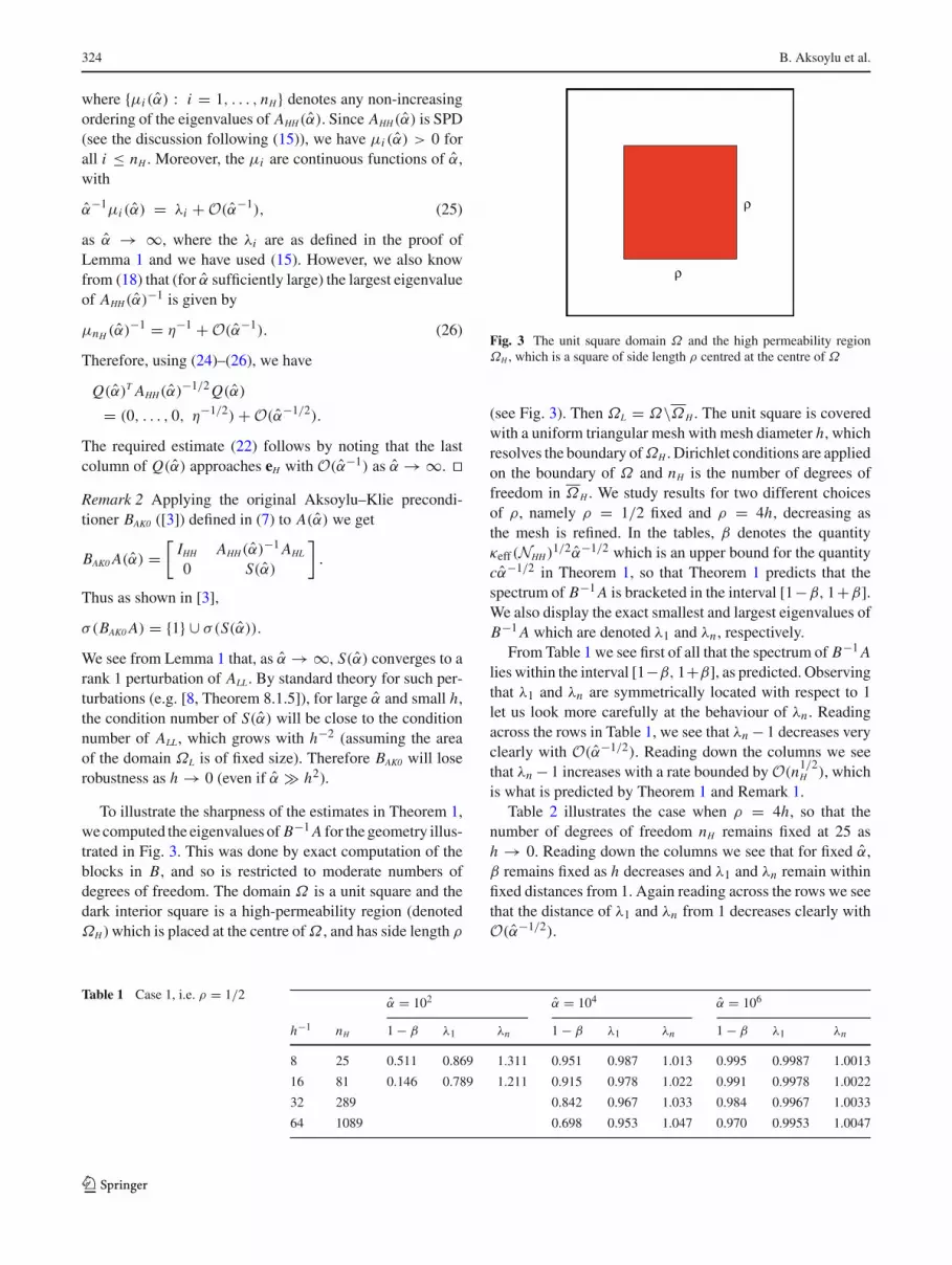
To illustrate the sharpness of the estimates in Theorem 1,we computed the eigenvalues of B−1 A for the geometry illus-trated in Fig. 3. This was done by exact computation of theblocks in B, and so is restricted to moderate numbers ofdegrees of freedom. The domain Ω is a unit square and thedark interior square is a high-permeability region (denotedΩH) which is placed at the centre of Ω , and has side length ρ

ρ

ρ

Fig. 3 The unit square domain Ω and the high permeability regionΩH , which is a square of side length ρ centred at the centre of Ω

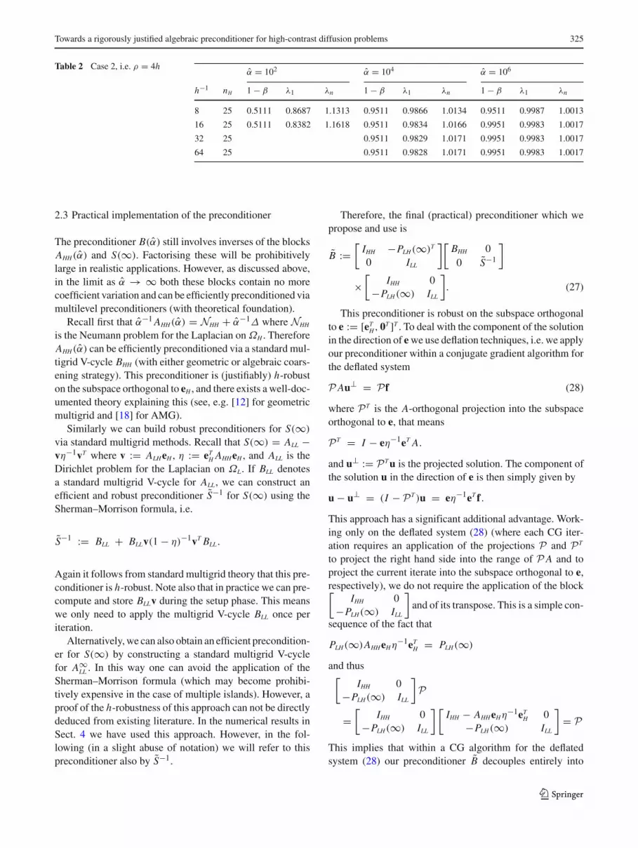
(see Fig. 3). Then ΩL = Ω\ΩH . The unit square is coveredwith a uniform triangular mesh with mesh diameter h, whichresolves the boundary of ΩH . Dirichlet conditions are appliedon the boundary of Ω and nH is the number of degrees offreedom in ΩH . We study results for two different choicesof ρ, namely ρ = 1/2 fixed and ρ = 4h, decreasing asthe mesh is refined. In the tables, β denotes the quantityκeff(NHH)1/2α−1/2 which is an upper bound for the quantitycα−1/2 in Theorem 1, so that Theorem 1 predicts that thespectrum of B−1 A is bracketed in the interval [1−β, 1+β].We also display the exact smallest and largest eigenvalues ofB−1 A which are denoted λ1 and λn , respectively.

From Table 1 we see first of all that the spectrum of B−1 Alies within the interval [1−β, 1+β], as predicted. Observingthat λ1 and λn are symmetrically located with respect to 1let us look more carefully at the behaviour of λn . Readingacross the rows in Table 1, we see that λn − 1 decreases veryclearly with O(α−1/2). Reading down the columns we seethat λn − 1 increases with a rate bounded by O(n1/2

H ), whichis what is predicted by Theorem 1 and Remark 1.

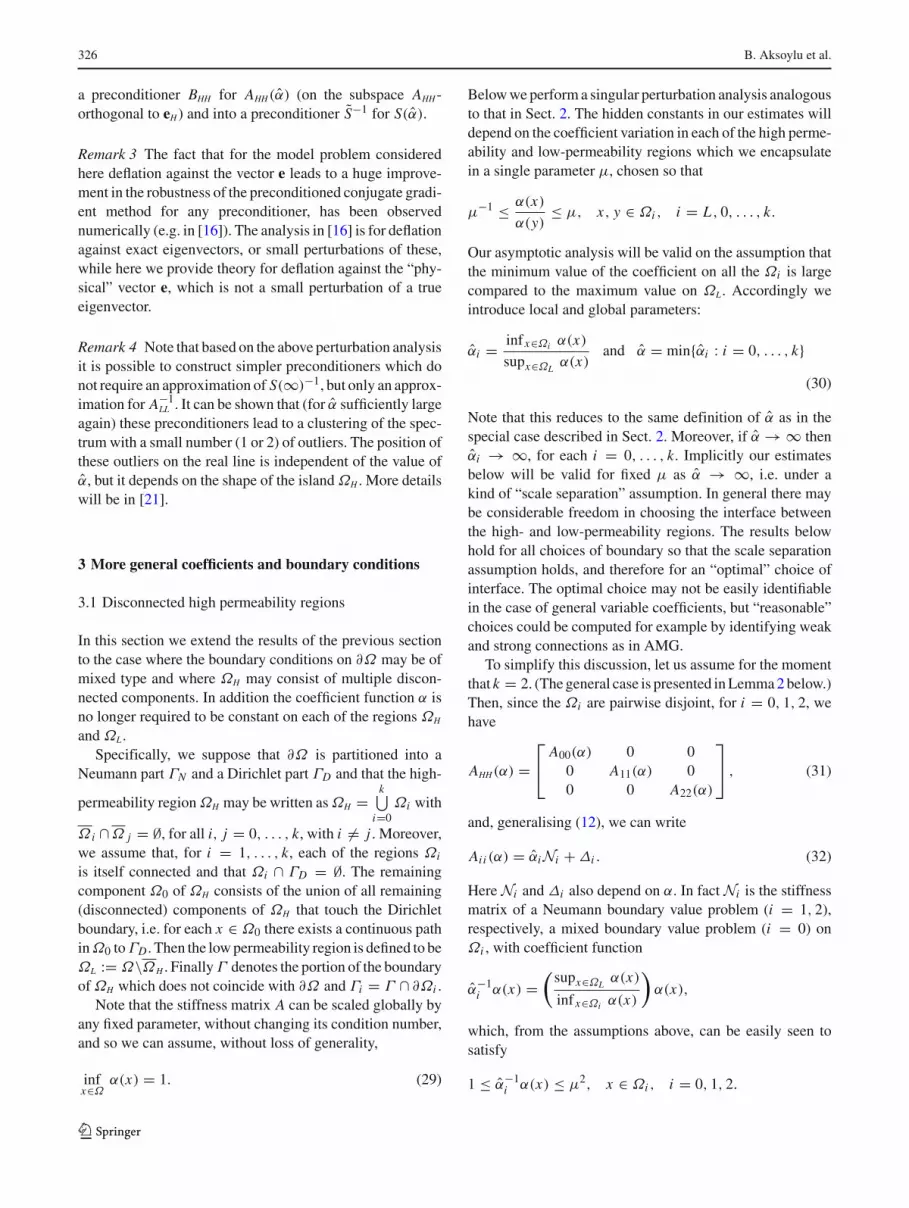
Table 2 illustrates the case when ρ = 4h, so that thenumber of degrees of freedom nH remains fixed at 25 ash → 0. Reading down the columns we see that for fixed α,β remains fixed as h decreases and λ1 and λn remain withinfixed distances from 1. Again reading across the rows we seethat the distance of λ1 and λn from 1 decreases clearly withO(α−1/2).

Table 1 Case 1, i.e. ρ = 1/2α = 102 α = 104 α = 106

h−1 nH 1 − β λ1 λn 1 − β λ1 λn 1 − β λ1 λn

8 25 0.511 0.869 1.311 0.951 0.987 1.013 0.995 0.9987 1.0013

16 81 0.146 0.789 1.211 0.915 0.978 1.022 0.991 0.9978 1.0022

32 289 0.842 0.967 1.033 0.984 0.9967 1.0033

64 1089 0.698 0.953 1.047 0.970 0.9953 1.0047

123


Table 2 Case 2, i.e. ρ = 4hα = 102 α = 104 α = 106

h−1 nH 1 − β λ1 λn 1 − β λ1 λn 1 − β λ1 λn

8 25 0.5111 0.8687 1.1313 0.9511 0.9866 1.0134 0.9511 0.9987 1.0013

16 25 0.5111 0.8382 1.1618 0.9511 0.9834 1.0166 0.9951 0.9983 1.0017

32 25 0.9511 0.9829 1.0171 0.9951 0.9983 1.0017

64 25 0.9511 0.9828 1.0171 0.9951 0.9983 1.0017

2.3 Practical implementation of the preconditioner

The preconditioner B(α) still involves inverses of the blocksAHH(α) and S(∞). Factorising these will be prohibitivelylarge in realistic applications. However, as discussed above,in the limit as α → ∞ both these blocks contain no morecoefficient variation and can be efficiently preconditioned viamultilevel preconditioners (with theoretical foundation).

Recall first that α−1 AHH(α) = NHH + α−1∆ where NHH

is the Neumann problem for the Laplacian on ΩH . ThereforeAHH(α) can be efficiently preconditioned via a standard mul-tigrid V-cycle BHH (with either geometric or algebraic coars-ening strategy). This preconditioner is (justifiably) h-robuston the subspace orthogonal to eH , and there exists a well-doc-umented theory explaining this (see, e.g. [12] for geometricmultigrid and [18] for AMG).

Similarly we can build robust preconditioners for S(∞)

via standard multigrid methods. Recall that S(∞) = ALL −vη−1vT where v := ALHeH , η := eT

H AHHeH , and ALL is theDirichlet problem for the Laplacian on ΩL. If BLL denotesa standard multigrid V-cycle for ALL, we can construct anefficient and robust preconditioner S−1 for S(∞) using theSherman–Morrison formula, i.e.

S−1 := BLL + BLLv(1 − η)−1vT BLL.

Again it follows from standard multigrid theory that this pre-conditioner is h-robust. Note also that in practice we can pre-compute and store BLLv during the setup phase. This meanswe only need to apply the multigrid V-cycle BLL once periteration.

Alternatively, we can also obtain an efficient precondition-er for S(∞) by constructing a standard multigrid V-cyclefor A∞

LL . In this way one can avoid the application of theSherman–Morrison formula (which may become prohibi-tively expensive in the case of multiple islands). However, aproof of the h-robustness of this approach can not be directlydeduced from existing literature. In the numerical results inSect. 4 we have used this approach. However, in the fol-lowing (in a slight abuse of notation) we will refer to thispreconditioner also by S−1.

Therefore, the final (practical) preconditioner which wepropose and use is

B :=[

IHH −PLH(∞)T

0 ILL

][BHH 00 S−1

]

×[


]. (27)

This preconditioner is robust on the subspace orthogonalto e := [eT

H, 0T ]T . To deal with the component of the solutionin the direction of e we use deflation techniques, i.e. we applyour preconditioner within a conjugate gradient algorithm forthe deflated system

P Au⊥ = Pf (28)

where PT is the A-orthogonal projection into the subspaceorthogonal to e, that means

PT = I − eη−1eT A.

and u⊥ := PT u is the projected solution. The component ofthe solution u in the direction of e is then simply given by

u − u⊥ = (I − PT )u = eη−1eT f .

This approach has a significant additional advantage. Work-ing only on the deflated system (28) (where each CG iter-ation requires an application of the projections P and PT

to project the right hand side into the range of P A and toproject the current iterate into the subspace orthogonal to e,respectively), we do not require the application of the block[


]and of its transpose. This is a simple con-

sequence of the fact that

PLH(∞)AHHeHη−1eTH = PLH(∞)

and thus[


]P

=[


] [IHH − AHHeHη−1eT

H 0−PLH(∞) ILL

]= P

This implies that within a CG algorithm for the deflatedsystem (28) our preconditioner B decouples entirely into

123


a preconditioner BHH for AHH(α) (on the subspace AHH-orthogonal to eH) and into a preconditioner S−1 for S(α).

Remark 3 The fact that for the model problem consideredhere deflation against the vector e leads to a huge improve-ment in the robustness of the preconditioned conjugate gradi-ent method for any preconditioner, has been observednumerically (e.g. in [16]). The analysis in [16] is for deflationagainst exact eigenvectors, or small perturbations of these,while here we provide theory for deflation against the “phy-sical” vector e, which is not a small perturbation of a trueeigenvector.

Remark 4 Note that based on the above perturbation analysisit is possible to construct simpler preconditioners which donot require an approximation of S(∞)−1, but only an approx-imation for A−1

LL . It can be shown that (for α sufficiently largeagain) these preconditioners lead to a clustering of the spec-trum with a small number (1 or 2) of outliers. The position ofthese outliers on the real line is independent of the value ofα, but it depends on the shape of the island ΩH . More detailswill be in [21].

3 More general coefficients and boundary conditions

3.1 Disconnected high permeability regions

In this section we extend the results of the previous sectionto the case where the boundary conditions on ∂Ω may be ofmixed type and where ΩH may consist of multiple discon-nected components. In addition the coefficient function α isno longer required to be constant on each of the regions ΩH

and ΩL.Specifically, we suppose that ∂Ω is partitioned into a

Neumann part ΓN and a Dirichlet part ΓD and that the high-

permeability region ΩH may be written as ΩH =k⋃

i=0Ωi with

Ω i ∩Ω j = ∅, for all i, j = 0, . . . , k, with i = j . Moreover,we assume that, for i = 1, . . . , k, each of the regions Ωi

is itself connected and that Ωi ∩ ΓD = ∅. The remainingcomponent Ω0 of ΩH consists of the union of all remaining(disconnected) components of ΩH that touch the Dirichletboundary, i.e. for each x ∈ Ω0 there exists a continuous pathin Ω0 to ΓD . Then the low permeability region is defined to beΩL := Ω\ΩH . Finally Γ denotes the portion of the boundaryof ΩH which does not coincide with ∂Ω and Γi = Γ ∩ ∂Ωi .

Note that the stiffness matrix A can be scaled globally byany fixed parameter, without changing its condition number,and so we can assume, without loss of generality,

infx∈Ω

α(x) = 1. (29)

Below we perform a singular perturbation analysis analogousto that in Sect. 2. The hidden constants in our estimates willdepend on the coefficient variation in each of the high perme-ability and low-permeability regions which we encapsulatein a single parameter µ, chosen so that

µ−1 ≤ α(x)

α(y)≤ µ, x, y ∈ Ωi , i = L , 0, . . . , k.

Our asymptotic analysis will be valid on the assumption thatthe minimum value of the coefficient on all the Ωi is largecompared to the maximum value on ΩL. Accordingly weintroduce local and global parameters:

αi = infx∈Ωi α(x)

supx∈ΩLα(x)

and α = minαi : i = 0, . . . , k(30)

Note that this reduces to the same definition of α as in thespecial case described in Sect. 2. Moreover, if α → ∞ thenαi → ∞, for each i = 0, . . . , k. Implicitly our estimatesbelow will be valid for fixed µ as α → ∞, i.e. under akind of “scale separation” assumption. In general there maybe considerable freedom in choosing the interface betweenthe high- and low-permeability regions. The results belowhold for all choices of boundary so that the scale separationassumption holds, and therefore for an “optimal” choice ofinterface. The optimal choice may not be easily identifiablein the case of general variable coefficients, but “reasonable”choices could be computed for example by identifying weakand strong connections as in AMG.

To simplify this discussion, let us assume for the momentthat k = 2. (The general case is presented in Lemma 2 below.)Then, since the Ωi are pairwise disjoint, for i = 0, 1, 2, wehave

AHH(α) =⎡

⎣A00(α) 0 0

0 A11(α) 00 0 A22(α)

⎤

⎦ , (31)

and, generalising (12), we can write

Aii (α) = αiNi + ∆i . (32)

Here Ni and ∆i also depend on α. In fact Ni is the stiffnessmatrix of a Neumann boundary value problem (i = 1, 2),respectively, a mixed boundary value problem (i = 0) onΩi , with coefficient function

α−1i α(x) =

(supx∈ΩL

α(x)

infx∈Ωi α(x)

)α(x),

which, from the assumptions above, can be easily seen tosatisfy

1 ≤ α−1i α(x) ≤ µ2, x ∈ Ωi , i = 0, 1, 2.

123


Moreover, analogously to (12),

∆i =[

0 00 A(L)

Γi ,Γi

],

where A(L)

Γi ,Γirepresents the coupling between nodes on Γi

coming from the low permeability region, in which (byassumptions above), the coefficient varies between 1 and µ.

As in Sect. 2 we find that, as α → ∞,

Aii (α)−1 = ei(eT

i ∆i ei)−1 eT

i + O(α−1) for i = 1, 2,

(33)

and, since N0 has trivial nullspace, we have

A00(α)−1 = O(α−1), α → ∞. (34)

Thus, if we denote by eH,i the nH-vector which coincideswith ei on Ω i and is 0 elsewehere, then

AHH(α)−1 =2∑

i=1

eH,i(eT

i ∆i ei)−1 eT

H,i + O(α−1) (35)

and

S(α) = ALL −2∑

i=1

(ALHeH,i

) (eT

i ∆i ei)−1 (

eTH,i AHL

)

+ O(α−1). (36)

As in Sect. 2.1 we define

AHH(∞)−1 := limα→∞

AHH(α)−1, S(∞) := limα→∞

S(α),

PLH(∞) := limα→∞

ALH AHH(α)−1,

and collect the results in a lemma that generalises Lemma 1.

Lemma 2

AHH(∞)−1 =k∑

i=1

eH,i(eT

i ∆i ei)−1 eT

H,i ,

S(∞) = ALL −k∑

i=1

(ALHeH,i

) (eT

i ∆i ei)−1 (

eTH,i AHL

),

PLH(∞) =k∑

i=1

(ALHeH,i )(eT

i ∆i ei)−1 eT

H,i .

Thus, in the limit as α → ∞ the Schur complement S(α)

is a simple rank-k update of the block ALL. As in the pre-vious section S(∞) can again be interpreted as the Schurcomplement of the k × k diagonal matrix

E := diag( n1eT1∆1e1, . . . , nkeT

k∆kek )

= diag( 1TH,1 AHH1H,1, . . . , 1T

H,k AHH1H,k )

in

A∞LL :=

[E FT

F ALL

]with F := ALH

[1H,1, . . . , 1H,k

](37)

and 1H,i := n1/2i eH,i , i.e. the nH-vector that is 1 on Ωi and 0

elsewhere.Thus, analogously to the discussion at the end of Sect. 2.1,

for large α, the problem again essentially decouples into Neu-mann or mixed boundary value problems on each of the Ωi

and a Dirichlet problem on Ω\Ω0 with the additional con-straint that the solution is constant on each of the Ωi , i =1, . . . , k. Again (and assuming of course that µ is small com-pared to α), there exist efficient and robust multilevel precon-ditioners for each of these decoupled problems.

With this insight, a suitable preconditioner B can bedefined exactly as in (20) and we then have, analogouslyto Theorem 1, the following result.

Theorem 2 For α sufficiently large we have

σ(B A) ⊂ [1 − cα−1/2, 1 + cα−1/2]for some constant c = c(µ, h), which is independent of α

and in which the dependence on h is understood. (Detailswill be in [21].)

3.2 Multiscale media

Finally, we also consider multiscale media, i.e. high-permeability regions within regions of intermediate strengthpremeability. We simply apply the above framework recur-sively. For simplicity let us consider the following modelsituation: as in Sect. 2, we assume that ΩH is connected andΩH∩∂Ω = ∅, but now we assume further that ΩH = Ω1∪Ω2

whereΩ1 is again connected andΩ1∩∂ΩH = ∅, i.e. an islandwithin an island. We will consider the case when α2 is highrelative to αL and α1 is high relative to α2, so we define

α1 =(

inf x∈Ω1 α(x)

supx∈Ω2α(x)

)

and α2 =(

inf x∈Ω2 α(x)

supx∈ΩLα(x)

),

and assume that α := minα1, α2 → ∞, i.e. we have athree-scale medium with good scale separation. Againassume moderate coefficient variation inside the subdomains,with µ defined as in Sect. 3.1.

We can now apply the above framework recursively. Pro-vided α2 is sufficiently large we obtain the limiting form ofthe Schur complement S(α) (of AHH in A) as before. How-ever, there is still strong coefficient variation in the Neumannproblem on ΩH and so we need to apply our analysis again.We write

AHH =[

A11 A12

A21 A22

]

and find as above that, since α1 → ∞, this problem againessentially decouples into a Neumann problem on Ω1 and aproblem on ΩH with the constraint that the solution is con-stant on Ω1. This latter problem can again be described either

123


through the limiting Schur complement of A11 in AHH , i.e.

S2(∞) := A22 − (A21e1)(eT

1∆1e1)−1 (

eT1 A12

),

or through the (n2 + 1) × (n2 + 1) matrix

A∞22 :=

[1T

1 A1111 1T1 A12

A2111 A22

],

and the preconditioner B can be extended accordingly.

4 Numerical experiments

In this section we apply the CG algorithm preconditionedusing our preconditioner B defined in (27) and we comparethis with several other possible choices of preconditionerin the context of several model problems. In the followingtables the notation CG + MG means that the CG algorithmis preconditioned using one V −cycle of standard geometricmultigrid with SSOR smoother, piecewise linear interpo-lation and full weighting restriction. The problem on thecoarsest grid is solved using the banded Cholesky solverdpbsv.f in LAPACK. The notation CG + AMG meansthat one V −cycle of the Ruge and Stüben AMG algorithmamg1r5.f [19] is used as preconditioner for CG. Finally thenotation CG+ B means that the preconditioner is B, which isconstructed using the (above) geometric multigrid V −cycleon sub-blocks of A as described in Sect. 2.3. κ(MG),κ(AMG) and κ(B A) are estimates (based on Ritz valuesobtained from the CG iteration) of the condition numbers ofthe respective preconditioned matrices.

The initial guess for the CG algorithm is taken to be zeroand the stopping criterion is taken to be a relative residualreduction of ε = 10−8 in the Euclidean norm. In all theexperiments below the domain is the unit square and therelevant elliptic problem is solved subject to a Dirichlet con-dition u(x) = 1 − x1 where x = (x1, x2), consistent withflow from left to right in the domain.

All computations are done using the GNU fortran95 com-piler gfortran on a linux intel core 2 laptop with clock-speed 2 GHz, 2 Gb of memory and cache size 4 Mb.

Example 1 Our first example concerns the geometry inFig. 3, with ρ = 1/2 where the central island is given acoefficient α = α and the surrounding region a coefficientα = 1. Table 3 gives the iteration numbers and (in brackets)the cpu times for fixed α = 106 as h → 0. Table 4 gives theiteration numbers and (in brackets) the cpu times for fixedh−1 = 1024 as α → ∞.

We observe from these tables that the B preonditioner per-forms almost identically to the MG and AMG precondition-ers for large enough α. In particular all three (as expected) areh−robust for α fixed. In all three cases the condition num-bers of the preconditioned matrices are very near to unity.

Table 3 Iteration numbers (cpu times) for the geometry given in Fig. 3,with ρ = 1/2 and α = 106 and associated condition numbers

h−1 CG + MG CG + AMG CG + B κ(MG) κ(AMG) κ(B A)

128 6 (0.11) 7 (0.10) 7 (0.11) 1.19 1.27 1.20

256 6 (0.30) 7 (0.36) 7 (0.40) 1.21 1.29 1.23

512 6 (1.29) 7 (1.48) 7 (1.48) 1.25 1.31 1.24

1024 6 (5.05) 7 (5.81) 7 (5.98) 1.24 1.35 1.26

Table 4 Iteration numbers (cpu times) for the geometry given in Fig. 3,with ρ = 1/2 and h−1 = 1, 024 and associated condition numbers

α CG + MG CG + AMG CG + B κ(MG) κ(AMG) κ(B A)

102 6 (5.06) 7 (5.83) 23 (17.7) 1.23 1.36 27.9

104 6 (5.04) 7 (5.81) 7 (5.98) 1.23 1.35 1.49

106 6 (5.05) 7 (5.81) 7 (5.98) 1.23 1.35 1.26

108 6 (5.05) 7 (5.81) 7 (5.98) 1.23 1.35 1.26

Fig. 4 The unit square domain Ω and the high permeability regionΩH , which consists of two squares of side length 1/5 centred at thepoints (3/10, 3/10) and (7/10, 7/10)

A proof of the robustness of the CG + MG method is givenin [26], under the assumption that the coarse grid resolvesthe discontinuous coefficient (which is the case here). Wehave given a proof of the robustness of B under quite generalassumption on the shape of the interface between low-andhigh permeability regions earlier in this paper. A proof of theα-robustness of the AMG preconditioner is still lacking.

Example 2 The second experiment is for the geometrydepicted in Fig. 4. For this we perform the same experimentsas in Example 1. Again the dark shaded regions are given acoefficient α = α and the remainder a coefficient α = 1.The results are given in Tables 5 and 6. The results lead tosimilar conclusions as in Example 1.

We also remark that preconditioner B does not work sowell as α gets smaller (see Table 6). This is to be expected,since this method is based on asymptotic expansions as α →∞. However as mentioned earlier our analysis demonstrates

123


Table 5 Iteration numbers (cpu times) for the geometry given in Fig. 4,with α = 106 and various condition numbers


160 6 (0.14) 7 (0.14) 7 (0.16) 1.20 1.39 1.21

320 6 (0.51) 7 (0.57) 7 (0.61) 1.21 1.38 1.23

640 6 (1.93) 7 (2.26) 7 (2.39) 1.22 1.38 1.24

1,280 6 (7.84) 7 (8.88) 7 (9.81) 1.24 1.43 1.25

Table 6 Iteration numbers (cpu times) for the geometry given in Fig. 4,with h−1 = 1, 280 and various condition numbers


102 6 (7.82) 8 (9.54) 19 (22.9) 1.23 1.57 11.8

104 6 (7.85) 7 (8.90) 7 (9.85) 1.24 1.43 1.28

106 6 (7.84) 7 (8.88) 7 (9.81) 1.24 1.43 1.25

108 6 (7.79) 7 (8.87) 7 (9.82) 1.24 1.42 1.25

theoretically the success of algebraic methods based onstrong and weak connections in the high contrast case. Also,of course, standard geometric multigrid works well in thelow-contrast case.

With respect to Examples 1 and 2, we would like to high-light a point that has already been made many times in theliterature, but so far without theoretical justification. Usingalgebraic procedures to identify strong and weak couplingsin the stiffness matrix arising from FE discretisations of high-contrast diffusion problems, it is indeed possible (as we haveproved in this paper) to design multigrid methods that areα-robust and have almost the same computational complex-ity as geometric multigrid methods for diffusion problemswith constant coefficents. In fact, applying CG + MG to theLaplace problem α = 1 with h−1 = 1, 280 we require 6 iter-ations and 7.72 s with our code which is only slightly fasterthan the performance of CG + AMG and CG + B for the highcontrast case.

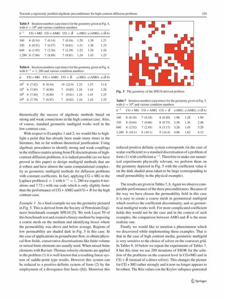
Example 3 As a final example we use the geometry picturedin Fig. 5. This is derived from the Society of Petroleum Engi-neers benchmark example SPE10 [5]. We took Layer 59 ofthis benchmark test and created a binary medium by imposinga coarse mesh on the medium and identifying boxes wherethe permeability was above and below average. Regions oflow permeability are shaded dark in Fig. 5 in this case. Inthe case of applications in groundwater flow, to obtain physi-cal flow fields, conservative discretisations like finite volumeor mixed finite elements are usually used. When mixed finiteelements with Raviart–Thomas velocity elements are appliedto the problem (1) it is well-known that a resulting linear sys-tem of saddle-point type results. However this system canbe reduced to a positive-definite system of form (2) by theemployment of a divergence-free basis ([6]). Moreover this

Fig. 5 The geometry of the SPE10-derived problem

Table 7 Iteration numbers (cpu times) for the geometry given in Fig. 5,with α = 106 and various condition numbers


160 8 (0.18) 7 (0.18) 8 (0.20) 1.96 1.28 1.90

320 8 (0.64) 7 (0.66) 8 (0.75) 2.56 1.36 2.48

640 8 (2.52) 7 (2.45) 8 (3.17) 3.26 1.45 3.20

1,280 8 (10.1) 8 (10.1) 9 (14.4) 4.06 1.62 4.12

reduced positive definite system corresponds (in the case ofscalar coefficient) to a standard discretisation of a problem ofform (1) with coefficient α−1. Therefore to make our numer-ical experiments physically relevant, we perform them onthe geometry depicted in Fig. 5 with the coefficient value α

on the dark shaded areas taken to be large (corresponding tosmall permeability in the physical example).

The results are given in Tables 7, 8. Again we observe com-parable performance of the three preconditioners. Because ofthe way we have chosen the permeability field in this caseit is easy to create a coarse mesh in geometrical multigridwhich resolves the coefficient discontinuity, and so geomet-rical multigrid works well. For more complicated coefficientfields this would not be the case and in the context of suchexamples, the comparison between AMG and B is the morerealistic one.

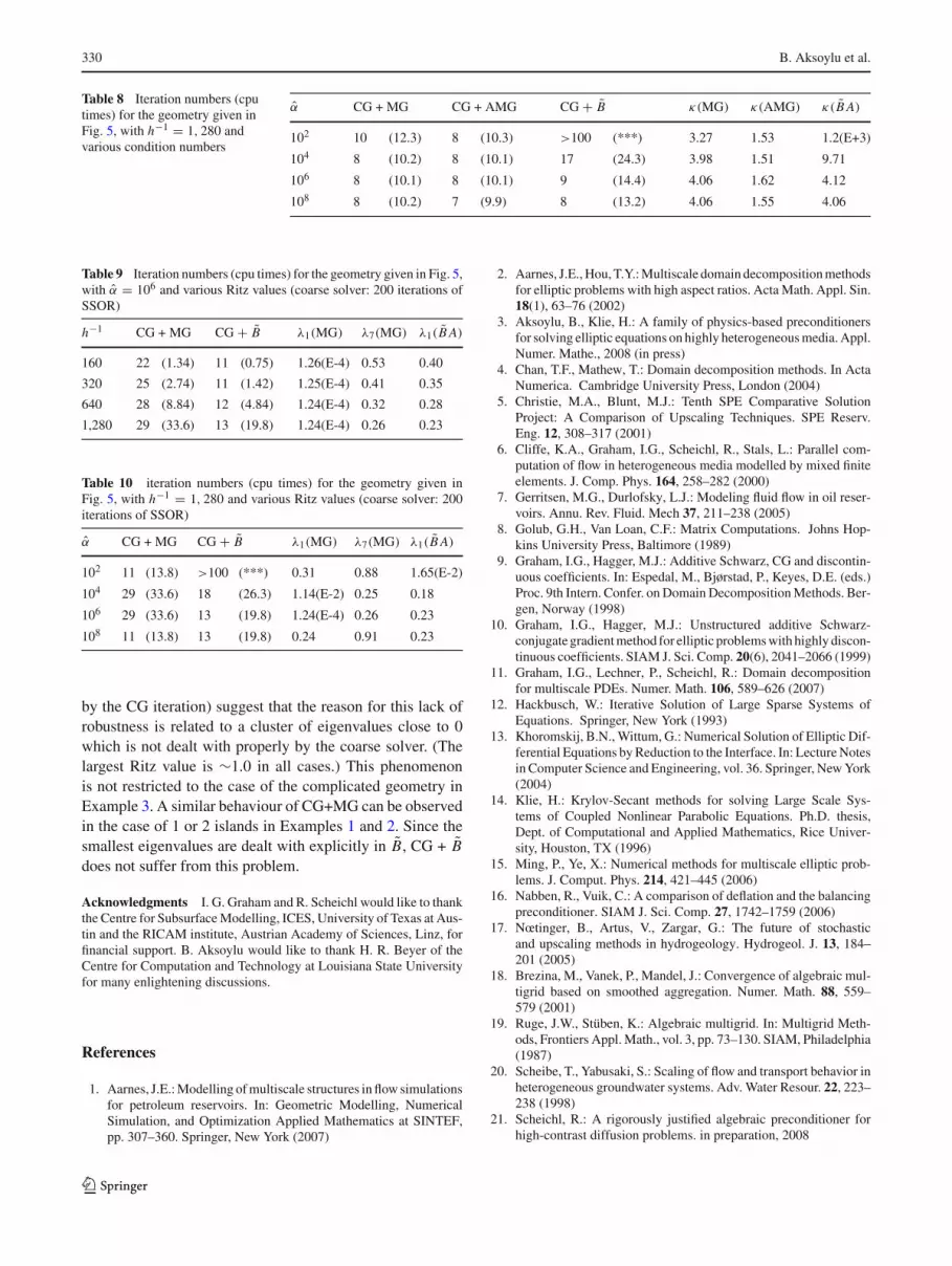
Finally we would like to mention a phenomenon whichwe discovered while implementing these examples. That isthat in the case of high contrast media, geometric multigridis very sensitive to the choice of solver on the coarseset grid.In Tables 9, 10 below we repeat the experiments of Tables 7,8 but this time we use 200 iterations of SSOR for the solu-tion of the problems on the coarsest level in CG+MG and inCG + B (instead of a direct solver). This changes the picturefor CG + MG rather strongly and it now no longer appears tobe robust. The Ritz values (on the Krylov subspace generated

123


Table 8 Iteration numbers (cputimes) for the geometry given inFig. 5, with h−1 = 1, 280 andvarious condition numbers


102 10 (12.3) 8 (10.3) >100 (***) 3.27 1.53 1.2(E+3)

104 8 (10.2) 8 (10.1) 17 (24.3) 3.98 1.51 9.71

106 8 (10.1) 8 (10.1) 9 (14.4) 4.06 1.62 4.12

108 8 (10.2) 7 (9.9) 8 (13.2) 4.06 1.55 4.06

Table 9 Iteration numbers (cpu times) for the geometry given in Fig. 5,with α = 106 and various Ritz values (coarse solver: 200 iterations ofSSOR)

h−1 CG + MG CG + B λ1(MG) λ7(MG) λ1(B A)

160 22 (1.34) 11 (0.75) 1.26(E-4) 0.53 0.40

320 25 (2.74) 11 (1.42) 1.25(E-4) 0.41 0.35

640 28 (8.84) 12 (4.84) 1.24(E-4) 0.32 0.28

1,280 29 (33.6) 13 (19.8) 1.24(E-4) 0.26 0.23

Table 10 iteration numbers (cpu times) for the geometry given inFig. 5, with h−1 = 1, 280 and various Ritz values (coarse solver: 200iterations of SSOR)

α CG + MG CG + B λ1(MG) λ7(MG) λ1(B A)

102 11 (13.8) >100 (***) 0.31 0.88 1.65(E-2)

104 29 (33.6) 18 (26.3) 1.14(E-2) 0.25 0.18

106 29 (33.6) 13 (19.8) 1.24(E-4) 0.26 0.23

108 11 (13.8) 13 (19.8) 0.24 0.91 0.23

by the CG iteration) suggest that the reason for this lack ofrobustness is related to a cluster of eigenvalues close to 0which is not dealt with properly by the coarse solver. (Thelargest Ritz value is ∼1.0 in all cases.) This phenomenonis not restricted to the case of the complicated geometry inExample 3. A similar behaviour of CG+MG can be observedin the case of 1 or 2 islands in Examples 1 and 2. Since thesmallest eigenvalues are dealt with explicitly in B, CG + Bdoes not suffer from this problem.

Acknowledgments I. G. Graham and R. Scheichl would like to thankthe Centre for Subsurface Modelling, ICES, University of Texas at Aus-tin and the RICAM institute, Austrian Academy of Sciences, Linz, forfinancial support. B. Aksoylu would like to thank H. R. Beyer of theCentre for Computation and Technology at Louisiana State Universityfor many enlightening discussions.

References

1. Aarnes, J.E.: Modelling of multiscale structures in flow simulationsfor petroleum reservoirs. In: Geometric Modelling, NumericalSimulation, and Optimization Applied Mathematics at SINTEF,pp. 307–360. Springer, New York (2007)

2. Aarnes, J.E., Hou, T.Y.: Multiscale domain decomposition methodsfor elliptic problems with high aspect ratios. Acta Math. Appl. Sin.18(1), 63–76 (2002)

3. Aksoylu, B., Klie, H.: A family of physics-based preconditionersfor solving elliptic equations on highly heterogeneous media. Appl.Numer. Mathe., 2008 (in press)

4. Chan, T.F., Mathew, T.: Domain decomposition methods. In ActaNumerica. Cambridge University Press, London (2004)

5. Christie, M.A., Blunt, M.J.: Tenth SPE Comparative SolutionProject: A Comparison of Upscaling Techniques. SPE Reserv.Eng. 12, 308–317 (2001)

6. Cliffe, K.A., Graham, I.G., Scheichl, R., Stals, L.: Parallel com-putation of flow in heterogeneous media modelled by mixed finiteelements. J. Comp. Phys. 164, 258–282 (2000)

7. Gerritsen, M.G., Durlofsky, L.J.: Modeling fluid flow in oil reser-voirs. Annu. Rev. Fluid. Mech 37, 211–238 (2005)

8. Golub, G.H., Van Loan, C.F.: Matrix Computations. Johns Hop-kins University Press, Baltimore (1989)

9. Graham, I.G., Hagger, M.J.: Additive Schwarz, CG and discontin-uous coefficients. In: Espedal, M., Bjørstad, P., Keyes, D.E. (eds.)Proc. 9th Intern. Confer. on Domain Decomposition Methods. Ber-gen, Norway (1998)

10. Graham, I.G., Hagger, M.J.: Unstructured additive Schwarz-conjugate gradient method for elliptic problems with highly discon-tinuous coefficients. SIAM J. Sci. Comp. 20(6), 2041–2066 (1999)

11. Graham, I.G., Lechner, P., Scheichl, R.: Domain decompositionfor multiscale PDEs. Numer. Math. 106, 589–626 (2007)

12. Hackbusch, W.: Iterative Solution of Large Sparse Systems ofEquations. Springer, New York (1993)

13. Khoromskij, B.N., Wittum, G.: Numerical Solution of Elliptic Dif-ferential Equations by Reduction to the Interface. In: Lecture Notesin Computer Science and Engineering, vol. 36. Springer, New York(2004)

14. Klie, H.: Krylov-Secant methods for solving Large Scale Sys-tems of Coupled Nonlinear Parabolic Equations. Ph.D. thesis,Dept. of Computational and Applied Mathematics, Rice Univer-sity, Houston, TX (1996)

15. Ming, P., Ye, X.: Numerical methods for multiscale elliptic prob-lems. J. Comput. Phys. 214, 421–445 (2006)

16. Nabben, R., Vuik, C.: A comparison of deflation and the balancingpreconditioner. SIAM J. Sci. Comp. 27, 1742–1759 (2006)

17. Nœtinger, B., Artus, V., Zargar, G.: The future of stochasticand upscaling methods in hydrogeology. Hydrogeol. J. 13, 184–201 (2005)

18. Brezina, M., Vanek, P., Mandel, J.: Convergence of algebraic mul-tigrid based on smoothed aggregation. Numer. Math. 88, 559–579 (2001)

19. Ruge, J.W., Stüben, K.: Algebraic multigrid. In: Multigrid Meth-ods, Frontiers Appl. Math., vol. 3, pp. 73–130. SIAM, Philadelphia(1987)

20. Scheibe, T., Yabusaki, S.: Scaling of flow and transport behavior inheterogeneous groundwater systems. Adv. Water Resour. 22, 223–238 (1998)

21. Scheichl, R.: A rigorously justified algebraic preconditioner forhigh-contrast diffusion problems. in preparation, 2008

123


22. Scheichl, R., Vainikko, E.: Additive Schwarz and aggregation-based coarsening for elliptic problems with highly variable coeffi-cients. Computing 80(4), 319–343 (2007)

23. Vuik, C., Segal, A., Meijerink, J.A.: An efficient preconditioned CGmethod for the solution of a class of layered problems with extremecontrasts of coefficients. J. Comp. Phys. 152, 385–403 (1999)

24. Guadagnini, A., Sanchez-Vila, X., Carrera, J.: Representativehydraulic conductivities in saturated groundwater flow. Rev. Geo-phys. 44, 1–46 (2006)

25. Durlofsky, L.J., Wen, X.H., Edwards, M.G.: Upscaling of channelsystems in two dimensions using flow-based grids. Transp. PorousMedia 51, 343–366 (2003)

26. Xu, J., Zhu, Y.: Uniform convergent multigrid methods for ellip-tic problems with strongly discontinuous coefficients. TechnicalReport Technical Report No. AM311, Dept of Mathematics, PennState, Pennsilvania, USA (2007)

123

Documents

Towards a rigorously justified algebraic preconditioner for high-contrast diffusion problems