Towards a Better Understanding of the Fundamental Period of

Towards a Better Understanding of the Fundamental Period ofMetal Building Systems

Santiago Bertero

Thesis submitted to the Faculty of the

Virginia Polytechnic Institute and State University

in partial fulfillment of the requirements for the degree of

Master of Science

in

Civil Engineering

Rodrigo Sarlo, Chair

Finley A. Charney

Matthew R. Eatherton

May 9, 2022

Blacksburg, Virginia

Keywords: Metal Buildings, Seismic Design, Operational Modal Analysis, Equivalent

Lateral Force, Non-Structural Elements

Copyright 2022, Santiago Bertero

Towards a Better Understanding of the Fundamental Period of MetalBuilding Systems

Santiago Bertero

(ABSTRACT)

Metal buildings account for over 40% of low-rise construction in the US. Despite this, predic-

tive fundamental period equations that were obtained empirically for mid-rise construction

are used in seismic design. Analytical modeling of metal building frames implied that these

equations significantly underpredict the period, which led to the development of a new pre-

dictive equation. However, experimental tests showed that these models may overestimate

the measured period.

In this work, further tests were carried out in order to single out possible causes. Buildings

were tested during different stages of construction to evaluate how non-structural elements

could affect the behavior. Both planar and three-dimensional models were developed to

determine if design assumptions are accurate for the purpose of estimating the period.

The results from tests showed that, unlike other single-story buildings, non-structural compo-

nents seem to have negligible effect on the structural behavior. However, several buildings

seemed to exhibit signs of fixed conditions at the column base. This assertion was cor-

roborated by updating the analytical models. The two modeling approaches showed good

agreement with each other as well, validating the use of planar models to predict the period.

Finally, new predictive equations are proposed that take into account the type of cladding,

as it was found to be an important variable not previously considered. However, low mass

participation ratios coupled with the stiffness provided by the secondary framing put the

use of the equivalent lateral force procedure into question.

Towards a Better Understanding of the Fundamental Period of MetalBuilding Systems

Santiago Bertero

(GENERAL AUDIENCE ABSTRACT)

When designing buildings for earthquake loads it is necessary to know their dynamic prop-

erties in order to define the equivalent forces that must be applied. Building codes provide

predictive equations that were obtained empirically for typical mid-rise construction. Metal

buildings do not fall within the range of buildings tested for their development, and so a new

equation was proposed for them based on a database of planar models. However, previous

tests implied that this equation was predicting larger periods than those obtained experi-

mentally.

In this work, further tests were carried out during different stages of construction to evaluate

how non-structural elements could affect the behavior. Models were also created for each

building in order to determine if the approach used to develop the metal building database

was adequate for estimating the period.

The results from tests showed that, unlike other single-story buildings, non-structural com-

ponents seem to have negligible effect on the structural behavior, and the modeling assump-

tions within the database were validated. Further analysis showed that the type of cladding

(concrete or metal sheeting) had a large influence on the properties of metal buildings. In

consequence, a new set of predictive equations is proposed that takes this into account.

Acknowledgments

First of all, I would like to thank my advisor Dr. Rodrigo Sarlo for trusting me as an

incoming student to work for him in different projects from which I can take a lot from. His

support is deeply appreciated, both from an academic and (especially) personal standpoint.

I would also like to extend my gratitude to my committee members, Dr. Finley A. Charney

and Dr. Matt R. Eatherton, whose feedback and commentary I believe made for a better

end product. I learned a lot not only from trying to answer their inquires, but also from the

knowledge they shared in the classroom and in casual conversation when available.

I would also like to thank the Metal Building Manufacturers Association for sponsoring this

research, and Igor Marinovic and Dr. W. Lee Shoemaker for their guidance. I would also

like to thank the industry people who provided vital information or access to the tested

buildings: Dustin Cole from Chief Buildings, Matt Bartels and Justin Kestler from Bartels

Construction Solutions, Herman Baber from Clark Nexsen Construction Services and Shane

West from TKS Contracting.

The experimental portion of this thesis would not have been possible without the help of my

fellow labmates who took time out of their own busy student lives to lend a hand: Tasha

Vipond, Hesam Soleimani, Amin Moghadam and Alan Smith.

On a personal note, I’d like to thank my friend Zayeem Zaman for helping me settle in

Blacksburg and having my back at all times. My family’s support, now at a distance, is also

invaluable to me and I can’t wait to be back close to them.

Finally, I’d like to thank Universidad de Buenos Aires and Argentina’s public education

system for making me the engineer I was when I came to Blacksburg, and Virginia Tech for

turning me into the engineer I am now.

iv

Contents

List of Figures xi

List of Tables xviii

1 Introduction 1

1.1 Background and Motivation . . . . . . . . . . . . . . . . . . . . . . . . . . . 1

1.2 Thesis Scope and Organization . . . . . . . . . . . . . . . . . . . . . . . . . 4

2 Literature Review 6

2.1 Seismic Design Principles and its Application to Metal Buildings . . . . . . . 6

2.1.1 Defining the Seismic Demand . . . . . . . . . . . . . . . . . . . . . . 6

2.1.2 Estimating the Fundamental Period . . . . . . . . . . . . . . . . . . 11

2.1.3 Force distribution along its members . . . . . . . . . . . . . . . . . . 19

2.1.4 Assumptions Made in Metal Building Design . . . . . . . . . . . . . 23

2.2 Structural modelling of the main lateral resisting system . . . . . . . . . . . 24

2.2.1 Modeling of web tapered elements . . . . . . . . . . . . . . . . . . . 25

2.2.2 Shear Deformations . . . . . . . . . . . . . . . . . . . . . . . . . . . 26

2.2.3 Panel Zone Deformations . . . . . . . . . . . . . . . . . . . . . . . . 27

2.2.4 Base Fixity . . . . . . . . . . . . . . . . . . . . . . . . . . . . . . . . 29

v

2.2.5 Discussion . . . . . . . . . . . . . . . . . . . . . . . . . . . . . . . . . 31

2.3 Modeling of steel sheeting . . . . . . . . . . . . . . . . . . . . . . . . . . . . 34

2.3.1 Developments in the U.S. . . . . . . . . . . . . . . . . . . . . . . . . 35

2.3.2 European approach . . . . . . . . . . . . . . . . . . . . . . . . . . . . 40

2.3.3 Limitations of current empirical equations . . . . . . . . . . . . . . . 44

2.4 Experimental Testing for Period Extraction . . . . . . . . . . . . . . . . . . 47

3 Methodology 51

3.1 Introduction . . . . . . . . . . . . . . . . . . . . . . . . . . . . . . . . . . . . 51

3.2 Operational Modal Analysis . . . . . . . . . . . . . . . . . . . . . . . . . . . 52

3.2.1 Background and Justification . . . . . . . . . . . . . . . . . . . . . . 52

3.2.2 State-Space Representation and Subspace Identification . . . . . . . 54

3.2.3 Process Automation . . . . . . . . . . . . . . . . . . . . . . . . . . . 58

3.3 Testing Procedure . . . . . . . . . . . . . . . . . . . . . . . . . . . . . . . . 60

3.3.1 Equipment . . . . . . . . . . . . . . . . . . . . . . . . . . . . . . . . 61

3.3.2 Sensor Placement . . . . . . . . . . . . . . . . . . . . . . . . . . . . . 62

3.3.3 Data gathering, pre and post-processing . . . . . . . . . . . . . . . . 65

3.4 3D Modeling of metal buildings . . . . . . . . . . . . . . . . . . . . . . . . . 66

3.4.1 Main framing . . . . . . . . . . . . . . . . . . . . . . . . . . . . . . . 66

3.4.2 Secondary framing and bracing . . . . . . . . . . . . . . . . . . . . . 69

vi

3.4.3 Cladding . . . . . . . . . . . . . . . . . . . . . . . . . . . . . . . . . 71

3.4.4 Other considerations . . . . . . . . . . . . . . . . . . . . . . . . . . . 73

3.5 Tested Buildings . . . . . . . . . . . . . . . . . . . . . . . . . . . . . . . . . 74

3.5.1 Building VA-1 . . . . . . . . . . . . . . . . . . . . . . . . . . . . . . 75

3.5.2 Building VA-2 . . . . . . . . . . . . . . . . . . . . . . . . . . . . . . 77

3.5.3 Building WV-1 . . . . . . . . . . . . . . . . . . . . . . . . . . . . . . 78

3.5.4 Building WV-2 . . . . . . . . . . . . . . . . . . . . . . . . . . . . . . 79

3.5.5 Building NC-1 . . . . . . . . . . . . . . . . . . . . . . . . . . . . . . 80

3.5.6 Building NC-2 . . . . . . . . . . . . . . . . . . . . . . . . . . . . . . 82

3.5.7 Building NC-3 . . . . . . . . . . . . . . . . . . . . . . . . . . . . . . 83

3.5.8 Summary . . . . . . . . . . . . . . . . . . . . . . . . . . . . . . . . . 84

4 Results 87

4.1 Building VA-1 . . . . . . . . . . . . . . . . . . . . . . . . . . . . . . . . . . . 88

4.1.1 Bare Frame Test . . . . . . . . . . . . . . . . . . . . . . . . . . . . . 88

4.1.2 Completed Building Test . . . . . . . . . . . . . . . . . . . . . . . . . 97

4.2 Building NC-2 . . . . . . . . . . . . . . . . . . . . . . . . . . . . . . . . . . . 102

4.2.1 Bare Frame Test . . . . . . . . . . . . . . . . . . . . . . . . . . . . . 102

4.2.2 Test with Walls installed . . . . . . . . . . . . . . . . . . . . . . . . . 106

4.2.3 Test on completed building . . . . . . . . . . . . . . . . . . . . . . . 109

vii

4.3 Building NC-1 . . . . . . . . . . . . . . . . . . . . . . . . . . . . . . . . . . . 111

4.3.1 Test on Bare Frame . . . . . . . . . . . . . . . . . . . . . . . . . . . 111

4.3.2 Test on fully clad building . . . . . . . . . . . . . . . . . . . . . . . . 116

4.4 Building VA-2 . . . . . . . . . . . . . . . . . . . . . . . . . . . . . . . . . . . 120

4.4.1 Test with roof installed . . . . . . . . . . . . . . . . . . . . . . . . . 120

4.4.2 Test on fully clad building . . . . . . . . . . . . . . . . . . . . . . . . 123

4.5 Building WV-2 . . . . . . . . . . . . . . . . . . . . . . . . . . . . . . . . . . 127

4.6 Building WV-1 . . . . . . . . . . . . . . . . . . . . . . . . . . . . . . . . . . 130

4.7 Building NC-3 . . . . . . . . . . . . . . . . . . . . . . . . . . . . . . . . . . . 134

4.8 Discussion . . . . . . . . . . . . . . . . . . . . . . . . . . . . . . . . . . . . . 136

4.8.1 Summary . . . . . . . . . . . . . . . . . . . . . . . . . . . . . . . . . 136

4.8.2 2D Model analysis of metal buildings . . . . . . . . . . . . . . . . . . 139

4.8.3 Modal mass participation factor . . . . . . . . . . . . . . . . . . . . . 141

4.8.4 Influence of purlins and flexible diaphragm assumption . . . . . . . . 143

4.8.5 Revisiting the VTH and BBTC buildings . . . . . . . . . . . . . . . . 148

5 Evaluation of the Smith and Uang Equation 151

5.1 Fundamental period comparison with best guess weight . . . . . . . . . . . . 151

5.2 Fundamental period comparison with design weight . . . . . . . . . . . . . . 155

5.3 Comparison between the synthetic data set and the tested buildings . . . . . 158

viii

5.3.1 Building classification . . . . . . . . . . . . . . . . . . . . . . . . . . 158

5.3.2 Differences with building classification . . . . . . . . . . . . . . . . . 160

5.3.3 Differences with loading conditions . . . . . . . . . . . . . . . . . . . 161

5.3.4 Geometric parameters . . . . . . . . . . . . . . . . . . . . . . . . . . 163

5.4 Summary and Discussion . . . . . . . . . . . . . . . . . . . . . . . . . . . . . 165

6 Development of new period prediction formulas 169

6.1 Introduction . . . . . . . . . . . . . . . . . . . . . . . . . . . . . . . . . . . . 169

6.2 Rational analysis for determining the equation type . . . . . . . . . . . . . . 170

6.3 Linear regression analysis . . . . . . . . . . . . . . . . . . . . . . . . . . . . 173

6.4 Proposed lower-bound equations . . . . . . . . . . . . . . . . . . . . . . . . . 176

6.5 Equation performance in tested buildings . . . . . . . . . . . . . . . . . . . . 180

7 Observations on the application of the Equivalent Lateral Force Method 181

7.1 Introdcution . . . . . . . . . . . . . . . . . . . . . . . . . . . . . . . . . . . . 181

7.2 Simplified N-DOF model of a metal building . . . . . . . . . . . . . . . . . . 182

7.3 Base shear distribution among frames . . . . . . . . . . . . . . . . . . . . . . 185

8 Conclusions and Future Work 189

8.1 Summary . . . . . . . . . . . . . . . . . . . . . . . . . . . . . . . . . . . . . 189

8.2 Main Conclusions . . . . . . . . . . . . . . . . . . . . . . . . . . . . . . . . . 193

8.3 Future Work . . . . . . . . . . . . . . . . . . . . . . . . . . . . . . . . . . . 194

ix

Bibliography 196

Appendix A Plan and Elevation Drawings for Tested buildings 203

Appendix B Summary of Tests on Fully-Clad Metal Buildings to Date 210

x

List of Figures

1.1 Typical components of a metal building system (Newman, 2015) . . . . . . . 2

2.1 Generic Design Response Spectrum (ASCE/SEI 7-16, 2017) . . . . . . . . . 9

2.2 Comparison of periods of steel moment frames from records for low-to-medium

rise buildings (Kim et al., 2009) . . . . . . . . . . . . . . . . . . . . . . . . . 12

2.3 Building period for one story building with varying wall and diaphragm stiff-

ness, and mass distribution (Fischer and Schafer, 2021) . . . . . . . . . . . . 14

2.4 Comparison between Smith and Uang formula and ASCE-7 formula for a

given mean roof height (Kumar et al., 2020) . . . . . . . . . . . . . . . . . . 16

2.5 Summary of the results of the experimental tests carried out on metal build-

ings by Kumar et al. (Kumar et al., 2020) . . . . . . . . . . . . . . . . . . . 17

2.6 Example of loading on a frame for illustrative purposes, taken from Smith

and Uang (Smith and Uang, 2013) . . . . . . . . . . . . . . . . . . . . . . . 20

2.7 Finite-element model for computing diaphragm flexibility (Charney et al., 2020) 22

2.8 Panel Zone Model Comparison (Smith and Uang, 2013) . . . . . . . . . . . . 28

2.9 Modeling of Column-to-Base Connection when Base Plate is Flexible (Bajwa

et al., 2010) . . . . . . . . . . . . . . . . . . . . . . . . . . . . . . . . . . . . 30

2.10 Diaphragm distortion for shear strength and shear stiffness calculations (Avci

et al., 2016) . . . . . . . . . . . . . . . . . . . . . . . . . . . . . . . . . . . . 36

xi

2.11 Profile of the Strukturoc system (Strukturoc, Inc.) . . . . . . . . . . . . . . 45

2.12 Schematic view of instrumentation layout (Wei et al., 2020) . . . . . . . . . 46

3.1 Example Power Spectral Density, obtained via ambient vibrations, showing

peaks at 2Hz and 2.5Hz: the first two natural frequencies of the structure

(Kumar et al., 2020). . . . . . . . . . . . . . . . . . . . . . . . . . . . . . . . 54

3.2 Example Stabilization diagram. . . . . . . . . . . . . . . . . . . . . . . . . . 59

3.3 Typical instrumentation of a frame. . . . . . . . . . . . . . . . . . . . . . . . 63

3.4 Example instrumentation scheme for metal building testing. In orange, sensor

locations for the first measurement. In blue, sensor locations for the second

measurement. . . . . . . . . . . . . . . . . . . . . . . . . . . . . . . . . . . . 64

3.5 Typical 3D model used for analysis of a metal building in its operative stage. 67

3.6 Main frame modelling. Left: 2D View of extruded frame. Right: close up

view of the beam-column connection. . . . . . . . . . . . . . . . . . . . . . . 67

3.7 Isometric view showing the connection of secondary framing elements to the

main frame. . . . . . . . . . . . . . . . . . . . . . . . . . . . . . . . . . . . . 70

3.8 Isometric view showing the introduction of cladding as thin shell elements . 72

3.9 Building VA-1 after completion of the cladding installation. . . . . . . . . . 76

3.10 Building VA-1 during the the first test on September 24, 2021. . . . . . . . . 76

3.11 Building VA-2 across different tests. . . . . . . . . . . . . . . . . . . . . . . . 78

3.12 Outside view of Building WV-1 . . . . . . . . . . . . . . . . . . . . . . . . . 78

3.13 Interior of building WV-1 . . . . . . . . . . . . . . . . . . . . . . . . . . . . 79

xii

3.14 Building WV-2 at the time of testing. . . . . . . . . . . . . . . . . . . . . . . 80

3.15 Building NC-1 during the second (Top) and first (Bottom) tests. . . . . . . . 81

3.16 Building NC-2 during different stages of construction. . . . . . . . . . . . . . 83

3.17 Building NC-3 . . . . . . . . . . . . . . . . . . . . . . . . . . . . . . . . . . . 84

4.1 Sensor locations for Test 1 in Building VA-1 . . . . . . . . . . . . . . . . . . 88

4.2 Collected data for the first test in Building VA-1 . . . . . . . . . . . . . . . 89

4.3 Spectrogram of the acceleration data recorded by sensor 3 on the first test in

Building VA-1 . . . . . . . . . . . . . . . . . . . . . . . . . . . . . . . . . . . 90

4.4 Stabilization diagram for test 1 in Building VA-1. Blue dots represent stable

poles. Red crosses represent unstable poles. and small blue circles represent

unstable modes in terms of damping. The selected modes are circled. . . . . 91

4.5 Final clusters from test 1 in Building VA-1 . . . . . . . . . . . . . . . . . . . 92

4.6 Experimental modes from test 1 in Building VA-1 . . . . . . . . . . . . . . . 93

4.7 SAP2000 model of building VA-1 for test 1 . . . . . . . . . . . . . . . . . . . 94

4.8 Mode prediction from SAP2000 for test 1 in Building VA-1 . . . . . . . . . . 95

4.9 crossMAC for building VA-1 – test 1 . . . . . . . . . . . . . . . . . . . . . . 97

4.10 Sensor locations for Test 2 in Building VA-1 . . . . . . . . . . . . . . . . . . 98

4.11 Collected data for the second test in Building VA-1 . . . . . . . . . . . . . . 99

4.12 First mode from test 2 in Building VA-1 . . . . . . . . . . . . . . . . . . . . 99


xiii


4.15 Sensor locations for Test 1 in Building NC-2. In orange: measurement 1. In

blue: measurement 2. . . . . . . . . . . . . . . . . . . . . . . . . . . . . . . . 103

4.16 Collected data for the second measurement of the first test in Building NC-2 103

4.17 Experimental modes from test 1 in Building NC-2 . . . . . . . . . . . . . . . 104

4.18 SAP2000 model of building NC-2 for test 1 . . . . . . . . . . . . . . . . . . . 105

4.19 Mode prediction from SAP2000 for test 1 in Building NC-2 . . . . . . . . . . 105

4.20 crossMAC for building NC-2 – test 1 . . . . . . . . . . . . . . . . . . . . . . 106

4.21 Collected data for the second measurement of the second test in Building NC-2107




4.25 Collected data for the second measurement of the third test in Building NC-2 110

4.26 First mode from test 3 in Building NC-2. Left: experimental. Right: predicted111

4.27 Sensor locations for Test 1 in Building NC-1. In orange: measurement 1. In

blue, measurement 2. . . . . . . . . . . . . . . . . . . . . . . . . . . . . . . . 112

4.28 Collected data for both measurements of the first test in Building NC-1 . . . 113




xiv

4.32 Acceleration record for sensor 5 during measurement 1, test 2 for building NC-1117

4.33 SAP2000 model of building NC-1 for test 2 . . . . . . . . . . . . . . . . . . . 118


4.35 Sensor locations for Test 1 in Building VA-2. In orange: measurement 1. In


4.36 Collected data for the second measurement of the first test in Building VA-2 121



4.39 Sensor locations for Test 2 in Building VA-2. In orange: measurement 1. In


4.40 Collected data for the second measurement of the first test in Building VA-2 124

4.41 Experimental modes from test 2 in Building VA-2 . . . . . . . . . . . . . . . 125


4.43 crossMAC for building VA-2 – test 2 . . . . . . . . . . . . . . . . . . . . . . 126

4.44 Sensor locations for the test in Building WV-2. In orange: measurement 1.

In blue: measurement 2. . . . . . . . . . . . . . . . . . . . . . . . . . . . . . 127

4.45 Collected data for the first measurement during the test in Building WV-2 . 128

4.46 Experimental modes from the test in Building WV-2 . . . . . . . . . . . . . 128

4.47 Analytical model of building WV-2 . . . . . . . . . . . . . . . . . . . . . . . 130

4.48 Experimental modes from the test in Building WV-1 . . . . . . . . . . . . . 131

xv

4.49 Analytical model of building WV-1 . . . . . . . . . . . . . . . . . . . . . . . 132

4.50 crossMAC for building WV-1 . . . . . . . . . . . . . . . . . . . . . . . . . . 133

4.51 Collected data during the test in Building NC-3 . . . . . . . . . . . . . . . . 135

4.52 Comparison between the empirical and analytical first mode for building NC-3135

4.53 Close up view of the column bases for two different metal buildings . . . . . 138

4.54 Deflections on Building NC-2 to a point load applied at the rafter level of

frame line 5. . . . . . . . . . . . . . . . . . . . . . . . . . . . . . . . . . . . . 144

4.55 First mode of building NC-2 seen from above. . . . . . . . . . . . . . . . . . 145

4.56 Deflections due to a surface unit load applied to the roof diaphragm. . . . . 146

4.57 Acceleration data from middle interior frame of the VTH building during the

free vibration test. . . . . . . . . . . . . . . . . . . . . . . . . . . . . . . . . 149

5.1 Comparison between the different period estimates (relative to Ttest) . . . . . 153

5.2 Ratio between model and predicted period based on different classifiers for

the Smith and Uang data set. . . . . . . . . . . . . . . . . . . . . . . . . . . 160

5.3 Ratio between model and predicted period based on loading conditions . . . 162

5.4 Scatter plot showing the geometric properties of different buildings. . . . . . 164

6.1 Simplified analysis of a single-story moment frame . . . . . . . . . . . . . . . 172

6.2 Performance of proposed equation for metal buildings with metal panels using

Smith and Uang’s data set . . . . . . . . . . . . . . . . . . . . . . . . . . . . 177

xvi

6.3 Performance of proposed equation for metal buildings with concrete hardwalls

using Smith and Uang’s data set . . . . . . . . . . . . . . . . . . . . . . . . 178

6.4 Performance of the alternative proposal for metal buildings with concrete

hardwalls using Smith and Uang’s data set . . . . . . . . . . . . . . . . . . . 179

7.1 Generic example of a simple N-DOF model for 3D analysis of metal buildings. 183

7.2 First three modes for simplified WV-2 model. . . . . . . . . . . . . . . . . . 186

A.1 Plan and elevation drawings for Building VA-1. . . . . . . . . . . . . . . . . 203

A.2 Plan and elevation drawings for Building VA-2. . . . . . . . . . . . . . . . . 204

A.3 Plan and elevation drawings for Building WV-1. . . . . . . . . . . . . . . . . 205

A.4 Plan and elevation drawings for Building WV-2. . . . . . . . . . . . . . . . . 206

A.5 Plan and elevation drawings for Building NC-1. . . . . . . . . . . . . . . . . 207



xvii

List of Tables

3.1 Summary of properties of the buildings tested – design parameters . . . . . . 85

3.2 Summary of properties of the buildings tested - structural classification . . . 86

4.1 Summary of fundamental period on bare frame structures . . . . . . . . . . 136

4.2 Comparison between tests for buildings in which applied mass stayed constant 137

4.3 Summary of tests done on fully clad buildings . . . . . . . . . . . . . . . . . 138


4.5 Modal mass participation ratios for the first mode . . . . . . . . . . . . . . . 142


5.1 Fundamental period of tested buildings using different methods . . . . . . . 152

5.2 Fundamental period of tested buildings using different methods . . . . . . . 156

5.3 Classification of tested metal buildings . . . . . . . . . . . . . . . . . . . . . 159

6.1 Regression models for metal buildings with metal cladding in high seismic areas.175

6.2 Regression models for metal buildings with concrete hardwalls in high seismic

areas. . . . . . . . . . . . . . . . . . . . . . . . . . . . . . . . . . . . . . . . 176

6.3 Fundamental period of tested buildings using the new proposed equations . . 180

7.1 Modal properties of simplified proxy of building WV-2 . . . . . . . . . . . . 186

xviii

7.2 Distribution of base shear among frames based on RSA and ELF, in units of

kip . . . . . . . . . . . . . . . . . . . . . . . . . . . . . . . . . . . . . . . . . 187

B.1 Summary of properties of the buildings tested to date - structural classification210

B.2 Summary of properties of the buildings tested – design parameters and mea-

sured period . . . . . . . . . . . . . . . . . . . . . . . . . . . . . . . . . . . . 211

xix

Chapter 1

Introduction

1.1 Background and Motivation

Metal buildings are quite popular in America, accounting for over 1, 000, 000tons of steel

yearly for low-rise commercial construction. A growing industry as well, in 2020 there was

a sharp increase in sales of buildings in excess of 150, 000ft2 due to the new demand for

storage warehouses for e-commerce (MBMA, 2020). These systems, mostly defined by the

use of web-tapered, built-up steel moment frames for the main lateral load resisting system

and cold-formed steel sections for secondary elements (Figure 1.1), provide ample floor plan

flexibility to the building owner as clear spans can extend over 100ft (MBMA, 2019a). This,

coupled with their fast shipment and erection times makes them a cost-effective solution,

reaching 65% of all new low-rise construction in 1995 (Newman, 2015). These buildings can

be classified as Clear Span when the interior frames span the whole width of the building

(Figure 1.1), or as Modular when interior gravity columns (hinged on both ends) are present.

Still referred to as pre-engineered buildings due to the use of standard designs in the 60’s,

they are now however custom-designed and optimized for each project.

A non-trivial portion of the design process is ensuring the structure will perform adequately

against seismic events. Historically, metal buildings have shown good performance due to

their light weight and flexible nature, an exception being those built with hardwalls (Langley,

2018). The moment frames used in metal buildings differ from those seen in conventional

1

Figure 1.1: Typical components of a metal building system (Newman, 2015)

mid-rise buildings. Since they consist of tapered beams and columns with bolted end-plate

connections, most of the research done following the 1994 Northridge earthquake and the

subsequent code changes (such as height limits for ordinary moment frames in high seismic

areas) may not fully apply to them. For example, most of the damage seen in Northridge

was related to the brittle failure of the welded beam-column connection, which is not present

in metal buildings. In fact, experimental testing has shown that the ductile mechanism of

gabled frames is a three-hinged arch due to alternating lateral torsional buckling at the rafter

level, unlike the conventional flexural hinge (Smith, 2013). The Metal Building Manufac-

tures Association (MBMA) has in response funded different research projects specific to the

structural systems commonly used by its members. Among them, work by the University of

California, San Diego (UCSD) led to the proposal of a new formula to estimate the period

of vibration of metal buildings (Smith and Uang, 2013).

2

The natural period of a structure is of great importance for seismic design as the seismic

load is dynamic in nature. Most buildings are usually designed using the equivalent lateral

force (ELF) method, which converts the seismic effects (forces due to displacements) into

equivalent applied forces. Generally speaking, the more flexible a structure is (that is, the

longer the period if the mass is kept constant), the lower the design forces will be.

The proposed equation by Smith and Uang was developed by doing a regression analysis of

192 analytical 2D-models of an interior bay of a given metal building designed according to

current industry practices (Smith and Uang, 2013). This equation, however, was shown to

overestimate the period when compared to field experiments carried out by Virginia Tech

(Kumar et al., 2020). In consequence, the use of this equation could underestimate the

design forces and result in unconservative designs.

The reasons for the discrepancy were not clear, though some possible explanations were

given. First of all, Smith and Uang’s analytical models assumed the columns were ideally

pinned at the base, though in reality the connection always has some degree of fixity (Bajwa,

2010; Verma, 2012). Beyond that, constructed buildings include partitions, appendices and

non-structural elements (such as metal sheeting and diaphragms) that are attached to the

main structure, affecting its stiffness. These effects were not captured by the models used.

With this in mind, it was proposed to do a set of field experiments – measuring the dynamic

properties of metal buildings during different construction stages – in order to better under-

stand and quantify the sources of such difference with the proposed formula. This project,

funded by the MBMA and carried out at Virginia Tech results in the masters thesis here

presented.

3

1.2 Thesis Scope and Organization

The main purpose of this thesis is to have a better understanding of how metal buildings

perform in service in terms of their fundamental period, and explain and quantify possible

sources of divergence between analytical models and test data. The agreement of predictive

equations with said results is also studied. In order to accomplish this, a set of experimental

tests was carried out at different stages of construction. For each construction stage, a

full 3D-model of the as-built structure was developed and calibrated in order to reduce

uncertainty in a sequential manner, including the effect of non-structural elements such as

the endwalls and roof sheeting if required.

Then, the use of 2D-models for the purpose of evaluating the natural period of metal building

systems with standing seam roofs (SSR) was evaluated, to potentially validate the analysis

that led to the development of Smith and Uang’s prediction formula. Finally, an analysis of

the goodness of fit of the formula itself was carried out in order to provide recommendations

on it applicability or how to improve its accuracy otherwise. The effects of the different

period formulas on the design of these buildings is out of the scope of this project. Similarly,

the adequacy of ELF will not be covered in detail, though some potential issues will be raised

and/or addressed in preliminary fashion.

The thesis is organized as follows:

• Chapters 1 and 2: Introduction and literature review, covering different aspects of

metal building systems, seismic design; and structural analysis and modeling

• Chapter 3: Methodology, detailing the theoretical and practical aspects of vibration

measuring and system identification; as well as a description of the tested buildings

and the assumptions made for 3D modeling

4

• Chapter 4: Results of experimental work and validation of different modeling ap-

proaches for metal building design

• Chapter 5: Evaluation of Smith and Uang’s formula in light of new test data, looking

at both the assumptions made and the overall accuracy in the tested parameter range.

• Chapter 6: Development of new predictive equations for metal buildings based on the

cladding type

• Chapter 7: A preliminary look at some potential shortcomings of the equivalent lateral

force procedure in light of the observed behavior in experimental tests

• Chapter 8: Conclusions, recommendations and future work

5

Chapter 2

Literature Review

2.1 Seismic Design Principles and its Application to

Metal Buildings

2.1.1 Defining the Seismic Demand

Design Philosophy

Along with gravity and wind loads, buildings are generally designed to withstand the effect of

ground motions, though the latter is dependent on the location of the structure. Given that

the design earthquake can be quite large in magnitude, it becomes economically unfeasible

to ensure that the building remains elastic during these events. As a result, the design

philosophy has evolved into allowing energy dissipation through inelastic yielding of some of

the structural components. This in turn means that some damage is allowed and expected

while still avoiding collapse.

The way the current version of ASCE-7 (ASCE/SEI 7-16, 2017) achieves this is by comput-

ing the loads assuming linear behavior, and then reduce them by a response modification

coefficient R for the design of the ductile system. The value of R will depend on the degree of

inelasticity the chosen structural system can reliably accommodate. For example, designing

a structure to remain elastic would imply the use of R = 1. Meanwhile, an ordinary steel

6

moment frame can be designed with value of R = 3.5 which reduces the design loads. How-

ever, prescriptive requirements need to be followed such as connection detailing requirements

and drift limits if applicable.

Describing The Design Earthquake

In any case, defining the design earthquake is the first step in the process. This will depend

on the location of the building and the soil characteristics (described by the site class as

per Chapter 20 of ASCE-7). The seismic hazard is not in itself a load, but an unknown

ground motion or set of possible ground motions. However, its properties can be effectively

summarized by the response it would produce on a linear-elastic, single degree-of-freedom

(1-DOF) system with what is called a response spectrum (Chopra, 2017). The response

spectrum shows the maximum elastic force (or a proxy of it) a 1-DOF system would be

subjected to by the earthquake given its natural period. This force is referred to as the base

shear. For a 1-DOF system with stiffness k and mass m, the base shear max{Fk} would be

max{Fk} = k max{x(t)} = k Sd (2.1)

where x(t) is the displacement response of the structure to the ground motion, which is

a function of its natural period T and the damping ratio ζ; and Sd is then known as the

spectral displacement. Knowing that

T = 2π

√m

k(2.2)

7

then Equation 2.1 can be rewritten as

max{Fk} = k Sd = m

(2π

T

)2

Sd = m Sa (2.3)

with Sa being the pseudo-acceleration or spectral acceleration, and is just as before a function

of the period and damping ratio for a given ground motion. The term “pseudo-acceleration”

is frequently used since the value is actually associated with the maximum displacement and

not the maximum acceleration, despite the units. The main reason for writing the base shear

as function of the mass instead of the stiffness lies in the fact that it is more common to

have a better estimate of the weight of the structure than its stiffness before the sections

are finalized and does not require previous structural analysis. It is also more intuitive to

describe the seismic load as an inertial force. This doesn’t mean that the stiffness doesn’t

play a role, as it’s embedded in the value of Sa which depends on the natural period.

Also, if the spectral acceleration is written in units of g, then the mass can be written in

units of kip/g to obtain the base shear in units of force. As a result, instead of referring to

the mass the concept of seismic weight W (in kip) is used instead.

The function Sa(T ) as defined in ASCE 7-16 can be seen in Figure 2.1. This design spectrum

is based on doing a uniform risk analysis on 2 periods (0.2 and 1s) and assuming constant

acceleration, constant velocity or constant displacement depending on the period range. The

value associated with 0.2s or “short periods” is effectively the plateau SDS where constant

acceleration is assumed. the value associated with a 1s period, SD1, is assumed to be within

the constant velocity portion of the spectrum, and so in its vicinity the spectrum is inversely

proportional to the natural period T . Connecting both lines the period at which the plateau

ends, Ts, can be found. The value of Ts is typically around 0.5s.

Interestingly, due to their short height, metal buildings tend to fall in the plateau range

8

Figure 2.1: Generic Design Response Spectrum (ASCE/SEI 7-16, 2017)

when using ASCE-7’s period equation (which will be discussed later), as it results in values

in the order of 0.4s. However, frame analysis would put a typical metal building in the

constant velocity range (periods larger than 0.5s). As a result, as T gets longer Sa becomes

smaller, and so the forces the structure would need to resist get smaller as well. Since metal

buildings are heavily optimized for economy, this change in loads due to the period used in

design could heavily impact fabrication costs.

The Equivalent Lateral Force Method

The design spectrum still only describes the hazard and there are different ways to translate

it into seismic demand. For metal buildings, given their relatively simple floor plans and

structural behavior, the equivalent lateral force (covered in ASCE-7 Section 12.8) procedure,

ELF, is the method of choice, which follows the result from Equation 2.3 for 1-DOF systems.

9

Assuming we can know the natural period of the building the value of Sa can be obtained,

and then the base shear V can be computed as

V = WIeRSa (2.4)

where Ie is an importance factor according to ASCE-7 Table 1.5-2 and is a function of the

building purpose. Note, then, that the force obtained through ELF builds upon the idea

that the structure responds exclusively in its first mode of vibration, which is an adequate

assumption when the mass participation ratio of the first mode is high enough. For mid-rise

buildings this is typically true. However, past studies have put into question the validity

of this assumption for Metal Buildings. When looking at the frame itself, Smith and Uang

found the mass participation ratio for the first mode could drop to as low as 40% when

the ratio between the span and the height of the main frame was higher than 3 (Smith and

Uang, 2013). This is because as the span gets longer, the vertical movement of the rafter

becomes more important. Meanwhile, Langley and Marshal found that – when modelling

metal buildings with hardwalls – the mass participation ratio for the first mode was also

below 50% with “hundreds” of modes required to reach even 90% (Langley and Marshall,

2017). The main reason for this is that an important portion of the mass is concentrated in

the hardwalls, which are essentially infinitely stiff compared to the moment frames (Langley,

2016). If the diaphragm is assumed to be fully flexible, the connection between the main

frames and the hardwall is done through the purlins and girts which are quite flexible, and

so the first mode shapes are related to the movement of individual frames.

10

2.1.2 Estimating the Fundamental Period

Equations in ASCE-7

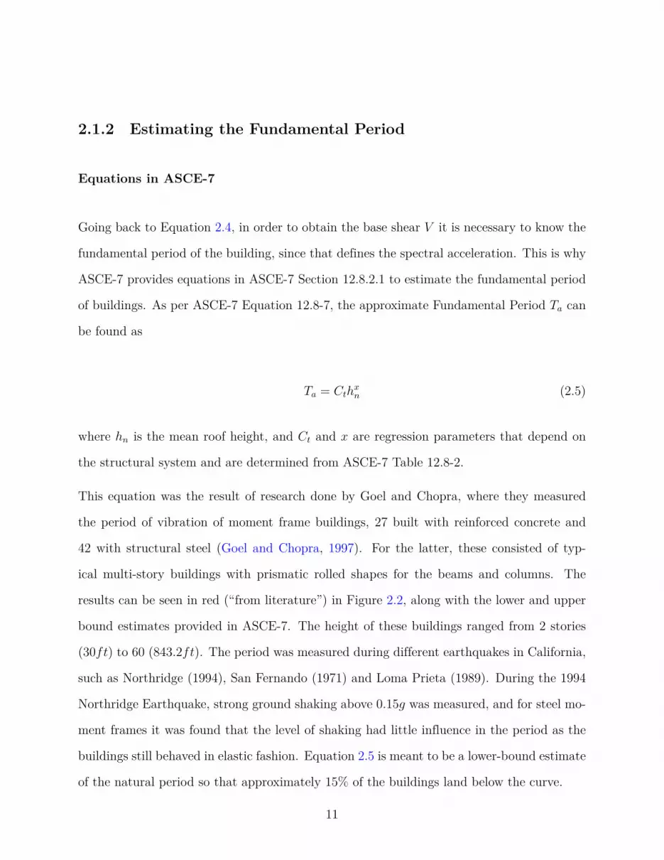
Going back to Equation 2.4, in order to obtain the base shear V it is necessary to know the

fundamental period of the building, since that defines the spectral acceleration. This is why

ASCE-7 provides equations in ASCE-7 Section 12.8.2.1 to estimate the fundamental period

of buildings. As per ASCE-7 Equation 12.8-7, the approximate Fundamental Period Ta can

be found as

Ta = Cthxn (2.5)

where hn is the mean roof height, and Ct and x are regression parameters that depend on

the structural system and are determined from ASCE-7 Table 12.8-2.

This equation was the result of research done by Goel and Chopra, where they measured

the period of vibration of moment frame buildings, 27 built with reinforced concrete and

42 with structural steel (Goel and Chopra, 1997). For the latter, these consisted of typ-

ical multi-story buildings with prismatic rolled shapes for the beams and columns. The

results can be seen in red (“from literature”) in Figure 2.2, along with the lower and upper

bound estimates provided in ASCE-7. The height of these buildings ranged from 2 stories

(30ft) to 60 (843.2ft). The period was measured during different earthquakes in California,

such as Northridge (1994), San Fernando (1971) and Loma Prieta (1989). During the 1994

Northridge Earthquake, strong ground shaking above 0.15g was measured, and for steel mo-

ment frames it was found that the level of shaking had little influence in the period as the

buildings still behaved in elastic fashion. Equation 2.5 is meant to be a lower-bound estimate

of the natural period so that approximately 15% of the buildings land below the curve.

11

Figure 2.2: Comparison of periods of steel moment frames from records for low-to-mediumrise buildings (Kim et al., 2009)

Alternatively, the code allows the computation of the period of vibration via structural

analysis in lieu of using the approximate equation. However, generally speaking the longer

the period, the lower the Spectral Acceleration will be. In turn, ASCE-7 sets an upper limit

on the the computed period in order to prevent unconservative designs due to unreasonable

assumptions in modeling, given that a lower Spectral Acceleration results in a smaller design

base shear. This upper limit is obtained by multiplying the lower-bound prediction Ta by

a factor Cu which is in essence an upper-bound estimate of the period done with the same

database (See Figure 2.2).

Looking closely at Figure 2.2, it is noticeable how there is significant scatter for short build-

ings, implying Equation 2.5 is a poor fit. Scatter is also present for taller buildings, though

more important here is that they results do not fall between the lower and upper bounds.

This is because the only parameter currently included in the period equation is height, but

as buildings become shorter other features may be better at predicting the frame stiffness.

Beyond that, the data set is limited when it comes to buildings below 50ft and there are

12

no buildings below 25ft, which is a common height for metal buildings. Also, the equa-

tion tends to overestimate the period for shorter buildings, at least those included in the

database. Bear in mind the equation was developed for multi-story buildings, far removed

from the single-story metal buildings that have not only vastly different loads and mass, but

different structural configurations as well. Different attempts have been made to develop an

equation that better predicts the period of vibration of single-story buildings in general and

metal buildings in particular, which will be covered below.

Alternative equations for single-story buildings

Lamarche et al. developed an equation for single-story buildings with steel concentrically-

braced frames on their exterior walls, based on regression analysis of 22 measured buildings

using ambient vibration data (Lamarche et al., 2009). These buildings, of course, differ

significantly from both the buildings included in Goel and Chopra (Goel and Chopra, 1997)

and also with typical metal buildings, where the main resisting system is web-tapered built-

up moment frames in the interior bays. However, some interesting conclusions can be taken

from this work. First of all, it showed that including new parameters such as the distance

between lateral load resisting systems (or bay spacing) improved the fit of the predictive

equation significantly for single-story buildings. The proposed formula is

Ta = 0.0035 (Dneffhn)0.7 (2.6)

where Dneff is the effective distance between lateral systems and hn is the same as in ASCE-

7. Both dimensions must be in meters. The inclusion of the bay spacing is because the roof

diaphragm is flexible and produces a lengthening effect on the fundamental period compared

to what would be obtained just by considering the stiffness of the lateral load resisting system.

13

The lengthening effect of diaphragm flexibility in the natural period of single-story buildings

was further studied by Fischer and Schafer, where it can be seen that the natural period

of the building Tb converges to the period of the isolated walls serving as the lateral force

resisting system, Tw, when the diaphragm is rigid (Fischer and Schafer, 2021). In addition,

it can be seen that the mode shape is governed by the deformation of the walls. Similarly, Tb

converges to the period of the diaphragm in isolation, Td, when it becomes fully flexible, with

the mode shape being governed by the deformation in the diaphragm. Meanwhile, when the

period of the diaphragm and the walls are similar, a significant lengthening effect can be

seen, which is a function of the diaphragm mass (Figure 2.3).

Figure 2.3: Building period for one story building with varying wall and diaphragm stiffness,and mass distribution (Fischer and Schafer, 2021)

Second, data showed that non-structural components had a significant effect on the measured

period. Tests were carried out both during construction and in service, and a decrease in

period of up to 38% was observed, implying that non-structural walls were adding significant

stiffness to the buildings. Tremblay and Rodgers modeled these structures considering only

the structural elements and found their predicted periods to be also much longer than those

measured in the field once the cladding was installed, even though it provided a good match

14

during construction (Tremblay and Rogers, 2011). The authors argue that the discrepancy

can be attributed to the low levels of vibration during testing, which is orders of magnitude

lower than the ones the structure will be subjected to during an earthquake event and

was captured by Goel and Chopra, putting into question the use of ambient vibrations

for period estimation. However, it must be mentioned that their models did not include

the effect of non-structural components for its period prediction, which has been shown to

underestimate the stiffness of structures even for design-level wind loads (Bajwa, 2010; Bajwa

et al., 2010; Gryniewicz et al., 2021; Kim et al., 2009). In any case, looking specifically at

roof diaphragms, experimental tests on roof specimens by Rogers and Tremblay show that by

increasing the amplitude of vibration, the natural period of the diaphragm quickly reduces

quite significantly, most probably due to overcoming internal friction at the connection level,

though the repercussions of this were not explored (Rogers and Tremblay, 2010).

It is also worth pointing out that the dataset from (Rogers and Tremblay, 2010; Tremblay

and Rogers, 2011) had untopped Wide-Rib steel deck for roofing and not standing-seam

roofing, the former being known to provide diaphragm action while the latter is assumed not

to. This, in turn, means that the results from their work cannot be extrapolated to metal

building systems, neither in terms of the effects of cladding and non-structural elements, nor

with respect to the natural period itself.

Proposed equation for metal buildings

Compared to the previous equations that were developed based on experimental testing,

Smith and Uang derived an expression specific for metal buildings by doing a regression

on the analytical computed period of over 100 buildings (Smith and Uang, 2013). There is

precedent to using analytical modeling for the purpose of developing a period equation. For

example, the period estimation formula for steel braced-frames within the National Building

15

Code of Canada (NBC 2015, 2015) was developed based an analytical study by Tremblay

(Tremblay, 2005).

For metal buildings, the proposed equation by Smith and Uang was a function of the seismic

weight W in kips, the span-to-height ratio α and the mean roof height of the building hn in

inches given by

Ta =

0.058 (Whn)

0.3 α ≤ 3

1.58W 0.16/α α > 3

(2.7)

As mentioned in the previous paragraph, α is the span-to-height ratio, taken as the maximum

ratio between the width of each bay and its mean roof height, which may differ in modular

frames. For clear span frames, α becomes the ratio between the main span and hn.

Figure 2.4 shows how the natural period changes with the span-to-height ratio and the

seismic weight for a given mean roof height. First, it can be seen that the ASCE-7 equation

stays constant as it does not include any other parameter beyond mean roof height, while

the Smith and Uang equation does show variation. More importantly, the latter formula is

discontinuous at α = 3, which at first glance is unintuitive and would need further revision.

Figure 2.4: Comparison between Smith and Uang formula and ASCE-7 formula for a givenmean roof height (Kumar et al., 2020)

16

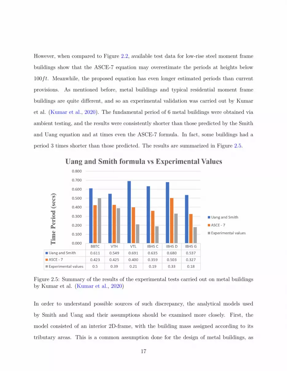
However, when compared to Figure 2.2, available test data for low-rise steel moment frame

buildings show that the ASCE-7 equation may overestimate the periods at heights below

100ft. Meanwhile, the proposed equation has even longer estimated periods than current

provisions. As mentioned before, metal buildings and typical residential moment frame

buildings are quite different, and so an experimental validation was carried out by Kumar

et al. (Kumar et al., 2020). The fundamental period of 6 metal buildings were obtained via

ambient testing, and the results were consistently shorter than those predicted by the Smith

and Uang equation and at times even the ASCE-7 formula. In fact, some buildings had a

period 3 times shorter than those predicted. The results are summarized in Figure 2.5.

Figure 2.5: Summary of the results of the experimental tests carried out on metal buildingsby Kumar et al. (Kumar et al., 2020)

In order to understand possible sources of such discrepancy, the analytical models used

by Smith and Uang and their assumptions should be examined more closely. First, the

model consisted of an interior 2D-frame, with the building mass assigned according to its

tributary areas. This is a common assumption done for the design of metal buildings, as

17

roof diaphragms of all types are usually treated as flexible – carrying no in-plane stiffness –

while neglecting the added stiffness of girts and purlins (MBMA, 2019b). Work by Bajwa et

al., who applied point loads one frame at a time in a metal building showed that the frame

stiffness was being affected by the constraint added by the secondary framing (Bajwa et al.,

2010). This was corroborated by developing a 3D-model of the structure, which provided

much better predictions than the 2D-Frame analysis (Bajwa, 2010).

Also, the flexible diaphragm assumption makes it so that the endwalls or endframes do not

affect the period of the building at large, as every bay is assumed to work independently.

As for the main frame model itself, the beams and columns were modeled as non-prismatic

elements, obtaining the element stiffness matrix by inverting the flexibility matrix (including

shear deformations) and lumping masses at nodes distributed along the elements. Despite

the low weight of metal buildings, both P −∆ and P −δ effects were included in the analysis

by use of the Geometric Stiffness matrix and a leaning column to add the second order effects

of the walls.

For steel moment frames usually the most important aspects of the model are defining

the boundary conditions and modeling the panel zone. In this case, the supports at the

base of the columns were idealized as pinned supports which is consistent with industry

practice, even if it has been shown that typical connection do offer some kind of rotational

restraint (Bajwa, 2010; Verma, 2012). Meanwhile, to account for the influence of panel

zone deformations, a new model was developed by introducing a rotational spring where the

inside flanges of the beams and columns meet, linked rigidly to their respective centroids.

This rotational spring was calibrated for each frame via a 3D Finite Element Analysis of the

connection using shell elements. Industry practice usually defaults instead to the use of a

centerline model with no rigid end zones due to its simplicity over any explicit modeling of

the panel zone MBMA (2019b).

18

From all of the above it can be concluded then that the Smith and Uang formula was

developed using almost every assumption that would increase the flexibility of the building. It

must be noted, however, that shear deformations, P −∆ effects and panel zone deformations

are not so much assumptions but actual components of frame flexibility. However, possible

stiffening effects (from base fixity, non-structural elements, diaphragm action, global system

behavior, etc.) where ignored. These assumptions may explain the overestimation of the

natural period of metal buildings when compared to the measured values by Kumar et al.

(Kumar et al., 2020).

2.1.3 Force distribution along its members

Another important aspect of the ELF approach is correctly assigning the load carried by each

frame of the lateral force resisting system along their height given the computed base shear.

In the case of metal buildings, which are typically single-story, the distribution along the

height reduces to applying the full equivalent force as point loads at the roof. Though ideally

this load should be distributed evenly across the rafter beam to simulate the distributed mass,

it’s usually recommended to apply the load as two point loads at both beam-column joint

nodes (MBMA, 2019b), as shown in Figure 2.6. This results in a less conservative estimate

of the axial load in the beam compared to applying the full load at just either one of the

joints.

Note that, though the MBMA Guide does mention the possibility of using more refined

approximations for the application of the distributed load, it does not provide clear recom-

mendations. In fact, it only mentions the possibility of including applied forces at every

beam-column joint, which may somewhat improve the results for modular metal buildings.

However, the load should ideally be applied wherever the mass is, and so the actual loading

19

Figure 2.6: Example of loading on a frame for illustrative purposes, taken from Smith andUang (Smith and Uang, 2013)

condition more closely resembles that of a distributed load at the roof level. This is im-

portant not only because it provides a better estimate of the axial force in the beams, but

also because it can more accurately capture the bending moment that appears in the beams

due to the roof pitch. In gabled, high pitched roofs, the added bending effect due to the

distributed horizontal loading (whi has a component perpendicular to the roof)) could be

significant and should be taken into account, especially considering that metal buildings are

optimized following the bending moment diagram.

As for how to assign the load to each frame, this would depend on the stiffness of the

diaphragm compared to the frames. A flexible diaphragm, assumed to carry no shear, makes

it so that the load in each frame is proportional to its tributary mass. On the other hand, a

fully rigid diaphragm that forces rigid movement at the roof level would distribute the loads

in accordance with the frame stiffness.Most diaphragms usually fall in between, and a full

3D-analysis would be required including the actual diaphragm stiffness. In early design of

typical mid-rise buildings, the worst-case scenario of both options can used to initialize the

size of the members.

20

Implied in the diaphragm classification is that the diaphragm stiffness is measured relative

to the stiffness of the lateral system. In turn, ASCE-7 has both prescriptive and analytical

ways to classify the diaphragm in ASCE-7 Section 12.3, which depend not only on the type

of diaphragm but also on the structural system. ASCE-7 Article 12.3.1.1 provides different

structural systems where the diaphragm can be idealized as flexible. If the diaphragm

consists of an untopped steel deck, then it can be considered flexible if any of the following

is true:

• The main lateral force resisting system consists of Steel-Braced Frames or Shear Walls

• The building is an up to two-story family dwelling

• Specific types of light-frame construction (wood structures)

From the above it follows that metal buildings are not by default included by the provision. In

those cases, ASCE-7 Equation 12.3-1 can be use to justify the idealization of the diaphragm

as flexible

δMDD

∆ADV E

> 2 (2.8)

where δMDD is the the portion of the deflection attributed to the diaphragm and ∆ADV E

is the portion of the deflection attributed to the frames when a distributed load is applied

across the diaphragm.

An example on how to apply this provision can be found in Chapter 9 of Charney et al.

(Charney et al., 2020). The structure analyzed, with reinforced concrete shear walls and

slab, can be seen in Figure 2.7, which was loaded with a distributed load in the plane of

the diaphragm at the diaphragm level (assigned as point loads at each node in of the ends

21

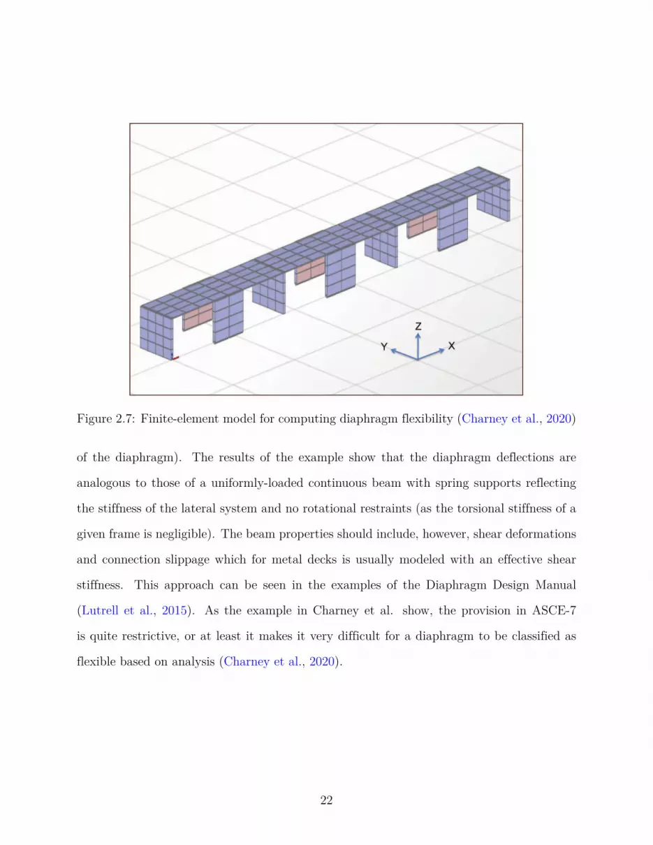
Figure 2.7: Finite-element model for computing diaphragm flexibility (Charney et al., 2020)

of the diaphragm). The results of the example show that the diaphragm deflections are

analogous to those of a uniformly-loaded continuous beam with spring supports reflecting

the stiffness of the lateral system and no rotational restraints (as the torsional stiffness of a

given frame is negligible). The beam properties should include, however, shear deformations

and connection slippage which for metal decks is usually modeled with an effective shear

stiffness. This approach can be seen in the examples of the Diaphragm Design Manual

(Lutrell et al., 2015). As the example in Charney et al. show, the provision in ASCE-7

is quite restrictive, or at least it makes it very difficult for a diaphragm to be classified as

flexible based on analysis (Charney et al., 2020).

22

2.1.4 Assumptions Made in Metal Building Design

From the previous sections it becomes noticeable that there are some gaps in the current

provisions regarding how to analyze metal buildings, and this is without taking into account

discussions on the ductile mechanism of web-tapered moment frames, the appropriate value

of R and other details regarding the seismic behaviour of the main lateral load resisting

system, which have spurred other research projects funded by the MBMA.

First of all, the classification of the roof diaphragm in metal buildings is not explicitly covered

by ASCE-7, which in theory would require to apply Equation 2.8 before proceeding with a

flexible diaphragm model. In practice this is not done, and roof diaphragms of all types are

considered flexible for the design of metal buildings (MBMA, 2019b).

The two most common types of roof cladding used are of the untopped steel variety: the

Standing-Seam Roof (SSR) and the Through-Fastened Roof. Through-fastened roofing is

the older of the two (Newman, 2015) and is not much different in essence to the metal

sheeting commonly used in walls. It consists of corrugated cold-formed steel panels that are

lapped together and fastened to the purlins by self-tapping or self-drilling screws. Meanwhile,

Standing-Seam Roofs attach the panels to the secondary framing by virtue of concealed clips.

This configuration reduces possible leakage due to drilling while also allowing for more

mobility, reducing problems related to thermal expansion. However, due to clip slipping

these roofs tend to be a lot more flexible than through-fastened roofing.

Even if through-fastened roofing is known to provide diaphragm action, and recent studies

by Wei et al. (Wei et al., 2020) have shown that the SSR does provide some stiffness (which

could be used to provide lateral buckling restraint to the purlins), it is still current practice to

consider the diaphragm as fully flexible without following ASCE-7 Equation 12.3-1 (MBMA,

2019b).

23

This leads, however, to some oddities in the design of metal buildings. It is common for the

inner bays to consist of web-tapered moment frames, with the endwalls being concentrically-

braced frames. Having two different structural systems along the same direction would

typically lead into estimating the building period in accordance with ASCE-7 Table 12.8-2

as “other”. However, given the flexible diaphragm assumption above it could be possible to

treat each bay as its own independent structure, treating the interior bays as “steel moment

frames” and the exterior bays as “other”. This is not what Equation 2.5 was derived for, given

that it was the result of measuring the global behavior of buildings with clear and specific

structural systems, and there is nothing that would imply that the equations would hold up

for individual frames of a given building. This becomes more egregious when considering

the equations themselves were derived with data from mid-rise buildings, and – whether

the diaphragm could classify as flexible or not – a single period for the whole structure was

extracted. Moreover, the results from Kumar et al. imply that that mode shapes of metal

buildings are also global in nature, and may not be directly related to the period of each

individual bay (Kumar et al., 2020). This also warrants a discussion on the accuracy of the

flexible diaphragm assumption.

2.2 Structural modelling of the main lateral resisting

system

If an analytical model of a metal building were to be built for the purpose of estimating the

natural period, then accurately predicting the stiffness of the primary framing is evidently

of great importance. For structural steel, the modulus of elasticity is quite consistent and

so most of the uncertainty comes in how the connections are modeled, as well at what

assumptions are made in the development of the frame element.

24

In turn, the focus ends up being placed on whether or not to include shear deformations,

how to account for the panel zone deformation and how to correctly model the boundary

conditions.

2.2.1 Modeling of web tapered elements

The American Institute of Steel Construction (AISC) has provided guidelines on how to

model web tapered members since 2011, with the second edition of the Design Guide coming

out in 2021 (White et al., 2021). Within, two methods are identified for modeling frame

elements. The first consists in discretizing the non-prismatic frame into shorter, prismatic

elements. This is essentially a finite element approximation, and the results will converge to

the true solution as the length of each discretized frame tends to zero.

Alternatively, the element stiffness matrix of the frame can be obtained through the inversion

of its flexibility matrix (Charney, 2008; McGuire et al., 2020). The main advantage of this

approach is the the exact solution can always be obtained as long as the variation of the

members sectional properties and centroid along the length are accurately described. It also

allows for simple, direct inclusion of shear deformations if so desired.

One of the difficulties with modeling web tapered members is that the centroidal axis is no

longer linear if the the section isn’t symmetric (i.e., the flanges have different thickness). In

that case there is an interaction between axial forces and bending moments. Though this

can be captured by the formulation described above, in some implementations this effect is

ignored, treating the centroidal axis as linear between nodal points (Smith, 2013). The loss

of accuracy due to this simplification is assumed to be small, especially if the member is

discretized along its length anyway to obtain a more realistic lumped mass representation

or to include P − δ effects in the analysis.

25

Finally, a similar difficulty with modeling web tapered members is how to properly account

for changes in flange or web thickness in non-symmetric sections. This change would create

a discrete jump in the centroid at the location of the discontuinity. For this case, AISC

Design Guide 25 proposes two options. The first (and “exact”) solution would be to include

a rigid link connecting the centroids at each end of the discontinuity. A simpler, approximate

approach would be to ignore this effect and slightly modify the node locations so that rigid

links can be avoided. Given that the shift in the location of the centroidal axis is very small

in comparison to the depth of the member, this second approach is reasonable and has been

used by Smith in the development of the metal building frame models (Smith, 2013).

As for how commercial software handles non-prismatic elements, the precise formulation is

not open-source and so no specific details can be provided. It is assumed, however, that

SAP2000 (CSI, 2021) uses a very similar framework to the one described above assuming a

linear centroid, as the only parameters that are input into the program are the start and end

cross sections, along with the assumed variation in the moment of inertia along the length.

2.2.2 Shear Deformations

Plenty of research has been done on what the main sources of deformation in steel moment

frames are, though most of this work has been done for mid to high-rise buildings. Charney

et al. found that shear deformations in the beams and columns could account for 8 to 26%

of the total displacement, the massive range being dependent on the clear span of the bays

and total number of floors (Charney et al., 2005). Metal buildings, however, fall out of the

range of the study, as they are usually 1-story buildings with a clear span of up to 100ft,

while the study covered bays with 10 to 20ft spans. Since the influence of shear decreases

with span length (as flexural behavior becomes dominant) it would be expected for metal

26

buildings to be much less sensitive to the inclusion of shear deformations in the analysis.

Smith and Uang analyzed the effect of shear deformations on 192 2D-models of metal build-

ings designed per current standards (Smith and Uang, 2013). Results showed that not

accounting for the effect of shear deformations would result in an overestimation of the stiff-

ness of about 5% in the worst-case scenario, with the average difference being close to 2%.

Considering that the natural period is proportional to the square root of the stiffness, then

neglecting shear deformations would result in a 1% underestimation of the period on average.

Based on these findings, the authors conclude that the inclusion of shear deformations is

not necessary for metal buildings. However, currently most structural analysis software is

able to account for it with no meaningful difference in computational cost. In fact, SAP2000

(CSI, 2021) has it on by default in their element formulation, and so there is no real reason

not to include them.

2.2.3 Panel Zone Deformations

Correctly accounting for panel zone deformations is harder to model than the former case,

as it may require a full finite element analysis of the of the panel to find the parameters that

need to be introduced into a simplified model of the connection (there are ways to estimate

the values given the sectional properties of the connection, and the reader is referred to

(Charney and Marshall, 2006) for more information). Panel zone deformations – a function

of panel zone shear and joint flexural deformations – can have a significant effect on story

drift.

At the subassemblage level, deformation of the panel zone in shear explains around 25% of

the total drift, while flexural deformations can account for 10% of the total drift (Charney

and Pathak, 2008a,b). This last result is significant because flexural deformations at the

27

joint level is not included in the most common panel zone models such as the Krawinkler or

Scissors models (Charney and Marshall, 2006).

Figure 2.8: Panel Zone Model Comparison (Smith and Uang, 2013)

In their analysis of metal buildings, Smith and Uang (Smith and Uang, 2013) used a cus-

tom model that consisted of a rotational spring where the inner flanges of the beams and

columns meet, linked to the centerline of each element through a rigid link (Figure 2.8a). As

mentioned before, this rotational spring was calibrated based on 3D Finite Element Analysis

of the connection using shell elements for its components. The choice in spring placement in

the proposed model was to obtain compatible deformations in the panel zone region, whereas

the centerline and scissors models assume unrealistic deformed shapes (such as allowing over-

lap between the column and beam flanges under negative moments) (Smith, 2013). Similar

results can be obtained when using the revised Krawinkler model (Charney and Marshall,

2006).

The use of more sophisticated models to compute drift in metal buildings is not standard

in the industry, which favors instead using a centerline model, either considering rigid frame

elements within the panel (rigid endzones), or simply extending the cross-sectional properties

of the beams and columns. The rigid endzone model, though commonly used for concrete

moment frames, has been shown to underestimate drift. The centerline model with no rigid

endzones, however, provides reasonable estimates for steel moment frames due to offsetting

28

inaccuracies. On one hand, it underestimates shear deformations at the joint level. On the

other hand, extending the beams and columns properties in the endzone rigions overestimates

the bending moments, and in turn results in larger overall deflections of the frame elements.

Charney and Pathak showed at the subassembly level of a typical steel moment frame that the

centerline model could underestimate displacements by 10% (Charney and Pathak, 2008a).

Smith and Uang arrived to similar conclusions in their own study, with the deflections of

the frames modeled with their panel zone model could be up to 15% more flexible than the

same frame using a centerline model (Smith and Uang, 2013). However, from a statistical

standpoint the models with the centerline model had on average a difference of 0.2% com-

pared to the more sophisticated ones. This result is actually quite interesting as it implies

that, even if the results have scatter, the centerline model actually does a very good job of

predicting the general behavior of the frames, which justifies its use in practice.

2.2.4 Base Fixity

Explicit modelling of the actual boundary conditions at the column base, similar to the

effect of panel zone deformations, is also not usually done in practice due to the cost and

complexity associated with it, even if in recent years there have been attempts to streamline

the process through automated applications (Verma, 2012). The connection of the columns to

the foundation is usually resolved by welding an endplate which is then bolted into place with

at least 4 anchor bolts (Newman, 2015). The overall rotational stiffness of the connection is

mostly controlled by the size of the column, the size and thickness of the baseplate, and the

number and location of the anchor bolts.

The main deflection mechanisms are, then, the bending of the end plate and the deformation

under stress of the anchor bolts in tension, with the column pivoting from the extreme

29

Figure 2.9: Modeling of Column-to-Base Connection when Base Plate is Flexible (Bajwaet al., 2010)

compression fiber of the baseplate (Figure 2.9). Flexibility of the underlying soil can also

play an important role, especially if the column has an isolated foundation.

For design purposes, metal buildings forego a detailed analysis of the column connection and

are instead designed as either fully fixed or fully pinned. Due to the lower total monetary

cost of the design, the pinned solution is the overwhelmingly favored choice (Newman, 2015).

Smith and Uang, following this design methodology, did not include the effect of base stiffness

in the analysis of 2D-frames (Smith and Uang, 2013). Their modeling approach was justified

based on full scale shake table testing of two metal building frames, that showed that, due to

the deformation of the base plate creating a dishing effect, there was essentially no rotation

stiffness of the column base for rotations smaller than 0.02rad. The behavior, however,

was extremely nonlinear. For larger rotations, contact between the flanges and the base

would impede the previous motion and significantly increase the rotational stiffness of the

connection (Smith, 2013).

On the other hand, Bajwa et al. studied the effect of the base rotational stiffness in the overall

stiffness of a metal building frame and found that, in theory, the stiffness lies somewhere in

between the pinned and fully fixed options (Bajwa et al., 2010). This is significant since the

30

difference in the drift estimation between the two extreme cases was found to be a factor

of 2. Similarly, Kumar et al. found that the fundamental period of a metal building in

Christiansburg, VA, obtained via a 3D Finite Element Model could decrease by 40% when

modeled with fixed supports instead of pinned, with the measured period lying in between

the two of them (Kumar et al., 2020).

2.2.5 Discussion

Previous subsections focused on different modelling aspects for the main frame of a metal

building, working under the assumption that a 2D-model of the bare frame is enough to

fully characterize the stiffness and – in consequence – the natural period. However, previous

experiences (Bajwa et al., 2010; Kumar et al., 2020; Lamarche et al., 2009) show that there

may be a significant difference in stiffness between the bare frame and the building in service

for single-story buildings, and that the Smith and Uang equation, developed using said

analytical models, seems to overestimate the natural period.

The effect of non-structural elements has been studied before for different structural sys-

tems. Kim et al. performed a literature review of reported differences between modeled and

measured periods of vibration, and found numerous cases where – when modeling only the

bare frame – the analytical period was overestimated by 40 to 70% in reinforced concrete

structures (Kim et al., 2009). He then proceeded to calibrate a sophisticated 3D-FEM of

3 different buildings and found that including the flexural stiffness of the diaphragm and

modelling the non-structural walls could reduce the inaccuracy by half, with the rest of the

difference explained by the actual modulus of elasticity of concrete compared to the one used

in design.

31

As mentioned before, Bajwa et al. attempted to use a detailed 2D Finite Element Model of

the main frame of a metal building with a standing-seam roof to predict drift (Bajwa et al.,

2010). As part of an experimental test, a force of a magnitude similar to the design wind load

was applied to the different bays of the structure, one at a time, with the deflection being

measured at the loaded frames and the adjacent ones. The model, which included shear

deformations, panel zone deformations and explicitly modeled realistic boundary conditions

still overestimated the drift by up to a factor of 2. It was not until a full 3D-model of

the structure was built using shell elements for the primary and secondary framing – and

including the added stiffness of the endwall and roof cladding – that better correlation

between the measured and tested displacements were reported (Bajwa, 2010). However,

even if the displacement on the internal frames was correctly accounted for, there were still

significant differences between the measured and predicted values of the displacements for

the endwalls, where most of the stiffness is provided by the cladding.

A very similar analysis was carried out by Wrzesien et al. (Wrzesien et al., 2015). In this case,

however the test was repeated for two different cases: First, with just the bare frame; second,

with the roof cladding installed. The experimental tests were used to validate the full 3D-

modeling of two different single-story building with cold-formed portal frames and through

fastened roofing. The framing model considered all column bases as ideally pinned and used

frame elements for the primary frames instead of using shell elements for the web and flanges,

and neglecting the secondary framing. Meanwhile, for the roof diaphragm an equivalent truss

element was used. The model generally agreed with the experimental results, which showed

the stiffness of the building increased by a factor of 10 due to diaphragm action of the roof,

since it in turn made the stiffer exterior frames to participate in the load distribution. Note

that, in Bajwa et al., which had a standing-seam roof, only limited diaphragm action was

seen, with each bay working fairly independently of each other.

32

Perhaps the most detailed calibrated model for single-story buildings including the cladding

was developed by Gryniewicz et al. (Gryniewicz et al., 2021). In this case, the structure

was quite similar to a metal building with gabled frames for endwalls and a truss beam

for a rafter in internal frames. The building was tested by applying a point load of 50%

the service wind load for the structure to behave in its elastic range in 3 different phases:

The bare frame; the frame with the roof installed and the completed building with the wall

sheeting. From the experimental tests it could be seen that the roof cladding increased

significantly the combined behavior of the frames, reducing the displacement at the loaded

frame by a factor of 3, and evening out the displacements of all the bays, the diaphragm

behaving as essentially rigid. Beyond that, the tests on the full building proved that, even

if the sheeting was not designed for diaphragm action, it still increased the stiffness of the

endwalls significantly, which in turn caused the displacements to drop by a factor of 10. Also,

since in the last test the walls were so much stiffer, the building exhibit more of a flexible

diaphragm behavior than in the second test, when only the roof was present. Going by the

work of Fischer and Schafer (Fischer and Schafer, 2021), it is fair to assume the stiffness of

the walls and roof was relatively close.

A 3D-model of the building was also developed and validated against the experimental

tests results (Gryniewicz et al., 2021). This consisted of frame elements for the main and

secondary framing, with its supports idealized as pinned. This is, again, a much simpler

and fairly standard approach to modelling framing. Instead, a large focus was put into

modelling the cladding. In this case, an orthotropic plate model was used to analyze the

panels, but a lot of care was put into its connection to the secondary framing, by using

spring supports to the purlins and girts for each of the fasteners in the roof. This level of

detail is, of course, prohibitive in design, as it is common for different people and trades

to be in charge of the main framing and the cladding respectively. For the wall cladding,

33

meanwhile, a simpler approach was used by defining a single effective shear modulus for the

whole diaphragm. However, the results were remarkable, with a 5% difference between the

estimated and measured displacements for the main frame tests, which stayed consistent in

the subsequent tests.

All these experiences show that modelling of the steel cladding elements could be essential

to adequately describe the behavior and stiffness of single-story buildings, and could even

accurately predict their non-linear response and collapse load (Roberts et al., 2021). Though

it is true that the the latter two case studies (Gryniewicz et al., 2021; Wrzesien et al., 2015)

both had Through Fastened Roofing, whose in-plane stiffness is believed to be significantly

higher than SSR, it seems as though 2D-modelling may not be enough for the SSR case

either. This puts into perspective the previous look into the main parameters and modelling

assumptions that influence the stiffness of metal buildings. If the main frame is relatively

only a small portion of the overall stiffness of the building, then it is valid to ask whether

it’s necessary to put most of the effort into it. Instead, it may be worth looking at the added

stiffness provided for cladding and how it can be modeled. Note, however, that the cladding

is not designed to carry lateral load.

2.3 Modeling of steel sheeting

Analytical modeling

Defining the stiffness of metal panels used in cladding is not an easy endeavor. First of all,

the panels themselves tend to be orthotropic in nature due to their one-way corrugation. In

shear, one of the main sources of deformation is the warping or distortion of the sheet due

bending of the corrugation, and then pure shear deformation. Given that the most common

34

way to model panels is by using flat plate elements, properly accounting for the behavior

would require finding equivalent rigidities to input to a flat plate model. One of such models

was proposed by Xia et al., and it is notable that not even an orthotropic model is able to

match all 8 rigidities described in the paper, as an orthotropic model only has 5 parameters

compared to 2 for an isotropic model (Xia et al., 2012).

Another significant deformation source of diaphragms is at the connection level. Both the

seam-fasteners splicing adjacent panels and the fasteners used to attach the cladding to the

girts and purlins create flexible connections that significantly reduce the overall stiffness of

the diaphragm in shear. This, in turn, means that the number, type and location of the

fasteners play a significant role in the overall behavior of the diaphragm and careful con-

sideration of the boundary conditions is required. In Bajwa (Bajwa, 2010), the boundary

conditions were modeled as roller supports in the corners of the panels, which probably

underestimates the stiffness provided by the connections. This becomes noticeable when

looking at the discrepancy between the measured and predicted displacements of the end-

walls. Gryniewicz et al., meanwhile, explicitly modeled each fastener as a spring support

connected to the secondary framing (Gryniewicz et al., 2021). The latter approach, though

it showed exceptional accuracy, is extremely costly and time consuming as it requires careful

modeling of every fastener, including its stiffness, and is not practicable for design consider-

ations.

2.3.1 Developments in the U.S.

The difficulties in predicting the stiffness of diaphragms through analytical procedures for

different types of sheeting profiles and connection types led to extensive experimental re-

search both in the U.S. and in Europe. In North America, extensive testing was done by

35

Larry Luttrell since 1965 (Luttrell, 1965), first as a Graduate Student in Cornell and then as

a Professor at the University of West Virginia. The results of his work are summarized in the

Steel Deck Institute’s (SDI) Diaphragm Design Manual, which is periodically updated and is

now in its fourth edition (Lutrell et al., 2015). The equations have not changed much since

they were first published and are now part of AISI S310-16, the North American standard

developed by the American Iron and Steel Institute (AISI S310-16, 2016). However, every

time a new deck system is developed, experimental tests are needed to create equations to

estimate their strength and stiffness in the same fashion. Considering that roof decks are in

constant evolution, a large number of tests have been done recently such as for aluminum

decks (Avci et al., 2016), cassette diaphragms, sandwich panels and Standing Seam roofs

(Davies and Bryan, 1982; Wei et al., 2020). The special case of diaphragms attached to

wood structures can be found in the book A Primer on Diaphragm Design (Luttrell and

Mattingly, 2004).

Figure 2.10: Diaphragm distortion for shear strength and shear stiffness calculations (Avciet al., 2016)

In any case, the stiffness of a roof or wall assembly is obtained by doing a cantilever test. A

schematic of the test setup can be seen in Figure 2.10 for a roof assembly specifically, placed

36

horizontally. It should be noted that, in all these tests the orientation of the panels stays

perpendicular to the span (i.e., the panels are fastened to the purlins which are perpendicular

to the applied loading), and all four sides are fastened, which greatly increases the stiffness

as it allows for the transfer of forces to the edge members in tension compared to when only

two sides are fastened. By measuring the force P required to impose a deflection ∆, it is

possible to find the distortion γ = ∆/a and the average shear stress τ = P/ (bt), where a

and b are the dimensions of the assembly and t its thickness. Then, treating the assembly

as an isotropic plate, the effective shear modulus G can be found as

G =τ

γ=

P

bt

a

∆(2.9)

The result, however, is more commonly reported as a stiffness G′ as it is independent of the

thickness and can be directly measured during testing as

G′ = G t =Pa/b

∆(2.10)

where Pa/b is the reaction at the supports. The predictive equation for the stiffness, as

presented in AISI S310-16 is

G′ =

(Et

2 (1 + µ) sd+ γcDn + C

)K (2.11)

where

• E is the modulus of elasticity of steel

• t is the thickness of the steel plate

37

• µ is the Poisson’s ratio

• d and s are the panel’s corrugation pitch and its width respectively

• K is equal to 1 when fasteners are placed at lap-down into steel supports, and to 0.433

if fasteners are placed at lap-up

• Dn is a warping factor which can be taken as D/L, with D calculated as per Appendix

1 and L being the total panel length. The values of D for different typical panel profiles

can be found in the Diaphragm Design Manual (Lutrell et al., 2015)

• γc is a support factor that considers the number of spans and goes from 1.0 for up to

2 spans to 0.58 for more than 7 spans

• C is a slip coefficient

The slip coefficient C is computed as

C =

(Et

w

)(2L

2α3 + npα4 + 2nsSf

Ss

)Ss (2.12)

where

• w is the cover width of the interior panels

• Sf and Ss are the connection flexibility to the structure and sidelaps respectively

and depend on the connection type. For screws into steel, the values are inversely

proportional to the square root of the plate thickness.

• α3 and α4 are a measure of the distribution of the interior and exterior fastener group

across the panel width.

• ns is the total number of sidelap connections, and np is the number of interior supports.

38

Example

For example, let’s apply this to a 0.0295in thick cold-formed Wide Rib panel Wall used as

a wall diaphragm in a metal building. The length of the panel is 20ft, and each panel has

a width of 36′′ for a total width of 80ft. For a Wide Rib panel, the ratio s/d can be taken

as 1.454, and the warping factor Dn as 53.6 assuming it is fastened at every other valley

as found taken from Diaphragm Design Manual (Lutrell et al., 2015). Also taken from the

Manual, With a 36-4 fastening pattern, α3 can be taken as 1.33. The number of spans is 4,

and so γc = 0.8 and np is 3. ns is 4 assuming one screw per span. Finally, considering the

use of self-drilling screws at lap-down, K = 1, Ss = 0.022 and Sf = 0.0097 as indicated in

AISI S310-16 (AISI S310-16, 2016).

Inserting the appropriate information into Equation 2.12 gives out a value of C = 20 for

the slip coefficient, and finally a stiffness G′ of approximately 13kip/in. Dividing by the

thickness gives an effective shear modulus of about 443ksi, which is only 4% of the shear

modulus of steel (G = 11, 500ksi).

That same wall configuration but used in a 30ft wall with 5 spans would result in G′ =

14kip/in. Similarly, using 15ft the value becomes 11.5kip/in meaning that the effective

shear modulus is not particularly sensitive to building height compared to the configuration

itself. For example, simply changing the fastener pattern at the panel edges to each valley (a

36-7 configuration) instead of every other one would result in Dn decreasing tenfold, causing

the overall stiffness to shoot up to 36.27kip/in. Given the sensitivity of Dn, the engineer

must be careful in its evaluation. Finally, note that, though the results here presented

appear small, the interior frames of metal building systems can have stiffness values as low

as 2kip/in, meaning that cladding could indeed contribute significantly to the building’s

overall stiffness.

39

2.3.2 European approach

The European equations for predicting the stiffness of wall and roof diaphragms were the re-

sult of research Eric Bryan on stressed-skin design, a design approach for buildings where the

sheeting is actively accounted for in the load path as diaphragms (Davies, 2006). The results

of his experimental research with J. Michael Davis led to the publishing of the book “Manual

of Stressed-Skin Design” in 1982 (Davies and Bryan, 1982). The equations presented there

have remained virtually the same since, and were first adopted by European Convention for

Constructional Steelwork in the “European Recommendations for the Application of Metal

Sheeting Acting as a Diaphragm – Stressed Skin Design” (ECCS, 1995). This document was

later adopted by reference by the Eurocode (Davies and Bryan, 1982).

Compared to the approach in AISI S310-16, the equations in the European Recommendations

explicitly distinguish the flexibility of each of the components of the cladding, differentiating

between profile distortion and shear deformation of the sheeting; fastener deformation for

both the seam fasteners and the connections to the girts and purlins; and the axial strain in

the edge members. The sum of all the component flexibilities gives out the total flexibility

of the system, defined as c = ∆/P

Another difference compared to the equations developed by Larry Luttrell is that the Euro-

pean Recommendations do a distinction between diaphragms connected on all 4 sides vs only

2 sides, the latter being a more flexible. Some components of the flexibility also have different

expressions whether the sheeting spans perpendicular to the diaphragm or in parallel.

Revisiting the previous example

This time, let’s look at the equations through an example: the same Wide Rib panels from

before. The reader is referred to the appropriate references for more detail for different cases

40

(Davies, 2006; Davies and Bryan, 1982; ECCS, 1995). The flexibility due to profile distortion

is

c1,1 = α1α4ad2.5K

Et2.5b2(2.13)

where α4 accounts for the number panels along the depth of the diaphragm (only applies to

sheeting perpendicular to the diaphragm); α1 accounts for the number of spans (similar to

γc in the AISI S310-6); a is the dimension of the panel perpendicular to the direction of the

corrugation; b is the dimension of the panel parallel to the corrugation; t is the thickness of

the metal sheet; d is the pitch of the corrugation; K is sheeting constant that depends on the

fastener profile and the properties of the corrugation (pitch and width); and E is Young’s

modulus.

For sheeting parallel to the span, a = 80ft and b = 20ft. For a structural wall, where a

single panel covers the depth of the diaphragm, α4 = 1. α1 becomes 0.70 considering 4 spans

as before (5 girts). d is 6in and t is 0.0295in. K, assuming fasteners in every other groove,

is 0.779. Replacing in Equation 2.13 (in SI units) gives out a value of c1,1 = 0.182in/kip.

The flexibility due to shear strain is given by

c1,2 =2aα2 (1 + µ) [1 + (2h/b)]

Etb(2.14)

where α2 is a function of the number of spans; µ is the Poisson’s ratio; and h is the height or

depth of the corrugation. For the case with 4 spans, α2 = 0.67, and considering a standard

h = 1.25in depth the resulting flexibility is c1,2 = 0.012in/kip (ECCS, 1995). Note, then, how

the deformation of the metal panel is almost exclusively due to distortion of the corrugations.

41

Next, the fastener deformation needs to be computed. The added flexibility by the fasteners

connected to the purlins is

c2,1 =2aspp

b2(2.15)

where sp is the slip per fastener which can be taken as 0.026in/kip (ECCS, 1995); p is pitch

of the fasteners (12in in the example); As a result, the flexibility is c2,1 = 0.011in/kip.

As for the seam fastener deformation, the expression to find the flexibility is

c2,2 =2sssp (nsh − 1)

2nssp + β1npss(2.16)

where ss is the slip per seam fastener (taken as 0.044in/kip) (ECCS, 1995); nsh is the number

of sheet widths per panel (for an 80ft building, this would be 27); ns is the number of seam

fasteners per side lap (4); np the number of purlins, including the edge ones (5); and β1 is

a function of the total number of fasteners per sheet (for 4 fasteners per purlin per width,

β1 = 1.04). Replacing above, the result is c2,2 = 0.137in/kip

The flexibility of connection to the end members differs greatly whether all 4 sides are

fastened or only 2 sides. Assuming 4 sides fastened, the equation is

c2,3 =2Ssc

nsc

(2.17)

where Ssc is essentially the same as sp; and nsc is the number of fasteners per end rafter

(108), which results in a value of c2,3 = 0.00049in/kip.

42

If, instead, only 2 sides are fastened the expression turns to

c2,3 =2

np

(spr +

spβ2

)(2.18)

where spr is the flexibility of the purlin-rafter connection, which can be conservatively taken

as 0.245in/kip (ECCS, 1995); and β2 is a function of the number of fasteners per sheet width

(for 4 fasteners per purlin, the value is 1.11). With these numbers, the flexibility considering

2 sides fastened would be c2,3 = 0.054in/kip, two orders of magnitude larger than if the

panel was fastened on all 4 sides (0.00049in/kip).

With all these flexibilities, the total flexibility in true shear can be computed as

c′ =b2

a2(c1,1 + c1,2 + c2,1 + c2,2 + c2,3) (2.19)

which results in 0.021in/kip for the case with fasteners in all four sides (0.025in/kip if con-

nected in two sides). Finally, the total flexibility can be obtained by adding the deformation

due to axial strain in the edge members

c = c′ + c3 (2.20)

with c3 = 2b3/3EAa2, where A is the area of the edge element. Assuming a W10x60 column

(A = 17.6in2), then c3 = 1× 10−5in/kip and the total flexibility c becomes 0.025in/kip. In

order to be able to compare this number with the G′ value obtained using AISI S310-16, it

is necessary to remember that1)

1The Equation is rewritten acknowledging a and b are inverted in the European Recommendations com-pared to Figure 2.10

43

G′ =P

∆

b

a, c =

∆

P(2.21)

from which follows that G′ = b/ac. Using the values from the example the European

Recommendations estimate a stiffness of 11.7kip/in, which is quite similar to the result

obtained before (14kip/in). It’s also notable that accounting for only 2 sides fastened would

drop the value to 10kip/in. Though not a significant change in this particular example,

the effect is more notable with the increase in number of fasteners, as the flexibility due to

profile distortion becomes less of a factor compared to the added flexibility of having only

two sides fastened.

2.3.3 Limitations of current empirical equations

As mentioned before, the cladding industry is constantly coming up with new systems and

sheet profiles that differ greatly from the original setups that were tested, and research can’t

keep up. One such example is the patented metal sheeting developed by Strukturoc (US

Patent 7,661,235 B2), which is essentially a flat plate with hidden fasteners and a male-

female sideclip creating a friction connection between adjacent panels (Figure 2.11). No

stiffness data is publicly available for this system. It could be argued that these panels

resemble a cassette profile. In that case, Davies argues that European Recommendations

can be used while neglecting the added flexibility due to profile distortion (i.e.: assuming

K = 0) as the panel is flat (Davies, 2006). Also, since the system does not make use of

seam-fasteners, the flexibility may be greatly increased similarly to a standing-seam roof

and bear no real structural strength or stiffness.

Similarly, there is little information on the stiffness standing-seam roofs despite their popu-

larity. Given their limited diaphragm action, as shown by Bajwa et al. (Bajwa et al., 2010),

44

Figure 2.11: Profile of the Strukturoc system (Strukturoc, Inc.)

both AISI S310-16 and the European Recommendations neglect their stiffness altogether

(AISI S310-16, 2016; ECCS, 1995). Knowing the stiffness, however, could be important to

obtain an accurate estimate of the natural period that can capture what is measured in the

field. Work by Wei et al. found small values of stiffness K – measured as the deflection at

midspan of a “simply supported” diaphragm due to a point load in the longitudinal direc-

tion (See Figure 2.12) – that could vary from 0.087kip/in to 8kip/in with a median value

of about 0.5kip/in depending on the clip and panel profile type (Wei et al., 2020). Most of

the deformation seemed to be explained by the deformation of the clips.

To convert the K stiffness values to a shear stiffness G, the solution to a simply supported

beam to a point load (including shear deformations) needs to be analyzed. For the purpose

of this analysis and just to get an approximate number, the portion of the displacement due

to flexure will be ignored. Given a point load P at midspan, the absolute value of the shear

in the deep beam remains constant at V = P/2. From there it follows that the displacement

δ at midspan is

δ =

∫ a/2

0

V

bG′ dx =V

2

a

bG′ =Pa

4bG′ (2.22)

Then, considering that K = P/δ, the stiffness G′ can be obtained as G′ = Ka/4b. Consid-

ering the tests had a length a of 22ft and a width b of either 9ft or 6.5ft depending on the

45

Figure 2.12: Schematic view of instrumentation layout (Wei et al., 2020)

panel width, the value of G′ for the SSR may be around 0.3kip/in which is indeed orders of

magnitude smaller than typical through fastened roofing and virtually negligible. However,

the tests had significant scatter, with some specimens reaching 2kip/in (No. 5 and 6) and,

in one case (No. 4), reaching a stiffness upwards of 7kip/in. This later number is closer in

range to what through-fastened roofing, not designed for diaphragm action, could provide. It

should be noted as well that most of the deformation in these tests was due the deformation

of the clips, which were working in the minor axis. However, the expected diaphragm action

between frames would find the clips acting in their major axis. Moreover, extrapolating the

results from tests to roof assemblies proves challenging as the connection of the roof to the

eaves can significantly increase the stiffness of the diaphragm, but the effect is dependent on

scale. Also, any test setup that does not include this connection would underestimate the

stiffness, as argued by Fisher and Nunnery (Fisher and Nunnery, 1996). In fact, the authors

46

recommend measuring the stiffness with a cantilever test with the purlins opposed. All this

means that the measured stiffness by Wei et al. may not be representative of the behavior

in the transverse direction for the purposes of evaluating the diaphragm action and inclusion

in a 3D-model.

In the end, the limited amount of information available for newer metal building construc-

tion makes it extremely hard to predict their natural period through analytical models since

the current available equations mostly do not apply to many types of common cladding.

Parameter calibration and narrowing down the potential stiffening effects of cladding via

experimental testing is then necessary before trying to extend the results to synthetic struc-

tures.

2.4 Experimental Testing for Period Extraction

Throughout this chapter it’s been brought up repeatedly how current methods of structural

analysis seem to fall short in correctly capturing the behavior of metal buildings, and the

importance of doing experimental testing to obtain a realistic value of the natural period.

One of the reasons the work by Goel and Chopra (Goel and Chopra, 1997) is so valuable

is that created a dataset of buildings excited with large amplitudes of shaking (even above

0.15g) with the structures remaining in the elastic range. This was possible because it is

reasonably common for tall buildings in California to be instrumented with accelerometers

and monitored during the lifespan, and even then it took years to capture medium-magnitude

seismic events.

For metal buildings, which are not usually instrumented, carrying out a similar study would

be more costly if even feasible. Another option is to purposely excite the structures to

increase the level of shaking using actuators or a rotating eccentric mass system. In recent

47

years it has become popular to perform system identification (extracting dynamic properties

of structures) by using ambient vibrations instead of actively exciting the structure, which

can sometimes be difficult and/or expensive to do. In fact, recent period estimation formulas

around the world have been obtained via ambient testing (Lamarche et al., 2009; Pan et al.,

2014). However, it is fair to wonder if the properties at low amplitudes of vibration captured

during ambient testing correlate well with those during a significant earthquake. Some argue

that the influence of non-structural elements and cladding reduces with the amplitude of

vibration, as most of the added stiffness can be attributed to friction at the connection level

such as sidelaps, which disappears during stronger shaking (Rogers and Tremblay, 2010). It

is then worth looking at how significant this effect has been in past experiences.

Maybe the first hint available for this is provided in the work by Goel and Chopra (Goel

and Chopra, 1997). The authors reported that the tested steel moment frames did not

show any significant change in natural period with the amplitude of shaking (such was not

the case for concrete moment frames due to cracking). Since then, plenty of articles have

compared the results from ambient analysis to those during seismic or other extreme events.

In Kohler et al., measurements in a 17-story steel moment frame building showed a 12%

reduction in period during ambient excitation compared to the period captured during the

2003 Encino Earthquake (ML = 2.9), and virtually no difference during the 2002 Yorba

Linda Earthquake (ML = 4.7) (Kohler et al., 2005). In Liu and Tsai (Liu and Tsai, 2010),

the difference between ambient testing and the period during the 1999 Chi-Chi Earthquake

(Mw = 7.6) was of about 9% for a 30-story steel building (again the value during ambient

vibrations being shorter). Meanwhile, when compared to a Typhoon event, the shortening

effect was found to be of about 1%. A study of reinforced concrete buildings in China by

Shan et al. found that the natural period of buildings changes through the years and different

testing conditions (Shan et al., 2013). In fact, in one of the buildings the change in natural

48

frequency between ambient vibration tests 2 years apart was larger than the one during an

aftershock event.

As for forced vibration experiments, Trifunac found no significant difference in a 9-story

reinforced concrete building compared to ambient vibration tests, even if the change in

vibration amplitude from ambient to forced vibration was of 6 orders of magnitude (Trifunac,

1972). However, a difference of about 4% was observed on a mid-rise structure with a mixed

system.

No comparison has been made for metal buildings or low-rise construction in general. How-

ever, from previous modeling attempts (Bajwa, 2010; Gryniewicz et al., 2021; Wrzesien et al.,

2015) there is evidence that including diaphragm action with values taken from the litera-

ture can lead to much improved estimates of deflections to service horizontal loads. This is

notable because it gives credibility to the point that cladding could provide stiffness even

when the structures are subjected to significant displacements, and that it is not an artifact

of low level of vibration.

Perhaps the most compelling case can be seen in Sparks and Sockalingam (Sparks and

Sockalingam, 1988). Looking into the potential of stressed skin design, a metal building was

tested by a rotating, eccentric mass placed in different bays (Sockalingam, 1988). Modeling

the structure as a simple N-DOF system with springs representing both the roof and endwall

stiffnesses, after calibration to the experimental results, stiffnesses G′ of 11.5kip/in and

9.1kip/in were found for the walls and roof respectively. These values are reasonable and

in-line with what could be obtained analytically through the equations studied in previous

sections. It’s important to note as well that the measured period was 0.22s, which is much

smaller to what both the Equation in ASCE-7 or Smith and Uang would predict.

49

Consequently, the results by Kumar et al. (Kumar et al., 2020) are indicative of the natural

period for larger levels of vibration, and ambient vibration testing is a viable way to not

only obtain the dynamic properties of metal buildings, but also to calibrate and evaluate

the actual stiffness of different cladding systems. The measured period could be at most

10% shorter than during a seismic event in a worst-case scenario, which is still small (and

conservative for design purposes), especially compared to current predictive equations.

50

Chapter 3

Methodology

3.1 Introduction

In the previous chapter we discussed the common assumptions made when modeling metal

building systems, and in particular how Smith and Uang developed their synthetic data set

that led to a new period estimation equation. Given that the tests by Kumar et al. seem to

put some of these assumptions into question, it was decided to run a new set of experimental

tests that – coupled with analytical modeling of the structures – could lead to a better

understanding of what contributes to the natural period of these buildings and whether our

assumptions are accurate. As mentioned in the previous Chapter, ambient vibrations have

been used before to characterize structures, and so it was deemed appropriate to do the same

in this project. Of particular interest was whether non-structural elements (i.e.: roof and

wall cladding) was contributing to the measured stiffness.

With this in mind, it was decided to do ambient vibration test during different stages of

construction, in order to be able to isolate the behavior of the different components: primary

and secondary framing on one side, and wall and roof cladding on the other side. Comparing

the results obtained during each construction stage could then provide valuable information

on how non-structural elements are affecting the response.

In order to assess the accuracy of the assumptions made for design, for each test in each stage

51

an associated analytical model was developed in SAP2000 and then updated. If necessary,

this model could be procedurally calibrated after each test in order to better quantify the

accuracy of our bare frame modeling approach, and also the contribution of the cladding to

the stiffness of the fully built structure.

This Chapter then focuses on describing in more detail the required tools needed to perform

this evaluation. First, the methods used to extract modal information from ambient vibration

tests (Operational Modal Analysis) will be discussed. Then, an overview of the test setup will

be discussed describing the equipment and the data gathering approach. This is followed by

a detailed description of how the buildings were modeled in SAP2000. Finally, a description

of the tested buildings is provided, along with an overview of which stages of construction

were tested for each of them.

3.2 Operational Modal Analysis

3.2.1 Background and Justification

As a significant portion of this work is devoted to experimental testing and system identi-

fication using ambient vibrations, the purpose of this section is to provide an overview of

the method used to extract natural periods and mode shapes of the tested buildings1. This

method falls under the umbrella of what is called Operational Modal Analysis (OMA), as it

doesn’t require any external excitation. Instead, the response of the structure to the natural

source of vibrations it is subjected to during service (e.g.: wind, traffic, human activity, etc.)

is used by itself. Since the input isn’t given or measured, the methods can also be referred

to as Output-Only.1This chapter borrows heavily from Santiago Bertero, Pablo A. Tarazaga and Rodrigo Sarlo, “In Situ

Seismic Testing for Experimental Modal Analysis of Civil Structures” (Under Review).

52

This is possible under the assumption that ambient vibrations take the shape of a white

noise, whose main characteristic is carrying the same energy across the whole frequency

band. Working in terms of the Power Spectral Density (PSD) of a signal, this means that

the PSD of the input Gxx(iω) is constant for every frequency ω. Then, the PSD of the output

Gyy(iω) is related to Gxx via the Transfer Function α(iω)

Gyy(iω) = ∥α(iω)∥2Gxx(iω) (3.1)

The Transfer Function is what defines the structural response to any input, and it is defined

(for a 1-DOF system) as

α(iω) =1

ω2n − ω2 + 2iζωnω

(3.2)

where ωn is the natural frequency of the structure and ζ is its damping ratio. Note that, if

damping is small, the above expression reaches its peak when ω ≈ ωn. Then applying the

white nose assumption it follows that

Gyy(iω) ∝ ∥α(iω)∥2 = 1

(ω2n − ω2)2 + (2ζωnω)

2 (3.3)

which means the the response of a structure to white noise shares the same poles as the

transfer function, and would have peaks at the same frequencies (the natural frequencies

of the structure). Then, by looking at the response of a structure to ambient vibrations in

the frequency domain (Gyy) it is possible find the natural frequencies of a structure as the

peaks in the PSD. Figure 3.1 shows an example from the testing carried out by Kumar et al.

(Kumar et al., 2020). In the plot the first two peaks at 2Hz and 2.5Hz can be identified,

53

which based on the result above are then the first two natural frequencies in the direction

of analysis. Other peaks can also be seen which are related to higher order modes, which

we won’t discuss here. Also, note that sensors 1 and 3 (S1 and S3)) do not peak along with

the rest of the sensors at 2.5Hz. This would imply that the sensors were placed at nodal

points. It is possible, then, to obtain a rough estimate of the mode shape by looking at the

ratio between the values of each sensor at a given peak or natural frequency.

Figure 3.1: Example Power Spectral Density, obtained via ambient vibrations, showing peaksat 2Hz and 2.5Hz: the first two natural frequencies of the structure (Kumar et al., 2020).

Given that the Power Spectral Density is related to correlation (Ryy(τ)) through the Fourier

Transform (Brinker and Ventura, 2015), it is possible to identify the natural frequencies in

the time-domain as well, a methodology that will be explained in the following subsection.

3.2.2 State-Space Representation and Subspace Identification

One of the most popular algorithms, the Subspace Identification (SSI) method, is one of such

time-domain techniques and has been implemented successfully in many civil structure case

studies. It is popular due to superior performance with noisy measurements and complex

systems (e.g.: those with closely-spaced modes). In the most general case, SSI algorithms

54

assume a physical system can be represented by the state-space form

xk = Axk−1 + Buk + wk,

yk = Cxk + vk.

(3.4)

The first equation describes a vector of system states xk which, at time instance k, is de-

termined by the states at the previous instance plus contributions from deterministic and

stochastic input sources, uk and wk. The second equation defines the measurement output

vector yk as a transformation of system states plus stochastic measurement noise vk. The

transformation matrices A,B, and C are referred to as the system, input, and output ma-

trices, respectively. The stochastic components wk and vk are both stationary, ergodic, and

gaussian random processes. The reader is directed to (Overschee and De Moor, 1996) for

more details.

Variations in SSI implementations are distinguished primarily by the definition of the sub-

space matrix of system measurements. In addition, by removing the deterministic inputs

(i.e. B = 0), most implementations can be adapted from input-output (EMA) to output-

only identification (OMA). Below, the covariance-driven SSI approach (SSI-Cov) will be

discussed briefly.

Covariance-driven Stochastic Subspace Identification (output-only)

As the name suggests, SSI-Cov works with correlation functions or covariances. One feature

of its formulation is that it lends itself well to estimating modal parameter uncertainties,

which are useful tools for judging the performance of the algorithm. The output-only SSI-

Cov algorithm was taken from Peeters and De Roeck (Peeters and De Roeck, 1999). In this

case, no deterministic inputs are assumed, so the underlying state space model in equation

55

3.4 can be simplified by setting B to 0. The output covariance matrix can be estimated as

H = Y+(Y−)T , (3.5)

where

Y+ ≡ 1√j

ys+1 ys+2 · · · ys+j

ys+2 ys+3 · · · ys+j+1

... ... . . . ...

y2s+1 y2s+2 · · · y2s+j

∈ Rl(s+1)×j, (3.6)

Y− ≡ 1√j

ys ys+1 · · · ys+j−1

ys−1 ys−2 · · · ys+j−2

... ... . . . ...

y1 y2 · · · yj

∈ Rls×j, (3.7)

where yk is a vector of l sensor outputs at time step k, s is a user-defined number of block

rows, N is the total number of samples and j = N − 2s− 1.

The matrix H can be decomposed into the product of observability and controllability ma-

trices, O and C, approximated via singular value decomposition (SVD) as

H = OC = USVT ≈[

Un 0] Sn 0

0 0

VT

n

0

. (3.8)

It is assumed that singular values greater than the true model order n are zero. Since n is

unknown, however, it must be selected by the user. The truncated singular value and left

singular vector matrices, Sn and Un, yields an estimate of the observability matrix, given

by O = UnS1/2n .

56

The state-space matrices can be solved from the observability matrix

A = ˆO†O =

C

CA...

CAs−2

†

CA

CA2

...

CAs−1

= IA ∈ Rn×n,

C =[In×l 0n×ls

]O ∈ Rl×n,

(3.9)

where † denotes the pseudo-inverse and the symbols ·, · denote that the last and first block

rows have been removed, respectively. Note that the output matrix C is simply obtained from

the top block row of the observability matrix. Neither the observability matrix nor the state-

space matrices are unique, but are invariant under linear transformations, always yielding

the same eigenvalues and eigenvectors. The system’s discrete-time poles are the eigenvalues

of the system matrix A and can be converted to continuous time poles for calculating the

natural frequency, damping and mode shapes. It is important to note that implementation

of the SSI-Cov requires the user to specify the measurement period (the number of samples

N), Hankel matrix block rows s, and number of singular values n.

Uncertainty Estimation

The modal parameter uncertainty was estimated numerically using the algorithm described

by Döler and Mevel (Döhler and Mevel, 2013). The algorithm performs a first order pertur-

bation analysis to estimate how variations in the output Hankel matrix H propagate to the

estimated modal parameters. This requires an empirical variance estimate of this matrix,

which is called �H. It is calculated using the standard variance from the sample mean formula

57

(assuming zero mean)

ΣH =1

nb(nb − 1)

nb∑j=1

(vec(Hj)− vec(H)(vec(Hj)− vec(H))T , (3.10)

where vec(·) converts a matrix to a vector. In this case, y is divided into nb equal segments

and the subspace matrix observation Hj is computed from the jth segment as described in

equations 3.5 through 3.7, with Nb = N/nb total number of samples. From �H, the standard

deviation estimates for each of the modal parameters (σf , σζ , and σu) can be computed

(Döhler and Mevel, 2013). The number subspace matrix observations nb are chosen by

the user and must be small enough to ensure that the observations of Hj are statistically

independent, yet large enough to yield an accurate sample variance. It has been observed

in literature (Reynders et al., 2016; Sarlo et al., 2018) that the standard deviation estimates

are not particularly sensitive to the choice of nb. The formulation above assumes that the

nb segments of y are statistically independent realizations of white noise excitation to the

system.

3.2.3 Process Automation

From the previous section it follows that the algorithm is parametric in nature and, in par-

ticular, it is impossible to know what model order n to use. Then, the method requires

extracting the poles assuming different model orders. It is expected that structural modes

would be systematically identified with little variation along a wide range of selected values

of n. On the other hand, non-structural or spurious modes would not be consistently iden-

tified as the model order changes. With this in mind, the selection of identified structural

modes is usually done through a stabilization diagram, where the identified poles are plotted

for different model orders and are classified as stable or unstable depending on the change

58

compared to the previous estimate. Figure 3.2 shows an example of such stabilization dia-

gram. Poles classified as stable can be seen as blue dots; Poles classified as unstable (change

in frequency compared to previous order model larger than 1%) can be found as red crosses;

and Poles classified as “damping unstable” (when the change in damping ratio is larger than

5%) are shown as blue circles.

Figure 3.2: Example Stabilization diagram.

The stabilization diagram is a great visual tool for identifying which modes are likely to

be structural, but it would still require manual identification and selection of the of the

final natural frequency and damping (at which model order the values are taken). Sarlo et

al. developed an automatic feature extraction algorithm based on work done by Reynders

et al. (Reynders et al., 2012; Sarlo et al., 2018). This method is based on a clustering

approach. First, the stabilization diagram is cleared by setting “hard validation criteria”

59

which separates likely structural modes from spurious mode. This can include, but is not

limited to, modes with very low or negative damping ratio (which are the result of noise and

not structural properties) or those that stem from an unidentified harmonic load. The latter

can be measured by using the Spectral Kurtosis (KY ) as done by Antoni (Antoni, 2006).

Then, a set of “soft validation criteria” is defined by creating a distance measure between

mode estimates, accounting for both the difference in frequency and the Modal Assurance

Criterion Value (MAC) (Allemang, 2003). Those estimates close together can then be clus-

tered in hierarchical fashion, by grouping clusters until the distance between clusters reaches

a user defined value. Then, after discarding outliers (identified due to their large variance in

their frequency and damping estimates) a new clustering approach is followed, after which

the largest clusters (which have within different estimates of the same mode) are chosen

as representative of the structural modes. From those clusters, the estimate with median

damping is chosen for the final frequency and damping values of a given mode.

If following this algorithm, then the stabilization diagram is only used as a visual aid, and

“unstable” modes may be selected as mode estimates. However, results generally agree

between both methodologies, while expediting the process.

3.3 Testing Procedure

Having described the algorithms used to extract modal information from data, this section

will discuss the instrumentation setup and the process in which acceleration data was ob-

tained for the different buildings tested. Since the main goal of this research was validating

the modeling approach adopted by Smith and Uang to develop their fundamental period

formula, the focus was placed on finding the modes of metal buildings in the transverse

direction (that is, in the direction of the main frames).

60

The set up itself did not differ significantly from the one use by Kumar et al. (Kumar et al.,

2020). In order to obtain the modes of vibrations in the transverse direction, uniaxial sensors

where utilized. This, in turn, means that longitudinal modes nor roof breathing modes were

able to be captured.

Compared to the previous work, where sensors were sometimes placed on both columns of

a given frame line, in all tests in this research the sensors were all placed on the same side.

Given the limited number of sensors available, this maximizes the number of frames that can

be measured in a single test, increasing the spatial resolution and providing more information

for mode shape extraction. This was possible as Kumar’s work showed that, for the modes

that were able to be captured, there was no significant difference in amplitude between each

column of a given frame line.

Another difference with previous work is that several buildings were tested in different stages

of construction. Though this will be discussed in more detail later, the objective was to see

whether the dynamic properties of metal buildings change as cladding is installed, whether

the roof is providing significant diaphragm action, and whether the assumptions made for

modeling of the primary and secondary framing was adequate before including the non-

structural elements. This last step is crucial, as reducing the uncertainty in the modeling

of the framing would provide greater confidence in the calibrated value the stiffness of the

non-structural components when updating the model to account for the final, operational

stage of metal buildings.

3.3.1 Equipment

Kumnar et al. also showed that a wireless setup was as accurate and less expensive than

wired equipment, and so the same sensing system was used for this set of tests. Each sensing

61

location was instrumented with the following

1. A PCB Model 393B04 accelerometer

2. A PCB Model 489E09 signal conditioner

3. An XNode wireless transmission node developed by Embedor Technologies

The different components can be seen in Figure 3.3. The accelerometer is effectively the

measurement equipment, converting structural accelerations into a continuous electric signal.

The PCB sensor has a high sensitivity of 1000mV /g while weighting only 1.8oz, making

it ideal to place in difficult to reach places. The sensor has to be connected to a signal

conditioner, which both powers up the sensor and also filters the signal. This particular

model is capable of amplifying a signal if required to stay within the voltage limitations

of the acquisition system. However, for all the tests in this research a 1:1 scale was used.

Finally, the conditioned signal is read by the XNode, which contains a 24bit analogue to

digital converter, translating the analogue voltage provided by the accelerometer into discrete

values at user defined intervals (described by the sampling frequency).

3.3.2 Sensor Placement

In total, up to 5 nodes (understanding by node the full sensing system including the ac-

celerometer, signal conditioner and transmission node) were available. However, most metal

buildings have more than 5 frame lines. In order to capture as much information as possible,

it was decided to perform more than one measurement per test. For multiple measurements

to be able to be merged together, it is required to have a reference sensor that is common to

both measurements. This was achieved by keeping at least one sensor in the same location

(frame) in between measurements. For example, in a 9 frame building, a full test consisted

62

(a) Mounted accelerometer (b) Signal conditioner (c) XNode transmitter

Figure 3.3: Typical instrumentation of a frame.

of two different sets of measurements. Frame lines 1 to 5 were instrumented for the first

measurement, and frame lines 5 to 9 were instrumented for the second one, as shown in Fig-

ure 3.4. This leaves one sensor (Sensor 5 in measurement 1, which is Sensor 1 in measurement

2) working as reference, which is vital for mode shape extraction.

For each measurement, the sensors were placed as close to the beam-column panel zone as

possible (See Figure 3.3a). Whenever a scissors lift wasn’t available and a ladder had to

be used, the sensor could only be placed as high as the topmost girt of the structure. In

any case, all sensors were magnetically attached to the frames on the inside of the outside

flange. The main reason for mounting the sensors on the outside flange was to keep the

sensing direction as horizontal as possible, given that the columns were usually web tapered

members with the outside flange standing perfectly upright and the inside flange slanted to

the inside of the building. From the mounting location it follows as well that the sensors were

measuring accelerations in the transverse direction as mentioned before. No measurements

were taken in the longitudinal direction as the period in such direction does not affect the

design of metal buildings’ interior moment frames, but that of the sidewall frames and bracing

63

Figure 3.4: Example instrumentation scheme for metal building testing. In orange, sensorlocations for the first measurement. In blue, sensor locations for the second measurement.

elements which are out of the scope of Smith and Uang’s formula.

Similarly, the XNodes were also magnetically attached to the frames in each case, as wireless

transmission works better when off the ground (Figure 3.3c). The main benefit of using a

wireless system was two-fold. One, the lack of wiring to a central system made it simpler to

quickly set up the instrumentation of the tested buildings. This was particularly important

for buildings that were already in operation, as it reduced the total testing time and – in

consequence – the amount of time normal operations were disturbed. Also, since many

tests actually consisted of more than one measurement, the lack of significant wiring made

it easier to switch sensor locations in timely manner so that the environmental conditions

didn’t change significantly from one measurement to another. For reference, the total time

inside a building during a typical deployment that required two sets of measurements was

on average around 90min.

Finally, a wireless system permitted setting up tests in buildings with a significant number

of partitions, where wiring would not have been possible due to the large distances between

64

frames (around 25ft) and the obstructions provided by the walls.

3.3.3 Data gathering, pre and post-processing

A typical measurement time was 300s, or 5min with a sampling rate of 50Hz. The total

time was kept short as the capturing data from as many frames as possible was prioritized

over minimizing the uncertainty in the frequency and damping estimations, as that would

offer more information in terms of the mode shapes. The accelerometers used are prone to

drifting, and so the collected data had to be high-pass filtered before running the system

identification algorithms, Since filtering is done via convolution, the start and end of the

filtered data has to be cropped out. In the end, approximately 250s of data was used to

extract modal information at any given time.

Going back to the 9-frame structure mentioned before, the results from running the system

identification algorithms need to be merged into a single set of parameters. For the frequency

and damping, this was done by taking the average between the frequency obtained by the

measurements. The use of reference sensors comes into play when trying to combine mode

shape information. Essentially, the mode shape from the first measurement (frame lines 2

to 6) is scaled so that the mode shape value at the reference sensor (in this case, taken as

the sensor placed on frame line 5) is equal between measurements. Then, the two 5 by 1

vectors can effectively be merged into a single 9 by 1 mode shape. Note that, for smaller

structures where more than one sensor location was repeated, only one of them (typically

the one with largest recorded amplitudes) was taken as reference, and for merging purposes

the average of the mode shape values after scaling was adopted for the other sensors shared

between measurements.

65

3.4 3D Modeling of metal buildings

Along with the experimental testing carried out, all tested buildings were also modeled in

SAP2000 (CSI, 2021) in order to try and predict the experimental results. This model, if

necessary, could also then be calibrated and used to explain the discrepancies, if any, between

the predicted and measured dynamic properties, from which the different assumptions made

in design could be evaluated. SAP2000 was chosen due to its integration with AutoCAD,

which streamlines the process of generating a model by importing a 3D-line file, as well

as its structural analysis capabilities, especially when it comes to the stiffness formulation

of non-prismatic elements and its eigenvalue analysis to obtain natural frequencies, mode

shapes and mass participation factors.

Since the work by Kumar et al. and Bajwa on metal buildings with standing seam roofs

showed that these building exhibit global behavior (Bajwa et al., 2010; Kumar et al., 2020),

it was decided to develop full 3D-models for each structure, including the primary and

secondary framing, as well as the cladding, as shown in Figure 3.5. Given the low weight of

the structures tested, only a first order analysis was performed.

3.4.1 Main framing

The primary framing consists of web tapered beams and columns. Instead of using 2D-shell

elements that explicitly model the flanges and web of the frame elements, a linear frame

element was used instead (Figure 3.6a). To account for the variable moment of inertia, the

non-prismatic formulation from SAP2000 was used. The main advantage of this formulation

is that it can handle both discrete changes in section (for example, when either the web or

flange thickness changes), as well as the change due to a variable web depth. For the latter,

an assumption has to be made regarding the rate of change of the sectional properties (area

66

Figure 3.5: Typical 3D model used for analysis of a metal building in its operative stage.

and moment of inertia) in between the specified ends. In the case of metal buildings, where

the depth changes linearly, it was decided to use a parabolic function to obtain the moment

of inertia along the length, and a linear function for the area.

(a) (b)

Figure 3.6: Main frame modelling. Left: 2D View of extruded frame. Right: close up viewof the beam-column connection.

As discussed before, several modeling options are available for the panel zone at the beam-

column joint. For the purpose of this research, it was decided to use a centerline model,

67

extending the properties of the beams and columns up to the intersection between the “cen-

terline” of the elements (Figure 3.6b). Given that Smith and Uang showed that, on average,

the centerline model caused only a 2% difference in the the stiffness of metal building frames

(Smith and Uang, 2013), it was decided to forgo a more detailed modeling of the joint. Note,

however, that SAP2000 sets by default a rigid endzone of 0.5 times the size of the panel zone,

defined as the length in which the extruded frame elements overlap. This value was set to 0

in our analysis.

It’s also worth mentioning that SAP2000 does have some limited capabilities when it comes

to modeling panel zones, though not as involved as its building-specific companion ETABS.

Essentially, SAP2000 has the option to automatically model the panel zone of a given joint

using the scissors model. However, in SAP2000 frame elements are only treated as columns if

they are perfectly vertical, and as beams if the reside in the horizontal plane. Given that the

rafters in metal buildings are sloped, it is not possible to use SAP2000’s panel zone model

directly, which is another reason why it was decided to go ahead with a centerline model.

It would be possible to explicitly model the connection, as done by Langley, though in said

case the rotational stiffness came from a full Finite Element Analysis of the connection in

Abaqus (Langley, 2016).

Finally, some of the simplifications made regarding the geometry should be made. First of

all, it is known that when the thickness of the flanges changes (if the thickness of the inside

and outside flanges are different), then a shift in centroid occurs. This could be modeled by

splitting the frame element at the location of the centroid change, each element following

its actual centroid and the connecting the 2 offset nodes with a rigid link. Though said

small change in centroid may have some influence on the force diagrams of the beams and

columns, it was assumed in this work that its impact on the overall stiffness of the structure

was negligible. Ignoring this change results in a significant reduction in the number of nodes

68

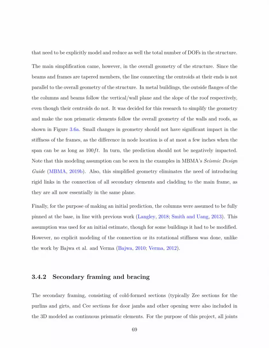
that need to be explicitly model and reduce as well the total number of DOFs in the structure.

The main simplification came, however, in the overall geometry of the structure. Since the

beams and frames are tapered members, the line connecting the centroids at their ends is not

parallel to the overall geometry of the structure. In metal buildings, the outside flanges of the

the columns and beams follow the vertical/wall plane and the slope of the roof respectively,

even though their centroids do not. It was decided for this research to simplify the geometry

and make the non prismatic elements follow the overall geometry of the walls and roofs, as

shown in Figure 3.6a. Small changes in geometry should not have significant impact in the

stiffness of the frames, as the difference in node location is of at most a few inches when the

span can be as long as 100ft. In turn, the prediction should not be negatively impacted.

Note that this modeling assumption can be seen in the examples in MBMA’s Seismic Design

Guide (MBMA, 2019b). Also, this simplified geometry eliminates the need of introducing

rigid links in the connection of all secondary elements and cladding to the main frame, as

they are all now essentially in the same plane.

Finally, for the purpose of making an initial prediction, the columns were assumed to be fully

pinned at the base, in line with previous work (Langley, 2018; Smith and Uang, 2013). This

assumption was used for an initial estimate, though for some buildings it had to be modified.

However, no explicit modeling of the connection or its rotational stiffness was done, unlike

the work by Bajwa et al. and Verma (Bajwa, 2010; Verma, 2012).

3.4.2 Secondary framing and bracing

The secondary framing, consisting of cold-formed sections (typically Zee sections for the

purlins and girts, and Cee sections for door jambs and other opening were also included in

the 3D modeled as continuous prismatic elements. For the purpose of this project, all joints

69

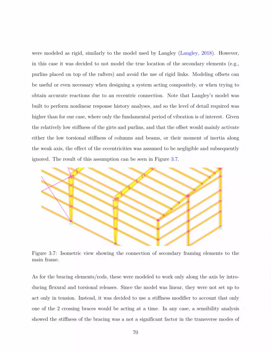
were modeled as rigid, similarly to the model used by Langley (Langley, 2018). However,

in this case it was decided to not model the true location of the secondary elements (e.g.,

purlins placed on top of the rafters) and avoid the use of rigid links. Modeling offsets can

be useful or even necessary when designing a system acting compositely, or when trying to

obtain accurate reactions due to an eccentric connection. Note that Langley’s model was

built to perform nonlinear response history analyses, and so the level of detail required was

higher than for our case, where only the fundamental period of vibration is of interest. Given

the relatively low stiffness of the girts and purlins, and that the offset would mainly activate

either the low torsional stiffness of columns and beams, or their moment of inertia along

the weak axis, the effect of the eccentricities was assumed to be negligible and subsequently

ignored. The result of this assumption can be seen in Figure 3.7.

Figure 3.7: Isometric view showing the connection of secondary framing elements to themain frame.

As for the bracing elements/rods, these were modeled to work only along the axis by intro-

ducing flexural and torsional releases. Since the model was linear, they were not set up to

act only in tension. Instead, it was decided to use a stiffness modifier to account that only

one of the 2 crossing braces would be acting at a time. In any case, a sensibility analysis

showed the stiffness of the bracing was a not a significant factor in the transverse modes of

70

vibration of these buildings.

3.4.3 Cladding

Based on the discussion within the previous chapter, it was decided to explicitly model the

metal cladding in order to evaluate its potential effect on the structural response. Both the

European and American provisions calculate an equivalent stiffness that allows to model the

cladding as either an equivalent flat plate, or even as an equivalent truss member (Lutrell

et al., 2015). Since using an equivalent flat plate makes it easier to introduce and distribute

the dead load across the structure, it was decided to use shell elements for the cladding model.

Note that the values provided in the reference are for the full roof assembly (cladding and

girts/purlins), while our model explicitly models the secondary framing, and so the values

are not directly applicable.

In particular, a thin shell element, which has both membrane and flexural behaviour was

chosen. The shell elements had a constant thickness equal to the plate thickness of the

metal panelS. However, this meant that stiffness modifiers had to be used to more precisely

account for the in-plane and out-of-plane stiffness. For the in-plane stiffness, the membrane

properties were significantly reduced. For typical walls, based on values available in the

literature and the examples showed in the previous chapter it was decided to use – for a

first estimate – a effective stiffness that was between 2− 3% that of the cladding if it were

a thin shell with no seams and perfectly connected on all four sides. For the roofs, the

initial assumption was that it provided no additional stiffness due to diaphragm action, and

so a very small value of 1 · 10−5 was adopted (this does not mean the roof diaphragm is

zero, but that it’s fully explained by the purlins given the low values reported by Wei et

al.). Meanwhile, their out-of-plane stiffness was increased in such a way that local breathing

71

modes of the cladding did not interfere with the modal analysis of the main frames. Again,

a sensitivity analysis was performed and showed that the first mode of vibration was not

sensitive to the change in bending stiffness of the cladding, even when using modification

factors of 100.

As for how the cladding was incorporated into the structure, the shell elements were rect-

angular whenever possible, with triangular elements used when the geometry did not allow

for the former. The nodes used were the intersections between the main framing and the

secondary framing. This created coarse elements, given that the spacing between frames

is usually around 25ft, as shown in Figure 3.8. Due to this, an automatic shell mesh was

used that refined the mesh further. After some sensitivity analysis, prioritizing mostly the

time it took to run the models, a subdivision into 8 elements was chosen. However, no real

difference was observed in the first mode shapes or natural frequencies of the structure with

mesh size, namely when it comes to the deflection of the interior frame elements.

Figure 3.8: Isometric view showing the introduction of cladding as thin shell elements

72

3.4.4 Other considerations

As mentioned before, the 3D modeling approach described includes effectively the main, web

tapered frame elements; the secondary, cold-formed girts, purlins and other framing; the rod

bracing when present, and the shell elements representing the cladding. By a process of

elimination, it then follows that the bracing elements meant to restrict buckling were not

included in the model. It was assumed that they provided no additional stiffness. Also,

given the model was kept linear and was built only for the purposes of obtaining dynamic

properties and not strength checks, their inclusion would not have had an effect.

Again, the main objective of the models, updated through the different construction stages

of each building, was to try and predict their modal properties, and evaluate if they change

throughout and why in the case they do. To that end the modal analysis capabilities of

SAP2000 were utilized. In order to get the most accurate results possible, the eigenvalue

solutions were utilized over the Rayleigh-Ritz method, which is an approximate solution

based on the adoption of a shape function for the mode shape.

Another point of interest in this research is whether the assumptions made by Smith and

Uang – namely, the flexible diaphragm assumption and the feasibility of obtaining the first

mode by using only a 2D model of the main frame – are valid for the purpose of developing

a predictive formula for the fundamental period. It becomes valuable, then, to compare not

only the experimental results to the prediction given by a 3D model, but also the prediction

obtained using a 2D model and two different methods.

A 2D Model of the main frame can easily be recovered from the 3D model by isolating one

of the frames, as seen in Figure 3.6a. The mass of the cladding and secondary framing can

be assigned to the frame as a linear added mass based on tributary areas, before running an

eigenvalue analysis on just the 2D frame.

73

Similarly, the “refined” approach developed by Smith and Uang (Smith and Uang, 2013) can

be followed. This method, which was a calibration based on Rayleigh’s Method, involves

measuring the lateral stiffness of the frame by virtue of applying a unit load at the rafter

level and looking at the generated displacement at that level, which is the flexibility or the

inverse of the lateral stiffness klat. A schematic example of how the unit load is applied and

where to measure the displacement can be seen back in Figure 2.6. In any case, knowing the

aspect ratio of the frame, α, the seismic weight tributary to the frame W and the measured

klat, the fundamental period can be estimated as (Smith and Uang, 2013)

T2 = 2π

√W/g

klat

(1 +

α2.5

425

)(3.11)

where g is the gravitational constant.

Finally, it should be mentioned that not all the elements mentioned in this section are present

in every metal building modeled. Some where measured during construction, before cladding

was installed, sometimes even before the secondary framing was complete (mainly the girts).

Other oddities where also present at times, such as added masses on top of the purlins, or

temporary bracing before the sidewalls were finished. All these things had to be considered

on a per case basis, and will be described in more detail when the results for each building

are presented.

3.5 Tested Buildings

Up until this point the methodologies used to obtain modal properties from test data, how to

perform said tests, and how to model metal buildings to do a prediction have been discussed.

In this section, the buildings in which tests were performed will be identified and described

74

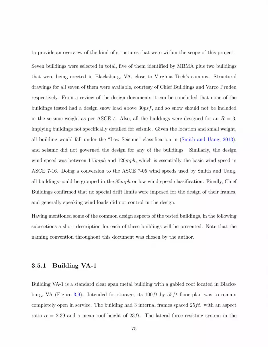
to provide an overview of the kind of structures that were within the scope of this project.

Seven buildings were selected in total, five of them identified by MBMA plus two buildings

that were being erected in Blacksburg, VA, close to Virginia Tech’s campus. Structural

drawings for all seven of them were available, courtesy of Chief Buildings and Varco Pruden

respectively. From a review of the design documents it can be concluded that none of the

buildings tested had a design snow load above 30psf , and so snow should not be included

in the seismic weight as per ASCE-7. Also, all the buildings were designed for an R = 3,

implying buildings not specifically detailed for seismic. Given the location and small weight,

all building would fall under the “Low Seismic” classification in (Smith and Uang, 2013),

and seismic did not governed the design for any of the buildings. Similarly, the design

wind speed was between 115mph and 120mph, which is essentially the basic wind speed in

ASCE 7-16. Doing a conversion to the ASCE 7-05 wind speeds used by Smith and Uang,

all buildings could be grouped in the 85mph or low wind speed classification. Finally, Chief

Buildings confirmed that no special drift limits were imposed for the design of their frames,

and generally speaking wind loads did not control in the design.

Having mentioned some of the common design aspects of the tested buildings, in the following

subsections a short description for each of these buildings will be presented. Note that the

naming convention throughout this document was chosen by the author.

3.5.1 Building VA-1

Building VA-1 is a standard clear span metal building with a gabled roof located in Blacks-

burg, VA (Figure 3.9). Intended for storage, its 100ft by 55ft floor plan was to remain

completely open in service. The building had 3 internal frames spaced 25ft. with an aspect

ratio α = 2.39 and a mean roof height of 23ft. The lateral force resisting system in the

75

longitudinal direction was mixed, with bracing rods in the back sidewall and a portal frame

in the front sidewall, the latter allowing for the door openings that can be seen Figure 3.9.

The building was tested twice. First on September 24, 2021, once the main framing was

completed. Due to disruptions in the supply chain, at the time of testing several girts had

not yet been installed, and the temporary bracing was present to provide stability to the

endwalls (Figure 3.10). The second test was carried out on February 12, 2022, once the

cladding was fully installed and the building was essentially complete.

(a) (b)

Figure 3.9: Building VA-1 after completion of the cladding installation.

(a) (b)

Figure 3.10: Building VA-1 during the the first test on September 24, 2021.

76

3.5.2 Building VA-2

Across the road from the previous metal building, Building VA-2 is a fairly unique building

as it was erected to serve as a barn. As such, the main framing, with a clear span of 78ft

and a mean roof height of 20.8ft (α = 3.77) has an almost 6ft clerestory on top. If the

clerestory is accounted in the mean roof height, a value of approximately 300in would be

reached. Also, while the main building has a fairly open space of 148ft by 78ft provided by

7 frames with no partitions connected to the structure, the building has an appendix with

office floor space. As a results, all the interior frames could actually be thought of as two

bay frames, with one bay having a much larger span (and height) than the other. The reader

is referred to the appendix for an elevation view of a typical interior frame.

Building VA-2 was also tested twice. It was not possible to perform tests on the bare frame,

the first test on November 11, 2021 occurring instead once the back sidewall and roof panels

were installed, but before the endwalls’ cladding was put in place (Figure 3.11b. From the

figure it’s also apparent that a significant number of girts were still missing from the endwalls

at this time.

The second test took place on December 16, 2021, after the cladding had been installed on

the endwalls of the main building. As shown in Figure 3.11a, at the time of testing the

cladding on the appendix had not yet been installed, as they were still installing its interior

partitions.

77

(a) Exterior during the second test. (b) Interior during the first test.

Figure 3.11: Building VA-2 across different tests.

3.5.3 Building WV-1

Building WV-1 is a clear span metal building with single-slope roof built as an expansion to

an existing masonry building in order to serve a storage room for a food services company

(Figure 3.12). The building was located in Buckhannon, WV and was fully operational at

the time of testing on March 1, 2022. The building has 6 interior frames with prismatic

columns, a span of 80ft and a mean roof height of 31.5ft (α = 2.54), spaced 26ft, for a

total open space of 181ft by 80ft with no interior partitions.

Figure 3.12: Outside view of Building WV-1

78

The building was tested during normal working hours, and vehicles were driving back and

forth across the aisles seen on Figure 3.13a. However, compared to buildings VA-1 and VA-2,

which were located in a mostly rural area, building WV-1 is on a relatively small shopping

center in Buckhannon, and little to no wind was present at the time of testing. It should

be noted as well that this was an extension to an existing masonry building. Though the

building is not structurally connected to it, this may still affect the overall stiffness of the

structure (Figure 3.13b).

(a) (b)

Figure 3.13: Interior of building WV-1

3.5.4 Building WV-2

Only a few minutes away from building WV-1, WV-2 is a clear span, gabled roof metal

building spanning 100ft (α = 3.7), with 9 frame lines distanced 25ft from each other with

no partitions. The building was located in the outskirts of Buckhanon, WV, at a higher

elevation and with no surrounding buildings. Though the building was tested on the same

day as building WV-1, the difference in wind speed was apparent.

79

An interesting feature of this building is that the interior space of the building is actually only

150ft as the endwall on one the sides is located two frame lines in. In turn, two of the frames

had no cladding attached to them beyond the roof (Figure 3.14b). At the time of testing the

main framing had been fully erected and the cladding installed on the roof, sidewalls and back

endwall. However, the front endwall was not finished, missing girts and cladding, in order

to allow for construction equipment to get inside the structure (Figure 3.14a). Similarly, the

grade slab had not been cast yet.

(a) (b)

Figure 3.14: Building WV-2 at the time of testing.

3.5.5 Building NC-1

Building NC-1, located in Maiden, NC, is the main building and storefront for a construction

equipment rental company and one of three buildings tested at the site. It’s a mono-slope roof

building with a clear span of 80ft and a mean roof height of 21.6ft (α = 3.7). The building

has a total of 7 interior bays with variable spacing, ranging from 16ft to 25ft in the center.

Three main characteristics differentiate this building from others tested. First of all, the

cladding included a stone veneer at the front endwall. Second, the structural had appendices

on several frame lines, sometimes on both sides of the main frame (Figure 3.15). However,

80

unlike Building VA-2, these were not present at every frame line. Similarly, this building has

the most partitions out of the set, with either metal panel or plaster walls spanning the width

of the building along 3 different interior frame lines. It is then an interesting case to see the

effect non-structural components may have on the modal properties of metal buildings.

(a) (b)

(c) (d)

Figure 3.15: Building NC-1 during the second (Top) and first (Bottom) tests.

The building was first tested on November 5, 2021, when the framing was already up and

and some cladding had been installed on the back endwall. Interestingly, at the time of

testing the metal panels that would comprise the roof were bundled on top of the purlins,

so the structure already had nominally almost its full dead load mass (Figure 3.15). It then

could have provided an interesting case study as the effect of the roof being installed could

81

be explored.

Due to fire safety detailing requirements, it was not possible to test the structure with the

roof installed, as the roof, wall cladding and partitions had to be built simultaneously. The

second test took place on February 2nd, 2022, once the building was essentially complete.

All the cladding and partitions were up, and most of the work seemed to be focused on

architectural aspects.

3.5.6 Building NC-2

Building NC-2 is the second of three buildings in the Maiden, NC site tested. This building

was quite standard, with a 150ft by 60ft open floor plan, possible due to five clear span,

interior frames with a single slope roof spaced 25ft from each other (Figure 3.16). The most

interesting aspect of this building is that was possible to test in three different opportunities,

all of them having essentially the same total mass. The first test, on November 5, 2021, was

performed once the framing was completely erected. The back sidewall had been installed

already, and worked had started on one of the endwalls. Otherwise the structure was free of

other non-structural elements. Similar to Building NC-1, at this time the roof panels were

bundled on top of the purlins.

The second test was carried out on December 13, 2021, after the wall cladding was completed.

These two tests make it possible to evaluate how the change in endwall stiffness could affect

the fundamental period. Finally, the third test, done on February 10, 2022, took place once

the roof cladding had been installed. With these three tests it was possible to see how the

roof and wall cladding affects the dynamic properties, and especially for the former get a

better understanding on the diaphragm stiffness provided by standing seam roofing, if any.

82

(a) (b)

(c)

Figure 3.16: Building NC-2 during different stages of construction.

3.5.7 Building NC-3

The last building on the set, Building NC-3, is a small metal building intended for storage

in Maiden, NC. It’s an open metal building with a 100ft by 20ft footprint. 5 frames with

a short 20ft span and a mean roof height of 14ft (α = 1.43) compose the lateral force

resisting system in the transverse direction. The building had a single slope configuration

and straight columns, similar to Building WV-1. In this case, the rafters were also prismatic

elements (Figure 3.17). The test was performed on December 13, 2021.

83

Figure 3.17: Building NC-3

3.5.8 Summary

A summary of the main properties of each building can be found in Table 3.1, identifying

the main parameters needed to predict their natural period as per the Smith and Uang

formula. The seismic weights were calculated on a tributary area basis considering a 1.2psf

load for the metal roof and cladding, a 3.37lb/ft load for each purlin, and the weight of

the frame (taken as the total weight of the rafter plus half the weight of each column) as

provided in the structural drawings. No snow was included as the design snow loads were

below the threshold of 30psf set by ASCE-7. This, in turn, makes the comparison between

the measured tests and the period used for design easier, as well as resulting in very small

seismic weights.

Comparing these seismic weights with the information provided by Kumar et al., it was

found that the seismic weights of the buildings in this new set are much lower. However,

the estimated load from the deck and purlins was approximately equal (around 2psf), which

means that the disparity is largely explained by the difference in the weight of the main

frames. For example, Building IBHS D in Kumar et al. had similar dimensions to Building

NC-2 in this report, yet had an estimated seismic weight of 8.3kip in large part due to an

84

Table 3.1: Summary of properties of the buildings tested – design parameters

Name Length [ft] Mean Roof Height [ft] Aspect Ratio α Seismic Weight W [kips]VA-1 55 23 2.39 5.3VA-2 78 20.8 3.74 11.5WV-1 80 31.5 2.54 9.5WV-2 100 27 3.70 11.4NC-1 80 21.6 3.70 7.0NC-2 60 21 2.86 5.2NC-3 20 14 1.43 1.8

estimated frame load of 2psf (Kumar et al., 2020). From the drawings for Building NC-2,

its frame contributed 1.1psf to the seismic weight, leading to a much lower value 5.2kip.

Another important note is that the total load shown here effectively represents a best guess

estimate of the situation at the time of testing. However, the load used for design differs

and is generally larger. For example, Smith and Uang used a roof dead load of 5psf to

generate their models (Smith and Uang, 2013). Also, going through the design documents

for the buildings tested in this report it was found that collateral loads ranging from 2psf

to 7psf were added, sometimes to account for future installations. MBMA’s Seismic Design

Guide (MBMA, 2019b) uses a reference value of 4psf for the total roof load, plus 2psf for

an estimate of the main frame weight for an initial design, which would double the estimated

seismic weight of these buildings.

85

Having said that, the set exhibits a good range of clear spans, from 20ft to 100ft, and

mean roof heights from 14ft to 31.5ft. Table 3.2 shows as well that there was a good mix

of roof types and different partition and appendix situations that allowed the field test to

cover a wide range of cases. However, all the buildings are of the clear span type, with no

modular buildings in the set. Also, as mentioned before, all buildings were designed for low

wind speeds and seismic loads. Since the design was controlled by gravity loads, it would be

expected for the buildings to be more flexible than buildings in regions with higher wind or

seismic loads.

Table 3.2: Summary of properties of the buildings tested - structural classification

Name Cladding Type Roof Partitions CommentsVA-1 Metal Panels Clear Span Gabled None N/AVA-2 Metal Panels Clear Span Gabled None Appendices in every interior

frame, ClerestoryWV-1 Metal Panels Clear Span Monoslope None Expansion to existing build-

ingWV-2 Metal Panels Clear Span Gabled None Endwall at an “interior”

frameNC-1 Metal Panels Clear Span Monoslope Heavy Appendices several framesNC-2 Metal Panels Clear Span Monoslope None N/ANC-3 Metal Panels Clear Span Monoslope None N/A

86

Chapter 4

Results

In the previous chapter we have gone over the metal buildings that were chosen for this

project, as well as the methodology and justification behind both the experimental analysis

of the buildings and their 3D modeling with the goal of identifying and predicting the

fundamental period. This chapter will focus on presenting the results for each of the tests

carried out. In total, 12 tests were carried out, as several buildings were tested during

different stages of construction. The order in which they are presented was selected in order

to streamline the analysis and extract important partial conclusions in an organized fashion.

Given the heavy number of figures required to properly describe each test (sensor locations,

collected data in the time and frequency domain, stabilization diagrams) and the finite ele-

ment models, only those that were deemed of importance to fully understand the procedures

will be presented. As a consequence, some tests will be covered in more detail to explain

the common steps taken in all tests and the main conclusions that can be taken from them,

while others will simply show the results that are of interest to the project.

87

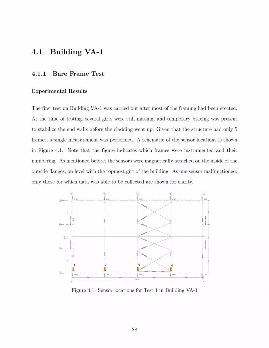
4.1 Building VA-1

4.1.1 Bare Frame Test

Experimental Results

The first test on Building VA-1 was carried out after most of the framing had been erected.

At the time of testing, several girts were still missing, and temporary bracing was present

to stabilize the end walls before the cladding went up. Given that the structure had only 5

frames, a single measurement was performed. A schematic of the sensor locations is shown

in Figure 4.1. Note that the figure indicates which frames were instrumented and their

numbering. As mentioned before, the sensors were magnetically attached on the inside of the

outside flanges, on level with the topmost girt of the building. As one sensor malfunctioned,

only those for which data was able to be collected are shown for clarity.

Figure 4.1: Sensor locations for Test 1 in Building VA-1

88

Figure 4.2 shows the recorded time history after applying a high-pass filter at 1Hz to elimi-

nate low frequency noise, as well as the associated Power Spectrum Density for each sensor.

The first thing to notice is the low amplitude of the accelerations in ambient vibration. As

mentioned before, the database in Goel and Chopra included buildings with peak acceler-

ations of 0.15g (Goel and Chopra, 1997), where here it’s below 0.005g, 30 times smaller.

Moreover, it can be seen that the amplitude does not stay constant across the entire test

length. From approximately 60 to 150s, there is a noticeable increase in acceleration ampli-

tude, most probably due to larger sustained winds.

Figure 4.2: Collected data for the first test in Building VA-1

The effect of acceleration amplitude in the response can be seen in what is called a spectro-

gram, a plot that tracks the frequencies carrying the most energy (shown in red) in time. It

can be thought of a time dependent version of the PSD shown in the previous figure, which

89

is an average or global result for the whole test. Figure 4.3 shows the spectrogram for sensor

3. Two clear horizontal red lines can be seen at around 2Hz and 3Hz, implying that the

PSD is peaking at those frequency values (which can be corroborated by looking at the PSD

on Figure 4.2). However, the most significant detail is how the line at 2Hz is not visible

throughout the whole test. Up to the 60s mark the frequency does not stand out. This is

an example of how some modes may not be excited strongly enough to obtain a measurable

response, especially during short tests.

Figure 4.3: Spectrogram of the acceleration data recorded by sensor 3 on the first test inBuilding VA-1

In any case, going back to Figure 4.2, three peaks can be clearly identified by inspection at

around 2Hz (0.5s), 2.5Hz (0.4s) and 3.5Hz (0.29s). Following what was seen in the previous

chapter, these would then be 3 natural frequencies of the structure. Some information about

the mode shapes can also be identified via inspection. At 2Hz (0.5s), sensor 1 (located at

90

the endwall before the cladding went up) shows a much higher peak than the rest of the

sensors. Then, it can be assumed that the deflections for this mode are largely concentrated

in the endwall. Similar considerations can be made for the mode shapes at around 2.5Hz

(0.4s) and 3.5Hz (0.29s), which will most probably be dominated by sensors 3 and 4 in the

former, and sensor 2 in the latter.

So far the results have only been discussed qualitatively in order to provide some intuition

behind the dynamic properties the stochastic subspace algorithm will identify. For reference,

in Figure 4.4 the stabilization diagram is shown, where the poles of the system (the natural

frequencies) can be seen for a range of model orders n. This stabilization diagram, as

mentioned before, is used for visualization purposes only, as a clustering algorithm is used

instead to select the final modes.

Figure 4.4: Stabilization diagram for test 1 in Building VA-1. Blue dots represent stablepoles. Red crosses represent unstable poles. and small blue circles represent unstable modesin terms of damping. The selected modes are circled.

91

Though several modes can be identified, the limited number of sensors means that reliable

mode shape data can only be recovered for a few of them (the lower order ones) before

encountering spatial aliasing issues. But, in any case, the 3 frequencies previously mentioned

clearly show up as straight vertical lines of stable poles, indicating the these are likely

structural in nature. The final estimated natural frequencies for the first three identified

modes are 1.86Hz, 2.70Hz and 3.40hz. Note the use of the word identified. It’s important

to remember that due to sensor placement and orientation some modes cannot be captured,

such as longitudinal or roof modes of the building. Similarly, given that the right endwall

wasn’t measured, it is not possible to know from the test data whether it was exhibiting an

isolated modes shape similar to what was discussed for the left endwall.

As mentioned before, the algorithm uses a clustering approach to automatically select the

natural frequencies and at which model order to select the dynamic properties. The final

clusters of the method can be seen in Figure 4.5.

Figure 4.5: Final clusters from test 1 in Building VA-1

92

In any case, what is important to take away from the procedure is that the first three

modes that were extracted from the test had natural periods of 0.54s, 0.37s and 0.29s. The

mode shapes, meanwhile, are plotted in Figure 4.6. Note, then, how the results match the

previous analysis based on the PSD of the measured signals. It’s important to remark here

that Figure 4.6 is only plotting known values of the mode shapes at the measured degrees-

of-freedom. First, the black dots at certain beam-column joints indicate locations where

sensors were places. In this test, for example, no sensor was located in the right endwall.

Similarly, the mode shape shown is limited by the degrees of freedom measured. Since only

uniaxial sensors were used in the direction of the main frames, only said transverse motion

can be captured (and drawn). As such, there could be motions in the longitudinal directions

that are not being captured by test nor shown in the modeshapes, though results from the

analytical models can confirm these are predominantly transverse modes. Finally, it was

decided to only show values in measured locations instead of interpolating or assuming a

deformed shape for frame lines without sensors. As a result, in Figure 4.6 the right endwall

is drawn assuming it does not participate at all in any of the modes. All these considerations

apply generically for every experimental mode shape extracted in this chapter.

(a) (b) (c)

Figure 4.6: Experimental modes from test 1 in Building VA-1

93

3D Model prediction

In order to identify the effect of nonstructural elements, it is necessary to first reduce the

uncertainty in the bare frame model. Otherwise it becomes harder – if not impossible

– to know what should be calibrated to match the results, if the frame stiffness or the

cladding. Figure 4.7 shows the SAP2000 model for the building, which attempts to match

the conditions at the time of testing, accounting for the missing girts and temporary bracing

on display in Figure 3.10.

Other than that, the results shown here come from the initial prediction, without any mod-

ification of the mechanical properties of the materials. In summary, no calibration was

done.

Figure 4.7: SAP2000 model of building VA-1 for test 1

94

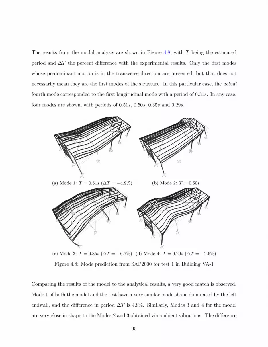
The results from the modal analysis are shown in Figure 4.8, with T being the estimated

period and ∆T the percent difference with the experimental results. Only the first modes

whose predominant motion is in the transverse direction are presented, but that does not

necessarily mean they are the first modes of the structure. In this particular case, the actual

fourth mode corresponded to the first longitudinal mode with a period of 0.31s. In any case,

four modes are shown, with periods of 0.51s, 0.50s, 0.35s and 0.29s.

(a) Mode 1: T = 0.51s (∆T = −4.9%) (b) Mode 2: T = 0.50s

(c) Mode 3: T = 0.35s (∆T = −6.7%) (d) Mode 4: T = 0.29s (∆T = −2.6%)

Figure 4.8: Mode prediction from SAP2000 for test 1 in Building VA-1

Comparing the results of the model to the analytical results, a very good match is observed.

Mode 1 of both the model and the test have a very similar mode shape dominated by the left

endwall, and the difference in period ∆T is 4.8%. Similarly, Modes 3 and 4 for the model

are very close in shape to the Modes 2 and 3 obtained via ambient vibrations. The difference

95

in period was 6.7% and 2.6%. In all cases the model underestimated the period, implying

it was stiffer than the actual structure. The results were considered good enough to justify

not going through a calibration process.

It must be mentioned, however, that Mode 2 of the model, which consists on the displacement

of the right endwall, was not seen during testing. Considering that the mode is localized

to a particular frame line, and that there was no (working) sensor located there, it is more

likely than not that it wasn’t identified by the rest of the sensors as they would have less

energy content at this frequency. The mode shape would not have been able to be recovered

anyway as the maximum value would be at a place that was not measured. In summary,

that mode is believed to exist, but wasn’t identified during testing due to limitations of the

instrumentation.

Finally, it was discussed before that the modes were found to be very similar in shape

between the model and the test data. This usually is a more convincing proof that the

structure and the model are behaving similarly, as the frequencies could be similar even if

the mode shapes are not. In order to quantify the assertion that these shapes are similar,

the Modal Assurance Criterion (MAC) is used. In this case, it’s referred to as a crossMAC,

as what will be evaluated is the MAC between two different sets of mode shapes. The results

can be seen in Figure 4.9.

Each cell in the plot is color coded, with dark red meaning a crossMAC of 1 and dark

blue a crossMAC of 0. Ideally, the crossMAC should return approximately the identity

matrix. That would mean that the mode shape given by the model and the experimental

test are equal to each other, while different modes have no correlation or are approximately

orthogonal to each other. Usually, a value of 0.7 is considered good enough for two modes

to be considered the same, with values above 0.9 implying a very good correlation.

96

Figure 4.9: crossMAC for building VA-1 – test 1

In this case, it follows from Figure 4.9 that the modes predicted by the model correlate

very well with the experimental results, with the lowest value being 0.96 for the second

experimental mode. In conclusion, the bare frame model accurately captured what was

measured on the field, and could be used for the next stage in the analysis.

4.1.2 Completed Building Test

Experimental Results

The second test took place once all the framing was erected and the cladding on the walls

and roof was installed. The sensor locations can be seen in Figure 4.10. It should be noted

that for this test there is available data for both end walls as well as the inner frames, which

will allow to see the effect the cladding had on the stiffness of the endwalls.

97

Figure 4.10: Sensor locations for Test 2 in Building VA-1

Figure 4.11 shows the recorded accelerations in each location. Compared to Figure 4.2, the

amplitude stays within the same order of magnitude as the previous test, and the same

variability with time can be seen. More importantly, looking at the PSD, only a single peak

can be seen in the previous range between 0 and 4Hz. Specifically, when looking at sensors

1 and 4, related to the endwalls, it can be seen that they no longer show a peak around

2Hz, and generally speaking their energy content is much lower, implying that the endwall

cladding added a significant amount of stiffness.

In the end, only a single mode could be confidently identified from the test data, with a

natural frequency of 2.35Hz (0.43s). The associated mode shape can be seen in Figure 4.12.

Note that, since frame line 4 was not measured the displacement value for that frame is set

to 0, but that does not necessarily represent the actual value. Setting it to 0 over finding

an interpolation was a conscious decision made to avoid introducing personal bias into the

mode shape estimation. Instead, measured frames can be identified by the black circle at

the beam to column connection.

98

Figure 4.11: Collected data for the second test in Building VA-1

(a)

Figure 4.12: First mode from test 2 in Building VA-1

99

3D Model prediction

Following from the results in test 1, the 3D SAP model was updated to fully represent

the structure at the time of testing, by removing the temporary bracing, and adding the

originally missing girts. The cladding for the roof and walls was included as well in the

form of shell elements as explained in the previous chapter. Following the assumption that

Standing Seam Roofs provide little to no diaphragm action, its membrane properties were

reduced by 105. Note that this does not mean that there’s no diaphragm action at all.

The G′ value given by the Diaphragm Design Manual (Luttrell, 1965) includes the effect

of the purlins in its formulation as what is tested is the complete roof assembly. As such,

reducing the stiffness of the shell elements to effectively zero does not imply that there is

no diaphragm stiffness, but that almost all the stiffness is being provided by the purlins.

As later shown in this Chapter, as well as in Chapter 7, the stiffness of the purlins alone is

already around 1kip/in, which is consistent with the stiffness taken from Wei et al. (Wei

et al., 2020). In turn, since the stiffness of the purlins already reasonably agrees with the

limited experimental data available, it was considered appropriate to neglect any additional

stiffness due to the sheeting alone, which is what is needed for the SAP model.

For the walls, meanwhile, the effective stiffness was considered to be 2% that of a flat plate

of identical thickness. The full model is shown in Figure 4.13.

After performing a modal analysis, the most notable difference compared to the previous

model was that the modes associated with the endwalls were no longer the ones with longer

period. In fact, it would take hundreds of modes for them to appear in SAP, mostly because

of several local modes related to the shell elements and the secondary framing. In the end,

however, given that experimental modal information did not provide any hints regarding

the stiffness of the walls, no real calibration can be done. All that can be said is that the

100

endwalls are significantly stiffer than the interior framing once the cladding is installed.

Second, as can be seen on Figure 4.14, the structure was predicted to have a fundamental

period of 0.42, less than 2% off from the experimental result. The computed crossMAC for

the first mode was 0.98, showing an excellent correlation. Thus, for building VA-1 the roof

was found to provide no diaphragm action, and the model predicted the response very well.


(a) Mode 1: T = 0.42s (∆T = −1.8%)


101

4.2 Building NC-2

4.2.1 Bare Frame Test

Experimental Test

Building NC-2 was the only metal building for which it was possible to perform tests in all

three relevant stages of construction. The first test was carried out after all the primary and

secondary framing had been erected. Work had also started on the cladding, with the back

sidewall finished and about half of the left endwall installed. As mentioned before, at the

time of testing the roof panels were bundled together and sitting on top of the purlins, which

means that almost the full weight of the building was already in place. This provided an

excellent opportunity to isolate the effect of cladding, as the mass would remain essentially

the same for each test, unlike the building VA-1.

Given that the building had 7 total frames, the test consisted of two different measurements

linked by reference sensors that stayed in place for both measurements. The sensor locations

can be seen on Figure 4.15.

Given that measurement 2 includes measurements on an endwall before the cladding was

installed, it was chosen to show the collected response from said measurement in Figure 4.16.

Similar to building VA-1, the first peak at around 1Hz (1s) for sensor 4 (the right endwall)

is orders of magnitude larger than for the rest of the sensors, showing the great flexibility of

these walls before the cladding went up. Meanwhile, the interior frames are showing peaks

at around 2Hz (0.5s). These latter peaks were also present in the first measurement, while

the peak at 1Hz (1s) was not.

The identified modes can be found in Figure 4.17, with the first mode dominated by the

102

Figure 4.15: Sensor locations for Test 1 in Building NC-2. In orange: measurement 1. Inblue: measurement 2.

Figure 4.16: Collected data for the second measurement of the first test in Building NC-2

103

individual movement of the right endwall, and the other two appearing to be representative

of a more global, system behavior. Note that in this case a mode shape related to the dis-

placement of the left endwall was not identified, most probably because the partial cladding

was already providing a significant amount of stiffness.

(a) (b) (c)

Figure 4.17: Experimental modes from test 1 in Building NC-2

3D Model Prediction

An isometric view of the 3D model can be seen in Figure 4.18, showing the inclusion of the

back sidewall and the partial construction of the left endwall. To account for the added

mass of the bundled roof panels, an equivalent linear mass was added to the main frame

rafters, using the lever rule (i.e., assuming the purlins to be pinned between main frames,

solving for the reactions dof a simply supported beam with a concentrated load where the

roof panels were bundled provides the distribution factor) to assign distribution factors on

an approximate basis given photographic evidence. The choice of modeling the mass directly

on the frames instead of the purlins was to avoid introducing irrelevant modes at the purlin

level that would make discerning the overall behavior of the structure more difficult.

The resulting mode shapes from the model can be seen in Figure 4.19. The first mode,

which is the right endwall mode, did not show the same accuracy as the others, with a 12%

overestimation of the period. However, the second and third modes which are the most

104

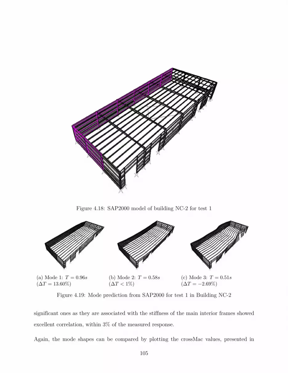
Figure 4.18: SAP2000 model of building NC-2 for test 1

(a) Mode 1: T = 0.96s(∆T = 13.60%)

(b) Mode 2: T = 0.58s(∆T < 1%)

(c) Mode 3: T = 0.51s(∆T = −2.69%)

Figure 4.19: Mode prediction from SAP2000 for test 1 in Building NC-2

significant ones as they are associated with the stiffness of the main interior frames showed

excellent correlation, within 3% of the measured response.

Again, the mode shapes can be compared by plotting the crossMac values, presented in

105

Figure 4.20. The results were excellent, with lowest crossMAC value in the diagonal being

0.86. In summary, the bare frame model seemed to be adequate without the need for any

calibration, especially considering that the actual distribution of the roof mass was not

known.

Figure 4.20: crossMAC for building NC-2 – test 1

4.2.2 Test with Walls installed

Experimental results

The second test was performed once the installation of the metal panels in every wall was

completed. At the time of testing, the roof panels were still bundled on top, so the only

significant difference between tests was that the endwalls now had the sheeting in place.

Figure 4.21 shows the acceleration recordings during the second measurement, with the

naming convention being equal to that of the first test.

106

Figure 4.21: Collected data for the second measurement of the second test in Building NC-2

Note that – when compared to the results of the first test in Figure 4.16 – the response

from the inner frames (sensors 1 to 4) has not changed. However, the right endwall (sensor

5) exhibits much smaller acceleration amplitudes, and the peak at 2Hz (0.5s) not present

anymore. This is evidence of the stiffening effect of the endwall cladding, though it does not

seem to affect the main frames or the overall response of the structure, at least while the

roof isn’t in place.

Since the endwall mode is no longer present (for the frequency range studied at least), the

two modes identified by the SSI algorithm are presented in Figure 4.22. Note that these are

virtually unchanged from modes 2 and 3 of test 1.

107

(a) (b)


3D Model Prediction

The previous model was updated to reflect the new testing conditions, mainly incorporating

the rest of the cladding with the same properties as before. Given its similarity to the

previous model, the model won’t be shown. The first two modes in the transverse direction

can be seen in Figure 4.23.

(a) Mode 1: T = 0.59s(∆T < 1%)

(b) Mode 2: T = 0.52s(∆T < 1%)


The periods for both modes matched almost exactly with the experimental results. The

mode shapes however weren’t as accurate, though still satisfactory, with the lowest value

being 0.72. The crossMAC plot is presented in Figure 4.24

108


4.2.3 Test on completed building


The third and final test on building NC-2 was carried out after the roof panels were installed.

Given that the panels were already sitting on top of the purlins before, this test can help

to directly compare the behavior of the building before and after the roof is in place, and

evaluate whether diaphragm action is observed or not. The acceleration records are shown

again for the second measurement, which included mainly the frames on the right side of the

building (Figure 4.25).

The most significant difference is that now a single peak was present in the 1.5Hz (0.67s) to

2Hz (1s) range. Similar to building VA-1, despite experiencing similar levels of vibration, the

installation of the roof seems to make the identification of higher order modes more difficult.

109

Figure 4.25: Collected data for the second measurement of the third test in Building NC-2

One possible explanation for this, as Rogers and Tremblay (Rogers and Tremblay, 2010)

showed, is that the stiffness of decks can be very sensitive to amplitude. Higher order modes

tend to create greater distortions at the roof level due to the relative movement between

frames, and so they would be more sensitive to any added friction stiffness only present

at low level vibrations compared to the fundamental mode. However, it is not possible to

draw any definite conclusions from the test results, as no measurements exhibited larger

amplitudes to test this hypothesis.

In the end, only the fundamental mode was able to be identified from the data, presented

in Figure 4.26a. Note that no displacement is shown for frame line 3, as the sensor malfunc-

tioned.

110

3D model prediction

The last update to the 3D model was removing the linear mass in each frame line and include

the roofing as shell elements. Working under the assumption that it provided no stiffness

and all diaphragm stiffness is explained by the purlins, its in-plane stiffness were reduced by

105. The first mode taken from the model can be seen in Figure 4.26b, again showing a very

good correlation in terms of period (∆T < 5%) and crossMAC (0.80).

(a)(b) Mode 1: T = 0.60s(∆T < −4.47%)

Figure 4.26: First mode from test 3 in Building NC-2. Left: experimental. Right: predicted

4.3 Building NC-1

4.3.1 Test on Bare Frame

Experimental Test

The first two buildings shown up until this point were characterized by their regular geometry

and open floor space, with no partitions. Building NC-1 is an interesting case study due to the

presence of appendices in several frame lines, as well as including (in its final configurations)

either plaster or cladding walls that extended onto the roof and across the whole span of

certain frames.

111

The first test on building NC-1 took place after the erection of the main and secondary fram-

ing, including the appendices. Some cladding, mainly on the near the base of the columns,

had already been installed on the perimeter. The sensor locations for both measurements

comprising test 1 can be seen in Figure 4.27.

Figure 4.27: Sensor locations for Test 1 in Building NC-1. In orange: measurement 1. Inblue, measurement 2.

The recorded data for both measurement 1 and 2 are shown in Figure 4.28. Looking closely

at the frequency domain data, it can be seen that the sensors in measurement 1 all tend to

peak at around 2Hz (0.5s). Meanwhile, the sensors in measurement two peak at a higher

frequency of 2.5Hz (0.4s). The exception to this is Sensor 1 (the reference sensor). It looks

as though the structure is essentially behaving as two different buildings. The left side of

the building, with fewer appendices being more flexible than the right side of the building

with appendices on both sides. The fact that such disjointed behavior can be observed is

indicative of the low stiffness provided by the purlins interconnecting each frame line.

112

(a) First measurement.

(b) Second measurement.

Figure 4.28: Collected data for both measurements of the first test in Building NC-1

113

This analysis can be confirmed by looking the modes obtained from running the SSI algo-

rithm, which are shown in Figure 4.29. Three modes were identified in total, the first being

similar in shape to the first two modes of a simply supported beam spanning from frame

1 up to frame 6 (where appendices on both sides appear), and the third mode similar to a

simply supported beam in the right side of the building.

Compared to previous tests, the endwalls in this case seemed to already be stiffer than

the interior frames even without the cladding installed. This is most probably due to the

fact that in the previous buildings the endwalls consisted of simply portal frames, while in

building NC-1 the left endwall was braced on its middle bay and the right endwall actually

consisted of a web tapered frame in similar fashion to the interior frames plus the framing

required to install the veneer facade in the future.

(a) (b) (c)


3D Model prediction

Figure 4.30 shows the first three mode shapes in the transverse direction obtained in SAP2000.

The model was created using the same assumptions and following the same steps as in pre-

vious cases. Similarly to building NC-2, since the roof mass from the panels was already in

place – bundled on top of the purlins – at the time of testing, these were explicitly included

as a linear mass.

114

(a) Mode 1: T = 0.45s(∆T = −10.6%)

(b) Mode 2: T = 0.43s(∆T − 15.29%)

(c) Mode 3: T = 0.39s(∆T = −2.91%)


Comparing the periods with the results from the experimental data, it can be seen that the

model tends to overestimate the stiffness of the inner frames. Since the modes are exhibiting

global behavior, this could also be related to an overestimation of the purlin stiffness, as

the connection was modeled as rigid. The effect of purlin stiffness will be discussed in later

sections.

Finally, Figure 4.31 shoes the crossMAC evaluation, which shows the the model mode shapes

are remarkably similar the ones obtained via ambient vibrations. the lowest value being 0.90

for the first mode.

115


4.3.2 Test on fully clad building


The second test on building NC-1 took place once the cladding was installed and interior

partitions had been built. These partitions (shown back in Figure 3.15) were located in

frame lines 2, 6 and 7 of the building, starting from the left. For reference, these correspond

to sensor 2 of measurement 1, and sensors 2 and 3 of measurement 2 (See Figure 4.27).

Measured data was only available for frame lines 1, 2 5 and 9 of the building. Since frame

lines 1 and 9 correspond to the endwalls, and frame line 2 had a metal panel wall attached

to the frame, these sensors did not pick up any significant acceleration records. However,

this shows that the interior partitions in this case were introducing significant stiffness to the

frame the were attached to. The acceleration record from sensor 5 along with its associated

116

Figure 4.32: Acceleration record for sensor 5 during measurement 1, test 2 for building NC-1

spectrogram is shown in Figure 4.32.

Comparing the amplitudes to those seen in Figure 4.28, it’s clear to see that during the

second tests the amplitudes were smaller, by at least a factor of 2. This translated into the

structure’s lower frequency not being excited consistently during the test. The spectrogram

shows that only when there was an increase in amplitude up to around 0.0005g the first

mode of the structure was participating in the response, as noted by the red line around

2Hz (0.5s) from the 90s up to approximately the 120s mark. Again, obtaining full modal

information of the fully clad buildings using ambient vibrations is a challenge.

The SSI algorithm was capable of identifying the fundamental mode of the structure, which

only had significant displacements where sensor 5 was located. Due the lack of spatial

information the mode shape is not shown, but the fundamental period of the fully clad

building was 2.0Hz (T = 0.5s). This is a small, largely insignificant change in the period,

117

though it’s not possible to take further conclusions from this without having mode shape

information.

3D Model prediction

The full model for building NC-1 including the cladding and partitions can be seen in Fig-

ure 4.33. Up until this point it has been show that the stiffness cannot be calibrated with

the available data. The reason is mainly that endwall cladding and partitions effectively

act as infinitely rigid elements relative the main frames. With this in mind, it was decided

to include the partitions in the model as restraints in the transverse direction. This simple

approach was only taken for the purpose of finding the mode shape information in the fre-

quency range of interest, and should not be taken as a definitive statement on the amount

of stiffness introduced by the partitions (e.g.: for deflection calculations or load transfer).

Figure 4.33: SAP2000 model of building NC-1 for test 2

118

The first mode obtained in SAP200 is shown in Figure 4.34. Note that the added restrictions

due to the partitions does not affect the natural period of the structure, which stayed at

0.45s in the model. This is consistent with the experimental results, that showed no change

in the period from the test 1 to test 2. However, the mode shape was affected, as now frame

2 exhibits no movement. This is a manifestation of the low stiffness provided by the roof

system and negligible effect of the standing seam roof. The frames that were not restrained

by partitions (in this case, frame lines 3 to 5) are still able to deform almost freely, explaining

why the period does not change from one case to the other.

Note that three consecutive frames are partition free in this case. The structure could

be imagined as three interior frames with stiff walls at the ends. This is essentially the

configuration for building VA-1, which also showed no interference of the endwall cladding

in the response of the inner frames.

(a) Mode 1: T = 0.45s(∆T = −10.0%)


119

4.4 Building VA-2

4.4.1 Test with roof installed


Building VA-2 was the other building in this set (along with building NC-1) that had appen-

dices attached to its frames, though in this case they were present in every interior frame.

The first test was performed after most of the framing had been erected, and the roof and

back sidewall panels installed. At the time of testing the endwalls had not been fully built

yet, with several missing girts and door jambs missing. Also, since the endwalls are the only

frame lines without appendices, it was expected for them be more flexible than the inner

frames before the cladding was installed.

The building then provides a good opportunity to see if endwall-only modes are present or

if the roof cladding introduced some diaphragm action, and how the inclusion of cladding

affects the dynamic properties of the completed building.

The sensor locations can be seen in Figure 4.35. Note there was no reference sensor across

measurements to generate mode shape data. The recorded acceleration data can be seen on

Figure 4.36. At the time of testing, there was active construction in the clerestory section,

which is reflected in the larger vibration amplitudes seen during the test,

Again, it wasn’t possible to reliability identify mode shapes, but the structural modes were

obtained from the SSI algorithm, with frequencies of 1.97Hz (0.50s), 2.67Hz (0.37s) and

3.51Hz (0.28s).

120

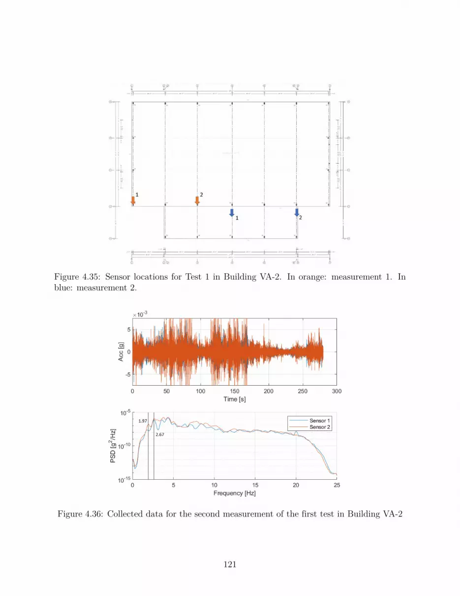
Figure 4.35: Sensor locations for Test 1 in Building VA-2. In orange: measurement 1. Inblue: measurement 2.

Figure 4.36: Collected data for the second measurement of the first test in Building VA-2

121

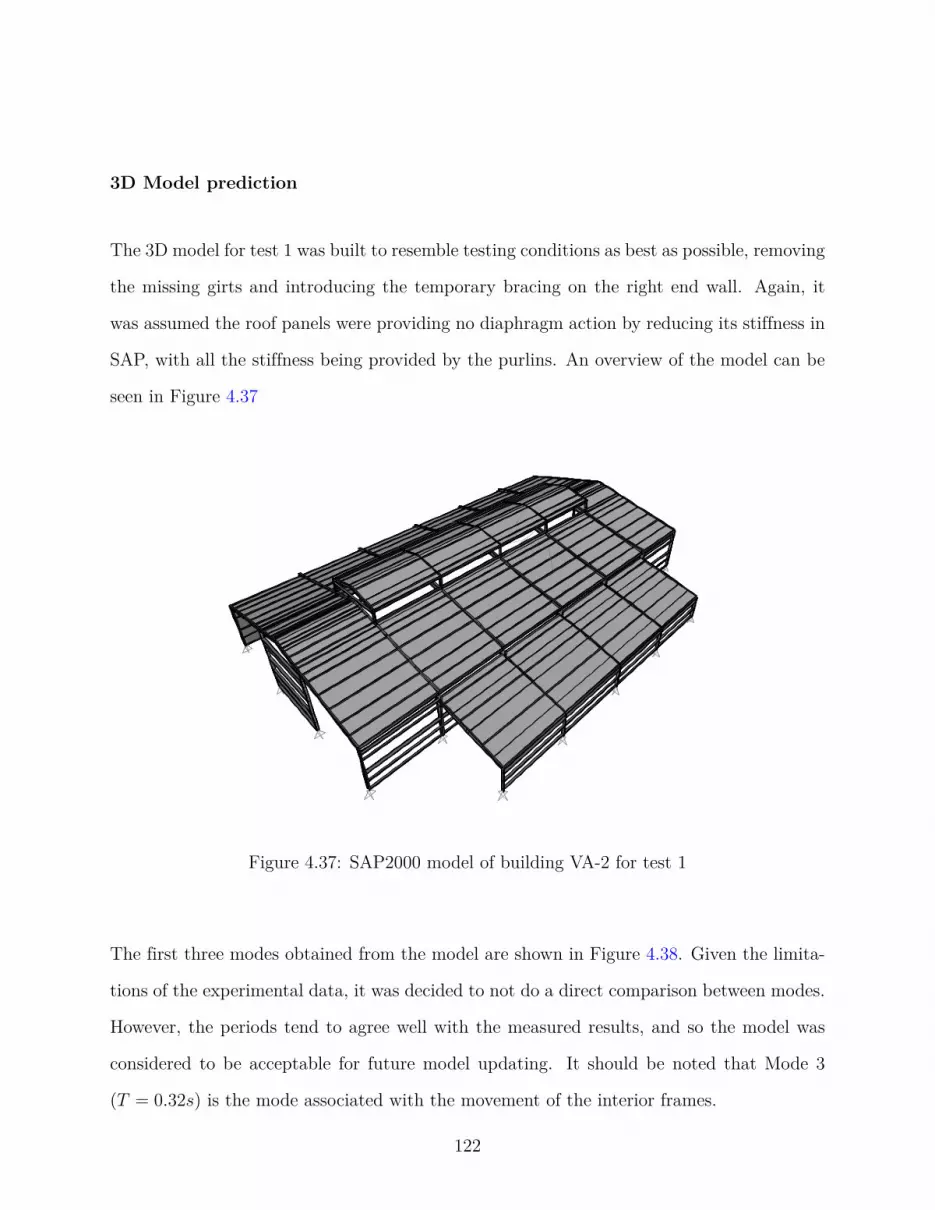
3D Model prediction

The 3D model for test 1 was built to resemble testing conditions as best as possible, removing

the missing girts and introducing the temporary bracing on the right end wall. Again, it

was assumed the roof panels were providing no diaphragm action by reducing its stiffness in

SAP, with all the stiffness being provided by the purlins. An overview of the model can be

seen in Figure 4.37


The first three modes obtained from the model are shown in Figure 4.38. Given the limita-

tions of the experimental data, it was decided to not do a direct comparison between modes.

However, the periods tend to agree well with the measured results, and so the model was

considered to be acceptable for future model updating. It should be noted that Mode 3

(T = 0.32s) is the mode associated with the movement of the interior frames.

122

(a) Mode 1: T = 0.56s (b) Mode 2: T = 0.38s (c) Mode 3: T = 0.32s


4.4.2 Test on fully clad building


The second test was carried after all the cladding had been installed on the main building,

not so in the office section (the floor space generated by the appendices). This time around a

denser instrumentation was available. The sensor locations for each measurement are shown

in Figure 4.39

Figure 4.40 shows the recorded accelerations during measurement 2, both in the time and

frequency domains. Two main differences can be seen with respect to previous test. First,

measured amplitudes are significantly smaller than during test 1. This is mainly a conse-

quence of the test conditions, as the only significant source of vibrations for this test was

wind, given the remote location of the building and the lack of active construction work at

the time.

The second main difference is in the frequency content, as there are no longer any peaks in

the 1Hz (1s) to 3Hz (0.33s) range which, according to the previous model, were related to

the endwalls. Instead a peak at around 3Hz (0.33s) is visible.

From the experimental data two modes were identified based on the SSI method. The first

123

Figure 4.39: Sensor locations for Test 2 in Building VA-2. In orange: measurement 1. Inblue: measurement 2.

Figure 4.40: Collected data for the second measurement of the first test in Building VA-2

124

mode had a natural frequency of 3.24Hz (0.31s) and the second mode was found at 3.57Hz

(0.28s). Note that the first mode here identified is very close to the third mode found in

test 1 (0.28s) which was later found to be associated with the displacement of the interior

frames.

The mode shapes for the identified modes are shown in Figure 4.41, where it can be seen

that they are both related to the movement of the interior frames.

(a) (b)

Figure 4.41: Experimental modes from test 2 in Building VA-2

3D Model prediction

Figure 4.42 shows the first two transverse modes of the structures obtained from the updated

3D model for Building VA-2, which now includes the metal panels on walls of the main

open floor space. The model still assumes the roof cladding is not providing any additional

stiffness, using the same modifier as in previous models. Note that the first mode is essentially

identical to the third mode shown for the Test 1 prediction. This is expected, as the walls do

not provide a significant amount of mass to the building, while the roof weight was already

in place. This is a direct result of the negligible added stiffness provided by the roof.

More importantly though. the periods from the model match very closely with the results

from the experimental tests, with differences smaller than 5%. In turn, once again it follows

125

(a) Mode 1: T = 0.32s(∆T = 4.24%)

(b) Mode 2: T = 0.29s(∆T = 4.41%)


that assuming the roof of a metal building introduces no diaphragm action provides good

estimates of the building behavior. Similarly, the first mode of the test 1 model, which was

dominated by the endwall, is no longer present after the cladding is install.

Figure 4.43 shows the crossMAC between mode shapes obtained from both the model and

from test 2. The values for this case were lower, though still above 0.7 in the diagonal and

below 0.1 otherwise, implying a good correlation between the mode shapes.

Figure 4.43: crossMAC for building VA-2 – test 2

126

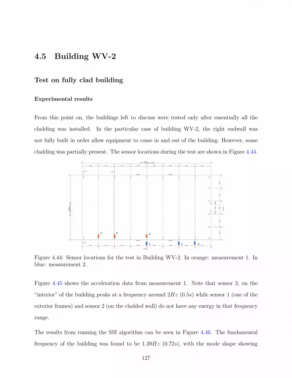
4.5 Building WV-2

Test on fully clad building


From this point on, the buildings left to discuss were tested only after essentially all the

cladding was installed. In the particular case of building WV-2, the right endwall was

not fully built in order allow equipment to come in and out of the building. However, some

cladding was partially present. The sensor locations during the test are shown in Figure 4.44.

Figure 4.44: Sensor locations for the test in Building WV-2. In orange: measurement 1. Inblue: measurement 2.

Figure 4.45 shows the acceleration data from measurement 1. Note that sensor 3, on the

“interior” of the building peaks at a frequency around 2Hz (0.5s) while sensor 1 (one of the

exterior frames) and sensor 2 (on the cladded wall) do not have any energy in that frequency

range.

The results from running the SSI algorithm can be seen in Figure 4.46. The fundamental

frequency of the building was found to be 1.39Hz (0.72s), with the mode shape showing

127

typical global behavior in between the cladded endwalls. Note frame 2 does not participate

in this mode.

Figure 4.45: Collected data for the first measurement during the test in Building WV-2

(a)

Figure 4.46: Experimental modes from the test in Building WV-2

128

3D Model prediction

Figure 4.47 shows the full 3D model of building WV-2, built based on the state of the building

at the time of testing, along with the the first two modes in the transverse direction. Even

though mode 1 was identified during testing, mode 2 is shown in order to shed light on

the behavior of the building. The frames on frame lines 1 and 2 were marginally more

flexible than the ones on the rest of the building. Were the frames to be behave perfectly

independently from each other, it would be expected for the first modes of the structure to

be associated with the movement of these two frames.

However, from the resulting mode shapes it’s clear that that isn’t the case. Even if the roof

isn’t providing diaphragm action, the limited stiffness coming from the purlins is enough to

create global behavior in conjunction with the endwalls, the first mode dominated by the

concurrent movement of the frames on the interior of the building, and the second mode

described by the displacement of the exterior frames.

In any case, the model underpredicted the period by about 9%, while the mode shape

matched very well with the experimental one (crossMAC = 0.95).

129

(a) Overview of the 3D model for building WV-2

(b) Mode 1: T = 0.65s (∆T =8.9%) (c) Mode 2: T = 0.57s

Figure 4.47: Analytical model of building WV-2

4.6 Building WV-1



The test on building WV-1 was carried out with the building fully operational. Two mea-

surements were taken covering the 6 interior frames of the building, as experience had shown

130

at this point that endwalls do not participate in the first mode of these buildings. Figure 4.48

shows the experimental modes resulting from applying the SSI method.

(a) (b)

Figure 4.48: Experimental modes from the test in Building WV-1

3D Model prediction

Figure 4.49 shows the model used to the predict the modal properties of building WV-1,

following the structural drawings available. Also in the Figure the first two modes in the

transverse direction are presented.

It’s clear that the periods predicted by the model are not consistent with the results obtained

empirically. The overestimation was almost by a factor of 2 (100%), which was concerning. A

few possible explanations were singled out for this. First, it would be possible that the roof of

this building was providing significant diaphragm action and making the walls participate in

the mode. However, based on all previous tests that showed the roofs providing no stiffness,

and the mode shapes in Figure 4.48 where the displacements approach 0 as the frames get

closer to the endwalls, this option was discarded.

The second possible explanation would be a strong influence of the adjacent building, even

if they weren’t connected, which is plausible. The gap between the adjacent structures

can be seen in Figure 3.13b, showing that the two structures were designed to act largely

131

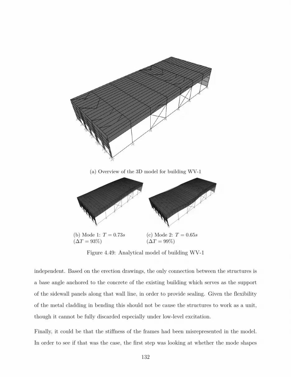
(a) Overview of the 3D model for building WV-1

(b) Mode 1: T = 0.73s(∆T = 93%)

(c) Mode 2: T = 0.65s(∆T = 99%)

Figure 4.49: Analytical model of building WV-1

independent. Based on the erection drawings, the only connection between the structures is

a base angle anchored to the concrete of the existing building which serves as the support

of the sidewall panels along that wall line, in order to provide sealing. Given the flexibility

of the metal cladding in bending this should not be cause the structures to work as a unit,

though it cannot be fully discarded especially under low-level excitation.

Finally, it could be that the stiffness of the frames had been misrepresented in the model.

In order to see if that was the case, the first step was looking at whether the mode shapes

132

obtained by the model correlated well with those obtained experimentally. If that were the

case, then it could be argued that the difference in period would be mostly explained by a

difference in stiffness of the frames alone. Other changes (like the restraints provided by the

adjacent building, or cladding stiffness) would result in a change in mode shapes.

Figure 4.50 shows the crossMAC plot between the experimental test and the original model.

Given the high MAC values (0.79 and 0.97), it was concluded that a miscalculation of the

frame stiffness was the most probable cause of the discrepancy. Note that a change in period

of a factor of 2 implies that the stiffness was off by a factor of 4, since the period scales with

the square root of the stiffness.

Figure 4.50: crossMAC for building WV-1

One possible explanation for this, as shown both previous studies (Bajwa et al., 2010; Kumar

et al., 2020) is the rotational stiffness of the column base, which can have a significant impact

on the overall stiffness of the frames. However, a fully fixed based is not to be expected either.

In order to see the influence of the the column base stiffness, the model was updated assuming

133

a fixed column base, from which a fundamental period of 0.39s was obtained, which is about

a 5% difference compared to the experimental result. Thus, there is large difference in frame

stiffness depending on base fixity. It is possible that building WV-1 is more sensitive to

this because of its straight columns, meaning that the moment of inertia is constant along

their length instead of being an order of magnitude smaller at the base, as well as causing

the bolts anchoring the column to be further apart, increasing the connection stiffness. The

details of the connection, however, were not significantly different to those tested by Smith

(Smith, 2013), both having a 0.375in thick baseplate with 0.75in anchor rods.

4.7 Building NC-3



The final test in the study, building NC-3, was tested after all the cladding was installed.

All five frames were measured, and the acceleration records can be seen in Figure 4.51. The

fundamental frequency as per the SSI method, was 6.3Hz (0.15s), with the mode shown in

Figure 4.52.

3D Model prediction

From the analytical model created on SAP2000, the first mode of the building in the trans-

verse direction was found to be 3.75Hz (0.25s). The prediction given by the model was off

by 73% in period, despite a high crossMAC value of 0.88. Similar to building WV-1, it is

believed that the most possible explanation is an underestimation of the frame stiffness due

134

Figure 4.51: Collected data during the test in Building NC-3

(a) Experimental result (b) T = 0.25s(∆T = 73%)

Figure 4.52: Comparison between the empirical and analytical first mode for building NC-3

to the pinned base assumption.

The model was updated to account for the possible fixity of the base, and it was found that

assuming a fixed connection reduces the first period of vibration to 0.16s, which is very close

the test results. Similar to building WV-2, building NC-3 – with straight columns – is very

sensitive to the base fixity compared to other buildings tested with web tapered members.

135

4.8 Discussion

4.8.1 Summary

In total, 13 tests were carried out in 7 different buildings during different stages of construc-

tion. In three of the buildings (VA-1, NC-1, NC-2) it was possible to test the buildings when

only the bare frame was present. Table 4.1 summarizes the results, showing the fundamental

period (defined as the period for the mode with largest mass participation ratio in the trans-

verse direction) obtained via ambient vibrations and through 3D modeling. From the results

it follows that the assumptions made in the modeling of these structures were appropriate

to obtain accurate results.

Table 4.1: Summary of fundamental period on bare frame structures

Name Ttest [s] Tmodel [s] crossMAC ∆T [%]VA-1 0.54 0.51 0.96 -6.7NC-1 0.51 0.45 0.90 -10.6NC-2 0.58 0.58 0.86 < 1

The other important aspect of this data set is that it allows us to compare the results during

different stages of construction with the same – or almost the same – total mass applied

to the structure. That was the case in buildings NC-1 and NC-2, which in all their tests

had the roof mass acting on the structure, and also in building VA-2, where the difference

between tests was the addition of the endwall cladding. Table 4.2 shows that in all 3 cases,

the fundamental period stayed essentially the same across stages of construction.

This last result is extremely valuable, as it shows that the roof cladding in metal building

systems is not engaging in diaphragm action. More than that, no significant influence of

non-structural elements was observed. These two observations seem to be unique to metal

buildings compared to other single-story buildings found in the literature, which experienced

136

Table 4.2: Comparison between tests for buildings in which applied mass stayed constant

Name Ttest1 [s] Ttest2 [s] Ttest3 [s]VA-2 0.28 0.31 -NC-1 0.51 0.50 -NC-2 0.58 0.59 0.63

large differences in stiffness across construction stages (Gryniewicz et al., 2021; Lamarche

et al., 2009; Rogers and Tremblay, 2010; Tremblay, 2005; Wrzesien et al., 2015). Instead, it

validates the 3D-modelling assumptions used by Langley (Langley, 2018) for metal buildings,

who modeled the purlins but ignored the roof cladding, including their mass as a line mass

to the main frame elements, similar to what was shown in this research for buildings NC-1

and NC-2.

It should be noted, however, that the previous table refers to the fundamental period as

defined by the mass participation factor, which in all cases was associated with the displace-

ment of the interior frames. The mode with largest period did not necessarily stay constant.

As shown in buildings VA-1, VA-2 and NC-2, the addition of endwall cladding introduced

enough stiffness for the endwall-dominant modes to not be identifiable during ambient vi-

bration. However, the extent in which they do so (i.e., what their effective shear value G′

is) cannot be recovered from the data as even low values of G′ turn the endwalls essentially

infinitely stiff compared to the interior frames.

Finally, Table 4.3 summarizes the results for all tests carried out on completed buildings, as

well as comparing the fundamental period between the tests and the 3D model predictions.

All the 3D models assumed the roof to provide no diaphragm action, and the columns to be

pinned at their base. In general, very good correlation was found between the models and

the tests, with most periods being within 10% and crossMAC values above 0.7.

137

Table 4.3: Summary of tests done on fully clad buildings

Name Ttest [s] Tmodel [s] crossMAC ∆T [%]VA-1 0.43 0.42 0.98 -1.8VA-2 0.31 0.32 0.72 4.2WV-1 0.38 0.73 0.79 93WV-2 0.72 0.65 0.95 -8.9NC-1 0.50 0.45 N/A -10NC-2 0.63 0.60 0.80 -4.5NC-3 0.15 0.25 0.88 73

The two exceptions were buildings WV-2 and NC-3. Given the results for other buildings,

the most probable explanation for the discrepancy of almost 2 in the natural period between

the tests and the models is the degree of fixity at the base. Those models were updated to

consider an idealized fixed base condition, and the resulting periods estimates were within

5% of the test results, while keeping the same crossMAC values. The reason as to why these

buildings exhibit significant rotational stiffness at the base is not clear. Both buildings had

prismatic columns, which means they were more sensitive to a change in base fixity as the

moment of inertia was constant along the height. Figure 4.53 shows the column bases for

two different buildings, VA-1 and WV-1.

(a) VA-1 (b) WV-1

Figure 4.53: Close up view of the column bases for two different metal buildings

138

Comparing the details from VA-1, which behaved as pinned, and WV-1, which is presumably

working as fixed, two small differences can be made out (note that both bases are anchored

to a concrete grade slab) . The first is the number of bolts, two on each side in VA-1 and

three in WV-1. More importantly, the centroid of the column and the bolts seems to be

significantly off-center in building WV-1. This was the case for every column in the building.

The resulting increase in eccentricity could explain the larger rotational stiffness of the detail.

However, no real conclusions can be made as it is also not known if this stiffness would remain

in place for larger amplitudes of vibration. Work by Moen et al. (Moen et al., 2019), who

calibrated nonlinear models for the rotational stiffness based on the shake table tests carried

out by Smith (Smith, 2013) showed that said stiffness can vary by 60% depending on the

type of bolts used for anchoring the base plate given the same geometry.

Perhaps more importantly, With the exception of building WV-1, all buildings tested had

essentially the same detail at the column base, with a 0.375in and 4 0.75in anchor rods. This

detail was also used by Smith in his full scale shake table tests, which showed no rotational

stiffness for rotations below 0.02, due to the deformation of the base plate creating a dishing

effect (Smith, 2013). He also noted that, for larger rotations, highly nonlinear behavior was

present as the connection becomes significantly stiffer due to the flanges impeding the rota-

tion. It is possible then, that tightening of the bolts can restrain the base plate deformation,

causing the increase in rotational stiffness though this can’t be proven with the available

information.

4.8.2 2D Model analysis of metal buildings

One of the main takeaways from the test results is that the roof in metal building system

indeed does not contribute any significant stiffness to the structure, with most of the stiffness

139

of the roof system being explained by the purlins acting in their minor axis.

This was the basis for Smith and Uang to use 2D-modelling of the isolated frames to obtain

their predictive period equation (Smith and Uang, 2013). It is of interest then to look at

how the results differ between the 3D-models here presented and a 2D-model of an isolated

frame. For all buildings, one of their interior frames was modeled separate from the rest of

the structure, and assigned linear masses on its columns and rafters based on tributary areas

to represent the cladding, girt and purling weight. The results of these analyses can be seen

on Table 4.4.


Name T3D [s] T2D [s] ∆T [%] Ttest [s]VA-1 0.42 0.42 < 1 0.43VA-2 0.32 0.33 3.1 0.31WV-1 0.73 0.75 2.7 0.38WV-2 0.65 0.69 6.2 0.72NC-1 0.45 0.50 10.0 0.50NC-2 0.60 0.60 < 1 0.63NC-3 0.25 0.28 10.7 0.15

The results show that the fundamental periods of metal buildings (given by the interior

frames) can be effectively explained by the fundamental period of an isolated frame. 2D-

models show larger periods, as expected given that they ignore the (albeit small) stiffening

effect, though in general stay within 10% of the 3D model analysis and even then they are

still very close to the experimental results.

The 3D-models tended to under predict the period, most probably as the connection of the

purlins to the columns is not perfectly rigid. Though said connection could be modeled more

accurately, as it stands a 2D model can predict the period of metal buildings with similar

accuracy as a full 3D model.

140

Then, based on the test data and the comparison between models of different levels of detail,

Smith and Uang’s assumptions for the modeling of metal buildings in their synthetic database

seem to hold true in the vast majority of cases. The one partial exception to this seems to

be the idealized pin at the column base, which fails to describe the observed behavior in 2

out of 7 cases, though it’s not possible to offer a taxative explanation for this discrepancy.

4.8.3 Modal mass participation factor

In previous work the applicability of the ELF method for metal buildings was put into the

question due to the low mass participation factors for the first mode of vibration in their

models (Langley, 2016; Smith, 2013). In Smith and Uang, the mass participation factor for

the 2D frame on its own was found to be largely dependent on the aspect ratio of the frame.

Low aspect ratios coincided with participation factors close to or above 0.9. This would

be in line with the assumptions made by ASCE-7 for the ELF procedure. However, aspect

ratios above 3.0 showed values that could drop below 0.8, and values below 0.4 for cases

with α = 9. These buildings exhibited large vertical displacements in the rafters in the first

mode, something not accounted for when assigning load using the ELF procedure.

Meanwhile, Langley found that the participation factors for first mode in the transverse di-

rection for their 3D models were between 0.42 and 0.5. The buildings in Langley’s study had

aspect rations between 1.3 to 5.3. The 3D models then showed much lower mass participation

factor than what would be expected based on the Smith and Uang data.

In order to be able to do a proper comparison, the mass participation factor Uy was computed

for both the 2D and 3D models of all the buildings tested. The results are shown in Table 4.5.

From the table it follows that the difference between Langley’s values and the ones in Smith

and Uang hold true here as well. The 3D models had much lower participation for the

141

Table 4.5: Modal mass participation ratios for the first mode

Name α N o frames Uy 3D Uy 2DVA-1 2.39 5 0.60 0.86VA-2 3.74 7 0.60 0.91WV-1 2.54 8 0.48 0.96WV-2 3.70 9 0.40 0.85NC-1 3.70 9 0.22 0.86NC-2 2.86 7 0.50 0.91NC-3 1.43 5 0.56 0.87

first mode, with typical values from 0.40 to 0.60, which are consistent with previous work

(Langley and Marshall, 2017), if somewhat higher. The one exception to this is building

NC-1, which had interior partitions restraining the movement of several frame lines and so

the first mode was limited to a relatively small portion of the building.

Similarly, the values obtained for the 2D models are in line with the values expected based

on the analysis by Smith and Uang (Smith and Uang, 2013). The main reason why the mass

participation factor is so different between the type of model is that they are effectively

measuring different things.

The mass participation factor on a 2D frame model is looking at how the horizontal displace-

ment of a given frame is explained by the first mode. If Uy is small, applying loads based

only on the shape of the first mode may misrepresent the internal forces in the members.

Meanwhile, the Uy for 3D buildings is in large part looking at the system behavior and how

the total seismic load effect is transferred into each frame. The reason the value encountered

for metal buildings is so low is because of the relatively flexible nature of the roof. Look-

ing for example at the first mode of building NC-2 (Figure 4.55), only approximately half

the frames are showing significant displacements. And the walls, which carry a significant

amount of mass, are not participating in the mode shape. This also explains why the modal

142

participation factors for the 3D models here are somewhat higher than the results in Langley

and Marshal (Langley and Marshall, 2017). Their models had hardwalls for cladding instead

of metal panels. Since hardwalls are much heavier than the metal panels, the fact that the

endwalls do not participate in the fundamental period causes UY to be smaller.

In any case, what these low Uy values imply is that the first mode alone cannot be used

to assign a distribution of a total base shear to each frame, and also puts into question the

use of the fundamental period to define the total base shear. However, due to the flexible

diaphragm assumption this distribution is carried out in practice by tributary areas anyway.

That assumption implies that each frame is acting independently of each other, and at that

point then the results from the 2D analysis would be more relevant for the evaluation of the

applicability of ELF than those obtained through a 3D model.

An example of the difference between using tributary areas and accounting for the different

modes from a 3D model to define the base shear in each frame line will be shown in Chapter 7.

4.8.4 Influence of purlins and flexible diaphragm assumption

Reasoning behind the use of a 2D model

Though it was mentioned in the previous section that a 2D model can effectively be used

to predict the fundamental period of metal buildings, that does not necessarily mean the

purlins offer negligible stiffness to the structure. Bajwa et al. applied a point load on the

interior frame of a metal building and found that a 2D model of the frame by itself could

overestimate the deflections given by a 3D model by 10 to 20% for that loading condition

(Bajwa et al., 2010).

This loading condition was recreated for building NC-2. Building NC-2 was chosen because

143

of its regular geometry and because the period obtained from the 3D and 2D models were

virtually the same. It is then a good case study on how the secondary framing may affect

the stiffness.

A unitary point load was applied at the beam column joint of frame line 5. Figure 4.54

shows the deflected shape from a top down view. The first thing that should be pointed

out is that essentially only the frame with an applied load is deflecting in a meaningful way.

The ratio between the displacement in frame 5 and the second largest displacement (frame

6) turned out to be 40. The model is then behaving in similar fashion. Put another way, the

adjacent frame’s displacement was 2.5% that of the loaded frame, which is consistent with

the results in Bajwa et al. (Bajwa et al., 2010).

Figure 4.54: Deflections on Building NC-2 to a point load applied at the rafter level of frameline 5.

The displacement of frame 5 was 0.40in. Meanwhile, that same unit load applied to the

isolated frame resulted in a displacement of 0.63in. The difference between the two values

is almost 37%, a ratio similar to the one informed by Bajwa.

The purpose of this analysis was to first show that the 3D models used show similar behavior

not only to the new test data, but also to past work done on metal buildings. The second

objective was to try and explain why, despite the clear added stiffness due to the secondary

144

framing, the stiffness taken from a 2D model is a good predictor of the fundamental period.

Going back to Figure 4.54, the deflected shape due to a point load is mostly concentrated on

the loaded frame. That large relative displacement between frames causes the purlins and

girts to try and restrain the displacement.

Meanwhile, the fundamental mode shape of building NC-2 (and in all tested buildings as

part of this project) is not associated with the displacement of each frame in isolation, but

shows a more global response akin to a distributed loading condition (Figure 4.55). As a

consequence, the relative displacement between frames is significantly smaller, and so not

much force is being transferred through the secondary framing and the displacement of any

given frame is not restrained as much.

Figure 4.55: First mode of building NC-2 seen from above.

Indeed then, the stiffness of an isolated 2D frame is more representative of the “loading

condition” associated with the fundamental mode.

145

Flexible diaphragm assumption

Though the results in Bajwa et al. (Bajwa et al., 2010), as well as the test results in this

work seem to provide significant evidence that the roof diaphragm in metal buildings would

be classified as flexible, no formal evaluation as required by ASCe-7 has been done. In this

section, this analysis will be carried out for building NC-2 to see whether metal buildings

satisfy the limits set forth by ASCE-7 to treat the diaphragm as flexible.

A unit surface load was applied in the transverse direction in all shell elements composing

the roof of the buildings. A top down view of the resulting displacements are shown in

Figure 4.56. At the end span, the deflections are 0.1858in on the endwall and 1.1484in on

frame line 2.

Figure 4.56: Deflections due to a surface unit load applied to the roof diaphragm.

The average drift can then be computed as

∆ADV E =0.1858 + 1.1484

2= 0.667in (4.1)

Meanwhile, the maximum displacement of the diaphragm, which occurs roughly at midspan

between the endwall and frame line 2, is 1.1277in, Then, the maximum diaphragm deflection

is

146

δMDD = 1.1277− 0.667 = 0.461in (4.2)

from which the ratio can be finally computed

δMDD/∆ADV E = 0.461/0.667 = 0.69 < 2 (4.3)

which is smaller than 2. As such, the diaphragm would not qualify as flexible. This calcula-

tion was redone without the shell elements for the roof and instead introducing the load as a

linearly distributed in each purlin. The ratio between the maximum “diaphragm” displace-

ment and the average drift of the frames was 1.2, larger than before but still significantly

below 2.

This means that, despite the very low diaphragm stiffness of the roof, due to the flexible

nature of the main frames the diaphragm would qualify as semirigid as per ASCE-7. Given

that metal buildings have historically been built using the flexible diaphragm action this

result should not be taken at face value as an indication the metal buildings should be

modeled with a 3D diaphragm.

However, some early signs that the diaphragm would not qualify as flexible could be taken

from the mode shapes shown in this chapter. Were the diaphragm to be truly flexible,

then several closely spaced (or even identical for regular structures) modes representing the

individual movement of each frame would appear. Instead, as seen in Figure 4.55 for Building

NC-2 and other buildings as well, the modes exhibit signs of global behavior, similar to a

beam supported by the endwalls.

How this behavior affects load distribution for seismic design, and possible shortcomings of

assigning load based on tributary areas will be discussed in Chapter 7.

147

4.8.5 Revisiting the VTH and BBTC buildings

Finally, it is interesting to compare how the results from the tests in this project compared

to those by Kumar et al. (Kumar et al., 2020). In their report, 6 metal buildings were

tested, and the results were compared against both the ASCE-7 and Smith and Uang pre-

diction equations, with most of the buildings exhibiting significantly shorter periods than as

predicted by Smith and Uang.

In this test we’ve seen so far that both 3D and 2D modeling of structures can provide accurate

fundamental period estimations. In light of this, it was decided two revisit two buildings in

the report for which member sizes were available, the buildings named BBTC and VTH.

2D Models were created for both buildings following the same procedure as for the rest of

the buildings in this work. The results are summarized on Table 4.6


Name T2D [s] Ttest [s] ∆T [%]0BBTC 0.52 0.50 4VTH 0.64 0.39 64

The BBTC building shows excellent agreement between the 2D model and the test data,

while the VTH prediction was off by about 60% similar to buildings WV-1 and VA-3. In

fact, if the latter model is updated with the column base designed as fixed, the estimated

period becomes 0.42s which within 8% of the experimental result.

In order to check if vibration amplitude could be the cause of the apparent fixity of the

base, two sets of tests were carried out the VTH building. A free vibration test, done by

closing and opening the mechanical hangar door at one of the endwalls, and also an ambient

vibration test.

Figure 4.57 shows the free vibration response of the center interior frame after the door was

148

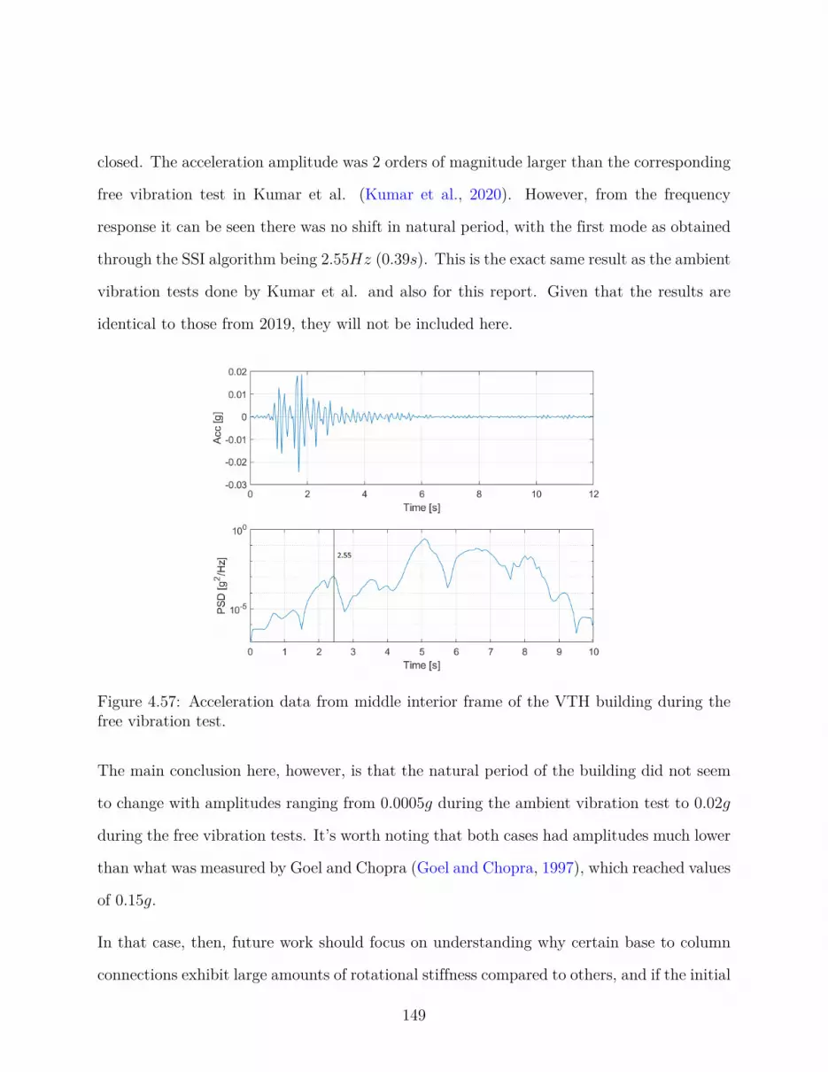
closed. The acceleration amplitude was 2 orders of magnitude larger than the corresponding

free vibration test in Kumar et al. (Kumar et al., 2020). However, from the frequency

response it can be seen there was no shift in natural period, with the first mode as obtained

through the SSI algorithm being 2.55Hz (0.39s). This is the exact same result as the ambient

vibration tests done by Kumar et al. and also for this report. Given that the results are

identical to those from 2019, they will not be included here.

Figure 4.57: Acceleration data from middle interior frame of the VTH building during thefree vibration test.

The main conclusion here, however, is that the natural period of the building did not seem

to change with amplitudes ranging from 0.0005g during the ambient vibration test to 0.02g

during the free vibration tests. It’s worth noting that both cases had amplitudes much lower

than what was measured by Goel and Chopra (Goel and Chopra, 1997), which reached values

of 0.15g.

In that case, then, future work should focus on understanding why certain base to column

connections exhibit large amounts of rotational stiffness compared to others, and if the initial

149

stiffness captured here is representative of the base conditions for a large earthquake.

As a summary though, the test results from Kumar et al. (Kumar et al., 2020) for are

consistent with the results reported in this chapter. In the next chapter, the Smith and Uang

period formula will be evaluated and compared to both the experimental data collected, as

well as the different models created for each building.

150

Chapter 5

Evaluation of the Smith and Uang

Equation

In the previous chapter the results from the experimental campaign were described in detail

and compared to analytical models of the builds to validate some of the assumptions made

when modeling metal buildings. Other important results regarding the behavior of metal

buildings were investigated. More importantly, though, it largely served as a validation of

the modeling approach used by Smith and Uang (Smith and Uang, 2013) to generate a metal

building data set, from which their fundamental period equation formula was derived.

This chapter will then focus on whether the equation itself provides good estimates of the

fundamental period of the tested buildings, and whether those results are enough to fully

validate the equation.

5.1 Fundamental period comparison with best guess

weight

For reference, the Smith and Uang period formula – meant to be a lower bound estimate –

will be shown again. The natural period of a metal building with an aspect ratio α, mean

roof height (in inches) H and seismic Weight (in kips) W can be first estimated as

151

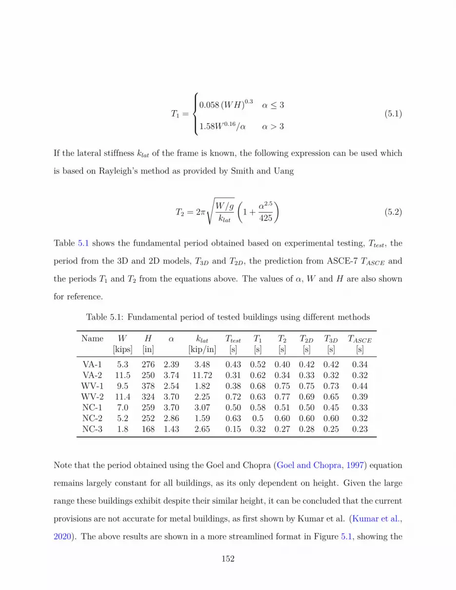
T1 =

0.058 (WH)0.3 α ≤ 3

1.58W 0.16/α α > 3

(5.1)

If the lateral stiffness klat of the frame is known, the following expression can be used which

is based on Rayleigh’s method as provided by Smith and Uang

T2 = 2π

√W/g

klat

(1 +

α2.5

425

)(5.2)

Table 5.1 shows the fundamental period obtained based on experimental testing, Ttest, the

period from the 3D and 2D models, T3D and T2D, the prediction from ASCE-7 TASCE and

the periods T1 and T2 from the equations above. The values of α, W and H are also shown

for reference.

Table 5.1: Fundamental period of tested buildings using different methods

Name W H α klat Ttest T1 T2 T2D T3D TASCE

[kips] [in] [kip/in] [s] [s] [s] [s] [s] [s]VA-1 5.3 276 2.39 3.48 0.43 0.52 0.40 0.42 0.42 0.34VA-2 11.5 250 3.74 11.72 0.31 0.62 0.34 0.33 0.32 0.32WV-1 9.5 378 2.54 1.82 0.38 0.68 0.75 0.75 0.73 0.44WV-2 11.4 324 3.70 2.25 0.72 0.63 0.77 0.69 0.65 0.39NC-1 7.0 259 3.70 3.07 0.50 0.58 0.51 0.50 0.45 0.33NC-2 5.2 252 2.86 1.59 0.63 0.5 0.60 0.60 0.60 0.32NC-3 1.8 168 1.43 2.65 0.15 0.32 0.27 0.28 0.25 0.23

Note that the period obtained using the Goel and Chopra (Goel and Chopra, 1997) equation

remains largely constant for all buildings, as its only dependent on height. Given the large

range these buildings exhibit despite their similar height, it can be concluded that the current

provisions are not accurate for metal buildings, as first shown by Kumar et al. (Kumar et al.,

2020). The above results are shown in a more streamlined format in Figure 5.1, showing the

152

Figure 5.1: Comparison between the different period estimates (relative to Ttest)

different periods predictions normalized by the value of the test results.

Excluding the buildings that exhibited large rotational stiffness at their base (WV-1 and

NC-3), it’s clear from the above results that both the 2D and 3D models match very well

with the measured response, as discussed in the previous chapter. More importantly, the

refined equation to obtain the period T2 shows excellent correlation with the full dynamic

analysis (T2D and T3D). This means that the period could be estimated only by modeling

an isolated 2D-frame, and a simple static analysis to determine its stiffness can be used

coupled with Equation 5.2. Not having to run a dynamic analysis means that it becomes

unnecessary to discretize the elements in between joints and assign masses in correspondence

to the tributary loads, which simplifies the modeling.

However, even though the refined estimation does a very good job of predicting the natural

period, the base prediction from using Equation 5.1 seems to over predict the measured

period and, in general, the results of the modeled periods as well. This is concerning because

the Smith and Uang equation is not meant to predict the period, but to provide a lower

bound. The Smith and Uang equation only provided a lower bound (ratio < 1 in Figure 5.1)

153

of the tested period in 2 out of 7 buildings, and only was below the refined estimate in 3

cases.

There are some outliers in the dataset that worth discussing however. As mentioned before,

buildings WV-2 and NC-3 were showing a fixed base behavior and so naturally all predictions

were significantly off. Even the ASCE-7 formula, which sometimes under predicted the period

by a factor of 2 (WV-2, NC-2), was not providing a conservative lower bound. Though

this may not have major implications in design (as using the ASCE-7 equation for metal

buildings general puts the building in the plateau of the spectral acceleration plot) currently,

adopting the Smith and Uang equation may lead to underestimating the base shear. It must

be highlighted again, then, that further studies need to be done to understand why some

base to column connections show increased rotational stiffness, whether this stiffness stays

constant for larger amplitudes of shaking, and whether this ultimately has consequences in

terms of reliability.

The other major outlier is building VA-2. Figure 5.1 shows that, despite the models and

the refined prediction doing a great job estimating the observed period, Smith and Uang’s

formula was off by a factor of 2, when in the other cases the difference was within 20%. The

main reason for this is that building VA-2 had appendices in every interior frame, essentially

creating a 2-bay frame. It could also be thought of as a modular metal building with a

fixed connection at the top, whereas all the Smith and Uang models assumed any interior

column to be a gravity column. T2D, T3D and T2 all take into account the appendix in

their formulation, while T1 does not. This is a limitation of the Smith and Uang (and any

other potential) formula, and should be properly acknowledged if the equation ends up being

adopted by building codes.

Also, a minor note should be made regarding building NC-2. This building had a aspect

ratio of 2.84, which is very close to the cutoff point of 3 where the expression to estimate

154

the period changes. As mentioned in the literature review, this causes a discontinuity in

the predicted period. For this building for example, the value using the “incorrect” equation

would lead to period of 0.72s, which is 44% larger than the value of 0.5s obtained considering

α < 3. This again shows that this discontinuity should most probably be revised.

5.2 Fundamental period comparison with design weight

Based on the results of the previous section, it would seem at first glance that the Smith

and Uang formula is not providing the intended lower bound estimate for metal buildings.

However, it should be noted that all buildings were designed for much higher loads that those

present at the time of testing. It is generally the case that the dead loads used in design will

be somewhat higher than those seen in service. For example, building NC-1 was designed

to accommodate the installation of solar panels in the future, which resulted in a collateral

load of 7psf .

This may affect the results because, looking at Equation 5.2 and based on structural dynam-

ics theory (Chopra, 2017), the period of a structure increases with the square root of the

mass. Meanwhile, the Smith and Uang formula, as shown in Figure 5.1 scales with the W 0.3

or W 0.16, depending on the aspect ratio. The discrepancy in scaling is because the Equation

is, in some fashion, trying to estimate the stiffness of the structure in order to provide a

fundamental period, and the stiffness also tends to increase with W as the member sizes get

larger to deal with higher dead loads.

It is possible then, that considering the best estimate of the building mass (i.e.: the mass

present during testing) in equation 5.1 would be providing a lower bound estimate of the

period for a building designed for these lower loads, which would be more flexible than the

actual building tested. The refined equation is not affected by this as it uses the actual

155

frame stiffness.

It was deemed more appropriate, then, to do a comparison between the predictive equation

and the refined expression when accounting for a seismic weight closer to its design value

(as close as possible given the available documentation). The use of the refined equation is

justified based on the previous section, which showed excellent correlation between T2 and

the periods from the models.

Table 5.2 shows the results when the collateral load adopted for design is included in the

seismic weight. The collateral load Dc was taken from the design documents for each building

and is presented in the Table as well. Only buildings VA-1, VA-2, WV-2, NC-1 and NC-2

are shown, as these buildings showed very good correlation between the test data and the

models, which provides confidence in extrapolating the period for a larger weight.

Table 5.2: Fundamental period of tested buildings using different methods

Name Dc W T1 T2 TASCE T1/T2

[psf] [kips] [s] [s] [s]VA-1 3 9.4 0.61 0.54 0.34 1.13VA-2 5 24.5 0.70 0.49 0.32 1.43WV-2 2 16.4 0.67 0.92 0.39 0.73NC-1 7 21.0 0.77 0.89 0.32 0.87NC-2 3 9.7 0.60 0.81 0.32 0.73

The results when accounting for the design level weight paint a different picture. As expected,

the Smith and Uang formula is still overpredicting the period for building VA-2, due to the

presence of appendices that are were not part of their modeling. However, for buildings

WV-2, NC-1 and NC-2 the values obtained using Equation 5.1 are shorter than those of

the extrapolated test results. In those cases, then, the Smith and Uang equation is indeed

providing a lower bound of the natural period.

156

It is possible to convert the lower bound estimate to a best guess estimate by multiplying

the period by√Cu, with Cu = 1.6 (Smith and Uang, 2013). By doing so for buildings WV-2,

NC-1 and NC-2, the “best guess” estimate from the Smith and Uang formula would be 0.85s,

0.97s and 0.76s respectively. These values all fall within 10% of the extrapolated experi-

mental results, with the periods for buildings WV-2 and NC-2 being slightly underpredicted

and the period for building NC-1 slightly overpredicted.

In those three cases, then, not only is the Smith and Uang predictive equation providing

a good lower bound estimate, its best guess estimate is also quite accurate. Though the

latter result is not important for design purposes as the “best guess” estimate is not used, it

does show that the building tested fall close to the original regression line which led to the

predictive equation.

For VA-1, however, the lower bound estimate proved to be overpredicting the period, being

10% larger than the extrapolated period considering the design loads. Statistically, it would

be expected for some of the buildings to fall outside the defined bounds, so no real conclusions

can be taken from this case.

Finally, looking at Table 5.2 it’s clear that using the equation in ASCE-7 can result is

excessively short periods, and is not adequate for metal buildings.

All in all, when accounting for the design level loads, the results from the Smith and Uang

formula seemed to provide reasonable lower bounds estimates for the buildings that fell

within the scope of their data set, as long as the column bases behaved as pinned. However,

it should be noted that those only represent four out of the 7 buildings tested for this project.

157

5.3 Comparison between the synthetic data set and the

tested buildings

5.3.1 Building classification

It should be understood that the results presented here apply to the set of buildings that were

tested, which may not necessarily be representative of the complete field of metal buildings

that were included in Smith and Uang’s research.

The buildings in Smith and Uang’s data set can be classified (beyond their weight, aspect

ratio and height that is) by the following properties

1. Cladding type: Metal Panels (MP) or Concrete (C)

2. Roof type: Monoslope (M) or Gabled (G)

3. Structural system: Clear Span (CS) or Modular (MO)

with the difference between clear span and modular buildings being the presence of interior

gravity columns. Given that the final design of a metal building may be governed by different

load combinations depending on its location, two more classes were evaluated in accordance

with the loading conditions

1. Seismic Load: Low (LS) and High (HS)

2. Wind Load: Low Wind (LW) and High Wind (HW)

where classes L and H are associated with a spectral acceleration for short periods of 0.17g

and 1.0g respectively, and classes LW and HW with basic wind speeds of 85mph and 120mph

158

respectively, with these values arbitrarily chosen by Smith and Uang so as to cover different

extremes of ASCE-7 hazard maps. Table 5.3 shows how the tested buildings are classified

as per the above.

Table 5.3: Classification of tested metal buildings

Name MP/C M/G CS/MO LS/HS LW/HWVA-1 MP G CS LS LWVA-2 MP G CS LS LWWV-1 MP M CS LS LWWV-2 MP G CS LS LWNC-1 MP M CS LS LWNC-2 MP M CS LS LWNC-3 MP M CS LS LW

From the table it becomes clear that some building types were not covered by the tests

carried out in this project. A similar conclusion can be reached for the work done by Kumar

et al. (Kumar et al., 2020). In the end, there is no available test data for buildings with

concrete walls, no data for modular buildings, and no data for buildings in either high wind

or high seismic areas. This means that the observations made in this project are only valid

for a (potentially) small percentage of the total building population.

Based on the above classification, only two combinations of buildings were tested: clear span

buildings in low wind and seismic regions with metal panel cladding and a gabled roof, and

the same buildings with a monoslope roof. Out of the 192 buildings in the Smith and Uang

dataset, only 4 and 6 buildings meet each criteria, respectively, which is less than 3%.

Smith and Uang used weighted linear regression, so it could be argued that the sum of the

weights of those buildings should be used. In which case, then these classes comprise 5%

and 3% of the population. However, it should be noted that between this work and the work

of Kumar et al., effectively more buildings with these characteristics have been tested than

similar data points in the Smith and Uang’s predictive equation.

159

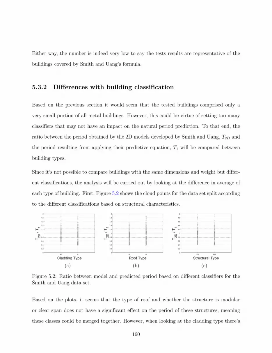
Either way, the number is indeed very low to say the tests results are representative of the

buildings covered by Smith and Uang’s formula.

5.3.2 Differences with building classification

Based on the previous section it would seem that the tested buildings comprised only a

very small portion of all metal buildings. However, this could be virtue of setting too many

classifiers that may not have an impact on the natural period prediction. To that end, the

ratio between the period obtained by the 2D models developed by Smith and Uang, T2D and

the period resulting from applying their predictive equation, T1 will be compared between

building types.

Since it’s not possible to compare buildings with the same dimensions and weight but differ-

ent classifications, the analysis will be carried out by looking at the difference in average of

each type of building. First, Figure 5.2 shows the cloud points for the data set split according

to the different classifications based on structural characteristics.

(a) (b) (c)

Figure 5.2: Ratio between model and predicted period based on different classifiers for theSmith and Uang data set.

Based on the plots, it seems that the type of roof and whether the structure is modular

or clear span does not have a significant effect on the period of these structures, meaning

these classes could be merged together. However, when looking at the cladding type there’s

160

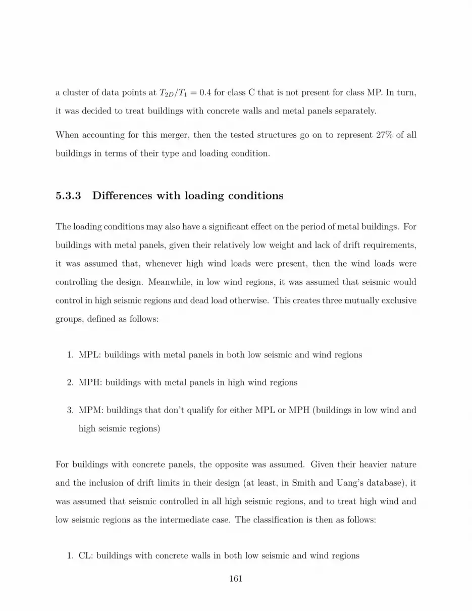
a cluster of data points at T2D/T1 = 0.4 for class C that is not present for class MP. In turn,

it was decided to treat buildings with concrete walls and metal panels separately.

When accounting for this merger, then the tested structures go on to represent 27% of all

buildings in terms of their type and loading condition.

5.3.3 Differences with loading conditions

The loading conditions may also have a significant effect on the period of metal buildings. For

buildings with metal panels, given their relatively low weight and lack of drift requirements,

it was assumed that, whenever high wind loads were present, then the wind loads were

controlling the design. Meanwhile, in low wind regions, it was assumed that seismic would

control in high seismic regions and dead load otherwise. This creates three mutually exclusive

groups, defined as follows:

1. MPL: buildings with metal panels in both low seismic and wind regions

2. MPH: buildings with metal panels in high wind regions

3. MPM: buildings that don’t qualify for either MPL or MPH (buildings in low wind and

high seismic regions)

For buildings with concrete panels, the opposite was assumed. Given their heavier nature

and the inclusion of drift limits in their design (at least, in Smith and Uang’s database), it

was assumed that seismic controlled in all high seismic regions, and to treat high wind and

low seismic regions as the intermediate case. The classification is then as follows:

1. CL: buildings with concrete walls in both low seismic and wind regions

161

2. CH: buildings with concrete walls in high seismic regions

3. CM: buildings that don’t qualify for either CL or CH (buildings in high wind and low

seismic regions)

Figure 5.3 shows how the ratio between the modeled period and the prediction changes for

each of these groups. For buildings with concrete walls, the groups are clearly separate from

each other, with the period of the CL class being underestimated (ratio larger than one)

and the CH class being severely overestimated (ratios lower than 0.8). In fact, almost all

buildings in the CH class fall below the dotted line at around 0.8, which means that they

all have shorter periods than what even the lower bound estimate is predicting. This is

extremely concerning as it is precisely the buildings in high seismic regions the ones to be

most affected by seismic loads, and overpredicting the period would result in underpredicting

the seismic loads which would probably control the design.

Figure 5.3: Ratio between model and predicted period based on loading conditions

162

A similar effect can be seen for buildings with metal panels, though not as pronounced.

The periods of buildings in high wind regions is, on average, underpredicted by 20%, and

about half of the data points have periods shorter than the lower bound. For this class,

however, wind is expected to control over seismic and so whether this result is significant

can be argued. As for Classes MPM and MPL, these are relatively similar to each other. It

seems, then, that the equation is providing accurate results for buildings in low wind regions

in general and these two classes could be grouped together.

Considering groups MPL and MPM to be roughly equal, and accounting for the analysis in

the previous subsection, the buildings tested in this project represent 70% of all buildings in

the set (summing the weights of 49 buildings in the set). Note that this number is only with

respect to building classification.

5.3.4 Geometric parameters

Another point of interest is whether the geometry of the tested buildings covers in reasonable

fashion the wide range of possible building designs. This will be done based on the three

fundamental parameters that are needed to estimate the period as per Equation 5.1: The

mean roof height H, the seismic weight W and the aspect ratio α. Given that the predictive

equation is in reality two different expressions – one dependent on W and H for α < 3, and

another dependent on W and α for α > 3, two plots are presented that show the combination

of the variables that play a part in each respective equation (Figure 5.4). The gray circles are

data points from Uang and Smith, the blue triangles are the buildings tested by Kumar, and

the red squares are buildings tested for this project. Note that the seismic weights plotted

for the new tests are using the design level loads and not the “best guess” estimate during

testing.

163

(a) (b)

Figure 5.4: Scatter plot showing the geometric properties of different buildings.

It becomes immediately clear that the tested buildings do not cover the complete parameter

space included in Smith and Uang’s database. The largest difference is in the seismic weight.

The tested building had weights ranging from 3kip to 25kip. Most of the buildings in Smith

and Uang extend past that, with weight 50kip, 100kip and up to 200kip. The reason for

this is two-fold. On one hand, some of the buildings in Smith and Uang were designed for a

flat roof snow of 40psf , which means that a portion of the snow mass had to be included in

the seismic weight as per ASCE-7. Similarly, buildings with concrete walls would generally

have larger seismic weight as well.

On the other hand, the total length of modular buildings can be significantly larger than that

of clear span buildings. Total lengths of 240ft and 300ft were identified when going through

the database. Given the lengths of these buildings is almost triple what was measured both

in these projects and by Kumar, it follows as well that their weight would be larger in similar

scale.

Similar shortcomings can also be observed for the mean roof height and aspect rations covered

by the tests. Aspect ratios above 5 do not seem to be common, but a significant number of

164

buildings in the database have mean roof heights above 40ft, which was the tallest building

tested. Future work should focus on covering a higher range of heights and weights to cover

the full spectrum of metal buildings.

As mentioned before, Smith and Uang weighted their buildings based on their statistical

likelihood. These weights were assigned based on feedback by an industry expert, who

established frequencies based on the production history of their company (Smith, 2013).

Considering these weights, and assuming that the tested buildings are representative of any

building with weight less then 25kip, mean roof height lesser than 40ft and aspect ratios

smaller than 5, the tested buildings represent 46% of the building database based on geometry

alone.

5.4 Summary and Discussion

In this chapter the results of the experimental testing work were compared to different period

estimation equations: The predicted equation by Smith and Uang (Smith and Uang, 2013),

their refined equation if the lateral stiffness known, and the ASCE-7 equation. From the

comparison it followed that the Smith and Uang predictive equation can provide a lower

estimate for metal buildings with metal panels for cladding as long as the column bases

exhibited pinned behavior and the frames were free of appendices. However, that was not

the case for two of the buildings in this test set, as well as the VTH building in Kumar et

al. (Kumar et al., 2020), which seemed to show fixed base supports. The reason as to why

this happens is not clear, but nonetheless is a significant road block as it can shorten the

building’s period by a factor of 2.

The refined equation was shown to have excellent correlation with test results, and is an

excellent alternative in lieu of performing modal analysis of 2D or 3D models. ASCE-7’s

165

equation was consistently underpredicting the period in most cases, which reinforces the

need for a specific equation for metal buildings.

The test set available after this project still falls short of covering the complete building

space used by Smith and Uang. Based on building classification and loading conditions, the

test set represented about 70% of the built environment. Doing the same for the geometry

of the buildings, about 46% of all buildings were covered by this test. When combining

both criteria, the tested buildings represent only 35% of all metal buildings, according to

the weights used by Smith and Uang (Smith and Uang, 2013). This means a large portion

of metal buildings are still unaccounted for.

More importantly though, the tests are limited to buildings with W < 25kip, H < 40ft and

α < 5 which is only a fraction of what the Smith and Uang formula intends to cover. That

means, that, beyond what percentage of metal buildings fall under the test scope, it should

be made clear that the results cannot be extrapolated to buildings with larger spans, heights

and aspect ratios, nor to buildings in high wind regions or with concrete walls.

A look at the different building types and loading conditions showed the fundamental period

of buildings with concrete cladding can differ significantly from those with metal panels.

Especially for the former, high loading conditions (in this case, defined by high seismic

loads) can result in much stiffer structures due to drift limitations. This, in turn, makes

the predictive equation by Smith and Uang not suitable to estimate their period. Almost

all buildings falling under this category had periods shorter than the lower bound estimate,

which would underpredict the base shear.

Given that estimating the period becomes more important in regions of high seismic risk, it

is fair to ask why include buildings in low seismic regions to develop the equation, especially

for the case with concrete walls where the stiffness difference appears to be significant. The

166

equation in ASCE-7, for example, was developed by measuring buildings in California (Goel

and Chopra, 1997), Including buildings from low seismic regions would result in a more

scattered data set, as well as an overall overestimation of the period, which is unconservative

for design.

For metal buildings, the difference between loading conditions is not as clear. Generally

speaking, though, whether a single formula can be used to described buildings with such

different characteristics should be debated. It would probably be more adequate to only

consider structures in high seismic regions, and also split the results between buildings with

concrete walls and those with metal panels.

Finally, a note should be made about the use of weighted linear regression for the development

of the equation. Including weights in the regression, as argued by Smith and Uang (Smith

and Uang, 2013), ensures that buildings that are more common are estimated better than

outliers. However, the weights used should be carefully considered.

In the Smith and Uang’s database, Frame 97 (a gabled, modular frame with metal panels,

H = 15ft in a low wind, high seismic region) has a weight of 0.32, meaning that a single data

point out of all 192 buildings represents 32% of the population. The next highest weight is

6%. This has the potential to significantly bias the results.

For example, the sum of the weights of all buildings with concrete walls in high seismic

regions – which are the most sensitive type of metal buildings to earthquake loading – is

2.6% (from 43 data points). To offer a comparison, there are 7 buildings in the data set that

on their own have a larger weight. This explains in large part why the predictive equation

performs poorly for the buildings labeled as CH, as they carry almost negligible weight in the

regression. The weighting function, if buildings of all types are to be included in one single

equation, should probably be revised so that the impact an estimation error could have on

167

the safety of the structure is accounted for. That is, how critical the period estimation is for

the design of the structure.

168

Chapter 6

Development of new period prediction

formulas

6.1 Introduction

The analysis from the previous chapter showed that the assumptions Smith and Uang made

to develop their synthetic database are reasonably accurate and adequately represent the

natural period of metal buildings (at least buildings with metal panels, based on the limited

experimental data). However, though their proposed equation does provide a lower-bound

estimate for regular buildings with metal cladding, the equation may overpredict the period

of buildings with concrete hardwalls. The reason for this was two-fold: first, due to the use of

a single equation to describe buildings with very different properties and design requirements,

and second due to the use of a weighted linear regression that effectively ignored the data

from buildings with concrete cladding in high seismic regions. Building NC-2, which had

a height of span-to-height to ratio near 3, where the piecewise function for the prediction

became non-continuous, also showed the necessity to address said discontinuity.

Similarly, the evaluation of the data set showed that the building location plays a significant

role in the building period, with buildings in high seismic regions having shorter periods.

Since the equations in ASCE-7 were developed from tests done in California, it is probably

more appropriate to only consider buildings in high seismic regions for the development of a

169

predictive equation that is consistent with the rest of the building code.

In this Chapter, a new set of predictive equations will be proposed that addresses this

drawbacks, by using only data from buildings in high seismic regions and by separating

buildings with metal panels from those with concrete hardwalls.

6.2 Rational analysis for determining the equation type

Similar to the work by Goel and Chopra (Goel and Chopra, 1997), it was decided that

the best approach to develop a new equation was to first obtain a rational expression to

determine the period. In their case, by assuming the mass was evenly distributed across

each floor and using Rayleigh’s method assuming a linear first mode shape they found that

the period of a multi-story building could be mostly predicted by its height h. For a single-

story building controlled by seismic loading, as shown by Lamarche et al., the natural period

could also be largely be described by the height (Lamarche et al., 2009). An equation of the

type

Ta = a hbn (6.1)

with hn being the mean roof height (in inches), and constants a and b would probably be

adequate for buildings with concrete hardwalls in high seismic regions.

The design of metal buildings with metal panels, however, is essentially controlled by the

gravity loading. As such, the lateral stiffness would be largely independent of the building

height. In turn, a new equation type should be formulated for them.

In order, to find the parameters that best describe the natural period of buildings with

170

metal panels, the lateral stiffness of a single story clear span frame was evaluated. As this is

only meant to be simplified analysis, for the purpose of calculating the lateral stiffness the

following assumptions were made:

• Frame elements are axially rigid, and shear deformations can be ignored

• Columns are ideally pinned at the base

• The cross-sectional properties EI of beams and columns are constant along the length

and equal to each other

• The roof is perfectly flat (monoslope roof with no pitch)

Figure 6.1 shows a schematic view of the frame with height h, span L and cross-sectional

properties EI, along with the resulting moment diagram when a unit load is applied at

the rafter level (note that, due to the axial rigidity assumption, where that load is applied

along the rafter does not affect the results). Interestingly, the moment diagram (and thus,

the deformed shape as well) is anti-symmetric, and there would be no vertical displacement

at midspan due to horizontal loads. This is important because it means that an interior

gravity column at midspan would not affect the lateral stiffness of the frame, which gives

another degree of confidence that modular buildings and clear span buildings could be mostly

grouped together when developing period estimation equations.

In any case, using virtual work the lateral stiffness of the building flat can be obtained as

flat = 2(0.5h)2h

3EI+ 2

(0.5h)2(0.5L)

3EI(6.2)

If instead of the span L, the span-to-height ratio α = L/h is used, then the flexibility can

be expressed as

171

Figure 6.1: Simplified analysis of a single-story moment frame

flat =h3

6EI(1 + 0.5α) (6.3)

However, the design of these buildings is controlled by their dead weight, where the maxi-

mum moments increase with the square of the length and height, with the moment of inertia

needing to increase at the same rate to keep stresses below a given threshold. As a simplifi-

cation, we can assume then that the stiffness will be a function of (1 + 0.5α)2 based on the

above. As such, then the lateral flexibility would be approximately

flat ∝1

(1 + 0.5α)(6.4)

effectively inverting the relationship between the flexibility and the span-to-height ratio.

Remember as well, that the lateral stiffness Klat is the inverse of the flexibility. Finally,

then, for a single degree-of-freedom system the natural period is

T = 2π

√W

g klat∝(

W

1 + 0.5α

)0.5

(6.5)

172

where W is the weight of the building and g is the gravitational constant. Finally, then, the

proposed equation is of the type

Ta = a

(W

1 + 0.5α

)b

(6.6)

with a and b calibration constants. Note the new equation is not a function of height hn

(as is Equation 6.1) but of the seismic weight W (in kip) and span-to-height ratio. Also,

despite having two variables instead of a single one, it still only has two constants that need

calibration. Both equations are suitable for power regression, similar to the equations in

ASCE-7.

6.3 Linear regression analysis

Out of the 192 buildings in the Smith and Uang data set, 39 were identified as buildings with

metal panels, and 44 as buildings with concrete hardwalls, both in high seismic regions. The

number of buildings in each case is close to those used in similar studies to develop period

estimation equations (Goel and Chopra, 1997; Lamarche et al., 2009; Shan et al., 2013). It

was decided, unlike Smith and Uang, to perform a standard linear regression, ignoring the

statistical weights. First, there wasn’t enough confidence in the assigned weights for some of

the buildings, as discussed on the previous Chapter. Moreover, a predictive equation should

provide a similar level of confidence across the variable space (i.e.: different heights, weights

and span-to-height ratios), and so it was believed that a standard linear regression would

be more suitable to achieve this over improving the accuracy in a smaller, perhaps more

common variable range.

In any case, 5 total equations types were studied, all of them being variations of Equa-

173

tions 6.1 and 6.6 with different degrees of complexity (such as introducing more calibration

constants, or simplifying the relationship between period and α). The adequacy of the cali-

brated equations was evaluated in two ways. First, through the use of adjusted coefficient of

determination R2adj. The coefficient determination in this case is a measure of the percentage

of the variance in the period that is explained by the selected variables used in the regres-

sion. Values close to 1 would indicate a very good fit, and generally speaking high values

are desired.

Note that the adjusted value was used over the traditional R2 because adding more constants

will always improve the results, though that doesn’t necessarily mean the predictive capa-

bilities of the equation are better. Instead, R2adj penalizes equations with more constants in

order to be able to compare them to each other on equal ground.

The other way the goodness of fit was evaluated was by the parameter Cu, as used by Goel

and Chopra, and Smith and Uang (Goel and Chopra, 1997; Smith and Uang, 2013). Cu is a

measure of the dispersion in the data, and is calculated by first linearizing the problem by

taking the natural logarithm of both the predicted and model periods, and then evaluating

the standard deviation of the error in the estimate se. Finally, Cu can be obtained as

Cu = e2se (6.7)

which is, effectively, 2 times the standard deviation of error in the data for a power regression.

Table 6.1 shows the results of the regression for the different equation types that were

evaluated. The expressions presented are the best-fit results. The two major takeaways

from the table are that, first, the period of metal buildings with metal panels is effectively

not a function of height with Equation 6.1 showing the worst coefficient of variation. As

Smith and Uang showed before, this is another reason why the ASCE-7 equation is not

174

suitable for metal buildings and why a new predictive equation is necessary (Smith and

Uang, 2013).

Table 6.1: Regression models for metal buildings with metal cladding in high seismic areas.

EQ. Best-fit R2adj Cu

0.35W 0.4H0.01 (1 + 0.5α)−0.43 0.589 1.56

0.36 [W/ (1 + 0.5α)]0.4 0.610 1.54

0.30W 0.4α−0.18 0.568 1.59

0.44 (W/α)0.32 0.474 1.67

0.56H0.22 0.042 1.99

Perhaps more notable, the equation that performed the best was Equation 6.6, which was

developed specifically for single-story buildings designed for gravity loads. What is more,

the exponent is 0.43, very close to the 0.5 obtained with a rational analysis. Though the

R2adj value is low, this about the best fit one can obtain with a limited number of variables.

Perhaps more notable, the Cu value is close is essentially 1.6, which is identical to the one

found by Goel and Chopra in his study of mid-rise buildings (Goel and Chopra, 1997). Thus,

the amount of scatter in the results can be considered appropriate.

Table 6.2 shows the results for buildings with concrete hardwalls. Since the design of these

buildings is controlled by drift due to seismic loads, height is indeed the variable that best

explains their natural period. Given its simplicity, Equation 6.1 is considered the best

equation type for the development of a period estimation formula. Note the much higher

R2adj value compared to the case with metal panels. The better fit is explained, again, by the

controlling load in the design. Buildings with metal panels, as seen in the previous chapter,

tend to be controlled either by gravity loading or wind, and so there is larger scatter in the

results than for buildings with concrete hardwalls.

175

Table 6.2: Regression models for metal buildings with concrete hardwalls in high seismicareas.

EQ. Best-fit R2adj Cu

0.06W 0.05H0.66 (1 + 0.5α)0.25 0.863 1.22

0.22 [W/ (1 + 0.5α)]0.35 0.457 1.47

0.11W 0.45α−0.07 0.477 1.47

0.40 (W/α)0.20 0.332 1.55

0.10H0.61 0.818 1.25

6.4 Proposed lower-bound equations

Given the results in the previous section, Equations 6.1 and 6.6 were identified as the best

possible expression for a period prediction formula among those evaluated. The expressions

shown before were the results of best-guess fit. However, for design we want a lower-bound

estimate. Similar to both Goel and Chopra, and Smith and Uang, the lower bound estimates

were obtained by dividing the best-guess equation by√Cu, which essentially means taking

for an estimate the mean value minus one standard deviation. It then follows that the upper

bound estimate can be obtained from the lower bound estimate by multiplying by Cu, with

the upper bound representing the mean value plus one standard deviation.

Proposed equation for metal buildings with metal panels

Adopting Cu = 1.6, the proposed equation for metal buildings with metal panels becomes

Ta = 0.28 [W/ (1 + 0.5α)]0.4 , Cu = 1.6 (6.8)

176

with W being the seismic weight in kip, and α the span-to-height ratio as defined by Smith

and Uang (Smith and Uang, 2013). Figure 6.2 shows the lower and upper bounds resulting

from the proposed equation. The Figure shows that most of the data set in Smith and

Uang’s data set falls within the bounds, indicating that the proposed equation does a good

job of predicting the natural period of these buildings.

Figure 6.2: Performance of proposed equation for metal buildings with metal panels usingSmith and Uang’s data set

Proposed equation for metal buildings with concrete hardwalls

Adopting Cu = 1.25, and rerunning the linear regression with the exponent fixed at 0.6, the

proposed equation for metal buildings with concrete hardwalls becomes

Ta = 0.095h0.6n , Cu = 1.25 (6.9)

177

with hn being the mean roof height in ft. Figure 6.3 shows the lower and upper bounds

resulting from the proposed equation. The Figure shows that most of the data set in Smith

and Uang’s data set falls within the bounds, indicating that the proposed equation is effective

at predicting the natural period of these buildings.

Figure 6.3: Performance of proposed equation for metal buildings with concrete hardwallsusing Smith and Uang’s data set

Alternate expression for buildings with concrete hardwalls

The possibility of merging both equations into a single equation was also evaluated in order

to streamline its application in practice. To that end, Equation 6.6 was calibrated with a

fixed value of b = 0.4 (identical to the one obtained for metal panels). The resulting best-fit

equation becomes

178

0.18 [W/ (1 + 0.5α)]0.4 , R2adj = 0.449, Cu = 1.46 (6.10)

which is effectively the result obtained from metal panels divided by a factor of 2. Thus,

the period estimation equation for buildings with metal panels could be used for buildings

with concrete cladding reducing the result in half. As shown in Figure 6.4, the alternative

proposal results in larger scatter, also verified by the low R2adj value of 0.449. Despite this,

adopting Cu = 1.6, as used for buildings with metal panels causes most data points to still

fall within the bounds.

Figure 6.4: Performance of the alternative proposal for metal buildings with concrete hard-walls using Smith and Uang’s data set

179

6.5 Equation performance in tested buildings

Finally, it is worth revisiting the buildings tested as part of this project and evaluate whether

the new proposed equations offer suitable lower bounds for their period, as covered in the

previous Chapter for the Smith and Uang formula. Table 6.3 shows the result for the 5

buildings that exhibited pinned behavior at the base, with T1 being the estimated period

using Smith and Uang’s formula, T2 the period using their refined equation (which was shown

to correlate very well with 2D-modeling) and Ta the period estimated with Equation 6.8.

Table 6.3: Fundamental period of tested buildings using the new proposed equations

Name Dc W T1 T2 Ta Ta/T2

[psf] [kips] [s] [s] [s]VA-1 3 9.4 0.61 0.54 0.50 0.93VA-2 5 24.5 0.70 0.49 0.66 1.35WV-2 2 16.4 0.67 0.92 0.67 0.73NC-1 7 21.0 0.77 0.89 0.62 0.70NC-2 3 9.7 0.60 0.81 0.49 0.60

The results show that the new equation is indeed providing a lower-bound estimate for all

buildings except building VA-2, which had appendices, with ratios ranging from 0.6% to

0.93%. VA-1, for which the Smith and Uang equation was overpredicting the period, now

falls within the boundaries with the new formula. Compared to Smith and Uang the resulting

underprediction tends to be bigger, though this was expected as Equation 6.8 was developed

with buildings in high seismic regions, while the buildings tested were in low seismic regions.

Either way, with the exception of building NC-2, all buildings fall within the upper bound

as well (for building NC-2, the difference between the upper-bound and the modeled period

is 4%). Note that, comparing to the results using the ASCE-7 equation (see Table 5.2), the

proposed equation still predicts periods that can be as much as double those obtained with

the current code provisions.

180

Chapter 7

Observations on the application of the

Equivalent Lateral Force Method

7.1 Introdcution

The final chapter is meant to provide a preliminary analysis on the consequences of the

observations made in Chapter 4 about the dynamic behavior of metal buildings.

A case study will be evaluated, in order to see if the behavior seen during experimental

testing, with the global mode shapes due to stiffness of secondary framing and low mass

participation ratios has an effect of the base shear distribution to the different frames in a

metal building system.

It should be noted that this is not the only potential issue with the application of ELF.

As mentioned by Smith, low mass participation was also seen at the individual frame level,

which may mean that higher order modes could affect the moment and shear diagrams

(Smith, 2013). Similarly, it was found that that some buildings exhibited large vertical

deformations, which are not accounted for introducing forces as purely horizontal when

using ELF. Remember that the forces from ELF are the result of considering the deformed

shape, and so if the mode shape has large vertical deformations then the equivalent forces

may need to include vertical components along the beams. Given that metal buildings are

181

heavily optimized structures, and that alternating lateral torsional buckling of the rafter

seems to govern the inelastic behavior of the frames, more work should be done to obtain

procedures that can accurately calculate the bending moment diagram given the base shear.

The procedure found in the guide by MBMA (MBMA, 2019b), which consists of point loads

at each beam column joint, should be evaluated to see if leads to satisfactory results or if this

methodology could be improved by, for example, considering the base shear as distributed

along the roof.

7.2 Simplified N-DOF model of a metal building

As discussed in Chapter 4, the first mode in metal building systems exhibit very low mass

participation ratios, well below the 0.9 threshold typically used to be allowed to consider

only the first mode in the analysis. Building WV-2, for example, had a mass participation

factor of 0.4 based on its 3D-model. With the first mode only exciting the frames in the

interior of the building (Figure 4.46).

Along these lines, as shown for building NC-2, the roof diaphragm of metal buildings does

not qualify as flexible when checked following ASCE-7. Again, this should not be taken as

indication that the flexible diaphragm assumption shouldn’t be used, as history has shown

that metal buildings designed this way have performed well during earthquakes. If anything,

it may be a commentary on how difficult it is to actually fulfill the ASCE-7 provisions for

flexible diaphragms.

In any case, the objective of this section is to evaluate how the base shear of each frame

applying the ELF procedure and flexible diaphragm assumption compares to the result of

considering the low mass participation ratios and purlin/girt stiffness observed in test data

and the associated 3D models.

182

To that end, a simplified multiple degree-of-freedom model of building WV-2 was designed.

This model consists of a series of linear springs representing the different frame lines, in-

terconnected by another set of springs representing the purlin and girt stiffness. Figure 7.1

presents a generic version of this model, which is essentially identical as the one used by

Sparks and Sockalingam for calibrating metal building parameters (Sparks and Sockalingam,

1988).

Figure 7.1: Generic example of a simple N-DOF model for 3D analysis of metal buildings.

The generic model for a metal building with n frames can be described in terms of the

stiffness of frame i, ki, its mass mi, and the stiffness of the deck kd as follows

K =

k1 + kd −kd

−kd k2 + 2k2 −kd

−kd k3 + 2kd −kd

. . .

−kd kn

, diag(M) =

m1

m2

m3

. . .

mn

(7.1)

where K is the global stiffness matrix and M is the global mass matrix. For this model, the

following properties were used:

183

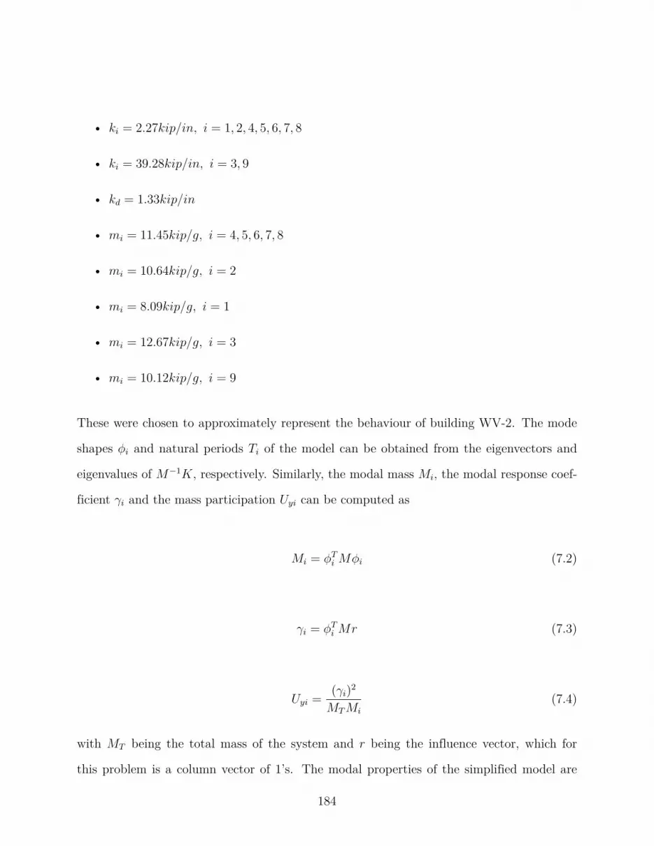
• ki = 2.27kip/in, i = 1, 2, 4, 5, 6, 7, 8

• ki = 39.28kip/in, i = 3, 9

• kd = 1.33kip/in

• mi = 11.45kip/g, i = 4, 5, 6, 7, 8

• mi = 10.64kip/g, i = 2

• mi = 8.09kip/g, i = 1

• mi = 12.67kip/g, i = 3

• mi = 10.12kip/g, i = 9

These were chosen to approximately represent the behaviour of building WV-2. The mode

shapes ϕi and natural periods Ti of the model can be obtained from the eigenvectors and

eigenvalues of M−1K, respectively. Similarly, the modal mass Mi, the modal response coef-

ficient γi and the mass participation Uyi can be computed as

Mi = ϕTi Mϕi (7.2)

γi = ϕTi Mr (7.3)

Uyi =(γi)

2

MTMi

(7.4)

with MT being the total mass of the system and r being the influence vector, which for

this problem is a column vector of 1’s. The modal properties of the simplified model are

184

shown in Table 7.1. Note that the sum of mass participation factors does not reach 0.9 until

effectively all modes are considered in the analysis. This is due to the large stiffness of the

endwalls, which is why Response Spectrum Analysis (RSA) would require several modes in

a complete 3D-model of a metal building. As Langley and Marshal mentioned, it could take

“hundreds” of modes to reach 0.9 mass participation (Langley and Marshall, 2017). With

modern computational capabilities, this is not necessarily a limitation, however. In any case,

since this simplified model has a reduced number of modes, RSA will be used in order to

show how the different modes are contributing to the base shear of each frame.

7.3 Base shear distribution among frames

For the purpose of this example, the building will be located in Chester, CT, with site class

D. This is “Site 1” in the examples found within the MBMA guide (MBMA, 2019b), and the

reader is referred to the book for more information on the design spectrum for this site. The

spectral acceleration for each mode, Si are also in Table 7.1. Comparing with Figure 4.49,

it can be shown that natural periods of the first two modes are roughly equivalent to those

of the full 3D model. The participation factor is larger, mainly due to the lumped mass

formulations as the mass on the bottom half of the structure is not accounted for. This was

considered good enough for a preliminary analysis. The mode shapes (shown in Figure 7.2)

were also similar.

In order to obtain the maximum base shear in each frame i, the contribution of each mode j

to the base shear of said frame must be calculated. Given the spectral acceleration for mode

j, Saj, the spectral displacement Dj can be computed as

185

(a) (b) (c)

Figure 7.2: First three modes for simplified WV-2 model.

Table 7.1: Modal properties of simplified proxy of building WV-2

Mode Ti [s] Mi [kip/g] γi [kip/g] Ui Sai [g]1 0.67 11.45 -25.11 0.56 0.0482 0.58 9.29 17.72 0.18 0.0563 0.57 11.22 4.11 0.02 0.0564 0.49 11.45 -6.73 0.04 0.0615 0.43 11.45 -2e-3 2e-9 0.0616 0.42 9.26 -1.47 2e-3 0.0617 0.40 11.45 1.84 3e-3 0.0618 0.18 12.66 -11.76 0.11 0.0619 0.16 10.12 -9.75 0.095 0.061

Dj =

(Tj

2π

)2

Saj (7.5)

from which the maximum displacement of frame i due to the response of mode j, Yi,j can

be taken as

Yi,j = ϕi,jγjMj

Dj (7.6)

Finally, the base shear Vi,j in each frame i due to mode j is simply the displacement of the

frame times its stiffness

186

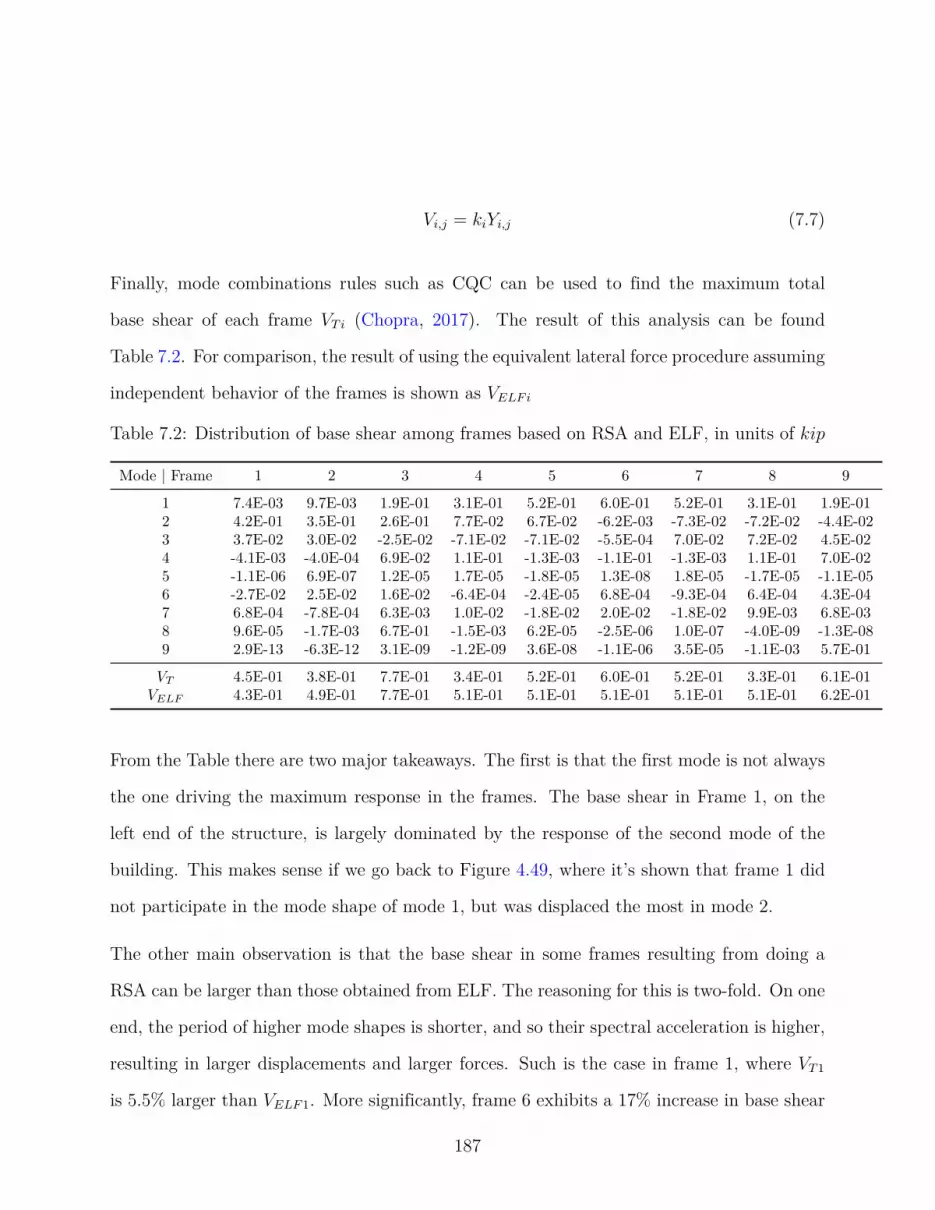
Vi,j = kiYi,j (7.7)

Finally, mode combinations rules such as CQC can be used to find the maximum total

base shear of each frame VT i (Chopra, 2017). The result of this analysis can be found

Table 7.2. For comparison, the result of using the equivalent lateral force procedure assuming

independent behavior of the frames is shown as VELFi

Table 7.2: Distribution of base shear among frames based on RSA and ELF, in units of kip

Mode | Frame 1 2 3 4 5 6 7 8 9

1 7.4E-03 9.7E-03 1.9E-01 3.1E-01 5.2E-01 6.0E-01 5.2E-01 3.1E-01 1.9E-012 4.2E-01 3.5E-01 2.6E-01 7.7E-02 6.7E-02 -6.2E-03 -7.3E-02 -7.2E-02 -4.4E-023 3.7E-02 3.0E-02 -2.5E-02 -7.1E-02 -7.1E-02 -5.5E-04 7.0E-02 7.2E-02 4.5E-024 -4.1E-03 -4.0E-04 6.9E-02 1.1E-01 -1.3E-03 -1.1E-01 -1.3E-03 1.1E-01 7.0E-025 -1.1E-06 6.9E-07 1.2E-05 1.7E-05 -1.8E-05 1.3E-08 1.8E-05 -1.7E-05 -1.1E-056 -2.7E-02 2.5E-02 1.6E-02 -6.4E-04 -2.4E-05 6.8E-04 -9.3E-04 6.4E-04 4.3E-047 6.8E-04 -7.8E-04 6.3E-03 1.0E-02 -1.8E-02 2.0E-02 -1.8E-02 9.9E-03 6.8E-038 9.6E-05 -1.7E-03 6.7E-01 -1.5E-03 6.2E-05 -2.5E-06 1.0E-07 -4.0E-09 -1.3E-089 2.9E-13 -6.3E-12 3.1E-09 -1.2E-09 3.6E-08 -1.1E-06 3.5E-05 -1.1E-03 5.7E-01

VT 4.5E-01 3.8E-01 7.7E-01 3.4E-01 5.2E-01 6.0E-01 5.2E-01 3.3E-01 6.1E-01VELF 4.3E-01 4.9E-01 7.7E-01 5.1E-01 5.1E-01 5.1E-01 5.1E-01 5.1E-01 6.2E-01

From the Table there are two major takeaways. The first is that the first mode is not always

the one driving the maximum response in the frames. The base shear in Frame 1, on the

left end of the structure, is largely dominated by the response of the second mode of the

building. This makes sense if we go back to Figure 4.49, where it’s shown that frame 1 did

not participate in the mode shape of mode 1, but was displaced the most in mode 2.

The other main observation is that the base shear in some frames resulting from doing a

RSA can be larger than those obtained from ELF. The reasoning for this is two-fold. On one

end, the period of higher mode shapes is shorter, and so their spectral acceleration is higher,

resulting in larger displacements and larger forces. Such is the case in frame 1, where VT1

is 5.5% larger than VELF1. More significantly, frame 6 exhibits a 17% increase in base shear

187

when considering the the effect of the secondary framing in the response.

Consequently, the example here shows that ELF may not be applicable to metal buildings

due to their flexible nature and low mass participation ratio in the first mode. However, it

should be noted that this analysis assumes that the secondary framing is behaving elastically

and its stiffness remains unchanged. Whether this is possible under design level loads is not

clear. It’s not clear how Langley modeled the secondary framing behavior, as much of the

discussion on the nonlinear modelling is focused on other elements of the structure (Langley,

2016).

Another point that should be made is that, in the example above, Frame 6 (if designed with

ELF) would start exhibiting nonlinear behavior earlier than the rest of the frames, and it

may be possible for the seismic load to redistribute to other frame lines creating a more

uniform base shear distribution in the end. However, this would also mean that the drift

along frame line 6 would be larger than that predicted with a 2D-analysis. Work by Smith

(Smith, 2013) showed that metal building moment frames can exhibit very large amount

of drift before collapse, and so it’s plausible that the increased ductility demand this case

study is implying would not negatively impact the design of metal buildings with metal

panels. However, the potentially larger drift may have an effect on the safety of buildings

with hardwalls.

Only nonlinear 3D-analysis would be able to answer the questions here presented, mainly

regarding the maximum drift during the design earthquake, and whether designs using ELF

and 2D-analysis can accommodate the increased loading and displacements in certain frames

that this case study imply, and if the current value of Cd for estimating the inelastic dis-

placement is adequate for metal buildings as is.

188

Chapter 8

Conclusions and Future Work

.

8.1 Summary

Initial Objectives

The purpose of this work was to provide a better understanding of the structural behavior

of metal building systems – namely their fundamental period – looking at the influence of

non-structural elements and evaluating how different modeling approaches of varied levels of

complexity (2D and 3D) perform as predictors. As part of this work, the results were used to

assess the accuracy the assumptions made by Uang and Smith that led to the development

of their period estimation formulas, as well as validate the equations themselves. Given that

past test data, as well as experiences in other types of single-story buildings seemed to imply

that non-structural elements and cladding could be playing a significant role in the dynamic

response of metal buildings, it was decided to carry out an experimental testing program

that could help provide an answer on whether this was the case for metal buildings as well.

189

Experimental testing

Seven buildings were tested in total using ambient vibration data, four of them in different

stages of construction for a total of thirteen tests. To the author’s knowledge, this is the first

study of its kind for metal buildings. The tests across construction stages – before and after

the cladding was installed – showed that the endwall stiffness is affected by their cladding,

though the cladding stiffness could not be evaluated from the test results as the endwalls

tended to become essentially infinitely rigid compared to the flexible interior frames.

The difference in period between tests results across construction stages also showed that that

the introduction of the roof cladding did not affect the fundamental mode of the buildings,

implying that no diaphragm action was being developed. This result seems to be unique

to metal buildings, as other experiences in Europe and Canada for single-story buildings

showed significant changes in stiffness after the inclusion of non-structural elements.

Analytical Modeling of metal buildings

3D models were created for all buildings and all stages of construction. These 3D models

assumed a pinned base, and a simplified geometry and connections between the secondary

and primary framing. They also used a centerline model for the panel zone of the beam-

column joint. These models where shown to accurately describe the behavior of metal

building in all cases where bare frame testing was possible.

Some buildings showed an increased stiffness compared to what was predicted by the models.

Unfortunately, none of these buildings was tested before its final configuration. However, the

results from other tests, as well as the mode shape information implies that the main reason

for this was an increased fixity at the base of the columns. In fact, in all cases updating the

model to a fixed base provided accurate results for the fundamental period.

190

The applicability of 2D modelling for metal buildings was also evaluated by looking at

their correlation with both 3D modeling results and the test data. Results showed that 2D

modeling of isolated frames can accurately predict the fundamental period.

Evaluation of Smith and Uang’s formulas

Given that the weight of the buildings during testing did not match the values used for design,

the stiffness obtained from the models, validated against the experimental results, was used

to extrapolate the natural period for the design seismic weight. For regular buildings without

appendices, the Smith and Uang’s formula seemed to provide a reasonable lower estimate of

the natural period. In fact, the “best guess” estimate from the linear regression proved to

be within 10% of the extrapolated periods.

The refined equation based Rayleigh’s method was also studied, and in all cases it showed

excellent correlation with a full dynamic analysis of the buildings.

The buildings tested were estimated to represent only about 37% of the built environment.

Looking into the different types of building types included in Smith and Uang’s formula,

it was found that that the equation may severely overpredict the period for buildings with

concrete walls in high seismic areas. Given that seismic loads are critical to the safety

of these structures, it would be prudent to evaluate them separately from the rest of the

buildings. In fact, building with concrete panels in general seemed to be more sensitive to

loading conditions, and so grouping all buildings classes into a single equation may result in

overpredicting the period for certain types of buildings.

Building NC-2, with an aspect ratio close to 3, showed that the discontinuity in the formula

should be addressed. Abnormally large weights for some buildings used in the regression

should also be revised to avoid introducing bias into the equation

191

Development of new period estimation equations

Based on the above, two new period estimation equations were developed for metal buildings:

one for buildings with with metal sheeting and one for concrete hardwalls. These equations

were developed in semi-empirical fashion, with the controlling parameters being obtained

from rational analysis of a single-story moment frame and the final constants calibrated

using standard linear regression.

These equations focused only on buildings in high seismic regions, where seismic loads may

govern the design and are consistent with the current formulas in ASCE-7. The equations

proposed are continuous, and exhibited similar or reduced levels of scatter compared to the

equations developed by Goel and Chopra for mid-rise construction.

It should be noted that these new proposed equations are only applicable for the interior

moment frames of standard metal building systems with no appendices, and do not apply

to the endwall framing.

Applicability of the ELF method

The 3D models, validated against the test results, showed that first mode of metal build-

ings exhibit very low mass participation factors, and evaluation of the flexible diaphragm

assumption showed that, even if the roof diaphragm provided no additional stiffness, the

secondary framing was enough to qualify the diaphragm as semirigid. These two results

together imply that the ELF method may not be applicable to metal buildings.

A preliminary analysis using a simplified N-DOF model showed that the ELF method may

underestimate the base shear which could also lead to larger inelastic displacements if de-

signed using ELF. However, the consequences for this in design are not known.

192

8.2 Main Conclusions

• A new data base with metal building tested during different phases of construction has

been developed, the first for these types of buildings

• The cladding in the endwalls of metal buildings can significantly increase their stiff-

ness. This, however, does not affect the fundamental period of the buildings, which in

controlled by the stiffness of the interior frames. This is due to the flexibility of the roof

diaphragm, which allows for the interior frames to deform without being restrained by

the end walls.

• The roof cladding does not seem to provide any diaphragm action, and its stiffness can

be considered to be negligible, which is consisted with low values reported by previous

tests on roof assembly. Effectively all the stiffness at the roof level is provided by the

purlins and not the sheeting.

• 2D models of metal buildings are just as capable as 3D models in predicting the

fundamental period. However, important information regarding mode shapes and mass

participation factors are lost.

• Some metal buildings exhibit what seems to be unintended rotational stiffness at the

base of the columns, and more work needs to be done to understand what construc-

tion details may cause this, and whether it’s representative of the behavior at higher

amplitudes.

• The Smith and Uang formula can provide reasonable lower bound estimates for metal

buildings with metal panels as long as they exhibit pinned base behavior. However,

a non-negligible number of tests have so far been more consistent with a fixed base

connection.

193

• The Smith and Uang formula may severely overestimate the period for metal buildings

with concrete walls in high seismic areas. These buildings had very low contribution to

linear regression due to low weights. Buildings with concrete walls seemed to be more

sensitive to loading conditions and this should be accounted for in a period estimation

equation.

• New prediction equations for adoption in ASCE-7 are proposed, which includes the

effect of the type of cladding and provide reasonable lower bounds for the tested build-

ings. These equations were calibrated based on a rational analysis for the parameter

estimation and using standard linear regression on metal buildings in high seismic

regions.

• The ELF method may underestimate the base shear in some frame lines of a metal

building system when compared to the results of a 3D model, though the consequences

and significance of this are yet to be explored.

• Since the period of the endwalls was not able to be extracted from experimental tests,

no real recommendation can be offered. However, they seem to be much stiffer than

the interior frames, and so the current equations in ASCE-7 are probably sufficient as

they would make the base shear be governed by the plateau of the spectral acceleration

plot.

8.3 Future Work

Given the results, future research should focus on why some column bases exhibit significantly

larger rotational stiffness despite similar details on the structural drawings. Full scale testing

for different configurations is recommended to see if the fixed base condition is an artifact

194

of low level vibrations or a direct result of the base detail.

The new proposed equations for period estimation are applicable as long as the synthetic

database created by Smith and Uang is an accurate representation of the true behavior of

metal building systems. This can only be reasonably justified for buildings with metal panels

based on the tests carried out in this work, though there is no reason to believe at the moment

that different conclusions will be reached for buildings with concrete hardwalls. Either way,

the database of tested buildings should be expanded to cover current shortcomings. Modular

frames with large seismic weights, buildings with concrete walls, and metal buildings in high

seismic and wind regions need to be tested in order to provide certainty that the database

developed by Smith and Uang is consistent with the built environment.

Finally. the applicability of the ELF procedure should be studied in detail. 3D, nonlinear

response history analysis is recommended to evaluate the interaction between the primary

and secondary framing under design level loads, as well as looking at the inelastic displace-

ments and drift demands in the most loaded frames. A 2D analysis may not be enough to

ensure adequate reliability.

195

Bibliography

AISI S310-16 (2016). North American Standard for the Design of Profiled Steel Diaphragm

Panels, 2016 Edition. American Iron and Steel Institute, Washington, D.C.

Allemang, R. J. (2003). The modal assurance criterion - twenty years of use and abuse.

Sound and Vibration.

Antoni, J. (2006). The spectral kurtosis: a useful tool for characterising non-stationary

signals. Mechanical Systems and Signal Processing, 20(2):282–307.

ASCE/SEI 7-16 (2017). Minimum Design Loads and Associated Criteria for Buildings and

Other Structures. American Society of Civil Engineers, Reston, VA.

Avci, O., Luttrell, L. D., Mattingly, J., and Easterling, W. S. (2016). Diaphragm shear

strength and stiffness of aluminum roof panel assemblies. Thin-Walled Structures, 106:51–

60.

Bajwa, M. S. (2010). Assessment of analytical procedures for designing metal buildings for

wind drift serviceability. Master’s thesis, Virginia Tech, Blacksburg, VA.

Bajwa, M. S., Charney, F. A., and Moen, C. D. (2010). Assessment of analytical procedures

for designing metal buildings for wind drift serviceability. Technical Report No. CE/VPI-

ST 10/05, Virginia Tech, Blacksburg, VA.

Brinker, R. and Ventura, C. E. (2015). Introduction to Operational Modal Analysis. John

Wiley and Sons, Ltd, Chichester, UK.

196

Charney, F. A. (2008). A transformational approach to teaching matrix structural analy-

sis, and visual implementation using mathcad. In Structures Congress 2008, Vancouver,

Canada.

Charney, F. A., Heausler, T. F., and Marshall, J. D. (2020). Seismic Loads: Guide to the

Seismic Load Provisions of ASCE 7-16. American Society of Civil Engineers, Reston, VA.

Charney, F. A., Iyer, H., and Spears, P. W. (2005). Computation of major axis shear

deformations in wide flange steel girders and columns. Journal of Constructional Steel

Research, 61(11):1525–1558.

Charney, F. A. and Marshall, J. D. (2006). A comparison of the krawinkler and scissors

models for including beam column joint deformations in the analysis of moment resisting

steel frames. AISC Engineering Journal, 43:23–48.

Charney, F. A. and Pathak, R. (2008a). Sources of elastic deformation in steel frame and

framed-tube structures: Part 1: Simplified subassemblage models. Journal of Construc-

tional Steel Research, 64(1):87–100.

Charney, F. A. and Pathak, R. (2008b). Sources of elastic deformations in steel frame and

framed-tube structures: Part 2: Detailed subassemblage models. Journal of Constructional

Steel Research, 64(1):101–117.

Chopra, A. K. (2017). Dynamics of Structures: Theory and Applications to Earthquake

Engineering. Pearson, Hoboken, NJ, 5th edition.

CSI (2021). SAP2000 Integrated Software for Structural Analysis and Design. Computers

and Structures Inc., Berkeley, CA.

Davies, J. M. (2006). Developments in stressed skin design. Thin-Walled Structures,

44(12):1250–1260.

197

Davies, J. M. and Bryan, E. R. (1982). Manual of Stressed Skin Diaphragm Design. Granada

Publishing, London, England.

Döhler, M. and Mevel, L. (2013). Efficient multi-order uncertainty computation for stochastic

subspace identification. Mechanical Systems and Signal Processing, 38(2):346–366.

ECCS (1995). European Recommendations for Application of Metal Sheeting Acting as

Diaphragm No. 88. TC7, European Convention for Constructional Steelwork.

Fischer, A. W. and Schafer, B. W. (2021). Wall-diaphragm interactions in seismic response

of single-story building systems. Engineering Structures, 247:113150.

Fisher, J. M. and Nunnery, J. N. (1996). Stability of standing seam roof-purlin systems. In

13th International Specialty Conference on Cold-Formed Steel Structures, St Louis, MO.

Goel, R. K. and Chopra, A. K. (1997). Period formulas for moment-resisting frame buildings.

Journal of Structural Engineering, 123(11):1454–1461.

Gryniewicz, M., Roberts, M. J., and Davies, J. M. (2021). Testing and analysis of a full-

scale steel-framed building including the consideration of structure-cladding interaction.

Journal of Constructional Steel Research, 181:106611.

Kim, J. Y., Yu, E., Kim, D. Y., and Kim, S.-D. (2009). Calibration of analytical mod-

els to assess wind-induced acceleration responses of tall buildings in serviceability level.

Engineering Structures, 31(9):2086–2096.

Kohler, M. D., Davis, P. M., and Safak, E. (2005). Earthquake and ambient vibration

monitoring of the steel-frame ucla factor building. Earthquake Spectra, 21(3):715–736.

Kumar, A., Charney, F. A., and Sarlo, R. (2020). Development of methodology for measuring

the period of vibration for metal buildings. Technical Report No. CE/VPI-ST 20/04,

Virginia Tech, Blacksburg, VA.

198

Lamarche, C.-P., Proulx, J., Paultre, P., Turek, M., Ventura, C. E., Le, T. P., and Lévesque,

C. (2009). Toward a better understanding of the dynamic characteristics of single-storey

braced steel frame buildings in canada. Canadian Journal of Civil Engineering, 36(6):969–

979.

Langley, M. and Marshall, J. D. (2017). 3-d analytical modeling of metal building systems

with hard walls. In 16th World Conference on Earthquake Engineering, Santiago, Chile.

Langley, M. J. (2016). 3-d model development of metal building systems with hard walls.

Master’s thesis, Auburn University, Auburn, AL.

Langley, M. J. (2018). Development, Testing, and Analysis of a Rotational Friction Connec-

tion for Improving the Seismic Performance of Metal Building Systems with Hard Walls.

PhD thesis, Auburn University, Auburn, AL.

Liu, K.-S. and Tsai, Y.-B. (2010). Observed natural frequencies, damping ratios, and mode

shapes of vibration of a 30-story building excited by a major earthquake and typhoon.

Earthquake Spectra, 26(2):371–397.

Lutrell, L. D., Mattingly, J. A., Schultz, W., and Sputo, T. (2015). Diaphragm Design

Manual. Steel Deck Institute, St. Louis, MI, 4th edition.

Luttrell, L. D. (1965). Structural Performance of Light Gage Steel Diaphragms. PhD thesis,

Cornell University, Ithaca, NY.

Luttrell, L. D. and Mattingly, J. A. (2004). A Primer on Diaphragm Design. Metal Con-

struction Association, Glenview, IL, 1st edition.

MBMA (2019a). Metal Building Systems Manual. Internation Code Council, Washington,

D.C., 2018 edition.

199

MBMA (2019b). Seismic Design Guide for Metal Building Systems. Internation Code

Council, Washington, D.C., 3rd edition.

MBMA (2020). MBMA Annual Report. Metal Building Manufacturers Association, Cleve-

land, OH.

McGuire, W., Gallagher, R. H., and Ziemian, R. D. (2020). Matrix Structural Analysis.

Faculty Books, 2nd edition.

Moen, C. D., Torabian, S., and Schafer, B. W. (2019). Evaluation of metal building system

seismic response modification coefficients. Technical Report No. CFSRC;R-2019-05, NBM

Technologies, Inc., Blacksburg, VA.

NBC 2015 (2015). National Building Code of Canada: 2015. Canadian Commission on

Building and Fire Codes, Ottawa, Canada.

Newman, A. (2015). Metal Building Systems: Design and Specifications. McGraw-Hill

Education, New York, NY, 3rd edition.

Overschee, P. V. and De Moor, B. (1996). Subspace Identification for Linear Systems. Kluwer

Academic Publishers, Amsterdam, Netherlands.

Pan, T.-C., Goh, K. S., and Megawati, K. (2014). Empirical relationships between natural

vibration period and height of buildings in singapore. Earthquake Engineering & Structural

Dynamics, 43(3):449–465.

Peeters, B. and De Roeck, G. (1999). Reference-based stochastic subspace identification for

output-only modal analysis. Mechanical Systems and Signal Processing, 13(6):855–878.

Reynders, E., Houbrechts, J., and De Roeck, G. (2012). Fully automated (operational)

modal analysis. Mechanical Systems and Signal Processing, 29:228–250.

200

Reynders, E., Maes, K., Lombaert, G., and De Roeck, G. (2016). Uncertainty quantifica-

tion in operational modal analysis with stochastic subspace identification: Validation and

applications. Mechanical Systems and Signal Processing, 66-67:13–30.

Roberts, M. J., Davies, J. M., and Wang, Y. C. (2021). Numerical analysis of a clad portal

frame structure tested to destruction. Structures, 33:3779–3797.

Rogers, C. A. and Tremblay, R. (2010). Impact of diaphragm behavior on the seismic design

of low-rise steel buildings. AISC Engineering Journal, 47:21–36.

Sarlo, R., Tarazaga, P. A., and Kasarda, M. E. (2018). High resolution operational modal

analysis on a five-story smart building under wind and human induced excitation. Engi-

neering Structures, 176:279–292.

Shan, J., Shi, W., and Wang, J. (2013). Regional study on structural dynamic property of

buildings in china. Earthquake Engineering & Structural Dynamics, 42(7):1013–1029.

Smith, M. D. (2013). Seismic Testing and Analytical Studies for the Development of New

Seismic Force Resisting Systems for Metal Buildings. PhD thesis, University of California,

San Diego, La Jolla, CA.

Smith, M. D. and Uang, C.-M. (2013). Approximate natural periods for metal building

moment frames. Technical Report No. SSRP–12/07, University of California, San Diego,

La Jolla, CA.

Sockalingam, B. (1988). A dynamic test procedure for analyzing low-rise metal buildings.

Master’s thesis, Clemson University, Clemson, SC.

Sparks, P. R. and Sockalingam, B. (1988). Frame-diaphragm interaction in an enclosed metal

building. Technical report, Clemson University, Clemson, SC.

201

Tremblay, R. (2005). Fundamental periods of vibration of braced steel frames for seismic

design. Earthquake Spectra, 21(3):833–860.

Tremblay, R. and Rogers, C. A. (2011). Seismic design of low-rise steel buildings with flexible

steel roof deck diaphragms – a canadian perspective. Steel Construction, 4(4):242–250.

Trifunac, M. D. (1972). Comparisons between ambient and forced vibration experiments.

Earthquake Engineering & Structural Dynamics, 1(2):133–150.

Verma, A. (2012). Influence of column-base fixity on lateral drift of gable frames. Master’s

thesis, Virginia Tech, Blacksburg, VA.

Wei, G., Schafer, B. W., Seek, M., and Eatherton, M. R. (2020). Experimental study

on the in-plane behavior of standing seam roof assembly and its use in lateral bracing of

rafters. Technical Report No. CFSRC R-2020-02, Cold-Formed Steel Research Consortium,

Baltimore, MD.

White, D. W., Jeong, W. Y., and Slein, R. (2021). Aisc design guide 25: Frame design

using nonprismatic members, second edition. Technical report, American Institute of

Steel Construction, Chicago, IL.

Wrzesien, A. M., Lim, J. B., Xu, Y. Y., MacLeod, I. A., and Lawson, R. M. (2015). Effect

of stressed skin action on the behaviour of cold-formed steel portal frames. Engineering

Structures, 105:123–136.

Xia, Y., Friswell, M. I., and Saavedra Flores, E. I. (2012). Equivalent models of corrugated

panels. International Journal of Solids and Structures, 49(13):1453–1462.

202

Appendix A

Plan and Elevation Drawings for

Tested buildings

Figure A.1: Plan and elevation drawings for Building VA-1.

203

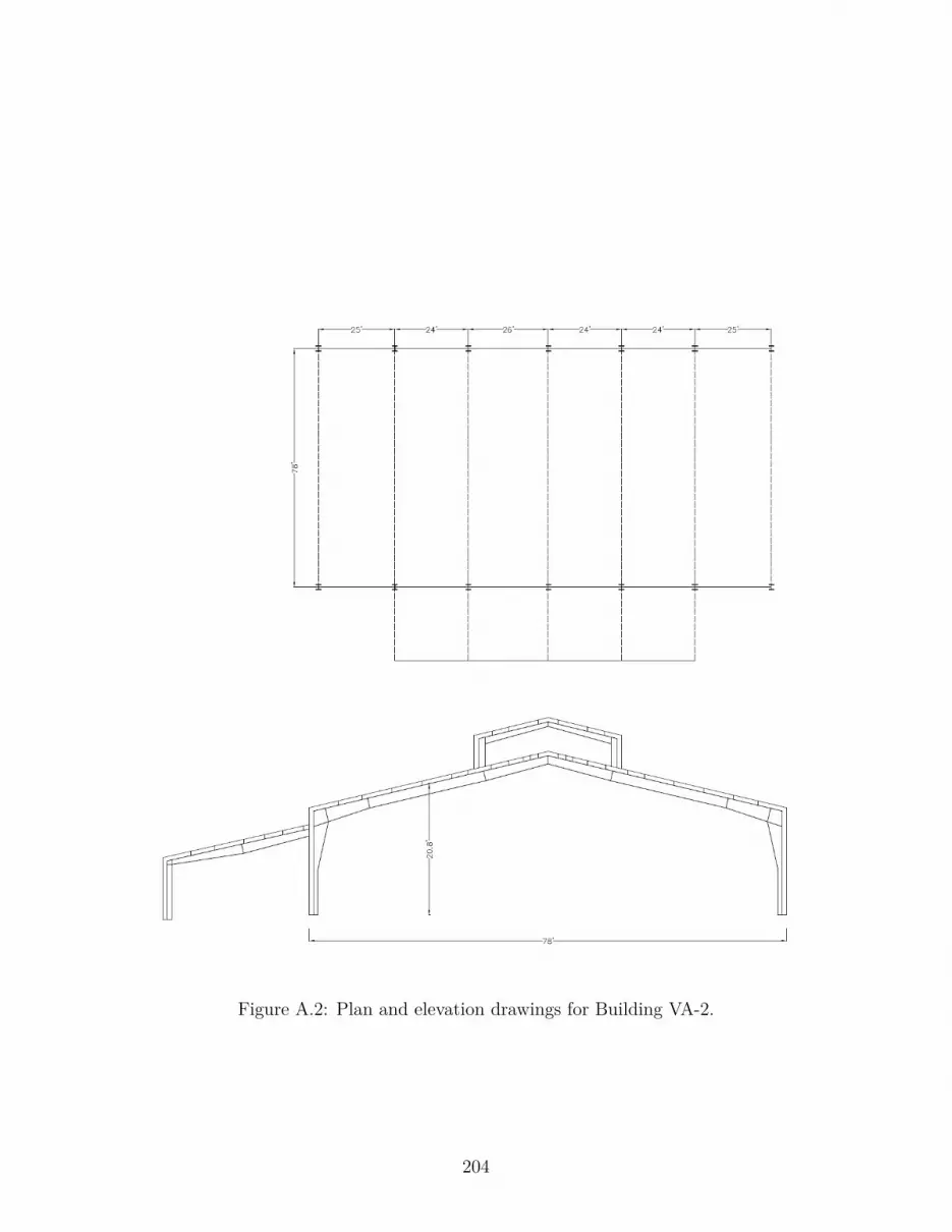
Figure A.2: Plan and elevation drawings for Building VA-2.

204

Figure A.3: Plan and elevation drawings for Building WV-1.

205

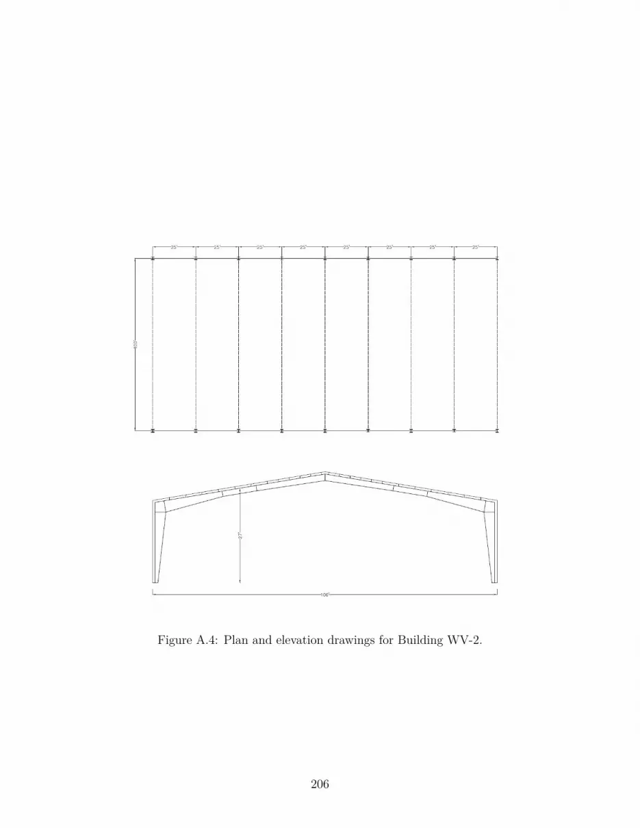
Figure A.4: Plan and elevation drawings for Building WV-2.

206

Figure A.5: Plan and elevation drawings for Building NC-1.

207


208


209

Appendix B

Summary of Tests on Fully-Clad

Metal Buildings to Date

Table B.1: Summary of properties of the buildings tested to date - structural classification

Name Cladding Type Roof Partitions CommentsVA-1 Metal Panels Clear Span Gabled None N/AVA-2 Metal Panels Clear Span Gabled None Appendices in every interior

frame, ClerestoryWV-1 Metal Panels Clear Span Monoslope None Expansion to existing build-

ingWV-2 Metal Panels Clear Span Gabled None Endwall at an “interior”

frameNC-1 Metal Panels Clear Span Monoslope Heavy Appendices in several

framesNC-2 Metal Panels Clear Span Monoslope None N/ANC-3 Metal Panels Clear Span Monoslope None N/ABBTC Metal Panels Clear Span Gabled None Mezzanine (Kumar et al.,

2020)VTH Metal Panels Clear Span Gabled None Hangar door (Kumar et al.,

2020)VTL Metal Panels Clear Span Gabled None 2-story structure attached

(Kumar et al., 2020)IBHS C Metal Panels Clear Span Monoslope Moderate (Kumar et al., 2020)IBHS D Metal Panels Clear Span Monoslope Light (Kumar et al., 2020)IBHS G Metal Panels Clear Span Monoslope Moderate (Kumar et al., 2020)

210

Table B.2: Summary of properties of the buildings tested – design parameters and measuredperiod

Name Length [ft] Height hn [ft] Aspect Ratio α Weight W [kips] Period T [s]VA-1 55 23 2.39 5.3 0.43VA-2 78 20.8 3.74 11.5 0.31WV-1 80 31.5 2.54 9.5 0.38WV-2 100 27 3.70 11.4 0.72NC-1 80 21.6 3.70 7.0 0.50NC-2 60 21 2.86 5.2 0.63NC-3 20 14 1.43 1.8 0.15BBTC 120 29.75 4.03 16.0 0.50VTH 140 30 4.67 20.6 0.39VTL 54 27.75 1.95 11.7 0.21

IBHS C 60 24.3 2.47 10.0 0.19IBHS D 55 37 1.49 8.3 0.33IBHS G 40 21.6 1.85 6.5 0.18

211

Documents

Towards a Better Understanding of the Fundamental Period of