Too Odd (Not) to Be True: A Reply to Olsson

Too Odd (Not) to Be True?

A Reply to OlssonLuc Bovens, Branden Fitelson,

Stephan Hartmann and Josh Snyder

ABSTRACT

In ‘Corroborating Testimony, Probability and Surprise’, Erik J. Olsson ascribes to L.

Jonathan Cohen the claims that if two witnesses provide us with the same information,

then the less probable the information is, the more confident we may be that the

information is true (C), and the stronger the information is corroborated (C*). We

question whether Cohen intends anything like claims (C) and (C*). Furthermore, he

discusses the concurrence of witness reports within a context of independent witnesses,

whereas the witnesses in Olsson’s model are not independent in the standard sense. We

argue that there is much more than, in Olsson’s words, ‘a grain of truth’ to claim (C),

both on his own characterization as well as on Cohen’s characterization of the

witnesses. We present an analysis for independent witnesses in the contexts of decision-

making under risk and decision-making under uncertainty and generalize the model

for n witnesses. As to claim (C*), Olsson’s argument is contingent on the choice of a

particular measure of corroboration and is not robust in the face of alternative

measures. Finally, we delimit the set of cases to which Olsson’s model is applicable.

1 Claim (C) examined for Olsson’s characterization of the relationship

between the witnesses

2 Claim (C) examined for two or more independent witnesses

3 Robustness and multiple measures of corroboration

4 Discussion

In ‘Corroborating Testimony, Probability and Surprise’, Erik J. Olsson

([2002]) takes L. Jonathan Cohen to be making the following claims in The

Probable and the Provable ([1977], p. 98):

(C) The smaller the prior probability of the proposition that two court witnesses

agree upon, the greater our degree of confidencewill be that their testimony is true.

(C*) The smaller the prior probability of the proposition that two court

witnesses agree upon, the stronger it is corroborated1 by their testimony.

Brit. J. Phil. Sci. 53 (2002), 539–563

&British Society for the Philosophy of Science 2002

1 It would be more fitting for Cohen and Olsson to talk about the strength of confirmation, since‘corroboration’ carries with it the vestiges of Popper’s program which turns its back oninductive approaches to investigate the relationship between hypothesis and evidence.

Olsson constructs a clever and elegant model to assess under what

conditions these claims are true. The upshot of his argument is that there is

only ‘a grain of truth’ in claim (C): the claim is not ‘correct as it stands [ . . . ],

not even under a charitable rendering’. Claim (C*) purportedly holds only if

we make certain special assumptions about our epistemic status with respect

to the reliability of the witnesses.

The first question that concerns us is whether Cohen really intends to be

making claims like (C) and (C*). Let us look at the pages preceding the ones

from which Olsson draws his quotes. Cohen is trying to give an account of

the fact that concurring reports (i.e. reports with the same content) from

independent witnesses corroborate what is being reported to a greater extent

than a single report does. He discusses Boole’s account of this fact, which

originated in Jakob Bernoulli’s Ars conjectandi. Either the two witnesses

whose reports concur are truth-tellers or they are liars. Let the chance that

they are truth-tellers be p and q for the respective witnesses. If the witnesses

have a choice between reporting one of two options, then their reports will

concur if and only if they are both telling the truth or they are both lying.

Hence, the chance that they are both truth-tellers given that their reports

concur is:

PðTruth-TellersjConcurrenceÞ ¼PðTruth-Tellers & ConcurrenceÞ

PðConcurrenceÞ

¼PðTruth-Tellers)

PðTruth-Tellers or LiarsÞ

¼pq

pqþ ð1� pÞð1� qÞ

Notice, however, that the chance that we are dealing with truth-tellers goes

up as the number of reports increases from one to two if and only if p,

q > 0:50 on Boole’s formula. Cohen objects to this result. He envisions two

independent witnesses who are rather unreliable, i.e. p, q < 0:50. If their

reports are concurring, then ‘Boole’s formula produces a lower probability

for their joint veracity, whereas normal juries would assign a higher one’

(ibid., p. 96). Indeed, if p ¼ q ¼ 0:20, then it is easy to verify that the chance

that two witness reports rather than one witness report is true goes down

from 0.20 to approximately 0.06 on Boole’s formula. The reason that the

formula fails is that there are not just two options in a typical case of witness

reports in court, but ‘so many different things can be said instead of the truth’

(ibid., p. 97). Hence, the chance that two liars will produce concurring reports

is no longer ð1� pÞð1� qÞ, but much lower.

It is in this context that we should assess the claim of Cohen quoted by

Olsson: ‘Where agreement is relatively improbable (because so many different

things might be said), what is agreed is more probably true’ (ibid., p. 98). The

540 L. Bovens, B. Fitelson, S. Hartmann and J. Snyder

question is: more probably true than when? More probably true than when

the agreement had been less improbable (because there were fewer things to

say)? This is Olsson’s way of filling in the ellipsis. Or more probably true than

when there had been only one witness report? This is the comparison that

Cohen intended. Cohen is arguing that concurring reports yield a higher

degree of confidence that what is reported is true than does a single report.

This is so even when the chance that the witnesses are reliable is relatively

low. The reason that Boole’s formula fails in this context is that it is typically

not the case in court proceedings that ‘the domain of possibilities is a binary

one’ (ibid., p. 97). Cohen then goes on to develop his own account and lays

out a set of sufficient conditions for concurring reports to yield a higher

degree of confidence than a single report.

But we are not sticklers for textual interpretation. Although it is not what

Cohen had in mind, claims (C) and (C*) do seem to square with a certain

intuition and it is worth investigating whether we can give a probabilistic

account of this intuition.

There is a second caveat. Olsson chooses to model claims (C) and (C*) for

witnesses who are both either fully reliable or fully unreliable. But Cohen is

discussing court witnesses who are independentwhereas the witnesses inOlsson’s

set-up are not independent in the standard sense of the term. Nonetheless, it is

interesting to see whether there is indeed no more than a grain of truth to claim

(C) for witnesses who are either both reliable or both unreliable.

In Section 1, we defend claim (C) against Olsson’s charge while adopting

his own probabilistic characterization of the relationship between the

witnesses. In Section 2, we defend claim (C) against Olsson’s charge while

respecting the stipulation that the witnesses are independent. In Section 3, we

focus on claim (C*). Olsson’s argument points to an interesting feature in

confirmation theory. A wide range of measures of corroboration (or

measures of confirmation, support, relevance, weight-of-evidence, . . .) have

been developed and defended in the literature. These measures behave very

differently as a function of the prior probability of the hypothesis. Olsson

argues against claim (C*) by focusing on one such measure. We will show

that his conclusion is not robust in the face of alternative measures. In Section

4, we sketch some historical background of ‘too odd not to be true’ reasoning

and argue that Olsson’s model only applies to a restricted set of cases.

1 Claim (C) examined for Olsson’s characterization of the

relationship between the witnesses

Cohen discusses concurring reports for propositions that are relatively

improbable. It is fair to say that a claim is relatively improbable only if—at

the very least—it is less probable than not. This is also in keeping with

Too Odd (Not) to Be True? A Reply to Olsson 541

Cohen’s examples. He points to examples where there are multiple equally

plausible suspects for a crime. In Section 3, Olsson shows that claim (C) does

not hold when we know the degree of reliability of the witnesses. This is fair

enough and entirely in the spirit of the context that Cohen is discussing. In

medicine, we often have knowledge of the percentage of false positives and

false negatives (and hence of the reliability) of medical tests that ‘bear

witness’ of some disease. However, we do not have any such knowledge at

our disposal in a court situation. Olsson shows that a substantially weaker

version of (C) holds true when the reliability of the witnesses is unknown.

This he takes to be the grain of truth in claim (C). We will argue that, his

results notwithstanding, there is significantly more than just a grain.

Cohen’s quotes concerning concurring reports occur within the context of

two independent witnesses.2 Smith and Jones are independent witnesses in the

standard sense of the term3 if and only if the following condition holds

(Bovens and Hartmann [2002], p. 37; Earman [2000], p. 57; Fitelson [2001a],

pp. 127–30):

PðEijH, EjÞ ¼ PðEijHÞ for i, j ¼ 1, 2 and i 6¼ j ð1Þ

PðEij:H, EjÞ ¼ PðEij:HÞ for i, j ¼ 1, 2 and i 6¼ j ð2Þ

Olsson examines claim (C) for witnesses who do not satisfy these

independence conditions. There are two crucial features to Olsson’s set-up.


2 Cohen goes on to show that a set of conditions that are weaker than independence is sufficientfor concurring reports to yield a higher degree of confidence than a single report ([1977],pp. 101–7). It is easy to show that Olsson’s set-up does not satisfy these conditions either.However Cohen’s conditions are not necessary conditions and it can be shown that concurringreports will also yield a higher degree of confidence than a single report in Olsson’s set-up.

3 Cohen also subscribes to this conception of independent witnesses. First, he argues that thereports of the witnesses can only be causally connected through the truth of what is testified:there should be ‘no special reason’, i.e. other than the truth of what is testified, ‘to suppose thatthe two testimonies would be identical’ ([1977], p. 94). Hence, if we know the truth-value ofwhat is testified, i.e. the truth-value of H, then learning that one witness testified that H shouldnot affect the chance that the other witness testified that H. Second, when Cohen lays outsufficient conditions for corroboration, his conditions (4) and (5) ([1977], p. 104) are entailed byour conditions (1) and (2), respectively: Cohen argues that we do not need strict independence,but there may also be negative relevance between the reports, given that H is false, and theremay also positive relevance between the reports, given that H is true, for corroboration tooccur. Finally, for readers who are familiar with the graphical representation of conditionalindependence structures in Bayesian Networks, the structure of Olsson’s set-up for unknownreliability can be represented by a Bayesian Network with four nodes, one for the hypothesis,one for the reliability of the witnesses, and a node for the report of each witness. There arearrows from the hypothesis and from the reliability to the witness reports. The causal linkbetween the reports is not only through the hypothesis as a confounder, but also through thereliability as a confounder: hence, the causal link between the reports is not only through ‘thetruth of what is testified’. Independence requires that there is no other causal link than throughthe hypothesis as a confounder. In our set-up for independent witnesses, we have five nodes—one for the hypothesis, one for the report of each witness, and one for the reliability of eachwitness. There are arrows from the hypothesis to the reports and from the reliability of thewitnesses to their respective reports. The only causal link between the reports is through thehypothesis as a confounder.

First, either both witnesses are reliable (R) or both witnesses are not reliable

(U). Hence, PðUÞ ¼ 1� PðRÞ. Second, if they are reliable, they are truth-

tellers, and if they are not reliable, then the chance that they will incriminate

Forbes is equal to the prior probability that Forbes committed the crime. The

assumptions of the model are captured in premises (i) through (viii) in Section

5 in Olsson: for i, j ¼ 1, 2 and i 6¼ j, (i) PðEijH, RÞ ¼ 1; (ii) PðEij:H, RÞ ¼ 0;

(iii) PðEijH, UÞ ¼ PðHÞ; (iv) PðEij:H, UÞ ¼ PðHÞ; (v) PðEijH, U, EjÞ ¼

PðEijH, UÞ; (vi) PðEij:H, U, EjÞ ¼ PðEij:H, UÞ; (vii) PðRjHÞ ¼ PðRÞ ¼

PðRj:HÞ; (viii) PðUjHÞ ¼ PðUÞ ¼ PðUj:HÞ.4 To see that Olsson’s witnesses

are not independent, consider the following two theorems. (All theorems are

proven in the Appendix.)

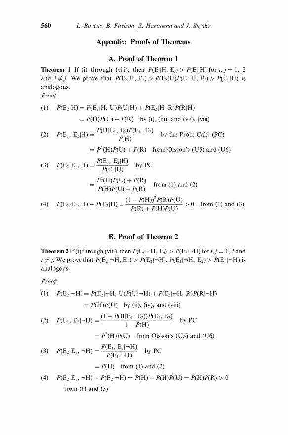
Theorem 1 If (i) through (viii), then PðEijH, EjÞ > PðEijHÞ for i, j ¼ 1, 2 and

i 6¼ j.

Theorem 2 If (i) through (viii), then PðEij:H, EjÞ > PðEij:HÞ for i, j ¼ 1, 2

and i 6¼ j.

Obviously theorems 1 and 2 conflict with (1) and (2). However, Olsson’s set-

up is not without interest: we may well wish to know whether claim (C) holds

up when both witnesses are either fully reliable or fully unreliable. Let the

prior probability that the witnesses are fully reliable be PðRÞ ¼ r; the prior

probability that Forbes committed the crime be PðHÞ ¼ h, and the posterior

probability that Forbes committed the crime after having learned from both

witnesses that he committed the crime be PðHjE1, E2Þ ¼ h*. To assess

Olsson’s claim that there is only a grain of truth in claim (C), picture a box in

which h is plotted against r. The variable r is contained in the open set (0, 1),

while h is contained in the open set (0, 0.5), since we are only interested in

relatively improbable propositions. What we want to know is the following.

For which pairs (r, h) in this box does claim (C) hold? In other words, for

which pairs (r, h) can it be said that if the prior probability h had been lower,

then the posterior probability h* would have been higher, for the particular

value of the variable r. If there is only a grain of truth to (C), then this should

become evident when we determine the area in the box where (C) is true.

So let us turn to this task. Olsson derives a formula to calculate the

posterior probability h*.5 We introduce the convention that �xx stands for

(1� x) for any probability value x. Olsson’s formula (U6) can be written as


4 Note that the conditional probabilities are defined only if we assume that the probabilitydistribution over the random variables H (whose values are H and :H) and R (whose valuesare R and :R) is non-extreme. We adopt this assumption throughout the paper.

5 Compare Theorem 1 in Bovens and Hartmann ([2002]) within the context of confirmation withmultiple unreliable instruments. The expression in this theorem contains three more variables,but if the hypothesis is tested directly, then p ¼ 1 and q ¼ 0, and if an unreliable instrumentrandomizes at a ¼ h, then one obtain the same results.

h* ¼rþ h2 �rr

rþ h�rr. ð3Þ

Olsson’s Figure 2 shows that for r ¼ 0:10, there is only a very small range of

values of h for which the posterior probability h* is a decreasing function of

h. The grain of truth that he recognizes in claim (C) is that for any value of r,

there is a range of values in which the posterior probability h* is indeed a

decreasing function of h.

But is this just a grain of truth? Indeed, what Olsson’s example shows is

that there are some cases in which claim (C) holds true. But to assess the

breadth of this claim, we need to turn his analysis one small notch further. In

Olsson’s Figure 2, we see that the posterior probability h* has a minimum for

some value of h, when r ¼ 0:10. To the left of this minimum the claim is true,

and to the right of this minimum the claim is false. So we need to find the

minimum for each value of r 2 (0, 1). How do we find the minimum in

Olsson’s Figure 2? The standard technique to do so is to take the partial

derivative of h* with respect to h,

@h*

@h¼ �rr

h2 � �hh2r

ðrþ h�rrÞ2, ð4Þ

and to set this partial derivative to 0 and solve for h. The solution for h,

r 2 (0, 1) is

hmin ¼

ffiffir

p

1þffiffir

p . ð5Þ

For r ¼ 0:10, this solution yields hmin < 0:24, which is indeed where the curve

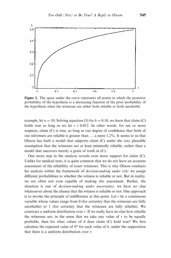
in the graph in Olsson’s Figure 2 reaches its minimum.6 We plot the function

in (5) to determine the minima for any value of r 2 ð0, 1Þ in Figure 1. For

value pairs of (r, h) underneath this curve, claim (C) turns out to be true.

Olsson is correct that we need to impose certain constraints on this claim, but

it seems to us that given the relative size of the area underneath the curve,

there is not just a grain of truth, but rather a heap of truth to claim (C).

Furthermore, we have interpreted relative improbability as being less

probable than not. But the case that Cohen has in mind is a case in which the

court witnesses identify a suspect ‘out of so many possible criminals’ (op. cit.,

p. 98). In this case, we need to consider the area under the curve under the

constraint that h ¼ 1=n, when there are n equally probable suspects. For


6 To assure ourselves that this solution yields a minimum rather than a maximum over r 2 ð0, 1Þ,observe that the second derivative of h* with respect to h is

@2h*

@h2¼

2r �rr

ðrþ h �rrÞ3

which is positive for r 2 ð0, 1Þ.

example, let n ¼ 10. Solving equation (5) for h ¼ 0:10, we learn that claim (C)

holds true as long as we let r > 0:012. In other words, for ten or more

suspects, claim (C) is true, as long as our degree of confidence that both of

our informers are reliable is greater than . . . a mere 1.2%. It seems to us that

Olsson has built a model that supports claim (C) under the very plausible

assumption that the witnesses are at least minimally reliable, rather than a

model that uncovers merely a grain of truth in (C).

One more step in the analysis reveals even more support for claim (C).

Unlike for medical tests, it is quite common that we do not have an accurate

assessment of the reliability of court witnesses. This is why Olsson conducts

his analysis within the framework of decision-making under risk: we assign

different probabilities to whether the witness is reliable or not. But in reality,

we are often not even capable of making this assessment. Rather, the

situation is one of decision-making under uncertainty: we have no clue

whatsoever about the chance that the witness is reliable or not. One approach

is to invoke the principle of indifference at this point. Let r be a continuous

variable whose values range from 0 (for certainty that the witnesses are fully

unreliable) to 1 (for certainty that the witnesses are fully reliable). We

construct a uniform distribution over r. If we really have no clue how reliable

the witnesses are, in the sense that we take any value of r to be equally

probable, then for what values of h does claim (C) hold true? We first

calculate the expected value of h* for each value of h, under the supposition

that there is a uniform distribution over r:


Figure 1. The space under the curve represents all points in which the posterior

probability of the hypothesis is a decreasing function of the prior probability ofthe hypothesis when the witnesses are either both reliable or both unreliable.

hh*i ¼

ð10

rþ h2 �rr

rþ h �rrdr ¼ �hh�1ð1� h2 þ h lnðhÞÞ for h 2 ð0, 1Þ ð6Þ

To calculate the minimum, we take the derivative of this function with respect

to h:

dhh*i

dh¼ �hh�2ðh2 � 3hþ lnðhÞ þ 2Þ ð7Þ

set this derivative equal to 0 and solve numerically for h 2 (0, 1):

hmin � 0:32 ð8Þ

Hence, if we have no clue whatsoever about the reliability of the witnesses

and there are more than three equally probable suspects (so that the prior

probability that a particular suspect committed the crime is no greater than

0.25, and thus less than 0.32), then claim (C) holds. The less probable the

information is that the witnesses agree upon, the greater our degree of

confidence will be that the information is true. Considering that Cohen is

interested in a scenario in which there is a wide range of n suspects, it is not an

overly charitable read to set the number of suspects at n>3. Furthermore,

our judgment about the reliability of a witness in a court is typically a

judgment neither under certainty nor under risk, but rather under

uncertainty. If we build these plausible assumptions into Olsson’s analysis,

then the model provides direct validation for claim (C).

2 Claim (C) examined for two or more independent witnesses

What happens when we run Olsson’s analysis for witnesses who are genuinely

independent, i.e. who satisfy our conditions (1) and (2) in Section 1? Let us

follow the same route of analysis for independent witnesses. In the Appendix

we have calculated the posterior probability after receiving corroborating

reports from two independent witnesses, making similar assumptions as in

Olsson’s model:7

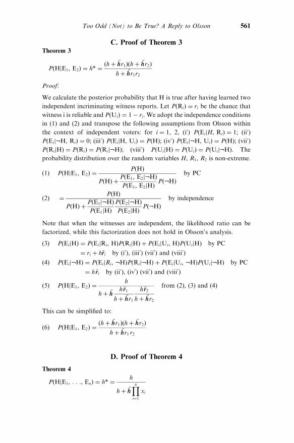
Theorem 3

PðHjE1, E2Þ ¼ h* ¼ðhþ �hhr1Þðhþ �hhr2Þ

hþ �hhr1 r2

in which ri is the probability that witness i is reliable for i ¼ 1, 2. From here

on we follow the same procedure as in Section 1. We have plotted the curve


7 Compare Theorem 2 in Bovens and Hartmann ([2002]) within the context of confirmation withmultiple unreliable instruments. Making the same substitutions as in note 3, this result can beobtained for the special case r1 ¼ r2 ¼ r.

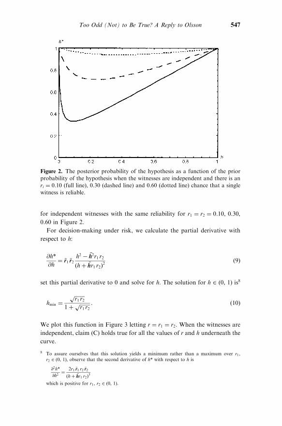
for independent witnesses with the same reliability for r1 ¼ r2 ¼ 0:10, 0.30,

0.60 in Figure 2.

For decision-making under risk, we calculate the partial derivative with

respect to h:

@h*

@h¼ �rr1 �rr2

h2 � �hh2r1 r2

ðhþ �hhr1 r2Þ2

ð9Þ

set this partial derivative to 0 and solve for h. The solution for h 2 (0, 1) is8

hmin ¼

ffiffiffiffiffiffiffiffir1 r2

p

1þffiffiffiffiffiffiffiffir1 r2

p . ð10Þ

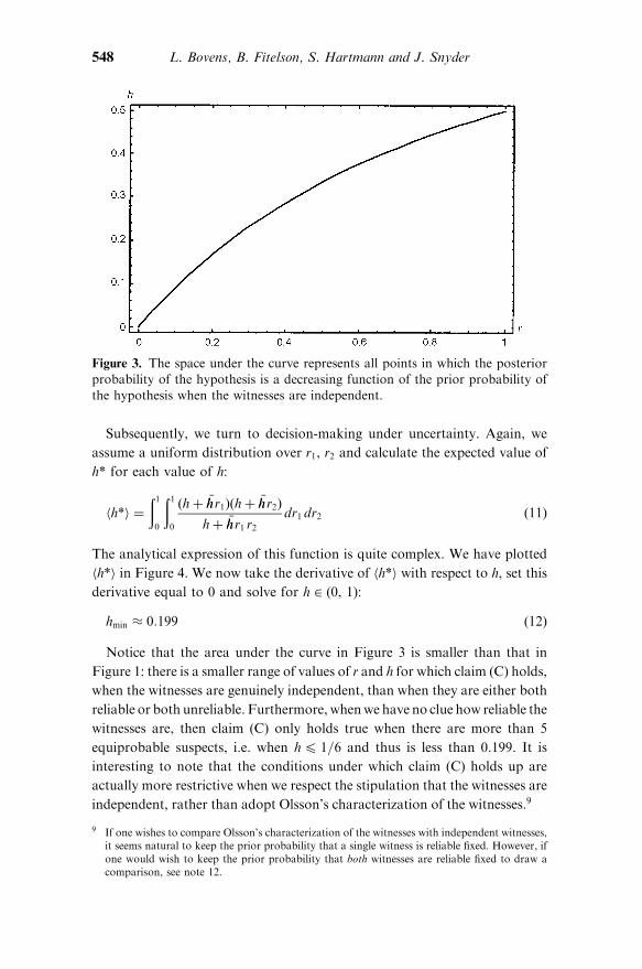
We plot this function in Figure 3 letting r ¼ r1 ¼ r2. When the witnesses are

independent, claim (C) holds true for all the values of r and h underneath the

curve.


Figure 2. The posterior probability of the hypothesis as a function of the priorprobability of the hypothesis when the witnesses are independent and there is anri ¼ 0:10 (full line), 0.30 (dashed line) and 0.60 (dotted line) chance that a single

witness is reliable.

8 To assure ourselves that this solution yields a minimum rather than a maximum over r1,r2 2 ð0, 1Þ, observe that the second derivative of h* with respect to h is

@2h*

@h2¼

2r1 �rr1 r2 �rr2

ðhþ �hhr1 r2Þ3

which is positive for r1, r2 2 ð0, 1Þ.

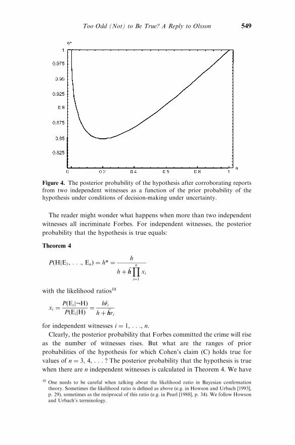
Subsequently, we turn to decision-making under uncertainty. Again, we

assume a uniform distribution over r1, r2 and calculate the expected value of

h* for each value of h:

hh*i ¼

ð10

ð1

0

ðhþ �hhr1Þðhþ �hhr2Þ

hþ �hhr1 r2dr1 dr2 ð11Þ

The analytical expression of this function is quite complex. We have plotted

hh*i in Figure 4. We now take the derivative of hh*i with respect to h, set this

derivative equal to 0 and solve for h 2 ð0, 1Þ:

hmin � 0:199 ð12Þ

Notice that the area under the curve in Figure 3 is smaller than that in

Figure 1: there is a smaller range of values of r and h for which claim (C) holds,

when the witnesses are genuinely independent, than when they are either both

reliable or both unreliable. Furthermore, whenwe have no clue how reliable the

witnesses are, then claim (C) only holds true when there are more than 5

equiprobable suspects, i.e. when h4 1=6 and thus is less than 0.199. It is

interesting to note that the conditions under which claim (C) holds up are

actually more restrictive when we respect the stipulation that the witnesses are

independent, rather than adopt Olsson’s characterization of the witnesses.9


Figure 3. The space under the curve represents all points in which the posteriorprobability of the hypothesis is a decreasing function of the prior probability ofthe hypothesis when the witnesses are independent.

9 If one wishes to compare Olsson’s characterization of the witnesses with independent witnesses,it seems natural to keep the prior probability that a single witness is reliable fixed. However, ifone would wish to keep the prior probability that both witnesses are reliable fixed to draw acomparison, see note 12.

The reader might wonder what happens when more than two independent

witnesses all incriminate Forbes. For independent witnesses, the posterior

probability that the hypothesis is true equals:

Theorem 4

PðHjE1, : : :, EnÞ ¼ h* ¼h

hþ �hhYni¼1

xi

with the likelihood ratios10

xi ¼PðEij:HÞ

PðEijHÞ¼

h�rri

hþ �hhri

for independent witnesses i ¼ 1, : : :, n.

Clearly, the posterior probability that Forbes committed the crime will rise

as the number of witnesses rises. But what are the ranges of prior

probabilities of the hypothesis for which Cohen’s claim (C) holds true for

values of n ¼ 3, 4, : : : ? The posterior probability that the hypothesis is true

when there are n independent witnesses is calculated in Theorem 4. We have


Figure 4. The posterior probability of the hypothesis after corroborating reports

from two independent witnesses as a function of the prior probability of thehypothesis under conditions of decision-making under uncertainty.

10 One needs to be careful when talking about the likelihood ratio in Bayesian confirmationtheory. Sometimes the likelihood ratio is defined as above (e.g. in Howson and Urbach [1993],p. 29), sometimes as the reciprocal of this ratio (e.g. in Pearl [1988], p. 34). We follow Howsonand Urbach’s terminology.

calculated these values for decision-making under risk and for decision-

making under uncertainty. For decision-making under risk,11

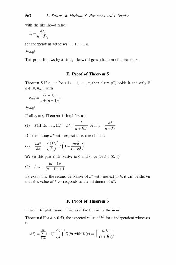
Theorem 5 If ri ¼ r for all i ¼ 1, : : :, n, then claim (C) holds if and only if

h 2 ð0, hminÞ with

hmin ¼ðn� 1Þr

1þ ðn� 1Þr.

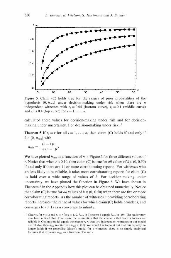
We have plotted hmin as a function of n in Figure 5 for three different values of

r. Notice that when r is 0.10, then claim (C) is true for all values of h 2 (0, 0.50)

if and only if there are 11 or more corroborating reports. For witnesses who

are less likely to be reliable, it takes more corroborating reports for claim (C)

to hold over a wide range of values of h. For decision-making under

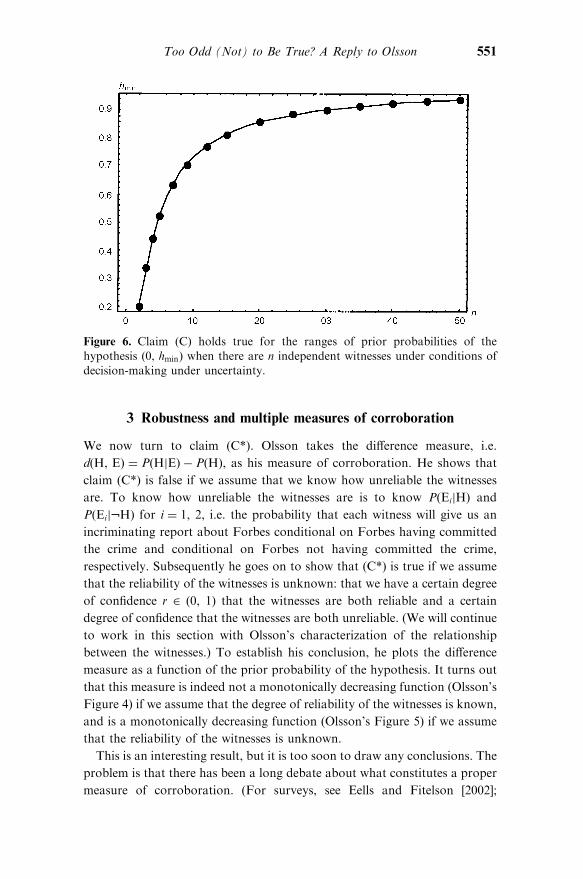
uncertainty, we have plotted the function in Figure 6. We have shown in

Theorem 6 in the Appendix how this plot can be obtained numerically. Notice

that claim (C) is true for all values of h 2 ð0, 0:50Þ when there are five or more

corroborating reports. As the number of witnesses n providing corroborating

reports increases, the range of values for which claim (C) holds broadens, and

converges to (0, 1) as n converges to infinity.


Figure 5. Claim (C) holds true for the ranges of prior probabilities of thehypothesis (0, hmin) under decision-making under risk when there are nindependent witnesses with ri ¼ 0:04 (bottom curve), ri ¼ 0:1 (middle curve)

and ri is 0.4 (top curve) for i ¼ 1, : : :, n.

11 Clearly, for n ¼ 2 and ri ¼ r for i ¼ 1, 2, hmin in Theorem 5 equals hmin in (10). The reader mayalso have noticed that if we make the assumption that the chance r that both witnesses arereliable in Olsson’s model equals the chance r1 r2 that two independent witnesses in our modelare reliable, then hmin in (5) equals hmin in (10). We would like to point out that this equality nolonger holds if we generalize Olsson’s model for n witnesses: there is no simple analyticalformula that expresses hmin as a function of n and r.

3 Robustness and multiple measures of corroboration

We now turn to claim (C*). Olsson takes the difference measure, i.e.

dðH, EÞ ¼ PðHjEÞ � PðHÞ, as his measure of corroboration. He shows that

claim (C*) is false if we assume that we know how unreliable the witnesses

are. To know how unreliable the witnesses are is to know PðEijHÞ and

PðEij:HÞ for i ¼ 1, 2, i.e. the probability that each witness will give us an

incriminating report about Forbes conditional on Forbes having committed

the crime and conditional on Forbes not having committed the crime,

respectively. Subsequently he goes on to show that (C*) is true if we assume

that the reliability of the witnesses is unknown: that we have a certain degree

of confidence r 2 (0, 1) that the witnesses are both reliable and a certain

degree of confidence that the witnesses are both unreliable. (We will continue

to work in this section with Olsson’s characterization of the relationship

between the witnesses.) To establish his conclusion, he plots the difference

measure as a function of the prior probability of the hypothesis. It turns out

that this measure is indeed not a monotonically decreasing function (Olsson’s

Figure 4) if we assume that the degree of reliability of the witnesses is known,

and is a monotonically decreasing function (Olsson’s Figure 5) if we assume

that the reliability of the witnesses is unknown.

This is an interesting result, but it is too soon to draw any conclusions. The

problem is that there has been a long debate about what constitutes a proper

measure of corroboration. (For surveys, see Eells and Fitelson [2002];


Figure 6. Claim (C) holds true for the ranges of prior probabilities of thehypothesis (0, hmin) when there are n independent witnesses under conditions ofdecision-making under uncertainty.

Fitelson [1999] and [2001a].) The difference measure certainly has received

some support but it is by no means a privileged measure in the set of

proposed measures. Furthermore these measures are extremely fickle in their

behavior as a function of the prior probability of the hypothesis. To show

how fragile Olsson’s findings are, we will calculate the log-ratio measure,

which has been defended by Milne ([1995]) for the case in which the reliability

is known and the Carnap measure ([1962], Section 67) for the case in which

the reliability is unknown.

For Olsson’s argument to stand, the measure must be a function of the

prior probability of the hypothesis that is not monotonically decreasing when

the reliability of the witnesses is known and is a monotonically decreasing

function when the reliability of the witnesses is unknown. The difference

measure certainly provides him with this result. But a choice of other

measures does not provide this result. As a matter of fact, we can turn

Olsson’s result around by varying the choice of confirmation measures. We

will show that the log-ratio measure is a monotonically decreasing function

when the reliability of the witnesses is known and that the Carnap measure is

not a monotonically decreasing function when the reliability of the witnesses

is unknown.

The log-ratio measure is defined as:

rðH, EÞ ¼ ln

�PðHjEÞ

PðHÞ

�ð13Þ

The Carnap measure is defined as:

cðH, EÞ ¼ PðE & HÞ � PðEÞPðHÞ ¼ PðEÞðPðHjEÞ � PðHÞÞ ¼ PðEÞdðH, EÞ

ð14Þ

Let us first consider the case of known reliability. In Olsson, the evidence E

consists of two witness reports E1 and E2. We remind the reader of the

relevant calculations in Olsson’s paper. First, we present a more standard

expression of Olsson’s calculation of the posterior probability of the

hypothesis when the reliability of the witnesses is known and make the

following substitution for the likelihood ratio x ¼ PðEij:HÞ=PðEijHÞ for

i ¼ 1, 2:

PðHjE1, E2Þ ¼PðHÞ

PðHÞ þPðE1j:HÞ

PðE1jHÞ

PðE2j:HÞ

PðE2jHÞPð:HÞ

¼h

hþ �hhx2ð15Þ

We can now insert the expression in (15) for known reliability into (13), i.e.

into the log-ratio measure. Some algebraic manipulations yield:

rðH, EÞ ¼ � lnðhþ �hhx2Þ ð16Þ


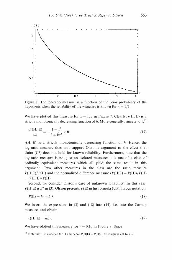
We have plotted this measure for x ¼ 1=3 in Figure 7. Clearly, rðH, EÞ is a

strictly monotonically decreasing function of h. More generally, since x < 1,12

@rðH, EÞ

@h¼ �

1� x2

hþ �hhx2< 0. ð17Þ

rðH, EÞ is a strictly monotonically decreasing function of h. Hence, the

log-ratio measure does not support Olsson’s argument to the effect that

claim (C*) does not hold for known reliability. Furthermore, note that the

log-ratio measure is not just an isolated measure: it is one of a class of

ordinally equivalent measures which all yield the same result in this

argument. Two other measures in the class are the ratio measure

PðHjEÞ=PðHÞ and the normalized difference measure ðPðHjEÞ � PðHÞÞ=PðHÞ

¼ dðH, EÞ=PðHÞ.

Second, we consider Olsson’s case of unknown reliability. In this case,

PðHjEÞ is h* in (3). Olsson presents PðEÞ in his formula (U5). In our notation:

PðEÞ ¼ hrþ h2 �rr ð18Þ

We insert the expressions in (3) and (18) into (14), i.e. into the Carnap

measure, and obtain

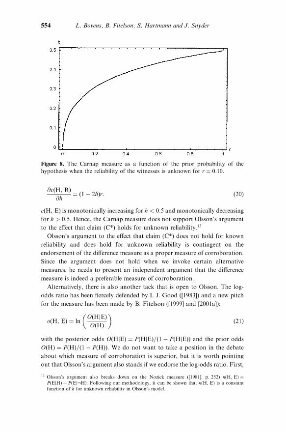
cðH, EÞ ¼ h �hhr. ð19Þ

We have plotted this measure for r ¼ 0:10 in Figure 8. Since


Figure 7. The log-ratio measure as a function of the prior probability of the

hypothesis when the reliability of the witnesses is known for x ¼ 1=3.

12 Note that E is evidence for H and hence PðHjEÞ > PðHÞ. This is equivalent to x < 1.

@cðH, RÞ

@h¼ ð1� 2hÞr. ð20Þ

cðH, EÞ is monotonically increasing for h < 0:5 and monotonically decreasing

for h > 0:5. Hence, the Carnap measure does not support Olsson’s argument

to the effect that claim (C*) holds for unknown reliability.13

Olsson’s argument to the effect that claim (C*) does not hold for known

reliability and does hold for unknown reliability is contingent on the

endorsement of the difference measure as a proper measure of corroboration.

Since the argument does not hold when we invoke certain alternative

measures, he needs to present an independent argument that the difference

measure is indeed a preferable measure of corroboration.

Alternatively, there is also another tack that is open to Olsson. The log-

odds ratio has been fiercely defended by I. J. Good ([1983]) and a new pitch

for the measure has been made by B. Fitelson ([1999] and [2001a]):

oðH, EÞ ¼ ln

�OðHjEÞ

OðHÞ

�ð21Þ

with the posterior odds OðHjEÞ ¼ PðHjEÞ=ð1� PðHjEÞÞ and the prior odds

OðHÞ ¼ PðHÞ=ð1� PðHÞÞ. We do not want to take a position in the debate

about which measure of corroboration is superior, but it is worth pointing

out that Olsson’s argument also stands if we endorse the log-odds ratio. First,


Figure 8. The Carnap measure as a function of the prior probability of the

hypothesis when the reliability of the witnesses is unknown for r ¼ 0:10.

13 Olsson’s argument also breaks down on the Nozick measure ([1981], p. 252) nðH, EÞ ¼PðEjHÞ � PðEj:HÞ. Following our methodology, it can be shown that nðH, EÞ is a constantfunction of h for unknown reliability in Olsson’s model.

calculate the log-odds ratio for known reliability by inserting PðHjEÞ ¼

PðHjE1, E2Þ as calculated in (15) into (21):

oðH, EÞ ¼ lnð1=x2Þ ð22Þ

Clearly, oðH, EÞ is independent of H and hence a constant function of the

prior probability h. This is sufficient for Olsson: for known reliability, oðH, EÞ

is not a decreasing function of h.

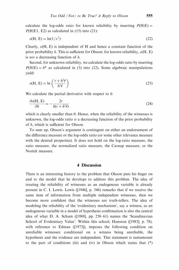
Second, for unknown reliability, we calculate the log-odds ratio by inserting

PðHjEÞ ¼ h* as calculated in (3) into (22). Some algebraic manipulations

yield:

oðH, EÞ ¼ ln

�rþ h2 �rr

h2 �rr

�ð23Þ

We calculate the partial derivative with respect to h:

@oðH, EÞ

@h¼ �

2r

hðrþ h2 �rrÞð24Þ

which is clearly smaller than 0. Hence, when the reliability of the witnesses is

unknown, the log-odds ratio is a decreasing function of the prior probability

of h, which is sufficient for Olsson.

To sum up, Olsson’s argument is contingent on either an endorsement of

the difference measure or the log-odds ratio (or some other relevance measure

with the desired properties). It does not hold on the log-ratio measure, the

ratio measure, the normalized ratio measure, the Carnap measure, or the

Nozick measure.

4 Discussion

There is an interesting history to the problem that Olsson puts his finger on

and to the model that he develops to address this problem. The idea of

treating the reliability of witnesses as an endogenous variable is already

present in C. I. Lewis. Lewis ([1946], p. 346) remarks that if we receive the

same item of information from multiple independent witnesses, then we

become more confident that the witnesses are truth-tellers. The idea of

modeling the reliability of the ‘evidentiary mechanism’, say a witness, as an

endogenous variable in a model of hypothesis confirmation is also the central

idea of what D. A. Schum ([1988], pp. 258–61) names the ‘Scandinavian

School of Evidentiary Value’. Within this school, Hansson ([1983], p. 78),

with reference to Edman ([1973]), imposes the following condition on

unreliable witnesses: conditional on a witness being unreliable, the

hypothesis and the evidence are independent. This statement is tantamount

to the part of conditions (iii) and (iv) in Olsson which states that (*)


PðEjH, UÞ ¼ PðEj:H, UÞ. Bonjour ([1985]) takes inspiration from the C. I.

Lewis passage in order to support his version of a coherence theory of

justification, and it is through Bonjour that (*) enters into Huemer ([1997])

and into Bovens and Olsson ([2000]). Also within the Scandinavian school, it

is Ekelof ([1983], p. 22) who at least hints in the direction of claim (C). He

proposes a particular formula to calculate our degree of confidence after

concurring reports, but concedes that when two witnesses report something

‘quite extraordinary’, then each report may count very little in the way of

evidence, but both reports together raise our degree of confidence that what is

reported is true beyond the value which the formula yields.

The idea in (*) is that if witnesses are fully unreliable, then they do not even

look at the world to provide a report that H is the case. They act no

differently from randomizers. It is as if they flip a coin or roll a die to decide

whether to report that H is the case, and hence whether H is or is not the case

is of no import. The chance that they report that H is the case, i.e. the level at

which they are randomizing, ranges over the open interval (0, 1). In Bovens

and Hartmann’s model ([2002], p. 32) of hypothesis confirmation with

unreliable instruments, this chance is the value of a randomization parameter

a. Olsson’s crucial insight is the following. Fully unreliable witnesses are

witnesses that did not see anything and hence can do no better than we could.

We know that Forbes is one out of n equiprobable suspects, and hence the

chance that he did it is h ¼ 1=n, i.e. the prior probability of the hypothesis.

So the chance that an unreliable suspect will pick Forbes is exactly

PðEjH, :RÞ ¼ PðEj:H, :RÞ ¼ h. This is what leads to Olsson’s result that

the posterior probability of H is a decreasing function of the prior probability

of H for certain ranges of prior probabilities that the witnesses are fully

unreliable.

What is important to realize is that Olsson’s result does not occur when we

merely assume that the reliability of the witnesses is unknown without setting

the randomization parameter at h. The reliability of the witnesses is just as

unknown when we stipulate that the witnesses may or may not be fully

reliable, and if they are fully unreliable, then they flip a coin to determine

whether theywill report thatH is true, i.e.PðEjH, :RÞ ¼ PðEj:H, :RÞ ¼ 1=2.

If we impose this stipulation on Olsson’s model, then the posterior

probability will simply be an increasing function of the prior probability

for all values of the variable r.

So, how reasonable is it to set the randomization parameter at the prior

probability of the hypothesis h? This stipulation is contingent on the

following two assumptions, viz. (i) all the alternative hypotheses are equally

probable and (ii) an unreliable witness acts as if he knows no more than we

do. This story can be made plausible for a lineup of suspects. It may well be

the case that we take it to be equally probable for each suspect to be the


criminal. And it may well be the case that fully unreliable witnesses act as if

they are randomizers, with the chance that an arbitrary suspect is picked

being 1/n. But presumably, concurrence in witness reports concerning a ‘quite

extraordinary’ option also constitutes strong evidence, even if there is no

uniform distribution over the alternatives. For instance, suppose that you are

shopping around for some specialized consumer product, say a bread

machine, a DVD player, or what have you. There is one better-known and a

range of less well-known brand names on the market. It is shared knowledge

that better products tend to come from better-known brand names, but there

are many exceptions to this rule. Hence, the prior probability that the better

product comes from one of the better-known brand names exceeds the prior

probability that it comes from one of the less well-known brand names. You

are soliciting advice from independent sources. It is not clear to you who

really knows anything more than you do about the consumer product in

question. Now compare two cases. In case one, all your sources recommend

the better-known brand name. In case two, all your sources recommend a

very obscure brand name. In what case is your degree of confidence greater

that the recommended product is the better product? Presumably ‘too odd

not to be true’ reasoning should carry some weight here as well. Sometimes, I

will find myself more convinced by the concurring recommendations of the

less well-known product, since the recommendations of the better-known

product give me no reason to believe that my informers know any more than

I do.

A general model of ‘too odd not to be true’ reasoning should also be

capable of handling cases in which there is no uniform distribution over

the possible alternatives. But is it plausible in this case to stipulate that

PðEjH, :RÞ ¼ PðEj:H, :RÞ ¼ h? There seems to be no justification to build

this assumption into the model. We could stipulate the idealization that an

unreliable witness is fully ignorant and will just randomize over the n

alternative products with probability 1/n. An alternative idealization is that

an unreliable witness knows precisely what we know and will just pick the

more probable alternative, i.e. the product from the better-known brand

name. But we do not see how one could argue in this case that an unreliable

witness randomizes over the alternatives so that the chance of picking some

alternative matches our prior probability distribution over the alternatives.

We conclude that Olsson’s insight to set the randomization parameter for

unreliable witness equal to the prior probability of the hypothesis provides an

interesting route towards giving an account of ‘too odd not to be true’

reasoning in a restricted range of cases. However, as soon as we give up the

assumptions of a uniform prior distribution over the alternatives, it remains

an open question as to how to model this type of reasoning in a Bayesian

framework.


Acknowledgements

We thank Erik J. Olsson for providing us with an early version of his paper

and Robert Rynasiewicz and Jørgen Hilden for helpful discussion. Luc

Bovens’s research was supported by the National Science Foundation,

Science and Technology Studies (SES 00–8058) and by the Alexander von

Humboldt Foundation, the Federal Ministry of Education and Research,

and the Program for the Investment in the Future (ZIP) of the German

Government. Stephan Hartmann’s research was supported by the Transcoop

Program and the Feodor Lynen Program of the Alexander von Humboldt

Foundation.

Luc Bovens

University of Colorado at Boulder

Department of Philosophy – CB 232

Boulder, CO 80309, USA

[email protected]

Branden Fitelson

San Jose State University

Department of Philosophy

San Jose, CA 95192–0096, USA

[email protected]

Stephan Hartmann

University of Konstanz

Department of Philosophy

78457 Konstanz, Germany

[email protected]

Josh Snyder

University of Colorado at Boulder

Department of Philosophy – CB 232

Boulder, CO 80309, USA

[email protected]

References

Bonjour, L. [1985]: The Structure of Empirical Knowledge, Cambridge, MA: Harvard

University Press.

Bovens, L. and Hartmann, S. [2002]: ‘Bayesian Networks and the Problem of

Unreliable Instruments’, Philosophy of Science, 69, pp. 29–72.


Bovens, L. and Olsson, E. J. [2000]: ‘Coherentism, Reliability and Bayesian

Networks’, Mind, 109, pp. 685–719.

Carnap, R. [1962]: Logical Foundations of Probability, Chicago: The University of

Chicago Press.

Cohen, L. J. [1977]: The Probable and the Provable, Oxford: Clarendon.

Earman, J. [2000]: Hume’s Abject Failure—The Argument against Miracles, Oxford:

Oxford University Press.

Edman, M. [1973]: ‘Adding Independent Pieces of Evidence’, in S. Hallden (ed.),

Modality, Morality and Other Problems of Sense and Nonsense, Lund: Gleerup,

pp. 180–8.

Eells, E. and Fitelson, B. [2002]: ‘Symmetries and Asymmetries in Evidential Support’,

Philosophical Studies, 107, pp. 129–42.

Ekelof P. O. [1983]: ‘My Thoughts on Evidentiary Value’, in: P. Gardenfors, B.

Hansson and N. Sahlin (eds) Evidentiary Value: Philosophical, Judicial and

Psychological Aspects of a Theory—Essays Dedicated to Soren Hallden on his

Sixtieth Birthday. Lund: Gleerup–Library of Theoria, 15, pp. 9–26.

Fitelson, B. [1999]: ‘The Plurality of Bayesian Measures of Confirmation and the

Problem of Measure Sensitivity’, Philosophy of Science, 63, pp. 652–60.

Fitelson, B. [2001a]: ‘Studies in Bayesian Confirmation Theory’, PhD Thesis,

Department of Philosophy, University of Wisconsin, Madison.

Fitelson, B. [2001b]: ‘A Bayesian Account of Independent Evidence with

Applications’, Philosophy of Science, 68 (Proceedings), pp. 123–40.

Good, I. J. [1983]: Good Thinking: the Foundations of Probability and its Applications,

Minneapolis: University of Minnesota Press.

Hansson, B. [1983]: ‘Epistemology and Evidence’, in P. Gardenfors, B. Hansson and

N. Sahlin (eds), Evidentiary Value: Philosophical, Judicial and Psychological Aspects

of a Theory—Essays Dedicated to Soren Hallden on his Sixtieth Birthday, Lund:

Gleerup, Library of Theoria, 15, pp. 75–97.

Howson, C. and Urbach, P. [1993]: Scientific Reasoning—The Bayesian Approach, 2nd

edn, Chicago: Open Court.

Huemer, M. [1997]: ‘Probability and Coherence Justification’, The Southern Journal of

Philosophy, 35, pp. 463–72.

Lewis, C. I. [1946]: An Analysis of Knowledge and Valuation, LaSalle, IL: Open Court.

Milne, P. [1995]: ‘A Bayesian Defense of Popperian Science?’ Analysis, 55, pp. 213–15.

Nozick, R. [1981]: Philosophical Explanations, Cambridge, MA: Harvard University

Press.

Olsson, E. J. [2002]: ‘Corroborating Testimony, Probability and Surprise’, The British

Journal for the Philosophy of Science, 53, pp. 273–88.

Pearl, J. [1988]: Probabilistic Reasoning in Intelligent Systems, San Mateo, CA:

Morgan Kaufmann.

Schum, D. A. [1988]: ‘Probability and the Processes of Discovery, Proof and Choice’,

in P. Tillers and E. D. Green (eds), Probability and Inference in the Law of

Evidence—The Uses and Limits of Bayesianism, London: Kluwer, pp. 213–70.


Appendix: Proofs of Theorems

A. Proof of Theorem 1

Theorem 1 If (i) through (viii), then PðEijH, EjÞ > PðEijHÞ for i, j ¼ 1, 2

and i 6¼ j. We prove that PðE2jH, E1Þ > PðE2jHÞPðE1jH, E2Þ > PðE1jHÞ is

analogous.

Proof:

ð1Þ PðE2jHÞ ¼ PðE2jH, UÞPðUjHÞ þ PðE2jH, RÞPðRjHÞ

¼ PðHÞPðUÞ þ PðRÞ by (i), (iii), and (vii), (viii)

ð2Þ PðE1, E2jHÞ ¼PðHjE1, E2ÞPðE1, E2Þ

PðHÞby the Prob. Calc. (PC)

¼ P2ðHÞPðUÞ þ PðRÞ from Olsson’s (U5) and (U6)

ð3Þ PðE2jE1, HÞ ¼PðE1, E2jHÞ

PðE1jHÞby PC

¼P2ðHÞPðUÞ þ PðRÞ

PðHÞPðUÞ þ PðRÞfrom (1) and (2)

ð4Þ PðE2jE1, HÞ � PðE2jHÞ ¼ð1� PðHÞÞ

2PðRÞPðUÞ

PðRÞ þ PðHÞPðUÞ> 0 from (1) and (3)

B. Proof of Theorem 2

Theorem 2 If (i) through (viii), then PðEij:H, EjÞ > PðEij:HÞ for i, j ¼ 1, 2 and

i 6¼ j. We prove that PðE2j:H, E1Þ > PðE2j:HÞ. PðE1j:H, E2Þ > PðE1j:HÞ is

analogous.

Proof:

ð1Þ PðE2j:HÞ ¼ PðE2j:H, UÞPðUj:HÞ þ PðE2j:H, RÞPðRj:HÞ

¼ PðHÞPðUÞ by (ii), (iv), and (viii)

ð2Þ PðE1, E2j:HÞ ¼ð1� PðHjE1, E2ÞÞPðE1, E2Þ

1� PðHÞby PC

¼ P2ðHÞPðUÞ from Olsson’s (U5) and (U6)

ð3Þ PðE2jE1, :HÞ ¼PðE1, E2j:HÞ

PðE1j:HÞby PC

¼ PðHÞ from (1) and (2)

ð4Þ PðE2jE1, :HÞ � PðE2j:HÞ ¼ PðHÞ � PðHÞPðUÞ ¼ PðHÞPðRÞ > 0

from (1) and (3)


C. Proof of Theorem 3Theorem 3

PðHjE1, E2Þ ¼ h* ¼ðhþ �hhr1Þðhþ �hhr2Þ

hþ �hhr1r2

Proof:

We calculate the posterior probability that H is true after having learned two

independent incriminating witness reports. Let PðRiÞ ¼ ri be the chance that

witness i is reliable and PðUiÞ ¼ 1� ri. We adopt the independence conditions

in (1) and (2) and transpose the following assumptions from Olsson within

the context of independent voters: for i ¼ 1, 2, (i0) PðEijH, RiÞ ¼ 1; (ii0)

PðEij:H, RiÞ ¼ 0; (iii0) PðEijH, UiÞ ¼ PðHÞ; (iv0) PðEij:H, UiÞ ¼ PðHÞ; (vii0)

PðRijHÞ ¼ PðRiÞ ¼ PðRij:HÞ; (viii0) PðUijHÞ ¼ PðUiÞ ¼ PðUij:HÞ. The

probability distribution over the random variables H, R1, R2 is non-extreme.

ð1Þ PðHjE1, E2Þ ¼PðHÞ

PðHÞ þPðE1, E2j:HÞ

PðE1, E2jHÞPð:HÞ

by PC

ð2Þ ¼PðHÞ

PðHÞ þPðE1j:HÞ

PðE1jHÞ

PðE2j:HÞ

PðE2jHÞPð:HÞ

by independence

Note that when the witnesses are independent, the likelihood ratio can be

factorized, while this factorization does not hold in Olsson’s analysis.

ð3Þ PðEijHÞ ¼ PðEijRi, HÞPðRijHÞ þ PðEijUi, HÞPðUijHÞ by PC

¼ ri þ h�rri by (i0), (iii0) (vii0) and (viii0)

ð4Þ PðEij:HÞ ¼ PðEijRi, :HÞPðRij:HÞ þ PðEijUi, :HÞPðUij:HÞ by PC

¼ h �rri by (ii0), (iv0) (vii0) and (viii0)

ð5Þ PðHjE1, E2Þ ¼h

hþ �hhh �rr1

hþ �hhr1

h �rr2

hþ �hhr2

from (2), (3) and (4)

This can be simplified to:

ð6Þ PðHjE1, E2Þ ¼ðhþ �hhr1Þðhþ �hhr2Þ

hþ �hhr1 r2

D. Proof of Theorem 4

Theorem 4

PðHjE1, : : :, EnÞ ¼ h* ¼h

hþ �hhYni¼1

xi


with the likelihood ratios

xi ¼h �rri

hþ �hhri

for independent witnesses i ¼ 1, : : :, n.

Proof:

The proof follows by a straightforward generalization of Theorem 3.

E. Proof of Theorem 5

Theorem 5 If ri ¼ r for all i ¼ 1, : : :, n, then claim (C) holds if and only if

h 2 ð0, hminÞ with

hmin ¼ðn� 1Þr

1þ ðn� 1Þr.

Proof:

If all ri ¼ r, Theorem 4 simplifies to:

ð1Þ PðHjE1, : : :, EnÞ ¼ h* ¼h

hþ �hhxnwith x ¼

h �rr

hþ �hhr

Differentiating h* with respect to h, one obtains:

ð2Þ@h*

@h¼

�h*

h

�2

xn

�1�

nr �hh

rþ h �rr

�

We set this partial derivative to 0 and solve for h 2 ð0, 1Þ:

ð3Þ hmin ¼ðn� 1Þr

ðn� 1Þrþ 1

By examining the second derivative of h* with respect to h, it can be shown

that this value of h corresponds to the minimum of h*.

F. Proof of Theorem 6

In order to plot Figure 6, we used the following theorem:

Theorem 6 For h > 0:50, the expected value of h* for n independent witnesses

is

hh*i ¼X1k¼0

ð�1Þk� �hh

h

�k

I nkðhÞ with IkðhÞ ¼

ð10

hxkdx

ðhþ �hhxÞ2.


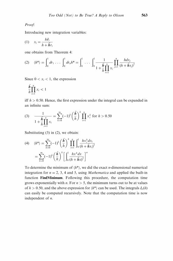
Proof:

Introducing new integration variables:

ð1Þ xi ¼h �rri

hþ �hhri

one obtains from Theorem 4:

ð2Þ hh*i ¼

ð10

dr1 : : :

ð1

0

drnh* ¼

ð10

: : :

ð10

1

1þ�hh

h

Yni¼1

xi

Ynj¼1

hdxj

ðhþ �hhxjÞ2

Since 0 < xi < 1, the expression

�hh

h

Yni¼1

xi 5 1

iff h > 0:50. Hence, the first expression under the integral can be expanded in

an infinite sum:

ð3Þ1

1þ�hh

h

Yni¼1

xi

¼X1k¼0

ð�1Þk� �hh

h

�k Yni¼1

xki for h > 0:50

Substituting (3) in (2), we obtain:

ð4Þ hh*i ¼X1k¼0

ð�1Þk� �hh

h

�k Yni¼1

ð1

0

hxki dxi

ðhþ �hhxiÞ2

¼X1k¼0

ð�1Þk� �hh

h

�k� ð10

hxkdx

ðhþ �hhxÞ2

�n

To determine the minimum of hh*i, we did the exact n-dimensional numerical

integration for n ¼ 2, 3, 4 and 5, using Mathematica and applied the built-in

function FindMinimum. Following this procedure, the computation time

grows exponentially with n. For n > 5, the minimum turns out to be at values

of h > 0:50, and the above expression for hh*i can be used. The integrals IkðhÞ

can easily be computed recursively. Note that the computation time is now

independent of n.


Documents

Too Odd (Not) to Be True: A Reply to Olsson