Embed Size (px)
Citation preview
The Pennsylvania State University
The Graduate School
College of Engineering
INTERFACE CHARACTERIZATION AND
DEFECT EVOLUTION OF COATED SAMPLES
UNDER THERMAL AND PRESSURE
TRANSIENTS
A Dissertation in
Engineering Science and Mechanics
by
Jason T. Harris
© 2012 Jason T. Harris
Submitted in Partial Fulfillment
of the Requirements
for the Degree of
Doctor of Philosophy
August 2012

ii
The dissertation of Jason T. Harris was reviewed and approved* by the following:
Albert Segall
Professor of Engineering Science and Mechanics
Dissertation Adviser
Chair of Committee
Panagiotis Michaleris
Professor of Mechanical Engineering
Ivi Smid
Associate Professor of Engineering Science and Mechanics
Sulin Zhang
Assistant Professor of Engineering Science and Mechanics
Judith Todd
Professor, Head of the Department of Engineering Science and Mechanics
*Signatures are on file in the Graduate School
iii
ABSTRACT
Coatings are vital to the performance of gun tubes, as they protect the structural steel substrate
from both the thermal and chemical affects of the hot, erosive, combustion gases. Gun tube
coatings are often evaluated by the pulsed-laser heating experiment, though it does not include
pressure affects. Live firing tests included all effects, but are expensive and difficult to conduct.
Recognizing the short-comings of current evaluation techniques, a method was developed to
evaluate interfacial properties by introducing an indentation induced flaw, and studying the flaws
evolution under thermal and pressure transients.
The effects of severe thermal- and pressure-transients on coated substrates with indentation-
induced, blister defects were then analyzed using experimental and finite element methods. Both
explicit and implicit FEA approaches were used to assess the transient thermal- and stress-states
and the propensity for fracture related damage and evolution, while undergoing uniform
convective heating and pressure transients across the surface. Spherical indentations along with
in-situ acoustic emissions, c-scans, and finite element modeling were utilized to induce the
defects, and to quantify interfacial adhesion and cohesive zone properties. Preliminary results
indicated complex interactions between the boundary conditions and their timing and the
resulting propensity for damage birth and evolution. Given the need for robust coatings, the
experimental and modeling procedures explored by this study will have important ramifications
for coated tube designs and the evaluation of candidate materials.
iv
TABLE OF CONTENTS
List of Figures ............................................................................................................................... vi
Acknowledgements ..................................................................................................................... xiii
Chapter 1. Introduction ................................................................................................................ 1
1.1 Purpose ............................................................................................................................. 1
1.2 Research Objective ........................................................................................................... 3
Chapter 2. Background ................................................................................................................. 4
2.1 Gun Tubes ........................................................................................................................ 4
2.1.1 Coatings ........................................................................................................... 5
2.2 Erosion ............................................................................................................................. 7
2.2.1 Thermo-Chemical Erosion .............................................................................. 7
2.2.2 Thermal Erosion .............................................................................................. 9
2.2.3 Mechanical Erosion ....................................................................................... 10
2.3 Erosion Mitigation.......................................................................................................... 10
2.4 Predicting Erosion .......................................................................................................... 10
2.5 Experimentally Analyzing Erosion ................................................................................ 12
2.5.1 Laser Pulsed Heating ..................................................................................... 13
2.6 Thermal Stresses in Gun Tubes ...................................................................................... 14
2.7 The Bauschinger Effect and Autofrettage ...................................................................... 18
2.8 Cold Spray Coating Deposition...................................................................................... 20
2.9 Coating Delamination .................................................................................................... 23
2.10 Cohesive Zone Elements ................................................................................................ 25
2.11 Finite Element Modelling of Progressive Crack Growth ............................................... 32
2.12 Evaluating Cohesive Zone Properties ............................................................................ 39
2.12.1 Mode I: The Wedge-Peel and Peel Tests ...................................................... 40
2.12.2 Mode II: The Dual-Cantilevered Beam and End-Notched Flexure Tests ..... 42
2.12.3 The Shear Button Test ................................................................................... 43
2.12.4 Mixed Mode Tests ......................................................................................... 44
2.12.5 Four-Point Bend Test .................................................................................... 46
2.12.6 The Blister Test ............................................................................................. 58
2.12.7 Indentation Tests ........................................................................................... 60
2.12.8 Fracture Energy as a Function of Phase Angle ............................................. 68
2.13 Thermal Gap Conductance ............................................................................................. 72
Chapter 3. Problem Statement ................................................................................................... 75
3.1 Objective ........................................................................................................................ 75
3.2 Technical Background.................................................................................................... 75
3.3 Experimental Procedure ................................................................................................. 76
Chapter 4. Property Measurement and Validation ................................................................. 78
4.1 Experimental Procedures................................................................................................ 78
4.1.1 Sample Preparation ....................................................................................... 78
4.1.2 The Four-point Bend Test ............................................................................. 82
4.1.3 The Ball Indentation Test .............................................................................. 85
4.2 Modelling ....................................................................................................................... 93
4.2.1 Introduction to Cohesive Zone Elements ...................................................... 93
4.2.2 Two-Dimensional Axisymmetric Model .................................................... 102
v
4.2.3 Coupled Axisymmetric FEA Model with Interface Crack .......................... 109
4.2.4 Four-Point Bend Test Simulation ................................................................ 112
4.2.5 Ball Indentation Simulation ........................................................................ 117
4.3 Experimental Results.................................................................................................... 119
4.3.1 Indentation Test Results .............................................................................. 119
4.3.2 Four-Point Bend Test Results ..................................................................... 136
4.4 Modelling Results ........................................................................................................ 139
4.4.1 Effects of Thermal and Pressure Transients (Cracked and Uncracked
Tubes)….. ..................................................................................................................... 139
4.4.2 Thermal Loading of Indentation-Induced Flaws ......................................... 144
4.4.3 Numerical Evaluation of Cohesive Zone Properties ................................... 150
4.4.4 Parameteric Study of Variations in Cohesive Zone Parameters ................. 181
Chapter 5. Flaw Evolution ........................................................................................................ 188
5.1 Thermal Loading on a Coating with an Interfacial Pre-crack Model .......................... 188
5.2 Flaw Evolution Modelling Results ............................................................................... 192
5.2.1 Gun Tube Boundary Conditions – The Effects of Thermal and Pressure
Transients on Flaw Evolution ...................................................................................... 196
5.2.2 Effects of Coating Thermal Capacity on Flaw Evolution ........................... 205
5.2.3 Effects of Phase Difference between Pressure and Thermal Transients on
Flaw Evolution ............................................................................................................. 211
5.2.4 Effects of Phase Difference between Internal Flaw Pressure and Surface
Boundary Conditions on Flaw Evolution ..................................................................... 218
5.2.5 Discussion of Thermal-Structural Simulation of Flaw Evolution Results .. 225
5.2.6 Discussion in Context of Existing Gun Tube Coatings............................... 231
Chapter 6. Conclusions and Reccomendations ....................................................................... 234
References .................................................................................................................................. 240
Appendix A. Nickel Coated Steel Test Results ....................................................................... 249
a. Preliminary Test Results on Nickel-Coated Steel .................................................... 249
b. Indentation Results Loaded 0.5 mm of Nickel-Coated Steel ................................... 254
c. Indentation Results Loaded to Intermediate Levels of Nickel-Coated Steel ............ 260
d. Aluminum-Coated Aluminum Indentation Test Results .......................................... 269
Appendix B. Computer Code ................................................................................................... 280
a. ANSYS Axisymmetric Indentation Model of Nickel Thermally Sprayed onto Steel
………...…………………………………………………………………………………..…….280
b. Abaqus Explicit thermal-Structural Model simulation Flaw Evolution Under
Severe Coating Surface Thermal and Pressure Transients .......................................................... 290
c. Abaqus Aluminum Cold-Sprayed onto Aluminum four-Point Bend Test
Simulation ................................................................................................................................... 297
d. Abaqus Aluminum Cold-Sprayed onto Aluminum Indentation Test Simulation .... 305
e. User Sub-routine to Apply Pressure as a funciton of Crack Size in Explicit
Thermal-Stuructural Simulation .................................................................................................. 314
f. User Sub-routine to Residual Stress in Four-Point Bend Simulation ....................... 316
Appendix C. Non-Technical Abstract ..................................................................................... 317
vi
LIST OF FIGURES
Figure 2.1 : Illustration of Bauschinger Effect. ............................................................................. 19
Figure 2.2: The four-point bend loading arrangement. ................................................................. 47
Figure 2.3: Illustration of assumed interface geometry of crack tip. ............................................ 70
Figure 4.1: Indentation experiment arrangement, showing (a) the load frame, computer, and
stage, and (b) a close-up of the stage and specimen arrangement. ........................... 88
Figure 4.2: Shear and normal contact separation curve for loading on (a) Mode I and (b)
Mode II. .................................................................................................................... 94
Figure 4.3: Mesh geometry of the two-dimensional axisymmetric model. ................................ 104
Figure 4.4: Finite element and analytical comparison of circumferential stress at time
t=0.1s. ..................................................................................................................... 107
Figure 4.5: Finite element and analytical comparison of circumferential at time t=0.5s. ........... 108
Figure 4.6: Finite element and analytical comparison of circumferential stress at steady
state. ........................................................................................................................ 108
Figure 4.7: Collapsed elements at interface crack tip. ................................................................ 110
Figure 4.8: Thermal and Pressure Boundary Conditions. ........................................................... 111
Figure 4.9: Four-point bend test configuration. .......................................................................... 113
Figure 4.10: Comparison of FEA and experimental results. ....................................................... 116
Figure 4.11: Meshed geometry of the indentation test. ............................................................... 118
Figure 4.12: Acoustic emission events as a function load of 3.2 kN load indentation test,
run 2. ....................................................................................................................... 121
Figure 4.13: SAM image of sample loaded to 2.6 kN (0.4 mm indenter displacement). ........... 128
Figure 4.14: C-scan image of sample loaded to 2.6 kN (0.4 mm indenter displacement). ......... 129
Figure 4.15: Scan of (a) amplitude and (b) time of flight of the signal for a 2.0 mm indenter
loaded to 4.75 kN. .................................................................................................. 132
Figure 4.16: C-scan image of (a) amplitude and (b) time of flight of the first-wall reflection
of aluminum-coated aluminum samples. ................................................................ 134
Figure 4.17: Load-Displacement results of the 7075 aluminum-coated aluminum bend test. .... 138
Figure 4.18: Maximum stress normal to the interface. ............................................................... 140
Figure 4.19: Maximum shear stress at the tip of an interface crack as a function of coating
thickness. ................................................................................................................ 141
Figure 4.20: The stress component normal to the interface at the tip of an interface crack as
a function of elastic modulus. ................................................................................. 143
Figure 4.21: Shear stress at the tip of an interface crack as a function of elastic modulus. ........ 143
Figure 4.22: Deformed geometry after indentation. .................................................................... 145
Figure 4.23: The length of debonding as a function of critical fracture energy. ......................... 147
Figure 4.24: The length of debond as a function of bond strength ............................................. 148
Figure 4.25: Comparison of experimental and finite element results of (a) inner and (b)
outer delamination diameter of nickel-coated steel. ............................................... 154
vii
Figure 4.26: Comparison of finite element predictions of the inner and our diameters for a
sample indented onto nickel-coated steel samples loaded to 3.2 kN overlaid on
c-scan images of the delamination flaw. ................................................................ 155
Figure 4.27: Load-displacement results from finite element simulations of an indentation of
2.0 mm made by an indenter in a nickel-coated steel sample. ............................... 156
Figure 4.28: Comparison of von Mises stress plots from finite element simulations of
indentations of 2.0 mm made by an indenter loaded at (a) 2.4 kN and (b) 3.2
kN. .......................................................................................................................... 157
Figure 4.29: Comparison of the equivalent plastic strain for the indentation of 2.4 kN on (a)
coating and (b) substrate. ........................................................................................ 159
Figure 4.30: Comparison the equivalent plastic strain for the indentation of 3.2 kN on (a)
coating and (b) substrate. ........................................................................................ 159
Figure 4.31: A plot of the damage variable, d, of the interface between the nickel coating
and the steel substrate as a function of distance from the center of the
indentation. ............................................................................................................. 161
Figure 4.32: Stereomicroscopic images of indentations showing cracks and other surface
features for samples indented to (a) 2.4 and (b) 3.2 kN. ........................................ 163
Figure 4.33: (a) Residual stress distribution applied to four-point bend test simulations, and
(b) curvature measurements used to calculate the residual stresses. ...................... 167
Figure 4.34: Comparison of experimental and finite element results for the four-point bend
test of aluminum cold sprayed on aluminum.......................................................... 168
Figure 4.35: Comparison of finite element simulations of aluminum cold sprayed onto
aluminum, with (a) coating thickness of 0.37 mm, indented to a load of 5.4 kN
(b) coating thickness of 0.89 mm, indented to a load of 5.0 kN............................. 172
Figure 4.36: Load-displacement results from finite element simulations of indentations of
5.4 and 5.0 kN, indented into substrates of 4.8 mm (3/16 in), with coatings of
thicknesses equal to 0.37 and 0.89 mm, respectively. ............................................ 173
Figure 4.37: Comparison of finite element simulations of aluminum cold sprayed onto
aluminum showing normal and shear stresses in the cohesive zone for samples
with (a) 0.37 mm thick coating and (b) 0.89 mm thick coating. ............................ 174
Figure 4.38: Comparison of finite element simulations of aluminum cold sprayed onto
aluminum, with (a) coating thickness of 0.37 mm, indented to a load of 5.4 kN
(b) coating thickness of 0.89 mm, indented to a load of 5.0 kN............................. 176
Figure 4.39: Comparison of finite element simulations of aluminum cold sprayed onto
aluminum, with (a) coating thickness of 0.37 mm, indented to a load of 5.4 kN
(b) coating thickness of 0.89 mm, indented to a load of 5.0 kN............................. 177
Figure 4.40: Normal displacement of the substrate surface for a coating thickness of 0.89
mm, indented to a load of 5.0 kN. .......................................................................... 178
Figure 4.41: Normal displacement of the substrate surface for a coating thickness of 0.89
mm indented to a load of 5.0 kN. ........................................................................... 179
Figure 4.42: (a) Inner and (b) outer radii as functions of interfacial cohesive strength.
Experimentally measured values are shown as black circles. ................................ 182
viii
Figure 4.43: (a) Inner and (b) outer radii as functions of interfacial stiffness.
Experimentally measured values are shown as black circles. ................................ 184
Figure 4.44: (a) Inner and (b) outer radii as functions of Mode I critical energy release rate.
Experimentally measured values are shown as black circles. ................................ 185
Figure 4.45: (a) Inner and (b) outer radii as functions of Mode II critical energy release
rate. Experimentally measured values are shown as black circles. ........................ 186
Figure 5.1: Interfacial gap conductance as a function of gap separation distance. ..................... 190
Figure 5.2: Initial and boundary conditions for thermal and pressure transient simulation. ....... 191
Figure 5.3: (a) Convective coefficient, (b) convective gas temperature, and pressure
transient applied to the coating surface. ................................................................. 195
Figure 5.4: Crack radius as a function of radial position for simulations with thermal
transient, and thermal and pressure transients. ....................................................... 197
Figure 5.5: Interfacial damage accumulated during stages of the transient in simulations
with (a) only a thermal transient, and (b) thermal and pressure transients. ............ 199
Figure 5.6: Interfacial damage accumulated during stages of the transient in simulations
showing a magnification of the crack tip with (a) only a thermal transient and
(b) thermal and pressure transients. ........................................................................ 200
Figure 5.7: Comparison of final damage states between simulations with and without
pressure transients, with the crack tip conditions inlayed on the plot. ................... 201
Figure 5.8: Coating temperature after the completion of the thermal transient in simulations
(a) with pressure transient and (b) without pressure transient. ............................... 204
Figure 5.9: Crack radius as a function of radial position for simulations with thermal
transient and with thermal and pressure transients. ................................................ 206
Figure 5.10: Interfacial damage accumulated during stages of the transient in simulations
with specific heat of (a) 440 kJ/kg K, (b) 600 kJ/kg K, and (c) 800 kJ/kg K. ........ 208
Figure 5.11: Close-up of the crack tip showing interfacial damage accumulated during
stages of the thermal transient in simulations with specific heat of (a) 440, (a)
600, and (c) 800 kJ/kg K. ....................................................................................... 209
Figure 5.12: Comparison of state of final damage between simulations with and without
pressure transients, with the crack tip conditions inlayed. ..................................... 210
Figure 5.13: Crack radius as a function of radial position in simulations for which internal
and pressure transients were offset from their original position relative to the
thermal transient. .................................................................................................... 212
Figure 5.14: Interfacial damage accumulated during stages of the transient in simulations
for which relative to the thermal transient the internal and external pressure
transients were offset by (a) 0.25 ms before its original time, and (b) 0 ms. ......... 214
Figure 5.15: Interfacial damage accumulated during stages of the transient in simulations
for which relative to the thermal transient the internal and external pressure
transients were offset by (a) 0.3 ms, and (b) 1.0 ms after its original time. ........... 215
ix
Figure 5.16: Interfacial damage accumulated during stages of the transient in simulations
for which the internal and external pressure transients relative to the thermal
transient were offset by (a) 0.25 ms before its original time, (b) 0 ms, and (c)
1.0 ms after its original time. .................................................................................. 216
Figure 5.17: Comparison of state of final damage between which the pressure transient was
shifted relative to the thermal transient, with the crack tip conditions inlayed
on the plot. .............................................................................................................. 218
Figure 5.18: Crack radius as a function of radial position in simulations for which internal
and pressure transients were offset from their original positions relative to the
thermal conditions. ................................................................................................. 219
Figure 5.19: Interfacial damage accumulated during stages of the transient in simulations
for which the internal and external pressure transients were offset relative to
the thermal transient by (a) 0 ms, (b) 0.15 ms after its original time. .................... 221
Figure 5.20: Interfacial damage accumulated during stages of the transient in simulations
for which the internal and external pressure transients were offset relative to
the thermal transient by (a) 0.25 ms, and (b) 0.275ms after its original time. ....... 222
Figure 5.21: Interfacial damage accumulated during stages of the transient in simulations
for which the internal and external pressure were offset after its original time
relative to the thermal by (a) 0.15 ms and (b) 0.25ms. ........................................... 223
Figure 5.22: Comparison of state of final damage between which the pressure transient was
shifted relative to the thermal transient, with the crack tip conditions inlayed
on the plot. .............................................................................................................. 224
Figure 5.23: Temperature distribution in the coating after the completion of the thermal
transient, t=10 ms, for a coating with specific heat of (a) 440 kJ/kg K, and (b)
800 kJ/kg K. ............................................................................................................ 229
Figure A.1: Load as a function of displacement for preliminary displacement indentation
tests. ........................................................................................................................ 249
Figure A.2: Acoustic emission events as a function of displacement for 0.2 mm
displacement indentation test. ................................................................................ 249
Figure A.3: C-scan showing dimension of delamination for 0.2 mm displacement
indentation test. ....................................................................................................... 250
Figure A.4: Acoustic emission events as a function of displacement for 0.3 mm
displacement indentation test. ................................................................................ 250
Figure A.5: C-scan showing dimension of delamination for 0.3 mm displacement
indentation test. ....................................................................................................... 251
Figure A.6: Acoustic emission events as a function of displacement for 0.4 mm
displacement indentation test. ................................................................................ 252
Figure A.7: C-scan showing dimension of delamination for 0.4 mm displacement
indentation test. ....................................................................................................... 252
x
Figure A.8: Acoustic emission events as a function of displacement for 0.5 mm
displacement indentation test. ................................................................................ 253
Figure A.9: C-scan showing dimension of delamination for 0.5 mm displacement
indentation test. ....................................................................................................... 253
Figure B.1: Load as a function of displacement for 0.5 mm displacement indentation test
for samples 3A, 3B, and 3C. ................................................................................... 254
Figure B.2: Acoustic emission events as a function of load for 0.5 mm displacement
indentation test for sample 3A. ............................................................................... 254
Figure B.3: C-scan showing dimension of delamination for 0.5 mm displacement
indentation test for sample 3A. ............................................................................... 255
Figure B.4: Acoustic emission events as a function of load for 0.5 mm displacement
indentation test for sample 3B. ............................................................................... 255
Figure B.5: C-scan showing dimension of delamination for 0.5 mm displacement
indentation test for sample 3B. ............................................................................... 256
Figure B.6: C-scan showing dimension of delamination for 0.5 mm displacement
indentation test for sample 3D. ............................................................................... 256
Figure B.7: Load as a function of displacement for 0.5 mm displacement indentation test
for sample 4A. ........................................................................................................ 257
Figure B.8: C-scan showing dimension of delamination for 0.5 mm displacement
indentation test for sample 4A. ............................................................................... 257
Figure B.9: C-scan showing dimension of delamination for 0.5 mm displacement
indentation test for sample 4B. ............................................................................... 258
Figure B.10: C-scan showing dimension of delamination for 0.5 mm displacement
indentation test for sample 4D. ............................................................................... 258
Figure B.11: C-scan showing dimension of delamination for 0.5 mm displacement
indentation test for sample 4D. ............................................................................... 259
Figure C.1: Load as a function of displacements for 1.5 kN, and 2.0 kN load indentation
tests. ........................................................................................................................ 260
Figure C.2: Acoustic emission events as a function load of 1.5 kN load indentation test, run
1. ............................................................................................................................. 260
Figure C.3: C-scan showing dimension of delamination for 1.5 kN load indentation test,
run 1. ....................................................................................................................... 261
Figure C.4: Acoustic emission events as a function load of 1.5 kN load indentation test, run
2. ............................................................................................................................. 261
Figure C.5: C-scan showing dimension of delamination of 1.5 kN load indentation test, run
2. ............................................................................................................................. 262
Figure C.6: Acoustic emission events as a function load of 2.0 kN load indentation test, run
1. ............................................................................................................................. 262
Figure C.7: C-scan showing dimension of delamination for 2.0 kN load indentation test,
run 1. ....................................................................................................................... 263
xi
Figure C.8: Acoustic emission events as a function load of 2.0 kN load indentation test, run
2. ............................................................................................................................. 263
Figure C.9: C-scan showing dimension of delamination of 2.0 kN load indentation test, run
2. ............................................................................................................................. 264
Figure C.10: Load as a function of displacement for 2.6 kN load indentation test, run 1. ......... 264
Figure C.11: Acoustic emission events as a function load of 2.6 kN load indentation test,
run 1. ....................................................................................................................... 265
Figure C.12: C-scan showing dimension of delamination for 2.6 kN load indentation test,
run 1. ....................................................................................................................... 265
Figure C.13: Acoustic emission events as a function load of 2.6 kN load indentation test,
run 2. ....................................................................................................................... 266
Figure C.14: C-scan showing dimension of delamination of 2.6 kN load indentation test,
run 2. ....................................................................................................................... 266
Figure C.15: Acoustic emission events as a function load of 3.2 kN load indentation test,
run 1. ....................................................................................................................... 267
Figure C.16: C-scan showing dimension of delamination for 3.2 kN load indentation test,
run 1. ....................................................................................................................... 267
Figure C.17: Acoustic emission events as a function load of 3.2 kN load indentation test,
run 2. ....................................................................................................................... 268
Figure C.18: C-scan showing dimension of delamination of 3.2 kN load indentation test,
run 2. ....................................................................................................................... 268
Figure D.1: Load as a function of displacement for indentation with 4.8 mm (3/16”)
diameter indenter into 0.37 mm average thickness coating for Sample Al1. ......... 269
Figure D.2: Acoustic emission events as a function of load for indentation with 4.8 mm
(3/16”) diameter indenter into 0.37 mm average thickness coating for sample
Al1. ......................................................................................................................... 269
Figure D.3: Load as a function of displacement for indentation with 2.0 mm diameter
indenter into 0.58 mm average thickness coating, loaded to 1.02 kN for
sample Al2. ............................................................................................................. 270
Figure D.4: Acoustic emission events as a function of load for indentation with 2.0 mm
diameter indenter into 0.58 mm average thickness coating, loaded to 1.02 kN
for sample Al2. ....................................................................................................... 270
Figure D.5: Load as a function of displacement for indentation with 2.0 mm diameter
indenter into 0.58 mm average thickness coating, loaded to 4.0 kN for sample
Al3. ......................................................................................................................... 271
Figure D.6: Acoustic emission events as a function of load for indentation with 2.0 mm
diameter indenter into 0.58 mm average thickness coating, loaded to 4.0 kN
for sample Al3. ....................................................................................................... 271
Figure D.7: Load as a function of displacement for indentation with 2.0 mm diameter
indenter into 0.37 mm average thickness coating for sample Al4.......................... 272
xii
Figure D.8: Acoustic emission events as a function of load for indentation with 2.0 mm
diameter indenter into 0.37 mm average thickness coating for sample Al4........... 272
Figure D.9: Load as a function of displacement for indentation with 2.5 mm diameter
indenter into 0.37 mm average thickness coating for sample Al5.......................... 273
Figure D.10: Acoustic emission events as a function of load for indentation with 2.5 mm
diameter indenter into 0.37 mm average thickness coating for sample Al5........... 273
Figure D.11: Load as a function of displacement for indentation with 2.5 mm diameter
indenter into 0.5 mm average thickness coating for sample Al6. .......................... 274
Figure D.12: Acoustic emission events as a function of load for indentation with 2.5 mm
diameter indenter into 0.5 mm average thickness coating for sample Al6............. 274
Figure D.13: Load as a function of displacement for indentation with 2.0 mm diameter
indenter into 0.9 mm average thickness coating for samples B1, A2, and A3. ...... 275
Figure D.14: C-scan of the (a) amplitude (b) and time of flight of the first wall reflection of
delamination following an indentation with 2.0 mm diameter indenter into 0.9
mm average thickness coating for sample B1. ....................................................... 275
Figure D.15: Acoustic emission events as a function of displacement for indentation with
2.0 mm diameter indenter into 0.9 mm average thickness coating for sample
A2. .......................................................................................................................... 276
Figure D.16: C-scan of the (a) amplitude (b) and time of flight of the first wall reflection of
delamination following an indentation with 2.0 mm diameter indenter into 0.9
mm average thickness coating for sample A2. ....................................................... 277
Figure D.17: Acoustic emission events as a function of displacement for indentation with
2.0 mm diameter indenter into 0.9 mm average thickness coating for sample
A3. .......................................................................................................................... 278
Figure D.18: C-scan of the (a) amplitude (b) and time of flight of the first wall reflection of
delamination following an indentation with 2.0 mm diameter indenter into 0.9
mm average thickness coating for sample A3. ....................................................... 279
xiii
ACKNOWLEDGEMENTS
I would first like to thank the Department of Defense for their funding of this project, and Dr.
Rob Carter for providing all of the assistance I needed throughout the course of the research. I
also would like to thank my adviser Dr. Segall for giving me the opportunity to study at Penn
State. During the course of the project, he was always extremely helpful and instructive. His
sense of humor was always appreciated. I would like to thank my committee members, Dr.
Michaleris, Dr. Smid, and Dr. Zhang for their time, contributions, and guidance throughout the
project. The contributions of Dr. Eden and Mr. Potter at ARL were much appreciated for their
discussions and help producing cold-sprayed samples. I would also like to thank Brian Reinhardt
and Dr. Tittmann for the use of their equipment and their expertise during ultrasonic
measurements. I would also like to thank my lab mates that I’ve worked with during my studies,
including David Robinson, who worked with me during parts of this research.
I would like to thank my friends and family, especially my brothers and sister, Zach, Sean, and
Ashley, for their love and support. I would especially like to thank my parents, without whom,
none of my accomplishments would be possible.
1
CHAPTER 1. INTRODUCTION
1.1 Purpose
During gun firings, the bore of large caliber cannons experiences a severe combination of
temperature and pressure gradients; surface temperature increases approximately 1,500K in less
than 2 ms before cooling down nearly as rapidly, while internal pressures reach over 300 MPa.
In recent history, gun tube thermal damage has increased considerably because of higher
combustion gas temperatures associated with improved performance, according to Underwood et
al. [1]. Thermal loading causes a rapid expansion of the interior of the tube that can result in
yielding, phase changes in the structural steel, and/or the release of beneficial residual stresses
that were applied during an autofrettage process. In addition, hydrogen embrittlement of steel
will occur if combustion gases penetrate the coating and will result in lower fracture toughness.
The thermo-mechanical-chemical loading conditions also contribute to a process known as
erosion, which leads to premature failure of gun tubes. Recognizing the prospect of imminent
gun tube failure after coating and steel separation, gun tube researchers have focused efforts
towards improving the coating bond. Understanding crack driving forces and stress states at the
tip of an interfacial crack, through finite element modeling, analytical analysis, and experimental
work, will provide insight for improving gun tube coating systems.
Cohesive zone models were developed to model progressive crack growth. The model is based
on a traction-separation relationship for which stresses, as a function of interface separation
distance, at the crack tip increase to a maximum value, before decreasing until the surfaces
completely separate. Combined with a coupled thermal-mechanical finite element model of the
coating and steel, the cohesive zone is ideally suited to model the interfacial crack growth for
gun tube coating systems. For mixed mode fracture there are four basic cohesive zone

2
parameters; Mode I and II cohesive strength, which are the maximum interfacial stresses, and
Mode I and II critical fracture energy, which are the integrations of the traction as a function of
separation for the respective mode. Several studies have been attempted to measure the critical
fracture energy as a function of the contribution of modes I and II, however no standard has been
established. In addition, cohesive strengths are extremely difficult to measure, and are more
often used as tuning parameters; they are varied in finite element models until experimental and
numerical results agree.
The four-point bend test has been chosen to evaluate the properties of the cohesive zone for gun
tube coating systems. The four-point bend test can measure the critical fracture energy for
samples with various coating and substrate thicknesses, in addition to samples with residual
stresses, which are usually associated with thermal and cold spray coatings. Because of the
ambiguity in the measurement of the four cohesive zone properties the cohesive zone properties
should be verified in an independent experiment. Indentation tests provide an opportunity for
property verification by applying the properties measured with the four-point bend test to a
model of a spherical indenter penetrating a coated substrate. Property verification will be
confirmed by comparing the numerical and experimental results after the initiation of
delamination.
Laser-pulsed heating tests have been shown to be an effective technique to simulate the thermal-
mechanical loads experienced by gun tubes during firings, according to Underwood et al. [2] and
will be studied experimentally and with cohesive zone finite element models. Interfacial crack
growth will be studied experimentally by first introducing a blister flaw in coated samples before
applying laser heating to the coating surface above the defect. Recognizing that the ball indenter
will introduce plastic deformations and cohesive zone damage in addition to the blister, the
3
indentation experiment will be modeled in the first part of an implicit-explicit simulation before
the thermal loads are applied in the second part. The approach was used to more closely
approximate experimental conditions, as the entire material state will become the initial
conditions for the laser heating explicit simulation. System parameters, such as the coating and
substrate material, thermal and pressure transients phase difference, and blister pressure with the
goal of understanding defect evolution and improving coating response to thermal transients.
1.2 Research Objective
The primary objective of this research is to develop and verify a model to study the response of
refractory coatings, gun tube steel, and their interface to several thermal transients. Substrates
will be coated and machined to produce various samples. The samples will be used to evaluate
the cohesive zone properties using a combination of experimental, analytical, and numerical
methods. Once the properties are measured, the capability of the cohesive zone to model fracture
will be verified with the spherical indentation test. Finally, the response of the coating system to
thermal boundary conditions will be investigated. The cohesive zone model can be used in an
explicit, thermal-structural, coupled model to study the adhesion of the coating and investigate
possible mechanisms to reduce crack growth and ultimately extend the gun tube’s life.
4
CHAPTER 2. BACKGROUND
2.1 Gun Tubes
After World War II the possibilities of different coatings and steel alloys were explored for their
applications to gun tubes. Research intensified during the Vietnam War, when gun tubes became
an important area of research due to performance and reliability issues with machine guns and
the 175-mm gun [3, 4]. Army cannons initially became a focused area of research after the
unexpected failure of a 175-mm inner diameter (ID) cannon tube in 1966. The fracture toughness
of the failed tube was well below the average toughness of tubes from the same time. Davidson
et al. addressed the problem by applying an autofrettaged design, by which a residual
compressive stress was applied to offset the tensile stresses associated with firing [5]. In addition
research focused on the use of liners, coatings and additives [3]. Current research for gun tubes
includes functionally graded ceramics, magnetron sputtered coatings, and linings [3].
Several gun tube variations exist today. The two main categories of artillery tubes are monobloc
and jacketed tubes. True monobloc tubes consist of only one piece of material. However, a
monobloc tube with a liner is known as a variant. The tube liner generally does not contribute
significantly to the strength of the tube and may extend through various lengths of the tube. The
second type of tube is the jacketed type of tube, which consists of two concentric tubes [6]. Other
weapon tubes include small arms, recoilless and expendable tubes [6].
Gun tubes generally consist of several distinct regions. The first region is the breech, through
which the round is inserted. The round then rests in the chamber before firing. The bore is the
inner surface of the gun tube cylinder through which the projectile travels before it exits through
5
the muzzle. The bore is often rifled to introduce a torque on the round. The angular momentum
of the round improves its range and accuracy.
The inside of a gun tube during firing experiences an unfavorable combination of thermal,
mechanical and chemical loading. Propellant gases can reach temperatures in excess of 3000°K.
The thermal loading causes a rapid expansion of the interior of the tube that can cause yielding, a
phase change in the structural steel, and/or release beneficial residual stresses that were applied
during an autofrettage process. The pressure associated with the resisted expansion of the
propellant gases is out of phase with the heat flux associated with the combustion gases (it
slightly lags the thermal pulse) and factors into the stresses in the gun tube. Also, the combustion
of the propellant creates hydrogen, which can lead to hydrogen embrittlement if it can penetrate
any coatings present. Hydrogen embrittlement lowers the fracture toughness of the material
leading to crack extension and further damage. The thermo-mechanical-chemical loading
conditions also contribute to a process known as erosion, which leads to premature failure of gun
tubes.
2.1.1 Coatings
Coatings are designed to not react with propellant gases and insulate the gun steel from the
thermal flux caused by the combustion of the propellant. Coatings have been designed with the
main purpose to protect the structural steel of the gun barrel. One of the many purposes served
by coatings is resisting erosion and protecting the steel from erosion. Recent research has been
concentrated on understanding the mechanisms of coating failure, assessment of known coatings
and coating application techniques [7].
6
Chromium is a common gun tube coating; it was developed over 60 years ago and is the most
common coating used on battle guns. Low contractile (LC) chromium coatings are tougher and
stronger, but weaker according to Cote [8]. Other possible experimental coating techniques
include physical vapor deposition, chemical vapor deposition or metal-organic chemical vapor
deposition (MOCVD) [7]. Sopok compared the erosion of several different coatings which
included chromium, tantalum, molybdenum, rhenium and niobium together with [9]. Sopok’s
results showed that all the materials have significantly different erosion performance. Rhenium
and niobium had the lowest erosivity threshold, as defined by the threshold surface temperature
at the start of erosion, while chromium and tantalum had the highest. Sopok also demonstrated
that the chromium performance varied little in different combustion environments.
Coatings contain cracks of varying size from the time of their manufacturing. The pressure on
the gun tube inner wall and thermal heat transfer of the combustion gases that occur during the
repeated firings cause the cracks to grow, and eventually cracks may reach the substrate
structural steel. Once the coating cracks reach the substrate, the hot and chemically erosive
combustion gases can reach into the depths of the cracks where they can react with the steel.
During subsequent firings cracks can form networks that lead to the so-called mud-flap cracks in
the coatings. The array of cracks can result in the detachment of the coating from the steel. The
dimensions of these islands are on the same order as the coating thickness according to Johnston
[7].
Underwood et al. investigated hydrogen cracking in compressively yielded fired cannons [10].
They were able to develop a threshold stress intensity factor that would govern the crack spacing
of longitudinal and circumferential cracks (the circumferential cracks extend due to hoop or
7
circumferential stress, while the longitudinal cracks extend from the axial stress). The
circumferential cracks had a larger spacing than expected, and were actually closer to
longitudinal crack spacing as predicted by the threshold stress intensity factor. The researchers
predicted that this was a result of the compressive residual stress from the autofrettage stress
field. Based on their analysis, the researchers concluded that hydrogen embrittlement had
occurred in the tube.
2.2 Erosion
One of the most thoroughly researched aspects of gun tube design is erosion. Erosion is a cause
for concern because of high tube replacement costs and the reduced effectiveness of gun barrels
after the onset of erosion. Permissible erosion in tank guns that require significant accuracy is
about 0.5-1% and between 5 and 8% can be permitted for indirect firing weapons according to
Lawton [11]. Erosion damage is generally most serious at the origin of rifling [11]. The
temperature is highest here and even though the tube is only at this temperature for a short period
of time, it allows the harmful combustion compounds to diffuse into the steel creating a weak
brittle zone which can be susceptible to removal by the high velocity of the combustion gases
[11]. Erosion mechanisms are categorized as chemical, thermal, and mechanical. Erosion can be
experimentally studied several ways, such as canon firing has been simulated by laser pulse
heating [12], ion beams [13] or by analyzing fired guns [8, 11, 14-17]
2.2.1 Thermo-Chemical Erosion
Johnston noted that the combustion of the propellant produces a mixture of gases, which includes
carbon monoxide, carbon dioxide, hydrogen, water vapor, and nitrogen [7]. The combustion
8
products can react with coating or the substrate. To make matters worse, the products can
penetrate into the cracks beneath the coatings when the cracks are very small according to Cote
and Rickard [8].
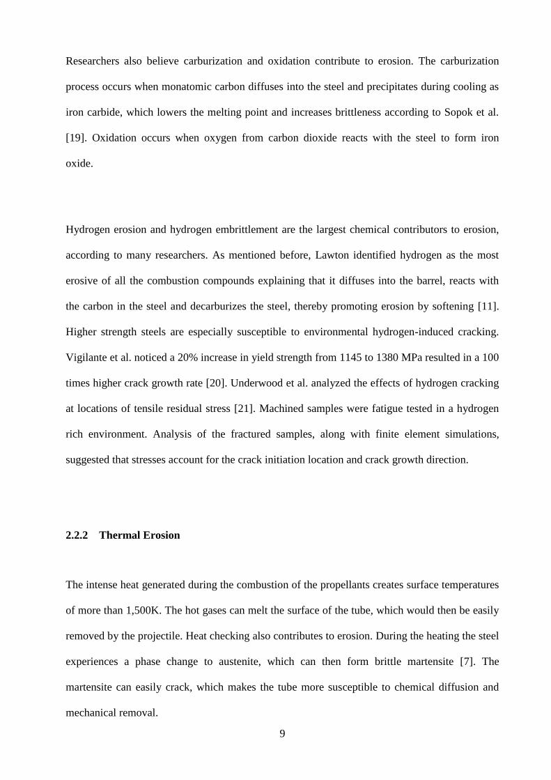
All of the mentioned gases contribute to erosion according to a correlation developed by Lawton
for the wear per round, which is given in Equation ((2.1) [11].
max0
0 expTR
E
T
TAtw
a
i (2.1)
where t0 is the time-constant that has been determined by Lawton [18], Tmax is the maximum bore
temperature, Ti is the initial surface temperature, Ta is 300K, ΔE is the activation energy, R0 is
the universal gas constant and A is an expression based on multiple linear regression of
experimental data and is a function of the contribution of each of the combustion gases. The
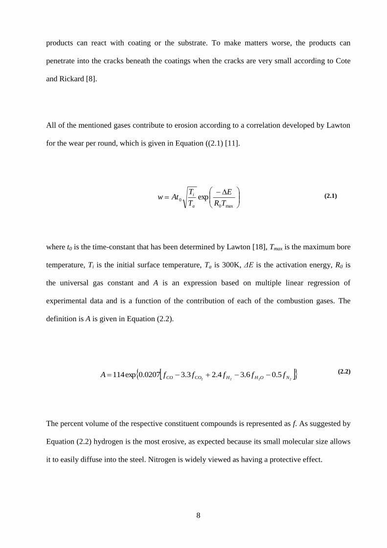
definition is A is given in Equation (2.2).
2222
5.06.34.23.30207.0exp114 NOHHCOCO fffffA (2.2)
The percent volume of the respective constituent compounds is represented as f. As suggested by
Equation (2.2) hydrogen is the most erosive, as expected because its small molecular size allows
it to easily diffuse into the steel. Nitrogen is widely viewed as having a protective effect.
9
Researchers also believe carburization and oxidation contribute to erosion. The carburization
process occurs when monatomic carbon diffuses into the steel and precipitates during cooling as
iron carbide, which lowers the melting point and increases brittleness according to Sopok et al.
[19]. Oxidation occurs when oxygen from carbon dioxide reacts with the steel to form iron
oxide.
Hydrogen erosion and hydrogen embrittlement are the largest chemical contributors to erosion,
according to many researchers. As mentioned before, Lawton identified hydrogen as the most
erosive of all the combustion compounds explaining that it diffuses into the barrel, reacts with
the carbon in the steel and decarburizes the steel, thereby promoting erosion by softening [11].
Higher strength steels are especially susceptible to environmental hydrogen-induced cracking.
Vigilante et al. noticed a 20% increase in yield strength from 1145 to 1380 MPa resulted in a 100
times higher crack growth rate [20]. Underwood et al. analyzed the effects of hydrogen cracking
at locations of tensile residual stress [21]. Machined samples were fatigue tested in a hydrogen
rich environment. Analysis of the fractured samples, along with finite element simulations,
suggested that stresses account for the crack initiation location and crack growth direction.
2.2.2 Thermal Erosion
The intense heat generated during the combustion of the propellants creates surface temperatures
of more than 1,500K. The hot gases can melt the surface of the tube, which would then be easily
removed by the projectile. Heat checking also contributes to erosion. During the heating the steel
experiences a phase change to austenite, which can then form brittle martensite [7]. The
martensite can easily crack, which makes the tube more susceptible to chemical diffusion and
mechanical removal.
10
2.2.3 Mechanical Erosion
The shear stress caused by sliding friction is sufficient to cause material removal when the inside
of the gun tube is already cracked or embrittled. Mechanical erosion is especially dominant in
low temperatures when the temperatures are too low for thermal erosion and too low to assist in
the diffusion of chemical compounds into the steel. Different types of erosion include abrasion,
sweeping and washing from the combustion gases.
Another form of erosion occurs when the combustion gases leak past the projectile. The leaking
can create jetting, which contributions to erosion. The blow-by effect was found to increase local
erosion by between 200-300% [22].
2.3 Erosion Mitigation
Several different techniques have been researched to mitigate the effects of erosion. Work on the
effects of propellant additives has been limited since the review done by Barcuti of additive
research, up to the point of the review [23]. Titanium dioxide is one common additive. Many
researchers believe it works by reducing heat transfer to the barrel, thereby reducing erosion [7].
2.4 Predicting Erosion
11
Researchers have been concentrating recent efforts at predicting and modeling erosion in order to
more accurately evaluate gun tube life and optimum replacement intervals. Modeling also allows
for the addition and removal of variables. Variables can also be optimized to limit erosion.
Sopok et al. developed the computer code for the first model able to predict thermochemical
erosion [24]. The model had the ability to include the effects of wall degradations from steel
phase transformations, chemical reactions, and cracking. The five different analyses of the code
provided profiles for thermo-chemical ablation, conduction, and erosion for each material as a
function of time, travel, and round. Later, Sopok et al. developed an updated code [19]. The
unified computer does not require significant validation, but simulations require substantial user
intervention to integrate the different inputs and outputs of the analyses.
Cote et al. also utilized two finite element models to understand the onset of coating-substrate
separation, and plastic deformation and stresses associated with the island effect [25]. The first
model was of an island crack. The model included the effects of plastic deformation and
demonstrated the cupping in the crack. The lifting of the edges of islands suggests the
mechanism by which the islands separate from the substrate leaving the steel exposed. The
second model was designed to simulate the shear and peeling stress between the coating and the
steel. The stresses were in excess of the yield strengths. It was also observed that if the crack
extended through the interface and into the steel, instead of stopping at the interface, it was
beneficial in terms of preventing peeling and coating separation. The thermal stresses of the
firing were found to dominate, while the compressive thermal stresses from cooling were found
to be more likely to cause spallation than those created during heating.
12
2.5 Experimentally Analyzing Erosion
The erosion mechanisms are often most easily understood by experimentally analyzing fired gun
tubes. Visual observations in addition to several different levels of microscopy can provide
insight into the mechanisms, causes, and locations of erosion damage. The understanding gained
experimentally can often provide insight in ways to prevent erosion and extend the gun tube’s
useful life.
Turley analyzed a chromium plated tank gun tube after erosive wear was seen at the origin of
rifling [15]. The tube was analyzed visually, with a scanning electronic microscope (SEM),
optical microscopy, and by x-ray scans. The gun tube coating experienced spalling in small
areas, which were bounded by craze cracks. It was also observed that in some cases copper from
the round penetrated into the cracks as it was forced through the tube. The mismatched
coefficient of thermal expansion of the copper and chromium forced the crack to open during
firing, expediting the crack growth. A more thorough study of chromium loss was done by Cote
et al. [25]. The goal of the study was to establish coating loss factors. The gun tube fired
sufficient rounds of two different types to obtain the erosion before being fatigue tested and
analyzed using optical microscopy, confocal microscopy, electron microprobe analysis, scanning
electron microscope (SEM), and Energy-dispersive X-ray spectroscopy (EDAX). Cote et al.
noticed high temperature corrosion on the surface, leading to chromium loss. Like Turley, it was
noticed that as soon as the steel was exposed to the combustion gases it was rapidly corroded and
pitted.
13
The erosion process was well characterized by Underwood et al. [17]. It was observed that the
process occurred in three steps. In the first, the cracks were permanently opened from tensile
stresses. The coatings are softened, allowing the steel to be transformed. Finally, islands are
formed that eventually crack off the surface. Underwood also noted that the most critical axial
location in the 120 mm gun barrel for erosion is 0.6 m forward of the breech [17]. After 118
firings, the gun tube at the location had transformation and cracking in both the chromium
coating and the steel.
2.5.1 Laser Pulsed Heating
Actual gun barrel firing for evaluating coatings and gun steel and characterizing damage is an
expensive and cumbersome process. Researchers prefer to evaluate coatings damaged through a
laser pulse heating process designed to simulate firings. However, the laser heating can only
simulate the thermal effects of the firing, and not the effects of the combustion gases and the
mechanical effects caused by a projectile. Underwood et al. used a Nd:YAG laser to apply a
single pulse to the surface of a sample [26]. Thermal damage cracks from laser heating were
observed in ZrO2, Al2O3, SiAlON, Si3N4, and SiC. The cracking mechanism believed to be
behind the damage was thermal expansion during heating that lead to compressive deformation
and tensile residual deformation that lead to cracking after cooling. All of the samples
experienced significant cracking, while the Al2O3 sample underwent fragmentation in cracked
areas, the ZrO2 and Si3N4 samples showed normal cracks forming and opening followed by
parallel cracks, indicating that the normal cracks occurred first. The SiAlON sample experienced
a significant amount of material loss.
14
Underwood et al. also conducted experiments on laser pulse heated tantalum and chromium
coated steel samples [1]. The samples cracked in the coating, but not in the steel substrate. This
was expected because hydrogen embrittlement could not occur due to the only trace amounts of
hydrogen present during the laser pulse heating. The addition of the hydrogen from the
combustion gases present during the actual firing is perhaps responsible for the crack penetration
and extension into the steel. Underwood et al. also observed recrystallization that occurred in the
steel at a depth of two-thirds of the coating thickness.
Warrender et al. were able to closely replicate the heat transfer equivalent to a firing using a
variable pulse duration laser, as opposed to the fixed pulse duration laser used in most other
studies [2]. The surface temperature experienced during firing and the pulsed laser simulations
were very similar. The samples, also tantalum or chromium coated steel, showed failure
consistent with firing results. The firing resulted in circumferential cracks in the tantalum, the
spacing of which was a function of the pulse duration and fluence of the laser beam. Increasing
the pulse duration of the laser appeared to increase the crack spacing and the fracture toughness
of the sample, suggesting it might be an effective coating pre-treatment.
2.6 Thermal Stresses in Gun Tubes
Thermo-mechanical modeling of the firing process is important for understanding the failure
mechanisms in gun tubes given the complex interactions between the severe pressure and
thermal conditions; the resulting stresses in-turn drive the formation and propagation of cracks
that ultimately cause a variety of failures (fatigue, debonds, erosion etc.).
15
Generally, there are two main types of cracks often observed in gun tubes after the application of
a thermal/pressure pulse as seen during firing. According to the leading authority on gun tube
failure mechanisms (Underwood et al. [27]), circumferential-radial cracks tend to grow because
of the dominant hoop stresses. While longitudinal-radial stresses also tend to occur in practice
due to a number of factors including curvature effects, an analysis of SEM images led to the
conclusion that one reason for these cracks was a thermal expansion-residual and stress-
environmental cracking scenario. In this scenario, the residual stresses in the coating caused
hydrogen induced cracking normal to the axial stress.
Using this information, Underwood and co-workers [1, 14, 17, 26-30] developed a thermo-
mechanical model which used the finite difference method to first evaluate the transient
temperature distributions as a function of the depth for a coated steel plate; the temperatures
calculations were done using measurements from bore locations where the thermal heat transfer
was the most severe. For the model, linearly temperature dependent material properties were
used to account for the wide temperature range that the coating and steel substrate experienced.
The pulse duration and magnitude, coating thickness, and convection coefficient were all
variables input into the model.
For the subsequent analysis, the transient, in-plane, and bi-axial thermal stress was approximated
using Equation (2.3) as shown below.
1
, i
T
TtxTE (2.3)
16
where E is the elastic modulus, α is the coefficient of thermal expansion, ν is the Poisson’s ratio,
T(x,t) is the temperature as a function of depth, x, and time, t, and Ti is the initial, uniform
temperature.
Residual stress calculations were then made by taking the negative of the sum of the stress
calculated above and the yield strength as shown by Equation (2.4).
YTR (2.4)
In Equation (2.4) σY is the yield strength. In the most recent application of the model, a
modification was applied which included the temperature dependence of the yield strength.
Under these assumptions, the temperature distribution was then verified by analyzing the
microstructure of the steel in order to determine the depth of the steel transformation that occurs
at 1020 K; the finite-difference calculations agreed with the temperature at the transformation
depth.
After comparing the temperature distributions in the steel substrate when chromium, tantalum,
and molybdenum coatings were used, it was observed that the molybdenum transferred the most
heat and thus, had the highest temperatures in the substrate. However, it had approximately the
same surface temperature as the chromium coating. In addition, the temperature distribution of
tantalum was between the chromium and molybdenum, with the model predicting the highest
17
surface temperatures. Predicted stress magnitudes in the coating increased consistently from
chromium, tantalum, to molybdenum.
Increasing the coating thickness also enlarged the tensile residual stresses in the coating, but had
varying effects on the temperature distributions. Interestingly, the surface temperature was lower
for the thicker coating, as well as at the interface. However, the overall temperature was higher
as a function of the distance from the surface for the thicker coatings. Increasing the heating
pulse duration had the predictable effect of amplifying the temperature in both the coating and
substrate, while also moving the tensile residual-stresses further from the surface.
The temperature used for the shear-stress evaluations was the difference between the
temperatures determined at locations 0.5 and 1.5 times the crack depth; this difference reflects
the temperature that governs the shear failure and removal of the coating segment. Recognizing
that when a crack opens, transient compressive stresses are released, a force balance was
developed and rearranged to provide an expression for the shear stress at the interface.
*2/32/y
zTTE zzzz (2.5)
In Equation (2.5), τ is the interface shear stress, Ez and αz are the elastic modulus and coefficient
of thermal expansion at the depth of the crack, Tz/2 is the temperature at a depth of half of the
crack length, T3z/2 is the temperature at a depth of one and a half crack lengths, z is the crack
length and y* is the length of the segment from the crack, parallel to the surface. The term inside
the brackets is an estimate of the transient residual stress. Results indicated that the maximum
18
shear stresses in the chromium coating agreed well with the observed shear-strength for that
material as determined by micro-hardness measurements. In another important study, Petitpas
and Campion [31] predicted the fatigue life of uncoated gun barrels using finite elements. The
authors discovered that the pressure pulse governed the growth of cracks over a four millimeter
range and that the fatigue life was increased by a factor of 10 after an autofrettage.
Crack growth at the interface leads to coating delamination, which exposes the underlying
substrate to erosion. According to Newaz et al. [32], thermal stresses cause compressive yielding
and residual tensile stress and cracking during cooling. As such, graded coatings where the
composition varies functionally from the interface to the surface (Bao and Cai [33, 34]) are often
used. Despite these efforts, many coatings typically fail when cracks parallel to the surface form
at the interface, eventually leading to delamination in various forms (Zhu et al. [35] and
Hutchinson and Evans [36]).
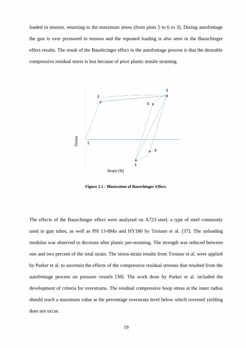
2.7 The Bauschinger Effect and Autofrettage
The Bauschinger effect is often observed in gun steels. Effective numerical modeling of the
effect requires accurately measuring experimental stress-strain results. The Bauschinger effect is
characterized by several principal features, shown in Figure 2.1.
The material is first loaded linearly until the yield strength, at which point plastic nonlinear
stress-strain behavior can be observed (from points 1 to 2 to 3). The loading is then reversed to
compressive stress, which has a reduced elastic modulus and after passing the yield point,
nonlinear compressive stress-strain behavior (from points 3 to 4 to 5). The material is then
19
loaded in tension, returning to the maximum stress (from pints 5 to 6 to 3). During autofrettage
the gun is over pressured in tension and the repeated loading is also seen in the Bauschinger
effect results. The result of the Baushcinger effect in the autofrettage process is that the desirable
compressive residual stress is lost because of prior plastic tensile straining.
Figure 2.1 : Illustration of Bauschinger Effect.
The effects of the Bauschinger effect were analyzed on A723 steel, a type of steel commonly
used in gun tubes, as well as PH 13-8Mo and HY180 by Troiano et al. [37]. The unloading
modulus was observed to decrease after plastic pre-straining. The strength was reduced between
one and two percent of the total strain. The stress-strain results from Troiano et al. were applied
by Parker et al. to ascertain the effects of the compressive residual stresses that resulted from the
autofrettage process on pressure vessels [38]. The work done by Parker et al. included the
development of criteria for overstrains. The residual compressive hoop stress at the inner radius
should reach a maximum value at the percentage overstrain level below which reversed yielding
does not occur.
20
In another study by Troiano et al., several gun tube sections were overstrained before slit tests
were conducted [39]. A finite element model was developed to simulate the process and was
found to agree well with analytical techniques for the prediction of residual stress in thick-walled
autofrettaged cylinders. An important result was that it appeared that the Bauschinger effect was
minimized by performing a post-autofrettage thermal treatment, which consisted of loading to
1.2% strain in tension, 0.25% strain in compression, the removal of loading and the application
of heat at 360°C for one hour. Parker also did research on efforts to minimize the Bauschinger
effect [40]. The fatigue-based life of the tube can be extended by between a factor of 2 and 30
using the process that consisted of an initial autofrettage, one or more heat soak and autofrettage
sequences and a final heat soak, which was deemed optional.
Geometric changes in cylinders complicate the autofrettage process. Possible disruptions in
axisymmetry in gun tubes include erosion groves, rifling or cross-bore holes sometimes used for
cooling. Parker et al. explored the effects of cross bore holes in gun tubes in terms of stress
concentrations, stress intensities and fatigue life in autofrettaged tubes [41]. For cracks
originating from the holes, the lifetime is only 60% of the lifetime if the crack originates from
the bore.
2.8 Cold Spray Coating Deposition
Cold spray is a coating process where small particles, typically 1 to 50 μm, are directed towards
a target surface. A supersonic gas jet carries the unmelted particles at velocities greater than 500
m/s. The cold spray process is characterized by excessive deformations in both the target surface
and the particles. The concept of cold spray was derived as an offshoot of supersonic wind tunnel
21
testing by Alkhimov et al. [42] and Tokarev [43]. In order to cold spray a material, it must first
be available in powder form, which is fluidized after mixing with high-pressure preheated gas.
The gas and powder are then fed into the nozzle, accelerated to supersonic speeds, and then
cooled to room temperature and in the divergent section of the nozzle. Several variations of the
original design have been researched, in addition to the effects of various characteristic
dimensions. Further details of the cold spray procedure have been described by Stoltenhoff et al.
[44]. The exact mechanisms that bond the particles to the target surface is not well understood.
The prevailing theory is that the plastic deformation removes any surface films that might
prevent bonding, such as oxides, and allows for intimate conformal contact at high uniform
contact pressure according to Dykhuizen et al. [45].
Current studies of cold spray focus on optimizing the nozzle dimensions and designs, research on
the interfacial bonding mechanisms, and material combinations according to Gärtner et al. [46].
Finite element simulations of particles impacts at the target surface is one of the most common
approaches to understanding the bonding mechanisms; Assadi et al. [47] and Li et al. [48, 49]
have published research on the topic. Current finite element models are thermomechanical and
utilize advanced material models, such as Johnson-Cook. Given the short duration of particle
impact events, the problems are well-suited to be solved with explicit finite element codes. The
particles also undergo excessive deformation during impacts, causing significant distortion in the
original shape and finite element mesh. In order to overcome the excessive deformation of the
elements in the mesh, the Arbitrary Lagrangian-Eulerian method is sometimes used, where the
finite element mesh is not attached to the material. The computational mesh can move within the
boundaries to optimize the individual element shape. Alternatively, remeshing is often used to
optimize the mesh during sub-steps of the solution at points in time when the deformation in
individual elements becomes excessive.
22
The velocity of the particle at impact is one of the key parameters during cold spray coating
deposition. A critical velocity, below which particles fail to adhere to the target surface, is
generally between 300 and 1200 m/s and is a function of a wide range of parameters. However,
excessive particle velocity can lead to erosion on the target surface and particle shattering upon
impact according to Bala et al. [50]. Further experimental and theoretical details about the
critical velocity of the particles during cold spray can be found elsewhere, such as the work of Li
et al. [48]. The carrying gas, which is usually nitrogen, helium, or air, is pressurized to typically
around 1.7 MPa according to Bala et al. [50]. The gas is preheated before the addition of the
power to prevent particle softening and to increase the speed of the gas as it expands in the
nozzle. The speed of the powder is a strong function of the gas preheating temperature. The
critical velocity of successful deposition is determined by correlating the deposition efficiency
with the particle size distribution. Deposition efficiency is a function of the nozzle geometry as
well as other process parameters, such as gas temperature and pressure according to Gärtner et
al. [46].
Cold spray coating technology offers significant benefits compared to thermal spray techniques
and other coating deposition methods. Lima et al. [51] suggested using cold spraying to apply
nanostructured coatings. Nanostrucutred coatings are desirable due to their unique
microstructure. When such coatings are thermally sprayed, any partial melting will cause the
particles to revert to the regular microstructure after resolidification. Avoiding bulk melting and
composition and phase changes is often also desirable for standard coatings as well. The
elimination of solidification stresses also allows for the deposition of thicker coatings than are
achievable with other methods. For chromium coating applications, the cold spray technique is
preferable to electroplating as it does not require the use of hexavalent chromium, a known
23
carcinogen. The cold spray technique is also often used because it can deposit coatings with few
undesirable inclusion-type defects and very little oxidation according to Bala et al. [50].
2.9 Coating Delamination
Gun tube coating delaminating exposes the underlying gun tube to the erosion mechanisms,
which were discussed earlier, and is expedited by the thermal gradients experienced during
firing. Most thermal barrier coatings are ceramics generally applied to turbine blades, which
experience much different transient thermal loading [32]. Thermal expansion stresses cause
compressive yielding and residual tensile stress leading to cracking during cooling [30].
Oftentimes thermal barrier coatings are graded, the composition of which varies linearly from
the coating-substrate interface to the surface. Ceramics are commonly used as coatings to protect
steels from melting, wear, corrosion and oxidation. Failure of thermal barrier coatings is usually
a result of the coefficient of thermal expansion mismatch between the coating and the substrate.
The mismatch problem is often dealt with through the use of functionally graded coatings (FGC)
[33, 34] Thermal barrier coatings in the presence of nonlinear thermal gradients generally fail by
cracks forming parallel to the surface, causing the delamination of the coating. In the regions that
separate from the surface, a portion of the coating is often left on the substrate, as observed by
Zhu et al. [35].
Hutchinson and Evans analyzed two examples of delamination associated cracks [36].
The types analyzed were an isolated crack or edge delamination parallel to the interface and a
shrinkage crack caused by sintering of the top layer of the coating. Hutchinson et al. were able to
24
develop the relationships for the energy release rates for the two types of cracks. Analyzing their
relationships for the energy release rates, they determined that increasing the coating modulus or
the difference between the deposition and surface temperatures increases the likelihood of
delamination.
The buckling and energy release rates and stress intensity factors associated with coating
delamination have also been addressed by Bao et al. analytically [33]. Evans and Hutchinson
further explored the mechanics of coating delamination in thermal gradients for oxide coatings
experiencing cooling in a later paper [52].
Newaz et al. analyzed the delamination of the crack mainly from buckling [32]. The mechanism
that promotes the coating buckling is not well understood. Some researchers believe that the
crack initiates from planar compressive stresses due to the rapid cooling, others believe it is
because of the coalescence of cracks or a through thickness shear crack. El-Borgi et al. also
studied the delamination of thermal coatings by buckling after the appearance of a crack [34].
Equations were developed for the displacement, buckling load and stress intensity factors.
Conroy et al. [53] briefly analyzed the problem of interfacial delamination for interfacial flaws.
The authors cited the interruption of heat conduction across the interface for a crack that opens
during the thermal cycling, though conduction at the edges takes place. With only inefficient
convection through gas conduction across the interface, the temperature difference between the
peak coating and substrate temperature increases dramatically. As the crack region increases, so
does the temperature difference. The authors speculated that the crack growth rate grows as the
service life increases. In addition the gases in the crack will become pressurized as the
25
temperature of the coating increases, further driving crack growth. The mechanism discussed led
the authors to hypothesize three methods for coating removal: complete separation from the
substrate, gas choking during blowdown, whereby the crack retains high pressure gas, and an
oxide forms at the interface pushing the coating upwards and into the path of the projectile.
2.10 Cohesive Zone Elements
Researchers have used cohesive zone elements to model the separation or delamination of at an
interface. Cohesive zone modeling (CZM) is one of the most common methods of modeling
separation. Other methods include the Virtual Crack Closure Technique (VCCT) used by Xie et
al. [54], crack growth simulation by advancing the crack front when the local energy release rate
reaches a critical value as shown by Alam and Wahab [55], and Shi and Zhang [56], material
models that degenerate from Continuum Damage Mechanics studied by Chaboche et al. [57], a
mixed-mode embedded-process-zone (EPZ) shown by Yang and Thouless [58], and several
other finite element interface models [55, 59, 60].
Cohesive zone models have been used to simulate fracture in a variety of materials including
polymers, metals, ceramics, bi-material systems, metal matrix composites, and fiber-reinforced
plastic composites. The concept of CZM was first proposed by Barrenblatt [61] and Dugdale
[62]. Barrenblatt first developed the idea of CZM as a traction-separation law for decohesion.
Dugdale modeled the crack tip analytically and observed that the normal stress at a crack tip is
limited by the yield strength of elastic-perfectly-plastic materials. According to the traction
separation law, the traction across the interface first increases as a function of separation to a
maximum value before decreasing and eventually decreasing to zero.
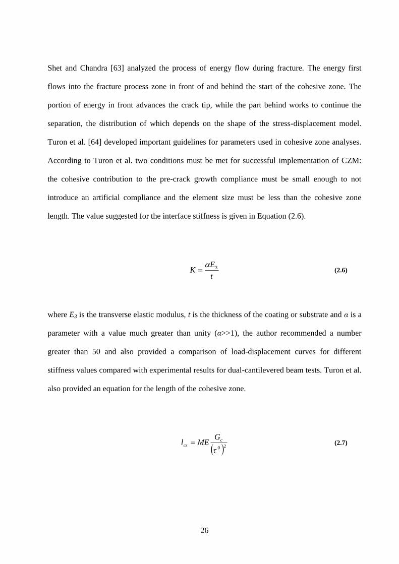
26
Shet and Chandra [63] analyzed the process of energy flow during fracture. The energy first
flows into the fracture process zone in front of and behind the start of the cohesive zone. The
portion of energy in front advances the crack tip, while the part behind works to continue the
separation, the distribution of which depends on the shape of the stress-displacement model.
Turon et al. [64] developed important guidelines for parameters used in cohesive zone analyses.
According to Turon et al. two conditions must be met for successful implementation of CZM:
the cohesive contribution to the pre-crack growth compliance must be small enough to not
introduce an artificial compliance and the element size must be less than the cohesive zone
length. The value suggested for the interface stiffness is given in Equation (2.6).
t
EK 3 (2.6)
where E3 is the transverse elastic modulus, t is the thickness of the coating or substrate and α is a
parameter with a value much greater than unity (α>>1), the author recommended a number
greater than 50 and also provided a comparison of load-displacement curves for different
stiffness values compared with experimental results for dual-cantilevered beam tests. Turon et al.
also provided an equation for the length of the cohesive zone.
20
c
cz
GMEl (2.7)
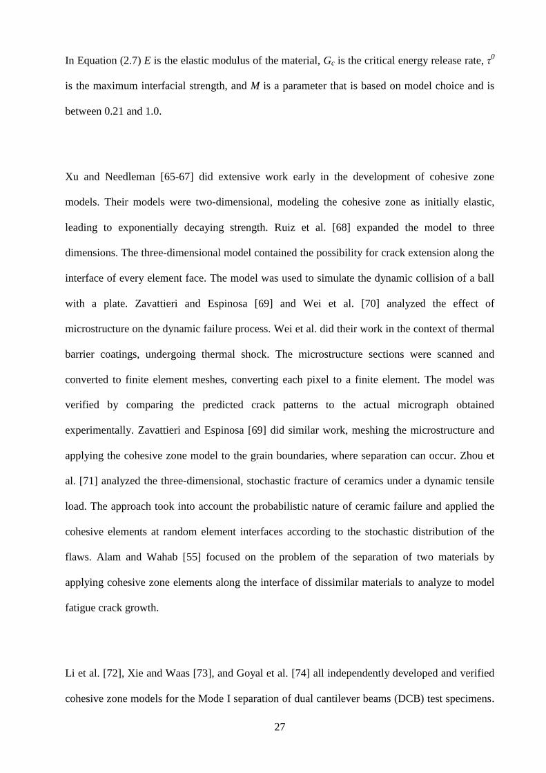
27
In Equation (2.7) E is the elastic modulus of the material, Gc is the critical energy release rate, τ0
is the maximum interfacial strength, and M is a parameter that is based on model choice and is
between 0.21 and 1.0.
Xu and Needleman [65-67] did extensive work early in the development of cohesive zone
models. Their models were two-dimensional, modeling the cohesive zone as initially elastic,
leading to exponentially decaying strength. Ruiz et al. [68] expanded the model to three
dimensions. The three-dimensional model contained the possibility for crack extension along the
interface of every element face. The model was used to simulate the dynamic collision of a ball
with a plate. Zavattieri and Espinosa [69] and Wei et al. [70] analyzed the effect of
microstructure on the dynamic failure process. Wei et al. did their work in the context of thermal
barrier coatings, undergoing thermal shock. The microstructure sections were scanned and
converted to finite element meshes, converting each pixel to a finite element. The model was
verified by comparing the predicted crack patterns to the actual micrograph obtained
experimentally. Zavattieri and Espinosa [69] did similar work, meshing the microstructure and
applying the cohesive zone model to the grain boundaries, where separation can occur. Zhou et
al. [71] analyzed the three-dimensional, stochastic fracture of ceramics under a dynamic tensile
load. The approach took into account the probabilistic nature of ceramic failure and applied the
cohesive elements at random element interfaces according to the stochastic distribution of the
flaws. Alam and Wahab [55] focused on the problem of the separation of two materials by
applying cohesive zone elements along the interface of dissimilar materials to analyze to model
fatigue crack growth.
Li et al. [72], Xie and Waas [73], and Goyal et al. [74] all independently developed and verified
cohesive zone models for the Mode I separation of dual cantilever beams (DCB) test specimens.
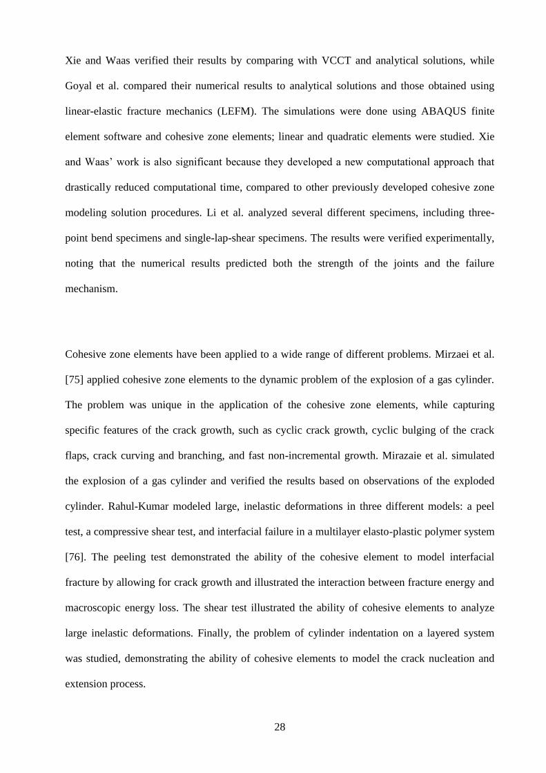
28
Xie and Waas verified their results by comparing with VCCT and analytical solutions, while
Goyal et al. compared their numerical results to analytical solutions and those obtained using
linear-elastic fracture mechanics (LEFM). The simulations were done using ABAQUS finite
element software and cohesive zone elements; linear and quadratic elements were studied. Xie
and Waas’ work is also significant because they developed a new computational approach that
drastically reduced computational time, compared to other previously developed cohesive zone
modeling solution procedures. Li et al. analyzed several different specimens, including three-
point bend specimens and single-lap-shear specimens. The results were verified experimentally,
noting that the numerical results predicted both the strength of the joints and the failure
mechanism.
Cohesive zone elements have been applied to a wide range of different problems. Mirzaei et al.
[75] applied cohesive zone elements to the dynamic problem of the explosion of a gas cylinder.
The problem was unique in the application of the cohesive zone elements, while capturing
specific features of the crack growth, such as cyclic crack growth, cyclic bulging of the crack
flaps, crack curving and branching, and fast non-incremental growth. Mirazaie et al. simulated
the explosion of a gas cylinder and verified the results based on observations of the exploded
cylinder. Rahul-Kumar modeled large, inelastic deformations in three different models: a peel
test, a compressive shear test, and interfacial failure in a multilayer elasto-plastic polymer system
[76]. The peeling test demonstrated the ability of the cohesive element to model interfacial
fracture by allowing for crack growth and illustrated the interaction between fracture energy and
macroscopic energy loss. The shear test illustrated the ability of cohesive elements to analyze
large inelastic deformations. Finally, the problem of cylinder indentation on a layered system
was studied, demonstrating the ability of cohesive elements to model the crack nucleation and
extension process.

29
Siegmund and Brocks simulated the ductile fracture of metals using a cohesive zone model by
adapting it to the mechanical behavior of voided cells [77]. The cohesive zone parameters are
triaxially dependent, which is achieved by a coupling of the cohesive elements to the adjacent
solid elements. The authors developed a global toughness measure that included the
contributions of global plasticity and local separation. The crack growth resistance allows for
local and global contributions of crack growth resistance, the effect of the specimen size and
geometry and the local stress triaxiality influences local quantities.
Xie et al. compared two different approaches: a progressive failure analysis (PFA) with complete
and partial bond void representation and the virtual crack closure technique with complete and
partial bonding [78]. Continuous and discrete cohesive zone models were compared and
determined to be equivalent, though discrete elements are more convenient for reasons of
convergence and gap dimension restrictions. By the continuum cohesive zone model (CCZM),
the region ahead of the process zone ahead of the crack tip is treated as a continuous compliant
layer, whereas in the discrete cohesive zone model (DCZM), elements are treated as point wise.
If proper contact surface information can be evaluated, PFA and VCCT can both be used to
simulate debonding. In a separate work, Xie et al. used a Fernlund-Spelt (FS) test structure to
evaluate coupon level mixed mode fracture tests and use the bond properties to model full size
hat stiffened adhesively bonded structures using the VCCT.
Secchi et al. verified a thermal mechanical interface crack numerical model experimentally [79].
A crack was modeled without a pre-determined crack path. The unknown nature of crack growth
direction was accomidated by successive remeshing of the geometry based on fracture evolution
using a posteriori refinement technique. Fagerstrom and Larsson also developed a cohesive zone
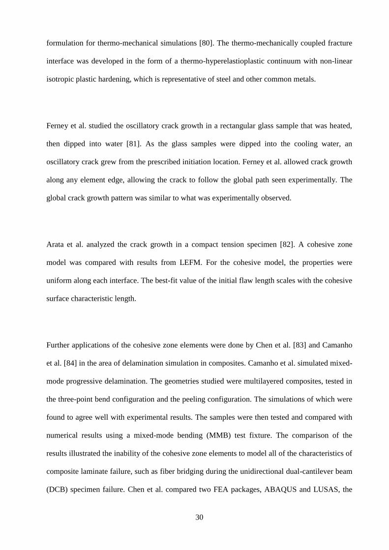
30
formulation for thermo-mechanical simulations [80]. The thermo-mechanically coupled fracture
interface was developed in the form of a thermo-hyperelastioplastic continuum with non-linear
isotropic plastic hardening, which is representative of steel and other common metals.
Ferney et al. studied the oscillatory crack growth in a rectangular glass sample that was heated,
then dipped into water [81]. As the glass samples were dipped into the cooling water, an
oscillatory crack grew from the prescribed initiation location. Ferney et al. allowed crack growth
along any element edge, allowing the crack to follow the global path seen experimentally. The
global crack growth pattern was similar to what was experimentally observed.
Arata et al. analyzed the crack growth in a compact tension specimen [82]. A cohesive zone
model was compared with results from LEFM. For the cohesive model, the properties were
uniform along each interface. The best-fit value of the initial flaw length scales with the cohesive
surface characteristic length.
Further applications of the cohesive zone elements were done by Chen et al. [83] and Camanho
et al. [84] in the area of delamination simulation in composites. Camanho et al. simulated mixed-
mode progressive delamination. The geometries studied were multilayered composites, tested in
the three-point bend configuration and the peeling configuration. The simulations of which were
found to agree well with experimental results. The samples were then tested and compared with
numerical results using a mixed-mode bending (MMB) test fixture. The comparison of the
results illustrated the inability of the cohesive zone elements to model all of the characteristics of
composite laminate failure, such as fiber bridging during the unidirectional dual-cantilever beam
(DCB) specimen failure. Chen et al. compared two FEA packages, ABAQUS and LUSAS, the
31
former with a user-defined subroutine for the cohesive zone model. Both numerical approaches
agreed well with experimental and analytical results for dual-cantilever beam and end-loading
split tests and simulations.
Recently, researchers have been studying the problem of interface failure of coated solids under
contact loading [85-87]. Xia et al. characterized the bilinear cohesive law by its strength in
normal and shear and fracture toughness, which was assumed to be the same for all fracture
modes [85]. The authors noted both shear and normal cracks and used the model to investigate
the effects of different parameters such as coating thickness and material properties on the force
and depth needed to separate the coating from the substrate. Abdul-Baqi and Van der Giessen
similarly investigated the delamination of a hard film on a soft substrate during indentation [86,
87]. The authors applied an exponential form of the cohesive law and analyzed the
nondimensional effects of geometry, material, interface and loading parameters on delamination.
An important conclusion of the work of Abdul-Baqi and Van der Giessen was their analysis of
the indentation test to estimate the work of interfacial debonding from the maximum indentation
depth and the final delamination radius [86]. The test method to determine the work of interfacial
debonding was done by Hainsworth et al [88]. Based on fracture mechanics, the authors were
able to develop an equation for the critical fracture energy in Equation (2.8).
4
23
3
2
r
EtGc
(2.8)
In Equation (2.8) E is the elastic modulus of the coating, t is the coating thickness Δδ is (δmax-
δres) which can be determined from the nanoindentation curve, and r is the radius of the coating
debonding. The authors noted the importance of having a better method to more accurately
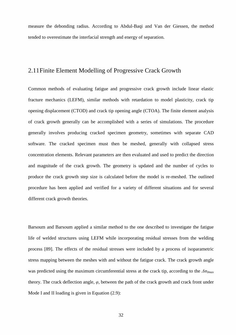
32
measure the debonding radius. According to Abdul-Baqi and Van der Giessen, the method
tended to overestimate the interfacial strength and energy of separation.
2.11 Finite Element Modelling of Progressive Crack Growth
Common methods of evaluating fatigue and progressive crack growth include linear elastic
fracture mechanics (LEFM), similar methods with retardation to model plasticity, crack tip
opening displacement (CTOD) and crack tip opening angle (CTOA). The finite element analysis
of crack growth generally can be accomplished with a series of simulations. The procedure
generally involves producing cracked specimen geometry, sometimes with separate CAD
software. The cracked specimen must then be meshed, generally with collapsed stress
concentration elements. Relevant parameters are then evaluated and used to predict the direction
and magnitude of the crack growth. The geometry is updated and the number of cycles to
produce the crack growth step size is calculated before the model is re-meshed. The outlined
procedure has been applied and verified for a variety of different situations and for several
different crack growth theories.
Barsoum and Barsoum applied a similar method to the one described to investigate the fatigue
life of welded structures using LEFM while incorporating residual stresses from the welding
process [89]. The effects of the residual stresses were included by a process of isoparametric
stress mapping between the meshes with and without the fatigue crack. The crack growth angle
was predicted using the maximum circumferential stress at the crack tip, according to the Δσ0max
theory. The crack deflection angle, φ, between the path of the crack growth and crack front under
Mode I and II loading is given in Equation (2.9):
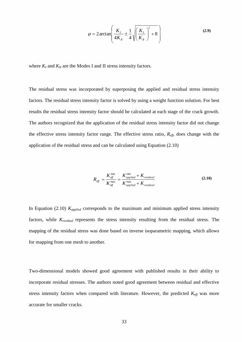
33
8
4
1
4arctan2
2
II
I
II
I
K
K
K
K
(2.9)
where KI and KII are the Modes I and II stress intensity factors.
The residual stress was incorporated by superposing the applied and residual stress intensity
factors. The residual stress intensity factor is solved by using a weight function solution. For best
results the residual stress intensity factor should be calculated at each stage of the crack growth.
The authors recognized that the application of the residual stress intensity factor did not change
the effective stress intensity factor range. The effective stress ratio, Reff, does change with the
application of the residual stress and can be calculated using Equation (2.10)
residualapplied
residualapplied
eff
eff
effKK
KK
K
KR
max
min
max
min
(2.10)
In Equation (2.10) Kapplied corresponds to the maximum and minimum applied stress intensity
factors, while Kresidual represents the stress intensity resulting from the residual stress. The
mapping of the residual stress was done based on inverse isoparametric mapping, which allows
for mapping from one mesh to another.
Two-dimensional models showed good agreement with published results in their ability to
incorporate residual stresses. The authors noted good agreement between residual and effective
stress intensity factors when compared with literature. However, the predicted Keff was more
accurate for smaller cracks.
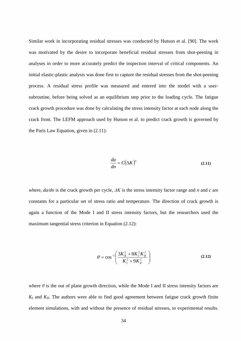
34
Similar work in incorporating residual stresses was conducted by Hutson et al. [90]. The work
was motivated by the desire to incorporate beneficial residual stresses from shot-peening in
analyses in order to more accurately predict the inspection interval of critical components. An
initial elastic-plastic analysis was done first to capture the residual stresses from the shot-peening
process. A residual stress profile was measured and entered into the model with a user-
subroutine, before being solved as an equilibrium step prior to the loading cycle. The fatigue
crack growth procedure was done by calculating the stress intensity factor at each node along the
crack front. The LEFM approach used by Hutson et al. to predict crack growth is governed by
the Paris Law Equation, given in (2.11):
n
KCdn
da (2.11)
where, da/dn is the crack growth per cycle, ΔK is the stress intensity factor range and n and c are
constants for a particular set of stress ratio and temperature. The direction of crack growth is
again a function of the Mode I and II stress intensity factors, but the researchers used the
maximum tangential stress criterion in Equation (2.12):
22
2221
9
83cos
III
IIIII
KK
KKK (2.12)
where θ is the out of plane growth direction, while the Mode I and II stress intensity factors are
KI and KII. The authors were able to find good agreement between fatigue crack growth finite
element simulations, with and without the presence of residual stresses, to experimental results.
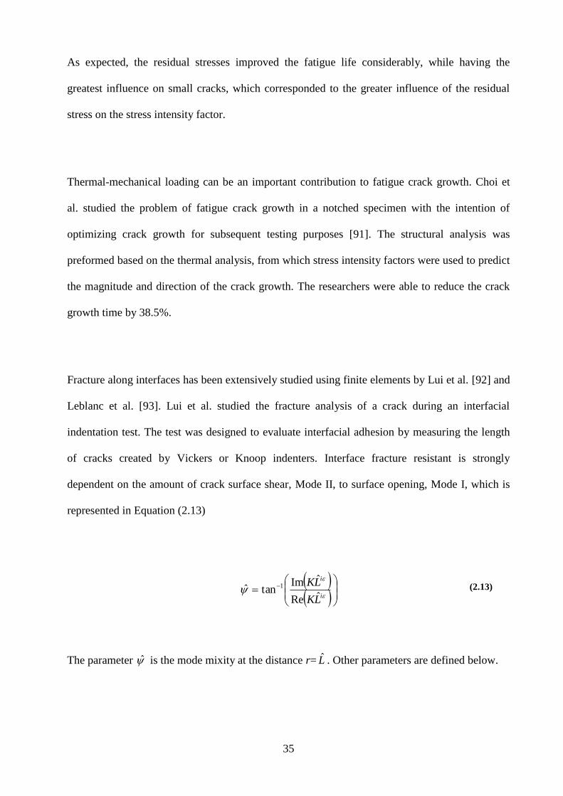
35
As expected, the residual stresses improved the fatigue life considerably, while having the
greatest influence on small cracks, which corresponded to the greater influence of the residual
stress on the stress intensity factor.
Thermal-mechanical loading can be an important contribution to fatigue crack growth. Choi et
al. studied the problem of fatigue crack growth in a notched specimen with the intention of
optimizing crack growth for subsequent testing purposes [91]. The structural analysis was
preformed based on the thermal analysis, from which stress intensity factors were used to predict
the magnitude and direction of the crack growth. The researchers were able to reduce the crack
growth time by 38.5%.
Fracture along interfaces has been extensively studied using finite elements by Lui et al. [92] and
Leblanc et al. [93]. Lui et al. studied the fracture analysis of a crack during an interfacial
indentation test. The test was designed to evaluate interfacial adhesion by measuring the length
of cracks created by Vickers or Knoop indenters. Interface fracture resistant is strongly
dependent on the amount of crack surface shear, Mode II, to surface opening, Mode I, which is
represented in Equation (2.13)
i
i
LK
LK
ˆRe
ˆImtanˆ 1
(2.13)
The parameter ̂ is the mode mixity at the distance r= L̂ . Other parameters are defined below.
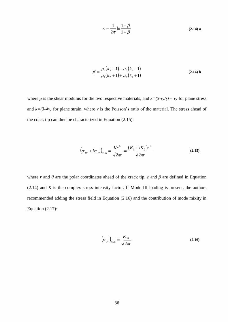
36
1
1ln
2
1 (2.14) a
11
11
1221
1221
kk
kk
(2.14) b
where μ is the shear modulus for the two respective materials, and k=(3-ν)/(1+ ν) for plane stress
and k=(3-4ν) for plane strain, where ν is the Poisson’s ratio of the material. The stress ahead of
the crack tip can then be characterized in Equation (2.15):
r
riKK
r
Kri
ii
xyyy
22
21
0
(2.15)
where r and θ are the polar coordinates ahead of the crack tip, ε and β are defined in Equation
(2.14) and K is the complex stress intensity factor. If Mode III loading is present, the authors
recommended adding the stress field in Equation (2.16) and the contribution of mode mixity in
Equation (2.17):
r
K IIIyz
2
0
(2.16)
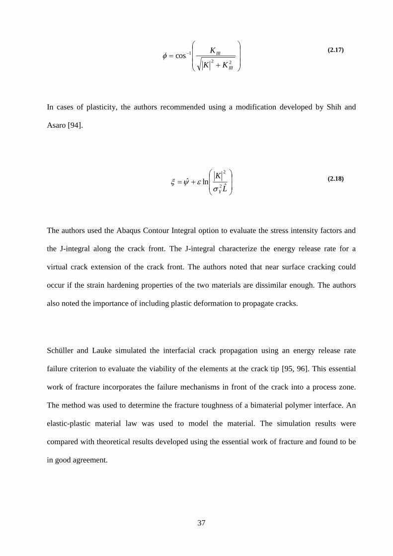
37
22
1cos
III
III
KK
K
(2.17)
In cases of plasticity, the authors recommended using a modification developed by Shih and
Asaro [94].
L
K
Yˆ
lnˆ2
2
(2.18)
The authors used the Abaqus Contour Integral option to evaluate the stress intensity factors and
the J-integral along the crack front. The J-integral characterize the energy release rate for a
virtual crack extension of the crack front. The authors noted that near surface cracking could
occur if the strain hardening properties of the two materials are dissimilar enough. The authors
also noted the importance of including plastic deformation to propagate cracks.
Schüller and Lauke simulated the interfacial crack propagation using an energy release rate
failure criterion to evaluate the viability of the elements at the crack tip [95, 96]. This essential
work of fracture incorporates the failure mechanisms in front of the crack into a process zone.
The method was used to determine the fracture toughness of a bimaterial polymer interface. An
elastic-plastic material law was used to model the material. The simulation results were
compared with theoretical results developed using the essential work of fracture and found to be
in good agreement.
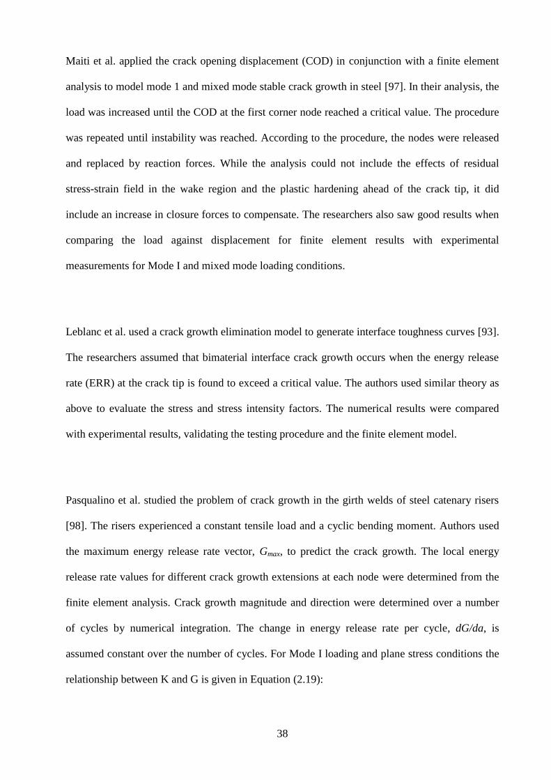
38
Maiti et al. applied the crack opening displacement (COD) in conjunction with a finite element
analysis to model mode 1 and mixed mode stable crack growth in steel [97]. In their analysis, the
load was increased until the COD at the first corner node reached a critical value. The procedure
was repeated until instability was reached. According to the procedure, the nodes were released
and replaced by reaction forces. While the analysis could not include the effects of residual
stress-strain field in the wake region and the plastic hardening ahead of the crack tip, it did
include an increase in closure forces to compensate. The researchers also saw good results when
comparing the load against displacement for finite element results with experimental
measurements for Mode I and mixed mode loading conditions.
Leblanc et al. used a crack growth elimination model to generate interface toughness curves [93].
The researchers assumed that bimaterial interface crack growth occurs when the energy release
rate (ERR) at the crack tip is found to exceed a critical value. The authors used similar theory as
above to evaluate the stress and stress intensity factors. The numerical results were compared
with experimental results, validating the testing procedure and the finite element model.
Pasqualino et al. studied the problem of crack growth in the girth welds of steel catenary risers
[98]. The risers experienced a constant tensile load and a cyclic bending moment. Authors used
the maximum energy release rate vector, Gmax, to predict the crack growth. The local energy
release rate values for different crack growth extensions at each node were determined from the
finite element analysis. Crack growth magnitude and direction were determined over a number
of cycles by numerical integration. The change in energy release rate per cycle, dG/da, is
assumed constant over the number of cycles. For Mode I loading and plane stress conditions the
relationship between K and G is given in Equation (2.19):

39
2/1
21
EGK (2.19)
The authors found that the addition of plastic strains did not have significant effects on the
fatigue life of the weld because the strains were insignificant when compared to the plastic
strains at the crack tip. Significant fatigue life reductions were seen when the non-time-
dependent tensile force was increased.
2.12 Evaluating Cohesive Zone Properties
The evaluation of the cohesive zone properties for an interface is not a trivial problem. Universal
standards or procedures for measuring the properties do not exist. Most often the properties are
evaluated using a combination of experiments and numerical modeling, although analytical
solutions have been developed for select cases. The properties generally used to define the
cohesive zone are critical fracture energy and maximum stress for each of the fracture modes
considered. Most researchers have discovered that the actual shape of the cohesive zone is
insignificant, while the stiffness is most often used as a tuning parameter or approximated based
on geometry and material properties.
The critical fracture energy is recognized as an experimentally measureable parameter. However,
significant issues exist in terms of experimentally measuring the strength of an interface. As
strength is used to characterize an interface, it generally refers to a critical uniform stress, in
tension or shear, required to produce interfacial failure. The problem with this approach is that
interface failure frequently initiates at a flaw or the region of high stress due to factors such as
stress concentrations, resulting in fast fracture along the interface. Such test are notorious for
40
producing large amounts of scatter, as the apparent strength of the interface is a strong function
of flaws, specimen preparation, and testing procedures. Recognizing such limitations for
interfacial strength measurement, researchers often use the normal and shear cohesive strength
parameters as tuning parameters in a finite element model. In such an approach, Mode I and II
fracture energies are first measured and input to the model, while the normal and shear cohesive
strengths are adjusted to reproduce experimental results with the numerical model. Such an
approaches has been used by Yang et al. [58, 99] and Omiya [100], while a similar inverse
approach has been used by Bocciarelli and Bolzon [101, 102].
2.12.1 Mode I: The Wedge-Peel and Peel Tests
Two common methods to evaluate the Mode I fracture properties of adhesives and interfaces are
the wedge test and the peel test. The wedge-peel test is generally used to evaluate the interface
properties for which the adherents are the same material and thickness. Alternatively, the peel
test is used to evaluate the adhesion of thin films or coatings, which are pulled from the interface
at different angles.
The wedge test evaluates the properties of the interface by forcing a wedge between the
interfaces of two similar adherents. The wedge-peel test requires the presence of bending-
induced plastic deformation to evaluate the cohesive zone parameters. Kim and Kim [103] and
Kim and Aravas [104] developed a relation between material properties and test parameters that
were required for valid results:
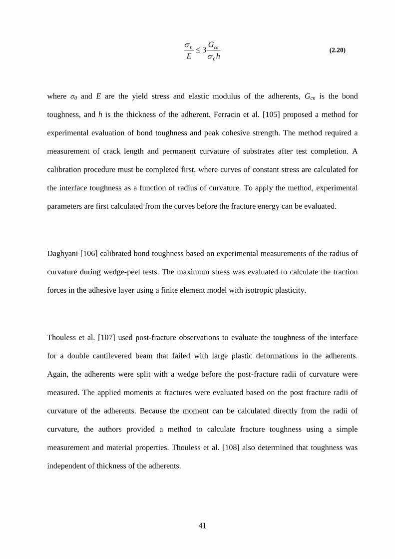
41
h
G
E
cn
0
0 3
(2.20)
where σ0 and E are the yield stress and elastic modulus of the adherents, Gcn is the bond
toughness, and h is the thickness of the adherent. Ferracin et al. [105] proposed a method for
experimental evaluation of bond toughness and peak cohesive strength. The method required a
measurement of crack length and permanent curvature of substrates after test completion. A
calibration procedure must be completed first, where curves of constant stress are calculated for
the interface toughness as a function of radius of curvature. To apply the method, experimental
parameters are first calculated from the curves before the fracture energy can be evaluated.
Daghyani [106] calibrated bond toughness based on experimental measurements of the radius of
curvature during wedge-peel tests. The maximum stress was evaluated to calculate the traction
forces in the adhesive layer using a finite element model with isotropic plasticity.
Thouless et al. [107] used post-fracture observations to evaluate the toughness of the interface
for a double cantilevered beam that failed with large plastic deformations in the adherents.
Again, the adherents were split with a wedge before the post-fracture radii of curvature were
measured. The applied moments at fractures were evaluated based on the post fracture radii of
curvature of the adherents. Because the moment can be calculated directly from the radii of
curvature, the authors provided a method to calculate fracture toughness using a simple
measurement and material properties. Thouless et al. [108] also determined that toughness was
independent of thickness of the adherents.

42
The peel test has the advantage, compared to the wedge test, of being able to evaluate interface
properties for thin coatings. Kinloch et al. [109] developed a method to measure adhesive
toughness for the peel test that included the effects of energy absorption and deformation in the
coating, or peeling arm. The peeling arm was treated as a beam that allowed rotation at the crack
front and expressions were provided to calculate the fracture toughness for different conditions
of plasticity. The authors found that interface toughness was not a factor of material properties,
but was affected by the rate of propagation of the peel front.
Kim and Aravas [104] used an energy balance to relate peel force to fracture energy, assuming
beam theory and that the coating is an elasto-plastic beam under plane strain. For elastic peeling,
it was found that peel force is a direct function of interface fracture energy. Including elasto-
plastic effects requires that the work consumed by plasticity be subtracted from the peel force per
unit thickness of adherent. Kim and Kim [103] considered the different stages in crack growth in
terms of plasticity and compared experimental and theoretical results, while providing a closed
form solution for peel strength contributions from decohesion and bending. A diagram was
constructed that allowed for the determination of interface toughness from peel tests for elastic
perfectly plastic coatings.
2.12.2 Mode II: The Dual-Cantilevered Beam and End-Notched Flexure Tests
The end-notched flexure (ENF) specimen is commonly used to measure Mode II fracture
properties of an adhesive that joins two beams. Before the test, a crack is started on the edge of
the specimen. After which, the specimen is loaded into a three-point bend configuration to grow
the crack. In the event that stable crack growth occurs before the crack reaches the center of the
beam, the loading geometry provides an ideal experiment for studying Mode II fracture. The test
43
has already been used to analyze fracture using LEFM concepts by Chai [110]. Yang et al. [99]
expanded the concept to include extensive plastic deformation accompanying failure.
Experimental and numerical results were compared to evaluate the cohesive zone properties.
First the shear strength of the interface was measured using a butt joint experiment. After the
shear strength was evaluated, a finite element model was developed with cohesive zone elements
at the interface. Experimental results were compared with numerical simulations in order to
select the interface fracture toughness that reproduced the experimental results with the
numerical model. Once the interface properties were evaluated, they were used to predict the
response of ENF samples with beams of different thicknesses and found to produce results that
matched experiments.
2.12.3 The Shear Button Test
The shear button test has been used to measure both fracture toughness and normal and shear
strength of bi-material interfaces. Samples are produced by manufacturing an island or button of
coating on the substrate. A displacement is applied perpendicular to the button until the island
separates from the substrate; the applied load as a function of displacement is measured
throughout the test.
Interfacial adhesion button tests have been used by many authors to evaluate the bond strength
[111-114] and fracture energy [111, 115]. Szeto et al. [114] used experimental results in
conjunction with a finite element model to evaluate the normal and shear strength of an interface.
Two different tests were conducted; one test where the displacement was applied at the bottom
of the button, closer to the interface, and another at the top. After the test was simulated
44
numerically, a stress averaging method was used to avoid the stress singularity and measure the
normal and shear strength.
Tay et al. [111] developed a modified shear button test to measure the fracture toughness of a
bimaterial interface. The researchers started a pre-crack for the button and continued the rest of
the test following the same procedure as a conventional shear button test. A finite element model
was used to evaluate the stress intensity factors for Mode I and II loading at the crack tip. The
relationship between the stress intensity factors and fracture energy release rate developed by
Hutchinson and Suo [116] was used to determine the fracture toughness. The energy release rate
could then be decomposed using the phase angle.
2.12.4 Mixed Mode Tests
Researchers have attempted to use a single test method to measure the critical fracture energies
of different modes. By using the same method to measure properties of both modes, the
properties can be measured with a single test, and will be consistent between the different modes.
A common test to determine the fracture energy as a function of the combined modes is the peel
test. The angle between the force applied to the coating and the substrate can be varied between
0° and 180° in order to introduce varying contributions from each mode into the fracture. At the
extremes, pure Mode I or II fracture occurs.
Kinloch et al. [109] discussed the effects of mode mixity on the fracture toughness and neglected
the effects. The conclusion was justified since the peel angles were not near the extremes and the
45
authors suspected that there would be little difference between the Mode I and II fracture
toughness values.
The peel test was used by Karbhari et al. [117-119] to analyze the contributions of the different
fracture modes and the Mode I and II fracture toughness values. The researchers analyzed
different composites bonded to concrete. The authors assumed that the bond failure occurred at a
controlled rate, the peel force was directly related to the work of detachment and failure occurred
due to mixed mode loading. In order to include the effects of both modes, the authors first
recognized that the interfacial fracture energy can be decomposed as follows:
III GGG (2.21)
where G is the total fracture energy and GI and GII are the contributions from each mode.
Further, a measure of the contributions of each Mode is defined by the phase angle, given in
Equation (2.22).
I
II
G
G2tan (2.22)
where ψ is the phase angle of the loading, defined by Equation (2.23)
sin1
cos11tan 1
(2.23)
46
where ε is the strain in the peel arm and α is the angle between the substrate and the force that
the coating is peeled at. The authors measured the fracture energy for different peel angles, α,
and decomposed the fracture energy to the different modes. The critical fracture energies were
then measured by plotting the Mode II fracture energy as a function of mode I fracture energy,
and recognizing that at pure Mode I or II fracture, the other mode’s contribution is zero. A
similar analysis of the peel test was done by Moidu et al. [120]. The main focus of the research
was to characterize the amount of energy dissipated in the coating arm as it was pulled.
2.12.5 Four-Point Bend Test
The four-point bend test is popular because it consistently and accurately evaluates the fracture
energy at a bimaterial interface. Because of the configuration, it is especially useful for coating
applications. Sample preparation is generally straightforward; a crack is first inserted through the
coating thickness at the center, before being extended into both sides of the interface. However,
Ashcroft et al. [121] have completed the test without pre-cracking. The four-point bend test is an
attractive configuration for determining interfacial fracture energy because the fracture energy is
a simple function of experimental parameters, load and displacement, and material and specimen
parameters. Though the experiment is relatively straightforward, several factors such as plastic
deformation and brittle crack growth limit the applicability of the method.
The four-point bend test geometry is shown in Figure 2.1. A precrack is first inserted into the
coating, generally using a diamond-coated saw blade. Researchers generally introduce the
interface precrack by loading the sample in a three- or four-point bend configuration. The effect
of the precrack length has been analyzed by Clyne and Gill [122], who found that at half-crack
lengths of more than twice the coating thickness, the energy release rate was no longer a function
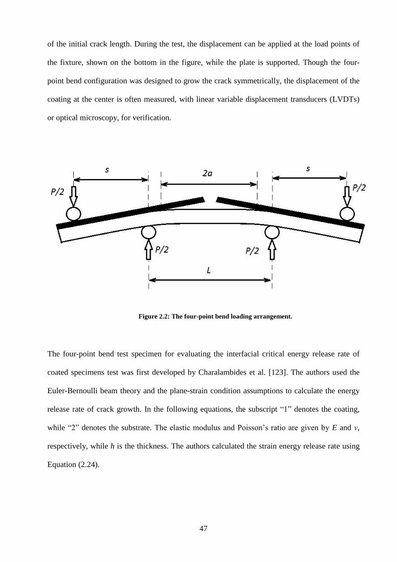
47
of the initial crack length. During the test, the displacement can be applied at the load points of
the fixture, shown on the bottom in the figure, while the plate is supported. Though the four-
point bend configuration was designed to grow the crack symmetrically, the displacement of the
coating at the center is often measured, with linear variable displacement transducers (LVDTs)
or optical microscopy, for verification.
Figure 2.2: The four-point bend loading arrangement.
The four-point bend test specimen for evaluating the interfacial critical energy release rate of
coated specimens test was first developed by Charalambides et al. [123]. The authors used the
Euler-Bernoulli beam theory and the plane-strain condition assumptions to calculate the energy
release rate of crack growth. In the following equations, the subscript “1” denotes the coating,
while “2” denotes the substrate. The elastic modulus and Poisson’s ratio are given by E and ν,
respectively, while h is the thickness. The authors calculated the strain energy release rate using
Equation (2.24).

48
cIIE
MG
22
22 1
2
1 (2.24)
where M=Ps/2b is the bending moment per unit width, where P is the total load, s is defined in
the above figure, and b is the specimen width. Subsequent research [124] included the effects of
friction at the loading points. To account for this, the moment, M, from Equation (2.24) can be
replaced with Equation (2.25).
s
h
b
PsMMM FP
12
(2.25)
where μ is the coefficient of friction between the loading points and the specimen, and h is the
total specimen height. The remaining parameters, λ, Ic, and I2, are defined below.
2
21
2
12
1
1
E
E (2.26)
21
2121
3
2
3
1
41212 hh
hhhhhhI c
(2.27)
12
3
22
hI (2.28)
49
The authors could not obtain unique critical strain energy release rates if the friction term was
neglected. The importance of residual stress effects, if present, was also noted in the research.
Another analysis of the crack propagation for the four-point bend test was provided by Howard
et al. [125] based on the change in compliance of the beam that results from the extension of an
interfacial crack. The strain energy release rate, G, for crack propagation can be calculated
according to Equation (2.29).
da
dC
b
P
a
C
b
PPG a
44
2
21lim
0 (2.29)
where P1 and P2 are the loads at the initiation and termination of the crack, and ∆C is the change
in compliance resulting from the change in half-crack length, ∆a. If one assumes steady crack
growth, the change in compliance with respect to the half-crack length, dC/da, is a constant.
The displacement of the rollers can be related to the load and half-crack length.
46
11
2
22 Ls
K
Ps
KK
Psau
ccs
(2.30)
where s and L are illustrated in Figure 2.2, and Ks and Kc are the stiffness of the debonded and
bonded (composite) beam, respectively. The stiffness or compliance of a beam can be calculated
from the integral shown in Equation (2.31).
50
beam
dAyyEK 2
(2.31)
The distance from the neutral axis is y and E(y) is the elastic modulus as a function of the
distance from the neutral axis. Ks and Kc are given in Equations (2.32) through (2.34).
2
2
2
2
2
2 3131
d
d
d
d
d
s
s
s
s
s
c hh
bhE
hh
bhE
K (2.32)
2
3
112 s
ss
s
bhEK
(2.33)
d
d
ds
s
s
s
s
s
d
d
d
hE
hE
hE
hE
2
2
2
2
2
11
11
2
1
(2.34)
The subscripts for the deposit (coating) and substrate are d and s, respectively. The thicknesses
of the deposit and substrate are given by hd and hs, s is defined in Figure 2.2, b is the sample
width, and the elastic modulus and Poisson’s ratio are E and ν. The distance that the neutral axis
is moved from the center is δ and is defined as positive if it moves from the center in the
direction of the coating.
From Equation (2.30), the compliance can be defined as the rate of change of roller displacement
with respect to the load, as shown in Equation (2.35).
51
46
11
2
22 Ls
K
s
KK
as
dP
duC
cds
(2.35)
From Equation (2.35), the rate of change of compliance with respect to the half-crack length can
then be defined.
ds KK
s
da
dC 11
2
2
(2.36)
Equation (2.37) can then be obtained by combining Equations (2.29) and (2.36) and assuming
symmetric crack growth.
ds KKb
sPG
11
8
22
(2.37)
The criterion for the critical strain energy release rate is then: cGG . In other words the critical
energy release rate is the energy release rate required to grow a previously arrested crack and
corresponds to a critical load, Pc. Howard et al. [125] outlined how to calculate the critical
energy release rate for stable and unstable crack propagation. For the case of crack bursting, the
authors recommended that the P2 be replaced with the crack initiation and termination loads, P1
and P2. After the development of a procedure to measure the fracture energy for the four-point
bend test, the authors also included an analysis of the effects of asymmetry and residual stresses
and recommended using a floating platen to negate the effects of asymmetric crack growth.
52
Finally, the authors developed an additional term for the strain energy release rate to include the
effects of the residual stress.
In subsequent research on the topic, Howard et al. [126] expanded on the research summarized
above. Contributions to the energy release rate for the residual stress were included for the
residual stresses expected in the absence of applied loading and an interaction term that is
dependent on the applied loading and residual stress state. The updated energy release rate is
given in Equation (2.38).
da
du
b
P
da
dC
b
PG r
24
2
(2.38)
where ur is the residual displacement measured after unloading and Ω is the available strain
energy release rate for the unloaded beam. The residual stress terms can then be defined in
Equations (2.39) and (2.40):
cs
r sda
du (2.39)
d
drdd
s
srss
drdsrs
AEAEKK
b
112
122
22 (2.40)
The cross-sectional areas of the deposit and substrate are given by Ad=bhd and As=bhs, s is
defined in Figure 2.2, the elastic modulus and Poisson’s ratio are E and ν, the average axial
strains in the bonded substrate and coating are εs and εd, the unbonded curvature of the substrate
53
is κs, the curvature of the bonded composite beam is κc, while κsr and κdr are the average strain
gradients through the unbonded substrate and deposit. The same approach to account for residual
stress was used by Yamazaki et al. [127].
Based on the experimentally measured curvatures mentioned above, the curvatures before, κc,
and after, κd and κs, debonding can be related to the assumed linear residual stress distribution
according to Clyne and Gill [122].
dcddcdscdd
d yEHhbh
KK
22 (2.41)
scsscdscdd
s yEHhbh
KK
22 (2.42)
where σs and σd are the stresses in the in the substrate and deposit, respectively, while ys and yd
are the distance coordinates from the respective neutral axes for the substrate and deposit.
In addition, the phase angle can be calculated based on the applied moment and the assumed
residual stresses. The moments and forces per unit thickness at the crack tip, while in the
constant moment region between the inner loading lines, were calculated by Howard et al. [128]
for the debonded side of the crack tip in the coating, M1 and F1, and substrate, and the composite
side of the beam, M3 and F3.
54
sd
csscdd
drddhh
AEF
5.0
*
1
(2.43)
03 F (2.44)
cdddrdM 1 (2.45)
b
PsMM app
23 (2.46)
The above moment equations can then be applied to the scheme of Suo and Hutchinson [129] to
determine the phase angle of the fracture during the four-point bend test. The phase angle can
then be calculated according to Equation (2.47).
sincos
cossintan 1
(2.47)
The parameter ω is a function of the Dundars’ parameters, and the ratio of coating and substrate
thicknesses, defined below.
11
11
12
12
(2.48)
55
11
11
12
12
(2.49)
2
1
(2.50)
where μ is the shear modulus, in addition κ=3-4ν for plane strain and κ=(3-ν)/(1+ν) for plane
stress. The subscript 1 signifies the deposit, while the 2 is used for the substrate. The parameters
A, I, angle γ, Σ, and η are defined below.
32 3641
1
A (2.51)
3112
1
I (2.52)
AI 16sin 2
(2.53)
1
1 (2.54)
H
h (2.55)
56
where h is the thickness of the deposit and H is the thickness of the substrate. The load terms,
defined in terms of Equations (2.43) through (2.46), P and M are given by:
h
MCPCPP 3
2311 (2.56)
331 MCMM (2.57)
where,
0
1A
C
(2.58)
2
11
0
2I
C (2.59)
0
312I
C
(2.60)
10A (2.61)
57
3
2
0
1131
13
13
3
1
I
(2.62)
12
21 2
(2.63)
Recognizing that interfacial fracture during the four point bend test is highly mixed mode, the
phase angle is an important component of the critical fracture energy. Equation (2.47) calculates
the phase angle for the four-point bend test as a function of applied loading and includes the
significant effects caused by residual stresses.
Tsui et al. [130] used the above equations to compare model predictions with experimental data.
The authors used Ti-6Al-4V substrates coated with boron carbide by plasma spraying. The
authors first measured the curvatures of the samples, cut a notch through the coating with a
diamond impregnated wire on a slow speed saw, before an interface precrack was introduced.
During four-point bend testing, the load and displacement were continually monitored until the
crack had propagated to the inner load point. The stable or critical crack load was recorded and
used, in addition to the measured curvatures and strains of the debonded coating and substrate, to
calculate the critical energy release rate. Numerically calculated residual stresses, determined
based on finite element modeling of the coating deposition process, matched well with the
distribution based on the curvature and strain measurements. The authors also observed that
significant error would have been introduced had the residual stresses been ignored.
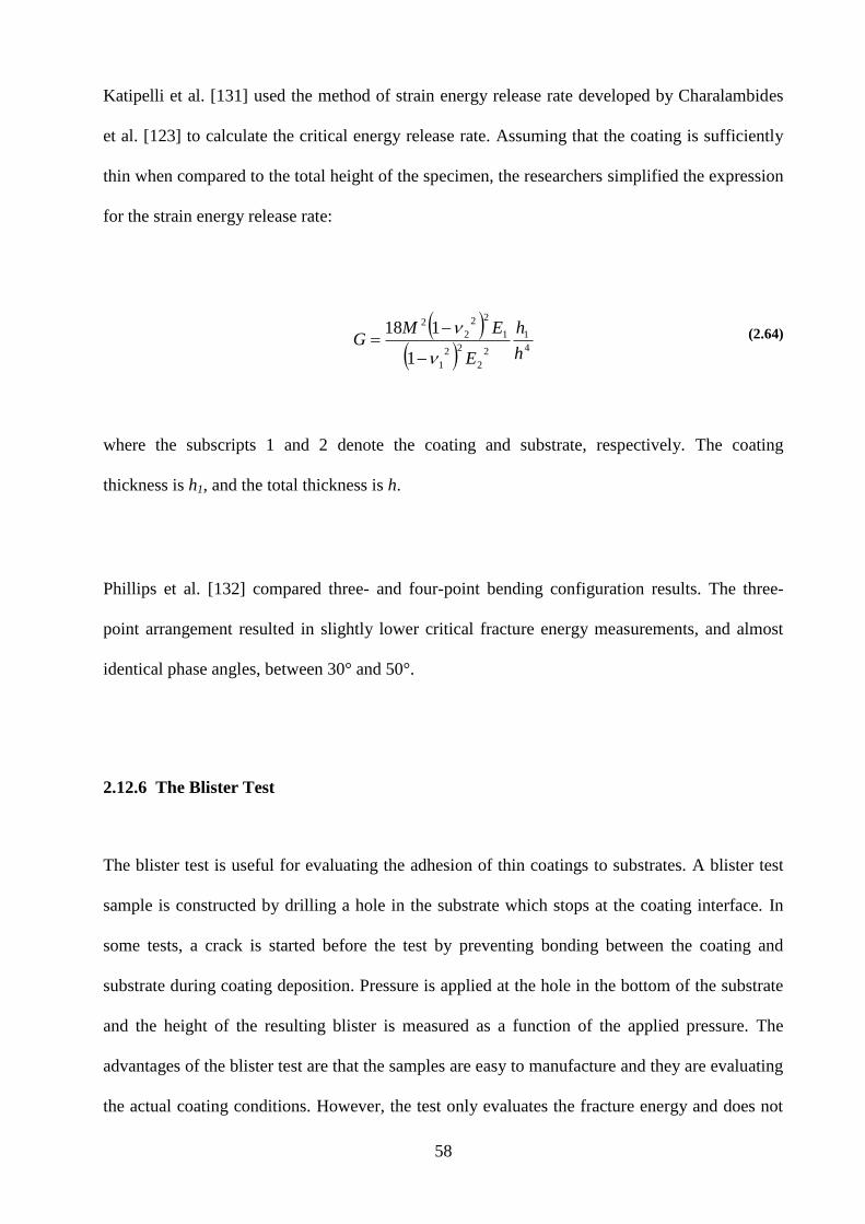
58
Katipelli et al. [131] used the method of strain energy release rate developed by Charalambides
et al. [123] to calculate the critical energy release rate. Assuming that the coating is sufficiently
thin when compared to the total height of the specimen, the researchers simplified the expression
for the strain energy release rate:
4
1
2
2
22
1
1
22
2
2
1
118
h
h
E
EMG
(2.64)
where the subscripts 1 and 2 denote the coating and substrate, respectively. The coating
thickness is h1, and the total thickness is h.
Phillips et al. [132] compared three- and four-point bending configuration results. The three-
point arrangement resulted in slightly lower critical fracture energy measurements, and almost
identical phase angles, between 30° and 50°.
2.12.6 The Blister Test
The blister test is useful for evaluating the adhesion of thin coatings to substrates. A blister test
sample is constructed by drilling a hole in the substrate which stops at the coating interface. In
some tests, a crack is started before the test by preventing bonding between the coating and
substrate during coating deposition. Pressure is applied at the hole in the bottom of the substrate
and the height of the resulting blister is measured as a function of the applied pressure. The
advantages of the blister test are that the samples are easy to manufacture and they are evaluating
the actual coating conditions. However, the test only evaluates the fracture energy and does not
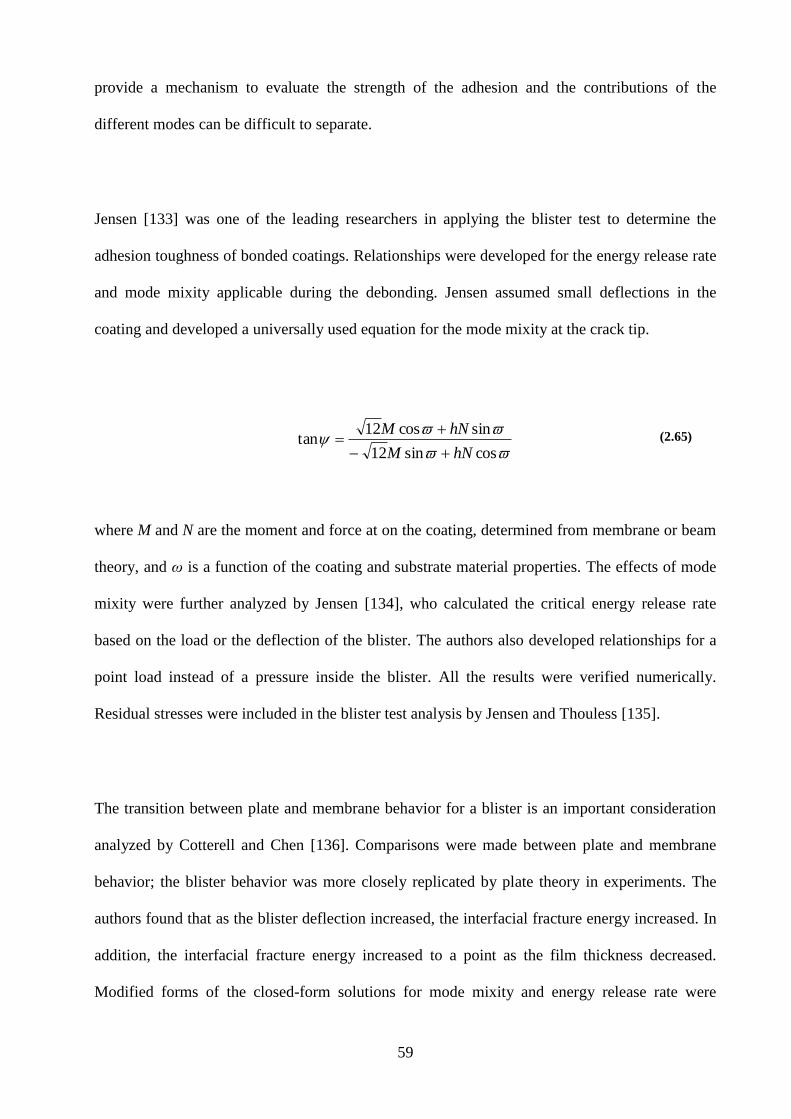
59
provide a mechanism to evaluate the strength of the adhesion and the contributions of the
different modes can be difficult to separate.
Jensen [133] was one of the leading researchers in applying the blister test to determine the
adhesion toughness of bonded coatings. Relationships were developed for the energy release rate
and mode mixity applicable during the debonding. Jensen assumed small deflections in the
coating and developed a universally used equation for the mode mixity at the crack tip.
cossin12
sincos12tan
hNM
hNM
(2.65)
where M and N are the moment and force at on the coating, determined from membrane or beam
theory, and ω is a function of the coating and substrate material properties. The effects of mode
mixity were further analyzed by Jensen [134], who calculated the critical energy release rate
based on the load or the deflection of the blister. The authors also developed relationships for a
point load instead of a pressure inside the blister. All the results were verified numerically.
Residual stresses were included in the blister test analysis by Jensen and Thouless [135].
The transition between plate and membrane behavior for a blister is an important consideration
analyzed by Cotterell and Chen [136]. Comparisons were made between plate and membrane
behavior; the blister behavior was more closely replicated by plate theory in experiments. The
authors found that as the blister deflection increased, the interfacial fracture energy increased. In
addition, the interfacial fracture energy increased to a point as the film thickness decreased.
Modified forms of the closed-form solutions for mode mixity and energy release rate were
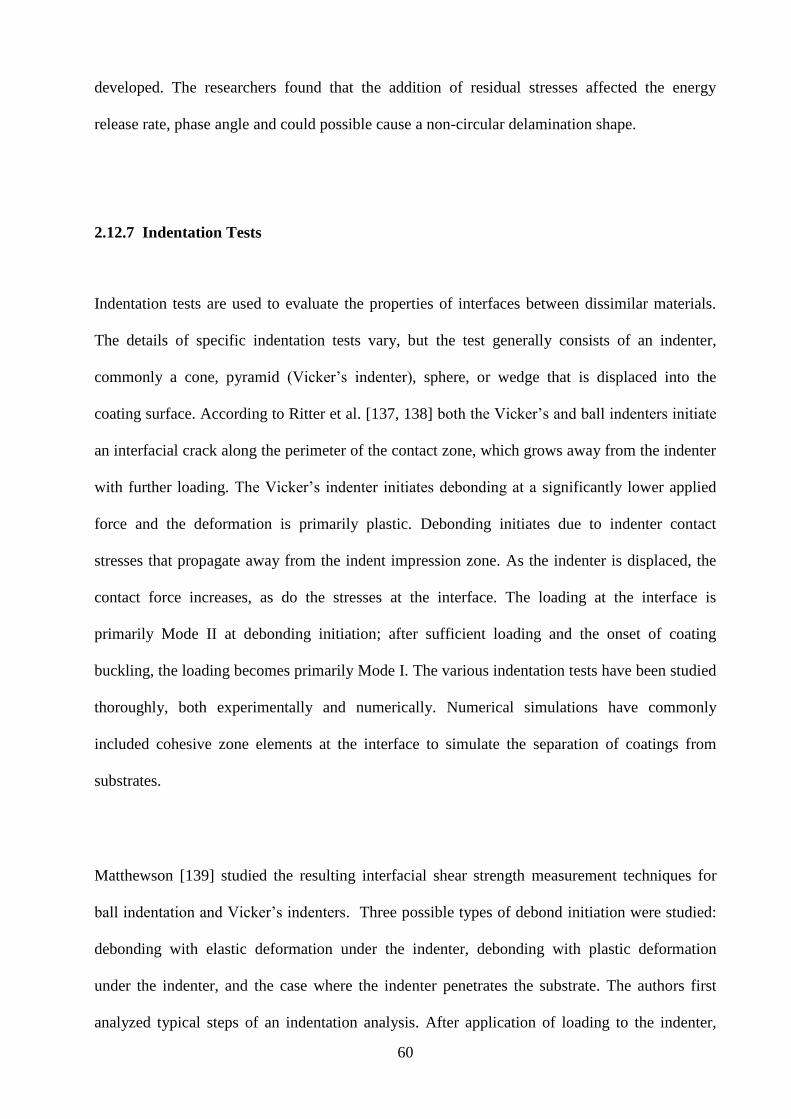
60
developed. The researchers found that the addition of residual stresses affected the energy
release rate, phase angle and could possible cause a non-circular delamination shape.
2.12.7 Indentation Tests
Indentation tests are used to evaluate the properties of interfaces between dissimilar materials.
The details of specific indentation tests vary, but the test generally consists of an indenter,
commonly a cone, pyramid (Vicker’s indenter), sphere, or wedge that is displaced into the
coating surface. According to Ritter et al. [137, 138] both the Vicker’s and ball indenters initiate
an interfacial crack along the perimeter of the contact zone, which grows away from the indenter
with further loading. The Vicker’s indenter initiates debonding at a significantly lower applied
force and the deformation is primarily plastic. Debonding initiates due to indenter contact
stresses that propagate away from the indent impression zone. As the indenter is displaced, the
contact force increases, as do the stresses at the interface. The loading at the interface is
primarily Mode II at debonding initiation; after sufficient loading and the onset of coating
buckling, the loading becomes primarily Mode I. The various indentation tests have been studied
thoroughly, both experimentally and numerically. Numerical simulations have commonly
included cohesive zone elements at the interface to simulate the separation of coatings from
substrates.
Matthewson [139] studied the resulting interfacial shear strength measurement techniques for
ball indentation and Vicker’s indenters. Three possible types of debond initiation were studied:
debonding with elastic deformation under the indenter, debonding with plastic deformation
under the indenter, and the case where the indenter penetrates the substrate. The authors first
analyzed typical steps of an indentation analysis. After application of loading to the indenter,
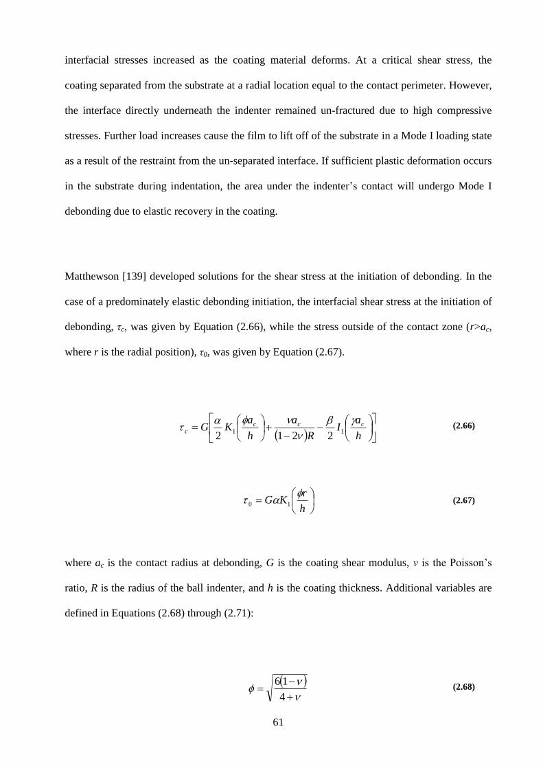
61
interfacial stresses increased as the coating material deforms. At a critical shear stress, the
coating separated from the substrate at a radial location equal to the contact perimeter. However,
the interface directly underneath the indenter remained un-fractured due to high compressive
stresses. Further load increases cause the film to lift off of the substrate in a Mode I loading state
as a result of the restraint from the un-separated interface. If sufficient plastic deformation occurs
in the substrate during indentation, the area under the indenter’s contact will undergo Mode I
debonding due to elastic recovery in the coating.
Matthewson [139] developed solutions for the shear stress at the initiation of debonding. In the
case of a predominately elastic debonding initiation, the interfacial shear stress at the initiation of
debonding, τc, was given by Equation (2.66), while the stress outside of the contact zone (r>ac,
where r is the radial position), τ0, was given by Equation (2.67).
h
aI
R
a
h
aKG ccc
c
11
2212 (2.66)
h
rKG
10 (2.67)
where ac is the contact radius at debonding, G is the coating shear modulus, ν is the Poisson’s
ratio, R is the radius of the ball indenter, and h is the coating thickness. Additional variables are
defined in Equations (2.68) through (2.71):
4
16 (2.68)
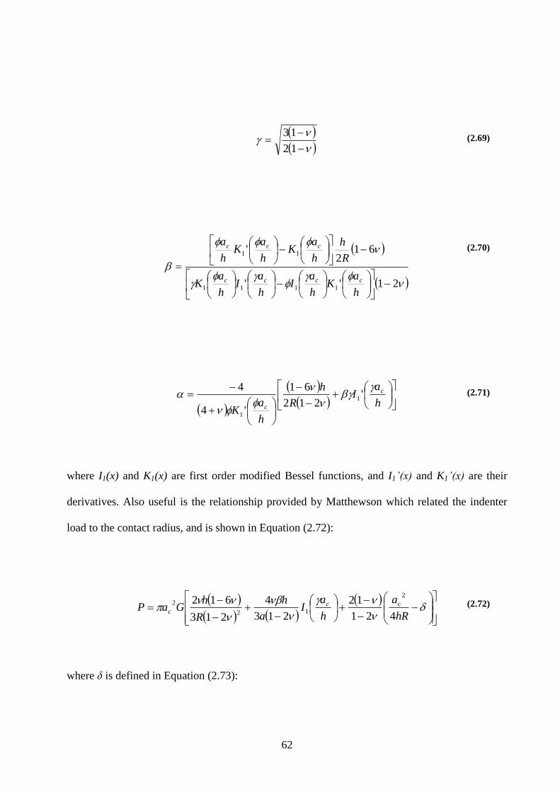
62
12
13 (2.69)
21''
612
'
1111
11
h
aK
h
aI
h
aI
h
aK
R
h
h
aK
h
aK
h
a
cccc
ccc
(2.70)
h
aI
R
h
h
aK
c
c
'212
61
'4
41
1
(2.71)
where I1(x) and K1(x) are first order modified Bessel functions, and I1’(x) and K1’(x) are their
derivatives. Also useful is the relationship provided by Matthewson which related the indenter
load to the contact radius, and is shown in Equation (2.72):
hR
a
h
aI
a
h
R
hGaP cc
c421
12
213
4
213
6122
12
2 (2.72)
where δ is defined in Equation (2.73):
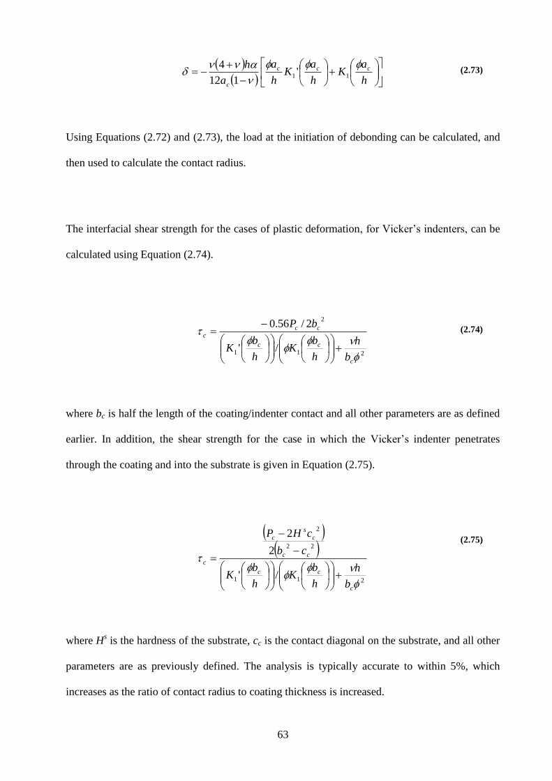
63
h
aK
h
aK
h
a
a
h ccc
c
11 '
112
4 (2.73)
Using Equations (2.72) and (2.73), the load at the initiation of debonding can be calculated, and
then used to calculate the contact radius.
The interfacial shear strength for the cases of plastic deformation, for Vicker’s indenters, can be
calculated using Equation (2.74).
211
2
/'
2/56.0
c
cc
cc
c
b
h
h
bK
h
bK
bP
(2.74)
where bc is half the length of the coating/indenter contact and all other parameters are as defined
earlier. In addition, the shear strength for the case in which the Vicker’s indenter penetrates
through the coating and into the substrate is given in Equation (2.75).
211
22
2
/'
2
2
c
cc
cc
c
s
c
c
b
h
h
bK
h
bK
cb
cHP
(2.75)
where Hs is the hardness of the substrate, cc is the contact diagonal on the substrate, and all other
parameters are as previously defined. The analysis is typically accurate to within 5%, which
increases as the ratio of contact radius to coating thickness is increased.
64
The solutions presented above were also employed by Ritter et al. [137, 138] to study adhesion
of thin polymer coatings on glass. Experimental observations and results were used with the
solutions of Matthewson [139] to analyze interfacial crack growth during indentation [138].
During indentation, a crack was initiated at the perimeter of the contact zone and grew outwards.
The authors noted that the primary difference between Vicker’s and ball indenters was that
debonding initiation for tests with the Vicker’s indenter occurred at a significantly lower load
and the deformation at debonding was primarily plastic.
Good agreement was observed when the experimental and analytical results were compared for
the contact radius as a function of applied load and the interfacial shear strength as a function of
the coating thickness. In a subsequent paper [137], the authors compared shear stresses measured
with indentation tests to those measured using lap-shear tests. The measured indentation
interfacial strengths were over an order of magnitude higher than those measured using the lap
shear test. The authors suspected the discrepancy was a result of the indentation test measuring
the intrinsic interfacial shear strength, while the measured lap shear strength was controlled
primarily by large flaws at the location of the stress concentration.
Sun et al. [140] and Sen et al. [141] have studied indentation of a sphere onto a coated substrate
using finite element simulations. Sun et al. [140] studied the plastic deformation of TiN coatings.
For the system studied, the authors observed plastic deformation in the substrate underneath the
indenter before such deformation was seen in the coating, except for the cases of thick coatings.
Overall, the authors noted that thin coatings on soft substrates experience adhesive and substrate
failure, while thick coatings on strong substrates will experience cohesive failure in the coating.
65
Sen et al. [141] studied the problem of the indentation of an elastic sphere on an bilinear elastic-
plastic substrate with a thin, elastic coating layer that is stiffer than the substrate. Plots were
provided of the stresses on the surface, the stresses along the central axis underneath the indenter
and the stresses along the interface. The authors also reported that the undesirable (for the
purposes of parameter evaluation) interface yielding occurs for thicker layers, while the normal
and shear stresses at the interface decrease as the layer thickness is increased.
Sriram et al. [142] have studied the problem of cracks through the coating during the indentation
process in terms of the energy release rate of the cylindrical cracks. The authors found that
cracks near the indenter experienced stable growth; the energy release rate decreased with crack
length. Additionally, the stable crack growth regime dissipates at radii away from the indenter.
The effects of a rigid indenter versus a deformable indenter were studied by Faulkner et al.
[143]. The authors found that the assumption of a rigid indenter underestimated the radial tensile
stress that is responsible for the film cracking at the interface. In terms of delamination, the rigid
indenter actually proved to provide conservative estimations of the interfacial stress; interfacial
shear stress decreases as the stiffness of the indenter was increased.
Abdul-Baqi et al. studied interface delamination for strong films on ductile substrates [87, 144]
and cracking of brittle coatings on ductile substrates [145] using a cohesive zone to model the
interface, and the crack surfaces in the case of the later study. In the former study, the
indentation induced delamination of an elastic coating on an elastic-perfectly plastic substrate
was simulated. The authors found that delamination occurred in a shear mode, and not a normal
66
one. Debonding initiation was also found to occur at a radial position at two to three times the
contact radius, opposed to the perimeter of the contact radius predicted by the researchers
referenced earlier. Also, in contradiction to the works cited earlier, the authors found that after
debonding was initiated, the crack grew in both directions, and arrested on the inner front when
it reached the highly compressive stress under the indenter. Though, delamination is largely due
to shear stresses associated with plastic substrate plastic deformation, the normal stresses
contribution is significant due to the coupling effect of the stress components assumed by the
researchers. The same authors also analyzed the process of delamination resulting from indenter
unloading [144] with the same basic assumptions as the earlier study. Unloading delamination
was found to be driven by stresses normal to the interface. The bending moment caused the
region directly under the contact area to be lifted off of the substrate. For constant indenter
depth, thicker and stiffer coatings, and substrates with a higher yield strength resulted in larger
interfacial normal stresses. The authors also found that compressive residual stresses delayed
film delamination. Cohesive surfaces were also used to simulate through-coating cracks [145] for
brittle coatings. The initiation of a through coating crack can be easily seen on a kink on the plot
of the load against displacement. The load drop is larger for cracks that initiated at larger radii
because the energy released by a crack is proportional to its surface area. Cracks in the coating
initiate on the surface and almost immediately travels through the coating, stopping before the
interface because of compressive stresses.
Hu et al. [146, 147] studied interface behavior during spherical indentation tests. Unlike other
papers found on the topic, which lacked experimental verification, the authors verified their
finite element model. The authors used parameters from an experimental analysis conducted by
Huang et al. [148] and compared delamination as a function of load and coating thickness. Good
overall trend agreement was observed, though the average relative difference was 170%. Given
the complexity of the system, the authors recognized this as good agreement, citing the work of
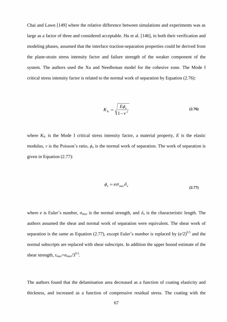
67
Chai and Lawn [149] where the relative difference between simulations and experiments was as
large as a factor of three and considered acceptable. Hu et al. [146], in both their verification and
modeling phases, assumed that the interface traction-separation properties could be derived from
the plane-strain stress intensity factor and failure strength of the weaker component of the
system. The authors used the Xu and Needleman model for the cohesive zone. The Mode I
critical stress intensity factor is related to the normal work of separation by Equation (2.76):
21
n
Ic
EK (2.76)
where KIc is the Mode I critical stress intensity factor, a material property, E is the elastic
modulus, ν is the Poisson’s ratio, ϕn is the normal work of separation. The work of separation is
given in Equation (2.77):
nn e max (2.77)
where e is Euler’s number, σmax is the normal strength, and δn is the characteristic length. The
authors assumed the shear and normal work of separation were equivalent. The shear work of
separation is the same as Equation (2.77), except Euler’s number is replaced by (e/2)0.5
and the
normal subscripts are replaced with shear subscripts. In addition the upper bound estimate of the
shear strength, τmax=σmax/30.5
.
The authors found that the delamination area decreased as a function of coating elasticity and
thickness, and increased as a function of compressive residual stress. The coating with the
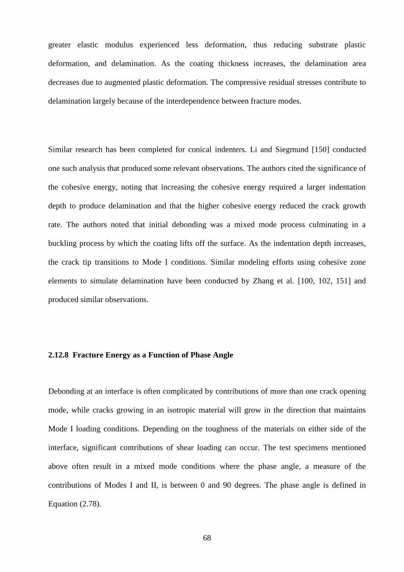
68
greater elastic modulus experienced less deformation, thus reducing substrate plastic
deformation, and delamination. As the coating thickness increases, the delamination area
decreases due to augmented plastic deformation. The compressive residual stresses contribute to
delamination largely because of the interdependence between fracture modes.
Similar research has been completed for conical indenters. Li and Siegmund [150] conducted
one such analysis that produced some relevant observations. The authors cited the significance of
the cohesive energy, noting that increasing the cohesive energy required a larger indentation
depth to produce delamination and that the higher cohesive energy reduced the crack growth
rate. The authors noted that initial debonding was a mixed mode process culminating in a
buckling process by which the coating lifts off the surface. As the indentation depth increases,
the crack tip transitions to Mode I conditions. Similar modeling efforts using cohesive zone
elements to simulate delamination have been conducted by Zhang et al. [100, 102, 151] and
produced similar observations.
2.12.8 Fracture Energy as a Function of Phase Angle
Debonding at an interface is often complicated by contributions of more than one crack opening
mode, while cracks growing in an isotropic material will grow in the direction that maintains
Mode I loading conditions. Depending on the toughness of the materials on either side of the
interface, significant contributions of shear loading can occur. The test specimens mentioned
above often result in a mixed mode conditions where the phase angle, a measure of the
contributions of Modes I and II, is between 0 and 90 degrees. The phase angle is defined in
Equation (2.78).
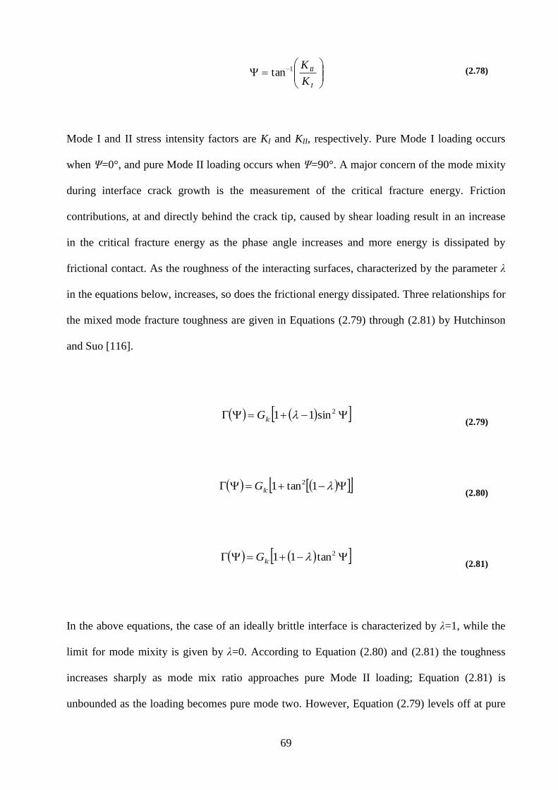
69
I
II
K
K1tan (2.78)
Mode I and II stress intensity factors are KI and KII, respectively. Pure Mode I loading occurs
when Ψ=0°, and pure Mode II loading occurs when Ψ=90°. A major concern of the mode mixity
during interface crack growth is the measurement of the critical fracture energy. Friction
contributions, at and directly behind the crack tip, caused by shear loading result in an increase
in the critical fracture energy as the phase angle increases and more energy is dissipated by
frictional contact. As the roughness of the interacting surfaces, characterized by the parameter λ
in the equations below, increases, so does the frictional energy dissipated. Three relationships for
the mixed mode fracture toughness are given in Equations (2.79) through (2.81) by Hutchinson
and Suo [116].
2sin11 IcG (2.79)
1tan1 2
IcG (2.80)
2tan11 IcG (2.81)
In the above equations, the case of an ideally brittle interface is characterized by λ=1, while the
limit for mode mixity is given by λ=0. According to Equation (2.80) and (2.81) the toughness
increases sharply as mode mix ratio approaches pure Mode II loading; Equation (2.81) is
unbounded as the loading becomes pure mode two. However, Equation (2.79) levels off at pure
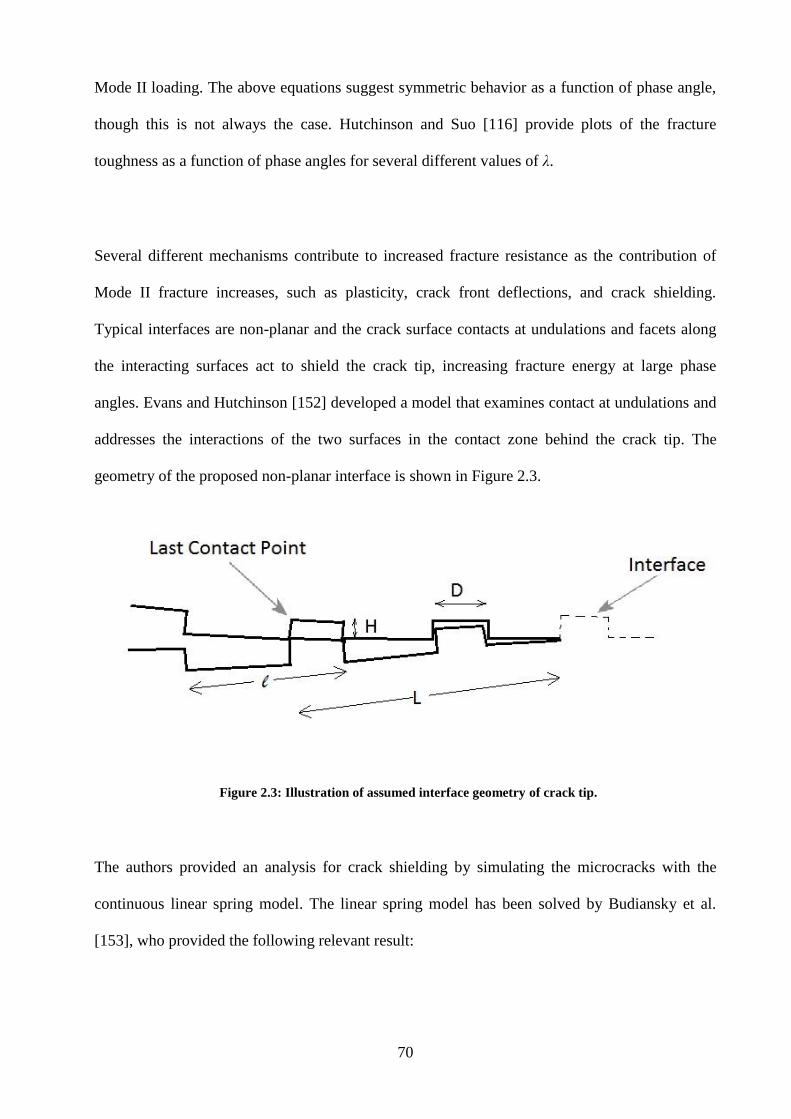
70
Mode II loading. The above equations suggest symmetric behavior as a function of phase angle,
though this is not always the case. Hutchinson and Suo [116] provide plots of the fracture
toughness as a function of phase angles for several different values of λ.
Several different mechanisms contribute to increased fracture resistance as the contribution of
Mode II fracture increases, such as plasticity, crack front deflections, and crack shielding.
Typical interfaces are non-planar and the crack surface contacts at undulations and facets along
the interacting surfaces act to shield the crack tip, increasing fracture energy at large phase
angles. Evans and Hutchinson [152] developed a model that examines contact at undulations and
addresses the interactions of the two surfaces in the contact zone behind the crack tip. The
geometry of the proposed non-planar interface is shown in Figure 2.3.
Figure 2.3: Illustration of assumed interface geometry of crack tip.
The authors provided an analysis for crack shielding by simulating the microcracks with the
continuous linear spring model. The linear spring model has been solved by Budiansky et al.
[153], who provided the following relevant result:
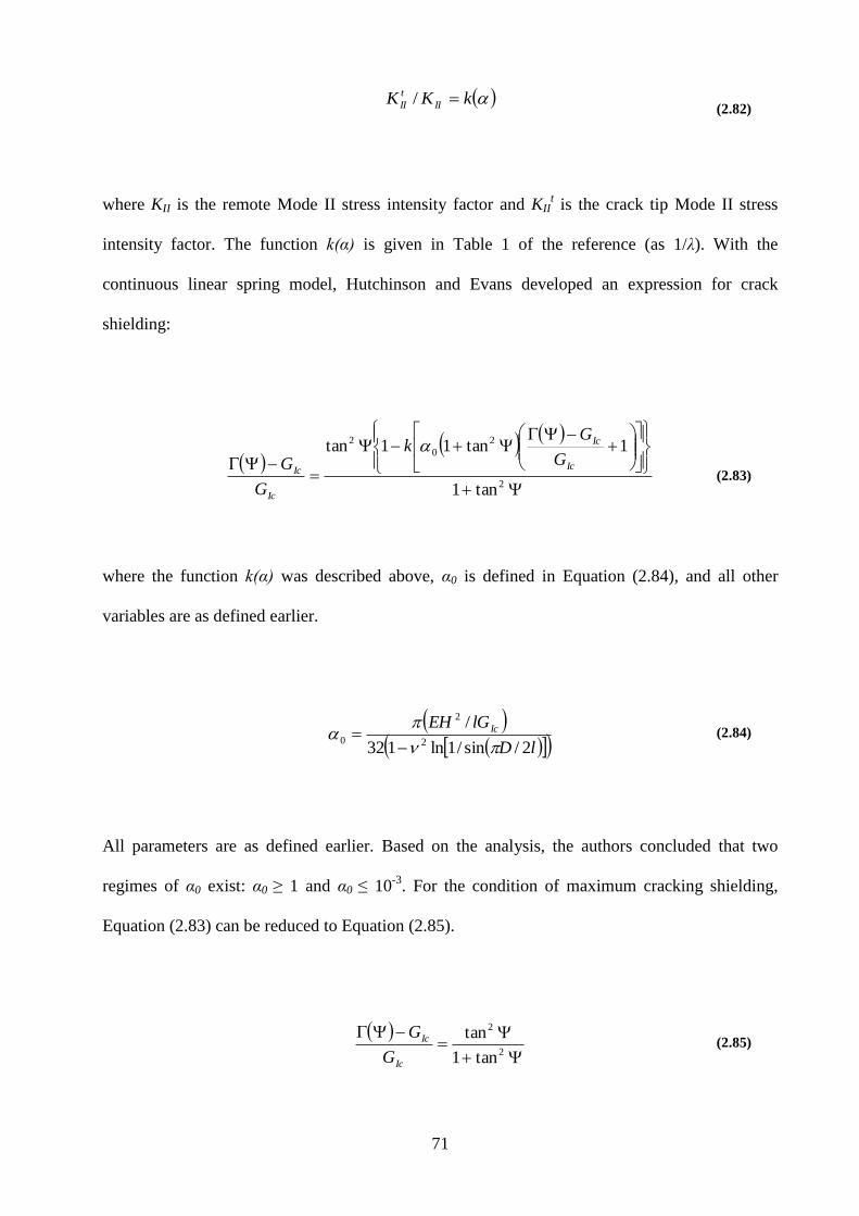
71
kKK II
t
II / (2.82)
where KII is the remote Mode II stress intensity factor and KIIt is the crack tip Mode II stress
intensity factor. The function k(α) is given in Table 1 of the reference (as 1/λ). With the
continuous linear spring model, Hutchinson and Evans developed an expression for crack
shielding:
2
2
0
2
tan1
1tan11tanIc
Ic
Ic
IcG
Gk
G
G
(2.83)
where the function k(α) was described above, α0 is defined in Equation (2.84), and all other
variables are as defined earlier.
lD
lGEH Ic
2/sin/1ln132
/2
2
0
(2.84)
All parameters are as defined earlier. Based on the analysis, the authors concluded that two
regimes of α0 exist: α0 ≥ 1 and α0 ≤ 10-3
. For the condition of maximum cracking shielding,
Equation (2.83) can be reduced to Equation (2.85).
2
2
tan1
tan
Ic
Ic
G
G (2.85)
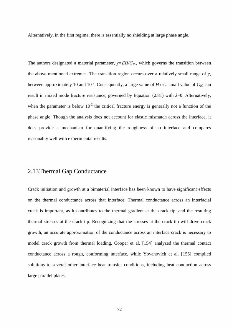
72
Alternatively, in the first regime, there is essentially no shielding at large phase angle.
The authors designated a material parameter, χ=EH/GIC, which governs the transition between
the above mentioned extremes. The transition region occurs over a relatively small range of χ,
between approximately 10 and 10-2
. Consequently, a large value of H or a small value of GIC can
result in mixed mode fracture resistance, governed by Equation (2.81) with λ=0. Alternatively,
when the parameter is below 10-2
the critical fracture energy is generally not a function of the
phase angle. Though the analysis does not account for elastic mismatch across the interface, it
does provide a mechanism for quantifying the roughness of an interface and compares
reasonably well with experimental results.
2.13 Thermal Gap Conductance
Crack initiation and growth at a bimaterial interface has been known to have significant effects
on the thermal conductance across that interface. Thermal conductance across an interfacial
crack is important, as it contributes to the thermal gradient at the crack tip, and the resulting
thermal stresses at the crack tip. Recognizing that the stresses at the crack tip will drive crack
growth, an accurate approximation of the conductance across an interface crack is necessary to
model crack growth from thermal loading. Cooper et al. [154] analyzed the thermal contact
conductance across a rough, conforming interface, while Yovanovich et al. [155] complied
solutions to several other interface heat transfer conditions, including heat conduction across
large parallel plates.
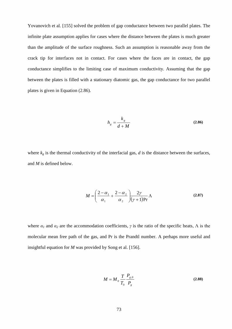
73
Yovanovich et al. [155] solved the problem of gap conductance between two parallel plates. The
infinite plate assumption applies for cases where the distance between the plates is much greater
than the amplitude of the surface roughness. Such an assumption is reasonable away from the
crack tip for interfaces not in contact. For cases where the faces are in contact, the gap
conductance simplifies to the limiting case of maximum conductivity. Assuming that the gap
between the plates is filled with a stationary diatomic gas, the gap conductance for two parallel
plates is given in Equation (2.86).
Md
kh
g
g
(2.86)
where kg is the thermal conductivity of the interfacial gas, d is the distance between the surfaces,
and M is defined below.
Pr1
222
2
2
1
1
M (2.87)
where α1 and α2 are the accommodation coefficients, γ is the ratio of the specific heats, Λ is the
molecular mean free path of the gas, and Pr is the Prandtl number. A perhaps more useful and
insightful equation for M was provided by Song et al. [156].
g
g
P
P
T
TMM
0,
0
0 (2.88)

74
where T and Pg are the temperature and pressure of the gas, respectively, M0 is the gas parameter
value at the reference values of gas temperature and pressure, T0 and Pg,0. The thermal
conductivity for air is kg=0.026 W/mK, while the gas parameter at T0=50 ºC and Pg,0=1 atm is
M0=0.373x10⁶
m. The authors found good agreement with the model and experiments done for
which the gap was filled with helium, argon, and nitrogen gases.
75
CHAPTER 3. PROBLEM STATEMENT
3.1 Objective
The present research investigated the feasibility of using an experiment wherein a ball indentation is
made in a coated sample surface to evaluate the mechanical properties of the interface. Those
properties will then be applied to a thermal-structural model to study the evolution of an indentation-
induced flaw.
3.2 Technical Background
The technique of using a combination of numerical and experimental methods to evaluate the
cohesive zone properties of a coated specimen was proposed, with the ultimate goal of simulating the
response of an interfacial flaw during the application of thermal and pressure transients to the coating
surface. A proposed concept takes its cue from the ball indentation test’s application for the
interfacial strength measurement of transparent coatings. Cohesive strength was measured based on
observations of the crack front as a function of the applied load. It was expected that this crack size
as a function of the maximum load was also a function of the critical energy release rate, such that a
unique combination of material properties governing the growth of the interfacial crack resulted. The
method can accurately predict the responses of the coating separation mechanism. Therefore, it was
expected that the method would also be capable of accurately applying the same properties to
numerically predicting the response of properties in a second test that would extend the crack by
different mechanisms. Thus, validation for the technique would be provided. Given the validation of
the cohesive zone, and its application in the material set, the effects of surface thermal and pressure
transients on flaw evolution could then be studied.
76
3.3 Experimental Procedure
The following theoretical and experimental studies will be conducted in order to develop the
technique of material property measurement and to apply those properties to studying interfacial flaw
evolution.
1. A preliminary analysis of the stress state at the tip of a through coating crack will be analyzed
with a thermal-structural analysis of gun tube coatings. The effects of various material
parameters will be analyzed in terms of the stress state at the crack tip.
2. In order to evaluate the response of an interfacial flaw, a method for evaluating the cohesive
zone properties of the coating–substrate interface must be developed. How best to measure
cohesive zone properties is an area of research under debate, as techniques of evaluating
individual property components and combining them to form an accurate description of the
interface are still being developed. Most researchers maintain that the strength measurements
taken in button-type tests are not representative of the entire interface. Therefore, a method
that measures all the properties on the same sample, thereby presenting a complete
description of the interface, is preferred. It should be recognized, too, that as a function of the
cohesive zone properties, the indentation test introduces an interfacial flaw and also provides
a context for measuring the resulting flaw evolution under thermal and pressure transients.
Therefore, it is necessary to develop a model to determine the properties of the cohesive zone
based on experimental results that include the evolution of the flaw size at different
indentation loads, as determined by ultrasonic analysis after the indention test has been
completed.
3. As stated previously, the experimentally evaluated properties were used in a simulation of the
indentation experiment, first to evaluate the properties, and then to introduce damage for
77
further study. A comprehensive finite element simulation will be developed, for which results
obtained from a different finite element simulation of an indentation experiment simulation
will be imported as the initial conditions for considering the evolution of an interfacial flaw
to severe thermal and pressure transients. The contributions of the individual boundary
conditions will be explored in order to evaluate current experimental techniques, as well as
improvements in coating performance. As a last step, the damage mechanisms of the final
gun tube coating will be explored in depth, as the internal blister pressure is delayed relative
to the surface.
4. Conclusions will be drawn from the experimental and numerical results. Recommendations
for improving the experimental and theoretical protocols presented herein will also be
offered.
78
CHAPTER 4. PROPERTY MEASUREMENT AND
VALIDATION
4.1 Experimental Procedures
4.1.1 Sample Preparation
A first set of samples tested comprised a nickel-aluminum coating thermally sprayed onto steel
substrates. Samples were prepared by Michael Schroeder of Metallic Bonds, Ltd., in Beloit, WI,
by spraying onto 0.14 m (5.5 in) square steel substrates. The plates were then machined into the
appropriate samples for testing. For the indentation tests, the samples were machined into
squares, approximately 2.5 mm, in order to better simulate axisymmetric conditions. The four-
point bend samples were machined to the same thickness and width dimensions, but were 11.43
mm long.
A second set of samples was prepared from 7075 aluminum sprayed onto 7075 aluminum
substrates with T6 heat treatment. The four-point bend samples were machined to the same
length and width dimensions as the nickel-coated steel, whereas the indentation tests were
performed on samples of various coating thickness dimensions.
4.1.1.1 Substrate Preparation
The cold-spray substrate was a 1 foot (0.305 m) and 1/8 inch (3.18 mm) thick square plate with
polished surfaces that was ordered from McMaster-Carr. Subsequently, the top surface was
lightly sanded in order to facilitate better bonding with the cold-spray coating. Not only did
79
sanding remove most of the surface oxidation and contaminants that could otherwise adversely
affect bonding, it also created a slightly irregular surface, which by increasing surface area,
improved bonding. However, even with sanding, it is likely that some contaminants remain on
the interface where they may have a negative effect on bonding.
4.1.1.2 Coating Deposition
Aluminum 7075 powder was used for the cold spraying. A -325 µm mesh powder was chosen
because the particle size and distribution facilitate cold spraying. Powder 7075 aluminum was
purchased from Valimet, Inc., and was dried before being applied. The cold spray application
was performed by the Applied Research Lab (ARL) at the Pennsylvania State University.
4.1.1.3 Four-Point Bend Sample Preparation
4.1.1.3.1 Thermally Sprayed Nickel on Steel
After the coatings had been applied, the plates were machined into four-point bend test samples
with approximate measurements of 0.020 m (0.79 in) wide and 0.11 m (4.5 in) long. To mitigate
friction between the coating and the load points, the surface was ground in order to achieve a
smoother finish, resulting in a final thickness of 0.60 mm. For the samples in this study, the
coating was notched at the center across the width with a wire EDM (electric discharge
machining) to the interface. In recognition of the fact that the four-point bend test evaluates the
critical energy release rate based on the change in compliance of the beam as the crack grows,
the substrate was machined down to a thickness of 2.6 mm with the wire EDM. In addition, the
samples were oriented on the plate to mitigate the effects of residual stresses on crack growth by
aligning the samples perpendicular to the direction of the curvature. Visual inspection indicated
80
that the residual stresses were primarily uniaxial based on slight curvatures in one direction of
the plate. As this was the case, the samples were oriented perpendicular to the direction of the
residual stresses so that the contribution of the stresses to crack growth, and ultimately to the
energy release rate would be minimal. Six initial samples were produced from the original
substrate, from which the remaining metal was saved for subsequent indentation tests.
4.1.1.3.2 Cold-Sprayed Aluminum on Aluminum Substrates
In order to produce a unique set of samples, with properties that would differ from the nickel-
coated steel described above, aluminum beams were also produced by cold spraying. A cold-
spray powder of 7075 with a -325 mesh was sprayed onto a 7075 aluminum plate that was 1/16"
(0.00152 m) thick. Two coatings were sprayed; one equal to the thickness of the substrate, and
the other equal to half the thickness of the substrate. Several passes were required to build up the
appropriate coating thickness. To prepare the surface for cold spraying, it was lightly sanded to
remove oxidation and contaminates. Helium was used as the carrier gas, because nitrogen cannot
achieve the speeds required for deposition. The nozzle temperatures for the spraying varied from
approximately 180 to 195˚C, and the gas pressure for the runs was approximately 2.07 MPa (300
psi). The coating was sprayed in passes along the length of the sample. Due to surface roughness,
and in order to remove surface oxidation, the samples were sanded with an emery cloth, resulting
in a smoother surface finish for reduced friction between the sample and the loading fixture. The
samples were machined into four-point bend bars, and a notch was milled into the center with a
1/32" mill bit. The four-point bend samples were 10 mm wide and 114 mm long, and the final
thickness of the coating was 1.5 mm.
4.1.1.4 Indentation Sample Preparation
81
4.1.1.4.1 Thermally Sprayed Nickel on Steel
The indentation tests were planned in order to meet the ultimate goal of simulating the
experiment with a finite element model as already described in Section 4.2.5. Therefore, the
samples and experiment were designed to best accommodate the assumptions of the model. The
nickel-coated steel samples were cut into squares to create loading conditions accurately
described by the axisymmetric indentation finite element model. Indentation samples were cut
from the 10 mm by 115 mm four-point bend samples into 10 mm squares. In addition, curvature
resulting from residual stresses along the length of the sample was easily observable. During
testing, any flattening of the curvature caused by the residual stress would have created a
uniaxial stress in the direction of the length of the sample. To mitigate such stress, the
rectangular plate was cut into squares.
4.1.1.4.2 Cold-Sprayed Aluminum on Aluminum Substrates
Several different indenters were simulated on the aluminum samples with a coating thickness of
1.5 mm (Section 4.1.1.3) with the finite element model (Section 4.2.5), and based on the results,
it became clear that this coating was too thick to produce the interfacial stresses required to
induce delaminations at the interface even for very weak bonds. Based on this preliminary
analysis, the samples described in Section 4.1.1.3 were repurposed for the indentation test after
some of the coating had been removed to produce samples more suitable for indentation testing.
The coating was milled down to a thickness of between 0.5 and 0.75 mm; this variation is a
function of the residual stress curvature that made it impossible to create a coating surface that
was completely parallel to the interface. For each indentation test, the coating thickness at the
indentation site was recorded.
82
4.1.2 The Four-point Bend Test
As described in Section 2.12.5, the four-point bend test can be used to evaluate the interfacial
fracture energy between coatings and substrates. The calculation of the critical energy release
rate based on the four-point bend experiments requires accurate elastic modulus and Poisson’s
ratio information for the coating and substrate, in addition to the residual stress state
characterization. Additionally, four-point bend tests require that the coated specimen be pre-
cracked and inserted into a fixture with an outer load span that supports the sample and an inner
load span that bends the sample to progressively separate the coating from the substrate. From
the recorded load-displacement measurements, the critical load can be identified as the plateau
and used to calculate the critical energy release rate. However, the four-point bend test, as
described here, presents several significant challenges, which make it impractical for all but a
select few material systems. In fact, the systems that can be evaluated must have a relatively
low-modulus and high-yield strength coatings and substrates, such that before yielding
delamination occurs. Additionally, once crack growth begins, it must continue steadily in order
to determine the load at which stable crack growth occurs for the evaluation of the critical energy
release rate.
The aluminum samples described above constitute a challenging material combination for
cohesive zone property measurement. Based on previous experience with cold spraying, it was
expected the deposited coating system would form a strong bond and yet exhibit brittle
interfacial fracture characteristics. Therefore, stable crack growth would not occur during steady-
state conditions, even if it were possible to introduce a pre-crack. The particular material used
herein highlights one of the shortcomings of the four-point bend test in calculating the critical
energy release rate: i.e., the method only works in cases where a pre-crack can be introduced and
grows as a function of the applied load. To overcome these obstacles, modifications were made
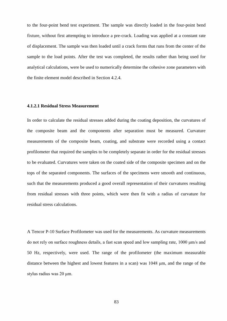
83
to the four-point bend test experiment. The sample was directly loaded in the four-point bend
fixture, without first attempting to introduce a pre-crack. Loading was applied at a constant rate
of displacement. The sample was then loaded until a crack forms that runs from the center of the
sample to the load points. After the test was completed, the results rather than being used for
analytical calculations, were be used to numerically determine the cohesive zone parameters with
the finite element model described in Section 4.2.4.
4.1.2.1 Residual Stress Measurement
In order to calculate the residual stresses added during the coating deposition, the curvatures of
the composite beam and the components after separation must be measured. Curvature
measurements of the composite beam, coating, and substrate were recorded using a contact
profilometer that required the samples to be completely separate in order for the residual stresses
to be evaluated. Curvatures were taken on the coated side of the composite specimen and on the
tops of the separated components. The surfaces of the specimens were smooth and continuous,
such that the measurements produced a good overall representation of their curvatures resulting
from residual stresses with three points, which were then fit with a radius of curvature for
residual stress calculations.
A Tencor P-10 Surface Profilometer was used for the measurements. As curvature measurements
do not rely on surface roughness details, a fast scan speed and low sampling rate, 1000 μm/s and
50 Hz, respectively, were used. The range of the profilometer (the maximum measurable
distance between the highest and lowest features in a scan) was 1048 μm, and the range of the
stylus radius was 20 μm.
84
The curvatures of the sample were measured before fracture and those of the coating and
substrate after fracture. Then, the linear residual stress distribution was approximated using
Equations (2.41) and (2.42) based on the radius of the composite beam curvature before fracture,
and the coating and substrate after.
4.1.2.2 Mechanical Testing
The specimens were prepared for testing by first cutting through the coating to create a notch.
For the nickel-coated steel specimens, the notch was created with a wire EDM, and for the
aluminum samples with a 1/32" thick mill bit. As already mentioned, the aluminum samples
described above provide a challenging material combination for cohesive zone property
measurement. Previous experience with cold spraying suggests that the deposited coating system
would form a strong bond and have brittle crack growth characteristics. Based on these
expectations, the system would not provide the opportunity to create a precrack. In the unlikely
event that a precrack were to be introduced, the system would not allow for steady-state crack
growth. This particular material set highlights one of the shortcomings of the four-point bend test
in terms of calculating the critical energy release rate; the method only works in cases where a
pre-crack can be introduced and then grow as a function of the applied load without yielding. To
overcome these obstacles, modifications were made to the four-point bend test experiment; the
test was loaded in the four-point bend fixture without first attempting to introduce a pre-crack.
Loading was applied with a mechanical loading frame (Instron 5866, Instron Corp., Norwood,
MA), and the load and displacement data recorded. The sample was loaded until a crack, which
was expected to grow instantaneously, formed. After the test was completed, the results were not
used for analytical calculations; instead, they were applied to determine the cohesive zone
parameters numerically with the finite element model described above.
85
Specimens were prepared for four-point bend testing by creating a right-angle notch by first
milling through the coating to the interface with a 1/32" mill bit. A mill was used to avoid any
possible thermal effects associated with the wire EDM at the interface. However, the nickel
coatings were notched with a wire EDM as the thermal effects at the crack tip were not first
considered. The inner and outer span lengths of the test fixture were completely adjustable. A
floating plate, which allowed for self-alignment, was used to aid symmetric crack growth. The
fixture span inner and outer dimensions maintained the preferred 2:1 ratio, with support and load
dimensions of 110 and 55 mm, respectively. The rollers were made of steel and each had a
diameter of 6.35 mm. The fixture was placed in an Instron tensile tester with a 10 kN load cell,
and in order to simulate quasi-static loading conditions the load was applied at a rate of 1
mm/min. The samples were carefully aligned in the fixture to ensure that the notch would be
both centered and parallel to the load and support fixtures. The output was recorded in an Excel
workbook for subsequent analysis.
In order to calculate the residual stresses that arose during coating deposition, the composite
beam’s curvature must be measured before the test, and the coating and substrate after they are
separated. Curvature measurements were recorded using a contact profilometer, as described
above.
4.1.3 The Ball Indentation Test
In addition to measuring the geometry and material parameters, ball indentation tests are often
used to calculate the critical energy release rate, which is a function of the radius of the
86
debonded region under the indenter. However, because the test requires the debonded region to
be measured as a function of the applied load, it is difficult to apply the method to opaque
coatings as an in situ determination of the radius is impossible. Despite this limitation, the
potential of the ball indentation test to obtain interfacial properties has been recognized, as the
onset of debonding and debonded area are strong functions of the cohesive zone properties.
Hence, the indenter load-displacement output, the load at which the interface begins to separate,
and the final crack dimensions can be compared to the finite element simulations of the
indentation test in order to determine the cohesive zone properties.
Traditional techniques for measuring interfacial properties have several disadvantages that make
them unsuitable for this application. As mentioned above, the four-point bend test showed large-
scale yielding before damage initiation in the case of the nickel-coated steel set, or instantaneous
failure in the case of the aluminum samples. This made initiating a pre-crack and subsequent
steady state crack growth impossible in both cases. Other tests, such as the scratch test, are more
qualitative in nature, whereas peel and wedge tests, are difficult to perform on thin coatings.
Given these deficiencies, a new approach, based on the indentation test was developed to
evaluate the cohesive zone properties of the coating and substrate systems.
As such, a new method to measure the cohesive zone properties using indentation tests will be
based on a numerical and experimental approach to the finite element model. Indentation
experiments will be conducted with a mechanical loading frame (Instron 5866, Instron Corp.,
Norwood, MA) capable of applying loads from 1N to 10kN. However, only the 10 kN load cell
was used for the indentation experiments in the present study. A tungsten-carbide indenter ball
was placed between the ram and the sample surface. Based on how likely they were to cause
damage at the interface as suggested by preliminary finite element modeling, several different
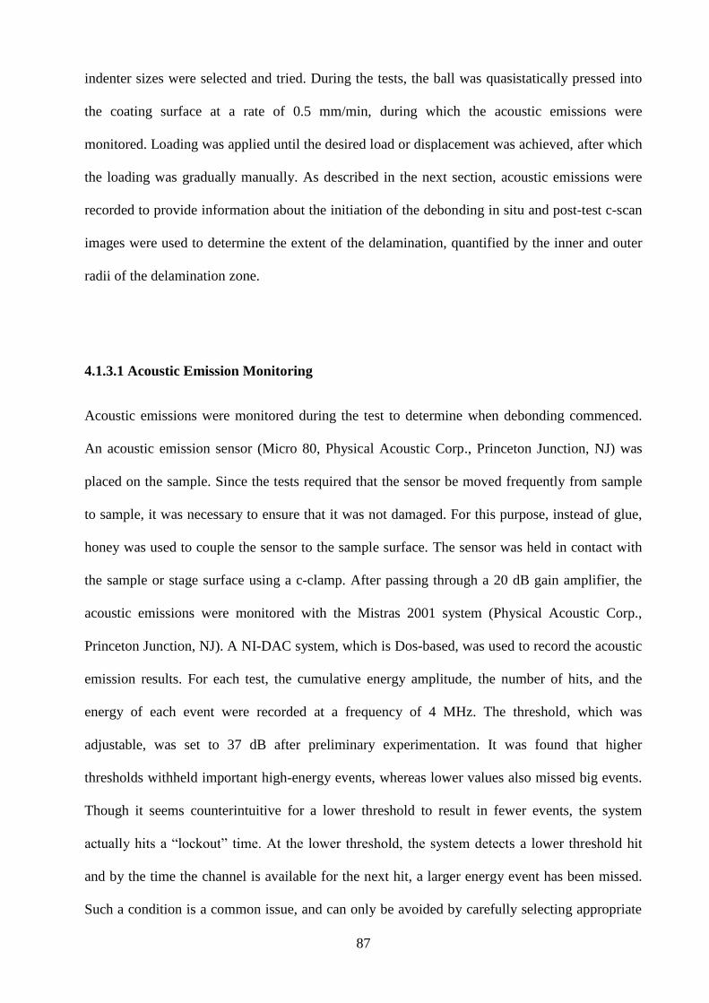
87
indenter sizes were selected and tried. During the tests, the ball was quasistatically pressed into
the coating surface at a rate of 0.5 mm/min, during which the acoustic emissions were
monitored. Loading was applied until the desired load or displacement was achieved, after which
the loading was gradually manually. As described in the next section, acoustic emissions were
recorded to provide information about the initiation of the debonding in situ and post-test c-scan
images were used to determine the extent of the delamination, quantified by the inner and outer
radii of the delamination zone.
4.1.3.1 Acoustic Emission Monitoring
Acoustic emissions were monitored during the test to determine when debonding commenced.
An acoustic emission sensor (Micro 80, Physical Acoustic Corp., Princeton Junction, NJ) was
placed on the sample. Since the tests required that the sensor be moved frequently from sample
to sample, it was necessary to ensure that it was not damaged. For this purpose, instead of glue,
honey was used to couple the sensor to the sample surface. The sensor was held in contact with
the sample or stage surface using a c-clamp. After passing through a 20 dB gain amplifier, the
acoustic emissions were monitored with the Mistras 2001 system (Physical Acoustic Corp.,
Princeton Junction, NJ). A NI-DAC system, which is Dos-based, was used to record the acoustic
emission results. For each test, the cumulative energy amplitude, the number of hits, and the
energy of each event were recorded at a frequency of 4 MHz. The threshold, which was
adjustable, was set to 37 dB after preliminary experimentation. It was found that higher
thresholds withheld important high-energy events, whereas lower values also missed big events.
Though it seems counterintuitive for a lower threshold to result in fewer events, the system
actually hits a “lockout” time. At the lower threshold, the system detects a lower threshold hit
and by the time the channel is available for the next hit, a larger energy event has been missed.
Such a condition is a common issue, and can only be avoided by carefully selecting appropriate
88
thresholds. The location of the acoustic emission sensor is shown in Figure 4.1b As previous
experience had shown that a second acoustic emission sensor mounted onto a loading ram
provides redundant information; only one such sensor was used in these experiments.
Figure 4.1: Indentation experiment arrangement, showing (a) the load frame, computer, and stage, and (b) a
close-up of the stage and specimen arrangement.
89
4.1.3.2 Indenter Selection
Special care was taken to select an appropriate indenter. If the chosen indenter is too small, it
will cause excessive plastic deformation and penetrate the coating without creating the interfacial
stresses necessary to cause separation. On the other hand, an indenter that is too large will
require a large load to deform the surface and may not induce delamination for thin samples. As
the goal of the experiment was to induce delamination at the interface, numerical simulations
were run to aid in the selection of an indenter with an appropriate diameter. The first requirement
of the chosen indenter is that it must induce delamination before the load cell limit of 10 kN was
reached. In addition, the goal of introducing damage at a load within the acceptable range of the
load cell must be balanced with minimizing plastic deformation, because large-scale deformation
introduces numerical difficulties. In addition, accurate material property information for large
plastic deformations is difficult to obtain.
The experiment was designed for the specific purpose of measuring the interface properties;
therefore, the indenter selection process was complicated by the fact that these were not known.
The material properties for similar systems were assumed based on published research and
varied within reasonable limits to approximate how the coating system might delaminate under
indentation. Based on the preliminary simulations, an indenter diameter of 2 mm was chosen for
the first set of experiments on the nickel-coated steel system. As already discussed, indenter
selection was seen as a compromise between excessive deformation and the maximum load level
to initiate delamination.
90
4.1.3.3 Indentation Testing
As discussed earlier, the indentation test was used in conjunction with numerical analysis to
determine the properties of the interface in the coating systems. Indentation tests were performed
at a constant loading rate of 0.05 mm/min. A 10 kN load cell was attached to the load frame to
allow the large loads required to initiate delamination in even strong coatings. A ram extension
was attached to the load cell to provide a flat surface for impressing the indenter ball into the
coating surface. Plastic deformation occurred during the first indentation in the ram extension.
For subsequent indentations, the indenter ball was placed in the grove formed during the first
sequence to minimize the contributions of the loading ram plastic deformation to the load and
displacement measurements. The experimental set-up is shown in Figure 4.1
Before each indentation experiment, an acoustic emission sensor was placed on the end of the
sample. Honey was used as a coupling medium, as it is an excellent conductor of acoustic
energy. A c-clamp was used to hold the sensor to the surface and was clamped over the stage,
sample, and sensor. However, the nickel-coated steel samples are too small to fit under the
indenter when the sensor is attached to the sample. For these tests, the sensor was attached to the
stage, again with honey as the coupling fluid. Mineral oil was placed between the bottom of the
stage and the sample to facilitate the transmission of acoustic emissions from the sample, to the
stage, and then to the sensor. Such an arrangement is not ideal, as attaching the sensor to the
stage may mean the sensor picks up acoustic noise from the load frame that would otherwise be
reduced if it were attached to the sample. In addition, the acoustic emissions from the sample
may be damped, as they must now travel through the stage before being received by the sensor.
However, this was the only way to monitor acoustic emissions in the sample.
91
After the load cell had been balanced and the gage length reset, the indenter ball was placed in
the grove on the load ram above the sample and then slowly moved towards the sample surface
until the load began to increase. Once the contact was confirmed, manual loading was stopped
and the BlueHill software controlling the Instron was engaged. The software was programmed to
load the same at a constant rate. In addition, the acoustic emission monitoring system was
engaged to provide data to match the load and displacement measurements. After the desired
load and/or displacement were achieved, the loading and acoustic emissions monitoring were
stopped and the sample was slowly unloaded manually. Once all the data based on the
measurements had been saved, the samples were labeled, and saved for subsequent c-scan
analysis.
For later tests, it was decided that the acoustic emissions should also be recorded during
unloading. In order to do this, the setpoint of the sample load frame was adjusted over a time of
100 seconds to slowly unload the sample back to its original position. During the unloading,
acoustic emissions were recorded as a function of time, which would later be correlated with a
load level based on information about the distance the ram must travel to reach the setpoint and
the 100 s that it would take to get there. One hundred seconds was the maximum time allowed to
reach the setpoint because this was the limit of the Instron control software, and though it varied
by the extent to which the indenter was displaced, it was faster than the loading rate.
4.1.3.4 C-Scan and Scanning Acoustic Microscope Imaging of Interfacial Defects
After being indented, the sample interface was imaged by ultrasonic c-scan in order to find areas
where the coating and substrate had separated. During c-scan inspection using an Okos Hydra
scanner (Okos Solutions, LLC, Chantilly, VA) the sample was placed in a tank of water, which

92
carried the ultrasonic signal from the transducer to the sample. To monitor the reflections on
ultrasonic energy reflected from the sample, the c-scan system was used in pulse-echo mode, for
which the transducer was also the receiver. As is the case with c-scan imaging, and especially for
composite samples, special care must be taken when analyzing the signal returned to the
transducer. At every discontinuity in the sample such as a flaw, delamination, or interface,
portions of the signal are both reflected and transmitted. The signal, which originates at the
transducer travels to the surface, where some of the signal is reflected directly back to the
transducer, and the rest is transmitted into the sample. After traveling into the sample, the energy
reaches the interface, at which point it is again reflected and transmitted. Reflection and
transmission repeats every time the energy reaches an interface, resulting in multiple signals
separated in time being returned to the transducer. The signal returned to the transducer can be
interpreted based on the time that it takes different parts of the signal to return. An equation for
the time it takes for a signal to pass through a composite sample, to reflect from a surface, and to
return to the transducer is given below:
2
2
1
1 222
v
x
v
x
v
xt
w
w
(4.1)
where Δt is the time it takes for the wave to travel through the sample, vw is the wave speed of
sound in water, Δxw is the distance between the sample and the transducer, v1 is the wave speed
through the first layer of the sample, Δx1 is the thickness of the first layer of the sample, v2 is the
wave speed through the second layer of the sample, Δx2 is the thickness of the second layer of
the sample, and where more terms can be added if required for a sample with more than two
layers.
93
To use Equation (4.2), it is necessary to first choose an interface of interest. As the terms for the
materials between the transducer and the chosen interface must be included in Equation (4.2), it
is possible to determine the time at which to expect the portion of the signal for the reflection.
Based on this determination, gates can be added to the signal analysis software, Odis version
3.11.15 software (Okos Solutions, LLC, Chantilly, VA), to capture the amplitude and time of
flight information of the portion of the signal during the scan. A gate was included in every
measurement, to record amplitude over a few different portions of the sample. The first
interfacial reflection was measured, as was the first back-wall reflection (when apparent) as was
the second interface reflection and perhaps other portions of the signal as deemed necessary.
Because of the curvature of the sample, the signal will arrive at slightly different times at
different ends of the sample. In order to keep the gate on the correct part of the signal, a follower
gate was added to ensure that the other gates would measure the correct portion of the signal as
the arrival time changes with variations in sample curvature. The signal amplitude can then be
plotted based on a custom color palette, a black-and-white scheme, or grayscale. In addition,
when a particular part of the signal is of interest, for example the back-wall reflection, the energy
of the transducer can be focused on that portion of the sample to maximize the amplitude of that
portion of the signal and so to create a greater contrast between the delaminations and the
undamaged interface.
4.2 Modelling
4.2.1 Introduction to Cohesive Zone Elements
The cohesive zone model (CZM) was developed as an alternative to the singularity-driven
fracture approach, where the crack tip is assumed to be infinitely sharp, producing a singularity
in the stress field. However, neither condition exists in most conditions. In addition to providing
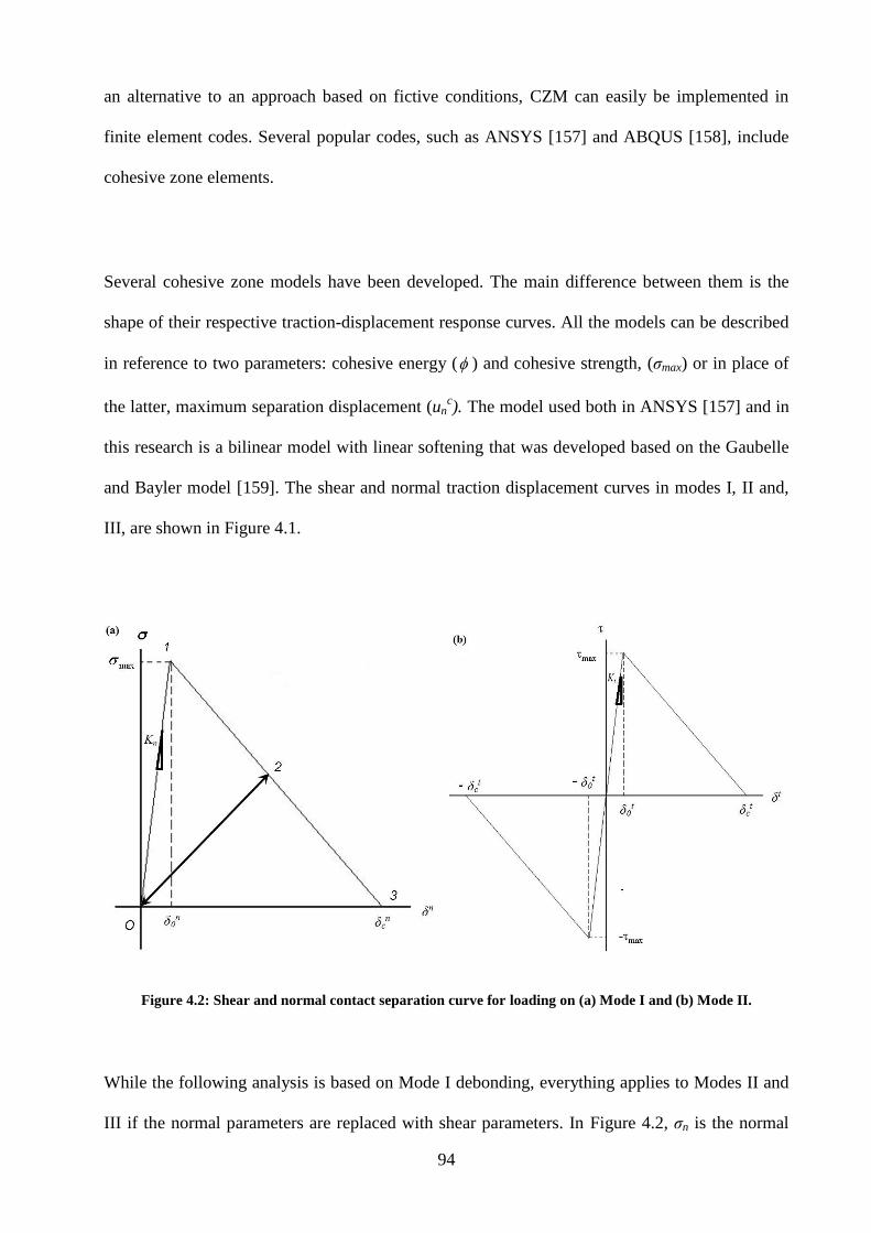
94
an alternative to an approach based on fictive conditions, CZM can easily be implemented in
finite element codes. Several popular codes, such as ANSYS [157] and ABQUS [158], include
cohesive zone elements.
Several cohesive zone models have been developed. The main difference between them is the
shape of their respective traction-displacement response curves. All the models can be described
in reference to two parameters: cohesive energy ( ) and cohesive strength, (σmax) or in place of
the latter, maximum separation displacement (unc). The model used both in ANSYS [157] and in
this research is a bilinear model with linear softening that was developed based on the Gaubelle
and Bayler model [159]. The shear and normal traction displacement curves in modes I, II and,
III, are shown in Figure 4.1.
Figure 4.2: Shear and normal contact separation curve for loading on (a) Mode I and (b) Mode II.
While the following analysis is based on Mode I debonding, everything applies to Modes II and
III if the normal parameters are replaced with shear parameters. In Figure 4.2, σn is the normal
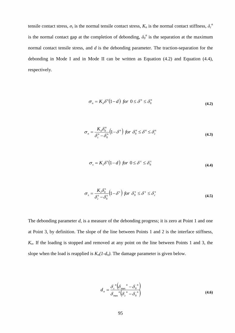
95
tensile contact stress, σs is the normal tensile contact stress, Kn is the normal contact stiffness, δcn
is the normal contact gap at the completion of debonding, δ0n is the separation at the maximum
normal contact tensile stress, and d is the debonding parameter. The traction-separation for the
debonding in Mode I and in Mode II can be written as Equation (4.2) and Equation (4.4),
respectively.
dK n
nn 1 for nn
00 (4.2)
n
nn
c
n
nn
K
1
0
0 for n
c
nn 0 (4.3)
dK s
ss 1 for ss
00 (4.4)
s
ss
c
s
ss
K
1
0
0 for s
c
ss 0 (4.5)
The debonding parameter d, is a measure of the debonding progress; it is zero at Point 1 and one
at Point 3, by definition. The slope of the line between Points 1 and 2 is the interface stiffness,
Kn. If the loading is stopped and removed at any point on the line between Points 1 and 3, the
slope when the load is reapplied is Kn(1-dn). The damage parameter is given below.
nn
c
n
nnn
cnd
0max
0max
(4.6)
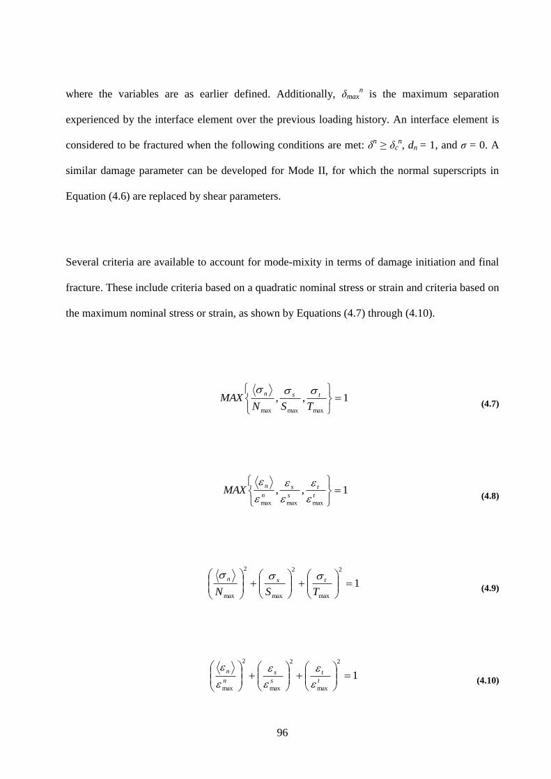
96
where the variables are as earlier defined. Additionally, δmaxn is the maximum separation
experienced by the interface element over the previous loading history. An interface element is
considered to be fractured when the following conditions are met: δn ≥ δc
n, dn = 1, and σ = 0. A
similar damage parameter can be developed for Mode II, for which the normal superscripts in
Equation (4.6) are replaced by shear parameters.
Several criteria are available to account for mode-mixity in terms of damage initiation and final
fracture. These include criteria based on a quadratic nominal stress or strain and criteria based on
the maximum nominal stress or strain, as shown by Equations (4.7) through (4.10).
1,,maxmaxmax
TSNMAX tsn
(4.7)
1,,maxmaxmax
t
t
s
s
n
nMAX
(4.8)
1
2
max
2
max
2
max
TSN
tsn
(4.9)
1
2
max
2
max
2
max
t
t
s
s
n
n
(4.10)
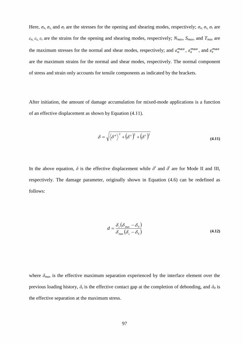
97
Here, σn, σs, and σt are the stresses for the opening and shearing modes, respectively; σn, σs, σt are
εn, εs, εt are the strains for the opening and shearing modes, respectively; Nmax, Smax, and Tmax are
the maximum stresses for the normal and shear modes, respectively; and , , and
are the maximum strains for the normal and shear modes, respectively. The normal component
of stress and strain only accounts for tensile components as indicated by the brackets.
After initiation, the amount of damage accumulation for mixed-mode applications is a function
of an effective displacement as shown by Equation (4.11).
222tsn (4.11)
In the above equation, δ is the effective displacement while δs and δ
t are for Mode II and III,
respectively. The damage parameter, originally shown in Equation (4.6) can be redefined as
follows:
0max
0max
c
cd (4.12)
where δmax is the effective maximum separation experienced by the interface element over the
previous loading history, δc is the effective contact gap at the completion of debonding, and δ0 is
the effective separation at the maximum stress.
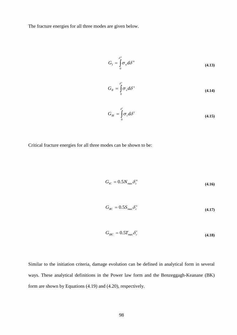
98
The fracture energies for all three modes are given below.
n
nI dG
n
0
(4.13)
s
sII dG
s
0
(4.14)
t
tIII dG
t
0
(4.15)
Critical fracture energies for all three modes can be shown to be:
n
cIC NG max5.0 (4.16)
s
cIIC SG max5.0 (4.17)
t
cIIIC TG max5.0 (4.18)
Similar to the initiation criteria, damage evolution can be defined in analytical form in several
ways. These analytical definitions in the Power law form and the Benzeggagh-Keanane (BK)
form are shown by Equations (4.19) and (4.20), respectively.

99
1
IIIC
III
IIC
II
IC
I
G
G
G
G
G
G
(4.19)
IIICIICIC
IIIIII
IIIIIICIICIC GGG
GGG
GGGGG
(4.20)
The fracture energy in the normal mode is given by GI while the two shearing states by GII
(Mode II), and GIII (Mode III). Critical fracture energies are denoted by GIC, GIIC, and GIIIC, and
the exponent is given by α in the Power law form, and η in the BK form.
If the form of the damage evolution shown in Equation (4.19) is used with the assumption that
the Mode III fracture energy is irrelevant, it is reasonable to expect that for a two-dimensional,
axisymmetric application, the Power law exponent is 1. The resulting traction-based damage
initiation and energy-based failure a criterion are shown in Equations (4.21) and (4.22).
1
2
max
2
max
SN
sn
(4.21)
1IIC
II
IC
I
G
G
G
G
(4.22)
It is useful to define the mode mix ratio, ψ, between the normal and shear tractions:
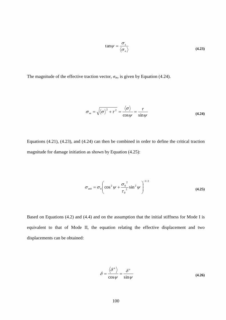
100
n
s
tan
(4.23)
The magnitude of the effective traction vector, σm, is given by Equation (4.24).
sincos
22m
(4.24)
Equations (4.21), (4.23), and (4.24) can then be combined in order to define the critical traction
magnitude for damage initiation as shown by Equation (4.25):
2/1
2
2
0
2
02
00 sincos
m
(4.25)
Based on Equations (4.2) and (4.4) and on the assumption that the initial stiffness for Mode I is
equivalent to that of Mode II, the equation relating the effective displacement and two
displacements can be obtained:
sincos
sn
(4.26)
101
After combining Equations (4.26) and (4.12), the damage parameter can be redefined as follows:
s
c
s
c
n
c
n
cd
0
0
0
0 sincos
(4.27)
After Equation (4.27) is combined with the traction equations (4.2) and (4.4), the following
relationships for the normal transaction and the shear traction, respectively, can be obtained:
n
c
c
n
K
cos
0
00 (4.28)
s
c
c
s
K
sin
0
00 (4.29)
where K0 is the initial normal and shear stiffness. When the final failure occurs, the
displacements for the normal and shear conditions are <δn>=δccosψ and δ
s=δcsinψ, respectively.
The displacements can then be combined with Equations (4.13) and (4.14), to give the work
done by tractions:
2
0 cos5.0 cmIG (4.30)
2
0 sin5.0 cmIIG (4.31)
102
By combining the above with the fracture criteria, Equation (4.32) is obtained:
1
2020 sin2
cos2
IIC
m
IC
m
cGG
(4.32)
Finally, the total mixed-mode fracture energy per unit area, Γ, is defined by Equation (4.33):
1
22
0 sincos5.0
IIC
IC
ICcmIIIG
GGGG
(4.33)
From the above analysis, it is evident that for mixed mode loading, five independent parameters
need to be defined before an analysis; the normal and shear strengths, σ0 and τ0, two toughness
values, GIC and GIIC, and one stiffness, K0. The respective responses of modes I and II in terms of
fracture energy or bond strength are sometimes assumed to be equivalent in order to further
reduce the problem complexity by one or two parameters. In addition, as it is hard to measure,
the stiffness is often calculated using Equation (2.6) which is based on geometric and material
properties. However, the problem cannot be simplified beyond three parameters.
4.2.2 Two-Dimensional Axisymmetric Model
Preliminary finite element modeling was completed in terms of simulating the effects of
subjecting coatings to simultaneous and severe thermal and pressure transients. The preliminary
work focused on developing and verifying two-dimensional models. The results achieved and the
103
experience gained from the preliminary modeling was then applied to the more sophisticated
undertakings discussed in the following sections. Considerations such as multiple dimensions,
cohesive zone formulation, cylindrical geometry, non-linearity, and temperature-dependent
material properties and cracks was the focus of all subsequent research as detailed herein.
The first step of the modeling was to develop and verify a two-dimensional axisymmetric finite
element representation of a coated tube subjected to thermal and pressure transients. Stress
distributions for the geometry were determined in two steps. In the first step, a thermal model
with a pulse, thermal boundary condition applied to the inside surface was solved. Two-
dimensional thermal PLANE55 elements were used with the axisymmetric formulation
activated; the element has four nodes with a single degree of freedom (temperature) at each
node. The top nodes were coupled to simulate an infinitely long cylinder whereas the bottom
nodes were given symmetry boundary conditions. For all the calculations, the outside of the
cylinder was insulated and the initial temperature set to zero.
After the thermal simulation was completed, the structural response was evaluated for each
chosen time quasi-statically. In order to interpolate the thermal response from the thermal to
structural elements, the models each had the exact same mesh, elements, and nodes. To facilitate
this, two-dimensional structural solid PLANE182 elements were used, again with the
axisymmetric formulation activated. The inside surfaces experienced pressure, whereas the
outside surfaces were stress free; zero displacement boundary conditions were applied to the
bottom of the cylinder and the nodes on the top surface were coupled to move together in the
axial direction. The meshed geometry is shown in Figure 4.3.
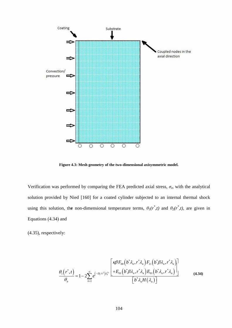
104
Figure 4.3: Mesh geometry of the two-dimensional axisymmetric model.
Verification was performed by comparing the FEA predicted axial stress, σz, with the analytical
solution provided by Nied [160] for a coated cylinder subjected to an internal thermal shock
using this solution, the non-dimensional temperature terms, θ1(r*,t) and θ2(r
*,t), are given in
Equations (4.34) and
(4.35), respectively:
2 21
* * * *
00 11
* * * **01 01/1
*1
, ,
, ,,1 2
tn
n n n n
n n n nD c
na n n
F b r F b r
E b r E b rr te
b H
(4.34)

105
2 21 /* *
2 01
2 *21
, ,41
tnD c
n n
na n n
r t e E r
b H
(4.35)
When the function H(λn) is defined as:
2 * * * * 1 *
00 01 01
** * * * *
01 00 11*
** * * * *
11 01 01*
* * * * 1 *
01 11 00
, , ,
, , ,
, , ,
, , ,
n n n n n n n
n n n n n n
n n n n n n
n n n n n n
H F a b E b b E b
aE b F a b F a b
b
aF b E a b E a a
b
E a b F b b F b
(4.36)
The roots, λn can be determined from the transcendental equation:
* * *
00 11
1* * *
01 01
, ,
, , 0
n n n n
n n n n
F a b F b
E b E a b
(4.37)
While the functions F00, F11, and E01 are shown below:
00 0 0 0 0
11 1 1 1 1
01 0 1 1 0
, ( ) ( )
, ( ) ( )
, ( ) ( )
F x y J x Y y J y Y x
F x y J x Y y J y Y x
E x y J x Y y J y Y x
(4.38)
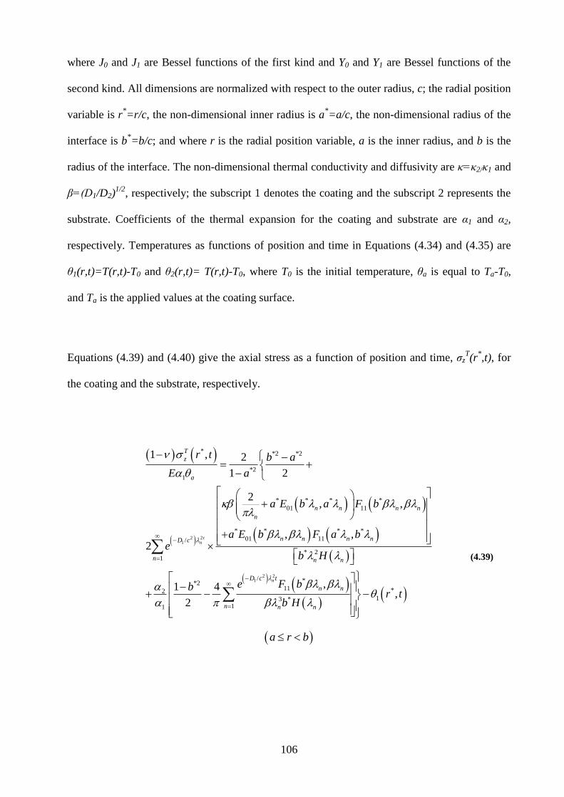
106
where J0 and J1 are Bessel functions of the first kind and Y0 and Y1 are Bessel functions of the
second kind. All dimensions are normalized with respect to the outer radius, c; the radial position
variable is r*=r/c, the non-dimensional inner radius is a
*=a/c, the non-dimensional radius of the
interface is b*=b/c; and where r is the radial position variable, a is the inner radius, and b is the
radius of the interface. The non-dimensional thermal conductivity and diffusivity are κ=κ2/κ1 and
β=(D1/D2)1/2
, respectively; the subscript 1 denotes the coating and the subscript 2 represents the
substrate. Coefficients of the thermal expansion for the coating and substrate are α1 and α2,
respectively. Temperatures as functions of position and time in Equations (4.34) and (4.35) are
θ1(r,t)=T(r,t)-T0 and θ2(r,t)= T(r,t)-T0, where T0 is the initial temperature, θa is equal to Ta-T0,
and Ta is the applied values at the coating surface.
Equations (4.39) and (4.40) give the axial stress as a function of position and time, σzT(r
*,t), for
the coating and the substrate, respectively.
2 21
2 21
* *2 *2
*2
1
* * * *
01 11
* * * *
01 11/
* 21
/ **2112
3 *11
1 , 2
1 2
2, ,
, ,2
,1 4
2
tn
n
T
z
a
n n n n
n
n n n nD c
n n n
D c t
n n
n n n
r t b a
E a
a E b a F b
a E b F a be
b H
e F bb
b H
*
1 ,r t
a r b
(4.39)
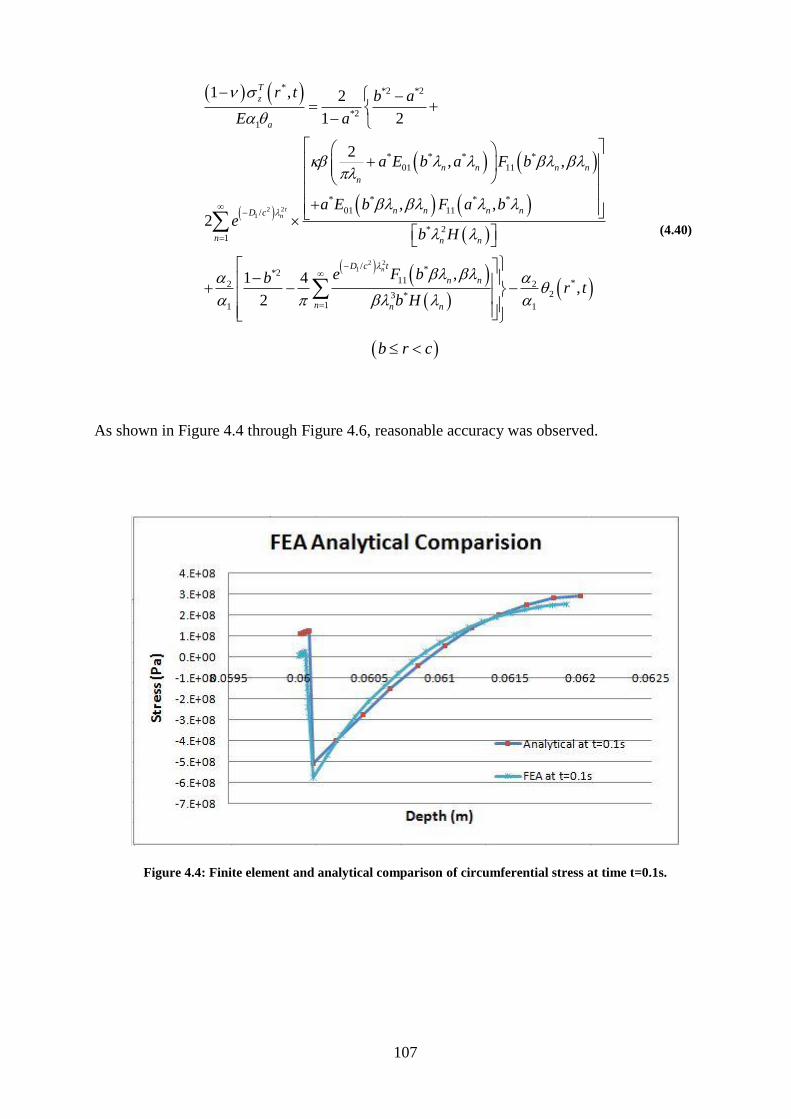
107
2 21
2 21
* *2 *2
*2
1
* * * *
01 11
* * * *
01 11/
* 21
/ **2112
3 *11
1 , 2
1 2
2, ,
, ,2
,1 4
2
tn
n
T
z
a
n n n n
n
n n n nD c
n n n
D c t
n n
n n n
r t b a
E a
a E b a F b
a E b F a be
b H
e F bb
b H
*22
1
,r t
b r c
(4.40)
As shown in Figure 4.4 through Figure 4.6, reasonable accuracy was observed.
Figure 4.4: Finite element and analytical comparison of circumferential stress at time t=0.1s.
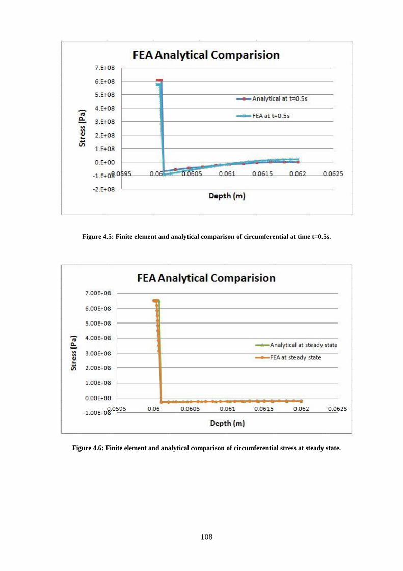
108
Figure 4.5: Finite element and analytical comparison of circumferential at time t=0.5s.
Figure 4.6: Finite element and analytical comparison of circumferential stress at steady state.
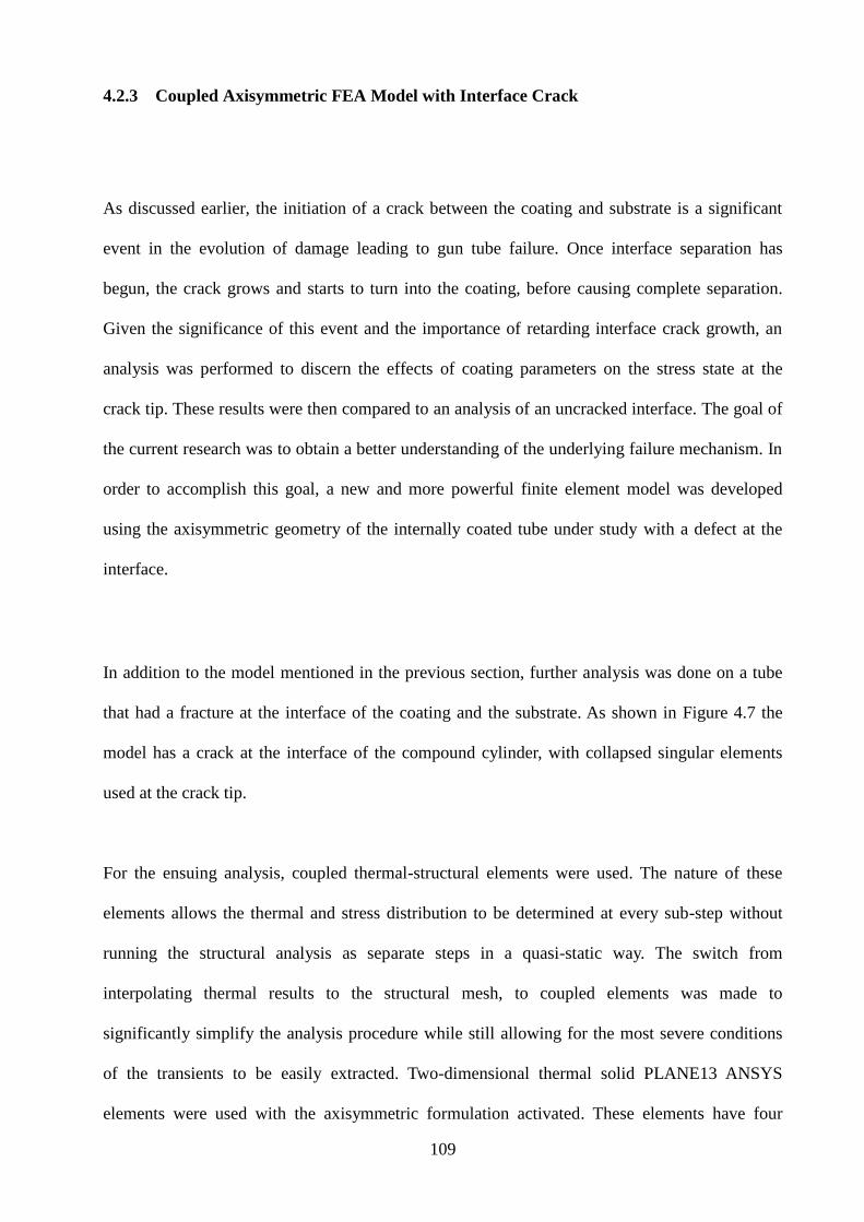
109
4.2.3 Coupled Axisymmetric FEA Model with Interface Crack
As discussed earlier, the initiation of a crack between the coating and substrate is a significant
event in the evolution of damage leading to gun tube failure. Once interface separation has
begun, the crack grows and starts to turn into the coating, before causing complete separation.
Given the significance of this event and the importance of retarding interface crack growth, an
analysis was performed to discern the effects of coating parameters on the stress state at the
crack tip. These results were then compared to an analysis of an uncracked interface. The goal of
the current research was to obtain a better understanding of the underlying failure mechanism. In
order to accomplish this goal, a new and more powerful finite element model was developed
using the axisymmetric geometry of the internally coated tube under study with a defect at the
interface.
In addition to the model mentioned in the previous section, further analysis was done on a tube
that had a fracture at the interface of the coating and the substrate. As shown in Figure 4.7 the
model has a crack at the interface of the compound cylinder, with collapsed singular elements
used at the crack tip.
For the ensuing analysis, coupled thermal-structural elements were used. The nature of these
elements allows the thermal and stress distribution to be determined at every sub-step without
running the structural analysis as separate steps in a quasi-static way. The switch from
interpolating thermal results to the structural mesh, to coupled elements was made to
significantly simplify the analysis procedure while still allowing for the most severe conditions
of the transients to be easily extracted. Two-dimensional thermal solid PLANE13 ANSYS
elements were used with the axisymmetric formulation activated. These elements have four
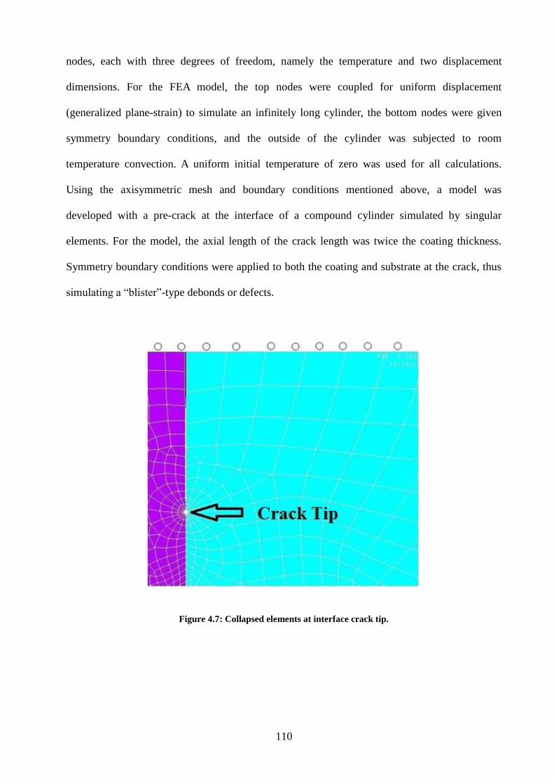
110
nodes, each with three degrees of freedom, namely the temperature and two displacement
dimensions. For the FEA model, the top nodes were coupled for uniform displacement
(generalized plane-strain) to simulate an infinitely long cylinder, the bottom nodes were given
symmetry boundary conditions, and the outside of the cylinder was subjected to room
temperature convection. A uniform initial temperature of zero was used for all calculations.
Using the axisymmetric mesh and boundary conditions mentioned above, a model was
developed with a pre-crack at the interface of a compound cylinder simulated by singular
elements. For the model, the axial length of the crack length was twice the coating thickness.
Symmetry boundary conditions were applied to both the coating and substrate at the crack, thus
simulating a “blister”-type debonds or defects.
Figure 4.7: Collapsed elements at interface crack tip.
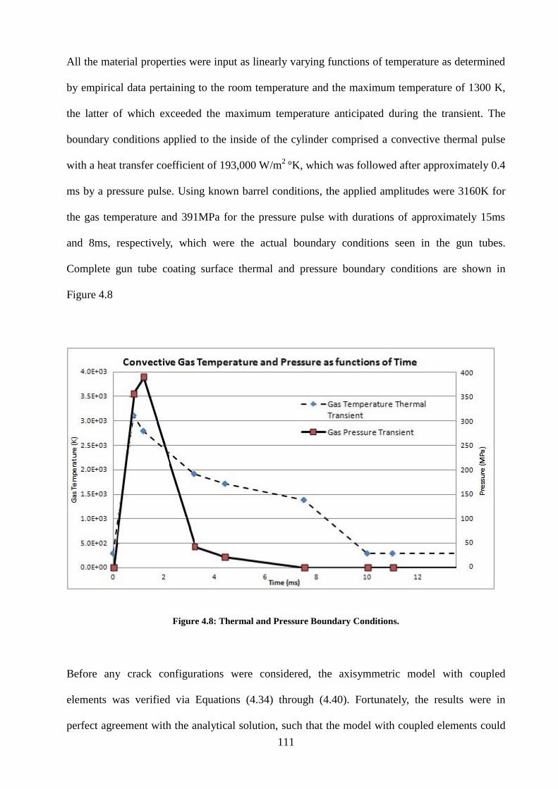
111
All the material properties were input as linearly varying functions of temperature as determined
by empirical data pertaining to the room temperature and the maximum temperature of 1300 K,
the latter of which exceeded the maximum temperature anticipated during the transient. The
boundary conditions applied to the inside of the cylinder comprised a convective thermal pulse
with a heat transfer coefficient of 193,000 W/m2
°K, which was followed after approximately 0.4
ms by a pressure pulse. Using known barrel conditions, the applied amplitudes were 3160K for
the gas temperature and 391MPa for the pressure pulse with durations of approximately 15ms
and 8ms, respectively, which were the actual boundary conditions seen in the gun tubes.
Complete gun tube coating surface thermal and pressure boundary conditions are shown in
Figure 4.8
Figure 4.8: Thermal and Pressure Boundary Conditions.
Before any crack configurations were considered, the axisymmetric model with coupled
elements was verified via Equations (4.34) through (4.40). Fortunately, the results were in
perfect agreement with the analytical solution, such that the model with coupled elements could
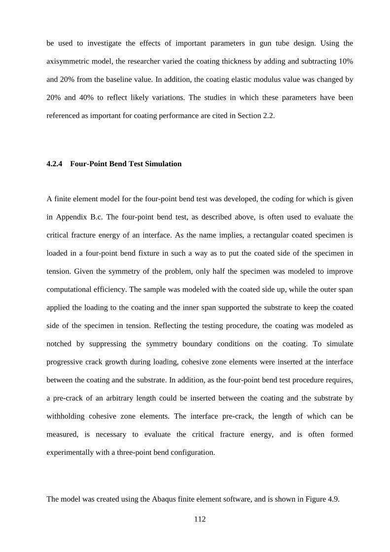
112
be used to investigate the effects of important parameters in gun tube design. Using the
axisymmetric model, the researcher varied the coating thickness by adding and subtracting 10%
and 20% from the baseline value. In addition, the coating elastic modulus value was changed by
20% and 40% to reflect likely variations. The studies in which these parameters have been
referenced as important for coating performance are cited in Section 2.2.
4.2.4 Four-Point Bend Test Simulation
A finite element model for the four-point bend test was developed, the coding for which is given
in Appendix B.c. The four-point bend test, as described above, is often used to evaluate the
critical fracture energy of an interface. As the name implies, a rectangular coated specimen is
loaded in a four-point bend fixture in such a way as to put the coated side of the specimen in
tension. Given the symmetry of the problem, only half the specimen was modeled to improve
computational efficiency. The sample was modeled with the coated side up, while the outer span
applied the loading to the coating and the inner span supported the substrate to keep the coated
side of the specimen in tension. Reflecting the testing procedure, the coating was modeled as
notched by suppressing the symmetry boundary conditions on the coating. To simulate
progressive crack growth during loading, cohesive zone elements were inserted at the interface
between the coating and the substrate. In addition, as the four-point bend test procedure requires,
a pre-crack of an arbitrary length could be inserted between the coating and the substrate by
withholding cohesive zone elements. The interface pre-crack, the length of which can be
measured, is necessary to evaluate the critical fracture energy, and is often formed
experimentally with a three-point bend configuration.
The model was created using the Abaqus finite element software, and is shown in Figure 4.9.
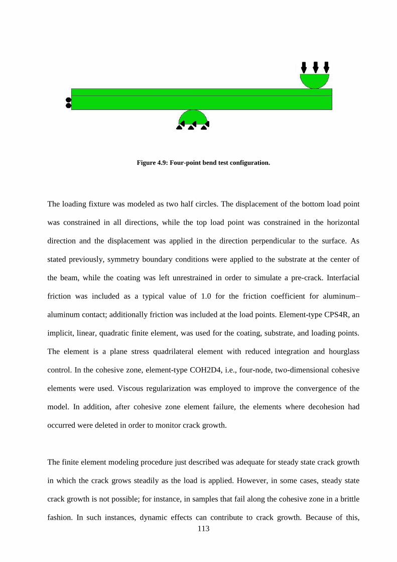
113
Figure 4.9: Four-point bend test configuration.
The loading fixture was modeled as two half circles. The displacement of the bottom load point
was constrained in all directions, while the top load point was constrained in the horizontal
direction and the displacement was applied in the direction perpendicular to the surface. As
stated previously, symmetry boundary conditions were applied to the substrate at the center of
the beam, while the coating was left unrestrained in order to simulate a pre-crack. Interfacial
friction was included as a typical value of 1.0 for the friction coefficient for aluminum–
aluminum contact; additionally friction was included at the load points. Element-type CPS4R, an
implicit, linear, quadratic finite element, was used for the coating, substrate, and loading points.
The element is a plane stress quadrilateral element with reduced integration and hourglass
control. In the cohesive zone, element-type COH2D4, i.e., four-node, two-dimensional cohesive
elements were used. Viscous regularization was employed to improve the convergence of the
model. In addition, after cohesive zone element failure, the elements where decohesion had
occurred were deleted in order to monitor crack growth.
The finite element modeling procedure just described was adequate for steady state crack growth
in which the crack grows steadily as the load is applied. However, in some cases, steady state
crack growth is not possible; for instance, in samples that fail along the cohesive zone in a brittle
fashion. In such instances, dynamic effects can contribute to crack growth. Because of this,
114
dynamic effects were included by using an implicit dynamic load step. Because the sample is
loaded quasi-statically, the loading fixture should not directly introduce dynamic effects into the
specimen. Based on this premise, the quasi-static dynamic approach was chosen to prevent the
inclusion of any dynamic effects of the loading fixture in the simulation, and yet still allow for
dynamic effects once crack initiation begins.
As mentioned in Section 2.12.5, the accumulated residual stresses significantly affect the
measured interfacial properties. This is the case whether the residual stresses are the result of
deformations associated with cold spraying, the coefficient of the thermal expansion difference
during thermal spraying, or some other mechanism. As mentioned earlier, assuming they have
linear profiles, residual stresses can be quantified based on the curvatures of the debonded
coating and the substrate after separation and on the composite sample. Given the importance of
residual stresses in interfacial crack growth and property measurement, the profile of the
measured residual stress distribution can be applied to the four-point bend test model through a
user subroutine, shown in Appendix B.f. The “sigini.f” subroutine can be used to apply three-
dimensional residual stresses as functions of any of the coordinate directions. In addition, the
coating and the substrate can have independent residual stress distributions.
An important point in implementing cohesive zone elements is that the cohesive zone can be
meshed independently of the two sides of the interface. In fact, the cohesive zone can be meshed,
collapsed to zero-thickness, and then the top and bottom tied to the coating and substrate,
respectively. The independence of the cohesive zone mesh is useful, as it allows the cohesive
zone to require smaller elements for the resolution in order to simulate small increments of crack
growth, and yet the model remains computationally efficient. It is recommended that the ratio of
the size of the cohesive zone to the structural elements not significantly exceed three. In order to
115
allow for easier parameterization, mesh adjustment, and simplicity, the input file was written in
Python scripting.
Preliminary verifications for the four-point bend test were completed via Tsui et al. [161], since
the researchers who developed the testing procedure often used to calculate the critical energy
release rate under four-point bending conditions, also provided load-displacement results for one
of their experiments. In addition, they provided sample dimensions, material properties, residual
stress distributions, and the calculated critical energy release rate. Based on these parameters,
simulations were run during which the interfacial bond strengths were varied until proper
agreement was observed between the experimental and finite element results. The sample
parameters can be found in Tsui et al. [161], whereas the Mode I and II strengths that provided
the best agreement were found to be 40 MPa and 10 MPa, respectively. The interfacial strength
parameters were bounded by bond strength measurements calculated for other thermal spray
coatings calculated from button tests. A plot of the comparison of the results is shown in Figure
4.10
The finite element simulation results began with a preload on the fixture caused by the residual
stresses; as such, experimental results were adjusted to match the preload. The stiffness of the
linear region reported and numerical results do not match perfectly, which is likely to have been
caused by a discrepancy in the elastic modulus of the substrate. In addition, it should be noted
that the results providing the best agreement included a normal strength that was higher than the
shear strength. Though it is not possible to be certain why this configuration provided the best
agreement, it is likely to be because mode-independent fracture energy was assumed as opposed
to mode-dependent fracture energies. With the fracture energy constant, the strength of the
interface is the only adjustable parameter implicated in the behavior of the interface. As can be
seen in Figure 4.2, when the interface stiffness and fracture energy (the area under the load-
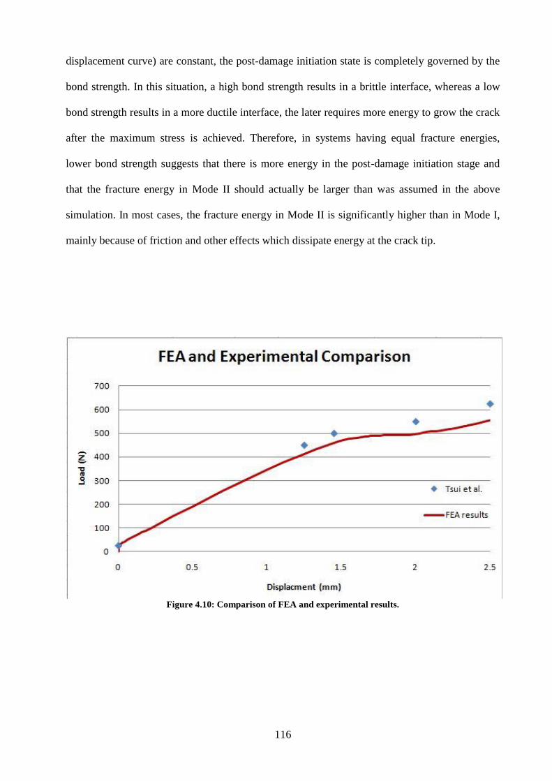
116
displacement curve) are constant, the post-damage initiation state is completely governed by the
bond strength. In this situation, a high bond strength results in a brittle interface, whereas a low
bond strength results in a more ductile interface, the later requires more energy to grow the crack
after the maximum stress is achieved. Therefore, in systems having equal fracture energies,
lower bond strength suggests that there is more energy in the post-damage initiation stage and
that the fracture energy in Mode II should actually be larger than was assumed in the above
simulation. In most cases, the fracture energy in Mode II is significantly higher than in Mode I,
mainly because of friction and other effects which dissipate energy at the crack tip.
Figure 4.10: Comparison of FEA and experimental results.
117
4.2.5 Ball Indentation Simulation
A ball indentation model, the code for which is given in Appendix B.a and Appendix B.d was
developed for two purposes. The model was used first as verification for the cohesive zone
elements, and the properties were measured during four-point bend experiments. In addition, the
model was used in an implicit to explicit analysis to quasistatically introduce an interfacial flaw
before the effects of rapid thermal transients were analyzed.
To simulate the delamination under loading from a spherical indenter, an Abaqus finite element
model of the experiment was also developed. The model simulates a ball indenter being
displaced into the surface of a coated substrate. Axisymmetry was utilized, as the geometry,
loading, and subsequent structural response are not functions of the angle of rotation. In addition,
residual stresses can be applied to the coating and substrate through a user subroutine, as
described in the previous section. The meshed geometry of the problem is show in Figure 4.11.
The regions at the axis of the axisymmetry were constrained to prevent rotation and
displacement in the radial direction, while the bottom of the model was constrained in the y-
direction. The outside surface, shown in red, was coupled in the radial direction in order to
simulate an infinitely large plate. Coupling was accomplished in Abaqus through a constraint
equation for which the displacement of the outside edge was set equal to the top corner of the
coating. The spherical indenter was modeled with quarter symmetry, while the displacement
loading condition was applied to the top symmetry surface. Surface-to-surface contact
interaction properties were defined at the area of possible contact between the coating and
indenter surfaces, while an appropriate friction coefficient of 0.6 for steel nickel contact was
defined. The coefficient was also applied to the coating surface and indenter interface.
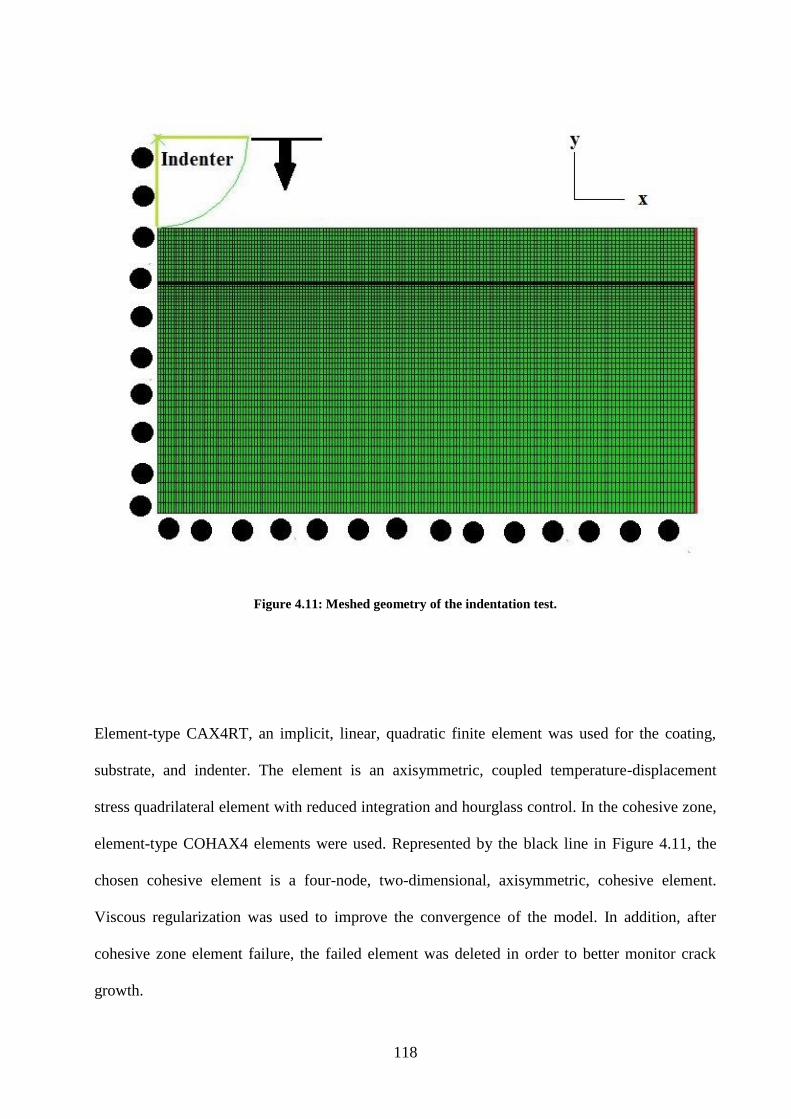
118
Figure 4.11: Meshed geometry of the indentation test.
Element-type CAX4RT, an implicit, linear, quadratic finite element was used for the coating,
substrate, and indenter. The element is an axisymmetric, coupled temperature-displacement
stress quadrilateral element with reduced integration and hourglass control. In the cohesive zone,
element-type COHAX4 elements were used. Represented by the black line in Figure 4.11, the
chosen cohesive element is a four-node, two-dimensional, axisymmetric, cohesive element.
Viscous regularization was used to improve the convergence of the model. In addition, after
cohesive zone element failure, the failed element was deleted in order to better monitor crack
growth.
119
As mentioned earlier in this section, the model was used in a sequential implicit-to-explicit
analysis. Though the quasistatic ball indentation step of the analysis only requires structural
degrees of freedom, coupled thermal-structural elements were necessary to import the results
into the subsequent thermal-structural analysis. Because of the large number of increments
necessary for the subsequent explicit analysis, the implicit analysis was set to double precision to
improve accuracy.
4.3 Experimental Results
4.3.1 Indentation Test Results
Indentation tests were performed on the samples in order to provide the information necessary to
evaluate the interfacial fracture energy and bond strength. Following the procedure described in
Section 4.1.3.3, various indentation tests were performed on the coated specimens. Different
techniques, such as in situ acoustic emission monitoring, post-test c-scans, and finite element
modeling, were all used to develop a new method to determine cohesive zone properties. The
resulting technique is unique in that it provides a way to determine cohesive zone properties,
which are both notoriously difficult to measure and applicable to a wider range of samples than
existing tests. Such a technique is not limited to the very narrow range of materials that can be
appropriately evaluated with the four-point bend test due to the multitude of difficulties already
discussed.
In order to study cases with relatively strong interfacial bonding, or for which constant crack
growth is not possible, a method to evaluate a wider range of material combinations is developed
120
in the present study. In addition to its applications to a wider range of material combinations, the
method described will be used to determine both the interfacial fracture energy and bond
strength, whereas most analytical solutions are capable of determining only one property for a
given test.
Acoustic emission monitoring will also be used to help determine the occurrence of major events
such as crack growth initiation and re-initiation. In addition, samples will be loaded to various
levels, enabling a flaw to evolve as a function of the applied force. Finally, as the flaw size from
the c-scan results as a function of maximum load, and the approximate load of delamination
initiation are known, finite element simulations will be used to evaluate the interfacial properties.
In the simulations, the properties of the interface are varied until the experimental and numerical
results match up in terms of flaw size and the onset of damage at the interface.
4.3.1.1 Test Results for the Nickel-Coated Steel Samples
4.3.1.1.1 Acoustic Emission Results
Indentation tests were completed for the nickel-coated steel specimens. The samples, described
in Section 4.1.1.3, were produced by using a wire EDM to reduce the substrate and coating
thicknesses to 2.0 and 0.6 mm, respectively. Additionally, before testing, the samples were cut
into 20 mm squares. All indentation tests are load-controlled at a rate of 0.05 mm/min with a 2
mm indenter. All the results of all the nickel-coated steel tests are given in Appendix A.
Nickel-coated steel indentation tests were conducted to methodically determine the final flaw
dimensions and the load at which delamination initiates. Several tests were conducted and
stopped at intermediate indentation loads. Preliminary tests were conducted to determine the
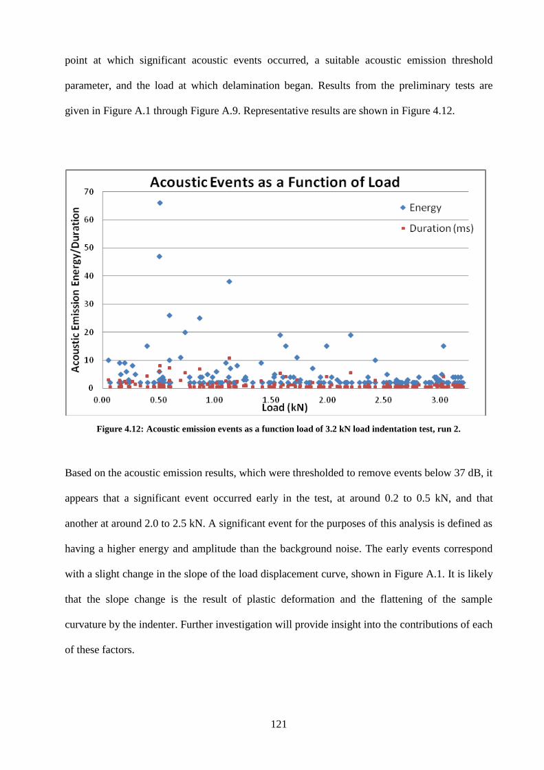
121
point at which significant acoustic events occurred, a suitable acoustic emission threshold
parameter, and the load at which delamination began. Results from the preliminary tests are
given in Figure A.1 through Figure A.9. Representative results are shown in Figure 4.12.
Figure 4.12: Acoustic emission events as a function load of 3.2 kN load indentation test, run 2.
Based on the acoustic emission results, which were thresholded to remove events below 37 dB, it
appears that a significant event occurred early in the test, at around 0.2 to 0.5 kN, and that
another at around 2.0 to 2.5 kN. A significant event for the purposes of this analysis is defined as
having a higher energy and amplitude than the background noise. The early events correspond
with a slight change in the slope of the load displacement curve, shown in Figure A.1. It is likely
that the slope change is the result of plastic deformation and the flattening of the sample
curvature by the indenter. Further investigation will provide insight into the contributions of each
of these factors.
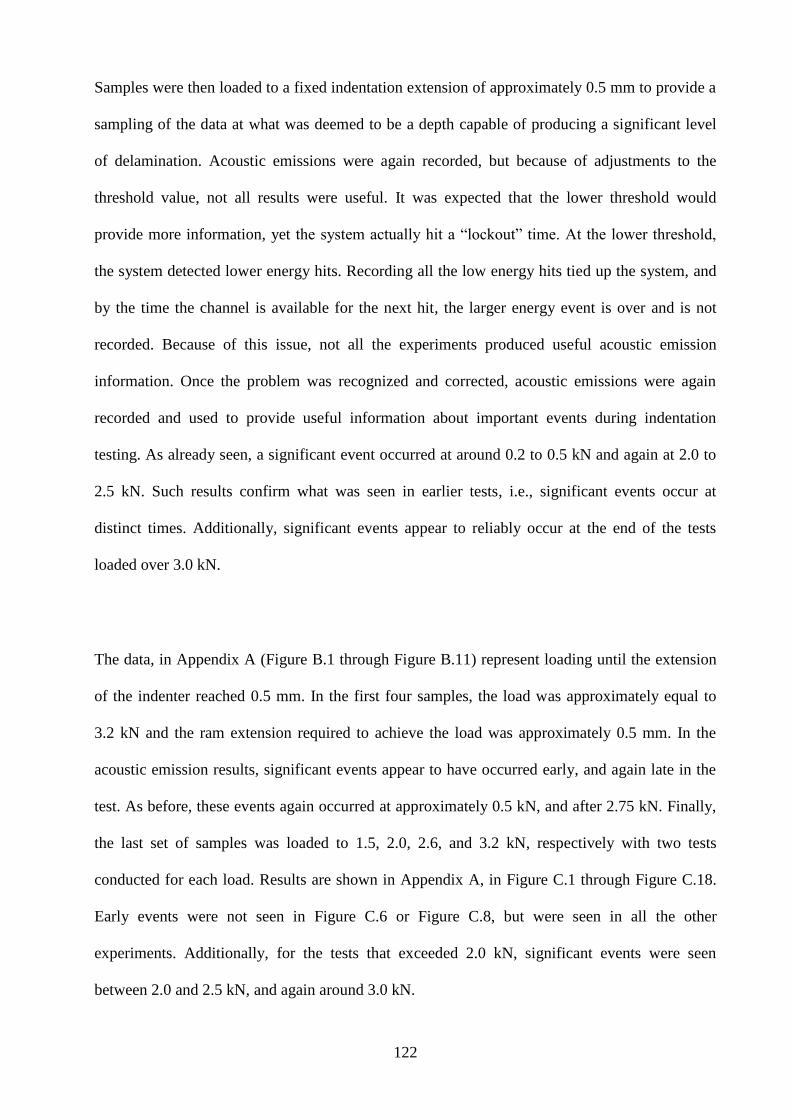
122
Samples were then loaded to a fixed indentation extension of approximately 0.5 mm to provide a
sampling of the data at what was deemed to be a depth capable of producing a significant level
of delamination. Acoustic emissions were again recorded, but because of adjustments to the
threshold value, not all results were useful. It was expected that the lower threshold would
provide more information, yet the system actually hit a “lockout” time. At the lower threshold,
the system detected lower energy hits. Recording all the low energy hits tied up the system, and
by the time the channel is available for the next hit, the larger energy event is over and is not
recorded. Because of this issue, not all the experiments produced useful acoustic emission
information. Once the problem was recognized and corrected, acoustic emissions were again
recorded and used to provide useful information about important events during indentation
testing. As already seen, a significant event occurred at around 0.2 to 0.5 kN and again at 2.0 to
2.5 kN. Such results confirm what was seen in earlier tests, i.e., significant events occur at
distinct times. Additionally, significant events appear to reliably occur at the end of the tests
loaded over 3.0 kN.
The data, in Appendix A (Figure B.1 through Figure B.11) represent loading until the extension
of the indenter reached 0.5 mm. In the first four samples, the load was approximately equal to
3.2 kN and the ram extension required to achieve the load was approximately 0.5 mm. In the
acoustic emission results, significant events appear to have occurred early, and again late in the
test. As before, these events again occurred at approximately 0.5 kN, and after 2.75 kN. Finally,
the last set of samples was loaded to 1.5, 2.0, 2.6, and 3.2 kN, respectively with two tests
conducted for each load. Results are shown in Appendix A, in Figure C.1 through Figure C.18.
Early events were not seen in Figure C.6 or Figure C.8, but were seen in all the other
experiments. Additionally, for the tests that exceeded 2.0 kN, significant events were seen
between 2.0 and 2.5 kN, and again around 3.0 kN.
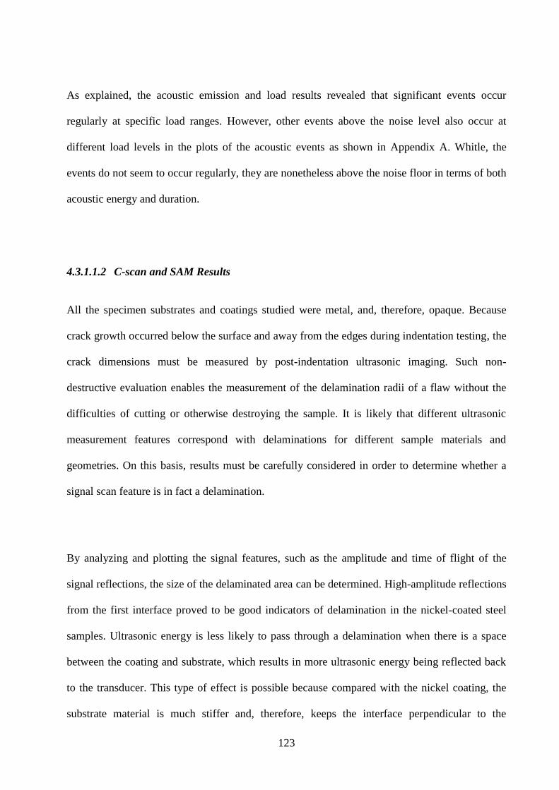
123
As explained, the acoustic emission and load results revealed that significant events occur
regularly at specific load ranges. However, other events above the noise level also occur at
different load levels in the plots of the acoustic events as shown in Appendix A. Whitle, the
events do not seem to occur regularly, they are nonetheless above the noise floor in terms of both
acoustic energy and duration.
4.3.1.1.2 C-scan and SAM Results
All the specimen substrates and coatings studied were metal, and, therefore, opaque. Because
crack growth occurred below the surface and away from the edges during indentation testing, the
crack dimensions must be measured by post-indentation ultrasonic imaging. Such non-
destructive evaluation enables the measurement of the delamination radii of a flaw without the
difficulties of cutting or otherwise destroying the sample. It is likely that different ultrasonic
measurement features correspond with delaminations for different sample materials and
geometries. On this basis, results must be carefully considered in order to determine whether a
signal scan feature is in fact a delamination.
By analyzing and plotting the signal features, such as the amplitude and time of flight of the
signal reflections, the size of the delaminated area can be determined. High-amplitude reflections
from the first interface proved to be good indicators of delamination in the nickel-coated steel
samples. Ultrasonic energy is less likely to pass through a delamination when there is a space
between the coating and substrate, which results in more ultrasonic energy being reflected back
to the transducer. This type of effect is possible because compared with the nickel coating, the
substrate material is much stiffer and, therefore, keeps the interface perpendicular to the
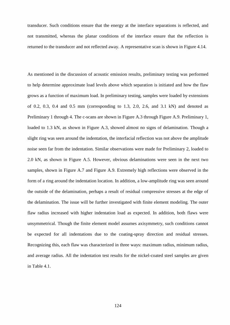
124
transducer. Such conditions ensure that the energy at the interface separations is reflected, and
not transmitted, whereas the planar conditions of the interface ensure that the reflection is
returned to the transducer and not reflected away. A representative scan is shown in Figure 4.14.
As mentioned in the discussion of acoustic emission results, preliminary testing was performed
to help determine approximate load levels above which separation is initiated and how the flaw
grows as a function of maximum load. In preliminary testing, samples were loaded by extensions
of 0.2, 0.3, 0.4 and 0.5 mm (corresponding to 1.3, 2.0, 2.6, and 3.1 kN) and denoted as
Preliminary 1 through 4. The c-scans are shown in Figure A.3 through Figure A.9. Preliminary 1,
loaded to 1.3 kN, as shown in Figure A.3, showed almost no signs of delamination. Though a
slight ring was seen around the indentation, the interfacial reflection was not above the amplitude
noise seen far from the indentation. Similar observations were made for Preliminary 2, loaded to
2.0 kN, as shown in Figure A.5. However, obvious delaminations were seen in the next two
samples, shown in Figure A.7 and Figure A.9. Extremely high reflections were observed in the
form of a ring around the indentation location. In addition, a low-amplitude ring was seen around
the outside of the delamination, perhaps a result of residual compressive stresses at the edge of
the delamination. The issue will be further investigated with finite element modeling. The outer
flaw radius increased with higher indentation load as expected. In addition, both flaws were
unsymmetrical. Though the finite element model assumes axisymmetry, such conditions cannot
be expected for all indentations due to the coating-spray direction and residual stresses.
Recognizing this, each flaw was characterized in three ways: maximum radius, minimum radius,
and average radius. All the indentation test results for the nickel-coated steel samples are given
in Table 4.1.
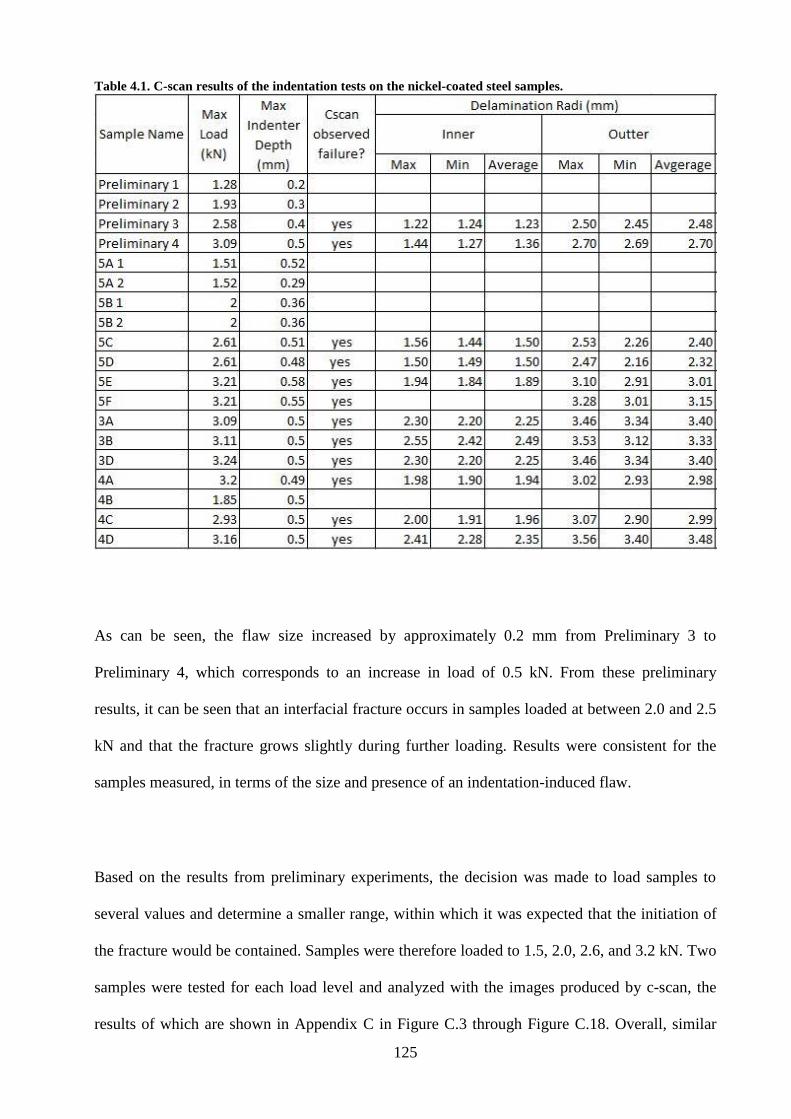
125
Table 4.1. C-scan results of the indentation tests on the nickel-coated steel samples.
As can be seen, the flaw size increased by approximately 0.2 mm from Preliminary 3 to
Preliminary 4, which corresponds to an increase in load of 0.5 kN. From these preliminary
results, it can be seen that an interfacial fracture occurs in samples loaded at between 2.0 and 2.5
kN and that the fracture grows slightly during further loading. Results were consistent for the
samples measured, in terms of the size and presence of an indentation-induced flaw.
Based on the results from preliminary experiments, the decision was made to load samples to
several values and determine a smaller range, within which it was expected that the initiation of
the fracture would be contained. Samples were therefore loaded to 1.5, 2.0, 2.6, and 3.2 kN. Two
samples were tested for each load level and analyzed with the images produced by c-scan, the
results of which are shown in Appendix C in Figure C.3 through Figure C.18. Overall, similar
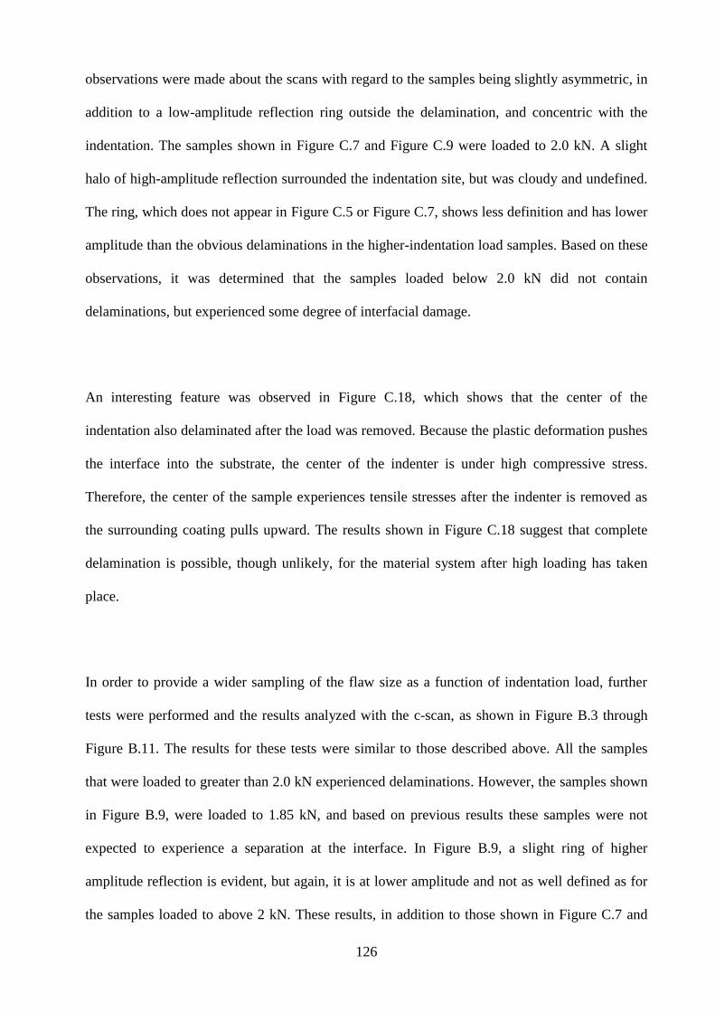
126
observations were made about the scans with regard to the samples being slightly asymmetric, in
addition to a low-amplitude reflection ring outside the delamination, and concentric with the
indentation. The samples shown in Figure C.7 and Figure C.9 were loaded to 2.0 kN. A slight
halo of high-amplitude reflection surrounded the indentation site, but was cloudy and undefined.
The ring, which does not appear in Figure C.5 or Figure C.7, shows less definition and has lower
amplitude than the obvious delaminations in the higher-indentation load samples. Based on these
observations, it was determined that the samples loaded below 2.0 kN did not contain
delaminations, but experienced some degree of interfacial damage.
An interesting feature was observed in Figure C.18, which shows that the center of the
indentation also delaminated after the load was removed. Because the plastic deformation pushes
the interface into the substrate, the center of the indenter is under high compressive stress.
Therefore, the center of the sample experiences tensile stresses after the indenter is removed as
the surrounding coating pulls upward. The results shown in Figure C.18 suggest that complete
delamination is possible, though unlikely, for the material system after high loading has taken
place.
In order to provide a wider sampling of the flaw size as a function of indentation load, further
tests were performed and the results analyzed with the c-scan, as shown in Figure B.3 through
Figure B.11. The results for these tests were similar to those described above. All the samples
that were loaded to greater than 2.0 kN experienced delaminations. However, the samples shown
in Figure B.9, were loaded to 1.85 kN, and based on previous results these samples were not
expected to experience a separation at the interface. In Figure B.9, a slight ring of higher
amplitude reflection is evident, but again, it is at lower amplitude and not as well defined as for
the samples loaded to above 2 kN. These results, in addition to those shown in Figure C.7 and
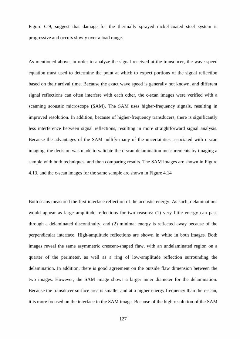
127
Figure C.9, suggest that damage for the thermally sprayed nickel-coated steel system is
progressive and occurs slowly over a load range.
As mentioned above, in order to analyze the signal received at the transducer, the wave speed
equation must used to determine the point at which to expect portions of the signal reflection
based on their arrival time. Because the exact wave speed is generally not known, and different
signal reflections can often interfere with each other, the c-scan images were verified with a
scanning acoustic microscope (SAM). The SAM uses higher-frequency signals, resulting in
improved resolution. In addition, because of higher-frequency transducers, there is significantly
less interference between signal reflections, resulting in more straightforward signal analysis.
Because the advantages of the SAM nullify many of the uncertainties associated with c-scan
imaging, the decision was made to validate the c-scan delamination measurements by imaging a
sample with both techniques, and then comparing results. The SAM images are shown in Figure
4.13, and the c-scan images for the same sample are shown in Figure 4.14
Both scans measured the first interface reflection of the acoustic energy. As such, delaminations
would appear as large amplitude reflections for two reasons: (1) very little energy can pass
through a delaminated discontinuity, and (2) minimal energy is reflected away because of the
perpendicular interface. High-amplitude reflections are shown in white in both images. Both
images reveal the same asymmetric crescent-shaped flaw, with an undelaminated region on a
quarter of the perimeter, as well as a ring of low-amplitude reflection surrounding the
delamination. In addition, there is good agreement on the outside flaw dimension between the
two images. However, the SAM image shows a larger inner diameter for the delamination.
Because the transducer surface area is smaller and at a higher energy frequency than the c-scan,
it is more focused on the interface in the SAM image. Because of the high resolution of the SAM
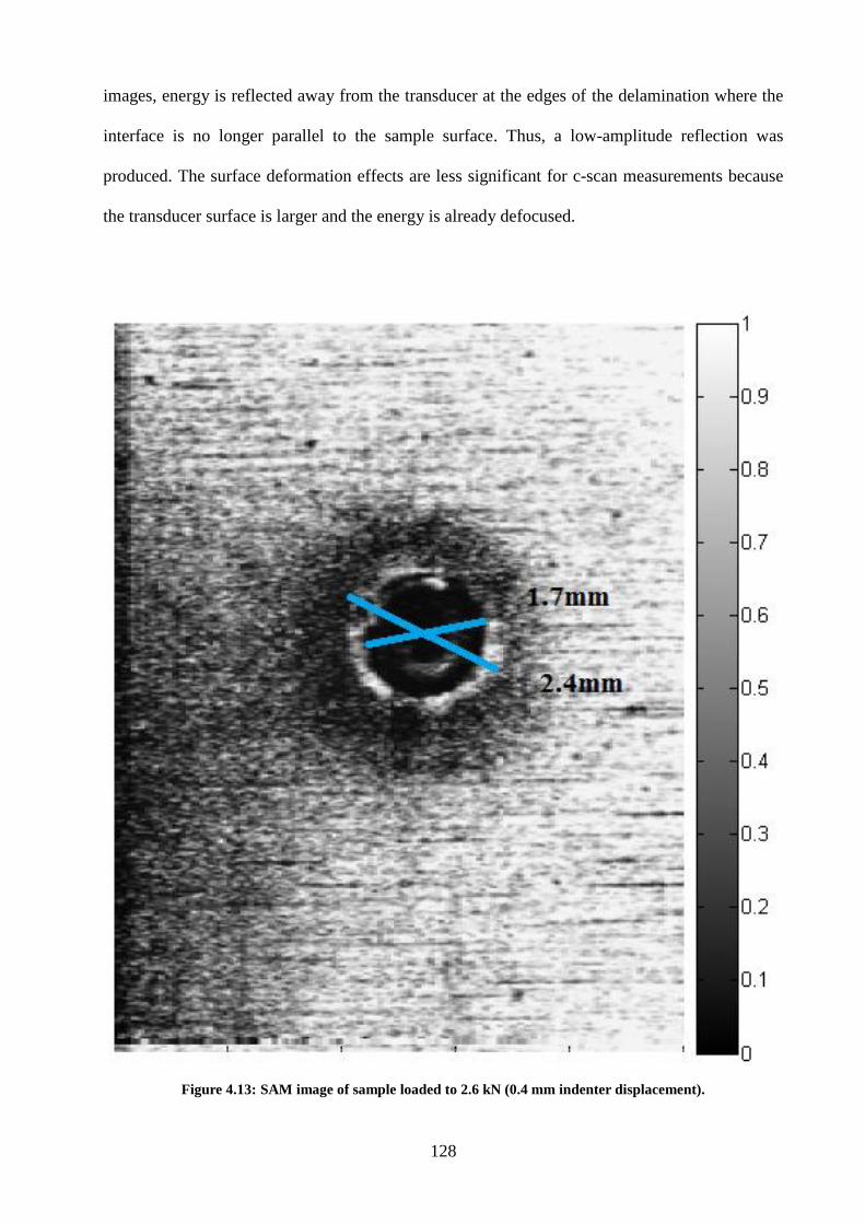
128
images, energy is reflected away from the transducer at the edges of the delamination where the
interface is no longer parallel to the sample surface. Thus, a low-amplitude reflection was
produced. The surface deformation effects are less significant for c-scan measurements because
the transducer surface is larger and the energy is already defocused.
Figure 4.13: SAM image of sample loaded to 2.6 kN (0.4 mm indenter displacement).
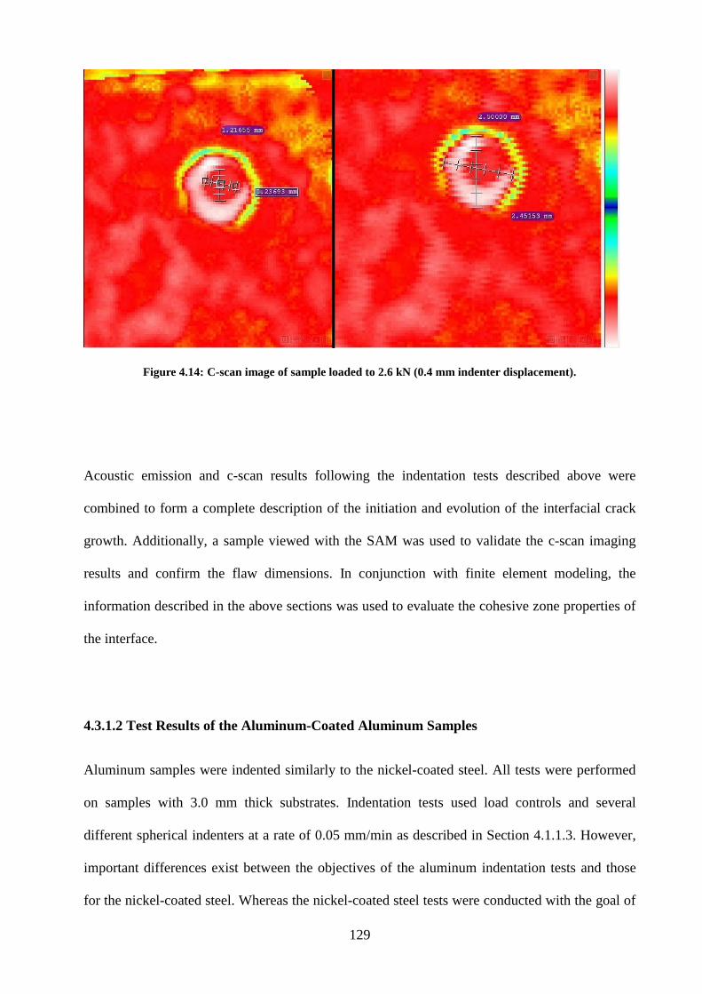
129
Figure 4.14: C-scan image of sample loaded to 2.6 kN (0.4 mm indenter displacement).
Acoustic emission and c-scan results following the indentation tests described above were
combined to form a complete description of the initiation and evolution of the interfacial crack
growth. Additionally, a sample viewed with the SAM was used to validate the c-scan imaging
results and confirm the flaw dimensions. In conjunction with finite element modeling, the
information described in the above sections was used to evaluate the cohesive zone properties of
the interface.
4.3.1.2 Test Results of the Aluminum-Coated Aluminum Samples
Aluminum samples were indented similarly to the nickel-coated steel. All tests were performed
on samples with 3.0 mm thick substrates. Indentation tests used load controls and several
different spherical indenters at a rate of 0.05 mm/min as described in Section 4.1.1.3. However,
important differences exist between the objectives of the aluminum indentation tests and those
for the nickel-coated steel. Whereas the nickel-coated steel tests were conducted with the goal of
130
accurately determining cohesive zone properties based on experiments and finite element
modeling, the aluminum experiments were designed to validate the cohesive zone and the
indentation models in addition to the property measurement technique.
Coating thickness varied significantly on the four samples tested, which made repeated tests
difficult. In addition, plastic deformation in the cold-sprayed aluminum coating released high
amounts of acoustic energy due to cracking, making it difficult to analyze the emissions data
during loading because of the high background noise level throughout the test. On the basis of
these difficulties, the decision was made to use the aluminum-coated aluminum indentation and
four-point bend samples for the purpose of validating the indentation model. Because the
interfaces of indentation and four-point bend tests were the same, even though the coating was
milled down to a thickness more appropriate for indentation testing, the cohesive zone properties
measured based on the indentation test can be applied to the four-point bend test. Accurately
predicting the results of one test with properties measured from a different experiment provides
validation for the indentation, four-point bend, and cohesive zone models. After the indentation
tests were completed and the acoustic emissions collected, according to the procedures described
in Section 4.1.3, c-scan images of the samples were recorded.
4.3.1.2.1 Acoustic Emission Results for the Aluminum-Coated Aluminum Samples
As with the nickel-coated steel, acoustic emissions were recorded during indentation testing of
the aluminum-coated aluminum samples. However, the results pertaining to the indentation of
the latter could not be analyzed because they included too much noise; the samples experienced
significant cracking during the indentation test, creating high-energy events that were frequent
enough to raise the noise level to a point that made it impossible to determine whether any other
significant events were occurring. For completeness, plots of the acoustic emission results
131
corresponding to the aluminum indentation results and the c-scans for the individual tests are
included in 0.
Crack growth is also likely to occur during unloading. Because further cracking and plastic
deformation are less likely during load removal than during loading, acoustic emissions were
recorded during unloading for several samples; one such plot is shown in Figure D.17. As the
results were recorded during unloading, acoustic emission collection began at a load of 5 kN, and
recording was stopped at the end of the test, when the load was 0 kN. As can be seen in the
figure, large energy acoustic events occur at low load levels at the end of unloading. It is possible
that these events are delamination initiation and growth during unloading and will require further
analysis in order to determine whether they are the result of delamination or of a source of noise
in the system.
4.3.1.2.2 C-scan Results for the Aluminum-Coated Aluminum Samples
C-scans were performed on the aluminum sample indentations to determine the amount of
delamination that took place. In order to image the interface of the samples, ultrasonic energy
was directed at the sample, the reflections of which are measured and plotted as described in
Section 4.1.3.4. In order to analyze the aluminum samples, the time of flight of the signal was
also recorded and used to determine the dimension of any delaminations present. Scans revealed
that delamination occurred in all the samples with a coating thicker than 0.9 mm, whereas it was
concluded that indentations on the thinner samples did not result in any interfacial separation.
A first set of scans was performed on the indentations of the samples with the thicker coatings,
i.e., coatings thicker than 0.8 mm. Scans of the time of flight and the first interface reflection for

132
all the samples are shown in 0. One particular indentation was close to the edge of the sample
and actually fractured to the edge. In this case, the fracture can be confirmed by visual
inspection, allowing for the scan results to be used to determine the features of the internal
delaminations in the aluminum samples. Such features will be used in future scans as indications
of interface separation. Scans showing the amplitude of the returned signal and the time of flight
for that signal are shown in Figure 4.15.
Figure 4.15: Scan of (a) amplitude and (b) time of flight of the signal for a 2.0 mm indenter loaded to 4.75 kN.
Because the scan was of a known delamination at the edge of a specimen, the characteristics of
the scan features shown in Figure 4.15 can be used to determine whether other samples also had
133
similar damage. As can be seen from the scan of the amplitude of the interface reflection, the
edges of the delaminations are characterized by low-amplitude reflections. In addition, the time
of flight scan showed a significantly shorter flight time for a signal reflected from a
delamination, as shown by the lighter portion of the spectrum in Figure 4.15b, than for a signal
reflected from the surrounding interface. As expected, the shorter time of flight confirms that the
signal travels a shorter distance at a delamination. Understanding and recognizing these
characteristics makes it possible to identify the internal delaminations in the other samples.
Two more scans of indentations in coatings of approximately the same thickness and load as
those just described are shown in 0, Figure D.16 and Figure D.18. In terms of the information
gained from the scans described above, the coating and substrate of the samples appear to have
separated. Consistent with observations from Figure 4.15, the indentations are characterized by a
low-amplitude first-wall reflection that encircles the indentation. In addition, the time of flight of
the reflection is shorter for the delaminated area than for the surrounding scan. Compared with
those in Figure 4.15, the scans have features consistent with those with a confirmed
delamination. Based on the features just described, it was concluded that delaminations were
present in the two scans using the data in Figure D.16 and Figure D.18; the diameters of the
delaminations were measured and recorded (see Table 4.4).
Indentations were also made in samples with thinner coatings, on the order of 0.37 to 0.6 mm.
The information from these scans is given in 0, Figure D.1 though Figure D.12. Though these
indentations were made with similar loads as those described above, they were on samples with
thin coatings, and none of the c-scan features described above was present. Scans of the first-
wall amplitude reflection, in addition to the time of flight, for the entire sample are shown in
Figure 4.16.
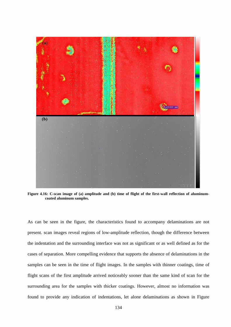
134
Figure 4.16: C-scan image of (a) amplitude and (b) time of flight of the first-wall reflection of aluminum-
coated aluminum samples.
As can be seen in the figure, the characteristics found to accompany delaminations are not
present. scan images reveal regions of low-amplitude reflection, though the difference between
the indentation and the surrounding interface was not as significant or as well defined as for the
cases of separation. More compelling evidence that supports the absence of delaminations in the
samples can be seen in the time of flight images. In the samples with thinner coatings, time of
flight scans of the first amplitude arrived noticeably sooner than the same kind of scan for the
surrounding area for the samples with thicker coatings. However, almost no information was
found to provide any indication of indentations, let alone delaminations as shown in Figure
135
4.16b. Based on the amplitude and time of flight scans, it was concluded that indentations did not
create delaminations on samples with coatings thinner than 0.75 mm for all of the load levels in
the experiments.
The scans shown in Figure 4.16 do not show the same first-amplitude reflection characteristics
and contain almost no information in the time of flight to suggest that there are delaminations
like those shown in Figure 4.25. The ultrasonic reflection characteristics of delamination in the
aluminum samples studied in this section differed significantly from those in Section 4.3.1.1.
Delamination characteristics varied between the two largely due to the differences in stiffness
between the coatings and substrates of each. In the case of the aluminum, it is likely that the low-
amplitude reflections are the result of large deflections from the interface. When ultrasonic
energy reaches an interface, it is reflected and transmitted, as described earlier. However, when
that interface is not perpendicular to the transducer, large portions of the energy are reflected
away from the transducer, creating the appearance of a low-energy reflection. It is likely that the
edges of the actual indentation are regions where the most energy would be deflected because of
this effect, whereas the area close to the indentation is more parallel and will reflect energy in a
way that is similar to the surrounding, unaffected interface. Substrate and coating-material
property similarities resulted in large deformations at the interface, and the relatively soft nickel
coating the steel substrates resulted in deformations predominantly in the coating. Therefore,
very little deformation occurred in the substrate relative to the coating. The interface, therefore,
remained perpendicular to the transducer. As the interface remains relatively flat, ultrasonic
energy can be reflected back toward the transducer, creating a high-amplitude reflection from the
interface. On the other hand, in the cases in which significant deformation was seen at the
interface, i.e., the aluminum samples, the energy is deflected away.
136
4.3.2 Four-Point Bend Test Results
Four-point bend tests on the samples of nickel-coated steel and on those of aluminum cold
sprayed on aluminum as described in Section 4.1.1.3, were completed. In both cases, the tests did
not produce results useful for directly calculating the critical fracture energy. In the case of the
aluminum-coated aluminum samples, the fracture occurred almost instantaneously; in fact, the
nickel-coated steel samples experienced significant plastic deformation before steady-state
fracture could occur. Given these results, it is clear that the samples chosen for this research
cannot be included in the narrow set of materials that can be properly evaluated with the four-
point bend test. Nevertheless, some information was gained from the four-point bend test that
was used in the later model and experimental work for interface characterization.
4.3.2.1 Test Results for the Nickel-Coated Steel Samples
Attempts to use the four-point bend test to evaluate the critical fracture energy of the nickel-
coated steel samples failed, as excessive plastic deformation occurred before a pre-crack could
be introduced. This plastic deformation was confined to the center of the specimen. As a result,
steady state crack growth as a function of four-point indenter displacement could not be
achieved. Because of the steady state crack growth requirement, the test could not be used to
evaluate the critical fracture energy, highlighting a major shortcoming of the four-point bend test
as it relates to interfacial characterization. In light of the difficulties associated with the
application of the four-point bend test for measuring the critical energy release rate, the decision
was made to test the unused specimens of the same dimensions using indentation experiments.

137
4.3.2.2 Test Results for the Aluminum-Coated Aluminum Samples
The aluminum samples, 7075 cold-sprayed aluminum on aluminum substrates, also proved to be
poorly suited for four-point bend test evaluation. However, unlike the nickel-coated steel
specimens, which showed excessive plastic deformation even before a pre-crack could be
introduced, the aluminum samples experienced near instantaneous crack growth to the load span
after initiation. Such instantaneous crack growth poses two problems in terms of using the four-
point bend test. The test requires that a pre-crack be introduced, as the critical fracture energy is
defined as the energy required for reinitiating crack growth at the tip of a pre-crack. In addition,
the four-point bend test requires that the crack growth be steady and constant as a function of the
applied load. As such, the aluminum samples presented enough problems for the four-point bend
test to be considered an unworkable option for evaluating the critical fracture energy of the
interface.
Clearly, the four-point bend test proved to be inadequate for critical fracture energy evaluation.
However, it did result in crack growth, the initiation and behavior of which were strong functions
of the bond strength and critical fracture energy. As such, the information from the four-point
bend test, specifically the load at which the fracture was initiated and the brittle behavior of the
fracture, are all functions of the interfacial properties. Therefore, once the cohesive zone
properties have been measured based on any given test, the application of those properties to
predict and compare results from another experiment provide a unique opportunity to validate
the cohesive zone and the property measurement procedures.
For instance, the load displacement results of the four-point bend test of an aluminum-coated
aluminum sample with a coating thickness of 1 mm are shown in Figure 4.17.
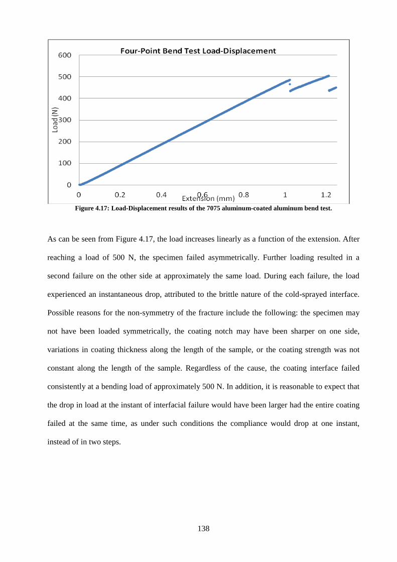
138
Figure 4.17: Load-Displacement results of the 7075 aluminum-coated aluminum bend test.
As can be seen from Figure 4.17, the load increases linearly as a function of the extension. After
reaching a load of 500 N, the specimen failed asymmetrically. Further loading resulted in a
second failure on the other side at approximately the same load. During each failure, the load
experienced an instantaneous drop, attributed to the brittle nature of the cold-sprayed interface.
Possible reasons for the non-symmetry of the fracture include the following: the specimen may
not have been loaded symmetrically, the coating notch may have been sharper on one side,
variations in coating thickness along the length of the sample, or the coating strength was not
constant along the length of the sample. Regardless of the cause, the coating interface failed
consistently at a bending load of approximately 500 N. In addition, it is reasonable to expect that
the drop in load at the instant of interfacial failure would have been larger had the entire coating
failed at the same time, as under such conditions the compliance would drop at one instant,
instead of in two steps.
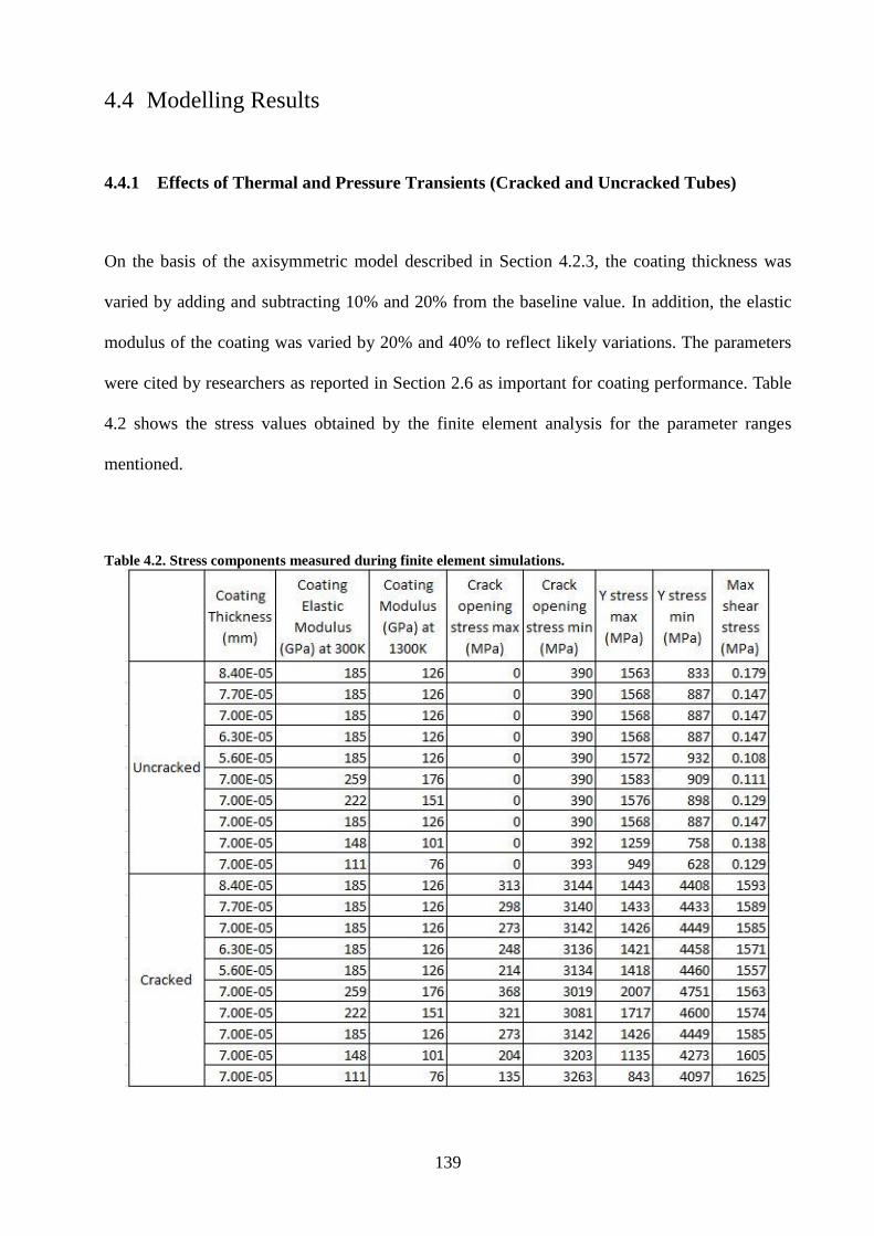
139
4.4 Modelling Results
4.4.1 Effects of Thermal and Pressure Transients (Cracked and Uncracked Tubes)
On the basis of the axisymmetric model described in Section 4.2.3, the coating thickness was
varied by adding and subtracting 10% and 20% from the baseline value. In addition, the elastic
modulus of the coating was varied by 20% and 40% to reflect likely variations. The parameters
were cited by researchers as reported in Section 2.6 as important for coating performance. Table
4.2 shows the stress values obtained by the finite element analysis for the parameter ranges
mentioned.
Table 4.2. Stress components measured during finite element simulations.
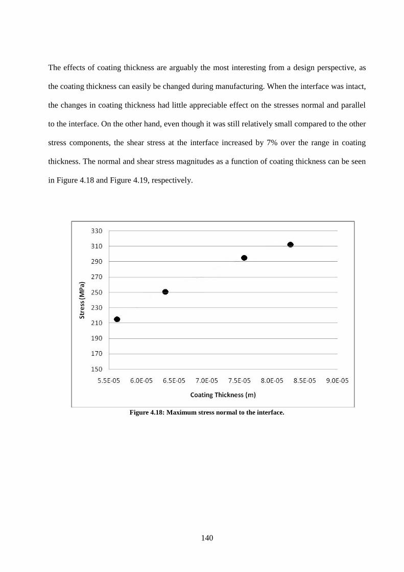
140
The effects of coating thickness are arguably the most interesting from a design perspective, as
the coating thickness can easily be changed during manufacturing. When the interface was intact,
the changes in coating thickness had little appreciable effect on the stresses normal and parallel
to the interface. On the other hand, even though it was still relatively small compared to the other
stress components, the shear stress at the interface increased by 7% over the range in coating
thickness. The normal and shear stress magnitudes as a function of coating thickness can be seen
in Figure 4.18 and Figure 4.19, respectively.
Figure 4.18: Maximum stress normal to the interface.
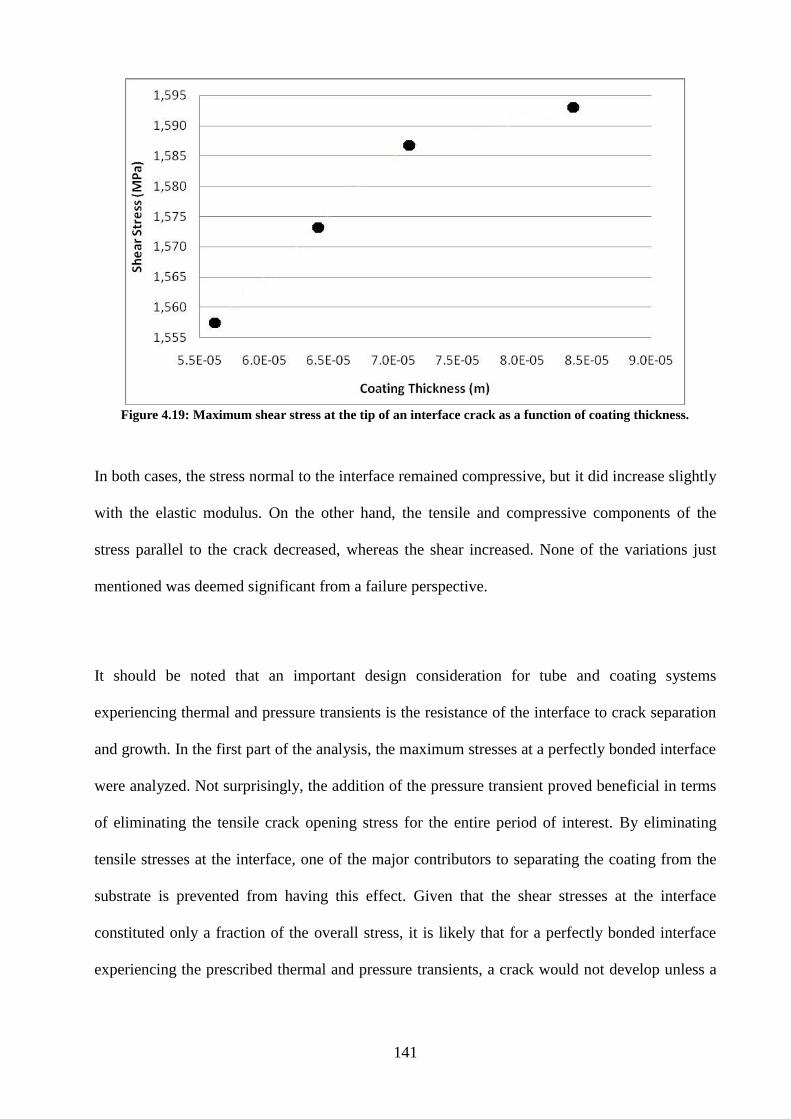
141
Figure 4.19: Maximum shear stress at the tip of an interface crack as a function of coating thickness.
In both cases, the stress normal to the interface remained compressive, but it did increase slightly
with the elastic modulus. On the other hand, the tensile and compressive components of the
stress parallel to the crack decreased, whereas the shear increased. None of the variations just
mentioned was deemed significant from a failure perspective.
It should be noted that an important design consideration for tube and coating systems
experiencing thermal and pressure transients is the resistance of the interface to crack separation
and growth. In the first part of the analysis, the maximum stresses at a perfectly bonded interface
were analyzed. Not surprisingly, the addition of the pressure transient proved beneficial in terms
of eliminating the tensile crack opening stress for the entire period of interest. By eliminating
tensile stresses at the interface, one of the major contributors to separating the coating from the
substrate is prevented from having this effect. Given that the shear stresses at the interface
constituted only a fraction of the overall stress, it is likely that for a perfectly bonded interface
experiencing the prescribed thermal and pressure transients, a crack would not develop unless a
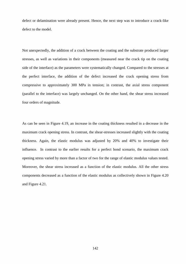
142
defect or delamination were already present. Hence, the next step was to introduce a crack-like
defect to the model.
Not unexpectedly, the addition of a crack between the coating and the substrate produced larger
stresses, as well as variations in their components (measured near the crack tip on the coating
side of the interface) as the parameters were systematically changed. Compared to the stresses at
the perfect interface, the addition of the defect increased the crack opening stress from
compressive to approximately 300 MPa in tension; in contrast, the axial stress component
(parallel to the interface) was largely unchanged. On the other hand, the shear stress increased
four orders of magnitude.
As can be seen in Figure 4.19, an increase in the coating thickness resulted in a decrease in the
maximum crack opening stress. In contrast, the shear-stresses increased slightly with the coating
thickness. Again, the elastic modulus was adjusted by 20% and 40% to investigate their
influence. In contrast to the earlier results for a perfect bond scenario, the maximum crack
opening stress varied by more than a factor of two for the range of elastic modulus values tested.
Moreover, the shear stress increased as a function of the elastic modulus. All the other stress
components decreased as a function of the elastic modulus as collectively shown in Figure 4.20
and Figure 4.21.
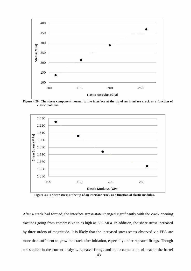
143
Figure 4.20: The stress component normal to the interface at the tip of an interface crack as a function of
elastic modulus.
Figure 4.21: Shear stress at the tip of an interface crack as a function of elastic modulus.
After a crack had formed, the interface stress-state changed significantly with the crack opening
tractions going from compressive to as high as 300 MPa. In addition, the shear stress increased
by three orders of magnitude. It is likely that the increased stress-states observed via FEA are
more than sufficient to grow the crack after initiation, especially under repeated firings. Though
not studied in the current analysis, repeated firings and the accumulation of heat in the barrel
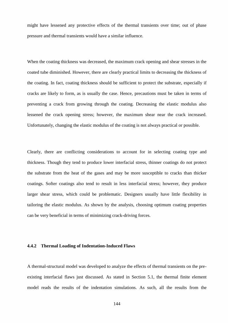
144
might have lessened any protective effects of the thermal transients over time; out of phase
pressure and thermal transients would have a similar influence.
When the coating thickness was decreased, the maximum crack opening and shear stresses in the
coated tube diminished. However, there are clearly practical limits to decreasing the thickness of
the coating. In fact, coating thickness should be sufficient to protect the substrate, especially if
cracks are likely to form, as is usually the case. Hence, precautions must be taken in terms of
preventing a crack from growing through the coating. Decreasing the elastic modulus also
lessened the crack opening stress; however, the maximum shear near the crack increased.
Unfortunately, changing the elastic modulus of the coating is not always practical or possible.
Clearly, there are conflicting considerations to account for in selecting coating type and
thickness. Though they tend to produce lower interfacial stress, thinner coatings do not protect
the substrate from the heat of the gases and may be more susceptible to cracks than thicker
coatings. Softer coatings also tend to result in less interfacial stress; however, they produce
larger shear stress, which could be problematic. Designers usually have little flexibility in
tailoring the elastic modulus. As shown by the analysis, choosing optimum coating properties
can be very beneficial in terms of minimizing crack-driving forces.
4.4.2 Thermal Loading of Indentation-Induced Flaws
A thermal-structural model was developed to analyze the effects of thermal transients on the pre-
existing interfacial flaws just discussed. As stated in Section 5.1, the thermal finite element
model reads the results of the indentation simulations. As such, all the results from the
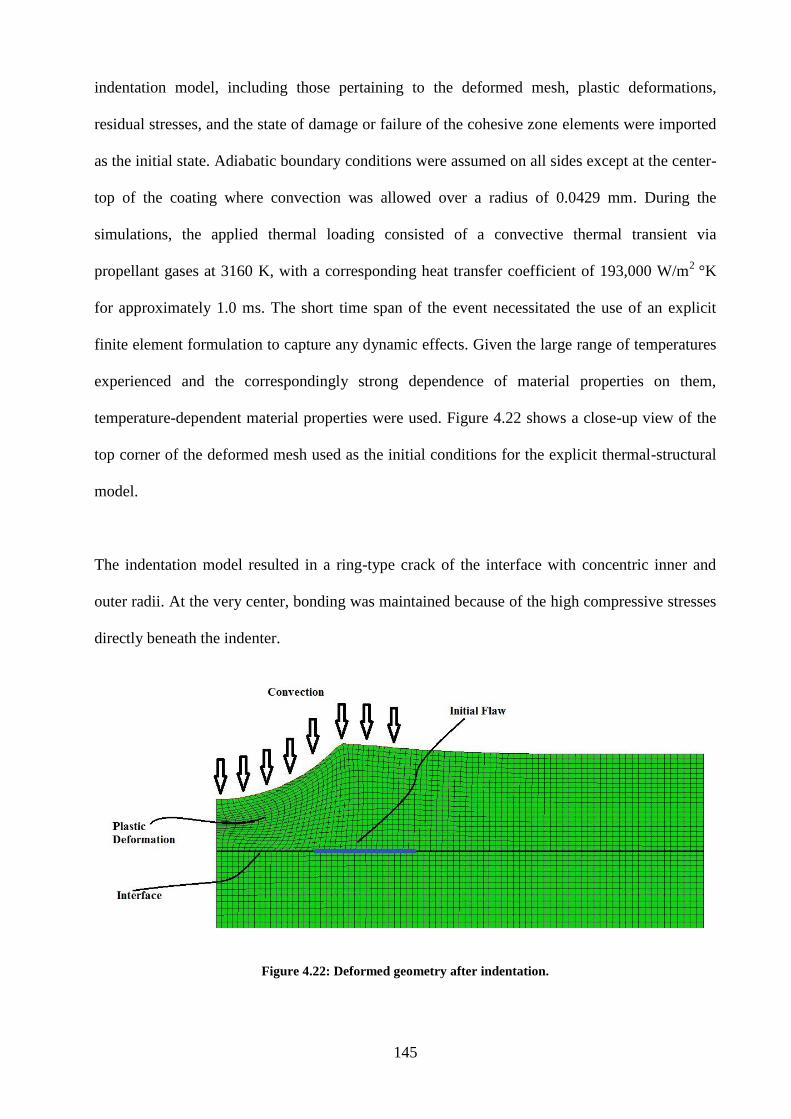
145
indentation model, including those pertaining to the deformed mesh, plastic deformations,
residual stresses, and the state of damage or failure of the cohesive zone elements were imported
as the initial state. Adiabatic boundary conditions were assumed on all sides except at the center-
top of the coating where convection was allowed over a radius of 0.0429 mm. During the
simulations, the applied thermal loading consisted of a convective thermal transient via
propellant gases at 3160 K, with a corresponding heat transfer coefficient of 193,000 W/m2
°K
for approximately 1.0 ms. The short time span of the event necessitated the use of an explicit
finite element formulation to capture any dynamic effects. Given the large range of temperatures
experienced and the correspondingly strong dependence of material properties on them,
temperature-dependent material properties were used. Figure 4.22 shows a close-up view of the
top corner of the deformed mesh used as the initial conditions for the explicit thermal-structural
model.
The indentation model resulted in a ring-type crack of the interface with concentric inner and
outer radii. At the very center, bonding was maintained because of the high compressive stresses
directly beneath the indenter.
Figure 4.22: Deformed geometry after indentation.
146
The effects of the bond-strength and critical fracture energy were also analyzed in terms of flaw
growth under thermal transients for indentation-induced flaws. In order to reduce the number of
interface parameters from four to two, Mode I and II fracture energies were coupled according to
Equation (4.41), whereas the normal and shear strengths were related according to Equation
(4.42).
12sin11
IcG (4.41)
maxmax
2
1S
eqN
n
t
(4.42)
As the phase angle increases so does the fracture energy, as represented by Hutchinson and Suo
[116] and shown in Equation (4.41). The parameter λ governs the influence of Mode II fracture
energy and is generally assumed to be a function of the surface roughness; for this study, the
parameter λ was assumed to be 0.3, which is a common value for an interface of moderate
roughness. In addition, the normal and shear strength of the interface can be considered
manifestations of the cohesive zone model given by Abdul-Baqi et al. [87] as shown in Equation
(4.42). The coupling parameter q was assumed to be 0.5 to relate the normal and shear strengths
of the cohesive zone.
The normal strength and Mode I fracture energy were independently varied to analyze their
effects on the initial flaw size after indentation, on any dimensional changes that occurred during
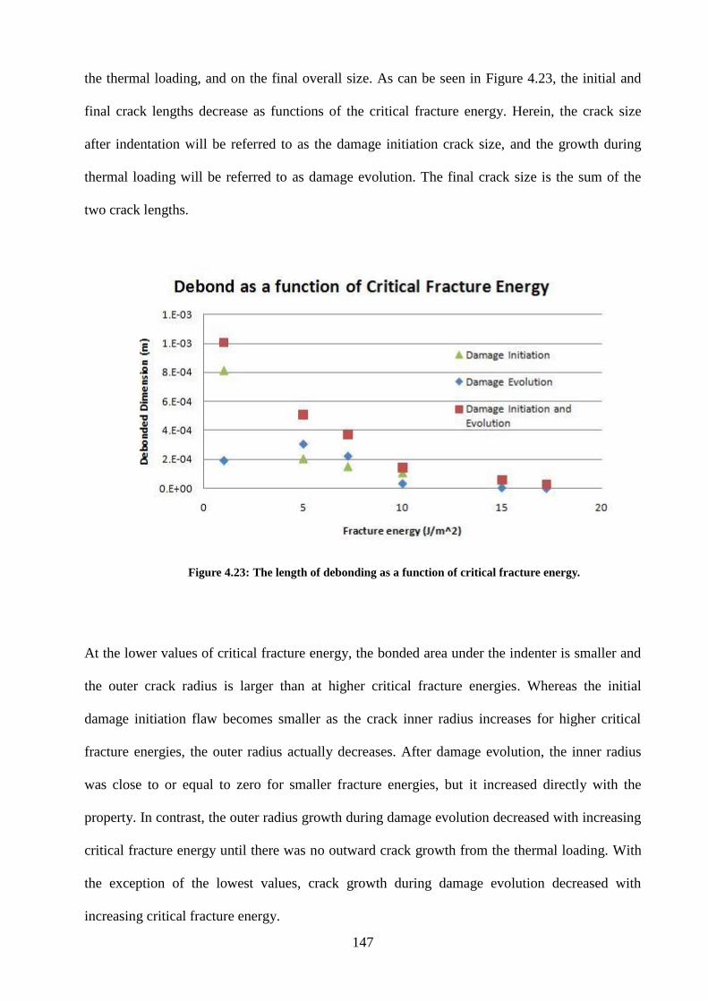
147
the thermal loading, and on the final overall size. As can be seen in Figure 4.23, the initial and
final crack lengths decrease as functions of the critical fracture energy. Herein, the crack size
after indentation will be referred to as the damage initiation crack size, and the growth during
thermal loading will be referred to as damage evolution. The final crack size is the sum of the
two crack lengths.
Figure 4.23: The length of debonding as a function of critical fracture energy.
At the lower values of critical fracture energy, the bonded area under the indenter is smaller and
the outer crack radius is larger than at higher critical fracture energies. Whereas the initial
damage initiation flaw becomes smaller as the crack inner radius increases for higher critical
fracture energies, the outer radius actually decreases. After damage evolution, the inner radius
was close to or equal to zero for smaller fracture energies, but it increased directly with the
property. In contrast, the outer radius growth during damage evolution decreased with increasing
critical fracture energy until there was no outward crack growth from the thermal loading. With
the exception of the lowest values, crack growth during damage evolution decreased with
increasing critical fracture energy.
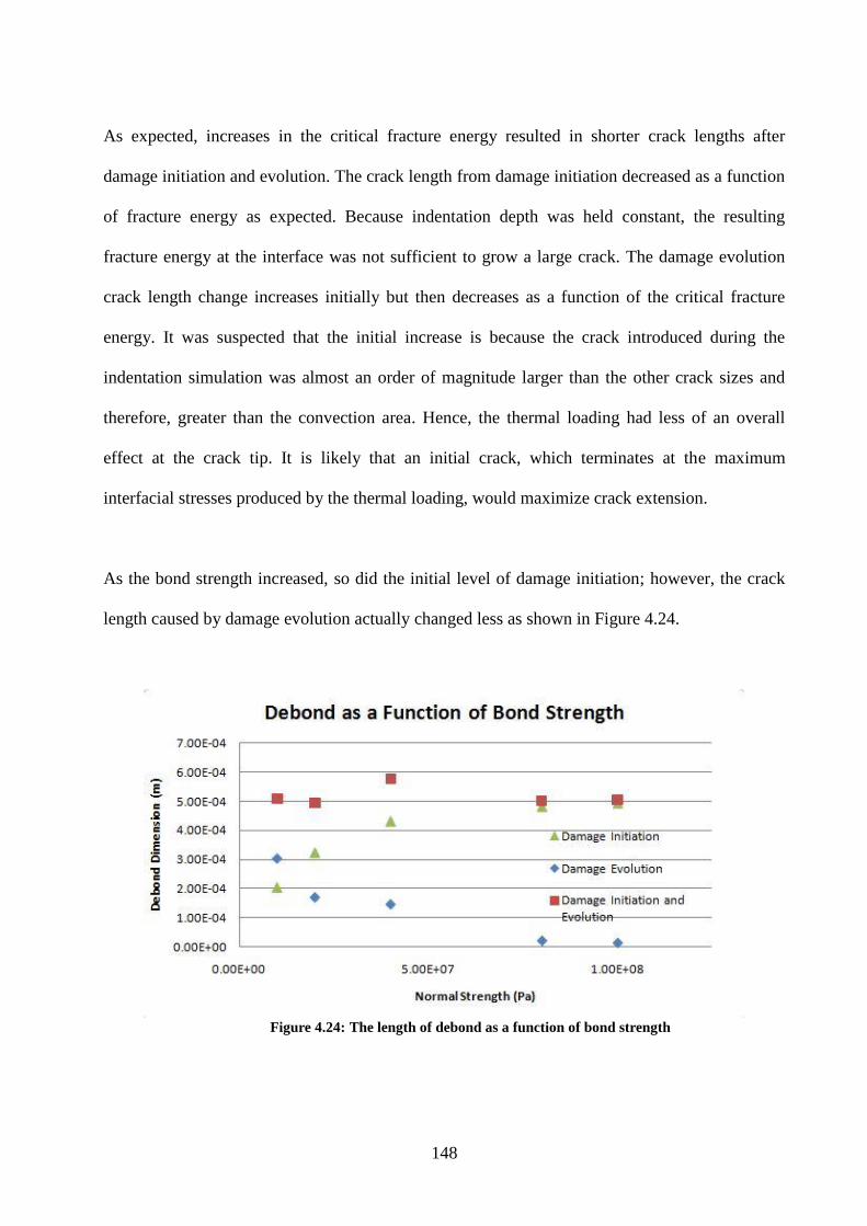
148
As expected, increases in the critical fracture energy resulted in shorter crack lengths after
damage initiation and evolution. The crack length from damage initiation decreased as a function
of fracture energy as expected. Because indentation depth was held constant, the resulting
fracture energy at the interface was not sufficient to grow a large crack. The damage evolution
crack length change increases initially but then decreases as a function of the critical fracture
energy. It was suspected that the initial increase is because the crack introduced during the
indentation simulation was almost an order of magnitude larger than the other crack sizes and
therefore, greater than the convection area. Hence, the thermal loading had less of an overall
effect at the crack tip. It is likely that an initial crack, which terminates at the maximum
interfacial stresses produced by the thermal loading, would maximize crack extension.
As the bond strength increased, so did the initial level of damage initiation; however, the crack
length caused by damage evolution actually changed less as shown in Figure 4.24.
Figure 4.24: The length of debond as a function of bond strength
149
After damage initiation as a function of cohesive strength, the inner radius initially increased, but
then held constant, whereas the outer radius increased. After damage evolution, the bonded
region maintained by the compressive stresses under the indenter disappeared, except for the
highest bond strength evaluated. The post-damage evolution outer radius was approximately the
same for all strengths. On the other hand, the amount of damage evolution decreased with
increasing cohesive strength. The final crack length was approximately the same for all
simulations, except when the bond strength was 4 MPa, which had a slightly higher final crack
length.
The constant displacement depth of the indenter can explain the seemingly counterintuitive
increase in the initial crack length with cohesive strength during damage initiation. Because the
stiffness of the interface and total energy required to grow the crack (critical fracture energy) are
constants, increasing the bond strength results in the expenditure of a larger portion of the
required energy to grow the crack before critical strength is achieved. Subsequently, less energy
is required to grow the crack to completion after damage is initiated, and the maximum
separation, shown as δc in Figure 4.2, is also lower due to the higher bond strength. In addition,
the crack length after damage evolution was found to be approximately constant for all the bond
strengths evaluated. It is likely that the constant post-damage evolution crack radii is a result of
the diminishing tensile/shear effects away from the convective heating that cannot extend crack
beyond a radius of approximately 0.5 mm. This is due to diminishing thermal effects because of
the constant radius of surface heating. Moreover, increasing the cohesive strength appears to
have opposite effects on damage evolution and damage initiation. However, because of the
complicated interaction between the initial crack length, the convective heating radius, and the
bond strength, it is not wise to suggest that decreasing the bond strength will decrease damage
evolution under thermal transients. In addition, after damage is initiated in the cohesive zone
elements, the model elements must still overcome the critical fracture energy before the crack
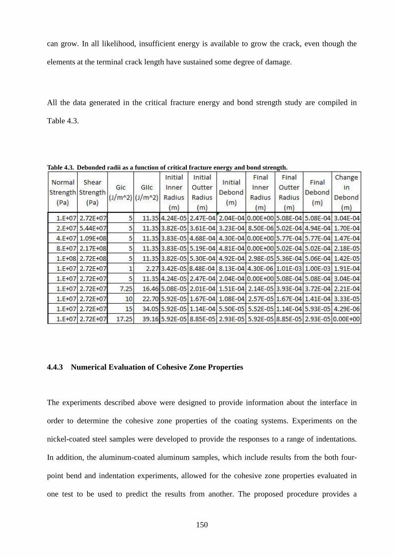
150
can grow. In all likelihood, insufficient energy is available to grow the crack, even though the
elements at the terminal crack length have sustained some degree of damage.
All the data generated in the critical fracture energy and bond strength study are compiled in
Table 4.3.
Table 4.3. Debonded radii as a function of critical fracture energy and bond strength.
4.4.3 Numerical Evaluation of Cohesive Zone Properties
The experiments described above were designed to provide information about the interface in
order to determine the cohesive zone properties of the coating systems. Experiments on the
nickel-coated steel samples were developed to provide the responses to a range of indentations.
In addition, the aluminum-coated aluminum samples, which include results from the both four-
point bend and indentation experiments, allowed for the cohesive zone properties evaluated in
one test to be used to predict the results from another. The proposed procedure provides a

151
rigorous validation of both the indentation and cohesive zone model and a procedure to measure
the properties.
The cohesive zone approach simulates all parts of the initiation and the evolution of damage.
Accurately simulating one part of crack evolution, for example crack initiation, does not
guarantee that the model will acceptably describe ensuing events. As such, accurately
determining the properties that describe all the crack growth events necessarily provides
confidence that the cohesive zone models the processes that contribute to crack growth, and not
just a single event. It is to be expected that indentations to different load levels will result in
varying crack-tip loading conditions. Therefore, modeling the crack growth at different
indentation loads will provide a more robust description of the cohesive zone properties that
accurately model crack growth in a coated sample.
Further validation of the indentation and cohesive zone models was provided by the four-point
bend test results for the aluminum-coated aluminum samples. It was not possible to rigorously
describe the important events of the crack growth process during the indentation tests, as was
done for the nickel-coated steel indentation samples. However, the information gained from the
two tests provides another opportunity to validate the indentation model, in addition to
confirming the cohesive zone model’s ability to describe progressive crack growth with
measured properties.
152
4.4.3.1 Cohesive Zone Property Measurements of the Nickel-Coated Steel Samples with
Delamination
Delamination at various loads have been determined for the nickel-coated steel samples, as has
information relating to the load at its onset based on in-situ acoustic emission analysis and on the
post-test scan results of tests stopped at intermediate load levels. Delamination was expected to
correspond to a high-energy acoustic event, the approximate time range of which can be
investigated through finite element modeling. Experiments and finite element modeling will
provide a thorough description of the delamination processes, from the crack initiation load, the
evolution of the crack size as a function of the maximum load, and the final crack size after
unloading.
Based on the empirically determined results, the described method proposes to evaluate cohesive
bond strength and critical energy release rate by matching experimental results with finite
element simulations. Such an analysis will be performed with simulations by choosing cohesive
zone properties, running the indentation simulation described in Section 4.2.5, and comparing
the experimental and numerical results. Such results include load-displacement data,
delamination radius as a function of load, and approximate load at the initiation of delamination.
Properties of the cold-sprayed nickel coating used in finite element modeling were obtained from
Sen et al. [162].
Experimental indentations on the nickel-coated steel specimens were completed, the results of
which are described in Section 4.3.1.1. Specimens were loaded to one of three loads, 2.6, 3.0,
and 3.2 kN, before being unloaded. Three or more tests were conducted for each load level,
before the delamination areas were measured and analyzed. Cohesive zone parameters were first
chosen for the finite element model to match experimental results for the indentation
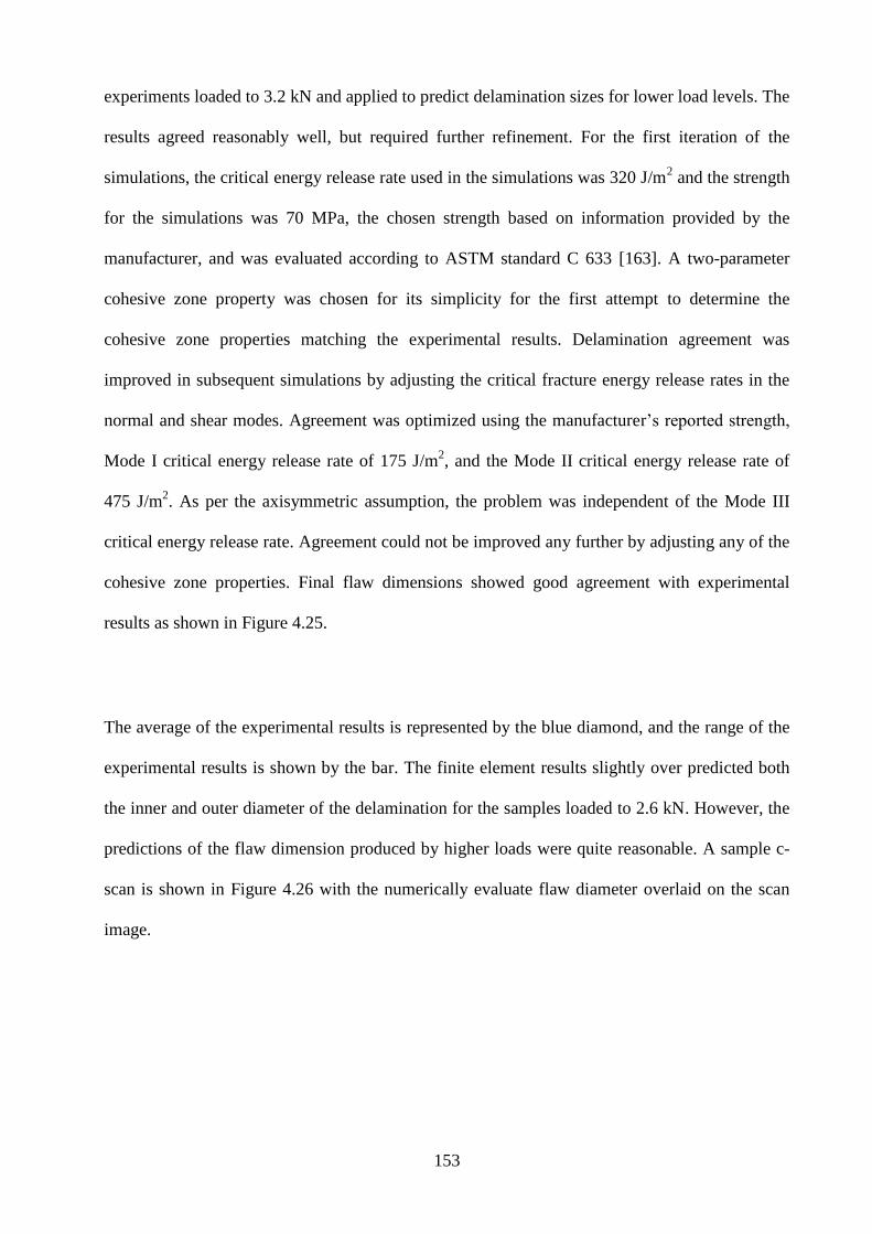
153
experiments loaded to 3.2 kN and applied to predict delamination sizes for lower load levels. The
results agreed reasonably well, but required further refinement. For the first iteration of the
simulations, the critical energy release rate used in the simulations was 320 J/m2 and the strength
for the simulations was 70 MPa, the chosen strength based on information provided by the
manufacturer, and was evaluated according to ASTM standard C 633 [163]. A two-parameter
cohesive zone property was chosen for its simplicity for the first attempt to determine the
cohesive zone properties matching the experimental results. Delamination agreement was
improved in subsequent simulations by adjusting the critical fracture energy release rates in the
normal and shear modes. Agreement was optimized using the manufacturer’s reported strength,
Mode I critical energy release rate of 175 J/m2, and the Mode II critical energy release rate of
475 J/m2. As per the axisymmetric assumption, the problem was independent of the Mode III
critical energy release rate. Agreement could not be improved any further by adjusting any of the
cohesive zone properties. Final flaw dimensions showed good agreement with experimental
results as shown in Figure 4.25.
The average of the experimental results is represented by the blue diamond, and the range of the
experimental results is shown by the bar. The finite element results slightly over predicted both
the inner and outer diameter of the delamination for the samples loaded to 2.6 kN. However, the
predictions of the flaw dimension produced by higher loads were quite reasonable. A sample c-
scan is shown in Figure 4.26 with the numerically evaluate flaw diameter overlaid on the scan
image.
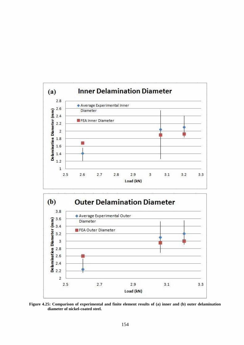
154
Figure 4.25: Comparison of experimental and finite element results of (a) inner and (b) outer delamination
diameter of nickel-coated steel.
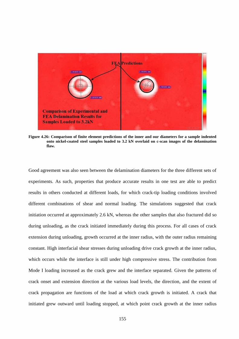
155
Figure 4.26: Comparison of finite element predictions of the inner and our diameters for a sample indented
onto nickel-coated steel samples loaded to 3.2 kN overlaid on c-scan images of the delamination
flaw.
Good agreement was also seen between the delamination diameters for the three different sets of
experiments. As such, properties that produce accurate results in one test are able to predict
results in others conducted at different loads, for which crack-tip loading conditions involved
different combinations of shear and normal loading. The simulations suggested that crack
initiation occurred at approximately 2.6 kN, whereas the other samples that also fractured did so
during unloading, as the crack initiated immediately during this process. For all cases of crack
extension during unloading, growth occurred at the inner radius, with the outer radius remaining
constant. High interfacial shear stresses during unloading drive crack growth at the inner radius,
which occurs while the interface is still under high compressive stress. The contribution from
Mode I loading increased as the crack grew and the interface separated. Given the patterns of
crack onset and extension direction at the various load levels, the direction, and the extent of
crack propagation are functions of the load at which crack growth is initiated. A crack that
initiated grew outward until loading stopped, at which point crack growth at the inner radius
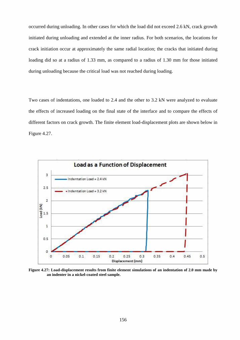
156
occurred during unloading. In other cases for which the load did not exceed 2.6 kN, crack growth
initiated during unloading and extended at the inner radius. For both scenarios, the locations for
crack initiation occur at approximately the same radial location; the cracks that initiated during
loading did so at a radius of 1.33 mm, as compared to a radius of 1.30 mm for those initiated
during unloading because the critical load was not reached during loading.
Two cases of indentations, one loaded to 2.4 and the other to 3.2 kN were analyzed to evaluate
the effects of increased loading on the final state of the interface and to compare the effects of
different factors on crack growth. The finite element load-displacement plots are shown below in
Figure 4.27.
Figure 4.27: Load-displacement results from finite element simulations of an indentation of 2.0 mm made by
an indenter in a nickel-coated steel sample.
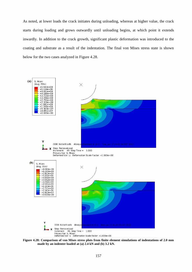
157
As noted, at lower loads the crack initiates during unloading, whereas at higher value, the crack
starts during loading and grows outwardly until unloading begins, at which point it extends
inwardly. In addition to the crack growth, significant plastic deformation was introduced to the
coating and substrate as a result of the indentation. The final von Mises stress state is shown
below for the two cases analyzed in Figure 4.28.
Figure 4.28: Comparison of von Mises stress plots from finite element simulations of indentations of 2.0 mm
made by an indenter loaded at (a) 2.4 kN and (b) 3.2 kN.
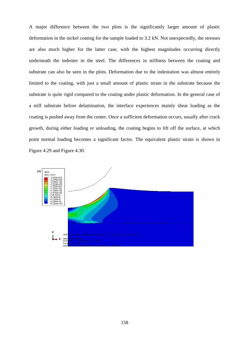
158
A major difference between the two plots is the significantly larger amount of plastic
deformation in the nickel coating for the sample loaded to 3.2 kN. Not unexpectedly, the stresses
are also much higher for the latter case, with the highest magnitudes occurring directly
underneath the indenter in the steel. The differences in stiffness between the coating and
substrate can also be seen in the plots. Deformation due to the indentation was almost entirely
limited to the coating, with just a small amount of plastic strain in the substrate because the
substrate is quite rigid compared to the coating under plastic deformation. In the general case of
a stiff substrate before delamination, the interface experiences mainly shear loading as the
coating is pushed away from the center. Once a sufficient deformation occurs, usually after crack
growth, during either loading or unloading, the coating begins to lift off the surface, at which
point normal loading becomes a significant factor. The equivalent plastic strain is shown in
Figure 4.29 and Figure 4.30.
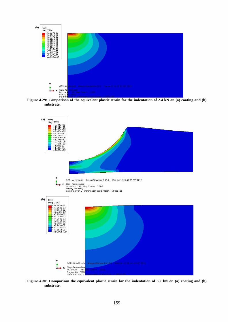
159
Figure 4.29: Comparison of the equivalent plastic strain for the indentation of 2.4 kN on (a) coating and (b)
substrate.
Figure 4.30: Comparison the equivalent plastic strain for the indentation of 3.2 kN on (a) coating and (b)
substrate.
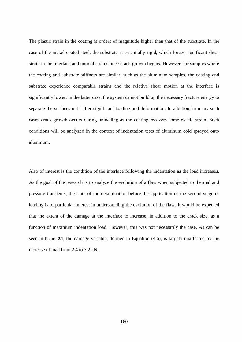
160
The plastic strain in the coating is orders of magnitude higher than that of the substrate. In the
case of the nickel-coated steel, the substrate is essentially rigid, which forces significant shear
strain in the interface and normal strains once crack growth begins. However, for samples where
the coating and substrate stiffness are similar, such as the aluminum samples, the coating and
substrate experience comparable strains and the relative shear motion at the interface is
significantly lower. In the latter case, the system cannot build up the necessary fracture energy to
separate the surfaces until after significant loading and deformation. In addition, in many such
cases crack growth occurs during unloading as the coating recovers some elastic strain. Such
conditions will be analyzed in the context of indentation tests of aluminum cold sprayed onto
aluminum.
Also of interest is the condition of the interface following the indentation as the load increases.
As the goal of the research is to analyze the evolution of a flaw when subjected to thermal and
pressure transients, the state of the delamination before the application of the second stage of
loading is of particular interest in understanding the evolution of the flaw. It would be expected
that the extent of the damage at the interface to increase, in addition to the crack size, as a
function of maximum indentation load. However, this was not necessarily the case. As can be
seen in Figure 2.1, the damage variable, defined in Equation (4.6), is largely unaffected by the
increase of load from 2.4 to 3.2 kN.
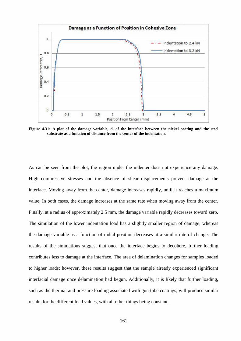
161
Figure 4.31: A plot of the damage variable, d, of the interface between the nickel coating and the steel
substrate as a function of distance from the center of the indentation.
As can be seen from the plot, the region under the indenter does not experience any damage.
High compressive stresses and the absence of shear displacements prevent damage at the
interface. Moving away from the center, damage increases rapidly, until it reaches a maximum
value. In both cases, the damage increases at the same rate when moving away from the center.
Finally, at a radius of approximately 2.5 mm, the damage variable rapidly decreases toward zero.
The simulation of the lower indentation load has a slightly smaller region of damage, whereas
the damage variable as a function of radial position decreases at a similar rate of change. The
results of the simulations suggest that once the interface begins to decohere, further loading
contributes less to damage at the interface. The area of delamination changes for samples loaded
to higher loads; however, these results suggest that the sample already experienced significant
interfacial damage once delamination had begun. Additionally, it is likely that further loading,
such as the thermal and pressure loading associated with gun tube coatings, will produce similar
results for the different load values, with all other things being constant.
162
4.4.3.2 Acoustic Emission and Finite Element Results
The finite element simulations described above can be used to further interpret the acoustic
emissions results described in Section 4.3.1.1 for nickel-coated steel specimens. From these
simulations, it can be seen that the delamination begins during unloading for the samples
indented to 2.4 kN, and begins again at around 2.6 kN for the samples loaded further. Therefore,
it is unlikely that high-energy acoustic emission hits generated earlier are the result of interfacial
cracks. Instead, it is reasonable to conclude that these hits are created by plastic deformation
and/or cracking in the nickel coating during indentation. As shown in Figure 4.32, significant
cracks and other surface features exist in the samples, and these could explain the high-amplitude
acoustic emissions throughout the test.
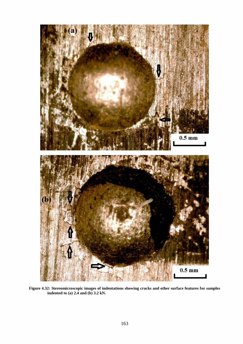
163
Figure 4.32: Stereomicroscopic images of indentations showing cracks and other surface features for samples
indented to (a) 2.4 and (b) 3.2 kN.
164
As shown in the figure, significant cracking can be seen at the edges of the indentations for
samples loaded to both 2.4 and 3.2 kN. It is likely that such cracking corresponds to a large
energy acoustic emission event and would be very difficult to discern from a delamination type.
The finite element simulations did not predict the onset of delamination at load levels below
approximately 2.6 to 2.8 kN; therefore, during loading, one would expect to see high-energy
events occurring around the same level as in the experimental results shown in Figure A.8,
Figure B.2, Figure B.4, Figure C.15, and Figure C.17. As also shown in these figures, a relatively
high-energy event occurs quite consistently at around 3.0 kN, which from the finite element
simulations, is the load range at which delamination occurs. Whereas some earlier events were
also accompanied by larger amounts of acoustic energy, the level of the events that occur later in
the test are still above the background floor. As a high-energy acoustic event consistently occurs
at approximately the same point, delamination is expected to initiate during the indentation
experiment. It is therefore likely that this event coincides with the onset of delamination.
The experimental results were compared to those from the finite element models with varying
parameters to determine the cohesive zone properties of the thermally sprayed nickel on steel
samples. Cohesive zone properties were chosen that accurately describe indentation-induced
crack growth for samples under different load levels, though the simulations featured crack
growth caused by different mechanisms. As mentioned before, the c-scan results varied
significantly and were difficult to measure. In addition, for various load levels, agreement was
observed between the predicted onset of delamination and significant acoustic energy events.
Given this reasonably strong agreement and the possible sources of uncertainty in the
experimental results, the properties measured through finite element simulations were judged to
reasonably model the interface. In addition, the properties were judged to constitute a sufficient
basis for further investigating the response of the coating system to different loading conditions,
such as thermal and pressure transients.
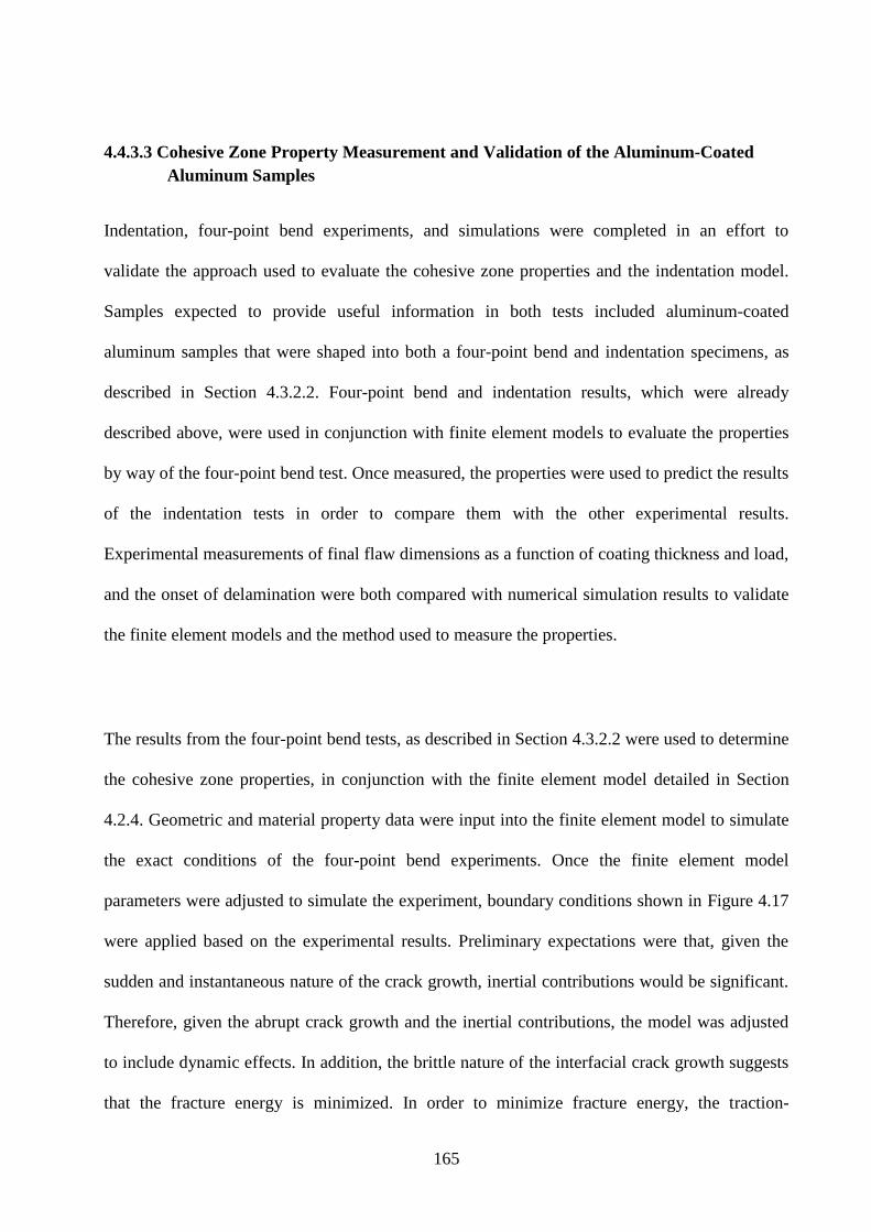
165
4.4.3.3 Cohesive Zone Property Measurement and Validation of the Aluminum-Coated
Aluminum Samples
Indentation, four-point bend experiments, and simulations were completed in an effort to
validate the approach used to evaluate the cohesive zone properties and the indentation model.
Samples expected to provide useful information in both tests included aluminum-coated
aluminum samples that were shaped into both a four-point bend and indentation specimens, as
described in Section 4.3.2.2. Four-point bend and indentation results, which were already
described above, were used in conjunction with finite element models to evaluate the properties
by way of the four-point bend test. Once measured, the properties were used to predict the results
of the indentation tests in order to compare them with the other experimental results.
Experimental measurements of final flaw dimensions as a function of coating thickness and load,
and the onset of delamination were both compared with numerical simulation results to validate
the finite element models and the method used to measure the properties.
The results from the four-point bend tests, as described in Section 4.3.2.2 were used to determine
the cohesive zone properties, in conjunction with the finite element model detailed in Section
4.2.4. Geometric and material property data were input into the finite element model to simulate
the exact conditions of the four-point bend experiments. Once the finite element model
parameters were adjusted to simulate the experiment, boundary conditions shown in Figure 4.17
were applied based on the experimental results. Preliminary expectations were that, given the
sudden and instantaneous nature of the crack growth, inertial contributions would be significant.
Therefore, given the abrupt crack growth and the inertial contributions, the model was adjusted
to include dynamic effects. In addition, the brittle nature of the interfacial crack growth suggests
that the fracture energy is minimized. In order to minimize fracture energy, the traction-
166
separation curve shown in Figure 4.2 was truncated such that once the cohesive zone reaches the
maximum stress, it immediately fails. In other words and in reference to Figure 4.2, the cohesive
zone was defined such that δ0n was equal to δ0
c. Additionally, the stiffness was defined according
to Equation (2.6). Residual stresses were included, since they have the potential to significantly
affect the crack growth. Residual stresses were calculated using Equations (2.41) and (2.42), and
based on the curvatures of the sample surface before and after separation. A plot of the applied
residual stress distribution and the curvature measurements used to calculate them are shown in
Figure 4.33.
As shown in Figure 4.33b, the curvatures are largest for the composite beam and the coating,
though the curvatures are in opposite directions. Such results are expected, as the residual
stresses result from the strain required to maintain equal displacements across the interface. In
addition, after separation, the substrate retains very little of the deformation. The residual stress
distribution, as described above, assumes a linear variation, is largely tensile in the substrate, and
compressive in the coating. Such behavior agrees with experimental observations, for which the
composite beam bent away from the spray nozzle. In such a case, the substrate resists the
curvature and keeps the coating in compression. Measured residual stress distributions were
applied to the finite element model by means of a user-defined subroutine. With all other
parameters defined, finite element simulations were conducted with the four-point bend model to
attempt to best reproduce experimental results by varying the normal and shear strengths.
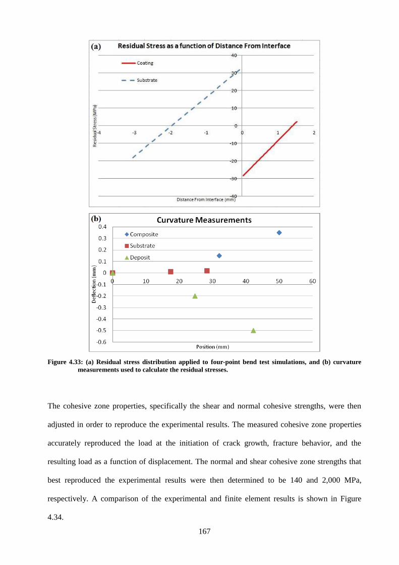
167
Figure 4.33: (a) Residual stress distribution applied to four-point bend test simulations, and (b) curvature
measurements used to calculate the residual stresses.
The cohesive zone properties, specifically the shear and normal cohesive strengths, were then
adjusted in order to reproduce the experimental results. The measured cohesive zone properties
accurately reproduced the load at the initiation of crack growth, fracture behavior, and the
resulting load as a function of displacement. The normal and shear cohesive zone strengths that
best reproduced the experimental results were then determined to be 140 and 2,000 MPa,
respectively. A comparison of the experimental and finite element results is shown in Figure
4.34.
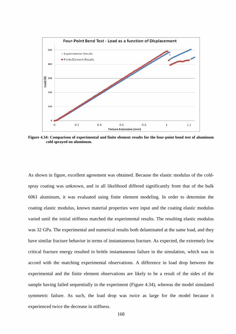
168
Figure 4.34: Comparison of experimental and finite element results for the four-point bend test of aluminum
cold sprayed on aluminum.
As shown in figure, excellent agreement was obtained. Because the elastic modulus of the cold-
spray coating was unknown, and in all likelihood differed significantly from that of the bulk
6061 aluminum, it was evaluated using finite element modeling. In order to determine the
coating elastic modulus, known material properties were input and the coating elastic modulus
varied until the initial stiffness matched the experimental results. The resulting elastic modulus
was 32 GPa. The experimental and numerical results both delaminated at the same load, and they
have similar fracture behavior in terms of instantaneous fracture. As expected, the extremely low
critical fracture energy resulted in brittle instantaneous failure in the simulation, which was in
accord with the matching experimental observations. A difference in load drop between the
experimental and the finite element observations are likely to be a result of the sides of the
sample having failed sequentially in the experiment (Figure 4.34), whereas the model simulated
symmetric failure. As such, the load drop was twice as large for the model because it
experienced twice the decrease in stiffness.
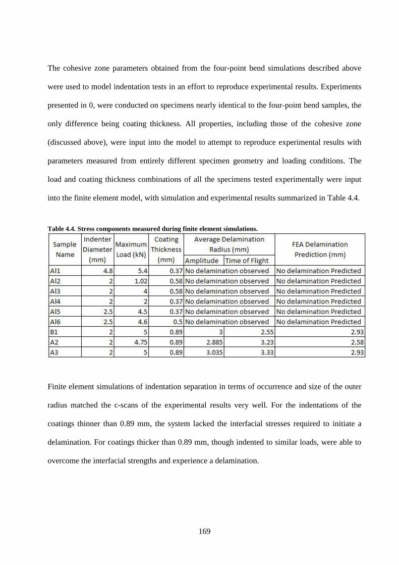
169
The cohesive zone parameters obtained from the four-point bend simulations described above
were used to model indentation tests in an effort to reproduce experimental results. Experiments
presented in 0, were conducted on specimens nearly identical to the four-point bend samples, the
only difference being coating thickness. All properties, including those of the cohesive zone
(discussed above), were input into the model to attempt to reproduce experimental results with
parameters measured from entirely different specimen geometry and loading conditions. The
load and coating thickness combinations of all the specimens tested experimentally were input
into the finite element model, with simulation and experimental results summarized in Table 4.4.
Table 4.4. Stress components measured during finite element simulations.
Finite element simulations of indentation separation in terms of occurrence and size of the outer
radius matched the c-scans of the experimental results very well. For the indentations of the
coatings thinner than 0.89 mm, the system lacked the interfacial stresses required to initiate a
delamination. For coatings thicker than 0.89 mm, though indented to similar loads, were able to
overcome the interfacial strengths and experience a delamination.
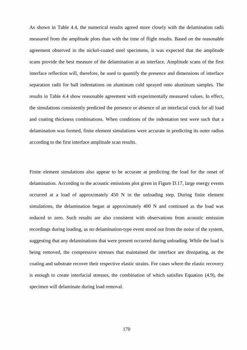
170
As shown in Table 4.4, the numerical results agreed more closely with the delamination radii
measured from the amplitude plots than with the time of flight results. Based on the reasonable
agreement observed in the nickel-coated steel specimens, it was expected that the amplitude
scans provide the best measure of the delamination at an interface. Amplitude scans of the first
interface reflection will, therefore, be used to quantify the presence and dimensions of interface
separation radii for ball indentations on aluminum cold sprayed onto aluminum samples. The
results in Table 4.4 show reasonable agreement with experimentally measured values. In effect,
the simulations consistently predicted the presence or absence of an interfacial crack for all load
and coating thickness combinations. When conditions of the indentation test were such that a
delamination was formed, finite element simulations were accurate in predicting its outer radius
according to the first interface amplitude scan results.
Finite element simulations also appear to be accurate at predicting the load for the onset of
delamination. According to the acoustic emissions plot given in Figure D.17, large energy events
occurred at a load of approximately 450 N in the unloading step. During finite element
simulations, the delamination began at approximately 400 N and continued as the load was
reduced to zero. Such results are also consistent with observations from acoustic emission
recordings during loading, as no delamination-type event stood out from the noise of the system,
suggesting that any delaminations that were present occurred during unloading. While the load is
being removed, the compressive stresses that maintained the interface are dissipating, as the
coating and substrate recover their respective elastic strains. For cases where the elastic recovery
is enough to create interfacial stresses, the combination of which satisfies Equation (4.9), the
specimen will delaminate during load removal.
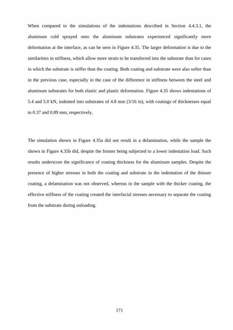
171
When compared to the simulations of the indentations described in Section 4.4.3.1, the
aluminum cold sprayed onto the aluminum substrates experienced significantly more
deformation at the interface, as can be seen in Figure 4.35. The larger deformation is due to the
similarities in stiffness, which allow more strain to be transferred into the substrate than for cases
in which the substrate is stiffer than the coating. Both coating and substrate were also softer than
in the previous case, especially in the case of the difference in stiffness between the steel and
aluminum substrates for both elastic and plastic deformation. Figure 4.35 shows indentations of
5.4 and 5.0 kN, indented into substrates of 4.8 mm (3/16 in), with coatings of thicknesses equal
to 0.37 and 0.89 mm, respectively.
The simulation shown in Figure 4.35a did not result in a delamination, while the sample the
shown in Figure 4.35b did, despite the former being subjected to a lower indentation load. Such
results underscore the significance of coating thickness for the aluminum samples. Despite the
presence of higher stresses in both the coating and substrate in the indentation of the thinner
coating, a delamination was not observed, whereas in the sample with the thicker coating, the
effective stiffness of the coating created the interfacial stresses necessary to separate the coating
from the substrate during unloading.
172
Figure 4.35: Comparison of finite element simulations of aluminum cold sprayed onto aluminum, with (a)
coating thickness of 0.37 mm, indented to a load of 5.4 kN (b) coating thickness of 0.89 mm,
indented to a load of 5.0 kN.
As mentioned above, the indentation of the sample with the thin coating was to a higher load. In
addition, because of less coating penetration and more loading in the substrate, this sample also
had higher indentation stiffness. The slope of load as a function of displacement, shown in
Figure 4.36, was higher for indentations in samples with thinner coatings, reflecting the higher
stiffness of the substrate when compared to the coating.
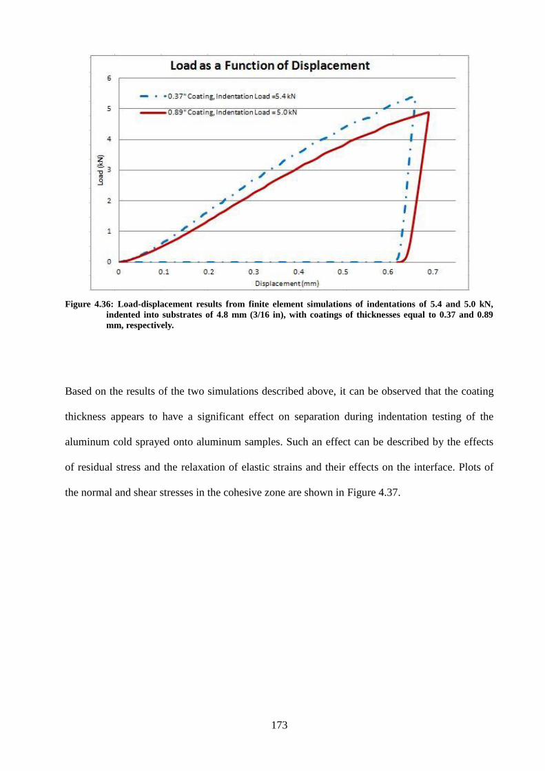
173
Figure 4.36: Load-displacement results from finite element simulations of indentations of 5.4 and 5.0 kN,
indented into substrates of 4.8 mm (3/16 in), with coatings of thicknesses equal to 0.37 and 0.89
mm, respectively.
Based on the results of the two simulations described above, it can be observed that the coating
thickness appears to have a significant effect on separation during indentation testing of the
aluminum cold sprayed onto aluminum samples. Such an effect can be described by the effects
of residual stress and the relaxation of elastic strains and their effects on the interface. Plots of
the normal and shear stresses in the cohesive zone are shown in Figure 4.37.
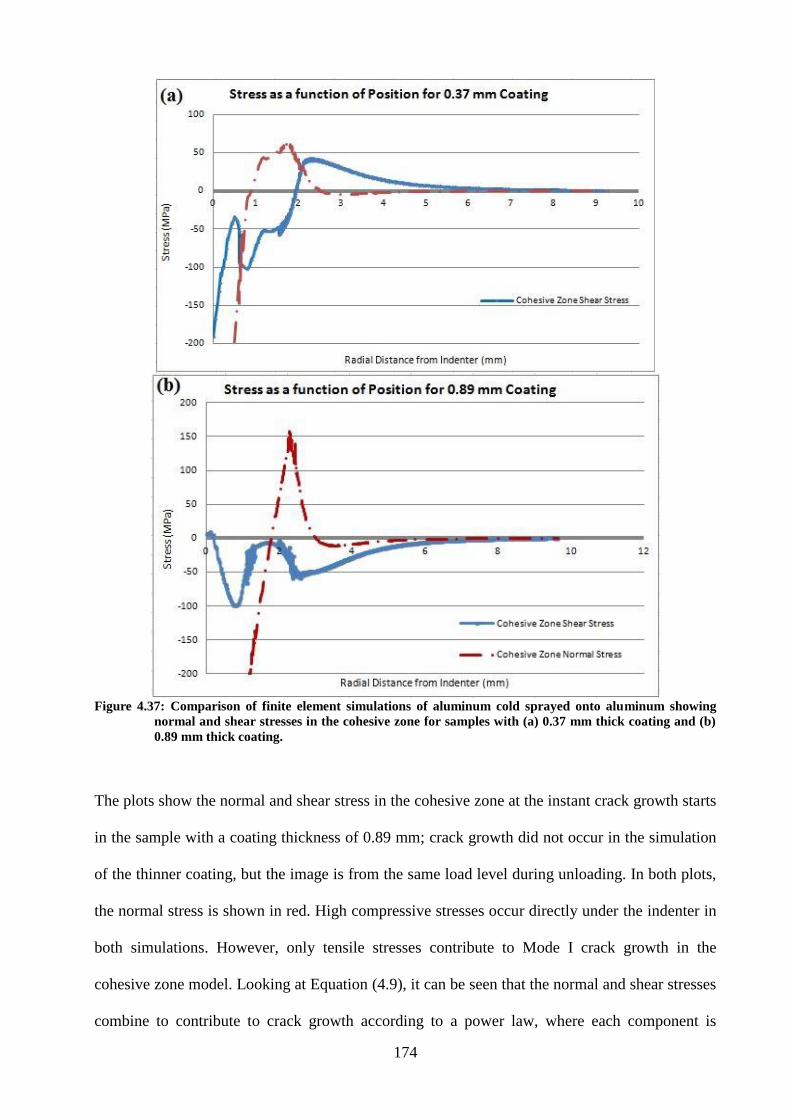
174
Figure 4.37: Comparison of finite element simulations of aluminum cold sprayed onto aluminum showing
normal and shear stresses in the cohesive zone for samples with (a) 0.37 mm thick coating and (b)
0.89 mm thick coating.
The plots show the normal and shear stress in the cohesive zone at the instant crack growth starts
in the sample with a coating thickness of 0.89 mm; crack growth did not occur in the simulation
of the thinner coating, but the image is from the same load level during unloading. In both plots,
the normal stress is shown in red. High compressive stresses occur directly under the indenter in
both simulations. However, only tensile stresses contribute to Mode I crack growth in the
cohesive zone model. Looking at Equation (4.9), it can be seen that the normal and shear stresses
combine to contribute to crack growth according to a power law, where each component is
175
divided by the respective strength, and then squared. According to the properties obtained from
the four-point bend testing and simulations, those values are 13 and 1400 MPa, respectively.
Recognizing this, and the fact that the tensile stresses are larger in magnitude than the shear
stresses, one would expect the normal stresses to contribute the most to fracture, relative to the
shear components. Unlike the simulations of the steel specimens with a nickel coating, where the
fracture is dominated by the shear stresses, the interfacial separation of the cold-sprayed deposit
from the aluminum substrate is driven almost entirely by tensile components. Whereas the hard
steel coating underwent very little deformation causing higher shear stresses at the interface as
compared to the nickel surface, the aluminum coating and substrate share the deformation.
Normal stress, shown in Figure 4.35a, is almost a third of the stress recorded from the simulation
shown in Figure 4.35b. In addition, as observed in Figure 4.35b, the shear and tensile stress
peaks are at approximately the same location at 2.35 mm from the center of the indenter.
Interfacial separation continues from the initiation point in both directions, driven mostly by high
tensile stresses at the interface.
After the loading was removed, significant plastic strain was observed in the simulations. It is
likely that the plastic strain contributes to the crack growth during unloading. Interfacial damage
also occurs during unloading. As such, it is the result of the relaxation of the elastic stresses.
Plastic stress and strain is, therefore, a function of unrecovered deformation. Images of the
plastic strains after unloading are shown in Figure 4.38 and Figure 4.39 for simulations with
coatings 0.37 and 0.89 mm thick, respectively.
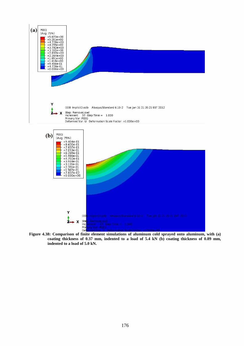
176
Figure 4.38: Comparison of finite element simulations of aluminum cold sprayed onto aluminum, with (a)
coating thickness of 0.37 mm, indented to a load of 5.4 kN (b) coating thickness of 0.89 mm,
indented to a load of 5.0 kN.
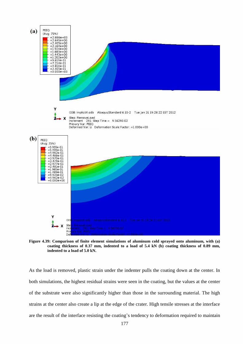
177
Figure 4.39: Comparison of finite element simulations of aluminum cold sprayed onto aluminum, with (a)
coating thickness of 0.37 mm, indented to a load of 5.4 kN (b) coating thickness of 0.89 mm,
indented to a load of 5.0 kN.
As the load is removed, plastic strain under the indenter pulls the coating down at the center. In
both simulations, the highest residual strains were seen in the coating, but the values at the center
of the substrate were also significantly higher than those in the surrounding material. The high
strains at the center also create a lip at the edge of the crater. High tensile stresses at the interface
are the result of the interface resisting the coating’s tendency to deformation required to maintain
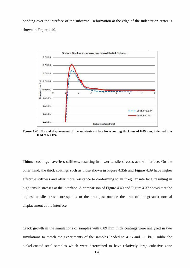
178
bonding over the interface of the substrate. Deformation at the edge of the indentation crater is
shown in Figure 4.40.
Figure 4.40: Normal displacement of the substrate surface for a coating thickness of 0.89 mm, indented to a
load of 5.0 kN.
Thinner coatings have less stiffness, resulting in lower tensile stresses at the interface. On the
other hand, the thick coatings such as those shown in Figure 4.35b and Figure 4.39 have higher
effective stiffness and offer more resistance to conforming to an irregular interface, resulting in
high tensile stresses at the interface. A comparison of Figure 4.40 and Figure 4.37 shows that the
highest tensile stress corresponds to the area just outside the area of the greatest normal
displacement at the interface.
Crack growth in the simulations of samples with 0.89 mm thick coatings were analyzed in two
simulations to match the experiments of the samples loaded to 4.75 and 5.0 kN. Unlike the
nickel-coated steel samples which were determined to have relatively large cohesive zone
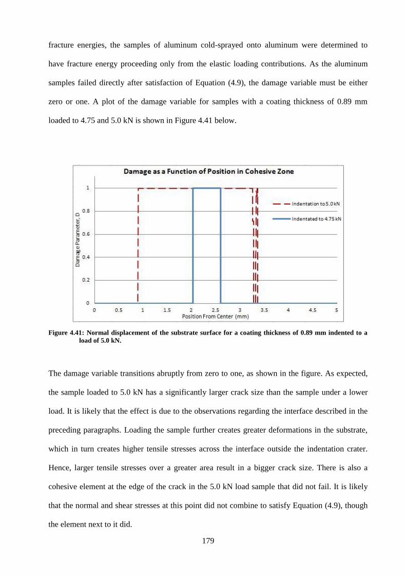
179
fracture energies, the samples of aluminum cold-sprayed onto aluminum were determined to
have fracture energy proceeding only from the elastic loading contributions. As the aluminum
samples failed directly after satisfaction of Equation (4.9), the damage variable must be either
zero or one. A plot of the damage variable for samples with a coating thickness of 0.89 mm
loaded to 4.75 and 5.0 kN is shown in Figure 4.41 below.
Figure 4.41: Normal displacement of the substrate surface for a coating thickness of 0.89 mm indented to a
load of 5.0 kN.
The damage variable transitions abruptly from zero to one, as shown in the figure. As expected,
the sample loaded to 5.0 kN has a significantly larger crack size than the sample under a lower
load. It is likely that the effect is due to the observations regarding the interface described in the
preceding paragraphs. Loading the sample further creates greater deformations in the substrate,
which in turn creates higher tensile stresses across the interface outside the indentation crater.
Hence, larger tensile stresses over a greater area result in a bigger crack size. There is also a
cohesive element at the edge of the crack in the 5.0 kN load sample that did not fail. It is likely
that the normal and shear stresses at this point did not combine to satisfy Equation (4.9), though
the element next to it did.
180
The conditions pertaining to interfacial damage, failure, and crack growth were analyzed for the
indentation tests. The aluminum samples were found to delaminate under different conditions
than the nickel-coated steel specimens. In both sets of materials, the cohesive zone properties
were measured. A four-point bend test was used to evaluate aluminum-coated aluminum
cohesive zone properties, which were then successfully applied to predict the onset and size of
the delaminations to those of identical samples subjected to indentation loading. The cohesive
zone properties were also evaluated using a similar method as that used for the nickel-coated
steel specimens, which accurately modeled the initiation and growth of an interfacial crack for
three different indentation loads. Indentations in the nickel-coated steel specimens created
significant deformations in the relatively softer coating, which resulting in high shear stresses at
the interface. Delaminations were observed during loading for samples at higher loads, whereas
the other samples delaminated during unloading under simulation conditions.
The cold-sprayed aluminum on aluminum substrates presented a completely different material
set for exploring the application of the cohesive zone modeling. Brittle fractures were observed
in the four-point bend tests, which were used to evaluate the cohesive zone parameters.
Properties were applied to the indentation tests and found to accurately model crack growth. The
steel substrate was found to be stiff relative to the coating in the other set of samples; however,
the aluminum coating and substrate had similar material properties and were found to delaminate
by normal and shear mechanisms during indentation unloading.
Given the thorough property measurement and validation procedure, the method of indentation
experimentation and finite element modeling were found to reasonably determine the cohesive
zone properties. In addition, the indentation test was found to adequately introduce damage to
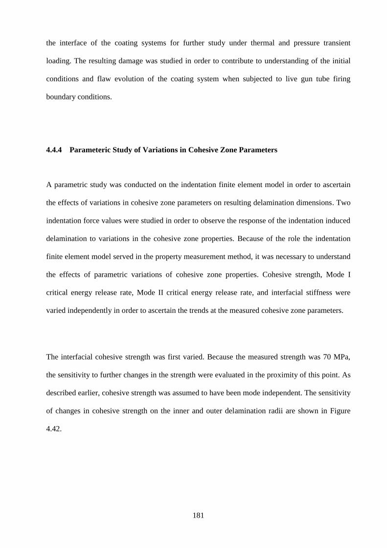
181
the interface of the coating systems for further study under thermal and pressure transient
loading. The resulting damage was studied in order to contribute to understanding of the initial
conditions and flaw evolution of the coating system when subjected to live gun tube firing
boundary conditions.
4.4.4 Parameteric Study of Variations in Cohesive Zone Parameters
A parametric study was conducted on the indentation finite element model in order to ascertain
the effects of variations in cohesive zone parameters on resulting delamination dimensions. Two
indentation force values were studied in order to observe the response of the indentation induced
delamination to variations in the cohesive zone properties. Because of the role the indentation
finite element model served in the property measurement method, it was necessary to understand
the effects of parametric variations of cohesive zone properties. Cohesive strength, Mode I
critical energy release rate, Mode II critical energy release rate, and interfacial stiffness were
varied independently in order to ascertain the trends at the measured cohesive zone parameters.
The interfacial cohesive strength was first varied. Because the measured strength was 70 MPa,
the sensitivity to further changes in the strength were evaluated in the proximity of this point. As
described earlier, cohesive strength was assumed to have been mode independent. The sensitivity
of changes in cohesive strength on the inner and outer delamination radii are shown in Figure
4.42.
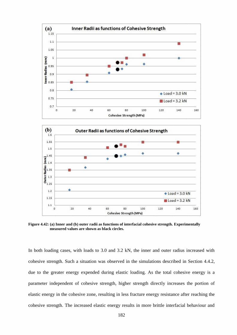
182
Figure 4.42: (a) Inner and (b) outer radii as functions of interfacial cohesive strength. Experimentally
measured values are shown as black circles.
In both loading cases, with loads to 3.0 and 3.2 kN, the inner and outer radius increased with
cohesive strength. Such a situation was observed in the simulations described in Section 4.4.2,
due to the greater energy expended during elastic loading. As the total cohesive energy is a
parameter independent of cohesive strength, higher strength directly increases the portion of
elastic energy in the cohesive zone, resulting in less fracture energy resistance after reaching the
cohesive strength. The increased elastic energy results in more brittle interfacial behaviour and
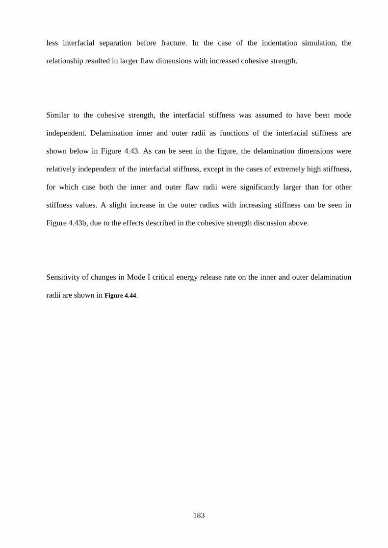
183
less interfacial separation before fracture. In the case of the indentation simulation, the
relationship resulted in larger flaw dimensions with increased cohesive strength.
Similar to the cohesive strength, the interfacial stiffness was assumed to have been mode
independent. Delamination inner and outer radii as functions of the interfacial stiffness are
shown below in Figure 4.43. As can be seen in the figure, the delamination dimensions were
relatively independent of the interfacial stiffness, except in the cases of extremely high stiffness,
for which case both the inner and outer flaw radii were significantly larger than for other
stiffness values. A slight increase in the outer radius with increasing stiffness can be seen in
Figure 4.43b, due to the effects described in the cohesive strength discussion above.
Sensitivity of changes in Mode I critical energy release rate on the inner and outer delamination
radii are shown in Figure 4.44.
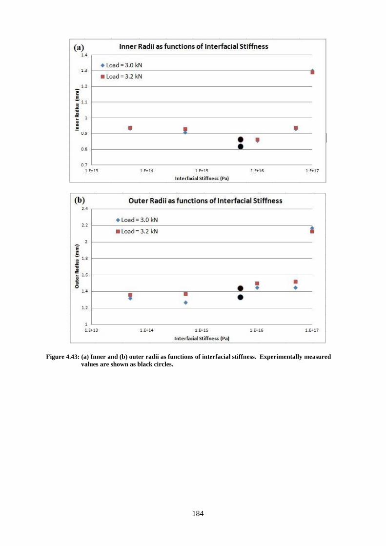
184
Figure 4.43: (a) Inner and (b) outer radii as functions of interfacial stiffness. Experimentally measured
values are shown as black circles.
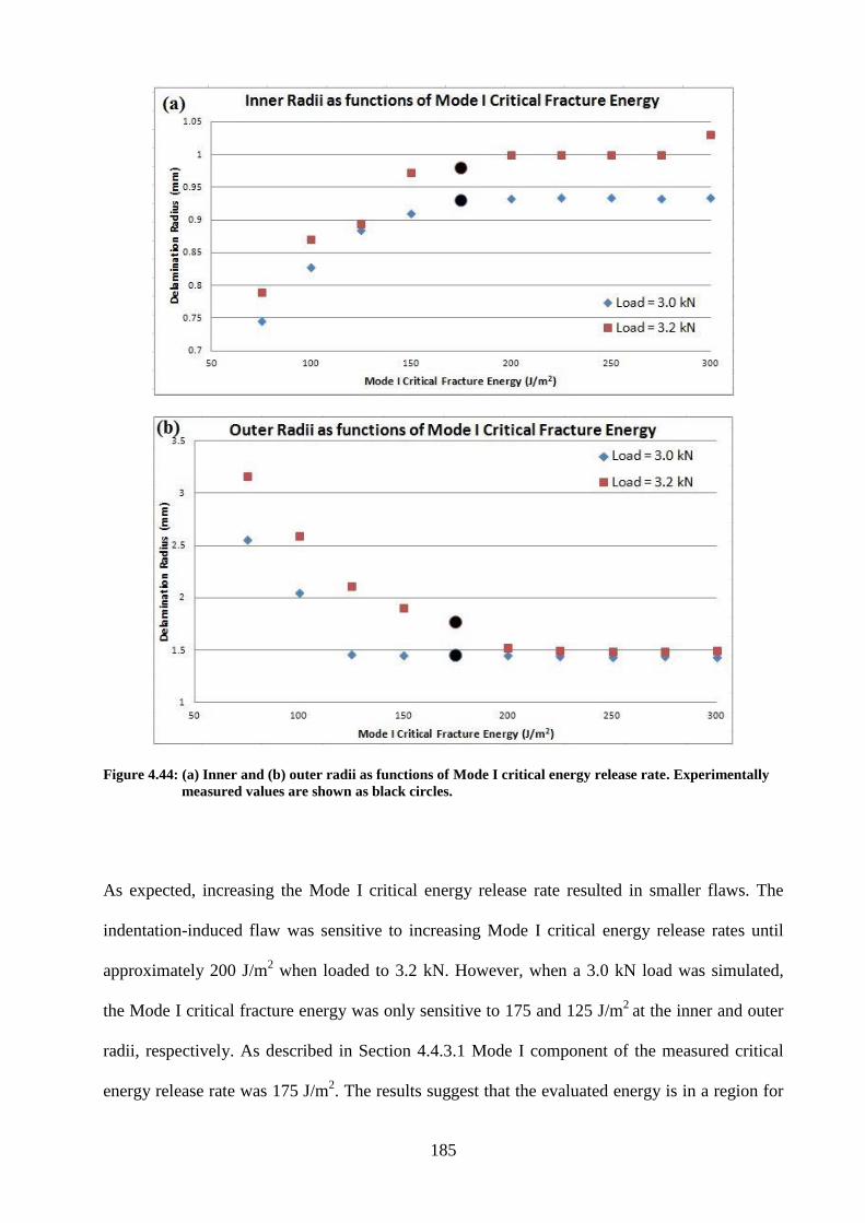
185
Figure 4.44: (a) Inner and (b) outer radii as functions of Mode I critical energy release rate. Experimentally
measured values are shown as black circles.
As expected, increasing the Mode I critical energy release rate resulted in smaller flaws. The
indentation-induced flaw was sensitive to increasing Mode I critical energy release rates until
approximately 200 J/m2 when loaded to 3.2 kN. However, when a 3.0 kN load was simulated,
the Mode I critical fracture energy was only sensitive to 175 and 125 J/m2
at the inner and outer
radii, respectively. As described in Section 4.4.3.1 Mode I component of the measured critical
energy release rate was 175 J/m2. The results suggest that the evaluated energy is in a region for
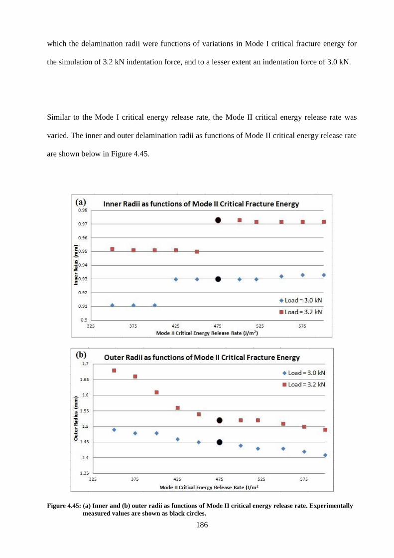
186
which the delamination radii were functions of variations in Mode I critical fracture energy for
the simulation of 3.2 kN indentation force, and to a lesser extent an indentation force of 3.0 kN.
Similar to the Mode I critical energy release rate, the Mode II critical energy release rate was
varied. The inner and outer delamination radii as functions of Mode II critical energy release rate
are shown below in Figure 4.45.
Figure 4.45: (a) Inner and (b) outer radii as functions of Mode II critical energy release rate. Experimentally
measured values are shown as black circles.
187
Similar observations to those made for the Mode I critical energy release rate also applied in
Mode II. The inner radius increased with the Mode II component, while the outer decreased. The
outer radius was a function of increasing Mode II critical energy release rate for all values tested,
while the inner radius was much less sensitive, showing only one jump in radius as the Mode II
component of the critical energy release rate increased. As mentioned in Section 4.4.3.1 the
Mode II component of the measured critical energy release rate was 425 J/m2. The results shown
in Figure 4.45 suggest that the evaluated energy is in a region for which the delamination outer
radii, and to a lesser extent, inner radii, were functions of the Mode I critical fracture energy.
Because the model assumed axisymmetry, the results were independent of the Mode III
component of interfacial fracture energy. The results described indicate the sensitivity of the
cohesive zone parameters in the range of the values measured by the method. Additionally,
delamination dimensions appear to be relatively independent of the cohesive zone stiffness,
except for the case of extremely high values.
188
CHAPTER 5. FLAW EVOLUTION
5.1 Thermal Loading on a Coating with an Interfacial Pre-crack Model
A thermal-structural model, the input file for which is included in Appendix B.b was developed
to analyze the effects of thermal transients on indentation-induced interfacial flaws. Unlike the
previously mentioned Abaqus finite element models, the thermal model was written in Abaqus
input file format language because the *import command used to interpolate the finite element
results from the implicit indentation was not available in Python scripting. The approach used
here is unique in that it includes all the effects of the damage initiation process and provides a
complete description of the coating, interface, and substrate state before thermal transients are be
applied.
For the required implicit-to-explicit analysis to be performed, the indentation model must be run
first and its results stored in a *.odb (output database file). During the explicit analysis, the
results, including plastic deformations and residual stresses, were applied as the initial state. The
state of damage for cohesive zone elements at completion of the indentation phase became the
initial conditions and failed elements were not imported. Only the implicit element types need to
be redefined as explicit elements, as the deformed mesh of the coating, substrate, and interface
was imported. Explicit, linear, axisymmetric elements, designated as CAX4RT, were used for
the coating and substrate. The elements had both thermal and structural degrees of freedom and
employed reduced integration and hourglass control; all cohesive elements were four-node,
axisymmetric, explicit elements, and were designated as COHAX4. During the analysis, failed
elements were deleted in order to easily monitor crack growth.
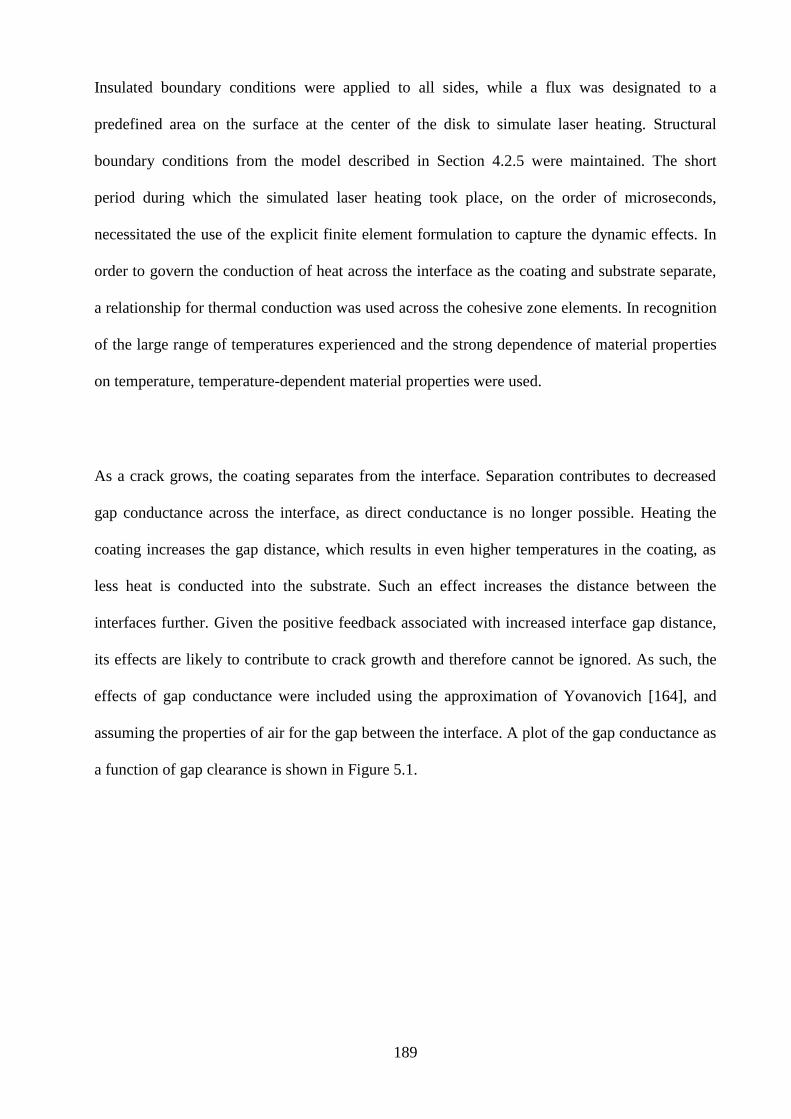
189
Insulated boundary conditions were applied to all sides, while a flux was designated to a
predefined area on the surface at the center of the disk to simulate laser heating. Structural
boundary conditions from the model described in Section 4.2.5 were maintained. The short
period during which the simulated laser heating took place, on the order of microseconds,
necessitated the use of the explicit finite element formulation to capture the dynamic effects. In
order to govern the conduction of heat across the interface as the coating and substrate separate,
a relationship for thermal conduction was used across the cohesive zone elements. In recognition
of the large range of temperatures experienced and the strong dependence of material properties
on temperature, temperature-dependent material properties were used.
As a crack grows, the coating separates from the interface. Separation contributes to decreased
gap conductance across the interface, as direct conductance is no longer possible. Heating the
coating increases the gap distance, which results in even higher temperatures in the coating, as
less heat is conducted into the substrate. Such an effect increases the distance between the
interfaces further. Given the positive feedback associated with increased interface gap distance,
its effects are likely to contribute to crack growth and therefore cannot be ignored. As such, the
effects of gap conductance were included using the approximation of Yovanovich [164], and
assuming the properties of air for the gap between the interface. A plot of the gap conductance as
a function of gap clearance is shown in Figure 5.1.
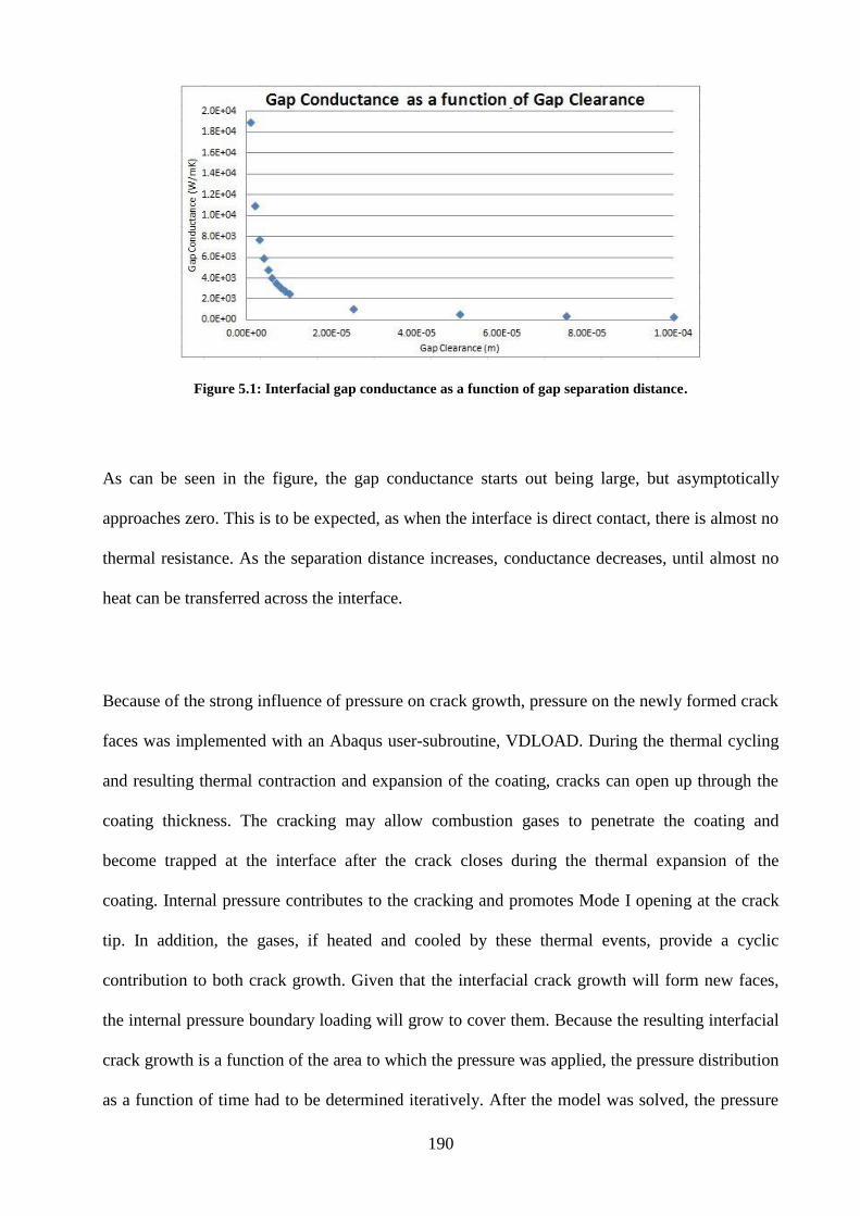
190
Figure 5.1: Interfacial gap conductance as a function of gap separation distance.
As can be seen in the figure, the gap conductance starts out being large, but asymptotically
approaches zero. This is to be expected, as when the interface is direct contact, there is almost no
thermal resistance. As the separation distance increases, conductance decreases, until almost no
heat can be transferred across the interface.
Because of the strong influence of pressure on crack growth, pressure on the newly formed crack
faces was implemented with an Abaqus user-subroutine, VDLOAD. During the thermal cycling
and resulting thermal contraction and expansion of the coating, cracks can open up through the
coating thickness. The cracking may allow combustion gases to penetrate the coating and
become trapped at the interface after the crack closes during the thermal expansion of the
coating. Internal pressure contributes to the cracking and promotes Mode I opening at the crack
tip. In addition, the gases, if heated and cooled by these thermal events, provide a cyclic
contribution to both crack growth. Given that the interfacial crack growth will form new faces,
the internal pressure boundary loading will grow to cover them. Because the resulting interfacial
crack growth is a function of the area to which the pressure was applied, the pressure distribution
as a function of time had to be determined iteratively. After the model was solved, the pressure
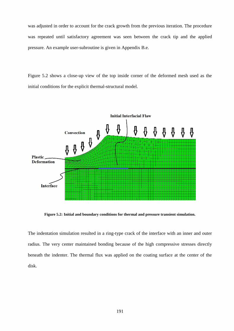
191
was adjusted in order to account for the crack growth from the previous iteration. The procedure
was repeated until satisfactory agreement was seen between the crack tip and the applied
pressure. An example user-subroutine is given in Appendix B.e.
Figure 5.2 shows a close-up view of the top inside corner of the deformed mesh used as the
initial conditions for the explicit thermal-structural model.
Figure 5.2: Initial and boundary conditions for thermal and pressure transient simulation.
The indentation simulation resulted in a ring-type crack of the interface with an inner and outer
radius. The very center maintained bonding because of the high compressive stresses directly
beneath the indenter. The thermal flux was applied on the coating surface at the center of the
disk.
192
5.2 Flaw Evolution Modelling Results
The evolution of indentation-induced flaws was also analyzed using the finite element method.
An explicit finite element model as described in Section 5.1 was applied in a sequential fashion
where finite element results of a ball indentation implicit finite element analysis were imported.
The indented state was then used as the initial conditions for studying the evolution of thermal
and pressure transients. Such a method applies all the effects resulting from the indentation
process, including plastic deformation, crack growth, and cohesive zone element damage as
initial conditions in the thermal-structural explicit simulation. Studies were conducted for which
a flaw was introduced through indentation via an implicit simulation. The results were imported
into an explicit model to study interfacial damage and crack growth under severe thermal and
pressure transients. Flaw evolution was studied in the nickel-coated steel specimens, for which
the cohesive zone property measurement was just discussed. An initial flaw with inner and outer
radii of 0.40 and 1.45 mm, respectively, was introduced with a 2.0 mm diameter indenter loaded
to 2.8 kN. In the final simulation in the analysis, several thermal and pressure transients were
applied to the coating surface and the evolution of the indentation-induced delamination was
analyzed.
A thermal-structural model, described above, was developed next to analyze the effects of
thermal transients on the pre-existing interfacial flaws just discussed. Nickel-coated steel
specimens were used for this study of the thermal and pressure transients. Explicit, linear,
axisymmetric elements were used for the coating and substrate. The chosen cohesive element
was a four-node, two-dimensional, axisymmetric element. Adiabatic boundary conditions were
assumed on all sides except at the top of the coating, where convection was applied as shown in
Figure 5.2. In addition, as the crack grew and the coating separated from the interface, the
conductance across the gap decreased as a function of separation distance.
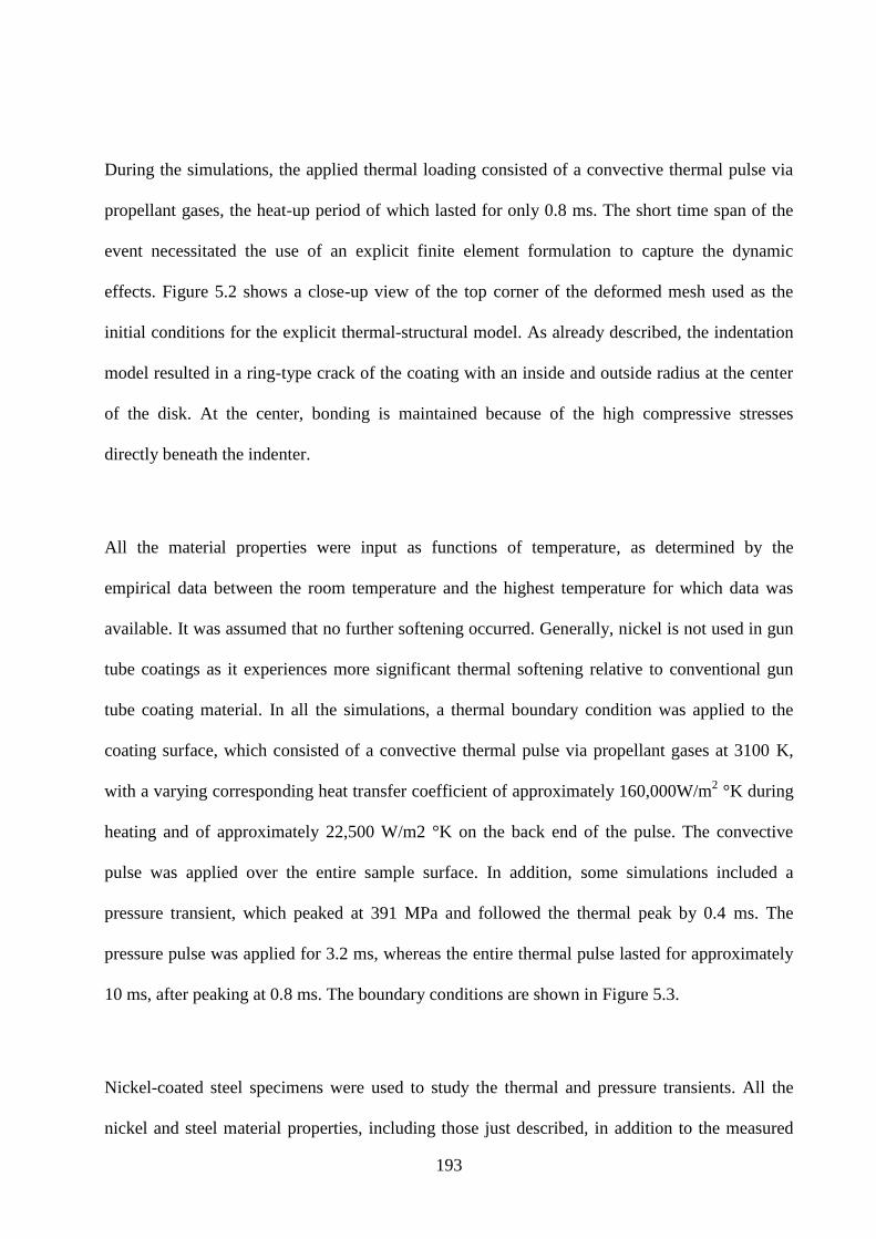
193
During the simulations, the applied thermal loading consisted of a convective thermal pulse via
propellant gases, the heat-up period of which lasted for only 0.8 ms. The short time span of the
event necessitated the use of an explicit finite element formulation to capture the dynamic
effects. Figure 5.2 shows a close-up view of the top corner of the deformed mesh used as the
initial conditions for the explicit thermal-structural model. As already described, the indentation
model resulted in a ring-type crack of the coating with an inside and outside radius at the center
of the disk. At the center, bonding is maintained because of the high compressive stresses
directly beneath the indenter.
All the material properties were input as functions of temperature, as determined by the
empirical data between the room temperature and the highest temperature for which data was
available. It was assumed that no further softening occurred. Generally, nickel is not used in gun
tube coatings as it experiences more significant thermal softening relative to conventional gun
tube coating material. In all the simulations, a thermal boundary condition was applied to the
coating surface, which consisted of a convective thermal pulse via propellant gases at 3100 K,
with a varying corresponding heat transfer coefficient of approximately 160,000W/m2 °K during
heating and of approximately 22,500 W/m2 °K on the back end of the pulse. The convective
pulse was applied over the entire sample surface. In addition, some simulations included a
pressure transient, which peaked at 391 MPa and followed the thermal peak by 0.4 ms. The
pressure pulse was applied for 3.2 ms, whereas the entire thermal pulse lasted for approximately
10 ms, after peaking at 0.8 ms. The boundary conditions are shown in Figure 5.3.
Nickel-coated steel specimens were used to study the thermal and pressure transients. All the
nickel and steel material properties, including those just described, in addition to the measured
194
cohesive zone properties, were also used in the thermal modeling. Adiabatic boundary conditions
were assumed on all sides except at the top of the coating, where convection was applied to the
entire coating surface. In addition, as the crack grows and the coating separates from the
interface, the conductance across the gap was expected to decrease. Effects of gap conductance
were included using the approximation of Yovanovich [164], and the properties of air for the gap
between the interface were assumed. The interfacial gap conductance was already shown in
Figure 5.1. Interstitial pressure was assumed in the simulations with the pressure transient. If and
when crack growth occurred, the interstitial pressure was assumed to follow the crack tip. The
interstitial pressure area was solved iteratively, using the crack tip from the previous simulation
as the new boundary for the pressure area until satisfactory agreement was achieved. Such an
analysis provides a useful context for the study of the effects of thermal and pressure transients
on the evolution of an interfacial, indentation-induced flaw.
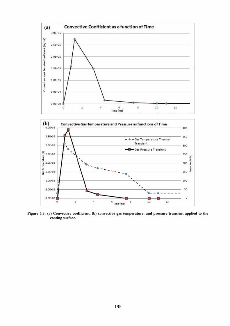
195
Figure 5.3: (a) Convective coefficient, (b) convective gas temperature, and pressure transient applied to the
coating surface.
196
5.2.1 Gun Tube Boundary Conditions – The Effects of Thermal and Pressure Transients
on Flaw Evolution
Gun tube boundary conditions applied in the finite element model contain both the thermal and
pressure boundary conditions described in the preceding section. A pulsed-laser heating test, as
described in Section 2.5.1, is often used to evaluate the thermal response of coatings, though the
pressure transient component is notoriously difficult to include in gun tube coating tests, with the
exception of live-firing tests. The pulsed-laser duration and energy were selected to best
approximate the thermals associated with combustion events. Finite element simulations with
only thermal boundary conditions are, therefore, analogous to the pulsed-laser heating test based
on the experimental conditions. Therefore, simulations of the thermal transient, with and without
the additional pressure transient, provide a unique opportunity to judge the contribution of
pressure, which is unaccounted for in the pulsed-laser heating experiment. In addition, pressure
transients are slightly out of phase from the peak combustion temperatures, further complicating
its understanding in experiments. Finite element modeling, therefore, is ideally suited to studying
the effects of the pressure transient relative to thermal loading. In order to do so, two simulations
have been run for which the boundary conditions include either thermal or thermal and pressure
transients. Analyzing the contributions of the pressure transient will provide a better context for
analyzing the pulsed-laser heating test in terms of its ability to model gun tube firing events. The
two cases described above were studied: a thermal transient alone, and in combination with
pressure pulse. Additionally, interstitial pressure will be applied inside the indentation-induced
blister in order to simulate a scenario in which gases have penetrated the coating. The cases
analyzed were chosen in order to study the contributions of each component of the gun tube
coating live firings and to compare the results to those of existing experimental techniques.
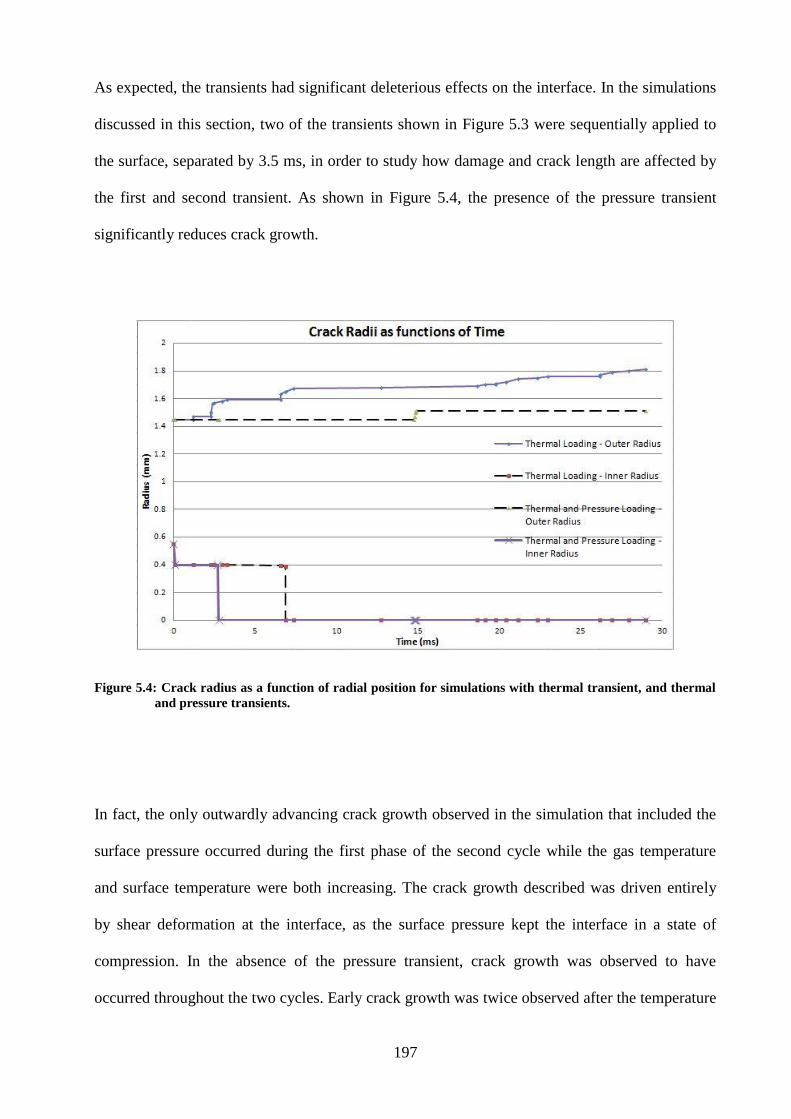
197
As expected, the transients had significant deleterious effects on the interface. In the simulations
discussed in this section, two of the transients shown in Figure 5.3 were sequentially applied to
the surface, separated by 3.5 ms, in order to study how damage and crack length are affected by
the first and second transient. As shown in Figure 5.4, the presence of the pressure transient
significantly reduces crack growth.
Figure 5.4: Crack radius as a function of radial position for simulations with thermal transient, and thermal
and pressure transients.
In fact, the only outwardly advancing crack growth observed in the simulation that included the
surface pressure occurred during the first phase of the second cycle while the gas temperature
and surface temperature were both increasing. The crack growth described was driven entirely
by shear deformation at the interface, as the surface pressure kept the interface in a state of
compression. In the absence of the pressure transient, crack growth was observed to have
occurred throughout the two cycles. Early crack growth was twice observed after the temperature
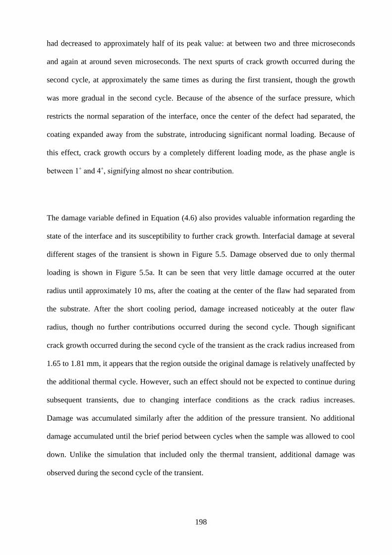
198
had decreased to approximately half of its peak value: at between two and three microseconds
and again at around seven microseconds. The next spurts of crack growth occurred during the
second cycle, at approximately the same times as during the first transient, though the growth
was more gradual in the second cycle. Because of the absence of the surface pressure, which
restricts the normal separation of the interface, once the center of the defect had separated, the
coating expanded away from the substrate, introducing significant normal loading. Because of
this effect, crack growth occurs by a completely different loading mode, as the phase angle is
between 1˚ and 4˚, signifying almost no shear contribution.
The damage variable defined in Equation (4.6) also provides valuable information regarding the
state of the interface and its susceptibility to further crack growth. Interfacial damage at several
different stages of the transient is shown in Figure 5.5. Damage observed due to only thermal
loading is shown in Figure 5.5a. It can be seen that very little damage occurred at the outer
radius until approximately 10 ms, after the coating at the center of the flaw had separated from
the substrate. After the short cooling period, damage increased noticeably at the outer flaw
radius, though no further contributions occurred during the second cycle. Though significant
crack growth occurred during the second cycle of the transient as the crack radius increased from
1.65 to 1.81 mm, it appears that the region outside the original damage is relatively unaffected by
the additional thermal cycle. However, such an effect should not be expected to continue during
subsequent transients, due to changing interface conditions as the crack radius increases.
Damage was accumulated similarly after the addition of the pressure transient. No additional
damage accumulated until the brief period between cycles when the sample was allowed to cool
down. Unlike the simulation that included only the thermal transient, additional damage was
observed during the second cycle of the transient.
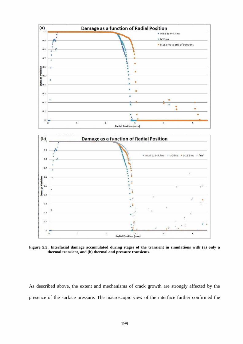
199
Figure 5.5: Interfacial damage accumulated during stages of the transient in simulations with (a) only a
thermal transient, and (b) thermal and pressure transients.
As described above, the extent and mechanisms of crack growth are strongly affected by the
presence of the surface pressure. The macroscopic view of the interface further confirmed the
200
beneficial effects of a surface pressure transient. The conditions at the crack tip are shown in
Figure 5.6.
Figure 5.6: Interfacial damage accumulated during stages of the transient in simulations showing a
magnification of the crack tip with (a) only a thermal transient and (b) thermal and pressure
transients.
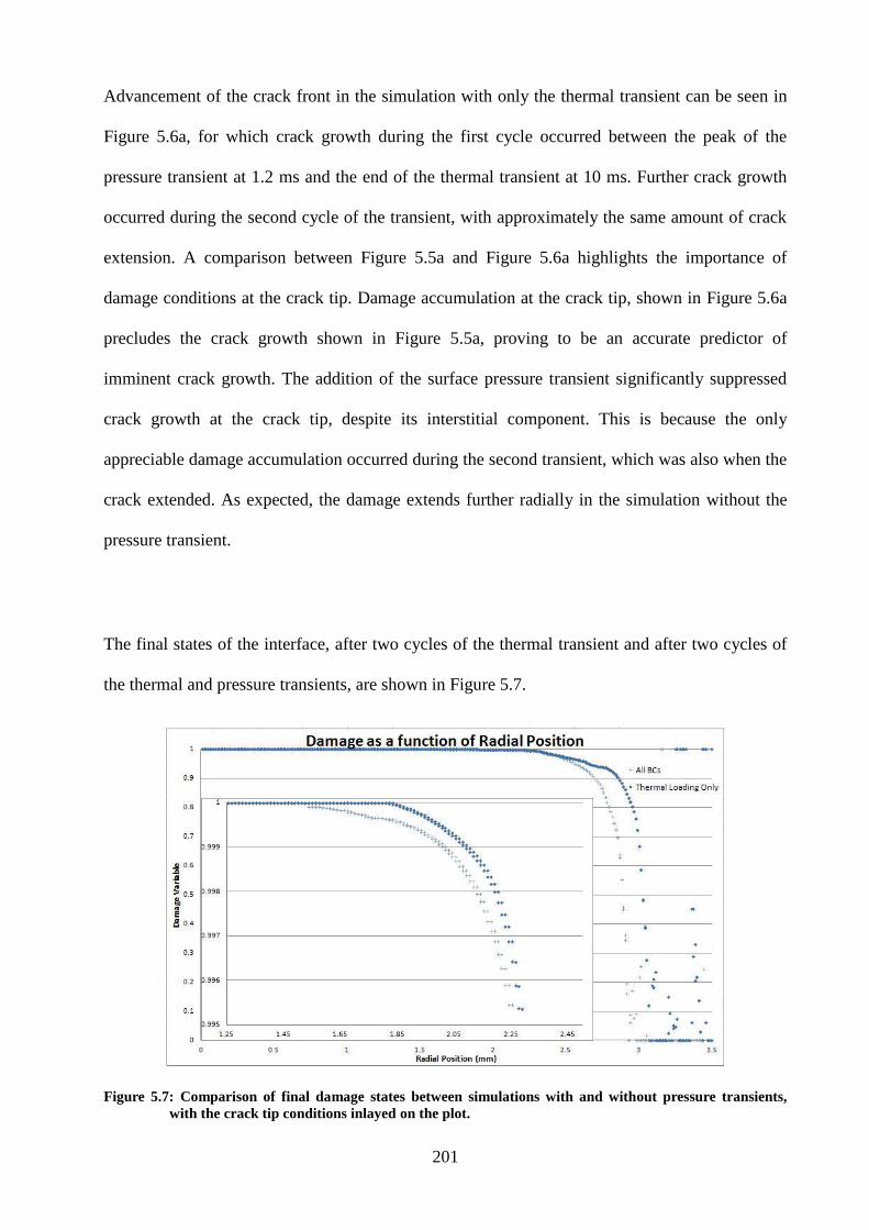
201
Advancement of the crack front in the simulation with only the thermal transient can be seen in
Figure 5.6a, for which crack growth during the first cycle occurred between the peak of the
pressure transient at 1.2 ms and the end of the thermal transient at 10 ms. Further crack growth
occurred during the second cycle of the transient, with approximately the same amount of crack
extension. A comparison between Figure 5.5a and Figure 5.6a highlights the importance of
damage conditions at the crack tip. Damage accumulation at the crack tip, shown in Figure 5.6a
precludes the crack growth shown in Figure 5.5a, proving to be an accurate predictor of
imminent crack growth. The addition of the surface pressure transient significantly suppressed
crack growth at the crack tip, despite its interstitial component. This is because the only
appreciable damage accumulation occurred during the second transient, which was also when the
crack extended. As expected, the damage extends further radially in the simulation without the
pressure transient.
The final states of the interface, after two cycles of the thermal transient and after two cycles of
the thermal and pressure transients, are shown in Figure 5.7.
Figure 5.7: Comparison of final damage states between simulations with and without pressure transients,
with the crack tip conditions inlayed on the plot.

202
Again, the presence of the surface pressure noticeably improved interfacial response to the
thermal transient. Despite crack opening forces resulting from interstitial pressure, the surface
pressure was more than sufficient to keep the interface in a state of compression throughout the
pressure transient. Such results suggest that mechanisms leading to catastrophic gun tube coating
failure include effects not accounted for in the above simulations. Pressure, though it penetrated
the coating, does not provide necessary crack opening forces to extend the crack. However,
interstitial pressure does contain highly corrosive combustion gases, which once exposed to the
steel, pose serious threats to the steel in terms of high temperatures and erosion.
The mechanisms of crack growth were significantly different after the addition of the coating
and blister pressure transient. Crack growth during the simulation with both transients, though
small, was dominated by the shear mode. However, in simulations without the pressure transient,
the crack growth observed was driven almost entirely by Mode I loading conditions at the crack
tip, as there was no longer surface pressure to keep the separated coating in close contact with
the substrate. Such results suggest that tests with only thermal effects, such as the pulsed-laser
heating test, possibly evaluate crack growth at different phase angles than would actually be
present in gun tubes, and this could be problematic as already described in Section 2.12.8 since
crack growth is a strong function of phase angle. The critical fracture energy for modes II and III
is often significantly higher than for mode 1, as reflected in the cohesive zone properties
evaluated in Section 4.4.3. As such, loading conditions with higher proportions of shear loading
are more resistant to crack growth. Results described in this section suggest that crack growth
under thermal conditions with pressure, which more closely approximates gun tubes extend an
already present flaw by different mechanisms under thermal loading alone.
203
Conductance across the interface during thermal loading also affects flaw evolution for the
samples subjected to thermal and pressure transients. It is likely, though, that the relationship
used for gap conductance overstates the effects of the clearance, as influence from radiation and
convection would still contribute to heat transfer after the interfaces separate. Yet, the
relationship does include for an important factor of crack growth, which is unaccounted for in
most previous models of crack growth in gun tube coatings. Once the gap clearance increases,
the coating loses most of its capacity to sink heat to the substrate. The coating then reaches even
higher temperatures and eventually separates, as seen in laser-pulse heating experiments [2, 17].
As shown in the plot of the temperature at the end of the pulse (Figure 5.8) the separated coating
is significantly hotter than the surrounding specimen, and lifts off the substrate; this is very
similar to what was seen in the previously cited pulsed-laser heating experiments.
In addition to beneficial compressive stresses introduced because of surface pressure loading, the
transient also acts to maintain contact between the coating and substrate. Improved interfacial
conductance allows more heat to be transferred to the substrate, resulting in lower coating
temperatures, and ultimately limiting thermal expansion. Such a tertiary effect of the pressure
loading is not included in the pulsed-laser experiments and significantly improves conduction
away from the coating, thus minimizing interfacial damage and crack growth.
The simulations of the damage evolution for coated plates with indentation-induced delamination
flaws under thermal-pressure transients provided insight into the contribution of each component
to the interface conditions. Such a simulation is similar to the pulse-laser heating tests, for which
significant damage and even complete coating and adhesive failure have been shown to occur in
a low number of cycles. However, the addition of the pressure transient had significant
advantageous effects on the integrity of the interface. Very little crack growth was seen, despite
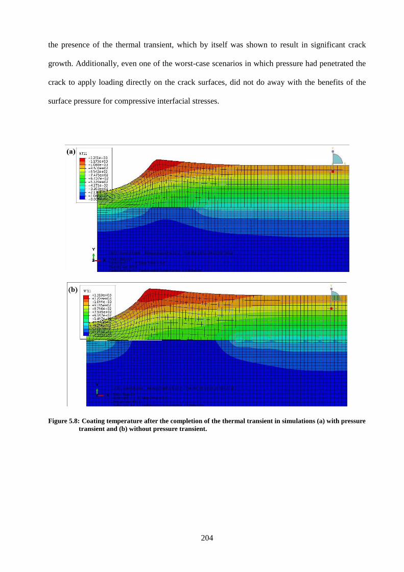
204
the presence of the thermal transient, which by itself was shown to result in significant crack
growth. Additionally, even one of the worst-case scenarios in which pressure had penetrated the
crack to apply loading directly on the crack surfaces, did not do away with the benefits of the
surface pressure for compressive interfacial stresses.
Figure 5.8: Coating temperature after the completion of the thermal transient in simulations (a) with pressure
transient and (b) without pressure transient.
205
5.2.2 Effects of Coating Thermal Capacity on Flaw Evolution
As observed in Section 5.2.1, thermal expansion resulting from convective heat transfer drives
crack growth in the absence of a pressure transient and contributes to interfacial damage in all
simulations. Significant crack growth was observed in the simulations in which the properties of
nickel were applied to the coating. The importance of heat transfer for thermal expansion and
resulting crack growth is a given. Therefore, the effects of a coating material’s thermal
capacitance were investigated as a possible mechanism for improving coating performance. For
nickel, the amount of energy required to raise the temperature of a unit of mass of the material
one unit of temperature (the specific heat) is approximately 440 kJ/kg K. However, other metals
have specific heats that range from between 100 to 900 kJ/kg K. An increase in the specific heat
would be expected to result in less heat transfer, less thermal expansion, and, therefore, less
crack growth. However, the decreased specific heat could also result in high thermal gradients,
and increased stresses at the interface for different coating thickness.
The specific energy of the coating material was increased by 50 and 100% of the value of nickel
in anticipation of reduced crack growth. Plots of the crack growth at different levels of specific
hear are shown in Figure 5.9.
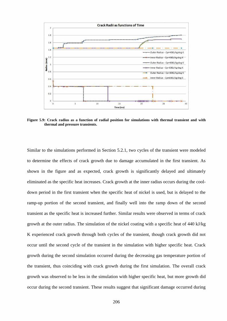
206
Figure 5.9: Crack radius as a function of radial position for simulations with thermal transient and with
thermal and pressure transients.
Similar to the simulations performed in Section 5.2.1, two cycles of the transient were modeled
to determine the effects of crack growth due to damage accumulated in the first transient. As
shown in the figure and as expected, crack growth is significantly delayed and ultimately
eliminated as the specific heat increases. Crack growth at the inner radius occurs during the cool-
down period in the first transient when the specific heat of nickel is used, but is delayed to the
ramp-up portion of the second transient, and finally well into the ramp down of the second
transient as the specific heat is increased further. Similar results were observed in terms of crack
growth at the outer radius. The simulation of the nickel coating with a specific heat of 440 kJ/kg
K experienced crack growth through both cycles of the transient, though crack growth did not
occur until the second cycle of the transient in the simulation with higher specific heat. Crack
growth during the second simulation occurred during the decreasing gas temperature portion of
the transient, thus coinciding with crack growth during the first simulation. The overall crack
growth was observed to be less in the simulation with higher specific heat, but more growth did
occur during the second transient. These results suggest that significant damage occurred during

207
the first transient, though not enough energy was present to drive the crack front. The respective
contributions of normal and shear loading at the crack front were similar to what was seen in the
simulation with only thermal boundary conditions described in baseline simulations as the phase
angle during crack growth was slightly higher at φ=6˚ as compared to φ=3˚. In both cases, the
shear contribution is almost negligible. As discussed earlier, the shear fracture energy is
significantly higher than normal and provides more resistance to crack growth at higher phase
angles. Finally, no outward crack growth was observed for the highest specific heat simulation.
The results show that increasing specific heat has the effect of both limiting and delaying crack
growth in pre-indented coated samples subjected to thermal transients on the coating surface.
A comparison of the accumulation of damage is shown in Figure 5.10, which correlates with
observations from the comparison of crack growth.
As discussed previously, damage is accumulated throughout the two cycles of the simulation.
Almost all the damage was accumulated in the first cycle, though crack growth occurred
throughout both cycles. However, as the specific heat increases, the amount of damaged
accumulated decreases, until almost no observable increment in damage is accumulated in the
simulation with the specific heat of 800 kJ/kg K. More information about the conditions of the
interface at the stages in the transient can be gained by observing the conditions at the crack tip,
which cannot be seen in the entire interface in Figure 5.10. Plots of the damage variable closer to
the crack tip are shown in Figure 5.11, which compares the damage for a coating with standard
nickel properties and a simulation where the specific heat is increased to 800 kJ/kg K as shown
in Figure 5.11b.
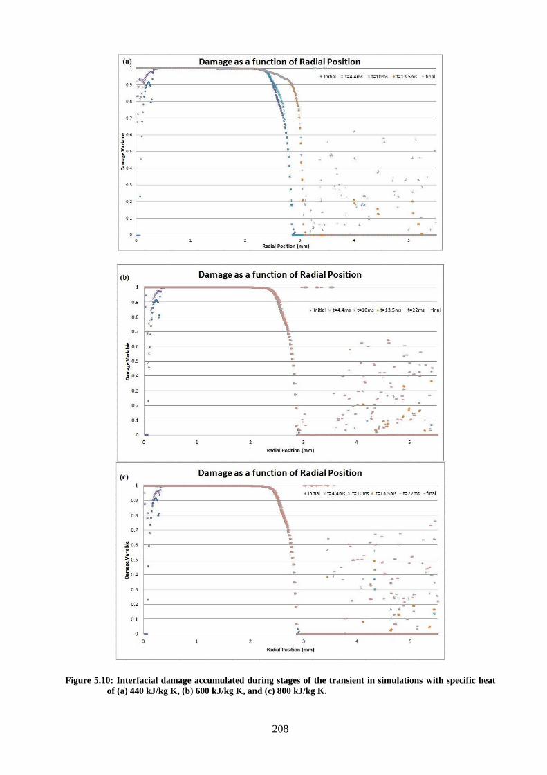
208
Figure 5.10: Interfacial damage accumulated during stages of the transient in simulations with specific heat
of (a) 440 kJ/kg K, (b) 600 kJ/kg K, and (c) 800 kJ/kg K.
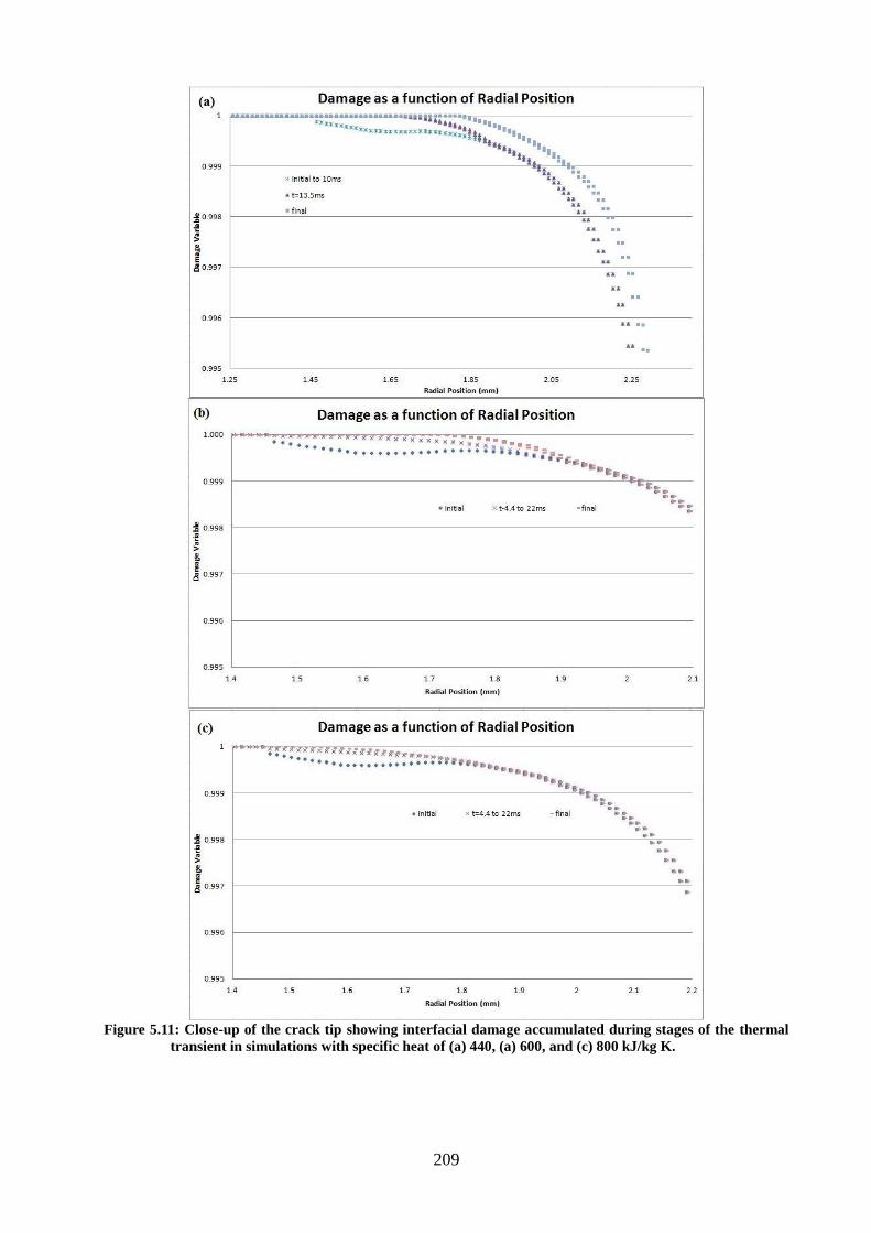
209
Figure 5.11: Close-up of the crack tip showing interfacial damage accumulated during stages of the thermal
transient in simulations with specific heat of (a) 440, (a) 600, and (c) 800 kJ/kg K.
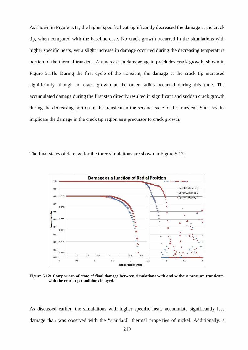
210
As shown in Figure 5.11, the higher specific heat significantly decreased the damage at the crack
tip, when compared with the baseline case. No crack growth occurred in the simulations with
higher specific heats, yet a slight increase in damage occurred during the decreasing temperature
portion of the thermal transient. An increase in damage again precludes crack growth, shown in
Figure 5.11b. During the first cycle of the transient, the damage at the crack tip increased
significantly, though no crack growth at the outer radius occurred during this time. The
accumulated damage during the first step directly resulted in significant and sudden crack growth
during the decreasing portion of the transient in the second cycle of the transient. Such results
implicate the damage in the crack tip region as a precursor to crack growth.
The final states of damage for the three simulations are shown in Figure 5.12.
Figure 5.12: Comparison of state of final damage between simulations with and without pressure transients,
with the crack tip conditions inlayed.
As discussed earlier, the simulations with higher specific heats accumulate significantly less
damage than was observed with the “standard” thermal properties of nickel. Additionally, a
211
second crack was formed outside the initial region of damage. Interestingly, the second crack
does not form in the original simulation, though damaged elements were observed. The near
crack tip conditions show crack growth that occurred for the middle specific heat value.
However, excepted for increased damage at the crack tip, and increased crack length, little
difference in the state of the interface can be seen over the remainder of the interface as the
specific heat was increased.
5.2.3 Effects of Phase Difference between Pressure and Thermal Transients on Flaw
Evolution
The surface and blister pressure transients were adjusted in time relative to the thermal shock in
order to study conditions that are possible in other barrel configurations. Effects such as riffling
can influence how the gases travel through the length of the barrel, resulting in higher and lower
convection coefficients, which in turn increase or decrease the rate of heat transfer into the
coating, respectively. Surface conditions can also affect the speed at which the thermal and
pressure transients move along the length of the tube. In addition, coating thermo-physical
material properties can also increase the rate at which thermal energy is transferred into the
coating and substrate, thus advancing or delaying the effects of thermal transient relative to the
pressure transient. As seen in the previous section, the thermal transient has significant effects on
the extent and type of crack growth. Therefore, the effects of the phase difference between the
thermal and pressure transients was studied to discern how the rate of heat transfer, and other
coating conditions, might affect damage and crack growth at the interface.
212
In order to study such effects, the phase difference of the pressure relative to the thermal
transient shown in Figure 5.3 were offset by three different increments of time in addition to the
phase difference already present. The pressure transient was delayed for 0.5 ms and 1.0 ms, in
addition to being advanced 0.25 ms form its original time. All three simulations of phase
differences were compared to the baseline presented in Section 5.2.1 for which the thermal
transient already preceded the pressure transient by 0.4 ms. Only one cycle of the transient is
simulated in the following analysis. A plot of the crack radius as a function of the time for the
simulations of the three amounts of phase difference is shown in Figure 5.13, in addition to the
case with the measured boundary conditions.
Figure 5.13: Crack radius as a function of radial position in simulations for which internal and pressure
transients were offset from their original position relative to the thermal transient.
As shown in Figure 5.13, crack growth at the outer radius occurred only when the pressure was
delayed for 1.0 ms from its original time relative to the thermal transient. Crack initiation
213
coincides with the onset of the pressure transient, and it is reinitiated at two other times during
the transient: as the pressure transient approaches zero and during the ramp-down of the thermal
transient. The phase angle of the crack tip during growth was between 70° and 85°, signifying
significant shear contributions to crack growth, as the pressure transient kept normal loading to a
minimum. However, it is likely that a 1.0 ms offset is unrealistic given the variations that might
be expected in gun tube conditions. By offsetting the pressure transient, crack growth at the inner
radius was delayed. Inward crack growth was most delayed in the final simulations when the
pressure peak was offset at 1.0 ms later than in the baseline case, even though outward crack
growth occurred throughout the transient.
The different cases of pressure offsets resulted in crack growth only in the extreme example of
the pressure transient delayed by 1.0 ms. However, interfacial damage accumulated in all cases,
as shown in Figure 5.15 and Figure 5.15.
As observed in the previous simulations, significant damage occurred following both the thermal
and pressure transients. The area of damage increases during the cool-down phase, though
accumulated damage at the edge of the region does not approach unity. Crack growth did not
occur during the cool-down period after the thermal transient, yet it is apparent that the interface
does experience damage as the heat is conducted through the sample. In addition, the surface was
exposed to room temperatures, though at a lower convective coefficient, thus creating a more
severe thermal gradient.
214
Figure 5.14: Interfacial damage accumulated during stages of the transient in simulations for which relative
to the thermal transient the internal and external pressure transients were offset by (a) 0.25 ms
before its original time, and (b) 0 ms.
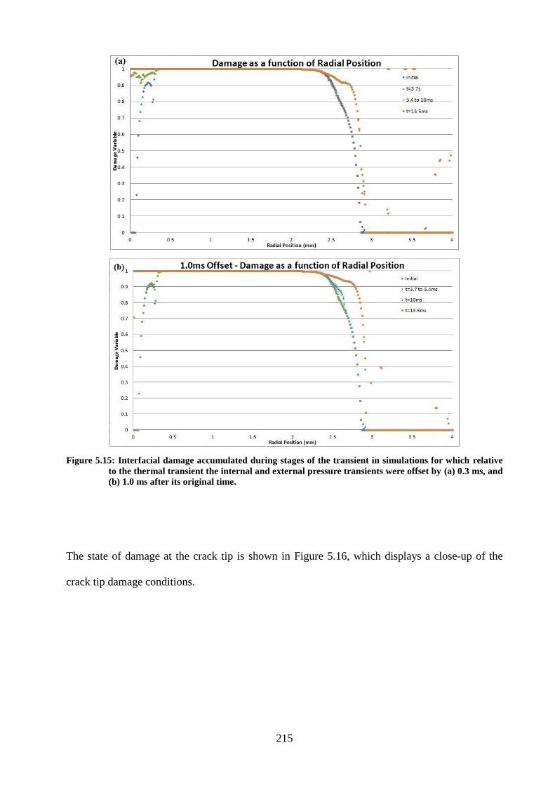
215
Figure 5.15: Interfacial damage accumulated during stages of the transient in simulations for which relative
to the thermal transient the internal and external pressure transients were offset by (a) 0.3 ms, and
(b) 1.0 ms after its original time.
The state of damage at the crack tip is shown in Figure 5.16, which displays a close-up of the
crack tip damage conditions.
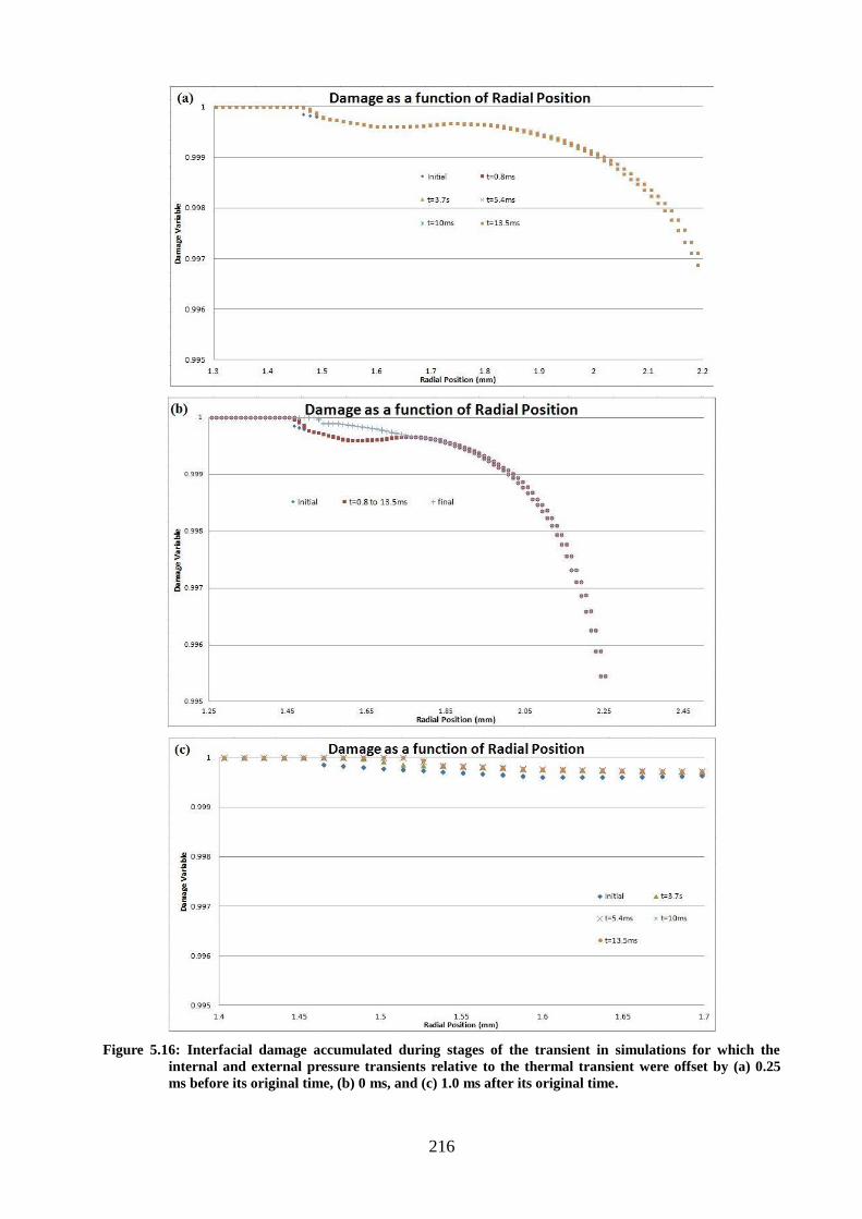
216
Figure 5.16: Interfacial damage accumulated during stages of the transient in simulations for which the
internal and external pressure transients relative to the thermal transient were offset by (a) 0.25
ms before its original time, (b) 0 ms, and (c) 1.0 ms after its original time.
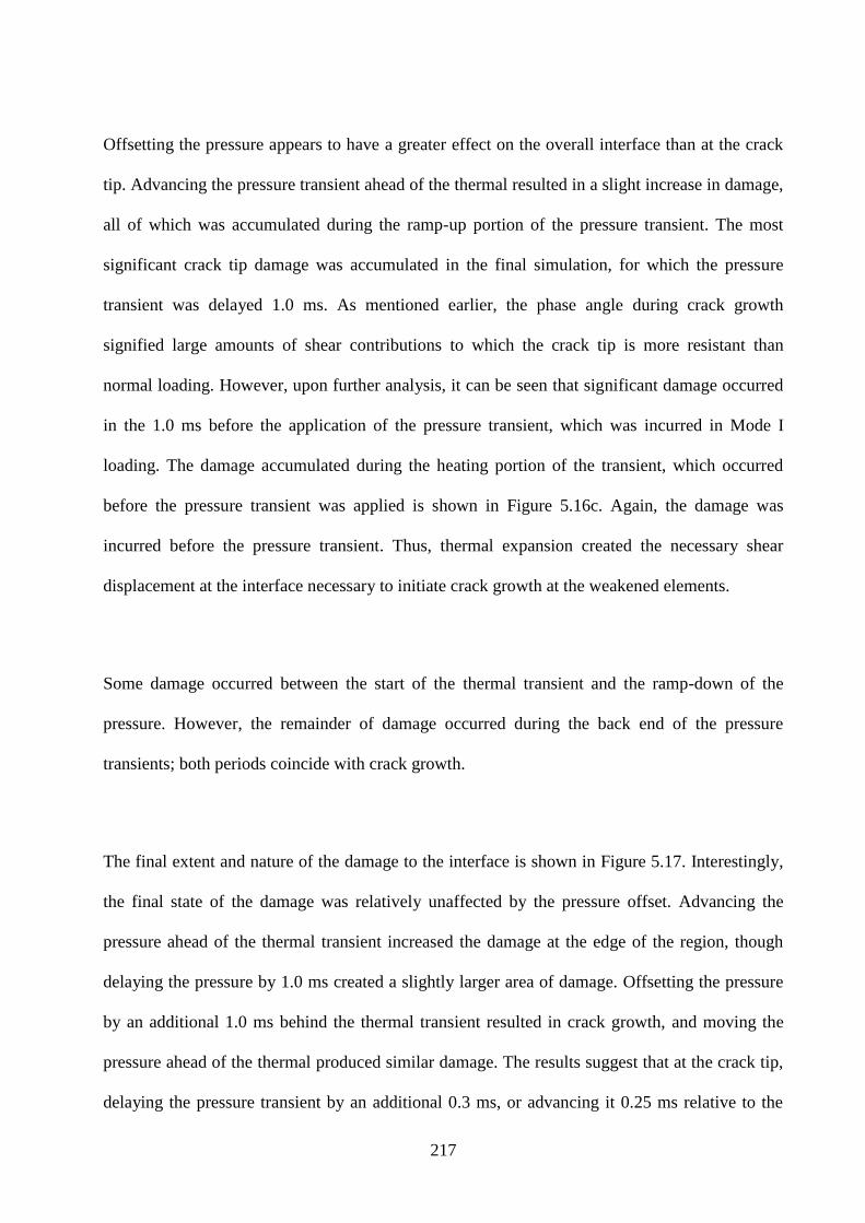
217
Offsetting the pressure appears to have a greater effect on the overall interface than at the crack
tip. Advancing the pressure transient ahead of the thermal resulted in a slight increase in damage,
all of which was accumulated during the ramp-up portion of the pressure transient. The most
significant crack tip damage was accumulated in the final simulation, for which the pressure
transient was delayed 1.0 ms. As mentioned earlier, the phase angle during crack growth
signified large amounts of shear contributions to which the crack tip is more resistant than
normal loading. However, upon further analysis, it can be seen that significant damage occurred
in the 1.0 ms before the application of the pressure transient, which was incurred in Mode I
loading. The damage accumulated during the heating portion of the transient, which occurred
before the pressure transient was applied is shown in Figure 5.16c. Again, the damage was
incurred before the pressure transient. Thus, thermal expansion created the necessary shear
displacement at the interface necessary to initiate crack growth at the weakened elements.
Some damage occurred between the start of the thermal transient and the ramp-down of the
pressure. However, the remainder of damage occurred during the back end of the pressure
transients; both periods coincide with crack growth.
The final extent and nature of the damage to the interface is shown in Figure 5.17. Interestingly,
the final state of the damage was relatively unaffected by the pressure offset. Advancing the
pressure ahead of the thermal transient increased the damage at the edge of the region, though
delaying the pressure by 1.0 ms created a slightly larger area of damage. Offsetting the pressure
by an additional 1.0 ms behind the thermal transient resulted in crack growth, and moving the
pressure ahead of the thermal produced similar damage. The results suggest that at the crack tip,
delaying the pressure transient by an additional 0.3 ms, or advancing it 0.25 ms relative to the
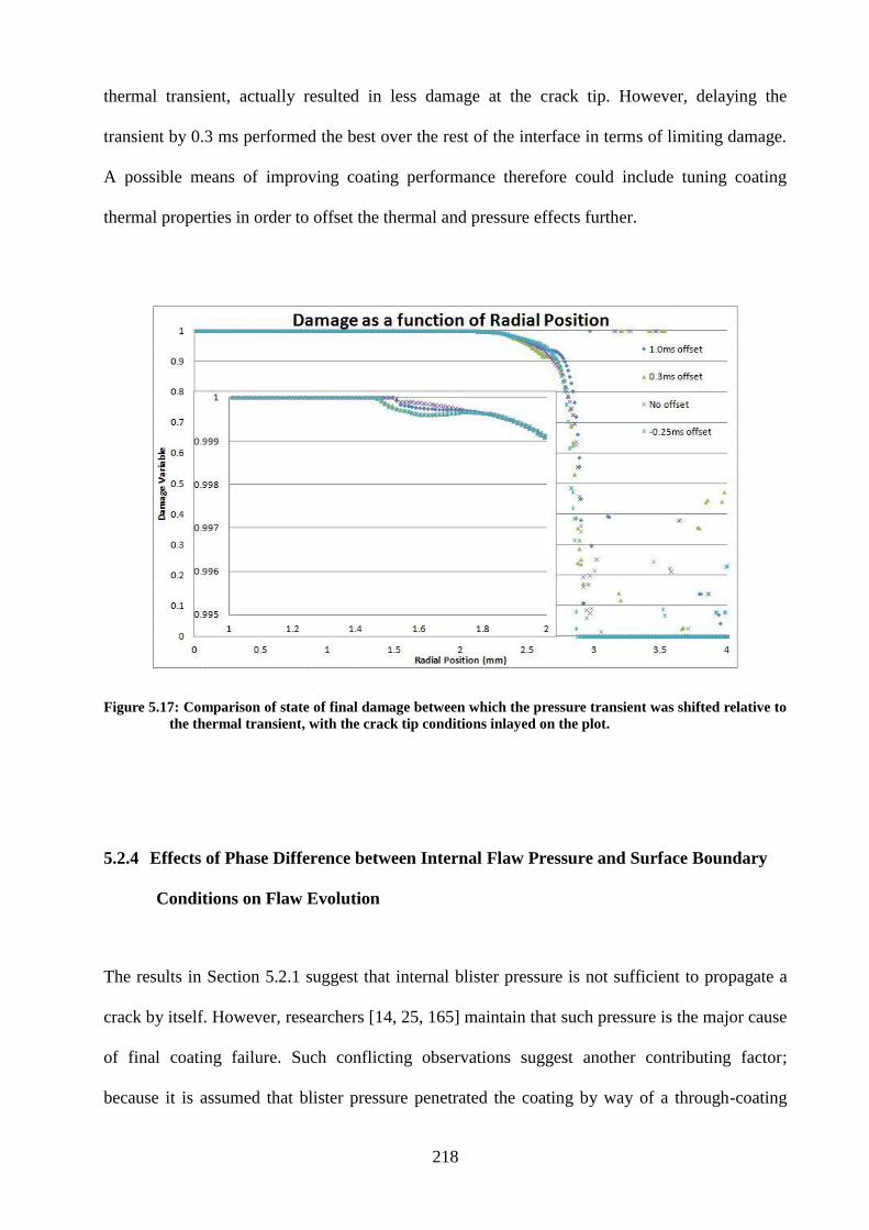
218
thermal transient, actually resulted in less damage at the crack tip. However, delaying the
transient by 0.3 ms performed the best over the rest of the interface in terms of limiting damage.
A possible means of improving coating performance therefore could include tuning coating
thermal properties in order to offset the thermal and pressure effects further.
Figure 5.17: Comparison of state of final damage between which the pressure transient was shifted relative to
the thermal transient, with the crack tip conditions inlayed on the plot.
5.2.4 Effects of Phase Difference between Internal Flaw Pressure and Surface Boundary
Conditions on Flaw Evolution
The results in Section 5.2.1 suggest that internal blister pressure is not sufficient to propagate a
crack by itself. However, researchers [14, 25, 165] maintain that such pressure is the major cause
of final coating failure. Such conflicting observations suggest another contributing factor;
because it is assumed that blister pressure penetrated the coating by way of a through-coating
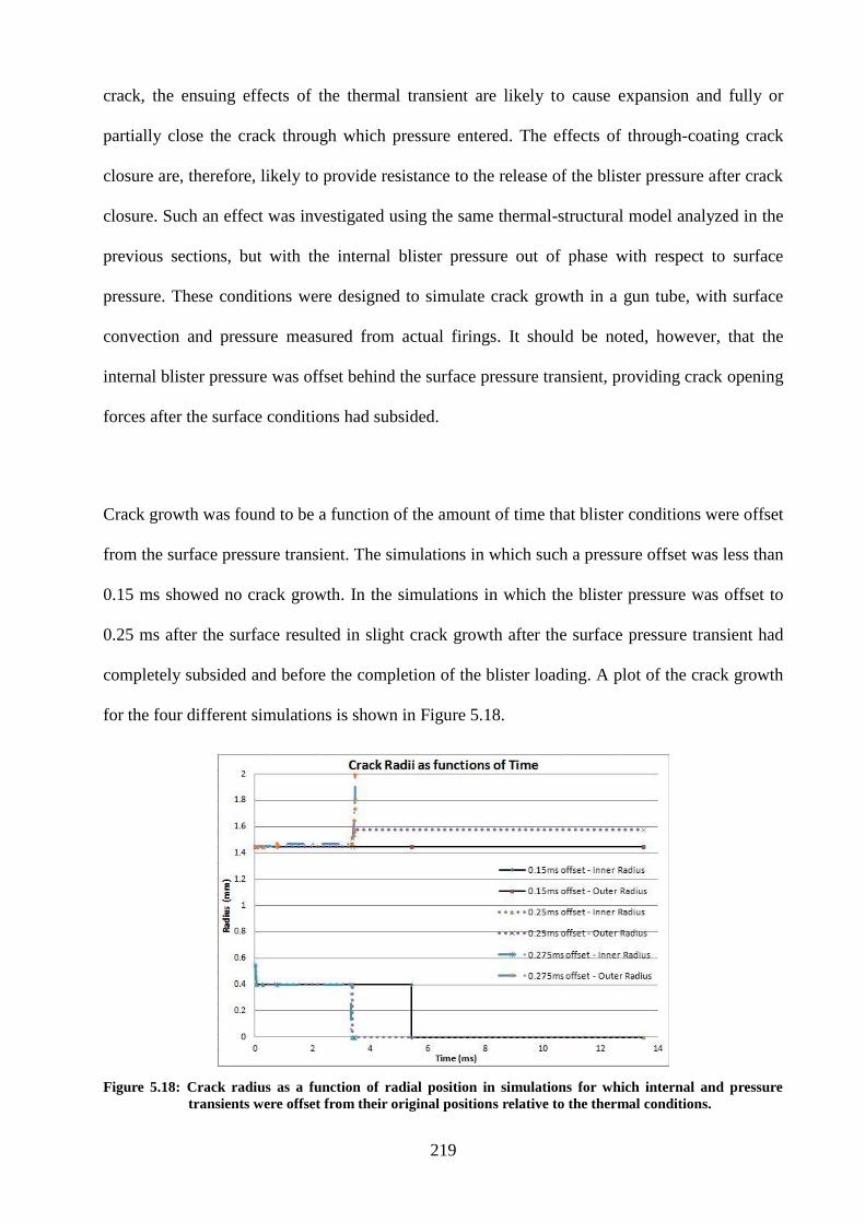
219
crack, the ensuing effects of the thermal transient are likely to cause expansion and fully or
partially close the crack through which pressure entered. The effects of through-coating crack
closure are, therefore, likely to provide resistance to the release of the blister pressure after crack
closure. Such an effect was investigated using the same thermal-structural model analyzed in the
previous sections, but with the internal blister pressure out of phase with respect to surface
pressure. These conditions were designed to simulate crack growth in a gun tube, with surface
convection and pressure measured from actual firings. It should be noted, however, that the
internal blister pressure was offset behind the surface pressure transient, providing crack opening
forces after the surface conditions had subsided.
Crack growth was found to be a function of the amount of time that blister conditions were offset
from the surface pressure transient. The simulations in which such a pressure offset was less than
0.15 ms showed no crack growth. In the simulations in which the blister pressure was offset to
0.25 ms after the surface resulted in slight crack growth after the surface pressure transient had
completely subsided and before the completion of the blister loading. A plot of the crack growth
for the four different simulations is shown in Figure 5.18.
Figure 5.18: Crack radius as a function of radial position in simulations for which internal and pressure
transients were offset from their original positions relative to the thermal conditions.
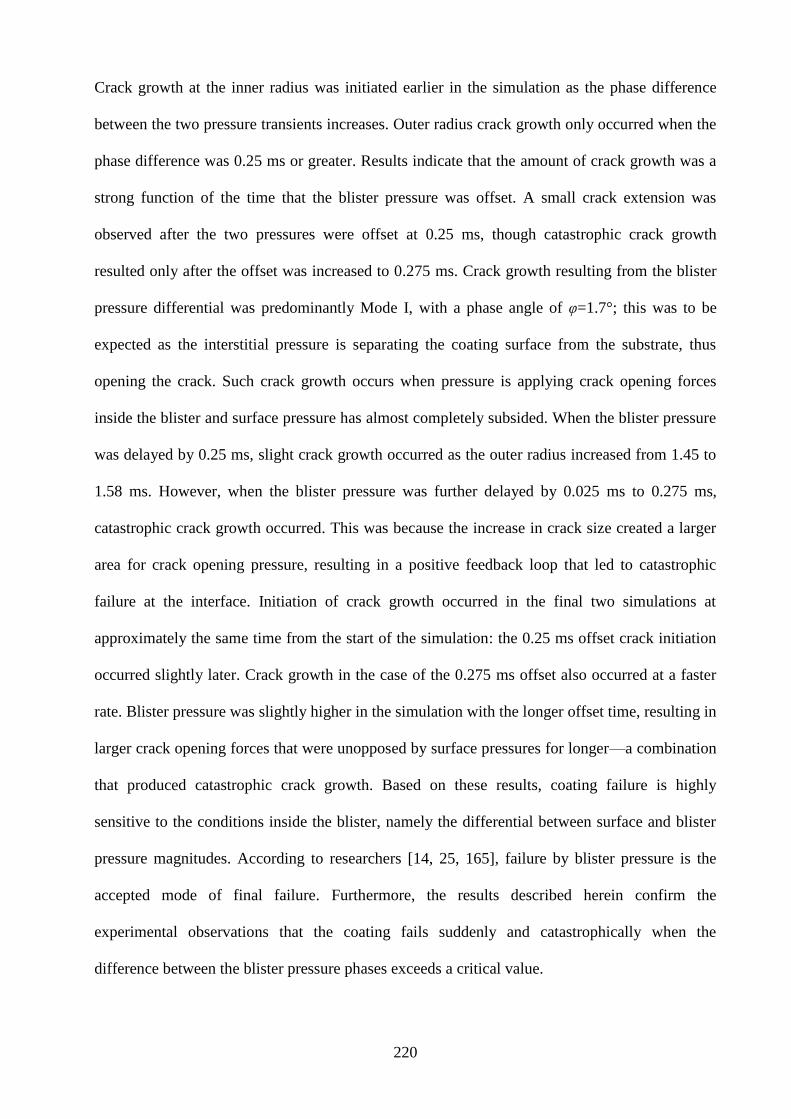
220
Crack growth at the inner radius was initiated earlier in the simulation as the phase difference
between the two pressure transients increases. Outer radius crack growth only occurred when the
phase difference was 0.25 ms or greater. Results indicate that the amount of crack growth was a
strong function of the time that the blister pressure was offset. A small crack extension was
observed after the two pressures were offset at 0.25 ms, though catastrophic crack growth
resulted only after the offset was increased to 0.275 ms. Crack growth resulting from the blister
pressure differential was predominantly Mode I, with a phase angle of φ=1.7°; this was to be
expected as the interstitial pressure is separating the coating surface from the substrate, thus
opening the crack. Such crack growth occurs when pressure is applying crack opening forces
inside the blister and surface pressure has almost completely subsided. When the blister pressure
was delayed by 0.25 ms, slight crack growth occurred as the outer radius increased from 1.45 to
1.58 ms. However, when the blister pressure was further delayed by 0.025 ms to 0.275 ms,
catastrophic crack growth occurred. This was because the increase in crack size created a larger
area for crack opening pressure, resulting in a positive feedback loop that led to catastrophic
failure at the interface. Initiation of crack growth occurred in the final two simulations at
approximately the same time from the start of the simulation: the 0.25 ms offset crack initiation
occurred slightly later. Crack growth in the case of the 0.275 ms offset also occurred at a faster
rate. Blister pressure was slightly higher in the simulation with the longer offset time, resulting in
larger crack opening forces that were unopposed by surface pressures for longer—a combination
that produced catastrophic crack growth. Based on these results, coating failure is highly
sensitive to the conditions inside the blister, namely the differential between surface and blister
pressure magnitudes. According to researchers [14, 25, 165], failure by blister pressure is the
accepted mode of final failure. Furthermore, the results described herein confirm the
experimental observations that the coating fails suddenly and catastrophically when the
difference between the blister pressure phases exceeds a critical value.
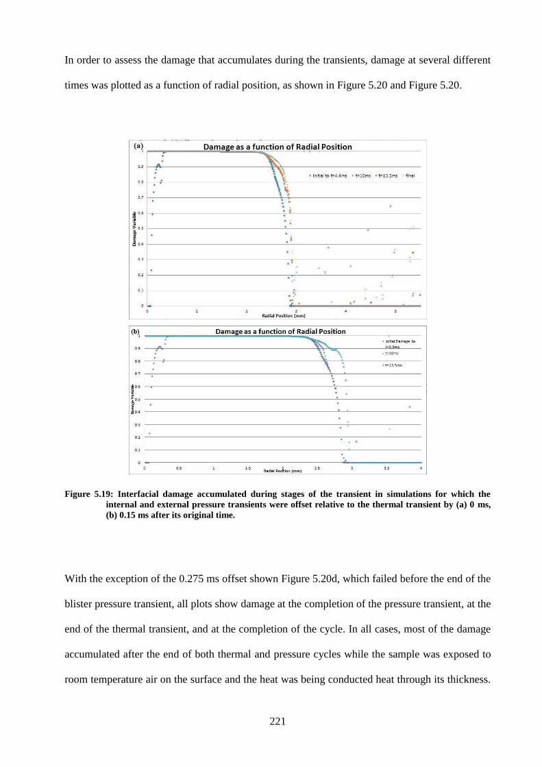
221
In order to assess the damage that accumulates during the transients, damage at several different
times was plotted as a function of radial position, as shown in Figure 5.20 and Figure 5.20.
Figure 5.19: Interfacial damage accumulated during stages of the transient in simulations for which the
internal and external pressure transients were offset relative to the thermal transient by (a) 0 ms,
(b) 0.15 ms after its original time.
With the exception of the 0.275 ms offset shown Figure 5.20d, which failed before the end of the
blister pressure transient, all plots show damage at the completion of the pressure transient, at the
end of the thermal transient, and at the completion of the cycle. In all cases, most of the damage
accumulated after the end of both thermal and pressure cycles while the sample was exposed to
room temperature air on the surface and the heat was being conducted heat through its thickness.
222
The damage accumulation plot in Figure 5.20d is incomplete, as the sample failed before the end
of the blister pressure transient.
Figure 5.20: Interfacial damage accumulated during stages of the transient in simulations for which the
internal and external pressure transients were offset relative to the thermal transient by (a) 0.25
ms, and (b) 0.275ms after its original time.
Damage accumulation on the entire interface occurred primarily during the cool-down phase of
the transient. However, observations at the crack tip show that significant damage occurred in
the time between the completion of the surface and interstitial pressure transients, as shown in
Figure 5.21.
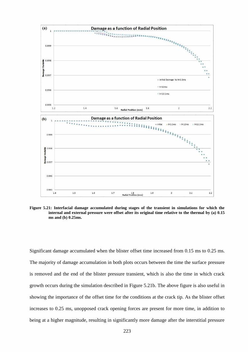
223
Figure 5.21: Interfacial damage accumulated during stages of the transient in simulations for which the
internal and external pressure were offset after its original time relative to the thermal by (a) 0.15
ms and (b) 0.25ms.
Significant damage accumulated when the blister offset time increased from 0.15 ms to 0.25 ms.
The majority of damage accumulation in both plots occurs between the time the surface pressure
is removed and the end of the blister pressure transient, which is also the time in which crack
growth occurs during the simulation described in Figure 5.21b. The above figure is also useful in
showing the importance of the offset time for the conditions at the crack tip. As the blister offset
increases to 0.25 ms, unopposed crack opening forces are present for more time, in addition to
being at a higher magnitude, resulting in significantly more damage after the interstitial pressure
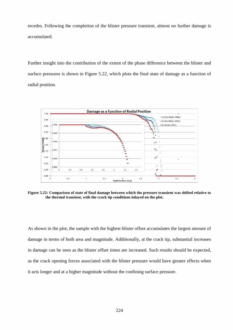
224
recedes. Following the completion of the blister pressure transient, almost no further damage is
accumulated.
Further insight into the contribution of the extent of the phase difference between the blister and
surface pressures is shown in Figure 5.22, which plots the final state of damage as a function of
radial position.
Figure 5.22: Comparison of state of final damage between which the pressure transient was shifted relative to
the thermal transient, with the crack tip conditions inlayed on the plot.
As shown in the plot, the sample with the highest blister offset accumulates the largest amount of
damage in terms of both area and magnitude. Additionally, at the crack tip, substantial increases
in damage can be seen as the blister offset times are increased. Such results should be expected,
as the crack opening forces associated with the blister pressure would have greater effects when
it acts longer and at a higher magnitude without the confining surface pressure.
225
5.2.5 Discussion of Thermal-Structural Simulation of Flaw Evolution Results
The simulations were conducted in order to ascertain the mechanisms and conditions for the
evolution of an indentation-induced interfacial flaw under severe thermal and pressure surface
transients. Complete boundary conditions, including surface pressure, were applied to the finite
element model, and the responses of the system without the pressure transient were compared.
By comparing the respective solutions of the simulations with and without the pressure transient,
the contribution to interfacial flaw evolution can be determined, thus gaining insight into the
pulsed-laser heating experiment. Additionally, blister pressure was included in the indentation-
induced flaw in a situation in which it was assumed that the surface pressure had penetrated the
coating through a crack, thus applying crack opening forces from inside the blister. Thermal and
pressure transients were also further offset, in order to examine the effects of the phase
difference between thermal and pressure transients, and by extension, factors that might expedite
or impede their effects. Finally, internal blister pressure has often been cited as a likely initiator
of final failure, though it has never been proven; therefore, blister pressure was delayed relative
to the surface pressure transient in order to simulate a gun tube in which combustion gases (and
pressure) penetrate the coating and subsequently cannot easily escape because thermal expansion
has caused the crack to close.
The plots of the damage variable are instructive in highlighting the effects of thermal and/or
pressure transients on the state of the interface away from the crack tip. Plots that show the entire
interface are slightly misleading, as it appears that the region for which the damage variable is
equal to one is much larger than it actually is. Upon closer inspection, the area of complete
damage is not as large as it first appears, as shown by the images of the damage variable at the
crack tip. Additionally, as can be seen in the relation between the damage variable and the
cohesive normal and shear stresses (Equations (4.2) and (4.4)) the damage variable is multiplied
226
by the cohesive stiffnesses, which are orders of magnitude larger than the strength of the
interface. Therefore, interfacial elements can still be in a state of high stress with magnitudes on
the order of megaPascals, despite a damage variable exceeding 0.999. Though the entire scope of
the interfacial damage provides insight into the distance from the crack that the damage reaches,
the near-crack tip damage offers more insight in terms of predicting the effects of the thermal
transient on future crack growth.
As discussed previously in Section 5.2.1 the contributions of surface thermal and pressure
transients have significant effects on the interface, specifically on flaw evolution. Two cycles of
the transient were simulated, in order to better quantify the effects of damage introduced during
the first cycle of the transient. In the absence of the pressure transient, crack growth occurred
during both cycles of the transient. Crack extension occurred during the ramp-down period of the
thermal transient, and again during a relatively steady portion during which combustion gases
were approximately 1300 K in both cycles. The coating had absorbed enough heat that it
separated at the center of the indentation, which allowed it to be detached from the interface.
Once the coating was free to expand from the substrate, heat conduction across the interface
decreased drastically as a function of separation distance before stopping completely, resulting in
higher coating temperatures and even greater thermal expansion. Clearly, the effects of the
increased coating temperature contribute to crack growth. However, they can also melt the
coating, as temperatures in excess of the melting point of nickel were observed at the edges of
the indentation. Given the effect of gap conductance, an added benefit of the pressure transient is
that it keeps the coating in contact with the interface should an interfacial flaw be present, which
aids heat transfer through the coating and limits thermal expansion. Additionally, because of the
thermal expansion of the coating and the absence of any confining pressure, the coating bows
upward, creating normal separation at the interface. In the absence of a pre-existing interfacial
flaw, the coating would remain in contact with the interface, resulting in radial expansion, and
227
higher shear stresses at the interface, to which the interface is more resistive. However, when a
flaw is present, and there is no confining surface pressure, crack tip loading is predominately
Mode I. It is likely that such conditions are similar to the pulsed-laser heating experiment, where
similar amounts of energy are introduced to the sample at approximately the same rate. Based on
observations from the simulation, such an experiment can be expected to initiate a flaw due to
shear forces. However, the contribution of Mode I loading will increase as the flaw grows until
the loading on the crack tip is entirely Mode I, as was the case in the simulations. Such loading
are not analogous to gun tube conditions, as demonstrated in Section 5.2.1. Simulations
performed with both thermal and pressure transients illustrated the beneficial effects of the
absence of Mode I crack tip loading conditions. Crack growth did not occur in the first cycle of
the transient that included pressure, but did manifest itself in the period of increasing combustion
gas temperatures during the second cycle due to shear interfacial loading. When the pressure
transients were applied, crack tip loading was entirely Mode II, but otherwise it was still
predominately Mode II, with a small Mode I component. Surface pressure, therefore, has a
significant effect on interfacial conditions and the resulting crack growth. Such effects must be
taken into consideration when analyzing pulsed-laser heating experimental results.
The addition of surface and blister pressure without additional offsets, significantly impeded
crack growth, which did not occur during the pressure transient due to the resulting interfacial
compressive stresses. However, crack growth did occur during the second cycle of the transient
as the convective gases were again heating up the coating surface. Interestingly, the interface
was in compression at this time due to the surface pressure, though the shear stresses at the
interface were enough to drive the crack a short length by entirely Mode II/III loading. Such
results confirm the significance of shear crack growth in the presence of surface pressure
transients.
228
The importance of the conditions of blister pressure should not be overlooked in terms of crack
interfacial crack growth and final coating failure. An analysis in which the pressure was assumed
to have penetrated the coating, but was in phase with the surface proved inconsequential in terms
of crack growth. Such results were not unexpected, as the entire surface experiences pressure
equal in magnitude and applied to the entire coating, providing more than sufficient force to
maintain compressive stresses ahead of the crack tip. Offsetting the entire pressure transient did
not have significant effects on the state of the interface, with the exception of the 1.0 ms offset,
which is larger than any anticipated variation in actual conditions. In this case, the crack
extension occurred by almost exclusively Mode I loading, which occurred after the pressure
transient was complete. Based on subsequent simulations, the effects of delaying the internal
blister pressure transient were evaluated in order to simulate the resistance interstitial pressures
might face after the coating expanded and the through-coating crack had completely or partially
closed. It was observed in the simulations that when pressures were offset by 0.25 ms, crack
growth began and that further offsets lead to catastrophic failure. Such results suggest the
sensitivity of the blister to gas pressures. Offsets in the phase between surface and interstitial
pressure have compounding effects: pressure is applied from inside the blister for a longer period
of time absent confining surface pressure, in addition to being larger in magnitude. Further
compounding the effects, the interstitial pressure application area increases with the crack front.
Once crack growth is initiated, the pressure area and resulting crack opening forces also increase,
further driving the crack. Interstitial pressure also opens the crack in its weakest mode, as
interfaces are significantly more resistant in the shear mode to fracture. According to this
analysis, it is highly likely that blister pressure is the instigator of final coating failure.
The thermal capacitance of the coating materials was analyzed in terms of its effects on crack
growth. Based on the expectations due to the role of specific heat in heat transfer, the property
was identified as possibly having a strong effect on crack growth. Higher specific heat requires
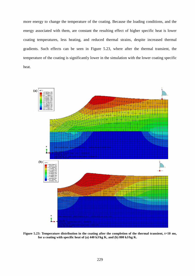
229
more energy to change the temperature of the coating. Because the loading conditions, and the
energy associated with them, are constant the resulting effect of higher specific heat is lower
coating temperatures, less heating, and reduced thermal strains, despite increased thermal
gradients. Such effects can be seen in Figure 5.23, where after the thermal transient, the
temperature of the coating is significantly lower in the simulation with the lower coating specific
heat.
Figure 5.23: Temperature distribution in the coating after the completion of the thermal transient, t=10 ms,
for a coating with specific heat of (a) 440 kJ/kg K, and (b) 800 kJ/kg K.
230
Because of decreased heat transfer and lower coating temperatures, the coating experienced
significantly less thermal expansion. Recognizing the effects of specific heat, it was confirmed as
a viable consideration in coating design as a means of improving performance and minimizing
interfacial crack growth.
Several different combinations of gun tube boundary conditions were applied to the surface of a
coated sample with an indentation-induced interfacial flaw. Flaw evolution under the thermal
transients was studied with and without the surface pressure transient, which was accompanied
by an interstitial pressure inside the flaw that was in phase with the surface pressure transient. A
comparison of the results with and without the pressure transient illustrated the beneficial effects
in terms of suppressing crack growth. Additionally, the results revealed the different mechanisms
of crack growth resulting from the addition of the surface pressure transient, which has the
beneficial effect of keeping the interface in compression, and reducing crack growth. Thermal
capacitance was also studied and found to have beneficial effects in terms of reducing heat
transfer and thermal expansion, leading to suppressed crack growth. The surface and interstitial
pressure transients were further offset relative to the thermal transient. In addition, though
interfacial damage increased, crack growth was found to be largely unaffected, except in the
extreme case of the 1.0 ms offset. Finally, the blister pressure was offset from the surface
pressure transient, which resulted in the occurrence of blister pressure after the surface pressure
had subsided. The pressure differential at the end of the blister transient was sufficiently
significant to extend the crack. Observations from simulations at different blister offset values
suggest that the crack growth is highly sensitive to blister pressure conditions. In cases in which
the blister pressure was offset by 0.25 ms, a small amount of outward crack growth was
observed. However, increasing the blister offset time to 0.275 ms resulted in catastrophic crack
growth such that coating completely separated from the substrate surface. These results provide
valuable insight into the crack growth process of interfacial, delamination-induced flaws, useful
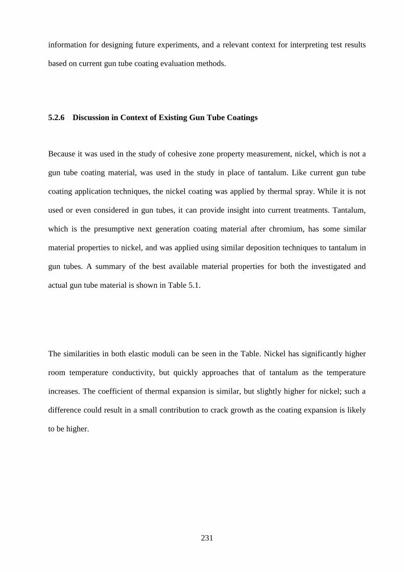
231
information for designing future experiments, and a relevant context for interpreting test results
based on current gun tube coating evaluation methods.
5.2.6 Discussion in Context of Existing Gun Tube Coatings
Because it was used in the study of cohesive zone property measurement, nickel, which is not a
gun tube coating material, was used in the study in place of tantalum. Like current gun tube
coating application techniques, the nickel coating was applied by thermal spray. While it is not
used or even considered in gun tubes, it can provide insight into current treatments. Tantalum,
which is the presumptive next generation coating material after chromium, has some similar
material properties to nickel, and was applied using similar deposition techniques to tantalum in
gun tubes. A summary of the best available material properties for both the investigated and
actual gun tube material is shown in Table 5.1.
The similarities in both elastic moduli can be seen in the Table. Nickel has significantly higher
room temperature conductivity, but quickly approaches that of tantalum as the temperature
increases. The coefficient of thermal expansion is similar, but slightly higher for nickel; such a
difference could result in a small contribution to crack growth as the coating expansion is likely
to be higher.
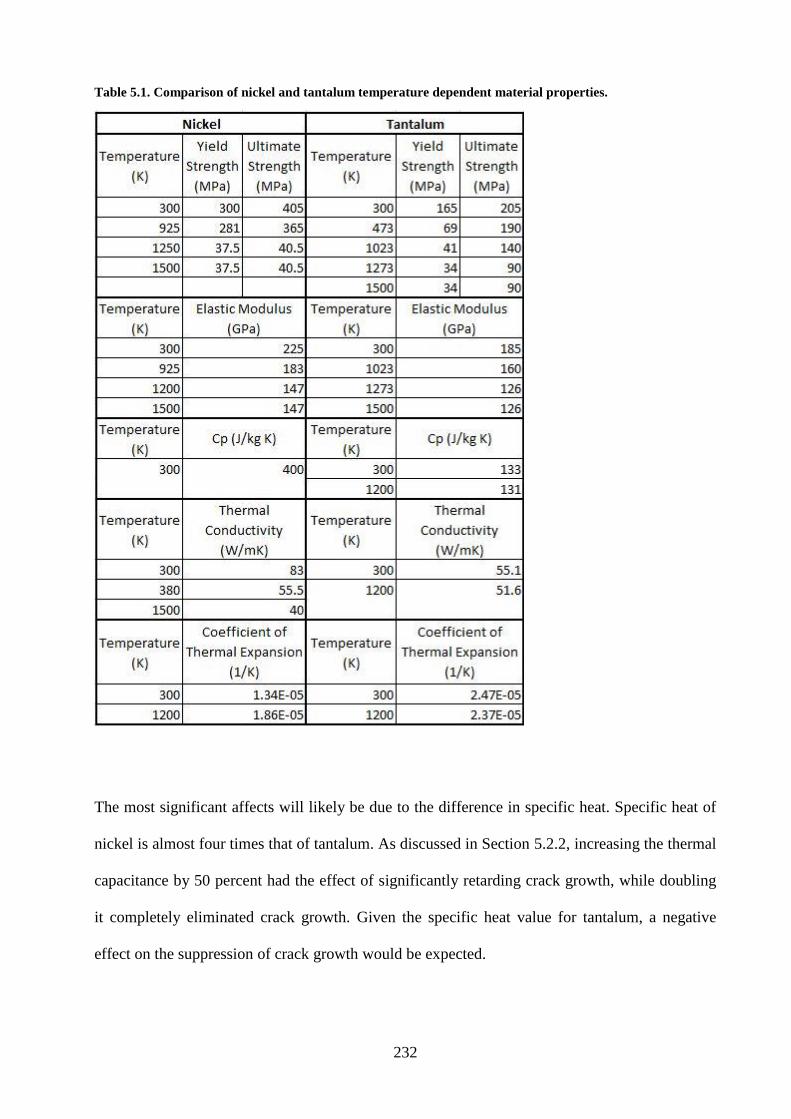
232
Table 5.1. Comparison of nickel and tantalum temperature dependent material properties.
The most significant affects will likely be due to the difference in specific heat. Specific heat of
nickel is almost four times that of tantalum. As discussed in Section 5.2.2, increasing the thermal
capacitance by 50 percent had the effect of significantly retarding crack growth, while doubling
it completely eliminated crack growth. Given the specific heat value for tantalum, a negative
effect on the suppression of crack growth would be expected.
233
A complete analysis of a prospective gun tube coating would require the determination of
cohesive zone properties using the technique described earlier. Once the properties have been
measured, they can be applied to simulate the evolution of a flaw, resulting from indentation or
other means, under combinations of thermal and pressure transients. The usefulness and
applicability of the technique have been demonstrated with nickel thermally sprayed onto steel.
A nickel-coated steel material set was applied using similar techniques for a test case of the
method. Affects of boundary conditions were investigated, in addition to mechanisms or coating
failure and current experimental techniques, such as the pulsed-laser experiment. The relevancy
of the method in terms of current investigations into new coating materials was commented on.
While findings can be extrapolated to understand the mechanisms that occur during flaw
evolution, caution must be applied when attempting to extrapolate findings for specific results.
234
CHAPTER 6. CONCLUSIONS AND RECCOMENDATIONS
The main objective of this thesis was to develop a method to evaluate the interfacial properties of
gun tube coatings and to use those properties to investigate the evolution of an indentation-
induced flaw under thermal and pressure transients. The idea of using the spherical indentation
test in conjunction with finite element models was hypothesized to be a reasonable solution. As
such, numerical models were developed to simulate the mechanical process whereby interfacial
flaws are introduced. The resulting delamination was then modeled numerically in order to
evaluate the cohesive zone properties. Finally, the numerical results from the indentation
modeling were applied as initial conditions to a second simulation of the evolution of the flaw in
response to severe thermal and pressure transients applied to the surface. These models were
then used to evaluate the effects of several variables on interfacial damage and crack extension.
The numerical and experimental studies performed led to the following conclusions.
1. Preliminary studies suggest that through-coating cracks and interfacial delaminations are
detrimental to the survivability of gun tubes. A preliminary model with collapsed stress
concentration elements at the crack tip provided a basis for an analysis of the resulting
stress state under severe thermal and pressure transients in a cylindrical geometry.
2. Though it provides an analytical solution for the critical fracture energy at interfaces in
the coated specimens, the four-point bend test was found to be an unreliable method for
interfacial critical fracture energy evaluation due to the burdensome requirements
necessary to achieve steady-state crack growth. Of these, the most notable are steady-
state crack growth before plastic deformation, and load-independent crack growth, once
initiated. Aluminum cold sprayed on aluminum produced catastrophic crack growth,
235
whereas nickel-coated steel specimens produced significant deformation in the substrate
before crack growth occurred.
3. The aluminum-coated aluminum samples and the nickel-coated steel specimens were
indented with a spherical indenter to produce an interfacial delamination, the presence
and size of which were quantified using ultrasonic measurement techniques. The results
of the experiments were applied to numerical indentation simulations. Cohesive zone
properties, critical fracture energy, and cohesive strength were chosen based on
knowledge of the interface, the fracture characteristics, and the combination that would
best reproduce the initial experimental results.
4. The described method was verified by evaluating the properties during four-point bend
testing and successfully using the properties to predict the radius of indentation-induced
delaminations at several different load levels, thereby providing validation for the
procedure. Reasonable agreement was observed between numerical predictions and
experimental results in terms of the prediction of the presence of a delamination, and the
size of the resulting flaw. The four-point bend tests application to flaw evaluation was
also explored, and found to be limited to a narrow set of materials.
5. The numerically/experimentally determined properties described in the previous
statement were applied to a sequential, implicit-to-explicit simulation in order to study
the evolution of indentation-induced interfacial flaws. Simulations included analysis of
the effects of the surface pressure transient compared to only thermal convective heating
in order to understand their relative contributions and thus, provide insight into the
effects unaccounted for in the pulsed-laser heating test. Both the surface and blister
pressure transients were offset in order to make general observations about the phase
difference between the two transients, and thus to understand the out-of-phase thermal
effects. Finally, blister pressure was offset, as gas penetration is often cited as a coating
236
failure mode and the previous analysis showed little contribution to crack growth when
surface and interstitial pressure were in phase. Additionally, once the gas penetrates the
coating delayed blister pressure should be expected, due to impeded gas exit after the
thermal transient.
It is recommended that the following changes or improvements be incorporated into existing
experimental setups and numerical models for a deeper understanding of the flaw evolution in
gun tubes and for more accurate predictions of the coating responses.
1. Though spherical indentations produced interfacial delaminations in the coatings studied,
both stronger or thinner coatings than those studied are likely to require higher
indentation loads if penetration and damage are possible. Other ways of introducing flaws
may be necessary to evaluate cohesive zone properties and to study the evolution of pre-
existing flaws experimentally. A possible area of future research includes cohesive zone
property evaluation using conical indenters. Additionally, techniques to introduce flaws
for experimentally studying flaw evolution could include masking the interface before
spraying.
2. Thermal-structural simulations were conducted with an axisymmetric model, showing
flaw evolution in two-dimensional space on a plate. Such conditions model
predominantly one-dimensional heat flow, though the presence of a flaw can affect heat
transfer. However, gun tube applications have two complicating factors not included in
the present research study because they could not be included in an axisymmetric model
and would almost certainly have required significantly more computational power. In gun
tubes, the heat moves along the gun tube as a thermal front. Such an effect is likely to
create further thermal stress caused by the no-planar thermal gradient and resulting
237
thermal stresses. It is likely that the impingement of this transient on a defect would have
different effects than it would on a planar thermal gradient. Additionally, the asymmetric
circumferential geometry of the gun tube is significantly different than that of the plate.
Effects such as the circumferential expansion of the tube moving along the axis are,
therefore, not accounted for in the present study.
3. It is likely that the cohesive zone properties are affected by increasing temperatures,
resulting in unpredictable effects on both the strength and critical fracture energy of the
interface. Higher temperatures can be expected to decrease the strength of the interface,
but the effects on fracture energy are more difficult to predict. Recognizing that these
effects could be significant in gun tube applications, especially in circumstances
involving repeated firings and the ensuing build-up of heat in the gun tube, they should
be investigated. Indentation tests could be done in a high-temperature furnace to evaluate
elevated temperature interfacial properties, though the heating would be more gradual
and uniform than present in gun tubes.
4. Finite element simulations reveal strain rates on the order of 1.5/s, which is significant
for most metals. High strain rates result in higher elastic modulus and yield strength, but
also decreased ductility. However, high strain rates occur during high surface temperature
transients, which increase the temperature of the material under high rates of strain. High
temperatures have the opposite effects, resulting in lower modulus and strength. Such
competing effects make the contribution of strain rate hardening difficult to predict, and
thus require significant material characterization work involving both high strain rates
and high temperatures.
5. The experiments in this research were conducted at room temperature, and they were
extrapolated so that we could analyze the evolution of a flaw at elevated temperatures.
Experimentally re-creating such temperatures over a sample surface would be a difficult

238
undertaking. Introducing high temperature in microseconds is certainly impossible, as
lasers can introduce such amounts of energy on only a small concentrated area. However,
experimental analysis of high-temperature transients on indentation-induced defects is
something that should be explored, even if only over a small area.
6. The described approach, while providing a comprehensive and thorough analysis of the
interface, does neglect possibly significant effects such as strain rate and temperature
dependent material properties. Hardening due to high strain rates will likely be partially
offset by high temperature softening. Additionally, strain rate and temperature effects
were ignored in the cohesive zone, as the properties were measured at room temperature
quasistatically.
7. Given the challenges and uncertainties associated with the assumption of negligible strain
rate effects, a different method of cohesive zone property analysis should be explored. A
laser produced stress wave experiment would therefore be recommended to
accommodate any high strain rate effects on the cohesive zone properties. In the
experiment a laser is used to rapidly heat the back of the substrate, resulting in a stress
wave that induces delaminations. The laser induced thermal waves can also be used to
study mode mixity by varying the angle of incidence. Computational requirements
associated with the method, though necessitating an accurate description of the energy
introduced by the laser, would be no more burdensome than those described herein. In
addition, as mentioned above, an accurate rate-dependent description of the materials
would improve results in both the current and proposed work.
The present research offers experimental and numerical techniques to evaluate interfacial
properties, before applying the properties to analyze the evolution of an interfacial flaw. This
concept as such could be used in a number of different situations such as:
239
1. Quantification of coating adhesion properties has applications in all fields where coating
separation is of concern. Applications could include coatings of a variety of materials,
such as ceramics, polymers, and metals. Quantifying the properties of the interfaces
would be helpful for evaluating coating adhesion. In addition, it would enable the
properties to be applied for further modeling in order to understand and mitigate the
mechanisms that lead to coating failure.
2. Flaw evolution under several thermal and pressure transients is a concern for a variety of
coating applications. Such concerns are especially relevant on turbine blades, which
experience both severe thermal and pressure loading. Coating flaw initiation exposes the
substrate high temperature gases, leading to many of the same thermal effects that, in
turn, lead to steel gun tube failure, such as phase transformation and melting.
240
REFERENCES
1. Underwood, J.H., A.P. Parker, G.N. Vigilante, P.J. Cote, Thermal damage, cracking and
rapid erosion of cannon bore coatings. Journal of Pressure Vessel Technology, 2003.
125: p. 299-304.
2. Warrender, J.M., C.P. Mulligan, J.H. Underwood, Analysis of thermo-mechanical
cracking in refractory coatings using variable pulse-duration laser pulse heating. Wear,
2007. 263: p. 1540-1544.
3. Conroy, P.J., P. Weinacht, M.J. Nusca, Gun tube coatings in distress. 2001, Army
Research Laboratory: Aberdeen Proving Ground, MD.
4. Gun Handbook, ed. F. Institute. 1964, Philadelphia, PA: The U.S. Government Printing
Office.
5. Davidson, T.E., J.F. Throop, J.H. Underwood, Failure of a 175 mm tube and the
resolution of the problem using an autofrettaged design. Case Studies in Fracture
Mechanics, 1977: p. 3.9.1-12.
6. handbook, g.t.
7. Johnston, I.A., Understanding and predicting gun barrel erosion. 2005, Weapons System
Division: DSTO Defence Science and Technology Organisation: Edinburgh, South
Australia, Australia.
8. Cote, P.J., C. Rickard, Gas-metal reaction products in the erosion of chromium plated
gun bores. Wear, 2000. 241: p. 17-25.
9. Sopok, S., Erosion modeling of vented combustor cannon bore materials, in 35th AIAA
Thermophysics Conference. 2001, AIAA: Anaheim, CA.
10. Underwood, J.H., A.P. Parker, P.J. Cote, S. Sopok, Compresive thermal yielding leading
to hydroven cracking in a fired cannon. Transactions of the ASME, 1999. 121: p. 116-
120.
11. Lawton, B., Thermo-chemical erosion in gun barrels. Wear, 2001. 251: p. 827-838.
12. Cote, P.J., M.E. todaro, G. Kendall, M. Witherell, Gun bore erosion mechanisms
revisited with laser pulse heating. Surface and Coatings Technology, 2003. 163-164: p.
478-483.
13. Hirvonen, J.K., J.D. Demaree, D.K. Marble, P. Conroy, C. Leveritt, J. Montgomery, A.
Bujanda, Gun barrel erosion studies utilizing ion beams. Surface & Coatings
Technology, 2005. 196: p. 167-171.
14. Underwood, J.H., G.N. Vigilante, C.P. Mulligan, Review of thermo-mechanical cracking
and wear mechanisms in large caliber guns. Wear, 2007. 263: p. 1616-1621.
15. Turley, D.M., Erosion of a chromium-plated tank gun barrel. Wear, 1989. 131: p. 135-
150.
16. Turley, D.M., Development of erosion resistant refractory metal and alloy coatings by
magnetron sputtering. Surface and Coatings Technology, 1989. 39-40: p. 135-142.
17. Underwood, J.H., M.D. Witherell, S. Sopok, J.C. McNeil, C.P. Mulligan, G.N. Vigilante,
Thermomechanical modeling of transient thermal damage in cannon bore materials.
Wear, 2003. 257: p. 992-998.
18. Lawton, B., G. Klingenberg, Transient Temperature in Engineering and Science. 1996,
Oxford, UK: Oxford University Press. 443-471.
19. Sopok, S., P. O'Hara, G. Pflegl, S. Dunn, D. Coats, G. Nickerson, Unified computer
model for predicting thermochemical erosion in gun barrels. Journal of Propulsion and
Power, 1999. 15(4): p. 601-612.
20. Vigilante, G.N., J.H. Underwood, D. Crayon, Use of the instrumented bolt and constant
displacement bold-loaded specimen to measure in-situ hydrogen crack growth in high-
strength steels. Fatigue and Fracture Mechanics, 1999. 33(ASTM STP 1360): p. 377-387.
241
21. Underwood, J.H., E. Toriano, G.N. Vigilante, A.A. Kapusta, S. Tauscher, Hydrogen
cracking during service of high strength steel cannon components. ASTM STP, 1997.
1332.
22. Lawton, B., M.P. Laird. Influence of gas leakage on heat transfer and wear in gun
barrels. in 16th International Symposium on Ballistics. 1996. San Francisco, United
States.
23. Bracuti, A.J., Wear-Reducing Additives - Role of the Propellant. Gun Propulsion
Technology. Vol. 109. 1988, Washington DC, United States: AIAA. 377-411.
24. Sopok, S., P. O'Hara, G. Pflegl, S. Dunn, D. Coats, First computer code for predicting
thermochemical erosion in gun barrels. Proceedings of the 20th Army Science
conference, 1996.
25. Cote, P.J., M.E. Todaro, M. Witherell, Factors affecting chrome loss in gun tubes. US
Army Armament Research, Development and Engineering Center, 2003. Technical
Report ARCCB-TR-03016.
26. Underwood, J.H., M.E. Todaro, G.N. Vigilante, Modeling of transient thermal damage in
ceramics for cannon bore applications. Ceramic Engineering and Science Proceedings,
2004. 25(3): p. 189-194.
27. Underwood, J.H., G.N. Vigilante, E. Toriano, Failure beneath cannon thermal barrier
coatings by hydrogen cracking; Mechanisms and Modeling. Fatigue and Fracture
Mechanics, 2002. 33(ASTM STP 1417): p. 101-115.
28. Underwood, J.H., A.P. Parker, G.N. Vigilante, P.J. Cote, Fatigue life analyses and tests
for thick-wall cylinders including effects of overstrain and axial grooves. Transactions of
the ASME, 1995. 117: p. 222-226.
29. Underwood, J.H., E. Toriano, Critical fracture processes in army cannons: A review.
Journal of Pressure Vessel Technology, 2003. 125: p. 287-292.
30. Underwood, J.H., G.N. Vigilante, C.P. Mulligan, M.E. Todaro, Thermo-mechanically
controlled erosion in army cannons: A review. Gun Tubes Conference, 2005: p. 1-6.
31. Petipas, E., B. Campion, Crack propagation in a gun barrel due to the firing thermo-
mechanical stresses. Journal of Pressure Vessel Technology, 2003. 125: p. 293-298.
32. Newaz, G.M., S.Q. Nusier, Z.A. Chaudhury, Damage accumulation mechanisms in
thermal barrier coatings. Journal of Engineering Materials and Technology, 1998. 120:
p. 149-153.
33. Bao, G., H. Cai, Delamination cracking in functionally graded coating/metal substrate
systems. Acta Metallurgica, 1997. 45(3): p. 1055-1066.
34. El-Borgi, S., W. Aloulou, A. Zghal, Buckling of a functionally graded coating with an
embedded crack bonded to a homogeneous substrate. International Journal of Fracture,
2006. 142: p. 137-150.
35. Zhu, D., R.A. Miller, B.A. Nagaraj, R.W. Bruce, Thermal conductivity of EB-PVD
thermal barrier coatings evaluated by a steady-state laser heat flux technique. Surface &
Coatings Technology, 2001. 138: p. 1-8.
36. Hutchinson, J.W., A.G. Evans, On the delamination of thermal barrier coatings in a
thermal gradient. Surface and Coatings Technology, 2002. 149: p. 179-184.
37. Troiano, E., A.P. Parker, J.H. Underwood, C. Mossey, Experimental data, numerical fit
and fatigue lIfe calculations relating to the Bauschinger Effect in high strength armament
steels. Transactions of the ASME, 2003. 125: p. 330-334.
38. Parker, A.P., J.H. Underwood, Influence of Bauschinger effect on residual stress and
fatigue lifetimes in autofrettaged thick-walled cylinders. Fatigue and Fracture Mechanics,
1998. 29(ASTM STP 1321): p. 565-583.
39. Troiano, E., J.H. Underwood, A.P. Parker, Finite element investigation of Bauschinger
Effect in high-strength A723 pressure vessel steel. Journal of Pressure Vessel
Technology, 2006. 128: p. 185-189.
242
40. Parker, A.P., A re-autofrettage procedure for mitigation of Bauschinger effect thick
cylinders. Journal of Pressure Vessel Technology, 2004. 126: p. 451-454.
41. Parker, A.P., S.N. Endersby, T.J. Bond, J.H. Underwood, S.L. Lee, J. Higgins, Stress
concentration, stress intensity, and fatigure lifetime calculations in autofrettaged tubes
containg axial perforations within the wall. Transactions of the ASME, 1997. 119: p.
488-493.
42. Alkhimovc, A.P., A.N. Papyrin, V.F. Kosarev, N.I. Nesterovich, M.M. Shushpanov, Gas-
Dynamic Spray Methode for Applying a Coating, U.S., Editor. 1994, A.N. Papyrin.
43. Tokarev, A.O., Structure of aluminum powder coatings prepared by cold gasdynamic
spraying. Metal Science and Heat Treatment, 1996. 38(3-4): p. 136-139.
44. Stoltenhoff, T., H. Kreye, H.J. Richter, An analysis of th ecoald spray process and its
coatings. Journal of Thermal Spray Technology, 2001. 11(4): p. 542-550.
45. Dykhuizen, R.C., M.F. Smith, D.L. Gilmore, R.A. Neiser, X. Jiang, S. Sampath, Impact
of high velocity cold spray particles. Journal of Thermal Spray Technology, 1999. 8(4):
p. 559-564.
46. Gärtner, F., T. Stoltenhoff, T. Schmidt, H. Kreye, The cold spray process and its
potential for industrial applications. Journal of Thermal Spray Technology, 2006. 15(2):
p. 223-232.
47. Assadi, H., F. Gärtner, T. Stoltenhoff, H. Kreye, Bonding mechanism in cold gas
spraying. Acta Materalia, 2003. 51: p. 4379-4394.
48. Li, C.-J., W.-Y. Li, H. Liao, Examination of the critical velocity for deposiotn of particles
in cold spraying. Journal of Thermal Spray Technology, 2006. 15(2): p. 212.
49. Li, C.-J., W.-Y. Li, H. Liao, Modelling aspects of high velocity impact of particle sin cold
spraying by explicit finite element analysis. Journal of Thermal Spray Technology, 2009.
18(5-6): p. 921-933.
50. Bala, N., H. Singh, S. Prakash, An overview of the cold spray technique. Materials
Science Forums, 2007. 561-565: p. 2419-2422.
51. Lima, R.S., J. Karthikeyan, C.M. Kay, J. Lindemann, C.C. Berndt, Microstructural
characteristics of cold-sprayed nanostructure WC-Co coatings. Thin Solid Films, 2002.
416: p. 129-135.
52. Evans, A.G., J.W. Hutchinson, The mechanics of coating delaminaion in thermal
gradients. Surface Coatings and Technology, 2007. 201: p. 7905-7916.
53. Conroy, P.J., P. Weinacht, M.J. Nusca, Gun Tube Coatings in Distress. 2001, Army
Research Laboratory: Aberdeen Proving Ground, MD.
54. Xie, D., S. Biggers Jr., Progressive crack growth analysis using interface element based
on the virtual crack closure technique. Finite Elements in Analysis and Design, 2006. 42:
p. 977-984.
55. Alam, M.S., M.A. Wahab, Modeling the fatigue crack growth and propagation life of a
joint of two elastic materials using interace elements. International Journal of Pressure
Vessels and Piping, 2005. 82: p. 105-113.
56. Shi, Z., R. Zhang, Numerical simulation of interfacial crack growth under fatigue
growth. Fatigue & Fracture of Engineering Materials and Structures, 2008. 32: p. 26-32.
57. Chaboche, J.L., R. Girard, A. Schaff, Numerical analysis of composite systems by using
interphase/interface models. Computational Mechanics, 1997. 20: p. 3-11.
58. Yang, Q.D., M.D. Thouless, Mixed-mode fracture analyses of plastically-deforming
adhesive joints. International Journal of Fracture, 2001. 110: p. 175-187.
59. Alfano, G., M.A. Crisfield, Finite element interface models for the delamination analysis
of laminated composites: mechanical and computational issues. International Journal for
Numerical Methods in Engineering, 2001. 50: p. 1701-1736.
60. Toygar, M.E., M. Toparli, F. Sen, M.A. Gungor, Fracture energy determination and
critical crack propagation between core and veneer ceramic interface by experiment and
finite element method. Materials and Design, 2009. 30: p. 2278-2282.
243
61. Barrenblatt, G.I., The mathematical theory of equilibrium of cracks in brittle fracture.
Advances in Applied Mechanics, 1962. 7: p. 55-129.
62. Dugdale, D.S., Yielding of steel sheets containing slits. Journal of the Mechanics and
Physics of Solids, 1960. 8: p. 100-104.
63. Shet, C., N. Chandra, Analysis of Energy Balance When Using Cohesive Zone Models to
Simulate Fracture Processes. Transactions of the ASME, 2002. 124: p. 440-450.
64. Turon, A., C.G. Davila, P.P. Camanho, J. Costa, An engineering solution for mesh size
effects in the simulation of delamination using cohesive zone models. Engineering
Fracture Mechanics, 2007. 74: p. 1665-1682.
65. Xu, X.-P., A. Needleman, Numerical simulations of fast crack growth in brittle solids.
Journal of Mechanics and Physics of Solids, 1994. 42(9): p. 1397-1434.
66. Xu, X.-P.a.A.N., Numerican simulations of dynamic interfacial crack growth allowing
for crack growth away from the bond line. International Journal of Fracture, 1995. 75: p.
253-275.
67. Xu, X.-P.a.A.N., Numerical simulations of dynamic crack growth along an interface.
International Journal of Fracture, 1996. 74: p. 289-324.
68. Ruiz, G., A. Pandolfi, M. Ortiz, Three dimensional cohesive modeling of dynamic mixed-
mode fracture. International Journal for Numerical Methods in Engineering, 2001. 52: p.
97-120.
69. Zavattieri, P., H.D. Espinosa, Grain level analysis of crack initiation and proagation in
brittle materials. Acta Materialia, 2001. 49: p. 4291-4311.
70. Wei, S., F. Qun-bo, W. Fu-chi, M. Zhuang, Modeling of micro-crack growth during
thermal shock based on microstructural images of thermal barrier coatings.
Computational Materials Science, 2009. 46: p. 600-602.
71. Zhou, F., J.-F. Molinari, Stochastic fracture of ceramics under dynamic tensile loading.
International Journal of Solids and Structures, 2004. 41: p. 6573-6596.
72. Li, S., M.D. Thouless, A.M. Waas, J.A. Schroeder, P.D. Zavattieri, Mixed-mode
choesive-zone models for fracture of an adhesively bonded polymer-matrix composite.
Engineering Fracture Mechanics, 2006. 73: p. 64-78.
73. Xia, D., A.M. Waas, Discrete cohesive zone model for mixed-mode fracture using finite
element analysis. Engineering Fracture Mechanics, 2006. 73: p. 1783-1796.
74. Goyal, V.K., E.R. Johnson, C.G. Davila, Irreversible constitutive law for modeling the
delamination process using interfacial surface discontinuities. Composite Structures,
2004. 65: p. 289-305.
75. Mirzaei, M., A. Harandi, R. Karimi, Finite element analysis of deformation and fracture
of an exploded gas cylinder. Engineering Failure Analysis, 2009. 16: p. 1607-1615.
76. Rahul-Kumar, P., A. Jagota, S.J. Bennison, S. Saigal, S. Muralidhar, Polymer interfacial
fracture simulations using cohesive elements. Acta Materialia, 1999. 47(15): p. 4161-
4169.
77. Siegmund, T., W. Brocks, A numerical study on the correlation between the work of
separation and the dissipation rate in ductile fracture. Engineering Fracture Mechanics,
2000. 67: p. 139-154.
78. Xie, D., M. Garg, D. Huang, F. Abdi, Cohesive zone model for surface cracks using finite
element analysis. American Institute of Aeronautics and Astronautics, 2008: p. 1-16.
79. Secchi, S., L. Simoni, B.A. Schrefler, Cohesive fracture growth in a thermoelastic
bimaterial medium. Computers and Structures, 2004. 82: p. 1875-1887.
80. Fagerstrom, M., R. Larsson, A thermo-mechanical cohesive zone formulation for ductile
fracture. Journal of Mechanics and Physics of Solids, 2008. 56: p. 3037-3058.
81. Ferney, B.D., M.R. DeVary, K.J. Hsia, and A. Needleman, Oscillatory Crack Growth in
Glass. Scripta Materialia, 1999. 41(3): p. 275-281.
244
82. Arata, J.J.M., A. Needleman, K.S. Kumar, and W.A. Curtin, Microcrack nucleation and
growth in elastic lamellar solids. International Journal of Fracture, 2000. 105: p. 321-
342.
83. Chen, J., M. Crisfield, A.J. Kinloch, E.P. Busso, F.L. Matthews, Y. Qiu, Predicting
progressive delamination of composite material specimens via interface elements.
Mechanics of composite Materials and Structures, 1999. 6: p. 301-307.
84. Camanho, P.P., C.G. Davila, M.F. De Moura, Numerical simulation of mixed-mode
progressive delamination in composite materials. Journal of Composite Materials, 2003.
37(16): p. 1415-1438.
85. Xia, S.M., Y.F. Gao, A.F. Bower, L.C. Lev, Y.-T. Cheng, Delamination mechanism
maps for a strong elastic coating on an elastic-plastic substrate subjected to contact
loading. International Journal of Solids and Structures, 2007. 44: p. 3685-3699.
86. Abdul-Baqi, A., E. Van der Giessen, Delamination of a strong film from a ductile
substrate during indentation unloading. Journal of Materials Research, 2001. 16(5): p.
1395-1407.
87. Abdul-Baqi, A., E. Van der Giessen, Indentation-induced interface delamination of a
strong film on a ductile substrate. Thin Solid Films, 2001. 381: p. 143-154.
88. Hainsworth, S.V., McGurk, T.F. Page, The effect of coating cracking on the indentatino
response of thin hard-coated systems. Surface and Coatings Technology, 1998. 102: p.
97-107.
89. Barsoum, Z., I. Barsoum, Residual stress effects on fatigue life of welded structures using
LEFM. Engineering Failure Analysis, 2009. 16: p. 449-467.
90. Hutson, A.L., M. Huelsman, D. Buchanan, R. John, S. Haering, Corner crack
propagation in the presence of residual stresses. 2006, Air Force Research Laboratory.
91. Choi, J., G. Lee, B. Lee, A study on the thermo-mechanical fatigue loading for attaining
minimum cycles in fabricating an artificial cracked specimen, in The Fourth China-
Japan-Korea Joint Symposium on Optimization of Structural and Mechanical Systems.
2006: Kumming, China.
92. Liu, G., A. Mouftiez, J. Lesage, S. Panier, A numerical fracture analysis of a stationary
semi-circular interface crack during interfacial indentation test. Surface & Coatings
Technology, 2006. 201: p. 2086-2091.
93. Leblanc, F., J. roger, A. Zimmermann, D. Coutellier, Determination of interfacial
toughness curves using experiments and simulations, in Journées Nationales sur les
Composites #14. 2005: UTC, Compiègne, France.
94. Shih, C.F., R.J. Asaro, Elastic-pastic analysis of cracks on bimaterial interfaces. I. Small
scale yielding. International Journal of Fracture, 1988. 42(2): p. 101-116.
95. Schuller, T., B. Lauke, Finite-element simulation of interfacial crack progagation:
Methods and tools for the complete failure process under large scale yielding.
Engineering Fracture Mechanics 2006. 73: p. 2252-2263.
96. Schuller, T., B. Lauke, Finite-element-simulation of interfacial crack propagation: cross-
check of simulation results with the essential work of interfacial fracture method. Key
Engineering Materials, 2006. 312: p. 9-14.
97. Maiti, S.K., S. Namdeo, A.H.I. Mourad, A scheme for finite element analysisof model I
and mixed mode stable crack growth and a case study with AISI 4340 steel. Nuclear
Engineering and Design, 2008. 238: p. 787-800.
98. Pasqualino, I.P., I.A. Valeriano, T.M.J. Alves, Crack growth prediction in girth welds of
steel catenary risers. Proceedings of ISOPE, 2002: p. 192-197.
99. Yang, Q.D., M.D. Thouless, S.M. Ward, Elastic-plastic mode-II fracture of adhesive
joints. International Journal of Solids and Structures, 2001. 38: p. 3251-3262.
100. Omiya, M., K. Kishimoto, T. Nakano, Evalution of the interfacial strength of layered
structures by indentation method. Journal of Applied Physics, 2008. 75.
245
101. Bocciarelli, M., G. Bolzon, Indentation and impring mapping for the indentification of
constitutive parameters of thin layers on substrate: Perfecly bonded interfaces. Materials
Science and Engineering, 2007. 448: p. 303-314.
102. Bolzon, G., M. Bocciarelli, E.J. Chiarullo, Applied Scanning Probe Methods XIII.
NanoScience and Technology, 2009. 2009: Springer Berlin Heidelberg.
103. Kim, K.-S., J. Kim, Elasto-plastic analysis of the peel test for thin film adhesion.
Transactions of the ASME, 1988. 110: p. 266-273.
104. Kim, K.-S., N. Aravas, Elastoplastic analysis of the peel test. International Journal of
Solids and Structures, 1988. 24(4): p. 417-435.
105. Ferracin, T., C.M. Landis, F. Delannay, T. Pardoen, On the rdetermination of the
cohesive zone properties of an adhesive layer from the analysis of the wedge-peel test.
International Journal of Solids and Structures, 2003. 40: p. 2889-2904.
106. Daghyani, H.R. Constraint effect on fracture behavior of adhesive joints with different
bond thickness. in Proceedings of the 1994 26th National Symposium on Fracture
Mechanics. 1995. Idaho Falls, ID: ASTM.
107. Thouless, M.D., J.L. Adams, M.S. Kafkalidis, S.M. Ward, R.A. Dickie, G.L. Westerbeek,
Determining the toughness of plastically deforming joints. Journal of Materials Science,
1998. 33: p. 189-197.
108. Thouless, M.D., M.S. Kafkaidis, S.M. Ward, Y. Bankowski, Toughness of plastically-
deforming asymmetric joints. Scripta Materialia, 1997. 37(7): p. 1081-1087.
109. Kinloch, A.J., C.C. Lau, J.G. Williams, The peeling of flexible laminates. International
Journal of Fracture, 1994. 66: p. 45-70.
110. Chai, H., Shear fracture (of adhesively bonded joints). International Journal of Fracture,
1988. 37(2): p. 137-159.
111. Tay, A.A.O., J.S. Phang, E.H.Wong, R. Ranjan. A modified button-shear method for
measuring fracture thoughness of polymer-metal interfaces in IC packages. in
Electronics Components and Technology Conference. 2003: IEEE.
112. Sham, M.-L., J.-K. Kim, Adhesion characterisitcs of underfill with flip chip package
components. Journal of Adhesion Science Technology, 2003. 17(14): p. 1923-1944.
113. Chien, C.-H., T. Chen, W.-B. Lin, C.-C Hsieh, W.-D. Wu, C.-H. Yeh, Experimental and
statistical study in adhesion features of bonded interfaces of IC packages.
Microelectronics Reliability, 2008. 48: p. 140-148.
114. Szeto, W.K., M.Y. Xie, J.K. Kim, M.M.F. Yuen, P.tong, S. Yi. Interface failure criterion
of button shear test as a means of interface adhesion measurement in plastic packages. in
International Symposium on Electronic Materials and Packaging. 2000: IEEE.
115. Fan, H.b., M.M.F. Yuen, E. Suhir. Prediction of delamination in a bi-material system
based on free-edge energy evaluations. in 2003 Electronic Components and Technology
Conference. 2003: IEEE.
116. Hutchinson, J.W., Z. Suo, Mixed mode cracking in layered materials. Advances in
Applied Mechanics, 1992. 29.
117. Karbhari, V.M., M. Engineer, Assessment of interfacial fracture energy between concrete
and glass reinforced composites. Journal of Materials Science Letters, 1995. 14: p. 1210-
1213.
118. Karbhari, V.M., M. Engineer, Investigation of bond between concrete and composites:
Use of a peel test. Journal of Reinforced Plastics and Composites, 1996. 15: p. 208-227.
119. Karbhari, V.M., M. Engineer, D.A. Eckel II, On the durability of composite
rehabilitation schemes for concrete. Journal of Materials Science, 1997. 32: p. 147-156.
120. Moidu, A.K., A.N. Sinclair, J.K. Spelt, Analysis of the peel test: prediction of adherend
plastic dissipation and extraction of fracture energy to metal-to-metal adhesive joints.
Journal of Testing and Evaluation, 1995. 23(4): p. 241-253.
121. Ashcroft, I.A., B. Derby, Adhesion testing of glass-ceramic thick films on metal
substrate. Journal of Materials Science, 1993. 28: p. 2989-2998.
246
122. Clyne, T.W., and S.C. Gill, Residual stresses in thermal spray coatings and their effect
on interfacial adhesion: a review of recent work. Journal of Thermal Spray Technology,
1996. 5(4): p. 401-418.
123. Charalambides, P.G., J. Lund, A.G. Evans, R.M. McMeeking, A test specimen for
determined the fracture resistance of bimaterial interfaces. Journal of Applied Physics,
1989. 56: p. 77-82.
124. Charalambides, P.G., H.C. Cao, J. Lund, A.G. Evans, Development of a test method for
measuring the mixed mode fracture resistance of bimaterial interfaces. Mechanics of
Materials, 1990. 8: p. 269-283.
125. Howard, S.J., A.J. Phillipps, T.W. Clyne, The interpretation of data from the four-point
bend delamination test to measure interfacail fracture toughness. Composites, 1992.
24(2): p. 102-112.
126. Howard, S.J., Y.C. Tsui, T.W. Clyne, The effect of residual stresses on the debonding of
coatings-I. A model for delamination at a bimaterial interface. Acta Metallurgica et
Materialia, 1994. 42(8): p. 2823-2836.
127. Yamazaki, Y., A. Schmidt, A. Scholz, The determination of the delamination resistance
in thermal barrier coating system by four-point bending tests. Surface and Coatings
Technology, 2006. 201: p. 744-754.
128. Howard, S.J., A.J. Phillipps, T.W. Clyne, The effect of residual stresses on the debonding
of coatings - I. A model for delamination at a bimaterial interface. Acta Metallurgica et
Materialia, 1993. 42(8): p. 2823-2836.
129. Suo, Z., J.W. Hutchinson, Interface crack between two elastic layers. International
Journal of Fracture, 1990. 43: p. 1-18.
130. Tsui, Y.C., S.J. Howard, T.W. Clyne, The effect of residual stresses on the debonding of
coatings - II. An experimental study of a thermally sprayed system. Acta Metallurgica et
Materialia, 1994. 42(8): p. 2837-2844.
131. Katipelli, L.R., A. Agarwal, N.B. Dahotre, Interfacial strength of laser surface
engineering TiC coating on 6061 Al using four-point bend test. Materials Science and
Engineering, 2000. A289: p. 34-40.
132. Phillips, A.J., W.J. Clegg, T.W. Clyne, Fracture behavior of ceramic laminates in
bending-II. Comparision of model predictions with experimental data. Acta Materalia,
1993. 41(3): p. 819-827.
133. Jensen, H.M., The blister test for interface toughness measurement. Engineering Fracture
Mechanics, 1991. 40(3): p. 475-486.
134. Jensen, H.M., Analysis of mode misity in blister tests. International Journal of Fracture,
1998. 94: p. 79-88.
135. Jensen, H.M., M.D. Thouless, Effects of residual stresses in the blister test. International
Journal of Solids and Structures, 1993. 30(6): p. 779-795.
136. Cotterell, B., Z. Chen, The blister test - Transition from plate to membrane behavior for
an elastic material. International Journal of Fracture, 1997. 86: p. 191-198.
137. Lin, M.R., J.E. Ritter, L. Rosenfeld, T.J. Lardner, Meausring the interfacial shear
strength of thin polymer coatings on glass. Journal of Materials Research, 1990. 5(5): p.
1110-1117.
138. Ritter, J.E., T.J. Lardner, L. Rosenfeld, M.R. Lin, Measurement of adhesion of thin
polymer coatings by indentation. Journal of Applied Physics, 1989. 66(8): p. 3626-3634.
139. Matthewson, M.J., Axi-symmetric contact on thin compliant coatings. Journal of
Mechanics and Physics of Solids, 1981. 29(2): p. 89-113.
140. Sun, Y., A. Bloyce, T. Bell, Finite element analysis of plastic deformation of various TiN
coating/substrate systems under normal contact with a rigid sphere. Thin Solid Films,
1995. 271: p. 122-131.
247
141. Sen, S., B. Aksakal, A. Ozel, A finite-element analysis of the indentation of an elastic-
work hardening layered half-space by an elastic sphere. International Journal of
Mechanical Sciences, 1998. 40(12): p. 1281-1293.
142. Sriram, K., R. Narasimhan, S.K. Biswas, A numerical fracture analysis of indentation
into thin hard films on soft substrates. Engineering Fracture Mechanics, 2003. 70: p.
1323-1338.
143. Faulkner, A., K.C. Tang, S. Sen, R.D. Arnell, Finite element solutions comparing the
normal contact of an elastic-plastic layered medium under loading by (a) a rigid and (b)
a deformable indenter. Journal of Strain Analysis, 1998. 33(6): p. 411-418.
144. Abdul-Baqi, A., E. Van der Giessen, Delamination of a strong film from a ductile
substrate during indentation unloading. Journal of Materials Research, 2000. 16(5): p.
1396-1407.
145. Abdul-Baqi, A., E. Van der Giessen, Numerical analysis of indentation-induced cracking
of brittle coatings on ductile substrates. International Journal of Solids and Structures,
2002. 39: p. 1427-1442.
146. Hu, J., Y.K. Chou, A numerical study of interface behavior of diamond coated cutting
tools. Transactions of NAMRI/SME, 2008. 36: p. 533-540.
147. Hu, J., Y.K. Chou, and R.G. Thompson, Cohesive zone effects on coating failure
evaluations of diamond-coated tools. Surface & Coatings Technology, 2008. 203: p. 730-
735.
148. Huang, B., M.-H. Zhao, T.-Y. Zhang, Indentation fracture and indentation delamination
in ZnO film/Si substrates systems. Philosophical Magazine, 2004. 84(12): p. 1233-1256.
149. Chai, H., B.R. Lawn, Fracture mode transisions in brittle coatings on compliant
substrates as a function of thickness. Journal of Materials Research, 2004. 19(6): p. 1752-
1761.
150. Li, W., T. Siegmund, An analysis of the indentation test to determine the interface
toughness in a weakly bonded thin film coating - substrate system. Acta Materalia, 2004.
52: p. 2989-2999.
151. Zhang, Y.W., K.Y. Zeng, R. Thampurun, Interface delamination generated by
indentation in thin film systems - a computational mechanics study. Materials Science
and Engineering, 2001. A319-321: p. 893-897.
152. Evans, A.G., and J.W. Hutchinson, Effects of non-planarity on the mised mode fracture
resistance of bimaterial interfaces. Acta Materalia, 1989. 37(3): p. 909-916.
153. Budiansky, B., J.C. Amazigo, A.G. Evans, Small-scale crack bridging and the fracture
toughness of particulate-reinforced ceramics. Journal of Mechanics and Physics of
Solids, 1988. 36(2): p. 167-187.
154. Cooper, M.G., B. B. Mikic, M. M. Yovanovich, Thermal Contact Conductance.
International Journal of Heat and Mass Transfer, 1969. 12: p. 279-300.
155. Yonavovich, M.M., E.E. Marotta, Heat Transfer Handbook, ed. A. Bejan. 2003,
Hoboken, NJ: John Wiley & Sons, Inc.
156. Song, S., M.M. Yovanovich, Correlation of Thermal Accomodation Coefficient for
Engineering Surfaces. ASME HTD-Vol 69. 1987. 107-116.
157. ANSYS. 2009, ANSYS: Cannonsburg, PA. p. Finite Element Software.
158. ABAQUS. 2009, SIMULIA: Providence, RI.
159. Gueubelle, P.H., J.S. Baylor, Impact-induced delamination of compostes: a 2D
simulation. Composites Part B, 1998. 29B: p. 589-602.
160. Nied, H.F., Thermal shock in a circumferentially cracked hollow cylinder with cladding.
Engineering Fracture Mechanics, 1984. 20(1): p. 113-137.
161. Tsui, Y.C., T.W. Clyne, An analytical model for predicting residual stresses in
progressively deposited coatings Part 2: Cylinderical geometry. Thin Solid Films, 1997.
306: p. 34-51.

248
162. Sen, F., E. Celik, M. Toparli, Transient thermal stress analysis of CeO2 thin films on Ni
Substrates using finite element methods for YBCO coated conductor. Materials and
Design, 2007. 28: p. 708-712.
163. Materials, A.S.f.T.a., Standar Test Method for Adhesion or Cohesion of Thermal Spray
Coatings. 2008, ASTM International West Conshohocken, PA.
164. Yovanovich, M., New Contact and Gap Correlations for Confroming Rough Surfaces, in
AIAA 16th Thermophysics Conference. 1981: Palo Alto, CA.
165. Sopok, S., C. Rickard, S. Dunn, Thermal-chemical-mechanical gun bore erosion of an
advanced artillery system Part one: Theories and mechanisms. Wear, 2005. 258: p. 659-
670.
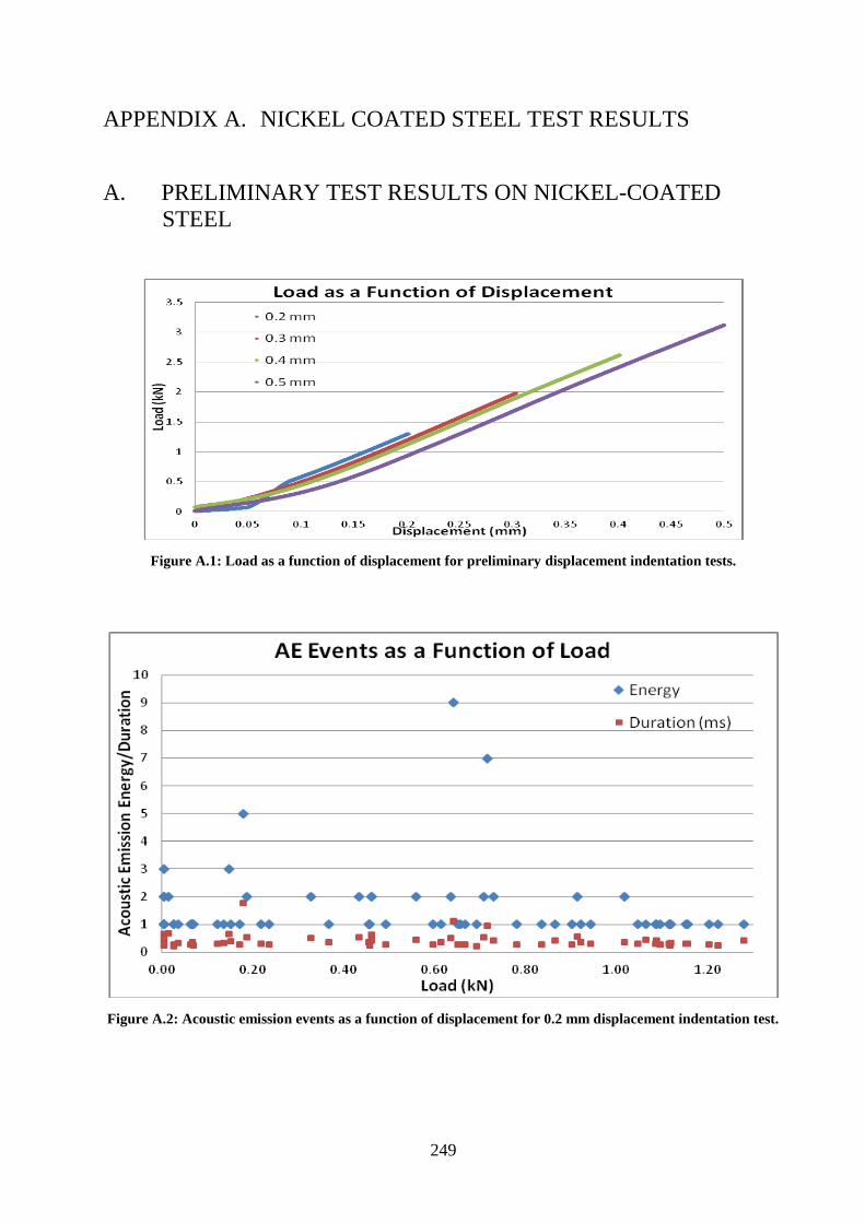
249
APPENDIX A. NICKEL COATED STEEL TEST RESULTS
A. PRELIMINARY TEST RESULTS ON NICKEL-COATED
STEEL
Figure A.1: Load as a function of displacement for preliminary displacement indentation tests.
Figure A.2: Acoustic emission events as a function of displacement for 0.2 mm displacement indentation test.
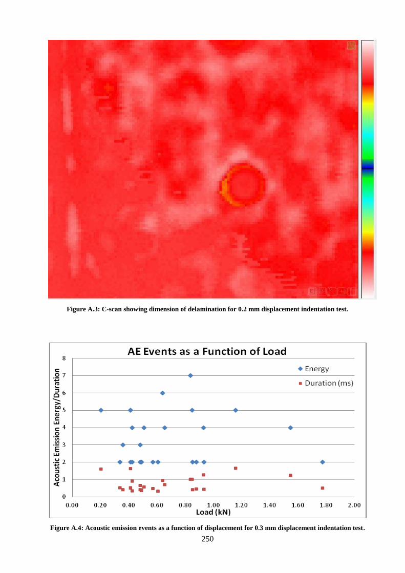
250
Figure A.3: C-scan showing dimension of delamination for 0.2 mm displacement indentation test.
Figure A.4: Acoustic emission events as a function of displacement for 0.3 mm displacement indentation test.
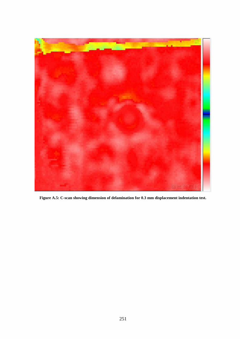
251
Figure A.5: C-scan showing dimension of delamination for 0.3 mm displacement indentation test.
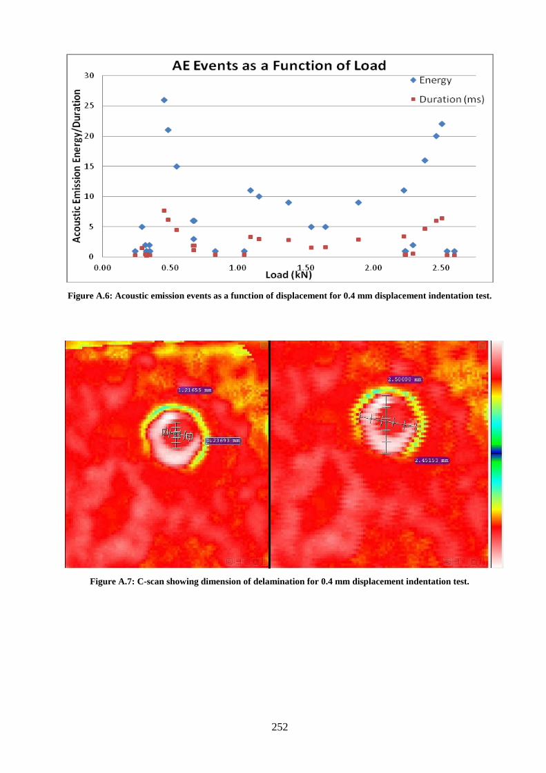
252
Figure A.6: Acoustic emission events as a function of displacement for 0.4 mm displacement indentation test.
Figure A.7: C-scan showing dimension of delamination for 0.4 mm displacement indentation test.
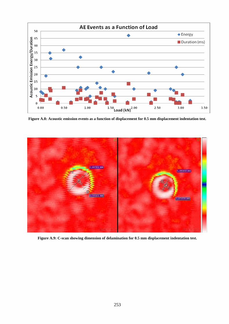
253
Figure A.8: Acoustic emission events as a function of displacement for 0.5 mm displacement indentation test.
Figure A.9: C-scan showing dimension of delamination for 0.5 mm displacement indentation test.
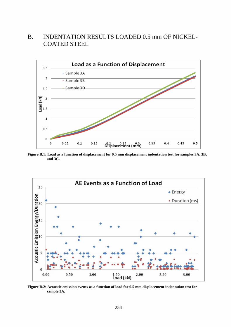
254
B. INDENTATION RESULTS LOADED 0.5 mm OF NICKEL-
COATED STEEL
Figure B.1: Load as a function of displacement for 0.5 mm displacement indentation test for samples 3A, 3B,
and 3C.
Figure B.2: Acoustic emission events as a function of load for 0.5 mm displacement indentation test for
sample 3A.
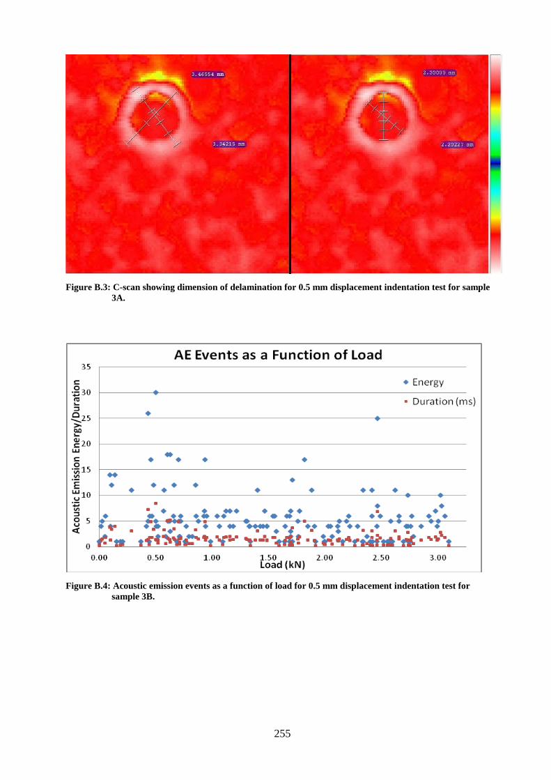
255
Figure B.3: C-scan showing dimension of delamination for 0.5 mm displacement indentation test for sample
3A.
Figure B.4: Acoustic emission events as a function of load for 0.5 mm displacement indentation test for
sample 3B.
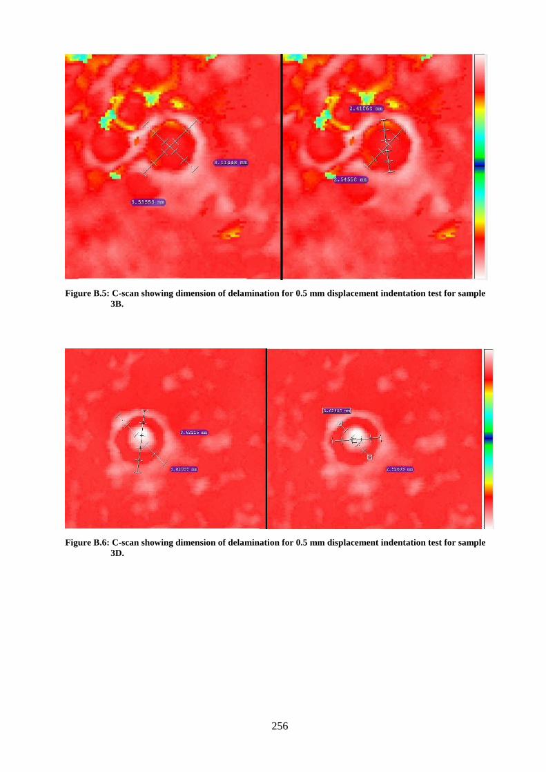
256
Figure B.5: C-scan showing dimension of delamination for 0.5 mm displacement indentation test for sample
3B.
Figure B.6: C-scan showing dimension of delamination for 0.5 mm displacement indentation test for sample
3D.
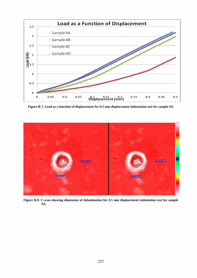
257
Figure B.7: Load as a function of displacement for 0.5 mm displacement indentation test for sample 4A.
Figure B.8: C-scan showing dimension of delamination for 0.5 mm displacement indentation test for sample
4A.
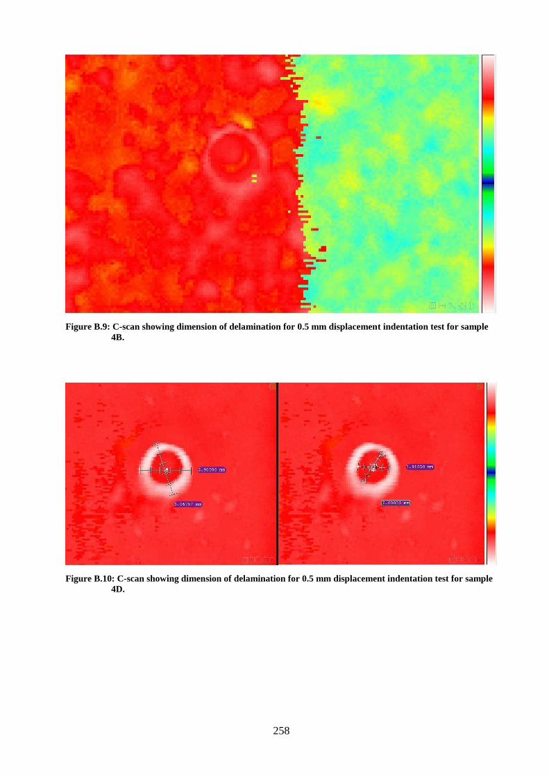
258
Figure B.9: C-scan showing dimension of delamination for 0.5 mm displacement indentation test for sample
4B.
Figure B.10: C-scan showing dimension of delamination for 0.5 mm displacement indentation test for sample
4D.
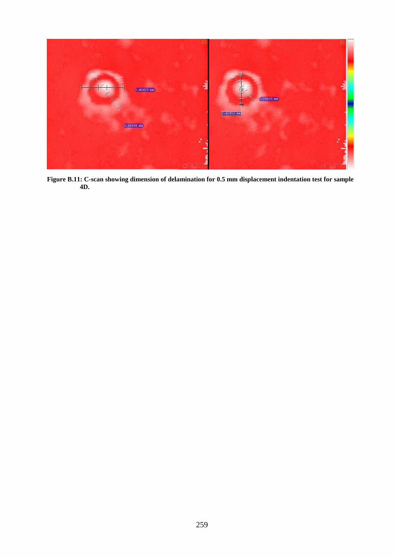
259
Figure B.11: C-scan showing dimension of delamination for 0.5 mm displacement indentation test for sample
4D.
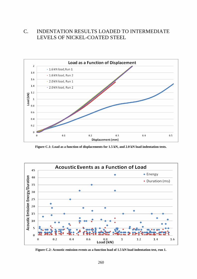
260
C. INDENTATION RESULTS LOADED TO INTERMEDIATE
LEVELS OF NICKEL-COATED STEEL
Figure C.1: Load as a function of displacements for 1.5 kN, and 2.0 kN load indentation tests.
Figure C.2: Acoustic emission events as a function load of 1.5 kN load indentation test, run 1.
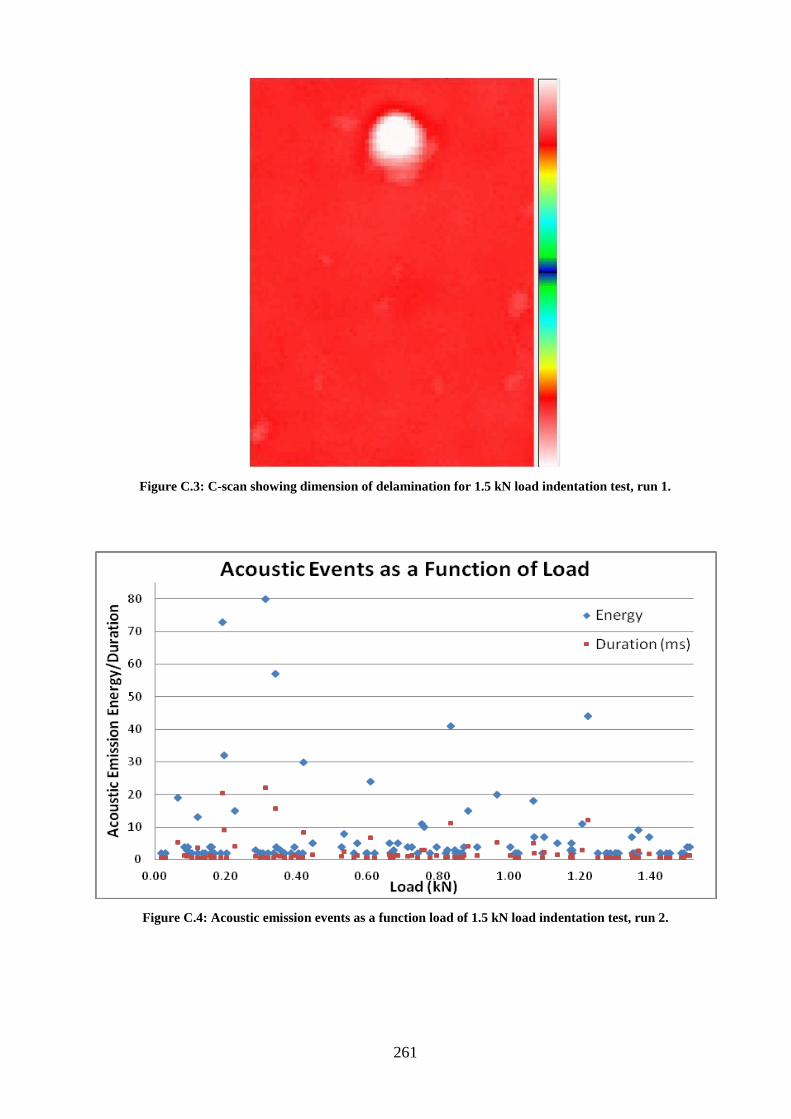
261
Figure C.3: C-scan showing dimension of delamination for 1.5 kN load indentation test, run 1.
Figure C.4: Acoustic emission events as a function load of 1.5 kN load indentation test, run 2.
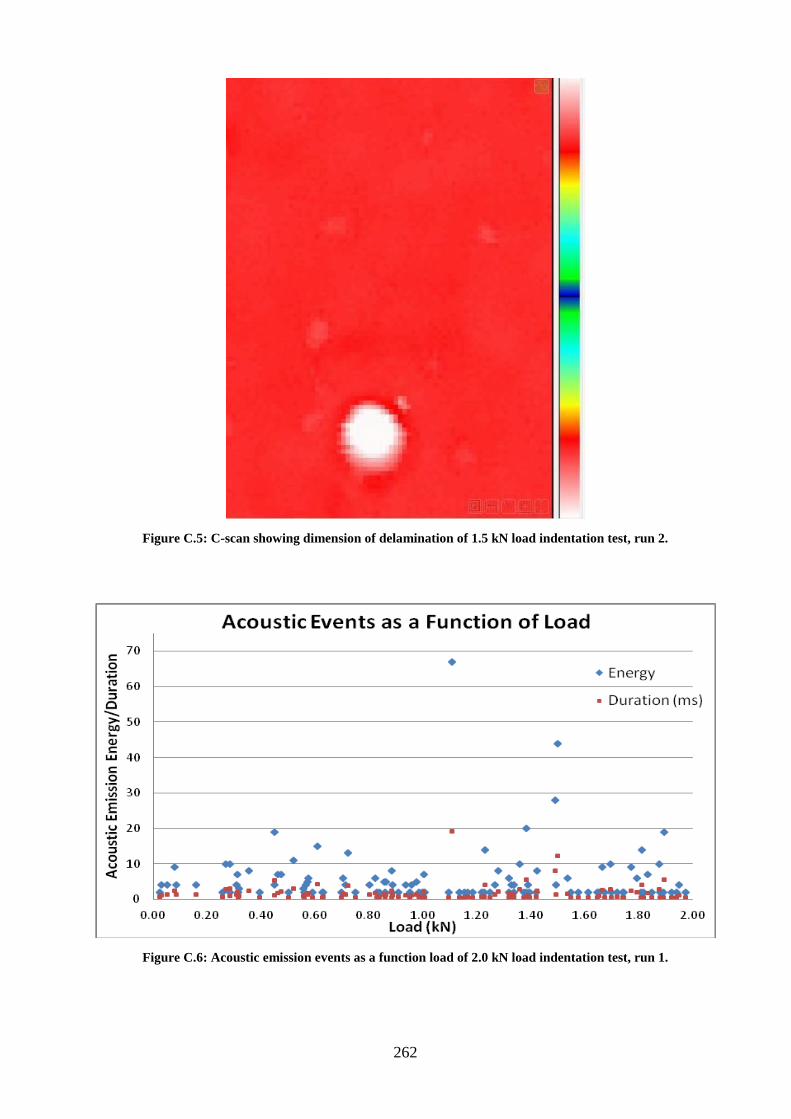
262
Figure C.5: C-scan showing dimension of delamination of 1.5 kN load indentation test, run 2.
Figure C.6: Acoustic emission events as a function load of 2.0 kN load indentation test, run 1.
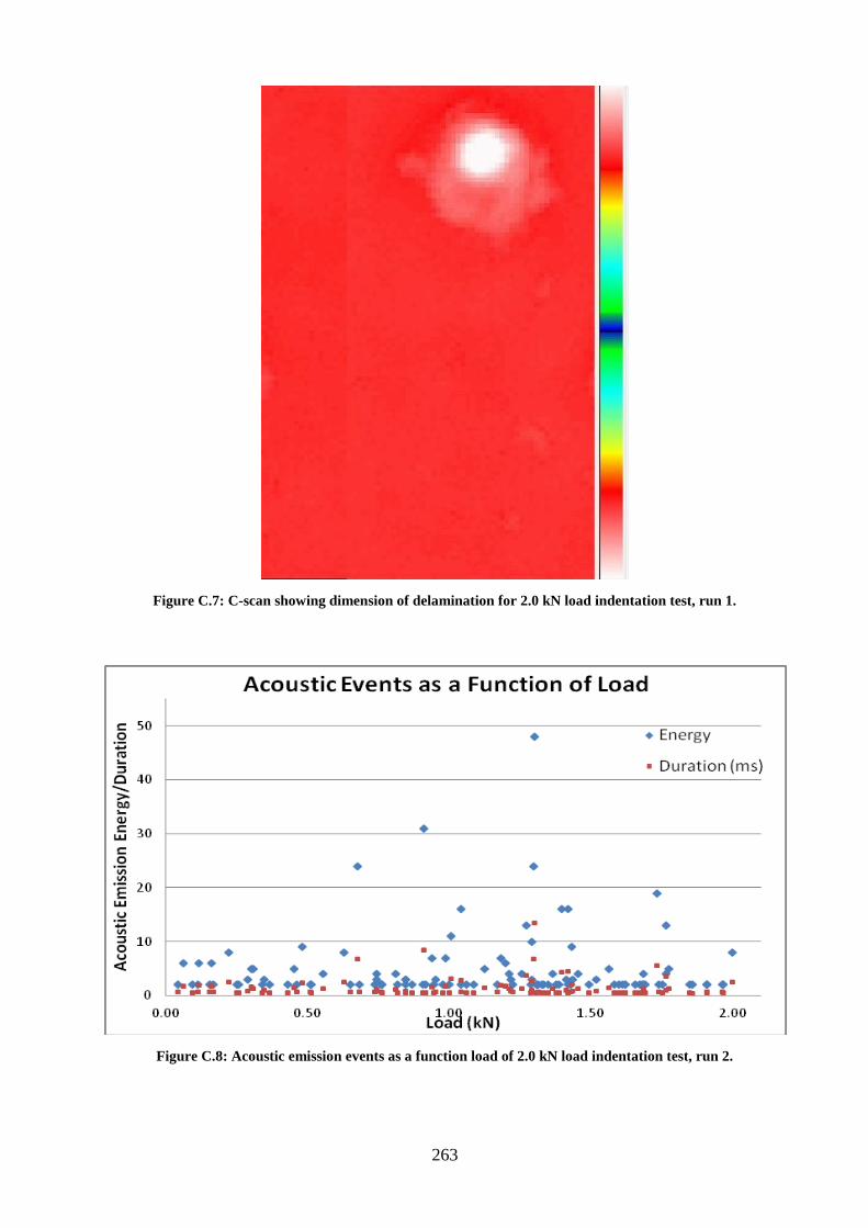
263
Figure C.7: C-scan showing dimension of delamination for 2.0 kN load indentation test, run 1.
Figure C.8: Acoustic emission events as a function load of 2.0 kN load indentation test, run 2.
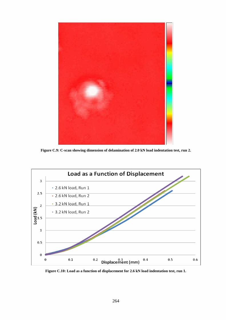
264
Figure C.9: C-scan showing dimension of delamination of 2.0 kN load indentation test, run 2.
Figure C.10: Load as a function of displacement for 2.6 kN load indentation test, run 1.
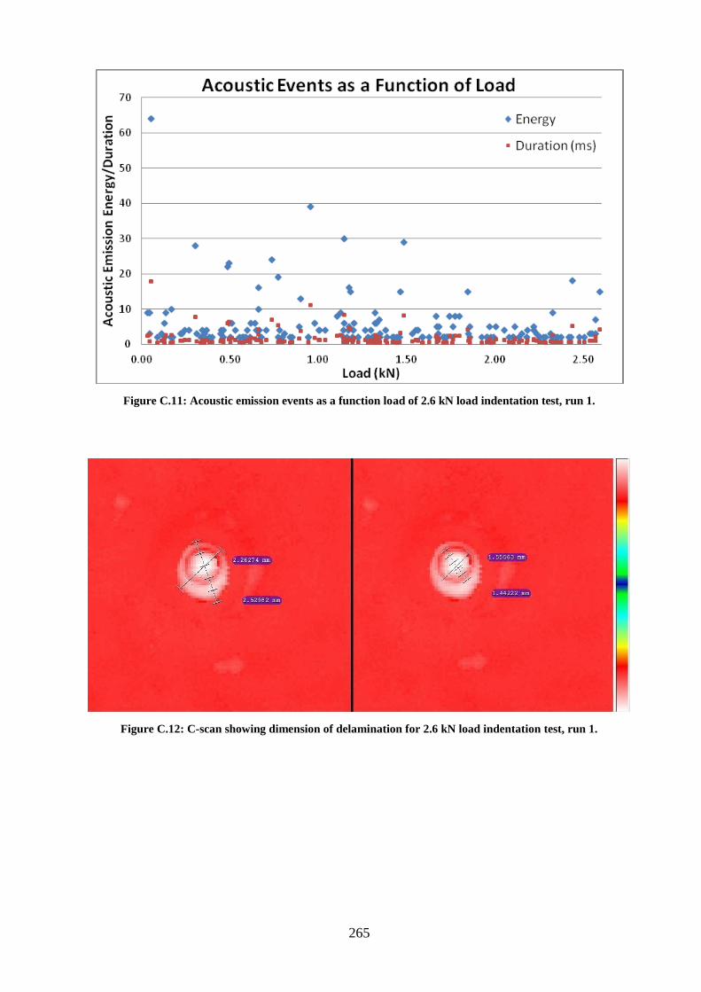
265
Figure C.11: Acoustic emission events as a function load of 2.6 kN load indentation test, run 1.
Figure C.12: C-scan showing dimension of delamination for 2.6 kN load indentation test, run 1.
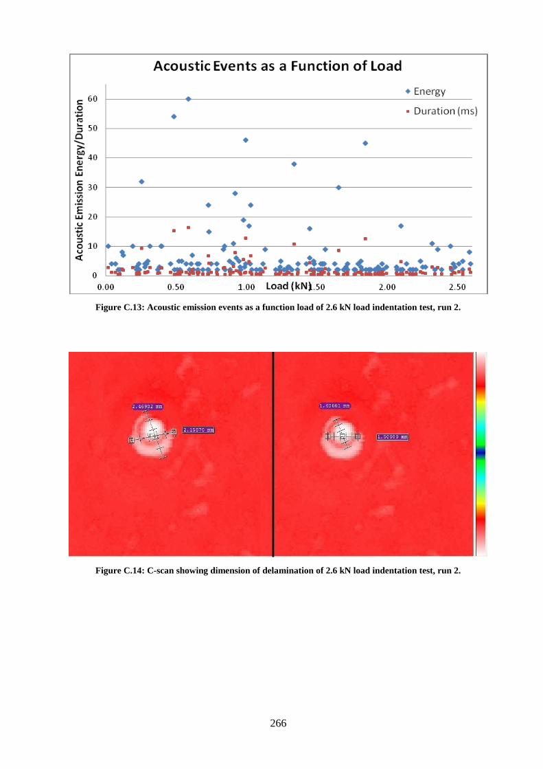
266
Figure C.13: Acoustic emission events as a function load of 2.6 kN load indentation test, run 2.
Figure C.14: C-scan showing dimension of delamination of 2.6 kN load indentation test, run 2.
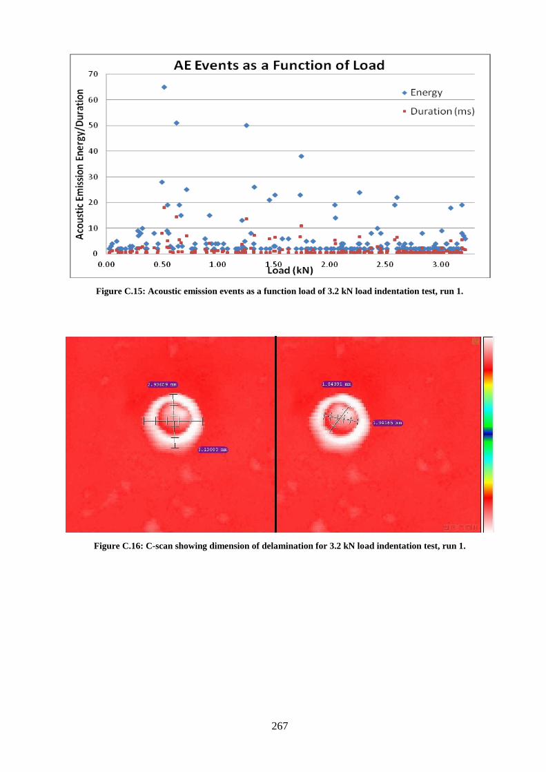
267
Figure C.15: Acoustic emission events as a function load of 3.2 kN load indentation test, run 1.
Figure C.16: C-scan showing dimension of delamination for 3.2 kN load indentation test, run 1.
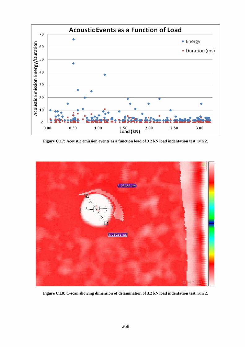
268
Figure C.17: Acoustic emission events as a function load of 3.2 kN load indentation test, run 2.
Figure C.18: C-scan showing dimension of delamination of 3.2 kN load indentation test, run 2.
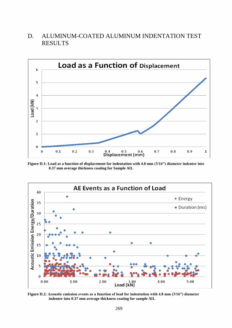
269
D. ALUMINUM-COATED ALUMINUM INDENTATION TEST
RESULTS
Figure D.1: Load as a function of displacement for indentation with 4.8 mm (3/16”) diameter indenter into
0.37 mm average thickness coating for Sample Al1.
Figure D.2: Acoustic emission events as a function of load for indentation with 4.8 mm (3/16”) diameter
indenter into 0.37 mm average thickness coating for sample Al1.
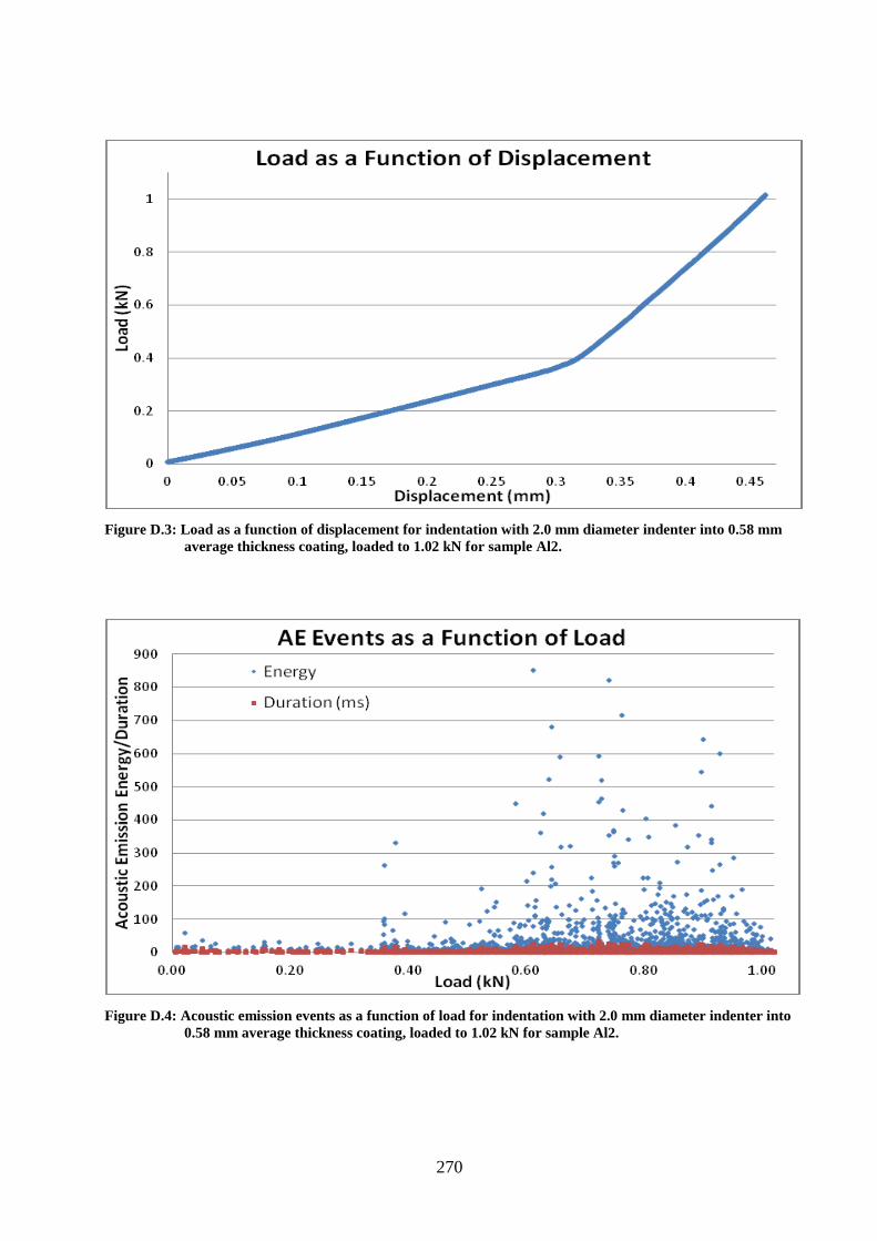
270
Figure D.3: Load as a function of displacement for indentation with 2.0 mm diameter indenter into 0.58 mm
average thickness coating, loaded to 1.02 kN for sample Al2.
Figure D.4: Acoustic emission events as a function of load for indentation with 2.0 mm diameter indenter into
0.58 mm average thickness coating, loaded to 1.02 kN for sample Al2.
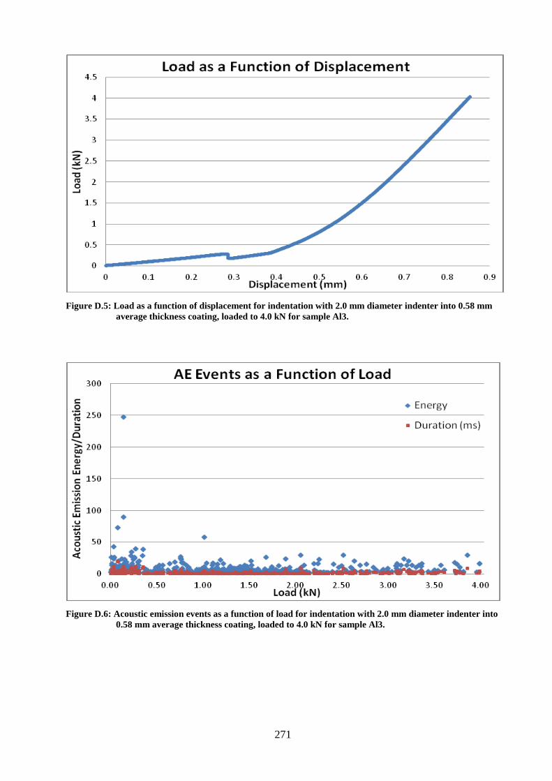
271
Figure D.5: Load as a function of displacement for indentation with 2.0 mm diameter indenter into 0.58 mm
average thickness coating, loaded to 4.0 kN for sample Al3.
Figure D.6: Acoustic emission events as a function of load for indentation with 2.0 mm diameter indenter into
0.58 mm average thickness coating, loaded to 4.0 kN for sample Al3.
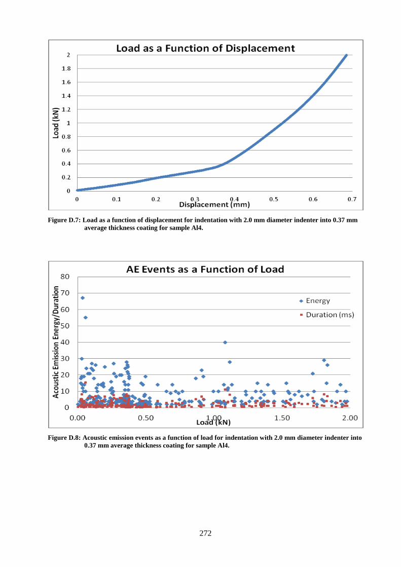
272
Figure D.7: Load as a function of displacement for indentation with 2.0 mm diameter indenter into 0.37 mm
average thickness coating for sample Al4.
Figure D.8: Acoustic emission events as a function of load for indentation with 2.0 mm diameter indenter into
0.37 mm average thickness coating for sample Al4.
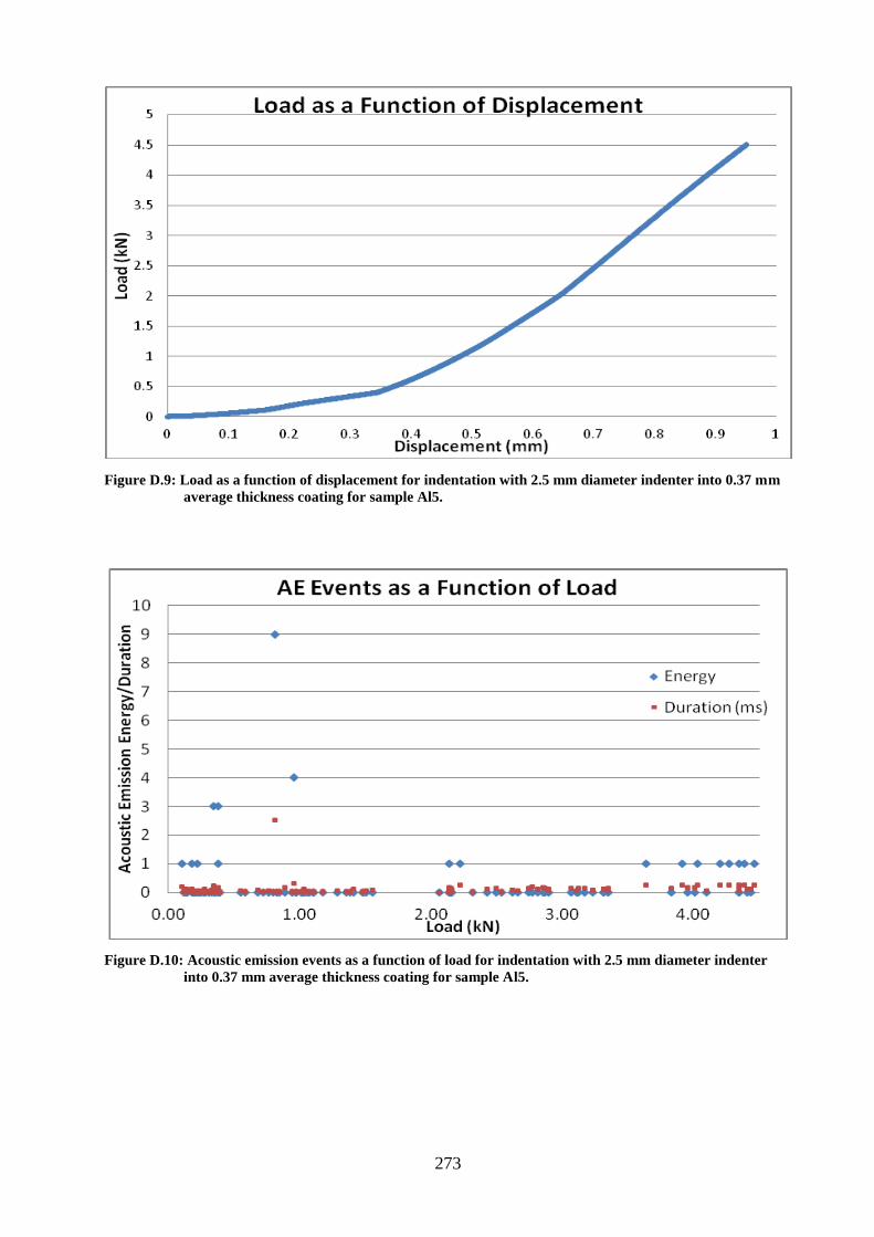
273
Figure D.9: Load as a function of displacement for indentation with 2.5 mm diameter indenter into 0.37 mm
average thickness coating for sample Al5.
Figure D.10: Acoustic emission events as a function of load for indentation with 2.5 mm diameter indenter
into 0.37 mm average thickness coating for sample Al5.
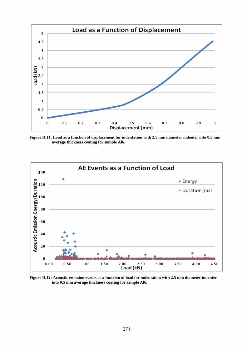
274
Figure D.11: Load as a function of displacement for indentation with 2.5 mm diameter indenter into 0.5 mm
average thickness coating for sample Al6.
Figure D.12: Acoustic emission events as a function of load for indentation with 2.5 mm diameter indenter
into 0.5 mm average thickness coating for sample Al6.
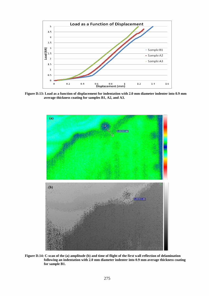
275
Figure D.13: Load as a function of displacement for indentation with 2.0 mm diameter indenter into 0.9 mm
average thickness coating for samples B1, A2, and A3.
Figure D.14: C-scan of the (a) amplitude (b) and time of flight of the first wall reflection of delamination
following an indentation with 2.0 mm diameter indenter into 0.9 mm average thickness coating
for sample B1.
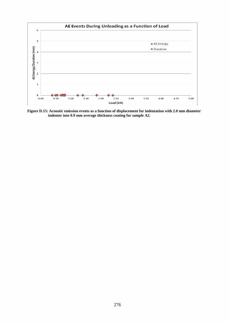
276
Figure D.15: Acoustic emission events as a function of displacement for indentation with 2.0 mm diameter
indenter into 0.9 mm average thickness coating for sample A2.
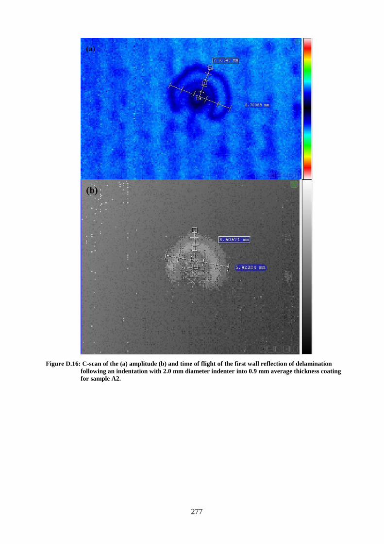
277
Figure D.16: C-scan of the (a) amplitude (b) and time of flight of the first wall reflection of delamination
following an indentation with 2.0 mm diameter indenter into 0.9 mm average thickness coating
for sample A2.
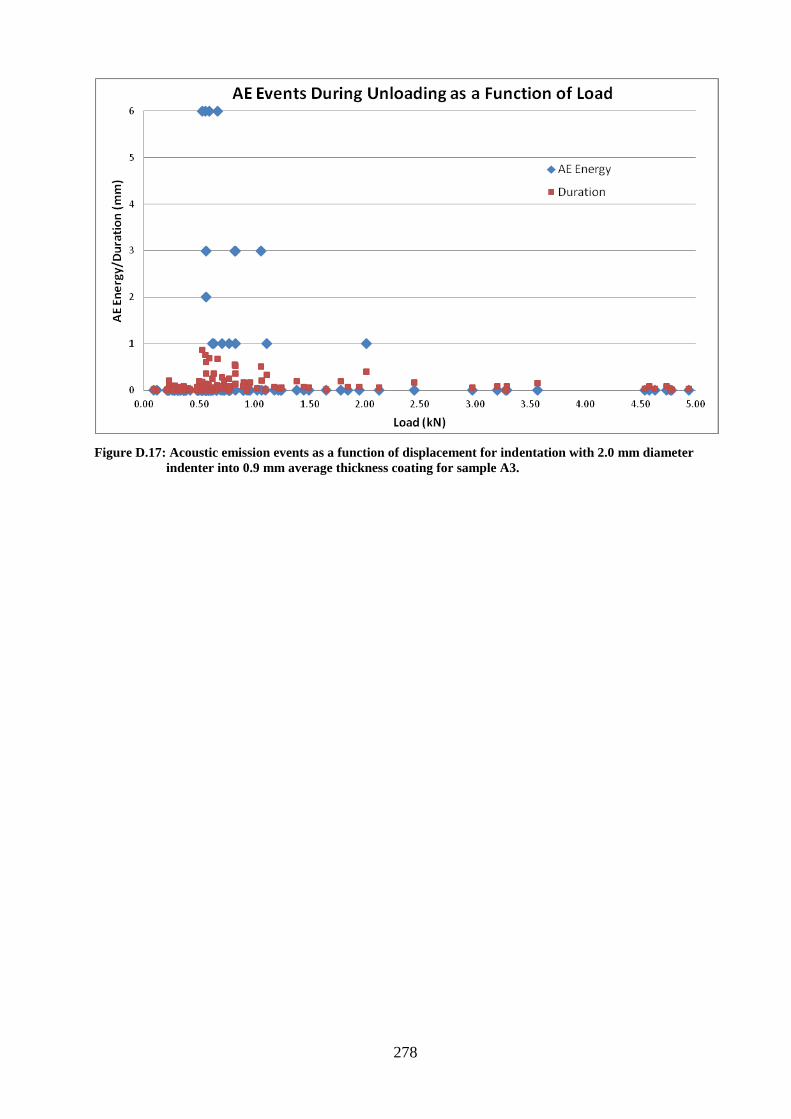
278
Figure D.17: Acoustic emission events as a function of displacement for indentation with 2.0 mm diameter
indenter into 0.9 mm average thickness coating for sample A3.
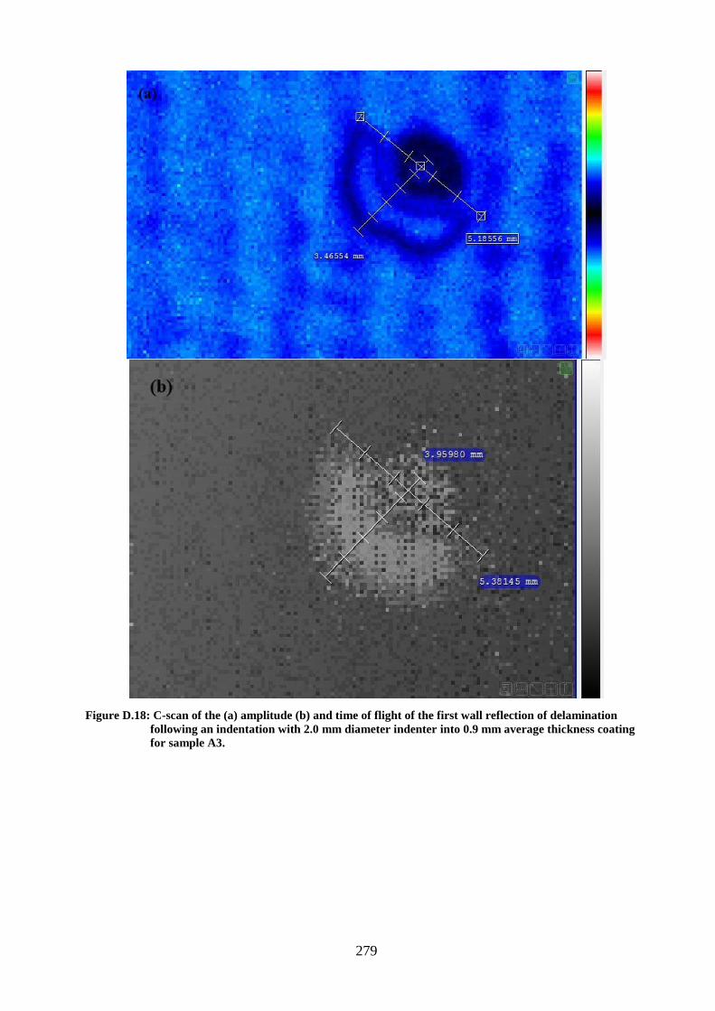
279
Figure D.18: C-scan of the (a) amplitude (b) and time of flight of the first wall reflection of delamination
following an indentation with 2.0 mm diameter indenter into 0.9 mm average thickness coating
for sample A3.
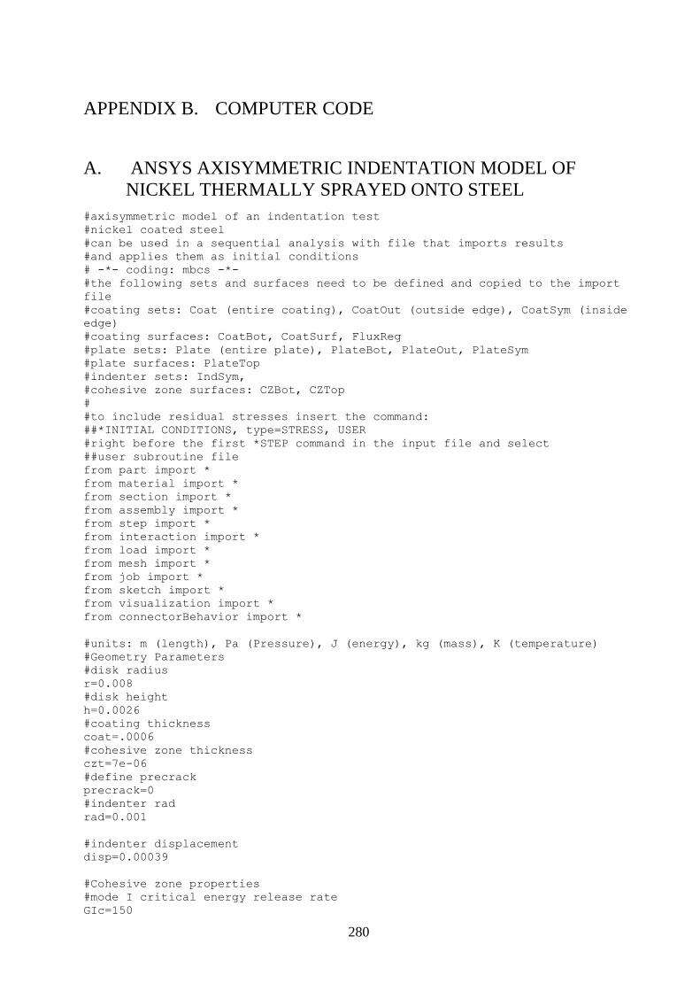
280
APPENDIX B. COMPUTER CODE
A. ANSYS AXISYMMETRIC INDENTATION MODEL OF
NICKEL THERMALLY SPRAYED ONTO STEEL
#axisymmetric model of an indentation test
#nickel coated steel
#can be used in a sequential analysis with file that imports results
#and applies them as initial conditions
# -*- coding: mbcs -*-
#the following sets and surfaces need to be defined and copied to the import
file
#coating sets: Coat (entire coating), CoatOut (outside edge), CoatSym (inside
edge)
#coating surfaces: CoatBot, CoatSurf, FluxReg
#plate sets: Plate (entire plate), PlateBot, PlateOut, PlateSym
#plate surfaces: PlateTop
#indenter sets: IndSym,
#cohesive zone surfaces: CZBot, CZTop
#
#to include residual stresses insert the command:
##*INITIAL CONDITIONS, type=STRESS, USER
#right before the first *STEP command in the input file and select
##user subroutine file
from part import *
from material import *
from section import *
from assembly import *
from step import *
from interaction import *
from load import *
from mesh import *
from job import *
from sketch import *
from visualization import *
from connectorBehavior import *
#units: m (length), Pa (Pressure), J (energy), kg (mass), K (temperature)
#Geometry Parameters
#disk radius
r=0.008
#disk height
h=0.0026
#coating thickness
coat=.0006
#cohesive zone thickness
czt=7e-06
#define precrack
precrack=0
#indenter rad
rad=0.001
#indenter displacement
disp=0.00039
#Cohesive zone properties
#mode I critical energy release rate
GIc=150
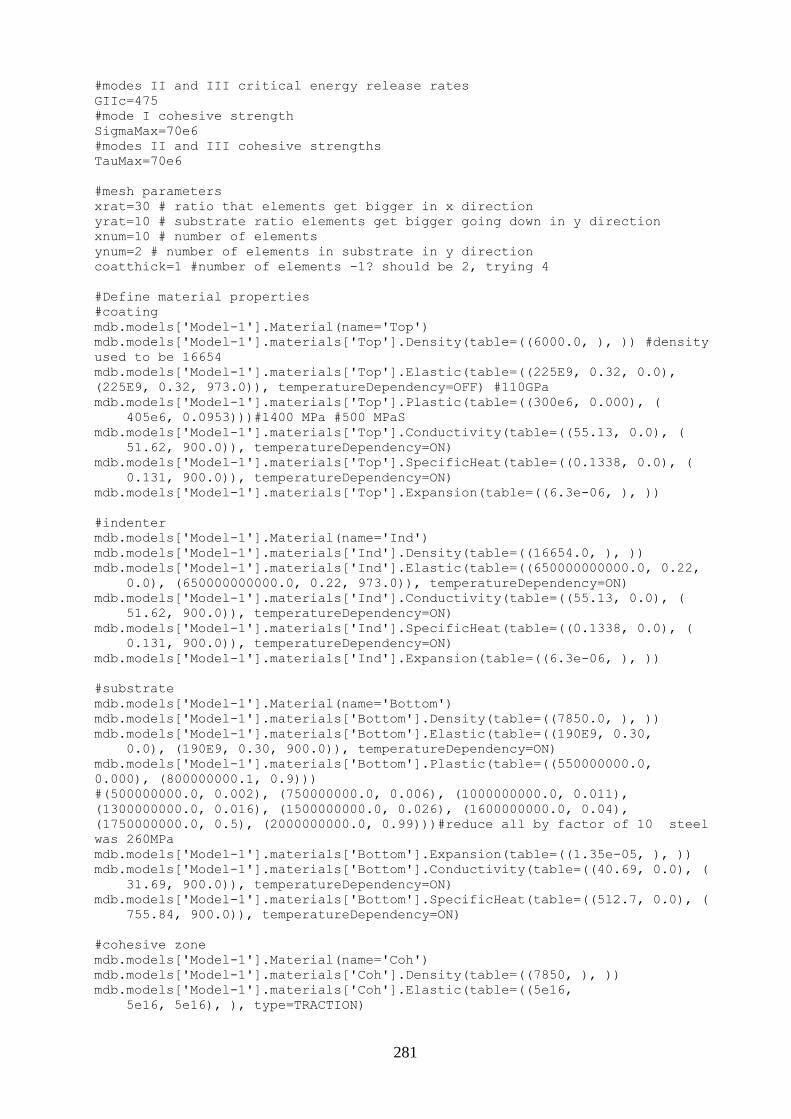
281
#modes II and III critical energy release rates
GIIc=475
#mode I cohesive strength
SigmaMax=70e6
#modes II and III cohesive strengths
TauMax=70e6
#mesh parameters
xrat=30 # ratio that elements get bigger in x direction
yrat=10 # substrate ratio elements get bigger going down in y direction
xnum=10 # number of elements
ynum=2 # number of elements in substrate in y direction
coatthick=1 #number of elements -1? should be 2, trying 4
#Define material properties
#coating
mdb.models['Model-1'].Material(name='Top')
mdb.models['Model-1'].materials['Top'].Density(table=((6000.0, ), )) #density
used to be 16654
mdb.models['Model-1'].materials['Top'].Elastic(table=((225E9, 0.32, 0.0),
(225E9, 0.32, 973.0)), temperatureDependency=OFF) #110GPa
mdb.models['Model-1'].materials['Top'].Plastic(table=((300e6, 0.000), (
405e6, 0.0953)))#1400 MPa #500 MPaS
mdb.models['Model-1'].materials['Top'].Conductivity(table=((55.13, 0.0), (
51.62, 900.0)), temperatureDependency=ON)
mdb.models['Model-1'].materials['Top'].SpecificHeat(table=((0.1338, 0.0), (
0.131, 900.0)), temperatureDependency=ON)
mdb.models['Model-1'].materials['Top'].Expansion(table=((6.3e-06, ), ))
#indenter
mdb.models['Model-1'].Material(name='Ind')
mdb.models['Model-1'].materials['Ind'].Density(table=((16654.0, ), ))
mdb.models['Model-1'].materials['Ind'].Elastic(table=((650000000000.0, 0.22,
0.0), (650000000000.0, 0.22, 973.0)), temperatureDependency=ON)
mdb.models['Model-1'].materials['Ind'].Conductivity(table=((55.13, 0.0), (
51.62, 900.0)), temperatureDependency=ON)
mdb.models['Model-1'].materials['Ind'].SpecificHeat(table=((0.1338, 0.0), (
0.131, 900.0)), temperatureDependency=ON)
mdb.models['Model-1'].materials['Ind'].Expansion(table=((6.3e-06, ), ))
#substrate
mdb.models['Model-1'].Material(name='Bottom')
mdb.models['Model-1'].materials['Bottom'].Density(table=((7850.0, ), ))
mdb.models['Model-1'].materials['Bottom'].Elastic(table=((190E9, 0.30,
0.0), (190E9, 0.30, 900.0)), temperatureDependency=ON)
mdb.models['Model-1'].materials['Bottom'].Plastic(table=((550000000.0,
0.000), (800000000.1, 0.9)))
#(500000000.0, 0.002), (750000000.0, 0.006), (1000000000.0, 0.011),
(1300000000.0, 0.016), (1500000000.0, 0.026), (1600000000.0, 0.04),
(1750000000.0, 0.5), (2000000000.0, 0.99)))#reduce all by factor of 10 steel
was 260MPa
mdb.models['Model-1'].materials['Bottom'].Expansion(table=((1.35e-05, ), ))
mdb.models['Model-1'].materials['Bottom'].Conductivity(table=((40.69, 0.0), (
31.69, 900.0)), temperatureDependency=ON)
mdb.models['Model-1'].materials['Bottom'].SpecificHeat(table=((512.7, 0.0), (
755.84, 900.0)), temperatureDependency=ON)
#cohesive zone
mdb.models['Model-1'].Material(name='Coh')
mdb.models['Model-1'].materials['Coh'].Density(table=((7850, ), ))
mdb.models['Model-1'].materials['Coh'].Elastic(table=((5e16,
5e16, 5e16), ), type=TRACTION)
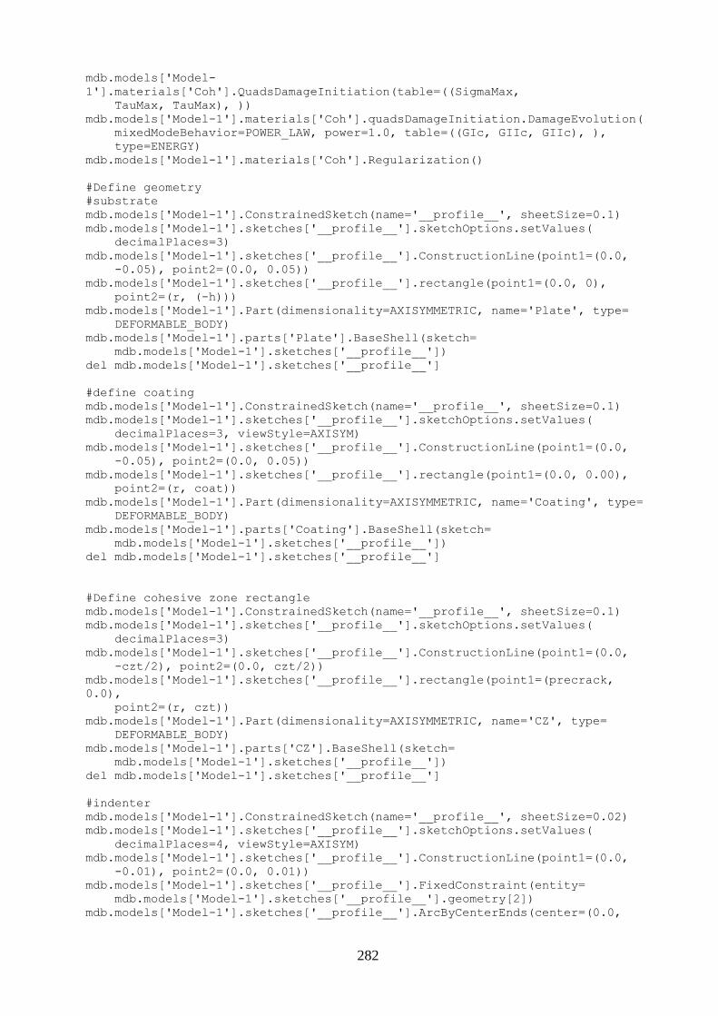
282
mdb.models['Model-
1'].materials['Coh'].QuadsDamageInitiation(table=((SigmaMax,
TauMax, TauMax), ))
mdb.models['Model-1'].materials['Coh'].quadsDamageInitiation.DamageEvolution(
mixedModeBehavior=POWER_LAW, power=1.0, table=((GIc, GIIc, GIIc), ),
type=ENERGY)
mdb.models['Model-1'].materials['Coh'].Regularization()
#Define geometry
#substrate
mdb.models['Model-1'].ConstrainedSketch(name='__profile__', sheetSize=0.1)
mdb.models['Model-1'].sketches['__profile__'].sketchOptions.setValues(
decimalPlaces=3)
mdb.models['Model-1'].sketches['__profile__'].ConstructionLine(point1=(0.0,
-0.05), point2=(0.0, 0.05))
mdb.models['Model-1'].sketches['__profile__'].rectangle(point1=(0.0, 0),
point2=(r, (-h)))
mdb.models['Model-1'].Part(dimensionality=AXISYMMETRIC, name='Plate', type=
DEFORMABLE_BODY)
mdb.models['Model-1'].parts['Plate'].BaseShell(sketch=
mdb.models['Model-1'].sketches['__profile__'])
del mdb.models['Model-1'].sketches['__profile__']
#define coating
mdb.models['Model-1'].ConstrainedSketch(name='__profile__', sheetSize=0.1)
mdb.models['Model-1'].sketches['__profile__'].sketchOptions.setValues(
decimalPlaces=3, viewStyle=AXISYM)
mdb.models['Model-1'].sketches['__profile__'].ConstructionLine(point1=(0.0,
-0.05), point2=(0.0, 0.05))
mdb.models['Model-1'].sketches['__profile__'].rectangle(point1=(0.0, 0.00),
point2=(r, coat))
mdb.models['Model-1'].Part(dimensionality=AXISYMMETRIC, name='Coating', type=
DEFORMABLE_BODY)
mdb.models['Model-1'].parts['Coating'].BaseShell(sketch=
mdb.models['Model-1'].sketches['__profile__'])
del mdb.models['Model-1'].sketches['__profile__']
#Define cohesive zone rectangle
mdb.models['Model-1'].ConstrainedSketch(name='__profile__', sheetSize=0.1)
mdb.models['Model-1'].sketches['__profile__'].sketchOptions.setValues(
decimalPlaces=3)
mdb.models['Model-1'].sketches['__profile__'].ConstructionLine(point1=(0.0,
-czt/2), point2=(0.0, czt/2))
mdb.models['Model-1'].sketches['__profile__'].rectangle(point1=(precrack,
0.0),
point2=(r, czt))
mdb.models['Model-1'].Part(dimensionality=AXISYMMETRIC, name='CZ', type=
DEFORMABLE_BODY)
mdb.models['Model-1'].parts['CZ'].BaseShell(sketch=
mdb.models['Model-1'].sketches['__profile__'])
del mdb.models['Model-1'].sketches['__profile__']
#indenter
mdb.models['Model-1'].ConstrainedSketch(name='__profile__', sheetSize=0.02)
mdb.models['Model-1'].sketches['__profile__'].sketchOptions.setValues(
decimalPlaces=4, viewStyle=AXISYM)
mdb.models['Model-1'].sketches['__profile__'].ConstructionLine(point1=(0.0,
-0.01), point2=(0.0, 0.01))
mdb.models['Model-1'].sketches['__profile__'].FixedConstraint(entity=
mdb.models['Model-1'].sketches['__profile__'].geometry[2])
mdb.models['Model-1'].sketches['__profile__'].ArcByCenterEnds(center=(0.0,
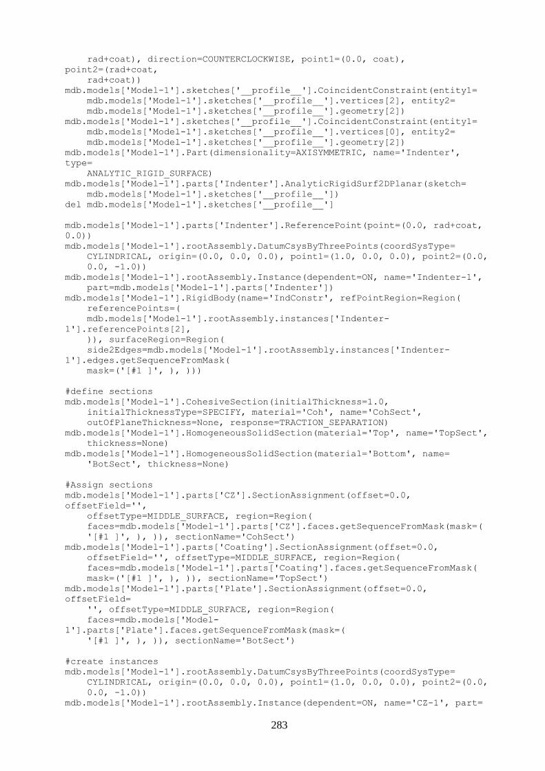
283
rad+coat), direction=COUNTERCLOCKWISE, point1=(0.0, coat),
point2=(rad+coat,
rad+coat))
mdb.models['Model-1'].sketches['__profile__'].CoincidentConstraint(entity1=
mdb.models['Model-1'].sketches['__profile__'].vertices[2], entity2=
mdb.models['Model-1'].sketches['__profile__'].geometry[2])
mdb.models['Model-1'].sketches['__profile__'].CoincidentConstraint(entity1=
mdb.models['Model-1'].sketches['__profile__'].vertices[0], entity2=
mdb.models['Model-1'].sketches['__profile__'].geometry[2])
mdb.models['Model-1'].Part(dimensionality=AXISYMMETRIC, name='Indenter',
type=
ANALYTIC_RIGID_SURFACE)
mdb.models['Model-1'].parts['Indenter'].AnalyticRigidSurf2DPlanar(sketch=
mdb.models['Model-1'].sketches['__profile__'])
del mdb.models['Model-1'].sketches['__profile__']
mdb.models['Model-1'].parts['Indenter'].ReferencePoint(point=(0.0, rad+coat,
0.0))
mdb.models['Model-1'].rootAssembly.DatumCsysByThreePoints(coordSysType=
CYLINDRICAL, origin=(0.0, 0.0, 0.0), point1=(1.0, 0.0, 0.0), point2=(0.0,
0.0, -1.0))
mdb.models['Model-1'].rootAssembly.Instance(dependent=ON, name='Indenter-1',
part=mdb.models['Model-1'].parts['Indenter'])
mdb.models['Model-1'].RigidBody(name='IndConstr', refPointRegion=Region(
referencePoints=(
mdb.models['Model-1'].rootAssembly.instances['Indenter-
1'].referencePoints[2],
)), surfaceRegion=Region(
side2Edges=mdb.models['Model-1'].rootAssembly.instances['Indenter-
1'].edges.getSequenceFromMask(
mask=('[#1 ]', ), )))
#define sections
mdb.models['Model-1'].CohesiveSection(initialThickness=1.0,
initialThicknessType=SPECIFY, material='Coh', name='CohSect',
outOfPlaneThickness=None, response=TRACTION_SEPARATION)
mdb.models['Model-1'].HomogeneousSolidSection(material='Top', name='TopSect',
thickness=None)
mdb.models['Model-1'].HomogeneousSolidSection(material='Bottom', name=
'BotSect', thickness=None)
#Assign sections
mdb.models['Model-1'].parts['CZ'].SectionAssignment(offset=0.0,
offsetField='',
offsetType=MIDDLE_SURFACE, region=Region(
faces=mdb.models['Model-1'].parts['CZ'].faces.getSequenceFromMask(mask=(
'[#1 ]', ), )), sectionName='CohSect')
mdb.models['Model-1'].parts['Coating'].SectionAssignment(offset=0.0,
offsetField='', offsetType=MIDDLE_SURFACE, region=Region(
faces=mdb.models['Model-1'].parts['Coating'].faces.getSequenceFromMask(
mask=('[#1 ]', ), )), sectionName='TopSect')
mdb.models['Model-1'].parts['Plate'].SectionAssignment(offset=0.0,
offsetField=
'', offsetType=MIDDLE_SURFACE, region=Region(
faces=mdb.models['Model-
1'].parts['Plate'].faces.getSequenceFromMask(mask=(
'[#1 ]', ), )), sectionName='BotSect')
#create instances
mdb.models['Model-1'].rootAssembly.DatumCsysByThreePoints(coordSysType=
CYLINDRICAL, origin=(0.0, 0.0, 0.0), point1=(1.0, 0.0, 0.0), point2=(0.0,
0.0, -1.0))
mdb.models['Model-1'].rootAssembly.Instance(dependent=ON, name='CZ-1', part=
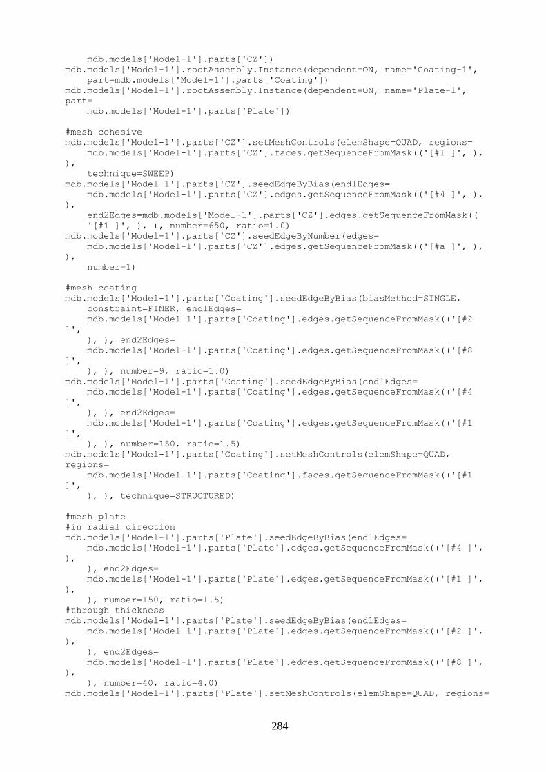
284
mdb.models['Model-1'].parts['CZ'])
mdb.models['Model-1'].rootAssembly.Instance(dependent=ON, name='Coating-1',
part=mdb.models['Model-1'].parts['Coating'])
mdb.models['Model-1'].rootAssembly.Instance(dependent=ON, name='Plate-1',
part=
mdb.models['Model-1'].parts['Plate'])
#mesh cohesive
mdb.models['Model-1'].parts['CZ'].setMeshControls(elemShape=QUAD, regions=
mdb.models['Model-1'].parts['CZ'].faces.getSequenceFromMask(('[#1 ]', ),
),
technique=SWEEP)
mdb.models['Model-1'].parts['CZ'].seedEdgeByBias(end1Edges=
mdb.models['Model-1'].parts['CZ'].edges.getSequenceFromMask(('[#4 ]', ),
),
end2Edges=mdb.models['Model-1'].parts['CZ'].edges.getSequenceFromMask((
'[#1 ]', ), ), number=650, ratio=1.0)
mdb.models['Model-1'].parts['CZ'].seedEdgeByNumber(edges=
mdb.models['Model-1'].parts['CZ'].edges.getSequenceFromMask(('[#a ]', ),
),
number=1)
#mesh coating
mdb.models['Model-1'].parts['Coating'].seedEdgeByBias(biasMethod=SINGLE,
constraint=FINER, end1Edges=
mdb.models['Model-1'].parts['Coating'].edges.getSequenceFromMask(('[#2
]',
), ), end2Edges=
mdb.models['Model-1'].parts['Coating'].edges.getSequenceFromMask(('[#8
]',
), ), number=9, ratio=1.0)
mdb.models['Model-1'].parts['Coating'].seedEdgeByBias(end1Edges=
mdb.models['Model-1'].parts['Coating'].edges.getSequenceFromMask(('[#4
]',
), ), end2Edges=
mdb.models['Model-1'].parts['Coating'].edges.getSequenceFromMask(('[#1
]',
), ), number=150, ratio=1.5)
mdb.models['Model-1'].parts['Coating'].setMeshControls(elemShape=QUAD,
regions=
mdb.models['Model-1'].parts['Coating'].faces.getSequenceFromMask(('[#1
]',
), ), technique=STRUCTURED)
#mesh plate
#in radial direction
mdb.models['Model-1'].parts['Plate'].seedEdgeByBias(end1Edges=
mdb.models['Model-1'].parts['Plate'].edges.getSequenceFromMask(('[#4 ]',
),
), end2Edges=
mdb.models['Model-1'].parts['Plate'].edges.getSequenceFromMask(('[#1 ]',
),
), number=150, ratio=1.5)
#through thickness
mdb.models['Model-1'].parts['Plate'].seedEdgeByBias(end1Edges=
mdb.models['Model-1'].parts['Plate'].edges.getSequenceFromMask(('[#2 ]',
),
), end2Edges=
mdb.models['Model-1'].parts['Plate'].edges.getSequenceFromMask(('[#8 ]',
),
), number=40, ratio=4.0)
mdb.models['Model-1'].parts['Plate'].setMeshControls(elemShape=QUAD, regions=
285
mdb.models['Model-1'].parts['Plate'].faces.getSequenceFromMask(('[#1 ]',
),
), technique=STRUCTURED)
#assign element types
mdb.models['Model-1'].parts['CZ'].setElementType(elemTypes=(ElemType(
elemCode=COHAX4, elemLibrary=STANDARD, elemDeletion=ON,
viscosity=0.0005),
ElemType(elemCode=UNKNOWN_TRI, elemLibrary=STANDARD)), regions=(
mdb.models['Model-1'].parts['CZ'].faces.getSequenceFromMask(('[#1 ]', ),
),
))
mdb.models['Model-1'].parts['Coating'].setElementType(elemTypes=(ElemType(
elemCode=CAX4RT, elemLibrary=STANDARD, secondOrderAccuracy=OFF,
hourglassControl=ENHANCED, distortionControl=DEFAULT),
ElemType(elemCode=CAX3T,
elemLibrary=STANDARD)), regions=(
mdb.models['Model-1'].parts['Coating'].faces.getSequenceFromMask(('[#1
]',
), ), ))
mdb.models['Model-1'].parts['Plate'].setElementType(elemTypes=(ElemType(
elemCode=CAX4RT, elemLibrary=STANDARD), ElemType(elemCode=CAX3T,
elemLibrary=STANDARD, secondOrderAccuracy=OFF,
hourglassControl=ENHANCED, distortionControl=DEFAULT)), regions=(
mdb.models['Model-1'].parts['Plate'].faces.getSequenceFromMask(('[#1 ]',
),
), ))
#generate meshes
mdb.models['Model-1'].parts['CZ'].generateMesh()
mdb.models['Model-1'].parts['Coating'].generateMesh()
mdb.models['Model-1'].parts['Plate'].generateMesh()
#collapse cohesive zone
mdb.meshEditOptions.setValues(enableUndo=True, maxUndoCacheElements=0.5)
mdb.models['Model-1'].parts['CZ'].editNode(coordinate2=0.0, nodes=
mdb.models['Model-1'].parts['CZ'].nodes.getSequenceFromMask(mask=(
'[#ffffffff:40 #3fffff ]', ), ))
#define necessary surfaces
mdb.models['Model-1'].parts['Coating'].Set(name='CoatSym', nodes=
mdb.models['Model-1'].parts['Coating'].nodes.getSequenceFromMask(mask=(
'[#1 #0:3 #800000 #0:4 #4000 #0:4 #20',
' #0:3 #10000000 #0:4 #80000 #0:4 #400 #0:4',
' #2 #0:3 #1000000 #0:4 #8000 ]', ), ))
mdb.models['Model-1'].parts['Plate'].Set(name='PlateSym', nodes=
mdb.models['Model-1'].parts['Plate'].nodes.getSequenceFromMask(mask=(
'[#0:4 #400000 #0:4 #2000 #0:4 #10 #0:3',
' #8000000 #0:4 #40000 #0:4 #200 #0:4 #1',
' #0:3 #800000 #0:4 #4000 #0:4 #20 #0:3',
' #10000000 #0:4 #80000 #0:4 #400 #0:4 #2',
' #0:3 #1000000 #0:4 #8000 #0:4 #40 #0:3',
' #20000000 #0:4 #100000 #0:4 #800 #0:4 #4',
' #0:3 #2000000 #0:4 #10000 #0:4 #80 #0:3',
' #40000000 #0:4 #200000 #0:4 #1000 #0:4 #8',
' #0:3 #4000000 #0:4 #20000 #0:4 #100 #0:3',
' #80000000 #0:4 #400000 #0:4 #2000 #0:4 #10',
' #0:3 #8000000 #0:4 #40000 #0:4 #200 #0:4',
' #1 #0:3 #800000 #0:4 #4000 ]', ), ))
mdb.models['Model-1'].parts['Plate'].Set(name='PlateBot', nodes=
mdb.models['Model-1'].parts['Plate'].nodes.getSequenceFromMask(mask=(
'[#0:188 #ff000000 #ffffffff:4 #7fff ]', ), ))
286
mdb.models['Model-1'].rootAssembly.regenerate()
mdb.models['Model-1'].rootAssembly.Set(name='Outside', nodes=
mdb.models['Model-1'].rootAssembly.instances['Coating-
1'].nodes.getSequenceFromMask(
mask=('[#0:9 #2000 #0:4 #10 #0:3 #8000000 #0:4',
' #40000 #0:4 #200 #0:4 #1 #0:3 #800000', ' #0:4 #4000 ]', ), )+\
mdb.models['Model-1'].rootAssembly.instances['Plate-
1'].nodes.getSequenceFromMask(
mask=('[#0:4 #800000 #0:4 #4000 #0:4 #20 #0:3',
' #10000000 #0:4 #80000 #0:4 #400 #0:4 #2',
' #0:3 #1000000 #0:4 #8000 #0:4 #40 #0:3',
' #20000000 #0:4 #100000 #0:4 #800 #0:4 #4',
' #0:3 #2000000 #0:4 #10000 #0:4 #80 #0:3',
' #40000000 #0:4 #200000 #0:4 #1000 #0:4 #8',
' #0:3 #4000000 #0:4 #20000 #0:4 #100 #0:3',
' #80000000 #0:4 #400000 #0:4 #2000 #0:4 #10',
' #0:3 #8000000 #0:4 #40000 #0:4 #200 #0:4',
' #1 #0:3 #800000 #0:4 #4000 #0:4 #20',
' #0:3 #10000000 #0:4 #80000 #0:4 #400 #0:4', ' #2 #0:3 #1000000 ]', ),
))
mdb.models['Model-1'].rootAssembly.Set(name='Corner', nodes=
mdb.models['Model-1'].rootAssembly.instances['Coating-
1'].nodes.getSequenceFromMask(
mask=('[#0:47 #20 ]', ), ))
mdb.models['Model-1'].parts['CZ'].Set(elements=
mdb.models['Model-1'].parts['CZ'].elements.getSequenceFromMask(mask=(
'[#ffffffff:20 #3ff ]', ), ), name='CZElements')
mdb.models['Model-1'].parts['CZ'].Surface(face3Elements=
mdb.models['Model-1'].parts['CZ'].elements.getSequenceFromMask(mask=(
'[#ffffffff:20 #3ff ]', ), ), name='CZTop')
mdb.models['Model-1'].parts['CZ'].Surface(face1Elements=
mdb.models['Model-1'].parts['CZ'].elements.getSequenceFromMask(mask=(
'[#ffffffff:20 #3ff ]', ), ), name='CZBot')
mdb.models['Model-1'].parts['Coating'].Surface(name='CoatSurf', side1Edges=
mdb.models['Model-1'].parts['Coating'].edges.getSequenceFromMask(('[#4
]',
), ))
mdb.models['Model-1'].parts['Coating'].Surface(name='CoatBot', side1Edges=
mdb.models['Model-1'].parts['Coating'].edges.getSequenceFromMask(('[#1
]',
), ))
mdb.models['Model-1'].parts['Plate'].Surface(name='PlateTop', side1Edges=
mdb.models['Model-1'].parts['Plate'].edges.getSequenceFromMask(('[#1 ]',
),
))
mdb.models['Model-1'].parts['Indenter'].Set(name='IndLoad', referencePoints=(
mdb.models['Model-1'].parts['Indenter'].referencePoints[2], ))
#define contact interactions
mdb.models['Model-1'].ContactProperty('InterfaceContact')
mdb.models['Model-
1'].interactionProperties['InterfaceContact'].TangentialBehavior(
formulation=FRICTIONLESS)
mdb.models['Model-
1'].interactionProperties['InterfaceContact'].NormalBehavior(
allowSeparation=ON, constraintEnforcementMethod=DEFAULT,
pressureOverclosure=HARD)
mdb.models['Model-
1'].interactionProperties['InterfaceContact'].tangentialBehavior.setValues(

287
dependencies=0, directionality=ISOTROPIC, elasticSlipStiffness=None,
formulation=PENALTY, fraction=0.005, maximumElasticSlip=FRACTION,
pressureDependency=OFF, shearStressLimit=None, slipRateDependency=OFF,
table=((0.3, ), ), temperatureDependency=OFF)
mdb.models['Model-
1'].interactionProperties['InterfaceContact'].normalBehavior.setValues(
allowSeparation=ON, clearanceAtZeroContactPressure=0.0,
constraintEnforcementMethod=PENALTY, contactStiffness=DEFAULT,
contactStiffnessScaleFactor=1.0, pressureOverclosure=HARD,
stiffnessBehavior=LINEAR)
mdb.models['Model-
1'].interactionProperties['InterfaceContact'].tangentialBehavior.setValues(
dependencies=0, directionality=ISOTROPIC, elasticSlipStiffness=None,
formulation=PENALTY, fraction=0.005, maximumElasticSlip=FRACTION,
pressureDependency=OFF, shearStressLimit=None, slipRateDependency=OFF,
table=((0.6, ), ), temperatureDependency=OFF)
mdb.models['Model-1'].SurfaceToSurfaceContactStd(adjustMethod=NONE,
clearanceRegion=None, createStepName='Initial', datumAxis=None,
enforcement=SURFACE_TO_SURFACE, initialClearance=OMIT,
interactionProperty=
'InterfaceContact', master=
mdb.models['Model-1'].rootAssembly.instances['Plate-
1'].surfaces['PlateTop']
, name='Int-1', slave=
mdb.models['Model-1'].rootAssembly.instances['Coating-
1'].surfaces['CoatBot']
, sliding=FINITE, surfaceSmoothing=NONE, thickness=ON)
mdb.models['Model-1'].Tie(adjust=ON, master=
mdb.models['Model-1'].rootAssembly.instances['Coating-
1'].surfaces['CoatBot']
, name='Top', positionToleranceMethod=COMPUTED, slave=
mdb.models['Model-1'].rootAssembly.instances['CZ-1'].surfaces['CZTop'],
thickness=ON, tieRotations=ON)
mdb.models['Model-1'].Tie(adjust=ON, master=
mdb.models['Model-1'].rootAssembly.instances['Plate-
1'].surfaces['PlateTop']
, name='Bottom', positionToleranceMethod=COMPUTED, slave=
mdb.models['Model-1'].rootAssembly.instances['CZ-1'].surfaces['CZBot'],
thickness=ON, tieRotations=ON)
mdb.models['Model-1'].SurfaceToSurfaceContactStd(adjustMethod=NONE,
clearanceRegion=None, createStepName='Initial', datumAxis=None,
initialClearance=OMIT, interactionProperty='InterfaceContact', master=
Region(
side2Edges=mdb.models['Model-1'].rootAssembly.instances['Indenter-
1'].edges.getSequenceFromMask(
mask=('[#1 ]', ), )), name='IndenterCont', slave=
mdb.models['Model-1'].rootAssembly.instances['Coating-
1'].surfaces['CoatSurf']
, sliding=FINITE, thickness=ON)
#define boundary conditions
mdb.models['Model-1'].DisplacementBC(amplitude=UNSET,
createStepName='Initial',
distributionType=UNIFORM, fieldName='', localCsys=None, name='SymCoat',
region=
mdb.models['Model-1'].rootAssembly.instances['Coating-
1'].sets['CoatSym'],
u1=SET, u2=UNSET, ur3=UNSET)
288
mdb.models['Model-1'].DisplacementBC(amplitude=UNSET,
createStepName='Initial',
distributionType=UNIFORM, fieldName='', localCsys=None, name='SymPlate',
region=
mdb.models['Model-1'].rootAssembly.instances['Plate-1'].sets['PlateSym'],
u1=SET, u2=UNSET, ur3=UNSET)
mdb.models['Model-1'].DisplacementBC(amplitude=UNSET,
createStepName='Initial',
distributionType=UNIFORM, fieldName='', localCsys=None, name='PlateBot',
region=
mdb.models['Model-1'].rootAssembly.instances['Plate-1'].sets['PlateBot'],
u1=UNSET, u2=SET, ur3=UNSET)
#define load and remove load step
mdb.models['Model-1'].StaticStep(initialInc=1e-06, maxNumInc=100000, minInc=
1e-21, name='LoadStep', nlgeom=ON, previous='Initial')
mdb.models['Model-1'].StaticStep(initialInc=1e-06, maxNumInc=75000, minInc=
1e-21, name='RemoveLoad', previous='LoadStep')
mdb.models['Model-1'].steps['LoadStep'].setValues(adaptiveDampingRatio=0.05,
continueDampingFactors=True, stabilizationMethod=
DISSIPATED_ENERGY_FRACTION)
mdb.models['Model-
1'].steps['RemoveLoad'].setValues(adaptiveDampingRatio=0.05,
continueDampingFactors=True, stabilizationMethod=
DISSIPATED_ENERGY_FRACTION)
#define load boundary conditions
mdb.models['Model-1'].DisplacementBC(amplitude=UNSET,
createStepName='LoadStep'
, distributionType=UNIFORM, fieldName='', fixed=OFF, localCsys=None,
name=
'IndenterLoad', region=
mdb.models['Model-1'].rootAssembly.instances['Indenter-
1'].sets['IndLoad'],
u1=0, u2=-disp, ur3=0)
mdb.models['Model-1'].boundaryConditions['IndenterLoad'].setValuesInStep(
stepName='RemoveLoad', u2=0.0)
#request restart files for explicit portion of sequential
#analysis
mdb.models['Model-1'].steps['RemoveLoad'].Restart(frequency=1,
numberIntervals=
0, overlay=ON, timeMarks=OFF)
#request field output
mdb.models['Model-1'].fieldOutputRequests['F-Output-1'].setValues(variables=(
'S', 'PE', 'PEEQ', 'PEMAG', 'LE', 'U', 'RF', 'CF', 'CSTRESS', 'CDISP',
'STATUS'))
mdb.models['Model-1'].FieldOutputRequest(createStepName='LoadStep', name=
'F-Output-2', rebar=EXCLUDE, region=
mdb.models['Model-1'].rootAssembly.instances['CZ-1'].sets['CZElements'],
sectionPoints=DEFAULT, variables=('SDEG', 'CFAILURE', 'DMICRT'))
#couple outside surface
mdb.models['Model-1'].Equation(name='CouplingEqn', terms=((1.0, 'Outside',
1),
(-1.0, 'Corner', 1)))
mdb.models['Model-1'].HistoryOutputRequest(createStepName='LoadStep', name=
'H-Output-2', rebar=EXCLUDE, region=
mdb.models['Model-1'].rootAssembly.instances['Indenter-
1'].sets['IndLoad'],
sectionPoints=DEFAULT, variables=('RF1', 'RF2'))

289
#define job
mdb.models['Model-1'].rootAssembly.regenerate()
mdb.Job(atTime=None, contactPrint=OFF, description='', echoPrint=OFF,
explicitPrecision=DOUBLE, getMemoryFromAnalysis=True, historyPrint=OFF,
memory=90, memoryUnits=PERCENTAGE, model='Model-1', modelPrint=OFF,
multiprocessingMode=DEFAULT, name='Nickel8', nodalOutputPrecision=FULL,
numCpus=1, numDomains=1, parallelizationMethodExplicit=DOMAIN,
queue=None,
scratch='', type=ANALYSIS, userSubroutine='', waitHours=0, waitMinutes=0)
290
B. ABAQUS EXPLICIT THERMAL-STRUCTURAL MODEL
SIMULATION FLAW EVOLUTION UNDER SEVERE
COATING SURFACE THERMAL AND PRESSURE
TRANSIENTS
*Heading
** Job name: Job-1 Model name: Model-1
** Generated by: Abaqus/CAE 6.9-2
** Imports cohesive zone, coating and substrate, including
** mesh, material state, and properties.
** will automatically import last available increment
** of second step (after the indenter load has been removed)
** of job "Nickel"
** units: m (length), Pa (Pressure), J (energy), kg (mass), K
** (temperature)
**
*Preprint, echo=NO, model=NO, history=NO, contact=NO
**
** ASSEMBLY
**
*Assembly, name=Assembly
**
**
**Cohesive zone
*Instance, Instance=CZ-1, Library=Nickel
**----------------Cohesive zone sets-----------------
*Nset, nset=_PickedSet2, internal, generate
1, 1302, 1
*Elset, elset=_PickedSet2, internal, generate
1, 650, 1
*Elset, elset=CZElements, generate
1, 650, 1
*Elset, elset=_CZTop_S3, internal, generate
1, 650, 1
*Surface, type=ELEMENT, name=CZTop
_CZTop_S3, S3
*Elset, elset=_CZBot_S1, internal, generate
1, 650, 1
*Surface, type=ELEMENT, name=CZBot
_CZBot_S1, S1
*Import, Step=2, State=Yes, Update=No
*End Instance
**
**Coating
*Instance, Instance=Coating-1, Library=Nickel
**----------------Coating sets------------------------
*Nset, nset=_PickedSet2, internal, generate
1, 3381, 1
*Elset, elset=_PickedSet2, internal, generate
1, 3200, 1
*Nset, nset=CoatSym, generate
1, 3221, 161
*Elset, elset=_CoatSurf_S3, internal, generate
3041, 3200, 1
*Surface, type=ELEMENT, name=CoatSurf
_CoatSurf_S3, S3
291
*Elset, elset=_CoatBot_S1, internal, generate
1, 160, 1
*Surface, type=ELEMENT, name=CoatBot
_CoatBot_S1, S1
*Elset, elset=_FluxReg_S3, internal, generate
3041, 3200, 1
*Surface, type=ELEMENT, name=FluxReg
_FluxReg_S3, S3
*Import, Step=2, State=Yes, Update=no
*End Instance
**
**Substrate
*Instance, Instance=Plate-1, Library=Nickel
**----------------Plate sets--------------------------
*Nset, nset=_PickedSet2, internal, generate
1, 6601, 1
*Elset, elset=_PickedSet2, internal, generate
1, 6400, 1
*Nset, nset=PlateBot, generate
6441, 6601, 1
*Nset, nset=PlateSym, generate
161, 6601, 161
*Elset, elset=_PlateTop_S1, internal, generate
1, 160, 1
*Surface, type=ELEMENT, name=PlateTop
_PlateTop_S1, S1
** Section: BotSect
*Import, Step=2, State=Yes, Update=No
*End Instance
**
**----------------Constraints--------------------------
*Nset, nset=Corner, instance=Coating-1
3381,
*Nset, nset=Outside, instance=Coating-1, generate
322, 3220, 161
*Nset, nset=Outside, instance=Plate-1, generate
162, 6441, 161
*Elset, elset=MassScale, instance=Coating-1
1, 2, 3, 4, 161, 162, 163, 164, 321, 322, 323, 324,
481, 482, 483, 484
641, 642, 643, 644, 801, 802, 803, 804, 961, 962, 963, 964,
1121, 1122, 1123, 1124
1281, 1282, 1283, 1284, 1441, 1442, 1443, 1444, 1601, 1602, 1603, 1604,
1761, 1762, 1763, 1764
1921, 1922, 1923, 1924, 2081, 2082, 2083, 2084, 2241, 2242, 2243, 2244,
2401, 2402, 2403, 2404
2561, 2562, 2563, 2564, 2721, 2722, 2723, 2724, 2881, 2882, 2883, 2884,
3041, 3042, 3043, 3044
** Constraint: Bottom
*Tie, name=Bottom, adjust=yes
CZ-1.CZBot, Plate-1.PlateTop
** Constraint: CouplingEqn
*Equation
2
Outside, 1, 1.
Corner, 1, -1.
** Constraint: Top
*Tie, name=Top, adjust=yes
CZ-1.CZTop, Coating-1.CoatBot
*End Assembly
*Amplitude, name=Amp-1, definition=SMOOTH STEP
0., 0., 0.0008, 1.
*Amplitude, name=Amp-2, definition=SMOOTH STEP
292
0., 1, 0.0004, 0.902
*Amplitude, name=Amp-3, definition=SMOOTH STEP
0., 0.902, 0.002, 0
*Amplitude, name=Amp-4, definition=SMOOTH STEP
0., 0, 0.0043, 0
*Amplitude, name=Amp-5, definition=SMOOTH STEP
0., 0., 0.0008, 0.913
*Amplitude, name=Amp-6, definition=SMOOTH STEP
0., 0.913, 0.0004, 1.
*Amplitude, name=Amp-7, definition=SMOOTH STEP
0., 1, 0.002, 0
*Amplitude, name=Amp-8, definition=SMOOTH STEP
0., 0, 0.0043, 0
**----------------Material Properties-------------------
** MATERIALS
**
*Material, name=Bottom
*Conductivity
40.69, 0.
31.69,900.
*Density
7850.,
*Elastic
1.9e+11, 0.3, 0.
1.446e+11, 0.3,900.
*Expansion
1.35e-05,
*Plastic
5.5e+08, 0.
8e+08, 0.9
*Specific Heat
512.7, 0.
755.84,900.
*Material, name=Coh
*Damage Initiation, criterion=QUADS
7e+07, 7e+07, 7e+07
*Damage Evolution, type=ENERGY, mixed mode behavior=POWER LAW, power=1.
175.,475.,475.
*Density
7850.,
*Elastic, type=TRACTION
5e+16, 5e+15, 5e+16
*Material, name=Top
*Conductivity
83., 0.
55.5, 267.
40., 1200.
*Density
6000.,
*Elastic
2.25e+11, 0.32, 0.
183.e9, 0.32, 625.
147.e9, 0.32, 900.
147.e9, 0.32, 1200.
*Expansion
1.34e-05, 0.
1.86e-05,1700.
*Plastic
3e+08, 0., 0.
4.05e+08, 0.0953, 0.
281.e06, 0., 625.
365.e06, 0.2, 625.
37.5e06, 0., 950.
293
40.5e06, 0.2, 950.
37.5e06, 0., 1200.
40.5e06, 0.2, 1200.
*Specific Heat
0.105, 0.
0.13,1000.
0.13,1200.
**
**----------------Interaction Properties--------------
**
*Surface Interaction, name=InterfaceContact
1.,
*Friction
0.6,
*Surface Behavior, pressure-overclosure=HARD
*Gap Conductance
1.5e7, 0.
1.45e7, 5e-18
1e7, 5e-15
0.9e7, 1e-13
0.8e7, 5e-11.
68000, 1e-8
55000., 1e-07
18936., 1e-06
4800., 5e-6
2506, 0.00001
26, 0.001
2.6, 0.01
** 100., 1e-06
** 100., 0.0001
** 0., 1.
**
**----------------Boundary conditions------------------
**
** Name: PlateBot Type: Displacement/Rotation
*Boundary
Plate-1.PlateBot, 2, 2
** Name: SymCoat Type: Displacement/Rotation
*Boundary
Coating-1.CoatSym, 1, 1
** Name: SymPlate Type: Displacement/Rotation
*Boundary
Plate-1.PlateSym, 1, 1
**
** ----------------------------------------------------------------
**
** STEP: Step-1
**
*Step, name=Step-1
*Dynamic Temperature-displacement, Explicit
, 0.0008
*Bulk Viscosity
0.24, 4.8
*FIXED MASS SCALING, FACTOR=10., ELSET=MassScale
**
** INTERACTIONS
**
** Interaction: Interface
*Contact Pair, interaction=InterfaceContact, mechanical constraint=PENALTY,
cpset=Interface
Coating-1.Coatbot, Plate-1.Platetop
** Interaction: Convection
*Sfilm, amplitude=Amp-1
294
Coating-1.FluxReg, F, 2800., 1.59e5
**Coating-1.FluxReg, F, 0., 193000.
** Interaction: Convection
**
** LOADS
**
** Name: PressCoatBot Type: Pressure
*Dsload, amplitude=Amp-5
Coating-1.CoatBot, PNU, 3.9e8
** Name: PressCoatSurf Type: Pressure
*Dsload, amplitude=Amp-5
Coating-1.CoatSurf, P, 3.9e8
** Name: PressCoatSurf Type: Pressure
*Dsload, amplitude=Amp-5
Plate-1.PlateTop, PNU, 3.9e8
** OUTPUT REQUESTS
**
*Restart, write, number interval=1, time marks=NO
**
** FIELD OUTPUT: F-Output-1
**
*Output, field
*Node Output
A, NT, RF, RFL, U, V
*Element Output, directions=YES
EVF, HFL, LE, PE, PEEQ, PEEQVAVG, PEVAVG, S, STATUS, SVAVG
*Contact Output
CSTRESS,
**
** FIELD OUTPUT: F-Output-2
**
*Element Output, elset=CZ-1.CZElements, directions=YES
CFAILURE, DMICRT, SDEG
**
** HISTORY OUTPUT: H-Output-1
**
*Output, history, variable=PRESELECT
*End Step
** ----------------------------------------------------------------
**
** STEP: Step-2
**
*Step, name=Step-2
*Dynamic Temperature-displacement, Explicit
, 0.0004
*Bulk Viscosity
0.06, 1.2
*FIXED MASS SCALING, FACTOR=10., ELSET=MassScale
**
** INTERACTIONS
**
** Interaction: Convection
*Sfilm, amplitude=Amp-2
Coating-1.FluxReg, F, 2800., 2.75e5
**Coating-1.FluxReg, F, 300., 193000.
** Interaction: Convection
**
** LOADS
**
** Name: PressCoatBot Type: Pressure
*Dsload, amplitude=Amp-6
Coating-1.CoatBot, PNU, 3.9e8
** Name: PressCoatSurf Type: Pressure
295
*Dsload, amplitude=Amp-6
Coating-1.CoatSurf, P, 3.9e8
** Name: PressCoatSurf Type: Pressure
*Dsload, amplitude=Amp-6
Plate-1.PlateTop, PNU, 3.9e8
**
** OUTPUT REQUESTS
**
*Restart, write, number interval=1, time marks=NO
**
** FIELD OUTPUT: F-Output-1
**
*Output, field
*Node Output
A, NT, RF, RFL, U, V
*Element Output, directions=YES
EVF, HFL, LE, PE, PEEQ, PEEQVAVG, PEVAVG, S, STATUS, SVAVG
*Contact Output
CSTRESS,
**
** FIELD OUTPUT: F-Output-2
**
*Element Output, elset=CZ-1.CZElements, directions=YES
CFAILURE, DMICRT, SDEG
**
** HISTORY OUTPUT: H-Output-1
**
*Output, history, variable=PRESELECT
*End Step
** ----------------------------------------------------------------
**
** STEP: Step-3
**
*Step, name=Step-3
*Dynamic Temperature-displacement, Explicit
, 0.002
*Bulk Viscosity
0.06, 1.2
*FIXED MASS SCALING, FACTOR=10., ELSET=MassScale
**
** INTERACTIONS
**
** Interaction: Convection
*Sfilm, amplitude=Amp-3
Coating-1.FluxReg, F, 2800., 22500.
**
** LOADS
**
** Name: PressCoatBot Type: Pressure
*Dsload, amplitude=Amp-7
Coating-1.CoatBot, PNU, 3.9e8
** Name: PressCoatSurf Type: Pressure
*Dsload, amplitude=Amp-7
Coating-1.CoatSurf, P, 3.9e8
** Name: PressCoatSurf Type: Pressure
*Dsload, amplitude=Amp-7
Plate-1.PlateTop, PNU, 3.9e8
**
** OUTPUT REQUESTS
**
*Restart, write, number interval=1, time marks=NO
**
** FIELD OUTPUT: F-Output-1
296
**
*Output, field
*Node Output
A, NT, RF, RFL, U, V
*Element Output, directions=YES
EVF, HFL, LE, PE, PEEQ, PEEQVAVG, PEVAVG, S, STATUS, SVAVG
*Contact Output
CSTRESS,
**
** FIELD OUTPUT: F-Output-2
**
*Element Output, elset=CZ-1.CZElements, directions=YES
CFAILURE, DMICRT, SDEG
**
** HISTORY OUTPUT: H-Output-1
**
*Output, history, variable=PRESELECT
*End Step
297
C. ABAQUS ALUMINUM COLD-SPRAYED ONTO ALUMINUM
FOUR-POINT BEND TEST SIMULATION
#Simulation of the four-point bend test of aluminum cold-sprayed
#onto aluminum
#
#this file, written in Python script must be run as an input
#file to include residual stresses. To include residual stresses #insert the
command: *INITIAL CONDITIONS, type=STRESS, USER
#right before the first *STEP command in the input file
#When submitting file,
#run with command abaqus job=jobname user=sigini interactive
#
from part import *
from material import *
from section import *
from assembly import *
from step import *
from interaction import *
from load import *
from mesh import *
from job import *
from sketch import *
from visualization import *
from connectorBehavior import *
#units: m (length), Pa (Pressure), J (energy), kg (mass), K (temperature)
#Geometry Parameters
#sample half-length
r=0.05715
#coating thickness
coat=0.001524
#substrate thickness
h=0.003048
#sample width
width=0.02
#cohesive zone thickness
czt=0.0002
#precrack length
precrack=0.000
#cohesive zone material properties
#Normal cohesive strength (mode I)
SigmaMax=140e06
#Shear cohesive strength (modes II and III)
TauMax=2000e06
#Critical energy release rates
GIc=0
GIIc=GIc
#define material stiffness
stiff=7.5e+15
opening=0
#support geometry
#outter half load span and indenter radius
a=0.0535
r1=0.003175
#inner half load span and indenter radius
b=0.0265
r2=r1
298
#Fixutre displacement
displacement=.0012
#Mesh parameters
xrat=10
yrat=10
xnum=25
ynum=20
coatthick=3
#Define material properties
#for coating
mdb.models['Model-1'].Material(name='Top')
mdb.models['Model-1'].materials['Top'].Density(table=((2810.0, ), ))
mdb.models['Model-1'].materials['Top'].Elastic(table=((71.7e9, 0.33), ))
mdb.models['Model-1'].Material(name='Fix')
mdb.models['Model-1'].materials['Fix'].Density(table=((7850.0, ), ))
mdb.models['Model-1'].materials['Fix'].Elastic(table=((300e9, 0.3), ))
#for substrate
mdb.models['Model-1'].Material(name='Bottom')
mdb.models['Model-1'].materials['Bottom'].Density(table=((2810, ), ))
#mdb.models['Model-1'].materials['Bottom'].Elastic(table=((205e9, 0.33), ))
#mdb.models['Model-1'].materials['Bottom'].Plastic(table=((1200e6, 0.0), ))
mdb.models['Model-1'].materials['Bottom'].Elastic(table=((71.7e9, 0.33), ))
#mdb.models['Model-1'].materials['Bottom'].Plastic(table=((50300e6, 0.0), ))
#for cohesive zone
mdb.models['Model-1'].Material(name='Coh')
mdb.models['Model-1'].materials['Coh'].Density(table=((7850, ), ))
mdb.models['Model-1'].materials['Coh'].Elastic(table=((stiff,
stiff, stiff), ), type=TRACTION)
mdb.models['Model-
1'].materials['Coh'].QuadsDamageInitiation(table=((SigmaMax,
TauMax, TauMax), ))
mdb.models['Model-1'].materials['Coh'].quadsDamageInitiation.DamageEvolution(
table=((opening, ), ), type=DISPLACEMENT)
#mdb.models['Model-
1'].materials['Coh'].quadsDamageInitiation.damageEvolution.setValues(
# table=((GIc, ), ), type=ENERGY)
mdb.models['Model-1'].materials['Coh'].Regularization()
#Define geometry
#Define Substrate Part
mdb.models['Model-1'].ConstrainedSketch(name='__profile__', sheetSize=0.1)
mdb.models['Model-1'].sketches['__profile__'].sketchOptions.setValues(
decimalPlaces=3)
mdb.models['Model-1'].sketches['__profile__'].ConstructionLine(point1=(0.0,
-0.05), point2=(0.0, 0.05))
mdb.models['Model-1'].sketches['__profile__'].rectangle(point1=(0.0, 0),
point2=(r, (-h)))
mdb.models['Model-1'].Part(dimensionality=TWO_D_PLANAR, name='Plate', type= DEFORMABLE_BODY)
mdb.models['Model-1'].parts['Plate'].BaseShell(sketch=
mdb.models['Model-1'].sketches['__profile__'])
del mdb.models['Model-1'].sketches['__profile__']
#coating
mdb.models['Model-1'].ConstrainedSketch(name='__profile__', sheetSize=0.1)
mdb.models['Model-1'].sketches['__profile__'].sketchOptions.setValues(
decimalPlaces=3)
mdb.models['Model-1'].sketches['__profile__'].ConstructionLine(point1=(0.0,
-0.05), point2=(0.0, 0.05))
mdb.models['Model-1'].sketches['__profile__'].rectangle(point1=(0.0, 0.00),
299
point2=(r, coat))
mdb.models['Model-1'].Part(dimensionality=TWO_D_PLANAR, name='Coating', type=
DEFORMABLE_BODY)
mdb.models['Model-1'].parts['Coating'].BaseShell(sketch=
mdb.models['Model-1'].sketches['__profile__'])
del mdb.models['Model-1'].sketches['__profile__']
#Define cohesive zone rectangle
mdb.models['Model-1'].ConstrainedSketch(name='__profile__', sheetSize=0.1)
mdb.models['Model-1'].sketches['__profile__'].sketchOptions.setValues(
decimalPlaces=3)
mdb.models['Model-1'].sketches['__profile__'].ConstructionLine(point1=(0.0,
-czt/2), point2=(0.0, czt/2))
mdb.models['Model-1'].sketches['__profile__'].rectangle(point1=(precrack, 0.0),
point2=(r, czt))
mdb.models['Model-1'].Part(dimensionality=TWO_D_PLANAR, name='CZ', type=
DEFORMABLE_BODY)
mdb.models['Model-1'].parts['CZ'].BaseShell(sketch=
mdb.models['Model-1'].sketches['__profile__'])
del mdb.models['Model-1'].sketches['__profile__']
#Define top loader
mdb.models['Model-1'].ConstrainedSketch(name='__profile__', sheetSize=0.001)
mdb.models['Model-1'].sketches['__profile__'].sketchOptions.setValues(
decimalPlaces=5)
mdb.models['Model-1'].sketches['__profile__'].ArcByCenterEnds(center=(a,
coat+r1), direction=COUNTERCLOCKWISE, point1=(a-r1,coat+r1), point2=(
a+r1, coat+r1))
mdb.models['Model-1'].sketches['__profile__'].Line(point1=(a-r1,coat+r1),
point2=(a+r1, coat+r1))
mdb.models['Model-1'].sketches['__profile__'].HorizontalConstraint(entity=
mdb.models['Model-1'].sketches['__profile__'].geometry[3])
mdb.models['Model-1'].sketches['__profile__'].PerpendicularConstraint(entity1=
mdb.models['Model-1'].sketches['__profile__'].geometry[2], entity2=
mdb.models['Model-1'].sketches['__profile__'].geometry[3])
mdb.models['Model-1'].Part(dimensionality=TWO_D_PLANAR, name='Outter', type=
DEFORMABLE_BODY)
mdb.models['Model-1'].parts['Outter'].BaseShell(sketch=
mdb.models['Model-1'].sketches['__profile__'])
del mdb.models['Model-1'].sketches['__profile__']
#Define bottom loader
mdb.models['Model-1'].ConstrainedSketch(name='__profile__', sheetSize=0.001)
mdb.models['Model-1'].sketches['__profile__'].sketchOptions.setValues(
decimalPlaces=5)
mdb.models['Model-1'].sketches['__profile__'].ArcByCenterEnds(center=(b,
-h-r2), direction=CLOCKWISE, point1=(b-r2, -h-r2), point2=(b+r2,
-h-r2))
mdb.models['Model-1'].sketches['__profile__'].Line(point1=(b-r2, -h-r2),
point2=(b+r2, -h-r2))
mdb.models['Model-1'].sketches['__profile__'].HorizontalConstraint(entity=
mdb.models['Model-1'].sketches['__profile__'].geometry[3])
mdb.models['Model-1'].sketches['__profile__'].PerpendicularConstraint(entity1=
mdb.models['Model-1'].sketches['__profile__'].geometry[2], entity2=
mdb.models['Model-1'].sketches['__profile__'].geometry[3])
mdb.models['Model-1'].Part(dimensionality=TWO_D_PLANAR, name='Inner', type=
DEFORMABLE_BODY)
mdb.models['Model-1'].parts['Inner'].BaseShell(sketch=
mdb.models['Model-1'].sketches['__profile__'])
del mdb.models['Model-1'].sketches['__profile__']
#define sections
mdb.models['Model-1'].CohesiveSection(initialThickness=1.0,
initialThicknessType=SPECIFY, material='Coh', name='CohSect',
outOfPlaneThickness=None, response=TRACTION_SEPARATION)
mdb.models['Model-1'].HomogeneousSolidSection(material='Top', name='TopSect',
thickness=None)
mdb.models['Model-1'].HomogeneousSolidSection(material='Bottom', name=
'BotSect', thickness=None)
mdb.models['Model-1'].HomogeneousSolidSection(material='Top', name='InnerSect',
thickness=None)
mdb.models['Model-1'].HomogeneousSolidSection(material='Top', name='OutterSect'
, thickness=None)
mdb.models['Model-1'].sections['BotSect'].setValues(material='Bottom',
thickness=width)
mdb.models['Model-1'].sections['CohSect'].setValues(material='Coh',
outOfPlaneThickness=width, response=TRACTION_SEPARATION)
mdb.models['Model-1'].sections['InnerSect'].setValues(material='Fix',
thickness=width)
300
mdb.models['Model-1'].sections['OutterSect'].setValues(material='Fix',
thickness=width)
mdb.models['Model-1'].sections['TopSect'].setValues(material='Top', thickness=
width)
#Assign sections
mdb.models['Model-1'].parts['CZ'].SectionAssignment(offset=0.0, offsetField='',
offsetType=MIDDLE_SURFACE, region=Region(
faces=mdb.models['Model-1'].parts['CZ'].faces.getSequenceFromMask(mask=(
'[#1 ]', ), )), sectionName='CohSect')
mdb.models['Model-1'].parts['Coating'].SectionAssignment(offset=0.0,
offsetField='', offsetType=MIDDLE_SURFACE, region=Region(
faces=mdb.models['Model-1'].parts['Coating'].faces.getSequenceFromMask(
mask=('[#1 ]', ), )), sectionName='TopSect')
mdb.models['Model-1'].parts['Plate'].SectionAssignment(offset=0.0, offsetField=
'', offsetType=MIDDLE_SURFACE, region=Region(
faces=mdb.models['Model-1'].parts['Plate'].faces.getSequenceFromMask(mask=(
'[#1 ]', ), )), sectionName='BotSect')
mdb.models['Model-1'].parts['Inner'].SectionAssignment(offset=0.0, offsetField=
'', offsetType=MIDDLE_SURFACE, region=Region(
faces=mdb.models['Model-1'].parts['Inner'].faces.getSequenceFromMask(mask=(
'[#1 ]', ), )), sectionName='InnerSect')
mdb.models['Model-1'].parts['Outter'].SectionAssignment(offset=0.0,
offsetField='', offsetType=MIDDLE_SURFACE, region=Region(
faces=mdb.models['Model-1'].parts['Outter'].faces.getSequenceFromMask(
mask=('[#1 ]', ), )), sectionName='OutterSect')
#create instances
mdb.models['Model-1'].rootAssembly.DatumCsysByThreePoints(coordSysType=
CYLINDRICAL, origin=(0.0, 0.0, 0.0), point1=(1.0, 0.0, 0.0), point2=(0.0,
0.0, -1.0))
mdb.models['Model-1'].rootAssembly.Instance(dependent=ON, name='CZ-1', part=
mdb.models['Model-1'].parts['CZ'])
mdb.models['Model-1'].rootAssembly.Instance(dependent=ON, name='Coating-1',
part=mdb.models['Model-1'].parts['Coating'])
mdb.models['Model-1'].rootAssembly.Instance(dependent=ON, name='Plate-1', part=
mdb.models['Model-1'].parts['Plate'])
mdb.models['Model-1'].rootAssembly.Instance(dependent=ON, name='Outter-1',
part=mdb.models['Model-1'].parts['Outter'])
mdb.models['Model-1'].rootAssembly.Instance(dependent=ON, name='Inner-1', part=
mdb.models['Model-1'].parts['Inner'])
#mesh controlS
mdb.models['Model-1'].parts['CZ'].setMeshControls(elemShape=QUAD, regions=
mdb.models['Model-1'].parts['CZ'].faces.getSequenceFromMask(('[#1 ]', ), ),
technique=SWEEP)
mdb.models['Model-1'].parts['Coating'].setMeshControls(elemShape=QUAD, regions=
mdb.models['Model-1'].parts['Coating'].faces.getSequenceFromMask(('[#1 ]',
), ), technique=STRUCTURED)
mdb.models['Model-1'].parts['Plate'].setMeshControls(regions=
mdb.models['Model-1'].parts['Plate'].faces.getSequenceFromMask(('[#1 ]', ),
), technique=STRUCTURED)
mdb.models['Model-1'].parts['Outter'].setMeshControls(elemShape=QUAD, regions=
mdb.models['Model-1'].parts['Outter'].faces.getSequenceFromMask(('[#1 ]',
), ))
mdb.models['Model-1'].parts['Inner'].setMeshControls(elemShape=QUAD, regions=
mdb.models['Model-1'].parts['Inner'].faces.getSequenceFromMask(('[#1 ]', ),
))
#assign element types
mdb.models['Model-1'].parts['CZ'].setElementType(elemTypes=(ElemType(
elemCode=COH2D4, elemLibrary=STANDARD, elemDeletion=ON, viscosity=0.001),
ElemType(elemCode=UNKNOWN_TRI, elemLibrary=STANDARD)), regions=(
mdb.models['Model-1'].parts['CZ'].faces.getSequenceFromMask(('[#1 ]', ), ),
))
mdb.models['Model-1'].parts['Coating'].setElementType(elemTypes=(ElemType(
elemCode=CPS4R, elemLibrary=STANDARD, secondOrderAccuracy=OFF,
hourglassControl=DEFAULT, distortionControl=DEFAULT), ElemType(
elemCode=CPS3, elemLibrary=STANDARD)), regions=(
mdb.models['Model-1'].parts['Coating'].faces.getSequenceFromMask(('[#1 ]',
), ), ))
mdb.models['Model-1'].parts['Plate'].setElementType(elemTypes=(ElemType(
elemCode=CPS4R, elemLibrary=STANDARD, secondOrderAccuracy=OFF,
hourglassControl=DEFAULT, distortionControl=DEFAULT), ElemType(
elemCode=CPS3, elemLibrary=STANDARD)), regions=(
mdb.models['Model-1'].parts['Coating'].faces.getSequenceFromMask(('[#1 ]',
), ), ))
mdb.models['Model-1'].parts['Outter'].setElementType(elemTypes=(ElemType(
301
elemCode=CPS4R, elemLibrary=STANDARD, secondOrderAccuracy=OFF,
hourglassControl=DEFAULT, distortionControl=DEFAULT), ElemType(
elemCode=CPS3, elemLibrary=STANDARD)), regions=(
mdb.models['Model-1'].parts['Outter'].faces.getSequenceFromMask(('[#1 ]',
), ), ))
mdb.models['Model-1'].parts['Inner'].setElementType(elemTypes=(ElemType(
elemCode=CPS4R, elemLibrary=STANDARD, secondOrderAccuracy=OFF,
hourglassControl=DEFAULT, distortionControl=DEFAULT), ElemType(
elemCode=CPS3, elemLibrary=STANDARD)), regions=(
mdb.models['Model-1'].parts['Inner'].faces.getSequenceFromMask(('[#1 ]',
), ), ))
#Seed parts
#cohesive
mdb.models['Model-1'].parts['CZ'].seedEdgeByBias(end1Edges=
mdb.models['Model-1'].parts['CZ'].edges.getSequenceFromMask(('[#4 ]', ), ),
end2Edges=mdb.models['Model-1'].parts['CZ'].edges.getSequenceFromMask((
'[#1 ]', ), ), number=800, ratio=2.0)
mdb.models['Model-1'].parts['CZ'].seedEdgeByNumber(edges=
mdb.models['Model-1'].parts['CZ'].edges.getSequenceFromMask(('[#a ]', ), ),
number=1)
#coating
mdb.models['Model-1'].parts['Coating'].seedEdgeByBias(end1Edges=
mdb.models['Model-1'].parts['Coating'].edges.getSequenceFromMask(('[#4 ]',
), ), end2Edges=
mdb.models['Model-1'].parts['Coating'].edges.getSequenceFromMask(('[#1 ]',
), ), number=400, ratio=2.0)
mdb.models['Model-1'].parts['Coating'].seedEdgeByNumber(edges=
mdb.models['Model-1'].parts['Coating'].edges.getSequenceFromMask(('[#a ]',
), ), number=15)
#plate
#along height
mdb.models['Model-1'].parts['Plate'].seedEdgeByBias(end1Edges=
mdb.models['Model-1'].parts['Plate'].edges.getSequenceFromMask(('[#2 ]', ),
), end2Edges=
mdb.models['Model-1'].parts['Plate'].edges.getSequenceFromMask(('[#8 ]', ),
), number=25, ratio=1.0)
#in radial driection
mdb.models['Model-1'].parts['Plate'].seedEdgeByBias(end1Edges=
mdb.models['Model-1'].parts['Plate'].edges.getSequenceFromMask(('[#4 ]', ),
), end2Edges=
mdb.models['Model-1'].parts['Plate'].edges.getSequenceFromMask(('[#1 ]', ),
), number=400, ratio=2.0)
#outter
mdb.models['Model-1'].parts['Outter'].seedPart(deviationFactor=0.1, size=r1/15)
#inner
mdb.models['Model-1'].parts['Inner'].seedPart(deviationFactor=0.1, size=r2/15)
#mesh
mdb.models['Model-1'].parts['CZ'].generateMesh()
mdb.models['Model-1'].parts['Coating'].generateMesh()
mdb.models['Model-1'].parts['Plate'].generateMesh()
mdb.models['Model-1'].parts['Outter'].generateMesh()
mdb.models['Model-1'].parts['Inner'].generateMesh()
#collapse cohesive zone
mdb.meshEditOptions.setValues(enableUndo=True, maxUndoCacheElements=0.5)
mdb.models['Model-1'].parts['CZ'].editNode(coordinate2=0.0, nodes=
mdb.models['Model-1'].parts['CZ'].nodes.getSequenceFromMask(mask=(
'[#ffffffff:50 #3 ]', ), ))
#surfaces
mdb.models['Model-1'].parts['Coating'].Surface(name='CoatBot', side1Edges=
mdb.models['Model-1'].parts['Coating'].edges.getSequenceFromMask(('[#1 ]',
), ))
mdb.models['Model-1'].parts['Plate'].Surface(name='PlateTop', side1Edges=
mdb.models['Model-1'].parts['Plate'].edges.getSequenceFromMask(('[#1 ]', ),
))
mdb.models['Model-1'].parts['CZ'].Surface(name='CZTop', side1Edges=
mdb.models['Model-1'].parts['CZ'].edges.getSequenceFromMask(('[#4 ]', ), ))
mdb.models['Model-1'].parts['CZ'].Surface(name='CZBot', side1Edges=
mdb.models['Model-1'].parts['CZ'].edges.getSequenceFromMask(('[#1 ]', ), ))
mdb.models['Model-1'].parts['Coating'].Surface(name='CoatSurf', side1Edges=
mdb.models['Model-1'].parts['Coating'].edges.getSequenceFromMask(('[#4 ]',
), ))
mdb.models['Model-1'].rootAssembly.Surface(name='CoupSurf', side1Edges=
302
mdb.models['Model-1'].rootAssembly.instances['Plate-1'].edges.getSequenceFromMask(
mask=('[#8 ]', ), )+\
mdb.models['Model-1'].rootAssembly.instances['Coating-1'].edges.getSequenceFromMask(
mask=('[#2 ]', ), ))
mdb.models['Model-1'].parts['Inner'].Surface(name='InnerCont', side1Edges=
mdb.models['Model-1'].parts['Inner'].edges.getSequenceFromMask(('[#2 ]', ),
))
mdb.models['Model-1'].parts['Inner'].Surface(name='OutterBC', side1Edges=
mdb.models['Model-1'].parts['Inner'].edges.getSequenceFromMask(('[#1 ]', ),
))
mdb.models['Model-1'].parts['Outter'].Surface(name='OutterCont', side1Edges=
mdb.models['Model-1'].parts['Outter'].edges.getSequenceFromMask(('[#2 ]',
), ))
mdb.models['Model-1'].parts['Outter'].Surface(name='OutterBC', side1Edges=
mdb.models['Model-1'].parts['Outter'].edges.getSequenceFromMask(('[#1 ]',
), ))
mdb.models['Model-1'].parts['Plate'].Surface(name='PlateBot', side1Edges=
mdb.models['Model-1'].parts['Plate'].edges.getSequenceFromMask(('[#4 ]', ),
))
mdb.models['Model-1'].parts['Outter'].nodes.getSequenceFromMask(mask=('[#1 ]',
))
mdb.models['Model-1'].parts['Outter'].Set(name='LoadPoint', nodes=
mdb.models['Model-1'].parts['Outter'].nodes.getSequenceFromMask(mask=(
'[#1 ]', ), ))
#ineteraction properties (interface and load points)
mdb.models['Model-1'].ContactProperty('InterfaceContact')
mdb.models['Model-1'].interactionProperties['InterfaceContact'].TangentialBehavior(
formulation=FRICTIONLESS)
mdb.models['Model-1'].interactionProperties['InterfaceContact'].NormalBehavior(
allowSeparation=ON, constraintEnforcementMethod=DEFAULT,
pressureOverclosure=HARD)
mdb.models['Model-1'].ContactProperty('TopLoadCont')
mdb.models['Model-1'].interactionProperties['TopLoadCont'].TangentialBehavior(
formulation=FRICTIONLESS)
mdb.models['Model-1'].interactionProperties['TopLoadCont'].NormalBehavior(
allowSeparation=ON, constraintEnforcementMethod=DEFAULT,
pressureOverclosure=HARD)
mdb.models['Model-1'].ContactProperty('BotLoadCont')
mdb.models['Model-1'].interactionProperties['BotLoadCont'].TangentialBehavior(
formulation=FRICTIONLESS)
mdb.models['Model-1'].interactionProperties['BotLoadCont'].NormalBehavior(
allowSeparation=ON, constraintEnforcementMethod=DEFAULT,
pressureOverclosure=HARD)
mdb.models['Model-1'].SurfaceToSurfaceContactStd(adjustMethod=NONE,
clearanceRegion=None, createStepName='Initial', datumAxis=None,
enforcement=SURFACE_TO_SURFACE, initialClearance=OMIT, interactionProperty=
'InterfaceContact', master=
mdb.models['Model-1'].rootAssembly.instances['Plate-1'].surfaces['PlateTop']
, name='Int-1', slave=
mdb.models['Model-1'].rootAssembly.instances['Coating-1'].surfaces['CoatBot']
, sliding=FINITE, surfaceSmoothing=NONE, thickness=ON)
mdb.models['Model-1'].SurfaceToSurfaceContactStd(adjustMethod=NONE,
clearanceRegion=None, createStepName='Initial', datumAxis=None,
enforcement=SURFACE_TO_SURFACE, initialClearance=OMIT, interactionProperty=
'TopLoadCont', master=
mdb.models['Model-1'].rootAssembly.instances['Coating-1'].surfaces['CoatSurf']
, name='TopLoader', slave=
mdb.models['Model-1'].rootAssembly.instances['Outter-1'].surfaces['OutterCont']
, sliding=FINITE, surfaceSmoothing=NONE, thickness=ON)
mdb.models['Model-1'].SurfaceToSurfaceContactStd(adjustMethod=NONE,
clearanceRegion=None, createStepName='Initial', datumAxis=None,
initialClearance=OMIT, interactionProperty='BotLoadCont', master=
mdb.models['Model-1'].rootAssembly.instances['Plate-1'].surfaces['PlateBot']
, name='BotCont', slave=
mdb.models['Model-1'].rootAssembly.instances['Inner-1'].surfaces['InnerCont']
, sliding=FINITE, smooth=0.2)
#constraints
mdb.models['Model-1'].rootAssembly.regenerate()
mdb.models['Model-1'].Tie(adjust=ON, master=
mdb.models['Model-1'].rootAssembly.instances['Coating-1'].surfaces['CoatBot']
, name='Top', positionToleranceMethod=COMPUTED, slave=
mdb.models['Model-1'].rootAssembly.instances['CZ-1'].surfaces['CZTop'],
303
thickness=ON, tieRotations=ON)
mdb.models['Model-1'].Tie(adjust=ON, master=
mdb.models['Model-1'].rootAssembly.instances['Plate-1'].surfaces['PlateTop']
, name='Bot', positionToleranceMethod=COMPUTED, slave=
mdb.models['Model-1'].rootAssembly.instances['CZ-1'].surfaces['CZBot'],
thickness=ON, tieRotations=ON)
#Boundary conditions
mdb.models['Model-1'].DisplacementBC(amplitude=UNSET, createStepName='Initial',
distributionType=UNIFORM, fieldName='', localCsys=None, name='Symmetry',
region=Region(
edges=mdb.models['Model-1'].rootAssembly.instances['Plate-1'].edges.getSequenceFromMask(
mask=('[#2 ]', ), )), u1=SET, u2=UNSET, ur3=UNSET)
mdb.models['Model-1'].DisplacementBC(amplitude=UNSET, createStepName='Initial',
distributionType=UNIFORM, fieldName='', localCsys=None, name='Inner',
region=Region(
edges=mdb.models['Model-1'].rootAssembly.instances['Inner-1'].edges.getSequenceFromMask(
mask=('[#1 ]', ), )), u1=UNSET, u2=SET, ur3=UNSET)
mdb.models['Model-1'].boundaryConditions['Inner'].setValues(u1=SET)
mdb.models['Model-1'].DisplacementBC(amplitude=UNSET, createStepName='Initial',
distributionType=UNIFORM, fieldName='', localCsys=None, name='Outter',
region=Region(
edges=mdb.models['Model-1'].rootAssembly.instances['Outter-1'].edges.getSequenceFromMask(
mask=('[#1 ]', ), )), u1=SET, u2=UNSET, ur3=UNSET)
mdb.models['Model-1'].boundaryConditions['Outter'].setValues(ur3=SET)
#load step
mdb.models['Model-1'].ImplicitDynamicsStep(description='Load Step', name='Load',
nlgeom=ON, previous='Initial')
mdb.models['Model-1'].steps['Load'].setValues(initialInc=1e-13, maxNumInc=4000
, minInc=1e-15)
mdb.models['Model-1'].steps['Load'].setValues(alpha=DEFAULT, amplitude=RAMP,
application=QUASI_STATIC, initialConditions=OFF, nohaf=OFF)
mdb.models['Model-1'].steps['Load'].setValues(alpha=DEFAULT, amplitude=STEP,
application=MODERATE_DISSIPATION, nohaf=OFF)
#couple nodes on top of load point
mdb.models['Model-1'].Coupling(controlPoint=Region(
vertices=mdb.models['Model-1'].rootAssembly.instances['Outter-
1'].vertices.getSequenceFromMask(
mask=('[#2 ]', ), )), couplingType=KINEMATIC, influenceRadius=WHOLE_SURFACE
, localCsys=None, name='LoadConst', surface=Region(
side1Edges=mdb.models['Model-1'].rootAssembly.instances['Outter-
1'].edges.getSequenceFromMask(
mask=('[#1 ]', ), )), u1=OFF, u2=ON, ur3=ON)
#apply load
mdb.models['Model-1'].TabularAmplitude(data=((0.0, 0.0), (1.0, 1.0)), name=
'Amp-1', smooth=SOLVER_DEFAULT, timeSpan=STEP)
mdb.models['Model-1'].DisplacementBC(amplitude=UNSET, createStepName='Load',
distributionType=UNIFORM, fieldName='', fixed=OFF, localCsys=None, name=
'Load', region=Region(
edges=mdb.models['Model-1'].rootAssembly.instances['Outter-1'].edges.getSequenceFromMask(
mask=('[#1 ]', ), )), u1=UNSET, u2=-displacement, ur3=UNSET)
mdb.models['Model-1'].boundaryConditions['Load'].setValues(amplitude='Amp-1')
#include output
mdb.models['Model-1'].parts['CZ'].Set(elements=
mdb.models['Model-1'].parts['CZ'].elements.getSequenceFromMask(mask=(
'[#ffffffff:25 ]', ), ), name='CZ elements')
mdb.models['Model-1'].rootAssembly.regenerate()
mdb.models['Model-1'].FieldOutputRequest(createStepName='Load', name=
'F-Output-2', rebar=EXCLUDE, region=
mdb.models['Model-1'].rootAssembly.instances['CZ-1'].sets['CZ elements'],
sectionPoints=DEFAULT, variables=('S', 'SDEG', 'CFAILURE'))
mdb.models['Model-1'].fieldOutputRequests['F-Output-1'].setValues(variables=(
'S', 'PE', 'PEEQ', 'PEMAG', 'LE', 'U', 'RF', 'CF', 'CSTRESS', 'CDISP',
'STATUS'))
#include reaction force in history output
mdb.models['Model-1'].historyOutputRequests['H-Output-1'].setValues(rebar=
EXCLUDE, region=
mdb.models['Model-1'].rootAssembly.instances['Outter-1'].sets['LoadPoint']
, sectionPoints=DEFAULT, variables=('RF2',
'ALLAE', 'ALLCD', 'ALLDMD', 'ALLEE', 'ALLFD', 'ALLIE', 'ALLJD',
'ALLKE', 'ALLKL', 'ALLPD', 'ALLQB', 'ALLSE', 'ALLSD', 'ALLVD', 'ALLWK',
'ETOTAL'))
#name job

304
mdb.Job(atTime=None, contactPrint=OFF, description='', echoPrint=OFF,
explicitPrecision=DOUBLE, getMemoryFromAnalysis=True, historyPrint=OFF,
memory=90, memoryUnits=PERCENTAGE, model='Model-1', modelPrint=OFF,
multiprocessingMode=DEFAULT, name='4ptbend', nodalOutputPrecision=FULL,
numCpus=1, numDomains=1, parallelizationMethodExplicit=DOMAIN, queue=None,
scratch='', type=ANALYSIS, userSubroutine='', waitHours=0, waitMinutes=0)
305
D. ABAQUS ALUMINUM COLD-SPRAYED ONTO ALUMINUM
INDENTATION TEST SIMULATION
#Simulation of the indentation of a ball indenter into a coated
#specimen to simulate indentation-induced interfacial
#crack growth.
#Axisymmetric model with cohesive zone elements at interface
#
#Used for verification of method
#
#To include residual stresses #insert the command:
#*INITIAL CONDITIONS, type=STRESS, USER
#right before the first *STEP command in the input file
#When submitting file,
#run with command abaqus job=jobname user=sigini interactive
#
from part import *
from material import *
from section import *
from assembly import *
from step import *
from interaction import *
from load import *
from mesh import *
from job import *
from sketch import *
from visualization import *
from connectorBehavior import *
#Geometry Parameters
#disk radius
r=0.006*1.75
#disk height
h=0.00489#14e-5
#coating thickness
coat=0.001
#cohesive zone thickness
czt=7e-05#7e-7
#define precrack
precrack=0#.00025
#indenter rad
rad=0.001#0.002 0.0024#
disp=.54e-3 #0.001524/7
disp=.67e-3 #0.001524/7
#disp=0.000
#Critical energy release rates
GIc=0#GIc=0.5*SigmaMax*SigmaMax/(5.7e15)#1325
GIIc=GIc
#define material stiffness
stiff=7.5e+15
opening=0
#mesh parameters
xrat=10
yrat=10
xnum=25
ynum=20

306
coatthick=3
#Define material properties
#for coating
mdb.models['Model-1'].Material(name='Top')
mdb.models['Model-1'].materials['Top'].Density(table=((2810.0, ), ))
mdb.models['Model-1'].materials['Top'].Elastic(table=((20e9, 0.33), ))
mdb.models['Model-1'].materials['Top'].Plastic(table=((300e6, 0.0), (
629e6, 0.30)))
mdb.models['Model-1'].materials['Top'].Conductivity(table=((55.13, 0.0), (
51.62, 900.0)), temperatureDependency=ON)
mdb.models['Model-1'].materials['Top'].SpecificHeat(table=((0.1338, 0.0), (
0.131, 900.0)), temperatureDependency=ON)
mdb.models['Model-1'].materials['Top'].Expansion(table=((6.3e-06, ), ))
#for substrate
mdb.models['Model-1'].Material(name='Bottom')
mdb.models['Model-1'].Material(name='Bottom')
mdb.models['Model-1'].materials['Bottom'].Density(table=((2810.0, ), ))
mdb.models['Model-1'].materials['Bottom'].Elastic(table=((72e9, 0.33), ))
mdb.models['Model-1'].materials['Bottom'].Plastic(table=((462e6, 0.0), (
524e6, 0.50)))
mdb.models['Model-1'].materials['Bottom'].Expansion(table=((1.35e-05, ), ))
mdb.models['Model-1'].materials['Bottom'].Conductivity(table=((40.69, 0.0), (
31.69, 900.0)), temperatureDependency=ON)
mdb.models['Model-1'].materials['Bottom'].SpecificHeat(table=((512.7, 0.0), (
755.84, 900.0)), temperatureDependency=ON)
#for cohesive zone
mdb.models['Model-1'].Material(name='Ind')
mdb.models['Model-1'].materials['Ind'].Density(table=((16654.0, ), ))
mdb.models['Model-1'].materials['Ind'].Elastic(table=((1000000000000.0, 0.3,
0.0), (167000000000.0, 0.3, 973.0)), temperatureDependency=ON)
mdb.models['Model-1'].materials['Ind'].Conductivity(table=((55.13, 0.0), (
51.62, 900.0)), temperatureDependency=ON)
mdb.models['Model-1'].materials['Ind'].SpecificHeat(table=((0.1338, 0.0), (
0.131, 900.0)), temperatureDependency=ON)
mdb.models['Model-1'].materials['Ind'].Expansion(table=((6.3e-06, ), ))
mdb.models['Model-1'].Material(name='Coh')
mdb.models['Model-1'].materials['Coh'].Density(table=((7850, ), ))
mdb.models['Model-1'].materials['Coh'].Elastic(table=((stiff,
stiff, stiff), ), type=TRACTION)
mdb.models['Model-
1'].materials['Coh'].QuadsDamageInitiation(table=((SigmaMax,
TauMax, TauMax), ))
mdb.models['Model-1'].materials['Coh'].quadsDamageInitiation.DamageEvolution(
table=((opening, ), ), type=DISPLACEMENT)
#mdb.models['Model-
1'].materials['Coh'].quadsDamageInitiation.DamageEvolution(
# mixedModeBehavior=POWER_LAW, power=1.0, table=((GIc, GIIc, GIIc), ),
# type=ENERGY)
mdb.models['Model-1'].materials['Coh'].Regularization()
#Define geometry
#Define Steel Part
mdb.models['Model-1'].ConstrainedSketch(name='__profile__', sheetSize=0.1)
mdb.models['Model-1'].sketches['__profile__'].sketchOptions.setValues(
decimalPlaces=3)
mdb.models['Model-1'].sketches['__profile__'].ConstructionLine(point1=(0.0,
-0.05), point2=(0.0, 0.05))
mdb.models['Model-1'].sketches['__profile__'].rectangle(point1=(0.0, 0),
point2=(r, (-h)))

307
mdb.models['Model-1'].Part(dimensionality=AXISYMMETRIC, name='Plate', type=
DEFORMABLE_BODY)
mdb.models['Model-1'].parts['Plate'].BaseShell(sketch=
mdb.models['Model-1'].sketches['__profile__'])
del mdb.models['Model-1'].sketches['__profile__']
mdb.models['Model-1'].ConstrainedSketch(name='__profile__', sheetSize=0.1)
mdb.models['Model-1'].sketches['__profile__'].sketchOptions.setValues(
decimalPlaces=3, viewStyle=AXISYM)
mdb.models['Model-1'].sketches['__profile__'].ConstructionLine(point1=(0.0,
-0.05), point2=(0.0, 0.05))
mdb.models['Model-1'].sketches['__profile__'].rectangle(point1=(0.0, 0.00),
point2=(r, coat))
mdb.models['Model-1'].Part(dimensionality=AXISYMMETRIC, name='Coating', type=
DEFORMABLE_BODY)
mdb.models['Model-1'].parts['Coating'].BaseShell(sketch=
mdb.models['Model-1'].sketches['__profile__'])
del mdb.models['Model-1'].sketches['__profile__']
#Define cohesive zone rectangle
mdb.models['Model-1'].ConstrainedSketch(name='__profile__', sheetSize=0.1)
mdb.models['Model-1'].sketches['__profile__'].sketchOptions.setValues(
decimalPlaces=3)
mdb.models['Model-1'].sketches['__profile__'].ConstructionLine(point1=(0.0,
-czt/2), point2=(0.0, czt/2))
mdb.models['Model-1'].sketches['__profile__'].rectangle(point1=(precrack,
0.0),
point2=(r, czt))
mdb.models['Model-1'].Part(dimensionality=AXISYMMETRIC, name='CZ', type=
DEFORMABLE_BODY)
mdb.models['Model-1'].parts['CZ'].BaseShell(sketch=
mdb.models['Model-1'].sketches['__profile__'])
del mdb.models['Model-1'].sketches['__profile__']
#indenter
mdb.models['Model-1'].ConstrainedSketch(name='__profile__', sheetSize=0.02)
mdb.models['Model-1'].sketches['__profile__'].sketchOptions.setValues(
decimalPlaces=4, viewStyle=AXISYM)
mdb.models['Model-1'].sketches['__profile__'].ConstructionLine(point1=(0.0,
-0.01), point2=(0.0, 0.01))
mdb.models['Model-1'].sketches['__profile__'].FixedConstraint(entity=
mdb.models['Model-1'].sketches['__profile__'].geometry[2])
mdb.models['Model-1'].sketches['__profile__'].ArcByCenterEnds(center=(0.0,
rad+coat), direction=COUNTERCLOCKWISE, point1=(0.0, coat),
point2=(rad+coat,
rad+coat))
mdb.models['Model-1'].sketches['__profile__'].CoincidentConstraint(entity1=
mdb.models['Model-1'].sketches['__profile__'].vertices[2], entity2=
mdb.models['Model-1'].sketches['__profile__'].geometry[2])
mdb.models['Model-1'].sketches['__profile__'].CoincidentConstraint(entity1=
mdb.models['Model-1'].sketches['__profile__'].vertices[0], entity2=
mdb.models['Model-1'].sketches['__profile__'].geometry[2])
mdb.models['Model-1'].Part(dimensionality=AXISYMMETRIC, name='Indenter',
type=
ANALYTIC_RIGID_SURFACE)
mdb.models['Model-1'].parts['Indenter'].AnalyticRigidSurf2DPlanar(sketch=
mdb.models['Model-1'].sketches['__profile__'])
del mdb.models['Model-1'].sketches['__profile__']
mdb.models['Model-1'].parts['Indenter'].ReferencePoint(point=(0.0, rad+coat,
0.0))
mdb.models['Model-1'].rootAssembly.DatumCsysByThreePoints(coordSysType=
308
CYLINDRICAL, origin=(0.0, 0.0, 0.0), point1=(1.0, 0.0, 0.0), point2=(0.0,
0.0, -1.0))
mdb.models['Model-1'].rootAssembly.Instance(dependent=ON, name='Indenter-1',
part=mdb.models['Model-1'].parts['Indenter'])
mdb.models['Model-1'].RigidBody(name='IndConstr', refPointRegion=Region(
referencePoints=(
mdb.models['Model-1'].rootAssembly.instances['Indenter-
1'].referencePoints[2],
)), surfaceRegion=Region(
side2Edges=mdb.models['Model-1'].rootAssembly.instances['Indenter-
1'].edges.getSequenceFromMask(
mask=('[#1 ]', ), )))
#define sections
mdb.models['Model-1'].CohesiveSection(initialThickness=1.0,
initialThicknessType=SPECIFY, material='Coh', name='CohSect',
outOfPlaneThickness=None, response=TRACTION_SEPARATION)
mdb.models['Model-1'].HomogeneousSolidSection(material='Top', name='TopSect',
thickness=None)
mdb.models['Model-1'].HomogeneousSolidSection(material='Bottom', name=
'BotSect', thickness=None)
#Assign sections mdb.models['Model-
1'].parts['CZ'].SectionAssignment(offset=0.0, offsetField='',
offsetType=MIDDLE_SURFACE, region=Region(
faces=mdb.models['Model-1'].parts['CZ'].faces.getSequenceFromMask(mask=(
'[#1 ]', ), )), sectionName='CohSect')
mdb.models['Model-1'].parts['Coating'].SectionAssignment(offset=0.0,
offsetField='', offsetType=MIDDLE_SURFACE, region=Region(
faces=mdb.models['Model-1'].parts['Coating'].faces.getSequenceFromMask(
mask=('[#1 ]', ), )), sectionName='TopSect')
mdb.models['Model-1'].parts['Plate'].SectionAssignment(offset=0.0,
offsetField=
'', offsetType=MIDDLE_SURFACE, region=Region(
faces=mdb.models['Model-
1'].parts['Plate'].faces.getSequenceFromMask(mask=(
'[#1 ]', ), )), sectionName='BotSect')
#create instances
mdb.models['Model-1'].rootAssembly.DatumCsysByThreePoints(coordSysType=
CYLINDRICAL, origin=(0.0, 0.0, 0.0), point1=(1.0, 0.0, 0.0), point2=(0.0,
0.0, -1.0))
mdb.models['Model-1'].rootAssembly.Instance(dependent=ON, name='CZ-1', part=
mdb.models['Model-1'].parts['CZ'])
mdb.models['Model-1'].rootAssembly.Instance(dependent=ON, name='Coating-1',
part=mdb.models['Model-1'].parts['Coating'])
mdb.models['Model-1'].rootAssembly.Instance(dependent=ON, name='Plate-1',
part=
mdb.models['Model-1'].parts['Plate'])
#mesh cohesive
mdb.models['Model-1'].parts['CZ'].setMeshControls(elemShape=QUAD, regions=
mdb.models['Model-1'].parts['CZ'].faces.getSequenceFromMask(('[#1 ]', ),
),
technique=SWEEP)
mdb.models['Model-1'].parts['CZ'].seedEdgeByBias(end1Edges=
mdb.models['Model-1'].parts['CZ'].edges.getSequenceFromMask(('[#4 ]', ),
),
end2Edges=mdb.models['Model-1'].parts['CZ'].edges.getSequenceFromMask((
'[#1 ]', ), ), number=650, ratio=1.0)
mdb.models['Model-1'].parts['CZ'].seedEdgeByNumber(edges=
mdb.models['Model-1'].parts['CZ'].edges.getSequenceFromMask(('[#a ]', ),
),

309
number=1)
#mesh coating
mdb.models['Model-1'].parts['Coating'].seedEdgeByBias(biasMethod=SINGLE,
constraint=FINER, end1Edges=
mdb.models['Model-1'].parts['Coating'].edges.getSequenceFromMask(('[#2
]',
), ), end2Edges=
mdb.models['Model-1'].parts['Coating'].edges.getSequenceFromMask(('[#8
]',
), ), number=13, ratio=1.0)
mdb.models['Model-1'].parts['Coating'].seedEdgeByBias(end1Edges=
mdb.models['Model-1'].parts['Coating'].edges.getSequenceFromMask(('[#4
]',
), ), end2Edges=
mdb.models['Model-1'].parts['Coating'].edges.getSequenceFromMask(('[#1
]',
), ), number=200, ratio=3.0)
mdb.models['Model-1'].parts['Coating'].setMeshControls(elemShape=QUAD,
regions=
mdb.models['Model-1'].parts['Coating'].faces.getSequenceFromMask(('[#1
]',
), ), technique=STRUCTURED)
#mesh plate
#in radial direction
mdb.models['Model-1'].parts['Plate'].seedEdgeByBias(end1Edges=
mdb.models['Model-1'].parts['Plate'].edges.getSequenceFromMask(('[#4 ]',
),
), end2Edges=
mdb.models['Model-1'].parts['Plate'].edges.getSequenceFromMask(('[#1 ]',
),
), number=200, ratio=3.0)
#through thickness
mdb.models['Model-1'].parts['Plate'].seedEdgeByBias(end1Edges=
mdb.models['Model-1'].parts['Plate'].edges.getSequenceFromMask(('[#2 ]',
),
), end2Edges=
mdb.models['Model-1'].parts['Plate'].edges.getSequenceFromMask(('[#8 ]',
),
), number=45, ratio=7.0)
mdb.models['Model-1'].parts['Plate'].setMeshControls(elemShape=QUAD, regions=
mdb.models['Model-1'].parts['Plate'].faces.getSequenceFromMask(('[#1 ]',
),
), technique=STRUCTURED)
#assign element types
mdb.models['Model-1'].parts['CZ'].setElementType(elemTypes=(ElemType(
elemCode=COHAX4, elemLibrary=STANDARD, elemDeletion=ON, viscosity=0.05),
ElemType(elemCode=UNKNOWN_TRI, elemLibrary=STANDARD)), regions=(
mdb.models['Model-1'].parts['CZ'].faces.getSequenceFromMask(('[#1 ]', ),
),
))
mdb.models['Model-1'].parts['Coating'].setElementType(elemTypes=(ElemType(
elemCode=CAX4RT, elemLibrary=STANDARD, secondOrderAccuracy=OFF,
hourglassControl=ENHANCED, distortionControl=DEFAULT),
ElemType(elemCode=CAX3T,
elemLibrary=STANDARD)), regions=(
mdb.models['Model-1'].parts['Coating'].faces.getSequenceFromMask(('[#1
]',
), ), ))
mdb.models['Model-1'].parts['Plate'].setElementType(elemTypes=(ElemType(
310
elemCode=CAX4RT, elemLibrary=STANDARD), ElemType(elemCode=CAX3T,
elemLibrary=STANDARD, secondOrderAccuracy=OFF,
hourglassControl=ENHANCED, distortionControl=DEFAULT)), regions=(
mdb.models['Model-1'].parts['Plate'].faces.getSequenceFromMask(('[#1 ]',
),
), ))
#generate meshes
mdb.models['Model-1'].parts['CZ'].generateMesh()
mdb.models['Model-1'].parts['Coating'].generateMesh()
mdb.models['Model-1'].parts['Plate'].generateMesh()
#collapse cohesive zone
mdb.meshEditOptions.setValues(enableUndo=True, maxUndoCacheElements=0.5)
mdb.models['Model-1'].parts['CZ'].editNode(coordinate2=0.0, nodes=
mdb.models['Model-1'].parts['CZ'].nodes.getSequenceFromMask(mask=(
'[#ffffffff:40 #3fffff ]', ), ))
#create surfaces
mdb.models['Model-1'].parts['CZ'].Surface(face3Elements=
mdb.models['Model-1'].parts['CZ'].elements.getSequenceFromMask(mask=(
'[#ffffffff:20 #3ff ]', ), ), name='CZTop')
mdb.models['Model-1'].parts['CZ'].Surface(face1Elements=
mdb.models['Model-1'].parts['CZ'].elements.getSequenceFromMask(mask=(
'[#ffffffff:20 #3ff ]', ), ), name='CZBot')
mdb.models['Model-1'].parts['Coating'].Surface(name='CoatSurf', side1Edges=
mdb.models['Model-1'].parts['Coating'].edges.getSequenceFromMask(('[#4
]',
), ))
mdb.models['Model-1'].parts['Coating'].Surface(name='CoatBot', side1Edges=
mdb.models['Model-1'].parts['Coating'].edges.getSequenceFromMask(('[#1
]',
), ))
mdb.models['Model-1'].parts['Coating'].Surface(name='FluxReg', side1Edges=
mdb.models['Model-1'].parts['Coating'].edges.getSequenceFromMask(('[#4
]',
), ))
mdb.models['Model-1'].parts['Plate'].Surface(name='PlateTop', side1Edges=
mdb.models['Model-1'].parts['Plate'].edges.getSequenceFromMask(('[#1 ]',
),
))
mdb.models['Model-1'].parts['Plate'].Set(name='PlateBot', nodes=
mdb.models['Model-1'].parts['Plate'].nodes.getSequenceFromMask(mask=(
'[#0:282 #ffe00000 #ffffffff:5 #3fffffff ]', ), ))
mdb.models['Model-1'].parts['Plate'].Set(name='PlateSym', nodes=
mdb.models['Model-1'].parts['Plate'].nodes.getSequenceFromMask(mask=(
'[#0:6 #100 #0:5 #20000 #0:5 #4000000 #0:6',
' #8 #0:5 #1000 #0:5 #200000 #0:5 #40000000',
' #0:6 #80 #0:5 #10000 #0:5 #2000000 #0:6',
' #4 #0:5 #800 #0:5 #100000 #0:5 #20000000',
' #0:6 #40 #0:5 #8000 #0:5 #1000000 #0:6',
' #2 #0:5 #400 #0:5 #80000 #0:5 #10000000',
' #0:6 #20 #0:5 #4000 #0:5 #800000 #0:6',
' #1 #0:5 #200 #0:5 #40000 #0:5 #8000000',
' #0:6 #10 #0:5 #2000 #0:5 #400000 #0:5',
' #80000000 #0:6 #100 #0:5 #20000 #0:5 #4000000',
' #0:6 #8 #0:5 #1000 #0:5 #200000 #0:5',
' #40000000 #0:6 #80 #0:5 #10000 #0:5 #2000000',
' #0:6 #4 #0:5 #800 #0:5 #100000 #0:5', ' #20000000 ]', ), ))
mdb.models['Model-1'].parts['CZ'].Set(elements=
311
mdb.models['Model-1'].parts['CZ'].elements.getSequenceFromMask(mask=(
'[#ffffffff:20 #3ff ]', ), ), name='CZElements')
mdb.models['Model-1'].rootAssembly.regenerate()
mdb.models['Model-1'].parts['Coating'].Set(name='CoatSym', nodes=
mdb.models['Model-1'].parts['Coating'].nodes.getSequenceFromMask(mask=(
'[#1 #0:5 #200 #0:5 #40000 #0:5 #8000000',
' #0:6 #10 #0:5 #2000 #0:5 #400000 #0:5',
' #80000000 #0:6 #100 #0:5 #20000 #0:5 #4000000',
' #0:6 #8 #0:5 #1000 #0:5 #200000 ]', ), ))
mdb.models['Model-1'].rootAssembly.regenerate()
mdb.models['Model-1'].rootAssembly.Set(name='Outside', nodes=
mdb.models['Model-1'].rootAssembly.instances['Coating-
1'].nodes.getSequenceFromMask(
mask=('[#0:12 #20000 #0:5 #4000000 #0:6 #8 #0:5',
' #1000 #0:5 #200000 #0:5 #40000000 #0:6 #80',
' #0:5 #10000 #0:5 #2000000 #0:6 #4 #0:5', ' #800 #0:5 #100000 ]', ), )+\
mdb.models['Model-1'].rootAssembly.instances['Plate-
1'].nodes.getSequenceFromMask(
mask=('[#0:6 #200 #0:5 #40000 #0:5 #8000000 #0:6',
' #10 #0:5 #2000 #0:5 #400000 #0:5 #80000000',
' #0:6 #100 #0:5 #20000 #0:5 #4000000 #0:6',
' #8 #0:5 #1000 #0:5 #200000 #0:5 #40000000',
' #0:6 #80 #0:5 #10000 #0:5 #2000000 #0:6',
' #4 #0:5 #800 #0:5 #100000 #0:5 #20000000',
' #0:6 #40 #0:5 #8000 #0:5 #1000000 #0:6',
' #2 #0:5 #400 #0:5 #80000 #0:5 #10000000',
' #0:6 #20 #0:5 #4000 #0:5 #800000 #0:6',
' #1 #0:5 #200 #0:5 #40000 #0:5 #8000000',
' #0:6 #10 #0:5 #2000 #0:5 #400000 #0:5',
' #80000000 #0:6 #100 #0:5 #20000 #0:5 #4000000',
' #0:6 #8 #0:5 #1000 #0:5 #200000 ]', ), ))
mdb.models['Model-1'].rootAssembly.Set(name='Corner', nodes=
mdb.models['Model-1'].rootAssembly.instances['Coating-
1'].nodes.getSequenceFromMask(
mask=('[#0:87 #20000000 ]', ), ))
mdb.models['Model-1'].parts['Indenter'].Set(name='IndLoad', referencePoints=(
mdb.models['Model-1'].parts['Indenter'].referencePoints[2], ))
#define contact ineteractions
mdb.models['Model-1'].ContactProperty('InterfaceContact')
mdb.models['Model-
1'].interactionProperties['InterfaceContact'].TangentialBehavior(
formulation=FRICTIONLESS)
mdb.models['Model-
1'].interactionProperties['InterfaceContact'].NormalBehavior(
allowSeparation=ON, constraintEnforcementMethod=DEFAULT,
pressureOverclosure=HARD)
mdb.models['Model-
1'].interactionProperties['InterfaceContact'].tangentialBehavior.setValues(
dependencies=0, directionality=ISOTROPIC, elasticSlipStiffness=None,
formulation=PENALTY, fraction=0.005, maximumElasticSlip=FRACTION,
pressureDependency=OFF, shearStressLimit=None, slipRateDependency=OFF,
table=((0.3, ), ), temperatureDependency=OFF)
mdb.models['Model-
1'].interactionProperties['InterfaceContact'].normalBehavior.setValues(
allowSeparation=ON, clearanceAtZeroContactPressure=0.0,
constraintEnforcementMethod=PENALTY, contactStiffness=DEFAULT,
contactStiffnessScaleFactor=1.0, pressureOverclosure=HARD,
stiffnessBehavior=LINEAR)
mdb.models['Model-
1'].interactionProperties['InterfaceContact'].tangentialBehavior.setValues(
312
dependencies=0, directionality=ISOTROPIC, elasticSlipStiffness=None,
formulation=PENALTY, fraction=0.005, maximumElasticSlip=FRACTION,
pressureDependency=OFF, shearStressLimit=None, slipRateDependency=OFF,
table=((0.6, ), ), temperatureDependency=OFF)
mdb.models['Model-1'].SurfaceToSurfaceContactStd(adjustMethod=NONE,
clearanceRegion=None, createStepName='Initial', datumAxis=None,
enforcement=SURFACE_TO_SURFACE, initialClearance=OMIT,
interactionProperty=
'InterfaceContact', master=
mdb.models['Model-1'].rootAssembly.instances['Plate-
1'].surfaces['PlateTop']
, name='Int-1', slave=
mdb.models['Model-1'].rootAssembly.instances['Coating-
1'].surfaces['CoatBot']
, sliding=FINITE, surfaceSmoothing=NONE, thickness=ON)
mdb.models['Model-1'].Tie(adjust=ON, master=
mdb.models['Model-1'].rootAssembly.instances['Coating-
1'].surfaces['CoatBot']
, name='Top', positionToleranceMethod=COMPUTED, slave=
mdb.models['Model-1'].rootAssembly.instances['CZ-1'].surfaces['CZTop'],
thickness=ON, tieRotations=ON)
mdb.models['Model-1'].Tie(adjust=ON, master=
mdb.models['Model-1'].rootAssembly.instances['Plate-
1'].surfaces['PlateTop']
, name='Bottom', positionToleranceMethod=COMPUTED, slave=
mdb.models['Model-1'].rootAssembly.instances['CZ-1'].surfaces['CZBot'],
thickness=ON, tieRotations=ON)
mdb.models['Model-1'].SurfaceToSurfaceContactStd(adjustMethod=NONE,
clearanceRegion=None, createStepName='Initial', datumAxis=None,
initialClearance=OMIT, interactionProperty='InterfaceContact', master=
Region(
side2Edges=mdb.models['Model-1'].rootAssembly.instances['Indenter-
1'].edges.getSequenceFromMask(
mask=('[#1 ]', ), )), name='IndenterCont', slave=
mdb.models['Model-1'].rootAssembly.instances['Coating-
1'].surfaces['CoatSurf']
, sliding=FINITE, thickness=ON)
#bcs
mdb.models['Model-1'].DisplacementBC(amplitude=UNSET,
createStepName='Initial',
distributionType=UNIFORM, fieldName='', localCsys=None, name='SymCoat',
region=
mdb.models['Model-1'].rootAssembly.instances['Coating-
1'].sets['CoatSym'],
u1=SET, u2=UNSET, ur3=UNSET)
mdb.models['Model-1'].DisplacementBC(amplitude=UNSET,
createStepName='Initial',
distributionType=UNIFORM, fieldName='', localCsys=None, name='SymPlate',
region=
mdb.models['Model-1'].rootAssembly.instances['Plate-1'].sets['PlateSym'],
u1=SET, u2=UNSET, ur3=UNSET)
mdb.models['Model-1'].DisplacementBC(amplitude=UNSET,
createStepName='Initial',
distributionType=UNIFORM, fieldName='', localCsys=None, name='PlateBot',
region=
mdb.models['Model-1'].rootAssembly.instances['Plate-1'].sets['PlateBot'],
u1=UNSET, u2=SET, ur3=UNSET)
313
mdb.models['Model-1'].StaticStep(initialInc=1e-06, maxNumInc=100000, minInc=
1e-21, name='LoadStep', nlgeom=ON, previous='Initial')
mdb.models['Model-1'].StaticStep(initialInc=1e-06, maxNumInc=75000, minInc=
1e-21, name='RemoveLoad', previous='LoadStep')
mdb.models['Model-1'].steps['LoadStep'].setValues(adaptiveDampingRatio=0.05,
continueDampingFactors=True, stabilizationMethod=
DISSIPATED_ENERGY_FRACTION)
mdb.models['Model-
1'].steps['RemoveLoad'].setValues(adaptiveDampingRatio=0.05,
continueDampingFactors=True, stabilizationMethod=
DISSIPATED_ENERGY_FRACTION)
mdb.models['Model-1'].DisplacementBC(amplitude=UNSET,
createStepName='LoadStep'
, distributionType=UNIFORM, fieldName='', fixed=OFF, localCsys=None,
name=
'IndenterLoad', region=
mdb.models['Model-1'].rootAssembly.instances['Indenter-
1'].sets['IndLoad'],
u1=0, u2=-disp, ur3=0)
mdb.models['Model-1'].boundaryConditions['IndenterLoad'].setValuesInStep(
stepName='RemoveLoad', u2=0.0)
mdb.models['Model-1'].steps['RemoveLoad'].Restart(frequency=1,
numberIntervals=
0, overlay=ON, timeMarks=OFF)
mdb.models['Model-1'].fieldOutputRequests['F-Output-1'].setValues(variables=(
'S', 'PE', 'PEEQ', 'PEMAG', 'LE', 'U', 'RF', 'CF', 'CSTRESS', 'CDISP',
'STATUS'))
mdb.models['Model-1'].FieldOutputRequest(createStepName='LoadStep', name=
'F-Output-2', rebar=EXCLUDE, region=
mdb.models['Model-1'].rootAssembly.instances['CZ-1'].sets['CZElements'],
sectionPoints=DEFAULT, variables=('SDEG', 'CFAILURE', 'DMICRT'))
mdb.models['Model-1'].Equation(name='CouplingEqn', terms=((1.0, 'Outside',
1),
(-1.0, 'Corner', 1)))
mdb.models['Model-1'].HistoryOutputRequest(createStepName='LoadStep', name=
'H-Output-2', rebar=EXCLUDE, region=
mdb.models['Model-1'].rootAssembly.instances['Indenter-
1'].sets['IndLoad'],
sectionPoints=DEFAULT, variables=('RF1', 'RF2'))
#define job
mdb.models['Model-1'].rootAssembly.regenerate()
mdb.Job(atTime=None, contactPrint=OFF, description='', echoPrint=OFF,
explicitPrecision=DOUBLE, getMemoryFromAnalysis=True, historyPrint=OFF,
memory=90, memoryUnits=PERCENTAGE, model='Model-1', modelPrint=OFF,
multiprocessingMode=DEFAULT, name='Implicit3', nodalOutputPrecision=FULL,
numCpus=1, numDomains=1, parallelizationMethodExplicit=DOMAIN,
queue=None,
scratch='', type=ANALYSIS, userSubroutine='', waitHours=0, waitMinutes=0)
314
E. USER SUB-ROUTINE TO APPLY PRESSURE AS A
FUNCITON OF CRACK SIZE IN EXPLICIT THERMAL-
STURUCTURAL SIMULATION
C
C User subroutine VDLOAD
subroutine vdload (
C Read only -
* nblock, ndim, stepTime, totalTime, amplitude,
* curCoords, velocity, dircos, jltyp, sname,
C Write only -
* value )
C
include 'vaba_param.inc'
parameter ( const = -4.d2 )
C
dimension curCoords(nblock,ndim), velocity(nblock,ndim),
* dircos(nblock,ndim,ndim), value(nblock)
*
character*80 sname
*
do k = 1, nblock
C
C For interface
C Before crack growth, to only apply pressure in ring
C delamination
C Initial Outer Radius
X=1.44D-3
C Initial Inner Radius
Y=3.94D-4
IF (CURCOORDS(k,1).LT.Y) THEN
VALUE(k)=0
END IF
IF (CURCOORDS(k,1).GT.X) THEN
VALUE(k)=0
END IF
IF (CURCOORDS(k,1).LT.X) THEN
IF (CURCOORDS(k,1).GT.Y) THEN
C Max load multiplied by the amplitude,
C amplitude=f(t), amplitude=<1
VALUE(k)=3.9D8*amplitude
END IF
END IF
C
C first phase of crack growth
C Define crack radii as functions of time
C Time interval for which phase of crack growth is valid
C In terms of Total Time (model starts at t=2)
IF (totaltime.GT.2.003393) THEN
IF (totalTime.LT.2.003475) THEN
C Define Inner radius as a function of total time
X=4.6*(totalTime-2.0032)+0.00006
C Define Outer Radius as a function of total time
Y=0
IF (CURCOORDS(k,1).LT.Y) THEN
VALUE(k)=0
END IF
IF (CURCOORDS(k,1).GT.X) THEN
VALUE(k)=0
END IF
IF (CURCOORDS(k,1).LT.X) THEN
IF (CURCOORDS(k,1).GT.Y) THEN
315
C Max load multiplied by the amplitude,
C amplitude=f(t), amplitude=<1
VALUE(k)=3.9D8*amplitude
END IF
END IF
END IF
END IF
C
C second phase of crack growth
C Define crack radii as functions of time
C Time interval for which phase of crack growth is valid
C In terms of Total Time (model starts at t=2)
IF (totaltime.GT.2.003475) THEN
IF (totalTime.LT.2.003614) THEN
C OUTER RADIUS
X=2.9104*(totalTime-2.0032)+0.0011
C INNER RADIUS
Y=0
IF (CURCOORDS(k,1).LT.Y) THEN
VALUE(k)=0
END IF
IF (CURCOORDS(k,1).GT.X) THEN
VALUE(k)=0
END IF
IF (CURCOORDS(k,1).LT.X) THEN
IF (CURCOORDS(k,1).GT.Y) THEN
C Max load multiplied by the amplitude,
C amplitude=f(t), amplitude=<1
VALUE(k)=3.9D8*amplitude
END IF
END IF
END IF
END IF
C
C After crack growth completion
C Time interval for which phase of crack growth is valid
C In terms of Total Time (model starts at t=2)
IF (totalTime.GT.2.003614) THEN
C OUTER RADIUS
X=2.32D-3
C INNER RADIUS
Y=0
IF (CURCOORDS(k,1).LT.Y) THEN
VALUE(k)=0
END IF
IF (CURCOORDS(k,1).GT.X) THEN
VALUE(k)=0
END IF
IF (CURCOORDS(k,1).LT.X) THEN
IF (CURCOORDS(k,1).GT.Y) THEN
C Max load multiplied by the amplitude,
C amplitude=f(t), amplitude=<1
VALUE(k)=3.9D8*amplitude
END IF
END IF
END IF
end do
end do
*
return
end
316
F. USER SUB-ROUTINE TO RESIDUAL STRESS IN FOUR-
POINT BEND SIMULATION
SUBROUTINE SIGINI(SIGMA,COORDS,NTENS,NCRDS,NOEL,NPT,LAYER,
1 KSPT,LREBAR,NAMES)
C
INCLUDE 'ABA_PARAM.INC'
C
DIMENSION SIGMA(NTENS), COORDS(NCRDS)
CHARACTER NAMES(2)*80
C
C substrate residual stress distribution
IF (COORDS(2).LT.0.0) THEN
C x-dir substrate residual stress
C Defined as a function of y (thickness) direction
SIGMA(1)=(7.34+16737*(COORDS(2)+0.00305/2))*1000000
C y-dir substrate residual stress
SIGMA(2)=0
C z-dir substrate residual stress
SIGMA(3)=0
END IF
C coating residual stress distribution
IF (COORDS(2).GT.0.0) THEN
C x-dir substrate residual stress
C Defined as a function of y (thickness) direction
SIGMA(1)=(-13.39+20566*(COORDS(2)-0.00152/2))*1000000
C y-dir substrate residual stress
SIGMA(2)=0
C z-dir substrate residual stress
SIGMA(3)=0
END IF
C
RETURN
END
317
APPENDIX C. NON-TECHNICAL ABSTRACT
Coatings are vital to the performance of gun tubes, as they protect the structural steel substrate
from both the thermal and chemical affects of the hot, erosive, combustion gases. Current tests to
evaluate gun tube coatings are limited to live-firing experiments, and the pulsed-laser heating
experiment. Live firing tests are expensive and cumbersome, while laser tests do not include
many affects including in firing experiments, such as gas pressure. Recognizing the short-
comings of current evaluation techniques, a method was developed to evaluate interfacial
properties. A flaw was first introduced by indenting the coating surface to create a flaw at the
interface. The evolution of the flaw can then be studied numerically, easily accouting for effects
not including in conventional experiments.
The effects of severe thermal- and pressure-transients on coated substrates with indentation-
induced, and blister defects were then analyzed using experimental and finite element methods.
Numerical modeling was used to assess the transient thermal- and stress-states and the
propensity for fracture related damage and evolution, while undergoing surface loading to
simulate actual internal gun tube conditions. Spherical indentations were evaluated based on the
size and loading force in which they were introduced. Indentation results were then compared to
FEA simulations in order to evaluate the strength and critical fracture energy of the ineterface.
Measured properties were then used to evaluate the growth of an interfacial indentation-induced
flaw to various combinations of surface thermal and pressure loading. Results indicated complex
interactions between the boundary conditions and their timing and the resulting damage initiation
and evolution. Given the need for robust coatings, the experimental and modeling procedures

318
explored by this study will have important ramifications for coated tube designs and the
evaluation of candidate materials.
319
VITA
Jason Thomas Harris was born in State College, Pennsylvania, the son of Janet Lee and Thomas
James Harris on July 30th, 1983. After completing high school at Bellefonte Area High School,
Bellefonte, Pennsylvania in 2002, he attended the Pennsylvania State University in University
Park, Pennsylvania from 2002 to 2006, receiving a Bachelor of Science degree in Mechanical
Engineering, and a Minor in Engineering Mechanics. Under the supervision of Dr. Albert Segall,
he pursued his Masters of Science in Engineering Mechanics at the same institution, studying
finite element modeling of particle failure in stressed particle beds. In May of 2008, he
successfully defended his thesis and graduated, before enrolling in the doctoral program in
Engineering Science and Mechanics, again under the guidance of Dr. Albert Segall. In his
research, he developed a method to characterize coating interfaces and model the evolution of
flaws that are subjected to severe thermal and pressure transients. He will be graduating with
Doctor of Philosophy from Pennsylvania State University in August of 2012.


