The Wright ω function

Robert M. Corless and D. J. Jeffrey

Ontario Research Centre for Computer Algebraand the Department of Applied Mathematics

University of Western OntarioLondon, Canada

{Rob.Corless,David.Jeffrey}@uwo.caReference: J. Calmet et al (Eds.): AISC-Calculemus 2002,

LNAI 2385, pp. 76-89, 2002, Springer-Verlag

Abstract. This paper defines the Wright ω function, and presents someof its properties. As well as being of intrinsic mathematical interest, thefunction has a specific interest in the context of symbolic computationand automatic reasoning with nonstandard functions. In particular, al-though Wright ω is a cognate of the Lambert W function, it presents adifferent model for handling the branches and multiple values that makethe properties of W difficult to work with. By choosing a form for thefunction that has fewer discontinuities (and numerical difficulties), wemake reasoning about expressions containing such functions easier. Afinal point of interest is that some of the techniques used to establishthe mathematical properties can themselves potentially be automated,as was discussed in a paper presented at AISC Madrid [3].

1 Notation and Definitions

The Wright ω function is a single-valued function, defined in terms of the Lam-bert W function. Lambert W satisfies W (z) exp(W (z)) = z, and has an infinitenumber of branches, denoted Wk(z), for k ∈ Z. See [4] for a discussion of whythe branches were chosen as they are. The Lambert W function is therefore mul-tivalued. The Wright ω function1 is a single-valued function, defined as follows:

ω(z) = WK(z) (ez) (1)

where K(z) = d(Im(z)− π)/(2π)e is the unwinding number of z. Note that thesign of this unwinding number is such that ln(exp(z)) = z + 2πiK(z), which isopposite to the sign used in [5], because we discovered after that publicationthat the present sign choice leads to fewer minus signs in formulas.

1 This nomenclature has never, to our knowledge, appeared in print before. We use theletter ω as a cognate of W , and we name this function after Sir Edward M. Wright,for his works [12] establishing the complex branching behaviour of this function as atool for investigating the roots of y exp(y) = z (later called the Lambert W function)

2 Graphs and special values

A graph of ω(z) for real z can be produced easily in Maple by the commandplot([y+ln(y),y,y=0.001..2]);. A section of the Riemann surface for ω(z)can be plotted by the following commands:

omega := mu + I*nu;x := evalc(Re(omega+ln(omega)));y := evalc(Im(omega+ln(omega)));plot3d( [x,y,mu], mu=-4..2, nu=-4..4,

colour=black, axes=BOXED,style=PATCHNOGRID, labels=["x","y","mu"],view=[-2..1, -5..5, -5..3],grid=[200,200], style=POINT );

See Table 1 for special values.

Table 1. Special values of ω(z).

z ω(z)

−∞ 00 W0(1)1 1

2 + ln 2 2

−1/3 + ln(1/3) + iπ −1/3 = W0

(− 1

3e−1/3

)

−1/3 + ln(1/3)− iπ W−1

(− 1

3e−1/3

)

−1 + iπ −1−1− iπ −1

−2 + ln 2 + iπ W0

(−2e−2)

−2 + ln 2− iπ −2 = W−1

(−2e−2)

∞ ∞

2.1 Summary of Results of This Note.

The main result is a clarification, using this new function, of results due originallyto Wright [12] and independently rediscovered in [11] and [9]. Although y = ω(z)satisfies the equation (in this paper ln(z) is the principal branch of the logarithmof z)

y + ln y = z , (2)

when z 6= t ± iπ for t ≤ −1, there should be a distinction made between thesolutions of the equation, and Wright ω. In other words, (2) is not a satisfactorydefinition of ω.

In addition to this basic point, we here present new branch point series (withthe correct closure), new asymptotic series (from the equivalent series for theLambert W function), and new proofs of the analytic properties of ω(z), usingproperties of the unwinding number.

h

f

d

e

b

c

a

π

−π

g

z

–3 –2 –1 1 2 3

Fig. 1. The z-plane, showing the slit (equivalently, branch cut) we call the “doublingline” (above) and its “reflection”, across each of which the Wright ω function is discon-tinuous. Along both slits, the closure (indicated by short lines extending down fromthe slits) is taken from below—clockwise around the branch points—to agree with theclosure of the unwinding number.

We here summarize some properties of ω, proved in [9]. First, equation (2) hasa unique solution, ω(z), for all z ∈ C except on the line LD defined by z = t± iπfor t ≤ −1. When z is on LD, the equation has precisely two solutions, thesebeing ω(z) and ω(z−2πi); we therefore call LD the “doubling line”. See Figure 1and Figure 2. On the reflection of the doubling line, namely, the line defined byz = t − iπ, with t ≤ −1, equation (2) has no solution at all2. Second, ω is ananalytic function of z except on the doubling line and its reflection z = t − iπfor t ≤ −1, where ω(z) is discontinuous. This immediately gives the following.

2 Unfortunately, in the paper [6], we got this wrong—we missed the fact that therewas no solution on this line. Indeed, at that time, we hadn’t realized this function isdiscontinuous there. Additionally, we were using the opposite sign for the unwindingnumber, which made the formulas messier.

Theorem: For all z ∈ C and integers k,

Wk(z) = ω(lnk(z)), (3)

where lnk(z) = ln z + 2πik. [This logarithmic notation is discussed further in alater section.]Proof. This holds at least provided z is not in the interval − exp(−1) ≤ z < 0and k = −1, which is the image in the domain of W of the critical doubling line(and also the image of its reflection). If z is in the interval− exp(−1) ≤ z < 0, andk = −1, then we have instead that W0(z) = ω(ln |z|+iπ) since K(ln |z|+iπ) = 0,and that W−1(z) = ω(ln |z| − iπ) since K(ln |z| − iπ) = −1. Phrasing this theother way, we have

W0(z) = ω(ln z)and

W−1(z) = ω(ln z − 2πi) .

\

da b c

f eh g

w

–3

–2

–1

0

1

2

3

–2 –1 0 1 2 3

Fig. 2. The ω-plane, showing the images of doubling slit and its reflection. The negativereal ω-axis is not, per se, a branch cut (this is the range of the function) but it is abranch cut of ω +ln ω, which is why that expression is not exactly the inverse functionfor ω.

2.2 Properties of ω

We group the properties into analytic properties and algebraic properties.

Analytic properties Theorems and lemmas:

(i) ω(z) is single-valued(ii) ω : C→ C is onto C \ {0}.

(ii)(a) Except at z = −1± iπ, where ω(z) = −1, ω : C→ C is injective; hence ω−1

exists uniquely except at 0 and −1.(iii) See Figure 2.

ω−1(y) =

y + ln(y)− 2πi −∞ < y < −1−1± iπ y = −1y + ln(y) otherwise.

(iv) (a) ω is continuous (in fact analytic) except at z = t± iπ for t ≤ −1.(b) For z = t± iπ and t ≤ −1, we have

(1) ω(t + iπ−) = ω(t + iπ) = ω(t− iπ−)(2) ω(t + iπ+) = ω(t− iπ) = ω(t− iπ+)

(v) (a) ω + ln ω = z ⇐⇒ K(ω + ln ω) = K(z).(b) K(ω + ln ω) = K(z) unless z = t− iπ, t ≤ −1.

(vi) If z 6= t− iπ for t ≤ −1, then ω(z) + ln ω(z) = z.

If moreover z 6= t+ iπ, t ≤ −1, then this solution is unique; if z = t+ iπ, t ≤ −1,then y = ω(t−iπ) is also satisfies y+ln y = z. There is no y such that y+ln y = zif z = t− iπ.

2.3 Proofs.

(i) The functions exp z, K(z) and Wk(z) (for each fixed k) are single-valued.Hence the composition WK(z)(exp z) is single-valued.

(ii) K(z) covers all of Z as z covers all of C, and the branches of W partitionthe plane, except that −1 is hit twice: W−1(−1/e) = W0(−1/e) = −1.Only W0(0) = 0, and 0 is the only point not in the range of ez; hence thereis no finite z such that ω(z) = 0, but no other points in the range are missed.

(iii) (v) =⇒ (iii) because ωeω = ez, and hence ln(ωeω) = lnω + ω − 2πiK(ω +ln ω) = z − 2πiK(z) and since K(ω + ln ω) = K(z) except on z = t − iπ fort ≤ −1, we have z = ω + ln ω for the “otherwise” case; the case y = −1is by computation; and the case where z = t − iω, ω(z) ∈ (−∞,−1) ⇐⇒K(z) = −1 and direct computation from ωeω = ez ∈ (−1/e, 0) gives z =ω + ln(−ω)− iπ as claimed. Equivalently, z = ω + ln(ω).

(iv) (iii) =⇒ (iv) because ω is the inverse of y → y + ln(y) except when −∞ <y ≤ −1 when ω has a different inverse. Moreover, y+ln y is continuous exceptwhen y ≤ 0. Its derivative is 1+1/y, which is zero only if y = −1. Thereforeω is continuous (analytic) except possibly when ω < 0. This is preciselyz = t±iπ, t ≤ 1. Inspection shows that ω really is discontinuous on z = t±iπfor t < 1; but ω(t + iπ) = ω(t + iπ−) and ω(t − iπ) = ω(t − iπ+) are bothcontinuous from below, because K(z) is. The fact that ω(t+iπ−) = ω(t−iπ−)follows from the analyticity of W0(z) in |z| < 1/e.

(v) (a) WK(z)(ez)eWK(z)(ez) = ez = ω(z)eω(z) by definition. Taking logs,

ln(ωeω) = ln ez, or ω + ln ω − 2πiK(ω + ln ω) = z − 2πiK(z). Therefore,ω + ln ω = z ⇐⇒ K(ω + ln ω) = K(z).

(v) (b) K(WK(z)(ez) + ln WK(z)(ez)) = K(z). K(a) can change only when a =t+(2k +1)π for k ∈ Z, or when a is itself discontinuous. We distinguish twocases, therefore:(1) WK(z)(ez)+ln WK(z)(ez) can be discontinuous at discontinuities of K(z),

namely z = t + (2k + 1)π for k ∈ Z, or when WK(z)(ez) < 0. We ignorediscontinuities of K(z) for the moment. WK(z)(ez) < 0 only when (i)K(z) = 0 and ez < 0 ⇐⇒ z = t + iπ, t ≤ −1, or (ii) K(z) = −1 andez < 0 ⇐⇒ z = t − iπ, t ≤ −1. Both (i) and (ii) are discontinuities ofK(z) anyway.

(2) K(ω(z)+ln ω(z)) can be discontinuous when ω+lnω = t+(2k+1)πi =⇒ωeω = −et ⇐⇒ ω(z) ⊆ an image of R− under W . Therefore z ⊆ a pre-image of R− under ez.

But this is just z = t + (2k + 1)πi, which is a place of discontinuity of K(z).Note that K is integral-valued. Therefore, if ω(z) is such that K(ω(z) +ln(ω(z))) = K(z) for any z in a strip (2k − 1)π < Imz ≤ (2k + 1)π, whereω + ln(ω) is continuous, then we have K(ω(z) + lnω(z)) = K(z) everywherein that strip. Let us choose k ∈ Z, and look at the pre-image of ω = 2kπi.Then ω + ln ω = 2kπi + ln(2kπ) + iπ/2 and hence K(ω + ln ω) = k. Sinceω = WK(z)(ez) we have ωeω = ez and 2kπi · e2kπi = ez ⇐⇒ ez = 2kπi;moreover 2kπi ∈ range WK(z), and therefore K(z) = k. Therefore

z = ln(2kπi) + 2kπi

= ω + ln ω.

This establishes that if ω(z) = WK(z)(ez), then ω + ln ω = z except possiblyon the edges of the strips z = t+(2k+1)πi. Now we haveK(ω(z)+ln(ω(z))) =K(z) if (2k − 1)π < Im(z) < (2k + 1)π, and hence ω + ln ω = z. Notethat ω(z) = WK(z)(ez) is continuous from below as Im(z) → (2k + 1)π−.Therefore, provided that ω(z) 6∈ R−, ω(z) + ln(ω(z)) will be continuousas Im(z) → (2k + 1)π−. Therefore, since Im(ω(z) + ln ω(z)) = Im(z) for(2k− 1)π < Im(z) < (2k + 1)π, we have K(ω + ln ω) = K(z) even if Im(z) =(2k + 1)π by continuity:

limIm(z)→(2k+1)π−

K(ω(z) + ln ω(z))

= limIm(z)→(2k+1)π−

K(z) .

Therefore K(ω(z) + lnω(z)) = K(z) unless ω(z) < 0, and Im(z) = −iπ.(vi) This now follows immediately.

2.4 Corollary

Define z(k, θ) = x + i · (2k + θ)π. Then z(k + 1,−1) = z(k, 1) since x + i · (2k +2− 1)π = x + i · (2k + 1)π, since K(x + i · (2k + θ)π) = k for −1 < θ ≤ 1. Since

Wk(ex+i(2k+θ)π) = Wk(ex+iπθ) = Wk(ex(cos πθ + i sin πθ)) ,

we have Wk(ex+iπθ) → Wk(−ex + i · 0+) as θ → 1−, and

limθ→−1+

WK(z(k+1,θ))(ez(k+1,θ)) = limθ→−1+

Wk+1(ex+i(2k+2+θ)π)

sinceK(x+i·(2k+2+θ)π) = k+1 for−1 < θ ≤ 1. Since Wk+1(ex+i·(2(k+1)+θπ)) =Wk+1(ex+iπθ) = Wk+1(ex(cos πθ + i sin πθ)) we have

Wk+1(ex+iπθ) → Wk+1(−ex + i · 0−)

as θ → −1+. By continuity of ω, then, unless k = 0 or k = −1 and 0 > −ex > 1

Wk(−ex + i · 0+) = Wk+1(−ex + i · 0−) .

Alternative (direct) proof of (iv) (a).Lemma : Wk(−ex + i · 0+) = Wk+1(−ex + i · 0−) unless −e−1 ≤ −ex < 0 and

k = 0.Proof .Images of the lines y = t, x = constant < 0, are smooth curves under

ω(x + iy), by inspection, except if ω(x + iy) < 0. This is what we have toprove. Can we define ez as a value on the Riemann Surface for W? Yes, exceptwhen −e−1 ≤ ez < 0, by placing it on the sheet with winding number K(z).This is a bijection between the Riemann Surface for log and for W , except on−e−1 ≤ ez < 0. Once this is done, the cut’s images on the Riemann Surface canobviously be moved at will. Since Wk(−ex + i · 0−) lies on the other side of thecut, we have equality.

Algebraic properties

– Derivatives and integrals:

dω

dz=

ω

1 + ω∫

ωn dz =

ωn+1−1n+1 + ωn/n if n 6= −1

ln ω − 1/ω if n = −1

The derivative formula is valid except on the doubling line and its reflection,when it is valid as a derivative in the real direction only. The integrals can beverified directly by differentiation of both sides. The addition of the constantterm −1/(n + 1) to the integral of ωn is a trick due, in the case

∫xn dx, to

W. Kahan. Using this trick, the formula for limiting case n = −1 is a simplelimit of the formula for n 6= −1.

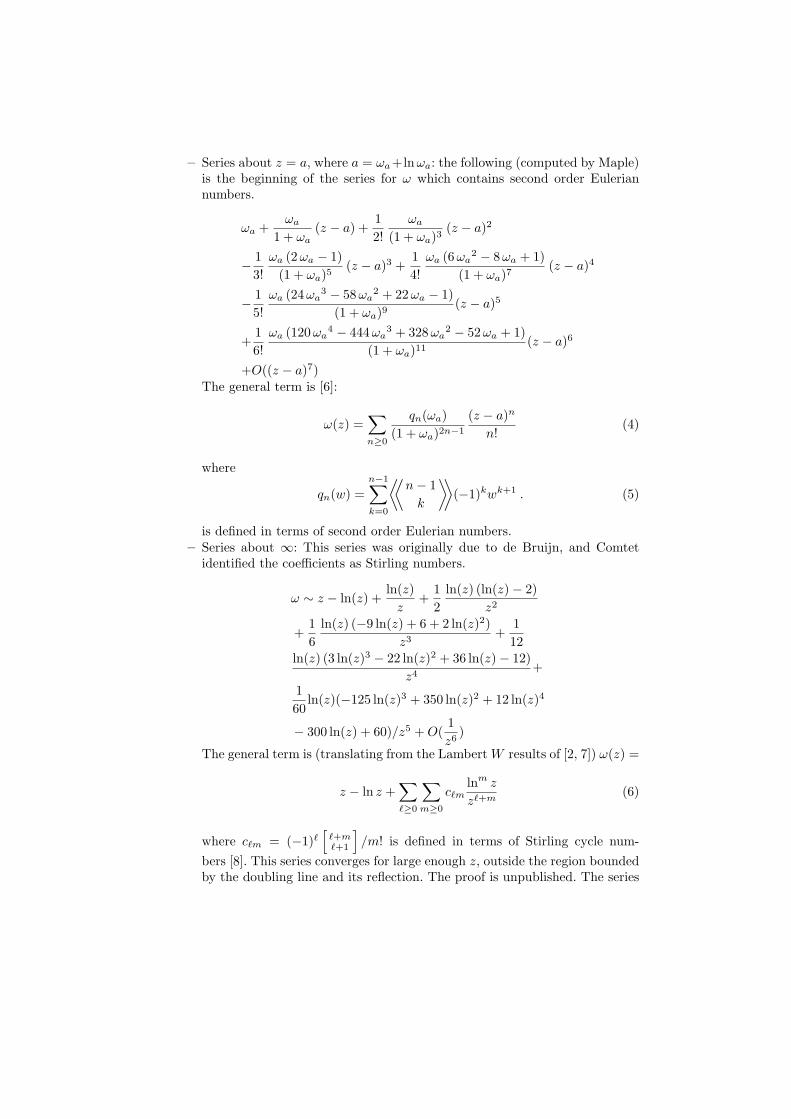
– Series about z = a, where a = ωa+ln ωa: the following (computed by Maple)is the beginning of the series for ω which contains second order Euleriannumbers.

ωa +ωa

1 + ωa(z − a) +

12!

ωa

(1 + ωa)3(z − a)2

− 13!

ωa (2ωa − 1)(1 + ωa)5

(z − a)3 +14!

ωa (6 ωa2 − 8ωa + 1)

(1 + ωa)7(z − a)4

− 15!

ωa (24ωa3 − 58 ωa

2 + 22 ωa − 1)(1 + ωa)9

(z − a)5

+16!

ωa (120ωa4 − 444 ωa

3 + 328 ωa2 − 52 ωa + 1)

(1 + ωa)11(z − a)6

+O((z − a)7)The general term is [6]:

ω(z) =∑

n≥0

qn(ωa)(1 + ωa)2n−1

(z − a)n

n!(4)

where

qn(w) =n−1∑

k=0

⟨⟨n− 1

k

⟩⟩(−1)kwk+1 . (5)

is defined in terms of second order Eulerian numbers.– Series about ∞: This series was originally due to de Bruijn, and Comtet

identified the coefficients as Stirling numbers.

ω ∼ z − ln(z) +ln(z)

z+

12

ln(z) (ln(z)− 2)z2

+16

ln(z) (−9 ln(z) + 6 + 2 ln(z)2)z3

+112

ln(z) (3 ln(z)3 − 22 ln(z)2 + 36 ln(z)− 12)z4

+

160

ln(z)(−125 ln(z)3 + 350 ln(z)2 + 12 ln(z)4

− 300 ln(z) + 60)/z5 + O(1z6

)

The general term is (translating from the Lambert W results of [2, 7]) ω(z) =

z − ln z +∑

`≥0

∑

m≥0

c`mlnm z

z`+m(6)

where c`m = (−1)`[

`+m`+1

]/m! is defined in terms of Stirling cycle num-

bers [8]. This series converges for large enough z, outside the region boundedby the doubling line and its reflection. The proof is unpublished. The series

can be rearranged in several ways, following [9] and [6]: ω(z) =

z − ln z +∑

n≥1

(−1)n

zn

n∑m=1

(−1)m

m!

[n

n−m + 1

]lnm z . (7)

Using a new variable ζ = z/(1 + z), we get ω(z) =

z − ln z +∑

m≥1

lnm z

m!zm

m−1∑p=0

(−1)p+m−1ζp+m

{p + m− 1

p

}

≥2

(8)

where the numbers in curly braces are 2-associated Stirling numbers. UsingLτ = ln(1 − τ) = ln(1 − ln z/z) and η = σ/(1 − τ) = 1/(z(1 − ln z/z)) =1/(z − ln z), series (83) and (84) from [6] become

ω(z) = z − ln z − Lτ

+∑

n≥1

(−η)nn∑

m=1

(−1)m

[n

n−m + 1

]Lm

τ

m!(9)

and

ω(z) = z − ln z − Lτ

+∑

m≥1

1m!

Lmτ ηm

m−1∑p=0

{p + m− 1

p

}

≥2

(−1)p+m−1

(1 + η)p+m.

(10)

The series converge for large enough real z, though the detailed regions ofconvergence are not yet settled. Curiously enough (10) is exact at z = 1 andat z = ∞, and moreover if we truncate it to N terms it agrees with the Nterm Taylor series expansion at z = e as well, making one think of ‘Hermite’interpolation at 1 and at ∞. Convergence is rapid.

– Series about −∞: from the series W (z) =∑

n≥1(−n)n−1zn/n!, for| exp(z)| < exp(−1) we have

ω(z) =∑

n≥1

(−n)n−1

n!enz (11)

2.5 Branch point series for ω(z)

The Wright ω function has branch points at z = −1 ± iπ. The following seriesobtain. Near z = −1 + iπ,

ω(z) = −∑

n≥0

an

(i

√2(z + 1− iπ)

)n

(1)

where the double conjugation gives us the correct closure from below on t + iπfor t ≤ −1. Near z = −1− iπ,

ω(z) = −∑

n≥0

an

(−i

√2(z + 1 + iπ)

)n

. (2)

In both cases an is given by the recurrence relation [10]

a0 = a1 = 1

ak =1

(k + 1)a1

(ak−1 −

k−1∑

i=2

iaiak+1−i

). (3)

The derivation of these series from the results of [10] is straightforward, exceptfor the use of

√z. We here verify that this construction, which is one of a family

of transformations modelled on some used by G.K. Batchelor, gives us the correctclosure. We know that ω(t + iπ−) = W0(−et) whilst ω(t + iπ+) = W1(−et), andω(t − iπ+) = W0(−et) whilst ω(t − iπ−) = W−1(−et). Putting z = t + iπ+ in√

2(z + 1− iπ) gives√

2(t + 1 + i · 0+), for t ≈ −1. If t + 1 ≥ 0 then we haveno branch cut to cross—this series will be continuous, therefore, along the linet+1+iπ, t ≥ −1. If t+1 < 0, we are on the branch cut. t + 1 + i · 0+ is t+1+i·0−,and arg

√2(t + 1 + i · 0−) = −π/2. Therefore arg

√2(t + 1 + i · 0−) = +π/2,

and this means that the series (2) can be written

ω(z) = −∑

n≥0

an(ρ)n

and by inspection of the signs of the series for W−1(−et) and hence W+1(−et)just above the branch cut, this is correct. [Here ρ =

√−2(t + 1) > 0.] Next,

consider z = −1 + iπ−. A similar argument leads to the conclusion

ω(z) = −∑

n≥0

an(−ρ)n

which is the series for W0(−et) for t ≈ −1, because its signs alternate. Consid-eration of z = t− iπ+ and t− iπ− gives, for t + 1 < 0,

ω(z) = −∑n≥0 an(−ρ)n z = t− iπ+

= −∑n≥0 anρn z = t− iπ−

and continuity if t + 1 ≥ 0.

Remark. The use of√

(z − a) to represent a square root function with a closuredifferent from the CCC closure, as explained by Kahan, is a useful tool in acomputer algebra setting. However, it relies on the designers to be sophisticatedenough to provide symbolic means of representing (and not over-simplifying)these series, and the users to be sophisticated enough to know that

√z 6= √

z onthe branch cut.

3 Interpolating Wk(z)

Finally, we interpret equation (3) as an interpolation scheme for Wk(z). We notethat k need not be an integer in that equation; the geometric interpretation isprecisely that of a circular cylinder cutting the Riemann surface for W . Notealso that k = 0 and k = −1 are special, and not interpolated by this scheme.

We deduce that Wk(z) is, in some sense, analytic in k, except if − exp(−1) ≤z < 0 and k = 0 or k = −1.

dWk(z)dk

=d

dkω(ln z + 2πik)

= 2πiω(ln z + 2πik)

1 + ω(ln z + 2πik).

By the analytic properties of ω, this derivative is not continuous on− exp(−1) ≤ z < 0 at k = 0 or k = −1. Otherwise, indeed, Wk(z) is analytic ink.

4 Why

Computer algebra is about expressiveness, and simplicity is power. There are anessentially infinite number of applications of the Lambert W function and itscognates.

1. The Lambert W function provides the first example of a function just outsidethe standard body of Risch-like theory: its derivative is rational in x and W ,not polynomial. One cannot use the same theorems, but one can hope to usesimilar methods, to establish its non-elementarity [1].

2. The Lambert W function is the simplest example of a root of an exponen-tial polynomial; and exponential polynomials are the next simplest class offunctions after polynomials. Computer algebra systems have a real edge overnumerical systems (though not everyone knows it) in dealing with polyno-mials; the next big area will be non-polynomials, starting with exponentialpolynomials. This is the field of Cylindrical Non-Algebraic Decomposition.

3. The Lambert W function is the first nontrivial example of a multivaluedfunction. The trivial ones (ln and the arc trig functions) have branching be-haviour so simple that it doesn’t even need a notation: we can say ln(z)+2πikand not have to invent a new notation lnk(z) to do so (though in fact wehave introduced and used this notation—one can’t use logk because the “logto the base k” interpretation would get in the way—for conciseness andas the thin entering point of the wedge for more complicated functions).The multivalued nature of W “stress tests” naming conventions, numericson branches, computer-aided analysis, and the results of series computa-tion. Right now, Maple knows the series for W0(z) about the branch pointz = − exp(−1), but it doesn’t know the series for W−1(z) or W1(z) about

the same point, even though these series were all introduced in the samepaper [4]. We think that this is because the series are defined piecewise:for W−1 and W1, the series about the branch point have to deal with thefact that the range is split by the branch cut, and so the series are (rad-ically) different if Im(z) > 0 or Im(z) < 0; each branch of W has botha Puiseux series and a Taylor series—about the same point! But differentseries apply above and below the branch cut. This remarkable behaviourputs a significant stress on the ability of series to express its answer to thequestion series(LambertW(-1,x),x=-exp(-1)) (which it currently refusesto answer).

4.1 Why Invent the Wright ω Function?

It is certain that for some applications, just the ordinary Lambert W functionwill be superior—this new function cannot supplant the old. Bill Gosper did notsucceed in introducing his cognate of W (which he jokingly called “the DilbertLambda Function”); Don Knuth has so far been unable to get action on ourpromise to him to introduce the TreeT function into Maple (T (x) = −W (−x),and this is more convenient for combinatorial applications). So why should webother with a new one?

In equation (1) we give the definition of the Wright ω function, in terms ofW and one new function, the unwinding number K(z), which we will be needinganyway. So why not just use the right hand side of the definition and not botherwith a notation?

1. W is multivalued, but ω is single-valued.2. Numerically evaluating ω(z) for large z by way of the definition (1) is like

driving from the south of London to the north of London via Waterloo3:it’s possible (unless there’s freezing rain) but unless you have a reason tobe in Waterloo, it’s probably better to go directly. Less metaphorically, tak-ing exp(z) for large z gives a significant risk of overflow, and a significantrestriction on the numerical range of z that we can do the computation for;but W is like ln, and in some sense just undoes the exponentiation, makingit wasted effort in any case. The asymptotics are that ω(z) ∼ z − ln z + · · ·;so we see just how wasted. This is not a theoretical consideration: Jon Bor-wein has had to implement his version of ω precisely to avoid this overflowdifficulty in his convex optimization problems.

3. Numerically evaluating omega( -0.9 + I*Pi ) by way of the formula un-covers a subtle difficulty: because ceil( (Im(z)-Pi)/(2*Pi) ) will do somesymbolic processing, it will compute K(z) exactly right, and cancel the sym-bolic Pi. But exp(-0.9+I*Pi) is left alone, until the user calls evalf. Thensomething awful happens: at 10 Digits, Pi rounds to something larger than

3 London, Ontario via Waterloo, Ontario, of course. That sentence reads quite differ-ently if you think of train travel in London, England, for example (thanks to ArthurNorman for pointing that out)

π; this then gives us a negative imaginary part on the order of roundoff inthe result of the call to exp. This is all explainable in terms of the Maplemodel of floating-point arithmetic, but it’s a disaster nonetheless—one madevisible by the next step, the computation of W0(x − i · ε), which is on thewrong side of the branch cut. The numerical value of W0(x − i · ε) is notat all close to the value of W0(x + i · ε), and this discontinuity is spurious.The ω function is continuous at this point. So: we should have a separateroutine for the numerical evaluation of ω that guarantees that we get conti-nuity (where ω is continuous), because the definition combines discontinuousfunctions in such a way that their discontinuities (mostly) cancel.

There are other advantages to using the Wright ω function directly.

1. In addition to being single-valued, ω is continuous (indeed analytic) for all znot on the two half-lines z = t ± iπ for t ≤ −1. It is discontinuous acrossthese lines.

2. The Wright ω function has a simpler Taylor series than the Lambert Wfunction does. Indeed, it is the series for the Wright ω function that leads tonearly all the series given in [6].

3. The fabulously simple equation Wk(z) = ω(ln z + 2πik) = ω(lnk z) explainsthe branching behaviour of W perfectly, once we understand the branchingbehaviour of ω.

4. The solution of the equation y + ln y = z is given by

y =

ω(z) z 6= t± iπ, t ≤ −1ω(z), ω(z − 2πi) z = t + iπ, t ≤ −1

nonesuch z = t− iπ, t ≤ −1(12)

The paper [11] seems to be the first to use this fact.

What are the disadvantages? Well, the principal one is that the countingapplications depend on the use of W (or, rather, TreeT) as a generating function.There, the series at the origin is what is important. With this transformation,we have moved this point to −∞. The series are still there—just less convenient.And, that is what introducing this function is all about: convenience. We willneed to have all of these functions around—well, certainly TreeT, but probablynot Dilbert Lambda. Even Bill Gosper has mostly given up on that one.

5 Concluding Remarks

This paper presents a number of mathematical results describing the propertiesof the function ω(z). These results have some intrinsic mathematical interest,and they are written here for the first time, and so in a technical sense the papercontains novel results. However, the results are really interesting only because:

1. Without symbolic computation making the function’s definition, simplifica-tion rules, and numerical evaluation widely available, the function is merelyarcane

2. Discontinuity (along the branch cuts) is especially visible, and nontrivial, inthis function. Therefore it will make a good test case for reasoning aboutcomplex-valued expressions.

3. The methods used to prove properties of ω are essentially old-fashionedmathematics, not commonly seen in standard curricula, and may poten-tially be automated. This is in the spirit of [3] and represents a potentiallyinteresting direction for future research.

Acknowledgements. The code for the numerical evaluation of ω(z) (whichwill be discussed in a future paper) was scrutinized by Dave Hare. The colourgraph of the Riemann Surface for ω (not shown here, but used in the upcom-ing Lambert W poster, was produced with a Maple program written by GeorgeLabahn (getting the colours to come out continuous, while making Maple showthe discontinuity, is not trivial.) Jon Borwein and Bill Gosper provided motiva-tion to look at ω. Our thanks also to Prof. John Wright (Reading & Oxford),and his father Sir Edward Maitland Wright, for permission to use a picture ofSir Edward on the poster of the Lambert W function.

References

[1] Bronstein, M., and Davenport, J. H. Algebraic properties of the Lambert Wfunction.

[2] Comtet, L. Advanced Combinatorics. Reidel, 1974.[3] Corless, R. M., Davenport, J. H., David J. Jeffrey, Litt, G., and Watt,

S. M. Reasoning about the elementary functions of complex analysis. In Pro-ceedings AISC Madrid (2000), vol. 1930 of Lecture Notes in AI, Springer. On-tario Research Centre for Computer Algebra Technical Report TR-00-18, athttp://www.orcca.on.ca/TechReports.

[4] Corless, R. M., Gonnet, G. H., Hare, D. E. G., Jeffrey, D. J., and Knuth,D. E. On the Lambert W function. Advances in Computational Mathematics 5(1996), 329–359.

[5] Corless, R. M., and Jeffrey, D. J. The unwinding number. Sigsam Bulletin30, 2 (June 1996), 28–35.

[6] Corless, R. M., Jeffrey, D. J., and Knuth, D. E. A sequence of seriesfor the Lambert W function. In Proceedings of the ACM ISSAC, Maui (1997),pp. 195–203.

[7] de Bruijn, N. G. Asymptotic Methods in Analysis. North-Holland, 1961.[8] Graham, R. L., Knuth, D. E., and Patashnik, O. Concrete Mathematics.

Addison-Wesley, 1994.[9] Jeffrey, D. J., Hare, D. E. G., and Corless, R. M. “Unwinding the branches

of the Lambert W function”. Mathematical Scientist 21 (1996), 1–7.[10] Marsaglia, G., and Marsaglia, J. C. “A new derivation of Stirling’s approx-

imation to n!”. American Mathematical Monthly 97 (1990), 826–829.[11] Siewert, C. E., and Burniston, E. E. “Exact analytical solutions of zez = a”.

Journal of Mathematical Analysis and Applications 43 (1973), 626–632.[12] Wright, E. M. “Solution of the equation zez = a”. Bull. Amer. Math Soc. 65

(1959), 89–93.