The Wetland Restoration Site Selection Problem Under Wetland

Mitigation Banking (WMB) in Minnesota

Tracy A. Boyer Department of Agricultural Economics, Oklahoma State University

Stillwater, OK 74078 boyert@okstate.edu

May 2003

Paper prepared for presentation at the American Agricultural Economics Association Annual Meeting

Montreal, Canada, July 27-30, 2003

Copyright 2003 by Tracy A. Boyer. All rights reserved. Readers may make verbatim copies of this document for non-commercial purposes by any means, provided that this copyright notice appears all such copies

The Wetland Restoration Site Selection Problem Under Wetland Mitigation

Banking (WMB) in Minnesota

Tracy Boyer

Department of Agricultural Economics, Oklahoma State University

Abstract

A spatial economic model is developed to guide regulatory policy for wetland

compensation under wetland mitigation banking in Minnesota. A binary integer-integer

programming model identifies restoration sites based on their potential for environmental quality

improvement. In contrast to results found in the application of reserve site selection for species

preservation (Ando et al, 1998, Polasky et al, 2001), the unique homogeneity of wetland

restoration sites in Minnesota and the inclusion of restoration costs that exhibit economies of

scale suggest that the private market may function adequately to create large, high quality

habitats for wetland restoration.

1. Introduction

In the last three decades renewed interest in wetlands as unique and useful ecosystems,

rather than disease-ridden swamps, has resulted in a progressive reversal of more than a century

of government policy favoring draining, filling and conversion of wetlands. Over half of the

wetlands in the lower 48 states were drained or filled between the late 1700’s and the mid 1980’s

for agriculture or urban development (Dahl and Johnson, 1989). Wetlands have multiple

important functions and values as habitats for wildlife, means of erosion and flood control,

dissipation of the effects of floods and storms, water filtration from pollutants and agricultural

runoff, recreation, and aesthetic value.

Today, the goal of federal policy is one of “no net loss of wetlands” which has led to a

profusion of regulations and technological innovations to restore and mitigate the loss of

wetlands under the increasing pressures of development. There are two levels of protection for

wetland ecosystems, state and federal regulations. Wetland Mitigation Banking (WMB) is

among the ideas gaining favor among states in order to create a more market oriented policy for

decision-making in wetlands permitting.

The idea of wetlands mitigation banking arose in the 1980’s as a way to ease the burdens

of on-site mitigation and reduce the transaction costs for the developer and the Army Corps of

Engineers (Institute for Water Resources (Army Corps of Engineers), 2000). Wetland banking

mitigation is a scheme by which an agency or developer typically restores a large tract a land to

wetland which is valued by the local or state regulator as a “bank” which holds wetland

compensation credits. In the Midwest, wetland banks, such as those created by the Wetlands

Foundation in Ohio, primarily consist of agricultural land that is restored to its original wetland

1

state by re-establishing water flow and replanting appropriate vegetation. Depending on the

state, the newly restored wetland bank must meet a set of performance guidelines or have been

established for a certain time period before the regulatory agency overseeing the bank assigns

credits based on acreage or a functional assessment of the wetland services. After the regulator

approves the bank, the bank creator may sell credits to another agency or developer or debit

credits for his or her own use for a number of smaller permitted impacts to wetlands elsewhere.

The individual state authority stipulates the minimum compensation ratio and types of wetlands

that are eligible for compensation under the banking program. For example, in Minnesota if a

developer uses credits from a shallow marsh wetland to compensate for the development of a

different type of wetland such as a fen, two acres worth of credits must be purchased for every

acre destroyed. When a developer buys banked credits to mitigate for wetland impacts under a

wetland mitigation banking program, he or she usually must have exhausted the possibilities for

on-site mitigation1 or avoidance of impacts under the Army Corps of Engineers guidelines for

permitting wetland development. After the a developer purchases banked credits for

compensation of wetlands impacts, he or she has no further obligation to care for or ensure the

success of the banked wetlands unless the credits were debited from his or her own bank. Unlike

the sulfur trading program, buyers and sellers of cannot freely trade banked credits for mitigation

since both the supplier and the demander must be permitted by the regulatory agency to enter the

market first.

A study by the Environmental Law Institute estimates that as of December 2001, there

were 219 approved wetland mitigation banks, besides umbrella banks such as the Minnesota

2

1 On site mitigation refers to compensatory mitigation conducted on or adjacent to the site of wetland development. Mitigation banking occurs off-site.

system (Environmental Law Institute, 2002). An additional 46 banks are pending approval.

These numbers represent a 376% increase in the decade since July 1992. Approximately 139,000

acres have been approved as wetland mitigation banks and an additional 8,000 acres are pending

approval. Mitigation banks range in size nationwide from six acres in Virginia to the 23,922-acre

Farmton Mitigation Bank in Florida (Not including Minnesota). The percentage of banks over

100 acres in size has increased from 35% in 1992 to 57% in 2001. Finally, in 2001, mitigation

banks existed in forty states in contrast to only eighteen states in 1992. Wetland bank creators

often are state agencies, private entrepreneurs or non-profit organizations. According to ELI, in

the 1990’s three quarters of WMBs were state or local government sponsored, but now roughly

62% are private commercial enterprises.

Compared to on-site mitigation, WMB is touted as more ecologically and economically

efficient. In theory, WMB banking nationally and in Minnesota assures that functions of drained

wetlands are replaced in kind in the same watershed through the purchase of credits. A

mitigation bank allows the developer to create one large wetland instead of restoring or

mitigating at each site. Ecologically, larger and less fragmented wetlands may provide better

habitat for sustainable ecosystems.2 Mitigation through the purchase of banked credits is also

more likely to be successful than on-site mitigation since the success of the restoration can be

evaluated before the wetland impacts occur elsewhere. Since banked wetlands are created in

advance of impacts, there is no lag between the loss of wetland acreage and replacement

compared to most projects where compensation occurs after impacts on the same site.

Furthermore, on-site mitigation usually consists of created wetlands that may not succeed

32 However, a diversity of sizes and types of wetlands remains important for providing a network of habitats.

ecologically or hydrologically because suitable soil and water conditions cannot be created.

Economically, larger sites for restoration allow developers to exploit economies of scale. King

and Bohlen (1994) estimate that there is a 31% decline in costs per acre for every 10% increase

in project size (Fernandez and Karp, 1998). Second, because of heterogeneous land values, the

purchase of banked credits gives the developer cheaper mitigation options than mitigating on-

site. Furthermore, the transaction costs of the permitting process are lessened for the credit

purchaser since he or she does not need to acquire the scientific expertise and financial resources

to personally mitigate wetland impacts.

In reality, wetlands are hard to build and failure is common. Wetland restoration is

usually more successful than creation because the proper soils and hydrology mechanisms are

already in place or can be repaired. Evidence suggests that certain types of wetlands are better

suited for mitigation than others, i.e., marshlands rather than forested lowlands (Dennison and

Berry, 1993). Furthermore, some wetlands are “valued” more highly than others for recreation,

water filtration, and habitat, etc. Improper design or construction of mitigation sites causes the

greatest number of restoration failures. Three basic issues, hydrology, soils, and vegetation must

be considered when restoring a wetland. However, even in the long term, restored wetlands are

harder to maintain than natural wetlands. Even a “successful” wetland is vulnerable to future

events such as storms, adjacent land uses, and invasion of dominant species such as purple

loosestrife.

Measuring “success” of wetland restoration poses another challenge since measuring loss

and replacement of functions and values is difficult. If we assume that no net loss is the ultimate

goal, then a 1:1 ratio of restored to destroyed original wetland area is unlikely to achieve no net

4

loss in function even if replacement was “in-kind” by type. Across types of wetlands, measuring

tradeoffs between high and low value wetland types is infinitely more difficult. Although the

Board of Water and Soil Resources (BWSR), the bank regulator in Minnesota, has chosen

replacement ratios under its new schemes to favor replacement in-kind and within the watershed,

the science of whether any compensation ratio across wetland types can adequately capture the

trade-offs between functions and values is uncertain. In Minnesota, if the replacement of the

wetland is in-kind, i.e., the same type in the same watershed, the replacement ratio is 1:1 in

regions retaining greater than 80% of their original wetlands or if the impacted wetland is on

agricultural land. The in-kind replacement ratio is 2:1 if the impact occurs in a region with less

than 80% or the impact site is non-agricultural. If the impacted wetland is replaced with a

different type of wetland or in a different watershed (out-of-kind replacement) in a region that

still has greater than 80% of its original wetlands, such as in the Northeast, the replacement to

impact ratio is 1.25:1. Out of kind replacement in areas with less than 80% original wetlands

requires a 2:25 to 1-acre replacement ratio.3 These ratios are based on the acreage of the

impacts, rather than a functional assessment of wetland services. The Minnesota WMB also

does not use any other ecosystem or habitat evaluation procedures to assign a measure of

functional equivalency between impacted wetlands and debited wetland credits.

In states such as California and Florida state conservation agencies determine sites for

restoration in the wetland mitigation banking program through “advanced identification”

(Fernandez, 1999). Only ten states have wetland siting criteria to prioritize according to wetland

5

3 Board of Water and Soil Resources, “Wetland Conservation Act Rules: Chapter 8420.” Temporary amendments adopted at 25 SR 143, effective for two years and expire on July 31, 2002. (2000)

functions and values or planning goals.4 Using advanced identification criteria serves to

designate priority restoration sites within the watershed by assessing potential wetland functions

and values. An advanced identification system can identify the most degraded wetlands for

future development while selecting others for priority restoration. Unfortunately, such

identification necessitates a great deal of public investment. At present, Minnesota does not have

any such system to identify wetlands that are most favorable for restoration, according to Bank

administrator, Bruce Sandstrom. (Sandstrom, personal communication, 2001).

In this paper, the problem of selecting potential wetland restoration sites by advanced

identification in the Minneapolis-St. Paul metropolitan counties is analyzed. Because

management of watershed resources involves a tradeoff between costs and ecological objectives,

different cost curves and spatial outcomes given different planning priorities are examined. Five

different cost curves and spatial outcomes under five policy outcomes are generated under two

different restoration cost assumptions: 1) the private investor’s goal to maximize the number of

acres restored subject to his or her budget, 2) the environmental planner’s goal to maximize the

number of high quality acres given the need to compensate for a target acreage of wetland

development and finally (3-5) the environmental planner’s choice to restore the maximum

number of quality acres at least cost under three different priority weightings to trade off

between nitrogen retention and habitat quality.

In the next section, I briefly review the literature that forms the theoretical basis for the

restoration site selection model used. In Section 3, I describe the derivation of the data used to

characterize potential restoration sites in the twin cities. The cost curves under the five scenarios

6

4 Arkansas, California, Colorado, Florida, Georgia, Indiana, Iowa, Maryland, South Carolina, and Virginia (ELI, 2002).

and illustrative spatial outcomes are given in section 4. Finally, the results are discussed and

future modeling objectives outline in section 5.

2. Literature Review

The “restoration site selection model” originates from the conservation biology literature

aimed at setting aside undeveloped land for species preservation. Multiple methods have been

used to contend with the issue of selecting conservation sites for species, known as the “reserve

site selection problem” in conservation biology. The simplest set-covering model selects the

smallest set of sites in which each species is represented at least once (Underhill, 1994). In the

MCLP, a set of n sites is chosen to maximize the coverage of species (Church et al, 1996a). This

approach implies that acquisition of all sites is equally costly since no budget constraint is

included.

The maximum coverage problem was first formulated as an integer programming

problem by Church and Revelle (1974). The formulation is as follows (Camm et al., 1996):

7

{ }{ }

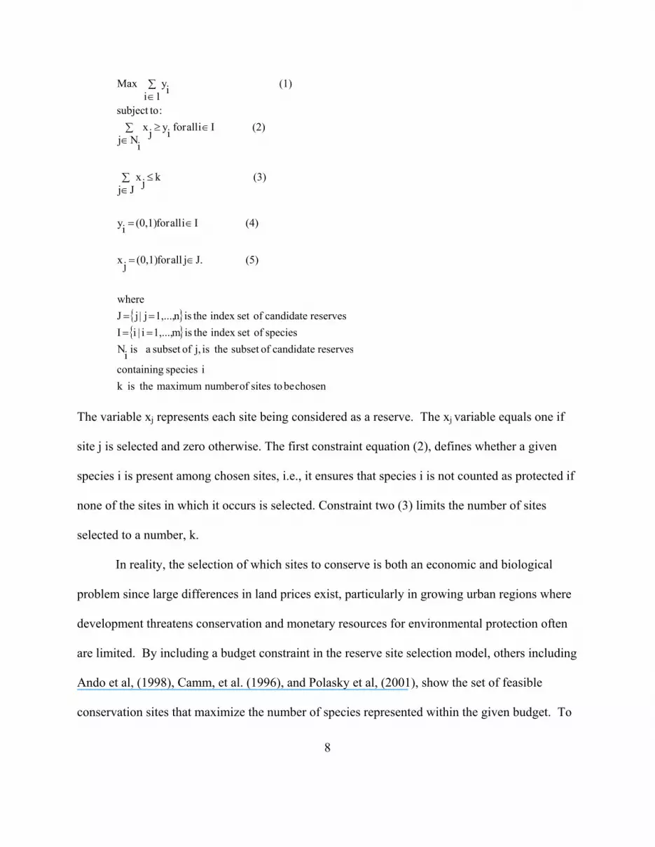
chosenbetositesofnumbermaximumtheiskispeciescontaining

reservescandidateofsubsettheisj,ofsubsetaisiNspeciesofsetindextheism1,...,i|iI

reservescandidateofsetindextheisn1,...,j|jJwhere

(5)J.jallfor(0,1)jx

(4)Iiallfor(0,1)iy

(3)Jj

kjx

iNj(2)Iiallforiyjx

:tosubject1i

(1)iyMax

====

∈=

∈=

∑∈

≤

∑∈

∈≥

∑∈

The variable xj represents each site being considered as a reserve. The xj variable equals one if

site j is selected and zero otherwise. The first constraint equation (2), defines whether a given

species i is present among chosen sites, i.e., it ensures that species i is not counted as protected if

none of the sites in which it occurs is selected. Constraint two (3) limits the number of sites

selected to a number, k.

In reality, the selection of which sites to conserve is both an economic and biological

problem since large differences in land prices exist, particularly in growing urban regions where

development threatens conservation and monetary resources for environmental protection often

are limited. By including a budget constraint in the reserve site selection model, others including

Ando et al, (1998), Camm, et al. (1996), and Polasky et al, (2001), show the set of feasible

conservation sites that maximize the number of species represented within the given budget. To

8

modify the above problem to include the cost of acquiring sites (the budget-constrained MCLP),

the second constraint equation (3) is replaced by a budget constraint wherein each site has a cost

of cj and B is the amount of the entire budget. Thus, equation 3 becomes:

)6(∑∈

≤Jj

jj Bxc

Such a budget-constrained reserve site selection model is applied in Ando et al. (1998)

using information on endangered species and average land value by county for the United States.

They find that the cost of achieving the same number of species preserved was far lower in the

budget constrained than the site constrained approach, i.e., choosing those sites rich with species

first without regard to cost. Polasky et al. (2001), use more detailed data for individual 635 km

cells of land with heterogeneous land values in Oregon. They too find that covering species using

a budget-constrained approach is cheaper than the site-constrained (no budget constraint)

solution by roughly 10% for coverage up to 350 species (Polasky et al, 2001).

The basic MCLP has been modified to include more complexity, such as constraining the

location of sites, weighting site quality (Church et al., 2000), or allowing for varying probability

that vegetation communities will be represented in a reserve network in Superior National Forest

(Haight et al, 2000). Polasky et al (2000) use a probabilistic model to find the reserve network

that represents the greatest number of expected species. The probabilistic approach is compared

to the formulation of the problem where the presence of species is known and given in the

problem. Using data on terrestrial vertebrates in Oregon, significant differences in the chosen

reserve sites are found when the probability of a species on a site approaches zero or one. Using

the same probabilistic data for vertebrate species in Oregon, Arthur, Haight, Montgomery, and

Polasky (2002) compare the expected coverage approach and the threshold approach. While any

9

probability that a species may exist in a site contributes to increasing the objective value of

protecting a species in the expected coverage approach, the threshold approach counts only the

number of species that are most certain to be present. Although these models do not consider

the spatial makeup of selected reserve sites or the probability of species occurrence conditioned

on the existence of the species or another species at another site, the incorporation of uncertainty

of whether a species will be present in a given area lends greater realism to the model as a

potential conservation tool.

This paper uses two environmental quality indicators derived from a GIS mapping of

potential wetland sites to inform economic management of a resource in an interdisciplinary

approach to wetlands economics and policy that is currently lacking in the environmental

economics literature. Historically, the analysis of wetlands in economics has focused on

economic valuation of their use and non-use benefits using hedonic analysis and contingent

valuation (Boyer and Polasky, 2003, Taff and Doss, 1997, Bateman et al, 1995, Oglethorp and

Miliadou, 2000, Earnhardt, 2001). Fernandez and Karp (1998) and Fernandez (1999) have

developed a dynamic optimal control model for characterizing the banker’s revenue

maximization problem, the only rigorous analysis of mitigation banking in the literature. They

find that the entrepreneur’s investment in restoration increases with a reduction in restoration

costs, an increase in biological uncertainty, or an increase in the value of wetlands credits.

Although the article addresses wetland growth under uncertainty, Fernandez and Karp only

examine the effects at one WMB site in California. Using a site selection model with actual data

mapped and characterized in GIS allows me to examine the potential for location bias and loss of

ecological functions under wetland mitigation at a landscape scale when site-specific ecological

10

criteria are imposed under the different policy objectives. In addition, the outcomes in this paper

are generated using two separate restoration cost assumptions of economies of scale, one from

from King and Bohlen (1994) and from the Minnesota Wetland Banking program itself (Boyer,

2003).

3. Wetland Restoration Site Data in Minnesota and Policy Scenario Models

Data on 7,031 potential wetland restoration sites in the seven county metropolitan area of

Minneapolis-St. Paul are analyzed to illustrate the relative cost and spatial makeup of wetland

restoration. The cost of achieving a given level of ecological quality as measured by the sites’

potential for water quality improvement through denitrification and habitat improvement as

measured by minimizing distance to the other potential site is compared. The mapping and

characterization of attributes for the 7,031 potential wetland restoration sites were compiled from

digitized data on hydric soils, the national wetlands inventory, land use, watershed profiles, and

land parcel value (NWI, 1994, Metcouncil, 1997, Metcouncil 2002). I assume that restoration of

former wetlands that have been drained for agriculture and development are superior to created

wetlands since the wetland soil characteristics remain and the hydrology is potentially easier to

restore (Mitsch and Gosselink, 2000). To be considered as a potential wetland site in this study, a

section of land must have been situated on hydric soil indicating that it may have been a former,

drained wetland.5 A site must not be developed, i.e., it must be agricultural or vacant land.

Because the restoration and creation of wetlands under Wetland Mitigation Banking is

irreversible by law after five years in Minnesota, the restoration of a parcel to wetland may be

seen as a form of land retirement. The costs of restoration involve both the cost of land

11

5 Hydric soils are soils that were formed by ponding, saturation, or flooding for long enough periods during the growing season to develop anaerobic conditions in the upper part (Mitsch and Gosselink, 2000).

retirement and the cost of restoration of the parcel to wetland. The cost of acquiring land to

restore as a wetland is assumed to be the opportunity cost or net present value of that land to the

owner. The value of the land lies in its potential to be developed or farmed, a choice, which the

bank creator relinquishes irreversibly by law after the land is restored as a wetland. Therefore,

market price should approximate opportunity cost to the landowner if we assume the market is

perfectly competitive. For each potential wetland site, a weighted average of estimated land

value was derived from parcel values from 2002 tax rolls using the percentage of each site that

overlapped known parcel values (Metcouncil, 2002).

Wetland restoration cost, the second component of cost in a restoration project, varies

widely with the type, size, and location of the wetland project. Because of the heterogeneity of

wetland projects nationally and the lack of available cost data on restoration, few estimates of

restoration costs exist for any type of regulatory scheme. King and Bohlen (King and Bohlen,

1994a) provide the only published cross-sectional estimates of wetland restoration costs for

wetland replacement in the U.S under habitat restoration and traditional mitigation projects. They

found that wetland mitigation costs varied from $5 per acre to $1.5 million per acre (King and

Bohlen, 1994). Although the claim that wetland mitigation banking allows for economies of

scale to be achieved for large restoration projects rather than small on-site projects, no empirical

estimates exist in the literature except for King and Bohlen’s estimates. The second set of

restoration costs used here and based on a mail survey of creators of the Minnesota wetlands

bank are the only estimates that solely look at restoration costs under wetland mitigation banking

(Boyer, 2003). The coefficient and alpha estimate for this functional form derives from the

assumption of a type two wet meadow for which the land was purchased by the bank creator.

12

The multiplier or slope on the estimated equation is $18,582 multiplied times acres restored for

which there is a minimal exponential term or elasticity that allows for restoration cost to increase

per acre with size, i.e., there is a very small marginal cost increase for project acreage. The two

functional forms for restoration costs used are below:

Minnesota Wetland Bank Estimate6

06.0)Acres(582,18CostTotal = King and Bohlen (1994)

64.0)Acres(704,30CostTotal =

Ecological studies and restoration ecology suggests position and setting are important for

achieving environmental quality goals in restoration, but few studies exist. Restoration ecology

strives to predict the specific outcomes of restoration actions. However, the demand for

prediction of restoration success has outstripped scientific knowledge (Zedler, Oct 2000).

Therefore, two indicators of environmental quality, potential for water quality improvement

through nitrogen retention and distance to existing habitat, were chosen as tractable ways to

assess whether a certain wetland would be more likely to succeed and improve the landscape

quality. Although the number of wetlands restored under the WMB in Minnesota yearly would

not significantly contribute to the reduction of non-point pollution, every site could potentially

retain nitrogen to complement other best management practices for curbing nutrient runoff. Soils

type and configurations were used to identify ephemeral wetlands that have higher value to

denitrify runoff as a recharge wetland. The habitat parameter, “distance to the nearest wetland”

was a measure of how close a potential restoration site was from an existing wetland. Restored

136 This estimate assumes a type two wet meadow and purchase of the land by the bank creator.

wetlands in close proximity to existing wetlands theoretically have greater potential for habitat

diversity because of positive spillover effects. Summary statistics for all potential sites are

provided in Table 1 (at the end of the paper).

When sites for restoration may be chosen freely based on cost alone, the expectation

would be that the cheapest lands would be restored first on lower-valued lands in areas on the

urban fringe. In the study area, Scott, Carver, Dakota, and Anoka counties had the highest

percentages of cheaper sites. A 1997 study by Herbert and King found that wetland

compensation through mitigation banking in Florida resulted in trading wetland losses from

urban areas to rural, low-population density areas. Because of high land values, wetland banks

were sited where the costs of land acquisition were lower (King and Herbert, 1997). Because of

the relatively higher cost of potential sites in Ramsey and Washington counties, it is expected

that when costs are considered under the site selection problem, sites in these counties will be

chosen last.

Scenarios

The private investor’s (banker’s) problem is to maximize the area of wetland restored

(i.e., potential credits to be sold) subject to a budget constraint. The dual problem, to minimize

cost of acquiring acres given an acreage constraint, is equivalent. Because no explicit functional

assessment of the restored banked wetland currently exists in order to enroll restored wetlands in

the banking program or to weigh the relative environmental services of wetland credits, the

private investor’s problem represents the status quo in the Minnesota wetland banking program.

With no incentive to invest money into higher cost restoration, the private investor typically

designs the restoration to the minimum standard at the least cost in order to maximize the credits

14

(acreage) to be sold as credits for a profit. The integer programming formulation for the private

investor’s problem is as follows:

Scenario 1: Private Investor’s (Banker’s) Acreage Maximization Problem (PIAM)

{ }

.nrestoratioallforallowedgetbudmaximumbacresinisiteofareaa

)problemingivenasentered,siteofacreageondepends(tcosnrestoratiototalplusisiteacquiringoftcosyopportunittotal,0)a(c

,n,....,1i,notif0,chosenisisiteif1xselectedbetositescandidateofsettheisn,...,1i|iI

where

)8(bx)a(c:tosubject

)7(xaMax

i

ii

i

Iiiii

Iiii

==

≥==

==

≤∑

∑

∈

∈

In the private investor’s problem above, the problem is formulated as one representative

entrepreneurial banker doing all the restoration allowed in the budget since they are assumed to

be homogeneous.

By contrast, the wetland bank administrator, as an environmental planner, is concerned

with replacing impacts to wetlands with the highest quality of banked wetland acres that are

available for sale as credits. In this scenario, the environmental planner explicitly considers the

potential of the site’s location to increase water quality and to improve habitat. First, a wetland

with higher potential to denitrify water because of its shape and retention time is considered

preferred over an alternative site. Second, locating a site near an existing wetland potentially

decreases habitat fragmentation and increases the chances for the re-colonization of the restored

wetland with wetland vegetation, amphibians, and birds. Using the presence of hydric, mineral

15

soils as an indicator of higher potential for water quality improvement, 6,124 potential sites were

rated as high denitrification value (ni equals one, otherwise a site was assigned a zero value). As

a measure of potential reversal of habitat fragmentation and of increased success of species’

recolonization, sites which were located closer to the next nearest existing wetland site were

assigned a proximity index di which was a normalized value of the site’s distance to an existing

wetland compared to the entire set of sites. This index was calculated as follows:

wetlandexistingnearestitsandsettheinsiteonebetweendistanceGreatestDwhere

)9()D(

wetland)existingnearestthetoisiteof(Distance(D)d

,1d0

i

i

=

−=

≤≤

Thus a potential wetland site i, which is adjacent to an existing wetland site, will have a value of

di equal to 1. Any site that is located at some distance up to 2 miles away from its nearest

existing wetland neighbor will have a proportional value on a scale of zero to one.7

First we consider the environmentalist’s objective to maximize the quality-adjusted acres

of restored land in order to reach a target objective of a given number of actual acres (k), the

environmental planner’s problem with no budget constraint (an acreage target). A restored

wetland is potentially of higher quality if it is located on a site of high value for denitrication and

in close proximity to another restoration site. The quality characteristics ni and di are used to

weight the objective function toward the selection of the highest quality sites.

16

7 All but four sites came within 2 miles of a wetland. Except for Blanding’s turtles which can travel several miles between wetlands, most species in Minnesota remain within half a mile of their habitat wetland. The distance of 2 miles was also chosen to enable computation of the distances in ArcView.

Scenario 2:Environmental Planner’s Problem (No Budget Constraint) (EPNBC)

{ }

distant.mosttheif0

adjacent,1,.wetlandexistingfromdistancerelativeofindexdacresactualrestoredforleveltargetk

not.if0ation,denitrificforpotentialhighhassitetheif1n|nacresinisiteofareaa

,n,....,1i,notif0,chosenisisiteif1xselectedbetositescandidateofsettheisn,...,1i|iI

where

)11(kxa.t.s

)10()xadxan(Max

i

ii

i

i

Iiii

Iiiiiiii

=

=

====

≤

+

∑

∑

∈

∈

The environmental planner’s non-budget-constrained problem can be viewed as the equivalent of

picking the highest quality sites first regardless of cost. In a policy setting, this might occur if

the agency that administered the bank permitting process identified sites in advance with an

actual acreage target for wetland acreage restoration and required that bankers restore the highest

quality sites first.

As discussed in the similar problem of the species reserve site selection model, we are

concerned with the budgetary consequences of maximizing the potential environmental quality

of acres restored. Note that although the environmental planner in scenario 2 uses an acreage

target as a constraint rather than a budget constraint, in reality every agency will have an upper

bound on budget. Scenario 2 shows a targeting mechanism for identifying sites that has no

budget constraint in the formulation of the problem. In the environmental planner’s problem,

the objective is to maximize the quality weighted acres of chosen sites subject to a given budget

constraint. In contrast to the previous scenario, the environmental planner that possesses an 17

understanding of economic optimization approaches the identification of restoration sites by

explicitly considering the agency budget. The environmental planner thus wants to restore as

much quality wetland acreage as possible, but would like to achieve that quality at the least cost

since public funds are often limited.

Scenarios 3-5: Environmental Planner’s Budget-constrained Problem (EPBC)

{ }

.acresallrestoringforallowedbudgetimummaxtheis0btcosnrestoratiototalplusisiteacquiringoftcosyopportunittotal,0)a(c

1pp1p0,1p0,lyrespective,habitatandretentionnitrogenforweightpriorityp,p

distant.mosttheif0adjacent,1,.wetlandexistingfromdistancerelativeofindexd.notif0,ationdenitrificforpotentialhighhassitetheif1n|n

acresinisiteofareaa,n,....,1i,notif0,chosenisisiteif1x

selectedbetositescandidateofsettheisn,...,1i|iIwhere

)13(bx)a(c.t.s

)12()xadpxanp(Max

ii

hn

hnhn

i

ii

i

i

Iiiii

Iiiii

hiii

n

>≥

=+

≤≤≤≤

==

====

≤

+

∑

∑

∈

∈

For the Environmental Planner’s budget-constrained problem, 3 policy weightings were

analyzed to show equal weighting of the nitrogen objectives (pn=.5 and ph=.5), priority for the

nitrogen only (pn=1, ph=0) and priority for habitat by valuing proximity to existing wetlands only

(pn=0, ph=1). The weights on the two quality criteria allow for differences in the environmental

planner’s preferences. For example, should the Board of Water and Soil Resources be solely

concerned with improving water quality, it would weight ph equal to one and pn equal to zero.

However, an ecologist might weight the preferences in the opposite direction. These two

extremes are tested to see if significant differences in cost between the multiple objectives

18

existed. Sensitivity to the form of the cost function was tested by running the scenarios under

two different restoration cost estimates, those of King and Bohlen and the Minnesota Wetland

Mitigation Banking. The five scenarios were solved using branch and bound mixed integer

programming in GAMS 20.7.11, OSL Solver (2000).

4. Results

The five maximization problems facing the private investor, the quality-adjusted acreage

optimizing environmental planner with no budget constraint, and the policy-weighted scenarios

for the budget-constrained environmental planner are presented. The five scenarios were solved

using a range of constraints on the budget for the banker and environmental planner problems

and on acreage for the environmentalist’s problem. All 5 scenarios were run twice using King

and Bohlen’s estimate of restoration costs (K-B estimate) and the estimate of restoration costs

under the wetland mitigation banking program in Minnesota (WMB estimate).8 The results of

the solutions to the five problems are summarized in Figures 1 and 2, which plot the 5 cost

curves under the different scenarios and two functional forms for restoration costs, the King-

Bohlen estimate and the WMB estimate respectively. The total number of quality-adjusted acres

restored is measured on the horizontal axis (quality-adjusted acreage =∑∈

+Ii

iiiiii )xadxan( ) at

each solution under a given budget constraint. The solutions for the private investor’s scenario

were converted to the quality-adjusted acre scale by calculating the number of quality acres

represented by the sites contained in the solution to the banker’s problem under the complete

19

8 The environmental planner’s budget-constrained problem was also run using only the land costs without restoration costs to test how the economies of scale in cost assumption affected the spatial pattern of solutions.

range of possible budget constraints. The total dollar cost of reaching a given level of quality-

weighted acreage restored is measured on the y-axis in 2002 dollars

The cost curves depicted in Figures 1 and 2 show that any given level of quality-weighted

acres is cheaper under the budget-constrained approaches than under the environmental planner’s

acreage target scenario without a budget constraint. To restore roughly 800 quality adjusted

acres using the K-B estimates under the environmental planner’s quality acreage maximization

problem without a budget constraint is $5.7 million dollars as compared to roughly $2.4 million

under the budget constrained quality maximization approach, two and a third times more

expensive. The environmental planner’s budget-constrained problem at 799 quality-adjusted

acres is 42% of the cost of acquiring the same level of quality under the EP acreage non-budget-

constrained problem. In fact, at that quality level, all four budget-constrained approaches using

the K-B restoration costs, including the private investor, choose the same three sites at the 799

quality-adjusted level.9

Under the WMB estimate for restoration costs, the budget-constrained environmental

planner also achieves roughly 800 acres at one quarter of the cost of the environmental planner

with an acreage constraint. In the WMB case, however, the budget-constrained environmental

planner (EPBC) is able to achieve the same quality level for 19% less expense than the private

investor or habitat maximizing scenarios (See Table 2).

The substantial gap between the costs of the area-constrained versus the budget-

constrained environmental planner’s problems shows that restoring quality lands without regard

to cost to reach a given target of restored actual acres will more rapidly deplete any restoration

20

9 Each point on the cost curve depicts an integer solution at a given budget or acreage constraint. Many of these sites are within 10% of the optimal LP non-integer solution. Roughly 25% of the solutions are optimal, meaning they lie directly on the budget constraint and coincide with the LP solution.

budget. For example, if the willingness to pay for restoration in the year were $5.7 million and

the environmental planner (EP) had two restoration scenarios to maximize quality acreage under

the area vs. budget-constrained scenarios, the amount of acreage obtained and the spatial

outcome would be drastically different. To clarify, note that the scenario is used to choose the

advanced identification of sites to be restored, and then credits are sold (theoretically) in a

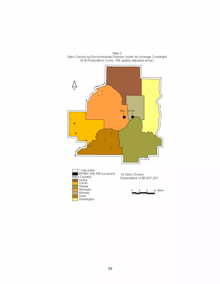
competitive market according to the cost of restoration. In Map 2, the environmental planner

who identifies sites without regard to budget chooses 18 sites and achieves 798 quality-adjusted

acres. 10 In Map 5, the environmental planner who optimally chooses high quality sites at the

least cost at the same $5.7 million budget level, restores 4 sites and attains 1,865 quality-adjusted

acres. First, the budget-constrained planner achieves almost 2.3 times the level of quality acres.

Secondly, because of the economies of scale built into the King Bohlen cost estimates, the four

sites chosen are massive and clumped in the outer fringe. The average site size for the budget-

constrained planner is 309 acres (excluding the fourth 3.8-acre site that ensures an optimal

solution) and all three large sites lie in either Dakota or Carver County on the urban fringe.

2110 Note that in the Maps 5.1, smaller sites chosen may not be visible at the scale presented.

22

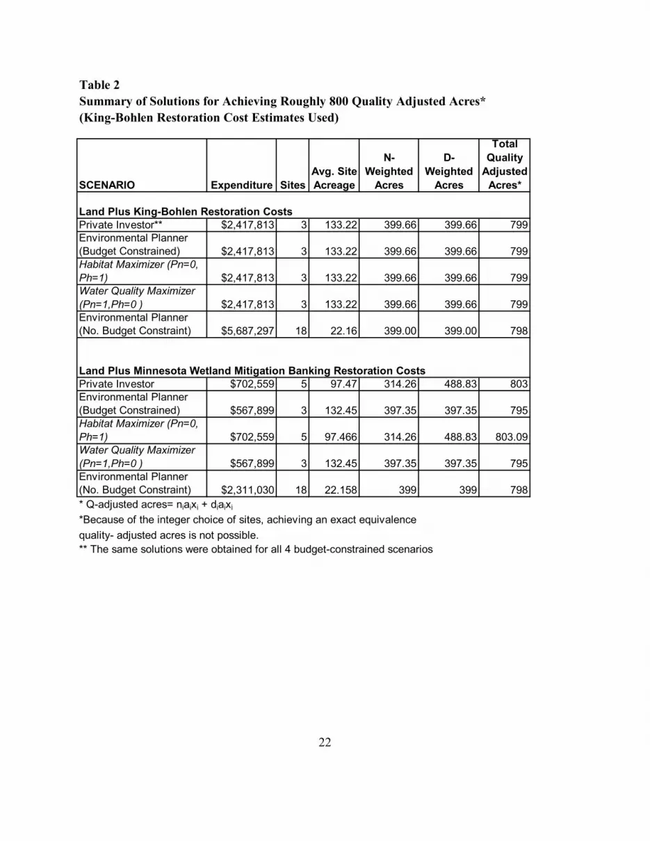
Table 2Summary of Solutions for Achieving Roughly 800 Quality Adjusted Acres* (King-Bohlen Restoration Cost Estimates Used)

SCENARIO Expenditure SitesAvg. Site Acreage

N-Weighted

Acres

D-Weighted

Acres

Total Quality

Adjusted Acres*

Private Investor** $2,417,813 3 133.22 399.66 399.66 799Environmental Planner (Budget Constrained) $2,417,813 3 133.22 399.66 399.66 799Habitat Maximizer (Pn=0, Ph=1) $2,417,813 3 133.22 399.66 399.66 799Water Quality Maximizer (Pn=1,Ph=0 ) $2,417,813 3 133.22 399.66 399.66 799Environmental Planner (No. Budget Constraint) $5,687,297 18 22.16 399.00 399.00 798

Private Investor $702,559 5 97.47 314.26 488.83 803Environmental Planner (Budget Constrained) $567,899 3 132.45 397.35 397.35 795Habitat Maximizer (Pn=0, Ph=1) $702,559 5 97.466 314.26 488.83 803.09Water Quality Maximizer (Pn=1,Ph=0 ) $567,899 3 132.45 397.35 397.35 795Environmental Planner (No. Budget Constraint) $2,311,030 18 22.158 399 399 798* Q-adjusted acres= niaixi + diaixi

quality- adjusted acres is not possible. ** The same solutions were obtained for all 4 budget-constrained scenarios

*Because of the integer choice of sites, achieving an exact equivalence

Land Plus King-Bohlen Restoration Costs

Land Plus Minnesota Wetland Mitigation Banking Restoration Costs

Clearly the assumption of economies of size in restoration results in the choice of larger

sites that are cheaper per quality acre than choosing many smaller sites. In Map 6, the three sites

selected by the environmental planner at 794 quality-adjusted acres using the WMB restoration

cost estimates are shown. Under the WMB costs, two large sites of 121 and 246 acres each and

one 9-acre site are chosen. As in the case with the KB estimates, several large sites are chosen

when restoration costs exhibiting economies of size are included in the cost of the wetland bank

or site than if the decision were based on land costs alone. The two large sites are held in

common between the two budget-constrained EP scenarios for the KB and WMB estimates at

roughly 800 quality-adjusted acres. None of the sites chosen by the “naïve” environmental

planner who does not use a budget constraint are held in common with the budget-constrained

environmental planner scenarios that included restoration costs at the 800 quality-adjusted

acreage level.

Figure 3 shows a detail of the cost curve under the two King-Bohlen cost assumptions,

illustrates that if a given level of quality restoration is desired, the environmental planner is able

to achieve that level at the same or lower cost than the private investor who does not consider

quality in the selection of acres to restore. The lack of a distinct difference in costs among the

budget-constrained approaches is not surprising because of the high number of choices among

the sites and the high incidence of cheaper sites in the outlying counties. Interestingly in the

detail of the K-B cost curve scenario in Figure 3, except for small segments, there is little or no

difference between the costs of the different budget –constrained solutions. Where the cost

curves do diverge, the private investor and habitat maximizing scenarios lie above those of the

23

multi-objective environmental planner and the water quality maximizer. Table 2 provides a

summary of the sites selected under the five scenarios when the King and Bohlen cost restoration

costs are used.

Above the level of two hundred thousand quality-adjusted acres, Figures 1 and 2 show

that the slope of the cost curves for all of the budget-constrained scenarios (1 and 3-5) increase

dramatically. At the level of roughly 181,000 quality-adjusted acres you can achieve 80% of the

total acreage to be restored at 34% of the entire cost of restoring all available acres if you

consider land costs only under the environmental planner’s budget-constrained maximization

problem (See Table 3). However, when economies of size in restoration costs are considered, the

savings bang for the buck in restoration is diminished Because the wetland mitigation banking

restoration costs an extremely low, the marginal increase in cost of restoring a wetland site which

increases in size (alpha=.06), the environmental planner’s budget-constrained scenario attains

80% of the available acreage at 28.8% of the cost. Using King and Bohlen’s restoration cost

estimates, which assume a higher increasing cost with acreage, the same area percentage costs

49.6% of the expense of restoring all available acres.

Table 3Relative Site Acquisition Among Cost Scenarios for the Budget-ConstrainedEnvironmental Planner

Land Plus King-Bohlen Restoration Costs

Land Plus WMB Restoration Costs

Land Costs Only

Percentage of Total Acreage Acquired 79.0% 80.0% 80.0%Percentage of Total Cost for Acquiring All Sites 49.6% 28.8% 34.0%Quality Acreage Level for Calculations 179,037 180,502 181,669

24

This hockey-stick shape of the cost curve in the budget-constrained environmental

planner’s scenario is a result of the cheapest high quality sites being chosen first. In the cost

curve using the K-B land plus restoration cost estimates, the marginal cost of acquiring

additional sites is higher in most cases than the curve generated using the WMB restoration cost

estimates. For example, at roughly 145 thousand acres, the King-Bohlen curve has a slope of

8.48 whereas the WMB scenario has a slope of 3.54 (Refer to Figure 4 for a comparison of the

two cost scenarios for the budget-constrained environmental planner). As the budget increases,

the marginal cost of an additional site rises substantially for many of the sites in Hennepin,

Washington, and Ramsey County. For instance, several wetland sites in Hennepin County,

valued at over 1 million dollars per acre, are located on highly prized lakeside residences on

Lake Minnetonka. The finding that 80% of the restoration can be achieved at 28% of the cost

(shown in Table 3) suggests that the policy maker could achieve the vast majority of restoration

relatively cheaply as long as the unlikely goal of complete restoration is not pursued under the

current system. However, as shown by the results under the King-Bohlen restoration costs, these

savings might not be as dramatic if restoration costs rise more sharply as site size increases, i.e.,

as in the King-Bohlen estimates. Furthermore, the functional form of the WMB and KB

restoration costs assumes that wetland project costs only vary by acreage, not type, meaning the

assumption of homogeneity may smooth out differences between land prices for parcels. When

restoration costs comprise a larger portion of the cost of returning a parcel to wetland as in the

King and Bohlen scenarios, the savings from heterogeneous land prices are diluted by the

assumption of large, increasing, and homogenous restoration costs.

25

The assumption of economies of size in restoration cost results in the selection of several

large sites on the fringe of the metro area. When King and Bohlen’s economies of size estimates

are used, the solutions between the four budget-constrained scenarios are highly coincident, if

not identical at any level. For example, Map 3 shows the solutions for the budget-constrained

solutions at 799 quality-adjusted acres. The average site size is 133 acres. In contrast, Map 2

shows the sites representing 800 quality acres when restoration costs are ignored. If the

environmental planner were to maximize quality considering land costs only to achieve roughly

the same quality level at 800 quality-adjusted acres, she would acquire 29 sites for $310,000 with

an average size of 13.79 acres in six counties excluding Ramsey county (Map 4). Thirteen of the

29 sites chosen in this scenario lie in Carver County where sites are cheaper.

5. Concluding Remarks and Future Directions

Although the number of wetlands restored under the WMB in Minnesota yearly would

not significantly contribute to non-point pollution reduction or other environmental goals, every

restoration banking site could potentially serve as a compliment to other best management

practices for improving water quality and maintaining connectivity of habitats in the landscape.

This research shows that the identification of potential restoration sites for wetland mitigation

banking is possible at a landscape level. Using ordinary least squares estimation of restoration

costs and combining that information with an integer programming site selection mechanism

illustrates that the assumption of economies of size is important in the cost and spatial make-up

of restoration sites.

26

By using actual data on land prices under two different assumptions of economies of

scale in restoration costs, the model shows that even when land costs comprise half of the total

cost of restoring a site, economies of scale will bias the selection toward the selection of a few

large sites. The estimated functional forms for both cost equations results in a lower per acre cost

of restoration for larger sites. The cost of acquiring all the land for all 7,031 sites represents 51%

and 87% of the total cost of acquiring and restoring all sites under the King and Bohlen and

Minnesota Wetland Bank estimates respectively. Even when the cost of restoration comprised

less than half of the total cost of acquiring a site under WMB, several large sites were selected

rather than many small sites. Since many of the larger sites are located on relatively cheap vacant

or agricultural land in Carver and Dakota counties on the urban fringe, these large sites provide a

double benefit of cheap restoration and acquisition per acre.

The inclusion of restoration costs in the wetland restoration site selection model and the

multiplicity of high quality sites in the twin cities landscape diminishes the dramatic cost savings

shown under budget-constrained approaches in the species site selection problem (Ando et al,

1998). Although the budget-constrained environmental planner is able to achieve 80% of the

total possible restoration acreage at 28% of the cost of restoring all the potential wetland acreage

available under mitigation banking, that ratio becomes less favorable as costs rise per acre.

Despite economies of scale, under the King-Bohlen restoration estimate plus land costs, the

planner achieves roughly the same portion of restoration at roughly half the cost of restoring

everything since the marginal cost of acquiring quality acres rises more steeply than under the

WMB estimates. Although the inclusion of restoration costs diminishes the dramatic savings

from the budget-constrained environmental planners approach, the results still refute using a

27

naïve approach with targets acreage without regard to cost. The environmental planner who

chooses restoration sites with full information will always achieve any given quality level at

lowest cost. In comparison to the naïve environmental planner, he or she will achieve those

quality levels more cheaply on several orders of magnitude.

Assuming the estimates of the economies of scale generally hold true despite differences

in wetland projects, the results from the metro area show that any budget-constrained approach

will result in high-quality, large restoration sites. Among the scenarios of whether to let private

investor’s choose freely or whether to target certain quality characteristics, relatively small

differences in cost and spatial outcomes were found. The homogeneity of site quality and

coincidence of simultaneously high quality and low budget sites in the Twin Cities area suggests

that perhaps over regulating the private investor’s choice bank location is unnecessary.

However, these results depend on the two quality indicators chosen, nitrogen retention potential

and distance to existing wetland. Adding in preferences for wetlands in urban centers or next to

complementary land uses might dramatically alter the results in the future. Since the Twin Cities

is both wetland rich and contains a majority of higher denitrifying wetlands, the environmental

planner may not need to dictate the identification of sites unless certain dispersal goals are

desired. For instance, since larger sites are naturally chosen, a planner may want to place limits

on the proportion of large banks created in the system to reduce monopoly power of credits sales

or to ensure a more diverse wetland landscape. Without additional constraints, the assumption of

economies of scale in restoration sites naturally results in large-habitat restorations.

The results demonstrate that under any budget-constrained approach when restoration

costs exhibit economies of scale, large sites are chosen without the addition of additional

28

constraints or targets in comparison to taking a best-quality sites-first approach. These simple

models suggest that if advanced identification is pursued as a policy to improve on private

incentives to locate wetland banks freely where they are easiest to restore, a budget-constrained

approach will produce more cost-efficient outcomes than a naïve ranking approach.

Furthermore, the relative cost of achieving restoration after the cheapest lands have been restored

is prohibitively expensive, placing a potential choke price on permitted development of wetlands

with no on-site mitigation options.

There are many factors that are important in wetlands restoration site selection such as

the habitat suitability for species, the probability of successful hydrological and vegetative

restoration, the potential for water quality improvement through denitrification, and the diversity

of wetlands in the entire landscape. Currently, the connections between restoration ecology and

environmental outcomes are not clear enough in the science. In addition, data on characterizing

restoration sites at a landscape level is not readily available at the scale or detail needed. Future

data would include physical characteristics such as slope of the land, pollutant loadings, the

effect of adjacent land use, the probability of restoration success for certain species, and the type

of wetland vegetation and hydrology to be restored, among others. Furthermore, inadequate

information is collected on the costs of restoration that tie those costs to relative success in

restoring wetland functions.

Future versions of this model ideally will include preferences for adjacent site selection

to allow for greater ecological sensitivity of the restoration site selection model and policy

relevance to changes in WMB regulation. The analysis could also explore how changing the

probability of successful restoration and institutional rules, such as trading ratios and inter-

29

watershed trading constraints affect the spatial arrangement, cost, amount, and quality of

restoration. However, because it is difficult to achieve optimality when more specific constraints

are imposed, future research should look at ways around the binary choice of a site when partial

selection of sites is feasible ecologically. Because of the exponential growth of potential

solutions to the binary integer site selection model, the addition of constraints makes

computation of optimality practically infeasible. Furthermore, heuristic mechanisms which do

not emphasize optimality might allow for dynamic selection of sites over time, creating the

possibility for updating information about past restoration success and land use change in the

vicinity of potential sites.

30

31

Table 1: Summary Statistics for Potential Wetland Restoration Sites in the Minneapolis-St. Paul Metropolitan Area

County ANOKA CARVER DAKOTA HENNEPIN RAMSEY SCOTT WASHINGTON All 7 Counties

SITES 1,014 1,935 792 1,273 126 1,345 546 7,031

ACREAGEAverage 17.46 18.27 23.51 13.43 4.79 18.08 12.60 17.15Total 17,702 35,360 18,620 17,101 604 24,324 6,880 120,590Minimum 1.09 0.46 0.59 0.96 2.01 0.56 2.00 0.46Maximum 704 339 611 302 46 639 558 704St. Deviation 39.81 27.57 53.33 21.13 4.83 34.25 27.95 34

Yards to Nearest Existing WetlandAverage 11.01 33.62 101.23 8.35 17.69 53.41 13.68 35.20Minimum 0 0 0 0 0 0 0 0Maximum 678.73 767.76 2469.09 257.50 610.36 1137.73 729.05 2464.00

High N ValueNumber 843 1,595 773 1,240 79 1,121 473 6,124

Continued on Next Page

County ANOKA CARVER DAKOTA HENNEPIN RAMSEY SCOTT WASHINGTON All 7 CountiesLAND VALUE/ACREAverage $15,694 $6,909 $14,691 $30,835 $48,119 $7,476 $24,629 $15,607Minimum $622 $305 $706 $534 $3,553 $732 $584 $305Maximum $440,618 $494,505 $301,293 $1,012,349 $257,000 $553,571 $600,056 $1,012,349St. Deviation $28,895 $21,356 $30,684 $66,274 $41,397 $22,687 $53,818 $40,008

TOTAL VALUE/SITE (King/Bohlen Estimates)*Average $388,240 $256,024 $367,022 $436,931 $304,746 $280,231 $343,096 $332,615County Total $393,675,311 $495,405,776 $290,681,528 $556,213,517 $38,398,048 $376,911,250 $187,330,503 $2,338,615,933Minimum $34,432 $19,467 $24,165 $38,394 $57,254 $22,317 $52,119 $19,467Maximum $23,846,416 $6,042,654 $9,637,461 $20,691,750 $2,867,627 $4,551,249 $8,125,300 $23,846,416St. Deviation $961,988 $302,108 $615,440 $1,003,998 $355,141 $341,858 $515,884 $658,328

TOTAL VALUE/SITE (Mn Wetland Banking)**Average $248,689 $105,881 $199,448 $314,945 $247,812 $131,936 $228,478 $191,916County Total $252,170,379 $204,879,438 $157,962,872 $400,924,485 $31,224,366 $177,453,547 $124,748,902 $1,349,363,989Minimum $22,397 $20,031 $22,065 $21,631 $28,997 $20,831 $23,087 $20,031Maximum $22,740,877 $5,578,068 $7,803,156 $19,533,907 $2,538,871 $3,013,289 $7,903,202 $22,740,877St. Deviation $874,412 $234,324 $477,106 $953,453 $325,830 $236,747 $463,191 $592,211

* Total Value includes land value plus the cost of restoration using King and Bohlen's (1994) estimate using Tcost of restoration=30,704(Acres)^0.64**Total value includes land value plus restoration cost from the survey of Minnesota's Wetland Mitigation Banks (Total Cost Rest.=$18,582(Acres)^0.06)

32

33

Figure 1 Cost Curves for 5 Scenarios

(Under King-Bohlen Restoration Costs)

0

500,000

1,000,000

1,500,000

2,000,000

2,500,000

0 50,000 100,000 150,000 200,000 250,000

Quality-Adjusted Acres

Expe

nditu

re (1

000'

s of

Dol

lars

)

S1:Priv. Inv (K-B)S2:Env.Plan (NBC/K-B)S3:Env.Plan (BC/K-B)S4: Habitat (King)S5: Nitrogen (King)

34

Figure 2Cost Curves for 5 Scenarios

Under Land plus Minnesota Wetland Banking Restoration Costs

0

200,000

400,000

600,000

800,000

1,000,000

1,200,000

1,400,000

1,600,000

0 50,000 100,000 150,000 200,000 250,000Quality-Adjusted Acres

Expe

nditu

re (1

000s

of D

olla

rs)

S1: Priv.Inv. (WMB)S2:Env.Plan(NBC/WMB)S3:Env.Plan (BC/WMB)S4:N.Retention(WMB)S5:Habitat(WMB)

35

Figure 3 Detail of Budget-Constrained Cost Curves (K-B Restoration Costs)

0

1,000

2,000

3,000

4,000

5,000

6,000

0 200 400 600 800 1,000 1,200 1,400 1,600 1,800

Quality-Adjusted Acres

Expe

nditu

re (1

000s

of D

olla

rs)

S1:Priv. Inv (K-B)S3:Env.Plan (BC/K-B)S4: Habitat (King)S5: Nitrogen (King)

36

Figure 4: Environmental Planner's Budget-Constrained Problem Under KB and WMB Restoration Cost Estimates

0

500000

1000000

1500000

2000000

2500000

0 50000 100000 150000 200000 250000

Quality-Adjusted Acres

Expe

nditu

re (1

000s

of D

olla

rs)

K-B Environmental PlannerMN WMB Environmental Planner

37

38

39

40

41

42

43

References

Ando, A., J. Camm, S. Polasky, and A. Solow. "Species Distributions, Land Values, and Efficient Conservation." Science. 279(1998):21-26.

Board of Water and Soil Resources. “Minnesota Wetland Report 1999/2000.” St. Paul, MN. (2000).

Boyer, Tracy A., The Wetland Mitigation Banking Credit market in Minnesota: A spatial economic analysis of its potential to achieve regulatory and ecological goals. Ph.D. Thesis, University of Minnesota (2003).

Boyer, Tracy and Stephen Polasky, “Valuing Urban Wetlands.” Forthcoming 2003 in Wetlands.

Camm, J.D., S. Polasky, A. Solow, and B. Csuti. "A Note on Optimal Algorithms for Reserve Site Selection." Biological Conservation. 78(1996):353-355.

Camm, J.D., Susan K. Norman, Stephen Polasky, and Andrew R. Solow. "Nature Reserve Site Selection to Maximize Expected Species Covered." Operations Research. (2003).

Church, R., D. Stoms, and F. Davis. "Reserve Selection as a Maximal Covering Problem." Biological Conservation. 76 (1996):105-112.

Church, R., R. Gerrard, A. Hollander, and D. Stoms. "Understanding the Tradeoffs Between Site Quality and Species Presence in Reserve Site Selection." Forest Science. 46 (2000):157-167.

Church, R.L. and C.S. Revelle. “The Maximal Covering Location Problem.” Papers of the Regional Science Association. 32(1974):101-108.

Cowardin, Lewis M. Classification of Wetlands and Deepwater Habitats of the United

States. Washington, D.C. Fish and Wildlife Service, Office of Biological Services, U.S. Dept of Interior. (1979).

Dahl, T.E. and C.E. Johnson. Status and Trends of Wetlands in the Coterminous United States, Mid-1970's-Mid-1980's. Washington, D.C.: U.S. Department of the Interior, Fish, and Wildlife Service, (1991).

Dennison, M.S. and J.F. Berry. Wetlands: Guide to Science, Law, and Technology. Park Ridge, N.J., U.S.A: Noyes Publications, (1993).

Environmental Law Institute. Banks and Fees: The Status of Off-Site Wetland Mitigation in the United States. Washington, D.C., Environmental Law Institute. (2002).

44

Fernandez, L. "An Analysis of Economic Incentives in Wetlands Policies Addressing Biodiversity." The Science of the Total Environment. 240(1999):107-22.

Fernandez, L. and L. Karp. "Restoring Wetlands Through Wetlands Mitigation Banks." Environmental and Resource Economics. 12(1998):323-44.

Haight, R.G., C.R. Revelle, and S. Snyder. "An Integer Optimization Approach to a Probabilistic Reserve Site Selection Problem." Operations Research. 48(2000):697-708.

Institute for Water Resources (Army Corps of Engineers). “Existing Wetland Mitigation Bank Inventory.” Available at URL:www.wrsc.usace.army.mil/iwr . (2000). Accessed March 2001.

King, D. and C. Bohlen. "Estimating the Costs of Restoration." Wetlands Newsletter. 16(1994):3-8.

King, Dennis M. and Bohlen, Curtis C. “A Technical Summary of Wetland Restoration Costs in the Continental United States.” Solomons, Maryland, University of Maryland, CEES. (1994).

King, Dennis M. and Bohlen, Curtis C. “Making Sense of Restoration Costs.” Solomons, Maryland, University of Maryland, CEES. (1994).

Lehtinen, R.M. and S.M. Galatowitsch. “Colonization of Restored Wetlands by

Amphibians in Minnesota.” American Midland Naturalist. 145 (2001): 388-395.

Lehtinen, R.M., S.M. Galatowitsch, and J.R. Tester. "Consequences of Habitat Loss and Fragmentation for Wetland Amphibian Assemblages." Wetlands. 19(1999):1-12.

MetroGIS. 1977,72. Digital Soil Surveys for Anoka and Ramsey. Content digitized from

NRCS mylar maps. Obtained from: http://www.datafinder.org. Metropolitan Area, ArcView Polygon Coverage. Content date 04/14/1997.

Metropolitan Council. 1997. Generalized Land Use 1997 for the Twin Cities. Metropolitan Council. 2002. Regional Parcel Data Set—Academic Version. ArcView

Polygon Coverage of Hennepin, Anoka, Carver, Dakota, Washington, Scott, and Ramsey Counties. Content date: 4/30/2002.

Minnesota Dept. of Natural Resource (MNDNR). “Minnesota Wetland Mitigation

Banking Study” March 1998. Addendum to Minnesota Wetlands Conservation Plan, Version 1.0, and in fulfillment of Minnesota Laws 1996, Chapter 462, Section 40. Also available at http://www.dnr.state.mn.us/fish_and_wildlife/wetlands/wetlandscon.html (March 1998).

45

Mitsch, W.J. and J.G. Gosselink. Wetlands. (3rd ed.) New York, Wiley. (2000).

Mitsch, William J. and James G. Gosselink, “The Value of Wetlands: Importance of Scale and Landscape Setting.” Ecological Economics. 35 (2000): 25-33.

Morrison, M., J. Bennet, and R. Blamey. "Valuing Improved Wetland Quality Using

Choice Modeling." Water Resources Research. 35(1999):2805-2814. Oglethorpe, D. R. and M. Despina. “Economic Valuation of the Non-use Attributes of a

Wetland: A Case-Study for Lake Kerkini.” Journal of Environmental Planning and Management 43 (6): 755-67.

Plantinga, A.J.; and D. J. Miller. “Agricultural Land Values and the Value of Rights to Future Land Development.” Land Economics. 77: 1 (Feb 2001): 56-67.

Polasky, S., J.D. Camm, B. Garber-Yonts. "Selecting Biological Reserves Cost-Effectively: An Application to Terrestrial Vertebrate Conservation in Oregon." Land Economics. 77(2001):68-78.

Underhill, L.G. "Optimal and Suboptimal Reserve Selection Algorithms." Biological Conservation 70(1994):85-87.

Zedler, J. B. “Progress in Wetland Restoration Ecology.” Trends in Ecology and Evolution. 15:10 (2000):402-405.

46