Embed Size (px)
Citation preview

arX
iv:h
ep-t
h/06
0402
0v1
4 A
pr 2
006
The Topological Cigar Observables
Sujay K. Ashoka and Jan Troostb
aPerimeter Institute for Theoretical PhysicsWaterloo, Ontario, ON N2L2Y5, Canada
bLaboratoire de Physique Theorique1, Ecole Normale Superieure24 Rue Lhomond Paris 75005, France
Abstract
We study the topologically twisted cigar, namely the SL(2, IR)/U(1) superconformalfield theory at arbitrary level, and find the BRST cohomology of the topologically twistedN = 2 theory. We find a one to one correspondence between the spectrum of the twistedcoset and singular vectors in the Wakimoto modules constructed over the SL(2, IR) cur-rent algebra. The topological cigar cohomology is the crucial ingredient in calculatingthe closed string spectrum of topological strings on non-compact Gepner models.
1 Introduction
String theory is able to describe dynamics on highly curved space-times. Using exactlysolvable conformal field theories, Gepner constructed models with N = 2 supersymmetryin four dimensions, that describe string propagation on highly curved compact backgroundswhich are special points in the moduli space of Calabi-Yau compactifications.
To code the non-trivial physics one is interested in, it often suffices to concentrate on aregion near a singularity, which may be embedded in a non-compact Calabi-Yau manifold. Itthen becomes interesting to describe and study exact conformal field theories that describespecial points in the “moduli space” of non-compact Calabi-Yau’s.
Furthermore, if sufficient supersymmetry is preserved, the background allows us to studya BPS sector of the full string theory, the topological string theory, which can be definedfor any flat 3 + 1 dimensional background tensored with a central charge c = 9 and N =2 superconformal field theory. The observables of the topological string theory lie in thecohomology of the BRST-operator of the twisted theory (one of the worldsheet superchargesof the untwisted model). We focus in this paper on the key ingredient to computing thiscohomology, which is the calculation of the cohomology of the relevant non-rational conformalfield theory.
A very large class of non-compact Gepner models (though not all [1, 2]) is obtainedby tensoring N = 2 minimal models with N = 2 Liouville theories (either in heterotic ortype II string theory – we concentrate on the latter here). Equivalently [3, 4, 5, 6], we cantensor N = 2 minimal models with superconformal cigar conformal field theories. Thesetheories come equipped with an N = 2 superconformal algebra on the worldsheet and onecan construct four dimensional supersymmetric string backgrounds provided the internalCFT has a total central charge c = 9. This constraint leaves us with a very large class of
1Unite Mixte du CRNS et de l’Ecole Normale Superieure, UMR 8549.
1

non-compact Gepner models (see e.g. [7, 8, 9, 10, 11, 12, 13]). Note that in general, thelevel k of the cigar theory can take on integer, fractional, and even irrational values (whencombined with yet another cigar theory at irrational central charge).
To be more concrete, we give a few simple examples that illustrate these general ideas.Lower dimensional or non-critical superstring backgrounds in even dimensions have beenextensively studied since they were first discussed in [7]. The conformal field theory (CFT)that describes these non-singular non-critical string vacua are a product of the flat spacetheory in d dimensions and an N = 2 supersymmetric generalization of the cigar background:
IR1,d−1 ×[
SL(2, IR)
U(1)
]
k
× . . . (1.1)
In the minimal case in which there are no other factors present, the level of the coset CFTis fixed to be a rational number by demanding absence of the conformal anomaly at thequantum level, i.e. by requiring c = 15. This fixes the supersymmetric level k in terms of thedimension d
3d
2+
(
3 +6
k
)
= 15 . (1.2)
Moreover, one can also consider backgrounds in which the level is not uniquely fixed by theconstraint on the central charge. This simplest example is the class of vacua
IR1,3 ×[
SL(2, IR)
U(1)
]
k
×[
SU(2)
U(1)
]
m
(1.3)
has c = 15 only if the supersymmetric level k of the cigar is given by the fraction
k =2m
m+ 2m = 2, 3, 4 . . . (1.4)
The level of the SU(2)-coset is quantized, as it descends from a compact group.These backgrounds are especially interesting in the context of non-critical holography
[3, 14] in which these closed string backgrounds are dual to certain non-gravitational theoriesobtained by taking a double scaling limit of strings on non-compact Calabi-Yau manifolds ofthe form
x2 + y2 + u2 +wm = µ . (1.5)
The most well studied example is that of the deformed conifold (m = 2 or k = 1). For thiscase, it has been proven [15, 16] that the B-model on the deformed conifold has a worldsheetdescription as a twisted supercoset SL(2, IR)/U(1) at level k = 1. A similar relationship forthe more general models in (1.3) has also recently been discussed in [17], by relating thesemodels to double scaling limits of certain matrix models.
Good progress in the k = 1 case was possible because the full set of observables in thetopologically twisted coset CFT was obtained by E. Frenkel in the appendix to [15]. Inthis paper, we address in detail the cohomology of the cigar at any level k and exhibit thecomplete set of topological observables by adapting the purely algebraic techniques used inE. Frenkel’s appendix to [15]. We will find that the topological observables are in one toone correspondence with the singular vectors in the Wakimoto modules constructed over theSL(2, IR) current algebra. This is reminiscent of statements in earlier work on the relationbetween N = 2 topological singular vectors, and their relation to SL(2, IR) singular vectors[18, 19, 20].
2

These non compact Gepner models are also intimately connected with some bosonic stringtheories, the most well-known example being the relationship between the k = 1 cigar and thec = 1 string [15]. More recently, a particular class of correlation functions in the (integer) levelk cigar times a level k minimal model has been mapped to those in the (k, 1) bosonic minimalstring [21, 22, 23] 2. The results we obtain should be instrumental in further clarifying therelation between topological cosets and bosonic string theories.
Organization
In section 2, we review the worldsheet formulation of the topologically twisted supercosetconformal field theory. In section 3, we compute the closed string cohomology of the twistedsupercoset. We first discuss the integer level case in some detail in section 3.3 to clarify thetechniques we use. The general proof for the rational level case is given in section 3.4. Anappendix discusses a concrete example in detail which illustrates the abstract proof in themain text. It also contains some of the background in affine algebra that is useful to fullyprove the statements in the main text.
2 The twisted cigar at level k
2.1 The N = 2 superconformal symmetry
To begin with, we consider the N = 2 supersymmetric topologically twisted cigar at level k.We briefly review the construction of the conformal field theory and the twisting procedure.
The N = 1 currents of the parent SL(2, IR) theory at level k has affine currents Ja andfermions ψa that satisfy the OPE
Ja(z)Jb(w) ∼ gab k/2
(z − w)2+fabc Jc
z − w
Ja(z)ψb(w) ∼ ifabc ψc
z −w
ψa(z)ψb(w) ∼ gab
z − w . (2.1)
Our conventions are left-right symmetric, with gab = diag(+,+,−) and f123 = f123
= 1. Inorder to define the N = 2 currents, we first define3
ja = Ja − Ja = Ja − i
2fabc ψ
b ψc . (2.2)
The currents ja commute with the free fermions ψa and generate a bosonic SL(2, IR) atlevel k + 2. The Hilbert space of the original N = 1 SL(2, IR) model factorizes into a purelybosonic SL(2, IR) at level k+2 and three free fermions. We now implement the coset followingKazama-Suzuki [25]. The currents of the N = 2 superconformal algebra are:
T = TSL(2,IR) − TU(1) G± =
√
2
kψ± j±
JR = −2
kj3 +
(
1 +2
k
)
ψ+ ψ− = −2
kJ3 + ψ+ψ− (2.3)
2See also [24] which relates twisted AdS3 × S3 with k units of flux through the S3 to the bosonic (k, 1)minimal string.
3We follow the conventions in [15]. With these conventions, j3 = J3 + ψ+ψ−.
3
where we have defined ψ± = ψ1±iψ2√
2and j± = j1±ij2√
2and
TU(1) = −1
kJ3J3 +
1
2ψ3∂ψ3 . (2.4)
One can check that these currents generate an N = 2 superconformal algebra with centralcharge c = 3 + 6
k .
2.2 Gauging
The axial gauging of the coset is done by adding an extra boson X and superpartner ψX , andrestricting to the cohomology of an additional gauging BRST charge QU(1), whose left-movingcurrent is
JBRST = C (J3 − i√
k
2∂X) + γ′ (ψ3 − ψX) . (2.5)
Here, (B,C) is a (1, 0) ghost system associated with this BRST symmetry with central chargec = −2. The field X indicates the boson which will be identified with the angular directionof the cigar geometry [26, 27]. The β′, γ′ superghosts combine with the fermions ψ3 and ψX
to form a Kugo-Ojima quartet that decouples from the cohomology [28]. We can thereforesafely ignore it in what follows.
The gauging current is defined to be
Jg = J3 − i√
k
2∂X (2.6)
From the definition, it is easy to check that it is a null-current and has non-singular operatorproduct expansions with the energy momentum tensor T , and U(1)R current JR, and alsowith itself. The BRST operator QU(1) of the cigar theory is defined to be
QU(1) =
∮
dz JBRST . (2.7)
The cohomology with respect to the gauging BRST operator is standard to compute [29][30].The calculation essentially follows from the QU(1) exactness of both the total scaling operator,as well as the total charge in the gauged direction, and from the fact these operators arediagonalizable in the Hilbert space. Those facts imply that non-trivial cohomology elementscarry no oscillator excitations in the original gauged direction, nor in the auxiliary directionX. Also, the gauging locks the charge in the direction X to the charge in the gauged directionof the original model. (There is a trivial degeneracy in the zero-mode of the ghosts which wecan safely ignore.) The details of this cohomological calculations are discussed in [30]. Thenet result, as explained, is according to intuition: excitations in the gauged directions areremoved from the theory.
2.3 Wakimoto Representation of SL(2, IR)
In what follows, we will make good use of the Wakimoto free field representation of theSL(2, IR) currents:
j− = β
j3 = β γ +
√
k
2∂φ
j+ = β γ2 +√
2k γ ∂φ+ (k + 2) ∂γ. (2.8)
4

Field ∆ Q c
X − 0 1
φ −√
2k 1 + 6
k
(ψ+, ψ−) (1/2, 1/2) − 1
(β, γ) (1, 0) − 2
(B,C) (1, 0) − −2
Table 1: List of fields in the untwisted theory, their conformal weight ∆, the backgroundcharge Q for the bosons and the central charge c.
The energy momentum tensor in these variables is given by
T(SL(2,IR) = β ∂γ − 1
2(∂φ)2 − 1√
2k∂2φ− 1
2ψ+∂ψ− − 1
2ψ−∂ψ+ . (2.9)
We collect the various fields and some of their properties in Table 1.
2.4 Twisting
We consider the topologically twisted theory whose stress tensor is defined by
T −→ T +1
2∂JR −
(
1− 1
k
)
∂Jg (2.10)
where JR is the R-current that appears in (2.3). We have modified the usual definitionof the twisted theory by adding a certain multiple times the gauging current Jg. As faras the physical obervables are concerned, this addition makes no difference, as all physicalquantities are uncharged under the gauging current. However, the twist as defined in (2.10)makes contact with early attempts [32, 21] to relate the twisted coset theory to a bosonicc < 1 string theory (i.e. c < 1 matter coupled to bc (reparametrization) ghosts). Let ussee how this comes about : using the explicit expressions for the currents in terms of theWakimoto free fields, the twisted energy momentum tensor in (2.10) can be written as
T = −∂βγ − 1
2(∂φ)2 − k + 1√
2k∂2φ− 1
2(∂X)2 + i
k − 1√2k
∂2X
− 1
2ψ+∂ψ− − 1
2ψ−∂ψ+ +
3
2∂(ψ+ψ−) (2.11)
We collect in Table 2, the conformal dimensions and central charges of the twisted theory.We remark here that the precise combination of R-current and gauging current in (2.10)was chosen to get the coefficient of the last term in (2.11) to be precisely 3/2. From thetable, we see that this has caused the fermions on the cigar (ψ+, ψ−) to have spins (−1, 2).Furthermore, we observe that the field content of the twisted theory is identical to the freefield formulation of the bosonic c < 1 string theory by identifying X with the matter field, φwith the Liouville field [31], and the fermions on the cigar with the (b, c) ghosts.
The above remark indicates that the results we obtain are pertinent to the tentativecorrespondence with bosonic string theories that was mentioned in the introduction (but weleave this question for future work). We continue to work with the (β, γ, φ,X, b, c) variablesin what follows, and will always consider states in the Hilbert space
Hsl2 ⊗Hb,c ⊗HX (2.12)
5

Field ∆ Q c
X − −i(√
2k −√
2k
)
1− 6 (k−1)2
k
φ −√
2k +√
2k 1 + 6 (k+1)2
k
(ψ+, ψ−) (−1, 2) − −26
(β, γ) (0, 1) − 2
(B,C) (1, 0) − −2
Table 2: List of fields in the twisted theory, their conformal weight ∆, the background chargeQ for the bosons and the central charge c.
where sl2 in the subscript refers to the free field (Wakimoto) module of the bosonic SL(2, IR)algebra at level k + 2 in terms of the (β, γ, φ) variables, and Hbc and HX are the usual Fockspaces of the fermions and bosons. As we will see, an important grading on states in thisproduct Hilbert space will be provided by the fermion number (charge under the bc current)which we will henceforth refer to as the ghost number, in analogy with the bosonic string.
2.5 The total BRST operator
In the topologically twisted cigar theory, the BRST currents are given by
Qtop := Q+ =
∮
G+ =
∮
ψ+j+ =
∮
c j+ (2.13)
while the other twisted supercurrents are identified with
G− = ψ− j− = b β (2.14)
where we have used the Wakimoto representation for the currents, and the renaming:
j− = β and (ψ+, ψ−) = (c, b) . (2.15)
The quartet of the ghosts (β, γ) and (B,C) have total central charge zero.We now restrict to the cohomology of the two BRST charges associated with the gauging
and twisting, and define the operator
Q = Qtop +QU(1)) =
∫
dz
[
C
(
j3 − i√
k
2∂X − cb
)
+ cj+
]
(2.16)
Thus, we have a sum of two commuting BRST operators. We already gave an intuition forthe role of the BRST term associated to gauging. In the following we study the additionaleffect of the twisting on the set of observables, i.e. we compute the total BRST cohomology.
3 Closed string cohomology
Our primary goal in this paper will be to compute the cohomology of Q in the Wakimotomodules Wj for all positive values of the supersymmetric level k. The discussion is very muchdependent on the submodule structure of the Wakimoto modules. In the following subsec-tions, for the readers convenience, we will discuss cases with increasing difficulty, culminatingin the general proof by induction for the most intricate case of rational level.
6

We first collect a few general results about Wakimoto modules and their cohomology. Asthe explicit Wakimoto representation of the current algebra generators suggest (see equation(2.8)), the Wakimoto modules Wj are defined by embeddings of the SL(2, IR) current algebrainto free fields such that the modules Wj are free over the Lie subalgebra spanned by j3nfor n < 0 and j−n for n ≤ 0 and co-free over the Lie subalgebra spanned by j−n for n > 0.(Co-free means that the dual representation is free with respect to this generator. Here, it isan invariant way of encoding that the operators γ−n act freely as creation operators on thevacuum.)
• For j ≥ −12 , the Wakimoto modules are isomorphic to the Verma modules built on the
same highest weight state while for j ≤ −12 , it is the dual W ∗
j that is isomorphic to theVerma module. This was proven in [33] by explicitly comparing determinant formulaecomputed in the respective modules, and by constructing a bijective map. (We use herethat the supersymmetric level k of the cigar is positive.)
• It should be noted then that since we can map Wakimoto modules to Verma modules,and vice versa, the results that we will derive for Wakimoto modules in the followingcan straightforwardly be translated into complete results for the cohomology in Vermamodules as well.
• For the dual Wakimoto module, a lemma in the appendix of [15] states that
Hq(W ∗j ) = δq,1{j} (3.1)
where q refers to the ghost number (of the corresponding operator) mentioned earlier.The proof of this fact stated in [15] can be found by noting that the scaling operatorsin the (b, c) sector, as well as in the (β, γ) sectors are BRST exact. Since both oper-ators are diagonalizable, it follows that no non-trivial excitations in these directionsare allowed for cohomologically non-trivial operators. Also, no φ oscillators are thenallowed, because of the gauging of the U(1) current. Then, in this zero-level subspace,one can explicitly find the form of the Qtop operator, which reduces to its zero-modeterm (Qtop = c0j
+0 ). It is then easy to show by direct calculation that the cohomology
does indeed localize as claimed in the lemma in the appendix of [15], for any level k,and any dual Wakimoto module (see equation (3.1)).4
It turns out that the above rather straightforward calculation of a cohomology in a dualWakimoto module, in a specific free field realization, is the only calculation that needs to bedone explicitly. Indeed, we have now seen that Wakimoto modules and Verma modules areinterchangeable (in the sense of [33]). Moreover, the embedding diagrams between Vermamodules have been constructed in the ground breaking work [34] (see also [35]). It willturn out that the short exact sequences that follow from the embedding diagrams of Vermamodules, along with the specific cohomology computed above, contain sufficient informationto compute the cohomology for all Wakimoto and Verma modules.
3.1 Singular vectors in Verma modules
The technique we use to compute the closed string cohomology relies on knowing the sub-module structure of a given Wakimoto module, and hence on the structure of embeddings of
4Explicitly, the one non-trivial state in the cohomology is the highest weight state of the dual Wakimotomodule tensored with the down ghost vacuum.
7

singular vectors in the module. Since Wakimoto modules are isomorphic to Verma modulesor their duals, we can use the results on embedding diagrams for the latter. Recall thatVerma modules can occur as submodules of a Verma module when they are built on singularvectors (which by definition are annihilated by all creation operators, and therefore constitutea new highest weight state). A most useful result is then the location of the singular vectorswithin a given Verma module. The Kac-Kazhdan formula [36] states that a Verma moduleVj of spin j over the (supersymmetric) level k SL(2, IR) current algebra has singular vectorswhenever the spin j satisfies, for some integer r, s:
2j + 1 = r + ks such that rs > 0 or r > 0, s = 0 . (3.2)
For each solution, there is a singular vector labeled by the spin j′
j′ = j − r and (3.3)
and at relative conformal dimension ∆h = rs with respect to the highest weight state inVj . It will turn out (see subsection 3.2) that when a Verma module has only one singularvector, the calculation of the cohomology is rather straightforward. It is also clear that inthe case when there are at least two solutions to the Kac-Kazhdan equation for a given valueof the spin j and the level k, the level is rational. Thus, the case of irrational levels will be(implicitly) included when we discuss the general calculation for the case of a single singularvector.
3.2 Linear submodule structure
We start out our discussion with a very much restricted subset of all cases we consider,in order to connect with results already obtained in the literature first. Some steps of thederivation will be postponed until the full treatment in the next subsections, in order to firstmotivate the use of the analysis.
For j values that satisfy 2j + 1 ∈ kZZ, the submodule structure of the Wakimoto modulesis very similar to those for the level k = 1, discussed in [15] and the singular vectors appearin a nested fashion. For j ≥ 0, the embedding diagram for the Wakimoto module Wj = Vj isgiven by:
Vj −→ V−j−1 −→ Vj−k −→ Vk−j−1 . . . −→ V−1/2 (3.4)
where we have shown the end point V−1/2 of the embedding diagram that always arises forj half-integer. For j integer, the end point is always j = −1. We will derive this embeddingdiagram in more detail in the next sections. Similarly, for j < 0, the sub-module structureof the Wakimoto module Wj is as follows :
Vj ←− V−j−k−1 ←− Vj+k ←− . . .←− V−1/2 (3.5)
The analysis of the cohomology is exactly as in the appendix to [15] and we obtain thefollowing result for the cohomology. (We restrict ourselves to the only non-trivial j-values,
8

which are either half-integer or integer.) We get:
For j = −k2, . . . ,−1,−1
2: H1(Wj) = {j}
For j > −1
2: H1(Wj) = {j, j − k, . . . , k − j − 1,−j − 1} and
H2(Wj) = {j − k, j − 2k . . . k − j − 1,−j − 1}
For j < −k2
: H1(Wj) = {−j − k − 1 . . . , j} and
H0(Wj) = {−j − k − 1, . . . , j + k} (3.6)
Following the discussion in [37], we can infer from these spin values and the ghost numberat which the cohomology arises, the values of the momentum of the auxiliary boson X, andwrite explicit cohomology representatives. It is easy to check that these coincide in the caseat hand with the representatives constructed in [21]. It was also observed there that thoserepresentatives are valid only for 2j + 1 ∈ kZZ, i.e. the case to which we restricted above.In the coming sections, we will see that these are only a subset of all possible cohomologyelements, and we now turn to finding these elements. Moreover, we give many more detailsof the derivation of the cohomology, and the above case will be included as a special case.
3.3 General Result for integer level
In this section, we give a proof by induction for the cohomology of the BRST operator Qin the Wakimoto modules for integer level k generalizing the examples worked out in theappendix (which can be consulted first by the reader prefering a warm-up). As we saw in theexamples in the appendix, the submodule structure of Wj takes the form
•
��000
0000
0000
0000
// • •
!!CCC
CCCC
C
Vj
??�������
��???
????
. . . . . . Vj0
•
GG���������������// • •
=={{{{{{{{
(3.7)
Here, the dots in the diagram indicate singular vectors that appear in either the originalmodule Vj , or those appearing in the submodules. Let us elaborate a bit more on how thespin j-values of the dots can be derived. For k integer, there is a simple way to generateall spins j appearing in the embedding at one go by using affine Weyl reflections aboutthe spin values j = −1
2 and j = −k+12 . We generate the diagram above using affine Weyl
reflections and show, by analyzing the Kac-Kazhdan equation, that the j-values generatedindeed correspond to all singular vectors.
By using reflections around the points j = −12 and j = −k+1
2 , we can reflect any half-integer j spin into the range
−(k + 1)
2≤ j0 ≤ −
1
2. (3.8)
where j0 denotes all possible end-points to an embedding diagram. First of all, we remarkthat all j0 within this bound have a trivial embedding diagram, consisting of a single point(since there are no singular vectors as is easily checked from the Kac-Kazhdan equation).The embedding diagrams for other j-values can be built up inductively by adding a pair of
9

dots at each step. The j-values of the successive dots are obtained by affine Weyl reflectionsabout the values j = −1
2 and j = − (k+1)2 . At the first level, this leads to the j values
{−j0− 1,−j0− k− 1}. Affine Weyl reflections on these dots lead to the pair {j0− k, j0 + k},{−j0−1+k,−j0−2k−1} and so on. Thus, reading the diagram backwards, the pairs followthe pattern {−j0−1+nk,−j0−1−(n+1)k} followed by the pair {j0−nk, j0 +nk} and so onrecursively. In this way, embedding diagrams for all half-integer j can be constructed, and theprecise labeling of the dots obtained. We exhibit the embedding diagram for j = −j0−1+nkas an example.
Vj0+nk
��>>>
>>>>
>>>>
>>>>
>>>>
// V−j0−1+(n−1)k Vj0+k
��888
8888
8888
8888
88// V−j0−1
$$IIIIIIIII
Vj
<<yyyyyyyyy
""EEE
EEEE
EE. . . . . . Vj0
Vj0−nk
@@�������������������// V−j0−1−nk Vj0−k
BB�����������������// V−j0−k−1
::uuuuuuuuu
(3.9)
We note that the case 2j + 1 ∈ kZ is a special case of the above, in which the double stringembedding diagram collapses onto a single string embedding diagram. That special case wastreated in subsection 3.2.
Singular vectors
From the embedding diagram, it is clear that there are four cases of j-values to be considered(for n > 0)
• j0 + nk : As mentioned earlier, singular vectors are solutions to the Kac-Kazhdanequation (3.2), i.e. pairs of integers (r, s) such that r + ks = 2j0 + 2nk + 1. Let usdiscuss the solution set in some detail: taking (r, s) = (2j0 + 2nk + 1, 0), we get thesingular vector labeled by j = −j0 − 1 − nk. Increasing s by one, we get the solution(r, s) = (2j0 + 1 + (2n − 1)k, 1) leading to the singular vector j = −j0 − 1 − (n − 1)k.Proceeding this way, we find all s values from 1 up to s = 2n − 1, in which casewe obtain the singular vector corresponding to j = −j0 − 1 + (n − 1)k. If we defineS+x,y = {j0 + xk, j0 + (x + 1)k, . . . , j0 + yk}, and S−
x,y = {−j0 − 1 + xk,−j0 − 1 + (x+
1)k, . . . ,−j0 − 1 + yk}, then the singular vectors corresponds to the list S−−n,n−1.
• j0 − nk : A similar analysis leads to the set of singular vectors identical to the caseabove, and we get the list of singular vectors S−
−n,n−1.
• −j0− 1+nk : We now get singular vectors of the form j0±mk with 0 ≤ m ≤ n, whichcorresponds to the list S+
−n,n.
• −j0− 1−nk : We get the list of singular vectors S+−n,n. We have thus verified that the
embedding diagram of V−j0−1+nk indeed coincides with (3.9).
Proof by induction
We now claim that the cohomology of the Wakimoto module is given in terms of the singularvectors appearing in the module. We will give the details of the proof in the case j =−j0−1+nk. The other cases can be proven similarly. We will prove this claim by induction,
10

by assuming that the result holds for all m ≤ n− 1 and then show that the result also holdsfor m = n. For j = −j0− 1 + nk, the embedding diagram is shown in (3.9). In this case, thefollowing short exact sequences are valid:
0 −→ Im(V−j0−1+(n−1)k⊕V−j0−1−nk) −→ Vj0+nk⊕Vj0−nk −→ Im(Vj0+nk⊕Vj0−nk) −→ 0
(3.10)
0 −→ Im(Vj0+nk ⊕ Vj0−nk) −→ V−j0−1+nk −→ I−j0−1+nk −→ 0 (3.11)
where Ij refers to the irreducible module obtained by modding out the singular vectors inVj . The second sequence indicates that when we mod out by the leading singular vectors,the Verma module becomes irreducible, while the first sequence quantifies the fact that inthat modding, we have double counted the submodules common to the two leading singularvectors. Now, we observe that in order to compute the cohomology using induction, we alsoneed to postulate the cohomology of the various images of direct sums of Verma modules inother Verma modules. We postulate the following ansatz for the Wakimoto modules
H1(W−j0−1±mk) = S+−m,m ∪ {−j0 − 1±mk}
H2(W−j0−1+mk) = H0(W−j0−1−mk) = S+−m,m
H1(Wj0±mk) = S−−m,m−1 ∪ {j0 ±mk}
H2(Wj0+mk) = H0(Wj0−mk) = S−−m,m−1 (3.12)
and introduce the following ansatz for the cohomology of the image modules
H1(Im(V−j0−1+(n−1)k ⊕ V−j0−1−nk)) = singular vectors in Vj0±nk
= S−−n,n−1 (3.13)
H2(Im(V−j0−1+(n−1)k ⊕ V−j0−1−nk)) = singular vectors in V−j0−1+(n−1)k
= S+−(n−1),(n−1) (3.14)
where in the right hand side of (3.14), we could have used V−j0−1−nk as well. Our ansatz canbe explained as follows: the ghost number one cohomology H1 of the image of the sum oftwo Verma modules Vj1 ⊕ Vj2 is given by the set of singular vectors in the Verma module Vjin which j1 and j2 are the leading singular vectors. Similarly, cohomology at ghost numbertwo H2 of the image is given by the singular vectors in either Vj1 or Vj2, which coincide inall cases we consider. We will see that this ansatz generalizes to the rational level case also.
We now have all the ingredients to complete our proof by induction. Let us consider theshort exact sequence in (3.10). By the induction hypothesis, we know the cohomology of thefirst and middle element in the sequence. Considering the long exact sequence of cohomology,and using the induction hypothesis, the long exact sequence collapses to
0 −→ S−−n,n−1 −→ S−
−n,n−1 ∪ {j0 − nk, j0 + nk} −→ H1(Im(Vj0+nk ⊕ Vj0−nk)) −→−→ S+
−(n−1),n−1 −→ S−−n,n−1 −→ H2(Im(Vj0+nk ⊕ Vj0−nk)) −→ 0 (3.15)
Solving for the cohomology, we get H0(Im(Vj0+nk ⊕ Vj0−nk)) = 0,
H1(Im(Vj0+nk ⊕ Vj0−nk)) = S+−n,n
= singular vectors in V−j0−1+nk (3.16)
H2(Im(Vj0+nk ⊕ Vj0−nk)) = S−−n,n−1
= singular vectors in Vj0±nk (3.17)
11
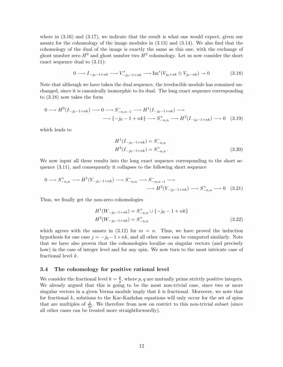
where in (3.16) and (3.17), we indicate that the result is what one would expect, given ouransatz for the cohomology of the image modules in (3.13) and (3.14). We also find that thecohomology of the dual of the image is exactly the same as this one, with the exchange ofghost number zero H0 and ghost number two H2 cohomology. Let us now consider the shortexact sequence dual to (3.11):
0 −→ I−j0−1+nk −→ V ∗−j0−1+nk −→ Im∗(Vj0+nk ⊕ Vj0−nk)→ 0 (3.18)
Note that although we have taken the dual sequence, the irreducible module has remained un-changed, since it is canonically isomorphic to its dual. The long exact sequence correspondingto (3.18) now takes the form
0 −→ H0(I−j0−1+nk) −→ 0 −→ S−−n,n−1 −→ H1(I−j0−1+nk) −→
−→ {−j0 − 1 + nk} −→ S+−n,n −→ H2(I−j0−1+nk) −→ 0 (3.19)
which leads to
H1(I−j0−1+nk) = S−−n,n
H2(I−j0−1+nk) = S+−n,n . (3.20)
We now input all these results into the long exact sequence corresponding to the short se-quence (3.11), and consequently it collapses to the following short sequence
0 −→ S+−n,n −→ H1(V−j0−1+nk) −→ S−
−n,n −→ S−−n,n−1 −→−→ H2(V−j0−1+nk) −→ S+
−n,n −→ 0 (3.21)
Thus, we finally get the non-zero cohomologies
H1(W−j0−1+nk) = S+−n,n ∪ {−j0 − 1 + nk}
H2(W−j0−1+nk) = S+−n,n (3.22)
which agrees with the ansatz in (3.12) for m = n. Thus, we have proved the inductionhypothesis for one case j = −j0−1+nk, and all other cases can be computed similarly. Notethat we have also proven that the cohomologies localize on singular vectors (and preciselyhow) in the case of integer level and for any spin. We now turn to the most intricate case offractional level k.
3.4 The cohomology for positive rational level
We consider the fractional level k = pq , where p, q are mutually prime strictly positive integers.
We already argued that this is going to be the most non-trivial case, since two or moresingular vectors in a given Verma module imply that k is fractional. Moreover, we note thatfor fractional k, solutions to the Kac-Kazhdan equations will only occur for the set of spinsthat are multiples of 1
2q . We therefore from now on restrict to this non-trivial subset (sinceall other cases can be treated more straightforwardly).
12

Embedding diagrams
For this case as well, we can algorithmically construct the embedding diagrams for all Vermamodules, using the results of Malikov [34] (see also [35]). The diagrams have the same“double-string” shape as before, but are now generated by ρ-centered affine Weyl reflectionsthat depend on the particular spin under study. We discuss in detail in the appendix Ahow these embedding diagrams are constructed. Although this is the most systematic andall-at-once procedure, below, we will follow a more pedestrian route. We will reconstruct theembedding diagrams inductively simply by locating the singular vectors in a given module.Although this approach may be more accessible and constructive, its a posteriori justificationlies in its agreement with the proof for the embedding diagram given in [34].
The cohomology for a simple case
To compute the cohomology, we follow an inductive procedure. First of all, when 2j + 1 isnot of the form
2j + 1 = r + ks such that rs > 0 or r > 0, s = 0 , (3.23)
then the module has no singular vectors and is irreducible. We have then that the Vermamodule is equivalent to its dual, and is equivalent to the Wakimoto module and its dual.This is because for irreducible Verma modules, there exists a non-degenerate Shapolov formwhich can be used to construct a canonical isomorphism between the Verma module and itsdual. This also implies that the cohomology of an irreducible module is the same as thatof its dual. Thus all these modules have cohomology Hn(Vj = Wj = W ∗
j ) = δ1,n{j}. Thiscompletes the calculation of the cohomology in the case of irreducible modules.
The cohomology in the case of one singular vector
Next, we move on to the case where the Verma module Vj1 under consideration has preciselyone singular vector. The values of j1 for which this is the case can be parameterized by thecorresponding values of (r1, s1), which are related to j1 by
2j1 + 1 = r1 + ks1 . (3.24)
When 2j1+1 is positive, the couple (r1, s1) satisfies r1 ∈ {1, 2, . . . , p} and s1 ∈ {0, 1, . . . , q−1}.When 2j1 + 1 is negative, we have that r1 ∈ {−1,−2, . . . ,−p} and s1 ∈ {−1,−2, . . . ,−q}.We have thus 2.p.q values of j1 with precisely one singular vector.
The singular vectors are at values of the spin j(1)1 which are given by 2j
(1)1 +1 = 2j1 +1−
2r1 = −r1 + ks1. (Note that this expression can be of either sign.) It is now not too difficultto prove that none of the Verma modules associated to the singular vectors can have anysingular vectors themselves. Thus, they are irreducible, and we have already computed theircohomology. We can then proceed to compute the cohomology for the case of one singularvector. We have the exact sequences:
0 −→ Vj(1)1−→ Vj1 −→ Ij1 −→ 0
0 −→ Ij1 −→ V ∗j1 −→ V
j(1)1
−→ 0 .
The first sequence indicates that modding out by the single singular vector gives an irreduciblemodule, while the second follows by dualizing and from the fact that the modules Ij1 and
13

Vj(1)1
are irreducible. Suppose that j1 is positive; then Vj1 = Wj1. Then we first use the
second exact sequence to compute the cohomology of Ij1 :
0 −→ H1(Ij1) −→ {j1} −→ {j(1)1 } −→ H2(Ij1) −→ 0 . (3.25)
We thus have that
H1(Ij1) = {j1} H2(Ij1) = {j(1)1 }. (3.26)
We can feed this information into the first exact sequence and we obtain:
0 −→ {j(1)1 } −→ H1(Wj1) −→ {j1} −→ 0 −→ H2(Wj1) −→ {j(1)1 } −→ 0 (3.27)
which gives us the result:
H1(Wj1) = {j1} ∪ {j(1)1 } H2(Wj1) = {j(1)1 } . (3.28)
These are the set of the parent spin and the singular vector, and the singular vector respec-tively.
For j1 negative, we have that the Verma module is equivalent to the dual Wakimotomodule, and repeating the analysis above, we find that
H1(Wj1) = {j1} ∪ {j(1)1 } H0(Wj1) = {j(1)1 } . (3.29)
Thus we have computed the cohomologies for all modules with a single singular vector.
The location of singular vectors in Verma modules
We now turn to a classification of the cases where the parent module has precisely n singularvectors. It is not too difficult to see that these cases are described as follows. Define the spinjn to be given by:
2jn + 1 = rn + ksn . (3.30)
For positive spin, we have that jn lies in the set corresponding to rn ∈ {(n − 1)p + 1, (n −1)p + 2, . . . , np} and sn ∈ {0, 1, . . . , q − 1}. When 2jn + 1 is negative, we have that rn ∈{−(n − 1)p − 1,−(n − 1)p − 2, . . . ,−np} and sn ∈ {−1,−2, . . . ,−q}. We thus always have2.p.q values of jn with precisely n singular vectors. In the case of positive spin, which willtake to be the case for our calculations, we have that the singular vectors correspond to thepairs (r, s) ∈ {(rn, sn), (rn − p, sn + q), . . . , (rn − (n− 1)p, sn + (n − 1)q)}.
We also have a claim that we will treat in more detail. Suppose we consider the moduleVjn , and label the leading singular vectors in them as V
j(1)n−1
and Vj(n)n−1
5. Now list the singular
vectors in these modules. We will find below that these are in fact, the same list of vectors.Once again, consider the leading singular vectors in this list of n − 1 singular vectors, and
label them V(1,1)jn−2
and V(1,n−1)jn−2
. Consider the singular vectors in these modules; we claim(and prove below) that the singular vectors in either of these modules make up the remainingn − 2 singular vectors in the original module Vjn . This is key to writing down short exactsequences of Verma modules that will lead to computing cohomology.
5The notation is such that the subscript tells us the number of singular vectors in a given module, whilethe superscripts keeps track of its line of descent from Vjn
.
14

Let’s prove these claims, and start with a spin jn module, associated to a module withn singular vectors. We have that 2jn + 1 = rn + ksn where (rn, sn) are taken in the setdescribed above (and we take them to be positive for simplicity). The resulting spins of themodules of the singular vectors are (ln = 1, 2, . . . , n):
2j(ln)n−1 + 1 = −rn + ksn + 2(ln − 1)p. (3.31)
In particular, we have the spins which we believe to be the nearest to jn in the embeddingdiagram of Vjn , namely those associated to ln = 1, n:
2j(1)n−1 + 1 = −rn + ksn = r
(1)n−1 + ks
(1)n−1
2j(n)n−1 + 1 = −rn + ksn + 2(n− 1)p = r
(n)n−1 + ks
(n)n−1. (3.32)
In the case of integer level, these appeared at an equal distance from jn but in the rationallevel, this need not be the case. Modules associated to each of these j values have n − 1
singular vectors. Indeed, the associated pairs (r(1)n−1, s
(1)n−1) and (r
(n)n−1, s
(n)n−1) are given by the
formulae
r(1)n−1 = p− rn ∈ {−(n− 2)p, . . . ,−(n− 1)p}s(1)n−1 = sn − q ∈ {−q, . . . ,−1}r(n)n−1 = 2(n− 1)p − rn ∈ {(n − 2)p, . . . , (n− 1)p}s(n)n−1 = sn ∈ {1, . . . , q} . (3.33)
Their ranges have been explicitly shown to make it clear that they indeed have n−1 singularvectors each. Let us now list the set of singular vectors in each of the modules V
j(1)n−1
and
Vj(n)n−1
. We will denote these respectively as j(1,l
(1)n−1)
n−2 and j(n,l
(n)n−1)
n−2 . These satisfy
2j(1,l
(1)n−1)
n−2 + 1 = −r(1)n + ks(1)n − 2(l(1)n−1 − 1)p with l
(1)n−1 ∈ {1 . . . n− 1}
= rn − p+ k(sn − q)− 2(l(1)n−1 − 1)p
= rn + ksn − 2l(1)n−1p (3.34)
and
2j(n,l
(n)(n−1)
)
n−2 + 1 = −r(n)n−1 + ks
(n)n−1 + 2(l
(n)n−1 − 1)p with l
(n)n−1 ∈ {1 . . . n− 1}
= rn − 2(n− 1)p + ksn + 2(l(n)n−1 − 1)p
= rn + ksn − 2(n− l(n)n−1)p (3.35)
It is clear from (3.35) that the singular vectors in each of the two lists is identical as each ofthe ln−1’s go from 1 to n− 1. In particular, we see that
j(1,l
(1)n−1)
n−2 = j(n,n−l(n)
(n−1))
n−2 . (3.36)
Without loss of generality, we may therefore safely omit the first superscript and denote
them as j(1)n−2 . . . j
(n−1)n−2 . Let us focus on either of the leading singular vectors, which have
15

ln−1 = 1, n − 1. These have the rn−2 and sn−2 values given by
r(1)n−2 = rn − 2p ∈ {(n − 3)p, . . . , (n − 2)p}s(1)n−2 = sn ∈ {1, . . . , q}
r(n−1)n−2 = rn − (2n − 3)p ∈ {−(n − 2)p, . . . ,−(n− 3)p}s(n−1)n−2 = sn − q ∈ {−q, . . . ,−1} . (3.37)
It is clear that their (rn−2, sn−2) values are such that the modules Vj(1)n−2
and Vj(n−1)n−2
have
n − 2 singular vectors each, which we label j(1,m
(1)n−2)
n−3 and j(n−1,m
(n−1)n−2 )
n−3 respectively. Thesesatisfy the equations
2j(1,m
(1)n−2)
n−3 + 1 = −r(1)n−2 + ks(1)n−2 + 2(m
(1)n−2 − 1)p
= −(rn − 2p) + ksn + 2(m(1)n−2 − 1)p
= −rn + ksn + 2m(1)p (3.38)
and
2j(n−1,m
(n−1)n−2 )
n−3 + 1 = −r(n−1)n−2 + ks
(n−1)n−2 − 2(m
(n−1)n−2 − 1)p
= (2n− 3)p − rn + ksn − p− 2(m(n−1)n−2 − 1)p
= −rn + ksn + 2((n − 1)−m(n−1)n−2 ) . (3.39)
where m(1)n−2 and m
(n−1)n−2 take values in {1, . . . , n − 2}. Once again, we see that both lists of
singular vectors coincide if we identify
j(1,m
(1)n−2)
n−3 = j(n−1,(n−1)−m(n−1)
n−2 )
n−3 . (3.40)
Once again, the first superscript index is redundant and we may denote them as j(1)n−3 . . . j
(n−2)n−3 .
Moreover, by comparing with (3.31), we observe that the singular vectors in both Vj(1)n−2
and
Vj(n−1)n−2
(the modules corresponding to the leading second generation singular vectors) pre-
cisely account for all but two of the singular vectors in the original module Vjn . We havethus proved the assertion made at the beginning of this section.
Proof by induction
We now make an educated guess for the embedding diagram of these modules. As alreadyremarked, the guess is exact, as proven in [34] (see also our appendix A)6:
Vj(1)n−1
��444
4444
4444
4444
4// Vj(n−1)n−2
Vj(1)2
��222
2222
2222
2222
2// Vj(2)1
BBB
BBBB
B
Vjn
=={{{{{{{{
!!CCC
CCCC
C. . . . . . Vj0
Vj(n)n−1
DD// Vj(1)n−2
Vj(3)2
FF����������������// Vj(1)1
>>||||||||
(3.41)
6Again, in exceptional cases, linear embedding diagrams arise. The calculation of the cohomology is theneasily adapted from the appendix to [15] and our subsection on the linear case for integer k.
16

The knowledge of the embedding diagram allows us to write down the exact sequences:
0 −→ Im(Vj(1)n−2
⊕ Vj(n−1)n−2
) −→ Vj(1)n−1
⊕ Vj(n)n−1
−→ Im(Vj(1)n−1
⊕ Vj(n)n−1
) −→ 0 (3.42)
0 −→ Im(Vj(1)n−1⊕ V
j(n)n−1
) −→ Vjn −→ Ijn −→ 0 (3.43)
The second sequence codes the irreducibility of the module obtained by modding out by theleading singular vectors, while the first one encodes the double counting in this moddingout. From here on, the proof for the cohomology of the BRST operator Q is identical to theinteger level case and we once again find that cohomology elements are given by the singularvectors. As for the integer level case, we need to postulate not only the cohomology of theWakimoto modules but also those of the image modules appearing in (3.42). We make thefollowing induction hypothesis for all m values in the range 0 ≤ m ≤ n− 1 :
For jm > −12 H1(Wjm = Vjm) = {j(1)m−1 . . . j
(m)m−1} ∪ {jm}
H2(Wjm = Vjm) = {j(1)m−1 . . . j(m)m−1}
For jm < −12 H1(Wjm = V ∗
jm) = {j(1)m−1 . . . j(m)m−1} ∪ {jm}
H0(Wjm = V ∗jm) = {j(1)m−1 . . . j
(m)m−1}
Hq(W ∗jm) = δq,1 {jm} ∀jm (3.44)
while for the image modules appearing in (3.42) and (3.43), we postulate
H1(Im(Vj(1)n−2⊕ V
j(n−1)n−2
)) = {j(1)n−2 . . . j(n−1)n−2 }
H2(Im(Vj(1)n−2
⊕ Vj(n−1)n−2
)) = {j(1)n−3 . . . j(n−2)n−3 }
= {j(2)n−1 . . . j(n−1)n−1 } (3.45)
where we have generalized (3.13) and (3.14). We will try to prove (3.44) for m = n. Webegin by using our induction hypothesis in the long exact sequence corresponding to the shortsequence in equation (3.42). We obtain the sequence
0 −→ H0(Vj(1)n−1⊕ V
j(n)n−1
) −→ {j(1)n−2 . . . j(n−1)n−2 } −→ {j
(1)n−1, j
(1)n−2 . . . j
(n−1)n−2 } −→
−→ H1(Im(Vj(1)n−1
⊕ Vj(n)n−1
) −→ {j(2)n−1 . . . j(n−1)n−1 } −→ H2(V
j(1)n−1
⊕ Vj(n)n−1
) −→ 0 (3.46)
from which we solve for the cohomology of the image modules :
H1(Im(Vj(1)n−1
⊕ Vj(n)n−1
) = {j(1)n−1 . . . j(n)n−1}
H2(Im(Vj(1)n−1⊕ V
j(n)n−1
) = {j(1)n−2 . . . j(n−1)n−2 }. (3.47)
Thus, we have inductively verified the ansatz for the cohomology of the image modules. Thecohomology for the dual of the image is computed similarly, and one obtains the same coho-mology with the ghost number zero H0 and ghost number two cohomology H2 interchanged.
17

We now plug this result into the long exact sequence corresponding to the dual of the shortexact sequence in (3.43) to get
0 −→ H0(Ijn) −→ 0 −→ {j(1)n−2 . . . j(n−1)n−2 } −→ H1(Ijn) −→−→ {jn} −→ {j(1)n−1 . . . j
(n)n−1} −→ H2(Ijn) −→ 0 (3.48)
leading to
H1(Ijn) = {jn} ∪ {j(1)n−2 . . . j(n−1)n−2 }
H2(Ijn) = {j(1)n−1 . . . j(n)n−1} . (3.49)
Substituting all these results into the long exact sequence corresponding to (3.43), we find
0 −→ H0(Wjn) −→ 0 −→ {j(1)n−1 . . . j(n)n−1} −→ H1(Wjn) −→ {jn, j(1)n−2 . . . j
(n−1)n−2 } −→
−→ {j(1)n−2 . . . j(n−1)n−2 } −→ H2(Wjn) −→ {j(1)n−1 . . . j
(n)n−1} −→ 0 (3.50)
from which we conclude
H1(Wjn) = {jn} ∪ {j(1)n−1 . . . j(n)n−1}
H2(Wjn) = {j(1)n−1 . . . j(n)n−1} (3.51)
By comparing with equation (3.44), we observe that we have derived the result for Wjn byassuming the result for all m < n. This is our answer for the cohomology of Wakimotomodules and thus the complete set of topological observables for the level k = p
q twistedSL(2, IR)/U(1) model.
3.5 Alternative proofs
An alternative inductive proof for the cohomology of the Wakimoto modules is possible,based on another pair of short exact sequences7. Again, for simplicity only, we restrict tothe case of positive 2jn + 1 = rn + ksn. The induction hypothesis consists of the validity ofthe cohomology that we found above for modules with less than n singular vectors in (3.44),and, of the cohomology of the corresponding irreducible modules. (The latter cohomologydepends on the sign of the spin.) Now, we can construct a first short exact sequence bymodding out the Verma module of spin jn by one of its two leading singular vectors, say
j(1)n−1, to produce a new module Xn:
0→ Vj(1)n−1→ Vjn → Xn → 0
0→ Ij(n)n−1→ Xn → Ijn → 0. (3.52)
We then used the module Xn in a second sequence which says that after eliminating the
further singular vector j(n)n−1 (and none of its descendants since they have already been modded
out), we obtain an irreducible module. Using these two short exact sequences and their dualsit is not hard to show that the induction step can be proven (both on the cohomology ofthe irreducible module and on the cohomology of the Wakimoto modules). For the reader’s
7We would like to thank Edward Frenkel for indicating to us the idea behind this alternative proof.
18

convenience we record an intermediate result, namely the cohomology of the modules Xn (forjn positive):
H1(Xn) = {jn} ∪ {j(1)n−2, . . . , j(n−1)n−2 }
H2(Xn) = {j(1)n−1} ∪ {j(1)n−2, . . . , j
(n−1)n−2 } . (3.53)
Furthermore, from the first alternative proof follows a second. We could choose to mod outfirst by the other leading singular vector. We obtain the short exact sequences:
0→ Vj(n)n−1→ Vjn → Yn → 0
0→ Ij(1)n−1
→ Xn → Ijn → 0. (3.54)
The proof follows familiar lines. We quote the intermediate result for the cohomology of thenew modules Yn:
H0(Yn) = {j(1)n−2, . . . , j(n−1)n−2 }
H1(Yn) = {jn} ∪ {j(1)n−1, . . . , j(n−1)n−1 } ∪ {j
(1)n−2, . . . , j
(n−1)n−2 }
H2(Yn) = {j(1)n−1, . . . , j(n)n−1}. (3.55)
Note that these modules have cohomology at three different ghost numbers.8
4 Concluding remarks
Our main result is that the cohomology of the topologically twisted coset theory is givenin terms of the singular vectors of the Wakimoto modules constructed over the SL(2, IR)current algebra. The precise form in which this is realized can be seen in equation (3.44).We conclude by making a few remarks on further avenues to explore, and on the uses of therather technical results we have obtained regarding the topological observables of the cigar.
• It is possible to give explicit representatives of the cohomology, using the formulaeobtained for singular vectors in SL(2, IR) modules [38][39]. Following the analysis in[15], rewriting these cohomology elements in Wakimoto variables could be very usefulin establishing the relation between twisted cosets and bosonic string theories.
• It would be instructive to further analyze, as was done in [37] for the particular caseof the topological cigar at level k = 1 (i.e. the conifold), how the operation of spectralflow acts on the observables of the topological cigar.
• The relationship between the statement that the cohomology localizes on singularvectors and the statement [20] that N = 2 topological singular vectors always arise(through the Kazama-Suzuki map) from SL(2, IR) singular vectors are tantalizinglyclose. It is fairly clear that clarifying the details of the relation will also illuminate therole of spectral flow.
8Algebraically, it is intuitive that the two leading singular vectors give rise to proofs with slightly differentstructure, since only one of the two leading singular spins is related to the parent spin by an elementary Weylreflection, as defined and discussed in the appendix A.
19

• An important application we have in mind for these results is in the context of theN = 2 topological string (see e.g. [40] for a review). Now that we obtained theobservables on the topological cigar, the algorithm to obtain the closed string spectrumof topological strings on non-compact Gepner models consisting of (twisted) N = 2minimal models and topological cigars is clear. Indeed, the chiral cohomology on theN = 2 minimal models is straightforward to compute, and is well-known. (Whenworking with a unitary spectrum, the powerful results of [41] make the calculationmuch easier.) Furthermore, one could then combine left- and right-movers to forma consistent spectrum, following Gepner’s technique of GSO projecting onto integerU(1)R charges. In the present context, the GSO projection will boil down to a simpleorbifold by an abelian group that will depend only on the levels involved in the non-compact Gepner model. (This is clear from the form of the N = 2 U(1)R current inthese models and is for instance discussed in [9][10][11][12][13], following Gepner.) Itwill then be very interesting to combine these observations together with the fact thatthe N = 2 topological string basically corresponds to a bosonic string theory (see e.g.[40]). This would be a worldsheet approach to isolate integrable subsectors of stringtheories on (non-compact) Calabi-Yau manifolds [42].
Acknowledgements
We are grateful to Wendy Lowen for helpful correspondence and to Edward Frenkel forinsightful comments on these problems and on the appendix to [15]. We are also thankfulto Eleonora Dell’Aquila, Jaume Gomis and Sameer Murthy for discussions and commentson the draft. Research of S.A at the Perimeter Institute is supported in part by funds fromNSERC of Canada and by MEDT of Ontario, and research of J.T. is partly supported byEU-contract MRTN-CT-2004-05104.
A A few notes on affine algebra
The calculation of the cohomology performed in the bulk of the paper heavily leans on anunderstanding of the embedding structure of Verma modules for the rank two Kac-Moodyalgebra sl2. In this appendix, we briefly review some of the mathematics involved in un-derstanding the embedding diagrams. We hope this will make the relevant mathematicsliterature more readable to the interested physicist.
We introduce some notation and refer to standard text books on affine algebras for furtherinformation on the following standard concepts. We introduce the algebra sl2, where thenotation is meant to indicate that we consider the algebra over the complex numbers. Wefollow (in this appendix only) su(2) conventions for the structure constants and metric of thecorresponding affine algebra (see e.g. [43] for standard conventions). The affine algebra hassimple positive roots α1 (the simple positive root of the ordinary, horizontal su(2) subalgebra)and α0 = δ−α1, where δ is the imaginary root. We take the algebra to be at (bosonic) levelksu(2).
We can define ρ-centered affine Weyl reflections (where ρ is defined in the usual way, ashaving inner product equal to one with all positive simple roots). These ρ-centered affineWeyl reflections sρα with respect to the root α are given in terms of the affine Weyl reflections
20

sα by the formula:
sαλ = λ− 2(α, λ)
(α,α)
sρα(λ) = sα(λ+ ρ)− ρ. (A.1)
We will mostly refer only to the action of the ρ-centered affine Weyl reflections on the part ofthe weight that lies in the direction of the horizontal su(2) subalgebra of the full Kac-Moodyalgebra (i.e. the standard spin of the base representation). On the spin j of a representation(corresponding to a horizontal weight λ1 = jα1, these Weyl reflections act as follows:
sρα1+lδ(j) = −l(ksu(2) + 2)− j − 1
sρ−α1+lδ(j) = l(ksu(2) + 2)− j − 1. (A.2)
Following [34] we also define an operation S on the spin and the level of the affine algebrawhich acts as (j, ksu(2)) 7→ (−j − 1,−ksu(2) − 4).
A.1 Flipping
The statements on the structure of the embedding of Verma modules derived in [34], andrestricted to the case of relevance here, can now be made more transparent, using the abovenotations.
First of all, the main theorem on the embedding structure in [34], in paragraph 2, caseA, pertains to the case where the level of the sl2 algebra, which we have named ksu(2) islarger than −2. However, the case of interest to us in the bulk can be reduced to this casevia the operation S. Indeed, consider a spin and bosonic su(2) level (jn,−k − 2) as in thebulk of our paper. (Note that ksu(2) = −k− 2, where k is the supersymmetric SL(2, R) levelused in the bulk of the paper.) By acting with the operation S, we find the spin and level(−jn − 1, k − 2). Since our supersymmetric level k is larger than zero, we do find that thenew bosonic level k− 2 is larger than −2, and that we now therefore fall into the frameworkof the embedding diagrams discussed in paragraph 2, case A of [34].
A.2 Constructing the embedding diagram
The results of Malikov [34] then permit us to construct the embedding diagrams for all cases.In particular, we concentrate on the most difficult case of k = p/q fractional (with p, q bothstrictly positive mutually prime integers). First note that the Kaz-Kazhdan equation can bewritten more invariantly as being satisfied for an affine weight λ when:
2(λ+ ρ, α) = m(α,α) (A.3)
for some positive root α and m ∈ N0 (i.e. m a strictly positive integer). This translatesdirectly into the equation used in the bulk of the paper. However, following [34], we will nowconsider solutions to this equation for m any integer. In other words, we will study solutionsto the equation:
−2jn − 1 = −m− kn (A.4)
which is the Kaz-Kazhdan equation for the flipped spin defined above, and with respect tothe flipped supersymmetric level k, and this for any integers m and n. Pick now the smallest
21

positive integer n such that the equation is satisfied, and the smallest strictly negative integern such that the equation holds. For the values jn defined in the bulk of the paper, in equation(3.30), it is not hard to see that these values correspond to sn, sn − q and sn + q, sn for jnpositive and negative respectively. These, via the Kac-Kazhdan equations above correspondto positive affine roots which are, for 2jn + 1 positive:
α1 + snδ
−α1 + (q − sn)δ (A.5)
while for 2jn + 1 negative, we consider the positive roots:
α1 + (q + sn)δ
−α1 − snδ. (A.6)
The results of [34] show that the embedding diagrams of the Verma module with spin jcan be constructed from an initial Verma module j0 by ρ-centered Weyl-reflecting from thisinitial point, and adding a node to the embedding diagram for each step on the way to thedestination j. The node j0 corresponds to the unique spin satisfying the equations:
0 ≤ −2j0 − 1 + snk ≤ p (A.7)
respectively
0 ≤ 2j0 + 1− snk ≤ p, (A.8)
and lying in the orbit of j under the above ρ-centered Weyl reflections.Since this prescription is rather abstract (although already more concrete than the original
one [34]), let us first illustrate this in the case where the level k is integer, and see how werecuperate the diagrams used in the bulk of the paper.
The case of k integer
For k integer, we have that q = 1, and that for 2jn + 1 positive, say, we have that sn = 0.Consequently, the allowed ρ-centered Weyl reflections are those with respect to α1 and α1+δ.These are the standard ρ-centered Weyl reflections, and those are precisely the ones we usedto construct the diagrams in the case of integer level. Moreover, the condition on the finalspin becomes 0 ≤ −2j0 − 1 ≤ k = p which is precisely what we found in the bulk of thepaper.
The general case
In the general case too, one can show with a bit more tedious but straightforward calculationsthat the above systematic construction of the embedding diagrams agrees on the nose withthe analysis in terms of singular vectors only performed in the bulk of the paper. In fact,this justifies the approach in the bulk of the paper, via the detailed proof of Malikov of theembedding structure of all Verma modules for the affine sl2 algebra.
22

B A case study
As we have seen, for j-values that are not of the form 2j+ 1 ∈ kZZ, the sub-module structureis not linear. The simplest example of a non-linear embedding of sub-modules occurs whenthe embedding diagram has only four entries (the “rhombus” diagram). From the generalembedding diagram (3.9) for integer k, we see that this happens for j = j0±k. Let us discusseach of these cases in turn and demonstrate explicitly how one would compute cohomologyinductively.
B.1 The case j = j0 + k
For j > −12 , the Wakimoto modules are isomorphic to the Verma modules and we can read
off the submodule structure from [34] to be (with Wj = Vj)
V−j0−1
$$IIIIIIIII
Vj0+k
%%KKKKKKKKK
99sssssssssVj0
V−j0−k−1
::uuuuuuuuu
(B.1)
In order to find the cohomology of Q in this module Wj , we have to first find the cohomologyof the modules W−j0−1 and W−j0−k−1. However, these have linear sub-module structure andtheir cohomology can be computed using the techniques of Frenkel in [15]. Let us illustratethis in the case of W−j0−1 = V−j0−1, which has the embedding structure
V−j0−1 −→ Vj0 . (B.2)
Now, it follows that the following sequence of modules is a short exact sequence :
0 −→ I−j0−1 −→W ∗−j0−1 −→Wj0 −→ 0 . (B.3)
So far we have only focused on the modules over the SL(2, IR) current algebra. In orderto compute the cohomology of the Q operator in (2.16), we have to tensor the SL(2, IR)modules with the Fock modules over the (b, c) and X algebra. Although we will suppressthese tensor products while writing out the sequences of modules, it is good to keep in mindthat the states (observables) we will find as cohomology elements belong to the Hilbert spacein (2.12).
The corresponding long exact sequence of cohomology is given by
. . . −→ Hq(I−j0−1) −→ Hq(W ∗−j0−1) −→ Hq(Wj0) −→ Hq+1(I−j0−1) −→ . . . (B.4)
Using (3.1) and (3.6), our long exact sequence collapses to the following short exact sequences
0 −→ H1(I−j0−1) −→ {−j0 − 1} −→ 0
0 −→ {j0} −→ H2(I−j0−1) −→ 0 (B.5)
all other cohomology groups being trivial. We thus get H1(I−j0−1) = {−j0 − 1} andH2(I−j0−1) = {j0}. Now consider the short exact sequence dual to the one considered above
0 −→W ∗j0 −→W−j0−1 −→ I−j0−1 −→ 0 . (B.6)
23

Once again, considering the corresponding long exact sequence and using the results derivedso far, we get the collapsed short exact sequences for the cohomology
0 −→ {j0} −→ H1(W−j0−1) −→ {−j0 − 1} −→ 0
0 −→ H1(W−j0−1) −→ {j0} −→ 0 (B.7)
Similar manipulations can be done for j = −k − j0 − 1 and we get the following result forthe cohomology :
For j = −j0 − 1, H1(W−j0−1) = {−j0 − 1, j0}H2(W−j0−1) = {j0}
For j = −k − j0 − 1, H1(W−k−j0−1) = {−k − j0 − 1, j0}H0(W−k−j0−1) = {j0} (B.8)
We now have the ingredients necessary to compute the cohomology ofWj0+k whose submodulestructure is shown in (B.1). We claim that the following sequences are exact
0 −→ Ij0 −→ V−k−j0−1 ⊕ V−j0−1 −→ Im(V−k−j0−1 ⊕ V−j0−1) −→ 0 (B.9)
0 −→ Im(V−k−j0−1 ⊕ V−j0−1) −→ Vj0+k −→ Ij0+k −→ 0 (B.10)
In all, there are four unknown cohomologies, those of the modules Vj0+k, Ij0+k, and thecohomology of the image module that appears in sequence (B.9) and its dual. Using thesetwo short exact sequences and their dual sequences, it is possible to compute the cohomologyof all four modules.
We first solve for the cohomology of Im(V−k−j0−1 ⊕ V−j0−1). Using the fact that
V−j0−k−1 = W ∗−j0−k−1 and V−j0−1 = W−j0−1 , (B.11)
the long exact sequence corresponding to the short exact sequence in (B.9) collapses to
0 −→ H0(Im(V−k−j0−1 ⊕ V−j0−1)) −→ {j0} −→ {−k − j0 − 1,−j0 − 1, j0} −→−→ H1(Im(V−k−j0−1 ⊕ V−j0−1)) −→ 0 (B.12)
0 −→ {j0} −→ H2(Im(V−k−j0−1 ⊕ V−j0−1)) −→ 0 (B.13)
This leads to
H1(Im(V−k−j0−1 ⊕ V−j0−1)) = {−k − j0 − 1,−j0 − 1}H2(Im(V−k−j0−1 ⊕ V−j0−1)) = {j0} . (B.14)
Let us now consider the sequence dual to (B.9). Using similar techniques, we find that thedual of the image module has the same cohomology, with H0 replaced by H2. Let us nowapply these results to the dual of the exact sequence in (B.10):
0 −→ Ij0+k −→ V ∗j0+k −→ Im∗(V−k−j0−1 ⊕ V−j0−1) −→ 0 . (B.15)
Since, Vj=j0+k = Wj0+k, the corresponding long exact sequence collapses to
0 −→ {j0} −→ H1(Ij0+k) −→ {j0 + k} −→ 0
0 −→ {−k − j0 − 1,−j0 − 1} −→ H2(Ij0+k) −→ 0 (B.16)
24

from which we get H1(Ij0+k) = {j0, j0 + k} and H2(Ij0+k) = {−k − j0 − 1,−j0 − 1}. Now,writing out the long exact sequence corresponding to the short exact sequence in (B.10) andusing all the results obtained so far, we get the following non-trivial long exact sequence
0 −→ {−k − j0 − 1,−j0 − 1} −→ H1(Wj0+k) −→ {j0, j0 + k} −→ {j0} −→−→ H2(Wj0+k) −→ {−k − j0 − 1,−j0 − 1} −→ 0 (B.17)
The long sequence breaks as shown in the equation into two subsequences, which can besolved to obtain
H1(Wj0+k) = {−k − j0 − 1,−j0 − 1, j0 + k}H2(Wj0+k) = {−k − j0 − 1,−j0 − 1} (B.18)
B.2 The case j = j0 − k
As mentioned at the beginning of this section, there is another value of j for which the sub-module structure is the same as in (B.1), j = j0 − k < 0. However, since for negative j,Wakimoto modules are isomorphic to dual Verma modules [15], the directions in the arrowsof the embedding diagram for the Wakimoto module are opposite to what was consideredearlier (since Wj0−k = V ∗
j0−k):
V ∗−j0−1
zzttttttttt
V ∗j0−k V ∗
j0
ccHHHHHHHHH
{{vvvvvvvvv
V ∗−k−j0−1
ddJJJJJJJJJ
(B.19)
Since this case is different from the j > 0 case, let us go through the exercise of computingcohomology explicitly. The short exact sequences in (B.9) and (B.10) remain the same, withj0+k replaced by j0−k. However, when writing out the long exact sequence of cohomologies,it is important to use the equality Vj0−k = W ∗
j0−k. With this in mind, let us proceed as before.The computation of the cohomology of Im(V−k−j0−1 ⊕ V−j0−1) using the sequence in
(B.10) remains unchanged. We are thus left with the sequence
0 −→ Im(V−k−j0−1 ⊕ V−j0−1) −→W ∗j0−k −→ Ij0−k −→ 0 . (B.20)
The corresponding long exact sequence breaks up into
0 −→ H0(Ij0−k) −→ {−k − j0 − 1,−j0 − 1} −→ 0
0 −→ {j0 − k} −→ H1(Ij0−k) −→ {j0,−j0 − 1} −→ 0 (B.21)
leading to H0(Ij0−k) = {−k − j0 − 1,−j0 − 1} and H1(Ij0−k) = {j0 − k, j0}. Consider nowthe sequence dual to (B.20)
0 −→ Ij0−k −→Wj0−k −→ Im∗(V−k−j0−1 ⊕ V−j0−1) −→ 0 . (B.22)
25

The long exact sequence is of the form
0 −→ {−k − j0 − 1,−j0 − 1} −→ H0(Wj0−k) −→ {j0} −→−→ {j0, j0 − k} −→ H1(Wj0−k) −→ {−k − j0 − 1,−j0 − 1} −→ 0 (B.23)
which breaks into two shorter sequences (as indicated in the diagram). Solving for thecohomology groups, we get
H1(Wj0−k) = {j0 − k,−k − j0 − 1,−j0 − 1}H0(Wj0−k) = {−k − j0 − 1,−j0 − 1} (B.24)
The notable feature of this analysis is the following :
• The spin j-values of the cohomology elements correspond to the singular vectors thatappear in the original module. For both j = j0 ± k, the module generated by j = j0is not a submodule (i.e. j0 not a singular vector within the original module). This canbe explicitly checked by finding solutions to the Kac-Kazhdan equation in (3.2).
This feature generalizes to the generic case with more nodes and also to the rational case, andhas inspired our ansatz in (3.44) which we have proven in the main text using the method ofinduction.
References
[1] E. Kiritsis, C. Kounnas and D. Lust, “A Large class of new gravitational and axionicbackgrounds for four-dimensional superstrings,” Int. J. Mod. Phys. A 9 (1994) 1361[arXiv:hep-th/9308124].
[2] K. Hori and A. Kapustin, “Worldsheet descriptions of wrapped NS five-branes,” JHEP0211, 038 (2002) [arXiv:hep-th/0203147].
[3] A. Giveon and D. Kutasov, “Little string theory in a double scaling limit,” JHEP 9910,034 (1999) [arXiv:hep-th/9909110].
[4] K. Hori and A. Kapustin, “Duality of the fermionic 2d black hole and N = 2 Liouvilletheory as mirror symmetry,” JHEP 0108 (2001) 045 [arXiv:hep-th/0104202].
[5] D. Tong, “Mirror mirror on the wall: On two-dimensional black holes and Liouvilletheory,” JHEP 0304, 031 (2003) [arXiv:hep-th/0303151].
[6] D. Israel, A. Pakman and J. Troost, “D-branes in N = 2 Liouville theory and its mirror,”Nucl. Phys. B 710, 529 (2005) [arXiv:hep-th/0405259].
[7] D. Kutasov and N. Seiberg, “Noncritical Superstrings,” Phys. Lett. B 251, 67 (1990).
[8] S. Mizoguchi, “Modular invariant critical superstrings on four-dimensional Minkowskispace x two-dimensional black hole,” JHEP 0004, 014 (2000) [arXiv:hep-th/0003053].
[9] T. Eguchi and Y. Sugawara, “Modular invariance in superstring on Calabi-Yau n-foldwith A-D-E singularity,” Nucl. Phys. B 577, 3 (2000) [arXiv:hep-th/0002100].
26

[10] S. Murthy, “Notes on non-critical superstrings in various dimensions,” JHEP 0311, 056(2003) [arXiv:hep-th/0305197].
[11] T. Eguchi and Y. Sugawara, “SL(2,R)/U(1) supercoset and elliptic genera of non-compact Calabi-Yau manifolds,” JHEP 0405, 014 (2004) [arXiv:hep-th/0403193].
[12] D. Israel, C. Kounnas, A. Pakman and J. Troost, “The partition function of the super-symmetric two-dimensional black hole and little string theory,” JHEP 0406, 033 (2004)[arXiv:hep-th/0403237].
[13] T. Eguchi and Y. Sugawara, “Conifold type singularities, N = 2 Liouville andSL(2,R)/U(1) theories,” JHEP 0501, 027 (2005) [arXiv:hep-th/0411041].
[14] A. Giveon, D. Kutasov and O. Pelc, “Holography for non-critical superstrings,” JHEP9910, 035 (1999) [arXiv:hep-th/9907178].
[15] S. Mukhi and C. Vafa, “Two-dimensional black hole as a topological coset model of c =1 string theory,” Nucl. Phys. B 407, 667 (1993) [arXiv:hep-th/9301083].
[16] D. Ghoshal and C. Vafa, “C = 1 string as the topological theory of the conifold,” Nucl.Phys. B 453, 121 (1995) [arXiv:hep-th/9506122].
[17] G. Bertoldi, “Double scaling limits and twisted non-critical superstrings,”[arXiv:hep-th/0603075].
[18] B. Gato-Rivera and A. M. Semikhatov, “d ≤ 1 ∪ d ≥ 25 and W constraints fromBRST invariance in the c 6= 3 topological algebra,” Phys. Lett. B 293 (1992) 72[Theor. Math. Phys. 95 (1993 TMPHA,95,535-545.1993 TMFZA,95,239-250.1993) 536][arXiv:hep-th/9207004].
[19] A. M. Semikhatov, “The MFF singular vectors in topological conformal theories,” Mod.Phys. Lett. A 9, 1867 (1994) [JETP Lett. 58, 860 (1993)] [arXiv:hep-th/9311180].
[20] B. L. Feigin, A. M. Semikhatov and I. Y. Tipunin, “Equivalence between chain categoriesof representations of affine sl(2) and N = 2 superconformal algebras,” J. Math. Phys.39, 3865 (1998) [arXiv:hep-th/9701043].
[21] T. Takayanagi, “c < 1 string from two dimensional black holes,” arXiv:hep-th/0503237.
[22] D. A. Sahakyan and T. Takayanagi, “On the connection between N = 2 minimal stringand (1,n) bosonic minimal string,” [arXiv:hep-th/0512112].
[23] V. Niarchos, “On minimal N = 4 topological strings and the (1,k) minimal bosonicstring,” arXiv:hep-th/0512222.
[24] L. Rastelli and M. Wijnholt, “Minimal AdS(3),” arXiv:hep-th/0507037.
[25] Y. Kazama and H. Suzuki, “New N=2 Superconformal Field Theories And SuperstringCompactification,” Nucl. Phys. B 321, 232 (1989).
[26] E. Witten, “On string theory and black holes,” Phys. Rev. D 44, 314 (1991).
[27] R. Dijkgraaf, H. L. Verlinde and E. P. Verlinde, “String propagation in a black holegeometry,” Nucl. Phys. B 371, 269 (1992).
27

[28] J. M. Figueroa-O’Farrill and S. Stanciu, “N=1 and N=2 cosets from gauged supersym-metric WZW models,” arXiv:hep-th/9511229.
[29] D. Karabali, Q. H. Park, H. J. Schnitzer and Z. Yang, Phys. Lett. B 216 (1989) 307.
[30] S. Hwang and H. Rhedin, “The BRST Formulation of G/H WZNW models,” Nucl. Phys.B 406 (1993) 165 [arXiv:hep-th/9305174].
[31] P. Bouwknegt, J. G. McCarthy and K. Pilch, “BRST analysis of physical states for 2-Dgravity coupled to c ≤ 1 matter,” Commun. Math. Phys. 145, 541 (1992).
[32] N. Ohta and H. Suzuki, “Bosonization of a topological coset model and noncritical stringtheory,” Mod. Phys. Lett. A 9, 541 (1994) [arXiv:hep-th/9310180].
[33] E. Frenkel, “Determinant formulas for the free field representations of the Virasoro andKac-Moody algebras,” Phys. Lett. B 286 (1992) 71.
[34] F. Malikov, Algebra y Analiz, 2 No. 2, 65 (1990).
[35] B. L. Feigin and E. V. Frenkel, “Representations Of Affine Kac-Moody Algebras AndBosonization,”
[36] V. G. Kac and D. A. Kazhdan, “Structure Of Representations With Highest Weight OfInfinite Dimensional Lie Algebras,” Adv. Math. 34, 97 (1979).
[37] S. K. Ashok, S. Murthy and J. Troost, “Topological cigar and the c = 1 string: Openand closed,” JHEP 0602, 013 (2006) [arXiv:hep-th/0511239].
[38] F. G. Malikov, B. L. Feigin and D. B. Fuchs, “ Singular vectors in Verma Modules overKac-Moody algebras”, Funk. An. Prilozh. 20 No 2, 25 (1986).
[39] M. Bauer and N. Sochen, Commun. Math. Phys. 152 (1993) 127 [arXiv:hep-th/9201079].
[40] M. Bershadsky, S. Cecotti, H. Ooguri and C. Vafa, “Kodaira-Spencer theory of gravityand exact results for quantum string amplitudes,” Commun. Math. Phys. 165 (1994)311 [arXiv:hep-th/9309140].
[41] W. Lerche, C. Vafa and N. P. Warner, “Chiral Rings In N=2 Superconformal Theories,”Nucl. Phys. B 324, 427 (1989).
[42] M. Aganagic, R. Dijkgraaf, A. Klemm, M. Marino and C. Vafa, “Topological strings andintegrable hierarchies,” Commun. Math. Phys. 261, 451 (2006) [arXiv:hep-th/0312085].
[43] P. Di Francesco, P. Mathieu and D. Senechal, “Conformal field theory,”, Springer-VerlagNew-York, 1997.
28