Embed Size (px)
Citation preview
THE SOLIDIFICATION OF DUCTILE CAST IRON
By
ROBERTO ENRIQUE BOERI
Ingeniero Mecanico, Universidad Nacional de Mar del Plata, 1982
A THESIS SUBMITTED IN PARTIAL FULFILLMENT OF
THE REQUIREMENTS FOR THE DEGREE OF
DOCTOR OF PHILOSOPHY
in
THE FACULTY OF GRADUATE STUDDZS
Department of Metals and Materials Engineering
We accept this thesis as conforming
to the required standard
THE UNIVERSITY OF BRITISH COLUMBIA
November 1989
©Roberto Enrique Boeri

In presenting this thesis in partial fulfilment of the requirements for an advanced
degree at the University of British Columbia, I agree that the Library shall make it
freely available for reference and study. I further agree that permission for extensive
copying of this thesis for scholarly purposes may be granted by the head of my
department or by his or her representatives. It is understood that copying or
publication of this thesis for financial gain shall not be allowed without my written
permission.
Department of
The University of British Columbia Vancouver, Canada
DE-6 (2/88)

- ii -
A B S T R A C T
The microsegregation of Mn, Cu, Cr, Mo, Ni and Si has been measured in cast
ductile iron and in ductile iron which has been quenched when partially solidified.
Effective segregation coefficients have been determined for each of the elements, and
used to calculate the segregation on the basis of the Scheil equation. The calculated
values agree reasonably well with the values of the solute concentration as a function of
the solid fraction measured in quenched samples.
The microstructure of the solid phases during the solidification of ductile iron has
been observed. Solidification of eutectic ductile iron begins with the independent
nucleation of austenite and graphite in the melt. Later the graphite nodules are
enveloped by austenite, and further solidification takes place by the thickening of the
austenite layers enveloping the graphite. Isolated pockets of interdendritic melt are the
last material to solidify.
On the basis of the measured segregation of the different alloying elements, the
mechanisms by which the segregation affects the microstructure are considered, and an
explanation for the effect of segregation on the hardenability of ductile iron is proposed.
A mathematical model of the solidification of eutectic ductile iron is formulated
which includes heat flow, nucleation and growth of graphite nodules, and the
segregation of Si. The model uses equilibrium temperatures given by the ternary
Fe-C-Si equilibrium diagram. Using the mathematical model, cooling curves, nodule

- iii -
count and nodular size distribution are determined as a function of position in the
casting sample. The results are compared to measured temperatures, nodule count and
nodule size in rod castings of 12.5, 20 and 43mm radius. There is good agreement
between the calculated and measured values for the 43mm radius rod, and not quite
good agreement for the rods of smaller radii. The changes in solidification predicted by
the model when some solidification parameters are varied are consistent with
experimental observations with the same variation in the parameters.

iv
T A B L E O F C O N T E N T S
ABSTRACT ii
TABLE OF CONTENTS iv
LIST OF TABLES viii
LIST OF FIGURES ix
LIST OF SYMBOLS xvii
ACKNOWLEDGMENT xxi
1 INTRODUCTION 1
2 LITERATURE REVIEW 6
2.1 Cast Iron Microstructure During Solidification 6 2.1.1 Summary 8
2.2 Segregation in Cast Iron 9 2.2.1 Summary 15
2.3 Mathematical Modelling of Solidification 15 2.3.1 Summary 31
2.4 Cooling Curves 32 2.4.1 Summary 38
3 OBJECTIVES OF THE PRESENT RESEARCH 40
4 EXPERIMENTAL METHODS AND APPARATUS 46
4.1 Melting 46 4.2 Sampling 47 4.3 Casting and Temperature Recording 51 4.4 Optical Metallography 55 4.5 Electron Metallography and Microanalysis 55

V
5 SEGREGATION AND MICROSTRUCTURE RESULTS AND 60 DISCUSSION
5.1 Segregation in Cast Samples 60 5.1.1 Segregation Pattern in the Vicinity of a Graphite Nodule 63 5.1.2 Quantitative Values for Segregation in Cast Samples 71
5.2 Analysis of Quenched Samples 73 5.2.1 Microstructure of Quenched Samples 73 5.2.2 Measurements of Solute Concentration as a Function of the 80
Fraction Solid 5.2.3 Estimation of Partition Coefficients of the Alloying Elements 88
5.3 Analysis of Segregation Results 93 5.3.1 Comparison of Measured Segregation with Calculations Based 100
on the Scheil Equation 5.3.1.1 Solute Concentration in the Liquid During Solidification 101
Using k,. 5.3.1.2 Solute Distribution in the Solid Using k,. 107 5.3.1.3 Solute Distribution in the Solid Using 1̂ 115 5.3.1.4 Solute Concentration in the Liquid During Solidification 121
using 5.3.1.5 Analysis of the Fit Between Calculations and Experiments 126
5.3.2 Correlation Between the Solidification Structure and the 128 Segregation Pattern Around Nodules
5.3.3 Comparison of the Segregation in Sand-Cast and Quenched 134 Samples
5.4 Effects of the Segregation on the Microstructure of Ductile Iron 134 5.4.1 Influence of Microsegregation on the Cast Structure 135 5.4.2 Influence of Solute Segregation on the Hardenability of Cast 139
Irons
6 SOLD3D7ICATION MODEL 141
6.1 Thermal Model 142 6.1.1 Assumptions and Boundary Conditions 142 6.1.2 Heat Conduction Equations 142 6.1.3 Initial Conditions 146 6.1.4 Surface Heat Transfer Coefficient at the Metal-Mould Interface 147

vi
6.2 Model For Graphite Nucleation 151 6.3 Growth Model 155
6.3.1 Growth of Graphite in Contact with the Melt 155 6.3.2 Growth of Austenite 159 6.3.3 Growth of Graphite Enveloped by Austenite 160 6.3.4 Calculation of the Fraction Solid and the Release of Latent Heat 163 6.3.5 Calculations of Nodular Size Distribution 165
6.4 Segregation Model 166 6.5 Selection of Material Properties 170
6.5.1 Thermophysical Properties of Ductile Iron 170 6.5.2 Sand Properties 171 6.5.3 Other Properties 173
6.6 Solidification Model 174
7 MODEL RESULTS AND APPLICATION 178
7.1 Sensitivity Analysis 178 7.1.1 Influence of the Mesh Fineness 178 7.1.2 Influence of the Time Step 179 7; 1.3 Influence of the Initial Temperature of the Melt 179 7.1.4 Selection of Parameters 179
7.2 Verification of the Heat Transfer Model 182 7.3 Analysis of the Sensitivity of the Models of Nucleation and Growth 183
7.3.1 Exponential Nucleation 185 7.3.2 Parabolic Nucleation 189
7.4 Model Output 195 7.5 Comparison of the Model Results and Calculations 202
7.5.1 Casting of 86mm Diameter Rods 203 7.5.1.1 Exponential Nucleation 203 7.5.1.2 Parabolic Nucleation 211
7.5.2 Casting of 40mm Diameter Rods 216 7.5.2.1 Exponential Nucleation 216 7.5.2.2 Parabolic Nucleation 220
7.5.3 Casting of 25mm Diameter Rod 223

vii
7.5.3.1 Exponential Nucleation 223 7.5.3.2 Parabolic Nucleation 227
7.5.4 Discussion 230 7.6 Application of the Model 232
7.7 Discussion 238
8 SUMMARY AND CONCLUSIONS 242
REFERENCES 245
Appendix 1 254
Appendix 2 257
Appendix 3 260
Appendix 4 263
Appendix 5 273
Appendix 6 279
Appendix 7 289
Appendix 8 295

viii
L I S T O F T A B L E S
TABLE I: Data concerning cooling curves of cast iron 39 TABLE II: Composition of charge materials 47 TABLE HI: Charge constitution 48 TABLE IV: Data of fifteen microprobe measurements of elemental 59
standards and test samples TABLE V: Alloying element content in the ductile irons examined 62 TABLE VI: Segregation in sand-cast ductile iron 72 TABLE VTJ: Local Mn concentration in quenched samples 84 TABLE VIII: Local concentration of Cu in quenched samples 85 TABLE EX: Local concentration of Cr, Mo, Ni and Si in quenched samples 87 TABLE X: Measured and published values of effective segregation 89
coefficients TABLE XI: Fit factor, F, for calculations based on kj and k̂ . 127 TABLE XII: Measurements of austenite shell radius (after[12]) 164 TABLE XIII: Parameters used in the model calculations 204 TABLE XTV: Variation of cooling curves and nodule counts as a function of 233
the pouring temperature TABLE XV: Assumed values of mould density and thermal conductivity 236

ix
L I S T O F F I G U R E S
Figure 2.1: Manganese concentration versus silicon concentration, for two 11 different section sizes, after [33]
Figure 2.2: Change of equilibrium partition coefficients of some elements 12 with carbon content in Fe-C base alloys, after [34]
Figure 2.3: Partition coefficients of a third element between austenite and 14 liquid iron. Markers indicate experimental values. Lines show calculations. After[35]
Figure 2.4: Cooling curves for varied number of eutectic cells and cooling 22 rate, after Fras [29].
Figure 2.5: Comparison of simulated and measured cooling curves, after 24 [28].
Figure 2.6: Simulated nodular size distribution and Wetterfall's data. After 25 [28].
Figure 2.7: Measured and calculated cooling curve for the center of a 50mm 27 diameter gray iron casting, after [38]
Figure 2.8: Measured and calculated cooling curves for gray iron, after [42]. 29 Figure 2.9: Cooling curves corresponding to different positions within a 30
cylindrical casting, (a) experimental, (b) calculated, after [43]. Figure 2.10: Celling curve illustrating characteristic temperature points. 33 Figure 2.11: Cooling curves of different cast iron types, after [ 14]. 34 Figure 2.12: Cooling curves for various types of cast irons poured in a sand 36
cup, after [44]. Figure 2.13: Temperature of eutectic undercooling recorded at the center of 37
cylindrical ductile iron castings, as a function of the section size. Figure 2.14: Length of the eutectic plateau at the center of cylindrical ductile 38
iron castings, as a function of the section size. Figure 3.1: Stable and metastable eutectic temperatures of cast iron as a 44
function of the silicon content, after [49]. Figure 3.2: Influence of the silicon content on the eutectic region of the 45
Fe-C-Si equilibrium diagram, after [47]. Figure 4.1: Schematic of the plunger. 49 Figure 4.2: Sampling and quenching procedure. 50 Figure 4.3: Schematic of the mould. 51 Figure 4.4: Position of the thermocouples. 53 Figure 4.5: Schematic of the long cylindrical mold. 54

X
Figure 5.1: Representation of the solute concentration along a line between 61 graphite nodules in ductile iron, a) k > 1; b) k < 1
Figure 5.2: Representation of equiaxed cellular growth in ductile iron. 62 Figure 5.3: Schematic of analysis along lines between nodules. 63 Figure 5.4: Solute concentration along lines 1 to 4. (a) Si, (b) Cu, (c) Mn. 66 Figure 5.5: Si and Mn segregation along lines between nodules, (a) line 1, 68
(b) line 2, (c) line 3. Figure 5.6: Solute concentration along line between nodules. 69 Figure 5.7: Qualitative composition profile along a line between nodules. 70 Figure 5.8: Concentration of Cu and Mn along circular path around a nodule. 70 Figure 5.9: Quenched liquid (x 1000) 75 Figure 5.10: Structure of quenched sample (x 40) 76 Figure 5.11: Quenched liquid at the bottom of the sample (x 500) 75 Figure 5.12: Microstructure of quenched sample for solid fraction 18% (x 77
100) Figure 5.13: Microstructure of quenched sample for solid fraction 67%; a) (x 78
100); b) (x400) Figure 5.14: Microstructure of quenched sample for solid fraction 94% (x 77
100) Figure 5.15: Microstructure of quenched sample for solid fraction 100% (x 79
100) Figure 5.16: Location of the microstructure at which solute concentration was 80
measured (x500). Figure 5.18: Effective segregation coefficient as a function of solid fraction 92
for Mn (a), Cu (b), Cr (c), Mo (d) and Ni (e). Figure 5.19: (a) Microstructure of a sample quenched during solidification, 95
graphite nodule A is enveloped by austenite, which has transformed into martensite during sample preparation, (b) Detail of nodule A and surrounding solid. Note grooves left by SIMS scans.
Figure 5.20: C dot map for area shown in Figure 5.19 (b). Note that horizontal 96 lines showing low density of points correspond to grooves left by the SIMS line scans.
Figure 5.21: C line scan between points A and C in Figure 5.19 (b). 97 Figure 5.22: Microstructure of cast sample. Note austenite patch D. 96 Figure 5.23: C map for: (a) Area shown in Figure 5.22. Note correspondence 98
between nodules and high point density zones, (b) Top right comer of Figure 5.23.

xi
Figure 5.24: C line scan along lines indicated in Figure 5.22. Vertical axis 99 offset.
Figure 5.25: Mn concentration in liquid as a function of solid fraction, 102 Mn=1.34%.
Figure 5.26: Mn concentration in liquid as a function of solid fraction, 103 Mn=1.05%.
Figure 5.27: Mn concentration in liquid as a function of solid fraction, 103 Mn=0.73%.
Figure 5.28: Mn concentration in liquid as a function of solid fraction, 104 Mn=0.41%.
Figure 5.29: Cu concentration in liquid as a function of solid fraction, 104 Cu=1.36%.
Figure 5.30: Cu concentration in liquid as a function of solid fraction, 105 Cu=0.50%.
Figure 5.31: Cu concentration in liquid as a function of solid fraction, 105 Cu=0.91%.
Figure 5.32: Cr concentration in liquid as a function of solid fraction, 106 Cr=0.50%.
Figure 5.33: Mo concentration in liquid as a function of solid fraction, 106 Mo=0.83%.
Figure 5.34: Ni concentration in liquid as a function of solid fraction, 107 Ni=0.83%.
Figure 5.35: Mn concentration in solid as a function of solid fraction, 109 Mn=1.34%.
Figure 5.36: Mn concentration in solid as a function of solid fraction, 109 Mn=1.05%.
Figure 5.37: Mn concentration in solid as a function of solid fraction, 110 Mn=0.73%.
Figure 5.38: Mn concentration in solid as a function of solid fraction, 110 Mn=0.41%.
Figure 5.39: Cu concentration in solid as a function of solid fraction, 111 Cu=1.36%.
Figure 5.40: Cu concentration in solid as a function of solid fraction, 111 Cu=0.50%.
Figure 5.41: Cu concentration in solid as a function of solid fraction, 112 Cu=0.91%.
Figure 5.42: Mo concentration in solid as a function of solid fraction, 112 Mo=0.83%.

XII
Figure 5.43: Cr concentration in solid as a function of solid fraction, 113 Cr=0.50%.
Figure 5.44: Si concentration in solid as a function of solid fraction, 113 Si=2.45%.
Figure 5.45: Ni concentration in solid as a function of solid fraction, 114 Ni=0.83%.
Figure 5.46: Schematic showing expected solute concentration in liquid and 114 solid.
Figure 5.47: Mn concentration in solid as a function of solid fraction, 116 Mn=1.34%.
Figure 5.48: Mn concentration in solid as a function of solid fraction, 116 Mn=1.05%.
Figure 5.49: Mn concentration in solid as a function of solid fraction, 117 Mn=0.73%.
Figure 5.50: Mn concentration in solid as a function of solid fraction, 117 Mn=0.41%.
Figure 5.51: Cu concentration in solid as a function of solid fraction, 118 Cu=1.36%.
Figure 5.52: Cu concentration in solid as a function of solid fraction, 118 Cu=0.50%.
Figure 5.53: Cu concentration in solid as a function of solid fraction, 119 Cu=0.91%.
Figure 5.54: Mo concentration in solid as a function of solid fraction, 119 Mo=0.83%.
Figure 5.55: Cr concentration in solid as a function of solid fraction, 120 Cr=0.50%.
Figure 5.56: Ni concentration in solid as a function of solid fraction, 120 Ni=0.83%.
Figure 5.57: Mn concentration in liquid as a function of solid fraction, 121 Mn=1.34%.
Figure 5.58: Mn concentration in liquid as a function of solid fraction, 122 Mn=1.05%.
Figure 5.59: Mn concentration in liquid as a function of solid fraction, 122 Mn=0.73%.
Figure 5.60: Mn concentration in liquid as a function of solid fraction, 123 Mn=0.41%.
Figure 5.61: Cu concentration in liquid as a function of solid fraction, 123 Cu=1.36%.
Figure 5.62: Cu concentration in liquid as a function of solid fraction, 124 Cu=0.50%.

xiii
Figure 5.63: Cu concentration in liquid as a function of solid fraction, 124 Cu=0.91%.
Figure 5.64: Cr concentration in liquid as a function of solid fraction, 125 Cr=0.50%.
Figure 5.65: Mo concentration in liquid as a function of solid fraction, 125 Mo=0.83%.
Figure 5.66: Ni concentration in liquid as a function of solid fraction, 126 Ni=0.83%.
Figure 5.67: Schematic representation of microstructure during solidification 130 (a), and corresponding segregation profile (b).
Figure 5.68: Schematic representation of microstructure during solidification 131 (a), and corresponding segregation profile (b).
Figure 5.69: Schematic representation of microstructure during solidification 132 (a), and corresponding segregation profile (b).
Figure 5.70: Schematic representation of microstructure during solidification 133 (a), and corresponding segregation profile (b).
Figure 6.1: Casting system, showing the assumed boundary conditions for 143 the thermal model.
Figure 6.2: Schematic of the volume elements arrangement. 147 Figure 6.3: (a) Motion of the mold and casting during the soldification of 148
ductile iron in a sand mold, (b) Cooling curves for the same casting in (a), after [67].
Figure 6.4: Calculated heat transfer coefficient (a) with imperfect contact 150 interface; (b) with gap formation, after [43].
Figure 6.5: Nucleation rate in heterogeneous nucleation. 153 Figure 6.6: Growth rate of the graphite spheroids as a function of time, for 158
interface controlled, (a) and (b), and diffusion controlled growth, (c) and (d).
Figure 6.7: Correction factor applied to the growth rate of graphite 161 enveloped by austenite.
Figure 6.8: Graphite nodule enveloped by austenite. 162 Figure 6.9: Concentration of C as a function of the solid fraction in: 167
-austenite in equilibrium with graphite, Ca/g; -austenite in equilibrium with liquid, Ca/1; -liquid in equilibrium with austenite, Cl/a; -liquid in equilibrium with graphite, Cl/g.
Figure 6.10: Difference in the austenite C concentration at the austenite/liquid 169 and austenite/graphite interfaces.
Figure 6.11: Specific heat of ductile iron as a function of temperature. 172

xiv
Figure 6.12: Thermal conductivity of silica sand as a function of the 173 Figure 6.12: temperature, measured by two different methods (after [70]).
Figure 6.13: Flow chart of program SOLI. 175 Figure 6.14: Flow chart of subroutine FRACSOL. 177 Figure 7.1: Influence of the number of nodes selected in the casting on the 180 Figure 7.1:
solidification time. Figure 7.2: Influence of the number of nodes selected in the sand mold on 180 Figure 7.2:
the solidification time. Figure 7.3: Influence of the time step on the solidification time. 181 Figure 7.4: Influence of the initial temperature of the melt on the cooling of 181 Figure 7.4:
the center of the casting. Figure 7.5: Analytical and numerical calculations of the cooling of a solid 183 Figure 7.5:
cylinder. Figure 7.6: Calculated cooling curve. 184 Figure 7.7: Model calculations for different values of the constant b. a) 186 Figure 7.7:
Cooling curves; b) Nodule counts. Figure 7.8: Model calculations for different values of the constant c. a) 187 Figure 7.8:
Cooling curves; b) Nodule counts. Figure 7.9: Model calculations for different imposed cooling rates, a)
Cooling curves; b) Nodule counts. 188
Figure 7.10: Model calculations for different values of the nucleation constant 190 Figure 7.10: a. a) Cooling curves; b) Nodule counts.
Figure 7.11: Model calculations for different values of the exponent n. a) 191 Figure 7.11: Cooling curves; b) Nodule counts.
Figure 7.12: Model calculations for different imposed cooling rates, a) Cooling curves; b) Nodule counts.
192
Figure 7.13: Model calculations for different values of the critical nucleation 193 Figure 7.13: supercooling, a) Cooling curves; b) Nodule counts.
Figure 7.14: Model calculations for different values of the segregation 194 Figure 7.14: coefficient of Si. a) Cooling curves; b) Nodule counts.
Figure 7.15: Calculated cooling curves at points distant 0,10, 21, 33 and 43 mm from the casting centre.
197
Figure 7.16: Calculated temperature distribution at different times from pouring.
198
Figure 7.17: Calculated transformation kinetics at points distant 0,10,21, 33 199 Figure 7.17: and 43 mm from the casting centre.
Figure 7.18: Calculated number of nodules per unit volume as a function of 200 Figure 7.18: the distance from the casting axis.

XV
Figure 7.19: Calculated nodular size distribution at the center, mid-radius and 201 edge of a 86mm diameter casting.
Figure 7.20: Calculated and measured cooling curves for casting C12. 206 Figure 7.21: Calculated and measured cooling curves for casting C13. 207 Figure 7.22: Variation of the nodule counts as a function of the distance from 207
the casting centre. Markers show measurements. Figure 7.23: Calculated graphite volume distribution, (a) centre, (b) mid 208
radius, (c) near the edge. Figure 7.24: Measured graphite area distribution on casting C12. (a) centre, 209
(b) mid-radius, (c) near the edge. Figure 7.25: Measured graphite area distribution on casting C13. (a) centre, 210
(b) mid-radius, (c) near the edge. Figure 7.26: Calculated and measured cooling curves for casting C12. 212 Figure 7.27: Calculated and measured cooling curves for casting CI3. 213 Figure 7.28: Variation of the nodule counts as a function of the distance from 214
the casting centre. Markers show measurements. Figure 7.29: Calculated graphite volume distribution, (a) centre, (b) mid 215
radius, (c) near the edge. Figure 7.30: Calculated and measured cooling curves for casting C14. 217 Figure 7.31: Calculated and measured cooling curves for casting C15. 217 Figure 7.32: Variation of the nodule counts as a function of the distance from 218
the casting centre. Markers show measurements. Figure 7.33: Calculated graphite volume distribution, average. 218 Figure 7.34: Measured graphite area distribution on casting C14. 219 Figure 7.35: Measured graphite area distribution on casting C15. 219 Figure 7.36: Calculated and measured cooling curves for casting C14. 221 Figure 7.37: Calculated and measured cooling curves for casting CI5. 221 Figure 7.38: Variation of the nodule counts as a function of the distance from 222
the casting centre. Markers show measurements. Figure 7.39: Calculated graphite volume distribution, average. 222 Figure 7.40: Calculated and measured cooling curves for casting C14. 224 Figure 7.41: Calculated and measured cooling curves for casting C15. 224 Figure 7.42: Variation of the nodule counts as a function of the distance from 225
the casting centre. Markers show measurements. Figure 7.43: Calculated graphite volume distribution, average. 225 Figure 7.44: Measured graphite area distribution on casting C14. 226 Figure 7.45: Measured graphite area distribution on casting C15. 226

xvi
Figure 7.46: Calculated and measured cooling curves for casting C14. 228 Figure 7.47: Calculated and measured cooling curves for casting C15. 228 Figure 7.48: Variation of the nodule counts as a function of the distance from 229
the casting centre. Markers show measurements. Figure 7.49: Calculated graphite volume distribution, average. 229 Figure 7.50: Temperature of eutectic undercooling as a function of the section 232
size, a) exponential nucleation formulation; b) parabolic nucleation formulation; c) experimental.
Figure 7.51: Nodule counts as a function of the casting radius. 234 Figure 7.52: Nodule counts at the mid-radius as a function of the casting 235
radius, for different values of the nucleation constant. Figure 7.53: Solidification time as a function of the mould factor. 237 Figure 7.54: Nodule counts at the center, mid-radius and near the edge of a 238
casting of 86mm diameter, as a function of the mould factor. Figure A3 -1: Melt solidified from one end. 261 Figure A4-1: Axial volume element. 264 Figure A4-2: Internal volume element of the casting. 265 Figure A4-3: Volume element at the surface of the casting. 267 Figure A4-4: Volume element at the internal surface of the mould. 268 Figure A4-5: Internal volume element of the mould. 269 Figure A4-6: Volume element at the mold surface in contact with the copper 271
coil. Figure A4-7: Volume element at the free surface of the mold. 272 Figure A5-1: Schematic of the eutectic region of the Fe-C-Si equilibrium 274
diagram for a given Si concentration. Figure A5-2: Curves describing the Fe-C-Si diagram for 2.5% Si. 277

L I S T O F S Y M B O L S
A = atomic weight a = constant b = constant c = constant C 0 = initial solute concentration in the liquid C L = concentration of solute in the liquid phase Cp = specific heat at constant pressure C s = concentration of solute in the solid phase C"y= carbon concentration in liquid equilibrated with austenite
C,,gr= carbon concentration in liquid equilibrated with graphite
C^F= carbon concentration in austenite equilibrated with graphite
Cy'= carbon concentration in austenite equilibrated with liquid
Cgr= carbon concentration in graphite D = diffusion coefficient DNU = number of graphite nuclei fs = fraction solid F(%) = fit factor g = solid fraction h = surface heat transfer coefficient H = heat generation J = correction factor ji = solute concentration calculated by the Scheil equation
= solute concentration measured by EPMA k = heat transfer coefficient ko = equilibrium segregation coefficient kg = effective segregation coefficient ke,. = fraction solid dependent effective segregation coefficient L = latent heat of solidification

n = constant N = number of measurements for a given alloy sample N = nucleation rate Q = heat flux r = radius r 0 = initial radius REAG = ratio between austenite and graphite radius RHA = rate of heat accumulation RHG = rate of heat generation RFfl = rate of heat input RHO = rate of heat output RNU = size of graphite nuclei s = radius of austenite shell S = diameter from volume from which X-rays are generated t = time tf = local solidification time T = temperature TAL = temperature of austenite liquidus T A S = temperature of austenite solidus T E = eutectic temperature T G L = temperature of graphite liquidus T N = critical supercooling for nucleation V = energy of incident electrons (KeV) V k = absorption edge of the element analyzed (KeV) VGR = total graphite volume VGR'= total graphite volume at room temperature X* = mean value of the sample of n elements Z = atomic number of the specimen
(3 = constant y = constant y'= constant 8 = Boltzman's constant

AT = supercooling AG D = activation energy for diffusion of attorns accross the interface melt/nucleus AG* = activation energy for nucleation u. = mean value of the distribution p = density a = standard deviation a* = standarized standard deviation y = Plank's constant

Dedicada a mi Familia
(To my Family)

xxi
A C K N O W L E D G M E N T
I would like to thank Dr. Fred Weinberg for his advice and encouragement during the
course of this work.
Help from Peter Musil, Mary Mager and Laurie Fredrick is gratefully acknowledged.
This investigation has been part of a joint research project on cast iron technology
between the Department of Metals and Materials Engineering of UBC, CANMET, and
LEMIT (Argentina). The financial support from IDRC, Canada, is gratefully
acknowledged.

-1-
Chapter 1
INTRODUCTION
Cast iron is one of the oldest engineering materials employed by man, its origin
going back to the second century BC. Cupola furnaces for producing cast irons have been
in use in Europe since the 14th century, and some operational practices applied then are
still in use today [1].
Gray cast iron is normally used for applications where high strength and ductility
are not required. Foundries were often associated with machine shops, providing the cast
blocks from which machine components were produced. In the past thirty years there has
been major improvements in the properties of the cast iron produced, with increased
strength, toughness and reliability. Cast iron has now replaced cast steels and forged
steels in some applications, with very significant savings in component costs. Some
critical components, such as gears for automotive transmissions, are now made from heat
treated ductile iron. Containers for nuclear waste disposal -a critical application- are now
made from ferritic ductile iron [2]. The improvement in cast iron properties comes in part

Chapter 1 : INTRODUCTION -2-
from better control of the quality and reliability of flake iron. The higher strength ductile
cast iron follows the discovery and development of a method to produce spheroidal
graphite cast iron about forty years ago [3,4].
At the present time, cast iron is primarily produced in electric furnaces. It is
probably the cheapest metallic material available for structural and machinery
applications. Large amounts of cast iron are produced; more than 37 million tons in 1986,
including over 8 million tons in North America [5]. Further increases in the production of
high grade cast iron is expected to occur in the next decade, as this material continues to
replace steel.
Cast iron has unique characteristics, which makes it one of the most complex alloys
used in metal casting. For example, depending upon the cooling rate and chemical
composition, cast iron can solidify in the manner defined by the stable Fe-C equilibrium
diagram, in which an austenite-graphite eutectic is formed. Alternatively, it can solidify
under non-equilibrium conditions defined by the metastable Fe-C equilibrium diagram, in
which the eutectic formed is of austenite and cementite, forming at a different eutectic
temperature and composition than the equilibrium eutectic. Even when the cast iron
solidifies under equilibrium conditions, the morphology of the graphite which forms can
vary widely, from flakes, to compacted or vermicular, and spheroidal or nodular shapes,
depending on the melt chemistry and cooling rate. The mechanical properties of the cast
iron are strongly dependent on the size, shape and distribution of the graphite.
The process by which the shape and size of the graphite is controlled is called
inoculation. In this process specific alloys such as ferrosilicon, magnesium bearing
ferrosilicon or other inoculants are added to the melt just prior to casting. The main

Chapter 1: INTRODUCTION -3-
objective usually is to increase the number of heterogeneous nucleation sites in the melt,
increasing the number of graphite particles, and to control the shape of the particles. The
effectiveness of the inoculants decrease with time after being added to the melt, which
makes analysis and control of the process difficult.
Numerous studies have been carried out related to the production and properties of
cast iron. In particular, advances have been reported in the following areas:
(a) Control of graphite morphology.
(b) Inoculation alloys and the inoculation process.
(c) Control of the matrix microstructure through alloying.
(d) Heat treatment.
(e) Moulding design and casting practice.
On the basis of the results of these investigations, cast iron foundries can produce,
routinely, castings of good quality with the desired structure and mechanical properties.
However there are still many aspects of the solidification of cast irons which are not
understood and cannot be defined, probably due to the complexity of the solidification
process in these materials. For example, although many studies of the nucleation and
growth of graphite have been reported in the literature [6-12], and a number of theories
formulated, no theory is properly validated, nor is one generally accepted [13]. In
addition, although it has been shown that cooling curves contain information that can be
used to determine the casting microstructure [14-20], and empirical methods have been
developed to use cooling curves for this purpose, there is no theoretical basis on which
the cooling curves can be related to specific structural features in the cast iron.

Chapter 1 : INTRODUCTION -4-
In recent years heat transfer mathematical models have been developed which
quantitatively define the solidification process in castings, using numerical methods and
computer calculations. The calculations are directed towards the design of molds, risers
and chills, and the selection of casting parameters to optimize the casting quality, reduce
or eliminate shrinkage porosity, and improve the efficiency of the casting process. The
models provide solutions more efficiently, accurately and economically than empirical
data based on extensive temperature measurements. However the models require
quantitative data on the physical characteristics of all the constituents in the system, some
of which are often unknown, and details of the solidification process between solidus and
liquidus temperatures which are generally not known.
In general mathematical models calculate the isotherms throughout the casting as a
function of time. The calculated temperatures at a given position can then be compared to
temperature measurements at the specified point to verify the model, at least at that point.
However in cast iron it is equally important to be able to predict the local microstructure,
including the graphite size and morphology, and the matrix structure and composition. In
addition it is important to know the residual stress after solidification and cooling.
Current heat transfer mathematical models do not provide this information; their results
are generally confined to predicting local cooling curves. Information concerning the
local structure and residual stress in a casting determined by calculations would allow
design engineers to optimize casting configurations using the predicted properties.
The microstructure in a casting of cast iron is complex and depends on a number of
factors. These include the local cooling conditions, melt chemistry, nucleation and
morphology of graphite, and in particular solute segregation during solidification. In
general the extent of local segregation of the multiple solutes in cast iron as the material

Chapter 1: INTRODUCTION -5-
solidifies is not known. Following solidification, solid state diffusion will occur as the
cast iron cools, which is rapid for carbon which diffuses interstitially. The solute
distribution is the major factor determining the relative amounts of ferrite and pearlite
present in the matrix.
Solute segregation in cast iron has been examined and reported in the literature.
However, the studies have generally been directed toward the characterization of
precipitate phases in areas of high solute concentration. Elements have been identified
which have positive or negative segregation. However, the basic mechanisms governing
the segregation process have not been identified, and the relationship of the segregation
pattern with the microstructure of the matrix has not been established.
The present investigation was undertaken to experimentally determine the local
segregation of the solute elements in cast iron during solidification, and the relationship
between the segregation and the microstructure. This information would provide the data
necessary to derive equations which could quantitatively describe the segregation during
solidification.
In the second part of the present investigation, a mathematical model of the
solidification of ductile iron of eutectic composition is developed, which combines
models of the heat transfer, the nucleation of graphite, the growth of eutectic phases, and
the segregation of Si. The model is solved numerically, and the solutions compared with
experimental results.

6
Chapter 2
LITERATURE REVIEW
2.1 C A S T I R O N M I C R O S T R U C T U R E D U R I N G S O L I D I F I C A T I O N
In general the evolution of the microstructure of cast iron as it solidifies has been
examined by rapidly quenching partially solidified samples and observing the structure of
polished and etched sections of the quenched specimens.
Wetterfall et al[12] examined the eutectic solidification of Fe-C-Ni alloys
inoculated with Mg. Solidification started with the growth of austenite dendrites and the
formation of graphite nodules in the melt between the dendrite branches. For samples
which were quenched early in the solidification process, nodules were observed which
had nucleated and grown in direct contact with the liquid phase. Samples that were
quenched later during solidification had nodules which were completely enveloped in an
austenite shell.
Itofuji et al.[21] studied the growth of graphite in vermicular and spheroidal
graphite cast irons. Small specimens were quenched at selected temperatures during the
solidification. Obsevation of the sectioned and etched surfaces of the specimens showed
that the austenite phase grew dendritically, and that some graphite nodules were

Chapter 2: LITERATURE REVIEW - 7 -
entrapped by the dendrites.
J. Su et al.[22] examined the appearance of the interfaces between the liquid iron,
the austenite phase and the graphite phase in quenched ductile iron grown
unidirectionally. They reported that the austenite phase grew dendritically. They observed
some graphite nodules, having diameters up to 40 microns, in direct contact with the
quenched liquid, without an austenite envelope.
D. Stefanescu and C. Kanetkar [23] showed that spheroidal graphite solidifies in a
cellular manner, with cells being formed by graphite spheroids enveloped by an austenite
shell.
J.C. Heindrix et al.[24] and D. Stefanescu [25] examined directionally solidified
cast iron, treated with cerium, varying the thermal gradients and freezing rates during
solidification. They reported that, for a given Ce content, it is possible to produce
spheroidal, compacted, or flake graphite iron, depending on the cooling rate imposed.
The solid-liquid interface, in the case of spheroidal graphite iron, is reported to be
irregular, and eutectic colonies consisting of single graphite nodules enveloped by
austenite are observed growing ahead of the solid interface.
A. Rickert and S. Engler [26] examined the solidification morphology of cast irons
using quenching, flow-out and tracer techniques to determine the solid/liquid interface.
Their results indicated that the structure in ductile iron is dominated by austenite
dendrites, with graphite nodules forming initially between the dendrites.
R. Hummer [27] found that during the eutectic growth of gray cast iron, graphite
flakes and austenite appeared to grow in a coupled manner, forming eutectic cells. For
spheroidal graphite cast iron this was not the case, in that the graphite grew independent

Chapter 2: LITERATURE REVIEW -8-
of the austenite. The nodules of graphite were observed to nucleate and grow directly
from the melt. As they grew, a solid layer of austenite formed arround the nodules.
Further growth was then dependent on the diffusion of C through the austenite shell.
Comparing the solidification of flake graphite and spheroidal graphite irons it was noted
that for flake graphite a solid layer of material, skin formation, develops at the melt
surface early in the solidification process. For spheroidal graphite, the dendritic growth of
the austenite phase extends the mushy zone such that skin formation only occurs towards
the end of solidification.
In the heat transfer mathematical models of the solidification of cast irons
[28,29,30], it is generally assumed that the solidification of eutectic ductile iron is
cellular, each cell consisting of a single spherical graphite nodule enveloped by a solid
shell of austenite.
2.1.1 S U M M A R Y
For flake graphite cast iron there is general agreement that coupled growth of the
graphite flakes with the austenite phase occurs forming eutectic colonies. In the case of
ductile iron, the growth process is not clear. The majority of the reported observations
indicate that the graphite nodules nucleate and grow in the melt initially, followed by the
formation of a solid austenite shell surrounding the nodule. The austenite grows
dendritically, independent of the graphite nodules, in the first part of the solidification
process. The results of other studies suggest that the solidification of eutectic ductile iron
is cellular, each cell consisting of a single spherical graphite nodule enveloped by a shell
of austenite.

Chapter 2: LITERATURE REVIEW -9-
2.2 S E G R E G A T I O N I N C A S T I R O N
Solute redistribution during solidification results in microsegregation of the alloy
components. The microsegregation leads to inhomogeneities in the microstructure, which
markedly influence the physical and chemical properties of the cast iron.
Alloying elements such as Mn, Cu, Ni, Cr and Mo are frequently added to cast
irons. Particular elements are added to improve mechanical and corrosion resistance; to
give required levels of hardenability; to improve the graphitization; and to control the
microstructure in the cast product. All of the added elements segregate during
solidification to some degree. As a result, the composition of the melt as solidification
progresses can deviate markedly from the initial melt composition. For the case of Mn,
Cr and Mo, concentration of these elements in the residual liquid, as a result of
segregation, can lead to carbide formation. The presence of carbides in the microstructure
reduces the ductility of the cast iron, and markedly reduces its machinability. In addition,
when these cast irons are heat treated to improve their mechanical properties, the local
variation in concentration of the segregated elements produces variations in the
hardenability of the material, and poorer overall behaviour of the casting.
The segregation of alloying elements in cast iron has not been examined
extensively.
N. Datta and N. Engel [31] studied the distribution of Si, Cu, Mn, Ni, Mo and Cr
between the austenite and carbide phases during the isothermal transformation of ductile
iron using electron probe microanalysis. Their qualitative observations indicated that
graphitizing elements Si, Cu and Ni tend to segregate to the austenite, and the carbide
stabilizing elements, Mo, Cr and Mn, tend to segregate to the carbide phase

Chapter 2: LITERATURE REVIEW -10-
P. Liu and C. Loper [32] used electron probe microanalysis to study the distribution
of P, Mo, Mn, Cr, V, Si, Cu, and Ti in as cast ductile iron of several section sizes. The
study was devoted to the quantification of the chemical composition of phases
precipitated in the intercellular regions. They found that carbide promoting elements tend
to concentrate in the residual liquid phase, and graphite promoting elements tend to
concentrate in the austenite, in agreement with the results of Datta et al.[31]. It was also
found that both Ti and P segregate strongly to the intercellular regions.
In a recent publication, K. Hayrynen et al. [33] compared the segregation of Si, Ni,
Cu, Mn and Mo in heavy section ductile iron with that in one inch sections. The results
indicated that more extensive segregation occurred in the heavier sections. The ratio
between the concentration of two different alloying elements at a specific location of the
microstructure, appeared to be predictable, and not very sensitive to the section size, as
shown in Figure 2.1, for Mn and Si. The observations indicated that Mn and Mo
segregate more extensively than Si, Cu and Ni.
The segregation of an alloying element is primarily related to the segregation
coefficient k, which is the ratio of the solute concentration in the. solid at the solid/liquid
interface, to the solute concentration in the liquid at the interface, under equilibrium
conditions. For most binary and ternary alloys, equilibrium partition coefficients can be
determined from equilibrium phase diagrams. In the solidification of cast irons which
contain Fe, C, Si and alloying elements, quaternary and higher phase diagrams are
required to determine the equilibrium segregation coefficients of the components in the
system. These phase diagrams are not available. In addition, the specific temperatures at
which the phase transformations occur in these complex alloys are not known. As a result

Chapter 2: LITERATURE REVIEW - 11 -
2.0 T
CD W CD C CO D) C CO
2
1.0
• MOOS i-iicx axrtR
• MOW l-INO* ixt
1 0 2 0
Silicon (Wt%) 3.0
Figure 2.1: Manganese concentration versus silicon concentration, for two different section sizes, after [33].
both the partition coefficients and the phase transformation temperatures can only be
determined experimentally for specific alloys, or from basic thermodynamic concepts
when this is feasible.
Values of equilibrium partition coefficients have been measured by Morita and
Tanaka [34] on specimens which were allowed to reach equilibrium at a specific
temperature and quenched. Electron probe microanalysis line scans across liquid-solid
interfaces were used to determine the relative amounts of solute in each phase. Actual

Chapter 2: LITERATURE REVIEW - 12-
LU 0 1 1 1 i I 005 0.10 0.15
Mole fraction of carbon
Figure 2.2: Change of equilibrium partition coefficients of some elements with carbon content in Fe-C base alloys, after [34].
compositions were estimated from calibration curves previously established for low
concentrations of the ternary elements. In addition to their own results, the authors list
partition coefficients reported by other researchers. In Figure 2.2 partition coefficients for
Ni, Si, Cu, Co Mn, Cr, Mo and V are plotted as a function of the carbon content in the
base alloy. Measurements are indicated by symbols. All the elements investigated have
partition coefficients below unity at low C concentrations. As the concentration of C
increases, partition coefficients become larger for Ni, Cu and Si, and smaller for Co, Mn,

Chapter 2: LITERATURE REVIEW -13-
Cr, Mo and V.
Kagawa and Okamoto [35] determined thermodynamically the partition coefficients
of third elements in Fe-C base alloys. Calculated values of the partition coefficients of Cr,
Mn Si and Ni as a function of temperature and alloying element content are shown by the
lines in Figure 2.3. Calculated values of the partition coefficient of C are also shown in
the figure. The symbols indicate experimental measurements. The partition coefficient
decreases with temperature for Ni and Si, and increases for Mn and Cr. The change in the
partition coefficient with the concentration of alloying element is small in all cases. The
calculations of Kagawa and Okamoto agree fairly well with the measured values.
R. Forrest and I. Hewaidy [36] studied the segregation of alloying elements in the
Fe-C metastable eutectic. Electron microprobe linescans across regions containing coarse
eutectic structure were used to determine the relative concentration of alloying elements
in austenite and cementite. The results indicated that graphitizing elements concentrate in
the austenite phase, while carbide promoting elements concentrate in the cementite phase.
Gundlach et al. [37] studied the relation between the formation of carbides in gray
cast iron and the segregation of the alloying elements during solidification. Partition
coefficients for some alloying elements taken from the literature were listed. The values
reported are: 1̂ =1.2, kSi=1.6, ks=0.002, kP=0.2, kMo=0.7, ̂ =0.85, kXi=0.6.

Chapter 2: LITERATURE REVIEW - 14-
0 6
06
04
02
* 0
1 a-
Mn JW. (PCJCQM... ....-.••-••"1
Si
......^
08 •
0.4 • 02-
]V.Si
e o
u 0 8
0
04
0 2-
1500 Equih bration
1600 I'OO 1800 Temperature ( K )
Figure 2.3: Partition coefficients of a third element between austenite and liquid iron. Markers indicate experimental values. Lines show calculations. After[35].

Chapter 2: LITERATURE REVIEW - 15-
2.2.1 S U M M A R Y
Graphitizing elements, such as Si, Ni and Cu, tend to segregate to the austenite
phase, while carburizing elements, such as Cr, Mn, and Mo, tend to concentrate in the
liquid phase during solidification.
Measurements and calculations of equilibrium partition coefficients have been
reported for ternary elements in Fe-C based alloys. No data has been reported for
partition coefficients of quaternary elements in Fe-C-Si based alloys.
2.3 M A T H E M A T I C A L M O D E L L I N G O F S O L I D I F I C A T I O N
Few mathematical models of the solidification of cast irons have been reported in
the literature [23,28,29,30,38]. The ability of such models to fit the experimental data is
varied.
Fredriksson and Svensson [30] modeled the solidification of nodular, flake and
white cast irons. The model predicts the conditions for the formation of white cast iron
during the solidification of gray cast iron. In the model, the temperature is assumed to be
uniform throughout the entire casting volume. The heat extraction from the melt is
calculated by applying the Chvorinov relation [39], shown in equation 2.1.
dQ _ k/Cp/pf (T-T0) (2.1)
dt { nt
Where:
Q = heat flux

Chapter 2: LITERATURE REVIEW -16-
kf = heat conductivity of the mould material
Cpf = heat capacity of the mould
pf = density of the mould
T0 = room temperature
T, = interface temperature
A heat balance is used to describe the temperature evolution of the volume element, as follows:
A^r = VpnCpJ?- (2.2) dt y n y n dt
Where:
A = total mould/casting interface area V = casting volume Cp„ = metal heat capacity p„ = metal density
When the temperature of the casting falls below the liquidus temperature calculated
from the binary Fe-C equilibrium diagram, the release of latent heat is accounted for in
the heat balance as:
Where:
AH = latent heat of fusion

Chapter 2: UTERATURE REVIEW - 17 -
fs = solid fraction
Eutectic cells are assumed to be spherical, growing radially. Nucleation of graphite
is assumed to be random, and all the nuclei are considered to be formed at the same time.
In consequence the growth can be described by the equation of Johnson-Mehl [40]
considering early saturation of nucleation sites:
/, = l-exp ( 4 ^ I 3 )
(2.4)
Where:
N = number of nuclei per unit volume
S = cell radius
Rearranging equation (2.4) and differentiating with respect to time leads to:
dS f 1 \0.33 f j \0.66
dt {367dV In
1 dfs
l-fsdt (2.5)
Equations reported in the literature for different types of cast irons were applied to
the calculation of the growth rate:
1) For flake graphite cast iron solidification:
(2.6)

Chapter 2: LITERATURE REVIEW - 18-
Where:
fg = mole fraction of graphite in eutectic
fy = mole fraction of austenite in the eutectic
Dl
c = diffusion coefficient of C in liquid
L = interlamellar spacing L* = critical interlamellar spacing u. = interface reaction constant
xHy - molar concentration of C in liquid equilibrated with austenite
Xo'r = molar concentration of C in liquid equilibrated with graphite
The ratio L/L* is given by:
(2.7)
and
L* = 1.8(10̂ )
At2 (2.8)
2) For white cast iron solidification:
— = 30.(10"*) (A7/)2 (2.9)

Chapter 2: LITERATURE REVIEW -19-
3) For ductile iron:
cVl 0.2435 (X*r-Xigr) (2.10)
Where:
V* = molar volume of graphite
VI = molar volume of austenite
Xgr =molar fraction of C in the graphite
Based on equations 2.1 to 2.10, Fredriksson and Svensson developed a numerical
model, and used it to calculate the influence of eutectic cell number and cooling rate on
the microstructure of cast irons after solidification. Although the results of the
calculations are qualitatively consistent with the actual characteristics of the solidification
of cast irons, the model has not been validated by comparison with the results of
experiments performed under conditions similar to those assumed in the model.
Fras [29] constructed a model of the solidification of spheroidal graphite iron which
accounts for the effect of impinging of the grains during growth. The approach to the
nucleation and growth processes is very similar to that of Fredriksson et al. [30]. The
temperature change of the liquid metal is assumed to be given by the following
relationship:
7 = Tpexp -2bFy[? (2.11)

Chapter 2: LITERATURE REVIEW -20-
Where:
Tp = pouring temperature
b = coefficient of heat accumulation of the mould F = casting surface area o = Pc,v
Cp = specific heat of the alloy
V = casting volume p = density of the alloy
The latent heat release, L, is accounted for in the heat balance of the metal volume
as follows:
df, dQ dAT L J r - ^ - = -4>^=L (2.12)
dt dt dt
The substitution of the Johnson-Mehl equation (2.4) and the equation developed by
Wetterfall et al. [12] for the growth rate of spheroidal graphite iron, results in a
differential equation for the rate of change in the degree of undercooling.
d(AT) _bF(Tt-AT - TJ -AE^ntjAT)3 (t + f,) d t + f i) (®-A E^ATt3)
Where:
Te = eutectic temperature
T„ = initial temperature of the mould

Chapter 2: LITERATURE REVIEW -21 -
rt = starting time for solidification
t = time elapsed from start of solidification AT = undercooling T - T,
A = 2nNVa3
N = number of eutectic cells a = 0.0561 V = casting volume
Once the sample is solidified, its change in temperature is calculated as:
Where:
Ts = temperature when f= 0.99
ts = time for/, =0.99
The results of the model are shown in Figure 2.4. The temperature of the casting
decreases until the rate of heat generation by the solidification is equal to the rate of heat
extracted by the mould. When equality is reached, recalescence starts. Figure 2.4 also
illustrates the predicted influence of the number of cells and the cooling rate on the
cooling curves. The model appears to give results qualitatively consistent with the
experiments, but, as pointed out by Fras, qualitative differences are expected. The model
has not been validated.
(2.14)
-26F(vr-Vf7) <Wit r = r,ex P (2.15)

Chapter 2: LITERATURE REVIEW - 2 2 -
1280
Figure 2.4: Cooling curves for varied number of eutectic cells and cooling rate, after
Fras [29]

Chapter 2: LITERATURE REVIEW -23-
Su et al. [28] formulated a mathematical model of the solidification of ductile iron,
in which both the temperature evolution and the nodular size distribution are calculated
for a two-dimensional geometry. The model consists of three parts, a nucleation model, a
growth model and a heat transfer model. The nucleation in the melt was considered to
proceed according to the formulation proposed by Oldfield [41], equation (2.16)
N =AAT2 (2.16)
Where:
N = number of graphite nuclei AT = supercooling A = nucleation constant
In order to calculate the nucleation rate, Equation (2.16) was differentiated with
respect to time and expressed in central finite differences. Nucleation was assumed to
stop when recalescence starts. In coincidence with other solidification models examined
earlier in this section, Su et al. calculated the growth rate of the eutectic cells on the basis
of the equation developed by Wetterfall et al. [12], which assumes that the eutectic
ductile iron cells are constituted by graphite spheres enveloped by an austenite shell. In
the model, it was assumed that graphite nodules grow enveloped by austenite at all times.
The growth rates of both graphite and austenite are then controlled by the diffusion of
carbon through the austenite shell.
Nucleation and growth models were coupled with a two dimensional transient
solution of the heat transfer equation for a cylindrical, sand cast. When the temperature of

Chapter 2: LITERATURE REVIEW -24-
a volume element falls below the eutectic temperature, the models of nucleation and
growth are used to calculate the number of eutectic cells and its size. On the basis of
these values, the fraction solid and the release of latent heat are calculated. The results of
this model were compared with temperatures measured in experimental casting.
Calculated and measured temperatures are shown in Figure 2.5. It can be seen that the
model predicts the solidification time fairly well, but the calculated supercooling is larger
than the measured values. In addition, calculated and measured nodular size distributions
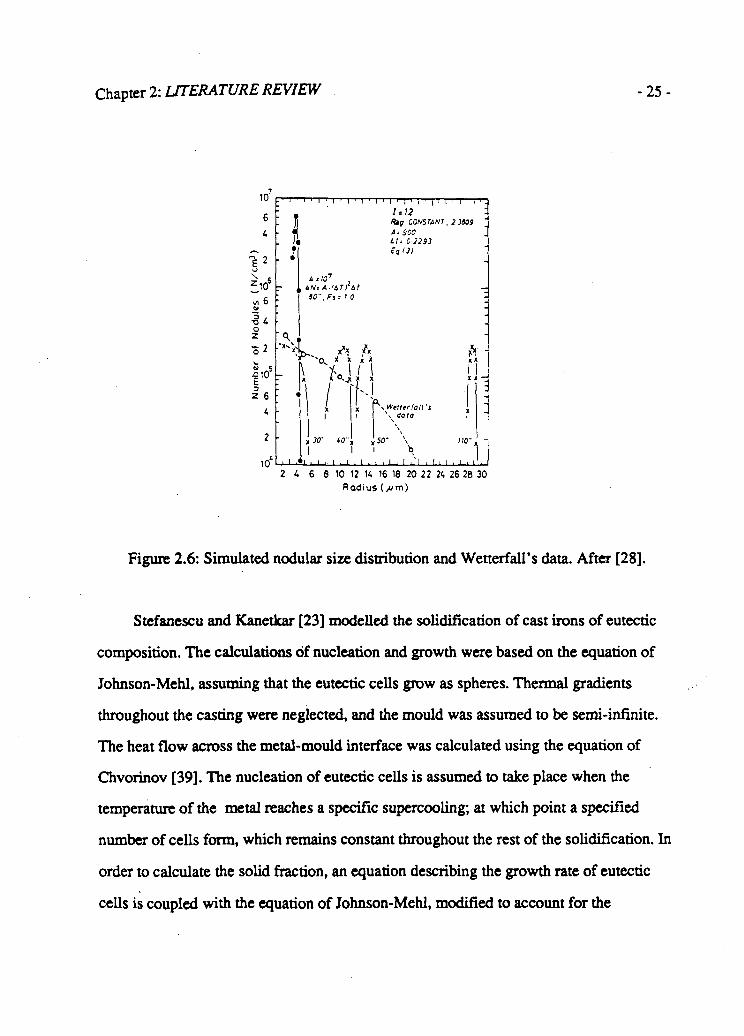
were substantially different, as shown in Figure 2.6. Su and co-workers concluded that
the equation of Oldfield is not suitable for the description of graphite nucleation in ductile
iron. They also suggested that the nucleation model should allow the nucleation to
continue even after recalescence begins.
1300
1270
1240
1210
f 1180
~Z ' 1 50
a 1090
° 1050
1030
VE&SUPSD
CALCULATED
MOLD
1CC0 10 20 30 40 50 60 70 80 90 100 110 120 130
T i m e ( sec.)
Figure 2.5: Comparison of simulated and measured cooling curves, after [28].
Chapter 2: LITERATURE REVIEW -25-
6 I i
i ' i • i ' 1 ' I ' I-.12
j • l 1 I 1 I 1 .
Rag CONSTANT, 2 3109 A = 900 Lt-. 0-2233
A-107
AN: A t&Tl &t SO". Fi= I 0
\ Wettrrlou i
fr -X X
2
Figure 2.6: Simulated nodular size distribution and We tt erf all's data. After [28].
Stefanescu and Kanetkar [23] modelled the solidification of cast irons of eutectic
composition. The calculations of nucleation and growth were based on the equation of
Johnson-Mehl, assuming that the eutectic cells grow as spheres. Thermal gradients
throughout the casting were neglected, and the mould was assumed to be semi-infinite.
The heat flow across the metal-mould interface was calculated using the equation of
Chvorinov [39]. The nucleation of eutectic cells is assumed to take place when the
temperature of the metal reaches a specific supercooling; at which point a specified
number of cells form, which remains constant throughout the rest of the solidification. In
order to calculate the solid fraction, an equation describing the growth rate of eutectic
cells is coupled with the equation of Johnson-Mehl, modified to account for the

Chapter 2: UTERATURE REVIEW -26-
impingement of the growing cells. Even though the calculations were not compared with
experiments, it is evident that the model does not describe the solidification of ductile
iron appropriately, since a cell number approximately five orders of magnitude larger
than that usually found in ductile iron had to be used in order to obtain cooling curves
qualitatively consistent with the experiments.
Kanetkar et al. [38] modelled the solidification of eutectic gray cast iron (flake
graphite) in sand molds. Similarly to models described above, the nucleation is assumed
to occur instantaneously at a unique temperature, and the equation of Johnson-Mehl is
used for the calculation of the solid fraction. In order to characterize the heat extraction
imposed on the casting, the temperature of the mould after pouring was measured at
several locations. These temperature readings were used to estimate the value of the heat
extraction as a function of the time elapsed from pouring. One-dimensional and
two-dimensional solutions of the heat transfer model were both tested. Figure 2.7 shows
the cooling curve for the center of a cylindrical casting of 50mm in diameter, as measured
and as calculated by the one-dimensional model (Eucast), and the two-dimensional model
(Bamacast). The two-dimensional model calculations are in good agreement with the
measurements.
In a more recent article, Stefanescu and Kanetkar [42] reported further work on the
mathematical modeling of the solidification of cast irons. As in earlier studies, they
assumed that the nucleation proceeds at a unique temperature simultaneously. This
assumption was based on experiments performed earlier, which showed that, for the case
of gray irons with uniform cell size, all nucleation occurred within a temperature range of
1°C. They also noted that the nucleation temperature and the number of nuclei are
functions of the cooling rate. Since Stefanescu and Kanetkar had not found enough

Chapter 2: LITERATURE REVIEW -27-
1300'
UJ
s OC 1 s Ui
• SIMULATED (BAMACAST)
A SIMULATED (EUCAST)
-EXPERIMENTAL
1000. 0 100 200 300
TIME, SECONDS 400 500 600
Figure 2.7: Measured and calculated cooling curve for the center of a 50mm diameter gray iron casting, after [38]
published data to establish the correlation between those variables, they used a simple
experiment to roughly estimate the relationship between the cell number and the casting
size for gray irons. The growth rate of eutectic cells was calculated applying the equation
derived for multidirectional non-isothermic solidification:
(2.17)
Where:
\ib =7.25 (108) to9.5 (lO"8) m/sK2

Chapter 2: LITERATURE REVIEW -28-
ATb = supercooling
The growth rate, as calculated by Equation 2.17, and the estimated number of
eutectic cells, have been used as input in an Avrami type equation to calculate the
fraction solid as a function of time. Measured and simulated cooling curves agreed fairly
well, as shown in Figure 2.8.
The model was also used to calculate the white/gray transition during solidification.
These calculations showed a significant discrepancy with the experiments.
The solidification of ductile iron was calculated by the model under assumptions
similar to those applied for gray iron. In this case, in order to obtain an acceptable fit
between experiments and calculations, Stefanescu and Kanetkar found it necessary to
assume cell counts approximately two orders of magnitude larger than the actual counts.
Zeng and Pehlke [43] modelled the cooling of gray cast iron during solidification.
The latent heat of solidification was released by means of a step-like function, between
1157 and 1143 C. Special care was taken in the selection of both sand mould and metal
properties, as well as in the estimation of the surface heat transfer coefficient between the
mould and the metal. Figure 2.9 shows temperature-time profiles for eight locations of
the casting, as measured and as calculated. There is agreement between the measured and
calculated curves, although some differences are evident.

Chapter 2: LITERATURE REVIEW -29-
Figure 2.8: Measured and calculated cooling curves for gray iron, after [42].

Chapter 2: LITERATURE REVIEW - 30
2200
2100 -
§ 1 9 0 0 g £ 1 8 0 0 2 UJ
H 1700
1600
1500
2200
7 i i 4
- 2 4 • 8
- 3 2 - 1 •
(a)
• - 1 1
200 400 600 800 1000 TIME (SEC.)
0 200 400 600 800 1000 TIME (SEC.)
Figure 2.9: Cooling curves corresponding to different positions within a cylindrical
casting, (a) experimental, (b) calculated, after [43].

Chapter 2: LITERATURE REVIEW -31 -
2.3.1 S U M M A R Y
In most cases the solidification models for cast iron are composed of two parts, a
heat transfer model and a nucleation and growth model. The following heat transfer
models have been investigated in the literature:
a) Simplified heat transfer models in which the heat extracted from the casting is
calculated on the basis of the Chvorinov equation or similar equations, and the
temperature is assumed to be uniform throughout the casting.
b) Complete heat transfer models, which include a description of the heat transfer at
the metal-mould interface, and the calculation of the temperature distribution
throughout the casting and mould.
Nucleation and growth have been approached in different ways. The following
nucleation models have been assumed:
c) Nucleation proceeds instantaneously at a given undercooling. The number of
nuclei is not calculated but estimated a priori.
d) The nucleation rate is a function of both the supercooling and a nucleation
constant. Nucleation stops when recalescence begins.
Most studies have considered that the growth rate of ductile iron eutectic cells is
controlled by the diffusion of C through the austenite layer enveloping the graphite
nodules.
In those cases in which the formation of all nuclei was assumed to proceed
simultaneously, Avrami type equations were applied to calculate the fraction solid. In the

Chapter 2: LITERATURE REVIEW -32-
cases based on a supercooling dependent nucleation rate, the growth of cells was
computed individually, which in turn allowed the nodular size distribution to be
calculated.
Some of the mathematical models reported in the literature predict cooling curves at
the centre of experimental gray iron castings accurately. This is not the case for ductile
iron, where calculated cooling curves and nodular size distributions do not entirely agree
with the experimental values.
2.4 C O O L I N G C U R V E S
The literature includes many articles describing different features of the cooling
curves of gray, compacted and ductile irons. Cooling curves are usually characterized by
four temperature points, the temperature of the austenite liquidus (TAL), the temperature
of eutectic start (TES), the temperature of eutectic undercooling (TEU) and the
temperature of eutectic recalescence (TER). These points are schematically shown in
Figure 2.10. In the case of cast irons of near eutectic composition TAL does not appear,
since no precipitation of primary austenite is expected. Highly hypereutectic cast irons
will show the precipitation of primary graphite (TGL), although this is difficult to detect
since the graphite is present in small amounts. Many studies have determined these
temperatures accurately by using differential thermal analysis (DTA). DTA is particularly
useful when an accurate determination of TAL and TES is required. Values of TEU and
TER can be readily obtained from conventional cooling curves.
L. Backerud et al. [14] studied the cooling curves of different types of cast iron.
They reported qualitative and quantitative differences in the solidification of cast irons of

Chapter 2: LITERATURE REVIEW - 3 3 -
different graphite morphology. In their experiments, melt samples were not poured but
extracted from the melt in a cup-like device. The cooling curves of eutectic cast irons of
different graphite morphology are shown in Figure 2.11. Eutectic gray iron solidifies with
a small supercooling, followed by a recalescence. Ductile iron shows a much larger
supercooling than gray iron, followed by a minor recalescence. Compacted graphite iron
shows a large supercooling, with the recalescence being more pronounced than that of
ductile iron. The differences in nucleation temperature are generally attributed to

Chapter 2: LITERATURE REVIEW -34-
differences in the chemistry of the irons. In the production of both ductile and compacted
irons, the melt is inoculated with alloys containing Mg, Ce, Al and Ti, or combinations of
those elements. The addition of these elements is considered to reduce the amounts of
oxygen and sulphur in the melt, which in nun diminishes the availability of certain
nucleation centres at low supercooling. The activation of new nucleation centers requires
a further temperature drop.
Figure 2.11: Cooling curves of different cast iron types, after [14].
The differences in the recalescence are explained by the growth characteristics of
the different cast irons. Gray iron eutectic grows with both austenite and graphite in
direct contact with the melt. The growth rate of the eutectic is then mainly controlled by

Chapter 2: LITERATURE REVIEW -35-
the diffusion of C in the melt, which is fast. Therefore shortly after nucleation the
temperature rises to near the eutectic temperature, as a result of the rapid heat generation
of the eutectic solidification. On the other hand, ductile iron graphite particles grow
mainly enveloped by austenite, therefore the growth rate is controlled by the C transport
from the liquid to the graphite through the solid austenite. The diffusion of C is slower in
the solid than in the liquid at similar temperature, therefore the release of latent heat is
slower for ductile iron than for gray iron. Thus, even though the supercooling is large at
the begining of the solidification, the recalescence is small. Eutectic compacted graphite
cast iron, on the other hand, is believed to grow with both austenite and graphite phases
in direct contact with the melt. Therefore the growth rate is considerably larger than that
of ductile iron, and the recalescence is intense.
D. Stefanescu et al. [15,44] also reported cooling curves for gray, ductile and
compacted irons. In their case, which differs from Backerud et al.[14], samples of the
melt were poured into sand cups, which were initially at room temperature. The results
are shown in Figure 2.12. In this case the TEU of compacted iron, curve (a), was lower
than that of ductile iron, curve (b), and the ductile iron did not show recalescence.
Table I summarizes the data in the literature concerning cooling curves of ductile
iron. Most of the data was obtained by using eutectometers, in which a small sample of
the melt (50 cm3) is poured into a sand cup, and the cooling curve obtained during
solidification with an immersed thermocouple.
One of the objectives of this investigation is to determine the effect of the cooling
rate on the characteristics of the cooling curve. In particular, how do TEU, TER and the
length of the eutectic plateau change with the heat extraction. This is not discussed

Chapter 2: LITERATURE REVIEW -36-
extensively in the literature. Rao et al.[45] reported cooling curves obtained at the centre
of cylinders having different diameters. Values of TEU and the length of the eutectic
plateau from the curves as a function of rod diameter are shown in Figures 2.13 and 2.14.
The results in Figure 2.13 show that the minimum temperature at the start of
solidification, TEU, is low for the smaller rod diameters, and increases for the larger
diameters. The length of the eutectic plateau, Figure 2.14, also increases with increasing
rod diameter.
270
E . SEC.
Figure 2.12: Cooling curves for various types of cast irons poured in a sand cup, after [44].

Chapter 2: UTERATURE REVIEW -37-
1-n H 1 1 1 1 1 1 1 20 40 60 80 100
Rod Diameter (mm)
Figure 2.13: Temperature of eutectic undercooling recorded at the center of cylindrical ductile iron castings, as a function of the section size.
Su et al. [28] measured cooling curves at several points of a casting with different
cooling rates. The curves are shown in Figure 2.5. None of the cooling curves show
recalescence, and the plateau or break in the curve occurs at different temperatures in
each case; the lower the plateau temperature, the shorter the plateau length.

Chapter 2: LITERATURE REVIEW - 3 8 -
Rod Diameter (mm)
Figure 2.14: Lenght of the eutectic plateau at the center of cylindrical ductile iron castings, as a function of the section size.
2.4.1 S U M M A R Y
There is enough evidence in the literature to conclude that gray iron solidifies with
a smaller supercooling than ductile iron, and that ductile iron shows little or no
recalescence.
For ductile iron, both the undercooling and the temperature of eutectic recalescence
depend on the size of the casting and the cooling rate.

Chapter 2: LITERATURE REVIEW
Table I: Data concerning cooling curves of cast iron.
- 3 9 -
Author Cast Iron Type
Mould Type
Section Size(mm)
TEU TER Length TEU(s)
Proeutectic Comments
Rao etal [45]
Ductile Shell 20 1020 1129 nil 1140 Rao etal [45] Ductile Shell 50 1111 1112 85 1150
Rao etal [45]
Ductile Shell 80 1134 1135 180 no
Rao etal [45]
Ductile Shell 90 1155 1155 290 no
Rao etal [45]
Ductile Sand 50 1114 1115 35 1170
Rao etal [45]
Ductile Sand 80 1139 1139 160 no
Rao etal [45]
Ductile Sand 90 1144 1144 190 1175
Rao etal [45]
Ductile Sand 100 1150 1150 280 no Cheng and Stefanescu
[17]
Ductile Eutectometer 1139 1140 55 1188 eutectic Cheng and Stefanescu
[17] Ductile Eutectometer 1140.5 1143 65 1188 hypoeutectic
Cheng and Stefanescu
[17] Ductile Eutectometer 1154.4 1157 120 1193 hypereutectic
Cheng and Stefanescu
[17] Ductile Eutectometer 1143 1143 140 no
Strong[19] Ductile Eutectometer 1145 1145 55 no Monroe and
Bates [18]
Ductile sand 22 1120 n/a n/a n/a uninoculated Monroe and Bates [18]
Ductile sand 22 1133 n/a n/a n/a inoculated Monroe and
Bates [18] Gray sand 22 1138 n/a n/a n/a base iron
Stefanescu etal[15]
Ductile Eutectometer 1140 1143 60 1190 hypoeutectic Stefanescu etal[15] Ductile Eutectometer 1151 1151 60 1190 hypoeutectic
Stefanescu etal[15]
Ductile Eutectometer 1140 1132 60 no eutectic Stefanescu et al[25]
Ductile Eutectometer 1143 1145 n/a n/a hypoeutectic Stefanescu et al[25] Ductile Eutectometer 1146 1148 n/a n/a eutectic
Stefanescu et al[25]
Ductile Eutectometer 1143 1145 n/a n/a eutectic
Stefanescu et al[25]
Ductile Eutectometer 1143 1143 n/a n/a eutectic Hummer[27] Ductile Sand 60 1150 1150 240 no eutectic

40
Chapter 3
OBJECTIVES OF THE PRESENT
RESEARCH
Mathematical modeling of the solidification and microstructure of ductile iron can
lead to the production of ductile iron under more controlled conditions and with
improved properties. Mathematical modelling, to be effective, requires detailed
information of the microsegregation of the alloying elements during solidification.
Microsegregation in ductile iron is not clearly understood, and the extent of the
microsegregation not well documented. As a result the first part of this investigation will
deal with microsegregation, with the following objectives:
1) To measure the effective partition coefficients of the alloying elements during
solidification.
2) To identify the mechanisms governing the segregation and to develop equations
which will enable the segregation to be calculated from first principles.
3) To correlate the segregation with the microstructure of ductile iron.

Chapter 3: OBJECTIVES OF . -41 -
Microsegregation of the solute elements will be measured in ductile iron samples,
both after casting and quenched during solidification, using electron probe microanalysis.
Examining quenched samples should provide a better understanding of both the
microsegregation pattern and the mechanisms leading to the segregation in ductile irons
solidified under normal conditions. In addition, the metallographic analysis of quenched
samples is essential for an understanding of the microstructural evolution during
solidification.
Samples will be quenched at progressive stages of solidification with different solid
fractions present. A general procedure for doing this is to extract portions of the melt
simultaneously in small containers, and place the individual containers in furnaces set at
temperatures between the liquidus and solidus temperatures of the melt. When
equilibrium between sample and furnace temperatures is reached, the samples are
quenched. An alternative procedure is to quench different melts of the same composition
at different times from the start of solidification. Both sampling methods described above
are laborious and difficult to reproduce. A different sampling technique, described in
detail in Chapter 4, has been devised for the present study, in which one sample
contained in a quartz tube, when quenched, has the full range of solid fraction.
The second part of this research program will model the solidification of ductile
iron. The analysis of the literature reviewed in Section 2.3 suggests that aspects of the
solidification of ductile iron have been either overlooked or not properly accounted for in
the reported models. Some of the main objections to the existing models are listed below:
1) None of the models take into account the fact that gray irons are, as a first
approximation, ternary Fe-C-Si alloys having Si contents between 2 and 3%. As

Chapter 3: OBJECTIVES OF . -42-
reported by Heine et al.[46,47,50] and Subramanian et al.[48,49], Si increases the
temperature gap between the stable and metastable eutectic temperatures
significantly, as shown in Figure 3.1. In addition, Si reduces the solubility of C in
austenite, shifting the point of maximum solubility of C in austenite and lowering
the carbon concentration at the eutectic point, as shown in Figure 3.2.
2) Most studies use simple formulations of the heat transfer problem, assuming, for
example, that the temperature throughout the casting is uniform. This reduces the
applicability of the model since temperature gradients normally exist in castings.
3) The solidification assumed in the models is cellular growth. Experimental
observations show growth of austenite is normally dendritic.
4) With one exception [28], graphite nucleation is considered to take place
instantaneously at a specified supercooling. With this assumption, nucleating sites,
and therefore the number of graphite nodules is specified for each calculation.
However this does not consider the dependence of the number of graphite nodules
on the cooling rate, which is significant. This factor must then be introduced in the
model as an input parameter.
5) The Johnson-Mehl equation is generally used to calculate the solid fraction during
solidification. This is incorrect as the equation only applies to the growth of
equiaxed spherical cells, which is not normally the case for ductile iron.
6) Growth rate calculations have been based on equations derived by Wetterfall et
al.[12], assuming that graphite nodules are enveloped by austenite immediately
after nucleation. Observations have been reported in which graphite nodules have
grown in the melt without an austenite envelope [12,22].

Chapter 3: OBJECTIVES OF . -43-
7) None of the models reviewed considers microsegregation of the solute elements.
Some authors [28] point out the need to include segregation for more accurate
calculations.
It is proposed in the second part of this investigation to develop an improved
mathematical model for the solidification of eutectic ductile iron. The model will include
the following:
1) Equilibrium temperatures and compositions will be calculated in the model based
on the ternary stable Fe-C-Si equilibrium diagram.
2) The thermal model will include a complete description of the heat transfer
throughout the casting-mold system.
3) The actual phase morphology during solidification will be included in the model.
4) Nucleation rate will be a function of the supercooling. Nodule density and nodule
size distribution will thus be determined from the model.
5) Graphite growth in direct contact with the melt will be considered.
6) The effect of Si segregation will be considered in the model.

Chapter 3: OBJECTIVES OF. -44-
Figure 3.1: Stable and metastable eutectic temperatures of cast iron as a function of the silicon content, after [49].

Chapter 3: OBJECTIVES OF -45-
2600
2000 .0 2J0 3J0 4.0 PERCENT CARBON OR CARBON EQUIVALENT
5.0
Figure 3.2: Influence of the silicon content on the eutectic region of the Fe-C-Si equilibrium diagram, after [47].

-46-
Chapter 4
EXPERIMENTAL METHODS AND
APPARATUS
4.1 M E L T I N G
Cast iron was melted in a 15 KW high frequency (10 KHz) induction furnace using
a silica crucible of 90 mm ID and 180 mm height. The charge materials were high quality
pig iron, low carbon steel scrap, electrolytic Mn, ferrosilicon, electrolytic copper,
electrolytic nickel, chrome, molybdenum and FeSiMgCe. The chemical composition of
the charge materials is listed in Table U, and the charge constitution for each of the
castings is listed in Table in. In order to produce ductile iron, the melt was inoculated
with 2 wt% of FeSiMgCe, and post-inoculated with 0.6 to 1 wt% of FeSi.
Charge materials were placed inside the crucible prior to heating. When the
temperature reached approximately 1380 C, the FeSiMgCe was added using the plunger
system shown in Figure 4.1. After the intense reaction between melt and FeSiMgCe was
completed, the slag was removed, and the FeSi added immediately. The melt was then
stirred, using a steel rod, to mix the FeSi in the melt.

Chapter 4: EXPERIMENTAL METHODS AND . -47-
Table II: Composition of charge materials.
Charge
Material
Composition (Wt%) Charge
Material Si C Mn Mg Ce Al Ca P S Fe
Pig Iron 0.18 4.3 0.009 " — ~ ~ — 0.027 0.015 balance Steel Scrap <0.10 0.18 0.75 — — — — <0.04 <0.05 balance
FeSi 76.6 — — — — 1.16 0.75 — — balance FeSiMgCe 45.1 — — 5.97 1.15 0.55 1.08 — — • balance
4.2 S A M P L I N G
Samples of partially solidified material were prepared in the following manner.
Quartz tubes of 15mm ID. Were inserted in the melt for 20 seconds, Figure 4.2-1, and
then filled with liquid metal, Figure 4.2-2. The tube was then slowly pulled from the
melt, progressively freezing the liquid from the top, Figure 4.2-3. With the metal in the
tube partially solidified, the tube was rapidly removed from the melt and quenched in
cold water, Figure 4.2-4. The cooling rate was estimated in one test by placing a Pt/Pt-Rd
thermocouple in the melt contained in the tube, and recording the temperature during
cooling. The cooling rate of the liquid was observed to be approximately l°C/sec.

Chapter 4: EXPERIMENTAL METHODS AND ...
Table HI: Charge constitution.
-48 -
TEST Kg Iron (grams)
Steel (grams)
FeSi (bath)(g)
FeSi (inocXg)
FeSiMgCe (grams)
Alloying (grams)
Cl 4800 700 55 55 110 Mn:60
C2 4200 800 43 50 110 Cu: 72
C3 4500 500 43 50 110 Cr: 23
C4 4500 500 43 50 110 Mo: 40
C5 4500 500 43 50 110 Ni: 52
C6 4500 500 43 50 120 ~
C7 5000 500 48 55 120 Mn: 17
C8 5000 500 48 55 120 Mn: 34
C9 5000 500 48 55 120 Mn: 51
CIO 4800 600 43 55 150 Cu: 25
C l l 4800 600 43 55 150 Cu: 50
C12 4800 600 43 55 150 — C13 4500 830 72 53 140 — C13 4800 600 43 55 150 — C14 4500 830 72 53 140 —

Chapter 4: EXPERIMENTAL METHODS AND -49-
protective lid — handle
FeSiMgCe -steel pipe tapered
stopper
Figure 4.1: Schematic of the plunger.

Chapter 4: EXPERIMENTAL METHODS AND ... -50

Chapter 4: EXPERIMENTAL METHODS AND . -51 -
4.3 C A S T I N G A N D T E M P E R A T U R E R E C O R D I N G
After samples were removed from the melt, the remaining melt was poured into a
resin coated silica sand mould, as shown schematically in Figure 4.3. The sand mould
was contained in a steel flask, as shown, to prevent expansion or cracking of the mould
due to the large stresses generated in the mould as the graphite nodules precipitate and
grow in the ductile iron. The melt was solidified primarily from the vertical side walls of
the mould. This was done by placing a refractory brick next to the bottom surface, to
reduce the heat flow, and a water cooled copper tube coil next to the vertical walls to
increase the heat flow. The copper tube was 10 mm ID and placed 10 mm from the
vertical surfaces of the mould.
SAND MOULD
86 mm
STEEL FLASK COPPER
COIL
REFRACTORY BRICK
Figure 4.3: Schematic of the mould.

Chapter 4: EXPERIMENTAL METHODS AND -52-
After pouring the top was covered by a lid made of refractory brick. Temperatures
during cooling were measured with four thermocouples placed at the positions shown in
Figure 4.4. Two bare thermocouples type K were used to measure the temperatures at the
mould next to the copper coil, TC4, and at the casting surface, TC3. Two thermocouples
type S protected by thin walled quartz tubes, TCI and TC2, were used to measure the
temperatures in the central region of the casting. The output of the thermocouples was
measured on a multichannel digital voltmeter Hewlett Packard 3480A. An ice/water bath
was used for the thermocouple cold junction. The measured voltages were converted to
temperatures using the polynomial function specified for the thermocouples [53]. The
accuracy of the temperature measurements was estimated to be +/- 3°C for the type S
thermocouples, and +/- 7°C for the type K thermocouples.
A long cylindrical mould, shown in Figure 4.5, was also used in which the heat
extraction is essentially unidirectional in the central portion of the casting. This mould
was made from the same materials used for the water cooled mould. Cooling curves at
two different points on a plane perpendicular to the cylinder axis were obtained. The
temperature of the casting surface was measured by using a bare type K thermocouple
marked TC6 in Figure 4.5. The temperature at the cylinder axis was measured by using a
type S thermocouple, TC5, protected by a thin-walled quartz tube. Internal diameters of
both 25 and 40mm were used in the tests.

Figure 4.4: Position of the thermocouples.

Figure 4.5: Schematic of the long cylindrical mold.

Chapter 4: EXPERIMENTAL METHODS AND . -55-
4.4 O P T I C A L M E T A L L O G R A P H Y
The quenched samples were mounted on a magnetic table and ground to produce a
plane section parallel to the sample rod axis, polished and etched for examination and
microanalysis. The cast ingot was sectioned at a plane perpendicular to TC2 and
containing TC3, polished and etched.
The fraction of quenched liquid and solid present at specific locations within the
quenched sample were measured using a Leitz Tas Plus Image Analyzer. The phases
present in the etched microstructure are identified on the basis of the differences in their
gray levels. The surface area occupied by each phase can then be measured. The solid
fraction was calculated as the ratio between the surface area occupied by austenite and
graphite, and the total surface area examined. Image analysis was also used to measure
nodule counts, and to characterize the nodular size distribution at different locations of
the cast ingots.
4.5 E L E C T R O N M E T A L L O G R A P H Y A N D M I C R O A N A L Y S I S
Quenched and as-cast samples were examined in a Hitachi scanning electron
microscope. Quantitative measurements of the composition of the samples at specific
locations were made with a MICROSPEC Wavelength Dispersive X-ray Analyzer
(WDX) attached to the SEM. Microanalysis was carried out at 20 Kv acceleration
potential and 45° take-off angle. Pure elemental standards were used in all cases. The
specimen current was carefully controlled during the operation of the probe. Typical
currents were 15 nanoampers. Peak and background count times were 10 and 5 seconds

Chapter 4: EXPERIMENTAL METHODS AND . -56-
respectively for the high concentration elements, such as Fe and Si. For low
concentration elements (0.1 to 2 wt%), the peak and background count times were
extended to 20 and 7 seconds respectively to obtain better statistics.
The output of the Wavelength Dispersive X-ray Analyzer is in counts per second at
a particular wavelength. This is converted to composition by comparing the output to that
of pure elemental standards and using the programme FRAME, supported by the
microprobe software. This programme corrects for absorption, fluorescence, atomic
number and dead time. A sample of the microprobe output and analyzed results is given
in Appendix 1. The output gives element composition values in weight percent and
atomic percent. Weight percents were used in this study.
Measurements of carbon concentration were not made since its consideration in the
analysis would require frequent changes in the acceleration potential of the microprobe
electron beam, which is time consuming, and would make it very difficult to collect the
number of readings necessary for this study. Since C diffuses interstitially in Fe at a high
rate, extensive diffusion would be anticipated during cooling of the casting. As a result
the carbon distribution at room temperature could be appreciably different from that at
the end of solidification.
The reproducibility of the results for specific operative conditions was determined
by repeat measurements. Fifteen measurements were made on each sample and the mean
value and standard deviation calculated for both the true peak counts and the background
counts. Table IV lists the results for the pure elemental standards and samples containing
low concentrations of Si and Mn. The dispersion of the values is small for all the
standards, the ratio of the standard deviation to the mean value ranging from 0.0063 for

Chapter 4: EXPERIMENTAL METHODS AND ... -57-
Si to 0.0031 for Cr. Note that this analysis is testing the performance of the overall probe
system, including variations on the acceleration voltage, beam current and detector
performance, together with the natural random characteristics of the X-rays. The count
readings on samples containing Si and Mn were used to estimate the experimental error
of the probe under actual analysis conditions. As shown in Table IV, for samples
containing Si and Mn, the ratio between the mean and the standard deviation is
approximately one order of magnitude larger than that obtained for the standards.
Assuming that the number of readings is large enough to consider the standard deviation
calculated as equal to the standard deviation of the random variable "counts per second",
the accuracy of the calculation of the median value of counts per second as a function of
the sample size can be calculated on the basis of the law of large numbers for a sample
mean [54], which states that the probability of the mean value of a sample of n elements
will fall outside an interval (u. - e, n + e), for any given e > 0, is given by the following
equation:
Where:
o = standard deviation u, = mean value of the distribution X* = mean value of the sample of n elements
The less favorable value of standard deviation in Table IV, which corresponds to
sample Mnl, is standardized as follows
P(\X*-\L\>E)<, (4.1) n
(4.2)

Chapter 4: EXPERIMENTAL METHODS AND -58-
Assuming a sample of three elements, and an interval X* ± 10%, the probability P is
equal to:
PQX*-\i\>0A)<. = 0.10 (4.3)
These results show that the probability of the median of a sample of three elements
is inside the interval u.± 10% is 90 %. It can be then assumed that if the median of a
sample of three elements is affected by a 10% error margin, there will be a 90%
probability that the median of the distribution is within the range. Following this, all
microprobe analysis reported below will be the average of three readings and will carry a
10% error bar, unless otherwise specified. Further contributions to the experimental error
can be expected from other factors, such as the dispersion in the standard readings, and,
more significantly, the dispersion in the background counts. Nevertheless, the error
margin of 10% adopted is considered to be large enough to account for the influence of
these factors. For simplicity, the error bars will not be calculated for every point, but will
be taken as ten percent of the average composition of the sample.

Chapter 4: EXPERIMENTAL METHODS AND . - 5 9 -
TABLEIV: Data of fifteen microprobe measurements of elemental standards and test samples.
Standard Samples (counts/sec) Test Samples (counts/sec)
Fe Si Mn Cu Cr Mo Mn 1 Mn2 Si
mean value true peak
5690 9817 5154 5134 5187 2083 26.9 37.4 134.3
Std. deviation true peak
22.2 62.0 17.0 2Z7 16.2 9.7 1.5 1.2 5.8
mean/std deviation true
peak 0.004 0.0063 0.0033 0.0044 0.0031 0.0038 0.056 0.03240 0.043
mean value background
13.17 2.89 9.97 23.4 9.08 6.1 8.95 8.74 3.55
Std. deviation background
0.817 0.38 0.79 0.90 0.89 0.64 0.632 0.51 1.65
mean/std deviation
background 0.062 0.130 0.079 0.038 0.098 0.105 0.071 0.058 0.46

-60-
Chapter 5
SEGREGATION AND
MICROSTRUCTURE
RESULTS AND DISCUSSION
Segregation was investigated in both as-cast and quenched samples. The
compositions of the ductile irons examined are listed in Table V. The irons were all of
near eutectic composition, with single alloying elements added, except for casting CO.
5.1 S E G R E G A T I O N I N C A S T S A M P L E S
It has been suggested [51,52] that the concentration of an alloying element with a
segregation coefficient, k, smaller than 1, when measured along a line between the
centers of two graphite nodules, will show segregation patterns as illustrated in Figure
5.1. If k is smaller than 1, the concentration would increase with distance from each
graphite nodule, as shown, until a maximum is reached midway between the nodules.
This concentration profile would be produced by the growth of equiaxed spherical cells,

Chapter 5: SEGREGATION AND MICROSTRUCTURE . -61-
as illustrated in Figure 5.2. The cells are formed by graphite spheroids enveloped by
austenite. Solidification mechanisms consistent with that shown in Figure 5.2 have been
supported by some authors, as described in section 2.2.
Figure 5.1: Representation of the solute concentration along a line between graphite nodules in ductile iron, a) k > 1 ; b) k < 1

Chapter 5: SEGREGATION AND MICROSTRUCTURE... - 62 -
Table V: Alloying element content in the ductile irons examined
TEST CO Cl C2 C3 C4 C5 C6 C7 C8 C9 CIO c n
Alloying
Concentration
Wt%
0.78Mn
0.98Cu 1.34Mn 1.36Cu 0.5Cr 0.83Mo 0.83Ni 2.45Si 0.4 lMn 0.74Mn 1.05Mn 0.50Cu 0.9 lCu
Figure 5.2: Representation of equiaxed cellular growth in ductile iron.
In an attempt to verify the solidification mechanisms described above, the
segregation pattern in the vicinity of a graphite nodule was measured on samples of cast
iron CO, alloyed with both Cu and Mn. These alloying elements were chosen because Cu
has k>\ and Mn has k<\.

-63-
5.1.1 S E G R E G A T I O N P A T T E R N I N T H E V I C I N I T Y O F A
G R A P H I T E N O D U L E .
Measurements of solute concentration were made using microprobe analysis at
points spaced at approximately 8 microns intervals along paths 1-4 between the nodules,
as shown schematically in Figure 5.3.
Figure 5.3: Schematic of analysis along lines between nodules.
The results of the analysis are given in Figure 5.4. For Si, Figure 5.4.(a),
measurements were started near the nodule/metal interface. The concentration along the
four directions, marked 1 to 4, are observed to differ appreciably, exhibiting marked
fluctuations in concentration with distance from the nodule. The Si concentration along

Chapter 5: SEGREGATION AND MICROSTRUCTURE . -64-
line 1 is essentially constant, with a small drop at 45 microns. Scans 2, 3, and 4, exhibit a
sharp drop initially, then the Si concentration rises to an essentially constant level, the
fluctuations differing for each scan. Results for Cu and Mn are shown in Figures 5.4 (b)
and (c) respectively. As in the case of Si, composition variations are small along line 1.
The concentration of Cu along lines 2, 3 and 4 decreases with the distance from the
nodule surface. The Mn concentration increases with the distance from the nodule.
A similar series of measurements was done along three lines starting at the surface
of a nodule, on a sample containing 0.88% Mn. The concentration variation with
distances from the nodule for Si and Mn are shown for each line in Figure 5.5(a-c). As
before, the scans show marked fluctuations. The concentration of Mn along line 1, Figure
5.5 (a), shows a marked increase near the nodule, followed by decrease, reaching a
minimum value of 0.7% Mn near the mid point between the nodules. After the mid point
the Mn concentration rises again to 0.95%, then drops to 0.7% as the scan approaches the
end graphite nodule. The Si concentration shown in the figure indicates that, with few
exceptions, the Si concentration mirrors the Mn concentration, with drops in Si
concentration corresponding to increases in Mn concentration. The concentration of Mn
along line 2, Figure 5.5 (b), increases with the distance from the nodule, reaching a
maximum value of 1.06% at 12 microns, after which the concentration of Mn drops
progressively, reaching a value of 0.8% in the vicinity of the second nodule. The
concentration of Si along line 2 shows a drop, coincident with the maximum Mn
concentration, but remains relatively constant otherwise. The segregation profile along
line 3, Figure 5.5 (c), shows relatively small variations in concentration for both Si and
Mn.

Chapter 5: SEGREGATION AND MICROSTRUCTURE ...
2.7 -r
2.6 -
1.7 -
1.6 -
1.5 H 1 1 1 1 1 1 -
0 20 40 60 Distance (microns)
Figure 5.4 (a)
1.7 - T
1.6 -
1.5 -
0.5 -
0.4 -I 1 1 1 1 1 r-0 20 40 60
Distance (microns)
Figure 5.4 (b)

Chapter 5: SEGREGATION AND MICROSTRUCTURE .
Figure 5.4: Solute concentration along lines 1 to 4. (a) Si, (b) Cu, (c) Mn.

Chapter 5: SEGREGATION AND MICROSTRUCTURE . -67 -
0 20 40 60
Distance (microns) Figure 5.5 (a)
0 10 20 30 40
Distance (microns) Figure 5.5 (b)

Chapter 5: SEGREGATION AND MICROSTRUCTURE . -68-
5 c g « c <D o c o O
CO
ti a
u
Distance (microns)
Figure 5.5: Si and Mn segregation along lines between nodules, (a) line 1, (b) line 2, (c) line 3.
Additional scans were made between adjacent nodules. The results were similar to
those illustrated in Figures 5.4 and 5.5 in the majority of the cases. However, in some
scans much larger variations in solute concentration were observed. For example, Figure
5.6 shows the variations in the concentration of Cu and Mn along a line between nodules
of the same sample from which the curves in Figure 5.4 were obtained. Both Si and Cu
exhibit a large drop in concentration near the mid-point between the nodules, and the Mn
a larger increase. The levels of segregation of Cu and Mn shown in Figure 5.6 are
considerably higher than those shown in Figure 5.4. Similarly, a qualitative analysis of
the concentration of Mn and Si along a line between graphite nodules, for the same alloy
from which the curves in Figure 5.5 were obtained, is shown in Figure 5.7. Marked

Chapter 5: SEGREGATION AND MICROSTRUCTURE . -69-
segregation of Mn is observed approximately at the mid point between nodules, in
coincidence with a drop in the concentration of Si. Although this results are qualitative,
the segregation shown in Figure 5.7 is clearly greater than that observed in Figure 5.5.
2.6 -•
2.4 -
2.2 -
I 2 " I 1.8 -
t: 1.6 -
1 » • ro 1-2 -c 2 1
< 0.8 -
0.6 -
0.4 -
0.2 -
0 -| 1 1 1 1 1 1 1 1 1 1 0 20 40 60 80 100
Distance (microns)
Figure 5.6: Solute concentration along line between nodules.
The spherical symmetry of the composition field around a graphite nodule was
investigated by measuring the solute concentration along a circular path, concentric with
the centre of a nodule. The results are shown in Figure 5.8. Small scale fluctuations in the
Cu and Mn concentrations are observed, but no large scale fluctuations are evident for
either element.

Chapter 5: SEGREGATION AND MICROSTRUCTURE .

Chapter 5: SEGREGATION AND MICROSTRUCTURE . -71 -
In summary, the analyses of the segregation of Cu, Mn and Si along lines between
nodules gives scattered results. In many cases Mn is preferentially concentrated near the
centre point between nodules, although the extent of the segregation varies widely from
one case to another. In other cases, different composition profiles were observed along
lines between nodules, as shown in Figure 5.5 (a), where two Mn peaks are observed
along the line, and in Figure 5.5 (c), where almost no variation of the Mn concentration is
observed. These observations do not correspond with the model of spherical cells
described above. It is believed that the examination of the microstructure of samples
quenched during solidification will allow a better interpretation of the results reported in
this section.
5.1.2 Q U A N T I T A T I V E V A L U E S F O R S E G R E G A T I O N I N C A S T
S A M P L E S
The segregation of the alloying elements between adjacent nodules in ductile iron
shows appreciable scatter for different pairs of nodules in a given casting, as shown in
section 5.1.1. As a result the measured solute distribution along a path between nodules
in a casting is not suitable to quantitatively describe the segregation of specific elements.
As an alternative the segregation will be characterized by the ratio between the solute
concentration in the vicinity of a large graphite nodule, and the solute concentration at
locations of the microstructure having the highest segregation. The position of highly
segregated areas in the microstructure of carbide-free ductile iron is not evident when the
polished surface is examined on the scanning electron microscope. However, after
several successful attempts to find areas of high concentration with the help of the WDX,

Chapter 5: SEGREGATION AND MICROSTRUCTURE . -72-
it was noted that either microporosity or finer pearlite were associated with regions
having the highest concentration of carbide promoting elements, and the lowest in
graphitizing elements.
Table VI: Segregation in sand cast ductile iron.
TEST ALLOYING ELEMENT
AVERAGE SOLUTE
CONCENTRATION
ADJACENT TO NODULE (1) (Wt%)
LAST TO SOLIDIFY (2) (Wt%)
RATIO (l)/(2)
CI Mn 1.34 0.92 2.62 2.85
C2 Cu 1.36 1.87 0.37 0.20
C3 Cr 0.50 0.28 2.58* 9.21*
C4 Mo 0.83 0.23 43.2* 188*
C5 Ni 0.83 0.98 0.54 0.55
C6 Si 2.45 2.63 1.25 0.47
* Contains precipitate phase.

Chapter 5: SEGREGATION AND MICROSTRUCTURE. - 7 3 -
Solute concentrations adjacent to large nodules and at the highly segregated areas
are listed in Table VI. Each value listed is the average of five readings. The concentration
of solute in the vicinity of large nodules is lower than the average concentration of the
alloy, for Mn, Mo and Cr, and higher than the average for Cu, Ni and Si. At the highly
segregated areas the concentration of Mn, Mo and Cr is higher than the average, and the
concentration of Cu, Ni and Si is lower. Segregation ratios listed in Table VI are
calculated as the ratio of the solute concentration in highly segregated areas over the
solute concentration adjacent to a graphite nodule. The segregation ratio is a measure of
the maximum segregation present in the sand cast ductile iron. Alloys containing Cr and
Mo contain carbides or other phase constituents. Therefore the ratios listed for those
elements can be misleading, since they do not correlate solute concentrations at two
locations of the same phase.
5.2 A N A L Y S I S O F Q U E N C H E D S A M P L E S
5.2.1 M I C R O S T R U C T U R E O F Q U E N C H E D S A M P L E S
The solidification of slowly cooled graphitic cast iron follows the stable Fe-C-Si
equilibrium diagram. At the eutectic temperature, austenite, graphite and liquid coexist. If
the solidification occurs more rapidly, with larger supercooling of the melt, metastable
cementite can nucleate. The growth rate of the metastable eutectic cementite-austenite is
much larger than that of the stable eutectic. In consequence, the precipitation of graphite
is prevented, and solidification is completed following the metastable Fe-C-Si
equilibrium diagram. Because the precipitation of graphite is prevented, it becomes
possible to quench the liquid iron without major restrictions in sample size or cooling
rate. In particular, for liquid near the stable eutectic temperature, a supercooling of

Chapter 5: SEGREGATION AND MICROSTRUCTURE . -74-
approximately 20°C is enough to result in the formation of metastable eutectic. The
appearance of the quenched liquid is illustrated in Figure 5.9. The microstructure consists
of a fine mixture of cementite, A, and austenite, B. Microprobe analyses showed that the
alloying elements are partitioned between the two phases, with the carbide forming
elements like Mn, Mo and Cr, concentrated in the cementite, and Cu, Ni and Si
concentrated in the austenite.
A typical microstructure of a quenched sample is shown in Figure 5.10. Note that
the austenite dendrites, appearing white, are randomly oriented. Microstructures of
quenched samples of alloy C6, observed at higher magnification are shown in Figures
5.11 to 5.15. The microstructure of quenched liquid at the bottom of the sample is shown
in Figure 5.11. Small spheroidal particles of graphite, (G), are present in the structure.
This suggests that the alloy is slightly hypereutectic. Further from the bottom, for a solid
fraction of 18%, a higher number of larger graphite spheroids are present, as shown in
Figure 5.12. An austenite dendritic structure is also evident, with the branches appearing
white, D, and the quenched liquid surrounding the dendrites gray, C. As we move up the
sample, Figure 5.13 (a) (fraction solid 67%), the graphite nodules become larger, and the
amount of austenite increases. At this point most graphite particles are enveloped by
austenite. Nevertheless, as shown in Figure 5.13 (b), some graphite particles remain in
contact with the liquid phase. As the fraction of solid increases to 94%, Figure 5.14, the
graphite nodules have further increased in size, and the dendritic structure can no longer
be resolved. The continuity of the liquid phase is lost, and isolated pockets of liquid are
evident. In Figure 5.15, for 100% solid fraction, the solidification was complete before
quenching. No second phase precipitates are observed.

Chapter 5: SEGREGATION AND MICROSTRUCTURE . 75-

Chapter 5: SEGREGATION AND MICROSTRUCTURE .
Figure 5.10: Structure of quenched sample (x 40)

Chapter 5: SEGREGATION AND MICROSTRUCTURE ... -77
j I
Figure 5.12: Microstructure of quenched sample for solid fraction 18% (x 100)
9 v v * - \ , i !-V? • • \ 1 " vr-^ ; . v . • • • • • •
Figure 5.14: Microstructure of quenched sample for solid fraction 94% (x 100)

Chapter 5: SEGREGATION AND MICROSTRUCTURE . -78-
b)(x400)

Chapter 5: SEGREGATION AND MICROSTRUCTURE ... - 79 -
Figure 5.15: Microstructure of quenched sample for solid fraction 100% (x 100)
The appearance of the microstructure of the quenched samples suggests that
austenite dendrites and graphite nodules nucleate and grow in the eutectic cast iron
independently. As solidification proceeds the austenite dendrite branches meet and
envelop the nodules, which progressively distorts the dendritic structure until it can no
longer be identified. Further growth occurs as a result of the thickening of the austenite
layer surrounding the graphite. At the end of solidification the continuity of the liquid
phase is lost, and isolated pockets of liquid are the last to solidify. Although these
observations are based on small samples cooled relatively rapidly, they clearly are in
agreement with the solidification mechanisms reported by several authors, as described in
section 2.1. In view of this agreement, the measurements of segregation in the quenched
samples will be assumed valid for cast samples as well. The validity of this assumption
will be assessed by comparing the maximum and minimum values of solute concentration
measured in quenched samples with those measured in cast samples.

Chapter 5: SEGREGATION AND MICROSTRUCTURE . -80-
5.2.2 M E A S U R E M E N T S O F S O L U T E C O N C E N T R A T I O N A S A
F U N C T I O N O F T H E F R A C T I O N S O L I D
Quantitative microprobe analyses were made within several areas of each of the
quenched rods. For each area analyzed, the composition was measured at three locations
of the rrucrostructure, as indicated in Figure 5.16. Position A is in austenite, next to a
large graphite nodule, or alternatively, at the centre of the austenite field for the smaller
solid fractions. Position B is in austenite, at approximately 1.5 microns from the
austenite/quenched liquid interface. Position C is in the quenched liquid.
Figure 5.16: Location of the microstructure at which solute concentration was measured (x500).

Chapter 5: SEGREGATION AND MICROSTRUCTURE . -81-
The distance from the quenched interface at which position B is located is selected
to avoid possible interference from the neighboring quenched liquid, which has a
different solute content. When the electron beam of the microprobe strikes the specimen
surface, X rays are produced. The X rays are generated from a nearly spheroidal volume,
of diameter, S. This diameter can be calculated using the following equation [55]:
5 =0,033(V1'7-Vi1-7)4: C5-1) pZ
Where:
S = diameter of region from which X rays are generated (microns) V = energy of the incident electrons [ KeV ] Vk = absorption edge of the element analyzed [ KeV ] A = atomic weight of the specimen p = density of the specimen Z = atomic number of the specimen
For pure iron, equation 5.1 gives a spot diameter of 1.2 microns. This calculation
does not account for the dimension of the incident electron beam. The true spot size can
be found by adding the electron beam diameter to the calculated spot size. Under the
present operational conditions the electron beam of the scanning electron microscope has
a diameter of approximately 0.2 microns, which gives an effective spot diameter of 1.4
microns. Thus, measurements of the composition of the austenite can be made with the
electron beam positioned at 1 micron or more from the interface between austenite and
quenched liquid. This can be related to Figure 5.17, in which Mn counts are plotted as a
function of distance along a line between the vicinity of a nodule and quenched liquid. A

Chapter 5: SEGREGATION AND MICROSTRUCTURE . - 8 2 -
gradual increase in Mn counts is observed between 0 and 3 microns. When the beam is
positioned within a micron of the interface, count readings are higher than expected, as a
result of the radiation from the quenched liquid. On the basis of the above considerations,
routine measurements of the composition of austenite in positions A and B, were made at
points located within 1 and 1.5 microns from the quenched interface.
80
30 H 1 1 1 H 0 2 4
Distance (microns)
Figure 5.17: Mn counts intensity along a line crossing an austenite/quenched-liquid interface.
As described above, quenching the melt results in a structure consisting of a fine
mixture of austenite and cementite. The presence of two different phases complicates the
analysis of the quenched liquid, since the area analyzed is not homogeneous. This
difficulty can be overcome by analyzing, whenever possible, large areas of the fine
structure of approximately 50 square microns.

Chapter 5: SEGREGATION AND MICROSTRUCTURE -83-
Measurements of Mn concentration were made at three locations in the quenched
irons, A, B and C, for areas having different solid fractions before quenching. Four
different Mn levels were investigated. The results are listed in Table VU.
The results, position A, show that as the solid fraction increases, there is little
change in the Mn concentration in the austenite adjacent to the nodules. Near the
quenched interface, position B, a gradual increase in the Mn concentration is observed for
the smaller solid fractions, with a more pronounced increase for solid fractions greater
than 80%. The concentration of Mn increases by a factor of 2 from the start to the end of
solidification. In the quenched liquid, position C, the concentration of solute is
appreciably higher than in positions A or B, and increases to higher levels as the solid
fraction increases. In Table VU the Mn concentration at position A is listed for 0 solid
fraction. This composition is equivalent to the composition at the centre of an austenite
dendrite near the start of solidification. The average alloy composition, listed in Table
VII, is measured by electron probe microanalysis in which an area at the bottom of the
sample, consisting entirely of quenched liquid, was scanned at 20,000 magnification to
give the average composition of the area.
The concentration of Cu at points A, B and C in quenched samples having three
different copper levels are listed in Table VIII. The concentration of Cu near the graphite
nodules, column A, is essentially independent of the solid fraction. There is a decrease in
the Cu concentration for the higher solid fractions in alloys C2 and C10. Near the
quenched interface, column B, a gradual decrease in the solute concentration is observed
as the solid fraction increases, the concentration of Cu decreasing by a factor of 2.2 to
2.5. In the quenched liquid, C, the concentration of Cu is appreciably lower than that in A
or B, and decreases with increasing solid fraction.

Chapter 5: SEGREGATION AND MICROSTRUCTURE ...
Table VII: Local Mn concentration in quenched samples.
TEST (Alloy)
Solid fraction
Position A
Position B
Position C
Ratio B/C
CI
(1.34%Mn)
0 0.95 - -- 0.70
CI
(1.34%Mn)
30 0.95 0.92 1.40 0.66
CI
(1.34%Mn)
31 1.07 0.94 1.51 0.62 CI
(1.34%Mn)
34 0.93 0.99 1.50 0.66 CI
(1.34%Mn) 48 1.02 1.21 1.60 0.75
CI
(1.34%Mn) 73 0.95 1.29 2.25 0.57
CI
(1.34%Mn) 86 0.91 1.23 2.60 0.47
CI
(1.34%Mn)
94 0.95 2.01 3.47 0.58
C7
(0.41%Mn)
0 0.27 -- - 0.66
C7
(0.41%Mn)
36 0.22 0.26 0.44 0.59 C7
(0.41%Mn)
51 0.27 0.32 0.52 0.61 C7
(0.41%Mn) 64 0.28 0.32 0.54 0.59
C7
(0.41%Mn) 83 0.28 0.49 0.81 0.60
C7
(0.41%Mn) 96 0.28 0.52 0.99 0.52
C8
(0.73 %Mn)
0 .54 -- -- 0.73
C8
(0.73 %Mn)
33 0.50 0.56 0.91 0.62 C8
(0.73 %Mn)
54 0.55 0.53 1.00 0.53 C8
(0.73 %Mn) 83 0.58 0.71 1.29 0.55
C8
(0.73 %Mn) 88 0.57 0.84 1.59 0.53
C8
(0.73 %Mn) 95 0.57 0.93 1.98 0.47
C9
(1.05%Mn)
0 0.75 ~ - 0.72
C9
(1.05%Mn)
44 0.78 0.86 1.44 0.60
C9
(1.05%Mn)
50 0.89 0.90 1.61 0.55 C9
(1.05%Mn)
80 0.77 1.00 1.77 0.54 C9
(1.05%Mn) 86 0.84 1.23 2.27 0.56
C9
(1.05%Mn) 92 0.87 1.25 2.40 0.55
C9
(1.05%Mn) 97 0.73 1.70 3.71 0.46

Chapter 5: SEGREGATION AND MICROSTRUCTURE . -85-
Table VTU: Local concentration of Cu in quenched samples.
TEST (alloy)
solid fraction
Position A
Position B
Position C
Ratio B/C
0 1.87 -- -- 1.37 32 1.93 1.91 1.37 1.39
C2 38 1.78 1.77 1.18 1.50 67. 1.84 1.59 1.03 1.54
(1.36%Cu) 84 1.84 1.30 0.64 2.03 92 1.88 0.92 0.47 1.95 96 1.57 0.79 0.40 1.98 97 1.48 0.89 0.38 2.34 0 0.66 -- - 1.32 27 0.60 0.67 0.45 1.48
CIO 44 0.66 0.57 0.40 1.43 69 0.66 0.54 0.37 1.46
(0.50%Cu) 76 0.62 0.46 0.24 1.92 89 0.58 0.34 0.22 1.53 94 0.55 0.29 0.21 1.40 0 1.12 -- - 1.25 53 1.14 1.03 0.63 1.63
Cl l 78 1.16 0.87 0.53 1.64 84 1.12 0.69 0.37 1.86
(0.91%Cu) 92 1.00 0.41 0.27 1.52 96 1.17 0.40 0.25 1.60

Chapter 5: SEGREGATION AND MICROSTRUCTURE . -86-
Local solute concentrations for alloys containing Cr, Mo, Ni and Si are listed in
Table DC Similar to Mn, the concentration of Cr remains almost unchanged next to the
nodules, and increases at positions B and C as the fraction solid increases. The quenched
liquid, C, is always richer in solute than A or B. In samples of alloy C3, massive
ledeburite was present for solid fractions greater than 75%. With ledeburite present,
measurements of solute concentration in the quenched liquid were not significant.
Carbide precipitation was evident in quenched samples of alloy C4, which contains
Mo, for solid fractions larger than 90%. The concentration of Mo at position A is
approximately constant with solid fraction, with some scatter. Positions B and C become
richer in solute as the solid fraction increases. The austenite next to the quenched
interface, B, for the largest solid fraction measured, is approximately 2.5 times richer in
solute than the austenite next to the graphite nodules, A. * -
Sample C5, alloyed with Ni, shows segregation characteristics similar to the
samples containing Cu. The concentration of Ni in both B and C decreases with
increasing solid fraction. The concentration of Ni at B, for the highest solid fraction
measured, is approximately half of the concentration at A.
Although Si is present in every sample, its segregation behavior was only accounted
for in detail in a sample of unalloyed iron C6, to avoid interference from other solutes.
Table DC lists solute concentrations for Si at position B only. The concentration of Si
tends to decrease as the solid fraction increases, but the amount of segregation is small.

Chapter 5: SEGREGATION AND MICROSTRUCTURE ...
Table DC: Local concentration of Cr, Mo, Ni and Si in quenched samples.
TEST (alloy)
Solid Fraction
Position A
Position B
Position C
Ratio B/C
0 0.30 -- -- 0.60 19 0.31 0.31 0.66 0.47
C3 21 0.31 0.29 0.70 0.41 48 0.31 0.35 0.72 0.49
(0.5%Cr) 66 0.31 0.36 0.81 0.44 71 0.28 0.44 0.98 0.45 0 0.21 -- - 0.26 9 0.21 0.20 1.04 0.19 24 0.17 0.16 0.85 0.19
C4 37 0.19 0.24 1.06 0.23 38 0.18 0.25 1.26 0.20
(0.83%Mo) 57 0.21 0.30 2.00 0.15 67 0.22 0.40 2.13 0.19 72 0.25 0.43 4.15 0.10 89 0.19 0.49 3.26 0.15 0 1.02 -- - 1.23 40 1.03 1.01 0.74 1.36
C5 43 1.08 0.95 0.69 1.38 50 1.08 1.06 0.63 1.68
(0.83%Ni) 71 1.10 0.98 0.51 1.92 89 1.05 0.88 0.45 1.95 94 1.02 0.69 0.31 2.22 98 1.02 0.63 0.34 1.85 0 2.67 -- -- 1.09. 22 -- 2.45 - --
C6 22 - 2.72 -- -29 -- 2.48 ~ --
(2.45%Si) 52 -- 2.31 -- --
82 ~ 2.18 -- --
91 - 1.96 - --

- 8 8 -
5.2.3 E S T I M A T I O N O F P A R T I T I O N C O E F F I C I E N T S O F T H E
A L L O Y I N G E L E M E N T S
Equilibrium segregation coefficients, k0, are defined as the ratio of the
concentration of solute in the homogeneous solid phase over the concentration of solute
in the liquid in equilibrium with the solid. Values of k0 can be determined from phase
diagrams. As shown in sections 5.2.1 and 5.2.2, during the solidification of ductile iron
solute is segregated within the austenite. Therefore solidification does not take place
under equilibrium conditions, where k0 is applicable. Under non-equilibrium conditions
an effective segregation coefficient is used, ke, defined as the ratio of the solute
concentrations in the solid and the liquid at the solid/liquid interface at a given stage
during solidification. The value of ke can only be determined experimentally, and depends
on the solidification conditions and the amount solidified.
An approximate method to determine the effective segregation coefficient has been
adopted for this study. The value of ke is calculated as the ratio of the concentration of
solute at the centerline of the dendrites which first appear in a quenched sample, over the
average solute concentration in the melt [66]. Values of ka, calculated from the solute
concentrations listed on Tables VI, VII and VIII, are listed on Table X. In this table, the
equilibrium segregation coefficients for Fe based binary alloys and three sets of
segregation coefficients reported in the literature for ternary Fe-C based alloys are listed,
followed by the values obtained in this investigation. The values calculated in this study
agree fairly well with the reported coefficients listed for Mn and Cr. For Si, Ni and Cu
the present results are closer to unity than the reported values. For Mo the present result
was farther from unity than the reported values. The equilibrium segregation coefficient

Chapter 5: SEGREGATION AND MICROSTRUCTURE . -89-
for Fe based binary alloys taken from the corresponding phase diagrams, are listed at the
top of Table X. It is apparent that the effective segregation coefficients differ markedly
from the equilibrium coefficients.
Table X: Measured and published values of effective segregation coefficients.
AUTHOR Effective Segregation Coefficient For: COMMENTS AUTHOR
Mn Cu Cr Mo Ni Si
COMMENTS
Equilibrium segregation coefficient
0.64 0.62 0.99 0.53 0.75 0.87 Fe based binary alloys
Morita and Tanaka[34]
0.75 1.5 0.60 0.40 1.30 1.17 Ternary alloys
Kagawa and Okamoto[35]
0.70 n/a 0.50 n/a 1.40 1.50 Ternary alloys
Gundlach et al [37]
0.85 n/a n/a 0.7 1.20 1.60 Ternary alloys
Present Study
0.70 1.37 0.60 0.26 1.23 1.09 Multicomponent alloys
An alternative way of defining ke is the ratio of the solute concentrations at
positions B and C in quenched samples for a given solid fraction. This ratio, B/C, is listed
on Tables VI, VII and VUI for the samples investigated. For the purposes of this study,
segregation coefficients determined in this manner will be referred to as ktt. The variation

Chapter 5: SEGREGATION AND MICROSTRUCTURE . -90-
of the effective segregation coefficient, k„, with the solid fraction is shown in Figure
5.18(a-c), for Mn, Cu, Cr, Mo and Ni respectively. For simplicity, and given the scatter in
the results, a linear regression was used to determine the best fit curve. The equation
corresponding to the plotted lines for each of the alloy additions is included in the
corresponding figure. The segregation coefficient decreases with solid fraction for
alloying elements having k„<l (Mn, Cr and Mo), and increases for Cu and Ni, having
kee>\. The values for the effective segregation coefficients shown in Figure 5.18 for Mn
and Cu, were obtained from a number of alloys of different solute content. However,
since sets of values for different alloy contents followed similar patterns, and in view of
the scatter in the values, linear regressions for these elements were based on all values
listed, without regard to the alloy content.
Figure 5.18 (a)

Chapter 5: SEGREGATION AND MICROSTRUCTURE ...
5 c o
c <D
8 o O o O
2.4
2.3 -
2.2 -
2.1 -
2
1.9 -
1.8 -
1.7 -
1.6 -
1.5 -
1.4
1.3
1.2
+ Cu:1.36% A Cu:0.91% o Cu:0.50%
1.286+ 0.0054*fs
20 40 60
Solid Fraction
so 100
Figure 5.18(b)
£= O
c 8 c o O 2 o
Solid Fraction
Figure 5.18(c)

Chapter 5: SEGREGATION AND MICROSTRUCTURE . -92-
o o c o O E 3 c <D
s o 2
Solid Fraction
Figure 5.18(d)
15 C
8 c o O <s 3
Solid Fraction
Figure 5.18: Effective segregation coefficient as a function of solid fraction for Mn (a), Cu (b), Cr (c), Mo (d) and Ni (e).

Chapter 5: SEGREGATION AND MICROSTRUCTURE . -93-
5.3 A N A L Y S I S O F S E G R E G A T I O N R E S U L T S
The segregation of solute in directionally solidified binary alloys has been
extensively studied, and analytical expressions have been derived for the segregation as a
function of the extent of diffusion in the solid and mixing in the liquid [56-58]. The
diffusion of solute in the solid can be neglected if ake « 1, where a is a function of both
the diffusion coefficient of the solute in the solid, the solidification rate and the
coarseness of the structure. This is shown in Appendix 2. Based on the calculations done
in Appendix 2, in the present investigation the liquid will be assumed fully mixed at all
times, and the diffusion of solute in the solid will be neglected. Carbon will be assumed
to be distributed within the microstructure as dictated by the equilibrium diagram at all
times, since it diffuses interstitially in the solid at a high rate.
To verify the uniform distribution of C in the iron, line scans and dot maps for C
were obtained on both cast and quenched samples. The detection of C in a high density
matrix is complicated, and EPMA does not have adequate sensitivity to detect the C
distribution. Secondary Ion Mass Spectroscopy (SIMS), is sensitive enough to detect very
small concentrations of C, but the data produced is qualitative, not quantitative. Both
SIMS dot mapping and line scanning were used to analyze the distribution of C.
The results are shown in Figure 5.19 (a,b) and 5.20. The area examined consists of
graphite nodules enveloped in austenite shells and surrounded by quenched liquid, Figure
5.19(a). The appearance of one nodule at higher magnification is shown in Figure
5.19(b). The bright lines, A,B,C, are grooves left by the SIMS scans. A carbon dot map
of the area in Figure 5.19(b), using SIMS is shown in Figure 5.20. High concentrations of

Chapter 5: SEGREGATION AND MICROSTRUCTURE. -94-
carbon produce a brighter image in the dot map. The round bright area A, is the graphite
nodule, the austenite ring around the nodule, B, is darker, and the quenched liquid, C,
lighter. The brightness of the austenite ring is uniform, indicating there is no significant C
segregation in the austenite as it solidified. Some inhomogeneities in the concentration of
C are observed within the quenched liquid. These correspond to the austenitic regions of
the quenched liquid, which contain less carbon then the cementite phase in the quenched
liquid. A SIMS carbon scan was made between points A and C in Figure 5.19(b) giving
the results shown in Figure 5.21. The concentration of carbon does not change
significantly within the austenite, point A to point B, but varies appreciably in the
quenched liquid, points B to C, reaching higher concentration levels. The large
fluctuations in carbon level in the quenched liquid are due to the presence of cementite
(higher signal) and austenite (lower signal) in the microstructure of the quenched liquid.
A similar analysis was carried out on a sample of sand cast ductile iron produced in
the following manner. After solidification was complete, the cast ingot was extracted
from the sand mold and quenched in water when the temperature was approximately
900° C. As a result, the microstructure consists of martensite and retained austenite. No
carbides were present. Mn was found to be segregated in the regions of retained austenite.
Since Mn has an effective partition coefficient of 0.70 and C is also less than 1, both
should segregate in a similar manner. To determine if the C did segregate with Mn, SIMS
dot maps and line scans for C were made in the areas indicated in Figure 5.22. The dot
maps, Figure 5.23(a,b), show high C levels in the nodules, as expected, but no variation
in level in the matrix. Three line scans across the matrix, shown in Figure 5.24, exhibit
small scale fluctuations in C level, but no longer range segregation pattern.

Chapter 5: SEGREGATION AND MICROSTRUCTURE . -95-
Figure 5.19: (a) Microstructure of a sample quenched during solidification, graphite nodule A is enveloped by austenite, which has transformed into martensite during sample preparation, (b) Detail of nodule A and surrounding solid. Note grooves left
by SIMS scans.

Chapter 5: SEGREGATION AND MICROSTRUCTURE . - 9 6 -
Figure 5.22: Microstructure of cast sample. Note austenite patch D.

Chapter 5: SEGREGATION AND MICROSTRUCTURE. -97-
CO
e g 1 V
15 microns
NODULE ! PRIOR AUSTENrTE QUENCHED
LIQUID
B
Distance
Figure 5.21: C line scan between points A and C in Figure 5.19 (b).

Chapter 5: SEGREGATION AND MICROSTRUCTURE . - 9 8 -
Figure 5.23: C map for: (a) Area shown in Figure 5.22. Note correspondence between nodules and high point density zones, (b) Top right corner of Figure 5.23.

Chapter 5: SEGREGATION AND MICROSTRUCTURE . -99-
1 1 0 m i c r o n s
D i s t a n c e
Figure 5.24: C line scan along lines indicated in Figure 5.22. Vertical axis offset.
In summary, the SIMS results show that carbon is distributed uniformly through the
solidified austenite prior to the eutectoid transformation. The carbon level in the
quenched liquid is higher than that in the austenite. This suggests that the last austenite to
solidify should contain higher carbon levels. This was not observed due, it is believed, to
the high rate of solid diffusion for carbon in solid iron.

Chapter 5: SEGREGATION AND MICROSTRUCTURE . -100-
5.3.1 C O M P A R I S O N O F M E A S U R E D S E G R E G A T I O N W I T H
C A L C U L A T I O N S B A S E D O N T H E S C H E I L E Q U A T I O N
The solute distribution in a directionally solidified binary alloy, assuming no
diffusion in the solid and complete mixing in the liquid, is given by the Scheil equation:
C, = * 0C 0(1-£) V 1 (5.1)
Where:
C, = concentration of solute in the solid k0 = equilibrium segregation coefficient C0 = initial solute concentration in the liquid g = fraction solid
Equation 5.1 can be rearranged to calculate the concentration of solute in the
residual liquid, CL, as follows:
^ = C t = C0(l-g)1_*° (5.2)
Under non-equilibrium conditions it is possible that the equation may describe the
solute segregation if k0 is replaced by an effective segregation coefficient, ke. This was
shown to be the case by Burton, Primm and Slichter [59] for vertical crystal growth with
the solid rotating during solidification.
To determine whether the Scheil equation can be applied to the present observations
of segregation, the experimental results were compared to the equation, using the
effective segregation coefficients determined experimentally (Table X).

Chapter 5: SEGREGATION AND MICROSTRUCTURE - 101 -
The fit between measurements of the solute concentration as a function of the solid
fraction, and the calculations based on the Scheil equation, has been quantified by a
parameter F, calculated according to the following expression:
F ( % ) = ^ I | ^ i | (5.3)
Where:
F(%) = parameter characterizing the fit, perfect fit for F=0 j) = solute concentration calculated by the Scheil equation /,' = solute concentration measured by EPMA N = number of measurements done for a given alloy sample
5.3.1.1 Solute concentration in the liquid during solidification using ke
The calculated solute concentration of the liquid as solidification progresses is
plotted in Figures 5.25 to 5.34. In each figure the solid line is the calculated curve using
equation 5.2 and ke in Table X. The experimental EPMA measurements from Tables VI,
VII and VIII are indicated by the points, including error bars as determined in section 4.5.
The horizontal axis corresponds to the fraction solid measured by Image Analysis. These
measurements should also include an experimental error bar, but the determination of the
magnitude of this error is difficult under the present experimental conditions, since the
fraction solid is changing continuously through the sample, and in consequence the areas
measured are small, and only one field can be analyzed for each experimental point. The
melt composition at the start of solidification is indicated by the horizontal line.
Comparing the experimental points with the calculated curves, in general there is a good

Chapter 5: SEGREGATION AND MICROSTRUCTURE . - 102-
correlation between the two in all the figures. The measured concentrations increase or
decrease in conformity with the calculated curves, and nearly all the points are close or
on the calculated curves.

Chapter 5: SEGREGATION AND MICROSTRUCTURE . -103 -
§ •a ca
a a o CA
I 00
S 2
3.5 -
3 -
2.5 -
2 -
+1
V
r-
20 40 60 80 100
Solid Fraction (%)
Figure 5.26: Mn concentration in liquid as a function of solid fraction, Mn=1.05%.
§ •a a I U
so
2.4
2.2
2
1.8
1.6
1.4
1.2
1
0.8
0.6
0.4 n 1 1 1 1 1 1 r
20 40 60 80
Solid Fraction (%)
100
Figure 5.27: Mn concentration in liquid as a function of solid fraction, Mn=0.73%.

Chapter 5: SEGREGATION AND MICROSTRUCTURE . -104-
0 - f 1 1 1 1 1 1 1 1 1 1 0 20 40 60 80 100
Solid Fraction (%)
Figure 5.28: Mn concentration in liquid as a function of solid fraction, Mn=0.41%.
2 -. : 1 1.8 -1.6 H
o H 1 1 1 1 1 1 1 1 1 1 0 20 40 60 80 100
Solid Fraction (%) Figure 5.29: Cu concentration in liquid as a function of solid fraction, Cu=1.36%.

Chapter 5: SEGREGATION AND MICROSTRUCTURE . - 105-
100
Solid Fraction (%)
Figure 5.30: Cu concentration in liquid as a function of solid fraction, Cu=0.50%.
§ •3
s § C
3 o U
Figure
100 , Solid Fraction (%)
5.31: Cu concentration in liquid as a function of solid fraction, Cu=0.91%.

Chapter 5: SEGREGATION AND MICROSTRUCTURE . -106-
0 20 40 60 80 100 Solid Fraction (%)
Figure 5.32: Cr concentration in liquid as a function of solid fraction, Cr=0.50%.
Solid Fraction (%)
Figure 5.33: Mo concentration in liquid as a function of solid fraction, Mo=0.83%.

Chapter 5: SEGREGATION AND MICROSTRUCTURE . - 107-
1.2 -r
1.1 -
1 -
0.9 -
0.1 -
0 4 1 1 1 1 1 1 1 1 1
0 20 40 60 80 100 Solid Fraction (%)
Figure 5.34: Ni concentration in liquid as a function of solid fraction, Ni=0.83%.
5.3.1.2 Solute distribution in the solid using ke
The concentration of solute in the solid as a function of fraction solid has been
calculated on the basis of equation 5.1, using the effective segregation coefficient ke. The
results for the alloying elements considered are plotted in Figures 5.35 to 5.45. The
results for Mn at four melt composition levels are shown in Figures 5.35 to 5.38. The
calculated curve and the experimental points show some agreement, with best fit obtained
for the 1.36%Mn alloy. In general the calculated values are higher than the experimental
values above 50% solid fraction. The results for three alloys containing copper, in which
kt>\, are shown in Figures 5.39 to 5.41. Some agreement is obtained between the
calculated and measured values. In this case the calculated values tend to be below the
experimental values.

Chapter 5: SEGREGATION AND MICROSTRUCTURE . -108-
A reasonably good fit between analysis and experiment is observed for the Mo
containing alloy, Figure 5.42, but not as good fit was evident for alloys containing Cr,
Figure 5.43, and Si, Figure 5.44.
The calculations for the alloy containing Ni, Figure 5.45, follow the experimental
results, but these are appreciably larger than the calculations.
Consideration of the results in Figures 5.35 to 5.45 shows that the measured solute
concentration tends be higher than the calculated concentrations for elements having
effective segregation coefficients greater than one, with the exception of the Si. The
measured concentrations of elements having segregation coefficients less than one are
generally lower than the calculated values. This difference between measurement and
calculation can be attributed in part to a systematic error. The composition of the
austenite next to the interface is actually measured at 1 to 1.5 microns from the interface
position, for reasons discussed in section 5.2.2. The expected segregation in a specimen
quenched during solidification is shown schematically in Figure 5.46. Curve 1 represents
the solute distribution for an alloying element of k>l. The concentration of the alloying
element measured near the interface, A', is higher than the actual concentration at the
interface, A. For elements of k<l, curve 2, the concentration of the alloying element near
the interface, B', is lower than the concentration at the interface, B. Therefore, the
experimental procedure introduces an error that can account for some of the misfit
between measurements and calculations. The anomalous behavior observed in Si
containing alloys can not be accounted for.

Chapter 5: SEGREGATION AND MICROSTRUCTURE ... -109 -
0 20 40 60 80 100
Solid Fraction (%)
Figure 5.35: Mn concentration in solid as a function of solid fraction, Mn=1.34%.
0.7 -
0.6 H 1 1 1 1 1 1 1 1 1 0 20 40 60 80 100
Solid Fraction (%)
Figure 5.36: Mn concentration in solid as a function of solid fraction, Mn=1.05%.

Chapter 5: SEGREGATION AND MICROSTRUCTURE . - 110-
Solid Fraction (%)
Figure 5.37: Mn concentration in solid as a function of solid fraction, Mn=0.73%.
0.2 H 1 1 1 1 1 1 1 1 1 1 0 20 40 60 80 100
Solid Fraction (%)
Figure 5.38: Mn concentration in solid as a function of solid fraction, Mn=0.41%.

Chapter 5: SEGREGATION AND MICROSTRUCTURE . - I l l -
20 40 60
Solid Fraction (%)
100
Figure 5.39: Cu concentration in solid as a function of solid fraction, Cu=1.36%.
100
Solid Fraction (%)
Figure 5.40: Cu concentration in solid as a function of solid fraction, Cu=0.50%.

Chapter 5: SEGREGATION AND MICROSTRUCTURE.
0.2 -i 1 1 1 1 1 1 1 1 1
0 20 40 60 80 100 Solid Fraction (%)
Figure 5.41: Cu concentration in solid as a function of solid fraction, Cu=0.91%.
0 20 40 60 80 100
Solid Fraction (%)
Figure 5.42: Mo concentration in solid as a function of solid fraction, Mo=0.83%

Chapter 5: SEGREGATION AND MICROSTRUCTURE .
§ •a
g U o I
Figure
100
Solid Fraction (%)
5.43: Cr concentration in solid as a function of solid fraction, Cr=0.50%.
e o •a
8 c o
U c
8
Figure
100
Solid Fraction (%)
5.44: Si concentration in solid as a function of solid fraction, Si=2.45%.

Chapter 5: SEGREGATION AND MICROSTRUCTURE . -114-
Solid Fraction
Figure 5.46: Schematic showing expected solute concentration in liquid and solid.

Chapter 5: SEGREGATION AND MICROSTRUCTURE . - 115 -
5.3.1.3 Solute distribution in the solid using kee
The segregation coefficient k„, depends on the fraction solid, different from ke
which is constant through solidification. The variation of the effective segregation
coefficient, with the fraction solid was considered in section 5.2.3. Equations
representing the change in the effective segregation coefficient kte with the fraction solid
are shown in Figure 5.18(a-e). The following equation, describing the segregation when
the segregation coefficient changes linearly with the solid fraction, has been derived in
Appendix 3:
Cs = (Y+ P*) C0exp{(|3 + y) ln(l - g) + pg} (5.4)
The calculated results, shown as lines, are plotted, together with the experimental
points, in Figures 5.47 to 5.56. The results for Mn containing alloys are shown in Figures
5.47 to 5.50. The calculated curve is observed to fit the experimental points fairly well.
For solid fractions above 80% the curve tends to be higher than the points. For Cu
containing alloys, Figures 5.51 to 5.53, the calculated values are generally lower than the
measured values, but the shape of the analytical curve tends to follow the path of the
measurements. For Mo, Figure 5.54, the calculated solute distribution is considerably
higher than the measurements. In the case of Cr, Figure 5.55, the fit is fairly good for
solid fractions up to 50%, but becomes poor for larger solid fractions. Similarly, for Ni,
Figure 5.56, the fit is good only for solid fractions below 50%.

Chapter 5: SEGREGATION AND MICROSTRUCTURE . - 116-
0 20 40 60 80 100
Sol id Fraction (%)
Figure 5.47: Mn concentration in solid as a function of solid fraction, Mn=1.34%.
0 20 40 60 80 100
Solid Fraction (%)
Figure 5.48: Mn concentration in solid as a function of solid fraction, Mn=1.05%.

Chapter 5: SEGREGATION AND MICROSTRUCTURE . - 117 -
0.4 -
0.3 H 1 1 1 1 1 i 1 1 1 0 20 40 60 80 100
Solid Fraction (%)
Figure 5.49: Mn concentration in solid as a function of solid fraction, Mn=0.73%.
0 H 1—: 1 1 1 1 1 1 1 1 0 20 40 60 80 100
Solid Fraction (%)
Figure 5.50: Mn concentration in solid as a function of solid fraction, Mn=0.41%.

Chapter 5: SEGREGATION AND MICROSTRUCTURE .
I § u
T
20 40 60
Solid Fraction (%)
100
Figure 5.51: Cu concentration in solid as a function of solid fraction, Cu=1.36%.
g •a
s I u
Figure
100
Solid Fraction (%)
5.52: Cu concentration in solid as a function of solid fraction, Cu=0.91%.

Chapter 5: SEGREGATION AND MICROSTRUCTURE . -119-
0.8
0.7 -
0 20 40 60 80 100
Solid Fraction (%)
Figure 5.53: Cu concentration in solid as a function of solid fraction, Cu=0.50%.

Chapter 5: SEGREGATION AND MICROSTRUCTURE . - 120-
0.2 -I 1 1 1 1 1 1 1 1 1
0 20 40 60 80 100 Solid Fraction (%)
Figure 5.55: Cr concentration in solid as a function of solid fraction, Cr=0.50%.
1.5 -i 1 1.4-
1.3 -
1.2 -
1.1 -
Solid Fraction (%)
Figure 5.56: Ni concentration in solid as a function of solid fraction, Ni=0.83%.

Chapter 5: SEGREGATION AND MICROSTRUCTURE . - 121 -
5.3.1.4 Solute concentration in the liquid during solidification using kee
The solute concentration in the liquid during solidification was calculated using the
following equation, derived in Appendix 3:
CL = C 0 exp{(f3 - r ) ln(l - g) + fe} (5.5)
The results are plotted as lines in Figures 5.57 to 5.66. For Mn, Figures 5.57 to 5.60,
the calculated values show a fairly good agreement with the experimental points plotted.
For Cu, Figures 5.61 to 5.63, the calculated values are generally lower than the
experimental points. For Cr, Figure 5.62, there is a fairly good fit. In the case of Mo,
Figure 5.63, the fit is generally good, with the exception of the point corresponding to a
solid fraction of 72%, which is probably erroneous. For Ni, Figure 5.64, the fit is only
good for solid fractions below 50%.
1 H 1 1 1 1 1 1 1 1 1 0 20 40 60 80 100
Solid Fraction (%) Figure 5.57: Mn concentration in liquid as a function of solid fraction, Mn=1.34%.

Chapter 5: SEGREGATION AND MICROSTRUCTURE . - 122-
4
3.5
3
c o S 2.5
c 8 c o O <D CO CD c rt o> c
2
1.5
1
0.5
0
I ~"~
20 40 60 80 100
Solid Fraction (%)
Figure 5.58: Mn concentration in liquid as a function of solid fraction, Mn=1.05%.
c o 13 h_
c 8 c o O <D
%
c ? as 2
100
Solid Fraction (%)
Figure 5.59: Mn concentration in liquid as a function of solid fraction, Mn=0.73%.

Chapter 5: SEGREGATION AND MICROSTRUCTURE . -123-
0.1 -I
0 H 1 1 1 1 1 1 1 1 1
0 20 40 60 80 100 Solid Fraction (%)
Figure 5.60: Mn concentration in liquid as a function of solid fraction, Mn=0.41%.
2 1 1.8 -|
1.6 H
0 20 40 60 80 100
Solid Fraction (%)
Figure 5.61: Cu concentration in liquid as a function of solid fraction, Cu=1.36%.

Chapter 5: SEGREGATION AND MICROSTRUCTURE . - 124-
1
0 20 40 60 80 100
Solid Fraction (%)
Figure 5.62: Cu concentration in liquid as a function of solid fraction, Cu=0.50%.
0.6 n 1
0 20 40 60 80 100
Solid Fraction (%)
Figure 5.63: Cu concentration in liquid as a function of solid fraction, Cu=0.91%.

Chapter 5: SEGREGATION AND MICROSTRUCTURE . - 125-
§ •a 3 §• I u E o
100
Solid Fraction (%)
Figure 5.64: Cr concentration in liquid as a function of solid fraction, Cr=0.50%.
c u
I
s 100
Solid Fraction (%)
Figure 5.65: Mo concentration in liquid as a function of solid fraction, Mo=0.83%.
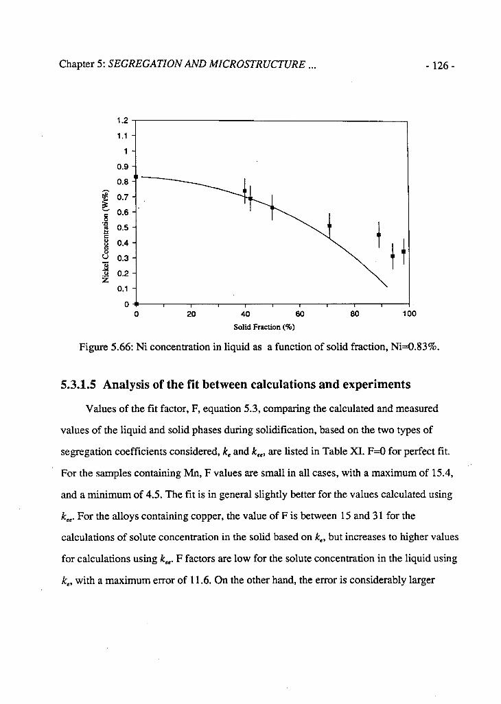
Chapter 5: SEGREGATION AND MICROSTRUCTURE . - 126 -
1.2
1.1 -
0.9 -
0.8
€ 0.7 -
~ 0.6-
| 0 4 " <-> 0.3-
0.1 -
0 + 0 20 40 60 80 100
Solid Fraction (%)
Figure 5.66: Ni concentration in liquid as a function of solid fraction, Ni=0.83%.
5.3.1.5 Analysis of the fit between calculations and experiments
Values of the fit factor, F, equation 5.3, comparing the calculated and measured
values of the liquid and solid phases during solidification, based on the two types of
segregation coefficients considered, ke and k„, are listed in Table XI. F=0 for perfect fit.
For the samples containing Mn, F values are small in all cases, with a maximum of 15.4,
and a minimum of 4.5. The fit is in general slightly better for the values calculated using
kte. For the alloys containing copper, the value of F is between 15 and 31 for the
calculations of solute concentration in the solid based on kt, but increases to higher values
for calculations using k„. F factors are low for the solute concentration in the liquid using
ke, with a maximum error of 11.6. On the other hand, the error is considerably larger

Chapter 5: SEGREGATION AND MICROSTRUCTURE - 127-
when kee is used. For Cr, F values are between 15 and 10 in all cases. For Mo, F values
for the liquid are small for both segregation factors. For the solid, the values using kt
show smaller error. For Ni, the fit is much better for the values calculated using ke.
The experimental error of the EPMA concentration measurements has been
estimated to be 10% (section 4.5). As a result values of F equal or smaller than 10
indicate very good fit. It is likely that a better fit would be obtained if the error in the
measurement of the solid fraction would have been considered in the value of F
determined.
Table XI: Fit factor, F, for calculations based on ke and k,
SAMPLE
(alloy)
F for SOLID F for LIQUID SAMPLE
(alloy) K K
Cl(Mn) 11.7 7.9 4.5 4.7
C7(Mn) 12.4 10.6 7.5 6.8
C8(Mn) 13.9 10.7 10.3 9.7
C9(Mn) 8.6 8.6 15.4 12.7
C2(Cu) 31.0 69.7 6.9 52.2
ClO(Cu) 19.5 33.8 6.9 34.3
Cll(Cu) 15.0 29.4 11.6 35.2
C3(Cr) 13.1 10.3 14!4 15.2
C4(Mo) 19.9 29.6 12.7 11.8
C5(Ni) 26.7 >100 8.4 93
C6(Si) 6.04 — — —

Chapter 5: SEGREGATION AND MICROSTRUCTURE . - 128-
5.3.2 C O R R E L A T I O N B E T W E E N T H E S O L I D I F I C A T I O N
S T R U C T U R E A N D T H E S E G R E G A T I O N P A T T E R N A R O U N D
N O D U L E S
The manner in which ductile iron solidifies, described as the equiaxed growth of
spherical eutectic cells, as shown in section 5.2.1, is not consistent with the observations
of the solidification morphology of quenched samples, illustrated in section 5.2. In order
to understand the segregation patterns obtained during the analysis of cast samples,
described in section 5.1.1, the microsegregation must be correlated with the
microstructure during solidification. It has been shown in section 5.3.1, that the
concentration of solute in the residual liquid can be calculated with good accuracy by
using the Scheil equation and effective segregation coefficients.
Considering the segregation of an alloying element of k,<\, in which case solute
concentration in the residual liquid increases with solid fraction, the following types of
segregation can occur along lines between nodules:
i) Two nodules are enveloped by adjacent austenite dendrite secondary branches, as
shown schematically in Figure 5.67 (a), during solidification. A plot of solute
concentration along the A-B after solidification is complete, will show an increase
in the concentration of solute at the mid-distance between nodules, as illustrated in
Figure 5.67 (b), since the liquid is richer in solute.

Chapter 5: SEGREGATION AND MICROSTRUCTURE . - 129-
ii) Two nodules are separated by a dendrite, as illustrated in Figure 5.68 (a), during
solidification. A solute concentration plot along line C-D after solidification is
complete, will show a decrease in the solute concentration at the mid-distance
between nodules, as shown in Figure 5.68 (b).
iii) Two nodules are enveloped by austenite secondary dendrite arms, which are in
turn separated by another dendrite arm, as illustrated in Figure 5.69 (a). A plot of
solute concentration along line E-F after solidification is complete, will show two
peaks of solute concentration, as illustrated in Figure 5.69 (b).
iv) Two nodules are separated by an area corresponding to the last liquid to solidify,
as illustrated in Figure 5.70 (a). The concentration along line G-H will be as shown
in Figure 5.70 (b). The intensity of the segregation is in this case greater than that
shown in Figure 5.67.
When line scans of solute concentration between two nodules are made by EPMA,
the specific solidification process and structure between the nodules is in general not
known. Considering the four possibilities outlined above, and the markedly different
solute segregation obtained in the four cases, the variation in the results shown in section
5.1 could be expected. From the results, it is concluded that the analysis of the extent of
solute segregation in ductile iron after solidification should not be based on composition
scans between randomly chosen pairs of nodules, but should rely on the identification and
analysis of highly segregated areas, as done in section 5.1.2. Note that if precipitate
phases are present in a highly segregated area, this area should not be used to calculate a
segregation ratio, since this would compare solute concentrations of different phases. The
stoichiometry of the precipitate phase may be independent of the segregation.

Chapter 5: SEGREGATION AND MICROSTRUCTURE . - 130-
Figure 5.67: Schematic representation of microstructure during solidification (a), and corresponding segregation profile (b).

Chapter 5: SEGREGATION AND MICROSTRUCTURE . - 131 -
Figure 5.68: Schematic representation of microstructure during solidification (a), and corresponding segregation profile (b).

Chapter 5: SEGREGATION AND MICROSTRUCTURE . -132-
Figure 5.69: Schematic representation of microstructure during solidification (a), and corresponding segregation profile (b).

Chapter 5: SEGREGATION AND MICROSTRUCTURE . - 1 3 3 -
Figure 5.70: Schematic representation of microstructure during solidification (a), and corresponding segregation profile (b).

Chapter 5: SEGREGATION AND MICROSTRUCTURE . - 134-
5.3.3 C O M P A R I S O N O F T H E S E G R E G A T I O N I N S A N D - C A S T
A N D Q U E N C H E D S A M P L E S
It has been reported that large section ductile iron castings contain a higher density
of precipitate compounds and carbides than small section castings of the same alloy
composition [80]. This is attributed to higher segregation levels in the large casting. The
results of the present investigation suggest that this is not necessarily the case. The
concentration of solute next to the graphite nodules and in the last material to solidify in
sand mould castings, as listed in Table VI, can be compared to the concentration of solute
at points A and C of the quenched samples, listed in Tables VIII, DC, and X. Comparing
the two it is evident that the segregation in the quenched samples is of the same
magnitude as that in the sand-cast samples. This result supports the assumption that
similar segregation mechanisms operate in cast and quenched samples, and that the
effective partition coefficients determined in quenched samples, can be used for the
calculation of segregation in ductile iron solidified at a slower rate than in a quenched
sample
5.4 E F F E C T S O F T H E S E G R E G A T I O N O N T H E
M I C R O S T R U C T U R E O F D U C T I L E I R O N
Recently, increasing attention is been paid to the understanding of the process
leading to the formation of the microstructure in cast irons. This requires the
microsegregation of alloy components to be known quantitatively. Nevertheless, no
analytical formulations suitable to predict segregation in cast iron have been published, to
the best of our knowledge, except for the present author [60].

Chapter 5: SEGREGATION AND MICROSTRUCTURE . - 135-
The influence of the microsegregation on both the microstructure formation in
ductile iron and its heat treatment, will be considered based on the segregation
characteristics of different alloy components determined in this investigation.
5.4.1 I N F L U E N C E O F M I C R O S E G R E G A T I O N O N T H E C A S T
S T R U C T U R E
The microstructure of ductile iron as it evolves during solidification under normal
conditions has been described in section 5.2.1. This section will deal with the phase
transformations in the solid state as the cast iron cools. It can be assumed that
immediately below the eutectic temperature the microstructure consists of austenite
saturated in carbon and graphite spheroids. The silicon, always present in the composition
of cast irons, has been shown to have a weak tendency to segregate towards the first solid
to form during solidification. This inhomogeneity in the concentration of Si will be
neglected at this point, and it shall be initially assumed that the austenite is chemically
homogeneous. As the casting cools from the eutectic to the eutectoid temperature, the
solubility of C in austenite diminishes. If the cooling rate is sufficiently slow, and the cast
iron unalloyed, the diffusivity of C in austenite is high enough to allow the carbon to
deposit on the graphite nodules, which act as carbon sinks. Therefore, no large C
gradients are expected to exist within the austenite. When the eutectoid temperature is
reached, the transformation proceeds according to the stable Fe-C-Si equilibrium
diagram, which indicates that almost all the C dissolved in the matrix must precipitate in
the form of graphite. At this point, for temperatures below the eutectoid, the matrix is
fully ferritic.

Chapter 5: SEGREGATION AND MICROSTRUCTURE . - 136-
Let us now restrain one of the initial assumptions, and consider a faster cooling rate.
In this case, some inhomogeneity can be present in the austenite immediately above the
eutectoid temperature, with C being concentrated in the austenite located far from
graphite nodules. The eutectoid ferrite will preferentially nucleate near the graphite,
where the C concentration is smaller. As the eutectoid transformation takes place, the
imposed high cooling rate can avoid the completion of the transformation predicted by
the equilibrium diagram, and metastable pearlite will form in C rich areas far from the
graphite.
As the cooling rate is further increased, less carbon is transferred from the austenite
to the nodules. As a result, the amount of pearlite formed increases. When very little time
for the diffusion of C is allowed at the eutectoid temperature, only minor amounts of
ferrite form surrounding the graphite, producing the structure called "bull's eye".
The presence of an additional alloying element will affect the microstructure mainly
due to the following effects:
i) Alloying elements will change both the solubility and the diffusivity of C in
austenite.
ii) Alloying elements segregate throughout the matrix. Inhomogeneities in the C
distribution can be therefore expected, since areas of different element
concentration will have different equilibrium C concentrations.
Alloying elements such as Mn, which increases the solubility of C in austenite and
segregates in the last liquid to solidify, will affect the microstructure formation as
follows:

Chapter 5: SEGREGATION AND MICROSTRUCTURE . - 137-
iii) During cooling from the eutectic temperature, Mn segregated areas formed during
solidification will be richer in C than the bulk of the matrix. Since such areas are
generally located far from graphite particles, the transport of C to the graphite will
be more difficult than for unalloyed iron. In consequence, even for slow cooling,
metastable Fe-Mn carbides can precipitate in the segregated areas when Mn is
present in the alloy.
iv) At the eutectoid temperature, the alloyed austenite has a higher C content than the
unalloyed austenite. In consequence, more C has to be transported to the graphite
particles in order to produce a fully ferritic matrix. Under normal cooling
conditions, and above a certain Mn level, it becomes essentially impossible to
obtain fully ferritic matrices.
Mn alloyed irons have less ferrite than unalloyed irons solidified under similar
conditions. The ferrite will preferentially form around the graphite nodules, where the Mn
concentration is at a minimum and C can be readily transported to the graphite.
Alloying elements are often used to produce as-cast pearlitic microstructures. It has
been shown [61,62] that strong pearlitizing elements such as Mn and Mo, cannot
produce a fully pearlitic matrix free from carbides. This can be explained on the basis of
the segregation characteristics of those elements. Both Mn and Mo are strongly
concentrated in the last material to solidify, and depleted in the areas surrounding the
graphite nodules. Therefore, if it is desired to obtain pearlite next to the graphite nodules,
it becomes necessary to use an alloy concentration large enough to bring the
concentration of solute in the vicinity of a nodule to a level necessary to avoid the
formation of ferrite, ie. to avoid completely the stable eutectoid transformation.

Chapter 5: SEGREGATION AND MICROSTRUCTURE . - 138 -
Nevertheless, when such a high concentration of the alloying element is used, the solute
concentration in the last liquid to solidify is enough to result in the precipitation of
carbides. Therefore, successful pearlitizing alloying usually consists of the combination
of two or more alloying elements having opposite segregation characteristics. For
example, considering combined Cu and Mn additions, Cu tends to concentrate in the first
solid to solidify, and thus is concentrated in the vicinity of the graphite nodules. Mn is
concentrated in the last material to solidify. The Cu enriched regions produce pearlite in
the vicinity of the nodule, and the Mn enriched regions in the areas remote from the
nodules. This can lead to a ductile iron which is fully pearlitized. Thus, multiple alloy
additions are generally used when pearlitization of the matrix is required.
If the production of fully ferritic structures is desired, the alloying elements must be
kept as low as possible. In practice, ferritic irons are generally unalloyed, and special care
is given to the selection of the charge materials. The utilization of steel scrap is limited to
low manganese grades.
Silicon is always present in gray cast iron, and therefore it is not usually referred to
as an alloying element. The Si presents unique characteristics; it is a graphitizing element
and diminishes the solubility of C in austenite. The larger the amount of Si present in the
cast iron, the larger the amount of ferrite in the structure at room temperature. In practice
the Si content is kept low in ferritic cast iron because of its tendency to embrittle the
ferrite.
Nickel, a graphitizing element in cast iron, is also a pearlitizing alloy, since it
increases the solubility of C in austenite. Similar to the effect of Mn, the austenite in Ni
alloyed cast iron has higher C content than unalloyed cast iron at the same temperature.

Chapter 5: SEGREGATION AND MICROSTRUCTURE . -139-
This effect becomes critical when the eutectoid temperature is reached during cooling,
since Ni alloyed austenite must reject a large amount of C in order to transform into the
stable eutectoid. It is possible to obtain pearlitic structures in ductile iron by using
only Ni, but this is highly inefficient when compared to the use of combined amounts of
Mn, Mo, Cu and Ni.
5.4.2 I N F L U E N C E O F S O L U T E S E G R E G A T I O N O N T H E
H A R D E N A B I L I T Y O F C A S T I R O N S
All alloying elements commonly used in cast iron increase the hardenability of the
material [62,63]. Mo and Mn additions increase the hardenability the most. Cu and Ni are
less effective, and Si has little effect. Lee and Voigt [63] studied the influence of
combined amounts of alloying elements on the hardenability of ductile iron. They found
that in some cases the combination of two or more elements has greater effect on the
hardenability than that expected from the individual elements. In particular, combinations
Mo-Ni, Mo-Cu and Mo-Cu-Ni, were reported to markedly enhance the hardenability of
ductile iron. This interaction effect was referred by Lee and Voigt as a synergistic effect,
with no further explanation given for the rational behind such interactions. Bearing in
mind the segregation characteristics of the alloying elements described earlier in this
chapter, it is evident that the interactions reported by Lee and Voigt always occur
between elements which have effective segregation coefficients greater and less than
unity. This suggests that the interactions may be related to the distribution of the alloying
elements within the matrix. To contemplate this possibility consider first the criterion
used to quantify hardenability. It is customary to define hardenability as the distance from
the end of a Jominy test bar at which pearlite ,(or lamellar constituents) is first observed.

Chapter 5: SEGREGATION AND MICROSTRUCTURE . - 140-
The first pearlite is generally formed next to graphite nodules. The alloying elements Mn
and Mo, which strongly influence the hardenability of ductile iron, are concentrated in
the last material to solidify, leaving the regions surrounding the larger graphite nodules
depleted in solute. The depleted areas have lower local hardenability, and will be the site
for the first pearlite to precipitate. When the alloying element has a segregation
coefficient greater than one, as in the case of Cu, the first pearlite in the Jominy test does
not necessarily appear next to the graphite nodules [63], where the concentration of Cu is
generally higher than the average concentration in the matrix. Therefore, it can be
concluded that the increased hardenability obtained in samples containing two alloying
elements having segregation coefficients greater and less than unity, results from the
segregation of each element in the iron. Elements having k>l contribute to the
hardenability of the first material to solidify; elements having k<l increase the
hardenability of the last material to solidify in the interdendritic regions.

141
Chapter 6
SOLIDIFICATION MODEL
The mathematical model of the solidification of ductile iron developed in this
investigation consists of four parts:
1) A thermal model that calculates temperatures throughout the casting and mold.
2) A nucleation model, which calculates the nucleation rate as a function of the
supercooling.
3) A growth model, which calculates the growth of both austenite and graphite.
4) A segregation model, which calculates the composition of the residual liquid
during solidification.
These models, when coupled together into an overall solidification model should be
able to predict the cooling curve for a casting of a given geometry, and to predict the
number of nodules and their size distribution.

Chapter 6: SOLIDIFICATION MODEL - 142-
6.1 THERMAL MODEL
A heat transfer mathematical model is applied to the casting system described in
section 4.3, in which the iron is cast in a water cooled cylindrical sand mould. The case of
non-cooled sand moulds is considered in Appendix 4.
6.1.1 ASSUMPTIONS AND BOUNDARY CONDITIONS
The following assumptions are made:
1) No heat is lost from top and bottom surfaces of the metal.
2) The heat transfer between the casting and the mould is characterized by a surface
heat transfer coefficient, h.
3) The water cooled copper coil acts as a constant temperature boundary surface. The
accuracy of this assumption was determined experimentally by measuring the sand
temperature between two turns in the copper coil ( TC4 in Figure 4.4) during
casting. The temperature did not exceed 25°C, which validates the assumption of
constant temperature boundary surface.
The boundary conditions are shown in Figure 6.1.
6.1.2 HEAT CONDUCTION EQUATIONS
The general equation for heat conduction in cartesian coordinates x, y, z is [64]:
BT V(fcV7) + / / = pcp^- (6.1)

Chapter 6: SOLIDIFICATION MODEL -143-
In the case of a cylindrical system, it is more appropriate to express equation (6.1)
in cylindrical coordinates by expressing x and y as:
x = r cos 0 (6.2)
y=r sinG (6.3)
Replacing equations (6.2) and (6.3) in (6.1):
(6.4)
t Q = 0
Figure 6.1: Casting system, showing the assumed boundary conditions for the thermal
model.

Chapter 6: SOLIDIFICATION MODEL - 144-
In accordance with the boundary conditions shown in Figure 6.1, the temperature
field is axisymmetric, and the temperature is uniform along z axis, therefore:
dT 30
= 0 (6.5)
(6.6)
Substituting equations (6.5) and (6.6) in (6.4) gives:
rdr[ dr + H = pCl
dT
dt (6.7)
The first term at the left side of equation (6.7) can be expanded to give:
lf.drT} if dkdT^
r drdr (6.8)
The derivative of k with respect to r can be written as:
dk_dk_dT
dr~dTdr (6.9)
Substituting equation (6.9) in (6.8) results in:
f ^\
dr'
1 +-r
r d±dT^
y*Tdr\
For most materials, the variation of k with temperature is small, and can be
neglected in (6.10). Therefore equation (6.7) can be written as:
1, d*T „ dT -k — + H = pc — r dr2 p dt
(6.10)
(6.11)

Chapter 6: SOLIDIFICATION MODEL - 145-
The fact that k, cp and p are temperature dependent greatly complicates the
analytical solution of the differential equation (6.11). It becomes necessary to solve the
heat conduction problem numerically. It has been shown in the literature [65] that the
method of implicit finite differences is suitable for the solution of equation (6.11).
The numerical solution of equation (6.11) requires the system to be divided into
volume elements. The arrangement of volume elements adopted is shown in Figure 6.2.
The volume elements are hollow cylinders of wall thickness dr. Six types of volume
elements can be found in the system. Heat transfer equations for each volume element
type have been derived in Appendix 4:
i) Axial volume element
dr2 Akdt Ti+l-—ji+1=-7^Ti+4rRHG(i)
1 dr2 4kdt 1 4k (6.12)
ii) Internal volume element of the casting
dr2
—TJ + 1 + 1 + -
PCp
dr2 (i-l.5)dr2 kdt 77+1 _ 1 1
{dr2 (i-l.5)dr2
Tj+i _ PCP Tj 1
kdt 1 k RHG(i)
(6.13)
iii) Volume element at the surface of the casting
LTV+I + r i - i ^ . PCP) r y + i h f i - l ^
Kdr2 + kdr L/-1.5J mkj kdr l i - 1 . 5 j
(6.14)

Chapter 6: SOLIDIFICATION MODEL - 146-
iv) Volume element at the internal surface of the mould.
kdra
ry + l
kdrt
J _ 1 + drl + 2redrt
2kdt
_1_ 1 dr? + 2rcdra
lM+2 -
k 2dtVu+1
(6.15)
v) Internal volume element of the mould
— T J + 1 + (
dr.
2 1 - r + — —
dr; rmdra
PC,
kdt 7Y+1 -
drl rmdraj i + 1 kdt
(6.16)
vi) Volume element at the external surface of the mould
—„T-dr,
1 +pcp
^drl rmdra kdt kdt '
1 1 1̂ ydrl + rndraJ
(6.17)
Equations (6.12) to (6.17) form a tridiagonal system.
6.1.3 INITIAL CONDITIONS
The solution of the system of equations requires the specification of the initial
conditions. The temperature of the melt at time t=0 is assumed to be uniform and equal to
the pouring temperature minus a temperature drop to account for the heat loss during
pouring. The initial temperature of the mold is taken as equal to the temperature of the
water in the copper coil.

Chapter 6: SOLIDIFICATION MODEL -147-
] Mold
Figure 6.2: Schematic of the volume elements arrangement.
6.1.4 SURFACE HEAT TRANSFER COEFFICIENT AT THE
METAL-MOULD INTERFACE
The formation of air gaps between ductile iron castings and sand molds has been
studied by Winter et al. [67]. Their investigation was carried out in a sand mold similar in
shape and dimensions to that used in the present investigation, but without steel flasks.
They measured the displacements of the mold and the casting with transducers, giving the
results shown in Figure 6.3(a). Shortly after pouring, the casting and the mold expand.
Since the expansion of the mold is larger than that of the ductile iron casting, a gap
between the mold and the casting is formed. Approximately five minutes after pouring

Chapter 6: SOLIDIFICATION MODEL - 148-
the dimension of the gap reaches a stationary value of about 0.06 mm. Cooling curves at
several points within the casting are shown in Figure 6.3(b). Comparing Figures 6.3(a)
and (b) show that the expansion of the ductile iron starts simultaneously with the
beginning of solidification. The volume of the casting remains almost unchanged until
the end of solidification, following which the ductile iron contracts as it cools. In the
present investigation the use of steel flasked molds, and copper coils in one case, prevents
the mold dilation, which in turn suppresses the formation of a gap between the mold and
the casting during solidification. However, a gap could form after the completion of
solidification, as a result of the contraction of the casting following solidification. Based
on Winter's measurements, Zeng and Pehlke [43] calculated the heat transfer coefficient
at the mold-casting interface for imperfect contact interfaces, Figure 6.4(a), and for air
gap interfaces, Figure 6.4(b). The calculated coefficient for imperfect contact interfaces
varies from 4.5 to 2.8 W/cm2K, depending on the time from pouring. When a gap forms,
the calculated coefficients are two orders of magnitude smaller than those calculated for
imperfect contact In the present investigation mold and casting are assumed to remain in
contact during solidification. Therefore, the heat transfer coefficient at the mold/casting
interface in the calculations will vary between 4.5 and 2.8 W/cm2K. Since the time at
which a gap forms at the casting/mold interface after solidification is complete is not
known, and can not be estimated with reasonable accuracy from the results of Winter et
al, the possible formation of a gap will be neglected. This may lead to some misfit
between calculated and measured temperatures after the end of solidification.

Chapter 6: SOLIDIFICATION MODEL -149-
2500
Figure 6.3: (a) Motion of the mold and casting during the solidification of ductile iron in a sand mold, (b) Cooling curves for the same casting in (a), after [67].

Chapter 6: SOLIDIFICATION MODEL -150-
TIME (SEC.)
Figure 6.4: Calculated heat transfer coefficient (a) with imperfect contact interface; (b) with gap formation, after [43].

151
6.2 M O D E L F O R G R A P H I T E N U C L E A T I O N
Su et al.[28] investigated the applicability of the nucleation model developed by
Oldfield [40] to the solidification of ductile iron. They concluded that Oldfield's
nucleation formula is not appropriate for ductile iron. No other relationship between
graphite nucleation rate and supercooling, for ductile iron, has been reported in the
literature, to the best of our knowledge.
R. Heine et al.[47] developed the following equation describing the variation of the
eutectic temperature as a function of the Si content, for the stable Fe-C-Si system:
7/£ = 1155 + 6.5%Si [°C] (6.18)
For 2.5% Si, the eutectic temperature is 1171°C. It was shown in section 2.4, Table
I, that, for ductile iron, both eutectic arrest and eutectic plateau temperatures occur well
below 1171°C. This suggests that the nucleation of the eutectic requires significant
supercooling. In addition, it has been shown by Wetterfall et al [12] that graphite
nucleation continues in the eutectic liquid well after the start of eutectic solidification.
In summary, eutectic nucleation starts at a given supercooling, and continues during
solidification. Under normal solidification conditions, for most multicomponent alloys,
the nucleation of solid phases from the liquid is heterogeneous. This is the case for the
eutectic graphite. In heterogeneous nucleation, the rate of formation of nuclei per unit
volume, N, as a function of the absolute temperature T, isgiven by equation (6.19) [77].
. oW nXT N = — = exp
dt V AGD+AG'
XT (6.19)

Chapter 6: SOLIDIFICATION MODEL - 152-
Where:
AGD = activation energy for diffusion of atoms across the interface melt/nucleus
AG * = activation energy for nucleation
n = number of atoms per unit volume of the liquid phase
X = Boltzman's constant
\|/ = Plank's constant
In liquids AGD « AG*; therefore the nucleation rate depends on AG*.
In the present investigation the nucleation rate has been calculated using equation
6.20.
dN . .„ ( c ^ N = — = b AT exp
dt K AT. (6.20)
Where b and c are constant values, for a given substrate and melt composition.
The temperature at which the nucleation rate becomes important depends on the
value of the interfacial energy between the nucleating phase and the substrate. Different
nucleating substrates and changes in the melt composition will influence the nucleation
rate. The variation in the nucleation rate with the supercooling given by equation (6.20) is
represented in Figure 6.5. The nucleation rate remains very small, until a supercooling,
generally referred to as critical supercooling, is reached. For greater supercooling the
nucleation rate becomes significant.
In the mathematical model, the nucleation rate will be calculated on the basis of
equation (6.20). This can be discretized as:

Chapter 6: SOLIDIFICATION MODEL - 153-
•5 c p "•S
I
Supercooling Figure 6.5: Nucleation rate in heterogeneous nucleation.
AN — — = ft AT exp Ar AT
(6.21)
The number of nodules nucleated in a node /, during a time step j, DNU(i,j), is
calculated by the following expression:
DNU(i,j) = b AT exp - — (1 -g(i))At (6.22)
The term (l-g(i)), where g(i) is the solid fraction in node i, is included in order to
account for the progressive decrease in the amount of liquid phase in the volume element.
Equation (6.22) will be referred to as "exponential nucleation equation".

Chapter 6: SOLIDIFICATION MODEL - 154-
Alternatively, it is proposed to test another formulation of the nucleation rate. A
variation of the nucleation rate with the supercooling similar to that predicted by equation
(6.20) is given by Equation (6.23).
oW
-^ = a(TE-TN-T)H (6.23)
Where:
a = nucleation constant TE = eutectic temperature, from equation (6.18) TN = critical supercooling for nucleation T = temperature of the melt n =exponent
As solidification advances the amount of residual melt diminishes, therefore,
equation (6.23) must be modified to:
dN = a(TE-TN-T)H (1 -g) (6.23.2)
In the model, the number of graphite nodules nucleated in a time step are calculated
as follows:
DNU(i,j) = a(TE(i)-TN-T(i)T(l-g(i))At (6.23.3)
Equation (6.23) will be referred to as "parabolic nucleation equation".
A nucleation model similar to that given by equation (6.23) was proposed by Su et
al[28], but they did not use a critical nucleation supercooling, and based the calculations
on the temperatures given by the binary Fe-C equilibrium diagram.

Chapter 6: SOLIDIFICATION MODEL -155-
It is important to note at this point that TE depends on the Si content in the residual
liquid. The residual liquid is progressively depleted in Si, therefore the value of TE
decreases as solidification progresses, resulting in a smaller effective supercooling. In
consequence, the segregation of Si will lead to slower nucleation rates than those
expected when segregation is not considered.
6.3 G R O W T H M O D E L
The growth model calculates the growth of austenite and graphite. The growth of
graphite can take place with the graphite surface in direct contact with the liquid phase, or
with the graphite enveloped by solid austenite. The following assumptions are made in
the formulation of the growth model:
i) Carbon is distributed throughout the cast structure according to the Fe-C-Si
equilibrium diagram.
ii) The proportion of carbon between austenite and graphite present in the casting
during solidification is given by the Fe-C-Si equilibrium diagram at the eutectic
temperature.
iii) The austenite/liquid and austenite/graphite interfaces are at equilibrium.
iv) Silicon segregates, affecting the equilibrium at the austenite/melt interface.
6.3.1 G R O W T H O F G R A P H I T E I N C O N T A C T W I T H T H E M E L T
The growth of graphite in contact with the melt can be controlled by either of the
following processes:

Chapter 6: SOLIDIFICATION MODEL - 156-
i) Rate of carbon transport at the graphite/liquid interface (interface controlled).
ii) Rate of carbon transport from the bulk of the liquid to the interface graphite/liquid
(diffusion controlled).
Subramanian et al. [48,49] proposed the following equation for the interface
controlled growth of graphite nodules in ductile iron:
^ = 5(10"*) (AT)2 [mm/sec] (6.24) dt
The integration of equation (6.24), assuming AT constant, leads to:
r=r 0 +5(10"*) (AT)2r (6.25)
On the other hand, Wetterfall et al [12] applied Zener's [69] equation for growth
controlled by diffusion, in order to estimate the growth rate of graphite spheroids in direct
contact with the melt. For our case, Zener's equation can be expressed as follows:
Where:
C"*1 = carbon concentration in the austenite in equilibrium with liquid
Cl,gr = carbon concentration in the liquid in equilibrium with graphite
C = carbon concentration in the graphite
p, and pgr = density of liquid and graphite respectively
Dc = diffusion coefficient of the carbon in the liquid

o Chapter 6: SOLIDIFICATION MODEL -157-
ValuesforC"randC"«r are derived in Appendix 5. Equation (6.26) can be
rearranged as:
The growth rate of the graphite spheroids was calculated on the basis of equations
(6.24) and (6.26), for interface controlled and diffusion controlled growth respectively.
The results are plotted in Figure 6.6, for different values of supercooling. For a
supercooling of 10°C, and very small time, the interface controlled growth rate, curve a,
is smaller than the diffusion controlled growth rate, curve c. After a very short period, the
diffusion controlled growth rate becomes smaller, and consequently the growth can be
considered to be controlled by the diffusion of C in the liquid during most of the period in
which the graphite is in direct contact with the liquid. For greater supercoolings, both
growth rates increase, but the diffusion controlled growth continues to be the smaller
after a very short initial period. In practice, as shown in Table I, the solidification of
ductile iron takes place at temperatures below 1150°C, which in turn involves
supercoolings greater than 20°C. As a result the growth of graphite in contact with liquid
is calculated using equation (6.26).
In order to calculate the size increment of a graphite particle in a given time
interval, on the basis of equation (6.26), it is necessary to derive an equation for Ar as a
function of r and At. The expected radius of a graphite particle after time tt and t2 is given
by equations (6.29) and (6.30) respectively.
(6.27)
(6.28)

Chapter 6: SOLIDIFICATION MODEL -158 -
Time (sec)
Figure 6.6: Growth rate of the graphite spheroids as a function of time, for interface controlled, (a) and (b), and diffusion controlled growth, (c) and (d).
rl = F{T)t,
r2
2=F{T)t2
(6.29)
(6.30)
The size increment can be calculated as:
Ar = r2-r1
r2 = rl + Ar (6.31)
Subtracting equation (6.29) from (6.30), and substituting in (6.31) gives:
(r1 + AT) 2 -r I
2 = F(r )^-f 1 ) (6.32)

Chapter 6: SOLIDIFICATION MODEL - 159-
Rearranging equation (6.32)
2rjAr + Ar 2 = F(T)At (6.33)
Where:
&t = h-tx
Rearranging (6.33):
Ar 2 + 2r, Ar -F(T)At = 0 (6.34)
Equation (6.34) can be solved as:
Ar = -r t + ^rf + F(T)At (6.35)
Based on the observations of Wetterfall et al. [12], it will be assumed that graphite
nodules are enveloped by austenite when their radii reach 6 microns.
6.3.2 G R O W T H O F A U S T E N I T E
In the model it is assumed that the ratio of the amount of austenite and the amount
of graphite is constant during solidification. Therefore, the amount of austenite is
calculated on the basis of the amount of graphite present. The ratio between austenite and
graphite volumes, REAG, is calculated in Appendix 5, and gives the following:
R E A G ~ 2.16-0.1015/ ( 6 3 6 )

Chapter 6: SOLIDIFICATION MODEL -160-
It is therefore possible to calculate the volume of austenite, VY as a function of the
volume of graphite, Vgr, as:
6.3.3 G R O W T H O F G R A P H I T E E N V E L O P E D B Y A U S T E N I T E
The cast structures described in section 5.2.1 indicate that as the solid fraction
increases, graphite nodules become enveloped by austenite. Further growth of graphite
requires the diffusion of C from the liquid to the graphite surface.
The simplest case to be considered is that of a single graphite nodule enveloped by
a spherical austenite shell. This case has been studied [12], and the following equation
describing the growth rate of the graphite is reported:
Equation (6.38) assumed that the external surface of the spherical austenite shell is
totally in contact with the melt. In reality, as shown in sections 2.1 and 5.1, the austenite
envelope results from the interaction of growing austenite dendrites and graphite nodules
In the example illustrated in Figure 6.8, only the thinner portions of the austenite
envelope, along path A, will significantly contribute to the graphite growth. In order to
account for this effect, a correction factor, J, is introduced in equation (6.38), based on
the formula used bu Su et al.[28], multiplied by 0.9. The correction factor is intended to
represent the reduction in surface-area of the austenite liquid interface actually
Vy = REAG.Vi (6.37)
dr [C^-Cnr\ 9PI (6.38)

Chapter 6: SOLIDIFICATION MODEL -161 -
contributing to the graphite growth. The correction factor used in the model is:
/ =0.9(l-s) 2/3 (6.39)
Equation (6.39) is represented in Figure 6.8. The correction factor can be introduced
in equation (6.38), resulting in equation (6.40):
c ^ ' - c ^ p ^ a - g f 3
* a 9 l dt {Cgr-C*gr
(6.40)
o o co UL c o 'o <u \— o o
0.4 0.6 Solid Fraction
Figure 6.7: Correction factor applied to the growth rate of graphite enveloped by austenite.
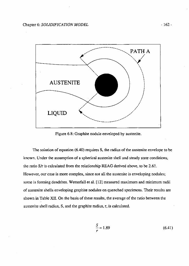
Chapter 6: SOLIDIFICATION MODEL - 162-
Figure 6.8: Graphite nodule enveloped by austenite.
The solution of equation (6.40) requires S, the radius of the austenite envelope to be
known. Under the assumption of a spherical austenite shell and steady state conditions,
the ratio S/r is calculated from the relationship REAG derived above, to be 2.61.
However, our case is more complex, since not all the austenite is enveloping nodules;
some is forming dendrites. Wetterfall et al. [12] measured maximum and minimum radii
of austenite shells enveloping graphite nodules on quenched specimens. Their results are
shown in Table XII. On the basis of these results, the average of the ratio between the
austenite shell radius, S, and the graphite radius, r, is calculated.
-=1.89 r
(6.41)

Chapter 6: SOLIDIFICATION MODEL -163 -
Equation (6.41) can be substituted into (6.40), leading to:
r .2/3
C-C*") pgrr (6.42)
Equation (6.42) can be expressed in finite differences as:
(cT'-C^PyDctt-gf* r- + 1 = r- + 1.911 V ^ (6.43)
Note that the growth rate is a function of the nodule size and fraction solid. In
addition, since the carbon concentration depends on the temperature and melt
composition, both temperature and composition influence the growth rate. It is therefore
necessary to calculate the growth rate for each nodule size and at each temperature during
solidification.
6.3.4 C A L C U L A T I O N O F T H E F R A C T I O N S O L I D A N D T H E
R E L E A S E O F L A T E N T H E A T
The release of latent heat per unit volume and time, RHG(I), is calculated from the
increment in the fraction solid during a time step, equation (6.44)
RHG(i) = AgipL (6.44)
Agi = increment in fraction solid during a time step
p = density of the cast iron
L = latent heat of solidification

Chapter 6: SOLIDIFICATION MODEL
Table XII: Measurements of austenite shell radius (after [12]).
-164-
Nodule Radius
c min
c "-"avge
Savge/r
7 . 15 16 15.5 2.21
10 20 26 23 2.30
14 26 33 29.5 2.11
19 36 42 39 2.05
21 36 46 41 1.95
24 32 52 42 1.75
25 48 56 52 2.08
17 26 28 27 1.59 14 22 22 22 1.57 17 26 34 30 1.76
21 37 40 38.5 1.83 21 43 43 43 2.04 25 48 56 52 2.08
32 62 65 63.5 1.98
13 23 24 23.5 1.80
18 30 35 32.5 1.80
19 31 36 33.5 1.76
22 32 42 37 1.68
25 41 42 41.5 1.66
Mean value of Savge/r = 1.89

Chapter 6: SOLIDIFICATION MODEL - 165 -
The information about number and size of graphite nodules in each volume element
is contained in two two-dimensional arrays, DNU(i,k) and RNU(i,k). DNU stores the
number of nodules of a given size existing in a volume element i. RNU stores the size of
the graphite nodules. Therefore, at time j, the total volume of graphite in node i, VGR,
can be calculated as:
VGRJ = I ^nRNU(i,k)3DNU(i,k) (6.45) t = i3
Note that VGR is dimensionless; in other words, it is measures volume of solid per
unit volume, which in turn is the solid fraction.
Applying the relation between austenite and graphite volumes shown in equation
(6.38), the solid fraction of a volume element i at time j is calculated from:
gj = VGRj(l +REAG) (6.46)
The change in solid fraction can be then calculated as:
Ag=*/ + 1-*/ (6.47)
6.3.5 C A L C U L A T I O N S O F N O D U L A R S I Z E D I S T R I B U T I O N
Information concerning nodular size distribution is contained in arrays DNU(i,k)
and RNU(i,k). In the present formulation, the growth of graphite is assumed to stop when
solidification is complete. In reality, graphite particles keep growing after the
solidification is complete, as a result of the decrease in the solubility of C in austenite. At
the eutectic temperature, austenite containing 2.5% Si dissolves 1.3 Wt% carbon. The.
eutectic alloy contains 3.49% carbon, therefore, only 63% of the C in the alloy is in the

Chapter 6: SOLIDIFICATION MODEL - 166-
form of graphite at the eutectic temperature. Depending on the cooling rate and chemical
composition, varying amounts of C will precipitate in the form of graphite during cooling
below the eutectic temperature. For ferritic irons, only a negligible amount of carbon
remains dissolved in the matrix; therefore, the volume of graphite increases
approximately 59% as room temperature is reached. The volume of graphite at room
temperature, VGR', can be calculated by the following equation:
VGR' = 1.59VGR = 1.59 £ ^nRNU(i,kfDNU(i,k) (6.48) *=i3
Equation (6.49) can be rearranged as follows:
VGRJ= £̂ rc[1.167/?M/(i,fc)]3DWl7(;,£) (6.49) k = l 3
In consequence, the precipitation of C in the solid state can be accounted for by
increasing the diameter of the nodules by a factor of 1.167. Smaller correction factors
should be applied for irons showing pearlitic or mixed matrices.
6.4 S E G R E G A T I O N M O D E L
As shown in Chapter 5, the concentration of solute in the residual liquid can be
calculated with good accuracy by applying the Scheil equation and using the effective
segregation coefficients listed on Table X.
C^k.d-g)^1 (6.50)
Detailed information about the influence of the alloying element on the equilibrium
temperatures and compositions was found only for Si. As a result, the calculations are

Chapter 6: SOLIDIFICATION MODEL -167 -
only for segregation of this element. As Si segregates, it influences the equilibrium
carbon concentration at the interfaces in the solidifying alloy. Figure 6.9 shows the
changes in the equilibrium concentrations of C in austenite equilibrated with graphite,
Cy*r, austenite equilibrated with liquid, C y\ and liquid equilibrated with both graphite,
Cilgr, and austenite, C"1, as a function of the solid fraction, when the Si segregation is
considered. As the solid fraction increases the concentration of Si in the residual liquid
decreases; therefore the equilibrium concentration of C increases with the solid fraction
for all interfaces, as illustrated in Figure 6.9.
0 20 40 60 80 100 Solid Fraction
Figure 6.9: Concentration of C as a function of the solid fraction in: -austenite in equilibrium with graphite, Ca/g; -austenite in equilibrium with liquid, Ca/1; -liquid in
equilibrium with austenite, Cl/a; -liquid in equilibrium with graphite, Cl/g.

Chapter 6: SOLIDIFICATION MODEL -168-
It has been shown in Chapter 5 that the diffusion of Si in austenite is small and can
be neglected for this analysis. In consequence, the Si concentration in the austenite
adjacent to a graphite nodule can be considered to remain constant through the cooling of
the casting to room temperature.
It is shown in Appendix 5 that the carbon concentration in austenite equilibrated
with graphite is given by the following equation:
Cigr = T-1154.6-6.55/ . 354.6 + 6.55/ (1.5 - 0.2165/) + 2.1 - 0.2165/ (6.51)
Assuming that the austenite surrounding most of the graphite nodules was formed
early during solidification, the Si content in the austenite next to graphite nodules can be
determined by:
5/^ = 5/ .kSi (6.52)
The carbon concentration at the austenite next to the graphite nodules, C,gr, can be
determined on the basis of the Si concentration, by substituting equation (6.52) in (6.51).
For an average Si concentration of 2.5%, the concentration of C in the austenite next to
the graphite is 1.48%.
Since the concentration of Si in the residual liquid is a function of the solid fraction,
the C concentration gradient within the austenite, Cy' - Cy*r, which is in turn the driving
force for the diffusion of C from the melt to the nodules, depends on the solid fraction.
Figure 6.10 shows the variation of Cy' - C y g r as a function of the solid fraction, for
negligible Si segregation, curve B, and Si segregation calculated by the Scheil equation,
curve A. For curve A the concentration of carbon in the austenite next to the graphite has

Chapter 6: SOLIDIFICATION MODEL -169 -
been considered equal to 1.48%. Comparing curves A and B, it is evident that the C
gradient within the austenite becomes larger when the segregation of Si is considered,
resulting in an increased driving force for C diffusion. In consequence, a faster growth
rate of the graphite would be expected when Si segregation is included in the
calculations.
Solid Fraction
Figure 6.10: Difference in the austenite C concentration at the austenite/liquid and austenite/graphite interfaces.

170
6.5 S E L E C T I O N O F M A T E R I A L S P R O P E R T I E S
6.5.1 T H E R M O P H Y S I C A L P R O P E R T I E S O F D U C T I L E I R O N
The thermophysical properties of ductile iron have not been studied extensively. A
database of properties of materials commonly used in castings has been published by
R.D. Pehlke et al.[70]. Since no values of the heat conductivity of ductile iron have been
reported for the temperature range of interest in our calculations, the thermal conductivity
of solid ductile iron will be assumed to be 29 W/m°C, which is the average thermal
conductivity of carbon steels between 800 and 1200 °C [81]. The variation of specific
heat with temperature is shown in Figure 6.11. For temperatures between 777 and
1130°C, which include the range of interest in our calculations, the specific heat of the
ductile iron is given by the following function:
Cp = 0.61 + 1.214(10̂ )7 [kJ/kg°C] (6.55)
For higher temperatures the ductile iron is in a liquid state. The specific heat of the
liquid does not change much with the temperature, with a value of 0.915 kJ/kg C.
Values of thermal conductivity of liquid cast iron have not been reported in the
literature to the best of our knowledge. It has been shown [71] that the effective thermal
conductivity of the liquid phase in the presence of a thermal gradient is increased by the
fluid flow resulting from natural convection. For our calculations it is assumed that the
thermal conductivity of fully liquid regions is equal to 100 W/m°C.

Chapter 6: SOLIDIFICATION MODEL -171 -
The liquid in partially solidified nodes is considered stagnant. Since no values are
reported for the conductivity of liquid cast iron, the thermal conductivity of partially
solidified portions of material will be considered equal to 20 W/m°C, which is smaller
than the thermal conductivity of the ductile iron at the solidification temperature.
The densities of liquid and solid ductile iron are very similar, since the precipitation
of the less dense graphite compensates for the liquid/solid contraction. The density will
be taken as 7 g/cm3.
Careful measurements of the latent heat of solidification of ductile iron have been
carried out by Upadhya et al.[72]. They reported a latent heat value of 258 kJ/kg.
6.5.2 S A N D P R O P E R T I E S
The thermal properties of the sand used in the calculations were taken from the work of Kubo and Pehlke [73]. The specific heat of silica sand is given by the following equations:
ForT<846°/i:
CP = 0.782 + 5.71(10~*)r - \.%%{\0A)T2[Ulkg°K\ (6.56)
FOTT>%46°K
CP = 1.00 + 1.35(lCTA)T[kJ/kg°K] (6.57)
The mould density has been measured to be 1.5 g/cm3.
The thermal conductivity of moulding sands depends on a number of factors, which
include sand density, binder type, moisture content, temperature, etc. Measurements of

Chapter 6: SOLIDIFICATION MODEL - 172-
the variation in the thermal conductivity of silica sands have been reported in the
literature. The results of different experimental methods are different, as shown in Figure
6.12. In view of the discrepancy in the values, it has been chosen to use the temperature
independent value of the heat conductivity of the silica sand reported by Kubo and Pehlke
[70]. The thermal conductivity of silica sands having a density of 1.5 g/cm3, is equal to
0.85W/m°C.
O)
< Ul X
y LL o UJ
0.9 -
0.8 -
0.7 -
0.6 -
0.5 — i 1 1 1—-i 1 1 1 1 1 1 1 1— 0 0.2 0.4 0.6 0.8 1 1.2 1.4
(Thousands) TEMPERATURE (C)
Figure 6.11: Specific heat of ductile iron as a function of temperature.

Chapter 6: SOLIDIFICATION MODEL -173-
2 JO-
1.5
E
0 5
0
250 500 750 1000 1250 1500 1750
T ( K )
Figure 6.12: Thermal conductivity of silica sand as a function of the temperature, measured by two different methods (after [70]).
6.53 OTHER PROPERTIES
Values of other properties required for the calculations have been obtained from the
literature [75]:
Density of graphite = Pgr = 1-92 g/cm3
Density of austenite = pT = 7 g/cm3
Diffusion coefficient of C in the melt = Dc = 0.50 (10'S) cm2/s
Diffusion coefficient of C in austenite = Dc = 0.90 (10"6) cm2/s

Chapter 6: SOLIDIFICATION MODEL - 174-
6.6 S O L I D I F I C A T I O N M O D E L
The model of the solidification of ductile iron calculates cooling curves, nodule
counts and nodular size distributions at points along the radius of an infinitely long
cylindrical ductile iron casting.
The temperature distribution is calculated using equations (6.12) to (6.17). The
resulting tridiagonal system of equations is solved by using the subroutine TRISOLV,
available in the UBC main frame computer. The release of latent heat for a given volume
element, RHG(i), which is necessary for the calculation of the temperature distribution, is
calculated by solving equation (6.44).
Calculations of graphite nucleation, and growth of austenite and graphite are
performed by the subroutine FRACSO, which also calculates the fraction solid, rate of
latent heat release, and composition of the residual liquid.
Temperature calculations are made with the program SOLI.
Flow charts of the program Soli and the subroutine FRACSO are shown in Figures
6.14 and 6.15 respectively. The computer programs, written in Fortran IV, are listed in
Appendix VI. The variables are defined at the beginning of the listing of program SOLI.

Chapter 6: SOLIDIFICATION MODEL
START
DEFINE VARIABLES
I INPUT
Initial Temperatures: TP, TO System Dimensions: RAO, RADF Material Properties: KL, RHO, CPL, L, KA, RA Limit time and Time steps: DTI, DTF, NDTI, NMAX Nucleation and Growth parameters: DTCR,
AA, EXP, DCL, DCA, RNUO Segregation Parameters: SIO, KSI Initial Heat Transfer Coefficient: H Mesh Data: M, MA Printing Data: PN1,PN2,PN3,PN4,PN5,PN6,PN7
I INITIALIZE
Nodal Temperatures: TV(I) Solid Fraction: FS(I) Counters: JO(l), Sl(l), RNU(I,J), DNU(I.J)
I CALCULATE AUXILIAR VARIABLES
t DR, DRA, TL, REAG* I
START COUNTED LOOP
EVALUATE HEAT TRANSFER COEFRCIENT
AND TIME STEP BASED ON TIME
Figure 6.14: Flow chart of program SOLI.

Chapter 6: SOLIDIFICATION MODEL - 176 -
ASSIGN LIQUID PROPERTIES
ASSIGN SOLID PROPERTIES
CALL FRACSO Evaluate properties, solid fraction and rate of heat generated
EVALUATE MATRIX COEFFICIENTS A, B, C, R
I SOLVE TRIDIAGONAL SYSTEM OF EQUATIONS
YES Print selected temperatures and solid fractions
INCREASE COUNTER
I CALCULATE AND PRINT NODULAR SIZE
DISTRIBUTION FOR SELECTED VOLUME ELEMENTS T END
Figure 6.14: Continued.

Chapter 6: SOLIDIFICATION MODEL -177-
START
DEFINE VARIABLES
H Z EVALUATE AUXILIAR PARAMETERS
CLA, CLG, CAL, CAG BASED ON SI(IO AND TV(I)
EVALUATE NUMBER OF MEW NUCLEI
r EVALUATE GROWTH OF GRAPHITE NODULES,
ON THE BASIS OF THEIR SIZE
I CALCULATE FRACTION SOLID
AND RATE OF LATENT HEAT GENERATED
* EVALUATE THE CONCENTRATION OF SI
IN THE RESIDUAL LIQUID BASED ON THE FRACTION SOLID
RETURN
Figure 6.14: Flow chart of subroutine FRACSOL.

178
Chapter 7
MODEL RESULTS AND
APPLICATION
7.1 S E N S I T I V I T Y A N A L Y S I S
The sensitivity of the model to changes in some of the input parameters was
evaluated on the basis of the change in the solidification time, for the solidification of
ductile iron in an 86mm diameter sand mold. The results, for the parabolic nucleation law
follow.
7.1.1 I N F L U E N C E O F T H E M E S H F I N E N E S S
The sensitivity of the model to the number of volume elements in the casting and in
the sand was evaluated. Increasing the number of nodes in the casting produces an
increase in the solidification time, as shown in Figure 7.1. When more than 40 nodes are
defined within the casting, the changes in the solidification time as the number of nodes
increases is small. Changing the number of nodes in the sand has little influence on the
solidification time, as shown in Figure 7.2.

179
7.1.2 I N F L U E N C E O F T H E T I M E S T E P
The implicit formulation of the heat transfer equations in finite differences is stable
for any given time step. However, the accuracy of the calculations is influenced by the
time step. Solidification times calculated for different time steps are shown in Figure 7.3.
The solidification time decreases for decreasing time steps. Refinement of the time step
below 1 sec has little influence on the solidification time.
7.1.3 I N F L U E N C E O F T H E I N I T I A L T E M P E R A T U R E O F T H E
M E L T
The influence of the initial temperature of the melt on the cooling curve of the <
center of the casting is shown in Figure 7.4. As expected, larger initial temperatures result
in increased solidification times. The length of the eutectic plateau and the supercooling
do not change markedly.
7.1.4 S E L E C T I O N O F P A R A M E T E R S
Following the results shown in sections 7.1.1 and 7.1.2, the calculation of the
solidification of an 86 mm diameter casting are done for 60 nodes in the casting and 10 in
the sand; with a time step of 1 second. Calculations of the solidification of ductile iron in
the smaller diameter cylindrical molds are done for smaller volume elements in the
casting, and smaller time steps. The number of nodes in the sand will be taken as one per
millimeter of radius.

Chapter 7: MODEL RESULTS AND APPLICATION - 180
o CD -52-CD E
o
1 [g O
CO
Number of Nodes in the Casting
Figure 7.1: Influence of the number of nodes selected in the casting on the solidification time.
580 -
570 J
560 -CD
tn_ CD 550 -E
i -c o 540 -
1 T J
530 -"o C/5 520 -
510 -
500 - - r -
7 ~\ r~
9 — i r 11
-1—
13 T 1—
15
Number of Nodes in the Sand Mold
-1 r 17
— i — 19
Figure 7.2: Influence of the number of nodes selected in the sand mold on the solidification time.

Chapter 7: MODEL RESULTS AND APPUCATIONS -181 -
565 H 1 1 1 1 1 1 1 1 1 0 2 4 6 8 10
Time Step (sec)
Figure 7.3: Influence of the time step on the solidification time.
0.8 -\ 1 1 1 1 1 1 1 0 200 400 600 800
Time (sec)
Figure 7.4: Influence of the initial temperature of the melt on the cooling of the center of the casting.

182
7.2 C O M P A R I S O N O F T H E R E S U L T S O F T H E H E A T T R A N S F E R
M O D E L W I T H A N A L Y T I C A L S O L U T I O N S
The results of the thermal model are compared to an analytical solution, in order to verify the accuracy of the model calculations. This is done for simplified boundary conditions. Analytical solutions of the heat conduction equation for an infinitely long solid cylinder of outside radius r0 have been reported in the literature [74] for the following boundary conditions:
- The cylinder axis is an insulated boundary.
- The surface heat extraction is given by:
Q=Ah(Ts-T0)
- The initial temperature of the cylinder is uniform.
The solutions are given in the form of dimensionless charts. The cooling curves of the center, surface, and mid-radius of the cylinder were calculated on the basis of the charts, for the following values of the relevant parameters:
Cylinder radius = 50 mm
Heat transfer coefficient = 0.04 W/cm2oC
Heat conductivity = 0.3 W/cirTC
Density = 7 g/cm3
Specific heat = 3 J/g°C
The analytical results are shown by the points in Figure 7.5. The model calculations for the same test conditions are shown by the solid lines. The maximum difference

Chapter 7: MODEL RESULTS AND APPLICATIONS -183-
between the calculations and the analytical solution is less than 1.8%. In particular, the
analytical and numerical solutions of the cylinder surface temperature are in very good
agreement.
0 200 400 600 800 Time (sec)
Figure 7.5: Analytical results (points) and numerical calculations (lines) of the cooling of a solid cylinder.
7.3 A N A L Y S I S O F T H E S E N S I T I V I T Y O F T H E M O D E L S O F
N U C L E A T I O N A N D G R O W T H
Tests of the formulations for the calculation of nucleation, growth and segregation
were initially carried out under simplified heat transfer conditions. The melt, consisting

Chapter 7: MODEL RESULTS AND APPLICATION - 184-
of a single volume element, was assumed to have uniform temperature at all times. The
rate of heat extraction .from the melt was assumed to be constant. A listing of the
computer program GROWTH is included in Appendix 7.
A typical cooling curve is shown in Figure 7.6. The calculated temperature of the
volume element falls below the critical nucleation temperature, until the rate of heat
generated by the phase change compensates and surpasses the rate of heat extraction,
giving place to the temperature recalescence. At the end of solidification, the rate of heat
generation becomes smaller, and the cooling rate increases to its initial level.
Tests of the sensitivity of the models were carried out for both the exponential and
parabolic nucleation laws.
1.05 -
104 H r 1 1 1 1 1 1 1 1 0 20 40 60 80 1 00
TIME (s)
Figure 7.6: Calculated cooling curve.

Chapter 7: MODEL RESULTS AND APPLICATIONS - 185-
7.3.1 E X P O N E N T I A L N U C L E A T I O N
Calculations of cooling curves and nodule counts based on the exponential
nucleation, equation 6.20, were done for different values of the constants b and c, and
different cooling rates. The following changes were observed.
1- An increase in the nucleation constant, b, causes an increase in both TEU and TER,
as shown in Figure 7.7(a), and an increase in the number of nodules per unit
volume, as shown in Figure 7.7(b).
2- Increasing the value of the constant c, decreases TEU and TER, as shown in Figure
7.8(a), and decreases the number of nodules per unit area, as shown in Figure
7.8(b). The increase in c from 450 to 550 produces a decrease in the nodule counts
of approximately 20%.
3- Increasing the heat extraction decreases both TEU and TER, as shown in Figure
7.9(a). The nodule counts increase almost linearly with the heat extraction within
the range examined, as shown in Figure 7.9(b). Changing the cooling rate from 100
to 300 J/sec, increases the nodule counts approximately three times.

Chapter 7: MODEL RESULTS AND APPLICATION -186-
Time (sec)
12 - •
11 -
10 -
1 H 1 1 1 1 1 1 0 2 4 6
(Thousands)
Nucleation Constant
Figure 7.7: Model calculations for different values of the constant b. a) Cooling curves; b) Nodule counts.

Chapter 7: MODEL RESULTS AND APPLICATIONS - 187-
0 20 40 60 80 100 120
Time (sec)
17
300 340 380 420 460 5 O 0 S 4 0 S 8 0
Nucleation Constant
Figure 7.8: Model calculations for different values of the constant c. a) Cooling curves; b) Nodule counts.

Chapter 7: MODEL RESULTS AND APPLICATION -188-
0 20 40 60 80 1 00
Time (sec)
Heat Extraction from the Mould (J/sec)
Figure 7.9: Model calculations for different imposed cooling rates, a) Cooling curves; b) Nodule counts.

Chapter 7: MODEL RESULTS AND APPUCATIONS -189-
7.3.2 P A R A B O L I C N U C L E A T I O N
Calculations of cooling curves and nodule counts based on parabolic nucleation,
equation 6.23, were done for different values of a and n, and for different nucleation
temperatures, TN. The influences of cooling rate and the segregation coefficient of Si
were also evaluated. The results are listed below.
1) Increasing the nucleation constant, a, increases both TEU and TER, Figure 7.10(a),
and increases the number of nodules per unit volume, Figure 7.10(b). Increasing the
nucleation constant ten times, from 100 to 1000, causes a 70% increase in the
nodule count.
2) Increasing the nucleation exponent, n, increases both TEU and TER, Figure 7.11(a),
and the number of graphite nodules, Figure 7.11(b). Doubling the nucleation
exponent, from 1 to 2, increases the nodule count by 120%.
3) Increasing the cooling rate decreases both TEU and TER, and reduces the
solidification time, Figure 7.12(a). The nodule count increases for increasing
cooling rate, Figure 7.12(b). Changing the cooling rate from 100 to 300 J/sec
increases the nodule count by 140%.
4) Increasing the critical nucleation supercooling, DTCR=TL-TN, decreases TEU and
TER, as expected, and increases the recalescence, (TEU-TER), Figure 7.13(a). The
nodule counts decreases with increasing DTCR, Figure 7.13(b)
5) Increasing the partition coefficient of Si, results in a small decrease in TER, Figure
7.14(a), and a small increase in the nodule count, Figure 7.14(b). This test was done
only to examine the sensitivity of the model to changes in the segregation
coefficient.

Chapter 7: MODEL RESULTS AND APPLICATION
TIME (s)
CO
E c
f ¥ o = o 2
_l Q o
NUCLEATION CONSTANT A
Figure 7.10: Model calculations for different values of the nucleation constant Cooling curves; b) Nodule counts.

Chapter 7: MODEL RESULTS AND APPUCATIONS - 191 -
120
TIME (s)
I i i i I I i I i I ; i i i 0.4 0.8 1.2 1.8 2 2.4 2.8
NUCLEATION EXPONENT [EXP]
Figure 7.11: Model calculations for different values of the exponent n. a) Cooling curves; b) Nodule counts.

Chapter 7: MODEL RESULTS AND APPUCATION - 192-
0 200 400 600
COOLING RATE (J/sec)
Figure 7.12: Model calculations for different imposed cooling rates, a) Cooling curves; b) Nodule counts.

Chapter 7: MODEL RESULTS AND APPUCATIONS
(a)
TIME (s)
30
28 -
26 -
CO 24 -E 24
o 22 -c
_ 20 — 1— to
UN
lio
n
18 _
ICO
16 _
LU _ l 14 -Q O 12 Z 12
10
0
6
(b) 0 10 20 30 40
CRITICAL NUCLEATION SUPERCOOLING [DTCR] (Celsius)
Figure 7.13: Model calculations for different values of the critical nucleation supercooling, a) Cooling curves; b) Nodule counts.

Chapter 7: MODEL RESULTS AND APPLICATION -194-
o LU DC Z> I— < DC LU 0-
LU
TIME (s)
SEGREGATION COEFFICIENT [KSI]
Figure 7.14: Model calculations for different values of the segregation coefficient of Si. a) Cooling curves; b) Nodule counts.

Chapter 7: MODEL RESULTS AND APPUCATIONS -195-
7.4 M O D E L O U T P U T
A sample of the model output is shown in Appendix 8. The output lists:
1- Temperatures at six positions within the casting, PN1 to PN6, and two points within
the mould, PN7 and MF. One hundred temperature values, corresponding to
different times, are listed for each volume element.
2- Values of the fraction solid for PN1 to PN6.
3- Number of nodules per unit volume in each volume element.
4- Nodular size distribution at five volume elements, PN1 to PN5.
5- Temperature and fraction solid distribution within the castings at seven time values,
PR1 to PR7.
Typical cooling curves at six points within the 86mm diameter casting, calculated
. by the model, are plotted in Figure 7.15. The markers indicate the beginning and end of
solidification. The cooling curves show that volume elements closer to the cylinder axis
have a longer local solidification time (given by the time difference between beginning
and end of solidification), and solidify over a larger temperature range (given by the
temperature difference between the start and end of solidification) than the volume
elements close to the periphery of the casting.
Temperature distributions throughout the casting at different times from pouring are
shown in Figure 7.16. The temperature gradients after pouring are large, progressively
decreasing for the first 200 s, when the first layer of fully solid material is formed in the
periphery of the casting. After 200s, with further solidification larger gradients develop in
the solid shell. When solidification is complete, after 810s, the temperature gradients

Chapter 7: MODEL RESULTS AND APPLICATION - 196-
become small again.
The calculated transformation kinetics at different distances from the centre of the
casting are shown in Figure 7.17. The initial transformation rate, for solid fractions less
than 40%, is higher for the volume elements closer to the casting surface. For larger solid
fractions, the transformation rate of the axial volume element, radius=0, is greater than
the transformation rate of the volume elements close to the mid-radius.
The calculated nodule count per unit volume as a function of the distance from the
casting axis is shown in Figure 7.18. A large peak in the nodule count is observed at the
casting surface, resulting from the fast cooling rate at this point in the casting. Moving
towards the centre of the casting, the nodule count reaches a minimum value, and then
progressively increases.
The nodular size distribution at the centre, mid-radius and edge of the casting is
shown in Figure 7.19(a-b). The largest number of small nodules is present in the centre of
the casting. There are more large nodules in the centre and mid-radius positions in the
casting, than at the edge.
Comparing Figures 7.15 and 7.17, shows that for most volume elements,
particularly those near the centre of the casting, most of the solidification occurs below
the plateau temperature during subsequent cooling.

Chapter 7: MODEL RESULTS AND APPUCATIONS -197 -
1.3
0.9 H 1 1 1 1 1 1 1 1 0 200 400 600 , 800
Time(sec)
Figure 7.15: Calculated cooling curves at points distant 0, 10, 21, 33 and 43 mm from the casting centre.

Chapter 7: MODEL RESULTS AND APPUCATION - 198-
Figure 7.16: Calculated temperature distribution at different times from pouring.

Chapter 7: MODEL RESULTS AND APPUCATIONS -199-
800 Time(sec)
Figure 7.17: Calculated transformation kinetics at points distant 0, 10, 21, 33 and 43 mm from the casting centre.

Chapter 7: MODEL RESULTS AND APPLICATION -200-
Figure 7.18: Calculated number of nodules per unit volume as a function of the distance from the casting axis.

Chapter 7: MODEL RESULTS AND APPUCATIONS -201 -
3. a - o u 5 •3 "8
6 10 14 18 22 26 30 34 38 42 46
Nodule Radius (microns)
6 10 14 18 22 26 30 34 38 42 46
Nodule Radius (microns) 4 - i
3.5 -
3 -
2.5 -
2 -a s i
1.5 -
•8 1 -z 1 -
0.5 -
0 -6 10 14 18 22 26 30 34 38 42 46
Nodule Radius (microns)
Figure 7.19: Calculated nodular size distribution at the centre, mid-radius and edge of a 86mm diameter casting.

Chapter 7: MODEL RESULTS AND APPUCATION -202-
7.5 COMPARISON OF MODEL RESULTS AND CALCULATIONS
The mathematical model was used to calculate the solidification of ductile iron of
eutectic composition cast into cylindrical sand moulds of 86,40 and 25 mm diameter.
The calculated cooling curves, nodule counts and graphite volume distributions were
compared with measured cooling curves from the four unalloyed castings, C12 to C15.
Comparisons of cooling curves for 86mm diameter castings C12 and C13 were made, as
well as 40 and 25 mm diameter castings C14 and C15.
A direct comparison of calculated and measured nodule counts and nodular volume
distributions cannot be made because the calculated values are volumetric, and the
measured values are obtained on a planar section. Noguchi et al.[78] proposed that the
number of nodules per unit volume, Nv, as a function of the number of nodules per unit
area, NA, could be calculated from equation 7.1.
iVv=10.6 (NA)135 (7.1)
Noguchi et al found that the graphite area and graphite volume distributions are
similar, and that the volume curve is slightly shifted to the larger nodule sizes. Secondary
peaks observed in the distributions for the larger nodule sizes are more evident in the
volume distribution than in the area distribution. Consequently, in the present
investigation the calculated volume distributions of graphite is compared to the measured
area distribution of graphite.
Chapter 7: MODEL RESULTS AND APPUCATIONS -203-
The model calculates the size of the nodules at near eutectic temperature. It was
shown in section 6.3.5 that the radius of each nodule can be assumed to increase by 16.7
% in order to account for the secondary precipitation of graphite. In the calculations of
graphite volume distribution, the nodule radius given by the model has been increased by
15%. This is smaller than 16.7% because small amounts of pearlite are present in the
samples. In comparing the measured and calculated results, the parameters for each
calculation will be identified by a RUN number, as listed in Table XITJ, in each figure.
Both the exponential and the parabolic nucleation laws were used in the
calculations.
7.5.1 C A S T I N G O F 8 6 m m D I A M E T E R R O D S
7.5.1.1 Exponent ia l Nucleation
a) Cooling Curves
The calculated cooling curves at three positions within the casting are shown by the
solid lines in Figures 7.20 and 7.21. The temperatures measured during the solidification
of casting C12, at the same positions in the casting are shown by the points in Figure
7.20. The agreement between calculated and measured cooling curves is very good at the
edge of the casting. The fit between measured and calculated values at points within the
casting is also good, although the calculated solidification time is slightly longer than the
measured solidification time. The cooling curves for the center and mid-radius of C12
show a short temperature plateau at 70 seconds after pouring. This can be attributed to the
precipitation of proeutectic austenite, which indicates that there is a small deviation from

Chapter 7: MODEL RESULTS AND APPUCATION - 204 -
Table XIII: Parameters used in the model calculations.
RUN
Number
Pouring
Temperature
CC)
Nucleation Parameters RUN
Number
Pouring
Temperature
CC)
a n TE-TN
CQ
b
(xlO5)
c
1 1245 — — ~ 400 340
2 1245 50 3 20 ~ ~
3 1200 — ~ — 400 340
4 1200 50 3 20 — — 5 1180 — — — 400 340
6 1180 50 3 20 ~ —
7 1300 — — ~ 400 340
8 1300 — — 400 340
9 1300 — — — 400 340
the eutectic composition in the casting.
The temperatures measured during the solidification of casting C13 at three
positions are shown by the points in Figure 7.21. Measured and calculated values do not
agree very well during the first 150 s after pouring. After 150s the fit is reasonably good.
The calculated solidification time is a little larger than the measured solidification time.
The cooling curves of C13 do not indicate the precipitation of proeutectic phase
components.

Chapter 7: MODEL RESULTS AND APPUCATIONS -205 -
b) Nodule Count
The calculated nodule count as a function of the distance from the casting centre is
shown in Figure 7.22. The values of the nodule counts measured at the central,
intermediate and external zones of sections of castings C12 and C13, calculated using
equation (7.1), are shown by the points. The measured nodule counts are in general
higher than the calculated values for casting C12 and lower for casting C13.
c) Graphite Volume Distribution
The calculated graphite volume distribution at the centre (a), mid-radius (b), and
near the edge (c) of casting C12, are shown in Figure 7.23. The volume distribution at the
center shows a prominent peak for nodules of 11.5 micron radius, and a secondary peak
for 32.2 micron radius. At the mid-radius position, two peaks are also present for 12 and
28 micron radii nodules. At the center of the casting, most of the graphite volume is made
up of small nodules, and a smaller contribution to the volume from nodules of the larger
radius than that observed at the casting centre is evident. Near the edge of the casting,
only one peak is observed for 20.7 microns.
The graphite area distributions, measured on samples C12 and C13 are shown in
Figures 7.24 and 7.25 respectively. The measured area distributions at the center, (a), and
mid-radius, (b), of casting C12 show a main peak at the nodule radius 18 microns. The
distribution is not symmetric with respect to this peak; the larger nodules contributing
more to the graphite area. The area distribution near the edge of the casting, (c), shows a
peak for a nodule radius of 22 microns. The distribution is approximately symmetric
about the peak.

Chapter 7: MODEL RESULTS AND APPUCATION -206-
The graphite area distribution for casting C13, shown in Figure 7.25, differs to
some extent from the results for casting C12. The smaller nodules contribute more to the
graphite area in C13, as compared to C12. The peak in the distribution at the centre of
both C13 and C12 occurs at a smaller nodule radius than at the edge of the casting.
Figure 7.20: Calculated and measured cooling curves for casting C12, shown by the lines and symbols respectively, RUN1.

Chapter 7: MODEL RESULTS AND APPLICATIONS -207 -
E c
I I 5 1 o — © 3
7 3 O z
Distance from Rod Axis (mm)
Figure 7.22: Calculated variation of the nodule counts as a function of the distance from the casting centre, shown by line, RUN1. Measured nodule counts shown by
points for castings C12 and C13.

Chapter 7: MODEL RESULTS AND APPLICATION . 208
>
s o •3
6.9 11.5 16.1 20.7 25 3 29.9 34.5 39.1 43.7
Nodule Radius (microns)
6.9 11.5 16.1 20.7 25.3 29.9 34.5 39.1 43.7
Nodule Radius (microns)
6.9 11.5 16.1 20.7 25.3 29.9 34.5 39.1 43.7
Nodule Radius (microns)
Figure 7.23: Calculated graphite volume distribution, RUN1. (a) centre, (b) mid radius, (c) near the edge.

Chapter 7: MODEL RESULTS AND APPLICATIONS . 209 -
! s o
O
o •a o
2 6 10 14 18 22 26 30 34 38 42 46
Nodule Radius (microns)
JS a. fl o O
fc! < "A
O c o •3
10 14 18 22 26 30 34 38 42 46
Nodule Radius (microns)
fl I " f l
22 26 30 34 38 42
Nodule Radius (microns)
Figure 7.24: Measured graphite area distribution on casting C12. (a) centre, (b) mid-radius, (c) near the edge.

Chapter 7: MODEL RESULTS AND APPUCATION - 210 -
I s o o « H
e o \3 U 2 6 10 14 18 22 26 30 34 38 42 46
Nodule Radius (microns)
Q. 2 a O A3
B <
O e o •3 u n tt. 2 6 10 14 18 22 26 30 34 38 42 46
Nodule Radius (microns)
2 6 10 14 18 22 26 30 34 38 42 46
Nodule Radius (microns)
Figure 7.25: Measured graphite area distribution on casting C13. (a) centre, (b) mid-radius, (c) near the edge.

Chapter 7: MODEL RESULTS AND APPLICATIONS -211 -
7.5.1.2 Parabol ic Nucleation
a) Cooling Curves
The calculated cooling curves for three positions within the casting are compared
with the temperatures at the same positions measured during the solidification of C12 and
C13, Figures 7.26 and 7.27. In both cases the calculated cooling curves at the centre and
mid-radius of the casting agree reasonably well with the measured values, particularly
during the first 600 seconds. The calculated temperatures at the edge of the casting are
lower than the measured temperatures, particularly after 200 seconds from the beginning
of the calculation.
b) Nodule Counts
The calculated nodule counts as a function of the distance from the casting axis is
shown by the curve in Figure 7.28. The measured nodule counts are indicated by the
points. The measured nodule counts are observed to be higher than the calculated values
for casting C12 and lower for casting C13.
c) Graphite Volume Distribution
The calculated graphite volume distributions at the centre (a), mid-radius (b), and
near the edge (c) of the casting are shown in Figure 7.29. The volume distributions at
positions (a) and (b) show two peaks. The more prominent peaks are observed for
nodules of 11.5 microns of radius, a large influence of the nodules of 9.2 microns on the
volume distribution is evident. Secondary peaks are observed at 29.9 microns, (a), and 26

Chapter 7: MODEL RESULTS AND APPUCATION -212-
microns (b). The volume distribution near the edge, c, shows only one peak for 11.5
microns. A greater contribution to the volume from the larger nodules is observed in (a)
and (b) than in (c).

Chapter 7: MODEL RESULTS AND APPUCATIONS -213-
Centre
•radius
800
Time (sec)
Figure 7.27: Calculated and measured cooling curves for casting C13, RUN2.
20
19 -18 17 -18 15 14 -13
to 1 2 " •+-» o C := 1 0
§ 1 9
o
CO
E c
03
O
7 -6 5 4
3 -2
1 H o —r-
40
Distance from Rod Axis (mm)
Figure 7.28: Calculated variation of the nodule counts as a function of the distance from the casting centre shown by line. Measured nodule counts shown by points for
casting C12 and C13.

Chapter 7: MODEL RESULTS AND APPLICATIONS -215-
o > o. e
C3
o § •a u
o >
Q. s o f-<*» o c o
•3
6.9 11.5 16.1 20.7 25 3 29.9 34.5 39.1 43.7 Nodule Radius (microns)
6.9 11.5 16.1 20.7 25.3 29.9 34.5 39.1 43.7 Nodule Radius (microns)
>
•g. 2 O
2.3 6.9 11.5 16.1 20.7 25.3 29.9 34.5 39.1 43.7 Nodule Radius (microns)
Figure 7.29: Calculated graphite volume distribution, RUN2. (a) centre, (b) mid radius, (c) near the edge.

Chapter 7: MODEL RESULTS AND APPUCATION -216-
7.5.2 C A S T I N G O F 40mm D I A M E T E R R O D S
7.5.2.1 Exponent ia l Nucleation
a) Cooling Curves
The calculated cooling curves for the centre and the edge of the 40mm diameter
casting are shown by the solid lines in Figures 7.30 and 7.31, and the measured
temperatures for castings C 14,-40 and C15-40 are shown by the points. The calculated
and measured temperatures are similar, but the measured values are generally lower than
the calculated values.
b) Nodule Count
The calculated nodule count as a function of the distance from the casting centre is
shown in Figure 7.32. The nodule count initially decrease with the distance from the rod
axis, and then increase to higher values next to the casting surface. The average nodule
count measured on samples C14-40 and C15-40, as shown in Figure 7.32, are slightly
smaller than the calculated values.
c) Graphite Volume Distribution
The average calculated graphite volume distribution is shown in Figure 7.33. The
distribution is essentially uniform between nodule radii of 9.2 and 23 microns. The
graphite area distributions measured on samples C14-40 and C15-40, shown in Figures
7.34 and 7.35 respectively, show a peak at 19 microns.

Chapter 7: MODEL RESULTS AND APPUCATIONS -217-
Time (sec)
Figure 7.31: Calculated and measured cooling curves for casting C15-40, RUN3.

Chapter 7: MODEL RESULTS AND APPLICATION -218-
0 1 1 1 1 1 1 1 1 1 r~1 1 1 1 1 1 1 1 1 1 — 0 2 4 6 8 10 12 14 16 18 20
Distance from Rod Axis (mm)
Figure 7.32: Calculated variation of the nodule counts as a function of the distance from the casting centre, RUN3. Points show measured values.
Nodule Radius (microns)
Figure 7.33: Calculated graphite volume distribution, average, RUN3.

Chapter 7: MODEL RESULTS AND APPLICATIONS -219-
+-*
lc Q. ca k_
O o OJ
o> < 15 o c g 'TJ ca
Nodule Radius (microns)
Figure 7.34: Measured graphite area distribution on casting C14-40.
-»-» Jz Q. ro
CD 03 © k
< " r o
•
o o c o rj 03
Nodule Radius (microns)
Figure 7.35: Measured graphite area distribution on casting C15-40.

Chapter 7: MODEL RESULTS AND APPLICATION -220-
7.5.2.2 Parabol ic Nucleation
a) Cooling Curves
The calculated cooling curves and the measured temperatures at the center and the
edge of the 40mm diameter castings C14-40 and C15-40 are shown in figures 7.36 and
7.37 respectively. The calculated and measured temperatures are similar, but the
measured values are generally lower than the calculated values during the alloy
solidification.
b) Nodule Count
The calculated nodule count as a function of the distance from the casting axis is
shown in Figure 7.38. The nodule count measured on castings C14-40 and C15-40 are
shown by the points. There is good agreement between the calculated and measured
nodule count.
c) Graphite Volume Distribution
The average calculated graphite volume distribution is shown in Figure 7.39. The
distribution is effectively uniform between 9.2 and 23 microns.

Chapter 7: MODEL RESULTS AND APPLICATIONS -221 -
Time (sec)
Figure 7.37: Calculated and measured cooling curves for casting C15-40, RUN4.

Chapter 7: MODEL RESULTS AND APPUCATION -222-
Distance from Rod Axis (mm)
Figure 7.38: Calculated variation of the nodule counts as a function of the distance from the casting centre, RUN4. Points show measured values for castings C14-40
and C15-40.
Nodule Radius (microns)
Figure 7.39: Average calculated graphite volume distribution, RUN4.

Chapter 7: MODEL RESULTS AND APPUCATIONS -223-
7.5.3 C A S T I N G O F 25mm D I A M E T E R R O D
7.5.3.1 Exponent ia l Nucleation
a) Cooling Curves
The calculated cooling curves and the measured temperatures at the centre and edge
of the 25mm diameter castings C14-25 and C15-25 are shown in Figures 7.40 and 7.41
respectively. The calculated and measured temperatures are similar, but the measured
values are generally lower than the calculated temperatures during the first 60 seconds
after pouring.
b) Nodule Count
The calculated nodule count as a function of the distance from the casting centre is shown in Figure 7.42. The average nodule counts measured on samples C14-25 and C15-25, shown in Figure 7.32, are slightly smaller than the average of the calculated counts.
c) Graphite Volume Distribution
The average graphite volume distribution calculated by using the model is shown in
Figure 7.43. Only nodules having radii between 4.6 and 13.8 microns contribute to the
volume distribution. The graphite area distributions measured on samples C14 and C15,
shown in Figures 7.44 and 7.45 respectively, show a peak at a nodule radius of 16
microns.

Chapter 7: MODEL RESULTS AND APPUCATION -224-
Time (sec)
Figure 7.41: Calculated and measured cooling curves for casting C15-25, RUN5.

Chapter 7: MODEL RESULTS AND APPUCATIONS -225 -
co E
c
1 I o I © 3 "D O
Distance from Rod Axis (mm)
Figure 7.42: Calculated variation of the nodule counts as a function of the distance from the casting centre, RUN5. Points show measured values on castings C15-25
and C14-25.
CD E O > CO
CL
ca O "ca
o 1
i 1 1 1 1 1 1 1 1 1 i 1 1 r 2 11 5 13.8 16.1 18.4 20.7 23 25.3 27.6 29.9 32.2 34.5 36.8 39.1 41.4 43.7 46 Nodule Radius (microns)
Figure 7.43: Calculated graphite volume distribution, average, RUN5.

Chapter 7: MODEL RESULTS AND APPUCATION - 226
CD «—» lc Q-
o CO CD
< CO o
c o 'XS CO
i r i i i i i I i r 10 12 14 1« 18 20 22 24 26 28 30 32 34 36 38 40 42 44 46
Nodule Radius (microns)
Figure 7.44: Measured graphite area distribution on casting C14-25.
CD ••—* !c Q. CO
O "6 CO CD < "CO o t-o c o Tj co
~l—I—I—I—I—I—I—I—I— 8 1 0 12 14 18 18 20 22 24 26 28 30 32 34 36 38 40 42 44 46
Nodule Radius (microns)
Figure 7.45: Measured graphite area distribution on casting C15-25.

Chapter 7: MODEL RESULTS AND APPUCATIONS -227-
7.5.3.2 Parabol ic Nucleation
a) Cooling Curves
The calculated cooling curves and the measured temperatures at the centre and the
edge of the 25mm diameter castings C14-25 and C15-25 are shown in Figures 7.46 and
7.47. The calculated and measured temperatures are similar, but the measured values are
generally lower than the calculated values during the alloy solidification.
b) Nodule Count
The calculated nodule count as a function of the distance from the casting axis is
shown in Figure 7.48. The nodule counts measured on castings C14-25 and C15-25 are
shown by the points. There is good agreement between the calculated and measured
nodule counts.
c) Graphite Volume Distribution
The average calculated graphite volume distribution is shown in Figure 7.49. Only
nodules having radii between 6.9 and 23 microns contribute to the graphite volume.

Chapter 7: MODEL RESULTS AND APPUCATION -228 -
Time (sec)
Figure 7.47: Calculated and measured cooling curves for casting C15-25, RUN6.

Chapter 7: MODEL RESULTS AND APPUCATIONS -229-
30
26 -26 -
CO 24 -
cm
22 -20 _
<= 20
3^ , . 18
v>
on
16 -c
— 3 14 -o O 12
CO 10 -3
T3 8 O
z 6
4 -2 -0
Distance fron Rod Axis (mm)
Figure 7.48: Calculated variation of the nodule counts as a function of the distance from the casting centre. RUN6. Points show measured values.
2.3 4.6 6.9 9.2 11.5 13.8 16.1 18.4 20.7 23 25.3 27.6 29 9 32.2 34.5 36.8 39.1 41.4 43.7 46
Nodule Radius (microns)
Figure 7.49: Average calculated graphite volume distribution, RUN6.

Chapter 7: MODEL RESULTS AND APPUCATION -230-
7.5.4 Discussion
The cooling curves calculated with the mathematical model are in good agreement
with the temperatures measured in the cylindrical castings of 86mm diameter. In general,
the exponential formulation of the nucleation process fitted the experimental results
slightly better than the parabolic equation. Nevertheless, none of the nucleation models
used was able to predict with some degree of accuracy the extent of the supercooling
during the solidification of the small diameter castings. Measured and calculated values
of TEU are shown in Figure 7.50. Note that two different melts of ductile iron were used
for the 86mm diameter casting and the smaller diameter castings, because of the limited
size of the melting facility available. Small amounts of ductile iron of similar
composition and graphite morphologies are difficult to produce. As a result, different
melts may produce materials having different characteristics, even when the production
methods used and the charge materials are the same. Because of the difficulty in
producing identical small heats of ductile iron, no attempt was made to carefully measure
the supercooling TEU and the recalescence TER as a function of casting diameter.
Accurate values would be of value in improving the accuracy of the calculated cooling
curves.
The present results, which show that the measured nodule count at the centre of the
86mm diameter casting is greater than at the mid-radius is in agreement with results of
other investigation [79]. The calculated nodule count, as a function of the distance from
the centre, are greater than the measured values, but show the same variation with
distance from the centre as the measured values. The difference between the measured
and the calculated values is attributed in part to the high solidification rate at the centre of
Chapter 7: MODEL RESULTS AND APPLICATIONS -231 -
the casting when one-dimensional heat extraction is assumed, as described in section 7.4.
The calculate large nodule count near the casting surface is in agreement with measured
nodule counts at the surface reported by Piaskowsky [79].
In considering the graphite volume distribution in a casting, it was pointed out that
the calculated volume distribution cannot be directly compared to the measured
distribution based on area of graphite on a sectioned surface. The measured and
calculated distributions were not similar. In the case of rods of 86mm diameter, the
maximum and minimum nodule size measured and calculated agreed well, but the
calculated distribution showed in general two peaks, while the measured showed only
one peak, and. As the rod diameter decreases, the differences between measured and
calculated distributions become more marked. For example, the calculated distribution
for the 25mm diameter rod using the exponential nucleation, presents nodules between
4.6 and 13.8 microns radii, while the measured distributions on C14-25 and C15-25 show
peaks for 16 microns radii. The models of graphite nucleation and growth are very much
dependent on the supercooling during solidification, which is not predicted accurately by
the model. Therefore, it is possible that the differences between measured and calcualted
distributions are due to the inaccuracy in the predictions of the solidification temperature.

Chapter 7: MODEL RESULTS AND APPUCATION - 232 -
1.15
1.1 H 1 1 1 1 1 1 1 1 1 1 1 1 1 1 1
12 16 20 24 28 32 36 40 44 Cast Rod Radius (mm)
Figure 7.50: Temperature of eutectic undercooling as a function of the section size, a) exponential nucleation formulation; b) parabolic nucleation formulation; c)
experimental.
7.6 A P P L I C A T I O N O F T H E M O D E L
In this section the quantitative effect of varying a number of casting parameters on
the calculated values of nodule count, supercooling, TEU, recalescence, TER, and
solidification time, TISOL, will be examined. The casting parameters considered are
pouring temperature, casting section size, inoculation and mould material.
a) Pouring Temperature
Calculations of temperatures and nodule count were made for a 43mm radius rod of
eutectic ductile iron for pouring temperatures between 1250 and 1400°C, giving the
results listed in Table XIV. No significant variation in the nodule count, TEU or TER are

Chapter 7: MODEL RESULTS AND APPLICATIONS -233 -
evident when the pouring temperature is increased. The solidification time, TISOL,
increases with increasing pouring temperature. The results are in agreement with
published data [83] which showed no major change in the nodule count with changes in
pouring temperature between 1310 and 1450°C.
Table XIV: Variation of cooling curves and nodule counts as a function of the pouring temperature.
Pouring Nodule Counts (xl06unit/cm3) TEU TER TISOL
Temperature Centre Mid-radius Near edge °C °C (s)
1250 11.25 8.64 7.07 1145 1146.9 589
1300 11.25 8.65 7.04 1145 1146.9 647
1350 11.26 8.64 7.08 1145 1146.9 705
1400 11.25 8.64 7.12 1145 1146.8 763
b) Section Size
Calculations of temperature and nodule count were made for casting of 12.5 to 40
mm radii. The variations in nodule count at the centre, the mid-radius, and the edge of the
casting with the rod radius are shown in Figure 7.51. The nodule count per unit volume
increases by a factor of between 3 and 4.5 as the rod radius increases from 12.5 to 40mm.
This is in good agreement with the results reported by Piaskowsky [79], who found an
increase of 2.5 to 3.5 times in the nodule count per unit area. This is equivalent to an
increase of 3.4 to 4.4 times in the nodule count per unit volume, according to formula
(7.1). The model predictions are also in good agreement with the measurements made in

Chapter 7: MODEL RESULTS AND APPUCATION -234-
the present investigation, in which the nodule count per unit volume in the castings of
12.5 mm of radius were found to be 2.2 to 3.9 times larger than the nodule count
measured in the 43mm diameter castings. Note that these measurements were made on
samples obtained from different melts; and thus the comparison can only be considered
as semiquantitative.
CO E
o O
3 TJ O
Figure Cast Rod Radius (mm)
7.51: Nodule counts as a function of the cast rod radius, RUN7.
c) Nucleation Rate
The nucleation rate depends on the inoculation practice. The influence of the
nucleation rate on the nodule counts at the mid-radius of cylindrical castings has been
calculated for samples of 12.5 to 40 mm radii, giving the results shown in Figure 7.52.
For rods of 12.5 mm radius the nodule count increases by approximately 25% as the

Chapter 7: MODEL RESULTS AND APPUCATIONS -235-
nucleation constant, b in equation 6.20, increases from 200 to 600. The increase in the
nodule counts is smaller for the larger samples. For rods of 40mm radius, the nodule
count does not change with an increase in the nucleation constant from 200 to 600.
12 16 20 24 28 32 36 40 Cast Rod Radius (mm)
Figure 7.52: Nodule counts at the mid-radius as a function of the casting radius, for values of the nucleation constant b of 200, 400 and 600, RUN8.
d) Thermophysical properties of the mould
The heat flow through a semi infinite mould is proportional to a parameter F [82],
which value is given by:
F=(kCpp) (7.2)

Chapter 7: MODEL RESULTS AND APPUCATION -236-
The solidification time and nodular size distribution in a rod of 43mm diameter has
been calculated for the values of thermal conductivity, k, and density of the mould, p,
given in TABLE XV.
TABLE XV: Assumed values of mould density and thermal conductivity.
Thermal Conductivity Density Mould Factor
(W/cm°C) (g/cm3) (k p) 1 / 2
0.0085 1.3 0.105
0.01 1.5 0.122
0.012 1.7 0.143
The variation of the solidification time with the mould factor, (k p a),is shown in
Figure 7.53. The variation in the solidification time as a result of small changes in the
mould properties is significant. In addition, the nodule counts increase with the mould
factor, as shown in Figure 7.54. This results show that accurate values of the
thermophysical properties of the mould material are necessary if good values of the
solidification time are to be determined from the model. Accurate determination of the
properties of the moulding sands is difficult, particularly when moisture or reactive
binders are mixed with the sand. The heat evolved in the vapourization of the water and
the combustion of the binder must be accounted for in the calculations.

Chapter 7: MODEL RESULTS AND APPLICATIONS -237 -
f*»u - i 1 1 1 1 1 1 1 1 0.105 0.115 0.125 0.135 0.145
Mould Factor Figure 7.53: Solidification time as a function of the mould factor, RUN9.

Chapter 7: MODEL RESULTS AND APPUCATION -238 -
0.105 0.115 0.125 0.135 0.145 Mould Factor
Figure 7.54: Nodule counts at the center , mid-radius and near the edge of a casting of 86mm diameter, as a function of the mould factor.
7.7 DISCUSSION
The ability of the mathematical model to predict the temperature variation with time
at several points within a casting, the nodule count and the nodular size distribution for
eutectic ductile iron, has been evaluated by comparing the results of the calculations with
observations made on cast rods of three different radii. Such an evaluation has not been
made for any models in the literature for ductile iron, to the best of our knowledge. The
evaluation is a demanding test of a model.
The comparison of the calculated and experimental values shows good agreement in
some cases, and not as good agreement in others. The best agreement was obtained with

Chapter 7: MODEL RESULTS AND APPLICATIONS -239-
exponential nucleation, for the cooling curves and nodule count of rods of 43mm radius.
The fit was not as good for the cooling curves of the rods of smaller diameter, but the
nodule count remained in good fit. In most cases the changes in temperature and nodule
count predicted by the model when some solidification parameter is changed, are
consistent with the corresponding changes observed experimentally.
Note that the present calculations for rods of different radii used the same values of
the parameters governing the heat extraction and nucleation and growth of the solid
phases. The only parameter changed was the initial melt temperature.
The effects of the segregation of Si on the equilibrium temperature and equilibrium
C concentration have been accounted for in the solidification model. The effect of the Si
segregation on the cooling curves and nodule count is negligible under the modelled
conditions. In the case of other alloying additions which segregate more extensively than
Si, this will not be the case.
When the results of the present model are compared with the results of other
published models of the solidification of ductile iron, the following differences are noted:
1) The prediction of the cooling curve at a single point within a casting, which is the
objective of some published models, has not been done in the present investigation,
since its utility is questionable.
2) In those cases in which cooling curves have been calculated for several points
within a casting [28,43], the calculations were done for one sample size, although
the models were two-dimensional. The calculated cooling curves for a casting of
43mm radius rod in the present investigation, Figure 7.20, are in better agreement
with the experimental temperature measurements, than the calculations of Su et

Chapter 7: MODEL RESULTS AND APPUCATION -240-
al[28], Figure 2.5. The calculated nodular size distributions in the present
investigation, fit the experimental results poorly, but are still in better agreement
with the experimental values than the calculations of Su et al.[28]. The model
developed by Zeng and Pehlke [43] releases the latent heat of solidification linearly
between two preset temperatures, and as a result did not calculate the nodule count
or the nodular size distribution. The agreement between their calculations and
measurements, shown in Figure 2.9, is not as good as that observed in the results of
the present investigation.
3) In those cases in which the solidification kinetics and the release of latent heat have
been calculated by applying Avrami type equations, nodule counts two orders of
magnitude greater than the counts observed experimentally were required to obtain
cooling curves similar to those measured during the solidification of ductile iron. In
the present study, the solidification kinetics was calculated on the basis of
formulations of the nucleation and growth of solid phases which were dependent on
the supercooling of the melt. As a result, nodule counts of the correct order of
magnitude were obtained for three different rod radii.
On the basis of the above comparisons, the present mathematical model constitutes
a step forward in the objective of formulating an accurate model of the solidification af
ductile iron of general applicability. However, the model is not complete since more
factors must be taken into account before the effect of the many variables involved in the
production of ductile iron casting can be entirely accounted for. More detailed models are
required to account for the solidification of non-eutectic alloys; to consider complex

Chapter 7: MODEL RESULTS AND APPLICATIONS -241 -
casting geometries; to calculate heat transfer during mould filling; to predict the
precipitation of carbides; to calculate the solid state transformations during cooling; to
account for the segregation of the alloying elements other than Si; and others.
It is believed that the exponential formulation of the nucleation of graphite
proposed in the present investigation can predict the solidification of ductile iron with
good accuracy in a wide range of casting sizes. This will require the identification of the
best values of the constants, b and c. As pointed out above, this is the objective of a
future investigation. For a given casting size and mould type, the supercooling and the
nodule counts in ductile iron depend on the chemical composition of the melt, the type
and amount of materials used for the inoculation and post-inoculation of the melt, the
time after inoculation, and other factors. The probability of finding a theoretical
explanation for the effects of these factors is still remote. Alternatively, experiments can
be carried out in which careful measurements of the solidification parameters are made
under specific cooling conditions. Such experiments should be designed to obtain enough
information to establish the nucleation constants b and c. These, in turn, could be applied
to the calculation of the solidification of castings of other size and shape.

-242-
Chapter 8
Summary and Conclusions
S U M M A R Y
1) The microsegregation of Mn, Cu, Cr, Mo, Ni and Si has been measured in cast ductile iron and in ductile iron which has been quenched when partially solidified.
2) From the microsegregation measurements effective partition coefficients have been determined for each of the elements.
3) Using the measured effective segregation coefficients, the solute distribution between nodules in cast samples has been calculated, using the Scheil equation, and compared to measured solute distribution.
4) Observations of the morphology of the solid phases during solidification were made on samples quenched during growth.
5) The measured solute distribution between adjacent graphite nodules was related to morphology of the solid phases present in the material as solidification progressed.
6) On the basis of the measured segregation of the different alloying elements, the mechanisms by which the segregation affects the microstructure of ductile iron have been discussed, and an explanation for the influence of the segregation on the hardenability of ductile iron has been proposed.

Chapter 8: SUMMARY AND CONCLUSIONS -243-
7) A mathematical model of the solidification of eutectic ductile iron has been
formulated which includes heat flow, nucleation and growth of graphite nodules,
and the segregation of Si. The model uses equilibrium temperatures given by the
ternary Fe-C-Si equilibrium diagram.
8) Using the mathematical model, cooling curves, nodule count and nodular size are
determined as a function of position in the cast sample. The results are compared to
measured temperatures, nodule count and nodule size, in rod castings of 12.5, 20
and 43mm radius.
9) Using the mathematical model, the effect of pouring temperature, inoculation,
casting size and mould thermal properties on die cooling curves and the nodule
count has been determined.
C O N C L U S I O N S
1) Mn, Cr and Mo segregate to the residual liquid. Cu, Ni and Si concentrate in the
first material to solidify. This is in agreement with other investigations.
2) Segregation measured on as-cast samples along lines between nodules, show poor
reproducibility and extensive scatter.
3) The amount of segregation in as-cast ductile iron can be characterized by the ratio
of the solute concentration in the first material to solidify over the solute
concentration in the last material to solidify.
4) The microstructure of samples quenched during solidification indicates that the
solidification of eutectic ductile iron begins with the independent nucleation of

Chapter 8: SUMMARY AND CONCLUSIONS -244-
austenite and graphite phases in the melt. Later, the graphite nodules are enveloped
by the austenite, and further sohdification takes place by the thickening of the
austenite layers enveloping the graphite. Isolated pockets of interdendritic melt are
the last material to solidify.
5) Effective segregation coefficients were determined for Mn, Cu, Mo, Cr, Ni and Si.
6) Measured values of the concentration of the alloying elements as a function of the
solid fraction agree reasonably well with solute concentrations as a function of the
solid fraction calculated using the Scheil equation and the measured effective
segregation coefficients.
7) A mathematical model of the solidification of ductile iron which includes the
nucleation and growth of graphite and accounts for the segregation of Si during
solidification has been formulated, and solved numerically.
8) The calculated temperatures for a cast 43mm radius rod are in good agreement with
experimental temperature measurements and nodule count for castings of the same
size. The agreement between measured and calculated values is not as good for cast
rods of smaller radii.
9) The changes in solidification predicted by the model when some solidification
parameters are changed, are consistent with experimental observations when the
same parameters are changed.
10) More experimentation is required to establish the constants associated with the
nucleation of graphite, to improve the accuracy of the model calculations.

-245-
R E F E R E N C E S
[ 1 ] Singer, Holmyard, Hall and Williams, "A History of Technology", Vol 2.
[2] P. Bralower, Modern Casting, (Dec 1987), pp 21-23.
[3] H. Morrogh and W.J. Williams, Journal Iron and Steel Inst., London, JL5_5_, pp 321, (1947) .
[4] H. Morrogh and W.J. Williams, Journal Iron and Steel Inst., London, 15_&, pp 306, (1948) .
[5] 21st Census of World Casting Production, Modern Casting, (Dec 1987), pp 24-25.
[6] Pan, K. Ogi and C. Loper, "Analysis of the solidification process of CompactecWermicular graphite in cast irons". AFS Transactions, 82-120, (1982), pp 509-527.
[7] Yamamoto, Chang, Kawano, Ozaki and Murakami, " A proposed theory of nodularization of graphite in cast irons". Metals Science, Vol 9, pp 360, (1975).
[8] S. Subramanian, D. Kay and G.Purdy, "Compacted graphite morphology control". AFS Transactions, 82-179, (1982), pp 589-603.
[9] M. Gadd and C. Bennett, "The physical chemistry of inoculation of cast iron". Materials Research Society Symposium Proceedings, Elsevier Science Publishing Co., Vol 34, (1985), pp 99-108.
[10] C. Loper, "Graphite morphology in cast irons", Materials Research Society Symposium Proceedings, Elsevier Science Publishing Co., Vol 34, (1985), pp 57-66.

References -246-
[11] I. Minkoff, "The spherulitic growth of graphite", Materials Research Society Symposium Proceedings, Elsevier Science Publishing Co., Vol 34, (1985), pp 37-45.
[12] S.E. Wetterfall, H. Fredriksson and M. Hillert, "Solidification process of nodular cast iron", Journal of the Iron and Steel Institute, (may 1972), pp 162-172.
[13] V. Murthy, K. Kishore and S. Seshan, "Morphology of flake, ductile and compacted graphite", Journal of Metals, (Dec 1986), pp 24-28.
[14] L. Backerud, N. Nilsson and H. Steen, "Study of nucleation and growth of graphite in magnesium-treated cast irons by means of thermal analysis". The Metallurgy of Cast Irons, Georgi Publishing Co., 2nd International Symposium of Cast Irons.
[15] D. Stefanescu, C. Loper, R. Voigt and I. Chen, "Cooling curve structure analysis of compacted/vermicular graphite in cast irons produced by different melt treatments", AFS Transactions, 82-71, (1982), pp 333-348.
[16] X. Guoying, Y. Zongsen and C. Mobley, "Solidification and structure in rare earth inoculated gray irons", AFS Transactions, 82-107, (1982), pp 943-958.
[17] I. Cheng and D. Stefanescu, "Computer aided differential thermal analysis of spheroidal and compacted graphite cast irons". AFS Transactions, 84-30, (1984), pp 947-964.
[18] R, Monroe and C. Bates, "Thermal analysis of ductile iron samples for graphite shape prediction". AFS Transactions 82-131, (1982), pp 615-624.
[19] G. Strong, "Thermal analysis as a ductile iron molten metal processing evaluation tool". AFS Transactions, 83-94, (1983), pp 151-156.
[20] D. Hui, K. Jingxiang and K. Davis, "Thermal effects during the solidification of cast irons", AFS Transactions, 85-178, (1985), pp 917-934.

References -247-
[21] H. Itofuji, Y. Kawano, N. Inoyama, S. Yamamoto, B. Chang and T. Nishi, "The formation mechanism of compacted/vermicular graphite in cast irons", AFS Transactions, 83-106, (1983), pp 831-840.
[22] J. Su, C. Chow and J. Wallace, "Solidification Behavior of compacted graphite". AFS Transactions, 82-85, (1982), pp 565-574.
[23] D. Stefanescu and C. Kanetkar, "Computer modeling of the solidification of eutectic alloys, the case of cast iron". Computer Simulation of Microstructural Evolution, D.J. Srolovitz ed., The Metallurgical Society of AJME, pp 171-188, (1986).
[24] J.C. Heindrix, P.A. Currieri and D. Stefanescu, "Directional Solidification of flake and spheroidal graphite cast iron in low and normal gravity environment". AFS Transactions, 84-99, (1984), pp 543-458.
[25] D. Stefanescu, "Solidification of flake. compactedVvermicular and spheroidal graphite cast irons as revealed by thermal analysis and directional solidification experiments". Materials Research Society Symposium Proceedings, Elsevier Science Publishing Co., Vol 34, (1985), pp 151-162.
[26] A. Rickert and S. Engler, "Solidification morphology of cast irons", Materials Research Society Symposium Proceedings, Elsevier Science Publishing Co., Vol 34, (1985), pp 165-174.
[27] R. Hummer, "A study of the shrinkage and dilation during solidification of nodular cast iron - its relation to the morphology of crystallization". Materials Research Society Symposium Proceedings, Elsevier Science Publishing Co., Vol 34, (1985), pp 213-222.

References -248-
[28] K. C. Su, I. Ohnaka, I. Yamauchi and T. Fukusako, "Computer simulation of solidification of nodular cast iron". Materials Research Society Symposium Proceedings, Elsevier Science Publishing Co., Vol 34, (1985), pp 181-189.
[29] E. Fras, "A computer-aided simulation of the kinetics of solidification of the eutectic ductile cast iron". Materials Research Society Symposium Proceedings, Elsevier Science Publishing Co., Vol 34, (1985), pp 191-199.
[30] H. Fredriksson and I. Svensson, "Computer simulation of the structure formed during solidification of gray cast iron". Materials Research Society Symposium Proceedings, Elsevier Science Publishing Co., Vol 34, (1985), 273-284.
[31] N. K. Datta and N. N. Engel, "Electron microprobe study of the distribution of Si, Cu, Ni, Mn, Mo and Cr in Ductile Iron". AFS Transactions, 76-83, (1976), pp 431-436.
[32] P.C. Liu and C. Loper, "Segregation of certain elements in cast irons". AFS Transactions, 84-109, (1984), pp 289-295.
[33] K.L. Hayrynen, D.J. Moore and K.B. Rundman, "Heavy section ductile iron, production and microsegregation". AFS Transactions, vol 96, (1988), pp 619-632.
[34] Z. Morita and T. Tanaka, "Thermodynamics of solute distributions between solid and liquid phases in iron-base ternary alloys". Transactions ISIJ, Vol 23, N° 10, pp 824-833, (1983).
[35] A. Kagawa and T. Okamoto, "Partition of alloying elements on eutectic solidification of cast irons". Materials Research Society Symposium Proceedings, Elsevier Science Publishing Co., Vol 34, (1985), pp 201-210.
[36] R. Forrest and I. Hewaidy, "Segregation of a third element in the Fe-C eutectic". AFS Cast Metals Research Journal, pp 190-195, (Dec 1968).

References -249-
[37] R.B. Gundlach, J.F. Janowak, S. Bechet and K. Rorig, "On the problems with carbide formation in gray cast iron". Materials Research Society Symposium Proceedings, Elsevier Science Publishing Co., Vol 34, (1985), pp 251-261.
[38] C. Kanetkar, I,Chen, D. Stefanescu and N. El-Kaddah, "A latent heat method for macro-micro modeling of eutectic solidification", Transactions of the ISJJ, Vol 28, pp 860-868, (1988).
[39] N. Chvorinov, "Theory of the solidification of castings". Giesserei, Vol 27, pp 177, (1940).
[40] W.A. Johnson and R.F. Mehl, "Reaction kinetics in processes of nucleation and growth", AIME Transactions, vol 135, pp 416, (1939).
[41] W. Oldfield, "A quantitative approach to casting solidification freezing of cast iron". Transactions of the ASM, Vol 59, (1966).
[42] D. Stefanescu and C. Kanetkar, "Modeling microstractural evolution of eutectic cast iron and the gray/white transition". AFS Transactions, Vol 95, (1987), pp 139-144.
[43] X.C. Zeng and R.D. Pehlke, "Analysis of heat transfer at metal-sand mould boundaries and computer simulation of solidification of a gray iron casting". AFS Transactions, 85-37, (1985), pp 275-282.
[44] D. Stefanescu, F. Martinez and I. Chen, "Solidification behaviour of hypoeutectic and eutectic compacted graphite cast irons. Chilling tendency and eutectic cells". AFS Transactions, 83-16, (1983), pp 205-216.
[45] A. Rao, K. Murthy and M. Seshadry, "Studies on solidification of nodular iron in shell molds". AFS Transactions, 84-77, (1984), pp 561-572.

References -250-
[46] R. Heine, "The carbon equvalent Fe-C-Si diagram and its applications to cast irons". AFS Cast Metals Research Journal, Vol 17, pp 49-54, (June 1971).
[47] R. Heine, "The Fe-C-Si solidification diagram for cast irons", AFS Transactions, 86-71, (1986), pp 391-402.
[48] S. Subramanian, D. Kay and G. Purdy, "Compacted graphite morphology control". AFS Transactions, 82-179, (1982), pp 589-603.
[49] S. Subramanian, D. Kay and G. Purdy, "Graphite morphology control in cast iron". Materials Research Society Symposium Proceedings, Elsevier Science Publishing Co., Vol 34, (1985), pp 47-56.
[50] A. Algarsamy, F. Jacobs, G. Strong and R. Heine, "Carbon equivalent vs austenite liquidus: what is the correct relationship for cast irons?". AFS Transactions, Vol 92, (1984), pp 871-880.
[51] J.M. Schissler and J. Savema, "The effect of segregation on the formation of austempered ductile iron". Journal of Heat Treating, Vol 4, pp 167-176, (1985).
[52] J.M. Schissler, J. Saverna, R. Bellocci and C. Bak, "SG cast iron, influence of hot shakeout on the microstructure obtained through varying heat treatments". Materials Research Society Symposium Proceedings, Elsevier Science Publishing Co., Vol 34, (1985), pp 335-344.
[53] Omega Complete Temperature Measurement Handbook and Encyclopedia ™. Omega Engineering Inc. (1987).
[54] "Introductory engineering statistics", I.Guttman, S.S. Wilks and J.S. Hunter, 2nd ed., (1971), John Wiley and Sons Inc. Ed.
[55] R. Castaign, Advanced Electron Physics, 13, pp 317 (1960).

References -251 -
[56] "Principles of Solidification, B. Chalmers. John Wiley and Sons Pub. (1964).
[57] T.W. Clyne and W. Kurz, "Solute redistribution during solidification with rapid solid state diffusion". Metallurgical Transactions A, Vol 12A, (June 1981), pp 965-971.
[58] H.D. Brody and M.C. Flemings, "Solute redistribution in dendritic solidification". Transactions of the metallurgical society of AIME, Vol 236, (May 1966), pp 615-623.
[59] J.A. Burton, R.C. Primn and W.P. Slichter Jr. Journal Chem. Phys., 21, (1953), pp 1987.
[60] R. Boeri and F. Weinberg, "Microsegregation in ductile iron". AFS Transactions, Vol 97, (1989), in press.
[61] J.A. Sikora, H. Dall'O, R. Boeri and H. Ortiz, "Use of Cu-Mn in low alloy nodular cast irons". The British Foundryman, pp 180-185, (May 1986).
[62] H. Dall'O, J. Sikora, S. Allende and C. Moline, "Fontes a graphite spheroidal: influence d'un faible pourcentage d'element d'alliage". Traitement Thermique, 175, (1983).
[63] Y.H. Lee and R.C. Voigt, "The hardenability of ductile irons". 93rd Casting Congress of the AFS, San Antonio TX, (may 1989), paper 89-173.
[64] Frank Kreith, "Principles of Heat Transfer", 3rd edition, Intext Educational Pub., NY, (1973), pp 137
[65] K. Ho and R. Pehlke, "Comparison of finite element and general finite difference methods for transient heat flow". Journal of Metals, p 466-476, (1987).

References -252 -
[66] F. Weinberg and R.K. Buhr, "Homogenization of a low alloy steel", Journal of the Iron and Steel Institute, (Aug. 1969), p 1114-1121.
[67] B. Winter, T. Ostrom, D. Hartman, P. Trojan and R. Pehlke, "Mould dilation and volumetric shrinkage of ductile cast irons". AFS Transactions, Vol 92, p 551-560, (1984).
[68] D. Porter and K. Easterling, "Phase Transformations in Metals and Alloys", Van Nostrand Reinhold Pub., NY, (1981), pp 193-196.
[69] C. Zener, Journal of Applied Physics, Vol 20, pp 994, (1949).
[70] R.D. Pehlke, A. Jeyarayan and H. Wada, "Summary of thermal properties for casting alloys and mold materials", NTIS PB 83-211003, Ann Arbor, MI (Dec 1982).
[71] C. Harrison and F. Weinberg, "The influence of convection on heat transfer in liquid tin". Metallurgical Transactions B, Vol 16B, (June 1985).
[72] K.T. Upadhya, D.M. Stefanescu, K. Lieu and D.P. Yeager, "Computer-aided cooling-curve-analysis principles and applications in metalcasting". 93rd Casting Congress of the AFS, San Antonio TX, (may 1989), paper 89-47.
[73] K. Kubo and R. Pehlke, "Thermal properties of molding sands". AFS Transactions, Vol 93, p 405-413, (1985).
[74] Conduction Heat Transfer, V.S. Arpaci. Addison Wesley Publishing Co. Massachusetts, (1966), p 290-300.
[75] C.J. Smithless, "Metals Reference Book", Third Ed, Vol2, pp 583-609, Butherworths, London, (1962).

References -253 -
[76] CF. Gerald and P.O. Wheatley, "Applied Numerical Analysis". Addison-Wesley Publishing Co. Third Ed. (1984), pp 465-476.
[77] I. Minkoff, "The Physical Metallurgy of Cast Iron". John Wiley and Sons Publisher, (1983), pp35.
[78] T. Noguchi and K. Nagaoka, "Three dimensional distribution of graphite nodules in spheroidal graphite cast iron". Transactions of the AFS, 85-13, (1985), pp 115-122.
[79] J. Piaskowsky and A. Jankowsky, Pr. Inst. Odlew, Vol 21(2), pp422, (1971).
[80] G. Jolley and G. Gilbert, "Segregation in nodular iron and its influence on mechanical properties", British Foundryman, pp 79-92, (march 1967).
[81] B. Thomas, PhD Thesis, The University of British Columbia, (1985).
[82] J.P. Holman, "Heat Transfer", 4th edition, Mc Graw-Hill Book Co., (1976), pp 103.
[83] J.F. Wallace, P. Du, H-G Su, R. Warrick and L.R. Jenkins, "The influence of foundry variables on nodule count in ductile iron", Transactions of the AFS, 85-134, (1985), pp 813-834.

Appendix 1 -254-
Appendix 1
Sample Output of the Wavelength Dispersive X - r a y Ana lyzer

Appendices -255 -
Procedure
sicu-f e 11 Aug 1989 — 15:23
Standard Unknown PkSk PkCt BkCt PkSk PkCt BkCt
Sym Z L i n Std Lambda Xtal Time Time Time Time Time Time (Ang) (Sec)(Sec)(Sec) (Sec)(Sec)(Sec)
Si 14 Ka Si 7.1261 PET 40 10 5 10 5 Fe 26 Ka Fe 1.9374 L i F 40 10 5 10 5 Cu 29 Ka Cu 1.5418 Li F 40 10 5 20 7
Acquired Data
sicu-f e 11 Aug 1989 — 15:23
SEM Beam Voltage = 20 k.V Stage T i l t = 4 5 Deg E l e v a t i o n Angle — 0 Deg
Standard
Sym Z L i n Beam Cur (nA)
Peak Counts
PkCt Ti me (Sec)
Bkgd Counts
BkCt Ti me (Sec)
Counts Per Sec
Si 14 Ka Fe 26 Ka Cu 29 Ka
15.0 15.0 15.0
104425 53840 49980
10 10 10
16 58 11 1
5. 5 5
10439.3 5372.4 4975.8
Un known
Sym Z L i n Beam Cur (nA)
Peak Counts
PkCt Ti me (Sec)
Bkgd Counts
BkCt Ti me (Sec)
Counts Per Sec
Si 14 Ka Fe 26 Ka Cu 29 Ka
15.0 15.0 15.
1090 50225 1 173
10 10 20
6 59 113
5 5 —> i
107.8 5010.7
42. 5

Appendices -256-
Comprehensive R e s u l t s
s i c u f e 11 Aug 1989 — 15:23
SEM Beam Voltage 20 kV Stag e T i l t = 45 Deg E l e v a t i o n Angle = 0 Deg
Sym Z L i n Unknown Standard K R a t i o
Si 14 Ka 107. 8 10439.3 0.0103 Fe 26 Ka 5010.6 5372.4 0.9327 Cu 29 Ka 42. 5 4975.7 0.0085
Sym Z L i n Z Corr A Corr F Corr
Si 14 Ka 1.113277 0.524417 1.001362 Fe 26 Ka 0.997821 0.999683 1.000931 Cu 29 Ka 0.967802 0.936338 1. (1)00000
Sym Z L i n Weight Normalized Atomi c Normali zed Percent Wt Percent Percent At Percent
Si 14 Ka 1.77 1.83 3.45 3. 59 Fe 26 Ka 93.60 97.19 92. 04 95.57 Cu 29 Ka 0.94 0.98 0.81 0. 85
96. 31 100.00 96.31 100.00

Appendices -257 -
Appendix 2
Solute Diffusion During Solidification
Brody and Flemings [58] studied the segregation in dendritic solidification when
the diffusion in the solid phase is not negligible. If the solid/liquid interface advances
with a constant rate, the concentration of solute in the solid is given by equation (A2-1).
When the advance of the interface is proportional to 1/VT, where t is time, the
concentration of solute in the solid can be calculated by using equation (A2-2).
cs=kch-—$—^ (A2-1)
C, = kC0(l - (1 -2aJc ) g y - ™ (A2-2)
Where:
a = — t L
Ds = diffusion coefficient of solute in solid
tf =local solidification time
L = one half dendrite spacing

Appendices -258 -
If the condition given by equation (A2-3) is satisfied, and the partition coefficient k
has a small value, equations (A2-1) and (A2-2), reduce to the Scheil equation, in which
the segregation in the solid in neglected. In order to determine the adequacy of the use of
the Scheil to describe the segregation values of a shall be calculated for the solidification
conditions of the melt samples taken in quartz tubes.
2ak<\ (A2-3)
At solidification temperature, the diffusion coefficient for alloying elements, which
diffuse substitutionally is approximately 10'12 m2/sec [75]. The distance between
dendrites in quenched samples is approximately 150 microns, and the local solidification
time 30 seconds. Therefore:
a = 0.005 (A2-5)
Assuming k = 2 results:
2a* =0.02
which can be considered much smaller than 1.
The solidification of ductile iron in sand molds will proceed at a slower rate than
that observed in the quenched specimens before quenching. Nevertheless, the influence
of the increased local solidification time will be compensated, at least in part, by the
coarsening of the dendritic structure. Therefore, equation (A2-3) may still be satisfied.

Appendices -259-
Carbon diffuses interstitially in the solid austenite, with a diffusion coefficient of
10"10 m2/sec, two orders of magnitude larger than that for substitutional diffusion [75].
Therefore, the value of a is significant, and extensive diffusion of C in the solid is
expected.
The diffusion coefficient for the alloying elements in the liquid phase is
approximately 10"9 m2/sec [75], this is three orders of magnitude larger than the
coefficient for diffusion in the solid. This supports the assumption of a fully mixed liquid.

Appendices - 260 - •
Appendix 3
Segregation in P lanar -Front Solidification with L i n e a r Var ia t ion of the
Partit ion Coefficient
An equation will be derived describing the solute segregation observed after a melt
is solidified with a plane front from one end, as shown in Figure A3.1. The following
assumptions are made:
1) The ratio of the composition of the liquid and solid at the solid/liquid interface is
defined by a segregation coefficent ktt.
2) Diffusion in the solid is negligible.
3) The liquid phase is homogeneous at all times.
Under the stated conditions, the mass balance when the solid fraction increases by a
small amount, dg, is:
(A3-1)

Appendices
dg
^ i i i l l l M l i i i i l l ^ i i i i i i l
SOUD LIQUID
J3- ±9-
Figure A3-1: Melt solidified from one end.
dg{CL-Cs) = (\-g)dCL
Substituting equation (A3-1) in (A3-2):
dgCL{\-ktt) = {\-g)dCL
Assuming that k„ is given by:
Where y and P are constants. Equation (A3-3) can be rearranged i
Calling:
Y = i-y
equation (A3-5) can be rearranged:

Appendices -262-
Y By dCL
-f—dg -f*-dg =7^ (A3-6) 1-g 1 -g CL
Which can be integrated:
0 6 0 * *~
which results in:
l n ^ = (B-r)ln(l-g) + Bg (A3-8)
Which reduces to:
Q = C0exp{(B-Y)ln(l-g) + B£} (A3-9)
Equation (A3-9) describes the concentration of solute in the liquid as a function of
the solid fraction. An equation for the solute distribution in the solid, (A3-10), is derived
by substituting equations (A3-1) and (A3-4) in (A3-9).
Cs = (Y+ Bs )C0exp{(B - Y) ln(l - g) + Bg} (A3-10)

Appendices -263 -
Appendix 4
Heat Transfer Equat ions in Finite Differences
Six types of nodes with particular heat transfer equations can be identified within
the system, as illustrated in Figure 6.2. We shall formulate the equations for each node
based on the heat balance, which gives accurate results when small volume elements and
time steps are used [76].
1) Axial Volume Element
The volume element containing the cylinder axis is schematized in Figure A4-1. If a
unitary dimension is assumed along the cylinder axis, the components of the heat balance
result:
Rate of heat input = RHI = 0
Rate of heat output = RHO = nk (T[+1 - TJ
2
+1)
(A4-1)
(A4-2)
1 Rate of heat accumulation =RHA =-TipCpdr'
( 7 V + 1 T'\ 2 1 1 ~ 1 1 (A4-3)
1 9
Rate of heat generated =RHG =-ndr2RHG(i) (A4-4)
The heat balance is:

Appendices -264-
Figure A4-1: Axial volume element.
RHI - RHO+RHG = RHA (A4-5)
Substituting equations A4-1 to A4-4 into A4-5 results:
-k (j{+1 - Ti+*)+^ dr2RHG (i) = <Ti+1 - T{) (A4-6)
Equation (A4-6) can be rearranged as:
f 1 , P^V»__Lr/* i.P^ri, 1
^dr* 4kdtfl dr2 2 4*dr 1 4* RHG(i) (A4-7)
2) Internal volume element of the casting
An internal volume element of the casting is shown in Figure A4-2. The
components of the heat balance are:

Appendices -265
RHI = 2n^-kr(j{*l-7/+1) dr
(A4-8)
RHO = 2n^-k(r + dr) (TJ+l- TJ?}) dr
RHA=2npCpjtrdr[Trl-T.^
RHG=2nrdrRHG(i)
(A4-9)
(A4-10)
(A4-11)
r
Figure A4-2: Internal volume element of the casting.
The heat balance gives:
_ r ' + 1 -dr2 rdr kdt dr2 + rdr
VTJ + 1 _ _ pC • /?//G(Q
(A 4-12)

Appendices -266-
The radius r can be expressed as a function of i and dr
r = (i-L5)dr (A4-13)
Equation (A4-13) is substituted into (A4-12), giving:
dr2 - 1 +
pC„V,., ( 1 [dr2 (i-\.5)dr2 kdt)1 {dr2 (i-1.5)dr
(A4-14)
3) Volume element at the surface of the casting
The surface volume element of the casting is shown in Figure (A4-3). The
components of the heat balance are:
RHI = In-^kriT^-Ti;1) (A4- 15)
dr RHO = 2nh\r +— (TM'-TLW) (A4-16)
RHA=TxpCpjtrdr(Tit+1-Til) (A4-17)
RHG = nrdrRHG (Af) (A 4 - 18)
The heat balance results:

Appendices -267-
J * \ A MOULD
dr/2 Figure A4-3: Volume element at the surface of the casting.
dr dr 2 * Kdr + 2r j 2kdt
L ; + i P ^ T , RHGjM)
^ M + l ~ 2 k d t M + 2k
(A4-19)
The radius r can be calculated by using equation (A4-14), which substituted in
(A4-19) gives::
L7V+1 , dr2 + kdr{i-1.5 + 2kdt 1 m kdr
( i - l P C
P T / MRHG(M)
{i-1.5)lM+1~2kdtlM+ 2k
(A 4-20)
4) Volume element at the internal surface of the mold

Appendices -268 -
The volume element at the internal surface of the mold is represented in Figure
(A4-4). The radial size of the volume elements of the mold, dra, is different from that of
the volume elements of the casting. The components of the heat balance are:
RHI = 2ithrc(Tl;l-Ti;+\) (A4-21)
R H O = Ink ydra 2 ,
(A 4-22)
RHA =JcpCJ,^redr-fTiV1-ri+1) (A 4-23)
RHG=0 (A 4 -24)
OULD
dra/2
Figure A4-4: Volume element at the internal surface of the mold.
The heat balance results:

Appendices -269-
kdra
Ti + X + h J _ 1 pCp
kdra
+drt +2rcdra
+2kdt 177 + 1
1M + l 1 ^
\dra — c t » ' a j 7 + 1 _ - J 7-7 + 1 _ J p_~,y
2 2redra i M + 2 ~ 2 ^ r i M + 1
(A 4-25)
5) Internal volume element of the mould
The internal volume element of the casting is represented in Figure A4-5. In this
case the radius, r m, can be calculated as:
rm = rc + (i-M-l.5)dra (A 4-26)
The terms of the heat balance are similar to those for the internal volume element of
the casting, although in this case:

Appendices -270-
RHG(i) = 0 (A4-27)
dr=dra (A 4-28)
The governing equation for this type of volume element is obtained by substituting
equations (A4-26), (A4-27) and (A4-28) in (A4-13)
•y + l _ r P Tj
kdt
(A 4-29)
6) Volume element at the external surface of the mold
Two different conditions are modeled:
6. (a) Constant surface temperature
This condition applies to the water cooled mold. The volume elements next to the
copper coil are shown schematically in Figure (A4-6). The heat transfer equation for node
(F-l) can be obtained by replacing TM by T F in equation (A4-29)
F
(A 4-30)
6.(b) Free surface exposed to air

Appendices -271 -
This condition applies to the non-water-cooled cylindrical moulds. The surface
node of the casting is represented in Figure (A4-7). The terms of the heat balance are:
RHI = 2nk rF~ ^ 1 2 J
*F ~lF-\
\ dr> J
RHO = 2nh*rF(TF
+1-TA)
1 RHA = nrFdraPCp ^ (TJ
F
+1 - T'F)
(A4-31)
(A 4-32)
(A4-33)
Where:
surface heat transfer coefficient between the mould external surface and the
surrounding air = 20 W/m 2°C

Appendices
room temperature = 20°C
The heat balance results:
dra/2
Figure A4-7: Volume element at the free surface of the mold.

Appendices -273 -
Appendix 5
Equations Describing the Fe-C-Si Equilibrium Diagram Near Eutectic
Temperature
The models for graphite nucleation and growth assume that the carbon
concentrations at the different interfaces present within the microstructure during
solidification are defined by the equilibrium diagram Fe-C-Si. The model requires
equations defining the concentration of C as a function of the Si content and the
temperature. In particular, equations are required for: (a) the carbon concentration in the
austenite in equilibrium with liquid, Cr'; (b) the carbon concentration in the austenite in
equilibrium with graphite, Cygr; (c) the carbon concentration in the liquid in equilibrium
with austenite, Cl\ (d) the carbon concentration in the liquid in equilibrium with
graphite, C"gr. In addition, it is necessary to have an equation describing the variation in
the eutectic temperature, TE, with the Si content. The eutectic region of the equilibrium
diagram Fe-C-Si, for a given Si concentration, is represented schematically in Figure
A5-1. The curves of interest are marked 1 to 5.
Equations representing curves 1, 2 and 3 of Figure A5-1, in the form of temperature
as a function of C and Si concentration, have been reported by Heine [47]. The
temperatures of the austenite liquidus, T^, the austenite solidus, TAS, and the graphite
liquidus, TGL, representing curves 1 to 3 respectively, are given by the following
equations:

Appendices -274-
Carbon Concentration
Figure A5-1: Schematic of the eutectic region of the Fe-C-Si equilibrium diagram for a given Si concentration.
7/^ = 1569-97.3 f 1 ^ C+-Si
\ 4 J
= 1528.4- 177.9(C +0.185i)
TGL = 389.11 C +-Si I - 503.2
(A5-1)
(A5-2)
(A5-3)
Where:

Appendices -275 -
C = carbon concentration in weight percent
Si= silicon concentration in weight percent
T = temperature in degrees Celsius
Equations (A5-1) to (A5-3) can be rearranged, considering the temperature as the
independent variable. Expressions for the C concentration are then derived.
From equation (A5-1):
C'̂ = ̂ (1569-7/-24.325/) (A 5-4)
From equation (A5-2):
C1" = ̂ (1528.4 - T - 325/) (A 5 - 5)
From equation (A5-3):
C"gr = —\— (T - 129.75/ + 503.2) (A 5 - 6)
An equation describing the C content of the austenite in equilibrium with graphite,
Cil, has not been found. Minkoff [77] reproduced a cut of the ternary Fe-C-Si diagram,
for 2.4% Si, due to Piwowarsky. The eutectoid point is situated at 800 C and 0.6% C. In
the present calculation, it will be assumed that the line indicating the maximum solubility
of C in austenite is straight, starting at the eutectic temperature, and ending at the
eutectoid point. The solubility limit of C in austenite at eutectic temperature, C^, is
obtained by intersecting the curves defining T A S and TE. Heine [47] defines the eutectic

Appendices -276-
temperature as:
TE= 1154.6 + 6.5S/ (A 5-7)
Equating (A5-2) and (A5-7) and rearranging gives:
CTE = 2.1 -0.2165/ (A5-8)
The carbon concentration in the austenite in equilibrium with graphite results:
c n , JT-1154*-«^)(lJ-CUl«n + 2 t _ Q n 6 5 . (354.6 + 6.55i)
Equations for C,/T, Cy', C'/fr, C r ? r and T E are plotted in Figure A5-2.
The ratio between the amounts of austenite and graphite forming the equilibrium
eutectic, REAG(%), is given by the ratio:

Appendices -277-
1 -f 1 1 1 1 i 1 r—*—i 1 r 1 1 1 r 1 1.4 1.8 2.2 2.6 3 3.4 3.8
Carbon Content (Wt%)
Figure A5-2: Curves describing the Fe-C-Si diagram for 2.5% Si.
REAG(%) = 100-C, Cp-C
(A5-10) TE
The carbon content of the eutectic, C E is given by:
CE = 4.26 -0.3175/ (A5-11)
Replacing Equations (A5-11) and (A5-8) into (A5-10) gives:
(A5-11)

Appendices -278 -
REAG(%) is a weight ratio. It can be converted into volume ratio, REAG, by
ltiplying by the density of graphite, p r, and dividing by the density of the austenite,
REAG=REAG{%)^- (A5-12) Pr
Taking:
p r - 1 .92
p7 = 7
REAG results:
(A5-13)

Appendices
Appendix 6
Lis t ing of P r o g r a m S O L I a n d Subroutine F R A C S O

Appendices -280-
1 C L I S T I N G OF PROGRAM SOL I 2 C 3 C TH I S PROGRAM S IMULATES THE U N I D I R E C T I O N A L S O L I D I F I C A T I O N 4 C OF A CAST IRON INGOT 5 C 6 C 7 C D E F I N I T I O N OF V A R I A B L E S AND ARRAYS 8 C 9 C
10 R E A L ' 8 D T , D R . T L , K L , K M , K S , R H O , C P L , C P M , C P S , H , L , R A D , K P 11 REAL * 8 R A D F , K A , R A , C P A , D R A , T O , T P , R R , D T I , D T F , S I O , A A , D C L , R N U O 12 R E A L " 8 R E A G , N U C L E I , D C A , E X P , D T C R , K S I , T N U C , T C H , T I S O L 13 REAL * 4 RA I , RAM 14 INTEGER N , M , Q , M F , N M A X , P , M M , M A , M L , M M M , M F M , T O T , P A R , J O ( 8 1 ) , N D T I 15 INTEGER M F F , P N 1 , P N 2 , P N 3 , P N 4 , P N 5 , P N 6 , P N 7 , R A D I O , R A D I 0 1 , R A D I O M 16 D IMENS ION T N ( 1 0 1 ) , T V ( 1 0 1 ) , A ( 1 0 1 ) , B ( 1 0 1 ) , C ( 1 0 1 ) . R ( 1 0 1 ) 17 D IMENS ION F S ( 8 1 ) , R H G ( 8 1 ) , D N U ( 8 1 . 7 0 0 ) , R N U ( 8 1 , 7 0 0 ) , I N D I ( 8 1 . 51 ) 18 D IMENS ION K( 101 ) , C P M 0 1 ) , ROC 101) . AL ( 101) . SI ( 101) 19 DOUBLE P R E C I S I O N T N . T V , A , B , C , R , K , C P , R O , A L , F S , D N U , R N U , R H G , I N D I 20 DOUBLE P R E C I S I O N S I 21 C 22 C 23 C D E S C R I P T I O N OF V A R I A B L E S 24 C 25 C 26 C T0= I N I T I A L TEMPERATURE OF COOLING WATER AND MOULD 27 C TP= POURING TEMPERATURE OF THE MELT 28 C TNUC= TEMPERATURE AT WHICH NUCLEAT ION RATE I S CONS IDERABLE 29 C TN AND TV = ARRAYS CONTA IN ING THE TEMPERATURE OF THE VOLUME ELEMENTS 30 C TL= E U T E C T I C TEMPERATURE 31 C DTCR= C R I T I C A L NUCLEAT ION SUPERCOOL ING 32 - C DT= TIME STEP 33 C DT I= I N I T I A L T IME STEP 34 C DTF= F I N A L T IME STEP 35 C NDT I= NUMBER OF C A L C U L A T I O N S US ING DTI 36 C T I SOL= S O L I D I F C A T I O N T IME 37 C TCH= T IME L I M I T 38 C DR= S I Z E OF CAS ING VOLUME ELEMENTS 39 C DRA= S I Z E OF MOULD VOLUME ELEMENTS 40 C RAD= CAST ING RAD IUS 41 C RAOF= MOULD RAD IUS 42 C RNUO= I N I T I A L RADIUS OF NODULES 43 C RA I AND RAM= AXUL IAR V A R I A B L E S FOR C A L C U L A T I O N OF NODULAR D I S T R I B U T I O N 44 C K L . KM, KS= THERMAL CONDUCT IV ITY OF L I Q U I D , MUSHY AND SOL ID 45 C C P L , CPM, CPS= S P E C I F I C HEAT OF L I Q U I D , MUSHY AND SOL ID 46 C RHO= CAST ING DENS ITY 47 C H= SURFACE HEAT TRANSFER C O E F F I C I E N T AT THE CAST ING/MOULD INTERFACE 48 C L= LATENT HEAT OF S O L I D I F I C A T I O N 49 C KA= THERMAL CONDUCT IV ITY OF THE MOULD 50 C RA= DENS ITY OF THE MOULD 51 C CPA= S P E C I F I C HEAT OF THE MOULD 52 C DCL= D I F F U S I O N C O E F F I C I E N T OF C IN THE L I Q U I D 53 C DCA= D I F F U S I O N C O E F F I C I E N T OF C IN THE A U S T E N I T E 54 C S IO= AVERAGE S I L I C O N CONCENTRATION 55 C SI (I )= ARRAY FOR THE S I C O N C E N T R A T I O N IN THE RES IDUAL MELT 56 C AA AND EXP= NUCLEAT ION CONSTANTS 57 C K S I = P A R T I T I O N C O E F F I C I E N T OF S I 58 C N U C L E I = COUNTER OF THE NUMBER OF NUCLE I

Appendices -281 -
59 C N= NUMBER OP T IME S T E P S IN THE RUN 60 C PAR= A U X I L I A R CONTA IN ING THE REAL T IME 61 C M= NUMBER OF NODES IN THE CAST ING 62 C MA= NUMBER OF NODES IN THE MOULD 63 C MF= TOTAL NUMBER OF NOOES 64 C MM,ML,MMM,MFM,MFF = A U X I L I A R VALUES I D E N T I F Y I N G SOME NODES 6 5 C J 0 ( I ) = INTEGER ARRAY 66 C PN1 TO PN7= NODEL FOR WHICH VALUES ARE STORED AND PR INTED 67 C RAD IO , RAD IO ! :, RADIOM= USED FOR THE C A L C U L A T I O N OF 68 C NODULAR S I Z E D I S T R I B U T I O N 69 C A , B. C, R= COMPONENTS OF THE MATRIX 70 C F S ( I ) = ARRAY CONATINS THE SOL ID F R A C T I O N FOR EACH N00E 71 C R H G ( I ) = RATE OF HEAT GENERATED IN A NODE PER UNIT T IME AND 72 C VOLUME 73 c D N U ( I . J ) = NUMBER OF NODES CREATED IN NODE I AT T IME J 74 c R N U ( I , J ) = S I Z E OF NODES CREATED IN NODE I AT T IME J 75 c IND I = A U X I L I A R COUNTER 76 77 c 78 c 79 c INPUT PARAMETERS FROM D A T A F I L E 80 c 81 c 82 R E A D ( 5 , 1 0 ) DTF 83 R E A D ( 5 , 1 0 ) DTI 84 R E A D ( 5 , 1 0 ) RAD 85 R E A D ( 5 , 1 0 ) DTCR 86 R E A D ( 5 , 1 0 ) KL 87 88 R E A D ( 5 . 1 0 ) RHO 89 R E A D ( 5 , 1 0 ) CPL 90 R E A D ( 5 , 1 0 ) H 91 R E A D ( 5 , 1 0 ) L 92 R E A D ( 5 , 1 0 ) KA 93 R E A D ( 5 , 1 0 ) RA 94 R E A D ( 5 , 1 0 ) RADF 95 R E A D ( 5 , 10) TP 96 R E A D ( 5 , 10) TO 97 R E A D ( 5 , 1 0 ) AA 98 R E A D ( 5 , 1 0 ) S IO 99 R E A D ( 5 , 1 0 ) K S I
100 R E A D ! 5 , 1 0 ) EXP 101 READf 5 , 1 1 ) DCL 102 R E A D ( 5 , 11) DCA 103 READf 5 , 1 0 ) RNUO 104 10 F O R M A T ( F 1 0 . 4) 105 11 F O R M A T ( E 1 2 . 3) 106 R E A D ! 5 , 1 2 ) M,NMAX,MA,NDT I 107 12 F O R M A T ( 4 G 5 ) 108 R E A D ( 5 . 1 4 ) P N 1 , P N 2 , P N 3 , P N 4 , P N 5 , P N 6 , P N 7 109 14 F O R M A T ( 7 G 5 ) 1 10 c 111 c 112 c 113 c P R I N T PARAMETERS 1 14 c 1 15 c 1 16 W R I T E ( 6 , 7 0 0 ) DT I

Appendices -282-
117 W R I T E ( 6 , 7 0 1 ) DTF 118 W R I T E ( 6 , 7 0 2 ) NDTI 119 W R I T E ( 6 , 7 0 3 ) TP 120 W R I T E ( 6 , 7 1 2 ) DTCR 121 W R I T E ( 6 , 7 0 4 ) S IO 122 W R I T E ( 6 . 7 0 5 ) AA 123 W R I T E ( 6 , 7 0 6 ) DCL 124 W R I T E ( 6 , 7 0 7 ) DCA 125 W R I T E ( 6 . 7 0 8 ) RNUO 126 W R I T E ( 6 , 7 0 9 ) M 127 W R I T E I 6 . 7 1 0 ) MA 128 W R I T E ( 6 , 7 1 1 ) EXP 129 700 F O R M A T ( ' D T I = ' , F 6 . 3 ) 130 701 F O R M A T ( ' D T F = ' , F 6 . 3 ) 131 702 F O R M A T t ' N D T I = ' , G 4 ) 132 703 F O R M A T ( ' T P = ' ,F7 . 1 ) 133 704 F O R M A T ( ' S I = ' , F 4 . 2 ) 134 7 05 F O R M A T ( ' A A = ' ,F7 . 1) 135 706 F O R M A T ( ' D C L = 1 , E 1 2 . 3 ) 136 707 F O R M A T ( ' D C A = ' ,E 1 2 . 3 ) 137 708 F O R M A T ( ' R N U O = ' , F 7 . 5 ) 138 709 F O R M A T ( ' M = ' , G 4 ) 139 710 F O R M A T ( ' M A = ' , G 4 ) 140 711 F O R M A T ( ' E X P = ' , F 4 . 2 ) 141 712 F O R M A T ( ' D T C R = ' , F 6 . 3 ) 142 C 143 C 144 C 145 C C A L C U L A T E A U X I L I A R V A R I A B L E S 146 C : 147 C 148 MF=M+MA- 1 149 MFM=MF- 1 150 C 151 DR=RAD/(M-1 ) 152 DRA= (RADF - RAD )/ (MA - 1) 153 C 154 C 155 C 156 C I N I T I A L I Z E NODAL TEMPERATURES , SOL IO FRACT ION AND COUNTER 157 C 158 C 159 T I S 0 L = 2 0 . 0 160 DO 20 1 = 1 ,M 161 T V ( I ) = T P 162 J O ( I ) = 0 163 F S ( I ) = 0 164 S I ( I ) = S I 0 165 20 CONTINUE 166 C 167 DO 22 J = 1 , M 168 DO 21 1 = 1 , 7 0 0 169 R N U ( J , I ) = 0 170 D N U ( J , I ) = 0 171 21 CONTINUE 172 22 CONTINUE 173 C 174 C

Appendices -283 -
175 C 176 C 177 C C A L C U L A T E TL AND REAG 178 C 179 c 180 T L = 1 1 5 4 . 6 + 6 . 5 * S I 0 181 c 182 R E A G = ( 2 6 . 2 6 + 0 . 0 7 8 " S I 0 ) / ( 2 . 1 6 - 0 . 1 0 1 * S I 0 ) 183 c 184 c 185 c SET TEMPERATURE OF MOULD NODES 186 c 187 c 188 MM=M+1 189 DO 30 I=MM,MF 190 T V ( I ) = T 0 191 30 CONTINUE 192 TV(MM)=TO 193 C 194 C 195 c 196 c WRITE HEADINGS OF PR INTOUT 197 c 198 c 199 W R I T E ( 6 , 170) P N 1 , P N 1 , P N 2 , P N 2 , P N 3 , P N 3 , P N 4 , P N 4 , P N 5 , PN5 , PN6 , PN7 ,MFM 200 170 F O R M A T ( ' T I M E = ' , 4 X , ' T ( ' , G 3 , ' ) ' , 3 X , ' F S ( ' , G 3 , ' ) ' , 3 X , ' T ( ' , G 3 , ' ) ' , 201 13X, ' F S ( ' , G 3 , ' ) ' , 3 X , ' T ( ' , G 3 , 1 ) ' , 3 X , ' F S ( ' , G 3 , ' ) ' , 3 X , ' T ( ' , G 3 , ' ) ' , 2 02 2 3X, ' F S ( ' , G 3 , ' ) ' , 3 X , ' T ( ' , G 3 , ' ) ' , 3X , ' F S ( ' , G 3 , ' ) ' , 3 X , ' T ( ' , G 3 , 2 0 3 3 ' ) ' , 3 X , ' T ( ' , G 3 , ' ) ' , 3 X . ' T ( ' , G 3 , ' ) ' ) 2 04 C 2 05 c 206 c 207 c START SOLUT ION 208 c 209 c 210 DO 500 N=1,NMAX 211 c 212 c 2 1 3 c ADJUST HEAT TRANSFER C O E F F I C I E N T 214 c 2 15 c 216 I F t N . L E . N D T I ) GOTO 909 217 p A R = N D T I * D T I + ( N - N D T I ) * D T F 218 GOTO 919 219 909 P A R = D T I " N 220 919 I F ( P A R . L T . 4 0 0 ) G 0 T 0 81 221 H=3 .0 2 22 I F ( P A R . L T . 5 0 0 ) GOTO 81 223 H = 3. 0 224 C 225 C 226 C 227 C ADJUST T IME STEP 228 c 229 c 230 81 I F ( N . G T . N D T I ) GOTO 90 231 DT=DTI 232 GOTO 95

Appendices -284-
233 90 0T=0TF 234 C 235 C 236 C 237 C CALCULATE PROPERTIES FOR EACH NODE 238 C 239 • C 240 95 DO 108 1=1,M 24 1 C 242 C SORT NODES ACCORDING TO CONDITION 243 C "SOLID, LIQUID OR MUSHY" 244 C 245 TL=1154.6 + 6.5'SKI) 246 TNUC=TL-OTCR 247 IF((TV(I).GT.TNUC).AND.(FS(I) .LT.0.000001)) GOTO 100 248 IF(FS(I).GT.0.999) GOTO 102 249 K(I)=0.35*FS(I)+0.20'(1 -FS(I)) 250 R0(I)=RH0 251 CP(I)=FS(I)'(0.61+1.214E-4"TV(I))•<1-FSd))'CPL 252 AL(I)=RO(I)'CP(I)/K(I) 253 CALL FRACSO(TV,TL,FS,DNU,RNU,DT,RHG.L.I,AA,SI,RNUO.DCL,JO.REAG 254 4,DCA,EXP,KSI.SIO.DTCR) 255 GOTO 108 256 100 IF(N.LE.NOTI) GOTO 810 257 PAR=NDTI*DTI+(N-NDTI)"DTF 258 GOTO 820 259 810 PAR=DTI*N 260 820 TCH=5 261 IF(PAR.LT.TCH) GOTO 830 262 IF(PAR.GT. 10) GOTO 841 263 K(I)=KLM5-4*(PAR-TCH)/5) 264 GOTO 840 265 841 K(I)=KL 266 GOTO 840 267 830 K(I)=KL * 5 268 840 CP(I)=CPL 269 R0(I)=RHO 270 AL(I)=RO(I)'CP(I)/K(I) 271 RHG(I)=0 272 GOTO 108 273 102 K ( I)=0.29 274 R0(I)=RH0 275 CP(I)=0.61+1.214E-4*TV<I) 276 AL(I)=RO(I)*CP(I)/K(I) 277 RHG(I)=0 278 108 CONTINUE 279 DO 110 I=MM,MF 280 IF(TV(I).GT.573) GOTO 112 281 CP(I)=0.782 + 5.71E-4*(TV(I) + 273)- 1.88E4*(TV(I)+273)*"(- 2) 282 GOTO 114 283 112 CP(I) = 1 + 1.35E-4MTV(I)+273) 284 114 K(I)=KA 285 R0(I)=RA 286 AL(I)=RO(I)'CP(I)/KA 287 110 CONTINUE 288 C 289 C 290 c

Appendices -285 -
291 C 292 C 293 C C A L C U L A T E MATRIX C O E F F I C I E N T S 294 C 2 95 C 296 1=1 297 B ( I ) = 1 / D R " 2 + A L ( I ) / ( 4 ' D T ) 298 C ( I ) = •1/DR* * 2 299 R ( I ) = A L ( I ) / ( 4 * D T ) * T V ( I ) + R H G ( I ) / ( 4 * K( I ) ) 3 00 C 301 ML=M-1 302 DO 120 1=2,ML 303 A ( I ) = - 1 / D R ' ' 2 304 B ( I ) = 2 / D R * " 2 + 1 / ( ( I - 1 . 5 ) * D R * • 2 ) + A L ( I ) / D T 305 C( I > = - 1/( ( I - 1 . 5) * D R " 2 ) - 1 / D R " 2 306 R ( I ) = A L ( I ) / D T * T V ( I ) + R H G ( I ) / K ( I ) 307 120 CONTINUE 308 C 309 I=M 310 A ( I ) = - 1 / D R * ' 2 311 B( I ) = 1 / D R " 2 + H ' ( I - 1 ) / (K ( I ) * D R ' ( I - 1 .5 ) ) * A L ( I ) / ( 2 ' D T ) 312 C ( I ) = - H * ( I - 1 ) / ( K ( I ) * D R ' ( 1 - 1 . 5 ) ) 313 R ( I ) = ( ( A L ( I ) / D T ) ' T V ( I ) + R H G ( I ) / K ( I ) )/2 314 C 315 I=M+1 316 A ( I ) = ( - H / ( K ( I ) ' D R A ) ) ' K ( I ) 317 B( I ) = ( H / ( K ( I ) ' DRA ) + 1/DRA"* 2 + 1 / ( 2 * R A D * D R A ) + A L ( I ) / ( 2 * D T ) ) * K ( I ) 318 C( I ) = ( - 1 / D R A " 2 - 1 / ( 2 ' R A D ' D R A ) ) *K ( I ) 319 R ( I ) = ( A L ( I ) / ( 2 * D T ) * T V ( I ) ) * K ( I ) 320 C 321 MMM=M+ 2 322 MFM=MF- 1 323 DO 130 I=MMM,MFM 324 R R = R A D + ( I - M - 1 . 5 ) ' D R A 325 A ( I ) = - 1 / D R A " 2 326 B ( I ) = 2 / D R A * * 2 + 1 / ( R R ' D R A ) + A L ( I ) / D T 327 C ( I ) = - 1 / D R A " 2 - 1 / ( D R A * R R ) 328 R ( I ) = A L ( I ) / D T ' T V ( I ) 329 130 CONT INUE 330 C 331 I=MF 332 R R = R A D + ( I - M - 1 . 5 ) * D R A 333 A ( I ) = - 1/DRA* * 2 334 B( I ) = 2 / D R A ' ' 2 + 1 / ( R R ' D R A ) + A L ( I ) / D T 335 R ( I ) = A L ( I ) ' T V ( I ) / D T + ( 1 / D R A " 2*1/(RR'DRA))'TO 336 C 337 C 338 C SOLUT ION OF TR ID IAGONAL MATRIX 339 C 340 C 341 C A L L T R I S L V ( I , A , B . C , R , 0 , & 150) 342 C : 343 C 344 C A S S I G N VALUES G I V E N BY T R I S L V TO TN 345 C 346 C 347 150 DO 140 1=1,MF 348 T N ( I ) = R ( I )

Appendices -286-
349 140 CONTINUE 350 C 351 C 352 C 353 C WRITE RESULTS 354 C 355 c 356 I F ( N . L E . N D T I ) GOTO 400 357 P A R = ( N - N D T I ) " D T F + N D T I " D T I 358 DO 160 J = 1 , 1 0 0 359 N P = ( N M A X - N D T I ) * J / 1 0 0 - ( N - N D T I ) 360 I F ( N P . N E . O ) GOTO 160 361 c 362 W R I T E ( 6 , 2 2 0 ) P A R , T N ( P N 1 ) , F S ( P N 1 ) , T N ( P N 2 ) , F S ( P N 2 ) , T N ( P N 3 ) , F S ( P N 3 ) 36 3 2 , T N ( P N 4 ) , F S ( P N 4 ) , T N ( P N 5 ) , F S ( P N 5 ) , T N ( P N 6 ) , T N ( P N 7 ) , T N ( M F M ) 364 220 F O R M A T ( G 4 , 3 X , F 8 . 2 , F 7 . 3 . F 8 . 2 , F 7 . 3 , F 8 . 2 , F 7 . 3 , F 8 . 2 . F 7 . 3 , F 8 . 2 , 365 3 F 7 . 3 . 3 F 8 . 2 ) 366 160 CONTINUE 367 C 368 C A S S I G N VALUES OF TN TO TV 369 c 370 4 0 0 DO 450 1=1,MF 371 T V ( I ) = T N ( I ) 372 4 5 0 CONTINUE 3 7 3 C 374 C 375 C 376 C CHECK FOR S O L I D I F I C A T I O N COMPLETION AND STORE TIME T I SOL 377 c 378 c 379 I F ( ( F S ( D - . G T . 0 . 9 9 8 ) . A N D . ( T I S O L . L T . 3 0 ) ) GOTO 497 380 GOTO 500 381 497 T I SOL=PAR 382 500 CONTINUE 383 C 384 C 385 C 386 c P R I N T NODULAR S I Z E D I S T R I B U T I O N 387 c 388 c 389 DO 501 1=1,M 390 DO 5 1 0 J=1 , 50 391 I N D I ( I , J ) = 0 392 510 CONT INUE 393 501 CONTINUE 394 C 395 DO 5 2 0 1=1.M 396 397 I F ( ( I . E Q . P N 1 ) . O R . ( I . E Q . P N 2 ) . O R . ( I . E Q . P N 3 ) . O R . ( I . E Q . P N 4 ) . 398 7 0 R . ( I . E Q . P N 5 ) ) GOTO 545 399 GOTO 520 400 5 45 N U C L E I = 0 401 P A R = J O ( I ) 402 DO 5 3 0 J=1 ,PAR 4 0 3 RADIO=0 404 521 RAD I0=RAD I0+2 405 R A I = R N U ( I . J ) * 1 0 0 0 0 406 RAD I 0 I =RAD I 0+1

Appendices -287 -
407 RAD I0M=RAD I0 -1 408 I F ( ( R A I . G T . R A D I O I ) . O R . ( R A I . L T . R A D I O M ) ) GOTO 550 409 INOI ( I , RAD 10) = IND I ( I , RADIO)-"-DNU ( I , J ) 4 10 550 I F ( R A D I 0 . G E . 5 0 ) GOTO 530 4 1 1 GOTO 521 412 530 CONTINUE 4 1 3 520 CONTINUE 414 C 4 15 C 416 C 417 C C A L C U L A T E AND PR INT TOTAL NODULE COUNTS 418 C 419 C 420 DO 567 1=1,M 421 NUCLE I = 0 422 P A R = J 0 ( I ) 4 3 3 DO 6 1 0 J=1 .PAR 424 N U C L E I = N U C L E I * D N U ( I , J ) 4 2 5 6 1 0 CONT INUE 426 W R I T E < 6 , 5 5 5 ) I , N U C L E I 4 27 5 55 F O R M A T ( ' N U C L E I IN NODE ' , 1 X , G 3 . ' = ' , F 1 2 . 0 ) 428 56 7 CONT INUE 429 W R I T E ( 6 , 5 2 2 > T I SOL 4 3 0 522 F O R M A T ( ' S O L I D I F I C A T I O N T I M E = ' . F 1 0 . 2 ) 431 W R I T E ( 6 , 5 7 0 ) PN 1 . P N 2 . P N 3 , P N 4 , P N 5 4 3 2 570 F O R M A T ( ' S I Z E ' , 4 X , G 3 , 4 X , G 3 , 4 X , G 3 , 4 X , G 3 , 4 X , G 3 ) 4 3 3 DO * 8 0 J = 2 . 5 0 , 2 434 Wf< . 6, 5 9 0 ) J , I N D K P N 1 , J ) , IND I ( P N 2 , J ) , IND I ( PN3 . J ) , I N D K P N 4 , J ) , 4 3 5 2 I N L . . r>N5 , J ) 436 590 F O R M A T ( G 4 , 3 X , F 1 1 . 1 , 2 X , F 1 1 . 1 , 2 X , F 1 1 . 1 . 2 X , F 1 1 . 1 , 2 X , F 1 1 . 1 ) 437 C 438 C 439 580 CONTINUE 440 C 441 c 442 c 4 4 3 STOP 4 4 4 END 4 4 5 c 446 c 447 c 448 c 449 c -450 c L I S T OF SUBROUT INE FRACSO 451 c TH I S C A L C U L A T E S N U C L E A T I O N . GROWTH, SEGREGAT ION 452 c AND RATE OF HEAT GENERATED 4 5 3 c 454 c 455 SUBROUT INE F R A C S O ( T V , T L , F S , D N U , R N U , D T , R H G , L , I , A A , S I , R N U O , D C L , 456 8 J 0 . R E A G . D C A . E X P . K S I , S I O , D T C R ) 457 INTEGER P E , I , J 0 ( 8 1 ) 458 REAL * 8 V G R , F S V , D F S . C L A , C L G , C A L , T L , D T , L , A A , S I O . R N U O , D C L , K K , R E A G 459 REAL * 8 K G , C A G , O C A , E X P . K S I , S U P C , D T C R 460 D IMENS ION TV( 101 ) , F S ( 101 ) ,DNU(81 . 7 00 ) , RNU(81 , 7 0 0 ) , R H G ( 8 1 ) 461 D IMENS ION S I ( 101) 462 DOUBLE P R E C I S I O N TV , F S , D N U , R N U , R H G , S I 4 6 3 c 464 c

Appendices -288 -
465 C 466 C 467 C 468 C 469 C C A L C U L A T E A U X I L I A R V A R I A B L E S 470 C 471 C 472 I F ( T V ( I ) . G T . T L ) GOTO 330 47 3 CLA = ( - T V ( I 1 + 1 5 6 9 - 2 4 . 3 2 * S I ( I ) )/97 . 3 4 74 C L G = ( T V ( I ) + 5 0 3 . 2 - 1 2 9 . 7 ' S K I ) ) / 3 8 9 . 1 4 75 CAL = ( - T V ( I ) + 1 5 2 8 . 4 - 3 2 " S I ( I ) ) / 177 . 9 476 C A G = ( T V ( I ) - 1 1 5 4 . 6 - 6 5 ' S I ( I ) ) • ( 1 . 5 - 0 . 2 1 6 ' S I ( I ) ) / ( 3 5 4 . 6 + 6 . 5 • S I ( I ) ) 477 8 + 2 . 1 - 0 . 2 1 6 ' S K I ) 4 78 C 479 C 480 C 481 C COMPARE TEMPERATURE WITH C R I T I C A L SUPERCOOL ING 482 C 4 8 3 C 484 S U P C = T L - D T C R - T V ( I ) 4 8 5 I F ( S U P C . L T . 0 . 0 1 ) GOTO 300 486 C 487 C 488 C NUCLEAT ION PROCEEDS 489 C 4 9 0 C 491 J 0 ( I ) = J 0 ( I ) + 1 492 D N U ( I , J 0 ( I ) ) = A A * S U P C ' * EXP * ( 1 - F S ( I ) ) * DT 4 9 3 R N U ( I , J O ( I ) ) = R N U O 494 C 4 9 5 C 496 C 497 C GROWTH OF G R A P H I T E 498 C 499 C 500 300 P E = J O ( I ) 501 DO 305 J = 1 , P E 502 C 5 0 3 I F ( R N U ( I , J ) . G E . 0 . 0 0 0 6 ) GOTO 306 504 K K = ( C L A - C L G ) / ( 1 0 0 - C L G ) ' 3 . 6 4 6 * D C L 5 05 R N U ( I , J ) = R N U ( I . J ) + (- 2 * R N U ( I , J ) + ( ( 2 " R N U ( I , J ) ) • * 2 + 506 8 4 * K K ' D T ) * ' 0 . 5 ) / 2 507 GOTO 305 508 306 K G = ( C A L - C A G ) ' D C A * 3 . 6 4 6 / ( 1 0 0 - C A G ) 509 R N U ( I , J ) = R N U ( I , J ) + 1 . 9 1 1 * K G ' ( 1 - F S ( I ) ) * ' 0 . 6 6 * D T / R N U ( I , J ) 5 10 305 CONT INUE 511 C 512 C 513 C 514 C C A L C U L A T E NEW F R A C T I O N S O L I D 515 C 516 310 VGR=0 517 P E = J 0 ( I ) 518 DO 315 J = 1 , P E 519 V G R = V G R + 4 . 1 9 ' D N U ( I . J ) * R N U ( I . J ) * * 3 5 20 315 CONTINUE 521 F S V = F S ( I ) 522 F S ( I ) = V G R * ( 1 + R E A G )

Appendices - 2 8 9 -
523 DFS=FS(I)-FSV 524 IF(FS(I) . LE . 1 .0)GOTO 406 525 FS(I)=1.0 526 C 527 C 528 C 529 C CALCULATE SILICON CONCENTRATION AT RESIOUAL LIQUID 530 C 531 C 532 406 S I ( I )=SI0 ' (1-FS( I ) ) " (KSI -1) 533 C 534 C 535 C 536 C CALCULATION OF RATE OF HEAT GENERATED AT NODE 537 C 538 C 539 408 RHG(I)=DFS*L*7/DT 540 GOTO 340 541 330 RHG(I)=0. 542 C 54 3 C 544 C 545 340 RETURN 546 END 547 C

Appendix 1
Appendix 7
Sample of the Output from Program SOLI

Appendices -291 -
O T I » 0.500 OTFa 2.000 NDTI« 50 TP« 1230.0 DTCR= 0.000 S I -2 .50 kkm 400.0 OCL» 0.500E-05 OCAa 0.900E-06 RNUO=0.00010 Ms 80 U A > 10 EXP> 340.0
COOLING CURVES ANO SOLIDIFICATION KINETICS
TIME TC ) FS( 1) T( 151 FS(15) T(35l FS(35) T(42) FS(42) T(54) FS i54) T<60) T(61) T( 88) 33 1239 71 0 000 1238 57 0 000 1214 53 0 000 1 198 43 0 000 1157 03 0 000 1130 93 1127 74 191 19 41 1235 99. 0 000 1232 18 0 000 1206 98 0 000 1 190 11 0 000 1150 93 0 000 1128 57 1125 58 208 75 49 1231 56 0 000 1227 14 0 000 1199 93 0 000 1 183 22 0 000 1148 11 0 000 1130 00 1127 11 219 85 57 1228 54 0 000 1221 88 0 000 1193 71 0 000 1 177 89 0 000 1147 27 0 000 1132 24 1129 42 227 05 65 1221 12 0 000 1216 02 0 000 1188 41 0 000 1 173 82 0 000 1147 07 0 000 1133 99 1131 22 231 68 73 1215 54 0 000 1210 40 0 000 1183 91 0 000 1 170 59 0 000 1146 79 0 000 1134 88 1132 15 235 14 81 1209 99 0 000 1204 98 0 000 1180 02 0 000 1 167 85 0 000 1146 28 0 001 1135 04 1132 34 237 33 89 1204 83 0 000 1199 85 0 000 1178 58 0 000 1 165 39 0 000 1145 44 0 001 1134 62 1131 94 238 79 97 1199 55 0 000 1195 06 0 000 1173 40 0 000 1 163 06 0 000 1144 35 0 002 1133 74 1131 08 239 73
10S 1194 78 0 000 1190 59 0 000 1170 45 0 000 1 160 80 0 000 1143 06 0 003 1132 53 1129 89 240 29 113 ttao 34 0 000 1186 43 0 000 1187 84 0 000 1 158 56 0 000 1141 30 0 005 1129 36 1126 77 240 58 121 1186 20 0 000 1162 55 0 000 1184 87 0 000 1 156 10 0 000 1138 59 0 010 1126 11 1123 51 240 61 129 1182 32 0 000 1178 90 0 000 1162 08 0 000 1 153 60 0 000 1137 07 0 022 1124 53 1121 93 240 41 137 1178 68 0 000 1175 44 0 000 1159 43 0 000 1 151 44 0 000 1136 45 0 048 1123 78 1121 16 240 13 146 1175 22 0 000 1172 15 0 000 1157 07 0 000 1 149 72 0 000 1136 33 0 084 1123 37 1120 76 239 65 153 1171 95 0 000 1189 05 0 000 1155 02 0 000 1 148 37 0 000 1136 22 0 135 1122 90 1120 29 239 62 181 1168 87 0 000 1186 18 0 000 1153 25 0 000 1 147 26 0 000 1 135 94 0 198 1122 26 1119 65 239 43 169 1166 00 0 000 1163 49 0 000 1151 89 0 000 1 148 26 0 000 1135 39 0 274 1121 33 1118 73 239 27 177 1163 36 0 000 1161 05 0 000 1150 29 0 000 1 145 36 0 000 1134 51 0 361 1120 05 1117 45 239 10 185 1160 93 0 000 1158 82 0 000 1148 99 0 000 1 144 45 0 001 1133 39 0 459 1118 52 1115 93 238 91 193 1158 72 0 000 1156 79 0 000 1147 77 0 000 1 143 57 0 002 1132 06 0 561 1116 86 1114 27 238 69 201 1156 89 0 000 1154 92 0 000 1146 85 0 000 1 142 77 0 004 1130 63 0 684 1115 14 1112 57 238 44 209 1154 83 0 000 1153 21 0 000 1145 64 0 000 1 142 07 0 006 1129 18 0 764 1113 46 1110 89 238 15 217 1153 13 0 000 1151 65 0 000 1144 77 0 001 1 141 50 0 011 1127 65 0 852 1111 80 1109 24 237 85 225 1151 57 0 000 1150 23 0 000 1144 05 0 001 1 141 07 0 017 1128 10 0 921 1110 19 1107 63 237 53 233 1150 17 0 000 1148 96 0 000 1143 49 0 003 1 140 74 0 026 1124 52 0 988 1108 80 1106 03 237 20 241 1148 92 0 000 1147 85 0 000 1143 07 0 005 1 140 48 0 038 1122 87 0 992 1106 97 1104 41 236 B8 249 1147 83 0 000 1148 91 0 000 1142 77 0 008 140 20 0 054 1121 15 0 989 1105 30 1102 75 238 55 257 1148 91 0 000 1146 13 0 000 1142 55 0 012 1 139 90 0 073 1119 39 0 999 1103 57 1101 02 236 22 285 1148 17 0 000 1145 53 0 001 1142 40 0 017 1 139 56 0 097 1117 55 0 999 1101 78 1099 24 235 88 273 1145 61 0 001 1145 10 0 001 1142 27 0 024 1 139 14 0 126 1115 67 0 999 1089 94 1097 40 235 54 281 1145 23 0 001 1144 83 0 002 1142 16 0 033 1 138 61 0 160 1113 72 0 999 1098 04 1095 51 235 18 289 1145 02 0 002 1144 70 0 003 1142 03 0 043 137 97 0 200 1111 73 0 999 1096 09 1093 57 234 82 297 1144 97 0 003 1144 70 0 005 1141 87 0 056 1 137 22 0 247 1109 70 0 999 1094 10 1091 58 234 44 305 1145 05 0 004 1144 80 0 007 1141 67 0 070 138 31 0 302 1107 62 0 999 1092 07 1089 56 234 06 313 1145 22 0 008 1 144 97 0 009 1141 40 0 087 135 24 0 385 1105 51 0 999 1090 01 1087 50 233 67 321 1145 46 0 008 1145 17 0 012 1 141 05 0 106 134 01 0 437 1103 37 0 999 1087 91 1085 40 233 28 329 1145 73 0 O i l 1145 40 0 015 1140 61 0 128 132 59 0 519 1 101 19 0 999 1085 76 1083 27 232 85 337 1148 02 0 014 1145 81 0 019 1140 07 0 (53 130 99 0 805 1098 97 0 999 1083 59 1081 10 232 43 345 1148 29 0 017 1145 79 0 023 1139 41 0 182 129 18 0 697 1096 71 0 999 1081 37 1078 69 232 01 353 1148 52 0 020 1145 93 0 026 1138 63 0 215 127 18 0 789 1094 40 0 999 1079 12 1076 64 231 57 361 1148 70 0 024 1146 00 0 032 1137 7 1 0 254 124 93 0 874 1092 06 0 989 1078 82 1074 35 231 13 369 1146 82 0 028 1148 00 0 037 1136 66 0 299 122 54 0 941 1089 88 0 999 1074 49 1072 02 230 88 377 1146 67 0 032 1145 94 0 043 1135 44 0 352 120 01 0 983 1087 26 0 999 1072 12 1069 65 2 30 22 385 1146 85 0 038 1145 60 0 049 1134 07 0 415 1 117 38 0 999 1084 79 0 999 1069 70 106 7 24 229 75 393 1148 76 0 041 1145 59 0 055 1132 48 0 489 1 114 70 1 000 1082 29 0 999 1087 24 1064 79 229 28 401 1146 80 0 046 1145 31 0 082 1130 68 0 571 111 97 1 000 1079 76 0 999 1064 82 1061 59 228 80 409 1146 38 0 051 1144 97 0 069 1128 65 0 684 109 21 1 000 1077 20 0 999 1062 28 1059 04 228 30 417 1148 10 0 057 1144 57 0 077 1128 35 0 763 106 40 1 000 1074 57 0 999 1059 70 1058 47 227 77

Appendices - 2 9 2 -
425 1145 78 0 063 1144 12 0 086 1123 77 0 860 1103 53 1 .000 1071 90 0 999 1057 08 1053 85 227 24 433 1145 41 0 069 1143 63 0 095 1120 91 0 939 1100 62 1 .000 1069 18 0 999 1054 41 1051 19 226 70 441 1 145 02 0 078 1143 11 0 108 1117 84 0 988 1097 65 1.000 1066 41 0 999 1051 89 1048 48 226 16 449 1144 59 0 083 1142 54 0 117 1114 63 1 000 1094 63 1.000 1063 59 0 999 1048 93 1045 73 225 82 457 1144 15 0 091 1141 93 0 130 1111 36 1 000 1091 56 1.000 1080 72 0 999 1048 12 1042 93 225 07 465 1143 89 0 100 1141 29 0 145 1108 01 1 000 1088 42 1 .000 1057 80 0 999 1043 25 1040 07 224 51 473 1143 22 0 109 1140 59 0 161 1104 61 1 000 1085 22 1 .000 1054 82 0 999 1040 34 1037 17 223 95 481 1142 73 0 120 1139 82 0 181 1101 13 1 000 1081 96 1 .000 1051 79 0 999 1037 37 1034 21 223 37 488 1142 21 0 132 1138 97 0 204 1097 58 1 000 1078 64 1 .000 1048 70 0 999 1034 34 1031 19 222 79 497 1141 85 0 145 1138 00 0 231 1093 95 1 000 1075 24 1.000 1045 54 0 999 1031 25 1028 11 222 20 505 1141 05 0 160 1136 86 0 265 1090 23 1 000 1071 77 1.000 1042 33 0 999 1026 10 1024 97 221 59 513 1140 36 0 177 1135 51 0 307 1088 42 1 000 1068 22 1.000 1039 04 0 999 1024 88 1021 76 220 97 521 1139 56 0 197 1133 85 0 361 1082 51 1 000 1064 58 1.000 1035 88 0 999 1021 59 1018 49 220 35 529 1138 88 0 221 1131 81 0 428 1078 49 1 000 1060 88 1.000 1032 24 0 999 1018 23 1015 13 219 70 537 1137 60 0 250 1129 21 0 515 1074 36 1 000 1057 03 1 .000 1028 72 0 999 1014 78 1011 70 219 05 545 1136 27 0 268 1125 86 0 629 1070 10 1 000 1053 09 1.000 1025 10 0 999 1011 25 1008 16 218 38 553 1134 80 0 331 1121 42 0 773 1085 69 1 000 1049 04 1.000 1021 39 0 999 1007 62 1004 57 217 69 551 1132 23 0 391 1115 50 0 924 1061 12 1 000 1044 98 1 .000 1017 58 0 999 1003 89 1000 85 216 99 589 1129 19 0 470 1107 95 1 000 1058 38 1 000 1040 52 1.000 1013 64 0 999 1000 OS 997 02 218 27 577 1124 50 0 588 1099 21 1 000 1051 37 1 000 1036 00 1.000 1009 57 0 999 998 08 993 07 215 53 565 1115 80 0 779 1089 22 1 000 1048 08 1 000 1031 27 1.000 1005 34 0 999 991 96 988 98 214 77 593 1091 48 1 000 1076 90 1 000 1040 38 1 000 1026 25 1.000 1000 92 0 999 987 68 984 88 213 99 001 1071 32 1 000 1064 03 1 000 1034 06 1 000 1020 84 1.000 996 25 0 999 983 13 980 17 213 17 609 1056 88 1 000 1053 27 1 000 1027 39 1 000 1015 04 1.000 991 28 0 999 976 32 975 38 212 33 617 1048 73 1 000 1043 91 1 000 1020 63 1 000 1009 01 1.000 966 01 0 999 973 21 970 29 211 45 625 1039 78 1 000 1035 48 1 000 1013 91 1 000 1002 85 1.000 980 49 0 999 967 85 964 95 210 51 633 1031 61 1 000 1027 60 1 000 1007 28 1 000 996 64 1.000 974 80 0 999 962 30 959 42 209 53 641 1023 95 1 000 1020 16 1 000 1000 73 1 000 990 41 1.000 988 98 0 999 956 80 953 75 208 51 649 1016 65 1 000 1013 02 1 000 994 25 1 000 984 18 1.000 963 09 0 999 950 82 947 99 207 44 857 1009 62 1 000 1006 11 1 000 987 83 1 000 977 98 1.000 957 15 0 999 944 99 942 17 208 33 665 1002 76 1 000 999 37 1 000 961 47 1 000 971 75 1 .000 951 19 0 999 939 12 938 33 205 19 673 996 10 1 000 992 75 1 000 975 16 1 000 965 58 1 .000 945 22 0 999 933 24 930 47 204 04 681 989 53 1 000 986 24 1 000 966 90 1 .000 959 42 1.000 939 25 0 999 927 37 924 61 202 88 689 983 06 1 000 979 81 1 000 962 68 1 000 953 30 1 .000 933 30 0 999 921 50 918 76 201 68 697 976 88 1 000 973 45 1 000 958 51 1 000 947 21 1.000 927 36 0 999 915 65 912 93 200 49 705 970 32 1 000 967 15 1 000 950 37 1 .000 941 15 1.000 921 45 0 999 909 61 907 11 199 29 713 984 05 1 000 960 90 1 000 944 28 1 .000 935 12 1 .000 915 56 0 999 904 00 901 32 198 10 721 957 82 1 000 954 70 1 000 936 20 1 .000 929 12 1 .000 909 70 0 999 898 22 695 56 196 90 729 951 64 1 000 948 54 1 000 932 16 1 000 923 15 1.000 903 87 0 999 892 47 889 82 195 71 737 945 49 1 000 942 43 1 000 926 17 1 000 917 22 1 .000 898 07 0 999 686 74 884 11 194 52 745 9 39 39 1 000 936 35 1 000 920 20 1 000 911 32 1 .000 892 30 0 999 881 04 878 43 193 34 753 933 33 1 000 930 31 1 000 914 27 1 .000 905 45 1 .000 886 56 0 999 875 38 872 78 192 16 761 927 30 1 000 924 30 1 000 908 38 1 000 899 81 1 .000 880 85 0 999 889 74 887 16 191 00 769 921 31 1 000 918 33 1 000 902 52 1 000 893 81 1.000 875 17 0 999 864 14 881 58 189 84 777 915 36 1 000 912 39 1 000 896 89 1 .000 888 04 1 .000 869 53 0 999 858 57 856 03 188 70 785 909 43 1 000 906 49 1 000 890 89 1 000 882 31 1.000 863 92 0 999 853 03 850 51 187 55 793 903 55 1 000 900 83 1 000 885 13 1 .000 876 80 1 .000 858 34 0 999 847 52 845 01 186 40 801 897 89 1 000 894 79 1 000 679 40 1 000 870 93 1 .000 852 79 0 999 842 04 839 55 185 26 809 891 88 1 000 888 99 1 000 873 71 1 .000 885 29 1 .000 847 27 0 .999 838 60 834 12 184 13 817 886 09 1 000 883 23 1 000 868 04 1 000 859 88 1 .000 841 78 0 999 831 18 828 72 183 00 825 880 34 1 000 877 49 1 000 882 41 1 000 854 10 1 .000 836 32 0 999 825 79 823 34 181 87
N O O U L E COUNTS
N U C L E I IN NOOE 1 = 14778807 N U C L E I I N NODE 2= 14686524 N U C L E I IN NOOE 3= 14531554 N U C L E I I N NOOE 4s 14363988 N U C L E I I N NOOE 5» 14228945 N U C L E I I N NOOE 8« 13873778 N U C L E I I N NOOE 7 = 13601985 N U C L E I I N NOOE 8» 13229953 N U C L E I I N NOOE 9« 12888770 N U C L E I I N NOOE 10« 12591899 N U C L E I I N NOOE 1 ID 12326239 N U C L E I IN NOOE 12* 12055747 N U C L E I I N NOOE 13- 11769205 N U C L E I I N NOOE 14a 11525600 N U C L E I I N NOOE 15» 11274167 N U C L E I IN NOOE 16s 11058400 N U C L E I IN NOOE 17 = 10825873 N U C L E I I N NOOE 18* 10827886 N U C L E I I N NOOE 19= 10434807 N U C L E I IN NOOE 20° 10222505

Appendices
NUCLEI IN NOOE 21a 10042735 NUCLEI IN NODE 22s 9892259 NUCLEI IN NOOE 23= 9720866 NUCLEI IN NOOE 24* 9553520 NUCLEI IN NOOE 25* 9390269 NUCLEI IN NOOE 28s 9253512 NUCLEI IN NOOE 27s 9094705 NUCLEI IN NODE 28s 8955847 NUCLEI IN NOOE 29s 8799745 NUCLEI IN NOOE 30= 8684432 NUCLEI IN NOOE 31 = 8526804 NUCLEI IN NOOE 32= 8388397 NUCLEI IN NODE 33= 8250299 NUCLEI IN NOOE 34= 81 16473 NUCLEI IN NOOE 35= 7980909 NUCLEI IN NOOE 38= 7844658 NUCLEI IN NOOE 37 = 7734062 NUCLEI IN NOOE 38= 7808123 NUCLEI IN NOOE 39= 7505564 NUCLEI IN NODE 40a 7 390605 NUCLEI IN NOOE 41 = 7301787 NUCLEI IN NOOE 42= 7225366 NUCLEI IN NOOE 43= 7157975 NUCLEI IN NODE 44= 7101581 NUCLEI IN NOOE 45= 7055845 NUCLEI IN NOOE 46 = 7034914 NUCLEI IN NOOE 47= 7011106 NUCLEI IN NOOE 48= 7013849 NUCLEI IN NOOE 49= 7046300 NUCLEI IN NOOE 50= 7093162 NUCLEI IN NOOE 51 = 7144472 NUCLEI IN NODE 52= 7161429 NUCLEI IN NOOE 53= 7138027 NUCLEI IN NOOE 54= 7083790 NUCLEI IN NOOE 55= 7133401 NUCLEI IN NODE 58= 7607367 NUCLEI IN NOOE 57 = 7643899 NUCLEI IN NOOE 58= 8545600 NUCLEI IN NOOE 59= 6028130 NUCLEI IN NOOE 80= 9968371
SOLIDIFICATION TIME- 593.00
NOOULAR SIZE DISTRIBUTION
SIZE 1 15 35 42 54
2 0 .0 0 0 0 .0 0 .0 0 .0 4 0. ,0 0 0 3092 8 2485 . 3 1977 5 8 397700 .5 53889 8 335317. 8 486782 9 375227. 3 8 10401773 .7 6513769 9 3187134 1 2278240 .8 1537744. .8
10 2079769 .0 2265385 5 1707976. 6 1405317 6 1 185848. 6 12 710498 .9 933684 . 1 809775. 1 788363 .9 1015855 8 14 480115 7 689391 3 70882 V 5 7 35924 8 1061568. 8 16 268094 3 306302 0 371086. 9 535628 .5 1149220. .7 16 149119 2 178587 3 273307 3 432930 1 652068. 5 20 7 3083 5 83171. 5 227934 4 350641. .8 68387. 9 22 38321 .2 43099 a 206008 8 195712 .5 18269 2 24 24770 .0 44346 7 129812. 3 34599 9 23. .7 26 42402 .4 73639. 8 20583. 6 538 8 0 0 28 78430 . 1 78026. 6 57 5 0. 0 0. 0 30 34425 0 10672 .7 0. 0 0 .0 0 .0 32 303 1 0. 3 0 0 0 .0 0. .0 34 0 .0 0. 0 0 0 0 .0 0 .0 36 0 0 0. 0 0 0 0 .0 0 .0 38 0 0 0 0 0 0 0 0 0 .0 40 0 .0 0 0 0. .0 0 .0 0 .0 42 0 0 0 0 0 0 0 .0 0 .0 44 0 0 0. 0 0 0 0 .0 0 .0 48 0. 0 0 0 0. ,0 0 .0 0 .0 48 0 .0 0 .0 0. .0 0 .0 0 .0 50 0 .0 0 .0 0 0 0 .0 0 .0

Appendices
TEMPERATURE DISTRIBUTION
NOOE TPR1 TPR2 TPR3 TPR4 TPR5 TPR8 TPR7
1 1242 0 1214 1 184 2 151 8 1145 6 1145 8 1039 8 2 1242 0 1214 1 184 2 151 8 1145 6 1145 8 1039 a 3 1242 0 1214 1 184 2 151 8 1145 8 1 145 8 1039 7 4 1242 0 1214 0 184 1 151 5 1 145 8 1 145 7 1039 6 5 1241 9 1213 8 184 0 151 5 1145 6 1145 7 1039 5 6 1241 8 1213 6 183 8 151 4 1145 8 1145 6 1039 3 7 1241 8 1213 3 183 7 151 4 1145 6 1145 5 1039 1 8 1241 5 1213 0 183 4 151 3 1 145 5 1 145 4 1038 a 9 1241 3 1212 6 183 2 151 2 1 145 5 1145 3 1038 5
10 1241 0 1212 1 182 a 151 0 1145 5 1 145 2 1038 1 11 1240 8 1211 6 1182 5 150 9 1145 5 1 145 0 1037 7 12 1240 5 1211 1 1182 1 150 8 1145 4 1 144 8 1037 2 13 1240 1 1210 4 181 7 150 6 1145 4 1 144 8 1036 7 14 1239 8 1209 8 181 2 150 4 1145 3 1 144 4 1038 1 15 1239 4 1209 0 180 7 150 2 1145 3 1144 1 1035 5 18 1238 9 1208 2 180 2 150 0 1145 2 1143 8 1034 8 17 1238 4 1207 4 1179 6 149 8 1145 2 1143 5 1034 1 18 1237 9 1208 5 179 0 149 8 1145 1 1143 2 1033 3 19 1237 3 1205 5 178 3 149 3 1145 0 1142 a 1032 5 20 1236 7 1204 5 177 8 149 1 1144 9 1142 4 1031 6 21 1236 1 1203 4 178 9 148 8 1144 a 1141 9 1030 a 22 1235 4 1202 2 176 1 148 5 1144 7 1141 4 1029 8 23 1234 6 1201 0 1175 3 148 2 1 144 8 1140 8 1028 a 24 1233 8 1199 a 174 5 147 9 1 144 4 1140 1 1027 8 25 1232 9 1198 5 173 7 147 8 1144 3 1139 4 1026 7 28 1232 0 1197 1 172 a 147 3 1 144 1 1138 6 1025 8 27 1231 0 1195 7 171 9 147 0 1143 9 1137 7 1024 5 28 1229 9 1194 3 170 9 148 8 1143 6 1138 8 1023 3 29 1228 8 1192 8 169 9 148 3 1143 4 1135 5 1022 1 30 1227 6 1191 2 168 9 145 9 1143 1 1 134 1 1020 8 31 1228 3 1189 7 167 9 145 a 1142 7 1 132 5 1019 5 32 1224 9 1188 0 166 a 145 2 1142 4 1 130 7 1018 1 33 1223 5 1186 3 165 7 144 8 1141 9 1128 7 1018 8 34 1221 9 1184 6 184 6 144 4 1141 4 1126 4 1015 4 35 1220 2 1182 9 163 5 144 1 1140 8 1123 8 1013 9 38 1218 5 1181 1 162 3 143 7 1140 2 1120 9 1012 4 37 1216 6 1179 3 161 1 143 3 1139 4 1118 0 1010 9 38 1214 6 1177 5 159 9 142 a 1138 8 1115 0 1009 4 39 1212 5 1175 6 158 7 142 4 1137 5 1112 1 1007 8 40 1210 3 1173 7 157 4 142 0 1136 3 1 109 2 1006 2 41 1207 9 1171 8 156 1 141 5 1135 0 1106 3 1004 5 42 1205 4 1169 9 154 8 141 1 1133 3 1103 5 1002 9 43 1202 7 1167 9 153 5 140 6 1131 4 1100 8 1001 1 44 1200 0 1188 0 152 2 140 0 1129 3 1098 0 999 4 45 1197 0 1 164 0 150 8 139 4 1126 8 1095 3 997 6 48 1193 9 1182 1 149 4 138 7 1124 2 1092 6 995 9 47 1190 7 1160 1 148 0 137 9 1121 4 1089 9 994 0 48 1187 3 1158 2 148 6 137 0 1118 6 1087 3 992 2 49 1183 7 1156 2 145 1 135 9 1115 8 1084 7 990 3 50 1180 0 1154 3 143 7 134 5 1113 0 1082 1 988 4 51 1176 1 1152 3 142 2 132 9 1110 3 1079 5 986 5 52 1172 1 1150 4 140 7 130 9 1107 6 1077 0 984 5 53 1187 9 1148 6 139 2 128 6 1104 9 1074 4 982 5 54 1163 8 1148 7 137 7 126 1 1102 3 1071 9 980 5 55 1159 2 1144 8 1 136 1 123 4 1099 7 1069 4 978 5 58 1154 8 1143 0 1 134 4 120 7 1097 1 1086 9 978 4 57 1149 9 1141 2 132 5 118 0 1094 5 1084 4 974 3 58 1145 1 1139 4 130 3 115 4 1091 9 1062 0 972 2 59 1140 2 1137 3 127 8 112 8 1089 4 1059 5 970 0 60 1135 3 1135 0 125 2 110 2 1086 8 1057 1 967 9

Appendices
NODE TPR1 TPR2 TPR3 TPR4 TPR5 TPR8 TPR7
1 0 .0000 0 .0000 0. 0000 0. 0000 0. 0097 0. 0627 1 . 0000 2 0 .0000 0 .0000 0. 0000 0. 0000 0 0097 0. 0628 1 . 0000 3 0 .0000 0 .0000 0. 0000 0. 0000 0. 0097 0. 06 30 1. 0000 4 0 .0000 0 .0000 0. 0000 0 0000 0. 0098 0. 0833 1 . 0000 5 0 .0000 0 .0000 0 .0000 0. 0000 0 0099 0 0639 1 . 0000 S 0 .0000 0 .0000 0 0000 0. 0000 0 0100 0. 0847 1 . 0000 7 0 .0000 0 .0000 0. .0000 0 0000 0 0102 0. 0657 1 . 0000 a 0 .0000 0 .0000 0 .0000 0 .0000 0 .0105 0. 0670 1 . 0000 9 0 .0000 0 0000 0 .0000 0 0000 0 0107 0. 0686 1 . 0000
10 0 .0000 0 .0000 0 0000 0 .0000 0 0110 0. 0704 0. 9993 11 0 .0000 0 .0000 0 .0000 0 .0000 0 .0114 0. 0728 1 . 0000 12 0 .0000 0 .0000 0 .0000 0 0000 0 0119 0. 0752 1 . 0000 13 0 .0000 0 .0000 0 .0000 0 .0000 0 0124 0. 0783 0. 9990 14 0 .0000 0 .0000 0 .0000 0 .0000 0 0130 0. 0818 1. 0000 15 0 .0000 0 .0000 0 .0000 0 .0000 0 .0137 0. 0858 1 0000 18 0 .0000 0 .0000 0 .0000 0 .0000 0 .0145 0 0905 1. 0000 17 0 .0000 0 .0000 0 0000 0 .0000 0 0154 0 0960 1. 0000 18 0 .0000 0 0000 0 .0000 0 0000 0 .0184 0 1023 1. 0000 19 0 .0000 0 .0000 0 .0000 0 .0000 0 .0178 0 1096 1. 0000 20 0 .0000 0 .0000 0 .0000 0 .0000 0 .0189 0 1182 1 0000 21 0 .0000 0 .0000 0 0000 0 .0000 0 0205 0 1283 1 0000 22 0 .0000 0 .0000 0 .0000 0 .0000 0 .0223 0 1402 1 .0000 23 0 .0000 0 .0000 0 .0000 0 .0000 0 .0244 0 . 1544 1 .0000 24 0 .0000 0 .0000 0 .0000 0 .0000 0 .0289 0 .1713 0 .9999 25 0 .0000 0 .0000 0 .0000 0 .0001 0 .0297 0 . 1918 0 .9998 28 0 .0000 0 .0000 0 .0000 0 .0001 0 .0330 0 .2187 1 .0000 27 0 .0000 0 .0000 0 .0000 0 .0001 0 .0370 0 2472 1 .0000 28 0 .0000 0 .0000 0 .0000 0 .0001 0 .04 17 0 .2851 0 .9991 29 0 .0000 0 .0000 0 .0000 0 .0002 0 .0472 0 3322 0 9998 30 0 .0000 0 .0000 0 .0000 0 0003 0 .0539 0 .3911 1 .0000 31 0 .0000 0 .0000 0 .0000 0 .0004 0 .0620 0 4634 0 .9999 32 0 0000 0 .0000 0 .0000 0 .0005 0 .0717 0 .5475 0 9995 33 0 .0000 0 .0000 0 .0000 0 .0007 0 .0837 0 6482 0 .9991 34 0 0000 0 .0000 0 .0000 0 .0010 0 .0983 0 . 7548 1 .0000 35 0 .0000 0 .0000 0 .0000 0 .0015 0 . 1185 0 .8800 1 .0000 38 0 0000 0 .0000 0 .0000 0 .0021 0 . 1392 0 .9432 0 .9991 37 0 0000 0 .0000 0 .0000 0 .0029 0 . 1678 0 . 9888 0 .9994 38 0. .0000 0 .0000 0 .0000 0 .0041 0 .2040 0 .9997 0 .9997 39 0 .0000 0 .0000 0 0000 0 .0056 0 .2501 1 0000 1 .0000 40 0. .0000 0 .0000 0 .0000 0 .0083 0 .3089 0 .9996 0 .9996 41 0 0000 0. .0000 0. .0000 0 .0119 0 . 3837 0 9991 0 .9991 42 0 .0000 0 0000 0 .0000 0 .0170 0 .4773 0 9999 0 .9999 43 0 0000 0 .0000 0 0000 0 .0245 0 .5858 0 9998 0 .9998 44 0 .0000 0 .0000 0 0000 0 .0353 0 7064 0 9998 0 .9998 45 0 .0000 0 .0000 0 .0000 0 .0511 0 .8272 0 9999 0 .9999 48 0 .0000 0 0000 0 0000 0 .0741 0 .9280 0 9993 0 .9993 47 0 .0000 0 .0000 0 0000 0 . 1079 0 .9838 0 9997 0 .9997 48 0 .0000 0 0000 0 .0000 0 . 1572 0 .9993 0 .9993 0 .9993 49 0. .0000 0 0000 0 .0001 0 .2282 0 .9991 0 .9991 0 .9991 50 0. 0000 0. .0000 0. 0003 0 .3283 0 .9990 0 9990 0 .9990 51 0. 0000 0. .0000 0. .0009 0 .4802 0 .9992 0 .9992 0 .9992 52 0. 0000 0 0000 0 .0022 0 .6189 0 .9995 0 .9995 0 .9995 53 0. 0000 0. 0001 0 0058 0 7836 0
.999 1 0 .9991 0 .9991 54 0. 0000 0. 0004 0. 0149 0 .9215 0 .9992 0 9992 0 .9992 55 0. 0000 0. 0023 0 0394 0 9909 0 .9997 0 .9997 0 .9997 58 0 0000 0 0114 0. 1061 0 9997 0 .9997 0 9997 0 .9997 57 0. 0000 0. .0467 0. 2685 0 .9998 0 .9998 0 .9996 0 .9998 58 0. 0000 0 1591 0. 5833 0 .9998 0 .9998 0 .9998 0 .9996 59 0. 0002 0. 4090 0. 9217 0 .9992 0 .9992 0 .9992 •0 .9992 80 0. 0020 0. 7976 0. 9998 0. .9998 0 .9998 0 .9998 0 .9998

Appendices -296-
Appendix 8
Lis t ing of P r o g r a m m e G R O W T H

Appendices -297-
1 c , 2 C 3 C LIST OF PROGRAM GROWTH 4 C 5 C 6 C 7 C THIS PROGRAM CALCULATES THE COOLING CURVE AND NODULAR SIZE 8 C DISTRIBUTION OF A SINGLE VOLUME ELEMENT UNDER IMPOSED COOLING 9 C CONDITIONS BASED ON NUCLEATION AND GROWTH
10 C 1 1 C 12 C DEFINE VARIABLES 13 C 14 C 15 REAL * 8 DT,TL,RHO.CP,L.VOL,TP,TI,DFS,A,B,RNUO.KSI,TMAX 16 REAL*8 SIO,SI,AA,DCL,DCA,DTCR,EXP,T,FS,FSV,CLA,CLG,CAG,CAL,REAG 17 REAL'8 SUPC,KK.KG,TNUC,TOTNOD 18 INTEGER JO 19 DIMENSION RNU(500).DNU(500) 20 DOUBLE PRECISION RNU.DNU 21 C 22 C 23 C 24 C INPUT VALUE 25 C 26 C 27 READ(5,10) DT 28 READ( 5.10) RHO 29 READ(5,10) L 30 READ!5,10) VOL 31 READ(5,10) TP 32 READ(5,10) SIO 33 READ(5,10) AA 34 R E A D ( 5 ,10 ) EXP 35 READ(5,14) DCL 36 READ15,14) DCA 37 READ(5.10) KSI 38 READ( 5,10) DTCR 39 READ(5,10) TMAX 40 READ(5,10) A 41 READ!5,10) B 42 READ(5,10) RNUO 43 C 44 10 F0RMATIF10.4) 45 14 FORMAT(E12.3) 46 C 47 C 48 C 49 C PRINT PARAMETERS 50 C . , 51 C 52 WRITE(6,200)DT 53 WRITE(6,201)VOL 54 WRITE(6,202)TP 55 WRITE(6,203)SI0 56 WRITE(6,204)AA 57 WRITE(6,205)EXP 58 WRITE(6,206)DTCR

Appendices
59 WRITE(6,207)A 60 WRITE(6,208)8 61 WRITE(6,209)KSI 62 C 63 200 FORMAT('DT=' ,F6 . 3) 64 201 FORMAT('VOL=',F6.3) 65 202 FORMAT('TP='.F10.3) 66 203 FORMAT('SI=',F6.3) 67 204 FORMAT('AA=' ,F8 . 1 ) 68 205 FORMAT('EXP=',F6.3) 69 206 FORMAT('DTCR=',F6.3) 70 207 FORMAT('A=',F8.3) 71 208 FORMAT('_=',F6.3) 72 209 FORMAT('KSI=' ,F5. 3) 73 C 74 C 75 C 76 C CALCULATE AUXILIAR VALUES 77 C 78 C 79 TL=1154.6+6.5'SI0 80 REAG=0.274«(100 - 4.26 + 0.317 *SIO)/((4 . 26 -0.317*SIO)-(-TL 81 1+1528.4-32'SIO)/177.9) 82 C 83 c 84 c 85 c INITIALIZE COUNTERS 86 c 87 c 88 TI=0 89 FS=0 90 TOTNOD=0 91 J0=0 92 T = TP 93 SI=SIO 94 c 95 c 96 c START CALCULATION 97 c 98 c 99 c
100 15 TI=TI+DT 101 IF(TI GT.TMAX) GOTO 300 102 TL=1154.6+6.5*SI 103 c 104 c 105 c 106 c SORT NODES ACCORDING TO CONDITION 107 c 108 c 109 TNUC=TL-DTCR 1 10 IF((T.GT .TNUC).AND.(FS.LT.0.001)) GOTO 30 1 1 1 IF(FS.GT.0.999) GOTO 40 1 12 GOTO 50 113 c 1 14 30 DFS=0 115 CP=0.915 1 16 GOTO 100

Appendices . 299
1 17 C 118 40 DFS=0 119 CP=0.61+1.214E-4*(T+273) 120 GOTO 100 121 C 122 50 IF(T.GT.TL) GOTO 100 123 CLA=(-T+1590.5-24. 32*SI)/97. 3 124 CLG=(T + 503.2- 129.7*SI )/389 . 1 125 CAL=(-T+1528.4-32*SI)/177.9 126 CAG=(T-1154.6-6.5'SI)*(1.5-0.216*SI)/(354.6+6.5"SI)+2.1-0.216*SI 127 C 128 C 129 C 130 C CALCULATE NUCLEATION AND GROWTH 131 C 132 C 133 SUPC=TL-DTCR-T 134 IF(SUPC.LT.O.OI) GOTO 90 135 J0=J0+1 136 DNU(JO)=AA* 100000*SUPC*2.718* *(-EXP/SUPC)•(1-FS)*0T 137 RNU(J0)=RNU0 138 90 DO 80 J=1 ,JO 139 C 140 IF(RNU(J).GE.0.0006) GOTO 70 141 KK=(CLA-CLG)/( 100-CLG)"3.646*DCL 142 RNU(J)=RNU(J) + (- 2 * RNU(J) + ((2*RNU(J))**2 + 4*KK*DT)**0.5)/2 143 GOTO 80 144 C 145 70 KG=(CAL-CAG)/(100 - CAG ) *DCA* 3.646 146 RNU(J)=RNU(J) + 1 .911*KG'(1-FS)* *0.66*DT/RNU(J) 147 C 148 80 CONTINUE 149 C 150 C 151 C 152 C CALCULATE FRACTION SOLID AND RHG 153 C 154 C 155 VGR=0 156 DO 60 J=1.JO 157 VGR=VGR + 4.19*DNU(J)*RNU(J)* * 3 158 60 CONTINUE 159 C 160 FSV=FS 161 FS=VGR*(1+REAG) 162 DFS=FS-FSV 163 IF(FS.LE.1.0)GOTO 400 164 FS=1.0 165 400 CP=(1-FS)*0.915+FS*(0.61+1 214E-4*(T+273)) 166 SI=SIO'( 1-FS)**(KSI-1) 167 C 168 C 169 C 170 C CALCULATE TEMPERATURE 171 C 172 C 173 100 T=T + DFS*L/CP-(A -B * TI)*DT/(RHO* CP* VOL) 174 C

Appendices -300-
175 C 176 C 177 C PRINT RESULTS 178 C 179 C 180 WRITEI6.199) TI.T.FS 181 199 FORMAT(3F10.4) 182 GOTO 15 183 C 184 300 DO 120 1 = 1 ,JO 185 C WRITE(6.130) DNU(I),RNU(I) 186 TOTNOD=TOTNOD+DNU(I) 187 130 FORMAT(F10.1,5X,F10.8) 188 120 CONTINUE 189 WRITE(6,131) TOTNOD 190 131 FORMAT('TOTAL NUMBER OF NODES=' ,F 15 . 1 ,'[NOD/CM* * 2] ' ) 191 STOP 192 ' END