The Role of Recent Admixture in Forming the Contemporary West Eurasian Genomic Landscape

Report

The Role of Recent Admix
ture in Forming theContemporary West Eurasian Genomic Landscape
Highlights

d Recent admixture events involved outside groups at the

edges of West Eurasia

d Admixture within Europe tended to fall within the European

Migration Period

d West Eurasian genetic structure today is likely to have been

maintained by admixture

Busby et al., 2015, Current Biology 25, 1–9October 5, 2015 ª2015 Elsevier Ltd All rights reservedhttp://dx.doi.org/10.1016/j.cub.2015.08.007

Authors

George B.J. Busby, Garrett Hellenthal,

Francesco Montinaro, ...,

James F. Wilson, Simon Myers,

Cristian Capelli

[email protected] (G.B.J.B.),[email protected] (C.C.)

In Brief

Using cutting edge statistical machinery,

Busby et al. show that recent admixture is

ubiquitous across West Eurasia, with the

majority of populations showing evidence

of population mixing. Dating of these

admixture events demonstrates that the

Medieval Migration Period was a key

period in establishing the current West

Eurasian genetic landscape.

Accession Numbers

GSE71603

mailto:[email protected]


http://dx.doi.org/10.1016/j.cub.2015.08.007

Please cite this article in press as: Busby et al., The Role of Recent Admixture in Forming the Contemporary West Eurasian Genomic Landscape,Current Biology (2015), http://dx.doi.org/10.1016/j.cub.2015.08.007

Current Biology

Report

The Role of Recent Admixture in Formingthe ContemporaryWest Eurasian Genomic LandscapeGeorge B.J. Busby,1,2,* Garrett Hellenthal,3 Francesco Montinaro,1 Sergio Tofanelli,4 Kazima Bulayeva,5 Igor Rudan,6

Tatijana Zemunik,7 Caroline Hayward,8 Draga Toncheva,9 Sena Karachanak-Yankova,9 Desislava Nesheva,9

Paolo Anagnostou,10,11 Francesco Cali,12 Francesca Brisighelli,1,13 Valentino Romano,14 Gerard Lefranc,15

Catherine Buresi,15 Jemni Ben Chibani,16 Amel Haj-Khelil,16 Sabri Denden,16 Rafal Ploski,17 Pawel Krajewski,18

Tor Hervig,19 Torolf Moen,20 Rene J. Herrera,21 James F. Wilson,6,8 Simon Myers,2,22 and Cristian Capelli1,*1Department of Zoology, University of Oxford, South Parks Road, Oxford OX1 3PS, UK2Wellcome Trust Centre for Human Genetics, University of Oxford, Roosevelt Drive, Oxford OX3 7BN, UK3UCL Genetics Institute, University College London, Gower Street, London WC1E 6BT, UK4Department of Biology, Universita di Pisa, Via Ghini 13, 56126 Pisa, Italy5N.I.Vavilov Institute of General Genetics, 3 Gubkin Street, Moscow 119991, Russia6Centre for Global Health Research, Usher Institute of Population Heath Sciences and Informatics, University of Edinburgh, Teviot Place,

Edinburgh EH8 9AG, UK7Department of Medical Biology, School of Medicine Split, Soltanska 2, Split 21000, Croatia8MRC Human Genetics Unit, Institute of Genetics and Molecular Medicine (IGMM), University of Edinburgh, Western General Hospital,

Crewe Road, Edinburgh EH4 2XU, UK9Department of Medical Genetics, National Human Genome Center, Medical University Sofia, Sofia 1431, Bulgaria10Department of Environmental Biology, Universita La Sapienza, Roma 00185, Italy11Istituto Italiano di Antropologia, Roma 00185, Italy12Laboratorio di Genetica Molecolare, IRCCS Associazione Oasi Maria SS, Troina 94018, Italy13Forensic Genetics Laboratory, Institute of Legal Medicine, Universita Cattolica del Sacro Cuore, Rome 00168, Italy14Dipartimento di Fisica e Chimica, Universita di Palermo, Palermo 90128, Italy15Institute of Human Genetics, CNRS UPR 1142, and Montpellier University, Place Eugene Bataillon, 34095 Montpellier Cedex 5, France16Laboratory of Biochemistry and Molecular Biology, Faculty of Pharmacy, 1 Avenue Avicenne, 5019 Monastir, Tunisia17Department of Medical Genetics, Warsaw Medical University, 3c Pawinskiego Street, Warsaw 02-106, Poland18Department of Forensic Medicine, Warsaw Medical University, 1 Oczki Street, Warsaw 02-007, Poland19Department of Clinical Science, University of Bergen, Bergen 5021, Norway20NTNU, Trondheim 7491, Norway21Department of Human and Molecular Genetics, Florida International University, University Park, Miami, FL 33174, USA22Department of Statistics, University of Oxford, South Parks Road, Oxford OX1 3TG, UK

*Correspondence: [email protected] (G.B.J.B.), [email protected] (C.C.)http://dx.doi.org/10.1016/j.cub.2015.08.007

SUMMARY

Over the past few years, studies of DNA isolated fromhuman fossils and archaeological remains havegenerated considerable novel insight into the his-tory of our species. Several landmark papers havedescribed the genomes of ancient humans acrossWest Eurasia, demonstrating the presence of large-scale, dynamic population movements over the last10,000 years, such that ancestry across present-day populations is likely to be a mixture of severalancient groups [1–7]. While these efforts are bringingthe details of West Eurasian prehistory intoincreasing focus, studies aimed at understandingthe processes behind the generation of the currentWest Eurasian genetic landscape have been limitedby the number of populations sampled or havebeen either too regional or global in their outlook[8–11]. Here, using recently described haplotype-based techniques [11], we present the results of asystematic survey of recent admixture history acrossWestern Eurasia and show that admixture is a univer-

Current Biolog

sal property across almost all groups. Admixture inall regions except North Western Europe involvedthe influx of genetic material from outside of WestEurasia, which we date to specific time periods.Within Northern, Western, and Central Europe,admixture tended to occur between local groupsduring the period 300 to 1200 CE. Comparisons ofthe genetic profiles of West Eurasians before and af-ter admixture show that population movementswithin the last 1,500 years are likely to have main-tained differentiation among groups. Our analysisprovides a timeline of the gene flow events thathave generated the contemporary genetic landscapeof West Eurasia.

RESULTS AND DISCUSSION

The Genetic Structure of West EurasiaPrevious analyses of population structure have shown that

despite high genetic similarity, European genetic structure is

clinal and therefore heavily influenced by geography [12, 13].

But Eurasian populations are also genetically heterogeneous;

y 25, 1–9, October 5, 2015 ª2015 Elsevier Ltd All rights reserved 1




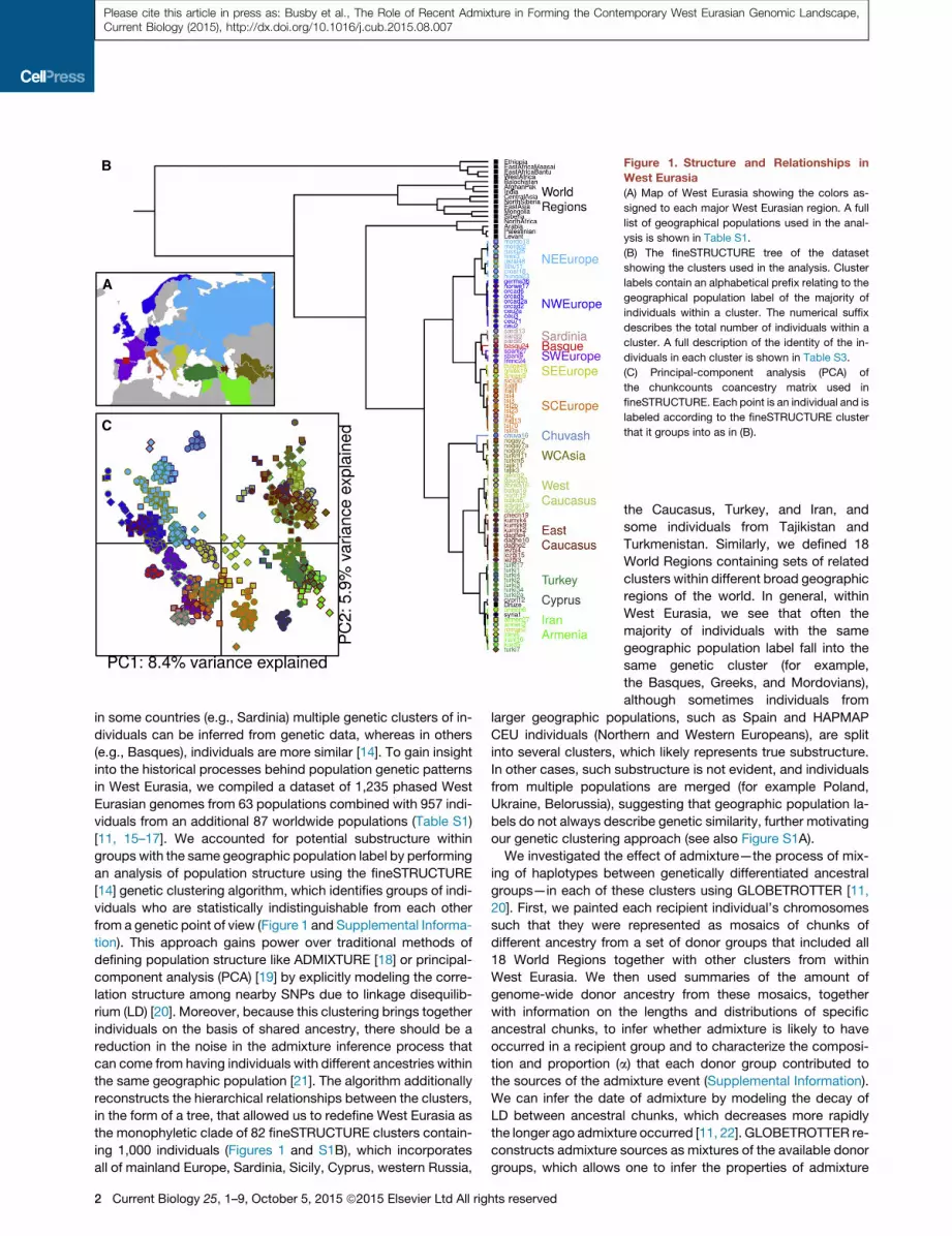
Figure 1. Structure and Relationships in

West Eurasia

(A) Map of West Eurasia showing the colors as-

signed to each major West Eurasian region. A full

list of geographical populations used in the anal-

ysis is shown in Table S1.

(B) The fineSTRUCTURE tree of the dataset

showing the clusters used in the analysis. Cluster

labels contain an alphabetical prefix relating to the

geographical population label of the majority of

individuals within a cluster. The numerical suffix

describes the total number of individuals within a

cluster. A full description of the identity of the in-

dividuals in each cluster is shown in Table S3.

(C) Principal-component analysis (PCA) of

the chunkcounts coancestry matrix used in

fineSTRUCTURE. Each point is an individual and is

labeled according to the fineSTRUCTURE cluster

that it groups into as in (B).


in some countries (e.g., Sardinia) multiple genetic clusters of in-

dividuals can be inferred from genetic data, whereas in others

(e.g., Basques), individuals are more similar [14]. To gain insight

into the historical processes behind population genetic patterns

in West Eurasia, we compiled a dataset of 1,235 phased West

Eurasian genomes from 63 populations combined with 957 indi-

viduals from an additional 87 worldwide populations (Table S1)

[11, 15–17]. We accounted for potential substructure within

groups with the same geographic population label by performing

an analysis of population structure using the fineSTRUCTURE

[14] genetic clustering algorithm, which identifies groups of indi-

viduals who are statistically indistinguishable from each other

from a genetic point of view (Figure 1 and Supplemental Informa-

tion). This approach gains power over traditional methods of

defining population structure like ADMIXTURE [18] or principal-

component analysis (PCA) [19] by explicitly modeling the corre-

lation structure among nearby SNPs due to linkage disequilib-

rium (LD) [20]. Moreover, because this clustering brings together

individuals on the basis of shared ancestry, there should be a

reduction in the noise in the admixture inference process that

can come from having individuals with different ancestries within

the same geographic population [21]. The algorithm additionally

reconstructs the hierarchical relationships between the clusters,

in the form of a tree, that allowed us to redefine West Eurasia as

the monophyletic clade of 82 fineSTRUCTURE clusters contain-

ing 1,000 individuals (Figures 1 and S1B), which incorporates

all of mainland Europe, Sardinia, Sicily, Cyprus, western Russia,

2 Current Biology 25, 1–9, October 5, 2015 ª2015 Elsevier Ltd All rights reserved

the Caucasus, Turkey, and Iran, and

some individuals from Tajikistan and

Turkmenistan. Similarly, we defined 18

World Regions containing sets of related

clusters within different broad geographic

regions of the world. In general, within

West Eurasia, we see that often the

majority of individuals with the same

geographic population label fall into the

same genetic cluster (for example,

the Basques, Greeks, and Mordovians),

although sometimes individuals from

larger geographic populations, such as Spain and HAPMAP

CEU individuals (Northern and Western Europeans), are split

into several clusters, which likely represents true substructure.

In other cases, such substructure is not evident, and individuals

from multiple populations are merged (for example Poland,

Ukraine, Belorussia), suggesting that geographic population la-

bels do not always describe genetic similarity, further motivating

our genetic clustering approach (see also Figure S1A).

We investigated the effect of admixture—the process of mix-

ing of haplotypes between genetically differentiated ancestral

groups—in each of these clusters using GLOBETROTTER [11,

20]. First, we painted each recipient individual’s chromosomes

such that they were represented as mosaics of chunks of

different ancestry from a set of donor groups that included all

18 World Regions together with other clusters from within

West Eurasia. We then used summaries of the amount of

genome-wide donor ancestry from these mosaics, together

with information on the lengths and distributions of specific

ancestral chunks, to infer whether admixture is likely to have

occurred in a recipient group and to characterize the composi-

tion and proportion (a) that each donor group contributed to

the sources of the admixture event (Supplemental Information).

We can infer the date of admixture by modeling the decay of

LD between ancestral chunks, which decreases more rapidly

the longer ago admixture occurred [11, 22]. GLOBETROTTER re-

constructs admixture sources as mixtures of the available donor

groups, which allows one to infer the properties of admixture


when the donor groups are themselves admixed, making it

particularly suited to the current setting. We attempted to infer

admixture in all 82 West Eurasian clusters, but, with the excep-

tion of a Finnish cluster (finni3) that contained both of the Finnish

individuals in the analysis (together with a Norwegian), to allow

the algorithm to concentrate on identifying admixture from

genetically well-defined donor groups, we removed all clusters

with fewer than five individuals from being admixture donors,

all of which were sub-groups of larger populations (Table S3).

Admixture Is Common in West EurasiaThe vast majority of clusters (78%; 64 out of 82) showed

evidence of admixture, suggesting that admixture-facilitated

gene flow is a fundamental property of almost all West Eurasian

groups (Tables S4 and S5; Supplemental Information). Here, we

discuss the broader patterns of ancestry across West Eurasia,

with a more detailed assessment of admixture events provided

in the Supplemental Information. Throughout, we refer to the in-

ferred groups characterized byGLOBETROTTER as contributing

to an admixture event as ‘‘sources’’ and the sampled groups

contributing ancestry to these sources as ‘‘donors.’’ It is also

important to note that in the discussion presented below, we

use current-day geographic labels to describe ancestry of histor-

ical sources of admixture. When we describe the ancestry of a

particular source as, for example, ‘‘Mongolian,’’ this is a conve-

nient but less precise proxy for ‘‘ancestry in a historical group

that is related to the ancestry that we observe in contemporary

Mongolian populations today.’’ This shorthand aids reading,

but one must bear in mind that while the inferred sources of

admixture are likely to be closely related genetically to the true

historical admixing groups, because of subsequent population

movements and migration, they may be less closely related

geographically to the original source of that ancestry.

To visualize ancestry acrossWest Eurasia, we constructed cir-

cos plots [23] where each segment of the circle represents a

recipient group. These summaries describe the recent ancestry

of the clusters: each admixture source is colored by contribu-

tions from different donor groups. We can then compare these

mixed sources to the set of admixture donors to find the best-

matching present-day donor group that is connected to events

by links across the middle of the circles (Figures 2 and S3; Table

S4). For any given event, based on the compositions of the sour-

ces, we identify the best-matching major admixture source,

which is always most similar to a West Eurasian donor group,

and the best-matching minor admixture source, which can be

most similar to either a West Eurasian or World Region donor,

and therefore define events in this way. The barplots in Figure 2B

show that almost all of West Eurasia has some ancestry from the

World Regions. Such World Region ancestry can be seen in the

composition of sources involved in events in northern European

groups (NWE and NEE), yet only three of the clusters containing

individuals from this region derive ancestry from a source best

matched by aWorld Region donor. Deconstruction of the admix-

ture events in these northern European clusters shows that most

mixing involves groups already present within West Eurasia (Fig-

ures 2C and S3). Assuming a generation time of 29 years [24],

dates for these events center around the late first millennium

CE, a time known to have involved significant upheaval in Europe

(Figure 2B) [25].

Current Biolog

Recent Gene Flow into West Eurasia from SurroundingWorld RegionsIn contrast to relatively low levels in Northern Europe, ancestry

from East Asia is much more visible in the West Central Asian,

Caucasus, and Turkish clusters, where the influence of Mongolia

(mon) in particular can be seen through the pink links and bars in

Figure 2B and in Figure 4A. InWest Central Asia (WA), someCen-

tral (cas) and East Asian (eas) ancestry is also present across this

region.Within Anatolia (here defined as Armenia and Iran, IA, and

Turkey, TK), West Central Asia (WA; including Nogai, Tajik, and

Turkmen individuals), and several other groups from the Cauca-

sus (EC and WC), events largely involve Asian sources, with the

period after 1000 CE appearing to be important in the generation

of the ancestry of this region (Figure 3B). Interestingly, the three

events that do involve a Mongolian-like source in Northern

Europe, in the Chuvash (CH; chuva16: 829 CE [627–940 CE]),

Russians (russi25: 913 CE [754–1007 CE]), and Mordovians

(mordo13: 792 CE [564–975 CE]) all date prior to 1000 CE, sug-

gesting an origin from a different historical event to the more

eastern groups (Figure 3B). Of the other Asian world regions,

we only see direct admixture from North Siberia (nsib) into a

Finnish cluster (finni3: 469 CE [213 BCE–1011 CE]; Figure 3B

and Table S4) and from India (ind) into a cluster of two Roma-

nians (roman2: 990 CE [741–1245 CE]), putatively of Romany

origin. Nevertheless, observable ancestral components from

Afghanistan and Pakistan groups (afp and bal) in WA, EC, WC,

and IA suggests that ancestry from across Asia is shared with

the more easterly West Eurasian groups.

Southern European groups (SEE, SCE, SDN, SWE, and BA) on

the other hand derive ancestry from African and Near Eastern

World Regions. In particular, ancestry from groups most similar

to contemporary populations from in and around the Levant

(lev; which we define as the World Region containing individuals

from Syria, Palestine, Lebanon, Jordan, Saudi, Yemen, and

Egypt) is present across Italy (SCE), Sardinia (SDN), France

and Spain (SWE), and Armenia (IA; Figure 2B). Interestingly,

North (nafII) andWest (waf) African ancestry is also seen entering

Southern Europe, suggesting a key role for the Mediterranean in

supporting gene flow back into Europe [8, 26, 27]. Dates for the

influx of this admixture are broad and generally fall within the first

millennium CE (Figure 3B) although are more recent in BA and

SWE, including French (frenc24: 728 CE [424–1011 CE]) and

Spanish (spani27: 1042 CE [740–1201 CE]; spani9: 668 CE

[286–876 CE]) clusters, consistent with migrations associated

with the Arabic Conquest of the Iberian peninsula [8, 11, 28]

and earlier movements in and around Italy [29].

Movement within Europe during the Medieval MigrationPeriodWhen we consider the composition of sources from within West

Eurasia (minor sources in Figure 2C and major sources in Fig-

ure 2D), while the majority of a group’s ancestry tends to come

from its own regional area, there is a substantial contribution of

both Northern European (light and dark blue) and Armenian

groups (light green) to most WA, EC, WC, and TK clusters, as

well as some clusters from both SEE and SCE. As previously re-

ported [11], the formation of the Slavic people at around 1000 CE

had a significant impact on the populations of Northern and

Eastern Europe, a result that is supported by an analysis of


A B

C D

Figure 2. Summary of Eurasian Admixture Events Inferred by GLOBETROTTER

(A) Key showing the position of each cluster in the circos plot. The inner circle describes the type of event inferred in each cluster: gray = no admixture; red = one

date; green = one date multiway, blue = two dates. For the latter two types of events, two sets of sources are shown. Second event sources are suffixed with a 2.

Clusters are ordered clockwise by increasing date within regions around the circle. Labels for plots B–D are shown in bold in (A) for West Eurasian source regions

inside the circle and World Regions sources around the edge.

(B) All events involvingminorWorld Region sources. For each event, the two sources are shown as barplots; each source is split bywhitespace, and the size of the

two sources reflects the proportion that that source contributes to the admixture event. Each source is made up from a number of components whose colors

reflect theWorld Region that the source component comes from. All Eurasian source components are grayed out. Althoughmade up of components, each source

can also be represented by a ‘‘best-matching’’ source, and the central links join the best-matching source (thick end of the link) to the recipient cluster (thin end).

(C and D) Equivalent plots to (B) showingWest Eurasian admixture components in color andWorld Region components in gray. Links in (C) join the best-matching

minor West Eurasian sources to the clusters. Links in (D) join the best-matching major admixture source, which is always from West Eurasia, to the relevant

cluster. Colors in (C) and (D) represent different regions to those in (B).


identity by descent segments in European populations [10].

Here, despite characterizing populations by genetic similarity

rather than geographic labels, we infer the same events involving

a ‘‘Slavic’’ source (represented here by a cluster of Lithuanians;

lithu11 and colored light blue) across all Balkan groups in the

analysis (Greece, Bulgaria, Romania, Croatia, and Hungary) as

well as in a large cluster of Germanic origin (germa36) and a com-

4 Current Biology 25, 1–9, October 5, 2015 ª2015 Elsevier Ltd All rig

posite cluster of eastern European individuals (ukrai48; Figures

4A and 4B). Dates for these events mostly overlap, although

are older in Croatia and Greece, and appear to concentrate at

the end of the first millennium CE (Figure 2B), a time known as

the European Migration Period, or Volkerwanderung [25]. We

additionally infer events during the period 300–1200 CE across

Northern and Western Europe involving minor West Eurasian

hts reserved

Figure 3. Dates of Eurasian Admixture Events Inferred by GLOBETROTTER

(A) Example co-ancestry curves that we use to infer the date of admixture and composition of sources. For a given cluster, CHROMOPAINTER identifies the

chunks of DNA within each individual’s genome that are most closely related ancestrally to each donor group. GLOBETROTTER measures the decay of as-

sociation versus genetic distance between the chunks copied from a given pair of donor groups. Assuming a single pulse of admixture between two or more

distinct admixing source groups, theoretical considerations predict that this decay will be exponentially distributed with rate equal to the time (in generations) that

this admixture occurred [22]. GLOBETROTTER jointly fits an exponential distribution to the decay curves for all pairwise combinations of donor groups and

determines the single best fitting rate, hence determining the most likely single admixture event and estimating the date it occurred. GLOBETROTTER aims to

infer the haplotype composition of each source group for the admixture as a linear combination of those carried by sampled groups. This results in the admixed

groups themselves automatically being represented in the same form—as a mixture of mixtures. The left-most plot of the four large plots shows the relative

probability of jointly copying two chunks from West Africa and North Italian (itali13) donors, at varying genetic distances, in a Sardinian cluster (sardi13). The

curves closely fit an exponential decay (green line) with a rate of 65 generations, or 36 CE. The negative slope for this WestAfrica-itali13 curve suggests that these

(legend continued on next page)

Current Biology 25, 1–9, October 5, 2015 ª2015 Elsevier Ltd All rights reserved 5



source groups from Europe (Figures 2D, 3B, and 4C). The date

and composition of these events suggest a substantial amount

of movement during the Volkerwanderung [25], providing

persuasive evidence that this period had a visible effect on

contemporary populations across Northern, Western, and Cen-

tral Europe (Figure 4C).

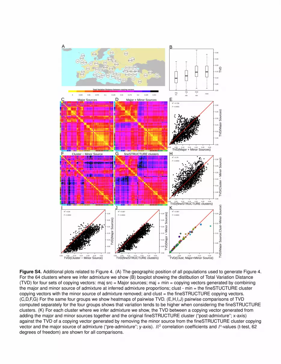
The Effect of Recent Admixture on Genomic Variation inWest EurasiaAll peripheral populations analyzed have experienced recent

admixture from World Regions (Figure 4A), and we also inferred

recent mixing between many of the groups within West Eurasia

(Figure 4C). We performed a variety of analyses using total vari-

ation distance (TVD) to understand and quantify the effect of

these events on genetic variation (Figure 4 and Supplemental In-

formation). Using the output of GLOBETROTTER, we considered

‘‘pre-admixture’’ variation in two ways: by using the inferred ma-

jor source copying vectors directly and by removing the minor

admixing source from the original cluster copying vector.

Likewise, ‘‘post-admixture’’ variation can be inferred either by

combining the inferred major and minor admixture sources in

the appropriate admixture proportions or by using the cluster

copying vectors directly. While the two sets of pre- and post-

admixture copying vectors should be similar, in practice, they

are unlikely to be identical, both because the admixture infer-

ence is unlikely to be perfect and because GLOBETROTTER is

unable to fully account for genetic drift that may have occurred

after admixture [11]. Comparisons of TVD between pairs of

copying vectors inferred in these two ways show that when we

re-generate a cluster from the admixture inference (Figure S4J),

we systematically underestimate variation compared to the

variation we observe when we use the contemporary clusters.

In fact, for a given group, the differences between the two pre-

admixture copying vectors and the two post-admixture copying

vectors are highly correlated (Figure S4K), suggesting that the

variation is mainly down to differences between the (observed)

cluster copying vectors andGLOBETROTTER’s inferred sources

of admixture. If this error is in part due to drift, then this suggests

that drift after admixture may have acted to increase genetic

differentiation.

When we compare the relative differences between pre- and

post-admixture groups, we observe no appreciable difference

between them, suggesting that admixture has not had a signifi-

cant impact on genetic variation inWest Eurasia (Figure 4G). Me-

dian TVD does, however, marginally decrease in the pre-admix-

ture variation estimates (Figure 4G), which appears to be driven

by differences between western (top left quadrant of Figures 4E

and 4F) and eastern (lower right quadrant)West Eurasian groups.

When we plot all admixture sources on a PCA based on contem-

porary individuals (Figure 4D), they tend to occur closer to the

center of the plot, resembling the West Eurasian population

donors contribute to different sides of an admixture event. The inset tsi70-itali13 c

side of the admixture event. We show similar pairs of curves for three other grou

(B) We define each admixture event by the West Eurasian region that the recipie

group to theminor admixture source (colors). We show dates separately for events

and West Eurasian minor sources (right, events shown by links in Figure 2C). Fo

from the specified donor region are combined to generate a density. The integra

generate them.


structure inferred in a recent study of Bronze Age individuals

[6]. Additional recent research using ancient DNA from multiple

populations and time points in West Eurasia has demonstrated

that there has been large-scale genetic turnover in Europe over

the last 5,000 years [4–6, 30]. Our analysis supports this work

by providing evidence that recent population movements have

acted on top of this Bronze Age structure but also highlights a

potential role for admixture and/or genetic drift in contributing

to the genetic variation present in West Eurasia today.

Our results show that it is possible to draw complex inferences

about recent human evolutionary past through the genomes of

people alive today that are complementary to those made from

ancient DNA.We caution that we are unlikely to have included in-

dividuals from all potential genetic donor groups to the current

West Eurasian gene pool, and therefore, the gene flow events

that we present should be viewed in the context of the dataset

that we have used. Future work providing a better understanding

of the phenotypic effects of World Region ancestry on contem-

porary populations as well as placing this work within the context

of ancient DNA samples will further aid our understanding

of Eurasian prehistory and disease. Nonetheless, the current

analysis demonstrates that admixture has left a record in the

genomes of all contemporary West Eurasians.

EXPERIMENTAL PROCEDURES

Dataset

Our dataset included 40 newly genotyped individuals (20 each from Croatia

and Daghestan) together with published data, choosing samples on the basis

of shared genotyping platform (Illumina 550, 610, 660W) and relevance to the

peopling of Western Eurasia [11, 15–17, 31] (Figure 1; Table S1). All datasets

and genetic maps were based on build 36 of the human genome. We merged

the datasets using PLINK (v.1.07) [32], and individuals and SNPs with call rates

of less than 98% were dropped. Further quality control to remove cryptically

related individuals based on identity by descent (IBD) and PCA was also per-

formed. The final dataset contained 2,192 individuals from 144 populations

typed on 477,812 SNPs (Table S1), which were computationally phased

together using SHAPEITv1 [33]. Individuals who provided samples gave

informed consent following ethical approval by the ethics committees at the

various universities where the samples were collected.

Defining Analysis Clusters

We ran fineSTRUCTURE [14] to cluster individuals and identified 18 World

Regions based on this clustering (Figure 1; Table S2). Fixing these groups,

we re-ran the algorithm twice, identifying the final list of 82 Eurasian clusters

(Table S3) based on comparisons between these two runs. Clusters are there-

fore based on genetic similarity only (see also Figure S1). PCAs in Figures 1 and

S4 were generated by performing a PCA on the CHROMOPAINTER chunk-

countsmatrix using the prcomp function in R [34]. Further details are described

in the Supplemental Information.

Inferring Complex Admixture with GLOBETROTTER

Wedescribe the detailed process of inferring admixture with GLOBETROTTER

in the Supplemental Information. Briefly, we first used CHROMOPAINTER, a

chromosome-painting method that reconstructs each individual genome as

urve has a positive slope, showing that tsi70 and itali13 contribute to the same

ps (turkm11, croat18, and ceu71) with varying dates and donors of admixture.

nt group comes from (rows) and the identity of the best-matching current-day

involvingWorld Region minor sources (left, events shown by links in Figure 2B)

r each region, all date bootstraps for events involving a best-matching source

ls of the densities are proportional to the number of admixture events used to

hts reserved

Figure 4. The Impact of Recent Admixture in West Eurasia

(A) For each geographic sampling location, we estimated the proportion of ancestry coming from outside of West Eurasia by averaging GLOBETROTTER’s

admixture inference across individuals from a sampling location. The sampling locations of each point are shown in Figure S4A; Caucasus populations are spread

out to aid visibility. Points are stacked vertically in cases where multiple ancestries are present in a population.

(B) Copying vectors of 82 West Eurasian fineSTRUCTURE clusters projected onto PCA based on the copying vectors of 1,000 West Eurasian individuals (faded

colors; symbols and colors are as in Figure 1B); lines link World Region admixture sources to the clusters in which admixture from them is inferred.

(C) Gene flow within West Eurasia is shown by lines linking the best-matching donor group to the sources of admixture with recipient clusters (arrowhead). Line

colors represent the regional identity of the donor group, and line thickness represents the proportion of DNA coming from the donor group. Ranges of the dates

(point estimates) for events involving sources most similar to selected donor groups are shown.

(D and E) The pre-admixture structure of West Eurasian groups is shown by projecting all admixture source copying vectors that most closely match a West

Eurasian group (n = 81) and the cluster copying vectors where we do not infer admixture (n = 18) onto the same PCA as (B). Heatmaps showpairwise total variation

distance (TVD) between the Major admixture source copying vectors of all clusters where we infer admixture (n = 64; E) and copying vectors generated by

combining the Major and Minor admixture sources at inferred admixture proportions.

(legend continued on next page)

Current Biology 25, 1–9, October 5, 2015 ª2015 Elsevier Ltd All rights reserved 7



a mosaic of all donor groups, to identify the subset of donors that share mate-

rial with the recipient group. Next, because closely related individuals share

long stretches of DNA, with the length of these chunks shortening as individ-

uals become less related, we used the paintings to infer the distribution of

ancestral chunks at different genetic distances along the genome, and build

‘‘coancestry curves’’ for each pair of putative donor populations (Figure 3A).

Assuming a single pulse of admixture involving two genetically distinct sour-

ces, the exponential decay of these curves is proportional to the time since ge-

netic material from the two donor groups came together and thus provides a

date of the admixture event [11, 22]. Finally, we sequentially removed donor

groups from the analysis where such curves were no different from back-

ground noise, a step that allowed us to (re-)assess the makeup of the contrib-

uting source groups and to identify whether two groups occur on the same

side of an admixture event. We performed further tests on these curves, allow-

ing us to assess whether admixture has occurred at multiple times in a group

(i.e. we tried to fit multiple exponentials to the coancestry curves) and whether

admixture occurred with more than two admixing source groups. We tested

the robustness of the admixture inference by comparing these curves with

those generated by considering CHROMOPAINTER painting samples from

different individuals, leveraging the idea that ancestry LD characteristically

decays within individual genomes much more strongly than when ancestry

is measured in different individuals (Supplemental Information).

Characterizing Admixture Events and Source Copying Vectors

In cases where we inferred admixture (p < 0.01), we then characterized the

admixture as one date (1D), one date multiway (1MW), or multiple dates

(2D). For each event in each cluster, we inferred the proportion, a and date(s),

l, of admixture together with a set of bs, which describe the composition of the

admixing sources. 1D events have two admixing sources; 1MWand 2D events

have four admixing sources. To infer copying vectors for the admixture sour-

ces, we took the b coefficients for a given source and multiplied each by their

respective copying vectors (see the Supplemental Information for a detailed

discussion of this approach). In Figure 4, to assay pre-admixture variation,

we showed comparisons between major source copying vectors (Major) and

clusters with admixture sources removed (Cluster � Minor), and for post-

admixture variation, we use the inferred admixed group (Major + Minor) and

contemporary cluster copying vectors.

We generated 100 date bootstraps by re-estimating the date of admixture

sampling the painted samples from all individuals in a cluster with replacement.

In the text, figures, and tables, we converted time in admixture in generations to

historical timeassumingageneration timeof29years [24]. InFigure3, dateboot-

straps are combined across all events involving best-matching sources from a

given region and then grouped by the region that the target cluster comes from.

Comparing Sets of Copying Vectors

We used TVD to compare copying vectors [20]. As the copying vectors are

discrete probability distributions over the same set of donors, TVD is a natural

metric for quantifying the difference between them. For a given pair of groupsA

and Bwith copying vectors describing the copying from i donors, ai and bi, we

can estimate TVD with the following equation:

TVD=0:53Xn

i = 1

ðjai � bi j Þ

To compare variation in West Eurasia before and after admixture, we esti-

mated TVD for each pair of copying vectors and show the distribution as violin

plots (Figure 4G) and boxplots (Figure S4B).

ACCESSION NUMBERS

The accession number for the Croatian samples genotyped for this study is

GEO: GSE71603.

(F) In cases where we infer one date multiway or two dates, we show the major so

from top to bottom as in the tree in Figure 1, and axis colors describe the geogra

(G) Violin plots comparing the distribution of TVD between the same two sets of c

25–75 percentiles; and the plots are truncated at the 2.5 and 97.5 percentiles. Th


SUPPLEMENTAL INFORMATION

Supplemental Information includes Supplemental Experimental Procedures,

four figures, and five tables and can be found with this article online at

http://dx.doi.org/10.1016/j.cub.2015.08.007.

AUTHOR CONTRIBUTIONS

C.C. and G.B.J.B. conceived and designed the research. G.H., S.M., and

G.B.J.B. developed methods. G.B.J.B. and F.M. performed analyses. S.T.,

K.B., I.R., T.Z., C.H., D.T., S.K.-Y., D.N., P.A., F.C., F.B., V.R., G.L., C.B.,

J.B.C., A.H.-K., S.D., R.P., P.K., T.H., T.M., R.J.H., and J.F.W. provided

DNA samples for genotyping. G.B.J.B. and C.C. wrote the paper, which was

reviewed by all authors.

ACKNOWLEDGMENTS

We thank all anonymous donors of DNA. Additionally, we thank the staff of the

Unita Operativa Complessa di Medicina Trasfusionale, Azienda Ospedaliera

Umberto I, Siracusa, Italy. We are grateful to the John Fell Fund at the Univer-

sity of Oxford (C.C.), theWellcome Trust (S.M., grant 098387/Z/12/Z), theWell-

come Trust and Royal Society (G.H., grant 098386/Z/12/Z), the Biotechnology

and Biological Sciences Research Council (G.B.J.B.), and the British Academy

(C.C., grant BARDA-47870) for funding. Request for access to the Daghestan

data should be directed to K.B. at [email protected]. J.F.W. is a share-

holder, employee, and director of the commercial genetic ancestry testing

company ScotlandsDNA.

Received: April 1, 2015

Revised: June 29, 2015

Accepted: August 5, 2015

Published: September 17, 2015

REFERENCES

1. Haak, W., Balanovsky, O., Sanchez, J.J., Koshel, S., Zaporozhchenko, V.,

Adler, C.J., Der Sarkissian, C.S., Brandt, G., Schwarz, C., Nicklisch, N.,

et al.; Members of the Genographic Consortium (2010). Ancient DNA

from European early neolithic farmers reveals their near eastern affinities.

PLoS Biol. 8, e1000536.

2. Skoglund, P., Malmstrom, H., Raghavan, M., Stora, J., Hall, P., Willerslev,

E., Gilbert, M.T., Gotherstrom, A., and Jakobsson, M. (2012). Origins and

genetic legacy of Neolithic farmers and hunter-gatherers in Europe.

Science 336, 466–469.

3. Malmstrom, H., Gilbert, M.T.P., Thomas, M.G., Brandstrom, M., Stora, J.,

Molnar, P., Andersen, P.K., Bendixen, C., Holmlund, G., Gotherstrom, A.,

and Willerslev, E. (2009). Ancient DNA reveals lack of continuity between

neolithic hunter-gatherers and contemporary Scandinavians. Curr. Biol.

19, 1758–1762.

4. Lazaridis, I., Patterson, N., Mittnik, A., Renaud, G., Mallick, S., Kirsanow,

K., Sudmant, P.H., Schraiber, J.G., Castellano, S., Lipson, M., et al.

(2014). Ancient human genomes suggest three ancestral populations for

present-day Europeans. Nature 513, 409–413.

5. Haak, W., Lazaridis, I., Patterson, N., Rohland, N., Mallick, S., Llamas, B.,

Brandt, G., Nordenfelt, S., Harney, E., Stewardson, K., et al. (2015).

Massive migration from the steppe was a source for Indo-European lan-

guages in Europe. Nature 522, 207–211.

6. Allentoft, M.E., Sikora, M., Sjogren, K.G., Rasmussen, S., Rasmussen, M.,

Stenderup, J., Damgaard, P.B., Schroeder, H., Ahlstrom, T., Vinner, L.,

urce for the first and/or most recent event only. Clusters are in the same order

phical origin of the cluster.

opying vectors. The white point indicates the median value; the box shows the

e colored shapes show kernel densities.

hts reserved



http://refhub.elsevier.com/S0960-9822(15)00949-5/sref1

























et al. (2015). Population genomics of Bronze Age Eurasia. Nature 522,

167–172.

7. Brandt, G., Haak, W., Adler, C.J., Roth, C., Szecsenyi-Nagy, A., Karimnia,

S., Moller-Rieker, S., Meller, H., Ganslmeier, R., Friederich, S., et al.;

Genographic Consortium (2013). Ancient DNA reveals key stages in the

formation of central European mitochondrial genetic diversity. Science

342, 257–261.

8. Moorjani, P., Patterson, N., Hirschhorn, J.N., Keinan, A., Hao, L., Atzmon,

G., Burns, E., Ostrer, H., Price, A.L., and Reich, D. (2011). The history of

African gene flow into Southern Europeans, Levantines, and Jews. PLoS

Genet. 7, e1001373.

9. Patterson, N., Moorjani, P., Luo, Y., Mallick, S., Rohland, N., Zhan, Y.,

Genschoreck, T., Webster, T., and Reich, D. (2012). Ancient admixture

in human history. Genetics 192, 1065–1093.

10. Ralph, P., and Coop, G. (2013). The geography of recent genetic ancestry

across Europe. PLoS Biol. 11, e1001555.

11. Hellenthal, G., Busby, G.B.J., Band, G., Wilson, J.F., Capelli, C., Falush,

D., and Myers, S. (2014). A genetic atlas of human admixture history.

Science 343, 747–751.

12. Novembre, J., Johnson, T., Bryc, K., Kutalik, Z., Boyko, A.R., Auton, A.,

Indap, A., King, K.S., Bergmann, S., Nelson, M.R., et al. (2008). Genes

mirror geography within Europe. Nature 456, 98–101.

13. Lao, O., Lu, T.T., Nothnagel, M., Junge, O., Freitag-Wolf, S., Caliebe, A.,

Balascakova, M., Bertranpetit, J., Bindoff, L.A., Comas, D., et al. (2008).

Correlation between genetic and geographic structure in Europe. Curr.

Biol. 18, 1241–1248.

14. Lawson, D.J., Hellenthal, G., Myers, S., and Falush, D. (2012). Inference

of population structure using dense haplotype data. PLoS Genet. 8,

e1002453.

15. Rasmussen, M., Li, Y., Lindgreen, S., Pedersen, J.S., Albrechtsen, A.,

Moltke, I., Metspalu, M., Metspalu, E., Kivisild, T., Gupta, R., et al.

(2010). Ancient human genome sequence of an extinct Palaeo-Eskimo.

Nature 463, 757–762.

16. Behar, D.M., Yunusbayev, B., Metspalu, M., Metspalu, E., Rosset, S.,

Parik, J., Rootsi, S., Chaubey, G., Kutuev, I., Yudkovsky, G., et al.

(2010). The genome-wide structure of the Jewish people. Nature 466,

238–242.

17. Yunusbayev, B., Metspalu, M., Jarve, M., Kutuev, I., Rootsi, S., Metspalu,

E., Behar, D.M., Varendi, K., Sahakyan, H., Khusainova, R., et al. (2012).

The Caucasus as an asymmetric semipermeable barrier to ancient human

migrations. Mol. Biol. Evol. 29, 359–365.

18. Alexander, D.H., Novembre, J., and Lange, K. (2009). Fast model-based

estimation of ancestry in unrelated individuals. Genome Res. 19, 1655–

1664.

19. Price, A.L., Patterson, N.J., Plenge, R.M., Weinblatt, M.E., Shadick, N.A.,

and Reich, D. (2006). Principal components analysis corrects for stratifica-

tion in genome-wide association studies. Nat. Genet. 38, 904–909.

20. Leslie, S., Winney, B., Hellenthal, G., Davison, D., Boumertit, A., Day, T.,

Hutnik, K., Royrvik, E.C., Cunliffe, B., Lawson, D.J., et al.; Wellcome

Current Biolog

Trust Case Control Consortium 2; International Multiple Sclerosis

Genetics Consortium (2015). The fine-scale genetic structure of the

British population. Nature 519, 309–314.

21. Montinaro, F., Busby, G.B.J., Pascali, V.L., Myers, S., Hellenthal, G., and

Capelli, C. (2015). Unravelling the hidden ancestry of American admixed

populations. Nat. Commun. 6, 6596.

22. Falush, D., Stephens, M., and Pritchard, J.K. (2003). Inference of popula-

tion structure using multilocus genotype data: linked loci and correlated

allele frequencies. Genetics 164, 1567–1587.

23. Krzywinski, M., Schein, J., Birol, I., Connors, J., Gascoyne, R., Horsman,

D., Jones, S.J., and Marra, M.A. (2009). Circos: an information aesthetic

for comparative genomics. Genome Res. 19, 1639–1645.

24. Fenner, J.N. (2005). Cross-cultural estimation of the human generation

interval for use in genetics-based population divergence studies. Am. J.

Phys. Anthropol. 128, 415–423.

25. Heather, P. (2009). Empires and Barbarians: Migration, Development and

the Birth of Europe (London: Macmillan).

26. Auton, A., Bryc, K., Boyko, A.R., Lohmueller, K.E., Novembre, J.,

Reynolds, A., Indap, A., Wright, M.H., Degenhardt, J.D., Gutenkunst,

R.N., et al. (2009). Global distribution of genomic diversity underscores

rich complex history of continental human populations. Genome Res.

19, 795–803.

27. Botigue, L.R., Henn, B.M., Gravel, S., Maples, B.K., Gignoux, C.R.,

Corona, E., Atzmon, G., Burns, E., Ostrer, H., Flores, C., et al. (2013).

Gene flow from North Africa contributes to differential human genetic

diversity in southern Europe. Proc. Natl. Acad. Sci. USA 110, 11791–

11796.

28. Roberts, J. (2007). The New Penguin History of the World, Fifth Edition

(London: Penguin Books).

29. Metcalfe, A. (2009). The Muslims in Medieval Italy (Edinburgh: Edinburgh

University Press).

30. Brotherton, P., Haak, W., Templeton, J., Brandt, G., Soubrier, J., Jane

Adler, C., Richards, S.M., Sarkissian, C.D., Ganslmeier, R., Friederich,

S., et al.; Genographic Consortium (2013). Neolithic mitochondrial

haplogroup H genomes and the genetic origins of Europeans. Nat.

Commun. 4, 1764.

31. Hodo�glugil, U., and Mahley, R.W. (2012). Turkish population structure and

genetic ancestry reveal relatedness among Eurasian populations. Ann.

Hum. Genet. 76, 128–141.

32. Purcell, S., Neale, B., Todd-Brown, K., Thomas, L., Ferreira, M.A., Bender,

D., Maller, J., Sklar, P., de Bakker, P.I., Daly, M.J., and Sham, P.C. (2007).

PLINK: a tool set for whole-genome association and population-based

linkage analyses. Am. J. Hum. Genet. 81, 559–575.

33. Delaneau, O., Marchini, J., and Zagury, J.F. (2012). A linear complexity

phasing method for thousands of genomes. Nat. Methods 9, 179–181.

34. R Development Core Team (2011). R: A language and environment for

statistical computing (R Foundation for Statistical Computing). http://

www.r-project.org.

































































































http://www.r-project.org

http://www.r-project.org

Current Biology

Supplemental Information

The Role of Recent Admixture in Forming

the Contemporary West Eurasian Genomic Landscape

George B.J. Busby, Garrett Hellenthal, Francesco Montinaro, Sergio Tofanelli, Kazima

Bulayeva, Igor Rudan, Tatijana Zemunik, Caroline Hayward, Draga Toncheva, Sena

Karachanak-Yankova, Desislava Nesheva, Paolo Anagnostou, Francesco Cali,

Francesca Brisighelli, Valentino Romano, Gerard Lefranc, Catherine Buresi, Jemni Ben

Chibani, Amel Haj-Khelil, Sabri Denden, Rafal Ploski, Pawel Krajewski, Tor Hervig,

Torolf Moen, Rene J. Herrera, James F. Wilson, Simon Myers, and Cristian Capelli

1.53

12.5

23.4

34.4

45.3

56.2

67.2

78.1

89.1

100

South

Europ

e

North

Europ

e

Anato

lia

North

Cauca

sus

South

Cauca

sus

Leva

nt

Palesti

nian

Druze

Arabia

North

Africa

India

Afgha

nPak

Baloch

istan

Mon

golia

Siberia

Centra

lAsia

North

Siberia

EastA

sia

EastA

frica

Maa

sai

Ethiop

ia

EastA

frica

Bantu

Wes

tAfri

ca

South

Europ

eNor

thEur

opeAna

tolia

North

Cauca

sus

South

Cauca

susLe

vantPale

stinia

nDru

zeArabia

North

Africa

India

Afgha

nPak

Baloch

istanM

ongo

liaSiberia

Centra

lAsia

North

SiberiaEas

tAsia

EastA

frica

Maa

sai

Ethiop

ia

EastA

frica

Bantu

Wes

tAfri

ca

●● ●●● ●

●●

●

●

●●

●●

●

●●●

●●●

●

●

●

●

●

●●

●

●●●

●

● ●

●

●

●

● ●

●

●

●●

●

●

●●

● ●

●

●

●

●

●

●

●●●

●●

●

●

●

●

●●

●●

●●●

●

●

●●

●

●

●

●

●●

●

●● ●

●

●

●●●

●●

●

●

●●

●● ●

●

●

●●

●●

● ●

●

●● ●●

●●

●

●

●●●

●

●

●

●

●

●●

●●

●

●

●

●●

●

●

●●

●

●● ●●

●●

●●

●●

●

●

●●

●

●

●

●

●●

●

●●

●

●

●

●

●

●

●●● ●

●

●●●

●●●

●

●

●

●●● ●●

●

●●●

●

●

●

●

● ●●

●

●

●

●

●

●

●●

●

●●

●

●●

●

●

●

●●●

● ●

●

●

●

●

●

●

●●

●

●●

●

●

●●

●

●●

●

● ●●

● ●

●

● ●●

●●

●

●

●

● ●

●●

●

●

●

●

●

●●

●

●●

●

●

●

●●

●

●●

● ●●

●

●

●●

●

●

●●

●

●●●

●

●

●

●

●●

●

●

●●

●

●

●●●

●

● ●●

●

●

●

●●●

●●

● ●

●

●●●

●

●

● ●

● ●

●

●

● ●●

●

●

●

●

●

●●

●

●●●

●●●

●

●

●

● ● ●●●

● ●

●●

●

●

●

●●●

●●

●

●

●

●

●

●

●

●

● ●

●●

●●

●

●

●

●

●●●●

●

●

●

●

●●

●

●

●●

●

●

●

●

●● ●●

●●

●●

●

●

●

●●

●

●

●

●●

●

●

●●

●●

●●

●●

● ●

●●●

●

●

●

●

●●

●

●

●

●● ●

●●

●●

●

●●

●

●

● ●●●

●

●●●

● ●●

●

●

●●●●●

●●●

● ●

●

●●

●

●●

●●●

●

●●●

●

●

●● ●● ●

●● ●

●

●

●●

●● ●● ●

●

●●●

●●

●●

●●

● ●●

● ●

●

●

●

● ●●● ●

●

●●

●

●●●●

●

●

● ●

●● ●

●

●●

● ●● ●

●

●

●●

●

●●

●

●

● ●●●

●●

●

●

●●

●●

●

●●

●●●●

●●

●

●

●●●● ●

● ●

●●●● ●●

●

●●●

●

●●

● ●●

●●

●

●●●●●

●

●

●

●●●

●

●

●●●

●●

●

●

●●

●

●

● ● ●●

●

●

●●

●●

●●

●

● ●

●● ●●

● ●

●

●●

●● ●

●

●

−0.10 −0.05 0.00 0.05 0.10

−0.

050.

000.

05

PC2

PC

1North ItalianSouth ItalianSardinianEast SicilianWest SicilianTuscan

A

CPalestinianLevantDruzeArabiaNorthAfricaAnatoliaNorthCaucasusSouthCaucasusSouthEuropeNorthEuropeAfghanPakIndiaBalochistanMongoliaSiberiaNorthSiberiaCentralAsiaEastAsiaEastAfricaBantuWestAfricaEastAfricaMaasaiEthiopia

B

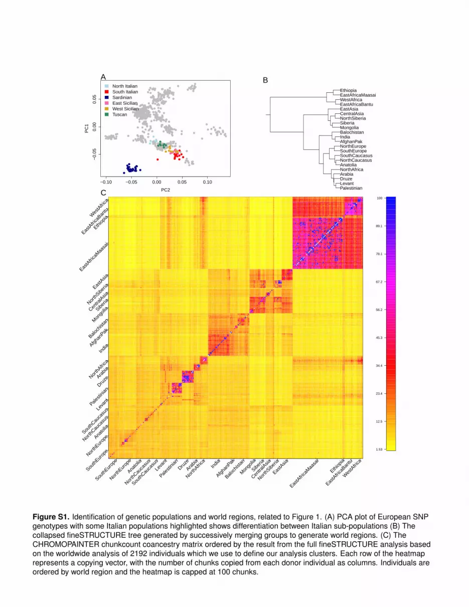
Figure S1. Identification of genetic populations and world regions, related to Figure 1. (A) PCA plot of European SNPgenotypes with some Italian populations highlighted shows differentiation between Italian sub-populations (B) Thecollapsed fineSTRUCTURE tree generated by successively merging groups to generate world regions. (C) TheCHROMOPAINTER chunkcount coancestry matrix ordered by the result from the full fineSTRUCTURE analysis basedon the worldwide analysis of 2192 individuals which we use to define our analysis clusters. Each row of the heatmaprepresents a copying vector, with the number of chunks copied from each donor individual as columns. Individuals areordered by world region and the heatmap is capped at 100 chunks.

●●●●●●●●●●

●●●●●●●●●●

●●●●●●●●●●

●●●●●●●●●●●●●●●●●●●● ●●●●●●●●●● ●●●●●●●●●● ●●●●●●●●●● ●●●●●●●●●● ●●●●●●●●●● ●●●●●●●●●● ●●●●●●●●●● ●●●●●●●●●● ●●●●●●●●●●

K

cros

s va

lidat

ion

erro

r

0.49

0.50

0.51

0.52

K1 K2 K3 K4 K5 K6 K7 K8 K9 K10 K11 K12 K13 K14

●

● lowest CV error

K=2

K=3

K=4

K=5

K=6

K=7

K=8

K=9

K=10

K=11

K=12

K=13

K=14

Wes

tAfri

caE

astA

frica

Ban

tu

Eas

tAfri

caM

aasa

i

Eth

iopi

aN

orth

Afri

ca

Sou

thE

urop

e

Nor

thE

urop

e

Nor

thC

auca

sus

Sou

thC

auca

sus

Ana

tolia

Leva

ntD

ruze

Pale

stin

ian

Ara

bia

Cen

tralA

sia

Bal

ochi

stan

Afg

hanP

akIn

dia

Mon

golia

Eas

tAsi

aS

iber

iaN

orth

Sib

eria

Wes

tAfr

ica(

45)

Eas

tAfr

icaB

antu

(109

)E

astA

fric

aMaa

sai(9

0)E

thio

pia(

20)

Nor

thA

fric

aI(2

4)N

orth

Afr

icaI

I(35

)ar

men

9(9)

balk

a5(5

)ba

squ2

4(24

)bu

lga4

6(46

)cy

pri1

2(12

)fr

enc2

4(24

)gr

eek1

9(19

)ita

li1(1

)ita

li13(

13)

itali8

(8)

sard

i13(

13)

sard

i6(6

)sa

rdi9

(9)

sici

l30(

30)

span

i27(

27)

span

i9(9

)ts

i2(2

)ts

i23(

23)

tsi2

a(2)

tsi2

b(2)

tsi3

(3)

tsi4

(4)

tsi7

0(70

)tu

rki4

(4)

ceu2

(2)

ceu2

a(2)

ceu3

(3)

ceu7

1(71

)cr

oat1

8(18

)fin

ni3(

3)ge

rma3

6(36

)hu

nga2

3(23

)lit

hu11

(11)

mor

do13

(13)

mor

do2(

2)no

rwe1

7(17

)or

cad2

(2)

orca

d2a(

2)or

cad5

(5)

orca

d6(6

)ru

ssi2

5(25

)uk

rai4

8(48

)ab

hka1

6(16

)ad

yge1

3(13

)ad

yge6

(6)

balk

a16(

16)

chec

h19(

19)

dagh

e10(

10)

dagh

e2(2

)da

ghe4

(4)

geor

g2(2

)ge

org2

0(20

)ku

myk

2(2)

kum

yk4(

4)ku

myk

9(9)

lezg

i15(

15)

lezg

i3(3

)le

zgi4

(4)

nort

h15(

15)

chuv

a16(

16)

noga

y2(2

)no

gay7

(7)

noga

y7a(

7)ta

jik11

(11)

tajik

3(3)

turk

m11

(11)

turk

m5(

5)ar

men

2(2)

arm

en27

(27)

arm

en6(

6)ira

ni10

(10)

irani

5(5)

kurd

5(5)

rom

an2(

2)sy

ria1(

1)tu

rki1

(1)

turk

i17(

17)

turk

i2(2

)tu

rki2

a(2)

turk

i3(3

)tu

rki3

4(34

)tu

rki7

(7)

Leva

nt(1

03)

Dru

ze(3

3)P

ales

tinia

n(31

)A

rabi

a(38

)C

entr

alA

sia(

41)

Bal

ochi

stan

(71)

Afg

hanP

ak(8

3)In

dia(

122)

Mon

golia

(93)

Eas

tAsi

a(17

5)S

iber

ia(5

4)N

orth

Sib

eria

(25)

Figure S2. An ADMIXTURE analysis of the dataset showing the average admixture proportions for each cluster andworld region. The top plot shows the cross validation error across multiple runs picking 8 as the optimum number ofclusters. The number of individuals in each cluster world/region is in parentheses after the cluster/region name. Weused an LD (R2) threshold of 0.2.

mordo13 ●

russi25 ●

finni3 ●

ukrai48 ●

lithu11 ●

lithu11 ●

croat18 ●

hunga23 ●

germa36 ●

norwe17 ●

orcad6 ●

orcad5 ●

ceu71 ●

ceu71 ●

sardi13 ●

sardi9 ●

sardi6 ●

basqu24 ●

basqu24 ●

spani27 ●

spani27 ●

spani9 ●

spani9 ●

frenc24 ●

bulga46 ●

greek19 ●

armen9 ●

armen9 ●

sicil30 ●

itali8 ●

tsi23 ●

itali13 ●

tsi70 ●

chuva16 ●

nogay7 ●

nogay7a ●

nogay2 ●

nogay2 ●

turkm11 ●

turkm5 ●

tajik11 ●

tajik3 ●

georg20 ●

abhka16 ●

balka16 ●

north15 ●

balka5 ●

balka5 ●

adyge13 ●

adyge13 ●

adyge6 ●

chech19 ●

kumyk4 ●

kumyk4 ●

kumyk9 ●

kumyk2 ●

daghe4 ●

daghe4 ●

daghe10 ●

daghe10 ●

daghe2 ●

lezgi4 ●

lezgi4 ●

lezgi15 ●

lezgi15 ●

lezgi3 ●

turki17 ●

turki4 ●

turki3 ●

turki34 ●

turki2a ●

cypri12 ●

cypri12 ●

armen27 ●

armen27 ●

roman2 ●

irani5 ●

irani10 ●

irani10 ●

kurd5 ●

turki7 ●

turki7 ●

1500 1000 500 0 −500 −1000DATE (CE/BCE)

West Eurasian sourcecomponents (left)

NWEuropeNEEuropeBasqueSWEuropeSCEuropeSardiniaSEEuropeIran+ArmeniaNearEastTurkeyChuvashCyprusWCAsiaEastCaucasusWestCaucasusWorld Regions

World Region sourcecomponents (right)

EastAfricaBantuEastAfricaMaasaiWestAfricaEthiopiaNorthAfricaINorthAfricaIIBalochistanAfghanPakCentralAsiaIndiaMongoliaEastAsiaNorthSiberiaSiberiaArabiaDruzeLevantPalestinianWest Eurasia

Figure S3. Proportions and dates of admixture shown in Figures 2 and 3. For each cluster we show the result ofadmixture inference, red = 1D (one date of admixture), darkgreen = 1MW (one date, multiple admixing groups), anddarkblue = 2D (two admixture dates). Proportions of the two admixing sources of either side of an admixture event areshown as barplots with their components coloured by donor region. In the left-hand barplot, all non-West Eurasiancomponents are greyed out, whereas the opposite is true for the right hand barplots. The colours of the bars representthe ancestry components detailed in the legends on the right. The date of admixture, with bootstrap CI is also shown inthe central plot.

abhkasianadygei

armenian

balkar

basque

belorussian

british

bulgarian

ceu

chechen

chuvash

croatian

cypriot

daghestani

siciliane

english

finnish

french

georgian

german

greek

hungarian

iranian

irish

italian

kumyk

kurd

lezgin

lithuanianmordovian

nogay

italiann

northossetian

norwegian

orcadian

polish

romanian

russian

sardinian

scottish

italiansspanish

syrian

tajik

tsi

turkishturkisheturkishnturkishs

turkmen

ukrainian

uzbekistani

welsh

sicilianw

turkish

turkishe

turkishn

turkishs

A

Total Variation Distance between copying vectors

0 0.025 0.05 0.075 0.1 0.125 0.15 0.175 0.2 0.225 0.25+

Major SourcesC Major + Minor SourcesD

Cluster − Minor SourceF fineSTRUCTURE clustersG

●

●

●

●

●

●●

●

●

●

●

●

●●

●

●

●

●

●

●

●

●

●

●

●

●

●

●●

●

●

●

●●

●●

●

●

●

●

●

●

●

●

●

●

●

●

●

●

●

●

●

●

●

●

●●

●

●

●

●

●

●

●

●

●

●

●

●

●

●

●●

●●

●

●

●

●

●●

●

●

●

●

●●

●

●●

●

●

●

●

●

●

●●

●

●

●

●

●

●

●●

●

●

●

●●

●

●

●

●

●

●

●

●

●

●

●

●

●

●

●

●

●●

●

●

●

●●

●●

●

●

●

●

●

● ●

●

●●

●●

●

●

●

●

●

●

●

●

●

●

●

●

●

●

●

●

●

●

●

●

●

●

●

●

●

●

●

●

●

●

●●

●

●

●

●

●

●

●

●●

●

●

●

●●

●●

●

●

●

●

●

●●

●

●

●● ● ●

●

●

●

●

●●

●

●

●

●

●

●

●●

●

●

●

●

●

●

●

●

●

●

●

●

●

●

●

●●

●

●

●●

●

●

●●

●

●

●

●●

●●

●

●

●

●

●

● ●

●

●●

●●

●

●

●

●

●

●

●

●

●

●

●

●

●

●

●

●

●

●

●

●

●●

●

●

●

●

●

●

●

●

●●

●●

●

●

●

● ●

●

●

●

●

●

● ●

●

●

●

●

●

● ●

●

●●

●●

●

●

●

●

●

●

●

●

●

●

●

●

●

●

●

●

●

●

●

●

●

●

●

●

●

●

●

●

●

●

●●

●

●

●

●

●

●

●●

●

● ●

●●

●

●

●

●

●●

●

●

●

●

●●

●

●

●

●

●

●

●

●

●

●

●

●●●

●

●

●

●●

●

●

●

●

●

●

●

●

●

●

●

●

●

●

●

●

●

●

●

●

●

●●

●●

●

●

●

●

●●

●

●

●

●

●●

●

●

●

●

●

●

●

●

●

●

●● ●●

●

●

●

●●

●

●

●

●

●

●●

●

●

●

●

●

●

●

●

●

●

●

●

●

●●

●●

●

●

●

●

●●

●

●

●

●

●●

●

●

●●

●

●

●

●

●

●

●●●●

●

●

●

●●

●

● ●

●

●

●

●

●

●

●

●

●

●

●

●

●

●

●

●●

●

●●

●

●

●

●

●●

●

●

●

●

●●

●

●

●

●

●

●

●

●

●

●

●●● ●

●

●

●

●●

●

● ●

●

●

●

●

●

●

●

●

●

●

●

●

●

●

●

●●

●●

●

●

●

●

●●

●

●

●

●

●●

●

●

●●

●

●

●

●

●

●

● ●●●

●

●

●

●●

●

●●

●

●

●

●

●

●

●

●

●

●

●

●

●

●

●

●

●●

●

●

●

●

●●

●

●

●

●

●●

●

●●

●

●

●

●

●

●

●

●

●●

●

●

●

●

●●

●

●

●

●

●

●

●

●

●

●

●

●

●

●

●

●

●

●

●●

●

●

●

●

●●

●

●

●

●

●●

●

●

●

●

●

●

●

●

●

●

●

●●

●

●

●

●

●●

●

●

●

●

●

●

●

●

●

●

●

●

●

●

●

●

●

●

●

●

●

●

●

●

● ●

●

●

●

●●

●

●

●

●

●

●

●

●

●

●

●

●

●

●●

●

●

●

●

●

●●

●

●

●

●

●

●

●

●

●●

●●

●

●

●

●

●

●

●

●

●●

●

●

●

●●

●

●

●

●

●

●

●

●

●

●

●

●

●

●●

●

●

●

●

●

●●

●

●

●

●

●

●

●

●

●●

●●

●

●

●

●

●

●

●●

●

●

●

●

●●

●

●

●●

●

●

●

●

●

●

●●●●

●

●

●

●●

●

●

●

●

●

●●

●

●

●

●

●

●

●

●

●

●

●

●

●●

●●

●

●

●●●

●

●

●

●

●

●

●

●

●

●

●

●

●

●

●

●

●

●

●

●

●

●

●

●

●

●

●

●

●

●

●●

●

●

●

●

●●

●

●

●

●

●●

●

●

●

●●

●

●

●

●

●

●

●

●

●

●●

●

●

●

●

●

●

●●

●

●

●

●

●

●

●

●

●●

●

●

●

●

●

●

●

●

●

●

●

●

●

●

●

●

●

●

● ●●

●

●

●

●

●

●●

●

●

●

●

●

●

●

●

●

●

●

●

●

●

●

●●

● ●

●●

●

●

●

●

●

●

●

●

●

●

●

●

●

●

●●

●

●

●

●

●

● ●

●

●

●

●

●●

●

●

●

●

●

●

●

●

●

●●

●

●

●●

●

●

●

●●

●

●

●

●●

●

●

●●

●

●

●

●

●●

●

●

●

●

●

●

●

●●

●

●

●

●

●

●

●●

●●

●

●

●

●

●

●

●

●

●●

●

●●

●

●

●●

●

●

●

●

●

●

●

●

●

●

●

●

●

●●

●

●

●

●

●

●

●

●

●●

●●

●

●

●

●

●

●

●

●

●

●

●

●

●

●

●

●

●

●

●

●

● ●

●

●

●

●

●

●

●

●

●

●

●

●

●

●

●

●●

●

●

● ●

●

● ●●

●

●

●

●

●

●●

●

●

●

●

●

●

●

●

●

●

●

●

●

●

●

●

●

●

●

●

●

●●

●●

● ●

●

●

●

●

●

●

●

●

●

●

●●

●

●

●

●

●

●

● ●

●

●

●

●

●

●

●

●

●

●

●

●

●

● ●

●●

●

●

●

●

●

●

●

●

●

●

●

●

●

●

●

●

●

●●

●

●

●

●

●

●

●

●●

●

●

●

●

●

●

●

●

●●

●

●

●

●

●

●

●

●

●

●

●●

●

●

●

●●●

●

●

●

●

●

●

●

●●

●

●

●

●

●

●

●●

●●

●

●

●

●

●

●

●

●

●

●

●

●

●

●●

●

●●

●

●

●

●

●

●

●●

●

●

●

●

●

●

●

●

●●

●

●

●

●

●●

●

●

●

●

●

●

●

●

●

●

●

●

●

●

●

●

●

●●

●

●

●

●

●

●

●

●

●●

●●

●

●

●

●

●

●●

●

●

●

●

●

●

●

●

●

●

●

●

●

●

●

●

●

●

●

●

●

●●

●●

● ●

●

●

●

●

●

●

●

●

●

●●

●

●

●

●

●

●

●

●

●●

●

●

●

●

●

●

●

●

●●

●

●

●

●

●

●●

●

●

●

●

●

●●

●

●

●

●

●

●

●●

●

●

●

●

●

●

●●

●●

●

●

●

●

●●

●

●

●

●●●

●

●

●

●

●

●

●

●●

●

●

●

●

●

●

●

●

●●

●

●

●

●

●

●

●

●

●

●

●

●

●

●

●

●

●

●

●

●

●

●

●

●

●

●●

●

●●

●

●

●●●

●

●

●

●

●

●

●

●

●

●

●

●

●

●

●

●

●

●

●

●

●

●

●●

●

●

●

●

●

●●

●

●

●

●

●

●

●

●

●

●

●

●

●●

●

●

●

●

●

●●

●

●

● ●

●

●

●●

●

●

●

●

●

●

●

●●

●

●

●

●

●

●

●●

●●

●

●

●

●

●●

●

●

●

●

●

●

●

●

●

●

●

●

●

●

●

●

●●

●●

●

●

●

●

●

●

●●

●

●

●

●

●

●

●

●

●

●

●

●

●

●●

●●

●

●

●

●

●

●

●

●

●

●

●

●

●

●

●

●

●

●

●

●

●

●

●●

●

●

●

●

●

●

●

●

●

●

●

●●

●

●

●

●

●

●

●●

●●

●●

●

●

●

●

●

●

●

●

●●

●

●

●

●

●

●

●

●

●●

●

●

●

●

●

●

●

●

●

●

●

●

●

●

●

●

●

●

●

●

●

●

●

●

●

●

●

●

●

●●

●

●

●

●

●

●

● ●

●●

●●

●

●

●

●

●

●

●●

●

●

●

●

●

●

●●

●

●

●

●

●

●

●

●

●●

●

●

●

●

●

●

●

●●

●

●

●

●

●

●●

●

●

●

●

●

●

●

●

● ●

●

●

●

●

●

●

●

●

●

●

●

●

●

●

●●

●

●

●

●

●

●

●●

●

●

●

●

●

●●

●

●

●●

●

●

●

●

●

●

●

●

●

●

●

●

●

●

●

●

●

●

●

●

●

●●

●

●

●

●

●

●

●

●

●

●

●

●

●

●

●

●

●

●

●

●

● ●

●

●

●

●

●

●

●

●

●

● ●

●

●

●

●

●

●

●

● ●

●

●

●●

●

●

● ●

●

●

●

●

●

● ●

●

●●

●

●

●

●

●

●●

●●

●

●

●

●

●

●

●

●

●

●

●

●

●

●

0.00 0.05 0.10 0.15 0.20 0.25 0.30

0.00

0.05

0.10

0.15

0.20

0.25

0.30

TV

D(M

ajor

Sou

rces

)

TVD(Major + Minor Sources)

ER2 = 0.728

P < 0.0001

●

●

●

●●

●

●

●

●

●

●

●

●

●

●●

●●

●●

●

●●●

● ●

●

●

●

●

●

●

●

●

●

●

●

●

●

●

●

●

●

●

●

●

●

●●

●

●

●

●

●

●

●

●

●

●

●

●

●

●

●

●

●

●

●

●

●

●

●

●

●

●

●

●

●●

●

●

● ●

●

●●

● ●

●

●

●

●●

●

●

●

●

●

●

●

●

●

●

●

●

●

●

●

●

●

●

●

●

●

●

●

●

●

●

●

●

●

●

●

●

●

●

●

●

●

●

●

●

●

●

●

●

●

●● ●

●●

●

●●●

● ●

●

●

●

●●

●

●●

●

●

●

●

●

●

●

●

●

●

●

●

●

●

●

●●

● ●

●

●

●

●

●

●

●

●

●

●

●

●

●

●

●

●

●

●

●

●

●

●

●

●

●

●

●

●●

●●

●●

●

●

●

●

●

●

●

●

●

●

●

●

●

●

●

●●

●

●

●

●

●

●

●

●

●

●

●

●

●

●

●

●

●

●

●

●

●

●

●

●

●

●

●

●

●

●

●

●●

●

●

●

●

●●●

● ●

●

●

●

●●

●

●

●●

●

●

●

●

●

●

●

●

●

●

●

●

●

●

●

●

●

●

●

●

●

●

●

●

●

●

●

●

●

●●

●

●

●

●

●

●

●

●

●

●

●

●

●

●●●

● ●

●

●

●●

●●

● ●

●

●

●

●

●

●

●

●

●

●

●

●

●

●

●

●●

●●

●

●

●

●

●

●

●

●

●

●

●

●

●

●

●

●

●

●

●

●●

●

●

●●

●

●●

● ●

●

●

●

●●

●

●

●

●

●

●

●

●

●

●

●

●

●

●

●

●

●

●

●

●

●

●

●

●

●

●

●

●

●

●

●

●

●

●

●

●

●

●●

●

●●

●

●

●●

●

●●

● ●

●

●●

●●

●

●

●

●

●

●

●

●

●

●

●

●

●

●

●

●

●

●

●

●

●

●

●

●

●

●

●

●

●

●

●

●

●

●

●

●

●

●

●

●

●

●

●

● ●

●

●●

● ●

●

●

●

●●

●

●

●

●

●

●

●

●

●

●

●

●

●

●

●

●

●

●

●

●

●

●

●

●

●

●

●

●

●

●

●

●

●

●

●

●

●

●

●

●

●

●

●●

●

●●

●●

●

●

●

●

●

●

●

●

●

●

●

●

●

●

●

●

●

●

●

●

●

●

●

●

●

●

●

●

●

●

●

●

●

●

●

●

●

●

●

●

●

●

●●

●

●

●●

●

●●

● ●

●

●

●

●●

●

●

●

●

●

●

●

●

●

●

●

●

●

●

●

●●

●

●

●

●

●

●

●

●

●

●

●

●

●

●

●

●

●

●

●

●

●

●

●

●●

●

●●

● ●

●

●

●

●●

●

●

●

●

●

●

●

●

●

●

●

●

●

●

●

● ●

●

●

●

●

●

●

●

●

●

●

●

●

●

●

●

●

●

●

●

●

●

●

● ●

●

●●

● ●

●

●

●

●●

●

●

●

●

●

●

●

●

●

●

●

●

●

●

●

● ●

●

●

●

●

●

●

●

●

●

●

●

●

●

●

●

●

●

●

●

●

●

●

●

●

●

●

●

●

●

●

●

●

●

●

●

●

●

●

●

●

●

●

●

●

●

●

●

●

●

●

●

●●

●

●

●

●

●

●

●

●

●

●

●●

●

●

●

●

●

●

●

●

●

●

●

●

●

●

●

●

●

●

●

●

●

●

●

●

●

●

●

●

●

●

●

●

●

●

●

●●

●

●

●

●

●

●

●

●

●

●

●●

●

●

●

●

●●

●

●●

●●

●

●

●

●●

●

●

●

●

●

●

●

●

●

●

●

●

●

●

●

●

●

●

●

●

●

●

●

●

●

●

●

●

●

●

●

●

●

●● ●

●

●

●

●

●●

●

●

●

●

●

●

●

●

●

●●

●

●

●

●

●

●

●

●

●

●

●

●

●

●

●

●

●

●

●

●

●

●

●

●

●

●

●

●

●

●

●●

●

●

●

●

●●●

●

●●

●

●

●

●● ●

●

●

●

●

●

●

●

●

●

●

●●

●

●

●

●

●

●

●

● ●

●

●

●

●

●

●

● ●

●

●

●

●

●

●

● ●● ●●

●

●

●

●

●

●

●

●

●

●

●

●

●

●

●

●

●

●

●

●

●●

●

●

● ●

●

●

●

●

●

●

●

●

●

●

●

●

●

●●●

●●

●

●

●

●●

●

●

●

●

●

●

●

●

●

●

●

●

●

●

●

●

●

●

●

●

●

●

●

●

●

●

●

●●

●

●

●

●●

●

●●

●

●

●

●

●

●

●

●

●

●

●

●

●

●

●

●

●

●

●

●

●

●

●

●

●

● ●

●

●

●

●

●

●

●

●

●

● ●

●

●

●●

●

●

●

●

●●●

●

●

●

●

●

●

● ●

●

●

●

●

●

●

●

●

●

●

● ●

●

●

●

●

●

●

●

●

●

●

●

●

●

●

● ●●

●

●

●

●

●

●

●

●

●

●

●

●

●

●

●

●

●

●

●

●

●

●

●

●

●

●

●

●

●

●

●

●

●

●

●

●

●●

●

●

●

●●

●

●

●

●

●

●

●

●

●

●

●

●

●

●

●

●

●

●

●

●

●

●

●

●

●

●

●

●

●

●

●

●●

●

●

●

●

●

●

●

●

●

●

●

●

●

●

●

●

●

●

●

●

●

●●

●

●

●

●

●

●

●

●

●

●●

●

●

●●

●

●

●

●●

●●

●

●

●

●

●

●

●●

●

●●

●

●

●

●

●

●

●

●●

●

●

●

●

●

●

●

●

●●●

●

●

●

●

●

● ●

●

●

●

●

●

●

●

●

●

●

●

●

●

●●

●

●

● ●

●

●

●

●

●

●

●

●

●

●

●

●●

●

●

●

●

●

●

●

●

●

●

●

●

●

●

●

●

●

●

●

●

●

●

●

●

●

●

●

●

●●

●

●

●

●

●

●

●

●

●

●

●

●

●

●

●

●

●

●

●

●

●

●

●

●

●

●

●●

●

●

●

●

●

●

●●

●

●

●

● ●

●

●

●

●

●

●

●●

●

●

●

●

●

●

●

● ●

●

●

●

●

●

●

●

●

●

●

●

●

●●

●

●

●

●

●

●

●

●

●

●

●

●

●

●

●

●

●

●

●

●

●

●

●

●

●

●

●●

●

●

●

●

●

●

●

●

●

●

●

●

●

●

●

●

●●

●

●

●

●

●

●

●

● ●

●

●

●

●

●

●

●●

●

●

●

●

●

●

●

●

●

●

●

●

●

●

●

●

●

●

●

●

●

●

●

●

●

●

●

●

●

●

●

●

●

●

●

●

●

●

●

●

●

●

●

●

●●

●

●

●

●

●

●

●

●

●

●

●

●

●

●

●

●

●

●

●

●

●

●

●

●

●

●

●

●

●

●

●

●

●

●

●

●

●

●

●

●

●

●

●

●

●

●

● ●

●●

●

●

●

●

●

●

●

●●

●

●

●

●

●

●

●

●

●

●

●

●

●

●

●

●

●

●

●

●

●

●●

●

●

●

●●

●

●

● ●

●

●

●

●

●

●

●

●

●

●

●

●

●

●

●

●●

●

●

●

●

●

●

●

●

●

●

●

●

●

●

●

●

●

●

●

●

●

●

●

●●

●

●

●

●●

●

●

●

●

●

●

●

●

●

●

●

●

●

●

●

●

●

●●

●

●

●

●

●

●

●

●

●

●

●●

●

●

●

●

●

●

●

●

●

●●

●

●

●

●

●

●

●

●●

●

●

● ●

●

●

●

●

●

●

●

●●

●

●

●

●

●

●

●

● ●

●

●

●

●

●

●

●

●

●

●

●

●

●

●

●

●

●

●

●

●

●●

●

●

●

●

●

●

●

●

●●

●

●

●

●●

●

●

●●

●

●

●

●

●

●

●

●

●

●●

●

●

●

●●

●

●

●

●

●

●

●

●

●

●

●

●●

●

●

●

●

●

●

●

●

●

●

●

●

●

●

●●

●

●

●

●

●

●

●

●

●

●

●

● ●

●

●

●

●

●

●

●

●

●

●

●

●

●

●

●

●

●

●

●

●

●

●

●

●

●

●

●

●

●

●

●

●

●

●

●

●

●

●

●

●

●

●

●

●

●

●

●

●

●

●

●

●

●

●

●

●

●

●

●

●

●

●

●

●

●

●

●

●

●

●

●

●

●

●

●

●

●

●

●

●

●

●

●

●

●

●

●

●

●

●

●

●

●

●

●

●

●

●

●

●

●

●

●

●

●

●

●

●

●

●

●

●

●

●

●

●

●

●

●

●

●

●

●

●

●

●

●

●

●

●

●

●

●

●

●

0.00 0.05 0.10 0.15 0.20 0.25 0.30

0.00

0.05

0.10

0.15

0.20

0.25

0.30

TV

D(C

lust

er −

Min

or S

ourc

e)

TVD(fineSTRUCTURE clusters)

HR2 = 0.78

P < 0.0001

●

●

●

●

●

● ●

●

●

●

●

●

● ●

●

●

●

●

●

●

●

●

●

●

●

●

●

●●

●

●

●

●●

●●

●

●

●

●

●

●

●

●

●

●

●

●

●

●

●

●

●

●

●

●

●●

●

●

●

●

●

●

●

●

●

●

●

●

●

●

●●

● ●

●

●

●

●

●●

●

●

●

●

●●

●

●●

●

●

●

●

●

●

●●

●

●

●

●

●

●

●●

●

●

●

●●

●

●

●

●

●

●

●

●

●

●

●

●

●

●

●

●

● ●

●

●

●

●●

● ●

●

●

●

●

●

●●

●

●●

●●

●

●

●

●

●

●

●

●

●

●

●

●

●

●

●

●

●

●

●

●

●

●

●

●

●

●

●

●

●

●

● ●

●

●

●

●

●

●

●

●●

●

●

●

●●

●●

●

●

●

●

●

●●

●

●

●●● ●

●

●

●

●

●●

●

●

●

●

●

●

●●

●

●

●

●

●

●

●

●

●

●

●

●

●

●

●

●●

●

●

●●

●

●

●●

●

●

●

●●

●●

●

●

●

●

●

●●

●

●●

●●

●

●

●

●

●

●

●

●

●

●

●

●

●

●

●

●

●

●

●

●

●●

●

●

●

●

●

●

●

●

●●

●●

●

●

●

● ●

●

●

●

●

●

● ●

●

●

●

●

●

●●

●

●●

●●

●

●

●

●

●

●

●

●

●

●

●

●

●

●

●

●

●

●

●

●

●

●

●

●

●

●

●

●

●

●

● ●

●

●

●

●

●

●

●●

●

● ●

●●

●

●

●

●

● ●

●

●

●

●

●●

●

●

●

●

●

●

●

●

●

●

●

●●

●

●

●

●

●●

●

●

●

●

●

●

●

●

●

●

●

●

●

●

●

●

●

●

●

●

●

●●

●●

●

●

●

●

● ●

●

●

●

●

●●

●

●

●

●

●

●

●

●

●

●

●●● ●

●

●

●

●●

●

●

●

●

●

●●

●

●

●

●

●

●

●

●

●

●

●

●

●

●●

●●

●

●

●

●

● ●

●

●

●

●

●●

●

●

●●

●

●

●

●

●

●

●●● ●

●

●

●

●●

●

● ●

●

●

●

●

●

●

●

●

●

●

●

●

●

●

●

●●

●

●●

●

●

●

●

● ●

●

●

●

●

●●

●

●

●

●

●

●

●

●

●

●

●●● ●

●

●

●

●●

●

● ●

●

●

●

●

●

●

●

●

●

●

●

●

●

●

●

●●

●●

●

●

●

●

● ●

●

●

●

●

●●

●

●

●●

●

●

●

●

●

●

● ●● ●

●

●

●

●●

●

●●

●

●

●

●

●

●

●

●

●

●

●

●

●

●

●

●

●●

●

●

●

●

● ●

●

●

●

●

●●

●

●●

●

●

●

●

●

●

●

●

●●

●

●

●

●

●●

●

●

●

●

●

●

●

●

●

●

●

●

●

●

●

●

●

●

●●

●

●

●

●

● ●

●

●

●

●

●●

●

●

●

●

●

●

●

●

●

●

●

●●

●

●

●

●

●●

●

●

●

●

●

●

●

●

●

●

●

●

●

●

●

●

●

●

●

●

●

●

●

●

●●

●

●

●

●●

●

●

●

●

●

●

●

●

●

●

●

●

●

●●

●

●

●

●

●

●●

●

●

●

●

●

●

●

●

● ●

●●

●

●

●

●

●

●

●

●

●●

●

●

●

●●

●

●

●

●

●

●

●

●

●

●

●

●

●

● ●

●

●

●

●

●

●●

●

●

●

●

●

●

●

●

● ●

●●

●

●

●

●

●

●

● ●

●

●

●

●

●●

●

●

●●

●

●

●

●

●

●

● ●● ●

●

●

●

●●

●

●

●

●

●

●●

●

●

●

●

●

●

●

●

●

●

●

●

●●

●●

●

●

●●●

●

●

●

●

●

●

●

●

●

●

●

●

●

●

●

●

●

●

●

●

●

●

●

●

●

●

●

●

●

●

● ●

●

●

●

●

● ●

●

●

●

●

●●

●

●

●

●●

●

●

●

●

●

●

●

●

●

●●

●

●

●

●

●

●

●●

●

●

●

●

●

●

●

●

● ●

●

●

●

●

●

●

●

●

●

●

●

●

●

●

●

●

●

●

●●●

●

●

●

●

●

●●

●

●

●

●

●

●

●

●

●

●

●

●

●

●

●

● ●

●●

●●

●

●

●

●

●

●

●

●

●

●

●

●

●

●

●●

●

●

●

●

●

● ●

●

●

●

●

●●

●

●

●

●

●

●

●

●

●

● ●

●

●

●●

●

●

●

●●

●

●

●

●●

●

●

●●

●

●

●

●

●●

●

●

●

●

●

●

●

●●

●

●

●

●

●

●

●●

● ●

●

●

●

●

●

●

●

●

●●

●

●●

●

●

●●

●

●

●

●

●

●

●

●

●

●

●

●

●

●●

●

●

●

●

●

●

●

●

● ●

●●

●

●

●

●

●

●

●

●

●

●

●

●

●

●

●

●

●

●

●

●

● ●

●

●

●

●

●

●

●

●

●

●

●

●

●

●

●

● ●

●

●

●●

●

● ●●

●

●

●

●

●

●●

●

●

●

●

●

●

●

●

●

●

●

●

●

●

●

●

●

●

●

●

●

●●

● ●

●●

●

●

●

●

●

●

●

●

●

●

●●

●

●

●

●

●

●

●●

●

●

●

●

●

●

●

●

●

●

●

●

●

●●

● ●

●

●

●

●

●

●

●

●

●

●

●

●

●

●

●

●

●

●●

●

●

●

●

●

●

●

●●

●

●

●

●

●

●

●

●

● ●

●

●

●

●

●

●

●

●

●

●

●●

●

●

●

●●●

●

●

●

●

●

●

●

●●

●

●

●

●

●

●

●●

● ●

●

●

●

●

●

●

●

●

●

●

●

●

●

●●

●

●●

●

●

●

●

●

●

●●

●

●

●

●

●

●

●

●

● ●

●

●

●

●

●●

●

●

●

●

●

●

●

●

●

●

●

●

●

●

●

●

●

●●

●

●

●

●

●

●

●

●

● ●

●●

●

●

●

●

●

●●

●

●

●

●

●

●

●

●

●

●

●

●

●

●

●

●

●

●

●

●

●

●●

● ●

●●

●

●

●

●

●

●

●

●

●

●●

●

●

●

●

●

●

●

●

●●

●

●

●

●

●

●

●

●

● ●

●

●

●

●

●

●●

●

●

●

●

●

●●

●

●

●

●

●

●

●●

●

●

●

●

●

●

●●

● ●

●

●

●

●

●●

●

●

●

●●●

●

●

●

●

●

●

●

●●

●

●

●

●

●

●

●

●

● ●

●

●

●

●

●

●

●

●

●

●

●

●

●

●

●

●

●

●

●

●

●

●

●

●

●

●●

●

● ●

●

●

●● ●

●

●

●

●

●

●

●

●

●

●

●

●

●

●

●

●

●

●

●

●

●

●

● ●

●

●

●

●

●

●●

●

●

●

●

●

●

●

●

●

●

●

●

●●

●

●

●

●

●

● ●

●

●

●●

●

●

●●

●

●

●

●

●

●

●

●●

●

●

●

●

●

●

●●

● ●

●

●

●

●

●●

●

●

●

●

●

●

●

●

●

●

●

●

●

●

●

●

●●

● ●

●

●

●

●

●

●

●●

●

●

●

●

●

●

●

●

●

●

●

●

●

●●

● ●

●

●

●

●

●

●

●

●

●

●

●

●

●

●

●

●

●

●

●

●

●

●

● ●

●

●

●

●

●

●

●

●

●

●

●

●●

●

●

●

●

●

●

●●

● ●

●●

●

●

●

●

●

●

●

●

●●

●

●

●

●

●

●

●

●

● ●

●

●

●

●

●

●

●

●

●

●

●

●

●

●

●

●

●

●

●

●

●

●

●

●

●

●

●

●

●

●●

●

●

●

●

●

●

●●

● ●

●●

●

●

●

●

●

●

●●

●

●

●

●

●

●

●●

●

●

●

●

●

●

●

●

●●

●

●

●

●

●

●

●

●●

●

●

●

●

●

●●

●

●

●

●

●

●

●

●

● ●

●

●

●

●

●

●

●

●

●

●

●

●

●

●

●●

●

●

●

●

●

●

●●

●

●

●

●

●

● ●

●

●

●●

●

●

●

●

●

●

●

●

●

●

●

●

●

●

●

●

●

●

●

●

●

●●

●

●

●

●

●

●

●

●

●

●

●

●

●

●

●

●

●

●

●

●

● ●

●

●

●

●

●

●

●

●

●

● ●

●

●

●

●

●

●

●

● ●

●

●

●●

●

●

● ●

●

●

●

●

●

● ●

●

●●

●

●

●

●

●

●●

●●

●

●

●

●

●

●

●

●

●

●

●

●

●

●

0.00 0.05 0.10 0.15 0.20 0.25 0.30

0.00

0.05

0.10

0.15

0.20

0.25

0.30

TV

D(M

ajor

Sou

rces

)

TVD(Cluster − Minor Source)

IR2 = 0.84

P < 0.0001

●●●

●

●●

●

●●

●

●

●

●●

●

●

●

●

●

●

●

●

●●

●

●

●

●

●

●

●

●

●

●

●

●

●●

● ●

●

●

●

●

●

●

●

●

●

●

●

●

●

●

●

●●

●

●

●

●●

●

●

●●

●

●●

●

●

●

●

●

●●

●

●

●

●

●

●

●

●

●●

●

●

●

●

●

●

●

●

●

●

●

●

●●

● ●

●

●

●

●

●

●

●

●

●

●

●

●

●

●

●

●

●

●

●

●

●

●

●

●

●●

●

●

●●

●

● ●

●●

●

●

●

●

●

●

●

●

●●

●

●

●

●

●

●

●

●

●

●

●

●

●

●●●

●

●

●

●

●

●

●

●

●●

● ●

●

●

●

●

●

●

●

●

●

●

●

●

●

●

●

●●

●

●

●

●●

●

●

●

●

●

●

●

●

●●

●

●

●

●

●

●

●

●

●

●

●

●

● ●

● ●

●

●

●

●

●

●

●

●

●

●

●

●

●

●

●

●

●

●

●

●

●

●

●

●

●

●

●●

●●●

●●

●

●

●

●

●

●

●

●

●●

●

●

●

●

●

●

●

●

●

●

●

●

● ●

● ●

●

●

●

●

●

●

●

●

●

●

●

●

●

●

●

●

●

●

●

●

●●

●

●

●

●●

●

●

●

●●

●

●

●

●

●

●

●

●

●●

●

●

●

●●

●

●

●

●

●

●

●

●

●

●

●

●

●

●

●

●

●

●

●

●

●

●●

●

●

●

●

●●

●

● ●

●

●

●

●●

●

●

●

●●

●

●

●

●

●

●

●

●

●●

●

●

●

●

●

●

●

●

●

●

●

●

●●

● ●

●

●

●

●

●

●

●

●

●

●●

●

●

●

●

●

●

●

●

●

●

●

●

●●

●

●

●

●●

●

●

●

●

●

●

●

●

●

●

●

●

●

●

●

●

●

●

●

●

●

●

● ●● ●

●

●

●

●

●

●

●

●

●

●

●

●

●

●

●

●

●

●

●

●

●

●

●

●

●

●

●

●●

●

●

●

●

●

●

●

●

●●

●

●

●

●

●

●

●

●

●

●

●

●

●●

●●

●

●

●

●

●

●

●

●

●

●

●

●

●

●

●

●

●

●

●

●

●

●

●

●

●

●

●●

●

●

●

●

●

●

●

●

●●

●

●

●

●

●

●

●

●

●

●

●

●

●

●●●

●

●

●

●

●

●

●

●

●

●●

●

●

●

●

●

●

●

●

●

●

●

●

●

●

●●

●

●

●

●

●

●

●

●

●●

●

●

●

●

●

●

●

●

●

●

●

●

●●

●●

●

●

●

●

●

●

●

●

●

●

●

●

●

●

●

●

●

●

●

●

●

●

●

●

●●

●

●

●

●

●

●

●

●

●●

●

●

●

●

●

●

●

●

●

●

●

●

●

●●

●

●

● ●

●

●

●

●

●

●

●

●

●

●

●

●

●●

●

●

●

●●

●

●●

●

●

●

●

●

●

●

●

●●

●

●

●

●●

●

●

●

●

●

●

●

●

●

●

●

●

●

●

●

●

●

●

●

●

●

●

●

●

●

●

●

●●

●

●

●

●

●

●

●

●

●

●●

●

●

●

●●

●

●

●

●

●

●

●

●

●●

●

●●

●

●

●

●

●

●

●

●

●

● ●

●

●

●

●

●

●

●

●

● ●

●

●

●

●

●

●

●

●

●●

●●

●

● ●

●●

●

●●

●

●

●

●

●

●

●

●

●

●

●●

●

●

●

●

●

●

●

●

●

●

●

●

●

●

●

● ●

●

●

●

●

●

●

●

●

●

●

●●

●

●

●

●

●

●

●

●

●

●

●

●

●

●

● ●● ●

●

●

●

●

●

●

●

●

●

●

●

●

●

●

●

●

●

●

●

●

●

●

●

●

●●

●

●

●

●

●

●

●

●

●

●

●

●

●

●

●

●

●

●

●

●●

●

●

●

●

●

●

●

●

●

●

●●

●

●

●

●

● ●

●

●

●

●

●

●

●

●

●

●

●●

●

●

●

●●

●

●

●

●

●

●

●

●

●

●

●

●

●

●

●

●

●

●●

●

●

●

●

●

●

●●

● ●

● ●

●

●

●

●

●

●

●

●

●

●

●●

●

●

●

●

●

●

●

●

●●

●

●

●

●

●

●

●

●

●

●

●

●●

●●

●

●

●

●

●●

●

●

●

●

●

●

●

●

●●

●

●

●

●

●

●

●

●

●

●

●

●●

●

●

●

●

●

●

●

●

●

●

●

●●

●●

●

●

●

●

●●

●

●

●

●

●

●

●

●

●

●

●

●

●

●

●

●

●

●

●

●

●

●

●●

●

●

●

●

●

●

●

●●

●

●

●●

●

●

● ●

● ●

●●

●

●

●

●

●

● ●

●

●

●●

●

●

●

●

●

●

●●

●

●

●●

●

●

●●

●

●

●

●

●

●●

●

●

●

●

● ●

●

●

●

●

●

●●

●

●

●

●

●

●

●

●

●

●

●

●●

●

●

●

●

●

●

●

●

●

●

●

●●

●●

●

●

●●

●●

●

●

●

●

●

●

●

●

●

●

●

●

●

●

●

●

●

●●

●

●

●

●

●

●

●●

●●

●

●

●

●●

●

●

●●

● ●

●

●

●

●

●

●

●

●

●

●

●

●

●

●●

●

●●

●

●

●

●

●

●

●●

●

●

●

●

●

●●

●

●

●

●

● ●

●●

●

●

●

●

●

●

●

●

●

●

●

●

●

●

●

● ● ●

●

●

●

●

●

●

●●

●

●

●●

●

●

● ●

● ●

●●

●

●

●

●

●

●

●

●

●

●●

●

●

●● ●

● ●

●

●

●●

●

●

●

●

●

●●

●

●

●

●

● ●

●

●

●

●

● ●

●

●

●

●

●

●

●

●

●

●

●

●

●

●

●

●

●

●

●

●

●

●

●●

●

●

●

●

●●

●

●

●

●

●

●

●

●

●

●

●

●

●

●

●

●

●●

●

●

●

●

●

●●

●

●

●

●

●

●

●

●

●●

●

●

●

●

●

●

●

●

●●

●

●

●●

●

●

●

●

●

●

●

●

●

●

●

●

●●

●

●

●●

● ●

●

●

●

●

●

●

●

●

●

●

●

●

●

● ●

●

●

●

●

●

●

●

●

●

●

●●

●

●

●

●

● ●

●

●

●

●

●●

●

●

●

●

●

●

●●

●

●

●

●

●

●

●●

●

●

●●

●

●

●●

● ●

●●

●

●

●

●

●

●

●

●

●

●●

●

●

●

●

●

●

●

●

●

●

●●

●

●

●

●

●●

●

●

●

●

●

●

●

●

●

●

●

●

●

●

●

●

●

●●

●

●

●

●● ●

●

●

●

● ●

●

●

●

●

●●

●

●

●

●

●

●

●

●

●

●

●

●

●

●

●

●●

●

●

●

●

●●

●

●

●

●

●

●

●

●●●

●

●

●

●

●

●

●

●● ●

●●

●

●

●

●

●

●

●

●

●

●

●

●

●● ●

●

●

●

●

●

●

●●

●

●

●●

●

●

● ●

● ●

●●

●

●

●

●

●

●●

●

●

●

●

●

●

●

●

●

●

●

●

●

●

●

●●

●

●

●

●

● ●

●

●

●

●

●

●

●●

●

●

●

●●

●

●

●●

● ●

●

●

●

●

●

●

●

●

●

●●

●

●

●

●

●

●

●

●

●

●

●

● ●

●

●

●

●

●

●

●

●

●●

●

●

●

●

●

●●

●

●

●

●

● ●

●

●

●

●

●

●

●

●

●

●

●●

●

●

●●

●

●

●●

● ●

●●

●

●

●

●

●

●

●

●

●

●

●

●

●

●

●

●

●

●

●

●

●

●

●

●

●●

●

●

●

●

●

●●

●

●

●

●

● ●

●

●

●

●

●

●

●

●

●●

●

● ●

●

●

●

●●

●

●●

●●

●

●

●

●

●

●

●

●

●

●

●

●

●

●

●

●

●

●

●

●

●

●

●

●

●

●

●

●

●

●

●

●

●

●

●

●

●

●

●

●●

●

●

●

●

●

●

●

●

●●

●

●●

●●

● ●

● ●

● ●

●

●

●●

●

●●

●

●

●

●

●

●

●

●

●

●

●

●

●

●

●

●

●

●

●

●

●

●

●

●

●

●

●

●

●

● ●●

●

●

●

●

●

●

●

●

●

●

●

●

●

●

●

●

●

●

●

●

●

●●

●

●

●

●

●

●

●

●

●

●

●

●

●

●

●

●

●

●

●

●●

●

●

●●

●

●

●

●

●

●

●

●

●

●

●

●

●

●

●

●

●

●

●

●

●

●

●

0.00 0.05 0.10 0.15 0.20 0.25 0.30

0.00

0.05

0.10

0.15

0.20

0.25

0.30

TV

D(M

ajor

+ M

inor

Sou

rces

)

TVD(fineSTRUCTURE clusters)

JR2 = 0.907

P < 0.0001

TV

D

0.00

0.05

0.10

0.15

0.20

0.25

0.30

majsrc

maj+

min

clust−

minclust

B

0.00 0.05 0.10 0.15 0.20

0.00

0.05

0.10

0.15

0.20

TV

D(M

ajor

Sou

rce;

Clu

st−

Min

or S

ourc

e)

TVD(Clust; Major+Minor Source)

●●

●

●

●●

●

●

●

●

●

●●

●●

●●●●

●●

●

●●

KR2 = 0.957

P < 0.0001

Figure S4. Additional plots related to Figure 4. (A) The geographic position of all populations used to generate Figure 4.For the 64 clusters where we infer admixture we show (B) boxplot showing the distibution of Total Variation Distance(TVD) for four sets of copying vectors: maj src = Major sources; maj + min = copying vectors generated by combiningthe major and minor source of admixture at inferred admixture proportions; clust - min = the fineSTUCTURE clustercopying vectors with the minor source of admixture removed; and clust = the fineSTRUCTURE copying vectors.(C,D,F,G) For the same four groups we show heatmaps of pairwise TVD. (E,H,I,J) pairwise comparisons of TVDcomputed separately for the four groups shows that variation tends to be higher when considering the fineSTRUCTUREclusters. (K) For each cluster where we infer admixture we show, the TVD between a copying vector generated fromadding the major and minor sources together and the original fineSTRUCTURE cluster (“post-admixture”; x-axis)against the TVD of a copying vector generated by removing the minor source from the fineSTRUCTURE cluster copyingvector and the major source of admixture (“pre-admixture”; y-axis). R2 correlation coefficients and P -values (t-test, 62degrees of freedom) are shown for all comparisons.

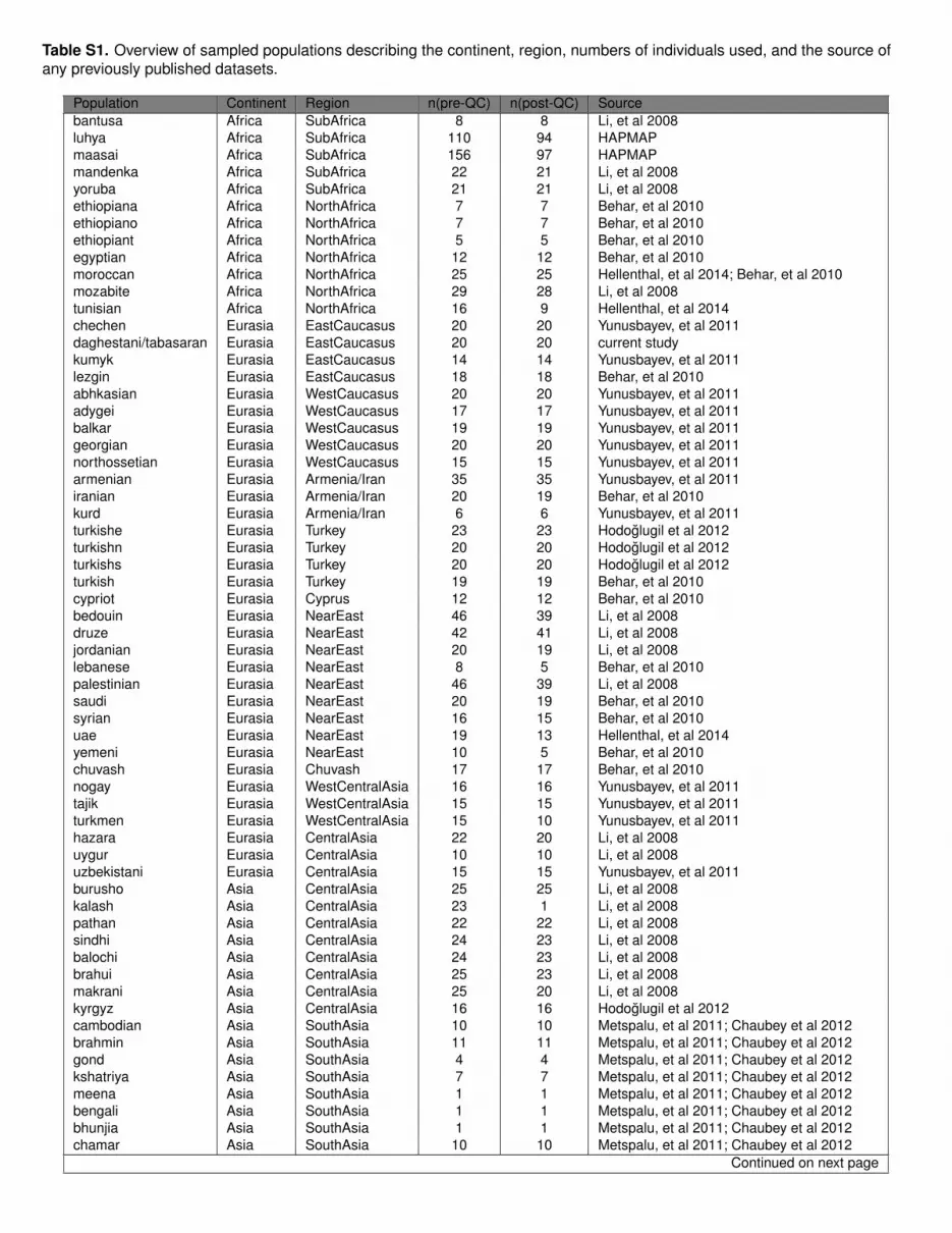
Table S1. Overview of sampled populations describing the continent, region, numbers of individuals used, and the source ofany previously published datasets.

Population Continent Region n(pre-QC) n(post-QC) Sourcebantusa Africa SubAfrica 8 8 Li, et al 2008luhya Africa SubAfrica 110 94 HAPMAPmaasai Africa SubAfrica 156 97 HAPMAPmandenka Africa SubAfrica 22 21 Li, et al 2008yoruba Africa SubAfrica 21 21 Li, et al 2008ethiopiana Africa NorthAfrica 7 7 Behar, et al 2010ethiopiano Africa NorthAfrica 7 7 Behar, et al 2010ethiopiant Africa NorthAfrica 5 5 Behar, et al 2010egyptian Africa NorthAfrica 12 12 Behar, et al 2010moroccan Africa NorthAfrica 25 25 Hellenthal, et al 2014; Behar, et al 2010mozabite Africa NorthAfrica 29 28 Li, et al 2008tunisian Africa NorthAfrica 16 9 Hellenthal, et al 2014chechen Eurasia EastCaucasus 20 20 Yunusbayev, et al 2011daghestani/tabasaran Eurasia EastCaucasus 20 20 current studykumyk Eurasia EastCaucasus 14 14 Yunusbayev, et al 2011lezgin Eurasia EastCaucasus 18 18 Behar, et al 2010abhkasian Eurasia WestCaucasus 20 20 Yunusbayev, et al 2011adygei Eurasia WestCaucasus 17 17 Yunusbayev, et al 2011balkar Eurasia WestCaucasus 19 19 Yunusbayev, et al 2011georgian Eurasia WestCaucasus 20 20 Yunusbayev, et al 2011northossetian Eurasia WestCaucasus 15 15 Yunusbayev, et al 2011armenian Eurasia Armenia/Iran 35 35 Yunusbayev, et al 2011iranian Eurasia Armenia/Iran 20 19 Behar, et al 2010kurd Eurasia Armenia/Iran 6 6 Yunusbayev, et al 2011turkishe Eurasia Turkey 23 23 Hodoglugil et al 2012turkishn Eurasia Turkey 20 20 Hodoglugil et al 2012turkishs Eurasia Turkey 20 20 Hodoglugil et al 2012turkish Eurasia Turkey 19 19 Behar, et al 2010cypriot Eurasia Cyprus 12 12 Behar, et al 2010bedouin Eurasia NearEast 46 39 Li, et al 2008druze Eurasia NearEast 42 41 Li, et al 2008jordanian Eurasia NearEast 20 19 Li, et al 2008lebanese Eurasia NearEast 8 5 Behar, et al 2010palestinian Eurasia NearEast 46 39 Li, et al 2008saudi Eurasia NearEast 20 19 Behar, et al 2010syrian Eurasia NearEast 16 15 Behar, et al 2010uae Eurasia NearEast 19 13 Hellenthal, et al 2014yemeni Eurasia NearEast 10 5 Behar, et al 2010chuvash Eurasia Chuvash 17 17 Behar, et al 2010nogay Eurasia WestCentralAsia 16 16 Yunusbayev, et al 2011tajik Eurasia WestCentralAsia 15 15 Yunusbayev, et al 2011turkmen Eurasia WestCentralAsia 15 10 Yunusbayev, et al 2011hazara Eurasia CentralAsia 22 20 Li, et al 2008uygur Eurasia CentralAsia 10 10 Li, et al 2008uzbekistani Eurasia CentralAsia 15 15 Yunusbayev, et al 2011burusho Asia CentralAsia 25 25 Li, et al 2008kalash Asia CentralAsia 23 1 Li, et al 2008pathan Asia CentralAsia 22 22 Li, et al 2008sindhi Asia CentralAsia 24 23 Li, et al 2008balochi Asia CentralAsia 24 23 Li, et al 2008brahui Asia CentralAsia 25 23 Li, et al 2008makrani Asia CentralAsia 25 20 Li, et al 2008kyrgyz Asia CentralAsia 16 16 Hodoglugil et al 2012cambodian Asia SouthAsia 10 10 Metspalu, et al 2011; Chaubey et al 2012brahmin Asia SouthAsia 11 11 Metspalu, et al 2011; Chaubey et al 2012gond Asia SouthAsia 4 4 Metspalu, et al 2011; Chaubey et al 2012kshatriya Asia SouthAsia 7 7 Metspalu, et al 2011; Chaubey et al 2012meena Asia SouthAsia 1 1 Metspalu, et al 2011; Chaubey et al 2012bengali Asia SouthAsia 1 1 Metspalu, et al 2011; Chaubey et al 2012bhunjia Asia SouthAsia 1 1 Metspalu, et al 2011; Chaubey et al 2012chamar Asia SouthAsia 10 10 Metspalu, et al 2011; Chaubey et al 2012

Continued on next page

Table S1 Continued from previous pagePopulation Continent Region n(pre-QC) n(post-QC) Sourcechenchu Asia SouthAsia 4 4 Metspalu, et al 2011; Chaubey et al 2012dharkar Asia SouthAsia 12 8 Metspalu, et al 2011; Chaubey et al 2012dhurwa Asia SouthAsia 1 1 Metspalu, et al 2011; Chaubey et al 2012dusadh Asia SouthAsia 10 7 Metspalu, et al 2011; Chaubey et al 2012hakkipikki Asia SouthAsia 4 3 Metspalu, et al 2011; Chaubey et al 2012kanjar Asia SouthAsia 8 5 Metspalu, et al 2011; Chaubey et al 2012karnataka Asia SouthAsia 9 8 Behar, et al 2010kol Asia SouthAsia 17 16 Metspalu, et al 2011; Chaubey et al 2012kurmi Asia SouthAsia 1 1 Metspalu, et al 2011; Chaubey et al 2012kurumba Asia SouthAsia 4 4 Metspalu, et al 2011; Chaubey et al 2012lambadi Asia SouthAsia 1 1 Metspalu, et al 2011; Chaubey et al 2012malayan Asia SouthAsia 1 1 Behar, et al 2010mawasi Asia SouthAsia 1 1 Metspalu, et al 2011; Chaubey et al 2012meghawal Asia SouthAsia 1 1 Metspalu, et al 2011; Chaubey et al 2012muslim Asia SouthAsia 5 5 Metspalu, et al 2011; Chaubey et al 2012myanmar Asia SouthAsia 3 3 Behar, et al 2010nihali Asia SouthAsia 2 2 Metspalu, et al 2011; Chaubey et al 2012piramalaikallar Asia SouthAsia 8 8 Metspalu, et al 2011; Chaubey et al 2012sakd Asia SouthAsia 4 4 Behar, et al 2010tamilnadu Asia SouthAsia 2 2 Metspalu, et al 2011; Chaubey et al 2012tharus Asia SouthAsia 2 2 Metspalu, et al 2011; Chaubey et al 2012upcaste Asia SouthAsia 5 5 Metspalu, et al 2011; Chaubey et al 2012velamas Asia SouthAsia 10 9 Metspalu, et al 2011; Chaubey et al 2012han Asia EastAsia 34 34 Li, et al 2008hannchina Asia EastAsia 10 10 Li, et al 2008japanese Asia EastAsia 28 28 Li, et al 2008naga Asia EastAsia 4 4 Metspalu, et al 2011; Chaubey et al 2012naxi Asia EastAsia 8 7 Li, et al 2008tu Asia EastAsia 10 10 Li, et al 2008xibo Asia EastAsia 9 9 Li, et al 2008yi Asia EastAsia 10 10 Li, et al 2008dai Asia EastAsia 10 10 Li, et al 2008lahu Asia EastAsia 8 6 Li, et al 2008miao Asia EastAsia 10 10 Li, et al 2008she Asia EastAsia 10 9 Li, et al 2008tujia Asia EastAsia 10 10 Li, et al 2008buryat Asia EastAsia 17 15 Metspalu, et al 2011; Chaubey et al 2012daur Asia EastAsia 9 9 Li, et al 2008hezhen Asia EastAsia 8 7 Li, et al 2008mongolian Asia EastAsia 19 19 Li, et al 2008oroqen Asia EastAsia 9 9 Li, et al 2008yakut Asia EastAsia 25 25 Li, et al 2008altai Asia Siberia 13 13 Rasmussen, et al 2010burya Asia Siberia 2 2 Rasmussen, et al 2010tuva Asia Siberia 16 13 Rasmussen, et al 2010chukchi Asia Siberia 15 5 Rasmussen, et al 2010dolgan Asia Siberia 7 7 Rasmussen, et al 2010evenk Asia Siberia 16 12 Rasmussen, et al 2010ket Asia Siberia 2 2 Rasmussen, et al 2010koryake Asia Siberia 18 5 Rasmussen, et al 2010selkup Asia Siberia 10 10 Rasmussen, et al 2010yukagir Asia Siberia 9 4 Rasmussen, et al 2010nganassan Asia Siberia 15 10 Rasmussen, et al 2010basque Europe Basque 24 24 Li, et al 2008finnish Europe NEEurope 2 2 Hellenthal, et al 2014belorussian Europe NEEurope 10 9 Behar, et al 2010lithuanian Europe NEEurope 10 10 Behar, et al 2010mordovian Europe NEEurope 15 15 Behar, et al 2010polish Europe NEEurope 18 17 Hellenthal, et al 2014russian Europe NEEurope 25 25 Li, et al 2008ukrainian Europe NEEurope 20 20 Yunusbayev, et al 2011german Europe NWEurope 30 30 current studyceu Europe NWEurope 59 59 HAPMAPenglish Europe NWEurope 8 8 Hellenthal, et al 2014


Table S1 Continued from previous pagePopulation Continent Region n(pre-QC) n(post-QC) Sourceirish Europe NWEurope 7 7 Hellenthal, et al 2014norwegian Europe NWEurope 18 18 Hellenthal, et al 2014scottish Europe NWEurope 8 6 Hellenthal, et al 2014welsh Europe NWEurope 4 4 Hellenthal, et al 2014orcadian Europe NWEurope 15 15 Li, et al 2008sardinian Europe Sardinia 28 28 Li, et al 2008italiann Europe SCEurope 12 12 Li, et al 2008tsi Europe SCEurope 102 98 HAPMAPtuscan Europe SCEurope 8 8 Li, et al 2008bulgarian Europe SEEurope 31 31 Hellenthal, et al 2014; Yunusbayev, et al 2011croatian Europe NEEurope 20 19 current studyhungarian Europe NEEurope 20 19 Behar, et al 2010romanian Europe SEEurope 16 16 Behar, et al 2010greek Europe SEEurope 22 20 Hellenthal, et al 2014italians Europe SCEurope 18 18 Hellenthal, et al 2014siciliane Europe SCEurope 10 10 Hellenthal, et al 2014sicilianw Europe SCEurope 10 10 Hellenthal, et al 2014french Europe SWEurope 28 28 Li, et al 2008spanish Europe SWEurope 36 34 Hellenthal, et al 2014; Behar, et al 2010144 4 21 2422 2192

Table S2. Composition of the World Regions identified by the fineSTRUCTURE analysis. For each World Region we reportthe geographic origin of all individuals within the group. The n(by population) column displays the population followed by thenumber of individuals from that population.

WorldRegion n(total) n(by population)Palestinian 31 palestinian31Levant 103 jordanian19 bedouin18 syrian13 egyptian11 druze8 palestinian8 saudi7

lebanese5 uae5 yemeni5 iranian4Druze 33 druze33Arabia 38 bedouin21 saudi12 uae5NorthAfricaI 24 mozabite24NorthAfricaII 35 moroccan24 tunisian9 mozabite2Armenia/Iran 126 armenian32 turkishe20 turkish18 iranian15 turkishn15 turkishs15 kurd6

romanian2 syrian2 kumyk1NorthCaucasus 159 chechen20 daghestani20 abhkasian19 georgian19 lezgin18 balkar17

adygei16 northossetian15 kumyk13 turkish1 turkishe1WestCentralAsia 62 chuvash16 nogay16 tajik15 turkmen10 uzbekistani4 hazara1SouthEurope 363 tsi98 spanish34 bulgarian31 sardinian28 french25 basque24 greek20

italians18 romanian13 cypriot12 italiann12 siciliane10 sicilianw10 tus-can8 turkishn5 turkishs5 armenian2 balkar2 turkishe2 abhkasian1adygei1 ceu1 georgian1

NorthEurope 290 ceu58 german30 russian25 ukrainian20 croatian19 hungarian19 norwe-gian18 polish17 mordovian15 orcadian15 lithuanian10 belorussian9 en-glish8 irish7 scottish6 welsh4 french3 finnish2 armenian1 chukchi1 chu-vash1 koryake1 romanian1

AfghanPak 83 burusho25 pathan22 sindhi18 brahmin7 kshatriya5 balochi2 gond1kalash1 meena1 uae1

India 122 kol16 chamar10 velamas9 dharkar8 karnataka8 piramalaikallar8 du-sadh7 kanjar5 muslim5 upcaste5 brahmin4 chenchu4 kurumba4 sakd4gond3 hakkipikki3 myanmar3 kshatriya2 nihali2 tamilnadu2 tharus2 ben-gali1 bhunjia1 dhurwa1 kurmi1 lambadi1 malayan1 mawasi1 meghawal1

Balochistan 71 brahui23 balochi21 makrani20 sindhi5 uae2Mongolia 93 buryat15 kyrgyz14 altai13 tuva13 mongolian12 daur9 oroqen7 hezhen6

burya2 nganassan1 uygur1Siberia 54 yakut23 evenk12 nganassan7 dolgan5 koryake2 oroqen2 yukagir2

chukchi1NorthSiberia 25 selkup10 chukchi3 dolgan2 ket2 koryake2 nganassan2 yakut2 yukagir2CentralAsia 41 hazara19 uzbekistani11 uygur9 kyrgyz2EastAsia 175 han34 japanese28 cambodian10 dai10 hannchina10 miao10 tu10 tu-

jia10 yi10 she9 xibo9 mongolian7 naxi7 lahu6 naga4 hezhen1EastAfricaBantu 109 luhya94 bantusa8 maasai7WestAfrica 45 mandenka21 yoruba21 mozabite2 moroccan1EastAfricaMaasai 90 maasai90Ethiopia 20 ethiopiana7 ethiopiano7 ethiopiant5 egyptian1

Table S3. The final fineSTRUCTURE clusters used in the analysis. ClusterName refers to a unique short name given to eachcluster which is named for the population that contributes the most individuals to a cluster; the Region and total number ofindividuals, which is also referred to in the Cluster Name are also listed. As with Table S2, the n(by population) column refersto the geographic population origin of the individuals in each cluster, with a numerical suffix representing the number ofindividuals from that population.

ClusterName Region n(total) n(by population)armen2 Armenia/Iran 2 armenian2armen27 Armenia/Iran 27 armenian24 syrian1 turkishn1 turkishs1armen9 Armenia/Iran 9 armenian2 bulgarian2 turkishe2 turkishn2 turk-

ishs1armen6 Armenia/Iran 6 armenian6irani10 Armenia/Iran 10 iranian10irani5 Armenia/Iran 5 iranian5kurd5 Armenia/Iran 5 kurd5basqu24 Basque 24 basque24chuva16 Chuvash 16 chuvash16cypri12 Cyprus 12 cypriot12chech19 EastCaucasus 19 chechen19daghe2∗ EastCaucasus 2 daghestani2daghe4† EastCaucasus 4 daghestani4daghe10† EastCaucasus 10 daghestani9 lezgin1kumyk2 EastCaucasus 2 kumyk2kumyk4 EastCaucasus 4 kumyk3 chechen1kumyk9 EastCaucasus 9 kumyk9lezgi15 EastCaucasus 15 lezgin10 daghestani5lezgi3 EastCaucasus 3 lezgin3lezgi4 EastCaucasus 4 lezgin4syria1 NearEast 1 syrian1croat18 NEEurope 18 croatian18finni3 NEEurope 3 finnish2 norwegian1hunga23 NEEurope 23 hungarian19 armenian1 croatian1 german1 roma-

nian1lithu11 NEEurope 11 lithuanian9 belorussian1 polish1mordo13 NEEurope 13 mordovian13mordo2 NEEurope 2 mordovian2russi25 NEEurope 25 russian25ukrai48 NEEurope 48 ukrainian20 polish16 belorussian8 chukchi1 chu-

vash1 koryake1 lithuanian1nogay2 WestCentralAsia 2 nogay2nogay7 WestCentralAsia 7 nogay7nogay7a WestCentralAsia 7 nogay7tajik11 WestCentralAsia 11 tajik10 turkmen1tajik3 WestCentralAsia 3 tajik3turkm11 WestCentralAsia 11 turkmen4 uzbekistani4 tajik2 hazara1turkm5 WestCentralAsia 5 turkmen5ceu2 NWEurope 2 ceu2ceu2a NWEurope 2 ceu2aceu3 NWEurope 3 ceu3ceu71 NWEurope 71 ceu43 english8 irish7 scottish6 welsh4 french2

german1germa36 NWEurope 36 german28 ceu8norwe17 NWEurope 17 norwegian17orcad2 NWEurope 2 orcadian2orcad2a NWEurope 2 orcadian2aorcad5 NWEurope 5 orcadian5orcad6 NWEurope 6 orcadian6sardi13 Sardinia 13 sardinian13sardi6 Sardinia 6 sardinian6sardi9 Sardinia 9 sardinian9itali13 SCEurope 13 italiann12 french1itali1 SCEurope 1 italians1itali8 SCEurope 8 italians8sicil30 SCEurope 30 siciliane10 sicilianw10 italians9 greek1


∗Individuals from Daghestan belong to the Tabasaran ethnic group

Table S3 continued from previous pageClusterName Region n(total) n(by population)tsi2 SCEurope 2 tsi2tsi23 SCEurope 23 tsi23tsi2a SCEurope 2 tsi2atsi2b SCEurope 2 tsi2btsi3 SCEurope 3 tsi3tsi4 SCEurope 4 tsi4tsi70 SCEurope 70 tsi62 tuscan8bulga46† SEEurope 46 bulgarian29 romanian13 turkishs3 turkishn1greek19 SEEurope 19 greek19roman2 SEEurope 2 romanian2frenc24 SWEurope 24 french23 ceu1spani27 SWEurope 27 spanish27spani9 SWEurope 9 spanish7 french2turki2 Turkey 2 turkish1 turkishe1turki2a Turkey 2 turkish1 turkishe1aturki34 Turkey 34 turkishe14 turkish13 turkishn6 turkishs1turki3 Turkey 3 turkishe3turki4 Turkey 4 turkishn2 turkishs2turki7 Turkey 7 turkishn3 turkish2 kurd1 turkishe1turki1 Turkey 1 turkishs1turki17 Turkey 17 turkishs11 turkishn5 turkish1abhka16 WestCaucasus 16 abhkasian15 georgian1adyge13 WestCaucasus 13 adygei12 turkishe1adyge6 WestCaucasus 6 adygei4 balkar1 turkish1balka16 WestCaucasus 16 balkar16balka5 WestCaucasus 5 balkar2 abhkasian1 adygei1 georgian1georg20 WestCaucasus 20 georgian16 abhkasian4georg2 WestCaucasus 2 georgian2north15 WestCaucasus 15 northossetian15

†Turkish individuals in this cluster likely have ancestors that recently moved to Turkey from Bulgaria or Romania and are most probably of Bulgarian /Romanian origin

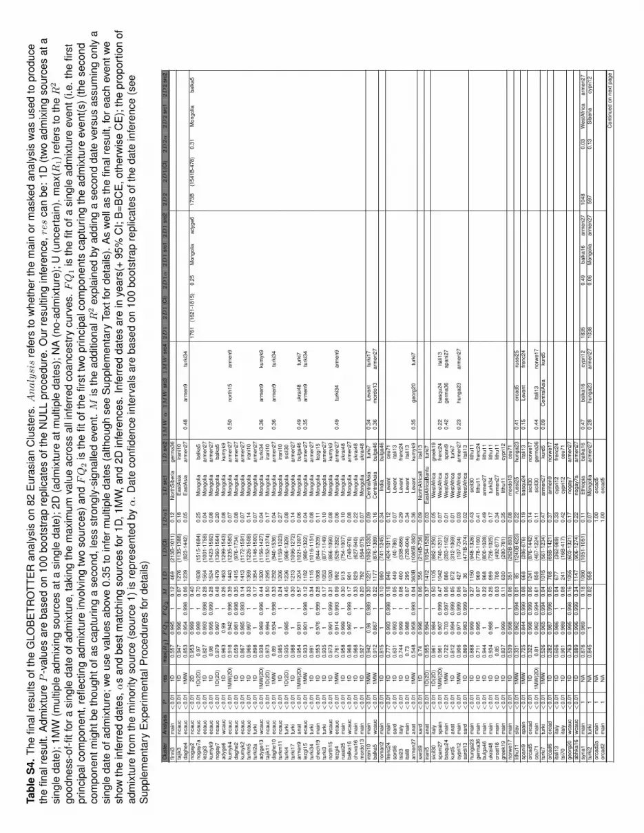
Tabl

eS

4.Th

efin

alre

sults

ofth

eG

LOB

ETR

OTT

ER

anal

ysis

on82

Eur

asia

nC

lust

ers.Analysis

refe

rsto

whe

ther

the

mai

nor

mas

ked

anal

ysis

was

used

topr

oduc

eth

efin

alre

sult.

Adm

ixtu

reP

-val

ues

are

base

don

100

boot

stra

pre

plic

ates

ofth

eN

ULL

proc

edur

e.O

urre

sulti

ngin

fere

nce,res

can

be:

1D(tw

oad

mix

ing

sour

ces

ata

sing

leda

te);

1MW

(mul

tiple

adm

ixin

gso

urce

sat

asi

ngle

date

);2D

(adm

ixtu

reat

mul

tiple

date

s);N

A(n

o-ad

mix

ture

);U

(unc

erta

in).

max

(R1)r

efer

sto

theR

2

good

ness

-of-fi

tfor

asi

ngle

date

ofad

mix

ture

,tak

ing

the

max

imum

valu

eac

ross

alli

nfer

red

coan

cest

rycu

rves

.FQ

1is

the

fitof

asi

ngle

adm

ixtu

reev

ent(

i.e.

the

first

prin

cipa

lcom

pone

nt,r

eflec

ting

adm

ixtu

rein

volv

ing

two

sour

ces)

andFQ

2is

the

fitof

the

first

two

prin

cipa

lcom

pone

nts

capt

urin

gth

ead

mix

ture

even

t(s)(

the

seco

ndco

mpo

nent

mig

htbe

thou

ghto

fas

capt

urin

ga

seco

nd,l

ess

stro

ngly

-sig

nalle

dev

ent.M

isth

ead

ditio

nalR

2ex

plai

ned

byad

ding

ase

cond

date

vers

usas

sum

ing

only

asi

ngle

date

ofad

mix

ture

;we

use

valu

esab

ove

0.35

toin

ferm

ultip

leda

tes

(alth

ough

see

Sup

plem

enta

ryTe

xtfo

rdet

ails

).A

sw

ella

sth

efin

alre

sult,

fore

ach

even

twe

show

the

infe

rred

date

s,α

san

dbe

stm

atch

ing

sour

ces

for1

D,1

MW

,and

2Din

fere

nces

.In

ferr

edda

tes

are

inye

ars(

+95

%C

I;B

=BC

E,o

ther

wis

eC

E);

the

prop

ortio

nof

adm

ixtu

refro

mth

em

inor

ityso

urce

(sou

rce

1)is

repr

esen

ted

byα

.D

ate

confi

denc

ein

terv

als

are

base

don

100

boot

stra

pre

plic

ates

ofth

eda

tein

fere

nce

(see

Sup

plem

enta

ryE

xper

imen

talP

roce

dure

sfo

rdet

ails

)

Clu

ster

Ana

lysi

sP

res

max

(R1

)FQ

1FQ

2M

1D

1D

(CI)

1Dα1

1D

src1

1D

src2

1MWα

1MW

src3

1MW

src4

2D

12D

1(C

I)2D

1α

2D

1sr

c12D

1sr

c22D

22D

1(C

I)2D

2α

2D

2sr

c12D

2sr

c2fin

ni3

mai

n<

0.01

1D0.

557

0.99

51

0.12

469

(213

B-1

011)

0.12

Nor

thS

iber

iage

rma3

6ta

jik3

ncau

c<

0.01

1D0.

947

0.99

61

0.07

1276

(113

5-13

88)

0.18

Eas

tAsi

aira

ni10

dagh

e4ec

auc

<0.

011M

W0.

853

0.95

40.

998

0.06

1239

(823

-144

2)0.

05E

astA

sia

arm

en27

0.48

arm

en9

turk

i34

noga

y2nc

auc

<0.

012D

0.95

30.

999

10.

4017

61(1

621-

1815

)0.

25M

ongo

liaad

yge6

173B

(154

1B-4

78)

0.31

Mon

golia

balk

a5no

gay7

anc

auc

<0.

011D

(2D

)0.

970.

999

10.

7016

38(1

515-

1684

)0.

25M

ongo

liaba

lka5

lezg

i3ec

auc

<0.

011D

0.82

70.

993

0.99

80.

2815

64(1

001-

1758

)0.

04M

ongo

liaar

men

27ku

myk

9ec

auc

<0.

011D

0.98

0.99

50.

999

0.28

1524

(142

3-15

92)

0.08

Mon

golia

arm

en27

noga

y7nc

auc

<0.

011D

(2D

)0.

979

0.99

71

0.48

1479

(136

0-15

64)

0.20

Mon

golia

balk

a5ad

yge6

wca

uc<

0.01

1D0.

963

0.99

10.

2614

63(1

299-

1543

)0.

08M

ongo

liaku

myk

9ku

myk

4ec

auc

<0.

011M

W(2

D)

0.91

80.

942

0.99

60.

3914

43(1

235-

1580

)0.

07M

ongo

liaar

men

270.

50no

rth1

5ar

men

9da

ghe2

ecau

c<

0.01

1D0.

659

0.98

10.

998

0.35

1415

(976

-173

4)0.

08M

ongo

liaar

men

27ku

myk

2ec

auc

<0.

011D

0.86

70.

985

0.99

30.

1414

13(1

172-

1591

)0.

07M

ongo

liaar

men

27tu

rkm

5nc

auc

<0.

011D

0.96

60.

997

10.

3313

69(1

226-

1508

)0.

14M

ongo

liaira

ni10

turk

i2a

turk

i<

0.01

1D0.

898

11

0.17

1354

(114

6-15

00)

0.07

Mon

golia

arm

en27

adyg

e13

wca

uc<

0.01

1MW

(2D

)0.

938

0.96

90.

996

0.44

1320

(115

6-14

27)

0.04

Mon

golia

turk

i34

0.36

arm

en9

kum

yk9

tajik

11nc

auc

<0.

011D

(2D

)0.

973

0.99

41

0.50

1295

(115

2-13

74)

0.17

Mon

golia

irani

10da

ghe1

0ec

auc

<0.

011M

W0.

890.

934

0.99

80.

3312

92(9

40-1

536)

0.04

Mon

golia

arm

en27

0.36

arm

en9

turk

i34

turk

m11

ncau

c<

0.01

1D0.

985

11

0.24

1266

(115

9-13

23)

0.27

Mon

golia

irani

10tu

rki4

turk

i<

0.01

1D(2

D)

0.93

50.

985

10.

4512

36(9

86-1

329)

0.08

Mon

golia

sici

l30

turk

i17

turk

i<

0.01

1D0.

988

11

0.30

1213

(109

6-12

72)

0.14

Mon

golia

arm

en27

arm

en9

anat

<0.

011M

W(2

D)

0.95

40.

931

10.

5712

04(1

021-

1307

)0.

06M

ongo

liabu

lga4

60.

49uk

rai4

8tu

rki7

lezg

i15

ecau

c<

0.01

1MW

0.93

30.

901

0.99

80.

1211

82(9

80-1

322)

0.04

Mon

golia

arm

en27

0.35

arm

en9

turk

i34

turk

i34

turk

i<

0.01

1D0.

991

11

0.34

1115

(101

6-11

51)

0.08

Mon

golia

arm

en27

chec

h19

mai

n<

0.01

1D0.

953

0.97

60.

999

0.28

1068

(844

-120

9)0.

11M

ongo

liale

zgi1

5tu

rki3

turk

i<

0.01

1D0.

935

11

0.17

1053

(877

-114

9)0.

10M

ongo

liaar

men

27no

rth1

5w

cauc

<0.

011D

0.97

30.

991

0.99

90.

3110

20(8

66-1

090)

0.08

Mon

golia

kum

yk9

lezg

i4ec

auc

<0.

011M

W0.

761

0.91

40.

993

0.09

992

(529

-128

2)0.

06M

ongo

liaar

men

270.

49tu

rki3

4ar

men

9ru

ssi2

5m

ain

<0.

011D

0.95

80.

999

10.

3091

3(7

54-1

007)

0.10

Mon

golia

ukra

i48

balk

a16

wca

uc<

0.01

1D0.

968

0.99

70.

999

0.17

901

(748

-976

)0.

08M

ongo

liaar

men

27ch

uva1

6m

ain

<0.

011D

0.96

81

10.

3382

9(6

27-9

40)

0.22

Mon

golia

ukra

i48

mor

do13

mai

n<

0.01

1D0.

927

11

0.20

792

(564

-975

)0.

07M

ongo

liauk

rai4

8ira

ni10

mai

n<

0.01

1MW

0.94

20.

960.

989

0.30

1221

(106

3-13

30)

0.09

Cen

tralA

sia

turk

i70.

34Le

vant

turk

i17

balk

a5w

cauc

<0.

011M

W0.

912

0.86

71

0.22

1177

(876

-138

9)0.

16C

entra

lAsi

abu

lga4

60.

36m

ordo

13ar

men

27ro

man

2m

ain

<0.

011D

0.81

51

10.

1099

0(7

41-1

245)

0.34

Indi

abu

lga4

6fre

nc24

mai

n<

0.01

1D0.

777

0.99

30.

998

0.18

846

(424

-101

1)0.

12Le

vant

ceu7

1sa

rdi6

sard

<0.

011D

0.63

10.

993

10.

0544

9(4

0-78

6)0.

07Le

vant

itali1

3ts

i23

italy

<0.

011D

0.74

40.

999

10.

0840

0(3

3B-6

86)

0.29

Leva

ntfre

nc24

itali8

mai

n<

0.01

1D0.

730.

988

10.

0729

5(7

2B-6

04)

0.34

Leva

ntita

li13

arm

en27

anat

<0.

011M

W0.

548

0.95

80.

993

0.04

363B

(108

5B-3

82)

0.36

Leva

ntku

myk

90.

35ge

org2

0tu

rki7

sard

i9sa

rd<

0.01

1D0.

740.

996

10.

0635

6(2

14B

-736

)0.

09N

orth

Afr

icaI

Iita

li13

irani

5an

at<

0.01

1D(2

D)

0.95

50.

994

10.

3714

12(1

054-

1526

)0.

03E

astA

fric

aBan

tutu

rki7

sici

l30

italy

<0.

011D

(2D

)0.

961

0.98

41

0.50

1105

(882

-125

0)0.

05W

estA

fric

agr

eek1

9sp

ani2

7sp

ain

<0.

011M

W(2

D)

0.96

10.

907

0.99

90.

4710

42(7

40-1

201)

0.07

Wes

tAfr

ica

frenc

240.

22ba

squ2

4ita

li13

basq

u24

mai

n<

0.01

1MW

0.72

20.

703

0.99

70.

0688

6(2

83-1

162)

0.01

Wes

tAfr

ica

span

i90.

42ge

rma3

6sp

ani2

7ku

rd5

anat

<0.

011D

0.81

20.

994

0.99

90.

0587

2(3

12-1

069)

0.01

Wes

tAfr

ica

turk

i7cy

pri1

2m

ain

<0.

011M

W0.

906

0.97

10.

999

0.06

427

(107

-734

)0.

03W

estA

fric

aar

men

270.

23hu

nga2

3ar

men

27sa

rdi1

3sa

rd<

0.01

1D0.

869

0.98

30.

999

0.07

36(4

71B

-374

)0.

02W

estA

fric

aita

li13

hung

a23

mai

n<

0.01

1D0.

888

0.99

91

0.27

1150

(948

-132

6)0.

43si

cil3

0lit

hu11

germ

a36

mai

n<

0.01

1D0.

711

0.99

51

0.07

969

(778

-116

0)0.

41lit

hu11

frenc

24bu

lga4

6m

ain

<0.

011D

0.94

41

10.

2296

8(8

00-1

028)

0.49

arm

en27

lithu

11uk

rai4

8m

ain

<0.

011D

0.93

40.

988

10.

2689

9(7

26-1

025)

0.17

turk

i34

lithu

11cr

oat1

8m

ain

<0.

011D

0.85

11

0.03

708

(492

-877

)0.

34ar

men

27lit

hu11

gree

k19

mai

n<

0.01

1D0.

837

0.99

91

0.11

630

(280

-781

)0.

35lit

hu11

cypr

i12

norw

e17

mai

n<

0.01

1D0.

539

0.99

81

0.06

351

(262

B-8

93)

0.08

mor

do13

ceu7

1lit

hu11

slav

<0.

011M

W0.

331

0.96

20.

994

0.01

85(1

240B

-623

)0.

22ru

ssi2

5hu

nga2

30.

41or

cad5

russ

i25

span

i9sp

ain

<0.

011M

W0.

725

0.84

40.

999

0.08

668

(286

-876

)0.

19ba

squ2

4ita

li13

0.15

Leva

ntfre

nc24

orca

d5or

cad

<0.

011D

0.32

20.

998

0.99

90.

0612

41(8

76-1

442)

0.14

sici

l30

norw

e17

ceu7

1m

ain

<0.

011M

W(2

D)

0.81

0.96

20.

994

0.61

858

(467

-122

4)0.

11si

cil3

0ge

rma3

60.

44ita

li13

norw

e17

turk

i7tu

rki

<0.

011M

W0.

526

0.96

50.

994

0.04

1015

(561

-123

4)0.

47ar

men

27ku

rd5

0.09

Cen

tralA

sia

kurd

5or

cad6

orca

d<

0.01

1D0.

282

0.98

70.

996

0.05

708

(65B

-142

1)0.

37ar

men

9no

rwe1

7ita

li13

italy

<0.

011D

0.60

60.

986

10.

0467

7(3

62-9

89)

0.33

cypr

i12

frenc

24ts

i70

italy

<0.

011D

0.90

10.

989

10.

0824

1(1

6B-4

17)

0.42

cypr

i12

ceu7

1ge

org2

0w

cauc

<0.

011D

0.76

30.

995

0.99

80.

1610

55(6

03-1

321)

0.17

noga

y7ar

men

27ab

hka1

6w

cauc

<0.

011D

0.88

90.

996

0.99

90.

3411

47(9

06-1

274)

0.22

noga

y7a

arm

en27

syria

1m

ain

1N

A0.

876

0.96

91

0.18

1080

(105

1-10

51)

0.11

Eth

iopi

aba

lka1

60.

47ba

lka1

6cy

pri1

218

350.

49ba

lka1

6ar

men

2710

480.

03W

estA

fric

aar

men

27tu

rki2

turk

i1

NA

0.84

51

10.

0295

80.

07M

ongo

liaar

men

270.

28hu

nga2

3ar

men

2710

380.

06M

ongo

liaar

men

2759

70.

13S

iber

iacy

pri1

2or

cad2

am

ain

1N

A1.

00or

cad5

orca

d2m

ain

1N

A1.

00or

cad5

Con

tinue

don

next

page

Tabl

eS

4C

ontin

ued

from

prev

ious

page

Clu

ster

Ana

lysi

sP

res

max

(R1

)FQ

1FQ

2M

1D

1D

(CI)

1Dα1

1D

src1

1D

src2

1MWα

1MW

src3

1MW

src4

2D

12D

1(C

I)2D

1α

2D

1sr

c12D

1sr

c22D

22D

1(C

I)2D

2α

2D

2sr

c12D

2sr

c2ita

li1ita

ly1

NA

0.40

90.

939

0.99

60.

0411

83(1

154-

1154

)0.

40sa

rdi1

3cy

pri1

20.

17sa

rdi9

gree

k19

1350

0.4

sard

i13

arm

en9

162

0.18

Nor

thA

fric

aII

span

i9tu

rki1

turk

i1

NA

0.95

90.

954

10.

7318

03(1

774-

1774

)0.

07W

estA

fric

aku

myk

90.

23C

entra

lAsi

acy

pri1

218

70(1

841-

1841

)0.

07W

estA

fric

aku

myk

911

37(1

108-

1108

)0.

13M

ongo

liacy

pri1

2ts

i2m

ain

<0.

01U

0.40

40.

928

10.

0458

2(2

9-96

4)0.

14ba

lka1

6ts

i23

0.45

hung

a23

tsi2

313

180.

24ba

lka5

tsi2

355

00.

1Le

vant

tsi2

3ce

u2a

mai

n<

0.01

U0.

484

0.99

60.

998

0.04

1010

(423

B-1

429)

0.10

finni

3ce

u71

0.32

frenc

24ce

u71

1625

0.46

frenc

24or

cad6

1162

0.12

hung

a23

ceu7

1ar

men

6m

ain

<0.

01U

0.13

40.

987

0.99

80.

0314

3B(2

881B

-132

6)0.

42ge

org2

0si

cil3

00.

41ira

ni5

gree

k19

1344

0.31

arm

en9

arm

en27

1604

B0.

43ab

hka1

6cy

pri1

2ge

org2

mai

n<

0.01

U0.

622

0.99

91

0.19

1785

(160

5-18

53)

0.27

hung

a23

geor

g20

0.13

noga

y7ge

org2

019

080.

28uk

rai4

8ge

org2

076

30.

2m

ordo

13ge

org2

0ts

i2a

mai

n<

0.01

U0.

286

0.99

91

0.13

907B

(194

6B-5

65)

0.39

Leva

ntno

rwe1

70.

37m

ordo

13ts

i23

1619

0.41

frenc

24ts

i23

494B

0.16

Leva

ntfre

nc24

tsi4

mai

n<

0.01

U0.

357

0.99

10.

999

0.11

91(6

88B

-569

)0.

16Le

vant

tsi2

30.

39m

ordo

13ts

i23

1580

0.38

mor

do13

tsi2

341

00.

06N

orth

Afr

icaI

Its

i23

tsi3

mai

n<

0.01

U0.

277

0.98

50.

997

0.03

208

(315

B-6

93)

0.23

Leva

ntts

i23

0.45

balk

a5ts

i23

1547

0.42

arm

en9

tsi2

37B

0.22

Leva

ntts

i23

arm

en2

mai

n<

0.01

U0.

155

0.91

70.

969

0.04

1594

(691

-189

2)0.

15Le

vant

arm

en27

0.48

arm

en27

arm

en27

1892

0.44

arm

en27

irani

516

490.

16Le

vant

arm

en27

mor

do2

mai

n<

0.01

U0.

583

0.92

40.

996

0.08

558

(179

-843

)0.

12M

ongo

liauk

rai4

80.

30fin

ni3

mor

do13

1804

0.28

finni

3m

ordo

1380

40.

05M

ongo

liam

ordo

13ce

u2m

ain

0.59

U0.

0523

11

0.01

1825

(109

49B

-189

2)0.

06or

cad5

ceu7

10.

37or

cad6

ceu7

118

690.

06or

cad5

ceu7

112

008B

0.5

bulg

a46

orca

d5ts

i2b

mai

n<

0.01

U0.

491

0.99

30.

999

0.09

1512

(113

3-16

70)

0.31

span

i27

tsi2

30.

04Le

vant

tsi2

316

790.

26sp

ani2

7ts

i23

1250

0.39

orca

d5ts

i70

ceu3

mai

n<

0.01

U0.

108

0.93

60.

973

0.03

347B

(200

2B-1

892)

0.32

span

i27

finni

30.

48or

cad5

frenc

2419

210.

14sp

ani2

7ce

u71

1237

B0.

35sa

rdi9

finni

3

Table S5. Results of All GLOBETROTTER Analyses Performed on 82 Eurasian Clusters, Related to Figure 4. Columnheadings are as in Table S4. All clusters were analyzed once using all clusters with at least five individuals as surrogates(main analysis). Others were also analyzed with bespoke masked analyses, as noted in the main text. The NULL procedurewas run for each of these analyses for comparative purposes.

Supplemental Experimental Procedures

S1 Dataset and identification of genetic populations

S1.1 Outlier removal with PLINK IBD and PCA

We used pairwise IBD analysis to remove potentially related individuals from further analysis. UsingPLINK, we compared the proportion of SNPs that were IBD for each individual in a population withevery other individual from their population using the pi-hat statistic. Evolutionary history, genetic drift,and relative isolation will lead to differences in the background level of IBD in different populations. Totake this into account, we chose a variable threshold of exclusion for putatively related individuals. Weused the larger value of the 97.5% quantile of population IBD or 0.2, as the threshold for exclusion,and for all pairs above this threshold, dropped the individual with the lower genotyping rate from furtheranalysis. We next used smartpca in the EIGENSOFT package [S?] to perform PCA on the pruneddataset. Individuals were split into broad geographical regions (Europe; Near East; Asia; Africa) andseparate runs of the program were performed. Each region contained individuals typed from differentstudies on different chips, and visual inspection of PC1 v PC2 plots allowed a qualitative assessmentof the merging process. For European populations, smartpca was run with no outlier iterations and allindividuals were kept for futher analysis; for the remaining three regions, three outlier iterations wereperformed, with the resulting outliers dropped from the full analysis. The final dataset contained 2,192individuals from 144 populations typed on 477,812 SNPs (Table S1).

S1.2 Phasing

We used SHAPEITv1 [S?] to phase the data. SHAPEITv1 conditions the underlying hidden Markovmodel (HMM) from ref. [S?] on all available haplotypes to quickly estimate haplotypic phase from geno-type data. We split our dataset (in binary PLINK format) by chromosome and phased all individualssimulataneously, and used the most likely pairs of haplotypes (using the –output-max option) for eachindividual for downstream applications. Based on the numbers of individuals from Europe, Asia andAfrica in our dataset and the instructions of SHAPEITv1 available at the time of phasing, we used anestimated effective population size of 13,887. (1189 Asians; Asian Ne: 14,269; 334 Africans; African Ne17,469; 669 Europeans; European Ne: 11,418.)

S1.3 Visualising broad-scale population structure with ADMIXTURE

We used ADMIXTURE [S?] to describe the genome-wide ancestry of our dataset and by way of com-parison of our method to commonly used procedures (Figure S2). We thinned the dataset to remove theeffect of LD by removing SNPs whose pairwise correlation across the sample was greater than 0.2. Thisthinned dataset contained 135,101 SNPs, and ADMIXTURE was run for all values of K ∈ [2, ..., 14].

S1.4 Rationale for using genomic data to group individuals

The major aim of our paper is to explore the different ancestral contributions to different “groups” ofindividuals across Western Eurasia. Often, researchers group individuals based on labels associatedwith geography (e.g. population), or less often a cultural label such as religion, language or life history.Whilst this is generally satisfactory, it is far from perfect. What constitutes a “population” has been, andstill is, a topic of much debate [S?]. However, we nevertheless believe that it is important to considerhow to split a dataset into constituent groups when investigating human evolutionary history. Take Italy

as an example. Figure S1A is a PCA of Europe with different population labels assigned to individuals,which are each represented by a point, who all fall under the general geographic descriptive label ofItaly (HAPMAP TSI individuals are included in the PCA, but are not coloured). From this plot it is clearthat Northern and Southern Italians are genetically distinct, which may potentially be due to differentancestries. Sardinia and Sicily are Italian islands, so fall under the geographic population label of Italy,but (as has been known for a long time [S?]) Sardinians are clearly distinct from the rest of Italy, whilstfor Sicilians and Southern Italians it is not as clear-cut. Whilst this sort of difference is not necessarilypresent across all European countries, this example serves to show us that geographic labels can beimproved upon. With this in mind, we constructed new groups of individuals based on an objectiveassessment of genetic similarity alone.

S1.5 Grouping individuals on the basis of genetic similarity

We used an inferential framework for investigating population structure from haplotypic data [S?]. Ini-tially, haplotypic chromosomes are “painted” sequentially using an updated implementation of a modelinitially introduced by Li & Stephens [S?] and which is exploited by the CHROMOPAINTER package [S?].The Li & Stephens copying model explicitly relates linkage disequilibrium to the underlying recombinationprocess and CHROMOPAINTER uses an approximate method to reconstruct each “recipient” individ-ual’s haplotypic genome as a series of recombination “chunks” from a set of sample “donor” individuals.The aim of this approach is to identify, at each SNP as we move along the genome, the closest relativegenome among the members of the donor sample. Because of recombination, the identity of the closestrelative will change depending on the admixture history between individual genomes. Even distantlyrelated populations share some genetic ancestry since most human genetic variation is shared, [S?,S?]but the amount of shared ancestry can differ widely. We use the term “painting” here to refer to theapplication of a different label to each of the donors, such that – conceptually – each donor is repre-sented by a different colour. Donors may be coloured individually, or in groups based on a priori definedlabels, such as the geographic population that they come from. By recovering the changing identity ofthe closest ancestor along chromosomes we can understand the varying contributions of different donorgroups to a given population, and by understanding the distribution of these chunks we can begin touncover the historical relationships between groups.

CHROMOPAINTER reconstructs each recipient individual’s haplotypes as mosaics of a set of donorsand efficiently summarises this ancestry painting in the form of a ’copying vector’, which is the total pro-portion of genome-wide DNA (either by total expected number of shared chunks, or total expected lengthof chunks) copied from each labelled donor group (i.e. colour). These copying vectors contain a richsummary of the (genome-wide) relationships between individuals, and similarities in these vectors implyshared ancestral history [S?]. We therefore decided to use these copying vectors and fineSTRUCTUREto group individuals based on this measurement of shared ancestral history.

S1.6 Using CHROMOPAINTER to generate a ’coancestry matrix’ for fineSTRUC-TURE

S1.6.1 Estimating Ne and θ using Expectation-Maximisation

We performed an initial CHROMOPAINTER run to estimate the two nuisance parameters, Ne and θusing the expectation-maximisation (EM) option. (These are not Ne and θ in the traditional sense butrefer to parameters from the Li and Stephens model that are used to estimate the recombination ratedistribution underlying the model.) We note the process of estimating them here and their values forreproducibility. The EM algorithm iterates over the data to find the local optimum values for these pa-rameters, given the data. Ne is the ’recombination scaling constant’ and is directly related to the effective

population size. It is used by CHROMOPAINTER to convert the values of the genetic distance betweenSNPs (taken from the genetic map) to the population-scaled values for these distances required by thealgorithm. We used the human genome build 36 genetic map downloaded from the HAPMAP website(http://hapmap.ncbi.nlm.nih.gov/downloads/recombination/). θ is the per site mutation rate parameterand is used by the CHROMOPAINTER HMM to allow for imperfect copying between haplotypes.

We used CHROMOPAINTER with 10 Expectation-Maximisation (E-M) steps to jointly estimate theprogram’s parameters Ne and θ, repeating this separately for chromosomes 1, 5, 8, 12, 17, 22 andweight-averaging (using centimorgan sizes) the Ne and θ from the final E-M step across the six chromo-somes with the following command line:

chromopainter −g < i n f i l e > −r <recomrates> − f <d o n o r f i l e> −o <o u t f i l e >−a 0 0 −s 0 − i 10 − i n −iM

Due to the exhaustive nature of this estimation, we averaged these values across a subset of populations(Armenian, Bedouin, Bulgarian, German, Mandenka, Mozabite, Palestinian). We used the global valuesestimated from these populations of 318.8 and 0.0002 for Ne (-n flag) and θ (-M flag) respectively

S1.7 Using the coancestry matrix to identify clusters with fineSTRUCTURE

We then ran CHROMOPAINTER on each chromosome separately for each individual as a recipient,using every other individual (i.e. 2191) as donors with the following command line:

chromopainter −g < i n f i l e > −r <recomrates> − f <d o n o r f i l e> −o <o u t f i l e >−a 0 0 −s 0 −M 0.0002 −n 318.8

This generated a 2192 v 2192 matrix of copying vectors that was then passed to fineSTRUCTURE tocluster individuals on the basis of the similarities of these copying vectors. fineSTRUCTURE is a modelbased Bayesian clustering algorithm that efficiently uses the output of CHROMOPAINTER to identifypopulation structure. Individuals are initially assumed to have independent ancestry proportions (i.e.copying vectors), but because historical relationships among individuals result in correlations in theircopying vectors, individuals can be grouped together on the basis of this similarity. At each iteration,a series of splits and merges are performed on random samples of individuals, such that clusters withhigher partition probability are kept at the end of each iteration. We ran fineSTRUCTURE for 10 millioniterations, sampling every 10,000, using the following command:

f i n e s t r u c t u r e −X −Y −x 0 −y 1e7 −z 1e5 <chunkcounts> <mcmcfi le>

As the aim of this step was to group individuals into major world regions, we checked pairwise coinci-dence across all 10 million iterations. Pairwise coincidence (i.e. the number of times a pair of individualsare placed in the same cluster) within and across the two runs was high indicating that individuals tendedto occur in the same clusters across all 10 million iterations of the algorithm.

We used the fineSTRUCTURE run with the highest posterior probability to produce a tree relatingthese clusters by running the maximum a posteriori (MAP) state from the initial run and used 10 millioniterations of the tree building model and a very large value for the maxtreestates (t) option, to ensurethat a large number of trees were considered at each iteration, using the following command:

f i n e s t r u c t u r e −X −Y −m T − t 1e8 −x 1e6 <chunkcounts> <mcmcfi le> < t r e e f i l e >

To find the tree, fineSTRUCTURE starts from the MAP state and successively merges clusters, choosingthe merge giving the highest probability for the merge at each step, which results in a bifurcating tree

relating the clusters [S?]. Bipartition uncertainties are produced for the nodes of the tree, which are theproportion of MCMC samples for which all individuals on one side of the split merge with each otherprior to merging with any individual from the other side of the split.

S1.8 Identifying donor World Regions using fineSTRUCTURE

We used the full fineSTRUCTURE analysis to group individuals based on their position in the tree (Fig.S1C). We found 301 clusters in total and visually inspected the tree to identify 22 major clades on thetree and successively merged all non-European clusters to reduce the number from 2192 to 22 world-wide clades, containing individuals that broadly matched geographical regions of the world, and that weuse to represent the donor genomes of these different regions (Table S2; Fig. S1B).

The purpose of this step was to identify fineSTRUCTURE “continents” (which we term “world re-gions”) to be used for a second run of the algorithm. The processing time of the algorithm is directlyrelated to the number of individuals included in the analysis, so reducing the number of individualsspeeds up the analysis. Furthermore, fineSTRUCTURE initially uses a prior that assumes that all indi-viduals are equally distant from each other, which in the case of worldwide populations is likely to beuntrue: European populations are more closely related to each other than to African populations, for ex-ample. The result is that not all of the substructure is identified in one run. We therefore generated a setof world-regions, which combine all of the copying vectors from the individuals within them to look like(re-weighted) normal individuals but cannot be split and do not contribute to parameter inference, andcan thus be considered as copying vectors that contain the average of the individuals within them. Theycan therefore be included in the algorithm at minimal extra computational cost and exist primarily to pro-vide chunks to (and from) the remaining groups. We additionally use these world regions, together withthe Eurasian clusters, throughout the subsequent analysis as our donor (and in the case of the Eurasianclusters recipient) groups in the GLOBETROTTER analysis. Noting that the North African World Regioncontained the drifted Mozabites together with Tunisians, and Moroccans, we split the North Africa WorldRegion into two, keeping the Mozabites separate from the other North Africans.

S1.9 Identifying the final Eurasian clusters using fineSTRUCTURE

We performed 2 runs of the fineSTRUCTURE algorithm using the 18 non-Eurasian world regions as’continents’ with the 1000 Eurasian individuals belonging to the 5 world regions (Anatolia, SouthCauca-sus, NorthCaucasus, SouthEurope, NorthEurope), using the following command:

f i n e s t r u c t u r e −X −Y −m T − t 10e6 −x 1e6 −F <wor ld reg ions> <chunkcounts><mcmcfi le> < t r e e f i l e >

The two runs of fineSTRUCTURE gave very similar results, inferring 82 and 83 clusters. 74 of theclusters were identical, with the remaining clusters containing cases where at most two individuals wereswapped between clusters. Given the high similarity between the clusters, we chose the run with thehighest posterior probability containing 100 clusters (82 Eurasian plus 18 world regions) as the finalgroups for the analysis (Table S3). We use these 82 clusters with GLOBETROTTER to assess thepresence of admixture across Europe, and subsequently to infer the proportion, timing, and identity ofadmixture in these groups.

S1.10 Results of the fineSTRUCTURE analysis

Figure S1 shows summary results of the fineSTRUCTURE analysis. The heatmap clearly suggeststhat different European groups copy different amounts of their genome from different parts of the world.

These differences are subtle however, and are often not much more than a few percent. The aim of ouranalysis is to use GLOBETROTTER to try to explain these differences and to assess the evidence thatgenetic admixture may have caused them.

S1.11 Principal components analysis of the CHROMOPAINTER coancestry ma-trix

As final justification for the use of fineSTRUCTURE clusters we show a visualisation of a principal com-ponents of the CHROMOPAINTER chunklengths coancestry matrix (Fig. S4B-D). The PCA is somewhatsimilar to PCAs based on genotype data [S?,S?] although the inclusion of Caucasus and Turkish indi-viduals causes the plot to differ from the familiar map of Europe. The points are labelled with the samelabels as Figure 1 in the main paper (which is also reproduced in the legend). Whilst generally individu-als with the same label (i.e. from the same fineSTRUCTURE cluster) appear close to each other on theplot, some clusters are more spread out. The first two (ten) PCs explain 14.4% (35.4%) of the variancein the data suggesting that not all variation described by the clustering is captured by the highest PCs.

S2 Description of ADMIXTURE analysis

We used ADMIXTURE [S?] to initially survey the dataset for evidence of admixture. We performed 10independent runs of the algorithm on the pruned dataset of 132K SNPs (see Experimental Procedures),with different randomly selected seeds at all values of K ∈ [2, ..., 14]. Multiple runs at the same Kwere merged with CLUMPP [S?] using 10,000 iterations of the LargeKGreedy option. Figure S2 showsthe results of this analysis, with bars showing the averaged admixture proportions from each of the Kinferred groups across all individuals from a given cluster or world region. Admixture is largely visible inall clusters (and some of the world regions) at higher values of K.

In particular, West Eurasian populations tend to be some mixture of 3 main ancestral components(dark blue, dark green, light green), with clear examples of admixture from components outside of thesemain three (for example the light blue ’Middle Eastern’ component present in most European groups),with the Caucasus tending to be a mixture of the same components, with a comparatively larger amountof dark green ancestry, compare to the dark blue/light green of Europe.

S3 GLOBETROTTER: description of method to infer admixture

S3.1 The GLOBETROTTER pipeline

We used GLOBETROTTER to characterise admixture in Eurasian populations. This procedure aimsto identify and date admixture among clusters in our dataset, as well as identify the admixing groupsinvolved and the proportions of DNA contributed from each group. The analysis presented here followsclosely that of Hellenthal et al [S?] with the key difference that we (a) initially use fineSTRUCTUREto group individuals based on genetics alone; and (b) combine non-Eurasian individuals into broadgeographic “world regions” as outlined above. We describe some of the testing and validation performedpreviously in Section S3.2 below.

To run GLOBETROTTER, we must generate a copying vector for each donor group and a set ofpainted chromosomes for each recipient group.

Using CHROMOPAINTER to generate DONOR copying vectors for the 18 non-Eurasian worldregions and 82 Eurasian clusters

To estimate a set of copying vectors (f i in the notation of Hellenthal et al [S?]) for j donor groups, foreach recipient cluster k we used the original coancestry matrix (where we painted all 2192 with everyother) and summed the contributions from each individual in each of the j 6= k ∈ [1, ...,K] non-recipientgroups separately (i.e. 18 non-West Eurasian world regions and 82 West Eurasian clusters), producinga j 6= k ∈ [1, ...,K] element copying vector for each donor group in the analysis. Note that we thereforegenerate a separate set of copying vectors for each recipient group, describing the amount of copyingfrom each j 6= k donor groups to that recipient group. In practice, this meant that we estimated the meancopying from each of the j 6= k (i.e. 99) donor groups across all individuals in each recipient group toproduce a single donor copying-vector for each of the 100 groups in the analysis.

Using CHROMOPAINTER to generate painting samples of the 82 RECIPIENT Eurasian clusters

We calculated cluster-specific values of Ne and θ by performing a ’leave-one-out’ procedure where eachindividual from a given cluster k is allowed to copy from every other individual with the same clusterlabel and nj − 1 randomly chosen individuals from each donor cluster j 6= k ∈ [1, ...,K] (nj is thenumber of individuals with cluster label j). Because then there are nj samples to copy from each clusterj 6= k ∈ [1, ...,K], while only nk − 1 samples to copy from their own cluster (as they cannot be used topaint them-self), we avoid this reduction by 1 causing problems later, by instead removing one individualfrom each of the other clusters j 6= k ∈ [1, ...,K] when painting. Thus all individuals in the dataset copyfrom the same number of individuals from each labelled cluster ensuring that each individual from eachcluster copies from the exact same number of individuals from every other cluster label including theirown.

Accounting for the fact that each recipient group is now copying from a different (i.e. j 6= k) set ofdonors, we used the cluster-specific values of Ne and θ calculated above, and re-ran CHROMOPAINTERfor each of the K (82) Eurasian clusters with all individuals from the other j 6= k clusters and WorldRegions (99) as donors, this time without allowing individuals to copy from other individuals in the samecluster, and generating 10 painting samples for each recipient cluster.

chromopainter −g < i n f i l e > −r <recomrates> − f <d o n o r f i l e> −o <o u t f i l e >−s 10 −M mu −n Ne

S3.2 Characterising admixture events

To test the robustness of the admixture inference, we use the idea that in truly admixed populations,ancestry segments producing “admixture LD” occur within individual genomes, resulting in ancestry LDcharacteristically decaying within individual genomes much more strongly than when ancestry is mea-sured in different individuals. To construct a test of this based on our method’s inference of geneticancestry, we first generate “across-individual” coancestry curves, by considering CHROMOPAINTERpainting samples from different individuals (using the NULL procedure outlined in the GLOBETROTTERmanual and here [S?]), and use these to normalise our original coancestry curves. We re-infer ad-mixture using this “NULL” individual, generating 100 date bootstraps, and test to see if the results aredifferent from the non-NULL inference. Specifically, we assess evidence of any admixture, by obtainingan empirical P -value as P = D/101, where D is the number of NULL date bootstraps with a date λ,where λ ≤ 1 or λ ≥ 400, rejecting the null of no admixture only if P < 0.01. We also compare howwell the modelled date of admixture (i.e. the coancestry curve R2) changes between the normal andNULL run of the algorithm, and reject the null of no-admixture only when this reduction is less than 1/3.In practice, this meant that we have little confidence in admixture inference in most clusters containingsmall numbers of individuals (n <4). Admixture in such clusters is defined as uncertain (U) or, whenP >0.01, as no-admixture (NA).

A key aspect of GLOBETROTTER is that we do not need to identify a priori the admixing sourcegroups: all that is needed is a set of surrogate groups from which to infer admixture events. Moreover,this approach allows us to define source groups as mixtures of these available surrogate groups. We ranGLOBETROTTER under a number of different scenarios, changing the identity of the available donorgroups (outlined in full in Supplemental Experimental Procedures Section S4). We note that in generalGLOBETROTTER will identify the most recent admixture event.

S3.3 Validation of GLOBETROTTER

We reported the full description of the GLOBETROTTER method, and our extensive testing of its ro-bustness to different conditions in real and simulated data, in Hellenthal et al [S?] and its associatedSupplementary Material. We also conducted comparisons of GLOBETROTTER to other available meth-ods, such as ROLLOFF and ADMIXTURE, in that publication. We re-iterate here several key aspects ofthe validation we performed.

S3.3.1 GLOBETROTTER simulations undertaken by Hellenthal et al 2014

To test GLOBETROTTER under diverse single, complex, and no-admixture scenarios, incorporatingmany of the complexities (such as unsampled or admixed donor groups) likely to be present in real data,we simulated admixture scenarios involving real (but hidden to our analysis) human populations [S?]and populations generated under a coalescent framework [S?] incorporating inferred [S?,S?,S?,S?]past demographic events.

Admixture was simulated between 7 and 160 generations [200 to 4400 years] ago, with admixturefractions 3 to 50% and genetic differentiation (FST ) between the admixing groups varying from 0.018(similar to Europe versus Central Asia) to 0.185 (similar to West Africa versus Europe). Results aredetailed in Hellenthal et al 2014 [S?]. All populations simulated without admixture, including those withlong-term migration, showed no admixture evidence (P >0.1). Power to detect admixture (P <0.01)when present was 94%, and 95% of our 95% bootstrapped confidence intervals (CIs) contained thetrue admixture date, including cases with two distinct incidents of admixture or multiple groups admixingsimultaneously.

In our simulations, inferred source accuracy was very high, with, for example, the mixture repre-sentation predicting a haplotype composition more correlated to the true, typically unsampled, source

population than to any single sampled population >80% of the time. However, source accuracy waslower for admixing sources contributing only 5% of DNA, with around 40% of such scenarios yieldingelevated (>25%) rates of falsely inferring multiple admixture times and/or admixing groups.

Further testing demonstrated robustness of GLOBETROTTER, in simulations and real data, to haplo-typic phase inference approach used, inclusion/exclusion of particular chromosomes, genetic map cho-sen to provide genetic distances, and the presence of population bottlenecks since admixture, whereasGLOBETROTTER admixture dating was improved relative to ROLLOFF [S?].

Even so, there are multiple settings that we believe are challenging for GLOBETROTTER:

1. although the admixing sources need not be sampled—often impossible because of genetic drift,extinction, or later admixture into the sources themselves—source inference is improved whenmore similar extant groups are sampled, and GLOBETROTTER may miss events where we lackany extant group that can separate sources.

2. sampling of several genetically very similar groups can mask admixture events they share. Simi-larly, a caveat is that where genuine, recent bidirectional gene flow has occurred, admixture frac-tions are difficult to define and interpret. However, date estimation is predicted to still be useful,and in real data the majority of our inferred events do not appear to be bidirectional in this manner.

3. even in theory our approach finds it challenging to distinguish distinct continuous “pulses” of ad-mixture and continuous migration over some time frame, because of the difficulty of separatingexponential mixtures [S?]. If the time frame were narrow, we expect to infer a single admixturetime within the range of migration dates. Where we infer two admixture dates, in particular with thesame source groups, the exponential decay signal could also be consistent with more continuousmigration, and so we conservatively refer to this as admixture at multiple dates.

4. we only attempt to analyze populations with signals consistent with at most three groups admixingand infer at most two admixture times, and we can provide only less precise inference of sourcesfor the weaker or older admixture signal in these complex cases.

S3.3.2 Other considerations

We note from the above that the presence of admixed donor groups, as is the case in the current analysisshould not affect the power of GLOBETROTTER to identify admixture events. In fact, the program isdesigned to account for this situation by identifying admixture sources as mixtures of the available donorgroups.

The variation in the size of the different donor groups in our analysis is large. This may have aneffect on the chromosome painting step of the analysis, as larger groups will provide a greater poolof donor individuals for the recipient individuals to copy from. We try to mitigate against this by usingfineSTRUCTURE to initially group together individuals who are statistically indistinguishable from eachother, from a genetic point of view. The effect of this step is to standardise individuals into groups thatare similarly (un-)related to each other. In this situation, individuals will be equally likely to copy from allindividuals from a group, irrespective of group size, because they have, at a given position of genome,the similar haplotype to other individuals in their group.

S3.4 Running GLOBETROTTER

We used GLOBETROTTER (v2) as per the author’s guidelines, initially using the samples and donorcopying vectors described above and using all clusters with more than 5 individuals as surrogates. A full

description of the GLOBETROTTER algorithm is provided in Hellenthal et al 2014 [S?]. A brief descrip-tion of the use of GLOBETROTTER in the current context is provided in the Experimental Proceduressection of the main paper.

We performed several further analyses where we removed different groups from being putative ad-mixture surrogates. Whilst our fineSTRUCTURE analysis generated independent clusters of individuals,it is still the case that Eurasian groups are in fact very similar. Including very closely related groups assurrogates is not recommended as there needs to be sufficient differences between the surrogates andtarget such that the target can be reconstructed as a mixture of surrogates. Put in a different way, if asurrogate copying vector is so similar to the target copying vector that they are very highly correlatedthen the inference procedure will not work.

S3.5 Selecting surrogate clusters for use with GLOBETROTTER

When characterising admixture, GLOBETROTTER uses a set of surrogate populations, whose copyingvectors are used to describe the composition of the admixing sources. Whilst theoretically any sampledpopulation who has been painted with the same set of donors can be used, we decided to limit thesurrogate populations such that two analyses were performed for most clusters:

1. main analysis in this analysis, we used all clusters containing at least 5 individuals as surrogategroups. The only exception to this was the finni3 cluster, containing one Norwegian and both ofthe Finnish individuals included in the analysis, and which we kept in the analysis to include arepresentative Scandinavian cluster.

2. masked analyses using the main analysis surrogate set meant including related groups in theadmixture analysis of some of the clusters. For example, with fineSTRUCTURE, we inferred threeSardinian clusters, each of which contained more than five individuals and which were all thereforeincluded as surrogates in the main analysis. In previous work [S?], we showed that masking closelyrelated groups from the analysis can uncover subtle admixture signals.

Practically to achieve this we split the clusters into European and non-European west Eurasiangroups and re-ran the inference removing all clusters from the same fineSTRUCTURE clade in thenon-European west Eurasian clusters as defined in Figure 1 and Table S3, (i.e. the Caucasus, Anatolia,and Turkey), whilst for European clusters, we re-ran only those clusters where we inferred multiple clus-ters from the same geographic population. In Tables S4 and S5, the Analysis column records whetherthe main or masked analysis was used and whether the null procedure was additionally used. Note inthese analyses, we did not repaint the individuals, but excluded these groups as surrogates. Specifically,we ran the following masked analyses:

1. slav masked lithu11 from ukrai48, mask ukrai48 from lithu11

2. orcad the four Orcadian clusters were masked as donors from each other

3. Southern Europe

(a) italy we reran the the Italian clusters disallow all other mainland Italian clusters being surro-gates

(b) sard we masked the Sardininian groups from each other

(c) spani we masked the other Spanish cluster from both of these clusters

4. turk we re-ran GLOBETROTTER for each Turkish cluster disallowing all other Turkish clusters frombeing surrogates

5. anat we re-ran GLOBETROTTER for each Armenian/Iran cluster disallowing all other Anatolianclusters from being surrogates

6. wca we re-ran GLOBETROTTER for each West Central Asia cluster disallowing all other NorthCaucasus clusters from being surrogates

7. ecauc we re-ran GLOBETROTTER for each East Caucasus cluster disallowing all other East Cau-casus clusters from being surrogates

8. wcauc we re-ran GLOBETROTTER for each West Caucasus cluster disallowing all other WestCaucasus clusters from being surrogates

S4 Results of GLOBETROTTER admixture analysis on 82 EurasianGroups

S4.1 Obtaining an admixture result with GLOBETROTTER

For completeness, we include the results of all GLOBETROTTER analyses performed on the dataset aswell as the final set of results that we use to inform the Results and Discussion in the main paper. Furtherinformation and a version of the program available to download can be found at www.paintmychromosomes.com.In each run of the program, GLOBETROTTER produces one of the following characterisations of admix-ture:

1. no admixture (NA): we generate an admixture P value by running 100 date bootstraps using thenull procedure and compute the number of these bootstraps where the inferred data is > 400 and< 1. If the P value ≥ 0.01, we infer no admixture.

2. uncertain (U): admixture is detected but difficult to describe (combined fit quality for two events“fit.quality.2events” < 0.985, or R2 coefficient of determination of the coancestry curves < 0.2)

3. one-date (1D): a single date of admixture between two sources (combined fit quality for two events≥ 0.985; two-date score “maxScore.2events” < 0.35; fit-quality for a single event “fit.quality.1event”≥ 0.975)

4. one-date-multiway (1MW):a single date of admixture between more than two sources (combinedfit quality for two events ≥ 0.985; two-date score < 0.35; fit-quality for a single event < 0.975)

5. multiple-dates (2D): two (or more) distinct dates of admixture between two or more sources (com-bined fit quality for two events ≥ 0.985; two-date score ≥ 0.35)

Additionally, for all events where we infer multiple dates, we checked the results of 100 two datebootstraps. In such cases, if the lower bound of the more recent admixture date bootstrap interval was≤ 3 generations, we switched the final result to either 1D, if the fit quality for the first event < 0.975 or1MW if ≥ 0.975.

S4.2 Summary of the GLOBETROTTER results tables

To identify our final results used in the paper, we chose the masked analysis in preference to the mainanalysis, unless the event inferred in the masked analysis was uncertain. In such cases we insteadused the result from the main analysis. The final results are shown in Table S4. We also provide the fulloutput from all main and masked runs as well as associated runs in Table S5. We also report the resultsof running GLOBETROTTER with the null procedure for these analyses. In general, the results of thesetwo analyses were qualitatively similar: the effect of removing closely related clusters from the analysistends to result in the next most similar cluster being chosen as the best matching source.

As noted above, in some cases where the initial GLOBETROTTER results was inferred to be twodates it was necessary to alter the admixture event inference based on the date bootstraps. In thesecases the res column contains both the original result (in parentheses) as well as the final result used inthe paper. In such cases we include this information in the final table for reference.

In general, when reading the GLOBETROTTER results tables one should identify the admixtureresult, from the res column and then identify the set of columns header with this value to find thedetailed admixture characteriations

S4.3 Inferring admixture source copying vectors

GLOBETROTTER estimates the proportion that each source contributes to an admixture event α to-gether with the proportions that all donor copying vectors contribute to each source, which we term β.For each admixing source, the βs sum to one. We can thus recreate the genomic identity for each ofthe the admixing sources on either side of an event in the form of a copying vector. To do so, for eachgroup involved in the mixture of a source, we take their original copying vector and multiply this by β togenerate an ’inferred’ copying vector for each source involved in an event. Therefore, in addition to theinference of admixing proportions and dates, we are also able to gain insight into the genetic identity ofthe sources of admixture.

We can use these source copying vectors in a number of ways. We can compare them to the setof donor (in this case, the fineSTRUCTURE cluster) copying vectors to identify the closest matchingcontemporary group to the admixture source, which we do to find the “best-matching” donor for eachadmixture source in Tables S4 and S5 and the figures in the main paper. We can also compare them bothto each other and to different sets of copying vectors to provide further understanding on the variationpresent in the dataset. This approach appeals because it allows us to characterise the genetic profile ofthe sources of admixture back in time, when they are unlikely to be most similar to a single contemporarygroup, so viewing them as mixtures is a more appropriate method of viewing these events that happenedin the past.

In practice, to compute an inferred source copying vector, we use the βs and our original copyingvectors (e.g. fdonor) and generate the genetic profile of the admixture source simply as the product ofthe β coefficients and these fs. For example, if an admixture source, fsource, is inferred to be made upof 50% East Asia (βEastAsia=0.5) and 50% Mongolia (βMongolia=0.5), then:

fsource = βEastAsia × fEastAsia + βMongolia × fMongolia = 0.5× fEastAsia + 0.5× fMongolia

More formally, we have mixture coefficients β1, β2, ..., βK corresponding to the mixing coefficients forpopulations 1 ≤ l ≤ K, where βl > 0, so:

f =

K∑l=1

βlfl

For each event we can generate a major and minor source copying vector in this way, which, as beforewe normalise to sum to 1, and which is of exactly the same form as copying vectors of both present-dayindividuals and present-day clusters. This also allows us to (a) project the source genetic profiles ontoPCA space computed from the present-day individuals, an aspect which we utilise in Figure 4, and (b)estimate the variation present within groups of copying vectors both before and after admixture.

S4.4 Inferring admixture source copying vectors prior to admixture

We show above the procedure for using GLOBETROTTER to infer a genetic profile for the sources ofadmixture. In the current setting we are interested in characterising the genetic profile of our Eurasiangroups prior to admixture. There are two ways to generate such profiles. The first is to generate themajor admixture source exactly as described above:

fPRE = fMAJOR =

K∑l=1

βMAJORl f l

where βMAJORl are the mixture coefficients for the l donor groups involved in the major admixture source

mixture inferred by GLOBETROTTER. However, because we model admixture between a major and mi-nor source mixing at proportion α, an alternative estimate of the pre-admixture source copying vectorcan be made by “removing” the minor source of admixture from the original (post-admixture) fineSTRUC-TURE cluster copying vector:

fPRE = fPOST − (α× fMINOR)

The estimate of fPOST , which is in practice the cluster copying vector inferred from the painting, implicitlyincludes a drift component. As such, our estimates of the pre-admixture source group copying vectorsinferred in these two ways should be similar, but are unlikely to be identical. This is because, in thesecond case, we incorporate an error term into our estimate. That is, our estimate of the pre-admixturesource copying vector is in fact:

fPRE = fPOST − (α× fMINOR) = fMAJOR + ε

The main two sources of the error (ε) here are likely to be imperfect characterisation of the admixtureprocess and genetic drift specific to the cluster being considered (fPOST ), which is unlikely to be wellidentified in the GLOBETROTTER admixture source inference. At present we are unable to fully modelthis error, but we are able to account for it when we compare copying vectors to each other.

S4.5 Estimating diversity in West Eurasia before and after admixture

Although, as outlined above, we identified two alternative approaches for estimating the pre-admixturegenetic profile of a cluster, we are still interested in attempting to quantify the change in diversity beforeand after admixture. We can therefore perform an analysis where we compare the two different pre-admixture sources to separate estimates of the current post-admixture West Eurasian diversity. For the64 clusters where we inferred admixture we computed the total variation distance (TVD; see below) [S?]for all pairs of copying vectors in the the following four groups (for clusters with multiple sources or dates,we only used the sources from the first event):

1. pre-admixture 1: fMAJOR – the major sources of admixture

2. pre-admixture 2: fPOST − αfMINOR – the minor source of admixture “removed” from the clustercopying vector

3. post-admixture 1: (1−α)×fMAJOR+α×fMINOR – the admixed group inferred by GLOBETROT-TER

4. post-admixture 2: fPOST – the fineSTRUCTURE cluster copying vector

In order to disregard the additional error (drift) components that will not be characterised well by GLO-BETROTTER, we compared (a) the average TVD (pre-admixture1) with TVD (post-admixture1) and (b)TVD (pre-admixture2) with TVD (post-admixture2). We report (a) in Figure 4 and (a) and (b) in FigureS4. In general we see that variation is greater when we consider the fineSTRUCTURE clusters (e.g.Figure S4I and Figure S4J), but that in general there are no large differences between the TVD esti-mated across copying vectors within the four groups (Figure S4B), with the caveat that there is perhapsa suggestion that the TVD amongst the major sources of admixture is less than in the other groups.Figure S4K shows that when we compare, for each of the 64 groups where we infer admixture, the TVDbetween the two methods of inferring “pre-admixture” sources (x-axis) and the two methods for inferring“post-admixture” groups, the variation is highly correlated. This suggests that the differences betweenthe two estimation methods are likely to be because of the same error.

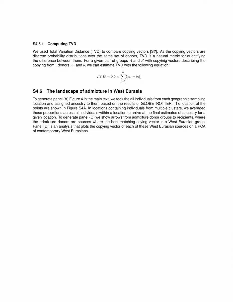
S4.5.1 Computing TVD

We used Total Variation Distance (TVD) to compare copying vectors [S?]. As the copying vectors arediscrete probability distributions over the same set of donors, TVD is a natural metric for quantifyingthe difference between them. For a given pair of groups A and B with copyinig vectors describing thecopying from i donors, ai and bi we can estimate TVD with the following equation:

TV D = 0.5×n∑

i=1

(|ai − bi|)

S4.6 The landscape of admixture in West Eurasia

To generate panel (A) Figure 4 in the main text, we took the all individuals from each geographic samplinglocation and assigned ancestry to them based on the results of GLOBETROTTER. The location of thepoints are shown in Figure S4A. In locations containing individuals from multiple clusters, we averagedthese proportions across all individuals within a location to arrive at the final estimates of ancestry for agiven location. To generate panel (C) we show arrows from admixture donor groups to recipients, wherethe admixture donors are sources where the best-matching coying vector is a West Eurasian group.Panel (D) is an analysis that plots the copying vector of each of these West Eurasian sources on a PCAof contemporary West Eurasians.

S5 Additional discussion of results

In the following section we first provide a brief, direct, comparison of admixture events that we infer inSardinia and the Balkans with previous studies using different methods and datasets. We then discussthe inferred admixture events from our study in more detail. Except in a couple of cases, we restrict thefollowing discussion to the 57 recipient clusters containing at least four individuals.

S5.1 Comparison to previous results

1. Moorjani et al [S?], who use a method based on allele frequency comparisons, and not haplotypes(ROLLOFF), found evidence for sub-Saharan African admixture in Sardinia 71±28 generationsago, at a proportion of 3%. These are the same Sardinians included in our analysis. In the largestSardinian (sardi13) cluster in our analysis we infer West African admixture 66 (53-82) generationsago at a proportion of 2%.

2. Ralph and Coop [S?] using a method that infers tracts of ancestry by inferring Identity by Descent(IBD) along chromosomes, showed evidence that individuals from the Balkans have a high numberof shared ancestors, with the length of these shared IBD tracts consistent with common ancestryfrom the Migration Period. We also find admixture events dating to this period in groups from theBalkans, for example in groups from Hungary (hunga23), Bulgaria (bulga46) and Croatia (croat18),in which we infer north east European ancestry flowing into more southerly regions. Ralph andCoop use a different dataset (POPRES) and different methods to produce qualitatively similarresults to us.

S5.2 Continuous low level African admixture in the Mediterranean and Anatolia

We infer West African admixture across broad date ranges, but at low admixture proportions (admixtureα < 0.07; Figs. 2 and S3) in several Mediterranean groups, consistent with a long term movement be-tween sub-Saharan Africa and southern Europe [S?,S?]. Specific West African admixture dating to theArabic conquest of the Mediterranean [S?] is seen in Spanish (spani27: 1042 (740-1201CE)), SouthernItalian and Sicilian (sicil30: 1105 (882-1250CE)), and Basque (basqu24: 886 (283-1162CE)) clusters.Earlier African admixture at low admixture proportion is inferred in the Cypriots (cypri12: 427(107-734CE)), and a Sardinian cluster (sardi13: 36 (458BCE-430CE); α = 0.02). This latter event is con-sistent with the occurrence of A3b2-M13 (0.6%) and E1a-M44 (0.4%) African Y chromosome lineagesin Sardinia [S?]. and the dating is more compatible with documented exchanges between the island andMauretania Cesariensis in Roman times (2nd century BCE to 2nd century CE) than later displacementsof northern-African males to Sardinia at the time of the Vandals rule (5th century CE) [S?].

Two Iranic clusters show evidence of African admixture, from West Africa in a Kurdish cluster (kurd5:872CE (312-1069CE)), and from East Africa in an Iranian cluster (irani5: 1412CE (1054CE-1526CE)).The low admixture proportion (α = 0.01) in the Kurdish cluster suggests a very subtle event, the datesof which roughly align with the Arabic conquest of the Mediterranean and the increased movement ofsub-Saharan African slaves in the region [S?]. Admixture is more recent in the Iranian cluster, andsimilarly at a low admixture proportion (α = 0.03), but the distinct eastern origin of the African ancestryin this group suggests a different route of African admixture into the region, across the Indian Oceanand Arabia. We observe subtly different signatures of admixture in each of the three Sardinian clusters,as already discussed from West Africa, but also from North Africa, specifically Tunisian and Moroccansources (sardi9: 356 (507BCE-756CE); α = 0.09), and also from the Levant source at a proportion

of α = 0.07 (sardi6: 449 (11BCE-755CE)). The dates for these events overlap, consistent with Africanancestry originating from a number of different sources. Previous admixture analysis of these individualsfound evidence for a small amount of sub-Saharan admixture [S?,S?] around 40 generations ago, whichwe corroborate here, with the additional suggestion of multiple complex African ancestral histories withinindividuals from the island.

S5.3 A key role for the Levant in the genetic history of the Mediterranean

Early admixture involving source groups most similar to contemporary populations from in and aroundthe Levant (which we define as the World Region containing individuals from Syria, Palestine, Lebanon,Jordan, Saudi, Yemen and Egypt) is seen at high proportions in several clusters from Italy dating tothe first half of the first millennium CE, from Southern Italy (itali8: 295CE (72BCE-604CE); α = 0.34),Tuscany (tsi23: 400CE(30BCE-686); α = 0.29), and Sardinia, as well as in a large cluster from Armeniaat an early date (armen27: 363BCE(1085BCE-383CE)). Traces of Phoenician ancestry (1200-300BCE)have been observed using uni-parental markers from populations around the Mediterranean [S?] which,based on the dates, is unlikely to be the source of ancestry we observe here. Instead these eventsloosely coincide with the formation of the pan-Mediterranean Roman Empire [S?], which may also haveallowed increased gene flow from east to west Mediterranean. A significant amount of ancestry (α =0.36) in a large Armenian cluster (armen27) is the result of a complex ancient event involving multipleadmixture sources from the Caucasus, Turkey, and the Levant. Armenia was at various times acrossthis period part of Roman, Christian, Parthian and Arabic empires. Whilst it is impossible to identify aparticular event that caused the admixture that we see, the proportion, timing and identity of the sourcegroups in this event are consistent with Armenia’s geographic and political position at a junction betweenEurope and west Asia. Similarly, we also infer a complex event involving the Levant, Central Asia andTurkish sources in an Iranian cluster (irani10), although dates for this event are more recent (1221CE(1063-1330CE)) and therefore more consistent with influx on ancestry from the Near East during andafter the Mongolian expansions into western Eurasia. We infer more recent Levant admixture in theFrench (frenc24: 728(424-1011CE)) and in a complex multiway event in a Spanish cluster (spani9: 668(286-876CE)). The dates and sources of admixture in these cases are consistent with movements ofMiddle Eastern and North African individuals during the Islamic Conquest of Spain [S?], and suggest alegacy of this key moment in southern European history in the genomes of French as well as Spanishpopulations.

S5.4 Multiple waves of admixture from east Asia

The Caucasus contain many linguistically diverse but genetically homogeneous populations [S?]. Thehistorical influence of Asia is particularly clear in the Caucasus and Anatolia, where most events in-volve Mongolian sources and occur after 1000CE (Figs. 2 and S3, Table S4). Two clusters from Turkey(turki34, turki17) show clear evidence of admixture from Mongolia, which is also present in severalgroups from the steppe east of the Caucasus, in clusters containing individuals from Tajikistan (tajik11:1295(1152-1374CE)) and Turkmenistan (turkm11: 1266(1159-1323CE); turkm5: 1369 (1226-1508CE)).Dates for these events centre around 1250CE, suggesting further evidence of the large-scale impact ofChinnghid Mongolian nomads in Western Eurasia [S?,S?] in a wide set of populations. The more re-cent events involving Mongolian sources in Eastern and Northern Caucasus clusters containing Nogay,Kumyk, Lezgin, and Tabasaran individuals centre around 1400-1500CE which may related to the post-Mongol Timurud dynasty which ruled Central Asia and the Caucaus between 1360 and 1425CE [S?].

Among the Caucasus clusters where we do not specifically infer Mongolian admixture, we find evi-dence of events, often involving multiple admixture sources including Central Asian (Uzbek and Hazara)sources, in clusters containing Turkish (turki7: 1015 (541-1309CE)), Balkasian (balka5: 1177 (876-1389CE)), and Iranian (irani10: 1221 (1063-1330CE)) individuals. The dates for these events, whichpeak around 750 years ago, together with the non-Mongolian source groups, suggest a role for sec-ondary movement into this area at the time of the Mongolian expansion, but from Asian groups withdistinct non-Mongolian ancestry.

A cluster of two individuals from Romania (roman2: 990 (741-1245CE)) have clear evidence of anadmixture event involving a source most similar to India. Romany gypsies have been shown to haveancestry from the India subcontinent, which has been dated to an event between 780 and 900 yearsago [S?,S?]. Our date of 800 years ago, or 1200CE broadly agrees with these inferences. The identityof these two individuals as Romani is not possible from the data associated with the samples, but ifconfirmed, shows that in certain settings GLOBETROTTER can produce accurate historical inferenceeven with limited sample sizes.

Among the northern Europeans, the Finnish (finni3) show evidence of an admixture event involvinga minority source most similar to contemporary North Siberians (469CE (213BCE-1011CE)). Finns arethought to have originated from the northward migration, and subsequent contact, between Central Eu-ropeans and indigenous Scandinavian hunter-gatherers closely related to the Saami [S?]. The Saamiare closely related to the individuals that make up the North Siberian world region, and whilst our con-fidence in this admixture date is low because of the small size of the cluster, the event we see is likelyto represent this key period in Finnish history. Within our dataset, only the Finnish, Hungarians andMordovians speak Finno-Ugric languages, the latter of which we group into two clusters (mordo13: 792(564-975CE); mordo2: 558 (179-843CE)) and, together with the Russians (russi25: 913(754-1007CE))and Chuvash (chuva16: 829 (627-940CE)) populations, infer admixture at approximately the same time(500-900CE) involving Mongolian, Central European, and Finnish donors. In a recent analysis that re-constructed the ancestry of Eurasia on the basis of ancient DNA [S?], the ancestry of these groups couldnot be explained without a putative stream of recent Asian admixture, a scenario which we confirm in ouranalysis. As such, the Asian admixture in these groups is unlikely to be associated with the Mongolianexpansion described above and may instead be related to earlier Turkic movements, involving the Hunsand Avars [S?], but separate to the event inferred in the Finnish.

S5.5 Admixture within Europe: the Medieval Migration Period

A separate set of events involves admixture between groups within West Eurasia. As we previouslyreported [S?], the formation of the Slavic people at around 1000CE had a significant impact on thepopulations of northern and eastern Europe, a result that is supported by a related but different anal-ysis [S?]. We infer events involving a “Slavic” source (represented here by a cluster of Lithuanians;lithu11) across all Balkan groups in the analysis (Greece, Bulgaria, Romania, Croatia, and Hungary) aswell as in a large cluster of Germanic origin (germa36) and a composite cluster of eastern Europeanindividuals (ukrai48). Dates for these events mostly overlap, although are older in Croatia and Greece,and appear to concentrate on the end of the first millenium CE (Figure 3), a time known as the EuropeanMigration Period, or Volkerwanderung [S?]. We additionally infer events during this period in the Spanish(spani9: 668 (286-876CE)), involving Basque- and northern Italian-like sources, in the British (ceu71:858 (467-1224CE) involving German-, Central and Southern Italian-, and Norwegian-like sources , inthe Orcadians (orcad5: 1241 (889-1412CE); orcad6: 708 (94BCE-1399)) involving Norwegian-, South-ern Italian-, and Armenian-like sources, in the Norwegians (norwe17: 351 (262BCE-893CE)) involv-ing Mordovian- and British- like sources, in the northern Italians (itali13: 677 (362-989CE)) involvingCypriot- and French-like sources, and in a large cluster of Tuscans (tsi70: 241 (16BCE-417CE)) involv-

ing Cypriot- and British-like sources. Interestingly, these groups contain individuals that are largely fromnorth-western and central European regions with historically attested influences from different groupsduring the Volkerwanderung [S?], suggesting that this period had a further visible effect on the contem-porary populations across Northern and Central Europe.

Documents

The Role of Recent Admixture in Forming the Contemporary West Eurasian Genomic Landscape