THE RETURN TO CAPITAL IN CAPITAL-SCARCE

COUNTRIES∗

Anusha Chari† Jennifer Rhee ‡

December 13, 2019

Abstract

Capital flows from rich (capital-abundant) to poor (capital-scarce) countries fall shortof what neoclassical theory predicts. In this paper, we use firm-level data to investigatethe link between the marginal product of capital and financial rates of return acrosscountries. Computed estimates from financial statement data show that capital-scarcecountries display higher marginal products of capital. However, inflation-adjusted fi-nancial returns are roughly equal across capital-scarce and capital-abundant countries.The divergence between the marginal products of capital and financial returns impliesthat there may be little incentive for capital to flow to capital-scarce countries. Wesuggest that domestic capital-accumulation frictions such as sufficiently large capitaladjustment costs can decouple financial rates of return from the marginal product ofcapital across countries.

Keywords: Marginal Product of Capital, Financial Returns, Lucas Paradox, Firm-LevelDataJEL classifications: E13, F49, G32, O16∗We thank seminar participants at UNC-Chapel Hill and the Federal Deposit Insurance Corporation.

We thank Wayne Landsman, Francesco Caselli, Pierre-Oliver Gourinchas, Sebnem Kalemli-Ozcan, AlwynYoung, Peter Blair Henry, Ju Hyun Kim, Simon Alder, Patrick Conway, and Lutz Hendricks for helpfuldiscussions. Opinions expressed in this paper are those of the authors and not necessarily those of the FDIC.†Corresponding Author: Professor of Economics and Finance, Department of Economics & Kenan-Flagler

Business School, University of North Carolina at Chapel Hill & NBER. CB3305, UNC-Chapel Hill, ChapelHill NC 27599. Email: achari@unc.edu.‡Financial Economist, Federal Deposit Insurance Corporation, 550 17th Street NW, Washington DC

20429 Email:jrhee@fdic.gov.

1 Introduction

The neoclassical model predicts that poor countries (capital-scarce) will have a higher rateof return to capital than rich countries (capital-abundant). Accordingly, scholars expendconsiderable effort trying to understand why capital does not flow from rich to poor nations(Lucas, 1990; Alfaro, et al., 2008; and Reinhart and Rogoff, 2004). An emerging body ofempirical work based on national income accounts suggests that the neoclassical predictionsabout capital scarcity and higher rates of return do not hold up in the macro data. Themarginal product of capital is apparently no higher in poor countries than it is in rich ones(Caselli and Feyrer, 2007, and Gourinchas and Jeanne, 2013). If recent empirical studies areaccurate then it is unsurprising that capital does not flow from rich to poor countries; withequalized marginal products, it has little incentive to do so.

In this paper, we investigate the link between the marginal product of capital and financialrates of return in emerging and developed economies. In a one-sector neoclassical model,a firm’s first-order condition states that the marginal product of capital (MPKt) and thefinancial return (rt) should differ only by the depreciation rate (δ), which is often assumedconstant across countries (rt = MPKt − δ). Therefore, theory predicts that high financialreturns and high marginal products of capital should go hand in hand. If this link breaksdown (i.e., if a high marginal product of capital does not turn into high financial returns),it is not clear that capital ought to flow to countries with high marginal products of capital.

Notwithstanding the significance of this first-order condition that lies at the heart ofthe Lucas Paradox, aggregate data pose limitations for testing its validity. In this paper,we use firm-level accounting and stock market data from a set of developed and emergingcountries between 1997 and 2014 to examine the link between the marginal product of capitaland financial returns. Much of the international macro literature imputes an aggregatemarginal product of capital using calibration techniques. The imputations rely on underlyingassumptions about functional form, such as technology, capital shares, and elasticities ofsubstitution. The innovation in Caselli and Feyrer (2007) was to measure the aggregatereturn on capital using national income accounts instead of relying on calibration. In general,however, delivering the finding that marginal products of capital are essentially the sameacross rich and poor countries requires adjustments for (i) the capital per effective workerand a human capital externality (Lucas, 1990), (ii) non-reproducible capital and the priceof capital goods (Caselli and Feyrer, 2007), or (iii) technology catch-up and distortions insaving and investment decisions (Gourinchas and Jeanne, 2013).

Our paper offers an alternative approach to measuring the return to capital using microdata. In contrast to previous literature about the return to capital that uses (i) calibrated

2

estimates, or (ii) aggregate data, we directly compute rates of return at the firm level andaggregate them up to produce estimates of country-level rates of return. Inspite of thecentrality of firm productivity in macroeconomic modelling, the link between accountingearnings and the macroeconomy remains relatively unexplored (Konchitchki and Patatoukas,2014). The paper therefore contributes to a recent body of literature that uses firm-levelaccounting data to draw macroeconomic insights.

Our main finding is that the link between the marginal product of capital and the finan-cial return, which is often assumed in the international capital flows literature, does not holdfor a sample of developed and emerging countries between 1997 and 2014. Consistent withpredictions from the neoclassical framework, the results show that firm marginal productsof capital are indeed higher in emerging countries relative to their developed market coun-terparts. The evidence suggests an inverse correlation between marginal products of capitaland per capita levels of output per worker. The pattern is robust to controlling for firm-and industry-specific effects and remarkably consistent across different sample periods andcountries.

The neoclassical model also implies that the higher marginal product of capital shouldtranslate to higher financial returns in emerging markets. Contrary to this prediction, we findthat inflation-adjusted financial returns are roughly equal between developed and emergingcountries. The result is significant as it casts new light on the use of differences in themarginal products of capital to explain international capital flow patterns. The firm-levelevidence using computed estimates suggests that the marginal product of capital might notbe a valid proxy for financial returns. The divergence between marginal products of capitaland investment returns is consistent with the capital wedge documented in Gourinchas andJeanne (2013).

In addition, the results confirm the view that there is no prima facie evidence thatinternational credit frictions play a major role in preventing capital flows from rich to poorcountries (Caselli and Feyrer, 2007). If marginal product of capital differentials correctlytranslate to higher financial returns in emerging markets, then the shortfall in the capital flowto these countries points to international capital market frictions and investment barriers.However, if financial returns are equalized across developed and emerging countries, analternative hypothesis may be that there is little incentive for capital to flow to less-developedcountries.

To further explore this hypothesis, note that the firm’s first-order condition that linksthe marginal product of capital and financial returns stems from the capital accumulationequation, which suggests that the capital stock tomorrow is the sum of capital stock todayand the investment net of depreciation (Kt+1 = (1 − δ)Kt + It such that Kt and It are

3

the capital stock, and investment in period t, respectively). On the other hand, if a unitinvestment does not lead to a unit increase in the capital stock, the cross-country investmentreturn and marginal product of capital patterns can differ. Although models with capitaladjustment factors are widely used in the investment literature (see Cochrane, 1991; Hayashi,1982; Abel and Blanchard, 1986), domestic capital accumulation frictions are relativelyunexplored in the international capital flows literature. Jin (2012) is an exception as sheuses a capital accumulation equation with adjustment costs from Abel (2003). However,Jin’s empirical analysis focuses on the revealed comparative advantage using internationalcapital flows rather than the measurement of marginal product of capital. In this paper,we show that capital accumulation frictions can help model the divergence between theinvestment returns and marginal product of capital patterns observed in the data between1997 and 2014. We also show that the model with capital accumulation frictions provides ananalytical framework that links cross-country differences in the relative price of capital andthe capital wedge, explanations used to resolve the Lucas Paradox in the literature (Caselliand Feyrer, 2007; Gourinchas and Jeanne, 2013).

In large part, cross-country differences in capital accumulation processes have not beenempirically explored in the capital flows literature because of data limitations.1 With aggre-gate data, estimates of the aggregate capital stock are constructed from aggregate investmentdata (such as from the Penn World Tables) using the perpetual inventory method, whichrequires one to posit a capital accumulation process. Since this process is typically assumedto follow a model where a unit increase in investment leads to a unit increase in capitalstock, the aggregate capital stock estimate itself implicitly relies on the assumption that thelink between marginal product of capital and the investment return holds. A key advantageof the firm-level data we use in this paper is that unlike aggregate estimates, we can directlyobserve capital stock measures from accounting and market values. This allows us to directlycompute the marginal product of capital and investment returns, and to empirically test thetightness of the link between the two.

The paper limits the analysis to listed firms in MSCI emerging and developed countriesthat have relatively well-established stock markets, which substantially reduces the numberof countries in the sample. But, as Reinhart and Rogoff (2004) suggest, roughly 25 emergingmarkets account for the bulk of international financial flows. Therefore, the analysis of thefirms in these countries can provide useful insights into the factors that drive internationalcapital flows. We also restrict the period of analysis to the post-1996 period because of the

1It is important to note the extensive use of the implications of capital accumulation frictions withinthe international capital flows literature. For example, the cross-country differences in the relative price ofcapital introduced in Caselli and Feyrer (2007) and the capital wedge used by Gourinchas and Jeanne (2013)can both be derived within the neoclassical model using capital accumulation frictions.

4

limited availability of reliable firm-level data from emerging countries in the early 1990s.Although firm-level data have many advantages, some drawbacks exist. For example,

available firm-level data do not provide insight into the productivity of self-employed workersor informal sector firms. This is a significant drawback as these types of households and firmsmake up a large part of the economy in developing countries. Unlike aggregate data, firm-level market variables are also susceptible to market volatility. Since the period of analysisincludes the global financial crisis (2007-2008), we control for year-specific effects and runa robustness test excluding these years. We suggest that despite these shortcomings, thefirm-level data provide useful insights about the relationship between financial returns andfirm productivity. The paper provides an alternative lens to complement existing literaturethat primarily uses macroeconomic data to perform aggregate analysis.

An important concern with using cross-country firm-level data is the difference in theaccounting standards used to report data from different countries. For example, the defi-nition of “assets” in the U.S. Generally Accepted Accounting Principles (U.S. GAAP) maydiffer from the definition in the International Financial Reporting Standards (IFRS). Tominimize the effects of these differences, we use financial and accounting data from World-scope Datastream. Datastream not only provides extensive accounting and market dataon listed firms across countries but also aims to “provide the data in a manner that allowsmaximum comparability between one company and another, and between various reportingregimes” (Worldscope/Disclosure Partners, 1992). Thus, the numbers reported in the firm’sannual/quarterly audit reports could differ from the numbers provided by Worldscope, whichadjusts the data to make the definitions more comparable to their U.S. counterparts (Wald,1999). Although Datastream takes extensive measures to increase firm comparability acrosscountries, we further check for the effects of cross-country differences in accounting standardsthat may remain in the data, by running a robustness test restricted to firms from countriesthat adopt the IFRS. We find that the main results remain robust.

Other potential concerns include the overseas operations of the listed firms. Overseassubsidiaries are common among the major firms in both developed and emerging marketcountries and could influence the outcome of analysis. The globalization of firms also mayincrease the noise in the data. We further test the robustness of our results by looking atthe cross-country patterns within industries that are less likely to have multinational firmpresence (e.g., utilities). We find that the main findings remain intact within these industries.

Our paper relates to a vast international capital flows literature on the Lucas Paradox.Alfaro et al. (2008) sort the literature into two groups. The first group relies on differences infundamentals that affect the production structure of the economy, such as technological dif-ferences, missing factors of production, government policies, and the institutions, to explain

5

the paucity of capital flows to poor countries. The second group focuses on international cap-ital market imperfections that stem from sovereign risk and asymmetric information (Stulz,2005; Reinhart and Rogoff, 2004; Monteil, 2006; David et al., 2014). Much of the inter-national macro and growth literature that uses cross-country marginal product of capitaldifferences to explain international capital flow patterns relies on macroeconomic fundamen-tals and endowments that affect differences in productive efficiency to explain the LucasParadox (see Lucas, 1990, and King and Rebelo, 1993).

In their 2005 paper, Banerjee and Duflo outline an exhaustive list of methods used tocalibrate the marginal product of capital in the development literature. Approaches includeproxies for firm returns to capital using lending rates in the emerging countries that showextremely high risk-adjusted costs of borrowing in these countries. Caselli and Feyrer (2007)argue that interest rates may be poor proxies for the firm-level cost of capital in financiallyrepressed/ distorted economies. Other method posit a production function and derive theexpression for marginal product of capital. Using this approach, Lucas (1990) shows thatadjusting for productivity differences lead marginal product of capital differences to fallsubstantially. Caselli and Feyrer (2007) take an alternative approach and directly measuremarginal product of capital using national income accounts without assuming the productionfunction. Their results show that the return to capital is roughly equal between emergingand developed countries once we adjust for the relative price of capital, and complementaryfactors of production such as land.

The findings in this paper are closely related to Gourinchas and Jeanne (2013), Banerjeeand Duflo (2005), and Chirinko and Mallik (2008). Although the approaches differ, all ofthese papers investigate the role of domestic capital frictions on marginal product of capitaldifferences. Hsieh and Klenow (2008) and Alfaro, et al. (2008) also study domestic capitalmarket imperfections (i.e., the misallocation of capital within countries). However, theseanalyses focus on aggregate total factor of productivity (TFP) and institutional quality dif-ferences across countries rather than return differences. This paper adds to the literature byexamining the impact of domestic capital frictions on the relationship between the marginalproduct of capital and financial investment returns. The paper is also related to the ex-tensive literature on measurement of real returns in the economy. The efforts to correctlymeasure the real return in the economy at a macro level involve improving the measurementof income and capital shares in production (see Gollin, 2002; Karabarbounis and Neiman,2013; and Jorda et al., 2017).

The paper proceeds as follows. In section 2, we introduce the basic neoclassical model andits predictions about the relationship between the marginal product of capital and financialinvestment returns, and explain the empirical methodology. Section 3 describes the firm-

6

level data used in the analysis and presents summary statistics. We analyze the cross-countrymarginal product of capital and investment return patterns in section 4 and investigate analternative model that can explain the divergence between the two patterns in section 5.Section 6 concludes.

2 A Benchmark Model and the Empirical Methodology

In this section, we present a simple neoclassical model to fix ideas and motivate the empiricalanalysis. Following that we describe the empirical methodology.

2.1 A Benchmark Neoclassical Model

To fix ideas, in this section we introduce a neoclassical one-sector model with perfectlycompetitive factor markets. This simple, benchmark model delivers useful predictions andillustrates the first order condition that we use to motivate the empirical analysis. We alsoconsider a brief extension to a multi-sector setting.

2.1.1 One-Sector Model

Consider a neoclassical one-sector economy where the representative firm faces competitivefactor and goods markets. The production function is given by Yt = F (Kt, Lt) where thefirm chooses capital, investment, and labor ({Kt, It, Lt}∞t0 ) to maximize the net present valueof future cash flows, taking the interest rate as given:

max{Kt,It,Lt}∞t0

∑t≥t0

1

Rt

(Yt − It − wtLt) (1)

The capital accumulation process is defined as Kt+1 = G(Kt, It) = (1 − δ)Kt + It, and theaggregate investment return between period t0 and t is Rt = (1 + rt)(1 + rt−1)...(1 + rt0). Ytis the period output of the representative firm, and wt is the exogenously determined wage.Note that there is no capital rental market in this economy, as the firms own the capital usedin production. Rt is the aggregate compounded investment return from period t0 to t, andδ is the depreciation rate of the physical capital, which is assumed constant. The first-order

7

conditions yield:

1 + rt =

(F1(Kt, Lt) +

G1(Kt, It)

G2(Kt, It)

)G2(Kt−1, It−1)

= F1(Kt, Lt) + 1− δ (2)

and,F2(Kt, Lt) = wt (3)

for all periods t > t0. It is evident from equation (2) that the key determinant of therelationship between the period marginal product of capital (F1(Kt, Lt)) and the investmentreturn (rt) is the capital accumulation equation (G(Kt, It)). Thus, if friction exists in thecapital accumulation process, then the cross-country investment return and marginal productof capital patterns may diverge.

To illustrate, assume a constant return to scale Cobb-Douglas production function (Y =

AKαL1−α), such that yt = YtLt

and A is total factor of productivity or productive efficiency.Note that if alpha is the measured capital share in income,MPK = α yt

ktholds for neoclassical

production functions of any functional form in a one-sector setting with perfect competition.The Cobb-Douglas production function serves as a simple example. The capital share ofoutput (α) is assumed less than unity. Since we also assume that all firms in the economyshare an identical production function, the output per unit of labor should be identical acrossall entities.

F1(kt) = αA1αy

α−1α

t

= αytkt

(4)

It follows from equations (2) and (4) that both the period investment return and marginalproduct of capital should decline with increases in the output per unit of labor. With thesesimplifying assumptions, the model predicts that firm-level marginal products of capital andinvestment returns should be inversely correlated with the aggregate output per unit of labor.

2.1.2 Multisector Model

Consider a multi-sector neoclassical economy that produces J final goods and a capital good.The production function for firms that produce a final good i is given by Yt = F i(Kt, Lt)

where the firm chooses level of capital, investment, and labor ({Kt, It, Lt}∞t0 ) to maximize

8

the net present value of future cash flows:

max{Kt,It,Lt}∞t0

∑t≥t0

1

RNt

(P1,tYt − PK,tIt − wtLt) (5)

The capital accumulation process of the firm is defined as Kt+1 = G(Kt, It) = (1− δ)Kt + It,and the aggregate investment return between period t0 and t is Rt = (1 + rt)(1 + rt−1)...(1 +

rt0). Note that RNt in the equation (5) is the aggregate nominal investment return, such that

RNt = (1+rNt )(1+rNt−1)...(1+rNt0 ). The real investment return (rt) is defined as 1+rt =

1+rNt1+πt

,where πt is inflation in period t. The first-order condition for producers of good i yields:

1 + rt =

(P1,t

PK,tF i

1(Kt, Lt) +G1(Kt, It)

G2(Kt, It)

)G2(Kt−1, It−1)

=P1,t

PK,tF i

1(Kt, Lt) + 1− δ (6)

for all periods t > t0.P1,t

PK,tF i

1(Kt, Lt) is the price adjusted marginal product of capital introduced in Caselli andFeyrer (2007). In their paper, Caselli and Feyrer show that adjusting for the cross-countrydifference in the price of capital significantly reduces marginal product of capital differencesbetween developed and developing economies. However, this cross-country difference in therelative price of capital does not affect the relationship between the price-adjusted marginalproduct of capital( P1,t

PK,tF i

1(Kt, Lt)) and the real return(rt)-the two only differ by a constantδ. Therefore, if the price-adjusted marginal product of capital is higher in emerging marketcountries, the real investment return ought also be higher.

Further, if capital is efficiently allocated within the economy, rt should be identical forall firms within the economy and thus, Pj,t

PK,tF j

1 (Kt, Lt) = P1,t

PK,tF i

1(Kt, Lt). Therefore, if for

any sector i, P1,t

PK,tFKi (Kt, Lt) is higher in emerging market countries relative to developed

ones, the price-adjusted marginal product of capital for all final goods should be higher inemerging market countries.

Firm-level data allow us to test these implications at a more granular level than aggregatedata. The next section describes how we map the theoretical predictions to the firm-levelaccounting and stock market data.

2.2 Mapping the Theory to Firm-Level Data

In this subsection, we describe the methodology to estimate marginal products of capitaland investment returns used in the empirical analysis. To map the two variables of interest

9

from the theory to the data, we use accounting and financial measures of profitability withsome modifications to better align the measures with the economic definitions described inthe benchmark model.

From equation (4), the marginal product of capital is equal to α ytkt, or in the multi-sector

case, αPyytPkkt

. Given that α is the capital share of output, this expression suggests that themarginal product of capital is the ratio between the portion of earnings that accrue to capitalholders (in the model simply the firm), and firm assets. The empirical estimations use returnon assets (ROA) as a measure of the marginal product of capital as follows:

ROAf,i,c,t =EBITDAf,i,c,tMVAf,i,c,t−1

(7)

EBITDAf,i,c,t is the earnings before interest, tax, depreciation, and amortization, andmeasures the income that accrues to capital holders or the firm f in industry i in period t incountry c. We use this measure of earnings rather than net income since the model assumesthat the firm owns all of its capital assets, and, therefore, there are no interest costs. Inthe analysis, we further adjust this measure of income for extraordinary gains/costs. Theadjustment is necessary as these costs/gains are often unrelated to business operations, andthey can increase the volatility of earnings by inflating or deflating the income from theoperations.

MVAf,i,c,t is the current market value of the firm’s assets2 and is defined as MVAf,i,c,t =

Debtf,i,c,t + MVf,i,c,t. Debtf,i,c,t is the book value of debt, and MVf,i,c,t is the market valueof equity for the firm f in industry i in period t in country c. Poterba (1998) uses a similarmeasure to estimate the return to tangible capital at an aggregate level. This measurediffers from the standard accounting ROA, which uses the book value of the assets in thedenominator as the measure of capital. Although this ratio is widely used in finance andaccounting3, assets on the balance sheet are measured at the acquisition cost. As the marketvalue of an asset can change over time (e.g., the value of buildings or land may appreciateor depreciate), the value of assets on financial statements may not correctly reflect currentvalues. Therefore, we replace the denominator of the indicator with the sum of the book valueof debt and market value of equity. As total assets necessarily equal the sum of liabilitiesand equity, this measure ought to provide a more accurate estimate of the replacement valueof an asset in period t− 1 under perfect capital markets.4 The value of assets at the end of

2This is also the replacement value of the asset based on the q-theory of investment.3See Eisenberg et al. (1998), Guenther and Young (2000), Chaney et al. (2004), Bowen et al. (2008).4Debt also enters financial statements at a historical cost, and the interest rate on debt may differ across

time. However, the income used in the analysis is income before interest. Therefore, even if debt is refinancedat a “current” rate of interest, it should not affect the ROA measure used in the analysis.

10

period t−1 is used in the denominator as a measure of what the firm owns entering period t.This is the capital employed during period t to generate the income EBITDAf,i,c,t. Due to atime period mismatch between the numerator and denominator, we adjust the MVAf,i,c,t−1

for inflation using the consumer price inflation (CPI) index.We can rewrite the capital accumulation equation as 1−δ = Kt+1−It

Kt. Then, if investment

efficiency holds,

rt =αYt − It +Kt+1 −Kt

Kt

(8)

Note that this is the rate of return equation commonly used in finance to assess the profitabil-ity of an investment 5. It measures the investment return that capital owners can receive bypurchasing one unit of capital at time t and selling it at time t+ 1.

Using equation (8) as the benchmark, we derive the following expression to measure theinvestment return:

IRRf,i,c,t =EBITDAf,i,c,t + [∆MVAf,i,c,t −∆BV AAdjf,i,c,t]

MVAf,i,c,t−1

(9)

∆MVAf,i,c,t is the change in the market value of assets, (MVAf,i,c,t−MVAf,i,c,t−1). ∆BV AAdjf,i,c,t =

∆BV Af,i,c,t + depreciationf,i,c,t, such that ∆BV Af,i,c,t is the change in the book value of as-sets. ∆BV AAdjf,i,c,t measures the current value of gross investments by firms. Recall that ahistorical-cost approach is used to measure assets on the balance sheet that are recorded atacquisition prices. Therefore, while balance sheet assets do not reflect the current marketvalue of aggregate capital, the gross change in assets measures the capital investment of firmsat current market (acquisition) prices.

This definition is similar to a period investment return measure used by Fama and French(1999) for the U.S. stock market. In their paper, this estimate is termed the “internal rateof return on value” and is used as the measure of the required rate of return by investors,or more precisely, an estimate of investor earnings during the sample period through passiveinvestment in all corporate securities as they enter the sample. We note that this measureof investment does not include a significant portion of the research and development (R&D)spending by the firm. Due to accounting conservatism and uncertainty about the successof the R&D activity, R&D spending is considered a cost rather than an asset and is, thus,expensed. However, this should not affect the measurement of IRRf,i,c,t as the spending isreflected in the EBITDAf,i,c,t. We also adjust the investment return for inflation acrossdifferent countries. It is important to note that equations (7) and (9) apply in both the

5See Gordon (1974), Salamon(1985), Fama and French(1999), Graham and Harvey(2001)

11

single- and multi-sector cases. Further, we estimate the value of the capital assets usingmarket prices. In turn these market values of capital assets imply that the observed valuesare adjusted for differences in the relative price of capital goods across countries. Thereforeif the market value for capital assets is higher in emerging markets relative to developedmarkets, the market value firm assets will reflect this higher price of capital goods.

3 The Data and Summary Statistics

Financial and market data used to calculate the firm-level marginal product of capital andinvestment return are from Worldscope Datastream. Datastream is a preferred source ofdata for the cross-country comparison because it not only provides extensive accountingand market data on listed firms across countries, but it also aims to “provide the data in amanner that allows maximum comparability between one company and another, and betweenvarious reporting regimes” (Worldscope/Disclosure Partners, 1992). These adjustments byWorldscope help minimize the potential bias from the cross-country differences in accountingstandards.

Although Datastream takes extensive measures to increase the accounting comparabilityacross countries, we further check for the effects of cross-country differences in account-ing standards by running a robustness test restricting the analysis to the countries thatadopted IFRS. Since the mid-2000s there has been increasing attempt led by Euro-zonecountries to unify accounting standards across countries. These efforts led to formation ofthe International Accounting Standards Board (IASB), whose explicit goal is “to developan internationally acceptable set of high quality financial reporting standards” (Barth et al.2008). Although the United States is yet to adopt IFRS, the standards were adopted byEU countries by 2005 and a majority of MSCI developed and emerging countries by 2011(the Appendix provides a list). Many other countries that have yet to adopt IFRS haveannounced their plans for convergence in the near future. For example, India’s Ministry ofCorporate Affairs released a road map for convergence with the IFRS, and all Indian com-panies whose securities traded in a public market other than the SME Exchange, will berequired to use IFRS by 2017. These efforts may lead to even greater data comparabilitygoing forward facilitating firm-level research. In this paper, we test that the main resultsremain robust to the cross-country differences in accounting standards.

The countries used in the analysis are MSCI emerging and developed countries thathave relatively well-established stock markets.6 Exchange floors in developing countries are

6Saudi Arabia is dropped from the sample due to the limited availability of firm-level data in early 2000s.

12

often very new (e.g., Laos opened its stock exchange in 2011, Syria in 2009, and Somaliain 2012), and in many cases Datastream does not carry data on the firms traded on theseexchanges as the market capitalization of these countries is small (e.g., the Maldives StockExchange had only five firms listed as of 2008). Some developing countries do not have anational stock exchange (e.g., Angola, Brunei). Restricting the analysis to MSCI emergingand developed countries reduces the countries in the sample, but as Reinhart and Rogoff(2004) point out, roughly 25 emerging markets account for the bulk of the financial flows.Therefore, analyzing the marginal product of capital and the investment returns of the firmsin the MSCI developed and emerging country sample can provide useful insights into factorsthat drive international capital flows.

The period of analysis is 1997 to 2014. A longer period may be preferred for the anal-ysis as it provides more reliable estimates of return on assets (ROA) and internal rates ofreturn (IRR) patterns. But unlike macroeconomic aggregate data, which date back to mid-1900s, firm level data for emerging countries are often unavailable before 1995. Even thoughthe estimation period used in the paper is relatively short compared with papers that usemacroeconomic data, the period after 1995 is characterized by a large volume of interna-tional capital investment following a series of trade and financial liberalization programsundertaken since the mid-1980s. Therefore, the period post-1990 is especially relevant foranswering questions related to the marginal product of capital, investment returns, and theobserved patterns of international capital flows. A major drawback, however, is that thesample period includes the global financial crisis, which was characterized by high levels ofvolatility in both earnings and market values. Thus, in the empirical analysis, we control fortime fixed-effects and also run a robustness check excluding the crisis period.

Within the Worldscope dataset, we exclude firm-years with missing market value, assets,liabilities, depreciation, EBITDA, or extraordinary gains/cost. We also exclude balance-sheet insolvent firm-years where total liabilities exceed total assets. As period t − 1 assetvalues are used to calculate the period t ROA and IRR, firm-years without debt and mar-ket value from the previous year are also excluded from the sample. The remaining dataare winsorized at 1% and 99% by country to control for the outliers, following accountingpractice.7

To adjust for industry-specific effects, we sort the firms into the 48 Fama-French indus-

7Some of the major outliers in the sample are due to merger/acquisitions. Consider a listed firm thatmerged with another (listed or unlisted) firm in January 2000. The ROA2000 will be the ratio between thepost-merger EBITDA and the pre-merger asset value, and the indicator will be inflated. Major mergers arehighly uncommon, but they can upwardly bias the results. For robustness, we repeat the analysis withoutwinsorization, and the results remain unchanged.

13

tries.8 Firms in the financial sector are dropped from the analysis as the paper focuses onthe real economy. To test for the robustness of the empirical results to changes in the in-dustry classification schemes, we repeat the exercise using the two-digit Standard IndustryClassification (SIC) codes. After these exclusions, the main analysis uses 334,471 firm-yearsfrom 42 countries. Table 1 provides summary statistics for the raw data.

3.1 Summary Statistics

Table I shows a large variation in sample sizes across countries. The United States hasthe largest sample size with 68,438 firm-years, followed closely by Japan with 52,501 firm-years. The sample size is the smallest for Colombia, which has only 365 firm-years. Industrydiversity also differs across countries; all 44 Fama-French (FF) industries are observed inCanada, Japan, the United Kingdom, and the United States. In contrast, only 23 FFindustries are observed in Hungary. Purchasing power parity (PPP)-adjusted real GDP9,population, employment, and average hours worked per employed are from the Penn WorldTables 9.0. In this paper, we use GDP per capita as the measure of output per unit labor,and we check the robustness of the results using GDP per employed and GDP per hoursworked. Consumer price indices are from the World Bank database.

Table I also provides summary statistics for the return on assets (ROA) and internalrates of return (IRR) estimates across countries. The bottom of the table reports unweightedaverages of ROA and IRR for MSCI developed and emerging market countries. On average,MSCI developed and emerging market countries have an ROA of 9.2% and an IRR of 8.3%between 1997 and 2014. While this pattern is consistent with the benchmark model (r =

MPK−δ), two notable patterns emerge from the data. First, emerging market countries havea higher ROA, but lower IRR compared with developed countries. This pattern holds for bothaverage and median values and suggests that a potential explanation for the Lucas Paradoxmay lie in the gap between investment return and marginal product of capital. Second,among developed countries, the average IRR is higher than the average ROA, in contrastto the implications of the benchmark model. This is likely due to the right skewness in thedistribution of investment returns, illustrated in Figure I. The figure shows that comparedwith the ROA distribution (Figure Ia), which is almost perfectly symmetric across the mean,the IRR distribution (Figure Ib) is skewed to the right. Indeed, even for developed countries,

8The actual number of industries used in the analysis is 44, as four financial industries are dropped fromthe sample.

9A detailed discussion about the construction of the PPP adjusted GDP is available on Feenstra et al.(2015)

14

the median ROA is higher than the median IRR.10

Figure II shows two-way plots between firm-level ROA and IRR against the log of percapita GDP (PCGDP). The figure includes the best-fit line with a 95% confidence inter-val for the mean trend. Figure II(a) shows a steep downward sloping line of best-fit witha very narrow confidence interval, suggesting a negative correlation between ROA and thelog(PCGDP). On the other hand, the Figure II(b), which shows the two-way plot for the IRRand the log(PCGDP), depicts an upward sloping line of best-fit with a wide confidence inter-val suggesting a potential deviation between the cross-country marginal product of capitaland the financial return patterns. While this positive mean-trend contradicts the predictionsof the neoclassical model, it is consistent with the uphill international capital flows patterndocumented in Prasad et al. (2007).

Although the two-way plots are revealing, firm-specific factors may drive the observedpatterns. Firms in emerging countries may be more risky and may face greater financialconstraints relative to their peers in the developed markets. To delve deeper, we control forfirm- and industry-specific factors in the following sections.

4 Cross-Country Marginal Products of Capital and In-

vestment Returns

4.1 The Return on Assets and Per Capita GDP

To formally assess the relationship between aggregate output per unit of labor and firm-levelprofitability (return on assets), we estimate the following benchmark specification:

ROAf,i,c,t = α + β1log(PCGDP )c,t + β2Dt + β3Fi + γXf,i,c,t + εf,i,c,t (10)

ROAf,i,c,t is the return on assets (ROA) for a firm f in industry i in country c in period t,and PCGDPc,t is the purchasing power parity adjusted real GDP per capita in country c inperiod t in 2011 U.S. dollars (USD) that we use as a proxy for labor productivity. Note thatwe repeat the exercise using labor productivity which reduces the sample of countries. Thebenchmark regressions use GDP per capita as a proxy for labor productivity. Dt and Fi aretime and industry dummies to control for global macroeconomic shocks and industry-specificeffects. Xf,i,c,t is the vector of firm-specific factors, which include size (the log of the book

10A third pattern observed is the negative mean ROA for Australia. This is due to the significant under-performance of the metal mining industry during and after the financial crisis; excluding the metal miningcompanies (SIC 2-digit code: 10), Australia’s mean ROA turns positive.

15

value of assets denominated in USD, adjusted for inflation using the CPI index), leverage(the book debt to asset ratio), and the equity price-to-book ratio. The set of firm-specificcontrols come from Fama and French (1992) to proxy for alternative firm-level risks.

Standard errors are clustered at the country-year level to control for the firm-level errorcorrelation within the country-year groups.11 We do not include country fixed effects in thebenchmark regression due to the relatively limited time dimension of the dataset (less than20 years). The Appendix presents regression results with country clusters and with countryfixed effects. The main findings remain robust.

Table II reports the results from the benchmark regression specification. Column (1)shows the results for the MSCI developed and emerging countries between 1997 and 2014.The coefficient on per capita GDP is negative and statistically significant at the 1% level.Consistent with the predictions of the neoclassical model, the result suggests that the firm-level ROA (our proxy for the marginal product of capital) is negatively correlated withincome per capita during our sample period and holds for firms in both MSCI developedand emerging countries after controlling for firm-, industry-, and time-specific effects. Inother words, as the model predicts, firm ROA falls with increases in the proxy for laborproductivity. This finding also suggests that if, on average, the first-order condition thatequates the marginal product of capital and the investment return holds, then investmentreturns should also be negatively correlated with per capita GDP.

Column (1) shows that, on average, firm-level ROA declines with increases in per capitaGDP but the specification is silent about how the pattern varies within the sample. Forexample, does the relationship between firm-level ROA and per capita GDP change whenwe examine high-productivity firms with an above-average return on assets? Quantile re-gressions make up for this shortcoming of the ordinary least squares benchmark by modelingthe relationship between the specified percentile of the response variable and the controlvariables (i.e. the median quantile regression portrays the relationship between the medianmarginal product of capital and the predictor variables). Also note the quantile regressionstake on particular importance when analyzing the differences between internal rates of re-turn (IRR) and the return on assets, owing to the high level of skewness observed in thedistribution of the IRR in Figure I.

Columns (2) through (4) show that the coefficient on per capita GDP is consistentlystatistically significant across the 25th, 50th, and 75th percentiles. The coefficient is themost negative for firms in the 75th percentile of ROA, and there is little difference in thecoefficients between the 25th and the 50th percentiles. This finding suggests that the effect

11The errors are clustered by country-year rather than country due to the limited number of countryclusters.

16

of the changes in the aggregate output per unit labor is most acutely apparent for the mostproductive firms in the economy.

As stated in the data section, the period of analysis includes the global financial crisis,during which financial systems went through substantial stresses. We repeat the exercisein column (1) for the 2011 to 2014 post-financial crisis period. Owing to the short periodof analysis, the values are susceptible to skewness from market volatility, but the regressionresults presented in column (5) confirm the findings in column (1). Columns (6) and (7)check for the effect of the cross-country differences in the accounting standards. Column(6) repeats the regression in column (5) using firms from the countries that adopted theInternational Financial Reporting Standards (IFRS) during the post-financial crisis period,and column (7) shows the results using firms in MSCI EU countries between 2006 and201412. Greece is excluded in the post-financial crisis (2011-2014) and in the 2005 to 2014EU samples because of the Greek government-debt crisis that severely affected its stockmarket and firm performance between 2011 and 2013. The results presented in columns(5) through (7) of Table II show that the negative relationship between per capita GDPand the firm-level return on assets is surprisingly consistent across time, and is robust tocross-country differences in accounting standards.

Figure III(a) examines the relationship between the return on assets and per capita GDPby industry with year fixed effects. We estimate the following industry-by-industry regressionfor each of the 48 Fama-French industries (44 excluding financial industries) using the basesample of firms in the MSCI developed and emerging countries between 1997 and 2014.

ROAf,c,t = α + β1log(PCGDPc,t) + β2Dt + γXf,c,t + εf,c,t (11)

Figure III(a) shows that the negative coefficient on per capita GDP is remarkably consistentacross industries. In other words, across industries, a negative relationship exists betweenper capita GDP and the firm-level return on assets-our measure of the marginal product ofcapital. The figure plots industry-by industry point estimates with whiskers that representthe 95% confidence intervals. Points to the left of the zero line line have a statisticallysignificant negative coefficient at the 5% level, and those with points to the right of the zerohave a statistically significant positive coefficient. There is a statistically significant declinein firm-level returns on assets with increases in per capita GDP in almost all 44 non-financialFama-French industries. Forty industries have statistically significant negative coefficients forper capita GDP, and only one industry (aircraft manufacturing) has a statistically significantpositive coefficient. The coefficient is most negative for defense and medical/pharmaceutical

12The European Union officially adopted IFRS starting 2005.

17

industries, both of which require high levels of human and physical capital.Estimating year-by-year regressions, Figure IV(a) shows that the observed results are also

consistent across time. The figure visually depicts the results for the following estimatingequation using the base sample:

ROAf,i,c = α + β1log(PCGDPc) + β2Fi + γXf,i,c + εf,i,c (12)

In the figure, yearly point estimates and confidence intervals (whiskers) all lie below zerobetween 1997 and 2014, suggesting a statistically significant negative coefficient for all yearsin the sample. The incline of the negative slope is steep during the financial crisis (2007-2010)and early-2000 recession but slowly flattens in recovery periods. Conversely, the negativeslope is relatively flat during the Asian financial crisis (1997) and slowly increases as theAsian tigers move out of their deep recessions.

The results in this section show that consistent with the neoclassical model, the marginalproduct of capital is higher in countries with low per capita GDP. In the next subsection,we repeat the exercises using investment returns (or the IRR).

4.2 Internal Rates of Return and Per Capita GDP

To test for the validity of the firm first-order condition described in equation (2), we use thefollowing regression specification:

IRRf,i,c,t = α + β1log(PCGDPc,t) + β2Dt + β3Fi + γXf,i,c,t + εf,i,c,t (13)

The predictor variables in the equation are identical to those in the benchmark regressionspecification, equation (10), but the dependent variable is now the internal rate of return(IRRf,i,c,t). As in equation (10), firm-level factors, such as size, leverage, and the price-to-book ratio, control for the firm-specific characteristics, and industry and time dummiescontrol for industry- and time-specific effects. If the neoclassical relationship between thefirm investment return and marginal product of capital holds, then the internal rate of returnshould also be inversely correlated with per capita GDP.

Table III presents the results. Column (1) reports the results for the MSCI developedand emerging countries between 1997 and 2014. Despite the statistically significant nega-tive relationship with marginal product of capital observed in the previous subsection, thecoefficient on per capita GDP is not statistically significant when controlling for firm- andindustry-specific factors. This result implies that the cross-country marginal product of cap-ital and investment return patterns do not necessarily mirror each other-as the neoclassical

18

model predicts. The finding also suggests that even accurate measures of marginal productsof capital may not explain patterns of international capital flows, as the marginal productof capital may itself be an inaccurate proxy for investment returns.

As Lucas (1990) suggests, if investment returns are inversely correlated with per capitaGDP, capital ought to flow from developed to emerging countries and any deficiencies inthese flows imply international financial market frictions. However, the results in column(1) suggest that the investment returns are roughly equal across developed and emergingcountries. Therefore, an incentive may not exist for capital to flow to emerging markets, sinceopportunities that deliver similar investment returns also exist within developed economies.The result also suggests that a potential resolution to the Lucas paradox lies in the within-country gap between marginal products of capital and investment returns.

As in the previous subsection, we run a quantile regression to identify the within-sampleheterogeneity in response to changes in per capita GDP. Given the large rightward skewnessin the data from the summary statistics in Figure I, this analysis is particularly importantfor internal rates of return. Compared with the results in Table II, the quantile regressionresults in Table III vary more across percentiles. The regression results presented in columns(2),(3), and (4) show that the coefficient on per capita GDP is positive and statisticallysignificant at the 5% level for the bottom 25th percentile and statistically insignificant forfirms in the 50th and 75th percentile. The estimates suggest that even the best-performingfirms within emerging countries cannot successfully translate their higher marginal productsof capital to higher investment returns. A potential resolution to the Lucas paradox maytherefore lie in macroeconomic factors that affect all firms within emerging economies.

Column (5) presents the results for the post-financial crisis period and reaffirms thedivergence between the marginal product of capital and the investment return patternsobserved in column (1). The coefficient on PCGDP is statistically insignificant, whichimplies that the investment return in developed countries is statistically indifferent fromthat in emerging countries during the sample period. Column (6) repeats the regression incolumn (5) using only the firms that adopted IFRS accounting standards during the period,and documents that the cross-country pattern observed in column (5) is robust to cross-country differences in the accounting standards. Column (7) repeats the exercise in column(1) using the MSCI EU countries and finds that PCGDP is statistically insignificant.

Figure III(b) shows the results for the following specification to check for any variation incross-country internal rate of return patterns across industries. We run industry-by-industryregressions with year fixed effects to examine whether the negative correlation between return

19

on assets and per capita GDP also holds for internal rates of return by industry:

IRRf,c,t = α + β1log(PCGDPc,t) + β2Dt + γXf,c,t + εf,c,t (14)

The results confirm the aggregate pattern observed in Table III. Unlike Figure III(a),Figure III(b) point estimates and confidence intervals lie on/cross over the zero line and thecoefficient estimate is statistically insignificant in the regression. In particular, the coefficienton per capita GDP is statistically insignificant in 42 out of 44 industries. Only the defenseindustry has a statistically significant negative coefficient. This pattern for cross-industryfirm-level IRR estimates contrasts sharply with Figure III(a), in which 40 industries have astatistically significant negative coefficient, and confirms the finding that the cross-countryinvestment return pattern diverges from the marginal product of capital pattern.

Figure IV(b) displays the results for the following estimating equation to check for annualvariation in the cross-country internal rates of return pattern with industry fixed effects:

IRRf,i,c = α + β1log(PCGDPc) + β2Fi + γXf,i,c + εf,i,c (15)

Unlike Figure IV(a), in which all point estimates lie below zero, Figure IV(b) shows coefficientestimates both above and below zero. Between 1997 and 2014, the coefficient on PCGDPis statistically insignificant or positive and significant for 10 years. For eight years, thecoefficient is negative and significant; four of the eight years occur around the financial crisis(2006-2008, and 2010). The negative slope is also the steepest during this period (2006 and2007). The patterns once again confirm that the negative correlation between the marginalproduct of capital and per capita GDP does not necessarily translate to a negative correlationwith investment returns.

The empirical results in this section document a divergence between the cross-countryinvestment returns and the marginal product of capital patterns-a finding that is surprisinglyrobust across different sets of countries and time periods. In the following subsection, wecheck the impact of cross-country differences in employment and taxes to further confirmthe robustness of the results documented thus far.

4.3 Additional Tests and Robustness Checks

4.3.1 Output per worker

In the previous two subsections, we used per capita GDP as the measure of output perunit labor. While this is a widely used measure of labor productivity (see Banerjee andDuflo, 2005; Gourinchas and Jeanne, 2013), the literature also uses alternative measures.

20

In this section, we check the robustness of the results using an alternative measure of laborproductivity: output per worker. Output per worker is estimated using PEGDPc,t=

GDPc,tEmpc,t

.Empc,t is the total number of employees and self-employed in country c, in time t. Themeasure considers only the fraction of the population directly involved in production. Thismeasure, which is used in Caselli and Feyrer (2007), is potentially more precise relative toPCGDPc,t, but coverage in the data is less reliable, especially for developing countries.13

To further check the robustness of the results in sections 4.1 and 4.2, we replace log(PCGDPc,t)

in the benchmark regressions with log(PEGDPc,t). Table IV presents the regression results.Columns (1) and (2) confirm the negative relationship between output per unit labor andfirm-level ROA observed in section 4.1. The coefficient on per worker GDP is negative andsignificant in the main sample (column 1) and in the countries that adopted IFRS duringthe post-financial crisis period (column 2). Columns (3) and (4) reinforce the findings oncross-country investment return patterns presented in section 4.2. The coefficient on perworker GDP is statistically insignificant in the main sample (column 3) and in the coun-tries that adopted IFRS during the post-financial crisis period (column 4). The empiricalresults presented in this section confirm the findings of section 4.1 and 4.2, and show thatthe results hold across different measures of labor productivity. The findings strengthen theargument that within-country inefficiencies in resource allocation may explain the shortfallin international capital flows from rich to poor countries.

4.3.2 Tax-adjusted income

Previous sections use EBITDA as a measure of capital owner earnings to calibrate firm ROAsand investment returns. This approach is consistent with the benchmark neoclassical model,but corporate tax rates can also affect firm decisions and economic behavior. Corporate taxrates tend to be lower in emerging markets relative to developed countries, which suggeststhat tax rate differences are an unlikely friction in the international flow of capital. Forrobustness, we calibrate the firm-level tax-adjusted ROA and investment returns using the

13Yet another measure of output per unit labor is output per hour worked (PHGDPc,tGDPc,t

AHWc,t∗Empc,t).

AHWc,t is the average annual hours worked by persons employed, and Empc,t is the fraction of the employedpopulation in country c in time t. PHGDPc,t is frequently used as a measure of labor productivity in themacroeconomics literature (see Freeman, 1988; O’Mahony and Boer, 2002; Prescott, 2004) and is an evenmore precise measure than output per worker, as it measures the labor input by hour. However, lack of reliablehourly data substantially reduces its use. For example, China had to be dropped from the sample becauseof a lack of data, and some major assumptions are made to interpolate missing values. For completeness, werepeat the estimations of the benchmark regression specification using PHGDPc,t as a measure of outputper unit labor in the Appendix, and the results remain robust. When regressed against ROA, not only doeslog(PHGDPc,t) have a negative and statistically significant coefficient, but the incline of its slope is alsosteeper relative to log(PEGDPc,t). The measure, however, has a statistically insignificant positive coefficientwhen regressed against IRR.

21

three-year average income tax rate. We exclude firm-years with tax rates exceeding 100%

and use the three-year average income tax rate rather than an annual income tax rate tosmooth large variations in tax rates.14 For completeness, we run a regression with annualincome tax rate for the main sample and the results remain unchanged.15

The tax-adjusted measures of ROA and IRR reduce the size of the sample, as firm-yearswithout three-year average tax-rate data are dropped from the sample. Therefore, the cross-country pattern is estimated using 122,465 firm-years across 42 countries, in contrast to334,471 firm-years in the main sample. Table IV presents the results using the tax-adjustedROA and IRR. Columns (5) and (6) confirm the inverse relationship between log(PCGDPc,t)

and the marginal product of capital. The coefficient is negative and statistically significantin the main sample (column 5) and in countries that adopted IFRS during the post-financialcrisis period (column 6). Column (7) and (8) on the other hand show that the log(PCGDPc,t)

is a statistically insignificant predictor of investment returns in the base sample.These findings corroborate the evidence about the differences between the cross-country

marginal product of capital patterns and the investment return patterns observed in sections4.1 and 4.2 and remain robust across alternative specifications. A significant gap existsbetween the cross-country marginal product of capital pattern and the investment returnpattern, suggesting that an explanation for the shortfall in international capital flows maylie in understanding the factors that drive the gap. In the following section we propose amodification to the traditional neoclassical model, as a potential explanation for the gapbetween marginal product of capital and investment returns.

5 Explaining the Divergence between Marginal Products

of Capital and Investment Returns

5.1 Domestic Capital Accumulation Frictions

The empirical patterns documented in the previous sections show that while a statisticallysignificant negative relationship exists between GDP per capita and the marginal productof capital, no such relationship exists between GDP per capita and investment returns.This finding suggests that differences in the marginal product of capital across countries do

14This modification is necessary as EBITDAf,i,c,t used in the analysis excludes extraordinarygains/losses. Thus, any major fluctuations in tax rate caused by unusual event can bias the corporatetax-adjusted ROA and IRR.

15An alternative expression for tax-adjusted income is EBITDAf,i,c,t − Taxf,i,c,t, where Taxf,i,c,t is theincome tax on firm f . However, this estimate is heavily affected by the capital structure of a firm.

22

not necessarily translate into corresponding differences in investment returns, and the linkassumed between marginal products and investment returns appears not to hold.

In this section, we turn our attention to the nature of the capital accumulation processthat governs the relationship between the marginal product of capital and the investmentreturns. We discuss the implications introducing adjustment costs and connect this to theLucas Paradox.

Consider the benchmark one-sector model introduced in section 2.1. Cochrane (1991)shows that the following holds in this one-sector setting:

1 + rt =

(F1(Kt, Lt) +

G1(Kt, It)

G2(Kt, It)

)G2(Kt−1, It−1)

=F1(Kt, Lt)

pktt−1

+G1(Kt, It)pkt+1

t

pktt−1

(16)

pkt+1

t is the price of installed capital in period t + 1 in measured in period t output. Theprocess follows from the fact that G2(Kt, It) is the marginal rate of transformation of aconsumption good in period t to installed capital in period t + 1. Therefore in equilibrium,the price of an installed capital in period t+ 1 in period t output is

pkt+1

t =1

G2(Kt, It)(17)

and F1(Kt,Lt)

pktt−1

is a price corrected measure of marginal product of capital. With a standard

capital accumulation equation, pkt+1

t = 1 for all t, which suggests that buying a unit ofperiod t installed capital costs a unit of period t − 1 consumption good; therefore cross-country differences in the price of installed capital are perfectly correlated with cross-countrydifferences in the price of output. However, if friction exists in the capital accumulationprocess, the relative price of capital can diverge from a unity. In the benchmark model insection 2, the relative price of capital difference played a role in the multiple-sector case. Theabove equation suggests that when there are cross-country differences in capital accumulationprocesses, relative price differences can also create a wedge in a single-sector case.

In the benchmark model without adjustment costs, G1(Kt, It) = 1 − δ, the investmentreturn and the marginal product of capital differ only by a constant depreciation rate, δ.However, with adjustment costs, G1(Kt, It) is no longer constant, and is a function of levelof capital (Kt) and investment (It). This divergence between the marginal product of capitaland the investment return is consistent with the capital wedge in Gourinchas and Jeanne(2013). There, investors receive only a fraction of gross return owing to the capital wedge

23

caused by distortion in the market, and this capital wedge-adjustment substantially re-duces the cross-country variation in returns across developed- and emerging-market coun-tries. Gourinchas and Jeanne (2013) suggest that the source of the capital wedge may betaxes, corruption, and capital market frictions, among other factors. Using a capital ac-cumulation friction, we explicitly depict how a within-country capital market friction cangenerate the capital wedge introduced in Gourinchas and Jeanne (2013).

The capital accumulation friction also affects the multi-sector model. In the multi-sectormodel with a capital adjustment factor,

1 + rt =

(Pj,tPK,t

F1(Kt, Lt) +G1(Kt, It)

G2(Kt, It)

)G2(Kt−1, It−1)

=Pj,t

PK,t ∗ pktt−1

F1(Kt, Lt) +G1(Kt, It)pkt+1

t

pktt−1

(18)

With the capital accumulation friction, the relative price of capital has two components: thecross-country differences in the capital accumulation process (pktt−1), and the cross-countrydifferences in price of capital relative to price of good j (PK,t

Pj,t).

The price of capital used in Caselli and Feyrer (2007) is from PWT, which is compiledusing the United Nations International Comparisons Program (ICP) price data. The ICPspecifically states that the reported price includes “import duties and other product taxesactually paid by the purchaser, the costs of transporting the asset to the place where it willbe used, and any charges for installing the asset so it will be ready for use in production.”The transportation/installation costs are some of the most commonly cited sources of thecapital accumulation friction. Therefore, the explanation from the ICP is consistent withthe PK,t∗p

ktt−1

Pj,tadjustment used in the above equation.

In the next section, we use a capital accumulation process with adjustment costs com-monly used in the investment theory literature and empirically test its validity using firm-level data.

5.2 Capital Accumulation with Quadratic Adjustment Costs

The benchmark neoclassical model assumes capital accumulation without adjustment costs,where a unit increase in investment leads to a unit increase in capital stock. In this section, weintroduce a modified capital accumulation equation with an adjustment cost factor, whichaccounts for installation costs and/or potential synergistic gains with the existing capitalstock.

24

We assume the following modified capital accumulation condition:

Capital accumulation: Kt+1 = G(Kt, It) = (1− δ)Kt + It + βI2t

Kt

(19)

The process commonly used in the investment literature yields the traditional capital accu-mulation equation if we set β = 0. The adjustment term, which is quadratic in investment,accounts for the nonlinear costs incurred in the installation process.16 Moreover, the adjust-ment costs are inversely proportional to the size of the existing capital stock, as firms are lessaffected by the reallocation of resources when they have a large capital base. Chirinko(1993),Gilchrist and Himmelberg (1995), and Jin (2010) assume quadratic adjustment costs, whileChocrane (1991) assumes a cubic adjustment cost. In this paper, we use a quadratic adjust-ment cost term. The results, however remain robust even with a cubic adjustment cost.

The investment theory literature assumes that β is negative, as it is the cost incurredin the installation process. However, extensive research in the finance literature studiespotential synergies in corporate mergers. Here, the fact that the value of the combined firmcan exceed the sum of assets in the individual firms suggests that a unit investment canlead to a greater than one-unit increase in the aggregate capital stock. Therefore, we areagnostic about placing restrictions on the sign of β. If β < 0, then a unit of investmentleads to a less than one unit increase in the aggregate capital stock (a friction). If β > 0, aunit of investment leads to a greater than one-unit increase in the aggregate capital stock (asynergy).

With the above-modified capital accumulation model, the following relationship holdsbetween the price-adjusted marginal product of capital and investment return:

1 + rt =F1(Kt, Lt)

pktt−1

+

(1− δ + β

(ItKt

)2)pkt+1

t

pktt−1

(20)

With the additional quadratic term, the investment return now depends not only on themarginal product of capital but also the investment-capital ratio. This implies that thecross-country investment return pattern may deviate from the marginal product of capitalpattern depending on the sign and the magnitude of β.

In the following section, we test the validity of this modified capital accumulation equationusing firm-level data.

16This assumption implies, for example, that large investments will increase installation costs, as firmsneed to set aside more resources for the installation.

25

5.3 Empirical Analysis

Note that we can rewrite the capital accumulation process with adjustment costs as:

Kt+1 −Kt

Kt

= −δ +ItKt

+ β

(ItKt

)2

The modified equation includes a higher-order investment-capital ratio to describe the capitalaccumulation process.

To test the validity of the quadratic capital adjustment cost, we first define the followingtwo variables:

IKf,i,c,t =∆BV AAdjf,i,c,t

MVAf,i,c,t−1

(21)

MKf,i,c,t =∆MVAf,i,c,tMVAf,i,c,t−1

(22)

IKf,i,c,t is the ratio between change in book value of an asset adjusted for depreciation andthe market value of an asset. MKf,i,c,t measures the growth rate of a firm’s capital stockat market price. Also, note that there is a quadratic adjustment cost term, the square ofinvestment to capital ratio (IK2

f,i,c,t). Both ratios are further adjusted for inflation in therespective countries. If the benchmark model without adjustment costs holds, thenMKf,i,c,t

should be independent of IK2f,i,c,t. As in the previous sections, following accounting practice,

we winsorize the IKf,i,c,t, IK2f,i,c,t andMKf,i,c,t at the 1% level by country.17 Table V provides

summary statistics for the two variables. It shows that the unweighted averages and themedian for MKf,i,c,t are smaller in emerging market countries relative to their developedpeers, despite the higher levels of IKf,i,c,t. This suggests that the effect of adjustment costs,IK2

f,i,c,t, on the capital accumulation process, MKf,i,c,t, may depend on the relative level ofdevelopment.

As stated earlier, ∆BV AAdjf,i,c,t does not include investment in research and development(R&D), as R&D costs are considered expenses on financial statements. This does not affectthe measurement of IRRf,i,c,t as both expenses and investment are deducted from the periodincome, but it may lead to a downward bias in the estimate of IKf,i,c,t by underestimatingthe level of investment in R&D intensive industries. In contrast, the market value of assets,MVAf,i,c,t−1, includes the value of the intangible assets in the firm, as the market observesthe outcome of R&D activities. However, if the omitted R&D expense is the sole driverof the observed gap, then IK2

f,i,c,t may not have statistical significance in the regressionanalysis as the effect of omission on MKf,i,c,t should be linear; in other words, omitted R&D

17For robustness, we repeat the exercise without winsorization and the results remain unchanged.

26

investment may affect the level of IKf,i,c,t, but it should not affect the curvature of thecapital accumulation process.

Another related concern is that while R&D activities conducted by the firm are consideredan expense (thus, not included in the book value of asset), patents purchased from externalfirms are considered capital and are included in the firm’s asset account at market value.This differential treatment of intangible assets can potentially create a bias by inflating theinvestment level of firms that conduct extensive M&A activities relative to those that focuson in-house research. To address this issue, we use the following definition of investment-to-capital ratio to check for the robustness of the results:

CapexIKf,i,c,t =Capexf,i,c,tMVAf,i,c,t−1

(23)

Capexf,i,c,t measures capital expenditure of firm f in industry i in period t in country c.Capital expenditure is the total amount of investment in fixed assets, such as plant andmachinery, and excludes current assets and intangible assets. Therefore, the measure isshielded from the differential treatment of the intangible assets described above.

We run the following specification to incorporate the impact of adjustment costs in thecapital accumulation process:

MKf,i,c,t = α + β1Dt + β2Fi + η1IKf,i,c,t + η2IK2f,i,c,t + γXf,i,c,t + εf,i,c,t (24)

Column (1) of Table VI shows that IK2f,i,c,t is positive and statistically significant between

1997 and 2014. This finding suggests that the aggregate capital estimates, which rely ona linear capital accumulation process, require modification. Column (2) confirms the re-sult in column (1) and shows that the quadratic adjustment term is statistically significantand continues to hold even when the sample is reduced to countries with IFRS accountingstandards.

To further test the robustness of the result, we replace IKf,i,c,t with CapexIKf,i,c,t. Col-umn (3) of Table VI shows that results remain unchanged; the quadratic adjustment factorremains positive and statistically significant between 1997 and 2014. This result furtherstrengthens the view that the capital adjustment process is non-linear with respect to theinvestment-to-capital ratio. Column (4) shows that the result continues to hold for MSCIdeveloped and emerging market countries that adopted IFRS accounting standards duringthe post-financial crisis period.

We also test whether the effect of the adjustment term is homogeneous across countriesby including an interaction effect between the capital adjustment factor and the level of

27

development (IK2f,i,c,t ∗ log(PCGDPc,t)). To control for industry- and time-specific effects,

we run the regression using industry and time fixed effects. In addition, we include firm-specific factors. The results in column (5) show that the effect of the adjustment term isnot homogeneous. IK2

f,i,c,t is negative and statistically significant, suggesting a friction in acapital accumulation process. However, the interaction between IK2

f,i,c,t with log per capitaGDP in the regression specification is positive and statistically significant during the sampleperiod. The results remain robust for CapexIKf,i,c,t. This suggests that while most emergingmarket countries may suffer from capital accumulation friction, the effect slowly dissipatesas the economy develops. The result is not however statistically significant when sample isrestricted to countries that adopted IFRS accounting standards in the post-financial crisisperiod. This may be due to the limited number of observations and a high correlationbetween IK2

f,i,c,t and IK2 ∗ log(PCGDP )f,i,c,t in the post-crisis period.

6 Conclusion

According to textbook neoclassical theory, if two countries share identical production func-tions, and trade in capital is free and competitive, new investment will occur only in thepoorer country since the marginal return to capital should be higher in economies with lesscapital (owing to the law of diminishing returns). However, as Lucas points out in his sem-inal 1990 paper, observed capital flows from developed to developing countries fall short ofwhat should be observed according to the theory.

In this paper, we use firm-level data to show that higher marginal products of capitalin emerging countries do not translate into higher financial returns in emerging countries.We suggest that the marginal product of capital patterns do not mirror investment returnpatterns because of cross-country differences in capital accumulation efficiency. Sufficientlylarge capital adjustment costs can decouple the cross-country financial returns pattern fromthe marginal product of capital. This finding also suggests that a key explanation for thepattern of international capital flows may indeed be domestic rather than internationalfrictions that affect the capital accumulation process. Thus, what matters is not only factorsthat affect productive efficiency but also those that affect capital accumulation efficiency.

This paper differs methodologically from most others in the literature in that it usesfirm-level data instead of aggregate data to explain cross-country differences in return andmarginal product of capital. Firm-level data have an advantage over macroeconomic data inthat they allow direct computation of marginal products of capital and the financial returns.Future research using data that encompasses unlisted firms and self-employed workers may

28

help increase our understanding of domestic capital market frictions.

29

7 References

Abel, A. (2003). The Effects of a Baby Boom on Stock Prices and Capital Accumulation in thePresence of Social Security. Econometrica, 71(2), 551-578

Abel, A., and Blanchard, O. (1986). The Present Value of Profits and Cyclical Movements in In-vestment. Econometrica, 54(2), 249-273

Acemoglu, D., and Angrist, J. (2000). How Large Are Human-Capital Externalities? Evidence fromCompulsory Schooling Laws. NBER Macroeconomics Annual, 15, 9-59

Alfaro, L., Kalemli-Ozcan, S. and Sayek, S. (2009). FDI, Productivity and Financial DevelopmentThe World Economy, 32(1), 111-135.

Alfaro, L., Kalemli-Ozcan, S. and Volosovych, V. (2008). Why Doesn’t Capital Flow from Richto Poor Countries? An Empirical Investigation The Review of Economics and Statistics, 90(2),347-368.

Banerjee, A., and Duflo, E. (2005). Growth Theory through the Lens of Development Economics.In Handbook of Economic Growth ed.1 Durlauf, S., and Aghion, P., vol. 1(A) (Elsevier Science)chapter 7, pp. 473-552

Barth, M., Landsman, W., and Lang, M. (2008). International Accounting Standards and Account-ing Quality. Journal of Accounting Research, 46(3), 467-498.

Bowen, R., Rajgopal, S., and Venkatachalam, L. (2008). Accounting Discretion, Corporate Gover-nance,and Firm Performance. Contemporary Accounting Research, 25(2), 351-405.

Caselli, F., and Feyrer, J. (2007). The Marginal Product of Capital. The Quarterly Journal ofEconomics, 122(2), 535-568.

Chaney, R., Jeter, D., and Shivakumar, L. (2004). Self-Selection of Auditors and Audit Pricing inPrivate Firms. The Accounting Review, 79(1), 51-72.

Chirinko, R. (1993). Business Fixed Investment Spending: Modeling Strategies, Empirical Results,and Policy Implications. Journal of Economic Literature, 31(4), 1875-1911.

Chirinko, R. and Mallick, D. (2008). The Marginal Product of Capital: A Persistent InternationalPuzzle., CESifo Working Paper Series 2399, CESifo Group Munich

30

Cochrane, J. (1991). Production-Based Asset Pricing and the Link Between Stock Returns andEconomic Fluctuations. The Journal of Finance, 46(1), 209-237.

David, J., Henriksen, E., and Simonovska, I. (2014). The Risky Capital of Emerging Markets,NBER Working Papers, no 20769.

Eisenberg, T., Sundgren, S., and Wells, M. (1998). Larger Board Size and Decreasing Firm Valuein Small Firms. Journal of Financial Economics, 48, 35-54.

Fama, E., and French, A. (1999). The Corporate Cost of Capital and the Return on CorporateInvestment. The Journal of Finance, 54, 1939-1967.

Freeman, A., and Nickell, S.(1988). Labour Market Institutions and Economic Performance. Eco-nomic Policy, 3(6), 63-80.

Gilchrist, S., and Himmelberg, C. (1995). Evidence on the Role of Cash Flow for Investment. Jour-nal of Monetary Economics, 36(3), 541-572.

Gollin, D. (2002). Getting Income Shares Right Journal of Political Economy, 110(2), 458-474.

Gordon, L. (1974). Accounting Rate of Return vs. Economic Rate of Return. Journal of BusinessFinance & Accounting, 1(3), 343-356.

Gourinchas, P., and Jeanne, O. (2013). Capital Flows to Developing Countries: The AllocationPuzzle. The Review of Economic Studies, 82(3), 347-368.

Graham, J., and Harvey, C. (2001). The Theory and Practice of Corporate Finance: Evidence Fromthe Field. Journal of Financial Economics, 60(2,3), 187-243.

Guenther, D., and Young, D. (2000). The Association Between Financial Accounting Measures andReal Economic Activity: a Multinational Study. Journal of Accounting and Economics, 29(1),53-72.

Hayashi, F. (1982). Tobin’s Marginal q and Average q: A Neoclassical Interpretation. Economet-rica, 50(1), 213-224.

Horne, J. (1983). Financial Management and Policy, 6th Ed., Englewood Cliffs, N.J.: Prentice-Hall,

31

Inc.

Hsieh, C., and Klenow, P. (2009). Misallocation and Manufacturing TFP in China and India. TheQuarterly Journal of Economics, 4, 1403-1448.

Jin, K. (2012). Industrial Structure and Capital Flows. American Economic Review, 102(5), 2111-2146.

Jorda, O., Knoll K., Kuvshinov D., Schularick M., & Taylor A. (2017). The Rate of Return onEverything, 1870-2015. National Bureau of Economic Research Working Paper.

Karabarbounis, L., and Neiman, B. (2014). The Global Decline of the Labor Share. QuarterlyJournal of Economics, 129, 61-103.

King, R., and Rebelo, S. (1993). Transitional Dynamics and Economic Growth in the NeoclassicalModel. American Economic Review, 83(4), 908-31.

Konchitchki, Y., and Patatoukas, P. (2014). Accounting Earnings and Gross Domestic Product.Journal of Accounting and Economics, 57(1), 76-88.

Lucas, R. (1990). Why Doesn’t Capital Flow from Rich to Poor Countries. American EconomicReview, 80,92-96

Montiel, P. (2006). Obstacles to Investment in Africa: Explaining the Lucas Paradox. SeminarPaper, IMF Seminar, Tunis, 28 Feb.-12 Mar. 2006

O’Mahony, M., and Boer, W. (2002). Britain’s Relative Productivity Performance: Has AnythingChanged?. National Institute Economic Review , 179, 38-43.

Portes, R., and Rey, H. (2005). The Determinants of Cross-Border Equity Flows. Journal of Inter-national Economics, 65, 269-296.

Poterba, J. (1998). The Rate of Return to Corporate Capital and Factor Shares: New Estimatesusing Revised National Income Accounts and Capital Stock Data. Carnegie-Rochester Confer-ence Series on Public Policy, 48, 211-246.

Prasad, E., Rajan, R., and Subramanian,A. (2007). Foreign Capital and Economic Growth. Brook-ings Paper on Economic Activity 1, 153-230.

32

Prescott, E. (2004). Why Do Americans Work So Much More Than Europeans? Federal ReserveBank of Minneapolis Quarterly Review, 28(1), 2-13.

Reinhart, C., and Rogoff, K. (2004). Serial Default and the "Paradox" of Rich-to-Poor CapitalFlows. American Economic Review, 94(2), 53-58.

Reinhart, C., Rogoff, K. and Savastano, M. (2004). Debt Intolerance. NBER Working Paper, 9908.

Salamon, G. (1985). Accounting Rates of Return. The American Economic Review, 75(3), 495-504.

Stulz, R. (2005). The Limits of Financial Globalization. The Journal of Finance, 31(4), 1875-1911.

Wald, J. (1999). How Firm Characteristics Affect Capital Structure: An International Comparison.The Journal of Financial Research, 22(2), 161-187.

33

Table I: Summary Statistics (1997-2014)This table presents summary statistics for the firm-level return on assets (ROA) and internal rates of return (IRR) estimates

across MSCI developed and emerging market countries within the sample. The table also presents number of firm-years and

Fama-French industries by country.

Firm-years Fama-French ROA IRRIndustries Mean Median SD Mean Median SD

Australia AUS 14,839 43 (0.001) 0.020 0.183 0.185 0.007 0.922Austria AUT 1,147 28 0.098 0.098 0.069 0.065 0.042 0.275Brazil BRA 1,450 35 0.093 0.097 0.072 0.060 0.042 0.278Belgium BEL 3,250 38 0.139 0.124 0.108 0.102 0.052 0.354Canada CAN 12,624 44 0.065 0.084 0.139 0.131 0.037 0.626Chile CHL 2,080 30 0.107 0.099 0.085 0.062 0.025 0.303China CHN 20,090 43 0.062 0.052 0.061 0.146 0.012 0.577Colombia COL 365 24 0.132 0.119 0.093 0.062 0.007 0.365Czech Republic CZE 436 24 0.145 0.134 0.098 0.040 0.021 0.254Denmark DNK 1,890 36 0.085 0.092 0.087 0.071 0.032 0.342Finland FIN 1,929 36 0.094 0.097 0.070 0.088 0.061 0.313France FRA 8,621 42 0.087 0.087 0.076 0.067 0.042 0.303Germany DEU 9,039 42 0.080 0.088 0.095 0.063 0.040 0.345Greece GRC 3,643 37 0.072 0.069 0.075 0.120 (0.015) 0.823Hong Kong HKG 11,342 41 0.063 0.064 0.118 0.150 0.011 0.749Hungary HUN 423 23 0.104 0.109 0.094 0.002 (0.025) 0.333India IND 17,621 43 0.113 0.104 0.087 0.058 (0.029) 0.459Indonesia IDN 3,826 37 0.111 0.099 0.105 0.072 (0.019) 0.489Ireland IRL 782 26 0.075 0.084 0.079 0.137 0.065 0.551Israel ISR 3,189 40 0.068 0.076 0.103 0.083 0.034 0.425Italy ITA 3,141 36 0.079 0.082 0.064 0.030 0.020 0.229Japan JPN 52,501 44 0.081 0.077 0.059 0.055 0.027 0.244Malaysia MYS 11,428 41 0.090 0.088 0.085 0.044 0.015 0.317Mexico MEX 1,470 35 0.107 0.102 0.071 0.066 0.040 0.292Netherlands NLD 2,120 39 0.095 0.097 0.063 0.084 0.063 0.305New Zealand NZL 1,380 35 0.087 0.100 0.100 0.082 0.060 0.330Norway NOR 2,260 33 0.075 0.086 0.108 0.087 0.039 0.454Peru PER 986 26 0.155 0.137 0.127 0.157 0.074 0.510Philippines PHL 1,706 33 0.095 0.089 0.101 0.110 0.022 0.527Poland POL 3,053 40 0.085 0.084 0.094 0.073 0.011 0.473Portugal PRT 812 30 0.090 0.086 0.063 0.037 0.018 0.194Russia RUS 1,869 35 0.148 0.123 0.137 0.040 (0.014) 0.476Singapore SGP 7,146 43 0.085 0.082 0.090 0.068 0.013 0.407South Africa ZAF 3,621 40 0.126 0.123 0.118 0.105 0.058 0.422South Korea KOR 16,905 42 0.091 0.093 0.113 0.068 0.018 0.391Spain ESP 1,883 36 0.090 0.087 0.062 0.077 0.049 0.268Sweden SWE 4,761 42 0.040 0.072 0.130 0.092 0.037 0.500Switzerland CHE 2,936 33 0.084 0.087 0.064 0.096 0.070 0.302Thailand THA 5,740 40 0.116 0.109 0.095 0.125 0.055 0.386Turkey TUR 2,907 36 0.108 0.091 0.106 0.016 (0.047) 0.566United Kingdom GBR 18,822 44 0.066 0.086 0.106 0.085 0.037 0.489United States USA 68,438 44 0.063 0.081 0.112 0.110 0.048 0.535Total 334,471 44 0.092 0.092 0.094 0.083 0.028 0.421MSCI Developed 234,852 0.078 0.084 0.093 0.089 0.039 0.411MSCI Emerging 99,619 0.108 0.101 0.096 0.075 0.013 0.434

34

Table II: The Relationship Between Firm-Level Returns on Assetsand Per Capita GDPThis table presents the regression results from the benchmark regression specification. Size is the inflation-adjusted book value

of the firm’s assets in U.S. dollars, and leverage is the ratio between the book value of liabilities and assets. Price-to-book

measures the ratio between the market and the book value of the firm’s equity. Time fixed effects and industry fixed effects

for the 48 Fama-French industries are included in all regressions. Robust standard errors are reported in the parenthesis.

Column (1) shows the results for the MSCI developed and emerging countries in the sample between 1997 and 2014. Columns

(2) through (4) show quantile regression results for the 25th, 50th, and 75th percentiles, and column (5) presents the result for

post-financial crisis periods. Column (6) repeats the regression in column (5) using firms from the countries that adopted the

International Financial Reporting Standards (IFRS) post-financial crisis, and column (7) shows the results using firms in

MSCI EU countries between 2006 and 2014 (Greece is excluded from the sample of EU countries because of its debt crisis).

ROAf,i,c,t = α + β1log(PCGDP )c,t + β2Dt + β3Fi + γXf,i,c,t + εf,i,c,t

ROAf,i,c,t is the return on assets (ROA) for a firm f in industry i in country c in period t, and PCGDPc,t is the purchasing

power parity adjusted real GDP per capita in country c in period t in 2011 U.S. dollars. Dt and Fi are time and industry

dummies to control for global macroeconomic shocks and industry-specific effects. Xf,i,c,t is the vector of firm-specific factors.

(*), (**), and (***) refer to the 10%, 5%, and 1% levels of significance, respectively.

(1) (2) (3) (4) (5) (6) (7)Variables ROA ROA ROA ROA ROA ROA ROA

97-14 97-14 (25th) 97-14 (50th) 97-14 (75th) 11-14 11-14 (IFRS) 06-14 (EU)log(PCGDP) -0.0218*** -0.0113*** -0.00981*** -0.0138*** -0.0176*** -0.0277*** -0.0287***

(0.00220) (0.00198) (0.00256) (0.00234) (0.00451) (0.00445) (0.00549)log(size) 0.0141*** 0.0141*** 0.00757*** 0.00200*** 0.0138*** 0.0197*** 0.0145***

(0.000636) (0.000527) (0.000455) (0.000410) (0.00145) (0.00192) (0.000754)Leverage -0.0443*** -0.0246*** -0.0345*** -0.0608*** -0.0463*** -0.0366*** -0.0278***

(0.00386) (0.00294) (0.00426) (0.00467) (0.00666) (0.0120) (0.00578)Price-to-Book -1.75e-05** -0.000230** -0.000115 -2.47e-05*** -1.95e-05 -5.24e-05*** -6.48e-05***

(7.63e-06) (0.000112) (9.69e-05) (5.34e-06) (1.22e-05) (1.92e-05) (2.31e-05)Constant 0.163*** -0.000293 0.116*** 0.280*** 0.105** 0.129*** 0.223***

(0.0221) (0.0208) (0.0272) (0.0241) (0.0441) (0.0462) (0.0539)Observations 334,471 334,471 334,471 334,471 87,775 35,204 34,084R-squared 0.139 0.112 0.119 0.059 0.144 0.200 0.134Time FE Y Y Y Y Y Y YIndustry FE Y Y Y Y Y Y Y

35

Table III: The Relationship Between Firm-Level Internal Rates ofReturn and Per Capita GDPThis table presents the regression results from the benchmark regression specification. Size is the inflation-adjusted book value

of the firm’s assets in U.S. dollars, and leverage is the ratio between the book value of liabilities and assets. Price-to-book

measures the ratio between the market and the book value of the firm’s equity. Time fixed effects and industry fixed effects

for the 48 Fama-French industries are included in all regressions. Robust standard errors are reported in the parenthesis.

Column (1) shows the results for the MSCI developed and emerging countries in the sample between 1997 and 2014. Columns

(2) through (4) show quantile regression results for the 25th, 50th, and 75th percentiles, and column (5) presents the results

for post-financial crisis periods. Column (6) repeats the regression in column (5) using firms from the countries that adopted

the International Financial Reporting Standards (IFRS) post-financial crisis, and column (7) shows the results using firms in

MSCI EU countries between 2006 and 2014 (Greece is excluded from the sample of EU countries becuase of its debt crisis).

IRRf,i,c,t = α + β1log(PCGDPc,t) + β2Dt + β3Fi + γXf,i,c,t + εf,i,c,t

IRRf,i,c,t is the internal rate of return (IRR) for a firm f in industry i in country c in period t, and PCGDPc,t is the

purchasing power parity-adjusted real GDP per capita in country c in period t in 2011 U.S. dollars. Dt and Fi are time and

industry dummies to control for global macroeconomic shocks and industry-specific effects. Xf,i,c,t is the vector of

firm-specific factors. (*), (**), and (***) refer to the 10%, 5%, and 1% levels of significance, respectively.

(1) (2) (3) (4) (5) (6) (7)Variables IRR IRR IRR IRR IRR IRR IRR

97-14 97-14 (25th) 97-14 (50th) 97-14 (75th) 11-14 11-14 (IFRS) 06-14 (EU)log(PCGDP) -0.00289 0.0235** 0.0108 -0.0142 0.0300 0.0245 -0.00620

(0.0184) (0.0117) (0.0124) (0.0169) (0.0208) (0.0259) (0.0619)log(size) 0.00262 0.0212*** 0.0112*** 0.000110 0.000562 -0.000693 0.0108***

(0.00234) (0.00144) (0.00134) (0.00162) (0.00343) (0.00433) (0.00201)Leverage -0.125*** 0.117*** -0.0442*** -0.270*** -0.0911*** -0.118*** -0.103***

(0.0183) (0.0126) (0.0129) (0.0208) (0.0311) (0.0404) (0.0196)Price-to-Book 0.000213** 2.15e-05** 0.000462*** 0.0140*** 0.000103 0.000421** 0.000277***

(8.43e-05) (1.03e-05) (5.32e-06) (0.00173) (8.70e-05) (0.000166) (5.86e-05)Constant 0.109 -0.706*** -0.206 0.458*** -0.334 -0.222 0.141

(0.181) (0.118) (0.129) (0.171) (0.211) (0.235) (0.653)Observations 334,471 334,471 334,471 334,471 87,775 35,204 34,084R-squared 0.064 0.019 0.044 0.003 0.037 0.019 0.126Time FE Y Y Y Y Y Y YIndustry FE Y Y Y Y Y Y Y

36

Table IV: Robustness Checks: Output per Worker and Tax-Adjusted IncomeThis table presents the robustness test results for the baseline sample of firms in MSCI developed and emerging market

countries. Size is the inflation-adjusted book value of firm assets in U.S. dollars, and leverage is the ratio between the book

value of liabilities and assets. Price-to-book measures the ratio between the market and the book value of the firm’s equity.

Time fixed effects and industry fixed effects for the 48 Fama-French industries are included in all regressions. Robust standard

errors are reported in the parenthesis. Columns (1) through (4) show the regression result when output per unit labor is

measured using purchasing power parity adjusted GDP per employed. Columns (5) through (8) present regression results

from tax-adjusted ROA and IRR. (*), (**), and (***) refer to the 10%, 5%, and 1% levels of significance, respectively.

(1) (2) (3) (4) (5) (6) (7) (8)Variables ROA ROA IRR IRR ROA ROA IRR IRR

97-14 11-14 (IFRS) 97-14 11-14 (IFRS) 97-14 11-14 (IFRS) 97-14 11-14 (IFRS)log(PEGDP) -0.0203*** -0.0300*** -0.00491 0.0296

(0.00273) (0.00609) (0.0206) (0.0305)log(PCGDP) -0.00543*** -0.00311* -0.0132 0.0220

(0.00167) (0.00177) (0.0225) (0.0213)log(size) 0.0138*** 0.0197*** 0.00269 -0.000658 -0.00352*** -0.00356*** -0.00511** -0.0119***

(0.000655) (0.00192) (0.00238) (0.00432) (0.000276) (0.000465) (0.00260) (0.00281)Leverage -0.0435*** -0.0354*** -0.125*** -0.119*** -0.0368*** -0.0317*** -0.0909*** -0.0911***

(0.00388) (0.0121) (0.0184) (0.0410) (0.00246) (0.00436) (0.0221) (0.0218)Price-to-Book -1.77e-05** -5.29e-05*** 0.000213** 0.000422** -0.000240*** -0.00230*** 0.00396*** 0.0319***

(7.69e-06) (1.93e-05) (8.43e-05) (0.000166) (7.56e-05) (0.000335) (0.00146) (0.00377)Constant 0.167*** 0.175*** 0.132 -0.297 0.196*** 0.176*** 0.226 -0.0940

(0.0294) (0.0650) (0.217) (0.301) (0.0176) (0.0186) (0.216) (0.222)Observations 334,471 35,204 334,471 35,204 122,465 10,128 122,465 10,128R-squared 0.135 0.199 0.064 0.019 0.119 0.125 0.113 0.164Time FE Y Y Y Y Y Y Y YIndustry FE Y Y Y Y Y Y Y Y

37

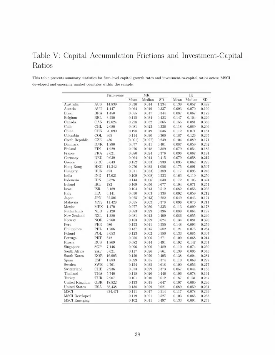
Table V: Capital Accumulation Frictions and Investment-CapitalRatiosThis table presents summary statistics for firm-level capital growth rates and investment-to-capital ratios across MSCI

developed and emerging market countries within the sample.

Firm-years MK IKMean Median SD Mean Median SD

Australia AUS 14,839 0.330 0.014 1.234 0.139 0.057 0.488Austria AUT 1,147 0.064 0.019 0.337 0.093 0.070 0.190Brazil BRA 1,450 0.055 0.017 0.344 0.087 0.067 0.179Belgium BEL 3,250 0.115 0.034 0.423 0.147 0.104 0.220Canada CAN 12,624 0.228 0.032 0.865 0.155 0.081 0.386Chile CHL 2,080 0.081 0.023 0.336 0.118 0.089 0.206China CHN 20,090 0.198 0.049 0.636 0.112 0.071 0.181Colombia COL 365 0.114 0.030 0.360 0.187 0.126 0.265Czech Republic CZE 436 (0.001) (0.027) 0.249 0.104 0.089 0.171Denmark DNK 1,890 0.077 0.011 0.401 0.087 0.059 0.202Finland FIN 1,929 0.076 0.018 0.389 0.079 0.054 0.185France FRA 8,621 0.080 0.024 0.376 0.096 0.067 0.181Germany DEU 9,039 0.064 0.014 0.415 0.079 0.058 0.212Greece GRC 3,643 0.152 (0.033) 0.939 0.095 0.062 0.225Hong Kong HKG 11,342 0.276 0.035 1.056 0.175 0.091 0.507Hungary HUN 423 0.011 (0.033) 0.389 0.117 0.095 0.246India IND 17,621 0.109 (0.008) 0.533 0.163 0.110 0.250Indonesia IDN 3,826 0.143 0.006 0.630 0.172 0.103 0.324Ireland IRL 782 0.169 0.056 0.677 0.104 0.071 0.254Israel ISR 3,189 0.104 0.013 0.512 0.082 0.056 0.236Italy ITA 3,141 0.050 0.003 0.338 0.092 0.059 0.212Japan JPN 52,501 0.025 (0.013) 0.282 0.049 0.043 0.124Malaysia MYS 11,428 0.055 (0.002) 0.378 0.096 0.070 0.211Mexico MEX 1,470 0.077 0.030 0.335 0.113 0.099 0.178Netherlands NLD 2,120 0.083 0.029 0.396 0.089 0.064 0.197New Zealand NZL 1,380 0.081 0.012 0.409 0.086 0.055 0.240Norway NOR 2,260 0.153 0.029 0.624 0.134 0.081 0.320Peru PER 986 0.153 0.041 0.550 0.148 0.093 0.259Philippines PHL 1,706 0.137 0.015 0.582 0.121 0.075 0.284Poland POL 3,053 0.123 0.002 0.580 0.133 0.085 0.307Portugal PRT 812 0.058 0.006 0.271 0.109 0.068 0.214Russia RUS 1,869 0.082 0.014 0.491 0.192 0.147 0.261Singapore SGP 7,146 0.096 0.006 0.489 0.110 0.074 0.250South Africa ZAF 3,621 0.117 0.026 0.561 0.139 0.095 0.345South Korea KOR 16,905 0.120 0.020 0.495 0.138 0.094 0.284Spain ESP 1,883 0.099 0.035 0.374 0.110 0.069 0.227Sweden SWE 4,761 0.154 0.035 0.618 0.100 0.056 0.277Switzerland CHE 2,936 0.073 0.029 0.373 0.057 0.044 0.168Thailand THA 5,740 0.118 0.026 0.446 0.106 0.078 0.191Turkey TUR 2,907 0.101 0.010 0.612 0.187 0.131 0.257United Kingdom GBR 18,822 0.133 0.015 0.647 0.107 0.060 0.296United States USA 68,438 0.138 0.029 0.621 0.089 0.059 0.231MSCI 334,471 0.111 0.017 0.514 0.117 0.078 0.249MSCI Developed 0.119 0.021 0.527 0.103 0.065 0.253MSCI Emerging 0.102 0.011 0.497 0.133 0.094 0.243

38

Table VI: Capital Accumulation Frictions and Investment-CapitalRatiosThis table presents baseline regression results for firm-level capital growth rates across MSCI developed and emerging market

countries within the sample. Size is the inflation-adjusted book value of the firm’s assets in U.S. dollars, and leverage is the

ratio between the book value of liabilities and assets. Price-to-book measures the ratio between the market and the book

value of the firm’s equity. Time fixed effects and fixed effects for the 48 Fama-French industries are included in all regressions.

Standard errors are reported in parenthesis.

MKf,i,c,t = α + β1Dt + β2Fi + η1IKf,i,c,t + η2IK2f,i,c,t + γXf,i,c,t + εf,i,c,t

MKf,i,c,t = α + β1Dt + β2Fi + η1IKf,i,c,t + η2IK2f,i,c,t + η3IK

2f,i,c,t ∗ log(PCGDPc,t)

+ γXf,i,c,t + εf,i,c,t

PCGDPc,t is the purchasing power parity adjusted real GDP per capita in country c in period t in 2011 US dollars. Dt and

Fi are time and industry dummies to control for global macroeconomic shocks and industry-specific effects. Xf,i,c,t is the

vector of firm-specific factors: size, price-to-book and leverage. (*), (**), and (***) refer to the 10%, 5%, and 1% levels of

significance, respectively.

(1) (2) (3) (4) (5) (6) (7) (8)Variables MK MK MK MK MK MK MK MK

97-14 11-14 (IFRS) 97-14 11-14 (IFRS) 97-14 11-14 (IFRS) 97-14 11-14 (IFRS)IK 1.152*** 1.031*** 1.164*** 1.039***

(0.0251) (0.0429) (0.0243) (0.0468)IK2 0.200*** 0.200*** -0.382* -0.672

(0.0159) (0.0288) (0.197) (0.711)capexIK 1.148*** 0.531* 1.206*** 0.560*

(0.122) (0.284) (0.110) (0.295)capexIK2 2.924*** 4.419*** -6.187*** -0.0165

(0.410) (1.070) (2.150) (15.25)IK2 ∗ log(PCGDP ) 0.0552*** 0.0816

(0.0195) (0.0680)capexIK2 ∗ log(PCGDP ) 0.893*** 0.411

(0.226) (1.448)log(size) -0.00961*** -0.0171*** -0.00143 -0.00389 -0.00994*** -0.0173*** -0.00180 -0.00393

(0.00244) (0.00531) (0.00241) (0.00422) (0.00244) (0.00538) (0.00240) (0.00430)Leverage -0.0692*** -0.0524 -0.0814*** -0.0811 -0.0681*** -0.0522 -0.0782*** -0.0811

(0.0177) (0.0410) (0.0203) (0.0492) (0.0175) (0.0408) (0.0199) (0.0491)Price-to-Book 0.000257** 0.000543** 0.000232** 0.00116* 0.000257** 0.000543** 0.000232** 0.00116*

(0.000101) (0.000211) (0.000104) (0.000677) (0.000101) (0.000211) (0.000104) (0.000678)Constant 0.0688 0.106 0.0854* 0.0951 0.0742 0.109 0.0879* 0.0948

(0.0456) (0.0964) (0.0464) (0.106) (0.0453) (0.0976) (0.0459) (0.106)Observations 334,471 35,204 327,107 34,394 334,471 35,204 327,107 34,394R-squared 0.412 0.428 0.109 0.096 0.413 0.428 0.110 0.096Time FE Y Y Y Y Y Y Y YIndustry FE Y Y Y Y Y Y Y Y

39

Figure I: The Return on Assets and Internal Rates of ReturnThis figure plots the distribution of firm-level return on assets and internal rates of return for the entire sample. Histogram is

plotted in density units, and the k-density line estimates density function f(x) of the respective variable.

(a) Return on Assets (ROA)

(b) Internal Rate of Return (IRR)

40

Figure II: The Return on Assets, Internal Rates of Return, and PerCapita GDPThis figure plots the best-fit line and 95% confidence interval of firm-level return on assets and internal rates of return for the

entire sample against log of purchasing power parity (PPP)-adjusted real per capita GDP.

(a) Return on Assets and log(PCGDP)

(b) Internal Rates of Return and log(PCGDP)

41

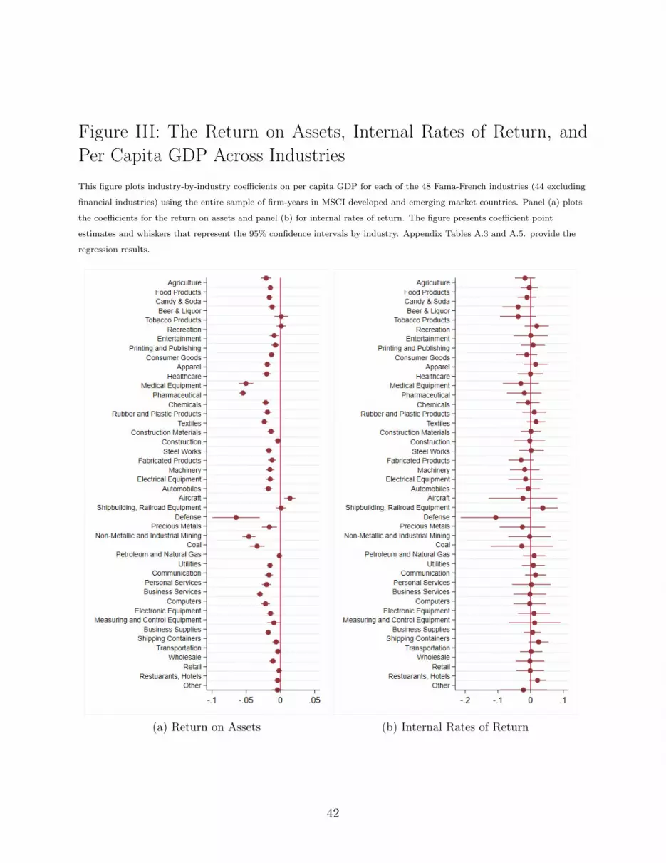
Figure III: The Return on Assets, Internal Rates of Return, andPer Capita GDP Across IndustriesThis figure plots industry-by-industry coefficients on per capita GDP for each of the 48 Fama-French industries (44 excluding

financial industries) using the entire sample of firm-years in MSCI developed and emerging market countries. Panel (a) plots

the coefficients for the return on assets and panel (b) for internal rates of return. The figure presents coefficient point

estimates and whiskers that represent the 95% confidence intervals by industry. Appendix Tables A.3 and A.5. provide the

regression results.

(a) Return on Assets (b) Internal Rates of Return

42

Figure IV: The Return on Assets, Internal Rates of Return, andPer Capita GDP Across TimeThis figure plots yearly regression coefficients on per capita GDP for each year between 1997 and 2014 using the entire sample

of firm-years in MSCI developed and emerging market countries. Panel (a) plots the coefficients for the return on assets and

panel (b) for internal rates of return. The figure visually presents coefficient point estimates and whiskers that represent the

95% confidence intervals by year. Appendix Tables A.4 and A.6. provide the regression results.

(a) Return on Assets

(b) Internal Rates of Return

43

A Online Appendix

Figure A.1: Countries with IFRS StandardsMSCI developed and emerging market countries in the sample are highlighted in red and green. Countries colored in red had

adopted IFRS accounting standard by 2017.

44

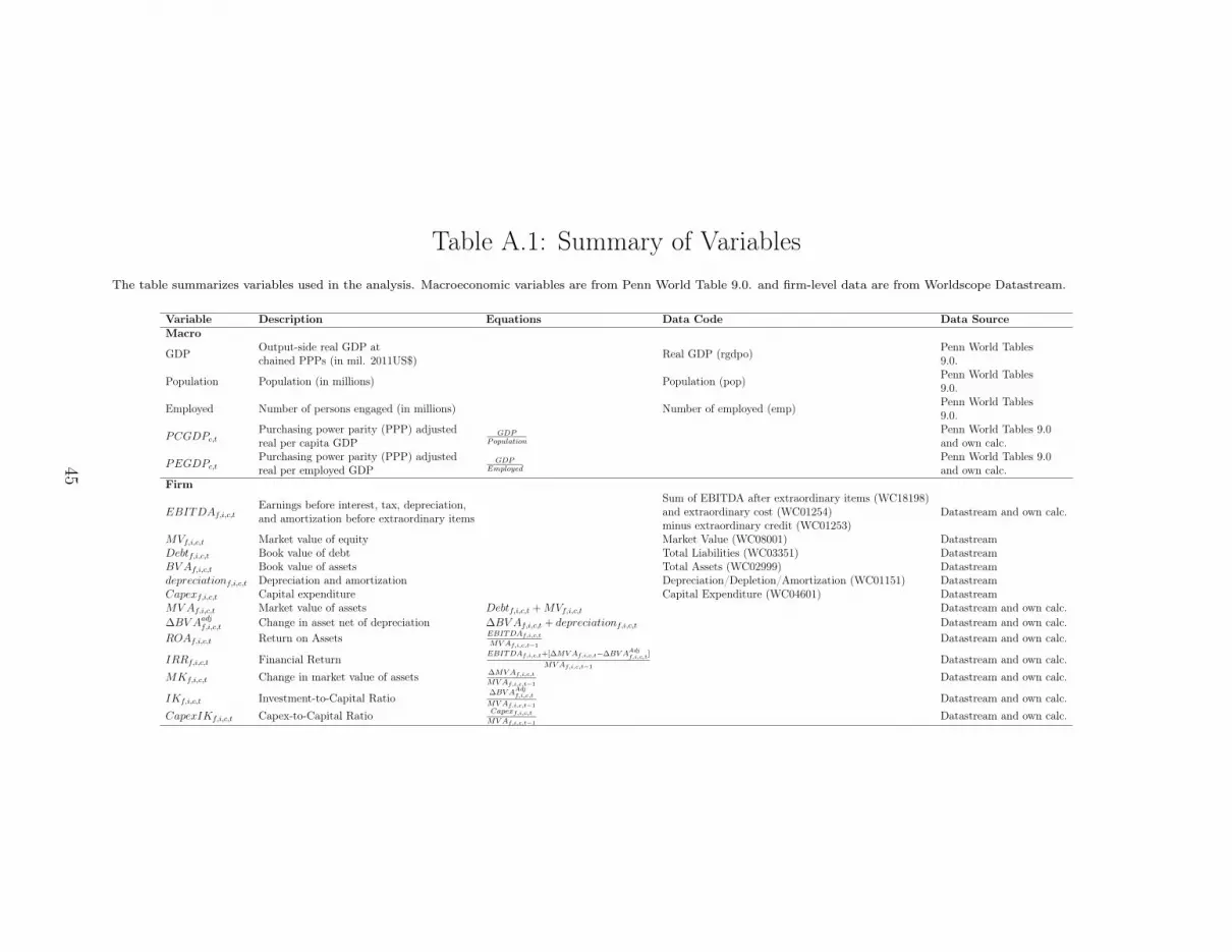
Table A.1: Summary of VariablesThe table summarizes variables used in the analysis. Macroeconomic variables are from Penn World Table 9.0. and firm-level data are from Worldscope Datastream.

Variable Description Equations Data Code Data SourceMacro

GDP Output-side real GDP atchained PPPs (in mil. 2011US$) Real GDP (rgdpo) Penn World Tables

9.0.

Population Population (in millions) Population (pop) Penn World Tables9.0.

Employed Number of persons engaged (in millions) Number of employed (emp) Penn World Tables9.0.

PCGDPc,tPurchasing power parity (PPP) adjustedreal per capita GDP

GDPPopulation

Penn World Tables 9.0and own calc.

PEGDPc,tPurchasing power parity (PPP) adjustedreal per employed GDP

GDPEmployed

Penn World Tables 9.0and own calc.

Firm

EBITDAf,i,c,tEarnings before interest, tax, depreciation,and amortization before extraordinary items

Sum of EBITDA after extraordinary items (WC18198)and extraordinary cost (WC01254)minus extraordinary credit (WC01253)

Datastream and own calc.

MVf,i,c,t Market value of equity Market Value (WC08001) DatastreamDebtf,i,c,t Book value of debt Total Liabilities (WC03351) DatastreamBV Af,i,c,t Book value of assets Total Assets (WC02999) Datastreamdepreciationf,i,c,t Depreciation and amortization Depreciation/Depletion/Amortization (WC01151) DatastreamCapexf,i,c,t Capital expenditure Capital Expenditure (WC04601) DatastreamMVAf,i,c,t Market value of assets Debtf,i,c,t +MVf,i,c,t Datastream and own calc.∆BV Aadjf,i,c,t Change in asset net of depreciation ∆BV Af,i,c,t + depreciationf,i,c,t Datastream and own calc.ROAf,i,c,t Return on Assets EBITDAf,i,c,t

MVAf,i,c,t−1Datastream and own calc.

IRRf,i,c,t Financial ReturnEBITDAf,i,c,t+[∆MVAf,i,c,t−∆BV AAdjf,i,c,t]

MVAf,i,c,t−1Datastream and own calc.

MKf,i,c,t Change in market value of assets ∆MVAf,i,c,tMVAf,i,c,t−1

Datastream and own calc.

IKf,i,c,t Investment-to-Capital Ratio∆BV AAdjf,i,c,t

MVAf,i,c,t−1Datastream and own calc.

CapexIKf,i,c,t Capex-to-Capital Ratio Capexf,i,c,tMVAf,i,c,t−1

Datastream and own calc.

45

Table A.2: Accounting Standards and IFRS Adoption DatesThis table presents the accounting standard and IFRS adoption date for MSCI developed and emerging market countries in

the analysis.

Country Accounting Standard IFRS Adoption DateAustralia IFRS 2005Austria IFRS 2005Belgium IFRS 2005Brazil IFRS 2010Canada IFRS 2011Chile IFRS 2010China Chinese Accounting Standards NAColombia IFRS 2015Czech Republic IFRS 2005Denmark IFRS 2005Finland IFRS 2005France IFRS 2005Germany IFRS 2005Greece IFRS 2005Hong Kong IFRS 2005Hungary IFRS 2005India India accounting standards NAIndonesia Indonesian national GAAP NAIreland IFRS 2005Israel IFRS 2008Italy IFRS 2005Japan Japanese Accounting Standards NAMalaysia IFRS 2017Mexico IFRS 2012Netherlands IFRS 2005New Zealand IFRS 2007Norway IFRS 2005Peru IFRS 2012Philippines IFRS 2005Poland IFRS 2005Portugal IFRS 2005Russia IFRS 2012Singapore Singapore Financial Reporting Standards (SFRS) NASouth Africa IFRS 2011South Korea IFRS 2011Spain IFRS 2005Sweden IFRS 2005Switzerland Swiss GAAP NAThailand Thai Accounting Standards NATurkey IFRS 2005UK IFRS 2005US US GAAP NA

46

Table A.3: The Relationship Between Industry Returns on Assetsand Per Capita GDPThis table presents the regression results from industry-by-industry regression for each of the 48 Fama-French industries (44

excluding financial industries). Size is the inflation-adjusted book value of the firm’s asset in U.S. dollars, and leverage is the

ratio between the book value of liability and assets. Price-to-book measures the ratio between the market and the book value

of the firm’s equity. Time fixed effects are included in the regression but are not reported. (*), (**), and (***) refer to the

10%, 5%, and 1% levels of significance, respectively.

Fama-French Industries log(PCGDP) log(size) Leverage Price-to-Book Observations R-squaredAgriculture -0.0216*** 0.0144*** -0.0623*** -0.000257 4,145 0.091Food Products -0.0161*** 0.00657*** -0.0858*** -0.000247** 9,753 0.099Candy & Soda -0.0183*** 0.00901*** -0.0477*** -0.000215 2,141 0.107Beer & Liquor -0.0119*** 0.00471*** -0.0437*** -0.00135** 2,757 0.083Tobacco Products 0.000411 0.00711*** -0.0691*** -0.000392* 481 0.180Recreation 0.000403 0.00994*** -0.0929*** -7.86e-05*** 2,990 0.090Entertainment -0.0125*** 0.0140*** -0.0237*** -0.000106 5,172 0.063Printing and Publishing -0.0111*** 0.00853*** -0.0466*** -0.000476*** 3,756 0.087Consumer Goods -0.0144*** 0.00861*** -0.0826*** -0.00101** 7,320 0.085Apparel -0.0216*** 0.00817*** -0.135*** -0.000403** 4,111 0.128Healthcare -0.0302*** 0.0122*** 0.00433 -0.00145*** 3,151 0.120Medical Equipment -0.0625*** 0.0280*** -0.0382*** -3.76e-05*** 5,590 0.228Pharmaceutical Products -0.0537*** 0.0239*** -0.0441*** -1.92e-05 10,888 0.255Chemicals -0.0221*** 0.0109*** -0.0899*** -3.62e-05 12,388 0.098Rubber and Plastic Products -0.0209*** 0.00723*** -0.0901*** -0.000512** 3,533 0.095Textiles -0.0254*** 0.00860*** -0.0837*** -0.000709*** 5,259 0.098Construction Materials -0.0143*** 0.00765*** -0.0904*** -0.000395*** 13,180 0.086Construction -0.00482* 0.00564*** -0.0661*** -1.84e-05 17,799 0.044Steel Works -0.0164*** 0.00676*** -0.0981*** -0.000666*** 10,213 0.121Fabricated Products -0.0107*** 0.00829*** -0.0955*** -0.00567*** 1,530 0.116Machinery -0.0155*** 0.00752*** -0.0590*** -0.000510** 14,777 0.062Electrical Equipment -0.0151*** 0.00925*** -0.0462*** -0.000918* 5,411 0.068Automobiles -0.0174*** 0.00795*** -0.0727*** -0.000159*** 8,900 0.076Aircraft 0.0133*** 0.00158 -0.0273** -0.000165 1,190 0.067Shipbuilding, Railroad Equipment 0.00106 -0.000131 -0.0910*** -0.00286 867 0.090Defense -0.0681*** 0.00945*** -0.103*** -0.00526** 325 0.170Precious Metals -0.0302*** 0.0371*** -0.0142 2.92e-05*** 5,036 0.254Non-Metallic and Industrial Mining -0.0517*** 0.0317*** -0.00443 -0.000109** 5,832 0.336Coal -0.0390*** 0.0276*** 0.0286 -1.69e-06 1,902 0.268Petroleum and Natural Gas -0.00564** 0.0223*** -0.00982 -0.000152 11,754 0.225Utilities -0.0161*** 0.00901*** -0.0503*** -2.87e-05 9,841 0.091Communication -0.0221*** 0.0171*** -0.0403*** -8.48e-06 9,283 0.183Personal Services -0.0255*** 0.0159*** -0.0155* -0.000646** 3,370 0.103Business Services -0.0348*** 0.0186*** 0.000422 -6.66e-06 36,652 0.129Computers -0.0252*** 0.0149*** -0.0400*** -7.47e-05 8,760 0.117Electronic Equipment -0.0188*** 0.0164*** -0.0248*** -3.49e-05 15,711 0.100Measuring and Control Equipment -0.0147** 0.0144*** -0.0405*** -0.000162* 4,433 0.093Business Supplies -0.0185*** 0.00536*** -0.108*** -1.78e-05*** 5,242 0.121Shipping Containers -0.00843*** 0.00594*** -0.0940*** -0.000352 1,665 0.092Transportation -0.00412* 0.00300*** -0.0463*** -1.67e-05 12,377 0.029Wholesale -0.0145*** 0.0110*** -0.0687*** -2.05e-05 17,701 0.071Retail -0.00449* 0.00761*** -0.0601*** -3.90e-05 17,253 0.056Restaurants, Hotels -0.00506** 0.00318*** -0.0298*** -1.91e-05 7,915 0.022Other -0.0196*** 0.0170*** -0.0287*** -0.000309* 2,117 0.136

47

Table A.4: The Relationship Between Firm-Level Returns on As-sets and Per Capita GDP, By YearThis table presents the regression results of year-by-year analysis using the firm-level ROA of MSCI developed and emerging

market countries in the sample. Size is the inflation-adjusted book value of the firm’s assets in U.S. dollars, and leverage is the

ratio between the book value of liability and assets. Price-to-book measures the ratio between the market and the book value

of the firm’s equity. Industry fixed effects are included in the regression but are not reported. (*), (**), and (***) refer to the

10%, 5%, and 1% levels of significance, respectively.

log(PCGDP) log(Size) Leverage Price-to-Book Observations R-squared1997 -0.0103*** 0.00657*** -0.0376*** -1.27e-05* 11,701 0.0841998 -0.0129*** 0.00810*** -0.0372*** -0.000100*** 12,081 0.0911999 -0.0271*** 0.0110*** -0.0543*** -2.99e-05** 13,588 0.1322000 -0.0196*** 0.0117*** -0.0367*** -6.81e-05 14,348 0.1392001 -0.0265*** 0.0137*** -0.0401*** -0.000246*** 15,990 0.1682002 -0.0329*** 0.0154*** -0.0451*** -4.50e-06 16,742 0.1782003 -0.0198*** 0.0161*** -0.0512*** -2.59e-05 17,543 0.1522004 -0.0184*** 0.0151*** -0.0513*** 6.75e-08 17,796 0.1502005 -0.0171*** 0.0152*** -0.0447*** -0.000251*** 18,433 0.1682006 -0.0209*** 0.0165*** -0.0348*** -2.34e-05 19,892 0.1792007 -0.0259*** 0.0150*** -0.0357*** -2.42e-05 21,530 0.1682008 -0.0217*** 0.0127*** -0.0382*** -1.84e-05* 22,130 0.1412009 -0.0273*** 0.0174*** -0.0781*** -0.000701*** 22,184 0.1602010 -0.0286*** 0.0148*** -0.0314** -0.000128** 22,012 0.1562011 -0.0171*** 0.0134*** -0.0386*** -2.57e-05** 22,502 0.1412012 -0.0170*** 0.0145*** -0.0521*** -4.17e-05*** 22,348 0.1412013 -0.0170*** 0.0138*** -0.0550*** -7.82e-06 21,856 0.1482014 -0.0201*** 0.0134*** -0.0411*** -5.86e-05 21,795 0.151

48

Table A.5: The Relationship Between Industry Internal Rates ofReturn and Per Capita GDPThis table presents the regression results from industry-by-industry regression for each of the 48 Fama-French industries (44

excluding financial industries). Size is the inflation adjusted book value of the firm’s assets in U.S. dollars, and leverage is the

ratio between the book value of liability and assets. Price-to-book measures the ratio between the market and the book value

of the firm’s equity. Time fixed effects are included in the regression but are not reported. (*), (**), and (***) refer to the

10%, 5%, and 1% levels of significance, respectively.

Fama-French Industries log(PCGDP) log(size) Leverage Price-to-Book Observations R-squaredAgriculture -0.0193 0.0220*** -0.115*** 0.00126 4,145 0.096Food Products -0.00521 0.00380 -0.160*** 0.00191 9,753 0.064Candy & Soda -0.0105 -0.00378 -0.0609 -0.000281 2,141 0.092Beer & Liquor -0.0391 0.00725* -0.197*** 0.0203*** 2,757 0.141Tobacco Products -0.0401 0.0169 -0.0407 0.00378** 481 0.109Recreation 0.0195 -0.00146 -0.157*** 8.66e-05 2,990 0.063Entertainment -0.00125 0.00556 -0.124*** 0.000736 5,172 0.042Printing and Publishing 0.00659 0.00192 -0.130*** 0.000959 3,756 0.096Consumer Goods -0.0126 0.00815** -0.204*** 0.00799** 7,320 0.093Apparel 0.0131 0.00398 -0.202*** 0.00822*** 4,111 0.108Healthcare -0.00594 0.00561 -0.184*** 0.00835** 3,151 0.077Medical Equipment -0.0342 0.00909 -0.149*** 0.000337*** 5,590 0.101Pharmaceutical Products -0.0197 0.0131** -0.171*** 0.000378 10,888 0.091Chemicals -0.0113 0.00907** -0.117*** 0.000140 12,388 0.084Rubber and Plastic Products 0.00925 0.00463 -0.161*** 0.00270 3,533 0.092Textiles 0.0143 0.00337 -0.104** 0.00478* 5,259 0.072Construction Materials -0.000676 0.00870*** -0.127*** 0.00762*** 13,180 0.116Construction -0.00234 -0.00581 -0.0767** 0.000519* 17,799 0.088Steel Works -0.00179 0.00765 -0.117*** 0.00626*** 10,213 0.121Fabricated Products -0.0288 0.0166** -0.288*** 0.0467*** 1,530 0.208Machinery -0.0200 0.00807** -0.112*** 0.00558** 14,777 0.124Electrical Equipment -0.0179 0.0129** -0.135*** 0.00389 5,411 0.097Automobiles -0.0128 0.00773** -0.131*** 0.000583** 8,900 0.103Aircraft -0.0189 -0.00912* -0.0826 0.000554 1,190 0.160Shipbuilding, Railroad Equipment 0.0345 0.00954 -0.363*** 0.0652*** 867 0.325Defense -0.114** 0.0226* -0.346** 0.0579*** 325 0.212Precious Metals -0.0247 0.00490 -0.163** 0.000292*** 5,036 0.120Non-Metallic and Industrial Mining -0.00374 0.00780 -0.340*** 0.000895 5,832 0.120Coal -0.0228 0.00103 -0.275** -1.09e-05 1,902 0.110Petroleum and Natural Gas 0.0105 0.00158 -0.291*** 0.00332*** 11,754 0.109Utilities 0.00757 -0.00103 -0.0897*** 0.000185 9,841 0.081Communication 0.0158 -0.00248 -0.0694** 6.89e-05* 9,283 0.128Personal Services 0.00147 0.00252 -0.150*** 0.0106** 3,370 0.079Business Services -0.00338 0.00532 -0.100*** 7.53e-05 36,652 0.080Computers -0.00347 0.00390 -0.135*** 0.00164*** 8,760 0.114Electronic Equipment 0.0101 0.00173 -0.164*** 0.000328 15,711 0.135Measuring and Control Equipment 0.0114 0.00470 -0.103** 0.000756 4,433 0.119Business Supplies 0.00214 0.00685** -0.141*** 0.000475*** 5,242 0.123Shipping Containers 0.0238 0.00355 -0.0967* 0.00513 1,665 0.106Transportation 0.00168 0.000402 -0.127*** 0.000245** 12,377 0.091Wholesale -0.00218 6.98e-06 -0.107*** 0.000234 17,701 0.051Retail -0.00279 0.00423 -0.129*** 0.00107** 17,253 0.066Restaurants, Hotels 0.0245* -0.00803** -0.0795*** 0.000388* 7,915 0.070Other -0.0187 0.00621 -0.202*** 0.000884** 2,117 0.074

49

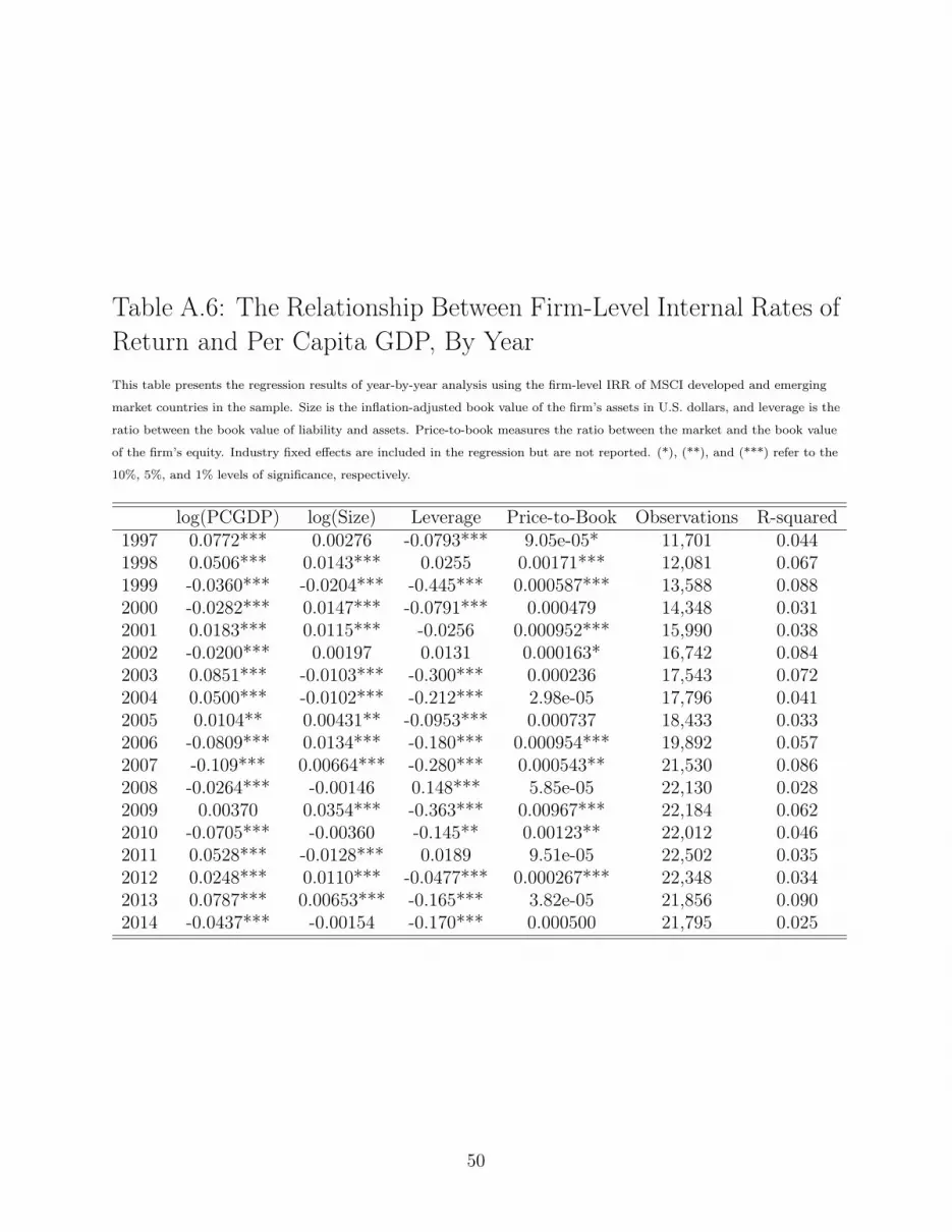
Table A.6: The Relationship Between Firm-Level Internal Rates ofReturn and Per Capita GDP, By YearThis table presents the regression results of year-by-year analysis using the firm-level IRR of MSCI developed and emerging

market countries in the sample. Size is the inflation-adjusted book value of the firm’s assets in U.S. dollars, and leverage is the

ratio between the book value of liability and assets. Price-to-book measures the ratio between the market and the book value

of the firm’s equity. Industry fixed effects are included in the regression but are not reported. (*), (**), and (***) refer to the

10%, 5%, and 1% levels of significance, respectively.

log(PCGDP) log(Size) Leverage Price-to-Book Observations R-squared1997 0.0772*** 0.00276 -0.0793*** 9.05e-05* 11,701 0.0441998 0.0506*** 0.0143*** 0.0255 0.00171*** 12,081 0.0671999 -0.0360*** -0.0204*** -0.445*** 0.000587*** 13,588 0.0882000 -0.0282*** 0.0147*** -0.0791*** 0.000479 14,348 0.0312001 0.0183*** 0.0115*** -0.0256 0.000952*** 15,990 0.0382002 -0.0200*** 0.00197 0.0131 0.000163* 16,742 0.0842003 0.0851*** -0.0103*** -0.300*** 0.000236 17,543 0.0722004 0.0500*** -0.0102*** -0.212*** 2.98e-05 17,796 0.0412005 0.0104** 0.00431** -0.0953*** 0.000737 18,433 0.0332006 -0.0809*** 0.0134*** -0.180*** 0.000954*** 19,892 0.0572007 -0.109*** 0.00664*** -0.280*** 0.000543** 21,530 0.0862008 -0.0264*** -0.00146 0.148*** 5.85e-05 22,130 0.0282009 0.00370 0.0354*** -0.363*** 0.00967*** 22,184 0.0622010 -0.0705*** -0.00360 -0.145** 0.00123** 22,012 0.0462011 0.0528*** -0.0128*** 0.0189 9.51e-05 22,502 0.0352012 0.0248*** 0.0110*** -0.0477*** 0.000267*** 22,348 0.0342013 0.0787*** 0.00653*** -0.165*** 3.82e-05 21,856 0.0902014 -0.0437*** -0.00154 -0.170*** 0.000500 21,795 0.025

50

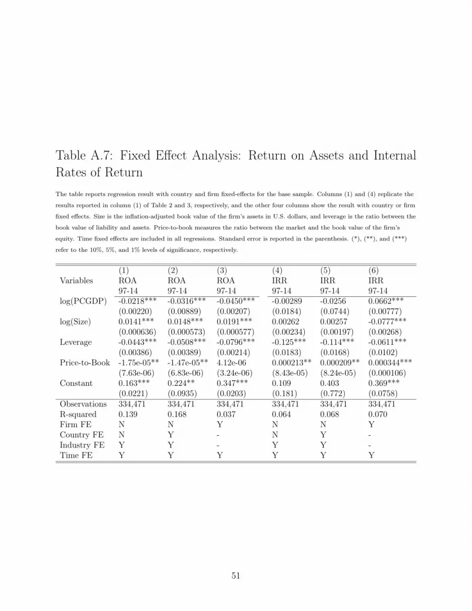
Table A.7: Fixed Effect Analysis: Return on Assets and InternalRates of ReturnThe table reports regression result with country and firm fixed-effects for the base sample. Columns (1) and (4) replicate the

results reported in column (1) of Table 2 and 3, respectively, and the other four columns show the result with country or firm

fixed effects. Size is the inflation-adjusted book value of the firm’s assets in U.S. dollars, and leverage is the ratio between the

book value of liability and assets. Price-to-book measures the ratio between the market and the book value of the firm’s

equity. Time fixed effects are included in all regressions. Standard error is reported in the parenthesis. (*), (**), and (***)

refer to the 10%, 5%, and 1% levels of significance, respectively.

(1) (2) (3) (4) (5) (6)Variables ROA ROA ROA IRR IRR IRR

97-14 97-14 97-14 97-14 97-14 97-14log(PCGDP) -0.0218*** -0.0316*** -0.0450*** -0.00289 -0.0256 0.0662***

(0.00220) (0.00889) (0.00207) (0.0184) (0.0744) (0.00777)log(Size) 0.0141*** 0.0148*** 0.0191*** 0.00262 0.00257 -0.0777***

(0.000636) (0.000573) (0.000577) (0.00234) (0.00197) (0.00268)Leverage -0.0443*** -0.0508*** -0.0796*** -0.125*** -0.114*** -0.0611***

(0.00386) (0.00389) (0.00214) (0.0183) (0.0168) (0.0102)Price-to-Book -1.75e-05** -1.47e-05** 4.12e-06 0.000213** 0.000209** 0.000344***

(7.63e-06) (6.83e-06) (3.24e-06) (8.43e-05) (8.24e-05) (0.000106)Constant 0.163*** 0.224** 0.347*** 0.109 0.403 0.369***

(0.0221) (0.0935) (0.0203) (0.181) (0.772) (0.0758)Observations 334,471 334,471 334,471 334,471 334,471 334,471R-squared 0.139 0.168 0.037 0.064 0.068 0.070Firm FE N N Y N N YCountry FE N Y - N Y -Industry FE Y Y - Y Y -Time FE Y Y Y Y Y Y

51

Table A.8: Country Clustered Errors: Return on Assets and Inter-nal Rates of ReturnThe table report regression result for the main sample when errors are clustered at a country level. Size is the

inflation-adjusted book value of the firm’s assets in U.S. dollars, and leverage is the ratio between the book value of liability

and assets. Price-to-book measures the ratio between the market and the book value of the firm’s equity. Time fixed effects

and industry fixed effects for the 48 Fama-French industries are included in all regressions. Standard errors are reported in the

parenthesis. (*), (**), and (***) refer to the 10%, 5%, and 1% levels of significance, respectively.

(1) (2) (3) (4)Variables ROA ROA IRR IRR

97-14 11-14 97-14 11-14log(PCGDP) -0.0218*** -0.0176* -0.00289 0.0300**

(0.00739) (0.00890) (0.00719) (0.0122)log(size) 0.0141*** 0.0138*** 0.00262 0.000562

(0.00218) (0.00285) (0.00164) (0.00233)Leverage -0.0443*** -0.0463*** -0.125*** -0.0911***

(0.0110) (0.0127) (0.0131) (0.0126)Price-to-Book -1.75e-05*** -1.95e-05 0.000213*** 0.000103

(6.26e-06) (1.23e-05) (7.68e-05) (8.55e-05)Constant 0.163** 0.105 0.109* -0.334***

(0.0696) (0.0850) (0.0630) (0.122)Observations 334,471 87,775 334,471 87,775R-squared 0.139 0.144 0.064 0.037Time FE Y Y Y YIndustry FE Y Y Y Y

52

Table A.9: Robustness Check: log(PCGDP) vs. log(PEGDP) vs.log(PHGDP)This table reports regression results using different measures of output per capita. PCGDP is GDP per capita, PEGDP is

GDP per employed, and PHGDP is GDP per hour employed. Size is the inflation-adjusted book value of the firm’s assets in

U.S. dollars, and leverage is the ratio between the book value of liability and assets. Price-to-book measures the ratio between

the market and the book value of the firm’s equity. Time fixed effects and industry fixed effects for the 48 Fama-French

industries are included in all regressions. Standard errors are reported in the parenthesis. (*), (**), and (***) refer to the

10%, 5%, and 1% levels of significance, respectively.

(1) (2) (3) (4) (5) (6)Variables ROA IRR ROA IRR ROA IRR

97-14 97-14 97-14 97-14 97-14 97-14log(PCGDP) -0.0218*** -0.00289

(0.00739) (0.00719)log(PEGDP) -0.0203*** -0.00491

(0.00273) (0.0206)log(PHGDP) -0.0292*** 0.00307

(0.00136) (0.0153)log(size) 0.0141*** 0.00262 0.0138*** 0.00269 0.0150*** 0.00179

(0.00218) (0.00164) (0.000655) (0.00238) (0.000602) (0.00202)Leverage -0.0443*** -0.125*** -0.0435*** -0.125*** -0.0447*** -0.123***

(0.0110) (0.0131) (0.00388) (0.0184) (0.00405) (0.0177)Price-to-Book -1.75e-05*** 0.000213*** -1.77e-05** 0.000213** -1.54e-05** 0.000198**

(6.26e-06) (7.68e-05) (7.69e-06) (8.43e-05) (6.94e-06) (7.99e-05)Constant 0.163** 0.109* 0.167*** 0.132 0.0316*** 0.0805

(0.0696) (0.0630) (0.0294) (0.217) (0.0111) (0.0654)Observations 334,471 334,471 334,471 334,471 314,381 314,381R-squared 0.139 0.064 0.135 0.064 0.154 0.059Time FE Y Y Y Y Y YIndustry FE Y Y Y Y Y Y

53