Electronic copy available at: http://ssrn.com/abstract=1484628Electronic copy available at: http://ssrn.com/abstract=1484628

The relationship between resilience and

sustainability of ecological-economic systems

Sandra Derissena,∗, Martin F. Quaasa

and Stefan Baumgärtnerb

a Department of Economics, University of Kiel, Germanyb Department of Sustainability Sciences and Department of Economics,

Leuphana University of Lüneburg, Germany

10 December 2010, forthcoming in Ecological Economics

Abstract: Resilience as a descriptive concept gives insight into the dynamic prop-

erties of an ecological-economic system. Sustainability as a normative concept

captures basic ideas of intergenerational justice when human well-being depends

on natural capital and services. Thus, resilience and sustainability are indepen-

dent concepts. In this paper, we discuss the relationship between resilience and

sustainability of ecological-economic systems. We use a simple dynamic model

where two natural capital stocks provide ecosystem services that are complements

for human well-being, to illustrate dierent possible cases of the relationship be-

tween resilience and sustainability, and to identify the conditions under which

each of those will hold: a) resilience of the system is necessary, but not sucient,

for sustainability; b) resilience of the system is sucient, but not necessary, for

sustainability; c) resilience of the system is neither necessary nor sucient for

sustainability; d) resilience is both necessary and sucient for sustainability. We

conclude that more criteria than just resilience have to be taken into account when

designing policies for the sustainable development of ecological-economic systems,

and, vice versa, the property of resilience should not be confused with the positive

normative connotations of sustainability.

Keywords: ecosystem resilience, dynamics, management of ecological-economic

systems, sustainability

JEL-Classication: Q20, Q56, Q57

∗Corresponding author: Department of Economics, University of Kiel, Wilhelm-Seelig-Platz,

D-24118 Kiel, Germany. Phone +49.431.880-5633, email: derissen@economics.uni-kiel.de.

Electronic copy available at: http://ssrn.com/abstract=1484628Electronic copy available at: http://ssrn.com/abstract=1484628

1 Introduction

Speaking about resilience and sustainability is speaking about two highly abstract

and multi-farious concepts, each of which has a great variety of interpretations

and denitions. Here we adopt what seems to be the most general and at the

same time most widely accepted denitions of resilience and sustainability.1 We

understand sustainable development as the Brundtland Commission denes it as

development that meets the needs of the present without compromising the ability

of future generations to meet their own needs (WCED 1987). In this denition,

sustainability is a normative concept capturing basic ideas of intra- and intergen-

erational justice2. Concerning obligations towards future generations, the primary

question of sustainability then is to what extent do natural capital stocks have to

be maintained to enable future generations to meet their needs.3

In contrast, resilience is a descriptive concept. In a most common denition

that goes back to Holling (1973), resilience is thought of as [. . . ] the magnitude

of disturbance that can be absorbed before the system changes its structure by

changing the variables and processes that control behavior (Holling & Gunderson

2002: 4). The underlying idea is that a system may ip from one domain of at-

traction into another one as a result of exogenous disturbance. If the system will

not ip due to exogenous disturbance, the system in its initial state is called re-

silient. Although Holling-resilience can be quantitatively measured (Holling 1973),

we focus on the qualitative classication, where a system in a given state is either

resilient, or it is not.4

1Evidently, as denitions are not universal and are appropriate for a certain objective only (Jax

2002), the relationship between resilience and sustainability depends on the particular denitions

of these two terms.

2We do not consider the issue of intragenerational justice in this paper, but focus on an

operational notion of sustainability that captures intergenerational justice.

3The term natural capital was established to distinguish services and functions of ecosystems

from other capital stocks (Pearce 1988).

4An alternative denition of resilience is due to Pimm (1984), who denes resilience as the

2

In the literature, many connections have been drawn between resilience and

sustainability (e.g. Folke et al. 2004, Walker & Salt 2006, Mäler 2008). In some

contributions, resilience is seen as a necessary precondition for sustainability. For

example, Lebel et al. (2006: 2) point out that [s]trengthening the capacity of

societies to manage resilience is critical to eectively pursuing sustainable devel-

opment. Similarly, Arrow et al. (1995: 93) conclude that economic activities

are sustainable only if the life-support ecosystems upon which they depend are

resilient, and Perrings (2006: 418) states that [a] development strategy is not

sustainable if it is not resilient.

Some authors explicitly dene or implicitly understand the notions of resilience

and sustainability such that they are essentially equivalent: A system may be

said to be Holling-sustainable, if and only if it is Holling-resilient (Common &

Perrings 1992: 28), or similarly: A resilient socio-ecological system is synonymous

with a region that is ecologically, economically, and socially sustainable (Holling

& Walker 2003: 1). Levin et al. (1998) claim in general that [r]esilience is the

preferred way to think about sustainability in social as well as natural systems,

thus also suggesting an equivalence of resilience and sustainability.

In contrast to this view, it has been noted that [r]esilience, per se, is not

necessarily a good thing. Undesirable system congurations (e.g. Stalin's regime,

collapsed sh stocks) can be very resilient, and they can have high adaptive capac-

ity in the sense of re-conguring to retain the same controls on function (Holling

& Walker 2003: 1). In other words, resilience is not sucient for sustainability,

and it can therefore not be taken as an objective of its own.

While systems with multiple stable states are widely discussed, a systematic

rate at which a system returns to equilibrium following a disturbance. Resilience, according

to Pimm's denition, is not dened for unstable systems. Nevertheless, it is a useful concept

for ecological-economic analyses. Martin (2004), for example, suggests a quantitative measure of

resilience sensu Pimm, namely the costs of the restoration of the system after a disturbance where

costs are dened as the minimal time of crisis, i.e. the minimal time the system is violating

pre-specied state-restrictions and, thus, is outside the viability kernel (Béné at al. 2001).

3

analysis of the relationship between the concepts of resilience and sustainability

in a system with multiple stable states has not yet been conducted. To illustrate

this research gap, the statements quoted above do not take into account the fol-

lowing possibilities: if some particular management does not conserve a system's

resilience, such that under exogenous disturbance the system may ip from an un-

desirable state into a desirable one, or from a desirable state into another desirable

state, the system management might still achieve sustainable development of the

system, even though it is not resilient. As a consequence, one may conclude that

resilience is neither desirable in itself nor is it in general a necessary or sucient

condition for sustainable development.

In general, four relationships between resilience and sustainability are logically

possible, and any of those may hold in a given system: a) resilience of the system

is necessary, but not sucient, for sustainability; b) resilience of the system is suf-

cient, but not necessary, for sustainability; c) resilience of the system is neither

necessary nor sucient for sustainability; d) resilience of the system is both neces-

sary and sucient for sustainability. In order to clarify and illustrate the dierent

possibilities, and to identify the conditions under which each of those will hold, we

use a simple dynamic ecological-economic model where two natural capital stocks

provide ecosystem services that are complementary in the satisfaction of human

needs.

This model is not meant to represent a real ecological-economic system, or

to give a fully general representation of ecological-economic systems. Rather, it

is meant to illustrate the complexity of relationships between resilience and sus-

tainability even in a simple dynamic model. In contrast to other models used to

study resilience of ecological-economic systems, such as the shallow lake model

(e.g. Scheer 1997, Mäler et al. 2003) or rangeland models (e.g. Perrings & Stern

2000, Anderies et al. 2002, Janssen et al. 2004), it features more than two domains

of attraction and the possibility of more than one desirable state. In traditional

models of bistable systems only two relationships of resilience and sustainability

are possible: (i) the system is resilient in a desired state, such that the system's

4

resilience has to be maintained for sustainability; (ii) the system is resilient in its

current state which is, however, not a desired one, such that resilience prevents

sustainability. A situation in which the system is not resilient in a desired state

but nevertheless on a path of sustainability cannot by construction of these

traditional models possibly occur. Our dynamic model, as simple as it is, over-

comes this shortcoming and may therefore add another valuable dimension to the

model-based study of resilience and sustainability.

The outline of the paper is as follows. In the following section, we present the

model (Section 2.1), analyze its basic dynamics (Section 2.2), introduce formal

denitions of resilience and sustainability (Section 2.3), and discuss the possible

relationships between resilience and sustainability (Section 2.4). In Section 3, we

discuss our ndings and draw conclusions concerning the sustainable management

of ecological-economic systems.

2 Resilience and sustainability in a simple dynamic

model of an ecological-economic system

2.1 Model

The model describes the use of two natural capital stocks say, sh and wood and

features multiple equilibria with dierent domains of attraction. The deterministic

dynamics of the two stocks of sh (x) and wood (w) are described by the following

dierential equations, referring to the growth of the stocks of sh x and wood w:

x = f(x)− C = rx (x− vx)(

1− x

kx

)− C (1)

w = g(w)−H = rw (w − vw)

(1− w

kw

)−H (2)

where rx and rw denote the intrinsic growth rates, vx and vw the minimum viable

populations, and kx and kw the carrying capacities of the stocks of sh and wood,

respectively. Let x0 = x(0) and w0 = w(0) denote the initial state of the system.

5

The dierential equations (1) and (2) do not contain ecological interactions, al-

though, of course, in reality ecological interactions may exist. As a consequence,

interactions of the stock dynamics are only due to the interrelated harvests of sh

and timber. We use C and H to denote the aggregate amounts of harvested sh

and timber; f(·) and g(·) describe the intrinsic growth of the two stocks. We

assume logistic growth functions for simplicity and because using a well-known

functional form of the growth functions helps to clarify the argument.

Suppose that myopic prot-maximizing rms harvest the resources under open-

access to ecosystems and sell these ecosystem services as market products to con-

sumers at prices px and pw for sh and timber, respectively. Assuming Schaefer

production functions, the amounts of sh and timber harvested from the respective

stocks by individual rms are described by

C = qx x ex and (3)

H = qw w ew , (4)

where ex and ew denote the aggregate eort, measured in units of labor, spent

by sh-harvesting-rms and timber-harvesting-rms, respectively, and qx and qw

denote the productivity of harvesting sh and timber, respectively. Firms can

enter and exit the two industries at no costs.

Society consists of n identical utility-maximizing individuals who derive utility

from the consumption of manufactured goods (y) as well as from the consumption

of the two ecosystem services, sh (c) and timber (h). We assume that all three

goods are essential for individual well-being. The utility function of a representa-

tive household is

u(y, c, h) = y1−α[c

σ−1σ + h

σ−1σ

]α σσ−1

, (5)

where α ∈ (0, 1) is the household's elasticity of marginal utility for consumption of

ecosystem services, and σ is the elasticity of substitution between the consumption

of sh and timber. Both ecosystem services are assumed to be complements in

satisfying human needs, i.e. σ < 1.

6

Each household inelastically supplies one unit of labor either to one of the

resource-harvesting rms or to the manufactured-goods sector. We assume that

labor is the only input in the manufactured-goods sector and that production

exhibits constant returns to scale. Assuming that labor supply is large enough, the

wage rate is thus determined by the marginal product of labor in the manufacturing

sector, which we denote by λ. Taking the manufactured good as numeraire, the

household's budget constraint then is

λ = y + pxc+ pwh . (6)

As an exogenous disturbance to this system we consider an unforeseen, one-time

random shock ∆ = (∆x,∆w) that aects the state of the system at time t∆. The

random shock ∆ is distributed over the support Ω ⊆ [0,∞)× [0,∞). The random

time of disturbance t∆ is distributed over [0,∞). The shock aects the stock

variables in a multiplicative way, such that they instantaneously shift from the

current state (x(t∆), w(t∆)) to another, disturbed state (x(t∆ + dt), w(t∆ + dt)) =

(∆x · x(t∆),∆w · w(t∆)) an innitesimal time increment dt later. Thus, the shock

decreases or increases the stocks x and w by a fraction of ∆x and ∆w, respectively.

The same equations of motion, (1) and (2), govern the dynamic development of the

system before and after the disturbance, but due to the one-time and instantaneous

shift in the stock variables at time t∆ the dynamic regime of the system may be

altered.

2.2 Basic dynamics

In this model, the deterministic dynamics of the ecological-economic system that is

at all times t in a general market equilibrium where prot-maximizing harvesting

rms have open access to ecosystems are described by the following system of

coupled dierential equations (see Appendix):

x = rx (x− vx)(

1− x

kx

)− nα (qxx)σ

(qxx)σ−1 + (qww)σ−1, (7)

w = rw (w − vw)

(1− w

kw

)− nα (qww)σ

(qxx)σ−1 + (qww)σ−1. (8)

7

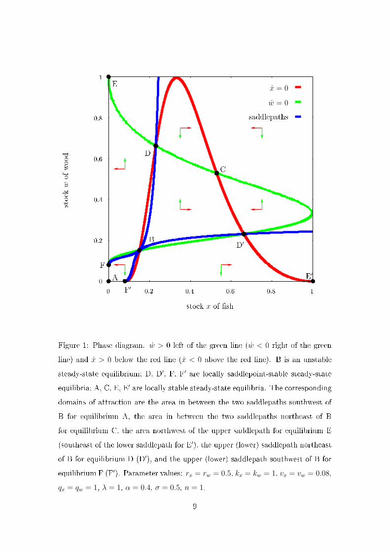
These dynamics are represented by the state-space diagram in Figure 1 for param-

eter values rx = rw = 0.5, kx = kw = 1, vx = vw = 0.08, qx = qw = 1, λ = 1,

α = 0.5, σ = 0.5 and n = 1. The green line is the isocline for w = 0, the red

line is the isocline for x = 0. Left (right) of the w = 0-isocline the dynamics are

characterized by w > 0 (< 0). Likewise, below (above) the x = 0-isocline the dy-

namics are characterized by x > 0 (< 0). In each segment of the state space, the

green and red arrows indicate this direction of dynamics. With these dynamics, B

is an unstable steady-state equilibrium; D and D′ as well as F and F′ are locally

saddlepoint-stable steady-state equilibria; and A, C, E and E′ are locally stable

steady-state equilibria.5

Let (x?i , w?i ) denote the stock levels in steady-state equilibrium i ∈A, B, C,

D, D′, E, E′, F, F′. The domain of attraction Ai of equilibrium i is the set of all

initial states for which the system converges towards equilibrium i:

Ai =

(x0, w0) ∈ R+ × R+

∣∣∣ limt→∞

(x(t), w(t)) = (x?i , w?i ), (9)

where (x(t), w(t)) denotes the solution of (7) and (8) for initial state (x0, w0).

The model features eight domains of attraction: the area in between the two sad-

dlepaths southwest of B for equilibrium A, the area in between the two saddlepaths

northeast of B for equilibrium C, the area northwest of the upper saddlepath for

equilibrium E (southeast of the lower saddlepath for E′), the upper (lower) sad-

dlepath northeast of B for equilibrium D (D′), and the upper (lower) saddlepath

southwest of B for equilibrium F (F′).

Each domain of attraction comprises only a limited part of the state space, so

that the system may ip from one domain of attraction to another one as a result

of exogenous disturbance. Thus, if the system was initially, for example, on the

saddlepath converging towards equilibrium D it may be disturbed such that it no

longer converges towards equilibrium D, but ips into the domain of attraction of

another equilibrium, e.g. C or E.

5For an explicit analysis of transitional dynamics and sustainability, see Martinet et al. (2007),

Bretschger and Pittel (2008).

8

saddlepaths

w = 0

x = 0

F′

E′

D′

D

E

F

C

B

A

stock x of sh

stockwof

wood

10.80.60.40.20

1

0.8

0.6

0.4

0.2

0

Figure 1: Phase diagram. w > 0 left of the green line (w < 0 right of the green

line) and x > 0 below the red line (x < 0 above the red line). B is an unstable

steady-state equilibrium; D, D′, F, F′ are locally saddlepoint-stable steady-state

equilibria; A, C, E, E′ are locally stable steady-state equilibria. The corresponding

domains of attraction are the area in between the two saddlepaths southwest of

B for equilibrium A, the area in between the two saddlepaths northeast of B

for equilibrium C, the area northwest of the upper saddlepath for equilibrium E

(southeast of the lower saddlepath for E′), the upper (lower) saddlepath northeast

of B for equilibrium D (D′), and the upper (lower) saddlepath southwest of B for

equilibrium F (F′). Parameter values: rx = rw = 0.5, kx = kw = 1, vx = vw = 0.08,

qx = qw = 1, λ = 1, α = 0.4, σ = 0.5, n = 1.

9

2.3 Formal denitions of resilience and sustainability

As we are considering a setting under uncertainty where the system may be sub-

ject to an exogenous random shock, we shall briey discuss dierent meanings of

sustainability and resilience with respect to uncertainty, before giving the exact

denitions of resilience and sustainability that we will use in the analysis.

To guide today's decision-making in a world of uncertainty, sustainability has

to be a meaningful and operational concept ex ante, i.e. given today's (incom-

plete) information. Such an ex-ante concept of sustainability makes an ex-ante

assessment of the future consequences of today's actions with respect to some nor-

mative sustainability criterion which refers to the actual future state of the world

and given today's information about the uncertain future consequences of today's

action.

If, for example, a notion of strong sustainability is adopted, the normative

sustainability criterion is that, in the actual future development, critical stocks

and services of (natural) capital are maintained above some minimum levels. A

corresponding ex-ante concept is then ecological-economic viability (Baumgärtner

and Quaas 2009), which demands that, roughly speaking, the critical stocks and

services of (natural) capital are maintained above some minimum levels with some

minimum probability. If, as another example, a notion of weak sustainability is

adopted, the normative sustainability criterion is that, in the actual future devel-

opment, a given level of aggregate wealth or welfare is maintained. A corresponding

ex-ante concept is then that the certainty equivalent of the next generation's aggre-

gate wealth is not smaller than the current generation's aggregate wealth (Asheim

and Brekke 2002).

Ex ante, and under uncertainty, the normative sustainability criterion what-

ever it may be cannot be met for sure, but only with a certain probability.

Even if some action is found to be sustainable ex-ante, i.e. the action meets the

ex-ante concept of sustainability, it may ex post turn out to actually not be sus-

tainable with respect to the normative sustainability criterion. While meeting the

10

ex-ante concept of sustainability is, of course, the best that today's actors can do

under uncertainty, our interest here is to study the question of what is the role

of resilience to exogenous disturbances for actually meeting the normative sus-

tainability criterion in some ecological-economic system. To study this question,

we have to consider the normative sustainability criterion rather than an ex-ante

concept of sustainability. In this paper, we therefore use the term sustainability

synonymous to the statement that the normative sustainability criterion has been

actually met.

We dene the resilience of the ecological-economic system based on Holling

(1973) and Carpenter et al. (2001): the ecological-economic system in a given

state is resilient to an exogenous disturbance if it does not ip to another domain

of attraction.

Denition 1 (Resilience)

The ecological-economic system in state (x(t∆), w(t∆)) is called resilient to dis-

turbance by an actual shock ∆ at time t∆ if and only if the disturbed system is

in the same domain of attraction in which the system has been at the time of

disturbance:6

(x(t∆), w(t∆)) ∈ Ai ⇒ (x(t∆ + dt), w(t∆ + dt)) ∈ Ai . (10)

Thus, resilience is dened relative to the system state at the time of disturbance,

(x(t∆), w(t∆)), and the actual extent of disturbance, ∆.7 Whether the system is

actually resilient (or not) in this sense can therefore only be assessed for sure

ex post, after the disturbance has actually occurred. This means, the notion of

resilience employed here is one of ex-post. In particular, it does not express any ex-

ante expectation or assessment of resilience to all possibly occurring disturbances.

The normative criterion for sustainability applied here is that utility shall at

6In slight notational sloppiness, we denote the realization of the random variable by the same

symbol as the random variable.

7In the following, we will still simply speak of the system as being resilient for short, but

this implicitly means resilient in state (x(t∆), w(t∆)) to the actual disturbance ∆.

11

no time fall below a specied level, the so-called sustainability threshold u.

Denition 2 (Sustainability)

A consumption path (y(t), c(t), h(t)) is called sustainable with respect to sustain-

ability threshold u if and only if utility at no time falls below the specied threshold

level u:

u(y(t), c(t), h(t)) ≥ u for all t . (11)

Thus, sustainability is dened relative to a sustainability threshold u.8 This

captures intergenerational equity in the sense that an equal minimum level of

well-being, u, is sustained for all generations, with ecosystem services and manu-

factured goods being substitutes in generating well-being. Obviously, the choice

of a particular sustainability threshold u requires a normative judgment.

As with the property of resilience (Denition 1), whether a consumption path

is actually sustainable or not (sensu Denition 2) can only be assessed for sure ex

post, after the disturbance has actually occurred. Therefore, the notion of sustain-

ability (as the notion of resilience) employed here is one of ex-post. In particular,

it does not express any ex-ante expectation or assessment of sustainability under

all possibly occurring disturbances.9

Although utility u(y, c, h) directly depends only on the manufactured good and

the two ecosystem services, and not on the two stocks of natural capital per se,

the two natural capital stocks are nevertheless important to meet the sustainabil-

ity criterion (11) because the ecosystem services are to be obtained from these

stocks. In other words, sustainability criterion (11) can only be met if the levels of

8In the following, we will still simply speak of sustainability for short, but this implicitly

means sustainability of consumption path (y(t), c(t), h(t)) with respect to sustainability thresh-

old u.

9As we are not interested here in the issue of management or (optimal) control of the

ecological-economic system, we do not need to employ ex-ante notions. Ex-ante notions would be

needed, though, for studying forward-looking decision-making under uncertainty. We have elab-

orated elsewhere on an ex-ante criterion of ecological-economic sustainability under uncertainty

(Baumgärtner and Quaas 2009).

12

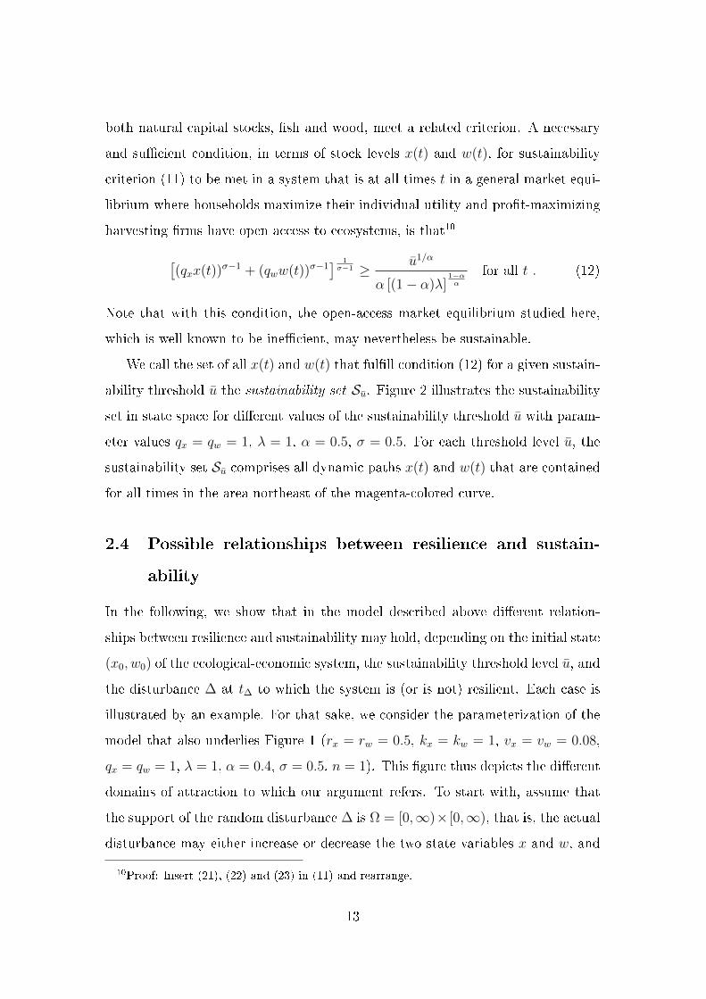
both natural capital stocks, sh and wood, meet a related criterion. A necessary

and sucient condition, in terms of stock levels x(t) and w(t), for sustainability

criterion (11) to be met in a system that is at all times t in a general market equi-

librium where households maximize their individual utility and prot-maximizing

harvesting rms have open access to ecosystems, is that10

[(qxx(t))σ−1 + (qww(t))σ−1

] 1σ−1 ≥ u1/α

α [(1− α)λ]1−αα

for all t . (12)

Note that with this condition, the open-access market equilibrium studied here,

which is well known to be inecient, may nevertheless be sustainable.

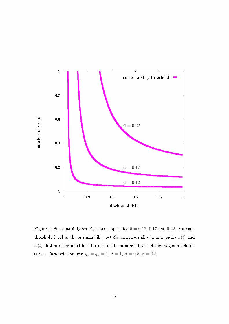
We call the set of all x(t) and w(t) that fulll condition (12) for a given sustain-

ability threshold u the sustainability set Su. Figure 2 illustrates the sustainability

set in state space for dierent values of the sustainability threshold u with param-

eter values qx = qw = 1, λ = 1, α = 0.5, σ = 0.5. For each threshold level u, the

sustainability set Su comprises all dynamic paths x(t) and w(t) that are contained

for all times in the area northeast of the magenta-colored curve.

2.4 Possible relationships between resilience and sustain-

ability

In the following, we show that in the model described above dierent relation-

ships between resilience and sustainability may hold, depending on the initial state

(x0, w0) of the ecological-economic system, the sustainability threshold level u, and

the disturbance ∆ at t∆ to which the system is (or is not) resilient. Each case is

illustrated by an example. For that sake, we consider the parameterization of the

model that also underlies Figure 1 (rx = rw = 0.5, kx = kw = 1, vx = vw = 0.08,

qx = qw = 1, λ = 1, α = 0.4, σ = 0.5, n = 1). This gure thus depicts the dierent

domains of attraction to which our argument refers. To start with, assume that

the support of the random disturbance ∆ is Ω = [0,∞)× [0,∞), that is, the actual

disturbance may either increase or decrease the two state variables x and w, and

10Proof: Insert (21), (22) and (23) in (11) and rearrange.

13

sustainability threshold

u = 0.22

u = 0.17

u = 0.12

stock w of sh

stockxof

wood

10.80.60.40.20

1

0.8

0.6

0.4

0.2

0

Figure 2: Sustainability set Su in state space for u = 0.12, 0.17 and 0.22. For each

threshold level u, the sustainability set Su comprises all dynamic paths x(t) and

w(t) that are contained for all times in the area northeast of the magenta-colored

curve. Parameter values: qx = qw = 1, λ = 1, α = 0.5, σ = 0.5.

14

the states can potentially assume any non-negative values after the disturbance.

Proposition 1

There exists an initial state (x0, w0) of the system and a sustainability threshold

level u, so that under any actual disturbance ∆ at any time t∆ resilience is neces-

sary for sustainability. In particular, this is the case for all (x0, w0) ∈ Su if there

exists an equilibrium i with Su ⊆ Ai.

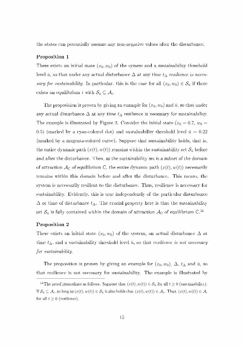
The proposition is proven by giving an example for (x0, w0) and u, so that under

any actual disturbance ∆ at any time t∆ resilience is necessary for sustainability.

The example is illustrated by Figure 3. Consider the initial state (x0 = 0.7, w0 =

0.5) (marked by a cyan-colored dot) and sustainability threshold level u = 0.22

(marked by a magenta-colored curve). Suppose that sustainability holds, that is,

the entire dynamic path (x(t), w(t)) remains within the sustainability set Su before

and after the disturbance. Then, as the sustainability set is a subset of the domain

of attraction AC of equilibrium C, the entire dynamic path (x(t), w(t)) necessarily

remains within this domain before and after the disturbance. This means, the

system is necessarily resilient to the disturbance. Thus, resilience is necessary for

sustainability. Evidently, this is true independently of the particular disturbance

∆ or time of disturbance t∆. The crucial property here is that the sustainability

set Su is fully contained within the domain of attraction AC of equilibrium C.11

Proposition 2

There exists an initial state (x0, w0) of the system, an actual disturbance ∆ at

time t∆, and a sustainability threshold level u, so that resilience is not necessary

for sustainability.

The proposition is proven by giving an example for (x0, w0), ∆, t∆ and u, so

that resilience is not necessary for sustainability. The example is illustrated by

11The proof generalizes as follows. Suppose that (x(t), w(t)) ∈ Su for all t ≥ 0 (sustainability).

If Su ⊆ Ai, as long as (x(t), w(t)) ∈ Su it also holds that (x(t), w(t)) ∈ Ai. Thus, (x(t), w(t)) ∈ Ai

for all t ≥ 0 (resilience).

15

(x0, w0)

path after disturbance

sustainability threshold

saddlepaths

F′

E′

D′

D

E

F

C

B

A

∆

stock x of sh

stockwof

wood

10.80.60.40.20

1

0.8

0.6

0.4

0.2

0

Figure 3: Phase diagram illustrating Propositions 1 and 4: Resilience of the system

in state (x0 = 0.7, w0 = 0.5) to any disturbance at any time is necessary for

sustainability at threshold level u = 0.22. Resilience of the system in state (x0 =

0.7, w0 = 0.5) to disturbance ∆ = (0.643, 0.9) at time t∆ = 0 is not sucient for

sustainability at threshold level u = 0.22. Other parameter values as in Figure 1.

16

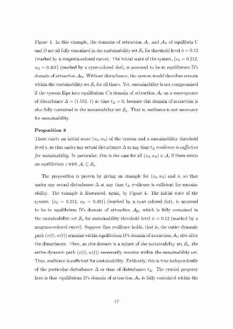
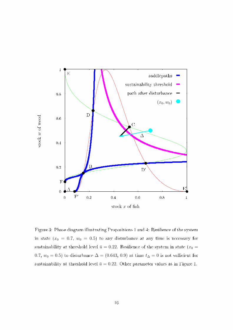
Figure 4. In this example, the domains of attraction AC and AD of equilibria C

and D are all fully contained in the sustainability set Su for threshold level u = 0.12

(marked by a magenta-colored curve). The initial state of the system, (x0 = 0.212,

w0 = 0.401) (marked by a cyan-colored dot), is assumed to be in equilibrium D's

domain of attraction AD. Without disturbance, the system would therefore remain

within the sustainability set Su for all times. Yet, sustainability is not compromised

if the system ips into equilibrium C's domain of attraction AC as a consequence

of disturbance ∆ = (1.552, 1) at time t∆ = 0, because this domain of attraction is

also fully contained in the sustainability set Su. That is, resilience is not necessary

for sustainability.

Proposition 3

There exists an initial state (x0, w0) of the system and a sustainability threshold

level u, so that under any actual disturbance ∆ at any time t∆ resilience is sucient

for sustainability. In particular, this is the case for all (x0, w0) ∈ Ai if there exists

an equilibrium i with Ai ⊆ Su.

The proposition is proven by giving an example for (x0, w0) and u, so that

under any actual disturbance ∆ at any time t∆ resilience is sucient for sustain-

ability. The example is illustrated, again, by Figure 4. The initial state of the

system, (x0 = 0.212, w0 = 0.401) (marked by a cyan-colored dot), is assumed

to be in equilibrium D's domain of attraction AD, which is fully contained in

the sustainability set Su for sustainability threshold level u = 0.12 (marked by a

magenta-colored curve). Suppose that resilience holds, that is, the entire dynamic

path (x(t), w(t)) remains within equilibrium D's domain of attraction AD also after

the disturbance. Then, as this domain is a subset of the sustainability set Su, the

entire dynamic path (x(t), w(t)) necessarily remains within the sustainability set.

Thus, resilience is sucient for sustainability. Evidently, this is true independently

of the particular disturbance ∆ or time of disturbance t∆. The crucial property

here is that equilibrium D's domain of attraction AD is fully contained within the

17

(x0, w0)

path after disturbance

sustainability threshold

saddlepaths

F′

E′

D′

D

E

F

C

B

A

∆

stock x of sh

stockwof

wood

10.80.60.40.20

1

0.8

0.6

0.4

0.2

0

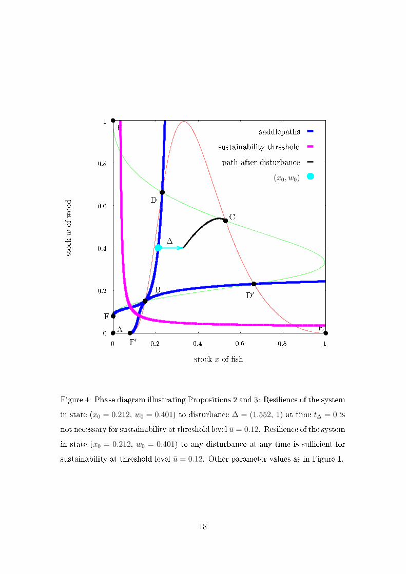
Figure 4: Phase diagram illustrating Propositions 2 and 3: Resilience of the system

in state (x0 = 0.212, w0 = 0.401) to disturbance ∆ = (1.552, 1) at time t∆ = 0 is

not necessary for sustainability at threshold level u = 0.12. Resilience of the system

in state (x0 = 0.212, w0 = 0.401) to any disturbance at any time is sucient for

sustainability at threshold level u = 0.12. Other parameter values as in Figure 1.

18

sustainability set Su.12

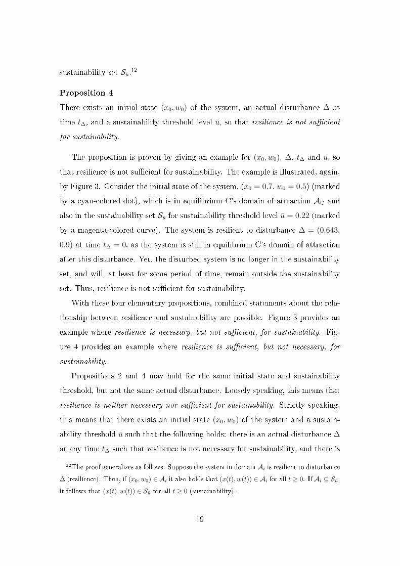
Proposition 4

There exists an initial state (x0, w0) of the system, an actual disturbance ∆ at

time t∆, and a sustainability threshold level u, so that resilience is not sucient

for sustainability.

The proposition is proven by giving an example for (x0, w0), ∆, t∆ and u, so

that resilience is not sucient for sustainability. The example is illustrated, again,

by Figure 3. Consider the initial state of the system, (x0 = 0.7, w0 = 0.5) (marked

by a cyan-colored dot), which is in equilibrium C's domain of attraction AC and

also in the sustainability set Su for sustainability threshold level u = 0.22 (marked

by a magenta-colored curve). The system is resilient to disturbance ∆ = (0.643,

0.9) at time t∆ = 0, as the system is still in equilibrium C's domain of attraction

after this disturbance. Yet, the disturbed system is no longer in the sustainability

set, and will, at least for some period of time, remain outside the sustainability

set. Thus, resilience is not sucient for sustainability.

With these four elementary propositions, combined statements about the rela-

tionship between resilience and sustainability are possible. Figure 3 provides an

example where resilience is necessary, but not sucient, for sustainability. Fig-

ure 4 provides an example where resilience is sucient, but not necessary, for

sustainability.

Propositions 2 and 4 may hold for the same initial state and sustainability

threshold, but not the same actual disturbance. Loosely speaking, this means that

resilience is neither necessary nor sucient for sustainability. Strictly speaking,

this means that there exists an initial state (x0, w0) of the system and a sustain-

ability threshold u such that the following holds: there is an actual disturbance ∆

at any time t∆ such that resilience is not necessary for sustainability, and there is

12The proof generalizes as follows. Suppose the system in domain Ai is resilient to disturbance

∆ (resilience). Then, if (x0, w0) ∈ Ai it also holds that (x(t), w(t)) ∈ Ai for all t ≥ 0. If Ai ⊆ Su,

it follows that (x(t), w(t)) ∈ Su for all t ≥ 0 (sustainability).

19

another actual disturbance ∆′ at the same or another time t′∆ such that resilience

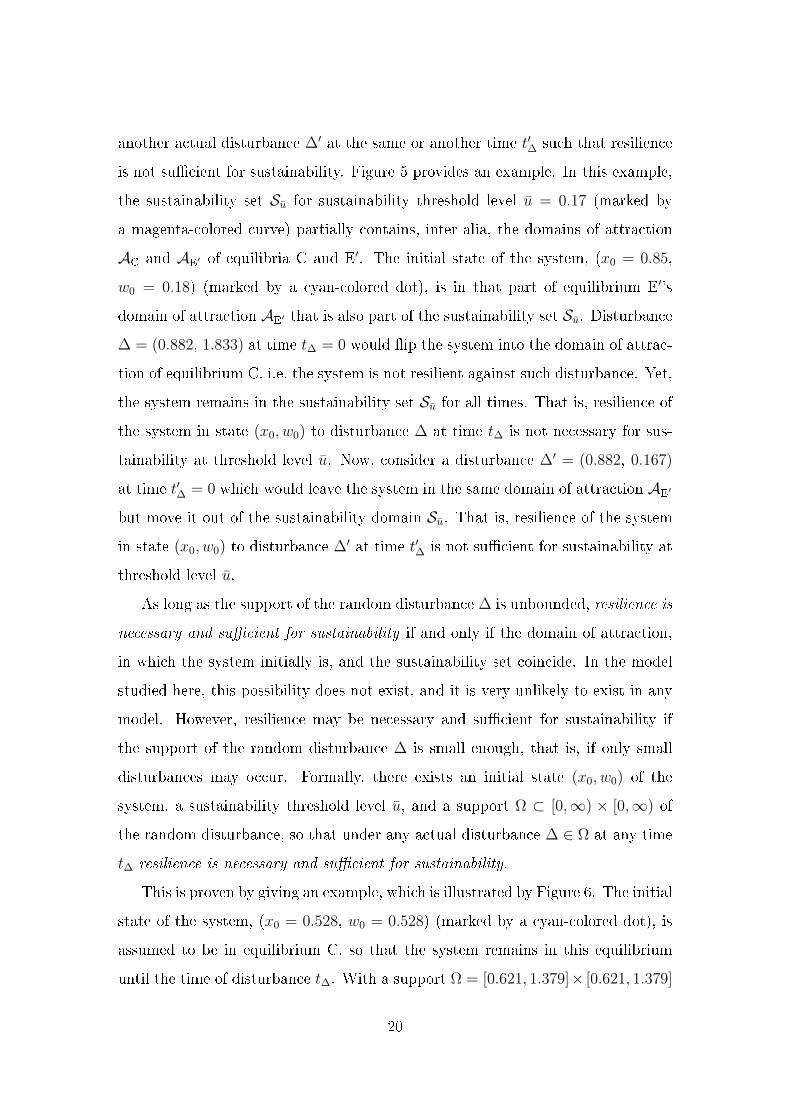
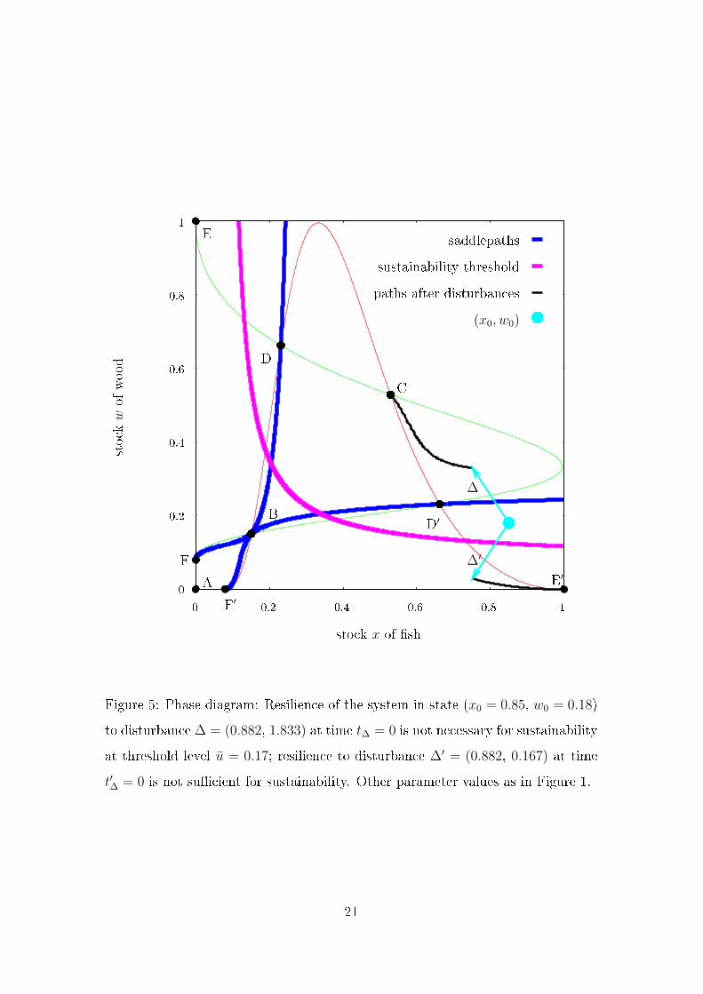
is not sucient for sustainability. Figure 5 provides an example. In this example,

the sustainability set Su for sustainability threshold level u = 0.17 (marked by

a magenta-colored curve) partially contains, inter alia, the domains of attraction

AC and AE′ of equilibria C and E′. The initial state of the system, (x0 = 0.85,

w0 = 0.18) (marked by a cyan-colored dot), is in that part of equilibrium E′'s

domain of attraction AE′ that is also part of the sustainability set Su. Disturbance

∆ = (0.882, 1.833) at time t∆ = 0 would ip the system into the domain of attrac-

tion of equilibrium C, i.e. the system is not resilient against such disturbance. Yet,

the system remains in the sustainability set Su for all times. That is, resilience of

the system in state (x0, w0) to disturbance ∆ at time t∆ is not necessary for sus-

tainability at threshold level u. Now, consider a disturbance ∆′ = (0.882, 0.167)

at time t′∆ = 0 which would leave the system in the same domain of attraction AE′

but move it out of the sustainability domain Su. That is, resilience of the system

in state (x0, w0) to disturbance ∆′ at time t′∆ is not sucient for sustainability at

threshold level u.

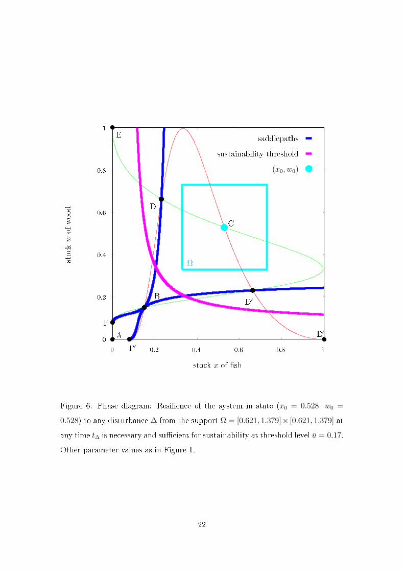
As long as the support of the random disturbance ∆ is unbounded, resilience is

necessary and sucient for sustainability if and only if the domain of attraction,

in which the system initially is, and the sustainability set coincide. In the model

studied here, this possibility does not exist, and it is very unlikely to exist in any

model. However, resilience may be necessary and sucient for sustainability if

the support of the random disturbance ∆ is small enough, that is, if only small

disturbances may occur. Formally, there exists an initial state (x0, w0) of the

system, a sustainability threshold level u, and a support Ω ⊂ [0,∞) × [0,∞) of

the random disturbance, so that under any actual disturbance ∆ ∈ Ω at any time

t∆ resilience is necessary and sucient for sustainability.

This is proven by giving an example, which is illustrated by Figure 6. The initial

state of the system, (x0 = 0.528, w0 = 0.528) (marked by a cyan-colored dot), is

assumed to be in equilibrium C, so that the system remains in this equilibrium

until the time of disturbance t∆. With a support Ω = [0.621, 1.379]× [0.621, 1.379]

20

(x0, w0)

paths after disturbances

sustainability threshold

saddlepaths

F′

E′

D′

D

E

F

C

B

A

∆

∆′

stock x of sh

stockwof

wood

10.80.60.40.20

1

0.8

0.6

0.4

0.2

0

Figure 5: Phase diagram: Resilience of the system in state (x0 = 0.85, w0 = 0.18)

to disturbance ∆ = (0.882, 1.833) at time t∆ = 0 is not necessary for sustainability

at threshold level u = 0.17; resilience to disturbance ∆′ = (0.882, 0.167) at time

t′∆ = 0 is not sucient for sustainability. Other parameter values as in Figure 1.

21

(x0, w0)

sustainability threshold

saddlepaths

F′

E′

D′

D

E

F

C

B

A

Ω

stock x of sh

stockwof

wood

10.80.60.40.20

1

0.8

0.6

0.4

0.2

0

Figure 6: Phase diagram: Resilience of the system in state (x0 = 0.528, w0 =

0.528) to any disturbance ∆ from the support Ω = [0.621, 1.379]× [0.621, 1.379] at

any time t∆ is necessary and sucient for sustainability at threshold level u = 0.17.

Other parameter values as in Figure 1.

22

of the random disturbance, whatever disturbance ∆ ∈ Ω actually occurs at time t∆

will not move the system outside of the cyan-colored rectangle. Given the system

dynamics (depicted in Figure 1), the system will return to equilibrium C along a

dynamic path that is entirely within both the sustainability set Su for sustainability

threshold level u = 0.17 and equilibrium C's domain of attraction AC, because the

cyan-colored rectangle is fully contained within both the sustainability set Su and

equilibrium C's domain of attraction AC. Thus, both sustainability and resilience

hold, so that resilience is necessary and sucient for sustainability.

3 Discussion and conclusion

In this paper, we have studied how, in general, resilience is related to sustainability

in the development of an ecological-economic system. Resilience is in the rst

place a purely descriptive concept of system dynamics. In contrast, sustainability

is a normative concept capturing basic ideas of intergenerational justice when

human well-being depends on natural capital and services. Thus, resilience and

sustainability are independent concepts characterizing the dynamics of ecological-

economics systems.

We have distinguished and specied four possible relationships between re-

silience and sustainability: a) resilience of the system is necessary, but not su-

cient, for sustainability; b) resilience of the system is sucient, but not necessary,

for sustainability; c) resilience of the system is neither necessary nor sucient

for sustainability; d) resilience of the system is both necessary and sucient for

sustainability. All of those are logically possible, and any may hold in the sim-

ple dynamic ecological-economic model that we have presented here, depending

on the initial state of the system, the normative sustainability threshold, and the

uncertain disturbance to the system.

The result that there are four potential relationships between resilience and

sustainability has a much broader validity and generally holds for all systems with

more than two domains of attraction. Generalizing from our particular model,

23

we conjecture that the following holds. If the sustainability set is a subset of the

domain of attraction and the system initially is in the sustainability set, resilience of

the system is necessary for sustainability. Resilience is sucient for sustainability,

on the other hand, if the entire domain of attraction in which the system initially

is, is contained in the sustainability set. Finally, resilience and sustainability are

equivalent if the domain of attraction in which the system initially is coincides

with the sustainability set.

All taken together, in general the deduction from sustainability to resilience, or

vice versa, is not possible. This has implications for the sustainable management

of ecological-economic systems. In particular, the property of resilience should

not be confused with the positive normative connotations of sustainability, and,

vice versa, more criteria than just resilience have to be taken into account when

designing policies for the sustainable development of ecological-economic systems.

Rather, for the sustainable management of an ecological-economic system it is

decisive to know (1) the current state of the system, (2) the domains of attraction

of the system, (3) the sustainability norm and the associated sustainability set in

state space, and (4) the potential extent of disturbance.

Acknowledgments

We are grateful to two anonymous reviewers for critical discussion and to the

German Federal Ministry of Education and Research for nancial support under

grant 01UN0607.

Appendix

With the harvesting functions (3) and (4), assuming that the unit costs of harvest-

ing eort are simply given by the wage rate, and given that the wage rate equals

the marginal product λ of labor in the manufactured-goods sector, the aggregate

24

prots of rms harvesting sh and timber are given by:

πx = pxC − λex = (pxqxx− λ)ex , (13)

πw = pwH − λew = (pwqww − λ)ew . (14)

If rms can freely enter and exit the industry, an open-access equilibrium is char-

acterized by complete dissipation of resource rents, i.e. zero prots for all rms:

πx = 0 and πw = 0 . (15)

With (13) and (14), this condition implies that equilibrium market prices px for

sh and pw for timber are related to resource stocks x and w as follows:

px =λ

qxx−1 , (16)

pw =λ

qww−1 . (17)

The Marshallian demand functions of a representative household can be ob-

tained from solving the utility maximization problem

maxy,c,h

u(y, c, h) subject to (6) , (18)

where u(y, c, h) is the utility function (5), and (6) is the budget constraint. The

rst-order conditions lead to the Marshallian demand functions for sh and timber,

c(px, pw, λ) = αλp−σx

p1−σx + p1−σ

w

, (19)

h(px, pw, λ) = αλp−σw

p1−σx + p1−σ

w

, (20)

as well as to the demand for the manufactured good,

y(px, pw, λ) = (1− α)λ . (21)

With labor income λ and the open-access equilibrium prices of the two re-

sources, (16) and (17), this gives consumption of an individual household as a

function of the two resource stocks:

c(x,w) = α(qxx)σ

(qxx)σ−1 + (qww)σ−1, (22)

h(x,w) = α(qww)σ

(qxx)σ−1 + (qww)σ−1. (23)

25

Using the market-clearing conditions C = nc and H = nh in the equations of

motion (1 and 2) for the two resource stocks, these become

x = f(x)− n c(x,w) , (24)

w = g(w)− nh(x,w) . (25)

Inserting c(x,w) and h(x,w) from Equations (22) and (23), and f(x) and g(w)

from Equations (1) and (2), yields Equations (7) and (8).

References

[1] Anderies, J.M., Janssen, M.A. and Walker, B.H. (2002). Grazing manage-

ment, resilience, and the dynamics of a re-driven rangeland system. Ecosys-

tems 5, 2344.

[2] Arrow, K., Bolin, B., Costanza, R., Dasgupta, P., Folke, C., Holling, C.S.,

Jansson, B.-O., Levin, S., Mäler, K.-G., Perrings, C. and Pimentel, D.

(1995). Economic growth, carrying capacity, and the environment. Science

268(5210), 520521.

[3] Asheim, G.B. and Brekke, K.A. (2002). Sustainability when capital manage-

ment has stochastic consequences. Social Choice and Welfare 19, 921940.

[4] Baumgärtner, S. and Quaas, M.F. (2009). Ecological-economic viability as

a criterion of strong sustainability under uncertainty. Ecological Economics,

68(7), 20082020.

[5] Béné, C., Doyen, L. and Gabay, D. (2001). A viability analysis for a bio-

economic model. Ecological Economics 36, 385396.

[6] Bretschger, L. and Pittel, K. (2008). From time zero to innity: transitional

and long-run dynamics in rapital resource economies. Environment and De-

velopment Economics 13, 673689.

26

[7] Carpenter, S.R., Walker, B., Anderies, J.M. and Abel, N. (2001). From

metaphor to measurement: resilience of what to what? Ecosystems 4, 765

781.

[8] Common, M. and Perrings, C. (1992). Towards an ecological economics of

sustainability. Ecological Economics 6, 734.

[9] Folke, C., Carpenter, S.R., Walker, B.H., Scheer, M., Elmqvist, T., Gun-

derson, L.H. and Holling, C.S. (2004). Regime shifts, resilience, and biodi-

versity in ecosystem management. Annual Review of Ecology, Evolution and

Systematics 35, 557581.

[10] Holling, C.S. (1973). Resilience and stability of ecological systems. Annual

Review of Ecology and Systematics 4, 123.

[11] Holling, C.S. and Gunderson, L. (2002). Resilience and adaptive cycles. In:

Gunderson, L. & Holling, C. S. (eds.): Panarchy. Understanding Transfor-

mations in Human and Natural Systems. Island Press, Washington DC, pp.

2562.

[12] Holling, C.S. and Walker B.H. (2003). Resilience dened.

In: International Society of Ecological Economics (ed.), In-

ternet Encyclopedia of Ecological Economics. [online] URL:

http://www.ecoeco.org/education_encyclopedia.php.

[13] Janssen, M.A., Anderies, J.M. and Walker, B.H. (2004). Robust strategies

for managing rangelands with multiple stable attractors. Journal of Envi-

ronmental Economics and Management 47(1), 140162.

[14] Jax, K. (2002). Die Einheiten der Ökologie. Frankfurt.

[15] Lebel, L., Anderies, J.M., Campbell, B., Folke, C., Hateld-Dodds, S.,

Hughes, T.P. and Wilson, J. (2006). Governance and the capacity to manage

resilience in regional social-ecological systems. Ecology and Society 11(1), 19.

[online] URL: http://www.ecologyandsociety.org. vol11/iss1/art19/.

27

[16] Levin, S.A., Barrett, S., Anyar, S., Baumol, W., Bliss, C., Bolin, B., Das-

gupta, P., Ehrlich, P., Folke, C., Gren, I. M., Holling, C.S., Jansson, A.,

Jansson, B.-O., Mäler, K.-G., Martin, D. Perrings, C. and Sheshinski, E.

(1998). Resilience in natural and socioeconomic systems. Environment and

Development Economics 3, 221235.

[17] Mäler, K.-G. (2008). Sustainable development and resilience in ecosystems.

Environmental and Resource Economics 39, 1724.

[18] Mäler, K.-G., Xepapadeas, A. and de Zeeuw, A. (2003). The economics of

shallow lakes. Environmental and Resource Economics 26(4), 603624.

[19] Martin, S. (2004). The cost of restoration as a way of dening resilience: a

viability approach applied to a model of lake eutrophication. Ecology and

Society 9(2), 8.

[20] Martinet, V., Thébaud, O. and Doyen, L. (2007). Dening viable recovery

paths toward sustainable sheries. Ecological Economics, 64(2), 411422.

[21] Pearce, D.W. (1988). Economics, equity and sustainable development. Fu-

tures 20, 598605.

[22] Perrings, C. (2006). Resilience and sustainable development. Environment

and Development Economics 11, 417427.

[23] Perrings, C. and Stern, D.I. (2000). Modelling loss of resilience in agroecosys-

tems: rangelands in Botswana. Environmental and Resource Economics 16,

185210.

[24] Pimm, S.L. (1991). The Balance of Nature? University of Chicago Press,

Chicago.

[25] Scheer, M. (1997). Ecology of Shallow Lakes. Kluwer, New York.

[26] Walker, B.H. and Salt, D. (2006). Resilience Thinking. Sustaining Ecosys-

tems and People in a Changing World. Island Press, Washington DC.

28

[27] World Commission on Environment and Development (WCED) (1987). Our

Common Future. Oxford University Press, New York.

29