The Polytope Model for Optimizing Cache LocalityBenoît Meister, Vincent Loechner and Philippe ClaussICPS, Université Louis Pasteur, StrasbourgPôle API, Bd Sébastien Brant67400 Illkirch FRANCEe-mail: {meister,loechner,clauss}@icps.u-strasbg.frAbstractAn essential way to obtain high performance on todays computers consists in optimiz-ing spatial and temporal locality of the data. Many scienti�c applications contain loopnests that operate on large multi-dimensional arrays whose sizes are often parameterized.In this work, temporal reuse occuring from several references in a same statement of aparameterized loop is modeled geometrically. More precisely, iterations are classi�ed de-pending on the kind of temporal reuse associated to their references. This classi�cationde�nes a partitioning of the iteration space as a union of disjoint parameterized convexpolytopes. A convenient scanning of these polytopes allows to construct a new programthat achieves optimal temporal locality for any values of the parameters. Moreover, op-timal spatial locality is obtained by transforming the memory layout as presented in ourpreceding work.Keywords Cache memory, spatial and temporal locality, loop nests, program performance optimiza-tion, optimizing compiler, parameterized polyhedron.1 IntroductionAs the disparity between processor cycle times and main memory access times grows, perfor-mances of programs are greatly dependent on the way the cache memory is e�ectively used.The unit of data transfer between main memory and cache is a block. If the same data in thecache is reused successively, this is called temporal locality. On the other hand, since the unitof data in cache is a block, once the block is brought into the cache, any access to the dataelements in the block will be a cache hit. This is called spatial locality. Typically, a cache hittakes one processor cycle, while a cache miss takes 8 to 32 cycles. The ideal scheme for allmemory references is to hit the cache, however, since cache size is much smaller than mainmemory, once new data need to be brought in from main memory, some data in the cachehave to be replaced. There will be a cache miss when the replaced data is accessed againafterwards. Therefore, high performance requires programs to possess cache locality, i.e., toreuse the data in the cache before it is replaced.Most of the scienti�c and engineering applications contain loop nests that operate on largemulti-dimensional arrays. Unfortunately, most of these loops are written without any specialattention paid to cache memory performance. It has already been observed that compiler

techniques are useful for optimizing locality. Programmers and compiler writers often attemptto modify the access patterns of a program so that the majority of accesses are made tothe nearby memory. Several e�orts have been aimed at iteration space transformations andscheduling techniques to improve locality [6, 7, 12, 11], and also at data transformations toimprove spatial locality [5, 3, 4, 8, 2].We presented in a recent work [2] a method dedicated to spatial locality optimization basedon the computation of a new reference evaluation function. This approach is equivalent totransforming the memory layout. But in this �rst proposal, the application �eld is limitedto loops containing one unique reference to a given array. In this work, we consider moregeneral loops containing several di�erent references to a same array. At our knowledge, suchcases were never considered in other works at this time. The main di�culty is related to thetemporal reuse occuring from these several references.We propose a geometrical model that consists in classifying iterations relatively to theirreference to a same data. This classi�cation results in a partitioning of the iteration spaceby disjoint polytopes. Temporal locality is then obtained by scanning some of these sets andby merging the statements of the other ones. Spatial locality is also obtained by extendingour method presented in [2] : data referenced by the merged statements are interleaved inmemory. The mathematical tools we use are operations on polyhedral sets (unions, intersec-tions, di�erences, a�ne transformations) and implemented in the polyhedral library PolyLib(http://icps.u-strasbg.fr/PolyLib). The �nal scanning loops are automatically generated byusing the Fourier-Motzkin algorithm also implemented in the polyhedral library PolyLib [9].At this time, the algorithm presented in this paper has the following limitations :� any data can be accessed at most once through a given reference occuring in the consid-ered loop,� no loop-carried data dependence is allowed.� our geometrical approach involves some other restrictions on the a�ne references. Theseare precisely explained in the following section.The objective of our next developments is to overcome these limitations. Anyway, thispaper is dedicated to introduce a new geometrical model of memory accesses for which somenatural directions of extensions are given in conclusion. Moreover, the kind of programsconsidered at this time covers a very large �eld of concrete cases.The paper is organized as follows. In section 2, the considered loops nests structure isde�ned precisely. Our geometrical model of memory accesses is described in section 3, givingthe classi�cation criteria of the iterations. In section 4, we show how optimal temporal andspatial locality is obtained, by merging statements, transforming data, and generating the newprogram. Finally, conclusions and future directions are given in section 5.2 ContextWe consider a parameterized loop nest of depth n where more than one a�ne reference ismade to a same array at each iteration. These references can also contain parameters in theconstant part of the involved a�ne functions. The iteration space is an n�dimensional convex2

polyhedron D where each integer point is associated to an iteration of the loop nest. Thereferences have di�erent access matrices R1, R2,. . . , Rq and o�set vectors r1; r2; : : : ; rq, whereq is the number of accesses made in the loop. Hence, each reference R� is characterized bythe couple R� = (R�; r�).As said in the introduction, any reference made by the loop has to induce one uniqueaccess to a given data. It means that no temporal reuse is allowed for each reference byitself and that any access matrix R� is an invertible matrix. On the other hand, temporalreuse occuring from several di�erent references to a same array is considered. Let I; J be twodi�erent iterations. If I references the same data through reference R� as J through referenceR�, then R�I + r� = R�J + r�. That is to say :R�1� R�I + R�1� r� � R�1� r� = J () T��I + t�� = Jwith T�� = R�1� � R� and t�� = R�1� r� � R�1� r�. Thus, for each point I of D accessing anarray element through R�, we can determine which point J accesses the same data throughR� by J = T��I + t�� .Conversely, since R� and R� are invertible, T�� is invertible too, and we can determine, foreach point J of D accessing a data through R� which point I accesses the same data throughR� by I = T�1�� J � T�1�� t�� .We call T�� = (T��; t��) the temporal reuse relation of references R� and R�.In order to avoid some additional geometrical di�culties in this �rst proposal of the method,we have to ensure that R� and R� span the same lattice of integer points. Hence, the accessmatrices must be such that jdet(R�)j = jdet(R�)j for any �; � 2 [1::k], where det(R) denotesthe determinant of matrix R. Since det(T��) = det(R�)=det(R�) = �1, T�� is unimodular.Loop-carried data-dependences are not allowed at this time by the method, since theywould constrain the possible program transformations. This restriction, as the other onesstated above, is discussed in conclusion.The paper is illustrated with the following example:Example 1 Let us consider the following loop nest:for i = �N to Nfor j = �N to NX [i; j] = Y [i; i+ j + 3] + Y [i+ j; j]Two references are made to array Y :R1 = R1I + r1 = 1 01 1 ! I + 03 ! R2 = R2I + r2 = 1 10 1 ! I + 00 !where I = (i; j)T is a point in the 2-dimensional iteration space D = fI 2 Z2j � N � i �N;�N � j � Ng. The temporal reuse relation T12 is given by T12 = R�12 �R1 = 0 �11 1 !and t12 = R�12 r1 �R�12 r2 = �33 !. 3

For example, iteration I = (8;�5)T references the same array element through Y [i; i+j+3]as iteration J = 0 �11 1 ! 8�5 !+ �33 ! = 26 !through Y [i+ j; j].All the iterations will now be classi�ed depending on the kind of temporal reuse that isinduced by their references. This process is explained in the following section.3 The polyhedral model of memory accessesFor the sake of clarity, we describe our model for only two references R1 and R2 to a samearray. Then we explain how the model can be extended to any number of references. Sincethere is no possible confusion, T12, T12 and t12 will be denoted by T , T and t in the following.The iteration space is divided into four main iteration sets characterized by the followingclassi�cation criteria :� The iterations referencing through R1 a data also referenced by an other iterationthrough R2. Those are the iteration points having an image by T in the iterationspace D. This iteration set is denoted by P1. It de�nes a convex polytope:P1 = fI 2 DjTI + t 2 Dg� The iterations that are the images through T of the iterations in P1. These are theiterations referencing through R2 a data also referenced by an other iteration throughR1. This iteration set is denoted by P2. It de�nes a convex polytope:P2 = fI 2 DjT�1I � T�1t 2 Dg� The iterations whose referenced data are never referenced by any other iteration. Theseare the iterations which are neither in P1 nor in P2. This set is denoted by L, and de�nesa union of convex polytopes L = D � P1 � P2.We denote by C the set of iterations belonging simultaneously to P1 and P2, C = P1 \P2.We also de�ne the set D1 (respectively D2) containing the points of P1 (resp. P2) that donot belong to P2 (resp. P1), D1 = P1 � P2 = P1 � C (resp. D2 = P2 � P1 = P2 � C). D1(respectively D2) is the set of iterations of P1 (resp. P2) referencing through R2 (resp. R1) adata that is never referenced by any other iteration of D.Finally, iteration space D is partitioned into four disjoint sets : D1, D2, C and L. Thispartitioning process is schematized on �gure 1.Example 2 (continued)The set P1 is de�ned by:P1 = f(i; j)T 2 Dj(�j � 3; i+ j)T 2 Dg= f(i; j)T 2Z2j �N + 3 � i � N;�N � j � N � 6;�N � i+ j � Ng4

R1 R2

R1 R

2

R1 R

2R1 R2

R1 R

2

R1 R

2

R1 R

2

R1 R2L

CD1

D2

Figure 1: Schematization of the partitioning process where each line represents a reference tothe same data.Since T�1 = 1 1�1 0 !, P2 is de�ned by :P2 = f(i; j)T 2 Dj(i+ j;�i� 3)T 2 Dg= f(i; j)T 2Z2j �N + 3 � i � N � 3;�N � j � N;�N + 3 � i+ j � NgHence, L;C;D1 and D2 are deduced :L = D � P1 � P2= f(i; j)T 2Z2ji � �N; j � �N; i+ j � �N � 4g[ f(i; j)T 2Z2ji � N; j � N; i+ j � N + 1g[ f(i; j)T 2Z2ji � N; i+ j � N; i+ j � N � 2; i � N � 2gC = P1 \ P2= f(i; j)T 2Z2j �N � i � N � 3;�N � j � N � 3;�N � i+ j � N � 3gD1 = P1 � P2= f(i; j)T 2Z2jN � 2 � i � N; j � �N; i+ j � N � 3g[ f(i; j)T 2Z2ji � �N; j � �N;�N � 3 � i+ j � N + 1gD2 = P2 � P1= f(i; j)T 2Z2ji � �N;N � 2 � j � N; i+ j � Ng[ f(i; j)T 2Z2ji � N � 3; j � N;N � 2 � i+ j � NgD1; D2; L and C are represented on �gure 2 for N = 8.Iterations referencing the same data are linked by relation T : iteration I1 referencesthrough R1 the same data as iteration TI1 + t = I2 through R2, if and only if I1 2 D1 orI1 2 C according to the de�nitions of D1 and C. Moreover in such a case, it comes that I2 2 Cor I2 2 D2. If I2 2 C, then I2 references through R1 another data that is also referenced byiteration TI2 + t = I3 through R2. 5

D1

D2

D1C

L

Li

j

Figure 2: Partitioning the iteration space D by D1, D2, C and L.In order to ensure temporal locality, iterations I1, I2 and I3 should be computed consecu-tively. But the number of iterations that can be linked by T do vary. The next step consistsnow in de�ning sets of iterations characterized by the number of other iterations that arelinked to it by T . These sets are constructed as follows:1) All the iterations of D1 that are linked to iterations of D2 by T :DC1 = fI 2 D1jTI + t 2 D2g1') All the iterations of C that are linked to themselves by T :C1 = fI 2 CjTI + t = Ig2) All the iterations of D1 that are linked to iterations of C, and these iterations are linkedto iterations of D2. In other words, these are the iterations of D1 that are linked toiterations of D2 by T 2 :DC2 = fI 2 D1jTI + t 2 C; T 2I + Tt + t 2 D2g2') All the iterations of C that are linked to other iterations of C, and these iterations arealso linked to the �rst ones. Observe that the elements of C1 have to be excluded. Inother words, these are the iterations of C that are linked to themselves by T 2 :C2 = fI 2 CjTI + t 2 C; T 2I + Tt+ t = Ig � C1. . . 6

k) All the iterations of D1 that are linked to iterations of D2 by T k :DCk = fI 2 D1jTI + t 2 C; T 2I + Tt+ t 2 C; T 3I + T 2t + Tt + t 2 C; : : :;T kI + T k�1t + : : :T t+ t 2 D2gk') All the iterations of C that are linked to themselves by T k :Ck = fI 2 CjTI+ t 2 C; T 2I+Tt+ t 2 C; : : :; T kI+T k�1t+ : : :T t+ t = Ig� [1�q�k�1Cq. . .R1 R

2

R1 R

2

L

CD1

D2

R1 R2

R1 R2

L

CD1

D2

R1 R

2

L

CD1

D2

R1 R2

R1 R

2

R1 R2

L

CD1

D2

DC1

C1

DC2

C2Figure 3: De�nitions of sets DC1, C1, DC2 and C2.The de�nitions of sets DC1, C1, DC2 and C2 are schematized on �gure 3.Sets DCk and Ck are computed by applying the a�ne transformation de�ned by T tocompositions of D1, D2 or C. Application of T to any set S is denoted by T (S) and to anypoint I by T (I). Hence, the sets de�ned above can also be de�ned as follows :1) DC1 = D1 \ T �1(D2)2) DC2 = D1 \ T �1(C)\ T �2(D2)2') C2 = C \ T �1(C) \ fI 2 CjT 2I + Tt+ t = Ig � C1. . . 7

k) DCk = D1 \ T �1(C)\ T �2(C)\ : : :\ T �k(C)\ T �k(D2)k') Ck = C \ T �1(C)\ T �2(C)\ : : :\ T �k(C)\ fI 2 CjT kI + T k�1t+ : : :T t + t = Ig �S1�q�k�1 Cq. . .Sets Ck de�ne cycles of length k composed of points linked by T . We partition any set Ckby sets C0k ; C1k ; : : : ; Ck�1k such that any set Cqk contains one unique member of each cycle. Thechosen partitioning criteria is the lexicographic order of the points in each cycle:C0k = fI 2 CkjI � T (I); I � T 2(I); : : : ; I � T k�1(I)gwhere � denotes the lexicographic order. Any set Cqk , where 0 < q � k � 1, is consequentlydetermined by Cqk = T q(C0k).Similarly, we de�ne DCqk = T q(DCk) for any 0 � q � k.Example 3 (continued)The iteration space D is fully partitioned for k = 1 to 6 by the following sets :( DC01 = f(i; j)T 2Z2ji+ j � N � 3; i � N; j � �N; i � N � 2gDC11 = f(i; j)T 2Z2ji+ j � N � 2; i � N � 3; i+ j � N; j � Ng8>>><>>>: DC03 = f(i; j)T 2Z2ji+ j � �N � 3; i+ j � �N � 1; j � �N; j � �N + 2gDC13 = f(i; j)T 2Z2ji � N � 5; j � �N; i � N � 3; j � �N + 2gDC23 = f(i; j)T 2Z2ji+ j � N � 5; i � N � 3; i+ j � N � 3; i � +N � 5gDC33 = f(i; j)T 2Z2jj � N � 2; i+ j � N � 3; j � N; i+ j � N � 5g8>>>>><>>>>>: DC04 = f(i; j)T 2Z2ji � �N; j � �N + 3; i+ j � �N � 3; i+ j � �N � 1gDC14 = f(i; j)T 2Z2ji � N � 6; i+ j � �N; j � �N + 2; j � �NgDC24 = f(i; j)T 2Z2ji+ j � N � 6; j � �N + 3; i � N � 5; i � N � 3gDC34 = f(i; j)T 2Z2jj � N � 3; i � N � 6; i+ j � N � 5; i+ j � N � 3gDC44 = f(i; j)T 2Z2ji � �N; i+ j � N � 6; j � N � 2; j � NgC01 = f(�3; 0)Tg8>>>>>>><>>>>>>>: C06 = f(i; j)T 2Z2ji � �N; j � 0; i+ j � �4gC16 = f(i; j)T 2Z2ji+ j � �N; i � �3; j � �1gC26 = f(i; j)T 2Z2jj � �N + 3; i+ j � �3; i � �2gC36 = f(i; j)T 2Z2ji � N � 6; j � 0; i+ j � �2gC46 = f(i; j)T 2Z2ji+ j � N � 6; i � �3; j � 1gC56 = f(i; j)T 2Z2jj � N � 3; i+ j � �3; i � �4gL = f(i; j)T 2Z2ji � �N; j � �N; i+ j � �N � 4g[ f(i; j)T 2Z2ji � N; j � N; i+ j � N + 1g[ f(i; j)T 2Z2ji � N; i+ j � N; i+ j � N � 2; i � N � 2gThis partitioning is shown on �gure 4 for N = 8.8

L

L

DC04 DC14 DC24DC34DC44

DC03 DC13DC23

DC33C06

C16 C26 C36C46C56 C01

DC01

DC11i

j

Figure 4: The �nal partitioning of DThe main di�culty of this partitioning process is to determine the maximum value of k sothat D is completely partitioned. Two cases can occur depending on the existence of a lowestvalue kmax > 0 such that T kmax = I, where Idenotes the identity matrix:1. if such a value exists, the set Ckmax will contain all the remaining points of C at thekmax-th step of the partitioning process. Hence D will be completely partitioned.2. if such a value does not exist, we a�ect kmax a high value. Our partitioning processstops as soon as C has been detected as being empty or kmax has been reached. Butsince the iteration space D can be parameterized, the number of necessary partitioningsteps can also be parameterized and there is no convenient value of kmax. In such acase, there will be some remaining iterations in D1; D2 and C that are not consideredby our locality optimization process and kmax can be seen as an optimization level.We �rst have to determine if there exists a lowest value kmax > 0 such that T kmax = I.Our method proceeds as follows.Since T (I) = TI + t, we write T in the homogeneous form of a single matrix:T = T t0 : : : 0 1 !Then, by computing the eigenvalues and eigenvectors of this matrix T , we can write T =P�1 �A � P , where the columns of P are the eigenvectors and A is the diagonal matrix of theeigenvalues. Since T q = P�1 �Aq � P for any q > 0, we resolve the equation Akmax = I.The eigenvalues vq can be complex numbers or rational numbers. Hence, the rationaleigenvalues must be equal to 1 or -1 in order to get a integer solution kmax. Moreover, if atleast one eigenvalue is equal to -1 then kmax must be even.9

For the complex eigenvalues, we use their polar coordinates (�q; �q): any complex numbera + bi can be written as � cos � + i sin � = � ei� with � � 0 and �� < � < �. Since1 = 1 + 0i = 1 ei2k� ; k 2Z, we have to resolve for each eigenvalue vq:(�q ei�q )kmax = 1 ei2kq� , ( �q = 1i�qkmax = i2kq� , ( �q = 1�qkmax = 2kq� , ( �q = 1kmax = 2kq ��qHence, there may be a solution if the polar coordinates of all the eigenvalues are such that�q = 1. Moreover, there is at least one integer solution kmax if any �q is of the form �q�q �,with �p; �q 2Z. If so, kmax is de�ned as being equal to any 2kq �q�q . Since kq has to be chosensuch that 2kq is a multiple of �q to get an integer solution, the lowest solution kmax is equalto the lower common multiple of the 2kq�q �q's, lcmq(2kq�q �q), where kq = �q if �q mod 2 6= 0 andkq = �q=2 if �q mod 2 = 0.Example 4 (continued)In the homogeneous form, T can be written as the matrix:T = 0B@ 0 �1 �31 1 30 0 1 1CAWe want to resolve T kmax = I. We �rst compute the eigenvalues of T : 1; 12 + 12ip3; 12 � 12 ip3.The polar coordinates of the two complex ones are (1; �=3), (1;��=3). Since any �q = 1 andsince any �q is in a convenient form, there exists a lowest value kmax which is equal to thelower common multiple of 2k11 3 and 2k2�1 3. Since 1 mod 2 = 1 and �1 mod 2 = 1, we havek1 = 1 and k2 = �1. Finally, kmax = lcm(6; 6) = 6. One can verify that T 6 = I.Hence, our partitioning process stops at the 6-th step where D is completely partitioned.Once all the setsDCqk and Cqk have been de�ned, we generate the �nal program by scanningby loops two representative sets of each partitioning step k, and by merging into one iterationthe statements that are linked through T . This process is explained in detail in the followingsection.This geometrical model is extensible to more than two references. Since we consider a verygeneral case, the sets where temporal reuse happens are becoming exponentially more highlystructured as the number of references is increasing. Hence, trying to fully optimize such asystem may become very complex for great values of kmax. For example, if we consider aloop with three references Y [R1(I)]; Y [R2(I)] and Y [R3(I)], these three references will de�nethree temporal reuse relations T12; T13 and T23. The result of our partitioning process wouldconsist in sets Sk de�ned by a non-oriented and connex graph Gk of k nodes, whose degreesd are such that 1 � d � 3 (except for the set L where any d = 0). Each edge is associatedto one of the three temporal reuse relations T12, T13 and T23 and each node is associated toiterations I . Since several sets of iterations would match such a graph, any set Sqk is de�nedas the set of all iterations that match the q-th node.10

4 Generation of the �nal program4.1 Optimizing temporal localityFor any partitioning step k, we consider the sets DC0k , DC1k , . . . ,DCkk and C0k , C1k , . . . , Ck�1k .By chosing for example DC0k (resp. C0k) as the representative set, we generate a scanning loopfor this set by using the Fourier-Motzkin algorithm implemented in the polyhedral libraryPolyLib. The instructions put in the resulting loop are those associated to all the sets DCqk(resp. Cqk). A given iteration I of this loop computes the statements associated to points I ,T (I), T 2(I), . . . and temporal locality occurs between any two successive statements.Example 5 (continued)By generating scanning loops for the sets DC01 , DC03 , DC04 , C01 , C06 and L shown on �gure5 for N = 8, and by merging the convenient statements, we obtain the program shown on�gure 6. Observe that the same references occur between successive statements.L

L

DC04 DC03C06 C01

DC01i

j

Figure 5: The scanned sets DC01 , DC03 , DC04 , C01 , C06 and L.Let us see how the �nal program could be generated in the case of more than two referencesin the original loop. Starting from the partitioning result described at the end of section 3, the�nal program would be constructed by scanning sets S0k by loops and by merging all iterationsde�ned by the sets Sk. This merging process would be more complicated: since the iterationsare associated to di�erent paths of Gk, they should be interleaved cleverly so that temporallocality would be ensured.4.2 Optimizing spatial localityIn order to achieve spatial locality for all these generated loops, we extend our method pre-sented in [2]. Its principle is to provide a new array reference evaluation function such that11

the order of the data in memory matches exactly the order in which they are referenced bythe loop. Hence, any block loaded in the cache is completely accessed until it is replaced andthe corresponding data will no more be reused in the future.This function is determined by counting the number of iterations occuring before a givenreference. The result is an Ehrhart polynomial [1] whose variables are the indices of theconsidered array. Hence, this polynomial de�nes a new reference function and the consideredarray is transformed into a one-dimensional array.The best use of this technique is to implement it in a compiler in order to de�ne a newarray reference evaluation process. However, it can also be written directly in the source code:during the execution of the loop, any successive references are made to sucessively storeddata, the reference function simply consists in adding one to the previous reference indexvalue, starting from a given base address for the considered array.In order to be used in the source code resulting from our temporal locality optimization, thismethod has to be extended: since several statements occurs in the loops, a polynomial mustbe computed for each di�erent reference. Moreover, these polynomials have to be transformedsuch that the referenced data are interleaved in memory:� if the loop results from sets Cqk , iteration I is of the form:Y [R0(I)] : : :Y [Rk�1(I)]Y [R1(I)] : : :Y [R0(I)]Y [R2(I)] : : :Y [R1(I)]. . .Y [Rk�1(I)] : : :Y [Rk�2(I)]A polynomial is computed for each reference R0; : : : ;Rk�1. The results are polynomialsEP0; : : : ; EPk�1. At this step and for a given I , the evaluation of all the polynomials willresult in the same value. In order to obtain k sucessive values, we rather consider thepolynomials kEP0� k+ 1; kEP1� k+2; : : : ; kEPk�1. Iteration I can then be rewrittenas:Y [r] : : :Y [r + k � 1]Y [r + 1] : : :Y [r]Y [r + 2] : : :Y [r + 1]. . .Y [r + k � 1] : : :Y [r + k � 2]r = r + kwhere r is initialized at the base address of array Y .� if the loop results from sets DCqk , Iteration I is of the form:Y [R1(I)] : : :Y [R0(I)]Y [R2(I)] : : :Y [R1(I)]Y [R3(I)] : : :Y [R2(I)] 12

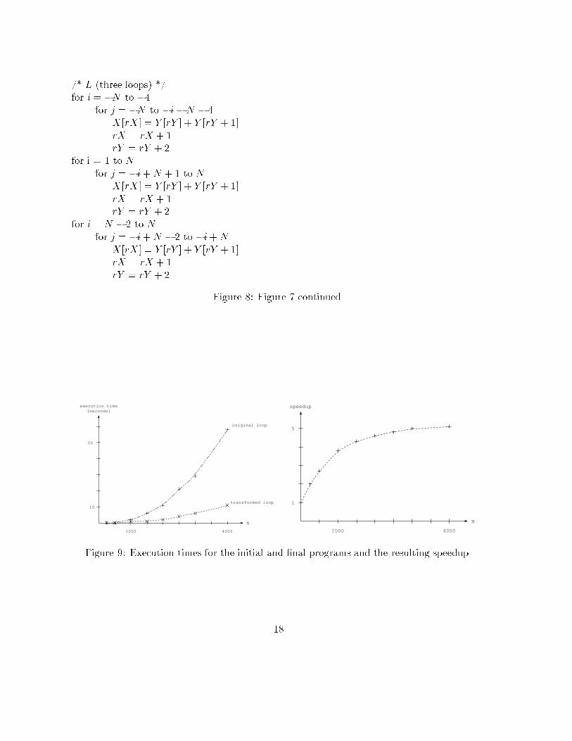
. . .Y [Rk(I)] : : :Y [Rk�1(I)]No temporal reuse occurs for reference Y [R0(I)]. Hence, a polynomial has also to becomputed for this reference. We consider the polynomials (k+1)EP0� k; (k+1)EP1�k + 1; : : : ; (k+ 1)EPk. Iteration I can then be rewritten as:Y [r + 1] : : :Y [r]Y [r + 2] : : :Y [r + 1]Y [r + 3] : : :Y [r + 2]. . .Y [r + k] : : :Y [r+ k � 1]r = r + k + 1� if the loop results from the set L, Iteration I is of the form:Y [R1(I)] : : :Y [R2(I)]A polynomial is computed for each reference ; 2EP1 � 1 and 2EP2 are considered.Iteration I can then be rewritten as:Y [r] : : :Y [r + 1]r = r + 2Example 6 (continued)For each loop shown on �gure 6, the convenient polynomials are computed. Consequently,Y is now a one-dimensional array whose elements are referenced in the order of their storageby the �nal program shown on �gures 7 and 8.We now present performance results to demonstrate the impact of our locality optimizationmethod. Our experimental platform is an 32-processor SGI Origin 2000 at the University LouisPasteur in Strasbourg France. This machine uses 195 MHz R10000 processors, each with a32 KB L1 data cache and a 4 MB L2 uni�ed cache. The processors can fetch and decodefour instructions per cycle and can run them on �ve pipelined functionnal units. Both cachesare two-way associative and nonblocking. Up to four outstanding misses from the combinedtwo-levels of cache are supported. The R10000 processor dynamically schedules instructionswhose operands are available in order to hide the latency of cache misses. For the L1 cachehits, the latency is 2 to 3 cycles; and for the L1 misses that hit in the L2 cache, the latency is8 to 10 cycles. The main memory accesses take 62 cycles.We compare the execution times on one processor between the initial program and our �nalprogram by making N vary from 300 to 4000, corresponding to matrices of sizes 600� 600 to8000� 8000 of �oating point numbers. Results are shown on �gure 9, showing an executiontime of 58:60 seconds for the original program and a execution time of 11:55 seconds for our�nal programwith N = 4000. The speedup tends to be greater than 5 between both sequentialprograms. 13

5 ConclusionWe proposed in this work a new model to fully optimize both spatial and temporal cache mem-ory locality of parameterized loop nests with a�ne references to arrays. Our algorithm is basedon a geometric representation of the program, and manipulates parameterized polytopes. In-tersections, unions, di�erences, a�ne transformations, and loop generation are performed usingthe Polylib (http://icps.u-strasbg.fr/PolyLib). We have developed an implementation of thedomain splitting algorithm presented in section 3, which can be downloaded at http://icps.u-strasbg.fr/PolyLib/Split. The �gures presented in this paper are screenshots of the resultingdomains, using the PolyLib tool VisuDomain.The restrictions of the current algorithm are the following. Firstly, the access functionsof the data have to be a�ne and bijective functions of the loop indices and the parameters.This restriction could be removed in the future by considering sets of points referencing asame data through a given reference, and by linking such sets by a temporal reuse relation.Secondly, the temporal reuse relation T has to be unimodular in order for the linked iterationsto touch the same lattice of integer points in our geometrical model. This constraint willeventually be removed once the geometrical tools to manipulate Z-polyhedra are available.Union and di�erence are non-trivial operations, but some works have already been started inthis direction [10].Moreover at this time, we did not take into account the data dependencies induced by theloop nest in order to get an unconstrained code generation: if there are loop-carried data depen-dences, the resulting code has to verify the causal constraints in order to be valid. This wouldconstrain the partitioning, the scanning directions, and the loop schedule. But it also mayyield impossible loop generation as presented in section 4, because of the unrolling/mergingstep of our algorithm. In this case, we can still transform the program for spatial optimization,and perform temporal locality wherever possible.We have shown that our method allows to greatly improve the performance of even simpleprograms. In the proposed example, we generate a sequential program which is longer than theoriginal one, but running �ve times faster. This shows that many codes may be appreciablyoptimized for no cost at all compared to investing in expensive parallel calculators. Moreover,our locality optimization framework can also be used for parallelizing programs, since it yieldsa minimum number of communications between processors.References[1] Ph. Clauss and V. Loechner. Parametric Analysis of Polyhedral Iteration Spaces. Journalof VLSI Signal Processing, Vol. 19, No. 2, Kluwer Academic Pub., July 1998.[2] Ph. Clauss et B. Meister. Automatic Memory Layout Transformations to Optimize Spa-tial Locality in Parameterized Loop Nests. 4th Annual Workshop on Interaction betweenCompilers and Computer Architectures, INTERACT-4, Toulouse, France, january 2000.[3] M. Kandemir, A. Choudhary, J. Ramanujam, and P. Banerjee. Optimizing Spatial Local-ity in Loop Nests using Linear Algebra. Proc. 7th Int. Workshop on Compilers for ParallelComputers, Sweden, June 1998. 14

[4] M. Kandemir, A. Choudhary, N. Shenoy, P. Banerjee, and J. Ramanujam. A HyperplaneBased Approach for Optimizing Spatial Locality in Loop Nests. Proc. 11th ACM Int.Conf. on Supercomputing, Melbourne, Australia, July 1998.[5] S.-T. Leung et J. Zahorjan. Optimizing data locality by array restructuring. Universityof Washington, Department of Computer Science and Engineering. Technical Report 95-09-01, 1995.[6] W. Li. Compiling for NUMA parallel machines. Ph.D. dissertation, Dept. Computer Sci-ence, Cornell University, Ithaca, NY, 1993.[7] K. McKinley, S. Carr and C. Tseng. Improving data locality with loop transformations.ACM Transactions on Programming Languages and Systems, 1996.[8] M.F.P. O'Boyle et P.M.W. Knijnenburg. Nonsingular Data Transformations: De�nition,Validity, and Applications. Int. J. of Parallel Programming, Vol. 27, No. 3, pp. 131-159,juin 1999.[9] F. Quilleré, S. Rajopadhye and D. Wilde. Generation Of E�cient Nested Loops FromPolyhedra. To appear in Int. J. of Parallel Programming, 2000.[10] P. Quinton, S. Rajopadhye and Tanguy Risset. On Manipulating Z-polyhedra using aCanonical Representation. Parallel Processing Letters, 1997.[11] M. Wolf and M. Lam. A data locality optimizing algorithm. Proc. ACM SIGPLAN 91Conf. Programming Language Design and Implementation, pages 30-44, Toronto, Ont.,June 1991.[12] M. Wolf. Improving locality and parallelism in nested loops. Ph.D. dissertation, Dept.Computer Science, Stanford University, CSL-TR-92-538, 1992.15

/* DC1 */for i = N � 2 to Nfor j = �N to �i+N � 3X [i; j] = Y [i; i+ j + 3] + Y [i+ j; j]X [�j � 3; i+ j + 3] = Y [�j + 3; i+ 3] + Y [i; i+ j + 3]/* C1 */X [�3; 0] = Y [�3; 0] + Y [�3; 0]/* DC3 */for i = �5 to �1for j = max(�i�N � 3;�N) to min(�N + 2;�i�N � 1)X [i; j] = Y [i; i+ j + 3] + Y [i+ j; j]X [�j � 3; i+ j + 3] = Y [�j � 3; i+ 3] + Y [i; i+ j + 3]X [�i� j � 6; i+ 3] = Y [�i� j � 6;�j] + Y [�j � 3; i+ 3]/* DC4 */for i = �N to �4for j = max(�N + 3;�i�N � 3) to �i�N � 1X [i; j] = Y [i; i+ j + 3] + Y [i+ j; j]X [�j � 3; i+ j + 3] = Y [�j � 3; i+ 3] + Y [i; i+ j + 3]X [�i� j � 6; i+ 3] = Y [�i� j � 6;�j] + Y [�j � 3; i+ 3]X [�i� 6;�j] = Y [�i� 6;�i� j � 3] + Y [�i� j � 6;�j]/* C6 */for i = �N to �4for j = 0 to �i � 4X [i; j] = Y [i; i+ j + 3] + Y [i+ j; j]X [�j � 3; i+ j + 3] = Y [�j � 3; i+ 3] + Y [i; i+ j + 3]X [�i� j � 6; i+ 3] = Y [�i� j � 6;�j] + Y [�j � 3; i+ 3]X [�i� 6;�j] = Y [�i� 6;�i� j � 3] + Y [�i� j � 6;�j]X [j � 3;�i� j � 3] = Y [j � 3;�i� 3] + Y [�i� 6;�i� j � 3]X [i+ j;�i� 3] = Y [i+ j; j] + Y [j � 3;�i� 3]/* L (three loops) */for i = �N to �4for j = �N to �i�N � 4X [i; j] = Y [i; i+ j + 3] + Y [i+ j; j]for i = 1 to Nfor j = �i+N + 1 to NX [i; j] = Y [i; i+ j + 3] + Y [i+ j; j]for i = N � 2 to Nfor j = �i+N � 2 to �i+NX [i; j] = Y [i; i+ j + 3] + Y [i+ j; j]Figure 6: The program after temporal locality optimization.16

rY = 1rX = 1/* DC1 */for i = N � 2 to Nfor j = �N to �i+N � 3X [rX ] = Y [rY + 1] + Y [rY ]X [rX + 1] = Y [rY + 2] + Y [rY + 1]rX = rX + 2rY = rY + 3/* C1 */X [rX ] = Y [rY ] + Y [rY ]rX = rX + 1rY = rY + 1/* DC3 */for i = �5 to �1for j = max(�i�N � 3;�N) to min(�N + 2;�i�N � 1)X [rX ] = Y [rY + 1] + Y [rY ]X [rX + 1] = Y [rY + 2] + Y [rY + 1]X [rX + 2] = Y [rY + 3] + Y [rY + 2]rX = rX + 3rY = rY + 4/* DC4 */for i = �N to �4for j = max(�N + 3;�i�N � 3) to �i�N � 1X [rX ] = Y [rY + 1] + Y [rY ]X [rX + 1] = Y [rY + 2] + Y [rY + 1]X [rX + 2] = Y [rY + 3] + Y [rY + 2]X [rX + 3] = Y [rY + 4] + Y [rY + 3]rX = rX + 4rY = rY + 5/* C6 */for i = �N to �4for j = 0 to �i � 4X [rX ] = Y [rY ] + Y [rY + 5]X [rX + 1] = Y [rY + 1] + Y [rY ]X [rX + 2] = Y [rY + 2] + Y [rY + 1]X [rX + 3] = Y [rY + 3] + Y [rY + 2]X [rX + 4] = Y [rY + 4] + Y [rY + 3]X [rX + 5] = Y [rY + 5] + Y [rY + 4]rX = rX + 6rY = rY + 6Figure 7: The program after temporal and spatial locality optimizations.17

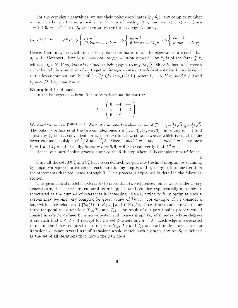
/* L (three loops) */for i = �N to �4for j = �N to �i�N � 4X [rX ] = Y [rY ] + Y [rY + 1]rX = rX + 1rY = rY + 2for i = 1 to Nfor j = �i+N + 1 to NX [rX ] = Y [rY ] + Y [rY + 1]rX = rX + 1rY = rY + 2for i = N � 2 to Nfor j = �i+N � 2 to �i+NX [rX ] = Y [rY ] + Y [rY + 1]rX = rX + 1rY = rY + 2 Figure 8: Figure 7 continued.1000

10

50

N

execution time(seconds)

4000

original loop

transformed loop

1000

1

5

N

speedup

4000Figure 9: Execution times for the initial and �nal programs and the resulting speedup.18