The Multi-Target Monopulse CRLB for MatchedFilter Samples

Peter Willett, William Dale Blair and Xin Zhang

Abstract— It has recently been found that via jointly processingmultiple (sum, azimuth- and elevation-difference) matched filtersamples it is possible to extract and localize several (more thantwo) targets spaced more closely than the classical interpretationof radar resolution. This paper derives the Cramer-Rao lowerbound (CRLB) for sampledmonopulse radar data. It is worth-while to know the limits of such procedures; and in additionto its role in delivering the measurement accuracies requiredby a target tracker, the CRLB reveals an estimator’s efficiency.We interrogate the CRLB expressions for cases of interest. Ofparticular interest are the CRLB’s implications on the numberof targets localizable: assuming a sampling-period equal to arectangular pulse’s length, five targets can be isolated betweentwo matched filter samples given the target’s SNRs are known.This reduced to three targets when the SNRs are not known, butthe number of targets increases back to five (and beyond) when adithered boresight strategy is used. Further insight to the impactof pulse shape and of the benefits of over-sampling are given.

I. I NTRODUCTION

Conventional monopulse-ratio radar signal processing isappropriate to the case that only one target falls in a givenresolution cell, meaning that each matched filter sample cancontain energy from at most one target. If the returns fromtwo or more unresolved targets fall in the same range bin andbeam, the measurements from these targets become merged,and conventional processing fails [1][8][24][25]. The case oftwo unresolved targets and a single (complex) matched filtersample has been studied extensively: Peebles and Berkowitz[22] modify the antenna configuration to aid in the resolutionprocess, while Blair and Brandt-Pearce [5][6][7] develop aform of complex monopulse ratio processing. In [26] Sinhaet al. present a numerical maximum likelihood (ML) angleestimator for both Swerling I and III targets; comparison ofthe monopulse ratio and ML approaches is given in [29], andit is there shown that the iterative ML of [26] could in factbe explicit. It can be shown, using the approach of [32], thatthe above can identify no more than two targets; this limitis imposed by the lack of observation information diversitywithin their models, which represent the case of two targetsboth located at the matched filter sampling point. In fact, thisassumption limits the applicability of these results for realworld problems.

Much more recently, Farina et al. [10] and Gini et al.[12][13] develop a method to jointly estimate complex ampli-tudes, Doppler frequencies and DOA of multiple unresolvedtargets for a rotating radar, again with only one receivingchannel. Their method utilizes the spatial diversity by the

nature of a rotating radar to detect and localize more thantwo targets; its processing strategy is similar to that of [32].Brown et al. [9] explore spatial diversity for a monopulse radarto estimate the DOA of more than two unresolved targets —this is the “dithering” idea that we shall investigate further inthis paper.

With the exception of [9], the above consider radar returnsat only one matched filter sampling point; that is, the targetsare assumed to be located exactly where the matched filter issampled, and hence that there is no “spillover” of target energyto adjacent matched filter returns. However, it was recentlyfound [32][33] that target spillover ought to be considered: infact, using two matched filter samples, it was found that upto five targetsmight be discerned; and similarly more targetswhen more matched filter samples entered the processing.

It is important to know the accuracies of radar measure-ments, since usually such measurements are to be provided toa target tracker [2][3][4]; most high quality trackers need toknow how accurate their data is in order that it be given an ap-propriate weight. Extensive results on single target monopulseestimation accuracy are available [15][16][19][20][21][30].The unresolved case has also recently been treated recently:Blair et al. [5][6][7] analyze the estimation accuracies for theirmonopulse ratio based estimator of two unresolved targets,while Sinha et al. [26] also derive a CRLB for the ML basedestimator. Farina, Gini and Greco [10] and [12] developedmulti-target CRLBs for their rotating radar model. A keyconcern in this paper is the possible benefit, in terms ofresolution of closely-spaced targets, of over-sampling radarreturn data.

From the above, we have a well-developed literature forboth estimators and their accuracies forsingle-target/singlematched filter samplemonopulse data. We also have a goodrepresentation fortwo-target estimators and their associatedbounds/accuracies froma single matched filter sample. Wenow have estimators formultiple targetsandmultiple matchedfilter samples; this paper presents the associated CRLB.

It is important to recognize the limits imposed by sampling:a CRLB for one – or many – targets based on waveform(i.e., continuous-time) data is available from [28]. But basedon such waveform data the number of targets discernibleseems only to be limited by the SNR; whereas the many ofthe results quoted above indicate that from sampled matchedfilter data the number becomes very much circumscribed.Conversely, however, the traditional viewpoint is that targetsmust be resolved in range, via high-bandwidth waveforms

2

and matched filter sampling at high time-bandwidth products;whereas the newer joint-bin processing results [32] indicatethat this traditional intuition deserves a rethinking. Is it SNR,bandwidth or sampling frequency that is most important to theisolation of multiple targets?

In Section II, a general statistical model is given for themonopulse return, matched filtering, sampling and the noisecorrelation due to oversampling. Section III derives the CRLBfor the estimation of the unresolved target locations with themodel formulated in Section II. With the CRLB as our majortool, Section IV studies the effects of various pulse shapesand various sampling rates on the performance of the rangeand electronic angle extractions, in the case of known targetstrengths. The cross-correlations between angles and rangesfrom multiple targets are also explored. Section V concentrateson the case where target strengths are unknown, that is, theyare also estimated. In Section VI, we consider the effect ofthe two-way (transmit and receive) antenna pattern and theantenna-steer direction. The CRLB accounting for these effectsare developed and tested under various conditions. Summarycomments given in Section VII.

II. M ODELING

A. Waveforms and Matched Filter Samples

Let us assume that the transmitted signal has unit-energycomplex pulse shapep(t) (for example, a rectangular pulse),and that there areN targets illuminated within the radar beam,as shown in Figure 1. These are assumed to bepoint-targets,and hence we model the return from thekth target asAp(t−τk), in whichA is a complex random variable withE{Ak} = 0and E{|Ak|2} = σ2

k denoting the strength, whileτk is theround-trip delay of the radar waveform. In the monopulse case,we have three channels

xs(t) =N∑

k=1

Akp(t− τk) + ns(t)

xda(t) =N∑

k=1

Akηakp(t− τk) + nda(t)

xde(t) =N∑

k=1

Akηekp(t− τk) + nde(t) (1)

referring respectively to the return on the antennasum,azimuthal- and elevation-differencechannels1. In (1) ns(t),nda(t) and nde(t) are complex white Gaussian noises withrespective power spectral densitiesσ2

s , σ2da and σ2

de. The“electronic” monopulse anglesηak and ηek denote the off-boresight excursion of thekth target, respectively in azimuthand elevation, and are limited to unity in their magnitude:according to fairly standard modeling (e.g., [7], [32] etc.) theseelectronic angles can easily be related to the true off-boresightangles through knowledge of the antenna beam-patterns.

The next step is, of course, matched filtering: each of thethree random processes in (1) is passed through a filter with

1As a practical matter the sum and difference “channels” may not reallyexist until after matched filtering and digital processing; but to consider themas random processes is convenient.

impulse responseh(t)2, and we thus have

s(t) = xs(t) ? h(t)∗ =N∑

k=1

Akq(t− τk) + νs(t)

da(t) = xda(t) ? h(t)∗ =N∑

k=1

Akηakq(t− τk) + νda(t)

de(t) = xde(t) ? h(t)∗ =N∑

k=1

Akηekq(t− τk) + νde(t)(2)

in which ? denotes convolution,q(t) ≡ p(t) ? h(t), r(t) ≡h(t) ? h(t), and theν’s represent independent complex Gaus-sian random processes that are no longer white3. After sam-pling at rate1/∆ Hz we have

s(i) =N∑

k=1

Akq(i∆− τk) + νs(i)

da(i) =N∑

k=1

Akηakq(i∆− τk) + νda(i)

de(i) =N∑

k=1

Akηekq(i∆− τk) + νde(i) i = 1, 2, 3, . . .(3)

in which for convenient notation (i.e., to avoid carrying∆’salong) we have removed thetildes: for example, we uses(i) ≡ s(i∆). At an operational level the goal would be toestimateΘ = {τk, ηak, ηek}N

k=1 given thatN and {σ2k}N

k=1

are known; and more generally to estimate these too. In thispaper we are not so much interested in this estimation thanin its performance limits – estimation is treated in [32]. Butnote that (6) allows for sampling beyond the Nyquist rate:the noise samples in the time-series become autocorrelated. In[32] Nyquist sampling is assumed, such that all noise samplesare independent (Figure 2).

B. The Joint Probability Density and the Correlation Matrix

For notational reasons we construct the observation vectorzl for the lth pulse as

zl = [s(1) . . . s(M) da(1) . . . da(M) de(1) . . . de(M)]T

(4)in which M is the total number of samples. The vectorzl isGaussian, with zero mean and correlation matrixE {

zlzHl

}=

R having elements as given in

E{s(i)s(j)∗} =∑N

k=1σ2

kq(i∆−τk)q(j∆−τk)∗ + σ2sr((i−j)∆)

E{s(i)da(j)∗} =∑N

k=1σ2

kηakq(i∆−τk)q(j∆−τk)∗ (5)

E{s(i)de(j)∗} =∑N

k=1σ2

kηekq(i∆−τk)q(j∆−τk)∗

E{da(i)da(j)∗} =∑N

k=1σ2

kη2akq(i∆−τk)q(j∆−τk)∗ + σ2

dar((i−j)∆)

E{da(i)de(j)∗} =∑N

k=1σ2

kηakηekq(i∆−τk)q(j∆−τk)∗

E{de(i)de(j)∗} =∑N

k=1σ2

kη2ekq(i∆−τk)q(j∆−τk)∗ + σ2

der((i−j)∆)

2For the case that there is no Doppler shift we useh(t) = p(−t)∗, wherethe asterisk superscript means complex conjugation. To allow more freedomin the derivation – specifically to interrogate the effect of a Doppler shift –we keep the filter ash(t).

3Unless we are interested in Doppler information, we takeh(t) = p(−t)andr(t) = q(t).

3

For the case of a rectangular-envelope transmitted pulse andno Doppler shift, bothq(t) and r(t) are triangular pulses ofduration twice the pulse length; and∆ is the sampling interval.Construction of the matrixR from (6) is according to

R =

E{s(i)s(j)∗} E{s(i)da(j)∗} E{s(i)de(j)∗}. .. E{da(i)da(j)∗} E{da(i)de(j)∗}. ..

.. . E{de(i)de(j)∗}

(6)in which

E{s(i)de(j)∗} ≡ (7)

E{s(1)de(1)∗} E{s(1)de(2)∗} . . . E{s(1)de(M)∗}E{s(2)de(1)∗} E{s(2)de(2)∗} . . . E{s(2)de(M)∗}

.... ..

. . ....

E{s(M)de(1)∗} E{s(M)de(2)∗} . . . E{s(M)de(M)∗}

with similar construction for the other blocks inR. We havethe joint probability density function (pdf) [31]

p(zl) =1

|πR| exp(−zH

l R−1zl

)(8)

for the returns from thelth pulse, and note that the dependenceof this pdf onΘ is implicit through the correlation matrixR.For the case of a Swerling II target (e.g., [17]), we have

p ({zl}) =1

(|πR|)Pexp

(−

P∑

l=1

(zl)T R−1zl

)(9)

since allP pulses are independent.

III. T HE CRLB AND ITS DETERMINATION

A classical result is the Cramer-Rao lower bound (CRLB)(e.g. [27], [18]) for mean-square error of an unbiased esti-mator. Let us assume access to an observationZ which hasprobability density function (pdf)p(Z; Θ), meaning that thepdf depends on a parameter vectorΘ which is to be estimated.Then under fairly broad regularity conditions the CRLB hasit that

E{[

Θ(Z)−Θ] [

Θ(Z)−Θ]T

}≥ J−1 (10)

in which

J ≡ E{

[∇Θ log (p(Z; Θ))] [∇Θ log (p(Z; Θ))]T}

(11)

is Fisher’s information matrix (FIM) andΘ(Z) is any un-biased estimator. Again under broad regularity conditions, ifa maximum-likelihood estimator (MLE) forx exists, then itachieves the CRLB asymptotically. From [23] (among others,the result is widely available), we have for theP -pulse case

Jm,n = 2PTr

(R−1

(∂R∂θm

)R−1

(∂R∂θn

))(12)

as a neat expression for an arbitrary element of the FIM. Recallthat θn ∈ Θ is any parameter of interest, such as monopulseelectronic angle or delay. Note that the derivatives are easy toderive from (6).

IV. CASE OFKNOWN TARGET STRENGTHS

In the following section we explore (12) for various casesand parameters. Note that since the number of pulses appearsmultiplicatively it affects only scaling, and hence with littleloss in generality we chooseP = 1. We also see that allresults can be taken relative to the pulse length; for example,if the error is 50 m with a pulse length of 1000 m, then apulse length of 100 m would yield an accuracy of 5 m. Finally,when we discuss accuracy we primarily explore the case oftwo targets only.

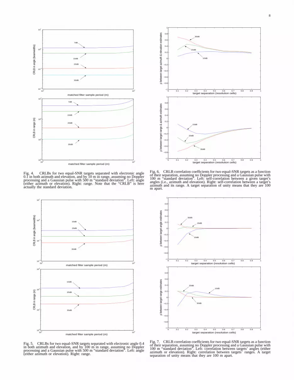
In Figure 3 we plot the CRLB4 for range and for electronicangle using a 1000 m rectangular pulse (i.e.,cT = 1000 m, orwith pulse duration approximately3.3µs). In Figure 4 the sameplots and parameters persist, except here the pulse shape isGaussian with 95% of its energy in a 1000 m swath. For rangeresolution it appears that while the Gaussian pulse exhibits a“floor” below which finer matched filtering sampling offersno improvement, the rectangular pulse appears to continueto improve as matched filter sampling effort increases. Thisis a manifestation of the Nyquist rate and the bandwidth forthe two signals: since the rectangular pulse is sharp, detailedrange information is obtainable from looking for its peakswith increasing closeness. In fact, the rectangular pulse maynot be realistic, given the bandwidth constraints of a practicalradar system; we do not continue with the rectangular pulse. InFigure 3 we also plot some results of likelihood maximizationaccording to [32], and it appears that the CRLB is a reasonableproxy for obtainable estimation accuracy. It is interestingthat there appears to be no reason for finer sampling thanapproximately twice as often as would be suggested by thepulse length. In Figure 5 we show the case for targets thatare further separated than in Figure 4. Remarkably, it appearsthat the performance is somewhat worse, indicating that thereis some mutual benefit to the targets’ proximity (close targetscan be better estimated than ones far away from each other).

The CRLB also provides information on estimation cross-covariance in the off-diagonal terms ofJ−1. To explore this,we allow two targets to “approach” one another from oppositeends of the resolution cell; they are constrained to lie on astraight (diagonal) line joining the pointsηa = ηe = −1 andmatched filter samplen; and ηa = ηe = 1 and matchedfilter sample n + 1. Figure 6 shows correlations betweeneach target’s estimates; that is, between either of the target’sazimuth and elevation estimates, and between its azimuthand range estimates, and the strength of these correlations issurprising. That the azimuth and elevation angular estimatesfor a single target should be correlated was observed in [30],but it is interesting here to see that as two targets coalesce,the correlation becomes greater still. Figure 7 shows cross-correlations between angles and ranges (i.e., between theangle estimate for one target and that for the other, andcorrespondingly for the ranges). These interactions appear tobe fairly light, and especially so for stronger targets.

In Figure 8 we hold the matched filtering effort and target

4In the figures we (ab)use “CRLB” to refer to standard deviation, meaningthe square root of the corresponding diagonal entry of the inverse of the Fisherinformation matrix.

4

type fixed – two 30dB targets separated by 10 m, and matchedfilter samples taken every 100 m – and vary the pulse, bothits type and its length. When the pulse length matches thesampling effort (100 m), it appears that in terms of rangeestimation most pulses are equivalent. On the other hand, whenthe pulses are long, the higher-bandwidth binary phase-codedpulse (Barker [17]) is better. However, it is interesting thatthe angle-estimation performance of all waveforms benefitsfrom a lower-bandwidth pulse, as is clear from the left panelof Figure 8. (Note that the raised cosine pulse exhibits poorrange estimation when the pulse length is equal to the samplinginterval: detailed investigation has shown that this is causedby cases in which the targets are close to the matched filtersampling points – the raised cosine’s excessive flatness inhibitsgood range estimation in these cases, and these cases tendto dominate the averaged CRLBs.) Turning to Figure 9, wehave the same situation for matched filters sampled with tentimes the effort. We focus particularly on the Barker plot,and it appears that with such a heavily sampled waveform theBarker waveform’s extra bandwidth does pay off. However, theangular estimation ability of the coded pulse remains seriouslyimpaired.

A singular CRLB means that estimation is not possible. InFigure 10 we show the largest diagonal element of the CRLBplotted against number of targets, and for various combinationsof signal types and sampling rates: for example, “rcos/4”means thatp(t) for the signal is a raised cosine, and thatthe sampling rate is four times per pulse. From this plot weobserve that with a single sample per pulse length up to fivetargets are estimable – this is as reported in [32]. We alsosee that there is a considerable degradation in performancewhen one attempts to estimate the locations of this manytargets: five targets is clearly on the edge of estimability. Ifthe sampling rate is twice the pulse length (oversampling bya factor of two), then it would appear that up to nine targetsare estimable via a rectangular pulse – oversampling was notexplored in [32]. Indeed, this number stretches to the mid teensif the oversampling factor is again doubled (to four), althoughthe quality of these estimates makes them questionable. Wealso find, perhaps surprisingly, that the smooth raised-cosinepulse is apparently much more effective at delivering multipletargets’ estimates than is the rectangular pulse, at least whenthe matched filter is oversampled.

The CRLB can also be used to predict estimability for casesin which the targets stretch over a range swath that exceedsa single pulse length. The results are less easy to plot, but itis found, with targets distributed in a range as long as twopulse lengths, that up to five targets in the first length (bin) orup to five in the second; but not both. That is, with numbersindicating the quantities of targets estimable in the first andsecond bins, (5,4) is possible, as is (4,5); but (5,5) is not.In fact, this exceeds the results of [32], which conservativelyshowed that (4,4) was the most targets that could be localized.

V. CASE WHERE TARGET STRENGTHS AREESTIMATED

Reference [32] assumed that all target radar cross sections(i.e., SNRs) are known; and for the most part they were

assumed equal, too. While it is not unreasonable to estimateor track these, there are many cases in which the targetSNRs cannot be reliably known a-priori. In this section weexplore the impact of unknown SNR by assuming that theparameters to be estimated – nominally target range, azimuth-and elevation-angles to this point – are augmented by SNRs:everything is estimated. In fact, the CRLB expression of(12) is general enough to accommodate this new model; butinstead of estimating3K parameters (K being the number oftargets) the FIMJ is now 4K × 4K. The correlations in (6)explicitly show the{σ2

k}Kk=1, and the requisite differentiation

is straightforward.In Figures 11 and 12 we show the CRLBs, respectively

in angle and in range, for the case that the target SNRsmust be estimated. The left parts of these figures are directlycomparable with Figure 5: there is clearly some loss fromthe need to estimate the SNR, but that loss is manageable.Figure 13 shows the CRLB for estimation of the target SNR,and these, given that they are based on a single pulse, seemappropriately large. The left parts of Figures 11, 12 and 13show the case that the true SNRs of the two targets areidentical; the right parts present the case that the SNR of targettwo is ten times that of target one – recall that the CRLBs ofthe first target are in all cases those reported. It is interestingthat the localization for the first target is actuallyimprovedby a more powerful (and presumably more estimable) secondtarget, and while there is some loss in the quality of the targetRCS estimate, this loss appears negligible.

It would appear from these figures that there is little costassociated with estimation of the SNRs. Unfortunately, we alsohave Figure 14, showing the relative CRLBs for location as afunction of the number of targets between two matched filtersampling points, and to be compared to Figure 10. Apparentlythe need to estimate targets’ SNRs requires its price paid interms of the number of targets that can be estimated: forexample, when matched filter samples are taken one pulselength apart, onlythree targetscan be estimated if the SNRis unknown, rather thanfive for the known-SNR case. Figure14 refers to the case that the maximum separation between alltargets is less than one pulse length; a separate result for thetwo-pulse-length case shows that up to three per pulse lengthare possible (a total of six); note that this – up to (3,3) – is tobe compared to (4,5) and (5,4) in the known-SNR case.

VI. CASE WITH BEAM PATTERN CONSIDERED

In the previous analysis we have assumed that the sum-channel power observed by the radar is independent of thetarget’s bearing, as long as the target is within the beam.However, real radar antennas do have a response pattern. Assuch, let us now modify (3) to

s(i) =∑N

k=1Ak|G(ηak−ηa0,ηek−ηe0)|2q(i∆−τk) + νs(i) (13)

da(i) =∑N

k=1Akηak|G(ηak−ηa0,ηek−ηe0)|2q(i∆−τk) + νda(i)

de(i) =∑N

k=1Akηek|G(ηak−ηa0,ηek−ηe0)|2q(i∆−τk) + νde(i)

in which |G(ηak − ηa0, ηek − ηe0)|2 denotes the effect of thetwo-way (transmit and receive) antenna pattern for a targetwhose (electronic-angle) bearing is(ηak, ηek) and for which

5

the basic antenna-steer direction is(ηa0, ηe0). In SubsectionsVI-A and VI-B, we will take (ηa0, ηe0) = (0, 0), since allpulses may be considered as resulting from an antenna pointedthe same direction; but in Subsection VI-C we shall departfrom this, with interesting results.

In light of (13), we now have

E{s(i)s(j)∗} (14)

=∑N

k=1σ2

k|G(ηak−ηa0,ηek−ηe0)|4q(i∆−τk)q(j∆−τk)∗

+ σ2sr((i−j)∆)

E{s(i)da(j)∗} (15)

=∑N

k=1σ2

kηak|G(ηak−ηa0,ηek−ηe0)|4q(i∆−τk)q(j∆−τk)∗

E{s(i)de(j)∗} (16)

=∑N

k=1σ2

kηek|G(ηak−ηa0,ηek−ηe0)|4q(i∆−τk)q(j∆−τk)∗

E{da(i)da(j)∗} (17)

=∑N

k=1σ2

kη2ak|G(ηak−ηa0,ηek−ηe0)|4q(i∆−τk)q(j∆−τk)∗

+ σ2dar((i−j)∆)

E{da(i)de(j)∗} (18)

=∑N

k=1σ2

kηakηek|G(ηak−ηa0,ηek−ηe0)|4q(i∆−τk)q(j∆−τk)∗

E{de(i)da(j)∗} (19)

=∑N

k=1σ2

kη2ek|G(ηak−ηa0,ηek−ηe0)|4q(i∆−τk)q(j∆−τk)∗

+ σ2der((i−j)∆) (20)

for the correlations; (12) still holds, but now the derivativesin (20) with respect to{ηak, ηek}K

k=1 are more complicated.We need a realistic example on which to present results, andfollowing [7] and [29] we will take the beam pattern

|G(ηa−ηa0,ηe−ηe0)|4= cos4((ηa−ηa0)π/(4ηbw)) cos4((ηe−ηe0)π/(4ηbw)) (21)

× I(|ηa−ηa0|<1)I(|ηe−ηe0|<1)

in which ηbw is a beamwidth parameter for which we shallinsertηbw = 0.8, andI(·) denotes the indicator function. Thisis plotted in one dimension in Figure 15.

A. Known Target Strengths

We consider first the case that the target strengths are known– in fact, we expect that the most significant improvementswill be observed for unknown SNR, since the beampatterninformation is strongest in its effect on return amplitude, butthese results are most comparable with the extensive onespresented earlier in section IV. In Figure 16 we show theCRLBs for range and angle with beampattern considered – tobe compared to Figure 5 (no beampattern) – and there appearsto be little difference. Comparing Figure 17 to Figure 10 –describing estimation bounds on number of targets respectivelywith and without beampattern considered – we again find littleimprovement, although with matched filter samples taken onepulse length apart it now appears that five targets is morea matter of course. For the case that targets are distributedamong two pulse lengths, the critical operating points remain(5,4) and (4,5).

B. Unknown Target Strengths

We next examine the case that target strengths are unknownand must be estimated; can knowledge of the beampattern help

here? It turns out that in terms of estimation of location (i.e.,range and angle) there is little difference: the plots look verysimilar to those in Figures 11 and 12. However, when thetargets’ SNRs are estimated we get Figure 18, and it appearsthat there is almost a factor of two improvement in SNRestimation when there is beampattern information.

Since target strengths are necessary to discern the numberof targets, we expect better results in this also. ComparingFigure 19 to Figure 14 we find that with beampattern effectsconsidered a rectangular pulse can extractfour targets ratherthan three, with matched filter samples every pulse length;and likewise a more-reliable seven targets with double thesampling effort. For the case that targets are distributed amongtwo pulse lengths, the critical operating points are now (4,3)and (3,4), as opposed to (3,3) when the beampattern is uniform(and ignored).

C. Unknown Target Strengths with Multiple Beam Steers

In the previous sections we have observed that knowledgeand incorporation of the beampattern is quite helpful: if thebeampattern is considered, then the sum channel, in additionto the difference channels, contains direct angular information;however, it remains difficult to distinguish a weak target froma strong one that is at the beam edge. The authors in [9]attacked this by suggesting that monopulse target detectionand localization ought to be based on data from multiple steerdirections: the idea is illustrated in Figure 20.

Consider Figure 21, and suppose that the angular locationsof the targets (theη’s) are well-estimated – we have seenthat even unknown SNR is not a barrier to estimation oflocation; but that estimated SNRs are not good, and that theaccompanying problem of ascertainment of target number (see[32]) is hence a concern. In Figure 21 we have that the firstboresight results in equal response patterns (say, 75%), whileusing the second boresight the responses are 50% for target 1and 100% for target 2. If the total (sum-channel) returns for thetwo cases were respectively 300 and 360 and we ignore (forthe purposes of this discussion) thermal noise, we have that theamplitude of the returns are respectively 80 and 320. Withoutmultiple boresights there would be no way to disambiguatethe target’s return strengths.

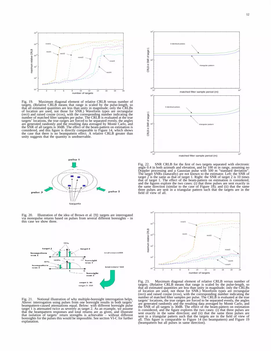
Figure 22 shows the effects of multiple-boresight pulses onestimation of target SNRs – here we use three pulses in atriangular pattern, each with an offset of 20% beamwidth. Wesee that the triangular pattern offers improvement over the“staring” (i.e., three pulses with the same boresight) pattern,and this improvement becomes impressive as the distancebetween matched filter samples approaches the pulse length.

Comparing Figure 23 to Figures 19 and 14, we find thatwith scattered multi-pulse boresights a rectangular pulse canextract as many assix targets– rather than four with beam-pattern effects and constant boresight, and three with uniformbeampattern – with matched filter samples every pulse length;and likewise a more-reliable seven targets with double thesampling effort. For the case that targets are distributed amongtwo pulse lengths, the critical operating points are now (6,4),(5,5) and (4,6), as opposed to (4,3)/(3,4) (constant boresight)and (3,3) (beampattern ignored).

6

VII. C ONCLUSIONS

It has recently become clear that, by consideration of thelikelihood function of multiple matched filter samples in ajointfashion, it is possible to extract and localize a suprising numberof closely spaced targets using monopulse observations. Forexample, it had been found that five targets could be distin-guished from among two matched filter samples taken onepulse length apart. Viewing monopulse returns from a purelystatistical perspective – as opposed to confining attention tothe real part of the monopulse ratio – appears promising, andit seems worthwhile to ask its limits. The natural vehicle forlimits is the CRLB. There have been numerous treatmentsof the CRLB for monopulse data, but few have focused onthe multiple target case, nor the realistic case that all thatis available is sampled matched filter data, as opposed towaveform returns.

In this paper we have developed an exact simple expressionfor the CRLB for sampled monopulse radar, and we haveinterrogated it for many multitarget cases of interest. Generallythe results depend on true target locations, and we haveaveraged over these in the Monte Carlo sense. Among ourfindings we have:

• For a smooth basic radar pulse, there can be improve-ment for fine matched filter sampling as opposed to thestandard once-per-pulse-length sampling strategy. Notethat with such fine sampling the thermal noise becomescorrelated, and our analysis incorporates this.

• For a rectangular pulse this trend of improvement doesnot appear to end, presumably due to its large bandwidth.In practice a perfect rectangular pulse is not achievable.

• When targets are close their estimates are bound to becorrelated, and we have quantified this for the case of twotargets. We find that results depend both on proximity andSNR. It appears that the appearance of a second target cansignificantly increase dependence among a given target’sestimated parameters, but that the correlationbetweentargets is light.

• Taking the Barker-7 pulse (rectangular subpulses) asa proxy for coded pulses, it appears that while the“thumbtack” ambiguity function is appealing, that evenwith optimal likelihood function processing coded (high-bandwidth) waveforms do offer some improvement inrange resolution. However, it appears that such wave-forms can affect angular estimation quite negatively inthe multiple target situation.

• While it is confirmed that five targets can be isolatedwithin two pulse lengths when matched filter samplesare taken one pulse length apart, it appears that manymore are isolatable for finer sampling. For example,with double the matched filter sampling effort and arectangular pulse up to nine targets appear resolvable;and even more with a smoother pulse.

• When the target SNRs are not known, the previous fiveresolvable targets drops to three: when the target SNRparameters need estimation, other parameters must beremoved from the problem.

• If the beampattern shape is also considered, the number

of targets estimatable increases from three to four. Anonuniform beampattern offers additional clues for targetlocalization.

• If monopulse measurements are taken from slightly dif-ferent boresight perspectives (we use a triangular pat-tern with boresights offset by 20% beamwidth), thenby correlating the return strength information from thevarious viewpoints additional information is available,information particularly relating to the targets’ SNRs. Theresult is that even if the SNRs are unknown, as many assix targets appear resolvable, even more than the originalfive of the known-SNR but uniform-beampattern case.

It appears that use of increased sampling rate and ditheredboresight are particularly attractive, and development of algo-rithms to estimate using these is currently underway.

7

REFERENCES

[1] S. J. Asseo, “Detection of Target Multiplicity Using Monopulse Quadra-ture Angle”, IEEE Transactions on Aerospace and Electronic Systems,Vol. 17, pp. 271-280, March 1981.

[2] Y. Bar-Shalom, X. Li, and T. Kirubarajan,Estimation with Applications,Tracking and Navigation, New York: Wiley, 2001.

[3] Y. Bar-Shalom, and X. Li,Multitarget-Multisensor Tracking: Principlesand Techniques, Storrs, CT: YBS Publishers, 1995.

[4] S. Blackman and R. Popoli,Design and Analysis of Modern TrackingSystems, Boston, MA: Artech House, 1999.

[5] W. D. Blair, and M. Brandt-Pearce, “Unresolved Rayleigh Target Detec-tion Using Monopulse Measurements”,IEEE Transactions on Aerospaceand Electronic Systems, pp. 543-552, April 1998.

[6] W. Blair, and M. Brandt-Pearce, “Statistical Description of MonopulseParameters for Tracking Rayleigh Targets”,IEEE Transactions onAerospace and Electronic Systems, pp. 597-611, April 1998.

[7] W. D. Blair and M. Brandt-Pearce, “Monopulse DOA Estimation ofTwo Unresolved Rayleigh Targets”,IEEE Transactions on Aerospaceand Electronic Systems, Vol. AES-37, pp. 452-469, April 2001.

[8] P. L. Bogler, “Detecting the Presence of Target Multiplicity”,IEEETransactions on Aerospace and Electronic Systems, Vol. 22, pp. 197-203, March 1986.

[9] G. C. Brown, W. D. Blair, T. Ogle and A. H. Register, “StatisticalAOA Estimates with Merged Measurements from Monopulse Data”,Proceedings of the SPIE Conference on Signal and Data Processingof Small Targets, August 2003, San Diego, CA.

[10] A. Farina, F. Gini and M. Greco, “DOA Estimation by Exploiting theAmplitude Modulation Induced by Antenna Scanning”,IEEE Transac-tions on Aerospace and Electronic Systems, Vol. AES-38, pp. 1276-1286,October 2002.

[11] A. Gelb, Applied Optimal Estimation, TASC Press, 1974.[12] F. Gini, M. Greco and A. Farina, “Multiple Radar Targets Estimation

by Exploiting Induced Amplitude Modulation”,IEEE Transactions onAerospace and Electronic Systems, Vol. AES-39, pp. 1316-1332, October2003.

[13] F. Gini, F. Bordoni and A. Farina, “Multiple Radar Targets Detectionby Exploiting Induced Amplitude Modulation”,IEEE Transactions onSignal Processing, Vol. SP-52, pp. 903-913, April 2004.

[14] G. Golub and C. Van Loan,Matrix Computations, 2nd edition, JohnsHopkins Press, 1989.

[15] E. Hofstetter and D. DeLong, “Detection and Parameter Estimation inan Amplitude-Comparison Monopulse Radar”,IEEE Transactions onAerospace and Electronic Systems, January 1969.

[16] D. Kehr, “Variance Analysis of the Angle Output Voltage for anAmplitude Monopulse Receiver,”IEEE Transactions on Aerospace andElectronic Systems, Vol. 4, July 1968.

[17] N. LevanonRadar Principles, Wiley, 1988.[18] L. Ljung, System Identification: Theory for the User, Prentice-Hall,

1987.[19] E. Mosca, “Angle Estimation in Amplitude Comparison Monopulse

System”,IEEE Transactions on Aerospace and Electronic Systems, Vol.5, No. 2, pp. 205-12, March 1969.

[20] U. Nickel, “Monopulse Estimation with Adaptive Arrays”,IEEProceedings-F, Vol. 140, No. 5, pp. 303-308, 1993.

[21] U. Nickel, “Performance of Corrected Adaptive Monopulse Estimation”,IEE Proceedings Part F, February 1999.

[22] P. Peebles, and R. Berkowitz,“Multiple-Target Monopulse Radar Pro-cessing Techniques”,IEEE Transactions on Aerospace and ElectronicSystems, Vol. 4, pp. 845-54, November 1968.

[23] B. Porat,Digital Processing of Random Signals,Prentice-Hall, 1994.[24] S. Sherman,Monopulse Principles and Techniques, Artech House, Inc.,

MA, 1984.[25] S. Sherman,“Complex Indicated Angles Applied to Unresolved Radar

Targets and Multipath”,IEEE Transactions on Aerospace and ElectronicSystems, Vol. 7, No. 1, pp. 160-170, January 1971.

[26] A. Sinha, T. Kirubarajan and Y. Bar-Shalom, “Maximum LikelihoodAngle Extractor for Two Closely Spaced Targets”,IEEE Transactions onAerospace and Electronic Systems, Vol. 38, No. 1, pp. 183-203, January2002.

[27] H. Van Trees,Detection, Estimation, and Modulation Theory, Volume1, Wiley, 1968.

[28] H. Van Trees,Detection, Estimation and Modulation Theory: Part III,Wiley, 1971.

[29] Z. Wang, A. Sinha, P. Willett and Y. Bar-Shalom, “Angle Estimation forTwo Unresolved Targets with Monopulse Radar”IEEE Transactions onAerospace and Electronic Systems, Vol. 40, No. 3, pp. 998-1019, July2004.

[30] P. Willett, W.D. Blair and Y. Bar-Shalom, “On the Correlation BetweenHorizontal and Vertical Monopulse Measurements”,IEEE Transactionson Aerospace and Electronic Systems, April 2003.

[31] R. Wooding, “The Multivariate Distibution of Complex Normal Vari-ates,”Biometrika, Vol. 43, pp. 212-215, 1956.

[32] X. Zhang, P. Willett and Y. Bar-Shalom, “Monopulse Radar Detectionand Localization of Multiple Unresolved Targets via Joint Bin Process-ing”, IEEE Transactions on Signal Processing, Vol. 53, No. 4, pp. 1225-1236, April 2005.

[33] X. Zhang, P. Willett and Y. Bar-Shalom, “Monopulse Radar Detectionand Localization of Multiple Targets via Joint Multiple-Bin Processing”,Proceedings of IEEE Radar Conference, Huntsville AL, May 2003.

Fig. 1. Idea of using radar returns at two consecutive matched filter samplingpoints for angle extraction and multi-target detection.

Fig. 2. Illustration of the model of targets located betweenL (L ≥ 3)sampling points. This figure corresponds to a rectangular pulse for which theoutput of a matched filter for a single point target is triangular.

102

103

10−2

10−1

100

101

matched filter sample period (m)

CR

LB in

ang

le (b

eam

wid

ths)

7dB

10dB

20dB

30dB

20dB simulation

102

103

100

101

102

103

matched filter sample period (m)

CR

LB in

rang

e (m

)

7dB

10dB

20dB

30dB

20dB simulation

Fig. 3. CRLBs for two equal-SNR targets separated with electronic angle 0.1in both azimuth and elevation, and by 10 m in range, assuming no Dopplerprocessing and a 1000 m rectangular pulse. Left: angle (either azimuth orelevation). Right: range. Both figures show simulation results (100 MC trials)using optimization of likelihood according to [32]. Note that the “CRLB” ishere actually the standard deviation.

8

102

103

10−2

10−1

100

101

matched filter sample period (m)

CR

LB in

ang

le (b

eam

wid

ths)

7dB

10dB

20dB

30dB

102

103

100

101

102

103

matched filter sample period (m)

CR

LB in

rang

e (m

)

7dB

10dB

20dB

30dB

Fig. 4. CRLBs for two equal-SNR targets separated with electronic angle0.1 in both azimuth and elevation, and by 10 m in range, assuming no Dopplerprocessing and a Gaussian pulse with 500 m “standard deviation”. Left: angle(either azimuth or elevation). Right: range. Note that the “CRLB” is hereactually the standard deviation.

102

103

10−2

10−1

100

101

matched filter sample period (m)

CR

LB in

ang

le (b

eam

wid

ths)

10dB

20dB

30dB

102

103

100

101

102

103

matched filter sample period (m)

CR

LB in

rang

e (m

)

10dB

20dB

30dB

Fig. 5. CRLBs for two equal-SNR targets separated with electronic angle 0.4in both azimuth and elevation, and by 100 m in range, assuming no Dopplerprocessing and a Gaussian pulse with 500 m “standard deviation”. Left: angle(either azimuth or elevation). Right: range.

0 0.1 0.2 0.3 0.4 0.5 0.6 0.7 0.8 0.9 1−1

−0.8

−0.6

−0.4

−0.2

0

0.2

0.4

0.6

0.8

1

target separation (resolution cells)

ρ be

twee

n ta

rget

azi

mut

h &

elev

atio

n es

timat

es

30dB

20dB

10dB

0 0.1 0.2 0.3 0.4 0.5 0.6 0.7 0.8 0.9 1−1

−0.8

−0.6

−0.4

−0.2

0

0.2

0.4

0.6

0.8

1

target separation (resolution cells)ρ

betw

een

targ

et ra

nge

& az

imut

h es

timat

es

10dB

20dB

30dB

Fig. 6. CRLB correlation coefficients for two equal-SNR targets as a functionof their separation, assuming no Doppler processing and a Gaussian pulse with100 m “standard deviation”. Left: self-correlation between a given target’sangles (i.e., azimuth and elevation). Right: self-correlation between a target’sazimuth and its range. A target separation of unity means that they are 100m apart.

0 0.1 0.2 0.3 0.4 0.5 0.6 0.7 0.8 0.9 1−1

−0.8

−0.6

−0.4

−0.2

0

0.2

0.4

0.6

0.8

1

target separation (resolution cells)

ρ be

twee

n ta

rget

ang

le e

stim

ates

30dB

20dB

10dB

0 0.1 0.2 0.3 0.4 0.5 0.6 0.7 0.8 0.9 1−1

−0.8

−0.6

−0.4

−0.2

0

0.2

0.4

0.6

0.8

1

target separation (resolution cells)

ρ be

twee

n ta

rget

rang

e es

timat

es

30dB

10dB

20dB

Fig. 7. CRLB correlation coefficients for two equal-SNR targets as a functionof their separation, assuming no Doppler processing and a Gaussian pulse with100 m “standard deviation”. Left: correlation between targets’ angles (eitherazimuth or elevation). Right: correlation between targets’ ranges. A targetseparation of unity means that they are 100 m apart.

9

102

103

10−2

10−1

100

101

pulse length (m)

CR

LB in

ang

le (b

eam

wid

ths)

CRLB for 2 targets, SNR=1000

Barker 7

raised cosine Gaussian

rectangular

102

103

10−2

10−1

100

101

102

pulse length (m)

CR

LB in

rang

e (m

)

Barker 7

raised cosine Gaussian rectangular

Fig. 8. CRLB for two 30dB targets separated by 10 m, with matched filterinter-sample distance 100 m, plotted as a function of pulse length, and forvarious pulse types. Left: angle (either azimuth or elevation). Right: range.

101

102

10−2

10−1

100

101

pulse length (m)

CR

LB in

ang

le (b

eam

wid

ths)

raised cosine

Barker 7

101

102

10−2

10−1

100

101

102

pulse length (m)

CR

LB in

rang

e (m

)

Barker 7

raised cosine

Fig. 9. CRLB for two 30dB targets separated by 10 m, with matched filterinter-sample distance 10 m, plotted as a function of pulse length, and forvarious pulse types. Left: angle (either azimuth or elevation). Right: range.As compared to Figure 8, the rectangular and Gaussian plots have beensuppressed to focus on the Barker results.

0 2 4 6 8 10 12 14 16 18 2010

−5

100

105

1010

1015

1020

number of targets

max

imum

rela

tive

CR

LB

rect/1

rcos/1

rect/2 rcos/2

rect/4

rcos/4

Fig. 10. Maximum diagonal element of relative CRLB versus numberof targets. (Relative CRLB means that range is scaled by the pulse-length,so that all estimated quantities are less than unity in magnitude.) Waveformtypes are rectangular (rect) and raised cosine (rcos), with the correspondingnumber indicating the number of matched filter samples per pulse. The CRLBis evaluated at the true targets’ locations, the true ranges are forced to beseparated evenly, the angles are generated randomly and the resulting dataaveraged by Monte Carlo, and the SNR of all targets is 30dB.

102

103

10−2

10−1

100

101

matched filter sample period (m)

CR

LB in

ang

le (b

eam

wid

ths)

10dB

20dB

30dB

102

103

10−2

10−1

100

101

matched filter sample period (m)

CR

LB in

ang

le (b

eam

wid

ths)

10dB

20dB

30dB

Fig. 11. Angular CRLB for the first of two targets separated with electronicangle 0.4 in both azimuth and elevation, and by 100 m in range, assuming noDoppler processing and a Gaussian pulse with 500 m “standard deviation”.The target SNRs are not known to the estimator. Left: the SNR of target 2 isthe same as that of target 1. Right: the SNR of target 2 is 10 times that oftarget 1. This plot is comparable to the left plot in Figure 5.

10

102

103

100

101

102

103

matched filter sample period (m)

CR

LB in

rang

e (m

)

10dB

20dB

30dB

102

103

100

101

102

103

matched filter sample period (m)

CR

LB in

rang

e (m

)

10dB

20dB

30dB

Fig. 12. Range CRLB for the first of two targets separated with electronicangle 0.4 in both azimuth and elevation, and by 100 m in range, assuming noDoppler processing and a Gaussian pulse with 500 m “standard deviation”.The target SNRs are not known to the estimator. Left: the SNR of target 2 isthe same as that of target 1. Right: the SNR of target 2 is 10 times that oftarget 1. This plot is comparable to the right plot in Figure 5.

102

103

100

101

102

103

matched filter sample period (m)

CR

LB in

SN

R o

f tar

get 1

30dB

20dB

10dB

102

103

100

101

102

103

matched filter sample period (m)

CR

LB in

SN

R o

f tar

get 1

30dB

20dB

10dB

Fig. 13. SNR CRLB for the first of two targets separated with electronicangle 0.4 in both azimuth and elevation, and by 100 m in range, assuming noDoppler processing and a Gaussian pulse with 500 m “standard deviation”.The target SNRs (naturally) are not known to the estimator. Left: the SNRof target 2 is the same as that of target 1. Right: the SNR of target 2 is 10times that of target 1.

0 2 4 6 8 10 12 14 16 18 2010

−5

100

105

1010

1015

1020

number of targets

max

imum

rela

tive

CR

LB

rect/1

rcos/1

rect/2

rcos/2 rect/4

rcos/4

Fig. 14. Maximum diagonal element of relative CRLB versus number oftargets. (Relative CRLB means that range is scaled by the pulse-length, sothat all estimated quantities are less than unity in magnitude; only the CRLBsof location are used, not those for SNR.) Waveform types are rectangular(rect) and raised cosine (rcos), with the corresponding number indicating thenumber of matched filter samples per pulse. The CRLB is evaluated at the truetargets’ locations, the true ranges are forced to be separated evenly, the anglesare generated randomly and the resulting data averaged by Monte Carlo, andthe SNR of all targets is 30dB.

11

−2 −1.5 −1 −0.5 0 0.5 1 1.5 20

0.1

0.2

0.3

0.4

0.5

0.6

0.7

0.8

0.9

1

norm

aliz

ed re

spon

se (|

G(η

,ηbw

)|2 )

Fig. 15. The beampatterncos2((ηa − ηa0)π/(4ηbw)) (ηbw = 0.8) used.

102

103

10−2

10−1

100

101

matched filter sample period (m)

CR

LB in

ang

le (b

eam

wid

ths)

10dB

20dB

30dB

102

103

100

101

102

103

matched filter sample period (m)

CR

LB in

rang

e (m

)

10dB

20dB

30dB

Fig. 16. CRLBs for two equal-SNR targets separated with electronic angle0.4 in both azimuth and elevation, and by 100 m in range, assuming noDoppler processing and a Gaussian pulse with 500 m “standard deviation”.Left: angle (either azimuth or elevation). Right: range. The effect of the beam-pattern on estimationis considered, and this Figure is directly comparable toFigure 5, which shows the case that there is no beampattern effect.

0 2 4 6 8 10 12 14 16 18 2010

−5

100

105

1010

1015

1020

number of targets

max

imum

rela

tive

CR

LB

rcos/1

rect/1

rect/2 rcos/2

rect/4

rcos/4

Fig. 17. Maximum diagonal element of relative CRLB versus number oftargets. (Relative CRLB means that range is scaled by the pulse-length, sothat all estimated quantities are less than unity in magnitude; only the CRLBsof location are used, not those for SNR.) Waveform types are rectangular(rect) and raised cosine (rcos), with the corresponding number indicating thenumber of matched filter samples per pulse. The CRLB is evaluated at the truetargets’ locations, the true ranges are forced to be separated evenly, the anglesare generated randomly and the resulting data averaged by Monte Carlo, andthe SNR of all targets is 30dB. The effect of the beam-pattern on estimationisconsidered, and this Figure is directly comparable to Figure 10, which showsthe case that there is no beampattern effect.

102

103

100

101

102

103

matched filter sample period (m)

CR

LB in

SN

R o

f tar

get 1 SNR=30dB

SNR=20dB

SNR=10dB

102

103

100

101

102

103

matched filter sample period (m)

CR

LB in

SN

R o

f tar

get 1 SNR=30dB

SNR=20dB

SNR=10dB

Fig. 18. SNR CRLB for the first of two targets separated with electronicangle 0.4 in both azimuth and elevation, and by 100 m in range, assuming noDoppler processing and a Gaussian pulse with 500 m “standard deviation”.The target SNRs (naturally) are not known to the estimator. Left: the SNR oftarget 2 is the same as that of target 1. Right: the SNR of target 2 is 10 timesthat of target 1. The effect of the beam-pattern on estimationis considered,and this Figure is directly comparable to Figure 13, which shows the casethat there is no beampattern effect.

12

0 2 4 6 8 10 12 14 16 18 2010

−5

100

105

1010

1015

1020

number of targets

max

imum

rela

tive

CR

LB

rcos/1

rect/1 rect/2

rcos/2

rcos/4

rect/4

Fig. 19. Maximum diagonal element of relative CRLB versus number oftargets. (Relative CRLB means that range is scaled by the pulse-length, sothat all estimated quantities are less than unity in magnitude; only the CRLBsof location are used, not those for SNR.) Waveform types are rectangular(rect) and raised cosine (rcos), with the corresponding number indicating thenumber of matched filter samples per pulse. The CRLB is evaluated at the truetargets’ locations, the true ranges are forced to be separated evenly, the anglesare generated randomly and the resulting data averaged by Monte Carlo, andthe SNR of all targets is 30dB. The effect of the beam-pattern on estimationisconsidered, and this figure is directly comparable to Figure 14, which showsthe case that there is no beampattern effect. A relative CRLB greater thanunity suggests that the quantity is unobservable.

Fig. 20. Illustration of the idea of Brown et al. [9]: targets are interrogatedvia monopulse returns based on pulses from several different boresights – inthis case we show three.

Fig. 21. Notional illustration of why multiple-boresight interrogation helps.Above: interrogation using pulses from one boresight results in both targets’beampattern-caused attenuations equal. Below: with different boresight pulsetarget 1 is attenuated twice as severely as target 2. As an example, we assumethat the beampattern responses and total returns are as given, and illustratethat isolation of targets’ return strengths is achievable – without differentboresights for the pulses this would be impossible. See section VI-C for furtherexplanation.

102

103

100

101

102

matched filter sample period (m)

CR

LB in

SN

R o

f tar

get 1

3 identical pulses

triangular pattern

102

103

100

101

102

matched filter sample period (m)

CR

LB in

SN

R o

f tar

get 1

3 identical pulses

triangular pattern

Fig. 22. SNR CRLB for the first of two targets separated with electronicangle 0.4 in both azimuth and elevation, and by 100 m in range, assuming noDoppler processing and a Gaussian pulse with 500 m “standard deviation”.The target SNRs (naturally) are not known to the estimator. Left: the SNR oftarget 2 is the same as that of target 1. Right: the SNR of target 2 is 10 timesthat of target 1. The effect of the beam-pattern on estimationis considered,and the figures explore the two cases: (i) that three pulses are sent exactly inthe same direction (similar to the case of Figure 18); and (ii) that the samethree pulses are sent in a triangular pattern such that the targets are in thefield of view of all.

0 2 4 6 8 10 12 14 16 18 2010

−5

100

105

1010

1015

1020

number of targets

max

imum

rela

tive

CR

LB

rcos/1

rect/1 rect/2

rcos/2

rect/4

rcos/4

Fig. 23. Maximum diagonal element of relative CRLB versus number oftargets. (Relative CRLB means that range is scaled by the pulse-length, sothat all estimated quantities are less than unity in magnitude; only the CRLBsof location are used, not those for SNR.) Waveform types are rectangular(rect) and raised cosine (rcos), with the corresponding number indicating thenumber of matched filter samples per pulse. The CRLB is evaluated at the truetargets’ locations, the true ranges are forced to be separated evenly, the anglesare generated randomly and the resulting data averaged by Monte Carlo, andthe SNR of all targets is 30dB. The effect of the beam-pattern on estimationis considered, and the figure explores the two cases: (i) that three pulses aresent exactly in the same direction; and (ii) that the same three pulses aresent in a triangular pattern such that the targets are in the field of view ofall. This figure is comparable to Figure 14 (no beampattern) and Figure 19(beampattern but all pulses in same direction).