Embed Size (px)
Citation preview
The Measurement Of The Complexation Of Heavy Metals And Radionuclides
With Natural Humic Substances
Eleanor Margaret Logan
Submitted For The Degree Of Doctor Of Philosophy
Department Of Environmental Chemistry University Of Glasgow
October 1995

ProQuest Number: 11007863
All rights reserved
INFORMATION TO ALL USERS The quality of this reproduction is dependent upon the quality of the copy submitted.
In the unlikely event that the author did not send a com p le te manuscript and there are missing pages, these will be noted. Also, if material had to be removed,
a note will indicate the deletion.
uestProQuest 11007863
Published by ProQuest LLC(2018). Copyright of the Dissertation is held by the Author.
All rights reserved.This work is protected against unauthorized copying under Title 17, United States C ode
Microform Edition © ProQuest LLC.
ProQuest LLC.789 East Eisenhower Parkway
P.O. Box 1346 Ann Arbor, Ml 48106- 1346

lOtt r Cf?
GLASGOW IDinvERsmr!
“It requires great love o f it deeply to read The configuration o f a land,
Gradually grow conscious o f fine shadings, O f great meanings in slight sym bols ”
from “Scotland” by Hugh M acDiarm id
ACKNOWLEDGMENTS
As with any such work there are volumes of family, friends and colleagues to thank. I could not have undertaken the degree if it hadn’t been for the love and support of my mother and sister and I certainly wouldn’t have finished it without their belief in me.
Professional support and guidance was always on tap from my three supervisors, Ian Pulford, Gus Mackenzie, and Gordon Cook - many thanks for both and for not letting me give up!
At both Glasgow University and SURRC, technical support was invaluable. Well done Michael for not losing your temper too often and for keeping me suppliedin pipettes, volumetric flasks, centrifuges, etc Thanks also go to Alison, Bob andColin for all the counting undertaken and for assistance in the ins and outs of Gamma Spectroscopy and Neutron Activation Analysis. I am indebted to Dr Bob Hill for his guidance in interpreting infra-red spectra and to George for guidance in achieving readable spectra. The ion selective electrode work was made possible through the kind loan of a copper electrode from the Electrochemistry Department of Glasgow University, as well as advice on their usage. Thanks also go to Mr Gordon Caskie of South Drumboy Farm for allowing us access to his land for the field studies.
I wouldn’t have started all of this if it hadn’t been for Ian B. planting the seed - look how it grew! In getting there I appreciated all the moral support, advice and good times supplied by the following - Jackie, Gawen, Phil, Fiona, Elaine, Kenna, Alison S, Petra, Lesley, Ian, Juan and all the wardening staff at Dalrymple Hall and Horselethill House (1992-1994). Many thanks also go to Richard for all the proof reading, who never realised just how many commas I could insert in a sentence, and will probably never offer to help me ever again!
Lastly, the whole project would not have been possible without a research grant from the Natural Environment Research Council (reference number 4/91/AAPS/22).
SUMMARY OF THE WORK CARRIED OUT IN THIS THESIS
Ombrotrophic (rain-water fed) peat bogs have been used to study the contents and distributions of heavy metals and radionuclides. If these systems are dated, a chronology of atmospheric deposition can be assigned to the profiles. Humic substances are an integral, characteristic and substantial component of organic soils such as peats, and complexation of metals with these substances plays an integral role in the dynamics of their interactions in peat soils.
Studies on the complexation of metals to humic substances have centred around monitoring the interaction of metals with humic or fulvic acids. These are operationally-defined fractions which are extracted in order to reduce the heterogeneity of humic substances, and remove contaminants such as silicates or polysaccharide materials. The main problem with such an approach is the question of whether isolation of humic acid leads to chemical or structural changes which may invalidate any results from complexation studies. This question was addressed in this thesis by carrying out all analyses on both humic acid and unextracted peat. The results indicated that isolation of humic acid led to a change in the functional group content and reactivity as well as an increased capacity to bind with metals, as a result of chemical and structural changes. The effect of isolation of humic acid on the stability of interaction depended on the metal being studied, but still demonstrated a difference between unextracted peat and humic acid.
The binding of a range of elements with humic substances was studied, with particular emphasis on the difference in reactions between Cu2+, Pb2+ and Cs+. Qualitative studies on the nature of binding were carried out using infra-red analysis and highlighted how Cs+ binds through predominantly ionic-type linkages, whilst Pb2+ and Cu2+ show evidence of more covalent linkages. The stability of these interactions was investigated using three different methods: the Base Titration method, Scatchard analysis of titration data and based on this, an Incremental Addition Method. Each had its own set of limitations and advantages, and analysis of how accurately these methods quantify metal binding was carried out
These studies on the nature and stability of metal binding to humic substances are laboratory based, questioning whether or not they reflect the interactions of metals in the environment. Field-based studies were also carried out, looking at the distributions and contents of metals and radionuclides in undisturbed peat cores under differing conditions. Interpretation of these data was carried out with the knowledge gained from the laboratory-based studies.
Peat cores were collected from a site to the south west of Glasgow on the Fenwick Moor. This site was chosen since it was affected by the Chernobyl accident, and previous studies had recorded significant levels of radiocaesium on the site. Accordingly, six cores were collected from the site, at different aspects and altitudes in order to investigate more fully the contamination of the site by Chernobyl-derived caesium. In addition, the effects of changes in geochemistry, water content and table, peat type, altitude and aspect on the distribution and content of radiocaesium, 210Pb, Cu, Br, Pb, Mn, Fe, Ta, La, Hf, Sm, Sc, Se, Ce, Th, Hg, Sb, As & Co were investigated.
Where no redeposition of 210Pb was observed the 210Pb profiles were used to provide a chronology for the core, using the constant initial concentration model. Consequently, if no redeposition of the pollutant metals was observed, changes in the fluxes of these metals to the profile could then be dated. In addition, analysis of the changes in the 206pb/207pb ratios over time was carried out in order to attribute different sources to the total content of Pb within each core.
The results produced from the different studies all demonstrated the importance of humic substances on the behaviour of heavy metals and radionuclides in the environment, as well as the complexity of their interactions.
v
TABLE OF CONTENTSChapter 1: The aims and background to the research..............................................1
1.1 Introduction to the main objectives and aims of the research.................... 2
1.2 The aims of the research..............................................................................3
1.3 The origin of humic substances................................................................... 4
1.4 Structural investigations.............................. 5
1.5. The extraction and fractionation of humic substances............................... 71.5.1 Extraction..................................................................................................... 71.5.2 Fractionation and purification....................................................................101.5.2.1 Fractionation and purification of humic substances based on
solubility differences.................................................................................101.5.2.2 Fractionation and purification based on molecular size differences 111.5.2.3 Fractionation and purification of humic substances on the basis of
charge........................................................................................................12
1.6. The characterisation of humic substances................................................. 131.6.1 Elemental analysis.....................................................................................131.6.2 Spectroscopic investigations of humic substances................................... 141.6.2.1 UV-visible spectroscopy..........................................................................141.6.2.2 Electron-spin resonance...........................................................................151.6.2.3 Infra-red spectrometry..............................................................................151.6.2.4 Nuclear magnetic resonance.....................................................................171.6.3 Functional group analysis.........................................................................181.6.3.1 Determination of the total acidity............................................................ 181.6.3.2 Determination of the carboxyl content.................................................... 201.6.3.3 Determination of the metal binding capacity..........................................20
1.7 The interaction of metals with humic substances....................................221.7.1 The nature of the interaction between metals and humic substances.... 231.7.1.1 Classifying complexation........................................................................ 231.7.1.2 Humic substances as ligands................................................................... 241.7.2 Quantifying metal binding....................................................................... 251.7.2.1 Models of metal binding.......................................................................... 27
1.8 Natural humic substances and their role in monitoring the depositionof heavy metals and radionuclides from the atmosphere........................33
1.8.1 Peat as a source of natural humic substances.......................................... 331.8.2 Sources of heavy metals and radionuclides in the atmosphere...............341.8.2.1 Sources of pollutant metals.......................................................... 341.8.2.2 Sources of radionuclides in the environment.......................................... 391.8.3 Factors affecting the distribution of deposited metals and
radionuclides in peat profiles.................................................................. 471.8.4 Dating the peat profile: establishing a history of deposition....................52
Chapter 2: The Isolation of and Characterisation of Humic Substances 562.1 Introduction............................................................................................... 572.2 Methods..................................................................................................... 59
2.2.1 Extraction, fractionation and purification of humic acid ......................... 592.2.2 Protonation of peat....................................................................................602.2.3 Elemental analysis.....................................................................................602.2.4 Infra-red characterisation..........................................................................612.2.4.1 Pellet preparation....................................................................................... 612.2.4.2 Ionisation studies....................................................................................... 612.2.5 Determination of the total acidity............................................................. 612.2.6 Determination of the carboxyl content..................................................... 62
2.3 Results and discussion...............................................................................632.3.1 Elemental analysis.................................................................................... 632.3.2 Infra-red characterisation..........................................................................642.3.2.1 General features of the spectra................................................................. 642.32.2 Effect of peat type on the spectra............................................................. 652.3.2.3 Influence of extraction and fractionation on the spectra.......................... 682.3.2.4 Effect of protonation and titration on the spectra......................................722.3.3 Total acidity determinations of humic substances....................................782.3.4 Carboxyl group content determination..................................................... 80
2.4 Conclusions....................................................................................... 82
Chapter 3: Infra-red Studies of the Interaction of Metals withHumic Substances..................................................................................83
3.1. Introduction............................................................................................... 843.2. Methods..................................................................................................... 86
3.2.1. The addition of metals to humic acid and peat........................................863.2.2. The addition of metals to phthalic and salicylic acids..............................86
3.3 Results and discussion ......................................................................... 883.3.1 Comparison of the reactivity of Huxter and Lunga Water humic
substances................................................................................................. 883.3.2 The effect of metal additions to humic acid.............................................. 933.3.2.1 Cs+- reated humic acid.............................................................................. 933.3.2.2 Sr2+ & Pb2+-treated humic acid................................................................ 9633.2.3 Cu2+ & Zn2+-treated humic acid..............................................................1023.3.2.4 Ag+-treated humic acid.............................................................................1053.3.3 Metal additions to unextracted peat.......................................................... 1073.3.3.1 Cs+-treated peat.........................................................................................1073.3.3.2 Sr2+-treated peat...................................................................................... 1103.3.3.3 Pb2+- reated peat...................................................................................... 1133.3.4 Metal additions to model compounds....................................................... 1163.3.4.1 Changes in the spectra on salt formation.................................................. 1163.3.4.2 Cs+ and Ag+-treated phthalic and salicylic acid.......................................1193.3.4.3 Pb2+ and Sr2+-treated phthalic and salicylic acid.....................................124
3.4 Conclusions.............................................................................................. 129
Chapter 4: The Measurement of the Degree of Complexation of Metalswith Humic Substances.........................................................................130
4.1 Introduction............................................................................................. 1314.2 Methods................................................................................................... 133
4.2.1 The base titration method - the Bjerrum approach.................................. 1334.2.1.1 Theoretical considerations of the Base Titration method........................ 1334.2.1.2 Establishing the potential of the humic acid to ionise..............................1354.2.1.3 Monitoring and measuring metal binding................................................ 1354.2.2 The Scatchard and Incremental techniques.............................. 1374.2.2.1 Theoretical considerations of the Scatchard and Incremental
techniques................................................................................................ 1374.2.2.2 The theory of ion selective electrode measurements............................... 1394.2.2.3 Ion selective electrode conditioning and calibration...............................1404.2.2.4 I.S.E. measurement of metal binding in humic acid ...............................1414.2.2.5 I.S.E. measurement of metal binding in peat..........................................141
4.3. Results and discussion............................................................................. 1424.3.1 The Base Titration method...................................................................... 1424.3.1.1 Calculation of A t............................................................. 1424.3.1.2 Formation constant results....................................................................... 1434.3.2 Incremental Additions results.................................................................. 1534.3.2.1 Calibration of the ion selective electrodes.................. 1534.3.2.2 Considerations on error calculations....................................................... 1544.3.2.3 Calculation of the maximum binding capacity........................................1554.3.2.4 Scatchard analysis of metal binding data ......................................1594.3.2.5 Calculation of Incremental formation constants.....................................164
4.4 Conclusions................................................ 167
Chapter 5: The Study Of The Heavy Metal & Radiocaesium Contents Of Organic Soils From An Upland Hill Farm In South West Scotland................ 169
5.1 Introduction.............................................................................................1705.2 Description of sampling sites chosen for the study.................................1715.3 Methods................................................................................................... 175
5.3.1 Sampling procedures................... 1755.3.2 Determination of the properties of the peats...........................................1755.3.3 7 -spectrometry.......................................................................................1755.3.3.1 Interaction of 7 radiation with matter.....................................................1755.3.3.2 Detection of 7 radiation................................................ 1765.3.3.3 Specifications of the 7-detection systems utilised...............................1775.3.3.4 Energy calibration of 7 -detection system..............................................1775.3.3.5 Efficiency calibration of the 7-detection system....................................1785.3.3.6 Analysis of radionuclide concentrations................................................. 1925.3.4 Analysis of the metal contents of the cores ...............................1925.3.4.1 Acid digestion of peat samples................................................................ 1935.3.4.2 FAAS analysis of the digests................................................................... 1945.3.4.3 ICP-MS analysis of the digests............................................................... 1955.3.4.4 Neutron Activation Analysis of the peat samples.................................. 195
5.4 Results and discussion.............................................................................201
5.4.1 The physical properties of the cores.......................................................... 2015.4.2 The contents and distributions of radionuclides and metals within
South Drumboy peat profiles..................................................................... 2085.4.3 Discussion of the results recorded and the relationships between..........
the South Drumboy cores.......................................................................... 263
5.5 Conclusions................................................................................................273
Chapter 6: Final conclusions and suggestions for future research ..................... 274
Bibliography.............................................................................................................. 277
Appendices................................................................................................................ 305
Appendix 1 ................................................................................................................. 306
A 1.1 Total acidity data and calculations............................................................307
A 1.2 Carboxyl content data and calculations.....................................................315
A 1.3 Salicylic & phthalic acid titration data & calculations..............................323
Appendix 2 ................................................................................................................. 325
A 2.1 Formation plots for Bjerrum calculations.................................................326
A 2.2 Scatchard and Incremental data and graphs..............................................329A 2.2.1 Cu2+ binding to unextracted peat at pH 4 .................................................329A 2.2.2 Cu2+ binding to unextracted peat at pH 5 ......................................... .......331A 2.2.3 Cu2+ binding to humic acid at pH 4.8 ................................................... 333A 2.2.4 Cu2+ binding to humic acid at pH 5.12.....................................................335A 2.2.5 Cu2+ binding to humic acid at pH 5.8.......................................................337A 2.2.6 Pb2+ binding to unextracted peat at pH 4 ..................................................339A 2.2.7 Pb2+ binding to unextracted peat at pH 5..................................................341A 2.2.8 Pb2+ binding to humic acid at pH 4 .8 .......................................................343A 2.2.9 Pb2+ binding to humic acid at pH 5.12..................................................... 345A 2.2.10 Pb2+ binding to humic acid at pH 5 .8 .......................................................347
Appendix 3 ................................................................................................................. 349
A 3.1 Cellulose standard and reference peat reproducibility data........................ 350
A 3.2 Metal contents of the peat cores...................................................................358
INDEX OF FIGURESFigure 1.1 Extraction and fractionation of humic substances utilising solubility
differences..............................................................................................11Figure 1.2 The interaction of a metal to form an outer sphere complex.................23Figure 1.3 The different types of inner sphere complexes....?................................ 23Figure 1.4 The uranium and thorium natural decay series...................................... 41Figure 1.5 Radionuclide transfer in the food chain..................................................46
Figure 2.1 The characterisation procedures utilised in the study of theisolation of humic acid.......................................................................... 58
Figure 2.2 The isolation and protonation of humic acid.........................................60Figure 2.3 Infra-red spectra of untreated Lunga Water and Huxter peat.............. 66Figure 2.4 Infra-red spectra of untreated Lunga Water and Huxter humic acids.. 67Figure 2.5 Infra-red spectra of untreated Huxter peat and humic acid .................. 70Figure 2.6 Infra-red spectra of untreated Lunga Water peat and humic acid......... 71Figure 2.7 Infra-red spectra of Lunga Water peat after various treatments............ 74Figure 2.8 Infra-red spectra of Lunga Water humic acid
after various treatments.........................................................................75Figure 2.9 Infra-red spectra of Huxter peat after various treatments......................76Figure 2.10 Infra-red spectra of Huxter humic acid after various treatments...........77Figure 2.11 Sample total acidity titration.................................................................. 78Figure 2.12 Sample carboxyl content titration...........................................................80
Figure 3.1 Titration of salicylic acid with 0.5M KOH, titration 2 ......................... 87Figure 3.2 Lunga Water peat treated with Pb2+ to different levels of addition
at pH 3................................................................................................... 89Figure 3.3 Huxter peat treated with Pb2+ to different levels of addition
at pH 3...................................... 90Figure 3.4 Lunga Water humic acid treated with Pb2+ to different levels of
addition at pH 3.....................................................................................91Figure 3.5 Huxter humic acid treated with Pb2+ to different levels of addition
at pH 3................................................................................................... 92Figure 3.6 Lunga water humic acid treated with Cs+ to different
levels of addition at pH 3...................................................................... 94Figure 3.7 Lunga Water humic acid treated with Cs+ to different
levels of addition at pH 5...................................................................... 95Figure 3.8 Coordination of a metal with conjugated ketones..................................96Figure 3.9 Lunga Water humic acid treated with Sr2+ to different
levels of addition at pH 3...................................................................... 98Figure 3.10 Lunga Water humic acid treated with Sr2+ to different
levels of addition at pH 5 ...................................................................99Figure 3.11 Lunga Water humic acid treated with Pb2+ to different levels
of addition at pH 3...............................................................................100Figure 3.12 Lunga Water humic acid treated with Pb2+ to different
levels of addition at pH 5 ................................................................... 101Figure 3.13 Lunga Water humic acid treated with Cu2+ to different levels
of addition at pH 5...............................................................................103Figure 3.14 Lunga Water humic acid treated with Zn2+ to different levels of
addition at pH 5................................................................................... 104
x
Figure 3.15 Lunga Water humic acid treated with Ag+ to different levelsof addition at pH 5 .............................................................................106
Figure 3.16 Lunga Water peat treated with Cs+ to different levels ofaddition at pH 3................................. 108
Figure 3.17 Lunga Water peat treated with Cs+ to different levels of additionat pH 5................................................................................................. 109
Figure 3.18 Lunga Water peat treated with Sr2+ to different levels ofaddition at pH 3................................................................................... I l l
Figure 3.19 Lunga Water peat treated with Sr2+ to different levels of additionat pH 5................................................................................................. 112
Figure 3.20 Lunga Water peat treated with Pb2+ to different levels of additionat pH 3................................................................................................. 114
Figure 3.21 Lunga Water peat treated with Pb2+ to different levels of additionat pH 5................................................................................................. 115
Figure 3.22 Salicylic acid at pH 2.8, and the K+ salt of salicylic acidat pH 4.5.............................................................................................. 117
Figure 3.23 Phthalic acid at pH 2.2, and the K+ salt of phthalic acidat pH 4.5.............................................................................................. 118
Figure 3.24 Phthalic acid treated with Cs+ at pH 4.5............................................120Figure 3.25 Salicylic acid treated with Cs+ at pH 4.5..............................................121Figure 3.26 Phthalic acid treated with Ag + at pH 4.5............................................122Figure 3.27 Salicylic acid treated with Ag+ at pH 4.5...........................................123Figure 3.28 Salicylic acid treated with Sr2+ at pH 4.5..... 125Figure 3.29 Phthalic acid treated with Sr2+ at pH 4.5............................................126Figure 3.30 Salicylic acid treated with Pb2+ at pH 4.5.......................................... 127Figure 3.31 Phthalic acid treated with Pb2+ at pH 4.5.............................................128
Figure 4.1 Titration of Huxter humic acid with 0.01M KOH at 0.1M................142Figure 4.2 The sequential additions of buffered copper acetate to Huxter
humic acid at pH 4 and pH 5...............................................................145Figure 4.3 The sequential additions of buffered lead acetate to Huxter
humic acid at pH 4 and pH 5 ...............................................................145Figure 4.4 The sequential additions of unbuffered caesium chloride to Huxter
humic acid at pH 4 and pH 5...............................................................146Figure 4.5 The sequential additions of unbuffered silver nitrate to Huxter
humic acid at pH 5.4...........................................................................146Figure 4.6 Formation plot for the additions of buffered copper acetate
at pH 5 .................................................................................................147Figure 4.7 Formation plot for the additions of buffered lead acetate
at pH 5 .................................................................................................148Figure 4.8 The sequential additions of unbuffered copper chloride to Huxter
humic acid at pH 4 and pH 5................................................... 151Figure 4.9 The sequential additions of unbuffered lead nitrate to Huxter
humic acid at pH 4 and pH 5...............................................................151Figure 4.10 Formation plot for the additions of unbuffered copper chloride
at pH 5 ................................................................................................ 152Figure 4.11 Formation plot for the additions of unbuffered lead nitrate
at pH 5 .................................................................................................152Figure 4.12 Calibration line for the copper ion selective electrode.......................153Figure 4.13 Calibration line for the lead ion selective electrode............................153Figure 4.14 Relationship between the amount of metal bound and the
% error for copper...............................................................................154
Figure 4.15 Langmuir isotherm for lead binding to humic acid at pH 4.8 ........156Figure 4.16 Two-surface Langmuir isotherm for lead binding to humic
acid at pH 4 .8 ...................................................................................... 157Figure 4.17 Scatchard plot for lead binding to humic acid at pH 4.8.................... 160Figure 4.18 Scatchard plot for copper binding to unextracted peat at pH 4 ........... 160Figure 4.19 Scatchard plot for copper binding to unextracted peat at pH 5 ........... 161Figure 4.20 Scatchard plot for lead binding to humic acid at pH 5.6.................... 164Figure 4.21 Variation in log k values with extent of binding of copper to
unextracted peat at pH 4 ......................................................................165
Figure 5.1 Map of Scotland showing the location of the study site..................... 173Figure 5.2 The relationships between the sampling sites on Drumboy Hill......... 174Figure 5.3 Outline of a typical ^-detection system.............................................. 177Figure 5.4 Relationship between organic matter content and pellet height
for pellets of lOg................................................................................ 181Figure 5.5 Detector Efficiencies for Calibration 1, Detector B,
% LOI values of 98-90%............................................................ 183Figure 5.6 Detector Efficiencies for Calibration 2, Detector B,
% LOI values of 90-40%....................................................................184Figure 5.7 Detector Efficiencies for Calibration 3, Detector A,
% LOI values of 40-15%....................................................................185Figure 5.8 Correlation of bulk density and pellet height with correction factor
for 15 g pellets..................................................................................... 190Figure 5.9 Correlation of pellet height and bulk density with correction factor
for lOg pellets...................................................................................... 191Figure 5.10 Physical Properties of Core 1 .............................................................. 201Figure 5.11 Physical properties of Core 2 .............................................................. 202Figure 5.12 Physical properties of Core 3 .............................................................. 203Figure 5.13 Physical properties of Core 4 .............................................................. 204Figure 5.14 Physical properties of Core 5 .............................................................. 205Figure 5.15 Physical properties of Core 6 .............................................................. 206Figure 5.16 21°Pb profiles for Core 1 .................................................................... 212Figure 5.17 Chernobyl and weapons testing l37Cs in Core 1 ................................214Figure 5.18 A1 concentration and % loss on ignition in Core 1 .............................215Figure 5.19 La and Ce concentrations in Core 1 .................................................... 215Figure 5.20 Mn and Fe concentrations in Core 1 .................................................. 216Figure 5.21 Cu and Zn concentrations in Core 1.................................................... 216Figure 5.22 Br concentration in Core 1 .................................................................. 217Figure 5.23 Pb, Co and Hg concentrations in Core 1 ............................................. 217Figure 5.24 206pb/207pb ratios & Pb concentration in Core 1 ...............................218Figure 5.25 210Pb profiles for Core 2 ..................................................................... 222Figure 5.26 Weapons testing & Chernobyl 137Cs in Core 2 ..................................223Figure 5.27 Weapons testing 137Cs & % loss on ignition in Core 2 ..................... 224Figure 5.28 A1 concentration and % loss on ignition in Core 2 .............................225Figure 5.29 La concentration and % loss on ignition in Core 2 .............................225Figure 5.30 Ce concentration and % loss on ignition in Core 2 .............................225Figure 5.31 Mn and Fe concentrations in Core 2 ................................................... 226Figure 5.32 Cu and Zn concentrations in Core 2 .................................................... 226Figure 5.33 Br concentration and % loss on ignition in Core 2 ............................. 227Figure 5.34 Pb, Co and Hg concentrations of Core 2 ............................................. 227Figure 5.35 206pb/207pb ratios and Pb concentration in Core 2...... ....................... 228Figure 5.36 21°Pb profiles for Core 3 ......................................................................232Figure 5.37 Chernobyl and Weapons testing 137Cs in Core 3 ............................... 234
Figure 5.38 A1 concentration in Core 3 ..................................................................235Figure 5.39 La and Ce concentrations in Core 3 ....................................................235Figure 5.40 Mn and Fe concentrations in Core 3 ...................................................236Figure 5.41 Cu and Zn concentrations in Core 3....................................................236Figure 5.42 Br concentration in Core 3 ..................................................................237Figure 5.43 Pb, Co and Hg concentrations in Core 3 .............................................237Figure 5.44 206pb/207pb ratios for Core 3, and their relationship
to the chronology................................................................................ 238Figure 5.45 Total 2l°Pb & 226Ra specific activities in Core 4 .............................. 240Figure 5.46 134Cs and 137Cs specific activities in Core 4 ......................................241Figure 5.47 A1 concentration in Core 4 ..................................................................242Figure 5.48 La and Ce concentrations in Core 4 ....................................................242Figure 5.49 Pb, Cu, and Br concentrations in Core 4 .............................................243Figure 5.50 ^ P b / ^ P b ratios and % loss on ignition in Core 4 .......................... 243Figure 5.51 210Pb profiles for Core 5 .....................................................................246Figure 5.52 Chernobyl and weapons testing 137Cs in Core 5 ............................... 248Figure 5.53 A1 content and % loss on ignition in Core 5 .......................................249Figure 5.54 La and Ce concentrations in Core 5 ....................................................249Figure 5.55 Mn and Fe concentrations in Core 5 ...................................................250Figure 5.56 Cu and Zn concentrations in Core 5 ....................................................250Figure 5.57 Br content and % loss on ignition in Core 5 .......................................251Figure 5.58 Pb, Co and Hg concentrations in Core 5 .............................................251Figure 5.59 206pb/207pb ratios for Core 5, and their relationship
to the chronology.........................................................................' ......252Figure 5.60 210Pb profiles for Core 6 ..................................................... 255Figure 5.61 Chernobyl and weapons testing 137Cs in Core 6 ............................... 257Figure 5.62 A1 concentration and % loss on ignition in Core 6 ............................ 258Figure 5.63 La and Ce concentrations in Core 6 ....................................................258Figure 5.64 Mn and Fe concentrations in Core 6 ...................................................259Figure 5.65 Cu, Zn and Br concentrations in Core 6 .............................................260Figure 5.66 Pb, Co and Hg concentrations in Core 6 .............................................261Figure 5.67 206pb/207pb ratios in Core 6, and their relationship
to the chronology................................................................................ 262Figure 5.68 Relationship between Pb content of Core 1 and number of
households in the Burgh of Kilmarnock............................................271
xiii
INDEX OF TABLESTable 1.1 Industrial sources of atmospheric chemicals......................................... 35Table 1.2 World-wide emissions of metals to the atmosphere from natural and
anthropogenic sources (as 109 g y 1)......................................................35Table 1.3 Average concentrations of metals at selected sites around the United
Kingdom, for 1990/1991 in ng n r3........................................................36Table 1.4 Radionuclides introduced into the atmosphere as a consequence
of weapons testing.................................................................................42Table 1.5 Radioactive atmospheric discharges for 1991 in TBq........................... 44Table 1.6 Radionuclides emitted during the Chernobyl accident in PBq..............45Table 2.1 Results of elemental analysis.................................................................. 63Table 2.2 Molar ratios of elements for Lunga Water and Huxter humic acids. ...63Table 2.3 The main absorption bands observed in infra-red spectra of humic
substances...............................................................................................64Table 2.4 Summary of the results for the determination of the total acidities.......79Table 2.5 Summary of the results for the determination of carboxyl contents......81Table 4.1 Ion Selective Electrode specifications................................................. 141Table 4.2 Mean Log B values and their standard deviations................................ 148Table 4.3 Mean M.B.C. values for Cu2+ and Pb2+ binding to humic acid
and peat................................................................................................. 157Table 4.4 Log K values calculated from Scatchard plots......................................162Table 4.5 Formation Constants for Cu2+ binding to peat at pH 4......... :.............166Table 5.1
Table 5.2
Table 5.3
Table 5.4 Table 5.5 Table 5.6 Table 5.7 Table 5.8
Table 5.9
Table 5.10
Table 5.11
Table 5.12 Table 5.13 Table 5.14
Table 5.15 Table 5.16 Table 5.17
Table 5.18 Table 5.19
xiv
Specifications of standard solutions (Amersham International) and DH1A ore used to prepare the standard pellets, and the amount ofactivity used in standard preparation................................................... 180Specifications of bulk peats used to prepare pellets for efficiencycalibrations............................................................................................181Background levels of radionuclides present in bulk peat samplesused to make standard pellets of 20g, counted over 4 days................. 181% Detection Efficiency for Calibration 1, Detector B .........................182% Detection Efficiency for Calibration 2, Detector B .........................182% detection efficiency for Calibration 3, Detector A...........................182Reproducibility of standard pellets.......................................................186The correction factors, sample heights and bulk densities for pelletsof 5g......................................................................................................186The correction factors, sample heights and bulk densities for pelletsof lOg................................................................................................... 187The correction factors, sample heights and bulk densities for pelletsof 15g................................................................................................... 188The correction factors, sample heights and bulk densities for pelletsof 20g.................................................................................................... 188Standard deviations of correction factors.............................................189Precision of the method, calculated using a lOg pellet........................ 189Metals studied and the analytical techniques utilised in theirdetection ...................................................... 193Specifications of the FAAS system....................... 194Specifications of ICP-MS for lead isotope determination................... 195The standard deviations of replicate analyses of the nuclide contentof the cellulose standards..................................................................... 197The standard deviations of replicate analyses of the bulk peat............199Elements determined by NAA and their counting schemes................ 200
Table 5.20 210Pb and 226Ra specific activities and excess 210Pb inventoriesfor Core 1 .............................................................................................212
Table 5.21 134Cs and 137Cs specific activities and inventories in Core 1..............213Table 5.22 Chernobyl and weapons testing 137Cs specific activities and
inventories in Core 1............................................................................214Table 5.23 210Pb and 226Ra specific activities and excess 210Pb inventories
for Core 2 ............................................. ............................................... 222Table 5.24 134Cs and 137Cs specific activities and inventories in Core 2 ............. 223Table 5.25 Chernobyl and weapons testing 137Cs specific activities and
inventories for Core 2 ..........................................................................224Table 5.26 210Pb and 226Ra specific activities and excess 210Pb inventories
for Core 3 .............................................................................................232Table 5.27 134Cs and 137Cs specific activities and inventories in Core 3..............233Table 5.28 Chernobyl and weapons testing 137Cs specific activities and
inventories in Core 3 ............................................................................234Table 5.29 Fluxes of Br, As, Sb, Co, Pb, Cu & Hg to Core 3 in mg m-2 y 1........238Table 5.30 210Pb and 226Ra specific activities and excess 210Pb inventories
for Core 4 .............................................................................................240Table 5.31 134Cs and 137Cs specific activities and inventories in Core 4 ............. 241Table 5.32 210Pb and 226Ra specific activities and excess inventories
in Core 5 ............................................................................................246Table 5.33 134Cs and 137Cs specific activities and inventories in Core 5 ............. 247Table 5.34 Chernobyl and weapons testing 137Cs activities and inventories
in Core 5 ..............................................................................................248Table 5.35 Fluxes of Br, As, Sb, Hg, Pb, Cu & Co to Core 5, in mg n r2 y_1........ 252Table 5.36 210Pb and 226Ra specific activities and excess inventories
in Core 6 ..............................................................................................255Table 5.37 134Cs and 137Cs specific activities and inventories in Core 6 ............. 256Table 5.38 Chernobyl and weapons testing 137Cs specific activities and
inventories in Core 6 ............................................................................257Table 5.39 Fluxes of Br, As, Sb Pb, Cu, Hg & Co to Core 6, in mg n r2 y*1.........262Table 5.40 210Pb flux and inventory data for the South Drumboy profiles........... 264Table 5.41 Some previously reported 210Pb fluxes to ombrotrophic peats
at various locations...............................................................................264Table 5.42 Summary of radiocaesium inventories for the
South Drumboy cores...........................................................................266Table 5.43 Depths of penetration of radiocaesium within the
South Drumboy cores............................................ 266Table 5.44 The % of 137Cs inventories within the top 7cm of the cores............... 267Table 5.45 Some previously recorded radiocaesium inventories in peat cores.... 267Table 5.46 Total inventories of Mn, Fe, Zn, Pb, Cu, As, Sb, Co Hg and B r ........268Table 5.47 Trace element concentrations in coals used in power stations
in the UK, in mg kg’1 (Health & Safety Commission, 1980)..............269Table 5.48 The average populations and number of households for the Burgh of
Kilmarnock between 1763 and 1991 (McKinlay etal., 1841)........... 271Table 5.49 Ranges in the concentrations of metals in the Drumboy Cores,
in mg kg’1 ............................................................................................272Table 5.50 Peak concentrations of Pb, Cu and Zn in ombrotrophic peats
from various sites around Scotland, in mg kg’1.................................. 272
xv
DECLARATION
Except where specific reference is made to other sources, the work presented in this thesis is the original work of the author. It has not been submitted, in part or in whole, for any other degree. Certain of the results
have been published elsewhere.
Eleanor M Logan
October 1995
xvi

CHAPTER 1
THE AIMS OF AND BACKGROUND TO THE
RESEARCH
1
1.1 INTRODUCTION TO THE MAIN OBJECTIVES AND AIMS OF THE RESEARCH
In studying the interaction of metals and radionuclides in organic soils, two main approaches can be adopted - namely laboratory-based studies where interactions are modelled on a microsite scale with purified materials, or field-based studies where interactions are studied on raw, unpurified materials. Both adopt quite separate stances, making quite different assumptions, and can ultimately often show quite different conclusions. One of the main aims of the research presented here was to use both approaches in the study of the interactions of caesium, copper and lead with humic substances and to investigate whether there was any parallel in the conclusions made. Of particular interest was the stability of their interactions and how this affected their mobility and consequently bioavailability in the environment.
The laboratory-based studies generally focus on the reactions between a metal or radionuclide with a purified, operational fraction of organic matter, such as humic acid. A variety of methods can be used to extract and fractionate the humic substances from the organic matter, which can also lead to ambiguity in the results obtained. The humic or fulvic acids are extracted from the organic matter in an effort to reduce the inherent heterogeneity of the materials, allowing the specific reaction between the metal and humic acid to be studied. However, to extract these fractions the organic matter is subjected to a rigorous and caustic extraction and fractionation procedure, involving strong alkali and concentrated acid. In many cases it is also subjected to further purificaton, as will be discussed further in the chapter. The effects of the extraction and fractionation procedures on the chemical nature of the organic matter has yet to be established conclusively, with conflicting results reported in the literature. Few studies have also focussed on the interaction of metals with unextracted, unpurified materials and how these differ to the purified extracts. Accordingly, little information has been gained on how the interactions between metals and organic matter varies with the extracted materials and the consequences on the conclusions on stability or nature of interaction. Thus, one of the main aims of the research was to investigate how the extraction and fractionation processes have affected the nature and reactivity of humic substances and their interactions with metals and radionuclides through carrying out all investigations on both humic acid and unextracted peat.
It has been suggested that organic soils such as peats be used to globally monitor the effects of atmospheric pollution, providing the peat is ombrotrophic. This is of course dependent on the pollutant materials being complexed by the organic matter and not subject to any post-depositional movement.
2
The study site chosen for the field-based studies had been significantly affected by the Chernobyl accident and therefore provided an ideal site for the investigation of the interactions of radiocaesium from both weapons testing fallout and Chernobyl in organic soils. Previous work has established that radiocaesium is inherently mobile in such systems and therefore one of the aims of the research was to investigate the nature of the mobility, with knowledge gained from the laboratory studies.
The potential mobility of Pb is of interest due to its prevalence in environmental systems to pollutant levels. Again conflicting results of Pb mobility are published in the literature, as also for Cu. Should Pb be mobile under certain conditions then this will potentially invalidate any 210Pb dating, making it unwise to assign a chronology through this method.
In order to fully investigate the mobility of Pb, Cu and Cs a series of cores were extracted to allow the investigation of changes in topography and geochemistry on the behaviour of the elements.
1.2 SUMMARY OF THE AIMS OF RESEARCH
1. To investigate the effects of the extraction and fractionation process on the characteristics and interactions of humic substances.
2. To investigate the process of complexation of metals with humic substances and its effect on the bioavailability of the metals.
3. To investigate the capacity of unextracted and extracted humic substances to complex various metals, utilising different techniques.
4. To study the interaction of metals with humic substances in natural systems, with particular emphasis on their potential mobility and bioavailability, relating the results to knowledge gained from complexation studies.
5. To evaluate the validity of dating peat profiles with 210Pb.
6. To study the impact of Chernobyl on the content and movement of radiocaesium in organic soils.
7. To potentially evaluate a chronology of past atmospheric deposition of metals within undisturbed peat cores.
3
1.3 THE ORIGIN OF HUMIC SUBSTANCES
The natural organic matter component of soils, sediments and waters is a dynamic system composed of live organisms and their undecomposed, partially decomposed and transformed remains. It is highly complex and can be subdivided into groups of species which have similar morphological or chemical characteristics. One such subdivision is the separation of humic from non humic substances:
(a) Non-humic substances.These include the soil mineral matter, fresh animal and plant debris, and breakdown products of plant matter such as polysaccharides and proteins.
(b) Humic substances.These are amorphous, polydisperse, polyelectrolytic, yellow to black coloured polymers which bear no resemblance to the soil components from which they are derived.
Humic substances are the most widely distributed natural products on the earth's surface, occurring in soils, rivers, lakes, sediments and the sea (Schnitzer &Khan, 1972) and comprise a significant proportion of the total organic carbon in theglobal carbon cycle. In addition, they have the capacity for diverse chemical and physical interactions in the environment (Horth et al., 1988) and are often viewed as highly complex biopolymers. It is convenient to describe polymers in terms of primary, secondary and tertiary structures, e.g. in proteins, primary structure can be defined as the sequence of amino acids, the secondary structure the helical conformations that the chains form via intramolecular bonding, and the tertiary structure the folding of the macromolecule. By knowing these, it is possible to predict the behaviour of the polymer in different environments. This is not possible with humic substances since synthesis does not appear to be under any kind of control resulting in a highly irregular structure (Hayes, 1991).
Humic substances are considered to be formed from constituents in the soil by two main processes - degradation and synthesis. In degradation, organic macromolecules such as lignins, paraffins, waxes and polysaccharides are broken down biologically by the soil micro-organisms, to produce humic substances directly or building blocks for the second main process, synthesis. Synthetic processes involved include the Maillard reaction of reducing sugars and amino acids, and polymerisation and polycondensation reactions of quinones (Stevenson, 1982). The
4
predominant reaction which occurs, and the rate of this reaction, is controlled by the soil environment, and this can vary on a microsite basis. This, along with the heterogeneity of substrates, results in humic substances being highly heterogeneous and complex materials. Malcolm and McCarthy (1991) sum up this heterogeneity by stating that:
“each humic component in each environment possesses an individuality that distinguishes it from other components in the same environment and from the same component in different environments. ”
1.4 STRUCTURAL INVESTIGATIONS
As yet no chemical or molecular structure for humic substances has been elucidated although many theories exist. Flaig et al. (1964) proposed that it was not possible to write a chemical structure for humic substances because such a structure would represent a temporary state only.
Degradation studies have been used extensively in an attempt to characterise the structural building blocks of humic substances. These studies showed that humic substances contain a variety of aromatic groupings including bound phenolic groupings, quinone structures, and COOH groups variously placed on aromatic rings. Many workers then concluded that humic substances consisted of an aromatic core with branches of aromatic and aliphatic groupings arranged and linked in various ways, often with nitrogen and oxygen ligands acting as bridge units (Stevenson, 1982).
One example of such a theory on structure came from electron spin resonance studies. Haworth (1971) concluded that humic acid contained or readily gave rise to a complex aromatic core responsible for the electron spin resonance signal and to which the following are attached chemically and physically:
(a) polysaccharides(b) proteins(c) simple phenols(d) metals.
More recently Curie-point mass spectrometry was used to show that the structural network of humic substances consists of aromatic rings joined by long alkyl structures, through covalent bonds, to give a flexible network. The oxidative
5
degradation of the structure would produce the benzene carboxylic acids which have been isolated repeatedly as major oxidation products of humic acids (Schulten, 1991).
This chemical network theory is similar to that of Khan and Schnitzer (1971) who suggested that fulvic acid was composed of phenolic and benzene-carboxylic acids joined by hydrogen bonds to form a stable polymeric structure which can adsorb organic and inorganic compounds. The proposed structure also has voids or holes of different dimensions which can trap or fix molecules, and this was also a feature of the chemical network structure.
A slightly different theory was proposed by Wershaw et a l (1977) who suggested that humic substances are composed of a hierarchy of structural elements. The lowest level consists of simple phenolic, quinoid and benzene-carboxylic acid groups joined by covalent bonds onto smaller species with molecular weights of a few thousand or less. Groups of these species are linked together by weak covalent and non-covalent bonds into aggregates, with the degree of aggregation being controlled by the pH, the amount of metal ions present and the oxidation state of the system. Humic substances are then formed by mixtures of aggregates combining randomly, and these can then bind to the mineral matter to form larger aggregates within the soil.
Cross polarisation magic angle spinning 13c nuclear magnetic resonance (CPMAS 13c NMR) is now widely used to study humic substances and the spectra produced are highly resolved. One of the main advantages of the technique is that it is non-destructive unlike previous structural investigations which include highly degradative procedures. The most striking conclusion to result from these studies is that humic substances are highly aliphatic in composition.
Ikan et al.. (1992) used a combination of methods including 13c NMR and concluded that humic substances were composed of various heterocyclic components as building blocks rather than the aromatic benzenoid structures as previously proposed.
This clearly contrasts with the conclusion from the degradative studies that most humic substances were predominantly aromatic in composition, indicating that the degradative studies were chemically changing the materials. This conclusion can be supported by studies on the hydrolysis of humic substances in 6M HC1, which results in losses of mass amounting to as much as 40-50% of the starting material. The non-hydrolysable residues then give high values for aromaticity (Hayes, 1991).
Current research is leading to many advances in structural investigations of humic substances, although a definite structure for these materials will probably never be attained due to their heterogeneous nature. However, it is not necessary to know the structure of humic substances when studying their dynamics and interactions with
6
pollutants. It is more important to understand and characterise their behaviour and properties.
1.5 THE EXTRACTION AND FRACTIONATION OF HUMIC SUBSTANCES
Due to the heterogeneity of humic substances and the complexity of the organic matter with which they are associated, it is desirable firstly to extract the humic substances from the organic matter, and then fractionate them into less heterogeneous components. This then provides a more suitable starting material for studies of structure, composition and metal binding.
1.5.1 EXTRACTION
The extraction step is concerned with removing the humic substances from the other components of the soil organic matter e.g. polysaccharides and proteins as well as the mineral matter. Humic substances are bound in the soil in the following ways:
1. As insoluble macromolecular complexes
2. As macromolecular complexes bound together by polyvalent cations, such as Ca2+« Fe3+,and Al3+
3. Bound to clay minerals and sesquioxides through bridging by polyvalent cations, hydrogen bonding, and Van Der Waals forces.
The extractant must interfere with the binding mechanisms to release the humic substances and the ideal extraction method would satisfy the following objectives:
(a) The isolation of unaltered material
(b) The extraction of humic substances free of contaminants such as silicates and polysaccharides
(c) A complete extraction
(d) A method universally applicable to all soils.
(Stevenson, 1982).
However, these objectives are not met by any of the current extraction methods. The most commonly used method of extraction is alkali extraction using sodium hydroxide (NaOH) or sodium carbonate (Na2CC>3) solutions of 0.1 to 0.5M and a soil to solution ratio of 1:2 to 1:5 (g ml*1). NaOH was the first extractant used in the attempt to isolate humic substances from soil (Aiken et al., 1985). The alkali is
7
effective in removing the humic substances from the soil since raising the pH results in the acidic groupings becoming ionised causing repulsion of charges and an opening up of the structure. The dissociated sites can then be readily solvated. But alkali extraction has associated problems:
(a) Alkali solutions dissolve silica from the mineral matter
(b) Alkali solutions also dissolve protoplasmic and structural components from organic tissues which can become fixed on humic substances
(c) In alkaline conditions autoxidation of some organic constituents can occur in contact with air
(d) Chemical changes can also occur in alkaline solutions, such as condensation between amino acids and the carbonyl groups of aromatic aldehydes or quinones to form humic type compounds
(e) Carbohydrates and proteins may be covalently bound to the humic substances and therefore difficult to remove.
(Stevenson, 1982).
To alleviate the problems of autoxidation extraction of humic materials with NaOH under a nitrogen atmosphere was proposed (Choudri & Stevenson, 1957). Swift and Posner (1972) confirmed that autoxidation of extracted humic acid can occur under alkaline conditions and showed that under nitrogen the effect was markedly reduced. However, recently a comparative study between NaOH extraction in air and a nitrogen atmosphere produced only small differences in composition and spectral characteristics of the humic compounds and failed to show that extraction in an inert atmosphere was superior to extraction in air (Tan et al. , 1991). In order to standardise the extraction procedure the International Humic Substances Society (IHSS), recommend that humic substances from the soil be extracted using 0.1M NaOH under nitrogen and can provide reference materials extracted with the recommended procedure.
Investigations on the alkaline extraction method have given conflicting conclusions as to whether or not the humic substances are altered.
Chemical, spectroscopic and gel filtration studies have previously failed to provide evidence that extraction with alkali causes modification of the organic matter (Schnitzer & Skinner, 1968), and more recently solid state 13C NMR studies have shown no significant change in the distribution of functional groups after chemical treatment with acid or base (Krosshavn, 1992). In a similar study Alberts et al. (1992) isolated humic and fulvic acids from bulk humic substances using NaOH extraction followed by purification with XAD resin, and showed that the materials produced
8
were similar to each other in elemental composition, FTIR and 13c NMR spectra, as well as copper-binding capacities.
However, differences have been seen between alkali-extracted material and resin-extracted material when they were oxidised with alkaline permanganate after methylation. The alkali-extracted humic acid was less condensed and degraded than the resin-extracted humic acid, yet as observed in the above studies the functional group and spectroscopic analyses were similar. The alkaline extraction process has also been shown to lead to increases in molecular complexity and can increase the amount of aromatic groupings in the extracted material (Campanella & Thomasseti, 1990). Gregor and Powell (1987) also reported changes in the physical properties of humic substances after alkali extraction as well as increasing the ability to form stable complexes with copper.
This conflicting evidence could be due to the different sources of the humic substances and differing reaction times in alkali. The incorporation of a standard method of extraction and reference materials from the IHSS in all analyses may result in this ambiguity being reduced.
Since amide groups and some amino groups are labile in alkaline solutions, extraction can result in losses of nitrogen. The ammonia which is liberated in this process can react with other components, particularly quinones at high pH, to give artefacts (Parsons, 1988). In an attempt to stop degradation of structure and the formation of artefacts on extraction, some milder extractants have been used as an alternative to the classical extraction with strong alkali. Sodium pyrophosphate at pH 7 and pH 10 has been used to extract humic substances (Swift & Posner, 1972). At pH 7, the oxidative effects of the alkali are reduced and the bridging cations are complexed by the pyrophosphate allowing the acidic groups to become ionised and expand and solvate.
Other extractants include EDTA, acetylacetone, and various organic solvents. These may cause less alteration of the organic material but are conversely less effective, producing lower yields of material which are less representative of the organic matter (Stevenson, 1982). Marley et a l (1992) used ultrafiltration to separate out aquatic humic substances on the basis of molecular weight and proposed that this method can be used to give a milder extraction process which can extract a sufficient amount of material.
Pre-extraction treatments can also be used to increase effectiveness e.g. organic solvents can be used to remove waxy materials and mineral acids can remove carbonates, silicates and cations (Hayes & Swift, 1978). HC1/HF mixtures can be used
9
to remove carbonates, silicates and adsorbed materials but can result in weight losses and chemical changes (Stevenson, 1982).
It may be necessary to alter the extraction procedure depending on the study being carried out, as in some studies chemical changes will be less desirable than others. A sequence of extractants may also be used to give a more complete and effective extraction.
1.5.2 FRACTIONATION AND PURIFICATION
Extracted humic substances are still highly heterogeneous and it is often desirable to further reduce this through fractionation into groups of substances with similar characteristics or properties. This can help purification and characterisation, although it is often necessary to further purify the samples to remove contaminants such as proteins. A wide range of techniques exist for fractionation and purification and these generally exploit differences in solubility, adsorption behaviour, molecular weight or charge characteristics.
1.5.2.1 FRACTIONATION AND PURIFICATION OF HUMIC SUBSTANCES BASED ON SOLUBILITY DIFFERENCES
The earliest and most commonly used method of fractionation of humic substances is based on the difference in acid solubility of the alkali-extracted material. The procedure gives rise to three main fractions, fulvic acids, which are soluble in alkali and acid, humic acids which are soluble in alkali but insoluble in acid and humin, which is insoluble in acid and alkali (Figure 1.1). The same nomenclature is often used even when neutral salts or organic solvents replace the alkali.
Humic acid is usually precipitated at pH 1, but the pH can be manipulated in order to decrease the effects of the acidic conditions on the extracted material. Flaig et al (1975) used pH values of 1.5 or 2.
The fractionation procedure can result in contamination in particular fractions. The fulvic acid fraction is often contaminated with polysaccharide material or other low molecular weight organic substances, whereas the humic acid fraction is more commonly contaminated by lignified materials (Hayes & Swift, 1978). Humic extracts from mineral soils are generally contaminated with silicates and salts. The salts can be removed by dialysis whereas the silicates are often removed by further treatment with HF or HF-HC1 mixtures which may result in some chemical modifications of the humic substances (Mortensen & Schendinger, 1963).
10
The removal of polysaccharide material by hydrolysis with 6M HC1 can also give weight losses and chemical changes. Lipids and other fat soluble contaminants can be removed by treatment with solvents such as ether (Stevenson, 1982).
The three fractions produced are not individual chemical components but can be seen as gross mixtures of similar properties and composition spanning a range of molecular weights (Stevenson & Butler, 1969).
Parsons (1988) questioned the validity of the procedure when he pointed out, that for the majority of soils, dilute acid extraction fails to dissolve much fulvic material, yet, once an alkaline extract has been acidified a significant proportion remains in acid solution.
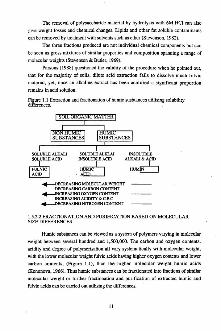
Figure 1.1 Extraction and fractionation of humic susbtances utilising solubility differences.
SOIL ORGANIC MATTER
NON HUMIC SUBSTANCES
■HUMIC--------SUBSTANCES
SOLUBLE ALKALI SOLUBLE ACID
FULVICACID
SOLUBLE ALKLAI INSOLUBLE ACID
HUMIC
INSOLUBLE ALKALI & ACID
h u m [n
)ECREASING MOLECULAR WEIGHT DECREASING CARBON CONTENT
^ ---- INCREASING OXYGEN CONTENTINCREASING ACIDITY & C.E.C )ECREASING NITROGEN CONTENT
1.5.2.2 FRACTIONATION AND PURIFICATION BASED ON MOLECULAR SIZE DIFFERENCES
Humic substances can be viewed as a system of polymers varying in molecular weight between several hundred and 1,500,000. The carbon and oxygen contents, acidity and degree of polymerisation all vary systematically with molecular weight, with the lower molecular weight fulvic acids having higher oxygen contents and lower carbon contents, (Figure 1.1), than the higher molecular weight humic acids (Kononova, 1966). Thus humic substances can be fractionated into fractions of similar molecular weight or further fractionation and purification of extracted humic and fulvic acids can be carried out utilising the differences.
11
Gel permeation chromatography can be used to fractionate, purify and characterise humic substances on the basis of molecular size. The method does have some problems associated with it, the most important being gel/solute interactions. However, these problems can be minimised by manipulating the gel and buffer types (Swift & Posner, 1971).
Ultrafiltration has been used to isolate humic substances from aquatic systems but has not been used as commonly with soil humic substances. The method involves the use of membrane filters of known pore size with nominal cut off values ranging from 50 to 1,000,000. One problem with the method is that the cut off values supplied by the manufacturers may not be as sharp as published and they should be interpreted with caution (Swift, 1985). The method is not as suitable for determining molecular weights as gel permeation chromatography, but is useful for preparative fractionation of aquatic humic substances and removal of small molecular weight materials.
1.5.2.3 FRACTIONATION AND PURIFICATION OF HUMIC SUBSTANCES ON THE BASIS OF CHARGE
One of the most fundamental properties of humic substances is their polyelectrolytic nature, resulting from the presence of ionised functional groupings.
Electrophoresis has been used to give a gradation of fractions by utilising the charge on humic substances. This procedure has recently been combined with gel permeation chromatography to give PAGE (polyacrylamide gel electrophoresis). The polyacrylamide gel, e.g. XAD-8, is used as the support medium and the sample is simultaneously subjected to fractionation on the basis of charge by electrophoresis and on the basis of molecular weight by gel permeation chromatography. The procedure is most applicable to purification of the fulvic acid fraction produced by alkali extraction, since this is present in a soluble form. Humic acids can be dissolved in dimethyl sulphoxide (DMSO) before passing into XAD-8 columns and once the contaminants and DMSO have passed through the humic substances can be recovered by raising the pH and then precipitating the fractions which are produced with acid (Hayes, 1991).
Anion exchange can also be used to fractionate humic substances via their charge characteristics, as well as providing a means for purification. However, the fractionation obtained is rather crude (Swift, 1985).
12
1.6 THE CHARACTERISATION OF HUMIC SUBSTANCES
Even after extraction and fractionation, humic substances are highly heterogeneous materials and their properties can vary on a microsite basis. When working with these substances, it is important that their nature and properties be characterised as far as current procedures allow. The characterisation procedures described here are primarily concerned with determining the number and nature of the reactive functional groups since these are particularly relevant to metal binding studies.
1.6.1 ELEMENTAL ANALYSIS
Elemental or ultimate analysis involves the determination of the elements present in a compound and this is an important chemical property of humic substances, potentially providing information on their nature and source.
Schnitzer and Khan (1978) carried out elemental analysis for a large number of humates extracted from arctic, temperate, subtropical, and tropical soils. The values centred around 54-56% carbon, 4-5% hydrogen and 34-36% oxygen. However, the simplest way to express the results of elemental analysis is to use atomic ratios. The ratios of H/C,0/C, and N/C can prove useful in the following ways:
1. To identify types of humic substances.2. To monitor structural changes of humic substances in
soils and sediments.3. To devise structural formulae for humic substances.
(Steelink, 1985).
In the identification of the type of humic substance the O/C ratio is particularly instructive and soil and aquatic humic acids tend to show ratios of around 0.5. Soil fulvic acids centre around 0.7 with aquatic fulvic acids showing lower ratios of around0.6 which could reflect the lower carbohydrate content of the waters (Thurman and Malcolm, 1983). The H/C ratios can also be used to identify the type of humic substance with lake and marine humic substances extracted from the sediment having higher H/C ratios than their soil counterparts (Steelink, 1985).
The elemental composition of humic substances varies with the extractant used, so comparisons can only be made between humic substances extracted with the same extractant and procedure (Hayes & Swift, 1978).
Steelink (1985) proposed that the elemental analysis of a humic substance could be used to give a potential structural formula or chemical structure. However, he
13
also pointed out that fulvic acid and wood share the same empirical formula, and as such to write a structural formula for any humic substance other information such as titration results and functional group contents should be utilised.
One inherent problem in the study of humic substances is the lack of reproducibility of results due to the heterogeneity of the materials. This also affects elemental analysis leading to variability in the results, even with the same sample and extraction procedure (MacCarthy, 1976).
1.6.2 SPECTROSCOPIC INVESTIGATIONS OF HUMIC SUBSTANCES
1.6.2.1 UV-VISIBLE SPECTROSCOPY
Absorption in the ultraviolet and visible region is caused by atomic and electronic vibrations, and involves the elevation of electrons in orbitals from the ground state to higher energy levels. Systems containing conjugated C=C bonds and unbonded electrons on oxygen are capable of showing absorption. Humic substances, since they contain aromatic groupings, such as phenolic groups, as well as conjugated aliphatic groupings, can show absorption in the visible and ultraviolet regions of the electromagnetic spectrum and these groupings are usually referred to as chromophores. However, the spectra recorded for humic substances tend to be featureless, lacking the well defined peaks which are seen in simple organic compounds (Hayes & Swift, 1978).
Absorption near 465nm has been used for quantitative analysis since it is simple, non-destructive and requires very small amounts of material. Extinction coefficients obtained increase with an increase in molecular weight, degree of condensation, percentage carbon, and the ratio of carbon in aromatic structures to carbon in aliphatic structures (Kononova, 1966). However the results obtained vary between soils and within the same soil extract and are ultimately related to the molecular weight of the humic acid fractions (Swift et al. , 1970). Therefore, as with any analysis, the results can only be compared when components from the same or different soils are subjected to the same isolation and fractionation techniques.
As well as these differences in extinction coefficients, humic substances display differences in colour which can be recorded by changes in the gradient of the UV/VIS spectrum. The gradient is measured between 400 and 600nm and is known as the E4/E6 ratio. This ratio decreases with increasing molecular weight and condensation and has been used to give an indication of the degree of humification (Stevenson, 1982).
14

1.6.2.2 ELECTRON SPIN RESONANCE
When molecules containing unpaired electrons are placed in a magnetic field, the energy of each electron is split into two discrete states through interaction of the magnetic moment of the electrons with the applied field. These molecules can be excited from the lower to the higher energy level by absorption of electromagnetic radiation in the microwave region. This is called electron spin resonance spectroscopy and is used to study species which contain free radicals. Humic substances have been found to contain high concentrations of free radicals and these may influence many of the reactions which they are involved in, e.g. metal complexing. Free radicals are also important in the synthesis and degradation procedures in the soil which result in the formation of humic substances (Stevenson, 1982). Steelink & Tollin (1967) proposed that the sources of free radicals in humic acids could include hydroxyquinone, semiquinone polymer, adsorbent complexes, trapped radicals and polynuclear hydrocarbons.
The ESR spectrum of humic acid or fulvic acid consists of a single line identified by its position and width and, on its own, contains very little information on the nature of these materials since the signal comes from only a small fraction of the total number of molecules that comprise the humic or fulvic acid.
1.6.2.3 INFRA-RED SPECTROMETRY
Infra-red analysis can be used to provide information on the reactivity, nature and structural arrangement of the oxygen containing functional groups as well as information on the occurrence of protein and carbohydrate constituents and impurities such as metal ions and mineral material. It is primarily a qualitative method of analysis which is non-destructive and requires minimal sample preparation.
The development of Fourier Transform Infra-Red Spectroscopy (FTER) has led to increased resolution in the spectra produced. Fourier transformation is a way of computing mathematically the spectrum of radiation passing through an interferometer from an interferogram. It results in high resolution spectra and observes the radiation of all wavenumbers all the time (Griffiths, 1975). A more recent development is Diffuse Reflectance Infra-Red Spectroscopy (DRIFT) which does not incorporate the problems of hygroscopic moisture encountered in normal FTIR (Baes and Bloom, 1989).
The infra-red spectra of humic substances have broad bands due to the heterogeneous nature of the materials. In order to try to elucidate chemical structure,
15
humic substances have been modified by chemical treatment such as methylation or acetylation. Wood et a l (1961) found infra-red bands characteristic of cyclic anhydrides in lignite humic acid that had been refluxed with acetic anhydride, indicating that many of the carboxylic acid groupings occupied positions sufficiently close together to form anhydrides. Wagner and Stevenson (1965) subjected humic acid to methylation, acetylation and saponification in an attempt to determine the number and arrangement of functional groups. They found that about one third of the carboxylic acid groupings could form cyclic anhydrides and also that about two thirds of the hydroxyl groupings were phenolic in nature. However the results of such studies can be ambiguous due to non-specificity of the reactions and side reactions as well as the destructive nature of the treatments.
Infra-red spectroscopy has been used to provide information on the effects of differing geochemistry and source on the composition of humic substances and a combination of chemical and spectroscopic investigations is often used.
Deina et a l (1990) studied humic acids extracted from sewage sludges, manure and worm compost. The humic acids from the sewage sludge were more akin to aquatic humic substances whereas those extracted from worm and manure compost were akin to soil derived humic acids. The spectra of fungal melanins were also shown to be similar to those of soil humic polymers indicating that they play a role in the formation of humic substances (Paim et a l , 1990).
Stevenson and Goh (1971) studied humic and fulvic acids from several different sources and separated the materials into three main spectral types according to their absorption characteristics. They also studied the humification process and how it affects the spectra. Humification was seen to result in a loss of carboxyl groupings and a change in the environment of the carbonyl group from free or weakly bonded states to strongly adsorbed forms. Humification has also been seen to result in a decrease in the polysaccharide content of humic substances with an increase in amide content as fatty acids are converted into bound forms (Hempfling et al., 1988).
FTIR has also been used for quantitative analysis of the carboxyl content of fulvic acid. Interference from water was corrected for by spectral subtraction. The results were then compared to those calculated by potentiometry and were found to be comparable to the spectroscopic method (Cabaniss, 1991).
Studies of unextracted organic matter have become more frequent in an attempt to overcome the problems of alkaline extraction. Humification of peat samples resulted in a decrease in the polysaccharide intensity, as seen in humic acids, whilst the intensity of carbonyl groupings and aromatic bands increased on humification (Niemeyer et al, 1992). This study utilised DRIFT spectroscopy which was also
16
utilised by Holmgren and Norden (1988) to characterise Sphagnum and Car ex peat. They observed differences in the spectra due to the plant origin and also showed that DRIFT spectroscopy can be used to give a quantitative determination of amino acids and sugars in peat. The results were in excellent agreement with values calculated by Kjeldahl measurements.
DRIFT spectroscopy will undoubtedly become more important in infra-red studies, not only for quantitative determinations, but also in the study of unextracted humic substances.
1.6.2.4 NUCLEAR MAGNETIC RESONANCE
The nuclei of certain atoms (e.g.^H and l^C) can exhibit magnetic spin momentum when placed in a magnetic field, causing energy transitions to occur. The spectrum produced can provide valuable information regarding the immediate chemical environment of the atom under study and is seen as a powerful new tool for the determination of functional groups in humic substances providing more information on the functional groups. But, the measurement of the functional group concentration of humic substances by both and *H NMR spectroscopy in both liquid and solid samples is at best semi-quantitative (Hatcher et a l , 1983).
Baldock et a l (1991) also highlighted another major problem when using solid state l^ c NMR in mineral soils, namely, the low carbon content coupled with the low natural abundance of nuclei. Therefore long scan periods are necessary to give adequate signal resolution, unless the soil is incubated with a l^C-labelled substrate. Organic soils, with their higher carbon content, are not affected as much by this disadvantage.
The development of cross polarisation magic angle spinning (CPMAS) NMR has improved the resolution of the method and it is now widely used in structural and chemical investigations. In particular greater understanding of the role of aliphatic carbon in humic substances has been gained through CPMAS NMR studies. This aliphatic material would have previously been hydrolysed in the degradation procedures used in earlier structural investigations. Thus, concepts of the compositional nature of humic substances were challenged.
The method has been utilised to identify different chemical forms of carbon in mor and mull humus as well as other variations in the types of humus (Hopkins & Shiel, 1991). NMR has also been instrumental in confirming that humic acids from each environment are very different in composition from the fulvic acids from the same environment (Malcolm & MacCarthy, 1991).
17
Baldock et a l (1991) showed that organics in whole soil samples could be characterised without resorting to lengthy extraction and/or fractionation procedures, thus minimising changes within the humic substances. They showed that combining
NMR with pyrolysis had far greater potential than a single technique and they proposed that applying combinations of techniques such as NMR, IR and MS to unextracted organic matter in soils and waters could lead to significant advances in the understanding of the behaviour of these materials in the natural environment.
1.6.3 FUNCTIONAL GROUP ANALYSIS
The acidity of humic substances and their reactivity towards heavy metals and radionuclides is ultimately related to their content of oxygen-containing functional groups, although the involvement of other functional groups cannot be discounted. The qualitiative determination of parameters such as total acidity or carboxyl group content is complicated by the heterogeneity of the humic substances. Many of the analytical techniques used lack specificity in reaction or result in undesirable oxidation, reduction or derivatisation reactions which can affect the results. In addition, the reactions are often non-stoichiometric. Consequently, comparison of the results produced with published results can be ambiguous due to a lack of standardisation of methods for extraction, fractionation and purification (Stevenson, 1982).
Dubach and Mehta (1963) concluded that the following could easily result in contradictory results being published:
(a) Divergent origin of humic substances.
(b) Lack of adequate criteria for purity.
(c) Variable molecular weights, leading to incomplete reactions, adsorption of reagents and undesirable fractionation during manipulation.
(d) The proximity of many and different functional groups which influence the reactivity of the groups and the specificity used for their detection and measurement.
1.6.3.1 DETERMINATION OF THE TOTAL ACIDITY
Determination of the total acidity is one of the most commonly used methods of chemical characterisation. Since it is based on the acidity of the reactive groupings it has its own set of problems, one of the most important being the complex nature of the humic substances resulting in the overlapping acidities of various groups (Stevenson, 1982).
18
One method of determining the total acidity involves reacting the humic substances with barium hydroxide and then determining the amount of bound barium by titrating the unused base with standard acid. The main advantage of the method is its simplicity, although it does suffer some interferences, one being associated with the filtration step. If any weakly ionised groups remain in solution they will be re-titrated and consequently lower the value. If a coloured filtrate is obtained, ultrafiltration should be employed (Davis, 1982). Oxygen can also interfere with the method, and all measurements should consequently be carried out under nitrogen.
Regardless of the potential interferences, Perdue (1985) reported that the barium hydroxide method is potentially an accurate method of analysis if the filtration step is approached with care, and all measurements are carried out under nitrogen.
Potentiometric titration with dilute alkali can also be used to calculate the total acidity. The sample is equilibriated with a reagent at very high pH so that even the weakest acids will react. This can pose problems in that it is difficult to determine accurately how much base has reacted in the presence of the extreme excess of base which is required to give a high pH.
Humic acids are viewed as complex polyelectrolytes. Their acidic properties are complicated by electrostatic charge accumulation on the polymer as neutralisation proceeds, resulting in the remaining acidic groups becoming weaker in acidity (Stevenson, 1982). Thus a continuous distribution of pKa values is seen, resulting in no recognisable end point. To compensate for this, Posner (1966) used the end point where the rate of change of pH became a maximum to calculate the end point. Stevenson (1977) also calculated the total acidity from the titration curve in this way, as well as defining a value for the amount of available reactive groups present at any pH value. It is also preferable to have equilibrium achieved as soon as possible to avoid base-catalysed side reactions, such as the hydrolysis of esters and peptides which may lead to releases of carboxylic acids (Perdue, 1985).
Piccolo & Camici (1990) compared the two methods and found that the barium hydroxide method always gave higher results than the potentiometric method due to the precipitation of humic subtances before measurement, which led to an underestimation of the total acidity. However, potentiometric titration gave better precision and did not suffer from the interferences that affect the barium hydroxide method.
19
1.632 DETERMINATION OF THE CARBOXYL CONTENT
Due to the abundance of carboxyl groupings and their importance in the reactivity of the materials, determination of the carboxyl content of humic substances is often carried out. Bonn & Fish (1991) suggested that the carboxyl content provided a better indication of the complexing potential of humic matter that the total acidity measurements, since it excludes the phenolic groupings which will not be dissociated at most soil pH values.
The calcium acetate method has been widely used for determining the carboxyl content of humic substances. The method yields fractionally defined carboxyl contents and is based on the release of acetic acid when humic substances react with calcium acetate (Schnitzer & Khan, 1972). It is a simple method which yields accurate results when compared to direct decarboxylation. However, as with the determination of the total acidity, interferences can occur. Calcium acetate (0.1M) is poorly buffered and the equilibrium pH, which determines the extent to which acidic functional groups react, is dependent on the amount of humic substances added. Also, additional protons can be released in the reaction with calcium acetate (Perdue, 1990). There is also a problem with groups other than the carboxyl groups reacting with the calcium acetate leading to an over-estimation of the carboxyl content. In addition, functional groups less acidic than carboxyl groups which do not react with calcium acetate could still react with the sodium hydroxide on titration.
As with calculation of the total acidity, the filtration step can also cause problems, which led Holtzclaw & Sposito (1978) to modif the method accordingly. However, they could not avoid the other interferences described above.
Bonn & Fish (1991) studied the method using laboratory experiments with humic acids, as well as computer stimulations with hypothetical acids. From these studies they concluded that unless the exact reactions are known, individual carboxyl content measurements cannot be compared. Also, no titration method can be assumed to quantify the acidic group content for humic acids which have a continuous pK distribution.
1.6.3.3 DETERMINATION OF THE METAL BINDING CAPACITY
In determining the content of reactive functional groups for metal binding, the maximum binding capacity (MBC) of a humic substance for that metal may be calculated, and this can give information on the availability and movement of the metal in the environment. Van Dijk (1970) proposed that the capacity of humic acids
20
to bind metal ions was at most equal to the number of titratable hydrogen ions divided by the valency of the metal. However, it is preferable to titrate the humic substance with the metal being studied until no further metal can be bound, since the interaction of a metal with the humic substance varies between different metals. This approach was suggested to be the most accurate for determining the total ligand concentration of humic substances for metal binding studies (Fish et al, 1986).
Perdue (1989) proposed that the MBC is a compositional rather than thermodynamic parameter, unlike the conditional stability constant for the reaction of a metal with a humic substance. Thus it should not be dependent on pH, ionic strength, nature of the metal or concentration of ligand. Yet, the MBC appears to vary with reaction conditions and appears highest at near-neutral pH, low ionic strength, high ligand concentration and with highly polarisable metals such as Cu2+. The MBC of such a humic substance is a weighted average of the complexation capacities of the individual ligands present in the mixture and these ligands in binding energy or log K. It is this binding energy which is affected by changes in pH, ionic strength, etc., and thus it makes it more difficult to realise the MBC under less than optimum conditions (Perdue, 1989). Therefore, the MBC should always be assessed for the reaction conditions being employed in the study.
Interpretation of the titration data and calculation of the MBC has involved using the Langmuir equation (Zunino & Martin, 1977, McLaren & Crawford, 1973), a mathematical expression originally developed by Langmuir (1918, cited in Mott, 1988) to describe the adsorption of a gas on a clean solid. The equation assumes that the complexing strength remains constant as the proportion of complexing sites increases, and that only one type of complexing site is present.
Zunino & Martin (1977) studied copper complexing by colloidal organic matter and achieved linear Langmuir plots. They concluded that many small successive Langmuir responses may be happening as different strengths or classes of binding site are occupied. These cannot be detected but combine to give an overall Langmuir response.
Sanders (1980) also studied organic matter-copper complexes and found that humified organic matter gave curved graphs instead of a linear relationship. This could be indicating that not all binding sites have the same strength. Alternatively, the presence of adsorbed metal ions could be making further adsorption more difficult. Indeed both effects could be contributing to the lack of linearity and many authors have proposed the existence of more than one class of binding site (Buffle et al., 1977: Mantoura & Riley, 1977). Therefore, many researchers utilise the double surface Langmuir isotherm which assumes two distinct classes of binding site whose
21
complexing strength remains constant as they become filled (Sposito, 1982). Sanders (1980) found that the data which gave a curved Langmuir response fitted the double surface Langmuir well and this was reinforced by Fitch and Stevenson (1984), who also showed that the Langmuir plots gave an underestimation of the MBC as calculated from the double surface isotherm. Since the functional groups on humic substances are dominated by weak acid sites such as carboxylic acids, the optimum conditions for saturating these sites with a metal often result in flocculation. This process could give ambiguous results, and resulted in Perdue (1989) proposing that the total acidity could instead be utilised to give an estimate of the MBC of a humic substance.
The values for the MBC are conditional, yet provide information on the reactivity of the humic substance towards a particular metal. Zunino & Martin (1977) proposed that the MBC is more important in the study of natural systems than studies on structure or the calculation of stability constants.
1.7 THE INTERACTION OF METALS WITH HUMIC SUBSTANCES
The ability of humic substances to react with cations via the negatively charged functional groups has long been recognised (Stevenson, 1982). They therefore play a significant role in controlling the behaviour of pollutant metals in the environment. The reactions involved are highly complex and differ depending on the metal, humic material and pH. However, in terms of the environmental implications of metal binding the following effects can be seen:
1. Metal ions which would normally form insoluble precipitates may form a soluble organic complex, with the potential to contaminate groundwater systems or be available for plant uptake. Mierle and Ingram (1991) reported that Hg can be remobilised into water systems through soluble organic complexes, and the mobility of Pb in organic soils under reducing conditions is correlated with the contents of dissolved organic matter (Urban et al. , 1990).
2. Alternatively, insoluble complexes can be formed which result in a reduction in bioavailability and consequently ecotoxicity of metals as they become immobilised by the complexation process (Dissanayake, 1983). Copper and cadmium have been shown to react with humic substances in this way (Brennan et al. , 1983).
22
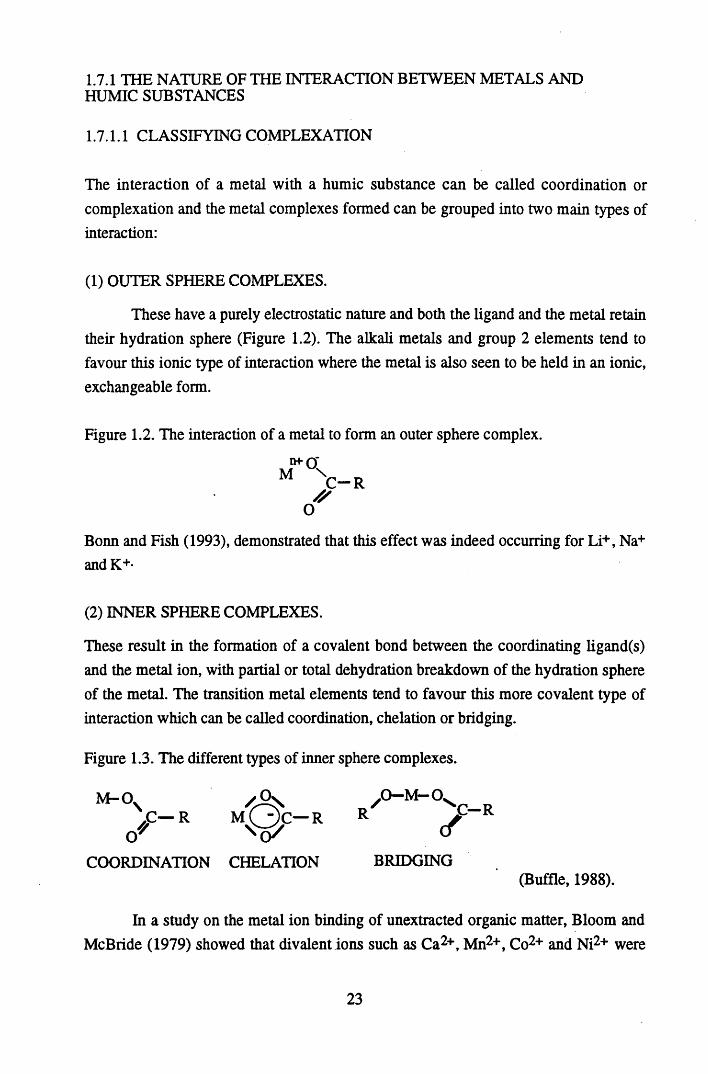
1.7.1 THE NATURE OF THE INTERACTION BETWEEN METALS AND HUMIC SUBSTANCES
1.7.1.1 CLASSIFYING COMPLEXATION
The interaction of a metal with a humic substance can be called coordination or complexation and the metal complexes formed can be grouped into two main types of interaction:
(1) OUTER SPHERE COMPLEXES.
These have a purely electrostatic nature and both the ligand and the metal retain their hydration sphere (Figure 1.2). The alkali metals and group 2 elements tend to favour this ionic type of interaction where the metal is also seen to be held in an ionic, exchangeable form.
Figure 1.2. The interaction of a metal to form an outer sphere complex.
Bonn and Fish (1993), demonstrated that this effect was indeed occurring for Li+, Na+ and K+*
(2) INNER SPHERE COMPLEXES.
These result in the formation of a covalent bond between the coordinating ligand(s) and the metal ion, with partial or total dehydration breakdown of the hydration sphere of the metal. The transition metal elements tend to favour this more covalent type of interaction which can be called coordination, chelation or bridging.
Figure 1.3. The different types of inner sphere complexes.
Mw-CT\
C - R/ /
O
,0—M—OR
COORDINATION CHELATION BRIDGING(Buffle, 1988).
In a study on the metal ion binding of unextracted organic matter, Bloom and McBride (1979) showed that divalent ions such as Ca2+, Mn2+, Co2+ and Ni2+ were
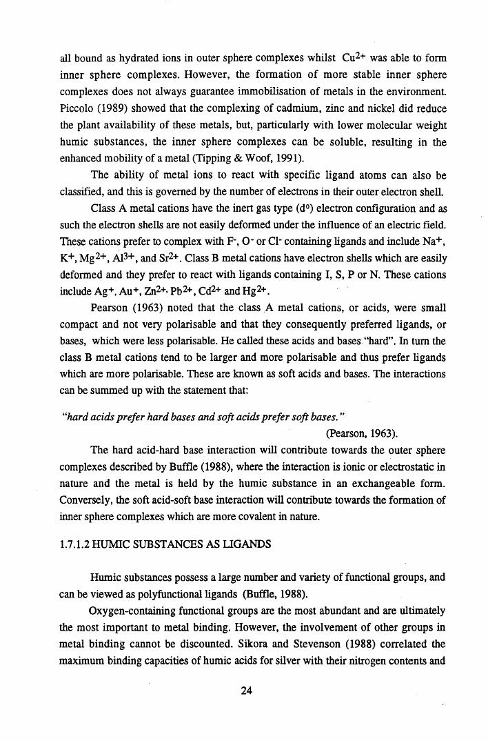
all bound as hydrated ions in outer sphere complexes whilst Cu2+ was able to form inner sphere complexes. However, the formation of more stable inner sphere complexes does not always guarantee immobilisation of metals in the environment. Piccolo (1989) showed that the complexing of cadmium, zinc and nickel did reduce the plant availability of these metals, but, particularly with lower molecular weight humic substances, the inner sphere complexes can be soluble, resulting in the enhanced mobility of a metal (Tipping & Woof, 1991).
The ability of metal ions to react with specific ligand atoms can also be classified, and this is governed by the number of electrons in their outer electron shell.
Class A metal cations have the inert gas type (d°) electron configuration and as such the electron shells are not easily deformed under the influence of an electric field. These cations prefer to complex with F_, O" or Cl" containing ligands and include Na+, K+, Mg2+, Al3+, and Sr2+. Class B metal cations have electron shells which are easily deformed and they prefer to react with ligands containing I, S, P or N. These cations include Ag+, Au+, Zn2+» Pb2+, Cd2+ and Hg2+.
Pearson (1963) noted that the class A metal cations, or acids, were small compact and not very polarisable and that they consequently preferred ligands, or bases, which were less polarisable. He called these acids and bases “hard”. In turn the class B metal cations tend to be larger and more polarisable and thus prefer ligands which are more polarisable. These are known as soft acids and bases. The interactions can be summed up with the statement that:
“hard acids prefer hard bases and soft acids prefer soft bases. ”(Pearson, 1963).
The hard acid-hard base interaction will contribute towards the outer sphere complexes described by Buffle (1988), where the interaction is ionic or electrostatic in nature and the metal is held by the humic substance in an exchangeable form. Conversely, the soft acid-soft base interaction will contribute towards the formation of inner sphere complexes which are more covalent in nature.
1.7.1.2 HUMIC SUBSTANCES AS LIGANDS
Humic substances possess a large number and variety of functional groups, and can be viewed as polyfunctional ligands (Buffle, 1988).
Oxygen-containing functional groups are the most abundant and are ultimately the most important to metal binding. However, the involvement of other groups in metal binding cannot be discounted. Sikora and Stevenson (1988) correlated the maximum binding capacities of humic acids for silver with their nitrogen contents and
24

Ephraim et a l (1986) proposed the existence of a linkage between copper and an amino-carboxylic acid group.
Infra-red studies have not only been integral in elucidating the prescence of these groups, but have also been used to observe the changes which occur on metal binding. The main changes in the infra-red spectrum on metal binding occurs in the 1720-1600 cm-* region, where the carboxylic acids, quinone and ketonic groups absorb. Changes in the hydroxyl groupings can be difficult to interpret (Piccolo & Stevenson, 1982).
Although the importance of the carboxyl groupings has been established, the exact nature of this linkage has yet to be elucidated. Stevenson (1977) suggested that salicylate or phthalate type ligands could be responsible. Cu2+ has been used extensively to study metal humic interactions, often with salicylic and phthalic acids as model compounds. From these studies it appears that salicylate and phthalate type linkages alone do not provide a model for Cu2+ binding and are weaker than humic metal interactions (Livens, 1991).
It is accepted that metals such as Cu2+ can complex with more than one binding site, often forming 2:1 linkages (Buffle et a l, 1977: Stevenson e ta l , 1993). Polydentate linkages, involving up to 3 or 4 donor ligands have also been proposed and these could potentially be any combination of phthalate or salicylate type groupings (Bresnahan et a l, 1978). Gregor et al. (1989) alternatively postulated that the donor ligands came from malonate, peptide and citrate type groupings, with a possible contribution from nitrogen containing heterocycles. This was also observed by Town & Powell (1993) in a study of soil-derived humic and fulvic acids.
Certainly the polyfunctional nature of humic acid substances will encourage such chelation reactions, and it should be remembered that the irregular structure of these materials means that no two functional groups will be chemically identical (Gamble et a l , 1980).
1.7.2 QUANTIFYING METAL BINDING
With humic substances being important metal binding agents in the environment it would be desirable to quantify their reactions and therefore be able to predict their behaviour. Quantification of metal binding generally involves the calculation of a formation or equilibrium constant for the metal-humate complex, e.g. for the reaction,
M + L <=> MLthe thermodynamic equilibrium constant, by the law of mass action, is:
25
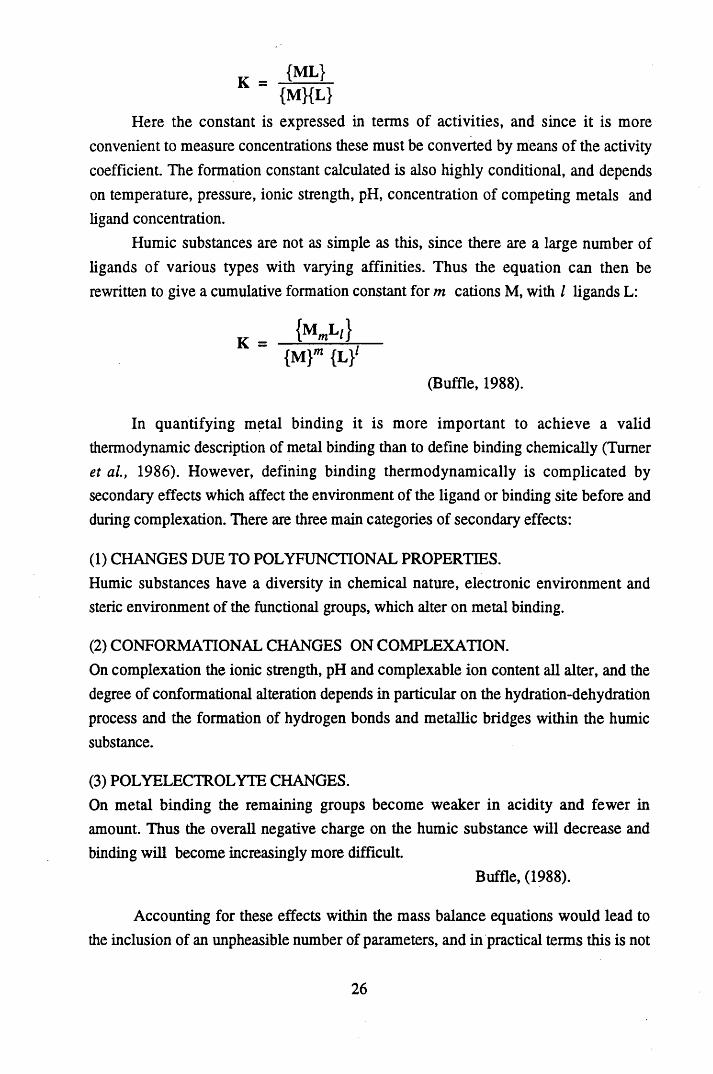
{ML)" {M}{L}
Here the constant is expressed in terms of activities, and since it is more convenient to measure concentrations these must be converted by means of the activity coefficient. The formation constant calculated is also highly conditional, and depends on temperature, pressure, ionic strength, pH, concentration of competing metals and ligand concentration.
Humic substances are not as simple as this, since there are a large number of ligands of various types with varying affinities. Thus the equation can then be rewritten to give a cumulative formation constant for m cations M, with I ligands L:
c _ KM{M}m {L}'
(Buffle, 1988).
In quantifying metal binding it is more important to achieve a valid thermodynamic description of metal binding than to define binding chemically (Turner et al, 1986). However, defining binding thermodynamically is complicated by secondary effects which affect the environment of the ligand or binding site before and during complexation. There are three main categories of secondary effects:
(1) CHANGES DUE TO POLYFUNCTIONAL PROPERTIES.Humic substances have a diversity in chemical nature, electronic environment and steric environment of the functional groups, which alter on metal binding.
(2) CONFORMATIONAL CHANGES ON COMPLEXATION.On complexation the ionic strength, pH and complexable ion content all alter, and the degree of conformational alteration depends in particular on the hydration-dehydration process and the formation of hydrogen bonds and metallic bridges within the humic substance.
(3) POLYELECTROLYTE CHANGES.On metal binding the remaining groups become weaker in acidity and fewer in amount. Thus the overall negative charge on the humic substance will decrease and binding will become increasingly more difficult.
Buffle, (1988).
Accounting for these effects within the mass balance equations would lead to the inclusion of an unpheasible number of parameters, and in practical terms this is not
26
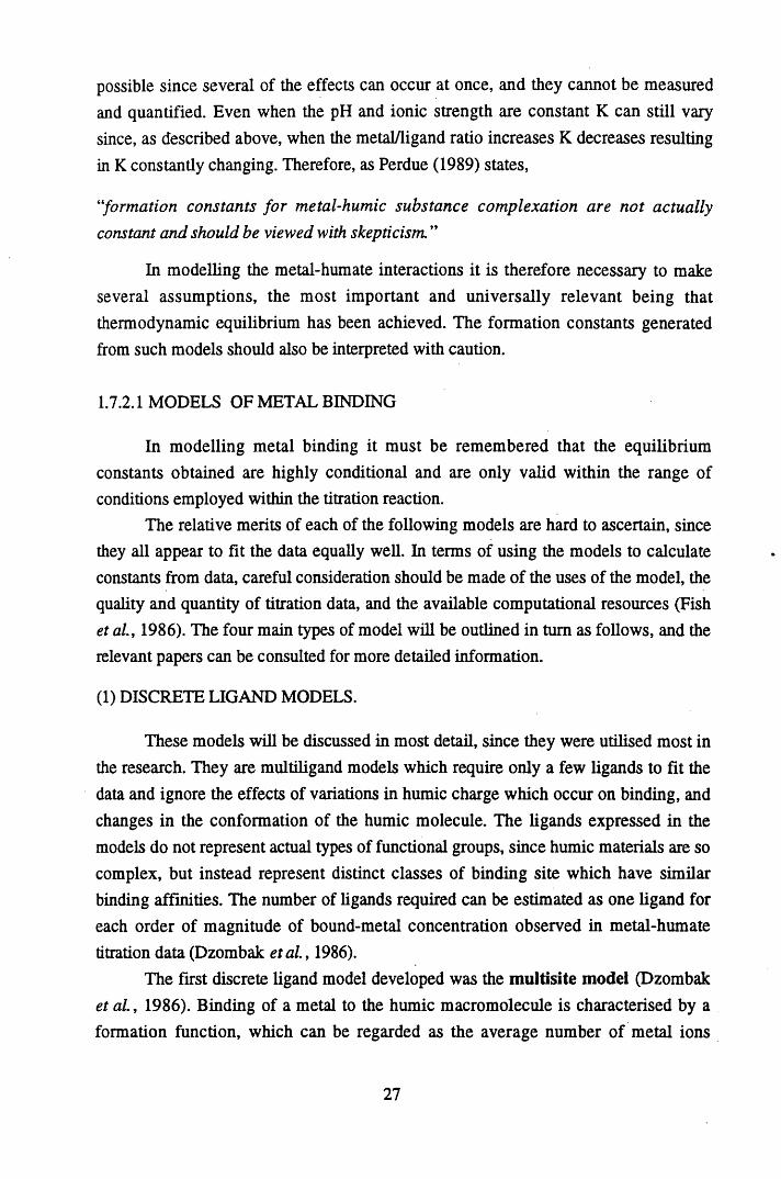
possible since several of the effects can occur at once, and they cannot be measured and quantified. Even when the pH and ionic strength are constant K can still vary since, as described above, when the metal/ligand ratio increases K decreases resulting in K constantly changing. Therefore, as Perdue (1989) states,
“formation constants for metal-humic substance complexation are not actually constant and should be viewed with skepticism. ”
In modelling the metal-humate interactions it is therefore necessary to make several assumptions, the most important and universally relevant being that thermodynamic equilibrium has been achieved. The formation constants generated from such models should also be interpreted with caution.
1.7.2.1 MODELS OF METAL BINDING
In modelling metal binding it must be remembered that the equilibrium constants obtained are highly conditional and are only valid within the range of conditions employed within the titration reaction.
The relative merits of each of the following models are hard to ascertain, since they all appear to fit the data equally well. In terms of using the models to calculate constants from data, careful consideration should be made of the uses of the model, the quality and quantity of titration data, and the available computational resources (Fish et al., 1986). The four main types of model will be outlined in turn as follows, and the relevant papers can be consulted for more detailed information.
(1) DISCRETE LIGAND MODELS.
These models will be discussed in most detail, since they were utilised most in the research. They are multiligand models which require only a few ligands to fit the data and ignore the effects of variations in humic charge which occur on binding, and changes in the conformation of the humic molecule. The ligands expressed in the models do not represent actual types of functional groups, since humic materials are so complex, but instead represent distinct classes of binding site which have similar binding affinities. The number of ligands required can be estimated as one ligand for each order of magnitude of bound-metal concentration observed in metal-humate titration data (Dzombak etal.y 1986).
The first discrete ligand model developed was the multisite model (Dzombak et al., 1986). Binding of a metal to the humic macromolecule is characterised by a formation function, which can be regarded as the average number of metal ions
27
associated with each humic macromolecule. The humic macromolecule is assumed to be the central group, with the metal interacting with sites on it. If more than one class of binding site is present, then treatment of the titration data results in a curve. Thus, further treatment of the titration data is required to determine the formation constant for that class of binding site. This approach has been utilised by Bresnahan et al (1978), Saar & Weber (1979) and Sikora & Stevenson (1988) in the determination of formation constants for the reaction of various cations with humic substances, and generally two distinct classes of binding site were identified.
The multidentate model, developed by Buffle et al. (1977) is mathematically similar to the Scatchard approach, in that a degree of complexation function is determined, and treatment of the data can result either in a linear relationship suggesting one class of binding site, or a curve indicating the existence of more than one class of binding site. Formation constants can then be calculated by manipulation of the titration data accordingly. However, in this approach the metal ion is the central group, and more than one humic acid molecule can potentially interact with the metal.
Stevenson (1976) utilised the modified Bjerrum approach, developed by Gregor (1955) for the analysis of metal polyacrylate titration curves. In this approach complex formation is regarded as a competitive reaction between the metal ion and protons for the ligand sites, with the metal acting as the central group in binding. The reactions between the ligand and the metal are expressed by two successive formation constants, one for each ligand group reacting with the metal, and these are combined to give an overall constant B2 . The method was developed further to incorporate the assumption that the metal interacts with a dissociated ligand site, with the protons being released from the re-establishment of ionisation equilibrium (Stevenson, 1977).
The most recent discrete ligand model, the fixed-k model, adopts a slightly different approach by having pre-decided equilibrium constants. The experimental data is then fitted to these constants to provide values for the discrete ligands present on the humic substance, and also to assess the goodness of fit of the titration data when the reaction conditions varies (Tao, 1992).
28
(2) CONTINUOUS DISTRIBUTION MODELS.
Due to the complexity of humic materials and the variety in type and affinity of the binding sites, continuous distribution models were developed. These models assume that a stability constant K, represents a continuum of binding sites on the humic substances, rather than discrete classes of binding site (Dzombak et al. , 1986), and that the continuum is produced from the above secondary effects, which alter the affinities of the binding sites as binding proceeds. The ligand frequency distributions are then integrated over the distribution of log K. Examples of these include the affinity spectrum approach (Thakur et al. 1980), the constant stability function model Gamble etal. (1983) and the normal distribution model (Perdue and Lytle, 1983).
Stevenson and Chen (1991) adapted the Scatchard multi site approach from a discrete model into a continuous distribution model with the Incremental Stability Constant model. In this model, instead of graphically calculating a log K value for a distribution of binding sites, a continuum of average stability constants is calculated for each increment of metal added.
(3) THE ELECTROSTATIC MODEL.
This approach to modelling attempts to take into account the electrostatic effects which affect metal binding, particularly as a titration proceeds. The electrostatic model was developed by Wilson & Kinney (1977) and assumes that all binding sites are chemically the same, with variations in apparent log K being ascribed to the effects of electrostatic interactions resulting from the change in humic charge on metal binding. This was also the basis of a model developed by Backes and Tipping (1987) for the study of aluminium and proton binding. No parameters are included for the heterogeneity of the humic substances.
(4) DISCRETE SITE/ELECTROSTATIC MODELS.
These models take the ideas developed by Wilson & Kinney (1977) further by including parameters for more than one binding site and ionic strength, and are the most advanced models for metal binding. Ephraim et al. (1986) were the first to consider such an approach through the developement of the polyelectrolyte gel model. Tipping and co-workers further developed these ideas with a series of models, with the integral concept that metal and proton binding take place at a number of chemically discrete binding sites, with electrostatic secondary effects being accounted for (Tipping & Hurley, 1992: Tipping & Woof, 1990: Tipping etal.t 1991: Tipping & Hurley, 1988: Backes & Tipping, 1987).
29
No single approach can be regarded as being superior, each has its own set of limitations. Fish et al. (1986) and Turner et al. (1986) independently reviewed the various discrete and continuous models using both synthetic and experimental data. Both groups of workers concluded that the discrete ligand models, although conceptually and mathematically the simplest, were the most useful as well as accurate way of fitting titration data. In particular, the discrete ligand models can be used to predict competitive interactions among metal ions. However, the ligands classes are also easily incorporated into chemical equilibrium computer programmes such as MINEQL, and can successfully predict metal ion binding by humic material in the absence of competing ions and within the range of calibrating titrations (Dzombak et al, 1986).
Turner et al. (1986) found the multi-site model most able to fit the experimental data and cope with the heterogeneity of fulvic acid. But, the Scatchard plots used in the discrete models to analyse the data and provide equilibrium constants do suffer from errors, one in particular being the curvilinearity of the plots. Two discrete lines are then fitted to the plots to give two discrete binding zones and equilibrium constants. The fitting of these lines is arbitrary and often unfounded (Saar & Weber 1980: Perdue & Lytle 1983). In addition the approach relies on an accurate measure of total ligand concentration, since all other parameters in the model rely on this. This cannot be measured unambiguously due to the nature of humic substances and the secondary effects that they suffer from (Fish et al., 1986).
The discrete models have also been critiscised since they do not take into account the electrolytic nature of humic substances and consequently cannot be applied at salt concentrations different from those used in the formulation of the models (Marinsky & Ephraim, 1986). Also, the discrete models are producing equilibrium constants which are fitting parameters, and not actually representing distinct classes of binding site (Tao, 1992). As Masini (1993) demonstrates, if the electrolytic nature of humic susbtances and the corresponding secondary effects are ignored then 2 to 3 distinct classes of binding site do give a good mathematical fit.
Stevenson et al. (1993) recognised the value of the Scatchard approach, as well as its limitations. Therefore they used the Incremental Technique where the Scatchard slopes are used to calculate a continuum of average stability constants, which reflect variations in the binding energies of humic substances. The constants that they calculated from this model were in good agreement with those calculated from the Bjerrum approach. They also found that the Normal Distribution Model, a continuous distribution model, did not model copper humic acid binding well since to
30
calculate the constants a linear effect is needed and a linear effect can only occur with a single class of binding sites where electrostatic effects are negligible.
Marinsky & Ephraim (1986) proposed that the continuous distribution models can overestimate the complexity of the polyelectrolytic nature of the humic substances. The polyelectrolyte gel model was the first model to attempt to account for both the secondary effects of heterogeneity and polyelectrolytic properties. Ephraim et al (1986) were able to demonstrate that the polyelectrolytic nature was more significant in metal binding than heterogeneity, since it directly affected the accessibility of metal binding sites. The inherent problem with this approach is its complexity, no attempts were made to simplify the model and instead the aim was to attempt to understand more fully the humic-proton-metal equilibria.
Backes & Tipping (1987) found that the polyelectrolyte gel model was able to fit the data, but they preferred to adapt the model and its philosophy to give a more simplified model, with fewer parameters which could then be utilised in a more practical way. As Tipping and Hurley (1992) point out:
“there is no justification for increasing the complexity o f the model as long as it can describe the observed behaviour satisfactorily. The key is to find the minimum degree of complexity that has to be assumed ”
Tipping and co-workers have undoubtedly approached the modelling of metal binding in the most comprehensive and advanced way, with compensations for secondary effects and attempts at modelling the competition reactions of protons and metals with humic substances, as well as the competition reactions of different types of metals. In particular, their model V interprets the competition effects between trace metal species such as copper and alkaline earth cations such as Mg and Ca. It also allows for sites with different relative affinities for different metals, mono- and bidentate binding sites and the effect on alkaline earth binding of the contribution of non-specific counterion accumulation on the charge.
Their models do suffer from errors in fitting the experimental data. In two of the models, namely Model IV and CHAOS, there is an underestimation of binding at low pH values and an overestimation at high pH values. This could be due to many factors, the most likely being analytical error, although a deficiency in the model which is neglecting competition effects from other cations cannot be discounted. After all, in the environment metal binding will be complicated by many factors including competition. These factors though can never be quantified since they are so numerous and would require more parameters than could be effectively computed. Also, they are highly conditional and in the environment will deviate on a microscopic basis. From
31
this it is easy to see the attraction of the simple discrete type models which have also been shown to be accurate in fitting data.
All of the above studies have been carried out using humic or fulvic acids, apart from Tipping & Hurley (1988), who used alkali-extracted humic substances with no acid precipitation. However, as Baes & Bloom (1988a) pointed out, soil organic matter is a solid phase cation binder, not an operationally-derived extract. Bloom and McBride (1979) suggested, from studies on the metal binding of peat, that modelling the metal binding of organic matter need not take into account the secondary effects of heterogeneity. Instead these materials can be modelled well by assuming a cross- linked polycarboxylic acid type structure. Baes and Bloom developed this idea (1988a, 1988b) in modelling the exchange of alkaline earth cations in soil organic matter. They used a model developed by Eisenman (1962; cited in Baes and Bloom 1988a), originally developed to model exchange in aluminosilicate glasses. From these studies it was seen that the organic matter can exchange cations and that the material acts as a weak field exchanger, due to the distance between fixed anionic sites. By increasing the ionic strength, swelling of the structure was reduced and binding sites were brought closer together, enhancing bidentate interactions. Gamayunov & Maslennikov (1992) also studied the interaction of cations with peat soil and concluded that interaction depends on the overall charge of the material, and again heterogeneity did not seem as important a factor as it is in the modelling of humic and fulvic acid interactions.
Allen et a l (1992) modelled the interaction of cations with peat and found that the equilibrium data conformed to a linear Langmuir plot, whereas humic acids tend to give curvilinear Langmuir plots (Sanders, 1980).
From the few studies on metal binding with unextracted organic matter such as peat it can be seen that the interactions are quite different and consequently modelling has been approached in a different way. To understand further the behaviour of metals, in particular pollutant metals, in the environment it may be necessary to develop this approach.
32
1.8 NATURAL HUMIC SUBSTANCES AND THEIR ROLE IN MONITORING THE DEPOSITION OF HEAVY METALS AND RADIONUCLIDES FROM THE ATMOSPHERE
1.8.1 PEAT AS A SOURCE OF NATURAL HUMIC SUBSTANCES
Humic substances are an integral, characteristic and substantial constituent of organic soils and consequently play a vital role in the dynamics of these systems.
Peat soils are highly organic soils which contain up to 97% organic matter in the solid phase, with the moisture content often 90% by weight. Globally they cover around 500 million hectares and have a carbon content of 67 billion x 1012 metric tons (Bramryd, 1980). Thus they play a significant role in the regulation of climate since they are a sink for carbon dioxide, but as a consequence of human activity, they are also increasingly a source of carbon dioxide due to practices such as the drainage of large areas of peatlands (Moore & Bellamy, 1974).
Peat soils are formed by the accumulation of organic matter due to seasonal or continual waterlogging which limits degradation and humification. They vary in their botanical origin, extent of humification, present flora, and physical and chemical properties, with these differences being utilised in their classification (Mathur & Famham, 1985). An important classification system is based on the nutrient content of the peat and leads to the distinction between ombrotrophic or nutrient deficient peats and minerotrophic or nutrient rich peats (Gore, 1983). Ombrotrophic peats are also assumed to be rainwater fed, being raised above the mineral groundwater limit and two major hydromorphological types exist, namely raised bogs and blanket bogs. Blanket bogs are the most extensive type of peat ecosystem in Britain. They “blanket” large areas of land with a cover of peat, and can occur at a wide variety of topographical locations. However, they can often be minerotrophic in part (Wheeler, 1993). Raised bogs occur in the bottom of broad valleys or in basins, and can be distinguished by shallow domes of peat formed when Sphagnum moss begins to colonise the nutrient poor, acidic peat surface. The Sphagnum mosses lower the pH of the system discouraging colonisation by other bog species, and producing an even more dense matt of vegetation cover on the bog surface. Sphagnum mosses also have a high water holding capacity. Their colonisation results in the hydraulic conductivity of the peat being lowered, further removing the peat from groundwater influences (Shotyk, 1988).
Since ombrotrophic peats are rainwater dependent they are able to retain a record of the past atmospheric deposition of heavy metals and radionuclides, and are particularly useful due to the following properties:
33
1. All inputs are from the atmosphere, via wet or dry deposition.2. Long term records of deposition can be provided in deeper cores giving information on changes in atmospheric content throughout the Holocene period.3. The profile can be dated utilising a variety of techniques, depending on the time period being studied.4. They are abundant and easily sampled.
(Barber, 1993).
These properties led to the proposal that ombrotrophic peats could be used as a global pollution monitoring system, since they are present in every continent of the world (Markert & Thornton, 1990). Obviously, there are problems associated with using ombrotrophic peats as a monitoring system, with a major one being establishment that the peat system is in fact ombrotrophic and removed from groundwater influences. There is no clear botanical or chemical fingerprint for ombrotrophicity, and the chemistry of ombrotrophic substrates formed under, different environmental regimes will vary. Therefore, in order to establish ombrotrophicity data on the chemistry of the peat profile, water chemistry and plant species present are needed (Karlin & Bliss, 1984). The other problems surrounding utilisation of these systems as records of deposition, are discussed in greater detail in sections 1.8.3 and 1.8.4.
1.8.2 SOURCES OF HEAVY METALS AND RADIONUCLIDES IN THE ATMOSPHERE
1.8.2.1 SOURCES OF POLLUTANT METALS
To avoid confusion, in the following sections the term heavy metal will be replaced by metal. Heavy metal usually refers to metal ions which have a relative density greater than 5 g cm-3 (Morgan & Stumm, 1991). However, the term has been used indiscriminately in the past to include both ferrous and non-ferrous metals, and even non-metals and metalloids (Niebor & Richardson, 1980). Pollution is easier to define than heavy metals, and the following definition by Holdgate (1979) is widely accepted. This states that pollution is: “the introduction by man into the environment of substances or energy liable to cause hazards to human health, harm to living resources and ecological systems, damage to structure or amenity, or interference with legitimate uses o f the environment”.
Metals are released into the atmosphere from a variety of industrial and domestic activities, with the principle sources of metals being as shown in Table 1.1.
34
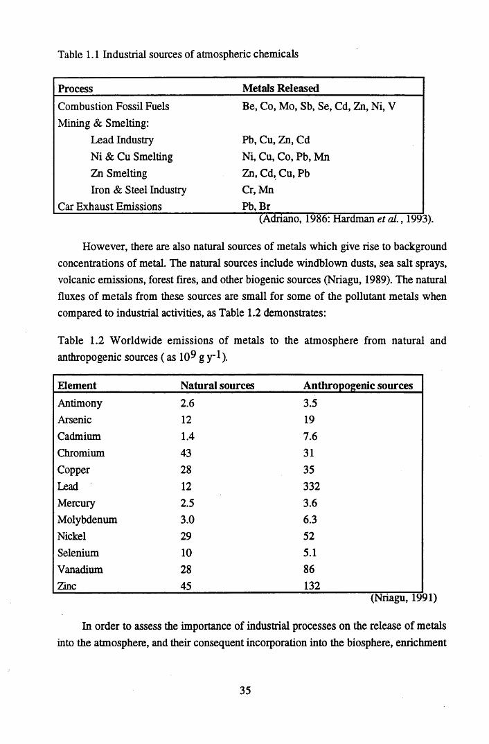
Table 1.1 Industrial sources of atmospheric chemicals
Process Metals ReleasedCombustion Fossil Fuels Be, Co, Mo, Sb, Se, Cd, Zn, Ni, VMining & Smelting:
Lead Industry Pb, Cu, Zn, CdNi & Cu Smelting Ni, Cu, Co, Pb, MnZn Smelting Zn, Cd, Cu, PbIron & Steel Industry Cr, Mn
Car Exhaust Emissions Pb, Br(Adriano, 1986: Hardman et al. , 1993).
However, there are also natural sources of metals which give rise to background concentrations of metal. The natural sources include windblown dusts, sea salt sprays, volcanic emissions, forest fires, and other biogenic sources (Nriagu, 1989). The natural fluxes of metals from these sources are small for some of the pollutant metals when compared to industrial activities, as Table 1.2 demonstrates:
Table 1.2 Worldwide emissions of metals to the atmosphere from natural and anthropogenic sources ( as 10^ g y-1).
Element Natural sources Anthropogenic sourcesAntimony 2.6 3.5Arsenic 12 19Cadmium 1.4 7.6Chromium 43 31Copper 28 35Lead 12 332Mercury 2.5 3.6Molybdenum 3.0 6.3Nickel 29 52Selenium 10 5.1Vanadium 28 86Zinc 45 132
(Nriagu, 1991)
In order to assess the importance of industrial processes on the release of metals into the atmosphere, and their consequent incorporation into the biosphere, enrichment
35
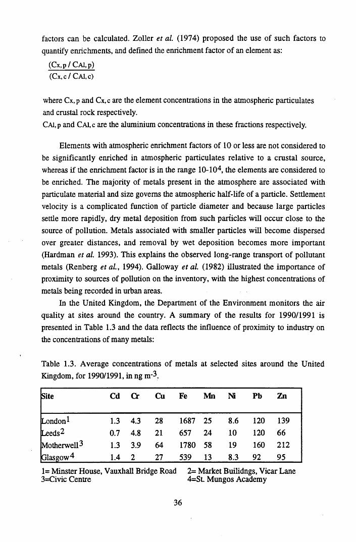
factors can be calculated. Zoller et a l (1974) proposed the use of such factors to quantify enrichments, and defined the enrichment factor of an element as:
(Cx, p / Cai, p)(Cx, c / Cai, c)
where Cx,p and Cx,c are the element concentrations in the atmospheric particulates and crustal rock respectively.CAl,p and CAl,c are the aluminium concentrations in these fractions respectively.
Elements with atmospheric enrichment factors of 10 or less are not considered to be significantly enriched in atmospheric particulates relative to a crustal source, whereas if the enrichment factor is in the range 10-104, the elements are considered to be enriched. The majority of metals present in the atmosphere are associated with particulate material and size governs the atmospheric half-life of a particle. Settlement velocity is a complicated function of particle diameter and because large particles settle more rapidly, dry metal deposition from such particles will occur close to the source of pollution. Metals associated with smaller particles will become dispersed over greater distances, and removal by wet deposition becomes more important (Hardman et a l 1993). This explains the observed long-range transport of pollutant metals (Renberg et al., 1994). Galloway et a l (1982) illustrated the importance of proximity to sources of pollution on the inventory, with the highest concentrations of metals being recorded in urban areas.
In the United Kingdom, the Department of the Environment monitors the air quality at sites around the country. A summary of the results for 1990/1991 is presented in Table 1.3 and the data reflects the influence of proximity to industry on the concentrations of many metals:
Table 1.3. Average concentrations of metals at selected sites around the United Kingdom, for 1990/1991, in ng m-3.
Site Cd Cr Cu Fe Mn Ni Pb Zn
London1 1.3 4.3 28 1687 25 8.6 120 139Leeds^ 0.7 4.8 21 657 24 10 120 66Motherwell 1.3 3.9 64 1780 58 19 160 212Glasgow 4 1.4 2 27 539 13 8.3 92 95
1= Minster House, Vauxhall Bridge Road 2= Market Builidngs, Vicar Lane 3=Civic Centre 4=St. Mungos Academy
36
The high concentrations of the metals at the Motherwell site are due to the presence, at that time, of the Ravenscraig Steel Works and can be seen as an example of a point source of pollution.
Changes in the atmospheric concentrations of metals have been studied using ombrotrophic peat profiles, and these reflect the environmental impact of industrial activity over the last 1,500 years (Livett 1988). Lee & Tallis (1973) reported short but distinct increases in metal deposition in a peat core collected from Snake Pass in Derbyshire, dated to between 1500 and 2000 BP. It was concluded that Roman smelting operations close to the site had produced measurable fluxes of the metals. Renberg et a l (1994) in a study of pre-industrial atmospheric lead contamination in Swedish lake sediments demonstrated the importance of these pre-industrial events, not only at a local level, but globally. They reported that the cumulative deposition from anthropogenic sources in pre-industrial times (600 BC to AD 1800), was at least as large as the cumulative deposition during the industrial period (AD 1800 to present).
The latter part of the eighteenth century marked the beginning of a major period of prosperity of the lead industry in the United Kingdom, with the metal profiles at sites close to the smelters showing corresponding fluctuations (Livett et a l , 1979: Sugden et a l , 1991). Fluctuations were also recorded in remote sites, indicating that the lead smelters caused widespread contamination (Livett et a l , 1979: Livett, 1982). The Industrial Revolution, which began in the eighteenth century, also resulted in widespread increases in atmospheric metal content, which have been recorded in peat profiles (Livett et a l , 1979: Martin et al., 1979: Markert & Thornton, 1990) and sediment profiles (Farmer et a l , 1980).
Ruhling & Tyler (1968) and Lee & Tallis (1973) investigated the twentieth century trends in atmospheric contents of heavy metals, suggested a lowering in the deposition rates of metals in certain localities of the United Kingdom and Scandinavia over the last 50-60 years. However, Livett (1988) in a summary of all the stratigraphic evidence produced from studies in Britain and Scandinavia concluded that these reductions were confined to specific rural sites, where the decline in local industries had led to an improvement in air quality. Recent reports do, however, suggest that the levels of metals in the atmosphere are being reduced and airborne concentrations of metals in the United Kingdom do not at present exceed internationally accepted guidelines (Harrison et a l , 1993).
Studies in North America have shown the dependence of the atmospheric Pb content on car exhaust emissions, and car exhausts have been described as the greatest single source of air contamination in the United States (Adriano, 1986). Pb alkyls were
37
first introduced to petrol as anti-knock additives in the 1920s, and led to significant increases in the output of lead from cars which peaked in the 1960s. Decreases in Pb fluxes by up to 80% between 1979 and 1983 have been proposed to be due to decreases in the Pb content of petrol (Eisenreich et a l , 1986). Miller & Friedland (1991) also reported decreases in the atmospheric Pb flux in North American forest soils, with the atmospheric fluxes measured in the 1990s being 90% less than those in the 1980s. They proposed that this was due to a combination of a reduction in heavy industry, as well as a reduction in the use of leaded petrol.
The source of atmospheric Pb can be studied by utilising the stable Pb isotope ratios. Elemental Pb is composed of four stable isotopes. 204Pb is a primordial radionuclide whereas 206Pb, 207Pb and 208Pb are the products of the U/Th radioactive decay series (Figure 1.4), with 206Pb being the stable daughter product of the 238U series, 207Pb the stable product of the 235U series, and 208Pb the stable daughter product of the 232Th series. Isotopic ratios of natural Pb vary considerably throughout the world. Uranium bearing minerals and ores contain a greater amount of 206Pb, whereas thorium bearing minerals will be enriched in 208Pb. Thus the isotopic ratio of mined Pb will depend on the uranium content of the ore, which determines the contribution of the radiogenic isotopes (Ault et a l , 1970).
Most Pb ores have 206pb/207pb ratios less than natural Pb of soils and soil- related components, since the accumulation of 206Pb due to radioactive decay stops when lead is separated from U in the formation of ore bodies. Since virtually all Pb now present in the atmosphere originates from industrial sources, its isotopic composition is determined mainly by that of the ores which are used in the industrial processes or manufacture of petrol. The residence time of Pb particulates in the atmosphere is around 1-2 weeks, so the isotopic composition of the atmosphere will change accordingly (Shirahata et a l , 1980). The major contemporary source of Pb pollution is from car exhaust emission and interpretation of atmospheric isotopic Pb data is often complicated by temporal variations in the types of ore used in the manufacture of petrol Pb additives world-wide. Therefore, to accurately identify the source of deposited Pb in environmental systems it is necessary to establish the isotopic compositions of Pb ores and petrol in the region being studied (Sturges & Harrison, 1986). However, stable Pb isotopes have been used successfully in a variety of different studies, including the identification of the sources of childhood exposure to Pb, studies on Pb contamination in aquatic systems (Shirahata, et a l , 1980) and the study of the effect of the source of Pb on the Pb signatures of aquatic and terrestrial systems (Sugden e ta l , 1991).
38
Isotopic ratios of a 210Pb-dated sediment core from a rural pond in North America showed a decrease in value at the surface when compared to natural values at depth. This effect was explained by inputs of Pb from industrial sources which have been steadily increasing into the remote system over the last 100 years (Shirahata et al, 1980). The input of pollutant lead into isolated systems was also demonstrated by Chow & Johnstone (1965) in a study of the isotope ratios of freshly fallen snow in an isolated region of California. The 206pb/207pb ratios of the snow closely matched those of petrol sold in the region. Sugden et a l (1991) demonstrated the importance of car exhaust emissions on the 206Pb/207Pb ratios of ombrotrophic peat cores in the United Kingdom. Decreases in the 206Pb/207Pb ratios were observed over the last 40- 50 years due to the input into the atmosphere of particulate Pb with a low 206pb content from car exhausts. In the United Kingdom, the alkyl Pb compounds in petrol are manufactured from a mixture of Australian and Canadian ores, which give a lower 206pb/207Pb ratio (-1.037), than industry and coal combustion (-1.170).
The Br/Pb ratio has also been utilised in an attempt to assign the importance of industry and car exhaust emission to the content of atmospheric particulate Pb, since bromine is also added to petrol. However, there are a number of problems with the method. Firstly, the Br/Pb content of petrol can be variable, and the specific ratio of the petrol in the area being studied must therefore be established. Also in order to assess the importance of industry on the ratios, suitable “background” or pre-industrial levels must be established (Harrison & Sturges, 1983). Sturges & Harrison (1986) were able to demonstrate the effect of industrial Pb from a lead smelter in West Yorkshire on the atmospheric Br/Pb ratio, and were also able to establish consistent pre-industrial background ratios.
The isotope signature studies reinforce the importance of car exhaust emissions on the atmospheric Pb content. In urban areas the influence of exhaust Pb is balanced by contributions from industrial and domestic emissions. But in rural and isolated regions, car emissions have predominated over industrial emissions for the last 40 years (Shirihata et al. , 1980: Sturges & Harrison, 1986: Sugden etal. , 1991).
1.8.2.2 SOURCES OF RADIONUCLIDES IN THE ENVIRONMENT
The sources of atmospherically-derived radionuclides, like atmospherically- derived metals, can be divided into two main groups - natural radionuclides, and anthropogenically-derived radionuclides produced as a consequence of human activities. Both sources result in the exposure of the public to ionising radiation.
39
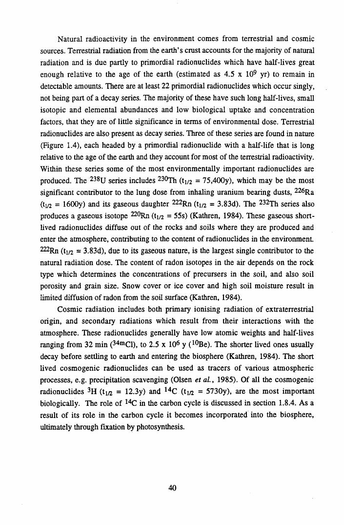
Natural radioactivity in the environment comes from terrestrial and cosmic sources. Terrestrial radiation from the earth’s crust accounts for the majority of natural radiation and is due partly to primordial radionuclides which have half-lives great enough relative to the age of the earth (estimated as 4.5 x 10⁹ yr) to remain in detectable amounts. There are at least 22 primordial radionuclides which occur singly, not being part of a decay series. The majority of these have such long half-lives, small isotopic and elemental abundances and low biological uptake and concentration factors, that they are of little significance in terms of environmental dose. Terrestrial radionuclides are also present as decay series. Three of these series are found in nature (Figure 1.4), each headed by a primordial radionuclide with a half-life that is long relative to the age of the earth and they account for most of the terrestrial radioactivity. Within these series some of the most environmentally important radionuclides are produced. The 238U series includes 230Th (ti/2 = 75,400y), which may be the most significant contributor to the lung dose from inhaling uranium bearing dusts, 226Ra (ti/2 = 1600y) and its gaseous daughter 222Rn (ti/2 = 3.83d). The 232Th series also produces a gaseous isotope ^ R n (ti/2 = 55s) (Kathren, 1984). These gaseous shortlived radionuclides diffuse out of the rocks and soils where they are produced and enter the atmosphere, contributing to the content of radionuclides in the environment. 222Rn (ti/2 = 3.83d), due to its gaseous nature, is the largest single contributor to the natural radiation dose. The content of radon isotopes in the air depends on the rock type which determines the concentrations of precursers in the soil, and also soil porosity and grain size. Snow cover or ice cover and high soil moisture result in limited diffusion of radon from the soil surface (Kathren, 1984).
Cosmic radiation includes both primary ionising radiation of extraterrestrial origin, and secondary radiations which result from their interactions with the atmosphere. These radionuclides generally have low atomic weights and half-lives ranging from 32 min (34mCl), to 2.5 x 10⁶ y ( 10Be). The shorter lived ones usually decay before settling to earth and entering the biosphere (Kathren, 1984). The short lived cosmogenic radionuclides can be used as tracers of various atmospheric processes, e.g. precipitation scavenging (Olsen et al., 1985). Of all the cosmogenic radionuclides 3H ( t ^ = 12.3y) and 14C (tm = 5730y), are the most important biologically. The role of 14C in the carbon cycle is discussed in section 1.8.4. As a result of its role in the carbon cycle it becomes incorporated into the biosphere, ultimately through fixation by photosynthesis.
40
Figure 1.4 The uranium and thorium natural decay series.
13903 / !
T; / 3 , . f
'23*TW/ ;23T h :: 7.SZ!8V i
:22aRa 1 isa j >/■ |
!222Rr.I 133 <t
| 2*U iII 7 ’.I03 r •
i ( 3 Iona z q c a y !^ a io r ,eca* ,
! r T 11
1 ✓ c a t a c e c a ^1 I
- I n o r je c a t j !I '* T 1
22 j r
' 211
I 36.1 run
:23?Th |' ! 33 10 *.r I
2*T H |•3 v r ;
1 -28A ci 1,3T ✓
226o !
5,'5 s i:2 ,Ra1»4 a
R n )?5.8 9 I
: 2,«Oq0 145 «
2I2Po1IT'\
,212 gj/
(. 2'2pb-: :M h1
iiT
288 OK »tabi«
238-'-•11 TOI
41
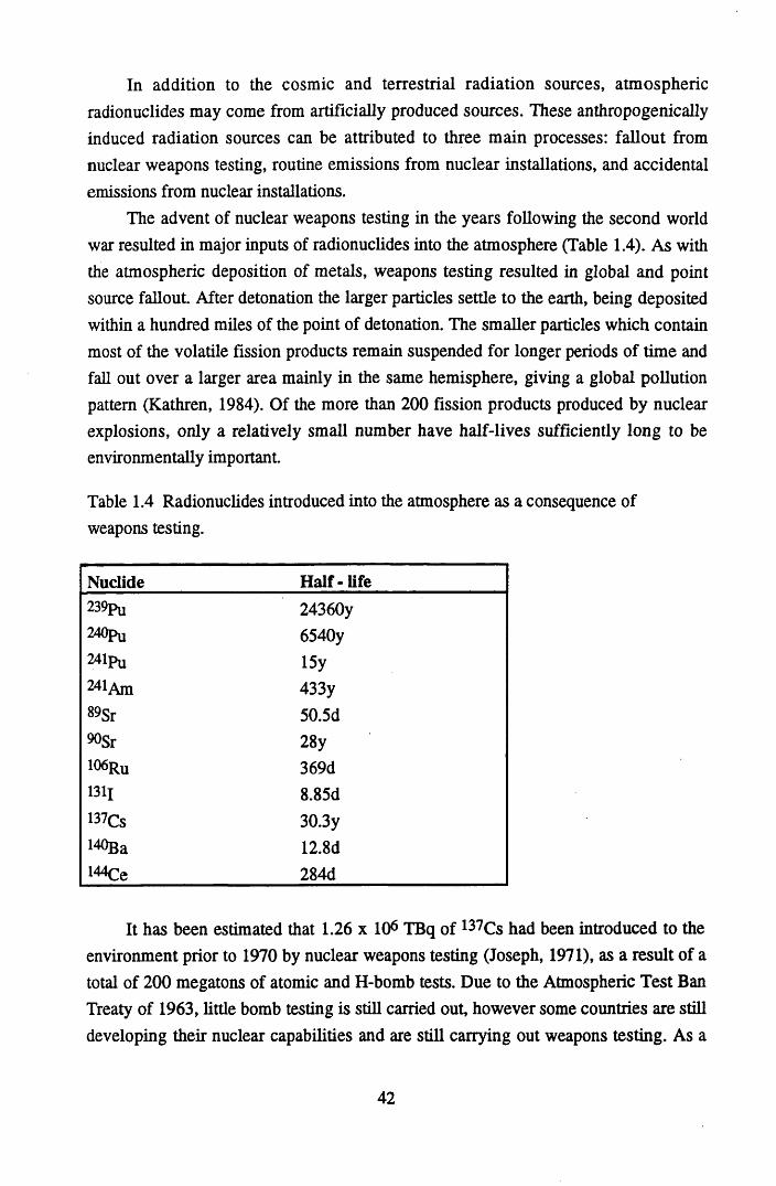
In addition to the cosmic and terrestrial radiation sources, atmospheric radionuclides may come from artificially produced sources. These anthropogenically induced radiation sources can be attributed to three main processes: fallout from nuclear weapons testing, routine emissions from nuclear installations, and accidental emissions from nuclear installations.
The advent of nuclear weapons testing in the years following the second world war resulted in major inputs of radionuclides into the atmosphere (Table 1.4). As with the atmospheric deposition of metals, weapons testing resulted in global and point source fallout. After detonation the larger particles settle to the earth, being deposited within a hundred miles of the point of detonation. The smaller particles which contain most of the volatile fission products remain suspended for longer periods of time and fall out over a larger area mainly in the same hemisphere, giving a global pollution pattern (Kathren, 1984). Of the more than 200 fission products produced by nuclear explosions, only a relatively small number have half-lives sufficiently long to be environmentally important.
Table 1.4 Radionuclides introduced into the atmosphere as a consequence of weapons testing.
Nuclide Half - life239pu 24360y240pu 6540y241pu I5y24lAm 433y89Sr 50.5d90Sr 28y106r u 369d131i 8.85d137CS 30.3yi40Ba 12.8dI44ce 284d
It has been estimated that 1.26 x 10⁶ TBq of 137Cs had been introduced to the environment prior to 1970 by nuclear weapons testing (Joseph, 1971), as a result of a total of 200 megatons of atomic and H-bomb tests. Due to the Atmospheric Test Ban Treaty of 1963, little bomb testing is still carried out, however some countries are still developing their nuclear capabilities and are still carrying out weapons testing. As a
42
consequence of this it is estimated that another 9.6 x 10⁵ TBq have been introduced into the atmosphere since 1970 (UNSCEAR, 1982). Widespread global fallout of l37Cs derived from weapons testing occurred during the early 1960s, when weapons testing was at its maximum. In the middle stratosphere 137Cs has a residence time of 6-12 months (Joseph, 1971), and due to its 30y half life, l37Cs is environmentally persistent. i37Cs can be immobilised by the clay fraction of soils, resulting in reduced bioavailability (Segal & Morris, 1991) however, in some organic soils it can be mobile, and this will be discussed further in section 1.8.3.
As far as other radionuclides are concerned, 108 MBq of 13iI, 106 MBq of W S r and 105 MBq of 239,240pu were released (Santschi & Honeyman, 1989). Of these 239Pu is the most important due to its long half-life, and persistence in the environment. Most of the Pu injected into the atmosphere has fallen out onto the soil surface and is present in the soil as an oxide, resulting in potential immobility (Kathren, 1984). However, as discussed in section 1.8.3, Pu has some mobility in organic soils.
Two cosmogenic radionuclides, 3H and l4C, have had their atmospheric content increased due to neutron activation induced by atmospheric weapons testing. This led to increases in the content of 3H in the atmosphere, and during 1962 it was estimated that 3 x 10⁷ TBq of 3H were added to the atmosphere (Kathren, 1984). In addition, approximately 2.2 x 10⁵ TBq of 14C was introduced to the atmosphere through weapons testing (UNSCEAR, 1982), which along with the contradictory Suess effect has significantly distorted the natural 14C levels, thus affecting radiocarbon dating.
The atmospheric discharge of radionuclides from nuclear reactors represents a point source of pollution. It does not contribute to the global radionuclide loadings produced from weapons testing. However, longer range transport of radionuclides cannot be discounted. Radioactive noble gases, along with tritium are the main source of activity released from operating nuclear power reactors, with the quantity and constituents of release varying from plant to plant (Table 1.5).
The most important radiological effects of nuclear power, apart from accidental discharges such as Chernobyl, are connected to the mining of uranium, which can also result in the localised release of radionuclides to the environment. To remove the build-up of radioactive dusts and 222Rn gas, uranium mines are well ventilated, with the exhausted air discharged directly to the atmosphere. Uranium mines exhaust 103- 106 cubic feet of air per minute, containing 650-2600 Bq/m3. For an estimated 200 days per year production, this would give a release of 3 TBq of 222Rn into the atmosphere annually (Kathren, 1984).
43
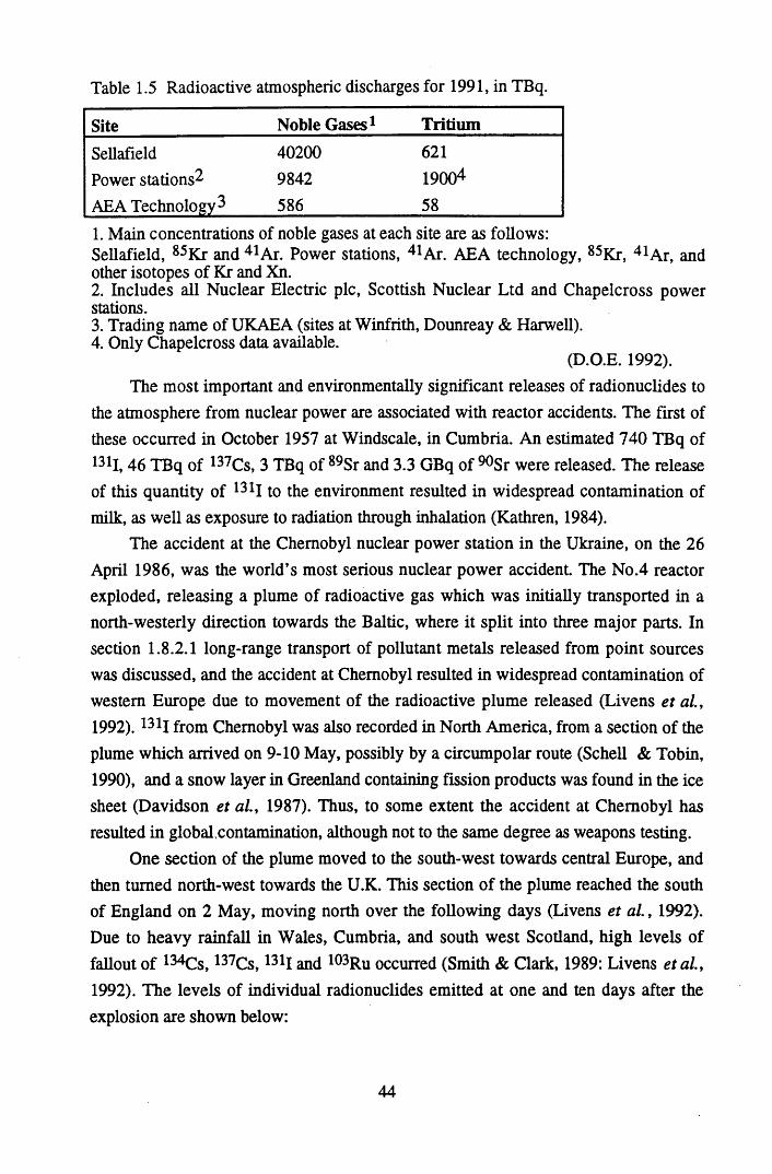
Table 1.5 Radioactive atmospheric discharges for 1991, in TBq.
Site Noble Gases1 Tritium
Sellafield 40200 621Power stations^ 9842 19004AEA Technology 586 581. Main concentrations of noble gases at each site are as follows:Sellafield, 85Kr and 41 Ar. Power stations, 41 Ar. AEA technology, 85Kr, 41Ar, and other isotopes of Kr and Xn.2. Includes all Nuclear Electric pic, Scottish Nuclear Ltd and Chapelcross power stations.3. Trading name of UKAEA (sites at Winfrith, Dounreay & Harwell).4. Only Chapelcross data available.
(D.O.E. 1992).The most important and environmentally significant releases of radionuclides to
the atmosphere from nuclear power are associated with reactor accidents. The first of these occurred in October 1957 at Windscale, in Cumbria. An estimated 740 TBq of 131I ,46 TBq of 137Cs, 3 TBq of 89Sr and 3.3 GBq of 90Sr were released. The release of this quantity of 13 *1 to the environment resulted in widespread contamination of milk, as well as exposure to radiation through inhalation (Kathren, 1984).
The accident at the Chernobyl nuclear power station in the Ukraine, on the 26 April 1986, was the world’s most serious nuclear power accident. The No.4 reactor exploded, releasing a plume of radioactive gas which was initially transported in a north-westerly direction towards the Baltic, where it split into three major parts. In section 1.8.2.1 long-range transport of pollutant metals released from point sources was discussed, and the accident at Chernobyl resulted in widespread contamination of western Europe due to movement of the radioactive plume released (Livens et al., 1992). 131I from Chernobyl was also recorded in North America, from a section of the plume which arrived on 9-10 May, possibly by a circumpolar route (Schell & Tobin,1990), and a snow layer in Greenland containing fission products was found in the ice sheet (Davidson et al., 1987). Thus, to some extent the accident at Chernobyl has resulted in global contamination, although not to the same degree as weapons testing.
One section of the plume moved to the south-west towards central Europe, and then turned north-west towards the U.K. This section of the plume reached the south of England on 2 May, moving north over the following days (Livens et al. , 1992). Due to heavy rainfall in Wales, Cumbria, and south west Scotland, high levels of fallout of 134Cs, 137Cs, 131I and 103Ru occurred (Smith & Clark, 1989: Livens et a l ,1992). The levels of individual radionuclides emitted at one and ten days after the explosion are shown below:
44
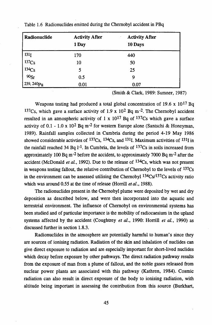
Table 1.6 Radionuclides emitted during the Chernobyl accident in PBq
Radionuclide Activity After 1 Day
Activity After 10 Days
131j 170 440137Cs 10 50134Cs 5 2590Sr 0.5 9
239, 240pu 0.01 0.07
(Smith & Clark, 1989: Sumner, 1987)
Weapons testing had produced a total global concentration of 19.6 x 10¹⁷ Bq 137Cs, which gave a surface activity of 1.9 x 10² Bq n r 2. The Chernobyl accident resulted in an atmospheric activity of 1 x 10¹⁷ Bq of 137Cs which gave a surface activity of 0.1 - 1.0 x 10² Bq n r2 for western Europe alone (Santschi & Honeyman,1989). Rainfall samples collected in Cumbria during the period 4-19 May 1986 showed considerable activties of 137Cs, 134Cs, and 131I. Maximum activities of 13ll in the rainfall reached 34 Bq I-1. In Cumbria, the levels of 137Cs in soils increased from approximately 100 Bq n r2 before the accident, to approximately 7000 Bq n r2 after the accident (McDonald et al., 1992). Due to the release of 134Cs, which was not present in weapons testing fallout, the relative contribution of Chernobyl to the levels of 137Cs in the environment can be assessed utilising the Chernobyl 134Cs/137Cs activity ratio which was around 0.55 at the time of release (Horrill etal., 1988).
The radionuclides present in the Chernobyl plume were deposited by wet and dry deposition as described below, and were then incorporated into the aquatic and terrestrial environment. The influence of Chernobyl on environmental systems has been studied and of particular importance is the mobility of radiocaesium in the upland systems affected by the accident (Coughtrey et al., 1990: Horrill et al., 1990) as discussed further in section 1.8.3.
Radionuclides in the atmosphere are potentially harmful to human’s since they are sources of ionising radiation. Radiation of the skin and inhalation of nuclides can give direct exposure to radiation and are especially important for short-lived nuclides which decay before exposure by other pathways. The direct radiation pathway results from the exposure of man from a plume of fallout, and the noble gases released from nuclear power plants are associated with this pathway (Kathren, 1984). Cosmic radiation can also result in direct exposure of the body to ionising radiation, with altitude being important in assessing the contribution from this source (Burkhart,
45
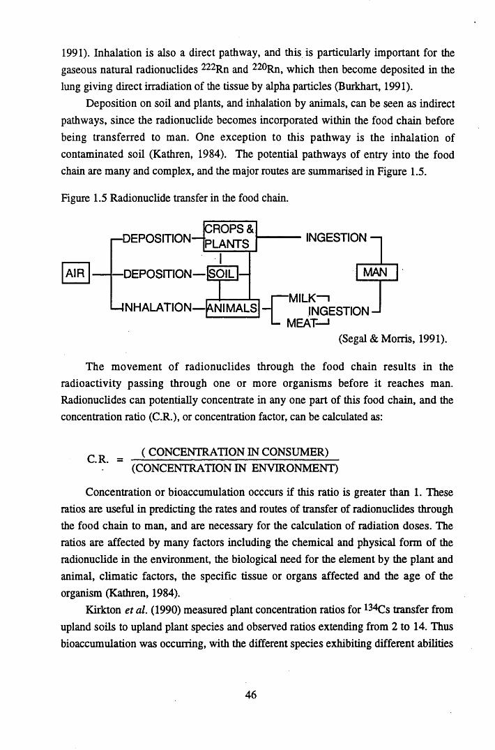
1991). Inhalation is also a direct pathway, and this is particularly important for the gaseous natural radionuclides 222Rn and 220Rn, which then become deposited in the lung giving direct irradiation of the tissue by alpha particles (Burkhart, 1991).
Deposition on soil and plants, and inhalation by animals, can be seen as indirect pathways, since the radionuclide becomes incorporated within the food chain before being transferred to man. One exception to this pathway is the inhalation of contaminated soil (Kathren, 1984). The potential pathways of entry into the food chain are many and complex, and the major routes are summarised in Figure 1.5.
Figure 1.5 Radionuclide transfer in the food chain.
AIR
^D EPO SITIO N — iCROPS & PLANTS
■DEPOSITION— SOIL -
L—INHALATION— ANIMALS
INGESTION
MAN
■ C .
MILK—i INGESTION-*
MEAT— *(Segal & Morris, 1991).
The movement of radionuclides through the food chain results in the radioactivity passing through one or more organisms before it reaches man. Radionuclides can potentially concentrate in any one part of this food chain, and the concentration ratio (C.R.), or concentration factor, can be calculated as:
C R _ ( CONCENTRATION IN CONSUMER)V (CONCENTRATION IN ENVIRONMENT)
Concentration or bioaccumulation occcurs if this ratio is greater than 1. These ratios are useful in predicting the rates and routes of transfer of radionuclides through the food chain to man, and are necessary for the calculation of radiation doses. The ratios are affected by many factors including the chemical and physical form of the radionuclide in the environment, the biological need for the element by the plant and animal, climatic factors, the specific tissue or organs affected and the age of the organism (Kathren, 1984).
Kirkton et al. (1990) measured plant concentration ratios for 134Cs transfer from upland soils to upland plant species and observed ratios extending from 2 to 14. Thus bioaccumulation was occurring, with the different species exhibiting different abilities
46
to accumulate 134Cs. An interesting observation from the study was that 134Cs from Chernobyl was more available for uptake than pre-Chernobyl 137Cs.
1.8.3 FACTORS AFFECTING THE DISTRIBUTION OF DEPOSITED METALS AND RADIONUCLIDES IN PEAT PROFILES
Heavy metals and radionuclides can become incorporated in peat profiles either directly through the exposed surface peat, or indirectly via the vegetation cover. Once incorporated within the peat profile a number of factors can affect their distribution.
One such factor is the vegetation itself. First of all this plays an important role in trapping the pollutants and conveying them to the peat profile, and unvegetated sites have been shown to give lower inventories of 210Pb than vegetated sites (Olsen, 1985). In addition, the type of vegetation is also important in this transfer process.
Sphagnum spp. have been shown to be particularly efficient at trapping metals since they have no vascular system and can allow unrestricted exchange of solutes between the plant tissue and the atmosphere (Livett, 1988). The metals then accumulate in the cell wall and intracellular membranes, and the ability of these species to retain metals is attributed to their high polyuronic acid content, which can complex the metals (Clymo, 1963). However, Sphagnum mosses are not the only plant species present in bog ecosystems. Vascular plants such as Eriophorum spp. or Carex spp. are often predominant, and do not take up metals across the leaf surface like the Sphagnum spp. Instead, metals are captured on the leaf surface and incorporated within the peat profile on leaf fall. The turnover rate of the plant litter can therefore affect the residence time of these metals in the vegetation. Therefore, a time lapse could occur before incorporation of a metal into the peat profile, and erosion could remove significant amounts of the metal from the surfaces of the litter (Livett, 1988).
Remobilisation of metals within the peat profile can be caused by the vegetation. The root systems of vascular plants are involved in the active uptake of the pore water, and therefore any element which is present in that water. Downward movement of metals within the profile can also be facilitated by the root channels which penetrate the peat (Clymo, 1983). Most species root systems concentrate within the top 20 cm of peat profiles, but some root systems, e.g. Eriophorum spp., can extend to 60 cm (Livett, 1988). Metals which are essential for plant growth could be recycled within the surface peat by the above processes, and the distribution of 137Cs in peat profiles has been proposed to occur in this way (Oldfield et al.t 1979: Clymo, 1983: Mitchell, et al., 1992). Damman (1978) was able to demonstrate that K and Na were actively
47
taken up from surface peat by the vegetation, in particular the vascular plants. The Sphagnum mosses were also showing some active uptake of K, challenging the hypothesis that they were obtaining all of their nutrients from the atmosphere. Pakarinen (1978) also demonstrated small scale redistribution of metals by Sphagnum mosses. Sphagnum spp. and Calluna vulgaris have also been shown to have higher 137Cs concentrations than other vascular plants (Horrill et al., 1990: Colgan et al.,1990).
K, Na and Cs will favour this kind of cycling because of their chemistry. They tend to form outer sphere complexes (for full classification refer to section 1.7.1.1.), and thus are retained in exchangeable forms within the peat. Tipping & Hurley (1988) in a model of metal complexation processes in acid soils were able to demonstrate that Na was held by electrostatic interactions, whereas Al was predominately complexed with the humic substances. The Na was then in direct contact with the soil solution making it readily exchangeable.
Cs is however less mobile in soils with higher clay content, in particular micaceous clays, which can trap the Cs in interstitial layers, thus removing it from the soil solution. However, in organic soils this occurs only to a limited extent depending on the clay content, and the Cs is predominately present in the soil solution (Maguire,1993).
The rate of incorporation of plant material into the peat profile is affected by the temperature, water supply, oxygen supply, the nature of the plant material, and the microbiological environment (Clymo, 1983). All of these factors are highly interactive and affect the rate of accumulation of the peat profile. Peat accumulation depends on the amount of plant material produced at the surface and the rate at which this is decayed and compacted (Johnson et al., 1990). Therefore a more waterlogged peat profile will result in a low rate of decay and low degree of humification, low oxygen content, reducing conditions at depth, specialised plant species and a higher accumulation rate. A more aerated, humified system will result in the breakdown of the organic matter with a loss of structure of the plant material, a change in chemical state of the peat, an increase in bulk density, and a lower accumulation rate (Clymo, 1984).
The difference in peat type caused by the different moisture regime can affect the distribution of metals within a profile by affecting:
(1) COMPACTION & DECOMPOSITION PROCESSES(2) THE REDOX ENVIRONMENT(3) THE MOVEMENT OF WATER IN THE PROFILE.
48
Urban et al. (1990) commented on the distortion of metal profiles due to compaction and decomposition processes. As with all the processes which affect these profiles, the processes also affect the relationship between the depth and age, and therefore the chronology of the system (Damman, 1978).
Decomposition is most likely to occur in aerated, humified profiles, such as peat colonised by Eriophorum spp., and this results in loss of structure and a greater bulk density. The loss of carbon gives accumulation of metals at that point in the profile (Urban et a l , 1990). In waterlogged systems, decomposition is reduced and as plant matter accumulates compaction can occur. Partial decay weakens the structure of the plant material, usually Sphagnum mosses, until eventually the weakened moss can no longer support the weight of the waterlogged system giving collapse and compaction. This is illustrated in the profile by a sudden increase in bulk density (Clymo, 1983). Compaction can cause increases in metal content at the point of compaction and causes irregularities when assessing accumulation rates in a profile (Appleby & Oldfield, 1978).
The redox environment is ultimately controlled by the water content of the peat. In many peat systems there is a surface zone of aerobic decay overlying a subsurface anoxic zone. The surface zone is often referred to as the acrotelm, and is distinguished by its high hydraulic conductivity, as compared to the anoxic catotelm (Ingram, 1978). The depth of each layer is dependent on the depth of the water table, and the distinction between the oxic and anoxic conditions is often not clear cut, giving a zone of water table fluctuation with a fluctuating redox environment (Clymo, 1991: Damman, 1978).
Aaby & Jacobsen (1979) observed that enrichment of metals in peat profiles, which is often assumed to be due to increases in deposition often coincides with the junction between well and poorly humified peat, at the zone of water table fluctuation. Damman (1978) studied the distribution of Na, K, Mg, P, Ca, Al, Fe, Mn, Pb, and Zn in ombrotrophic peat cores and showed that the redox environment can affect the distribution of Al, Fe, Mn, Pb, and Zn, whereas biological and hydrological effects accounted for the distribution of the other elements. Fe and Mn were removed from waterlogged, anoxic profiles, and were retained in the aerated profiles. Al, Pb and Zn were removed from the anoxic, permanently waterlogged profiles, but were shown to accumulate at the zone of water table fluctuation. Glooschenko etal. (1986) observed secondary peaks for Cu and Pb at depth in peat profiles and proposed that this could be due to fluctuation at the zone of water table fluctuation. The loss of Fe and Mn from peat profiles was also observed by Sugden (1993), with no loss of Pb, indicating that
49
water saturation had been transitory and only caused enough of a redox change to influence the Mn and Fe.
Urban et al (1990) also observed loss of Pb from permanently saturated profiles, and enhancement at the zone of water table fluctuation. However, here, the enhancement was proposed to be due to the combination of decomposition of organic matter in the aerobic zone, and leaching effects in the anaerobic zone. No relationship between the redox environment and redistribution of Al, Pb and Zn was seen in peat cores analysed by Jones & Hao (1992), although the three metals did show similar distribution profiles.
The redistribution of deposited metals in peat profiles is also catalysed by the movement of water through the peat profile. Dumontet et a l (1990) proposed that chemical diffusion was involved in the downward migration of Cu and Zn, although Clymo (1983) proposed that diffusion was of less importance to metal migration than biological cycling or mass flow. Vertical and lateral flow of water can occur, and in the aerated surface layers of the peat hydraulic conductivity tends to be high favouring vertical flow. Olsen (1985) demonstrated that rainwater can penetrate to depths of 10 cm in unsaturated surface peat and move easily due to the high hydraulic conductivity. However, if the profile was saturated little penetration and movement could occur. Clymo (1983) proposed that once the water table is reached, and hydraulic conductivity is reduced, lateral flow becomes more important to metal movement than vertical flow. Oldfield et a l (1979), El-Daoushy (1988) and Urban et a l (1990) proposed that the loss of metals from peat cores was due to lateral flow. Vertical mobility of Cs was reported by Mitchell et a l (1992), and up to 50% of Cs was estimated to be lost from a peatland through a combination of vertical and lateral flow (Clymo, 1978). Coughtrey et a l (1990) found that 137Cs was moving predominantly through lateral flow in upland pasture.
Although ombrotrophic peats are assumed to be removed from groundwater influences, the effect of the groundwater on the profile cannot always be discounted. Hill & Siegel (1991) demonstrated that major variations in the concentrations of the cations Ca, Mg, Sr, Fe, and Na were due to groundwater discharge only, whereas the concentrations of Cu, Ni, Pb, and Zn in the profile were related to groundwater discharge combined with atmospheric loadings. The hydraulic conductivity at depth is often assumed to be low due to waterlogging and compaction effects, yet if macrostructures such as buried wood exist, the hydraulic conductivity could be enhanced.
From the above studies it can be seen that the assumption that metals are immobilised on incorporation into peat profiles through complexation processes is
50
often unfounded. As well as the conditions within the peat profile, and the peat type, metal type appears to play an important role in the interaction of the metal with the peat, and its diagenesis within the profile. The Class A metal cations, such as Na, K, Mg and Cs which bind through outer sphere complexes show considerable mobility since they are held in readily exchangeable forms (Bonn & Fish 1993) and are unaffected by redox transformations within the peat profile (Damman 1978). The Class B metal cations, such as Pb, Zn and Cu, however, can form inner complexes with the soil organic matter, and the formation constants of these complexes are often high (Stevenson, 1982) so movement of these metals through a profile is not expected. However, Shotyk et al. (1992) proposed that complexation by organic matter was not the main process controlling the behaviour of these metals in peatlands, with the redox environment being a more important control. Fe and Mn were shown to be present as aqueous species illustrating their solubility in reducing conditions, whereas Cu was present in an insoluble form in reducing conditions. Jones (1987) utilised sequential extraction to study the chemical forms of Cu, Zn, Pb, Fe and Mn in peats. Cu was found to be associated with the organic matter fraction, giving predominantly insoluble forms, particularly at depth in the profile, indicating that incorporation of deposited Cu from particulate to organic form can take time. Mn and Fe were found to occur largely in oxide form whereas Pb and Zn were found to occur in high proportions in exchangeable, soluble forms, as well as in the residual fraction. In particular higher proportions of Pb and Zn were found in soluble forms in waterlogged peat profiles. There was evidence to suggest that the Fe and Mn oxides were scavenging Pb and Zn, perhaps when in association with low molecular weight organic matter. The oxides, when coming into solution in reducing conditions, released Pb and Zn and gave increases in soluble forms of Pb and Zn in waterlogged systems. Harrison et al. (1981), in a study of the chemical associations of Pb, Cd, Cu and Zn in soils, found that Pb and Zn were again present predominantly in oxide form, with Cu being predominantly associated with the organic material. The solubility of Zn and Pb in acidic peat profiles was also demonstrated by Shotyk etal. (1992), but in this study these metals did not have a redox dependency.
The solubility and movement of metals has also been proposed to be due to the concentration of dissolved organic matter. Urban et a l (1990) showed that the leaching of Pb from waterlogged profiles was correlated with the concentration of dissolved organic matter. The formation of dissolved organic matter, or the release of soluble humic substances from the organic matter, is dependent on the pH and metal content which controls humic charge (Tipping & Woof, 1990). At pH values below 5, Tipping and Woof (1991) found that the majority of Al in solution was in inorganic
51
form, whilst at higher pH values soluble organic complexes were more important for the movement of Al.
The profiles of metal concentration with depth, should therefore, always be interpreted with caution since as Jones and Hao (1992) point out:
“there is insufficient evidence to support the assumption that all metal deposition records retain their chronological integrity”
1.8.4 DATING THE PEAT PROFILE: ESTABLISHING A HISTORY OF DEPOSITION
In calculating the chronology of a peat profile, a relationship is established between depth and age, which can be applied to the profiles of metal concentration versus depth to give the deposition history of the profile. Problems do exist in establishing these relationships due to variations in the accumulation rates, the remobilisation of elements, and the decay and compaction processes discussed in section 1.8.3, which upset the chronological integrity of the profile. Consequently, care must be taken in the interpretation of these profiles.
A variety of dating mechanisms can be used to establish a chronology in a peat, and the mechanism used depends on the time scale being studied. Since the vegetation of ombrotrophic peat systems is dominated by Sphagnum mosses, the annual growth increments of these can be used to provide a chronology of deposition over the last 50 years (Pakarinen & Tolonen, 1977). The method involves utilising the seasonal growth periodicity which is reflected by a cyclic zonation in branching patterns and pigmentation in straightened Sphagnum stems. From this, the annual increments are calculated, by dividing the mean stem length with the mean increment length (El- Daoushy et al., 1982). The technique is particularly useful in dating surface peat horizons where other methods cannot be used. However, it requires a well established colony of Spagnum and its application is limited to poorly humified, waterlogged systems where the structure of the vegetation is maintained (Livett, 1988).
One of the most widely applied dating mechanisms is a radiometric technique, which utilises 210Pb. In rocks and soils the decay of 226Ra (half life 1600y) generates the gaseous daughter isotope 222Rn (half life 3.83d), which diffuses into the atmosphere and decays to give 210Pb (half life 22.26y). The 210Pb is then removed from the atmosphere by wet and dry deposition with a mean atmospheric residence time of 5 days (Nozaki etal., 1978). Thus, there is a direct input of unsupported 210Pb
52
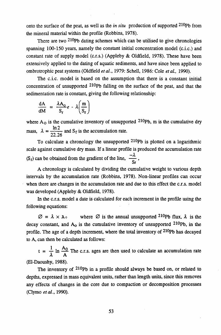
onto the surface of the peat, as well as the in situ production of supported 210Pb from the mineral material within the profile (Robbins, 1978).
There are two 2l°Pb dating schemes which can be utilised to give chronologies spanning 100-150 years, namely the constant initial concentration model (c.i.c.) and constant rate of supply model (c.r.s.) (Appleby & Oldfield, 1978). These have been extensively applied to the dating of aquatic sediments, and have since been applied to ombrotrophic peat systems (Oldfield et al., 1979: Schell, 1986: Cole et al, 1990).
The c.i.c. model is based on the assumption that there is a constant initial concentration of unsupported 2l°Pb falling on the surface of the peat, and that the sedimentation rate is constant, giving the following relationship:
dA AA0 = — —e - A —dM Sr v^r >
where A 0 is the cumulative inventory of unsupported 2l°Pb, m is the cumulative dry In 2mass, A = and Sr is the accumulation rate.
22.26To calculate a chronology the unsupported 2l°Pb is plotted on a logarithmic
scale against cumulative dry mass. If a linear profile is produced the accumulation rate-A
(Sr) can be obtained from the gradient of the line, — ,Sr
A chronology is calculated by dividing the cumulative weight to various depth intervals by the accumulation rate (Robbins, 1978). Non-linear profiles can occur when there are changes in the accumulation rate and due to this effect the c.r.s. model was developed (Appleby & Oldfield, 1978).
In the c.r.s. model a date is calculated for each increment in the profile using the following equations:
0 = A x Ao where 0 is the annual unsupported 210Pb flux, A is the decay constant, and A<, is the cumulative inventory of unsupported 210Pb, in the profile. The age of a depth increment, where the total inventory of 210Pb has decayed to A, can then be calculated as follows:
1 Ant = — In — The c.r.s. ages are then used to calculate an accumulation rate A A
(El-Daoushy, 1988).The inventory of 2l°Pb in a profile should always be based on, or related to
depths, expressed in mass equivalent units, rather than length units, since this removesany effects of changes in the core due to compaction or decomposition processes (Clymo etal., 1990).
53
Cole et al. (1990) observed changes in the accumulation rate in the surface of ombrotrophic peat, and therefore utilised the c.r.s. model to determine the chronology, and resultant deposition history. El-Daoushy et al. (1982) applied both models and compared the results to dates derived from the moss increment method. They found that the dates calculated using the c.i.c. model were underestimated in comparison to the moss increment dates. The c.r.s.-derived dates gave good agreement with the moss increment dates, but with higher statistical uncertainties at depth. Urban etal. (1990) found that the c.r.s. model was underestimating ages of ombrotrophic peat, when the dates were compared to those derived from pollen diagrams and horizons of trace organics, and they proposed that this was due to leaching of 210Pb from the profiles. However, they also proposed that in some profiles sporadic leaching could result in errors which may cancel each other out, resulting in the model appearing valid. The leaching of Pb from profiles was discussed in depth in section 1.8.3., and can be seen to be a potential disadvantage to the method. 210Pb can cycle within the surface peat, causing fluctuations in the dates. As a result, Maimer & Holm (1984) proposed that the method could not be used as a dating technique for the surface peat. Robbins & Herche (1993) pointed out that the c.r.s. model is a point transform model, rather than a true process model and therefore it cannot be used to predict profiles and carries no test of validity. As a result the c.r.s. model can potentially fit any profile and give a reasonable depth profile.
Another radiometric dating technique is radiocarbon dating, which can be used to date profiles older than 200 years. 14C is produced continually in the upper atmosphere by the irradiation of atmospheric nitrogen by neutrons from cosmic radiation. After formation 14C quickly combines with oxygen to form 14CC>2 which mixes with the CO2 in the biosphere and becomes incorporated into the carbon cycle through photosynthesis and the oceans as dissolved carbonate. In organic matter which is no longer exchanging carbon, there is loss of 14C by radioactive decay with no subsequent replenishment (Aitken, 1990).
Radiocarbon dating has been important in assigning timescales for studies of preindustrial atmospheric deposition (Renberg et al., 1994), and is also used to assign dates which validate pollen diagrams (Aitken, 1990).
Pollen diagrams can be utilised to derive a chronology, providing a series of independent dating features are present which reinforce each other. Some dating features may be reasonably specific e.g., the increase in cereal cultivation during the Napoleonic Wars period 1790-1815 A.D., whereas other pollen features have more diffuse limits e.g., the cessation of hemp cultivation, sometime between 1730-1770 A.D. (Livett et al., 1979). The use of pollen diagrams to date profiles has been
54

significantly reduced by the advent and development of radiocarbon dating and instead is mainly used to reconstruct past climatic changes (Aitken, 1990). However, it is often used in combination with other dating mechanisms to give independent verification of a chronology (Oldfield et al, 1979: Clymo et al., 1990: Cole et al., 1990: Gorres & Frenzel, 1993).
Another group of radiometric dating mechanisms utilises the distribution of fission-product radionuclides in the profile, based on the history of radioactive fallout. In particular, the atmospheric testing of nuclear weapons began in 1954, and the period of peak fallout was 1963-1964. 137Cs was originally used to date lake sediments, and has also been applied to the dating of peat profiles (Aaby & Jacobsen, 1979: Oldfield et al. 1979). From the discussions on the redistribution of elements in peat profiles, in particular the mobility of 137Cs, this nuclide is no longer utilised as a dating mechanism (Schell, 1986: Clymo, 1984). Other products of weapons testing such as 239pu and 241 Am have also been shown to be remobilised in peat profiles (Oldfield et al., 1979), with this movement being proposed to be due to the movement of dissolved organic matter (Mitchell et al., 1992).
55
CHAPTER 2
THE ISOLATION OF AND CHARACTERISATION OF HUMIC
SUBSTANCES
56
2.1 INTRODUCTION
In this chapter the effect on the functional group arrangement and content of the extraction and fractionation procedure used to isolate humic acid will be considered.
As discussed in section 1.7, there is controversy over whether the extraction and fractionation procedure does alter the humic substances in any way. In particular, the alkali extraction step is seen as potentially the most destructive step due to the oxidative properties of the alkali and the long reaction times used (Stevenson, 1982). The aim of the extraction procedure is to extract humic acid from the soil free of contaminants such as polysaccharides or ash, with minimal disturbance to the material. In this study NaOH was used as an extractant since it is highly efficient at extracting humic substances from the soil. It acts by raising the pH, causing the acidic groups to ionise giving an opening up of the structure. The ionised groups are also soluble and result in the humic substances coming into solution (Hayes, 1991). It was also chosen in order to investigate whether or not any changes in the functional group contect could be detected after alkali extraction. Protonation of the humic acid and unextracted peat was also carried out. Protonation is a common purification procedure aimed at removing further any existing metals on humic substances (Piccolo & Stevenson, 1982).
A diagram of the extraction and fractionation procedure is presented in Figure 2.2. 0.5M NaOH was chosen since it is a stronger extractant than the 0.1M recommended by the I.H.S.S., and can potentially give a lower ash content. Therefore, no further purification step was required to remove the ash (Schnitzer & Khan, 1972). In order to minimise any possible auto-oxidation effects, the extraction process was carried out in a nitrogen atmosphere, as recommended by Swift & Posner (1972).
The functional groups are the reactive constituents of the humic substances and any potential alteration of these groupings has consequences for the reactivities of the substances towards metals. To investigate changes in the functional group content, several different methods were utilised, which collectively gave a more representative investigation than one method. The total acidity and carboxyl content determinations are well established characterisation procedures (Schnitzer & Khan, 1972: Stevenson, 1982), which have been used extensively to characterise humic and fulvic acids, but little information on these contents in unextracted humic substances exists in the literature.
Infra-red spectroscopy was also utilised since it was readily accessible and can give information on the functional group content. Unlike the total acidity and carboxyl
57

group determinations, is a non-destructive estimation which requires no further chemical treatment (Stevenson, 1982).
The characterisation procedures used are summarised in Figure 2.1, and with the exception of elemental analysis were carried out for both unextracted peats, their protonated forms, their humic acids and the protonated forms of the humic acids.
Figure 2.1 The characterisation procedures utilised in the study of the isolation of humic acid.
HUMIC ACID
MICROANALYSIS INFRA-REDANALYSIS
TOTAL ACIDITY CARBOXYL CONTENT
The phenolic content of the humic substances was not estimated, although it can be estimated from the difference in values between the total acidity and carboxyl values. However, this can result in the errors associated with both methods being carried directly into the phenolic estimation (Bonn & Fish, 1991). The modified Ubaldini procedure (Stevenson, 1982) can be used to calculate the phenol content, but cannot be viewed as satisfactory with materials which exhibit a wide range of pKa values (Hayes & Swift, 1978). Therefore it was not a parameter which was viewed as useful in this study.
58
2.2 METHODS
2.2.1 EXTRACTION, FRACTIONATION AND PURIFICATION OF HUMIC ACID
The origin of a humic substance, and in particular the vegetational background, can affect the composition and reactivity of the substance (Bonnet and Cousins, 1987 : Krosshavn, 1992). Therefore, two peats and their corresponding humic acids were characterised, in order to investigate the relationship between origin and functional group content.
Both peat samples came from the Shetland Islands. Huxter peat was black in colour and contained only a few roots. The peat was sticky to touch and appeared to be highly humified. Lunga Water peat, by contrast, was light brown in colour and had a high content of root material.
Prior to extraction, the peat samples were air dried for 24 hours before being macerated in a blender. lOOg of the macerated peat was then suspended in 11 of 0.5M NaOH and stirred for 24 hours to give maximum extraction of humic substances. The suspension was then centrifuged at 5,000 rpm for 30 minutes to separate the humin from the humic substances. The supernatant was decanted off and stored under nitrogen whilst the precipitate was re-extracted with NaOH for a further 24 hours. The remaining precipitate was washed with 0.5M NaOH and the washings combined with the supernatants.
In order to fractionate the humic acid the humic substances were acidified to pH 1 using concentrated HC1. This was left stirring for 2 hours to allow complete precipitation of the humic acid, which was then isolated by centrifugation at 5,000 rpm for 30 minutes. The supernatant, or fulvic acid, was discarded and the precipitate of humic acid was washed with dilute HC1. The humic acid was then dialysed against distilled water to remove Cl“ and an aliquot of the unprotonated humic acid was removed and freeze dried.
The humic acid suspension was titrated to pH 8 with 0.1M NaOH to bring it into solution before applying to the column of cation exchange resin for protonation. Dowex 50W-X8 resin was prepared by swelling in 2M HC1 for 24 hours to convert it to the hydrogen form, before being washed with distilled water to remove any Cl" ions, which could potentially cause precipitation of humic acid on the column. Columns of 10 cm length, 2 cm diameter plugged with glass wool were used. Care was taken to ensure a slow and regular flow rate which would allow a complete and uniform protonation of the humic acid, and the optimum flow rate used was 1 ml min-
59
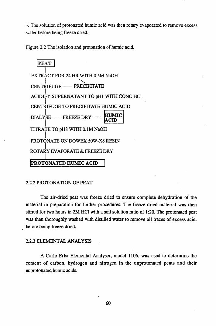
!. The solution of protonated humic acid was then rotary evaporated to remove excess water before being freeze dried.
Figure 2.2 The isolation and protonation of humic acid.
PEAT
EXTRACT FOR 24 HR WITH 0.5M NaOHI \
CENTRIFUGE PRECIPITATE
ACIDIFY SUPERNATANT TO pHl WITH CONC HC1
CENTRIFUGE TO PRECIPITATE HUMIC ACID
DIALYSE------FREEZE DRY— HUMICACID
TITRATE TO pH8 WITH 0.1M NaOH
PROTONATE ON DOWEX 50W-X8 RESIN
ROTARY EVAPORATE & FREEZE DRY
PROTONATED HUMIC ACID
2.2.2 PROTONATION OF PEAT
The air-dried peat was freeze dried to ensure complete dehydration of the material in preparation for further procedures. The freeze-dried material was then stirred for two hours in 2M HC1 with a soil solution ratio of 1:20. The protonated peat was then thoroughly washed with distilled water to remove all traces of excess acid, before being freeze dried.
2.2.3 ELEMENTAL ANALYSIS
A Carlo Erba Elemental Analyser, model 1106, was used to determine the content of carbon, hydrogen and nitrogen in the unprotonated peats and their unprotonated humic acids.
60
2.2.4 INFRA-RED CHARACTERISATION
2.2.4.1 PELLET PREPARATION
In order to analyse the samples, they first have to pelleted with anydrous KBr, and consequently care has to be taken in the preparation of the pellets since moisture can become incorporated in the pellet causing interference in the spectra produced (Stevenson & Goh, 1974). To minimise hygroscopic moisture the materials were always freeze dried and stored in a desiccator containing silica gel before pelleting.
0.7 mg of humic substance was ground with 300 mg of anhydrous KBr powder and pelleted under vacuum. The quantity of humic substance used is important since too much, or too little, can result in poor spectra which are difficult to interpret. The pellets produced were then desiccated under vacuum with silica gel before analysis in a Phillips PU9800 Spectrophotometer in the single-beam mode.
2.2.4.2 IONISATION STUDIES
To investigate the effects of alkali on the infra-red spectra of humic substances the protonated samples were titrated to pH 5 and pHl 0 with 0.05M KOH.
10 mg of the peat samples were suspended in 10 ml of de-ionised water and titrated to the required pH. After equilibration had been achieved the peat samples were washed with de-ionised water to remove any residual salt. The peats were then freeze dried before pelleting.
The protonated humic acid was titrated to pH 5 and pH 10, after the protonation step on the Dowex column. Thus it had not been freeze dried before titration and was still in a suspension. After titration and equilibration to the required pH value the humic acids were rotary evaporated to dryness and freeze dried before pelleting.
2.2.5 DETERMINATION OF THE TOTAL ACIDITY
The barium hydroxide method was used, which involved reacting the humic substances with barium hydroxide and then determining the amount of barium bound by titrating the unused base with standard acid (Piccolo & Camici, 1990).
The first step in the procedure involves the preparation of the 0.1 M barium hydroxide used in the method. Contamination by CO2 was minimised by preparing the solution using 11 of CO2 free distilled water to which 36 g of Ba(OH) 2 was added. This was then sealed, taking care to displace all air with N2 , and the solution was
61
stirred for 24 hours, whilst gently heating. The solution was then cooled and settled before checking the concentration with standard 0.1M HC1.
50-100 mg of the humic substances were shaken for 24 hours with 20 ml of the Ba(OH) 2 under nitrogen. A blank sample containing only Ba(OH)2 was also run. On completion of shaking the samples were filtered and washed with CO2 free distilled water. The filtrate and the washings were combined and stored under N2 until being titrated potentiometrically with standard acid to pH 8.4. An Orion pH meter was used to record the pH, and to obtain an accurate measurement of the end point a microburette was used. The blank sample was also titrated and is included in the calculation below.
Initially the acid used was 0.5M HC1 (Schnitzer & Khan, 1972). Since the end point was too sharp with this acid 0.1M HC1 was standardised against 1M NaOH and used in all measurements. The calculation used is as follows:
(end point blank - end point sample) x Macid x 1000 , , , ... -------------------- = mmole/g total aciditymg of sample
- where mmole = millimoles of charge on the humic substance.
2.2.6 DETERMINATION OF THE CARBOXYL CONTENT
The method used involved reacting the humic substances with calcium acetate to give acetic acid and calcium humate. The released acetic acid is then titrated with standard base to determine how many groups have reacted (Schnitzer & Khan, 1972).
As with the total acidity determination care must be taken to avoid interference from CO2 and all determinations were carried out under nitrogen. Again between 50- 100 mg of humic substance is required.
The humic substances were shaken with 10 ml of 1M calcium acetate, and 40 ml of CO2 free distilled water for 24 hours, along with a blank sample. The suspensions and blanks were then filtered and washed with CO2 free distilled water and the filtrates and washings combined. These were titrated potentiometrically with standard 0.1M sodium hydroxide to pH 9.8. The carboxyl content is determined through the following equation:
(end point sample - end point blank ) x M base x 1000 . , ----- = mmole/gCOOHmg of sample
62
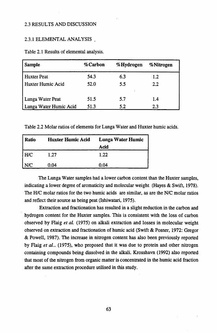
2.3 RESULTS AND DISCUSSION
2.3.1 ELEMENTAL ANALYSIS .
Table 2.1 Results of elemental analysis.
Sample % Carbon % Hydrogen % Nitrogen
Huxter Peat 54.3 6.3 1.2Huxter Humic Acid 52.0 5.5 2.2
Lunga Water Peat 51.5 5.7 1.4Lunga Water Humic Acid 51.3 5.2 2.3
Table 2.2 Molar ratios of elements for Lunga Water and Huxter humic acids.
Ratio Huxter Humic Acid Lunga Water HumicAdd
H/C 1.27 1.22
N/C 0.04 0.04
The Lunga Water samples had a lower carbon content than the Huxter samples, indicating a lower degree of aromaticity and molecular weight (Hayes & Swift, 1978). The H/C molar ratios for the two humic acids are similar, as are the N/C molar ratios and reflect their source as being peat (Ishiwatari, 1975).
Extraction and fractionation has resulted in a slight reduction in the carbon and hydrogen content for the Huxter samples. This is consistent with the loss of carbon observed by Flaig et al. (1975) on alkali extraction and losses in molecular weight observed on extraction and fractionation of humic acid (Swift & Posner, 1972: Gregor & Powell, 1987). The increase in nitrogen content has also been previously reported by Flaig et al.. (1975), who proposed that it was due to protein and other nitrogen containing compounds being dissolved in the alkali. Krosshavn (1992) also reported that most of the nitrogen from organic matter is concentrated in the humic acid fraction after the same extraction procedure utilised in this study.
63

2.3.2 INFRA-RED CHARACTERISATION
2.3.2.1 GENERAL FEATURES OF THE SPECTRA
The most striking feature of any infra-red spectrum of a humic substance is the broadness of the bands. This occurs due the heterogeneity of the humic substances, where there is a wide diversity in the types of functional group present as well as the diversity in the chemical environment of each functional group.
Table 2.3 The main absorption bands observed in infra-red spectra of humic substances.
Wavenumber(cm-1)
Functional Group
3400 O-H stretching and N-H stretching.2920 &2860 Aliphatic C-H stretching.1720 C=0 stretching, mainly from carboxyl groupings1650-1600 C=C vibrations, conjugated with C=0 or COO-.
H-bonded C=0 from quinones.1590 COO- symmetric stretching.1400 COO- antisymmetric stretching.1250 C-0 stretching, & OH deformation of COOH groups.1100-1020 Si-0 stretching (intense).1040 C-0 stretching of polysaccharides.
64
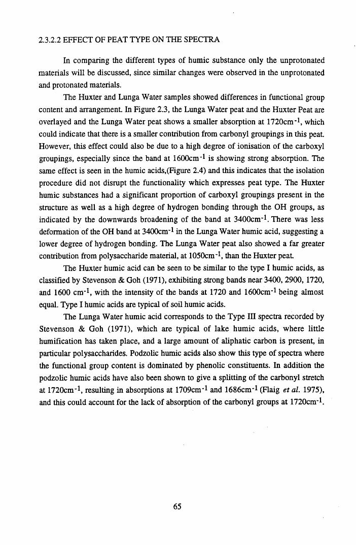
2 3 .2.2 EFFECT OF PEAT TYPE ON THE SPECTRA
In comparing the different types of humic substance only the unprotonated materials will be discussed, since similar changes were observed in the unprotonated and protonated materials.
The Huxter and Lunga Water samples showed differences in functional group content and arrangement. In Figure 2.3, the Lunga Water peat and the Huxter Peat are overlayed and the Lunga Water peat shows a smaller absorption at 1720cm-1, which could indicate that there is a smaller contribution from carbonyl groupings in this peat. However, this effect could also be due to a high degree of ionisation of the carboxyl groupings, especially since the band at 1600cm-1 is showing strong absorption. The same effect is seen in the humic acids,(Figure 2.4) and this indicates that the isolation procedure did not disrupt the functionality which expresses peat type. The Huxter humic substances had a significant proportion of carboxyl groupings present in the structure as well as a high degree of hydrogen bonding through the OH groups, as indicated by the downwards broadening of the band at 3400cm-1. There was less deformation of the OH band at 3400cm-1 in the Lunga Water humic acid, suggesting a lower degree of hydrogen bonding. The Lunga Water peat also showed a far greater contribution from polysaccharide material, at 1050cm-1, than the Huxter peat
The Huxter humic acid can be seen to be similar to the type I humic acids, as classified by Stevenson & Goh (1971), exhibiting strong bands near 3400, 2900,1720, and 1600 cm-l, with the intensity of the bands at 1720 and 1600cm-1 being almost equal. Type I humic acids are typical of soil humic acids.
The Lunga Water humic acid corresponds to the Type m spectra recorded by Stevenson & Goh (1971), which are typical of lake humic acids, where little humification has taken place, and a large amount of aliphatic carbon is present, in particular polysaccharides. Podzolic humic acids also show this type of spectra where the functional group content is dominated by phenolic constituents. In addition the podzolic humic acids have also been shown to give a splitting of the carbonyl stretch at 1720cm-1, resulting in absorptions at 1709cm-1 and 1686cm-1 (Flaig et al. 1975), and this could account for the lack of absorption of the carbonyl groups at 1720cm-l.
65
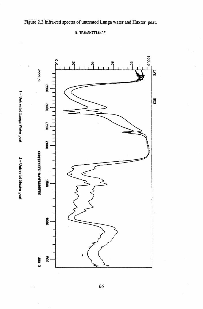
3999.9 COM
PRESSED-WAVENUM
BERS 400.3
Figure 2.3 Infra-red spectra of untreated Lunga water and Huxter peat.
X TRANSMITTANCE
©ro O)
LJCJ1oo
O)
(Jl
roo©
CJI©
oo
CJI
66
LW2 HX3
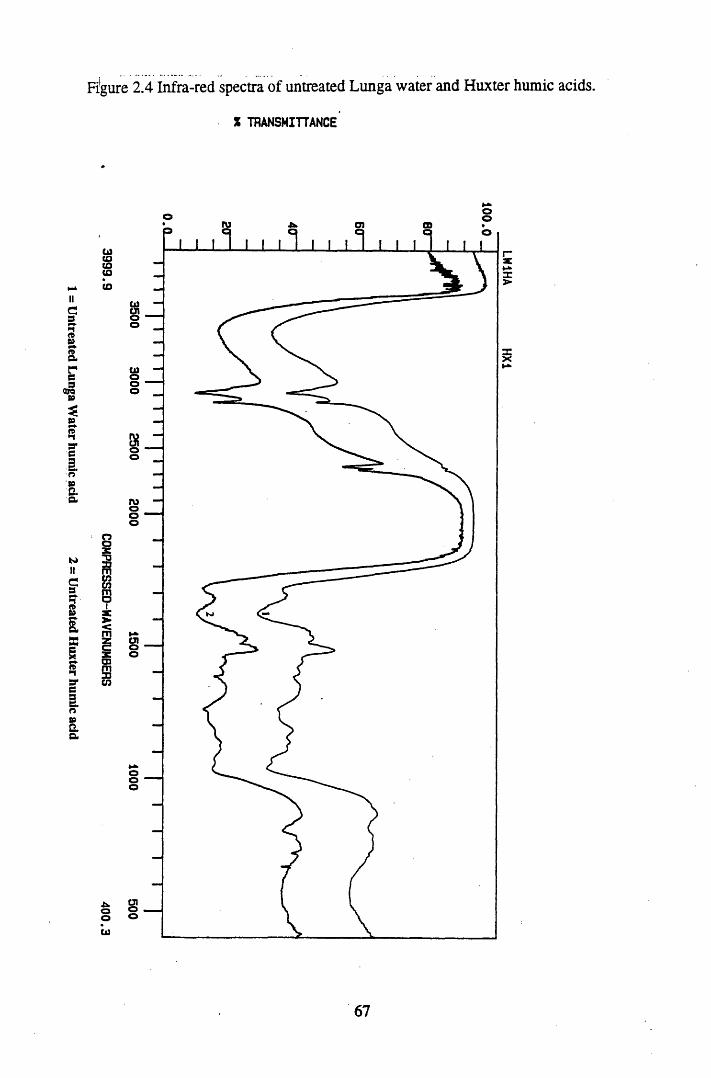
= U
ntreated Lunga
Water
humic
acid 2
= U
ntreated H
uxter hum
ic acid
Figure 2.4 Infra-red spectra of untreated Lunga water and Huxter humic acids.
% TRANSMITTANCE
o O!
U1(O(0(0CO
r*acx
x
o
roo
8X■oscncnm01x>IsCO
.uooCO
67
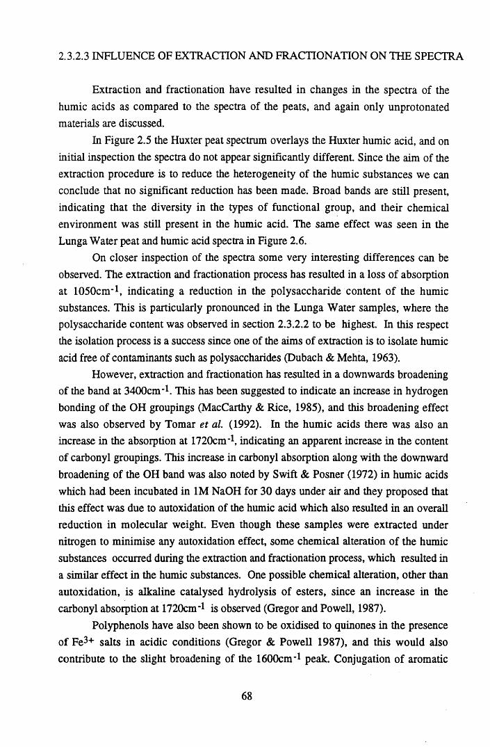
Z3.2.3 INFLUENCE OF EXTRACTION AND FRACTIONATION ON THE SPECTRA
Extraction and fractionation have resulted in changes in the spectra of the humic acids as compared to the spectra of the peats, and again only unprotonated materials are discussed.
In Figure 2.5 the Huxter peat spectrum overlays the Huxter humic acid, and on initial inspection the spectra do not appear significantly different. Since the aim of the extraction procedure is to reduce the heterogeneity of the humic substances we can conclude that no significant reduction has been made. Broad bands are still present, indicating that the diversity in the types of functional group, and their chemical environment was still present in the humic acid. The same effect was seen in the Lunga Water peat and humic acid spectra in Figure 2.6.
On closer inspection of the spectra some very interesting differences can be observed. The extraction and fractionation process has resulted in a loss of absorption at 1050cm-1, indicating a reduction in the polysaccharide content of the humic substances. This is particularly pronounced in the Lunga Water samples, where the polysaccharide content was observed in section 2.3.2.2 to be highest. In this respect the isolation process is a success since one of the aims of extraction is to isolate humic acid free of contaminants such as polysaccharides (Dubach & Mehta, 1963).
However, extraction and fractionation has resulted in a downwards broadening of the band at 3400cm-1. This has been suggested to indicate an increase in hydrogen bonding of the OH groupings (MacCarthy & Rice, 1985), and this broadening effect was also observed by Tomar et a l (1992). In the humic acids there was also an increase in the absorption at 1720cm-1, indicating an apparent increase in the content of carbonyl groupings. This increase in carbonyl absorption along with the downward broadening of the OH band was also noted by Swift & Posner (1972) in humic acids which had been incubated in 1M NaOH for 30 days under air and they proposed that this effect was due to autoxidation of the humic acid which also resulted in an overall reduction in molecular weight. Even though these samples were extracted under nitrogen to minimise any autoxidation effect, some chemical alteration of the humic substances occurred during the extraction and fractionation process, which resulted in a similar effect in the humic substances. One possible chemical alteration, other than autoxidation, is alkaline catalysed hydrolysis of esters, since an increase in the carbonyl absorption at 1720cm-1 is observed (Gregor and Powell, 1987).
Polyphenols have also been shown to be oxidised to quinones in the presence of Fe3+ salts in acidic conditions (Gregor & Powell 1987), and this would also contribute to the slight broadening of the 1600cm-1 peak. Conjugation of aromatic
68
C=C bonds with C=0 bonds on alkali treatment, or hydrogen bonding of conjugated ketones and quinones could also contribute to this broadening. Tomar et a l (1992) observed that the carbonyl absorption band for quinones shifted downwards when hydrogen bonding occurred.
However, the results must be interpreted with caution due to the possibility of adsorbed moisture causing interferences in the 3300 to 3000cm'1 and 1720 to 1500cm-1 regions (Stevenson 1982).
69
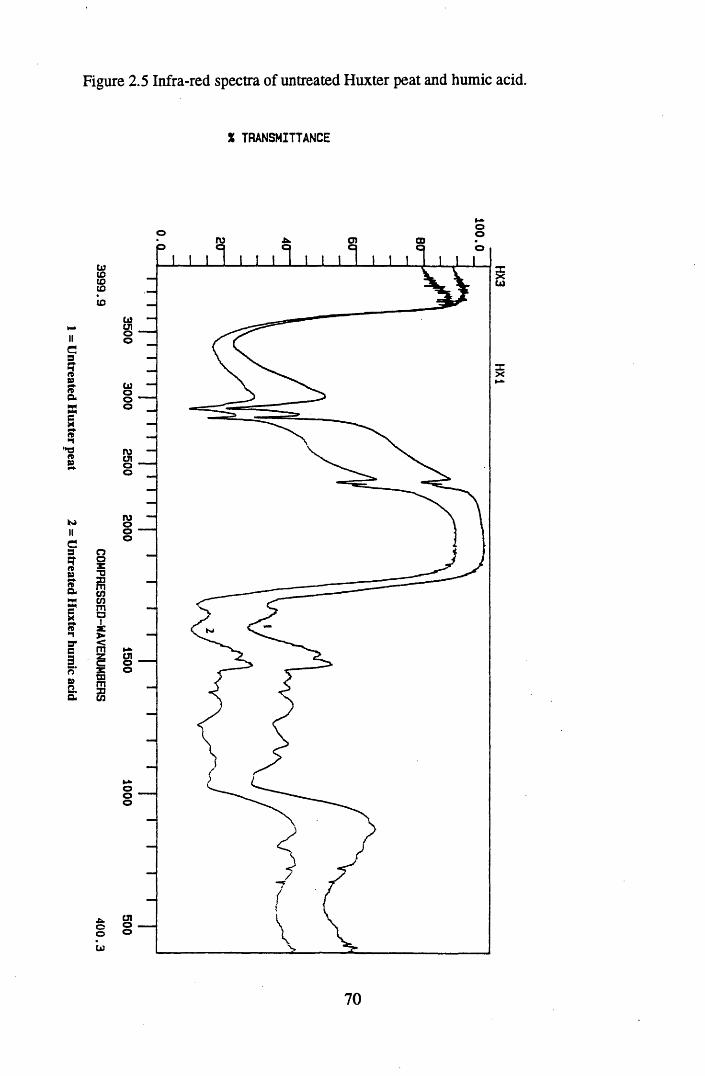
= U
ntreated H
uxter peat
2 =
Untreated
Huxter
humic
acid
Figure 2.5 Infra-red spectra of untreated Huxter peat and humic acid.
X TRANSMITTANCE
ru cn CD
cnIDtototo
XXCl)
o
XX
too
ruoooo5£cncnmaix►<mzcX o03mxcn
CJIx.ooto
70
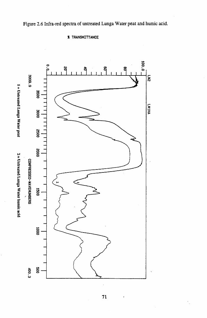
= U
ntreated Lunga
Water
peat 2
= U
ntreated Lunga
Water
humic
acid
Figure 2.6 Infra-red spectra of untreated Lunga Water peat and humic acid.
X TRANSMITTANCE
03COCOCOCO
o0 sc *o s m cn cn m □1a:►<mzcsc03mascn
oo02
O ru cn a>
r~x;ru
&oo
02ooo
rucnoo
ruooo
cnoo
ooo
cnoo
71
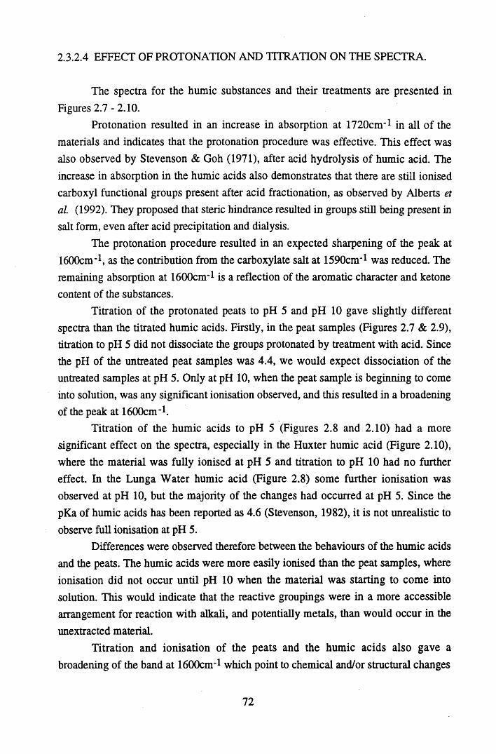
2.3.2.4 EFFECT OF PROTONATION AND TITRATION ON THE SPECTRA.
The spectra for the humic substances and their treatments are presented in Figures 2.7 - 2.10.
Protonation resulted in an increase in absorption at 1720cm'1 in all of the materials and indicates that the protonation procedure was effective. This effect was also observed by Stevenson & Goh (1971), after acid hydrolysis of humic acid. The increase in absorption in the humic acids also demonstrates that there are still ionised carboxyl functional groups present after acid fractionation, as observed by Alberts et al (1992). They proposed that steric hindrance resulted in groups still being present in salt form, even after acid precipitation and dialysis.
The protonation procedure resulted in an expected sharpening of the peak at 1600cm'1, as the contribution from the carboxylate salt at 1590cm'1 was reduced. The remaining absorption at 1600cm'1 is a reflection of the aromatic character and ketone content of the substances.
Titration of the protonated peats to pH 5 and pH 10 gave slightly different spectra than the titrated humic acids. Firstly, in the peat samples (Figures 2.7 & 2.9), titration to pH 5 did not dissociate the groups protonated by treatment with acid. Since the pH of the untreated peat samples was 4.4, we would expect dissociation of the untreated samples at pH 5. Only at pH 10, when the peat sample is beginning to come into solution, was any significant ionisation observed, and this resulted in a broadening of the peak at 1600cm-1.
Titration of the humic acids to pH 5 (Figures 2.8 and 2.10) had a more significant effect on the spectra, especially in the Huxter humic acid (Figure 2.10), where the material was fully ionised at pH 5 and titration to pH 10 had no further effect. In the Lunga Water humic acid (Figure 2.8) some further ionisation was observed at pH 10, but the majority of the changes had occurred at pH 5. Since the pKa of humic acids has been reported as 4.6 (Stevenson, 1982), it is not unrealistic to observe full ionisation at pH 5.
Differences were observed therefore between the behaviours of the humic acids and the peats. The humic acids were more easily ionised than the peat samples, where ionisation did not occur until pH 10 when the material was starting to come into solution. This would indicate that the reactive groupings were in a more accessible arrangement for reaction with alkali, and potentially metals, than would occur in the unextracted material.
Titration and ionisation of the peats and the humic acids also gave a broadening of the band at 1600cm-1 which point to chemical and/or structural changes
72
in the peat samples on protonation and alkali treatment. On ionisation the carboxyl groupings become negatively charged and repulsion of the like charges may occur, giving an opening of structure (Stevenson 1982). Consequently, not only will different functional groupings become exposed, but the environment of the functional groupings will alter, resulting in the broadening effect seen. However, the alkali treatment itself may be causing chemical changes to the groups, resulting in broadening of the 1600cm"1 peak, with hydrogen bonding being a distinct possibilty. Extraction and fractionation of humic acid has previously been shown in section 2.3.2.3 to give this effect, along with a broadening of the OH peak which is also seen in the titrated peat samples, further indicating that the alkali treatment caused the changes observed in the humic acids.
The remaining absorption at 1720cm-1 seen in the samples at pH 10, could indicate that some COOH groupings were structurally not available for ionisation. In addition ketonic and quinone carbonyl groupings will also contribute to absorption in this region, and will not be ionised by alkali (Piccolo &Stevenson, 1982).
On protonation, the Lunga Water peat (Figure 2.7) and its humic acid (Figure 2.9) showed greater increases in absorption at 1720cm-1 than the Huxter samples indicating that there was a greater content of ionisable groupings present. This also points to a higher metal content of the peat, since these will be present as counter ions to the negtively charged groups. The Lunga Water samples were also more responsive to the effect of titration, indicating there was a higher content of oxygen containing functional groups in these samples.
73
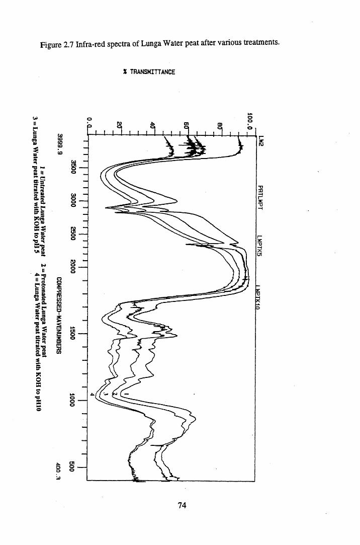
1 =
Untreated Lunga
Water
peat 2
= Protonated
Lunga W
ater peat
= Lunga
Water
peat titrated with
KOH to
pH 5
4 =
Lunga W
ater peat titrated
with KOH
to pH
IO
Figure 2.7 Infra-red spectra of Lunga Water peat after various treatments.
X TRANSMITTANCE
o*
03IDtototo
0 a
3cncnma1<m
csScn
cn o
ru
■oCD
Z
ru
cn
o
74
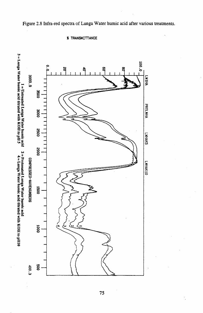
1 =
Untreated
Lunga W
ater hum
ic add
2 =
Protonated Lunga
Water
humic
acid =
Lunga W
ater hum
ic add
titrated with
KOH to
pH 5
4 -
Lunga W
ater humic
add titrated
with KOH
to pH
IO
Figure 2.8 Infra-red spectra of Lunga Water humic acid after various treatments.
X TRANSMITTANCE
utotototo
o0X"O33mcncnma1ae>■<m
03m33cn
ooCO
ro O)c
X>cnCJIoo
XCOooo
roCJIoo
CJI
ruooo
X
CJIoo
ooo
CJIoo
75
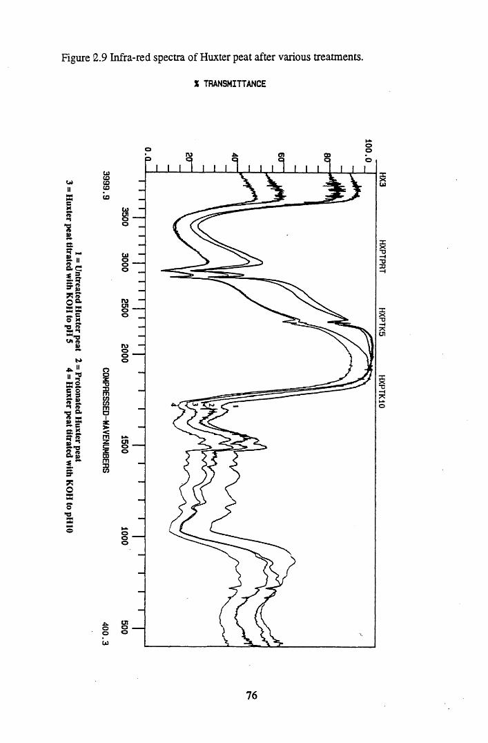
Figure 12.9 Infra-red spectra of Huxter peat after various treatments.
X TRANSMITTANCE
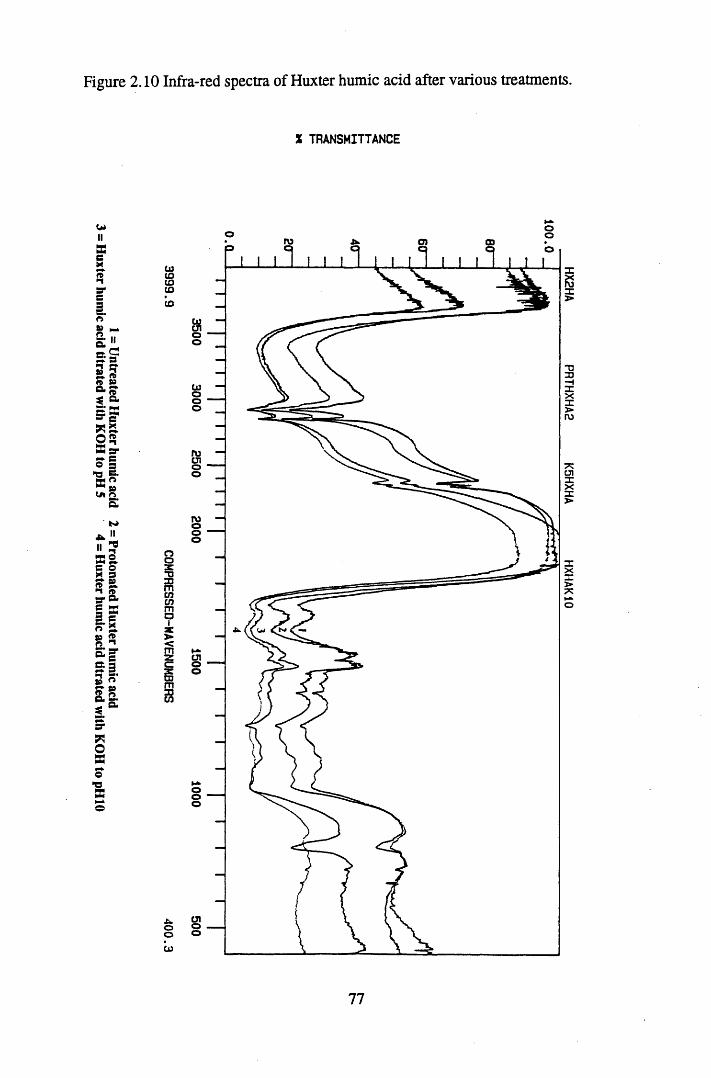
1 =
Untreated
Huxter
humic
add 2
= Protonated
Huxter
humic
acid =
Huxter
humic
acid titrated
with KOH
to pH
5 4
= H
uxter hum
ic acid
titrated with
KOH to
pHIO
Figure 2.10 Infra-red spectra of Huxter humic acid after various treatments.
X TRANSMITTANCE
03toCO(JO
CO
O0X“O33mcnO)ma1x►<mzcXCDm3303
.uoo03
o ru O)
03CJIoo
03ooo
ru(71Oo
ruooo
(31oo
77
HX2HA PR
THX
HA2
K5HXH
A H
XH
AK
10
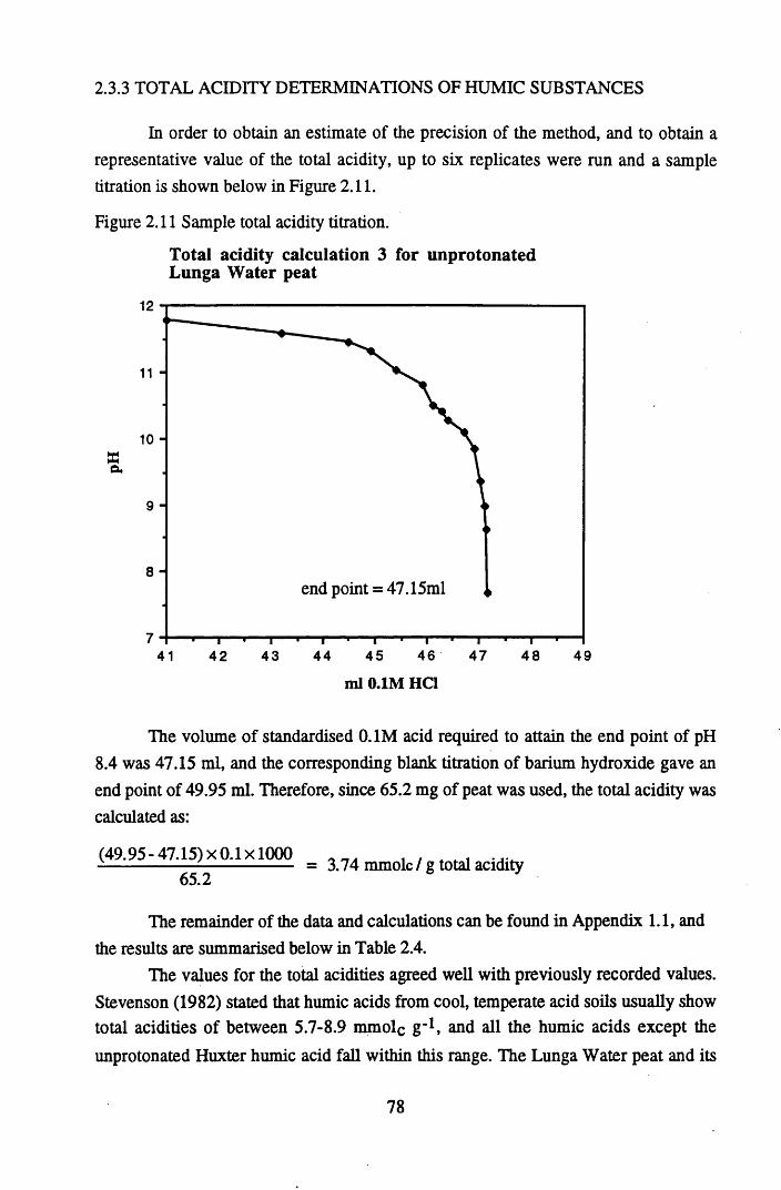
2.3.3 TOTAL ACIDITY DETERMINATIONS OF HUMIC SUBSTANCES
In order to obtain an estimate of the precision of the method, and to obtain a representative value of the total acidity, up to six replicates were run and a sample titration is shown below in Figure 2.11.
Figure 2.11 Sample total acidity titration.
Total acidity calculation 3 for unprotonated Lunga Water peat
12
11
10
9
8end point = 47.15ml
746 4745 48 4941 42 43 44
ml 0.1M HC1
The volume of standardised 0.1M acid required to attain the end point of pH8.4 was 47.15 ml, and the corresponding blank titration of barium hydroxide gave an end point of 49.95 ml. Therefore, since 65.2 mg of peat was used, the total acidity was calculated as:
(49.95-47.15)x 0.1x1000 , . ...2------------------------- = 3.74 mmole/g total acidity65.2
The remainder of the data and calculations can be found in Appendix 1.1, and the results are summarised below in Table 2.4.
The values for the total acidities agreed well with previously recorded values. Stevenson (1982) stated that humic acids from cool, temperate acid soils usually show total acidities of between 5.7-8.9 mmolc g"1, and all the humic acids except the unprotonated Huxter humic acid fall within this range. The Lunga Water peat and its
78
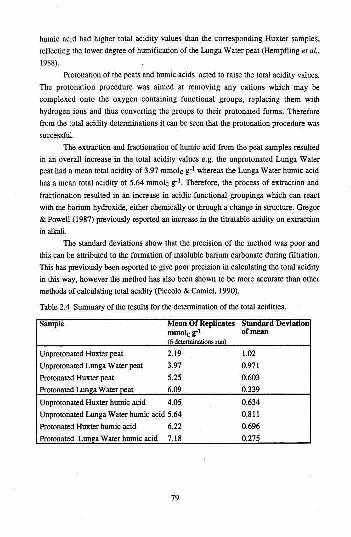
humic acid had higher total acidity values than the corresponding Huxter samples, reflecting the lower degree of humification of the Lunga Water peat (Hempfling et al, 1988).
Protonation of the peats and humic acids acted to raise the total acidity values. The protonation procedure was aimed at removing any cations which may be complexed onto the oxygen containing functional groups, replacing them with hydrogen ions and thus converting the groups to their protonated forms. Therefore from the total acidity determinations it can be seen that the protonation procedure was successful.
The extraction and fractionation of humic acid from the peat samples resulted in an overall increase in the total acidity values e.g. the unprotonated Lunga Water peat had a mean total acidity of 3.97 mmole g '1 whereas the Lunga Water humic acid has a mean total acidity of 5.64 mmole g-1. Therefore, the process of extraction and fractionation resulted in an increase in acidic functional groupings which can react with the barium hydroxide, either chemically or through a change in structure. Gregor & Powell (1987) previously reported an increase in the titratable acidity on extraction in alkali.
The standard deviations show that the precision of the method was poor and this can be attributed to the formation of insoluble barium carbonate during filtration. This has previously been reported to give poor precision in calculating the total acidity in this way, however the method has also been shown to be more accurate than other methods of calculating total acidity (Piccolo & Camici, 1990).
Table 2.4 Summary of the results for the determination of the total acidities.
Sample Mean Of Replicates Standard Deviation mmolc g”1 °f mean(6 determinations run)
Unprotonated Huxter peat 2.19 1.02
Unprotonated Lunga Water peat 3.97 0.971Protonated Huxter peat 5.25 0.603Protonated Lunga Water peat 6.09 0.339Unprotonated Huxter humic acid 4.05 0.634Unprotonated Lunga Water humic acid 5.64 0.811Protonated Huxter humic acid 6.22 0.696Protonated Lunga Water humic acid 7.18 0.275
79
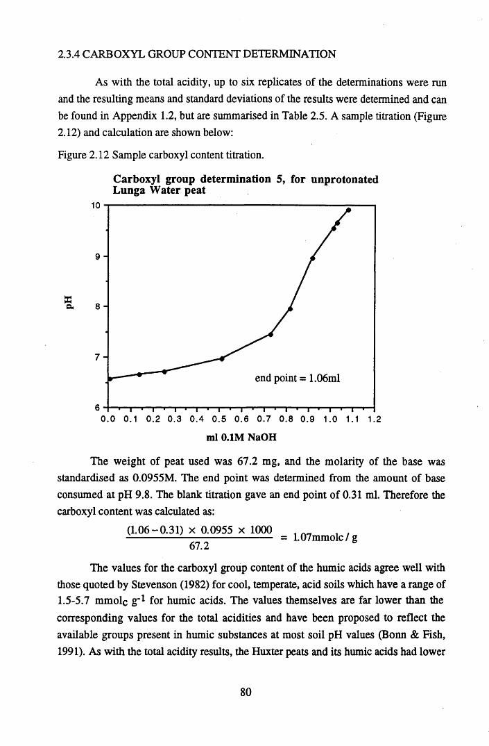
2.3.4 CARBOXYL GROUP CONTENT DETERMINATION
As with the total acidity, up to six replicates of the determinations were run and the resulting means and standard deviations of the results were determined and can be found in Appendix 1.2, but are summarised in Table 2.5. A sample titration (Figure 2.12) and calculation are shown below:
Figure 2.12 Sample carboxyl content titration.
Carboxyl group determination 5, for unprotonated Lunga Water peat
Xa.
10
9
8
7
end point = 1.06ml
60.0 0.1 0.2 0.3 0.4 0.5 0.6 0.7 0.8 0.9 1.0 1.1 1.2
ml 0.1M NaOH
The weight of peat used was 67.2 mg, and the molarity of the base was standardised as 0.0955M. The end point was determined from the amount of base consumed at pH 9.8. The blank titration gave an end point of 0.31 ml. Therefore the carboxyl content was calculated as:
(1.06-0.31) x 0.0955 x 100067.2
= 1.07 mmole / g
The values for the carboxyl group content of the humic acids agree well with those quoted by Stevenson (1982) for cool, temperate, acid soils which have a range of 1.5-5.7 mmole g"1 for humic acids. The values themselves are far lower than the corresponding values for the total acidities and have been proposed to reflect the available groups present in humic substances at most soil pH values (Bonn & Fish, 1991). As with the total acidity results, the Huxter peats and its humic acids had lower
80
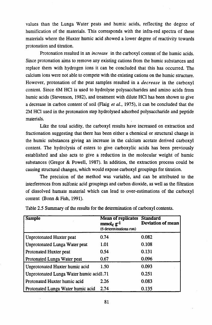
values than the Lunga Water peats and humic acids, reflecting the degree of humification of the materials. This corresponds with the infra-red spectra of these materials where the Huxter humic acid showed a lower degree of reactivity towards protonation and titration.
Protonation resulted in an increase in the carboxyl content of the humic acids. Since protonation aims to remove any existing cations from the humic substances and replace them with hydrogen ions it can be concluded that this has occurred. The calcium ions were not able to compete with the existing cations on the humic structure. However, protonation of the peat samples resulted in a decrease in the carboxyl content. Since 6M HC1 is used to hydrolyse polysaccharides and amino acids from humic acids (Stevenson, 1982), and treatment with dilute HC1 has been shown to give a decrease in carbon content of soil (Flaig et al., 1975), it can be concluded that the 2M HC1 used in the protonation step hydrolysed adsorbed polysaccharide and peptide materials.
Like the total acidity, the carboxyl results have increased on extraction and fractionation suggesting that there has been either a chemical or structural change in the humic substances giving an increase in the calcium acetate derived carboxyl content. The hydrolysis of esters to give carboxylic acids has been previously established and also acts to give a reduction in the molecular weight of humic substances (Gregor & Powell, 1987). In addition, the extraction process could be causing structural changes, which would expose carboxyl groupings for titration.
The precision of the method was variable, and can be attributed to the interferences from sulfonic acid groupings and carbon dioxide, as well as the filtration of dissolved humate material which can lead to over-estimations of the carboxyl content (Bonn & Fish, 1991).
Table 2.5 Summary of the results for the determination of carboxyl contents.
Sample Mean of replicates mmolc g"1(6 determinations run)
Standard Deviation of mean
Unprotonated Huxter peat 0.74 0.082Unprotonated Lunga Water peat 1.01 0.108Protonated Huxter peat 0.54 0.131Protonated Lunga Water peat 0.67 0.096Unprotonated Huxter humic acid 1.50 0.093Unprotonated Lunga Water humic acidl.71 0.251Protonated Huxter humic acid 2.26 0.083Protonated Lunga Water humic acid 2.74 0.135
81
2.4 CONCLUSIONS
One of the aims of the project was to investigate the nature of humic acid and whether it is a representative fraction of the soil humic substances, since controversy surrounds whether or not its properties are affected by the extraction and fractionation process. The characterisation studies utilised here show clearly that humic acid does show differences from unextracted materials.
The total acidity and carboxyl contents, even though they were operationally defined (Perdue, 1985) indicated that the reactivity of the humic acid was increased by the extraction and fractionation process, since increases in both of these parameters were observed. These changes could be due to structural effects, since on extraction the humic acid was removed from the other components of the soil and the complexity of the structure was broken down, making groups more available for reaction, and/or chemical changes. The titration of the samples showed how reactivity to alkali was affected by these changes. The humic acid was able to attain full ionisation at pH 5, whereas the peat did not achieve any degree of ionisation until pH 10, when the material was beginning to come into solution and more groups could be exposed for reaction. The infra-red and elemental analysis results reinforce the theory of chemical changes occurring. The infra-red spectra of the humic acids indicated that hydrogen bonding was occurring and the elemental analysis showed an increase in nitrogen content in the humic acid after extraction and fractionation.
The characterisation procedures clearly demonstrate the differences in the nature and reactivity of the two peats and their humic acids. The Lunga Water samples had greater total acidity, carboxyl content, lower carbon content, a greater polysaccharide content and in the infra-red spectra showed a greater reaction towards alkali. Conversely, the Huxter peat had a greater degree of aromatic carbon and a higher carbon content.
The study also demonstrated the potential of the procedures to give useful information on the nature of humic substances, in particular unextracted materials. The values for the total acidity and carboxyl contents can also be utilised in metal binding studies, and indeed the total acidity was used in this way, as will be discussed in Chapter 3.
Since the behaviour and reactivity of extracted humic substances is dependent on the functional group content, and from the results presented here this parameter is affected by extraction, the effect of the extraction on behaviour and reactivity will be discussed further in Chapter 3 and Chapter 4.
82
CHAPTER 3
INFRA-RED STUDIES OF THE INTERACTION OF METALS WITH
HUMIC SUBSTANCES
83
3.1 INTRODUCTION
The isolation of humic acid from peat was shown to give alterations in the amount of reactive functional groupings, their distribution and possibly even the type of functional group present. In the work presented in this chapter the reactivity of metals to humic substances, before and after isolation is investigated qualitatively, as well as the nature of the reaction between a humic substance and a metal.
Infra-red spectroscopy is used to study the interaction of metals with humic substances, since changes can be observed in the arrangements of the oxygen containing functional groups, in particular the degree of complex formation (Piccolo & Stevenson, 1982). The main changes which are observed occur in the region between 1750-1350cm-1, where the carboxyl groupings absorb. On formation of a carboxylate salt the carbonyl absorption is reduced significantly due to formation of the carboxylate anion, which is resonance stabilised. Correspondingly, two characteristic frequencies for the antisymmetric and symmetric carboxylate stretch are formed and occur at ~ 1590cm-1 and ~1390cm-1 accordingly. The exact position of these bands depends on the nature of the linkage between the carboxylic acid grouping and the metal. It was demonstrated that the difference in frequency between these two bands, A (vaC02‘ - vC02‘ ), can be used to characterise complexes.
A carboxylate grouping can complex with a metal ion through chelation, coordination or bridging reactions (see Figure 1.3). The formation of coordinate complexes gave A values which were greater than ionic complexes, whilst chelate complexes gave A values which were significantly lower than ionic values. The bridging complexes were intermediate between the chelate and ionic A values (Nakamoto, 1986).
Vinkler et al. (1976) utilised these differences in the A values to determine complex formation between humic substances and various metals. They found that the alkaline metals, such as Cs+, Na+ and K+ were showing frequencies of antisymmetric stretch characteristic of ionic linkages. By contrast Mn2+, Fe2+, Cu2+, Mg2+, Al3*, Cr2+ and Zn2+ all showed shifts towards lower frequencies, with Al^" and Cr2+ showing the greatest shifts and correspondingly the greatest degrees of covalency. In a later study, Piccolo and Stevenson (1982) proposed that this type of study could lead to ambiguous conclusions, due to the possibility of the metais interacting with groupings which also absorb in the 1600-1660cm-1 region. They demonstrated that Cu2+, Pb2+ and Ca2+ were able to interact with groupings that K+ was not able to, and proposed that the reactive groupings could be conjugated ketonic structures which absorb in the range 1660-1600cm-1 when weakened by resonance. Mg2+, Sr2+ and
84
Zn2+ have also been shown to give this effect, particularly at high degrees of metal loading, indicating again that they can form more covalent inner sphere complexes, perhaps with conjugated ketones (Maguire et al. , 1991). Conversely Cs+ and K+ react to give more ionic, outer sphere complexes (Piccolo & Stevenson, 1982: Maguire et a l , 1991).
The ability of metals to form covalent coordinate linkages is related to their hard or soft character, with the softer Class B metal cations such as Pb2+ and Zn2+ being more polarisable and amenable to coordination reactions. The Class A metal cations such as Na+, K+ and Sr2+ are less polarisable and participate more in ionic interactions (Pearson, 1963). Thus, in the work presented here a range of metals which incorporated both groups of cations were chosen in order to investigate the potential of different cations to undergo coordination reactions with humic substances, providing valuable information on their potential mobility and bioavailabilty in the environment. The metals were also chosen for their environmental importance as contaminating metals in many systems e.g. Pb, Cu, Zn and Cs. This is of particular importance since they were reacted with the humic substances at levels which would be contaminating in environmental systems.
The effect of metal additions to salicylic and phthalic acids were studied in order to investigate the covalency of interaction in simple compounds which have a known chemical structure. These acids were also chosen since they have been proposed to be the main arrangement of the oxygen-containing functional groupings on humic substances (Stevenson, 1977).
85
3.2 METHODS
3.2.1 THE ADDITION OF METALS TO HUMIC ACID AND PEAT
Metal additions were carried out to both the peats and their corresponding humic acids which were characterised in Chapter 2. Thus, the investigation on the effects of peat type on reactivity could be continued.
The levels of metal addition were based on the values for the total acidity presented in section 2.3.3, with additions being made at half the total acidity, total acidity and twice the total acidity. All metals were added as 0.02M chloride salts, except for Pb2+ and Ag+ which were added as 0.02M nitrate salts. Cs+, Pb2+, Sr2+, Zn2+, Cu2+ and Ag+ were added to the humic acids, and the effects in the spectra investigated. In the peats, only the effects of additions of Cs+, Pb2+ and Sr2+ were studied.
Metal additions were made to the protonated peats and humic acids, with the pH being recorded as being between pH 2.5 and 3. Metal additions were also made to the peats and humic acids after titration with 0.05M KOH to pH 5, and KOH was also used to re-adjust the pH to 5 after metal addition. Thus the effect of ionisation on the reactivity of the humic substances could also be investigated. The addition of alkali was made utilising a Gilsen microburrete and the pH was recorded with an Orion pH meter. After metal addition all materials were washed with de-ionised water to remove excess salt before freeze drying and stored in a vacuum desiccator until analysis. The metal-humate complexes were analysed as KBr pellets, as outlined in section 2.2.4.1.
3.2.2 THE ADDITION OF METALS TO PHTHALIC AND SALICYLIC ACIDS
The addition of CsCl, SrCl2 , Pb(N0 3 )2 , and AgN0 3 to phthalic and salicylic acids was also studied. The metals were added to the total titratable acidity, as calculated from the end point of the titration of the acids with 0.5M KOH. The buffer curves and the calculation of their end points are in Appendix 1.3, and gave a mean value of 8.15 mmole g’1 titratable acidity for salicylic acid and 14.52 mmole g"1 titratable acidity for phthalic acid. A sample buffer curve and calculation are shown in Figure 3.1.
As with the metal additions to humic substances, metal additions were made to the compounds with no pH adjustment and with the pH adjusted before and after
86
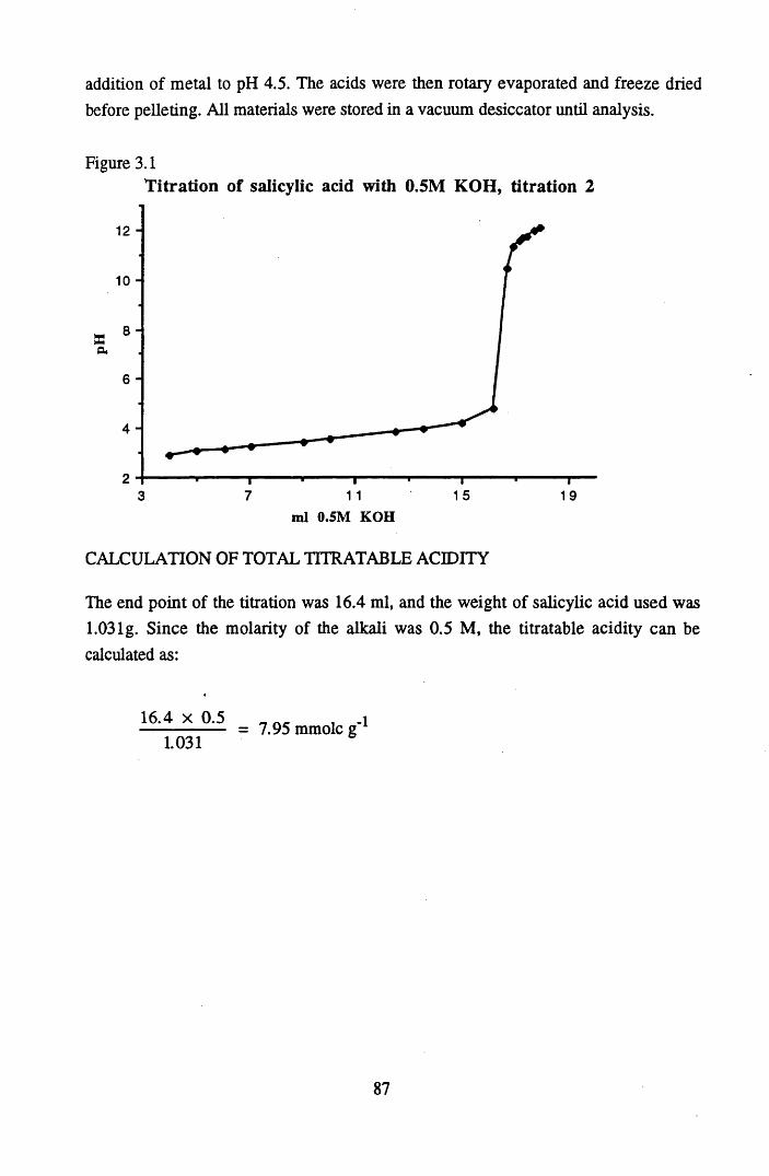
addition of metal to pH 4.5. The acids were then rotary evaporated and freeze dried before pelleting. All materials were stored in a vacuum desiccator until analysis.
Figure 3.1Titration of salicylic acid with 0.5M KOH, titration 2
12 -
10 -
Ea.
1 57 1 1 193ml 0.5M KOH
CALCULATION OF TOTAL TITRATABLE ACIDITY
The end point of the titration was 16.4 ml, and the weight of salicylic acid used was 1.03lg. Since the molarity of the alkali was 0.5 M, the titratable acidity can be calculated as:
16.4 x 0.5 ___ . _i--------------- = 7.95 mmole g1.031
87
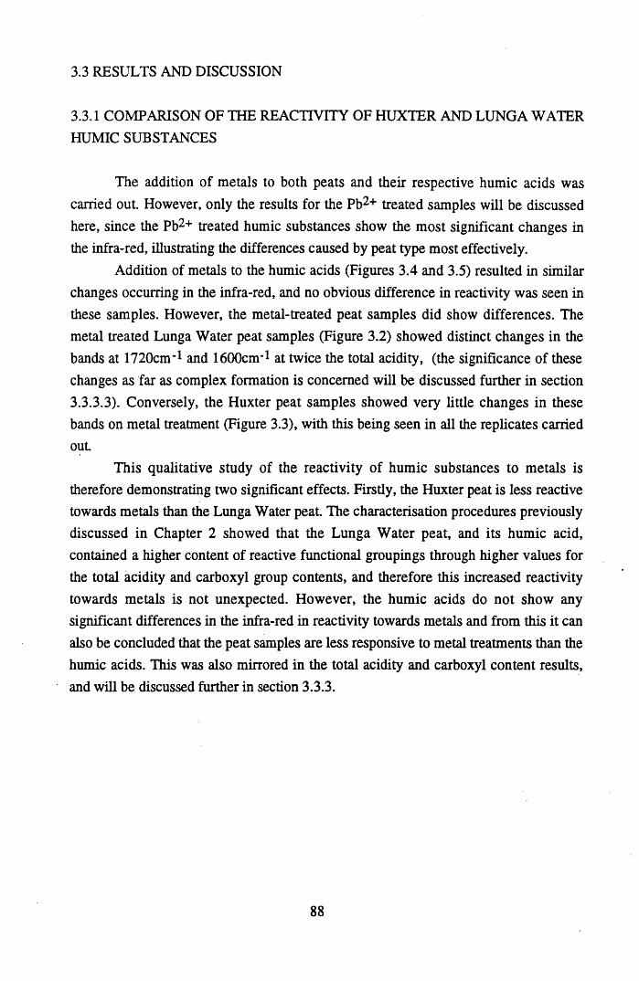
3.3 RESULTS AND DISCUSSION
3.3.1 COMPARISON OF THE REACTIVITY OF HUXTER AND LUNGA WATER HUMIC SUBSTANCES
The addition of metals to both peats and their respective humic acids was carried out. However, only the results for the Pb2+ treated samples will be discussed here, since the Pb2+ treated humic substances show the most significant changes in the infra-red, illustrating the differences caused by peat type most effectively.
Addition of metals to the humic acids (Figures 3.4 and 3.5) resulted in similar changes occurring in the infra-red, and no obvious difference in reactivity was seen in these samples. However, the metal-treated peat samples did show differences. The metal treated Lunga Water peat samples (Figure 3.2) showed distinct changes in the bands at 1720cm-1 and 1600cm-1 at twice the total acidity, (the significance of these changes as far as complex formation is concerned will be discussed further in section 3.3.3.3). Conversely, the Huxter peat samples showed very little changes in these bands on metal treatment (Figure 3.3), with this being seen in all the replicates carried out
This qualitative study of the reactivity of humic substances to metals is therefore demonstrating two significant effects. Firstly, the Huxter peat is less reactive towards metals than the Lunga Water peat. The characterisation procedures previously discussed in Chapter 2 showed that the Lunga Water peat, and its humic acid, contained a higher content of reactive functional groupings through higher values for the total acidity and carboxyl group contents, and therefore this increased reactivity towards metals is not unexpected. However, the humic acids do not show any significant differences in the infra-red in reactivity towards metals and from this it can also be concluded that the peat samples are less responsive to metal treatments than the humic acids. This was also mirrored in the total acidity and carboxyl content results, and will be discussed further in section 3.3.3.
88
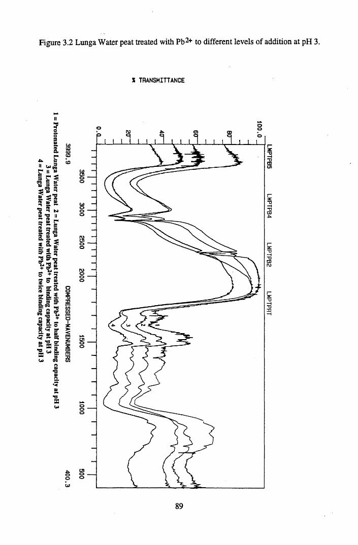
Figure 3.2 Lunga Water peat treated with Pb2+ to different levels of addition at pH 3.
X TRANSMITTANCE
89
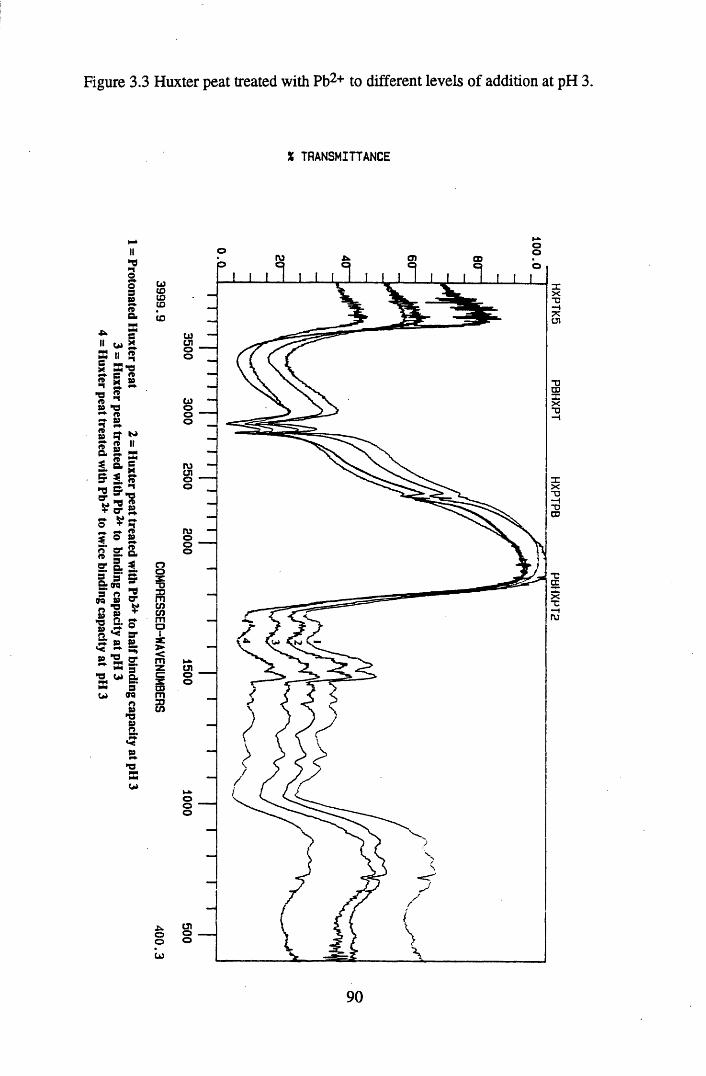
= Protonated
Huxter
peat 2
= H
uxter peat treated
with P
b24 to
half binding capacity
at pH 3
3 =
Huxter
peat treated with
Pb2*
to binding
capacity at pH
3 4
= H
uxter peat treated
with P
b2* to
twice binding
capacity at
pH 3
Figure 3.3 Huxter peat treated with Pb2+ to different levels of addition at pH 3.
X TRANSMITTANCE
90
HXPTK5
PBHXPT H
XPTPB P
BH
XP
T2
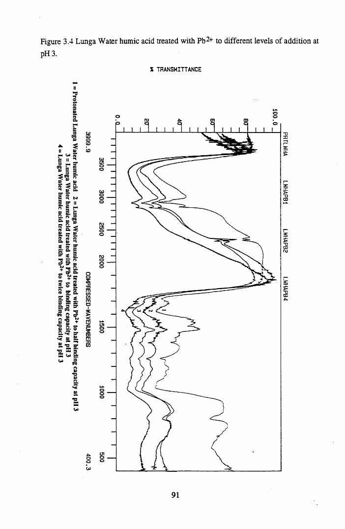
= Protonated
Lunga W
ater hum
ic acid
2 =
Lunga W
ater hum
ic acid
treated with
Pb2+ to
half binding capacity
at pH 3
3 =
Lunga W
ater hum
ic acid
treated with
Pb2+ to
binding capacity
at pH 3
4 =
Lunga W
ater hum
ic acid
treated with
Pb2+ to
twice binding
capacity at pH
3
Figure 3.4 Lunga Water humic acid treated with Pb2+ to different levels of addition atpH 3.
% TRANSMITTANCE
CUCOCOCD(D
n0 z ■o23mcocoma1x><
CDm23CO
oo03
ro at o
U)CJIoo
uooo
roCJIoo
roooo
u>t-*CJIoo
ooo
91
PRTLW
HA
LWH
APB1
LWH
APB2 I.W
HA
PB
4
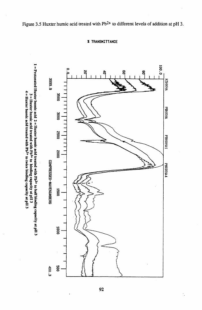
Protonated H
uxter humic
acid 2
= H
uxter humic
acid treated
with Pb2*
to half binding
capacity at pH
3 3
= H
uxter humic
acid treated
with Pb2+
to binding
capacity at pH
3 4
= H
uxter hum
ic acid
treated with
Pb2+ to
twice binding
capacity at pH
3
Figure 3.5 Huxter humic acid treated with Pb2+ to different levels of addition at pH 3.
X TRANSMITTANCE
oru o> CD
cutotoCOto
CJIXX>
u>CJI
TJCD
u X
ruCJI *tj
CD
XX
ru
8XTJ3Jmcocom01
X>
><mzcXO Jmxco
ooo
CJIoo.uoo03
92
3.3.2 THE EFFECT OF METAL ADDITIONS TO HUMIC ACID
In order to simplify interpretation only the Lunga Water humic acid treatments will be discussed, since as demonstrated in section 3.3.1., the effect of metal treatment was the same in both humic acids.
3.3.2.1 CS+-TREATED HUMIC ACID
The effect of Cs+ additions to humic acid at different levels of metal addition was investigated in protonated humic acid, at pH 3, and also humic acid which had been titrated to pH 5.
In the protonated humic acid (Figure 3.6), treatment with Cs+ resulted in changes in the spectra which indicate that ionisation of carboxyl groupings is occurring. As outlined in section 3.1, this gives a loss of the carbonyl absorption at 1720cm-1, with a corresponding appearance of bands at ~1590cm-1 and ~1400cm-1. This effect is clearly seen in the Cs+ treated samples in Figure 3.6, and also results in a slight broadening of the band at 1600cm-1. In addition, at twice the total acidity, the band at 3400-1 shows downward broadening which is indicative of formation of water of crystallisation on formation of the salt (Kemp, 1991).
The Cs+ additions at pH 5 are displayed in Figure 3.7, and can be compared to the corresponding K+ salt at pH 5. From the spectra it can be seen that both Cs+ and K+ are binding in a similar manner through an ionic interaction, as demonstrated by previous infra-red studies (Vinkler et al., 1976; Maguire et al., 1991). Bonn and Fish (1993) also showed through adsorption studies that K+ binds as a hydrated ion, forming ionic complexes with humic acid.
In both Figures 3.6 and 3.7, level of addition has little effect on the changes seen at 1720cm-1 and 1600cm-1, with only slight increases in reaction at twice the total acidity, indicating that the maximum binding capacity of the humic acid for Cs+ was reached at half the total acidity. There is also a remaining carbonyl absorption which is due to ketonic and aldehydic groupings present in the humic substances (Piccolo & Stevenson, 1982). There may also be the interacting effect of some groupings being sterically hindered, and therefore unavailable for reaction.
93
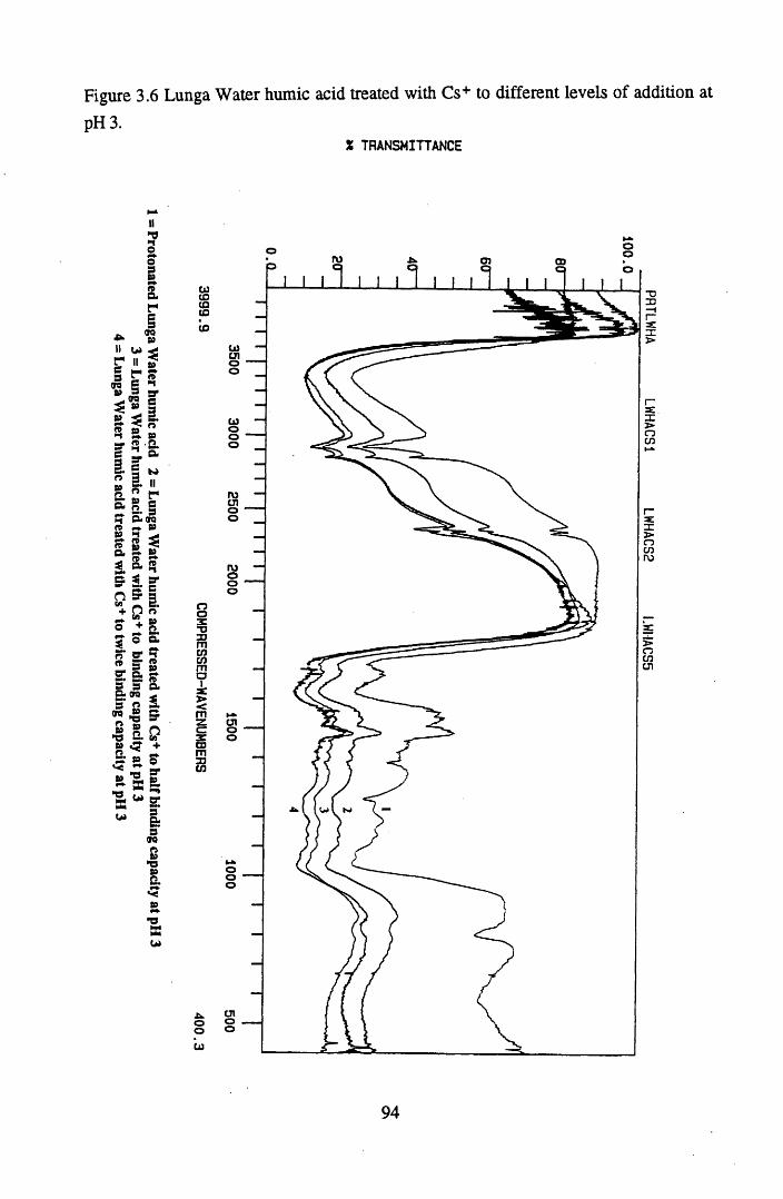
= Protonated
Lunga W
ater hum
ic acid
2 =
Lunga W
ater hum
ic acid
treated with
Cs+ to
half binding capacity
at pH 3
3 =
Lunga W
ater hum
ic acid
treated with
Cs+
to binding
capacity at pH
3 4
= Lunga
Water
humic
acid treated
with Cs+
to twice
binding capacity
at pH 3
Figure 3.6 Lunga Water humic acid treated with Cs+ to different levels of addition at
pH 3.X TRANSMITTANCE
cototototo
ooacT333mCOCOm01s:><mzc3ECDm33CO
OOCD
Oru oi CD
CD
IUCJI
CJI
CJI
94
PRTLWHA
LWH
ACS1
LWHAC
S2 LH
HA
CS
5
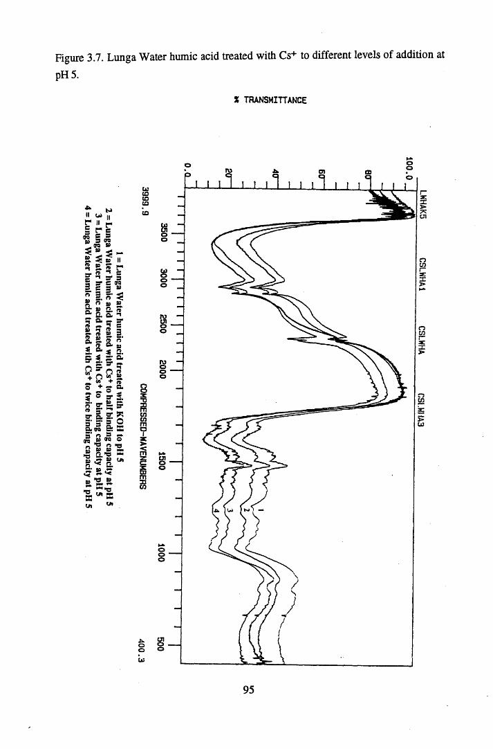
Figure 3.7. Lunga Water humic acid treated with Cs+ to different levels of addition at
pH 5.
X TRANSMITTANCE
II u>r iiB r*3 «% iL. 90^ i 5 s.M AB 2- 3 B « 3s. 25 8.ft ^ 69 5
a? a5 in ? + 0S "? »o' £MS a 5 3* Ss90 3* ft« £ T3S gns C.1 *ST 3- K 1“
bJIIrcs
00s»
to II5 ^ ft e s* s e oo3 3ft' ^ {0 692. S’ a ft s- 3* ft 38 3 J? o a M* g.ST O* 2 ~£? l+ ft
S' 2.69 *■* “ STcr ^ 3* O6 X3 ~00 oo >o to M *o »+£ <* 2.•S?*aasin
tttCO(Ototo
X*offlCflCOmai
m
§mxco
.twOoin
95
LWHAK5
CSLW
HA1
CSLWHA
CS
LWH
A3
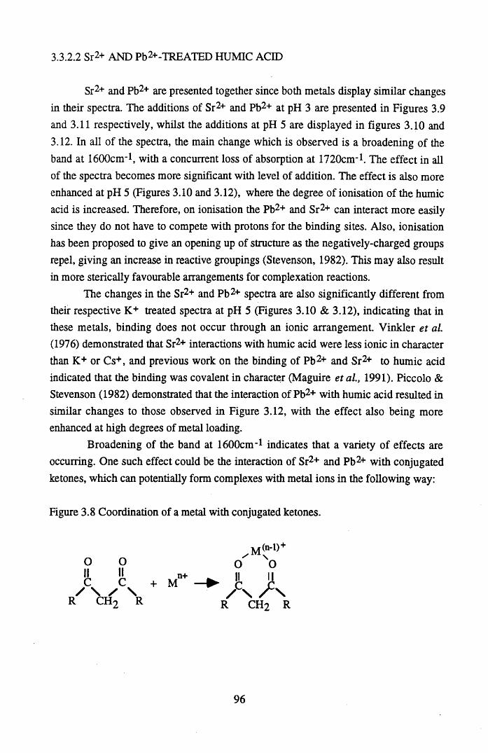
3.3.22 Sr2+ AND Pb2+-TREATED HUMIC ACID
Sr2+ and Pb2+ are presented together since both metals display similar changes in their spectra. The additions of Sr2+ and Pb2+ at pH 3 are presented in Figures 3.9 and 3.11 respectively, whilst the additions at pH 5 are displayed in figures 3.10 and 3.12. In all of the spectra, the main change which is observed is a broadening of the band at 1600cm-1, with a concurrent loss of absorption at 1720cm-1. The effect in all of the spectra becomes more significant with level of addition. The effect is also more enhanced at pH 5 (Figures 3.10 and 3.12), where the degree of ionisation of the humic acid is increased. Therefore, on ionisation the Pb2+ and Sr2+ can interact more easiiy since they do not have to compete with protons for the binding sites. Also, ionisation has been proposed to give an opening up of structure as the negatively-charged groups repel, giving an increase in reactive groupings (Stevenson, 1982). This may also result in more sterically favourable arrangements for complexation reactions.
The changes in the Sr2+ and Pb2+ spectra are also significantly different from their respective K+ treated spectra at pH 5 (Figures 3.!0 & 3.12), indicating that in these metals, binding does not occur through an ionic arrangement. Vinkler et a l (1976) demonstrated that Sr2+ interactions with humic acid were less ionic in character than K+ or Cs+, and previous work on the binding of Pb2+ and Sr2+ to humic acid indicated that the binding was covalent in character (Maguire et al, 1991). Piccolo & Stevenson (1982) demonstrated that the interaction of Pb2+ with humic acid resulted in similar changes to those observed in Figure 3.12, with the effect also being more enhanced at high degrees of metal loading.
Broadening of the band at 1600cm-1 indicates that a variety of effects are occurring. One such effect could be the interaction of Sr2+ and Pb2+ with conjugated ketones, which can potentially form complexes with metal ions in the following way:
Figure 3.8 Coordination of a metal with conjugated ketones.
O OII II
R CH2 R
96
The carbonyl groupings become weakened by this resonance and the frequency of absorption is correspondingly reduced (Bellamy, 1975). This interaction thus explains the observed reduction in absorption at 1720cm*1, which is not observed in the K+ spectra, and would also contribute to the broadening seen in the spectra of Pb2+ and Sr2+ humates. The frequency of absorption is also affected by the arrangement of the metal-ketone interaction. Nakamoto (1986) showed that if the metal was bound in the keto form (as shown above), then absorption of the carbonyl group centres around 1700cm*1. However, if the enol form occurs, then absorption is shifted to around 1627cm*1. In humic acid where a variety of ketonic groupings could be present, with different environments, then a mixture of enol and keto arrangements could occur.
In addition, the variety in type and arrangement of functional groupings present could also contribute to the broadening effect. In section 1.7.1.1 the different forms of coordinate covalent complex which a metal could potentially form were presented. As explained in section 3.1 each type of complex, i.e. bridging, coordination and chelation, will result in different frequencies of carbonyl absorption. Therefore, since potentially a combination of effects can occur on binding, it is not surprising that broadening is observed in this region of the spectra. This is best summed up in the following statement:
“ given the variety of functional groups in humic molecules, and the various ways in which they can interact with metals, a near infinite number o f metal-humic complexes is possible in principle ” (Livens, 1991).
Broadening of the band at 1600 cm*1 was also observed on titration of humic substances (section 2.3.2.4) and was attributed in this instance to structural changes. On binding, the configuration of the humic acid could alter, causing exposure of previously unreactive groupings. As Sr2+ and Pb2+ bind, a pH drop was observed, indicating that in order to re-establish ionisation equilibrium, protons had been displaced from adjacent acid groupings, as was also observed by Perdue et a l (1980) in a study of Ca-humate binding. This generation of negative charges would also result in an opening of structure due to the charges repelling, and may explain why increases in the level of binding are still being observed at twice the total acidity, since this parameter is effectively operationally defined.
97

Figure 3.9 Lunga Water humic acid treated with Sr2+ to different levels of addition atpH3.
X TRANSMITTANCE
ii|i©o33¥+■ma.
ii
rs3era3
3. 3
fjiIIresora3
3S’3S .o
era3
33to■n3“33R*32.a
sQ.oraSts
IIr3 3 W
** 3
3 ^8“ £a. J?i fsr 3
+ 3R a o a£ S ’3&3
ora r>3
■a
to3STa
*<3*3sCO
g s
s ?•q srBS £■ **■co cr
3*a3 ‘
< ra
<■>3
*332 .
3
»3MCO
ro 0 )
COCOCOID(D
O
COOO
oo
roo
o0 a:T333mcnCDma1
3C3*<mzcz
oo03m33CD
OO
O© ©
98
PRTLWHA
LWH
ASR1
LWHASR
LWH
AS
R4
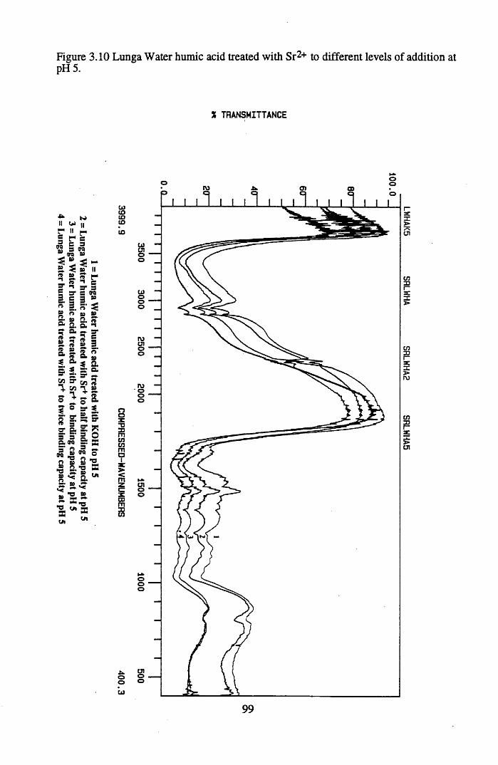
Figure 3.10 Lunga Water humic acid treated with Sr2+ to different levels of addition atpH 5.
X TRANSMITTANCE
99
LWHAK5
SRLWHA
SRLW
HA2
SR
LWH
A5
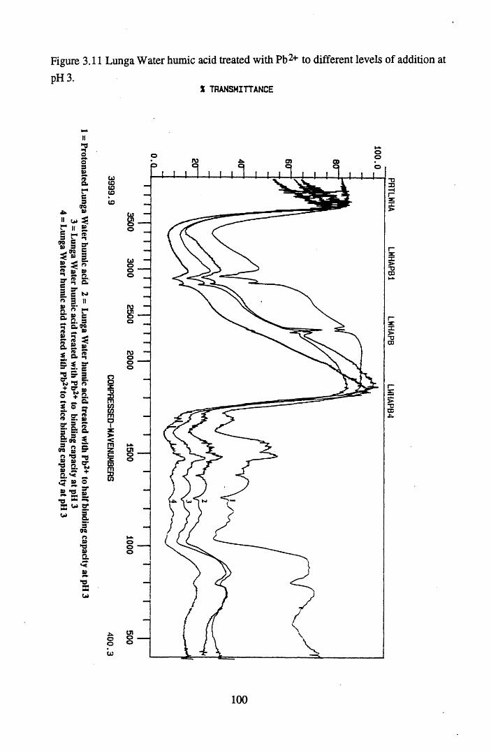
Figure 3.11 Lunga Water humic acid treated with Pb2+ to different levels of addition atpH 3.
X TRANSMITTANCE
ii u*
f "s n ora g 83 3
& 363
O363
ar33(TO63
363(V*1S'3§.( f t
•1S'§•1 Pi 3
B. *o- E
o<K>
g IIPi* rE =2. 3
ST &CS83 " t ^ST n ^8. s. ■sr* a s? i gr 5 5 i.w'd n + S ' u
0 + S. ** ®*
% *2 s* ?<6 3 . 83S ' 3 «1 & &
a3 (ft 3; 83 —
Pi "3•S 8.5» 55. + 2 .^ ^ ^ ■ ® S.*3 »npm Slg •O **S3 w S
3 3.3* 99 Pito•ato 2
to
W
U>
03
O ro O) ootototototo a:
toCJIoo
to
ru(71
ro
ooz"033mCOCOm01
>X05
z><mzz005(A
(716.Ooto
1 0 0
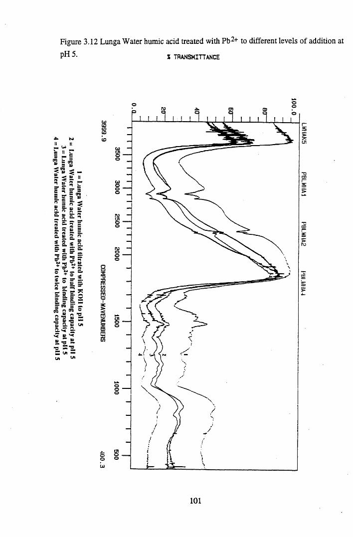
Figure 3.12 Lunga Water humic acid treated with Pb2+ to different levels of addition at
pH 5. % TRANSMITTANCE
&ii■m oas It3 I—tre i- 83 3
<TQ^ 89* ^» ■<n. Si ^
o' E ss EL 2. « c . 83*» S. n e.Si *n n B . S3
i l5 *
Ec* -
J:-3o $
s S’ =s o r e 3 83
« ^ 83 33* ** & 1rt83
« -^ 69 3 2.E JW MSi
2. ©n — » e*=■ 1 5_ E? 5:* s s; s’ 3. — w
. 5 E - • o r e s _« 2 99 - 89 rs ^3s ■g s -«5 89 *T3 ^ 2. 8: LnS.« gr 15 S'S» - o Si ra =■»SI Ln —wi **
ttftOtotoCD
O0 Z “0 30 m cn cn m a1
<mzcz0 3m303
Oo03
o o03
CJIoo
o
ru
oo
CJIo
oo
o
1 0 1
LWHAK5 PBLW
IIA1 PBLWHA2
PUI.WIIA4
92
18
39
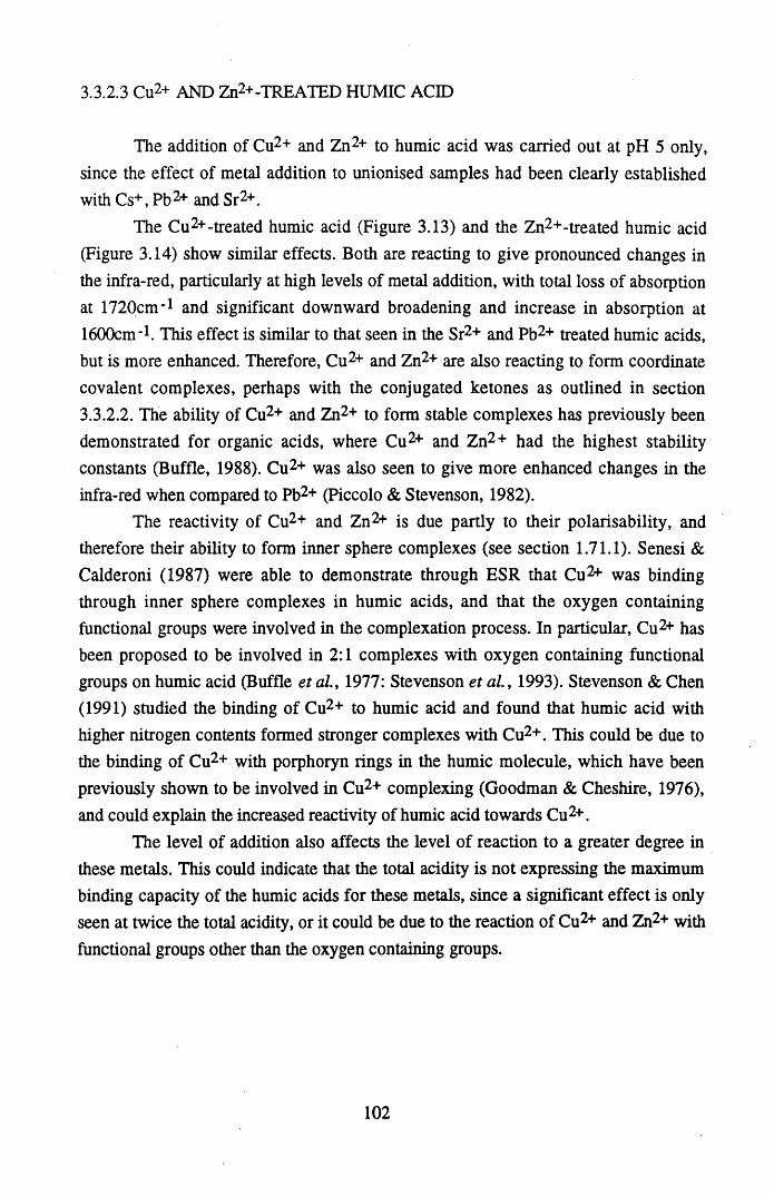
3.3.2.3 Cu2+ AND Zn2+-TREATED HUMIC ACID
The addition of Cu2+ and Zn2+ to humic acid was carried out at pH 5 only, since the effect of metal addition to unionised samples had been clearly established with Cs+, Pb2+ and Sr2+.
The Cu2+-treated humic acid (Figure 3.13) and the Zn2+-treated humic acid (Figure 3.14) show similar effects. Both are reacting to give pronounced changes in the infra-red, particularly at high levels of metal addition, with total loss of absorption at 1720cm'1 and significant downward broadening and increase in absorption at 1600cm'1. This effect is similar to that seen in the Sr2+ and Pb2+ treated humic acids, but is more enhanced. Therefore, Cu2+ and Zn2+ are also reacting to form coordinate covalent complexes, perhaps with the conjugated ketones as outlined in section 3.3.2.2. The ability of Cu2+ and Zn2+ to form stable complexes has previously been demonstrated for organic acids, where Cu2+ and Zn2+ had the highest stability constants (Buffle, 1988). Cu2+ was also seen to give more enhanced changes in the infra-red when compared to Pb2+ (Piccolo & Stevenson, 1982).
The reactivity of Cu2+ and Zn2+ is due partly to their polarisability, and therefore their ability to form inner sphere complexes (see section 1.71.1). Senesi & Calderoni (1987) were able to demonstrate through ESR that Cu2+ was binding through inner sphere complexes in humic acids, and that the oxygen containing functional groups were involved in the complexation process. In particular, Cu2+ has been proposed to be involved in 2:1 complexes with oxygen containing functional groups on humic acid (Buffle et al., 1977: Stevenson et a l , 1993). Stevenson & Chen (1991) studied the binding of Cu2+ to humic acid and found that humic acid with higher nitrogen contents formed stronger complexes with Cu2+. This could be due to the binding of Cu2+ with porphoryn rings in the humic molecule, which have been previously shown to be involved in Cu2+ complexing (Goodman & Cheshire, !976), and could explain the increased reactivity of humic acid towards Cu2+.
The level of addition also affects the level of reaction to a greater degree in these metals. This could indicate that the total acidity is not expressing the maximum binding capacity of the humic acids for these metals, since a significant effect is only seen at twice the total acidity, or it could be due to the reaction of Cu2+ and Zn2+ with functional groups other than the oxygen containing groups.
1 0 2
Figure 3.13 Lunga Water humic acid treated with Cu2+ at different levels of additionat pH 5.
% TRANSMITTANCE
11 ii r w c ii r3 r SB S n
? 3 ^ *-^ S " » 2
S ' f? — = 6 >1 J S S Sri'S" i I» B. 2o <-*a tj r ««f S. 5 1B # A Ssr 2 83 32 n j* S . O. p £> . oB* A*
IIr
1 8 . *
a p ■ ■ »» ro a .
c f n i t* ? * o
ft 2 *o’ 3 £ ft9 5:9 2 a 3 P. •— S* a © •* S TO — s f S•o 8 ~P M *■*"2. TbpC.<5
p *5" a «h 89 *o B*o S m 3Ul Ul
toCOCOCOCO
o0 z *o30mcncnma13C►<mzczCDm30cn
&ooLo
o ro 05
CO
roCJI
CJI
o
CJI
103
LWHAK5
CULWHA3
CULWHA4
CU
LWH
A5
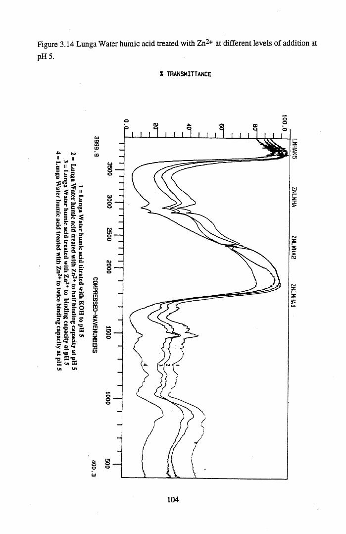
Figure 3.14 Lunga Water humic acid treated with Zn2+ at different levels of addition atpH 5.
% TRANSMITTANCE
104
LWHAK5 ZNLWHA
ZNLWHA2 ZNLW
HAl
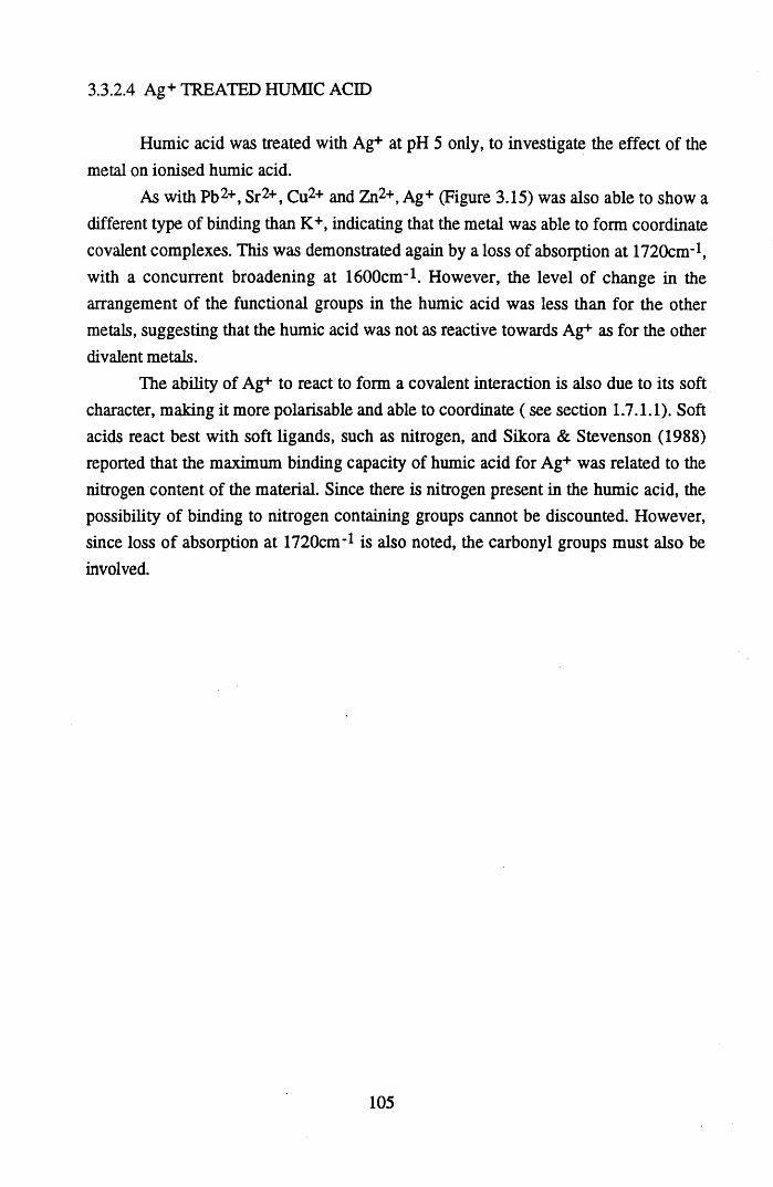
3.3.2.4 Ag+ TREATED HUMIC ACID
Humic acid was treated with Ag+ at pH 5 only, to investigate the effect of the metal on ionised humic acid.
As with Pb2+, Sr2+, Cu2+ and Zn2+, Ag+ (Figure 3.15) was also able to show a different type of binding than K+, indicating that the metal was able to form coordinate covalent complexes. This was demonstrated again by a loss of absorption at 1720cm-1, with a concurrent broadening at 1600cm-1. However, the level of change in the arrangement of the functional groups in the humic acid was less than for the other metals, suggesting that the humic acid was not as reactive towards Ag+ as for the other divalent metals.
The ability of Ag+ to react to form a covalent interaction is also due to its soft character, making it more polarisable and able to coordinate ( see section 1.7.1.1). Soft acids react best with soft ligands, such as nitrogen, and Sikora & Stevenson (1988) reported that the maximum binding capacity of humic acid for Ag+ was related to the nitrogen content of the material. Since there is nitrogen present in the humic acid, the possibility of binding to nitrogen containing groups cannot be discounted. However, since loss of absorption at 1720cm-1 is also noted, the carbonyl groups must also be involved.
105
Figure 3.15 Lunga Water humic acid treated with Ag+ to different levels of addition atpH 5.
X TRANSMITTANCE
106
LWHAK5 AGLWHA1
AGLWHA2 AGLW
HA
3.3.3 METAL ADDITIONS TO UNEXTRACTED PEAT
3.3.3.1 CS+-TREATED PEAT
Cs+ additions were made to protonated peat at pH 3 and to peat which had been titrated to pH 5 with KOH. Figure 3.16 shows the spectra obtained when Cs+ is added to protonated peat. The level of addition has little effect on the extent of reaction, with the changes which occur in the spectra being evident at half the total acidity. The changes involved are a slight loss of absorption at 1720cm-l, with a slight broadening at 1600cm-1 which, as explained in section 3.3.2.1, are indicative of the formation of the carboxylate salt on ionisation. These effects were also observed in the Cs+ treated humic acid (Figure 3.6), but to a greater degree.
In the samples which have been titrated to pH 5 before and after addition of metal, the same changes are observed. These are displayed in Figure 3.17, and the Cs+ treated spectra are similar to the K+ treated spectra, indicating that again the Cs+ is binding in an ionic arrangement, but with a lower degree of reaction than in the humic acid (Figure 3.7). This reduced reaction of unextracted organic matter towards metals was also observed by Warwick et a l (1992), where humic acid showed higher binding capacities.
107
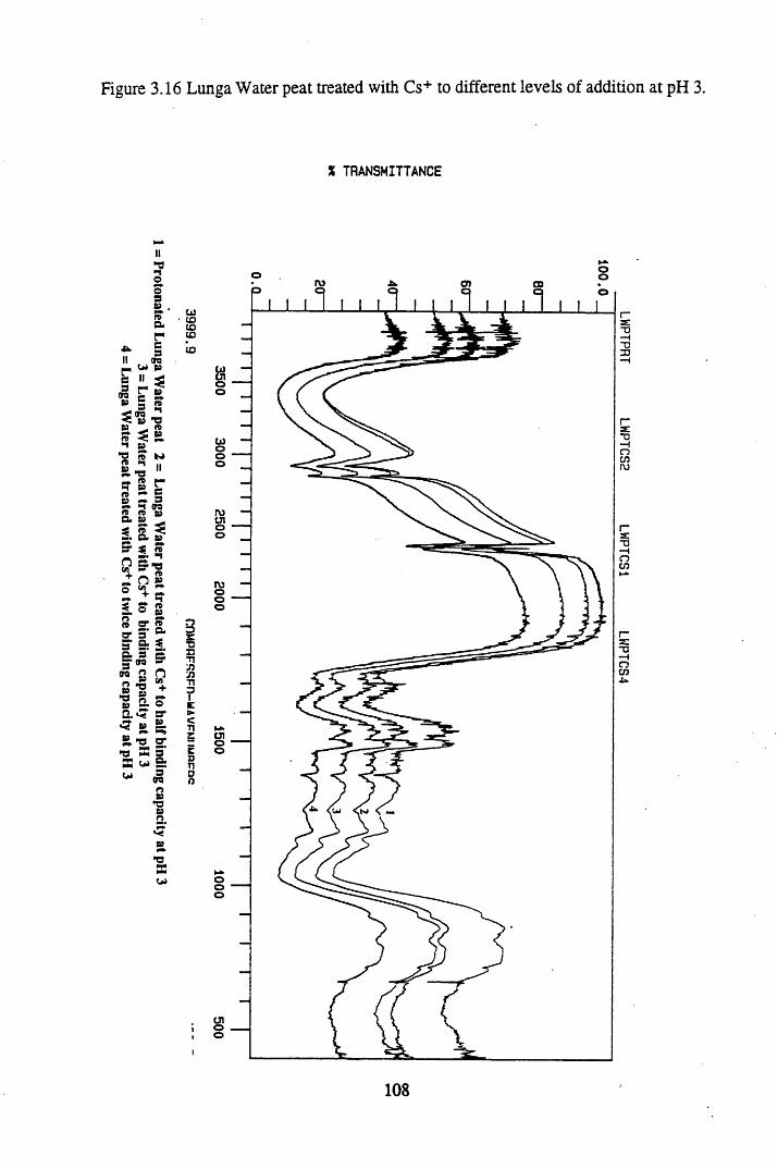
= Protonated
Lunga W
ater peat
2 =
Lunga W
ater peat treated
with Cs+
to half binding
capacity at pH
3 3
= Lunga
Water
peat treated with
Cs+ to
binding capacity
at pH 3
4 =
Lunga W
ater peat treated
with C
s+ to
twice binding
capacity at pH
3
Figure 3.16 Lunga Water peat treated with Cs+ to different levels of addition at pH 3.
X TRANSMITTANCE
CDCOCOCOCO
r\j a) a
o
o
routo
o
CJ1o
o
108
LWPTPR
T LW
PTCS2
LWPTC
S1 LW
PTC
S4
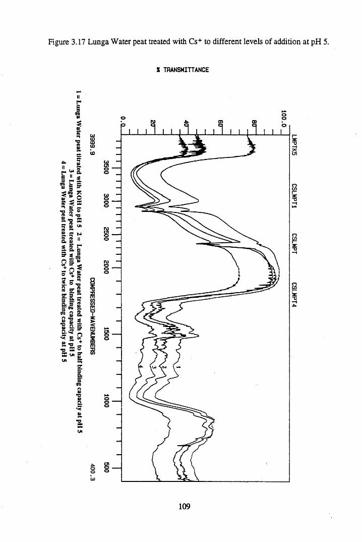
= Lunga
Water
peat titrated with
KOH to
pH 5
2 =
Lunga W
ater peat treated
with Cs+
to half binding
capacity at pH
53
= Lunga
Water
peat treated with
Cs+ to
binding capacity
at pH 5
4 =
Lunga W
ater peat treated
with C
s+ to
twice binding
capacity at pH
5
Figure 3.17 Lunga Water peat treated with Cs+ to different levels of addition at pH 5.
X TRANSMITTANCE
toCDCOtoC O
8533mC OC OmaiX><
tnm3)co
Xk.ooUJ
0) C D
C OC J1oo
toooo
roUloo
roooo
oo
ooo
C 7Ioo
109
LWPTK5
CSLWPT1
CSLWPT CSLW
PT4
3.3.3.2 Sr2+-TREATED PEAT
As with Cs+, Sr2+ additions were made to protonated peat at pH 3, and peat which had been titrated to pH 5. In Figure 3.18, the Sr2+ additions at pH 3 are displayed and show similar changes to Cs+, with only slight loss of absorption at 1720cm"1, with a corresponding slight broadening at 1600cm-l. In Figure 3.9, the Sr2+ additions to protonated humic acid are displayed and show a different reaction than in the peat, with a marked loss at 1720cm-1 and a significant broadening of the 1600cm-1 peak.
The additions to titrated peat at pH 5 are displayed in Figure 3.19, and again a significantly reduced reaction is seen when compared to the corresponding additions to humic acid (Figure 3.10). The Sr2+ spectra are similar to the spectra for the K+ treated peat and indicate that in peat the Sr2+ is binding in an ionic arrangement, whereas in the humic acid Sr2+ was able to undergo complexation reactions.
This lack of complexation is consistent with the observations of Bloom and McBride (1979), who showed that Ca2+ was able to retain its water of hydration and bind in an ionic arrangement to unextracted peat. They viewed unextracted peat as a solid phase cation exchanger. In humic acid, which is an operationally-derived extract, Ca2+ has been shown to participate in complexation reactions (Perdue et al., 1980) as the Sr2+ does in the Lunga Water humic acid.
1 1 0
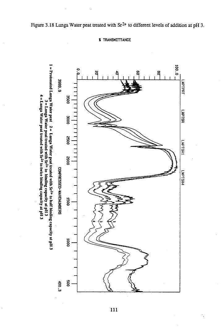
= Protonated
Lunga W
ater peat
2 =
Lunga W
ater peat treated
with Sr2+
to half binding
capacity at pH
3 3
= Lunga
Water
peat treated with
Sr2+ to
binding capacity
at pH 3
4 =
Lunga W
ater peat treated
with Sr2+
to twice
binding capacity
at pH 3
Figure 3.18 Lunga Water peat treated with Sr2+ to different levels of addition at pH 3.
X TRANSMITTANCE
b)CDIDCOCD
OOS.TJ33mCOCOmC3Iae>cm
£m£
oou
1 1 1
LWPTPR
T LW
PTSR LW
PTSR1
LWP
TSR
4
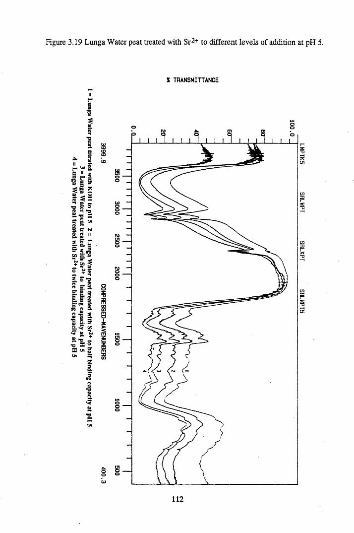
3 =
Lunga W
ater peat treated
with Sr2+
to binding
capacity at pH
5 =
Lunga W
ater peat treated
with Sr2+
to twice
binding capacity
at pH 5
Figure 3.19 Lunga Water peat treated with Sr2+ to different levels of addition at pH 5.
X TRANSMITTANCE
1 1 2
LWPTK5
SRLWPT
SRLXPT SRLW
PTS
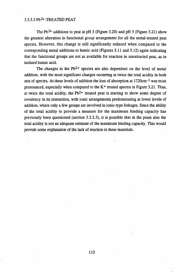
3 3 3 3 Pb2+-TREATED PEAT
The Pb2+ additions to peat at pH 3 (Figure 3.20) and pH 5 (Figure 3.21) show the greatest alteration in functional group arrangement for all the metal-treated peat spectra. However, this change is still significantly reduced when compared to the corresponding metal additions to humic acid (Figures 3.11 and 3.12) again indicating that the functional groups are not as available for reaction in unextracted peat, as in isolated humic acid.
The changes in the Pb2+ spectra are also dependent on the level of metal addition, with the most significant changes occurring at twice the total acidity in both sets of spectra. At these levels of addition the loss of absorption at 1720cm-1 was most pronounced, especially when compared to the K+ treated spectra in Figure 3.21. Thus, at twice the total acidity, the Pb2+ treated peat is starting to show some degree of covalency in its interaction, with ionic arrangements predominating at lower levels of addition, where only a few groups are involved in ionic-type linkages. Since the ability of the total acidity to provide a measure for the maximum binding capacity has previously been questioned (section 3.3.2.3), it is possible that in the peats also the total acidity is not an adequate estimate of the maximum binding capacity. This would provide some explanation of the lack of reaction in these materials.
113
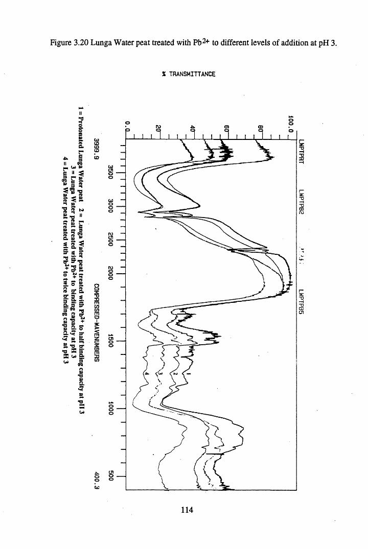
= Protonated
Lunga W
ater peat
2 =
Lunga W
ater peat treated
with Pb2+
to half binding
capacity at pH
3 3
= Lunga
Water
peat treated with
Pb2+ to
binding capacity
at pH 3
4 =
Lunga W
ater peat treated
with Pb2+
to twice
binding capacity
at pH 3
Figure 3.20 Lunga Water peat treated with Pb2+ to different levels of addition at pH 3.
% TRANSMITTANCE
CjJ(OtotoCO
33C*t>30mtocom01ac<Tmzc3CCOm33CO
oo
ro cs03o
COCJ1oo
O)ooo
rotnoo
roooo
ooo
C31oo
114
LWPTPRT
LWPTPB2
,'fAiL
WP
TP
B5
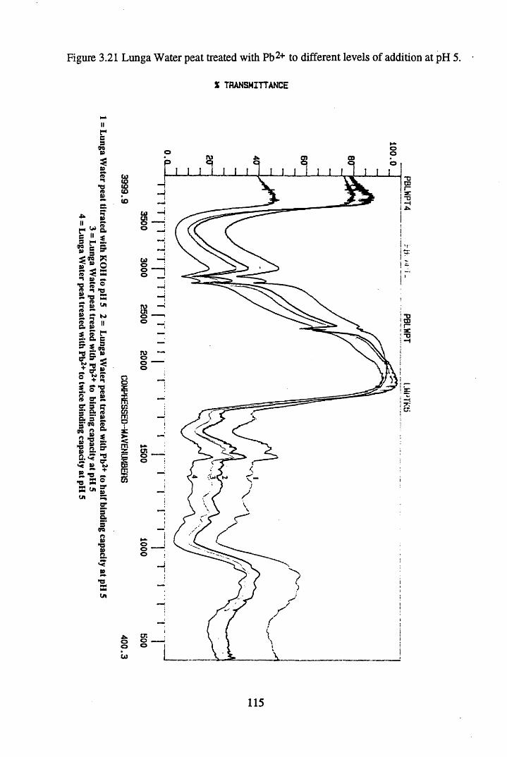
= Lunga
Water
peat titrated with
KO
II to
pH 5
2- Lunga
Water
peat treated with
Pb2+ to
half binding capacity
at pH 5
3 =
Lunga W
ater peat treated
with Pb2+
to binding
capacity at pH
5 4
= Lunga
Water
peat treated with
Pb24* to twice
binding capacity
at pH 5
Figure 3.21 Lunga Water peat treated with Pb2+ to different levels of addition at pH 5.
% TRANSMITTANCE
Cl)CDCDCDCD
C lo?ffiCDcnrr.o
<mz:
rr.Oj
ooCjJ
O O
CjJ8O
Cil©oo
soo
ruooo
»-»•ooo
cr.oo
115
PBLWPT4
PBLWPT
l.HPTKS
3.3.4 METAL ADDITIONS TO MODEL COMPOUNDS
3.3.4.1 CHANGES IN THE SPECTRA ON SALT FORMATION
Both the untreated salicylic acid and phthalic acids (Figures 3.22 & 3.23 respectively), show evidence of intramolecular hydrogen bonding, indicating that they exist mostly in the dimeric form (Bellamy, 1975). This is most clearly seen from the arrangements of the OH band at 3400-2600cm-1. In these spectra the OH band is seen as a jagged series of bands, which results from the lowering in frequency caused by hydrogen bonding (Williams & Flemming, 1989). The sharp band at 3400cm-1 can be attributed to a high frequency OH stretching vibration (Socrates, 1980). This arrangement, along with the carbonyl frequency, is characteristic of carboxylic acids, and is often utilised in their identification.
Intramolecular hydrogen bonding also lowers the frequency of the carbonyl stretch at 1720cm-1. 6-hydroxy carbonyl compounds are particularly affected by this effect, and this is reflected in the salicylic acid (6-hydroxy benzoic acid), where in Figure 3.22 the carbonyl stretch can be found at 1650cm-1. In Figure 3.23, the carbonyl frequency of phthalic acid (1,2-benzenedicarboxylic acid) is not as affected by hydrogen bonding, and the carbonyl stretch can be found at 1690cm-1. This is consistent with the observations made by previous workers on the positions of the carbonyl groupings in these acids (Bellamy, 1975).
Conversion to the K+ salt causes characteristic changes in the spectra of the acids. As discussed in section 3.1, ionisation of a carboxylic acid results in the formation of the carboxylate anion, which is resonance stabilised. The anion has two characteristic frequencies for the antisymmetric stretch (~ 1600cm-1) and the symmetric stretch (~1400cm-1). In salicylic acid (Figure 3.22), the antisymmetric peak is present at 1580cm-1, with a peak superimposed at 1600cm-1 which can be attributed to aromatic C=C stretching. The peak for the symmetric stretch is located at 1380cm-1. In phthalic acid (Figure 3.23), the antisymmetric peak is present at 1555cm-1 and is broader than the salicylic acid. This broadness is again due to aromatic C=C stretching. The symmetric stretch is located at 1380cm-1.
Both of the salts are contaminated by water, which can be detected by the OH stretch at 3500cm-1, and the band at 1640cm-1, for the HOH bending vibration which can be clearly detected in salicylic acid, but if present, is not resolved in the phthalic acid.
116
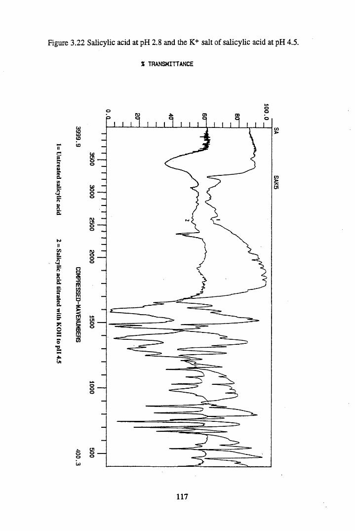
= U
ntreated salicylic
acid 2
= Salicylic
acid titrated
with K
OI! to
pH 4.5
Figure 3.22 Salicylic acid at pH 2.8 and the K+ salt of salicylic acid at pH 4.5.
X TRANSMITTANCE
cu to Io toCO
sXT33COCOmais>■<m
wm33CO
ooCjJ
Ooo
ro at aa
CO
COo©o
roC71oo
8oo
I-*CJ1oo
o©©
C7Ioo
117
SAK5
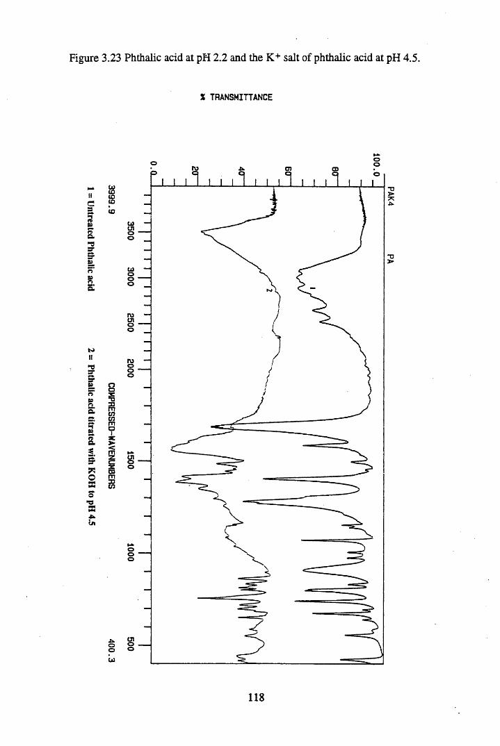
Untreated
Phthalic acid
2 =
Phthalic acid
titrated with
KOH to
pH 4.5
Figure 3.23 Phthalic acid at pH 2.2 and the K+ salt of phthalic acid at pH 4.5.
X TRANSMITTANCE
ro o> CD
tototototo
roLJl
ro
oooZT333mtocnmaisej*<mzczCDm33CO
C3IXk.oo
118
PAK4
3.3.4.2 Cs+ AND Ag+-TREATED PHTHALIC AND SALICYLIC ACID
Both the Cs+ and Ag+ additions were made at pH 4.5, and the pH was returned to this value after reaction.
Cs+ additions to phthalic acid (Figure 3.24) and salicylic acid (Figure 3.25) have resulted in the formation of the ionised form of these acids, and the spectra are virtually identical to the K+ treated spectra, showing no shift in the frequencies of the carbonyl frequencies. Thus, as in the humic acids and peats, Cs+ is reacting to give ionic linkages. In the Cs+ treated salicylic acid the spectrum is more significantly affected by contamination from water, which may be trapped in the crystalline lattice by a combination of weak hydrogen bonds to the anion, or weak ionic bonds to the metal (Bellamy, 1975).
Ag+ additions to phthalic acid (Figure 3.26) and salicylic acid (Figure 3.27), have also resulted in the formation of the ionised forms of these acid, showing very similar spectra to the K+ treated salt, with no shifts in the carbonyl frequencies. In the Ag+ spectra, there is also a broadening of the band at 1390cm-1, which is due to the presence of ionic nitrates, which absorb at 1380cm-1. These are present since Ag+ was added as the nitrate salt. This is different to the treatment of the humic acid with Ag+ where some degree of covalent interaction was detected, and would again indicate that Ag+ is reacting with nitrogen-containing groupings in the humic acid, since these are not present in the model compounds studied here.
H9
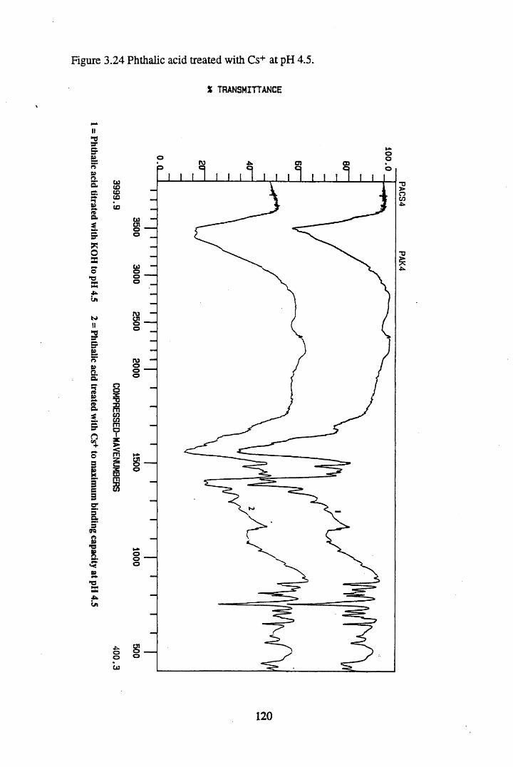
= Phthalic
acid titrated
with KOH
to pH
4.5 2
= Phthalic
acid treated
with C
s+ to
maxim
um
binding capacity
at pH 4.5
Figure 3.24 Phthalic acid treated with Cs+ at pH 4.5.
% TRANSMITTANCE
Cl]CDCDCOCD
O03fficnCDma1sc><m3C□ 3m3
.t.oocu
ro
cuCJ1oo
cuooo
rocnoo
roooo
*-*►cnoo
ooo
1 2 0
PACS4 PAK4
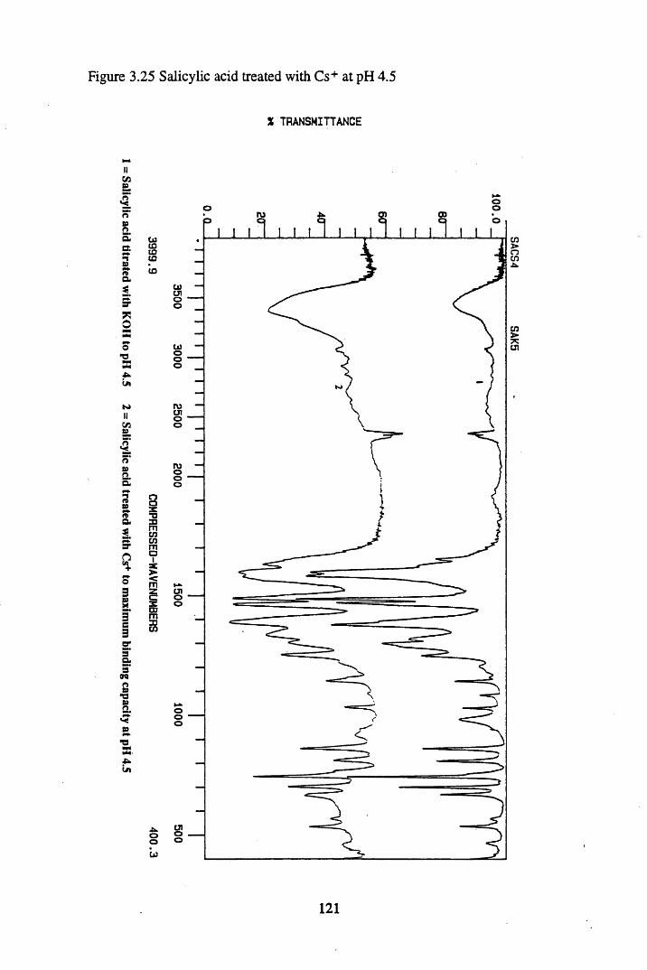
= Salicylic
acid titrated
with K
OII to
pH 4.5
2 =
Salicylic acid
treated with
Cs+ to
maxim
um
binding capacity
at pH 4.5
Figure 3.25 Salicylic acid treated with Cs+ at pH 4.5
X TRANSMITTANCE
r\i cn ooo
cuCOtoCOto
T 3
Rcncnm01
mzczcum3Dcn
oocu
o
cuCJIoo
cuoo©
roCJIoo
roooo
ooo
CJIoo
1 2 1
SACS4 S
AK
5
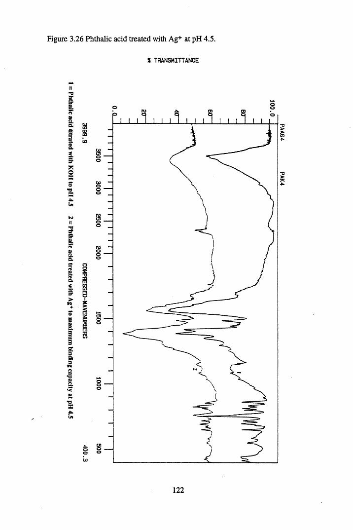
= Phthalic
add titrated
with KOH
to pH
4.5 2
= Phthalic
add treated
with Ag+
to m
aximum
binding
capadty at pH
4.5
Figure 3.26 Phthalic acid treated with Ag+ at pH 4.5.
X TRANSMITTANCE
ooO) CO
CDCOIDCO(O
CDCJIO
ro
ro
s3C"O33mcncnm013C>■<mz CJIc:zCDm33CO
CJIooCD
1 2 2
PAAG4 PAK4
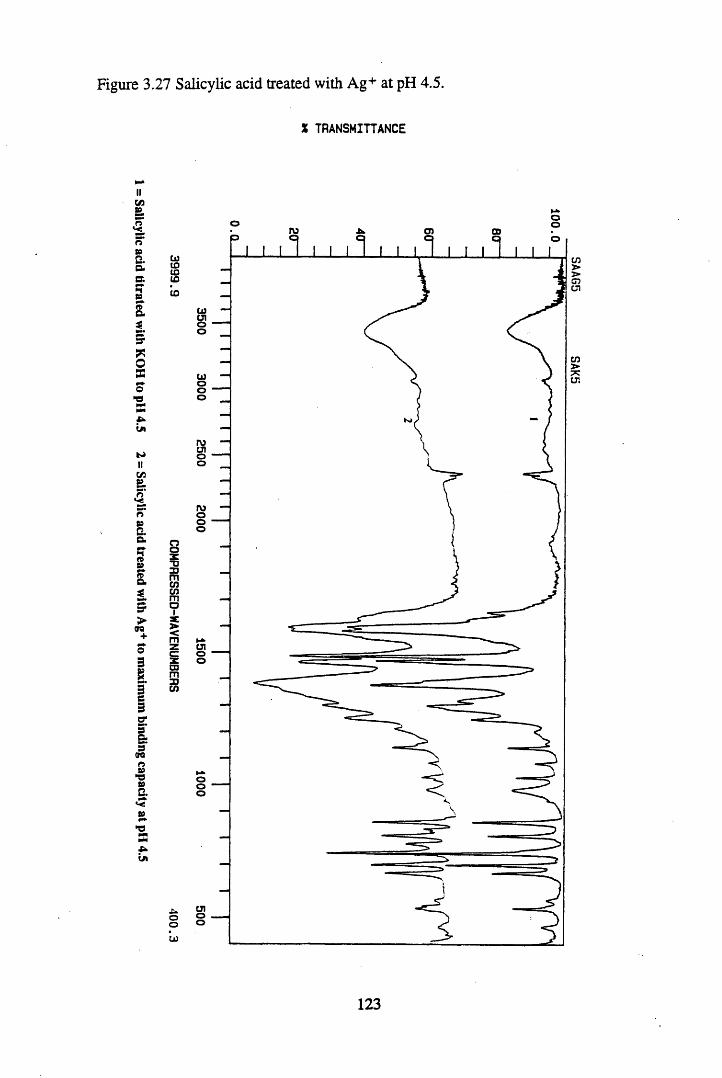
= Salicylic
acid titrated
with KOH
to pH
4.5 2
= Salicylic
acid treated
with A
g+ to
maxim
um
binding capacity
at pH 4.5
Figure 3.27 Salicylic acid treated with Ag+ at pH 4.5.
X TRANSMITTANCE
ro O) otototoID(O
CO
roCJI
rooo
s3CT333mcncnmaix><mzcz
CJIooCDm33cn
o
CJIoo
123
SAAG5 SAKS
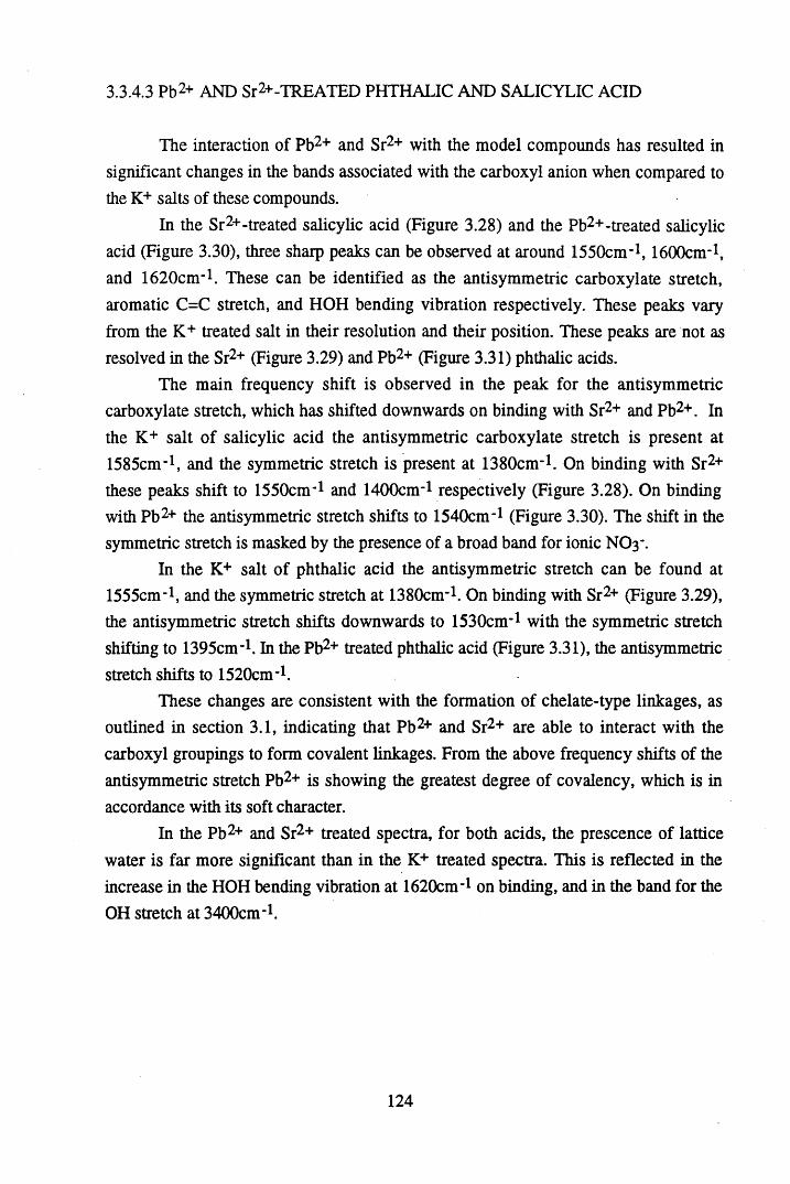
33.4.3 Pb2+ AND Sr2+-TREATED PHTHALIC AND SALICYLIC ACID
The interaction of Pb2+ and Sr2+ with the model compounds has resulted in significant changes in the bands associated with the carboxyl anion when compared to the K+ salts of these compounds.
In the Sr2+-treated salicylic acid (Figure 3.28) and the Pb2+-treated salicylic acid (Figure 3.30), three sharp peaks can be observed at around 1550cm-1,1600cm-l, and 1620cm-l. These can be identified as the antisymmetric carboxylate stretch, aromatic C=C stretch, and HOH bending vibration respectively. These peaks vary from the K+ treated salt in their resolution and their position. These peaks are not as resolved in the Sr2+ (Figure 3.29) and Pb2+ (Figure 3.31) phthalic acids.
The main frequency shift is observed in the peak for the antisymmetric carboxylate stretch, which has shifted downwards on binding with Sr2+ and Pb2+. In the K+ salt of salicylic acid the antisymmetric carboxylate stretch is present at 1585cm-1, and the symmetric stretch is present at 1380cm-1. On binding with Sr2+ these peaks shift to 1550cm-1 and 1400cm-1 respectively (Figure 3.28). On binding with Pb2+ the antisymmetric stretch shifts to 1540cm-1 (Figure 3.30). The shift in the symmetric stretch is masked by the presence of a broad band for ionic NO3 -.
In the K+ salt of phthalic acid the antisymmetric stretch can be found at 1555cm-1, and the symmetric stretch at 1380cm-1. On binding with Sr2+ (Figure 3.29), the antisymmetric stretch shifts downwards to 1530cm-1 with the symmetric stretch shifting to 1395cm-1. In the Pb2+ treated phthalic acid (Figure 3.31), the antisymmetric stretch shifts to 1520cm-1.
These changes are consistent with the formation of chelate-type linkages, as outlined in section 3.1, indicating that Pb2+ and Sr2+ are able to interact with the carboxyl groupings to form covalent linkages. From the above frequency shifts of the antisymmetric stretch Pb2+ is showing the greatest degree of covalency, which is in accordance with its soft character.
In the Pb2+ and Sr2+ treated spectra, for both acids, the prescence of lattice water is far more significant than in the K+ treated spectra. This is reflected in the increase in the HOH bending vibration at 1620cm-1 on binding, and in the band for the OH stretch at 3400cm-1.
124
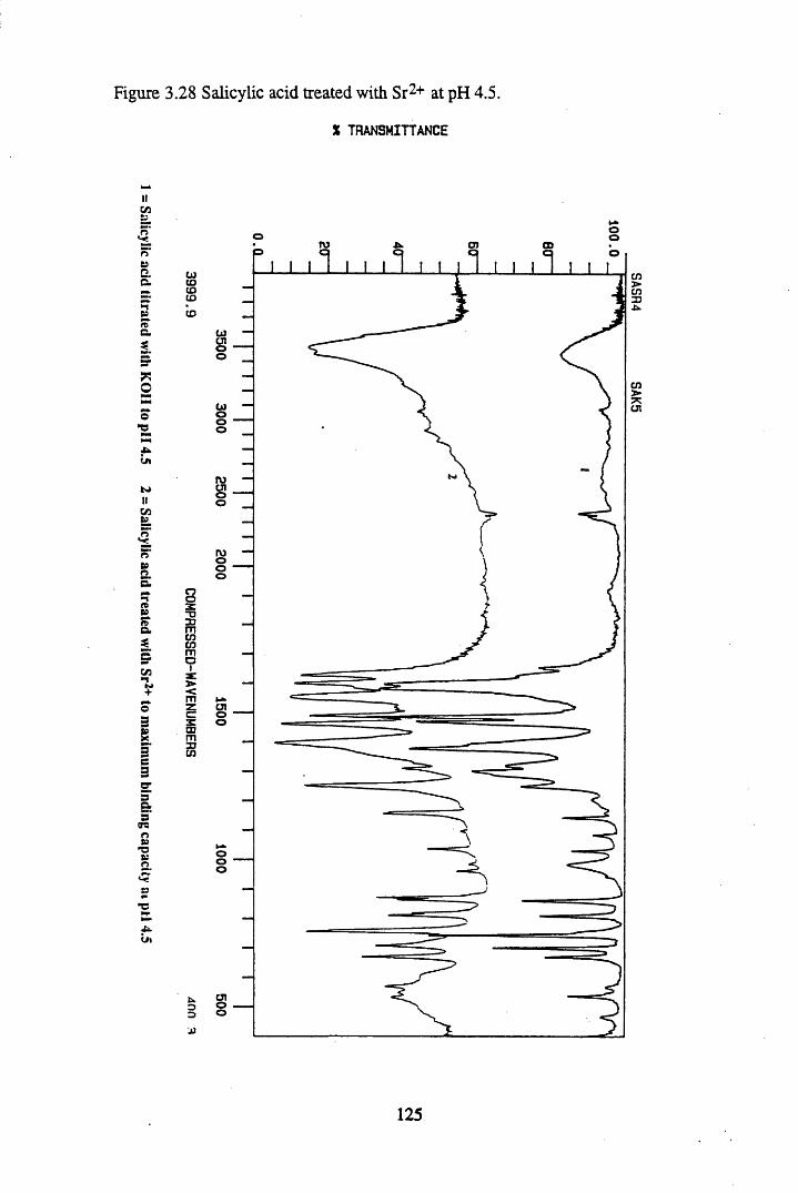
= Salicylic
acid titrated
with K
OII to
pH 4.5
2 =
Salicylic acid
treated with
Sr2+ to
maxim
um
binding capacity
ai pH 4.5
Figure 3.28 Salicylic acid treated with Sr2+ at pH 4.5.
X TRANSMITTANCE
cuCQ(0(0
(0
siaomcncnm01£>•<mzcx03m30cn
cn CDo
cuCJIoo
cuooo
rouioo
rooo©
I-*CJIoo
l-kooo
CJIo©
125
SASR4 SAK5
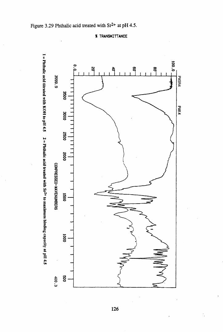
= Phthalic
add titrated
with KOH
to pH
4.5 2
= Phthalic
add treated
with Sr2+
to m
aximum
binding
capacity at pH
4.5
Figure 3.29 Phthalic acid treated with Sr2+ at pH 4.5.
X TRANSMITTANCE
o obO) CD
Ultototo'to
cn
U)
rocn
ooX-o33mcncnm01a:>■<mz CJIooCDm3 )cn
.ucou;
126
PASR4 PAK4
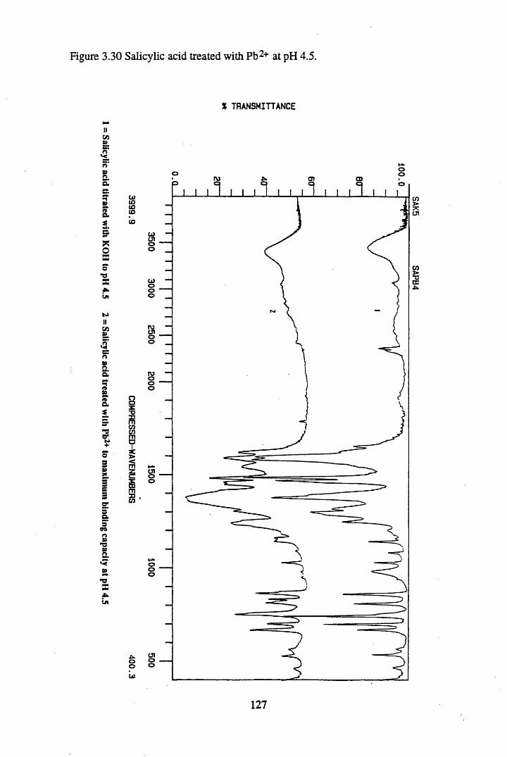
= Salicylic
acid titrated
with K
OII
to pH
4.5 2
= Salicylic
acid treated
with Pb2+
to m
aximum
binding
capacity at pH
4.5
Figure 3.30 Salicylic acid treated with Pb2+ at pH 4.5.
% TRANSMITTANCE
cotototo(0
35IDmcncnmai<m
csm3 0cn
ooC O
ro C D
COooo
roCJIoo
roooo
»-»cnoo
Oo©
CJIoo
127
SAK5 SAPB4
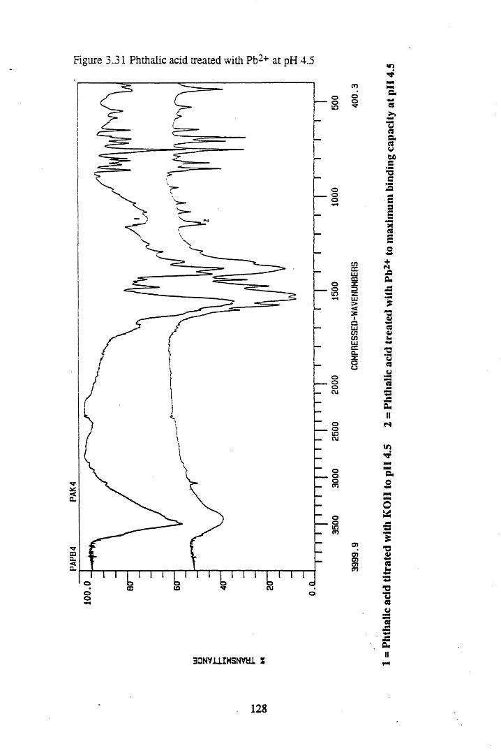
PAPB
4 P
AK
4
Figure 3.31 Phthalic acid treated with Pb2+ at pH 4.5
o
in
cu
o
cn
cucoCD
OoT
cnccUJ03X13ZUJ>cXt£3UJcncnUJcrQ_Xou
O)oi05cncn
33N V11IW SN VU 1 S
128
- Ph
thal
ic ac
id tit
rated
wi
th KO
H to
pH 4.5
2
= Ph
thal
ic aci
d tre
ated
wi
th Pb
2+ to
max
imum
bi
ndin
g ca
pacit
y at
pH 4.
5

3.4 CONCLUSIONS
The metal-treated spectra are giving information on the nature of the interaction of metals with humic substances. From all of the studies, it is clear that Cs+ is binding through ionic linkages only, making it potentially available in the environment. Conversely, Cu2+, Zn2+, Pb2+ and Sr2+ are binding through coordinate covalent linkages in humic acid, with Cu2+ and Zn2+ giving the most significant change at high levels of metal loading.
In salicylic and phthalic acid, Pb2+ and Sr2+ were also shown to form coordinate covalent linkages, with the results pointing to the formation of chelate-type complexes. With the functional groupings of humic acid being proposed to be formed from salicylate and phthalate type repeating units, (Gamble et al., 1980) it is not surprising that reaction with metals results in a broadening of the peak at 1600cm-1 in the humic acid. In the model compounds, which have simple structures in comparison to humic substances, metal treatment resulted in significant changes in the arrangements of the bands associated with the carboxylic groupings, yet in humic substances these effects will be magnified due to the complexity of structure.
In unextracted peat, only Pb2+ was able to show any evidence of coordination reactions and showed less of an effect than in the humic acid. This would indicate that for both Pb2+ and Sr2+, the total acidity was not an adequate estimation of the maximum binding capacities of these metals with unextracted peat, since the extent of reaction was greatly reduced. The increased reactivity of humic acid compared to unextracted peat was also observed in the infra-red spectra of titrated peat and humic acid samples in section 2.3.2.4. This was proposed to be due to structural changes on extraction, which allow the reactive groupings to be more exposed for reaction, instead of being bound up in the peat matrix. After all, this is the aim of the extraction procedure. In addition, chemical changes were also proposed to occur on isolation.
The increase in reactivity of humic substances after isolation of humic acid has implications for the use of such operationally-defined extracts in the study of metal interactions in environmental systems, if, in the environment, the humic substances have quite different reactivities and behaviours.
129
CHAPTER 4
THE MEASUREMENT OF THE DEGREE OF COMPLEXATION OF
METALS WITH HUMIC SUBSTANCES
130
4.1 INTRODUCTION
In the infra-red studies presented above it was evident that different metals reacted quite differently with humic substances, showing the potential to participate in complex formation. From these quantitative observations only, assumptions can be made regarding the stability of the interactions, but it is this feature which will govern their behaviour, in particular their bioavailablity, in environmental systems.
In contrast, the formation constant of a metal-humic complex can provide a quantitative measure of the affinity of a humic substance for a metal, therefore providing information on stability of the interaction. The use of formation constants in providing information on the potential environmental behaviour of a metal is complicated by the conditional nature of the constants, as outlined in section 1.7.2. In addition several assumptions must be made:
(a) There is a single homologous complexant with polyelectrolytic properties.(b) Only one ion or complex compound reacts with the ligand.(c) Chemically-specific reactions occur between the metal and the ligand.(d) Thermodynamic equilibrium is achieved.
(Buffle, 1988).
These conditions may not hold, especially when secondary reactions such as those outlined in section 1.7.2 are taking place. As yet no model exists which can compensate for these effects, since this would involve an inordinate number of parameters. Instead, a series of different models exists, which compensate in different ways for particular secondary effects (see section 1.7.2.1.).
In this study of the stability of metal-humic interactions three different approaches were utilised: the Base Titration Method, the Scatchard approach and an Incremental Technique with the theoretical basis of each method being discussed in greater detail in section 4.2. The Base Titration and Scatchard approaches were chosen since they are very different kinds of discrete ligand model, which have been demonstrated to model the interactions better than continous distribution models (Turner et al., 1986). The incremental constants were calculated in order to investigate how binding changes with extent of reaction.
The majority of such quantitative studies have been carried out on humic and fulvic acids which are operationally-defined fractions. Isolation of humic acid from peat has been shown in Chapter 2 to increase the reactive functional group content of the humic substances, an effect also demonstrated by Gregor & Powell (1987) for fulvic acid. In particular, there was an increase in the total acidity and carboxyl group content on extraction, as well as an increase in reactivity towards alkali. The infra-red
131
studies in Chapter 3 showed that the extracted materials had a greater reactivity towards metals, and revealed the existence of coordinate covalent complexes, which were not so apparent in the unextracted materials. Therefore, in order to provide further information on the effect of isolation on the properties of humic substances, unextracted peat samples were also incorporated into some of the quantitative studies of metal binding. The use of unextracted materials in parallel with the conventional humic acid will also investigate the validity of using the operationally-defined fraction for such studies.
132

4.2 METHODS
4.2.1 THE BASE TITRATION METHOD - THE BJERRUM APPROACH
This approach is a discrete ligand model which assumes that metal ions and protons compete for complexing sites on humic substances, and that the metal ion is regarded as the central group forming MLn complexes. It is based on a method developed by Gregor (1955), who modified the Bjerrum approach for calculating stepwise formation constants for metal complexes to polyacrylic acids.
4.2.1.1 THEORETICAL CONSIDERATIONS OF THE BASE TITRATION METHOD
The reactions between a weak acid polyelectrolyte such as humic acid, and a divalent metal ion can be illustrated as follows:
HA + M2+ MA+ + H+ (4.1)
* b 2 +HA + MA <=> MA2 + H+ (4.2)
where HA represents an acidic functional group, MA2 the complex formed and bi and b2 the stepwise formation constants for each reaction. The reactions represented by equations 4.1 and 4.2 show interactions with protonated groupings, yet the method assumes interactions between dissociated functional groupings as follows, with protons being released from re-establishment of ionisation equilibrium:
kl +M2+ + A" <=> MA (4.3)
HA <=> A" + H+ (4.4)
which combine to give,
M2+ + HA <=> MA+ + H+ (4.1)
However, in equation 4.3, there will be a net change in humic charge, which is not accounted for in this method, being a discrete ligand model and therefore equations 4.1 and 4.2 are utilised. Gregor (1955) proposed that the stepwise formation constants arising from equations 4.1 and 4.2 should be utilised in preference to the constant ki
133
arising from equation 4.3, and therefore developed the Bjerrum approach around this assumption.
The two stepwise formation constants (bi and b2 ) which arise from equations4.1 and 4.2 can be combined to give an overall constant B2 , which is defined as:
B2 = blb2 = (4.5)(HA)2 (M2+)
The average number of ligand molecules bound per metal ion is expressed by the formation function n, which provides an estimate of the number of complexing sites bound per mole of metal ion and this can be expressed as :
= (At) - (H A ).-JA -)(Mt)
where At is the overall concentration of binding site or ligand, and Mt is the overall concentration of metal ion. n is related to the formation constant B2 through the following relationship:
n = N T T A
£ ( n - n ) R ,( — )n = 0 (4.7)n= 0 H
For divalent metals, reacting as in equations 4.1 and 4.2, equation 4.7 can be solved using the method of least squares to give:
_ HA (2 -n)(— )
HA" = X B 2 ' bl (48)( n - l ) ( ^ ) (n ' 1)
H
B2 can then be computed graphically from equation 4.8.
134
Should a monovalent ion react with a humic substance, then the reaction can be written as:
HA + M+ <=> MA + H+ (4.9)
and the formation constant for the reaction can be calcuated from solving equation 4.7 to give:
B. = — — x (4.10)1 (1 -n ) (HA)
4.2.1.2 ESTABLISHING THE POTENTIAL OF THE HUMIC ACID TO IONISE
Huxter humic acid was isolated and protonated as in section 2.2.1, and used in all measurements in the Base Titration Method.
The total content of reactive functional groups At was determined by titrating the protonated humic acid with CO2 free 0.01M KOH, with the ionic strength adjusted to 0.1M with 5M KNO3 . All subsequent measurements were also carried out at 0.1M, with KNO3 as the supporting electrolyte. The protonated humic acid was in solution, and had not been freeze dried. Titration was carried out under nitrogen, in a closed cell, with the solution being constantly stirred. All additions of alkali were made using a Gilsen microburette, inserted through an inlet in the cell, and the pH was recorded with a Coming Ion Analyser 250 pH meter. The titrated humic acid or humate salt, KA, was retained for the next step in the method.
4.2.1.3 MONITORING AND MEASURING METAL BINDING
The same closed cell system used in section 4.2.1.2 for the titration of humic acid with KOH, was utilised in the recording of the pH drop on metal addition. The metals were added with a calibrated automatic pipette and the levels of addition were determined from the estimated total content of reactive functional groups. For the divalent ions, sequential additions of 0 .2 mmole were made and for the monovalent ions this was reduced to 0 .1 mmole.
To achieve the required starting pH aliquots of protonated humic acid (with the ionic strength adjusted to 0.1M) and humate salt were combined. The total volume of pH adjusted humic acid used in the titration was always 50ml for the divalent metals and 30ml for the monovalent metals.
To this equilibrated solution, successive aliquots of metal were then added, with the pH being returned to the starting pH between additions using CO2 free 0.01M
135
KOH added through a microburette as described in section 4.2.1.2. Additions were continued until no further drop in pH was detected. Cu2+ and Pb2+ were added as 0.02M acetates, with the pH of the salt buffered with CH3COOH to the pH value of the humic acid. Cs+ was added as 0.02M CsCl, and Ag+ was added as 0.02M AgN0 3 , both with no correction for the pH of the salts.
The pH was recorded with a combination electrode and Coming Ion Analyser 250 pH meter. The limit of detection of the pH electrode was defined as +/-0.04pH, from a combination of the specified acid and alkaline errors.
136
4.2.2 THE SCATCHARD AND INCREMENTAL TECHNIQUES
4.2.2.1 THEORETICAL CONSIDERATIONS OF THE SCATCHARD AND INCREMENTAL TECHNIQUES
In the approaches outlined below, the macromolecule is assumed to be the central group, with the metal reacting to give LM, LM2 and LMn complexes, with the formation constants being described by:
. (LM) (LM2 )k l = 7 7 7 7 7 7 7 k 2 =(L)(M) (LM)(M)and,
_ — (LMn)— n (LMn - 1)(M)
The extent of binding, or the formation function 0 , is then described by:
0 = (LM) + 2(LM2) + ..n(LMn) = Mb (L) + (LM) + ...(LMn) Lt
where Mb is the amount of metal bound and Lt is the total ligand concentration. For binding at identical and independent sites, 0 is described by Adairs equation:
0 = nKo(M) (4.13)1 + Ko(M)
where K0 is the microscopic formation constant and n is the number of binding sites per macromolecule. Equation 4.13 can be rearranged to give:
— = nKo - 0Ko (4.14)M
Equation 4.14 is known as the Scatchard approach and a Scatchard plot of 0/M vs 0 yields Ko as the slope (Stevenson et al., 1993).
The Scatchard approach has been utilised by a number of workers in the study of metal binding to humic substances (Bresnahan et al., 1978: Saar & Weber, 1979: Sahu & Baneijee, 1990: Stevenson & Chen, 1991). All workers reported a non- linearity in the plots obtained, and therefore the plots were divided into two straight line segments, from which two constants Ki and K2 were calculated, according to equation 4.14. Binding was therefore assumed to occur at two discrete classes of binding site, each represented by these constants. However, Bresnahan et al. (1978),
137
preferred to correct the curvature by further through calculating 0 ' ( 0 - ni). ni is the total number of binding sites of the first type and if there are two classes of binding site are present, then a plot of 0'/M vs 0 ’ will give a straight line, from which K2 the constant for the second class of binding site, can be assessed.
Stevenson & Chen (1991) recognised the arbitary nature of the curve fitting procedure and the errors which it introduced into the K values. In addition, Perdue & Lytle (1983) proposed that the curvilinearity was not due to two distinct classes of binding site, but was due to the polyelectrolytic nature of the humic acid which would result in binding becoming increasingly difficult at higher metal loadings. Therefore, Stevenson & Chen (1991) adapted the discrete ligand Scatchard approach into a continuous distribution model by calculating incremental formation constants from each point in the Scatchard plot. These incremental constants change with 0 , and an intrinsic constant Kint was calculated by extrapolating 0 to 0 , when these parameters are plotted against one another. Stevenson et al. (1993) proposed that this approach was scientifically more sound than the two component Scatchard approach, since it expresses the heterogeneity of the humic substances and how this varies with extent of metal binding.
Therefore, in the titrations carried out here, in addition to the Scatchard approach, a series of incremental formation constants was calculated for each incremental addition of metal. To investigate the nature of the complexes being formed and the stability of the resulting interaction, two constants were calculated:
M2+ + A ' » MA+ k3 = (MA )(M2 +)(A-)
M2+ + 2 A' » MA2 k4 = ( A 2)"V (4.15)(M X A’)
Integral to the Scatchard approach, and the above estimation of k3 and is the calculation of the metal binding capacity (MBC).
Adsorption of a cation onto a surface can be expressed by the Langmuir equation:
^ / A 1Xvx = -----— (4.16)1 + Kc
where c is the concentration of solute at equilibrium, x is the concentration of solute adsorbed per unit weight, k is a constant which represents the maximum binding capacity and K is also a constant which represents the affinity between the adsorbate
138
and the adsorbant. By plotting c/x vs c, k or the MBC can be calculated from the slope of the line (Zunino & Martin, 1977). However, a linear response may not be observed since the binding energy is not uniform amongst sites and the Langmuir equation is representing binding at a single layer of binding sites. Instead, a two-surface Langmuir plot may be assessed which can be calculated from the following equation:
kiKiC k2K2c . .x - — — — + — — (4.17)1 + Kxc 1 + K 2c
By plotting x/c vs c the MBC can be determined by extrapolating the line to the x axis.
In the work presented here, both techniques were used to calculate the MBC, and the results averaged to give a more representative estimate, since Fitch & Stevenson (1984) observed slight discrepancies in the values calculated by both methods.
4.2.2.2 THE THEORY OF ION SELECTIVE ELECTRODE MEASUREMENTS
When an ion selective electrode is exposed to a sample solution of ions for which it is sensitive, a potential develops across the surface of the membrane, which can be directly related to the activity of the ion being determined. In order to measure this potential, a second, unvarying potential is used in the form of a reference electrode. A filling solution completes the electrical circuit between the sample solution and the reference electrode, and the point of contact between the sample and filling solutions is the liquid junction.
The voltage difference between the ion selective electrode and the reference electrode is a measure of the activity of the metal being studied. This electrode response can be described by the Nemst equation:
E = E° + klog(a) (4.18)
where E is the measured voltage, E° is a combination of constants within the system, a is the activity of the ion being measured, k = RT/nF (or the slope), R is the gas constant, T is the temperature, F is Faraday’s constant and n is the number of electrons discharged. However, in order to relate the voltage difference or potential directly to concentration, the following relationship is utilised:
a = cf (4.19)
139

Since the activity coefficient, /, is a measure of the interaction of an ion with other ions present, and depends on the total ionic composition of the solution, by maintaining it at a constant value with a swamping concentration of electrolyte, the activity can be directly related to concentration.
The liquid junction potential should also be included in the Nemst equation, but when the ion selective electrode and the reference electrode are in the same cell this is not necessary. However, certain conditions must be made, and accounted for, namely:
(a) The ionic strength adjuster added to the sample must not introduce any contamination with it.
b) The sample solution must not contain any substance which will interfere with the reference electrode.
(c) The sample itself must not interfere with the reference electrode.
(d) Neither the reference nor the ion selective electrode must release substances into solution which are likely to interfere with each other.
(Midgely & Torrance, 1991)
4.2.23 ION SELECTIVE ELECTRODE CONDITIONING AND CALIBRATION
The ion selective electrodes utilised in this work were solid state membranes composed of crystalline solids, of which the determinant is also a component. The electrodes used, their reference electrodes, and their composition, operational limits, interferences and ionic strength adjusters (I.S.A.), are displayed in Table 4.1.
Each ion selective electrode was conditioned before use by polishing with the supplied polishing strip, and then immersing it in 10'6M standard solution overnight. The reference electrodes were also conditioned by soaking them in 0.1M solutions of the I.S.A. The electrodes were stored in their respective conditioning solutions. A calibration curve relating e.m.f (electro-motive force) with concentration of metal was prepared before each experiment, to ensure that the electrode was giving a Nemstian response in the correct range. Standards in the range of 10_1M to 10'7M with the ionic strength adjusted to 0.1M were used. Analar Cu(N03)2 was used to generate the Cu2+ standard solutions and Pb(C1 0 4 ) 2 was used to generate the Pb2+ standard solutions. Drift was also assessed and readings were only taken when the drift was less than 0.1m V over 2 minutes.
All ion selective electrode measurements were carried out in an enclosed container since the Ag/AgCl single junction reference electrode is sensitive to U.V. light. The temperature was constant at 25°C and a magnetic stirrer and stirrer bar were
140
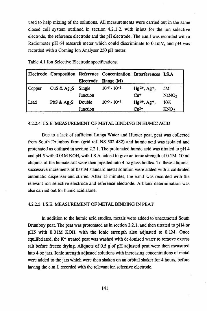
used to help mixing of the solutions. All measurements were carried out in the same closed cell system outlined in section 4.2.1.2, with inlets for the ion selective electrode, the reference electrode and the pH electrode. The e.m.f was recorded with a Radiometer pH 64 research meter which could discriminate to 0.1mV, and pH was recorded with a Coming Ion Analyser 250 pH meter.
Table 4.1 Ion Selective Electrode specifications.
Electrode Composition ReferenceElectrode
Concentration Range (M)
Interferences I.S.A
Copper CuS & Ag2S Single 1 0 -8 . 1 0 -1 Hg2+,Ag+, 5MJunction Cu+ NaNC>3
Lead PbS & Ag2S Double 1 0 -6 - 1 0 -1 Hg2+, Ag+, 10%Junction Cu2+ KNO3
4.2.2.4 I.S.E. MEASUREMENT OF METAL BINDING IN HUMIC ACID
Due to a lack of sufficient Lunga Water and Huxter peat, peat was collected from South Drumboy farm (grid ref. NS 502 482) and humic acid was isolated and protonated as outlined in section 2.2.1. The protonated humic acid was titrated to pH 4 and pH 5 with 0.01M KOH, with I.S.A. added to give an ionic strength of 0.1M. 10 ml aliquots of the humate salt were then pipetted into 4 oz glass bottles. To these aliquots, successive increments of 0.01M standard metal solution were added with a calibrated automatic dispenser and stirred. After 15 minutes, the e.m.f was recorded with the relevant ion selective electrode and reference electrode. A blank determination was also carried out for humic acid alone.
4.2.2.5 I.S.E. MEASUREMENT OF METAL BINDING IN PEAT
In addition to the humic acid studies, metals were added to unextracted South Drumboy peat. The peat was protonated as in section 2.2.1, and then titrated to pH4 or pH5 with 0.01M KOH, with the ionic strength also adjusted to 0.1M. Once equilibriated, the K+ treated peat was washed with de-ionised water to remove excess salt before freeze drying. Aliquots of 0.5 g of pH adjusted peat were then measured into 4 oz jars. Ionic strength adjusted solutions with increasing concentrations of metal were added to the jars which were then shaken on an orbital shaker for 4 hours, before having the e.m.f. recorded with the relevant ion selective electrode.
141
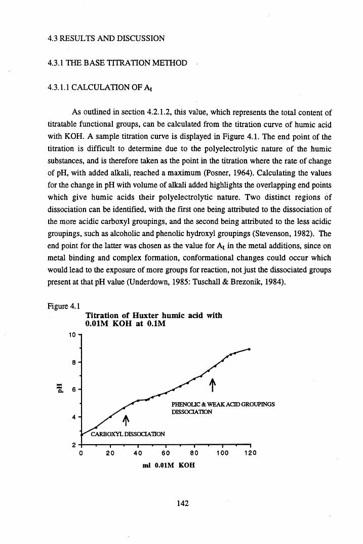
4.3 RESULTS AND DISCUSSION
4.3.1 THE BASE TITRATION METHOD
4.3.1.1 CALCULATION OF At
As outlined in section 4.2.1.2, this value, which represents the total content of titratable functional groups, can be calculated from the titration curve of humic acid with KOH. A sample titration curve is displayed in Figure 4.1. The end point of the titration is difficult to determine due to the polyelectrolytic nature of the humic substances, and is therefore taken as the point in the titration where the rate of change of pH, with added alkali, reached a maximum (Posner, 1964). Calculating the values for the change in pH with volume of alkali added highlights the overlapping end points which give humic acids their polyelectrolytic nature. Two distinct regions of dissociation can be identified, with the first one being attributed to the dissociation of the more acidic carboxyl groupings, and the second being attributed to the less acidic groupings, such as alcoholic and phenolic hydroxyl groupings (Stevenson, 1982). The end point for the latter was chosen as the value for At in the metal additions, since on metal binding and complex formation, conformational changes could occur which would lead to the exposure of more groups for reaction, not just the dissociated groups present at that pH value (Underdown, 1985: Tuschall & Brezonik, 1984).
Figure 4.1Titration of Huxter humic acid with0.01M KOH at 0.1M
10 - i
sQ*
PHENOLIC & WEAK ACID GROUPINGS DISSOCIATION
CARBOXYL DISSOCIATION
12080 1 0 020 4 0 600
ml 0.01M KOH
142
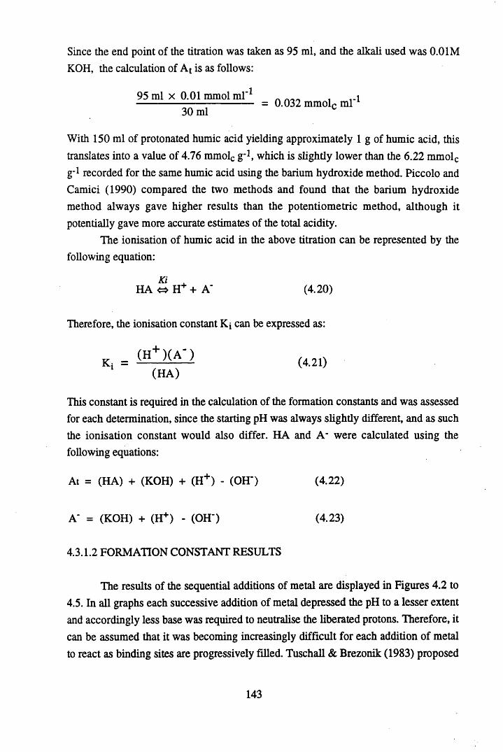
Since the end point of the titration was taken as 95 ml, and the alkali used was 0.01M KOH, the calculation of At is as follows:
95 ml x 0.01 mmol ml' 1 _-------------------------------- = 0.032 mmolc m l 1
30 ml c
With 150 ml of protonated humic acid yielding approximately 1 g of humic acid, this translates into a value of 4.76 mmolc g_1, which is slightly lower than the 6.22 mmolc g-1 recorded for the same humic acid using the barium hydroxide method. Piccolo and Camici (1990) compared the two methods and found that the barium hydroxide method always gave higher results than the potentiometric method, although it potentially gave more accurate estimates of the total acidity.
The ionisation of humic acid in the above titration can be represented by the following equation:
K iHA <=> H + A' (4.20)
Therefore, the ionisation constant Ki can be expressed as:
Kj = <SlK V)(HA)
This constant is required in the calculation of the formation constants and was assessed for each determination, since the starting pH was always slightly different, and as such the ionisation constant would also differ. HA and A’ were calculated using the following equations:
At = (HA) + (KOH) + (H+) - (OH') (4.22)
A' = (KOH) + (H+) - (OH') (4.23)
4.3.1.2 FORMATION CONSTANT RESULTS
The results of the sequential additions of metal are displayed in Figures 4.2 to4.5. In all graphs each successive addition of metal depressed the pH to a lesser extent and accordingly less base was required to neutralise the liberated protons. Therefore, it can be assumed that it was becoming increasingly difficult for each addition of metal to react as binding sites are progressively filled. Tuschall & Brezonik (1983) proposed
143
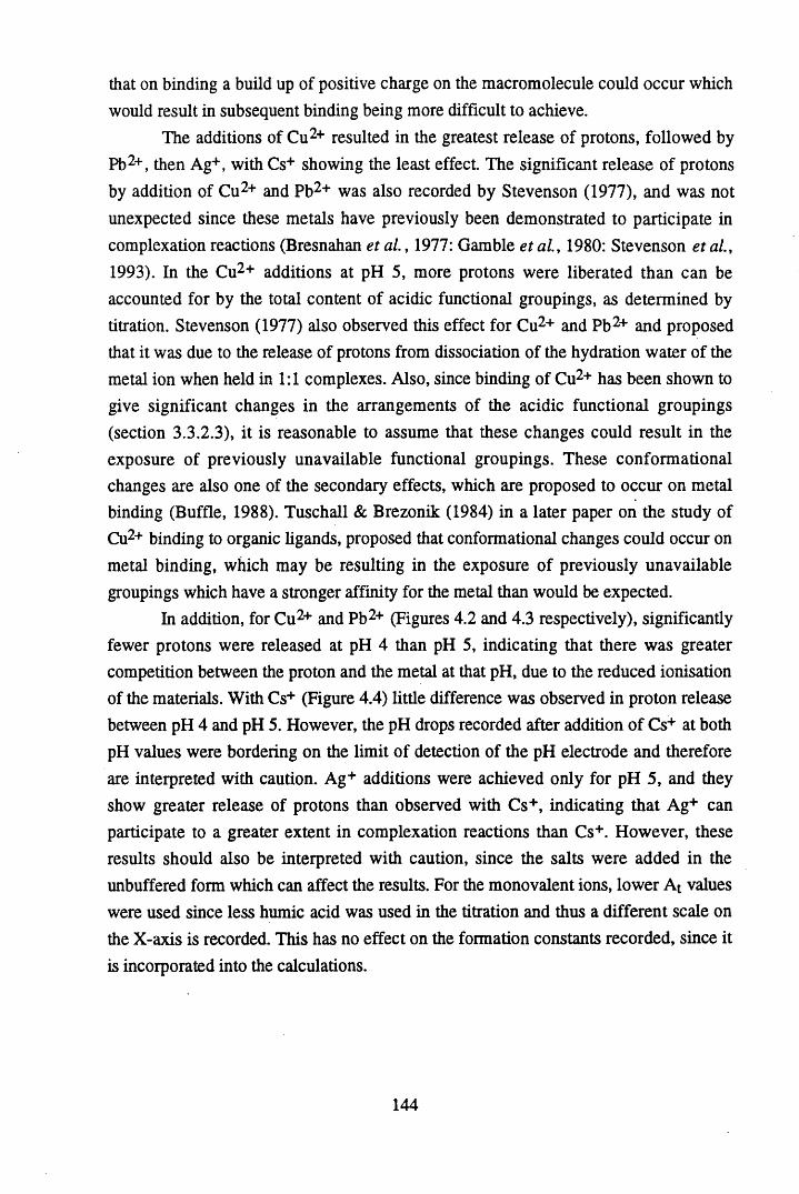
that on binding a build up of positive charge on the macromolecule could occur which would result in subsequent binding being more difficult to achieve.
The additions of Cu2+ resulted in the greatest release of protons, followed by Pb2+, then Ag+, with Cs+ showing the least effect. The significant release of protons by addition of Cu2+ and Pb2+ was also recorded by Stevenson (1977), and was not unexpected since these metals have previously been demonstrated to participate in complexation reactions (Bresnahan et a l , 1977: Gamble e ta l, 1980: Stevenson etal., 1993). In the Cu2+ additions at pH 5, more protons were liberated than can be accounted for by the total content of acidic functional groupings, as determined by titration. Stevenson (1977) also observed this effect for Cu2+ and Pb2+ and proposed that it was due to the release of protons from dissociation of the hydration water of the metal ion when held in 1:1 complexes. Also, since binding of Cu2+ has been shown to give significant changes in the arrangements of the acidic functional groupings (section 3.3.2.3), it is reasonable to assume that these changes could result in the exposure of previously unavailable functional groupings. These conformational changes are also one of the secondary effects, which are proposed to occur on metal binding (Buffle, 1988). Tuschall & Brezonik (1984) in a later paper on the study of Cu2+ binding to organic ligands, proposed that conformational changes could occur on metal binding, which may be resulting in the exposure of previously unavailable groupings which have a stronger affinity for the metal than would be expected.
In addition, for Cu2+ and Pb2+ (Figures 4.2 and 4.3 respectively), significantly fewer protons were released at pH 4 than pH 5, indicating that there was greater competition between the proton and the metal at that pH, due to the reduced ionisation of the materials. With Cs+ (Figure 4.4) little difference was observed in proton release between pH 4 and pH 5. However, the pH drops recorded after addition of Cs+ at both pH values were bordering on the limit of detection of the pH electrode and therefore are interpreted with caution. Ag+ additions were achieved only for pH 5, and they show greater release of protons than observed with Cs+, indicating that Ag+ can participate to a greater extent in complexation reactions than Cs+. However, these results should also be interpreted with caution, since the salts were added in the unbuffered form which can affect the results. For the monovalent ions, lower At values were used since less humic acid was used in the titration and thus a different scale on the X-axis is recorded. This has no effect on the formation constants recorded, since it is incorporated into the calculations.
144
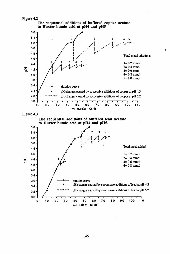
Figure 4.2The sequential additions of buffered copper acetate to Huxter humic acid at pH4 and pH5
Xa/ I S Y* ' 'S If
Total metal additions:
1= 0.2 mmol 2= 0.4 mmol 3= 0.6 mmol 4= 0.8 mmol 5= 1.0 mmol
titration curve
" pH changes caused by successive additions of copper at pH 4.3 ~ pH changes caused by successive additions of copper at pH 5.2-I— .— i— .— |— .— i— ■— i— >— i— >— i— i— i— «— i30 4 0 50 6 0 7 0 8 0 90 100 1 10
ml 0.01M K O H
Figure 4.3The sequential additions of buffered lead acetate to Huxter humic acid at pH4 and pH5.
5 .6 -j
5 .4 -
5 .2 -
5 .0 -
4 .8 -
4 .6 -
X 4 .4 -GU
4 .2 -
4 .0 -
3 .8 -
3 .6 -
3 .4 -
3 .2 -
3 .0 -
3
S ! *Total metal added:
1= 0.2 mmol 2= 0.4 mmol 3= 0.6 mmol 4 s 0.8 mmol
titration curvepH changes caused by successive additions of lead at pH 4.3
pH changes caused by successive additions of lead at pH 5.2
1 0
i20
i30
- I — «— I— 1— i— i— i— «— l— '— I— '— I50 6 0 7 0 8 0 9 0 100 110
ml 0.01M KOH
i40
145
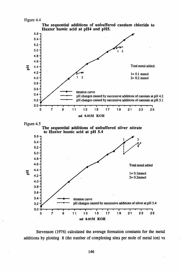
Figure 4.4The sequential additions of unbuffered caesium chloride to Huxter humic acid at pH4 and pH5.
5.6 -15.4
5 .2 -
5 .0 -
4 .8 -
4.6Total metal added:Xa
4 .2 - 1= 0.1 mmol 2= 0.2 mmol4 .0 -
3 .8 -
3 .6 -— titration curve
■’— pH changes caused by successive additions of caesium at pH 4.2 pH changes caused by successive additions of caesium at pH 5.1
3 .4 -
3 .2 -
3.0157 9 1 1 13 17 1 9 215 23 2 5
ml 0.01M KOH
Figure 4.5The sequential additions of unbuffered silver nitrate to Huxter humic acid at pH 5.4
5.6 -i
5 .4 -
5 .2 -
5 .0 -
4 .8 -
4 .6 - Total metal added
as 4 -4 :a 4 .2 -
1 - O.lmmol 2= 0.2mmol
4 .0 -
3 .8 -
3 .6 -
3 .4 - — titration curvepH changes caused by successive additions of silver at pH 5.43 .2 -
3.021 2 3 2515 17 197 9 1 1 135
ml 0.01M KOH
Stevenson (1976) calculated the average formation constants for the metal additions by plotting n (the number of complexing sites per mole of metal ion) vs
146

p(HA/H+), with bi and \>2 being assessed from interpolating at n values of 0.5 and1.5. Since the n values can exceed 0.5, an average formation constant has been determined by interpolating at h = 1.0 (Stevenson et a l , 1973). Stevenson et a l (1993) developed this approach further to calculate average formation constants from Bjerrum plots. In the humic acid used here, the n values ranged from around 1 to 0.2, making interpolation in the above way difficult, and highly speculative. Instead, the average formation constants for the divalent ions were determined graphically from equation 4.8 and samples of the graphs obtained are presented in Figures 4.6 & 4.7 with the remainder of the data in Appendix 2.1.
From Figure 4.6 a value of B2 is calculated as 1.0873xl0_l°, which gives a log B2 value of -9.96 for the additions of Cu2+, to Huxter humic acid at pH 5. Slight curvature of the graph is observed, and this was also seen in the graphs for buffered Cu(Ac)2 additions at pH 4 (see Appendix 2 .1 ). The lack of linearity comes from the excess of protons which are released, requiring excess base to return the pH to its previous value. This could be a consequence of the release of protons from the water of hydration in 1:1 complexes. Alternatively, it could be due to the release of protons from groups which were previously unavailable for reaction, but were exposed on binding due to conformational changes.
The Pb(Ac)2 additions at pH 5 (Figure 4.7), show a more sigmoidal shape, perhaps indicating that two distinct classes of binding site are present for Pb2+ in the humic acid, with the second class of binding site perhaps being these previously unavailable sites which are exposed on binding (Buffle, 1988: Underdown et a l , 1985: Tuschall & Brezonik, 1984).
Figure 4.6Formation plot for the additions of bufferedcopper acetate at pH5.
0.00e+0
-1.006-4 -
-2.006-4 -1e
-3.006-4 -e
-4.006-40 .0 0 e+ 0-1.006+6-3 .0 0 e+ 6
(2-n)(H A /H )/(n-l)
147

Figure 4.7Formation plot for the additions of buffered lead acetate at pH 5.
-1.00e-5
-1.20e-5 -
-1.400-5 -
-1.600-5 -C
c -1.800-5 -
-2.000-5-210000 -1 9 0 0 0 0 -1 7 0 0 0 0 -1 5 0 0 0 0-2 3 0 0 0 0
(2 -n)(H A /H )/(n -l)
The B i values for the monovalent ions were calculated from equation 4.10, for which no graphical treatment is required. When more than one pH drop was observed, the stepwise stability constants were averaged to give the overall formation constant B2 - The average formation constants for each metal are presented in Table 4.2 and are mean values for replicate titrations.
Table 4.2 Mean Log B values (of 3 calculations) and their standard deviations.
Metal Salt pH Mean StandardDeviation
Cu(Ac) 2 4 -8.99 0.369Cu(Ac) 2 5 -9.66 0.162Pb(Ac) 2 4 -8.62 0.147Pb(Ac) 2 5 -10.23 0.123Ag(NC>3) 5 -5.04 0.075CsCl 4 -4.55 0.085CsCl 5 -5.44 0.045
The log B2 values are lower than anticipated, indicating that very little metal was binding, with low stability of reaction. Yet, from the pH drops observed, considerable amounts of Cu2+ and Pb2+ interacted with the humic acid, giving significant drops in pH, but presumably with lower stability. This lower stability was also observed in the constants recorded at pH 5, where again more metal interacted,
148
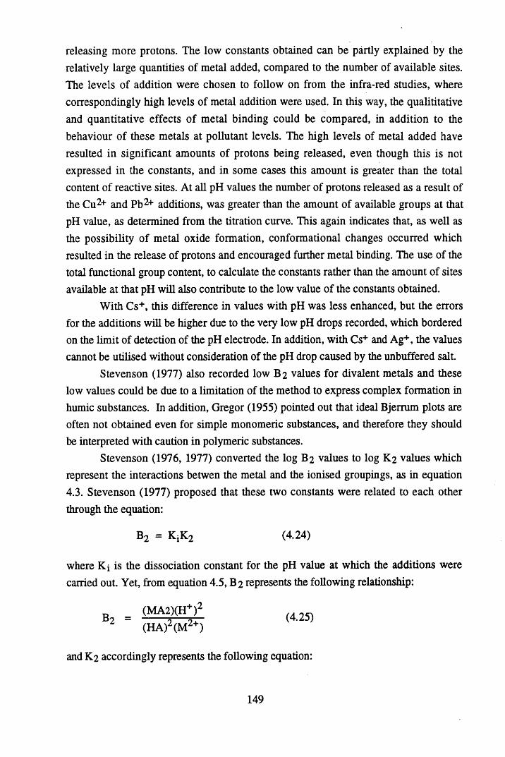
releasing more protons. The low constants obtained can be partly explained by the relatively large quantities of metal added, compared to the number of available sites. The levels of addition were chosen to follow on from the infra-red studies, where correspondingly high levels of metal addition were used. In this way, the quantitative and quantitative effects of metal binding could be compared, in addition to the behaviour of these metals at pollutant levels. The high levels of metal added have resulted in significant amounts of protons being released, even though this is not expressed in the constants, and in some cases this amount is greater than the total content of reactive sites. At all pH values the number of protons released as a result of the Cu2+ and Pb2+ additions, was greater than the amount of available groups at that pH value, as determined from the titration curve. This again indicates that, as well as the possibility of metal oxide formation, conformational changes occurred which resulted in the release of protons and encouraged further metal binding. The use of the total functional group content, to calculate the constants rather than the amount of sites available at that pH will also contribute to the low value of the constants obtained.
With Cs+, this difference in values with pH was less enhanced, but the errors for the additions will be higher due to the very low pH drops recorded, which bordered on the limit of detection of the pH electrode. In addition, with Cs+ and Ag+, the values cannot be utilised without consideration of the pH drop caused by the unbuffered salt.
Stevenson (1977) also recorded low B2 values for divalent metals and these low values could be due to a limitation of the method to express complex formation in humic substances. In addition, Gregor (1955) pointed out that ideal Bjerrum plots are often not obtained even for simple monomeric substances, and therefore they should be interpreted with caution in polymeric substances.
Stevenson (1976, 1977) converted the log B2 values to log K2 values which represent the interactions betwen the metal and the ionised groupings, as in equation 4.3. Stevenson (1977) proposed that these two constants were related to each other through the equation:
B2 = KjK2 (4.24)
where Ki is the dissociation constant for the pH value at which the additions were carried out. Yet, from equation 4.5, B 2 represents the following relationship:
= (4 2 5 )(HA)2 (M2+)
and K2 accordingly represents the following equation:
149
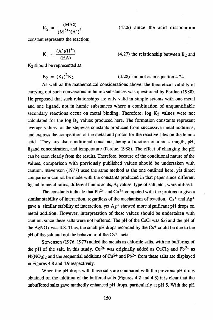
(MA2) (4.26) since the acid dissociation(M2+)(A-)2
constant represents the reaction:
(4.27) the relationship between B2 and
K2 should be represented as:
B2 = (Ki)2K2 (4.28) and not as in equation 4.24.
As well as the mathematical considerations above, the theoretical validity of carrying out such conversions in humic substances was questioned by Perdue (1988). He proposed that such relationships are only valid in simple sytems with one metal and one ligand, not in humic substances where a combination of unquantifiable secondary reactions occur on metal binding. Therefore, log K2 values were not calculated for the log B2 values produced here. The formation constants represent average values for the stepwise constants produced from successive metal additions, and express the competition of the metal and proton for the reactive sites on the humic acid. They are also conditional constants, being a function of ionic strength, pH, ligand concentration, and temperature (Perdue, 1988). The effect of changing the pH can be seen clearly from the results. Therefore, because of the conditional nature of the values, comparison with previously published values should be undertaken with caution. Stevenson (1977) used the same method as the one outlined here, yet direct comparison cannot be made with the constants produced in that paper since different ligand to metal ratios, different humic acids, At values, type of salt, etc., were utilised.
The constants indicate that Pb2+ and Cu2+ competed with the protons to give a similar stability of interaction, regardless of the mechanism of reaction. Cs+ and Ag+ gave a similar stability of interaction, yet Ag+ showed more significant pH drops on metal addition. However, interpretation of these values should be undertaken with caution, since these salts were not buffered. The pH of the CsCl was 6 .6 and the pH of the AgNC>3 was 4.8. Thus, the small pH drops recorded by the Cs+ could be due to the pH of the salt and not the behaviour of the Cs+ metal.
Stevenson (1976,1977) added the metals as chloride salts, with no buffering of the pH of the salt. In this study, Cu2+ was originally added as CuCl2 and Pb2+ as Pb(NC>3 )2 and the sequential additions of Cu2+ and Pb2+ from these salts are displayed in Figures 4.8 and 4.9 respectively.
When the pH drops with these salts are compared with the previous pH drops obtained on the addition of the buffered salts (Figures 4.2 and 4.3) it is clear that the unbuffered salts gave markedly enhanced pH drops, particularly at pH 5. With the pH
150
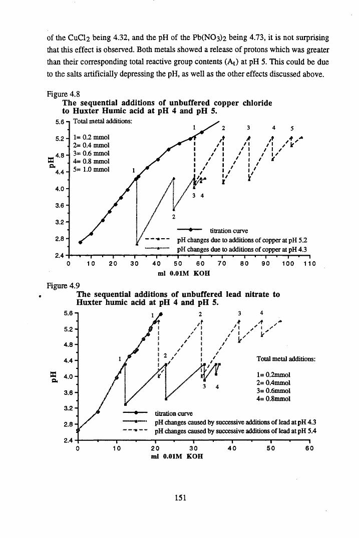
of the C11CI2 being 4.32, and the pH of the Pb(NC>3 )2 being 4.73, it is not surprising that this effect is observed. Both metals showed a release of protons which was greater than their corresponding total reactive group contents (At) at pH 5. This could be due to the salts artificially depressing the pH, as well as the other effects discussed above.
Figure 4.8The sequential additions of unbuffered copper chloride to Huxter Humic acid at pH 4 and pH 5.
5 .6 -1 Total metal additions:
1= 0.2 mmol 2= 0.4 mmol 3= 0.6 mmol 4= 0.8 mmol 5 - 1.0 mmol
5 .2 -
4 .8 -
4 .4 -
4 .0 -
3 .6 -
3 .2 -■ — ■ titration curvepH changes due to additions of copper at pH 5.2pH changes due to additions of copper at pH 4.3
2.8 -
2.41 0 20 40 7 0 900 30 50 60 80 100 110
ml 0.01M K O H
Figure 4.9The sequential additions of unbuffered lead nitrate to Huxter humic acid at pH 4 and pH 5.
5.6 -1
5 .2 -
4 .8 -
Total metal additions:4 .4 -
1= 0.2mmol 2= 0.4mmol 3= 0.6mmol 4= 0.8mmol
3 .6 -
3 .2 -►—- titration curve1— * pH changes caused by successive additions of lead at pH 4.3 ‘ ~ w pH changes caused by successive additions of lead at pH 5.4
2 .8 -
2.450 6010 20 30 4 00
ml 0.01M K O H
151
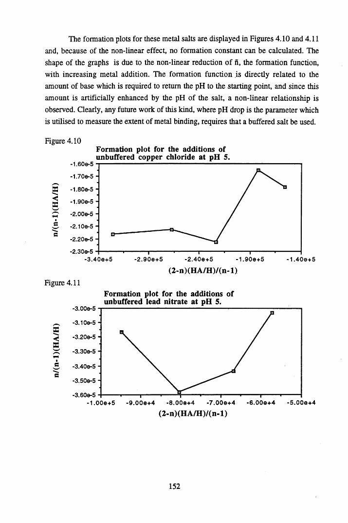
The formation plots for these metal salts are displayed in Figures 4.10 and 4.11 and, because of the non-linear effect, no formation constant can be calculated. The shape of the graphs is due to the non-linear reduction of n, the formation function, with increasing metal addition. The formation function is directly related to the amount of base which is required to return the pH to the starting point, and since this amount is artificially enhanced by the pH of the salt, a non-linear relationship is observed. Clearly, any future work of this kind, where pH drop is the parameter which is utilised to measure the extent of metal binding, requires that a buffered salt be used.
Figure 4.10Formation plot for the additions of unbuffered copper chloride at pH 5.
- 1.600-5
-1.700-5 -
X -1.800-5 -
g -1.900-5 -
-2.000-5 -Ie -2.100-5 -
C-2.200-5 -
-2.300-5-2.90O +5 -2 .400+ 5-3 .400+5 -1 .900+ 5 -1.40O +5
(2-n)(H A /H )/(n-l)Figure 4.11
Formation plot for the additions ofunbuffered lead nitrate at pH 5.
-3.000-5
-3.100-5 -
-3.200-5 -
-3.300-5 -
e'W' -3.400-5 -C
-3.500-5 -
-3.600-5-1 .000+ 5 -9 .0 0 0 + 4 -8 .000+ 4 -7 .0 0 0 + 4 -6 .0 0 0 + 4 -5 .0 0 0 + 4
(2-n)(H A /H )/(n-l)
152
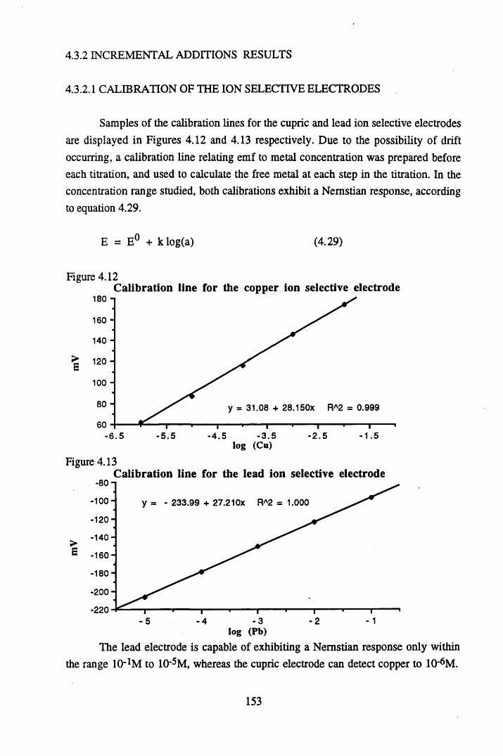
4.3.2 INCREMENTAL ADDITIONS RESULTS
4.3.2.1 CALIBRATION OF THE ION SELECTIVE ELECTRODES
Samples of the calibration lines for the cupric and lead ion selective electrodes are displayed in Figures 4.12 and 4.13 respectively. Due to the possibility of drift occurring, a calibration line relating emf to metal concentration was prepared before each titration, and used to calculate the free metal at each step in the titration. In the concentration range studied, both calibrations exhibit a Nemstian response, according to equation 4.29.
E = E° + klog(a) (4.29)
Figure 4.12Calibration line for the copper ion selective electrode
180 -i
160 -
140 -
£ 120 ’ E100 -
80 - y = 31.08 + 28.150x RA2 = 0.999
60-3 .5 1 .5-5 .5 -2 .5-6 .5 -4 .5
log (Cu)
Figure 4.13Calibration line for the lead ion selective electrode
- 100 - - 233.99 + 27.21 Ox RA2 = 1.000
- 120 -
^ -140->£ -160-
-180-
- 200 -
-220125 4 3
log (Pb)
The lead electrode is capable of exhibiting a Nemstian response only within the range 10_1M to 10“5M, whereas the cupric electrode can detect copper to lO^M.
153
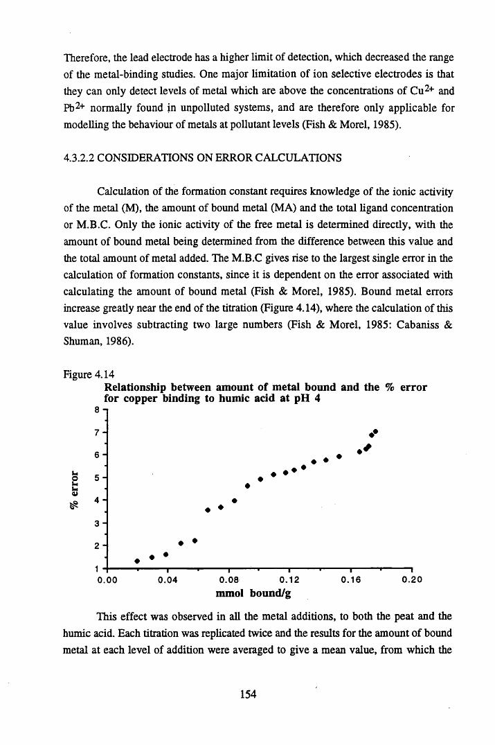
Therefore, the lead electrode has a higher limit of detection, which decreased the range of the metal-binding studies. One major limitation of ion selective electrodes is that they can only detect levels of metal which are above the concentrations of Cu2+ and Pb2+ normally found in unpolluted systems, and are therefore only applicable for modelling the behaviour of metals at pollutant levels (Fish & Morel, 1985).
4.3.2.2 CONSIDERATIONS ON ERROR CALCULATIONS
Calculation of the formation constant requires knowledge of the ionic activity of the metal (M), the amount of bound metal (MA) and the total ligand concentration or M.B.C. Only the ionic activity of the free metal is determined directly, with the amount of bound metal being determined from the difference between this value and the total amount of metal added. The M.B.C gives rise to the largest single error in the calculation of formation constants, since it is dependent on the error associated with calculating the amount of bound metal (Fish & Morel, 1985). Bound metal errors increase greatly near the end of the titration (Figure 4.14), where the calculation of this value involves subtracting two large numbers (Fish & Morel, 1985: Cabaniss & Shuman, 1986).
Figure 4.14Relationship between amount of metal bound and the % error for copper binding to humic acid at pH 4
8 -i
7 -
u _o 5u u 0>
4 -
3 -
2 -
0.00
♦ •♦ ♦
0 .0 4 0 .08 0 .1 2 mmol bound/g
0 .1 6—I0.20
This effect was observed in all the metal additions, to both the peat and the humic acid. Each titration was replicated twice and the results for the amount of bound metal at each level of addition were averaged to give a mean value, from which the
154
standard deviation was calculated. This was then divided by the mean to give the % error. Cabaniss & Shuman (1986) used this method of error calculation and showed a similar effect.
However, very few of the titration studies which utilise ion selective electrodes to produce the parameters for the subsequent calculations of the formation constants make any reference to the errors associated with such measurements and even fewer include any error calculation. Fish & Morel (1985) studied the error associated with various methods of titration and quantified the propagation of error for each of the methods which can be utilised if no replicate titrations are employed. Should replicate titrations be employed then the error associated in the method can be calculated using the standard error of the mean values.
Bresnahan et a l (1978) attributed the lack of error analysis in their analysis and calculations to the interdependence of the variables in the Scatchard approach, in particular the normalisation of bound metal to the M.B.C. In addition, the plots obtained are often curvilinear and division of the plots into two straight line segments is often arbitrary (Fitch & Stevenson, 1984). The problems associated with the Scatchard plots are discussed further in section 4.3.2.4.
4.3.2.3 CALCULATION OF THE MAXIMUM BINDING CAPACITY
The maximum binding capacity (M.B.C.) not only gives an estimation of the capacity of the material to adsorb metal, but is also integral to the measurement of formation constants and therefore it is important that this parameter be determined as accurately as possible. In section 4.3.2.2, it was demonstrated how a large error on this value can occur, and will then propagate throughout the rest of the calculations.
Since controversy exists as to the best method of calculating the M.B.C., both Langmuir and two-surface Langmuir isotherms were utilised and examples of these are displayed in Figures 4.15 and 4.16 respectively. The remainder of the graphs can be found in Appendix 2.2.
155
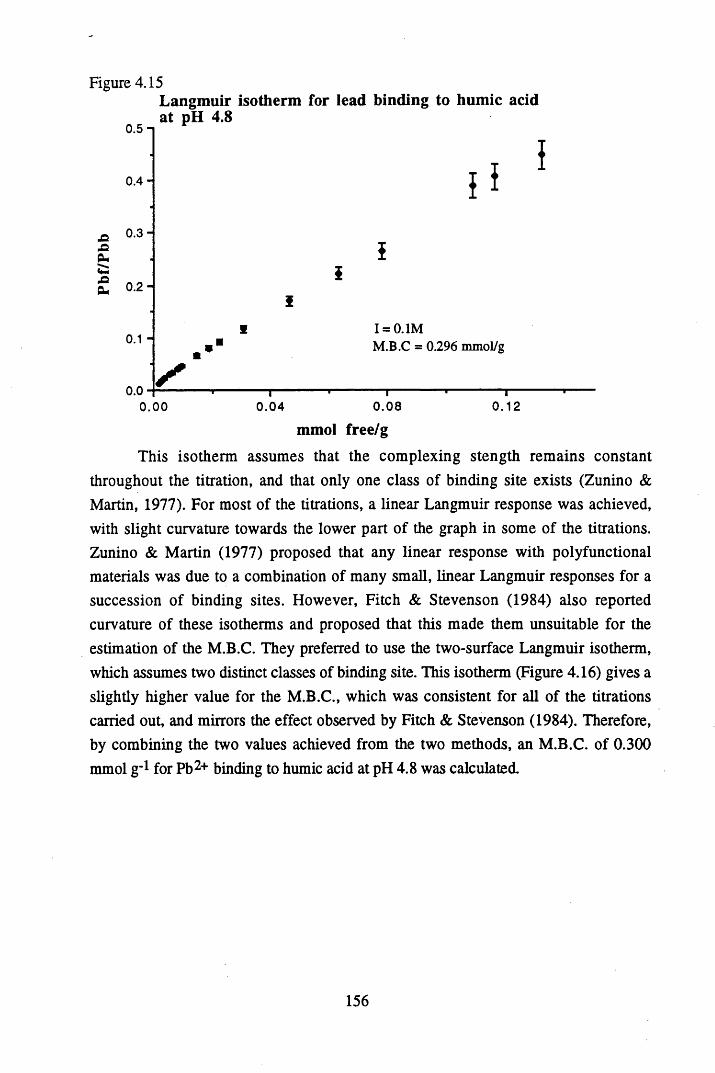
Figure 4.15
pOOn
0.5 -i
0 .4 -
0 .3 -
Langmuir isotherm for lead binding to humic acid at pH 4.8
£ 0.2 H
0.1 -
0.0
5
i
I = 0.1MM.B.C = 0.296 mmol/g
/0.00 0.120 .0 4 0 .0 8
mmol free/g
This isotherm assumes that the complexing stength remains constant throughout the titration, and that only one class of binding site exists (Zunino & Martin, 1977). For most of the titrations, a linear Langmuir response was achieved, with slight curvature towards the lower part of the graph in some of the titrations. Zunino & Martin (1977) proposed that any linear response with polyfunctional materials was due to a combination of many small, linear Langmuir responses for a succession of binding sites. However, Fitch & Stevenson (1984) also reported curvature of these isotherms and proposed that this made them unsuitable for the estimation of the M.B.C. They preferred to use the two-surface Langmuir isotherm, which assumes two distinct classes of binding site. This isotherm (Figure 4.16) gives a slightly higher value for the M.B.C., which was consistent for all of the titrations carried out, and mirrors the effect observed by Fitch & Stevenson (1984). Therefore, by combining the two values achieved from the two methods, an M.B.C. of 0.300 mmol g"1 for Pb2+ binding to humic acid at pH 4.8 was calculated.
156
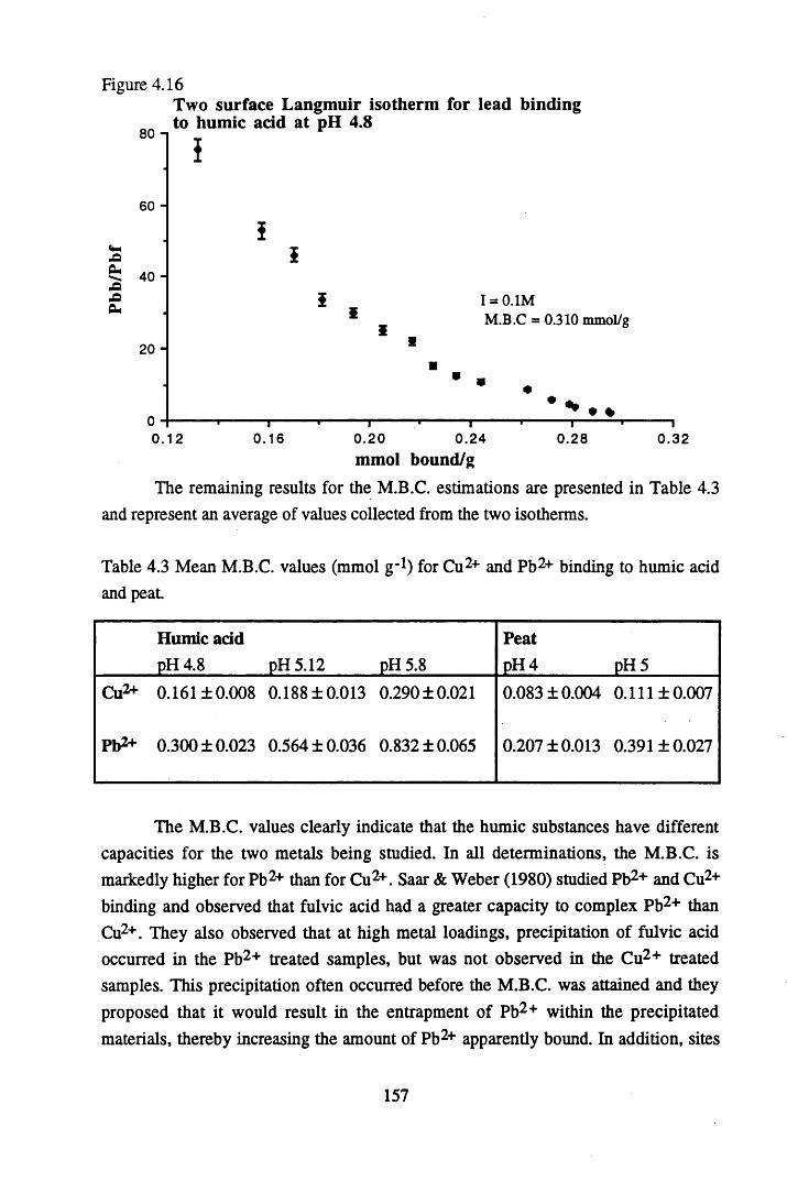
Figure 4.16Two surface Langmuir isotherm for lead binding to humic acid at pH 4.8
.aPm
-QPm
80 n
60 -
40 -
20 -
I
0.12
i
I = 0.1MM.B.C = 0.310 mmol/g
0 .16 0 .28 0 .3 20 .2 0 0 .24mmol bound/g
The remaining results for the M.B.C. estimations are presented in Table 4.3 and represent an average of values collected from the two isotherms.
Table 4.3 Mean M.B.C. values (mmol g-l) for Cu2+ and Pb2+ binding to humic acid and peat.
Humic addpH 4.8 pH 5.12 pH 5.8
PeatpH 4 pH 5
Cu2* 0.161 ±0.008 0.188 ± 0.013 0.290 ±0.021
Pb2* 0.300 ± 0.023 0.564 ± 0.036 0.832 ±0.065
0.083 ± 0.004 0.111 ±0.007
0.207 ±0.013 0.391 ±0.027
The M.B.C. values clearly indicate that the humic substances have different capacities for the two metals being studied. In all determinations, the M.B.C. is markedly higher for Pb2+ than for Cu2+. Saar & Weber (1980) studied Pb2+ and Cu2+ binding and observed that fulvic acid had a greater capacity to complex Pb2+ than Cu2+. They also observed that at high metal loadings, precipitation of fulvic acid occurred in the Pb2+ treated samples, but was not observed in the Cu2+ treated samples. This precipitation often occurred before the M.B.C. was attained and they proposed that it would result in the entrapment of Pb2+ within the precipitated materials, thereby increasing the amount of Pb2+ apparently bound. In addition, sites
157
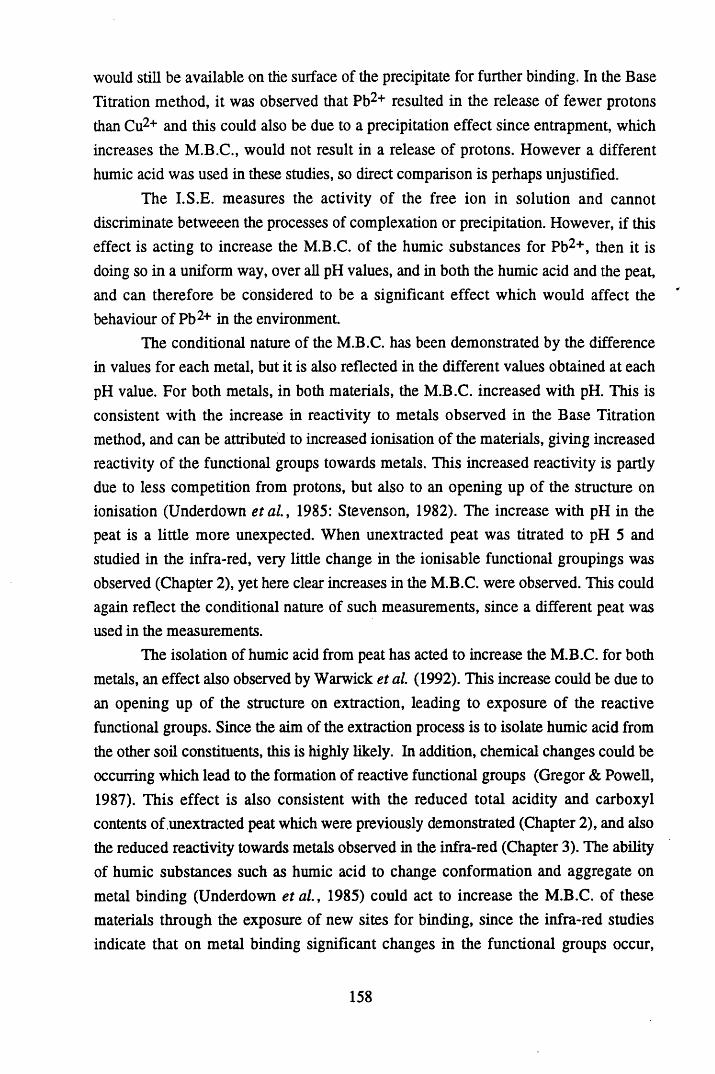
would still be available on the surface of the precipitate for further binding. In the Base Titration method, it was observed that Pb2+ resulted in the release of fewer protons than Cu2+ and this could also be due to a precipitation effect since entrapment, which increases the would not result in a release of protons. However a differenthumic acid was used in these studies, so direct comparison is perhaps unjustified.
The I.S.E. measures the activity of the free ion in solution and cannot discriminate betweeen the processes of complexation or precipitation. However, if this effect is acting to increase the M.B.C. of the humic substances for Pb2+, then it is doing so in a uniform way, over all pH values, and in both the humic acid and the peat, and can therefore be considered to be a significant effect which would affect the behaviour of Pb2+ in the environment.
The conditional nature of the M.B.C. has been demonstrated by the difference in values for each metal, but it is also reflected in the different values obtained at each pH value. For both metals, in both materials, the M.B.C. increased with pH. This is consistent with the increase in reactivity to metals observed in the Base Titration method, and can be attributed to increased ionisation of the materials, giving increased reactivity of the functional groups towards metals. This increased reactivity is partly due to less competition from protons, but also to an opening up of the structure on ionisation (Underdown e ta l , 1985: Stevenson, 1982). The increase with pH in the peat is a little more unexpected. When unextracted peat was titrated to pH 5 and studied in the infra-red, very little change in the ionisable functional groupings was observed (Chapter 2), yet here clear increases in the M.B.C. were observed. This could again reflect the conditional nature of such measurements, since a different peat was used in the measurements.
The isolation of humic acid from peat has acted to increase the M.B.C. for both metals, an effect also observed by Warwick et al. (1992). This increase could be due to an opening up of the structure on extraction, leading to exposure of the reactive functional groups. Since the aim of the extraction process is to isolate humic acid from the other soil constituents, this is highly likely. In addition, chemical changes could be occurring which lead to the formation of reactive functional groups (Gregor & Powell, 1987). This effect is also consistent with the reduced total acidity and carboxyl contents of unextracted peat which were previously demonstrated (Chapter 2), and also the reduced reactivity towards metals observed in the infra-red (Chapter 3). The ability of humic substances such as humic acid to change conformation and aggregate on metal binding (Underdown e ta l , 1985) could act to increase the M.B.C. of these materials through the exposure of new sites for binding, since the infra-red studies indicate that on metal binding significant changes in the functional groups occur,
158
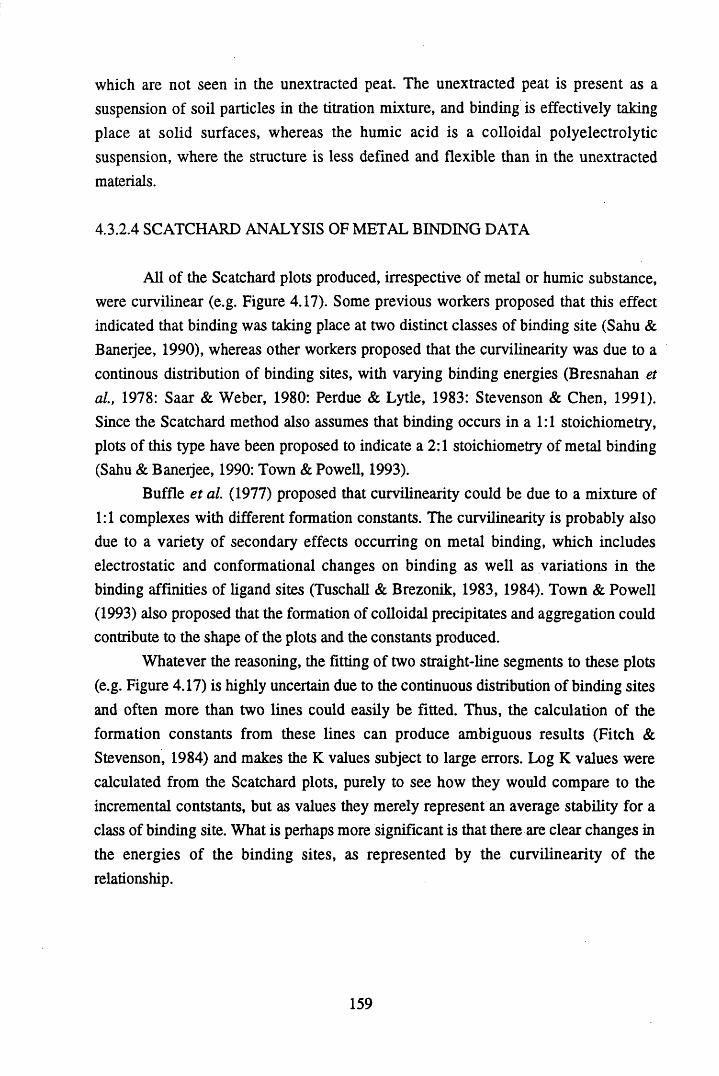
which are not seen in the unextracted peat. The unextracted peat is present as a suspension of soil particles in the titration mixture, and binding is effectively taking place at solid surfaces, whereas the humic acid is a colloidal polyelectrolytic suspension, where the structure is less defined and flexible than in the unextracted materials.
4.3.2.4 SCATCHARD ANALYSIS OF METAL BINDING DATA
All of the Scatchard plots produced, irrespective of metal or humic substance, were curvilinear (e.g. Figure 4.17). Some previous workers proposed that this effect indicated that binding was taking place at two distinct classes of binding site (Sahu & Banerjee, 1990), whereas other workers proposed that the curvilinearity was due to a continous distribution of binding sites, with varying binding energies (Bresnahan et al, 1978: Saar & Weber, 1980: Perdue & Lytle, 1983: Stevenson & Chen, 1991). Since the Scatchard method also assumes that binding occurs in a 1:1 stoichiometry, plots of this type have been proposed to indicate a 2:1 stoichiometry of metal binding (Sahu & Baneijee, 1990: Town & Powell, 1993).
Buffle et a l (1977) proposed that curvilinearity could be due to a mixture of 1:1 complexes with different formation constants. The curvilinearity is probably also due to a variety of secondary effects occurring on metal binding, which includes electrostatic and conformational changes on binding as well as variations in the binding affinities of ligand sites (Tuschall & Brezonik, 1983, 1984). Town & Powell (1993) also proposed that the formation of colloidal precipitates and aggregation could contribute to the shape of the plots and the constants produced.
Whatever the reasoning, the fitting of two straight-line segments to these plots (e.g. Figure 4.17) is highly uncertain due to the continuous distribution of binding sites and often more than two lines could easily be fitted. Thus, the calculation of the formation constants from these lines can produce ambiguous results (Fitch & Stevenson, 1984) and makes the K values subject to large errors. Log K values were calculated from the Scatchard plots, purely to see how they would compare to the incremental contstants, but as values they merely represent an average stability for a class of binding site. What is perhaps more significant is that there are clear changes in the energies of the binding sites, as represented by the curvilinearity of the relationship.
159
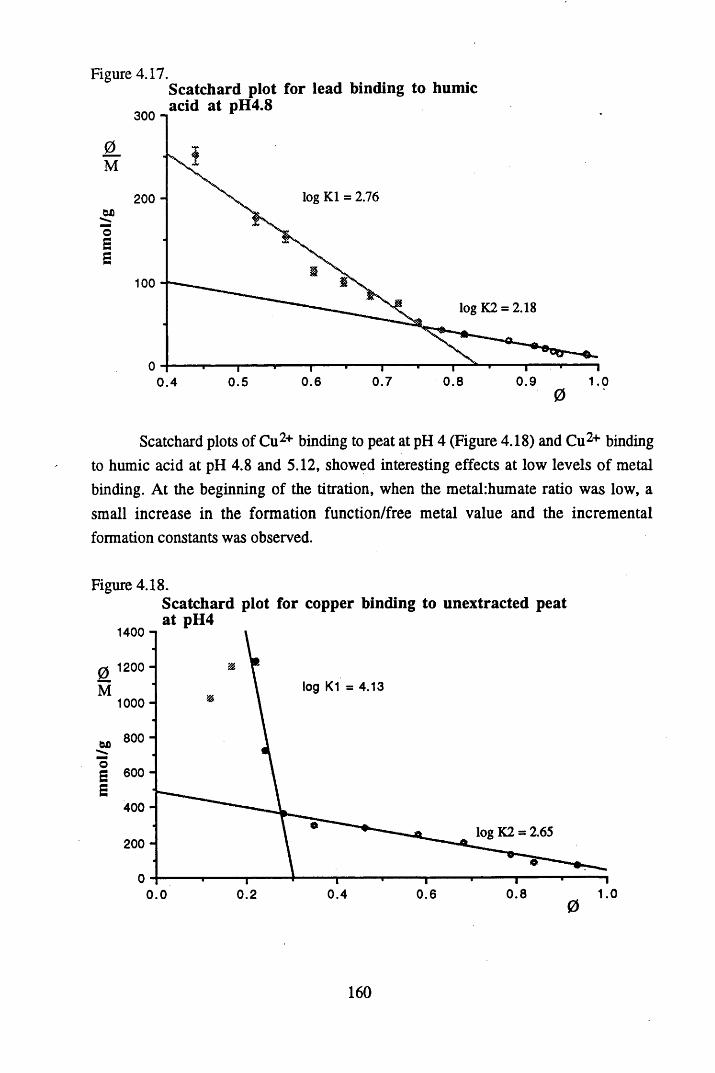
Figure 4.17.Scatchard plot for lead binding to humicacid at pH4.8
300 -]
0_M
log K1 = 2.76200 -
W)Os5
100log K2 = 2.18
0 .90 .7 0.8 1.00.60.50 .40
Scatchard plots of Cu2+ binding to peat at pH 4 (Figure 4.18) and Cu2+ binding to humic acid at pH 4.8 and 5.12, showed interesting effects at low levels of metal binding. At the beginning of the titration, when the metal:humate ratio was low, a small increase in the formation function/free metal value and the incremental formation constants was observed.
Figure 4.18.Scatchard plot for copper binding to unextracted peatat pH4
1400 n
0 1200 -
M1000 -
log K1 = 4.13
800 -M>©SB
400 -
log K2 = 2.65200 -
0.8 1.00.4 0.60.20.0
160
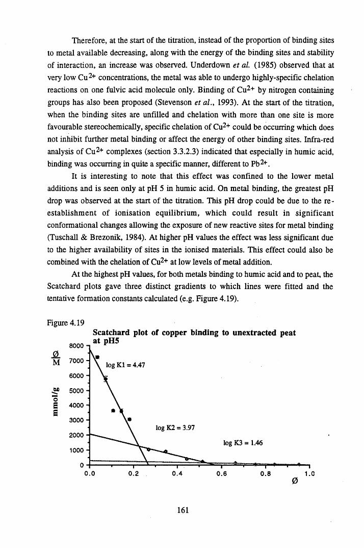
Therefore, at the start of the titration, instead of the proportion of binding sites to metal available decreasing, along with the energy of the binding sites and stability of interaction, an increase was observed. Underdown et a l (1985) observed that at very low Cu2+ concentrations, the metal was able to undergo highly-specific chelation reactions on one fulvic acid molecule only. Binding of Cu2+ by nitrogen containing groups has also been proposed (Stevenson et al., 1993). At the start of the titration, when the binding sites are unfilled and chelation with more than one site is more favourable stereochemically, specific chelation of Cu2+ could be occurring which does not inhibit further metal binding or affect the energy of other binding sites. Infra-red analysis of Cu2+ complexes (section 3.3.2.3) indicated that especially in humic acid, binding was occurring in quite a specific manner, different to Pb2+.
It is interesting to note that this effect was confined to the lower metal additions and is seen only at pH 5 in humic acid. On metal binding, the greatest pH drop was observed at the start of the titration. This pH drop could be due to the reestablishment of ionisation equilibrium, which could result in significant conformational changes allowing the exposure of new reactive sites for metal binding (Tuschall & Brezonik, 1984). At higher pH values the effect was less significant due to the higher availability of sites in the ionised materials. This effect could also be combined with the chelation of Cu2+ at low levels of metal addition.
At the highest pH values, for both metals binding to humic acid and to peat, the Scatchard plots gave three distinct gradients to which lines were fitted and the tentative formation constants calculated (e.g. Figure 4.19).
Figure 4.19Scatchard plot of copper binding to unextracted peat
onnrt at pH5 8000 -
Q.M 7000 log K1 = 4.47
6000
w> 5 0 0 0
og 4000B
3000log K2 = 3.97
2000log K3 = 1.46
1000
0.0 0.2 0 .4 0.6 1.00
161
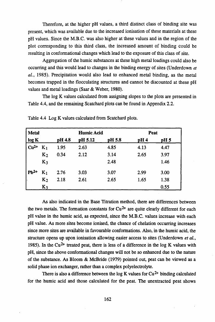
Therefore, at the higher pH values, a third distinct class of binding site was present, which was available due to the increased ionisation of these materials at these pH values. Since the M.B.C. was also higher at these values and in the region of the plot corresponding to this third class, the increased amount of binding could be resulting in conformational changes which lead to the exposure of this class of site.
Aggregation of the humic substances at these high metal loadings could also be occurring and this would lead to changes in the binding energy of sites (Underdown et a l , 1985). Precipitation would also lead to enhanced metal binding, as the metal becomes trapped in the flocculating structures and cannot be discounted at these pH values and metal loadings (Saar & Weber, 1980).
The log K values calculated from assigning slopes to the plots are presented in Table 4.4, and the remaining Scatchard plots can be found in Appendix 2.2.
Table 4.4 Log K values calculated from Scatchard plots.
MetallogK pH 4.8
Humic Add pH 5.12 pH 5.8
PeatpH 4 pH 5
Cu2+ Kl 1.95 2.63 4.85 4.13 4.47k 2 0.34 2.12 3.14 2.65 3.97k 3 2.48 1.46
Pb2* K i 2.76 3.03 3.07 2.99 3.00k 2 2.18 2.61 2.65 1.65 1.38k 3 0.55
As also indicated in the Base Titration method, there are differences between the two metals. The formation constants for Cu2+ are quite clearly different for each pH value in the humic acid, as expected, since the M.B.C. values increase with each pH value. As more sites become ionised, the chance of chelation occurring increases since more sites are available in favourable conformations. Also, in the humic acid, the structure opens up upon ionisation allowing easier access to sites (Underdown et al., 1985). In the Cu2+ treated peat, there is less of a difference in the log K values with pH, since the above conformational changes will not be so enhanced due to the nature of the substance. As Bloom & McBride (1979) pointed out, peat can be viewed as a solid phase ion exchanger, rather than a complex polyelectrolyte.
There is also a difference between the log K values for Cu2+ binding calculated for the humic acid and those calculated for the peat. The unextracted peat shows
162
higher values for each pH value and each constant, indicating that in this material binding is taking place in a more stable arrangement than in the humic acid. Firstly, there is less Cu2+ binding to the peat, as demonstrated in the M.B.C. values, and this will promote a more stable arrangement, as the first binding sites to react will have the highest binding energies (Tuschall & Brezonik, 1983). In addition, the Cu2+ could also be interacting with other components of the peat, such as the mineral matter and other organic materials such as amines and polysaccharides, which would be removed on isolation of the humic acid. Cu2+ has previously been shown to associate strongly with nitrogen containing materials, in particular porphoryn-based structures (Cheshire et a l , 1977), and these could be contributing to the stability of the interaction. The ability of Cu2+ to form inner sphere complexes with unextracted peat was shown by Bloom & McBride (1979) whereas other metals such as K+ and Mn2+, were only able to interact as outer sphere complexes.
The log K values for Pb2+ differ from those for Cu2+, in that they show little change with pH, and with isolation of humic acid, indicating that Pb2+ is reacting with a similar stability of reaction, in both humic acid and unextracted peat for all pH values. Warwick et a l (1991) found no difference in formation constants for the binding of Ni2+ with isolated and non-isolated materials.
In the humic acid in particular, the Scatchard plots for Pb2+ showed less curvilinearity than for Cu2+, (e.g. Figure 4.20), compared to the unextracted peat, and this is reflected in the similarity in the log Ki and log K2 values in the humic acid. The Scatchard plot was originally developed to calculate formation constants in systems with 1:1 stoichiometry, with one or two ligands (Falck, 1988). Since curvilinearity reflects heterogeneity in binding sites and energies, the Pb2+ could be binding with predominantly 1:1 arrangements in humic acid, which have little difference in binding energy. Conversely, in the Cu2+ binding to humic acid, the binding sites are more distinct. Stevenson et al (1993) studied the stability of Cu2+ binding using a variety of methods and concluded that, in humic acid, Cu2+ binds in a mixture of 1:1 and 2:1 arrangements.
It must also be remembered that the limit of detection of the Pb2+ electrode was poorer than for the Cu2+, and binding at higher energy sites which were detected in Cu2+ could not be detected in Pb2+ due to this limitation.
163
Figure 4.20Scatchard plot of lead binding to humic acid at pH 5.8
400 -i0M
300 ~ log K1 = 3.07
SU§ 200 -££
100 - log K2 = 2.65
0 .7 0 .9 1.00 .5 0.6 0.80 .4
0
4.3.2.5 CALCULATION OF INCREMENTAL FORMATION CONSTANTS
The incremental constants, calculated from the titration data, reflect the continuous distribution of binding energies which are shown in the curvilinear Scatchard plots (Stevenson et al., 1993). The formation constants were calculated from the titration data, using the following two equations, and the relevant stability of each arrangement could then be analysed:
2+ . - k 3 w . + . (MA+)M + A 4=> MA k3 =(M2+)(A‘)
M2+ + 2A’ « MA2 k4 = ■ (4.15)(M X A*)
The complete set of log k values for all of the titrations can be found in Appendix 2.2, with only examples being displayed here.
The incremental values obtained also reflect the variations between the metals which were expressed in the Scatchard values, as well as the differences between the humic acid and unextracted peat in Cu2+ binding. This is expected since the same titration data were used in the calculation of both sets of constants. However, in
164
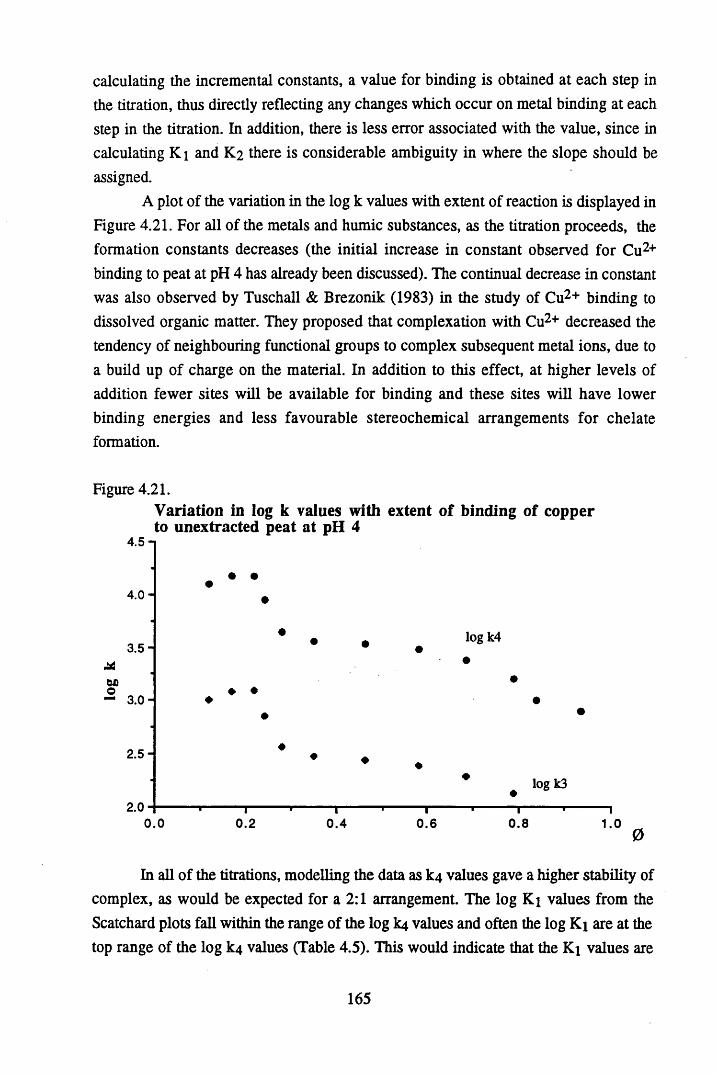
calculating the incremental constants, a value for binding is obtained at each step in the titration, thus directly reflecting any changes which occur on metal binding at each step in the titration. In addition, there is less error associated with the value, since in calculating K i and K2 there is considerable ambiguity in where the slope should be assigned.
A plot of the variation in the log k values with extent of reaction is displayed in Figure 4.21. For all of the metals and humic substances, as the titration proceeds, the formation constants decreases (the initial increase in constant observed for Cu2+ binding to peat at pH 4 has already been discussed). The continual decrease in constant was also observed by Tuschall & Brezonik (1983) in the study of Cu2+ binding to dissolved organic matter. They proposed that complexation with Cu2+ decreased the tendency of neighbouring functional groups to complex subsequent metal ions, due to a build up of charge on the material. In addition to this effect, at higher levels of addition fewer sites will be available for binding and these sites will have lower binding energies and less favourable stereochemical arrangements for chelate formation.
Figure 4.21.Variation in log k values with extent of binding of copper to unextracted peat at pH 4
4.5-1
4.0 -
log k43 .5 -
o- 3 .0 -
2 .5 -
log k3
2.00.0 0.2 0 .4 0.6 0.8 1.0
0
In all of the titrations, modelling the data as k4 values gave a higher stability of complex, as would be expected for a 2:1 arrangement. The log Ki values from the Scatchard plots fall within the range of the log k4 values and often the log Ki are at the top range of the log k4 values (Table 4.5). This would indicate that the Ki values are
165

expressing binding of metals in a 2:1 arrangement and this has been proposed as one explanation for the curvilinearity of the plots (Sahu & Baneijee, 1990: Falck, 1988). Similarly, the log K2 values for the Scatchard plots fall within the range of the 1:1 complexes expressed by the incremental log k3 values, indicating that, at this extent of reaction, 1:1 complexes predominate.
Table 4.5 Formation Constants for Cu2+ binding to peat at pH 4.
0 logk3 logk4 Scatchard values
0.119 3.01 4.10 log Ki = 4.130.168 3.08 4.170.220 3.09 4.180.241 2.86 3.95 log K2 = 2.650.281 2.56 3.650.350 2.47 3.560.464 2.45 3.530.583 2.39 3.480.683 2.29 3.380.787 2.29 3.210.839 2.12 3.000.934 1.91 2.91
The remainder of the incremental log k values can be found in Appendix 2.2 along with the relevant Scatchard plots.
166
4.4 CONCLUSIONS
The Base Titration method was not able to model the complexation of metals to humic substances as well as the other methods and the constants obtained should be interpreted with caution. The log B2 values express the competition of a metal and a proton for a reactive site and, in this sense, the model demonstrated well the differences between metals, provided buffered salts are used. In addition, the graphs of proton release gave valuable information on the behaviours of the different metals. In later papers, Stevenson and co-workers adapted the Bjerrum approach further and instead of modelling the competition of the metal and proton, modelled the interaction at the ionised sites, regardless of the charge differences (Stevenson etal., 1993). This method does give more realistic measurements of metal-humate stability but again the method relies on a secondary effect to provide a quantitative estimate of the amount of metal bound.
The ion selective electrodes, by measuring the amount of free metal directly, provide a more scientifically sound way of measuring the amount of bound metal with their limitations being their relatively high limits of detection and selectivity, making them applicable to only one metal. Analysis of the data by the Scatchard approach can lead to errors in the calculation of the K values, due to the curvilinearity of the plots, but calculation of the incremental K values overcomes this problem well. Where the Scatchard plots are so curvilinear, this method should be used in preference to the Scatchard approach in calculating formation constants.
From the results of the two methods, it is evident that Cu2+ and Pb2+ are binding by quite different mechanisms with both the peat and the humic acid and this has consequences for the stability of these interactions. In the Base Titration method, binding of Cu2+ resulted in a significantly greater release of protons from the humic acid than with Pb2+ binding. Although this could be due to release of protons from the hydration of oxides on 1:1 binding, this effect was also seen at pH 4, where hydration of the oxides would not normally be expected to occur. Therefore, it is more likely, that on Cu2+ binding, conformational changes are occurring, which result in the release of excess protons, greater than the amount expected from the titration curve.
In the Scatchard plots, the addition of small increments of Cu2+ was observed to increase the formation constant at the start of the titrations of humic acid and peat This would also indicate conformational changes, exposing new reactive sites of considerable binding energy. This effect was not seen at pH 5.8, where the increased ionisation of the materials had probably already resulted in the exposure of these sites, and due to the more open structure of the materials, secondary conformational changes
167
would be less likely to occur. The Scatchard plots and the Incremental Formation Constants also implied that Cu2+ was more able to interact via 2:1 complexes than Pb2+, where 1:1 complexes predominate, and significantly more metal was being bound.
However, it should be remembered that different peats were used to extract the humic acids used in the Base Titration method and the Scatchard method. It was unfortunate that South Drumboy peat could not have been used throughout all the research, as this would have made the comparison between methods, reactivities and the laboratory and field studies easier to evaluate.
The isolation of humic acid from peat had an effect on how the metals interacted and the constants which were produced. Significantly less metal was bound to the unextracted peat than to the humic acid, as reflected in the M.B.C. values for both the metals indicating again that isolation either exposed the reactive sites, or chemically altered the material to give formation of reactive groupings. The formation constants for the metals reacting with the unextracted peat also showed differences between the behaviour and stability of the interactions. Cu2+ reacts to form more stable complexes with unextracted peat than humic acid, indicating that in the unextracted material, Cu2+ can interact with other components of the soil, not just the humic substances to give stable interactions. However, Pb2+ showed little difference in stability between the two materials, regardless of the lower amounts being bound in the peat, as reflected in the M.B.C. values and in the infra-red studies. Therefore, again it can be concluded that the use of humic acid to model the interactions of metals in environmental systems is of dubious value, and further work should centre on the interactions of metals with unextracted peat, rather than an operationally defined fraction. In addition, the competition of cations for binding sites in unextracted materials would be more realistic than these one metal studies.
168
CHAPTER 5
THE STUDY OF THE HEAVY METAL AND RADIOCAESIUM
CONTENTS OF ORGANIC SOILS FROM AN UPLAND HILL FARM IN
SOUTH WEST SCOTLAND
169
5.1 INTRODUCTION
The laboratory-based experiments illustrated that the isolation of humic acid from peat led to changes in the characteristics of the humic substances, in particular the reactive functional group contents. Accordingly, the nature of the interaction of the metals and the stability of this interaction was altered. In the environment metals interact with the unaltered, unextracted material and being a multicomponent system many metals are present at one time, unlike the one-component systems studied in the metal complexation experiments. In parallel to the laboratory based experiments, field- based experiments were therefore carried out in which the interaction of Pb, Cu and Cs with humic substances within peats could be studied further.
Ombrotrophic or rainwater-fed peats have been used to provide a record of past atmospheric deposition of heavy metals and radionuclides (Oldfield et al. 1979:: Glooschenko etal., 1986: Markert & Thornton, 1990: Mitchell etal., 1992). The use of such systems in providing a historical record of deposition requires that all inputs of these metals are from the atmosphere, either through wet or dry deposition and that they are immobilised on contact with the peat and not subject to post depositional movement. As discussed in section 1.8.3, post-depositional movement of metals has been shown to occur in some peat deposits and therefore in the field-based study one of the aims was to investigate whether any such movement occurred in the peats studied and if so, what conditions promote remobilisation. To aid this, in addition to Pb, Cu and Cs a suite of elements were studied, which encompassed the rare earth elements and transition metals. These were studied to give information on the redox environment and generally how the geochemistry changed throughout the profiles.
Providing no remobilisation is occurring, a chronology of past atmospheric deposition of metals can be established. Many dating mechanisms exist (section 1.8.4) and which one is utilised depends ultimately on the time scale being studied. One such method utilises the radionuclide 210Pb and results in a chronology spanning approximately the last 150 years. The method requires that once 210Pb becomes incorporated into the peat it is immobilised, not being subject to any post-depositional movement which could distort the dates. Since Pb has been shown to be mobile within peat deposits (Damman, 1978: Aaby & Jacobsen, 1979: Urban etal., 1990), under certain conditions (section 1.8.3), the validity of using this technique in dating peat cores has been questioned (Urban et al., 1990). Therefore, the method was studied here, in order to investigate whether or not it can reliably be used to establish chronologies for peat cores, and where possible to utilise the dates in establishing the chronology.
170
5.2 DESCRIPTION OF SAMPLING SITES CHOSEN FOR THE STUDY
South Drumboy Farm (grid ref. NS 502 482) is situated to the South West of Glasgow (Figure 5.1) and is affected by the deposition of Chernobyl radiocaesium, with movement of lambs from the farm still being restricted when the first cores were collected. A series of cores was collected (Figure 5.2) from positions selected to investigate the effects of topography and the proximity of the A77 road on metal content. South Drumboy farm is 200-300 m above sea level and receives an annual precipitation of around 1400 mm. Drumboy Hill and the areas surrounding it are covered by extensive hill peat, formed due to the high levels of precipitation and the impermeability of the underlying basaltic till. In addition to the peat, a diverse range of soil types is found within the farm, and this led to variations in the characteristics of the 6 cores collected. One section of the farm had been drained, giving an area of improved grassland. These areas were not sampled directly, since the profiles would be obviously disturbed. Instead, as outlined below sampling took place around these areas to establsh whether there was any indirect effect of drainage on the profiles.
The peats were similar to those used to determine the incremental formation constants in Chapter 4.
CORE 1, NS 502482This core, of length 70 cm, was collected in October 1992, from a position close
to Kingswell Bum. The sampling site was south-easterly facing, at an altitude of 237m, making this the lowest sampling site on the farm and was directly below the improved grassland. The main vegetation comprised various types of grass with Sphagnum beginning to colonise the surface. On sampling, the core was extremely wet and black in colour with, at depth, large amounts of undecomposed birch remains.
CORE 2, NS 502485This core (length 55 cm) was collected in October 1992 and was taken from a
site 400m further up Drumboy Hill (altitude 247 m) from the position of Core 1, beyond the improved grassland. The vegetation was composed of grasses and sedges, and the core was characterised by a darkly coloured surface horizon of 20cm, overlying grey material which turned light brown on exposure to the air. This indicated reducing conditions within the core. The gleyed horizon became progressively more mineral with depth from 20 cm downwards.
171
CORE 3, NS 504493This core (length 70 cm), was collected in June 1993, close to the summit of
Drumboy Hill and was the highest sampling point, at an altitude of 267 m. The vegetation was predominantly composed of grasses and the peat was oxygenated, with a uniform degree of humification throughout the core.
CORE 4, NS 504493This core (length 65 cm) was collected in June 1993 from the boundary of the
farm, at an altitude of 257 m, close to a land-use change from farming to forestry. The sampling site was westerly facing, and was downslope from the ridge of Drumboy Hill. The site was extremely wet and Sphagnum mosses were the predominant vegetation. The core was characterised by a significant amount of mineral material in the middle section.
CORE 5, NS 504489This core (length 50 cm) was collected in June 1993 from the ridge of Drumboy
Hill, directly down from Core 1 on the south-westerly facing slope at an altitude of 247 m. The peat was black in colour, indicating a high degree of humification, and again Sphagnum mosses were beginning to colonise the surface vegetation.
CORE 6, NS 501488Core 6 was sampled in June 1993 and was the lowest sampling point on the ridge
of Drumboy Hill, directly below cores 3 and 5 on the south-westerly facing slope (altitude 240 m). Again, the peat was black in colour, indicating a high degree of humification, with Sphagnum mosses being the predominant vegetation. The peat could only be sampled to a depth of 40 cm since the bedrock was present at this depth.
172
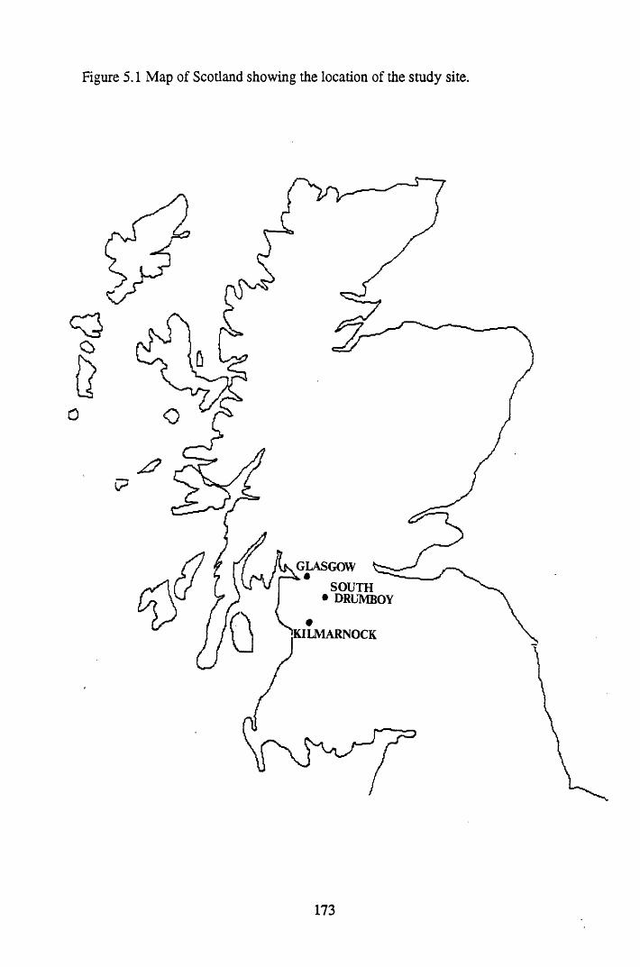
Figure 5.1 Map of Scotland showing the location of the study site.
o
GLASGOW
SOUTH • DRUMBOY
[KILMARNOCK
173
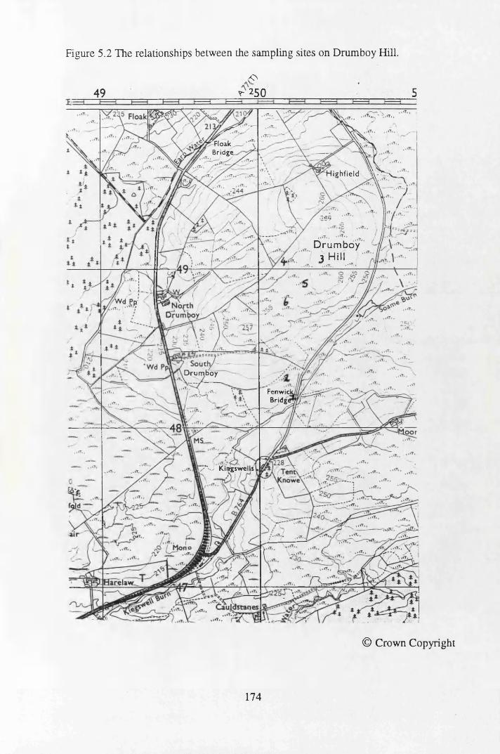
Figure 5.2 The relationships between the sampling sites on Drumboy Hill.
<o49 r25Q 5
F l o a kB r i d g e ^
ighfield \
D r u m b o y 3 Hill
. VT.
Drumboy
F e n w i c JB r i d g e
y ^J ' k i i t g s w e l l s L
© Crown Copyright
174
5.3 METHODS
5.3.1 SAMPLING PROCEDURES
The cores were collected by digging a pit and extracting consecutive blocks of approximately 20 cm x 20 cm x 20 cm with a clean spade. Cores were either sampled to a depth of approximately 60 cm, or until the bedrock was reached. The blocks were wrapped carefully in polyethylene for transportation, taking care to minimise disturbance and compaction, and were stored at 4 °C until processing.
The blocks were sectioned into 3 cm slices, taking care to remove the outer layer which could contain organic matter from further down or up the core. Before the sections were air dried, samples were removed for determination of bulk density, water content and organic matter content. The air-dried peat was then ground.
5.3.2 DETERMINATION OF THE PROPERTIES OF THE PEATS
The methods utilised to characterise the peat samples are all standard procedures, as outlined by MAFF (1986). Each section of each core had the % loss on ignition, moisture content, bulk density and pH determined.
5.3.3 7 - SPECTROMETRY
7 - spectrometry was used to measure the activities of 134Cs, 137Cs, 226Ra and 210Pb in the samples.
5.3.3.1 INTERACTION OF 7 RADIATION WITH MATTER
7 radiation consists of high energy photons of electromagnetic radiation, which are emitted as nuclei undergo transitions from higher energy states to lower excited states or the ground state. The 7 photons have a low probability of interaction with atoms encountered and the initial energy of the photon is retained until interaction with an absorber (or detector) occurs, by one of the following processes:
(a) THE PHOTOELECTRIC EFFECT. This process transfers all of the photon energy to a bound electron in an atom of the absorber and results in ejection of the electron as an energetic photoelectron and complete disappearance of the 7 ray. The photoelectric effect is more efficient at lower photon energies, and the efficiency of the process is
175
proportional to approximately E_7/2 when E (energy) is less then 1 MeV. At higher energies, the efficiency of the effect is proportional to 1/E. The probability of the photoelectric effect increases with the Z value (atomic number) of the material, and is approximately in proportion to Z5.
(b) COMPTON SCATTERING. In this process the photon transfers only part of its energy to an electron, which may be bound or free. As well as being degraded in energy, the photon is also deflected from its original path. Compton Scattering gives rise to electrons with a continuous distribution of energies absorbed in the detector with the probability of scattering depending on the number of electrons available, and is therefore proportional to the Z value of the absorber. For energies below 0.5 MeV, the probability of Compton scattering is approximately proportional to E_1. Thus the efficiency of the effect falls off more slowly than the photoelectric effect with increasing energy up to approximately 2 MeV.
(c) PAIR PRODUCTION. This effect is less common than the preceding two processes, and occurs when / rays are transformed, upon interaction with matter, into an electron-positron pair. The probability of pair production is proportional to Z2 of the absorber, and increases with photon energy above 1.022 MeV.
In summary, all three processes produce moving electrons (or positrons) in matter, which can either be detected directly, or can initiate other electron processes to obtain an electric charge pulse which is utilised in the detection of these processes in / spectrometry.
S.3.3.2 DETECTION OF /RADIATION
High purity semi-conductor germanium (Ge) crystals are widely used as detectors for / spectrometry. Semiconductor detectors have a P-I-N diode structure in which the intrinsic (I) region is extended by application of reverse bias across the diode. When photons interact with the Ge in the depletion region, charge carriers (holes and electrons) are produced and are swept to their respective collecting electrode by the electric field. The resulting charge pulse is collected by application of a high voltage to the crystal and this is integrated by a charge sensitive preamplifier and converted to a voltage pulse with an amplitude proportional to the photon energy. The signal is converted to a digital pulse by an analogue to digital convertor (ADC)
176
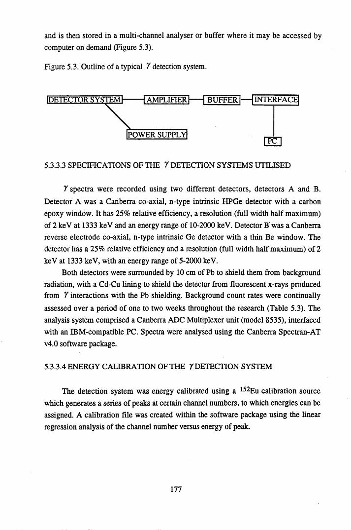
and is then stored in a multi-channel analyser or buffer where it may be accessed by computer on demand (Figure 5.3).
Figure 5.3. Outline of a typical 7 detection system.
IDETECTOR SYSTEM !■ BUFFERAMPLIFIER INTERFACE
POWER SUPPLY
5.3.3.3 SPECIFICATIONS OF THE 7 DETECTION SYSTEMS UTILISED
7 spectra were recorded using two different detectors, detectors A and B. Detector A was a Canberra co-axial, n-type intrinsic HPGe detector with a carbon epoxy window. It has 25% relative efficiency, a resolution (full width half maximum) of 2 keV at 1333 keV and an energy range of 10-2000 keV. Detector B was a Canberra reverse electrode co-axial, n-type intrinsic Ge detector with a thin Be window. The detector has a 25% relative efficiency and a resolution (full width half maximum) of 2 keV at 1333 keV, with an energy range of 5-2000 keV.
Both detectors were surrounded by 10 cm of Pb to shield them from background radiation, with a Cd-Cu lining to shield the detector from fluorescent x-rays produced from 7 interactions with the Pb shielding. Background count rates were continually assessed over a period of one to two weeks throughout the research (Table 5.3). The analysis system comprised a Canberra ADC Multiplexer unit (model 8535), interfaced with an IBM-compatible PC. Spectra were analysed using the Canberra Spectran-AT v4.0 software package.
5.3.3.4 ENERGY CALIBRATION OF THE 7 DETECTION SYSTEM
The detection system was energy calibrated using a 152Eu calibration source which generates a series of peaks at certain channel numbers, to which energies can be assigned. A calibration file was created within the software package using the linear regression analysis of the channel number versus energy of peak.
177
5.3.3.5 EFFICIENCY CALIBRATION OF THE 7 DETECTION SYSTEM
THEORETICAL COSIDERATIONS
The efficiency of the detector is a measure of how many pulses occur for a given number of 7 rays. The absolute count rate, A, of the source is related to the observed count.rate C, through the following equation,
CA = — where D is the detection efficiency. (5.1)
The detection efficiency is equal to the product of a number of factors:
D = / g V fcV saV e (5.2)
/ g is the geometry factor, fbs is the backscatter factor, / sa is the self-absorption factor and/e is the intrinsic efficiency factor.
Of most importance to the detection efficiency of 7 detection systems is the geometry factor, / g. Each arrangement of source and detector has its own geometry factor and any change in the position, volume or distribution of the activity will change the geometry factor, and consequently affect the efficiency as the detection efficiency is proportional to 1/d2, where d is the distance from the detector. In order to minimise variations in the geometry factor it is desirable to determine the detection efficiency experimentally using standard sources of identical size and volume as the samples.
The self-absorption factor can be significant in 7 determinations, particularly when analysing low activity samples, where thick samples are often required to give a measurable counting rate. The self absorption of 7 radiation follows the law:
T = I e’^px (5.3)
where T is the attenuated-beam intensity, I is the unattenuated-beam intensity, u is the total-attenuation coefficient, p is the density of the material and x is the path length, u is a function of the photon energy E and of the atomic number Z. It increases for a given Z with decreasing E and the energy dependence of u is generally greater the higher the Z value. Therefore, self absorption is more significant the lower the photon energy and heavier the element and is particularly relevant to the detection of 210Pb (Ey = 46.5 keV).
Coppola & Reiniger (1973) observed that the chemical composition of soils caused variations in the mass attenuation coefficients which were particularly significant when detecting 7 ray energies below 300 keV. Cutshall etal. (1983)
178
calculated a correction factor for self absorption of 210Pb in sediment samples, where composition or mineralogy also affects the attenuation coefficient, by combining the above equation for the self absorption of 7 radiation with the self absorption equation
i e^ P x>O = A— ------ (5.4)
T / I - l V '
(where O is the attenuated sample output and A is the sample photon emission rate). The correction factor was then calculated as:
— = is e m (5.5)O T / I - l V
This correction factor was calculated for each sample measured, and a wide range of transmissions (T/I) was recorded for the different samples.
STANDARD AND SAMPLE PREPARATION
In the preparation of samples and standards for the determination of detection efficiencies, due care was taken to minimise the effects of geometry and self absorption variation.
To give a standard geometry and minimise sample height, an aliqout of known weight was taken from each section and pelletised in a metal die (diameter 4.8cm) under a pressure of 8 tonnes. Care was taken in cleaning the equipment between samples to minimise contamination. The height of each pellet was then recorded with a micrometer.
To calculate detection efficiency, as outlined below, it is necessary to minimise any changes in sample height and Z value which would give an invalid estimate of efficiency. In order to mimic the Z value of the sample pellets, standard pellets were made from excess peat from the bottom of Core 1. The count rate for the radionuclides being investigated within the peat was recorded before spiking to ensure that it was minimal with only background levels of 210Pb and 226Ra being recorded (Table 5.3). Relevant amounts (Table 5.1) of standard radionuclide solutions of 210Pb and 134Cs and 137Cs were added to lOOg of the bulk peat. Before addition, the peat was wetted with 5 ml of 50:50 (v/v) methanol: water solution. The standards were added dropwise in 10 ml of this solution, whilst stirring the suspension to give even mixing. The spiked peat was then throughly stirred, before drying at 50° C. Once dry the spiked peat was further mixed by shaking on an orbital shaker for 6 hours. From this lOOg sample, sub-samples of 20g, 15g, lOg, and 5g were removed and pelleted, before gamma spectroscopy to determine the detection efficiency. Three lOg pellets were
179
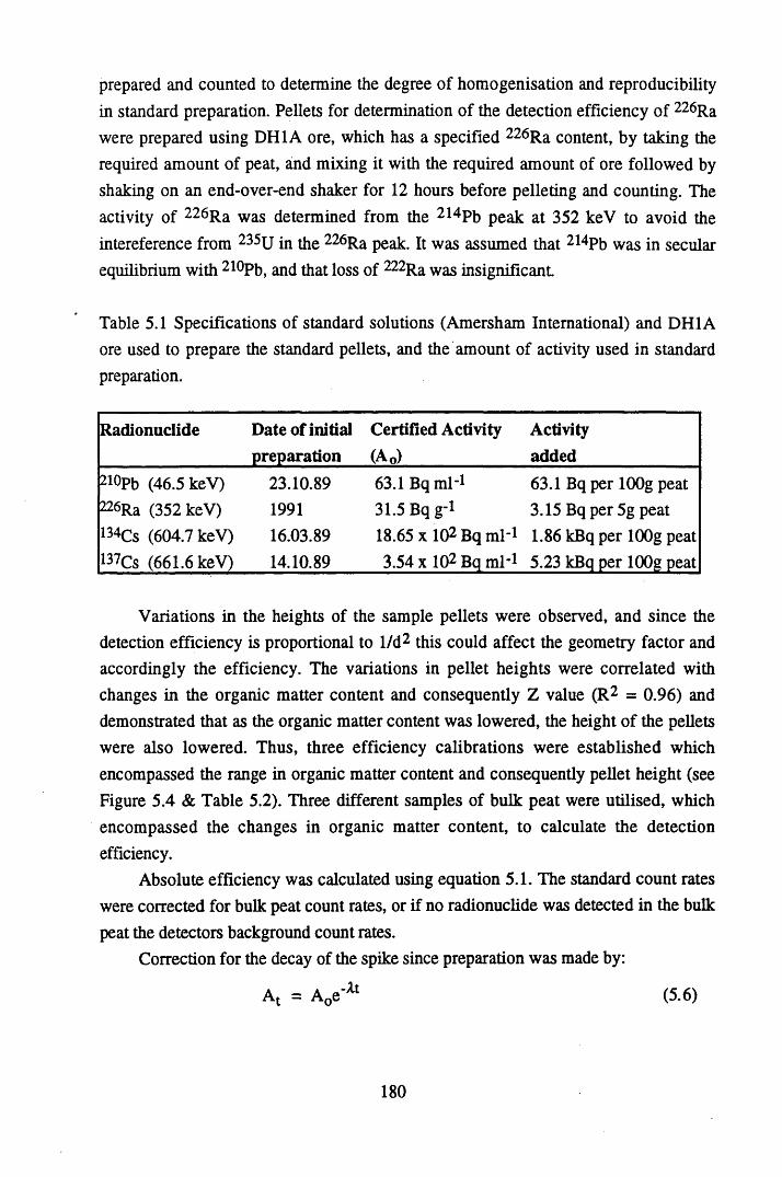
prepared and counted to determine the degree of homogenisation and reproducibility in standard preparation. Pellets for determination of the detection efficiency of 226Ra were prepared using DH1A ore, which has a specified 226Ra content, by taking the required amount of peat, and mixing it with the required amount of ore followed by shaking on an end-over-end shaker for 12 hours before pelleting and counting. The activity of 226Ra was determined from the 214Pb peak at 352 keV to avoid the interference from 235U in the 226Ra peak. It was assumed that 2i4Pb was in secular equilibrium with 210Pb, and that loss of ^ 2Ra was insignificant
Table 5.1 Specifications of standard solutions (Amersham International) and DH1A ore used to prepare the standard pellets, and the amount of activity used in standard preparation.
Radionuclide Date of initial Certified Activity Activitypreparation (A0)______________ added
210Pb (46.5 keV) 23.10.89 63.1 Bq ml’1 63.1 Bq per lOOg peat226Ra (352 keV) 1991 31.5Bq g-l 3.15 Bq per 5g peat134Cs (604.7 keV) 16.03.89 18.65 x 10² Bq ml-1 1.86 kBq per lOOg peat137Cs (661.6 keV) 14.10.89 3 .54x l02 B qm H 5.23 kBq per lOOg peat
Variations in the heights of the sample pellets were observed, and since the detection efficiency is proportional to 1/d2 this could affect the geometry factor and accordingly the efficiency. The variations in pellet heights were correlated with changes in the organic matter content and consequently Z value (R2 = 0.96) and demonstrated that as the organic matter content was lowered, the height of the pellets were also lowered. Thus, three efficiency calibrations were established which encompassed the range in organic matter content and consequently pellet height (see Figure 5.4 & Table 5.2). Three different samples of bulk peat were utilised, which encompassed the changes in organic matter content, to calculate the detection efficiency.
Absolute efficiency was calculated using equation 5.1. The standard count rates were corrected for bulk peat count rates, or if no radionuclide was detected in the bulk peat the detectors background count rates.
Correction for the decay of the spike since preparation was made by:
At = A0e-At (5.6)
180
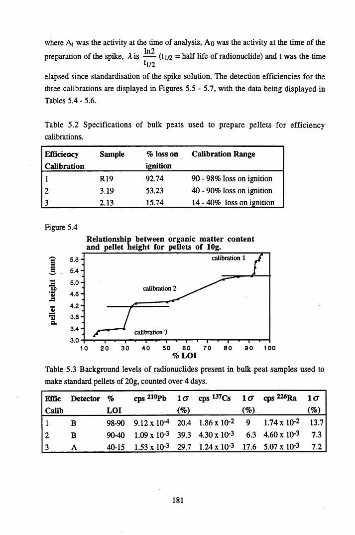
where At was the activity at the time of analysis, Ao was the activity at the time of the
preparation of the spike, A is {t\n = half life of radionuclide) and t was the timeh / 2
elapsed since standardisation of the spike solution. The detection efficiencies for the three calibrations are displayed in Figures 5.5 - 5.7, with the data being displayed in Tables 5.4 - 5.6.
Table 5.2 Specifications of bulk peats used to prepare pellets for efficiency calibrations.
Efficiency Sample % loss on Calibration RangeCalibration ignition1 R19 92.74 90 - 98% loss on ignition2 3.19 53.23 40 - 90% loss on ignition3 2.13 15.74 14-40% loss on ignition
Figure 5.4Relationship between organic matter content and pellet height for pellets of lOg.
calibration 15 .8 -
s 5 .4 -
5 .0 -calibration 2
4 .6 -
4 .2 -
3 .8 -
3 .4 - calibration 33.0
7 050 60 80 9 0 1002 0 30 4 010% LOI
Table 5.3 Background levels of radionuclides present in bulk peat samples used to make standard pellets of 20g, counted over 4 days.
EfficCalib
Detector %LOI
cps 210Pb l a(%)
cps 137Cs 1(7(%)
cps 226Ra 1(7(%)
1 B 98-90 9.12x10⁻⁴ 20.4 1.86 x 10⁻² 9 1.74 x 10⁻² 13.72 B 90-40 1.09xl0‘3 39.3 4.30x10⁻³ 6.3 4.60x10⁻³ 7.33 A 40-15 1.53 x 10⁻³ 29.7 1.24x10⁻³ 17.6 5.07 x 10⁻³ 7.2
181
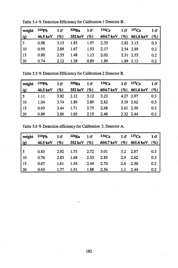
Table 5.4 % Detection Efficiency for Calibration 1 Detector B.
weight
(g)
21«Pb
46.5 keV1(T(%)
226Ra
352 keV1(7
(%)
334Cs 604.7 keV
1 (7 137Cs (%) 661.6 keV
1(7
(%)5 0.98 3.15 1.85 1.97 2.35 2.82 3.15 0.310 0.95 2.89 1.67 1.53 2.17 2.54 2.89 0.215 0.80 2.55 1.48 1.13 2.02 2.31 2.55 0.220 0.74 2.12 1.38 0.89 1.89 1.89 2.12 0.2
Table 5.5 % Detection Efficiency for Calibration 2 Detector B.
weight
(g)
2i0pb 46.5 keV
1(7
(%)
226Ra
352 keV1(7(%)
134Cs 604.7 keV
1 (7 137Cs (%) 661.6 keV
1(7(%)
5 1.11 3.92 2.12 3.12 3.23 4.27 2.97 0.310 1.04 3.74 1.89 2.89 2.82 3.19 2.62 0.315 0.93 3.44 1.71 2.75 2.68 2.61 2.50 0.320 0.89 2.86 1.65 2.15 2.48 2.32 2.44 0.2
Table 5.6 % Detection efficiency for Calibration 3, Detector A.
weight
(g)
210Pb
46.5 keV1(7(%)
226Ra 352 keV
1(7(%)
334Cs 604.7 keV
1(7(%)
137Cs 661.6 keV
1(7(%)
5 0.83 2.92 1.75 2.72 3.01 3.2 2.87 0.310 0.76 2.83 1.68 2.53 2.85 2.9 2.62 0.315 0.67 1.61 1.54 2.44 2.70 2.6 2.50 0.220 0.63 1.77 1.51 1.88 2.56 1.1 2.44 0.2
182
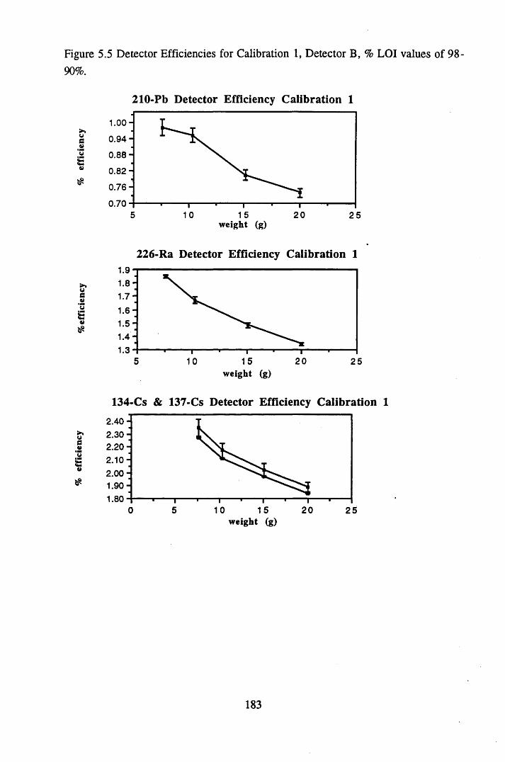
%
effic
ienc
y %
effic
ienc
y %
effi
cien
cy
Figure 5.5 Detector Efficiencies for Calibration 1, Detector B, % LOI values of 98- 90%.
1.00
0.94
0.88
0.82
0.76
0.705 10 15 20 2 5
w eight (g)
226-Ra Detector Efficiency Calibration 11.9 1.8 1.7 1.6 1.5 1.4 1.3
134-Cs & 137-Cs Detector Efficiency Calibration 12.40 2.30 2.20 2.10 2.00 1.90 1.80
0 5 10 15 2 0 2 5w eight (g)
T T T
5 15 2010 25w eight (g)
210-Pb Detector Efficiency Calibration 1
T T T
183
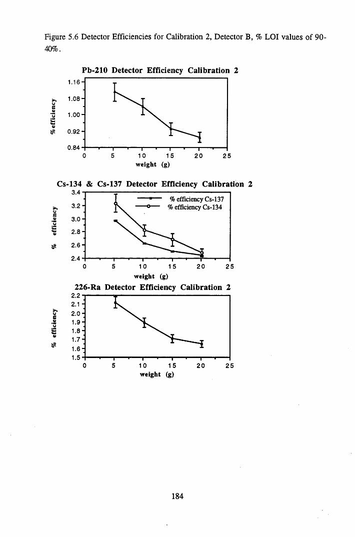
Figure 5.6 Detector Efficiencies for Calibration 2, Detector B, % LOI values of 90- 40%.
Pb-210 Detector Efficiency Calibration 2
1.08-
1.0 0 -
0 .92 -
0.84 T T T
0 5 10 15 2 0 25w eight (g)
Cs-134 & Cs-137 Detector Efficiency Calibration 23.4
> efficiency Cs-137 efficiency Cs-1343 .2 -
3 .0 -
2 .8 -
2 .6 -
2.40 5 1 5 20 2510
w eight (g)
226-Ra Detector Efficiency Calibration 22.2
2 .0 -
1 .7 -
50 10 15 20 25w eight (g)
184
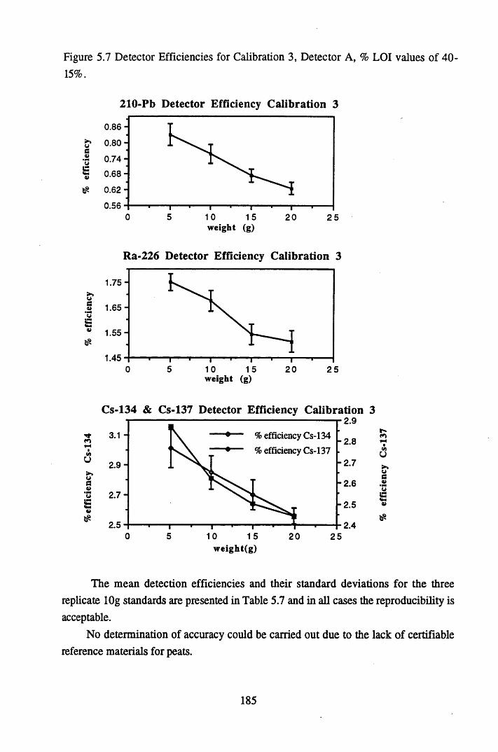
Figure 5.7 Detector Efficiencies for Calibration 3, Detector A, % LOI values of 40- 15%.
210-Pb Detector Efficiency Calibration 3
0 .8 6 -
>%ue4>
0 .80-
0 .74-
« 0.68 -
$ 0.62 -
0.5650 10 1 5 20 2 5
w eight (g)
Ra-226 Detector Efficiency Calibration 3
1.75-►>o5 1 .65-tj* 1 .55-£
1.4550 10 15 20 2 5
weight (g)
Cs-134 & Cs-137 Detector Efficiency Calibration 32.9
efficiency Cs-134 efficiency Cs-137
- 2.8COu -2 .72 .9 ->>os4) - 2.6IM(J 2 .7 -
-2 .59»2.5 2.4
0 5 10 1 5 20 25w eig h t(g )
The mean detection efficiencies and their standard deviations for the three replicate lOg standards are presented in Table 5.7 and in all cases the reproducibility is acceptable.
No determination of accuracy could be carried out due to the lack of certifiable reference materials for peats.
185
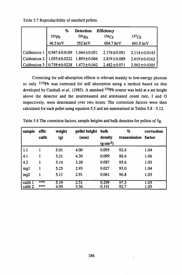
Table 5.7 Reproducibility of standard pellets.
% Detection Efficiency210pb 226Ra 134CS 137Cs
46.5 keV 352 keV 604.7 keV 661.6 keV
Calibration 1 0.947 ±0.0189 1.664 ±0.051 2.176 ±0.091 2.114±0.0145Calibration 2 1.055 ±0.0222 1.893 ±0.066 2.819 ±0.089 2.619±0.0162Calibration 3 0.758 ±0.0228 1.672 ±0.042 2.482 ±0.071 2.562 ±0.0202
Correcting for self-absorption effects is relevant mainly to low-energy photons so only 210Pb was corrected for self absorption using a method based on that developed by Cutshall et al.. (1983). A standard 210Pb source was held at a set height above the detector and the unattenuated and attenuated count rate, I and O respectively, were determined over two hours. The correction factors were then calculated for each pellet using equation 5.5 and are summarised in Tables 5.8 - 5.12.
Table 5.8 The correction factors, sample heights and bulk densities for pellets of 5g.
sample efficcalib
weight
(g)
pellet height (nun)
bulkdensity(gcnr3)
%transmission
correctionfactor
1.1 1 5.01 4.00 0.095 92.6 1.044.1 1 5.21 4.30 0.099 88.6 1.064.2 1 5.14 3.20 0.087 95.6 1.03mgl 1 5.25 2.93 0.027 93.0 1.04mg2 1 5.11 2.91 0.061 96.8 1.03
calib 1 *** 5.19 2.51 0.299 97.3 1.03calib 2 *** 4.95 3.56 0.141 92.7 1.03
186
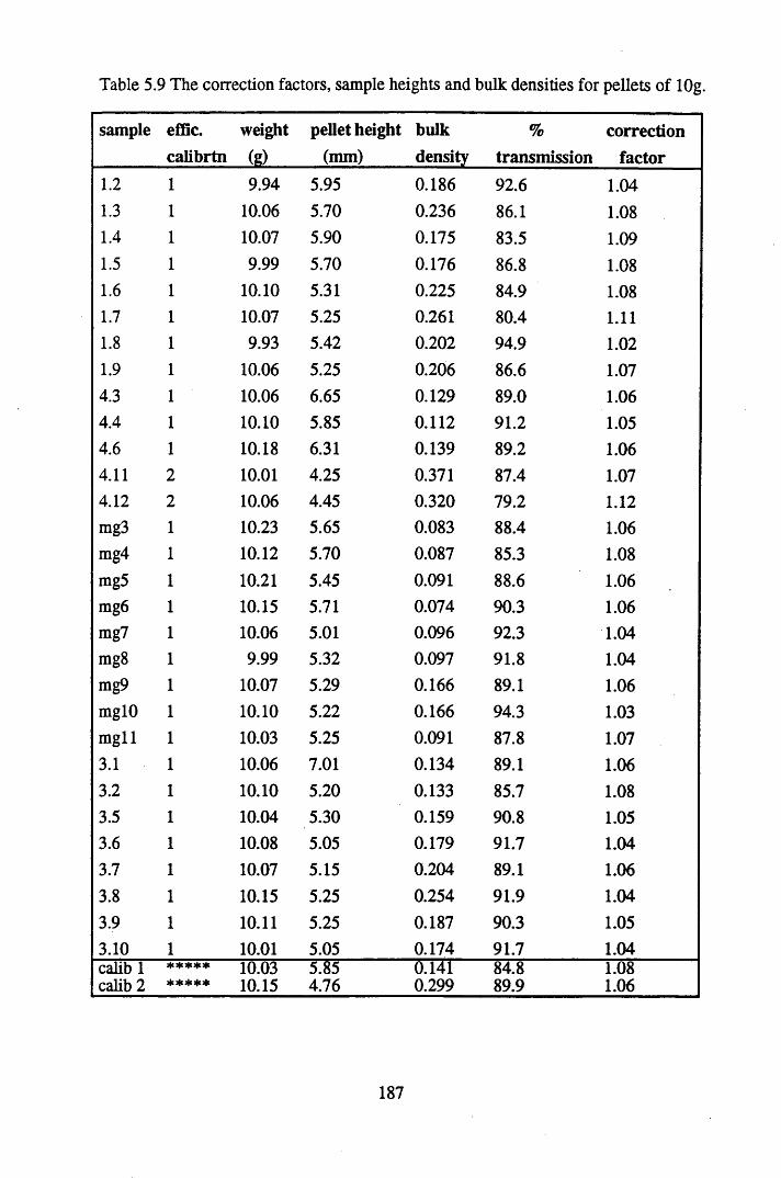
Table 5.9 The correction factors, sample heights and bulk densities for pellets of lOg.
sample effic. weight pellet height bulk % correctioncalibrtn (§) (mm) density transmission factor
1.2 1 9.94 5.95 0.186 92.6 1.041.3 1 10.06 5.70 0.236 86.1 1.081.4 1 10.07 5.90 0.175 83.5 1.091.5 1 9.99 5.70 0.176 86.8 1.081.6 1 10.10 5.31 0.225 84.9 1.081.7 1 10.07 5.25 0.261 80.4 1.111.8 1 9.93 5.42 0.202 94.9 1.021.9 1 10.06 5.25 0.206 86.6 1.074.3 10.06 6.65 0.129 89.0 1.064.4 1 10.10 5.85 0.112 91.2 1.054.6 1 10.18 6.31 0.139 89.2 1.064.11 2 10.01 4.25 0.371 87.4 1.074.12 2 10.06 4.45 0.320 79.2 1.12mg3 1 10.23 5.65 0.083 88.4 1.06mg4 1 10.12 5.70 0.087 85.3 1.08mg5 1 10.21 5.45 0.091 88.6 1.06mg6 1 10.15 5.71 0.074 90.3 1.06mg7 1 10.06 5.01 0.096 92.3 1.04mg8 1 9.99 5.32 0.097 91.8 1.04mg9 1 10.07 5.29 0.166 89.1 1.06mglO 1 10.10 5.22 0.166 94.3 1.03m gll 1 10.03 5.25 0.091 87.8 1.073.1 1 10.06 7.01 0.134 89.1 1.063.2 1 10.10 5.20 0.133 85.7 1.083.5 1 10.04 5.30 0.159 90.8 1.053.6 1 10.08 5.05 0.179 91.7 1.043.7 1 10.07 5.15 0.204 89.1 1.063.8 1 10.15 5.25 0.254 91.9 1.043.9 1 10.11 5.25 0.187 90.3 1.053.10 1 10.01 5.05 0.174 91.7 1.04calib 1 3fc Sfdfc 9|C 10.03 5.85 0.141 84.8 1.08calib 2 a)c 3|c 3|e 3|c 9)c 10.15 4.76 0.299 89.9 1.06
187
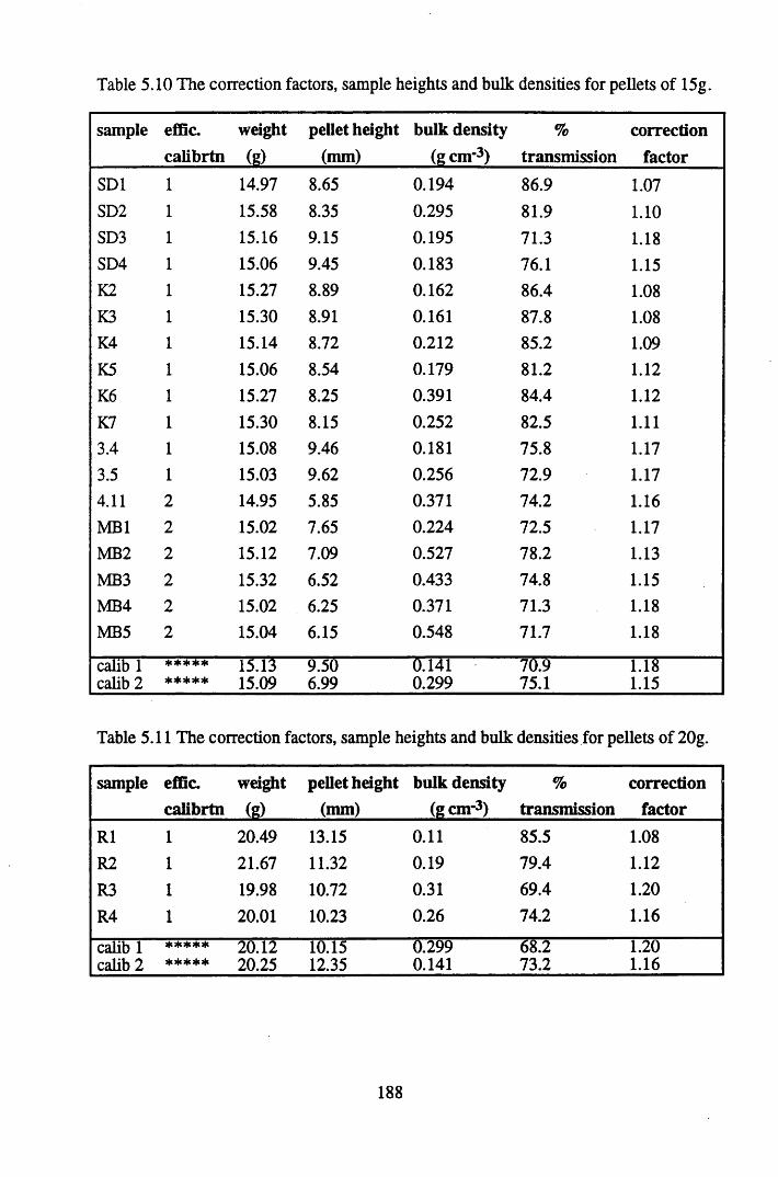
Table 5.10 The correction factors, sample heights and bulk densities for pellets of 15g.
sample effic. weight pellet height bulk density % correctioncalibrtn (g) (mm) (g cm"3) transmission factor
SD1 1 14.97 8.65 0.194 86.9 1.07SD2 1 15.58 8.35 0.295 81.9 1.10SD3 1 15.16 9.15 0.195 71.3 1.18SD4 1 15.06 9.45 0.183 76.1 1.15K2 1 15.27 8.89 0.162 86.4 1.08K3 1 15.30 8.91 0.161 87.8 1.08K4 1 15.14 8.72 0.212 85.2 1.09K5 1 15.06 8.54 0.179 81.2 1.12K6 1 15.27 8.25 0.391 84.4 1.12K7 1 15.30 8.15 0.252 82.5 1.113.4 1 15.08 9.46 0.181 75.8 1.173.5 1 15.03 9.62 0.256 72.9 1.174.11 2 14.95 5.85 0.371 74.2 1.16MB1 2 15.02 7.65 0.224 72.5 1.17MB2 2 15.12 7.09 0.527 78.2 1.13MB3 2 15.32 6.52 0.433 74.8 1.15MB4 2 15.02 6.25 0.371 71.3 1.18MB5 2 15.04 6.15 0.548 71.7 1.18
calib 1 He * * * * 15.13 9.50 0.141 70.9 1.18calib 2 ***** 15.09 6.99 0.299 75.1 1.15
Table 5.11 The correction factors, sample heights and bulk densities for pellets of 20g.
sample efBc. weight pellet height bulk density % correctioncalibrtn (g) (mm) (gem-3) transmission factor
R1 1 20.49 13.15 0.11 85.5 1.08R2 1 21.67 11.32 0.19 79.4 1.12R3 1 19.98 10.72 0.31 69.4 1.20R4 1 20.01 10.23 0.26 74.2 1.16
calib 1 ***** 20.12 10.15 0.299 68.2 1.20calib 2 ***** 20.25 12.35 0.141 73.2 1.16
188
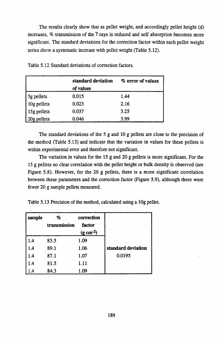
The results clearly show that as pellet weight, and accordingly pellet height (d) increases, % transmission of the Y rays is reduced and self absorption becomes more significant. The standard deviations for the correction factor within each pellet weight series show a systematic increase with pellet weight (Table 5.12).
Table 5.12 Standard deviations of correction factors.
standard deviation of values
% error of values
5g pellets 0.015 1.44lOg pellets 0.023 2.1615g pellets 0.037 3.2520g pellets 0.046 3.99
The standard deviations of the 5 g and 10 g pellets are close to the precision of the method (Table 5.13) and indicate that the variation in values for these pellets is within experimental error and therefore not significant.
The variation in values for the 15 g and 20 g pellets is more significant. For the 15 g pellets no clear correlation with the pellet height or bulk density is observed (see Figure 5.8). However, for the 20 g pellets, there is a more significant correlation between these parameters and the correction factor (Figure 5.9), although there were fewer 20 g sample pellets measured.
Table 5.13 Precision of the method, calculated using a lOg pellet.
sample %transmission
correctionfactor(gem-2)
1.4 83.5 1.091.4 89.1 1.06 standard deviation1.4 87.1 1.07 0.01951.4 81.5 1.111.4 84.3 1.09
189
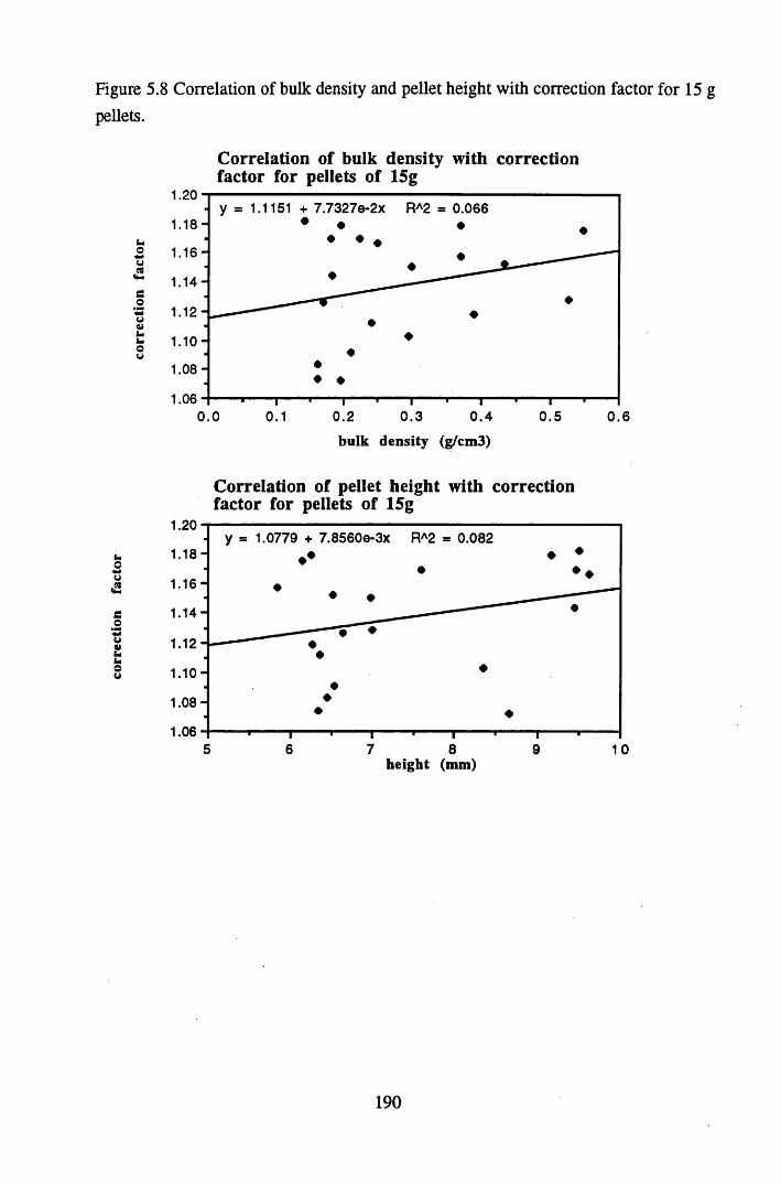
corr
ectio
n fa
ctor
Figure 5.8 Correlation of bulk density and pellet height with correction factor for 15 gpellets.
Correlation of bulk density with correction factor for pellets of 15g
1.201.1151 + 7.7327e-2x RA2 = 0.066
1.18I*o 1.16
1.14fio1.12
1.10
1.08
1.060.2 0 .3 0 .4 0 .50.0 0.1 0 .6
bulk density (g/cm3)
Correlation of pellet height with correction factor for pellets of 15g
1.201.0779 + 7.8560e-3x RA2 a 0.082
1.18-
1 .16-
1 .14-
1.12
1. 1 0 -
1.08-
1.065 6 7 8 9 10
heigh t (mm)
190
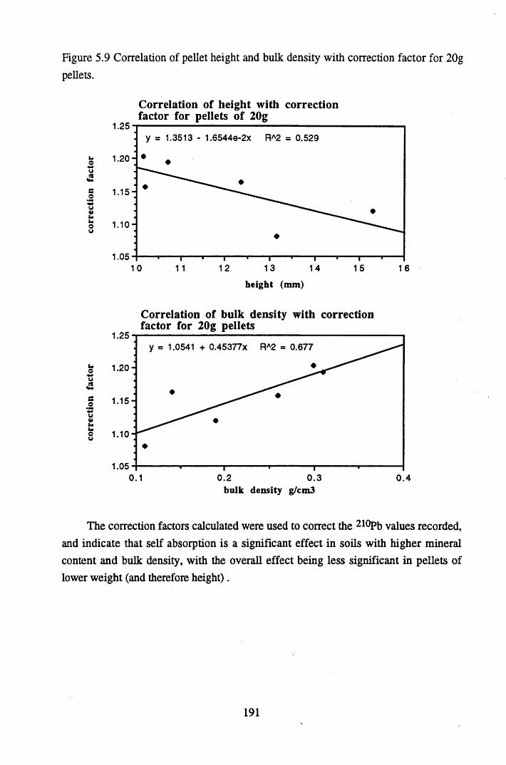
Figure 5.9 Correlation of pellet height and bulk density with correction factor for 20gpellets.
Correlation of height with correction factor for pellets of 20g
1.251.3513 - 1.6544e-2x RA2 = 0.529
1.2 0 -9fj
eouVhuo9 1. 1 0 -
1.0512 131 0 14 15 1 61 1
h eigh t (mm)
Correlation of bulk density with correction factor for 20g pellets
1.251.0541 + 0.45377X RA2 = 0.677
uo 1.2 0 -u
Cou4)uuo9 1.10
1.050.1 0.2 0 .3 0 .4
b u lk density g/cm3
The correction factors calculated were used to correct the 210Pb values recorded, and indicate that self absorption is a significant effect in soils with higher mineral content and bulk density, with the overall effect being less significant in pellets of lower weight (and therefore height).
191
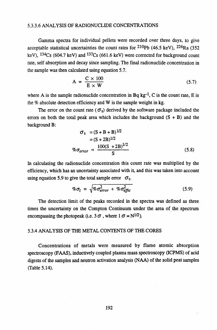
5.3.3.6 ANALYSIS OF RADIONUCLIDE CONCENTRATIONS
Gamma spectra for individual pellets were recorded over three days, to give acceptable statistical uncertainties the count rates for 210Pb (46.5 keV), 226Ra (352 keV), 134Cs (604.7 keV) and 137Cs (661.6 keV) were corrected for background count rate, self absorption and decay since sampling. The final radionuclide concentration in the sample was then calculated using equation 5.7.
A =E x W
where A is the sample radionuclide concentration in Bq kg’1, C is the count rate, E is the % absolute detection efficiency and W is the sample weight in kg.
The error on the count rate ( <TS) derived by the software package included the errors on both the total peak area which includes the background (S + B) and the background B:
<TS =(S + B + B) 1' 2
= (S + 2B) 1' 2
100(S +2B )1 /2'°&error ~~ g (5.8)
In calculating the radionuclide concentration this count rate was multiplied by the efficiency, which has an uncertainty associated with it, and this was taken into account using equation 5.9 to give the total sample error <7t.
% at ~ &error + (5.9)
The detection limit of the peaks recorded in the spectra was defined as three times the uncertainty on the Compton Continuum under the area of the spectrum encompassing the photopeak (i.e. 3 G , where 1G = Nly2).
5.3.4 ANALYSIS OF THE METAL CONTENTS OF THE CORES
Concentrations of metals were measured by flame atomic absorption spectroscopy (FAAS), inductively coupled plasma mass spectroscopy (ICPMS) of acid digests of the samples and neutron activation analysis (NAA) of the solid peat samples (Table 5.14).
192
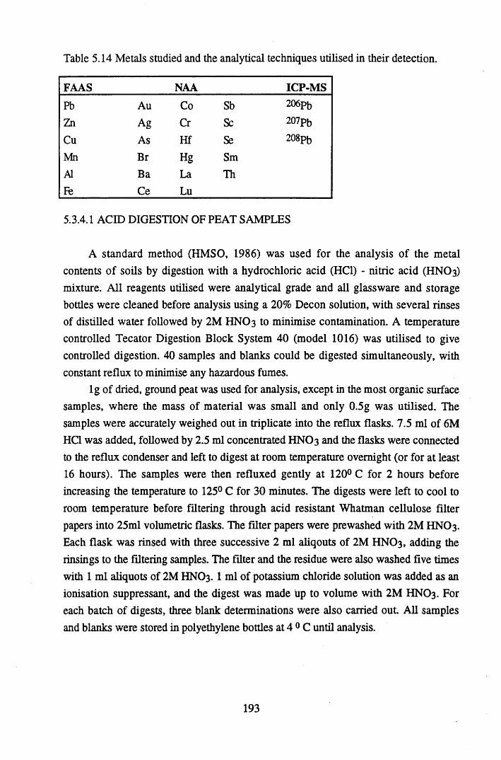
Table 5.14 Metals studied and the analytical techniques utilised in their detection.
FAAS NAA ICP-MSPb Au Co Sb 206pb
Zn Ag Cr Sc 207pb
Cu As Hf Se 208pb
Mn Br Hg SmA1 Ba La Th¥& Ce Lu
5.3.4.1 ACID DIGESTION OF PEAT SAMPLES
A standard method (HMSO, 1986) was used for the analysis of the metal contents of soils by digestion with a hydrochloric acid (HC1) - nitric acid (HNO3) mixture. All reagents utilised were analytical grade and all glassware and storage bottles were cleaned before analysis using a 20% Decon solution, with several rinses of distilled water followed by 2M HNO3 to minimise contamination. A temperature controlled Tecator Digestion Block System 40 (model 1016) was utilised to give controlled digestion. 40 samples and blanks could be digested simultaneously, with constant reflux to minimise any hazardous fumes.
lg of dried, ground peat was used for analysis, except in the most organic surface samples, where the mass of material was small and only 0.5g was utilised. The samples were accurately weighed out in triplicate into the reflux flasks. 7.5 ml of 6 M HC1 was added, followed by 2.5 ml concentrated HNO3 and the flasks were connected to the reflux condenser and left to digest at room temperature overnight (or for at least 16 hours). The samples were then refluxed gently at 120° C for 2 hours before increasing the temperature to 125° C for 30 minutes. The digests were left to cool to room temperature before filtering through acid resistant Whatman cellulose filter papers into 25ml volumetric flasks. The filter papers were prewashed with 2M HNO3 . Each flask was rinsed with three successive 2 ml aliqouts of 2M HNO3 , adding the rinsings to the filtering samples. The filter and the residue were also washed five times with 1 ml aliquots of 2M HNO3 . 1 ml of potassium chloride solution was added as an ionisation suppressant, and the digest was made up to volume with 2M HNO3 . For each batch of digests, three blank determinations were also carried out. All samples and blanks were stored in polyethylene bottles at 4 0 C until analysis.
193

5.3.4.2 FAAS ANALYSIS OF THE DIGESTS
Atomic absorption spectrometry utilises the absorption of light energy of a specific wavelength by an atom when it becomes "excited". As the number of atoms in the light path increases, the amount of light absorbed will correspondingly increase, allowing quantitative determination of the amount of atoms present if specific light sources and the characteristic wavelengths of the atoms are utilised. An atomic absorption spectrometer has five main components, a hollow cathode lamp as the light source, the absorption cell where atoms of the sample are produced (either flame or furnace), a monochromator for light dispersion, a detector which measures the light intensity and amplifies the signal and a display unit which shows the reading.
A Perkin Elmer 1100B Atomic Absorption Spectrometer with v3.5 operating software was utilised with the "cookbook settings" and standard linear ranges of the elements being applied. The ranges and setting used are presented in Table 5.15. The spectrometer was calibrated with the relevant standard solutions to give the results in units of concentration. The standard solutions were prepared from Spectrosol standard reagents, which had 1000 ug ml-1 of analyte in 0.5M HNO3 . These were diluted to the required range with 2M HNO3 , and stored in polyelethylene bottles at 4° C between determinations.
In calibrating the machine, the auto mode was chosen which automatically selects the most appropriate line fitting equation depending on the number of standards used in the calibration. A reslope function was also present and was utilised during the runs.
Table 5.15 Specifications of the FAAS system.
Element Wavelength Flame
(nm)
Sensitivity Linear Range Check (mg/1)
Lim it of detection
Pb 283.3 Air-Ac 2 0 0 - 2 0 0 . 2
Zn 213.9 Air-Ac 1 .0 0 - 1 0 .0 1
Mn 279.5 NO-Ac 2.5 0 -3 0.03Fe 248.3 NO-Ac 5 0 -5 0.05Cu 324.8 Air-Ac 4 0 -5 0.05A1 309.3 NO-Ac 50 0-150 1.5
194
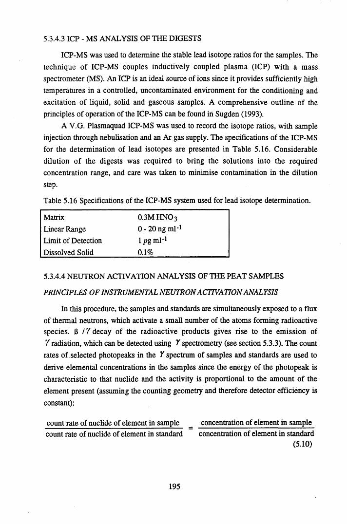
S.3.4.3 ICP - MS ANALYSIS OF THE DIGESTS
ICP-MS was used to determine the stable lead isotope ratios for the samples. The technique of ICP-MS couples inductively coupled plasma (ICP) with a mass spectrometer (MS). An ICP is an ideal source of ions since it provides sufficiently high temperatures in a controlled, uncontaminated environment for the conditioning and excitation of liquid, solid and gaseous samples. A comprehensive outline of the principles of operation of the ICP-MS can be found in Sugden (1993).
A V.G. Plasmaquad ICP-MS was used to record the isotope ratios, with sample injection through nebulisation and an Ar gas supply. The specifications of the ICP-MS for the determination of lead isotopes are presented in Table 5.16. Considerable dilution of the digests was required to bring the solutions into the required concentration range, and care was taken to minimise contamination in the dilution step.
Table 5.16 Specifications of the ICP-MS system used for lead isotope determination.
Matrix 0.3M H N 03
Linear Range 0 - 2 0 ng ml*1
Limit of Detection 1 pg ml-1
Dissolved Solid 0 .1%
5.3.4.4 NEUTRON ACTIVATION ANALYSIS OF THE PEAT SAMPLES
PRINCIPLES OF INSTRUMENTAL NEUTRON ACTIVATION ANALYSIS
In this procedure, the samples and standards are simultaneously exposed to a flux of thermal neutrons, which activate a small number of the atoms forming radioactive species. 6 / Y decay of the radioactive products gives rise to the emission of / radiation, which can be detected using Y spectrometry (see section 5.3.3). The count rates of selected photopeaks in the Y spectrum of samples and standards are used to derive elemental concentrations in the samples since the energy of the photopeak is characteristic to that nuclide and the activity is proportional to the amount of the element present (assuming the counting geometry and therefore detector efficiency is constant):
count rate of nuclide of element in sample _ concentration of element in sample count rate of nuclide of element in standard concentration of element in standard
(5.10)
195
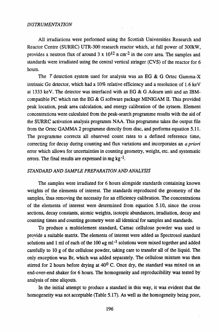
INSTRUMENTATION
All irradiations were performed using the Scottish Universities Research and Reactor Centre (SURRC) UTR-300 research reactor which, at full power of 300kW, provides a neutron flux of around 3 x 10¹² n cm-2 in the core area. The samples and standards were irradiated using the central vertical stringer (CVS) of the reactor for 6
hours.The y detection system used for analysis was an EG & G Ortec Gamma-X
intrinsic Ge detector, which had a 10% relative efficiency and a resolution of 1.6 keV at 1333 keV. The detector was interfaced with an EG & G Adeam unit and an IBM- compatible PC which ran the EG & G software package MINIGAM n. This provided peak location, peak area calculation, and energy calibration of the sytsem. Element concentrations were calculated from the peak-search programme results with the aid of the SURRC activation analysis programm NAA. This programme takes the output file from the Ortec GAMMA 2 programme directly from disc, and performs equation 5.11. The programme corrects all observed count rates to a defined reference time, correcting for decay during counting and flux variations and incorporates an a priori error which allows for uncertainties in counting geometry, weight, etc. and systematic errors. The final results are expressed in mg kg-1.
STANDARD AND SAMPLE PREPARATION AND ANALYSIS
The samples were irradiated for 6 hours alongside standards containing known weights of the elements of interest. The standards reproduced the geometry of the samples, thus removing the necessity for an efficiency calibration. The concentrations of the elements of interest were determined from equation 5.10, since the cross sections, decay constants, atomic weights, isotopic abundances, irradiation, decay and counting times and counting geometry were all identical for samples and standards.
To produce a multielement standard, Camac cellulose powder was used to provide a suitable matrix. The elements of interest were added as Spectrosol standard solutions and 1 ml of each of the 1 0 0 ug ml-1 solutions were mixed together and added carefully to 10 g of the cellulose powder, taking care to transfer all of the liquid. The only exception was Br, which was added separately. The cellulose mixture was then stirred for 2 hours before drying at 40® C. Once dry, the standard was mixed on an end-over-end shaker for 6 hours. The homogeneity and reproducibility was tested by analysis of nine aliqouts.
In the initial attempt to produce a standard in this way, it was evident that the homogeneity was not acceptable (Table 5.17). As well as the homogeneity being poor,
196
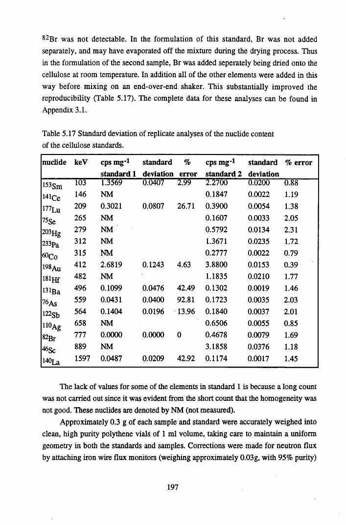
82Br was not detectable. In the formulation of this standard, Br was not added separately, and may have evaporated off the mixture during the drying process. Thus in the formulation of the second sample, Br was added seperately being dried onto the cellulose at room temperature. In addition all of the other elements were added in this way before mixing on an end-over-end shaker. This substantially improved the reproducibility (Table 5.17). The complete data for these analyses can be found in Appendix 3.1.
Table 5.17 Standard deviation of replicate analyses of the nuclide content of the cellulose standards.
nuclide keV cps mg-1 standard % cps mg-1 standard % errorstandard 1 deviation error standard 2 deviation
!53Sm 103 1.3569 0.0407 2.99 2.2700 0 .0 2 0 0 0 .8 8
141Ce 146 NM 0.1847 0 .0 0 2 2 1.19
177Lu 209 0.3021 0.0807 26.71 0.3900 0.0054 1.38
75Se 265 NM 0.1607 0.0033 2.05
203Hg233Pa
279 NM ’ 0.5792 0.0134 2.31
312 NM 1.3671 0.0235 1.72
60CO 315 NM 0.2777 0 .0 0 2 2 0.79
I98 Au 412 2.6819 0.1243 4.63 3.8800 0.0153 0.39
18lRf 482 NM 1.1835 0 .0 2 1 0 1.77
13lBa 496 0.1099 0.0476 42.49 0.1302 0.0019 1.46
76As 559 0.0431 0.0400 92.81 0.1723 0.0035 2.03
122sb 564 0.1404 0.0196 13.96 0.1840 0.0037 2 .0 1
noAg82Br
658 NM 0.6506 0.0055 0.85777 0 .0 0 0 0 0 .0 0 0 0 0 0.4678 0.0079 1.69
46sc 889 NM 3.1858 0.0376 1.18
14°La 1597 0.0487 0.0209 42.92 0.1174 0.0017 1.45
The lack of values for some of the elements in standard 1 is because a long count was not carried out since it was evident from the short count that the homogeneity was not good. These nuclides are denoted by NM (not measured).
Approximately 0.3 g of each sample and standard were accurately weighed into clean, high purity polythene vials of 1 ml volume, taking care to maintain a uniform geometry in both the standards and samples. Corrections were made for neutron flux by attaching iron wire flux monitors (weighing approximately 0.03g, with 95% purity)
197
to the vials and assuming that the specific activity induced in the flux monitor for each sample is proportional to the neutron fluence experienced by the sample. The iron wires were counted in a standard geometry and the activity of 59Fe calcuated at a defined reference time in each case. The individual and the average fluxes calculated from these results were used in the computer-based calculations of element concentration. The polyethylene vials, along with their flux monitors, were then individually wrapped in aluminium foil and labelled. Batches of 10 samples with 1 standard and 1 bulk reference peat were packaged together in aluminium foil and irradiated. In order to determine a wide range of elements two series of counts were utilised (see Table 5.19). This decay scheme also allowed the activity of the samples to be reduced to radiologically acceptable levels. The first series consisted of 30 minute counts, carried out 3-4 days after irradiation. The standard, reference peat and samples were counted at a distance of 1 0 cm from the detector to reduce dead time to below 5%. The second series of counts detects the longer lived nuclides, by allowing the short lived species to decay before counting. This was carried out approximately 28 days after irradiation, and the samples, standards and reference peats were counted for 3 hours by being placed directly on top of the detector, to maximise the counting efficiency.
Due to the lack of suitable certified reference materials, only an in-house reference material was run. This was a sample of bulk peat, which had previously been activated to determine the contents of the elements present, and was used to determine the reproducibility of the method. The bulk peat was first analysed ten times to assess its metal content, and then an aliquot was analysed with each batch of samples. The standard deviations of the replicate analyses of the bulk peat gives an estimate of the homogeneity of the material, with the standard deviations of the results from the between batch samples giving an estimate of the reproducibility of the method. These standard deviations are presented in Table 5.18, and the data can be found in Appendix 3.1.
The within-batch samples showed good reproducibility, making the bulk peat homogenous enough to be utilised as a reference material for all the elements shown. Ba, Sb, Ag and Au were not detected in the bulk peat.
198
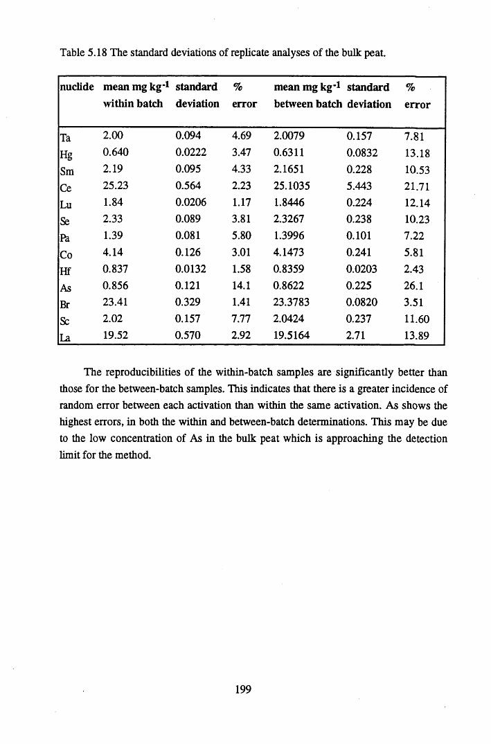
Table 5.18 The standard deviations of replicate analyses of the bulk peat.
nuclide mean mg kg ' 1
within batchstandarddeviation
%error
mean mg kg ’1 standard between batch deviation
%error
Ta 2 . 0 0 0.094 4.69 2.0079 0.157 7.81
Hg 0.640 0 .0 2 2 2 3.47 0.6311 0.0832 13.18Sm 2.19 0.095 4.33 2.1651 0.228 10.53Ce 25.23 0.564 2.23 25.1035 5.443 21.71Lu 1.84 0.0206 1.17 1.8446 0.224 12.14
Se 2.33 0.089 3.81 2.3267 0.238 10.23
P sl 1.39 0.081 5.80 1.3996 0 .1 0 1 7.22
Co 4.14 0.126 3.01 4.1473 0.241 5.81
Hf 0.837 0.0132 1.58 0.8359 0.0203 2.43
As 0.856 0 .1 2 1 14.1 0.8622 0.225 26.1
Br 23.41 0.329 1.41 23.3783 0.0820 3.51
Sc 2 .0 2 0.157 7.77 2.0424 0.237 11.60
La 19.52 0.570 2.92 19.5164 2.71 13.89
The reproducibilities of the within-batch samples are significantly better than those for the between-batch samples. This indicates that there is a greater incidence of random error between each activation than within the same activation. As shows the highest errors, in both the within and between-batch determinations. This may be due to the low concentration of As in the bulk peat which is approaching the detection limit for the method.
199
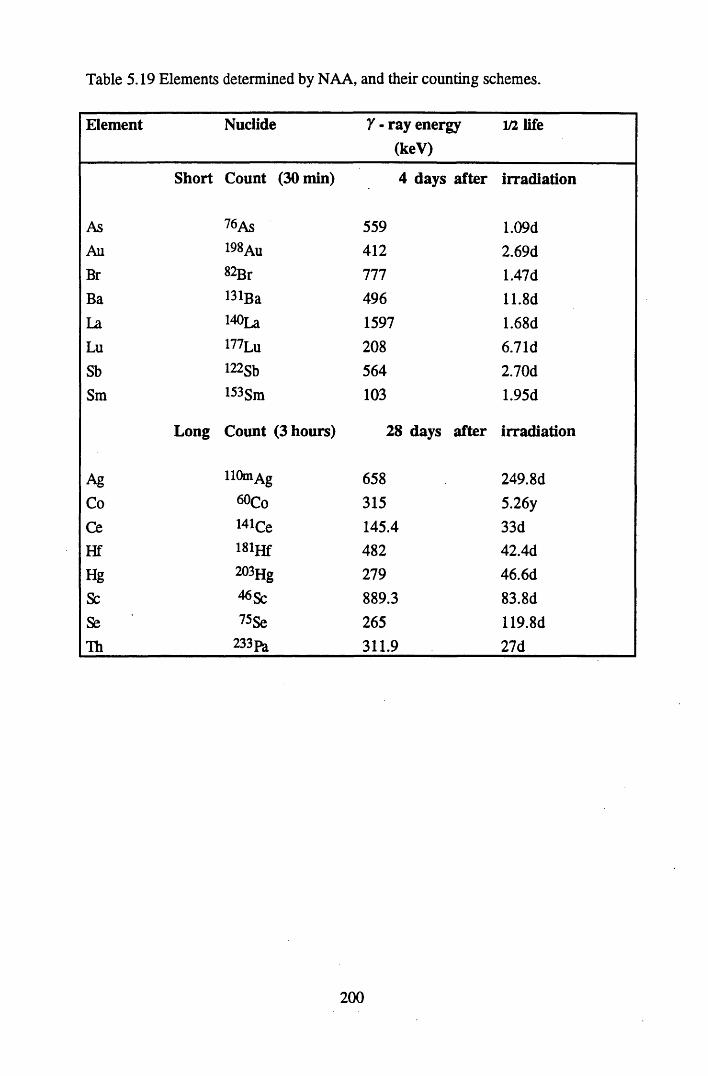
Table 5.19 Elements determined by NAA, and their counting schemes.
Element Nuclide Y - ray energy (keV)
1/2 life
Short Count (30min) 4 days after irradiation
As 76As 559 1.09dAu 19»Au 412 2.69dBr 82Br 111 1.47dBa 13lBa 496 1 1 .8 dLa l40La 1597 1 .6 8 dLu 177Lu 208 6.71dSb l2 2Sb 564 2.70dSm l53Sm 103 1.95d
Long Count (3 hours) 28 days after irradiation
Ag llOm^g 658 249.8dCo 60Co 315 5.26yCe Mice 145.4 33dHf lSlHf 482 42.4dHg 203Hg 279 46.6dSc 4«Sc 889.3 83.8dSe 75Se 265 119.8dTh 233pa 311.9 27d
200
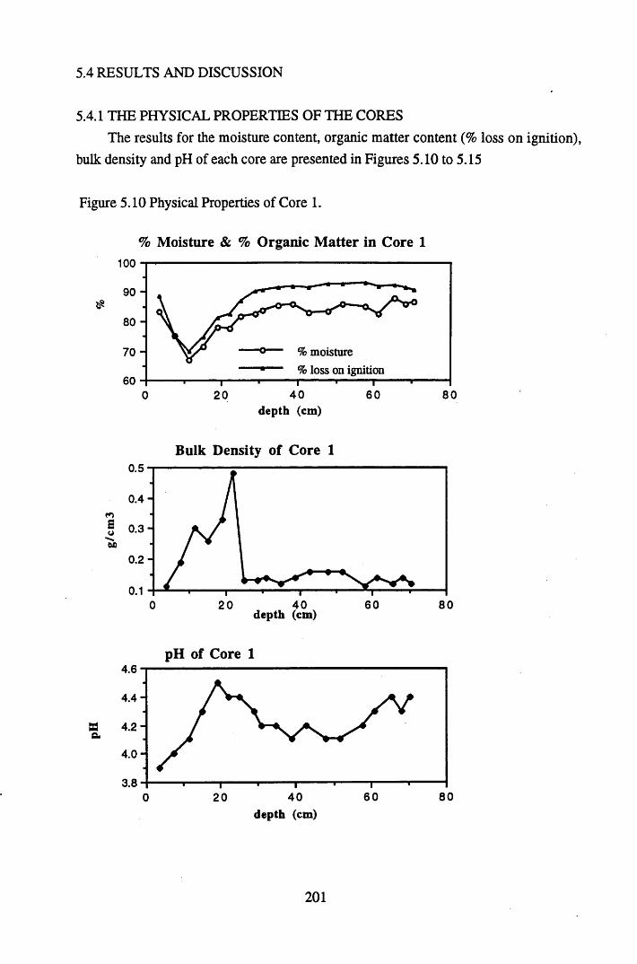
5.4 RESULTS AND DISCUSSION
5.4.1 THE PHYSICAL PROPERTIES OF THE CORESThe results for the moisture content, organic matter content (% loss on ignition),
bulk density and pH of each core are presented in Figures 5.10 to 5.15
Figure 5.10 Physical Properties of Core 1.
% Moisture & % Organic Matter in Core 1100
90
moisture loss on ignition
604 0 60 80200
dep th (cm)
Bulk Density of Core 10.5
0.4
0.2
0.140 60 800 20
dep th (cm)
pH of Core 14.6
4 .4 -
S 4 .2 -e*4 .0 -
3.8806040200
depth (cm)
201
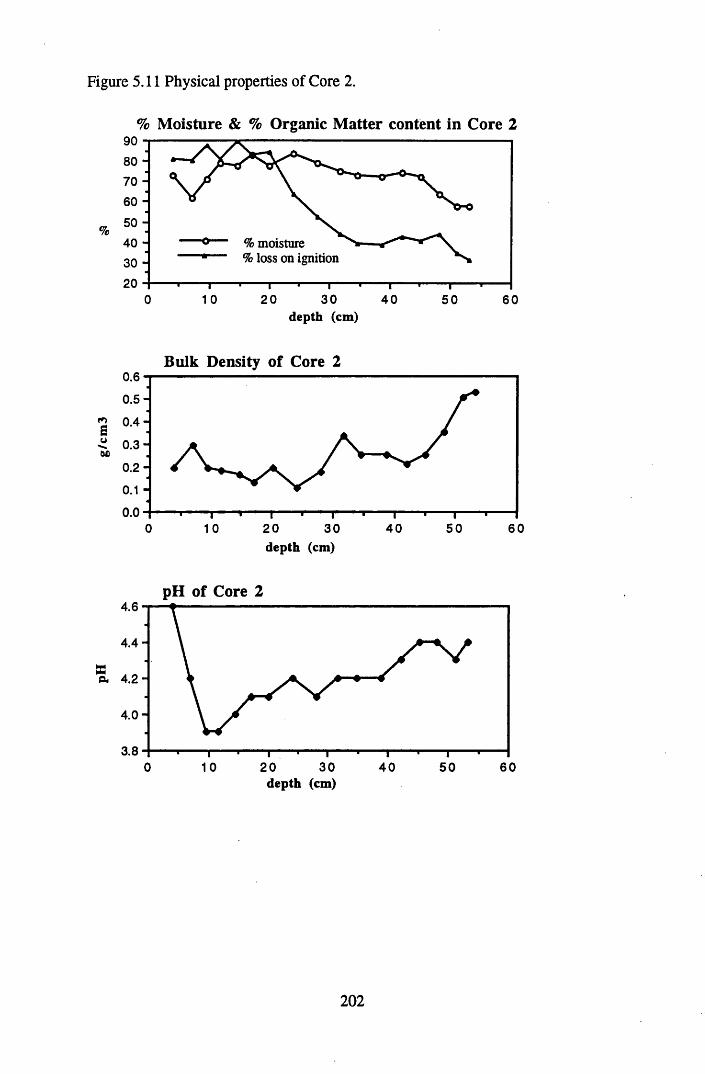
g/cm
3Figure 5.11 Physical properties of Core 2.
% Moisture & % Organic Matter content in Core 2
80 - 70 - 60 -
% 5 0 : 40 -30 -20 -
moisture loss on ignition
300 1 0 20 40 50 60depth (cm)
Bulk Density of Core 20.6
0 .5 -
0 .4 -
0 .3 -
0 .2 -
0.040 50 600 20 301 0
dep th (cm)
pH of Core 24.6
4 .4 -
Ka
4 .0 -
3.8300 1 0 2 0 4 0 50 60
dep th (cm)
202
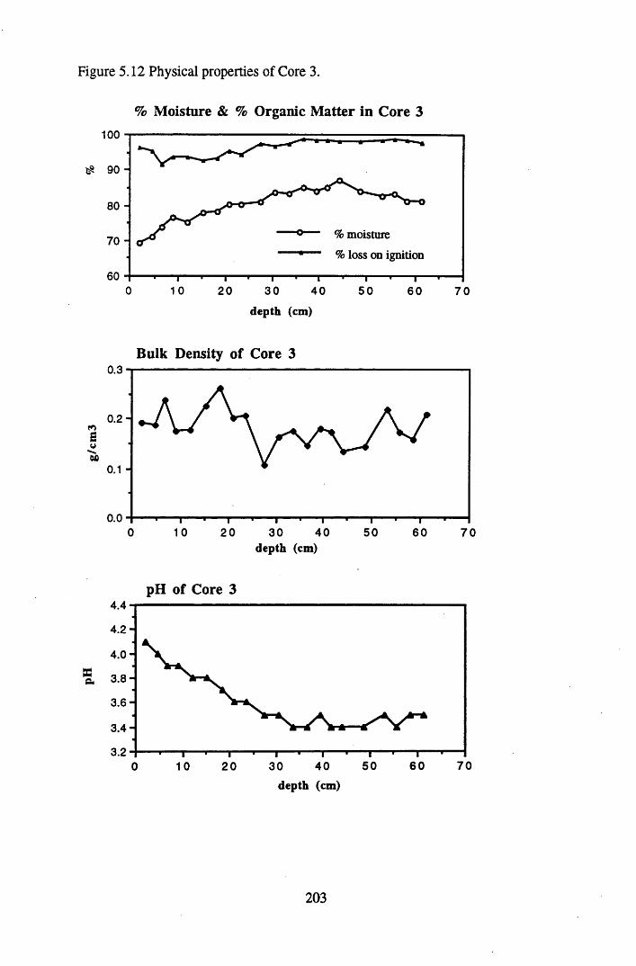
g/cm
3Figure 5.12 Physical properties of Core 3.
% Moisture & % Organic Matter in Core 3100
80 -
moisture70 -loss on ignition
0 1 0 2 0 30 5 040 60 7 0
depth (cm)
Bulk Density of Core 30.3
0 .2 -
0.00 1 0 2 0 40 50 60 7 030
depth (cm)
pH of Core 34.4
4 .2 -
4 .0 -
o. 3 .8 -
3 .6 -
3 .4 -
3.27050 604 010 20 300
depth (cm)
203
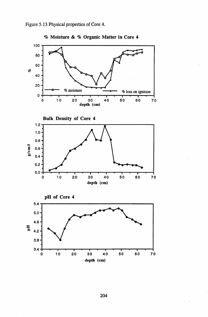
g/cm
3Figure 5.13 Physical properties of Core 4.
% Moisture & % Organic Matter in Core 4
100
80 -
60 -
40 -
2 0 -moisture loss on ignition
0 1 0 2 0 30 4 0 50 6 0 70dep th (cm)
Bulk Density of Core 4
0 .8 -
0 .6 -
0 .4 -
0 .2 -
0.0500 1 0 2 0 30 4 0 60 70
depth (cm)
pH of Core 45.4
5 .0 -
4 .6 -Ba 4 .2 -
3 .8 -
3.450 60 7030 4 00 10 20
depth (cm)
204
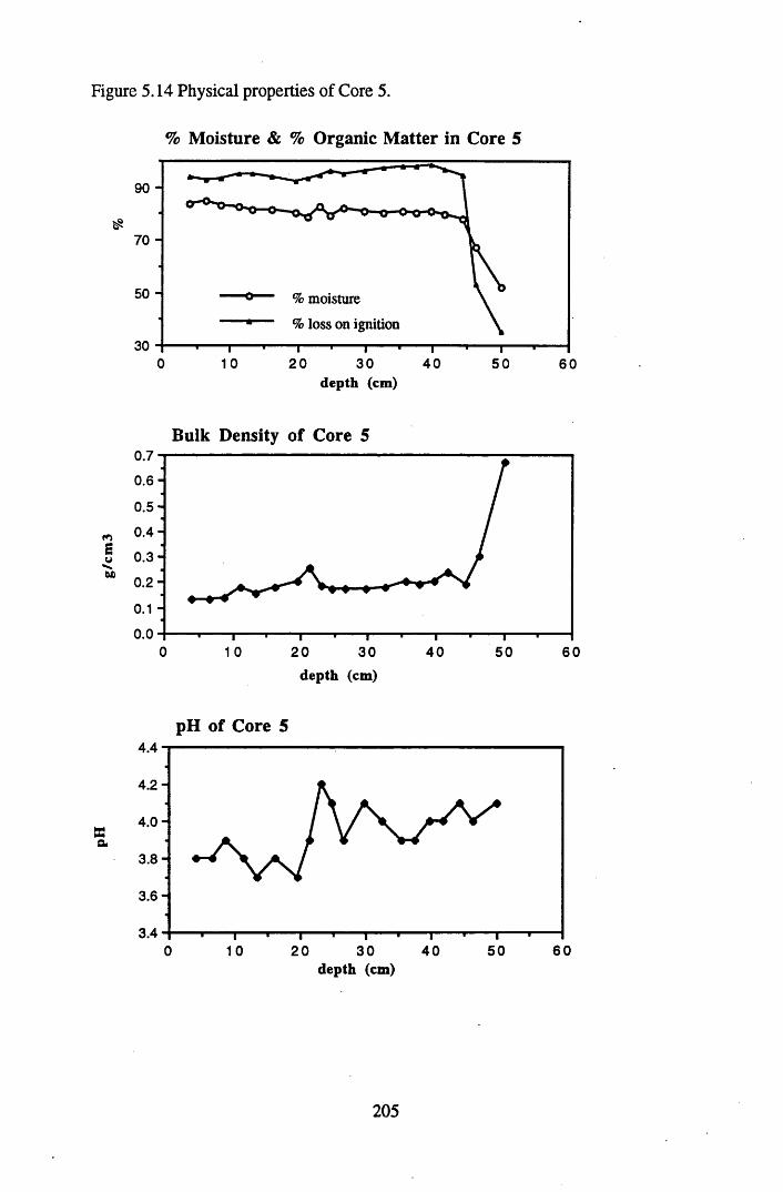
g/cm
3Figure 5.14 Physical properties of Core 5.
% Moisture & % Organic Matter in Core 5
90 -
70 -
50 - % moisture
loss on ignition
0 1 0 2 0 30 40 50 60depth (cm)
Bulk Density of Core 50.7
0 .6 -0 .5 -
0 .4 -
0 .3 -
0 .2 -
0.00 1 0 2 0 30 4 0 50 60
dep th (cm)
pH of Core 54.4
4 .2 -
4 .0 -
3 .8 -
3 .6 -
3.460500 10 20 30 40
depth (cm)
205
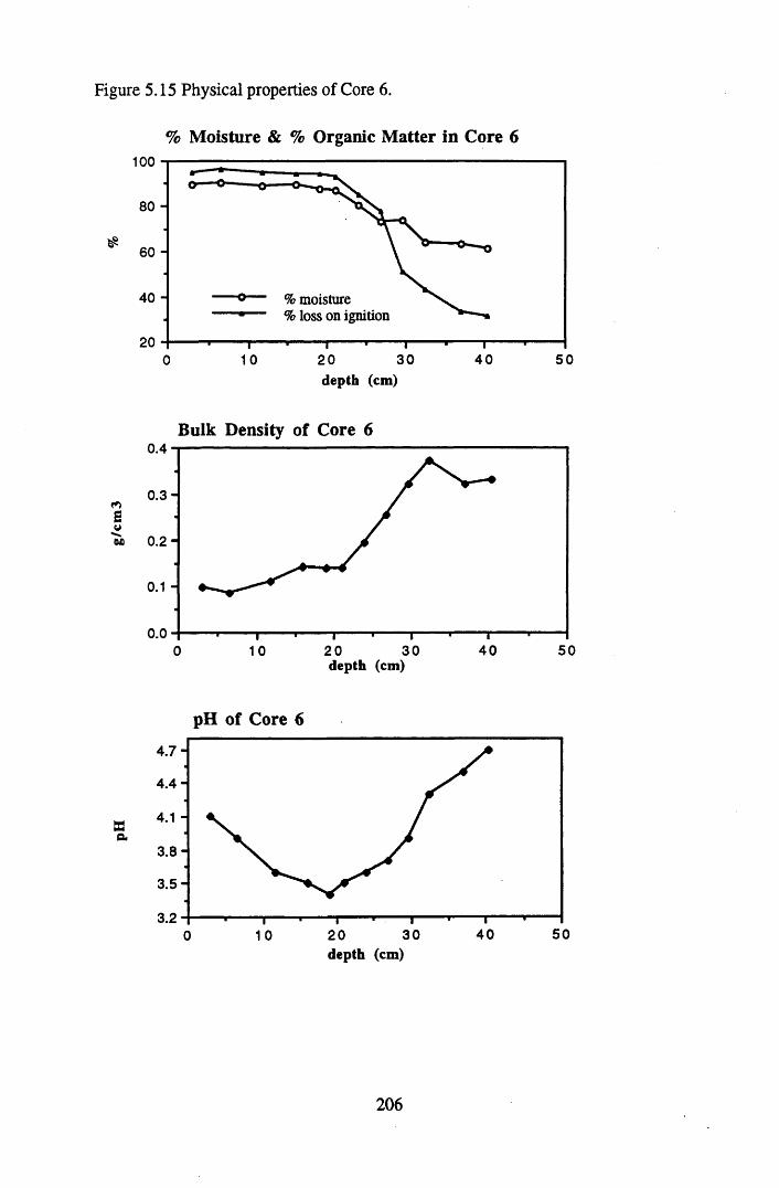
g/cm
3
Figure 5.15 Physical properties of Core 6.
% Moisture & % Organic Matter in Core 6100
80 -
60 -
40 - moisture loss on ignition
2030 4 0 501 0 2 00
depth (cm)
Bulk Density of Core 60.4
0 .3 -
0.2-
0.04 0 5020 300 10
depth (cm)
pH of Core 6
4 .7 -
4 .4 -
4.1 -a
3 .8 -
3 .5 -
3.2504030201 00
depth (cm)
206
RESULTS AND DISCUSSION
In all of the cores, the % moisture and % organic matter (L.O.I.) follow similar trends. In addition, in many cores a reduction in the values of the moisture and organic content was mirrored by a rise in bulk density values. In Cores 5 and 6 (Figures 5.14 and 5.15 respectively) this occurred at depth, when the bedrock was reached, and correspondingly the core became more mineral in nature. In Core 2 (Figure 5.11), there was a decrease in organic matter content, with an increase in bulk density at depth, as the gleyed mineral horizon was reached. In Core 1 (Figure 5.10), there was a sudden drop in organic matter content, with an increase in bulk density between 2 0
and 30 cm, indicating an increase in deposition of mineral material at this depth. With South Drumboy being a working hill farm, drainage channels have been inserted around the hill and Core 1 lay below a section of improved grassland where this had occurred. Accordingly, insertion of these may have caused disturbance giving an influx of mineral material into Core 1. Core 4 (Figure 5.13) also showed a pronounced mineral horizon, sandwiched between two organic horizons, which is again indicative of disturbance, perhaps due to the same reason. In addition, in Core 4, the pH values for the mineral horizon were significantly higher than for the organic horizons, rising to a value of 5.2.
The bulk density, % moisture and organic matter content reflect the botanical composition of the cores, as well as the above changes in composition. These herbaceous peats, show characteristic values of 0 . 1 2 - 0.16 g cm-3 for bulk density (Clymo, 1984). Had the peats been primarily formed from Sphagnum mosses, then the bulk density values would have been far lower (~ 0.05 g cm-3) with higher % moisture.
Because of the possibility of compaction effects occurring, the bulk density should always be measured when measuring rates of peat accumulation (Jones & Gore, 1978) and accordingly the values will be utilised in later calculations. The bulk density has also been shown to correlate with degree of humification or decomposition (Clymo, 1984), and this can also cause inaccuracies when calculating peat accumulation rates. The difference in degree of organic matter content (%LOI), was also used in the calculation of 7 detection efficiency (see section 5.3.3.5 and the following section).
207
5.4.2 THE CONTENTS AND DISTRIBUTIONS OF RADIONUCLIDES AND METALS WITHIN SOUTH DRUMBOY PEAT PROFILES
The activities of radionuclides in the peats are presented as specific activity (Bq kg-1) versus cumulative weight (g cm-2) which is used to compensate for the effects of any compaction processes in the peat (Clymo, 1990: El-Dahoushy, 1988: Swan etal., 1982). Total inventories (Bq n r2) were calculated, from which the average flux (calculated as inventory x A,, in units of Bq n r 2 y-l) of the radionuclides to the surface of the peat was derived. To calculate a chronology for the cores, the constant initial concentration (c.i.c.) model (Robbins, 1978) was used, as described in section 1.8.4.
In order to estimate the separate contributions of weapons testing and Chernobyl to the 137Cs content, the decay corrected Chernobyl 13 4Cs/137Cs activity ratio was calculated. At the time of deposition, this ratio was approximately 0.55 (Clark & Smith, 1988), so the Chernobyl 137Cs concentration At at the time of sampling (t) can be calculated from:
1T7 At (13 4Cs) £(0-33“0-023)-*At Cs = 1 ---------------- (5.11)
0.55
The weapons-testing fallout inventory, decay corrected to the time of collection, was then determined by subtracting the estimated Chernobyl contribution from the total 137Cs content of the section. All errors were calculated as in section 5.3.3.6, being fully propagated where necessary.
All metal and element profiles are plotted as concentration in mg kg-1 versus cumulative weight (g cm-2), which for convenience is referred to as depth. Where appropriate, to calculate a depositional flux for each metal, the peat accumulation rate was multiplied by the individual section concentrations of that metal.
208
SOUTH DRUMBOY CORE 1
Core 1 was the lowest altitude core sampled on the easterly facing slope, and lay directly downslope from a section of improved grassland. As discussed in section 5.4.1 the peat showed an increased mineral content between 1 and 4 g cm-2, as characterised by an increase in the bulk density and a decrease in the % loss on ignition. This was proposed to be an indicator of disturbance of the profile from the insertion of drainage channels further uphill.
The 210Pb profile (Figure 5.16 & Table 5.20) did not show an exponential decrease in activity with depth as would be expected for a situation of uniform accumulation. Unsupported 210Pb was detected only in the top three sections of the core to a depth of 4 g cm”2, which represents the top of the more mineral layer, suggesting that the surface peat is a reasonably new horizon. However, the accumulation rate was calculated to be 0.015 g cm-2 y 1, which is incompatible with recent disturbance, indicating that the data for this core must interpreted with caution. The 210Pb inventory was calculated as 2157 Bq n r 2, giving an average flux of 66.9 Bq nr2 y 1.
The radioacaesium data are presented in Tables 5.21 and 5.22. Of immediate note is the high concentration of 137Cs in the surface section and like the 2 1 0 Pb, the majority of the radiocaesium is in the top three sections of the core, in the surface organic horizon (Figure 5.17). The 137Cs inventory was 48953 Bq m-2, comprising a Chernobyl inventory of 3841 Bq m -2 and a weapons-testing component of 45075 Bq m-2. The 134Cs inventory was 292 Bq m-2. Thus, 92% of the 137Cs inventory was attributable to weapons-testing 137Cs and 96% of this weapons testing 137Cs was contained within the surface section. With the presence of the mineral layer suggesting disturbance of the profile from insertion of drainage channels, this may also be affecting the 137Cs profiles through promoting transport of 137Cs through the channels. Since this effect is confined to the weapons-testing 137Cs the disturbance must have occurred before the Chernobyl accident and is not a recent effect.
Although the majority of the radiocaesiumm was contained within the surface section some 137Cs had penetrated to depths well beyond 21 0Pb. 134Cs had penetrated to a lesser extent, indicating that the effect is time dependent. The penetration of radiocaesium to depths dated before the onset of weapons-testing has previously been recorded (Maguire, 1994: Sugden, 1993: Mitchell et oL, 1992: Schell et al., 1989: Clymo, 1979). Diffusive and advective processes have been proposed to be responsible and often lead to the loss of the peak in weapons-testing 137Cs (Mitchell et al., 1992: Schell etal., 1989).
209
The Al concentrations in Core 1 (Figure 5.18) increased as the mineral content increased and this trend was mirrored by Ta, La, Sm, Se, Hf, Sc and Th (Appendix 3.3), with La and Ce being displayed here (Figure 5.19). These profiles also indicate minor fluctuations in mineral content at depth.
The Mn and Fe profiles (Figure 5.20) indicate that conditions become increasingly reducing with depth. Mn shows a significant decrease in concentration from the surface section, indicating that from this depth conditions are sufficently reducing to bring Mn oxides into solution through the reaction:
Mn0 2 + 4H+ + 2e- = Mn2+ + 2H20 However, reduction does not give total loss of Mn, with between 10-20 mg kg-1
present to a depth of 9 g cm -2 beyond which total loss of Mn is observed as conditions become more reducing.
Fe does not show a surface reduction like Mn but instead shows loss from 9 g cm-2 further reinforcing that conditions become progressivly more reducing from this depth. Mn oxides are more sensitive to changes in Eh and consequently come into solution before Fe oxides (Alloway, 1990). The reduction of Fe oxides occurs through the following reaction:
Fe(OH) 3 + 3H+ + er = Fe2+ + 3H20 The dissolution of Fe and Mn oxides can cause the release of metals co
precipitated with them (Jones, 1987: Alloway, 1990) and this may explain the pattern of the Zn and Cu profiles (Figure 5.22) which show peaks in concentration between 6 - 9 g cm-2 where conditions start to become more reducing.
In addition changes in the redox potential not only mediate the dissolution of Fe and Mn oxides, but can also mediate the reduction of sulphate to sulphite leading to the precipitation of metal sulphides (Alloway, 1990). FeS2 is most readily formed with Mn participating to a lesser degree, especially where there is a high concentration of Fe *- ions (Rowell, 1988). Cu and Zn have been proposed to form metal sulphides and this could also be occurring in Core 1. Walton Day et al. (1990) proposed that Cu was co-precipitated with FeS2 rather forming CuS and this may also explain the pattern observed for Cu and Zn. Accumulation has been proposed to be an indication of the zone of water fluctuation, since the sulphides are continuously oxidised and mobilised, then reduced and precipitated (Damman, 1978).
Br (Figure 5.22) shows a slightly different relationship to Cu and Zn, with a peak in the surface organic layer, followed by reduction in concentration in the more mineral horizon and a bimodal peak between 7.5-10 g cm-2. This bimodal peak at depth could be related to the fluctuation in the water table levels as discussed for Cu and Zn.
210
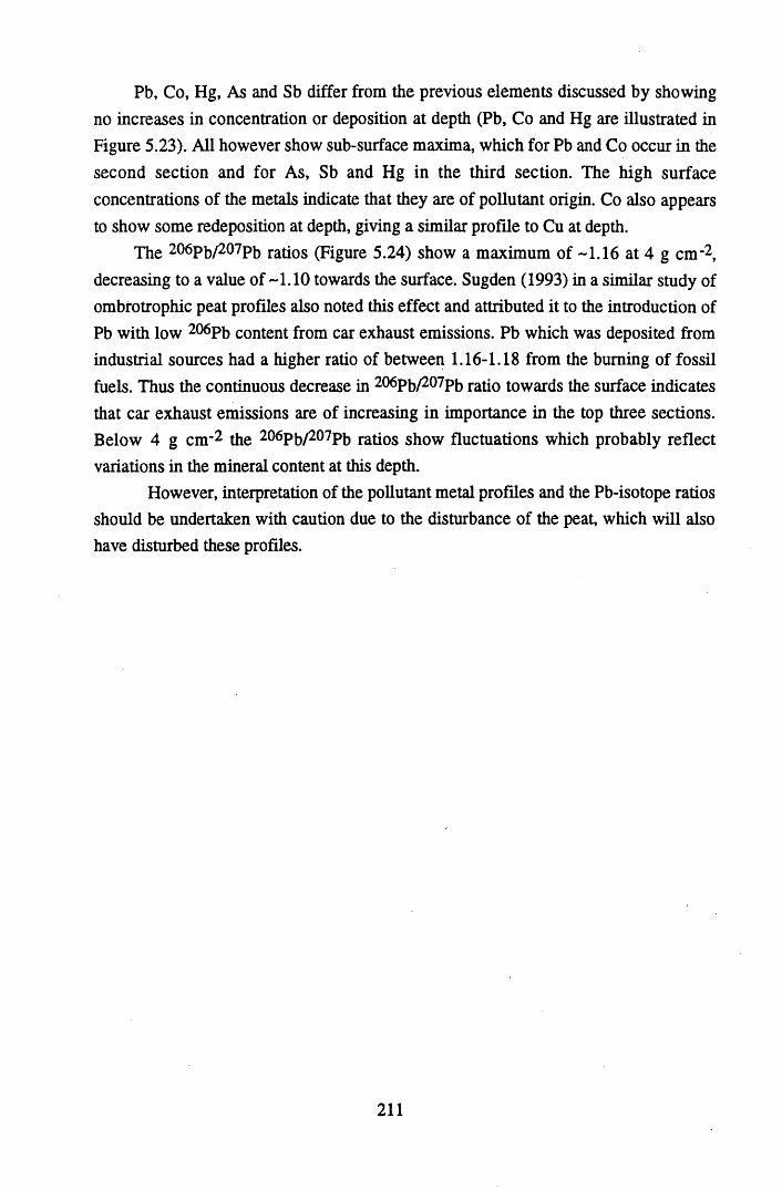
Pb, Co, Hg, As and Sb differ from the previous elements discussed by showing no increases in concentration or deposition at depth (Pb, Co and Hg are illustrated in Figure 5.23). All however show sub-surface maxima, which for Pb and Co occur in the second section and for As, Sb and Hg in the third section. The high surface concentrations of the metals indicate that they are of pollutant origin. Co also appears to show some redeposition at depth, giving a similar profile to Cu at depth.
The 206pb/207pb ratios (Figure 5.24) show a maximum of -1.16 at 4 g cm-2, decreasing to a value of -1.10 towards the surface. Sugden (1993) in a similar study of ombrotrophic peat profiles also noted this effect and attributed it to the introduction of Pb with low 2<*Pb content from car exhaust emissions. Pb which was deposited from industrial sources had a higher ratio of between 1.16-1.18 from the burning of fossil fuels. Thus the continuous decrease in 206pb/207pb ratio towards the surface indicates that car exhaust emissions are of increasing in importance in the top three sections. Below 4 g cm- 2 the 206pb/207pb ratios show fluctuations which probably reflect variations in the mineral content at this depth.
However, interpretation of the pollutant metal profiles and the Pb-isotope ratios should be undertaken with caution due to the disturbance of the peat, which will also have disturbed these profiles.
211
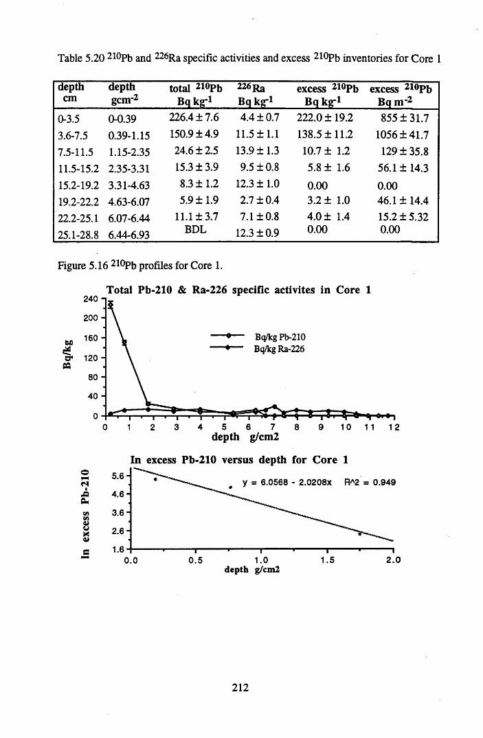
Table 5.20 210Pb and 226Ra specific activities and excess 210Pb inventories for Core 1
depthcm
depthgem-2
total 210Pb Bq kg’ 1
2 2 6 Ra Bq kg’1
excess 210Pb Bq kg’ 1
excess 210Pb Bq m -2
0-3.5 0-0.39 226.4 ±7.6 4.4 ±0.7 222.0 ±19.2 855 ± 31.73.6-7.5 0.39-1.15 150.9 ±4.9 11.5 ± 1 .1 138.5 ±11.2 1056 ± 41.77.5-11.5 1.15-2.35 24.6 ±2.5 13.9 ±1.3 10.7 ± 1.2 129 ± 35.811.5-15.2 2.35-3.31 15.3 ± 3.9 9.5 ± 0 .8 5.8 ± 1.6 56.1 ± 14.315.2-19.2 3.31-4.63 8.3 ± 1.2 12.3 ± 1 .0 0 . 0 0 0 . 0 0
19.2-22.2 4.63-6.07 5.9 ±1.9 2.7 ±0.4 3.2 ± 1.0 46.1 ± 14.422.2-25.1 6.07-6.44 11.1 ±3.7 7.1 ± 0 .8 4.0 ± 1.4 15.2 ± 5.32
25.1-28.8 6.44-6.93 BDL 12.3 ±0.9 0 . 0 0 0 . 0 0
Figure 5.16 210Pb profiles for Core 1.
Total Pb-210 & Ra-226 specific activites in Core 1240 n
200 -
Bq/kg Pb-210 Bq/kg Ra-226
160 -
O" 120 -
80 -
40 -
4 5 7 1 0 11 1 20 3 6 8 91 2depth g/cm2
In excess Pb-210 versus depth for Core 15 .6 -
y = 6.0568 - 2.0208X RA2 = 0.9494 .6 -
3 .6 -
2.6 -
2.01.51.00 .50.0dep th g/cm2
212
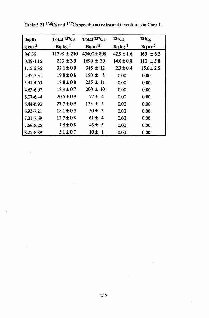
Table 5.21134Cs and 137Cs specific activites and inventories in Core 1.
depthgem -2
Total 137Cs Bq kg"1
Total 137Cs Bq m -2
134 Cs Bq kg-1
134Cs Bq m -2
0-0.39 11798 ±210 45400 ±808 42.9 ±1.6 165 ±6.30.39-1.15 223 ±3.9 1690 ± 30 14.6 ±0.8 110 ±5.81.15-2.35 32.1 ±0.9 385 ± 12 2.3 ±0.4 15.6 ±2.52.35-3.31 19.8 ±0.8 190 ± 8 0 .0 0 0 .0 0
3.31-4.63 17.8 ±0.8 235 ± 11 0 .0 0 0 .0 0
4.63-6.07 13.9 ±0.7 2 0 0 ± 1 0 0 .0 0 0 .0 0
6.07-6.44 20.5 ±0.9 77 ± 4 0 .0 0 0 .0 0
6.44-6.93 27.7 ±0.9 133 ± 5 0 .0 0 0 .0 0
6.93-7.21 18.1 ±0.9 50 ± 3 0 .0 0 0 .0 0
7.21-7.69 12.7 ±0.8 61 ± 4 0 .0 0 0 .0 0
7.69-8.25 7.6 ±0.8 43 ± 5 0 .0 0 0 .0 0
8.25-8.89 5.1 ±0.7 1 0 ± 1 0 .0 0 0 .0 0
213
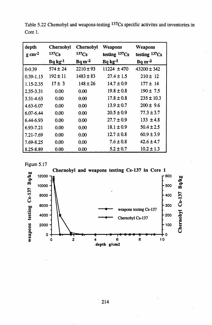
Table 5.22 Chernobyl and weapons-testing 137Cs specific activites and inventories inCore 1.
depthgem-2
Chernobyl137CSBq kg"1
Chernobyll37CsBq nr2
Weapons testing 137Cs Bq kg*1
Weapons testing 137Cs Bq m*2
0-0.39 574 ± 24 2210 ±93 11224 ±470 43200 ±3420.39-1.15 192 ±11 1483 ±83 27.4 ±1.5 2 1 0 ± 1 2
1.15-2.35 17 ± 3 148 ±26 14.7 ±0.9 177± 142.35-3.31 0 .0 0 0 .0 0 19.8 ±0.8 190 ± 7.53.31-4.63 0 .0 0 0 .0 0 17.8 ±0.8 235 ± 10.34.63-6.07 0 .0 0 0 .0 0 13.9 ±0.7 200 ± 9.66.07-6.44 0 .0 0 0 .0 0 20.5 ±0.9 77.3 ±3.76.44-6.93 0 .0 0 0 .0 0 27.7 ±0.9 133 ±4.86.93-7.21 0 .0 0 0 .0 0 18.1 ±0.9 50.4 ±2.57.21-7.69 0 .0 0 0 .0 0 12.7 ±0.8 60.9 ±3.97.69-8.25 0 .0 0 0 .0 0 7.6 ±0.8 42.6 ±4.78.25-8.89 0 .0 0 0 .0 0 5.2 ±0.7 10.2 ±1.3
Figure 5.17
en
tHceu&CC• MW0>V)COa«s£
Chernobyl and weapons testing Cs-137 in Core 112000 -
10000 -
8000 -
6000 -
4000 -
2000 -
0
weapons testing Cs-137
Chernobyl Cs-137
■OT
-6 0 0
-5 0 0
-4 0 0
-3 0 0
-200
- 100
010
dep th g/cm 2
214
Che
rnob
yl
Cs-1
37
Bq/
kg
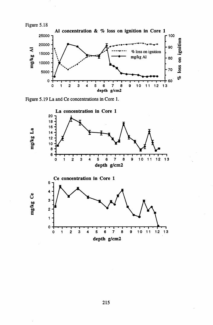
Figure 5.18
25000 -
20000 -<
15000 -61)63d 10000 -£
5000 H
0
Al concentration & % loss on ignition in Core 1
1 % loss on ignition'• mg/kg Al
■ I ■ l ■ I ■ I 1 I ■ I ■ i ■ I ■ I0 1 2 3 4 5 6 7 8 9
dep th g/cm2
Figure 5.19 La and Ce concentrations in Core 1.
La concentration in Core 1
et61)
I 1 I 1 I i10 11 12 13
- 100
-9 0
-8 0
-7 0
60
£S
20 - 18 “ 16 “ 14 -j 12 10 -
0 1 2 3 4 5 6 7 8 9 1 0 1 1 1 2 1 3depth g/cm2
Ce concentration in Core 15
4
3
2
1
00 1 2 3 4 5 6 7 8 9 1 0 1 1 1 2 1 3
depth g/cm2
215
% los
s on
igni
tion
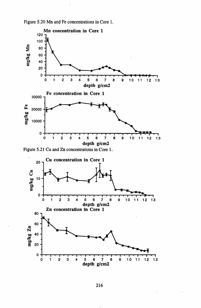
Figure 5.20 Mn and Fe concentrations in Core 1.
Mn concentration in Core 1120 "|100 -80 -
60 -
40 -
20 -
0 1 2 3 4 5 6 7 8 9 1 0 1 1 1 2 1 3depth g/cm2
Fe concentration in Core 130000 -i
4>20000 -
60
g 10000 -
0 1 2 3 4 5 6 7 8 9 10 1 1 1 2 13depth g/cm2
Figure 5.21 Cu and Zn concentrations in Core 1.
Cu concentration in Core 120 n
eo 10 -
o 1 2 3 4 5 6 7 8 9 1 0 1 1 1 2 1 3depth g/cm2
Zn concentration in Core 180 n
60 -
60 40
0 1 2 3 4 5 6 7 8 9 10 1 1 12 13depth g/cm2
216
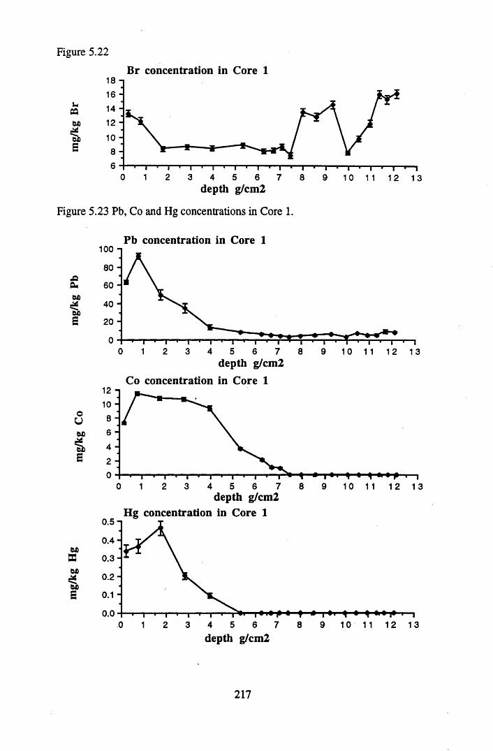
Figure 5.22
v*P3OX)
OX)5
Br concentration in Core 118 - 16 - 14 - 12 -1° - 8 -
0 21 3 4 5 6 7 8 9 10 11 12 13depth g/cm2
Figure 5.23 Pb, Co and Hg concentrations in Core 1.
Pb concentration in Core 1
cuOD■as
OV01)§E
OX)BOX)
OX)e
100 -i
80 -
60 -
40
20 -
2 50 1 3 4 6 7 8 9 10 11 12 13depth g/cm2
Co concentration in Core 112 - 10 -
0 1 2 3 4 5 6 7 8 9 10 11 12 13depth g/cm2
Hg concentration in Core 10.5 n
0 .4 -
0 .3 -
0.2-0.1 -
0.00 3 4 5 6 7 8 9 10 11 12 131 2
depth g/cm2
217
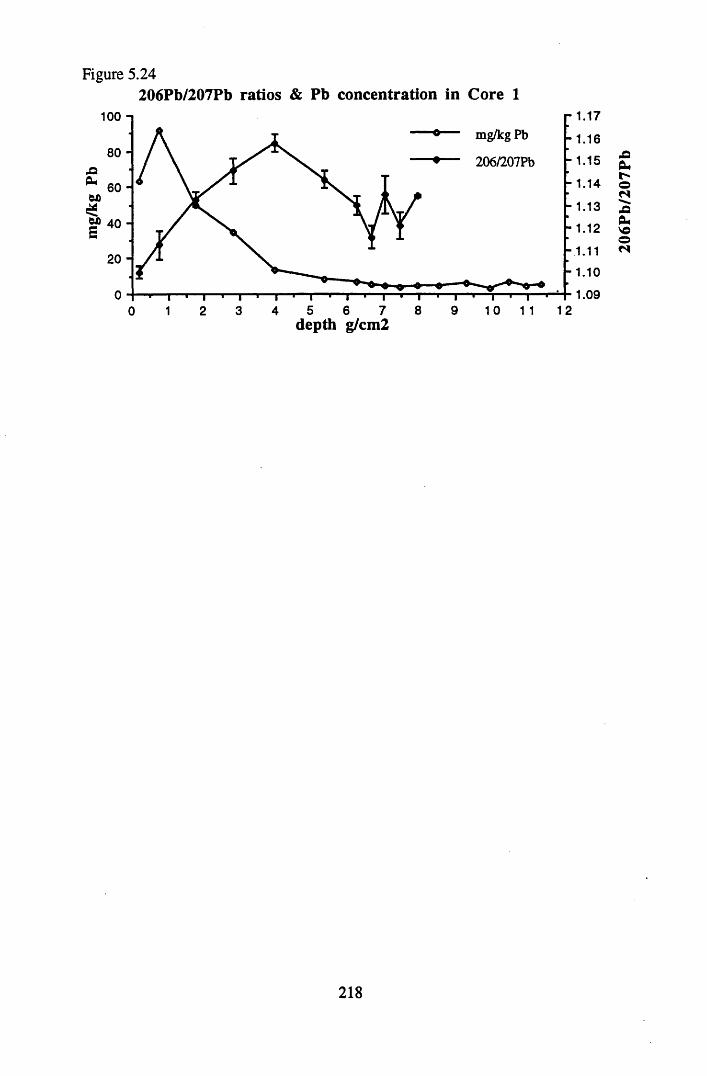
mg/
kg
PbFigure 5.24
206Pb/207Pb ratios & Pb concentration in Core 1r 1.17100 n
mg/kg Pb
206/207Pb
-1 .1 680 - - 1.15
- 1.1460 -- 1.13
40 - - 1.12
20 -- 1.10
1.095 6 7 8 9 10 11 1241 2 30
depth g/cm2
218
206P
b/20
7Pb
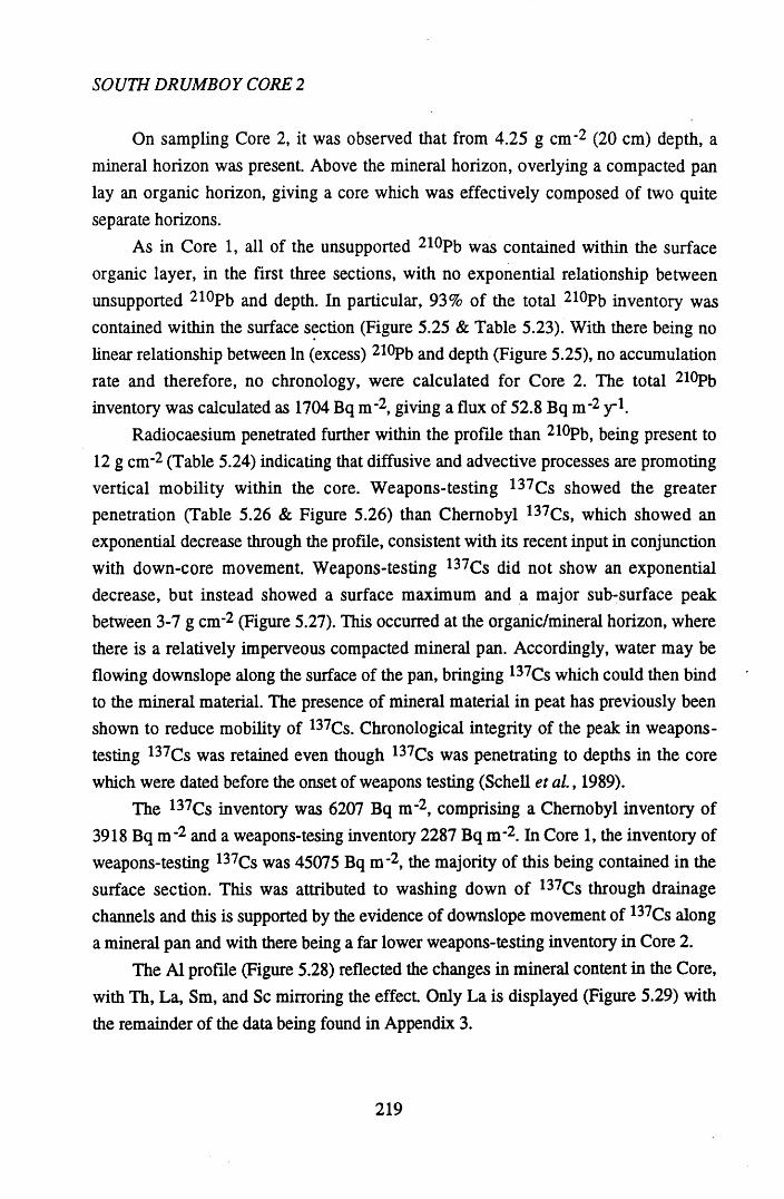
SOUTH DRUMBOY CORE 2
On sampling Core 2, it was observed that from 4.25 g cm-2 (20 cm) depth, a mineral horizon was present. Above the mineral horizon, overlying a compacted pan lay an organic horizon, giving a core which was effectively composed of two quite separate horizons.
As in Core 1, all of the unsupported 210Pb was contained within the surface organic layer, in the first three sections, with no exponential relationship between unsupported 210Pb and depth. In particular, 93% of the total 210Pb inventory was contained within the surface section (Figure 5.25 & Table 5.23). With there being no linear relationship between In (excess) 210Pb and depth (Figure 5.25), no accumulation rate and therefore, no chronology, were calculated for Core 2. The total 210Pb inventory was calculated as 1704 Bq m-2, giving a flux of 52.8 Bq m- 2 y 1-
Radiocaesium penetrated further within the profile than 210Pb, being present to 12 g cm-2 (Table 5.24) indicating that diffusive and advective processes are promoting vertical mobility within the core. Weapons-testing 137Cs showed the greater penetration (Table 5.26 & Figure 5.26) than Chernobyl 137Cs, which showed an exponential decrease through the profile, consistent with its recent input in conjunction with down-core movement. Weapons-testing 137Cs did not show an exponential decrease, but instead showed a surface maximum and a major sub-surface peak between 3-7 g cm-2 (Figure 5.27). This occurred at the organic/mineral horizon, where there is a relatively imperveous compacted mineral pan. Accordingly, water may be flowing downslope along the surface of the pan, bringing 137Cs which could then bind to the mineral material. The presence of mineral material in peat has previously been shown to reduce mobility of 137Cs. Chronological integrity of the peak in weapons- testing 137Cs was retained even though 137Cs was penetrating to depths in the core which were dated before the onset of weapons testing (Schell et al. , 1989).
The 137Cs inventory was 6207 Bq m-2, comprising a Chernobyl inventory of 3918 Bq m-2 and a weapons-tesing inventory 2287 Bq m '2. In Core 1, the inventory of weapons-testing 137Cs was 45075 Bq m-2, the majority of this being contained in the surface section. This was attributed to washing down of 137Cs through drainage channels and this is supported by the evidence of downslope movement of 137Cs along a mineral pan and with there being a far lower weapons-testing inventory in Core 2.
The Al profile (Figure 5.28) reflected the changes in mineral content in the Core, with Th, La, Sm, and Sc mirroring the effect. Only La is displayed (Figure 5.29) with the remainder of the data being found in Appendix 3.
219
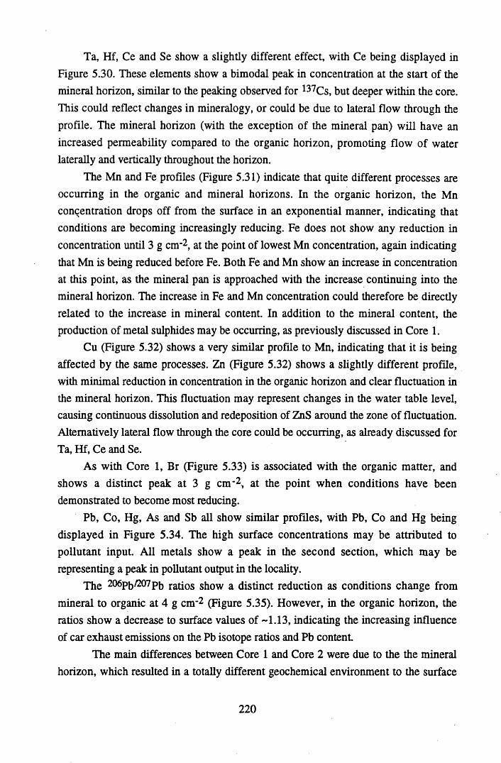
Ta, Hf, Ce and Se show a slightly different effect, with Ce being displayed in Figure 5.30. These elements show a bimodal peak in concentration at the start of the mineral horizon, similar to the peaking observed for l37Cs, but deeper within the core. This could reflect changes in mineralogy, or could be due to lateral flow through the profile. The mineral horizon (with the exception of the mineral pan) will have an increased permeability compared to the organic horizon, promoting flow of water laterally and vertically throughout the horizon.
The Mn and Fe profiles (Figure 5.31) indicate that quite different processes are occurring in the organic and mineral horizons. In the organic horizon, the Mn concentration drops off from the surface in an exponential manner, indicating that conditions are becoming increasingly reducing. Fe does not show any reduction in concentration until 3 g cm’2, at the point of lowest Mn concentration, again indicating that Mn is being reduced before Fe. Both Fe and Mn show an increase in concentration at this point, as the mineral pan is approached with the increase continuing into the mineral horizon. The increase in Fe and Mn concentration could therefore be directly related to the increiase in mineral content. In addition to the mineral content, the production of metal sulphides may be occurring, as previously discussed in Core 1.
Cu (Figure 5.32) shows a very similar profile to Mn, indicating that it is being affected by the same processes. Zn (Figure 5.32) shows a slightly different profile, with minimal reduction in concentration in the organic horizon and clear fluctuation in the mineral horizon. This fluctuation may represent changes in the water table level, causing continuous dissolution and redeposition of ZnS around the zone of fluctuation. Alternatively lateral flow through the core could be occurring, as already discussed for Ta, Hf, Ce and Se.
As with Core 1, Br (Figure 5.33) is associated with the organic matter, and shows a distinct peak at 3 g cm-2, at the point when conditions have been demonstrated to become most reducing.
Pb, Co, Hg, As and Sb all show similar profiles, with Pb, Co and Hg being displayed in Figure 5.34. The high surface concentrations may be attributed to pollutant input. All metals show a peak in the second section, which may be representing a peak in pollutant output in the locality.
Xhe 206pb/207p5 ratios show a distinct reduction as conditions change from mineral to organic at 4 g cm-2 (Figure 5.35). However, in the organic horizon, the ratios show a decrease to surface values of -1.13, indicating the increasing influence of car exhaust emissions on the Pb isotope ratios and Pb content.
The main differences between Core 1 and Core 2 were due to the the mineral horizon, which resulted in a totally different geochemical environment to the surface
220
organic horizon. In addition, the two horizons were seperated by a mineral pan which may have promoted downslope movement of peat water, leading to the observed peak in weapons-testing 137Cs, and the redeposition of reduced Mn and Fe. This may also have facilitated downslope washing of weapons-testing 137Cs, leading to the high inventory of 137Cs in Core 1. Lateral flow of 137Cs has been demonstrated to be more significant than vertical movement within the profile in soils of upland ecosystems (Coughtrey et al., 1990). In addition, leaching of 210Pb may have been promoted, leading to the observed profiles in both cores.
Thus, for Cores 1 and 2, interpretation of the chronology of pollutant metal deposition is complicated by disturbance of the peat, and also reduction and leaching processes.
221
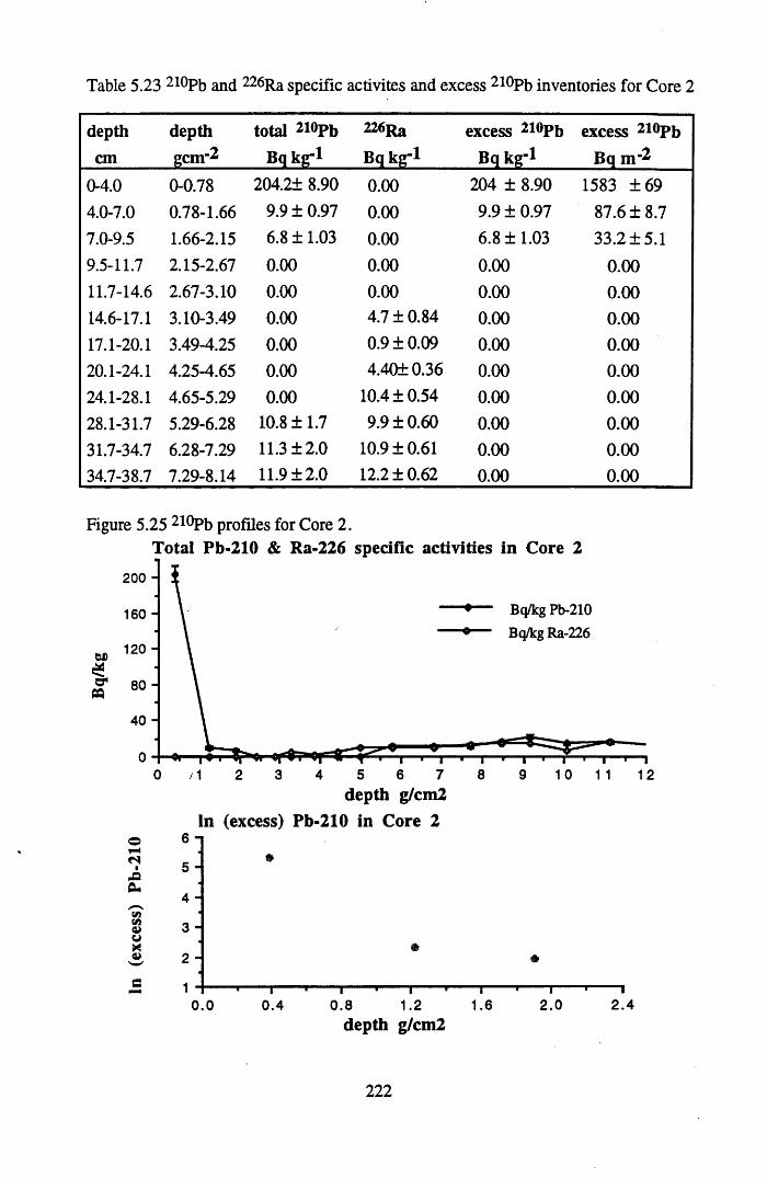
Table 5.23 2i°Pb and 226Ra specific activites and excess 2l°Pb inventories for Core 2
depth depth total 210Pb 226Ra excess 2l°Pb excess 2l°Pbcm gcnr2 Bqkg-1 Bq kg'1 Bq kg'1 Bq m"2
0-4.0 0-0.78 204.2± 8.90 0.00 204 ± 8.90 1583 ±694.0-7.0 0.78-1.66 9.9 ±0.97 0.00 9.9 ±0.97 87.6 ±8.77.0-9.5 1.66-2.15 6.8 ±1.03 0.00 6.8 ±1.03 33.2 ±5.19.5-11.7 2.15-2.67 0.00 0.00 0.00 0.0011.7-14.6 2.67-3.10 0.00 0.00 0.00 0.0014.6-17.1 3.10-3.49 0.00 4.7 ±0.84 0.00 0.0017.1-20.1 3.49-4.25 0.00 0.9 ±0.09 0.00 0.0020.1-24.1 4.25-4.65 0.00 4.4Q± 0.36 0.00 0.0024.1-28.1 4.65-5.29 0.00 10.4 ±0.54 0.00 0.0028.1-31.7 5.29-6.28 10.8 ± 1.7 9.9 ±0.60 0.00 0.0031.7-34.7 6.28-7.29 11.3 ±2.0 10.9 ±0.61 0.00 0.0034.7-38.7 7.29-8.14 11.9 ±2.0 12.2 ±0.62 0.00 0.00
Figure 5.25 210Pb profiles for Core 2.Total Pb-210 & Ra-226 specific activities in Core 2
o■.O
P*
200 -
Bq/kg Pb-210
Bq/kg Ra-226160 -
120 “
i ? 80 -CQ40 -
5 6 7 8 9 10 110 /1 2 12
6 -
5 -
4 -
3 -
2 -
1
depth g/cm2 In (excess) Pb-210 in Core 2
»
o.o“ i—0. 4
—I—0.8
—T1.2
“T—1.6
T —2.0
“ I2 .4
depth g/cm2
222
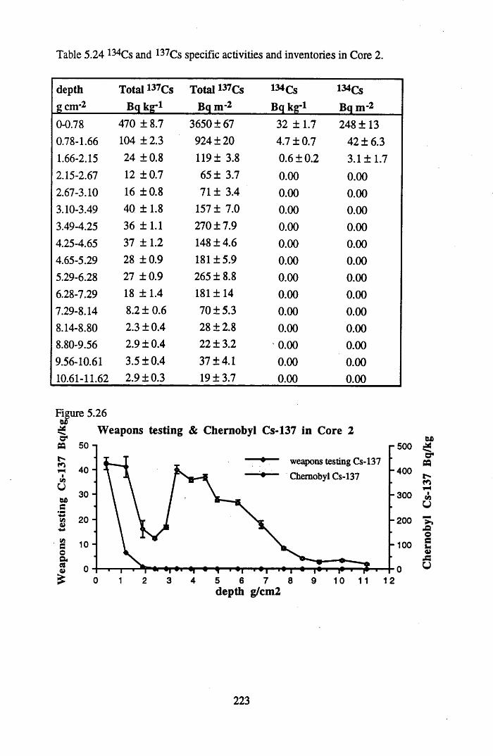
Table 5.24 134Cs and 137Cs specific activities and inventories in Core 2.
depthgcnr2
Total 137Cs Bq kg-l
Total 137Cs Bq m-2
134 Cs Bq kg-l
134Cs Bq nr2
0-0.78 470 ± 8.7 3650 ±67 32 ± 1.7 248 ±130.78-1.66 104 ±2.3 924 ±20 4.7 ±0.7 42 ±6.31.66-2.15 24 ±0.8 119 ± 3.8 0.6 ±0.2 3.1 ±1.72.15-2.67 12 ±0.7 65 ± 3.7 0.00 0.002.67-3.10 16 ±0.8 71 ± 3.4 0.00 0.003.10-3.49 40 ± 1.8 157 ± 7.0 0.00 0.003.49-4.25 36 ±1.1 270 ±7.9 0.00 0.004.25-4.65 37 ± 1.2 148 ±4.6 0.00 0.004.65-5.29 28 ±0.9 181 ±5.9 0.00 0.005.29-6.28 27 ±0.9 265 ±8.8 0.00 0.006.28-7.29 18 ± 1.4 181 ±14 0.00 0.007.29-8.14 8.2 ±0.6 70 ±5.3 0.00 0.008.14-8.80 2.3 ±0.4 28 ±2.8 0.00 0.008.80-9.56 2.9 ±0.4 22 ±3.2 0.00 0.009.56-10.61 3.5 ±0.4 37 ±4.1 0.00 0.0010.61-11.62 2.9 ±0.3 19 ±3.7 0.00 0.00
Figure 5.26^ Weapons testing & Chernobyl Cs-137 in Core 2PQ r 500
weapons testing Cs-137
Chernobyl Cs-13740 - -4 0 0
30 - -3 0 060C20 - -200
- 100
0 1 3 52 4 6 7 8 9 10 11 12depth g/cm2
223
Che
rnob
yl
Cs-1
37
Bq/
kg
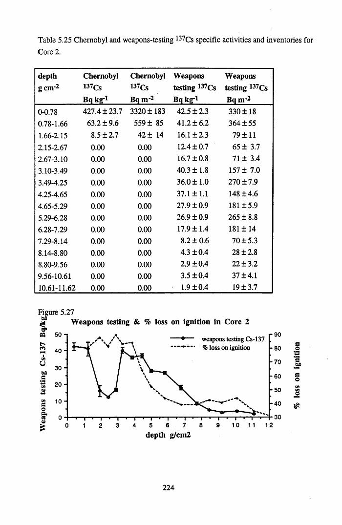
Table 5.25 Chernobyl and weapons-testing 137Cs specific activities and inventories forCore 2.
depth Chernobyl Chernobyl Weapons Weaponsgem*2 l37Cs *37Cs testing 137Cs testing 137Cs
Bq kg*1 Bq m*2 Bq kg*1 Bq m*20-0.78 427.4 ±23.7 3320 ±183 42.5 ±2.3 330 ±180.78-1.66 63.2 ±9.6 559 ± 85 41.2 ±6.2 364 ±551.66-2.15 8.5 ±2.7 42 ± 14 16.1 ±2.3 79 ±112.15-2.67 0.00 0.00 12.4 ±0.7 65 ± 3.72.67-3.10 0.00 0.00 16.7 ±0.8 71 ± 3.43.10-3.49 0.00 0.00 40.3 ±1.8 157 ± 7.03.49-4.25 0.00 0.00 36.0 ±1.0 270 ±7.94.25-4.65 0.00 0.00 37.1 ±1.1 148 ±4.64.65-5.29 0.00 0.00 27.9 ±0.9 181 ±5.95.29-6.28 0.00 0.00 26.9 ±0.9 265 ± 8.86.28-7.29 0.00 0.00 17.9 ±1.4 181 ±147.29-8.14 0.00 0.00 8.2 ±0.6 70 ±5.38.14-8.80 0.00 0.00 4.3 ±0.4 28 ±2.88.80-9.56 0.00 0.00 2.9 ±0.4 22 ±3.29.56-10.61 0.00 0.00 3.5 ±0.4 37 ±4.110.61-11.62 0.00 0.00 1.9 ±0.4 19 ±3.7
Figure 5.27Weapons testing & % loss on ignition in Core 2
r 90CQ 50 -
2 4 0 -IwU 3 0 - B
20 -
weapons testing Cs-137 % loss on ignition
v—♦-8 0
-7 0
-6 0
0> -5 0
23 10 - B O ft A V
-4 0
309 10 11 127 85 62 3 40 1
depth g/cm2
224
% los
s on
igni
tion
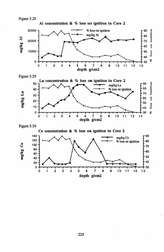
Figure 5.28
30000 -i
Al concentration & % loss on ignition in Core 2
a C T ,r \c c r v n i i m i f i r t n
61)'ei>s
20000 -
10000 -
T 1 1 1 1 1 1 1 1 1 1 1 1 1—I 1 1 1 1 1 ■ 11 2 3 4 5 6 7 8 9 1 0 1 1 1 2 1 3
depth g/cm2
Figure 5.29
0350 -
40 -
30 -6020 -(30s 10 -
0 -
La concentration & % loss on ignition in Core 2— V * mg/kg La* % — "* % loss on ignition
i—i—<—i—«—i—i—i—•—i—■—i—•—i—1—i—•—i—•—i—i—i—' T '
-9 0 -8 0
- 70 -6 0 -5 0
-4 0 30 ^
Figure 5.30
2 3 4 5 6 7 8 . 9 1 0 1 1 1 2 1 3depth g/cm2
Ce concentration & % loss on ignition in Core 2140120 -100 -
60 80 -
a 60 -
s 40 -20 -j
0 -
mg/kg Ce % loss on ignition
-» » +T 1--1--1--1--1--1--1--1--1--1--1-- 1---1-- '--1--1--1-->--1--1--1--
-9 0
-8 0
-7 0
-6 0
-5 0
-4 0
303 4 5 6 7 8 9
depth g/cm210 11 12 13
225
I acc
nn in
nitin
n In
cc
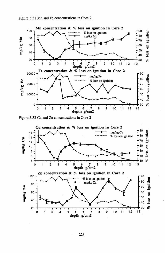
Figure 5.31 Mn and Fe concentrations in Core 2.
100 -iM n c o n c e n tra t io n & % loss o n ig n it io n in C o re 2
/ A' v —* ------’----- % loss on ignition* 4 4 ' * mg/kg Mn
30000 n
4>20000 HWD
0£S 10000 -
I ■ i ■ r3 4 5 6 7 8 9
d e p th g /cm 2F e c o n c e n tra t io n & % lo ss o n ig n it io n in C o re 2
* ♦- mg/kg Fe\ % loss on ignition
—i—i—|—i—|—i—|—i—|—i—|—i—i—i—i—i—i—i—i—i—i—r—nf-
-90
-80-70-60
-5 0
-4 030
0 1 2 3 4 5 6 7 8 9 1 0 1 1 1 2 1 3d e p th g /cm 2
Figure 5.32 Cu and Zn concentrations in Core 2.
C u c o n c e n tra t io n & % lo ss o n ig n it io n in C o re 2
aUwi
E
90mg/kg Cu % loss on ignition
16141210864
-470
40v,
9 10 11 12 1352 3 4 6 7 80 1
100 -
80 -eN "
60 -.
s 40 -
20 -
d e p th g /cm 2
Z n c o n c e n tra t io n & % lo ss o n ig n it io n in C o re 2 ♦ *\ / s mmt % loss on ignition♦—.y * \ . _\ • moflco Zn
-i—|—i—|—i—|—i—|—i—|—i—|—i—|—.—,1 2 3 4 5 6 7 8
d e p th g /cm 2
226
%
loss
on
igni
tion
loss
on
^g
11'^
011
% lo
ss
on ig
nitio
n %
lo
ss
on ig
nit
ion
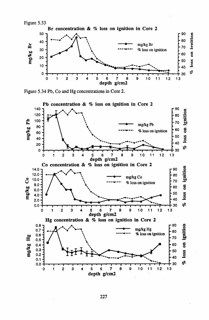
Figure 5.33
uffl6X
6X1
3
Br concentration & % loss on ignition in Core 2
“ mg/kg Br r — % ioss on ignition
5 6 7 8depth g/cm2
10 11 12 13
Figure 5.34 Pb, Co and Hg concentrations in Core 2.
Pb concentration & % loss on ignition in Core 2140 -n120 -
A 100 -Pnex 80 -
60 -ex3 40 -
20 -0 -
mg/kg Pb
% loss on ignition
14.0 n12.0-
O 10.0-O ToCO
ex6 .0 -
exa 4 .0 -G 2 .0 -
0 .0 -0
0.8-0.7-
ex 0.6-0.5-
ex 0.4-
'Sb 0.3-3 0 .2 ’
0.10.0-
depth g/cm2 Co concentration & % loss on ignition in Core 2
mg/kg Co— — % loss on ignition
T—'—1—r 4 5 6 7 8
depth g/cm2Hg concentration & % loss on ignition in Core 2
mg/kg Hg % loss on ignition
t—>—i—■—i—1—i—1—i—1—r 2 3 4 5 6 7 8 9
depth g/cm2
GO•mm‘364•mmgoViVio
co•mm*3ex•mmgoVIViO
GO•mm•p«G.5?GoViViO
227
% lo
ss
on
ign
itio
n
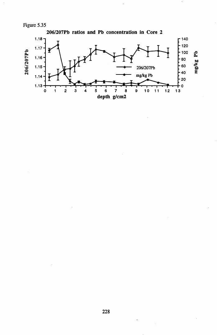
206/
207P
bFigure 5.35
206/207Pb ratios and Pb concentration in Core 21.18 140
- 1201.17-100
1.16 80
1.15- 206/207Pb
mg/kg Pb40
1.14 -201.13
5 70 2 3 4 6 8 9 10 11 12 131depth g/cm2
228
mg/
kg
Pb
SOUTH DRUMBOY CORE 3
This core was sampled close to the summit of Drumboy Hill, on the westerly facing slope and shows quite different characteristics and metal profiles from the previous cores discussed. The % moisture, loss on ignition and the bulk density are all effectively uniform throughout the profile and indicate that this is a well humified, ombrotrophic peat. In the top three sections of the core there appears to be mixing of the peat, disturbing the 210Pb profile (Figure 5.36). Mixing could be due to biological activity such as root growth or had the pH been higher earthworm activity could have been proposed. In addition, grazing sheep may be causing physical mixing of the surface sections. Whatever the explanation the mixing processes here are rapid and result in a reasonably constant In (excess) 210Pb activity over the mixed zone. Had mixing been slow the activity would not have been constant over the mixed zone but would have appeared as a change in accumulation rate. Below the mixing zone a normal radionuclide pattern was observed and an accumulation rate of 0.03lg cm-2 y 1 was calculated from linear regression of the In (excess) 210Pb activity from the base of the mixed sections. The total inventory of 210Pb was calculated as 3432 Bq n r2, giving a flux of 106 Bq m-2 y"1 (Table 5.26).
The mixing processes also affect the metal and radiocaesium profiles. Chernobyl caesium was deposited over a short period of time and rapid mixing would result in mixing of the radiocaesium deposited at the peat surface through the mixing zone to the older peat at the base of the mixed zone. This effectively increases the apparent time elapsed since the deposition event. Heavy metals such as Pb, Cu, Hg, etc. have been deposited on peats over a longer period of time with variations in the metal fluxes to the peat surface over this time. Rapid mixing smooths out short variations in input over the mixing depth and displaces peak pollutant metal fluxes and the onset of the increase in pollutant inputs by the depth of the peat in the mixed zone, again increasing the apparent time elapsed since the deposition event. To compensate for this effect the chronology calculated for the metals and radionuclides begins at the base of the mixed zone and is not the actual date of the peat deposit.
Radiocaesium shows considerable penetration through the peat, to depths dated well before the advent of weapons testing (Table 5.27). Weapons-testing 137Cs shows a slight peak in activity at 2 g cm-2 (Figure 5.37), which was dated as representing the period between 1964 and 1947 (Table 5.28). In Core 2, a peak in weapons-testing 137Cs was also observed, occurring over an imperveous mineral pan indicating that the peak in 137Cs was due to lateral flow. Thus, lateral flow could also be contributing to the peak in 137Cs activity observed in Core 3. The total inventory of 137Cs was
229
calculated as 11604 Bq m*2, with a weapons-testing inventory of 3528 Bq m-2 and a Chernobyl inventory of 8076 Bq m-2. The total inventory of 134Cs was 497 Bq n r2
The Al concentration (Figure 5.38) is an order of magnitude lower than for Cores 1 and 2, reflecting the lower mineral content of this peat. However, at depth, as the % loss on ignition decreases the Al concentration also decreases. Ce, Ta, Hf, Se, Sc, Sm, La, and Th also show this effect, as illustrated by La and Ce (Figure 5.39). Unlike Al, these elements also show a peak in concentration at 1.5 g cm-2 indicating an increase in the mineral content at this point. Interestingly, this occurs in the same section as the peak in weapons-testing i37Cs.
The Mn and Fe profiles (Figure 5.40) suggest that to a depth of 1.5 g cm-2, conditions are only reducing enough to bring Mn into solution. Beneath 1.5 g cm-2 conditions are reducing enough to promote the dissolution of Fe. The Fe concentration throughout the profile is an order of magnitude lower than for Cores 1 and 2, reflecting the reduced mineral content of the peat.
Cu (Figure 5.41) shows a distinct peak in concentration at 2 g cm-2 and below 3 g cm_2 there is no Cu detected. With conditions becoming more reducing from 1.5 g cm-2 this peak could be due to deposition of CuS around the zone of water fluctuation. However, there is no observed deposition of FeS2 which is more readily formed than CuS (Rowell, 1988). Accordingly the peak in Cu is more likely to be due to increases in pollutant input. Zn (Figure 5.41) does not show this distinct peak in deposition and instead shows a progressive decrease in concentration with depth. Jones (1987) attributed Zn mobility to it being co-precipitated with Mn and Fe oxides, whereas Cu was predominantly bound to organic matter. Zn mobility in surface sections has also been explained by it being an essential element for plant growth (Livett et al., 1979: Shotyk et al., 1990: Jones & Hao, 1993). However, Cu and Mn are also essential elements for plant growth.
Pb Co, Hg, As and Sb all show a distinct peak in concentration at 2 g cm-2, as previously seen for Cu (Figure 5.43,Table 5.29 & Appendix 3). In addition Br (Figure 5.42) shows a peak in concentration at depth, giving a very similar profile to Pb. This may be an indication of the importance of car exhaust emissions on the Pb concentration, since Te Haar & Bayard (1971) observed that when car exhaust particles are emitted they mainly consist of PbBr2 , PbBrCl, Pb(OH)Br, Pb(0)2PbBr2, and Pb(0)2PbBrCl. After around 18 hours, about 75% of the Br is lost from these particles. The Br/Pb ratio of soils has also been used to establish the relative importance of industry and car exhausts on the Pb content (Sturges & Harrison, 1986). However, the Br/Pb ratio of petrol can vary, and suitable background, or pre-industrial ratios must be established before the ratio can be used with any accuracy. But Br could
230
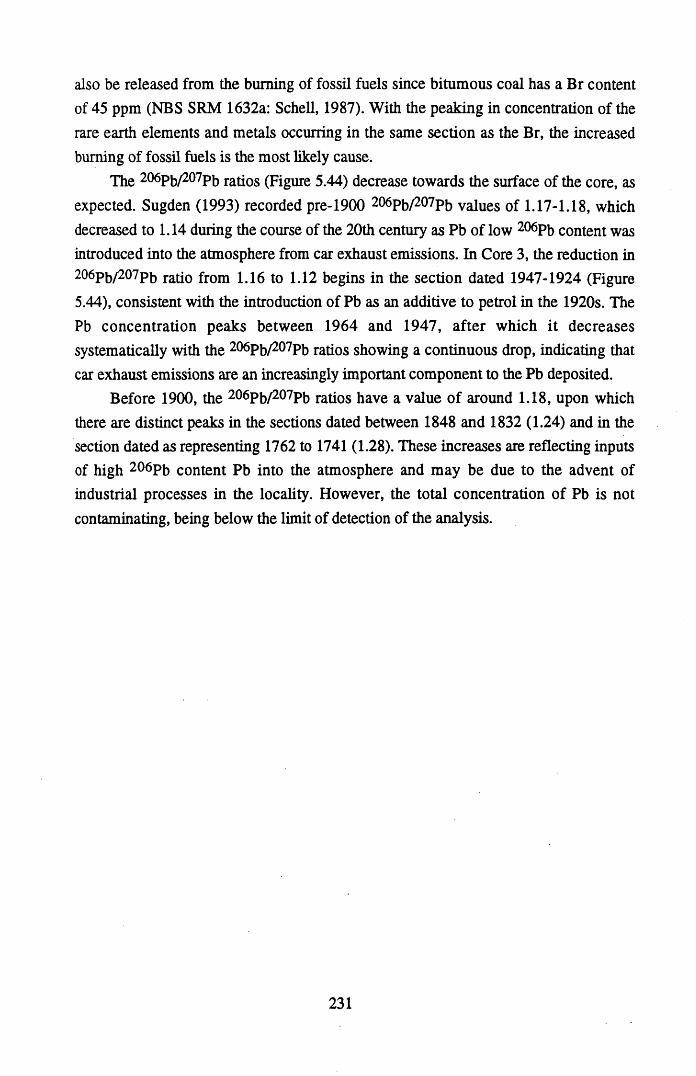
also be released from the burning of fossil fuels since bitumous coal has a Br content of 45 ppm (NBS SRM 1632a: Schell, 1987). With the peaking in concentration of the rare earth elements and metals occurring in the same section as the Br, the increased burning of fossil fuels is the most likely cause.
The 206pb/207pb ratios (Figure 5.44) decrease towards the surface of the core, as expected. Sugden (1993) recorded pre-1900 206pb/207pb values of 1.17-1.18, which decreased to 1.14 during the course of the 20th century as Pb of low 206pb content was introduced into the atmosphere from car exhaust emissions. In Core 3, the reduction in 206pb/207pb ratio from 1.16 to 1.12 begins in the section dated 1947-1924 (Figure 5.44), consistent with the introduction of Pb as an additive to petrol in the 1920s. The Pb concentration peaks between 1964 and 1947, after which it decreases systematically with the 206pb/207pb ratios showing a continuous drop, indicating that car exhaust emissions are an increasingly important component to the Pb deposited.
Before 1900, the 206Pb/207Pb ratios have a value of around 1.18, upon which there are distinct peaks in the sections dated between 1848 and 1832 (1.24) and in the section dated as representing 1762 to 1741 (1.28). These increases are reflecting inputs of high 206pb content Pb into the atmosphere and may be due to the advent of industrial processes in the locality. However, the total concentration of Pb is not contaminating, being below the limit of detection of the analysis.
231
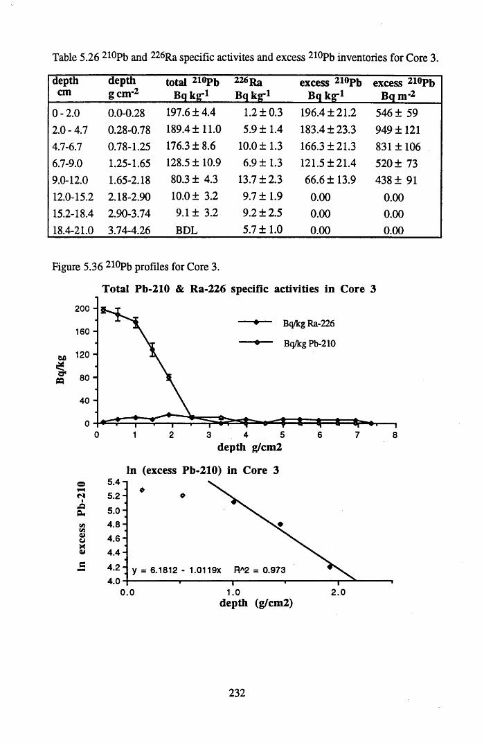
Table 5.26 210Pb and 226Ra specific activites and excess 210Pb inventories for Core 3.
depthcm
depthgem -2
total 210Pb Bq kg'1
226R a
Bq kg"1excess 210Pb
Bq kg-1excess 210Pb
Bqm-20-2.0 0.0-0.28 197.6 ±4.4 1.2 ±0.3 196.4 ±21.2 546 ± 59
to 0 1 ^4 0.28-0.78 189.4 ±11.0 5.9 ±1.4 183.4 ±23.3 949 ±1214.7-6.7 0.78-1.25 176.3 ± 8.6 10.0 ±1.3 166.3 ±21.3 831 ±1066.7-9.0 1.25-1.65 128.5 ± 10.9 6.9 ±1.3 121.5 ±21.4 520 ± 739.0-12.0 1.65-2.18 80.3 ± 4.3 13.7 ±2.3 66.6 ±13.9 438 ± 9112.0-15.2 2.18-2.90 10.0 ± 3.2 9.7 ± 1.9 0.00 0.0015.2-18.4 2.90-3.74 9.1 ± 3.2 9.2 ±2.5 0.00 0.0018.4-21.0 3.74-4.26 BDL 5.7 ±1.0 0.00 0.00
Figure 5.36 210Pb profiles for Core 3.
Total Pb-210 & Ra-226 specific activities in Core 3
200 -Bq/kg Ra-226
Bq/kg Pb-210160 -
40 -
0 2 51 3 4 6 7 8depth g/cm2
In (excess Pb-210) in Core 35 .4 - 5 .2 -
5 .0 - 4 .8 - 4 .6 -4 .4 -
4 .2 -4 .0 -
y s 6.1812 - 1.0119x RA2 = 0.973
2.00.0 1.0depth (g/cm2)
232
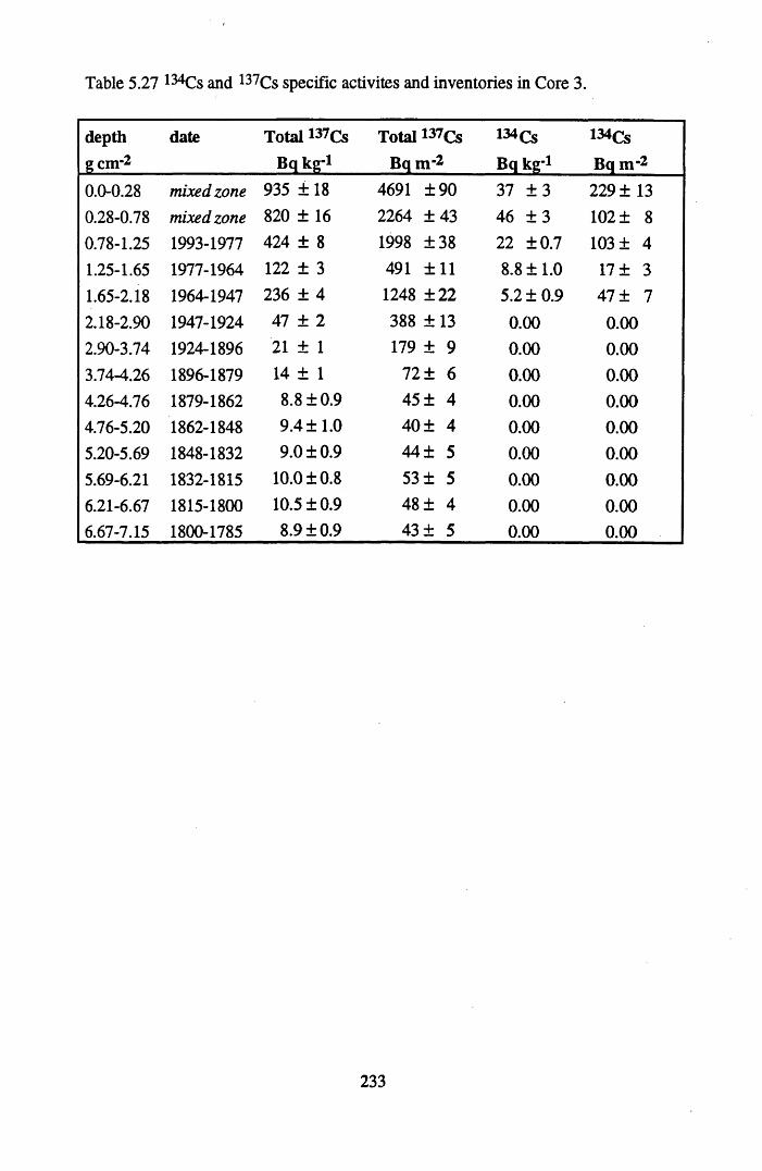
Table 5.27 134Cs and 137Cs specific activites and inventories in Core 3.
depth date Total 137cs Total 137Cs 134CS 134Csgem-2 Bq kg-l Bq m"2 Bq kg-l Bq m -20.0-0.28 mixed zone 935 ± 18 4691 ±90 37 ± 3 229 ± 130.28-0.78 mixed zone 820 ± 16 2264 ± 43 46 ± 3 102 ± 80.78-1.25 1993-1977 424 ± 8 1998 ±38 22 ±0.7 103 ± 41.25-1.65 1977-1964 122 ± 3 491 ±11 8.8 ±1.0 17 ± 31.65-2.18 1964-1947 236 ± 4 1248 ±22 5.2 ±0.9 47 ± 72.18-2.90 1947-1924 47 ± 2 388 ± 13 0.00 0.002.90-3.74 1924-1896 21 ± 1 179 ± 9 0.00 0.003.74-4.26 1896-1879 14 ± 1 72 ± 6 0.00 0.004.26-4.76 1879-1862 8.8 ±0.9 45 ± 4 0.00 0.004.76-5.20 1862-1848 9.4 ±1.0 40 ± 4 0.00 0.005.20-5.69 1848-1832 9.0 ±0.9 44 ± 5 0.00 0.005.69-6.21 1832-1815 10.0 ±0.8 53 ± 5 0.00 0.006.21-6.67 1815-1800 10.5 ±0.9 48 ± 4 0.00 0.006.67-7.15 1800-1785 8.9 ±0.9 43 ± 5 0.00 0.00
233
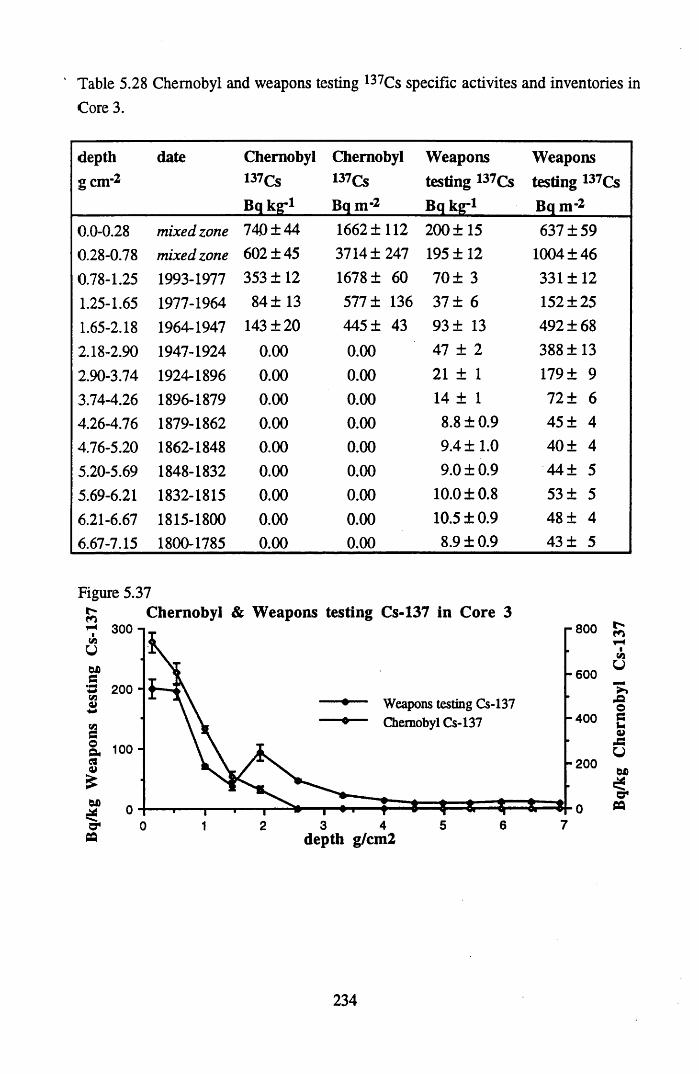
Table 5.28 Chernobyl and weapons testing 137Cs specific activites and inventories inCore 3.
depthgem -2
date Chernobyl 137Cs Bq kg’1
Chernobyl 137CSBq n r 2
Weapons testing 137Cs Bq kg-1
Weapons testing 137Cs Bq m -2
0.0-0.28 mixed zone 740 ±44 1662 ± 112 200 ±15 637 ±590.28-0.78 mixed zone 602 ±45 3714± 247 195 ± 12 1004 ±460.78-1.25 1993-1977 353 ± 12 1678 ± 60 70 ± 3 331 ±121.25-1.65 1977-1964 84 ± 13 577 ± 136 37 ± 6 152 ±251.65-2.18 1964-1947 143 ±20 445 ± 43 93 ± 13 492 ±682.18-2.90 1947-1924 0.00 0.00 47 ± 2 388 ±132.90-3.74 1924-1896 0.00 0.00 21 ± 1 179 ± 93.74-4.26 1896-1879 0.00 0.00 14 ± 1 72 ± 64.26-4.76 1879-1862 0.00 0.00 8.8 ±0.9 45 ± 44.76-5.20 1862-1848 0.00 0.00 9.4 ±1.0 40 ± 45.20-5.69 1848-1832 0.00 0.00 9.0 ±0.9 44 ± 55.69-6.21 1832-1815 0.00 0.00 10.0 ±0.8 53 ± 56.21-6.67 1815-1800 0.00 0.00 10.5 ±0.9 48 ± 46.67-7.15 1800-1785 0.00 0.00 8.9 ±0.9 43 ± 5
Figure 5.37Chernobyl & Weapons testing Cs-137 in Core 3
^ 300 n r 800
-6 0 0200 -
Weapons testing Cs-137 Chernobyl Cs-137 -4 0 0
-200
75 63 420 1
fOI
u
X5oei*VUSUW>
CQ
depth g/cm2
234
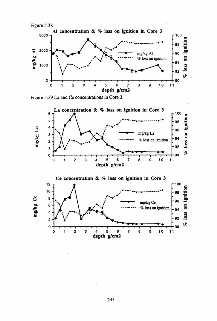
Figure 5.38A1 concentration & % loss on ignition in Core 3
3000 t r 100
5 2000 HW)
1000 -
/ ^-■r- w
mg/kg A1— % loss on ignition
t—i—|—i—r T T” 1—i—1—i— i—i—i—«—i—>-2 3 4 5 6 7 8 9 1 0 1 1
depth g/cm2
-98
-96
-94
-92
90
Figure 5.39 La and Ce concentrations in Core 3.
C3
CD*1)E
6 -
5 -
4 -
3 -
2 -
1 -
0
La concentration & % loss on ignition in Core 3
—
mg/kg La
* % loss on ignition
-I— |— i— i— i i i- r •— i— '— t- 1— r 1 2 3 4 5 6 7
depth g/cm2
“I 1 1 1 r8 9 10 11
- 100
-98
■96
-94
b 92
90
Ce concentration & % loss on ignition in Core 3r 100
10 - -98
-96mg/kg Ce % loss on ignition -94
-92
9065 7 8 9 10 112 3 410
depth g/cm2
235
% l
oss
on ig
nitio
n %
loss
on ig
nitio
n %
loss
on ig
nitio
n
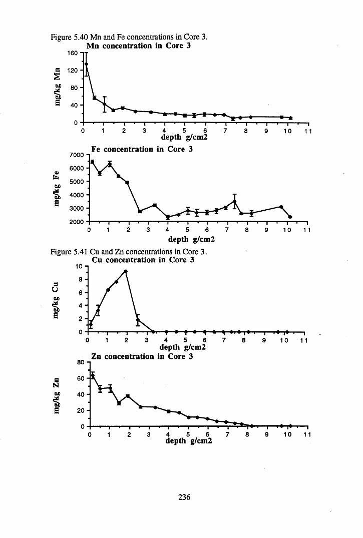
Figure 5.40 Mn and Fe concentrations in Core 3. Mn concentration in Core 3
160 n
fi 120 -ssSt 80 ■ 60S 40 -
3 4 51 2 6 70 8 9 10 1 1
60
7000 -
6000 -
5000 -
4000 -
3000 -
2000
depth g/cm2 Fe concentration in Core 3
"•—r1
t — 1— r3 4 5 6
depth g/cm2
I T7
i10
Figure 5.41 Cu and Zn concentrations in Core 3. Cu concentration in Core 3
s
60s
depth g/cm2 Zn concentration in Core 3
BN60
S
“ 11 1
10 -1
4 5 60 1 2 3 7 8 9 10 11
80 n
60 -
40 -
20 -
4 5 6 7 8 9 101 2 3 110depth g/cm2
236
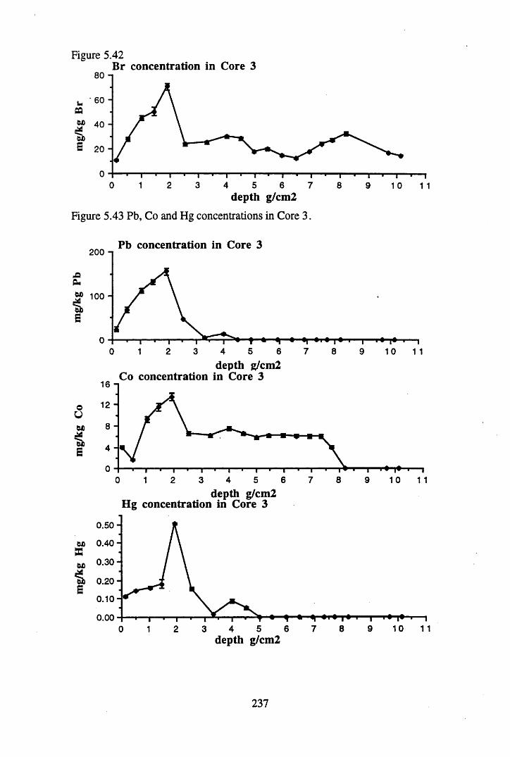
Figure 5.42Br concentration in Core 3
80 -i
w 4 0 - w>
20 1 3 4 5 6 7 8 9 1 0 1 1depth g/cm2
Figure 5.43 Pb, Co and Hg concentrations in Core 3.
Pb concentration in Core 32 0 0 -i
SP 10 0 -
2 5 6 70 3 4 8 91 10 11depth g/cm2
Co concentration in Core 316 -i
4 6 7 8 10 110 1 2 3 5 9depth g/cm2
Hg concentration in Core 3
0 .5 0 -
M> 0.40 -
0 .2 0 -
0 . 10 -
0.0010 115 7 8 92 4 630 1
depth g/cm2
237
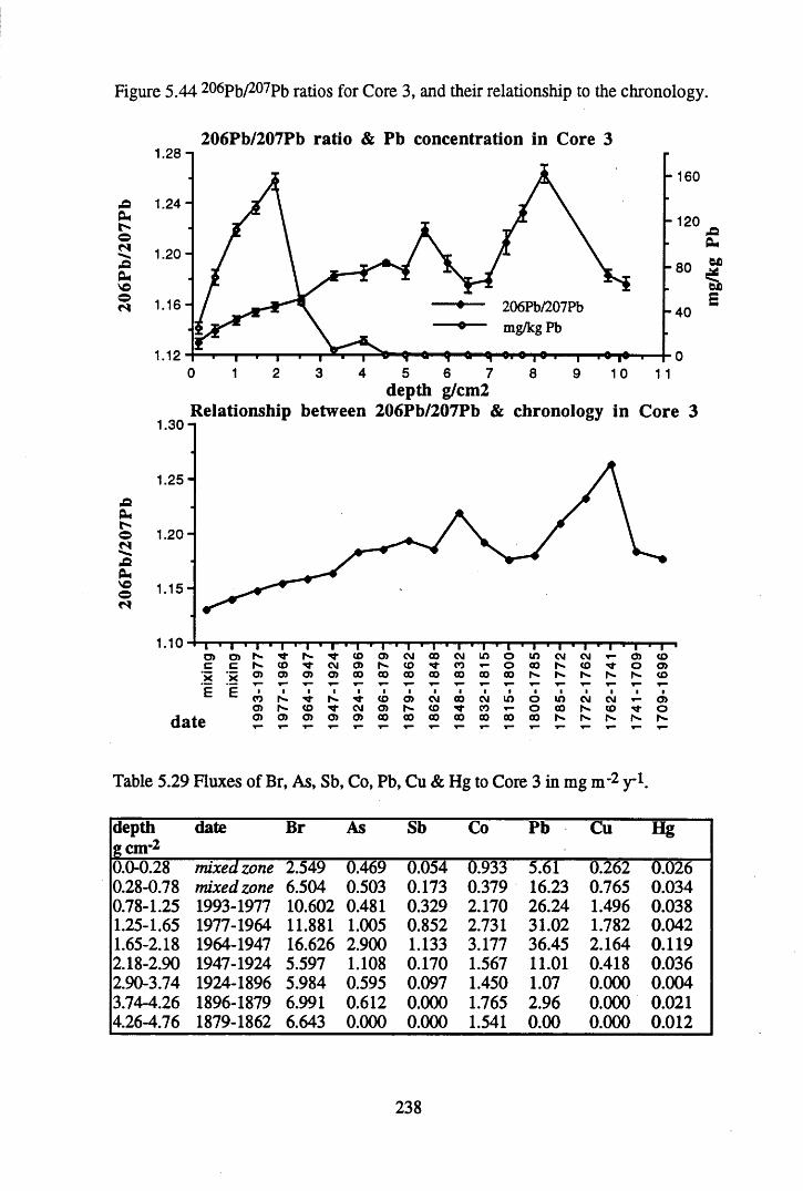
Figure 5.44 206pb/207p5 ratios for Core 3, and their relationship to the chronology.
206Pb/207Pb ratio & Pb concentration in Core 31.28 n
- 160
X! 1.24 - 0 U
o1.2 0 -*a
CUVO® 1.16-
- 120
-8 0
206Pb/207Pb mg/kg Pb
-4 0
1.122 3 50 1 4 6 7 8 9 1 0 1 1
depth g/cm2Relationship between 206Pb/207Pb & chronology in Core 3
1.30 -i
CUr-oNCUvoo
1.25-
1.2 0 -
1.15-
1.10
date
T"*“P r T n T " 1 rT ^rT"1T " r T nT '“T"’T " rT "1 1 n n ' 1 1’ 1 'n r -To> 05 h- r- ■M- CO 05 CM CO CM in o in CM CM T— 05 COc c CO CM 05 CO CO T— o CO h- CO O 05’x ’x 05 05 O) 05 00 CO CO CO CO CO 00 N. h* N. COc c. *- t_ T_ 'T— T“ T— ▼“ T—c c CO r»- ■M" N- •M- co 05 CM 00 CM in o in CM CM 4 05
o> co CM 05 1 - CO ■M- CO T— o CO r*. CO Tf ogk o> o> 0) 05 05 CO 00 CO 00 CO CO CO r*. h - h- N.c T— T“ T— T“ T— T- T“ T“ T” T— T“
Table 5.29 Fluxes of Br, As, Sb, Co, Pb, Cu & Hg to Core 3 in mg m"2 y 1.
depthgem-2
date Br As Sb Co Pb Cu Hg
0.0-0.28 mixed zone 2.549 0.469 0.054 6.933 5.61 0.262 0.0260.28-0.78 mixed zone 6.504 0.503 0.173 0.379 16.23 0.765 0.0340.78-1.25 1993-1977 10.602 0.481 0.329 2.170 26.24 1.496 0.0381.25-1.65 1977-1964 11.881 1.005 0.852 2.731 31.02 1.782 0.0421.65-2.18 1964-1947 16.626 2.900 1.133 3.177 36.45 2.164 0.1192.18-2.90 1947-1924 5.597 1.108 0.170 1.567 11.01 0.418 0.0362.90-3.74 1924-1896 5.984 0.595 0.097 1.450 1.07 0.000 0.0043.74-4.26 1896-1879 6.991 0.612 0.000 1.765 2.96 0.000 0.0214.26-4.76 1879-1862 6.643 0.000 0.000 1.541 0.00 0.000 0.012
238
mg/
kg
Pb
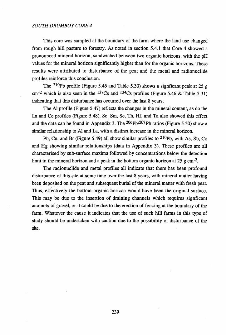
SOUTH DRUMBOY CORE 4
This core was sampled at the boundary of the farm where the land use changed from rough hill pasture to forestry. As noted in section 5.4.1 that Core 4 showed a pronounced mineral horizon, sandwiched between two organic horizons, with the pH values for the mineral horizon significantly higher than for the organic horizons. These results were attributed to disturbance of the peat and the metal and radionuclide profiles reinforce this conclusion.
The 2l°Pb profile (Figure 5.45 and Table 5.30) shows a signficant peak at 25 g cm-2 which is also seen in the 137Cs and 134Cs profiles (Figure 5.46 & Table 5.31) indicating that this disturbance has occurred over the last 8 years.
The A1 profile (Figure 5.47) reflects the changes in the mineral content, as do the La and Ce profiles (Figure 5.48). Sc, Sm, Se, Th, Hf, and Ta also showed this effect and the data can be found in Appendix 3. The 206pb/207pb rati0s (Figure 5.50) show a similar relationship to A1 and La, with a distinct increase in the mineral horizon.
Pb, Cu, and Br (Figure 5.49) all show similar profiles to 210Pb, with As, Sb, Co and Hg showing similar relationships (data in Appendix 3). These profiles are all characterised by sub-surface maxima followed by concentrations below the detection limit in the mineral horizon and a peak in the bottom organic horizon at 25 g cm-2.
The radionuclide and metal profiles all indicate that there has been profound disturbance of this site at some time over the last 8 years, with mineral matter having been deposited on the peat and subsequent burial of the mineral matter with fresh peat. Thus, effectively the bottom organic horizon would have been the original surface. This may be due to the insertion of draining channels which requires signficant amounts of gravel, or it could be due to the erection of fencing at the boundary of the farm. Whatever the cause it indicates that the use of such hill farms in this type of study should be undertaken with caution due to the possibility of disturbance of the site.
239
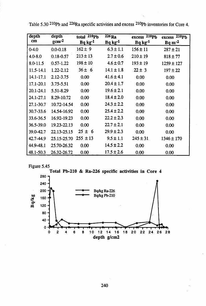
Table 5.30 210Pb and 226Ra specific activities and excess 210Pb inventories for Core 4.
depthcm
depthgem-2
total 210Pb Bq kg-1
226RaBq kg'1
excess 210Pb Bq kg-1
excess 210Pb Bq m -2
0-4.0 0.0-0.18 162 ± 9 6.3 ±1.1 156 ± 11 287 ±214.0-8.0 0.18-0.57 213 ±13 2.7 ±0.6 210± 19 818 ±778.0-11.5 0.57-1.22 198 ±10 4.6 ±0.7 193 ±19 1259 ±12711.5-14.1 1.22-2.12 36 ± 6 14.1 ±1.8 22 ± 3 197 ±2214.1-17.1 2.12-3.75 0.00 41.6 ±4.1 0.00 0.0017.1-20.1 3.75-5.51 0.00 20.4 ±1.7 0.00 0.0020.1-24.1 5.51-8.29 0.00 19.6 ±2.1 0.00 0.0024.1-27.1 8.29-10.72 0.00 18.4 ±2.0 0.00 0.0027.1-30.7 10.72-14.54 0.00 24.3 ±2.2 0.00 0.0030.7-33.6 14.54-16.92 0.00 25.4 ±2.2 0.00 0.0033.6-36.5 16.92-19.23 0.00 22.2 ±2.3 0.00 0.0036.5-39.0 19.23-22.13 0.00 22.7 ±2.1 0.00 0.0039.0-42.7 22.13-25.15 25 ± 6 29.9 ±2.3 0.00 0.0042.7-44.9 25.15-25.70 255 ± 13 9.5 ±1.1 245 ±31 1346 ±17044.9-48.1 25.70-26.32 0.00 14.5 ±2.2 0.00 0.0048.1-50.3 26.32-26.72 0.00 17.5 ±2.6 0.00 0.00
Figure 5.45Total Pb-210 & Ra-226 specific activities in Core 4
280 n
240 -
Bq/kg Ra-226 Bq/kg Pb-210
200 - fWDX 160"o'n 120-
80 -
40 -
0 2 4 6 8 10 12 14 16 18 20 22 24 26 28depth g/cm2
240
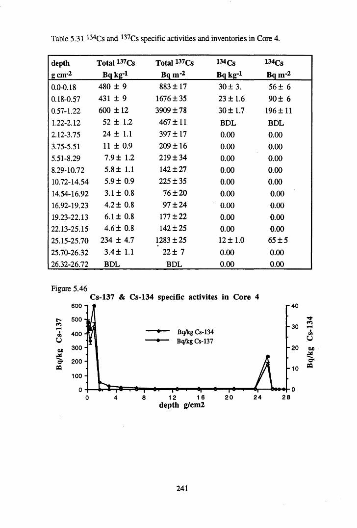
Table 5.31 134Cs and 137Cs specific activities and inventories in Core 4.
depthgem-2
Total 137Cs Bq kg-1
Total 137Cs Bq n r 2
134 Cs Bq kg*1
134Cs Bq n r 2
0.0-0.18 480 ± 9 883 ±17 30 ± 3 . 56 ± 60.18-0.57 431 ± 9 1676 ±35 23 ± 1.6 90 ± 60.57-1.22 600 ±12 3909 ±78 30 ±1.7 196 ±111.22-2.12 52 ± 1 .2 467 ±11 BDL BDL2.12-3.75 24 ± 1.1 397 ±17 0.00 0.003.75-5.51 11 ± 0.9 209 ±16 0.00 0.005.51-8.29 7.9 ± 1.2 219 ±34 0.00 0.008.29-10.72 5.8 ± 1.1 142 ±27 0.00 0.0010.72-14.54 5.9 ± 0.9 225 ±35 0.00 0.0014.54-16.92 3.1 ± 0.8 76 ±20 0.00 0.0016.92-19.23 4.2 ± 0.8 97 ±24 0.00 0.0019.23-22.13 6.1 ± 0.8 177 ±22 0.00 0.0022.13-25.15 4.6 ± 0.8 142 ±25 0.00 0.0025.15-25.70 234 ± 4.7 1283 ±25 12 ±1.0 65 ± 525.70-26.32 3.4 ± 1.1 ’ 22 ± 7 0.00 0.0026.32-26.72 BDL BDL 0.00 0.00
Figure 5.46Cs-137 & Cs-134 specific activites in Core 4
IVw>'o 'CQ
r 40600
500-30
Bq/kg Cs-134 Bq/kg Cs-137
400
300 -20
200- 10
100
024 28201 6120 4 8
Tfma
v
depth g/cm2
241
Bq/
kg
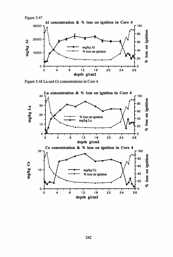
Figure 5.47A1 concentration & % loss on ignition in Core 4
r 10030000 n
-8 0
20000 --6 0
mg/kg A1 % loss on ignition10000 -
12 1 60 4 8 20 24 28d e p th g /cm 2
Figure 5.48 La and Ce concentrations in Core 4.
L a c o n c e n tra t io n & % loss o n ig n itio n in C o re 440 -1 r 100
-8 030 -
-6 020 -
% loss on ignition mg/kg La -4 0
10 - 20
12 16 20 2 4 2 80 4 8d e p th g /cm 2
C e c o n c e n tra t io n & % lo ss o n ig n itio n in C o re 420 r 100
-8 0
-6 010 mg/kg Ce
% loss on ignition -4 0
02812 16 20 2 44 80
depth g/cm2
242
%
loss
on
igni
tion
% lo
ss
on ig
nitio
n %
loss
on
ign
itio
n
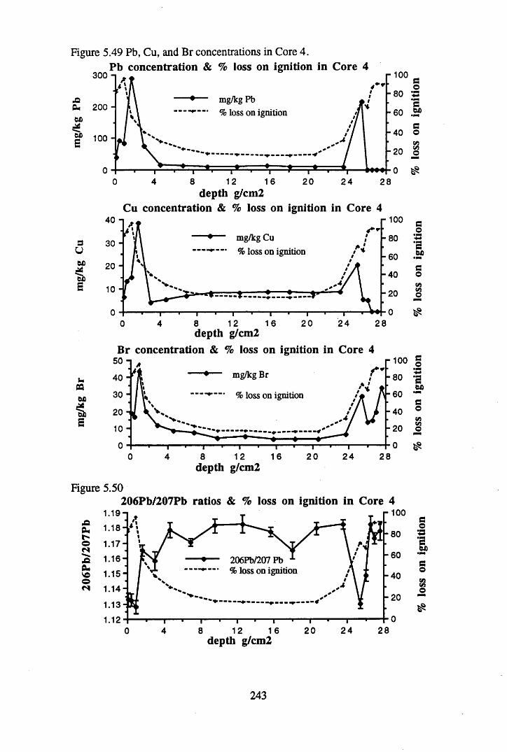
Figure 5.49 Pb, Cu, and Br concentrations in Core 4.Pb concentration & % loss on ignition in Core 4
300 n jf
,QP*W)«=£W>3
200 -
100 -
mg/kg Pb % ioss on ignition
20— i----1----- 1-----1— i I "
4 8 12 16depth g/cm2
Cu concentration & % loss on ignition in Core 4
- 100 c-80
o•mm
■•mme
-60 tSJD• M
■ C-40 O• V )
-20 O.- 0
r 10040 ”|
mg/kg Cu % loss on ignition
-8030 --60
20-40
10 -
12 20 24 288 1640
u
W)■as
depth g/cm2 Br concentration & % loss on ignition in Core 4
A♦ mg/kg Br
— % loss on ignition
—i ----1---- r-8 12 16
depth g/cm2
Figure 5.50
PmhON43CUvooN
206Pb/207Pb ratios & % loss on ignition in Core 4
i1.19-1.18-
1.17-1.16-1.15-1.14-
1.13 *:
206Pb/207 Pb % loss on ignition
> ----- - - -
T ----1---- 1---- 1---- 1“8 12 1 6 20 24
depth g/cm228
ao•m m
*3.5fcowjV 3o
r 100 C#o*3W>•P*soMWo
- 100e
-80o•-cc
-60WD•M
B C-40
owVi
-2 0O
■- 0
243
SOUTH DRUMBOY CORE 5
This core was collected directly downslope from Core 3, on the ridge of Drumboy Hill and was characterised by 50 cm of organic matter overlying bedrock. Accordingly, the influence of the bedrock was shown in section 5.4.1 by a decrease in % loss on ignition, an increase in bulk density and pH.
The 210Pb profiles showed some evidence of mixing (Figure 5.51 & Table 5.32) in the first section. However, the effect is minimal and does not significantly affect the acumulation rate which was calculated to be 0.021 g cm*2 y*1. The total inventory of 210Pb was calculated as 2165 Bq m-2, giving a flux of 67 Bq m-2 y 1.
As with the core 3, radiocaesium penetrates to sections dated before the advent of weapons testing (Tables 5.33 & 5.34, Figure 5.52). 137Cs is present to 9 g cm-2 with 134Cs present to 3 g cm'2. The total inventory of 137Cs was 6437 Bq m-2, comprising a Chernobyl inventory of 3933 Bq n r2 and a weapons-testing inventory of 2502 Bq n r2. The total 134Cs inventory was 245 Bq n r2.
The A1 profile (Figure 5.53) reflects the increase in mineral content as bedrock is approached. La and Ce (Figure 5.54) also show this effect, but also show sub-surface maxima. These maxima are seen in all the rare earth elements and the data can be found in Appendix 3. Sub-surface maxima in the profiles of these elements were also seen in Core 3 and proposed to be due to the burning of fossil fuels.
The Mn and Fe profiles (Figure 5.55) indicate that conditions are progressively reducing from the surface. The concentration of Mn is low throughout the core and decreases rapidly from the surface reflecting its sensitivity to changes in the redox potential. Fe also shows reduction in concentration from the surface with the effect being less pronounced. However, both Fe and Mn show an increase in concentration as bedrock is approached, with the increase occurring before the increase in concentrations of Al, La and Ce and drop in organic matter. However, the increases in Fe and Mn could be due to the influence of the bedrock, with Mn and Fe released from weathered minerals followed by diffusion and redeposition. Walton Day et a l (1990) observed that maxima in Fe, Mn and Co concentrations at the base of peat profiles were due to these metals being associated with a maximum in mineral matter content, resulting from a transition between the underlying inorganic sedimentary environment to an organic sedimentary environment within the peat. Mn and Fe could also be re- deposited due to the production of metal sulphides.
As in Core 3, Cu (Figure 5.56) shows a sub-surface maximum in concentration, which is not seen for Zn and which appears in the same section as the peak in the rare
244
earth elements. Both Cu and Zn show slight increases at the bottom of the core which can be attributed to weathering of the bedrock.
Br (Figure 5.56) also shows this sub-surface maximum in concentration, as also seen for Pb, Co, Hg, As and Sb (Figure 5.58 and Appendix 3). This mirrors Core 3, indicating that the processes which influenced the input of these elements into Core 3 may also have done so for Core 5. The peaks in fluxes of Cu, Pb, Br, Co, Hg, As, and Sb to Core 5 were dated as occurring between 1967 and 1951 (Table 5.35) agreeing well with the peaks in fluxes to Core 3 which were dated between 1964 and 1947 (Table 5.29). As with Core 3 the peaks in the concentrations of rare earth elements also occur in the same section as the maximum flux in the pollutant metals and this may be indicating the influx of atmospheric dust containing these pollutant metals, i.e. due to the burning of fossil fuels.
The 206pt>/207pb ratios (Figure 5.59) show large increases in ratio between 1868 and 1744, indicating that there was an input of Pb low in 20<5pb around this time, which compares well with the peaks in Core 3 which occurred between 1845 and 1741. It should be noted that the accuracy of dates calculated from 210Pb dating decreases with depth and cannot be assumed to be as reliable beyond 150 years. Between 1835 and 1951 the 206pb/207pb ratios are reasonably consistent around values of ~ 1.14. Only in the second section is there a drop in ratio to 1.12. These results are contrary to those observed in Core 3 and recorded by Sugden (1993) with no explanation being evident.
The increase in ratio in the surface section may be reflecting the decreased use of Pb in petrol. Previous research has indicated that Pb fluxes decreased by up to 80% between 1979 and 1983 due to the increased use of unleaded petrol (Eisenreich e ta l , 1986).
245

Table 5.32 210Pb and 226Ra specific activities and excess inventories in Core 5.
depth depth total 210Pb 226R a excess 210Pb excess 210Pbcm gem-2 Bq kg"1 B q k g l Bqkg-l B q n r2
0-4.0 0.0-0.54 212±7 10.2 ±0.3 202 ±13 1081 ±694.0-6.5 0.54-0.87 180 ± 6 7.9 ±0.1 172 ± 11 573 ±366.5-8.7 0.87-1.17 85 ± 4 3.2 ±0.1 82 ± 9 235 ±258.7-11.3 1.17-1.63 59 ± 4 12.8 ±0.2 46 ± 6 211 ±2811.3-13.3 1.63-2.11 24 ± 3 3.4 ±0.1 20 ± 3 65 ± 913.3-16.2 2.11-2.63 14 ± 2 10.4 ±0.1 0.00 0.00
Figure 5.51 210Pb profiles for Core 5.
226-Ra & excess 210-Pb in Core 5
200 -Bq/kg Pb-210
Bq/kg Ra-226160 -
120 -
80 -
40 -
0.0 1.0 2.0 3.0 4.0 5.0 6.0 7 .0 8.0 9.0 10.0depth g/cm2
In (excess Pb-210) in Core 56 1
O
w4>X0>
y s 5.8679 - 1.4755X RA2 = 0.980
1.51.0 2.00.0 0.5
depth g/cm2
246
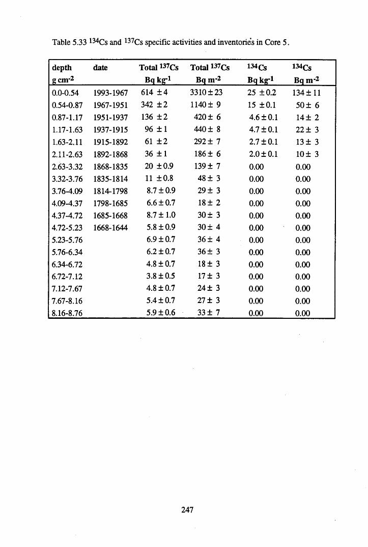
Table 5.33 134Cs and 137Cs specific activities and inventories in Core 5.
depthgem-2
date Total 137Cs Bq kg’1
Total 137Cs Bq nr2
134 Cs Bq kg’1
134Cs Bq nr2
0.0-0.54 1993-1967 614 ±4 3310 ±23 25 ±0.2 134 ± 110.54-0.87 1967-1951 342 ±2 1140± 9 15 ±0.1 50 ± 60.87-1.17 1951-1937 136 ± 2 420 ± 6 4.6 ±0.1 14± 21.17-1.63 1937-1915 96 ±1 440 ± 8 4.7 ±0.1 22 ± 31.63-2.11 1915-1892 61 ± 2 292 ± 7 2.7 ±0.1 13 ± 32.11-2.63 1892-1868 36 ±1 186 ± 6 2.0 ±0.1 10 ± 32.63-3.32 1868-1835 20 ±0.9 139 ± 7 0.00 0.003.32-3.76 1835-1814 11 ±0.8 48 ± 3 0.00 0.003.76-4.09 1814-1798 8.7 ±0.9 29 ± 3 0.00 0.004.09-4.37 1798-1685 6.6 ±0.7 18 ± 2 0.00 0.004.37-4.72 1685-1668 8.7 ±1.0 30 ± 3 0.00 0.004.72-5.23 1668-1644 5.8 ±0.9 30 ± 4 0.00 0.005.23-5.76 6.9 ±0.7 36 ± 4 0.00 0.005.76-6.34 6.2 ±0.7 36 ± 3 0.00 0.006.34-6.72 4.8 ±0.7 18 ± 3 0.00 0.006.72-7.12 3.8 ±0.5 17 ± 3 0.00 0.007.12-7.67 4.8 ±0.7 24 ± 3 0.00 0.007.67-8.16 5.4 ±0.7 27 ± 3 0.00 0.008.16-8.76 5.9 ±0.6 33 ± 7 0.00 0.00
247
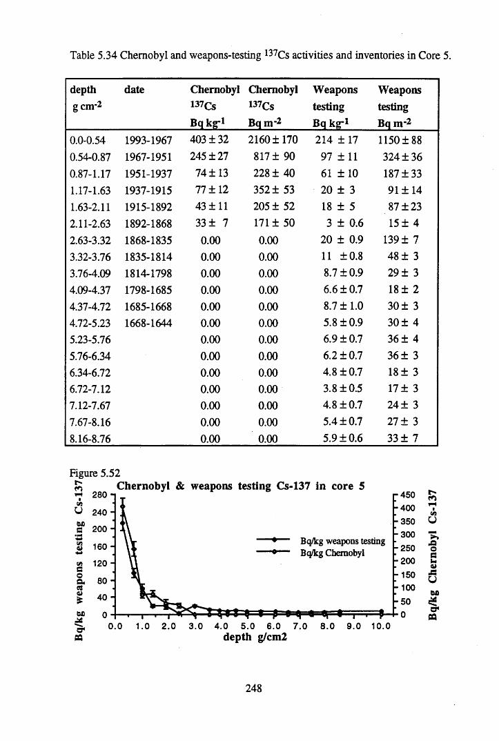
Table 5.34 Chernobyl and weapons-testing 137Cs activities and inventories in Core 5.
depthgem-2
date Chernobyl l37cs Bq kg-1
Chernobyl 127Cs Bq nr2
Weapons testing Bq kg-1
Weapons testing Bq m-2
0.0-0.54 1993-1967 403 ±32 2160 ±170 214 ± 17 1150 ±880.54-0.87 1967-1951 245 ±27 817 ± 90 97 ± 11 324 ±360.87-1.17 1951-1937 74 ±13 228 ± 40 61 ±10 187 ±331.17-1.63 1937-1915 77 ±12 352 ± 53 20 ± 3 91 ±141.63-2.11 1915-1892 43 ±11 205 ± 52 18 ± 5 87 ±232.11-2.63 1892-1868 33 ± 7 171 ± 50 3 ± 0.6 15 ± 42.63-3.32 1868-1835 0.00 0.00 20 ± 0.9 139 ± 73.32-3.76 1835-1814 0.00 0.00 11 ±0.8 48 ± 33.76-4.09 1814-1798 0.00 0.00 8.7 ±0.9 29 ± 34.09-4.37 1798-1685 0.00 0.00 6.6 ±0.7 18 ± 24.37-4.72 1685-1668 0.00 0.00 8.7 ±1.0 30 ± 34.72-5.23 1668-1644 0.00 0.00 5.8 ±0.9 30 ± 45.23-5.76 0.00 0.00 6.9 ±0.7 36 ± 45.76-6.34 0.00 0.00 6.2 ±0.7 36 ± 36.34-6.72 0.00 0.00 4.8 ±0.7 18 ± 36.72-7.12 0.00 0.00 3.8 ±0.5 17 ± 37.12-7.67 0.00 0.00 4.8 ±0.7 24 ± 37.67-8.16 0.00 0.00 5.4 ±0.7 21 ± 38.16-8.76 0.00 0.00 5.9 ±0.6 33 ± 7
Chernobyl & weapons testing Cs-137 in core 5Figure 5
w 120
Bq/kg weapons testing Bq/kg Chernobyl
-450 -400 j- 350 -300 j- 250j-200- 150I* 100-5 0
4.0 5.0 6.0 7.0depth g/cm2
8.0 9.0 10.0
vxu
A©Gu
J S
Uex>a*
248
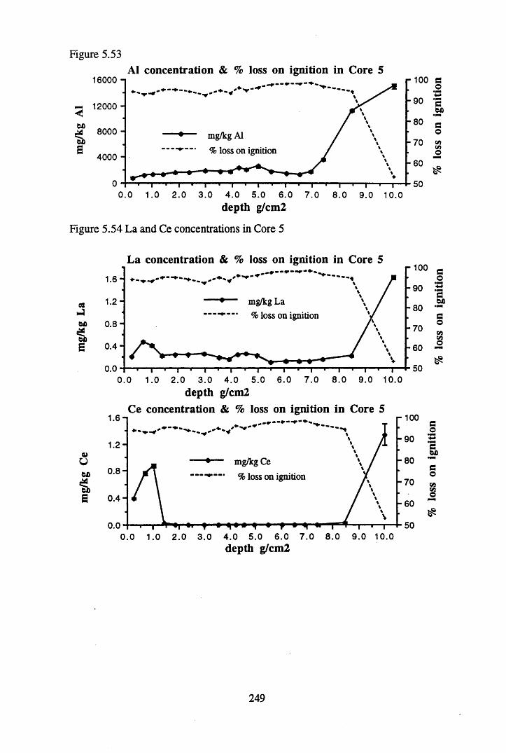
Figure 5.53Al concentration & % loss on ignition in Core 5
16000
12000
mg/kg Al % loss on ignition
4000
0.0 1.0 2.0 3.0 4.0 5.0 6.0 7 .0 8 .0 9.0 10.0depth g/cm2
Figure 5.54 La and Ce concentrations in Core 5
La concentration & % loss on ignition in Core 5
1.6-
ea 1.2-■
OX) 0 .8-& ■s 0 .4-
0 .0-0.
1.6-
1.2-<uUOJD 0.8-
s 0.4-
♦ mg/kg La% loss on ignition
« r
r 100 eo-90 •mm• cOX)-80 •mm
-70GOVi
-60Vi©
-50&
depth g/cm2 Ce concentration & % loss on ignition in Core 5
-----M
0.0
mg/kg Ce % loss on ignition
■ i K | i . »—T ■ I ■ i0.0 1.0 2.0 3.0 4.0 5.0 6.0 7 .0 8 .0 9.0 10.0
depth g/cm2
- 100 s
oo>
o•MeOil
• 1 CO o •mm
eo-7 0 ViVi-6 0
O
oin__L
249
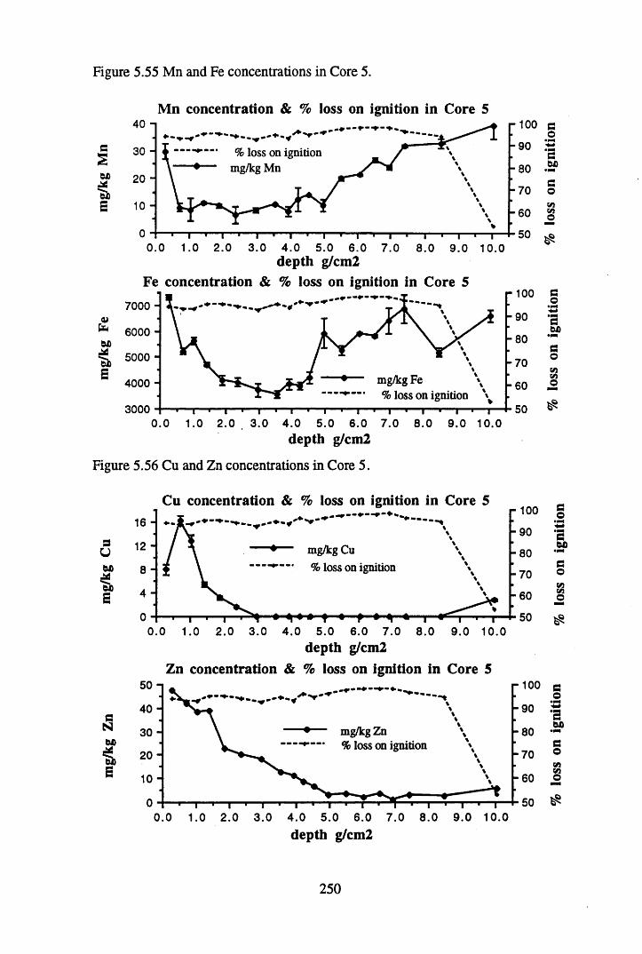
Figure 5.55 Mn and Fe concentrations in Core 5.
Mn concentration & % loss on ignition in Core 5
eStt>
E
40 -
30 -
20 -
10 -
0
% loss on ignition
-i—i—i—i—i— i—i—i—i—i—i—|—i—|—i— |—i—|—i—|—0 .0 1 .0 2 .0 3 .0 4 .0 5 .0 6 .0 7 .0 8 .0 9 .0 10 .0
depth g/cm2Fe concentration & % loss on ignition in Core 5
-100
-9 0
-8 0
-7 0
-6 0
50
7000 -
to 6000 -&A
£ 5000 -s
4000 -
3000 -
mg/kg Fe % loss on ignition
— i— 1— i— 1— i— 1— i— ■— i— 1— i— i— i— >— i— •— i— >— i—0 .0 1.0 2 .0 3 .0 4 .0 5 .0 6 .0 7 .0 8 .0 9 .0 10 .0
- 100
-9 0
-8 0
-7 0
-6 0
50
depth g/cm2
Figure 5.56 Cu and Zn concentrations in Core 5.
sUW>*S
16 -
12 -
8 -
4 -
0
Cu concentration & % loss on ignition in Core 5* \
%\mg/kg Cu \
------,---- % iQgg on ignition \
E
50 -
40 -N 30 -SL
t 2 0 -s 10 -
0 -
, , , , ■ I0 .0 1.0 2 .0 3 .0 4 .0 5 .0 6 .0 7 .0 8 .0 9 .0 10 .0
depth g/cm2 Zn concentration & % loss on ignition in Core 5
-100
-9 0
-8 0
-7 0
-6 0
50
r 100
mg/kg Zn— • % loss on ignition
0 .0 1.0 2 .0 3 .0 4 .0 5 .0 6 .0 7 .0 8 .0 9 .0 10 .0depth g/cm2
250
% los
s on
igni
tion
% |
oss
on ig
nitio
n
Ioss
011
*Sni
tion
Ios
s on
"S11*
^011
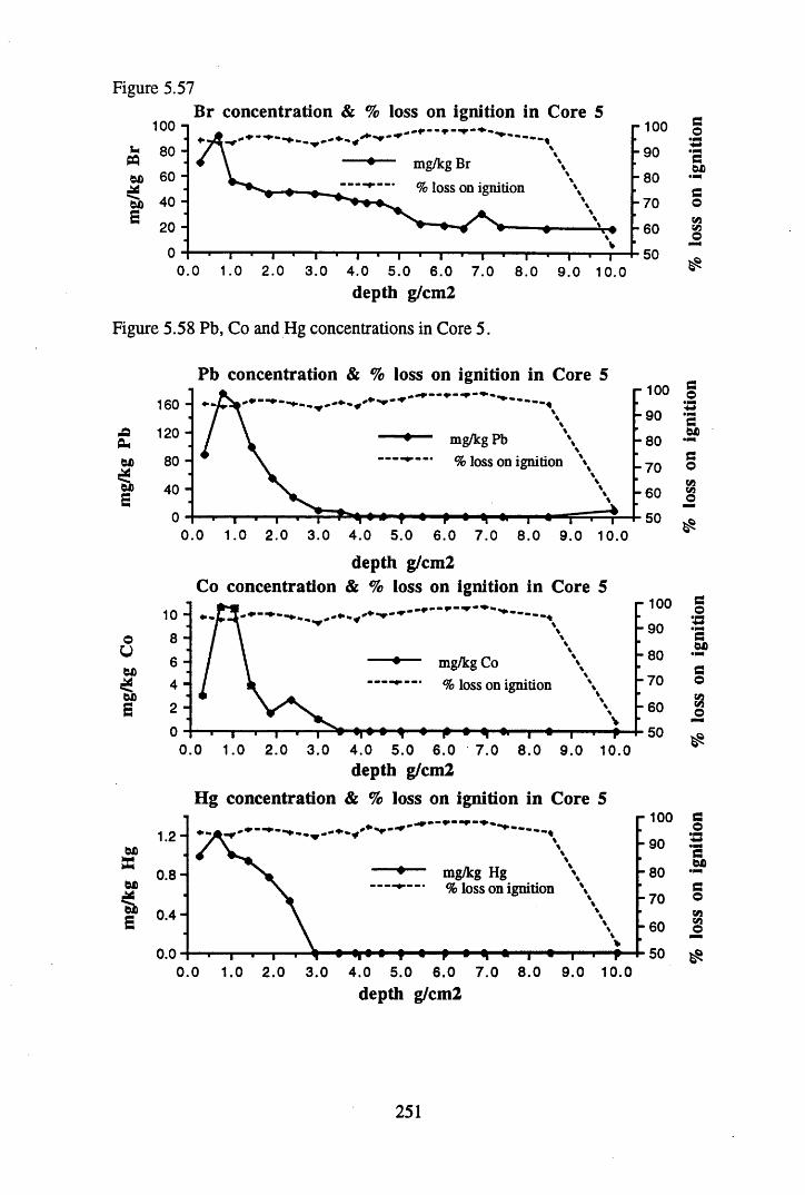
Figure 5.57
100 H
£ 80 Hwex 60 - a
"ox 40 -
® 20 -
Br concentration & % loss on ignition in Core 5***♦
mg/kg Br \
% loss on ignition \
— ♦— ■ ■ i ♦ \ vi—1—i—«—rT ' T
- 100-9 0
-8 0
-7 0
- 6 0
500 .0 1.0 2 .0 3 .0 4 .0 5 .0 6 .0 7 .0 8 .0 9 .0 10.0
depth g/cm2
Figure 5.58 Pb, Co and Hg concentrations in Core 5.
Pb concentration & % loss on ignition in Core 5
-Q
6X
'SiS
ox
exSE
160 H
120 80 -
40 -
mg/kg Pb % loss on ignition
10 -
o 8 -u
6 -ex4 -
exE 2 -
0 -
0 H—i—i—i—i—i—I » »- f ' • p • 4 * | • | , ,0 .0 1 .0 2 .0 3 .0 4 .0 5 .0 6 .0 7 .0 8 .0 9 .0 10.0
depth g/cm2Co concentration & % loss on ignition in Core 5
10090
80
70
60
50
mg/kg Co % loss on ignition
1.2-
0.8-
0 .4 -
0.0
I ' P—0 .0 1 .0 2 .0 3 .0 4 .0 5 .0 6 .0 7 .0 8 .0 9 .0 10.0
depth g/cm2Hg concentration & % loss on ignition in Core 5
\
10090
80
70
60
50
mg/kg Hg— % loss on ignition \
10090
80
70
60
500 .0 1.0 2 .0 3 .0 4 .0 5 .0 6 .0 7 .0 8 .0 9 .0 10 .0
depth g/cm2
251
% l
oss
on ig
nitio
n %
los
s on
igni
tion
*oss
on *8
niti
°n %
loss
on ig
nitio
n
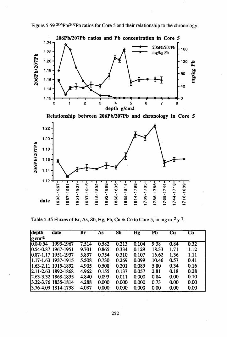
Figure 5.59 206Pb/207Pb ratios for Core 5 and their relationship to the chronology.
,aPU|r-oNAPuVOON
pOCuoNuaPmvoo
206Pb/207Pb ratios and Pb concentration in Core 5
206Pb/207Pb mg/kg Pb
1.24-
1.22-
1.20-
1.18-
1.16-
1 .14-
I I 0
- 160
- 120 jacuoc
-8 0W)S
-4 0
3 4 5depth g/cm2
Relationship between 206Pb/207Pb and chronology in Core 5
1.22-
1.20-
1.18-
1.16-
1 .14-
1.12
date
“ i— i----- 1---- 1-----1---- 1'---- 1---- 1----- 1---- ------T "■ n " "•— 1— i'---- 1---- 1>■” 1— i1— I— 11— 1— i1— l— i1----1---- 1r - T— N- in CM 00 in ■M- oo in 00 CO 05CO m CO ■r— 05 CO CO T- 05 00 CO COo> 05 o> O) CO 00 CO CO N- r*- 1^ CO* - *“ *— ▼- ■*“ ■*—CO 2 - in CM 00 in 05 in 00 0005 ID in CO T— 05 CO CO ■»— oo 00 CO ■M"a> O) o> 05 05 00 oo CO 00 r*. r* »*•» r^.T— T“ T— T— T“ y— T” T” T“ T—
Table 5.35 Fluxes of Br, As, Sb, Hg, Pb, Cu & Co to Core 5, in mg m-2 y 1.
depth date gem '2
Br As Sb Hg Pb Cu Co
0.0-0.54 1993-1967 7.514 6.5&2 0.213 0.104 9.38 0.84 0.320.54-0.87 1967-1951 9.701 0.865 0.334 0.129 18.33 1.71 1.120.87-1.17 1951-1937 5.837 0.754 0.310 0.107 16.62 1.36 1.111.17-1.63 1937-1915 5.508 0.730 0.269 0.099 10.46 0.57 0.411.63-2.11 1915-1892 4.905 0.508 0.201 0.083 5.80 0.34 0.162.11-2.63 1892-1868 4.962 0.155 0.137 0.057 2.81 0.18 0.282.63-3.32 1868-1835 4.840 0.093 0.011 0.000 0.84 0.00 0.103.32-3.76 1835-1814 4.288 0.000 0.000 0.000 0.73 0.00 0.003.76-4.09 1814-1798 4.087 0.000 0.000 0.000 0.00 0.00 0.00
252
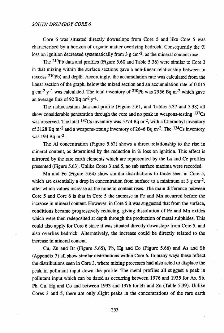
SOUTH DRUMBOY CORE 6
Core 6 was situated directly downslope from Core 5 and like Core 5 was characterised by a horizon of organic matter overlying bedrock. Consequently the % loss on ignition decreased systematically from 3 g cm*2, as the mineral content rose.
The 210Pb data and profiles (Figure 5.60 and Table 5.36) were similar to Core 3 in that mixing within the surface sections gave a non-linear relationship between In (excess 210Pb) and depth. Accordingly, the accumulation rate was calculated from the linear section of the graph, below the mixed section and an accumulation rate of 0.015 g cm-2 y_1 was calculated. The total inventory of 2l°Pb was 2956 Bq m-2 which gave an average flux of 92 Bq m-2 y 1.
The radiocaesium data and profile (Figure 5.61, and Tables 5.37 and 5.38) all show considerable penetration through the core and no peak in weapons-testing 137Cs was observed. The total 137Cs inventory was 5774 Bq n r2, with a Chernobyl inventory of 3128 Bq n r 2 and a weapons-testing inventory of 2646 Bq n r2. The 134Cs inventory was 194 Bq m-2.
The Al concentration (Figure 5.62) shows a direct relationship to the rise in mineral content, as determined by the reduction in % loss on ignition. This effect is mirrored by the rare earth elements which are represented by the La and Ce profiles presented (Figure 5.63). Unlike Cores 3 and 5, no sub surface maxima were recorded.
Mn and Fe (Figure 5.64) show similar distributions to those seen in Core 5, which are essentially a drop in concentration from surface to a minimum at 3 g cm-2, after which values increase as the mineral content rises. The main difference between Core 5 and Core 6 is that in Core 5 the increase in Fe and Mn occurred before the increase in mineral content. However, in Core 5 it was suggested that from the surface, conditions became progressively reducing, giving dissolution of Fe and Mn oxides which were then redeposited at depth through the production of metal sulphides. This could also apply for Core 6 since it was situated directly downslope from Core 5, and also overlies bedrock. Alternatively, the increase could be directly related to the increase in mineral content.
Cu, Zn and Br (Figure 5.65), Pb, Hg and Co (Figure 5.66) and As and Sb (Appendix 3) all show similar distributions within Core 6. In many ways these reflect the distributions seen in Core 3, where mixing processes had also acted to displace the peak in pollutant input down the profile. The metal profiles all suggest a peak in pollutant input which can be dated as occurring between 1976 and 1935 for As, Sb, Pb, Cu, Hg and Co and between 1993 and 1976 for Br and Zn (Table 5.39). Unlike Cores 3 and 5, there are only slight peaks in the concentrations of the rare earth
253
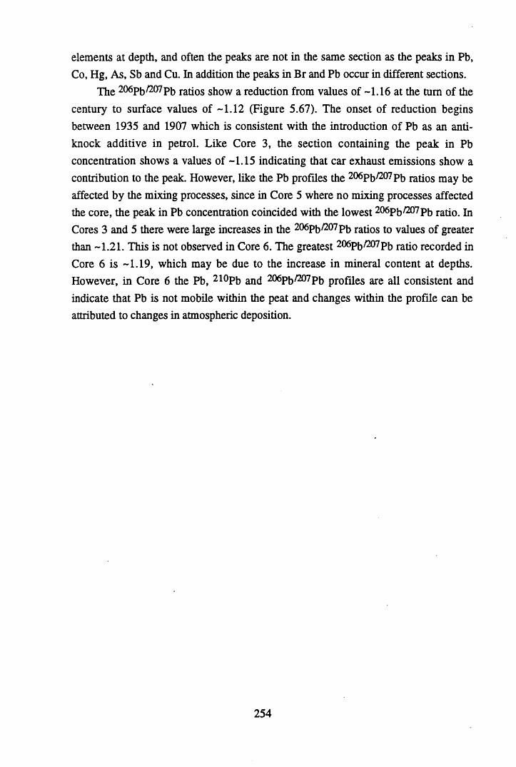
elements at depth, and often the peaks are not in the same section as the peaks in Pb, Co, Hg, As, Sb and Cu. In addition the peaks in Br and Pb occur in different sections.
The 206pb/207pb ratios show a reduction from values of -1.16 at the turn of the century to surface values of -1.12 (Figure 5.67). The onset of reduction begins between 1935 and 1907 which is consistent with the introduction of Pb as an antiknock additive in petrol. Like Core 3, the section containing the peak in Pb concentration shows a values of -1.15 indicating that car exhaust emissions show a contribution to the peak. However, like the Pb profiles the 206pb/207pb ratios may be affected by the mixing processes, since in Core 5 where no mixing processes affected the core, the peak in Pb concentration coincided with the lowest 206pb/207pb ratj0 jn Cores 3 and 5 there were large increases in the 206pb/207pt> ratios to values of greater than -1.21. This is not observed in Core 6. The greatest 206pb/207pb rati0 recorded in Core 6 is -1.19, which may be due to the increase in mineral content at depths. However, in Core 6 the Pb, 210Pb and 206pb/207pb profiles are all consistent and indicate that Pb is not mobile within the peat and changes within the profile can be attributed to changes in atmospheric deposition.
254
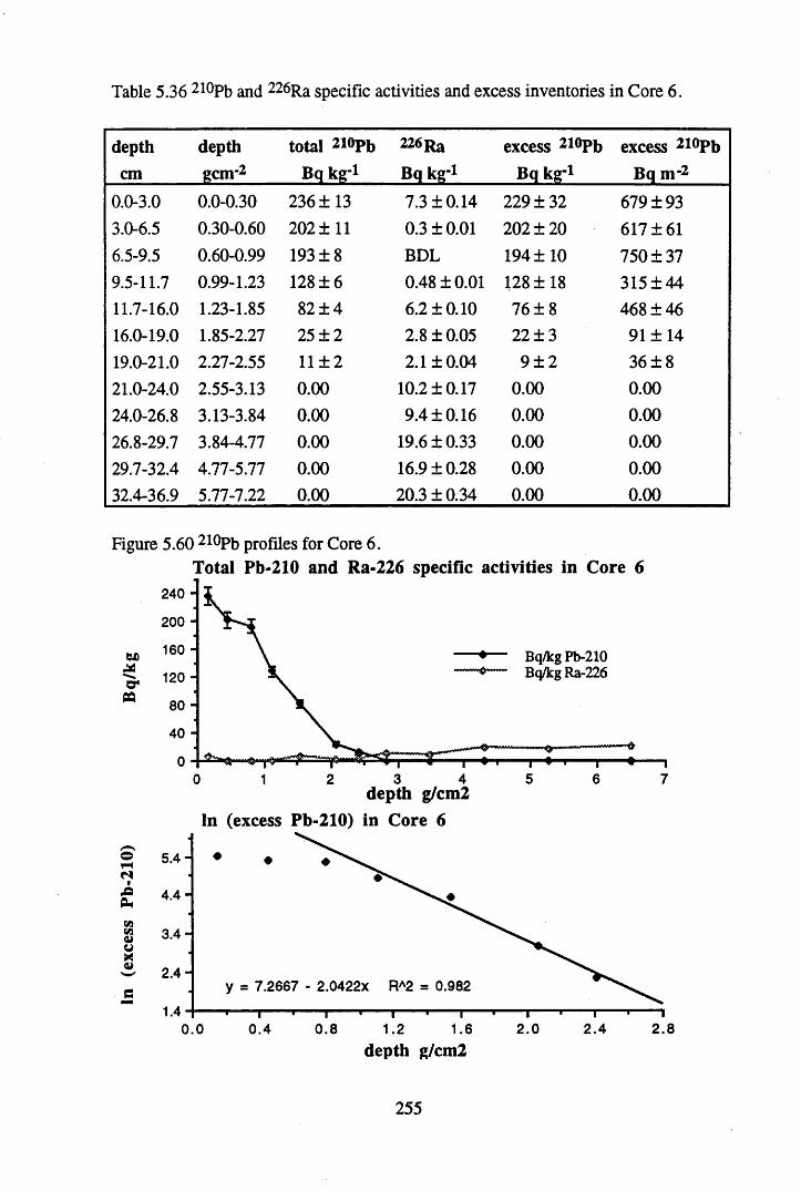
Table 5.36 210Pb and 226Ra specific activities and excess inventories in Core 6.
depth depth total 210Pb 226Ra excess 2i°Pb excess 2i°Pbcm gem-2 Bq kg-l Bq kg-l Bq kg-l Bq m-2
0.0-3.0 0.0-0.30 236 ±13 7.3 ±0.14 229 ±32 679 ±933.0-6.5 0.30-0.60 202 ±11 0.3 ±0.01 202 ±20 617 ±616.5-9.5 0.60-0.99 193 ±8 BDL 194 ±10 750 ±379.5-11.7 0.99-1.23 128 ± 6 0.48 ±0.01 128 ±18 315±4411.7-16.0 1.23-1.85 82 ± 4 6.2 ±0.10 76 ± 8 468 ±4616.0-19.0 1.85-2.27 25 ± 2 2.8 ±0.05 22 ±3 91 ±1419.0-21.0 2.27-2.55 11 ± 2 2.1 ±0.04 9 ± 2 36 ±821.0-24.0 2.55-3.13 0.00 10.2 ±0.17 0.00 0.0024.0-26.8 3.13-3.84 0.00 9.4 ±0.16 0.00 0.0026.8-29.7 3.84-4.77 0.00 19.6 ±0.33 0.00 0.0029.7-32.4 4.77-5.77 0.00 16.9 ±0.28 0.00 0.0032.4-36.9 5.77-7.22 0.00 20.3 ±0.34 0.00 0.00
Figure 5.60 210Pb profiles for Core 6.Total Pb-210 and Ra-226 specific activities in Core 6
240 -
200 -
Bq/kg Pb-210 Bq/kg Ra-226
40 -
"fr-TUQl nifli |1 2 4 5 6 70 3
depth g/cm2 In (excess Pb-210) in Core 6
o 5 .4 -
4 .4 -
3 .4 -
2 .4 -.2667 - 2.0422X RA2 a 0.982
1.42.4 2.80.8 1.2 1.6 2.00.0 0.4
depth g/cm2
255
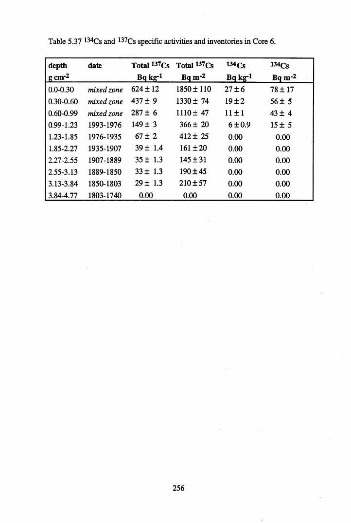
Table 5.37 134Cs and 137Cs specific activities and inventories in Core 6.
depthgem-2
date Total 137Cs Bq kg-l
Total l37Cs Bq n r 2
134Cs Bq kg-l
134cs Bq m -2
0.0-0.30 mixed, zone 624 ±12 1850 ±110 27 ± 6 78 ±170.30-0.60 mixed zone 437 ± 9 1330 ± 74 19 ± 2 56 ± 50.60-0.99 mixed zone 287 ± 6 1110 ± 47 11 ± 1 43 ± 40.99-1.23 1993-1976 149 ± 3 366 ± 20 6 ±0.9 15 ± 51.23-1.85 1976-1935 67 ± 2 412 ± 25 0.00 0.001.85-2.27 1935-1907 39 ± 1.4 161 ±20 0.00 0.002.27-2.55 1907-1889 35 ± 1.3 145 ±31 0.00 0.002.55-3.13 1889-1850 33 ± 1.3 190 ±45 0.00 0.003.13-3.84 1850-1803 29 ± 1.3 210 ±57 0.00 0.003.84-4.77 1803-1740 0.00 0.00 0.00 0.00
256

Table 5.38 Chernobyl and weapons-testing 137Cs specific activities and inventories inCore 6.
depth date Chernobyl Chernobyl Weapons Weaponsgem-2 137CS !37Cs testing 137Cs testing 137Cs
Bq kg-1 Bq nr2 Bq kg-1 Bq nr20.0-0.30 mixed zone 428 ±52 1267 ± 154 196 ±24 579 ±710.30-0.60 mixed zone 299 ±28 914 ± 85 137 ± 13 418 ±390.60-0.99 mixed zone 181 ±13 702 ± 56 106 ± 8 410 ±300.99-1.23 1993-1976 99 ±14 245 ± 35 67 ± 2 121 ± 81.23-1.85 1976-1935 0.00 0.00 49 ± 7 412 ± 251.85-2.27 1935-1907 0.00 0.00 39 ± 2 161 ±202.27-2.55 1907-1889 0.00 0.00 35 ± 2 145 ±312.55-3.13 1889-1850 0.00 0.00 33 ± 1 190 ±453.13-3.84 1850-1803 0.00 0.00 30 ± 1 210 ±573.84-4.77 1803-1740 0.00 0.00 0.00 0.00
Figure 5.61Chernobyl & Weapons testing Cs-137 in Core 6
U200
-400
-320Cfl4> weapons testing Cs-137 Chernobyl Cs-137
120 - -240
80 - - 160
40 - -80
2 3 4 50 1 6 7
t-
ViU
.c©Gu<u
J3UOA«O'CQ
depth g/cm2
257
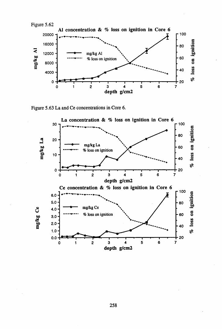
Figure 5.62AI concentration & % loss on ignition in Core 6
r 10020000 i
16000 - -8 0
^ 12000 - MO X"Sc 8000 -s
4000 -
mg/kg Al % loss on ignition -6 0
-4 0
205 63 4 71 20
depth g/cm2
Figure 5.63 La and Ce concentrations in Core 6.
r 10030
8020
mg/kg La % loss on ignition
60
40
2075 63 41 20
<wUWDW>E
depth g/cm2Ce concentration & % loss on ignition in Core 6
1006.05.0 -8 0
mg/kg Ce
% loss on ignition4.0
603.0
2.0-40
200.074 5 6320 1
depth g/cm2
258
% l
oss
on ig
nitio
n %
los
s on
igni
tion
% los
s on
igni
tion
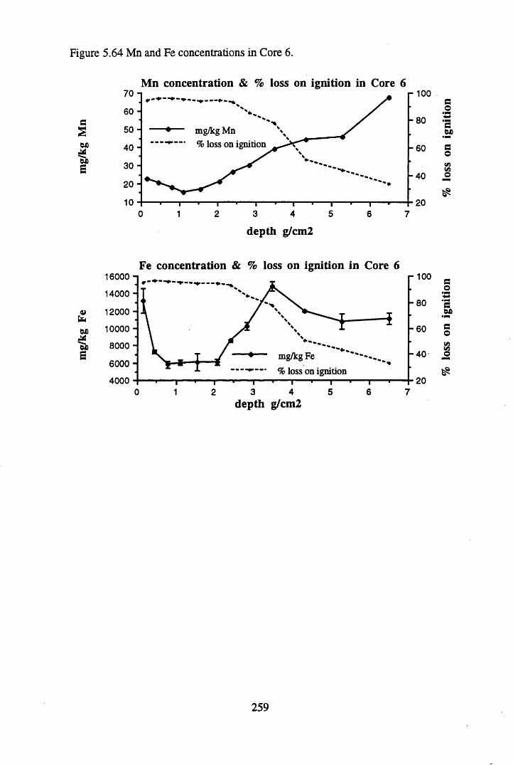
mg/k
g Fe
mg/k
g M
n
Figure 5.64 Mn and Fe concentrations in Core 6.
Mn concentration & % loss on ignition in Core 670 -1 r 100
60 --8 0
50 - — mg/kg Mn% loss on ignition40 - -6 0
30 --4 0
20 -
202 3 4 50 1 6 7
depth g/cm2
Fe concentration & % loss on ignition in Core 616000 10014000 -
8012000 -
10000 - 60
800040mg/kg Fe
% loss on ignition6000
20400043 5 6 70 1 2
depth g/cm2
259
% los
s on
igni
tion
% l
oss
on ig
nitio
n
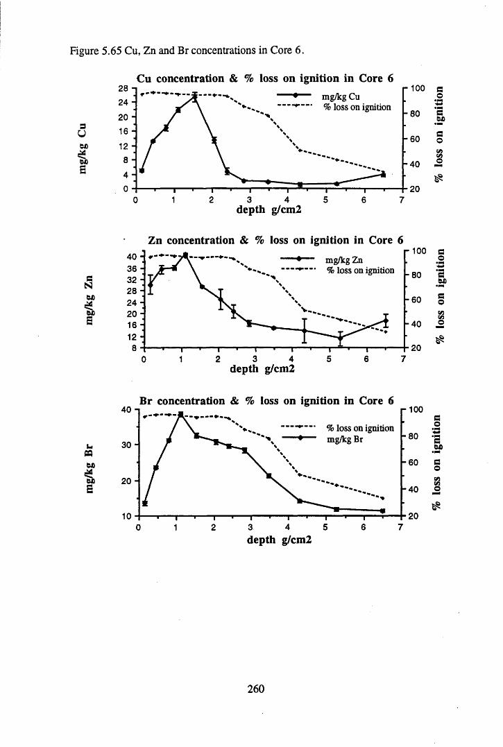
Figure 5.65 Cu, Zn and Br concentrations in Core 6.
Cu concentration & % loss on ignition in Core 610028
24 mg/kg Cu % loss on ignition
-8 02016
60128 4040 20
2 4 51 3 6 70depth g/cm2
eN6X1
E
Zn concentration & % loss on ignition in Core 6100
40 - 36 - 32 : 28 " 24 - 20 :
mg/kg Zn % loss on ignition -8 0
-6 0
-4 012 -
3 5 72 4 60 1depth g/cm2
uCQ6X1«=£6X5s
Br concentration & % loss on ignition in Core 6r 10040 -I
% loss on ignition mg/kg Br -8 0
30 -
-6 0
20 -40
2074 5 61 2 30
depth g/cm2
260
% l
oss
on ig
nitio
n %
joss
on ig
nitio
n %
loss
on ig
nitio
n
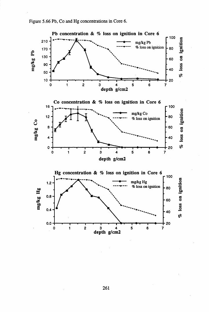
Figure 5.66 Pb, Co and Hg concentrations in Core 6.
Pb concentration & % loss on ignition in Core 6T r 100
* mg/kg Pb/ "* % loss on ignition - qq
0 1 2 3 4 5 6 7depth g/cm2
Co concentration & % loss on ignition in Core 6r 100
mg/kg Co % loss on ignition12 - -8 0
-6 0
-4 0
200 2 5 6 71 3 4
depth g/cm2
Hg concentration & % loss on ignition in Core 6r 100
mg/kg Hg % loss on ignition
1 .2 -
-00&AH*A 0 .8 -
S 0-4.-6 0
-4 0
0.0 206 70 1 2 3 4 5
depth g/cm2
261
% l
oss
on ig
nitio
n %
|oss
on
igni
tion
% los
s on
igni
tion
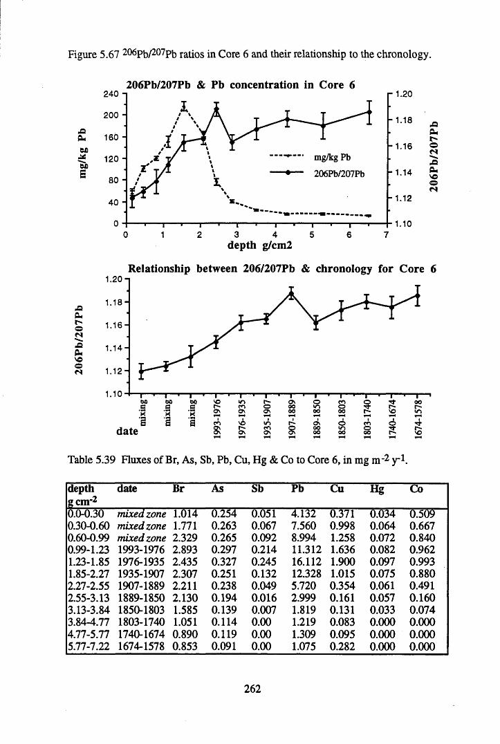
Figure 5.67 2°6pb/207pb ratios in Core 6 and their relationship to the chronology.
206Pb/207Pb & Pb concentration in Core 6
CUoN
OnVC©
240 -i 1.20
200 - 1.18
160 -
mg/kg Pb
206Pb/207Pb
1201.14
80
1.1240
1.103 4 50 1 2 76
jacut"oNSCUVOoN
depth g/cm2
Relationship between 206/207Pb & chronology for Core 6
1 .16-
1 .14-
1. 1 2 -
1.10ooo
OQa ON00oo
«r>mON
enooo00r-~«n
vor-ON
ONOOOO
mo00
ir> 00date
Table 5.39 Fluxes of Br, As, Sb, Pb, Cu, Hg & Co to Core 6, in mg m-2 y 1.
depthgem’2
date Br As Sb Pb Cu Hg Co
0.0-0.30 mixed zone 1.014 0.254 0.051 4.132 0.371 0.034 0.5090.30-0.60 mixed zone 1.771 0.263 0.067 7.560 0.998 0.064 0.6670.60-0.99 mixed zone 2.329 0.265 0.092 8.994 1.258 0.072 0.8400.99-1.23 1993-1976 2.893 0.297 0.214 11.312 1.636 0.082 0.9621.23-1.85 1976-1935 2.435 0.327 0.245 16.112 1.900 0.097 0.9931.85-2.27 1935-1907 2.307 0.251 0.132 12.328 1.015 0.075 0.8802.27-2.55 1907-1889 2.211 0.238 0.049 5.720 0.354 0.061 0.4912.55-3.13 1889-1850 2.130 0.194 0.016 2.999 0.161 0.057 0.1603.13-3.84 1850-1803 1.585 0.139 0.007 1.819 0.131 0.033 0.0743.84-4.77 1803-1740 1.051 0.114 0.00 1.219 0.083 0.000 0.0004.77-5.77 1740-1674 0.890 0.119 0.00 1.309 0.095 0.000 0.0005.77-7.22 1674-1578 0.853 0.091 0.00 1.075 0.282 0.000 0.000
262
5.4.3 DISCUSSION OF THE RESULTS RECORDED AND THE RELATIONSHIPS BETWEEN THE SOUTH DRUMBOY CORES
One of the main aims of this thesis was to evaluate the validity of using 210Pb as a dating mechanism in organic soils. The results for the South Drumboy cores clearly demonstrate that 210Pb should be used with caution in situations where land management practices can result in the disturbance of profiles and accordingly the disturbance of 210Pb profiles. Even though obviously disturbed areas were not sampled, this affected 3 out of the 6 cores studied with the most pronounced disturbance being noted in Core 4. The insertion of drainage channels on the easterly facing slope resulted in an increase in the total inventory and average flux of 2i°Pb in Core 1, compared to Core 2, with the majority of the 210Pb contained in the surface section (Table 5.40).
There was also a slight increase in inventory and flux values from Core 5 to Core 6, which may be indicating some lateral flow of 210Pb. Lateral flow of 2i°Pb in peat profiles has previously been suggested to occur (Maguire, 1994: El-Daoushy, 1988: Oldfield et al., 1979) and often results in a reduction in the 210Pb inventory of the profile up slope (Mitchell et a l , 1992). Urban et a l (1990) proposed that 210Pb could be moving with dissolved organic matter, particularly where the peat is waterlogged and consequently reduced.
The highest inventory and flux values were recorded in Core 3, which was situated towards the summit of Drumboy Hill. This may be indicating that the flux of 210Pb to these sites is affected by altitude with Core 3 receiving preferential deposition. Increased mist cover at higher altitudes has previously been reported to influence the deposition of 210Pb (Olsen etal, 1985: Urban et a l , 1990).
The average flux values correspond well to previous measurements in ombrotrophic peat cores (Table 5.41). The values recorded by Sugden (1993) in a study of ombrotrophic peat cores from various sites around Scotland agree particularly well, with average flux values ranging from 71.3 -150.0 Bq m-2 y 1. The higher values were recorded in sites with higher rainfall.
263
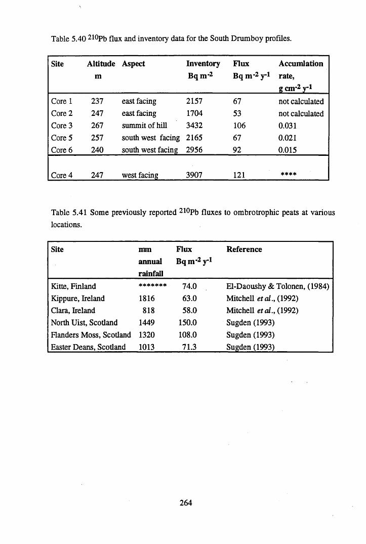
Table 5.40 210Pb flux and inventory data for the South Drumboy profiles.
Site Altitudem
Aspect InventoryB qm ’2
FluxBq n r 2 y 1
Accumlationrate,g cm-2 y 1
Core 1 237 east facing 2157 67 not calculatedCore 2 247 east facing 1704 53 not calculatedCore 3 267 summit of hill 3432 106 0.031Core 5 257 southwest facing 2165 67 0.021Core 6 240 south west facing 2956 92 0.015
Core 4 247 west facing 3907 121
Table 5.41 Some previously reported 210Pb fluxes to ombrotrophic peats at various locations.
Site mmannualrainfall
FluxBq m*2 y 1
Reference
Kitte, Finland ******* 74.0 El-Daoushy & Tolonen, (1984)Kippure, Ireland 1816 63.0 Mitchell etal., (1992)Clara, Ireland 818 58.0 Mitchell etal., (1992)North Uist, Scotland 1449 150.0 Sugden (1993)Flanders Moss, Scotland 1320 108.0 Sugden (1993)Easter Deans, Scotland 1013 71.3 Sugden (1993)
264
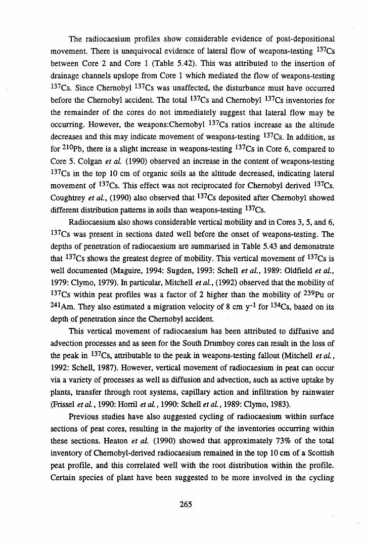
The radiocaesium profiles show considerable evidence of post-depositional movement. There is unequivocal evidence of lateral flow of weapons-testing 137Cs between Core 2 and Core 1 (Table 5.42). This was attributed to the insertion of drainage channels upslope from Core 1 which mediated the flow of weapons-testing 137Cs. Since Chernobyl 137Cs was unaffected, the disturbance must have occurred before the Chernobyl accident. The total 137Cs and Chernobyl 137Cs inventories for the remainder of the cores do not immediately suggest that lateral flow may be occurring. However, the weapons:Chemobyl 137Cs ratios increase as the altitude decreases and this may indicate movement of weapons-testing 137Cs. In addition, as for 210Pb, there is a slight increase in weapons-testing 137Cs in Core 6, compared to Core 5. Colgan et al (1990) observed an increase in the content of weapons-testing 137Cs in the top 10 cm of organic soils as the altitude decreased, indicating lateral movement of 137Cs. This effect was not reciprocated for Chernobyl derived 137Cs. Coughtrey e ta l , (1990) also observed that 137Cs deposited after Chernobyl showed different distribution patterns in soils than weapons-testing 137Cs.
Radiocaesium also shows considerable vertical mobility and in Cores 3, 5, and 6, 137Cs was present in sections dated well before the onset of weapons-testing. The depths of penetration of radiocaesium are summarised in Table 5.43 and demonstrate that 137Cs shows the greatest degree of mobility. This vertical movement of 137Cs is well documented (Maguire, 1994: Sugden, 1993: Schell e ta l , 1989: Oldfield et a l, 1979: Clymo, 1979). In particular, Mitchell et a l , (1992) observed that the mobility of 137Cs within peat profiles was a factor of 2 higher than the mobility of 239Pu or 241Am. They also estimated a migration velocity of 8 cm y_1 for 134Cs, based on its depth of penetration since the Chernobyl accident
This vertical movement of radiocaesium has been attributed to diffusive and advection processes and as seen for the South Drumboy cores can result in the loss of the peak in 137Cs, attributable to the peak in weapons-testing fallout (Mitchell et a l , 1992: Schell, 1987). However, vertical movement of radiocaesium in peat can occur via a variety of processes as well as diffusion and advection, such as active uptake by plants, transfer through root systems, capillary action and infiltration by rainwater (Frissel e ta l , 1990: Horril etal. , 1990: Schell e ta l , 1989: Clymo, 1983).
Previous studies have also suggested cycling of radiocaesium within surface sections of peat cores, resulting in the majority of the inventories occurring within these sections. Heaton et a l (1990) showed that approximately 73% of the total inventory of Chernobyl-derived radiocaesium remained in the top 10 cm of a Scottish peat profile, and this correlated well with the root distribution within the profile. Certain species of plant have been suggested to be more involved in the cycling
265
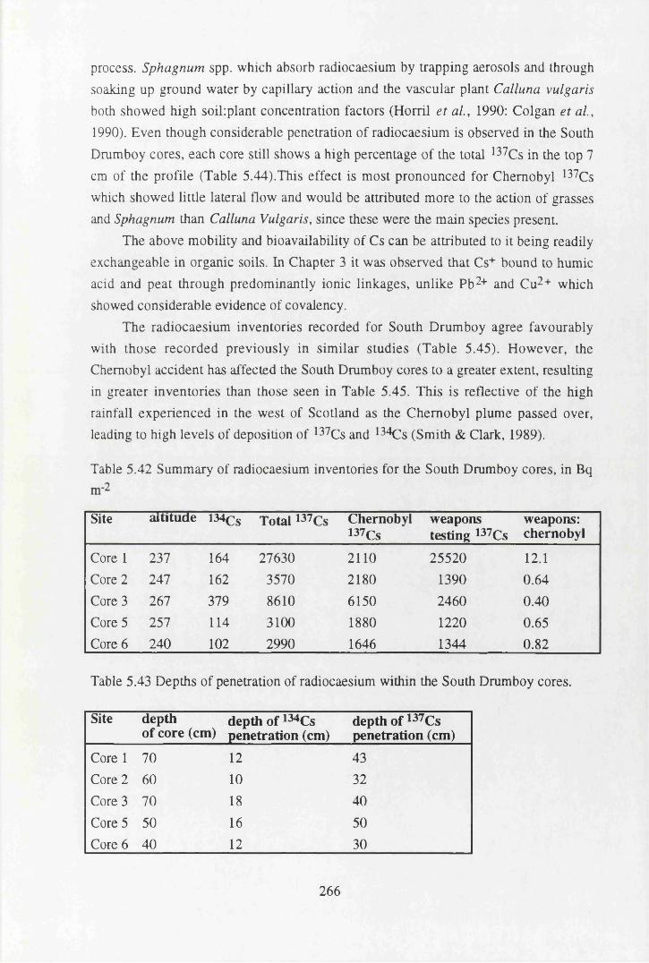
process. Sphagnum spp. which absorb radiocaesium by trapping aerosols and through
soaking up ground water by capillary action and the vascular plant Calluna vulgaris
both showed high soikplant concentration factors (Horril et al., 1990: Colgan et al.,
1990). Even though considerable penetration of radiocaesium is observed in the South
Drumboy cores, each core still shows a high percentage of the total 137Cs in the top 7
cm of the profile (Table 5.44).This effect is most pronounced for Chernobyl 137Cs
which showed little lateral flow and would be attributed more to the action of grasses and Sphagnum than Calluna Vulgaris, since these were the main species present.
The above mobility and bioavailability of Cs can be attributed to it being readily exchangeable in organic soils. In Chapter 3 it was observed that Cs+ bound to humic
acid and peat through predominantly ionic linkages, unlike Pb2+ and Cu2+ which showed considerable evidence of covalency.
The radiocaesium inventories recorded for South Drumboy agree favourably with those recorded previously in similar studies (Table 5.45). However, the
Chernobyl accident has affected the South Drumboy cores to a greater extent, resulting in greater inventories than those seen in Table 5.45. This is reflective of the high
rainfall experienced in the west of Scotland as the Chernobyl plume passed over, leading to high levels of deposition of 137Cs and 134Cs (Smith & Clark, 1989).
Table 5.42 Summary of radiocaesium inventories for the South Drumboy cores, in Bq
Site altitude 134CS Total 137Cs Chernobyl137Cs
weapons testing 137Cs
weapons:chernobyl
Core 1 237 164 27630 2110 25520 12.1Core 2 247 162 3570 2180 1390 0.64Core 3 267 379 8610 6150 2460 0.40Core 5 257 114 3100 1880 1220 0.65Core 6 240 102 2990 1646 1344 0.82
Table 5.43 Depths of penetration of radiocaesium within the South Drumboy cores.
Site depthof core (cm)
depth of 134Cs penetration (cm)
depth of 137Cs penetration (cm)
Core 1 70 12 43Core 2 60 10 32Core 3 70 18 40Core 5 50 16 50Core 6 40 12 30
266
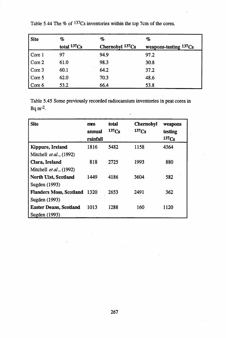
Table 5.44 The % of 137Cs inventories within the top 7cm of the cores.
Site %total 137Cs
%Chernobyl 137Cs
%weapons-testing 137Cs
Core 1 97 94.9 97.2Core 2 61.0 98.3 30.8Core 3 60.1 64.2 37.2Core 5 62.0 70.3 48.6Core 6 53.2 66.4 53.8
Table 5.45 Some previously recorded radiocaesium inventories in peat cores in Bq m-2
Site ran total Chernobyl weaponsannual 137Cs 137Cs testingrainfall 137Cs
Kippure, Ireland 1816 5482 1158 4364Mitchell etal., (1992)Clara, Ireland 818 2725 1993 880Mitchell etal., (1992)North Uist, Scotland 1449 4186 3604 582Sugden (1993)Flanders Moss, Scotland 1320 2653 2491 362Sugden (1993)Easter Deans, Scotland 1013 1288 160 1120Sugden (1993)
267
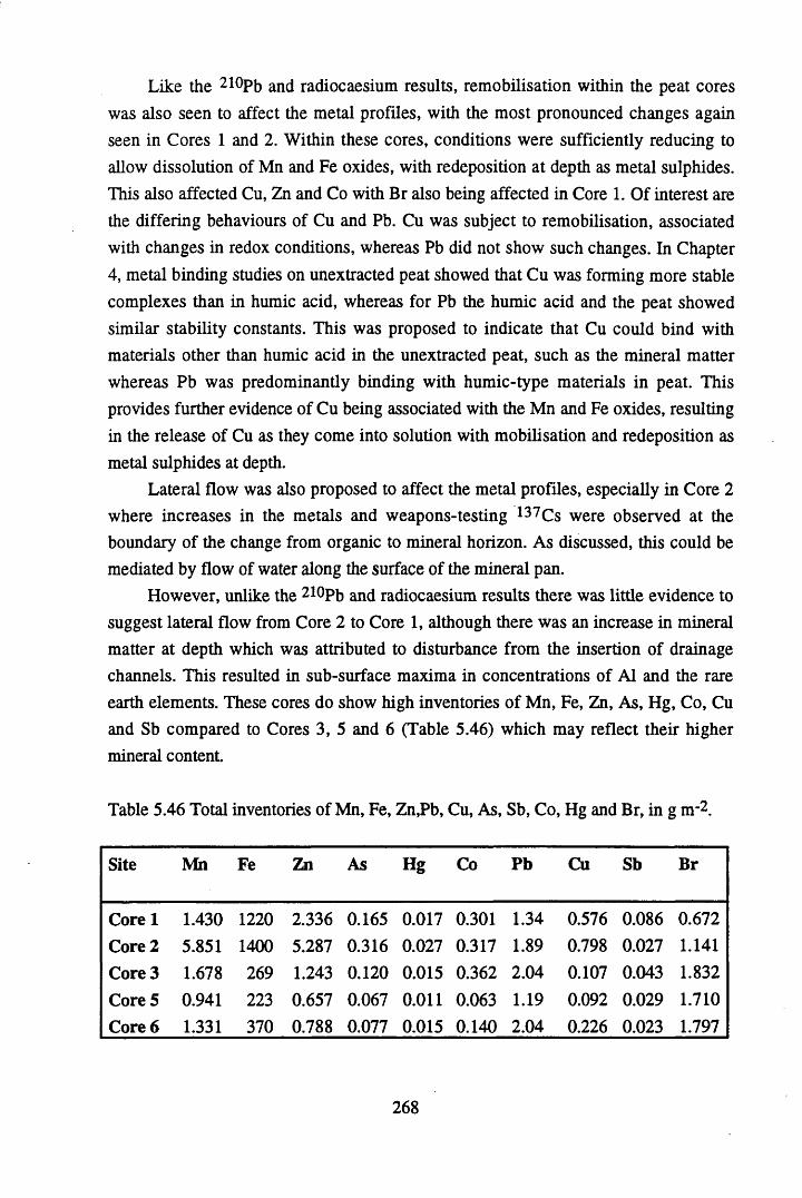
Like the 210Pb and radiocaesium results, remobilisation within the peat cores was also seen to affect the metal profiles, with the most pronounced changes again seen in Cores 1 and 2. Within these cores, conditions were sufficiently reducing to allow dissolution of Mn and Fe oxides, with redeposition at depth as metal sulphides. This also affected Cu, Zn and Co with Br also being affected in Core 1. Of interest are the differing behaviours of Cu and Pb. Cu was subject to remobilisation, associated with changes in redox conditions, whereas Pb did not show such changes. In Chapter 4, metal binding studies on unextracted peat showed that Cu was forming more stable complexes than in humic acid, whereas for Pb the humic acid and the peat showed similar stability constants. This was proposed to indicate that Cu could bind with materials other than humic acid in the unextracted peat, such as the mineral matter whereas Pb was predominantly binding with humic-type materials in peat. This provides further evidence of Cu being associated with the Mn and Fe oxides, resulting in the release of Cu as they come into solution with mobilisation and redeposition as metal sulphides at depth.
Lateral flow was also proposed to affect the metal profiles, especially in Core 2 where increases in the metals and weapons-testing 137Cs were observed at the boundary of the change from organic to mineral horizon. As discussed, this could be mediated by flow of water along the surface of the mineral pan.
However, unlike the 210Pb and radiocaesium results there was little evidence to suggest lateral flow from Core 2 to Core 1, although there was an increase in mineral matter at depth which was attributed to disturbance from the insertion of drainage channels. This resulted in sub-surface maxima in concentrations of Al and the rare earth elements. These cores do show high inventories of Mn, Fe, Zn, As, Hg, Co, Cu and Sb compared to Cores 3, 5 and 6 (Table 5.46) which may reflect their higher mineral content.
Table 5.46 Total inventories of Mn, Fe, Zn,Pb, Cu, As, Sb, Co, Hg and Br, in g n r2.
Site Mn Fe Zn As Hg Co Pb Cu Sb Br
Core 1 1.430 1220 2.336 0.165 0.017 0.301 1.34 0.576 0.086 0.672Core 2 5.851 1400 5.287 0.316 0.027 0.317 1.89 0.798 0.027 1.141Core 3 1.678 269 1.243 0.120 0.015 0.362 2.04 0.107 0.043 1.832Core 5 0.941 223 0.657 0.067 0.011 0.063 1.19 0.092 0.029 1.710Core 6 1.331 370 0.788 0.077 0.015 0.140 2.04 0.226 0.023 1.797
268
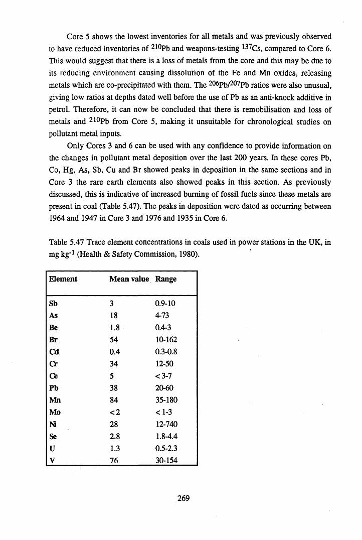
Core 5 shows the lowest inventories for all metals and was previously observed to have reduced inventories of 210Pb and weapons-testing 137Cs, compared to Core 6. This would suggest that there is a loss of metals from the core and this may be due to its reducing environment causing dissolution of the Fe and Mn oxides, releasing metals which are co-precipitated with them. The 206pb/207p5 ratios were also unusual, giving low ratios at depths dated well before the use of Pb as an anti-knock additive in petrol. Therefore, it can now be concluded that there is remobilisation and loss of metals and 210Pb from Core 5, making it unsuitable for chronological studies on pollutant metal inputs.
Only Cores 3 and 6 can be used with any confidence to provide information on the changes in pollutant metal deposition over the last 200 years. In these cores Pb, Co, Hg, As, Sb, Cu and Br showed peaks in deposition in the same sections and in Core 3 the rare earth elements also showed peaks in this section. As previously discussed, this is indicative of increased burning of fossil fuels since these metals are present in coal (Table 5.47). The peaks in deposition were dated as occurring between 1964 and 1947 in Core 3 and 1976 and 1935 in Core 6.
Table 5.47 Trace element concentrations in coals used in power stations in the UK, in mg kg-1 (Health & Safety Commission, 1980).
Element Mean value Range
Sb 3 0.9-10As 18 4-73Be 1.8 0.4-3Br 54 10-162Cd 0.4 0.3-0.8Cr 34 12-50Ce 5 <3-7Pb 38 20-60Mn 84 35-180Mo <2 <1-3Ni 28 12-740Se 2;8 1.8-4.4U 1.3 0.5-2.3V 76 30-154
269
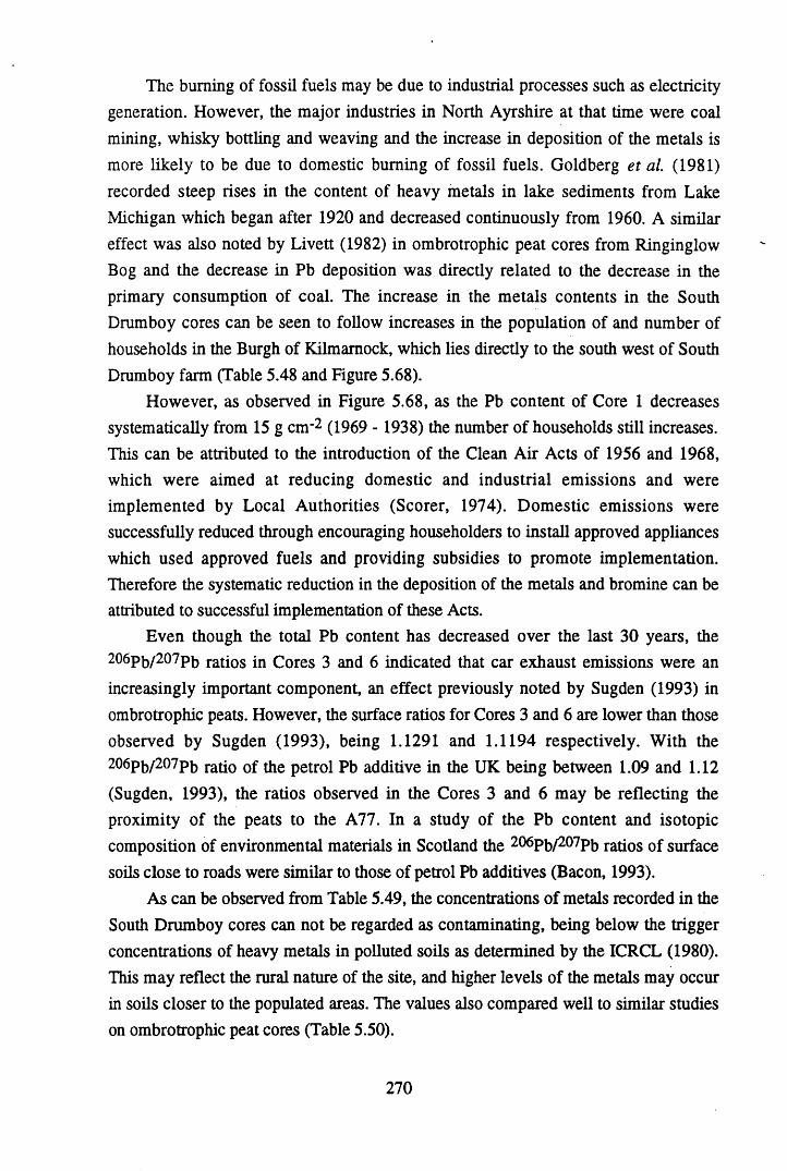
The burning of fossil fuels may be due to industrial processes such as electricity generation. However, the major industries in North Ayrshire at that time were coal mining, whisky bottling and weaving and the increase in deposition of the metals is more likely to be due to domestic burning of fossil fuels. Goldberg et a l (1981) recorded steep rises in the content of heavy metals in lake sediments from Lake Michigan which began after 1920 and decreased continuously from 1960. A similar effect was also noted by Livett (1982) in ombrotrophic peat cores from Ringinglow Bog and the decrease in Pb deposition was directly related to the decrease in the primary consumption of coal. The increase in the metals contents in the South Drumboy cores can be seen to follow increases in the population of and number of households in the Burgh of Kilmarnock, which lies directly to the south west of South Drumboy farm (Table 5.48 and Figure 5.68).
However, as observed in Figure 5.68, as the Pb content of Core 1 decreases systematically from 15 g cm-2 (1969 - 1938) the number of households still increases. This can be attributed to the introduction of the Clean Air Acts of 1956 and 1968, which were aimed at reducing domestic and industrial emissions and were implemented by Local Authorities (Scorer, 1974). Domestic emissions were successfully reduced through encouraging householders to install approved appliances which used approved fuels and providing subsidies to promote implementation. Therefore the systematic reduction in the deposition of the metals and bromine can be attributed to successful implementation of these Acts.
Even though the total Pb content has decreased over the last 30 years, the 206pb/207pb ratios in Cores 3 and 6 indicated that car exhaust emissions were an increasingly important component, an effect previously noted by Sugden (1993) in ombrotrophic peats. However, the surface ratios for Cores 3 and 6 are lower than those observed by Sugden (1993), being 1.1291 and 1.1194 respectively. With the 206pb/207pb ratio of the petrol Pb additive in the UK being between 1.09 and 1.12 (Sugden, 1993), the ratios observed in the Cores 3 and 6 may be reflecting the proximity of the peats to the A ll . In a study of the Pb content and isotopic composition of environmental materials in Scotland the 206pb/207pb ratios of surface soils close to roads were similar to those of petrol Pb additives (Bacon, 1993).
As can be observed from Table 5.49, the concentrations of metals recorded in the South Drumboy cores can not be regarded as contaminating, being below the trigger concentrations of heavy metals in polluted soils as determined by the ICRCL (1980). This may reflect the rural nature of the site, and higher levels of the metals may occur in soils closer to the populated areas. The values also compared well to similar studies on ombrotrophic peat cores (Table 5.50).
270
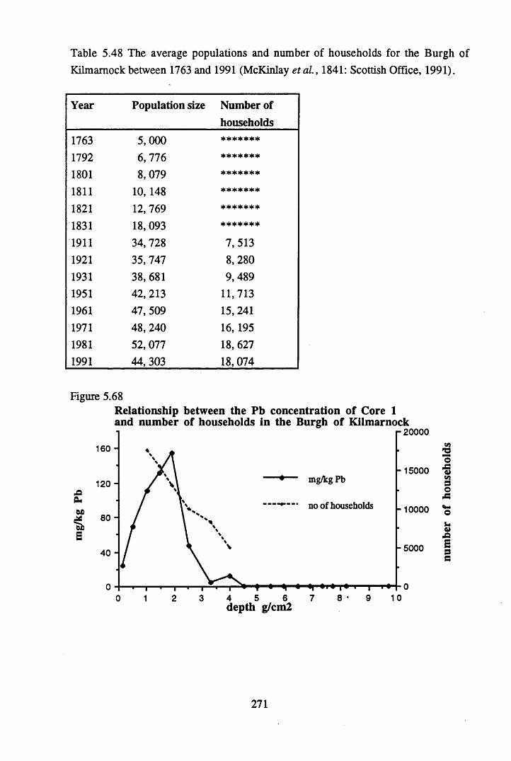
Table 5.48 The average populations and number of households for the Burgh of Kilmarnock between 1763 and 1991 (McKinlay etal., 1841: Scottish Office, 1991).
Year Population size Number of households
1763 5,000 *******
1792 6,776 *******
1801 8,079 *******
1811 10, 148 *******
1821 12,769 *******
1831 18,093 *******
1911 34, 728 7,5131921 35, 747 8, 2801931 38, 681 9,4891951 42, 213 11,7131961 47, 509 15, 2411971 48, 240 16,1951981 52, 077 18, 6271991 44, 303 18,074
Figure 5.68Relationship between the Pb concentration of Core 1 and number of households in the Burgh of Kilmarnock
r zoooo160 -
- 15000mg/kg Pb120 -
ft*wo
* 80‘ E
— no of households -10000
-5 0 0 040 -
7 8 • 9 105 60 2 3 41depth g/cm2
271
num
ber
of ho
useh
olds
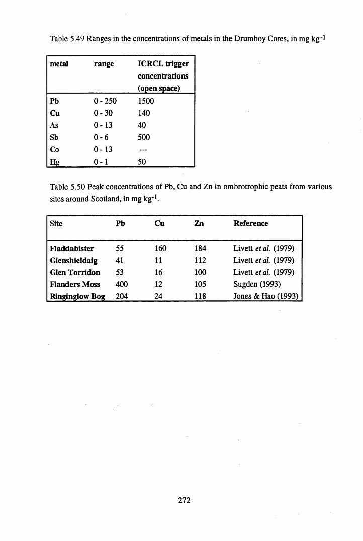
Table 5.49 Ranges in the concentrations of metals in the Drumboy Cores, in mg kg*1
metal range ICRCL trigger concentrations (open space)
Pb 0-250 1500Cu 0-30 140As 0-13 40Sb 0 -6 500Co 0-13 —
Hg 0 -1 50
Table 5.50 Peak concentrations of Pb, Cu and Zn in ombrotrophic peats from various sites around Scotland, in mg kg-1.
Site Pb Cu Zn Reference
Fladdabister 55 160 184 Livett etal. (1979)Glenshieldaig 41 11 112 Livett etal (1979)Glen Torridon 53 16 100 Livett etal (1979)Flanders Moss 400 12 105 Sugden (1993)Ringinglow Bog 204 24 118 Jones & Hao (1993)
272
5.5 CONCLUSIONS
With one of the main aims of the thesis being to evaluate the validity of dating peat profiles using 2l°Pb it can be concluded that the method can only be utilised where it is clear that there has been no post-depositional mobility of 210Pb, through lateral or vertical flow, or through past disturbance of the profile. This may seem an obvious conclusion, but in some cases disturbance of the profile can be difficult to assess and may affect profiles other than the one which has been disturbed. The effects of mixing of the profile should be taken into account in the calculation of the accumulation rate. It is also advisable to collect a group of peat cores, since the flux and inventory values from one core could give an ambiguous picture of 2l°Pb deposition at a site. In calculating the activity of 210Pb deposition, where the Z value of the peat changes significantly, the efficiency of the detection system should also be changed to incorporate this. Self absorption of 210Pb may also affect the accuracy of the detection and should be assessed and taken into account.
The Chernobyl accident is still showing a significant contribution to the radiocaesium inventories and both Chernobyl and weapons-testing l 37Cs showed mobility within the profiles, being present at depths dated below the advent of weapons testing. Weapons-testing 137Cs showed greater penetration and mobility within the profiles, as well as lateral flow between profiles. This was particularly prevalent in profiles which had been affected by disturbance and indicates that drainage of peats may be a route to decontamination of land affected by radiocaesium.
Post depositional mobility of Fe, Mn, Cu, Zn, Co and Br was observed in some of the cores studied and can be attributed to changes in the redox environment. By contrast Pb, Co, Hg, As and Sb were not affected by redox changes, nor did they exhibit the mobility which radiocaesium showed. Instead these elements, as well as Br when the redox environment allowed, showed peaks in deposition which can be attributed to burning of fossil fuels in the locality. Reductions in their concentrations towards the surface sections can be attributed to the introduction and implementation of the Clean Air Acts of 1956 and 1968.
In addition, the 206pb/207pb ratios indicated that even though the total Pb content has fallen over the last 30 years in Cores 3 and 6, car exhaust emissions had increasingly contributed to the Pb content over this period.
273
CHAPTER 6
FINAL CONCLUSIONS & SUGGESTIONS FOR FUTURE
RESEARCH
274
When studying the literature and planning the research, it was evident that there were two main ways to approach the study and this thesis combined these through utilising both laboratory and field-based studies. This approach proved useful since they both gave results and conclusions which were similar and also provided many avenues for further research. However, it did also highlight how different the approaches are and as such further work needs to be carried out on combining them, to give further insight into the interaction of metals with humic substances.
From the studies on the nature and stability of metal binding in Chapters 3 and 4 it was evident that Pb, Cu and Cs all bind in quite different ways, to differing degrees of stability. The infra-red studies showed that Pb and Cu were able to form coordinate, covalent linkages with humic acid whereas Csshowed a predominately ionic linkage. In addition Cu showed a greater degree of covalency which may indicate that it was able to undergo more specific reactions with the functional groupings. The binding studies in Chapter 4 also suggested this, with Cu releasing more protons on interaction with functional groupings and also showing more curvilinearity in the Scatchard plots (both indicating a greater degree of conformational changes on binding).
These differences in behaviour were also seen in the peat profiles, where radiocaesium exhibited a high degree of mobility both vertically and laterally, consistent with its ionic, exchangeable nature. Conversely, Pb and Cu showed minimal mobility, which is consistent with complexation with organic matter.
As also mentioned above, the binding studies illustrated a difference in behaviour between Pb and Cu, which was also seen in the field studies. Cu showed a greater stability of binding to unextracted peat, compared to humic acid, whereas Pb showed similar formation constants for both humic acid and unextracted peat. This was proposed to suggest that Cu was able to bind to other fractions of the peat, such as the oxide fraction, in addition to the humic substances, whereas Pb was predominantly associated with the humic fraction. The field-based studies provided further evidence for this, since in some of the profiles studied Cu showed evidence of post-depositional mobility, mediated by redox changes. As conditions became more reducing the Mn and Fe oxides came into solution and were leached from the profile. Metals such as Cu, which are co-precipitated with them, can also be released and with the evidence provided from the binding studies it is likely that this may have resulted in the peaks in Cu concentration at depth in the peat profiles. Pb did not show this behaviour, with post-depositional mobility being minimal and related to disturbance of the peat profiles.
275
Both the laboratory and field studies showed that the extraction and fractionation of humic acid resulted in chemical and structural changes in the functional groupings, affecting the stability and nature of metal binding. In particular, extraction resulted in an increase in the nitrogen content, carboxyl content, total acidity and metal binding capacity of the material. Consequently, as discussed above, metal binding was affected. The main aim of the extraction and fractionation procedure is to reduce the heterogeneity of the material, but as observed from the studies presented here it did not meet this aim and could result in conclusions which have no bearing on how a metal or radionuclide will behave in the environment.
Therefore, laboratory-based metal-binding studies which aim to investigate the stability of metal binding should bear this in mind and adopt the methods to study binding with unextracted materials. This may have limitations since the methods will be measuring binding to all fractions of the soil and not just the humic fractions, but the advantages of not using an operationally-defined fraction surely outweighs this. In addition, future research should investigate further the development of non destructive methods of analysis such as 13C NMR. Further research into metal-binding needs to be carried out on the competition of metals with binding sites, by reacting a variety of metals at one time, rather than the artificial one component studies carried out in this research. This was a major limitation when combining the results from the metal- binding studies with the metal profiles within the peat cores, since the constants and relationships produced represented a binding of one metal only to pre-treated peat at a defined pH and ionic strength.
The concept of combining the laboratory and field studies does need to be developed further to provide a more comprehensive picture of metal-soil relationships. Lysimeter studies may be one route, incorporating leaching of metal solutions through profiles and monitoring their uptake and extent of binding.
The field-based studies presented here involved taking a collection of cores and analysing for a wide variety of elements. Consequently, a plethora of data was generated, of which for the purpose of this thesis, only basic interpretation was carried out. In addition, three cores to the north of Glasgow were also collected which were not included. As a result the data will be analysed further in future publications, building on the conclusions presented here.
276

BIBLIOGRAPHY
Aaby B. & Jacobsen J. (1979). Changes in biotic conditions and metal deposition in the last millenium as reflected in ombrotrophic peat in Draved Mose, Denmark. Geological Survey o f Finland, Yearbook 1978, Copenhagen, 5-43.
Adriano D.C. (1986). Trace elements in the terrestial environment. Springer-Verlag. New York.
Aiken G.R., McKight D.M., Wershaw R.L. & MacCarthy P. (1985). Introduction. In Humic Substances in Soils, Sediments and Water. Geochemistry, Isolation & Characterisation. (G.R. Aiken, D.M. Me Knight, R.L. Wershaw, P. MacCarthy, eds.). Wiley Interscience, New York, pp 1-12.
Aitken M.J. (1990). Chapter 3: Radiocarbon 1. In Science based dating in archaeology. Longman Group Ltd.,U.K., pp56-76.
Alberts J.J., Filip Z. & Hertkom N. (1992). Fulvics and humic acids isolated from groundwater: compositional characteristics and cation binding. Journal o f Contaminant Hydrology, 11, 317-330.
Allen S., Brown P., McKay G. & Flynn O. (1992). An evaluation of single resistance transfer models in the sorption of metal ions by peat. Journal o f Chemical Technology and Biotechnology, 54, 271-276.
Alloway B J . (1990). Soil processes and the behaviour of metals. In Heavy metals in soils, (ed. B.J. Alloway), Blackie, London, pp 7-29.
Appleby P.G. & Oldfield F. (1978). The calculation of lead-210 dates assuming a constant rate of supply of unsupported 210Pb to the sediment. Catena, 5,1-8.
Ault W.A., Senechal R.G. & Erlebach W.E. (1970). Isotopic composition as a natural tracer of lead in the environment. Environmental Science and Technology, 4,305-313.
Baes A.U. & Bloom P.R. (1988a). Exchange of alkaline earth cations in soil organic matter. Soil Science, 146,6-14.
Baes A.U. & Bloom P.R. (1988b). Effect of ionic strength on swelling and the exchange of alkaline earth cations in soil organic matter. Soil Science, 146,67-72.
278
Baes A.U. & Bloom P.R. (1989). DRIFT spectroscopy of humic and fulvic acid. Journal o f the Soil Science Society o f America, 53, 695-700.
Backes C.A. & Tipping E. (1987). Aluminium complexation by an aquatic humic fraction under acidic conditions. Water Research, 21,211-216.
Bacon J.R. (1993). Characterisation of lead and other heavy metals in the Scottish upland environment using isotopic composition. In Heavy Metals in the Environment, 1,282-284, Toronto.
Baldock J.A., Oades J.M., Waters A.G., Peng X., Vassalo A.M. & Wilson M.A., (1991). Aspects of the chemical structure of soil organic materials, as revealed by solid state C 1 NMR spectroscopy. Bio geochemistry, 16 (1), 1-42.
Banerjee S.K. & Mukheijee S.K. (1972). Studies on the infra-red spectra of some divalent transitional metal humates. Journal o f the Indian Society o f Soil Science, 20, 91-96.
Barber K.E. (1993). Peatlands as scientific archives of past biodiversity. Biodiversity and Conservation, 2,474-489.
Bellamy L.J. (1975). The Infra red spectra o f complex molecules. J.Wiley & Sons, New York, pp 183-201.
Bennet B.G. (1990). Worldwide radiation exposure from the Chernobyl accident. In Environmental contamination following a major nuclear accident, vol. 2. IAEA-SM- 306 94, Vienna, 251-260.
Bloom P.R. & McBride M.B. (1979). Metal ion binding and exchange with hydrogen ions in acid-washed peat. Journal of the Soil Science Society o f America , 43,687-692.
Bonn B.A. & Fish W. (1991). Variability in the measurement of humic carboxyl content Environmental Science & Technology, 25, 232-240.
Bonn B.A. & Fish W. (1993). Measurement of electrostatic and site specific associations of alkali metal cations with humic acid. Journal o f Soil Science, 44,335- 346.
279
Bonnet R. & Cousins R.P.C. (1987). On the metal content and metal ion uptake of botanically specific peats and the derived humic acids. Organic Geochemistry, 11, 497-503.
Bramryd T. (1980). The role of peatlands for the global carbon dioxide balance. Proceedings o f the 6th International Peat Congress, pp 9-11.
Brennan R.F., Robson A.D. & Gartrell J.W. (1983). Reactions of copper with soil affecting its availablity to plants n. Effect of soil pH, sterilisation and organic matter on the availability of applied copper. Australian Journal o f Soil Research, 1,153-63.
Bresnahan W.T., Grant C.L., & Weber J.H. (1978). Stability constants for the complexation of copper (II) with water and soil fulvic acids, measured by ion selective electrode. Analytical Chemistry, 50 (12), 1675-1679.
Broadbent F.E. & Bradford S. (1952). Cation exchange groupings in soil organic matter. Soil Science, 74,447-452.
Buffle J. (1988). Complexation reactions in aquatic systems - an analytical approach. Ellis Horwood Ltd, London.
Buffle J., Greter F.G.L. & Haerdi W. (1977). Measurement of complexation properties of humic and fulvic acids in natural waters with lead and copper ion selective electrodes. Analytical Chemistry , 49, 216-221.
Buffle J., Langford C.H. & Gamble D.S. (1978). The use of ultrafiltration for the seperation and fractionation of organic ligands in freshwaters. Analytica ChimicaActa, 101, 339-357.
Burkhart W. (1991). Radiation biology of the Lung. Science o f the Total Environment., 89,1-230.
Cabaniss S.E. (1991). Carboxylic acid content of a fulvic acid determined by potentiometry and aqueous Fourier Transform Infra Red Spectroscopy. Analytica Chimica Acta , 255,23-30.
280
Cabaniss S.E. & Shuman M.S. (1986). Combined ion selective electrode and fluorescence quenching detection for Cu2+ dissolved organic matter titrations. Analytical Chemistry, 58, 398-401.
Cameron R.S., Thornton B.K., Swift E.S. & Posner A.M. (1972). Molecular weight and shape of humic acid from sedimentation and diffusion measurements on fractionated extracts. Journal of Soil Science, 23,394-408.
Campanella L. & Tomasseti M. (1990). Thermogravimetric and Infra Red analysis of different extracts of humic substances. Thermochimica Acta , 170, 67-80.
Cheshire M.V., Berrow M.I., Goodman B.A. & Mundie C.M. (1977). Metal distribution and nature of some Cu, Mn and V complexes in humic and fulvic fractions of soil organic matter. Geochimica et Cosmochimica Acta, 41,1131-1138.
Chow T.J. & Johnstone M.S. (1965). Lead isotopes in gasoline and aerosols of the Los Angeles Basin, California. Science, 147,502-503.
Clark M.J. & Smith F.B. (1988). Wet and dry deposition of Chernobyl releases. Nature, 332, 245-249.
Clymo R.S. (1963). Ion exchange in sphagnum and its relation to bog ecology. Annals Botany, 27, 309-324.
Clymo R.S. (1983). Peat. In Ecosystems o f the World 4A: Mires, swamp, bog, fen and moor (ed. Gore A.), pp 159-224, Elsevier, Amsterdam.
Clymo R.S. (1984). The limits to peat bog growth. Proceedings o f Royal Society of London, 8303,605-654.
Clymo R.S. (1991). Peat Growth. In Quaternary Landscapes (eds. Shane L.K. & Cushing E.J.) University of Minnesota Press, pp 76-112.
Clymo R.S. & Mackay D. (1987). Upwash and downwash of pollen and spores in the unsaturated surface layer of sphagnum dominated peat. New Phytologist, 105, 175- 183.
281
Clymo R.S., Oldfield F., Appleby P.G., Pearson G.W., Ratnesar P. & Richardson N. (1990). The record of atmospheric deposition in a rainwater dependent peatland. Philosophical Transactions o f the Royal Society of London , B327, 331-338.
Cole K.L., Ongstrom D.R., Futyma R.P. & Stottlemyer R. (1990). Past atmospheric deposition of metals in Northern Indiana measured in a peat core from Cowles Bog. Environmental Science & Technology, 24, 543-549.
Colgan P.A., McGee E.J., Pearce J., Cruikshank J.G., Mulvany N.E., McAdam J.H. & Moss B.W. (1990). Behaviour of radiocaesium in organic soils - some preliminary results of soil-plant transfers from a semi-natural ecosystem in Ireland. In Transfer of radionuclides in natural and semi-natural environments (Eds. Desmet G., Nassimbeni P. & Belli M.) Elsevier, Amsterdam, 341-355.
Coppola M & Reiniger P. (1974). Influence of the chemical composition on the gamma-ray attenuation by soils. Soil Science, 117, 331-335.
Coughtrey P.J., Kirkton J.A. & Mitchell N.G. (1990). Caesium distribution and cycling in upland pastures of N. Wales and Cumbria. In Transfer o f radionuclides in natural and semi-natural environments (Eds. Desmet G., Nassimbeni P. & Belli M.). Elsevier, Amsterdam, 259-267.
Cutshall N.H., Larsen I.L. & Olsen C.R. (1983). Direct analysis of 2l°Pb in sediment samples: self absorption corrections. Nuclear Instruments & Methods, 206, 309-312.
Damman A.W.H. (1978). The distribution and movement of elements in ombrotrophic peat bogs. Oikos, 30,480-495.
Davidson C.I., Harrington J.R., Stephenson M.J., Monoghan M. C., Pudykiewcz J. & Schell W.R. (1987). Radioactive caesium from the Chernobyl accident in the Greenland ice sheet Science, 237,633-634.
Davies B.E. & Jones L.H.P. (1988) Micronutrients and toxic elements, In Russell’s Soil Conditions and Plant Growth, 11th edition, (ed. A.Wild), Wiley & Sons, New York, pp 780-815.
282
Davies R.I., Cheshire M.V. & Graham-Bryce I.I. (1969). Retention of low levels of copper by humic acid. Journal o f Soil Science, 20,65-71.
Davis J.A. (1982). Coraplexation of trace metals by adsorbed natural organic matter. Geochimica et Cosmochimica Acta, 48, 679-691.
Deina S., Gessa C., Manunza B., Rausa R. & Seeber R. (1990). Analytical and spectroscopic characteristics of humic acids extracted from sewage sludge, manure and worm compost. Soil Science 150 (1), 419-424.
Dissanayake C.B. (1983). Metal organic interactions in environmental pollution. International Journal o f Environmental Studies, 22, 25-42.
Dubach P. & Mehta N.C. (1963). The chemistry of soil humic substances. Soils & Fertility, 26, 293-307.
Dumontet S., Levesque M. & Mathur S.P. (1990). Limited downward migration of pollutant metals in acidic virgin peat soils near a smelter. Water, Air & Soil Pollution, 49,329-342.
Dzombak D.A., Fish W. & Morel F.M. (1986). Metal-humate interactions. 1. Discrete ligand and continuous distribution models. Environmental Science & Technology, 20, 669-675.
Eisenreich S.J., Metzer M., & Urban N.R. (1986). Response of atmospheric lead to decreased use of lead in gasoline. Environmental Science and Technology, 20, 171 - 174.
El-Daoushy F. (1988). A summary on the lead-210 cycle in nature and related applications in Scandinavia. Environment International, 14, 305-319.
El-Daoushy F., Tolonen K. & Rosenberg R. (1982). Lead-210 and moss increment dating of peat in two Finnish sphagnum hummocks. Nature, 296,429-431.
El-Daoushy F. & Tolonen K. (1984). Lead-210 and heavy metal contents in dated ombrotrophic peat hummocks from Finland. Nuclear Instruments and Methods in Physics Research, 223, 392-399.
283
Ephraim J., Alegnet S., Mathuthu A., Bicking M., Malcolm R.L. & Marinsky J.A. (1986). A unified physicochemical description of the protonation and metal ion complexation equilibria of natural organic acids 2. Influence of polyelectreolytic properties and functional group heterogeneity on the protonation equilibria of fulvic acid. Environmental Science & Technology, 20, 354-366.
Falck W.E. (1988). A review of modelling the interaction between natural organic matter and metal cations. British Geological Technical Report, WE/88/49.
Farmer J., Swan D.S. & Baxter M.S. (1980). Records and sources of metal pollutants in a dated Loch Lomond sediment core. Science o f the Total Environment, 16, 131 - 147.
Fitch A. & Stevenson F.J. (1984). Models for stability constants of metal complexes with humic substances. Journal o f Soil Science Society o f America, 48,1044-1050.
Fish W. & Morel F.M. (1985). Propogation of error in fuvic acid titration data: a comparison of three analytical methods. Canadian Journal o f Chemistry, 63, 1185- 1193.
Fish W., Dzombak D.A. & Morel F.M. (1986). Metal humate interactions 2. Application and comparison of models. Environmental Science & Technology, 20, 676-683.
Flaig W., Beutelspacher H. & Reitz E. (1975). Chemical composition and physical properties of humic substances. In Soil Components: Volume 1. Organic components (ed. Gjessing J.E.) Springer-Verlag, New York, pp 1-211.
Friedland A.J., Miller E.K., Siccama T.G., & Dunham S. (1993). The redistribution of lead in forest soils in response to changing atmospheric deposition rates. Proceedings of Heavy Metals in the Environment, 2,526-529, Toronto.
Frissel M.J., Noordijk H., & Van Bergeijk K.E. (1990). The impact of extreme environmental conditions, as occurring in natural ecosystems, on the soil-plant transfer of radionuclides. In Transfer o f radionuclides in natural and semi-natural environments (eds. Desmet G., Nassimbeni P. & Belli M.), Elsevier, Amsterdam, pp 40-48.
284
Galloway J.N., Thornton J.D., Norton S.A., Volchok H.L. & McLean R.A.N. (1982). Trace metals in atmospheric deposition: a review and assessment. Atmospheric Environment, 1 6 ,1677-1700.
Gamayunov N.I. & Maslennikov B.I. (1992). Mechanism of the interaction of cations with the adsorptive complex of peat soil. Pochvovedeniye, 3,146-151.
Gamble D.S., Underdown A.W. & Langford C.H. (1980). Cu (II) titration of fulvic acid ligand sites with theoretical, potentiometric and spectrophotometric analysis. Analytical Chemistry, 52,1901-1908.
Gibbons D., Jones K.C. & Steinnes E. (1993). Deposition of heavy metals to Norwegian Ombrotrophic peat bogs. Proceedings of Heavy Metals in the Environment, 2, 89-92,Toronto.
Glooschenko W.A., Holloway L., & Arafat N. (1986). The use of mires in monitoring the atmospheric deposition of heavy metals. Aquatic Botany, 25,179-190.
Goldberg E.D., Hodge V.F., Griffen J.J., Koide M. & Edgington D.M. (1981) The impact of fossil fuel combustion on the sediments of Lake Michigan. Environmental Science & Technology, 15, 466-471.
Goodman B.A. & Cheshire M.V. (1976). The occurence of copper-porphoryn complexes in soil humic acids. Journal o f Soil Science, 27, 337-347.
Gore A.J.P. (1983). Introduction. In Ecosystems o f the World, 4A: General studies. (AJ.P. Gore ed.) ppl-34., Elsevier, Amsterdam.
Gorres M. & Frenzel B. (1993). The Pb, Br, and Ti content in peat bogs as indicators for recent and past depositions. Naturwissenschaften, 80 ,333-335.
Gregor J.E., Powell H.J.K. & Town R.M. (1989). Metal fulvic acid complexing: evidence supporting an aliphatic carboxylate mode of coordination. Science o f the Total Environment, 81782,597-614.
Gregor H.P. (1955). The polyacrylic acid-copper complex. Journal o f Physical Chemistry, 59,34-41.
285
Gregor J.E. & Powell HJ.K. (1987). Effects of extraction procedures on fulvic acid properties. Science of the Total Environment, 62,3-12.
Griffiths P.R. (1975). Chemical analysis volume 43: Chemical Infra Red Fourier transform Spectroscopy. J. Wiley & Sons, New York.
Hardman D.J., McEldowney S. & Waite S. (1993). Chapter 15: Environmental fate and effects of metals and radionuclides. In Pollution: Ecology and Biotreatment. pp233-260. Longman Group Ltd., U.K.
Harrison R.M. & Sturges W.T. (1983). The measurement and interpretation of Br/Pb ratios in airborne particles. Atmospheric Environment, 17, 311-328.
Harrison R.M, Laxen D.P.H. & Wilson S.J. (1981). Chemical associations of lead, cadmium, copper and zinc. Environmental Science and Technology, 15,1378-1383.
Harrison R.M., Luhana L., & Smith DJ.T. (1993). Urban air pollution by heavy metals: sources and trends. Proceedings of Heavy Metals in the Environment, 1, 81-84, Toronto.
Hatcher P.G., Breger I.A., Dennis L.W., & Maciel G.E. (1983). Solid state ^ C NMR of sedimentary humic substances: New revelations on their chemical composition. In Aquatic and Terrestial Humic Materials (eds. Christman R.F. & Gjessing E.T.), Ann Arbor Science, Ann Arbor, MI, pp 37-82.
Haworth R.D. (1971). The chemical nature of humic acid. Soil Science, 111, 71-77.
Hayes M.B.H. & Swift R.S. (1978). The chemistry of soil organic colloids. In The Chemistry o f soil constituents. (DJ. Greenland & M.B.H. Hayes, eds.). Wiley Interscience, New York, pp 179-230.
Hayes M.B.H. (1991). Concepts of the Origins, Composition, and Structures of humic substances. Advances in soil organic matter research:the impact o f agriculture on the environment (ed. W.S.Wilson) The Royal Society of Chemistry, pp 3-23.
286
Health & Safety Commission (1980). Study of Coal: evidence by the HSE to the Commission on Energy and the Environment concerning public health and amenity in the external environment HMSO, London.
Heaton B., Mitchell R.D.J., Veresoglou D.S. & Killham K. (1990) Caesium dynamics in the peats and associated vegetation of Greece and Northern Scotland. In Transfer of radionuclides in natural and semi-natural environments (eds. Desmet G., Nassimbeni P. & Belli M.) Elsevier, Amsterdam, 669-675.
Helmer E.H., Urban N.R. & Eisenreich S.J. (1990). Aluminium geochemistry in peatland waters. Bio geochemistry, 9, 247-276.
Hempfling R., Zech W. & Schulten H.R. (1988) Chemical components of the organic matter in forest soils 2: Moder profile. Soil Science, 146 (4), 262-276.
Hill B.M. & Siegel D.I. (1991). Groundwater flow and metal content of peat Journal of Hydrology, 123, 211-224.
Holdgate M.W. (1979). A perspective o f environmental pollution. Cambridge University Press.
Hogg E.H. (1993). Decay potential of hummock and hollow sphagnum peats at different depths in a Swedish raised bog. Oikos, 66,269-278.
Holmgren A Norden B.O. (1988). The characterisation of peat samples by diffuse reflectance FTIR spectroscopy. Applied Spectroscopy , 42 (2), 255-262.
Holtzclaw K.M. & Sposito G. (1978). Analytical properties of the soluble, metal complexing fractions in sludge-soil mixtures. Journal o f Soil Science Society of America, 43, 318-323.
Hopkins D.W. & Shiel R.S., (1991). Spectral characterisation of organic matter from soil with mor and mull humus forms. In Advances in soil organic matter research: die impact o f agriculture on die environment, (ed. W.S.Wilson) The Royal Society of Chemistry, pp 71-78.
287
II
Horth H., Frimmel F.R, Hargitai L., Hennes E.C., Muller-Wegener U., Hue A.Y., Niemeyer J., Nissenbaum A., Sekoulov I., Tipping E., Weber J.HA & Zepp R.G. (1988). Environmental reactions and functions. In Humic substances and their role in the environment, (eds. Frimmel F.H. and Christman R.F.), Wiley Interscience, New York, pp. 245-256.
Horrill AD., Kennedy V.H. & Harwood T.R. (1990). The concentrations of Chernobyl derived radionuclides in species characteristic of natural and semi-natural ecosystems. In Transfer o f radionuclides in natural and semi-natural environments (eds. Desmet G., Nassimbeni P. & Belli M). Elsevier, Amsterdam, pp 27-40.
Ikan R., Ioselip R., Rubinsztain Y., Aizenshtat Z., Miloslavsky L, Yariv S., Pugmire R., Anderson L.L., Woolfenden W.R., Kaplan I.R., Dorsey T., Peters K.E., Boon J.J., De Leeuw J.W., Ishiwatari R., Morinaga S., Yamamoto S., Macihara T., Muller- Vonmoos M. & Rub A. (1992). Chemical, isotopic, spectroscopic and geochemical aspects of natural and synthetic humic substances. Science o f the Total Environment, 117/118,1-12.
Ingram J. (1978). Soil layers in mires: function and terminology. Journal o f Soil Science, 29, 224-227.
Ishiwatari R. (1975). Chemical nature of sedimentary humic acid. In Humic Substances, Their Structure and Function in the Biosphere (eds. Povoledo D. &. Golterman H.L.). Centre for Agricultural Publications and Documentation, Wageningen, pp 109-121.
Jensen A. & Jensen A. (1991). Historical deposition rates of mercury in Scandinavia estimated by dating and measurement of mercury in cores of peat bogs. Water, Air & Soil Pollution, 56,769-777.
Johnson L.C., Damman A.W.K & Maimer N. (1990). Sphagnum macrostructure as an indicator of decay and compaction in peat cores from an ombrotrophic south Swedish peat bog. Journal o f Ecology, 78, 633-647.
Jones J.M. (1987). Chemical fractionation of Cu, Pb and Zn in ombrotrophic peat Environmental Pollution, 48,131-144.
288
Jones J.M. & Hao J. (1992). Ombrotrophic peat as a medium for historical monitoring of heavy metal pollution. Environmental Geochemistry & Health, 15, 61-1 A.
Joseph A.B. (1971). Sources of radioactivity and their characteristics. In Radioactivity in the Marine Environment, National Academy of Sciences, Washington, DC, 6-41.
Karlin E.F. & Bliss L.C. (1984). Variation in substrate chemistry along microtopographical and water chemistry gradients in peatlands. Canadian Journal of Botany, 62, 142-153.
Kathren R.L. (1984). Radioactivity in the Environment: Sources, Distribution and Surveillance. Harwood Academic Publishers.
Keough J.R. & Pippen R.W. (1983). The movement of water from peatland into surrounding groundwater. Canadian Journal o f Botany, 62, 835-839.
Kemp W. (1991). Infra red Spectroscopy. In Organic Spectroscopy, 3rd edition, MacMillan Education Ltd, Hong Kong, pp 19-57.
Keller C. (1988). Radiochemical age determination. In Radiochemistry, Ellis Horwood Chichester, pp 193-199.
Khan S.U. & Schnitzer M. (1971). Further investigations on the chemistry of fulvic acid, a soil humic fraction. Canadian Journal o f Chemistry, 49, 2302-2315.
Kononova M.M. (1966). Soil Organic Matter. Pergamon, Elmsford, New York.
Kirkton J.A., Coughtrey P.J. & Mitchell N.G. (1990). Derivation of soil to plant concntration ratios for upland systems in the glasshouse and comparison with field and experimental measurements. In Transfer o f radionuclides in natural and semi-natural environments (eds. Desmet G., Nassimbeni P. & Belli M.). Elsevier, Amsterdam, pp 267-275.
Krosshavn M. (1992). A study of some chemical properties o f soil organic matter: The influence o f vegetational background and degree o f humification on these properties, and the relationship between them. Ph.D.Thesis, University of Trondheim, AVH.
289
Lantzy R.J. & Mackenzie F.T. (1979). Atmospheric trace metals: global cycles and assessment of mans impact Geochimica et Cosmochimica Acta, 43, 511-525.
Lee J.A. & Tallis J.H. (1973). Regional and historical aspects of lead pollution in Great Britain, Nature, 245, 216-218.
Livens F.R. (1991). Chemical reactions of metals with humic material. Env.ronmental Pollution, 70,183-208.
Livens F.R., Fowler D. &Horrill A.D. (1992). Wet and dry deposition of 131I, 134Cs, and 137Cs at an upland site in Northern England. Journal of Environmental Radioactivity, 16, 243-254.
Livett E.A. (1982). The interaction o f Heavy Metals with peat and vegetation of blanket bogs ir\ Britain. Ph.D. Thesis, University of Manchester.
Livett E.A., Lee J.A., & Tallis J.H. (1979). Lead, zinc and copper analysis of British Blanket Peats. Journal o f Ecology, 67,865-891.
Livett E.A. (1988). Geochemical Monitoring of Atmospheric Heavy Metal Pollution: Theory and Applications. Advances in Ecological Research, 18, 65-174.
MacCarthy P. (1976). A proposal to establish a reference collection of humic materials for interlaboratory comparisons. Geoderma , 16,179-181.
MacCarthy P. & Rice J.A (1985). Spectroscopy of humic substances. In Humic Substances in Soils, Sediments, and Water: Geochemistry, Isolation and Characterisation, (eds. Aiken G.R., McKnight D.M., Wershaw R.L., MacCarthy P.). Wiley Interscience, New York, pp 527-559.
Macdonald P., Cook G.T., Baxter MS. & Thomson J.T. (1992). The terrestial distribution of artificial radioactivity in South West Scotland. Science o f the Total Environment, 111, 59-83.
Mackinley J., Strang D. & Hamilton A. (1842). The New Statistical Account of Ayrshire (Volume 5). William Blackwood & Sons, Edinburgh.
290
McLaren R.G. & Crawford D.V. (1973). Studies on soil copper 2. The specific adsorption of copper by soils. Journal o f Soil Science, 24, 443-453.
Maguire S. (1993). Natural and anthropogenic radionuclides in organic and mineral soils. Ph.D. Thesis, University of Glasgow.
Maguire S, Pulford I.D., Cook G.T. & MacKenzie A.B. (1991). Use of infra-red spectroscopy to elucidate the role of functional groups in the binding of metals to humic acids. In Heavy Metals in the Environment, 1, 88-91, Edinburgh.
Malcolm R.L. & MacCarthy P. (1991). The individuality of humic substances in diverse environments. Advances in soil organic matter research: the impact of agriculture on die environment, (ed. W.S.Wilson) The Royal Society of Chemistry, pp. 23-35.
Maimer N. & Holm E. (1984). Variations in C/N quotient of peat in relation to decomposition rate and age, determined with 210Pb. Oikos, 43,171-182.
Mantoura R. & Riley J.P. (1977). Metal binding of organic macromolecules in soil 2. Characterisation of the maximum binding ability of the macromolecules. Soil Science, 23,188.
Marinsky J.A & Ephraim J. (1986). A unified physicochemical description of the protonation and metal ion complexation equilibria of natural organic acids 1. Analysis of the influence of polyelectrolyte properties on protonation equilibria in ionic media: fundamental concepts. Environmental Science & Technology, 20,349-354.
Markert B. & Thornton I. (1990). Multielement analysis of an English peat bog soil. Water, Air and Soil Pollution, 49, 113-123.
Marley N.A., Gaffney J.S., Orlandini K.A., Picew K.C. & Choppin G.R. (1992). Chemical characterisation of size fractionated humic and fulvic materials in aqueous samples. Science o f the Total Environment, 113,159-177.
Martin M.H., Coughtrey P.J. & Ward P. (1979). Historical aspects of heavy metal pollution in the Gordano Valley. Proceedings o f the Bristol Naturalists Society, 37, 91-97.
291
Masini J.C. (1993). Evaluation of neglecting electrostatic interactions on the determination and characterisation of the ionisable sites in humic acid. Analytica Chimica Acta, 283, 803-810.
Mathur S.P. & Famham R.S. (1985). Geochemistry of humic substances in peat Humic Substances in Soils, Sediments, and Water: Geochemistry, Isolation and Characterisation, (eds. Aiken G.R., McKnight D.M., Wershaw R.L. & MacCarthy P) Wiley Interscience, New York, pp 53-88.
Midgley D. & Torrance K. (1991). Potentiometric Water Analysis (second edition). J. Wiley & Sons, London.
Mierle G. & Ingram R. (1991). The role of humic substances in the mobilisation of Hg from watersheds. Water, Air & Soil Pollution, 56, 349-357.
Miller E.K. & Friedland A.J. (1991). Recent reductions in the atmospheric lead flux to high elevation forests of the North Eastern USA. Heavy Metals in the Environment, 1., 86-89, Edinburgh.
Mitchell P.I., Schell W.R., McGarry P., Ryan T.P., Sanchez-Cabeza J.A. & Vidal- Quadras A. (1992). Studies on the vertical distribution of 134Cs, 137Cs, 238Pu, 239,240pUj 24lpu> 241 m, & 210Pb in ombrogenous mires at mid-latitudes. Journal of Radioanalytical & Nuclear Chemistry, Articles, 156(2), 361-387.
Moore P.D. & Bellamy D.J. (1974). Peatlands. Springer-Verlag, New York.
Morgan J.J. & Stumm W. (1991) Chemical processes in the environment, relevance of chemical speciation. In Metals and their compounds in the environment, (ed. Merian E.). VCH, Weinheim, pp 69-103.
Mortensen J.L. & Schwendinger R.B. (1963). Electrophoretic and spectroscopic characterisation of high molecular weight components of soil organic matter. Geochimica et Cosmochimica Acta , 27, 201-208.
Mott C.J.B. (1988). Surface Chemistry of Soil Particles. In Russell's Soil Conditions and Plant Growth, 11th edition, (ed. Wild A.), Wiley & Sons, New Yoik, pp 282-298.
292
Naeumann R. Steines E. & Guinn V.P. (1993). Feasibility of Instrumental Neutron Activation Analysis for trace element studies in natural soils. Journal of Radioanalytical and Nuclear Chemistry Articles, 168, 61-68.
Nakamoto K (1986). Infra-red and Raman spectra o f Inorganic and Coordination compounds, 4th edition, J. Wiley & Sons, London.
Niebor E. & Richardson D.H.S. (1980). The replacement of the term “heavy metals” by a biologically and chemically significant classification of metal ions. Environmental Pollution, B l, 3-26.
Niemeyer J. Chen Y., & Bollag J.M. (1992). The characterisation of humic acid, composts and peat by DRIFT. Journal o f Soil Science Society o f America , 56, 135- 140.
Njstaad O. Naeuman R. & SteinnesE. (1987). Variations in atmospheric trace element deposition studies by INAA of peat cores from ombrotrophic bogs. Journal of Radioanalytical and Nuclear Chemistry Articles, 114 (1), 69-75.
Nraigu J. (1989). Global inventory of natural and anthropogenic emissions of trace metals to the atmosphere. Nature, 279,409-411.
Nriagu J. (1991). Human influence on the global cycling of trace metals. In Heavy Metals in the Environment, 1,1-5, Edinburgh.
Nozaki Y., Demaster D.J., Lewis D.M, & Turekian K.K. (1978). Atmospheric Pb-210 fluxes determined from soil profiles. Journal o f Geophysical Research, 83,4047-4051.
Ohlson M & Dahlberg B. (1991). Rate of hummock and lawn communities on Swedish mires during the last 130 years. Oikos, 61,369-378.
Oldfield F. & Tolonen K. (1981). History of particulate atmospheric pollution from magnetic measurments in dated Finnish peat profiles. Ambio, 10,185-188.
Oldfield F., Appleby P.G., Cambray R.S., Eakins J.D., Barber K.E., Batterbee R.W., Pearson G.R. & Williams J.M. (1979). 210Pb, 137Cs & 239Pu profiles in ombrotrophic peat Oikos, 33,40-45.
293
Oldfield F., Appleby P.G., Crooks P., Hutchinson S. & Richardson N. (1989). Radioisotope dating of heavy metal deposition histories in sediments and peats: problems and approaches in their resolution. In Heavy Metals in the Environment, 1, 457-459, Geneva.
Olsen E.R. (1985). Atmospheric fluxes and marsh soil inventories of 7Be and 210Pb. Journal o f Geophysical Research. 90(6) 10487-10495.
Ortiz de Serra M. & Schnitzer M. (1978). Extraction of humic acid by alkali and a chelating resin. Canadian Journal o f Soil Science, 52, 365-374.
Paim S., Linhares C.F., Mangrich AS. & Martin J.P. (1990). Characterisation of fungal melanins and soil humic acids by chemical analysis and infra-red spectroscopy. Biology & Fertility o f Soils , 10, 72-76.
Pakarinen P. (1978). Distribution of heavy metals in the sphagnum layer of bog hummocks and hollows. Annales Botanici Fennici, 15, 287-292.
Pakarinen P & Tolonen K (1977). Distribution of lead in Sphagnum fuscum profiles in Finland. Oikos, 23, 69-73.
Parsons J.W. (1988). Isolation of Humic Substances from Soils and Sediments. In Humic substances and their role in the environment (eds. Frimmel F.H &. Christman R.F.) Wiley Interscience, New York, pp.3-14.
Patterson C.C., Shirahat H., & Ericson J.E. (1987). Lead in ancient human bones and its relevance to historical developments of social problems with lead. Science o f the Total Environment, 61, 167-200.
Pearson G.W. (1986). Precise calendrical dating of known growth-period samples using a curve-fitting technique. Radiocarbon, 28,292-299.
Pearson R.G. (1963). Hard and Soft Acids and Bases. Journal o f the American Chemical Society, 85, 3533-3539.
294
Perdue E.M. (1985). Acidic functional groups of humic sunstances. In Humic Substances in Soils, Sediments, and Water: Geochemistry, Isolation and Characterisation. ( eds. G.R. Aiken, D.M. McKnight, R.L. Wershaw, P MacCarthy). Wiley Interscience, New York, pp 493-526.
Perdue E.M (1989). Effects of humic substances on metal speciation. Advances in Chemistry, 219,281-295.
Perdue E.M. & Lytle C.R. (1983). Distribution model for binding of protons and metal ions by humic substances. Environmental Science & Technology, 17, 654-660.
Perdue E.M, Reuter J.H., & Ghosal M. (1980). The operational nature of acidic functional group analyses and its impact on mathematical descriptions of add-base equilibria in humic substances, Geochimica Cosmochirrica Acta, 44, 1841-1851.
Piccolo A. (1989). Reactivity of added humic substances towards plant available heavy metals. Science o f the Total Environment, 81/82, 607-614.
Piccolo A. & Camici L. (1990). A comparison of two methods for the determination of total addity in humic substances. International Journal o f Environmental & Analytical Chemistry, 41, 65-69.
Piccolo A. & Stevenson F.J. (1982). Infra red spectra of Cu, Pb and Ca complexes of soil humic substances. Geoderma, 27,195-202.
Posner A.M. (1964). Titration curves of humic add. Transactions of the 8th International Congress o f Soil Science, 2,161-174.
Renberg I., Persson M.W. & Emteryd O. (1994) Pre-industrial atmospheric lead contamination deected in Swedish lake sediments. Nature 368,323-326.
Robbins J.R. (1978). Geochemical and geophysical applications of radioactive lead. In The Biogeochemistry o f lead in the environment, (ed. Nriagu J.O.), Elsevier, Amsterdam, pp 285-393.
Robbins J.R. & Herche L.R. (1993). Thirty years of 210Pb dating; successes and problems. In Heavy Metals in the Environment, 2 ,202-203, Toronto.
295
Rowell D.L. (1988). Flooded and poorly drained soils. In Russell’s Soil Conditions and Plant Growth, 11th edition, (ed. Wild A.), Wiley & Sons, New York, pp 899-927.
Ruhling A. & Tyler G. (1968). An ecological approach to the lead problem. Botanical Notiser, 121, 321-342.
Ruhling A. & Tyler G. (1969). Ecology of heavy metals - a regional and historical study. Botanical Notiser, 122, 248-259.
Saar R.A. & Weber J.H. (1979). Complexation of cadmium(II) with water and soil derived fulvic acids: effect of pH and fulvic acid concentration. Canadian Journal of Chemistry, 57, 1263-1268.
Saar R.A. & Weber J.H. (1980). Lead (II) complexation by fulvic acid: how it differs from fulvic acid complexation of copper (II) and cadmium (II). Geochirrica et Cosmochimica Acta, 44, 1381-1384.
Sahu S. & Banerjee D.K. (1990). Complexation properties of typical soil and peat humic acids with copper (II) and cadmium (II). International Journal o f Environmental and Analytical Chemistry, 42,35-44.
Salomons W. & Forstner U. (1984). Metals in the atmosphere. In Metals in the Hydrocycle. Springer-Verlag, Berlin, pp 99-137.
Salt C. & Mayes R.W. (1990). Seasonal patterns of Cs uptake into hill pasture vegetation. In Transfer o f radionuclides in natural and semi-natural environments (eds. Desmet G., Nassimbeni P. & Belli M.), Elsevier, Amsterdam, pp 334-341.
Sanders J.R. (1980). Hie use of adsorption equations to describe copper complexing by humified organic matter. Journal o f Soil Science, 31, 633-641.
Santschi P.H. & Honeyman B.D., (1989). Radionuclides in the aquatic environment. Radiation Physics & Chemistry-International Journal o f Radiation Applications and Instruments, Part C, 34, 213-240.
Schell W.R. (1986). Deposited atmospheric chemicals. Environmental Science and Technology, 20, 847-853.
296
Schell W.R. (1987). A historical perspective of atmospheric chemicals deposited on a mountain top peat bog in Pennsylvania. International Journal of Coal Geology, 8, 147-173.
Schell W.R., Tobin M.J. & Massey C.D. (1989). Evaluation of trace metal deposition history and potential element mobility in selected cores from peat and wetland ecosystems. The Science o f the Total Environment, 87/88, 19-42.
Schell W.R. & Tobin M.J. (1990). Deposition and mobility of chemical elements in forest and wetland environments. In Transfer o f radionuclides in natural and seminatural environments (eds. Desmet G., Nassimbeni P. & Belli M.). Elsevier, Amsterdam, pp 118-129.
Schnitzer M. (1978). Humic Substances: Chemistry and reactions. In Soil Organic Matter (eds. Schnitzer M. & Khan S.U.). Elsevier, New York, pp 1-64.
Schnitzer M. & Gupta V.C. (1964). Some chemical characteristics of the organic matter extracted from the O and B2 horizons of a grey wooded soil. Soil Science Society o f America, Proceedings, 29 ,274-277.
Schnitzer M. & Khan S.U. (1972). Humic Substances in the Environment Marcell Dekker, New York.
Schnitzer M. & Khan S.U. (1978). Soil Organic Matter. Elsevier, New York.
Schnitzer M. & Skinner S. (1968). Alkali versus acid extraction of soil organic matter. Soil Science, 105,392-396.
Schulten H.R. (1991). A chemical structure for humic substances. Naturwissenschaften, 78, 311-313.
Scorer R.G. (1974). Pollution in die air: problems, policies & priorities. Routledge & Kegan Paul, London.
Segal M. & Morris C. (1991) The legacy of Chernobyl. Chemistry in Britain, 27, 904- 908.
297
Senesi N. & Calderoni G. (1987). Structural and chemical characteristics of Cu, Fe, & Mn complexes formed by paleosol humic acids. Organic Geochemistry, 13, 1145- 1151.
Sheppard M.I. & Thibault D.H. (1992). Migration of Tc, Np, U, Cs, & F in peat. Journal o f Environmental Quality , 17, 644-653.
Shirahata H., Elias R.W., Patterson C.C, & Koide M. (1980). Chronological variations in concentrations and isotopic compositions of anthropogenic atmospheric lead in sediments of a remote subalpine pond. Geochimica et Cosmochimica Acta, 44, 149- 162.
Shotyk W. (1988). Review of the inorganic geochemistry of peats and peatland waters. Earth-science reviews, 25, 95-176.
Shotyk W., Nesbitt H. & Fyfe W. (1990). The behaviour of major and trace elements in vertical peat profiles. International Journal of Coal Geology, 15,163-190.
Shotyk W., Nesbitt H., & Fyfe W.S. (1992). Natural and anthropogenic enrichments of trace metals in peat profiles. International Journal of Coal Geology, 20,49-84.
Shuman M.S., Collins G.J., Fitzgerald PJ. & Olson D.L. (1983). Distribution of stability constants and dissociation rate constants among binding sites in estuarine copper-organic complexes. In Aquatic and Terrestial Humic Materials (eds.. Christman R.F. & Gjessing E.T.) Ann Arbor Science, Ann Arbor, MI, pp 349-370.
Siegel D.I. & Glaser P.H. (1987). Groundwater flow in a bog-fen complex, Lost River Peatland, Northern Minnesota. Journal of Ecology, 75,743-754.
Sikora S. & Stevenson F.J (1988) Silver complexation by humic substances. Geoderma, 42, 353-361.
Smith F.B. & Clark M.J. (1989). The transport and deposition of airborne debris from the Chernobyl nuclear power plant accident with special emphasis on the consequences to the U.K. Meterological Office Paper, 42, HMSO, London.
298
Socrates G. (1980). Infra red characteristic group frequences. J. Wiley & Sons, London.
Sposito G. (1982). The use of the Langmuir equation in the interpretation of adsorption phenomena 2. Journal o f Soil Science Society o f America , 46, 1147.
Steelink C. (1985). Implications of Elemental Characteristics of Humic Substances. In Hurra c Substances in Soils, Sediments, and Water: Geochemistry, Isolation and Characterisation, (eds. Aiken G.R., McKnight D.M., Wershaw R.L., MacCarthy P) Wiley Interscience, New York, pp 457-475.
Steelink C. & Tollin G. (1967). Free radicals in soil. In Soil biochemistry (eds. Maclaren A.D. & Peterson G.H.) Marcell Dekker, New York, pp 147-169.
Stevenson F.J. (1976). Stability constants of Cu, Pb and Cd complexes with humic acids. Journal o f Soil Science Society o f America, 40, 655-672.
Stevenson F.J. (1977). Metal complexes of humic acids. Soil Science, 123,10-17.
Stevenson F.J. (1982). Humus Chemistry. Wiley Interscience, New York.
Stevenson F.J. & Butler J.H.A. (1969). Chemistry of humic acids and related pigments. In Organic Geochemistry (eds. Eglinton G. & Murphy M.T.J.). Springer- Verlag, New York, pp 534-557.
Stevenson F.J. & Chen Y. (1991). Stability constants of copper(II)-humate complexes determined by modified potentiometric titration. Journal o f Soil Science Society of America, 55, 1586-1591.
Stevenson F.J. & Goh K.M. (1971). Infra-red spectra of humic acids and related substances. Geochimica et Cosmochimica Acta 35,471-483.
Stevenson F.J. & Goh K.M. (1974). IR-Spectra of humic acids. Elimination of interferences due to hygroscopic moisture. Soil Science, 117,34-41.
Stevenson F.J., Krastanov S.A & Ardkani M.S. (1973). Formation constants of Cu complexes with humic and fulvic acids. Geoderma, 9,129-141.
299
Stevenson F.J., Fitch A. & Brar M.S. (1993). Stability constants of copper-humate complexes: comparison of select models. Soil Science, 155, 77-91.
Sturges W.T. & Harrison R.M. (1986). The use of Br/Pb ratios in atmospheric particles to discriminate between vehicular and industrial lead sources in the vicinity of a lead works, Thorpe, West Yorkshire. Atmospheric Environment, 20, 833-843.
Suess H.E. (1970). Bristlecone pine calibration time 5200BC to present In Radiocarbon dating, (ed. Berger R. & Suess H.E.) University of California Press, Berkely, pp 777-784.
Sugden C.I. (1993). Isotopic studies o f the environmental chemistry o f lead. Ph.D. Thesis, University of Edinburgh.
Sugden C.I., Farmer J.G. & Mackenzie A.B. (1991). Lead and 206/207pb proflies in 2l0pb-dated ombrotrophic peat cores from Scotland. In Heavy Metals in the Environment, 2, 90-93, Edinburgh.
Swan D.S., Baxter M.S., McKinley I.G., & Jack W. (1982). Radiocaesium and Pb in Clyde Sea Loch sediments. Estuarine, Coastal and Shelf Science, 15, 515-536.
Swift R.S. (1985). Fractionation of Soil Humic Substances. In Humic Substances in Soils, Sediments, and Water: Geochemistry, Isolation and Characterisation, (eds. Aiken G.R., McKnight D.M., Wershaw R.L. & MacCarthy P), Wiley Interscience, New York, pp 387-408.
Swift R.S., Thornton B.K., & Posner A.M (1970). Spectral characteristics of a humic acid fraction with respect to molecular weight using an agar gel Soil Science, 110, 93- 99.
Swift R.S. & Posner A.M. (1971). Gel chromatography of humic acid. Journal o f Soil Science, 22, 237-249.
Swift R.S. & Posner AM. (1972). Autoxidation of humic acid under alkaline conditions. Journal o f Soil Science, 2,381-393.
300
Tan K.H., Lobartini J.C., Himmelsbach D.S. & Asmussen L.E. (1991). The significance of solid state 13C NMR spectroscopy of whole soil in the characterisation of humic matter. Communication in Soil Science & Plant analysis, 22, 861-877.
Tao S. (1992). A fixed-*; model for metal-humate binding. Science of the Total Environment, 117/118,139-144.
Thakur A.K., Munson P.J., Hunston D.L. & Robbard D. (1980). Characteristics of ligand binding systems by continuous affinity distributions of arbitary shape. Analytical Biochemistry, 103, 240-254.
Thurman E.M. & Malcolm R.L. (1981). Preperative isolation of humic substances. Environmental Science & Technology, 15, 463-466.
Thurman E.M. & Malcolm R.L. (1983). Structural study of humic substances: New approaches and methods, la Aquatic and Terrestial Humic Materials (eds. Christman R.F & Gjessing E.T.) Ann Arbor Science, Ann Arbor, MI, pp 1-23.
Tipping E. (1993). Modelling the competition between alkaline earth cations and trace metal species for binding by humic substances. Environmental Science & Technology, 27, 520-529.
Tipping E. & Hurley M.A. (1988). A model of solid-solution interactions in acid organic soils, based in the complexation properties of humic substances. Journal of Soil Science, 39, 505-519.
Tipping E. & Woof C. (1990). Humic substances in acid organic soils: modelling their release to the soil solution in terms of humic charge. Journal o f Soil Science, 41, 573- 586.
Upping E. & Woof C. (1991). The distribution of humic substances between the solid and aqueous phases of acid organic soils; a description based on humic heterogeneity and charge-dependent sorption equilibria. Journal o f Soil Science, 42,437-448.
Tipping E. & Hurley M.A. (1992). A unifying model of cation binding by humic substances. Geochimica et Cosmochimica Acta, 56, 3627-3641.
301
Tipping E., Backes C.A. & Hurley M.A. (1988). The complexation of protons, aluminium and calcium by aquatic humic substances: a model incorporating binding- site heterogeneity and macroionic effects. Water Research, 22,597-611.
Tipping E., Woof C. & Hurley M.A. (1991). Humic substances in acid surface waters; modelling aluminium binding, contribution to ionic charge-balance, and control of pH. Water Research, 25,425-435.
Tolonen K. & Oldfield F. (1986). The record of magnetic-mineral and heavy metal deposition at Regent Street Bog, Fredricton, New Brunswick, Canada. Physics o f the Earth and Planetory Interiors, 42, 57-66.
Tomar N.K, Yadav R.P. & Relan RS. (1992). Characteristics of humic acid fulvic acids extracted with NaOH & NaOH-Na pyrophosphate mixture from soils of arid and subhumid regions 2. Spectroscopic properties. Arid Soil Research & Rehabilitation, 6, 187-200.
Town R.M. & Powell H.K.J. (1993). Ion-selective electrode potentiometric studies on the complexation of copper(D) by soil-derived humic and fulvic acids. Analytica Chimica Acta, 279, 221-223.
Tuschall J.R. Jnr. & Brezonik P.L. (1983). Application of continuous flow Ultrafiltration and competing ligand/differential spectrophotometry for measurement of heavy metal complexation by dissolved organic matter. Analytica Chimica Acta, 149,47-58.
Tuschall J.R. Jnr. & Brezonik P.L. (1984). Analytical methods for the measurement and interpretation of metal binding by aquatic humus and model compounds. In Complexation o f trace metals in natural waters, (eds. Kramer C. J.M & Duinker J.C.), Martinus Nijhoff/ Dr. W. Junk Publishers, The Hague, pp 83-94.
Turner D.R., Varney MS., Whitfield M., Mantoura R.F.C., & Riley J.P. (1986). Electrochemical studies of copper and lead complexation by fulvic acid. I. Potentiometric measurements and a critical comparison of metal binding models. Geochimica et Cosmochimica Acta, 50, 289-297.
302
Underdown AW., Langford C.H. & Gamble D.S. (1985). Light scattering studies of the relationship between cation binding and aggregation of a fulvic acid. Environmental Science & Technology, 19,132-136.
United Nations Scientific Committee on the Effects of Atomic Radiation (UNSCEAR, 1982). Ionising radiation: Sources and biological effects. United Nations Publication, E.77.IX.8, United Nations, New York.
Urban N.R., Eisenreich S.J., Grigal D.F. & Schurr K.T. (1990). Mobility and diagenesis of Pb and 21°Pb in peat Geochimica et Cosmochimica Acta, 54, 3329- 3346.
Van Dijk H. (1971). Cation binding of humic acids. Geoderma, 5,53-61.
Vinkler P., Lakatos B. & Meisel J. (1976). IR spectroscopic investigations of humic substances and their metal complexes. Geoderma, 15,231-242.
Walton-Day K., Filipek L.H. & Papp C.S.E. (1990) Mechanisms for controlling Cu, Fe, Mn and Co profiles in peat in the Filson Creek Fen, Northeastern Minnesota. Geochimica Cosmochimica Acta, 54, 2933-2966.
Warner B.G., Clymo R.S. & Tolonen K. (1993). Implications of peat accumulation at Pont Escuminac, New Brunswick. Quaternary Research, 39, 245-248.
Wagner G.H. & Stevenson F.J. (1965). Structural arrangements functional groups soil humic acid as revealed by infra-red analysis. Soil Science Society of America Proceedings, 29, 43-48.
Warwick P., Hall A. & Patterson M. (1991). Complexation of nickel with extracted and non-extracted humic and fulvic materials. Radiochimica Acta, 58/59,137-144.
WershawR.L., Pinkney DJ. & Booker S.E. (1977). Chemical structure of humic acid part 1: A generalised structural model. Journal o f Research o f the U.S. Geological Survey, 5, 565-569.
Wheeler B.D. (1993). Botanical diversity in British mires. Biodiversity and Conservation, 2,490-512.
303
Williams D.H. & Fleming I. (1989). Infra red spectra. In Spectroscopic melhods in Organic Chemistry, 4th edition, McGraw-Hill, London, pp 29-62.
Wilson D.E. & Kinney P. (1977). Effects of polymeric charge variations on the proton-metal ion equilibria of humic materials. Limnology & Oceanography, 22, 281- 289.
Wood J.C., Moschapedis S.E. & Elafson R.M. (1961). Studies in humic acid chemistry 1. Molecular weights of humic adds in sulfolane. Fuel, 40,193-201.
Zoller W.H., Gladney E.S. & Duce R.A (1974). Atmospheric concentrations and sources of trace metals at the South Pole. Science, 183,199-210.
Zunino H. & Martin J.P. (1977). Metal binding of organic macromolecules in soil 2. Soil Science, 123 (3), 188-202.
304

APPENDIX 1
DATA & GRAPHS FROM CHAPTERS 2 & 3
305
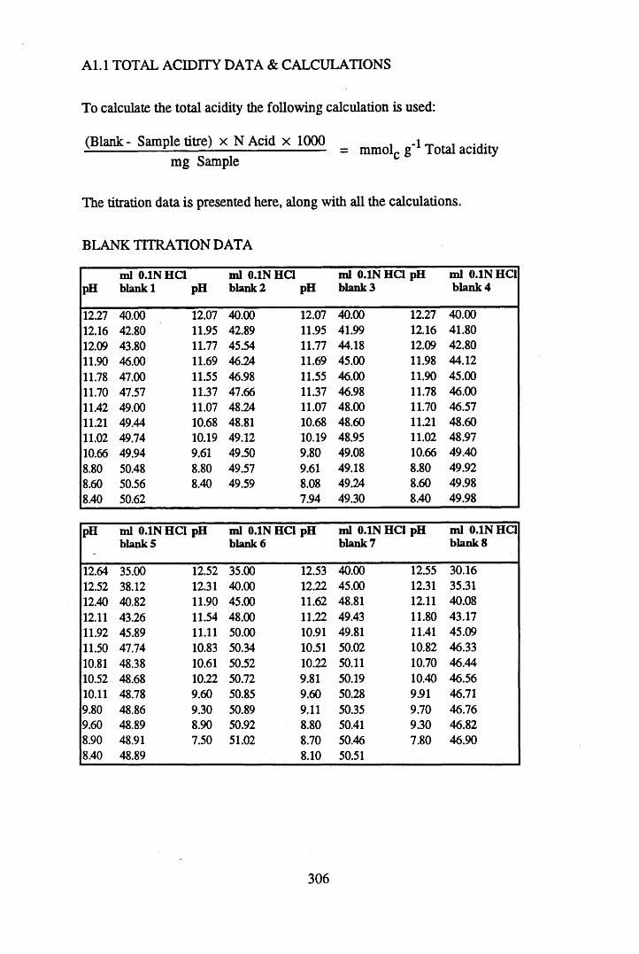
A l.l TOTAL ACIDITY DATA & CALCULATIONS
To calculate the total acidity the following calculation is used:
(Blank - Sample titre) x N Acid x 1000 _ mmoj -1 j otai acidity mg Sample c
The titration data is presented here, along with all the calculations.
BLANK TITRATION DATA
pHml 0.1NHC1 blank 1 pH
m l 0.1N HC1 blank 2 pH
ml 0.1N HC1 pH blank 3
m l 0.1NHC1 blank 4
12.27 40.00 12.07 40.00 12.07 40.00 12.27 40.0012.16 42.80 11.95 42.89 11.95 41.99 12.16 41.8012.09 43.80 11.77 45.54 11.77 44.18 12.09 42.8011.90 46.00 11.69 46.24 11.69 45.00 11.98 44.1211.78 47.00 11.55 46.98 11.55 46.00 11.90 45.0011.70 47.57 11.37 47.66 11.37 46.98 11.78 46.0011.42 49.00 11.07 48.24 11.07 48.00 11.70 46.5711.21 49.44 10.68 48.81 10.68 48.60 11.21 48.6011.02 49.74 10.19 49.12 10.19 48.95 11.02 48.9710.66 49.94 9.61 49.50 9.80 49.08 10.66 49.408.80 50.48 8.80 49.57 9.61 49.18 8.80 49.928.60 50.56 8.40 49.59 8.08 49.24 8.60 49.988.40 50.62 7.94 49.30 8.40 49.98
pH ml 0.1N HCI pH b lan k s
ml 0.1N HCI pH blank 6
ml 0.1N HCI pH blank 7
m l 0.1NHC1 blank 8
12.64 35.00 12.52 35.00 12.53 40.00 12.55 30.1612.52 38.12 12.31 40.00 12.22 45.00 12.31 35.3112.40 40.82 11.90 45.00 11.62 48.81 12.11 40.0812.11 43.26 11.54 48.00 11.22 49.43 11.80 43.1711.92 45.89 11.11 50.00 10.91 49.81 11.41 45.0911.50 47.74 10.83 50.34 10.51 50.02 10.82 46.3310.81 48.38 10.61 50.52 10.22 50.11 10.70 46.4410.52 48.68 10.22 50.72 9.81 50.19 10.40 46.5610.11 48.78 9.60 50.85 9.60 50.28 9.91 46.719.80 48.86 9.30 50.89 9.11 50.35 9.70 46.769.60 48.89 8.90 50.92 8.80 50.41 9.30 46.828.90 48.91 7.50 51.02 8.70 50.46 7.80 46.908.40 48.89 8.10 50.51
306
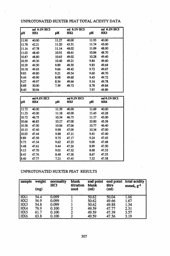
UNPROTONATED HUXTER PEAT TOTAL ACIDITY DATA
pHml 0.1N H Q HX1 pH
ml 0.1N H Q HX2 pH
ml 0.1N Ha HX3
11.90 40.00 11.27 40.00 11.93 40.0011.78 42.21 11.20 43.31 11.74 43.0011.16 47.78 11.14 48.02 11.09 48.0011.02 48.40 10.91 48.61 10.84 48.7010.87 48.80 10.63 49.02 10.28 49.4010.59 49.30 10.40 49.21 9.84 49.6010.39 49.50 9.89 49.30 9.83 49.6410.18 49.65 9.66 49.42 9.72 49.679.83 49.80 9.21 49.54 9.60 49.709.44 49.90 8.98 49.60 9.45 49.72921 49.97 8.34 49.66 9.16 49.788.88 50.00 7.39 49.72 8.78 49.848.40 50.04 7.97 49.89
pHm lO.lN H a HX4 pH
m lO.lN H a HX5 pH
m lO .lN H a HX6
11.72 40.00 11.39 40.00 11.69 40.0011.23 45.00 11.18 45.00 11.45 43.2810.72 46.75 10.54 46.75 11.17 45.0010.66 46.85 10.17 47.00 10.80 45.5810.58 47.00 10.06 47.06 10.77 46.4010.13 47.40 9.98 47.09 10.34 47.0010.03 47.44 9.88 47.11 9.41 47.409.89 47.50 9.75 47.17 9.24 47.459.73 47.54 9.62 47.23 9.00 47.489.48 47.61 9.44 47.26 8.99 47.509.15 47.70 9.01 47.32 8.68 47.538.45 47.76 8.48 47.38 8.67 47.558.40 47.77 7.21 47.43 7.52 47.58
UNPROTONATED HUXTER PEAT RESULTS
sample weight
(mg)
normalityHCI
blanktitrationused
end pointblank(ml)
end pointtitre(ml)
total addity mmole gr1
HX1 54.4 0.099 1 50.62 50.04 1.06HX2 56.9 0.099 1 50.62 49.66 1.67HX3 54.8 0.099 1 50.62 49.88 1.34HX4 78.9 0.100 2 49.59 47.77 2.31HX5 61.7 0.100 2 49.59 47.39 3.57HX6 63.8 0.100 2 49.59 47.56 3.19
307
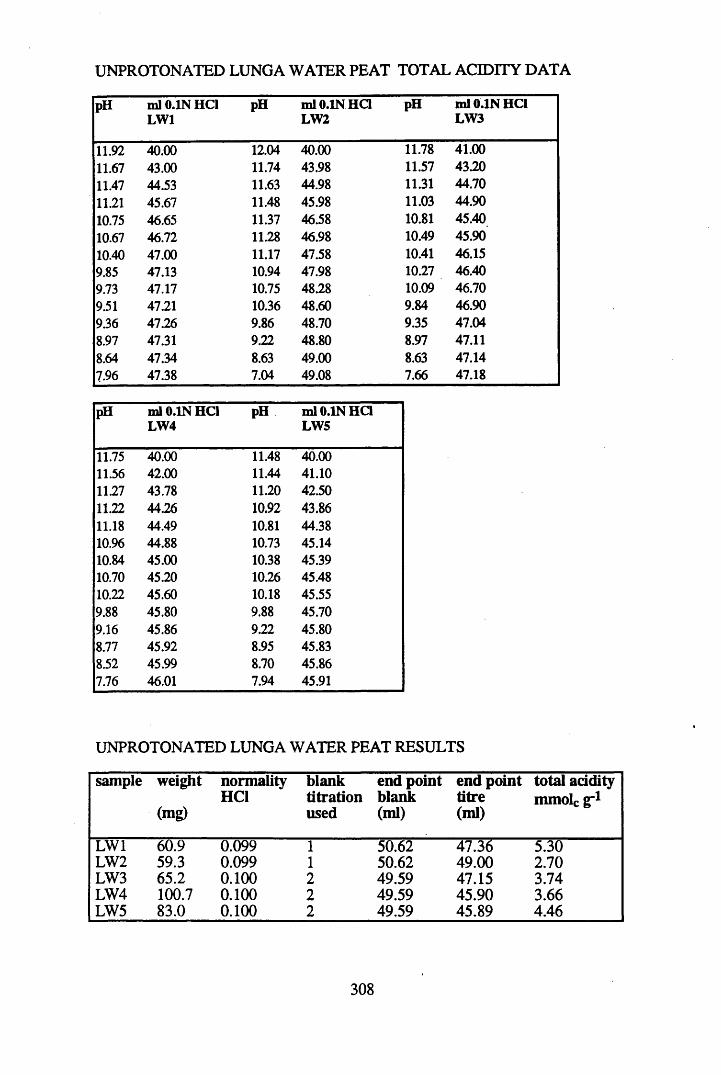
UNPROTONATED LUNGA WATER PEAT TOTAL ACIDITY DATA
pH ml 0.1N HC1 LW1
pH m lO .lN H C lLW2
pH m l 0.1N HC1 LW3
11.92 40.00 12.04 40.00 11.78 41.0011.67 43.00 11.74 43.98 11.57 43.2011.47 44.53 11.63 44.98 11.31 44.7011.21 45.67 11.48 45.98 11.03 44.9010.75 46.65 11.37 46.58 10.81 45.4010.67 46.72 11.28 46.98 10.49 45.9010.40 47.00 11.17 47.58 10.41 46.159.85 47.13 10.94 47.98 10.27 46.409.73 47.17 10.75 48.28 10.09 46.709.51 47.21 10.36 48.60 9.84 46.909.36 47.26 9.86 48.70 9.35 47.048.97 47.31 9.22 48.80 8.97 47.118.64 47.34 8.63 49.00 8.63 47.147.96 47.38 7.04 49.08 7.66 47.18
pH ml 0.1N HC1 LW4
pH m lO .lN H Q LW5
11.75 40.00 11.48 40.0011.56 42.00 11.44 41.1011.27 43.78 11.20 42.5011.22 44.26 10.92 43.8611.18 44.49 10.81 44.3810.96 44.88 10.73 45.1410.84 45.00 10.38 45.3910.70 45.20 10.26 45.4810.22 45.60 10.18 45.559.88 45.80 9.88 45.709.16 45.86 9.22 45.808.77 45.92 8.95 45.838.52 45.99 8.70 45.867.76 46.01 7.94 45.91
UNPROTONATED LUNGA WATER PEAT RESULTS
sample weight
(mg)
normalityHC1
blanktitrationused
end pointblank(ml)
end pointtitre(ml)
total acidity mmole g-1
LW1 60.9 0.099 1 50.62 47.36 5.30LW2 59.3 0.099 1 50.62 49.00 2.70LW3 65.2 0.100 2 49.59 47.15 3.74LW4 100.7 0.100 2 49.59 45.90 3.66LW5 83.0 0.100 2 49.59 45.89 4.46
308

PROTONATED HUXTER PEAT TOTAL ACIDITY DATA
pH ml 0.1N IJC1 HX1
pH m lO .lN HC1 HX2
pH m lO .lN H Q HX3
11.92 40.00 12.01 40.52 12.23 40.4411.73 43.19 11.61 45.05 11.61 45.1611.51 45.28 11.11 46.19 10.94 47.2611.10 46.09 10.95 47.30 10.71 47.5210.80 46.68 10.56 47.79 10.40 47.8210.20 46.98 10.12 48.03 10.10 47.949.40 47.58 9.81 48.12 9.60 48.049.10 47.64 9.62 48.23 9.30 48.118.50 47.68 9.16 48.28 8.90 48.167.41 47.72 8.10 48.37 8.40 48.20
pH m IO .IN H C lHX4
pH m lO .lN H Q HX5
12.52 40.40 12.41 40.3311.83 43.17 11.92 45.0811.51 45.23 10.81 47.3710.91 47.10 10.11 47.9210.70 47.28 9.80 47.9810.40 47.51 9.60 48.039.90 47.73 9.40 48.089.50 47.83 9.10 48.139.10 47.93 8.60 48.178.40 47.98 7.60 48.21
PROTONATED HUXTER PEAT RESULTS
sample weight
(mg)
normalityHC1
blanktitrationused
end pointblank(ml)
end pointtitre(ml)
total addity mmolc g-1
HX1 54.4 0.1 6 50.95 47.69 5.99HX2 58.0 0.1 6 50.95 48.35 4.48HX3 52.2 0.1 6 50.95 48.22 5.23HX4 52.3 0.1 6 50.95 47.98 5.68HX5 56.0 0.1 6 50.95 48.18 4.89
309
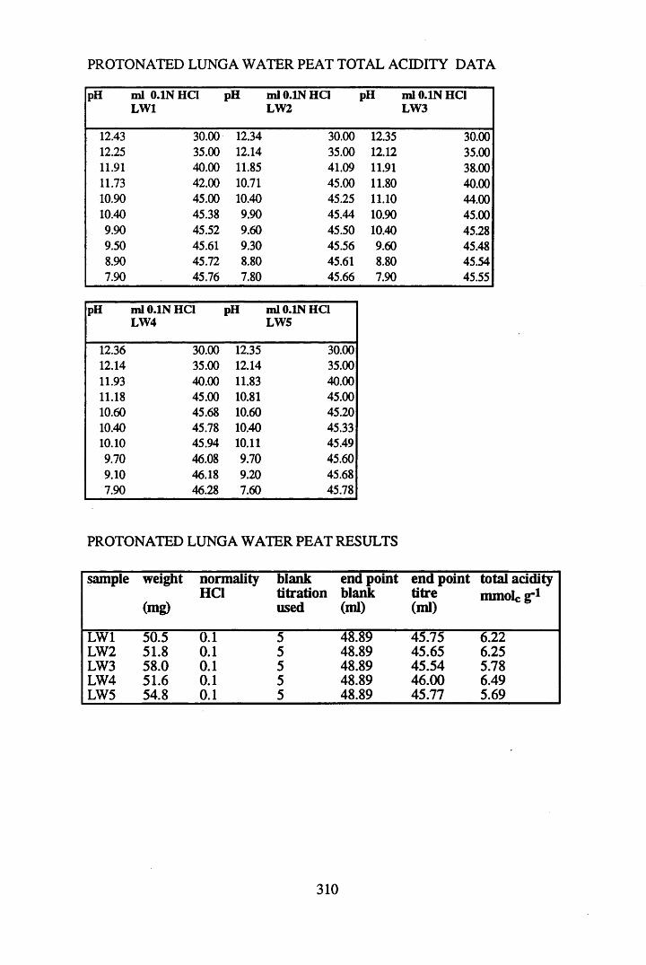
PROTONATED LUNGA WATER PEAT TOTAL ACIDITY DATA
pH ml 0.1NHC1 LW1
pH m l 0.1N HC1 LW2
pH ml 0.1N HC1 LW3
12.43 30.00 12.34 30.00 12.35 30.0012.25 35.00 12.14 35.00 12.12 35.0011.91 40.00 11.85 41.09 11.91 38.0011.73 42.00 10.71 45.00 11.80 40.0010.90 45.00 10.40 45.25 11.10 44.0010.40 45.38 9.90 45.44 10.90 45.009.90 45.52 9.60 45.50 10.40 45.289.50 45.61 9.30 45.56 9.60 45.488.90 45.72 8.80 45.61 8.80 45.547.90 45.76 7.80 45.66 7.90 45.55
pH ml 0.1N HC1 LW4
pH m l 0.1N HC1 LW5
12.36 30.00 12.35 30.0012.14 35.00 12.14 35.0011.93 40.00 11.83 40.0011.18 45.00 10.81 45.0010.60 45.68 10.60 45.2010.40 45.78 10.40 45.3310.10 45.94 10.11 45.499.70 46.08 9.70 45.609.10 46.18 9.20 45.687.90 46.28 7.60 45.78
PROTONATED LUNGA WATER PEAT RESULTS
sample weight
(mg)
normalityHC1
blanktitrationused
end pointblank(ml)
end pointtitre(ml)
total acidity mmolc g"1
LW1 50.5 0.1 5 48.89 45.75 6.22LW2 51.8 0.1 5 48.89 45.65 6.25LW3 58.0 0.1 5 48.89 45.54 5.78LW4 51.6 0.1 5 48.89 46.00 6.49LW5 54.8 0.1 5 48.89 45.77 5.69
310
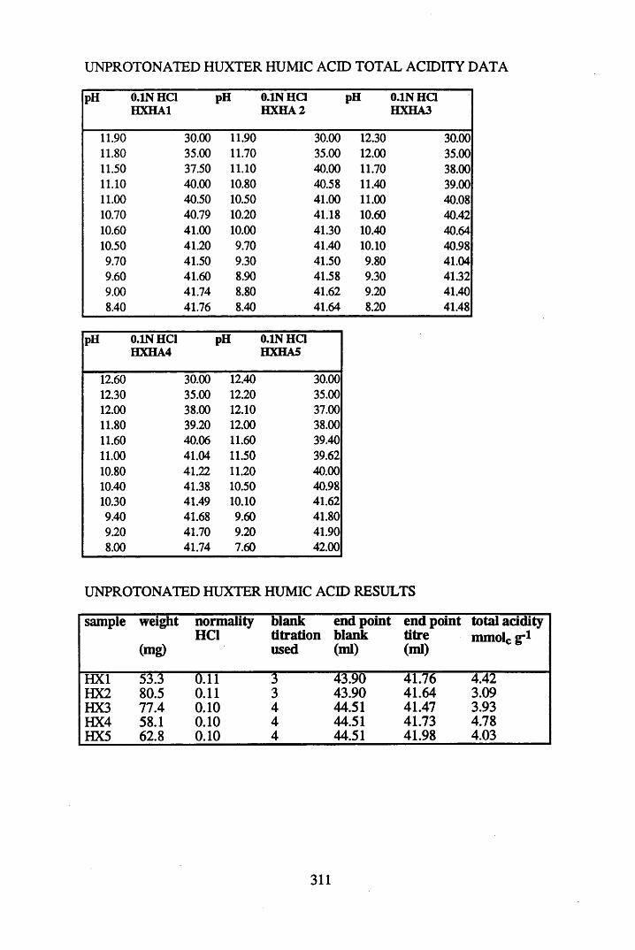
UNPROTONATED HUXTER HUMIC ACID TOTAL ACIDITY DATA
pH 0.1N HC1 pH 0.1N HC1 pH 0.1NHC1HXHA1 HXH A2 HXHA3
11.90 30.00 11.90 30.00 12.30 30.0011.80 35.00 11.70 35.00 12.00 35.0011.50 37.50 11.10 40.00 11.70 38.0011.10 40.00 10.80 40.58 11.40 39.0011.00 40.50 10.50 41.00 11.00 40.0810.70 40.79 10.20 41.18 10.60 40.4210.60 41.00 10.00 41.30 10.40 40.6410.50 41.20 9.70 41.40 10.10 40.989.70 41.50 9.30 41.50 9.80 41.049.60 41.60 8.90 41.58 9.30 41.329.00 41.74 8.80 41.62 9.20 41.408.40 41.76 8.40 41.64 8.20 41.48
pH 0.1N HC1 pH 0.1N H QHXHA4 HXHA5
12.60 30.00 12.40 30.0012.30 35.00 12.20 35.0012.00 38.00 12.10 37.0011.80 39.20 12.00 38.0011.60 40.06 11.60 39.4011.00 41.04 11.50 39.6210.80 41.22 11.20 40.0010.40 41.38 10.50 40.9810.30 41.49 10.10 41.629.40 41.68 9.60 41.809.20 41.70 9.20 41.908.00 41.74 7.60 42.00
UNPROTONATED HUXTER HUMIC ACID RESULTS
sample weight
(mg)
normalityHCI
blanktitrationused
end pointblank(ml)
end pointlitre(ml)
total acidity mmole g-1
HX1 53.3 0.11 3 43.90 41.76 4.42HX2 80.5 0.11 3 43.90 41.64 3.09HX3 77.4 0.10 4 44.51 41.47 3.93HX4 58.1 0.10 4 44.51 41.73 4.78HX5 62.8 0.10 4 44.51 41.98 4.03
311
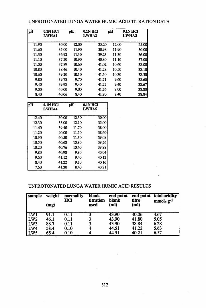
UNPROTONATED LUNGA WATER HUMIC ACID TITRATION DATA
pH 0.1N HC1 LWHA1
pH 0.1N HC1 LWHA2
pH 0.1NHC1LWHA3
11.90 30.00 12.00 25.20 12.00 25.0011.60 35.00 11.90 30.98 11.90 30.0011.30 36.92 11.30 39.23 11.30 36.0011.10 37.20 10.90 40.80 11.10 37.0011.00 37.89 10.60 41.02 10.60 38.0010.80 38.46 10.40 41.28 10.50 38.1010.60 39.20 10.10 41.50 10.30 38.309.80 39.78 9.70 41.71 9.60 38.609.40 39.98 9.40 41.75 9.40 38.679.00 40.00 9.00 41.76 9.00 38.808.40 40.06 8.40 41.80 8.40 38.84
pH 0.1N HC1 LWHA4
pH 0.1N HC1 LWHA5
12.40 30.00 12.30 30.0012.30 35.00 12.10 35.0011.60 39.40 11.70 38.0011.20 40.00 11.50 38.6010.90 40.50 11.30 39.0810.50 40.68 10.80 39.5610.20 40.76 10.40 39.889.80 40.98 9.80 40.049.60 41.12 9.40 40.128.40 41.22 9.10 40.167.60 41.30 8.40 40.21
UNPROTONATED LUNGA WATER HUMIC ACID RESULTS
sample weight
(mg)
normalityHC1
blanktitrationused
end pointblank(ml)
end pointtitre(ml)
total acidity mmolc g"1
LW1 91.1 0.11 3 43.90 40.06 4.67LW2 46.1 0.11 3 43.90 41.80 5.05LW3 88.7 0.11 3 43.90 38.84 6.28LW4 58.4 0.10 4 44.51 41.22 5.63LW5 65.4 0.10 4 44.51 40.21 6.57
312
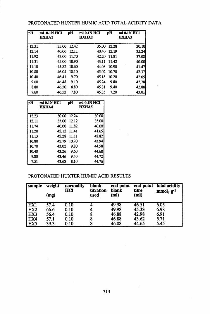
PROTONATED HUXTER HUMIC ACID TOTAL ACIDITY DATA
pH m l 0.1N HC1 HXHA1
pH m l 0.1N HC1 HXHA2
pH ml 0.1N HC1 HXHA3
12.31 35.00 12.42 35.00 12.28 30.1012.14 40.00 12.11 40.40 12.19 35.2411.92 43.00 11.70 42.20 11.81 37.0811.31 45.00 10.90 43.11 11.42 40.0011.10 45.82 10.60 44.08 10.90 41.4710.80 46.04 10.10 45.02 10.70 42.3710.40 46.41 9.70 45.18 10.20 42.659.60 46.48 9.10 45.24 9.80 42.788.80 46.50 8.80 45.31 9.40 42.887.60 46.53 7.80 45.35 7.20 43.01
pH m l 0.1N HC1 HXHA4
pH ml 0.1N HC1 HXHA5
12.23 30.00 12.24 30.0012.11 35.00 12.12 35.0011.74 40.00 11.82 40.0011.20 42.12 11.41 41.6511.13 42.28 11.11 42.8210.80 42.79 10.90 43.9410.70 43.02 9.80 44.5810.40 43.26 9.60 44.689.80 43.46 9.40 44.727.51 43.68 8.10 44.76
PROTONATED HUXTER HUMIC ACID RESULTS
sample weight
(mg)
normalityHCI
blanktitrationused
end pointblank(ml)
end pointtitre(ml)
total addity mmole g-1
HX1 57.4 0.10 4 49.98 46.51 6.05HX2 66.6 0.10 4 49.98 45.33 6.98HX3 56.4 0.10 8 46.88 42.98 6.91HX4 57.1 0.10 8 46.88 43.62 5.71HX5 39.3 0.10 8 46.88 44.65 5.45
313
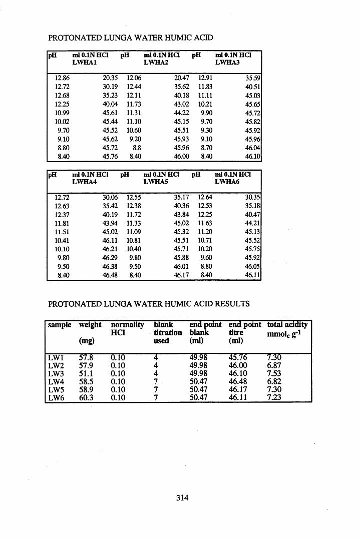
PROTONATED LUNGA WATER HUMIC ACID
pH m l 0.1N HC1 LWHA1
pH m lO .lN H Q LWHA2
pH ml 0.1N HC1 LWHA3
12.86 20.35 12.06 20.47 12.91 35.5912.72 30.19 12.44 35.62 11.83 40.5112.68 35.23 12.11 40.18 11.11 45.0312.25 40.04 11.73 43.02 10.21 45.6510.99 45.61 11.31 44.22 9.90 45.7210.02 45.44 11.10 45.15 9.70 45.829.70 45.52 10.60 45.51 9.30 45.929.10 45.62 9.20 45.93 9.10 45.968.80 45.72 8.8 45.96 8.70 46.048.40 45.76 8.40 46.00 8.40 46.10
pH ml 0.1N HC1 LWHA4
pH m l 0.1N H Q LWHA5
pH ml 0.1N HCI LWHA6
12.72 30.06 12.55 35.17 12.64 30.3512.63 35.42 12.38 40.36 12.53 35.1812.37 40.19 11.72 43.84 12.25 40.4711.81 43.94 11.33 45.02 11.63 44.2111.51 45.02 11.09 45.32 11.20 45.1310.41 46.11 10.81 45.51 10.71 45.5210.10 46.21 10.40 45.71 10.20 45.759.80 46.29 9.80 45.88 9.60 45.929.50 46.38 9.50 46.01 8.80 46.058.40 46.48 8.40 46.17 8.40 46.11
PROTONATED LUNGA WATER HUMIC ACID RESULTS
sample weight
(mg)
normalityHCI
blanktitrationused
end pointblank(ml)
end pointtitre(ml)
total acidity mmole g"1
LW1 57.8 0.10 4 49.98 45.76 7.30LW2 57.9 0.10 4 49.98 46.00 6.87LW3 51.1 0.10 4 49.98 46.10 7.53LW4 58.5 0.10 7 50.47 46.48 6.82LW5 58.9 0.10 7 50.47 46.17 7.30LW6 60.3 0.10 7 50.47 46.11 7.23
314
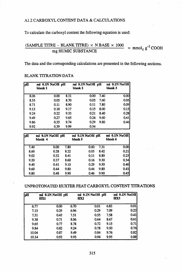
A1.2 CARBOXYL CONTENT DATA & CALCULATIONS
To calculate the carboxyl content the following equation is used:
(SAMPLE TTTRE - BLANK TITRE) x NBASE x 1000 , .1 _________ --------------------------------------------- --------------------------- = mmoL g 1 COOH
mg HUMIC SUBSTANCE c 6
The data and the corresponding calculations are presented in the following sections.
BLANK TITRATION DATA
pH ml 0.1N NaOH pH blank 1
ml O .INNaOH pH blank 2
ml 0.1N NaOH blank 3
8.06 0.00 8.31 0.00 7.40 0.008.33 0.05 8.70 0.05 7.60 0.058.71 0.11 8.90 0.11 7.80 0.099.13 0.18 9.17 0.15 8.00 0.159.24 0.22 9.33 0.21 8.40 0.289.49 0.27 9.65 0.26 9.60 0.419.86 0.35 9.74 0.29 9.80 0.469.92 0.39 9.99 0.34
pH m l 0.1N NaOH pH m l 0.1N NaOH pH ml 0.1N NaOHblank 4 blankS blank 6
7.40 0.00 7.80 0.00 7.31 0.008.60 0.28 8.22 0.05 8.42 0.219.02 0.32 8.41 0.11 8.80 0.259.20 0.37 8.60 0.16 9.30 0.349.40 0.41 9.10 0.29 9.50 0.409.60 0.44 9.80 0.44 9.80 0.439.80 0.48 9.90 0.46 9.90 0.45
UNPROTONATED HUXTER PEAT CARBOXYL CONTENT TITRATIONS
pH m l 0.1N NaOH pH ml 0.1N NaOH pH m l 0.1N NaOHHX1 HX2 HX3
6.77 0.00 6.70 0.01 6.82 0.017.13 0.29 6.96 0.29 7.09 0.227.51 0.43 7.51 0.55 7.58 0.419.38 0.71 8.06 0.64 8.67 0.619.65 0.77 8.78 0.72 9.15 0.719.84 0.82 9.24 0.78 9.50 0.76
10.04 0.87 9.49 0.84 9.76 0.8210.14 0.92 9.93 0.94 9.95 0.88
315
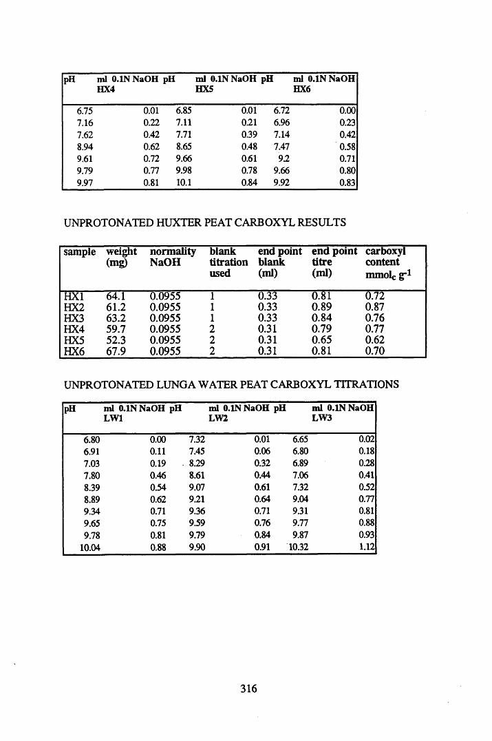
pH ml 0.1N NaOH pH m l O .INNaOH pH ml O .IN N aO H HX4 HX5 HX6
6.75 0.01 6.85 0.01 6.72 0.007.16 0.22 7.11 0.21 6.96 0.237.62 0.42 7.71 0.39 7.14 0.428.94 0.62 8.65 0.48 7.47 0.589.61 0.72 9.66 0.61 92 0.719.79 0.77 9.98 0.78 9.66 0.809.97 0.81 10.1 0.84 9.92 0.83
UNPROTONATED HUXTER PEAT CARBOXYL RESULTS
sample weight(mg)
normalityNaOH
blanktitrationused
end pointblank(ml)
end pointtitre(ml)
carboxyl content mmole g"1
HX1 64.1 0.0955 1 0.33 0.81 0.72HX2 61.2 0.0955 1 0.33 0.89 0.87HX3 63.2 0.0955 1 0.33 0.84 0.76HX4 59.7 0.0955 2 0.31 0.79 0.77HX5 52.3 0.0955 2 0.31 0.65 0.62HX6 67.9 0.0955 2 0.31 0.81 0.70
UNPROTONATED LUNGA WATER PEAT CARBOXYL TITRATIONS
pH ml 0.1N NaOH pH LW1
ml 0.1N NaOH pH LW2
m l 0.1N NaOH LW3
6.80 0.00 7.32 0.01 6.65 0.026.91 0.11 7.45 0.06 6.80 0.187.03 0.19 8.29 0.32 6.89 0.287.80 0.46 8.61 0.44 7.06 0.418.39 0.54 9.07 0.61 7.32 0.528.89 0.62 9.21 0.64 9.04 0.779.34 0.71 9.36 0.71 9.31 0.819.65 0.75 9.59 0.76 9.77 0.889.78 0.81 9.79 0.84 9.87 0.93
10.04 0.88 9.90 0.91 10.32 1.12
316
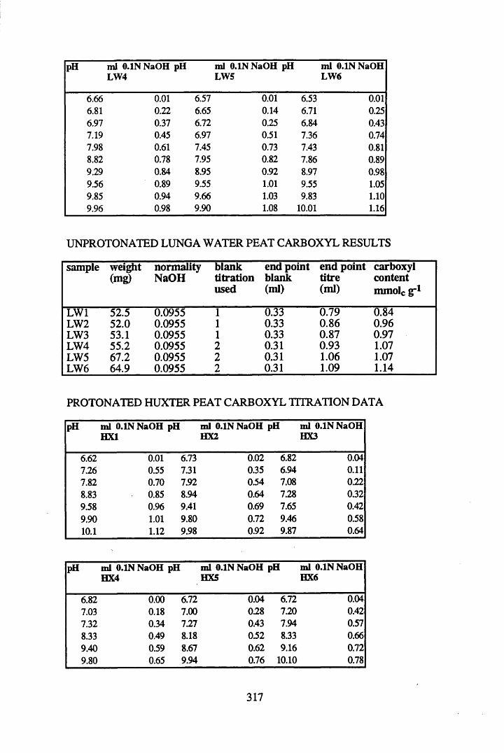
pH ml O .INNaOH pH LW4
ml O .INNaOH pH LW5
m l O.INNaOH LW6
6.66 0.01 6.57 0.01 6.53 0.016.81 0.22 6.65 0.14 6.71 0.256.97 0.37 6.72 0.25 6.84 0.437.19 0.45 6.97 0.51 7.36 0.747.98 0.61 7.45 0.73 7.43 0.818.82 0.78 7.95 0.82 7.86 0.899.29 0.84 8.95 0.92 8.97 0.989.56 0.89 9.55 1.01 9.55 1.059.85 0.94 9.66 1.03 9.83 1.109.96 0.98 9.90 1.08 10.01 1.16
UNPROTONATED LUNGA WATER PEAT CARBOXYL RESULTS
sample weight(mg)
normalityNaOH
blanktitrationused
end pointblank(ml)
end pointtitre(ml)
carboxyl content mmole g"1
LW1 52.5 0.0955 1 0.33 0.79 0.84LW2 52.0 0.0955 1 0.33 0.86 0.96LW3 53.1 0.0955 1 0.33 0.87 0.97LW4 55.2 0.0955 2 0.31 0.93 1.07LW5 67.2 0.0955 2 0.31 1.06 1.07LW6 64.9 0.0955 2 0.31 1.09 1.14
PROTONATED HUXTER PEAT CARBOXYL TITRATION DATA
pH ml 0.1N NaOH pH m l 0.1N NaOH pH ml 0.1N NaOH HX1 HX2 HX3
6.62 0.01 6.73 0.02 6.82 0.047.26 0.55 7.31 0.35 6.94 0.117.82 0.70 7.92 0.54 7.08 0.228.83 0.85 8.94 0.64 7.28 0.329.58 0.96 9.41 0.69 7.65 0.429.90 1.01 9.80 0.72 9.46 0.5810.1 1.12 9.98 0.92 9.87 0.64
pH m l 0.1N NaOH pH m l 0.1N NaOH pH ml 0.1N NaOH HX4 HX5 HX6
6.82 0.00 6.72 0.04 6.72 0.047.03 0.18 7.00 028 7.20 0.427.32 0.34 7.27 0.43 7.94 0.578.33 0.49 8.18 052 8.33 0.669.40 0.59 8.67 0.62 9.16 0.729.80 0.65 9.94 0.76 10.10 0.78
317
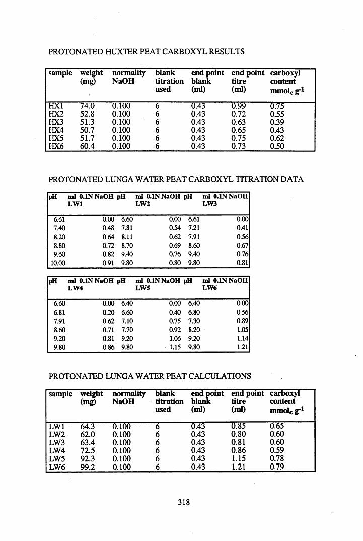
PROTONATED HUXTER PEAT CARBOXYL RESULTS
sample weight(mg)
normalityNaOH
blanktitrationused
end pointblank(ml)
end pointtitre(ml)
carboxyl content mmole g-1
HX1 74.0 0.100 6 0.43 0.99 0.75HX2 52.8 0.100 6 0.43 0.72 0.55HX3 51.3 0.100 6 0.43 0.63 0.39HX4 50.7 0.100 6 0.43 0.65 0.43HX5 51.7 0.100 6 0.43 0.75 0.62HX6 60.4 0.100 6 0.43 0.73 0.50
PROTONATED LUNGA WATER PEAT CARBOXYL TITRATION DATA
pH m l 0.1N NaOH pH m l 0.1N NaOH pH m l 0.1N NaOH LW1 LW2 LW3
6.61 0.00 6.60 0.00 6.61 0.007.40 0.48 7.81 0.54 7.21 0.418.20 0.64 8.11 0.62 7.91 0.568.80 0.72 8.70 0.69 8.60 0.679.60 0.82 9.40 0.76 9.40 0.76
10.00 0.91 9.80 0.80 9.80 0.81
pH m l O .IN N aO H pH m l O .INNaOH pH m l O .IN N aO H LW 4 LW5 LW6
6.60 0.00 6.40 0.00 6.40 0.006.81 0.20 6.60 0.40 6.80 0.567.91 0.62 7.10 0.75 7.30 0.898.60 0.71 7.70 0.92 8.20 1.059.20 0.81 9.20 1.06 9.20 1.149.80 0.86 9.80 1.15 9.80 1.21
PROTONATED LUNGA WATER PEAT CALCULATIONS
sample weight(mg)
normalityNaOH
blanktitrationused
end pointblank(ml)
end pointtitre(ml)
carboxyl content mmole g-1
LW1 64.3 0.100 6 0.43 0.85 0.65LW2 62.0 0.100 6 0.43 0.80 0.60LW3 63.4 0.100 6 0.43 0.81 0.60LW4 72.5 0.100 6 0.43 0.86 0.59LW5 92.3 0.100 6 0.43 1.15 0.78LW6 99.2 0.100 6 0.43 1.21 0.79
318
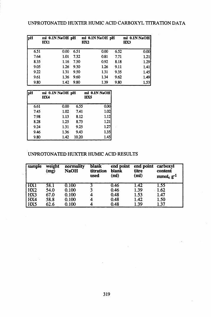
UNPROTONATED HUXTER HUMIC ACID CARBOXYL TITRATION DATA
pH ml O .IN N aO H pH ml O.INNaOH pH ml O .IN N aO H HX1 HX2 HX3
6.51 0.00 6.51 0.00 6.52 0.007.64 1.01 7.32 0.81 7.71 1218.35 1.16 7.50 0.92 8.18 1.299.05 1.26 9.30 1.26 9.11 1.419.22 1.31 9.50 1.31 9.35 1.459.61 1.36 9.60 1.34 9.62 1.499.80 1.42 9.80 1.39 9.80 1.53
pH ml 0.1N NaOH pH m l 0.1N NaOH HX4 HX5
6.61 0.00 6.55 0.007.45 1.02 7.41 1.027.98 1.13 8.12 1.128.28 1.25 8.73 1219.24 1.31 9.25 1.279.46 1.36 9.43 1.359.80 1.42 10.20 1.45
UNPROTONATED HUXTER HUMIC ACID RESULTS
sample weight(mg)
normalityNaOH
blanktitrationused
end pointblank(ml)
end pointtitre(ml)
carboxyl content mmole g-1
HX1 58.1 0.100 3 0.46 1.42 1.55HX2 54.0 0.100 3 0.46 1.39 1.62HX3 67.0 0.100 4 0.48 1.53 1.47HX4 58.8 0.100 4 0.48 1.42 1.50HX5 62.6 0.100 4 0.48 1.39 1.37
319
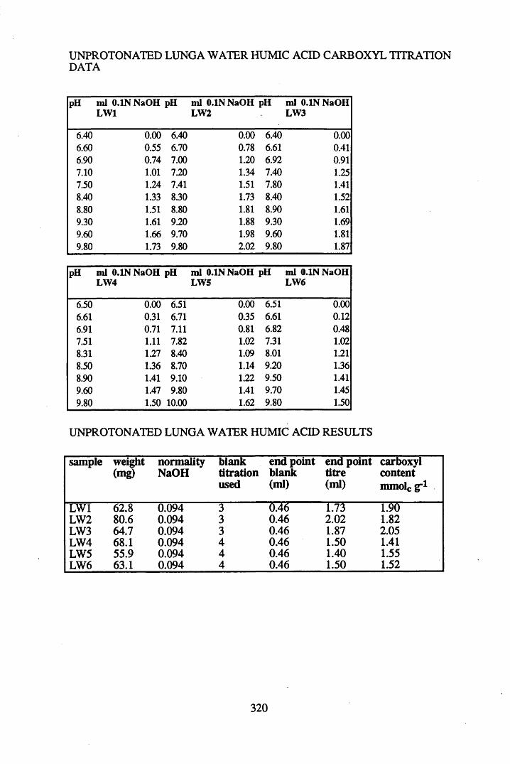
UNPROTONATED LUNGA WATER HUMIC ACID CARBOXYL TITRATION DATA
pH m l 0.1N NaOH pH m l 0.1N NaOH pH ml 0.1N NaOH LW1 LW2 LW3
6.40 0.00 6.40 0.00 6.40 0.006.60 0.55 6.70 0.78 6.61 0.416.90 0.74 7.00 1.20 6.92 0.917.10 1.01 7.20 1.34 7.40 1.257.50 1.24 7.41 1.51 7.80 1.418.40 1.33 8.30 1.73 8.40 1.528.80 1.51 8.80 1.81 8.90 1.619.30 1.61 9.20 1.88 9.30 1.699.60 1.66 9.70 1.98 9.60 1.819.80 1.73 9.80 2.02 9.80 1.87
pH m l O .IN N aO H pH ml O .INNaOH pH m l O .INNaOHLW4 LW5 LW6
6.50 0.00 6.51 0.00 6.51 0.006.61 0.31 6.71 0.35 6.61 0.126.91 0.71 7.11 0.81 6.82 0.487.51 1.11 7.82 1.02 7.31 1.028.31 1.27 8.40 1.09 8.01 1.218.50 1.36 8.70 1.14 9.20 1.368.90 1.41 9.10 1.22 9.50 1.419.60 1.47 9.80 1.41 9.70 1.459.80 1.50 10.00 1.62 9.80 1.50
UNPROTONATED LUNGA WATER HUMIC ACID RESULTS
sample weight(mg)
normalityNaOH
blanktitrationused
end pointblank(ml)
end pointtitre(ml)
carboxyl content mmolc g"1
LW1 62.8 0.094 3 0.46 1.73 1.90LW2 80.6 0.094 3 0.46 2.02 1.82LW3 64.7 0.094 3 0.46 1.87 2.05LW4 68.1 0.094 4 0.46 1.50 1.41LW5 55.9 0.094 4 0.46 1.40 1.55LW6 63.1 0.094 4 0.46 1.50 1.52
320
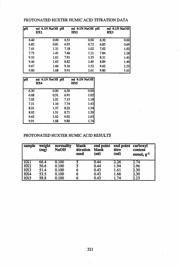
PROTONATED HUXTER HUMIC ACID TITRATION DATA
pH m l 0.1N NaOH pH m l 0.1N NaOH pH m l 0.1N NaOH HX1 HX2 HX3
6.40 0.00 6.51 0.00 6.30 0.006.82 0.81 6.92 0.72 6.85 0.697.41 1.31 7.18 1.02 7.02 1.027.73 1.41 7.46 1.21 7.84 1.289.33 1.61 7.91 1.35 8.31 1.419.46 1.63 8.82 1.49 8.89 1.499.67 1.66 9.16 1.52 9.62 1.559.80 1.68 9.91 1.61 9.80 1.61
pH ml 0.1N NaOH pH ml 0.1N NaOH HX4 HX5
6.30 0.00 6.30 0.006.68 0.51 6.91 1.027.05 1.01 7.15 1.187.31 1.16 7.74 1.438.01 1.37 8.22 1.548.92 1.51 8.71 1.599.65 1.62 9.02 1.639.91 1.68 9.80 1.74
PROTONATED HUXTER HUMIC ACID RESULTS
sample weight(mg)
normalityNaOH
blanktitrationused
end pointblank(ml)
end pointtitre(ml)
carboxyl content mmole g-1
HX1 66.4 0.100 5 0.44 2.26 2.74HX2 50.6 0.100 5 0.44 1.94 2.96HX3 51.4 0.100 6 0.43 1.61 2.30HX4 53.5 0.100 6 0.43 1.66 2.30HX5 58.8 0.100 6 0.43 1.74 2.23
321
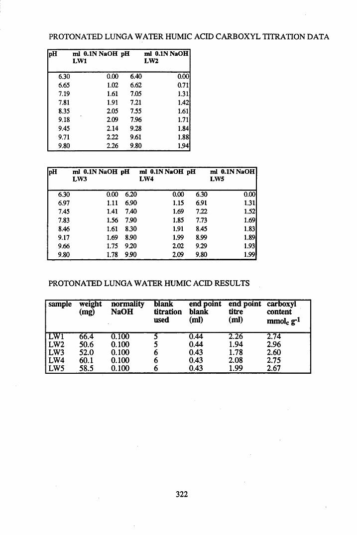
PROTONATED LUNGA WATER HUMIC ACID CARBOXYL TITRATION DATA
pH ml 0.1N NaOH pH m l 0.1N NaOH LW1 LW2
6.30 0.00 6.40 0.006.65 1.02 6.62 0.717.19 1.61 7.05 1.317.81 1.91 7.21 1.428.35 2.05 7.55 1.619.18 2.09 7.96 1.719.45 2.14 9.28 1.849.71 2.22 9.61 1.889.80 2.26 9.80 1.94
pH ml O .IN N aO H pH ml O .INNaOH pH ml O .IN N aO H LW3 LW4 LW5
6.30 0.00 620 0.00 6.30 0.006.97 1.11 6.90 1.15 6.91 1.317.45 1.41 7.40 1.69 7.22 1.527.83 1.56 7.90 1.85 7.73 1.698.46 1.61 8.30 1.91 8.45 1.839.17 1.69 8.90 1.99 8.99 1.899.66 1.75 920 2.02 9.29 1.939.80 1.78 9.90 2.09 9.80 1.99
PROTONATED LUNGA WATER HUMIC ACID RESULTS
sample weight(mg)
normalityNaOH
blanktitrationused
end pointblank(ml)
end pointtitre(ml)
carboxyl content mmole g"1
LW1 66.4 0.100 5 0.44 2.26 2.74LW2 50.6 0.100 5 0.44 1.94 2.96LW3 52.0 0.100 6 0.43 1.78 2.60LW4 60.1 0.100 6 0.43 2.08 2.75LW5 58.5 0.100 6 0.43 1.99 2.67
322
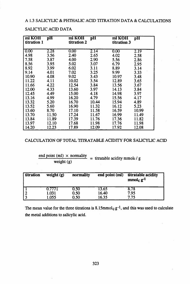
A 1.3 SALICYLIC & PHTHALIC ACID TITRATION DATA & CALCULATIONS
SALICYLIC ACID DATA
mlKOH titration 1
pH mlKOH titration 2
pH ml KOH titration 3
pH
0.00 2.28 0.00 2.14 0.00 2.194.98 3.56 2.40 2.65 4.02 2.587.58 3.87 4.00 2.90 5.56 2.868.56 3.95 5.02 3.07 6.79 2.958.92 3.99 6.02 3.11 8.89 3.149.14 4.01 7.02 3.25 9.99 3.3310.90 4.08 9.02 3.43 10.97 3.4811.22 4.11 10.02 3.54 12.89 3.6511.66 4.22 12.54 3.84 13.56 3.6712.00 4.33 13.60 3.97 14.13 3.8412.45 4.49 15.00 4.18 14.98 3.9713.16 4.99 16.20 4.79 15.56 4.1713.32 5.20 16.70 10.44 15.94 4.8913.52 5.60 16.90 11.32 16.12 5.2313.60 8.70 17.10 11.58 16.59 10.9913.70 11.50 17.24 11.67 16.99 11.4913.84 11.89 17.39 11.76 17.36 11.8213.97 12.10 17.68 11.98 17.76 11.9814.20 12.23 17.89 12.09 17.92 12.08
CALCULATION OF TOTAL TITRATABLE ACIDITY FOR SALICYLIC ACID
end point (ml) x normality t / ------ — ---------------- = titratable acidity mmole / gweight (g)
titration weight (g) normality end point (ml) titratable addity mmole g”1
1 0.7771 0.50 13.65 £.782 1.031 0.50 16.40 7.953 1.055 0.50 16.35 7.75
The mean value for the three titrations is 8.15mmolc g"1, and this was used to calculate the metal additions to salicylic acid.
323
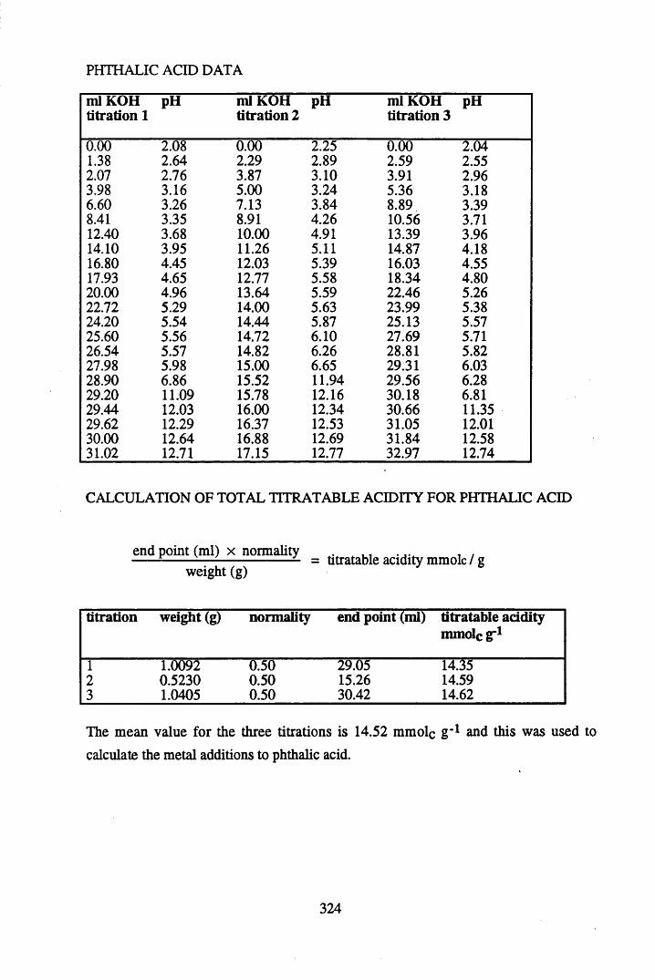
PHTHALIC ACID DATA
mlKOH titration 1
PH mlKOH titration 2
pH ml KOH titration 3
pH
0.00 2.08 0.00 2.25 0.00 2.041.38 2.64 2.29 2.89 2.59 2.552.07 2.76 3.87 3.10 3.91 2.963.98 3.16 5.00 3.24 5.36 3.186.60 3.26 7.13 3.84 8.89 3.398.41 3.35 8.91 4.26 10.56 3.7112.40 3.68 10.00 4.91 13.39 3.9614.10 3.95 11.26 5.11 14.87 4.1816.80 4.45 12.03 5.39 16.03 4.5517.93 4.65 12.77 5.58 18.34 4.8020.00 4.96 13.64 5.59 22.46 5.2622.72 5.29 14.00 5.63 23.99 5.3824.20 5.54 14.44 5.87 25.13 5.5725.60 5.56 14.72 6.10 27.69 5.7126.54 5.57 14.82 6.26 28.81 5.8227.98 5.98 15.00 6.65 29.31 6.0328.90 6.86 15.52 11.94 29.56 6.2829.20 11.09 15.78 12.16 30.18 6.8129.44 12.03 16.00 12.34 30.66 11.3529.62 12.29 16.37 12.53 31.05 12.0130.00 12.64 16.88 12.69 31.84 12.5831.02 12.71 17.15 12.77 32.97 12.74
CALCULATION OF TOTAL TITRATABLE ACIDITY FOR PHTHALIC ACID
end point (ml) x normality . . ... . . ------ — ---------------- = titratable acidity mmole / gweight (g)
titration weight (g) normality end point (ml) titratable acidity mmolc g"1
1 1.0092 0.50 29.05 14.352 0.5230 0.50 15.26 14.593 1.0405 0.50 30.42 14.62
The mean value for the three titrations is 14.52 mmolc g '1 and this was used to calculate the metal additions to phthalic acid.
324
APPENDIX 2:
METAL BINDING DATA & GRAPHS FROMCHAPTER 4
325
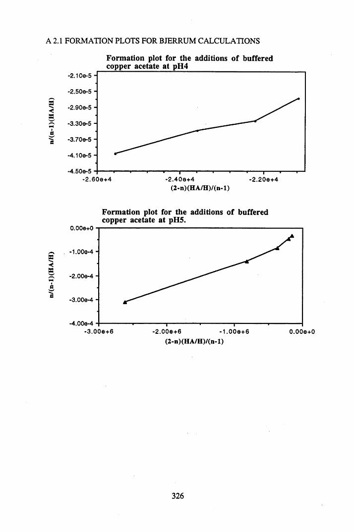
n/(n
-l)(
HA
/H)
n/(n
-l)(
HA
/H)
A 2.1 FORMATION PLOTS FOR BJERRUM CALCULATIONS
Formation plot for the additions of buffered copper acetate at pH4
-2.10e-5 -
-2.50©-5 -
-2.900-5 -
-3.300-5 -
-3.700-5 -
-4.100-5 -
-4.500-5-2 .600+ 4 -2 .400+ 4 -2 .200+ 4
(2 -n ) (H A /H ) / (n - l )
Formation plot for the additions of buffered copper acetate at pH5.
0 .000+0
-1.000-4 -
-2.000-4 -
-3.00O-4 -
-4.000-4- 2 . 000+6 - 1 . 0 00+ 6 0 .000+0
(2 -n ) (H A /H )/(n - l )
326
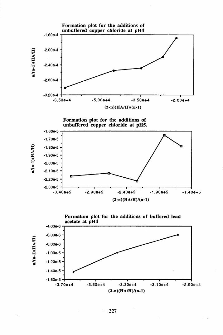
Formation plot for the additions ofunbuffered copper chloride at pH4
-1.600-4
-2.400-4 -
-2.800-4 -
-3.200-4-5 .000+ 4-6 .500+4 -2 .0 0 0 + 4
(2 -n ) (H A /H )/(n - l )
Formation plot for the additions of unbuffered copper chloride at pH5.
-1.600-5
-1.700-5 -
-1.800-5 -
-1.900-5 -
-2.000-5 -
-2.100-5 -
-2.200-5 -
-2.300-5-2 .400+5-3 .400+ 5 -2 .900+ 5 -1 .900+ 5 -1.40©+5
(2 -n ) (H A /H )/(n - l )
Formation plot for the additions of buffered lead acetate at pH4
-4.000-6
- 6 . 000-6 -
-1.000-5 -
-1.200-5 -
-1.400-5 -
-3.500+4 -3 .300+4 -3.100+4(2-n) (H A /H )/(n -1)
327
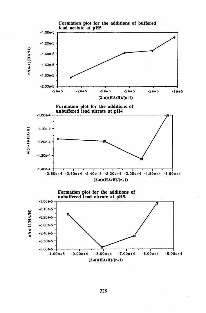
Formation plot for the additions of bufferedlead acetate at pH5.
-1.00e-5
-1.20e-5 -
-1.400-5 -
-1.600-5 -
-1.800-5 -
-2.000-5-20+5-20+5 -2©+5 -20+5 -10+ 5
(2 -n ) (H A /H )/ (n - l )
Formation plot for the additions of unbuffered lead nitrate at pH4
-1.00©-4
-1.100-4 -
-1.200-4 -
-1.300-4 -
-1.400-4-2 .800+ 4 -2 .600+ 4 -2 .400+4 -2 .200+ 4 -2 .0 0 0 + 4 -1 .800+4 -1 .6 0 0 + 4
(2 -n ) (H A /H )/(n - l )
Formation plot for the additions of unbuffered lead nitrate at pH5.
-3.000-5
-3.100-5 -
-3.300-5 -
-3.400-5 -
-3.500-5
-3.600-5-1 .000+ 5 -9 .000+ 4 -8 .000+ 4 -7 .000+ 4 -6 .000+ 4 -5 .0 0 0 + 4
(2 -n ) (H A /H )/(n - l )
328
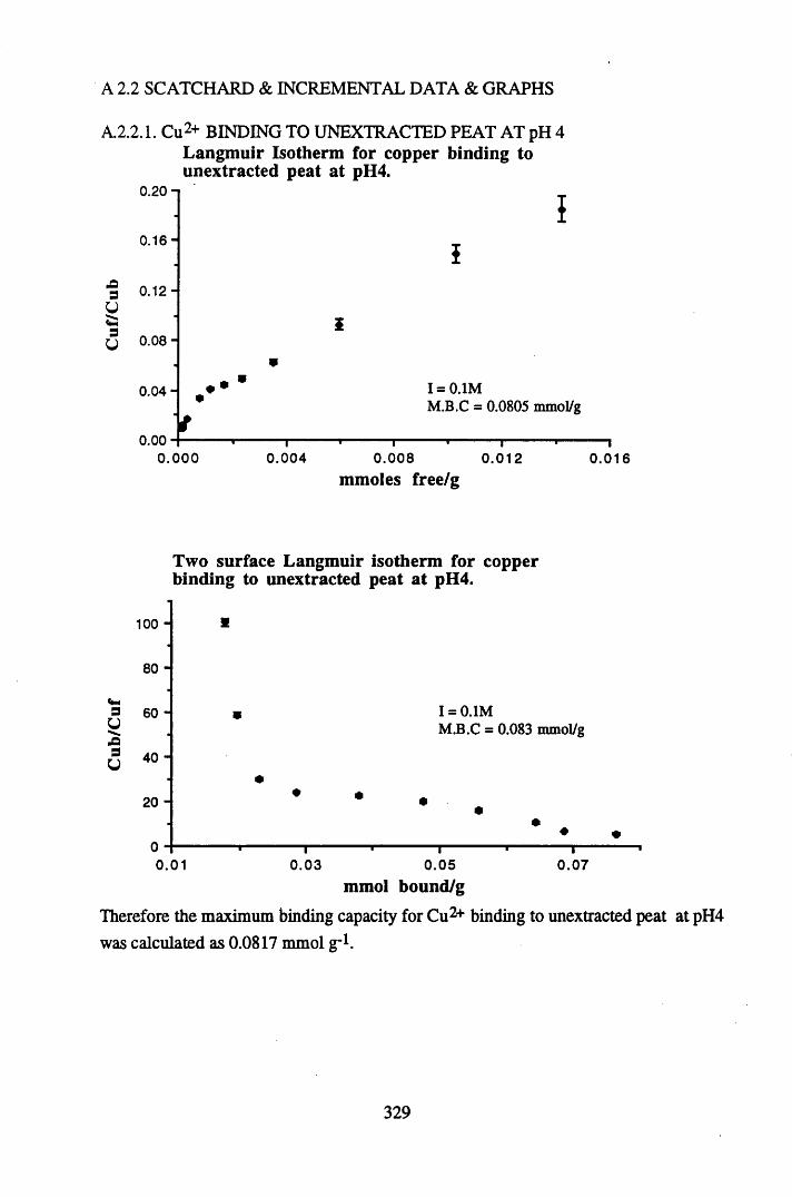
A 2.2 SCATCHARD & INCREMENTAL DATA & GRAPHS
A.2.2.1. Cu2+ BINDING TO UNEXTRACTED PEAT AT pH 4 Langmuir Isotherm for copper binding to unextracted peat at pH4.
0.20 n
AaU3V
0.16-
0 . 1 2 -
0.08-
0.04-
0.00
I
i
I = 0.1MM.B.C = 0.0805 mmol/g
0.000 1---0.004 0.008
mmoles free/g0.012 0.016
Two surface Langmuir isotherm for copper binding to unextracted peat at pH4.
100 -
80 -
40 -
20 -
0.01
I = 0.1MM.B.C = 0.083 mmol/g
0.070.03 0.05mmol bound/g
Therefore the maximum binding capacity for Cu2+ binding to unextracted peat at pH4 was calculated as 0.0817 mmol g’1.
329
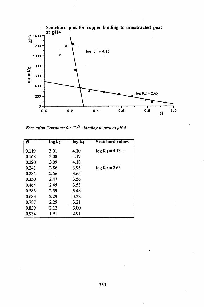
Scatchard plot for copper binding to unextracted peatat pH4
0 1400 M
1200log K1 = 4.13
1000
800
600
400
log K2 = 2.65200
0.6 1.00.80.2 0.40.0
Formation Constants for Cu2+ binding to peat at pH 4.
0 log k3 logk4 Scatchard values
0.119 3.01 4.10 logKi =4.13 •0.168 3.08 4.170.220 3.09 4.180.241 2.86 3.95 log K2 = 2.650.281 2.56 3.650.350 2.47 3.560.464 2.45 3.530.583 2.39 3.480.683 2.29 3.380.787 2.29 3.210.839 2.12 3.000.934 1.91 2.91
330
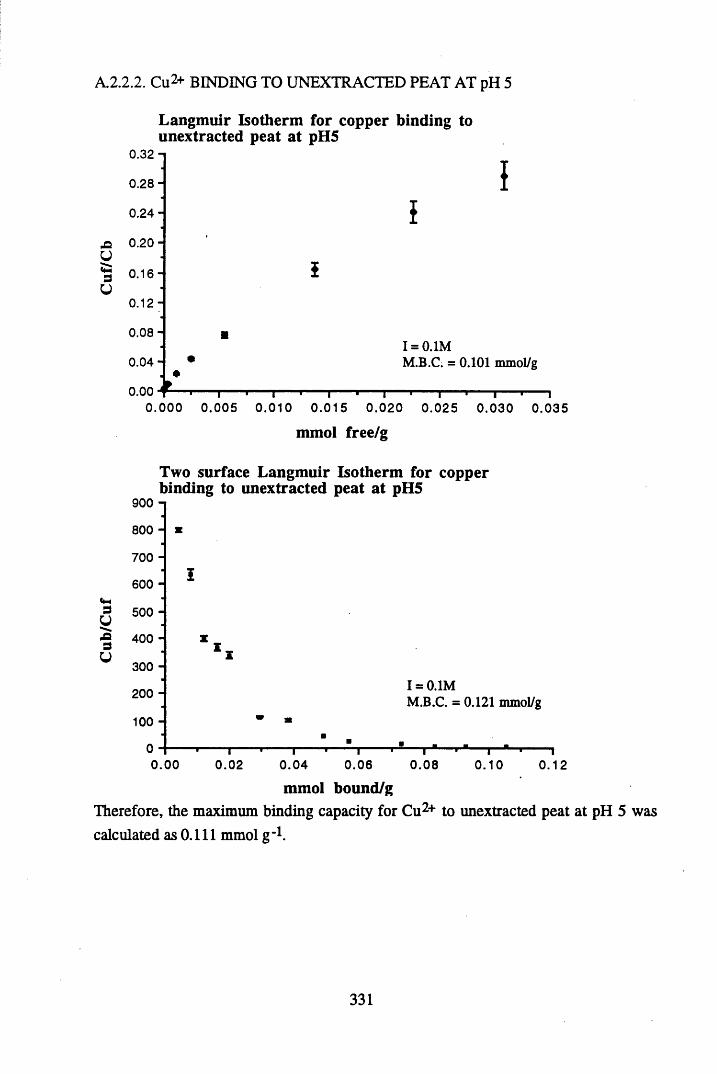
A.2.2.2. Cu2+ BINDING TO UNEXTRACTED PEAT AT pH 5
pOUsV
Langmuir Isotherm for copper binding to unextracted peat at pH5
0 .3 2 -
0 .2 8 -
0 .2 4 -
0.20-
0 .1 6 -
0.12-
0 .0 8 -
0 .0 4 -
0.00*1
}i
I = 0.1MM.B.C. = 0.101 mmol/g
i---- 1-----1-----1--------1-1------- 1------1-1---------1-1---- 1---- 10 .0 0 0 0 .0 0 5 0 .0 1 0 0 .0 1 5 0 .0 2 0 0 .0 2 5 0 .0 3 0 0 .035
mmol free/g
3u3V
Two surface Langmuir Isotherm for copper binding to unextracted peat at pH5
900 -i
800
700 H
600
500
400
300
200
100
I = 0.1MM.B.C. = 0.121 mmol/g
00 0.02 0.120 .0 4 0 .06 0 .0 8 0 .1 0
mmol bound/gTherefore, the maximum binding capacity for Cu2+ to unextracted peat at pH 5 was calculated as 0.111 mmol g_1.
331
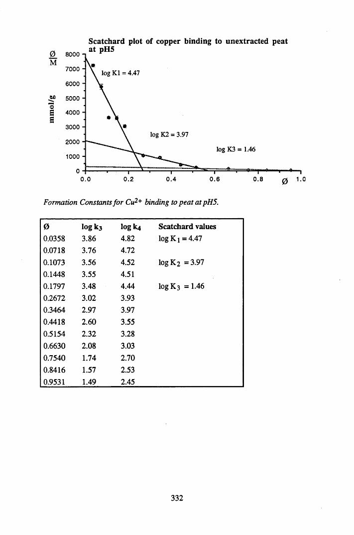
Scatchard plot of copper binding to unextracted peat^ at pH50_ 8000 -l vM
7000 - log K1 = 4.47
6000 -
5000 -
3000 -log K2 = 3.97
2000log K3 = 1.46
1000 -
•fTIHIjllllllllll0.80.2 0 .4 0.6 1.00.0
Formation Constants for Cu2+ binding to peat at pH5.
0 log k3 logk4 Scatchard values0.0358 3.86 4.82 log K i =4.470.0718 3.76 4.720.1073 3.56 4.52 log K2 =3.970.1448 3.55 4.510.1797 3.48 4.44 log K3 =1.460.2672 3.02 3.930.3464 2.97 3.970.4418 2.60 3.550.5154 2.32 3.280.6630 2.08 3.030.7540 1.74 2.700.8416 1.57 2.530.9531 1.49 2.45
332
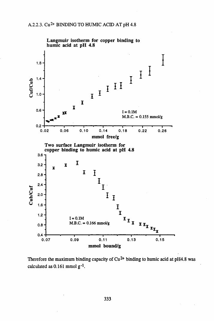
A2.2.3. Cu2+ BINDING TO HUMIC ACID AT pH 4.8
Langmuir isotherm for copper binding to humic acid at pH 4.8
■osU3y
1.8-
1 .4 -
1.0-
0.6-
0.2
II I I I I
I
I = 0.1MM.B.C. = 0.155 mmol/g
— ----- 1 ■ i----- 1----- 1----- 1-------- 1-- -------1——i----- 1—0 .0 2 0 .0 6 0 .1 0 0 .14 0 .1 8 0 .2 2 0 .2 6
mmol free/g
Two surface Langmuir isotherm for copper binding to humic acid at pH 4.8
3 .6 -
3 .2 -
2 .8 -
2 .4 -3y 2.0 -A3 ■
y 1.6-
1 .2-
o CO
i __1__
0 .4 -
Ii
i
I = 0.1MM.B.C. = 0.166 mmol/g 1 II.
0 .0 7 0 .09 0.11 0 .13
mmol bound/g0 .1 5
Therefore the maximum binding capacity of Cu2+ binding to humic acid at pH4.8 was calculated as 0.161 mmol g"1.
333
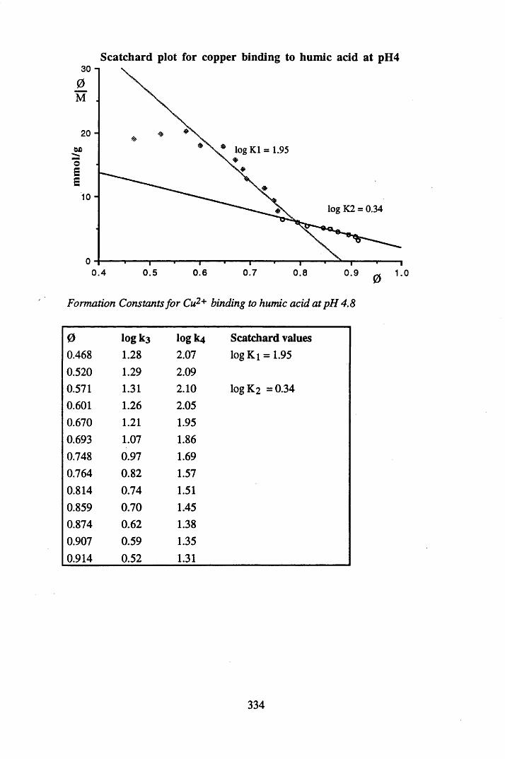
Scatchard plot for copper binding to humic acid at pH430 n
20 -
log K1 = 1.95
10 -log K2 = 0.34
0.70.4 0.5 0.6 0.8 0.9 1.0
Formation Constants for Cu2+ binding to humic acid at pH 4.8
0 l o g k 3 Iogk4 S c a tc h a rd values
0.468 1.28 2.07 log Ki = 1.950.520 1.29 2.090.571 1.31 2.10 logK2 =0.340.601 1.26 2.050.670 1.21 1.950.693 1.07 1.860.748 0.97 1.690.764 0.82 1.570.814 0.74 1.510.859 0.70 1.450.874 0.62 1.380.907 0.59 1.350.914 0.52 1.31
334
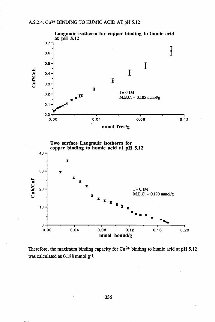
Cub
/Cuf
C
uf/C
ub
A.2.2.4. Cu2+ BINDING TO HUMIC ACID AT pH 5.12
0 .7 -
0.6-
0 .5 -
0 .4 -
0 .3 -
0.2-
0.1 -
Langmuir isotherm for copper binding to humic acid at pH 5.12
o.o
II I
I = 0.1MM.B.C. = 0.185 mmol/g
0.00 0 .0 4 0 .0 8
mmol free/g0.12
Two surface Langmuir isotherm for copper binding to humic acid at pH 5.12
30 -
20 -
10 -
I = 0.1MM.B.C. = 0.190 mmol/g
0.00 0 .04 0 .0 8 0 .12 mmol bound/g
0 .16 0.20
Therefore, the maximum binding capacity for Cu2+ binding to humic acid at pH 5.12 was calculated as 0.188 mmol g '1.
335
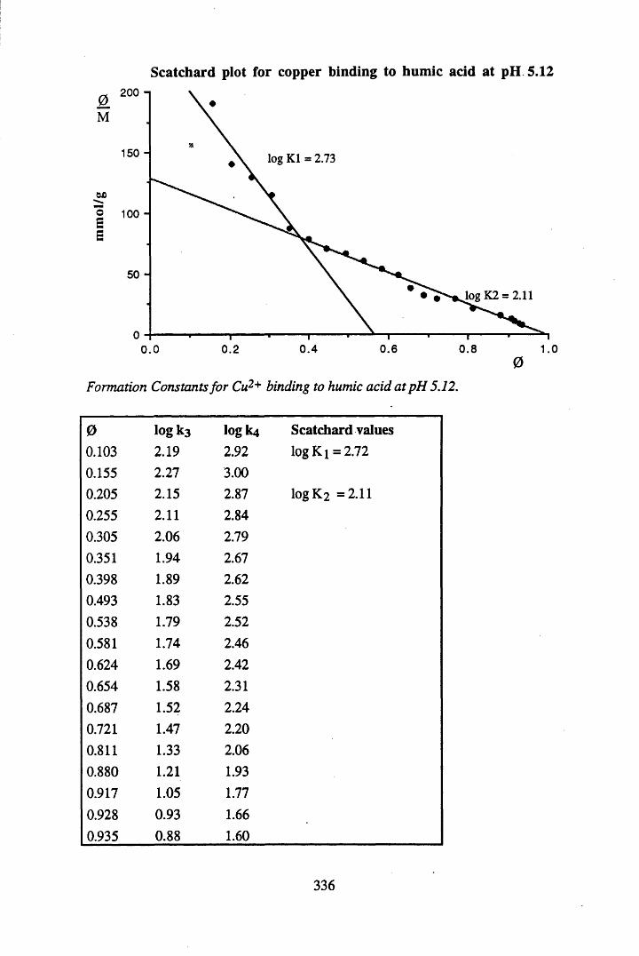
I
Scatchard plot for copper binding to humic acid at pH 5.12200 n
0M
150 - log K1 = 2.73
50 -
log K2 = 2.11
0 .4 0.6 0.8 1.00.0 0.20
Formation Constants for Cu2+ binding to humic acid at pH 5.12.
0 log k3 logk4 Scatchard values0.103 2.19 2.92 log Ki = 2.720.155 2.27 3.000.205 2.15 2.87 log K2 =2.110.255 2.11 2.840.305 2.06 2.790.351 1.94 2.670.398 1.89 2.620.493 1.83 2.550.538 1.79 2.520.581 1.74 2.460.624 1.69 2.420.654 1.58 2.310.687 1.52 2.240.721 1.47 2.200.811 1.33 2.060.880 1.21 1.930.917 1.05 1.770.928 0.93 1.660.935 0.88 1.60
336
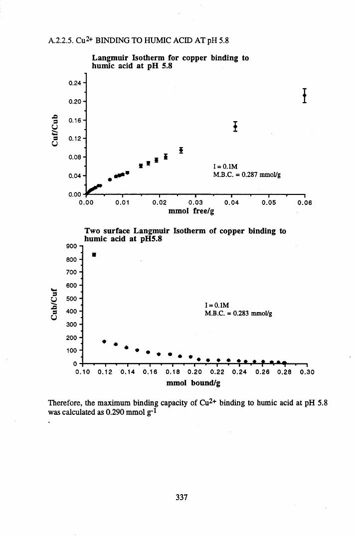
A.2.2.5. Cu2+ BINDING TO HUMIC ACID AT pH 5.8
Langmuir Isotherm for copper binding to humic acid at pH 5.8
0 .2 4 -
0.20-
S 0 .16 -
3 0 .1 2 -U
0 .0 8 -
0 .04 -
0.00
i
I = 0.1MM.B.C. = 0.287 mmol/g
“ 1-----------'----------1 ■----------1----------■.......... i—0 .0 0 0.01 0 .02 0 .0 3 0 .0 4
mmol free/g0 .05
I
0 .0 6
900 -
800 -
700 -
600 -
500 -
400 -
300 -
200 - 100 -
Two surface Langmuir Isotherm of copper binding to humic acid at pH5.8
I = 0.1MM.B.C. = 0.283 mmol/g
• • • •-i 1— i— |— i— |— i— |— i— |— i— |— .—
0 .1 0 0 .1 2 0 .1 4 0 .1 6 0 .1 8 0 .2 0 0 .22 0 .2 4 0 .2 6 0 .2 8 0 .3 0
mmol bound/g
Therefore, the maximum binding capacity of Cu2+ binding to humic acid at pH 5.8 was calculated as 0.290 mmol g '1
337
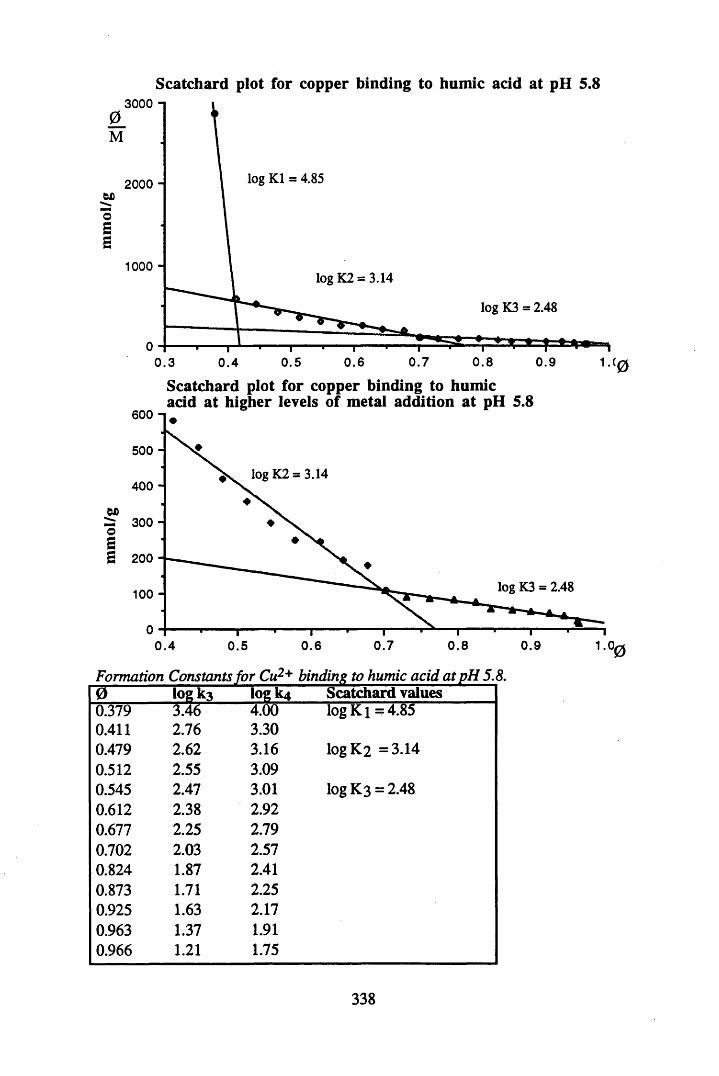
Scatchard plot for copper binding to humic acid at pH 5.83000 n
log K1 = 4.852000 -
1000 -log K2 = 3.14
log K3 = 2.48
0.6 0 .7 0.8 0.90.5 1.C,0 .3 0 .4 0Scatchard plot for copper binding to humicacid at higher levels of metal addition at pH 5.8
600 n
500 -
log K2 = 3.14400 -
©££
300 -
log K3 = 2.48100 -
0 .7 0.8 0.9 1.0,0.5 0.60 .4
Formation Constants for Cu2+ binding to humic acid at pH 5.8,0 log k3 logk4 Scatchard values0.379 3.46 4.00 log K i =4.850.411 2.76 3.300.479 2.62 3.16 logK 2 =3.140.512 2.55 3.090.545 2.47 3.01 log K3 = 2.480.612 2.38 2.920.677 2.25 2.790.702 2.03 2.570.824 1.87 2.410.873 1.71 2.250.925 1.63 2.170.963 1.37 1.910.966 1.21 1.75
338
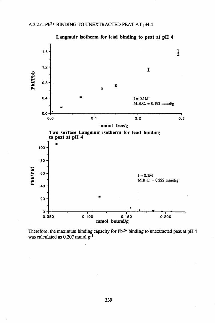
A2.2.6. Pb2+ BINDING TO UNEXTRACTED PEAT AT pH 4
Langmuir isotherm for lead binding to peat at pH 4
1.6-
1.2 H>o .aPu*5 0.8 - ■QPm
0 .4 -
0.0
I
I = 0.1MM.B.C. = 0.192 mmol/g
0.0
100 -
80 -■
pOeu 60 -.cpfiPm 40 -
20 -
0 -
0.1 0.2
mmol free/gTwo surface Langmuir isotherm for lead binding to peat at pH 4
X ■
—i0 .3
I = 0.1MM.B.C. = 0.222 mmol/g
0 .0 5 0 1 1 0 .1 0 0 0 .150
mmol bound/g0.200
Therefore, the maximum binding capacity for Pb2+ binding to unextracted peat at pH 4 was calculated as 0.207 mmol g"1.
339
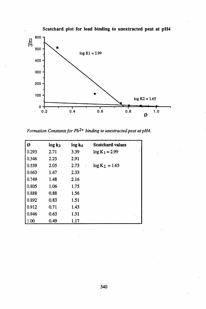
Scatchard plot for lead binding to unextracted peat at pH4
600 n0.Pb
500 -log K1 = 2.99
400 -
300 -
200 -
100 -log K2 = 1.65
0.6 0.8 1.00.2 0.4
Formation Constants for Pb2+ binding to unextracted peat at pH4.
0 Iogk3 logk4 Scatchard values0.293 2.71 3.39 log K i = 2.990.346 2.25 2.910.559 2.05 2.73 logK2 =1.650.663 1.67 2.330.749 1.48 2.160.805 1.06 1.750.888 0.88 1.560.892 0.83 1.510.912 0.71 1.430.946 0.63 1.311.00 0.49 1.17
340
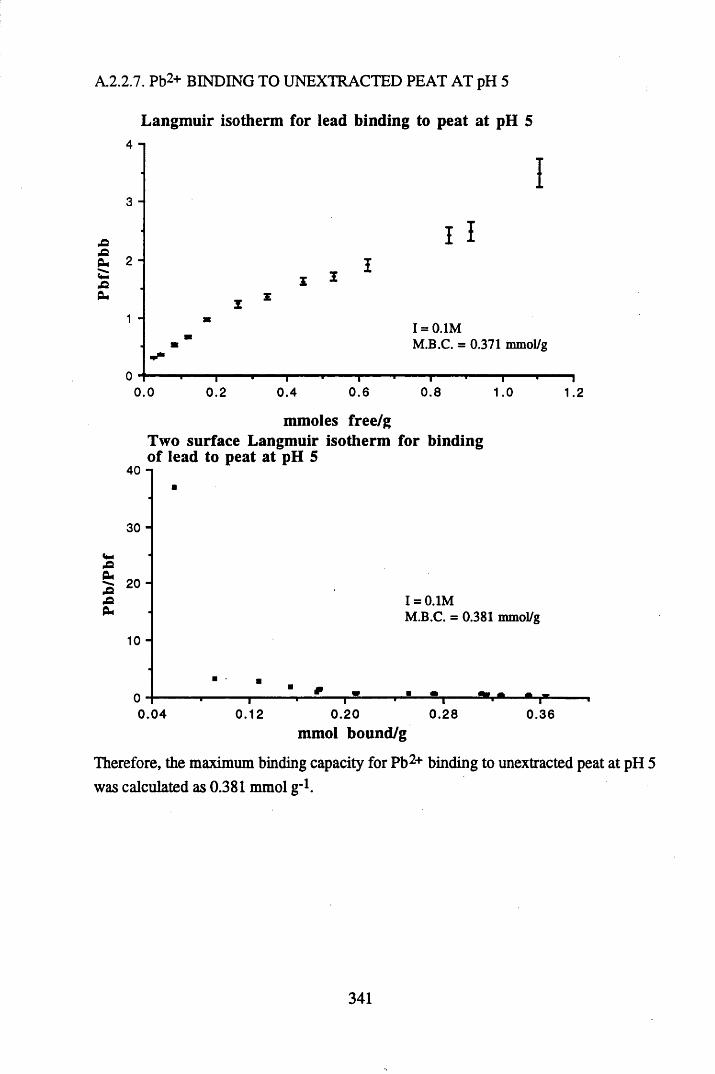
A2.2.7. Pb2+ BINDING TO UNEXTRACTED PEAT AT pH 5
Langmuir isotherm for lead binding to peat at pH 5
3 -
X 5
£ 2 i-Q Pm
1 H
i
11
I = 0.1MM.B.C. = 0.371 mmol/g
0.0 0.2—I—0.4
~T~0.6 0.8 1.0
i1.2
■OPm
30 -
20 -
10 -
mmoles free/g Two surface Langmuir isotherm for binding of lead to peat at pH 5
I = 0.1MM.B.C. = 0.381 mmol/g
0 .0 4 0 .360 .12 0 .2 0 0 .2 8 mmol bound/g
Therefore, the maximum binding capacity for Pb2+ binding to unextracted peat at pH 5 was calculated as 0.381 mmol g '1.
341
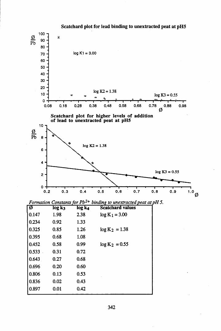
Scatchard plot for lead binding to unextracted peat at pH5
0Pb
100 -
90 -
80 -
70 -
60 -
50 -
40 -
30 -
20 - 10 -
log K1 = 3.00
log K 2= 1.38log K3 = 0.55m ^0 i ■ i ■ I ■ i ■ i 1 i ■ i ■ i 1 r
0.08 0.18 0.28 0.38 0.48 0.58 0.68 0.78 0.880
Scatchard plot for higher levels of addition of lead to unextracted peat at pH5
0.98
10 n
0Pb
lo g K 2 = 1 .38
log K3 = 0.55
0.6 0 .7 0.80.2 0 .3 0 .4 0 .5 0 .9 1.00
Formation Constants for Pb2+ binding to unextracted peat at pH 5,0 logk3 logk4 Scatchard values0.147 1.98 2.38 log K i = 3.000.234 0.92 1.330.325 0.85 1.26 logK2 =1.380.395 0.68 1.080.452 0.58 0.99 logK2 =0.550.533 0.31 0.720.643 0.27 0.680.696 0.20 0.600.806 0.13 0.530.836 0.02 0.430.897 0.01 0.42
342
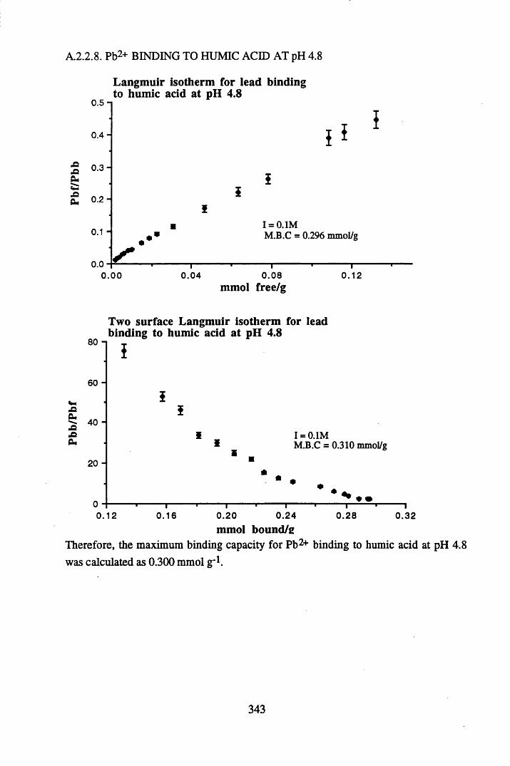
Pbb/
Pbf
Pbf
/Pbb
A.2.2.8. Pb2+ BINDING TO HUMIC ACID AT pH 4.8
0.5-1
0 .4 -
0 .3 -
0.2-
0.1 -
Langmuir isotherm for lead binding to humic acid at pH 4.8
o.o
I = 0.1MM.B.C = 0.296 mmol/g
I
—I—0.120.00 0 .0 4 0 .08
mmol free/g
80 n
60 -
40 -
20 -
Two surface Langmuir isotherm for lead binding to humic acid at pH 4.8
i
0.12
I = 0.1MM.B.C = 0.310 mmol/g
• •0 .16 0 .2 8 0 .3 20 .2 0 0 .2 4
mmol bound/sTherefore, the maximum binding capacity for Pb2+ binding to humic acid at pH 4.8 was calculated as 0.300 mmol g-1.
343
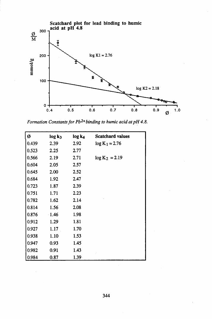
Scatchard plot for lead binding to humicacid at pH 4.8
3000 .M
log K1 = 2.76200
100log K2 = 2.18
0 .7 0 .90 .5 0.6 0.8 1.00 .4
Formation Constants for Pb2+ binding to humic acid at pH 4.8.
0 logk3 logk4 Scatchard values0.439 2.39 2.92 log Ki = 2.760.523 2.25 2.770.566 2.19 2.71 logK2 =2.190.604 2.05 2.570.645 2.00 2.520.684 1.92 2.470.723 1.87 2.390.751 1.71 2.230.782 1.62 2.140.814 1.56 2.080.876 1.46 1.980.912 1.29 1.810.927 1.17 1.700.938 1.10 1.530.947 0.93 1.450.982 0.91 1.430.984 0.87 1.39
344
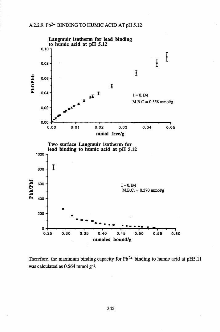
A2.2.9. Pb2+ BINDING TO HUMIC ACID AT pH 5.12
Langmuir isotherm for lead binding to humic acid at pH 5.12
0.10 n
0 .08-
2 0.06 H
ft* 0.04 -
0.02-
0.00
I II
I = 0.1M
M.B.C = 0.558 mmol/g
0 .0 0 0.01 0 .02 0 .03
mmol free/g0 .0 4 0 .0 5
1000 n
800 -
■P 600 -ft*•fi^ 400 -
200 -
Two surface Langmuir isotherm for lead binding to humic acid at pH 5.12
I
I = 0.1MM.B.C. = 0.570 mmol/g
—1------1--------1-1---------■-1-------- 1----- 1--i---------- ------10 .2 5 0 .3 0 0 .3 5 0 .4 0 0 .45 0 .5 0 0 .5 5 0 .6 0
mmoles bound/g
Therefore, the maximum binding capacity for Pb2+ binding to humic acid at pH5.11 was calculated as 0.564 mmol g_1.
345
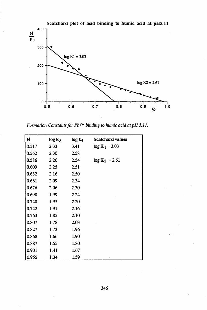
I!Ii
Scatchard plot of lead binding to humic acid at pH5.11400
300
log K1 = 3.03
200
log K2 = 2.61100
00.7 0.8 0.9 1.00.5 0.6
Formation Constants for Pb2+ binding to humic acid at pH 5.11.
0 log k 3 lo g k 4 S c a tc h a rd values
0.517 2.33 3.41 log Ki = 3.030.562 2.30 2.580.586 2.26 2.54 logK2 =2.610.609 2.25 2.510.632 2.16 2.500.661 2.09 2.340.676 2.06 2.300.698 1.99 2.240.720 1.95 2.200.742 1.91 2.160.763 1.85 2.100.807 1.78 2.030.827 1.72 1.960.868 1.66 1.900.887 1.55 1.800.901 1.41 1.670.955 1.34 1.59
346
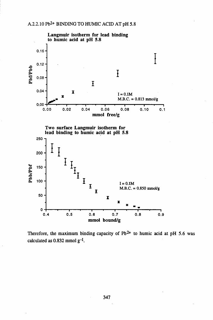
A.2.2.10 Pb2+ BINDING TO HUMIC ACID AT pH 5.8
Langmuir isotherm for lead binding to humic acid at pH 5.8
.a.oCUpQCu
0 .1 6 -
0.12-
0 .08 -
0 .04 -
0.00-0.
II
I = 0.1MM.B.C. = 0.813 mmol/g
l ' l00 0.02 0 .0 4 0 .0 6 0 .0 8
mmol free/g
—i----- ■ i0.10 0.1
Two surface Langmuir isotherm for lead binding to humic acid at pH 5.8
250 -i
200 -
43 150 H
4343 100
50 -
I
0 .4
II III
I I = 0.1MM.B.C. = 0.850 mmol/g
0 .5 0 .6 0 .7mmol bound/g
0.8 0.9
Therefore, the maximum binding capacity of Pb2+ to humic acid at pH 5.6 was calculated as 0.832 mmol g_1.
347
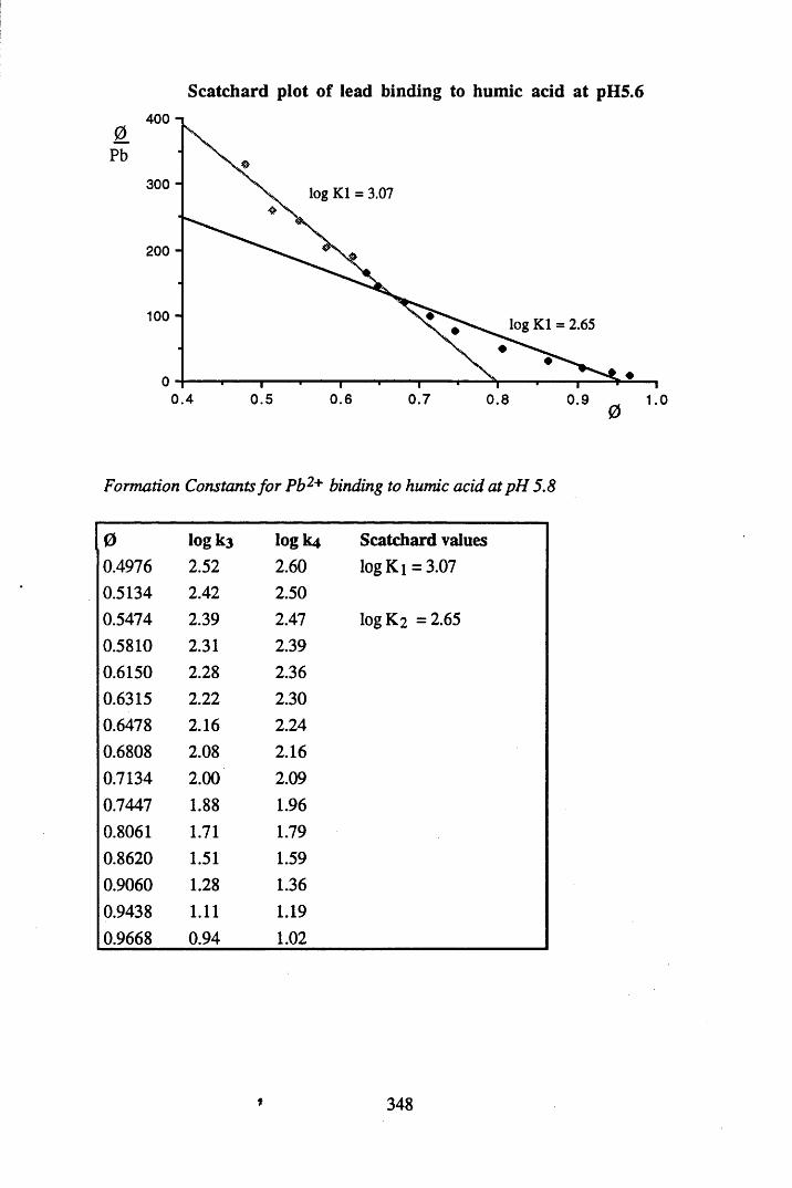
Scatchard plot of lead binding to humic acid at pH5.6400
0Pb
300 log K1 = 3.07
200
100 log K1 = 2.65
0.70 .4 0 .5 0.6 0.8 0 .9 1.0
Formation Constants for Pb2+ binding to humic acid at pH 5.8
0 log k3 logk4 Scatchard values0.4976 2.52 2.60 log K i = 3.070.5134 2.42 2.500.5474 2.39 2.47 logK2 =2.650.5810 2.31 2.390.6150 2.28 2.360.6315 2.22 2.300.6478 2.16 2.240.6808 2.08 2.160.7134 2.00 2.090.7447 1.88 1.960.8061 1.71 1.790.8620 1.51 1.590.9060 1.28 1.360.9438 1.11 1.190.9668 0.94 1.02
t 348
APPENDIX 3
DATA FROM CHAPTER 5: RADIONUCLIDE & HEAVY METAL
CONTENTS OF THE SOUTH DRUMBOY CORES
349
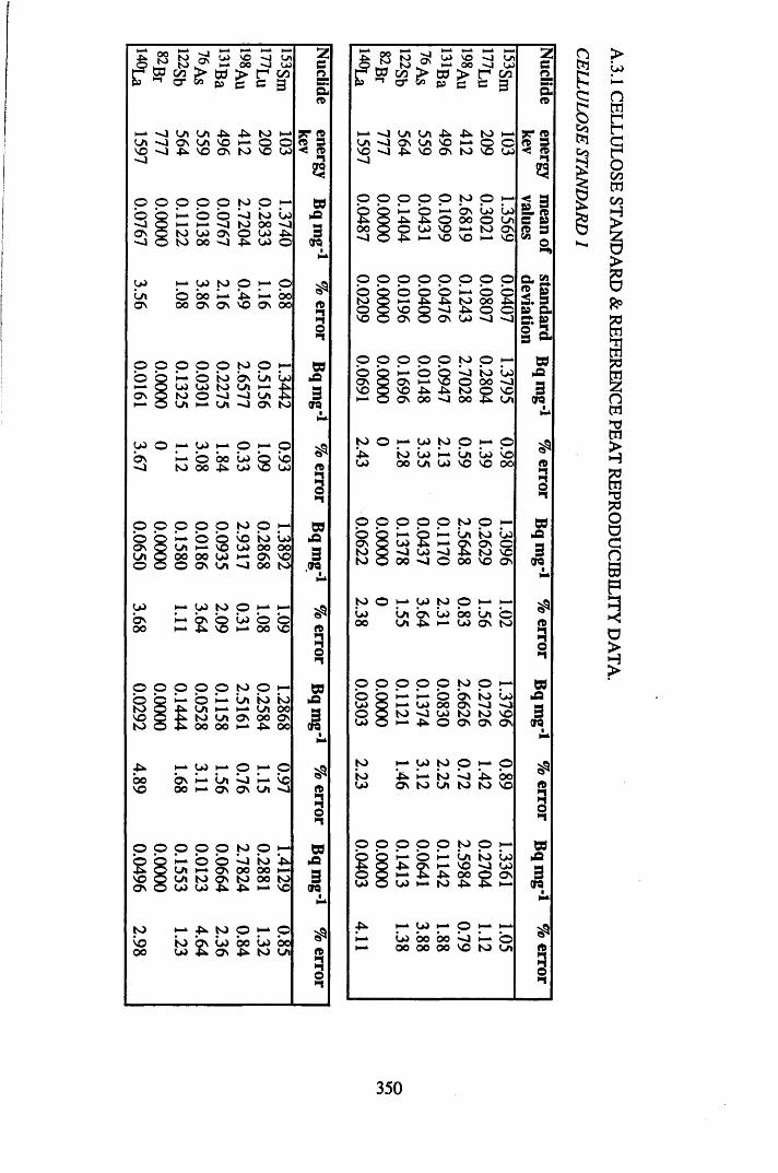
i—i i—i |_tu> VO -o Ul1—* OO ■o u>60 > r C/3
e 3 3
i—1 —3 LA LA 4^ 4^ tOU ( n 1 0 \ V i \ O h O O ' O s ] ^ V O O N ) \ O W -O
to O © b to u>m H si to 00 n)
tO 0 4 ON O 04 4 *iN ) OO >vl ^ W O
04 M w to O H OLa O bo b b b boos 00 ON On NO ON 00
p O p p p f O p N © b I— © io On La u>i - o w w t o u i M ^o \ g t o O 'J ' J i J i - LM O U M t y i > J O N M
0 4 o 1— 1 u > H - O 1— 1 o
O N< 1
h—1t o
oo o
b o4 *
u >u > s
b0 4
o o o o O IO © »—1
© 5 o o b io u>ON C5 LA »—i NO o> oo ooLA C5 oo 00 04 »—i ON NOo 25 o ON LA - a OO to
lo i—i 04 to o i—i 1—1ONOO I—* On
4*i si o1—1 o00 8
o O o o O to O 1—1b Q b-t o i—i La io toto LA i—i »—i LA 00NO to LA On 00 Onto OO OO i—i 4*1 00
4* »—i u> I—* O i—i OOO ON t—1La b b bNO 00 1—1On ON LA *o
o O O o O to O t—ib o 1—i o o b to VLA i—i ON 00 00 i—iNO Q LA to ON to 00 toON 04 04 4 4*1 1—1NO
to t—i 4*i to O 1—1ob to ON 1*4 bo u> bo0 0 04 4*i On 4 to LA
2cnEare
9 T t o § 3 < t o "iq
60>o3era
$t o>1§
aus3ora
$t o3*■*
us3
.era
t o
3aus3era
t o
ii-i
60us3era
t o
3•n
oo re to £ a £U> VO OO LAu> 213w 00 > CO > t- 1 OT! O
^ o* ») c c g g
1—1-0 LA LA 4i 4*i toLA ■o On LA NO i—i O oNO -0 4*1 NO ON to NO LO-O
o o O O O to o i—io p H- o l—i On Lo LO4* p 4*i 4*i o 00 o LAoo O 04 NO i—i to ON4 4*i »—i NO NO i—i NO
O O O O o O o oo o o o o l—i b oto I—* 4*i 4*i to oo 4*iO o NO Q •O 4*i O ONO On © ON 04 -o -o
o p O O o to oo o i—i o © b to LoON ON H-1 o oo «oNO ?5 NO 4»i 4*1 to o NOI-— ON oo -4 oo 4*1 LA
to o u> to o t—i o4* to Lo »—i La u> b04 oo LA 04 NO NO OO
are
p? ra re s < re
o o o o O to O H—o b t—1 o b La to LoOv Q LO 4*i h—i ON O n cto p < t LO ■o 4*i to NOto o 00 ■o o oo NO O n
to O LO to O h-Lo La ON Lo bo La b00 la 4*i ►—i LO O n to
O O o o o to o h-o Q i—i 1—1 o ON io LoLO »—i LO 00 ON x j •oo p to LO to to NOLO i—* 4*i o O n ON ON
to ►—i LO to O I—i Oto *4>i i—i to b *4*i OOLO ON to LA to to NO
o O O o O to Ob Q >—i o I—* La io U )b Q 4*i O n b—i NO -o 04o o i—i 4k 4*i OO o ONLO LO t—i to 4*i 4*1
4*i i—i LO 1—1 O i-^ )—+i—i Lo 00 00 b i—i oi—i oo 00 00 NO to LA
«3
£ 33. re 3 3 re 3“ o
Q, COre ““ 3.3 CU§ £ 3 O*
60us3
era
re►nI
60us3
era
60>a
I
re1
60333
era
rei
350
A.3.1 C
ELLULO
SE STA
ND
ARD
&
REFEREN
CE PEAT
REPR
OD
UC
IBILITY
D
ATA
.
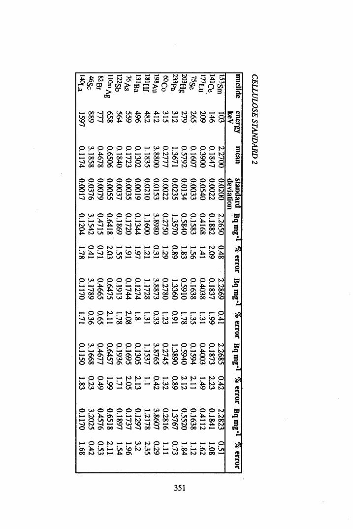
K AA ^ ^ ^ ^ M tO tO * ^ ^ ^r ? « 5 ^ v MMOO/ ? w w r i f ^ M Ws w > w f f i > n ^ w ^ r n w > 0 * 5 p R a O » ( j q ° b > g
£
M O O s J O \ y i W l ^ - U ^ W W W t O | O i - O l O O ' J U i a ^ ^ O O O M M M s J O N O - U O \ O ^ C > J O O ^ V O O N K ) N ) W i N ) ^ y \ V O O \ W •O
© OJ o o o O o 1—k NO o I—. O O o o to 3I—* 1—k 4k. O n t-^ t—k t—k t—k 00 to NO In t—k NO t—k to1—ko4 *
ooU loo
ONooo
U loO n
004k.o
OtoNO
NOoto
00NONUl s
-o■o«o
ON•o1—k
oNOto
ONo•o 3
OO4k.■O
■oi
o o o O o O o o o o o O o o O o a s .8
©u> g 8 8 g 8
oto
o g bto
ot—k g o
nui g oto
re J j 3
t—. -o ■o U l u> NO t—k t—k U l to NO NO NO 4k. to 5 * c l'-J ON NO U l -o <Ui NO o NO to N-/1 4k. NO O to 31 P
g aO u> o o o O O t—k NO o t—* O O O o to ni—* t—k 4k. ON t—k t—k t—k t—k OO to NO U l t—k 4>. l_k to .OtoO4^
U l4 *to
«ot—kU l
4k.
OO
ooONNO
-Otoo
NO
£ sNO00O
<1NUlo
NUl
OOO4k.O
NUlOONO
t—.ON00
00ooto
ON(UlO
3
t—* o o to t—k k-k t—k 1—k o t—k O t—k t—k t—k to Ob 4k. b o U l b b to lo to 00 00 U l 4k. o 4k.00 t—k 1—* u> U l t—k t—k 1—k NO no NO O n t—k NO OO re
i
o u> o o o o o 1—k NO o t—k O O O O to W1—k k—k 4k. ON t—k t—i l—k oo Io NO U l t—k 4k. t—k to kO1—>o
ooo
O nON
4k.-O
NOt—k
~o to'O
*oto
oo'O
■ooo
NOON
NOt—k
O nNO
ONO
00NO
ooON 3
o NO U l U l NO 4k. 00 NO o o o 00 00 <o NO era•
t-— o o to t—k to t—k t—k O t—k o t—k t—k t—k h-k oo u> ON 1—k b o OO NO NO to b b NO NO b 4k.1—k ON U l h-k 00 00 t—k NO NO t—k 00 NUl t—k NO t—k re
3
o u> o o o o o t—i NO O t—k o O O o to aI—*I—knui
1—kONO n
4k.O n-O
O n4k.U l
NOU>
t—kO nNO
t—kNOo
t—kU lNO
00-oON
to■o4k.
NOOONO
U lNO4k.
t—kNUlVO
*4k.
800-o
toO nOO
. o
3O OO ~o O ON NUI NUl -o <ui NUl o O 4k. NO NO (Ul 9 0
|L
»—k O o •—» l—k to to 1—* o I—* o to to t - to O00 to 4k. b b o t—k h—k 4k. NO b o t—» k—k 4k. to 4>.u> u> NO NO NUl NO to to NO to VO NO to re
3o•-i
o u> o o O o O 1—k NO o t—k o O O O to wl_k to 4* O n t—k t—k t—k to 00 to NO U l t—k 4k. k—. to kO►—k o U l U l OO o to t—k ON 00 «o NUl ON 0 0 o o-O to «o t-^ NO NO NO o O t—k ON to NO 1—k 4k. to 3o U l ON OO - o - o • o 0 0 - o O n < o o OO to NO 9 0
•l—i
I—k o o to 1—k t—k NO to o t—k o 1—k t—k t—k t—k O $O n 4k. U l t—k U l b to NO to >—k b b o t—k O n o U lOO to u> 1-^ 4k. ON U l NO t—k NO 4k. to to o o re
1
9SnM<are
sr re re 3< $q
SSotqOjH
gKJ
351
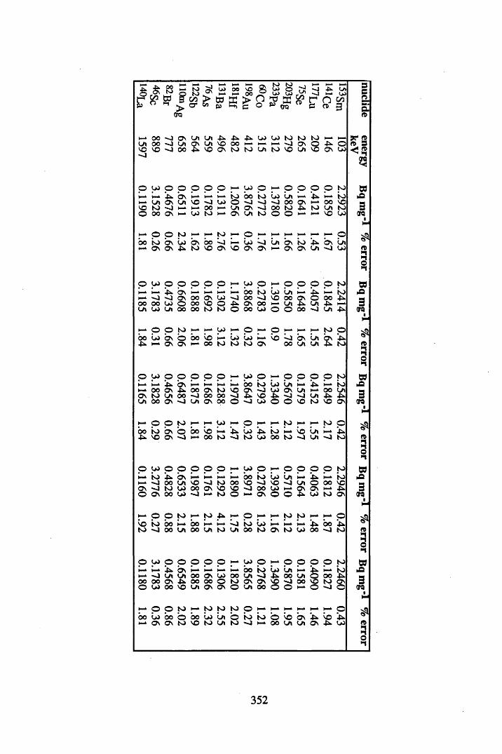
1—kOO •o Os Ul Ul -pH ■PH -pH u> u> to to to t—k t—kUi oo -o Ul OnUl VO OO 1—* H"k t—k -o ONo oVOVO*o 00 ■Ph VOON to to Ul to VOUl VOON 04 1 >1
Q
© 04 o o o O o t—kvo o t—ko o o O to wl—k1—I '.pn ON i—kI—kH-k to bo to lo Ul l—k‘.pHl—kto hQt—kUl ONUl VO•o u> o «o -o oo On 00 vo hVO to •o t—kt—k00 1—kUl On oo to •PHto Ul to 3o 00 ON 1—k 04 to 1—kOnUl to o o t—• t—kVO 04 crq
t—ko o to H t—kto H- O M t—kH—t—• H-k t—ko00 Io On lo ON bo ■o »—klo Ul ON to 4n On Ull—k ON On .pn to vo Onvo OnOn 1—kOn ON Ul ■O 04 f t•1
3
o 04 o o o O O VO O 1—ko o O © to at—kH-k '■Ph On H-k h—t—kt—koo to vo Ul t—k4h H-k tot—k -o -0 ON OOOn 04 ■o oo -o VOoo ON O 00 -pH Hoo 00 04 o oo VOO ■PHOn oo t—kUl -PHUl •PHH-k 3Ul 04 Ul oo 00 to to o oo vo o o 00 Ul ■Ph arqM
H- o o to 1—kt—ku> H-* OM o H—l—kH- to o $00 04 ON© 00 VO l—klo lo H-k vo ON Ul On '-Ph■k 1—kOnON H-k OOto to to ON 00 Ul Ul ■Ph to f t
§o 04 o o o o o J . vo o t—ko o o Oto
%
WH-k t—k'■Pn On 1—kt—kt—k t—kbo to vo Ul l—k ‘•Ph H—to tfi1—koo ON ■pHoo On to VO On-o vo On Ul H—OOUl hON to Ul oo •o OOoo ■o ■Fn vo -pH •o Ul -PH■pH 3Ul 00 ON -o Ul On oo o <o vo o o vo to VO ON ore•HHl—ko o to l—kH—vo H- o t—k H- to l—kl—kto o $00 to ONb bo VO HH ‘■pHlo ‘.pH to H VO Ul t—k■Ph■Pn VOON t—k00 to —4to vo 00 to «o Ul ■o to fD3o 04 o o Oo o t . vo o _ 4 o o o o to
•1wl—kio 4H ON 1—kH—l—kH-k bo to lo Ul l—k'■Fn l—kto tO1—k■o 00 Ul VO-O to OO vo •o vo Ul o oo VOOn «o to Ok) OOON VO vo oo vo ON ON t—k-pH 3o ON 00 04 ■o 1—kto O t—kON o © ■Ph u> to ON TOiH-
l—ko o to t—kto .•pHt—ko H H-k to to l—kH-k O$VO to 00 1—kbo 1—kM to lo t—kH—I—* ipHbo ‘■PHto ■o 00 Ul 00 Ul to Ul oo to ON to u> 00 -o to •13
o o> o o O o o H-k vo o t—ko o o o to• t
wt—kt—k'.pn ON t—kH-k l—kH-k bo to lo Ul t—k £ h l—k to tO1—k■o Ul Ul 00 Onu> 00 Ul ■o -pn 00 Ul O OO -Phoo 00 ON .pn oo OOo to ON ON vo -o oo VO to ON 3o 04 00 VOUl On ONo Ul OOo o l—ko -o o (10•M1—ko o to 1—kto to to o H-k 1—k1—kH-k l—kl—ko $bo lo 00 o bo lo Ul o to to o VOON '■Fn vo ipH1—kOn ON to vo to Ul to ■o oo Ul Ul ON -pH04 t t
3o•1
352
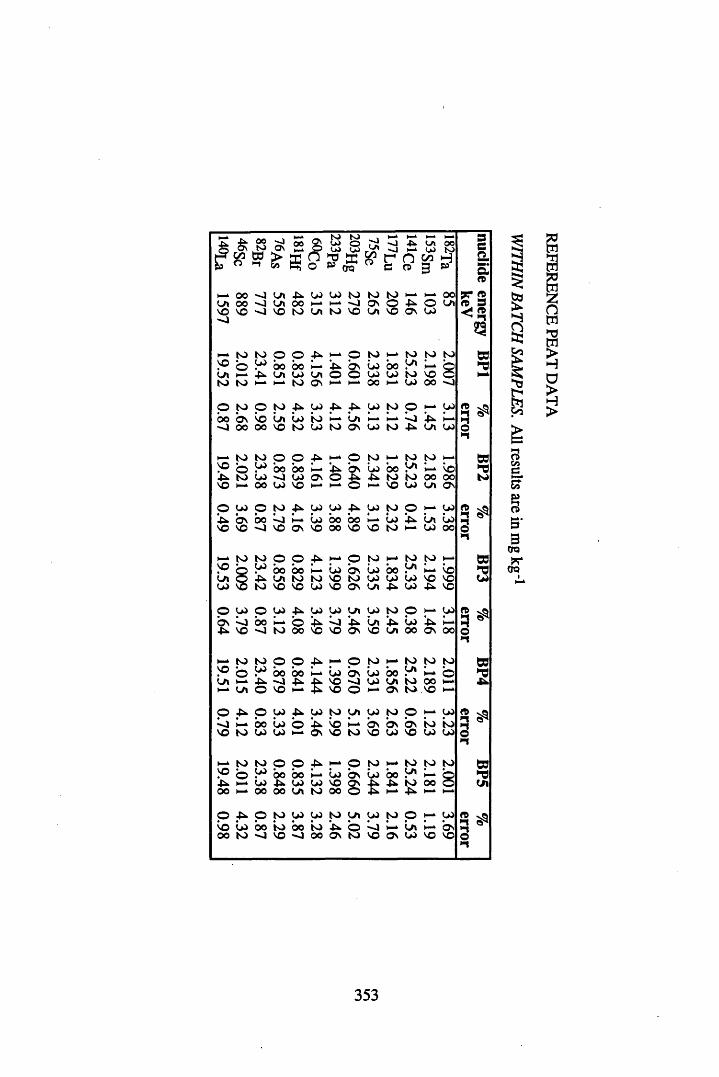
S 3 N > U> O UJ u> ^ Ul oo M W K)oo o 55 g\& ►-* J? vh> oj r'X" -j ►— U> n:
i— k O O • v l ( J i 43> 0 3 t O I O t O i ~ * m O OO i 0 0 v ] U 0 0 m m n J O \ O ^ O O i V O V O ' ^ J V O t O L A t O V O L A V O . O v L O-o
H-* to to o o Pn l—k © to H-k to to toVOLato
©l—ktoLO’■&.
00LAl—k
00LOto
H-LAas
PnoH-k
b voH-kLoLO00
00LOl—k
LAtoLO
l—kVO00 -o
O to o to Pn LO Pn Pn LO to o H—k Ui00■o b v00 VO00 Lavo Loto to
LOl—kto Laas LO to
L j-pH ipHLA
H-kLO
i—k to to o o Pn H-k © to M to to l-HVOPnvo
©tol o
Lo0000■ol o
b oLOvo
l-HONl—k
Phol—k
b vPno
Lo-pHH-kb otovo
LAioLO
o oLA
voooOv
o l o o to t k LO LO Pn LO to o HH LO‘.pHvo b v
VO00- j
L jvo as Lovo b o00 00voH-kvo Loto ■pHH-k La
LOLooo
l—k to to o o pn l—k o to H-k to to l—kpLal o § LO
pnto
00LAvo
00toVO
l—ktoLO
Lovovob vtoas
LoLOLA
b oLO-PH
LALoLO
H-kvoPn
bvovo
o l o o Ui Pn LO LO LA LO to o H—Uib v-pn
<1vo00-J l—k
to o00 4nVO
Ljvo
Pnas LaVO
PnLA
Lo00‘■Phas
H-koo
i—k to to o o Pn l—k © to H> to to topLah
oLA
LOPno
b o-Jvo
00pnl-H 5Lo
VOvob v*oo
LoLOH-*
00LAas
LAtoto
l—k00VO
ol—k
O ,-pn o U> Pn LO to LA LO to o H-k LOL jvo
H-nto 00
l oLOl o
o PnOv
SOvo
H-kto b vvo b v
LOb vvo to
LOtoLO
i—k to to o o Pn 1—* o to H-* to to tovo‘■pH0 0
ol—kl—ku >LO0 0
0 0pn0 0
b oLOLA
l—kLOto
Lovo0 0
b vas©
Lof c
b o-pHl—kLAto■pH
H-ko o HH
o Pn o to LO Ui to LA LO to o H-k LOvoo o
Loto b o-o
tovo b o■o to00 Pnas bto Lo
VO1—*as La
LOl—kvo b vvo
sco*■<a«
*• 2(V 9
sg
a
wto
3 $ 3•-I
wr®OO
$a
s ^o * 1
w
*0tn
3 $3*■»
oCO£
SfQ
B*3ooX00
asw325os
353
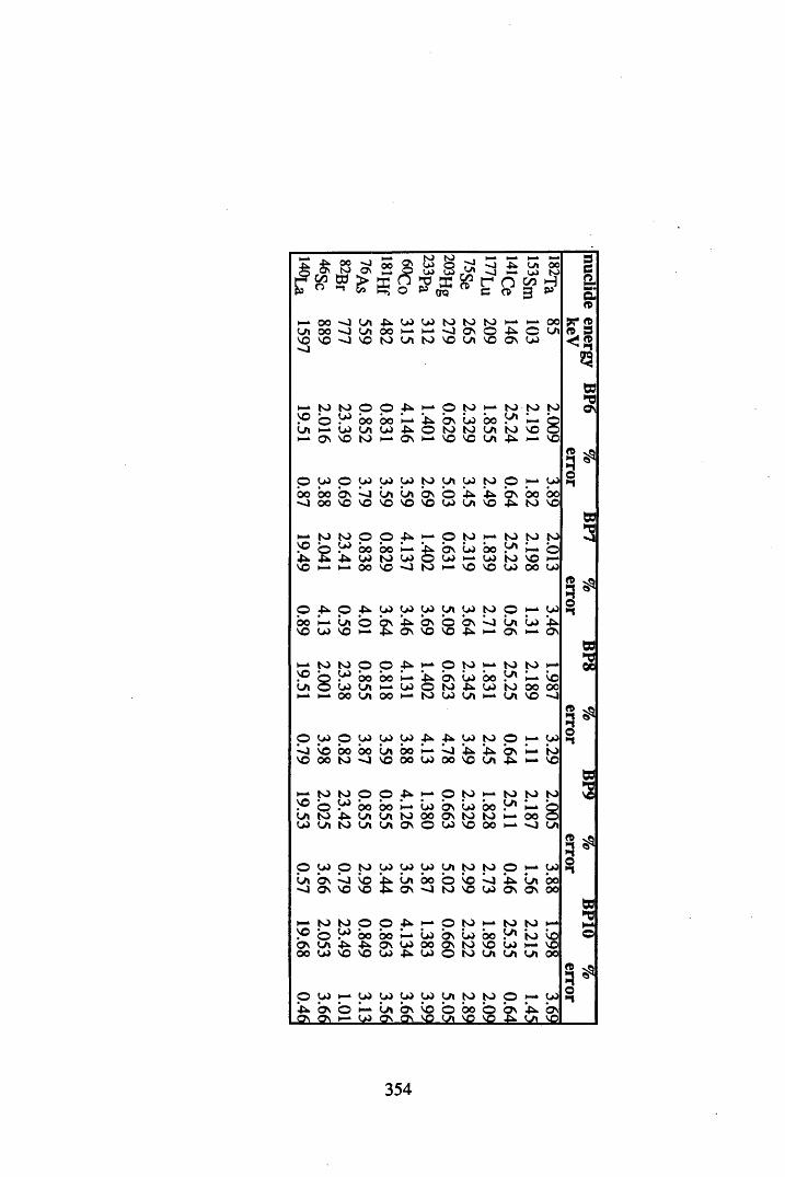
& 00 -J to ON^ to to ,oo SC vo o rr- w Q {n Ul 00 I-* u> tok—i WU' H-k VO U> -J l—k U> N> g
8 ’ £ 3 r S £ £ s £ £ £ g ’ Si |
M O O ' J U l i ^ W W t O t O t O M M O Ou t o o s j u i o o M H s j o N O ^ o y tl O ^ ) v l l £ ) t O U i S ) \ O U l \ C O \ W >0
l—k to to O o 4k H-k O to i—kp © LO o o b o h-* *4k ON LO 00Ul l—k LO Ul LO 4k O to to Ul1—* ON VO to I—* O n i—k vo VO Ul
o LO o LO LO LO to Ul LO to00 00 ON b Ul Ul ON o 4k 4k>o OO vo VO VOVOVOLO Ul vo
l—k to to O o 4k l—k o to H-kvo o LO OO b o 1* 4*. ON LO b o4k 4k LO to LO O LO l—k LOvo i—k hh OO vo •O to i—k VO VO
tOUito4k
ON4k
toui
to toV D 8
l o
O LO o to LO LO LO Ul to toUl■o ON
ON<1vo bvo '6 Ul
ON0 0•o oto bvo b
LO
o4k
VOONOO
OUl
O LO HH LO LO LO LO U l to4*. ON o H-k U l ON VO o OO2 1 .2 1 ±L_2l2 1 VO <4.
©On
&n7? » n 9<%sg
w *■0 Ov
vo
OO 0 0 to VO
to toI— ©VOOO LO
o 4* o 4>. Ui LO LO Ul LO to o k_k LO00 H-k Ul o ON 4*. ON o On b Ul LO 4kvo LO VO H-k 4k. ON VO VO 4k i—k ON H-k ON
l—k to to O o 4k o to H-k to to H-kp o LO oo bo i—k 4* ON LO 00 Ul H ^ bUi 5 LO Ul H-k LO O to 4 LO to OO 00l— k H -k 00 Ul OO H H to LO Ul H - k Ul vo o
o LO o LO LO LO 4- 4*. LO to o 1 ■ LOb b bo 00 Ul 00 H-k b 4k 4k On H-k toVO 00 to ■ o vo oo LO 00 VO Ui 4k l“kVO
to to o o 4*. H-k o to to .to top o LO bo bo l—k LO On LO 00 Ul H - k oUl to 4k Ul Ul to OO ON to to H - k oo 55LO Ul to Ul Ul ON o LO vo 00 H-k kkj Ul
i—» LOu i b o ON 0 0
to O O 4k 1— » O to H-k to to H-kLO OO OO H-k LO ON LO OO Ul to b4k 4k ON LO 0 0 ON to vo LO H—voVO VO LO 4k LO o to Ul Ul Ul 0 0
k - LO 4 k ONV£_V£
l aH•t
§ ^o •1
do3
£
2 v53 *o*1
354
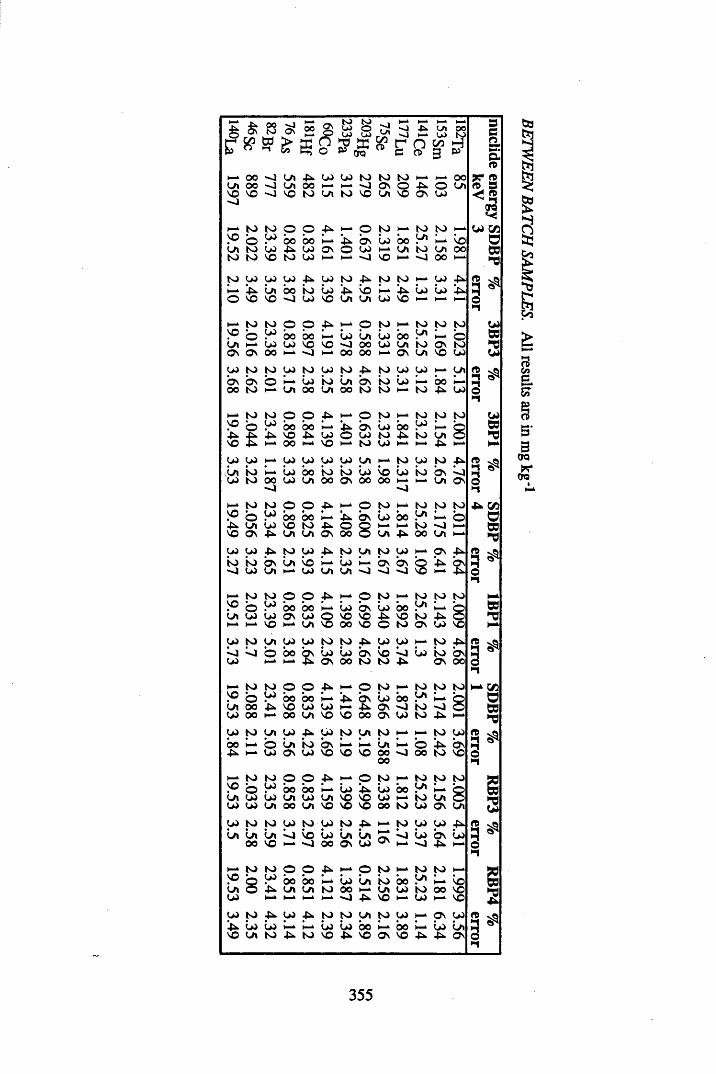
■£• 00 O O N K > 0 \
L AH— OO <1LA o o ■ ov o•O
v o -O
t o t oVO ©
0 4La t o 0 4t o t o VO
JO 0 4 0 4*.pn Lr»
O VO v o
i—k t o t oVO o 0 4LA H-k Lk4ON ON OO
0 4 t o t oON ON oOO t o H-k
h-k t o t oVO o 0 44*.VO 6 H-k0 4 0 4 H-kLA t o I—*0 4 t o 0 0
■ o
H-k t o t oVO © 0 4'■Ph LA 0 4VO ON -pH
0 4 0 4 4 ^t o t o O n■ o 0 4 La
H-k t o t ov o o 0 4LA 0 4 0 4H-k H-k v o
0 4 t o LAb • o o0 4 I—*
H-k t o t oP o 0 4Lo 0 0 ‘•Ph0 4 0 0 H-*0 4 t o LA0 0 L-k o-pn H-k 0 4
H-k t o t oVO o 0 4LA 0 4 0 40 4 0 4 LA
0 4 t o t oL o La La
OO VO
H-k t o t oVO
80 4
L o ’•Ph0 4 l—k0 4 t o ■Ph
4 h 0 4 0 4VO LA t o
©OO■Pn
vo
l o
00
58
oo
t o t o u i o u> u>
CTQ
- JLA
mo
H-k—1•o
£
H-k•Phl—k
nO
H—L AL O
m
3
l—l00
Pi
48
2
04i— k
LA
04H -k
to
27926520
9
i— k- P H
ON
1— k
oLO
ooLA
o J n o to H -k to to H - k
0 00404
H -k
ON‘■Ph
OI— *
b\LO
Loi— k
VO
00LAH -k
LAto-0
H -k
LA0 0
bo o
- P h 04 to to to H -k LO • P h
to0404VO
’•p HLA
bLA
H -k
LO'■PH
VOLoH -k
L OH ^
'■Ph
i—i
O ■PH l— k o to H -k to to to0 0v o«o
H -k
v ol— k
L o- oo o
L a
o oo o
LoLOH -k
0 0LAON
LAtoLA
l— k
ONVO
otoLO
to 04 to - p H t o LO LO H - LA04OO
*toLA
L a
o oONto
toto Loi— k
H -kto OO
- p H1— kLO
o - P h 1— k o to H -k to to to0 0•p H
H - k
0 4VO
'■pH
OH -k
O nLOto
LotoLO
0 0•PH
LOtoH ^
LA- P H
04 04 04 LA H -k to LO to - P H
o oLA too o
toON
Loo o
b0 0
L oH -k- o
tol— k
ONLA
bO n
O f k H -k O to l— k to to to0 0toL A
l— k- p HON
■pH
o0 0
O n
8
L oH -k
LA
00H —
•P H
LAtoOO
i— k
LA
o
04 ■PH to LA to LO l— k ON -P H
b04H ^LA
L oLA
H -k
- oON ON
- oov o
'■PH ON- P h
O -PH H - k o to H -k to to toOO0 4LA
H -k
s
L oVO0 0
ONv ov o
L o- p H
o0 0v oto
LAtoON
l— k
•P HLO
04 to to -P h LO LO H - k to •P H
ON-&•
04ON
L o0 0
ONto btob
•P HL o to
O nONOO
O ■PH O to l— k to to to0 004LA
H - k04v o
‘■pHl— k
VO
ON■Ph
0 0
L oONON
00HjLO
LAioto
H -k- o•P H §
■ f n 0 4 to LA to i—k H -k to LOto04 ON
VO VOH - k
v oL a
0 00 0
- oo0 0
’■PHto
O nVO
O - p H M o to H -k to to toOO04LA
H -k
LAVO
L oVOVO
! p Hvovo
L oLO0 0
OOH -kto
LAioLO
H -k
LAON
8LA
to 04 to ■PH H -k to LO LO ■pH
b-0
040 0
L a
ONLaLO
H -k
ON bH -k
L o ON■PH
L oH -k
o 4H H-k O to l— k to to H-*00LA
H - k
tol—k
L o0 0-0
La
£
ioLAvo
0 0LOH -k
LAioLO
H-k0 0H -k
bVOv o
45h to to LA to LO H - k ON 9 °H -kto
0 4v o
L o4H
0 0VO
H -k
ON0 0vo
H -k
-P HL o•P H
LaO n
saoa
S 'S> &ore
LO CZ5OCO
>0
ol-l04C3y04
3 ! *O •-I
04COhs
s $3£h in
g>d
CO
o•tC/5©CO©
o
3 $3•-»
hS
3 *o •1
a>CoCSfgo5*300K*00
355
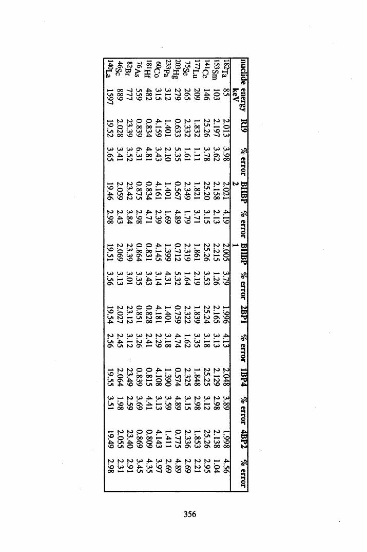
H-k to to l—k H Hk£ & 00to — ] Ok 00b-k u>u> s
oUl •o•-J 4k.H-k Ulu> ooto£
mo w*-1 e -sno p scIQ 5P £• n
oC/33 s '
l__k00 -0 Ul 4 vo vo to to to H-k 00Ui oo Ul oo l—k Ov o 4 . o UlVO vo -0 vo to Ul to vo Ul vo OV vo•O
_ l to to o o 4 l—k o to to to toVO b vo bo bo l—k 4 bv lo bo Ul H—oUl to l o vo vo Ul o vo vo vo to vo H-kto 00 vo vo 4 VO l—k vo to to ov *o vo
vo vo O pv 4 vo to Ul H-k l—k vo vo vobv 4. Ul lo 00 4 l—k lo bv i—k <) bv voUl l— k to l—k l—kvo o Ul M H-k oo to oo
1— * to to o o 4 l—k o to 1 . to to tovo © vo 00 00 l—k 4 * Ul lo 00 Ui i—kb4k Ul 4 - o vo Ov o Ov 4 to to Ul toov vo to Ul 4 l—k ■ o vo H-k o oo H-k
to to vo to 4 to l—k 4 1—- vo vo to 4k-VO 4. 00 vo lo bv 00 ^ 4 H -k H— i — k
00 vo 4 oo vo vo vo vo l— k Ui vo vo
I— * to to o o 41k l— k o to H - k to to tovo © vo 00 bo l— k vo lo bo Ul io ©Ul OV lo OV vo 4 VO l— k l— k Ov io 1—1—* vo vo 4 l— k Ul vo to vo H -k Ov Ul Ui
vo vo vo VO vo vo 4 Ul H -k to vo voUl l— k o lo 4 l— k lo vo b v H -k Ul toON vo I—* Ul vo 4 l— k to 4k. VO vo ov vo
to to o o 4 H -k o to H—to to H -k
p o vo bo bo l— k 4k vo bo UlH - * vo
Ul to l— k Ul to oo o Ul to vo io OV vo4 ■o to l— k 00 H -k l— k vo to vo 4 Ul ov
to to vo vo to to vo 4k H - k vo vo vo 4kUl 4k H -k to 4k to l— k b v vo H -k H - k l— k
Ov Ul to Ov l— k vo oo 4k to Ul oo vo vo
H — to to o o 4k H - k o to H - k to to top o vo 00 bo H - k lo Ul vo 00 Ul H ^ oUl Ov 4k vo l— k o vo -J to 4k io to 4kUl 4k vo vo Ul 00 o 4k Ul oo Ul vo 00
vo l— k to vo 4k vo vo 4k vo to vo to voUl vo Ul b v 4k l— k Ul bo H — vo H -k vo boH - k oo vo vo H - k vo vo vo Ul 00 to oo vo
H - k to to o o 4k H -k o to H -k to to , .
VO o vo 00 bo H -k 4k lo bo UlH - k vo4k. Ul 4k OV Q 4k H » «o vo Ui io vo vo
vo Ul o vo VO vo H -k Ul OV vo OV 00 00
to to to vo 4k vo to 4k to to to 4kvo lo vo 4k lo VO b v 00 b v to vo b Uloo H -k Ul Ul •o vo vo vo H - k Ul 4. Ov
seo,&rt
7? 2rt£TO«-<
to ec
rt•1o>i
OB•734
rti03>0IO
^1rtI*n
356
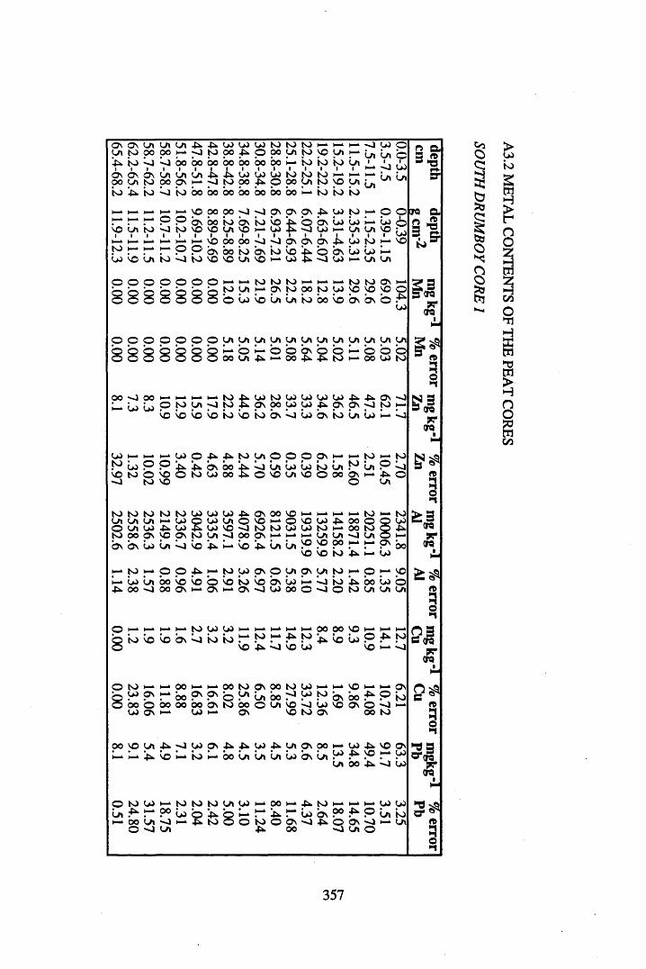
avovUiUiUi4t4tLOLOLOtototoi-*H-H--OLO©U ltO O O O O K -vJtO O O ^ pp O lT lN iV O y i^^ ^Q4XM^^bobobobobobobo^tok>k>L/ i ' ' .'
I I I I I I I i i • I I I I i i •—4 L OO N O \0 \U iL n ( J ) ^ ^ W W W S ) M IO M M h - ^ [ .ooyi_tooooN*--^JK)po: p p o y iN ) v o y i^ 1Vjnv' io in to o io 00 00 00 00 00 00 00 h- io to io
h-MMHMVOOOOOxJ.M .M ^ P P b \ i » i o b \ vo u ito -jto v o v o u iv o1 1 1 1 1 1 1 1 1m h m h h h \O0000!° r r r" P P 00 io _W 'O U \N ) O N ) '0 ,O U \ lO
O O O O O O O h- i—
0 0 0 0 0 0 0•— o 00 ui
OO s i OOi— Lo Lo O M Wl "1
toto
l o l_ I—4<0 0 4t 4tto Lo O 0 i t i t b v 00vo to 0 vo 0 to LO 00•0 to vo
£
£
4 Ov Ov Ov 4t LO to I—* © ©ioI—4VO
LO £ 3 b vLO
LoH-k LoUl i—kUl Lovp p
Lo>o *0 b v b v b v i»k LO to i-k VOb vvo
io1—* voLO £ 3
b vLO
Lo1—* LoUl i—kUltol—kto
p vtoJO 0°
1—*to
l—kLO
tovo
tovo
Ovvo
i—k©vo Ui ui io 00 VO b v b v © _-Pt
Lo
y* LO u » Ul Ul Ul Ul Ul Ul Ult—»O ©
00b v•1 ©-ft ©to l—k
1—k©00 ©LO
©to
LOp v
to00
LOLO
LOLO
LO4t LOOv
-ftp v
4t>;0Ovto ■0
1—kio b v ij LO b v io Ui Lo ■o
LO O © © p v 1—* to H-k toLjO
uiVO
LOUl Lovo
to©
Ul00
tob v©
Ull—k©i tUl
<1©
t o t o t o t o t o LO LO LO 4 t Ov 0 0 VO i— k HH l— k i— k t o l— k t o > 3U l U l U l l— k LO © LO U l © VO l— k © vO LO -pt 00 © LO© U l LO ■pt LO LO vo t o t o LO LO t o l—k 00 t o O ■pt erat o 00 Os SC Ov t o U l ■ o OO ov H -k i— k i— k U l U l ■ o U l 1— kbv bv Lo U l VO 4 t VO i t U l U l SO vo 00 l— k J-1 pv 00 era
VO vo io i t H — Lo < L
h - t o H ^ © © 4 t i— k t o LO Ov © U l Os U l t o l—k © h- voi— k Lo U l 00 VO VO © vo io VO b v Lo i— k ^ 0 io i t 0 0 Lo ©
h or*4 t 00 « o 00 Ov i— k Ov l—k Ov <o LO 00 © « o © t o U l U l U l
© i"- i--4 1—‘ h-ko io vo vo bs ^ io io
I O W W m m h m m O O O O V O h h
r* !° i t VO Lo P !°vo !tk o vo w vo h- «o
© to l— k 0° l— k l— k 00 to Os 00 to LO l— k l— k SO l— k H-k p sLO Ov l— k 00 Os OV © U l U l 00 ■—) LO to b v 00 -U © to00LO
©Ov
00l— k
00 00LO
b v1—k
to 00Ov
© U l vovo to
LoOV
vo o v ©00<1to
I—
OO VO U l 4 t <1 LO Os 4 t 4 t JO 4 t U l p s 00 H-k LO 4 t vo OvI—* i—kit VO l— k io i—k00 U l U l U l Lo b v U l u >
U l4 t00
voit
l— k
-oLOLo
© to LO H-k JO to to U l U) H-k 0 0 i—k4 t to H-k H H-kU l 4 t ^ k 0 0 Lo
8i t
8l—k H-k i t H—Lo b v 0 0 4t ©
H-k OO U i ^0 |—k to © io © b v ^4 4 t © b v •o© ■0 U l 4 t 00 •0 U l ©
U) VOi/i io
n e - 3 n3 *0
hhET
era a n *31to
13era7?ora
1 » 3o>-«
13oraSCera
o•iP 3c era
7Tora
9 ^n3o*1
3 3ar«oera
*T3a*3o*1
010C!3§
1o
0
1
357
A3.2 M
ETAL C
ON
TENTS
OF THE
PEAT C
OR
ES

ONONLALA LA 4 4* u> u> Li to to to 1—k1—kh—-0 Li O 2 aLAto 00 00 h-k to 00 p. O 00 y to VOLA»—kLA La O 3 0b to b b OO00 00 00 OO00 00 i-k to to to La 1h— 1-o 1Li T3ONONONLA LA LA b b Li Li VO to to to h—t—kt—k s*OOLAto OOON1—*-4 to 00 p. O 00 y to VOOnLa
VI‘to b to b to 00 00 00 00 00 00 00 l—kto to to
H- h- h-k h-k VO00 00 0 OnOnON4k. Li to H- O O era aI—k O O ON00 to ONto VOb © ONLi Li I—kLi O 2 ”b LAto <1 to vp VOLA VO•—ku> b Li 1—kLA LAvp Li 3l—kiJ—k1—kb h b vb OOOOb b OnONONb U) to h-k VO • s rkjto i-4 t—kO O ONOOto ONto VOb 0 OnLi Li bLi VOLA to b to VOVOLAVOh—kLi b Li 1—kLALA
00 O h-k h—OO t—k»—i 1—k1—k1—k_* h-k H-l 1—k»—»H- 1—k) 0 B tartLi O 4 OOLa O to ■O 0 0 t—kLi Li 4 <t VOJ—11 3era rfi3to to ONh-k O b 0 La to 00 O la OO •—]
9Tpr
JQ
U> h - -o -J 00 LA4 4k. b p. p. Li u> P Lito Li b 1—*Li ONON00 b La b La b 1—*VOVO*o
to VOLi 4k. ~o ON1—k00 la ONONONLi VO4*. LA On On
^ h - U l O O M M h - K ) | O t O t O t O K ) | O K ) \ 0 \ O X > ( ^ M v l ^ ) W W K ) W l f l W W Q \ CSO O O O O W O ^ ' O m I O O s O W VO»~. -^JQ-OOnONVOLAOOVC tO h— m «>J \fl W ^ h- VO ON
b b L i I— 00 b < i t o ‘
^ 00 VO NO NO VO h- VO _ _O n W W OO OO OO v jLi Li is) I— ^ y*u> o **J >J>slsJN Ct—k t o t—* © © -&k t o L*i O n © LA ON LA t o l—k © H - VOh-k L i La 00 VO VO © VO t o b ON L i b 'to b 00 L i ©■pk. 00 - j 00 ON 1—k O n H-k ON L»i 00 © -O © t o LA LA LA
0 O H-k H-k t—k ►—k 1—k t o t o |__k t o t o t o t o to t o ©H-k 1—k b bk La VO ON b b VO L i t o i—k 00 00 L i OO b00 t o VO 00 00 L*i -P^ 1—k -0 I—* VO t o LA -P^ -p^ 1—k 00 O i VO
1—k <1 Pk LA p . U i ■Pkk Pk -Pkk LA LA LA Ov O n ON -0 OO VO►—* 1—* L> ON La 00 b H-k VO H-k b b b b b L i La © 00t ou>
t o 1—k t o ON VO OO ON OO L»i 00 ON O n VO 00 I—* ON ON H—
I—k 1—k 1—k VO <J h-* I—* l—k -O 00 OO «o 00 00 00 0 0 l—k l—kONh-k
LAL i
O n
©1—»VO
b 00 p>La
t o00
u>La
b ON l—k b 00 b La L i t oto
LkiL i
to Li L»i Li -P*. Li Li p -pkk p - -Ph P -Pkkp 4kkLi Li Li Lib00
1—* VO
LiLki LaON
©OO
bvo
bOO
l—kLi 8
OOVO
bVO
LaLA©0 0
u>h-k 1—kO n
bLi OO-O
ONLALi1— k
to to to to i—k»—kH—to to to i—kto Li 4k. ON -O 4 kkLa00
to Li*0
b©
Lato Livo
btoh-kON
LiLi l—kbLAbvo
toto ©LAbto La
O n©Li ©
OOONON
00 VO 00 ■O 00 ~o -o 0 *0 OO 00 LA4>. p. 4k. ON LAbON
Lii—kON-P*.
b0 0
i— kLi bLi 0 0vo ©
0 0h-kLi bh-k OO
ON1— kLi Lii—kON4k. ONLA
1— *
Li ©toI— .Li La
i— k
3o>1
$ 3m oraKora
s 1^to3•-»
3 fQTQ S7 ?
Bra
c« >aton5*-i
? 3" t QTQPCera
3# 3(IQ
9Tora
5?to
3•1358
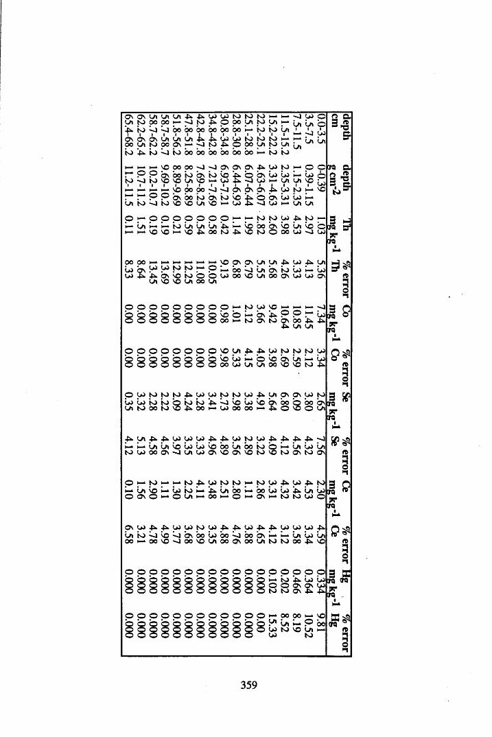
4^N>^^boboboboboool - i totoLA' 1. .'I I I I I I I I I I I I I I » - 1 " ■ J C O O N O N O \ y i U l W i ^ ^ W W t O S ) ( O M M [ . [ .o c y i K J O o o N M - v i t o ^ o o o y i t O L / i ^
Ko 4 ^ *tO ^ 4 tO 0 0 0 0 0 0 0 0 0 0 0 0 h- tO tO
m m m \ O O O O O O O O N O \ O N ^ W K )►— ©t o ^O t o v© v© CA v©I I I I I t I I ■ I I I I I Im m m i — ^ O O p o O O O N p N O N ^ W N )^ ^ o o ^ i j o i o o i o l c f b o w w
- — - c o ~
^ 0 \ O O t O ( J \ t O \ O ^ O O s W W H - W ----- _ ■■ S ^ W M U i l T i V OCO
CAtO-OtOVOVOCAVO O W m Ui Ui
© t—1© © © © © © © 1—1 to to CO 4n to I—*1—1 La 1—1 1—1to La La La '.pn 1—1VO 00 OnVO La vo ©1—1 ►—1 VO VO VO ■▻1 0 0 to 4n VO to © OO CO -0 CO
00 0 0 >—1 1—1 t—* 1—1 h-* VO ON ON a CA -Pn CO 4n CAL o ON OO OO to t o 1—1 © »—i 0 0 La ON to L o 1—1 L oc o -P* 4H b\ vo to © © c o 0 0 vo LA 00 ON CO CO ONCA *o vo <01 0 0 (A
© © © © © © © © © t—1to CO VO , ■, . -0§ 8 88 88 8 g vo
0 0©1- 1—*to ONOs ‘■Pnto
©ON
©0 0 4n L o4n
4n CA CA
© © © © © © © © vo CA ;pn -pn CO to to to CO8 8 88 88 8
8
vo0 0
L oCO t—*CA
©CA
vo00 ONVO LaVO to L o■P*
© c o t o to to 4n c o CO to to c o 4n CA O n ON u > toOO 00 to to © to to *-pn vo L o VO ON 0 0 © 0 0 Onca to 00 t o \o 4n 00 I—* c o 0 0 0 0 4n © <0 © CA
4H (a 4H c o 00 CO 4n 4n CO to CO 4n 4n 4^ -01—1 t—1 La La vo L o L o vo 00 La 0 0 to © »—i CA L o Lato 00 00 ON «o CA c o ON vo ON vo to vo to ON to On
© 1—1 t o 1—1 1—1 t o 4 h CO t o t o 1—1 t o CO 4 n CO _4h t o1—1©
CAON
vo© ►—11—1
L o©
t oCA - 0 0
La1-^
00©
1—1 t—*
0 0ON
L o >—1
L ot o
4 nt o
CACO j o
o n CO 4 n -pH CO CO t o CO 4 n 4 h y > 4 n 4 h CO CO CO 4HLa00
t oK-1
< 10 0
vovo 'O- o
ON0 0
0 0vo L oCA
000 0 ON
000 0
O nCA
»—1 t o
(—1t o
La00
L o-pH
Lavo
p p p p p p p p p p p p p p p p o>-+ to !pn Lo Lo© © ON ON COto 10 o\ A ^
O O O O O O O O O O O O i —‘ 0 0 0 0 * —* \ o • • •- •- • • • •■ ■- • - •■ ' - y u i H p o oCO to VO v-rt 1
co to
Q fr9 «>3 TJ5
era ao * 2 %
2eraj cera
ft§•1J PIpra sc era
5ft
3•nJ »era sc era
ft§
i s?
ft
i•-I
M *era Wu2Tera
era ®>-»i-to
359
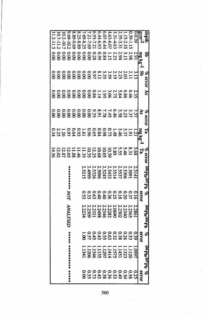
l—kl—kl—kvo 0° 00 ■o *o ov ov ov ■pk. tO to l—koI—* o o ON00 to bv to vo ‘■Pkk© bv to lo l—kloto L j to VOvo la vo l—kto - U OJ to l—kLA LA vpl—ki—kl—k1— * vo O O 00 «o *o b v bv bv ■p. tO to l—kl—ki—ko Obv 00 t o b v t o VO4 k . © b v lo lo l—kL a to Io to VOvo LA vo l—kto 4 * -o to l—kLA LAo o o Oo o o o o o o H - to to to to
8 8t O L A O O O O V O ^ L A t O
t o vo h - vo VOUl OO
33 aG mg *a7 .f f
3KrclOTQ
OSo*
© O O o o o O O VO0 0 y* to to to to to to
'S
8 8 8 8 8 8 VO•oH -kto LALALAVOvo toLAoto - to
© O o o O O O O o l—kl—kto to LAov ov to8 8 8
'8 8
88
boov H —■pkkVOLAoOv IoLAbv■p. 00ov 4k.ov l oLA
O o O © O ©o © vo 00 -O Ov to to to p
88
8'8
8 8 8 toLAvoH -k
Lj00 4 hLA !pk-Ov LAOO
toLA l o«o LA
O to »—kO O O 1— k O o o o o H - k to LJ l—kl—kklo to to VObv VObv vo bv 00 VOlo 4*. ‘-pkkto vo to■ 0 k LAOv ~o ■▻kto i—kOVLA4kk00 LAOOOv ■o l—kl—kk
h — i—ki—kl—ki—kH -k i—kH -k H -k l—kH - k H — LALALAOOLA4k. to to to H -k H ^ H -k O to o OO 00 LA4k. lo bvLA© bo o 00 4* lo lo io bv o LAVOLAOv H -k 00Ov to 'O LA00 Ov LALALAOOLAVO
* to to to to to to to to to to to*J L LA 4* LALALALALALALALALAJL to VOto o to 4k. La LA to o H -kJL H -k vo to vo to l—kto o VO 4 k -
* LAVOOVOv LA to -pkk Ov 1— 1—k
****
ISI
§
OOo o o o o o o o oLA lo b v '■pk.‘-Pkk l o io H -k to to H -k
to to to o Oo v LA OO O -J Ov
to to to to to to to to to to toio to to io to io o io to io ioto to to ■Pk.t o to Ov to to LA OOto Q to VO ■PkkOO voo ■pk. Ov ov
05 H -k 00 o v to o to o LA H —
8
o o o Oo o Oo o oLA■Pk. ’■p. LAbv to lo io LA lo' O LA to LA to to 0 0 ov to vo
i— k H— H - k H - k M H - k H>— H -k H -k H -k
H -k H - k | _ ^ l— k H - k H - k H - k l— k H -k bto to H - k to ■Pk. LA ■Pk. to H - VOo ■Ph LAVOH - k -O LA to to voOVOVLA-o ■Pk. LA H - k t o o o
W3 >a or &
3* »
>CA
6 "#to>1■Io> 1
3 H <re »u5*CTQ
M »Oi-l£
£
§• " 00 “
A
§* 1
1oe*S5
o r
s ^3*1
o o o o Oo o ©© ©©o LA Io ‘■Pk. t o to to 4k. l o LA toOv LAto LA00 OVt o vo © 00 LA
sr
*ecr
o■ I
360
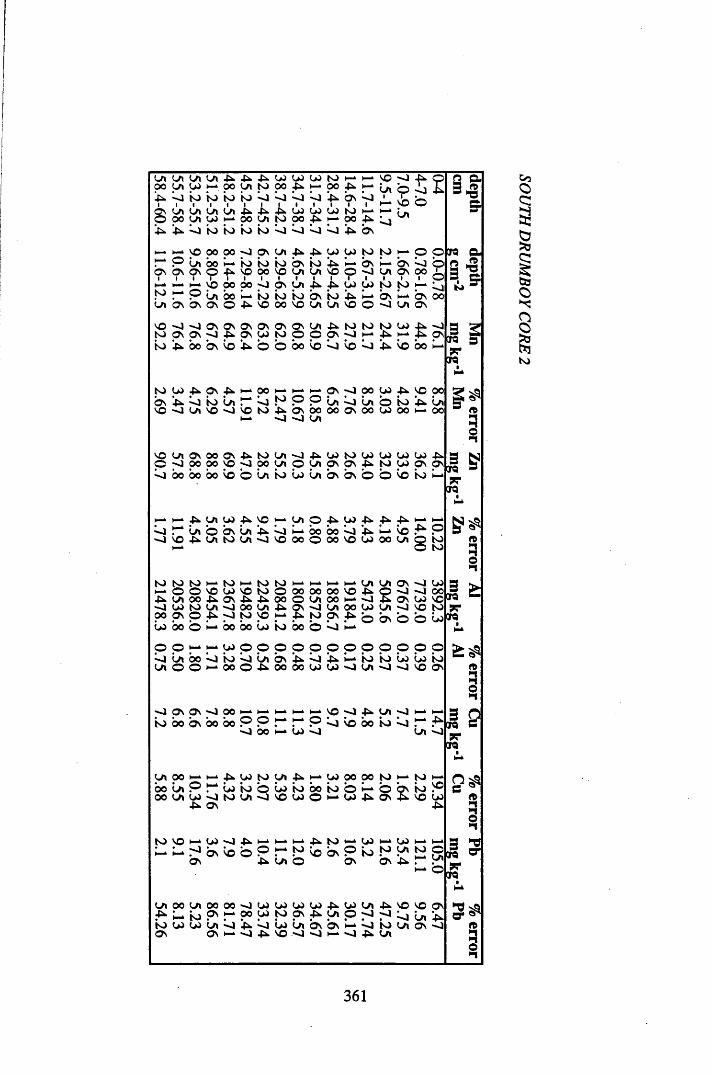
on on on on 4 -4k 4 . oo oo oo t o H-k H-k p 4 P 2 aOO on OO i—k 00 on t o 00 4k H— oo 4> H-k on o
i<-0 X 3 CD4 b to to to to b b b b 4 . ON b ■
H-ki
VO o*G
ON on on on on 4 4k 4 oo oo OO t o i—k H-k &o 00 on OO H^ 00 on to oo 4k H-k oo 4 - b*4 4 b to to to t o b b b b 4 ON
n-k p 00 00 -o O n on 4k 4k OO oo t o t o o © ere aH— O on bo H-k to t o t o O n t o 4 - H^ O n l—k O n b o n ftpm*ON ON ON O 4 NO oo NO on on NO O "O on ON OO io BH-k H-k l—i NO 00 00 b ON on 4k - 4 oo OO t o t o H-k b &t o ►—» o on 00 l—k to to t o O n t o 4* l—k O n i—k ON 00on ON On O n o -4k NO 00 VO on on VO o ■o on ON
VO -o *o O n ON ON ON O n ON on 4 - t o t o IO vo 4 «o 3 9t o On ON 4 ON oo t o o o ON - 0 H-k 4k H-k 4 as 3
ere &t o 4 00 ON b 4 o o bo b b b b 4 b oo b 9 9
ere4
t o OO 4 ON 4 H* 00 l—k H-k H-k On - o 00 OO 4 NO 00O n 4 b t o on l—k b t o © o on b on o i o 4 on er*VO ■—1 on NO •o b t o 4k ON bo oo ON oo oo 00 oo f t
l—k *o - 0 on MO•n
VO on ON 00 ON 4 t o on - o 4> vo ts) oo oo oo OO 4 3 NO <1 00 OO NO -0 00 on o on ON ON 4 t o vo ON ON 3nrob 00 00 00 b o on t o oo on ON ON o o b t o H-k 9?
ereHH
i—- 1—k 4 on oo 4 NO H-k on o 4k OO 4> 4k 4 l—k H-kb HH on o ON on 4k b k_k bo OO b 4 l—k b 4 o 3 cr*
NO 4 on t o on ■o NO oo O 00 NO oo oo on C i t o f ti—* © t o 3
O>1
t o to t o 1—* t o H-k t o t o H-k i—k l—k H-k on on ON «o vo 3I—* O o NO oo VO t o o 00 oo oo NO 4 p «o 00 3 £4 on 00 4*. ON -4k -4k 00 o on 00 - J 4 O n vo vo ere■o OO to on oo on 4 ON «o on 00 OO on -O NO t o 9900 On o 4 p t o NO H-k 4 . t o ON 4k b ON o b oo ereOO 00 © i—k 00 00 oo t o 00 o b H-k ■Hk
o © ►-* oo o o o o o O O o o o o o >b on 00 b t o b on ON 4k b 4k I—* is> t o oo vo t o mmon O o i—k 00 o 4k 00 00 OO OO on ~o - 0 VO O n f t
gO•1
~o on ON <1 00 l—k l—k H-k H-k H-k NO - o 4k on «o H-k H-k 3t o bo ON oo bo o o H-k H-k o b b 00 io b p 4 3
ore ¥b 00 H— oo b on b p?
ereHH
y* 0 ° i—* i—k 4 oo t o on 4k i—k OO 00 oo t o H- t o H-k n00 on o i—k oo t o o oo t o 00 ts> o l—k o ON io p G cf*OO on OO b t o on 'O NO oo o H— oo 4k O n 4 NO OO f t
4 ON 4 qO•-I
t o p »—- OO - o 4k H-k |_* H-k 4k t o H-k oo H-k VO H-k H-k 3 hgH-k ON b o o H-k t o b O n o is) t o on t o O 3
ere 3 “O n 4k on o ON O n 4 on
i—k o P9ere
H*
on OO on 00 00 ~o vo oo oo oo -4 oo on 4 VO p O n4 l—k io ON H-k 00 oo t o ON 4k on o - 0 •O b on 4 c rt o OO OO on b 4k b oo on O n ON H-k b t o on ON »o f tO n ON H-k «o 4k NO - 0 • o H^ >*0 4 - on 3
O
On0c;3§10
1to
361
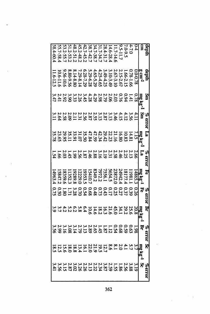
tottottotto,4k.4k.4k.iotototo^-H- O O tO t t O ►— O O U , t O O O 4 k . h - O O 4 k . h -
4 n b ’t o i o i o ‘t o b b b b 4 k b v bi i i i i i i i i i i i i0 \ U i l J l U ( ^ J i ^ ^ W W W N ) MO o o y i W H - o o u i t o o o ^ M o o ^45k 4k. b to io ‘tO k ) b b b b 4k Ov
VO ;0 4k ptot © b 4k m \b o
tot•O
^ i - ^ o o o o ^ p v y i ^ ^ w w t o t O H - p C ^ P bt 00 b io io io b\ io *4». b ovJ—c n ^ q OvOvOvO-^^OOOVOUiWiVOO^UiOvOoII I I * I I I I I I I I I I I I w M h - M ^ O O O O ^ p N ^ ^ ^ W W I O t O M ^N f-* P to, 00 I— to to io bv io b b on b bv oo UOvOvO\0 ^'OOOVOUi^voo>JUiOV
to to to tO to to to 4 k 4 k to to to to o o H — o4 k b V O vo io io b to to vo b © o b b b b•o l— k to o to O v tot 00 vo 00 vo O v to O V 4 k l— k o o
t o t o t o t o t o t o t o t o t o t o t o t o t o 4 k . 4 k . t o 4 k .
l— k b v t o . o l— k v o t o t b o t o . H ^ b o l— k 4 k . l— k H - k t o t H - kl— k 4 k o o v o O V - o t o . t o - J t o O V t o t t o O V
t O t o t o t o t o v o t o 4 k -Pkk 4 k . t o t o t o H -k H -k H -k
t o t t O v o y t o l— k y t o v o t o 1— k O s o 4 k . H —
b b v b i— k b o t O t b o i n t o 4 k . t o 1— k 0 0 b o b o t o ,o o t o t t o t i— k i— k ~ o o 4 k v o 4 k . t o t o O v o t o H - k
l— k l— k t o I— * i— k t o l— k t o t o t o t o t o t o t o t o t o t o
i o t b v o b b i n b o b b o H -k H — t o t o t 4 k . i o H -k b v4 k . o v t o t o , v o o v - 0 O v o o O v v o H ^ 0 0 O v t o t t o o v
l— k H ^ l— k »— k i - * 1— * l— k l— k 0 0 - o - o t o t t o t o H -k
4 k t O t o o i— k V O t o v o t O t t o V O t o , O v t o 4 k . o o H - k £v o o o t o t o t o t o t o 4 > . 4 k ■ o t O t t o t o o v o H -k v o o oO v 4 k t o , t o t o o t o t o * l— k P t o a s 4 k . 4 k . ~ o o o O Vt o < l
pt o
pv o t o o i o i o l— k t o ,
t o t o > o H - k t o ,
b t o b v t o b o o t O , b o 4 k . 4 k . H ^ t o
o © i— k l— k t o o o o o o o o o o o o o
b t O t b o b t o b i n b v 4 > . b 4 k . l _ k i o i o t o t o i ot o t o O i— k 0 0 o 4 k 0 0 0 0 t o t o • o t o t ■ o ■—1 v o o v
I O t o 4 k . t O , O v y O V l— k l— k 1— k t o 4 k . t o t o t o t o
b b t o t o t o b o b o 4 k . oo a s H - k t o t 4 k . v o y pb v b v t o t o b v o H -k i o b v oo
I O t o t o t o t o t o t o t o t o l— k l— k o o o o H -k
t o t b l— k o 1— * b l— k 0 0 b v 4 k . bo l _ k t o t b v t o t b v bO V v o O v 0 0 4 k . V O t o v o O v t o t ■ o t o 4 k . 0 0 v o t o oo
I—* i— k l— k l— k l— k l— k t o t o l— k l— k oo o o t o 4 k . t o t t o0 0 t o t o t oo
? °t o p v t o l— k
pt o
b v l— k o b bt o , O i b v o 0 0 b l— k o b t o t b
'
t O t o t o t o v o t o .to t o t o t o t o t o l— k H -k t o t o t o
b t o . b b o o i o t o l— k i o t o b o t o t t o t b o t o t 0 0 1— kl— k O v t O t • o t o O v o v t o t o 4 k k ■ o vo t o t O v O V oo v o
2 aS n3 *d
CTOO3Ki
a«
*3S'
J sf|VQ 3J5" fra
CA v § 3 or1»1>1
3 ^era » j r fra
»3o>1
3 ^CTQ «jr Era
«3o• i
^ 8? pra njrCTQ
-I ^ A§" i
£ »IQPC CTQ
A
3* i
362
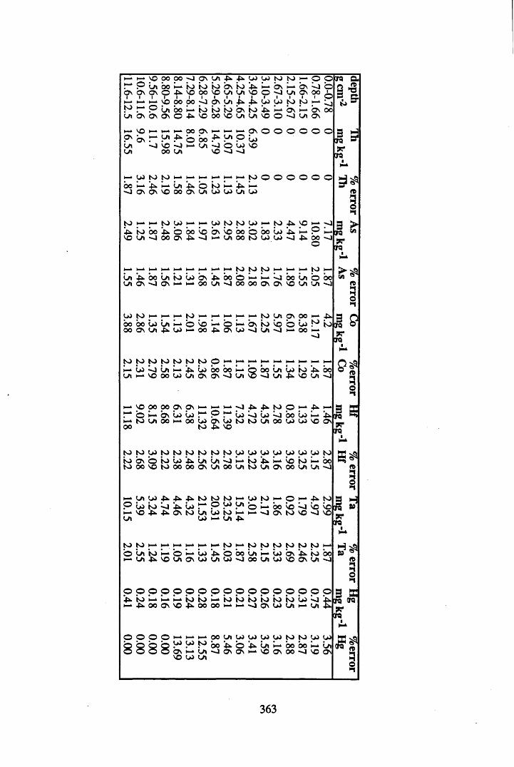
1—kl—kvo 00 OO • o O s la -pH 4*. VO v o t o t o l—ko o TOl—ko b b o i_ t t o t o i o a s i o b k l—kb s l_k b s b o QO n O n O s O 4*. vo o o vo V/l V/l Vp o - o LA O s OO i
© 3i—» i—ki—kvb 0 ° o o b a s b i k v o v o t o t o l—kbt o i—ko b 00 i—kt o t o i o b s t o 4 n l—kb s b b s o cb O n O s O s O 4 ^ vo 0 0 VO LA v/l vo O « o LA O s
i—»VO i—kI—* H^ o o O s l—ki—ki—kp v
00
o © o O sO s O s LA -pH
© b o -pkk V/l © bs
TOb VO b i—kv /i b o b VO ”V/1 0 0 LA VO - o < o
TO
i~* VO t o t o i—kI—* l—k»—ki—ki—kt o
00
o o o O H0 0 H-k 4 ^ l—kl/l b k o t o I—* b k l—k 3 1■ o O s O s VO 0 0 O s V /l v o v o LA VO
tO! ^ i o b o ^ b b o ^ b \ v o b o bVO(-rt'JOOON-tl.>«Ji-1 U)OOrO
OO LA -*JLA 4*> 0 0 LALA O s - o O s
VO jO l— k H -k
0 0 b o b LA0 0 o s V/l 4 *
t o t o t o t ol— k b b LALA I— * VO OO
i— k VO 0 0 o oo H - k b s
i— k t o LA 0 00 0
v o
t o© VO t—‘ o •—* Ov oo ^ Os W O
H -k t o VC H^o o b b i—k ov o v o • o -Pn 0 0
o
t o H -k t ob b 0 0 b oO s O s VO V/l V/l
t o V/i O s 0 0 I—*i o b o b t oLA - o H -k 0 0 1—k
^ W OO OO M ^ On On 'O Vi
t o O s t o 00
t o w ^
H - k H -k H >* - o 4*. -Pn t oH - k o H -k b b b bb b s b t o t o LA OOt o -p>kVO
t o t o t o t o VO VO 0 4l/i LA b H -k t o b H - *
O s LA 0 0 v /i t o LA O s
OO Vl w to 4 oo O Vl 4 Vi O
O •—*oo u ) !|^
VO t o 00- o
h-‘ V l W ^ ^ ^ t O t O t O > - ‘ WtOi-‘ O i - ‘ -^tOP b i o b ’.Ph b !"* P ^ M ' o b b o b b b bMNO^^ONtWlWtOMMOONtVVONjSO V/i W M V i !> .
to to i— k H -k H ^ i— k H - k H - to l— k to to to to to to H - k
oH -k
bV/l
i o-Pn
H -k
vooV/l O s
bvo
'■PHLA
ovo*00o b
o oi— kV/I
bvo
b svo
bO s
i oLA
*oo- o
o o Oo o o o Oo o Oo Oo O© o4*.H - k
i o-PhH -k
OOH -k
O sH -k
voi o-Ph
i oOO
i—k0 0
i oH - *
i oi—k
i o" j
i oO s
i ovo
i oV/l
bH - k
bV/l
b-PH
o o o o88885;
H -k H^ H - k o o LA VO v o VO v o t o t oVO (O t o 0 0 P h o b b H -k 0 0 0 0b s l— k b ■ o O s OS H -k VO O s 0 0 ■ ov o v o V/l
VO O s
aft*a
n3o
3 >► era »5T70
(M ® f t3"I
M PIpro on jr
CTO
9 t• t'-io•n
3CTQ 7?70
f t
3n3 Hrq P9?
00
f tn>to
3 SI00 QT07?70
< £ f t3o>1
363
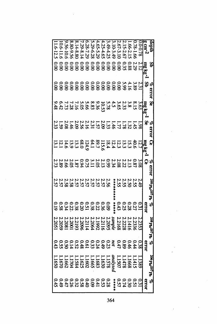
t o
O O
p 0° 00 ■o O n C/l 4 COCOto to l—koc/i 00 l—kto to to ONto 4 1—*ONl—kO n <1ONo 4 vo OO VOla la vo O ■o C/l ON00H- p oo 00 ■o ONc/t -k -k COCOto to l—ko c /i 00 l—kto to to ONio 4 l—kONl—kO nONON O 4k vo 00 vo C/l LA VOo ■o LA ONo o O o o o o o o O o o o to
c o o o t oC / l 0 0 V O t O
p p p p p p p p p p p p o
VO OV O O O
t o h - t o
c o c / i b -P*.
C / l p C O t o
V O h > - 0 0 C OV O O N v o l— k
c o v o 0 0 o s
LA? °
p H* C / l p > C O t o C O o o
O n 0 0 C O o b c/i on C O 0 0 l— kO n C O ON C / l
C O0 0 C / l C O c/i
t o t o l— k t o l— k H -k l— k l— k l— k l— k
l— k to C / l
8 C O ^ b k j C O ■kO n l— k C O O n 00 t o la
ON
sSO * n
o"I£ SPeraJT icra
h-k l—k l—k l—k l—k O n l—k O n o o H -CO to -pik CO CO 00 to 4*kp H-kl—k H -k ON vo CO o
■pk b y *b ON
to to to to H-k o o U> to tob 00 O n © bo b b l—k o l—kCOvo ON LA •o 4 C/l H -k LA CO
to to to to to to to to to toC/l C/l c /i C/l c /i C/l LA C/l LA LA-o *o oo 00 *0 -o »4
V O
H - k |— k |— k |— k |— k ^
o o t o t o c o y i o t o!pn l o c o u > b v b
p to to to to p cov o i oo tO M O oo vo ^ oo to (O o oo
O N
* t o t o t o t o t o
* la c / i l / i L n *4 .******
O o o o o o o o o o oi_k t / l CO to CO to C/l CO to CO oVO 00 ■Ph to 00 o H - k 00 to ON v o
okk
o O o Oto to io COLA 00 -o l—k
to to to to to to to to to to to to to to to toio io to io to to to to l— k io to to to u - k io too o o 8
H -k s l— k o vo H - k 8 l— k to 4 k co COLA LA 00 VO l— k ON vo H - k O n to H - k CO C/ll— k VO l— k H -k CO ON 4*. -ph to ON LA oo oo O n O n CO
0 0 0 0 0 0 0 0 0 0 0 3 !p*. c/i la h-* c/i 4x on co i o If*, t o 3.COC/l©4 tOOOH-C04^VOCO
On On On "O L/i On Ov On On On C / i Si C / i *0 O n O oo to O On oo c o >0 O O t o ^ 4vCntv)CAWOoo^
O O P O OCO 00
00 k 4 'J VO ON 5
o o O o O o o o o © okp*k -P- 4 ^ io C O LA 4 ^
s4 ^ C/l toLA VO ■O O n to 00 O i—k CO 00
H - k H - k H - H ^ H -
H - k H - k H -k l— k H -kLA ■pn ON -Ph CO© ■O ON 00- o 00 OO C/l v o
o o o o oLA • o CO C/l CO- o k^k O H - k
pro a■53 ^» & to
3*ra aisc pro
o*n3 f?o r a sc era
s ? ^
§•nK >©06
I5
3 *1o * »
i3g- j
3
3 *O " 1
I3§5
3 ^o> 1
364
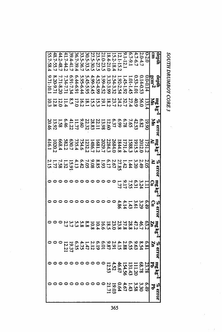
LnLn
4 HOO f t
-PhH - k
LONO
LOO n
LOu >
LOo t o<1
t oL - >
t o H - kOO
H -k
LnH - k
t op
H -k
ONb
-Phb
t o
©
b b t o b ’.p H b Ln Ln Ln Ln o ■fn t o H - k 1H - k
ib
iON
iL no o
LnLn
- p no o f t
-fnH -k
bNO
bON
bu>
bO
t ohJ
t oL 4
t o H -ko o
H -k
Lnt o
H -kH - k b b
. p n - a b t o b b b Ln Ln Ln Ln o t o
NO 0 0 ■ o - 0 O n ON Ln Ln -PH ■Ph lo LO t o H - H - M O ObH - k
i oo < 1H - k
b- p H
bH H f t
bLn
4 nLn
bNO
Lnt o
bNO
bt o
Ln-PH
bt o
'-PHLn
oH -k
LnLO
h—*- P H
H - k NO 0 0 b b ON ON Ln Ln - p H .-Phb b t o H -k H - k H - k OOM
bH - k
t oo bH -k
b- p H
bH -k f t
bL n
4 nLn
bNO
Lnt o
bNO
bt o
Ln-P h
bt o
'-P h
LnoH -k
LnLO
Mo H - kt o
M
t o
H -*H -k
o o
LnH -ko
H -k
ON o o
H -kLn
H -k
LnH -k
NOH - k
O Ot oLO
t o-PH
lot o
t o- o
-PHo L nON
b 0 0 © * .p n o t o H -k Ln b M t o b t o b -pH b o
to H - * H -k ON -PH H -k NO to to to H -k H O n ON ON - o 4 h ON H - k
o w Ln 4H H -k H -k ON to o o to LO to b b b O n to OO NO-Ph NO ON tO
oo ON toto
b■O
o bto
b oLO
H -kH -k
b0 0
ONo
■ o NO oo Ln LnLO
to bo
ON H - k ON Ln ON - o ■ O H -k H -k H -k t o t o t o M H -k H » H - k t o H -kH k o ON o o LO LO Ln t o -P h ON o to O n O O - o Ln NO OO n t o o o t o o Ln -PH LO 00 00 to OO OO -P h LO o o H -k H - k LnH - k o 4^. t o b ON t o O n H -k NO ■pH -P H H -k o o Ln t o H - k
to t o b i o b b o 0 0 ’•P h b Ln o t o
to H - k <1 H - k H -k
H - k b Ln b LnLn -O oo to b
H -k
4n p\ p yo ooh- 4n © © 00
H -k ON to to H - k
b H - k ON o 4 hLO ■o •o 0 0 to
Ln
H-k Oi to to it* io ip* © ^ O NO Ln
© © © © ( © © © © © © © © © H - p p p N W^ I- Lft w Ki—4 -O Ln •—* 4 h
0 0 0 0 0 0 0 0 0 0 0 0 0 .-^^^-WU>pNb o b !pn b \ is ) '-Pn O n -Ph LO ►— v o no
O O O t o w v i y i o o M M H i - t o w w t o ^ ^ o^ ^ w o o b o P P P N?°yj 'j i H ? 0 rJ ? ' !>J
0 0 ^ 9 \ U ) O 0 0 0 0 0 0 N)>]K)
OOO^-H-pN^H-KJpNpNNOtO^tOpNVOOOpN. ^ ^ b b b b H - k i D b o b b b o L n b N L n b o(OW^t^vltOVOh->Ji-‘ tJlOOLftW^^‘H - * - « J
o o o o o o o o o o
o o o o o o o o o o o
H - k 4h - p H H -k H - k H - k O n toto y i O n Ln LO H - k OO LOLn to ON ■Ph H - k H - k b bLO Ln I p H io OO 0 0
ON LO o
to H - k O -P H H - k LO LO ONH -k NO ON ON 4H Ln b 4 H
b o -Ph LO 0 0 O NOH -k LO
2 a3>8
5
ra aQ «g *t3Iff; sCTQ
s * ro r a
3 n3£ 3
QTQ7?QTQ
»
3•n£ 3B (TQ
wo r a
S t
i• 1
B?sQTQ9T
IQ
< £ l
»
33 3O* jq
7?QTQ
SfI• n
365
SOi/TO D/? UM
BOY CORE
3
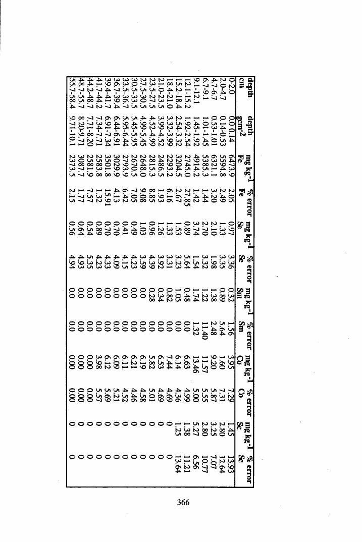
Ln 4 4 4 Lki Lki u> Lki to to to i—k »—k i—k p Ov 4* to O 2 aLn OO 4 vo Ov pi o p u> H-k o o Ln to I—* b b bi
to 2 »b1 bi toi bi 41 bi Lni Lni Lni Lni 01 4i toi i i
i—ki
piOV i
4 bLn Ln 4 4 4 u> u> u> Lki to to to l—k i—k to ST00 Ln OO 4 l-H vo ov pi O p p> i—kOO Ln l—k4 b b io b 4 b Ln Ln Ln In o 4* io
VO oo -o - j Ov Ov Ln Ln 4 4 u> u> to i—* l—k i—* C O o r c ab io b b b 4 b 4 b Ln b b Ln b 4 k o Ln b s «H-k1 01 ►—* i 4i ►—» i 1 Lni Lni v oi toi vo■ to• 4 .i toi Lni I—*i u>i - 4■
io = 1
H-k VOoo >o Ov Ov Ln Ln 4 4 u> pi to H-k i—k i— O t o s r© b to b b b 41* b 4 b Ln b b Ln b 4k b Ln £
1—* O i—* 4 i—» 4 Ln Ln vo to to 4 to Ln i—k Lki
to u> to to Lki Lki to to to to to to u> to 4k Ln Ov Ln Ov Bu> o Ln Ln Ln o -o Ov Ov oo 4 to to VO u> Lki Ln 4k » J 3■o 00 oo 00 O to vo "O 4 l—k OO vo o 4 k i—k oo to vo -O TOpi l—k pi vo Lki o OO Ln pv u> 4 k Ln 4 h Ln H — 4k LkiLn b b 00 00 b b Ln o b Ln io Ln o to b l— k 00 b TO
•l—i
t o H -k H -k i— k 4 k Ov -O VO 0 0 H -k p v t o t o i— k
H - k b Ln b Ln b 4 k o b b o b H -k b v o 4Ln •O t o b
H -kLki t o Ln o o Ln u> OV ■o b oLn t o
O OOOo o OO l— k O i— k I - h H ^ OLkiLn OV Ln 0 0 b b b b o b i o b Ln b o bOv ■ 4 4 k VO OO H -k VO u> Ov Ov u> u> VO • 4
►— Lki tO to 4 ‘tO 4 ©
Nl M w vo O O U) -o
■4 4 Ln 4 4 4 4 4 pi 4 Lki pi Lki Ln H -k pi H -k pi pib b b io b
8b io Ln b b b io bv Ln b b b b
■4 Lki Ln Lki Ui Ln Lki VO VO to H -* Lki 4 4 to 00 Ln ov
O O O o O o O O O O O O H -k O i— k H -k H — O Oo o o o o o o o o to
oob4
ooto
oLn 4oo
b4
toto
boo
bovo
bto
H -k i— k to Ln i—kb H -k 4 bv Lnto 4
O00 4 OV
o o o o o o o o o o o o o o
b b b b b b b b b b b b b b
p p p w p \ p \ p N < ? s p N y ip \ o p \ p NS b b ^ ! - b I - * k ) M b o l « ! u M b \ ^ r K J o \ ^ o O o o o m ^ i - > m \ o w w 5 ^ w a u o o u
i— k H- k VO l— k LkiLki l— k io b v b4 Ln o o LnOv « 0
o o o
8 8 8
© © ©
o o o o o o o o o o o o
Ln Ln Ln 4 4 4 Ln 4 4 4 4 Ln Ln pv •oLn b v to Ln 4 Ln o b v b v b b b Ln 00 b io- O vo H-k to OV 0 0 H-k VO VO Ov vo © Ln —] H-k VO
O o o O o O o o o i—k i—k Ln to pi to H-kio b to 0 0 io 00 4Ln oo « o o Ln o Ln
H -k H - k pv H -k ~ o H -k H -kLki H — Ln oo
to Lkibv to Ov b « o bv b4 H - k 4 Lki
s *
.17TTO
rt
flprTO
c*a va3 s5*! ffis•-I
P 3© <jqW*TO
? *a3
TO7?TO
'1
366
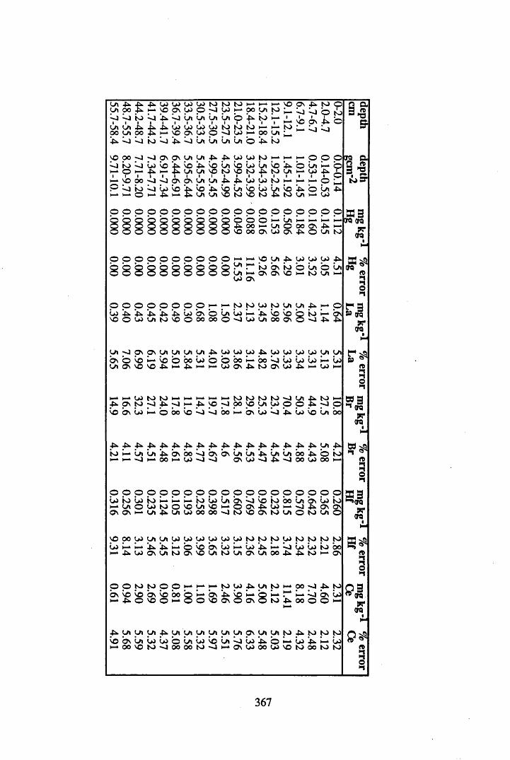
LnLnPkoo £
Pkl—kU) VO
LOOV
LOlo
LOo
to;~4 to
loLj to b Pk b Ln Ln Ln Ln
Lnoo
LnLn Pkoo £ ■ul—kLO
voLOo\
loLO LOO
to
Pk <J b to b Pk b Ln Ln Ln
VO00 -4 •o ONov Ln Ln Pk Pkbh - k
tOo
Ljl— k
LoPk bH — £ bLn PkLn b
voLnto
h- vb oo ■■bb ov ov Ln Ln -fk©i— k
bi— k
toO
bI— *
LoPk b
l— k ' £bLn
PkLn bvo
O O O o o o o O O o
t ol—k
i—ko o
l—kLn
l—kt o
O -pk t o l—kt ol o
t ol—k 0 0
l—kLn
Ln o P k t o
l o LO t o l—kv ov o
l ot o
LnP k
v ot o
P k l o LO t oLnt o
v ov o
LOt o
Ln■ u
O o o o
OP kVO
oo oo o
oH - kov
LnLO
v o ov P k tol—k ~o o
H - v o ov Pktol—k
H — •o - o
l—k i—kO o
PkLn oi—kLnLOl—kPk
l—k i—k 1—k p
bto bkLn oI—*
LnLO
o O o O
LnoOv
i—kooPk
i—kOvo
£Ln
o
©o
o o o o o o o o o o
8888888888H -k H -* v o Ln P k LOL n H -k
t o b v t o oL n H - k Ov o v v o H -kLO Ov
LO U> .PkLfi o ui to Ln
P P o o O O o o H -k i— k t o t o LO t o L n Ln . p k l—k o
L o P k P k b k P k b k LO b v b L n L o 1—k '■Pk b b 8 t o l—k b vv o o LO L n t o VO o o o o o o —4 LO L n o o Ov ^ 0 P k -Pk
Ln -4 OV o
OVOVLnLnLnLnPkUib ^ b b b o l o b b
LOLO Pk LO LO LO LOLn Ln00 H - k 00 b LO LOLO H - k LoOv Pk t o Ov LO P- H -k LO i— k
H - k H -k - P k O v
LOto to- 4
to-Pk H -k I— *H -k
H -k.-PkH - k
pHk to
o otovo to
L ntoLO
-JO
L nO £
to h - k
Ovo Ov Lo H - k o oo b b b 0 0 H - k b v LO b '■ Pk LO b Ln bo
■pk P k P k P k P k P k P k P k P k P k P k P k P k P k P k P k P k L n P -t o l— k Ln Ln P k b v 0 0 b b v b v Ln Ln P k Ln Ln OO P k o i oh —k H -k - 4 H - * 0 0 H -k LO - o ~ o o v LO P k - 4 OO LO oo H - k
o o O o o o O o o o o O o O O o o O o
LO t o Lo t o l— k l— k H -k t o LO Ln b v b b t o bo Ln bv Lo t oH - k L n o LO t o o v o L n VO H -k o OV P k LO i— k - o P k Ov OvOv Ov L n P k Ln LO 0 0 OO ■ o t o VO O V t o L n o t o L n o
v o oo LO L n L n LO LO LO LO LO LO t o t o t o LO t o t o t o t oLO H -k H - k P k P k i— k b b b v LO H -k LO P k l— k b LO LO t o boH -* P k LO Ov L n t o Ov v o L n t o L n Ov L n 0 0 P k P k t o o v
O O to to o o i—ki—kl—kto LO Pk Ln to l—k 00 -4 Pk tob v b b b v b 00 8 H-k b v Pk b i—k8 H -k
H -kH — b b v LO
H - Pk o v o o i—k O v o OV o OV t o PkH -k
00 O o H —
P k L n L n L n P k LA L n L n L n L n Ln p v L n L n t o P k t o t o t ob b v Ln Lo LO o Ln Lo b Ln b LO P k o H - k Lo P k H - k LoH - k oo VO t o 0 0 0 0 t o - 4 i— k OV LO 0 0 LO VO t o oo t o t o
a&*T3&
ora aQ to2 *Stos*
532QTQ QTQp r era
w «i-i*no•n
rg» ora
we r a
gjto•io■-»
? 2 ^ erawora
i- i ^too*i
317Tora
toi•-i
p 3< r a
prora
P*rt§•1
367
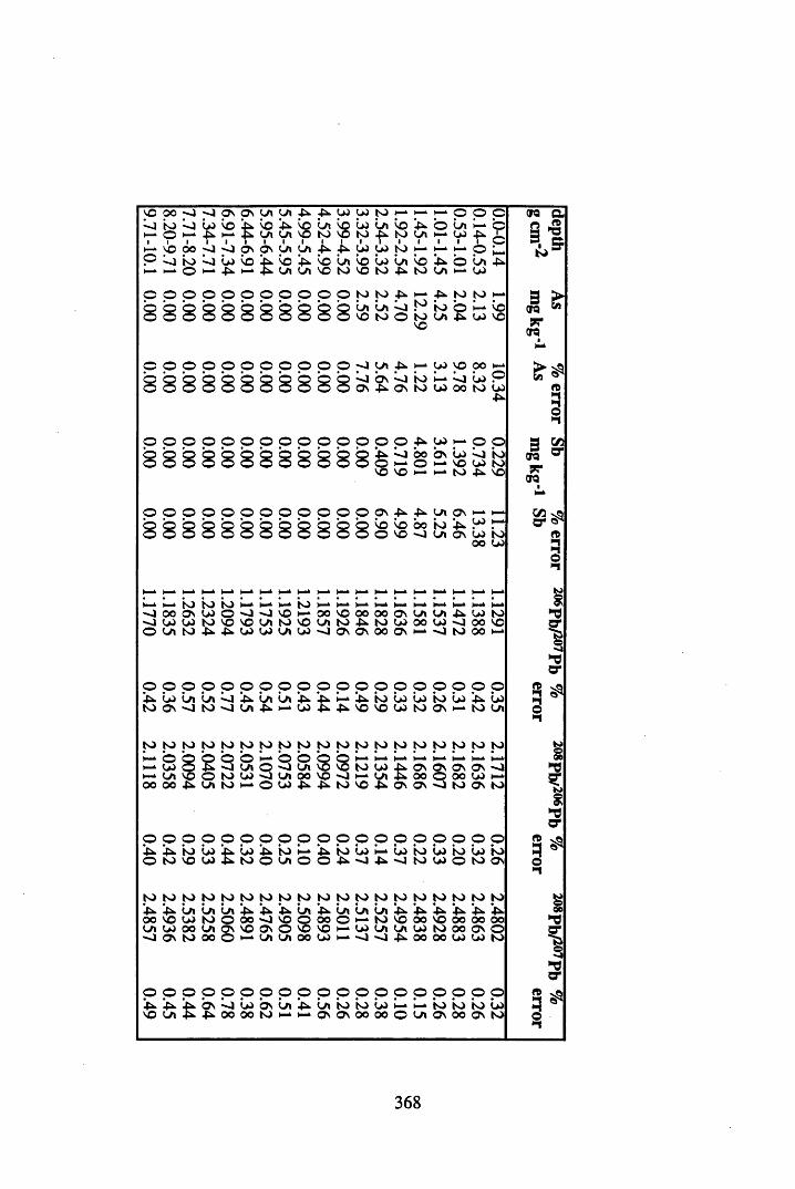
VOOO Ov Ov V/i-OH —
tOO
*oi— *
VOP
VOi— k fc voV/l
H - k VO00 ■o•o Ov OvO 1—■-J to
O l—kVOP VOi— k
PPo o O o o o O
8 8 8 8 8 8 8
V/l P PP vo V/lV/l vo toV/l V/l Pvo p VOV/l V/l VOo o O
VO vo to i—k i—k l—k O o oVO UJ Ln VO P © Ln i—k ovp to P to V/l l—k v o P 1oP vo VO to i—k l—k i—k O l—kV/l vo VO Ln vo P © Ln Pto vo to P to V/l l—k vo
o IO to P k—k P to to l—k
8 V/l Ln b to to © l—k bvo to O to
voV/l p VO VC
o o o o o o o o o o o
o o o o o o o o o o o
■o p p i—k p vo0° l—kb b v b to i—* b vo pOv P Ov to vo 00 to vo
p
O O o p vo l—k o o8 P b bo b s vo —] to
O i—k O H-k vo vo toVO vo i—k to ■pkk VC
o O s P P V/l Os l—k H -k
8 b b bo to p vo l—ko VO ~o V/l Os vooo to
vo
H - k l— k H -k H -k l— k H -k H -k l— k l— k H -k H -k H -k H — H -k H -* H — H - I—H - k H ^ to io io H H -k H -k io p H -k H-k H — H -k p p H -k 1—k 1—*00 Os vo o «o kO vo H -k 00 vo 00 oo Os V/l V/l p vo tovo vo to vo vo v/l to vo V/l to p to vo 00 vo ■o oo voo v-n to -Pk -Pk vo vo V/l vo -o Os Os 0 0 o s ~o to oo l— k
o o o o o o o o o o o o o Oo o o o op vo Ln Ln b p V/l Ln p p p p io vo vo to vo P voto OS -o to kkjV/l P H -k vo p p VOvovo to Os H - k to V/l
to to to to to to to to to to to to to to to to to to tol— k o p b b o H -k o o © © H -k p H -k l— k H - k H - k H - k l— kH - k vo o p -o V/l o -0 V/l b b to vo p OS OS OS os -Ol— k V/l o to vo ■o V/l 0 0 vo■o H - V/l p oo o oo vo H -koo 0 0 p V/l to l— k o vo ■pH p to vop Os Os «o to Os to
o o o o o o o o o o o o o o o o o o op p to vo p vo p io H - k p io vo H -k vo to vo io vo too to vo vo p to o V/l o o p ~o p •o to vo o to Os
to to to to to to to to to to to to to to to to to to to■Ph p Ln Ln Ln p p p Ln p Ln Ln Ln p p p p p pOO VOvo to o 0 0 -J voQ oo o H -* to vooo vo 0 0 oo oov/l vo 0 0 V/l Os voos o b vo H -k VOV/l v/l vo to oo os okkj os to 0 0 o H -k V/l V/l oo vo H - k »o-o p oo 0 0 vo vo to
o o o o o o o o o o o o o o o o o o o p pVC V/i S ^ O O O O N J m m OVOVOOOOOWi O\OOONN)
era an J23 ^0J IIO
3 >1 ora w7T
o r a
o■"»•-IoI-I3ora7T
o r a
V)a
Cfl »a cr re3•iI
>do*3 ^ 1•-Io"I
oooIcr
i•-I
I"8
1*3a*
3 o ■•-I
368
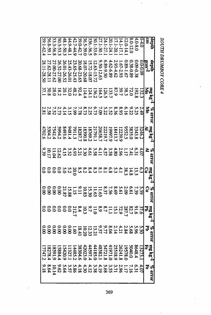
Ul U\ (yfl Lfl ^ p\ W O OO h* oo W W i-*I I I I ION Ln Ln Ln Ln to p p w p 4k h- 00 Lo Lo
fcvoI4k00
to to to to00 -o *0 onI— ON © LnH- to © to1 I I Ito to to to 00 00 -o Ui m o\ o O h- ioO
o 4k
LntoW W to M to wO O M 00 o | 0)—‘ 00 © "to 1— ©
to to ~o to 00 u i L n o
4k*0 o toON tO 4k
Oi o ^ 00 *o LO Ln VO 4k 4k
^ vo VO OO 4k W h> tO ON 4k
to
VOLovo
4k LO
o4k. to
0 0 0 0
8 8 8 8 b0 00
0 0 0 0 0 00 0 0 0 0 0
4*. LOLOLOLOto VOONLO©L j © Ln Os H-k
4 k LOLOLOto VOas LO
b b © Ln ONto to H—H-kLO© 00 Ln toONON© b O nLn 00 to LOto to to H-kLn LO© 00 Ln4k ONO n © bLOLn 00 to
4 k VO H-k H-k00 to H-k to LOto 4 k 4 k
4 k4 .H*
ONio
-0 -O 00 to ONb b b to bvo 00 LOLn LO
*0 H—H-k H-k tovo OO00 00 l—kH-k to LO•0 -OH-k 00 vo O n VOLO-0 © VOi—k
b 00 to >“ *
4k. Ln LO4 k LOb to Lo ONLnLOH-k © H-k 00
to 00 00 OO00©©
Ln to 4k LO
H-k p H—kH-k H—H-k H-k © Ln H-kLn H-k 00 Lo O nLO© LO
to 00 H-k voH—tob
4k ©LOb i—k
©
-o 4k o -4 4k to00
0 0 4 k 0 0 4k to©
4k0100©
94^©
2 a3-S
h- m VO Ov 4v tOO VO tv) LO O vo 001 1 1 1 1 1 1I—. VO ON 4k. to h— O
Li 00 bv vo Ov ‘On O VO S) LO OLO
O O O O^ s ?
00 LO VO 00
4*. ON LO Ln Ln b VO —1 LO O
O tO VO OO tO Ui OO LO tO ONtOV04k.tOLnL04k.4k. Ln 1— vo H* LO to vn LO OvO O vo O vo
4k. 4k. L0 4k. t0I— in Ln 00 b h - 4*.h-k -O OO © ON -O ►—
h O On LO
pppO LnLntopopopopooooopN Ln4k. b b b b b t o P L n t o * 4 s .L o U I —0 0 L0
LOi—ki—kOs0° 4k LOLOLO00 LO
lo Ln On On O Ov vo M
i—k-o to OO VO LOLn to 00 to H—«oH-k b •0 b ON ON
© © © © © © H -k |—k l—k l—k l—k
8 8 8 8 On©H-k H-k H-k H-k P vo OOto 4k- to y Ln Ln00 © to LOLn b © to 00 ONb Ln4k to LO to -O 'O 4k 4k i—k4k OOON©H-k © LOH-*
on aQ to3 *P© • a
H-k H-k OO LO LO '—]O VO OO tO VO LOto to
00 LO
1 stoff
!3CTQ99QTQ
tO tO 4k.
© H-k
toi
3oo9?9Q
to3•1
P <w9?era
H - H k H - H - o o o o o L n t o o N O L nON LO Ln H-k vo VO
H— H-k l—k H-k l—k I- - H — LO 4 k 4 k 4 k L n 4 k to to 1—k L n OO H-k- o 00 00 L n L n 1— k 4 k 0 0 to £ OO 4 k H - k L n O n vo © ON LO« o to L n 00 4 k LO £ LO © L n l—k L n VO L n to L n Jk 4 k to4 k -O vo 00 to to OO © to VO OO 00 to - J H-k 4 k ■ O © 0 0 - J• O 00 H - k 4 k © - 0
yLO • O L n to 1—- H - k OO H-k 00 O 4 t LO
io 4 k b 4 k b H — io ON © 4 . © H-k 0 0 © v o 0 0 © H-k
p 00 H-k VO L n LO L n 4 k 4 k 4 k LO 4 k L n LO LO to H ^ p Os 4 kl—k ON © ON ON Ln 00 H-k LO i—k LO i—k ON Ln <1 b H-k H-k LO ©00 4 k H-k to 4 k * 0 ON OO © to 0 0 VO 0 0 L n H-k O n - J ON H-k •O
4 k
g>#to5■I
3 J99 e r a
cr toi
S3°<W99e r a
toi■t
369
SOUTH D
RUM
BOY
CORE 4
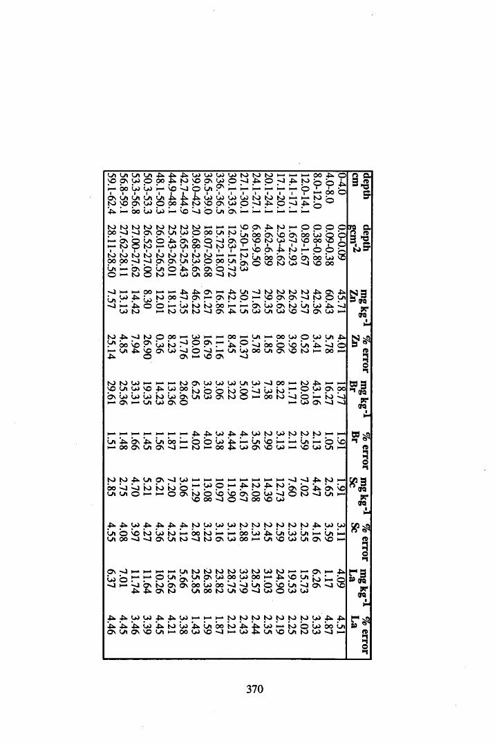
CA CA CA CA Pn V O O \ W p O O»—. 00 co co i—‘i i i i iOS CA CA CA CA N> VO p s CO © !t». h- oo w w
^ W W W W t O I C t O M MK)\OOnWO^AO^J-P>. OS *fcb L j © La
k km IO 'J O O i on h*
h - . i— i i— * I—* o
h- oo pn O10 © © in
t o^ W W W W t O t O t O M M t O V O O \ W O O ^ p O . P k . Q
to to to to00 O O ON L-. bs b ca k— to O to1 I I Ito to to to00 00 OLa L-. bs © O to o
t o t o t o t o so Os ^ to H-k o Op s C AU i p OO C At O ^ A Q o b s VO b s b o L oO ^ k O s O N O O O sM W S A O O O t O WI I I I I I Ito to to t o to M mOS OS CA Oi O 00 CAc a o p h b s b s © L jto m w CA 00 o to
tob sCO
so to w o vo 00I I I I I Ip p 4k to M oc a 00 b s b b s 00© VO to CO -O so
00 o o
o o
f tCO00
p j l—k i—k 00 l—k 1—k Pkk Pkk O s HH pH CA -O t o t o t o t o P h O s P h
CA CO P n CO t o 00 <1 O s H-* p s t o 0 H^ SO p s a s ^kj t o 0 CA•O l—k p n 0 0 l—k CO t o i o 00 H-* H-k b s CO b s t o CA CO P h L j
CO t o t o CA t o •0 Os Pkk CA CO CA CO SO -0 O s CO
t o P n >0 t o 0 0° H-k CO H-* H-k 00 H-k CA _ l 00 CO O CO CA P hCA 00 VO o s CO i o *0 0 O s 1— k pH O L j 00 0 b CA P h L o Ol—k CA P n so o s CO L j 0 L j l-H CA CO 00 CA O s so t o H-k OO H-kP n 0 os H-k SO ON -O
t o t o CO l—k H-k t o OS CO CO CO CA CO -0 0 0 H-k t o P h H-kso CA CO so -Pk CO 0 0 t o 0 O i o L j CO i o l—k O CO O s OOb s CO CO CO i o CO b s CA CO O s t o PS H-k 00 t o L j O H— t o L jl—k O s CA CO o s 0 H-k CO O s -0 k-J
h— i—k H-k l—k l—k l—k H-k Pkk P n CO P h Ph CO t o CO t o t o t o l—kCA P n b s P n CA 0 0 H-k 0 0 CO P h H-k CA b H-k l—k CA H-k 0 b
0 0 O s CA OS ■0 t o H-k 0 0 £ CO O s so CO 1—k so CO CA H-k
t o t o P n CA p s 70 CO H-k H-k H-k H-k H-k H-k H-k H-k - J ■0 P h t o H-k00 L j L j t o i o i o 0
H-k CO 0 P h t o P n t o b s 0 P h b s bCA CA O I—* HH 0 O s t o 0 L o so b s b CO L j 0 t o CA I—*so 00 - J 0 •0 00 so CO
P n P n CO P n Pk. Pkk Pk. t o CO CO CO t o t o t o t o t o t o P h CO COCA 0 so t o CO t o H-k 0 0 i o H-k H-k 00 CO P n CA CO CA L-k CA I—*CA 0 0 « o -0 O s CA t o •0 t o OS CO 00 l—k CA SO CO CA OS so l—k
p s ■0 l—k 1—* l—k l—k CA t o t o t o t o CO t o CO t o l—k H-k p s l—k P h
CO 0l—k l-H 0 CA b s CA a s CO 00 CO 00 H-k P h so CA t o H - k O
■0 H— L o b s t o b s O s 0 0 CO 00 L o L j CA O b CA L j o s - J SOP n •Pk. O s t o CA 0 0 to CA so -O CO 0 CO CO
P n k&k CO CO pn Pkk CO 1— * H-k H -k t o t o t o t o t o t o t o CO P h P hpn P n pn CO Pkk i o CO Pk- CA 0 0 t o P h £ h CO H-k t o 0 CO 0 0 CAO s CA O s so CA H— 00 CO so •0 H-k CO CA so CA t o CO -0 i— k
erg a Q n 3 *a
I s s to ET
6f3CTQ7?
QTQ
o>1
•"» crq P ? crq
|5| On f t3o►1
QTQpro r a
SPsSǤ*1
r 3* w
p rera
89f t3o>1
370
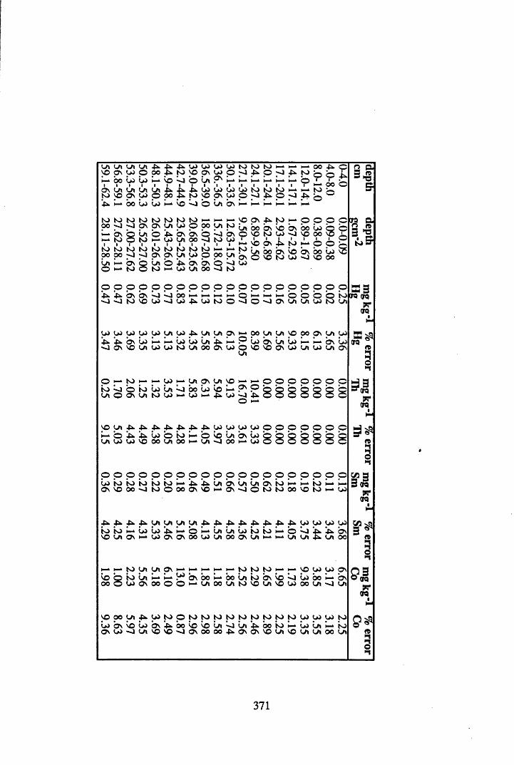
Lfl Ul Wt OtVOOs WO
to p pv pi^MOO Wto to to toOO O O O v
ONto
LAtoto to to toOO OO—] —] LA b On ©O ►— to ©
4k. 4* 4». LJ LJ LJ l j to to to i—k i—k i—k oo 4k.oo 4 . to NO p LJ o < t 4k. O <1 4k. to © ©H -k NO L j O LA p l—k b i— k H - k H ^ H -k o 1
H«—i
ooLA 4k. 4k. 4k. L*J LJ LJ LJ to to to b I—* too o° 4 . to NO p LJ p p 4k. p p 4k. © LJl j l—k NO L j © LA ON i—. i—k H — H - k H -k
to to to to i—» H -k H — p p 4k. to H -k O O OO n LA LO O 00 LA to LA oo ON b ON oo l j ©© 4* Ov O n © L j ON o NO to LJ o NO 00t—» i l j1 LAi 00i L j
ito
iDi
1H -k
1NO
iP
i4k.
1to
1H -k
iO
1p
toON
toON
toLA
tou>
toO
k—kOO
i— k
LAtoOn
LAo
OONO
O nto
bl j
ON-o
boNO
LJ00
L a © 4*. ON ON o L j LJ
©I4©
G a = *a
&
an aQ tog *a . ato ST
to M w w oo o to
p p p p p p p p p p o^ ^ b s O N O o b o M t - i i - i M v J O I O ' C W O W ^ W t O O
o o o o o o o o ob i—* H - k H -k o o o o t oo «o ON LA LA LJ t o LA
S 3o r e e r epp o r e
LJ LJ p p p p p 4k. LA LA p 00 La p p OO P p p4k. 4k. ON l j i— k H -k u> LO LA 4k. H -k O LO O n LA LO H -k H -k ON LO>o ON NO LA LJ l j to LA OO On LO o
LaNO NO ON LO LA LO LA ON
O j—‘ to >—* i o o o i o W W l oa O On on
P i—* p P LA P i— k H - k
LA b OO LO b i— k ON oLO H - k LO H -k 4k- LO b
O4k.i— k
O O O O O O O 8 8 8 8 8 8
5 s31 ” »i
33 o re pr o re
NO LA 4k. 4k. 4 h 4k. 4k. p 4k. LO p LO LOH -k O 4k. 4 h LO o t o H -k o b LA ON LOLA LO LO NO 00 LA 00 l— k LA - j 00 H -k LO
o o o o o o ©
o o O o o o o o o O OO Oo Oo o o o oLOON
toNO
to00
to toto
too H ^00
4k.ON
4k.NO
LAH -k
ONON
LA-o
LAO O nto totol— k
00l— k
NOtoto
l— k k —l— k
S *to3o•1
3s d
PC o r e
4k. 4k. 4 . 4k. LA LA p LA 4k. 4k. 4k. 4k. 4k. 4k. p 4k. LJ L J L J L Jto to •—» U> L J 4k- 1—. o H -k LA LA u> to to i—k o b 4k. OnNO LA ON H ^ LJ ON ON o o LJ LA OO O n LA i—k LA LA LA OO
H - k l— k to p p p H - k i— k H— l— k l— k to to to H -k h— P p p ONb b i o LA H -k H -k L J ON oo 1—k 00 LA io On b b LJ 00 H - k O n00 © LJ ON OO o o l— k LA 00 LA to NO LA NO LJ 00 LA - o LA
p oo p 4k. L J to o to to to to to to to to to p p p toL J ON b L J O n 4k. o o b b LA b LA 4hOO io 1—i LJ LA l— k ioON L J - o LA NO NO -o O n 00 00 4k. ON O n NO LA NO LA LA OO LA
3 s * »3
£ 3© ere prore
to•i•no
371
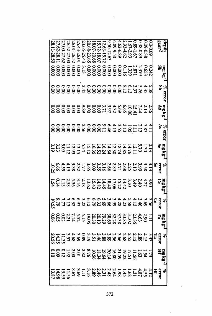
to00
to-O
to-0
toO s
toO s
l— k O sto 8
LAto
0h - k
to00
to00
to- J
to- J
toO s
LAO
l— kl— k
O sto 8
LAto
O O 0 0 O
p oo Ln toP h b b © " J O sW Wi OO >vj N) wI I I I I Ito to to to ►— ■—O M J l W O O O ^ l© p». b b © LjH* W Lft OO O K)O SO © o o o
S n OO OS SO O s OO0 s o t o U ) -O s o1 I I I I It—‘ so ps ^ t o ►-* J° sn 00 bs so bs O s o s o t o w oSO
0 0 0W O O00 s35 •1 1 op p o00 w s o so 00
0 0 0 0 0 0
8 8 8 8 8 8to 0 0 0 0 0 0 0
© H to to © ©i—k Lo 00 Lo b s toH-k to •0 ^ J sn ■PhO s s o SO SO to
s o OS t o sn P h yiH — H -k lo t o Lo Loso so - 0 OS sn 00
O O O O O O S O O O
8 8 8 8 8 S 3 8 8 8© so so Ph Sn Os H -k i— k
8 Lj so Lo bs b P Oli— k - J to so S/l 8 -P-
- o t o t o t—» 00
P n SO O s
0 0 0 0 0 0
8 8 k0 0 0 so O s P h t o t o H - * H -k t o t o P h
i— k
i— kP hO s
H -ks o
L/iS /l
H -k
s o©S n
l— k l— ks o
0 0- 4
l—kH —
Os
S n
LA t— P h P h
LA
o o o oOS LA
sn I—* l—ki—ky l—kl—kH-k M H-k l—kH-k l—kl—kH-k sn H-k0 H-k to so LA y Os Ph Os Ph to 00 Ph Ph to Lj Lovo H-*so l—kPh H* Lo LA to 00 Lo Lj 00 La H-k © ©to so LA to S/i to Ph Ph 00 Ph sn Os H-k
Ph Ph so to H-k to so so so to to to to to to so soS/I H-k Lo Lo Lj b © Ln l—kb 00 Lj b to H-k so snSn SO00 to ■0 S/I so LA OS os so H-k 00 sn SO so 00
H-k to yi so to H-k H-k H-k H-k H-k H-k H-k H-k so so to so1—k LA Lo l—kl—k so sn Ph Ph 00 J sn Ph Ph Ph toso 00 Os Os 00 b *4h00 Ph Ph © to Ph © so © «oto so to LA © Os to to
•0 J Os OS so ps os ps LA so so Ph Ph y Ph so soLj H-k Lo so to H-k La Lo b b so to to Ln H - k Ph b■0 so to ■0 to to so so so Os so 00 so 00 so Os so
© to <1 y y l—kto to -0 so so so so so to Ph to© to i—kS/I H-k so © © so 00 to -J so so b soto H-k Ph to LA © Lo l—kto b to Lo 00 © Lo so ©LA © so so so 00 00 sn to sn
to h-O -PhL/i lo lo Os S/i
SO -Ph
0 0 0i—k oO 3 5 t o
sot o
so © so so SO so so to SO to to tob 00 H -k Ln Ph 00 00 Ln b b Ln l— k
so so so i— k OS 00 so os os 00 sn to
to to 00 H -k l— k H ^ to H - k to 1— k H -k H - k
© 00 © 9° so © ps H -k SO J l— k
l—kto OS Ln Lo b H - k OO Ln to Ln LnO s Ph Ph Ph © so to l— k O s
to P h LA 00 L- lo
OS LA *0 w p. w
l— k H - k H - k H -k 0 0 so H -k SO to to to to to i— k H — H k H - k Ph Ph PhSO Ph so H -k b b l— k 0 0 Ph Lo Ph b so p h b Lo OOLn H - k
0 0 so"J 0 0LnSO
LnOs
■ 0 so Os so Os H - k 0 0 Ph 0 0 sn 0 0 H - k -O sn to
era aQ <D 2 *0 I f f
g so cra7?
ora
C fl O '
>1
3I-I
> 37?
ora
t *n
S
W 3o ra7?o ra
oi-t
ff 3ora7?o ra
H 2» o r a
7To ra
o> 1
:3i o ra 7r o r a
5 3 £
372
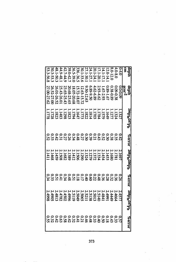
Ln Ln LO ©lo loi iLn Ln on LO
H 9s8 Ln
to■ ito to -oO N ©to ©
o o o o ^ . t o o o o o \ oJ t O t O O O ' C t O V O ^ OO O O O W W O O W ^ v l U )
4 .0 0
4 .4k
45.t o
LONO
LOON
LOLO
LOo
l—k NO ■o O Ln UN l—kLnO
45.OO *
4kto
LONO
LOON
LOLO
LO i—* NO - o O Ln O n
t oON
toLn
t oLO
too i—*0 0
t—.Ln
I—*to
o 1—*45.LO
ONLn
OvOO 3 - 0
toONLO
toON
toO n
t oLn
toLO
toO
H-kOO
i—*Ln
Lnto
Ot—*
4kLO
ONLn
ON0 0
O- o
~oto
to to to l— k l— k 00p 4 k O p 4 . to bl— k1 l— k1 h -
ii— k
iH ^
10
11
H -kLO to to to l— k H -k toO -J 4 . o p 4 . bi— k l— k i— k l— k l— k H -k
P ON 4 k to l— k O oL n 00 ON b ON OO LO9 NO to LO Np OOi— k NOON ■4. to H -k pto L n b o ON b ON b oONLO
O NO to LO • o NO
i— k i— k H - l— k _ k l— k _ H
i— k i— k h - l— k i— k l _ k H -k
OO o o • o -o L n ON toto l— k o o o * o 45k 'Oto 45. LO 45. NO NO -o
4k©Iooo
94kb
2 °- 3-a
&
© o?s
4 k <1
fro a2 n3 *9 i a
ks>
Ioo*0or
o o O © © © © © © © © © © © © © © ©Ln LO 45. LO to io LO 45. to Ln LO io 4 . Ln LO LO LO 4 .to LO to l—k O n 45. oo © NO H-kLO to © 0 0 Ln to
to to to to to to to to to to to to to to to to to toi—kH-k H-kH-* H-kH-k i—kl—kl—ki—kH-kH-ki—kI—. H-kl—kH-kH-k45. 4 45. Ln ON LO 45. Ln to LO to LO LO 4 . 45. ON -o ONi—kON Ln © 0 0 OO l—k© VO to •o ■OLO Ln Ln OO OO NOH-k 0 0 NO oo to NO to ON © 4 . NO to 45. 4 k LO © • o
o o O © © © © © © © © © © © © © © ©LO LO Ln 45. LO 45. Ln H-kH-k 4k ON to 4 . LO io LO LO to45. LO H-kI—. 45. OO i—k0 0 ■o © © to 0 0 ON 00 to ON O n
to to to to to to to to to to to to to to to to to to45. 4 k 45. 4 4 k 4 k Ln In Ln Ln Ln Ln Ln 4 . 4 . Ifck 4 . 4 kNO NO 0 0 ■OLn NO H-kO © to l—k© l—koo NO X ON LnNO O I—*OO © NO H-k4 ON i—kLO i—k45. 4k NO 4 ON -JOO Ln LO to to ON NO NO Ln i—k0 0 LO © H—H-kNO 4k ~o
$«§■iks>o00
3cr
»5•iK»eoo
£-Icr
p p p p p p p p p p p p p p p p p o Ln b 4 . b Ln 4 . b 4 . to 4 . 4 . LO 4 . In 'h- 4 . LO Ln L f t t O t O W O O S ) t O H - h - a \ O O W O O O O W W v l
to3o"1
373
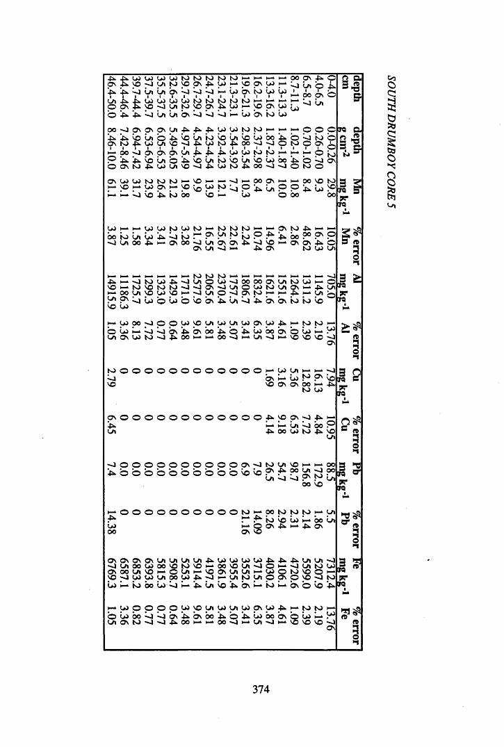
-p»ON 6
u>NO
u>- J
04Ln
u>to
toNO
toO n
to4*
toy
toH ^
i— k
NOi— k
ON 04H -kH ^
ooL j
ONLn
4*o
4 b L j Ln Ln bv L j Lj L j H -k1 041 ON to1 04| U >1
ii— k
•oo iON
Lno
■KON
04NO
04p
04y
04to to
NOtoO n
to4 -
to04
tol— k
H -*
NOH -kO n
H -k
u >
i— k
04L j Ln
© 4* 4 * L j Ln Ln bv L j Lj L j l— k 04 ON to U>
oo - J O n ON Ov y 4* 4* u> 04 to to h- H - l— k O O‘-HON
4*to NO■H
Ln04 ©
Lnb- j
Ln4*.
to04
bto Ln4* boo
04■o
bo«o £ sL j©
toO n
l— k 00 L j ON On ON Ln 4^ 4 - 04 04 to to l— k l— k ►1- Oo©
4O n
4*-to
NO4^Ln04
oLn
4 -NO
b- j
Ln4 -
too> bto Ln4^ boo
04-J
bo" O
4^O
otoL jO
ri9
39.131.723.926.421.219.8 6‘
6 13.912.1 L'
L 10.3
oo4k
6.5 l— k l— k
© O o oo
00'■ H
9.3
0 4 l— k H * 0 4 0 4 to 0 4 to 1— * to to to i— k i— k ON to 4 I—* |_-OO to Ln 0 4 4 - L j to l— k ON Ln to io o 4 4 b o OO ON o■ o o n 0 0 ■ 4 i— k ON 0 0 L j Ln bv b v 4 L j b i— k ON b v 4 o
O n Ln - o i— k 4 O n to 0 4 on
l— k l— k i— k i—* l— k to to to 1— * 1— i— k i— k »— * l— k H — - J4 * i— k « o to 0 4 4 - - J Ln O 0 4 - J 0 0 OO O n Ln to 0 4 H -k ONO i— k to NO to to - o *o ON - J Ln o 0 4 to Ln ON i— k 4 yl— k o o on NO 0 4 NO i— k - J Ln o < 1 ON to l— k i— k 4 H -k Ln ©on O n L j 0 4 o 0 4 o b ON 4 Ln L j 4 O n O n to io bb 0 4
i— k 0 4 o o p o O 0 4 v© on 04 Ln 0 4 p 0 4 4 H -k to to H - k
b 0 4 H ^ L j L j ON 4 ON 0 0 4 o 4 0 4 OO b v o 0 4 H -k0 4
on ON 0 4 to -o 4 0 0 l— k l— k 00 - o i— k Ln <1l— k NO NO NO L jON
to o o o O O o o O o o O O l— k 0 4 Ln H -k H — ^ J
L j ON l— k 0 4 to P bNO NO Ov ON b o 1— 4
tO 0 4
O N O O O O O O O O O O O ObL n
-O O O O O O O O O O O O N - J^ b b b b b b b b b b v o ' o
4 p p •o 4 H -
H -k H -k Ln L j bo o4 00 04 to 4 b
on
to L n NO H -k H - k o op 4 0 0 L n - J o oLn L j L j p to Ln
b o b
H - © ©
200000000
H - * 0° to to to H -k
4 H -k 4 to b 0 4 I—* OO0 4 H -k o O n 4 I—* 4 ONo o ON NO
ON O n O n ON L n L n L n Ln 4 04 04 04 04 £ 4 4 L n L n- J L n 00 04 00 NO to VO l— k 00 NO L n " J O H -k ■OL n toON 00 L n NO l— k o Ln H -k NO ON L n L n H - k 04 O to NO ONO Hj 04 04 L n 00 04 4 - J l— k L n to y o p o NO " J04 l— k to oo 04 L j l— k *4 Ln b 4* b v H - k io H -k on o b
i— k 04 O o o O 04 NO y 04 L n 04 P 04 4 l— k to too 04 00 L j L j b v 4 b v 00 4 o 4 04 00 b v © 04 H ^
on ON to - J - j 4 00 H -k H ^ 00 ■ o H -k L n -o i—k NO VO NO -jO n
Q a3 - 8
9
era a "■83I
33*era
§ ^ l3 to
i"Ij derawera
•-I3•i
I 91rr era
c to§■iJ 3era “ era
o"I
|3fJ* era
Q3o'i
374
SOUTH
DR
UM
BO
Y CORE
5
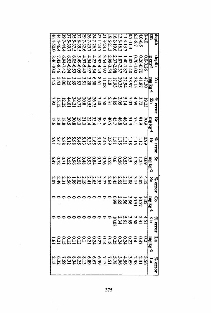
4n 4>. L O l o l o l o t o to t o t o t o H -k H - k H -k o o ps 4h ©O s £ s o - J
yt o S O O s 4 s . L O H - k S O O s L O H -k L j L a o
1
4s 4 s < 1 Ln Ln b s L j L j L j H -* Lo b s t o Lo Lo • io o
iO s o
L A 4 s 4 . L O l o l o L O t o t o t o to t o H - k l— k H - k H -k l jO O s 4 S O p
yt o s o O s 4 s . L O H — S O O s L O Lo
© 4 s 4 s L j L a L a b s L j L j L j H - k Lo b s t o Lo
0 0 • o O s ps O S L A 4 s . 4 4 s . L O L O t o t o l— k H - k i— k © © ©
4 s . 4 s . s o Ln © 4 s o L a t o S O L a s © Lo b o 4 © L j to ©O s to 4 - l o Ln S O * o 4 s . L O t o 4h o o ■ o © to © O s 1
©H -k 0 0 • o O s O S O s L A 4 4 s . 4 * . L O L O to t o H - k i—k i—k © i o© 4 s 4 S O L a © 4 ^ s o L a t o s o L a s o Lo b o 4 s , © L j O s© O s t o 4 s l o L A S O - J 4 s . L O t o 4 s . o o ' O ' O © to ©
_ l a L O H -* l o i— k u > l o ps O O i— * ►— H - k t o to L O L O 4 s . 4 s .4 s
4 . © t o b s 0 0 L a t o L a b si— k t o © to O O 0 ° H - k p
L a l o © Ln s o l o H -k o o 0 0 © 0 0 S O Lo S O s o H — o o LoO O L O L A 4 s . - J L A ■ o ©
" 0 1— * H-k 4 . l o t o t o l o t o L O py
4 s . L Oy
L A 4 s . L O l— k
s o yt o 4 ■ 4 © © © O s
4 s . L a Lo 0 0 © I— . © L a L j p
t o H-k t o © t o L j b o L a L j O O o o H— L A L A 4 s . L O S O t o t ot o t o h - k H -k - j L A L A L O
1— * H-k t o L O i—k t o t o L O L O L O 4 s . 4 s . 4 4 L A L A s o * oL O 0 0 o o © © s o H — to L O S O o o © L A ps ps H-k
yH— ©
b s 0 0 bo L a 0 0 © © 4 4 s . i— k b s L a L j o o Lo S O 1— 1 S O s o
L A L A LAy
Ln L Ay y
I—* U> t o t o i— k H -k H -kt .
H — ©
so b s b o i—k s o 4 >—* L o b s H -k 4 s . b o 0 0 L j Lo L-k ►— H - k s o1— . • o 0 0 I O 0 0 L A L O L O L A O O L A so LA i—k 0 0 L A t o S O
O S © © © © © © © © © © © © © © © l— k i— k ©
4 s . L j L j L a s o L a 4 s . s o o o L j Lo L a b s L a L a L a Lo to b s- J to i— k to O s 0 0 0 0 LO 4 H -k O s t o O s LO 0 0 LA s o
to to to to l— k to to to to to LO to to to to l o LO LO 4 s .
b o 4 . Lo L a s o © H -k 4 s . b s L a L j b v 4 . L a H -k © H - k © H -*" J s o 1— k O s s o LO SO H -k LA la LO 4 s . LA to l— k 0 0 LA t o to
o o o o o o o o o o o o © t o H - k u> l— k H —
SO b s La b o © ©so LA O s O s La
i— kLa- 0
O O O O O O O O O O O O ^ J O U i W W N ) ^P Lo ON bs La Lo LaO ^ M VO oo M 00
^ - © o o p p o o o p p p p p p p p p o bs io ►-* I— h- I— Lk to io 'to I— ►— io to to io 4s. 4n to
m Vi N) h- K) -O
N J O V O O O O O O O O O O S O S ^ O O y i W ^ W N J I O WI— lo La Lo Lo i o ►— bobsLAH-kLALjsolAbsLALoLA W K ) V O m ^ V i W V O O \ O W h * O O O n O S V O O O m O S
QTQ af t . s3IO
M B1CTQ s 7T
3 n33 wCrq ^7? cro
3•1
I »CTQ
■ **crq
IP
3 SIpqCrq
° <o3n
3 f l few » j r Crq
r 89 <t
3o
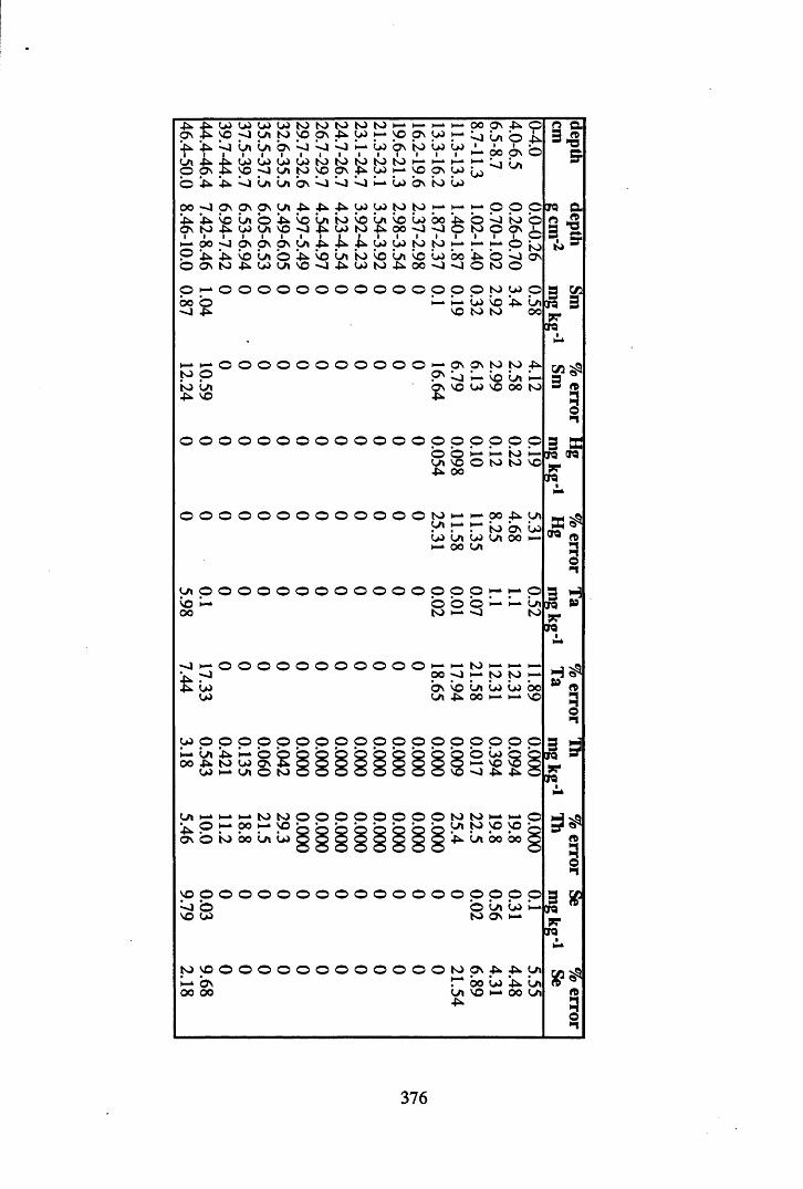
4*.Os fc 04vo4 4 -oon© 4*Os fcO 4 4*.00 *0 Os4k. 4 SOOs tO 4*i—kOO-Oo 4* 4k.o Os to©bo
1.04
O
- 4 0 n t O p O s 4 n 0 4 H - k JO p \ W oni^bs 'Obb'H-o^bv' toL^oji i i i i i i i i iW W W W K ) t O ( O t O N ) i - P p 0 n t o p p v 4 k - O 4 H - k V £' j 0 iu \b \ '« j '^ 'Oi - ‘ wbvK)w0\ p\ ^ ^ ^ W W to NJ H- Mo n b ^ b o n i o b o n b o o b o l u .W U i ' O ^ J I k W t O . t k O O ' J v J OI I I I I I I I I I I I0 \ O N O \ W > ^ ^ ^ W W t O I O h -b o n © 4 k . b o n t o b o n b o 4 o o4*.04onvo*o4*o4to4k.oo-j^oo o o o o o o o o o o o
i—k oo Os 4 *i—k " 4 Ln O0 4i
i ioo
iOs
i—k0 4
»—k04
" J on
i—k O O O© <1 t o ot o1 01 O s|
ich-* h~fc o i o4*.O
otO
bO
O s
O t o 0 4 Ou>tO
V Ot o
4k. Ln0 0
H - k H - O oooooooooo*—Os Os to to 4^to O as b b on bto on b s VO 0 4 VO oo to4^ vo 4k.
O O o o O po o i—k b to bLn4*
vo00 o to to so
O O o o o o o o 00 o o o to I— k H -k 0 0 4 * onon i— k H - to b s 0 40 4 on 04 on ooi— k oo on
on O o o o o o o 00 o o o o O O H^ Ob i— k o o o l— k i—* onoo to i— k —4 to
^4 o o o o o o 00 o o o l— k »— k to I—"* H - k
p oo -4 H -k to to H -k
0 4 bv b on 0 4 0 4 OO0 4 on 4* 0 0 H -k H* vo
w p p o p p p o p p p p p p p p p o c►— O Q Q Q Q Q Q Q Q Q Q O U J Q Q 0 0 4 » * t 0 0 4 0 s ^ © © © Q p p © p © > - k V O ' O Q
O 4 H - 0 n © t O © © © © © © © © Q 5 ' O 4 k . 4 i . ©
onb
H - k
O»— kH - k
l— k
9°toi— k
toVO
Os o to oo on 0 4
to to i_k H - k
on to p p4k. on 00 bo
so o o o o o o o o o o o o o o o o ob o o on 04VO 0 4 to Os i—-
t o p o o o o o o o o o o o o t o p s 4 k . 4 k . o n J— ON ^ 00 l>4 4k. onOO 00 vo H- OO Ul
4k.
2 a9 n3 *B&
era a ° *83a
ts>
M bJcro su?“era
3 n
i3 EC to crqJ**cro
EC^ crq n3
3 H few »sc crq
W A3•-IGra “ sc crq
3*to5►i
w *•crq
A3
376
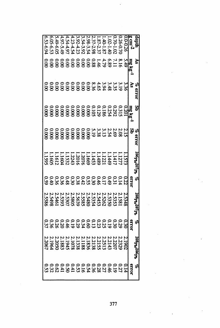
O n O n Ln 4 . 4 . 4 . c o c o t o t o i—k i—k l—k o oLno 4kb Lni o b Lnb CO 00 ‘- 4 o b t oCO Ln vo ■o - 4 t o t o 4k00 - o - o p t o O ONON 6\ ON Ln - 4 4 . - 4 CO CO t o t o i—k l—k i—k 6
b Lno 4 . b Lnt o b Lnb CO O O ‘■ 4 o b4 k c o L n VO - j - 4 CO t o 4ko o - o * o O t o oo o O o o O o o O o l—k p\ - 0 o o
8 8 8 8 8 8 8 8 8 b oo o
4 .O n
bv o
o ovo
l—k l—kON
0©1o‘too\
crq an JS3 *a, i to
o o o o o o o o o OO 4 CO CO CO CO COCO ON b ’■4 CO l—k COON Ln 4k OO Ln VO ON
o o o o O o ol—k l—k i—k to io CO too to oo Ln vo l—k oLn vo ON - 4 to Ln l—k
Ln CO CO to to to toi—k CO l—k Ln ON o l—kVO 00 CO 4k VO oo Ln
i— k )— * l— k i— k l— k l— k l— k H — i— k i— k i—. l— k j - H -k l— k
I— * I—* i— k l~k h ^ to to io I— * H -k H - i— k H - k H -k H -k l—kLn ON ON O n Ln to o o O n -P 4k. to •4. 4 k . to Lnvo o l- O CO -Pkk l— k •o ON Ln 00 to -4 i— k •oLn Ln to 4k to CO ON ON VO CO vo l—k VO ■O ■o CO
7? QTQ
01 f t •tO*1
3 Wnr|VQJCera
C/5a- n2•nK»
o o O O O o O O O O o o o O o oLn 4*. CO Lo ‘-4 CO CO 4- Ln CO 4k H -k 4k CO i— k iovo O O n O n 00 o 00 to cn o O n •—] VO l— k 4k to
to to to to to to to to to to to to to to to toLn Ln Ln Ln Ln Ln Ln Ln Ln Ln Ln Ln Ln Ln H - k LnLn -4 -Pk. CO CO oo ON Ln 4k CO 4k to CO CO Ln COoo VO O n vo o O CO 00 OO Ln Ln ON Ln Ln oo 4kON 00 CO 'O Ln VO Ln O 4k co to O CO H - k OO
O O O o O O o O O O O o O o o oCO CO io io 4^ H -k 'to CO ON i—kio io i— k Lo io CO«o ON ON o O vo vo 4k o CO CO Ln VO o VO o
to to to to to to to to to to to to to to to toio l— k io i— k l— k l— k H -k i— k l— k io to io io io io bO vo o oo vo O CO i— k OO i— H -k cn H - k to CO VOO n O n Ln oo 4. -o CO 00 CO CO cn 4k o to o•o 4k O CO cn 00 00 00 O n 00 Ln CO CO -o VO to
o o o o O o o p O o O o O o O OLn CO O n ‘-4k Ln 4 Ln H ^ Ln CO io io 4k l—k io H —
CO to to H -k O i— k CO ON 4 ON 00 *o O n vo -o 4k
I5s$S -
2 ° •n
K»■f?K>eo5
g00ns
s5
377
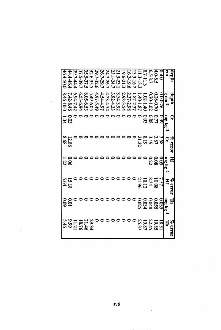
LO lo LO lo to to to to to 1—* 1—k h—i—kVO 70 y* to so OS 4k lo l—k SO OS LO i—kLj Ln Ln b s Lj Lj Lj H— Lo b s to Lo Lo
Ln 4*. lo LO lo 00 to to to to to H-k i—k H-kO O s VO ^0 y* to SO OS 4k lo l—k VO O s LOo '4k *4k Lj Ln Ln b s Lj Lj Lj l—k Lo b s to Lo
OO ^ J O s p s O s t-n 4k 4k 4k LO LO to to l—k H-4k 4k. b L n © 4k b Ln to b Ln b Lo 00 hOS to 4k. lo Ln SO -0 4k lo to 4k 00 •0h- 0 0 *o Os p s b s L n 4k 4k 4k l o LO to to H-kP *4k 4». b Ln © 4 . b Ln to b Ln b Lo OOO O s to 4k lo Ln vo *0 4k lo to 4k 00 -j ■O
0.0
3
1.3
4
O O © © © © © © © © © © ©
b s . ^ > oo oo O s to
H- 0 0 0 0 0 0 0 0 0 0 0 0 0 0 0 0 0 0t o © to OS
t - ^ ^ - O O O O O O O O O O O O t O i ^
osy*4 k h —oo
o o o o o o o o o o o o o o © oVO H-k
0 0 O s 4 k ©L j L n © 4 k
H - 00 p s ©
L j L nLO
H - k © © ©
© t o ©t o ©| O s 1
O© i o
4 k © L j o s© t o ©
© © © ©© 00 L j L oLO 00 v o
OO LO LO LOi— k H -k b s L nSO SO " j 00
© © © ©
t o © ©t o 00 Ln
i— k 0 0 H - - J© L o © LnM 4 k © - Jt o 0 0
© © © © ©© © © © ©t o LO 4 k L n LOL n 4 k 0 0 L n Ln
n »
3. Ifc>
|dj r
* « 3o•-»
3(JO jr* cro
55^
5•i
M SHJQ “j?ICTQ
L n vo 4k b . OS vo to
H - k I— * to 002 2000000
M to H ^ H -kH - * OO H — SO L n SO to SO 0 0
io Lj 4 k Lo Lo 0 0 4 k 0 0 LoH ^ O s OS 4 k ■ 0 «o L n L n
rt
►1
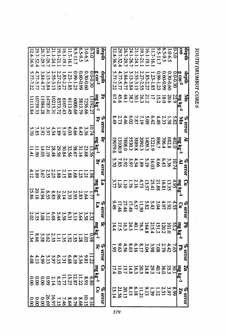
lo to to to to H^ i—k i—k p pv LOto vo Ov 4k l—k p ps »—k Ln Ln ©4ki L j1 L j< I—*i l—k1 l—k
1H1 L j
iil—k
■p
•ov
lo lo to to to to H— i—* l—k LyiOv to VO Ov 4k l—k p ps L jb 4k L j L j i—k l—k l—k
LA 4k u> U) to to l—k i—k O O OL j L j bo Ln to 00 to b Lo•o - j 4k LO Ln ■o Ln LO p O'O Ln 4k LO LO to to i—k
•i—k o 6
to L j L j 00 l—k Ln io 00 io b bvto -J «o 4k LO Ln «o Ln LO vo oi—k i—k i—k l—ki—k O i—k 4k O 00 Ov Ov Ov Ln -0 LO*—k -o vo ■—1 to Ln i—k H-k oo to i—ki—k Ln OO OO ^J o l—k © i—k Ln VOLO p 4k -o LO LO -o LO p LO ps tooo Lo io 4k Lo L j 4- 4k bv L j bv to4k LO oo l—k to LO Ln VO VO ov ^J
l—kLn p to LO 4* i—k Ln Ov 4k Ov LO OL j bo so SO Ln 00 i—k o OV 4k Lo L jO Ln to -o 4k vo VO LO Ov LO Ov 4 k-
i—k i—k l—k to to to LO LO LO LO tol—k l—k 4k l—k 00 so O to OO H- u> p4* SO o l—k 4k Ln 00 Ln bv l—k bv Lni—k © Ln VO OO OV 4k Ov ■—i 4 k oo Ov
4k. u > LO to to I— . to l— k l— k i— k I— . i - ^
I— . 00 b v Lo io 00 l— k 0 0 b v io io SOto vo Ln Ln 00 Ln oo oo Ln I— . 0 0
to to H -k
Ln o 4k- p ? ° to to to to to0 0 l— k s o Ln bo s o H -k LO SO OOOv 0 0 4k- Ln Ln Ov 4k LO LO LO
o-o
to LO LO LO Ov Ln p OV LO LO toO LO o i — k b v Ln Lo H -k b v Ln Loto Ln oo t o oo oo H - k LO 4 k oo to
l—k 00 Ln LO to I—. l—k i—k i— k H - k H - k oLn b v Ln b v Lo H -k Lo Ln Ln to o s o4 k OV oo t o Ln l—k Ln t o Ln oo LO 0 0
4kHlo
O O
O O
4 k Ln vo i—VO LO
© o8 b vo
Ln p ^ J Ov 0 0 Ln p1—»
SO H -k Lo b v H -k Lo bo io- J Ln H -* oo vo 4 k 1—» t o
to pv i-k Ln 4> -4
H -kl— k
I— .p
i— k
toH -kH -k 00 pLj io 00 io vo bo
»o - j -o to H - k O
t o I— H k
O Ov Ov ■ o ^J OO VO o o o
© Ov VO H -k 4 k Ov - o o H - k
O vo - J Ln OV 4 k VO 0 0 Ln
depthcm
o r a a3 *8 3 ©N) ^
3 8?e r a *EJQh-k
% error
Fe
3 ?o r a ^B*o r aH-k
^ to3O
3 ^o R »wo r aH-k
r #A3O•-I
I fPTQ7Te r a
H -k
rt3On
Com
g
7?o r aH*
% er
Co
o
u>to tovo
toOV
to4k toH-k l—k H-kVO Ov
H-kH-k4k -0 Lj i—kH-k i—kH-k Lju>Ov
LkJto to
votoOv
to4k toH-*H-kP
I—*p
b 4k Lj Lj H-k ;—Ln 4k L*J p j to to H-k H-kLjJ
Lj«o
OO4kH-kLOLnLn io>o ooLn to
LO•O Ln 4k LOLOto to H-kioto
Lj*0
Lj-O
004k
1—. LOLnLn to
■JOOLn
ov —) 4kLn
LOOO
LOO
toOvtoH-k
l— k
•o4k O H-k Lj H—Lo io
p p l o © l/i o wi i iH- p pvi-1 Ln Ln
o o o oig 9oH -k o 6 LOioLO
s o b v vo O o
H—k t-k to toLn oo O toio b b v SO
Icra a rs «3 . 1 N> —
3CTQ?rKTQ
00 to 4k Ov p4- Lj 4k o 00VO LO ov to J
si y» p m yioo I— © *4k *4k Lo Lo oo
VO vo to vo w oo to
H -k l— k -o Ln LOVO LO oo Ln OOo H - k O LO 00-o P oo O pVO o o LO 00b v vo
Ln p to LO 4kLj bo s o SO Lno Ln to *o 4k
J— Ln 0 0 H-»vo VO
OO -o OV 4kto o o OO oto Ov OV to toH - k Lj 4k 0 0 bs o
4 k Ov LO H —Ov b v 4k Lo ob OV LO Ov LjLO 4k
LO H - k H -k l— k to 4kl— k to to 1—k H -k 4kLj io l— k Lj H -k Lj O J Ln p p LO SOJOV o Ov Ov LO Ln
•o4 kH - k
oooo boH -k
LoLn
Ln
vo I— * to *—1 Ov I—* Ln Ln LO 4 k H -k
4k-J JH Ln H -k bo 4ko SO SOVO 4k
Ov4kOv
4k -JOv
Lno to LO 4k"J to
r °4n Ln Lo Lo
M to >4 h-‘ to I-*1—»►—‘C/l 0 \^OONO\H-UitOOUi
4k Ln h- p j-*oo *4. to to O
Ln to
LO -o to 4k ps o o Lj 4k bvoo oo vo to Ln
M p ^ o o p o o w w vo On Ln on h— h-» ©V/l W Ov W C\ O 4
Mh*MMM( 0 N)t0 4 iWWWs i H w ^ o o ^ \ o o o \ y i p4 k © L j b o L o L n b o L o L j o L o H - k
M Vtl M4 k ON 0 4
0 0 P l—k s o H - H - k p LO 0 0
H -k i _ k J—* i_t Lo H — Ln SO bLO 0 0 to LO vo to H -k vo
q a 3 >8
S
to3O>1
M PIQTQ B ?T
KTQ
3 » 3• i
3 31B r aJ * era
^ » i" i
J S3Bra 3J ? flra
5• i
37 y
.501/77/ DRUMBOY
CORE 6

lo to to to to H -k H -k H -k p ON 04 O 2 ato NO ON 4 H -k p ON H -k La La b i04 3 n”41 b1 b1 1 1 1 H -k1 bi i
H -ki
pi
ON o alo 04 to to to to H -k H -* H -* (^ | aON to NO ON 4 H -k P ON bNO 4 b b H -k H -k H -k H -k
LA 4 LO oo to to ^ k H - O O O oere ab b bo H -k Laio OO to 04 b n kH—- j 4 O) la -o LA 04
i© O i© 3 e±
b LA 4 U> 04 to to H -k H -k b o 04 toto b b bo H -k Laio oo io NO O n oto -o - j 4 04 LA -j LA 04 NO O
© p o o o o H -k 0 4 to H -k O o 3 C/5o o o o io ON Lj io OO io oo ON ore o*
o NO H k ON -j ~ o 04 NO 00 ?cere
o o
0 ^ - 0 0
H - N O - J 4 t o 04 t o 4 04O b H - k H -k O N L j b o H - k H -k
N O- J
0 0 L A L A 4 N O N O L A O N
t o t o t o t o t o t o t o t o t oH
o so- j
H -kt o
H - kt o
H -k04
H - k
0 4H - *
6
H *O N
N O O n 4 t o t o 04 4 oo H -k ■o O N - o t o O N OO 4
O O O O O O o O O O O oL j L j La b o L A La 4 4 La b o L a O NO n 4 l a O O O 0 4 H j O n o o O N o t o
to to to to to to to to to to to to4 4 4 4 4 4 4 4
f e4k 4k 4k
N O O O o o - J 0 4 O N hJ O n H -k i— k H -k
O N L A N O to L A 0 4 0 4 O N to to O OL A L A H -k O N L A V O to to 4 o 0 4 to
O O o o O O O O O o O O
H -k t o 0 4 t o La H - k i—k i o l—k i o Lo Lo- J H — O L A 0 0 V O L A o O O 0 4 N O 4 k
H — H -k l— k H -k H - k H - k H -k i— k l—k H -k
H - H -k H -k l— k H -k l—k i— k H - k H -k l—k H - k l—k00 ^ J 0 0 ~o O N 0 0 O N O N 4k 0 4 t o l—kL A L A O t o t o - o L A l—k L A t o 4 k N OL A H -k 0 4 L A O O N t o 0 0 O 0 4 O 4 k
o o o o O o O o o O O O
- J 00 L A • o La 4 0 4 La 4 o o Lo O n
4k 4 k H -k 0 4 O 0 4 N O l a 0 0 0 4 L A t o
o* a>nnonK>§
o*$<©
01
£00>dor
•vcr
1*nI— * H - k H - k H - * h i
*d
©Vj*0O'
04 to to to to H -k H -k i— k p ON 04 oto NO ON 4 k H -k P a \ H -k LA LA o i04
4 ki
bi
bl
i— ki
H -1
H -k 1 i b1
iH -k
ip
iO n b
0 4 0 4 to to to to i— k H— l— k I J t ( IkON to NO ON 4 k p ? \ b VI VINO 4 k b b l— k :— H -k
LA 4 k 0 4 0 4 JO to i— k H -k o o O ob <1 bo H -k La io 00 to 0 4 o- J —] 4k 0 4 la •o LA 0 4
1 o O io-O LA 4 k 0 4 0 4 to to H -k H -k b o Loto b b 00 H > La to bo to b O n oto » J •O 4 k 0 4 LA - J LA 0 4 NO OH -k H -k H - H -k to LO 0 4 4 n 0 4 0 4 0 4 04to LA L a 00 La H k Lo Lo b La La Loto NO 0 4 O n NO 00 L a - J ON la NO
LA LA 4k 4k to to 0 4 0 4 4 - 4 k 0 4 0 4
o o i— k O N Lo l— k 0 0 La La LA 0 4 La io0 0 0 0 — J LA to V O * o O n 0 0 H -k l a H -
0 4 to l— k O o o o H -k to 1— k H -k 1— k
Lo o o 4 k 0 0 bo b io o 4 . 0 4 H -kLA - j oo NO 0 4 to ON H -k ON to to 0 4
O n - j l— k H -k OO LA O n ■4 ( A
O n H -k to P ON ^ J N O H -k OO h - k b 1— kvo 0 4 l— k Lo 00 Lo o ON OO 0 4 0 0 0 4
LA 0 4 NO 0 4 LA
O O O o o o o O o O o o© © o b o H -k H -k io H -k M H -k bc5 © c5 4 -o l— k 00 LA N O LA --J
LA O n LA
o o O 0 4 H -k l— k O N ON ^ J 00 00 00b O N J A 7 - J b O N 1—k 4 H -k ON© io Lo LA -o OO to LA ON ' Jto LA N O
0 4 to o o O o o O O o oLo o o Lo to H -k H -k io to oo b La4 k ON LA O N 4 k 0 4 LA o - J oo to o
O n O N ON H -k M H -* H -k H -k l— k H -k i— k
io Lo O N 4 k 0 4 0 4 to to o H -k 4 H -k
oo 4 k - J H -k o Lo l— k bo 0 4 La Lo ON00 LA 00 to vo LA N O 4 hJ
4 k i— k O o o o o O O o o OLo 4 k M o o Q o b o b o oLA LA N O to H -k o H -k H -k LA 4 0 4 to
-J N O o to O O H - 4 O v
y * LA O N l— k H -k H -k l— k H -k H - k H -k H -k H -k
H -k 4 k Lo O N pv O N < A LA O to 4 4O O O N 00 o H -k to 00 ON La to o Lo
00 V O to 0 4 4 - 00 00 to i— k
J?ere
a
5
o r e a n »3 ^h>
3 £ere jc ere
Uin
i•i!
3 *3|££
« »1>1
3 H pre *u5“Cre
* »3•IJ SPere7?
s e ^
3n380
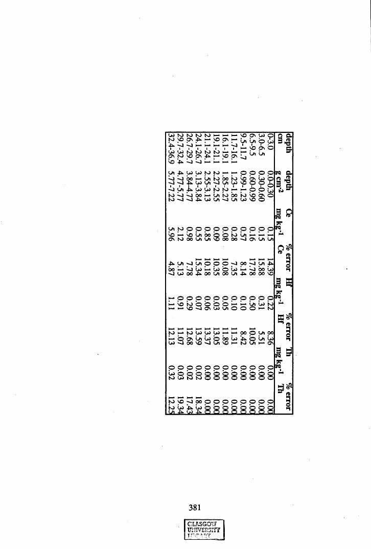
LO t o to to to H-k H-k HH p ON LO ©to P ON 4 H-k p ON H-k La LA ©
iLO
4 'Ji ibi
H-k1
H-k1
H-k1
H-k1
bi
iH-*
ip
iON ©
LO LO to to to t o H-k M H-k (P%ON t o NO ON 4 p ON b
V I
VO 4 b b H-k* - *
H-k
LA 4 LO LO to t o H - H - © © © ©b b 0 0 H-k La t o oo to ON Lo ©•O * o 4 LO l a - J LA LO
I © © i©
b LA 4 LO LO to to b H-k © © Loto b b oo H-k LA to 0 0 to b ON ©to -O 4 LO LA •o LA LO NO ©
LA to © © © © © © © © © ©VO i—k NO LA 0 0 © © to La H-k H-* H-kON to OO LA LA NO 0 0 OO - o ON LA LA
H-k H-k H-k H-k H-k H-k H -4 LA H j LA © © © p o o - J LA 4OO b Lo H-k Lo © Lo H-k b OO Lo- o LO OO 4 0 0 LA 0 0 LA 4 OO OO NO
l—k © © © © © © © © © © ©1—* NO to © © © © H-k H-k La Lo toH-k NO ON LO LA © © © H -k to
H-k H-k H-k H-k H-k H-k H-k H-kto H-k to LO LO LO H -k H - OO © LA 0 0H -» © ON LA Lo © 0 0 Lo 4 © LA LoLO > o OO NO LA NO H-k to LA ON
© o o o © © © © Lo © © ©t O L O t O t O 8 8
© © © ©
8 8 8
H -kto
H -kNO
H -kOO © © © © © © ©
toJA .
LO 4 LO s s s s 88 8
2 a i
&
ere a n n3hi
I aere
0 ^ * n3Jere!Cere
B?3*n£reere
^ 1
3•n
381
GLASGOWUUIVERSIT?T.T";r * riy


