Embed Size (px)
Citation preview
In Dale Jacquette (ed), Philosophy of Logic: 485–518
The Mathematics of Skolem’s Paradox
Timothy Bays
In 1922, Thoralf Skolem published a paper entitled “Some Remarks on Axiomatized Set Theory.” The paper
presents a new proof of a model-theoretic result originally due to Leopold Lowenheim and then discusses
some philosophical implications of this result. In the course of this latter discussion, the paper introduces a
model-theoretic puzzle that has come to be known as “Skolem’s Paradox.”
Over the years, Skolem’s Paradox has generated a fairly steady stream of philosophical discussion;
nonetheless, the overwhelming consensus among philosophers and logicians is that the paradox doesn’t
constitute a mathematical problem (i.e., it doesn’t constitute a real contradiction). Further, there’s general
agreement as to why the paradox doesn’t constitute a mathematical problem. By looking at the way first-
order structures interpret quantifiers—and, in particular, by looking at how this interpretation changes as we
move from structure to structure—we can give a technically adequate “solution” to Skolem’s Paradox. So,
whatever the philosophical upshot of Skolem’s Paradox may be, the mathematical side of Skolem’s Paradox
seems to be relatively straightforward.
In this paper, I challenge this common wisdom concerning Skolem’s Paradox. While I don’t argue that
Skolem’s Paradox constitutes a genuine mathematical problem (it doesn’t), I do argue that standard “solu-
tions” to the paradox are technically inadequate. Even on the mathematical side, Skolem’s Paradox is more
complicated—and quite a bit more interesting—than it’s usually taken to be. Further, because philosophical
discussions of Skolem’s Paradox typically start with an analysis of the paradox’s mathematics—and only
then examine how the interpretation of this mathematics reveals the paradox’s philosophical significance—it
is important to get the mathematics itself right before we start in on our philosophy.
From a structural standpoint, this paper breaks into six sections. In section 1, I formulate a simple
version of Skolem’s Paradox and try to disentangle the roles that set theory, model theory and philosophy
play in making it look plausible. In section 2, I sketch a generic solution to Skolem’s Paradox—a solution
which explains, in rough outline, why no version of the paradox generates a genuine contradiction. Sections
3–5 examine different ways of “filling out” this generic solution. Section 3 focuses on the role quantification
sometimes plays in Skolem’s Paradox and includes a discussion of the so-called “transitive submodel” version
of the paradox. Sections 4 and 5 look at some cases where quantification doesn’t help to explain Skolem’s
Paradox. Finally, section 6 presents some concluding philosophical reflections.1
1Let me emphasize that—with the exception of section 6 and some brief philosophical digressions—this paper focuses fairly
tightly on the mathematical side of Skolem’s Paradox. In particular, I don’t attempt to survey all the things philosophers have
said about the paradox or to assess the various ways the paradox has been used (and abused) in the philosophical literature.
1
In Dale Jacquette (ed), Philosophy of Logic: 485–518
1 Skolem’s Paradox
In its simplest form, Skolem’s Paradox involves a (seeming) conflict between two theorems of modern logic:
Cantor’s theorem from set theory and the Lowenheim-Skolem theorem from model theory. Cantor’s theorem
says that there are uncountable sets—sets which are too big to be put into one-to-one correspondence with the
natural numbers. The Lowenheim-Skolem theorem says that if a countable collection of first-order sentences
has a model, then it has a model whose domain is only countable. Skolem’s Paradox arises when we note
that the standard axioms of set theory are themselves a countable collection of first-order sentences. How
can the very axioms which prove the existence of uncountable sets be satisfied by a merely countable model?
This puzzle can be made somewhat more concrete by considering a specific case. Let T be a standard, first-
order axiomatization of set theory—say, ZFC. On the assumption that T has a model, the Lowenheim-Skolem
theorem ensures that it has a countable model. Call this model M.2 Now, as T ` ∃x “x is uncountable,”
there must be some m ∈M such that M |= “m is uncountable.” But, as M itself is only countable, there are
only countably many m ∈M such that M |= m ∈ m. On the surface, then, we seem to have a conflict: from
one perspective, m looks uncountable, while from another perspective, m is clearly countable.
In exploring this seeming conflict, I want to begin with three preliminary points. First there’s at least
one sense in which this appearance of conflict is clearly misleading. Strictly speaking, M doesn’t understand
ordinary English phrases like “x is uncountable,” so the sentence “M |= ‘m is uncountable’ ” makes no literal
sense. Literally, what’s going on is the following. There is a specific formula in the language of first-order
set theory which mathematicians sometimes find it convenient to abbreviate by “x is uncountable.” If we
avoid this abbreviation—and use, say, “Ω(x)” to denote the relevant formula—then the initial appearance
of paradox vanishes. The argument of the last paragraph simply shows that there is some m ∈M such that:
For discussion of such topics, I invite the reader to examine [1] (esp. chapter 3), [7], [13], and [15]. I also recommend the
illuminating exchange between [3] and [21]. For a quite different view, see [10] or [14].
That being said, this paper does serve two philosophical purposes. First, many versions of Skolem’s Paradox depend on
misleading (and/or outright mistaken) presentations of the underlying mathematics. I think, therefore, that a clear exposition
of this mathematics—highlighting all the little twists and turns—already does a lot towards “solving” the paradox. Second, I
think philosophers have tended to overemphasize the role quantification plays in Skolem’s Paradox, and that this overemphasis
colors most standard assessments of the paradox’s philosophical significance. In sections 4–5, I argue that quantification is less
important for Skolem’s Paradox than many commentators have supposed, and, in section 6, I say a little about the philosophical
upshot of de-emphasizing quantification.
A final comment is in order. Throughout the paper, I relegate a lot of technical machinery—particularly concerning the
construction of specific models—to the footnotes. Most of this machinery can be skipped without losing the main thread of
argument. The reader who is willing to accept technical claims on faith should feel free to bypass this material. All readers
should be warned that some footnotes, especially those in sections 4–5, presuppose substantial mathematical background.
2Throughout this paper, I use blackboard bold letters to denote models and the corresponding unbolded letters to denote
the domains of those models: so, M is a model and M is its domain, N is a model and N is its domain, etc. That being said, I
will often abuse notation and write things like “M is countable” or “m ∈ M” when I really mean that “M is countable” or that
m ∈M ; in context, this should never cause any confusion. Finally, unless otherwise specified, all models should be assumed to
be for the language of set theory—i.e., the language with “∈” as its sole non-logical primitive.
2
In Dale Jacquette (ed), Philosophy of Logic: 485–518
1. M |= Ω[m]
and, 2. m is countable.
Even on the surface, these claims look philosophically innocuous. After all, lots of models satisfy lots of
formulas with respect to lots of parameters, and there’s no general reason to think that these instances of
satisfaction have anything to do with countability and uncountability.
Unfortunately, Skolem’s Paradox is a bit harder than this. There’s a reason mathematicians often abbre-
viate Ω(x) by “x is uncountable,” and this reason goes a long way toward explaining why 1 and 2 might—even
under the surface—continue to look paradoxical. Consider the ordinary English sentence “x is uncountable.”
If asked what this sentence means, a set theorist will say something about the lack of a bijection between x
and the natural numbers. If asked about the phrase “is a bijection,” she might go on to talk about collections
of ordered pairs satisfying certain nice properties. Finally, if asked about the term “ordered pair,” she may
say something about the ways one can identify ordered pairs with particular sets.
Suppose our set theorist takes this explanatory process to its logical conclusion. By continuing to fill
in the details of “x is uncountable,” she will eventually obtain a single sentence which uses no phrases
other than “equals,” “is a member of,” “not,” “if. . . then,” and “there is a set y, such that.” Because this
sentence is quite long,3 she may chose to shorten it by abbreviating the above phrases with the symbols
=,∈,¬,→, and ∃y. Having done so, she will obtain an explication of the ordinary English sentence “x is
uncountable” which uses no symbols other than =,∈,¬,→, and ∃y (and, perhaps, some punctuation).
At this point, we should notice something interesting: the sentence our set theorist has just produced
looks exactly like the first-order formula that we’ve been calling Ω(x).4 That is, if we simply compare the
syntax of these two expressions on a symbol-by-symbol basis—ignoring any semantic information we may
happen to have about them—we will find that they contain exactly the same symbols in exactly the same
3It’s important to emphasize just how long this sentence really is. Written explicitly, even a simple phrase like “x is a
singleton” turns into the following:
There is a set a such that it is not the case that if a is a member of x, then there exists a set b such that it is not
the case that if b is a member of x then b is equal to a.
If we examine marginally more complicated phrases—say, “x is an ordered pair” or “f is a function”—then we get sentences
as long as good size paragraphs. Finally, a full explication of the phrase “x is uncountable” will require several (largely
incomprehensible) pages to write down explicitly!
4A caveat is in order here. There are many different ways of explicating the notion “x is uncountable,” depending on how
we decide to “code up” basic set theoretic notions—e.g., ordered pair or natural number. For convenience, I’m assuming our
set theorist has made the same decisions we made when we formulated Ω(x). For any particular Ω(x), there is an explication
of “x is uncountable” which has the same syntactic form as Ω(x); so, we don’t lose any generality in assuming that it’s the
explication our set theorist actually came up with (if it isn’t, then we can just find another, more accommodating, set theorist!).
Although this issue about coding is quite important when thinking about the semantics of ordinary English set theory, I
don’t think it has much to do with the issues underlying Skolem’s Paradox. After all, if we simply reformulate the paradox in
terms of some particular explication of “x is countable”—e.g., by rewriting claim 2 more explicitly—then we can avoid coding
issues altogether. For this reason, I’ll largely bypass these issues here (see [1], 1.2.1–1.2.2 for more on the matter).
3
In Dale Jacquette (ed), Philosophy of Logic: 485–518
order. This explains why set theorists find it so convenient to abbreviate the formula Ω(x) with the expression
“x is uncountable.” It also explains why we might continue to find claims 1 and 2 somewhat puzzling: after
all, the formula that M satisfies in 1 looks just like the negation of claim 2 (after, of course, claim 2 has been
fully explicated).
This brings me to my second preliminary point. In explicating claim 2, we need to start with an initial
interpretive question. When we say that the element m ∈M “is countable,” do we mean that
I. x | x ∈ m is countable
or do we mean that
II. x | M |= x ∈ m is countable?
These two interpretations lead to rather different understandings of what’s going on in Skolem’s Paradox. In
particular, although they each require us to put some constraints on our choice of M, they don’t require us to
put the same constraints on this choice. Hence, it’s important to get clear about these interpretations—and
their associated constraints—before we go any further.5
Let me begin with two comments concerning the difference between I and II. First, the two interpretations
differ only in the way they interpret the notion of “membership” vis-a-vis the element m. Interpretation I
assumes that we are interested in the real membership relation on m, while interpretation II assumes that
we are interested in whatever relation M thinks is the membership relation on m—i.e., in whatever relation
on M ×M serves as the interpretation of “∈” under the interpretation function of M.
Second, the two interpretations share the same conception of countability. On both interpretations,
claim 2 asserts the existence of a bijection between ω and some particular set, and, on both interpretations,
the existence of this bijection is an issue of ordinary (naive) set theory. The difference between the two
interpretations concerns the appropriate range of this bijection: interpretation I takes the range to be
x | x ∈ m, while interpretation II takes it to be x | M |= x ∈ m. To put this point another way, the two
interpretations agree on how we measure the countability of a given set, but they disagree on which set we
want to measure—i.e., which set contains the relevant “members” of the element m.6
Given this, which of these two interpretations provides the best reading of claim 2? From one perspective,
interpretation I is clearly the most natural reading of the phrase “m is countable.” Further, and as we’ll see
later, it’s the reading which makes our explication of claim 2 line up most cleanly with the syntax of Ω(x).
5Note that I’m going to resist the idea that any reasonably attractive version of Skolem’s Paradox can be formulated in
terms of an arbitrary countable model of ZFC. Whatever plausibility attaches to such formulations stems, I think, from some
surreptitious slide between the two interpretations of “m is countable” mentioned above.
6It’s important to keep this particular how/what distinction in mind. As we move along, we’ll encounter some formulations
of Skolem’s Paradox which turn on reinterpreting the notion of countability—i.e., on changing how we assess the countability of
some fixed set. We’ll encounter other formulations which turn on varying the set whose countability we wish to assess—i.e., on
changing which set is supposed to be uncountable. Keeping these issues distinct, therefore, will be important for understanding
the mathematical issues underlying the various formulations.
4
In Dale Jacquette (ed), Philosophy of Logic: 485–518
Nevertheless, there are (at least) two difficulties with adopting interpretation I in the context of thinking
about Skolem’s Paradox.
First, interpretation I runs the risk of making claim 2 straightforwardly false. As Paul Benacerraf has
noted, there is absolutely no reason to think that the countability of a model M entails that every member
of M is also countable—i.e., “countable” in the sense of interpretation I.7 In fact, it’s quite easy to construct
models of ZFC where the models themselves are countable but where some members of those models are
uncountable (again, “uncountable” in the sense of interpretation I).
Since constructing such models lets me introduce some machinery which will eventually prove useful, I
give two examples of this phenomenon here (the reader who’s simply looking for the big picture should feel
free to skip over these examples for the present). First, suppose that κ is an inaccessible cardinal and that
N is a countable, elementary submodel of Vκ. In this case, even though N is countable, and even though
N |= ZFC, N still contains the uncountable set (ℵ1)V as a member .8 Second, suppose that N is any countable
model for ZFC and that X is any set which doesn’t happen to be a member of the domain of N. Then, by
simply substituting X for some arbitrary member of N and then modifying the “membership” relation on
N so as to respect this substitution, we obtain another model N′ which 1.) contains X, 2.) has exactly the
same cardinality as N, and 3.) satisfies exactly the same sentences as N (e.g., ZFC). If, therefore, X happens
to be an uncountable set, then N′ will be a countable model of ZFC which contains an uncountable set as a
member.9
This, then, is one problem with taking interpretation I as the appropriate reading of “m is countable” in
claim 2. Fortunately, this problem isn’t as serious as it may appear to be at first. If we exercise a little care
7See [3], 102–3.
8For our purposes, there are two things which are important about this example. First, the fact that κ is inaccessible entails
that the model 〈Vκ,∈〉 satisfies ZFC. Second, the fact that N is an elementary submodel of Vκ entails both that N also satisfies
ZFC and that N and Vκ agree on the identity of cardinals which have unique first-order definitions—e.g., cardinals like ℵ1, ℵ2and ℵω . Hence, each of these (uncountable) cardinals must be an actual member of N. As a result, the countable model N is
literally bursting with uncountable elements.
9 This second example uses a technical trick which will reappear frequently throughout this paper, so it is useful to take a
few moments and explain it in more detail. The example depends on two theorems of model theory. First, if two models N and
N′ are isomorphic—i.e., if there exists a bijection f : N → N ′ such that for every a, b ∈ N , a ∈N b ⇐⇒ f(a) ∈N′f(b)— then
these models must also be elementarily equivalent—i.e., for every sentence φ, N |= φ⇐⇒ N′ |= φ.
Second, if N is a model and if f : N → A is a bijection, then f carries with it a canonical method for building a model which
has A as its domain and which is isomorphic to N. To obtain this model, we simply define a relation ∈A on A×A as follows:
a ∈A a′ ⇐⇒ f−1(a) ∈N f−1(a′).
Given this definition, 〈A,∈A〉 is the desired model, and f itself is the desired isomorphism.
Returning to the example from the text, we find that substituting X for an arbitrary n ∈ N amounts to constructing a
bijection f : N → (N ∪X) \ n such that f(n) = X and f (N \ n) = Id. Similarly, redefining ∈ in the manner suggested
above amounts to building the very model which this bijection canonically induces. Given this, claim 1 follows directly from
the definition of N′, claim 2 follows from the fact that f is a bijection, and claim 3 follows from the fact that f is an isomorphism
along with the fact that isomorphic models are elementarily equivalent.
5
In Dale Jacquette (ed), Philosophy of Logic: 485–518
in choosing our model M, then we can ensure that m really is countable in (even) the interpretation I sense.
So, for instance, Paul Benacerraf has suggested that we reformulate Skolem’s Paradox in terms of transitive
models.10 If we do so, then we ensure that for every m ∈ M, x | x ∈ m ⊂ M—in fact, we ensure that
x | x ∈ m = x | M |= x ∈ m.11 Hence, if M itself is countable, then so is x | x ∈ m, and Benacerraf’s
problem simply vanishes.
Unfortunately, transitive models are sometimes hard to come by. If we assume the existence of an
inaccessible cardinal—as we did, for instance, in the first example of the second-to-last paragraph—then we
can obtain such models easily.12 Without such an assumption, however, transitive models may be hard to
find. It is consistent with ZFC, for example, to accept the existence of non-transitive models of set theory
while rejecting the existence of transitive ones.13 Indeed, it is fairly easy to find consistent extensions of
ZFC which are incompatible with transitivity: even if ZFC has transitive models, these extensions do not.14
This, then, brings me to a second technique for solving Benacerraf’s problem—i.e., for building our model
M so as to ensure that x | x ∈ m is really countable. Let N be an arbitrary model of ZFC and let A be
a collection of countable sets such that |A| = |N |.15 Employing a trick from footnote 9, we can turn A into
10See [3], 102–3. I will discuss transitive models in some detail when we get to section 3, so I won’t say much about them
here. For present purposes, the fact mentioned in the main text—i.e., that x | x ∈ m ⊂ M when M is transitive—is enough
to be going on with.
11So, interpretations I and II coincide for transitive M.12The technique for obtaining such models involves a result called the “Mostowski Collapsing Lemma.” This lemma allows
us to take any well-founded model—i.e., any model which contains no infinite descending ∈-chains—and find a transitive model
which is isomorphic to it. Hence, if we start with an inaccessible cardinal κ and then apply the Collapsing Lemma to some
countable, elementary submodel of Vκ, we end up with a countable, transitive model of ZFC (see footnotes 8 and 9 for further
background concerning this construction).
13Here, I use the fact that if M is a transitive model of ZFC, and if M |= ∃N “N is a transitive model of ZFC,” then M must
really contain some transitive model of ZFC (to use the jargon, the property “being a transitive model of ZFC” is absolute
between M and V ). I also use the fact that every transitive model of ZFC satisfies the sentence ∃N “N is a model of ZFC”
(since this sentence is essentially arithmetical, and transitive models get arithmetical sentences right).
Suppose, then, that there is a transitive model of ZFC. As an infinite descending sequence of transitive models violates the
axiom of foundation, there must be a transitive model which contains no other transitive models as members (a so-called minimal
transitive model). This model satisfies ZFC plus ∃N “N is a model of ZFC” plus ¬∃N “N is a transitive model of ZFC”. Hence,
even if transitive models exist, it is consistent with ZFC + ∃N “N is a model of ZFC” to assume that they don’t .
14Here are two ways to obtain such extensions. The most straightforward way involves adding a new constant c to our
language and then adding the sentences “c is a natural number,” “c 6= 1,” “c 6= 2,” etc. to the axioms of ZFC. The resulting
theory is (by compactness) consistent; but, since the constant c names a non-standard natural number, the theory cannot have
transitive (or even well-founded) models.
Alternately, we could let T any consistent, axiomatizable extension of ZFC and then note that the theory T ′ = T ∪¬Con(T )
is still consistent but fails to have transitive models (since, in any model of T ′, the “natural number” witnessing ¬Con(T ) has
to be non-standard).
15Let me introduce some machinery here. Our goal is to find a set A such that 1.) A has the same size as N and 2.) every
member of A is a countably infinite set. Let Pω1 (N) be an abbreviation for X | X ⊂ N and |X| < ω1. Because N is infinite,
we know that there are at least |N | many countable subsets of N . Hence, we can find a subset of Pω1 (N) which has the same
size as N. This subset gives us just the A we want.
6
In Dale Jacquette (ed), Philosophy of Logic: 485–518
a model for the language of set theory which is isomorphic to our original N. This gives us a model which
1.) satisfies ZFC, 2.) has the same size as N, and 3.) contains only countable sets as members.16 So, if our
original N was countable, then this new model will have exactly the properties needed to solve Benacerraf’s
problem—i.e., for any m ∈M, x | x ∈ m will be countable.
This gives us two ways of responding to the first problem with interpretation I—to the (essentially
technical) worry that this interpretation might make claim 2 straightforwardly false. Unfortunately, the
second of these responses also serves to highlight a second problem with interpretation I. Suppose that the
model N from the last paragraph is uncountable. Then the argument of that paragraph allows us to generate
a model N′ such that 1.) N′ satisfies ZFC, 2.) N′ has the same size as N (indeed N′ is isomorphic to N), and
3.) N′ contains only countable sets as members. Given this, and given that we’re taking interpretation I as
our reading of claim 2, we can clearly use N′ as the basis for a new version of Skolem’s Paradox.17
But surely something’s gone wrong here. Skolem’s Paradox is supposed to involve the fact that countable
models of set theory satisfy sentences like “m is uncountable.” We now have a version of the paradox
which uses only the uncountable model N′. Indeed, since any model of set theory—whether countable or
uncountable—is isomorphic to a model all of whose members are countable, we can generate versions of
“Skolem’s Paradox” for models of any size—and, indeed, any isomorphism type—we happen to want.
There’s a flip side to this problem. Not only does interpretation I make the size of our model irrelevant,
it also makes the sentence “x is uncountable” irrelevant. Once again, let N be an arbitrary model of ZFC.
Applying tricks from the last few paragraphs, we can find a model N′ such that 1.) N′ is isomorphic to N
and 2.) N′ has only singletons as members.18 Then, if we give “interpretation I” style readings to phrases
like “is the empty set,” “is a doubleton,” “is infinite,” etc., we can generate obvious analogs of Skolem’s
Paradox for those phrases.19
Together, these examples show that there is something conceptually wrong with using interpretation
I to make sense of Skolem’s Paradox. A proponent of Skolem’s Paradox thinks that there is something
puzzling about the fact that countable models of set theory can satisfy sentences like “m is uncountable.”
16It is worth noting that there is nothing special about the fact that our final model contains only countable sets. The same
technique can be used to obtain a model all of whose members are finite, and a minor modification let us obtain a model all of
whose members have cardinality κ, for κ an arbitrary cardinal. In the first case, we let the domain of our model be a subset of
Pω(N) rather than Pω1 (N); in the second, we let this domain be a subset of Pκ+ (κ) \ Pκ(κ). (Note that we use κ rather than
N in this construction, because Pκ+ (N) \ Pκ(N) may be empty if |N | < κ).
17That is, since N′ |= ZFC, there must be some n ∈ N′ such that N′ |= Ω[n]. By our construction, however, every member of
N′ is countable (in the interpretation I sense of the phrase). So, we get obvious analogs of claims 1 and 2 above.
18We might, for instance, let A = n |n ∈ N and then follow through the argument from the third-to-last paragraph.
19For example, let Ω′(x) be the formula which “codes up” the phrase “x is the empty set.” Since N′ |= ZFC, there must be
some n ∈ N′ such that N′ |= Ω′[n]. Clearly, however, n isn’t really empty; by construction, n is really a singleton.
Note that this argument is perfectly general. If P is a set-theoretic property such that there are infinitely many sets which
don’t have P, then our isomorphism trick lets us build a model, N, such that no member of N has P. So, if ZFC ` ∃xP (x), then
we can generate an “interpretation I”-style analog of Skolem’s Paradox for the property P.
7
In Dale Jacquette (ed), Philosophy of Logic: 485–518
On interpretation I, the fact that these models are countable is irrelevant, and the puzzle at issue can be
formulated for sentences which are far simpler than those involving countability/uncountability. As a result,
interpretation I seems to miss the point of Skolem’s Paradox.
This brings me to interpretation II. Clearly, interpretation II avoids the two problems we’ve just been
discussing. If M is countable, then every set of the form x | M |= x ∈ m is also countable; hence,
Benacerraf’s problem doesn’t arise. Further, it’s because M is countable, that x | M |= x ∈ m has to be
countable; so, the countability of M plays, as it should, a real role in our argument.20 Nor does the argument
generalize to arbitrary set-theoretic properties. If M |= “m is the empty set,” then x | M |= x ∈ m really
is the empty set; if M |= “m is a doubleton,” then x | M |= x ∈ m really is a doubleton; etc.21 Hence,
interpretation II does a better job of capturing the point of Skolem’s Paradox than interpretation I did.
That being said, interpretation II does have one, relatively minor, problem. If we use interpretation II as
the basis for explicating claim 2, then it’s not obvious that our explication will line up syntactically with the
Ω(x) in claim 1. On the surface, explicating the claim “x | M |= x ∈ m is countable” should involve a fair
bit of machinery that’s devoted to characterizing the model M and to cashing out the notion of satisfaction.
But, there’s nothing corresponding to this machinery in (the most natural version of) the formula Ω(x). On
the purely syntactic level, it’s the explication of “x | x ∈ m is countable” which lines up most cleanly with
the formula Ω(x).
Fortunately, there are several ways of overcoming this problem. First, we could choose our model M
so as to ensure that interpretations I and II agree on this model. If we let M be transitive, for instance,
then x | M |= x ∈ m = x | x ∈ m for every m ∈ M. Similarly, if we start with a countable M and an
arbitrary m ∈ M, then a simple variant of our footnote 9 trick will allow us to find an isomorphic M′ and
m′ such that x | M′ |= x ∈ m′ = x | x ∈ m′.22 In either of these cases, then, the problem from the last
paragraph disappears: for these models, the syntax of Ω(x) lines up with a perfectly natural explication of
“x | M |= x ∈ m is countable.”
Second, since we’re particularly interested in the membership relation on m, we could simply use a new
20Some cautions are in order here. With enough care, it’s possible to build uncountable models which exhibit Skolem’s
Paradox-like phenomena (we’ll see some in sections 4–5). Nonetheless, interpretation II does two things for us. It ensures that
every countable model gives rise to a version of Skolem’s Paradox, and it ensures that uncountable models need to have a special
isomorphism-type if they are to give rise to Skolem’s Paradox (so, it’s not the case that every model of ZFC is isomorphic to a
model in which a variant of Skolem’s Paradox arises).
21Of course, there will still be notions other than countablity/uncountablity which the model gets wrong—e.g., “x is finite,”
“x is inaccessible,” “x is the power set of y,” etc. But these are relatively complicated set-theoretic notions, so it’s not too
surprising that models which get countablity/uncountablity wrong should also have problems with them. What interpretation
II does is to ensure that this problem isn’t completely general; on interpretation II, our models get easy notions—“being empty,”
“being a singleton,”etc.—correct.
22If x | M |= x ∈ m isn’t already a member of the domain of M, then we can just replace m with x | M |= x ∈ m to get
our M′. If x | M |= x ∈ m is a member of M, then we can let a be any set which isn’t a member of M. We get M′ by first
replacing x | M |= x ∈ m with a, and then replacing m with x | M |= x ∈ m.
8
In Dale Jacquette (ed), Philosophy of Logic: 485–518
symbol to represent this relation. So, for instance, let M be a countable model, let m be arbitrary element of
M, and let “∈m” be a new binary relation. Expand M so as make ∈m represent “membership” in m.23 Then,
there’s a natural formula Ω′(x) such that M′ |= Ω′[m] and such that the syntax of Ω′(x) lines up cleanly
with an equally natural explication of “x | M′ |= x ∈m m is countable.”24 This gives us a second technique
for making interpretation II work. Unlike the first, it allows us to start with an arbitrary countable model
of ZFC; but, like the first, it still requires us to use some trickery to make the Ω(x) in claim 1 line up with
a natural explication of claim 2.
In the long run, though, this kind of trickery is probably unavoidable. The preceding discussion shows
that, if we want to make Skolem’s Paradox look plausible, then we need to find an interpretation of claim
2 which satisfies the following three conditions: 1.) it makes claim 2 come out true, 2.) it ensures that
the truth of claim 2 is appropriately connected to the fact that M is a countable model of ZFC, and 3.) it
ensures that the syntax of our explication of claim 2 lines up neatly with the syntax of Ω(x). Interpretation
I does a good job with condition 3, but it requires some tricks to deal with condition 1 and it can’t deal with
condition 2 at all. Interpretation II takes care of conditions 1 and 2, but it requires some tricks to take care
of condition 3. In both cases, therefore, we need some tricks to ensure that our three conditions are jointly
satisfied—in particular, we need some constraints on the choice of our model M.
This need for care in choosing M brings me to my third preliminary point. So far, our discussion has
pretty much ignored our initial stipulation that M |= ZFC . (We’ve only used it to ensure that there exists
some m ∈ M such that M |= Ω[m].) Clearly, though, the fact that M |= ZFC plays a larger role in making
Skolem’s Paradox look plausible. After all, it’s not the members of M which make us think that this model
has something to do with set theory: there are many models for the language of set theory which contain
objects other than sets, and there are some models which contain no sets at all.25 So, unless these models
satisfy some set-theoretic axioms—say, a significant fragment of ZFC—it’s hard to see why they should be
regarded as having anything to do with our topic.
To reinforce this point, we should notice just how badly models for the language of set theory can fail to
satisfy ZFC, while nevertheless satisfying formulas like Ω(x). Consider the model whose domain consists of
the numbers 1–10 and which interprets “∈” by:
n ∈ m⇐⇒ n ≤ 5 and 5 < m ≤ 10.
23Some clarification may be in order here. In expanding M we’re not adding anything to M’s domain—indeed, we’re not
changing M’s domain at all. Nor are we changing the way M interprets the symbol “∈.” We’re simply stipulating that the
expanded model, M′, also interprets the symbol ∈m via the clause: M′ |= m1 ∈m m2 ⇐⇒ m2 = m and M′ |= m1 ∈ m2.
24The formula Ω′(x) is obtained by taking our original Ω(x) and replacing each instance of y ∈ x with y ∈m x. The explication
uses ∈m as an abbreviation for M′ |= x ∈ m. Note that, because M′ |= m ∈m m ⇐⇒ M′ |= m ∈ m, this also serves as a
reasonable explication of “x | M′ |= x ∈ m is countable.”
25We might, for instance, build a model which contained only my three cats as elements and which interpreted “∈” as identity.
This model wouldn’t be very interesting—and it certainly wouldn’t satisfy the axioms of set theory—but it would be a model
for the language of set theory.
9
In Dale Jacquette (ed), Philosophy of Logic: 485–518
In this model, all numbers greater than 5 satisfy Ω(x), although the model itself has no connection with set
theory and fails to satisfy even the axiom of extensionality.26 For that matter, if we let Ψ(y) be the formula
which codes “y = ω,” then any model which satisfies “¬∃yΨ(y)” will also satisfy “∀xΩ(x).”27 So, unless
we’re working with a model which satisfies some basic set-theoretic axioms, there’s just no reason to think
that the formula Ω(x) has any special significance.
At this point, then, we have an overview of the machinery needed to set up Skolem’s Paradox and to
make it look somewhat plausible. We start with a countable model for the language of set theory, M. This
model has several nice properties. Most importantly, M |= ZFC; but M also satisfies one of the structural
constraints discussed on pages 4–9 (e.g., M is transitive, or it’s been expanded with an appropriate ∈mrelation, or . . . ). Next, we note that there’s a formula Ω(x)—a formula which it’s awfully hard to resist
abbreviating with the phrase “x is uncountable”—and an element m ∈ M such that M |= Ω[m]. This gives
us, once again, the two claims highlighted on page 2:
1. M |= Ω[m]
2. m is countable.
Finally, we provide a natural explication of the phrase “m is countable” in claim 2 which 1.) follows the
lead given by interpretation II from page 4 and 2.) uses no symbols other than =,∈,¬,→, and ∃y (and,
perhaps, ∈m and/or some punctuation).
Given all this, Skolem’s paradox arises from two things. First, the sentence produced by our explication of
“m is countable” is true. (Since M is countable, x |M |= x ∈ m is also countable, and our sentence is just a
longwinded way of saying that x | M |= x ∈ m is countable.) Second, this sentence looks like an unnegated
version of the formula Ω(x). That is, if we simply inspect the syntax of these two expressions—ignoring the
initial negation in Ω(x)—then we will find that they contain exactly the same symbols in exactly the same
order. Together, these two facts explain why claims 1 and 2 may still look quite problematic: both of the
26With respect to the axiom of extensionality, note that all of the numbers n ≤ 5 have exactly the same “members,” as do
all of the numbers m > 5. With respect to the satisfaction of Ω(x), note that this formula has the overall form:
Ω(x) ≡df ¬∃f [“f is a bijection” & Domain(f) = ω & Range(f) = x].
Here, the phrases “x is a bijection,” “Range(f),” and “Domain(f)” are themselves mere abbreviations for further (rather
complicated) formulas. For our purposes, the important thing to notice is that the formulas “f is a bijection” and “Range(f) =
x” together entail that every member of x is also a member of a member of a member of f . Hence, since the interpretation of
“∈” in our model does not allow membership chains containing more than two elements, no f of the type forbidden by, e.g.,
Ω[6] lives in our model. Hence, the model satisfies Ω[6] (and Ω[7], and Ω[8], etc.).
It is worth noting that this model also satisfies Ω[n] for n ≤ 5, though unpacking the relevant definitions is more time-
consuming in these cases and depends on a particular definition of ω. The basic idea is that discussed in the next footnote.
27Again, this is a simple consequence of the definition of Ω(x). To see this, simply note that:
¬∃yΨ(y) ` ¬∃f [· · · & ∃y (y = Domain(f) & Ψ(y)) & · · · ]
for any possible values of “· · · ” (including those relevant to Ω(x)).
10
In Dale Jacquette (ed), Philosophy of Logic: 485–518
claims are true, and the formula that M satisfies in claim 1 looks just like the negation of claim 2 (after, of
course, claim 2 has been appropriately explicated).
That being said, looks aren’t everything, and syntax isn’t semantics. To make Skolem’s Paradox work—as
opposed to simply making it look superficially plausible—we need to uncover a stronger connection between
Ω(x) and some particular explication of “x is uncountable.” Ideally, we would like to find a deep semantic
connection between the two expressions: perhaps they mean the same thing or have the same sense. At the
very least, we need to establish a truth-functional implication between the formula Ω(x), as this formula gets
interpreted at the model M, and the particular explication in question. Without such a connection, Skolem’s
Paradox won’t get off the ground.
For convenience in discussing these issues, let me introduce two pieces of notation. First, I will use
ΩE(x) to denote our canonical explication of “x is uncountable.”28 Second, I will use ΩM(x) to denote the
interpretation of the formula Ω(x) on the model M. That is, ΩM(x) is the interpretation of Ω(x) which results
from letting the quantifiers in Ω(x) range over the domain of M, letting the significance of ∈ (and, perhaps,
∈m) be fixed by the interpretation function of M, and letting the significance of ¬,→, and = be given by
the recursion clauses in the the definition of first-order satisfaction. With these abbreviations in place, the
above discussion shows that Skolem’s Paradox turns on some variant of the following claim:
∀m ∈M [ΩM(m) =⇒ ΩE(m)]. (†)
This claim captures—in a purely truth-functional manner—the kind of connection between ΩM(x) and ΩE(x)
which would have to hold if Skolem’s Paradox were to constitute a genuine mathematical contradiction.29
To solve the paradox, therefore, we simply need to figure out what’s wrong with (†).
Of course, from one perspective, it’s easy to see what’s wrong with (†): it’s false. On the one hand,
if (†) were true, then we could use Skolem’s Paradox itself to generate a straightforward contradiction in
set theory. Since set theory isn’t contradictory, we should obviously apply modus tollens and reject claims
28Recall, here, that ΩE(x) is not generated by interpreting a formula of first-order set theory. We do not, that is, begin with
a string of uninterpreted first-order symbols and then stipulate that these symbols are to be understood in some particular
way. Instead, we begin with a sentence of ordinary mathematical English, and then use a certain collection of symbols—which
just happen to be commonly used in the formulation of first-order set theory—as abbreviations for terms and phrases which
already occur in this sentence. As a result, ΩE(x) has exactly the same semantics as an ordinary language explication of “x is
uncountable”—i.e., a completely unabbreviated one.
Of course, the fact that ΩE(x) has the same semantics as this ordinary English explication doesn’t mean that ΩE(x) is
semantically unproblematic. If there are problems with our original explication of “x is uncountable”—e.g., problems of
vagueness or ambiguity—then these will carry over to ΩE(x). It does, however, mean that there are no special problems arising
from the fact that ΩE(x) makes (purely abbreviatory) use of the symbols =,∈,¬,→ and ∃.29In [1], I isolate a general form of argument which encompasses many different versions of Skolem’s Paradox. I show that (†)
provides a necessary condition for any argument of this form to be sound, and I show that (†) provides a sufficient condition
for at least one argument of this form to be sound. In this sense, then, (†) really does lie at the heart of (the mathematical side
of) Skolem’s Paradox. For reasons of space, I’ll eshew a full discussion of these different variants of Skolem’s Paradox here. For
more on the subject, see chapter 1 of [1] (especially section 1.2.2).
11
In Dale Jacquette (ed), Philosophy of Logic: 485–518
like (†). On the other hand, it’s relatively easy to construct models of ZFC in which, for certain elements
m, ΩM(m) is true but ΩE(m) is clearly false. (We will, in fact, construct several such models later in this
paper.) This makes it look as though Skolem’s Paradox can—and perhaps even should—be dismissed rather
quickly.
Once again, though, I think Skolem’s Paradox is a bit harder than this. For one thing, although the
above argument shows that (†) is false, it doesn’t really explain why it’s false. That is, it doesn’t provide
an analysis of the semantic differences between ΩM(x) and ΩE(x) which explains why the former does not
entail the latter (or, at the very least, why the semantics of the two are sufficiently different that we should
not be surprised when the former doesn’t entail the latter with respect to a particular model M).
For another thing, this approach may seem to miss the point of Skolem’s Paradox. Someone worried
about Skolem’s Paradox starts out thinking that there’s enough of a relationship between ΩE(x) and ΩM(x)
that we should seriously consider re-construing classical set theory in light of this relationship. That is, he
is at least tempted by the idea that Skolem’s Paradox shows that classical set theory, when taken at face
value, just is contradictory, and that we need to appeal to philosophical notions like relativity or perspective
to ease the sting of this contradiction.
Given this, I think it is highly unlikely that a proponent of Skolem’s Paradox would be persuaded by the
kind of modus tollens argument I just gave. This proponant already knows that assumptions like (†) lead
to contradictions—that, after all, is the whole point of Skolem’s Paradox. By themselves, however, these
contradictions don’t lead him to abandon (†). Hence, unless my modus tollens argument is supplemented by
a more detailed analysis of why (†) fails—of where the semantics of ΩM(x) and ΩE(x) differ and of how this
difference leads to the failure of (†)—the proponent of Skolem’s Paradox is unlikely to find it persuasive.
2 A Quick Technical Solution
In this section, I discuss two, fairy obvious, differences between the semantics of ΩM(x) and ΩE(x). Together,
they explain why there’s nothing at all surprising about the failure of claims like (†). In doing so, they bolster
the plausibility of the basic modus tollens argument given at the end of the last section, and they show why
there’s no purely mathematical reason to be worried about Skolem’s Paradox.
Before beginning this discussion, a philosophical comment is in order. The solution to Skolem’s Paradox
that I sketch here—a solution I call the “technical solution”—simply explains why there’s no straightforward
contradiction between naive set theory and the Lowenheim-Skolem theorem. With a little care, it can
also be used to explain why the Lowenheim-Skolem theorem doesn’t introduce contradictions into various
forms of axiomitized set theory. As a result, the technical solution allows the working set theorist—or the
philosopher who is content to take a naively realistic attitude toward set theory—to remain untroubled by
Skolem’s Paradox.
Of course, many philosophers will be reluctant to take such an attitude toward set theory—e.g., those
12
In Dale Jacquette (ed), Philosophy of Logic: 485–518
with theoretical reasons for identifying the semantics of ΩE(x) with those of ΩM(x), or even just those who
have qualms about the overly-quick invocation of things like “the ordinary English significance of ‘∈’.” Such
philosophers are unlikely to find the solution developed in this section satisfactory. However, because the
main topic this paper—the mathematical side of Skolem’s Paradox—has more to do with the fine details
of the technical solution than with its ultimate philosophical adequacy, I won’t say too much about these
philosophers’ worries here (just a little bit in section 6). For more on their concerns, see [1] (chapter 3), [3],
[7], [10], [13], or [15].30
What, then, can we say about the semantic differences between ΩE(x) and ΩM(x)? First, we can note
that the semantics of ΩE(x) interpret the symbol “∈” so that:
E∈: “x ∈ y” is true iff y is a set and x is a member of y.
In contrast, let iM be the interpretation function for M. Then the semantics of ΩM(x) interpret “∈” so that:
M∈: “x ∈ y” is true iff 〈x, y〉 is a member of iM (∈).
Clearly, however, there is no reason to think that these two interpretations of “∈” are coextensive. This
is most obvious when some elements of M aren’t even genuine candidates for the ordinary membership
relation. It is possible, for instance, to build models of ZFC in which the “membership relation” holds
between ordinary housecats.31 Similarly, providing that there are infinitely many non-sets in the world, we
can find models of ZFC whose domains contain no sets at all.32 In cases like these, it should be quite clear
that the semantics of ΩM(x) and ΩE(x) are interpreting the symbol “∈” in radically different ways.
Further, even when a model does contain sets—and perhaps even only sets—there is no guarantee that
this model’s interpretation of “∈” agrees with the ordinary English interpretation of this symbol. To illustrate
this point, let N be an arbitrary model of ZFC, let X be the collection of singletons of members of N, and let
Y be the collection of doubletons of members of X. Applying our trick from footnote 9, we can build a model
N′ such that 1.) N′ has Y as its domain and 2.) N′ is isomorphic to N (and, hence, satisfies exactly the same
sentences as N does). Given this construction, all of the members of N′ are genuine sets, but N′ displays
30I should probably also note that I don’t view the technical solution as in any way original. Others have said quite similar
things (see, e.g., [3], [13] or [15]). Instead, the material in this section is preparatory for the more-detailed discussions of
quantification and membership presented in sections 3–5.
31To build such a model, we just let N be an arbitrary model of ZFC, and we let n and n′ be arbitrary elements of N such
that N |= n ∈ n′. Given this, let Puffy and Fluffy be two ordinary housecats (neither of which lives in the domain of N), and
let f : N → (N \ n, n′) ∪ Puffy,Fluffy be a bijection such that f(n) = Puffy, f(n′) = Fluffy and f (N \ n, n′) = Id.
Then, using f to induce a canonical “membership” relation on the domain (N \ n, n′) ∪ Puffy,Fluffy—i.e., in the manner
described in footnote 9—we obtain a model N′ such that N′ |= ZFC + “Puffy ∈ Fluffy.”
32Again, this follows from a simple application of our trick from footnote 9. We start by letting N be an arbitrary countable
model of ZFC. We then let X be a countable collection of non-sets, and let f : N → X be some arbitrary bijection. Following
the argument of footnote 9, we note that f induces a relation, ∈f , on X such that the model 〈X,∈f 〉 is isomorphic to N. Hence,
〈X,∈f 〉 satisfies ZFC as desired.
13
In Dale Jacquette (ed), Philosophy of Logic: 485–518
almost no agreement with ordinary English concerning the interpretation of “∈.” In particular, there are
many sets n1, n2 ∈ N′ such that N′ |= n1 ∈ n2, but there are no sets n1, n2 ∈ N′ such that n1 ∈ n2.33
These examples show that the semantics of ΩE(x) and ΩM(x) sometimes disagree about expressions of the
form “a ∈ b.” When we move to more complicated expressions, we find further disagreements. In particular,
the semantics of ΩE(x) interpret the expression “∃x” as synonymous with the phrase “there is a set x, such
that” (since the former is, after all, simply an abbreviation for the latter). In contrast, the semantics of
ΩM(x) interpret “∃x” via the recursion clause:
∃. M |= ∃xΦ(x)⇐⇒ there exists an m ∈M such that M |= Φ[m].
In practice, this amounts to identifying the expression “∃x” with the phrase “there is an element x ∈ M,
such that.” Given that the domain of M is not identical with the set-theoretic universe (as M is, after all, a
merely countable model), this introduces a second difference between the semantics of ΩE(x) and ΩM(x).
Let me make a few comments concerning these two semantic differences. To begin: there shouldn’t
be anything surprising—from either a mathematical or a philosophical standpoint—about the fact that
first-order model theory allows us to vary the interpretation of ∈ and ∃ (and, as a result, that it doesn’t
“capture” the ordinary English notions of membership and quantification over the set-theoretic universe).
From a mathematical standpoint, model theory is designed to allow substantial variation in the models at
which particular sentences can be interpreted (and, indeed, in the models at which particular sentences can
come out true). The point of model theory is to investigate the interaction between models and formulas.
So, if we give our formulas too specific a semantics—e.g., by fixing everything about the interpretation of
our language and leaving nothing to vary as we move from model to model—then we threaten to make those
formulas model-theoretically trivial.34
In the special case of first-order model-theory, we fix the interpretation of ¬,→, and =, but we allow
the interpretation of quantifiers and of other relations—e.g., ∈ or ∈m—to vary. (In particular, therefore,
we don’t even try to fix the significance of “∈” or “∃.”) The resulting system is interesting in part because
has nice meta-theoretic properties—e.g., completeness and compactness—which render it easy to work with.
More importantly, when we use first-order model theory to investigate the axioms of set theory , we find that
the ability to reinterpret ∈ and ∃ as we move from model to model underlies some standard set-theoretic
techniques—forcing, inner models, large-cardinal arguments, etc. These techniques turn out to be important
for understanding the structure of the real set-theoretic universe. Hence, not only is there nothing surprising
about the fact that first-order model theory doesn’t capture the ordinary English significance of “∈” or “there
33This latter claim follows from the fact that every element of Y is a doubleton which contains only singletons. Hence, there
are no elements y1, y2 ∈ A, such that y1 ∈ y2.
34In particular, then, we shouldn’t be surprised to find that first-order sentences can be satisfied by a whole variety of
structurally different models. In designating a sentence “first-order,” we say that it is to be evaluated at these kinds of models.
And while some sentences—e.g., ∀x∀y x = y—may do a good job at picking out the structure of their models, this cannot be
the case for all sentences. If it were, then first-order model theory would lose much of its mathematical interest.
14
In Dale Jacquette (ed), Philosophy of Logic: 485–518
is a set,” but there’s also nothing surprising about the fact that mathematicians—i.e., model theorists and
set theorists—continue to study it anyway.
From a more philosophical standpoint, the fact that model theory lets us vary the interpretation of
certain symbols is part of what makes the subject philosophically fruitful. It is, for instance, what allows us
to give model-theoretic analyses of the notion of logical consequence, and it’s what lets us to use models as
formal proxies for possible worlds in certain metaphysical arguments. Once again, then, the fact that model
theory doesn’t fix the significance of every symbol in our language—e.g., “∈” in the case of first-order model
theory—shouldn’t be viewed as a surprising flaw in the model-theoretic machinery; on the contrary, it’s part
of what makes this machinery so philosophically useful. To put this point in Microsoft’s jargon, variability
of interpretation is a feature of first-order model theory, it’s not a bug.
This brings me to two final comments. First, it’s important to note that differences in the way ΩE(x)
and ΩM(x) interpret “∈” and “∃x” give rise to many differences in the overall interpretation of these two
expressions. Because each expression contains several thousand instances of “∈” and “∃x,” there will be many
places where the semantics of ΩE(x) and ΩM(x) diverge. Hence, ground level differences in the interpretation
of “∈” and “∃x,” have the potential to ramify into deeper—and far more systematic—differences between
the overall semantics of ΩE(x) and ΩM(x). So, to the extent that we find differences in the interpretation
of “∈” and “∃x” unsurprising, we should find differences in the overall semantics of ΩE(x) and ΩM(x) even
less surprising.
Second, these differences in the semantics of ΩE(x) and ΩM(x) exist even when the expressions happen
to agree about some particular element of M—i.e., even when ΩE(m) and ΩM(m) both come out true (or
false) for some particular m. If we look carefully, we will usually find that these sentences are true (or false)
for structurally different reasons. The membership relations which make ΩE(m) true may have nothing to
do with the instances of M |= m1 ∈ m2 which make ΩM(m) true, and the particular sets which make “there
exists a set x such that . . . ” true may be different from the elements of M which make “there exists an
m ∈ M , such that . . . ” true. As a result, even when ΩE(m) and ΩM(m) do happen to agree, we should
view their agreement as little more than a happy accident.
At the end of the day, then, we should not be surprised to find that that claims like (†) fail rather
frequently. Since many of the corresponding parts of ΩE(x) and ΩM(x) have radically different semantics—
and semantics which differ in ways which directly affect the truth values of ΩE(x) and ΩM(x)—we have no
reason to expect that the two expressions will have the same truth-value. Indeed, as noted in the last two
paragraphs, the differences between ΩE(x) and ΩM(x) are sufficiently severe and pervasive that it’s little
more than an accident when they do happen to agree. If we find a case where they agree on all members of
a model’s domain, then this agreement itself should be viewed as a surprising fact which stands in need of
explanation; in cases where they don’t so agree, we should regard their disagreement as completely ordinary
and unsurprising.
This, therefore, gives us a generic—and a somewhat simpleminded—solution to Skolem’s Paradox. In its
15
In Dale Jacquette (ed), Philosophy of Logic: 485–518
simplest formulations—e.g., that presented at the beginning of section 1—the paradox rests on a straight-
forward equivocation between the (superficially similar) expressions ΩE(x) and ΩM(x). More sophisticated
formulations, although they may avoid outright equivocation, must still postulate a connection between
ΩE(x) and ΩM(x) which is strong enough to ground claims like (†). As we have just seen, however, there
is absolutely no reason to believe in such a connection. At the level of individual symbols, there are clear
differences in the way ΩE(x) and ΩM(x) interpret “∈” and “∃”; at the level of whole expressions, postulating
a connection between ΩE(x) and ΩM(x) leads to immediate contradictions—i.e., when we consider elements
like m. Given all this, we have no reason to regard Skolem’s Paradox as a genuine mathematical problem.
Indeed, on reflection, it’s not even a particularly surprising fact about the models of first-order set theory.
3 The Virtues of Quantification
In the last section, I gave a generic solution to Skolem’s Paradox. I noted that the paradox rests on conflating
the ordinary English significance of “∈” and “∃” with the significance given to these symbols by first-order
model theory—i.e., when we interpret them at a particular model. I did not, however, say anything about
which instances of “∈” and “∃” are really crucial to Skolem’s Paradox. For a generic solution, it’s enough to
notice that there are many places where the semantics of ΩE(x) and ΩM(x) diverge; hence, there’s nothing
surprising about the fact that these two expressions often have different truth-values.
In the philosophical literature, there’s a widespread tradition of wanting to go a bit further than this—of
wanting, that is, to pin down just which instances of “∈” and “∃” really serve to explain Skolem’s Paradox.
And, from one perspective, it seems like we should be able to accomplish this. Consider the formula we’ve
been calling Ω(x). Abbreviating wildly, we can represent this formula as follows:
Ω(x) ≡ ¬∃f “f : ω → x is a bijection”
where ω is the standard set-theoretic representation of the natural numbers. Clearly, any interpretation of
this formula will depend heavily on the significance we give to its initial existential quantifier—i.e., to the
“∃f” which follows the initial negation. As we have seen, however, ΩE(x) and ΩM(x) interpret this quantifier
quite differently.
Following this line of thought, let’s track the relevant differences through the details of our claim, (†).
On the one hand, it’s easy to see that the expression ΩE(m) means something like:
1. There is no f in the set-theoretic universe such that f : ω → x | M |= x ∈ m is a bijection.
On the other hand, the expression ΩM(m) means (at best):
2. There is no f ∈M such that f : ω → x | M |= x ∈ m is a bijection.
Given 1 and 2, the explanation for the failure of (†) looks quite simple. Because the domain of M is
countable, the set x | M |= x ∈ m must also be countable. Hence, there really is a bijection between ω and
16
In Dale Jacquette (ed), Philosophy of Logic: 485–518
x | M |= x ∈ m, and claim 1 is simply false. In contrast, as long as all the f ’s which falsify 1 happen to
live outside the domain of M, claim 2 can perfectly well be true. As a result, Skolem’s Paradox simply shows
that countable models don’t contain all the functions which live in the set-theoretic universe (no surprise
there!), and that some countable models don’t contain any functions belonging to a particular class—i.e.,
the class of bijections from ω to x | M |= x ∈ m.
Let’s look at this argument from a slightly different angle. We know that the quantifiers in ΩE(m) range
over a domain which is large enough to include several (indeed 2ℵ0 !) bijections f : ω → x | M |= x ∈ m.
Further, the semantics of ΩE(m) allows it to recognize these f ’s as bijections from ω to x | M |= x ∈ m.
So, ΩE(m) comes out false. The idea behind the present argument is that this kind of analysis should almost
work for ΩM(m) as well. If M only knew about some bijection f : ω → x | M |= x ∈ m, then M would
recognize f as a bijection from ω to x | M |= x ∈ m. As a result, M would satisfy some formula of the form
“f : ω → m is a bijection,” and it would fail to satisfy Ω(m). In short, if the quantifiers in ΩM(m) could
only know about the same functions that the quantifiers in ΩE(m) know about, then the analysis of ΩM(m)
would run exactly parallel to that of ΩE(m). However, the quantifiers in ΩM(m) don’t know about the same
functions as the quantifiers in ΩE(m), and this difference is what explains the failure of claims like (†).
This, then, gives us a simple—and a relatively attractive—solution to Skolem’s Paradox. It’s a solution
which focuses on differing interpretations of the initial existential quantifier in Ω(x), and which uses these
differences to explain the failure of claims like (†). It’s also a rather common solution in the philosophical
literature. Variants of it can be found in [3], [7], [12], and [13], and it’s even made its way into several
introductory textbooks (see, for instance, [16] and [20]). Further, although I don’t think this quantificational
analysis provides a complete solution to Skolem’s Paradox (for reasons we’ll discuss in sections 4–5), I do
think it gets some things deeply right.
First, the quantificational solution is right to insist that there is a difference in the way ΩE(x) and
ΩM(x) interpret the initial existential quantifier in Ω(x). More specifically, it’s right to insist that there exist
bijections f : ω → x | M |= x ∈ m which 1.) live within the range of the quantifiers in ΩE(x) (and, in so
doing, help to explain why ΩE(x) comes out false), but which 2.) live outside the range of the quantifiers in
ΩM(m). After all, there are only countably many elements in the domain of M, and there are 2ℵ0 bijections
between ω and x | M |= x ∈ m. So, at least some of these bijections (indeed 2ℵ0 many of them!) must live
outside the domain of M. As a result, there really is an important difference between the class of bijections
which gets “noticed” by the initial existential quantifier in ΩE(x) and that which gets “noticed” by the initial
existential quantifier in ΩM(x).
Second, there are some cases where this difference in quantifier-ranges really does explain what’s going
on in Skolem’s Paradox. To see this—and to further bring out real virtues of the quantificational solution
to Skolem’s Paradox—it’s worth looking at one such case in more detail. I begin with some terminology.
Let’s say that a model N is transitive if 1.) every member of N is itself a set, 2.) every member of a member
of N is also a member of N and 3.) the “membership” relation on N is just the real membership relation
17
In Dale Jacquette (ed), Philosophy of Logic: 485–518
restricted to N’s domain—i.e., iN(∈) = 〈n1, n2〉 ∈ N ×N | n1 ∈ n2.
This terminology puts us in a position to understand the so-called “transitive submodel” version of
Skolem’s Paradox. Suppose that our favorite model of ZFC—i.e., M—is actually a countable transitive
model.35 Then there are four things we should immediately notice. First, transitivity takes care of all
of the interpretation I/interpretation II type problems discussed in section 1. If M is transitive, then
x | x ∈ m = x | M |= x ∈ m for every m ∈ M. So, the fact that M is countable really does imply that
each m ∈ M is also countable. Further, the equivalence of “m ∈ m” with “M |= m ∈ m” implies that we
don’t need any ∈m-style tricks to ensure that the syntax of ΩE(x) and ΩM(x) line up appropriately.36
Second, the transitivity of M eliminates one of the semantic differences between ΩE(x) and ΩM(x) which
we discussed in the last section. For any elements m1 and m2 in M :
M |= m1 ∈ m2 if and only if m1 ∈ m2.
As a result, any purely extensional differences between the way ΩE(x) and ΩM(x) interpret the symbol “∈”
vanish on transitive models. This means that we have to explain the transitive submodel version of Skolem’s
Paradox in terms of the way ΩE(x) and ΩM(x) interpret their quantifiers.
Third, the transitivity of M ensures that M “gets it right” about a lot more than just the membership
relation. Let me say that a relation R is absolute for transitive models if there is some formula ΨR(x) such
that for any transitive N |= ZFC and any n ∈ N:
R holds of n⇐⇒ ΨRE(n)⇐⇒ ΨR
N (n)⇐⇒ N |= ΨR[n].37
Clearly, the definition of transitivity ensures that the relation “is a member of” is absolute for transitive
models. With a bit of work, we can show that the following are also absolute:
• f is a function; f is injective; f is surjective; f is bijective.
• x = Domain(f); x = Range(f).
• x is finite; x is infinite; x is an ordinal; x is a limit ordinal; x = ω.
Hence, transitive models “know” quite a lot about the sets they contain. For a wide range of set-theoretic
concepts, transitive models of ZFC pin these concepts down accurately (at least, that is, with respect to
elements living in those models’ domains).
35As I noted on page 6, the assumption that there exists a countable transitive model of ZFC is slightly stronger than the
assumption that there exists an arbitrary model of ZFC. That being said, it’s not a particularly strong assumption—it follows,
for instance, from almost any standard large cardinal assumptions. Nonetheless, it is stronger anything we’ve assumed so far.
36Note that when M is transitive, m = x | M |= x ∈ m. Hence, we can avoid writing things like f : ω → x | M |= x ∈ m
and just use the more perspicuous: f : ω → m. I will use this later notation throughout the remainder of this section.
37Here, ΨRE(n) is just the “ordinary English” interpretation of ΨR(n) and ΨRN (n) is the interpretation of this formula at N.
The notation is intended as a strict analog of the ΩE(x) and ΩM(x) notation introduce on page 11. I will use this type of
notation freely throughout the remainder of this paper.
18
In Dale Jacquette (ed), Philosophy of Logic: 485–518
Finally, the transitivity of M lets us determine just which symbol in ΩM(x) should “take the blame” for
Skolem’s Paradox. As we have already seen, the fact that M is transitive ensures that extensional differences
between ΩE(x) and ΩM(x) must be located in the interpretation of “∃x” (since differences involving the
interpretation of “∈” have already been eliminated). Further, the above discussion of absoluteness provides
us with the resources to isolate just which instance of “∃x” really does the explanatory work.
To see this, we should first note that the class of concepts which are absolute for transitive models is rich
enough to include the two-place relation “f is a bijection between ω and x.” That is, there exists a formula
Ψ(f, x) such that for any transitive N |= ZFC and any n1, n2 ∈ N,
n1 is a bijection between ω and n2 ⇐⇒ ΨE(n1, n2)⇐⇒ ΨN(n1, n2).38
Further, the formula we’ve been calling Ω(x) is closely related to this formula Ψ(f, x). In particular,
Ω(x) ≡df ¬∃f Ψ(f, x).
This gives us the technical machinery we need to explain where ΩE(x) and ΩM(x) really differ.
At the most general level, we can start with the fact that ΩE(x) and ΩM (x) clearly interpret the symbol
“¬” the same way: both make ¬φ true exactly when φ is false. Next, we note that the absoluteness of
Ψ(f, x) ensures that, for any particular f, x ∈M, the sentences ΨE(f, x) and ΨM(f, x) are also extensionally
equivalent. Hence, differences in the interpretation of symbols occurring inside of Ψ(f, x) won’t help to
explain the failure of (†). When we combine these two facts, we see that the only significant difference
between the semantics of ΩE(x) and ΩM(x) involves the interpretation of the initial existential quantifier in
Ω(x). For transitive models, therefore, the analysis of (†) given by the quantificational solution to Skolem’s
Paradox—i.e., the analysis which focuses solely on the range of the initial existential quantifier in Ω(x)—
really does explain the failure of (†).
Let’s take a closer look at this explanation by tracking it through a particular case. Since we already
know that m provides a witness to the failure of (†)—i.e., that the conditional ΩM(m) =⇒ ΩE(m) is both
false and an instantiation of (†)—we’ll focus our attention there. Given what we already know about Ψ(x, y),
the following two facts are clear:
1. For any set f , ΨE(f, m) is true if and only if f is a bijection between ω and m.
2. For any f ∈M, ΨM(f, m) is true if and only if f is a bijection between ω and m.
Further, the fact that M is countable entails that m is also countable. So, there really is a bijection f : ω → m.
38To get this Ψ, note that we already have formulas Ψ1(f), Ψ2(x, f), Ψ3(y, f), and Ψ4(y), which capture, respectively, the
concepts “f is a bijection,” “x = Range(f),” y = Domain(f), and “y = ω.” Note further that any transitive model of ZFC
must already contain the real ω (since ZFC ` ∃y y = ω and the formula y = ω is absolute for transitive models). Therefore, the
formula:
Ψ(f, x) ≡ Ψ1(f) ∧Ψ2(x, f) ∧ ∃y (Ψ3(y, f) ∧Ψ4(y))
accurately captures the concept “f is a bijection between ω and x.”
19
In Dale Jacquette (ed), Philosophy of Logic: 485–518
Now, because f is a bijection between ω and m, fact 1 entails that ΨE(f , m) is true. So, since the
quantifiers in ΩE(m) range over the whole universe of sets—in particular, then, over a domain large enough
to contain f—the expression ∃ f ΨE(f, m) must also be true. Hence, ΩE(m) ≡ ¬∃ f ΨE(f, m) must be false.
In contrast, fact 2 only entails that M recognizes those bijections which live in its domain. That is, if some
f ∈M is a bijection between ω and m, then M “knows” that it’s a bijection between ω and m, and if f ∈M
is not a bijection between ω and m, then M “knows” that it’s not. It so happens, however, that neither f
nor any other bijection between ω and m lives in the domain of M. Hence, the initial quantifier in ΩM(m)
doesn’t “see” any f for which ΨM(f, m) comes out true. As a result, ∃ f ΨM(f, m) comes out false, and
ΩM(m) comes out true.
This, then, gives us a more detailed explanation of the failure of (†). There are two things to note about
this explanation. First, our ability to pin down the particular quantifier which accounts for the failure of
(†) depends on the fact that M is a transitive model. It is because M is transitive that we know that the
expressions ΨE(f, x) and ΨM(f, x) are equivalent, and it is only because we know about this equivalence
that we can isolate the initial “∃f” in Ω(x) as the place where ΩE(x) and ΩM(x) really disagree. If M were
not transitive, then we would have no reason for believing that ΨE(f, x) and ΨM(f, x) are equivalent—in
particular, we would have none of the absoluteness results from page 18. In that case, therefore, any of the
instances of “∈” and “∃y” which occur inside of Ψ(f, x) could—at least in principle—explain the failure of
(†) just as well as the initial “∃f” in Ω(x) does.
Second, the clarity of this transitive model explanation helps, I think, to explain the popularity of
the quantificational solution to Skolem’s Paradox. As noted above, this is a case—and a very often cited
case—where the quantificational solution really does explain what’s going on in Skolem’s Paradox. When
we combine this with the fact—discussed on page 17—that countable models always do exclude genuine
bijections between ω and x | M |= x ∈ m from the range of their quantifiers, we can see the real virtues
of the quantificational solution. Even if it doesn’t provide a complete solution to Skolem’s Paradox, it does
provide an excellent partial solution—i.e., a solution which works perfectly well in some particular cases.
4 The Vices of Quantification I
So, why doesn’t the quantificational solution work in all cases? Why does it fail as a general solution to
Skolem’s Paradox? To answer these questions, recall one of the roles that transitivity played in the last
section. By making M transitive, we ensured that if M contains a bijection f : ω → m, then M also
recognizes f as a bijection from ω to m. This was the point of our discussion of absoluteness, and it played
a key role in allowing us to isolate a particular quantifier as the one which “explained” Skolem’s Paradox.
To generate an example where this kind of analysis breaks down, therefore, we should start by looking for a
model which contains various bijections without recognizing them as bijections.
Fortunately, it’s relatively easy to find such a model. The idea is to start with a transitive model, N,
20
In Dale Jacquette (ed), Philosophy of Logic: 485–518
and then use our footnote 9 trick to replace some element of N with a bijection of the relevant sort (while
leaving enough other things fixed that our new model, M, doesn’t recognize this new element as a bijection
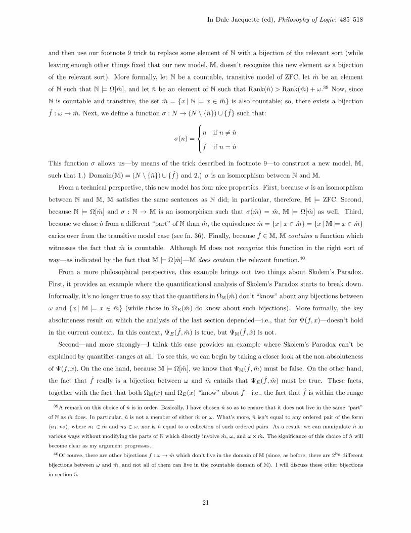
of the relevant sort). More formally, let N be a countable, transitive model of ZFC, let m be an element
of N such that N |= Ω[m], and let n be an element of N such that Rank(n) > Rank(m) + ω.39 Now, since
N is countable and transitive, the set m = x | N |= x ∈ m is also countable; so, there exists a bijection
f : ω → m. Next, we define a function σ : N → (N \ n) ∪ f such that:
σ(n) =
n if n 6= n
f if n = n
This function σ allows us—by means of the trick described in footnote 9—to construct a new model, M,
such that 1.) Domain(M) = (N \ n) ∪ f and 2.) σ is an isomorphism between N and M.
From a technical perspective, this new model has four nice properties. First, because σ is an isomorphism
between N and M, M satisfies the same sentences as N did; in particular, therefore, M |= ZFC. Second,
because N |= Ω[m] and σ : N → M is an isomorphism such that σ(m) = m, M |= Ω[m] as well. Third,
because we chose n from a different “part” of N than m, the equivalence m = x | x ∈ m = x |M |= x ∈ m
caries over from the transitive model case (see fn. 36). Finally, because f ∈M, M contains a function which
witnesses the fact that m is countable. Although M does not recognize this function in the right sort of
way—as indicated by the fact that M |= Ω[m]—M does contain the relevant function.40
From a more philosophical perspective, this example brings out two things about Skolem’s Paradox.
First, it provides an example where the quantificational analysis of Skolem’s Paradox starts to break down.
Informally, it’s no longer true to say that the quantifiers in ΩM(m) don’t “know” about any bijections between
ω and x | M |= x ∈ m (while those in ΩE(m) do know about such bijections). More formally, the key
absoluteness result on which the analysis of the last section depended—i.e., that for Ψ(f, x)—doesn’t hold
in the current context. In this context, ΨE(f , m) is true, but ΨM(f , x) is not.
Second—and more strongly—I think this case provides an example where Skolem’s Paradox can’t be
explained by quantifier-ranges at all. To see this, we can begin by taking a closer look at the non-absoluteness
of Ψ(f, x). On the one hand, because M |= Ω[m], we know that ΨM(f , m) must be false. On the other hand,
the fact that f really is a bijection between ω and m entails that ΨE(f , m) must be true. These facts,
together with the fact that both ΩM(x) and ΩE(x) “know” about f—i.e., the fact that f is within the range
39A remark on this choice of n is in order. Basically, I have chosen n so as to ensure that it does not live in the same “part”
of N as m does. In particular, n is not a member of either m or ω. What’s more, n isn’t equal to any ordered pair of the form
〈n1, n2〉, where n1 ∈ m and n2 ∈ ω, nor is n equal to a collection of such ordered pairs. As a result, we can manipulate n in
various ways without modifying the parts of N which directly involve m, ω, and ω× m. The significance of this choice of n will
become clear as my argument progresses.
40Of course, there are other bijections f : ω → m which don’t live in the domain of M (since, as before, there are 2ℵ0 different
bijections between ω and m, and not all of them can live in the countable domain of M). I will discuss these other bijections
in section 5.
21
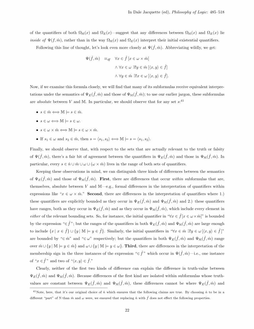
In Dale Jacquette (ed), Philosophy of Logic: 485–518
of the quantifiers of both ΩM(x) and ΩE(x)—suggest that any differences between ΩM(x) and ΩE(x) lie
inside of Ψ(f, m), rather than in the way ΩM(x) and ΩE(x) interpret their initial existential quantifiers.
Following this line of thought, let’s look even more closely at Ψ(f , m). Abbreviating wildly, we get:
Ψ(f , m) ≡df ∀x ∈ f [x ∈ ω × m]
∧ ∀x ∈ ω ∃!y ∈ m [〈x, y〉 ∈ f ]
∧ ∀y ∈ m ∃!x ∈ ω [〈x, y〉 ∈ f ].
Now, if we examine this formula closely, we will find that many of its subformulas receive equivalent interpre-
tations under the semantics of ΨE(f , m) and those of ΨM(f , m); to use our earlier jargon, these subformulas
are absolute between V and M. In particular, we should observe that for any set s:41
• s ∈ m⇐⇒M |= s ∈ m.
• s ∈ ω ⇐⇒M |= s ∈ ω.
• s ∈ ω × m⇐⇒M |= s ∈ ω × m.
• If s1 ∈ ω and s2 ∈ m, then s = 〈s1, s2〉 ⇐⇒M |= s = 〈s1, s2〉.
Finally, we should observe that, with respect to the sets that are actually relevant to the truth or falsity
of Ψ(f , m), there’s a fair bit of agreement between the quantifiers in ΨE(f , m) and those in ΨM(f , m). In
particular, every s ∈ n ∪ m ∪ ω ∪ (ω × m) lives in the range of both sets of quantifiers.
Keeping these observations in mind, we can distinguish three kinds of differences between the semantics
of ΨE(f , m) and those of ΨM(f , m). First, there are differences that occur within subformulas that are,
themselves, absolute between V and M—e.g., formal differences in the interpretation of quantifiers within
expressions like “x ∈ ω × m.” Second, there are differences in the interpretation of quantifiers where 1.)
these quantifiers are explicitly bounded as they occur in ΨE(f , m) and ΨM(f , m) and 2.) these quantifiers
have ranges, both as they occur in ΨE(f , m) and as they occur in ΨM(f , m), which include every element in
either of the relevant bounding sets. So, for instance, the initial quantifier in “∀x ∈ f [x ∈ ω×m]” is bounded
by the expression “∈ f ”; but the ranges of the quantifiers in both ΨE(f , m) and ΨM(f , m) are large enough
to include x | x ∈ f ∪ y | M |= y ∈ f. Similarly, the initial quantifiers in “∀x ∈ m ∃!y ∈ ω [〈x, y〉 ∈ f ]”
are bounded by “∈ m” and “∈ ω” respectively; but the quantifiers in both ΨE(f , m) and ΨM(f , m) range
over m∪y | M |= y ∈ m and ω ∪y | M |= y ∈ ω. Third, there are differences in the interpretation of the
membership sign in the three instances of the expression “∈ f ” which occur in Ψ(f , m)—i.e., one instance
of “x ∈ f ” and two of “〈x, y〉 ∈ f .”
Clearly, neither of the first two kinds of difference can explain the difference in truth-value between
ΨE(f , m) and ΨM(f , m). Because differences of the first kind are isolated within subformulas whose truth-
values are constant between ΨE(f , m) and ΨM(f , m), these differences cannot be where ΨE(f , m) and
41Note, here, that it’s our original choice of n which ensures that the following claims are true. By choosing n to be in a
different “part” of N than m and ω were, we ensured that replacing n with f does not effect the following properties.
22
In Dale Jacquette (ed), Philosophy of Logic: 485–518
ΨM(f , m) ultimately diverge. Similarly for differences of the second kind. Although the quantifiers in
ΨE(f , m) range over a larger domain than those in ΨM(f , m), none of the “extra” objects within the
range of ΨE(f , m)’s quantifiers are relevant to the truth-values of formulas like ∀x ∈ f [x ∈ ω × m] or
∀x ∈ m ∃!y ∈ ω [〈x, y〉 ∈ f ] (whether these formulas are interpreted after the fashion of ΨE or of ΨM).
Hence, none of these differences in quantifier-ranges can explain the final difference in truth-value between
ΨE(f , m) and ΨM(f , m).
This, therefore, brings us back to the third difference between ΨE(f , m) and ΨM(f , m)—their differing
interpretations of the membership sign in the expression “∈ f .” As this is the only difference which is not
covered by cases 1 and 2, it must be the one which explains the difference in truth-values between ΨE(f , m)
and ΨM(f , m). Further, this explanation is relatively intuitive. The notion captured by ΨE(x, y)—that “x
is a bijection between ω and y”—is a notion that’s defined in terms of the members of x. So, since M
doesn’t know about the real members of f (recall, the things M thinks are members of f are really members
of n), M doesn’t know that f is a bijection between ω and m. Hence, it’s not surprising that M fails to
satisfy the formula Ψ(f , m). It’s a simple consequence of the discrepancy between M’s understanding of the
membership relation on f and the real membership relation on f .
This gives us an analysis of the failure of (†) which is quite different from the one given in section 3.
There, the explanation for the failure of (†) involved the differing interpretations which ΩE(m) and ΩM(m)
give to their quantifiers (and, in particular, to one specific quantifier). Here, the explanation depends on
the way these expressions interpret the symbol “∈” in the embedded formula Ψ(f, m) (and, again, we can
limit our attention to a few specific instances of “∈”). Of course, there are other places where the semantics
ΩE(m) and ΩM(m) differ formally (that’s true in the transitive submodel case as well), but these are the
differences which really explain the present version of Skolem’s Paradox.
This example gives an initial indication as to why the standard, quantificational solution to Skolem’s
Paradox is inadequate. In particular, it shows that an analysis of Skolem’s Paradox which works fine for
transitive models does not work for all models (e.g., because we may lose the absoluteness of Ψ(f, x)).
Further, I’ve made a preliminary argument for the claim that this new example can’t be explained by
looking at quantifier-ranges at all. In the next section, I’ll bolster this argument by looking at two more
examples. Along the way, I’ll try to dispel a worry that the argument of this section may have occasioned.
I’ll end with some general remarks about Skolem’s Paradox.
5 The Vices of Quantification II
Let’s start with a possible concern about the analysis of the last section. In giving the analysis, I noted that
the bijection f lived in the domain of the quantifiers of both ΩE(m) and ΩM(m), and I then focused my
attention on the difference in truth value between ΨE(f , m) and ΨM(f , m). There are, however, 2ℵ0 other
bijections g : ω → m which don’t live in the domain of M. Why can’t one of these other bijections “explain”
23

In Dale Jacquette (ed), Philosophy of Logic: 485–518
the fact that ΩE(m) is false while ΩM(m) is true? Why, in short, can’t the difference between ΩE(m) and
ΩM(m) still be explained—if only partially—by the way these sentences interpret their initial existential
quantifiers?
There are, I think, three ways of responding to these questions. First, we should note that there is no
particular g : ω → m which plays a special role in explaining the differences between ΩE(m) and ΩM(m).
After all, for any particular g, we can easily build a new version of M which contains that g—i.e., by
substituting it for f in the preceding construction. Indeed, a trivial modification of that construction allows
us to include countably many bijections g : ω → m within the domain of M.42 So, there’s no sense in which
we’ve somehow used the wrong f in building our model M.
Second, it’s hard to see how some g : ω → m could explain the difference between ΩE(m) and ΩM(m).
Presumably, the thought goes something like this. In the case of ΩE(m), the quantifiers range over a domain
large enough to include the relevant g’s. Further, the semantics of ΩE(m) recognize these g’s as bijections
from ω to m. So, ∃f ΨE(f, m) comes out true, and ΩE(m) comes out false. The idea, then, is that this
kind of analysis should almost work for ΩM(m). If M knew about some bijection g : ω → m, then M would
recognize g as a bijection from ω to m. As a result, M would satisfy some formula of the form Ψ(g, m);
so, it would also satisfy ∃f Ψ(f, m), and it would fail to satisfy Ω(m). In short, if the quantifiers in ΩM(m)
only knew about the same functions that the quantifiers in ΩE(m) know about, then the analysis of ΩM(m)
would run exactly parallel to that of ΩE(m).
Why, though, should we believe any of this? After all, M already does contain one bijection f : ω → m,
and M doesn’t recognize f as a bijection (or, at least, not as a bijection between ω and m). Why should
we think M would do any better when it comes to other bijections? In the transitive model case, our
absoluteness results ensured that M got bijections right—that if M knew about some bijection g : m → n,
then M recognized g as a bijection from m to n. So, it was at least superficially plausible to think that if
M could know about some new g : ω → m, then M would properly recognize g as a bijection from ω to
m.43 But, once M misidentifies one bijection—i.e., f—then there’s no particular reason to think it should
do better with respect to other bijections.
These first two points suggest that the questions raised at the beginning of this section are not well-
motivated. Unlike in the transitive model case, there may simply be no coherent story about how initial
quantifiers could help to explain the version of Skolem’s Paradox we’re now considering. If so, then our
solution to this version of Skolem’s Paradox is going to have to look quite a bit different from the quantifier-
oriented solution presented in section 3. And, while this doesn’t directly show that the membership-oriented
solution presented in the last section is correct, it does lend that solution a good deal of indirect support.44
42I.e., we just use σ to replace countably many elements of N (all with sufficiently high rank) with new bijections g : ω → m.
43Of course, it’s hard to know how to evaluate this kind of subjunctive conditional, since its antecedent is necessarily false.
We can, however, say the following: if M were extended to a larger transitive model, M′, such that M′ contained a bijection
g : ω → m, then M′ would recognize this g as a bijection between ω and m.
44Recall, here, that the discussion of absoluteness and bounded quantification on pp 21–23 showed that most of the symbols
24
In Dale Jacquette (ed), Philosophy of Logic: 485–518
This brings me to a third point. As we saw earlier, part of the appeal of the quantificational solution
to Skolem’s Paradox comes from the fact that, for any countable model M and any m ∈ M, there are 2ℵ0
bijections g : ω → m | M |= m ∈ m which don’t live in the domain of M. Clearly, there’s no way of
formulating a version of Skolem’s Paradox which allows us to evade this fact.45 We can, however, formulate
puzzles that are closely analogous to Skolem’s Paradox and which do allow us to evade this fact. Further,
the solution to these later puzzles follows precisely the lines given in the last section. This leads me, once
again, to think that the solution from the last section is correct (and that the fact about “missing” bijections
is largely a red herring in our present context).
Let’s look at two of these analogous puzzles. The first involves the comparison of ΩE(x) and ΩM(x)
where M is a, suitably chosen, uncountable model of ZFC. As usual, we’ll start by letting N be a countable,
transitive model of ZFC. Applying a theorem of Keisler and Morley, we generate a model N′ such that 1.)
N′ is an elementary end extension of N and 2.) |N ′| = 2ℵ0 .46 Now, let m be an element of N such that
N |= Ω[m], and let X = g : ω → m | g is a bijection (so, X is the set of real bijections between ω and m).
Finally, using the fact that |N ′| = 2ℵ0 , we build a bijection σ : N ′ → N ′ ∪X such that σ N = Id; we let M
be the model induced by this σ—i.e., induced in the manner described in footnote 9.
At the end of this construction, our new model, M, has five nice properties: 1.) M |= ZFC, 2.) M |= Ω[m],
3.) m = x | M |= x ∈ m, 4.) m is countable, and 5.) every real bijection, g : ω → m, is actually a member
of M. Here, 1 follows from the fact that N satisfies ZFC, together with the fact that N′ is an elementary
extension of N and that σ : N′ → M is an isomorphism. 2 follows from the same facts, along with the fact
that σ(m) = m. 3 and 4 follow from the fact that N is countable and transitive, together with the fact that
N′ is an end extension of N and that σ N = Id. Finally, 5 follows from our choice of X, together with the
fact that X ⊂M.
There are two things to notice about all this machinery. First, properties 1–4 give rise to an obvious
analog of Skolem’s Paradox. After all, M is a model of ZFC which satisfies Ω[m] (properties 1 and 2),
despite the fact that the set m = x | M |= x ∈ m is only countable (properties 3 and 4). So, just as in
our previous examples, ΩM(m) is true, and ΩE(m) is false. Second, this analog of Skolem’s Paradox neatly
evades the concerns raised at the beginning of this section. After all, fact 5 ensures that all of the 2ℵ0
in Ω(x) are irrelevant to explaining this version of Skolem’s Paradox. If, as suggested above, the initial quantifier in Ω(x) is
also irrelevant, then the instances of “∈” isolated on page 23 provide the only possible focus for our explanation.
45As a matter of classification, I take it that “Skolem’s Paradox” always involves the comparison of ΩE(x) and ΩM(x), where
M is a countable model. Hence, the fact mentioned in the main text will always be present (though, as I have argued, it may
not always be relevant).
46 Some clarification is probably in order here. To say that N′ is an elementary extension of N means that for any formula
φ(x) and any sequence n ∈ N, N′ |= φ[n] ⇐⇒ N |= φ[n]. In particular, then, the fact that N satisfies ZFC entails that N′ also
satisfies ZFC; further, for any n ∈ N, N′ |= Ω[n] ⇐⇒ N |= Ω[n]. To say that N′ is an end extension of N means that for every
n ∈ N, x | N |= x ∈ n = x | N′ |= x ∈ n; so, moving to N′ doesn’t involve adding “new” elements to old members of N.
Given this, Keisler and Morley proved (see [9]) that any countable model of ZFC has elementary end extensions of arbitrarily
large cardinality.
25
In Dale Jacquette (ed), Philosophy of Logic: 485–518
bijections g : ω → m which witness the falsity of ΩE(m) live within the domain of M.
Indeed, we can go a bit further than this. It’s pretty clear that any solution to this analog of Skolem’s
Paradox has to run parallel to the solution sketched on pp 21–23. Since every bijection which witnesses the
falsity of ΩE(m)—i.e., every g which makes ΨE(g, m) come out true—is contained within the domain of M,
the difference in truth-value between ΩE(m) and ΩM(m) can’t be explained by looking at the interpretation
of the initial quantifiers in ΩE(m) and ΩM(m). Nor can we explain M’s failure to “recognize” elements of X
as bijections between ω and m by appealing to way M interprets the quantifiers in the embedded formula
Ψ(x, m). To be sure, the quantifiers in formulas like ΨE(g, m) do range over a larger domain than those
in ΨM(g, m). As before, however, every set which is relevant to the truth of ΨE(g, m) is a member of
ω∪m∪ (ω×m). These sets are within the range of the quantifiers in ΨM(g, m), and every set in the range of
the quantifiers of ΨM(g, m) is within the range of the quantifiers in ΨE(g, m).47 Hence, the only remaining
explanation for the difference in truth-values between ΩE(m) and ΩM(m) stems from the way these formulas
interpret the symbol “∈.”48
This, therefore, gives us an analog of Skolem’s Paradox whose solution has to follow the lines sketched
in the last section. I’ll close this section with a second such analog. Whereas my first example involved
the comparison of ΩE(x) and ΩM(x) for an uncountable model, M, this one will compare ΩN(x) and ΩM(x)
where N and M are both countable. As before, we can start by letting N be a countable, transitive model of
ZFC. Next, let N′ = N[G] be a generic extension of N such that ωN1 has been “collapsed” to have cardinality
ℵ0.49 Given this, let X = n ∈ N | N |= “Rank(n) < ωω”, and let σ : N ′ → N be a bijection such that
σ X = Id. Finally, using our trick from footnote 9, we can define a new membership relation on the domain
of N such that σ becomes an isomorphism between N′ and M (where M is the new model canonically induced
by this bijection).
At this point, we are in a position to formulate a puzzle very much like Skolem’s Paradox except that it
holds between N and M (rather than between N and the set-theoretic universe). To begin, note that the fact
that σ X = Id ensures that N and M agree about the membership relation on ωN1 . That is,
x | N |= x ∈ ωN1 = x | N′ |= x ∈ ωN
1 = x | M |= x ∈ ωN1 .50
However, N and M do not agree about the countability of ωN1 . On the one hand, N |= Ω[ωN
1 ]. On the other
47As in our original example, this point can be put in terms of “bounding sets.” For any particular g : ω → m, all of the
quantifiers in Ψ(g, m) are bounded by sets like g, m, ω, and ω × m. Since the elements of these bounding sets all live in the
domain of M, the quantifiers in ΨM(f, m) will “know” about all these elements.
48Again, as in the original example, a careful analysis allows us to isolate three specific instances of “∈” which do all the
explanatory work. Since there’s nothing new going on in this particular case, I omit the details of this further analysis.
49 The details of this construction are too complicated to explain fully here. The relevant facts about N′ are these: 1.) N′
is a countable, transitive model of ZFC, 2.) N′ is an “end extension” of N (cf. footnote 46), and 3.) N′ |= “ωN1 is countable”.
Note that 3 entails that N′ |= ¬Ω[ωN1 ] and that 1–3 together entail that N′ contains some (real) bijection g : ω → ωN
1 . Further
details about this kind of construction can be found in chapter 7 of [11] or chapter 3 of [8].
50The first of these equalities follows from the fact that N′ is an end extension of N. The second follows from the fact
26
In Dale Jacquette (ed), Philosophy of Logic: 485–518
hand, our forcing construction ensures that N′ |= ¬Ω[ωN1 ] (see footnote 49). So, the fact that σ : N′ → M is
an isomorphism, together with the fact that σ(ωN1 ) = ωN
1 , ensures that M |= ¬Ω[ωN1 ] as well.
This gives us a simple analog of Skolem’s Paradox: even though N and M agree about the members of
ωN1 , the expression ΩN(ωN
1 ) comes out true, and the expression ΩM(ωN1 ) comes out false. Further, there’s no
possibility of explaining this discrepancy by appealing to the differing ways ΩN(x) and ΩM(x) interpret their
quantifiers. Since N and M have the same domain, ΩN(x) and ΩM(x) interpret their quantifiers in exactly the
same way. Hence, any difference in truth-value between ΩM(ωN1 ) and ΩN′(ωN
1 ) must be explained in terms of
the differing ways N and M interpret the symbol “∈.” In short, this is a case where the only possible solution
to our puzzle follows the membership-oriented lines sketched in section 4.51
This, then, explains why I think the concerns raised at the beginning of this section are misguided.
Although it’s certainly true that, given any countable M |= ZFC and any m ∈M, there will be 2ℵ0 bijections
g : ω → x | M |= x ∈ m which don’t live in the domain of M, it’s not at all clear that these bijections are
relevant to the solution of (all versions of) Skolem’s Paradox. For the version of Skolem’s Paradox discussed
in the last section, it’s unclear how these bijections are supposed to explain the difference in truth-value
between ΩE(m) and ΩM(m) (while it’s quite clear how certain instances of “∈” could do this explanatory
work). Further, there are cases which involve the same kind of phenomena as Skolem’s Paradox where the
corresponding bijections simply don’t exist. Given this, we should be cautious about insisting that Skolem’s
Paradox has a single, uniform explanation which can be formulated in terms of quantifier ranges. Although
such quantificational solutions work well in certain cases—e.g., the transitive model case—there are other
solutions which work better when we turn to more complicated cases—e.g., the case discussed in section 4.
6 A Few Concluding Remarks
In the first five sections of this paper, I provided a tour through (some of) the mathematical issues involved
in Skolem’s Paradox. I looked at what it takes to make this paradox “look plausible,” what we need to
“solve” the paradox, what different solutions are appropriate for different versions of the paradox, etc. In
this section, I want to step back and take a somewhat broader view. I’ll start by highlighting a few of the
main points—both technical and philosophical—from the preceding sections. I’ll then examine what I take
to be the main philosophical worry which the preceding discussion may have provoked.
σ X = Id. Basically, the fact that σ is the identity in the “neighborhood” of ωN1 ensures that “locally-definable” properties of
ωN1 will be absolute between N and M (and, for that matter, between either of these models and V ). With a little work, we can
show that all of the properties listed on page 22 are absolute between N and M, when we put ωN1 in place of our previous m.
In particular, then, “x = ω” and “x ∈ ω × ωN1 ” will both be absolute.
51In fact, the solution of this puzzle follows our previous solution rather closely. By letting N′ be an end extension of N and
then setting σ X = Id, we ensured that the vast majority of the symbols in Ω(ωN1 ) occur within subformulas that are absolute
between N and M. This fact, together with the fact that N and M agree on the interpretation of their quantifiers, entails that
any differences between ΩN(ωN1 ) and ΩM(ωN
1 ) must be explained by ways these formulas interpret the usual three instances of
“∈”—i.e., the three instances highlighted in the “∈f” clauses in the formulation of Ψ(f, x) on page 22.
27
In Dale Jacquette (ed), Philosophy of Logic: 485–518
From a technical perspective, there are two points I want to emphasize. First, it’s a lot harder to formulate
a plausible-looking version of Skolem’s Paradox than it may seem to be at first. To make Skolem’s Paradox
look plausible, we need to exercise some care in choosing the countable model in terms of which the paradox
is formulated (in general, an arbitrary countable model of ZFC won’t do the job). We also need to think
about just how we explicate our ordinary English notion of countability. Finally, we need to ensure that
the choices we make with regard to these first two issues fit together appropriately: if, for instance, we use
a model with a designated ∈m-relation to formulate the paradox, then we need to explicate our notion of
countability in terms of that relation. So, even getting a superficially plausible version of the paradox onto
the table may require some careful technical work.
Second, Skolem’s Paradox isn’t just a puzzle concerning the interpretation of quantifiers. To be sure,
there are some versions of the paradox which are best solved by looking at the way first-order models interpret
quantification—e.g., the transitive submodel argument discussed in section 3. But, there are other versions
of the paradox which require quite different solutions—e.g., the versions examined in sections 4–5. Given
this, we should resist the idea that Skolem’s Paradox has a completely general explanation which can be
formulated in terms of quantifier ranges. Indeed, if we’re really looking for a general solution to Skolem’s
Paradox—a solution which applies to all formulations of that paradox—then I doubt we can find one which
is much more specific than the “generic solution” of section 2.
Let me make a comment about this second point. For expository reasons, sections 3–5 focused on cases
where we could pretty easily isolate the specific symbols whose interpretation served to “explain” Skolem’s
Paradox (instances of “∃x” in 3, and instances of “∈” in 4–5). I don’t, however, think that all cases are quite
this simple. As we saw on page 3, Ω(x) is an incredibly long formula, so there are many different symbols
which can, in the context of specific models, “take the blame” for particular instances of Skolem’s Paradox.
Further, there are cases where Skolem’s Paradox can’t be pinned on specific symbols at all—i.e., cases where
the paradox turns on a complicated interplay between the interpretation of several different symbols.52 So,
unless we’re willing to accept a wildly disjunctive solution—potentially one with 2ℵ0 cases—I don’t think we
can get a general solution to Skolem’s Paradox which is more specific than the one given in section 2.53
So much, then, for the technical issues. On the more philosophical side, there are also two points worth
emphasizing. First, there shouldn’t be anything too surprising about Skolem’s Paradox. At a general level,
we can isolate clear differences between the semantics of ordinary English set theory and the model-theoretic
52To explore this possibility, the reader is encouraged to think through the case where κ is an inaccessible cardinal and M is
a countable elementary submodel of 〈Vκ,∈〉. Let m = ℵ17, and analyze the version of Skolem’s Paradox which results from the
fact that M |= Ω[m].
53I do, however, think there’s a lot to learn from tracking Skolem’s Paradox through the details of various specific models.
In doing so, we learn about the particular pathologies which give rise to things like Skolem’s Paradox, about the strengths
and weaknesses of first-order formulations of set theory, and about the fine details of our (various) conceptions of cardinality.
There are a lot of open questions here, and I encourage philosophers—or, at least, those philosophers who are as fascinated by
Skolem’s Paradox as I am—to spend more time exploring this paradox in the context of specific models.
28
In Dale Jacquette (ed), Philosophy of Logic: 485–518
semantics of formulas like Ω(x)—e.g., in their interpretation of symbols like “∈” and “∃”—and we can see
how Skolem’s Paradox turns on an equivocation between these two kinds of semantics. At a more local level,
when we track these differences through the details of particular models, we can often isolate just which
symbols really give rise to Skolem’s Paradox, and we can explain how the interpretation of these symbols
gives rise to the paradox. Given all this, the paradox itself should no longer seem very puzzling.
Second, the argument of sections 4–5 should lead us to be cautious about any philosophical analysis of
Skolem’s Paradox which focuses overmuch on quantification or which overemphasizes certain special cases
of the paradox—e.g., the transitive submodel case. As we have seen, Skolem’s Paradox comes in many
forms, and, even at the technical level, these different forms require different kinds of solutions. This point
carries over to the philosophical level as well. It’s clear, for instance, that Skolem’s Paradox may lead us
to ask difficult questions about things like the indefinite extensibility of the concept of set or the coherence
of absolute notions of quantification, but I doubt very much that answers to these questions will enable us
to provide a (complete) solution to the paradox itself. At best, they will help us to solve those instances of
the paradox which most clearly turn on the interpretation of quantifiers. For philosophy, then, as much as
for mathematics, a full solution to Skolem’s Paradox will have to focus on the fine-grained analysis of many
different models of set theory (where these different models give rise to different philosophical questions).
These, then, are what I take to be the main points of the preceding discussion. I want to close by
considering a worry which this entire discussion may have provoked. So far, I have treated Skolem’s Para-
dox as though it were an essentially technical matter. I started by taking both Cantor’s theorem and the
Lowenheim-Skolem theorem at face value—by, that is, taking a naively realistic attitude towards the math-
ematics lying behind these two theorems—and I then tried to explain why, understood in this manner, the
theorems don’t conflict with each other. In doing so, I felt perfectly free to make use of expressions like “the
ordinary English understanding of membership,” “the real members of m,” “quantifiers which range over
the whole set-theoretic universe,” etc.
The worry here is that this analysis might be a bit too naive. At the most basic level, this worry flows from
simple incredulity at the idea that anything as strong as full classical set theory can simply be presupposed
when solving puzzles like Skolem’s Paradox.54 Moving deeper, our incredulity can be reinforced by recalling
other philosophical puzzles about the interpretation of mathematical language—i.e., puzzles which call into
question the determinacy of naive talk about things like “membership” or “the whole universe of sets.”55
Finally, the entire development of twentieth-century set theory may seem to tell against my approach to
Skolem’s Paradox. After all, the standard response to the classical paradoxes has been to move away from
naive approaches to set theory and toward formal axiom systems (and especially first-order axiom systems).
54In the literature, incredulity about appeals to our “ordinary English” understanding of set theory is often expressed in
terms of opposition to “Platonism.” See [5], [10], [18], and [19] for some examples of this way of putting things.
55See [10] for an attempt to parley one of Benacerraf’s classical puzzles—that presented in [2]—into this kind of challenge
to naively technical solutions to Skolem’s Paradox. See [21] for a similar argument based on Wittgensteinian considerations
concerning the relationship between meaning and use.
29
In Dale Jacquette (ed), Philosophy of Logic: 485–518
Clearly, addressing these kinds of worries in any detail would lead us rapidly into deep waters. I don’t
plan to do that here. Indeed, I won’t even try to develop these worries more completely or to track them
through the relevant literature. Instead, I’ll just make a few short remarks in defense of the kind of technical
solution given in sections 2–5. For obvious reasons, I don’t regard these remarks as a complete response to
the above worries; at best, they constitute a gesture in the direction of such a response.
Let’s begin by recalling the point of Skolem’s Paradox. In theory, the paradox highlights a certain
incoherence—or perhaps even an inconsistency—in our ordinary ways of thinking about set theory. More
specifically, it purports to show that there is a conflict between the naive acceptance of Cantor’s theorem and
certain instances of the Lowenheim-Skolem theorem. Since the Lowenheim-Skolem theorem is, presumably,
unassailable, this leads to the conclusion that Cantor’s theorem should not be taken at face value—i.e., that
we should view naive talk about “absolutely uncountable sets” as problematic and to be avoided.
Notice the order of argument here. We start with a naive acceptance of Cantor’s theorem. (At the
very least, we start with an open mind towards this theorem and towards the naive set theory which lies
behind it.) We then formulate Skolem’s Paradox. The paradox shows that there is a problem with our initial
naivete, and it forces us to abandon our original acceptance of “ordinary-English” formulations of set theory.
In short: Skolem’s Paradox does the philosophical work here, and the problematization of ordinary-English
set theory is (part of) the philosophical payoff.
My concern, then, is that the worries we’re now discussing effectively reverse this order of argument.
They start with a rejection of ordinary-English set theory—start, that is, with the very thing that Skolem’s
Paradox is supposed to help us establish—and they then use this rejection as a means of defending Skolem’s
Paradox against certain technical challenges (e.g., those in sections 2–5). On this way of proceeding, however,
it’s hard to see how Skolem’s Paradox still does any real philosophical work. On the surface, it’s our initial
worries—and whatever arguments may lie behind them—that do the real philosophical work; Skolem’s
Paradox just tags along for the ride.
Let me put this point another way. Anyone who comes to set theory with serious worries about the
determinacy (or even the coherence) of ordinary talk about sets and membership will, of course, have
corresponding worries about the solution to Skolem’s Paradox which I developed in sections 2–5. But, they
will also have independent worries about the notions of countability and uncountability (since these notions
are, after all, defined in terms of the problematic notions of membership and quantification over the set-
theoretic universe). As a result, there’s no need for them to bring Skolem’s Paradox into the discussion. Given
their initial worries, they have direct arguments against naive talk about “absolutely uncountable sets,” and
Skolem’s Paradox becomes completely superfluous. In short: taking these kinds of worries seriously doesn’t
help to make Skolem’s paradox more significant. On the contrary, it threatens to reduce the paradox to a
mere technical side show.
Here’s one more (and final) way of thinking about all this. To solve Skolem’s Paradox, we need to show
that there’s no conflict between Cantor’s theorem and the Lowenheim-Skolem theorem. But that’s all we
30
In Dale Jacquette (ed), Philosophy of Logic: 485–518
need to do. We don’t also have to solve every other problem in the philosophy of set-theory—i.e., we don’t
have to solve them before we can use words like “set” and “membership” to provide a solution to Skolem’s
Paradox. In saying this, I’m not trying to dismiss these other problems; I’m just emphasizing that they are,
in fact, other problems.56 When we focus resolutely on Skolem’s Paradox itself—on the purported conflict
between Cantor and Lowenheim—then we find that the technical analysis of sections 2–5 is exactly what we
need to solve this particular puzzle. In the present context, that’s all we need to do.
This, then, explains why I’m at least inclined towards a wholesale dismissal of the kinds of worries now
under discussion. It’s not that I think that these worries are trivial or misguided (some of them clearly
aren’t); it’s just that I don’t think that attending to these worries helps us to understand Skolem’s Paradox
itself (indeed, I think the worries tend to trivialize the paradox). Of course, I’m aware that I’m evading all
of the argumentative details here: to really make these thoughts stick, I’d have to develop the above worries
in far more depth and to explore their interaction with Skolem’s Paradox in far more detail. But that is a
project for another time. For now, I’ll simply end with a final summary of this paper: there is no conflict
between Cantor’s theorem and the Lowenheim-Skolem theorem.
References
[1] Timothy Bays. Reflections on Skolem’s Paradox. PhD thesis, UCLA, 2000.
[2] Paul Benacerraf. What the numbers could not be. In Philosophy of Mathematics, pages 272–294.
Cambridge University Press, Cambridge, 1983.
[3] Paul Benacerraf. Skolem and the skeptic. Proceedings of the Aristotelian Society, 59:85–115, 1985.
[4] H.D. Ebbinghaus, J. Flum, and W. Thomas. Mathematical Logic. Springer, Amsterdam, 1994.
[5] Arthur Fine. Quantification over the real numbers. Philosophical Studies, 19:27–31, 1968.
[6] Alexander George. Skolem and the Lowenheim-Skolem Theorems. History and Philosophy of Logic,
6:75–89, 1985.
[7] William Hart. Skolem’s promises and paradoxes. The Journal of Philosophy, 67:98–109, 1970.
[8] Thomas Jech. Set Theory. Academic Press, San Diego, 1978.
[9] Jerome Keisler and Michael Morley. Elementary extensions of models of set theory. Israel Journal of
Mathematics, 6:49–65, 1968.
56An analogy from ethics may be helpful here. Presumably, it’s legitimate to discuss topics like abortion or just war theory
without first solving the Liar Paradox and/or the problem of induction. This is true even though we may want to use the word
“truth” in our ethical discussions and/or make some empirical generalizations. To think otherwise is to think that we need to
solve all philosophical problems in order fruitfully discuss any of them. That’s neither a reasonable nor a profitable standard
for good philosophical discourse.
31
In Dale Jacquette (ed), Philosophy of Logic: 485–518
[10] Virginia Klenk. Intended models and the Lowenheim-Skolem Theorem. The Journal of Philosophical
Logic, 5:475–489, 1976.
[11] Kenneth Kunnen. Set Theory. North-Holland, Amsterdam, 1980.
[12] Clifton McIntosh. Skolem’s criticisms of set theory. Nous, 13:313–334, 1979.
[13] John Myhill. On the ontological significance of the Lowenheim-Skolem Theorem. In I. Copi and J. Gould,
editors, Contemporary Readings in Logical Theory, pages 40–51. Macmillan, New York, 1967.
[14] Hilary Putnam. Models and reality. In Realism and Reason, pages 1–25. Cambridge UP, Cambridge,
1983.
[15] Michael Resnik. On Skolem’s Paradox. The Journal of Philosophy, 63:425–438, 1966.
[16] Joseph Shoenfield. Mathematical Logic. Association for Symbolic Logic, Natick, MA., 67.
[17] Thoralf Skolem. Some remarks on axiomitized set theory. In Jean van Heijenoort, editor, From Frege
to Godel, pages 290–301. Harvard, Cambridge, Mass., 1967.
[18] William Thomas. Platonism and the Skolem Paradox. Analysis, 28:193–196, 1968.
[19] William Thomas. On behalf of the Skolemite. Analysis, 31:177–186, 1971.
[20] Dirk van Dalen. Logic and Structure. Springer, Amsterdam, 1997.
[21] Crispin Wright. Skolem and the skeptic. Proceedings of the Aristotelian Society, 59:116–137, 1985.
32


