MIT LIBRARIES

3 9080 02527 85

lb

:i

Digitized by the Internet Archive

in 2011 with funding from

Boston Library Consortium IVIember Libraries

http://www.archive.org/details/historyinstitutiOObane

!1

15

ubW^

Massachusetts Institute of TechnologyDepartment of Economics

Working Paper Series

History, Institutions and Economic Performance: Tlie

Legacy of Colonial Land Tenure Systems in India

Abhijit Baneq'ee

Lakshmi Iyer

Working Paper 02-27

June 2002

Room E52-251

50 Memorial Drive

Cambridge, MA 02142

This paper can be downloaded without charge from the

Social Science Research Network Paper Collection at

http://ssrn.com/abstract_ id=xxxxx

Slt^ZiMASSACHUSEHS INSTITUTE

OFTECHMOLOGY

LlD,.^ ICCJ

Massachusetts Institute ot TechnologyDepartment of Economics

Working Paper Series

History, Institutions and Economic Performance: The

Legacy of Colonial Land Tenure Systems in India

Abhijit Banerjee

Lakshmi Iyer

Working Paper 02-27

June 2002

Room E52-251

50 Memorial Drive

Cambridge, MA 02142

This paper can be downloaded without charge from the

Social Science Research Network Paper Collection at

http://ssrn.com/abstract_.id=xxxxx

History, Institutions and Economic Performance:

The Legacy of Colonial Land Tenure Systems in India*

Abhijit Banerjee ^ Lakshmi Iyer*

June 2002

Abstract

Do historical institutions have a persistent impact on economic performance? We analyze

the colonial institutions set up by the British to collect land revenue in India, and show that

differences in historical property rights institutions lead to sustained differences in economic

outcomes. Areas in which proprietary rights in land were historically given to landlords have

significantly lower agricultural investments, agricultural productivity and investments in public

goods in the post-Independence period than areas in which these rights were given to the cul-

tivators. We verify that these differences are not driven by omitted variables or endogeneity of

the historical institutions, and argue that they probablj' arise because differences in institutions

lead to very different policy choices.

Keywords: history, land tenure, development

JEL classification: OH, P16, P51

'We tfiank Daron Acemoglu, Sam Bowles, Esther Duflo, Maitreesh Ghatak, Karla Hoff, Kaivan Munshi, Raghuram

Rajan, Andrei Shleifer and participants in the the MIT-Harvard Development Seminar, the North-Eastern Universities

Development Conference and the MIT Development Economics and Organizational Economics Lunch for helpful

comments, Nabeela Alam and Theresa Cheng for research assistance and Michael Kremer for help in accessing

historical land tenure data.

^Department of Economics, MIT. banerjee@mit.edu

^Department of Economics, MIT. lakshmi@mit.edu

1 Introduction

The question of the role of history is one to which economists keep returning, most recently in the

form of a debate about convergence. Is the destiny of a people inscribed in their genes and their

geography, or do they also carry around the weight of their peculiar histories? Is the present misery

of so many poor nations merely a step in the gradual evolution towards a pre-ordained future or a

symptom of an unfortunate history that may keep them in its thrall for a very long time?

At one level this is perhaps an unresolvable question because one can never rule out the

possibihty that the effects of history will ultimately wash out. But even if we set ourselves the

more modest task of determining whether historical accidents have persistent effects, the task is by

no means straightforward. In part, this is because of the well-known problems with cross-country

comparisons (when do we say that two countries are alike?), in part due to the amorphous nature

of history (which aspect of history should we consider?) and in part because it is not easy to decide

what would be an acceptable timescale.

Moreover, even if one were to accept the proposition that history is important, there could

be at least two alternative (though not inconsistent) views of the nature of the link. In the new

institutionalist view,-^ history matters because history shapes institutions and institutions shape

the economy. By contrast, in what one might call the "increasing returns" view, historical accidents

put one country ahead in terms of aggregate wealth or human capital (or some other comparable

aggregate) and this turns into bigger and bigger differences over time because of the increasing

returns. The difference between these views is potentially very important: If increasing returns is

everything, then a one-time inflow of aid or some other windfall would set the economy on the way

to prosperity. If institutions were very important, one would tend to be less sanguine.

Within the institutionalist position there is a further distinction that has the potential to

be important: One could hold that institutions are important but essentially manipulable (when

there is the will to change them). Or one could be concerned about what one may call institutional

overhang, the possibility that the effects of institutions persist for a long time after they have been

formally changed.

Economists from Marx^ to Mankiw^ (and beyond) have grappled with these questions

using a variety of tools and approaches, but we are nowhere near a resolution. As is well-known,

^See North (1990).

^Karl Marx (1885).

^Mankiw, Romer and Weil (1992)

the evidence on unconditional convergence in the cross-country growth framework is rather weak"^

and while conditional convergence does significantly better, it does so at the cost of including

potentially endogenous variables (savings rate, etc.) as controls. One also does better by giving up

the idea of full convergence and focusing on club convergence a la Quah (1996), but then the role

of history remains a question.

Turning to the other side, a series of papers by La Porta et al (1998a; 1998b; and 2000)

have argued that the historical fact of being colonized by the British rather than any of the other

colonial powers, has a strong effect on the legal system of the country and through that on economic

performance. This evidence is highly suggestive but some obvious doubts about causality remain.

The role of history in determining the shape of present-day institutions is also at the heart of two

recent sets of papers, one by Acemoglu, Johnson and Robinson (2001; 2002) and the other by

Engerman and Sokoloff (1997; 2000; and 2002). Acemoglu et al show that mortality rates among

early European settlers is a strong predictor of whether these countries end up with what economists

today call "good" institutions and whether their economies are doing well today. They argue that

this is because Europeans settled in large numbers in the countries where the early settler mortality

was relatively low, and their presence was important in making sure that these countries ended up

with the right kinds of institutions. While the facts they report are clearly quite remarkable, it is

not entirely clear what we should make of them. In particular, to what extent was early settler

mortality a fact of history, in the sense that it could have easily been very different (say, if the

settlers had arrived a few years later). To what extent should it be seen as an indirect effect of

geography on economic outcomes through its effect on the disease matrix? How important was the

effect of population density at the time of conquest, given that it is easier to get infected if there

are lots of people around,'^ and if population density was important, should we see the difference

in population density as a matter of history or of geography? Furthermore, while they make a

strong case, it is not entirely obviovis that the channel of causation from settler mortality to current

economic performance has to go through the quality of institutions: Population density, for one,

influences both the disease environment and the labor supply, and labor supply can certainly have

^See Pritchett (1997), for example. Adding a range of geographical controls along the lines suggested by Gallup,

Sachs and Mellinger (1999) helps, but it is not always eeisy to separate the effect of geography from that of European

settlement, which is endogenous.

^In a later paper, Acemoglu, Johnson and Robinson (2002) report evidence showing that the countries that

performed the worst under colonial rule were the ones that were most densely populated under colonial rule.

an independent effect.

Labor supply is in fact central to Engerman and Sokoloff 's thesis on why the United States

and Canada ended up being so different from Latin America. They suggest that the reason why

Brazil is where it is today and the U.S. is where it is, has a lot to do with the fact that in the

early years after European conquest Brazil was deemed to be suitable for growing sugar and the

U.S. was not. Since sugar cultivation demanded the use of slave labor, Brazil ended up with a

much larger slave population and this, they argue, meant that Brazilian society was' much more

hierarchical than American society, causing a divergence in the types of institutions that evolved in

these two areas, and eventually a divergence in the rates of growth. Their discussion is rich in the

details of the exact channels through which social inequality affected the process of institutional

evolution and the case they make is quite compelling, but they make no secret of the fact that the

nature of their data does not permit rigorous hypothesis testing. Moreover, it is not entirely clear

from their discussion whether they want to emphasize the innate geographical differences as the

ultimate source of the problem or put the blame on the historical fact that growing sugar-cane was

particularly profitable during the early years of European colonialism.

In this paper we attempt to answer the same set of questions by studying a very specific

set of institutions, the different land revenue systems instituted by the British in India during

the early nineteenth century, and examining the impact of these systems on various present-day

economic indicators. This strategy has several advantages: First, obviously, we can focus on the

impact of history through a very specific instance of institutional change. This specificity makes

it easier for us to identify some of the causal mechanisms that link the history to the present-

day outcomes. Second, this specificity makes it possible to take advantage of all the information

we have about the reasons why there is variation in our explanatory variables. In particular, it

enables us to use historical information to construct instrumental variables estimates of the impact

of historical institutions. Third, since we are studying the variation of institutions within the same

country, under a single political system and ruled by the same colonial power, it enables us to avoid

some of the omitted variable problems associated with cross-country studies. Finally, since the

land revenue systems that the British introduced departed with the British—there are no direct

taxes on agricultural incomes in independent India—we have here a pure example of institutional

overhang.^

^This distinguishes this work from the recent empirical literature on the effects of land reform on economic

outcomes (see Banerjee, Gertler and Ghatak (2002), Besley and Burgess (2000) and Lin (1999) among others). The

The British rule in India extended from 1757 to 1947 and during this period land revenue

or land tax was a very important source of government revenue. Different areas had diiferent

systems for revenue collection: landlord-based systems made a landlord responsible for collecting

revenue in a specific area; in individual-based systems, the British government officers collected

revenue directly from the actual cultivators without the intermediation of a landlord; in village-

based systems, a village community body bore the revenue responsibility.

Our strategy is the following: For each district of British India, we use historical sources

to compute a crude measure of the proportion of the district for which the revenue liability was not

in the hands of landlords. We then regress post-Independence outcomes in agricultural investments

and productivity on this measure, after controlling for a wide variety of geographic variables, as

well as for the direct impact of the length of colonial rule. We find that areas which were formerly

landlord-controlled have significantly lower agricultural investments as measured by irrigation, fer-

tilizer use and the adoption of high-yielding varieties of rice, wheat and other cereals. The effects

we document are surprisingly large, given that we are looking at an institution that no longer exists

and the crudeness of the measure we use for our main explanatory variable. Irrigation levels are

25% higher in the non-landlord districts, fertilizer use is 45% higher and the adoption of high-

yielding varieties in rice is about 25% higher. Not surprisingly, they also have worse agricultural

performance: overall crop yields are 16% higher in non-landlord areas, rice yields are 17% higher

and wheat yields are 23% higher.

We use several strategies to control for omitted district characteristics and possible en-

dogeneity of the historical land tenure system. First, we construct a restricted sample of districts

that are geographical neighbors, but which happened to have different land systems for historical

reasons. On all our observed geographical variables, these districts look very similar, and it is not

unreasonable to assume that such neighboring districts would be similar in other unobservables

as well. For this restricted sample, we see significant differences in crop yields as well as in the

adoption of new agricultural technologies.

Second, we argue on the basis of historical evidence that it is legitimate to use the fact

of having been conquered by the British in the 1820-1856 period (rather than earlier or later) as

an instrument for the land tenure system, after controlling directly for the length of British rule.

We find that our instrumental variables (IV) estimates of the impact of historical land tenure are

Coase Theorem notwithstanding, there are obvious reasons to expect that the choice of land tenure systems would

have an effect on current economic performance, especially in countries where agriculture is important.

all larger in magnitude than the OLS estimates and usually significant, suggesting that our OLS

estimates were downward biased, probably because the non-landlord variable is poorly measured.

Third, we present data to indicate that it was the landlord areas that were more productive

during the colonial period, providing further confirmation that our results for the post-Independence

period are not driven by some unobserved time-invariant district characteristics. In particular,

geography is unlikely to be a driving factor behind our observed differences.

The differences between landlord and non-landlord areas are not restricted to agriculture

alone: We find substantial diflFerences in human capital investments and outcomes as well. Landlord

areas have much lower levels of local infrastructure such as primary schools, high schools and

health centers; the availability of village schools is 20% to 60% higher in non-landlord areas. Not

surprisingly, they also have lower levels of literacy and higher levels of infant mortality: OLS

estimates indicate that literacy rates are 18% higher and infant mortality rates are 40% lower in

non-landlord areas. For these outcomes as well, all our IV estimates are larger in magnitude than

the OLS estimates.

Institutions born out of specific histories continue, therefore, to have powerful repercus-

sions long after the institutions have vanished and the history has been half-forgotten. The puzzling

persistence of large and often growing differences across the states of India that have been noted

by a number of scholars, ' may well owe something to this or some other half-remembered accident

of history.

The paper is structured as follows: Section 2 describes the historical background and the

land tenure system under British rule. We discuss the reasons why the tenure system varies from

district to district and argue that the choice of tenure system can be reasonably regarded as a

source of exogenous variation. Section 3 outlines different mechanisms through which historical

land tenure might affect long-term outcomes. Sections 4 and 5 describe our data and empirical

strategy. Our empirical results are described in Section 6. Section 7 reports additional results on

human capital investments. Section 8 concludes by discussing potential mechanisms that might

explain the persistence of the eff'ect of British land tenure systems.

''See Chaudhuri (2000), Cashin and Sahay (1996), Clark and Wolcott (2000) and Datt and Ravallion (1998).

2 Historical Background

2.1 British Political Control

The British empire in India lasted for nearly 200 years. The British initially arrived as traders;

the English East India Company received their first permit from the Mughal emperor, Jahangir, to

build a factory at Surat in 1613. Their empire-building began with their victories in the battle of

Plassey in 1757 and the battle of Buxar in 1764, as a result of which they obtained political control

of the modern states of Bengal and Bihar (formerly Bengal Presidency). The British were formally

granted revenue-collection rights in these areas in 1765. After 1818, the British were the major

political power in India and by 1860, a large part of the territories of modern India, Pakistan and

Bangladesh was under British government. There were also a large number of princely states in

different parts of the country, all of whom were under British political control but had autonomy

in administrative matters.

Different parts of the country came under British rule in different periods. After Bengal

Presidency came into British hands in 1765, they went on to conquer further territories in the

eastern part of the country. Some parts of the modern state of Orissa were conquered in 1803,

and Assam was conquered in 1824 and 1826. Meanwhile, in south India, the British obtained

four districts (the "Northern Circars") as a grant from the Mughal emperor in 1765. These and

other areas conquered between 1792 and 1801 came to form the Madras Presidency. Parts of the

western state of Gujarat were conquered in 1803, and the rest, along with large parts of Bombay

Presidency, were obtained after conquering the Marathas in 1817-18. Some of these areas formed

part of the Central Provinces, to which other parts were added over a long period until 1860. In the

north, large parts of the North-West Provinces were obtained from the Nawab of Oudh in 1801-03,

but Oudh itself was annexed by the British only in 1856. The northwestern state of Punjab was

annexed after the Sikh wars in 1846 and 1849. Appendix table 1 gives district-wise details on the

date and mode of acquisition by the British.

The rule of the East India Company came to an end after the revolt of 1857, which

started when Indian troops revolted against their British officers. The revolt was soon suppressed,

but Indian administration came under the direct control of the British government. The British

left India in 1947, when the Indian empire was partitioned into India and Pakistan.^ Large parts of

former Bengal Presidency and Panjab Province are now in Bangladesh and Pakistan respectively.

Bangladesh, formerly East Pakistan, became an independent nation in 1975.

2.2 Pre-British and British Systems of Land Revenue

Land revenue or land tax was the major source of revenue for all governments of India, includ-

ing the British. During the period of Mughal rule in the 16th and 17th centuries, land revenue

was collected by non-hereditary, transferable state officials (the mansabdari system introduced by

Emperor Akbar). After the collapse of Mughal rule in the early 18th century, these local officials

gained power in several areas and often became de facto hereditary landlords and petty chiefs in

their local areas. By the time British rule was firmly established towards the end of the 18th

century, there was considerable doubt as to what the "original land revenue system" of India had

been, with different British administrators having widely diiTering views.

Land revenue or land tax continued to be the major source of government revenue during

British times as well: In 1841, it constituted 60% of total British government revenue, though this

proportion decreased over time as the British developed additional tax resources. Not surprisingly,

land revenue and its collection was the most important issue in policy debates during this period.

We use the terms "land revenue systems" or "land tenure systems" to refer to the arrangements

made by the British administration to collect the land revenue from the cultivators of the land.

These systems mainly defined who had the liability for paying the land tax to the British and by

implication, who had "property rights" on the land. The British adopted one of three land revenue

systems; landlord-based systems (also known as zamindari or malguzari), individual cultivator-

based systems (raiyatwari) or village-based systems (mahalwart) . The map in Figure 1 illustrates

the geographic distribution of these areas.

In the landlord areas, there was a landlord in charge of the revenue collection, and the

British administration had no direct dealings with the cultivating peasants. Landlords were in

effect given property rights on the land, though some measures for protecting the rights of tenants

and sub-proprietors were introduced in later years. Landlord systems were established mainly in

Bengal, Bihar, Orissa, the Central Provinces (modern Madhya Pradesh state) and some parts of

Madras Presidency (modern Tamil Nadu and Andhra Pradesh states). In some of these areas, the

British declared the landlords' revenue commitments to the government to be fixed in perpetuity

(the "Permanent Settlement" of 1793). In other areas, a "temporary" settlement was implemented

whereby the revenue was fixed for a certain number of years, after which it was subject to revision.

In most areas of Madras and Bombay Presidencies and also in Assam, the individual

cultivator raiyatwari system was adopted in which the revenue settlement was made directly with

the raiyat or cultivator. In these areas, an extensive cadastral survey of the land was done and a

detailed record-of-rights was prepared, which served as the legal title to the land for the cultivator.

Revenue rates were calculated as the money value of a share of the estimated average annual output.

This share typically varied from place to place, was different for different soil types and was also

adjusted in response to changes in the productivity of the land.

In the North-West Provinces and Panjab, the village-based {mahalwari) system was adopted

in which village bodies that jointly owned the village were responsible for the land revenue. Village

bodies could be in charge of varying areas, from part of a village to several villages. The composi-

tion of the village body varied from place to place: In some areas it was a single person or family

and hence very much like the Bengal landlord system {zamindari), while in other areas, the village

bodies were larger and each person was responsible for a fixed share of the revenue. This share

was either determined by ancestry (the pattidari system), or based on actual possession of the land

(the bhaiachara system), the latter being very much like the individual-based raiyatwari system.

2.3 Choice of Land Revenue System

Why did the British choose different systems in different areas? It is broadly agreed that their

major motivation was to ensure a large and steady source of revenue for the Government while also

maintaining a certain political equilibrium. It is also plausible that they based their decision on

very little hard information, at least in the first round—how were they to know what works best in

different places in India? Decisions were therefore often taken on the basis of some general principle,

and the ideology of the individual decision-maker and contemporary economic doctrines played an

important role, in combination with exigencies of the moment. Appendix Table 2 provides details

of how different land revenue systems came to be established in different Provinces of British India.

Here we summarize the main channels of influence:

Influence of individual administrators: The ideas of particular administrators seem to

have influenced the land revenue systems in whole provinces. For instance, in the 1790's, the

administrator. Sir Thomas Munro, tried the individual-based raiyatwari system in a few areas of

Madras Presidency and was convinced of its superiority. The Board of Revenue of the Province

disagreed with him and after considerable argument, their view prevailed and all the villages were

put under village-level landlords with 3-year or 5-year leases. These leases were renewed for 10 years

in 1811-12. However, Munro traveled to London and managed to convince the Court of Directors

of the East India Company of the merits of raiyatwari, and they then ordered the Madras Board

of Revenue to implement this pohcy all over the province once the leases expired (i.e., after 1820).

Similarly, the individual system was tried out in Bombay Presidency quite early, mainly because

the governor. Lord Elphinstone, was in favor of it and had been a supporter of Munro during the

debate in Madras.

Another instance of individual influence occurred in the North-West Provinces. Landlord

systems with short-term leases were implemented there initially, and there was considerable debate

as to whether or not there should be a Permanent Settlement along the lines of that prevailing in

Bengal. However in 1819, Holt Mackenzie, the Secretary of the Board of Revenue, wrote a famous

Minute which claimed that historically every village had had a proprietary village body, and felt

that no Settlement should be declared in perpetuity which did not give proper recognition to such

customary rights. This became the basis for Regulation VH of 1822, which laid the basis for village-

level settlements (Misra 1942). However, the previous actions could not always be undone, and in

several places the previously appointed large landlords {talukdars) retained their positions.^

Political events: The most notable example of this occurred in Oudh province. This

region was annexed by the British in 1856 and merged with the North-West Provinces to form the

United Provinces (state of Uttar Pradesh today). Since the North-West Provinces had a village-

based revenue system, it was proposed to extend the same to Oudh. However, the revolt broke

out in 1857 and after it was successfully subdued, the British felt that having the large landlords

(talukdars) on their side would be politically advantageous. There was thus a reversal of policy and

several talukdars whose land had been taken away under the village-based settlement had it given

back to them, and in 1859 they were declared to have a permanent, hereditary and transferable

proprietary right. Districts that used to be a part of Oudh thus came to have a larger area under

landlord control than the other districts of Uttar Pradesh.

Date of conquest: There are at least three reasons why areas that came under British

revenue administration at later dates were in general more likely to have non-landlord systems.

First, areas conquered later had some non-landlord precedents to follow and these made it easier to

make the case. For instance, Berar was put under an individual-based system because neighboring

Bombay had been, and similarly Panjab adopted the village-based system already in place in the

^For instance, the Aligarh settlement officer writes, "So far indeed had the action of our first officials sanctioned

the usurpations of the Talukdars, that among other cases they granted to Raja Bhagwant Singh a lease for life of the

whole of the pargana Mursan for Rs.80,000 leaving the old communities entirely at his mercy . . . ."(Smith 1882)

North-West Provinces. In fact, once Munro's victory over the Board of Revenue in Madras in

the above mentioned fight was sealed by a widespread conversion of landlord areas into raiyatwan

areas, and Holt Mackenzie had succeeded in making the case for village bodies, there were to be

no new landlord areas until the reversal in Oudh. Second, landlord-based systems required much

less administrative machinery to be set up by the British and so areas conquered in the early

periods of British rule were likely to have landlord-based systems. However, once a landlord-based

system was established, it was costly to change the system (this was most obviously true where

there was a Permanent Settlement) and hence the landlord system survived. Finally, the increasing

popularity of dealing directly with the peasant mirrored shifts in the views of economists and others

in Britain: In the 1790s, under the shadow of the French revolution across the Channel, the British

elites were inclined to side with the landlords; in the 1820s, with peasant-power long defeated and

half forgotten, they were more inclined to be sympathetic to the utilitarians and others who were

arguing for dealing directly with peasants.-"''''

Presence of a landlord class before the British took over: This was probably one of the

factors leading to the landlord system being favored, at least in Bengal. As the historian Tapan Ray

Chaudhuri says, ".. . in terms of rights and obligations, there was a clear line of continuity in the

zamindari system of Bengal between the pre- and the post-Permanent Settlement era." (Kumar, ed

1982). However, this was not always the case. For instance, it was decided to have a landlord-based

system in the Central Provinces, even though there was no pre-existing landlord class.'^

2.4 Exogeneity

We will be comparing agricultural investment and productivity between landlord-based and non-

landlord systems. Our strategy might give biased results if the British decision of which land tenure

system to adopt depended on other characteristics of the area in systematic ways.

As mentioned in the introduction, we deal with the endogeneity issue principally by us-

ing only the variation that comes from differences in the date of conquest. It is however worth

emphasizing that there is no reason to think that the choice of land tenure system at the district

' James Mill actually worked for the East India Company and George Wingate, who helped set up the individual-

cultivator system in Bombay, was heavily influenced by him.

For a discussion of the role of ideology and economic doctrines in the formation of the land revenue system, see

Stokes (1959, 1978a).

'^Baden-Powell (1892) states: "In the Central Provinces we find an almost wholly artificial tenure, created by our

revenue-system and by the policy of the Government of the day."

10

level was closely tied to the characteristics of the district. First, because the decision was typically

taken at the same time for a set of contiguous districts that could be as large as Britain itself, one

would expect that the decision to put in place a land-tenure system would be based, at best, on the

average characteristics of the area. It is therefore probably reasonable to assume that when two

districts lying directly across from each other on either side of the boundary between two settlement

regions ended up with different types of tenure systems, it was for reasons mostly unrelated to their

innate differences.

Second, because the decisions were often based on relatively little information, a lot of

the debate was almost entirely based on a priori arguments. For instance, in his debate with the

Board of Revenue, Munro argued for the individual system in Madras by arguing that it would

raise agricultural productivity by improving incentives; that the cultivators would be less subject

to arbitrary expropriation than under a landlord; that they would have a measure of insurance

(via government revenue remissions in bad times); that the government would be assured of its

revenue (since the small peasants are less able to resist paying what they need to pay); and that

this was the mode of land tenure prevailing in South India from ancient times. The Madras Board

of Revenue, in its turn, used more or less the same arguments (in reverse, of course) for favoring

landlords: Landlords invest more and therefore productivity will be higher; the peasants' long-

term relationship with the landlord would result in less expropriation than the short-term one

with a government official, a big landlord would provide insurance for small farmers, a steady

revenue would be assured because the landlords would be wealthy and could make up an occasional

shortfall from their own resources, and that this was the mode of tenure prevailing from ancient

times! (Mukherjee 1962).

Third, while the British often invoked history to justify the choices they made, they

frequently misread the history. For example, one reason they favored landlords in Bengal is because

they found landlords in Bengal when they arrived. However, as has been pointed out by a number

of scholars, ^•^ these landlords were really local chieftains, and not the large farmers that the British

had thought them to be.

One should not however overstate this point—it remains possible that the decisive ar-

gument was indeed based on the right set of facts. Moreover, some places did switch from one

system to another, often because the first system was not working too well. However, it is worth

"See Roy (2000) and Ray (1979).

11

noting that almost all such changes were in districts where a landlord-based settlement was first

introduced and later rescinded. As Roy (2000) remarks, "It is noteworthy that usually zamindari areas

were highly fertile areas which created enough rent to support a landlord-tenant-laborer hierarchy. In some parts of

zamindari, this condition was weak, defaults excessive, and these were later changed to different forms of settlement."

For instance, the landlord areas of Madras Presidency which were under the Permanent Settlement

were converted to the individual system only if the landlord defaulted on his revenue commitments.

Therefore, areas which ended up with non-landlord systems are more likely to be the ones which

were inherently less productive, or at least less productive in colonial times.

2.5 Post-Independence Developments in Land Policy

Under the constitution of independent India, states were granted the power to enact land reforms.

Several states passed legislation in the early 19.50's formally abolishing landlords and other inter-

mediaries between the government and the cultivator. Several other laws have also been passed

regarding tenancy reform, ceiling on land holdings and land consolidation measures by different

states at different times. Besley and Burgess (2000) provide a good review of these laws and their

impact on state-level poverty rates.

3 Why Should the Historical Land System Matter?

Why would we expect investment and productivity outcomes to differ between areas having greater

or lesser extent of landlord control? Why would these differences persist and not be wiped out

as soon as the landlord class is formally abolished? In this section we list some potential answers

to these questions, postponing to Section 8 any discussion of the empirical plausibility of these

answers.

Differences in the distribution of wealth: Under landlord systems, landlords were given

the authority to extract as much as they could from the tenants, and, as a result, they were in a

position to appropriate most of the gains in productivity. Indeed they could even use the judicial

and other administrative powers that were vested in them by the colonial state as a part of the

settlement, to coerce the peasants and extract maximal rents. Moreover, landlord areas were also

the only areas subject to the Permanent Settlement of 1793, and even where the settlement was

not permanent, the political power of the landlord class made it less likely that their rates would be

raised when their surplus grew. As the nineteenth century was a period of significant productivity

12

growth, the landlord class grew rich over this period and inequality went up. By contrast, in the

individual cultivator areas, rents were raised frequently by the British in an attempt to extract as

much as possible from the tenant. There was, as a result, comparatively little differentiation within

the rural population of these areas until, in the latter years of the nineteenth century, the focus

of the British moved away from extracting as much they could from the peasants. At this point,

there was indeed increasing differentiation within the peasant class, but overall one would expect

less inequality in the non-landlord areas.

This is indeed what we find in the data: The provinces with a higher non-landlord pro-

portion have lower Gini measures of land inequality in 1885 (Figure 2A). Further, the differences in

inequality do not disappear over time: In 1948, districts of Uttar Pradesh that had a higher land-

lord proportion had a much higher proportion of land revenue being paid by very large landlords,

and a correspondingly higher measure of inequality (Figure 2B). Even as late as 1990, the size

distribution of land holdings looks quite different across these two areas: 64% of all land holdings

in landlord areas were classified as "marginal" (less than 1 hectare), which is about 8 percentage

points higher than the corresponding figure in non-landlord areas. ^"^ Further, 48% of all holdings

are small to medium sized (1-10 hectares) in individual-based areas, but only 35% in landlord ar-

eas (Figure 2C). There is no significant difference in the measured proportion of extremely large

holdings, which is probably due to the impact of land ceiling laws passed after Independence.

The distribution of wealth is important for three reasons: First, because it determines the

size of the group within the peasantry that has enough land and other wealth to be able to make

the many somewhat lumpy and/or risky investments necessary to raise productivity.^^ Second,

because it affects the balance between those who cultivate mainly their own land and those who

cultivate other people's land. As is well-known, cultivating other people's land generates incentive

problems which reduces investment and productivity. Finally, it made it likely that the political

interests of the rural masses would diverge substantially from that of the elite. In particular, it

made it very tempting for the peasants to support political programs that advocate expropriating

the assets of the rich.

Differences in the Security of Property: It has been suggested that the concentration of

^""The difference of 8 percentage points is obtained by regressing the proportion of marginal (less than 1 hectare)

holdings on the non-landlord proportion, after controlling for geographic variables.

^^See Banerjee and Newman (1993) or Galor and Zeira (1993) for theoretical models of the link between income

distribution and long-run development.

13

power in the hands of the landlords made peasant property relatively insecure in the landlord areas.

Investments that made the land more productive were discouraged by the risk of being expropriated

by the landlord. In contrast, in the raiyatwari areas, proprietary peasants had an explicit, typically

written, contract with the colonial state which the colonial state was broadly committed to honor.

This may have resulted in better incentives for the peasants in these areas. '^ It is still not clear why

this effect would have persisted in the post-colonial era, but it is conceivable that the ex-landlords

continue to exercise arbitrary power in many of these areas, despite laws to the contrary.

The Nature of Political Power: It is also plausible that the nature of the settlement

affected the nature of political power in the post-Independence era. First, because the history of

the landlord areas was often a history of coercion of peasants by local landlords, the political ethos

of these areas was one of class-based resentment, undermining the trust that is essential for being

able to act together in the collective interest. Given that their interests were probably already

substantially misaligned, it is plausible that this made for an environment where the political

energies of the masses were directed more towards expropriating from the rich (via land reforms,

for example) than towards trying to get more public goods (schools, tap water, electricity) from

the state, and the political energies of the rich were aimed at trying to ensure that the poor did not

get their way.^'^ Second, it was not uncommon for the rural elites in the landlord areas to be quite

disassociated from the actual business of agriculture since they were typically more rent collectors

than farmers, and even the rent collection rights were often leased out. This would tend to weaken

the political pressure on the state to deliver public goods that were important to farmers. Moreover

they were often physically absent, preferring to live in the city and simply collect their rents, and

as a result had only rather limited stakes in improving the living conditions in rural areas.

The Relationship with the Colonial State: We have already stated that many landlord

areas had permanently fixed revenue commitments and also that it was more difficult to raise

rents in landlord areas due to the greater political power of large landlords. This meant that the

colonial state had more stake in the economic prosperity of non-landlord areas, since this could

be translated into higher rents. This is reflected in an increasing number of legislations trying to

On other hand, as pointed out by Roy (2000) and others, the colonial state was more inclined to pass legislations

to protect the interests of the tenants in the landlord areeis that had a permanent settlement, precisely because their

revenue earnings from these areais did not depend on how much was extracted from the peasant. On the other hand,

to some extent these regulations might have been a response to the way the landlords had been treating the peasants.

For instance, the rich could undercut democratic processes and resist public policies that would empower the

poor, very much along the lines taken by the Latin American elites (see Engerman and Sokoloff 2002).

14

protect the peasants from money-lenders and others in these areas starting in the second half of

the nineteenth century. It also meant that the state had more reason to invest in these areas in

irrigation, railways, schools and other infrastructure.^^ In this context, we should note that almost

all canals constructed by the British were in non-landlord areas. If indeed these areas had better

public goods when the British left, it is plausible that they could continue to have some advantage

even now.

4 Data

We use a combination of historical and recent data for our analysis. All data are at the district

level, a district in India being an administrative unit within a state. We chose to use district-level

rather than state-level data for two major reasons: first, modern Indian state boundaries do not

correspond to older British province boundaries due to the integration of several princely states in

1947, as well as the subsequent linguistic reorganization of states in 1956. However, the district

boundaries have not changed very much, though many of the older districts have been split into

two or more modern districts. Second, using district-level data gives us a larger sample size. The

drawback is that we are limited in the kind of data that we can get.

We use district-level data for agricultural investments and productivity over the period

1956-87, from the India Agriculture and Climate Data Set assembled by the World Bank. Each

district was then matched to an older British district using old and new maps. We retain only the

districts that were under direct British administrative control, because we do not have information

on the land systems in districts which were under native princes or tribal chiefs.-'^ For each district

of British India, we then proceed to compute a measure of non-landlord control as follows: For many

areas (the states of Uttar Pradesh, Madhya Pradesh, Panjab, Tamil Nadu and Andhra Pradesh),

we have district level information on the proportion of villages or estates or land area which was not

under the revenue liability of landlords. For other areas where we do not have the exact proportion

(Maharashtra, Bengal, Bihar, Orissa, Karnataka), we assign the non-landlord measure as being

either zero or one depending on what was the dominant land revenue system. The details of the

^ Bagchi (1976) also makes this point.

^ One exception is the princely state of Mysore (part of modern Karnataka state), where the British took over the

administration in 18.31 and ruled for 50 years, before reinstating the royal family in 1881. During this time, the British

instituted an individual-based land revenue system, which the ruler was obliged to continue after his reinstatement.

These districts are therefore classified as individual-based.

15

data sources and the construction of this variable are in Appendix Table 3.

The agricultural investment outcomes we consider are the proportion of gross cropped

area which is irrigated, quantity of fertilizer used per hectare of gross cropped area and the pro-

portion of area sown with high-yielding varieties (HYV) of rice, wheat and other cereals. Our

main productivity variables are the combined yield per hectare of 15 major crops, as well as yields

for some important individual crops, notably rice and wheat. In a later section, we will also con-

sider village-level investments in health and education facilities, as well as health and education

outcomes.

5 Empirical Strategy

We will compare agricultural investments and productivity between landlord and non-landlord

areas by running regressions of the form:

yu = constant + at + P NLi + X^-y + tn (1)

where j/jt is our outcome variable of interest (investment, productivity, etc.) in district i and year

t, at is a year fixed effect, NLi is the historical measure of the non-landlord control in district i

and X,t are other control variables. Our coefficient of interest is /3, which captures the average

difference between a non-landlord district and a landlord district in the post-Independence period.

In all our regressions we control for geographic variables like latitude, altitude, soil type,

mean annual rainfall and a dummy for whether the district is on the coast or not. In addition, we

also control for the length of time under British rule (or equivalently, the date of British conquest),

which may have independent effects, say because early British rule was particularly rapacious or

because the weakest and worst districts fell to the British first. Note that we do not include district

fixed effects in this regression, since NLi is fixed for district i over time (it is the historical land

arrangement). However, we do adjust our standard errors for within-district correlation, since our

data consists of repeated observations over time for each district.

We might be concerned that our estimates of /3 might not reflect the true impact of

historical institutions for several reasons. First, there could be measurement error in the way we

construct our NL measure. Second, there could be some omitted district characteristics that are

correlated both with the choice of land tenure systems and with our investment and productivity

outcomes. We propose to address these issues using a variety of strategies: First, we check that

16

our results remain robust even when we use only a binary measure of whether a district is mainly

landlord-based or non-landlord based. We construct this classification as follows: A district is

classified as "landlord" if it was under a landlord-based system, or if it was under a landlord-based

system and only partly converted to a different system (several districts of Madras) or if it was

in Oudh, which we have argued had a higher proportion of landlords due to the reversal of policy

in 1857. All other individual-based or village-based systems are classified as "non-landlord". We

should note that in this classification, the "landlord" districts have at most 40% of land under non-

landlord control, while some of our so-called "non-landlord" districts in fact have less than 20%

of their land under non-landlord control. This classification should therefore make our estimated

differences smaller than what we would get using our original measure. We also compute results

using a more restricted sample: Since we might be not be fully sure of the classification of village-

based districts, we exclude them and do a comparison of only landlord districts with individual-

based districts. Table 1 provides state-wise details of this classification.

We use two strategies to control for possible omitted variables and/or endogeneity. The

first is an instrumental variables strategy. As mentioned in Section 2, areas which came under

British revenue administration after 1820 all have predominantly non-landlord systems, except for

the policy reversal which occurred in Oudh (taken over in 1856) after the revolt of 1857. We posited

that this is mainly due to ideological changes and the existence of non-landlord precedents, and

use a dummy for whether the district was conquered between 1820 and 1856 as an instrument

for the non-landlord proportion, after controlling for the length of British rule.'^'^ Figure 3 shows

that all the districts conquered after 1820 and before 1856 in fact ended up having predominantly

non-landlord systems. Our second strategy to control for possible omitted variables is to consider

an extremely restricted sample: We consider only those sets of districts which happen to be geo-

graphical neighbors (i.e., share a common border) but which happened to have different historical

land systems. These were mainly due to historical factors, rather than any major geographical

differences. These districts and the reasons for their land system differences are listed in Appendix

Table 5. Given the geographic concentration of different land systems (see the map in Figure 1),

this is a small sample of only 35 districts.

^°The date of conquest is usually the date when the British took over revenue administration of a district, with

two exceptions. The first is the kingdom of Mysore, which was under British administration for the period when the

revenue systems were put in place, but was never part of the British empire. The second is the kingdom of Nagpur,

which was formally annexed in 1854, but had been under British revenue control in 1818 itself.

17

After establishing some robust differences in investment and productivity between landlord

and non-landlord areas, we analyze these outcomes in more detail. We first show that the differences

in agricultural productivity are mainly driven by the diiferences in investment. We then show that

differences in investment widened in the mid-1960's, when public action in rural areas became much

more important in fndia.

6 Differences Between Landlord and Non-Landlord Areas

6.1 Differences in Geography

There are significant geographical differences between landlord areas and non-landlord areas (Table

2). Landlord areas have somewhat lower altitudes, higher rainfall and less areas with black soil as

compared to non-landlord areas. This is not surprising given that they are concentrated in certain

provinces (see map). In particular, we note that landlord areas have a greater depth of topsoil,

which together with the greater rainfall and lower altitudes seems to indicate that these areas might

be inherently more fertile and productive. Landlord areas also have a higher total population and

a greater proportion of minorities like Scheduled Castes and Scheduled Tribes, but there are no

significant differences in population density. We also see that non-landlord areas devote less area

to rice and wheat and more to cash crops like cotton, oilseeds, tobacco and sugarcane. This could

be simply due to different climatic conditions, or could reflect a greater shift towards commercial

agriculture in non-landlord areas.

6.2 Differences in Agricultural Investments and Productivity

We mainly investigate investment and productivity differences in the period 1956-85. Even before

the start of our sample period, there were some differences in agricultural investments and produc-

tivity: For instance, landlord-controlled Bengal Presidency showed a decline in gross agricultural

output over the period 1891-1946, while non-landlord-controlled Madras and Punjab showed the

greatest increases in this period (Roy, 2000). Further, Punjab and Uttar Pradesh also showed large

increases in the proportion of irrigated area, mostly due to government-sponsored canal irrigation

projects during this period. However, these historical differences may have been wiped out once

landlords and other intermediaries were abolished by land reform in the 1950s.

Table 3 documents large and significant differences in measures of agricultural investments

18

and productivity. Each entry in this table represents the regression coefficient from the regression of

the dependent variable on the non-landlord proportion, controlling for year fixed effects, geograph-

ical variables and within-district clustering of errors. We show the detailed regression specification

for one of the dependent variables (log agricultural yield) in Appendix Table 4, listing the coeffi-

cients on all our control variables. We see that non-landlord districts have a 25% higher proportion

of irrigated area, 45% higher levels of fertilizer use and 28% higher proportion of rice area under

high-yielding varieties. Overall agricultural yields are 16% higher, rice yields are 17% higher and

wheat yields are 23% higher. These are differences after controlling for geographic variables and

the length of British rule. Further, column (2) shows that these differences are slightly bigger if we

exclude the states of West Bengal and Bihar, the two states which had the longest period of British

rule, and where the chances of the land system being determined by pre-existing conditions are the

greatest. This table constitutes our base specification, and the rest of this section is devoted to

checking the robustness of these results as well as taking a closer look at them.

We should note that these differences are not driven by substitution away from agriculture

in landlord districts, nor by a greater shift towards crops other than rice or wheat: As we see in

Table 2, landlord areas have a higher proportion of their working population engaged in farming,

and they also devote a lower proportion of area to growing cash crops.

6.3 Results Using Binary Measures of Non-Landlord Control

As detailed in section 5, we use a binary landlord/non-landlord classification to check that our

results are not driven by issues in computing the non-landlord proportion. The last two columns

of Table 3 show that many of these differences continue to be significant even when we restrict

ourselves to a binary classification. A few coefficients are no longer significant here, firstly because

we are deliberately mismeasuring our regressor, and secondly because some of the "non-landlord"

districts in our binary classification nevertheless have large areas under landlords (see section 5

for details). We also see that some of the coefficients in the last column are larger than our base

specification, and this is probably because when we leave out the village-based districts, we are

comparing almost wholly landlord areas with the other extreme, the individual-cultivator areas.

19

6.4 Results Using Instrumental Variables

The OLS results could be an overestimate of the impact of history if the land revenue systems were

determined endogenously. On the other hand, there could be measurement error in our measure

of the non-landlord proportion, in which case the IV estimates may in fact be larger than the

OLS estimates. As explained earlier, the date of British control over land revenue had a particular

impact on the kind of systems which were put into place. Our instrument therefore is a dummy

for whether the district was taken over between 1820 and 1856. This is a significant predictor of

the non-landlord proportion of the district, after we control for geography and a linear control for

the length of British rule (Table 4, Panel A). The first stage is signiiicant even when we include a

quadratic control for the length of British rule, as well as when we include state fixed effects.

Our IV strategy is illustrated in Figure 4, where we plot the kernel regression of the non-

landlord proportion and the mean log agricultural yield of the district against the date of conquest.

These graphs represent, respectively, the first stage and the reduced form of our IV strategy. We

see that both the non-landlord proportion and agricultural yields are significantly higher for areas

conquered between 1820 and 1856: This is the relationship our IV estimates will exploit. We also

note that our first stage is a highly non-linear relationship: The "hump" (or mode) on the left

is mainly due to the districts of Madras Presidency, which were conquered fairly early, but which

switched over to a non-landlord system after 1820. Our instrument exploits the "hump" on the

right which shows the great increase in the prevalence of non-landlord systems after 1820, until the

reversal of policy in 1857.

Our IV results confirm that non-landlord systems indeed have a large and significant

impact on current outcomes (Table 4, Panel B). In fact, all the IV coefficients are larger than

their OLS counterparts suggesting that the OLS results are probably downward biased because

of the measurement error in constructing our admittedly crude measure of the historical non-

landlord proportion. The standard errors for the IV estimates are also larger than the OLS, but

we still see statistically significant differences in the adoption of HYV crops, as well as in wheat

yields. Fertilizer usage, irrigation levels and rice yields are significantly greater at the 10% level.

Specifications involving a quadratic control for the length of British rule typically give coefficients

which are smaller in magnitude, but generally of the same level of significance (results not shown).

20

6.5 Results for Neighboring Districts

Even when we restrict our sample to only geographically neighboring districts, we still see large and

significant differences between landlord and non-landlord districts in fertilizer usage and agricultural

yields (Table 4, Panel B). fn particular, total yields are 14% higher and wheat yields 26% higher in

non-landlord areas than landlord areas; these estimates are very close to the estimates in our base

specification. The differences in irrigation rates and fertilizer use are also close to the magnitudes

obtained in our base specification. We expect that omitted variables, if any, would be much more

uniform across geographic neighbors than in our overall sample, and we do verify that there are no

significant differences in our observed geographic and demographic variables between these districts

(results not shown). These results serve to confirm that our original results are not being driven

by some omitted geographic or other variables.

6.6 Does Land Tenure Have an Independent Effect on Productivity?

We have established large and robust differences between landlord and non-landlord districts in

terms of agricultural investments and productivity, with the non-landlord districts showing better

performance in all of these measures. In table 6, we now establish that the differences in productivity

are largely due to differences in investments. We do this by regressing productivity measures on

the proportion of non-landlord control, as well as the measures of investment. All the measures of

investment (irrigation, fertilizer use and adoption of HYV) are positive and strongly significant as

we would expect. Addition of these measures reduce the coefficient on the non-landlord proportion

by 78% for total yields, 58% for rice yields and 52% for wheat yields. The historical variable is also

no longer statistically significant.

6.7 When Do the Differences Arise?

Non-landlord districts were not historically more productive than landlord-based districts. Looking

at data for rice yields in 10 districts of Madras Presidency^^ and rice and wheat yields for 17 districts

of Uttar Pradesh during the colonial period, ^^ we see in Figure 4 that yields were in fact lower for

^^Source: Yanagisawa (1996).

The data for Uttar Pradesh come from the same Settlement Reports we use to calculate our non-landlord

proportion, and are from the 1870's and 1880's. Very few of the Reports contain data on yields, resulting in a very

small sample.

21

non-landlord areas in this period. ^'^ Further, Figure 5 indicates that the differences in investments

(irrigation, fertilizer) and yields widen in the mid-1960's. Table 6 (Panel A) formally establishes

that the gap between landlord and non-landlord areas is larger after 1965 than in the 1956-65

period. This is further confirmed when we look at a sample of 10 districts of Tamil Nadu for

which we have time series data from the colonial period onwards. Figure 5D indicates that the

non-landlord areas overtake the landlord areas during the mid-1960's. We check this formally by

running regressions of the yield on a post-1965 dummy and its interaction with the non-landlord

proportion (Table 6, Panel B).

The period after 1965 saw the state in India becoming much more active in rural areas,

through the Intensive Rural Development Programs, the efforts to disseminate new high-yielding

varieties of crops (resulting in the "Green Revolution") and the stress on building public goods

in rural areas under the 1971 Garibi Hatao (poverty alleviation) program. As we have seen, the

landlord areas were slower in the adoption of high-yielding varieties. They also seem to have

benefited less from the growth in public investment in irrigation, though our numbers do not

distinguish between public and private irrigation facilities. This suggests that the landlord areas

were for some reason unable to benefit from the set of new opportunities that became available in

the 1960s. We will discuss some reasons for why this was the case in the concluding section.

7 Human Capital Investments and Outcomes

We find that landlord areas lag behind non-landlord areas in human capital investments. Table 7

shows that in 1981, landlord areas had a significantly lower proportion of villages with educational

and health facilities. Landlord areas had 21% lower villages (15 percentage points) equipped with

primary schools, while the gap in middle school and high school availability are 60% and 43%

respectively. Less than 2% of all villages are equipped with primary health centers, but the propor-

tion of such villages is 37% more in non-landlord areas compared to landlord areas. IV estimates

of these differences are, as before, larger that the OLS estimates. However, the standard errors are

also larger and some coefficients lose their significance. More interestingly, these differences persist

even when we include state fixed effects, though the magnitudes are smaller. This seems to indicate

that some of these differential investments might be driven by differences in the local demand for

Of course, these numbers do not control for differences in geography, nor is there any effort to control for potential

endogeneity—there is simply not enough data to do any more than a simple comparison of means.

22

public goods.

Given these differences in investments, it is not surprising to see differences in human

capital accumulation measures. Literacy rates are 5 percentage points higher in non-landlord areas

according to our OLS estimates and 16 percentage points higher according to the IV estimates

(Table 7). However, the difference is reduced to a much lower 2.4 percentage points when we

control for state fixed effects, indicating that state policies are the main channel of influence on this

variable. We also look at infant mortality rates as an important health outcome: Again, we see a

very large and significant difference between non-landlord and landlord areas in this regard. Non-

landlord areas have 40% lower infant mortality rates (70% lower according to the IV estimates).

This difference, though lower in magnitude, is still fairly large (19%) and statistically significant

even after we put in state fixed effects.

8 What is Wrong with the Landlord Districts?

In this section, we consider possible channels through which the historical non-landlord proportion

might affect current outcomes. Of the three basic channels of influence that we discussed in section

3, the one that seems least plausible is the one that emphasizes the incentives of the colonial state

to invest in non-landlord areas. To the extent that we have data on this point it seems that, if

anything, the non-landlord areas were behind at the end of the colonial period.

The view that emphasizes the direct effect of inequality on private investment is certainly

consistent with the evidence, but it is hard to imagine that it could explain the entire difference

between the landlord and non-landlord areas. As we reported earlier, landlord areas have 8 per-

centage points higher proportion of very small holdings of less than 1 hectare (see Section 3). If we

assume that the productivity difference of 16% in agricultural yields arises solely from the difference

in the distribution of land, then this implies that small holdings are only about 12% as productive

as larger holdings, which seems an implausibly low figure. ^"^ It is also unclear how, under this view,

we would explain the differences in public investment. One possibility is that the effect on public

investment is entirely the effect of the difference in agricultural productivity. To see whether this

Suppose small farms are 5 times as productive as large farms, z is the share of small farms and total productivity is

simply the sum of large farm and small farm productivity. Then the percentage productivity difference between non-

landlord and landlord areas equals ,_,-,_ 7-, — . Using productivity difference=0.16. Az = 0.08 and ztandiord =

0.64, we obtain S w 0.12.

23

is indeed the case, we re-estimated our public goods regressions, controlling for average yield in

the 1956-87 period. The estimates we obtain are actually slightly larger than the estimates when

we do not control for yield (results not shown here), suggesting that the effect does not come from

differences in productivity.

The view that emphasizes differences in the security of property is also problematic, though

it is conceivable that it is an important factor at least in some' areas (such as rural Bihar), where

landlord power seems to have continued unabated. The basic problem with this view is that the

landlord areas seem to have been ahead in the heyday of landlord power and have fallen behind

after landlord power has been formally abolished.

We therefore feel that differences in the political environment in the two areas must have

played an important role. There is some evidence that these differences were indeed policy driven.

We estimated the investment and yield equations as well as the equations for public goods after

including a fixed effect for each state. This reduces the estimated coefficient on the non-landlord

share substantially (by 50% or so), though the signs are unaltered and several remain significant

(Table 8). The instrumental variable estimates show a similar pattern: Once again the estimates

are smaller than the corresponding IV estimafes without state fixed effects (though always larger

than the OLS estimates) and significant only in a subset of cases. This is naturally interpreted as

saying that a part of the effect of being a landlord district goes through its effect on state level

policies, though there are clearly other possible interpretations.^^ However, we need to be cautious

while interpreting these results: Adding state fixed effects effectively drops the states which have

no within-state variation in non-landlord proportion. These states (West Bengal, Bihar, Gujarat

and Karnataka) account for about one-fourth of our sample, so putting in state fixed effects results

in a lack of power in our estimation.

The historically higher inequality of assets in landlord areas might lead to a higher demand

for redistribution, which might be articulated through the democratic process or through higher

levels of social conflict. Those familiar with recent Indian history will recognize one rather stark

difference in the pohtical ethos: The areas most associated with Maoist insurgency movements,

clearly the most extreme form of the politics of class conflict in India, are West Bengal, Bihar and

the Srikakulam district of Andhra Pradesh, all landlord areas. Looking at crime statistics also

points to the landlord areas being more conflict-ridden. Table 9 shows that landlord areas have

For example, it could be that landlord dominated states evolve a more "feudal" culture, which discourages

investment.

24

higher levels of crime than non-landlord areas. Further, the difference is mainly in the levels of

violent crime (which includes dacoities^^ and riots, which can be interpreted as indicators of social

conflict) and crimes like burglary and robbery, while petty crimes like cheating and counterfeiting

are not significantly different across the two types of areas.

We can also look directly at whether there was more redistribution in the landlord areas.

Using data from household surveys^^ we find that landlord areas do show a greater decline in

inequality (measured by the Gini coefficient of rural income) than non-landlord areas over the

period 1972-87 (Table 9), even after we include a range of geographical controls and a fixed effect

for the state.^^

A part of the story of the landlord areas thus seems to be that they got redistribution

instead of public goods. One can therefore ask whether the poor actually benefitted from these

policies. When we regress the change in poverty rates over the 1972-87 period (measured by the

head-count ratio)^^ on the non-landlord variable, we find a positive and significant OLS coefficient

(though the instrumental variables estimate is not). In other words, inequality fell by more in

landlord areas whereas poverty reduction was higher in non-landlord areas, though we cannot be

sure that this is a causal effect.'^°

It is tempting to interpret this evidence as saying that the poor in the landlord areas

would have been better off if they had not focussed so much on redistribution. This is however

unwarranted;'^^ It presumes that the same feasible policy choices were available to both areas, which

is not necessarily true. There are certainly enough instances of class-based conflicts that started

because the elite was against even the most basic reforms of the system (universal schooling, for

example). ~^^ Further, given the history of oppression and the resentment it had created, it is not

^Dacoities are armed robberies.

^^Source: National Sample Surveys (NSS). We should keep in mind that these data are not at the district level but

at the NSS region level, usually consisting of 3-10 districts. Our standard errors for these regressions are clustered

at the NSS region level to take care of this aspect of our data.

®The effect is reduced when we control for inequality in 1972 (significant at 10% level), which is not surprising given

that this was the problem they were trying to solve. It is not significantly different from zero when we instrument

for the non-landlord share, but it is worth emphasizing that we do not have the inequality data at the district level,

so that there are effectively only 41 data points.

Source: National Sample Surveys (NSS); see footnote 27.

This is similar to the finding in Besley and Burgess (2000) that the states in India that undertook more land

reforms had slower agricultural productivity growth.

^^Redistribution could in fact increase productivity: see Banerjee, Gertler and Ghatak (2002) for example.

See Engerman and Sokoloff (2002) for some examples from the Latin American context.

25

clear that a reformist path was poHtically feasible in the landlord areas, before some redistributive

actions were taken. It is quite possible that the slower growth over the last half century or so was a

part of a necessary blood-letting that will eventually make a take-off possible, though obviously we

cannot say anything definite on this point. What seems clear is that the concentration of economic

and political power in the hands of an elite, resulting from the landlord-based land tenure system,

continues to be a heavy burden on the economic life of these areas.

26

References

Acemoglu, Daron, Simon Johnson, and James A. Robinson (2001) 'The colonial origins of compar-

ative development: An empirical investigation.' American Economic Review 91(5), 1369-1401

(2002) 'Reversal of fortune: Geography and institutions in the making of the modern world

income distribution.' Quarterly Journal of Economics (forthcoming)

Baden-Powell, B.H. (1892) The Land-Systems of British India 3 vols. (Oxford: Clarendon Press)

(1894) Land Revenue in British India (Oxford: Clarendon Press)

Bagchi, Amiya K. (1976) 'Reflections on patterns of regional growth in India under British rule.'

Bengal Past and Present 95(1), 247-89

Banerjee, Abhijit, Paul J. Gertler, and Maitreesh Ghatak (2002) 'Empowerment and efficiency:

Tenancy reform in West Bengal.' Journal of Political Economy 110(2), 239-280

Banerjee, Abhijit V., and Andrew F. Newman (1993) 'Occupational choice and the process of

development.' Journal of Political Economy 101(2), 274-98

Besley, Timothy, and Robin Burgess (2000) 'Land reform, poverty reduction and growth: evidence

from India.' Quarterly Journal of Economics 115(2), 341-388

Cashin, Paul, and Ratna Sahay (1996) 'Internal migration, center-state grants and economic growth

in the states of India.' IMF Staff Papers 43(1), 123-171

Clark, Greg, and Susan Wolcott (2000) 'One polity, many countries: Economic growth in india

1873-2000.' Working paper

Datt, Gaurav, and Martin Ravallion (1998) 'Why have some Indian states done better than others

at reducing rural poverty?' Economica 65(257), 17-38

Engerman, Stanley L., and Kenneth L. SokoloflF (1997) 'Factor endowments, institutions, and dif-

ferential paths of growth among New World economies: A view from economic historians of

the United States.' In 'How Latin America fell behind: Essays on the economic histories of

Brazil and Mexico 1800-1914' (Stanford University Press) pp. 260-304

(2000) 'Institutions, factor endowments, and paths of development in the New World.' Journal

of Econmic Perspectives 14(3), 217-32

27

(2002) 'Factor endowments, inequality, and paths of institutional and economic development

among New World economies.' Working paper

Gallup, John L., Jeffrey D. Sachs, and Andrew D. Mellinger (1999) 'Geography and economic

development.' International Regional Science Review 22{2) , 179-232

Galor, Oded, and Joseph Zeira (1993) 'Income distribution and macroeconomics.' Review of Eco-

nomic Studies 60(1), 35-52

Gupta, Rai M.N. (1940) Land system of Bengal (University of Calcutta)

Kumar, Dharma, ed. (1982) The Cambridge Economic History of India vol.2 (Cambridge: Cam-

bridge University Press)

La Porta, Rafael, Florencio Lopez de Silanes, Andrei Shleifer, and Robert Vishny (1998a) 'Law and

finance.' Journal of Political Economy 106(6), 1113-1155

(1998b) 'The quality of government.' Journal of Law, Economics and Organization 15, 222-279

(2000) 'Investor protection and corporate governance.' Journal of Financial Economics

Lin, Justin Y. (1999) 'Collectivization and China's agricultural crisis in 1959-1961.' In 'The Eco-

nomics of Famine' (Elgar Reference Collection) pp. 386-410

Mankiw, N.Gregory, David Romer, and David N. Weil (1992) 'A contribution to the empirics of

economic growth.' Quarterly Journal of Economics 107(2), 407-37

Marx, Karl (1885) Capital

Misra, B.R. (1942) Land Revenue Policy in the United Provinces under British Rule (Benares:

Nand Kishore & Bros.)

Mukherjee, Nilmani (1962) The Ryotwari System in Madras 1792-1827 (Calcutta: Firma

K.L.Mukhopadhyay)

North, Douglass C. (1990) Institutions, Institutional Change and Economic Performance (Cam-

bridge University Press)

Patel, G.D. (1957) The Land Problem of Re-organized Bombay State (Bombay: N.M.Tripathi Pvt.

Ltd.)

28

Pritchett, Lant (1997) 'Divergence, big time.' Journal of Economic Perspectives 11(3), 3-17

Quah, Danny T. (1996) 'Convergence empirics across economies with (some) capital mobility.'

Journal of Economic Growth 1(1), 95-124

Roy, Tirthankar (2000) The Economic History of India 1857-1947 (New Delhi: Oxford University

Press)

Smith, W.H. (1882) Final report on the revision of settlement in the District of Aligarh (Allahabad:

North-Western Provinces and Oudh Government Press)

Stokes, Eric (1959) The English Utilitarians and India (Oxford: Clarendon Press)

(1978a) 'The land revenue systems of the North-Western Provinces and Bombay Deccan 1830-

80: Ideology and the official mind.' In 'The Peasant and the Raj: Studies in Agrarian Society

and Peasant Rebellion in Colonial India' (Cambridge: Cambridge University Press)

(1978b) -The structure of landholding in Uttar Pradesh 1860-1948.' In 'The Peasant and

the Raj: Studies in Agrarian Society and Peasant Rebelhon in Colonial India' (Cambridge:

Cambridge University Press)

Yanagisawa, Haruka (1996) A Century of Change: Caste and Irrigated Lands in Tamil Nadu 1860's-

1870's (New Delhi: Manohar)

29

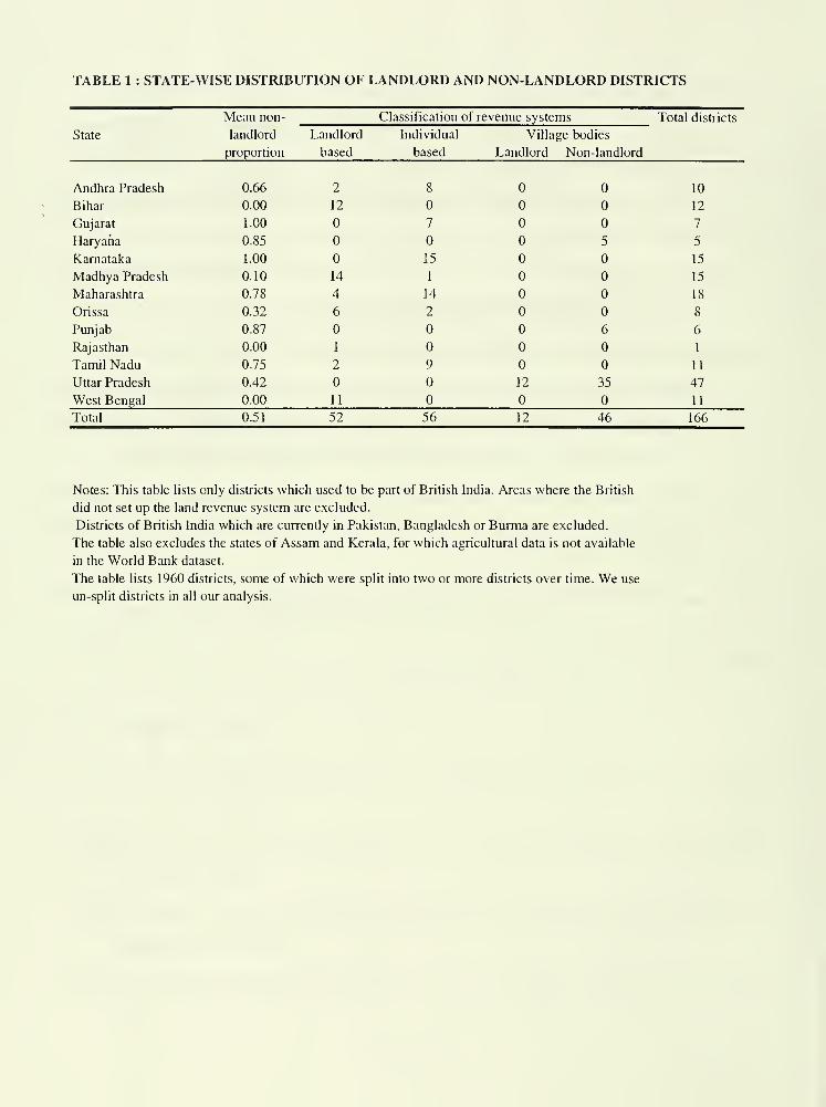
TABLE 1 : STATE-WISE DISTRIBUTION OF LANDLORD AND NON-LANDLORD DISTRICTS

Mean non-

landlord

Classification of revenue systems Total districts

State Landlord Individual Villagie bodies

proportion based based Landlord Non-landlord

Andhra Pradesh 0.66 2 8 10

Bihar 0.00 12 12

Gujarat 1.00 7 7

Haryafia 0.85 5 5

Kamataka 1.00 15 15

Madhya Pradesh 0.10 14 1 15

Maharashtra 0.78 4 14 18

Orissa 0.32 6 2 8

Punjab 0.87 6 6

Rajasthan 0.00 1 1

Tamil Nadu 0.75 2 9 11

Uttar Pradesh 0.42 12 35 47

West Bengal 0.00 11 11

Total 0.51 52 56 12 46 166

Notes: This table lists only districts which used to be part of British India. Areas where the British

did not set up the land revenue system are excluded.

Districts of British India which are currently in Pakistan, Bangladesh or Burma are excluded.

The table also excludes the states of Assam and Kerala, for which agricultural data is not available

in the World Bank dataset.

The table lists 1960 districts, some of which were split into two or more districts over time. We use

un-split districts in all our analysis.

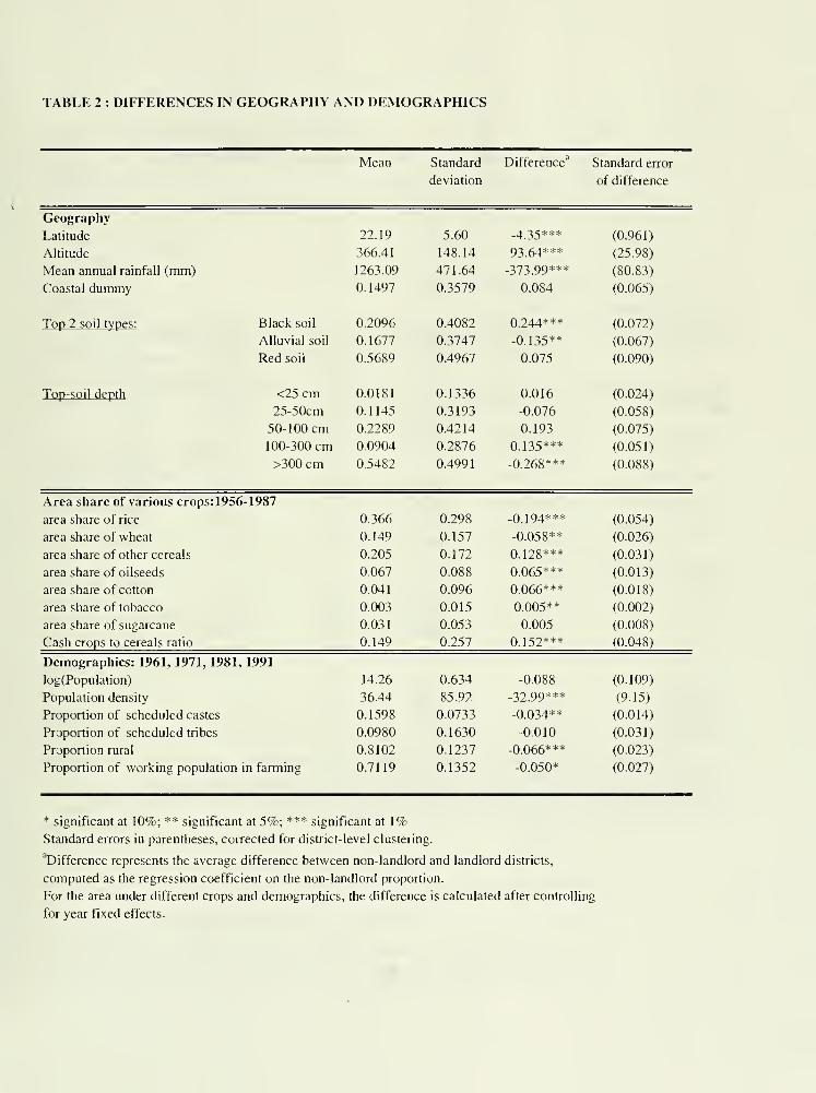
TABLE 2 : DIFFERENCES IN GEOGRAPHY AND DEMOGRAPHICS

Mean Standard

deviation

Difference'' Standard error

of difference

Geography

Latitude 22.19 5.60 -4.35*** (0.961)

Altitude 366.41 148.14 93.64*** (25.98)

Mean annual rainfall (mm) 1263.09 471.64 -373.99*** (80.83)

Coastal dummy 0.1497 0.3579 0.084 (0.065)

Top 2 soil types: Black soil 0.2096 0.4082 0.244*** (0.072)

Alluvial soil 0.1677 0.3747 -0.135** (0.067)

Red soil 0.5689 0.4967 0.075 (0.090)

Top-soil depth <25cm 0.0181 0.1336 0.016 (0.024)

25-50cm 0.1145 0.3193 -0.076 (0.058)

50-100 cm 0.2289 0.4214 0.193 (0.075)

100-300 cm 0.0904 0.2876 0.135*** (0.051)

>300 cm 0.5482 0.4991 -0.268*** (0.088)

Area share of various crops:1956-1987

area share of rice 0.366 0.298 -0.194*** (0.054)

area share of wheat 0.149 0.157 -0.058** (0.026)

area share of other cereals 0.205 0.172 0.128*** (0.031)

area share of oilseeds 0.067 0.088 0.065*** (0.013)

area share of cotton 0.041 0.096 0.066*** (0.018)

area share of tobacco 0.003 0.015 0.005** (0.002)

area share of sugarcane 0.031 0.053 0.005 (0.008)

Cash crops to cereals ratio 0.149 0.257 0.152*** (0.048)

Demographics: 1961, 1971, 1981, 1991

log(Population) 14.26 0.634 -0.088 (0.109)

Population density 36.44 85.92 -32.99*** (9.15)

Proportion of scheduled castes 0.1598 0.0733 -0.034** (0.014)

Proportion of scheduled tribes 0.0980 0.1630 -0.010 (0.031)

Proportion rural 0.8102 0.1237 -0.066*** (0.023)

Proportion of working population in fanning 0.7119 0.1352 -0.050* (0.027)

* significant at 10%; ** significant at 5%; *** significant at 1%Standard errors in parentheses, corrected for district-level clustering.

^Difference represents the average difference between non-landlord and landlord districts,

computed as the regression coefficient on the non-landlord proportion.

For the area under different crops and demographics, the difference is calculated after controlling

for year fixed effects.

TABLE 3 : DIFFERENCES IN AGRICULTURAL INVESTMENTS AND YIELDS

Mean non-landlord proportion = 0.5051 (s.d.=0.4274)

Dependent variable Mean of dependent Coefficient on non-landlord proportion

variable OLS OLS

Full sample Excluding Bengal

and BihiU"

Coefficient on non-landlord dummy

OLS OLS

Full sample Excluding village-

based districts

AGRICULTURAL INVF^STMENTS

Proportion of irrigated area

fertilizer use (kg/ha)

% rice area under HYV

% wheat area under HYV

% other cereals area under HYV

AGRICULTURAL PRODUCTIVITY

log(yield of 1 5 major crops)

log(rice yield)

]og(\vheat yield)

No, of districts

Year fixed effects

Geographic controls

Length of British rule

Clustering for errors

0.277 0.069* 0.070* 0.083*** O.OIO

(0.035) (0.036) (0.027) (0.035)

24.594 10.953*** 11.245*** 10.290*** 10.945***

(3.355) (3.424) (2.316) (3.038)

0.284 0.080* 0.096** 0.018 0.082**

(0.044) (0.043) (0.032) (0.039)

0.495 0.090* 0.119*** 0.029 0.095*

(0.046) (0.045) (0.036) (0.053)

0.189 0.056* 0.084*** -0.035 0.110***

(0.031) (0.024) (0.025) (0.041)

0.158** 0.153** 0.173*** 0.090

(0.071) (0.074) (0.053) (0.083)

0.168** 0.194** 0.100 0.177**

(0-081) (0.081) (0.062) (0.077)

0.228*** 0.228*** 0.188*** 0.139

(0.067) (0.070) (0.053) (0.096)

166 143 166 109

YES YES YES YES

YES YES YES YES

YES YES YES YES

YES YES YES YES

Standard errors in parentheses, corrected for district-level clustering. * significant at 10%; ** significant at 5%; *** significant at 1 %Each cell represents the coefficient from a regression of the dependent variable on the measure of non-landlord control.

Data are from 1956-87. Geographic controls are altitude, latitude, mean annual rainfall, and dummies for soil type and coastal regions.

The non-landlord dummy is assigned as follows: the dummy equals one for all individual-based districts and all village-based districts except those

in Oudh. For landlord-based districts and the village-based districts of Oudh, the dummy is zero.

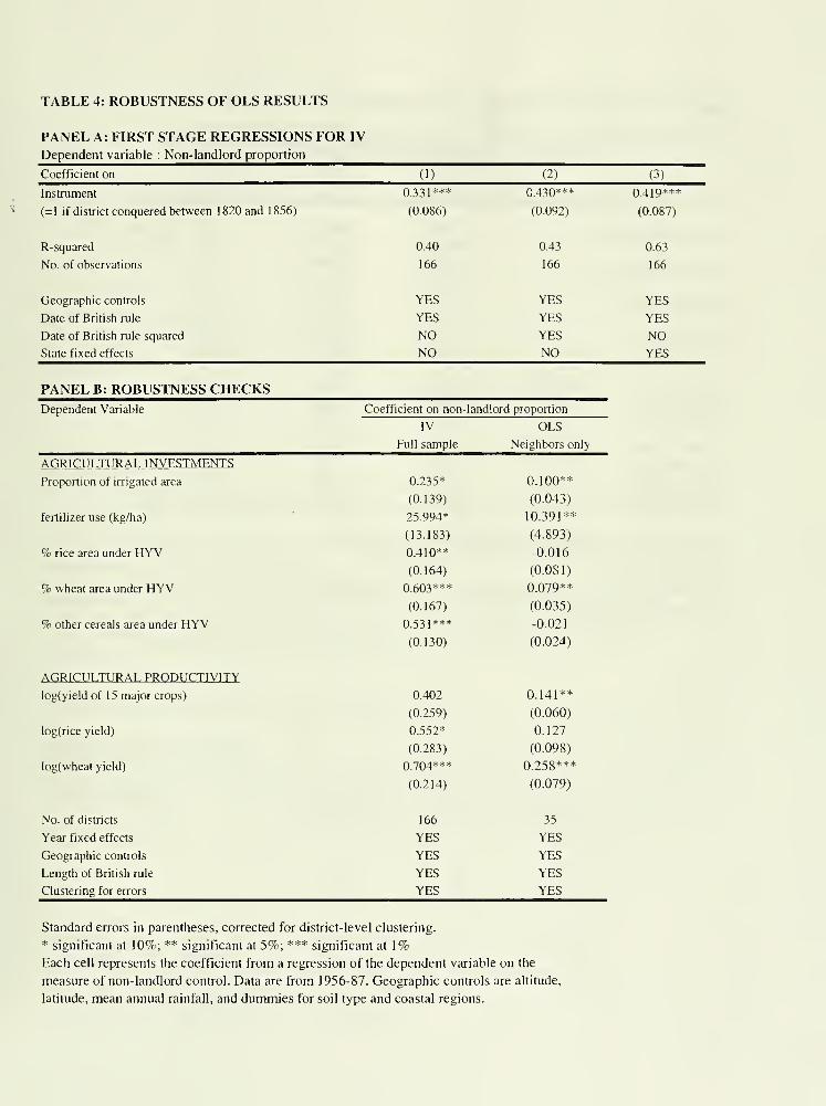
TABLE 4: ROBUSTNESS OF OLS RESULTS

PANEL A: FIRST STAGE REGRESSIONS FOR IV

Dependent variable : Non-landlord proportion

Coefficient on (1) (2) (3)

Instrument

(=1 if district conquered between 1820 and 1856)

R-squared

No. of observations

Geographic controls

Date of British rule

Date of British rule squared

State fixed effects

0.331*** 0.430*** 0.419*^

(0.086) (0.092) (0.087

0.40 0.43 0.63

166 166 166

YES YES YESYES YES YESNO YES NONO NO YES

PANEL B: ROBUSTNESS CHECKSDependent Variable Coefficient on non-landlord proportion

IV OLS

Full sample Neighbors only

AGRICULTURAL INVESTMENTS

Proportion of irrigated area

fertilizer use (kg/ha)

% rice area under HYV

% wheat area under HYV

% other cereals area under HYV

AGRICULTURAL PRODUCTIVITY

log(yield of 1 5 major crops)

log(rice yield)

log(wheat yield)

No. of districts

Year fixed effects

Geographic controls

Length of British rule

Clustering for errors

0.235* 0.100**

(0.139) (0.043)

25.994* 10.391**

(13.183) (4.893)

0.410** -0.016

(0.164) (0.081)

0.603*** 0.079**

(0.167) (0.035)

0.531*** -0.021

(0.130) (0.024)

0.402 0.141**

(0.259) (0.060)

0.552* 0.127

(0.283) (0.098)

0.704*** 0.258***

(0.214) (0.079)

166 35

YES YES

YES YES

YES YES

YES YES

Standard errors in parentheses, corrected for district-level clustering.

* significant at 10%; ** significant at 5%; *** significant at 1%Each cell represents the coefficient from a regression of the dependent variable on the

measure of non-landlord control. Data are from 1956-87. Geographic controls are altitude,

latitude, mean annual rainfall, and dummies for soil type and coastal regions.

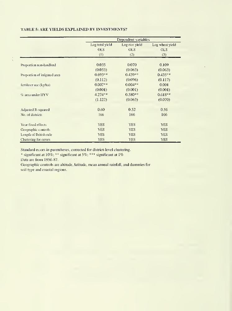
TABLE 5: ARE YIELDS EXPLAINED BY INVESTMENTS?

Dependent variables

Log total yield Log rice yield Log wheat yield

OLS OLS OLS

(1) (2) (3)

0.035 0.070 0.109

(0.053) (0.063) (0.063)

0.693** 0.439** 0.435**

(0.112) (0.096) (0.117)

0.007** 0.004** 0.001

(0.001) (0.001) (0.001)

4.274** 0.580** 0.618**

(1.122) (0.063) (0.070)

0.60 0.52 0.56

166 166 166

YES YES YES

YES YES YES

YES YES YES

YES YES YES

Proportion non-landlord

Proportion of irrigated area

fertilizer use (kg/ha)

% area under HYV

Adjusted R-squared

No. of districts

Year fixed effects

Geographic controls

Length of British rule

Clustering for errors

Standard errors in parentheses, corrected for district-level clustering.

* significant at 10%; ** significant at 5%; *** significant at 1%Data are from 1956-87.

Geographic controls are altitude, latitude, mean annual rainfall, and dummies for

soil type and coastal regions.

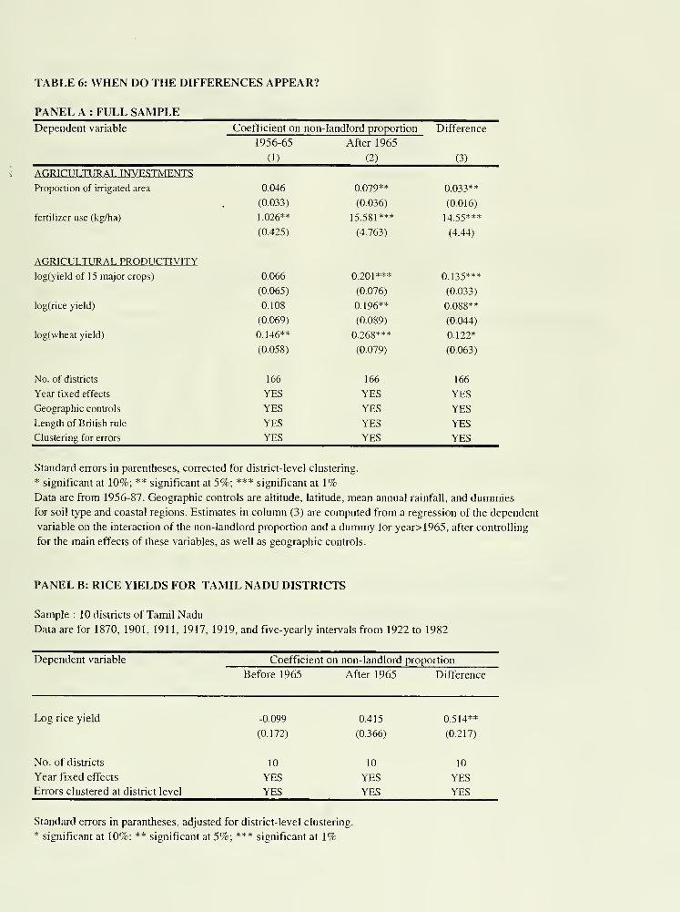
TABLE 6: WHEN DO THE DIFFERENCES APPEAR?

PANEL A : FULL SAMPLEDependent variable Coefficient on non-landlord proportion

1956-65 After 1965

(1) (2)

Difference

(3)

AGRICULTIJRAT. INVESTMENTS

Proportion of irrigated area

fertilizer use (kg/ha)

AGRICULTURAL PRODUCTIVITY

log(yield of 15 major crops)

log(rice yield)

]og(wheat yield)

No. of districts

Year fixed effects

Geographic controls

Length of British rule

Clustering for errors

0.046 0.079** 0.033**

(0.033) (0.036) (0.016)

1.026** 15.581*** 14.55***

(0.425) (4.763) (4.44)

0.066 0.201*** 0.135***

(0.065) (0.076) (0.033)

0.108 0.196** 0.088**

(0.069) (0.089) (0.044)

0.146** 0.268*** 0.122*

(0.058) (0.079) (0.063)

166 166 166

YES YES YES

YES YES YES

YES YES YES

YES YES YES

Standard errors in parentheses, corrected for district-level clustering.

* significant at 10%; ** significant at 5%; *** significant at 1%Data are from 1956-87. Geographic controls are altitude, latitude, mean annual rainfall, and dummies

for soil type and coastal regions. Estimates in colurrui (3) are computed from a regression of the dependent

variable on the interaction of the non-landlord proportion and a dummy for year>1965, after controlling

for the main effects of these variables, as well as geographic controls.

PANEL B: RICE YIELDS FOR TAMIL NADU DISTRICTS

Sample : 10 districts of Tamil Nadu

Data are for 1870, 1901, 1911, 1917, 1919, and five-yearly intewals from 1922 to 1982

Dependent variable Coefficient on non-landlord proportion

Before 1965 After 1965 Difference

Log rice yield

No. of districts

Year fixed effects

Errors clustered at district level

-0.099 0.415 0.514**

(0.172) (0.366) (0.217)

10 10 10

YES YES YES

YES YES YES

Standard errors in parantheses, adjusted for district-level clustering.

* significant at 10%; ** significant at 5%; *** significant at 1%

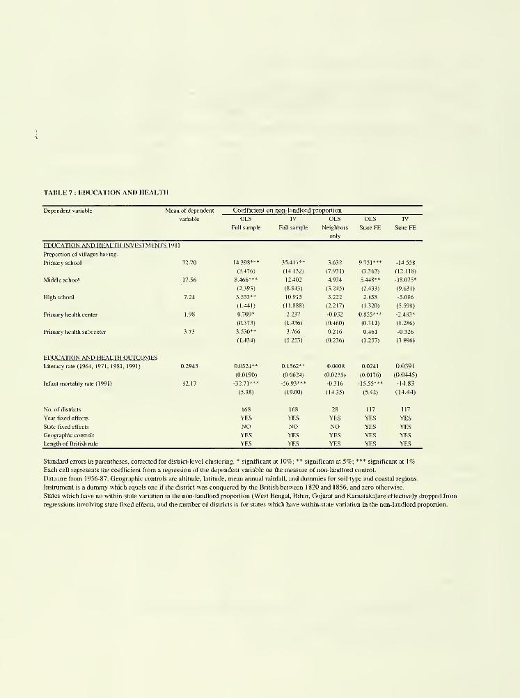
TABLE 7 : EDUCATION AND HEALTH

Dependent variable Mean of dependent

variable

Coefficient on non-landlord proportion

OLS

Full sample

IV

Full sample

OLS

Neighbors

only

OLS

State FE

IV

State FE

EDUCATION AND HEALTH INVESTMENTS l')S l

Proportion of villages having:

Primary school 72.70

Middle school

High school

Primary health center

Primary health subcenter

17.56

7.24

L98

3.73

14.398***

(3.476)

8.466***

(2.393)

3.553**

(1.441)

0.709*

(0.373)

3.530**

(1.434)

35.411**

(14.132)

12.402

(8.843)

10.915

(11.888)

2.237

(1.436)

3.766

(5.253)

3.632

(7.93 1

)

4.934

(3.245)

3.222

(2.217)

-0.032

(0,460)

0.216

(0.236)

9.751***

(3.363)

5.448**

(2.433)

2,158

(1.320)

0.855***

(0.311)

0,461

(1.257)

-14.558

(12.118)

-18.075*

(9.631)

5,086

(5.598)

-2,483*

(1,286)

-0.326

(3.896)

EDI ICATION AND HEAI .TH Ol ITCOMF.S

Literacy rate (1961, 1971, 1981, 1991) 0.2945

Infant mortality rate (1991) 82.17

0.0524**

(0.0190)

-32.71***

(5.38)

0.1562**

(0.0624)

56.93***

(19.00)

-0.0008

(0.0235)

0.316

(14.35)

0.0241

(0.0176)

-15.55***

(5.42)

0.0391

(0.0445)

-14.83

(14.44)

No. of districts

Year fixed effects

State fixed effects

Geographic controls

Length of British rule

158

YES

NOYES

YES

168

YES

NOYES

YES

28

YES

NOYES

YES

117

YES

YES

YES

YES

117

YES

YES

YES

YES

Standard errors in parentheses, corrected for district-level clustering. * significant at 10%; ** significant al 5%; *** significant at 1%Each cell represents the coefficient from a regression of the dependent variable on the measure of non-laiidlord control.

Data are from 1956-87. Geographic controls are altitude, latitude, mean annual rainfall, and dummies for soil type and coastal regions.

Instrument is a dummy which equals one if the district was conquered by the British between 1 820 and 1 856, and zero otherwise.

States which have no within-stale variation in the non-landlord proportion (West Bengal, Bihar, Gujarat and Kamataka)are effectively dropped from

regressions involving state fixed effects, and the number of districts is for slates which have witlun-state variation in the non-landlord proportion.

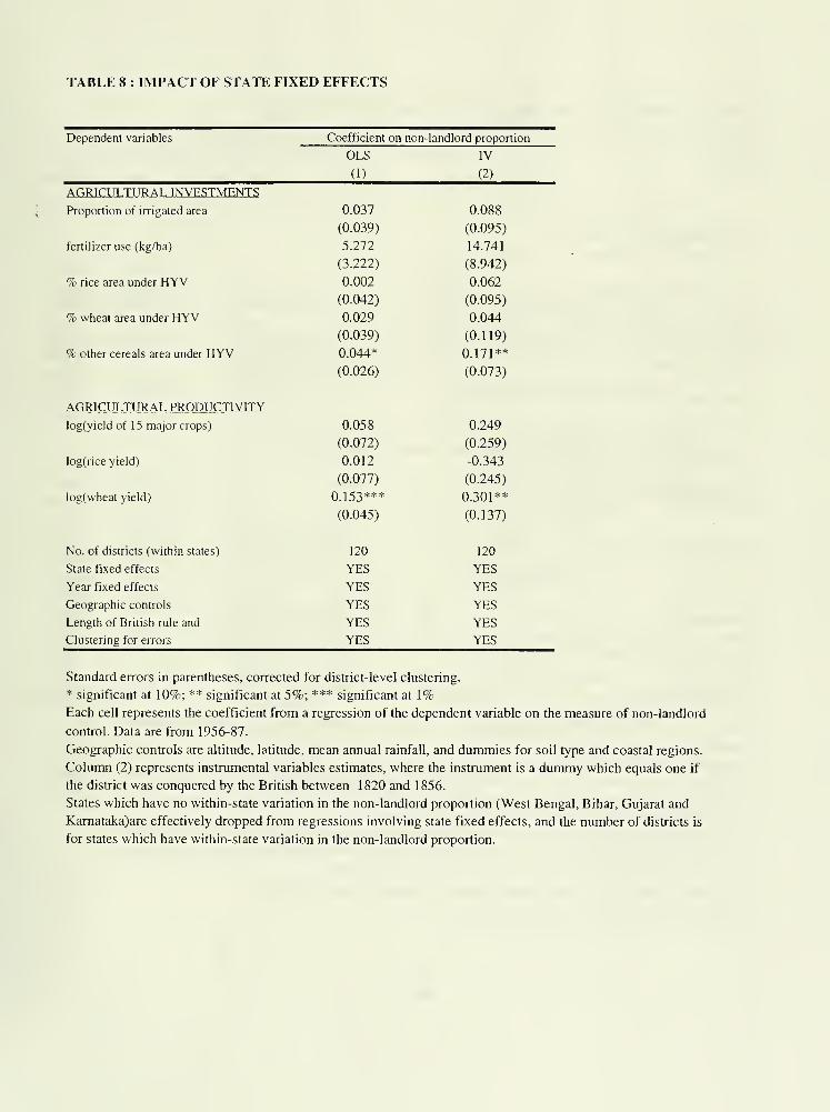
TABLE 8 : IMPACT OF STATE FIXED EFFECTS

Dependent variables Coefficient on non-landlord proportion

AGRICULTURAL INVESTMENTS

Proportion of irrigated area

fertilizer use (kg/ha)

% rice area under HYV

% wheal area under HYV

% other cereals area under HYV

AGRICULTURAL PRODUCTIVITY

log(yield of 15 major crops)

log(rice yield)

log(wheat yield)

No. of districts (within states)

State fixed effects

Year fixed effects

Geographic controls

Length of British rule and

Clustering for errors

OLS

(1)

IV

(2)

0.037 0.088

(0.039) (0.095)

5.272 14.741

(3.222) (8.942)

0.002 0.062

(0.042) (0.095)

0.029 0.044

(0.039) (0.119)

0.044* 0.171**

(0.026) (0.073)

0.058 0.249

(0.072) (0.259)

0.012 -0.343

(0.077) (0.245)

0.153*** 0.301**

(0.045) (0.137)

120 120

YES YES

YES YES

YES YES

YES YES

YES YES

Standard errors in parentheses, corrected for district-level clustering.

* significant at 10%; ** significant at 5%; *** significant at 1%Each cell represents the coefficient from a regression of the dependent variable on the measure of non-landlord

control. Data are from 1956-87.

Geographic controls are altitude, latitude, mean annual rainfall, and dummies for soil type and coastal regions.

Column (2) represents instrumental variables estimates, where the instrument is a dummy which equals one if

the district was conquered by the British between 1820 and 1856.

States which have no within-state variation in the non-landlord proportion (West Bengal, Bihar, Gujarat and

Kamataka)are effectively dropped from regressions involving state fixed effects, and the number of districts is

for states which have within-state variation in the non-landlord proportion.

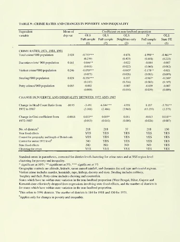
TABLE 9 : CRIME RATES AND CHANGES IN POVERTY AND INEQUALITY

Dependent Mean of

dep.var

Coefficient on non-landlord proportion

variable OLS OLS OLS IV OLSFull sample Full sample Neighbors only Full sample State FE

(1) (2) (3) (4) (5)

CRTMR RATES: 197L 1981. 1991

Total crime/'OOO population 2.024 -0.733*** -0.178 -1.998** -0.461**

(0.239) (0.423) (0.888) (0.223)

Dacoities+riots/ '000 population 0.161 -0.046** -0.022 -0.084 -0.007

(0.018) (0.022) (0.060) (0.012)

Violent crime/'OOO population 0.246 -0.070*** -0.045* -0.178** -0.021

(0.023) (0.026) (0.083) (0.019)

Stealing/'OOO population 0.824 -0.358*** 0.137 -0.967* -0.210*

(0.112) (0.316) (0.503) (0.119)

Petty crimes/'OOO population 0.055 -0.002 -0.007 -0.059 -0.007

(0.009) (0.010) (0.039) (0.009)

CHANGE IN POVERTY AND INEOUALITY BETWEEN 1972 AND 1987

Change in Head Count Ratio from -10.95 -3.491 -6.844*** -4.951 8.187 -5.701**

1972 to 1987 (3.108) (2.466) (2.965) (13.235) (2.275)

Change in Gini coefficient from -0.0018 0.033** 0.019* 0.011 -0.013 0.018**

1972-1987 (0.013) (0.010) (0.010) (0.026) (0.007)

No. of districts'* 218 218 37 218 150

Year fixed effects YES YES YES YES YESControl for geography and length of British rule YES YES YES YES YESControl for initial 1972 level'' NO YES YES YES YESState fixed effects NO NO NO NO YESClustering for errors YES YES YES ^TS YES

Standard errors m parentheses, corrected for district-level clustering for crime rates and at NSS region level

clustering for poverty and inequality.

* significant at 10%; ** significant at 5%; *** significant at 1%Geographic controls are altitude, latitude, mean annual rainfall, and dummies for soil type and coastal regions.

Violent crime includes murder, homicide, rape, kidnap, dacoity and riots. Stealing includes robbery,

burglary and theft. Petty crime includes cheating and counterfeit.

States which have no within-state variation in the non-landlord proportion (West Bengal, Bihar, Gujarat and

Kamataka)are effectively dropped from regressions involving state fixed effects, and the number of districts is

for states which have within-state variation in the non-landlord proportion.

"This refers to 1991 districts. The number of districts is 184 for 1981 and 150 for 1971.

Applies only for changes in poverty and inequality.

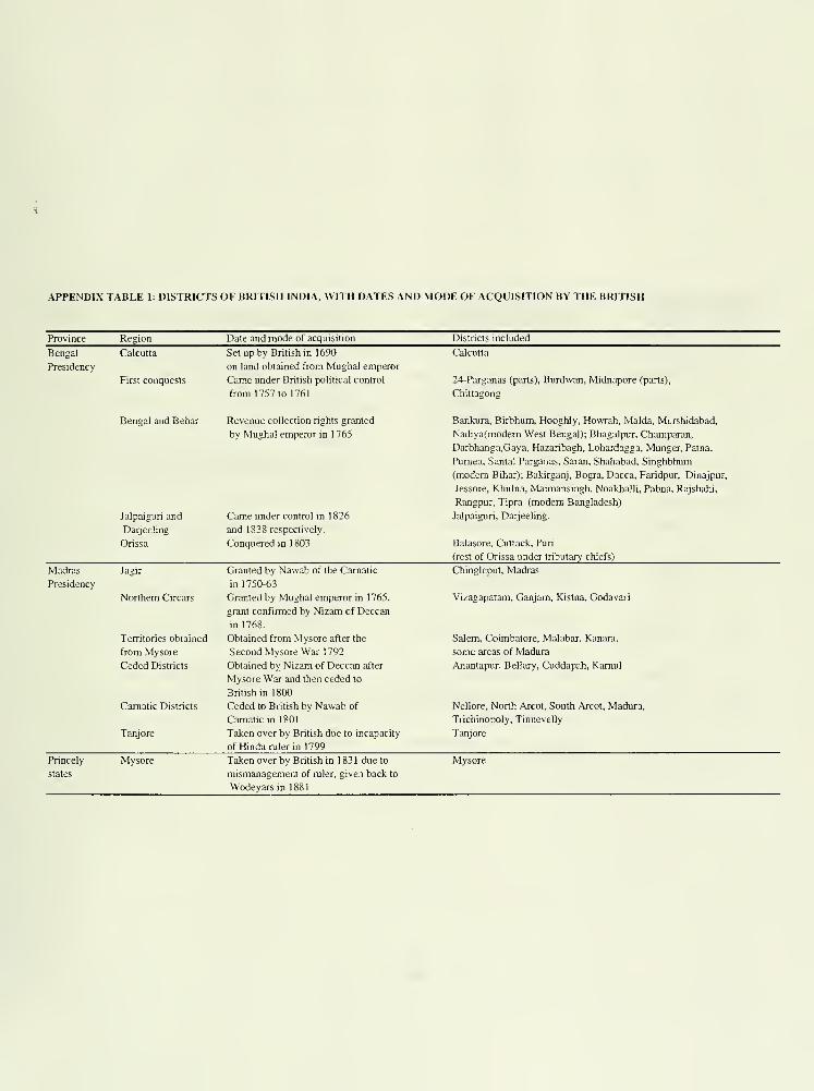
APPENDIX TABLE 1: DISTRICTS OF BRITISH INDIA, WITH DATES AND MODE OF ACQUISITION BY THE BRITISH

Province Resion Dale and mode of acquisilion Districts included

Bengal

Presidency

Calcutta

First conquests

Bengal and Behar

Jalpaiguri and

Darjeeling

Orissa

Set up by British m 1690

on land obtained from Mughal emperor

Came under British political control

from 1757 to 1761

Revenue collection rights granted

by Mughal emperor in 1765

Came under control in 1826

and 1 838 respectively.

Conquered in 1 803

Calcutta

24-Parganas (parts), Burdwan, Midnapore (parts),

Chittagong

Banlcura, Birbhum, Hooghly, Howrah, Malda, Murshidabad,

Nadiya(modem West Bengal); Bhagalpur, Champaran,

Darbhanga.Gaya, Hazaribagh, Lohardagga, Munger, Patna,

Pumea. Santal Parganas, Saran, Shahabad, Singhbhum

(modem Bihar); Bakirganj, Bogra, Dacca, Faridpur, Dinajpur,

Jessore. Khulna, Maimansingh, Noakhalli, Pabna, Rajshahi,

Rangpur. Tipra (modem Bangladesh)

Jalpaiguri, Darjeeling.

Balasore. Cuttack, Puri

(rest of Orissa under tributary chiefs)

Madras

Presidency

Jagir

Northern Circars

Territories obtained

from Mysore

Ceded Districts

Camatic Districts

Tanjore

Granted by Nawab of the Camatic

in 1750-63

Granted by Mughal emperor in 1765,

grant confirmed by Nizam of Deccan

in 1768.

Obtained from Mysore after the

Second Mysore War 1792

Obtained by Nizam of Deccan after

Mysore War and then ceded to

British in 1800

Ceded to British by Nawab of

Camatic in 1801

Taken over by British due to incapacity

of Hindu ruler in 1799

Chingleput, Madras

Vizagapatam, Ganjam. Kistna, Godavari

Salem, Coimbatore, Malabar, Kanara,

some areas of Madura

Anantapur. Bellary, Cuddapah, Kamul

Nellore, North Arcot, South Arcot, Madura,

Trichinopoly, Tinnevelly

Tanjore

Princely

states

Mysore Taken over by British in 1831 due to

mismanagement of ruler, given back to

Wodeyarsinl881

Mysore

Province Region Date and mode of acquisition Districts included

United

Provinces

Benares

Ceded Districts

Conquered Districts

Bundelkhand

Taken over

Dehradun

Oudh

Ceded by the Nawab of Oudh m 1775

Ceded by the Nawab of Oudh in 1 801

Conquered by Lord Lake from Scindia

and others in 1 803

Conquered in parts from 1803-17.

Taken over due to lapse, forfeiture etc.

in years after 1 840.

Ceded after the Nepal war in 1815

Annexed from Nawab of Oudh in 1856.

Benares, Mirzapur, Jaunpur, Ghazipur, Ballia,

Azamgarh, Gorakhpur, Basti, Allahabad, Fatehpur, Kanpur,

Farukhabad, Elawa, Mainpuri, Etah, Shahjahanptir, Badayun,

Bareli, Pilibhit, Moradabad, Bijnaur, Tarai Parganas

Agra, Mathura, Aligarh, Bulandshahr, Meerut,

Muzaffamagar, Saharanpur

Banda, Hamirpur

Jalaun, Jhansi, Lalitpur

Dehradun.

Kheri, Sitapur, Hardoi, Lucknow, Unao, Barabanki, Rai-Bareli,

Partabgarh, Sultanpur, Faizabad, Gonda, Bahraich

Bombay

Presidency

Assam

Surat

Gujarat

Maratha territory

Satara

Kanara

Sindh

Panch Mahals

From Bengal

Assam

Hill districts

Obtained from Nawab of Surat in 1 800

Conquered from Baroda in 1803 and

Marathas in 1818.

Conquered from Peshwa in 1818

Taken over by lapse in 1 848

Transferred from Madras in 1 862

Conquered in 1843

Obtained in 1861

Obtained as part of diwani in 1765,

later transferred to Assam

Conquered in 1824

Brought under control in 1 830-35

Surat

Ahmedabad, Kaira, Broach

Thana, Khandesh, Nasik, Ahmednagar, Poona, Sholapur.

Kolaba, Ratnagiri, Belgaum (some parts obtained in 1827),

Bijapur, Dharwar

Satara

Kanara

Karachi, Haidarabad, Shikarpur, Upper Sindh Frontier,

Thar & Parkar (modem Pakistan)

Panch Mahals

Goalpara (modem Assam), Sylhet (modem Bangladesh)

Darrang, Kamrup, Lakhimpur, Naugong, Sibsagar

Cachar, Cachar Hills, Eastern Dwars (1866), Jaintya

Parganas, Khasi and Jaintyas, Naga Hills.

Central Maratha territory Conquered from Bhonsle in 1818; some areas

Provinces left under Bhonsle till 1854

Sambalpur Conquered in 1818, under local chief

till 1849

Balaghat, Betul, Bhandara, Bilaspur, Chanda, Chhindwara,

Damoh, Hoshangabad, Jabalpur, Mandla, Nagpur,

Narsinghpur, Nimar (1820), Raipur, Sagar, Seoni, Wardah

Sambalpur

Province Region Dale and mode of acquisition

Panjab Delhi Conquered in 1 803

Sikh territory Obtained after Sikh War in 1 845-46

Sikh territory Obtained after Sikh War in 1 849

Shimla Obtained in 1815

Source: Baden-Powell (1892,1894), Kumar (1982)

Districts included

Delhi, Gurgaon, Hisar, Kamal

Ambala, Firozpur, Hoshiyarpur, Jalandhar, Kangra. Ludhiana

Amritsar, Gurdaspur, Rohtak (India); Bannu, Dera Ghazi Khan,

Dera Ismail Khan, Gujranwala, Gujrat, Hazara. Jhang, Jhelum,

Kohat, Lahore, Montgomerty, Multan, Muzaffargarh, Peshawar,

Rawalpindi. Shahpur, Sialkot (Pakistan)

Shimla

APPENDIX TABLE 2: ESTABLISHMENT OF LAND REVENUE SYSTEMS IN BRITISH INDIA

Province Dates of British conquest/ Formation of land tenure system

land revenue control

Bengal

Presidency

1757, 1765 Revenue auctions in early 1770s; old landlords dispossessed,

several defaults and famine;old landlords reinstated in 1-784;

Lord Comwallis announces Permanent Settlement in 1793:

landlords' rents fixed in perpetuity with stiff penalties for default.

Madras

Presidency

1765, 1790-1801 1765 territories came under Permanent Settlement.

Munro and Read tried individual system in some districts from

1796-1805; in 1807 all districts put under landlords for 3 years,

leases renewed for 10 years in 1810-11; Munro went to England

and convinced the Directors of the East India Company to order

an individual settlement in the whole of Madras;order implemented

after 1820 when leases expired; all future defaulting landlord

estates also converted to individual system.

Bombay

Presidency

1803, 1817-18 Individual system tried in Poona in 1820's, but failed; Wingate and

Goldsmid start Bombay Survey System in 1835 for individual

settlement system; a few long-standing landlords left in place in

certain areas.

North-West

Provinces

1775, 1801-03 Permanent Settlement in 1775 areas.

3 and 4-year landlord leases in 1802-1819. Question of Permanent

Settlement widely debated; revenue secretary Holt Mackenzie's

1819 Minute recognized the existence of village bodies and asked

for their rights to be protected in any settlement; regulation passed

in 1822.

Oudh 1856 Lord Dalhousie announced settlement with village bodies wherever

possible; Mutiny in 1857 before this could be done; Lord Canning

reverses policy in 1858 and brings back landlords {talukdars) with full

proprietary rights.

Central

Provinces

1818, 1849 No fixed policy until landlord settlement ("malguzari")

announced in 1853, implemented in 1850s. Sambhalpur

district however put under individual cultivator system.

Berar 1856 Was under Nizam till 1856; first landlord system was tried and it

failed; then Bombay Survey System (individual cultivator) was

applied.

Assam 1765, 1824-26 Some areas transferred from Bengal had Permanent Settlement;

others got individual-cultivator systems.

Panjab 1846, 1 849 Village-based system put into place everywhere; practically no

big landlords.

APPENDIX TABLE 3: DATA SOURCES AND CONSTRUCTION OF VARIABLES

Post-Independence data

Data on district geography, crop areas, yields, irrigation, fertilizer use, adoption of

high-yielding varieties: India Agriculture and Climate Data Set (World Bank)

http://wwvv-esd.worldbank.org/indian/home.cfm

District level data on literacy, occupation classes, proportion of scheduled castes etc:

Indian Database Project Vanneman, Reeve and Douglas Barnes (2000)

Indian District Data, 1961-1991: Machine-readable data file and codebook. Center on Population,

Gender, and Social Inequality, College Park, Maryland.

URL: http://www.bsos.umd.edu/socy/vanneman/districts/index.html

Districts and maps of modem India: http://www.mapsofindia.com

Village infrastructure variables: State statistical abstracts of 1981

Land-holdings by size category: Agricultural census of 1990-91.

Data on poverty and inequality (1972, 1987): based on National Sample Surveys.

Historical data

Districts and maps of British India: Baden-Powell (1892)

Non-landlord proportion:

For Uttar Pradesh, Madhya Pradesh and Panjab: computed from district-level Land Settlement

Reports as the proportion of villages, estates or land area not under the revenue liability of landlords.

The Settlement Reports were compiled by British administrators in the 1870's and 1880's.

For Madras Presidency: non-landlord proportion obtained from Baden-Powell (1892).

For Bombay Presidency, Bengal Presidency, Orissa, Berar and districts for which we do not have

district-level settlement reports: Non-landlord measure is assigned as zero or one based on

historical accounts of the dominant land tenure system in the district. Sources of information include

Baden-Powell (1892), Gupta (1940), Kumar (1982), Misra (1942), Mukherjee (1962) and Patel (1957).

Land revenue inequality 1885: Digital South Asia Library (http://dsal.uchicago.edu)

Land revenue inequality 1948 for districts of Uttar Pradesh:

Report of the United Provinces Zamindari Abolition Committee, 11 (Allahabad, 1948) pp. 12-17.

Reproduced in Stokes (1978b).

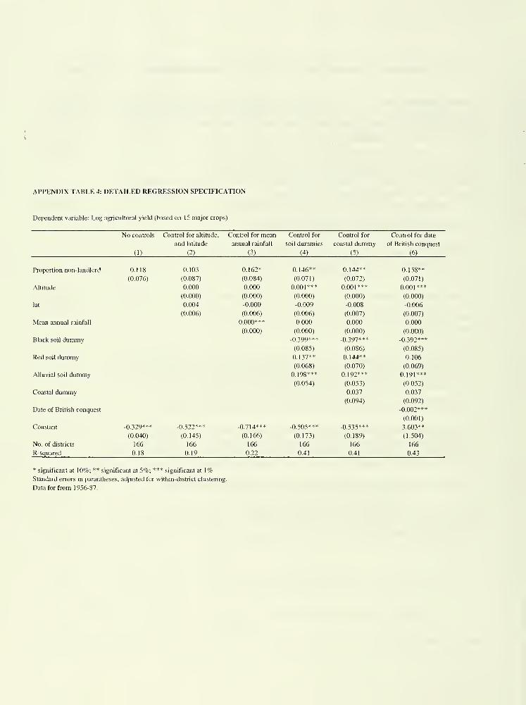
APPENDIX TABLE 4: DETAILED REGRESSION SPECIFICATION

Dependent variable: Log agricultural yield (based on 15 major crops)

No controls Control for altitude. Conu-ol for mean Control for Control for Control for date

and latitude annual rainfall soil dummies coastal dummy of British conquest

(1) (2) (3) (4) (5) (6)

Proportion non-landlord 0.118 0-103 0-162* 0.146** 0.144** 0.158**

(0.076) (0.087) (0.084) (0.071) (0.072) (0.071)

Altitude 0.000 0.000 0.001*** 0.001*** 0.001***

(0.000) (0.000) (0.000) (0.000) (0.000)

lat 0.004 -0.000 -0.009 -0-008 -0.006

(0.006) (0.006) (0.006) (0.007) (0.007)

Mean annual rainfall 0.000*** 0.000 0-000 0.000

(0.000) (0.000) (0-000) (0.000)

Black soil dummy -0.399***

(0.085)

-0.397***

(0.086)

•0.392***

(0.085)

Red soil dummy 0.137**

(0.068)

0.144**

(0.070)

0.106

(0.069)

Alluvial soil dummy 0.198***

(0.054)

0.192***

(0.053)

0.191***

(0.052)

Coastal dummy 0.037

(0.094)

0.037

(0.092)

Date of British conquest -0.002***

(0.001)

Constant -0.329*** -0.522*** -0.714*** -0.505*** -0.535*** 3.603**

(0.040) (0.145) (0.166) (0.173) (0.189) (1.504)

No. of districts 166 166 166 166 166 166

R-squared 0.18 0.19 0.22 0.41 0.41 0.43

* significant at 10%; ** significant at 5%; *** significant at 1%Standard errors in parantheses, adjusted for within-district clustering.

Data for from 1956-87.

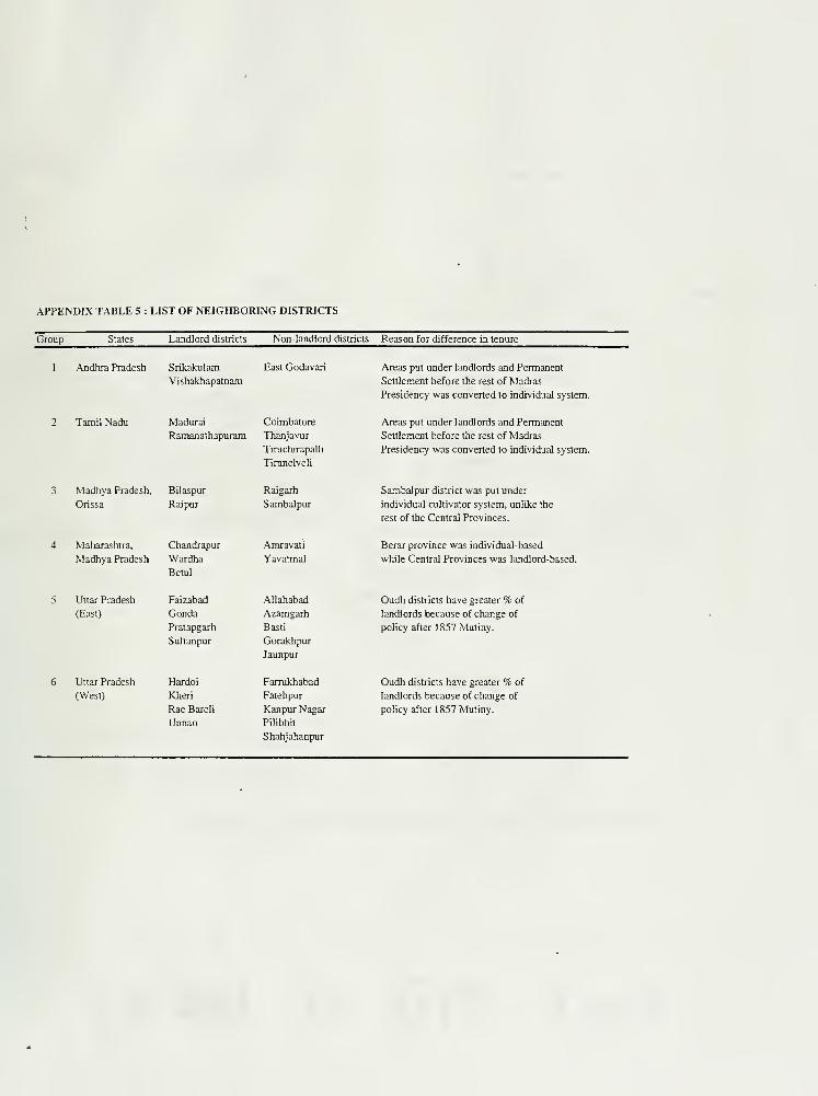
APPENDIX TABLE 5 : LIST OF NEIGHBORING DISTRICTS

Group States Landlord districts Non-landlord districts Reason for difference in tenure

1 Andhr2 Pradesh Srikakulam

Vishakhapatnam

East Godavari

2 Tamil Nadu Madurai Coimbatore

Ramanathapuram Thanjavur

Tirachirapalli

Tirunelveli

3 Madhya Pradesh, Bilaspur Raigarh

Orissa Raipur Sambalpur

4 Maharashtra, Chandrapur Amravati

Madhya Pradesh Wardha

Betul

Yavatmal

5 Uttar Pradesh Faizabad Allahabad

(East) Gonda Azamgarh

Pratapgarh Basti

Sultanpur Gorakhpur

Jaunpur

6 Uttar Pradesh Hardoi FarrukJiabad

(West) Kheri Fatehpur

Rae Bareli Kanpur Nagar

Unnao Pilibhit

Shahjahanpur

Areas put under landlords and Permanent

Settlement before the rest of Madras

Presidency was converted to individual system.

Areas put under landlords and Permanent

Settlement before the rest of Madras

Presidency was converted to individual system.

Sambalpur district was put under

individual cultivator system, unlike the

rest of the Central Provinces.

Berar province was individual-based

while Central Provinces was landlord-based.

Oudh districts have greater % of

landlords because of change of

policy after 1857 Mutiny.

Oudh districts have greater % of

landlords because of change of

policy after 1857 Mutiny.

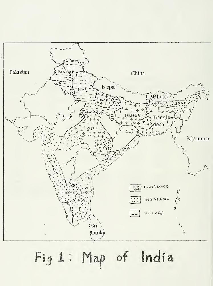
Pakistan

r/ '--'

china

Y—. ^ -/+

_^"'&£-

'^^^y X

+...

.^T^X^- •A S SA M/.'

uj^-

Mvanma]

:ii:a='

ft « • • » •'-1 ,*-

\ i. • < + J

iLarik^

/ ^

* * »

LANDLORD

t3

VILL AGs.£.

M':.'

t

ap of India

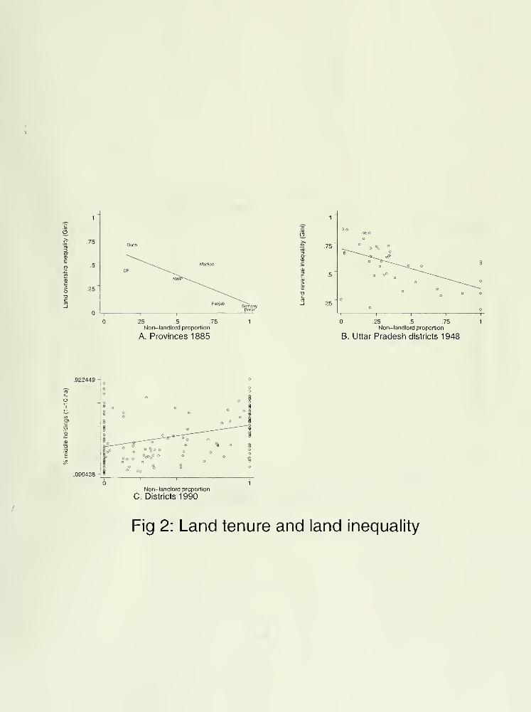
.75

.25

25 .5 75Non-landlord proportion

A. Provinces 1885

.25 .5 .75

Non-landlord proportion

B. Uttar Pradesh districts 1948

922449 -

o

o

o

g-

Q

o

O o

Io ^

e

Q

O

§

o

o

° o

-^—

^

i

——? °o % o %

1oo

o

1% o o

090438 1o Oo

Non-landlord proportion

C. Districts 1990

Fig 2: Land tenure and land inequality

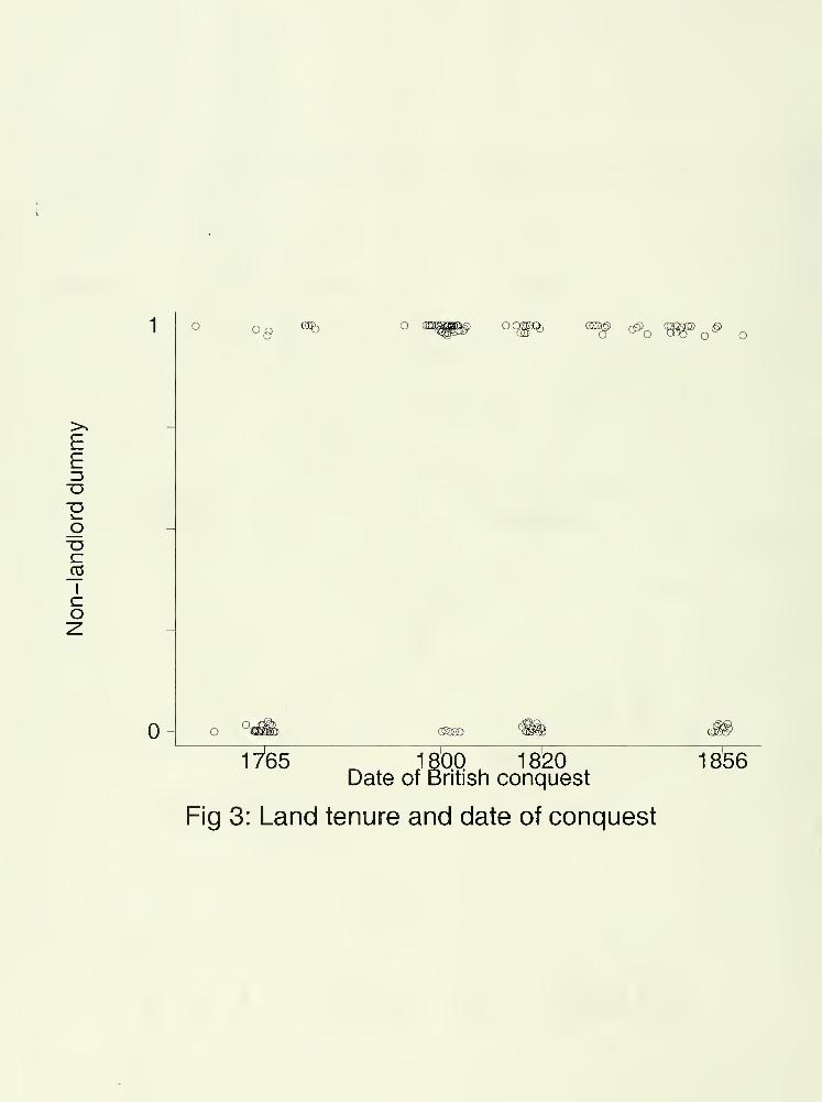
o

Z5D

DC

rco

1^65 1^00 18§0 1856Date of British conquest

Fig 3: Land tenure and date of conquest

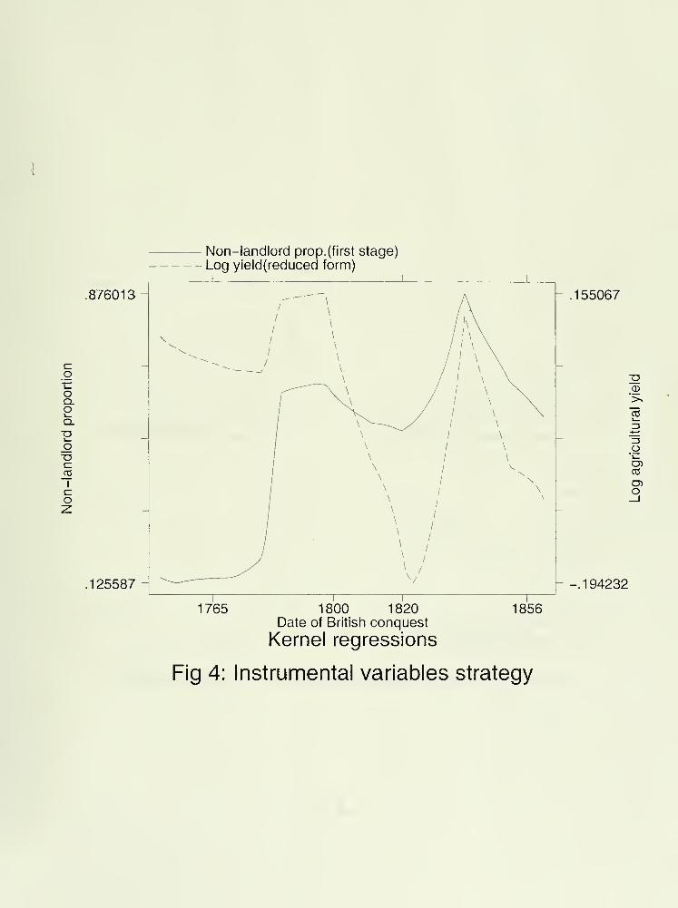
Non-landlord prop.(flrst stage)

Log yleld(reduced form)

.876013

goQ.O

DOT3C_cd

I

o

.125587

.155067

O

03

O

-.194232

1765 1800 1820Date of British conquest

Kernel regressions

1856

Fig 4: Instrumental variables strategy

.508931 1 .37976

-1.95945

1

Non-landlord proportion

A. Uttar Pradesh rice yields: 1870's

1

Non-landlord proportion

B. Uttar Pradesh wheat yields: 1870's

.373244 .99279Non-landlord proportion

C. Tamil Nadu districts 1911

Fig 5: Agricultural yields in Colonial period

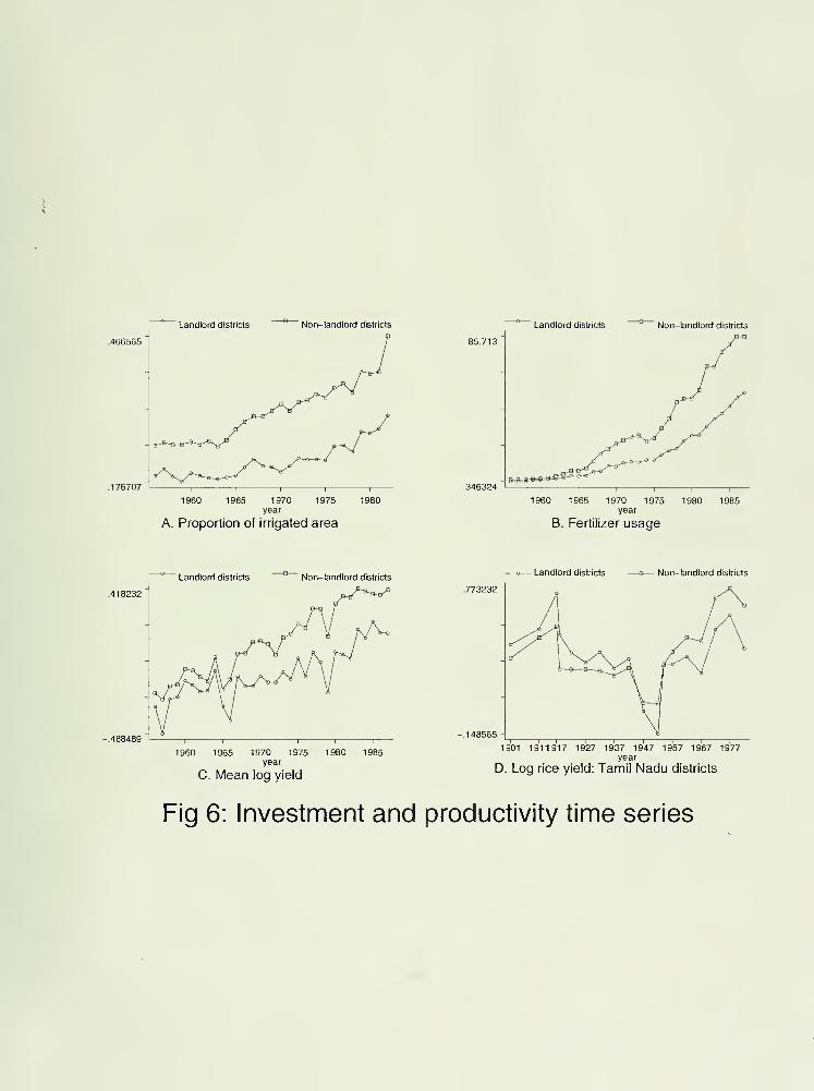
" Landlord districts Non-landlord districts " Landlord districts Non-landlord districts

.466565

1950 1965 1970 1975 1980year

A. Proportion of irrigated area

I960 1965 1970 1975 1980 1985year

B. Fertilizer usage

" Landlord districts Non-landlord districts—e— Landlord districts —b— Non- landlord districts

-.488489

1960 1965 1970 1975 1980 1985year

C. Mean log yield

.773232

1901 1911917 1927 1937 1947 1957 1967 1977year

D. Log rice yield: Tamil Nadu districts

Fig 6: Investment and productivity time series

I^pt^1

1^^"^

Date Due

Lib-26-67

MIT LIBRARIES

3 9080 02527 8513