Embed Size (px)
Citation preview
THE GEOMETRY OF QUADRATIC
POLYNOMIAL DIFFERENTIAL SYSTEMS
WITH A FINITE AND AN INFINITE
SADDLE–NODE (C)
JOAN C. ARTESDepartament de Matematiques, Universitat Autonoma de Barcelona,
08193 Bellaterra, Barcelona, SpainE–mail: [email protected]
ALEX C. REZENDE1 AND REGILENE D. S. OLIVEIRA2
Departamento de Matematica, Universidade de Sao Paulo,13566–590, Sao Carlos, Sao Paulo, Brazil,
E–mail: [email protected], [email protected]
Planar quadratic differential systems occur in many areas of applied mathematics. Althoughmore than one thousand papers have been written on these systems, a complete understandingof this family is still missing. Classical problems, and in particular, Hilbert’s 16th problem[Hilbert, 1900, Hilbert, 1902], are still open for this family. Our goal is to make a global studyof the family QsnSN of all real quadratic polynomial differential systems which have a finitesemi–elemental saddle–node and an infinite saddle–node formed by the collision of two infinitesingular points. This family can be divided into three different subfamilies, all of them withthe finite saddle–node in the origin of the plane with the eigenvectors on the axes and with theeigenvector associated with the zero eigenvalue on the horizontal axis and (A) with the infinitesaddle–node in the horizontal axis, (B) with the infinite saddle–node in the vertical axis and(C) with the infinite saddle–node in the bisector of the first and third quadrants. These threesubfamilies modulo the action of the affine group and time homotheties are three–dimensionaland we give the bifurcation diagram of their closure with respect to specific normal forms, inthe three–dimensional real projective space. The subfamilies (A) and (B) have already beenstudied [Artes et al., 2013b] and in this paper we provide the complete study of the geometryof the last family (C). The bifurcation diagram for the subfamily (C) yields 371 topologicallydistinct phase portraits with and without limit cycles for systems in the closure QsnSN(C)within the representatives of QsnSN(C) given by a chosen normal form. Algebraic invariantsare used to construct the bifurcation set. The phase portraits are represented on the Poincaredisk. The bifurcation set of QsnSN(C) is not only algebraic due to the presence of somesurfaces found numerically. All points in these surfaces correspond to either connections ofseparatrices, or the presence of a double limit cycle.
1
2 J.C. Artes, A.C. Rezende and R.D.S. Oliveira
1. Introduction, brief review of the litera-ture and statement of results
Here we call quadratic differential systems, or sim-ply quadratic systems, differential systems of theform
x = p(x, y),y = q(x, y),
(1)
where p and q are polynomials over R in x and ysuch that the max(deg(p),deg(q)) = 2. To sucha system one can always associate the quadraticvector field
ξ = p∂
∂x+ q
∂
∂y, (2)
as well as the differential equation
q dx− p dy = 0. (3)
The class of all quadratic differential systems (orquadratic vector fields) will be denoted by QS.
We can also write system (1) as
x = p0 + p1(x, y) + p2(x, y) = p(x, y),y = q0 + q1(x, y) + q2(x, y) = q(x, y),
(4)
where pi and qi are homogeneous polynomials of de-gree i in the variables x and y with real coefficientsand p22 + q22 6= 0.
Even after hundreds of studies on the topologyof real planar quadratic vector fields, it is kind ofimpossible to outline a complete characterizationof their phase portraits, and attempting to topo-logically classify them, which occur rather often inapplications, is quite a complex task. This familyof systems depends on twelve parameters, but dueto the action of the group Aff(2,R) of real affinetransformations and time homotheties, the class ul-timately depends on five parameters, but this is stilla large number.
The main goal of this paper is to complete thestudy of the class QsnSN of all quadratic systemspossessing a finite saddle–node sn(2) and an infinite
saddle–node of type(02
)SN . We recall that a fi-
nite saddle–node is a semi–elemental singular pointwhose neighborhood is formed by the union of twohyperbolic sectors and one parabolic sector. By asemi–elemental point we mean a point with zero de-terminant of its Jacobian with only one eigenvalueequal to zero. These points are known in classicalliterature as semi–elementary, but we use the term
semi–elemental introduced in [Artes et al., 2013a]as part of a set of new definitions more deeply re-lated to singularities, their multiplicities and, es-pecially, their Jacobian matrices. In addition, an
infinite saddle–node of type(02
)SN is obtained by
the collision of an infinite saddle with an infinitenode. There are two types of infinite saddle–nodes
and the second one is denoted by(11
)SN which is ob-
tained by the collision of a finite node (respectively,finite saddle) with an infinite saddle (respectively,infinite node) and which will appear in some of thephase portraits.
If we have a finite saddle–node sn(2), the pos-sibility of having two other finite singular points ispresent. Indeed, in case the remaining singularitiesdid not go to infinity, then there are two other sin-gularities in the finite plane, either real, or complex,or the origin may have higher multiplicity.
The class QsnSN is divided into three sub-families according to the position of the infinitesaddle–node, namely QsnSN(A), QsnSN(B) andQsnSN(C). In [Artes et al., 2014] the authorsgave a partition of the closure of the first twosubfamilies and this paper presents a continuationin the study of this subclass QsnSN presentingthe analysis of the closure of the last subfamilyQsnSN(C).
For this analysis we follow the pattern set outin [Artes et al., 2006] and, in order to avoid repeat-ing technical sections which are the same for bothpapers, we refer to the paper mentioned for morecomplete information.
We now give the notion of graphics, which playan important role in obtaining limit cycles whenthey are due to connection of separatrices, for ex-ample.
A (non-degenerate) graphic as defined in[Dumortier et al., 1994] is formed by a finite se-quence of singular points r1, r2, . . . , rn (with pos-sible repetitions) and non–trivial connecting orbitsγi for i = 1, . . . , n such that γi has ri as α–limitset and ri+1 as ω–limit set for i < n and γn hasrn as α–limit set and r1 as ω–limit set. Also nor-mal orientations nj of the non–trivial orbits mustbe coherent in the sense that if γj−1 has left–handorientation then so does γj . A polycycle is a graphicwhich has a Poincare return map.
A degenerate graphic is formed by a finite se-quence of singular points r1, r2, . . . , rn (with pos-
The geometry of quadratic polynomial differential systems with a finite and an infinite saddle–node (C) 3
sible repetitions) and non–trivial connecting orbitsand/or segments of curves of singular points γi fori = 1, . . . , n such that γi has ri as α–limit set andri+1 as ω–limit set for i < n and γn has rn as α–limit set and r1 as ω–limit set. Also normal ori-entations nj of the non–trivial orbits must be co-herent in the sense that if γj−1 has left–hand ori-entation then so does γj . For more details, see[Dumortier et al., 1994].
In [Artes et al., 1998] the authors proved theexistence of 44 topologically different phase por-traits for the structurally stable quadratic pla-nar systems modulo limit cycles, also known asthe codimension–zero quadratic systems. Roughlyspeaking, these systems are characterized by hav-ing all singularities, finite and infinite, simple, noseparatrix connection, and where any nest of limitcycles is considered as a single point with the sta-bility of the outer limit cycle. The next step is theclassification of the structurally unstable quadraticsystems of codimension–one which have one andonly one of the simplest structurally unstable ob-jects: a saddle–node of multiplicity two (finite orinfinite), a separatrix from one saddle point to an-other, and a separatrix forming a loop for a saddlepoint with its divergence nonzero. All the phaseportraits of codimension one are split into fourgroups according to the possession of a structurallyunstable element: (A) possessing a finite semi–elemental saddle–node, (B) possessing an infinite
semi–elemental saddle–node(02
)SN , (C) possessing
an infinite semi–elemental saddle–node(11
)SN , and
(D) possessing saddle connection.
The study of the codimension–one systems isalready in progress [Artes & Llibre, 2014], all topo-logical possibilities have already been found, someof them have already been proved impossible andmany representatives have been found, but somecases without candidate still remain. One of theways to obtain codimension–one phase portraits isconsidering a perturbation of known phase portraitsof quadratic systems of higher codimension. Thisperturbation would decrease the codimension of thesystem and a representative for a topological equiv-alence class in the family of the codimension–onesystems may be found and added to the existingclassification.
In order to contribute to this classification,some families of quadratic systems of codimen-
sion greater than one have been studied, e.g.systems with a weak focus of second order (see[Artes et al., 2006]), with a finite semi–elementaltriple node (see [Artes et al., 2013b]) and thetwo first subfamilies possessing saddle–nodes (see[Artes et al., 2014]). It is worth mentioning that in[Artes et al., 2013b], the authors show that, after aquadratic perturbation of one of the phase portraitsof that family, a new phase portrait of codimensionone is proved being realizable.
The present study is part of this attempt ofclassifying all the codimension–one quadratic sys-tems. Although the phase portraits from subfam-ilies QsnSN(A) and QsnSN(B) could not con-tribute in this goal, subfamily QsnSN(C) yieldsall of the phase portraits of group (A), and some ofgroup (B), of codimension–one quadratic systems,including missing cases, as stated in Corollary 1.4.
In the normal form (5), the class QsnSN(C)is partitioned into 1034 parts: 199 three–dimen-sional ones, 448 two–dimensional ones, 319 one–dimensional ones and 68 points. This partition isobtained by considering all the bifurcation surfacesof singularities, one related to the presence of in-variant straight lines, one related to connections ofseparatrices, one related to the presence of invari-ant parabola and one related to the presence of adouble limit cycle, modulo “islands”.
Theorem 1.1. There exist 371 topologically dis-tinct phase portraits for the closure of the family ofquadratic vector fields having a finite saddle–node
sn(2) and an infinite saddle–node of type(02
)SN
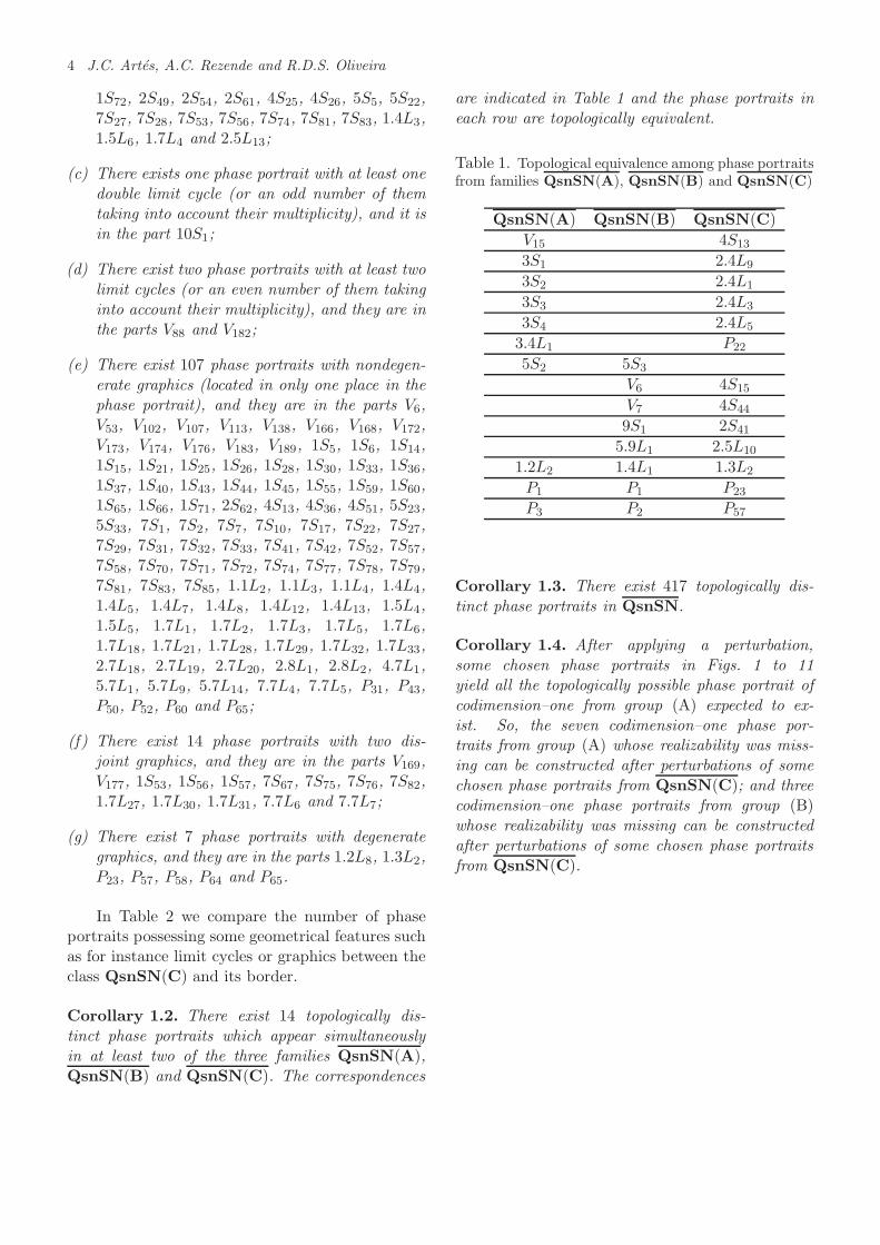
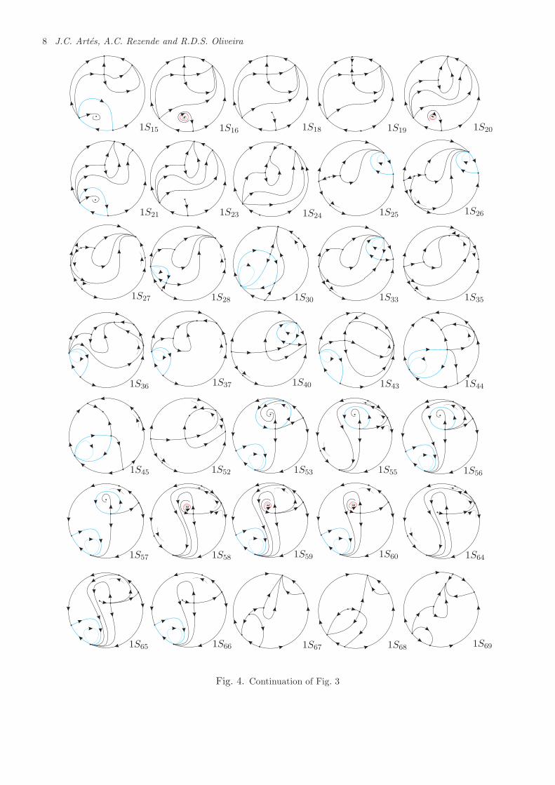
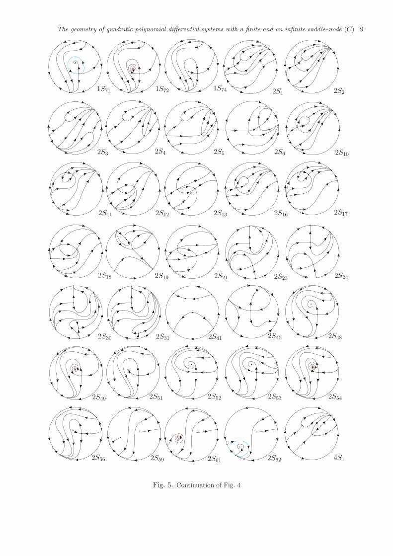
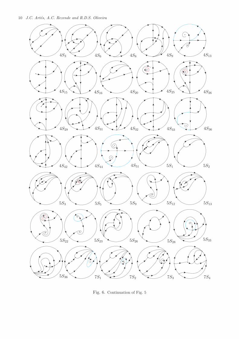
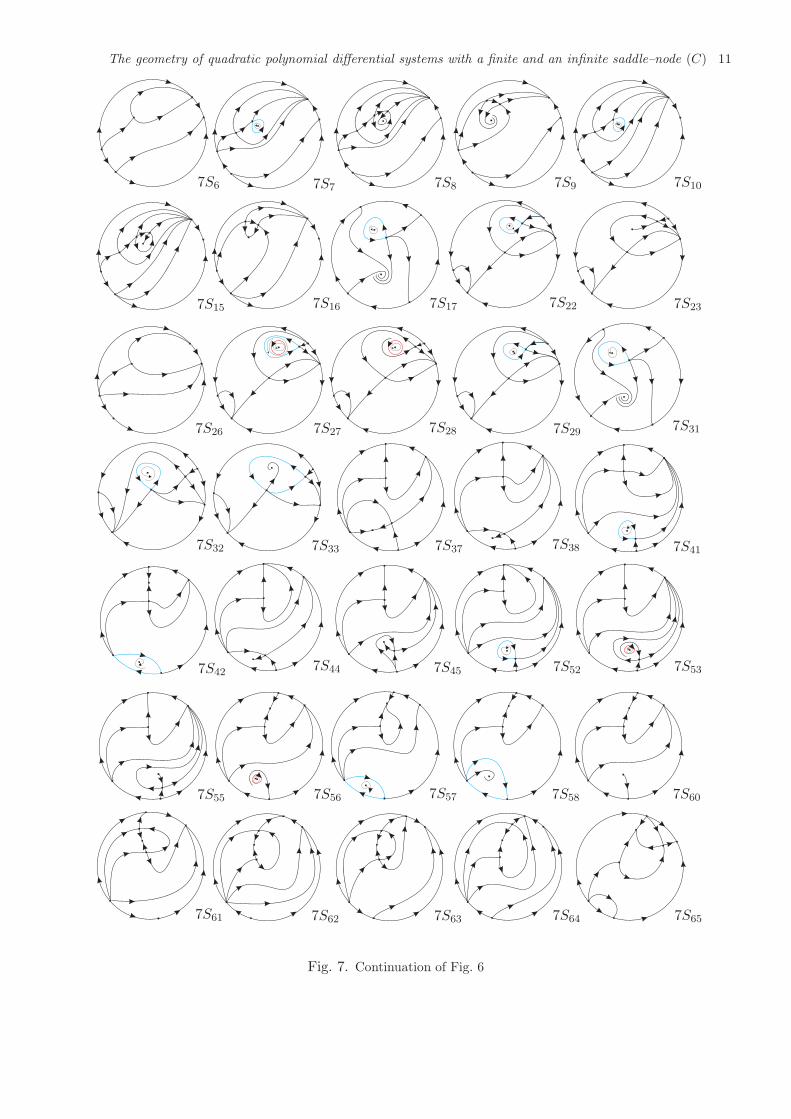
located in the bisector of the first and third quad-rants and given by the normal form (5) (classQsnSN(C)). The bifurcation diagram for this classis the projective tridimensional space RP3. All thesephase portraits are shown in Figs. 1 to 11. More-over, the following statements hold:
(a) There exist 259 topologically distinct phase por-traits in QsnSN(C);
(b) There exist 49 phase portraits possessing atleast one simple limit cycle (or an odd numberof them taking into account their multiplicity),and they are in the parts V5, V17, V27, V33, V54,V80, V89, V90, V94, V99, V100, V117, V118, V134,V137, V168, V176, V178, V179, V180, V183, V194,1S4, 1S12, 1S13, 1S16, 1S20, 1S58, 1S59, 1S60,
4 J.C. Artes, A.C. Rezende and R.D.S. Oliveira
1S72, 2S49, 2S54, 2S61, 4S25, 4S26, 5S5, 5S22,7S27, 7S28, 7S53, 7S56, 7S74, 7S81, 7S83, 1.4L3,1.5L6, 1.7L4 and 2.5L13;
(c) There exists one phase portrait with at least onedouble limit cycle (or an odd number of themtaking into account their multiplicity), and it isin the part 10S1;
(d) There exist two phase portraits with at least twolimit cycles (or an even number of them takinginto account their multiplicity), and they are inthe parts V88 and V182;
(e) There exist 107 phase portraits with nondegen-erate graphics (located in only one place in thephase portrait), and they are in the parts V6,V53, V102, V107, V113, V138, V166, V168, V172,V173, V174, V176, V183, V189, 1S5, 1S6, 1S14,1S15, 1S21, 1S25, 1S26, 1S28, 1S30, 1S33, 1S36,1S37, 1S40, 1S43, 1S44, 1S45, 1S55, 1S59, 1S60,1S65, 1S66, 1S71, 2S62, 4S13, 4S36, 4S51, 5S23,5S33, 7S1, 7S2, 7S7, 7S10, 7S17, 7S22, 7S27,7S29, 7S31, 7S32, 7S33, 7S41, 7S42, 7S52, 7S57,7S58, 7S70, 7S71, 7S72, 7S74, 7S77, 7S78, 7S79,7S81, 7S83, 7S85, 1.1L2, 1.1L3, 1.1L4, 1.4L4,1.4L5, 1.4L7, 1.4L8, 1.4L12, 1.4L13, 1.5L4,1.5L5, 1.7L1, 1.7L2, 1.7L3, 1.7L5, 1.7L6,1.7L18, 1.7L21, 1.7L28, 1.7L29, 1.7L32, 1.7L33,2.7L18, 2.7L19, 2.7L20, 2.8L1, 2.8L2, 4.7L1,5.7L1, 5.7L9, 5.7L14, 7.7L4, 7.7L5, P31, P43,P50, P52, P60 and P65;
(f) There exist 14 phase portraits with two dis-joint graphics, and they are in the parts V169,V177, 1S53, 1S56, 1S57, 7S67, 7S75, 7S76, 7S82,1.7L27, 1.7L30, 1.7L31, 7.7L6 and 7.7L7;
(g) There exist 7 phase portraits with degenerategraphics, and they are in the parts 1.2L8, 1.3L2,P23, P57, P58, P64 and P65.
In Table 2 we compare the number of phaseportraits possessing some geometrical features suchas for instance limit cycles or graphics between theclass QsnSN(C) and its border.
Corollary 1.2. There exist 14 topologically dis-tinct phase portraits which appear simultaneouslyin at least two of the three families QsnSN(A),QsnSN(B) and QsnSN(C). The correspondences
are indicated in Table 1 and the phase portraits ineach row are topologically equivalent.
Table 1. Topological equivalence among phase portraitsfrom families QsnSN(A), QsnSN(B) and QsnSN(C)
QsnSN(A) QsnSN(B) QsnSN(C)
V15 4S13
3S1 2.4L9
3S2 2.4L1
3S3 2.4L3
3S4 2.4L5
3.4L1 P22
5S2 5S3
V6 4S15
V7 4S44
9S1 2S41
5.9L1 2.5L10
1.2L2 1.4L1 1.3L2
P1 P1 P23
P3 P2 P57
Corollary 1.3. There exist 417 topologically dis-tinct phase portraits in QsnSN.
Corollary 1.4. After applying a perturbation,some chosen phase portraits in Figs. 1 to 11yield all the topologically possible phase portrait ofcodimension–one from group (A) expected to ex-ist. So, the seven codimension–one phase por-traits from group (A) whose realizability was miss-ing can be constructed after perturbations of somechosen phase portraits from QsnSN(C); and threecodimension–one phase portraits from group (B)whose realizability was missing can be constructedafter perturbations of some chosen phase portraitsfrom QsnSN(C).
The geometry of quadratic polynomial differential systems with a finite and an infinite saddle–node (C) 5
V1 V2 V3 V5 V6
V7 V9 V10 V13 V15
V17 V20 V21 V22 V23
V25 V27 V31 V33 V37
V41 V42 V44 V46 V49
V51 V53 V54 V61 V62
V64 V66 V69 V71 V78
Fig. 1. Phase portraits for quadratic vector fields with a finite saddle–node sn(2) and an infinite saddle–node of type(02
)SN in the bisector of first and third quadrants
6 J.C. Artes, A.C. Rezende and R.D.S. Oliveira
V80 V83 V84 V85 V88
V89 V90 V94 V99 V100
V102 V104 V107 V108 V109
V110 V113 V114 V117 V118
V121 V122 V123 V129 V134
V136 V137 V138 V140 V141
V142 V143 V144 V145 V147
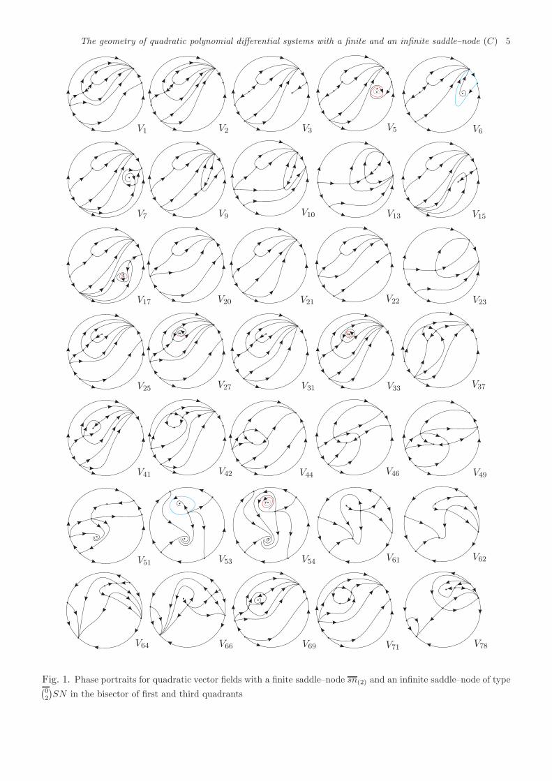
Fig. 2. Continuation of Fig. 1
The geometry of quadratic polynomial differential systems with a finite and an infinite saddle–node (C) 7
V149 V154 V155 V165 V166
V168 V169 V170 V172 V173
V174 V176 V177 V178 V179
V180 V182 V183 V189 V190
V191 V192 V194 V198 1S1
1S2 1S4 1S5 1S61S7
1S8 1S9 1S12 1S13 1S14
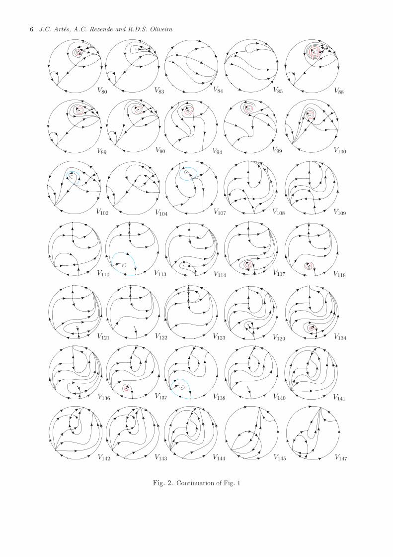
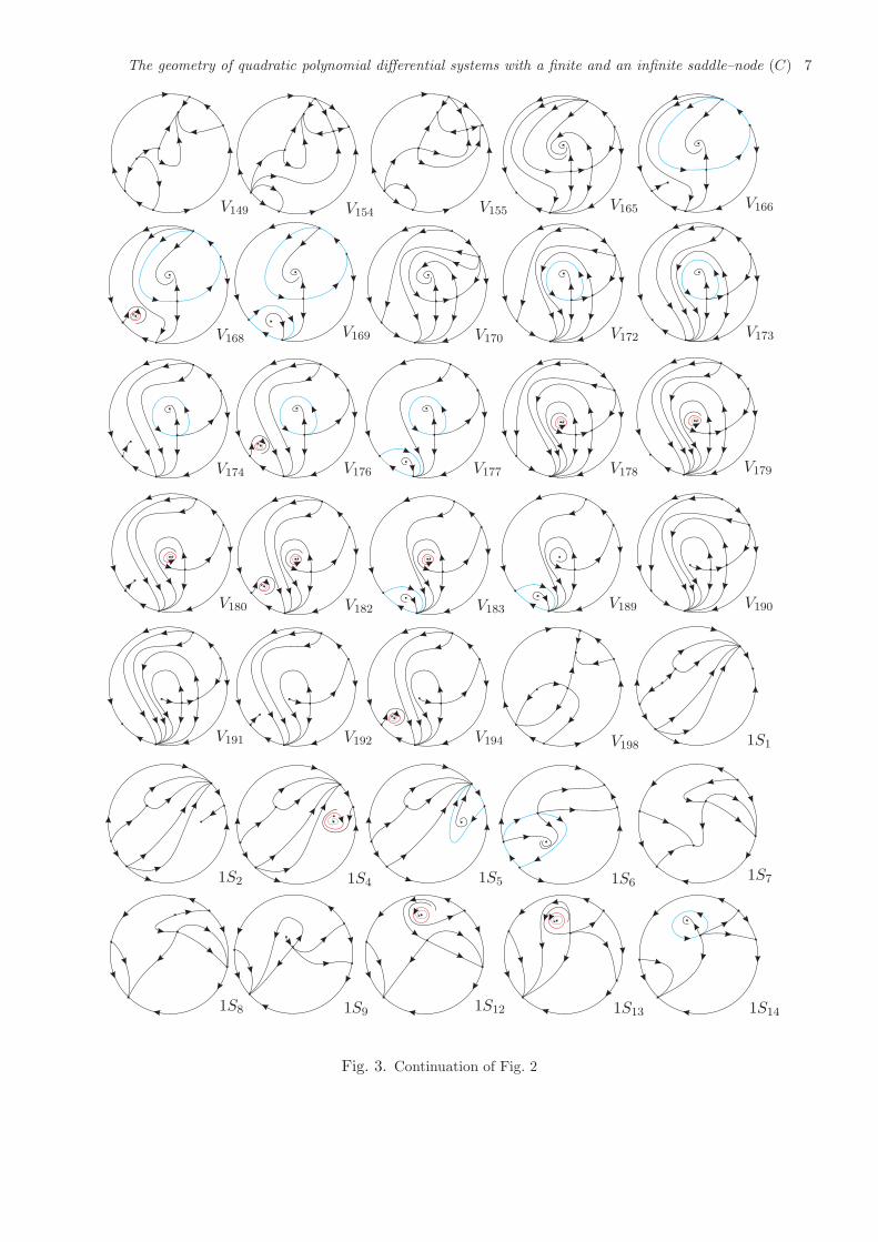
Fig. 3. Continuation of Fig. 2
8 J.C. Artes, A.C. Rezende and R.D.S. Oliveira
1S15 1S16 1S18 1S19 1S20
1S21 1S23 1S24 1S25 1S26
1S27 1S28 1S30 1S33 1S35
1S36 1S37 1S40 1S43 1S44
1S45 1S52 1S53 1S55 1S56
1S57 1S58 1S59 1S60 1S64
1S65 1S66 1S67 1S68 1S69
Fig. 4. Continuation of Fig. 3
The geometry of quadratic polynomial differential systems with a finite and an infinite saddle–node (C) 9
1S71 1S72 1S74 2S1 2S2
2S3 2S4 2S5 2S6 2S10
2S11 2S12 2S13 2S16 2S17
2S18 2S19 2S21 2S23 2S24
2S30 2S31 2S41 2S45 2S48
2S49 2S51 2S52 2S53 2S54
2S56 2S59 2S61 2S62 4S1
Fig. 5. Continuation of Fig. 4
10 J.C. Artes, A.C. Rezende and R.D.S. Oliveira
4S3 4S6 4S8 4S9 4S13
4S15 4S16 4S20 4S25 4S26
4S29 4S31 4S32 4S33 4S36
4S42 4S44 4S51 5S1 5S2
5S3 5S5 5S9 5S12 5S13
5S22 5S23 5S26 5S285S33
5S36 7S1 7S2 7S3 7S4
Fig. 6. Continuation of Fig. 5
The geometry of quadratic polynomial differential systems with a finite and an infinite saddle–node (C) 11
7S6 7S7 7S8 7S9 7S10
7S15 7S16 7S17 7S22 7S23
7S26 7S27 7S28 7S29 7S31
7S32 7S33 7S37 7S38 7S41
7S42 7S44 7S45 7S52 7S53
7S55 7S56 7S57 7S58 7S60
7S61 7S62 7S63 7S64 7S65
Fig. 7. Continuation of Fig. 6
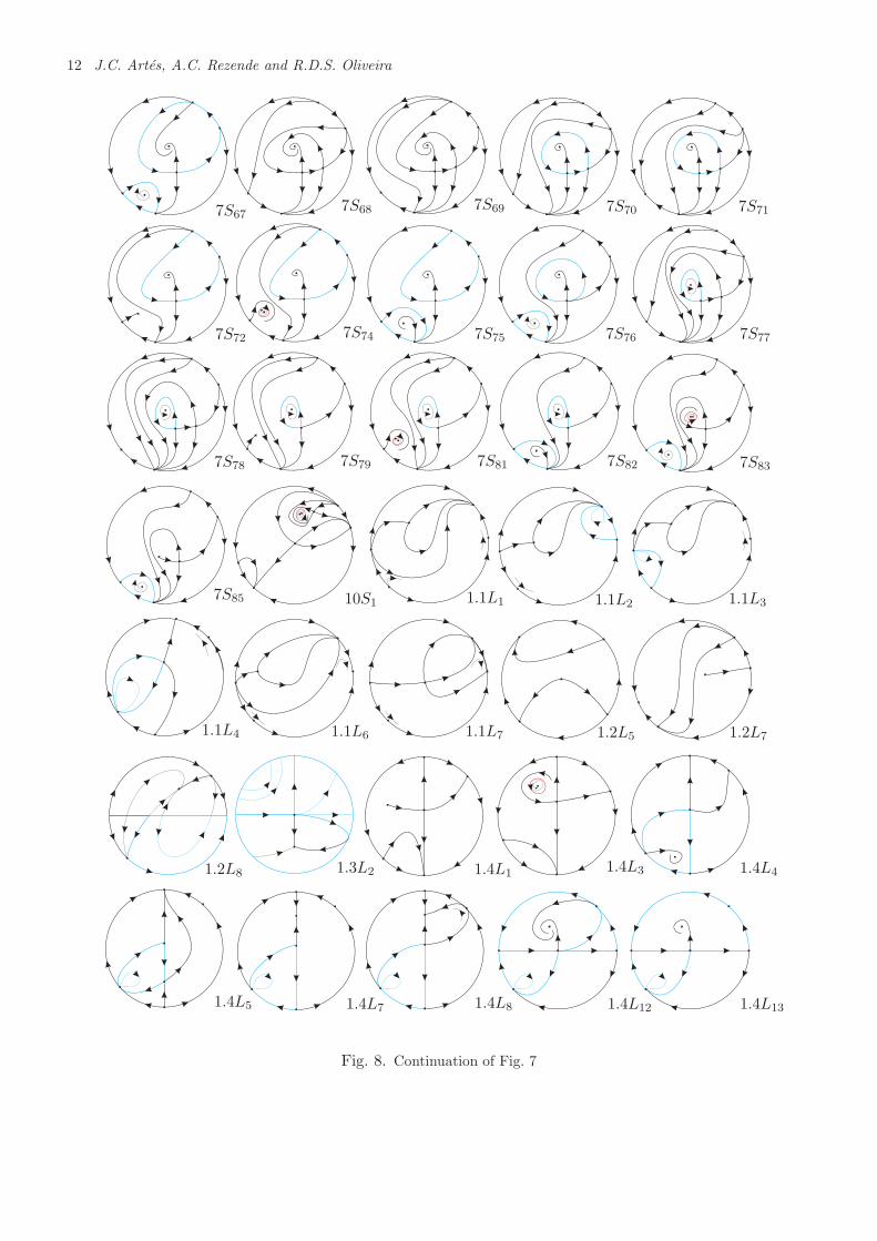
12 J.C. Artes, A.C. Rezende and R.D.S. Oliveira
7S677S68 7S69 7S70 7S71
7S72 7S74 7S75 7S76 7S77
7S78 7S79 7S81 7S82 7S83
7S85 10S1 1.1L1 1.1L2 1.1L3
1.1L4 1.1L6 1.1L7 1.2L5 1.2L7
1.2L8 1.3L2 1.4L1 1.4L3 1.4L4
1.4L5 1.4L7 1.4L8 1.4L12 1.4L13
Fig. 8. Continuation of Fig. 7
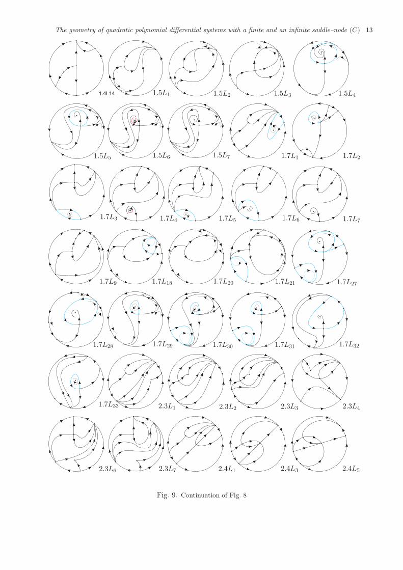
The geometry of quadratic polynomial differential systems with a finite and an infinite saddle–node (C) 13
1.4L14 1.5L1 1.5L2 1.5L3 1.5L4
1.5L5 1.5L6 1.5L7 1.7L1 1.7L2
1.7L3 1.7L4 1.7L5 1.7L6 1.7L7
1.7L9 1.7L18 1.7L20 1.7L21 1.7L27
1.7L28 1.7L29 1.7L30 1.7L31 1.7L32
1.7L33 2.3L1 2.3L2 2.3L3 2.3L4
2.3L6 2.3L7 2.4L1 2.4L3 2.4L5
Fig. 9. Continuation of Fig. 8
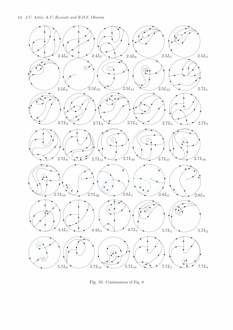
14 J.C. Artes, A.C. Rezende and R.D.S. Oliveira
2.4L6 2.4L7 2.4L9 2.5L1 2.5L3
2.5L4 2.5L10 2.5L11 2.5L13 2.7L1
2.7L2 2.7L3 2.7L4 2.7L5 2.7L7
2.7L9 2.7L11 2.7L16 2.7L17 2.7L18
2.7L19 2.7L20 2.8L1 2.8L2 2.8L3
4.4L1 4.4L3 4.7L1 5.7L1 5.7L2
5.7L9 5.7L11 5.7L14 7.7L1 7.7L4
Fig. 10. Continuation of Fig. 9
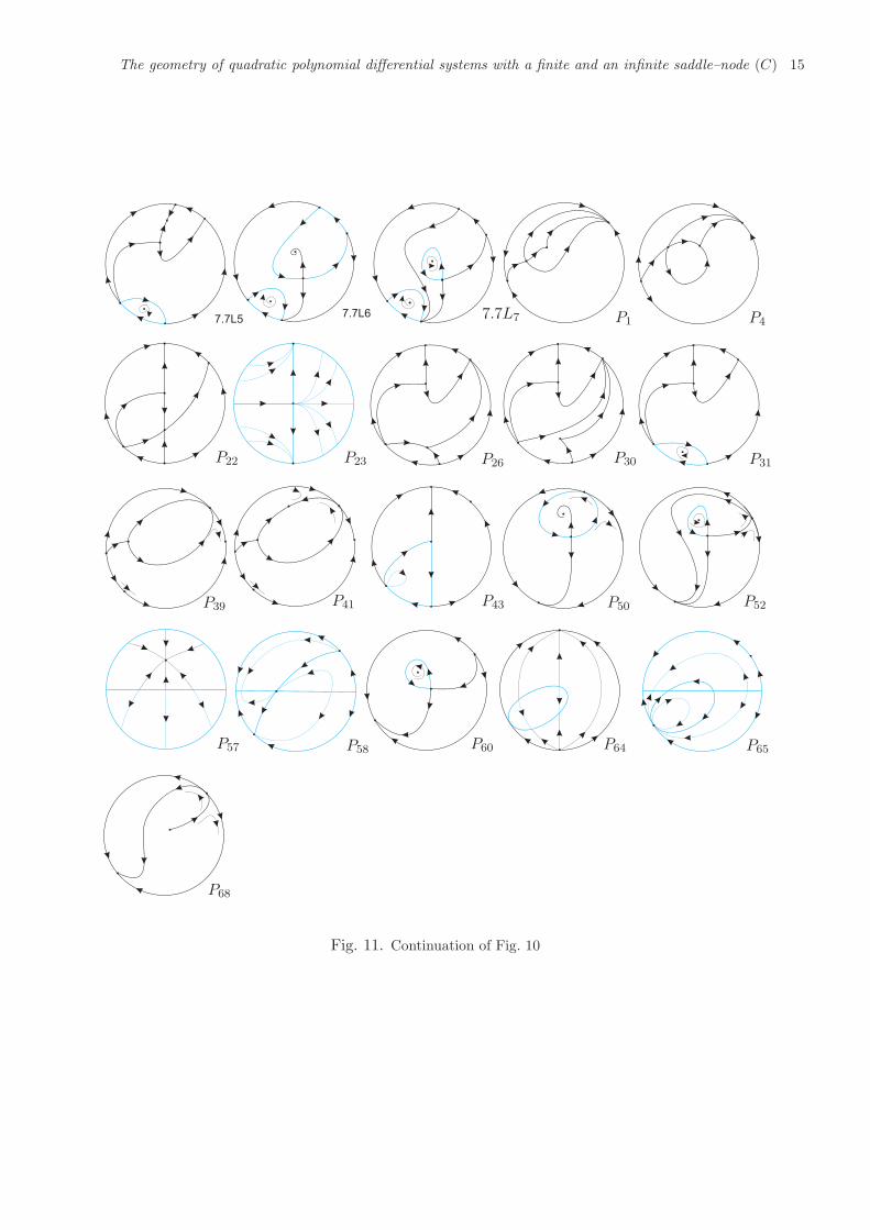
The geometry of quadratic polynomial differential systems with a finite and an infinite saddle–node (C) 15
7.7L67.7L5
7.7L7 P1 P4
P22 P23 P26 P30 P31
P39 P41 P43 P50 P52
P57 P58 P60 P64 P65
P68
Fig. 11. Continuation of Fig. 10

16 J.C. Artes, A.C. Rezende and R.D.S. Oliveira
Table 2. Comparison between the set QsnSN(C) and its border
QsnSN(C) border of QsnSN(C)
Distinct phase portraits 259 112
Phase portraits with exactly one limit cycle 39 10
Phase portraits with two/double limit cycles 2/1 0
Phase portraits with a finite72 14
number of nondegenerate graphics
Phase portraits with an infinite0 35
number of nondegenerate graphics
Phase portraits with degenerate graphics 0 7
The geometry of quadratic polynomial differential systems with a finite and an infinite saddle–node (C) 17
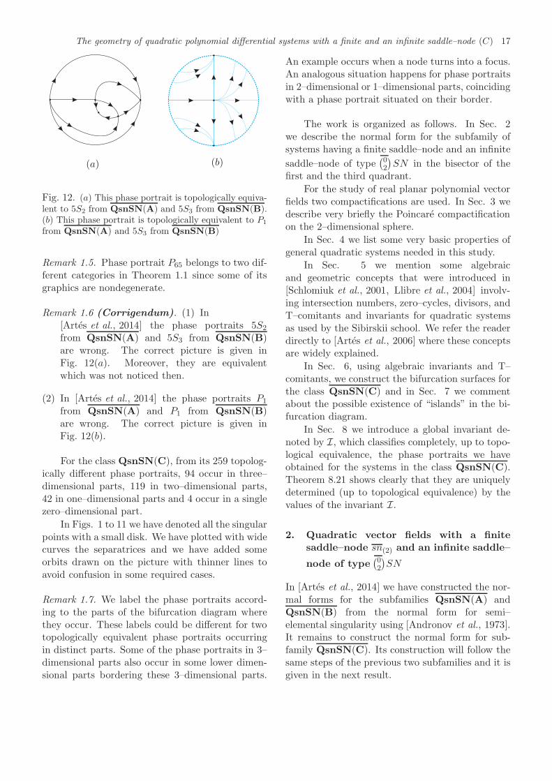
(a) (b)
Fig. 12. (a) This phase portrait is topologically equiva-lent to 5S2 from QsnSN(A) and 5S3 from QsnSN(B).(b) This phase portrait is topologically equivalent to P1
from QsnSN(A) and 5S3 from QsnSN(B)
Remark 1.5. Phase portrait P65 belongs to two dif-ferent categories in Theorem 1.1 since some of itsgraphics are nondegenerate.
Remark 1.6 (Corrigendum). (1) In[Artes et al., 2014] the phase portraits 5S2
from QsnSN(A) and 5S3 from QsnSN(B)are wrong. The correct picture is given inFig. 12(a). Moreover, they are equivalentwhich was not noticed then.
(2) In [Artes et al., 2014] the phase portraits P1
from QsnSN(A) and P1 from QsnSN(B)are wrong. The correct picture is given inFig. 12(b).
For the class QsnSN(C), from its 259 topolog-ically different phase portraits, 94 occur in three–dimensional parts, 119 in two–dimensional parts,42 in one–dimensional parts and 4 occur in a singlezero–dimensional part.
In Figs. 1 to 11 we have denoted all the singularpoints with a small disk. We have plotted with widecurves the separatrices and we have added someorbits drawn on the picture with thinner lines toavoid confusion in some required cases.
Remark 1.7. We label the phase portraits accord-ing to the parts of the bifurcation diagram wherethey occur. These labels could be different for twotopologically equivalent phase portraits occurringin distinct parts. Some of the phase portraits in 3–dimensional parts also occur in some lower dimen-sional parts bordering these 3–dimensional parts.
An example occurs when a node turns into a focus.An analogous situation happens for phase portraitsin 2–dimensional or 1–dimensional parts, coincidingwith a phase portrait situated on their border.
The work is organized as follows. In Sec. 2we describe the normal form for the subfamily ofsystems having a finite saddle–node and an infinite
saddle–node of type(02
)SN in the bisector of the
first and the third quadrant.
For the study of real planar polynomial vectorfields two compactifications are used. In Sec. 3 wedescribe very briefly the Poincare compactificationon the 2–dimensional sphere.
In Sec. 4 we list some very basic properties ofgeneral quadratic systems needed in this study.
In Sec. 5 we mention some algebraicand geometric concepts that were introduced in[Schlomiuk et al., 2001, Llibre et al., 2004] involv-ing intersection numbers, zero–cycles, divisors, andT–comitants and invariants for quadratic systemsas used by the Sibirskii school. We refer the readerdirectly to [Artes et al., 2006] where these conceptsare widely explained.
In Sec. 6, using algebraic invariants and T–comitants, we construct the bifurcation surfaces forthe class QsnSN(C) and in Sec. 7 we commentabout the possible existence of “islands” in the bi-furcation diagram.
In Sec. 8 we introduce a global invariant de-noted by I, which classifies completely, up to topo-logical equivalence, the phase portraits we haveobtained for the systems in the class QsnSN(C).Theorem 8.21 shows clearly that they are uniquelydetermined (up to topological equivalence) by thevalues of the invariant I.
2. Quadratic vector fields with a finitesaddle–node sn(2) and an infinite saddle–
node of type(02
)SN
In [Artes et al., 2014] we have constructed the nor-mal forms for the subfamilies QsnSN(A) andQsnSN(B) from the normal form for semi–elemental singularity using [Andronov et al., 1973].It remains to construct the normal form for sub-family QsnSN(C). Its construction will follow thesame steps of the previous two subfamilies and it isgiven in the next result.
18 J.C. Artes, A.C. Rezende and R.D.S. Oliveira
Proposition 2.1. Every system with a finitesemi–elemental double saddle–node sn(2) with itseigenvectors in the direction of the axes, with theeigenvector associated with the zero eigenvalue onthe horizontal axis, and an infinite saddle–node of
type(02
)SN located in the endpoints of the bisec-
tor of the first and third quadrants can be broughtvia affine transformations and time rescaling to thefollowing normal form
x = gx2 + 2hxy + (n− g − 2h)y2,
y = y + ℓx2 + (2g + 2h− 2ℓ− n)xy
+ (2h+ ℓ+ 2(n − g − 2h))y2,
(5)
where g, h, ℓ and n are real parameters and g 6= 0.
Proof. By Andronov et al. [Andronov et al., 1973],if a quadratic system has a semi–elemental singularpoint at the origin, it can always be written intothe form
x = gx2 + 2hxy + ky2,
y = y + ℓx2 + 2mxy + ny2.(6)
Moreover, if g 6= 0, then we have a double saddle–node sn(2) with its eigenvectors in the direction of
the axes. The next step is to place the point(02
)SN
at [1 : 1 : 0] of the local chart U1 with coordinates(w, z). For that, we must guarantee that the point[1 : 1 : 0] is a singularity of the flow in U1,
w = ℓ+ (−g + 2m)w + (−2h+ n)w2 − kw3 + wz,
z = (−g − 2hw − kw2)z.
Then, we set n = g + 2h + k − ℓ − 2m and, byanalyzing the Jacobian of the former system afterthe substitution in n, we set m = (g − k − 2ℓ)/2in order to have the eigenvalue associated to theeigenvector on z = 0 being null. Finally, we applythe rotation k = n− g− 2h in the parameter spaceand obtain the normal form (5). We note that thisrotation is just to simplify the bifurcation diagram.
To study the closure of the family QsnSN(C)within the set of representatives of QsnSN(C) inthe parameter space of the normal form (5) it isnecessary to consider the case g = 0.
The next result assures the existence of invari-ant straight lines under certain conditions for sys-tems (5).
Lemma 2.2. For all g ∈ R, systems (5) possessthe following invariant straight lines under the spe-cific condition:(i) {x = 0}, if h = (n− g)/2;
(ii) {y = 0}, if ℓ = 0;
(iii) {y = x− 1/n}, if ℓ = g and n 6= 0.
Proof. We consider the algebraic curves
f1(x, y) ≡ x = 0,
f2(x, y) ≡ y = 0,
f3(x, y) ≡ ny − nx+ 1 = 0,
and we show that the polynomials
K1(x, y) = gx+ (n − g)y,
K2(x, y) = 1 + (2g + 2h− n)x− 2(g + h− n)y,
K3(x, y) = ny,
are the cofactors of f1 = 0, f2 = 0 and f3 = 0,respectively, after restricting systems (5) to the re-spective conditions.
Systems (5) depend on the parameter λ =(g, h, ℓ, n) ∈ R
4. We consider systems (5) whichare nonlinear, i.e. λ = (g, h, ℓ, n) 6= 0. Applyingthe affine transformation X = αx, Y = αy, withα 6= 0, we obtain
X = α′gX2 + 2α′hXY + α′(n− g − 2h)Y 2,
Y = y + α′ℓx2 + α′(2g + 2h− 2ℓ− n)XY
+ α′(2h+ ℓ+ 2(n − g − 2h))Y 2,
for α′ = 1/α, α 6= 0.Then, this transformation takes the system
with parameters (g, h, ℓ, n) to a system with param-eters (α′g, α′h, α′ℓ, α′n). Hence, instead of consid-ering as parameter space R4, we may consider RP3.
But, since for α′ = −1 all the signs change,we may consider g ≥ 0 in [g : h : k : n]. Sinceg2+h2+k2+n2 = 1, then g =
√1− (h2 + k2 + n2),
where 0 ≤ h2 + k2 + n2 ≤ 1.We can therefore view the parameter space as
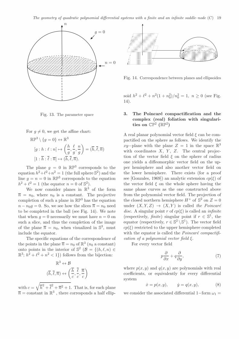
a ball B = {(h, ℓ, n) ∈ R3; h2 + ℓ2 + n2 ≤ 1}, where
on the equator two opposite points are identified.When n = 0, we identify the point [g : h : ℓ :0] ∈ RP
3 with [g : h : ℓ] ∈ RP2. So, this subset
{n = 0} ⊂ B can be identified with RP2, which can
be viewed as a disk with two opposite points on thecircumference (the equator) identified (see Fig. 13).
The geometry of quadratic polynomial differential systems with a finite and an infinite saddle–node (C) 19
n
n = 0
g = 0
Fig. 13. The parameter space
For g 6= 0, we get the affine chart:
RP3 \ {g = 0} ↔ R
3
[g : h : ℓ : n] 7→(h
g,ℓ
g,n
g
)= (h, ℓ, n)
[1 : h : ℓ : n] 7→ (h, ℓ, n).
The plane g = 0 in RP3 corresponds to the
equation h2+ℓ2+n2 = 1 (the full sphere S2) and theline g = n = 0 in RP
3 corresponds to the equationh2 + ℓ2 = 1 (the equator n = 0 of S2).
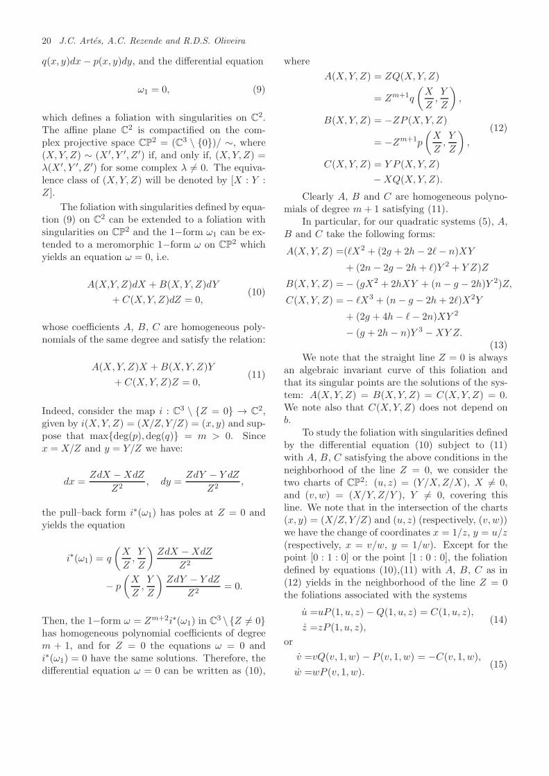
We now consider planes in R3 of the form
n = n0, where n0 is a constant. The projectivecompletion of such a plane in RP
3 has the equationn− n0g = 0. So, we see how the slices n = n0 needto be completed in the ball (see Fig. 14). We notethat when g = 0 necessarily we must have n = 0 onsuch a slice, and thus the completion of the imageof the plane n = n0, when visualized in S
3, mustinclude the equator.
The specific equations of the correspondence ofthe points in the plane n = n0 of R
3 (n0 a constant)onto points in the interior of S2 (B = {(h, ℓ, n) ∈R3; h2 + ℓ2 + n2 < 1}) follows from the bijection:
R3 ↔ B
(h, ℓ, n) ↔(h
c,ℓ
c,n
c
)
with c =
√h2+ ℓ
2+ n2 + 1. That is, for each plane
n = constant in R3 , there corresponds a half ellip-
Fig. 14. Correspondence between planes and ellipsoides
soid h2 + ℓ2 + n2(1 + n20)/n
20 = 1, n ≥ 0 (see Fig.
14).
3. The Poincare compactification and thecomplex (real) foliation with singulari-ties on CP
2 (RP2)
A real planar polynomial vector field ξ can be com-pactified on the sphere as follows. We identify thexy−plane with the plane Z = 1 in the space R
3
with coordinates X, Y , Z. The central projec-tion of the vector field ξ on the sphere of radiusone yields a diffeomorphic vector field on the up-per hemisphere and also another vector field onthe lower hemisphere. There exists (for a proofsee [Gonzales, 1969]) an analytic extension cp(ξ) ofthe vector field ξ on the whole sphere having thesame phase curves as the one constructed abovefrom the polynomial vector field. The projection ofthe closed northern hemisphere H+ of S
2 on Z = 0under (X,Y,Z) → (X,Y ) is called the Poincaredisc. A singular point r of cp(ξ) is called an infinite(respectively, finite) singular point if r ∈ S
1, theequator (respectively, r ∈ S
2 \S1). The vector fieldcp(ξ) restricted to the upper hemisphere completedwith the equator is called the Poincare compactifi-cation of a polynomial vector field ξ.
For every vector field
p∂
∂x+ q
∂
∂y, (7)
where p(x, y) and q(x, y) are polynomials with realcoefficients, or equivalently for every differentialsystem
x = p(x, y), y = q(x, y), (8)
we consider the associated differential 1−form ω1 =
20 J.C. Artes, A.C. Rezende and R.D.S. Oliveira
q(x, y)dx− p(x, y)dy, and the differential equation
ω1 = 0, (9)
which defines a foliation with singularities on C2.
The affine plane C2 is compactified on the com-
plex projective space CP2 = (C3 \ {0})/ ∼, where
(X,Y,Z) ∼ (X ′, Y ′, Z ′) if, and only if, (X,Y,Z) =λ(X ′, Y ′, Z ′) for some complex λ 6= 0. The equiva-lence class of (X,Y,Z) will be denoted by [X : Y :Z].
The foliation with singularities defined by equa-tion (9) on C
2 can be extended to a foliation withsingularities on CP
2 and the 1−form ω1 can be ex-tended to a meromorphic 1−form ω on CP
2 whichyields an equation ω = 0, i.e.
A(X,Y,Z)dX +B(X,Y,Z)dY
+ C(X,Y,Z)dZ = 0,(10)
whose coefficients A, B, C are homogeneous poly-nomials of the same degree and satisfy the relation:
A(X,Y,Z)X +B(X,Y,Z)Y
+ C(X,Y,Z)Z = 0,(11)
Indeed, consider the map i : C3 \ {Z = 0} → C2,
given by i(X,Y,Z) = (X/Z, Y/Z) = (x, y) and sup-pose that max{deg(p),deg(q)} = m > 0. Sincex = X/Z and y = Y/Z we have:
dx =ZdX −XdZ
Z2, dy =
ZdY − Y dZ
Z2,
the pull–back form i∗(ω1) has poles at Z = 0 andyields the equation
i∗(ω1) = q
(X
Z,Y
Z
)ZdX −XdZ
Z2
− p
(X
Z,Y
Z
)ZdY − Y dZ
Z2= 0.
Then, the 1−form ω = Zm+2i∗(ω1) in C3 \{Z 6= 0}
has homogeneous polynomial coefficients of degreem + 1, and for Z = 0 the equations ω = 0 andi∗(ω1) = 0 have the same solutions. Therefore, thedifferential equation ω = 0 can be written as (10),
where
A(X,Y,Z) = ZQ(X,Y,Z)
= Zm+1q
(X
Z,Y
Z
),
B(X,Y,Z) = −ZP (X,Y,Z)
= −Zm+1p
(X
Z,Y
Z
),
C(X,Y,Z) = Y P (X,Y,Z)
−XQ(X,Y,Z).
(12)
Clearly A, B and C are homogeneous polyno-mials of degree m+ 1 satisfying (11).
In particular, for our quadratic systems (5), A,B and C take the following forms:
A(X,Y,Z) =(ℓX2 + (2g + 2h− 2ℓ− n)XY
+ (2n − 2g − 2h+ ℓ)Y 2 + Y Z)Z
B(X,Y,Z) =− (gX2 + 2hXY + (n− g − 2h)Y 2)Z,
C(X,Y,Z) =− ℓX3 + (n− g − 2h+ 2ℓ)X2Y
+ (2g + 4h− ℓ− 2n)XY 2
− (g + 2h− n)Y 3 −XY Z.(13)
We note that the straight line Z = 0 is alwaysan algebraic invariant curve of this foliation andthat its singular points are the solutions of the sys-tem: A(X,Y,Z) = B(X,Y,Z) = C(X,Y,Z) = 0.We note also that C(X,Y,Z) does not depend onb.
To study the foliation with singularities definedby the differential equation (10) subject to (11)with A, B, C satisfying the above conditions in theneighborhood of the line Z = 0, we consider thetwo charts of CP2: (u, z) = (Y/X,Z/X), X 6= 0,and (v,w) = (X/Y,Z/Y ), Y 6= 0, covering thisline. We note that in the intersection of the charts(x, y) = (X/Z, Y/Z) and (u, z) (respectively, (v,w))we have the change of coordinates x = 1/z, y = u/z(respectively, x = v/w, y = 1/w). Except for thepoint [0 : 1 : 0] or the point [1 : 0 : 0], the foliationdefined by equations (10),(11) with A, B, C as in(12) yields in the neighborhood of the line Z = 0the foliations associated with the systems
u =uP (1, u, z) −Q(1, u, z) = C(1, u, z),
z =zP (1, u, z),(14)
or
v =vQ(v, 1, w) − P (v, 1, w) = −C(v, 1, w),
w =wP (v, 1, w).(15)
The geometry of quadratic polynomial differential systems with a finite and an infinite saddle–node (C) 21
In a similar way we can associate a real foliationwith singularities on RP
2 to a real planar polyno-mial vector field.
4. A few basic properties of quadratic sys-tems relevant for this study
The following results hold for any quadratic system:
(i) A straight line either has at most two (finite)contact points with a quadratic system (whichinclude the singular points), or it is formed bytrajectories of the system; see Lemma 11.1 of[Ye et al., 1986]. We recall that by definitiona contact point of a straight line L is a point ofL where the vector field has the same directionas L, or it is zero.
(ii) If a straight line passing through two real fi-nite singular points r1 and r2 of a quadraticsystem is not formed by trajectories, then it isdivided by these two singular points in threesegments ∞r1, r1r2 and r2∞ such that thetrajectories cross ∞r1 and r2∞ in one direc-tion, and they cross r1r2 in the opposite di-rection; see Lemma 11.4 of [Ye et al., 1986].
(iii) If a quadratic system has a limit cycle, thenit surrounds a unique singular point, and thispoint is a focus; see [Coppel, 1966].
(iv) A quadratic system with an invariant straightline has at most one limit cycle; see[Coll & Llibre, 1988].
(v) A quadratic system with more than one in-variant straight line has no limit cycle; see[Bautin, 1954].
The proof of the next result can be found in[Artes et al., 1998].
Proposition 4.1. Any graphic or degenerategraphic in a real planar polynomial differentialsystem must either
1) surround a singular point of index greater thanor equal to +1, or
2) contain a singular point having an elliptic sectorsituated in the region delimited by the graphic, or
3) contain an infinite number of singular points.
5. Some algebraic and geometric concepts
In this article we use the concept of intersectionnumber for curves (see [Fulton, 1969]). For a quicksummary see Sec. 5 of [Artes et al., 2006].
We shall also use the concepts of zero–cycle and divisor (see [Hartshorne, 1977])as specified for quadratic vector fields in[Schlomiuk et al., 2001]. For a quick summary seeSec. 6 of [Artes et al., 2006].
We shall also use the concepts of algebraic in-variant and T–comitant as used by the Sibirskiischool for differential equations. For a quick sum-mary see Sec. 7 of [Artes et al., 2006].
In the next section we describe the algebraicinvariants and T–comitants which are relevant inthe study of family (5), see Sec. 6.
6. The bifurcation diagram of the systemsin QsnSN(C)
6.1. Bifurcation surfaces due to thechanges in the nature of singularities
From Sec. 7 of [Artes et al., 2008] and[Vulpe, 2011] we get the formulas which givethe bifurcation surfaces of singularities in R12, pro-duced by changes that may occur in the local natureof finite singularities. From [Schlomiuk et al., 2005]we get equivalent formulas for the infinite singularpoints. These bifurcation surfaces are all algebraicand they are the following:
Bifurcation surfaces in RP3 due to multiplic-
ities of singularities
(S1) This is the bifurcation surface due to multi-plicity of infinite singularities involved with finitesingular points. This occurs when at least one fi-nite singular point collides with at least one infinitesingular point. This is a quartic whose equation is
µ = n2(−g2 − 2gh+ 2hℓ+ ℓ2 + gn) = 0.
(S2) Since this family already has a saddle–node atthe origin, the invariant D is always zero. The nextT−comitant related to finite singularities is T. Ifthis T−comitant vanishes, it may mean either theexistence of another finite semi–elemental singularpoint, or the origin being a singular point of higher
22 J.C. Artes, A.C. Rezende and R.D.S. Oliveira
multiplicity, or the system being degenerate. Theequation of this surface is
T = −12g2 (g2 + 2gh + h2 − gn) = 0.
(S5) Since this family already has a saddle–node atinfinity formed by the collision of two infinite sin-gularities, the invariant η is always zero. In thissense, we have to consider a bifurcation related tothe existence of either the double infinite singular-
ity(02
)SN plus a simple one, or a triple one. This
phenomenon is ruled by the T−comitant M . Theequation of this surface is
M = (g + 2h+ ℓ− n)2 = 0.
The surface of C∞ bifurcation points due toa strong saddle or a strong focus changingthe sign of their traces (weak saddle or weakfocus)
(S3) This is the bifurcation surface due to weakfinite singularities, which occurs when the trace ofa finite singular point is zero. The equation of thissurface is given by
T4 = n(−4g3 − 8g2h− 4g2ℓ− 4ghℓ − 8h2ℓ
− 4hℓ2 + 4g2n+ 4gℓn+ ℓ2n) = 0.
We note that this bifurcation surface can either pro-duce a topological change, if the weak point is afocus, or just a C∞ change, if it is a saddle. How-ever, in the case this bifurcation coincides with aloop bifurcation associated with the same saddle,the change is also topological, as we can see laterin the analysis of systems (5) (see page 55).
The surface of C∞ bifurcation due to a nodebecoming a focus
(S6) This surface will contain the points of the pa-rameter space where a finite node of the systemturns into a focus. This surface is a C∞ but nota topological bifurcation surface. In fact, when weonly cross the surface (S6) in the bifurcation dia-gram, the phase portraits do not change topologi-cally. However, this surface is relevant for isolatingthe parts where a limit cycle surrounding an anti-saddle cannot exist. The equation of this surface is
given by W4 = 0, where
W4 = n2(16g6 + 64g5h+ 64g4h2 − 32g5ℓ
− 160g4hℓ− 192g3h2ℓ− 16g4ℓ2 + 32g3hℓ2
+ 112g2h2ℓ2 − 32gh3ℓ2 + 32g3ℓ3 + 64g2hℓ3
+ 32h3ℓ3 + 16h2ℓ4 − 32g5n− 64g4hn
+ 64g4ℓn+ 160g3hℓn+ 8g3ℓ2n− 80g2hℓ2n
+ 16gh2ℓ2n− 40g2ℓ3n− 8ghℓ3n− 16h2ℓ3n
− 8hℓ4n+ 16g4n2 − 32g3ℓn2 + 8g2ℓ2n2
+ 8gℓ3n2 + ℓ4n2).
Bifurcation surface in RP3 due to the pres-
ence of invariant straight lines
(S4) This surface will contain the points of the pa-rameter space where an invariant straight line ap-pears (see Lemma 2.2). This surface is split in someparts. Depending on these parts, the straight linemay contain connections of separatrices from differ-ent points or not. So, in some cases, it may implya topological bifurcation and, in others, just a C∞
bifurcation. The equation of this surface is givenby
Inv = ℓ(ℓ− g) (g + 2h− n) = 0.
These bifurcation surfaces are all algebraic andthey, except (S4), are the bifurcation surfaces ofsingularities of systems (5) in the parameter space.We shall discover other two bifurcation surfaces notnecessarily algebraic. On one of them the systemshave global connection of separatrices different fromthat given by (S4) and on the other the systemspossess double limit cycle. The equations of thesebifurcation surfaces can only be determined approx-imately by means of numerical tools. Using argu-ments of continuity in the phase portraits we canprove the existence of these components not nec-essarily algebraic in the part where they appear,and we can check them numerically. We shall namethem surfaces (S7) (connection of separatrices) and(S10) (double limit cycles).
Remark 6.1. On surface (S10), the respective sys-tems have at least one double limit cycle. Althoughthis surface is obtained numerically, we can predictin which portion of the bifurcation diagram it canbe placed. It must be in the neighborhood of thepoints of the bifurcation diagram corresponding to
The geometry of quadratic polynomial differential systems with a finite and an infinite saddle–node (C) 23
a weak focus f (2) or a weak saddle s(1) which formsa loop. So, according to [Vulpe, 2011; Main The-orem, item (b2)], the necessary condition for theexistence of weak points of order two or higher isgoverned by T4 = F1 = 0. The expression of F1 isgiven by F1 = −2g2 − 4gh+4gℓ+6hℓ+2gn− 3ℓn.
We shall foliate the 3−dimensional bifurcationdiagram in RP
3 by the planes n = n0, n0 con-stant, plus the open half sphere g = 0 and we shallgive pictures of the resulting bifurcation diagramon these planar sections on a disk or in an affinechart of R2.
In what follows we work in the chart of RP3
corresponding to g 6= 0, and we take g = 1. To dothe study, we shall use pictures which are drawn onplanes n = n0 of RP3, having coordinates [1 : h :ℓ : n0]. In these planes the coordinates are (h, ℓ)where the horizontal line is the h−axis.
As the final bifurcation diagram is quite com-plex, it is useful to introduce colors for each one ofthe bifurcation surfaces. They are:
(a) the curve obtained from the surface (S1) isdrawn in blue (a finite singular point collideswith an infinite one);
(b) the curve obtained from the surface (S2) isdrawn in green (two finite singular points dif-ferent from the saddle–node collide);
(c) the curve obtained from the surface (S3) isdrawn in yellow (when the trace of a singularpoint becomes zero);
(d) the curve obtained from the surface (S4) isdrawn in purple (the presence of invariantstraight lines);
(e) the curve obtained from the surface (S5) isdrawn in red (three infinite singular points col-lide);
(f) the curve obtained from the surface (S6) isdrawn in black (an antisaddle is on the edge ofturning from a node to a focus or vice versa);
(g) the curve obtained from the surface (S7) isdrawn in purple (the connection of separatri-ces); and
(h) the curve obtained from the surface (S10) isdrawn in gray (presence of a double limit cy-cle).
The following lemmas of this section study thegeometrical behavior of the surfaces for g 6= 0 (thecase g = 0 will be considered separately), thatis, their singularities, their intersection points andtheir extrema (maxima and minima) with respectto the coordinate n. We will not provide the com-plete proof of all the following lemmas since manyof them are similar one of the other. Their completeproofs can be found in [Rezende, 2014].
Lemma 6.2. For gn 6= 0, surface (S1) has no sin-gularities and, for g 6= 0 and n = 0, it has twostraight lines of singularities given by [1 : h : 1 : 0]and [1 : h : −1− 2h : 0].
Proof. As surface (S1) is the union of a double planeand a conic with no singularities, its singularitieswill be the intersection between these two compo-nents. In this sense, we set n = 0 and, solving theexpression of the conic with respect to ℓ, we find thestraight lines [1 : h : 1 : 0] and [1 : h : −1−2h, 0].
Lemma 6.3. For g 6= 0, surface (S2) has no sin-gularities. Moreover, this surface assumes its min-imum (with respect to the coordinate n) at h = −1.
Proof. Setting g 6= 0, it follows straightforwardlyfrom the expression of T = −12(1 + 2h + h2 − n)and parameterizing this surface, we obtain [1 : h :ℓ : (1+h)2] which clearly has a minimum at h = −1,which corresponds to n = 0.
Lemma 6.4. For gn 6= 0, surface (S3) has astraight line of singularities given by [1 : 1/2 :−2 : n]. Moreover, in this surface there existtwo distinguished points: [1 : 1/2 : −2 : 2] and[1 : 1/2 : −2 : 9/4]. For g 6= 0 and n = 0,surface (S3) has two curves of singularities: thestraight line [1 : h : −1 − 2h : 0] and the hyper-bola [1 : h : −1/h : 0], and they intersect at thepoints [1 : −1 : 1 : 0] and [1 : 1/2 : −2 : 0].
Proof. For gn 6= 0, surface (S3) is the union of theplane {n = 0} and the cubic C = 4n−8h−4+(4n−4h − 8h2 − 4)ℓ + (n − 4h)ℓ2 = 0. Computing thederivatives of C and solving them (for g 6= 0) we get
24 J.C. Artes, A.C. Rezende and R.D.S. Oliveira
the straight line [1 : 1/2 : −2 : n] of singularities.We verify that the determinant of the Hessian ofC restricted to this straight line is identically zero.In addition, calculating the discriminant of C withrespect to h and ℓ, we obtain, respectively,
Discrimh(C) =16(2 + ℓ)2(1− 2ℓ+ ℓ2 + 2ℓn),
Discrimℓ(C) =16(2h − 1)2(1 + 2h+ h2 − n).
So, the resultant of both discriminants with re-spect to h vanishes if, and only if, ℓ = −2 orn = (−1 + 2ℓ − ℓ2)/(2ℓ), implying that n = 9/4(which is obtained by evaluating the resultant onthe line of singularities) is a distinguished point.
Now, we want to investigate the existence of avalue of the parameter n = n0 at which the cubic Cfactorizes, i.e. we want to rewrite C as one of thefollowing forms:
C(h, ℓ, n0) =(h− h0)D2(h, ℓ) or
C(h, ℓ, n0) =(ℓ− ℓ0)D2(h, ℓ),
where D2(h, ℓ) is a polynomial of degree 2 in thevariables h and ℓ. For this, we rewrite the cubic Cin the forms:
C1(h, ℓ, n0) =(n0 − 4h)ℓ2 − 4(1 + h+ 2h2 − n0)ℓ
− 4(1 + 2h− n0),
C2(h, ℓ, n0) =− 8ℓh2 − 4(2 + ℓ+ ℓ2)h
− 4− 4ℓ+ 4n0 + 4ℓn0 + ℓ2n0.
As we are interested in the set of zeroes of C, weequalize to zero the coefficients of C1 and C2 in thevariables ℓ and h, respectively, and we conclude thatonly possible solution comes from the zeroes of C1
which is h = 1/2, n0 = 2. Thus, we can factorize thecubic C as C(h, ℓ, 2) = −2(2h−1)(2+2ℓ+2hℓ+ℓ2),implying that n = 2 is also a distinguished value ofthe parameter n.
In the case g 6= 0 and n = 0, we have T4 ≡ 0.Denoting by F the derivative of T4 with respect ton, we obtain F = −4(1 + 2h+ ℓ)(1 + hℓ), implyingthat 1 + 2h+ ℓ = 0 and 1+ hℓ = 0 are the singularcurves of (S3) with n = 0, which correspond to theprojective curves [1 : h : −1 − 2h : 0] and [1 : h :−1/h : 0]. In addition, it is easy to see that bothcurves intersect at the points [1 : −1 : 1 : 0] and[1 : 1/2 : −2 : 0].
Lemma 6.5. For g 6= 0, surface (S4) has twostraight lines of singularities given by [1 : (n−1)/2 :0 : n] and [1 : (n− 1)/2 : 1 : n].
Lemma 6.6. For g 6= 0, surface (S5) has no sin-gularities.
Lemma 6.7. For gn 6= 0, surface (S6) has twocurves of singularities: [1 : (n − 1)/2 : 0 : n](a straight line) and [1 : (ℓ − 2)/ℓ : ℓ : 4(4 −7ℓ + 2ℓ2 + ℓ3)/(ℓ(−4 + 4ℓ + ℓ2))]. Moreover, thecurve [1 : (ℓ − 2)/ℓ : ℓ : 4(4 − 7ℓ + 2ℓ2 +ℓ3)/(ℓ(−4+4ℓ+ ℓ2))] assumes its extrema (with re-lation to the coordinate n) in the values ℓ = −4,ℓ = 1, ℓ = (−3 ±
√41)/4 and ℓ = f−1(n0), where
f = 4(4 − 7ℓ + 2ℓ2 + ℓ3)/(ℓ(−4 + 4ℓ + ℓ2)) andn0 = (3− (1548 − 83
√249)1/3/32/3 − 61/(3(1548 −
83√249))1/3)/2. For g 6= 0 and n = 0, its singu-
larities lie on the two straight lines [1 : h : 1 : 0]and [1 : h : −1 − 2h : 0] and on the two curves[1 : (1− 2ℓ±
√1− 4ℓ+ 5ℓ2 − 2ℓ3)/ℓ2 : ℓ : 0].
Proof. For the computation of the singular curvesof (S6) we refer to [Rezende, 2014]. To computethe extrema of the curve [1 : (ℓ − 2)/ℓ : ℓ : 4(4 −7ℓ + 2ℓ2 + ℓ3)/(ℓ(−4 + 4ℓ + ℓ2))], we equalize thelast coordinate to n and obtain the polynomial p =−4(ℓ−1)2(4+ ℓ)+ ℓ(−4+4ℓ+ ℓ2)n. Computing itsdiscriminant with respect to ℓ, we have:
Discrimℓ(p) = 256n(125 − 17n − 9n2 + 2n3),
whose solutions are n = 0 and n = (3 − (1548 −83√249)1/3/32/3 − 61/(3(1548 − 83
√249))1/3)/2 ≈
−3.40133804 . . .. Besides, we consider the lead-ing coefficient of p in ℓ and solve it with respectto n, obtaining n = 4. This proves that p hasdegree 3 for every n, except when n = 4. Fi-nally, solving the equation p = 0 by substitutingn by the singular values of n, we obtain ℓ = −4,ℓ = 1, ℓ = (−3 ±
√41)/4 and ℓ = f−1(n0), where
f = 4(4 − 7ℓ + 2ℓ2 + ℓ3)/(ℓ(−4 + 4ℓ + ℓ2)) andn0 = (3− (1548 − 83
√249)1/3/32/3 − 61/(3(1548 −
83√249))1/3)/2, which are the critical values of the
curve with respect to n.
Lemma 6.8. For g 6= 0, the invariant F1 definedin Remark 6.1 has a straight line of singularitiesgiven by [1 : (3n− 4)/6 : 2/3 : n].
Lemma 6.9. For g 6= 0, surfaces (S1) and (S2)intersect along the straight line [1 : −1 : ℓ : 0] andthe parabola [1 : h : −h : (1 + h)2]. Moreover, thecurve [1 : h : −h : (1 + h)2] assumes its extremum
The geometry of quadratic polynomial differential systems with a finite and an infinite saddle–node (C) 25
(with relation to the coordinate n) in the value h =−1 and, in addition, the contact along this curve iseven.
Proof. Solving the system of equations
(S1) : n2(−1− 2h+ 2hℓ+ ℓ2 + n) = 0,
(S2) :− 12(1 + 2h+ h2 − n) = 0,
we obtain the two solutions h = −1, n = 0 andℓ = −h, n = (1 + h)2, which correspond to thecurves [1 : −1 : ℓ : 0] and [1 : h : −h : (1 + h)2],respectively.
It is easy to see that the extremum of the co-ordinate n of the curve [1 : h : −h : (1 + h)2] isreached at h = −1 and its minimum value is n = 0.
To prove the contact between both surfacesalong the curve γ = [1 : h : −h : (1 + h)2],we apply the affine change of coordinates given byn = 1 + 2h + h2 − v, v ∈ R. Under this trans-formation, the gradient vector of (S2) along thecurve γ is ∇T(γ) = [1 : 0 : 0 : −12], whereasthe gradient vector of (S1) along the curve γ is∇µ(γ) = [1 : 0 : 0 : −1], whose last coordinateis always negative. As ∇µ(γ) does not change itssign, this vector will always point to the same di-rection in relation to (S2) restricted to the previouschange of coordinates. Then, the surface (S1) re-mains only on one of the two topological subspacesdelimited by the surface (S2).
Lemma 6.10. For g 6= 0, surfaces (S1) and (S3)has the plane {n = 0} as a common component.Besides, the surfaces intersect along the straightlines [1 : h : 1 : 0], [1 : h : −1 − 2h : 0] and[1 : h : 0 : 1 + 2h], the hyperbola [1 : h : −1/h : 0]and the curve [1 : −ℓ(ℓ+ 3)/4 : ℓ : (2− 3ℓ+ ℓ3)/2].Moreover, this last curve assumes its extrema (withrelation to the coordinate n) in the values ℓ = ±1and ℓ = ±2.
Lemma 6.11. For g 6= 0, surfaces (S1) and (S4)intersect along the straight lines [1 : −1/2 : ℓ : 0],[1 : h : 0 : 0], [1 : h : 1 : 0], [1 : h : 0 : 1 + 2h] and[1 : −ℓ/2 : ℓ : 1− ℓ].
Lemma 6.12. For g 6= 0, surfaces (S1) and (S5)intersect along the straight lines [1 : h : −1− 2h : 0]and [1 : (n− 1)/2 : 0 : n].
Lemma 6.13. For g 6= 0, surfaces (S1) and (S6)has the plane {n = 0} as a common component.Besides, the surfaces intersect along the straightlines [1 : h : 1 : 0], [1 : h : −1 − 2h : 0]and [1 : −(ℓ + 1)/2 : ℓ : 0] and the curves[1 : h : −(1 + 2h ± (1 + h)
√(1 + 2h))/h2 : 0] and
[1 : −ℓ(ℓ + 7)/8 : ℓ : (ℓ − 1)2(ℓ + 4)/4]. Moreover,this last curve assumes its extrema (with relation tothe coordinate n) in the values ℓ = −4, ℓ = −7/3,ℓ = 1 and ℓ = 8/3.
Lemma 6.14. For g 6= 0, surfaces (S2) and (S3)intersect along the straight line [1 : −1 : ℓ : 0] andthe curve [1 : h : 2h/(h − 1) : (1 + h)2]. Moreover,they have a contact of order two along the curve[1 : h : 2h/(h− 1) : (1+h)2], and this curve has thestraight line {h = 1} as an asymptote.
Lemma 6.15. For g 6= 0, surfaces (S2) and (S4)intersect along the parabolas [1 : h : 0 : (1 + h)2]and [1 : h : 1 : (1 + h)2] and the straight line [1 : 0 :ℓ : 1]. Moreover, the curves [1 : h : 0 : (1 + h)2] and[1 : h : 1 : (1 + h)2] assume their extremum (withrelation to the coordinate n) in the value h = −1.
Lemma 6.16. For g 6= 0, surfaces (S2) and (S5)intersect along the curve [1 : h : h2 : (1 + h)2].Moreover, the curve [1 : h : h2 : (1 + h)2] assumesits extrema (with relation to the coordinate n) inthe value h = −1.
Lemma 6.17. For g 6= 0, surfaces (S2) and (S6)intersect along the straight line [1 : −1 : ℓ : 0] andthe curve [1 : h : 2h/(h − 1) : (1 + h)2]. Moreover,they have a contact of order two along the curve[1 : h : 2h/(h− 1) : (1 + h)2] and this curve has thestraight line {h = 1} as an asymptote.
Lemma 6.18. For g 6= 0, surfaces (S3) and (S4)intersect along the straight lines [1 : −1/2 : ℓ : 0],[1 : h : 0 : 0], [1 : h : 1 : 0], [1 : 1/2 : ℓ : 2],[1 : h : 0 : 1 + 2h] and [1 : −ℓ/4 : ℓ : (2 − ℓ)/2] andthe parabola [1 : h : 1 : 8(1 + h)2/9]. Moreover, thisparabola assumes its extremum (with relation to thecoordinate n) in the value h = −1.
Lemma 6.19. For g 6= 0, surfaces (S3) and (S5)intersect along the straight lines [1 : h : −1−2h : 0],[1 : (n−1)/2 : 0 : n] and [1 : (3+n)/6 : 2(n−3)/3 :n].
26 J.C. Artes, A.C. Rezende and R.D.S. Oliveira
Lemma 6.20. For g 6= 0, surfaces (S3) and (S6)has the plane {n = 0} as a common component.Besides, the surfaces intersect along the curves [1 :h : −1 − 2h : 0], [1 : −1/ℓ : ℓ : 0], [1 : h : 1 : 0],[1 : h : −(1 + 2h ± (1 + h)
√1 + 2h)/h2 : 0], [1 : h :
0 : 1 + 2h], [1 : ℓ/(ℓ − 2) : ℓ : 4(ℓ − 1)2/(ℓ − 2)2]and [1 : (−2 + 2ℓ + ℓ2)/(−4 + 2ℓ + ℓ2) : ℓ : 4(ℓ −1)2(2+ℓ)(4+ℓ)/(−4+2ℓ+ℓ2)2]. Moreover, the curve[1 : ℓ/(ℓ− 2) : ℓ : 4(ℓ− 1)2/(ℓ− 2)2] has the straightline {ℓ = 2} as an asymptote and corresponds toa even contact between the surfaces, and the curve[1 : (−2 + 2ℓ+ ℓ2)/(−4 + 2ℓ+ ℓ2) : ℓ : 4(ℓ− 1)2(2 +ℓ)(4+ ℓ)/(−4+2ℓ+ ℓ2)2] assumes its extrema (withrelation to the coordinate n) in the values ℓ = −4,ℓ = −2, ℓ = 1, ℓ = −3 ±
√17, ℓ = −5 ±
√21 and
ℓ = 3−√21± 4
√2(13 − 2
√21)/17.
Lemma 6.21. For g 6= 0, surface (S3) and surface(SF1
) given by {F1 = 0} intersect along the curves[1 : (1 − 2ℓ)/(3ℓ − 2) : ℓ : 0], [1 : h : 0 : 1 + 2h] and[1 : (4−8ℓ+3ℓ2±
√3√
(2 + ℓ)3(3ℓ− 2))/(16−24ℓ) :ℓ : (12−24ℓ+3ℓ2±
√3√
(2 + ℓ)3(3ℓ− 2))/(8−12ℓ)].Moreover, this last curves assume their extrema(with relation to the coordinate n) in the valuesℓ = −2, ℓ = 7/10, ℓ = 1 and ℓ = (−7± 5
√5)/6.
Lemma 6.22. For g 6= 0, surfaces (S4) and (S5)intersect along the curves [1 : (n − 1)/2 : 0 : n] and[1 : n/2− 1 : 1 : n].
Lemma 6.23. For g 6= 0, surfaces (S4) and (S6)intersect along the curves [1 : −1/2 : ℓ : 0], [1 :h : 1 : 0], [1 : (n − 1)/2 : 0 : n] and [1 : (n −1)/2 : −4(n− 1)/(n− 2)2 : n]. Moreover, the curve[1 : (n − 1)/2 : −4(n − 1)/(n − 2)2 : n] assumes itsextrema (with relation to the coordinate n) in thevalue ℓ = 1.
Lemma 6.24. For g 6= 0, surfaces (S5) and (S6)intersect along the curves [1 : h : −1 − 2h : 0],[1 : −(ℓ + 1)/2 : ℓ : 0] and [1 : −(16 − 24ℓ + 9ℓ2 +ℓ3)/(8ℓ−6ℓ2) : ℓ : 4(ℓ−1)2(4+ℓ)/(ℓ(3ℓ−4))]. More-over, the curve [1 : −(16−24ℓ+9ℓ2+ℓ3)/(8ℓ−6ℓ2) :ℓ : 4(ℓ − 1)2(4 + ℓ)/(ℓ(3ℓ − 4))] assumes its ex-trema (with relation to the coordinate n) in thevalues ℓ = −4, ℓ = 1 and ℓ = f−1(n0), wheref(ℓ) = 4(ℓ − 1)2(4 + ℓ)/(ℓ(3ℓ − 4)) and n0 =(130− 4511/(208855 + 16956
√471)1/3 + (208855 +
16956√471)1/3)/27.
The purpose now is to find the slices in whichthe intersection among at least three surfacesor other equivalent phenomena happen. Sincethere exist 25 distinct curves of intersectionsor contacts between two any surfaces, we needto study 325 different possible intersections ofthese surfaces. As the relation is very long, wewill reproduce only a few of them deploying thedifferent algebraic techniques used to solve them.The full set of proves can be found on the web pagehttp://mat.uab.es/∼artes/articles/qvfsn2SN02/qvfsn2SN02.html.
Remark 6.25. In the next four lemmas we use thefollowing notation. A curve of intersection orcontact between two surfaces will be denoted bysolAByC, where A < B are the numbers of thesurfaces involved in the intersection or contact andC is a cardinal. Moreover, these four lemmas illus-trate the different techniques we use to solve theintersection among at least three surfaces or otherequivalent phenomena.
Lemma 6.26. Surfaces (S1), (S2) and (S3) inter-sect in slices when n = 0 and n = 1.
Proof. By Lemmas 6.9 and 6.10, we have the curvessol12y1 =
[1 : h : −h : (1 + h)2
]and sol13y2 =[
1 : −ℓ(3 + ℓ)/4 : ℓ : (2− 3ℓ+ ℓ3/2]. By equalizing
each corresponding coordinate and solving the ob-tained system, we have the solutions h = −1, ℓ = 1and h = ℓ = 0. Since the curves are parametrizedby h and ℓ, we must substitute the solutions of thesystem in the expressions of the curves and considerthe value of the coordinate n. Then, the values ofn where the three surfaces intersect are n = 0 andn = 1.
Lemma 6.27. Surfaces (S3), (S5) and (S6) inter-sect in slices when n = 6 and n = 9.
Proof. By Lemmas 6.19 and 6.24, we have thecurves sol35y2 = [1 : (3 + n)/6 : 2(n − 3)/3 : n] and
sol56y1 =[1 : (16 − 24ℓ+ 9ℓ2 + ℓ3)/2ℓ(3ℓ − 4) : ℓ :
4(ℓ− 1)2(4 + ℓ)/ℓ(3ℓ − 4)].
By equalizing each corresponding coordinate andsolving the obtained system, we get the solutionsℓ = 2, n = 6 and ℓ = 4, n = 9. Then, the values of
The geometry of quadratic polynomial differential systems with a finite and an infinite saddle–node (C) 27
n where the three surfaces intersect are n = 6 andn = 9.
Lemma 6.28. Surfaces (S1), (S3) and (S5) inter-sect in slice when n = 3.
Proof. By Lemmas 6.10 and 6.19, we have thecurves sol13y1 = [1 : h : 0 : 1 + 2h] and sol35y2 =[1 : (3 + n)/6 : 2(n− 3)/3 : n]. By equalizing eachcorresponding coordinate and solving the obtainedsystem, we have the solution h = 1, n = 3. Then,the value of n where the three surfaces intersect isn = 3.
Lemma 6.29. Surfaces (S1), (S4), (S5) and (S6)intersect in slice when n = 1.
Proof. By Lemmas 6.12 and 6.23, we havethe curves sol15y1 = [1 : (n− 1)/2 : 0 : n] andsol46y2 =
[1 : (n− 1)/2 : −4(n − 1)/(n − 2)2 : n
].
By equalizing each corresponding coordinate andsolving the obtained system, we get the solutionn = 1, which is the value of n where the four sur-faces intersect is n = 1.
The next result presents all the algebraic valuesof n corresponding to singular slices in the bifurca-tion diagram. Its proof follows from Lemmas 6.26to 6.29 and by computing all the remaining 321different possible intersections or contacts amongthree or more surfaces.
Lemma 6.30. The full set of needed algebraic sin-gular slices in the bifurcation diagram of familyQsnSN(C) is formed by 20 elements which corre-spond to the values of n in (16).
The numeration in (16) is not consecutive sincewe reserve numbers for other slices not algebraicallydetermined and for generic slices.
Now we sum up the content of the previouslemmas. In (16) we list all the algebraic values ofn where significant phenomena occur for the bifur-cation diagram generated by singularities. We firsthave the two extreme values for n, i.e. n = −∞(corresponding to g = 0) and n = 9. We remarkthat to perform the bifurcation diagram of all sin-gularities for n = −∞ we set g = 0 and, in the re-maining three variables (h, ℓ, n), yielding the point[h : ℓ : n] in RP
2, we take the chart n 6= 0 in which
we may assume n = −1.
n1 = 9, n15 = 6,
n17 =1
27
(
130− 45113√α
+ 3√α
)
, α = 208855 + 16956√471,
n25 = 4, n19 = 125/27, n21 = 9/2, n23 =3
100(102 + 7
√21),
n27 = (β−8)(β−2)(β+7)2(
3√2δ2+98 3
√
4δ2
+β+6
)2 , β=14 3√
2δ+
3√4δ, δ=61−9
√
29,
n29 = 2 +√2, n31 = 3, n33 = 8/3, n37 = 9/4,
n41 =3
100(102− 7
√21), n45 = 2, n55 = 1,
n57 = 2−√2, n59 = 1/2, n83 = 0,
n85 =1
2
(
3− 3√ρ
32/3− 61
3√3ρ
)
, ρ = 1548 − 83√249
n87 = −∞.(16)
In order to determine all the parts generated bythe bifurcation surfaces from (S1) to (S10), we firstdraw the horizontal slices of the three–dimensionalparameter space which correspond to the explicitvalues of n obtained in Lemma 6.30. However, as itwill be discussed later, the presence of nonalgebraicbifurcation surfaces will be detected and the singu-lar slices corresponding to their singular behavioras we move from slice to slice will be approximatelydetermined. We add to each interval of singularvalues of n an intermediate value for which we rep-resent the bifurcation diagram of singularities. Thediagram will remain essentially unchanged in theseopen intervals except the parts affected by the bi-furcation. All the sufficient values of n are shownin (17).
The values indexed by positive odd indices in(17) correspond to explicit values of n for whichthere exists a bifurcation in the behavior of the sys-tems on the slices. Those indexed by even valuesare just intermediate points which are necessary tothe coherence of the bifurcation diagram.
Due to the presence of many branches of non-algebraic bifurcation surfaces, we cannot point outexactly neither predict the concrete value of nwhere the changes in the parameter space happen.Thus, with the purpose to set an order for thesechanges in the parameter space, we introduce thefollowing notation. If the bifurcation happens be-tween two concrete values of n, then we add orsubtract a sufficiently small positive value εi or ε∗jto/from a concrete value of n; this concrete valueof n (which is a reference value) can be any of the
28 J.C. Artes, A.C. Rezende and R.D.S. Oliveira
two values that define the range where the non–concrete values of n are inserted. The representa-tion εi means that the ni refers to a generic slice,whereas ε∗j means that the nj refers to a singularslice. Moreover, considering the values εi, ε
∗i , εi+1
and ε∗i+1, it means that εi < ε∗i < εi+1 < ε∗i+1 mean-while they belong to the same interval determinedby algebraic bifurcations.
We now begin the analysis of the bifurcationdiagram by studying completely one generic sliceand after by moving from slice to slice and explain-ing all the changes that occur. As an exact drawingof the curves produced by intersecting the surfaceswith the slices gives us very small parts which aredifficult to distinguish, and points of tangency arealmost impossible to recognize, we have producedtopologically equivalent figures where parts are en-larged and tangencies are easy to observe.
The reader may find the exact pictures as wellas most of the proves of this chapter in the web pagehttp://mat.uab.es/∼artes/articles/qvfsn2SN02/qvfsn2SN02.html.
Notation. We now describe the labels used for eachpart of the bifurcation space. The subsets of dimen-sions 3, 2, 1 and 0, of the partition of the parameterspace will be denoted respectively by V , S, L and Pfor Volume, Surface, Line and Point, respectively.The surfaces are named using a number which cor-responds to each bifurcation surface which is placedon the left side of the letter S. To describe the por-tion of the surface we place an index. The curvesthat are intersection of surfaces are named by us-ing their corresponding numbers on the left side ofthe letter L, separated by a point. To describe thesegment of the curve we place an index. Volumesand Points are simply indexed (since three or moresurfaces may be involved in such an intersection).
We consider an example: the surface (S1) splitsinto 5 different two–dimensional parts labeled from1S1 to 1S5, plus some one–dimensional arcs labeledas 1.iLj (where i denotes the other surface inter-sected by (S1) and j is a number), and some zero–dimensional parts. In order to simplify the labels inall figures we see V1 which stands for the TEX no-tation V1. Analogously, 1S1 (respectively, 1.2L1)stands for 1S1 (respectively, 1.2L1). And the samehappens with many other pictures.
n0 = 10 n44 = 2+ ε12n1 = 9 n45 = 2n2 = 9− ε1 n46 = 19/10n3 = 9− ε∗1 n47 = 19/10− ε∗13n4 = 9− ε2 n48 = 17/10n5 = 9− ε∗2 n49 = 17/10− ε∗14n6 = 9− ε3 n50 = 17/10− ε14n7 = 9− ε∗3 n51 = 41/25 + ε∗15n8 = 9− ε4 n52 = 41/25n9 = 9− ε∗4 n53 = 8/5 + ε∗16n10 = 9− ε5 n54 = 8/5n11 = 9− ε∗5 n55 = 1n12 = 9− ε6 n56 = 81/100
n13 = 9− ε∗6 n57 = 2−√2
n14 = 9− ε7 n58 = 9/16n15 = 6 n59 = 1/2n16 = 119/20 n60 = 9/25n17 ≈ 5.89088 . . . n61 = 9/25− ε17∗n18 = 21/4 n62 = 81/40n19 = 125/27 n63 = 81/40− ε∗18n20 = 114/25 n64 = 81/40− ε18n21 = 9/2 n65 = 81/40− ε∗19n22 = 108/25 n66 = 81/40− ε19n23 = 3
100 (102 + 7√21) n67 = 81/40− ε∗20
n24 = 401/100 n68 = 81/40− ε20n25 = 4 n69 = 81/40− ε∗21n26 = 2304/625 n70 = 4/25n27 ≈ 3.63495 . . . n71 = 4/25− ε∗22n28 = 7/2 n72 = 4/25− ε22n29 = 2 +
√2 n73 = 4/25− ε∗23
n30 = 16/5 n74 = 4/25− ε23n31 = 3 n75 = 4/25− ε∗24n32 = 14/5 n76 = 4/25− ε24n33 = 8/3 n77 = 4/25− ε∗25n34 = 8/3− ε8 n78 = 9/100n35 = 8/3− ε∗8 n79 = 9/100− ε∗26n36 = 8/3− ε9 n80 = 9/100− ε26n37 = 9/4 n81 = 9/100− ε∗27n38 = 11/5 n82 = 1/25n39 = 11/5− ε∗9 n83 = 0n40 = 11/5− ε10 n84 = −1
n41 = 3100 (102− 7
√21) n85 ≈ −3.40133 . . .
n42 = 3100 (102− 7
√21)− ε11 n86 = −4
n43 = 2 + ε∗12 n87 = −∞(17)
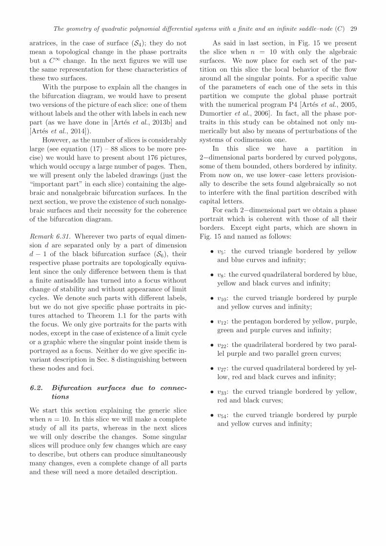
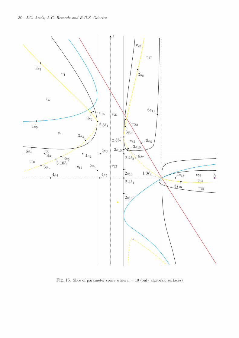
In Fig. 15 we represent the generic slice of theparameter space when n = n0 = 10, showing onlythe algebraic surfaces. We note that there are somedashed branches of surface (S3) (in yellow) and (S4)(in purple). This means the existence of a weak sad-dle, in the case of surface (S3), and the existence ofan invariant straight line without connecting sep-
The geometry of quadratic polynomial differential systems with a finite and an infinite saddle–node (C) 29
aratrices, in the case of surface (S4); they do notmean a topological change in the phase portraitsbut a C∞ change. In the next figures we will usethe same representation for these characteristics ofthese two surfaces.
With the purpose to explain all the changes inthe bifurcation diagram, we would have to presenttwo versions of the picture of each slice: one of themwithout labels and the other with labels in each newpart (as we have done in [Artes et al., 2013b] and[Artes et al., 2014]).
However, as the number of slices is considerablylarge (see equation (17) – 88 slices to be more pre-cise) we would have to present about 176 pictures,which would occupy a large number of pages. Then,we will present only the labeled drawings (just the“important part” in each slice) containing the alge-braic and nonalgebraic bifurcation surfaces. In thenext section, we prove the existence of such nonalge-braic surfaces and their necessity for the coherenceof the bifurcation diagram.
Remark 6.31. Wherever two parts of equal dimen-sion d are separated only by a part of dimensiond − 1 of the black bifurcation surface (S6), theirrespective phase portraits are topologically equiva-lent since the only difference between them is thata finite antisaddle has turned into a focus withoutchange of stability and without appearance of limitcycles. We denote such parts with different labels,but we do not give specific phase portraits in pic-tures attached to Theorem 1.1 for the parts withthe focus. We only give portraits for the parts withnodes, except in the case of existence of a limit cycleor a graphic where the singular point inside them isportrayed as a focus. Neither do we give specific in-variant description in Sec. 8 distinguishing betweenthese nodes and foci.
6.2. Bifurcation surfaces due to connec-tions
We start this section explaining the generic slicewhen n = 10. In this slice we will make a completestudy of all its parts, whereas in the next sliceswe will only describe the changes. Some singularslices will produce only few changes which are easyto describe, but others can produce simultaneouslymany changes, even a complete change of all partsand these will need a more detailed description.
As said in last section, in Fig. 15 we presentthe slice when n = 10 with only the algebraicsurfaces. We now place for each set of the par-tition on this slice the local behavior of the flowaround all the singular points. For a specific valueof the parameters of each one of the sets in thispartition we compute the global phase portraitwith the numerical program P4 [Artes et al., 2005,Dumortier et al., 2006]. In fact, all the phase por-traits in this study can be obtained not only nu-merically but also by means of perturbations of thesystems of codimension one.
In this slice we have a partition in2−dimensional parts bordered by curved polygons,some of them bounded, others bordered by infinity.From now on, we use lower–case letters provision-ally to describe the sets found algebraically so notto interfere with the final partition described withcapital letters.
For each 2−dimensional part we obtain a phaseportrait which is coherent with those of all theirborders. Except eight parts, which are shown inFig. 15 and named as follows:
• v5: the curved triangle bordered by yellowand blue curves and infinity;
• v8: the curved quadrilateral bordered by blue,yellow and black curves and infinity;
• v10: the curved triangle bordered by purpleand yellow curves and infinity;
• v12: the pentagon bordered by yellow, purple,green and purple curves and infinity;
• v22: the quadrilateral bordered by two paral-lel purple and two parallel green curves;
• v27: the curved quadrilateral bordered by yel-low, red and black curves and infinity;
• v33: the curved triangle bordered by yellow,red and black curves;
• v54: the curved triangle bordered by purpleand yellow curves and infinity;
30 J.C. Artes, A.C. Rezende and R.D.S. Oliveira
h
ℓ
v4
v5
v8
v16 v21
3s1
3s2
2.3ℓ1
2.3ℓ2
v10v12 v22
v26
v27
v32
v33
3s8
3s9
v52
v55
v543s16
4s13
4s3
2s13
2.4ℓ3
1.3ℓ2
1s5
6s4
3s3
6s11
5s53s10
6s7
2s10
4s1 4s2
4s4 4s5
v9
3s6
3s53.10ℓ1 2s5
2s14
2.4ℓ4
Fig. 15. Slice of parameter space when n = 10 (only algebraic surfaces)
The geometry of quadratic polynomial differential systems with a finite and an infinite saddle–node (C) 31
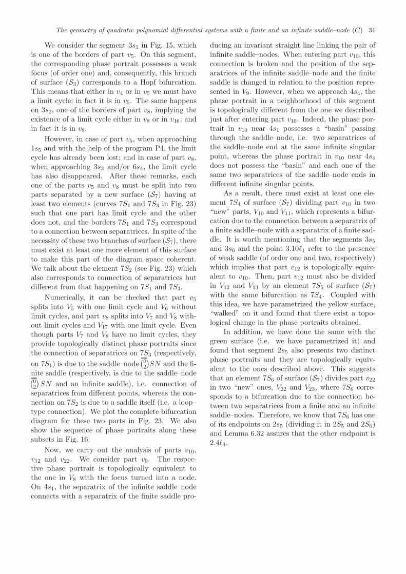
We consider the segment 3s1 in Fig. 15, whichis one of the borders of part v5. On this segment,the corresponding phase portrait possesses a weakfocus (of order one) and, consequently, this branchof surface (S3) corresponds to a Hopf bifurcation.This means that either in v4 or in v5 we must havea limit cycle; in fact it is in v5. The same happenson 3s2, one of the borders of part v8, implying theexistence of a limit cycle either in v8 or in v16; andin fact it is in v8.
However, in case of part v5, when approaching1s5 and with the help of the program P4, the limitcycle has already been lost; and in case of part v8,when approaching 3s3 and/or 6s4, the limit cyclehas also disappeared. After these remarks, eachone of the parts v5 and v8 must be split into twoparts separated by a new surface (S7) having atleast two elements (curves 7S1 and 7S3 in Fig. 23)such that one part has limit cycle and the otherdoes not, and the borders 7S1 and 7S3 correspondto a connection between separatrices. In spite of thenecessity of these two branches of surface (S7), theremust exist at least one more element of this surfaceto make this part of the diagram space coherent.We talk about the element 7S2 (see Fig. 23) whichalso corresponds to connection of separatrices butdifferent from that happening on 7S1 and 7S3.
Numerically, it can be checked that part v5splits into V5 with one limit cycle and V6 withoutlimit cycles, and part v8 splits into V7 and V8 with-out limit cycles and V17 with one limit cycle. Eventhough parts V7 and V8 have no limit cycles, theyprovide topologically distinct phase portraits sincethe connection of separatrices on 7S3 (respectively,
on 7S1) is due to the saddle–node(02
)SN and the fi-
nite saddle (respectively, is due to the saddle–node(02
)SN and an infinite saddle), i.e. connection of
separatrices from different points, whereas the con-nection on 7S2 is due to a saddle itself (i.e. a loop–type connection). We plot the complete bifurcationdiagram for these two parts in Fig. 23. We alsoshow the sequence of phase portraits along thesesubsets in Fig. 16.
Now, we carry out the analysis of parts v10,v12 and v22. We consider part v9. The respec-tive phase portrait is topologically equivalent tothe one in V8 with the focus turned into a node.On 4s1, the separatrix of the infinite saddle–nodeconnects with a separatrix of the finite saddle pro-
ducing an invariant straight line linking the pair ofinfinite saddle–nodes. When entering part v10, thisconnection is broken and the position of the sep-aratrices of the infinite saddle–node and the finitesaddle is changed in relation to the position repre-sented in V9. However, when we approach 4s4, thephase portrait in a neighborhood of this segmentis topologically different from the one we describedjust after entering part v10. Indeed, the phase por-trait in v10 near 4s1 possesses a “basin” passingthrough the saddle–node, i.e. two separatrices ofthe saddle–node end at the same infinite singularpoint, whereas the phase portrait in v10 near 4s4does not possess the “basin” and each one of thesame two separatrices of the saddle–node ends indifferent infinite singular points.
As a result, there must exist at least one ele-ment 7S4 of surface (S7) dividing part v10 in two“new” parts, V10 and V11, which represents a bifur-cation due to the connection between a separatrix ofa finite saddle–node with a separatrix of a finite sad-dle. It is worth mentioning that the segments 3s5and 3s6 and the point 3.10ℓ1 refer to the presenceof weak saddle (of order one and two, respectively)which implies that part v12 is topologically equiv-alent to v10. Then, part v12 must also be dividedin V12 and V13 by an element 7S5 of surface (S7)with the same bifurcation as 7S4. Coupled withthis idea, we have parametrized the yellow surface,“walked” on it and found that there exist a topo-logical change in the phase portraits obtained.
In addition, we have done the same with thegreen surface (i.e. we have parametrized it) andfound that segment 2s5 also presents two distinctphase portraits and they are topologically equiv-alent to the ones described above. This suggeststhat an element 7S6 of surface (S7) divides part v22in two “new” ones, V22 and V23, where 7S6 corre-sponds to a bifurcation due to the connection be-tween two separatrices from a finite and an infinitesaddle–nodes. Therefore, we know that 7S6 has oneof its endpoints on 2s5 (dividing it in 2S5 and 2S6)and Lemma 6.32 assures that the other endpoint is2.4ℓ3.
32 J.C. Artes, A.C. Rezende and R.D.S. Oliveira
V4V5
V8 V17
V6
V7
3S17S1
1.7L1
7S2
7S3
1S4 1S31.3L1
3S2 V16
1S5
Fig. 16. Sequence of phase portraits in parts v5 and v8 of slice n = 10. We start from v4. We recall that the phaseportrait 3S1 is equivalent to the phase portrait V4 up to a weak focus (represented by a little black square) insteadof the focus. When crossing 3s1, we shall obtain the phase portrait V5 in subset v5. From this point we may choosethree different ways to reach the subset v8 by crossing the blue curve: (1) from the phase portrait 1.3L1 to the V17;(2) from the phase portrait 1S4 to the V17; and (3) from the phase portrait 1.7L1 to the V7, V8, V17, 1S4, 7S2 and7S3
The geometry of quadratic polynomial differential systems with a finite and an infinite saddle–node (C) 33
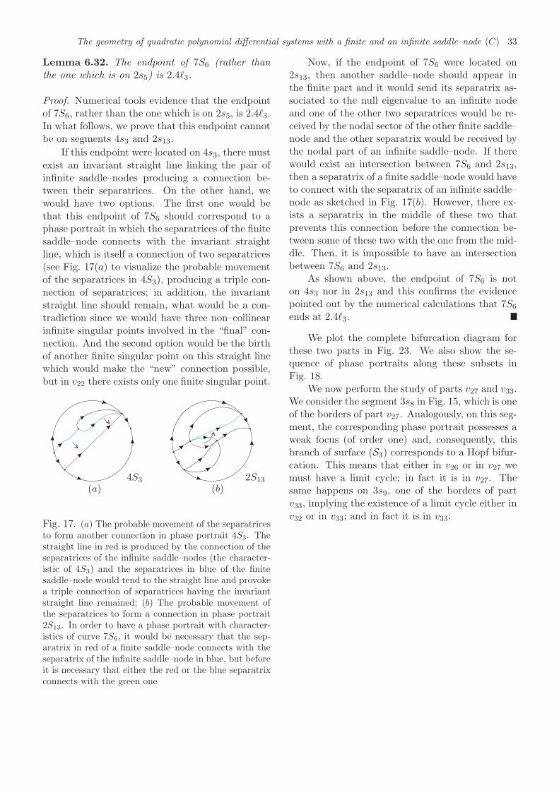
Lemma 6.32. The endpoint of 7S6 (rather thanthe one which is on 2s5) is 2.4ℓ3.
Proof. Numerical tools evidence that the endpointof 7S6, rather than the one which is on 2s5, is 2.4ℓ3.In what follows, we prove that this endpoint cannotbe on segments 4s3 and 2s13.
If this endpoint were located on 4s3, there mustexist an invariant straight line linking the pair ofinfinite saddle–nodes producing a connection be-tween their separatrices. On the other hand, wewould have two options. The first one would bethat this endpoint of 7S6 should correspond to aphase portrait in which the separatrices of the finitesaddle–node connects with the invariant straightline, which is itself a connection of two separatrices(see Fig. 17(a) to visualize the probable movementof the separatrices in 4S3), producing a triple con-nection of separatrices; in addition, the invariantstraight line should remain, what would be a con-tradiction since we would have three non–collinearinfinite singular points involved in the “final” con-nection. And the second option would be the birthof another finite singular point on this straight linewhich would make the “new” connection possible,but in v22 there exists only one finite singular point.
4S3 2S13
(a) (b)
Fig. 17. (a) The probable movement of the separatricesto form another connection in phase portrait 4S3. Thestraight line in red is produced by the connection of theseparatrices of the infinite saddle–nodes (the character-istic of 4S3) and the separatrices in blue of the finitesaddle–node would tend to the straight line and provokea triple connection of separatrices having the invariantstraight line remained; (b) The probable movement ofthe separatrices to form a connection in phase portrait2S13. In order to have a phase portrait with character-istics of curve 7S6, it would be necessary that the sep-aratrix in red of a finite saddle–node connects with theseparatrix of the infinite saddle–node in blue, but beforeit is necessary that either the red or the blue separatrixconnects with the green one
Now, if the endpoint of 7S6 were located on2s13, then another saddle–node should appear inthe finite part and it would send its separatrix as-sociated to the null eigenvalue to an infinite nodeand one of the other two separatrices would be re-ceived by the nodal sector of the other finite saddle–node and the other separatrix would be received bythe nodal part of an infinite saddle–node. If therewould exist an intersection between 7S6 and 2s13,then a separatrix of a finite saddle–node would haveto connect with the separatrix of an infinite saddle–node as sketched in Fig. 17(b). However, there ex-ists a separatrix in the middle of these two thatprevents this connection before the connection be-tween some of these two with the one from the mid-dle. Then, it is impossible to have an intersectionbetween 7S6 and 2s13.
As shown above, the endpoint of 7S6 is noton 4s3 nor in 2s13 and this confirms the evidencepointed out by the numerical calculations that 7S6
ends at 2.4ℓ3.
We plot the complete bifurcation diagram forthese two parts in Fig. 23. We also show the se-quence of phase portraits along these subsets inFig. 18.
We now perform the study of parts v27 and v33.We consider the segment 3s8 in Fig. 15, which is oneof the borders of part v27. Analogously, on this seg-ment, the corresponding phase portrait possesses aweak focus (of order one) and, consequently, thisbranch of surface (S3) corresponds to a Hopf bifur-cation. This means that either in v26 or in v27 wemust have a limit cycle; in fact it is in v27. Thesame happens on 3s9, one of the borders of partv33, implying the existence of a limit cycle either inv32 or in v33; and in fact it is in v33.
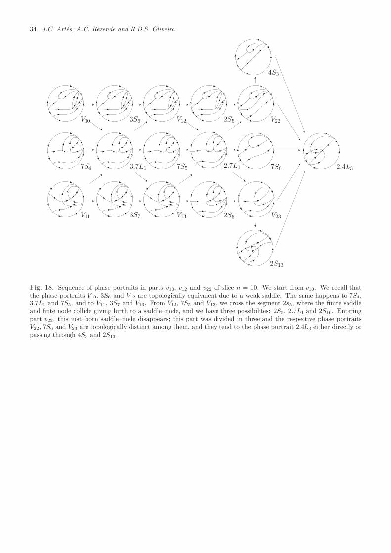
34 J.C. Artes, A.C. Rezende and R.D.S. Oliveira
V10 V12 V22
V11 V13 V23
3S6 2S5
4S3
7S4 7S5 7S6
3S7 2S6
2S13
3.7L1 2.7L1 2.4L3
Fig. 18. Sequence of phase portraits in parts v10, v12 and v22 of slice n = 10. We start from v10. We recall thatthe phase portraits V10, 3S6 and V12 are topologically equivalent due to a weak saddle. The same happens to 7S4,3.7L1 and 7S5, and to V11, 3S7 and V13. From V12, 7S5 and V13, we cross the segment 2s5, where the finite saddleand finte node collide giving birth to a saddle–node, and we have three possibilites: 2S5, 2.7L1 and 2S16. Enteringpart v22, this just–born saddle–node disappears; this part was divided in three and the respective phase portraitsV22, 7S6 and V23 are topologically distinct among them, and they tend to the phase portrait 2.4L3 either directly orpassing through 4S3 and 2S13
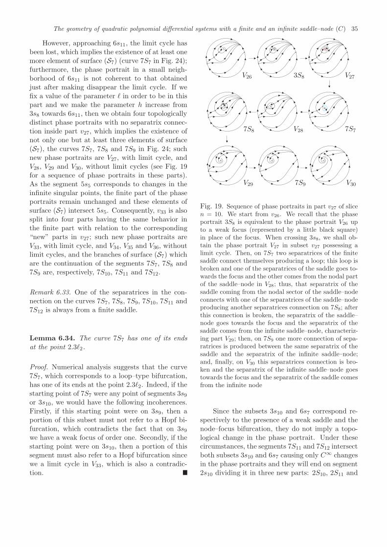
The geometry of quadratic polynomial differential systems with a finite and an infinite saddle–node (C) 35
However, approaching 6s11, the limit cycle hasbeen lost, which implies the existence of at least onemore element of surface (S7) (curve 7S7 in Fig. 24);furthermore, the phase portrait in a small neigh-borhood of 6s11 is not coherent to that obtainedjust after making disappear the limit cycle. If wefix a value of the parameter ℓ in order to be in thispart and we make the parameter h increase from3s8 towards 6s11, then we obtain four topologicallydistinct phase portraits with no separatrix connec-tion inside part v27, which implies the existence ofnot only one but at least three elements of surface(S7), the curves 7S7, 7S8 and 7S9 in Fig. 24; suchnew phase portraits are V27, with limit cycle, andV28, V29 and V30, without limit cycles (see Fig. 19for a sequence of phase portraits in these parts).As the segment 5s5 corresponds to changes in theinfinite singular points, the finite part of the phaseportraits remain unchanged and these elements ofsurface (S7) intersect 5s5. Consequently, v33 is alsosplit into four parts having the same behavior inthe finite part with relation to the corresponding“new” parts in v27; such new phase portraits areV33, with limit cycle, and V34, V35 and V36, withoutlimit cycles, and the branches of surface (S7) whichare the continuation of the segments 7S7, 7S8 and7S9 are, respectively, 7S10, 7S11 and 7S12.
Remark 6.33. One of the separatrices in the con-nection on the curves 7S7, 7S8, 7S9, 7S10, 7S11 and7S12 is always from a finite saddle.
Lemma 6.34. The curve 7S7 has one of its endsat the point 2.3ℓ2.
Proof. Numerical analysis suggests that the curve7S7, which corresponds to a loop–type bifurcation,has one of its ends at the point 2.3ℓ2. Indeed, if thestarting point of 7S7 were any point of segments 3s9or 3s10, we would have the following incoherences.Firstly, if this starting point were on 3s9, then aportion of this subset must not refer to a Hopf bi-furcation, which contradicts the fact that on 3s9we have a weak focus of order one. Secondly, if thestarting point were on 3s10, then a portion of thissegment must also refer to a Hopf bifurcation sincewe a limit cycle in V33, which is also a contradic-tion.
V26 V27
V28
V29 V30
3S8
7S77S8
7S9
Fig. 19. Sequence of phase portraits in part v27 of slicen = 10. We start from v26. We recall that the phaseportrait 3S8 is equivalent to the phase portrait V26 upto a weak focus (represented by a little black square)in place of the focus. When crossing 3s8, we shall ob-tain the phase portrait V27 in subset v27 possessing alimit cycle. Then, on 7S7 two separatrices of the finitesaddle connect themselves producing a loop; this loop isbroken and one of the separatrices of the saddle goes to-wards the focus and the other comes from the nodal partof the saddle–node in V28; thus, that separatrix of thesaddle coming from the nodal sector of the saddle–nodeconnects with one of the separatrices of the saddle–nodeproducing another separatrices connection on 7S8; afterthis connection is broken, the separatrix of the saddle–node goes towards the focus and the separatrix of thesaddle comes from the infinite saddle–node, characteriz-ing part V29; then, on 7S9 one more connection of sepa-ratrices is produced between the same separatrix of thesaddle and the separatrix of the infinite saddle–node;and, finally, on V30 this separatrices connection is bro-ken and the separatrix of the infinite saddle–node goestowards the focus and the separatrix of the saddle comesfrom the infinite node
Since the subsets 3s10 and 6s7 correspond re-spectively to the presence of a weak saddle and thenode–focus bifurcation, they do not imply a topo-logical change in the phase portrait. Under thesecircumstances, the segments 7S11 and 7S12 intersectboth subsets 3s10 and 6s7 causing only C∞ changesin the phase portraits and they will end on segment2s10 dividing it in three new parts: 2S10, 2S11 and
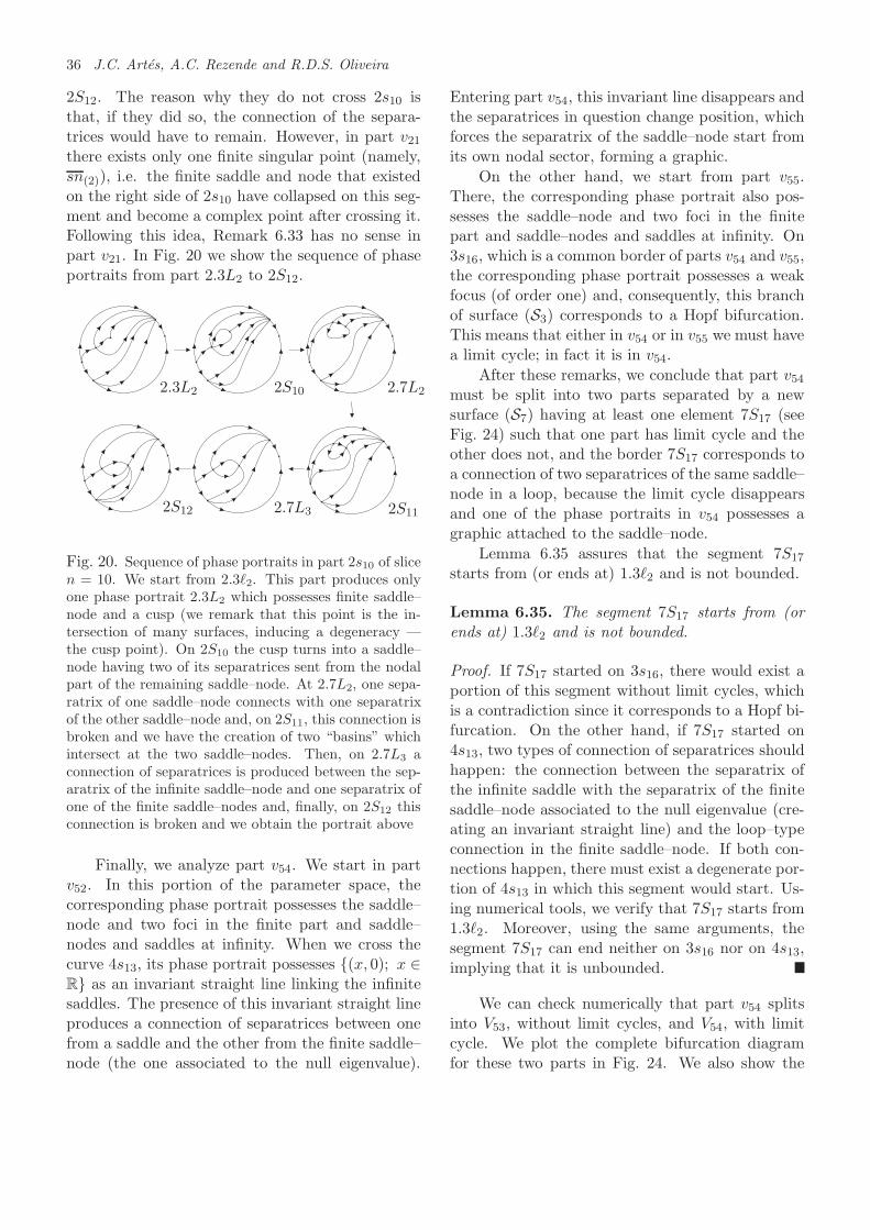
36 J.C. Artes, A.C. Rezende and R.D.S. Oliveira
2S12. The reason why they do not cross 2s10 isthat, if they did so, the connection of the separa-trices would have to remain. However, in part v21there exists only one finite singular point (namely,sn(2)), i.e. the finite saddle and node that existedon the right side of 2s10 have collapsed on this seg-ment and become a complex point after crossing it.Following this idea, Remark 6.33 has no sense inpart v21. In Fig. 20 we show the sequence of phaseportraits from part 2.3L2 to 2S12.
2S10
2S112S12
2.3L2 2.7L2
2.7L3
Fig. 20. Sequence of phase portraits in part 2s10 of slicen = 10. We start from 2.3ℓ2. This part produces onlyone phase portrait 2.3L2 which possesses finite saddle–node and a cusp (we remark that this point is the in-tersection of many surfaces, inducing a degeneracy —the cusp point). On 2S10 the cusp turns into a saddle–node having two of its separatrices sent from the nodalpart of the remaining saddle–node. At 2.7L2, one sepa-ratrix of one saddle–node connects with one separatrixof the other saddle–node and, on 2S11, this connection isbroken and we have the creation of two “basins” whichintersect at the two saddle–nodes. Then, on 2.7L3 aconnection of separatrices is produced between the sep-aratrix of the infinite saddle–node and one separatrix ofone of the finite saddle–nodes and, finally, on 2S12 thisconnection is broken and we obtain the portrait above
Finally, we analyze part v54. We start in partv52. In this portion of the parameter space, thecorresponding phase portrait possesses the saddle–node and two foci in the finite part and saddle–nodes and saddles at infinity. When we cross thecurve 4s13, its phase portrait possesses {(x, 0); x ∈R} as an invariant straight line linking the infinitesaddles. The presence of this invariant straight lineproduces a connection of separatrices between onefrom a saddle and the other from the finite saddle–node (the one associated to the null eigenvalue).
Entering part v54, this invariant line disappears andthe separatrices in question change position, whichforces the separatrix of the saddle–node start fromits own nodal sector, forming a graphic.
On the other hand, we start from part v55.There, the corresponding phase portrait also pos-sesses the saddle–node and two foci in the finitepart and saddle–nodes and saddles at infinity. On3s16, which is a common border of parts v54 and v55,the corresponding phase portrait possesses a weakfocus (of order one) and, consequently, this branchof surface (S3) corresponds to a Hopf bifurcation.This means that either in v54 or in v55 we must havea limit cycle; in fact it is in v54.
After these remarks, we conclude that part v54must be split into two parts separated by a newsurface (S7) having at least one element 7S17 (seeFig. 24) such that one part has limit cycle and theother does not, and the border 7S17 corresponds toa connection of two separatrices of the same saddle–node in a loop, because the limit cycle disappearsand one of the phase portraits in v54 possesses agraphic attached to the saddle–node.
Lemma 6.35 assures that the segment 7S17
starts from (or ends at) 1.3ℓ2 and is not bounded.
Lemma 6.35. The segment 7S17 starts from (orends at) 1.3ℓ2 and is not bounded.
Proof. If 7S17 started on 3s16, there would exist aportion of this segment without limit cycles, whichis a contradiction since it corresponds to a Hopf bi-furcation. On the other hand, if 7S17 started on4s13, two types of connection of separatrices shouldhappen: the connection between the separatrix ofthe infinite saddle with the separatrix of the finitesaddle–node associated to the null eigenvalue (cre-ating an invariant straight line) and the loop–typeconnection in the finite saddle–node. If both con-nections happen, there must exist a degenerate por-tion of 4s13 in which this segment would start. Us-ing numerical tools, we verify that 7S17 starts from1.3ℓ2. Moreover, using the same arguments, thesegment 7S17 can end neither on 3s16 nor on 4s13,implying that it is unbounded.
We can check numerically that part v54 splitsinto V53, without limit cycles, and V54, with limitcycle. We plot the complete bifurcation diagramfor these two parts in Fig. 24. We also show the
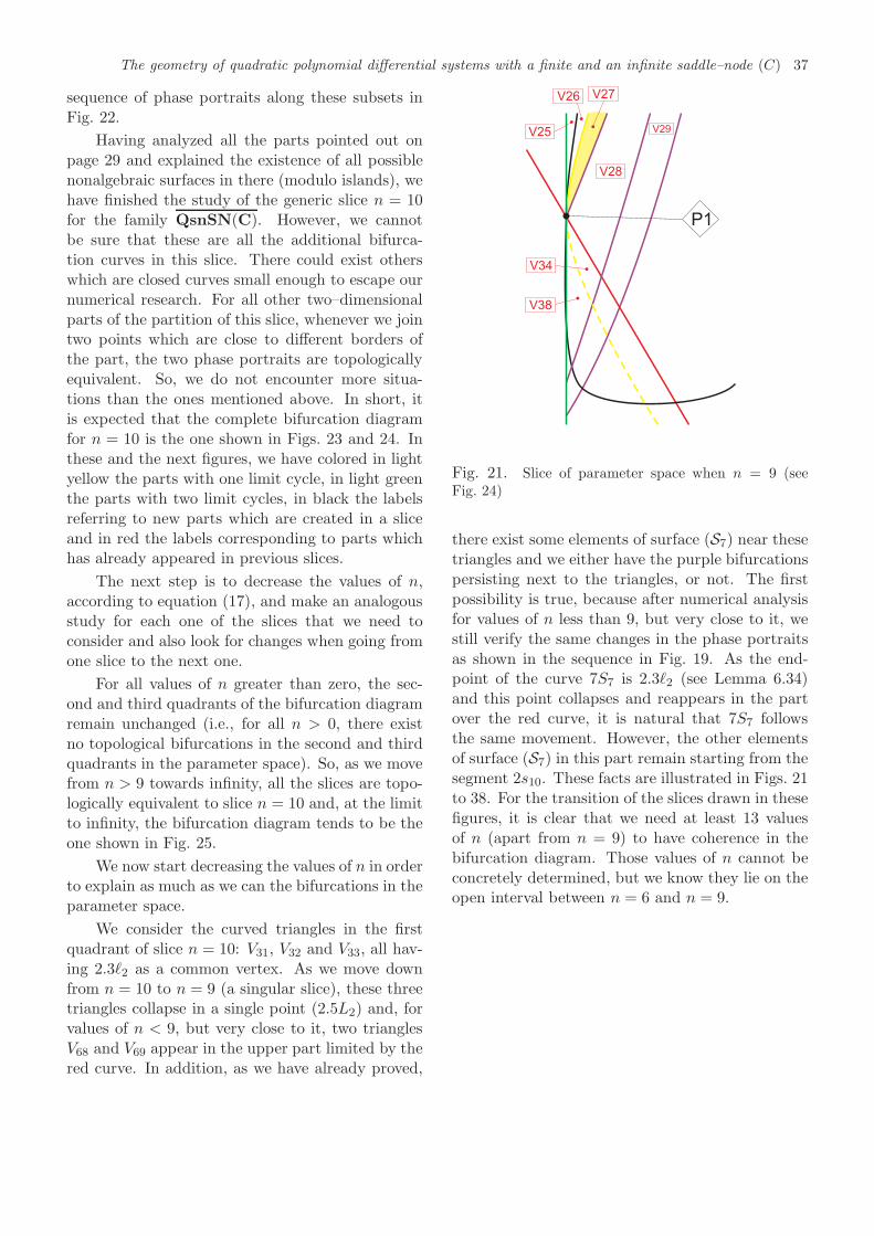
The geometry of quadratic polynomial differential systems with a finite and an infinite saddle–node (C) 37
sequence of phase portraits along these subsets inFig. 22.
Having analyzed all the parts pointed out onpage 29 and explained the existence of all possiblenonalgebraic surfaces in there (modulo islands), wehave finished the study of the generic slice n = 10for the family QsnSN(C). However, we cannotbe sure that these are all the additional bifurca-tion curves in this slice. There could exist otherswhich are closed curves small enough to escape ournumerical research. For all other two–dimensionalparts of the partition of this slice, whenever we jointwo points which are close to different borders ofthe part, the two phase portraits are topologicallyequivalent. So, we do not encounter more situa-tions than the ones mentioned above. In short, itis expected that the complete bifurcation diagramfor n = 10 is the one shown in Figs. 23 and 24. Inthese and the next figures, we have colored in lightyellow the parts with one limit cycle, in light greenthe parts with two limit cycles, in black the labelsreferring to new parts which are created in a sliceand in red the labels corresponding to parts whichhas already appeared in previous slices.
The next step is to decrease the values of n,according to equation (17), and make an analogousstudy for each one of the slices that we need toconsider and also look for changes when going fromone slice to the next one.
For all values of n greater than zero, the sec-ond and third quadrants of the bifurcation diagramremain unchanged (i.e., for all n > 0, there existno topological bifurcations in the second and thirdquadrants in the parameter space). So, as we movefrom n > 9 towards infinity, all the slices are topo-logically equivalent to slice n = 10 and, at the limitto infinity, the bifurcation diagram tends to be theone shown in Fig. 25.
We now start decreasing the values of n in orderto explain as much as we can the bifurcations in theparameter space.
We consider the curved triangles in the firstquadrant of slice n = 10: V31, V32 and V33, all hav-ing 2.3ℓ2 as a common vertex. As we move downfrom n = 10 to n = 9 (a singular slice), these threetriangles collapse in a single point (2.5L2) and, forvalues of n < 9, but very close to it, two trianglesV68 and V69 appear in the upper part limited by thered curve. In addition, as we have already proved,
P1
V34
V38
V25
V26 V27
V28
V29
Fig. 21. Slice of parameter space when n = 9 (seeFig. 24)
there exist some elements of surface (S7) near thesetriangles and we either have the purple bifurcationspersisting next to the triangles, or not. The firstpossibility is true, because after numerical analysisfor values of n less than 9, but very close to it, westill verify the same changes in the phase portraitsas shown in the sequence in Fig. 19. As the end-point of the curve 7S7 is 2.3ℓ2 (see Lemma 6.34)and this point collapses and reappears in the partover the red curve, it is natural that 7S7 followsthe same movement. However, the other elementsof surface (S7) in this part remain starting from thesegment 2s10. These facts are illustrated in Figs. 21to 38. For the transition of the slices drawn in thesefigures, it is clear that we need at least 13 valuesof n (apart from n = 9) to have coherence in thebifurcation diagram. Those values of n cannot beconcretely determined, but we know they lie on theopen interval between n = 6 and n = 9.
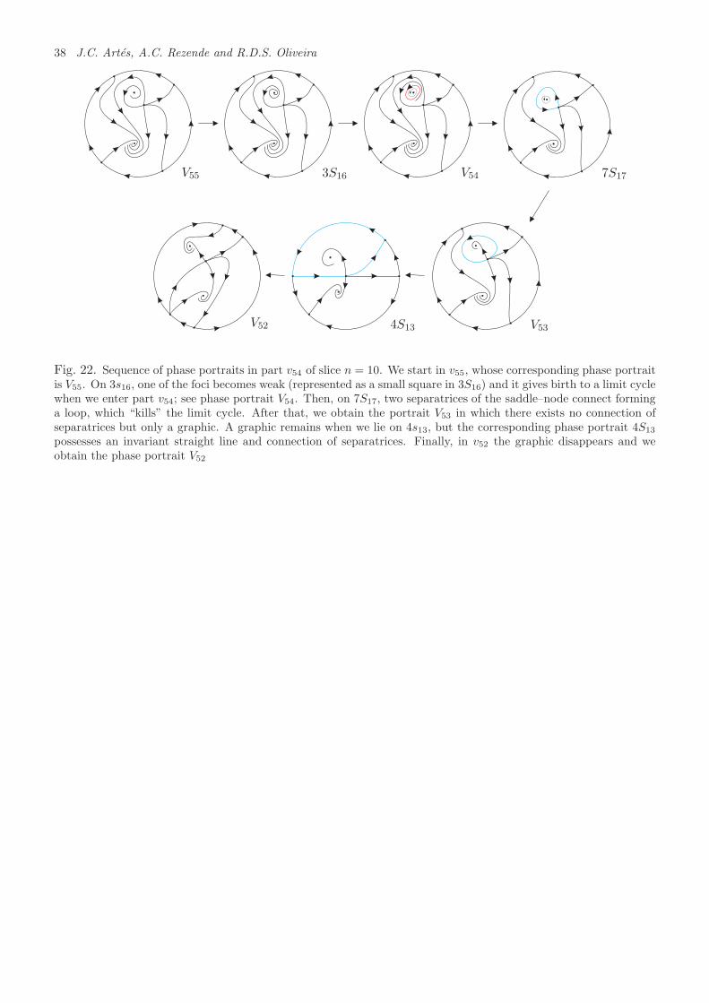
38 J.C. Artes, A.C. Rezende and R.D.S. Oliveira
V55 3S16 V54 7S17
V534S13V52
Fig. 22. Sequence of phase portraits in part v54 of slice n = 10. We start in v55, whose corresponding phase portraitis V55. On 3s16, one of the foci becomes weak (represented as a small square in 3S16) and it gives birth to a limit cyclewhen we enter part v54; see phase portrait V54. Then, on 7S17, two separatrices of the saddle–node connect forminga loop, which “kills” the limit cycle. After that, we obtain the portrait V53 in which there exists no connection ofseparatrices but only a graphic. A graphic remains when we lie on 4s13, but the corresponding phase portrait 4S13
possesses an invariant straight line and connection of separatrices. Finally, in v52 the graphic disappears and weobtain the phase portrait V52
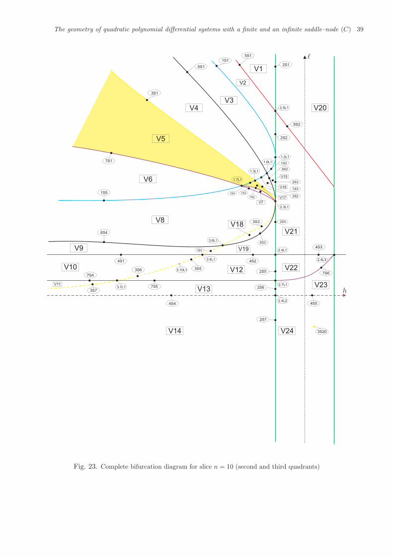
The geometry of quadratic polynomial differential systems with a finite and an infinite saddle–node (C) 39
V1
V2
V3
V4
V5
V6V15
V16
V17
V7
V8
V9
V10
V11
V12
V13
V14 V24
V23
V22
V21
V19
V18
V20
2S1
5S1
1S1
6S1
3S1
1S5
7S1
6S4
4S1
3S6
7S5
4S4
3S7
7S4
3S5
3S4
4S2
3S3
6S3
2S4
7S2
7S31S4
3S2
1S3
2S3
6S2
1S2
2S2
5S2
2S5
2S6
2S7
4S5
3S20
7S6
4S3
2.5L1
1.2L1
1.6L1
1.3L1
1.7L1
2.3L1
3.6L1
3.4L1
3.10L1
3.7L1
2.4L2
2.7L1
2.4L1
2.4L3
h
ℓ
Fig. 23. Complete bifurcation diagram for slice n = 10 (second and third quadrants)
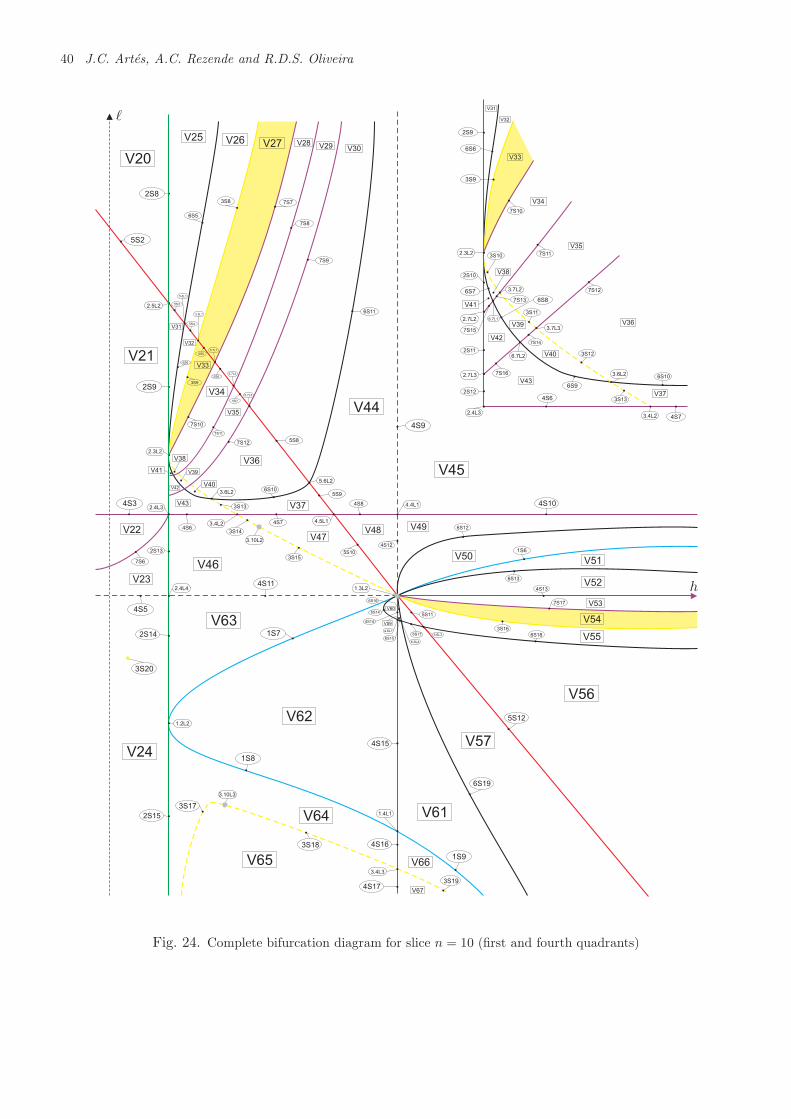
40 J.C. Artes, A.C. Rezende and R.D.S. Oliveira
V20
V21
V26V25V27 V28
V29 V30
V31
V32
V33
V34
V35
V36V38
V41 V39
V44
V45
V31
V32
V33
V34
V35
V36
V40
V43
V42
V39
V38
V41
V37
2S8
5S2
2S9
5S87S12
7S11
7S10
3S9
6S6
5S7
5S6
5S5
5S4
5S3
7S9
7S8
7S73S8
6S5
6S11
4S9
7S10
2S9
6S6
3S9
7S11
7S12
3S11
3S10
2S10
6S7
7S13
7S15
2S11
7S16
3S12
7S14
6S8
6S9
4S6
2S12
4S7
6S10
3S13
2.5L2
5.6L1
3.5L1
5.7L1
5.7L2
5.7L3
2.3L2
5.6L2
V22
V23
V24
3S20
V40
V43
V42
V37
V47
V46
V48 V49
V63
V62
V64
V65 V66
V67
V61
V57
V56
V55
V54
V53
V52
V51V50
V60
V59
4S3
7S6
2S13
4S5
2S14
4S11
1S7
4S6
4S7
3S14
3S13
3S15
4S8
5S96S10
4S10
4S12
5S10
6S12
1S6
6S13
4S13
7S17
3S16
6S18
5S11
6S17
6S16
6S14
4S14
6S15
1S8
1S9
4S15
5S12
6S19
3S18
3S17
4S16
2S15
4S173S19
2.4L3
3.4L2
3.10L2
4.5L1
3.6L2
4.4L1
1.3L2
4.6L1
6.6L4
5.6L3
1.2L2
2.4L4
1.4L1
3.4L3
3.10L3
2.3L2
2.7L2
3.7L2
3.7L3
6.7L1
6.7L2
3.6L2
3.4L22.4L3
2.7L3
h
ℓ
Fig. 24. Complete bifurcation diagram for slice n = 10 (first and fourth quadrants)
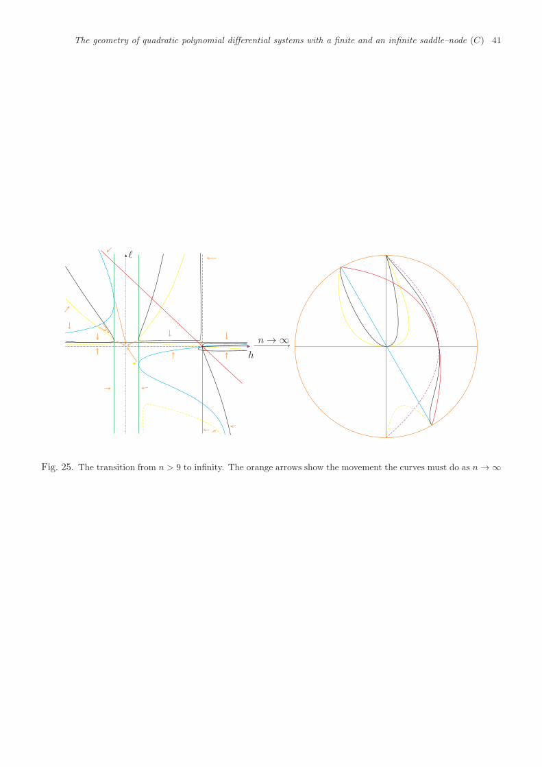
The geometry of quadratic polynomial differential systems with a finite and an infinite saddle–node (C) 41
n → ∞h
ℓ
Fig. 25. The transition from n > 9 to infinity. The orange arrows show the movement the curves must do as n → ∞
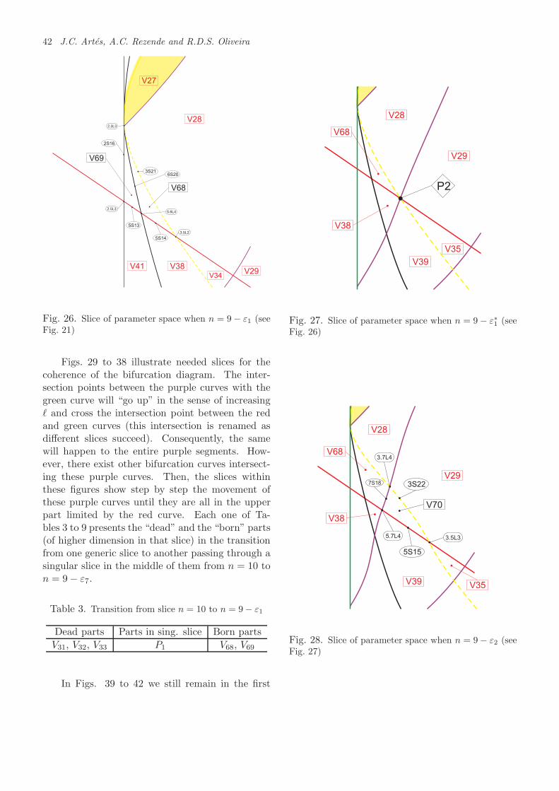
42 J.C. Artes, A.C. Rezende and R.D.S. Oliveira
3.5L2
3S216S20
2S16
5S13
5S14
5.6L42.5L3
2.3L3
V27
V28
V29V34
V38V41
Fig. 26. Slice of parameter space when n = 9− ε1 (seeFig. 21)
Figs. 29 to 38 illustrate needed slices for thecoherence of the bifurcation diagram. The inter-section points between the purple curves with thegreen curve will “go up” in the sense of increasingℓ and cross the intersection point between the redand green curves (this intersection is renamed asdifferent slices succeed). Consequently, the samewill happen to the entire purple segments. How-ever, there exist other bifurcation curves intersect-ing these purple curves. Then, the slices withinthese figures show step by step the movement ofthese purple curves until they are all in the upperpart limited by the red curve. Each one of Ta-bles 3 to 9 presents the “dead” and the “born” parts(of higher dimension in that slice) in the transitionfrom one generic slice to another passing through asingular slice in the middle of them from n = 10 ton = 9− ε7.
Table 3. Transition from slice n = 10 to n = 9− ε1
Dead parts Parts in sing. slice Born parts
V31, V32, V33 P1 V68, V69
In Figs. 39 to 42 we still remain in the first
P2
V35
V29
V28
V68
V38
V39
Fig. 27. Slice of parameter space when n = 9 − ε∗1 (seeFig. 26)
3S22
3.5L3
V70
5S15
7S18
5.7L4
3.7L4
V35
V29
V28
V68
V38
V39
Fig. 28. Slice of parameter space when n = 9− ε2 (seeFig. 27)
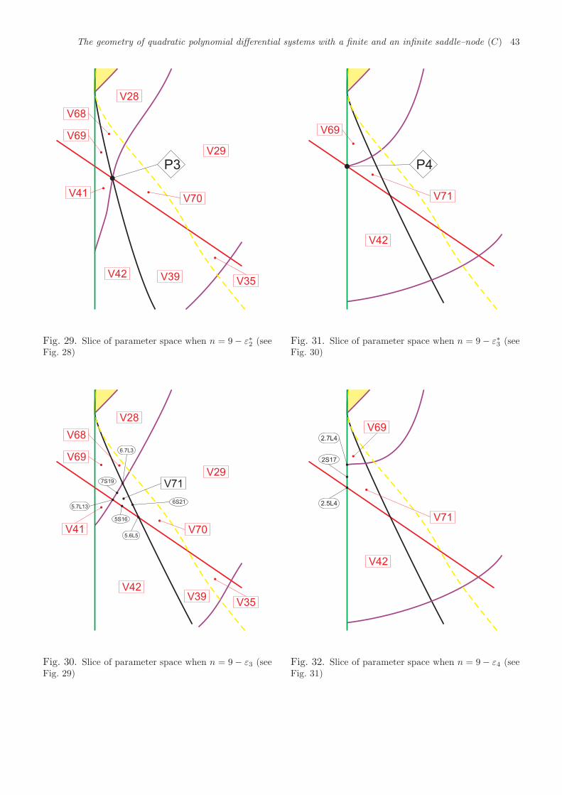
The geometry of quadratic polynomial differential systems with a finite and an infinite saddle–node (C) 43
P3
V35
V29
V28
V68
V41
V39V42
V69
V70
Fig. 29. Slice of parameter space when n = 9− ε∗2 (seeFig. 28)
V71
5S16
5.7L13
7S19
6S21
5.6L5
6.7L3
V35
V29
V28
V68
V41
V39V42
V69
V70
Fig. 30. Slice of parameter space when n = 9− ε3 (seeFig. 29)
P4
V42
V69
V71
Fig. 31. Slice of parameter space when n = 9 − ε∗3 (seeFig. 30)
2S17
2.7L4
2.5L4
V42
V69
V71
Fig. 32. Slice of parameter space when n = 9− ε4 (seeFig. 31)
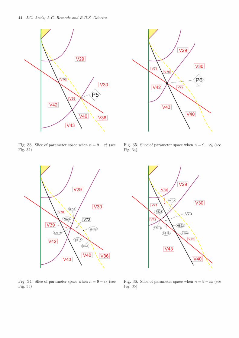
44 J.C. Artes, A.C. Rezende and R.D.S. Oliveira
P5
V70
V29
V30
V36V40
V39
V42
V43
Fig. 33. Slice of parameter space when n = 9− ε∗4 (seeFig. 32)
V72
3S23
3.5L4
7S20
5S17
3.7L5
5.7L14
V70
V29
V30
V36V40
V42
V43
V39
Fig. 34. Slice of parameter space when n = 9− ε5 (seeFig. 33)
P6
V70
V29
V30
V40
V42
V43
V72
V71
Fig. 35. Slice of parameter space when n = 9 − ε∗5 (seeFig. 34)
V73
6S22
5.6L6
7S21
5S18
6.7L4
5.7L15
V70
V29
V30
V40
V43
V72
V71
V42
Fig. 36. Slice of parameter space when n = 9− ε6 (seeFig. 35)
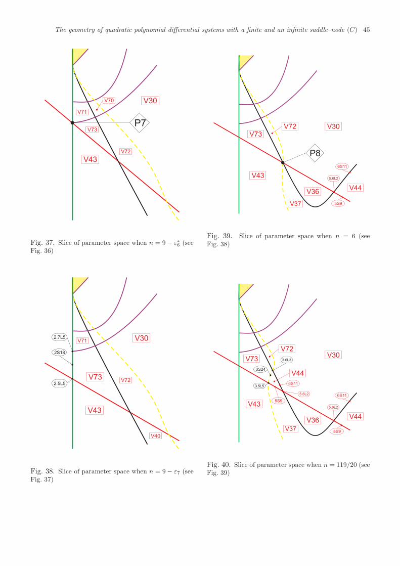
The geometry of quadratic polynomial differential systems with a finite and an infinite saddle–node (C) 45
P7
V70 V30
V43
V72
V71
V73
Fig. 37. Slice of parameter space when n = 9− ε∗6 (seeFig. 36)
2S18
2.7L5
2.5L5
V30
V73V72
V71
V43
V40
Fig. 38. Slice of parameter space when n = 9− ε7 (seeFig. 37)
P8
V43
V37
V36
V30V72
V73
V44
5.6L2
6S11
5S9
Fig. 39. Slice of parameter space when n = 6 (seeFig. 38)
6S11
5.6L2
3S24
5S9
3.6L3
3.5L5
V43
V37
V36
V30V72
V73
V44
5.6L2
6S11
V44
5S9
Fig. 40. Slice of parameter space when n = 119/20 (seeFig. 39)
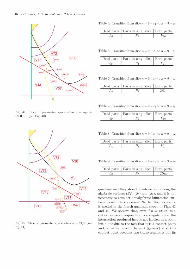
46 J.C. Artes, A.C. Rezende and R.D.S. Oliveira
5.6L2
V30
V44
V44V37
6S11
3S24
5S9
3.6L3
3.5L5
V43
V72
V73
6S11
5S9
Fig. 41. Slice of parameter space when n = n17 ≈5.8908 . . . (see Fig. 40)
V30
V44
V37
6S113S24
5S9
3.6L3
3.5L5
V43
V72
V73
V46 V473.10L2
3.4L2
3S14
3S15
Fig. 42. Slice of parameter space when n = 21/4 (seeFig. 41)
Table 4. Transition from slice n = 9− ε1 to n = 9− ε2
Dead parts Parts in sing. slice Born parts
V34 P2 V70
Table 5. Transition from slice n = 9− ε2 to n = 9− ε3
Dead parts Parts in sing. slice Born parts
V38 P3 V71
Table 6. Transition from slice n = 9− ε3 to n = 9− ε4
Dead parts Parts in sing. slice Born parts
V41 P4 2S17
Table 7. Transition from slice n = 9− ε4 to n = 9− ε5
Dead parts Parts in sing. slice Born parts
V35 P5 V72
Table 8. Transition from slice n = 9− ε5 to n = 9− ε6
Dead parts Parts in sing. slice Born parts
V39 P6 V73
Table 9. Transition from slice n = 9− ε6 to n = 9− ε7
Dead parts Parts in sing. slice Born parts
V42 P7 2S18
quadrant and they show the interaction among thealgebraic surfaces (S3), (S5) and (S6), and it is notnecessary to consider nonalgebraic bifurcation sur-faces to keep the coherence. Neither their existenceis needed in the fourth quadrant shown in Figs. 43and 44. We observe that, even if n = 125/27 is acritical value corresponding to a singular slice, theintersection produced here is not labeled as a pointbut a line due to the fact that it is a contact pointand, when we pass to the next (generic) slice, thiscontact point becomes two transversal ones but its
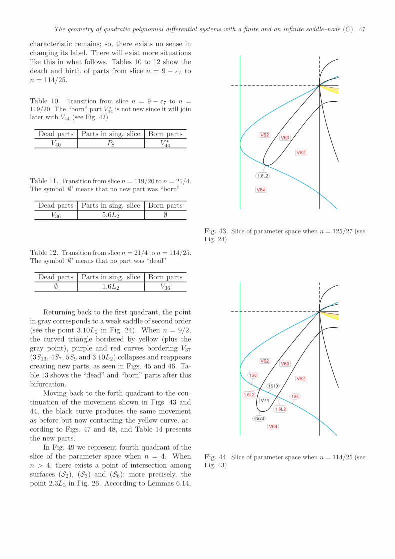
The geometry of quadratic polynomial differential systems with a finite and an infinite saddle–node (C) 47
characteristic remains; so, there exists no sense inchanging its label. There will exist more situationslike this in what follows. Tables 10 to 12 show thedeath and birth of parts from slice n = 9 − ε7 ton = 114/25.
Table 10. Transition from slice n = 9 − ε7 to n =119/20. The “born” part V ∗
44 is not new since it will joinlater with V44 (see Fig. 42)
Dead parts Parts in sing. slice Born parts
V40 P8 V ∗44
Table 11. Transition from slice n = 119/20 to n = 21/4.The symbol ‘∅’ means that no new part was “born”
Dead parts Parts in sing. slice Born parts
V36 5.6L2 ∅
Table 12. Transition from slice n = 21/4 to n = 114/25.The symbol ‘∅’ means that no part was “dead”
Dead parts Parts in sing. slice Born parts
∅ 1.6L2 V36
Returning back to the first quadrant, the pointin gray corresponds to a weak saddle of second order(see the point 3.10L2 in Fig. 24). When n = 9/2,the curved triangle bordered by yellow (plus thegray point), purple and red curves bordering V37
(3S13, 4S7, 5S9 and 3.10L2) collapses and reappearscreating new parts, as seen in Figs. 45 and 46. Ta-ble 13 shows the “dead” and “born” parts after thisbifurcation.
Moving back to the forth quadrant to the con-tinuation of the movement shown in Figs. 43 and44, the black curve produces the same movementas before but now contacting the yellow curve, ac-cording to Figs. 47 and 48, and Table 14 presentsthe new parts.
In Fig. 49 we represent fourth quadrant of theslice of the parameter space when n = 4. Whenn > 4, there exists a point of intersection amongsurfaces (S2), (S3) and (S6); more precisely, thepoint 2.3L3 in Fig. 26. According to Lemmas 6.14,
V62V60
V62
1.6L2
V64
Fig. 43. Slice of parameter space when n = 125/27 (seeFig. 24)
V74
6S23
1S10
1.6L2
V62V60
V62
V64
1.6L2
1S8
1S8
Fig. 44. Slice of parameter space when n = 114/25 (seeFig. 43)
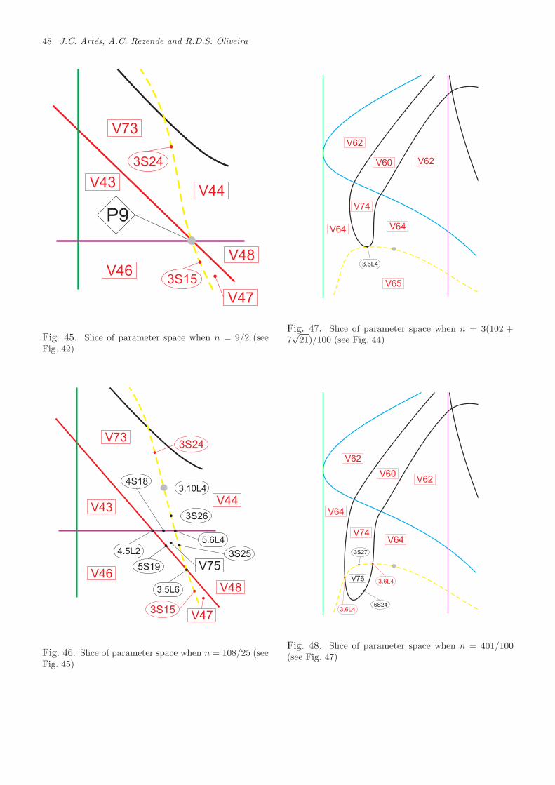
48 J.C. Artes, A.C. Rezende and R.D.S. Oliveira
P9
V73
3S24
V44
V48
V47
V46
V43
3S15
Fig. 45. Slice of parameter space when n = 9/2 (seeFig. 42)
3S26
5.6L4
3.10L4
5S19
3.5L6
4.5L2
4S18
V75
3S24
V44
V73
V43
V48
V47
V46
3S15
3S25
Fig. 46. Slice of parameter space when n = 108/25 (seeFig. 45)
3.6L4
V62
V60 V62
V64
V74
V64
V65
Fig. 47. Slice of parameter space when n = 3(102 +7√21)/100 (see Fig. 44)
3S27
V76
6S24
V62
V60V62
V64
V74V64
3.6L4
3.6L4
Fig. 48. Slice of parameter space when n = 401/100(see Fig. 47)
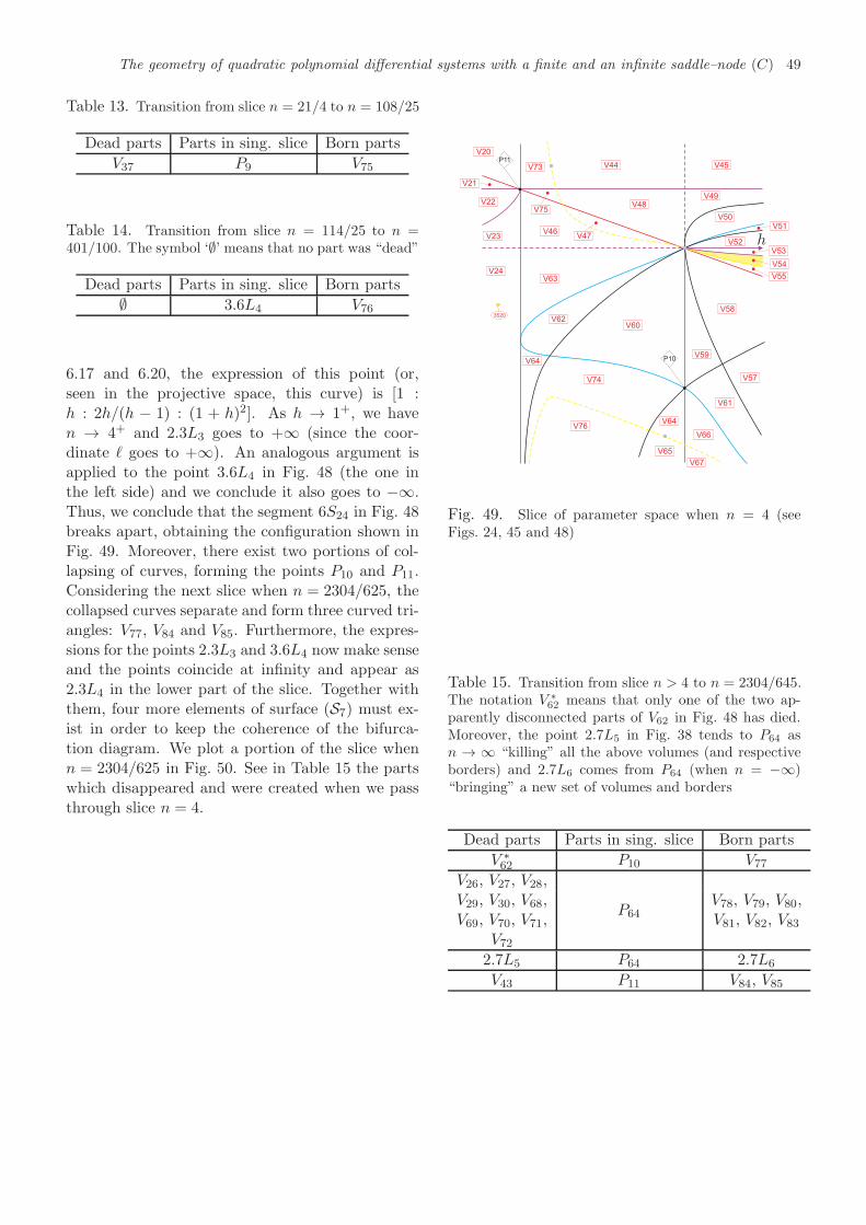
The geometry of quadratic polynomial differential systems with a finite and an infinite saddle–node (C) 49
Table 13. Transition from slice n = 21/4 to n = 108/25
Dead parts Parts in sing. slice Born parts
V37 P9 V75
Table 14. Transition from slice n = 114/25 to n =401/100. The symbol ‘∅’ means that no part was “dead”
Dead parts Parts in sing. slice Born parts
∅ 3.6L4 V76
6.17 and 6.20, the expression of this point (or,seen in the projective space, this curve) is [1 :h : 2h/(h − 1) : (1 + h)2]. As h → 1+, we haven → 4+ and 2.3L3 goes to +∞ (since the coor-dinate ℓ goes to +∞). An analogous argument isapplied to the point 3.6L4 in Fig. 48 (the one inthe left side) and we conclude it also goes to −∞.Thus, we conclude that the segment 6S24 in Fig. 48breaks apart, obtaining the configuration shown inFig. 49. Moreover, there exist two portions of col-lapsing of curves, forming the points P10 and P11.Considering the next slice when n = 2304/625, thecollapsed curves separate and form three curved tri-angles: V77, V84 and V85. Furthermore, the expres-sions for the points 2.3L3 and 3.6L4 now make senseand the points coincide at infinity and appear as2.3L4 in the lower part of the slice. Together withthem, four more elements of surface (S7) must ex-ist in order to keep the coherence of the bifurca-tion diagram. We plot a portion of the slice whenn = 2304/625 in Fig. 50. See in Table 15 the partswhich disappeared and were created when we passthrough slice n = 4.
P11
P10
3S20
V73
V20
V21
V22
V23
V24
V44 V45
V48
V49
V50V75
V46
V63
V47
V62
V64
V74
V60
V76V64
V65
V67
V66
V61
V59
V58
V57
V55
V54
V53
V52
V51
h
Fig. 49. Slice of parameter space when n = 4 (seeFigs. 24, 45 and 48)
Table 15. Transition from slice n > 4 to n = 2304/645.The notation V ∗
62 means that only one of the two ap-parently disconnected parts of V62 in Fig. 48 has died.Moreover, the point 2.7L5 in Fig. 38 tends to P64 asn → ∞ “killing” all the above volumes (and respectiveborders) and 2.7L6 comes from P64 (when n = −∞)“bringing” a new set of volumes and borders
Dead parts Parts in sing. slice Born parts
V ∗62 P10 V77
V26, V27, V28,
P64V29, V30, V68, V78, V79, V80,V69, V70, V71, V81, V82, V83
V72
2.7L5 P64 2.7L6
V43 P11 V84, V85
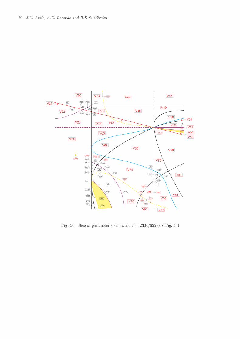
50 J.C. Artes, A.C. Rezende and R.D.S. Oliveira
V81
2.7L6
7S23
V77
1S11
4S19
6S25
1.4L2
4.6L2
1.6L4
7S24
7S25
3S29
7S22
2S20
6S27
3S282S19
6S26
2.3L4
6.7L5
3.7L6
V80
V78
V79
V82
V83
4S20
2S21
5S20
5S21
7S26
5.7L4
4.5L3 2.4L5
V85
V84
2.5L6
3.10L3
V73V20
V21
V22 V75
V23V46
V44V45
V48
V49
V50
V47V52
V51
V55
V54
V53
V63
V24
3S20
V62
V60V58
V59
V57
V61
V66
V67V65
V74
V76
V64
3S27
3S17
3.4L44S16
6S23
3S18
V64
3.10L4
2S15
6S23
1.3L2
h
Fig. 50. Slice of parameter space when n = 2304/625 (see Fig. 49)
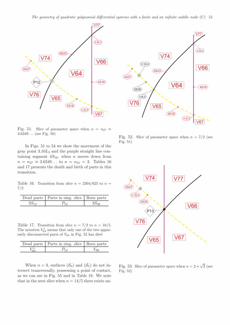
The geometry of quadratic polynomial differential systems with a finite and an infinite saddle–node (C) 51
P12
V66
V65
V74
V76
3S27
4.6L2
4S16
6S23
3S18
V64
V77
V67
3.4L3
Fig. 51. Slice of parameter space when n = n27 ≈3.6349 . . . (see Fig. 50)
In Figs. 51 to 54 we show the movement of thegray point 3.10L3 and the purple straight line con-taining segment 4S16, when n moves down fromn = n27 ≈ 3.6349 . . . to n = n31 = 3. Tables 16and 17 presents the death and birth of parts in thistransition.
Table 16. Transition from slice n = 2304/625 to n =7/2
Dead parts Parts in sing. slice Born parts
3S12 P12 3S30
Table 17. Transition from slice n = 7/2 to n = 16/5.The notation V ∗
64 means that only one of the two appar-ently disconnected parts of V64 in Fig. 52 has died
Dead parts Parts in sing. slice Born parts
V ∗64 P13 V86
When n = 3, surfaces (S3) and (S5) do not in-tersect transversally, possessing a point of contact,as we can see in Fig. 55 and in Table 18. We notethat in the next slice when n = 14/5 there exists an-
3S30
3.6L5
3.10L5
V64
V74
V66
4.6L2
4S16
V65
3S18
V76
3S27
6S23
V67
V77
3.4L3
Fig. 52. Slice of parameter space when n = 7/2 (seeFig. 51)
P13
V74 V77
V66
V67V65
V76
3.10L5
3S27
3S30
Fig. 53. Slice of parameter space when n = 2+√2 (see
Fig. 52)
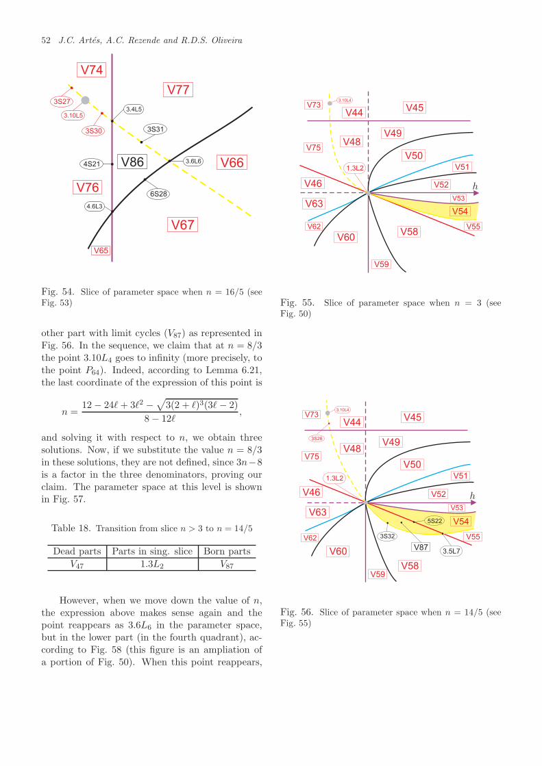
52 J.C. Artes, A.C. Rezende and R.D.S. Oliveira
4.6L3
6S28
V86
3S31
4S213.6L6
3.4L5
V74
V77
V66
V67
V65
V76
3S27
3S30
3.10L5
Fig. 54. Slice of parameter space when n = 16/5 (seeFig. 53)
other part with limit cycles (V87) as represented inFig. 56. In the sequence, we claim that at n = 8/3the point 3.10L4 goes to infinity (more precisely, tothe point P64). Indeed, according to Lemma 6.21,the last coordinate of the expression of this point is
n =12− 24ℓ+ 3ℓ2 −
√3(2 + ℓ)3(3ℓ− 2)
8− 12ℓ,
and solving it with respect to n, we obtain threesolutions. Now, if we substitute the value n = 8/3in these solutions, they are not defined, since 3n−8is a factor in the three denominators, proving ourclaim. The parameter space at this level is shownin Fig. 57.
Table 18. Transition from slice n > 3 to n = 14/5
Dead parts Parts in sing. slice Born parts
V47 1.3L2 V87
However, when we move down the value of n,the expression above makes sense again and thepoint reappears as 3.6L6 in the parameter space,but in the lower part (in the fourth quadrant), ac-cording to Fig. 58 (this figure is an ampliation ofa portion of Fig. 50). When this point reappears,
3.10L4
V73
V75
V44
V48V49
V46
V63
V62
V60
V59
V58
V50
V51
V53
V54
V55
V45
1.3L2
V52 h
Fig. 55. Slice of parameter space when n = 3 (seeFig. 50)
3.5L7
3S32
V87
5S22
3.10L4
V73
V44V45
V75V48
V49
V46
V50
V51
V52
V53V63
V62
V60
V59
V58
V54
V55
3S26
1.3L2
h
Fig. 56. Slice of parameter space when n = 14/5 (seeFig. 55)
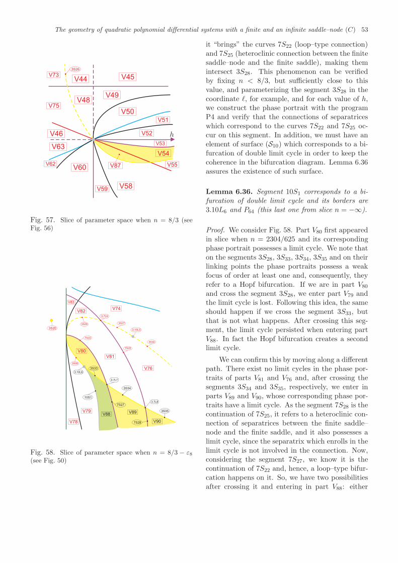
The geometry of quadratic polynomial differential systems with a finite and an infinite saddle–node (C) 53
V73V44 V45
V75V48
V49
V46
V50
V51
V53V63
V62V60
V59V58
V54
V55
3S26
V87
V52 h
Fig. 57. Slice of parameter space when n = 8/3 (seeFig. 56)
10S1
7S27
V88V89
3S34
7S28
3S35
3.7L7
3.7L8
3.10L6
V90
3S33
V80
3S203.10L5
V79
V78
3S28
7S22
7S25
3S27
V81
V76
V82V74
V83
3S30
3.7L6
3S29
Fig. 58. Slice of parameter space when n = 8/3 − ε8(see Fig. 50)
it “brings” the curves 7S22 (loop–type connection)and 7S25 (heteroclinic connection between the finitesaddle–node and the finite saddle), making themintersect 3S28. This phenomenon can be verifiedby fixing n < 8/3, but sufficiently close to thisvalue, and parameterizing the segment 3S28 in thecoordinate ℓ, for example, and for each value of h,we construct the phase portrait with the programP4 and verify that the connections of separatriceswhich correspond to the curves 7S22 and 7S25 oc-cur on this segment. In addition, we must have anelement of surface (S10) which corresponds to a bi-furcation of double limit cycle in order to keep thecoherence in the bifurcation diagram. Lemma 6.36assures the existence of such surface.
Lemma 6.36. Segment 10S1 corresponds to a bi-furcation of double limit cycle and its borders are3.10L6 and P64 (this last one from slice n = −∞).
Proof. We consider Fig. 58. Part V80 first appearedin slice when n = 2304/625 and its correspondingphase portrait possesses a limit cycle. We note thaton the segments 3S28, 3S33, 3S34, 3S35 and on theirlinking points the phase portraits possess a weakfocus of order at least one and, consequently, theyrefer to a Hopf bifurcation. If we are in part V80
and cross the segment 3S28, we enter part V79 andthe limit cycle is lost. Following this idea, the sameshould happen if we cross the segment 3S33, butthat is not what happens. After crossing this seg-ment, the limit cycle persisted when entering partV88. In fact the Hopf bifurcation creates a secondlimit cycle.
We can confirm this by moving along a differentpath. There exist no limit cycles in the phase por-traits of parts V81 and V76 and, after crossing thesegments 3S34 and 3S35, respectively, we enter inparts V89 and V90, whose corresponding phase por-traits have a limit cycle. As the segment 7S28 is thecontinuation of 7S25, it refers to a heteroclinic con-nection of separatrices between the finite saddle–node and the finite saddle, and it also possesses alimit cycle, since the separatrix which enrolls in thelimit cycle is not involved in the connection. Now,considering the segment 7S27, we know it is thecontinuation of 7S22 and, hence, a loop–type bifur-cation happens on it. So, we have two possibilitiesafter crossing it and entering in part V88: either
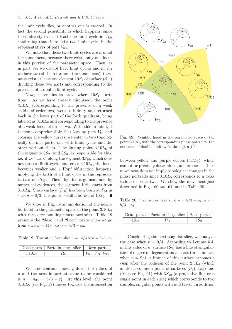
54 J.C. Artes, A.C. Rezende and R.D.S. Oliveira
the limit cycle dies, or another one is created. Infact the second possibility is which happens, sincethere already exist at least one limit cycle in V88,confirming that there exist two limit cycles in therepresentatives of part V88.
We note that these two limit cycles are aroundthe same focus, because there exists only one focusin this portion of the parameter space. Then, asin part V79 we do not have limit cycles and in V88
we have two of them (around the same focus), theremust exist at least one element 10S1 of surface (S10)dividing these two parts and corresponding to thepresence of a double limit cycle.
Now, it remains to prove where 10S1 startsfrom. As we have already discussed, the point3.10L4 (corresponding to the presence of a weaksaddle of order two) went to infinity and returnedback in the lower part of the forth quadrant, beinglabeled as 3.10L6 and corresponding to the presenceof a weak focus of order two. With this in mind, itis more comprehensible that leaving part V80 andcrossing the yellow curves, we enter in two topolog-ically distinct parts, one with limit cycles and theother without them. The linking point 3.10L6 ofthe segments 3S28 and 3S33 is responsible for this,i.e. if we “walk” along the segment 3S28, which doesnot possess limit cycle, and cross 3.10L6, the focusbecomes weaker and a Hopf bifurcation happens,implying the birth of a limit cycle in the represen-tatives of 3S33. Then, by this argument and bynumerical evidences, the segment 10S1 starts from3.10L6. Since surface (S10) has been born at P64 inslice n = 8/3, this point is still a border of 10S1.
We show in Fig. 59 an ampliation of the neigh-borhood in the parameter space of the point 3.10L6
with the corresponding phase portraits. Table 19presents the “dead” and “born” parts when we gofrom slice n = 14/5 to n = 8/3 − ε8.
Table 19. Transition from slice n = 14/5 to n = 8/3−ε8
Dead parts Parts in sing. slice Born parts
3.10L4 P64 V88, V89, V90
We now continue moving down the values ofn and the next important value to be consideredis n = n35 = 8/3 − ε∗8. At this level, the point3.10L5 (see Fig. 58) moves towards the intersection
10S1
3S34
3.7L7
3.10L6
3S33
3S28
V81
V89
V80
V88
V79
f (1)
f (2)
loop
7S22
7S27
Fig. 59. Neighborhood in the parameter space of thepoint 3.10L6 with the corresponding phase portraits: theexistence of double limit cycle through a f (2)
between yellow and purple curves (3.7L6), whichcannot be precisely determined, and crosses it. Thismovement does not imply topological changes in thephase portraits since 3.10L5 corresponds to a weaksaddle of order two. We show the movement justdescribed in Figs. 60 and 61, and in Table 20.
Table 20. Transition from slice n = 8/3 − ε8 to n =8/3− ε9
Dead parts Parts in sing. slice Born parts
3S27 P14 3S36
Considering the next singular slice, we analyzethe case when n = 9/4. According to Lemma 6.4,in this value of n, surface (S3) has a line of singular-ities of degree of degeneration at least three; in fact,when n = 9/4, a branch of this surface becomes acusp after the collision of the point 2.3L4 (whichis also a common point of surfaces (S2), (S6) and(S7); see Fig. 61) with 3S20 (a projective line or asingle point in each slice) which corresponds to twocomplex singular points with null trace. In addition
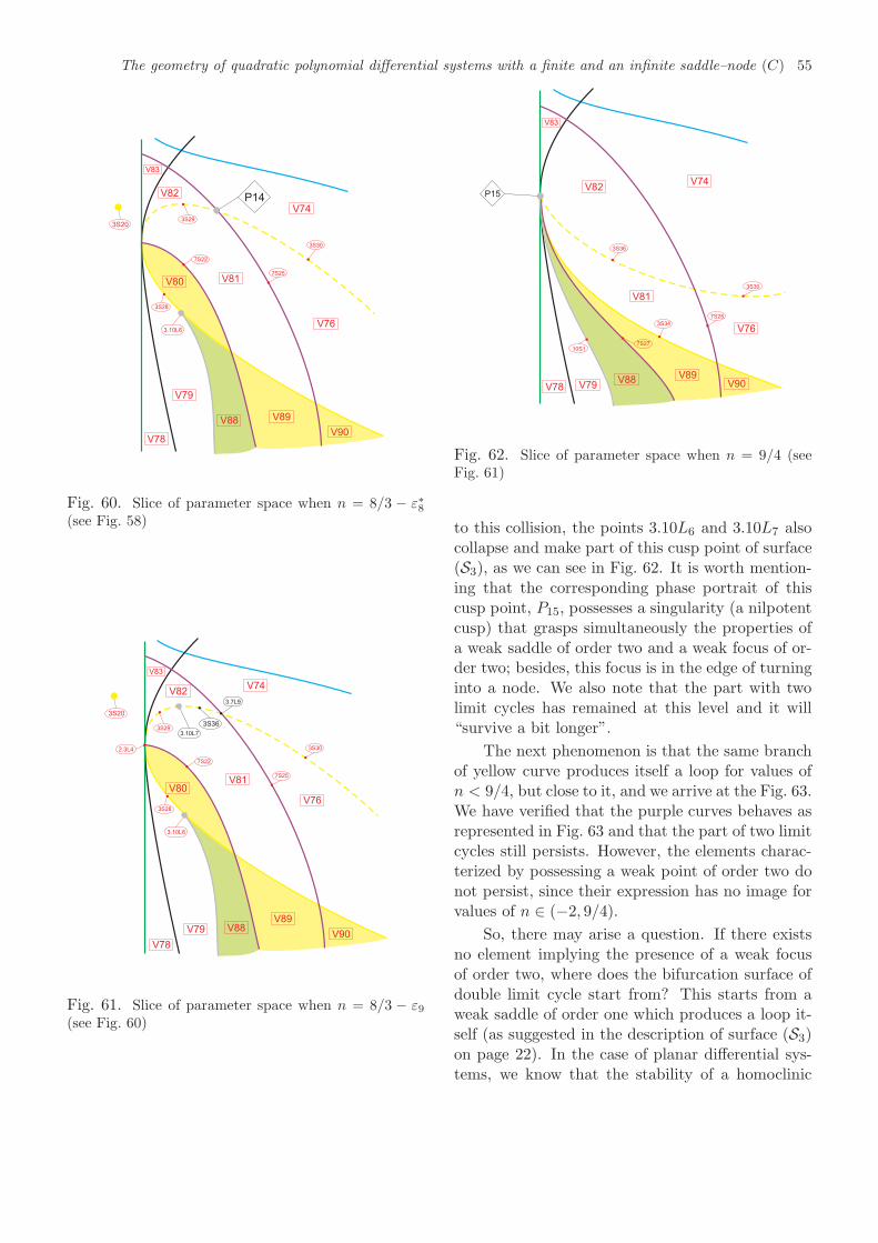
The geometry of quadratic polynomial differential systems with a finite and an infinite saddle–node (C) 55
P14
3S20
V76
V74
V82
V83
V81
3S30
V80
V78
V79
V88 V89
V90
3S29
7S25
3.10L6
3S28
7S22
Fig. 60. Slice of parameter space when n = 8/3 − ε∗8(see Fig. 58)
3S36
3.10L7
3.7L9
3.10L6
2.3L4
V82V74
V83
3S20
V76
V81V80
3S30
7S25
7S22
3S28
V78
V79 V88V89
V90
3S29
Fig. 61. Slice of parameter space when n = 8/3 − ε9(see Fig. 60)
P15V82
V83
V74
V76
V81
V78 V79V88
V89
3S36
3S30
7S25
V90
10S1
7S27
3S34
Fig. 62. Slice of parameter space when n = 9/4 (seeFig. 61)
to this collision, the points 3.10L6 and 3.10L7 alsocollapse and make part of this cusp point of surface(S3), as we can see in Fig. 62. It is worth mention-ing that the corresponding phase portrait of thiscusp point, P15, possesses a singularity (a nilpotentcusp) that grasps simultaneously the properties ofa weak saddle of order two and a weak focus of or-der two; besides, this focus is in the edge of turninginto a node. We also note that the part with twolimit cycles has remained at this level and it will“survive a bit longer”.
The next phenomenon is that the same branchof yellow curve produces itself a loop for values ofn < 9/4, but close to it, and we arrive at the Fig. 63.We have verified that the purple curves behaves asrepresented in Fig. 63 and that the part of two limitcycles still persists. However, the elements charac-terized by possessing a weak point of order two donot persist, since their expression has no image forvalues of n ∈ (−2, 9/4).
So, there may arise a question. If there existsno element implying the presence of a weak focusof order two, where does the bifurcation surface ofdouble limit cycle start from? This starts from aweak saddle of order one which produces a loop it-self (as suggested in the description of surface (S3)on page 22). In the case of planar differential sys-tems, we know that the stability of a homoclinic
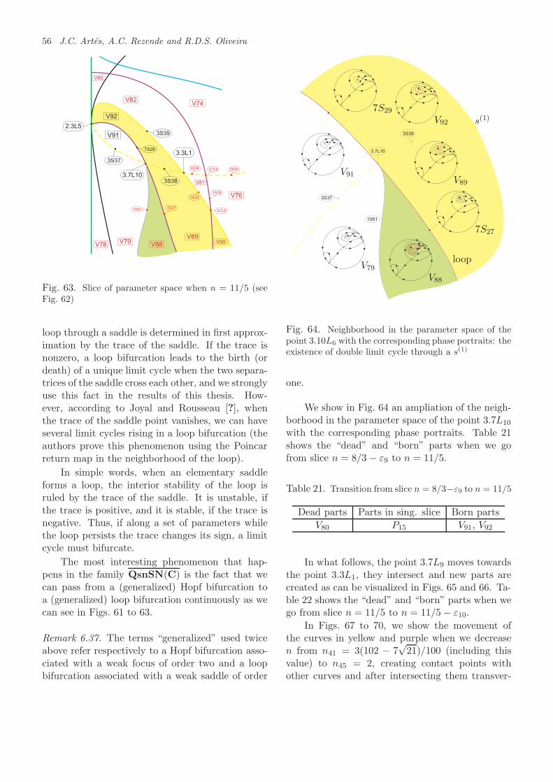
56 J.C. Artes, A.C. Rezende and R.D.S. Oliveira
2.3L5
3S37
V91
V92
3S38
3S39
7S29
3.7L10
3.3L1
V82
V83
V74
V76
V81
V78V79
V88
V89V90
3S30
7S25
3.7L9
7S2710S1
3S34
3.7L8
3S36
Fig. 63. Slice of parameter space when n = 11/5 (seeFig. 62)
loop through a saddle is determined in first approx-imation by the trace of the saddle. If the trace isnonzero, a loop bifurcation leads to the birth (ordeath) of a unique limit cycle when the two separa-trices of the saddle cross each other, and we stronglyuse this fact in the results of this thesis. How-ever, according to Joyal and Rousseau [?], whenthe trace of the saddle point vanishes, we can haveseveral limit cycles rising in a loop bifurcation (theauthors prove this phenomenon using the Poincarreturn map in the neighborhood of the loop).
In simple words, when an elementary saddleforms a loop, the interior stability of the loop isruled by the trace of the saddle. It is unstable, ifthe trace is positive, and it is stable, if the trace isnegative. Thus, if along a set of parameters whilethe loop persists the trace changes its sign, a limitcycle must bifurcate.
The most interesting phenomenon that hap-pens in the family QsnSN(C) is the fact that wecan pass from a (generalized) Hopf bifurcation toa (generalized) loop bifurcation continuously as wecan see in Figs. 61 to 63.
Remark 6.37. The terms “generalized” used twiceabove refer respectively to a Hopf bifurcation asso-ciated with a weak focus of order two and a loopbifurcation associated with a weak saddle of order
3S37
3S38
3.7L10
10S1
V91V89
V92
V88
V79
s(1)
loop
7S29
7S27
Fig. 64. Neighborhood in the parameter space of thepoint 3.10L6 with the corresponding phase portraits: theexistence of double limit cycle through a s(1)
one.
We show in Fig. 64 an ampliation of the neigh-borhood in the parameter space of the point 3.7L10
with the corresponding phase portraits. Table 21shows the “dead” and “born” parts when we gofrom slice n = 8/3 − ε9 to n = 11/5.
Table 21. Transition from slice n = 8/3−ε9 to n = 11/5
Dead parts Parts in sing. slice Born parts
V80 P15 V91, V92
In what follows, the point 3.7L9 moves towardsthe point 3.3L1, they intersect and new parts arecreated as can be visualized in Figs. 65 and 66. Ta-ble 22 shows the “dead” and “born” parts when wego from slice n = 11/5 to n = 11/5 − ε10.
In Figs. 67 to 70, we show the movement ofthe curves in yellow and purple when we decreasen from n41 = 3(102 − 7
√21)/100 (including this
value) to n45 = 2, creating contact points withother curves and after intersecting them transver-
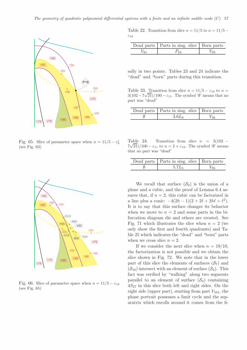
The geometry of quadratic polynomial differential systems with a finite and an infinite saddle–node (C) 57
P16
V76
V90V89V88
V79V78
V92
V82
3S30
3S39
3S38
3S35
7S24
7S28
Fig. 65. Slice of parameter space when n = 11/5− ε∗9(see Fig. 63)
V93
3S41
3.7L11
3.3L2
3S40
7S30
3.7L12
V76
V90V89
V88V79
V78
V92
V82
3S30
3S39
3S38
3S35
7S24
7S28
Fig. 66. Slice of parameter space when n = 11/5− ε10(see Fig. 65)
Table 22. Transition from slice n = 11/5 to n = 11/5−ε10
Dead parts Parts in sing. slice Born parts
V81 P16 V93
sally in two points. Tables 23 and 24 indicate the“dead” and “born” parts during this transition.
Table 23. Transition from slice n = 11/5− ε10 to n =3(102− 7
√21)/100− ε11. The symbol ‘∅’ means that no
part was “dead”
Dead parts Parts in sing. slice Born parts
∅ 3.6L8 V94
Table 24. Transition from slice n = 3(102 −7√21)/100− ε11 to n = 2 + ε12. The symbol ‘∅’ means
that no part was “dead”
Dead parts Parts in sing. slice Born parts
∅ 5.7L5 V95
We recall that surface (S3) is the union of aplane and a cubic, and the proof of Lemma 6.4 as-sures that, if n = 2, this cubic can be factorized ina line plus a conic: −4(2h − 1)(2 + 2ℓ + 2hℓ + ℓ2).It is to say that this surface changes its behaviorwhen we move to n = 2 and some parts in the bi-furcation diagram die and others are created. SeeFig. 71 which illustrates the slice when n = 2 (weonly show the first and fourth quadrants) and Ta-ble 25 which indicates the “dead” and “born” partswhen we cross slice n = 2.
If we consider the next slice when n = 19/10,the factorization is not possible and we obtain theslice shown in Fig. 72. We note that in the lowerpart of this slice the elements of surfaces (S7) and(S10) intersect with an element of surface (S4). Thisfact was verified by “walking” along two segmentsparallel to an element of surface (S4) containing4S27 in this slice both left and right sides. On theright side (upper part), starting from part V101, thephase portrait possesses a limit cycle and the sep-aratrix which enrolls around it comes from the fi-
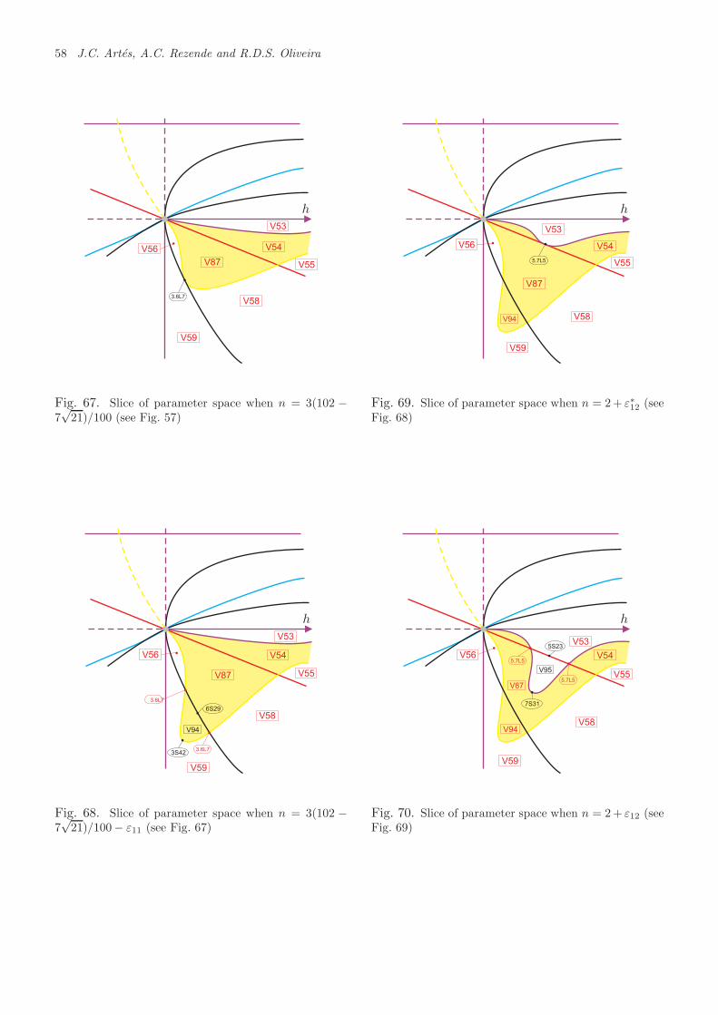
58 J.C. Artes, A.C. Rezende and R.D.S. Oliveira
3.6L7
V53
V54
V55
V58
V87
V56
V59
h
Fig. 67. Slice of parameter space when n = 3(102 −7√21)/100 (see Fig. 57)
3.6L73S42
V94
6S29
V53
V54
V55
V58
V87
V56
V59
3.6L7
h
Fig. 68. Slice of parameter space when n = 3(102 −7√21)/100− ε11 (see Fig. 67)
5.7L5
V53
V54
V55
V56
V87
V58
V59
V94
h
Fig. 69. Slice of parameter space when n = 2+ ε∗12 (seeFig. 68)
5.7L5
7S31
V95
5S23V53
V54
V55
V56
V87
V58
V59
V94
5.7L5
h
Fig. 70. Slice of parameter space when n = 2+ ε12 (seeFig. 69)
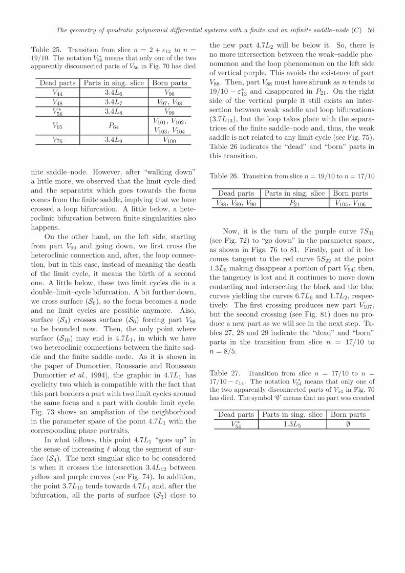
The geometry of quadratic polynomial differential systems with a finite and an infinite saddle–node (C) 59
Table 25. Transition from slice n = 2 + ε12 to n =19/10. The notation V ∗
56 means that only one of the twoapparently disconnected parts of V56 in Fig. 70 has died
Dead parts Parts in sing. slice Born parts
V44 3.4L6 V96
V48 3.4L7 V97, V98
V ∗56 3.4L8 V99
V65 P64V101, V102,V103, V104
V76 3.4L9 V100
nite saddle–node. However, after “walking down”a little more, we observed that the limit cycle diedand the separatrix which goes towards the focuscomes from the finite saddle, implying that we havecrossed a loop bifurcation. A little below, a hete-roclinic bifurcation between finite singularities alsohappens.
On the other hand, on the left side, startingfrom part V90 and going down, we first cross theheteroclinic connection and, after, the loop connec-tion, but in this case, instead of meaning the deathof the limit cycle, it means the birth of a secondone. A little below, these two limit cycles die in adouble–limit–cycle bifurcation. A bit further down,we cross surface (S6), so the focus becomes a nodeand no limit cycles are possible anymore. Also,surface (S4) crosses surface (S6) forcing part V88
to be bounded now. Then, the only point wheresurface (S10) may end is 4.7L1, in which we havetwo heteroclinic connections between the finite sad-dle and the finite saddle–node. As it is shown inthe paper of Dumortier, Roussarie and Rousseau[Dumortier et al., 1994], the graphic in 4.7L1 hascyclicity two which is compatible with the fact thatthis part borders a part with two limit cycles aroundthe same focus and a part with double limit cycle.Fig. 73 shows an ampliation of the neighborhoodin the parameter space of the point 4.7L1 with thecorresponding phase portraits.
In what follows, this point 4.7L1 “goes up” inthe sense of increasing ℓ along the segment of sur-face (S4). The next singular slice to be consideredis when it crosses the intersection 3.4L12 betweenyellow and purple curves (see Fig. 74). In addition,the point 3.7L10 tends towards 4.7L1 and, after thebifurcation, all the parts of surface (S3) close to
the new part 4.7L2 will be below it. So, there isno more intersection between the weak–saddle phe-nomenon and the loop phenomenon on the left sideof vertical purple. This avoids the existence of partV88. Then, part V88 must have shrunk as n tends to19/10 − ε∗13 and disappeared in P21. On the rightside of the vertical purple it still exists an inter-section between weak–saddle and loop bifurcations(3.7L13), but the loop takes place with the separa-trices of the finite saddle–node and, thus, the weaksaddle is not related to any limit cycle (see Fig. 75).Table 26 indicates the “dead” and “born” parts inthis transition.
Table 26. Transition from slice n = 19/10 to n = 17/10
Dead parts Parts in sing. slice Born parts
V88, V89, V90 P21 V105, V106
Now, it is the turn of the purple curve 7S31
(see Fig. 72) to “go down” in the parameter space,as shown in Figs. 76 to 81. Firstly, part of it be-comes tangent to the red curve 5S22 at the point1.3L5 making disappear a portion of part V54; then,the tangency is lost and it continues to move downcontacting and intersecting the black and the bluecurves yielding the curves 6.7L6 and 1.7L2, respec-tively. The first crossing produces new part V107,but the second crossing (see Fig. 81) does no pro-duce a new part as we will see in the next step. Ta-bles 27, 28 and 29 indicate the “dead” and “born”parts in the transition from slice n = 17/10 ton = 8/5.
Table 27. Transition from slice n = 17/10 to n =17/10 − ε14. The notation V ∗
54 means that only one ofthe two apparently disconnected parts of V54 in Fig. 70has died. The symbol ‘∅’ means that no part was created
Dead parts Parts in sing. slice Born parts
V ∗54 1.3L5 ∅
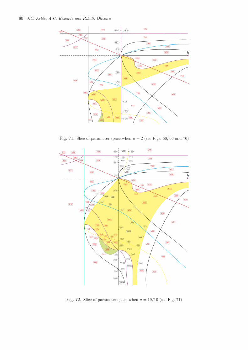
60 J.C. Artes, A.C. Rezende and R.D.S. Oliveira
3.4L6
3.4L7
3.4L8
3.4L9
3.4L10
P17
P18
P19
P20
V73
V75
V46
V63
V62
V60
V64
V74
V93V92
V82
V83
V91
V90V89
V88
V79
V78
V86
V67
V77
V66
V61
V57V59
V58
V94
V87
V95
V53
V54
V54
V55
V56
V52
V51
V50
V49
V45V20
V22
V85
V84
V24
V23
V21
h
Fig. 71. Slice of parameter space when n = 2 (see Figs. 50, 66 and 70)
V964S22
V97
V98
3S43
4S23
4S24
3S44
6S30
3S45
3.4L114.4L2
V99
V100
V101
V102
V103
V104
1.3L5
3S46
1S12
4S25
1.4L3
1.3L3
4S26
1S13
3S48
3S47
1.3L4
3.4L12
3.3L34S27
7S32
3S49
4.7L1
7S334S28
4.6L4
6S31
4S29
V20
V22
V85
V84
V24
V23
V21V73
V75
V46
V63
V62
V60
V64
V74
V93
V92
V82V83
V91
V90V89
V79
V88
V78
V66
V61
V57
V58
V53
V54
V55
V56
V52
V51
V50
V49
V45
V67V86
V77
V59
V87
V94
V95
V54
3S37
7S29
7S30
10S1
7S28
3S403S38
7S29
3.7L10
3.7L12
5S23
4S31
5S22
5S22
3.6L8
h
Fig. 72. Slice of parameter space when n = 19/10 (see Fig. 71)
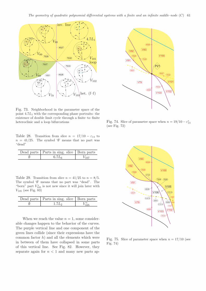
The geometry of quadratic polynomial differential systems with a finite and an infinite saddle–node (C) 61
10S1
7S27
7S28
4S27
7S32
7S33
4S28
V79
V88
V89
V90
V101
V102
V103
4.7L1
loop
inv. line
het. (f–f)
Fig. 73. Neighborhood in the parameter space of thepoint 4.7L1 with the corresponding phase portraits: theexistence of double limit cycle through a finite–to–finiteheteroclinic and a loop bifurcations
Table 28. Transition from slice n = 17/10 − ε14 ton = 41/25. The symbol ‘∅’ means that no part was“dead”
Dead parts Parts in sing. slice Born parts
∅ 6.7L6 V107
Table 29. Transition from slice n = 41/25 to n = 8/5.The symbol ‘∅’ means that no part was “dead”. The“born” part V ∗
105 is not new since it will join later withV105 (see Fig. 83)
Dead parts Parts in sing. slice Born parts
∅ 1.7L2 V ∗105
When we reach the value n = 1, some consider-able changes happen to the behavior of the curves.The purple vertical line and one component of thegreen lines collide (since their expressions have thecommon factor h) and all the elements which werein between of them have collapsed in some partsof this vertical line. See Fig. 82. However, theyseparate again for n < 1 and many new parts ap-
P21
V91
V92V93
V100
V79 V101
V102V103
3S37
7S29
7S30
4S26
3S477S32
7S33
4S28
Fig. 74. Slice of parameter space when n = 19/10− ε∗13(see Fig. 72)
7S34
V105
3S50
3S51
4S30
7S35
4.7L2
3.4L13
3.7L14
3.7L13V106
V91
V92
V93
V100
V102V103
V79
4S26
7S30
7S29
3S37
4S28
7S33
3S47
V101
7S32
Fig. 75. Slice of parameter space when n = 17/10 (seeFig. 74)
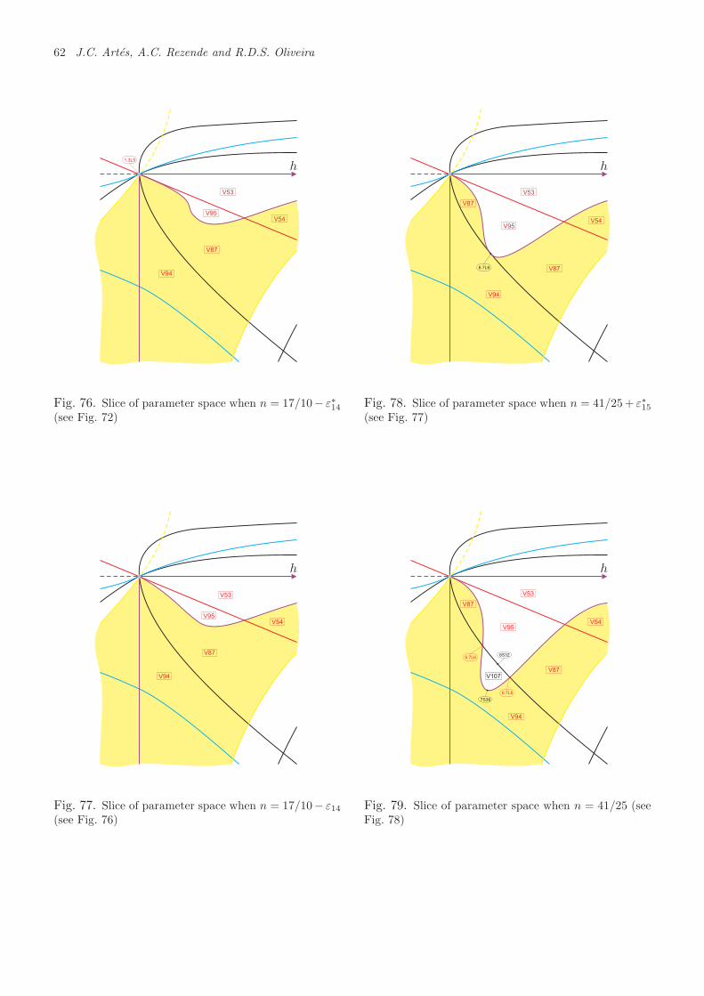
62 J.C. Artes, A.C. Rezende and R.D.S. Oliveira
V95
V53
V54
V87
V94
1.3L5
h
Fig. 76. Slice of parameter space when n = 17/10− ε∗14(see Fig. 72)
V95
V53
V54
V87
V94
h
Fig. 77. Slice of parameter space when n = 17/10− ε14(see Fig. 76)
6.7L6
V95
V53
V54
V87
V94
V87
h
Fig. 78. Slice of parameter space when n = 41/25+ ε∗15(see Fig. 77)
6.7L6
V107
6S32
7S36
V95
V53
V54
V87
V94
V87
6.7L6
h
Fig. 79. Slice of parameter space when n = 41/25 (seeFig. 78)
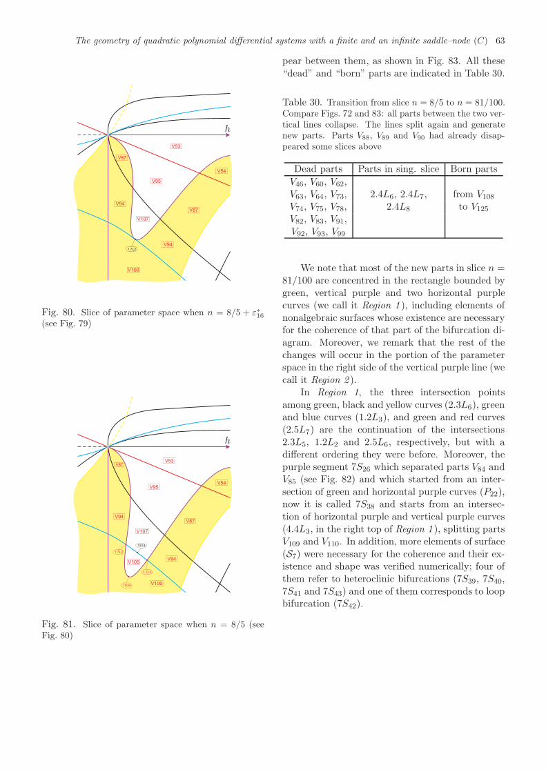
The geometry of quadratic polynomial differential systems with a finite and an infinite saddle–node (C) 63
1.7L2
V95
V53
V54
V87
V94
V87
V94
V100
V107
h
Fig. 80. Slice of parameter space when n = 8/5 + ε∗16(see Fig. 79)
1S14
7S34
1.7L2
V95
V53
V54
V87V94
V87
V94
V107
V100
1.7L2
V105
h
Fig. 81. Slice of parameter space when n = 8/5 (seeFig. 80)
pear between them, as shown in Fig. 83. All these“dead” and “born” parts are indicated in Table 30.
Table 30. Transition from slice n = 8/5 to n = 81/100.Compare Figs. 72 and 83: all parts between the two ver-tical lines collapse. The lines split again and generatenew parts. Parts V88, V89 and V90 had already disap-peared some slices above
Dead parts Parts in sing. slice Born parts
V46, V60, V62,V63, V64, V73, 2.4L6, 2.4L7, from V108
V74, V75, V78, 2.4L8 to V125
V82, V83, V91,V92, V93, V99
We note that most of the new parts in slice n =81/100 are concentred in the rectangle bounded bygreen, vertical purple and two horizontal purplecurves (we call it Region 1 ), including elements ofnonalgebraic surfaces whose existence are necessaryfor the coherence of that part of the bifurcation di-agram. Moreover, we remark that the rest of thechanges will occur in the portion of the parameterspace in the right side of the vertical purple line (wecall it Region 2 ).
In Region 1, the three intersection pointsamong green, black and yellow curves (2.3L6), greenand blue curves (1.2L3), and green and red curves(2.5L7) are the continuation of the intersections2.3L5, 1.2L2 and 2.5L6, respectively, but with adifferent ordering they were before. Moreover, thepurple segment 7S26 which separated parts V84 andV85 (see Fig. 82) and which started from an inter-section of green and horizontal purple curves (P22),now it is called 7S38 and starts from an intersec-tion of horizontal purple and vertical purple curves(4.4L3, in the right top of Region 1 ), splitting partsV109 and V110. In addition, more elements of surface(S7) were necessary for the coherence and their ex-istence and shape was verified numerically; four ofthem refer to heteroclinic bifurcations (7S39, 7S40,7S41 and 7S43) and one of them corresponds to loopbifurcation (7S42).
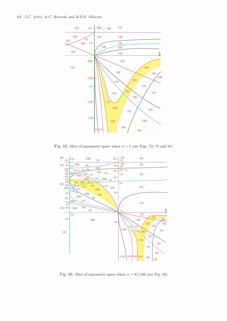
64 J.C. Artes, A.C. Rezende and R.D.S. Oliveira
2.4L6
2.4L7
2.4L8
P23
P22
V105
V45V20
V85
V84
V23
V45
V49V97
V96
V98
V50
V51
V52
V53
V95
V54
V87
V94
V100
V101
V102
V105
V22
V107
7S34
V55
V58
V59
V77
V86
V56
V57
V61
V66
V67V104
V106
V103
7S26
h
Fig. 82. Slice of parameter space when n = 1 (see Figs. 72, 75 and 81)
2.4L9
V109
V108
V110
V111
V115
V116
V117
V114
V118
V112
V113
V119
V121
V122
V120
V123
V124
V125
2S22 4S32
4S31
2S23 7S38
6S337S39
2S24
2S25
2S26
6S34
4S33
7S403S52
4S34
4S35
1S15
7S41
7S42
1S16
3S54
6S35
3S53
7S43
4S36
1S17
1S18
1S19
6S36
3S55
5S24
4S38
2S27
2S28
2S29
4S37
4.4L3
4.6L5
3.4L14
6.7L7
3.7L15
2.3L6
1.7L3
1.3L6
1.6L41.2L3
1.4L4
2.5L7
2.4L10
1.3L7
2.7L7
2.7L8
V53
V104
V95
V54
V55
V56
V57
V58
V87
V59
V103 V102 V101
V105V107
V106
V100
V77
V86
V67
V66
V61
V94
V52
V51
V50
V49
V45V96
V97
V98
V20
V85
V84
V23
V24
3.6L8
h
Fig. 83. Slice of parameter space when n = 81/100 (see Fig. 82)
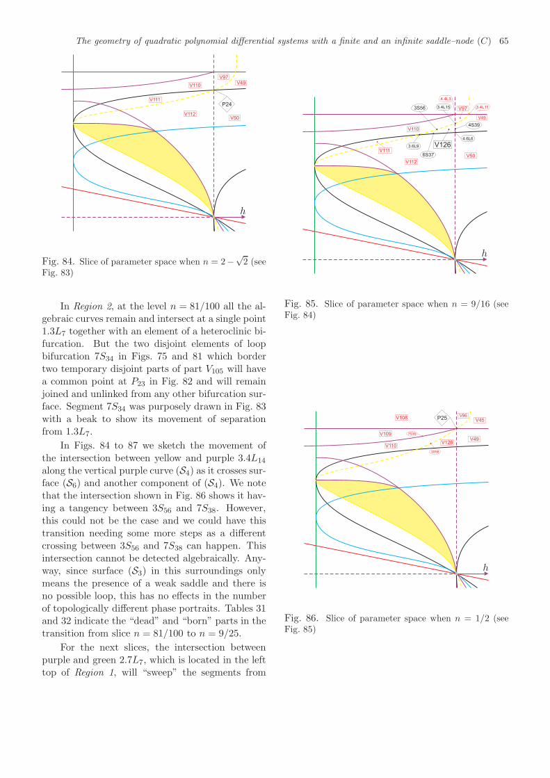
The geometry of quadratic polynomial differential systems with a finite and an infinite saddle–node (C) 65
P24
V49
V97
V50
V110
V111
V112
h
Fig. 84. Slice of parameter space when n = 2−√2 (see
Fig. 83)
In Region 2, at the level n = 81/100 all the al-gebraic curves remain and intersect at a single point1.3L7 together with an element of a heteroclinic bi-furcation. But the two disjoint elements of loopbifurcation 7S34 in Figs. 75 and 81 which bordertwo temporary disjoint parts of part V105 will havea common point at P23 in Fig. 82 and will remainjoined and unlinked from any other bifurcation sur-face. Segment 7S34 was purposely drawn in Fig. 83with a beak to show its movement of separationfrom 1.3L7.
In Figs. 84 to 87 we sketch the movement ofthe intersection between yellow and purple 3.4L14
along the vertical purple curve (S4) as it crosses sur-face (S6) and another component of (S4). We notethat the intersection shown in Fig. 86 shows it hav-ing a tangency between 3S56 and 7S38. However,this could not be the case and we could have thistransition needing some more steps as a differentcrossing between 3S56 and 7S38 can happen. Thisintersection cannot be detected algebraically. Any-way, since surface (S3) in this surroundings onlymeans the presence of a weak saddle and there isno possible loop, this has no effects in the numberof topologically different phase portraits. Tables 31and 32 indicate the “dead” and “born” parts in thetransition from slice n = 81/100 to n = 9/25.
For the next slices, the intersection betweenpurple and green 2.7L7, which is located in the lefttop of Region 1, will “sweep” the segments from
V126
4.6L6
6S37
3.4L15
3.6L9
3S56
4S39
V49
V97
V50
V110
V111
V112
3.4L11
4.4L3
h
Fig. 85. Slice of parameter space when n = 9/16 (seeFig. 84)
P25
V110
V49
V109
V108
V126
V45
V96
7S38
3S56
h
Fig. 86. Slice of parameter space when n = 1/2 (seeFig. 85)
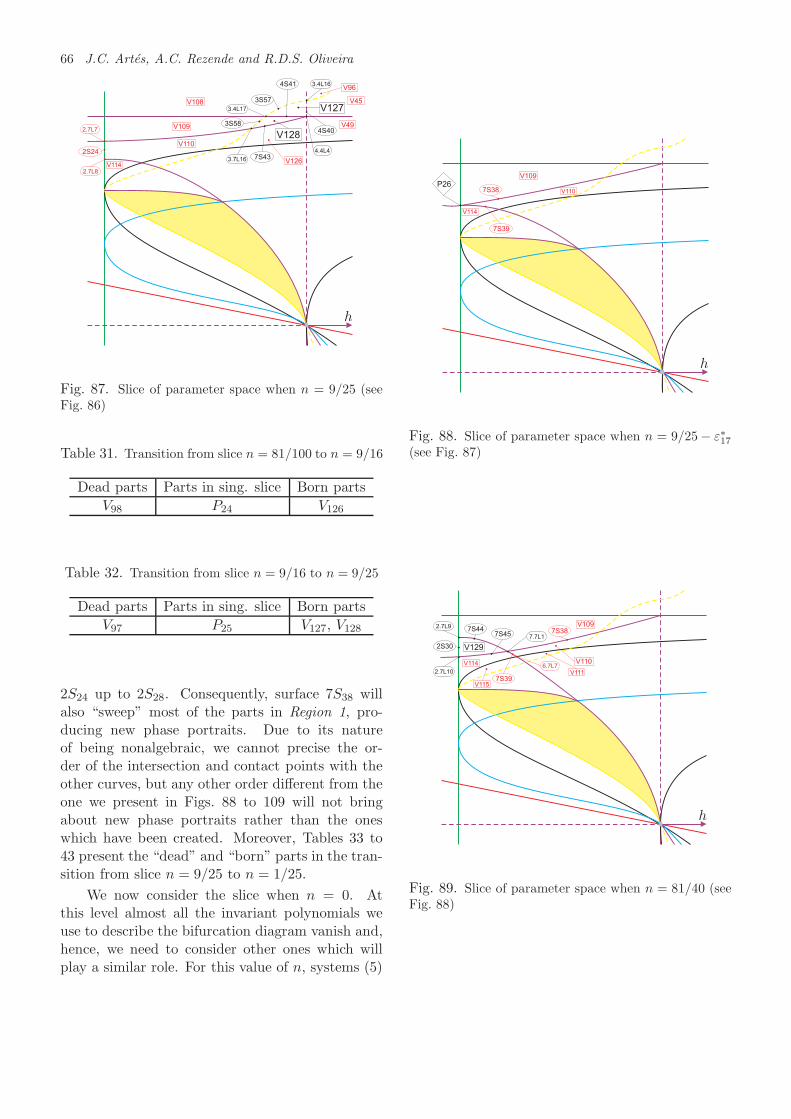
66 J.C. Artes, A.C. Rezende and R.D.S. Oliveira
V128
4.4L4
7S43
V127
4S40
3S58
3S57
4S41 3.4L16
3.4L17
3.7L16
V108
V109
V110
V126
V49
V45
V114
V96
2S24
2.7L7
2.7L8
h
Fig. 87. Slice of parameter space when n = 9/25 (seeFig. 86)
Table 31. Transition from slice n = 81/100 to n = 9/16
Dead parts Parts in sing. slice Born parts
V98 P24 V126
Table 32. Transition from slice n = 9/16 to n = 9/25
Dead parts Parts in sing. slice Born parts
V97 P25 V127, V128
2S24 up to 2S28. Consequently, surface 7S38 willalso “sweep” most of the parts in Region 1, pro-ducing new phase portraits. Due to its natureof being nonalgebraic, we cannot precise the or-der of the intersection and contact points with theother curves, but any other order different from theone we present in Figs. 88 to 109 will not bringabout new phase portraits rather than the oneswhich have been created. Moreover, Tables 33 to43 present the “dead” and “born” parts in the tran-sition from slice n = 9/25 to n = 1/25.
We now consider the slice when n = 0. Atthis level almost all the invariant polynomials weuse to describe the bifurcation diagram vanish and,hence, we need to consider other ones which willplay a similar role. For this value of n, systems (5)
P26
V114
V109
V1107S38
7S39
h
Fig. 88. Slice of parameter space when n = 9/25− ε∗17(see Fig. 87)
V129
2.7L10
2.7L97S44
7S45
2S30
7.7L1
V109
7S39
7S38
V110V1146.7L7
V115
V111
h
Fig. 89. Slice of parameter space when n = 81/40 (seeFig. 88)
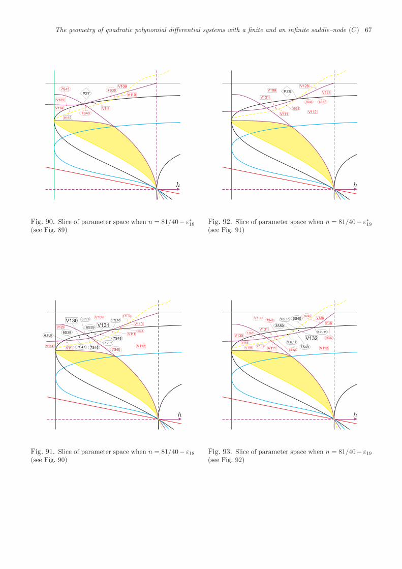
The geometry of quadratic polynomial differential systems with a finite and an infinite saddle–node (C) 67
P27
V114
V115
7S387S45
V110
V111
V129
V109
7S40
h
Fig. 90. Slice of parameter space when n = 81/40− ε∗18(see Fig. 89)
V131
6.7L86S38
7S47
6S39
7.7L2
V130
7S48
7S46
6.7L106.7L9
V114
V129
V109
V110
V111
7S40V115
3.7L16
3.6L4
V112
h
Fig. 91. Slice of parameter space when n = 81/40− ε18(see Fig. 90)
P28V109
V131
V111V112
V126
V128
6S377S43
3S52
h
Fig. 92. Slice of parameter space when n = 81/40− ε∗19(see Fig. 91)
6S40
V132
7S49
3.6L10
3S59
3.7L17
6.7L11
V109 V128
V126
V112V111
V131
3S52
6S37
7S43
3.7L15
7.7L2
V115
7S48
V130
V116
h
Fig. 93. Slice of parameter space when n = 81/40− ε19(see Fig. 92)
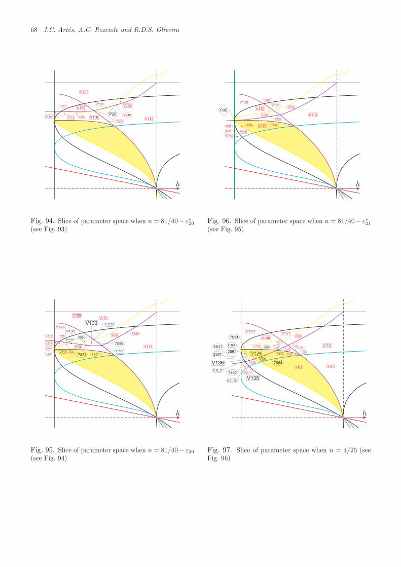
68 J.C. Artes, A.C. Rezende and R.D.S. Oliveira
P29
V109
V112
V132V131
V130
V115 V116V114
7S41
7S493S53
7S47
h
Fig. 94. Slice of parameter space when n = 81/40− ε∗20(see Fig. 93)
3S60
V133
7S50
3.7L19
7S51
7.7L3
3.7L18
V109V131
V130
V132
V112
7S49
7S41
V116
V115
V114
3S53
7S472.7L10
2S25
2.3L6
V129
h
Fig. 95. Slice of parameter space when n = 81/40− ε20(see Fig. 94)
P30
V129
V130
V131
V133
V132
V112
V116
V117
V119
V121
7S42
7S51
3S54
2S26
6S35
h
Fig. 96. Slice of parameter space when n = 81/40− ε∗21(see Fig. 95)
V134
7S52
6.7L12
2S31
7.7L4
2.7L11
V135
7S53
7S54
7S55
3S61
2.3L7
3.7L20
V136
6S41
V129
V130
V131V132
V133 V112
V117
V116
V119
V121
7.7L3
1.7L3
7S41
V118 V113
7S42
7S51
h
Fig. 97. Slice of parameter space when n = 4/25 (seeFig. 96)
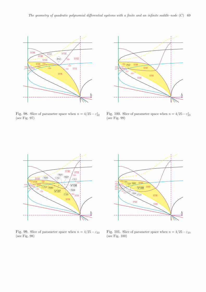
The geometry of quadratic polynomial differential systems with a finite and an infinite saddle–node (C) 69
P31
V129
V130
V131
V112
V113
V118
V117
V119
V121
V132
V134
V135V136
1S16
1S15
7S43
7S49
7S53
V133
h
Fig. 98. Slice of parameter space when n = 4/25− ε∗22(see Fig. 97)
V138
7S58
7.7L5
V137
7S56
1S20
1S21
7S571.7L6
1.7L7
1.7L5
V133
V132V112
V113
V118
V134
V117
V119
V121
V135V136
7S49
1S15
7S43
1S16
7S53
1.3L6
3.7L20
h
Fig. 99. Slice of parameter space when n = 4/25− ε22(see Fig. 98)
P32 V134
V135V136
V119
V121
V137
V118
V120
3S55
1S17
7S54
h
Fig. 100. Slice of parameter space when n = 4/25− ε∗23(see Fig. 99)
V139
3S62
7S593.7L21
1S22
1.3L8
1.7L7
V137
V134
V118
V120
V121
V119
V135V136
V122
6S35
1.6L4
6.7L12
1S17
7S54
h
Fig. 101. Slice of parameter space when n = 4/25− ε23(see Fig. 100)
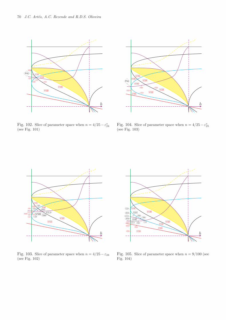
70 J.C. Artes, A.C. Rezende and R.D.S. Oliveira
P33V135
V139
V120
V122
V121
V136
1S18
6S36
7S55
h
Fig. 102. Slice of parameter space when n = 4/25− ε∗24(see Fig. 101)
V1407S60
6S421S23
6.7L13
1.7L8
1.6L5
2.7L11
V120
V122
V139
V135
V136
1S18
7S55
2S26
1.2L3
V121
h
Fig. 103. Slice of parameter space when n = 4/25− ε24(see Fig. 102)
P34
V120
V122
V139
V140
V136
V135
V123
2S27
1S19
7S60 6S36
h
Fig. 104. Slice of parameter space when n = 4/25− ε∗25(see Fig. 103)
V141
7S62
1S24
1.7L9
V142
2S32
2S33
7S61
1.2L4
2.7L13
2.7L12
V120
V122
V123
V139
V140
2S27
2.5L7
2S28
5S24
V124
h
Fig. 105. Slice of parameter space when n = 9/100 (seeFig. 104)
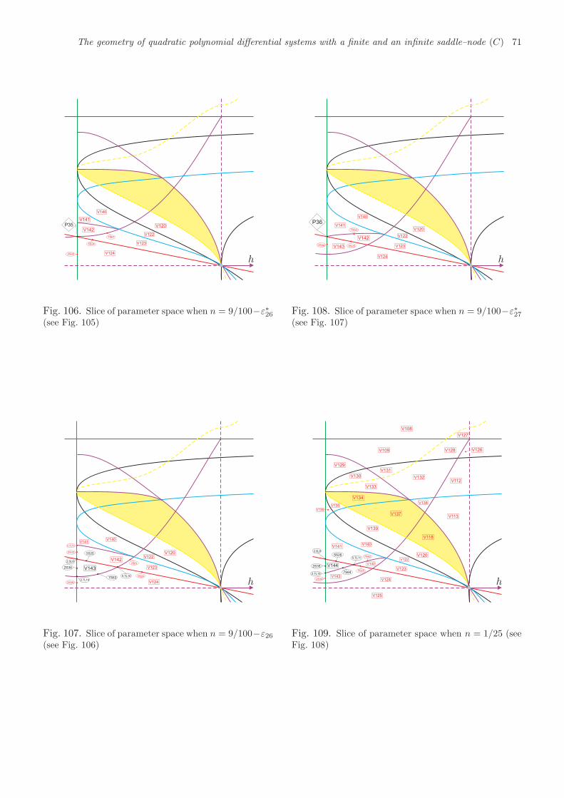
The geometry of quadratic polynomial differential systems with a finite and an infinite saddle–node (C) 71
P35
V124
V123
V122
V120
V140
V141
V142
2S28
5S24
7S61
h
Fig. 106. Slice of parameter space when n = 9/100−ε∗26(see Fig. 105)
V143
5S25
7S63
2.5L8
2S34
2.7L14
5.7L10
V120V122
V123
V124
V140V141
V142
2S28
5S24
7S61
2S33
2.7L12
h
Fig. 107. Slice of parameter space when n = 9/100−ε26(see Fig. 106)
P36
V124
V123
V122
V120
V140
V141
V142
V143
7S62
5S252S34
h
Fig. 108. Slice of parameter space when n = 9/100−ε∗27(see Fig. 107)
V144
5S26
2.7L15
2.5L9
7S64
2S35
5.7L11V120
V122
V123
V124
V142
V140V141
V1432S34
5S25
7S62
V125
V118
V139
V137V113
V138
V112V132
V134
V135
V136
V133
V130
V129
V109
V131
V128 V126
V127
V108
h
Fig. 109. Slice of parameter space when n = 1/25 (seeFig. 108)
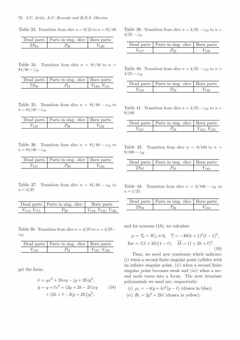
72 J.C. Artes, A.C. Rezende and R.D.S. Oliveira
Table 33. Transition from slice n = 9/25 to n = 81/40
Dead parts Parts in sing. slice Born parts
2S24 P26 V129
Table 34. Transition from slice n = 81/40 to n =81/40− ε18
Dead parts Parts in sing. slice Born parts
7S39 P27 V130, V131
Table 35. Transition from slice n = 81/40 − ε18 ton = 81/40− ε19
Dead parts Parts in sing. slice Born parts
V110 P28 V132
Table 36. Transition from slice n = 81/40 − ε19 ton = 81/40− ε20
Dead parts Parts in sing. slice Born parts
V111 P29 V133
Table 37. Transition from slice n = 81/40 − ε20 ton = 4/25
Dead parts Parts in sing. slice Born parts
V114, V115 P30 V134, V135, V136
Table 38. Transition from slice n = 4/25 to n = 4/25−ε22
Dead parts Parts in sing. slice Born parts
V116 P31 V137, V138
get the form:
x = gx2 + 2hxy − (g + 2h)y2,
y = y + ℓx2 + (2g + 2h− 2ℓ)xy
+ (2h+ ℓ− 2(g + 2h))y2,
(18)
Table 39. Transition from slice n = 4/25− ε22 to n =4/25− ε23
Dead parts Parts in sing. slice Born parts
V117 P32 V139
Table 40. Transition from slice n = 4/25− ε23 to n =4/25− ε24
Dead parts Parts in sing. slice Born parts
V119 P33 V140
Table 41. Transition from slice n = 4/25− ε24 to n =9/100
Dead parts Parts in sing. slice Born parts
V121 P34 V141, V142
Table 42. Transition from slice n = 9/100 to n =9/100− ε26
Dead parts Parts in sing. slice Born parts
2S27 P35 V143
Table 43. Transition from slice n = 9/100 − ε26 ton = 1/25
Dead parts Parts in sing. slice Born parts
2S33 P36 V144
and for systems (18), we calculate
µ = T4 = W4 ≡ 0, T = −48(h+ 1)4(ℓ− 1)2,
Inv = ℓ(1 + 2h)(1 − ℓ), M = (1 + 2h+ ℓ)2.(19)
Then, we need new comitants which indicate:(i) when a second finite singular point collides withan infinite singular point, (ii) when a second finitesingular point becomes weak and (iii) when a sec-ond node turns into a focus. The next invariantpolynomials we need are, respectively:
(i) µ1 = −4(g + h)2(g − ℓ) (drawn in blue);
(ii) B1 = 2g2 + 2hℓ (drawn in yellow);
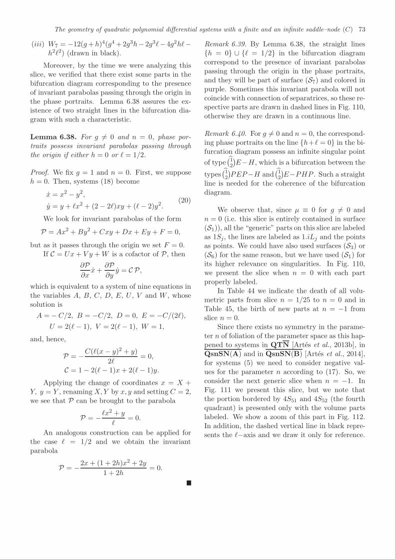
The geometry of quadratic polynomial differential systems with a finite and an infinite saddle–node (C) 73
(iii) W7 = −12(g+h)4(g4 +2g3h− 2g3ℓ− 4g2hℓ−h2ℓ2) (drawn in black).
Moreover, by the time we were analyzing thisslice, we verified that there exist some parts in thebifurcation diagram corresponding to the presenceof invariant parabolas passing through the origin inthe phase portraits. Lemma 6.38 assures the ex-istence of two straight lines in the bifurcation dia-gram with such a characteristic.
Lemma 6.38. For g 6= 0 and n = 0, phase por-traits possess invariant parabolas passing throughthe origin if either h = 0 or ℓ = 1/2.
Proof. We fix g = 1 and n = 0. First, we supposeh = 0. Then, systems (18) become
x = x2 − y2,
y = y + ℓx2 + (2− 2ℓ)xy + (ℓ− 2)y2.(20)
We look for invariant parabolas of the form
P = Ax2 +By2 + Cxy +Dx+ Ey + F = 0,
but as it passes through the origin we set F = 0.If C = Ux+ V y +W is a cofactor of P, then
∂P∂x
x+∂P∂y
y = C P,
which is equivalent to a system of nine equations inthe variables A, B, C, D, E, U , V and W , whosesolution is
A =− C/2, B = −C/2, D = 0, E = −C/(2ℓ),
U = 2(ℓ− 1), V = 2(ℓ− 1), W = 1,
and, hence,
P = −C(ℓ(x− y)2 + y)
2ℓ= 0,
C = 1− 2(ℓ− 1)x+ 2(ℓ− 1)y.
Applying the change of coordinates x = X +Y, y = Y , renamingX,Y by x, y and setting C = 2,we see that P can be brought to the parabola
P = −ℓx2 + y
ℓ= 0.
An analogous construction can be applied forthe case ℓ = 1/2 and we obtain the invariantparabola
P = −2x+ (1 + 2h)x2 + 2y
1 + 2h= 0.
Remark 6.39. By Lemma 6.38, the straight lines{h = 0} ∪ {ℓ = 1/2} in the bifurcation diagramcorrespond to the presence of invariant parabolaspassing through the origin in the phase portraits,and they will be part of surface (S7) and colored inpurple. Sometimes this invariant parabola will notcoincide with connection of separatrices, so these re-spective parts are drawn in dashed lines in Fig. 110,otherwise they are drawn in a continuous line.
Remark 6.40. For g 6= 0 and n = 0, the correspond-ing phase portraits on the line {h+ℓ = 0} in the bi-furcation diagram possess an infinite singular point
of type(12
)E−H, which is a bifurcation between the
types(12
)PEP−H and
(12
)E−PHP . Such a straight
line is needed for the coherence of the bifurcationdiagram.
We observe that, since µ ≡ 0 for g 6= 0 andn = 0 (i.e. this slice is entirely contained in surface(S1)), all the “generic” parts on this slice are labeledas 1Sj, the lines are labeled as 1.iLj and the pointsas points. We could have also used surfaces (S3) or(S6) for the same reason, but we have used (S1) forits higher relevance on singularities. In Fig. 110,we present the slice when n = 0 with each partproperly labeled.
In Table 44 we indicate the death of all volu-metric parts from slice n = 1/25 to n = 0 and inTable 45, the birth of new parts at n = −1 fromslice n = 0.
Since there exists no symmetry in the parame-ter n of foliation of the parameter space as this hap-pened to systems in QTN [Artes et al., 2013b], inQsnSN(A) and in QsnSN(B) [Artes et al., 2014],for systems (5) we need to consider negative val-ues for the parameter n according to (17). So, weconsider the next generic slice when n = −1. InFig. 111 we present this slice, but we note thatthe portion bordered by 4S51 and 4S52 (the fourthquadrant) is presented only with the volume partslabeled. We show a zoom of this part in Fig. 112.In addition, the dashed vertical line in black repre-sents the ℓ−axis and we draw it only for reference.
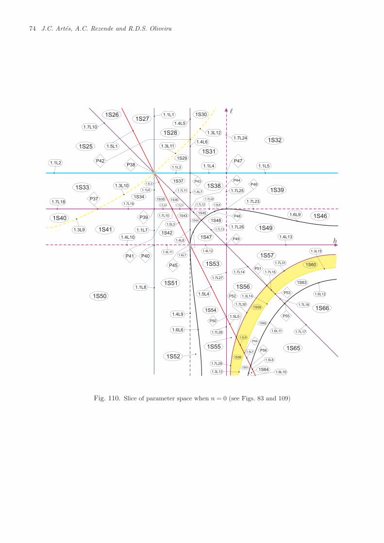
74 J.C. Artes, A.C. Rezende and R.D.S. Oliveira
1S25
1.1L2
1S261S27
1S28
1S29
1S31
1S30
1S32
1S33
1S40
1S41
1S50
1S34
1S39
1S46
1S49
1S381S37
1S42
1S48
1S51
1S54
1S53
1S57
1S56
1S52
1S55
1S66
1S65
1S64
1S35 1S36
1S43
1S44
1S45
1S47
1S61
1S62
1S63
1S60
1S59
1S58
1.7L10
1.5L1
1.1L1
1.3L11
1.4L5
1.3L12
1.4L6
1.1L4
1.7L24
1.1L51.1L3
1.7L181.7L19
1.1L6
1.7L10
1.7L111.4L7
1.7L12
1.7L22
1.7L25
1.7L23
1.3L10
1.7L20 1.7L21
1.5L2
1.6L8
1.3L9
1.4L10
1.1L7
1.5L3
1.4L8
1.4L11 1.4L12
1.7L131.7L26
1.4L13
1.1L8
1.4L9
1.6L6
1.5L4
1.6L7
1.7L27
1.7L28
1.7L14
1.5L5
1.7L29
1.5L6
1.5L7
1.5L8
1.3L13 1.6L10
1.7L30
1.3L14
1.7L31
1.3L15
1.6L11
1.6L12
1.7L15
1.7L16
1.7L17
P38
P37
P47P42
P39
P40
P45
P41
P43 P44
P48
P49
P46
P50
P51
P52P53
P54
P56
P55
1.6L9
ℓ
h
Fig. 110. Slice of parameter space when n = 0 (see Figs. 83 and 109)
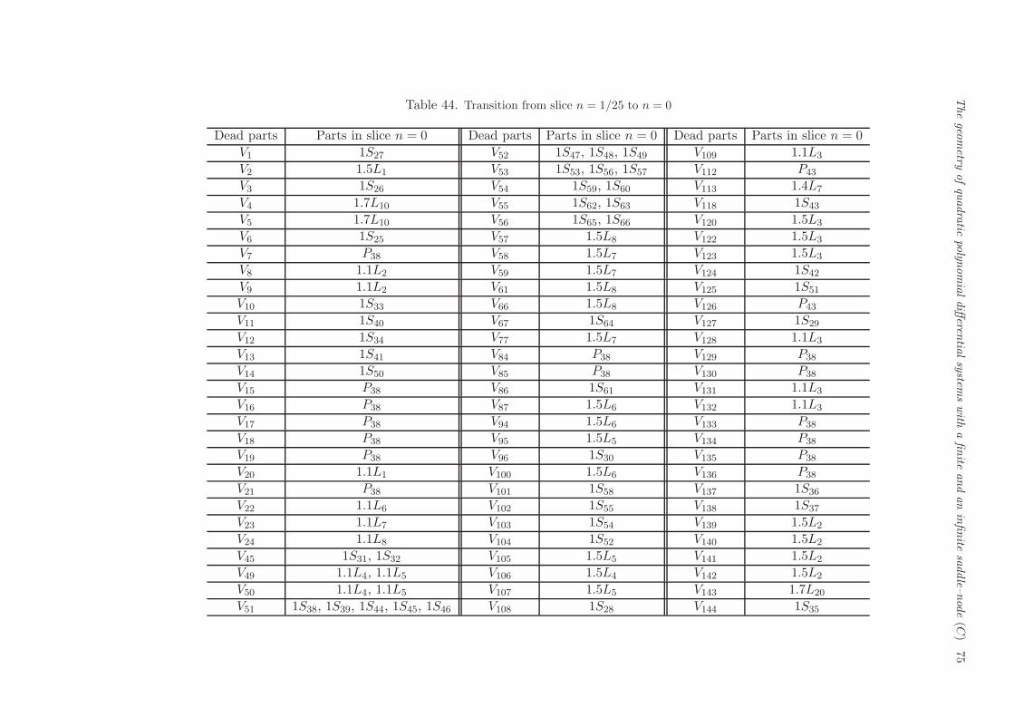
Thegeo
metry
ofquadratic
polyn
omialdifferen
tialsystem
swith
afinite
andaninfinite
saddle–
node(C
)75
Table 44. Transition from slice n = 1/25 to n = 0
Dead parts Parts in slice n = 0 Dead parts Parts in slice n = 0 Dead parts Parts in slice n = 0
V1 1S27 V52 1S47, 1S48, 1S49 V109 1.1L3
V2 1.5L1 V53 1S53, 1S56, 1S57 V112 P43
V3 1S26 V54 1S59, 1S60 V113 1.4L7
V4 1.7L10 V55 1S62, 1S63 V118 1S43
V5 1.7L10 V56 1S65, 1S66 V120 1.5L3
V6 1S25 V57 1.5L8 V122 1.5L3
V7 P38 V58 1.5L7 V123 1.5L3
V8 1.1L2 V59 1.5L7 V124 1S42
V9 1.1L2 V61 1.5L8 V125 1S51
V10 1S33 V66 1.5L8 V126 P43
V11 1S40 V67 1S64 V127 1S29
V12 1S34 V77 1.5L7 V128 1.1L3
V13 1S41 V84 P38 V129 P38
V14 1S50 V85 P38 V130 P38
V15 P38 V86 1S61 V131 1.1L3
V16 P38 V87 1.5L6 V132 1.1L3
V17 P38 V94 1.5L6 V133 P38
V18 P38 V95 1.5L5 V134 P38
V19 P38 V96 1S30 V135 P38
V20 1.1L1 V100 1.5L6 V136 P38
V21 P38 V101 1S58 V137 1S36
V22 1.1L6 V102 1S55 V138 1S37
V23 1.1L7 V103 1S54 V139 1.5L2
V24 1.1L8 V104 1S52 V140 1.5L2
V45 1S31, 1S32 V105 1.5L5 V141 1.5L2
V49 1.1L4, 1.1L5 V106 1.5L4 V142 1.5L2
V50 1.1L4, 1.1L5 V107 1.5L5 V143 1.7L20
V51 1S38, 1S39, 1S44, 1S45, 1S46 V108 1S28 V144 1S35
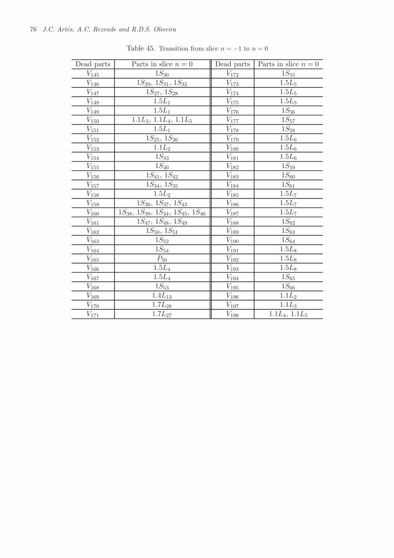
76 J.C. Artes, A.C. Rezende and R.D.S. Oliveira
Table 45. Transition from slice n = −1 to n = 0
Dead parts Parts in slice n = 0 Dead parts Parts in slice n = 0
V145 1S30 V172 1S55
V146 1S29, 1S31, 1S32 V173 1.5L5
V147 1S27, 1S28 V174 1.5L5
V148 1.5L1 V175 1.5L5
V149 1.5L1 V176 1S56
V150 1.1L3, 1.1L4, 1.1L5 V177 1S57
V151 1.5L1 V178 1S58
V152 1S25, 1S26 V179 1.5L6
V153 1.1L2 V180 1.5L6
V154 1S33 V181 1.5L6
V155 1S40 V182 1S59
V156 1S41, 1S42 V183 1S60
V157 1S34, 1S35 V184 1S61
V158 1.5L2 V185 1.5L7
V159 1S36, 1S37, 1S43 V186 1.5L7
V160 1S38, 1S39, 1S44, 1S45, 1S46 V187 1.5L7
V161 1S47, 1S48, 1S49 V188 1S62
V162 1S50, 1S51 V189 1S63
V163 1S52 V190 1S64
V164 1S54 V191 1.5L8
V165 P50 V192 1.5L8
V166 1.5L4 V193 1.5L8
V167 1.5L4 V194 1S65
V168 1S53 V195 1S66
V169 1.4L13 V196 1.1L2
V170 1.7L28 V197 1.1L3
V171 1.7L27 V198 1.1L4, 1.1L5
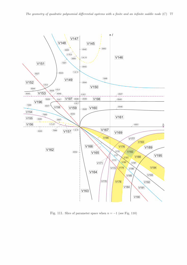
The geometry of quadratic polynomial differential systems with a finite and an infinite saddle–node (C) 77
5.6L6
V145
V146
V147
V148
V150
V149
V151
V152
V153
V196
V154
V155
V156
V162
V158
V157
V159 V160
V198
V161
V163
V164
V169
V168
V176
V197
V166
V165
V167
V182
V177
V183
V188
V194
V189
V195
V193
V192
V191V184
V178
V172
V170
V173
V179
V185
V186
V187
V181
V180
V175
V174
V171
V190
1S67
1S68
1S69
3S63
3S64
3S65
3S66 3S67
4S42
4S43
4S44
4S45 4S46 4S47
4S50
4S51
4S52
4S48
4S49
5S27
5S29
5S30
5S28
7S65
7S66
3.10L8
3.4L18
1.4L14
4.5L4
5.6L7
4.4L5
4.6L7
3.7L22
1.3L16
6S43
6S44
6S45
6S48
6S46
6S47
ℓ
h
Fig. 111. Slice of parameter space when n = −1 (see Fig. 110)
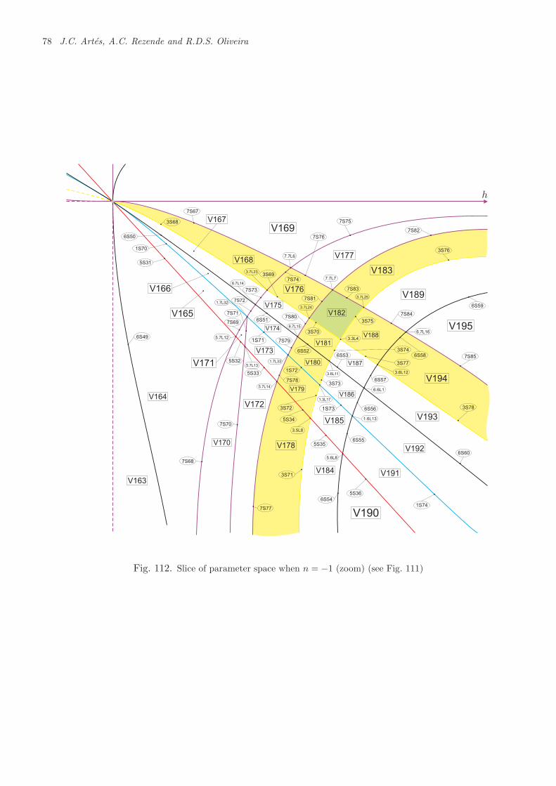
78 J.C. Artes, A.C. Rezende and R.D.S. Oliveira
7S67
7S76
7S83
3S75
7S84
7S85
3S68
3S69
3S70
3S77
3S74
3S78
1S70
5S31
5S32
5S331S72
3S72
5S34
3S73
5S35
5S36
1S74
3S76
7S75
7S74
7S73
7S72
7S69
7S71
7S68
7S70
7S77
3S71
7S78
7S79
7S80
7S81
7S82
6S50
6S49
6S51
6S526S53
6S57
6S60
6S54
6S55
6S56
6S58
6S59
3.5L8
5.7L12
5.7L13
5.7L14
1.7L32
1.7L33
5.6L8
1.6L13
6.6L1
3.6L12
6.7L16
1.3L17
3.6L11
3.3L4
3.7L25
6.7L15
3.7L24
7.7L7
7.7L6
3.7L23
6.7L14
h
Fig. 112. Slice of parameter space when n = −1 (zoom) (see Fig. 111)
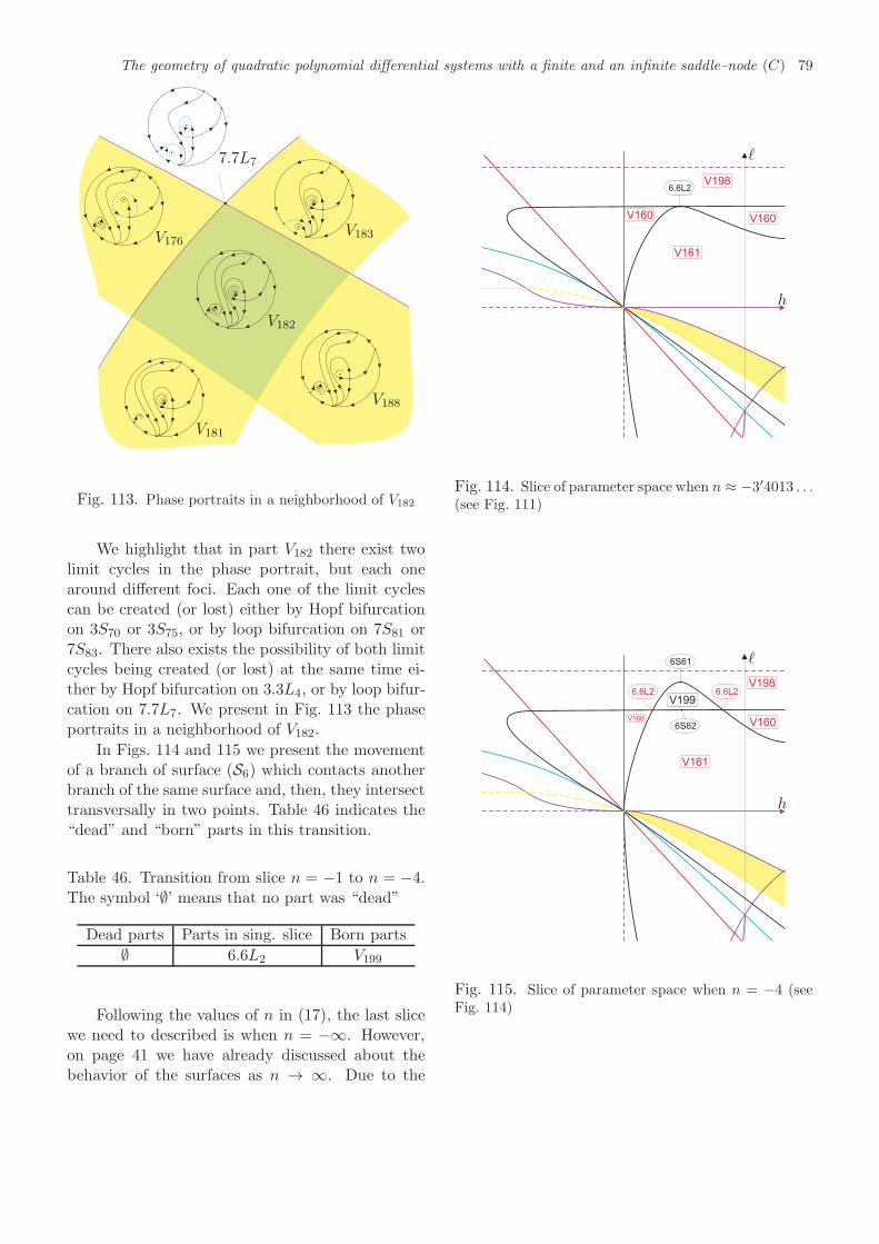
The geometry of quadratic polynomial differential systems with a finite and an infinite saddle–node (C) 79
V182
V183
V181
V188
V176
7.7L7
Fig. 113. Phase portraits in a neighborhood of V182
We highlight that in part V182 there exist twolimit cycles in the phase portrait, but each onearound different foci. Each one of the limit cyclescan be created (or lost) either by Hopf bifurcationon 3S70 or 3S75, or by loop bifurcation on 7S81 or7S83. There also exists the possibility of both limitcycles being created (or lost) at the same time ei-ther by Hopf bifurcation on 3.3L4, or by loop bifur-cation on 7.7L7. We present in Fig. 113 the phaseportraits in a neighborhood of V182.
In Figs. 114 and 115 we present the movementof a branch of surface (S6) which contacts anotherbranch of the same surface and, then, they intersecttransversally in two points. Table 46 indicates the“dead” and “born” parts in this transition.
Table 46. Transition from slice n = −1 to n = −4.The symbol ‘∅’ means that no part was “dead”
Dead parts Parts in sing. slice Born parts
∅ 6.6L2 V199
Following the values of n in (17), the last slicewe need to described is when n = −∞. However,on page 41 we have already discussed about thebehavior of the surfaces as n → ∞. Due to the
6.6L2
V161
V160 V160
V198
ℓ
h
Fig. 114. Slice of parameter space when n ≈ −3′4013 . . .(see Fig. 111)
6.6L2
V199
6S62
6S61
V160
V161
V198
V160
6.6L2
ℓ
h
Fig. 115. Slice of parameter space when n = −4 (seeFig. 114)
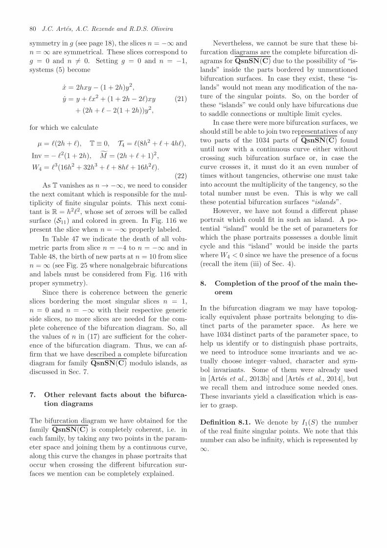
80 J.C. Artes, A.C. Rezende and R.D.S. Oliveira
symmetry in g (see page 18), the slices n = −∞ andn = ∞ are symmetrical. These slices correspond tog = 0 and n 6= 0. Setting g = 0 and n = −1,systems (5) become
x = 2hxy − (1 + 2h)y2,
y = y + ℓx2 + (1 + 2h− 2ℓ)xy
+ (2h+ ℓ− 2(1 + 2h))y2,
(21)
for which we calculate
µ = ℓ(2h + ℓ), T ≡ 0, T4 = ℓ(8h2 + ℓ+ 4hℓ),
Inv =− ℓ2(1 + 2h), M = (2h + ℓ+ 1)2,
W4 = ℓ3(16h2 + 32h3 + ℓ+ 8hℓ+ 16h2ℓ).(22)
As T vanishes as n → −∞, we need to considerthe next comitant which is responsible for the mul-tiplicity of finite singular points. This next comi-tant is R = h2ℓ2, whose set of zeroes will be calledsurface (S11) and colored in green. In Fig. 116 wepresent the slice when n = −∞ properly labeled.
In Table 47 we indicate the death of all volu-metric parts from slice n = −4 to n = −∞ and inTable 48, the birth of new parts at n = 10 from slicen = ∞ (see Fig. 25 where nonalgebraic bifurcationsand labels must be considered from Fig. 116 withproper symmetry).
Since there is coherence between the genericslices bordering the most singular slices n = 1,n = 0 and n = −∞ with their respective genericside slices, no more slices are needed for the com-plete coherence of the bifurcation diagram. So, allthe values of n in (17) are sufficient for the coher-ence of the bifurcation diagram. Thus, we can af-firm that we have described a complete bifurcationdiagram for family QsnSN(C) modulo islands, asdiscussed in Sec. 7.
7. Other relevant facts about the bifurca-tion diagrams
The bifurcation diagram we have obtained for thefamily QsnSN(C) is completely coherent, i.e. ineach family, by taking any two points in the param-eter space and joining them by a continuous curve,along this curve the changes in phase portraits thatoccur when crossing the different bifurcation sur-faces we mention can be completely explained.
Nevertheless, we cannot be sure that these bi-furcation diagrams are the complete bifurcation di-agrams for QsnSN(C) due to the possibility of “is-lands” inside the parts bordered by unmentionedbifurcation surfaces. In case they exist, these “is-lands” would not mean any modification of the na-ture of the singular points. So, on the border ofthese “islands” we could only have bifurcations dueto saddle connections or multiple limit cycles.
In case there were more bifurcation surfaces, weshould still be able to join two representatives of anytwo parts of the 1034 parts of QsnSN(C) founduntil now with a continuous curve either withoutcrossing such bifurcation surface or, in case thecurve crosses it, it must do it an even number oftimes without tangencies, otherwise one must takeinto account the multiplicity of the tangency, so thetotal number must be even. This is why we callthese potential bifurcation surfaces “islands”.
However, we have not found a different phaseportrait which could fit in such an island. A po-tential “island” would be the set of parameters forwhich the phase portraits possesses a double limitcycle and this “island” would be inside the partswhere W4 < 0 since we have the presence of a focus(recall the item (iii) of Sec. 4).
8. Completion of the proof of the main the-orem
In the bifurcation diagram we may have topolog-ically equivalent phase portraits belonging to dis-tinct parts of the parameter space. As here wehave 1034 distinct parts of the parameter space, tohelp us identify or to distinguish phase portraits,we need to introduce some invariants and we ac-tually choose integer–valued, character and sym-bol invariants. Some of them were already usedin [Artes et al., 2013b] and [Artes et al., 2014], butwe recall them and introduce some needed ones.These invariants yield a classification which is eas-ier to grasp.
Definition 8.1. We denote by I1(S) the numberof the real finite singular points. We note that thisnumber can also be infinity, which is represented by∞.
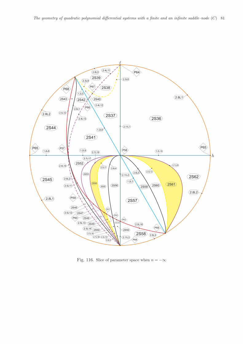
The geometry of quadratic polynomial differential systems with a finite and an infinite saddle–node (C) 81
2S362S37
2S402S42
2S41
2S43
2S44
2S45
2S52
2S53
2S55
2S46
2S56
2S57
2S592S60 2S61
2S62
2S54
2S58
2S38
2S39
2S47
2S48
2S49
2S50 2S50
2.8L1
P65
P642.4L11
2.3L8
P67
2.3L9
2.4L12
P66
1.2L5
P68
2.4L13
2.5L10
2.6L1
1.2L8 1.2L9P57
1.2L6
2.11L1
1.2L10
2.4L14
2.6L2
2.5L11
P59
P60
P61
P62
P63
2.5L12
2.5L13
2.5L14
2.5L15
2.5L16
1.2L7
P58P65
2.7L17
2.7L19
2.3L112.6L4
2.11L2
2.6L52.3L12
2.7L20
2.11L3
2.6L3
2.3L10
2.7L16
2.7L18
P64
2.8L1
2.8L2
2.8L2
2.8L3
2.8L3
P68
ℓ
h
Fig. 116. Slice of parameter space when n = −∞
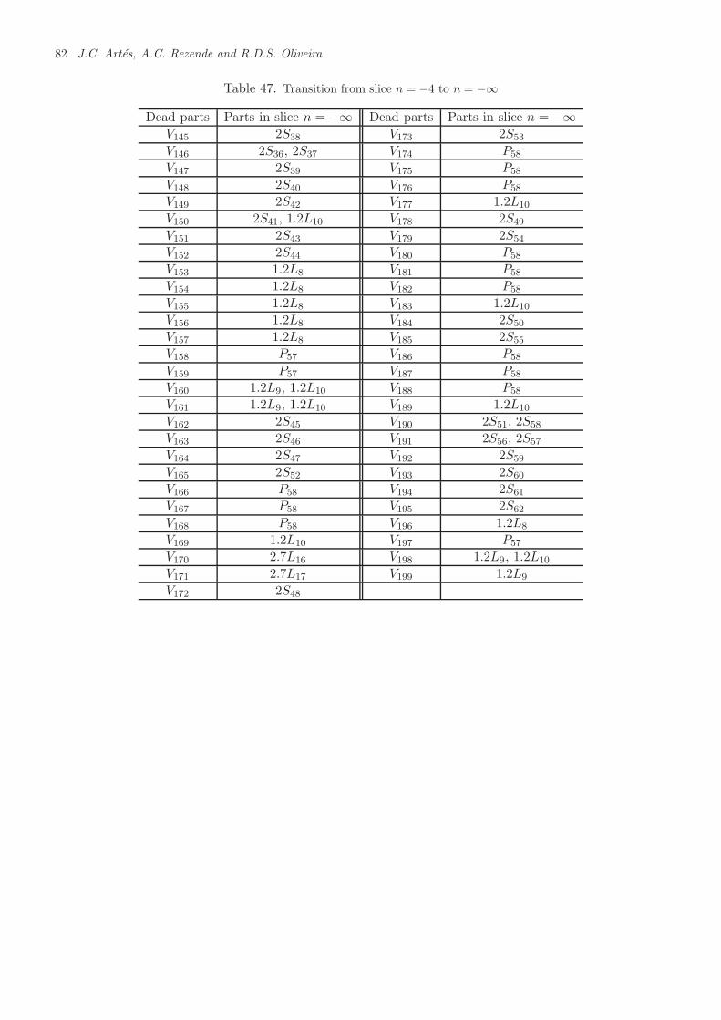
82 J.C. Artes, A.C. Rezende and R.D.S. Oliveira
Table 47. Transition from slice n = −4 to n = −∞
Dead parts Parts in slice n = −∞ Dead parts Parts in slice n = −∞V145 2S38 V173 2S53
V146 2S36, 2S37 V174 P58
V147 2S39 V175 P58
V148 2S40 V176 P58
V149 2S42 V177 1.2L10
V150 2S41, 1.2L10 V178 2S49
V151 2S43 V179 2S54
V152 2S44 V180 P58
V153 1.2L8 V181 P58
V154 1.2L8 V182 P58
V155 1.2L8 V183 1.2L10
V156 1.2L8 V184 2S50
V157 1.2L8 V185 2S55
V158 P57 V186 P58
V159 P57 V187 P58
V160 1.2L9, 1.2L10 V188 P58
V161 1.2L9, 1.2L10 V189 1.2L10
V162 2S45 V190 2S51, 2S58
V163 2S46 V191 2S56, 2S57
V164 2S47 V192 2S59
V165 2S52 V193 2S60
V166 P58 V194 2S61
V167 P58 V195 2S62
V168 P58 V196 1.2L8
V169 1.2L10 V197 P57
V170 2.7L16 V198 1.2L9, 1.2L10
V171 2.7L17 V199 1.2L9
V172 2S48
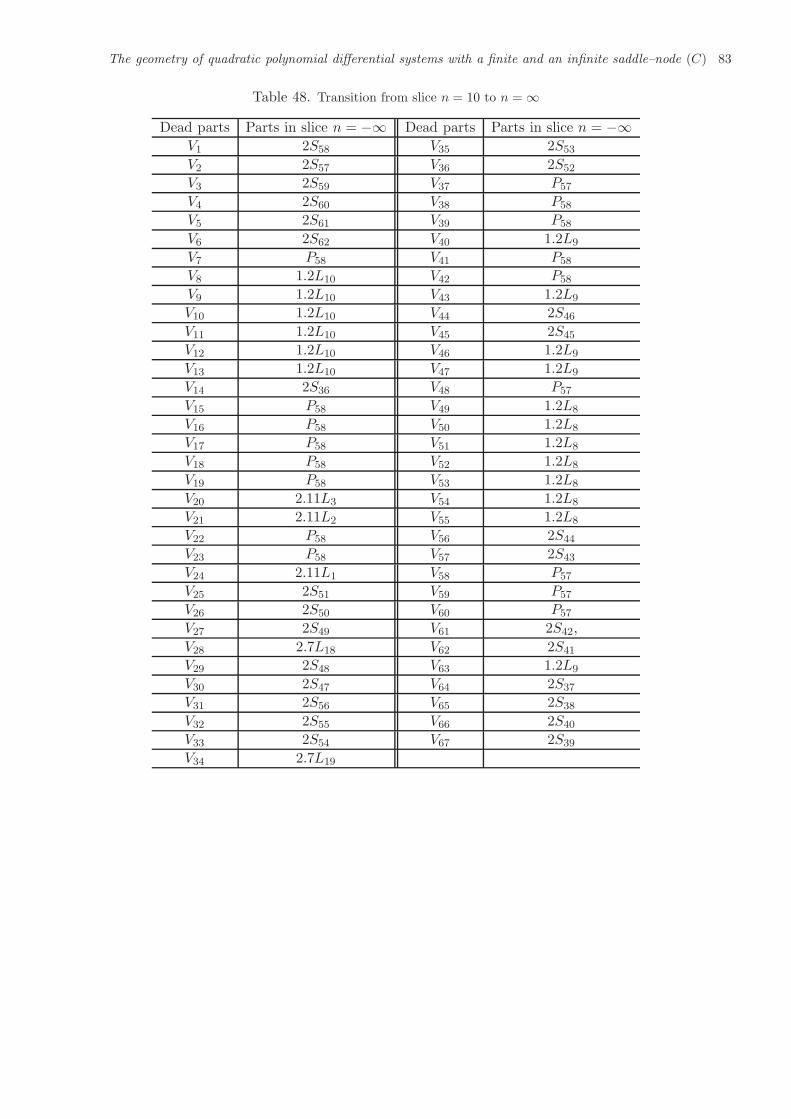
The geometry of quadratic polynomial differential systems with a finite and an infinite saddle–node (C) 83
Table 48. Transition from slice n = 10 to n = ∞
Dead parts Parts in slice n = −∞ Dead parts Parts in slice n = −∞V1 2S58 V35 2S53
V2 2S57 V36 2S52
V3 2S59 V37 P57
V4 2S60 V38 P58
V5 2S61 V39 P58
V6 2S62 V40 1.2L9
V7 P58 V41 P58
V8 1.2L10 V42 P58
V9 1.2L10 V43 1.2L9
V10 1.2L10 V44 2S46
V11 1.2L10 V45 2S45
V12 1.2L10 V46 1.2L9
V13 1.2L10 V47 1.2L9
V14 2S36 V48 P57
V15 P58 V49 1.2L8
V16 P58 V50 1.2L8
V17 P58 V51 1.2L8
V18 P58 V52 1.2L8
V19 P58 V53 1.2L8
V20 2.11L3 V54 1.2L8
V21 2.11L2 V55 1.2L8
V22 P58 V56 2S44
V23 P58 V57 2S43
V24 2.11L1 V58 P57
V25 2S51 V59 P57
V26 2S50 V60 P57
V27 2S49 V61 2S42,
V28 2.7L18 V62 2S41
V29 2S48 V63 1.2L9
V30 2S47 V64 2S37
V31 2S56 V65 2S38
V32 2S55 V66 2S40
V33 2S54 V67 2S39
V34 2.7L19
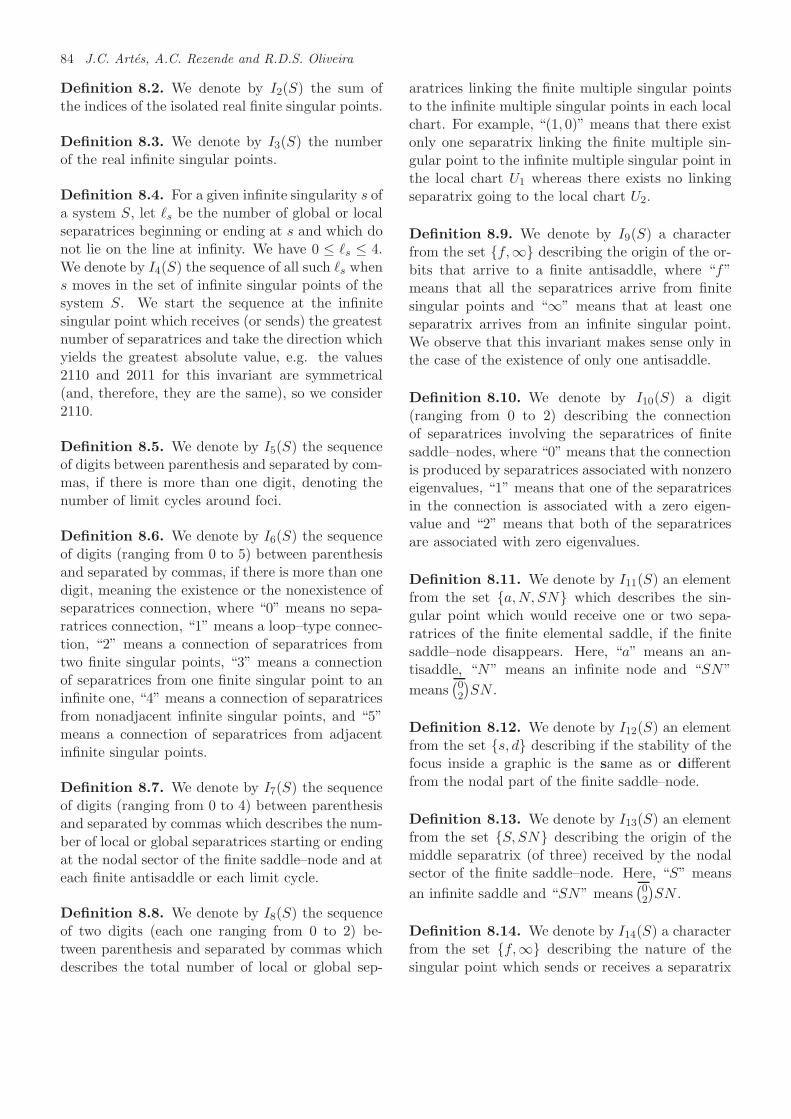
84 J.C. Artes, A.C. Rezende and R.D.S. Oliveira
Definition 8.2. We denote by I2(S) the sum ofthe indices of the isolated real finite singular points.
Definition 8.3. We denote by I3(S) the numberof the real infinite singular points.
Definition 8.4. For a given infinite singularity s ofa system S, let ℓs be the number of global or localseparatrices beginning or ending at s and which donot lie on the line at infinity. We have 0 ≤ ℓs ≤ 4.We denote by I4(S) the sequence of all such ℓs whens moves in the set of infinite singular points of thesystem S. We start the sequence at the infinitesingular point which receives (or sends) the greatestnumber of separatrices and take the direction whichyields the greatest absolute value, e.g. the values2110 and 2011 for this invariant are symmetrical(and, therefore, they are the same), so we consider2110.
Definition 8.5. We denote by I5(S) the sequenceof digits between parenthesis and separated by com-mas, if there is more than one digit, denoting thenumber of limit cycles around foci.
Definition 8.6. We denote by I6(S) the sequenceof digits (ranging from 0 to 5) between parenthesisand separated by commas, if there is more than onedigit, meaning the existence or the nonexistence ofseparatrices connection, where “0” means no sepa-ratrices connection, “1” means a loop–type connec-tion, “2” means a connection of separatrices fromtwo finite singular points, “3” means a connectionof separatrices from one finite singular point to aninfinite one, “4” means a connection of separatricesfrom nonadjacent infinite singular points, and “5”means a connection of separatrices from adjacentinfinite singular points.
Definition 8.7. We denote by I7(S) the sequenceof digits (ranging from 0 to 4) between parenthesisand separated by commas which describes the num-ber of local or global separatrices starting or endingat the nodal sector of the finite saddle–node and ateach finite antisaddle or each limit cycle.
Definition 8.8. We denote by I8(S) the sequenceof two digits (each one ranging from 0 to 2) be-tween parenthesis and separated by commas whichdescribes the total number of local or global sep-
aratrices linking the finite multiple singular pointsto the infinite multiple singular points in each localchart. For example, “(1, 0)” means that there existonly one separatrix linking the finite multiple sin-gular point to the infinite multiple singular point inthe local chart U1 whereas there exists no linkingseparatrix going to the local chart U2.
Definition 8.9. We denote by I9(S) a characterfrom the set {f,∞} describing the origin of the or-bits that arrive to a finite antisaddle, where “f”means that all the separatrices arrive from finitesingular points and “∞” means that at least oneseparatrix arrives from an infinite singular point.We observe that this invariant makes sense only inthe case of the existence of only one antisaddle.
Definition 8.10. We denote by I10(S) a digit(ranging from 0 to 2) describing the connectionof separatrices involving the separatrices of finitesaddle–nodes, where “0” means that the connectionis produced by separatrices associated with nonzeroeigenvalues, “1” means that one of the separatricesin the connection is associated with a zero eigen-value and “2” means that both of the separatricesare associated with zero eigenvalues.
Definition 8.11. We denote by I11(S) an elementfrom the set {a,N, SN} which describes the sin-gular point which would receive one or two sepa-ratrices of the finite elemental saddle, if the finitesaddle–node disappears. Here, “a” means an an-tisaddle, “N” means an infinite node and “SN”
means(02
)SN .
Definition 8.12. We denote by I12(S) an elementfrom the set {s, d} describing if the stability of thefocus inside a graphic is the same as or differentfrom the nodal part of the finite saddle–node.
Definition 8.13. We denote by I13(S) an elementfrom the set {S, SN} describing the origin of themiddle separatrix (of three) received by the nodalsector of the finite saddle–node. Here, “S” means
an infinite saddle and “SN” means(02
)SN .
Definition 8.14. We denote by I14(S) a characterfrom the set {f,∞} describing the nature of thesingular point which sends or receives a separatrix
The geometry of quadratic polynomial differential systems with a finite and an infinite saddle–node (C) 85
to or from a limit cycle.
Definition 8.15. We denote by I15(S) the sum ofthe indices of the isolated infinite multiple singularpoints (considered in only one local chart).
Definition 8.16. We denote by I16(S) a characterfrom the set {H,P}, where H determines that a fi-nite antisaddle sends (or receives) orbits to (from) aparabolic sector of a multiple infinite singular pointsituated in the local chart where the parabolic sec-tor is accompanied by other hyperbolic sectors, andP denotes that the parabolic sector is the only sec-tor of the infinite singular point in that local chart.This invariant is needed to distinguish 1.5L3 from1.5L4.
Definition 8.17. We denote by I17(S) a symbolto represent the configuration of the curves of sin-gularities. The symbols are: “−” to represent astraight line and “∪” to represent a parabola.
Definition 8.18. We denote by I18(S) a charac-ter from the set {n, y} describing the nonexistence(“n”) or the existence (“y”) of graphics.
Definition 8.19. We denote by I19(S) a characterfrom the set {c, s} describing the position of theseparatrix of the finite saddle–node associated withthe eigenvector with zero eigenvalue which arrives
to (or leaves from)(02
)SN when this point receives
3 separatrices. We use “c” for the central positionand “s” for the lateral (side) position.
Definition 8.20. We denote by I20(S) a charac-ter from the set {s, d} describing if each point ofthe pair of infinite saddle–nodes sends (or receives)two separatrices to/from the same or different fi-nite saddle–nodes. This invariant only makes sensein case of existence of two finite saddle–nodes.
As we have noted previously in Remark 6.31,we do not distinguish between phase portraitswhose only difference is that in one we have a fi-nite node and in the other a focus. Both phaseportraits are topologically equivalent and they canonly be distinguished within the C1 class. In casewe may want to distinguish between them, a newinvariant may easily be introduced.
Theorem 8.21. Consider the family QsnSN(C)and all the phase portraits that we have obtainedfor this family. The values of the affine in-variant I = (I1, I2, I3, I4, I5, I6, I7, I8, I9, I10, I11,I12, I13, I14, I15, I16, I17, I18, I19, I20) given in the fol-lowing diagram yield a partition of these phase por-traits of the family QsnSN(C).
Furthermore, for each value of I in this dia-gram there corresponds a single phase portrait; i.e.S and S′ are such that I(S) = I(S′), if and only ifS and S′ are topologically equivalent.
The bifurcation diagram for QsnSN(C) has1034 parts which produce 371 topologically differ-ent phase portraits as described in Tables 50 to 59.The remaining 663 parts do not produce any newphase portrait which was not included in the 371previous ones. The difference is basically the pres-ence of a strong focus instead of a node and viceversa and weak points.
The phase portraits having neither limit cy-cle nor graphic have been denoted surrounded byparenthesis, for example (5S2); the phase portraitshaving one or two limit cycles have been denotedsurrounded by brackets, for example [V80], pos-sessing one limit cycle, and [[V88]], possessing twolimit cycles; the phase portraits having one or twographics have been denoted surrounded by {∗} or{{∗}}, for example {1S28} and {{1S57}}; the phaseportraits having one limit cycle and one graphichave been denoted surrounded by [{∗}], for exam-ple [{1S60}].
Proof of Theorem 8.21. The above result followsfrom the results in the previous sections and a care-ful analysis of the bifurcation diagrams given inSec. 6, in Figs. 23 to 116, the definition of the in-variants Ij and their explicit values for the corre-sponding phase portraits.
We recall some observations regarding theequivalence relations used in this study: the affineand time rescaling, C1 and topological equivalences.
The coarsest one among these three is the topo-logical equivalence and the finest is the affine equiv-alence. We can have two systems which are topo-logically equivalent but not C1−equivalent. For ex-ample, we could have a system with a finite anti-saddle which is a structurally stable node and inanother system with a focus, the two systems being
86 J.C. Artes, A.C. Rezende and R.D.S. Oliveira
topologically equivalent but belonging to distinctC1−equivalence classes, separated by the surface(S6) on which the node turns into a focus.
In Tables 60 to 73 we listed in the first column371 parts with all the distinct phase portraits ofFigs. 1 to 11. Corresponding to each part listed incolumn 1 we have in its horizontal block, all partswhose phase portraits are topologically equivalentto the phase portrait appearing in column 1 of thesame horizontal block.
In the second column we have put all the partswhose systems yield topologically equivalent phaseportraits to those in the first column, but whichmay have some algebro–geometric features relatedto the position of the orbits. In the third column wehave presented all the parts which are topologicallyequivalent to the ones from the first column havinga focus instead of a node.
In the fourth (respectively, fifth; sixth; seventh;and eightieth) column we have listed all parts whosephase portraits have a node which is at a bifurcationpoint producing foci close to the node in perturba-tions, a node–focus to shorten (respectively, a finiteweak singular point; belong to disconnected parts;possess an invariant curve not yielding a connectionof separatrices; and have symmetry).
The last column refers to other reasons associ-ated to different geometrical aspects and they aredescribed as follows:
(1) it possesses a sn(4) as a finite singular point;
(2) it possesses a(21
)N at infinity;
(3) 3S20 is the singularity of the surface (S3), i.e.of the invariant polinomial T4, where the twofinite complex singularities are weak;
(4) it possesses a(12
)E −H at infinity;
(5) the antisaddle is triple;
(6) it possesses a(23
)N at infinity;
Whenever phase portraits appear on a horizon-tal block in a specific column, the listing is doneaccording to the decreasing dimension of the partswhere they appear, always placing the lower dimen-sions on lower lines.
8.1. Proof of the main theorem
The bifurcation diagram described in Sec. 6, plusTables 50 to 59 of the geometrical invariants distin-guishing the 371 phase portraits, plus Tables 60 to
79 giving the equivalences with the remaining phaseportraits lead to the proof of the main statement ofTheorem 1.1.
Moreover, the phase portraits P3 from familyQsnSN(A), P2 from family QsnSN(B) and P57
from family QsnSN(C) are topologically equiva-lent since there exists no geometrical invariant thatdistinguishes them. It has been needed to have thecurve at infinity filled up with an infinite number ofsingularities to have a common element in the threefamilies. The same argument is applied to prove theequivalence of the two other triplets. Also, thereare 10 more cases of coincidences between phaseportraits of family QsnSN(C) and one of eitherQsnSN(A) or QsnSN(B) and we have discoveredanother equivalence between 5S2 from QsnSN(A)and 5S3 from QsnSN(B) which have no equiva-lence in QsnSN(C). This proves Corollary 1.2.
Now, summing all the topologically dis-tinct phase portraits from families QsnSN(A),QsnSN(B) and QsnSN(C) and subtracting theintersections among them, according to Corol-lary 1.2, we obtain 38 + 25 + 371 − 17 = 417 topo-logically distinct phase portraits inQsnSN, and weprove Corollary 1.3.
In the family QsnSN(C), all the phase por-traits corresponding to parts of volume yield all thetopologically possible phase portraits of codimen-sion one from group (A) (see page ?? for the de-scription of this group). Many of them had alreadybeen discovered being realizable, and others whichrealization was missing have been found within theperturbations of familyQsnSN(C). In the next ex-ample we perturbe one phase portrait from familyQsnSN(C) and obtain one phase portrait of codi-mension one which was missing. Also three newphase portraits of group (B) can be found from per-turbations of family QsnSN(C).
Example 8.22. Phase portrait V177 yields an exam-ple of the “wanted” case A66 of codimension one.Indeed, by adding the small perturbation x2/100in a representative of the part V177 we obtain thefollowing system:
x = x2 + 12xy/5 − 22y2/5 + x2/100,
y = y − x2/10 + 28xy/5 − 13y2/2,(23)
and, hence, the infinite saddle–node(02
)SN splits
into a saddle and a node, and we obtain the
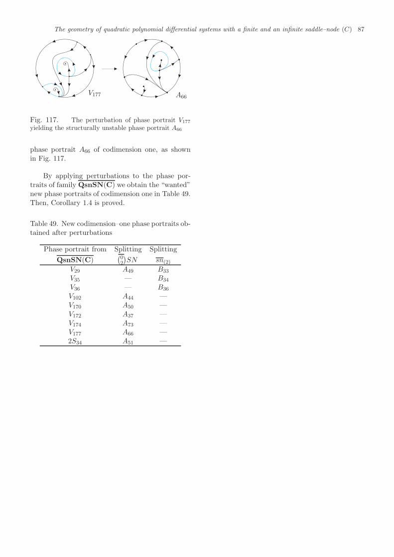
The geometry of quadratic polynomial differential systems with a finite and an infinite saddle–node (C) 87
A66V177
Fig. 117. The perturbation of phase portrait V177
yielding the structurally unstable phase portrait A66
phase portrait A66 of codimension one, as shownin Fig. 117.
By applying perturbations to the phase por-traits of family QsnSN(C) we obtain the “wanted”new phase portraits of codimension one in Table 49.Then, Corollary 1.4 is proved.
Table 49. New codimension–one phase portraits ob-tained after perturbations
Phase portrait from Splitting Splitting
QsnSN(C)(02
)SN sn(2)
V29 A49 B33
V35 — B34
V36 — B36
V102 A44 —V170 A50 —V172 A37 —V174 A73 —V177 A66 —2S34 A51 —
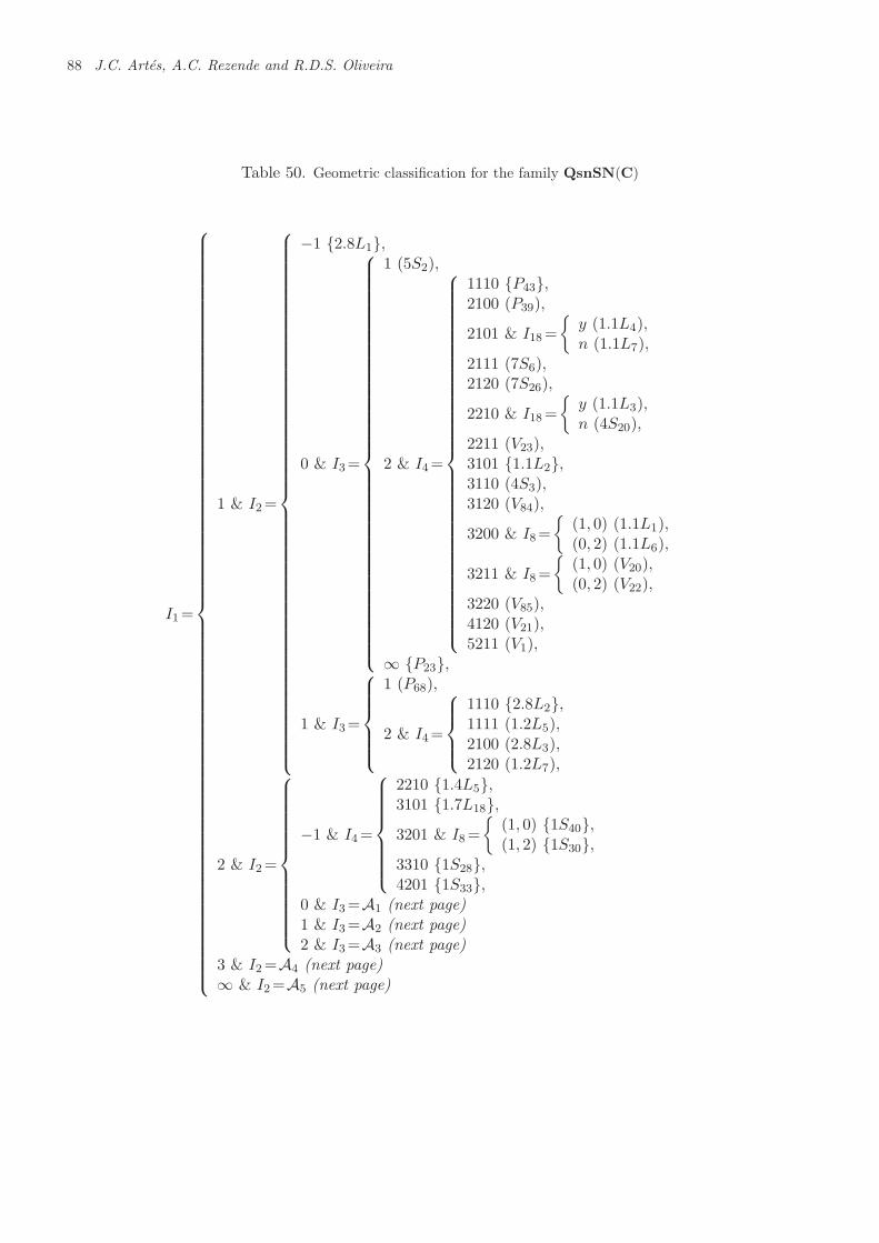
88 J.C. Artes, A.C. Rezende and R.D.S. Oliveira
Table 50. Geometric classification for the family QsnSN(C)
I1=
1 & I2=
−1 {2.8L1},
0 & I3=
1 (5S2),
2 & I4=
1110 {P43},2100 (P39),
2101 & I18=
{y (1.1L4),n (1.1L7),
2111 (7S6),2120 (7S26),
2210 & I18=
{y (1.1L3),n (4S20),
2211 (V23),3101 {1.1L2},3110 (4S3),3120 (V84),
3200 & I8=
{(1, 0) (1.1L1),(0, 2) (1.1L6),
3211 & I8=
{(1, 0) (V20),(0, 2) (V22),
3220 (V85),4120 (V21),5211 (V1),
∞ {P23},
1 & I3=
1 (P68),
2 & I4=
1110 {2.8L2},1111 (1.2L5),2100 (2.8L3),2120 (1.2L7),
2 & I2=
−1 & I4=
2210 {1.4L5},3101 {1.7L18},3201 & I8=
{(1, 0) {1S40},(1, 2) {1S30},
3310 {1S28},4201 {1S33},
0 & I3=A1 (next page)1 & I3=A2 (next page)2 & I3=A3 (next page)
3 & I2=A4 (next page)∞ & I2=A5 (next page)
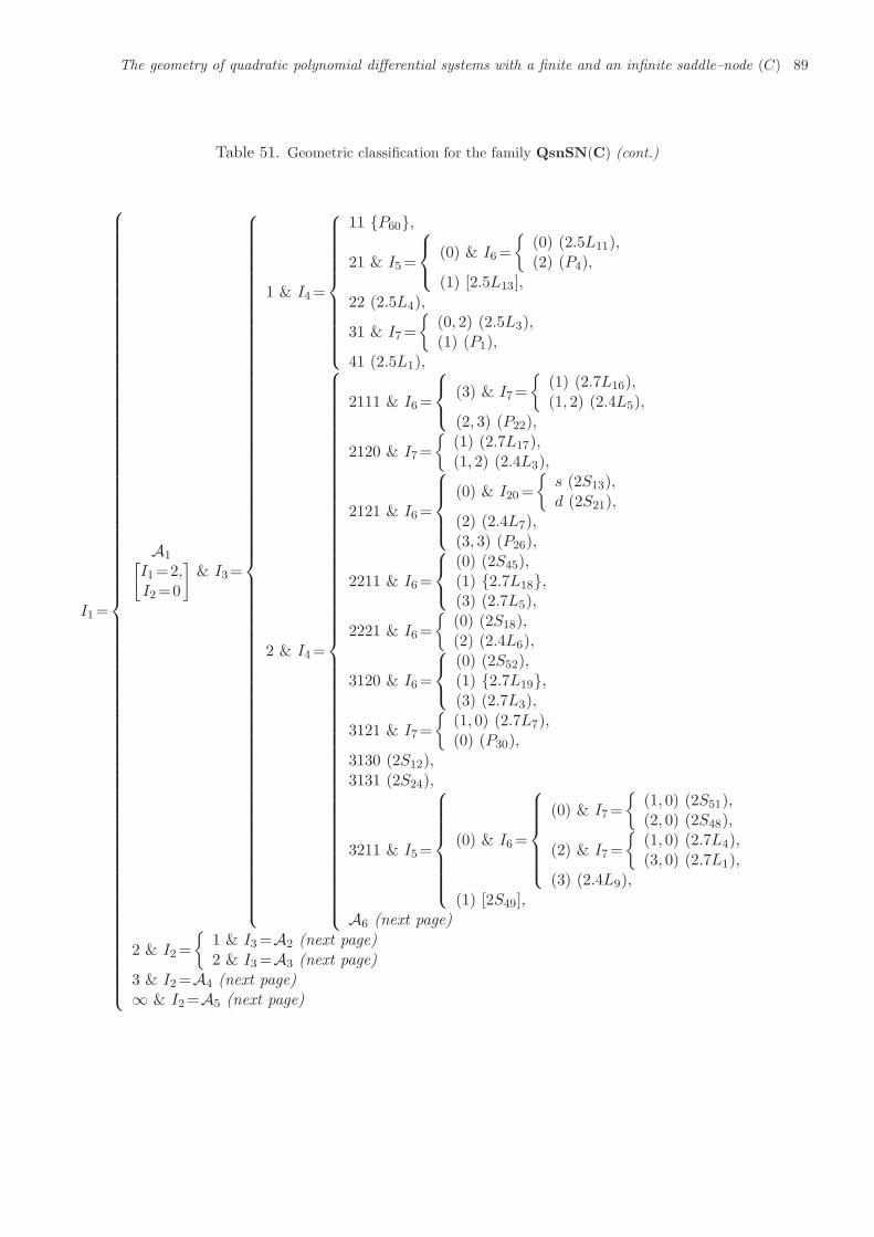
The geometry of quadratic polynomial differential systems with a finite and an infinite saddle–node (C) 89
Table 51. Geometric classification for the family QsnSN(C) (cont.)
I1=
A1[I1=2,I2=0
]& I3=
1 & I4=
11 {P60},
21 & I5=
(0) & I6=
{(0) (2.5L11),(2) (P4),
(1) [2.5L13],22 (2.5L4),
31 & I7=
{(0, 2) (2.5L3),(1) (P1),
41 (2.5L1),
2 & I4=
2111 & I6=
(3) & I7=
{(1) (2.7L16),(1, 2) (2.4L5),
(2, 3) (P22),
2120 & I7=
{(1) (2.7L17),(1, 2) (2.4L3),
2121 & I6=
(0) & I20=
{s (2S13),d (2S21),
(2) (2.4L7),(3, 3) (P26),
2211 & I6=
(0) (2S45),(1) {2.7L18},(3) (2.7L5),
2221 & I6=
{(0) (2S18),(2) (2.4L6),
3120 & I6=
(0) (2S52),(1) {2.7L19},(3) (2.7L3),
3121 & I7=
{(1, 0) (2.7L7),(0) (P30),
3130 (2S12),3131 (2S24),
3211 & I5=
(0) & I6=
(0) & I7=
{(1, 0) (2S51),(2, 0) (2S48),
(2) & I7=
{(1, 0) (2.7L4),(3, 0) (2.7L1),
(3) (2.4L9),(1) [2S49],
A6 (next page)
2 & I2=
{1 & I3=A2 (next page)2 & I3=A3 (next page)
3 & I2=A4 (next page)∞ & I2=A5 (next page)
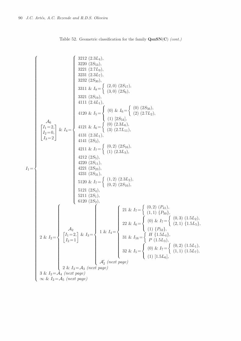
90 J.C. Artes, A.C. Rezende and R.D.S. Oliveira
Table 52. Geometric classification for the family QsnSN(C) (cont.)
I1=
A6I1=2,I2=0,I3=2
& I4=
3212 (2.3L4),3220 (2S53),3221 (2.7L9),3231 (2.3L7),3232 (2S30),
3311 & I8=
{(2, 0) (2S17),(3, 0) (2S6),
3321 (2S19),4111 (2.4L1),
4120 & I5=
(0) & I6=
{(0) (2S56),(2) (2.7L2),
(1) [2S54],
4121 & I6=
{(0) (2.3L6),(3) (2.7L11),
4131 (2.3L1),4141 (2S3),
4211 & I7=
{(0, 2) (2S16),(1) (2.3L3),
4212 (2S5),4220 (2S11),4221 (2S23),4231 (2S31),
5120 & I7=
{(1, 2) (2.3L2),(0, 2) (2S10),
5121 (2S4),5211 (2S1),6120 (2S2),
2 & I2=
A2[I1=2,I2=1
]& I3=
1 & I4=
21 & I7=
{(0, 2) (P41),(1, 1) {P50},
22 & I6=
(0) & I7=
{(0, 3) (1.5L2),(2, 1) {1.5L5},
(1) {P52},31 & I16=
{H {1.5L4},P (1.5L3),
32 & I5=
(0) & I7=
{(0, 2) (1.5L1),(1, 1) (1.5L7),
(1) [1.5L6],A′
2 (next page)
2 & I3=A3 (next page)3 & I2=A4 (next page)∞ & I2=A5 (next page)
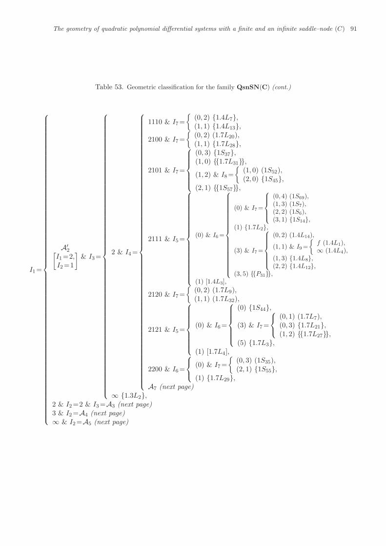
The geometry of quadratic polynomial differential systems with a finite and an infinite saddle–node (C) 91
Table 53. Geometric classification for the family QsnSN(C) (cont.)
I1=
A′2[
I1=2,I2=1
]& I3=
2 & I4=
1110 & I7=
{(0, 2) {1.4L7},(1, 1) {1.4L13},
2100 & I7=
{(0, 2) (1.7L20),(1, 1) {1.7L28},
2101 & I7=
(0, 3) {1S37},(1, 0) {{1.7L31}},(1, 2) & I8=
{(1, 0) (1S52),(2, 0) {1S45},
(2, 1) {{1S57}},
2111 & I5=
(0) & I6=
(0) & I7=
(0, 4) (1S69),(1, 3) (1S7),(2, 2) (1S6),(3, 1) {1S14},
(1) {1.7L2},
(3) & I7=
(0, 2) (1.4L14),
(1, 1) & I9=
{f (1.4L1),∞ (1.4L4),
(1, 3) {1.4L8},(2, 2) {1.4L12},
(3, 5) {{P31}},(1) [1.4L3],
2120 & I7=
{(0, 2) (1.7L9),(1, 1) (1.7L32),
2121 & I5=
(0) & I6=
(0) {1S44},
(3) & I7=
(0, 1) (1.7L7),(0, 3) {1.7L21},(1, 2) {{1.7L27}},
(5) {1.7L3},(1) [1.7L4],
2200 & I6=
(0) & I7=
{(0, 3) (1S35),(2, 1) {1S55},
(1) {1.7L29},A7 (next page)
∞ {1.3L2},2 & I2=2 & I3=A3 (next page)3 & I2=A4 (next page)∞ & I2=A5 (next page)
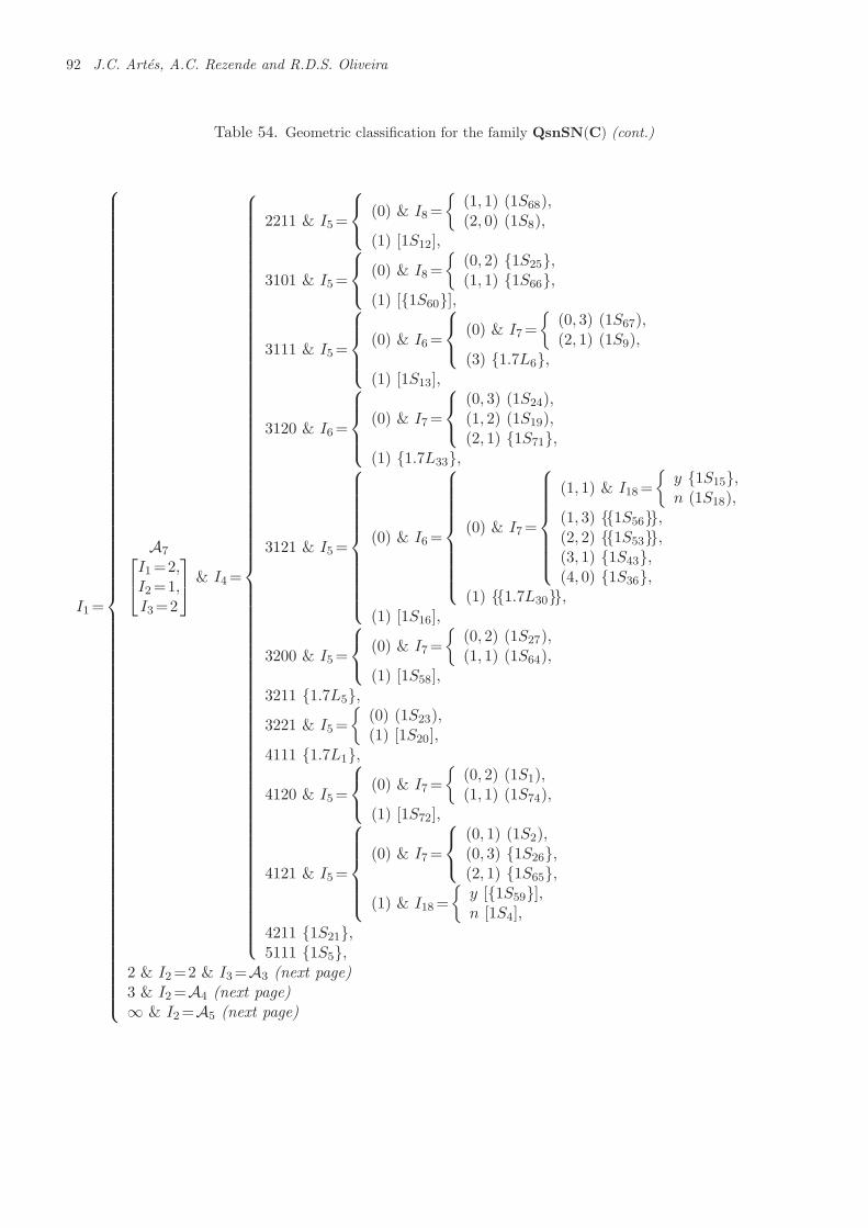
92 J.C. Artes, A.C. Rezende and R.D.S. Oliveira
Table 54. Geometric classification for the family QsnSN(C) (cont.)
I1=
A7I1=2,I2=1,I3=2
& I4=
2211 & I5=
(0) & I8=
{(1, 1) (1S68),(2, 0) (1S8),
(1) [1S12],
3101 & I5=
(0) & I8=
{(0, 2) {1S25},(1, 1) {1S66},
(1) [{1S60}],
3111 & I5=
(0) & I6=
(0) & I7=
{(0, 3) (1S67),(2, 1) (1S9),
(3) {1.7L6},(1) [1S13],
3120 & I6=
(0) & I7=
(0, 3) (1S24),(1, 2) (1S19),(2, 1) {1S71},
(1) {1.7L33},
3121 & I5=
(0) & I6=
(0) & I7=
(1, 1) & I18=
{y {1S15},n (1S18),
(1, 3) {{1S56}},(2, 2) {{1S53}},(3, 1) {1S43},(4, 0) {1S36},
(1) {{1.7L30}},(1) [1S16],
3200 & I5=
(0) & I7=
{(0, 2) (1S27),(1, 1) (1S64),
(1) [1S58],3211 {1.7L5},3221 & I5=
{(0) (1S23),(1) [1S20],
4111 {1.7L1},
4120 & I5=
(0) & I7=
{(0, 2) (1S1),(1, 1) (1S74),
(1) [1S72],
4121 & I5=
(0) & I7=
(0, 1) (1S2),(0, 3) {1S26},(2, 1) {1S65},
(1) & I18=
{y [{1S59}],n [1S4],
4211 {1S21},5111 {1S5},
2 & I2=2 & I3=A3 (next page)3 & I2=A4 (next page)∞ & I2=A5 (next page)
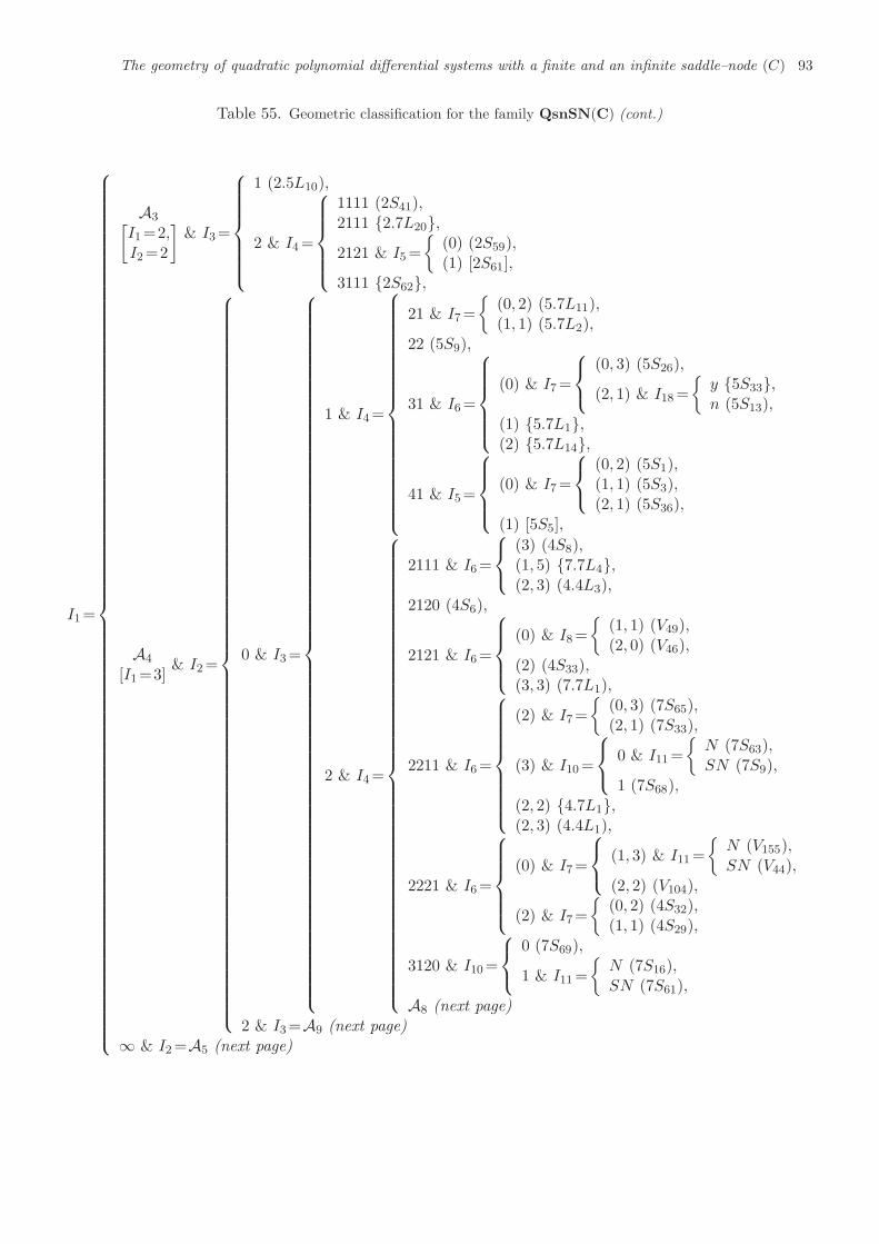
The geometry of quadratic polynomial differential systems with a finite and an infinite saddle–node (C) 93
Table 55. Geometric classification for the family QsnSN(C) (cont.)
I1=
A3[I1=2,I2=2
]& I3=
1 (2.5L10),
2 & I4=
1111 (2S41),2111 {2.7L20},2121 & I5=
{(0) (2S59),(1) [2S61],
3111 {2S62},
A4
[I1=3]& I2=
0 & I3=
1 & I4=
21 & I7=
{(0, 2) (5.7L11),(1, 1) (5.7L2),
22 (5S9),
31 & I6=
(0) & I7=
(0, 3) (5S26),
(2, 1) & I18=
{y {5S33},n (5S13),
(1) {5.7L1},(2) {5.7L14},
41 & I5=
(0) & I7=
(0, 2) (5S1),(1, 1) (5S3),(2, 1) (5S36),
(1) [5S5],
2 & I4=
2111 & I6=
(3) (4S8),(1, 5) {7.7L4},(2, 3) (4.4L3),
2120 (4S6),
2121 & I6=
(0) & I8=
{(1, 1) (V49),(2, 0) (V46),
(2) (4S33),(3, 3) (7.7L1),
2211 & I6=
(2) & I7=
{(0, 3) (7S65),(2, 1) (7S33),
(3) & I10=
0 & I11=
{N (7S63),SN (7S9),
1 (7S68),(2, 2) {4.7L1},(2, 3) (4.4L1),
2221 & I6=
(0) & I7=
(1, 3) & I11=
{N (V155),SN (V44),
(2, 2) (V104),
(2) & I7=
{(0, 2) (4S32),(1, 1) (4S29),
3120 & I10=
0 (7S69),
1 & I11=
{N (7S16),SN (7S61),
A8 (next page)2 & I3=A9 (next page)
∞ & I2=A5 (next page)
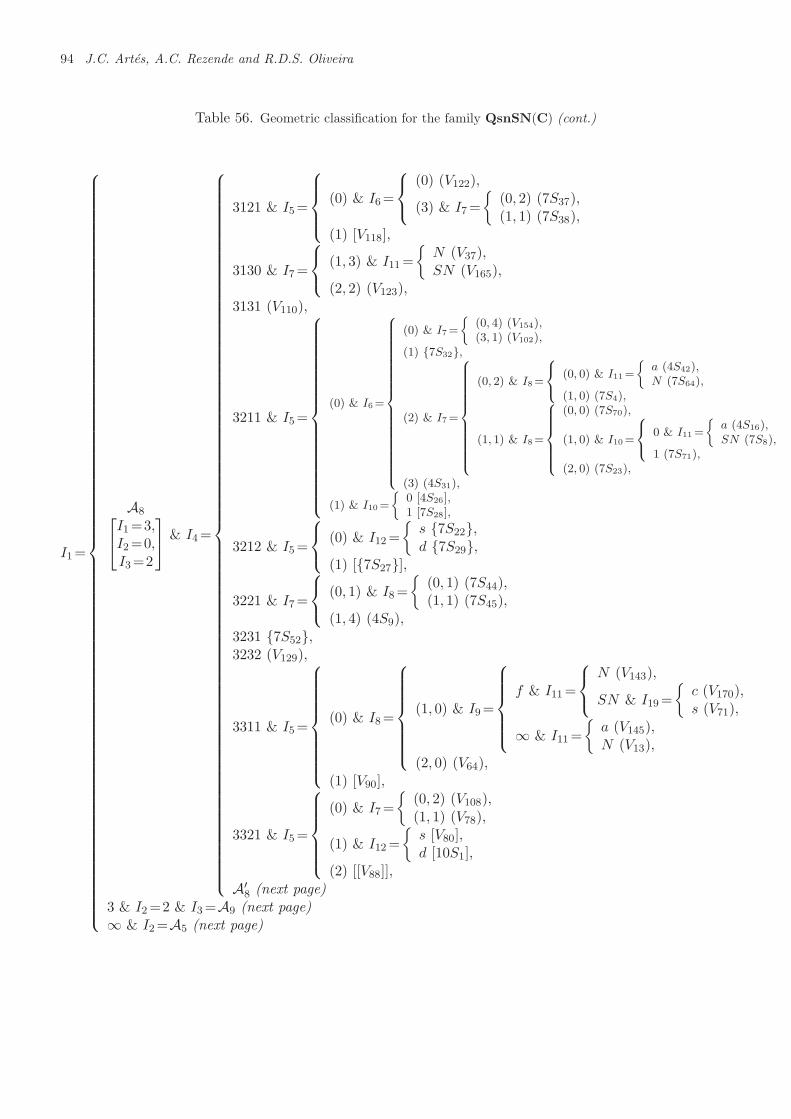
94 J.C. Artes, A.C. Rezende and R.D.S. Oliveira
Table 56. Geometric classification for the family QsnSN(C) (cont.)
I1=
A8I1=3,I2=0,I3=2
& I4=
3121 & I5=
(0) & I6=
(0) (V122),
(3) & I7=
{(0, 2) (7S37),(1, 1) (7S38),
(1) [V118],
3130 & I7=
(1, 3) & I11=
{N (V37),SN (V165),
(2, 2) (V123),3131 (V110),
3211 & I5=
(0) & I6=
(0) & I7=
{
(0, 4) (V154),(3, 1) (V102),
(1) {7S32},
(2) & I7=
(0, 2) & I8=
(0, 0) & I11=
{
a (4S42),N (7S64),
(1, 0) (7S4),
(1, 1) & I8=
(0, 0) (7S70),
(1, 0) & I10=
0 & I11=
{
a (4S16),SN (7S8),
1 (7S71),(2, 0) (7S23),
(3) (4S31),
(1) & I10=
{
0 [4S26],1 [7S28],
3212 & I5=
(0) & I12=
{s {7S22},d {7S29},
(1) [{7S27}],
3221 & I7=
(0, 1) & I8=
{(0, 1) (7S44),(1, 1) (7S45),
(1, 4) (4S9),3231 {7S52},3232 (V129),
3311 & I5=
(0) & I8=
(1, 0) & I9=
f & I11=
N (V143),
SN & I19=
{c (V170),s (V71),
∞ & I11=
{a (V145),N (V13),
(2, 0) (V64),(1) [V90],
3321 & I5=
(0) & I7=
{(0, 2) (V108),(1, 1) (V78),
(1) & I12=
{s [V80],d [10S1],
(2) [[V88]],A′
8 (next page)3 & I2=2 & I3=A9 (next page)∞ & I2=A5 (next page)
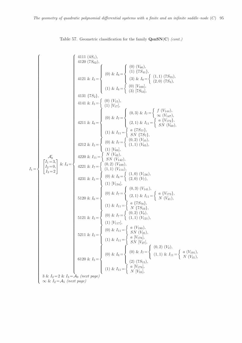
The geometry of quadratic polynomial differential systems with a finite and an infinite saddle–node (C) 95
Table 57. Geometric classification for the family QsnSN(C) (cont.)
I1=
A′
8I1=3,I2=0,I3=2
& I4=
4111 (4S1),4120 (7S62),
4121 & I5=
(0) & I6=
(0) (V66),(1) {7S41},(3) & I8=
{(1, 1) (7S55),(2, 0) (7S3),
(1) & I6=
{(0) [V100],(3) [7S53],
4131 {7S2},4141 & I5=
{(0) (V15),(1) [V17],
4211 & I6=
(0) & I7=
(0, 3) & I7=
{f (V144),∞ (V147),
(2, 1) & I11=
{a {V172},SN (V69),
(1) & I11=
{a {7S77},SN {7S7},
4212 & I5=
(0) & I7=
{(0, 2) (V10),(1, 1) (V83),
(1) [V89],
4220 & I11=
{N (V42),SN (V142),
4221 & I7=
{(0, 2) (V109),(1, 1) (V114),
4231 & I5=
(0) & I8=
{(1, 0) (V136),(2, 0) (V7),
(1) [V134],
5120 & I6=
(0) & I7=
(0, 3) (V141),
(2, 1) & I11=
{a {V173},N (V41),
(1) & I11=
{a {7S78},N {7S10},
5121 & I5=
(0) & I7=
{(0, 2) (V9),(1, 1) (V121),
(1) [V117],
5211 & I5=
(0) & I11=
{a (V190),SN (V25),
(1) & I11=
{a [V178],SN [V27],
6120 & I5=
(0) & I6=
(0) & I7=
(0, 2) (V2),
(1, 1) & I11=
{a (V191),N (V31),
(2) (7S15),
(1) & I11=
{a [V179],N [V33],
3 & I2=2 & I3=A9 (next page)∞ & I2=A5 (next page)
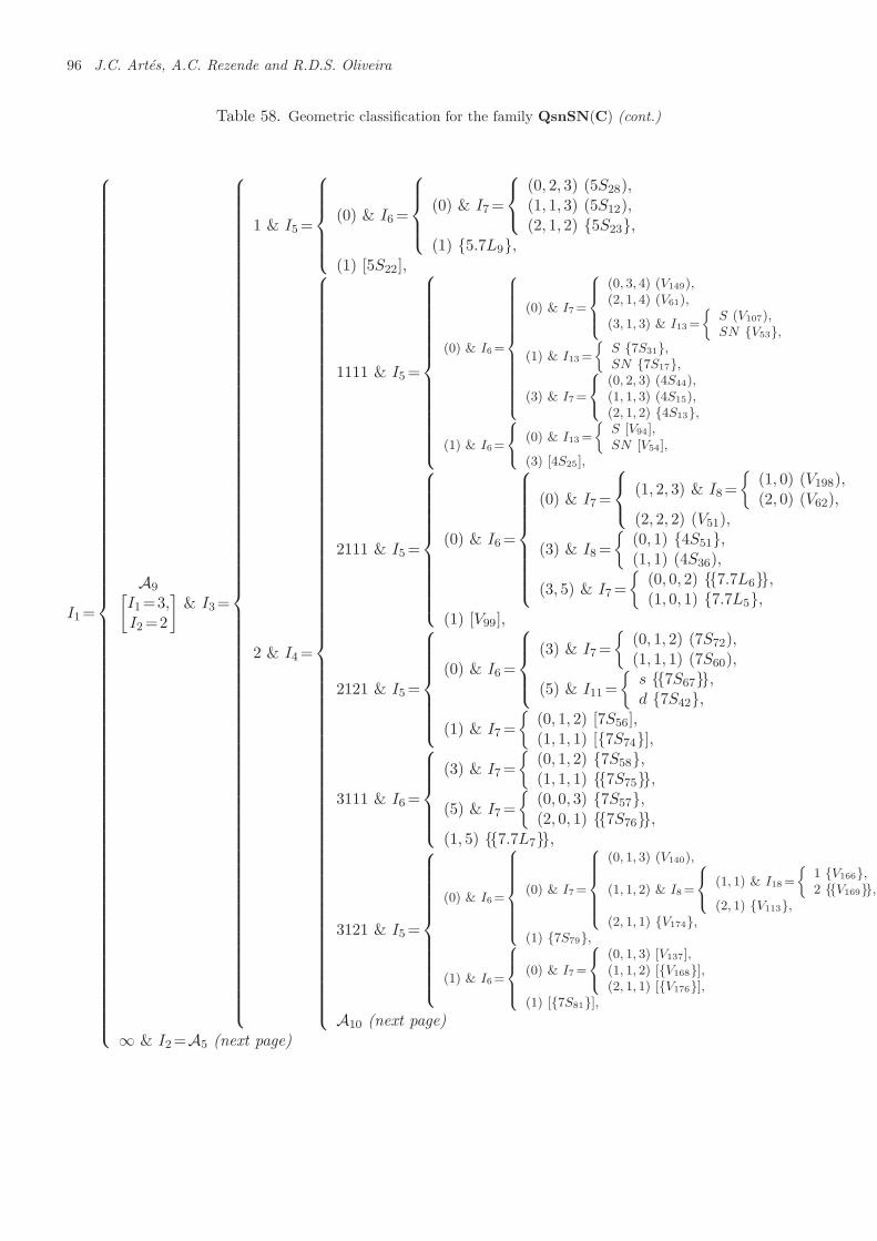
96 J.C. Artes, A.C. Rezende and R.D.S. Oliveira
Table 58. Geometric classification for the family QsnSN(C) (cont.)
I1=
A9[I1=3,I2=2
]& I3=
1 & I5=
(0) & I6=
(0) & I7=
(0, 2, 3) (5S28),(1, 1, 3) (5S12),(2, 1, 2) {5S23},
(1) {5.7L9},(1) [5S22],
2 & I4=
1111 & I5=
(0) & I6=
(0) & I7=
(0, 3, 4) (V149),(2, 1, 4) (V61),
(3, 1, 3) & I13=
{
S (V107),SN {V53},
(1) & I13=
{
S {7S31},SN {7S17},
(3) & I7=
(0, 2, 3) (4S44),(1, 1, 3) (4S15),(2, 1, 2) {4S13},
(1) & I6=
(0) & I13=
{
S [V94],SN [V54],
(3) [4S25],
2111 & I5=
(0) & I6=
(0) & I7=
(1, 2, 3) & I8=
{(1, 0) (V198),(2, 0) (V62),
(2, 2, 2) (V51),
(3) & I8=
{(0, 1) {4S51},(1, 1) (4S36),
(3, 5) & I7=
{(0, 0, 2) {{7.7L6}},(1, 0, 1) {7.7L5},
(1) [V99],
2121 & I5=
(0) & I6=
(3) & I7=
{(0, 1, 2) (7S72),(1, 1, 1) (7S60),
(5) & I11=
{s {{7S67}},d {7S42},
(1) & I7=
{(0, 1, 2) [7S56],(1, 1, 1) [{7S74}],
3111 & I6=
(3) & I7=
{(0, 1, 2) {7S58},(1, 1, 1) {{7S75}},
(5) & I7=
{(0, 0, 3) {7S57},(2, 0, 1) {{7S76}},
(1, 5) {{7.7L7}},
3121 & I5=
(0) & I6=
(0) & I7=
(0, 1, 3) (V140),
(1, 1, 2) & I8=
(1, 1) & I18=
{
1 {V166},2 {{V169}},
(2, 1) {V113},(2, 1, 1) {V174},
(1) {7S79},
(1) & I6=
(0) & I7=
(0, 1, 3) [V137],(1, 1, 2) [{V168}],(2, 1, 1) [{V176}],
(1) [{7S81}],A10 (next page)
∞ & I2=A5 (next page)
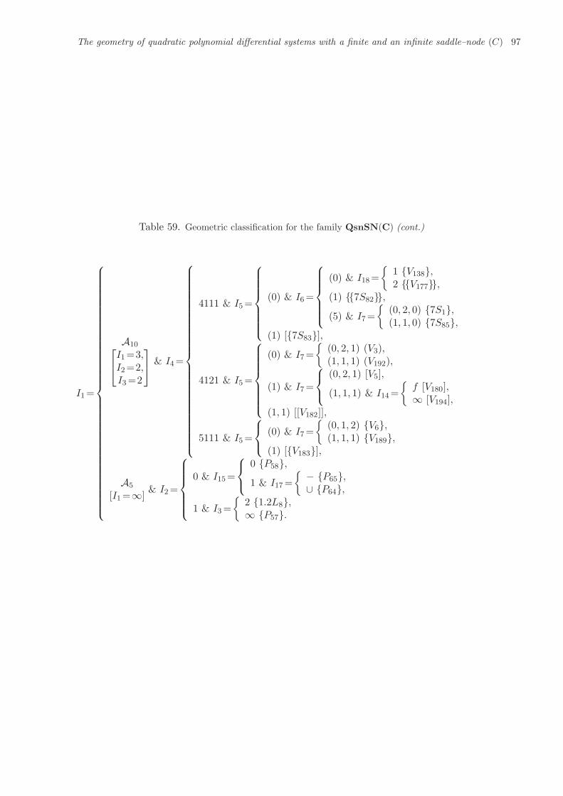
The geometry of quadratic polynomial differential systems with a finite and an infinite saddle–node (C) 97
Table 59. Geometric classification for the family QsnSN(C) (cont.)
I1=
A10I1=3,I2=2,I3=2
& I4=
4111 & I5=
(0) & I6=
(0) & I18=
{1 {V138},2 {{V177}},
(1) {{7S82}},(5) & I7=
{(0, 2, 0) {7S1},(1, 1, 0) {7S85},
(1) [{7S83}],
4121 & I5=
(0) & I7=
{(0, 2, 1) (V3),(1, 1, 1) (V192),
(1) & I7=
(0, 2, 1) [V5],
(1, 1, 1) & I14=
{f [V180],∞ [V194],
(1, 1) [[V182]],
5111 & I5=
(0) & I7=
{(0, 1, 2) {V6},(1, 1, 1) {V189},
(1) [{V183}],
A5
[I1=∞]& I2=
0 & I15=
0 {P58},1 & I17=
{− {P65},∪ {P64},
1 & I3=
{2 {1.2L8},∞ {P57}.
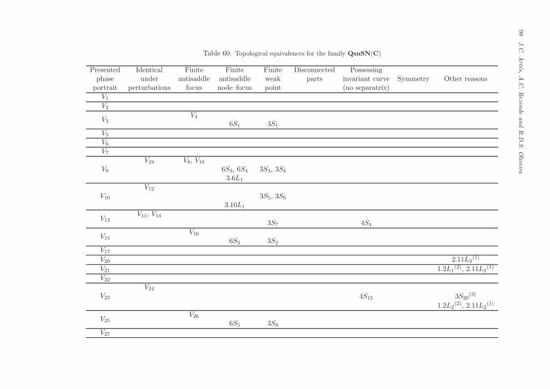
98
J.C
.Artes,
A.C
.Rezen
deandR.D
.S.Oliveira
Table 60. Topological equivalences for the family QsnSN(C)
Presented Identical Finite Finite Finite Disconnected Possessingphase under antisaddle antisaddle weak parts invariant curve Symmetry Other reasonsportrait perturbations focus node–focus point (no separatrix)
V1
V2
V3V4
6S1 3S1
V5
V6
V7
V9
V19 V8, V18
6S3, 6S4 3S3, 3S4
3.6L1
V10
V12
3S5, 3S6
3.10L1
V13V11, V14
3S7 4S4
V15V16
6S2 3S2
V17
V20 2.11L3(1)
V21 1.2L1(2), 2.11L2
(1)
V22
V23
V24
4S15 3S20(3)
1.2L2(2), 2.11L2
(1)
V25V26
6S5 3S8
V27
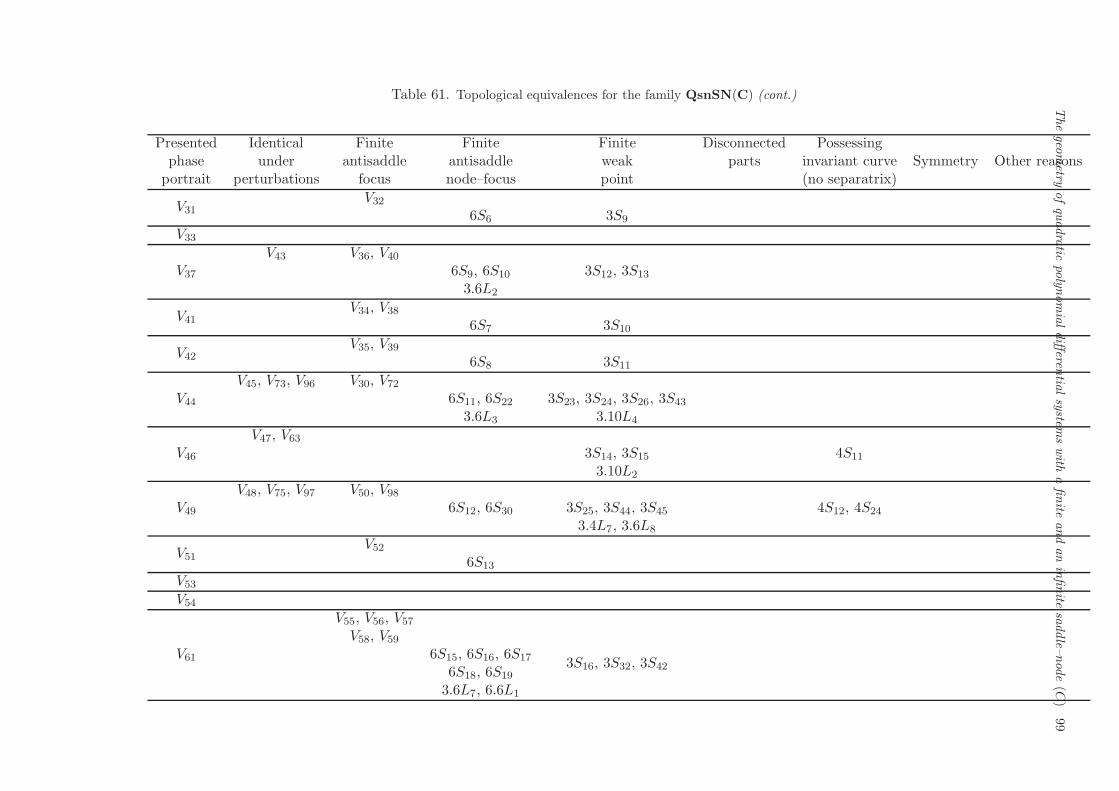
Thegeo
metry
ofquadratic
polyn
omialdifferen
tialsystem
swith
afinite
andaninfinite
saddle–
node(C
)99
Table 61. Topological equivalences for the family QsnSN(C) (cont.)
Presented Identical Finite Finite Finite Disconnected Possessingphase under antisaddle antisaddle weak parts invariant curve Symmetry Other reasonsportrait perturbations focus node–focus point (no separatrix)
V31V32
6S6 3S9
V33
V37
V43 V36, V40
6S9, 6S10 3S12, 3S13
3.6L2
V41V34, V38
6S7 3S10
V42V35, V39
6S8 3S11
V44
V45, V73, V96 V30, V72
6S11, 6S22 3S23, 3S24, 3S26, 3S43
3.6L3 3.10L4
V46
V47, V63
3S14, 3S15 4S11
3.10L2
V49
V48, V75, V97 V50, V98
6S12, 6S30 3S25, 3S44, 3S45 4S12, 4S24
3.4L7, 3.6L8
V51V52
6S13
V53
V54
V61
V55, V56, V57
V58, V59
6S15, 6S16, 6S17 3S16, 3S32, 3S426S18, 6S19
3.6L7, 6.6L1
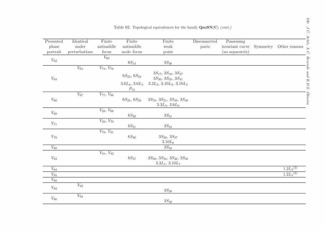
100
J.C
.Artes,
A.C
.Rezen
deandR.D
.S.Oliveira
Table 62. Topological equivalences for the family QsnSN(C) (cont.)
Presented Identical Finite Finite Finite Disconnected Possessingphase under antisaddle antisaddle weak parts invariant curve Symmetry Other reasonsportrait perturbations focus node–focus point (no separatrix)
V62V60
6S14 3S46
V64
V65 V74, V76
6S23, 6S243S17, 3S18, 3S27
3S30, 3S35, 3S41
3.6L4, 3.6L5 3.3L2, 3.10L3, 3.10L5
P12
V66
V67 V77, V86
6S25, 6S28 3S19, 3S31, 3S48, 3S49
3.3L3, 3.6L6
V69V28, V68
6S20 3S21
V71V29, V70
6S21 3S22
V78
V79, V91
6S26 3S28, 3S37
3.10L6
V80 3S33
V83
V81, V82
6S27 3S29, 3S34, 3S36, 3S39
3.3L1, 3.10L7
V84 1.2L3(2)
V85 1.2L4(2)
V88
V89V92
3S38
V90V93
3S40

Thegeo
metry
ofquadratic
polyn
omialdifferen
tialsystem
swith
afinite
andaninfinite
saddle–
node(C
)101
Table 63. Topological equivalences for the family QsnSN(C) (cont.)
Presented Identical Finite Finite Finite Disconnected Possessingphase under antisaddle antisaddle weak parts invariant curve Symmetry Other reasonsportrait perturbations focus node–focus point (no separatrix)
V94V87
6S29
V99
V100V101
3S47
V102V105
3S50
V104V103, V106 V125, V126
6S31 3S51 4S37, 4S38
V107V95
6S32
V108V127
3S57
V109
V128 V131, V132
6S39, 6S40 3S58, 3S59
3.6L10
V110
V126 V111, V112
6S33, 6S37 3S52, 3S56
3.6L9
V113
V114V115, V116
6S34 3S53
V117
V118
V121V119
6S35 3S54
V122V120
6S36 3S55
V123
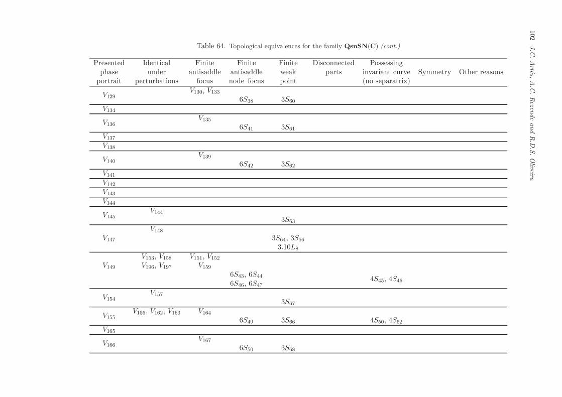
102
J.C
.Artes,
A.C
.Rezen
deandR.D
.S.Oliveira
Table 64. Topological equivalences for the family QsnSN(C) (cont.)
Presented Identical Finite Finite Finite Disconnected Possessingphase under antisaddle antisaddle weak parts invariant curve Symmetry Other reasonsportrait perturbations focus node–focus point (no separatrix)
V129V130, V133
6S38 3S60
V134
V136V135
6S41 3S61
V137
V138
V140V139
6S42 3S62
V141
V142
V143
V144
V145V144
3S63
V147
V148
3S64, 3S56
3.10L8
V149
V153, V158 V151, V152
V196, V197 V159
6S43, 6S44 4S45, 4S466S46, 6S47
V154V157
3S67
V155V156, V162, V163 V164
6S49 3S66 4S50, 4S52
V165
V166V167
6S50 3S68
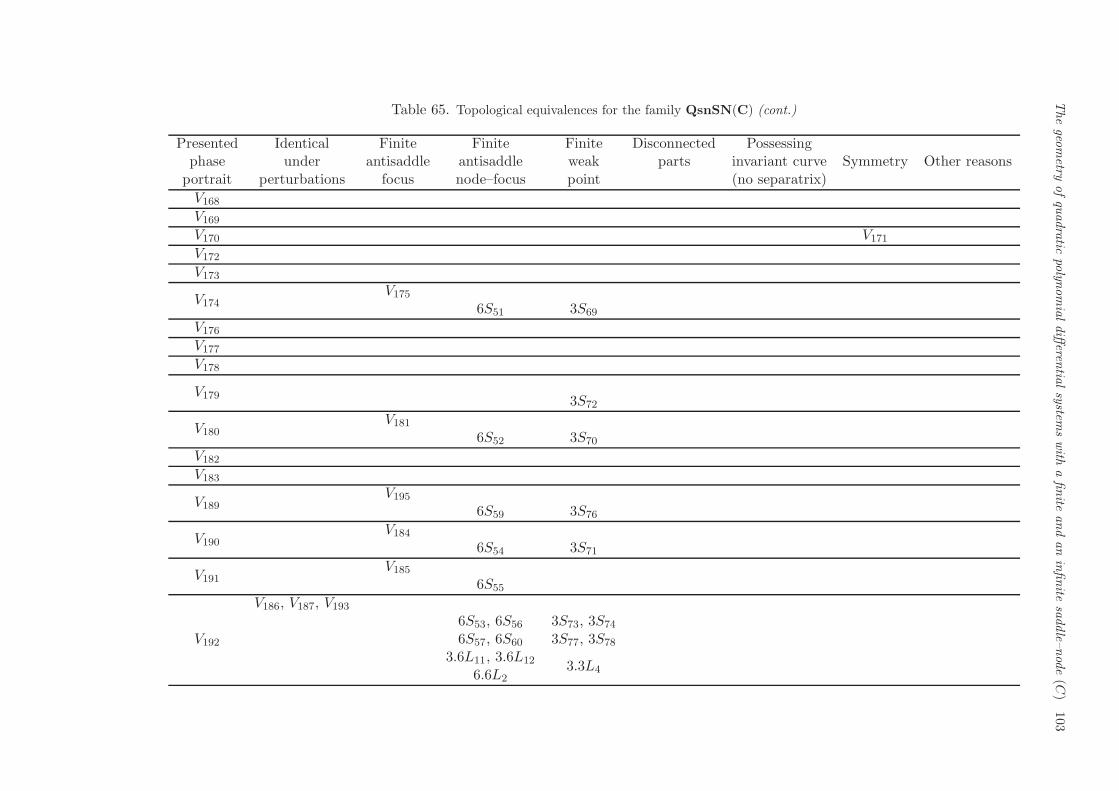
Thegeo
metry
ofquadratic
polyn
omialdifferen
tialsystem
swith
afinite
andaninfinite
saddle–
node(C
)103
Table 65. Topological equivalences for the family QsnSN(C) (cont.)
Presented Identical Finite Finite Finite Disconnected Possessingphase under antisaddle antisaddle weak parts invariant curve Symmetry Other reasonsportrait perturbations focus node–focus point (no separatrix)
V168
V169
V170 V171
V172
V173
V174V175
6S51 3S69
V176
V177
V178
V179 3S72
V180V181
6S52 3S70
V182
V183
V189V195
6S59 3S76
V190V184
6S54 3S71
V191V185
6S55
V192
V186, V187, V193
6S53, 6S56 3S73, 3S74
6S57, 6S60 3S77, 3S78
3.6L11, 3.6L12 3.3L46.6L2
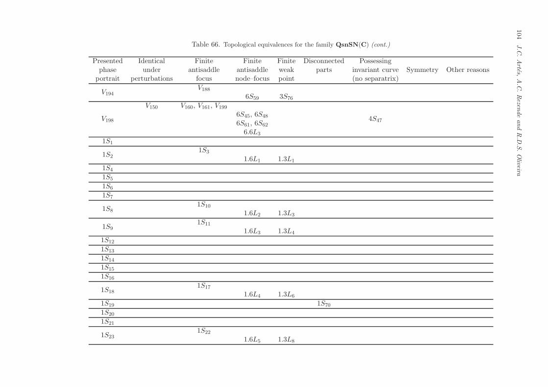
104
J.C
.Artes,
A.C
.Rezen
deandR.D
.S.Oliveira
Table 66. Topological equivalences for the family QsnSN(C) (cont.)
Presented Identical Finite Finite Finite Disconnected Possessingphase under antisaddle antisaddle weak parts invariant curve Symmetry Other reasonsportrait perturbations focus node–focus point (no separatrix)
V194V188
6S59 3S76
V198
V150 V160, V161, V199
6S45, 6S48 4S476S61, 6S62
6.6L3
1S1
1S21S3
1.6L1 1.3L1
1S4
1S5
1S6
1S7
1S81S10
1.6L2 1.3L3
1S91S11
1.6L3 1.3L4
1S12
1S13
1S14
1S15
1S16
1S181S17
1.6L4 1.3L6
1S19 1S70
1S20
1S21
1S231S22
1.6L5 1.3L8
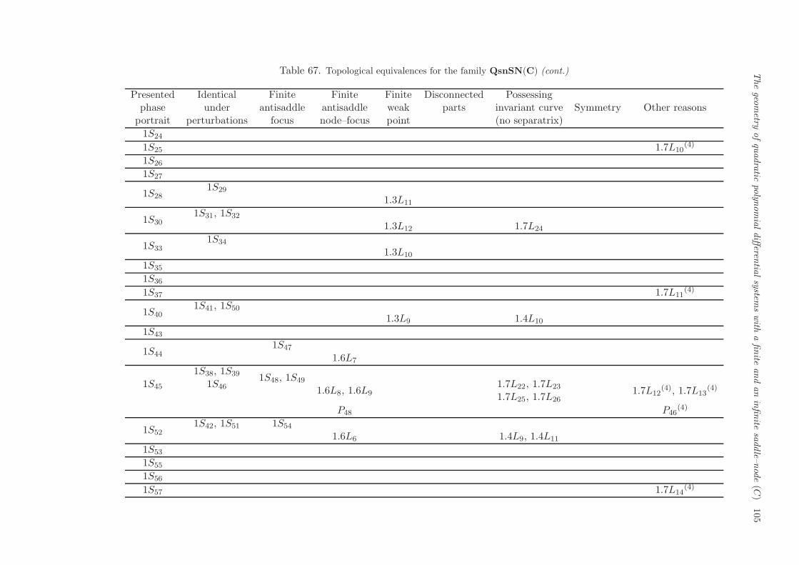
Thegeo
metry
ofquadratic
polyn
omialdifferen
tialsystem
swith
afinite
andaninfinite
saddle–
node(C
)105
Table 67. Topological equivalences for the family QsnSN(C) (cont.)
Presented Identical Finite Finite Finite Disconnected Possessingphase under antisaddle antisaddle weak parts invariant curve Symmetry Other reasonsportrait perturbations focus node–focus point (no separatrix)
1S24
1S25 1.7L10(4)
1S26
1S27
1S281S29
1.3L11
1S301S31, 1S32
1.3L12 1.7L24
1S331S34
1.3L10
1S35
1S36
1S37 1.7L11(4)
1S401S41, 1S50
1.3L9 1.4L10
1S43
1S441S47
1.6L7
1S45
1S38, 1S39 1S48, 1S491S46 1.6L8, 1.6L91.7L22, 1.7L23 1.7L12
(4), 1.7L13(4)
1.7L25, 1.7L26
P48 P46(4)
1S521S42, 1S51 1S54
1.6L6 1.4L9, 1.4L11
1S53
1S55
1S56
1S57 1.7L14(4)
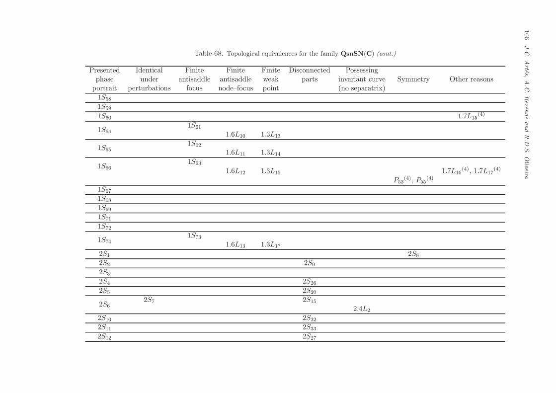
106
J.C
.Artes,
A.C
.Rezen
deandR.D
.S.Oliveira
Table 68. Topological equivalences for the family QsnSN(C) (cont.)
Presented Identical Finite Finite Finite Disconnected Possessingphase under antisaddle antisaddle weak parts invariant curve Symmetry Other reasonsportrait perturbations focus node–focus point (no separatrix)
1S58
1S59
1S60 1.7L15(4)
1S641S61
1.6L10 1.3L13
1S651S62
1.6L11 1.3L14
1S661S63
1.6L12 1.3L15 1.7L16(4), 1.7L17
(4)
P53(4), P55
(4)
1S67
1S68
1S69
1S71
1S72
1S741S73
1.6L13 1.3L17
2S1 2S8
2S2 2S9
2S3
2S4 2S26
2S5 2S20
2S62S7 2S15
2.4L2
2S10 2S32
2S11 2S33
2S12 2S27
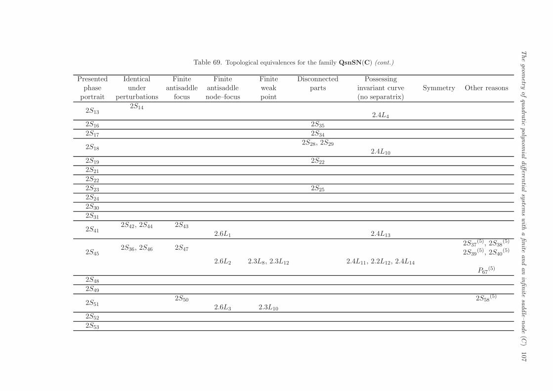
Thegeo
metry
ofquadratic
polyn
omialdifferen
tialsystem
swith
afinite
andaninfinite
saddle–
node(C
)107
Table 69. Topological equivalences for the family QsnSN(C) (cont.)
Presented Identical Finite Finite Finite Disconnected Possessingphase under antisaddle antisaddle weak parts invariant curve Symmetry Other reasonsportrait perturbations focus node–focus point (no separatrix)
2S132S14
2.4L4
2S16 2S35
2S17 2S34
2S182S28, 2S29
2.4L10
2S19 2S22
2S21
2S22
2S23 2S25
2S24
2S30
2S31
2S412S42, 2S44 2S43
2.6L1 2.4L13
2S452S36, 2S46 2S47
2S37(5), 2S38
(5)
2S39(5), 2S40
(5)
2.6L2 2.3L8, 2.3L12 2.4L11, 2.2L12, 2.4L14
P67(5)
2S48
2S49
2S512S50 2S58
(5)
2.6L3 2.3L10
2S52
2S53
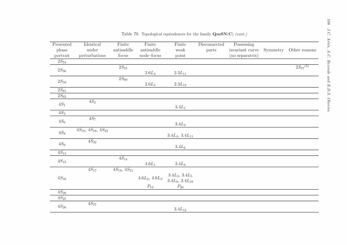
108
J.C
.Artes,
A.C
.Rezen
deandR.D
.S.Oliveira
Table 70. Topological equivalences for the family QsnSN(C) (cont.)
Presented Identical Finite Finite Finite Disconnected Possessingphase under antisaddle antisaddle weak parts invariant curve Symmetry Other reasonsportrait perturbations focus node–focus point (no separatrix)
2S54
2S562S55 2S57
(5)
2.6L4 2.3L11
2S592S60
2.6L5 2.3L12
2S61
2S62
4S14S2
3.4L1
4S3
4S64S7
3.4L2
4S84S10, 4S18, 4S23
3.4L4, 3.4L11
4S94S22
3.4L6
4S13
4S154S14
4.6L1 3.4L8
4S16
4S17 4S19, 4S21
4.6L2, 4.6L33.4L3, 3.4L5
3.4L9, 3.4L10
P13 P20
4S20
4S25
4S264S27
3.4L12
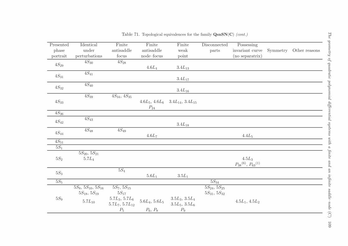
Thegeo
metry
ofquadratic
polyn
omialdifferen
tialsystem
swith
afinite
andaninfinite
saddle–
node(C
)109
Table 71. Topological equivalences for the family QsnSN(C) (cont.)
Presented Identical Finite Finite Finite Disconnected Possessingphase under antisaddle antisaddle weak parts invariant curve Symmetry Other reasonsportrait perturbations focus node–focus point (no separatrix)
4S294S30 4S28
4.6L4 3.4L13
4S314S41
3.4L17
4S324S40
3.4L16
4S33
4S39 4S34, 4S35
4.6L5, 4.6L6 3.4L14, 3.4L15
P24
4S36
4S424S43
3.4L18
4S444S48 4S49
4.6L7 4.4L5
4S51
5S1
5S2
5S20, 5S21
5.7L4 4.5L3
P38(6), P63
(1)
5S35S4
5.6L1 3.5L1
5S5 5S34
5S9
5S8, 5S10, 5S16 5S7, 5S15 5S24, 5S25
5S18, 5S19 5S17 5S31, 5S32
5.7L105.7L3, 5.7L6 5.6L4, 5.6L5
3.5L3, 3.5L4 4.5L1, 4.5L25.7L7, 5.7L12 3.5L5, 3.5L6
P5 P6, P8 P9
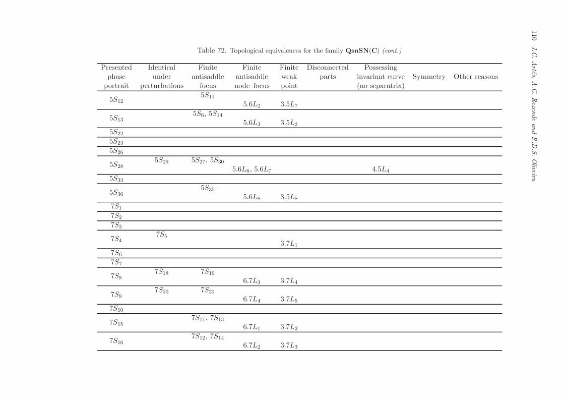
110
J.C
.Artes,
A.C
.Rezen
deandR.D
.S.Oliveira
Table 72. Topological equivalences for the family QsnSN(C) (cont.)
Presented Identical Finite Finite Finite Disconnected Possessingphase under antisaddle antisaddle weak parts invariant curve Symmetry Other reasonsportrait perturbations focus node–focus point (no separatrix)
5S125S11
5.6L2 3.5L7
5S135S6, 5S14
5.6L3 3.5L2
5S22
5S23
5S26
5S285S29 5S27, 5S30
5.6L6, 5.6L7 4.5L4
5S33
5S365S35
5.6L8 3.5L8
7S1
7S2
7S3
7S47S5
3.7L1
7S6
7S7
7S87S18 7S19
6.7L3 3.7L4
7S97S20 7S21
6.7L4 3.7L5
7S10
7S157S11, 7S13
6.7L1 3.7L2
7S167S12, 7S14
6.7L2 3.7L3
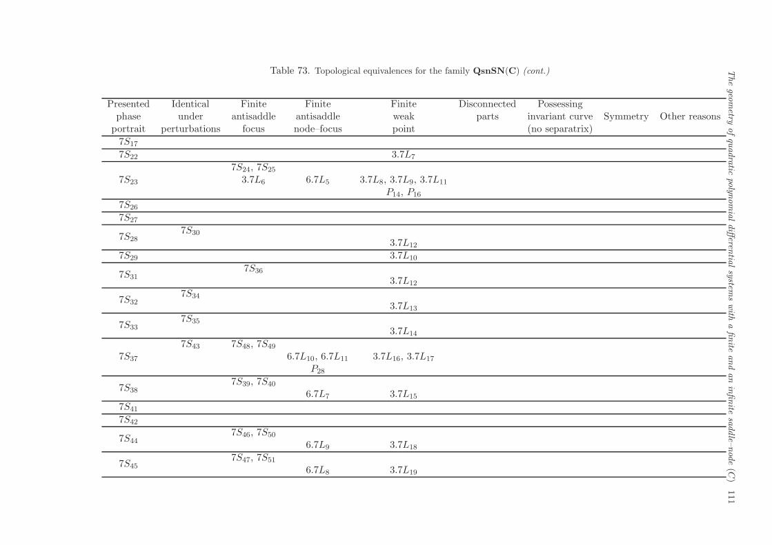
Thegeo
metry
ofquadratic
polyn
omialdifferen
tialsystem
swith
afinite
andaninfinite
saddle–
node(C
)111
Table 73. Topological equivalences for the family QsnSN(C) (cont.)
Presented Identical Finite Finite Finite Disconnected Possessingphase under antisaddle antisaddle weak parts invariant curve Symmetry Other reasonsportrait perturbations focus node–focus point (no separatrix)
7S17
7S22 3.7L7
7S23
7S24, 7S25
3.7L6 6.7L5 3.7L8, 3.7L9, 3.7L11
P14, P16
7S26
7S27
7S287S30
3.7L12
7S29 3.7L10
7S317S36
3.7L12
7S327S34
3.7L13
7S337S35
3.7L14
7S37
7S43 7S48, 7S49
6.7L10, 6.7L11 3.7L16, 3.7L17
P28
7S387S39, 7S40
6.7L7 3.7L15
7S41
7S42
7S447S46, 7S50
6.7L9 3.7L18
7S457S47, 7S51
6.7L8 3.7L19
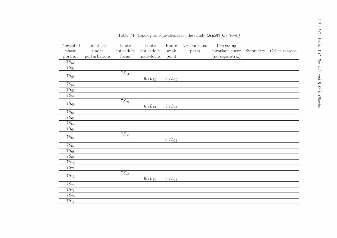
112
J.C
.Artes,
A.C
.Rezen
deandR.D
.S.Oliveira
Table 74. Topological equivalences for the family QsnSN(C) (cont.)
Presented Identical Finite Finite Finite Disconnected Possessingphase under antisaddle antisaddle weak parts invariant curve Symmetry Other reasonsportrait perturbations focus node–focus point (no separatrix)
7S52
7S53
7S557S54
6.7L12 3.7L20
7S56
7S57
7S58
7S607S59
6.7L13 3.7L21
7S61
7S62
7S63
7S64
7S657S66
3.7L22
7S67
7S68
7S69
7S70
7S71
7S727S73
6.7L14 3.7L23
7S74
7S75
7S76
7S77
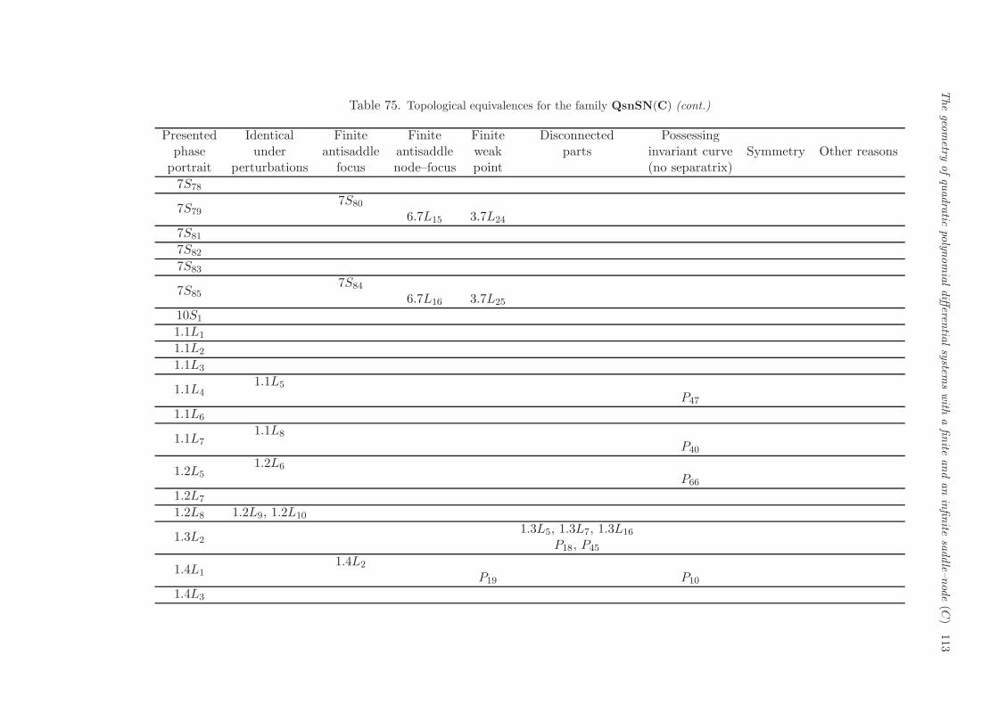
Thegeo
metry
ofquadratic
polyn
omialdifferen
tialsystem
swith
afinite
andaninfinite
saddle–
node(C
)113
Table 75. Topological equivalences for the family QsnSN(C) (cont.)
Presented Identical Finite Finite Finite Disconnected Possessingphase under antisaddle antisaddle weak parts invariant curve Symmetry Other reasonsportrait perturbations focus node–focus point (no separatrix)
7S78
7S797S80
6.7L15 3.7L24
7S81
7S82
7S83
7S857S84
6.7L16 3.7L25
10S1
1.1L1
1.1L2
1.1L3
1.1L41.1L5
P47
1.1L6
1.1L71.1L8
P40
1.2L51.2L6
P66
1.2L7
1.2L8 1.2L9, 1.2L10
1.3L21.3L5, 1.3L7, 1.3L16
P18, P45
1.4L11.4L2
P19 P10
1.4L3
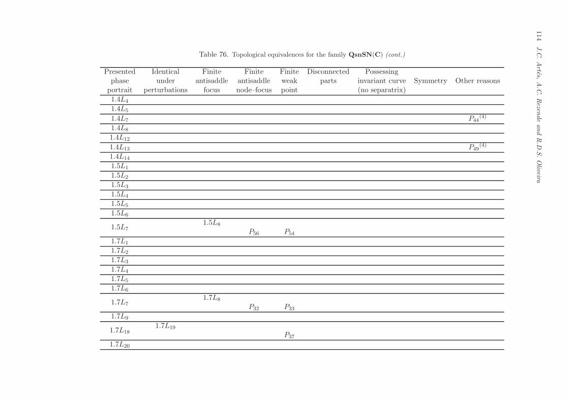
114
J.C
.Artes,
A.C
.Rezen
deandR.D
.S.Oliveira
Table 76. Topological equivalences for the family QsnSN(C) (cont.)
Presented Identical Finite Finite Finite Disconnected Possessingphase under antisaddle antisaddle weak parts invariant curve Symmetry Other reasonsportrait perturbations focus node–focus point (no separatrix)
1.4L4
1.4L5
1.4L7 P44(4)
1.4L8
1.4L12
1.4L13 P49(4)
1.4L14
1.5L1
1.5L2
1.5L3
1.5L4
1.5L5
1.5L6
1.5L71.5L8
P56 P54
1.7L1
1.7L2
1.7L3
1.7L4
1.7L5
1.7L6
1.7L71.7L8
P32 P33
1.7L9
1.7L181.7L19
P37
1.7L20
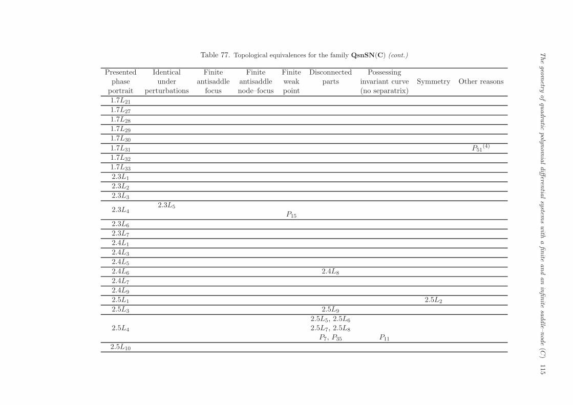
Thegeo
metry
ofquadratic
polyn
omialdifferen
tialsystem
swith
afinite
andaninfinite
saddle–
node(C
)115
Table 77. Topological equivalences for the family QsnSN(C) (cont.)
Presented Identical Finite Finite Finite Disconnected Possessingphase under antisaddle antisaddle weak parts invariant curve Symmetry Other reasonsportrait perturbations focus node–focus point (no separatrix)
1.7L21
1.7L27
1.7L28
1.7L29
1.7L30
1.7L31 P51(4)
1.7L32
1.7L33
2.3L1
2.3L2
2.3L3
2.3L42.3L5
P15
2.3L6
2.3L7
2.4L1
2.4L3
2.4L5
2.4L6 2.4L8
2.4L7
2.4L9
2.5L1 2.5L2
2.5L3 2.5L9
2.5L4
2.5L5, 2.5L6
2.5L7, 2.5L8
P7, P35 P11
2.5L10
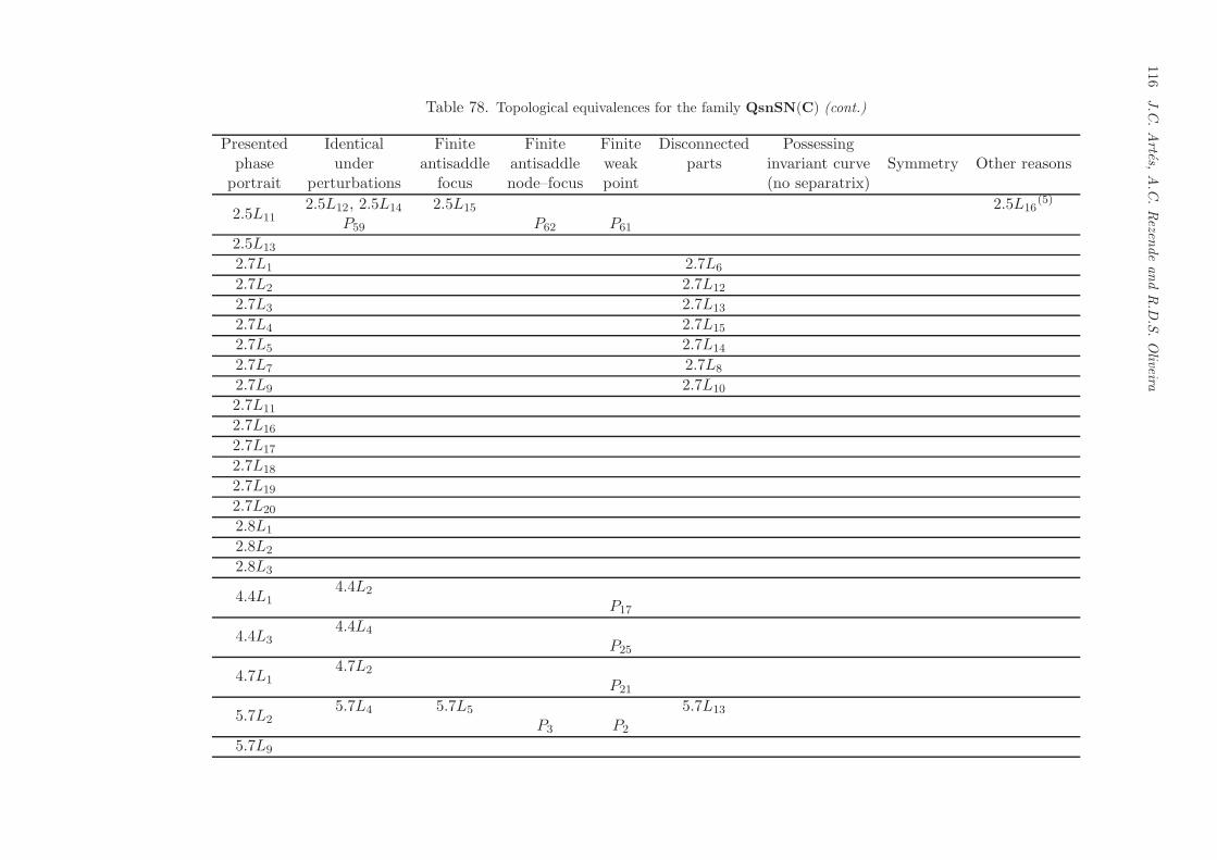
116
J.C
.Artes,
A.C
.Rezen
deandR.D
.S.Oliveira
Table 78. Topological equivalences for the family QsnSN(C) (cont.)
Presented Identical Finite Finite Finite Disconnected Possessingphase under antisaddle antisaddle weak parts invariant curve Symmetry Other reasonsportrait perturbations focus node–focus point (no separatrix)
2.5L112.5L12, 2.5L14 2.5L15 2.5L16
(5)
P59 P62 P61
2.5L13
2.7L1 2.7L6
2.7L2 2.7L12
2.7L3 2.7L13
2.7L4 2.7L15
2.7L5 2.7L14
2.7L7 2.7L8
2.7L9 2.7L10
2.7L11
2.7L16
2.7L17
2.7L18
2.7L19
2.7L20
2.8L1
2.8L2
2.8L3
4.4L14.4L2
P17
4.4L34.4L4
P25
4.7L14.7L2
P21
5.7L25.7L4 5.7L5 5.7L13
P3 P2
5.7L9

Thegeo
metry
ofquadratic
polyn
omialdifferen
tialsystem
swith
afinite
andaninfinite
saddle–
node(C
)117
Table 79. Topological equivalences for the family QsnSN(C) (cont.)
Presented Identical Finite Finite Finite Disconnected Possessingphase under antisaddle antisaddle weak parts invariant curve Symmetry Other reasonsportrait perturbations focus node–focus point (no separatrix)
5.7L11
5.7L14
7.7L17.7L3 7.7L2 5.7L13
P27 P29
7.7L4
7.7L5
7.7L6
7.7L7
P1
P4 P36
P22
P23
P26
P30
P31
P39
P41
P43
P50
P52
P57
P58
P60
P64
P65
P68
118 J.C. Artes, A.C. Rezende and R.D.S. Oliveira
Acknowledgements. The first author is par-tially supported by a MEC/FEDER grant num-ber MTM 2013–40998–P and by a CICYTgrant number 2014SGR 00568. The second au-thor is supported by CAPES/DGU grant num-ber BEX 9439/12–9 and CAPES/CSF–PVE’s88887.068602/2014–00. The last author is partiallysupported by FP7–PEOPLE–2012–IRSES–316338,CAPES/CSF–PVE’s 88881.030454/2013-01 andCNPq grant “Projeto Universal 472796/2013-5”.
References
Andronov, A.A., Leontovich, E.A., Gordon, I.I.& Maier, A.G. [1973] “Qualitative theory ofsecond–order dynamic systems.” Israel Programfor Scientific Translations (Halsted Press, A di-vision of John Wiley & Sons, NY-Toronto, On-tario).
Artes, J.C., Dumortier, F., Herssens, C., Llibre,J. & de Maesschalck, P. [2005] “Computer pro-gram P4 to study phase portraits of planarpolynomial differential equations,” Available at:<http://mat.uab.es/∼artes/p4/p4.htm>.
Artes, J.C., Kooij, R. & Llibre, J. [1998] “Struc-turally stable quadratic vector fields,” MemoiresAmer. Math. Soc., 134 (639).
Artes, J.C. & Llibre, J. [2014] “Structurally unsta-ble quadratic systems of codimension 1”, Workin progress.
Artes, J.C., Llibre, J. & Schlomiuk, D. [2006] “Thegeometry of quadratic differential systems with aweak focus of second order,” Internat. J. Bifur.Chaos Appl. Sci. Engrg. 16, 3127–3194.
Artes, J.C., Llibre, J. & Vulpe, N. [2008] “Singularpoints of quadratic systems: a complete classifi-cation in the coefficient space R
12,” Internat. J.Bifur. Chaos Appl. Sci. Engrg. 18, 313–362.
Artes, J.C., Llibre, J., Schlomiuk, D. & Vulpe, N.[2013a] “Geometric configurations of singulari-ties for quadratic differential systems with to-tal finite multiplicity lower than 2,” Bul. Acad.Stiinte Repub. Mold. Mat. 71, 72–124.
Artes, J.C., Rezende, A.C. & Oliveira, R.D.S.[2013b] “Global phase portraits of quadratic
polynomial differential systems with a semi–elemental triple node,” Internat. J. Bifur. ChaosAppl. Sci. Engrg. 23, 21pp.
Artes, J.C., Rezende, A.C. & Oliveira, R.D.S.[2014] “The geometry of quadratic polynomialdifferential systems with a finite and an infinitesaddle–node (A,B),” Internat. J. Bifur. ChaosAppl. Sci. Engrg. 24, 30pp.
Bautin, N.N. [1954] “On periodic solutions of a sys-tem of differential equations,” Prikl. Mat. Meh.18, 128.
Coll, B. & Llibre, J. [1988] “Limit cycles for aquadratic system with an invariant straight lineand some evolution of phase portraits,” Quali-tative Theory of Differential Equations, Colloq.Math. Soc. Janos Bolyai, Bolyai Institut, Szeged,Hungria 53, 111–123.
Coppel, W.A. [1966] “A survey of quadratic sys-tems,” J. Differential Equations 2, 293–304.
Dumortier, F., Llibre, J. & Artes, J.C. [2006]“Qualitative Theory of Planar DifferentialSystems,” Universitext, Springer–Verlag, NewYork–Berlin.
Dumortier, F., Roussarie, R. & Rousseau, C. [1994]“Hilbert’s 16th problem for quadratic vectorfields,” J. Differential Equations 110, 66–133.
Fulton, W. [1969] “Algebraic curves. An introduc-tion to Algebraic Geometry,” W.A. Benjamin,Inc., New York.
Gonzalez, E.A. [1969] “Generic properties of poly-nomial vector fields at infinity,” Trans. Amer.Math. Soc. 143, 201–222.
Hartshorne, R. [1977] “Algebraic geometry,” Grad-uate Texts in Math. 52, Springer.
Hilbert, D. [1900] “Mathematische probleme”, InNachr. Ges. Wiss., editor Second Internat.Congress Math. Paris, 1900, 253–297. GottingenMath.–Phys. Kl.
Hilbert, D. [1902] “Mathematical problems,” Bull.Amer. Math. Soc. 8, 437–479.
Llibre, J. & Schlomiuk, D. [2004] “The geometry ofquadratic differential systems with a weak focusof third order,” Canad. J. Math. 56, 310–343.
The geometry of quadratic polynomial differential systems with a finite and an infinite saddle–node (C) 119
Rezende, A.C. [2014] “The geometry of some tridi-mensional families of planar quadratic differen-tial systems,” (Doctoral dissertation) – Univer-sidade de Sao Paulo (ICMC), Sao Carlos.
Schlomiuk, D. & Pal, J. [2001] “On the geometry inthe neighborhood of infinity of quadratic differ-ential systems with a weak focus,” Qual. TheoryDyn. Syst. 2, 1–43.
Schlomiuk, D. & Vulpe, N.I. [2005] “Geometry ofquadratic differential systems in the neighbor-hood of the infinity,” J. Differential Equations215, 357–400.
Vulpe, N.I. [2011] “Characterization of the finiteweak singularities of quadratic systems via in-variant theory,” Nonlinear Anal. 74, 6553–6582.
Ye, Y.Q. et al. [1986] “Theory of limit cycles,”Trans. of Mathematical Monographs, 66. Amer.Math. Soc., Providence, RI, 2 edition.