The extended tanh method for solving systems of nonlinear wave equations

Applied Mathematics and Computation 217 (2010) 1997–2006

Contents lists available at ScienceDirect

Applied Mathematics and Computation

journal homepage: www.elsevier .com/ locate/amc

The extended tanh method for solving systems of nonlinear wave equations

Sami Shukri *, Kamel Al-KhaledDepartment of Mathematics and Statistics, Faculty of Science and Arts, Jordan University of Science and Technology, IRBID 22110, Jordan

a r t i c l e i n f o a b s t r a c t

Keywords:Nonlinear wave equationsThe extended tanh methodSoliton solutionsThe generalized coupled Hirota SatsumaKdV equation

0096-3003/$ - see front matter � 2010 Elsevier Incdoi:10.1016/j.amc.2010.06.058

* Corresponding author.E-mail addresses: [email protected] (S. Shu

The extended tanh method with a computerized symbolic computation is used for con-structing the traveling wave solutions of coupled nonlinear equations arising in physics.The obtained solutions include solitons, kinks and plane periodic solutions. The appliedmethod will be used to solve the generalized coupled Hirota Satsuma KdV equation.

� 2010 Elsevier Inc. All rights reserved.

1. Introduction

Nonlinear wave equations in mathematical physics play a major role in various fields, such as plasma physics, fluidmechanics, optical fibers, solid state physics, chemical kinetics, geochemistry, and so on [7].

The pioneer work of Malfiet and Hereman in [5] introduced the powerful tanh method for a reliable treatment of the non-linear wave equations. Later, the extended tanh method, developed by Wazwaz [9], is a direct and effective algebraic methodfor handling nonlinear equations. Various extensions of the method were developed as well [1].

The equations solvable by the extended tanh method possess moreover a particularly interesting class of solutions; sol-itons. The solitons are traveling waves that preserve their shape after a collision with other solitons. This property is used inmany applications; from hydrodynamics to nonlinear optics, from plasmas to shock waves, from tornados to the Great RedSpot of Jupiter, from traffic flow to internet, and from Tsunamis to turbulence [7]. More recently, solitons are of key impor-tance in the quantum fields and nanotechnology especially in nanohydrodynamics [8].

Solitons are the solutions in the form sech, sech2, the graph of soliton is a wave that goes up only. It is not like periodicsolutions sine, cosine, etc. as in trigonometric function, that goes above the horizontal and below the horizontal. Kink is alsocalled a soliton, it is in the form tanh (not tanh2, because tanh2 can be converted to sech2). In kink the limit as x approachesinfinity, the answer is a constant, not like solitons where the limit goes to 0 for more details see [11].

Many mathematicians used the extended tanh method to obtain solitons solutions, Wazwaz in [10], solved the Korteweg-de Vries equation, which is characterized by the convection term uux and the dispersion term uxxx. It reads:

ut þ 6uux � uxxx ¼ 0;

and by using the extended tanh method, the soliton solution is:

uðx; tÞ ¼ � c6

1� 3coth2 12

ffiffiffiffiffiffi�cp

ðx� ctÞ� ��

; c < 0:

Bekir in [1], solved the coupled Hirota Satsuma Korteweg-de Vries equation equations:

ut ¼14

uxxx þ 3uux � 6vvx;

v t ¼ �12

vxxx � 3uvx;

. All rights reserved.

kri), [email protected] (K. Al-Khaled).

http://dx.doi.org/10.1016/j.amc.2010.06.058

mailto:[email protected]

mailto:[email protected]

http://dx.doi.org/10.1016/j.amc.2010.06.058

http://www.sciencedirect.com/science/journal/00963003

http://www.elsevier.com/locate/amc

1998 S. Shukri, K. Al-Khaled / Applied Mathematics and Computation 217 (2010) 1997–2006

and by using the extended tanh method, the soliton solution is:

u ¼ bþ 13� coth2ðx� btÞ;

v ¼ffiffiffiffiffiffiffiffiffiffiffiffiffiffiffi1� 2b

3

rcothðx� btÞ:

And many other applications, see for example [2,6,12]. In this paper we solve new systems of nonlinear wave equationshave never been solved yet, and as a new application; we solve the generalized coupled Hirota Satsuma KdV equation.

2. The extended tanh method

Wazwaz in [9] has summarized for using extended tanh method. A partial differential equation

Pðu;ut ;ux;uxx; . . .Þ ¼ 0; ð2:1Þ

can be converted to an ordinary differential equation

QðU;U0;U000; . . .Þ ¼ 0: ð2:2Þ

Upon using the wave variable n = x � bt. Eq. (2.2) is then integrated as long as all terms contain derivatives where inte-gration constants are considered zeros. Introducing a new independent variable

Y ¼ tanhðlnÞ; n ¼ x� bt; ð2:3Þ

leads to change of derivatives:

ddn¼ lð1� Y2Þ d

dY;

d2

dn2 ¼ l2ð1� Y2Þ �2Yd

dYþ ð1� Y2Þ d2

dY2

!;

d3

dn3 ¼ l3ð1� Y2Þ ð6Y2 � 2Þ ddY� 6Yð1� Y2Þ d2

dY2 þ ð1� Y2Þ2 d3

dY3

!:

ð2:4Þ

The extended tanh method admits the use of the finite expansion

UðnÞ ¼ SðYÞ ¼Xm

k¼0

akYk þXm

k¼1

bkY�k; ð2:5Þ

where m is usually obtained by balancing the linear terms of the highest order in the resulting equation, with the highestorder nonlinear terms in Eq. (2.2). With m determined, equate the coefficients of powers of Y in the resulting of Eq. (2.2).This will give a system of algebraic equations involving the unknowns ak, bk, for k = 0, . . . ,m. Determining these parameters,knowing that m is a positive integer (in most cases) and using Eq. (2.5) we obtain an analytic solution in a closed form forEqs. (2.5) and (2.2).

3. Developed extended tanh method

For a given system of nonlinear evolution equations, say, in two variables [4]

Nðu;v ;ut ;v t;ux; vx;utt ;v tt;uxx;vxx; . . .Þ ¼ 0; ð3:1ÞMðu;v ;ut;v t ;ux;vx; utt; v tt ;uxx;vxx; . . .Þ ¼ 0: ð3:2Þ

We seek the following traveling wave solutions:

uðx; tÞ ¼ uðnÞ; vðx; tÞ ¼ vðnÞ; n ¼ x� ct;

which are of important physical significance, k and c are constants to be determined later. Then system (3.1) and (3.2) re-duces to a system of nonlinear ordinary differential equations

N0ðu;v ;un;vn;unn; vnn; . . .Þ ¼ 0; ð3:3ÞM0ðu;v ;un;vn;unn;vnn; . . .Þ ¼ 0: ð3:4Þ

Introducing a new independent variables in the form

Y ¼ tanhðlnÞ; n ¼ x� ct; ð3:5Þ

that leads to the change of derivatives

S. Shukri, K. Al-Khaled / Applied Mathematics and Computation 217 (2010) 1997–2006 1999

ddn¼ lð1� Y2Þ d

dY;

d2

dn2 ¼ �2l2ð1� Y2Þ ddYþ l2ð1� Y2Þ2 d2

dY2 ;

d3

dn3 ¼ 2l3ð1� Y2Þð3Y3 � 1Þ ddY� 6l3Yð1� Y2Þ2 d2

dY2 þ l3ð1� Y2Þ3 d3

dY3 : ð3:6Þ

The extended tanh method admits the use of the finite expansions:

uðnÞ ¼XM

i¼0

aiYiðnÞ þ

XM

i¼1

biY�iðnÞ;

vðnÞ ¼XN

i¼0

ciYiðnÞ þ

XN

i¼1

diY�iðnÞ;

ð3:7Þ

in which ai, bi for i = 0, . . . ,M and ci, di for i = 0, . . . ,N are all real constants to be determined later, the balancing numbers Mand N are positive integers which can be determined by balancing the highest order derivative terms with highest powernonlinear terms in Eqs. (3.3) and (3.4). We substitute Eqs. (3.7) and (3.6) into Eqs. (3.3) and (3.4) with computerized symboliccomputation, equating to zero the coefficients of all power Y±i yields a set of algebraic equations for ai, bi, ci, di and li.

4. Applications

Example 4.1. Consider a two-component evolutionary system of a homogeneous KdV equations of order 3

ut ¼ uxxx þ uux þ vvx;

v t ¼ �2vxxx � uvx:ð4:1Þ

Using the wave variable n = x � ct carries Eq. (4.1) into the ordinary differential equations

� cu0 ¼ u000 þ uu0 þ vv 0;� cv 0 ¼ �2v 000 � uv 0:

ð4:2Þ

Balancing u000 with vv0, v000 with uv0 in Eq. (4.2) gives

N þ 3 ¼ M þ N þ 1;M þ 3 ¼ N þM þ 1:

ð4:3Þ

So that N = M = 2.The extended tanh method admits the use of the finite expansion

u ¼ a0 þ a1yþ a2y2 þ b1

yþ b2

y2 ;

v ¼ c0 þ c1yþ c2y2 þ d1

yþ d2

y2 :

ð4:4Þ

Substituting (4.4) into (4.2), and collecting the coefficients of Y, we obtain a system of algebraic equations for a0, a1, a2, b1,b2, c0, c1, c2, d1, d2 and l

� cla1 þ 2l3a1 � la0a1 � clb1 þ 2l3b1 � la0b1 � la2b1 � la1b2 � lc0c1 � lc0d1 � lc2d1 � lc1d2 ¼ 0;

� la21 � 2cla2 þ 16l3a2 � 2la0a2 � lc2

1 � 2lc0c2 ¼ 0;

cla1 � 8l3a1 þ la0a1 � 3la1a2 þ la2b1 þ lc0c1 � 3lc1c2 þ lc2d1 ¼ 0;

la21 þ 2cla2 � 40l3a2 þ 2la0a2 � 2la2

2 þ lc21 þ 2lc0c2 � 2lc2

2 ¼ 0;

6l3a1 þ 3la1a2 þ 3lc1c2 ¼ 0;

24l3a2 þ 2la22 þ 2lc2

2 ¼ 0;

� lb21 � 2clb2 þ 16l3b2 � 2la0b2 � ld2

1 � 2lc0d2 ¼ 0;

clb1 � 8l3b1 þ la0b1 þ la1b2 � 3lb1b2 þ lc0d1 þ lc1d2 � 3ld1d2 ¼ 0;

lb21 þ 2clb2 � 40l3b2 þ 2la0b2 � 2lb2

2 þ ld21 þ 2lc0d2 � 2ld2

2 ¼ 0;

6l3b1 þ 3lb1b2 þ 3ld1d2 ¼ 0;

24l3b2 þ 2lb22 þ 2ld2

2 ¼ 0:


Also in the same manner, we get

� clc1 � 4l3c1 þ la0c1 � lb2c1 þ 2lb1c2 � cld1 � 4l3d1 þ la0d1 � la2d1 þ 2la1d2 ¼ 0;

la1c1 � lb1c1 � 2clc2 � 32l3c2 þ 2la0c2 � 2lb2c2 þ la1d1 þ 2la2d2 ¼ 0;

clc1 þ 16l3c1 � la0c1 þ la2c1 þ 2la1c2 � 2lb1c2 þ la2d1 ¼ 0;

� la1c1 þ 2clc2 þ 80l3c2 � 2la0c2 þ 2la2c2 ¼ 0;

� 12l3c1 � la2c1 � 2la1c2 ¼ 0;

� 48l3c2 � 2la2c2 ¼ 0;

lb1c1 þ 2lb2c2 � la1d1 þ lb1d1 � 2cld2 � 32l3d2 þ 2la0d2 � 2la2d2 ¼ 0;

lb2c1 þ cld1 þ 16l3d1 � la0d1 þ lb2d1 � 2la1d2 þ 2lb1d2 ¼ 0;

� lb1d1 þ 2cld2 þ 80l3d2 � 2la0d2 þ 2lb2d2 ¼ 0;

� 12l3d1 � lb2d1 � 2lb1d2 ¼ 0;

� 48l3d2 � 2lb2d2 ¼ 0:

The above equations are cumbersome to solve. Using a modern computer algebra system, say Mathematica, we obtain the sixsets of solutions

� The first set: a0 ¼ 0; a1 ¼ 0; a2 ¼ 32 c; b1 ¼ 0; b2 ¼ 3

2 c; c0 ¼ffiffiffiffiffiffiffiffi�9c2p ffiffi

2p ; c1 ¼ 0; c2 ¼ 3ðcc0Þ

2ð3cþa0Þ; d1 ¼ 0; d2 ¼ c2; l ¼ 1

4


.

� The second set: a0 ¼ 0; a1 ¼ 0; a2 ¼ 0; b1 ¼ 0; b2 ¼ 32 c; c0 ¼

ffiffiffiffiffiffiffiffi�9c2p ffiffi

2p ; c1 ¼ 0; c2 ¼ 0; d1 ¼ 0; d2 ¼ 3ðcc0Þ

2ð3cÞ ; l ¼ 14


.

� The third set: a0 ¼ �c; a1 ¼ 0; a2 ¼ 3c; b1 ¼ 0; b2 ¼ 3c; c0 ¼ iffiffiffi2p

c; c1 ¼ 0; c2 ¼ 3c02 ; d1 ¼ 0; d2 ¼ 3c0

2 ; l ¼ iffifficp

2ffiffi2p .

� The fourth set: a0 ¼ �3c; a1 ¼ 0; a2 ¼ 6c; b1 ¼ 0; b2 ¼ 0; c0 ¼ 0; c1 ¼ 0; c2 ¼ 3iffiffiffi2p

c; d1 ¼ 0; d2 ¼ 0; l ¼ iffifficp

2 .

� The fifth set: a0 ¼ �3c; a1 ¼ 0; a2 ¼ 0; b1 ¼ 0; b2 ¼ 6c; c0 ¼ 0; c1 ¼ 0; c2 ¼ 0; d1 ¼ 0; d2 ¼ 3iffiffiffi2p

c; l ¼ iffifficp

2 .

� The sixth set: a1 ¼ 0; a2 ¼ 0; b1 ¼ 0; b2 ¼ 3c; c0 ¼ 0; c1 ¼ 0; c2 ¼ 0; d1 ¼ffiffiffi6p ffiffiffiffiffiffiffiffiffiffiffi

�3c2p

; d2 ¼ 0; l ¼ 12


.

In view of this, we obtain the following solitons and kink solutions:

u1ðx; tÞ ¼3c

2tanh2 14


ð�ct þ xÞ� �þ 3

2ctanh2 1

4ffiffiffiffiffiffi�cp

ð�ct þ xÞ� �

;

v1ðx; tÞ ¼ �3ffiffiffiffiffiffiffiffiffi�c2pffiffiffi2p þ 3

ffiffiffiffiffiffiffiffiffi�c2p

2ffiffiffi2p

tanh2 14


ð�ct þ xÞ� �þ 3


tanh2 14


ð�ct þ xÞ� �2ffiffiffi2p ;

u2ðx; tÞ ¼3c

2tanh2 14


ð�ct þ xÞ� � ;

v2ðx; tÞ ¼ �3ffiffiffiffiffiffiffiffiffi�c2pffiffiffi2p þ 3


2ffiffiffi2p

tanh2 14



u3ðx; tÞ ¼ �c þ 3c

tanh2 iffifficpð�ctþxÞ2ffiffi2p

h iþ 3ctanh2 iffiffifficpð�ct þ xÞ2ffiffiffi2p

� �;

v3ðx; tÞ ¼ iffiffiffi2p

c þ 3icffiffiffi2p

tanh2 iffifficpð�ctþxÞ2ffiffi2p

h iþ 3ictanh2 iffifficpð�ctþxÞ2ffiffi2p

h iffiffiffi2p ;

u4ðx; tÞ ¼ �3c þ 6ctanh2 12

iffiffifficpð�ct þ xÞ

� �;

v4ðx; tÞ ¼ 3iffiffiffi2p

ctanh2 12

iffiffifficpð�ct þ xÞ

� �;

u5ðx; tÞ ¼ �3c þ 6c

tanh2 12 i

ffiffifficpð�ct þ xÞ

� � ;v5ðx; tÞ ¼

3iffiffiffi2p

c

tanh2 12 i

ffiffifficpð�ct þ xÞ

� � ;u6ðx; tÞ ¼

3c

tanh2 12



v6ðx; tÞ ¼3ffiffiffi2p ffiffiffiffiffiffiffiffiffi

�c2p

tanh2 12


ð�ct þ xÞ� � :


Example 4.2. Also consider a two-component evolutionary system of a homogeneous KdV equations of order 3

ut ¼ uxxx þ 2vux þ uvx;

v t ¼ uux:ð4:5Þ


� cu0 ¼ u000 þ 2vu0 þ uv 0;� cv 0 ¼ uu0:

ð4:6Þ

Balancing u000 with uv0, v0 with uu0 in Eq. (4.6) gives

N þ 3 ¼ M þ N þ 1;M þ 1 ¼ N þ N þ 1:

ð4:7Þ

So that N = 1, M = 2.The extended tanh method admits the use of the finite expansion

u ¼ a0 þ a1yþ b1

y;


yþ d2

y2 :

ð4:8Þ

Substituting (4.8) into (4.6), and collecting the coefficients of Y we obtain a system of algebraic equations for a0, a1, b1, c0, c1,c2, d1, d2 and l

cla1 � 2l3a1 þ clb1 � 2l3b1 þ 2la1c0 þ 2lb1c0 þ la0c1 þ la0d1 ¼ 0;3la1c1 þ lb1c1 þ 2la0c2 � la1d1 ¼ 0;

� cla1 þ 8l3a1 � 2la1c0 � la0c1 þ 4la1c2 ¼ 0;� 3la1c1 � 2la0c2 ¼ 0;

� 6l3a1 � 4la1c2 ¼ 0;� lb1c1 þ la1d1 þ 3lb1d1 þ 2la0d2 ¼ 0;

� clb1 þ 8l3b1 � 2lb1c0 � la0d1 þ 4lb1d2 ¼ 0:


� 3lb1d1 � 2la0d2 ¼ 0;

� 6l3b1 � 4lb1d2 ¼ 0;la0a1 þ la0b1 þ clc1 þ cld1 ¼ 0;

la21 þ 2clc2 ¼ 0;� la0a1 � clc1 ¼ 0;

� la21 � 2clc2 ¼ 0;

lb21 þ 2cld2 ¼ 0;

� la0b1 � cld1 ¼ 0;

� lb21 � 2cld2 ¼ 0:

The above equations are cumbersome to solve. Using a modern computer algebra system, say Mathematica, we obtain thethree sets of solutions:

� The first set: a0 ¼ 0; a1 ¼ 0; c0 ¼ �3c2þ26c ; c1 ¼ 0; c2 ¼ 0; d1 ¼ 0; d2 ¼ � 3

4 c þ 2 �3c2þ26c

; l ¼

ffiffiffiffiffiffiffiffiffiffiffiffiffiffiffifficþ2�3c2þ2

6c

p ffiffi2p ; b1 ¼ 1.

� The second set: a0 ¼ 0; b1 ¼ a1 ¼ 1; c0 ¼ �3c2þ26c ; c1 ¼ 0; c2 ¼ � 3

4 c þ 2 �3c2þ26c

; d1 ¼ 0; d2 ¼ � 3

4 c þ 2 �3c2þ26c

; l ¼ffiffiffiffiffiffiffiffiffiffiffiffiffiffiffiffi

cþ2�3c2þ26c

p ffiffi2p .

� The third set: a0 ¼ 0; b1 ¼ 0; c0 ¼ �3c2þ26c ; c1 ¼ 0; c2 ¼ � 3

4 c þ 2 �3c2þ26c

; d1 ¼ 0; d2 ¼ 0; l ¼ �

ffiffiffiffiffiffiffiffiffiffiffiffiffiffiffifficþ2�3c2þ2

6c

p ffiffi2p ; a1 ¼ 1.


u1 ¼ coth

ffiffiffiffiffiffiffiffiffiffiffiffiffiffiffiffiffiffic þ 2�3c2

3c

qð�ct þ xÞffiffiffi2p

24

35;

v1 ¼ �34

c þ 2� 3c2

3c

� �coth2


3c


24

35;


u2 ¼ coth


3c


24

35þ tanh


3c


24

35;

v2 ¼2� 3c2

6c� 3

4c þ 2� 3c2

3c

� �coth2


3c


24

35� 3

4c þ 2� 3c2

3c

� �tanh2


3c


24

35;

u3 ¼ � tanh


3c


24

35;

v3 ¼2� 3c2

6c� 3

4c þ 2� 3c2

3c

� �tanh2


3c


24

35:

5. Generalized coupled Hirota Satsuma KdV equation

Bekir in [1], solved the coupled Hirota Satsuma KdV equation:

ut ¼14

uxxx þ 3uux � 6vvx;

v t ¼ �12

vxxx � 3uvx;

ð5:1Þ

by using the extended tanh method and obtained the soliton and kink solutions.In this work, we solve the generalized coupled Hirota Satsuma KdV equation

ut ¼12

uxxx � 3uux þ 3ðvwÞx;

v t ¼ �vxxx þ 3uvx;

wt ¼ �wxxx þ 3uwx:

ð5:2Þ


� cu0 ¼ 12

u000 � 3uu0 þ 3ðvwÞ0;

� cv 0 ¼ �v 000 þ 3uv 0;� cw0 ¼ �w000 þ 3uw0:

ð5:3Þ

The extended tanh method admits the use of the finite expansions:

uðnÞ ¼XM

i¼0

aiYiðnÞ þ

XM

i¼1

biY�iðnÞ;

vðnÞ ¼XN

i¼0

ciYiðnÞ þ

XN

i¼1

diY�iðnÞ;

wðnÞ ¼XL

i¼0

eiYiðnÞ þ

XL

i¼1

fiY�iðnÞ:

ð5:4Þ

Balancing u000 with (v w)0, v000 with u v0, and w000 with u w0 in Eq. (5.3) gives

N þ 3 ¼ M þ Lþ 1;M þ 3 ¼ N þM þ 1;Lþ 3 ¼ N þ Lþ 1:

ð5:5Þ

So that N = 1, M = 2, and L = 2.The extended tanh method admits the use of the finite expansion

u ¼ a0 þ a1yþ a2y2 þ b1

yþ b2

y2 ;


yþ d2

y2 ;

w ¼ e0 þ e1yþ e2y2 þ f1

yþ f2

y2 :

ð5:6Þ


Substituting (5.6) into (5.3), and collecting the coefficients of Y, we obtain a system of algebraic equations for a0, a1, a2, b1,b2, c0, c1, c2, d1, d2, e0, e1, e2, f1 and f2 in the form

a1 � ca1 þ 3a0a1 þ b1 � cb1 þ 3a0b1 þ 3a2b1 þ 3a1b2 � 3c1e0 ¼ 0;� 3d1e0 � 3c0e1 � 3d2e1 � 3d1e2 � 3c0f1 � 3c2f1 � 3c1f2 ¼ 0;

3a21 þ 8a2 � 2ca2 þ 6a0a2 � 6c2e0 � 6c1e1 � 6c0e2 ¼ 0;� 4a1 þ ca1 � 3a0a1 þ 9a1a2 � 3a2b1 þ 3c1e0 þ 3c0e1 � 9c2e1 � 9c1e2 þ 3d1e2 þ 3c2f1 ¼ 0;

� 3a21 � 20a2 þ 2ca2 � 6a0a2 þ 6a2

2 þ 6c2e0 þ 6c1e1 þ 6c0e2 � 12c2e2 ¼ 0;3a1 � 9a1a2 þ 9c2e1 þ 9c1e2 ¼ 0;

12a2 � 6a22 þ 12c2e2 ¼ 0;

3b21 þ 8b2 � 2cb2 þ 6a0b2 � 6d2e0 � 6d1f1 � 6c0f2 ¼ 0;� 4b1 þ cb1 � 3a0b1 � 3a1b2 þ 9b1b2 þ 3d1e0 þ 3d2e1 þ 3c0f1 � 9d2f1 þ 3c1f2 � 9d1f2 ¼ 0;

� 3b21 � 20b2 þ 2cb2 � 6a0b2 þ 6b2

2 þ 6d2e0 þ 6d1f1 þ 6c0f2 � 12d2f2 ¼ 0;3b1 � 9b1b2 þ 9d2f1 þ 9d1f2 ¼ 0;

12b2 � 6b22 þ 12d2f2 ¼ 0:


� 2c1 � cc1 � 3a0c1 þ 3b2c1 � 6b1c2 � 2d1 � cd1 � 3a0d1 þ 3a2d1 � 6a1d2 ¼ 0;� 3a1c1 þ 3b1c1 � 16c2 � 2cc2 � 6a0c2 þ 6b2c2 � 3a1d1 � 6a2d2 ¼ 0;8c1 þ cc1 þ 3a0c1 � 3a2c1 � 6a1c2 þ 6b1c2 � 3a2d1 ¼ 0;3a1c1 þ 40c2 þ 2cc2 þ 6a0c2 � 6a2c2 ¼ 0;� 6c1 þ 3a2c1 þ 6a1c2 ¼ 0;� 24c2 þ 6a2c2 ¼ 0;� 3b1c1 � 6b2c2 þ 3a1d1 � 3b1d1 � 16d2 � 2cd2 � 6a0d2 þ 6a2d2 ¼ 0;� 3b2c1 þ 8d1 þ cd1 þ 3a0d1 � 3b2d1 þ 6a1d2 � 6b1d2 ¼ 0;3b1d1 þ 40d2 þ 2cd2 þ 6a0d2 � 6b2d2 ¼ 0;� 6d1 þ 3b2d1 þ 6b1d2 ¼ 0;� 24d2 þ 6b2d2 ¼ 0;� 2e1 � ce1 � 3a0e1 þ 3b2e1 � 6b1e2 � 2f 1 � cf1 � 3a0f1 þ 3a2f1 � 6a1f2 ¼ 0;� 3a1e1 þ 3b1e1 � 16e2 � 2ce2 � 6a0e2 þ 6b2e2 � 3a1f1 � 6a2f2 ¼ 0;

� 3a1e1 þ 3lb1e1 � 2cle2 � 16l3e2 � 6la0e2 þ 6lb2e2 � 3la1f1 � 6la2f2 ¼ 0;8e1 þ ce1 þ 3a0e1 � 3a2e1 � 6a1e2 þ 6b1e2 � 3a2f1 ¼ 0;3a1e1 þ 40e2 þ 2ce2 þ 6a0e2 � 6a2e2 ¼ 0;� 6e1 þ 3a2e1 þ 6a1e2 ¼ 0;� 24e2 þ 6a2e2 ¼ 0;� 3b1e1 � 6b2e2 þ 3a1f1 � 3b1f1 � 16f 2 � 2cf2 � 6a0f2 þ 6a2f2 ¼ 0;� 3b2e1 þ 8f 1 þ cf1 þ 3a0f1 � 3b2f1 þ 6a1f2 � 6b1f2 ¼ 0;3b1f1 þ 40f 2 þ 2cf2 þ 6a0f2 � 6b2f2 ¼ 0;� 6f 1 þ 3b2f1 þ 6b1f2 ¼ 0;� 24f 2 þ 6b2f2 ¼ 0:

The above equations are cumbersome to solve. Using a modern computer algebra system, say Mathematica, we obtain thefollowing six sets of solutions:

� The first set: a0 ¼ 4�c3 ; a1 ¼ 0; a2 ¼ 2; b1 ¼ 0; b2 ¼ 2; c2 ¼ 0; d1 ¼ 1; d2 ¼ 0; c1 ¼ 1; e1 ¼ � 2

3 ð�8þ 2cÞ; e2 ¼ 0;e0 ¼ � 2

3 ð�8þ 2cÞ; f 1 ¼ 16 ð6� 2ð�8þ 2cÞÞ; f 2 ¼ 0.

� The second set: a0 ¼ 13 ð�8� cÞ; a1 ¼ 0; a2 ¼ 2; b1 ¼ 0; b2 ¼ 2; c2 ¼ 0; d1 ¼ �1; d2 ¼ 0; c1 ¼ 1; e1 ¼ � 2

3 ð4þ 2cÞ;e2 ¼ 0; f 1 ¼ 1

6 ð�6� 2ð4þ 2cÞÞ; f 2 ¼ 0.� The third set: a0 ¼ 1

3 ð�2� cÞ; a1 ¼ 0; a2 ¼ 2; b1 ¼ 0; b2 ¼ 0; c2 ¼ 0; d1 ¼ 0; d2 ¼ 0; c1 ¼ 1; e1 ¼ � 4ð�1þcÞ3 ; e2 ¼ 0;

e0 ¼ 0; f 1 ¼ 0; f 2 ¼ 0.� The fourth set: a0 ¼ 1

3 ð�8� cÞ; a1 ¼ 0; a2 ¼ 4; b1 ¼ 0; b2 ¼ 4; c1 ¼ 0; d1 ¼ 0; d2 ¼ 1; e1 ¼ 0; c2 ¼ 1; e2 ¼ 4; e0 ¼1

12 ð�64� 32cÞ; f 1 ¼ 0; f 2 ¼ 4.


� The fifth set: a0 ¼ 13 ð�8� cÞ; a1 ¼ 0; a2 ¼ 4; b1 ¼ 0; b2 ¼ 0; c1 ¼ 0; d1 ¼ 0; d2 ¼ 0; e1 ¼ 0; c2 ¼ 1; e2 ¼ 4; e0 ¼

112 ð�64� 32cÞ; f 1 ¼ 0; f 2 ¼ 0.� The sixth set: a0 ¼ 1

3 ð�8� cÞ; a1 ¼ 0; a2 ¼ 0; b1 ¼ 0; b2 ¼ 4; c1 ¼ 0; c2 ¼ 0; d1 ¼ 0; e1 ¼ 0; e2 ¼ 0; d2 ¼ 1; e0 ¼� 4ð4þ2cÞ

3 ; f 1 ¼ 0; f 2 ¼ 4.


u1ðx; tÞ ¼4� c

3þ 2coth2ðct � xÞ þ 2tanh2ðct � xÞ;

v1ðx; tÞ ¼ � cothðct � xÞ � tanhðct � xÞ;

w1ðx; tÞ ¼ �23ð�8þ 2cÞ � 1

6ð6� 2ð�8þ 2cÞÞ cothðct � xÞ þ 2

3ð�8þ 2cÞ tanhðct � xÞ;

u2ðx; tÞ ¼13ð�8� cÞ þ 2coth2ðct � xÞ þ 2tanh2ðct � xÞ;

v2ðx; tÞ ¼ cothðct � xÞ � tanhðct � xÞ;

w2ðx; tÞ ¼ �16ð�6� 2ð4þ 2cÞÞ cothðct � xÞ þ 2

3ð4þ 2cÞ tanhðct � xÞ;

u3ðx; tÞ ¼13ð�2� cÞ þ 2tanh2ðct � xÞ;

v3ðx; tÞ ¼ � tanhðct � xÞ;

w3ðx; tÞ ¼43ð�1þ cÞ tanhðct � xÞ;

u4ðx; tÞ ¼13ð�8� cÞ þ 4coth2ðct � xÞ þ 4tanh2ðct � xÞ;

v4ðx; tÞ ¼ coth2ðct � xÞ þ tanh2ðct � xÞ;

w4ðx; tÞ ¼1

12ð�64� 32cÞ þ 4coth2ðct � xÞ þ 4tanh2ðct � xÞ;

u5ðx; tÞ ¼13ð�8� cÞ þ 4tanh2ðct � xÞ;

v5ðx; tÞ ¼ tanh2ðct � xÞ;

w5ðx; tÞ ¼1

12ð�64� 32cÞ þ 4tanh2ðct � xÞ;

u6ðx; tÞ ¼13ð�8� cÞ þ 4coth2ðct � xÞ;

v6ðx; tÞ ¼ coth2ðct � xÞ;

w6ðx; tÞ ¼ �43ð4þ 2cÞ þ 4coth2ðct � xÞ:

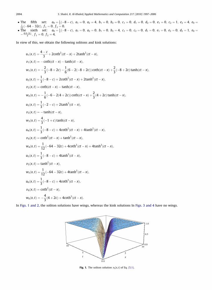
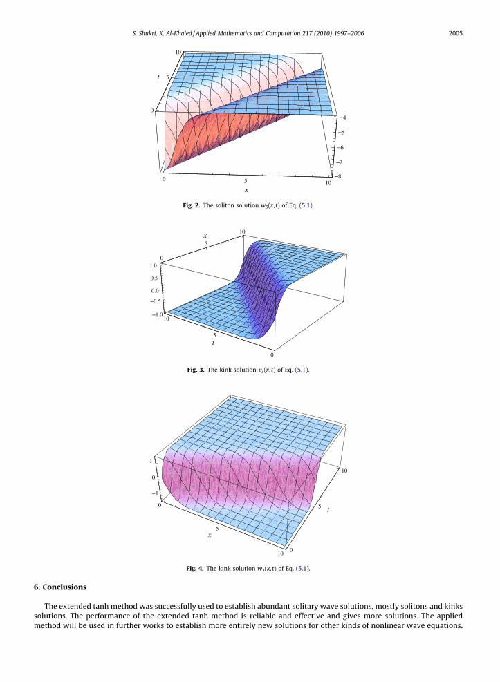
In Figs. 1 and 2, the soliton solutions have wings, whereas the kink solutions In Figs. 3 and 4 have no wings.

0

5

10

x0

5

10

t

0.0

0.5

1.0

Fig. 1. The soliton solution v5(x, t) of Eq. (5.1).

0 5 10x

0

5

10

t

8

7

6

5

—

—

—

—

—

4

Fig. 2. The soliton solution w5(x, t) of Eq. (5.1).

0

5

10x

0

5

10

t

—1.0

—0.5

0.0

0.5

1.0

Fig. 3. The kink solution v3(x, t) of Eq. (5.1).

0

5

10

x

0

5

10

t

1

0

1

—

Fig. 4. The kink solution w3(x, t) of Eq. (5.1).


6. Conclusions

The extended tanh method was successfully used to establish abundant solitary wave solutions, mostly solitons and kinkssolutions. The performance of the extended tanh method is reliable and effective and gives more solutions. The appliedmethod will be used in further works to establish more entirely new solutions for other kinds of nonlinear wave equations.


Acknowledgement

The authors are grateful for professor Abdul-Majid Wazwaz, who gave us an article contains tens of new systems of non-linear wave equations, see for more details [3].

References

[1] Ahmet Bekir, Applications of the extended tanh method for coupled nonlinear evolution equations, Communications in Nonlinear Science andNumerical Simulation 13 (2008) 1748–1757.

[2] Engui Fan, Y.C. Hon, Applications of extended tanh method to special types of nonlinear equations, Applied Mathematics and Computation 141 (2003)351–358.

[3] Mikhail V. Foursov, Marc Moreno Maza, On computer-assisted classification of coupled integrable equations, Journal of Symbolic Computation 33(2002) 647–660.

[4] W. Malfliet, Solitary wave solutions of nonlinear wave equations, American Journal of Physics 60 (1992) 650–654.[5] W. Malfliet, W. Hereman, The tanh method, exact solutions of nonlinear evolution and wave equations, Physica Scripta 54 (1996) 563–568.[6] Sami Shukri, The Extended Tanh Method for Solving Systems of Nonlinear Wave Equations, Master Thesis, Jordan University of Science and Technology,

July 2010.[7] Abdul-Majid Wazwaz, Nonlinear variants of KdV and KP equations with compactons, solitons and periodic solutions, Communications in Nonlinear

Science and Numerical Simulation 10 (2005) 451–463.[8] Abdul-Majid Wazwaz, Generalized Boussinesq type of equations with compactons, solitons and periodic solutions, Applied Mathematics and

Computation 167 (2005) 1162–1178.[9] Abdul-Majid Wazwaz, The extended tanh method for new soliton solutions for many forms of the fifth-order KdV equations, Applied Mathematics and

Computation 148 (2007) 1002–1014.[10] Abdul-Majid Wazwaz, The extended tanh method for abundant solitary wave solutions of nonlinear wave equations, Applied Mathematics and

Computation 187 (2007) 1131–1142.[11] Abdul-Majid Wazwaz, Partial Differential Equations and Solitary Waves Theory, Higher Education Press and Springer Verlag, 2009. pp. 479–491.[12] Luwai Wazzan, A modified tanh coth method for solving the KdV and the KdV Burgers equations, Communications in Nonlinear Science and Numerical

Simulation 14 (2009) 443–450.

Documents

The extended tanh method for solving systems of nonlinear wave equations