Embed Size (px)
Citation preview
The Expedition of the Research Vessel "Polarstern" to the Antarctic in 2007/2008 (ANT-XXIV/2) Edited by Ulrich Bathmann with contributions of the participants
604
2010
ALFRED-WEGENER-INSTITUT FÜR POLAR- UND MEERESFORSCHUNG In der Helmholtz-Gemeinschaft D-27570 BREMERHAVEN Bundesrepublik Deutschland
ISSN 1866-3192
Hinweis Die Berichte zur Polar- und Meeresforschung werden vom Alfred-Wegener-Institut für Polar-und Meeresforschung in Bremerhaven* in unregelmäßiger Abfolge herausgegeben. Sie enthalten Beschreibungen und Ergebnisse der vom Institut (AWI) oder mit seiner Unterstützung durchgeführten Forschungsarbeiten in den Polargebieten und in den Meeren. Es werden veröffentlicht:
— Expeditionsberichte (inkl. Stationslisten und Routenkarten)
— Expeditionsergebnisse (inkl. Dissertationen)
— wissenschaftliche Ergebnisse der Antarktis-Stationen und anderer Forschungs-Stationen des AWI
— Berichte wissenschaftlicher Tagungen
Die Beiträge geben nicht notwendigerweise die Auffassung des Instituts wieder.
Notice The Reports on Polar and Marine Research are issued by the Alfred Wegener Institute for Polar and Marine Research in Bremerhaven*, Federal Republic of Germany. They appear in irregular intervals.
They contain descriptions and results of investigations in polar regions and in the seas either conducted by the Institute (AWI) or with its support.
The following items are published:
— expedition reports (incl. station lists and route maps)
— expedition results (incl. Ph.D. theses)
— scientific results of the Antarctic stations and of other AWI research stations
— reports on scientific meetings
The papers contained in the Reports do not necessarily reflect the opinion of the Institute.
The „Berichte zur Polar- und Meeresforschung” continue the former „Berichte zur Polarforschung”
* Anschrift / Address Alfred-Wegener-Institut für Polar- und Meeresforschung D-27570 Bremerhaven Germany www.awi.de
Editor in charge: Dr. Horst Bornemann Assistant editor: Birgit Chiaventone
Die "Berichte zur Polar- und Meeresforschung" (ISSN 1866-3192) werden ab 2008 aus-schließlich als Open-Access-Publikation herausgegeben (URL: http://epic.awi.de). Since 2008 the "Reports on Polar and Marine Research" (ISSN 1866-3192) are only available as web based open-access-publications (URL: http://epic.awi.de)
The Expedition of the Research Vessel "Polarstern" to the Antarctic in 2007/2008 (ANT-XXIV/2)
Edited by Ulrich Bathmann with contributions of the participants Please cite or link this item using the identifier hdl:10013/epic.34024 or http://hdl.handle.net/10013/epic.34024 ISSN 1866-3192
ANT-XXVI/2
28 November 2007 - 4 February 2008
Cape Town - Cape Town Weddell Sea
Chief Scientist: Ulrich Bathmann
Koordinator / Coordinator
Eberhard Fahrbach
1
CONTENTS
1. Überblick und Fahrtverlauf 4
Itinerary and summary 6
2. SCACE: Synoptic Circum-Antarctic / Climate-processes and ecosystem study - a project of the IPY – 8
3. Physical Oceanography: Measurements at hydrographic stations 12
4. Physical Oceanography: Measurements of currents and backscatter strength with the Vessel-Mounted Acoustic Doppler Current Profiler (ADCP) 19
5. Plankton parameters: chlorophyll a, particulate organic carbon, biological silica 21
6. Continuous Plankton Recorder (CPR): Australian Antarctic Division Project 472 23
7. Multinet sampling during ANT-XXIV/2, December - January 2007/08 26
8. Biology of Oithona similis (Copepoda: Cylopoida) in the Southern Ocean 32
9. Salp distribution in the Lazarev Sea, December - January 2007/08 33
10. Carnivorous zooplankton in the mesopelagic food web of the Southern Ocean 38
11. Demography of Antarctic krill and other Euphausiacea in the Lazarev Sea in summer 2008 43
12. Macrozooplankton and micronekton in the surface layer and under sea ice 52
13. Marine birds and mammals in the Lazarev Sea: the summer influx 65
14. ANDEEP-SYSTCO (SYSTem COupling) System Coupling in the deep Southern Ocean - From census to ecosystem functioning 78
15. ANDEEP - SYSTCO: Work at the seafloor 84
ANT-XXIV/2
2
16. Geochemical investigations at the seafloor 95
17. Microbial communities within deep Antarctic sediments 100
18. Protists - Benthic foraminifera of the deep Southern Ocean: diversity and biogeography 101
19. Metazoan Meiofauna - The link between structural and functional biodiversity of the meiofauna communities in the Antarctic deep sea 106
20. An experimental approach to the meiobenthic food-web study in the Southern Ocean deep sea: What is the microbial carbon contribution to the diet of Nematoda? 108
21. Macrofauna – Biodiversity, ecology and zoogeography of peracarid crustaceans and Polychaeta 110
22. Indications for cryptic speciation in the Southern Ocean Ampharetidae and Trichobranchidae (Annelida, Polychaeta) 119
23. Biodiversity, phylogeny and tropho-dynamics of amphipod crustaceans in the Antarctic deep sea 121
24. Preliminary report on AGT catches during ANT-XXIV/2 124
25. Preliminary report on the Porifera (sponges) caught during the ANT-XXIV/2, ANDEEP-SYSTCO 129
26. Diversity of the Southern Ocean deep-sea anthozoan fauna 134
27. Gastropoda of the deep Southern Ocean - results from AGT catches during ANDEEP-SYSTCO 139
28. Biogeography of asteroids 145
29. Biodiversity and evolution of echinoids 147
30. Preliminary results of seabed video images 149
31. Domino - Dynamics of benthic organic matter fluxes in polar deep-ocean environments 151
32. Education and Outreach Report - Polarstern ANT-XXIV/2 153
33. Weather 155
34. Sea ice conditions during Polarstern expedition ANT-XXIV/2, December 2007 – January 2008 159
3
35. Acoustic survey of the horizontal and vertical distribution of krill, zooplankton and nekton 163
APPENDIX 165
A.1 Beteiligte Institute / Participating institutes 166
A.2 Fahrtteilnehmer / Participants 170
A.3 Schiffsbesatzung / Ship's crew 172
A.4 Stationsliste / station list PS071 174
4
1. ÜBERBLICK UND FAHRTVERLAUF Ulrich Bathmann
Alfred-Wegener-Institut
Die Expedition begann am 28. November 2007 in Kapstadt, führte zur
Antarktisstation Neumayer, wohin sie nach einer kurzen Forschungsperiode in der
Lazarew See am 6. Januar zurückkehrte, um eine Eisrampe für die Entladung der
Naja Arctica freizubrechen. Nach weiteren 14 Forschungstagen beendete Polarstern
die Expedition am 4. Februar 2008 in Kapstadt. Es wurden über 7600 Seemeilen in den 68 Tagen (= 1632 Stunden) zurückgelegt, in denen 456 Stunden Forschungsgeräte eingesetzt wurden. Die restliche Zeit wurde für Fahrtstrecken, Transit oder Logistik benötigt. Unsere Forschungsministerin A. Schavan besuchte mit ihrer südafrikanischen Kollegin N.C. Dlamini Zuma am 5. Februar das Schiff.
Die wissenschaftliche Forschung konzentrierte sich auf das IPY Kernprogramm ICED, dass das Dach für die 3 IPY Projekte dieser Fahrt bildet. SCACE, SYSTCO und LAKRIS trugen zum besseren Verständnis der biologischen, chemischen und physikalischen Prozesse in der Ozeandeckschicht, die durch Meereisdynamik beeinflusst wird, und deren Verbindungen durch die Wassersäule in die Tiefsee zur Biodiversität und den geochemischen Umsätzen. Die wichtigsten Ergebnissse, die unter den erschwerten Bedingungen der logistischen Aufgaben erreicht werden konnten, sind: • Beschreibung einer 700.000 km2 großen Eisrandblüte; ihre physikalischen
ursachen und biologischen Auswirkungen wie z.B. die Reduktion des pCO2 Partialdruckes im Oberflächenwasser von 380 auf 300 ppmv.
• Erstmalige Wiederholungsmessung biogeochemischer Flussraten im Tiefseesediment nach 7 Wochen, um den Effekt einer absinkenden Plankton-blüte auf die Tiefseebiogeochemie der Antarktis nachzuweisen.
• Erstmalige biogeochemische Beprobung der antarktischen Tiefsee im Anstand von 12 Seemeilen, um die mesoskalige Heterogenität im Sediment zu untersuchen.
• Weltweit südlichste Beprobung der in-situ Flüsse am Meeresboden bei 69°40.4’S, die hohe biologische Aktivitäten nachwies.
• Erstmalige Prozessstudien von der Meeresoberfläche zum Tiefseesediment in der Antarktis an 5 Stationen als Voruntersuchung künftiger Programme.
• Abschluss der saisonalen Untersuchungen zum Lebenszyklus antarktischen Krills mit dem Nachweis einer engen positiven Kopplung von Meereis und Krillhäufigkeit in der Lazarewsee.
1. Überblick und Fahrtverlauf
5
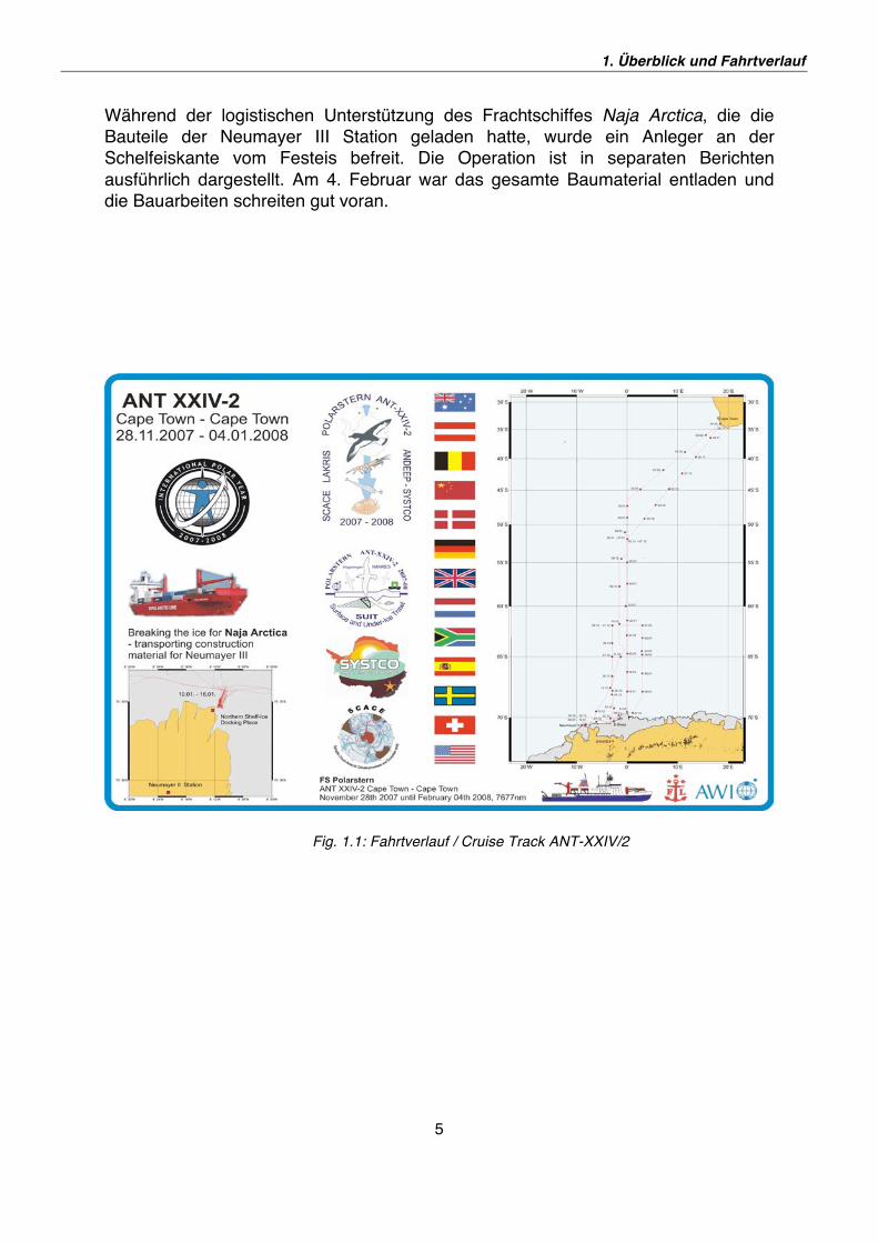
Während der logistischen Unterstützung des Frachtschiffes Naja Arctica, die die
Bauteile der Neumayer III Station geladen hatte, wurde ein Anleger an der
Schelfeiskante vom Festeis befreit. Die Operation ist in separaten Berichten
ausführlich dargestellt. Am 4. Februar war das gesamte Baumaterial entladen und
die Bauarbeiten schreiten gut voran.
Fig. 1.1: Fahrtverlauf / Cruise Track ANT-XXIV/2
6
ITINERARY AND SUMMARY
The cruise departed from Cape Town on 28 November 2007 headed south to Neumayer performed research in the Lazarev Sea, steamed back to Neumayer and had another 14 days research on its way north. In total we sailed more than 7,600 nautical miles. From the 68 days (= 1632 hours) at sea, we used 456 hours to deploy instruments, the rest was steaming time, transit or logistics. The cruise ended on 4 February 2008 in Cape Town. Our federal Minister for Science and Technology A. Schavan visited the ship with her South African counterpart N.C. Dlamini Zuma on 5 February in the afternoon. The scientific programme centred on the IPY core programme ICED that provided the umbrella for 3 IPY projects performed during this cruise. SCACE In combination with SYSTCO and LAKRIS contributed during the ANT-XXIV/2 expedition of Polarstern to a better understanding of upper ocean physical and biological processes influenced by sea ice and their linkage through the water column to the deep-sea abyss and its biogeochemistry and impact on biodiversity. Main achievements were reached despite the intense constrains set by logistic operation of Polarstern: The main results are: • Determination of 700.000 km2 large ice-edge bloom; its physical causes and
biological effects, e.g. the draw down of pCO2 in surface ocean waters from 380 to 300 ppmv (units).
• First biogeochemical in-situ measurement repeated after 7 weeks to investigate the effect of phytoplankton bloom on benthos and demonstration that surface productivity is linked to the seafloor biogeochemistry in the high Antarctic.
• First biogeochemical sampling of deep-sea stations 12 nm apart in order to look at small-scale heterogeneity in the sediment.
• Worldwide southernmost in-situ benthic flux measurement at 69°40.4’S (Polynia station), with indication of high benthic activity.
• First sampling through the complete water column in the Southern Ocean from surface and ice flora and fauna down to bathyal or abyssal depths (5 stations, partly incomplete) as precursor for later programmes.
• Completion of year round sampling to study life cycle patterns of Antarctic krill indicate strong correlation of krill abundance and success to sea ice occurrence.
In detail We observed an ice edge phytoplankton bloom. The bloom that Polarstern crossed in the eastern Weddell Sea was also clearly visible from space. As recorded by satellite-mounted ocean colour sensors it covered an area of about 700.000 km2, roughly two times the size of Germany. Measurements performed in the upper water
Summary and itinerary
7
column by a Conductivity-Temperature-Depth (CTD) probe revealed that the bloom developed in lenses of melt water left behind the seasonally retreating sea ice cover. Together with the chemical measurements made, the new data set will allow for a better quantification of the controversially debated role of ice edge blooms for the sequestration of atmospheric carbon dioxide. Better understanding of the physical control of the regional distribution of marine life and of biological processes that influence the uptake of carbon from the atmosphere and its transport to the ocean interior and underlying sediments is also the aim of the IPY project SCACE, led by AWI oceanographer Volker Strass. For this project, the Synoptic Circum-Antarctic Climate-processes and Ecosystem study, physical, biological and chemical data where collected down to 1,000 m depth every 55.6 kilo-metres (30 nautical miles) along a transect that extends over more than 2,600 km. The transect ran northward along the Greenwich Meridian from the Antarctic coast and crossed the major hydrographic features of the Southern Ocean, the Coastal Current, the Weddell Gyre and the Antarctic Circumpolar Current. The SCACE transect represents a major German contribution to an international endeavour to perform in the Polar Year similar meridional transects in all sectors of the Southern Ocean, aimed at a circumpolar assessment of the present status of its climate and ecosystem. The ANDEEP-SYSTCO team led by Prof. Angelika Brandt, University Hamburg investigated 5 deep-sea locations in detail. At 52°S the deep sea at the Southern Polar front is characterised by low diversity and abundance, in the macrofauna even after a slight plankton bloom in spring (revisit of stations after 7 weeks). The Eastern Weddell Sea and Lazarev Sea is generally poorer in species and abundance of organisms in the deep sea. Maud Rise (seamount) differs completely in taxon composition from the abyssal stations, perhaps due to the unique physical ocean characteristics including Taylor column influencing localised entrainment of larvae. Brooders, on the contrary, occur only as a minor fraction in the macrobenthic sample. The LAKRIS project lead by Prof. Ulrich Bathmann, AWI, investigates the life cycle patterns of Antarctic Krill in the Lazarev Sea that is part of the Southern Ocean facing the Neumayer Station. Krill abundance was rather poor this spring, especially compared to the 2006 winter situation. Only in the regions north of 62°S abundant swarms of adult krill occurred and attracted many top predators, especially Minke and Humpback Whales. One Blue Whale was seen in the ice, where it should not occur. The logistic operation to free the shelf ice for unloading the cargo vessel Naja Arctica that contained construction material for Neumayer III station is reported in detail in special reports. On 4 February, all cargo had been unloaded and the construction of the new base was up to full speed to secure the site before the next winter.
8
2. SCACE: SYNOPTIC CIRCUM-ANTARCTIC / CLIMATE-PROCESSES AND ECOSYSTEM STUDY - A PROJECT OF THE IPY – Volker Strass1), Ulrich Bathmann1),
Richard Bellerby2) (not on board),
Graham Hosie3) (not on board)
1)Alfred-Wegener-Institut, Bremerhaven,
Germany
2)Bjerknes Centre University Bergen,
Norway 3) Australian Antarctic Division, Australia
Objectives The overarching goal of SCACE is to use the outstanding chance provided by the International Polar Year (IPY) to collect in international collaboration a unique data set that can serve as a benchmark for comparison with existing and future data to identify and quantify polar changes. SCACE is listed as IPY project number 16 by the International Polar Year Programme Office (http://classic.ipy.org/development/eoi/details.php?id=16; for a German description of SCACE please see http://www.polarjahr.de/The-project.263+M54a708de802.0.html). SCACE aims at welding together a broad range of ocean science disciplines in order to address currently elusive questions such as: • Which physical, biological and chemical processes regulate the Southern
Ocean system and determine its influence on the global climate development? • How sensitive are Southern Ocean processes and systems to natural climate
change and anthropogenic perturbations? The Southern Ocean is critically involved in the machinery driving earth´s climate. The Antarctic Circumpolar Current (ACC) connects all the other oceans. Thus, it plays a major role in the global transports of heat and fresh-water and the ocean-wide cycles of dissolved substances. It harbours a series of distinct ecosystems that displace each other with changing climate regimes. Upwelling of deep water masses results in an extraordinary high supply of plant macronutrients, which could sustain much higher phytoplankton primary production and hence CO2 uptake than normally observed. While the Southern Ocean exerts a control on earth's climate, it is itself sensitive to climatic changes, which may occur on various time scales and affect the biota. There are, however, also direct anthropogenic influences on the ecosystem, for instance by harvesting marine living resources such as krill. Although much progress has been made during the last decades in documenting the Southern Ocean hydrographic and biographic features, in quantifying fluxes and in understanding the dominating forcing, there is still a big gap in knowledge, especially
2. SCACE: Synoptic circum-Antarctic/climate processes and ecosystem study - a project of the IPY
9
with regard to the interaction of physical, chemical and biological processes. While this gap in knowledge is basically due to the remoteness of the area and its inhospitality for humans, it is also due to the fragmentation of research as carried out usually. Collaboration across the traditional boundaries between the physical, chemical and biological disciplines of the marine sciences is hence an essential element of SCACE. By cooperation with the ocean circulation IPY lead project CASO (Climate in Antarctica and the Southern Ocean) and by coordination under the umbrella of the biogeochemistry lead project ICED (Integrated Climate and Ecosystem Dynamics), SCACE strives for performing in the same season and year meridional sections that extend from the Antarctic continent and cross the ACC at several key longitudes. Such synoptic circumpolar assessment is the only way to document the current state of the environment without bias introduced by interannual variability. With regard to the processes that potentially exert a control on global climate, SCACE is aimed at obtaining new insights into the coupling between atmospheric forcing of the mixed layer dynamics, phytoplankton primary production in the near-surface euphotic zone, the flow of energy from the primary producers through the food web, and subsequently the transport of biogenically fixed carbon to the deep ocean layers and the sea floor. Assessing the vertical transport of biogenic carbon, hence providing an indication of carbon sequestration from the atmosphere, is one of the particular objectives of SCACE. By cooperation with the IPY biodiversity lead project ANDEEP-SYSTCO (chapter 14) and the related DFG project DOMINO (chapter 16), which are focused on benthic biology and sediment geochemistry, respectively, SCACE is extending the investigation of the vertical carbon flux into the benthic biota and the sediment. Vice versa, SCACE provides ANDEEP-SYSTCO with information about processes and fluxes from the atmosphere-ocean interface through the whole watercolumn overlaying the seafloor.
Work at sea
A significant part of the measurements performed during Polarstern cruise ANT-XXIV/2 constitutes the German contribution to SCACE. The SCACE data set comprises physical measurements made with a CTD (Conductivity, Temperature, Depth) probe at hydrographic stations, from which vertical profiles of the state variables temperature, salinity and density are derived. The CTD range of variables is extended by accessory instruments such as a chlorophyll-sensitive fluorometer to provide an indication of the abundance of phytoplankton, a transmissiometer to measure the attenuation of light, which in the open ocean is determined by the concentration of particulate organic carbon (POC), and an oxygen sensor. The CTD measurements are described in more detail in section chapter 3. Samples taken from the carousel bottle water sampler attached to the CTD were used for chemical analyses performed to give the concentrations of the plant nutrients nitrate and silicate, of dissolved inorganic carbon and alkalinity, and of oxygen. A more rigorous description of the chemical measurements is provided in chapter 16. Also biological data, such as the concentration of phytoplankton pigments, of POC, and occasionally of the phytoplankton species composition, were collected from the CTD bottles. For details of the biological measurements see chapter 5.
ANT-XXIV/2
10
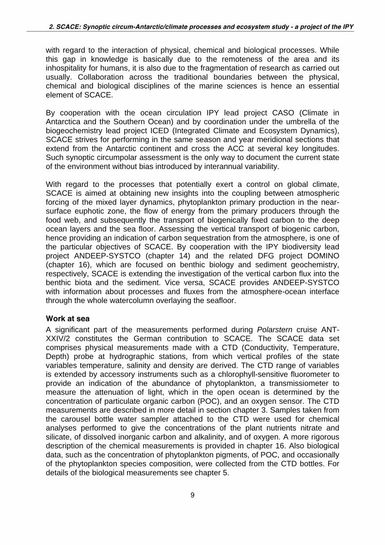
Hydrographic stations pertinent to SCACE are aligned at half a degree of latitude intervals along the Greenwich Meridian between the Antarctic continental shelf edge at 69.6°S and the northern flank of the Antarctic Circumpolar Current at 46.5°S. Stations south of 62°S along the Greenwich Meridian also constitute a contribution to LAKRIS, the BMBF-funded Lazarev Sea Krill Study, while all hydrographic stations along the 3°E and 3°W meridians constitute a contribution to both SCACE and LAKRIS. For a map of the station positions see Fig. 2.1.
Fig. 2.1: Positions of CTD stations performed as a contribution to SCACE and, south of 62°S, as a
contribution to SCACE as well as to LAKRIS
The majority of the biological measurements for SCACE were obtained with different types of plankton nets, deployed for vertical hols as well as for horizontal tows near the hydrographic stations. The various nets, their deployment position and the suite of data collected by them are described in chapter 7. Overall, only less than half of the planned measurements at hydrographic stations could however be performed because ten days of shiptime had to be sacrificed by marine science for the sake of ice breaker support by Polarstern for a freighter carrying construction material for the new German Antarctic Base Neumayer III. In consequence, the CTD was mostly lowered just to 1,000 m depth instead of down to the sea floor; the section worked southward along 3°E had to be stopped before the continental shelf break was reached; the Greenwich Meridional section could not be conducted northward enough to extend to the north of the Subantarctic Front, i.e. to fully cover the width of the ACC; and plankton nets could not be deployed as frequently as originally intended.
2. SCACE: Synoptic circum-Antarctic/climate processes and ecosystem study - a project of the IPY
11
Less affected by the rededication of shiptime than the hydrographic station work was the collection of data in quasi continuous mode. Physical data, consisting of vertical profiles of ocean currents down to about 250 m, were obtained almost continuously with the vessel-mounted acoustic Doppler current profiler (ADCP; detailed description in chapter 3 ‘underway measurements of ocean currents’) while operating outside of national Exclusive Economic Zones (South African EEZ in case of this cruise). Other physical data, such as sea-surface temperature and salinity as well as various meteorological variables were collected and stored by the Polarstern Data Acquisition System, PODAS. Quasi continuous data of the zooplankton assemblage have been obtained from the vessel-mounted multi-frequency echosounder Simrad EK-60 (details in chapter 35). Quasi continuous measurements of the zooplankton assemblage at a nominal depth of 10 m have also been obtained with a continuous plankton recorder (CPR; for details see chapter 6). The CPR was towed during periods of long-distance steaming, at the begin of the cruise after leaving the South African EEZ on the way towards Neumayer Base and at the end of the cruise after the final CTD station on the way back to the South African EEZ.
Preliminary results A scientific highlight contained in the SCACE data set certainly is the documentation of an ice edge bloom that occupied an area of approximately 700,000 km2 as revealed by satellite remote imaging (chlorophyll concentration from the official ESA MERIS satellite data algal-1 level-2 product composed to maps by T. Dinter (Institute of Environmental Physics, Bremen) and A. Bracher (AWI, Bremerhaven); personal communication). For a first impression of the collected data see chapter 3 ‘hydrograhic station work’ and chapter 4 ‘underway measurements of ocean currents’.
12
3. PHYSICAL OCEANOGRAPHY: MEASUREMENTS AT HYDROGRAPHIC STATIONS Volker Strass1), Silvia Maßmann1),
Falk Richter1), Daniela Ewe1), Mark
Olischläger1), Harry Leach2), Timo
Witte3)
1)Alfred-Wegener-Institut, Bremerhaven,
Germany
2)University of Liverpool, United Kingdom 3) Optimare Sensorsysteme AG,
Bremerhaven
Objectives and work at sea
Vertical profiles of temperature, salinity and density were derived from measurements
made by lowering a CTD (Conductivity, Temperature and Depth) probe at
hydrographic stations. The CTD used was of type Sea-Bird Electronics SBE 911plus,
supplemented by an oxygen sensor type SBE 43 and additional instruments such as
an altimeter (Benthos PSA-916) to measure the distance to the sea floor, a
transmissiometer type Wet Labs C-Star (660 nm wavelength) to measure the
attenuation of light, which in the open ocean is indicative of the concentration of
particulate organic carbon (POC), and a chlorophyll-sensitive fluorometer (Dr. Haardt
BackScat). The temperature and conductivity sensors (two pairs of sensors) were
calibrated at the factory prior to the cruise to an accuracy of better than 0.001°C and
0.001 S m-1, respectively. They will be sent to the manufacturer after the cruise for re-
calibration. The CTD data, as well as the data taken by the additional sensors and
instruments, at present are thus to be considered preliminary, subject to a later
correction for possible temporal drifts and to calibration in absolute units.
The CTD was mounted with a multi-bottle water sampler type Sea-Bird SBE 32
Carousel holding 24 12-liter bottles. Salinity derived from the CTD measurements will
later be re-calibrated by comparison to salinity samples taken from the water bottles,
which were analyzed by use of a Guildline-Autosal-8400A salinometer to an accuracy
generally better than 0.001 units on the practical salinity scale, adjusted to IAPSO
Standard Seawater. The water bottles also served to supply several other working
groups on board with samples. Water samples have, for instance, been taken to be
analyzed for the concentrations of particulate organic carbon (POC) and of
phytoplankton pigments such as chlorophyll (see chapter 5). The bottle data of
oxygen, POC and chlorophyll will, once finally analyzed, be also used for the
calibration of the respective CTD sensors and instruments.
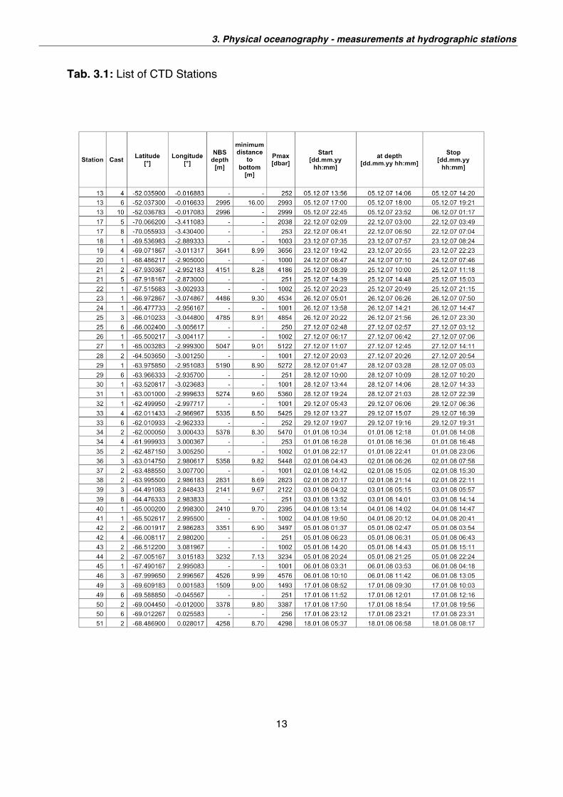
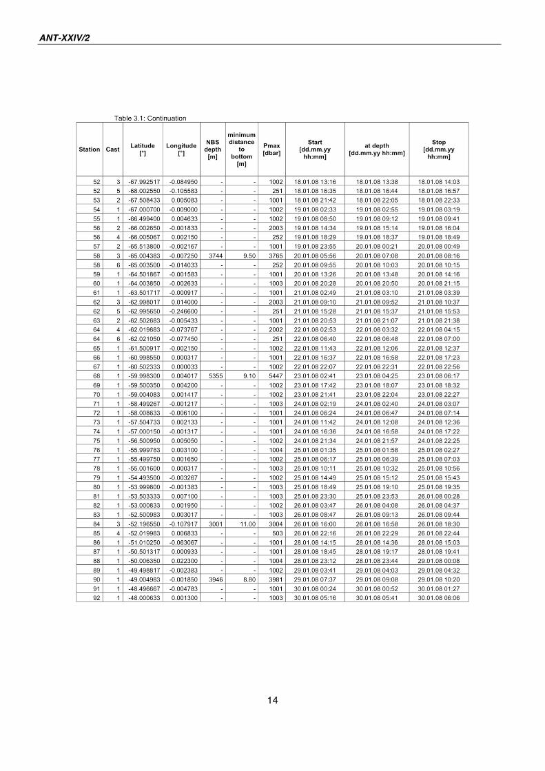
All together, 95 CTD casts were carried out (see Table 3.1). Of these, 24 extended to
full ocean depth while the others were limited mostly to the upper 1,000 m of the
water column, including 17 at which the CTD was lowered to just 250 m. The CTD
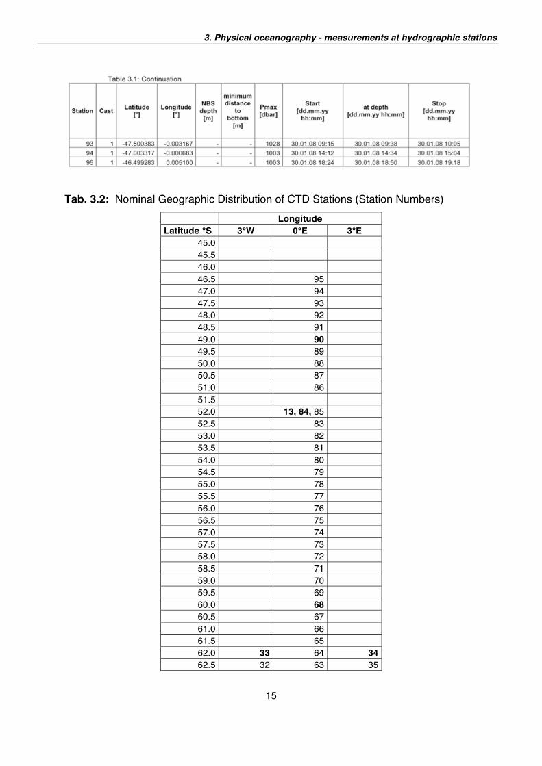
stations were distributed along three meridional sections (see Table 3.2) running
along 3°W, 0°E and 3°E. The distance between stations along the meridional
sections was nominally 30 nm.
3. Physical oceanography - measurements at hydrographic stations
13
Tab. 3.1: List of CTD Stations
ANT-XXIV/2
14
3. Physical oceanography - measurements at hydrographic stations
15
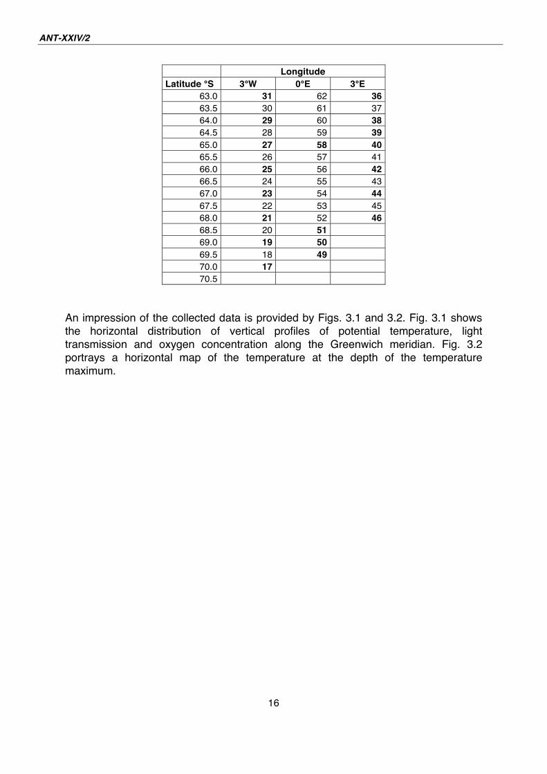
Tab. 3.2: Nominal Geographic Distribution of CTD Stations (Station Numbers)
Longitude Latitude °S 3°W 0°E 3°E
45.0 45.5 46.0 46.5 95 47.0 94 47.5 93 48.0 92 48.5 91 49.0 90 49.5 89 50.0 88 50.5 87 51.0 86 51.5 52.0 13, 84, 85 52.5 83 53.0 82 53.5 81 54.0 80 54.5 79 55.0 78 55.5 77 56.0 76 56.5 75 57.0 74 57.5 73 58.0 72 58.5 71 59.0 70 59.5 69 60.0 68 60.5 67 61.0 66 61.5 65 62.0 33 64 34 62.5 32 63 35
ANT-XXIV/2
16
Longitude Latitude °S 3°W 0°E 3°E
63.0 31 62 36 63.5 30 61 37
64.0 29 60 38 64.5 28 59 39 65.0 27 58 40 65.5 26 57 41
66.0 25 56 42 66.5 24 55 43
67.0 23 54 44 67.5 22 53 45
68.0 21 52 46 68.5 20 51
69.0 19 50 69.5 18 49
70.0 17 70.5
An impression of the collected data is provided by Figs. 3.1 and 3.2. Fig. 3.1 shows
the horizontal distribution of vertical profiles of potential temperature, light
transmission and oxygen concentration along the Greenwich meridian. Fig. 3.2
portrays a horizontal map of the temperature at the depth of the temperature
maximum.
3. Physical oceanography - measurements at hydrographic stations
17
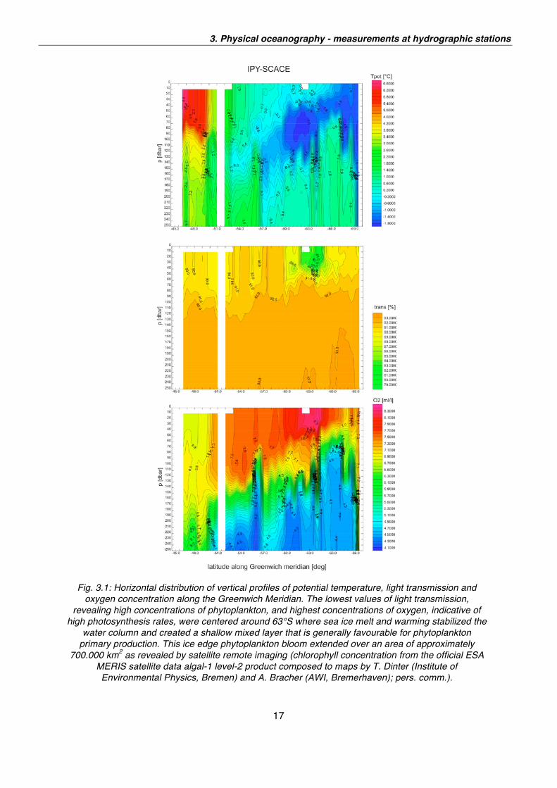
Fig. 3.1: Horizontal distribution of vertical profiles of potential temperature, light transmission and
oxygen concentration along the Greenwich Meridian. The lowest values of light transmission,
revealing high concentrations of phytoplankton, and highest concentrations of oxygen, indicative of
high photosynthesis rates, were centered around 63°S where sea ice melt and warming stabilized the
water column and created a shallow mixed layer that is generally favourable for phytoplankton
primary production. This ice edge phytoplankton bloom extended over an area of approximately
700.000 km2 as revealed by satellite remote imaging (chlorophyll concentration from the official ESA
MERIS satellite data algal-1 level-2 product composed to maps by T. Dinter (Institute of
Environmental Physics, Bremen) and A. Bracher (AWI, Bremerhaven); pers. comm.).
ANT-XXIV/2
18
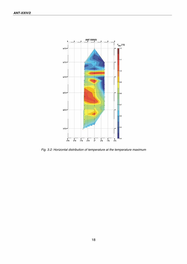
Fig. 3.2: Horizontal distribution of temperature at the temperature maximum
19
4. PHYSICAL OCEANOGRAPHY: MEASUREMENTS OF CURRENTS AND BACKSCATTER STRENGTH WITH THE VESSEL-MOUNTED ACOUSTIC DOPPLER CURRENT PROFILER (ADCP) Volker Strass1), Timo Witte2), Boris
Cisewski3) (not on board)
1)Alfred-Wegener-Institut, Bremerhaven,
Germany
2) Optimare Sensorsysteme AG,
Bremerhaven 3)Universität Bremen, Bremen
Objectives and work at sea
Vertical profiles of ocean currents down to 335 m depth were measured with a Vessel
Mounted Acoustic Doppler Current Profiler (type Ocean Surveyor ; manufacture of
RDI, 150 kHz nominal frequency), installed 11 m below the water line in the ship s
keel behind an acoustically transparent plastic window for ice protection. The
transducer emits/receives the acoustic signals from its flat face, which is composed
of an array of about 1,000 ceramic elements, covered in urethane. These elements
are arranged in a fixed pattern and are each wired to transmit a specific signal,
identified by its phase. The phase shift, with which the ceramic elements emit their
acoustic signals, is arranged in a way such that the signals interfere to form beams in
four distinct directions, slanted at 30 degrees from the vertical. The transducer also
records the echoes returned from particles in suspension in the water. Echoes
reflected by particles moving relative to the ADCP return with a change in frequency.
The ADCP measures this change, the so-called Doppler shift, as a function of depth
to obtain water velocity at a maximum of 128 depth levels. The instrument settings for
this cruise were chosen to give a vertical resolution of current measurements of 4 m
in 80 depth bins and a temporal resolution of 2 min for short time averages.
Determination of the velocity components in geographical coordinates, however,
requires that the attitude of the ADCP transducer head, its tilt, heading and motion is
also known. Heading, roll and pitch data are read by the ADCP deck-unit from the
ship s gyro platforms. The ship s velocity was calculated from position fixes obtained
from the Global Positioning System (GPS) or Differential GPS if available, and was
taken over from the ship s navigation system. Accuracy of the ADCP velocities mainly
depends on the quality of the position fixes and the ship s heading data. Further
errors stem from a misalignment of the transducer with the ship s centre-line and a
constant angular offset between the transducer and the GPS antenna array, and a
velocity scale factor. The ADCP data processing was done by using the CODAS3
software package (developed by E. Firing and colleagues, SOEST, Hawaii).
ANT-XXIV/2
20
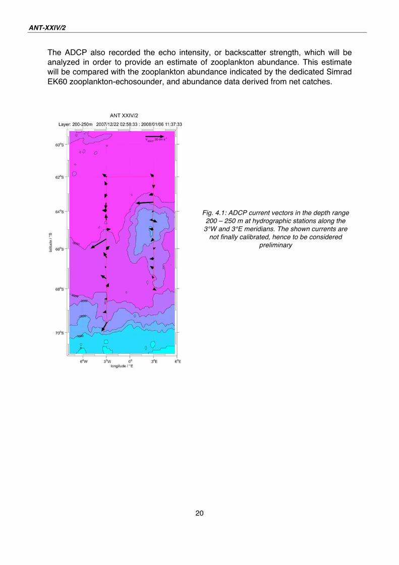
The ADCP also recorded the echo intensity, or backscatter strength, which will be
analyzed in order to provide an estimate of zooplankton abundance. This estimate
will be compared with the zooplankton abundance indicated by the dedicated Simrad
EK60 zooplankton-echosounder, and abundance data derived from net catches.
Fig. 4.1: ADCP current vectors in the depth range
200 – 250 m at hydrographic stations along the
3°W and 3°E meridians. The shown currents are
not finally calibrated, hence to be considered
preliminary
21
5. PLANKTON PARAMETERS: CHLOROPHYLL A, PARTICULATE ORGANIC CARBON, BIOLOGICAL SILICA Sarah Herrmann, Ulrich Bathmann
Alfred-Wegener-Institut,
Bremerhaven, Germany
Objectives and work at sea
The very basis in the food-chain in the water column is the primary producers, the
phytoplankton. For all studies dealing with the distribution of higher organisms like
Krill for example it is obligatory to compare between distributions of prey and
predators. In this case, the prey would be the phytoplankton. There is a simple way to
determine the relative concentration of phytoplankton by measuring the fluorescence
of photosynthetic pigments. As chlorophyll a is the universal antennae pigment of all
oxygenic organisms, the chlorophyll a content in a given amount of water is a good
unit to specify phytoplankton biomass.
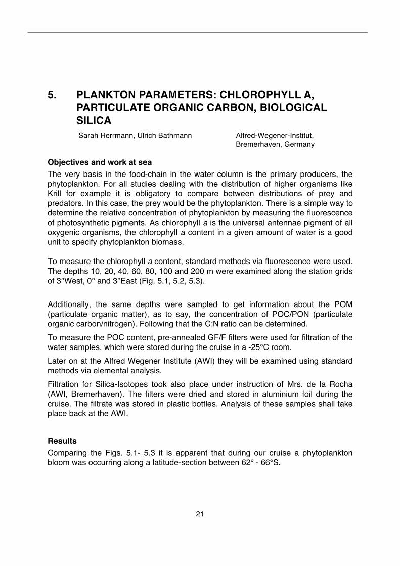
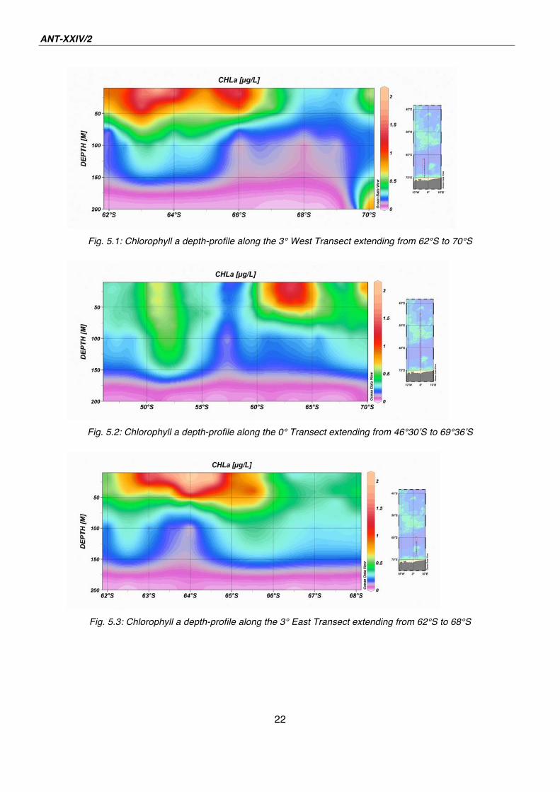
To measure the chlorophyll a content, standard methods via fluorescence were used.
The depths 10, 20, 40, 60, 80, 100 and 200 m were examined along the station grids
of 3°West, 0° and 3°East (Fig. 5.1, 5.2, 5.3).
Additionally, the same depths were sampled to get information about the POM
(particulate organic matter), as to say, the concentration of POC/PON (particulate
organic carbon/nitrogen). Following that the C:N ratio can be determined.
To measure the POC content, pre-annealed GF/F filters were used for filtration of the
water samples, which were stored during the cruise in a -25°C room.
Later on at the Alfred Wegener Institute (AWI) they will be examined using standard
methods via elemental analysis.
Filtration for Silica-Isotopes took also place under instruction of Mrs. de la Rocha
(AWI, Bremerhaven). The filters were dried and stored in aluminium foil during the
cruise. The filtrate was stored in plastic bottles. Analysis of these samples shall take
place back at the AWI.
Results
Comparing the Figs. 5.1- 5.3 it is apparent that during our cruise a phytoplankton
bloom was occurring along a latitude-section between 62° - 66°S.
ANT-XXIV/2
22
Fig. 5.1: Chlorophyll a depth-profile along the 3° West Transect extending from 62°S to 70°S
Fig. 5.2: Chlorophyll a depth-profile along the 0° Transect extending from 46°30 S to 69°36 S
Fig. 5.3: Chlorophyll a depth-profile along the 3° East Transect extending from 62°S to 68°S
23
6. CONTINUOUS PLANKTON RECORDER (CPR): AUSTRALIAN ANTARCTIC DIVISION PROJECT 472 John Kitchener1), Graham Hosie2)
(not on board)
1)Alfred-Wegener-Institut, Bremerhaven,
Germany 2) Australian Antarctic Division, Australia
Objectives
The Southern Ocean Continuous Plankton Recorder (SO-CPR) survey, which from
1997 had only involved Australia and Japan, has included Germany since 2004. This
serves to address AAD s Goal 1 of maintaining the Antarctic Treaty System and
enhancing Australia's influence through cooperating with Antarctic Treaty partners in
the involvement in setting the direction of international scientific programmes and
forums relating to Antarctic issues, e.g. international CPR survey, SCOR, SCAR,
GOOS and GLOBEC.
The SO-CPR survey primarily addresses AAD s Goal 2 of protecting the Antarctic
environment by providing information on the status or "health" of the Southern Ocean
through the monitoring of zooplankton.
Zooplankton are sensitive to environmental parameters such as temperature,
movement of currents and water quality. Due to their sensitivity, short life spans and
fast growth rates plankton populations respond rapidly to environmental change, and
consequently make excellent biological indicators.
The CPR programme is expected to provide information on natural variation in
zooplankton patterns as well as effects of global change. Zooplankton are also the
principal dietary components of many higher vertebrates, including penguins, seals
and sea-birds. Therefore, changes in zooplankton distribution and abundance in the
Southern Ocean are expected to have a significant effect on higher trophic levels. In
turn, this will serve as a reference to help distinguish fishing impact from natural or
other variation.
Consequently, the AAD has developed the CPR zooplankton monitoring programme,
under the leadership of Dr. Graham Hosie. The CPR programme is a key
methodology in the AAD Biology programme's objectives in addressing Goal 2 in
surveying biodiversity and mapping effects of climate change. It is now also a key
component of the Japanese Centre for Antarctic Environment Monitoring through
collaboration with the AAD. The German Antarctic programme has now joined the
SO-CPR survey with the mutual benefit of supporting their plankton studies while
providing the survey with another fixed transect. The survey to date mainly relies on
Aurora Australis for the majority of tows. These voyages cover a large area which is
ideal for mapping biodiversity, but they also have variable routes and schedules
ANT-XXIV/2
24
according to logistic and science programme demands which can complicate
attempts to assess temporal variation as distinct from spatial patterns. The Japanese
icebreaker Shirase has provided tows along two fixed transects 110°E and 150°E at
fixed times which provides useful references for the other data. The addition of the
fixed transect between Cape Town and Neumayer station, sampled several times a
year on Polarstern, has further improved our analyses, as well as improving our
spatial coverage for studying patterns in the Antarctic Circumpolar Current. Additional
fixed transects are also being developed with the French, New Zealand and United
Kingdom Antarctic vessels. Comparisons can also be made with other oceanic areas.
By employing a CPR, surface or near-surface zooplankton can be collected at normal
ship speed during a voyage. The unit is usually towed about 100 metres astern of the
ship for approximately 450 nautical miles at a time. By splicing consecutive tows
together one is able to produce an un-interrupted transect across the ocean,
providing information on zooplankton distribution patterns, community structure, and
abundance levels.
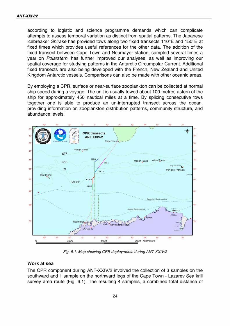
Fig. 6.1: Map showing CPR deployments during ANT-XXIV/2
Work at sea
The CPR component during ANT-XXIV/2 involved the collection of 3 samples on the
southward and 1 sample on the northward legs of the Cape Town - Lazarev Sea krill
survey area route (Fig. 6.1). The resulting 4 samples, a combined total distance of
6. Continuous Plankton Recorder (CPR): Australian Antarctic Division Project 472
25
1,190 nautical miles of continuous plankton recordings, will be analysed back at the
laboratory at AAD headquarters in Kingston, Tasmania, Australia.
All four routine CPR tows were successfully undertaken onboard Polarstern. There
were no problems encountered with the gear at any time.
To date, 15 routine CPR runs have been completed so far this 2007/08 season on
Aurora Australis, with another 7 planned for the remaining 2 voyages. A further 6
CPR tows are currently being undertaken during JARE 2007/08 onboard Shirase,
and now the addition of 4 more from ANT-XXIV/2 on Polarstern. The 2007/08 season
will be completed with the collection of 12 more samples from Umitaka Maru in the
southern Indian Ocean; 8 from Tangaroa in the southern Pacific Ocean; 4 from
Akademik Fedorov in the Amundsen and Bellinghausen Seas; and finally 3 more
from Yuzhmorgeologiya in the Ross Sea.
Acknowledgements
Sincere thanks again go to Uli Bathmann for his keen interest in furthering the SO-
CPR programme by incorporating CPR sampling into the voyage schedule, and of
course again to Master Uwe Pahl, boatswain Burkhardt Clasen and crew of
Polarstern, for their willing assistance and faultless deployment and retrieval of gear
in all weather conditions.
26
7. MULTINET SAMPLING DURING ANT-XXIV/2, DECEMBER - JANUARY 2007/08 John Kitchener1), Ulrich Bathmann2)
1) Australian Antarctic Division, Australia
2) Alfred-Wegener-Institut, Bremerhaven,
Germany
Background and objectives
Part of an ongoing continuous multi-frequency acoustic survey is to survey the spatial
distribution of Euphausia superba and other planktonic animals, including the
possible prey organisms of krill, in relation to hydrographical processes.
Using the difference in backscattering strength with different echo-sounder
frequencies, it is necessary to discriminate between distinct areas within the water
column along the transects, depicted by clear shifts in backscattering signatures. To
enable this, a combined data analysis of the results of different types of net hauls
(e.g. RMT, Multinet, SUIT etc), hydrographical and acoustic measurements needs to
be done to address the nature of such patterns in plankton distribution. This study
looks at the results of the Multinet sampling.
Work at sea
During the expedition ANT-XXIV/2 throughout December 2007 to January 2008,
stratified mesozooplankton samples were collected at 39 stations along 3 transects
(3oW, 3oE and 0o), generally sampling at each degree in latitude. The range of all 3
transects was from 70oS to 62oS, with the exception of the Greenwich meridian
transect which extended northwards until 46o30 S. The net used was a multiple
opening/closing net system (Multinet, Hydro-Bios Kiel). The smaller Multinet type Midi
with a mouth opening of 0.25 m2 and five nets equipped with 100 μm meshes was
used throughout. For qualitative estimates of zooplankton individuals, the water
column from 500 m to the surface was sampled at 5 standard depth intervals
(500 - 200, 200 - 100, 100 - 50, 50 - 25 and 25 - 0 m).
In general, each time the deployment of the Multinet was very successful without
technical problems. There were, however, some considerable differences between
the flow meter rates for the same depth interval between hauls. It has not been
ascertained as to why this occurred.
Samples were only qualitatively analysed on board, and each major taxa allocated a
percentage contribution to the overall estimated biovolume/biomass. Detailed sample
analyses will occur at the Alfred Wegener Institute, post voyage.
7. Multinet sampling during ANT-XXVI/2
27
Results
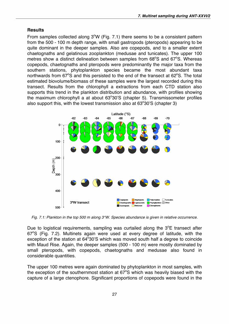
From samples collected along 3oW (Fig. 7.1) there seems to be a consistent pattern
from the 500 - 100 m depth range, with small gastropods (pteropods) appearing to be
quite dominant in the deeper samples. Also are copepods, and to a smaller extent
chaetognaths and gelatinous zooplankton (medusae and tunicates). The upper 100
metres show a distinct delineation between samples from 68oS and 67oS. Whereas
copepods, chaetognaths and pteropods were predominantly the major taxa from the
southern stations, phytoplankton species became the most abundant taxa
northwards from 67oS and this persisted to the end of the transect at 62oS. The total
estimated biovolume/biomass of these samples were the largest recorded during this
transect. Results from the chlorophyll a extractions from each CTD station also
supports this trend in the plankton distribution and abundance, with profiles showing
the maximum chlorophyll a at about 63o30 S (chapter 5). Transmissometer profiles
also support this, with the lowest transmission also at 63o30 S (chapter 3)
Fig. 7.1: Plankton in the top 500 m along 3°W. Species abundance is given in relative occurrence.
Due to logistical requirements, sampling was curtailed along the 3oE transect after
67oS (Fig. 7.2). Multinets again were used at every degree of latitude, with the
exception of the station at 64o30 S which was moved south half a degree to coincide
with Maud Rise. Again, the deeper samples (500 - 100 m) were mostly dominated by
small pteropods, with copepods, chaetognaths and medusae also found in
considerable quantities.
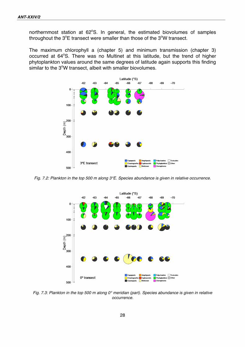
The upper 100 metres were again dominated by phytoplankton in most samples, with
the exception of the southernmost station at 67oS which was heavily biased with the
capture of a large ctenophore. Significant proportions of copepods were found in the
ANT-XXIV/2
28
northernmost station at 62oS. In general, the estimated biovolumes of samples
throughout the 3oE transect were smaller than those of the 3oW transect.
The maximum chlorophyll a (chapter 5) and minimum transmission (chapter 3)
occurred at 64oS. There was no Multinet at this latitude, but the trend of higher
phytoplankton values around the same degrees of latitude again supports this finding
similar to the 3oW transect, albeit with smaller biovolumes.
Fig. 7.2: Plankton in the top 500 m along 3°E. Species abundance is given in relative occurrence.
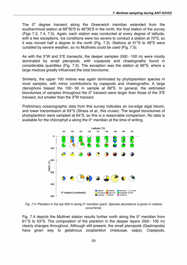
Fig. 7.3: Plankton in the top 500 m along 0° meridian (part). Species abundance is given in relative
occurrence.
7. Multinet sampling during ANT-XXVI/2
29
The 0o degree transect along the Greenwich meridian extended from the
southernmost station at 69o30 S to 46o30 S in the north, the final station of the survey
(Figs 7.3, 7.4, 7.5). Again, each station was conducted at every degree of latitude,
with a few exceptions. Ice conditions were too severe to conduct a station at 70oS, so
it was moved half a degree to the north (Fig. 7.3). Stations at 51oS to 49oS were
curtailed by severe weather, so no Multinets could be used (Fig. 7.5).
As with the 3°W and 3°E transects, the deeper samples (500 - 100 m) were mostly
dominated by small pteropods, with copepods and chaetognaths found in
considerable quantities (Fig. 7.3). The exception was the station at 66oS, where a
large medusa greatly influenced the total biovolume.
Similarly, the upper 100 metres was again dominated by phytoplankton species in
most samples, with minor contributions by copepods and chaetognaths. A large
ctenophore biased the 100 - 50 m sample at 68oS. In general, the estimated
biovolumes of samples throughout the 0o transect were larger than those of the 3oE
transect, but smaller than the 3oW transect.
Preliminary oceanographic data from this survey indicates an ice-edge algal bloom,
and lower transmission at 63°S (Strass et al., this cruise). The largest biovolumes of
phytoplankton were sampled at 64°S, so this is a reasonable comparison. No data is
available for the chlorophyll a along the 0° meridian at the time of writing.
Fig. 7.4: Plankton in the top 500 m along 0° meridian (part). Species abundance is given in relative
occurrence.
Fig. 7.4 depicts the Multinet station results further north along the 0° meridian from
61°S to 53°S. The composition of the plankton in the deeper layers (500 - 100 m)
clearly changes throughout. Although still present, the small pteropods (Gastropoda)
have given way to gelatinous zooplankton (medusae, salps). Copepods,
ANT-XXIV/2
30
chaetognaths, small euphausiids and amphipods are also present in considerable
numbers.
Phytoplankton also forms the bulk of samples taken in the upper depth ranges
(100 - 0 m). But the total estimated biovolumes are quite small compared to the
previous southern section in Fig. 7.3. The presence of increasing quantities of salps
is also apparent (chapter 3).
Approximately at 57°S is the northern boundary of the Weddell Gyre and the
circumpolar current, as indicated by this survey s oceanographic data (Strass et al.,
this cruise). There is no obvious change in the zooplankton data, only possibly
increasing numbers of salps to the north.
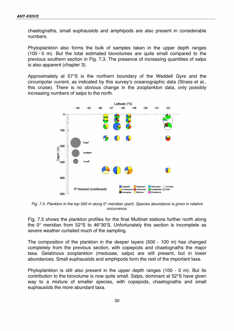
Fig. 7.5: Plankton in the top 500 m along 0° meridian (part). Species abundance is given in relative
occurrence.
Fig. 7.5 shows the plankton profiles for the final Multinet stations further north along
the 0° meridian from 52°S to 46°30 S. Unfortunately this section is incomplete as
severe weather curtailed much of the sampling.
The composition of the plankton in the deeper layers (500 - 100 m) has changed
completely from the previous section, with copepods and chaetognaths the major
taxa. Gelatinous zooplankton (medusae, salps) are still present, but in lower
abundances. Small euphausiids and amphipods form the rest of the important taxa.
Phytoplankton is still also present in the upper depth ranges (100 - 0 m). But its
contribution to the biovolume is now quite small. Salps, dominant at 52°S have given
way to a mixture of smaller species, with copepods, chaetognaths and small
euphausiids the more abundant taxa.
7. Multinet sampling during ANT-XXVI/2
31
Approximately at 49°30 S is the Polar Front. Unfortunately there are no samples
around that position, but it is quite clear that the plankton composition north of the
Polar Front is quite different from that to the south.
Concluding remarks
This study has served to show the preliminary results of stratified plankton
distribution and abundance from the Lazarev Sea survey area, and beyond to the
north, following the 0° meridian to 46°30 S. For the most part, the results seem to
reflect differences within the oceanographic processes. But in some instances it is
not so clear, especially north of the LAKRIS survey grid.
As the results of the plankton species abundance are only estimates of
biovolume/biomass for each sample, it will not be clear until all samples are fully
analysed back in the laboratories at the Alfred Wegener Institute. Although the
proportion of some plankton groups may seem to be unchanged from south to north
along each transect, it is extremely likely that the actual species compositions are
completely different. Only detailed sample analysis will realise this, and then
associations between plankton and oceanographic processes may be clearer.
32
8. BIOLOGY OF OITHONA SIMILIS (COPEPODA: CYLOPOIDA) IN THE SOUTHERN OCEAN Britta Wend, Ulrich Bathmann
Alfred-Wegener-Institut, Bremerhaven,
Germany
Objective
Oithona similis belongs to the order of cyclopoid copepods. It is highly abundant
throughout many parts of the world ocean and is supposed to be a cosmopolitan
species. The work on this cruise is part of a project that challenges whether O.
similis, a key species in three chosen study areas (Southern Ocean, Arctic Ocean
and North Sea), is indeed a cosmopolitan. A further goal is a better understanding of
its life cycle (or the cycles of the existing cryptic species).
Work at sea
It was possible to take samples at 17 stations throughout the three transects. Oithona
similis is an epipelagic copepod. Therefore sampling was restricted to the upper
250 m of the water column. Samples were collected via 23 Niskin bottles mounted on
a CTD and with an additionally towed multinet (mesh size: 55 μm). At each chosen
depth (10, 20, 40, 60, 80, 100, 125, 150, 200, 250 m) two or three bottles were
closed. The 12 l out of the Niskin bottles were directly concentrated through 20 μm
gauze to a final volume of 50 ml per depth. This volume was immediately fixed in
formalin for morphological identifications of species, reproduction in the field as well
as feeding habits. With this method higher numbers of the first developmental stages
were caught than by the multinet (used depths strata of the net: 250 - 200 m,
200 - 150 m, 150 - 100 m, 100 - 50 m, 50 - 0 m). For genetical investigations adult
individuals were picked out of all multinet samples and preserved in ethanol.
Additional adults were fixed in formalin for closer morphological investigations.
Outlook
The first step at the home laboratory will be the genetic investigations as they
determine the further procedure. If their results hint on the existence of cryptic
species in the nominal O. similis, the adult formalin fixed individuals will then be
analysed with a focus on eventually existing differences in the morphology. If the
existence of only one species is supported, the project will concentrate on the
analyses of reproduction, stage distribution and gut content for this species.
33
9. SALP DISTRIBUTION IN THE LAZAREV SEA, DECEMBER - JANUARY 2007/08 John Kitchener1), Sarah Herrmann2),
Evgeny Pakhomov3) (not on board)
1) Australian Antarctic Division, Australia
2) Alfred-Wegener-Institut, Bremerhaven,
Germany
3)University of British Columbia, Canada
Background and objectives
In the Southern Ocean the pelagic tunicates, in particular the salps Salpa thompsoni
and Ihlea racovitzai are very important components of the zooplankton community.
Salps are of great interest as they occur at certain seasons in dense concentrations
or swarms. They are a short-lived species, which exhibit rapid population growth.
Salps have high grazing rates and, as they are primarily herbivores (predominately
feeding upon marine phytoplankton), they must play an important role in consuming
significant quantities of primary production. Where their distributions overlap with
other key herbivores such as the Antarctic krill Euphausia superba, there must be
competition for food, and this has implications for the functioning and trophic
dynamics of the high Antarctic ecosystem.
Since the austral autumn of 2004, the LAKRIS project has conducted a regular
survey of the Lazarev Sea (3oE to 3oW), south of 60oS. Since the first survey, a
spring and winter survey followed soon after to maintain collection of data on the
seasonal and interannual variability of the krill distribution and demography in high
latitude areas, which are covered by sea ice for the most part of the year. Other
biomass dominant zooplankton species such as salps, collected along with krill,
provides an additional insight on processes influencing the high latitude Lazarev Sea
ecosystem.
Work at sea
This current cruise ANT-XXIV/2 formed part of an ongoing study of salp distribution
and abundance in the Lazarev Sea. Salps were collected whenever they occurred
throughout a sampling grid of double oblique RMT-8 net tows between 0 and 200 m.
Where possible, several salps representative of the size ranges were frozen at -80° C
for later HPLC analysis. These were only taken from the routine RMT-8 trawls. The
size and development stage of all aggregate and solitary salps was only done for
individuals being frozen. The remaining salps from each catch were fixed in 4 %
buffered formaldehyde for demographic and other biological studies back at the
Alfred Wegener Institute.
Additional salps for gut fluorescence analysis were collected opportunistically from
mesopelagic tows using the multiple RMT-8 (0 - 1,000 m) and SUIT nets conducted
ANT-XXIV/2
34
both during the grid survey and from the routine RMT-8 at a sampling station of 52oS
on the Greenwich Meridian.
Gut fluorescence measurement is a method to determine the amount of chlorophyll a
in the guts of the animals. As salps are filter-feeders a high amount of seawater flows
through their body. The phytoplankton distributed in the seawater is being
accumulated in their guts. It is common to specify the content of phytoplankton in the
water column by μg chlorophyll a per litre of seawater. The same is possible for
determining the chlorophyll a content in the guts of salps. The result is then divided
by the length in cm of the individual. In the end the chlorophyll a content can be seen
in relation to the body length or oral-atrial length of the salps, and furthermore in
relation to the total chlorophyll a content in the water column which forms the feeding
environment of the salps.
Immediately after capture the stomachs of ~5 salps from each size group,
representative of the size range, were dissected out and placed in 10 ml of 90 %
acetone for gut pigment extraction in darkness at -26°C for at least 12 hours.
9. Salp distribution in the Lazarev Sea, December - January 2007/08
35
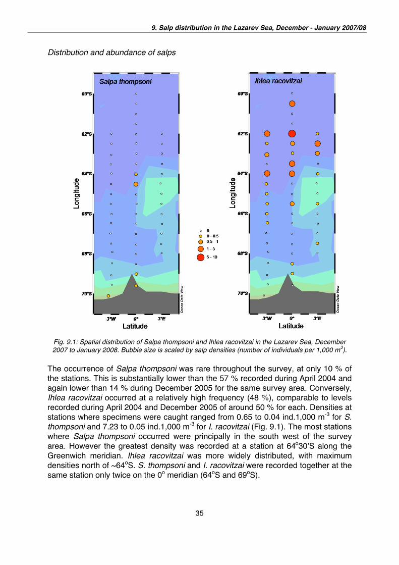
Distribution and abundance of salps
Fig. 9.1: Spatial distribution of Salpa thompsoni and Ihlea racovitzai in the Lazarev Sea, December
2007 to January 2008. Bubble size is scaled by salp densities (number of individuals per 1,000 m3).
The occurrence of Salpa thompsoni was rare throughout the survey, at only 10 % of
the stations. This is substantially lower than the 57 % recorded during April 2004 and
again lower than 14 % during December 2005 for the same survey area. Conversely,
Ihlea racovitzai occurred at a relatively high frequency (48 %), comparable to levels
recorded during April 2004 and December 2005 of around 50 % for each. Densities at
stations where specimens were caught ranged from 0.65 to 0.04 ind.1,000 m-3 for S.
thompsoni and 7.23 to 0.05 ind.1,000 m-3 for I. racovitzai (Fig. 9.1). The most stations
where Salpa thompsoni occurred were principally in the south west of the survey
area. However the greatest density was recorded at a station at 64o30 S along the
Greenwich meridian. Ihlea racovitzai was more widely distributed, with maximum
densities north of ~64oS. S. thompsoni and I. racovitzai were recorded together at the
same station only twice on the 0o meridian (64oS and 69oS).
ANT-XXIV/2
36
Salp size and stage structure
Apart from the frozen samples, salps were not measured before they were fixed. This
will be done post-voyage at AWI. Of the frozen samples, the Salpa thompsoni
population structure was dominated by aggregate forms, with only one solitary
specimen (78 mm) collected during the Lazarev Sea grid survey. The aggregate
population was comprised predominantly of individuals 10 -13 mm in length, with
specimens either being stage 1 or stage X. Ihlea racovitzai collected during the
survey were all solitary animals (420 individuals), apart from 3 aggregate forms. This
species was dominated by animals 20 -30 mm in length, however there was another
major size class between 50 - 70 mm.
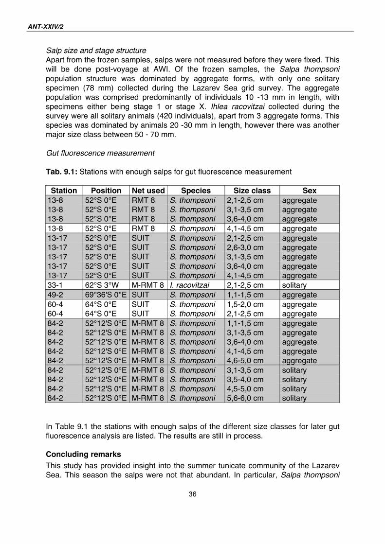
Gut fluorescence measurement
Tab. 9.1: Stations with enough salps for gut fluorescence measurement
Station Position Net used Species Size class Sex 13-8 52°S 0°E RMT 8 S. thompsoni 2,1-2,5 cm aggregate
13-8 52°S 0°E RMT 8 S. thompsoni 3,1-3,5 cm aggregate
13-8 52°S 0°E RMT 8 S. thompsoni 3,6-4,0 cm aggregate
13-8 52°S 0°E RMT 8 S. thompsoni 4,1-4,5 cm aggregate
13-17 52°S 0°E SUIT S. thompsoni 2,1-2,5 cm aggregate
13-17 52°S 0°E SUIT S. thompsoni 2,6-3,0 cm aggregate
13-17 52°S 0°E SUIT S. thompsoni 3,1-3,5 cm aggregate
13-17 52°S 0°E SUIT S. thompsoni 3,6-4,0 cm aggregate
13-17 52°S 0°E SUIT S. thompsoni 4,1-4,5 cm aggregate
33-1 62°S 3°W M-RMT 8 I. racovitzai 2,1-2,5 cm solitary
49-2 69°36'S 0°E SUIT S. thompsoni 1,1-1,5 cm aggregate
60-4 64°S 0°E SUIT S. thompsoni 1,5-2,0 cm aggregate
60-4 64°S 0°E SUIT S. thompsoni 2,1-2,5 cm aggregate
84-2 52°12'S 0°E M-RMT 8 S. thompsoni 1,1-1,5 cm aggregate
84-2 52°12'S 0°E M-RMT 8 S. thompsoni 3,1-3,5 cm aggregate
84-2 52°12'S 0°E M-RMT 8 S. thompsoni 3,6-4,0 cm aggregate
84-2 52°12'S 0°E M-RMT 8 S. thompsoni 4,1-4,5 cm aggregate
84-2 52°12'S 0°E M-RMT 8 S. thompsoni 4,6-5,0 cm aggregate
84-2 52°12'S 0°E M-RMT 8 S. thompsoni 3,1-3,5 cm solitary
84-2 52°12'S 0°E M-RMT 8 S. thompsoni 3,5-4,0 cm solitary
84-2 52°12'S 0°E M-RMT 8 S. thompsoni 4,5-5,0 cm solitary
84-2 52°12'S 0°E M-RMT 8 S. thompsoni 5,6-6,0 cm solitary
In Table 9.1 the stations with enough salps of the different size classes for later gut
fluorescence analysis are listed. The results are still in process.
Concluding remarks
This study has provided insight into the summer tunicate community of the Lazarev
Sea. This season the salps were not that abundant. In particular, Salpa thompsoni
9. Salp distribution in the Lazarev Sea, December - January 2007/08
37
numbers were quite rare within the LAKRIS survey area. Even though Ihlea racovitzai
were found in just under half the trawls, numbers of individuals were quite small.
Van Franeker et al. (chapter 12) reports that the sea ice edge for the 3oW and 3oE
transects were approximately at 62oS and 63o30 S respectively. By the time the survey
had commenced the 0o meridian, the sea ice had retreated to about 67o30 S. It is
notable that only one specimen of Salpa thompsoni was collected throughout the first
two survey transects (3oE and 3oW) where ice coverage was relatively high.
Conversely, the lower ice coverage of the 0o meridian transect revealed some, but not
many, S. thompsoni. As well, most of Ihlea racovitzai were found within the northern
half of the survey area, and mostly along the 0o meridian. It seems that possibly the
high ice coverage for this season may have contributed to the overall lower numbers
of salps collected during this survey.
38
10. CARNIVOROUS ZOOPLANKTON IN THE MESOPELAGIC FOOD WEB OF THE SOUTHERN OCEAN Svenja Kruse, Ulrich Bathmann
Alfred-Wegener-Institut,
Bremerhaven, Germany
Objectives
During this cruise the project was focused on the distribution and the abundance of
deep-living carnivorous chaetognaths and amphipods, their feeding habits and their
predation impact as well as their role in the carbon cycle. Special attention has been
given to the depth range between 500 and 2,500 m. As expedition ANT-XXIII/6
already provided information about the winter situation this expedition should
complete the existing picture of the mentioned carnivorous zooplankters in this area.
Among the chaetognaths special attention has been given to the species Eukrohnia
hamata and the two deep water species E. bathypelagica and E. bathyantarctica. In
addition the amphipods Cyllopus lucasii and Primno macropa were of special
interest.
Work at sea
Investigations on board Polarstern were done by a combination of sampling and
experimental approaches. Stratified sampling was performed at 15 stations along
three transects (3°W, 3°E and 0°) down to 2,000 m with a multinet. This multiple
opening/closing net was equipped with five nets of 100 m mesh size and sampled
the following 5 standard depth intervals: 2,000 - 1,500 m, 1,500 - 1,000 m, 1,000 -
750 m, 750 - 500 m, 500 - 0 m. All chaetognaths were sorted out of the four deeper
samples. The remaining zooplankton samples had been preserved in formaldehyde
(4 %) and will be analysed quantitavely at the Alfred Wegener Institute later on.
These data will complement the standard 500 m-multinet catch (compare multinet
sampling by John Kitchener, chapter 7).
The chaetognaths from these samples were all determined, staged, counted and
measured. Most of them, in particular the ones in good condition, were then
immediately stored at –80°C for later analysis (C/N, gut content, lipids and fatty
acids). Additional actively swimming specimens from depth layers between 500 and
1,000 m were kept in a cooling container at 0°C for respiration experiments
(according to the Winkler-method).
The amphipods were taken from 34 RMT 8 (rectangular midwater trawl; upper
200 m) and 4 SUIT (surface under ice trawl) samples along the three transects.
Among the two amphipods of main interest, Cyllopus lucasii was the more abundant
species. Therefore specimens of both species were frozen for later anlaysis, but
10. Carnivorous zooplankton in the mesopelagic food web of the Southern Ocean
39
experiments could only be conducted with Cyllopus lucasii. Respiration as well as
feeding experiments (with phytoplankton or zooplankton as food source) were done
after a starvation period of 48 h. The produced faecal pellets were taken for
measurements of the sinking velocities. The size has been measured, the CN-ratio
will be investigated later on.
Four multiple RMTs were additionally deployed throughout the cruise down to depth
between 1,900 and 2,500 m. This trawl consists of three pairs of nets, each of which
comprises an RMT 1 (0,33 mm mesh size, 1 m mouth area) and an RMT 8 (4,5 mm
mesh size, 8 m mouth area). By this means three depth intervals below 500 m water
depth could be sampled. The intervals were variable, but we tried to choose them
according to the intervals of the multinet (2,000 – 1,500 – 1,000 – 500 m).
Chaetognaths and amphipods were again separated from the other zooplankton
groups. Most chaetognaths were determined and counted. The quantitative analysis
of the complete samples will be done in the home laboratories.
Preliminary results
Frequency of occurrence and composition of chaetognaths caught with the multinet
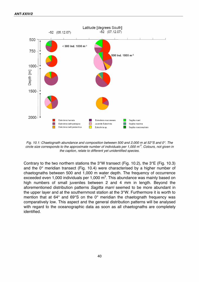
The first station was located on the prime meridian at 52° S, where two multinets
were taken two days apart from each other (Fig. 10.1). The number of chaetognaths
comprised of less than 500 individuals per 1,000 m3 over the total depth range in
both catches. The species Eukrohnia hamata occurred over the full depth range, but
decreased in number with the depth. This was also found with Sagitta marri which
were even missed between 1,500 and 2,000 m depth. However, the abundances of
the species Eukrohnia bathypelagica and Eukrohnia bathyantarctica increased with
the depth. Large chaetognaths like Sagitta gazellae were rarely caught with this type
of net. Despite of these similarities, both catches taken at the same station looked
quite different. Especially the occurrence of juvenile chaetognaths was unlike. The
difference in time between the sampling as well as the drifting of the ship (i.e.
geographical distinctions) may have caused this.
ANT-XXIV/2
40
Fig. 10.1: Chaetognath abundance and composition between 500 and 2,000 m at 52°S and 0°. The
circle size corresponds to the approximate number of individuals per 1,000 m-3
. Colours, not given in
the caption, relate to different yet unidentified species.
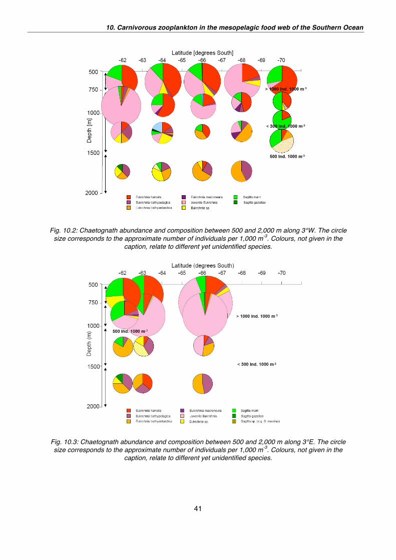
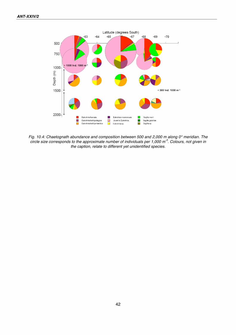
Contrary to the two northern stations the 3°W transect (Fig. 10.2), the 3°E (Fig. 10.3)
and the 0° meridian transect (Fig. 10.4) were characterised by a higher number of
chaetognaths between 500 and 1,000 m water depth. The frequency of occurrence
exceeded even 1,000 individuals per 1,000 m3. This abundance was mainly based on
high numbers of small juveniles between 2 and 4 mm in length. Beyond the
aforementioned distribution patterns Sagitta marri seemed to be more abundant in
the upper layer and at the southernmost station at the 3°W. Furthermore it is worth to
mention that at 64° and 69°S on the 0° meridian the chaetognath frequency was
comparatively low. This aspect and the general distribution patterns will be analysed
with regard to the oceanographic data as soon as all chaetognaths are completely
identified.
10. Carnivorous zooplankton in the mesopelagic food web of the Southern Ocean
41
Fig. 10.2: Chaetognath abundance and composition between 500 and 2,000 m along 3°W. The circle
size corresponds to the approximate number of individuals per 1,000 m-3
. Colours, not given in the
caption, relate to different yet unidentified species.
Fig. 10.3: Chaetognath abundance and composition between 500 and 2,000 m along 3°E. The circle
size corresponds to the approximate number of individuals per 1,000 m-3
. Colours, not given in the
caption, relate to different yet unidentified species.
ANT-XXIV/2
42
Fig. 10.4: Chaetognath abundance and composition between 500 and 2,000 m along 0° meridian. The
circle size corresponds to the approximate number of individuals per 1,000 m-3
. Colours, not given in
the caption, relate to different yet unidentified species.
43
11. DEMOGRAPHY OF ANTARCTIC KRILL AND OTHER EUPHAUSIACEA IN THE LAZAREV SEA IN SUMMER 2008 Volker Siegel (not on board), Jens
Edinger, Matilda Haraldsson, Karoline
Stürmer, Martina Vortkamp
J.H. von Thünen-Institut, Hamburg,
Germany
Introduction and objectives
Sea ice is one of the major environmental parameters that influence the Antarctic
marine ecosystem. Sea ice extent shows enormous seasonal fluctuations, ranging
from 4.1 * 106 km2 in summer to 21.5 * 106 km2 in winter. Seasonal as well as
interannual fluctuations in ice cover are likely to have an effect on the distribution, life
cycle and population dynamics of Antarctic krill, Euphausia superba, which is the key
prey species for most of the Antarctic pelagic and land-based predators. Recent
research results have indicated that krill may switch from a pelagic swarming and
filter feeding life in summer to a grazing behaviour on ice algae on the under-surface
of sea ice. However, information is still lacking on krill distribution, abundance, growth
and development of maturation and spawning in this sea ice habitat.
Due to great difficulties for research vessels to work in such ice-covered areas,
quantitative studies on krill population parameters are still extremely scarce in the
scientific literature. The Lazarev Sea is located in the high-latitude part of the E.
superba range, immediately adjacent to the Antarctic continent. Antarctic water
masses extend over more than 2,400 km between the continent and the Polar Front.
It is also one of the regions with greatest sea ice extent of the Antarctic Ocean in
winter, from the continent at 70°S to approximately 58°S, i.e. more than 1,300 km.
These conditions contrasting to the well-studied Antarctic Peninsula or Scotia Sea
regions, where even during winter part of the krill distribution range is free of sea ice.
Accordingly, one of the main objectives for the LAKRIS project onboard Polarstern
was to conduct several standardized surveys in the area during different. The primary
objective of the RMT-net sampling programme was to clarify krill population
distribution dynamics over the year and study the effects of the advancing or
retreating pack-ice on the demography and the maturation and spawning process of
krill. After we successfully conducted LAKRIS studies in autumn 2004, spring
2005/06 and winter 2006, the current summer survey in 2007/08 marked the final
point in this data collection series.
ANT-XXIV/2
44
Work at sea
Material and Methods
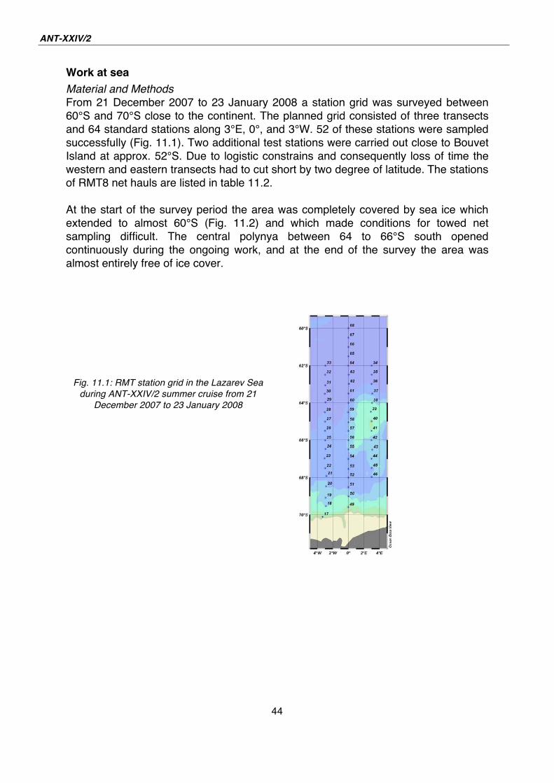
From 21 December 2007 to 23 January 2008 a station grid was surveyed between
60°S and 70°S close to the continent. The planned grid consisted of three transects
and 64 standard stations along 3°E, 0°, and 3°W. 52 of these stations were sampled
successfully (Fig. 11.1). Two additional test stations were carried out close to Bouvet
Island at approx. 52°S. Due to logistic constrains and consequently loss of time the
western and eastern transects had to cut short by two degree of latitude. The stations
of RMT8 net hauls are listed in table 11.2.
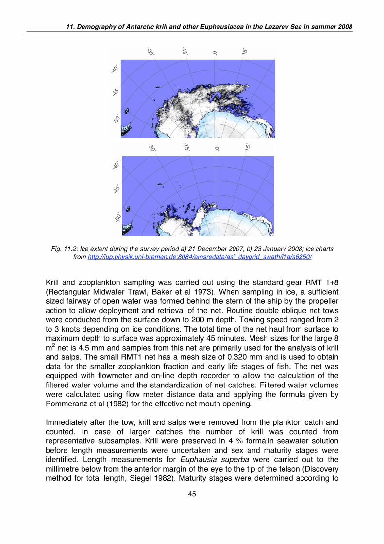
At the start of the survey period the area was completely covered by sea ice which
extended to almost 60°S (Fig. 11.2) and which made conditions for towed net
sampling difficult. The central polynya between 64 to 66°S south opened
continuously during the ongoing work, and at the end of the survey the area was
almost entirely free of ice cover.
Fig. 11.1: RMT station grid in the Lazarev Sea
during ANT-XXIV/2 summer cruise from 21
December 2007 to 23 January 2008
11. Demography of Antarctic krill and other Euphausiacea in the Lazarev Sea in summer 2008
45
Fig. 11.2: Ice extent during the survey period a) 21 December 2007, b) 23 January 2008; ice charts
from http://iup.physik.uni-bremen.de:8084/amsredata/asi_daygrid_swath/l1a/s6250/
Krill and zooplankton sampling was carried out using the standard gear RMT 1+8
(Rectangular Midwater Trawl, Baker et al 1973). When sampling in ice, a sufficient
sized fairway of open water was formed behind the stern of the ship by the propeller
action to allow deployment and retrieval of the net. Routine double oblique net tows
were conducted from the surface down to 200 m depth. Towing speed ranged from 2
to 3 knots depending on ice conditions. The total time of the net haul from surface to
maximum depth to surface was approximately 45 minutes. Mesh sizes for the large 8
m2 net is 4.5 mm and samples from this net are primarily used for the analysis of krill
and salps. The small RMT1 net has a mesh size of 0.320 mm and is used to obtain
data for the smaller zooplankton fraction and early life stages of fish. The net was
equipped with flowmeter and on-line depth recorder to allow the calculation of the
filtered water volume and the standardization of net catches. Filtered water volumes
were calculated using flow meter distance data and applying the formula given by
Pommeranz et al (1982) for the effective net mouth opening.
Immediately after the tow, krill and salps were removed from the plankton catch and
counted. In case of larger catches the number of krill was counted from
representative subsamples. Krill were preserved in 4 % formalin seawater solution
before length measurements were undertaken and sex and maturity stages were
identified. Length measurements for Euphausia superba were carried out to the
millimetre below from the anterior margin of the eye to the tip of the telson (Discovery
method for total length, Siegel 1982). Maturity stages were determined according to
ANT-XXIV/2
46
the classification of Makarov and Denys (1981). Other euphausiid species were
measured from the tip of the rostrum to the posterior end of the uropods (standard 1
length according to Mauchline 1980) and separated into males and females. The rest
of the zooplankton was preserved in 4 % formalin solution for later land based sorting
and analysis. All station data and the biological counts and measurements were
entered into the database of the Institut für Seefischerei Hamburg. A station summary
is given in the Appendix Table at the end.
Preliminary Results
Distribution and Abundance
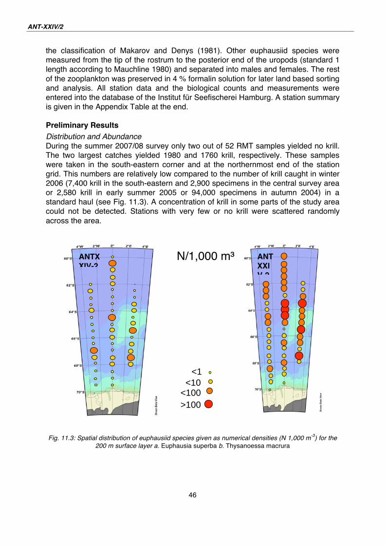
During the summer 2007/08 survey only two out of 52 RMT samples yielded no krill.
The two largest catches yielded 1980 and 1760 krill, respectively. These samples
were taken in the south-eastern corner and at the northernmost end of the station
grid. This numbers are relatively low compared to the number of krill caught in winter
2006 (7,400 krill in the south-eastern and 2,900 specimens in the central survey area
or 2,580 krill in early summer 2005 or 94,000 specimens in autumn 2004) in a
standard haul (see Fig. 11.3). A concentration of krill in some parts of the study area
could not be detected. Stations with very few or no krill were scattered randomly
across the area.
Fig. 11.3: Spatial distribution of euphausiid species given as numerical densities (N 1,000 m
-3) for the
200 m surface layer a. Euphausia superba b. Thysanoessa macrura
ANTXXIV-2
<1
<10 <100
>100
ANTXXIV 2
N/1,000 m
11. Demography of Antarctic krill and other Euphausiacea in the Lazarev Sea in summer 2008
47
Krill abundance estimates for the current summer Lazarev survey results in 4.3 krill
1,000 m-3, This is a significant decrease compared to the mean numerical densities
for the Lazarev Sea survey compared to the preceding winter survey 2006. However,
the recent results are comparable to the low results of the summer survey 2005/06
(see Tab. 11.1). Since the station grid covered more or less the same area since
2004, a regional effect can be excluded as the potential reason for the inter-survey
differences. At this stage, it is unclear, whether we are observing interannual effects
in stock size development caused by immigration and emigration or interannual
changes caused by dramatic fluctuations in stock size.
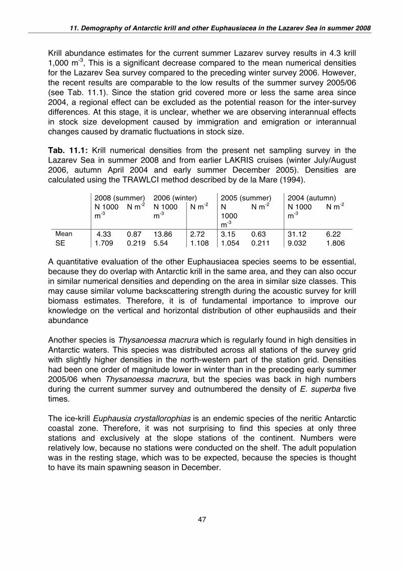
Tab. 11.1: Krill numerical densities from the present net sampling survey in the
Lazarev Sea in summer 2008 and from earlier LAKRIS cruises (winter July/August
2006, autumn April 2004 and early summer December 2005). Densities are
calculated using the TRAWLCI method described by de la Mare (1994).
2008 (summer) 2006 (winter) 2005 (summer) 2004 (autumn) N 1000
m-3
N m-2 N 1000
m-3
N m-2 N
1000
m-3
N m-2 N 1000
m-3
N m-2
Mean 4.33 0.87 13.86 2.72 3.15 0.63 31.12 6.22
SE 1.709 0.219 5.54 1.108 1.054 0.211 9.032 1.806
A quantitative evaluation of the other Euphausiacea species seems to be essential,
because they do overlap with Antarctic krill in the same area, and they can also occur
in similar numerical densities and depending on the area in similar size classes. This
may cause similar volume backscattering strength during the acoustic survey for krill
biomass estimates. Therefore, it is of fundamental importance to improve our
knowledge on the vertical and horizontal distribution of other euphausiids and their
abundance
Another species is Thysanoessa macrura which is regularly found in high densities in
Antarctic waters. This species was distributed across all stations of the survey grid
with slightly higher densities in the north-western part of the station grid. Densities
had been one order of magnitude lower in winter than in the preceding early summer
2005/06 when Thysanoessa macrura, but the species was back in high numbers
during the current summer survey and outnumbered the density of E. superba five
times.
The ice-krill Euphausia crystallorophias is an endemic species of the neritic Antarctic
coastal zone. Therefore, it was not surprising to find this species at only three
stations and exclusively at the slope stations of the continent. Numbers were
relatively low, because no stations were conducted on the shelf. The adult population
was in the resting stage, which was to be expected, because the species is thought
to have its main spawning season in December.
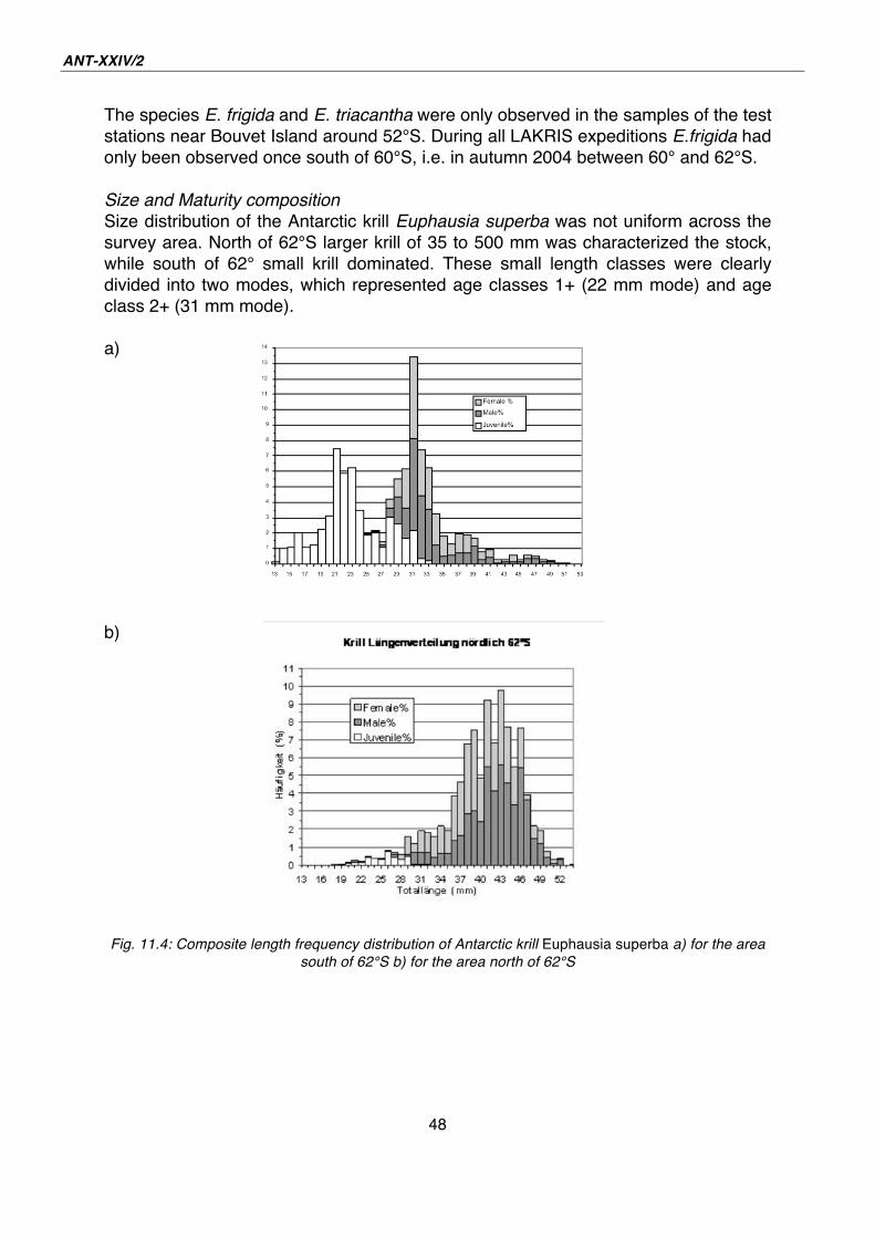
ANT-XXIV/2
48
The species E. frigida and E. triacantha were only observed in the samples of the test
stations near Bouvet Island around 52°S. During all LAKRIS expeditions E.frigida had
only been observed once south of 60°S, i.e. in autumn 2004 between 60° and 62°S.
Size and Maturity composition
Size distribution of the Antarctic krill Euphausia superba was not uniform across the
survey area. North of 62°S larger krill of 35 to 500 mm was characterized the stock,
while south of 62° small krill dominated. These small length classes were clearly
divided into two modes, which represented age classes 1+ (22 mm mode) and age
class 2+ (31 mm mode).
a)
b)
Fig. 11.4: Composite length frequency distribution of Antarctic krill Euphausia superba a) for the area
south of 62°S b) for the area north of 62°S
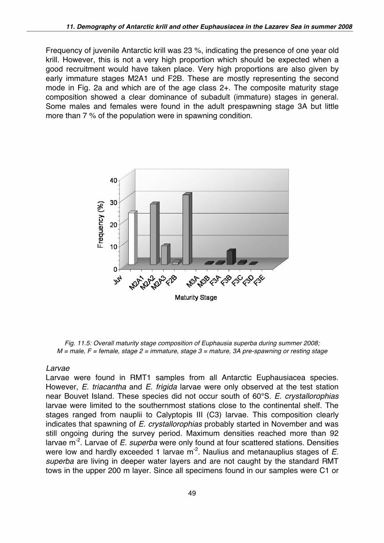
11. Demography of Antarctic krill and other Euphausiacea in the Lazarev Sea in summer 2008
49
Frequency of juvenile Antarctic krill was 23 %, indicating the presence of one year old
krill. However, this is not a very high proportion which should be expected when a
good recruitment would have taken place. Very high proportions are also given by
early immature stages M2A1 und F2B. These are mostly representing the second
mode in Fig. 2a and which are of the age class 2+. The composite maturity stage
composition showed a clear dominance of subadult (immature) stages in general.
Some males and females were found in the adult prespawning stage 3A but little
more than 7 % of the population were in spawning condition.
Fig. 11.5: Overall maturity stage composition of Euphausia superba during summer 2008;
M = male, F = female, stage 2 = immature, stage 3 = mature, 3A pre-spawning or resting stage
Larvae
Larvae were found in RMT1 samples from all Antarctic Euphausiacea species.
However, E. triacantha and E. frigida larvae were only observed at the test station
near Bouvet Island. These species did not occur south of 60°S. E. crystallorophias
larvae were limited to the southernmost stations close to the continental shelf. The
stages ranged from nauplii to Calyptopis III (C3) larvae. This composition clearly
indicates that spawning of E. crystallorophias probably started in November and was
still ongoing during the survey period. Maximum densities reached more than 92
larvae m-2. Larvae of E. superba were only found at four scattered stations. Densities
were low and hardly exceeded 1 larvae m-2. Naulius and metanauplius stages of E.
superba are living in deeper water layers and are not caught by the standard RMT
tows in the upper 200 m layer. Since all specimens found in our samples were C1 or
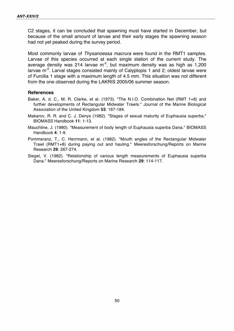
ANT-XXIV/2
50
C2 stages, it can be concluded that spawning must have started in December, but
because of the small amount of larvae and their early stages the spawning season
had not yet peaked during the survey period.
Most commonly larvae of Thysanoessa macrura were found in the RMT1 samples.
Larvae of this species occurred at each single station of the current study. The
average density was 214 larvae m-2, but maximum density was as high as 1,200
larvae m-2. Larval stages consisted mainly of Calyptopis 1 and 2; oldest larvae were
of Furcilia 1 stage with a maximum length of 4.5 mm. This situation was not different
from the one observed during the LAKRIS 2005/06 summer season.
References Baker, A. d. C., M. R. Clarke, et al. (1973). "The N.I.O. Combination Net (RMT 1+8) and
further developments of Rectangular Midwater Trawls." Journal of the Marine Biological
Association of the United Kingdom 53: 167-184.
Makarov, R. R. and C. J. Denys (1982). "Stages of sexual maturity of Euphausia superba."
BIOMASS Handbook 11: 1-13.
Mauchline, J. (1980). "Measurement of body length of Euphausia superba Dana." BIOMASS
Handbook 4: 1-9.
Pommeranz, T., C. Herrmann, et al. (1982). "Mouth angles of the Rectangular Midwater
Trawl (RMT1+8) during paying out and hauling." Meeresforschung/Reports on Marine
Research 29: 267-274.
Siegel, V. (1982). "Relationship of various length measurements of Euphausia superba
Dana." Meeresforschung/Reports on Marine Research 29: 114-117.
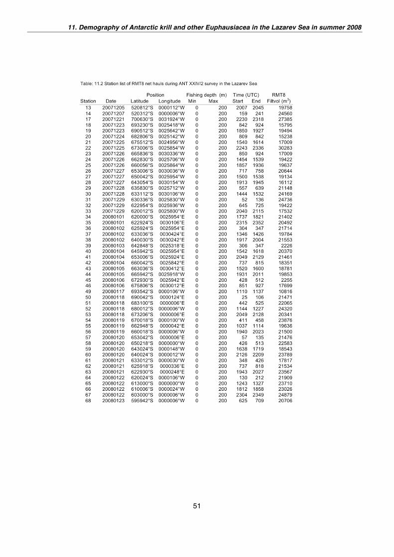
11. Demography of Antarctic krill and other Euphausiacea in the Lazarev Sea in summer 2008
51
52
12. MACROZOOPLANKTON AND MICRONEKTON IN THE SURFACE LAYER AND UNDER SEA ICE Hauke Flores, Jan Andries van Franeker,
Bram Feij, Andre Meijboom, Michiel van
Dorssen
IMARES, Texel, The
Netherlands
Introduction and objectives
The seasonal sea ice zone of the Southern Ocean is well known for its rich wildlife. In
summer, high densities of warm blooded top predators (birds, seals, whales)
concentrate at the ice edge and often increase towards the inner pack-ice, indicating
considerable primary and secondary production in these areas (Van Franeker et al.
1997). Water column primary production, however, is low in ice-covered waters. In
recent years, ice algae have gained increasing attention as a major source of
production in the sea ice system. However, the physical and biochemical complexity
of the ice environment has posed difficulties to an accurate determination of ice algal
productivity so far. Another way to shed light on the energy flow in the sea ice system
is to follow the food chains from higher trophic levels downwards (van Franeker et al.,
this volume). In order to explain feeding and prey distribution of the higher level
predators in the ice-covered ocean, a good understanding of the ice-associated
species community is essential. The structure and capacity of the sea ice system are
not yet clearly understood. Sea ice seems to be an important factor in the ecology of
larval and adult krill Euphausia superba (Loeb et al. 1997, Atkinson et al. 2004).
Repeated reports of dense aggregations of krill directly under ice stress the
importance of this habitat for the euphausiid (e.g. Brierly et al. 2002). To date, little is
known to which extent krill, fish, squid or other macrofauna can be found under the
sea ice. At IMARES Texel, the need to investigate the under-ice habitat in more detail
led to the development of a special under-ice trawl (SUIT = Surface and Under Ice
Trawl). Due to the dynamic nature of the subsurface environment, a close interaction
with the water column system can be expected. Therefore it is essential to view the
data collected from the surface layer in the context of physical, chemical and
biological data from the entire water column down to the sea floor. The summer
expedition ANT-XXIV/2 provided an excellent opportunity to collect a wide range of
data in a concerted manner, forming the basis for an integrated analysis.
Work at sea
Materials & Methods
Trawling of SUIT was attempted 19 times on the regular RMT station grid and twice
at one station in the Antarctic Circumpolar Current between 5 December 2007 and 22
January 2008 (Fig. 12.1). The net system consisted of a steel frame with a 2.1 x
2.1 m net opening and a 15 m long 7 mm halfmesh commercial shrimp net attached
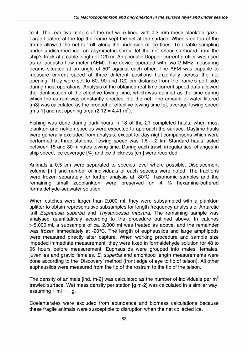
12. Macrozooplankton and micronekton in the surface layer and under sea ice
53
to it. The rear two meters of the net were lined with 0.3 mm mesh plankton gaze.
Large floaters at the top the frame kept the net at the surface. Wheels on top of the
frame allowed the net to roll along the underside of ice floes. To enable sampling
under undisturbed ice, an asymmetric sprout let the net shear starboard from the
ship s track at a cable length of 120 m. An acoustic Doppler current profiler was used
as an acoustic flow meter (AFM). The device operated with two 2 MHz measuring
beams situated at an angle of 50° against each other. The AFM was capable to
measure current speed at three different positions horizontally across the net
opening. They were set to 60, 90 and 120 cm distance from the frame s port side
during most operations. Analysis of the obtained real-time current speed data allowed
the identification of the effective towing time, which was defined as the time during
which the current was constantly directed into the net. The amount of water filtered
[m3] was calculated as the product of effective towing time [s], average towing speed
[m s-1] and net opening area (2.12 = 4.41 m2).
Fishing was done during dark hours in 18 of the 21 completed hauls, when most
plankton and nekton species were expected to approach the surface. Daytime hauls
were generally excluded from analysis, except for day-night comparisons which were
performed at three stations. Towing speed was 1.5 – 2 kn. Standard hauls lasted
between 15 and 30 minutes towing time. During each trawl, irregularities, changes in
ship speed, ice coverage [%] and ice thickness [cm] were recorded.
Animals 0.5 cm were separated to species level where possible. Displacement
volume [ml] and number of individuals of each species were noted. The fractions
were frozen separately for further analysis at -80°C. Taxonomic samples and the
remaining small zooplankton were preserved on 4 % hexamine-buffered
formaldehyde-seawater solution.
When catches were larger than 2,000 ml, they were subsampled with a plankton
splitter to obtain representative subsamples for length-frequency analysis of Antarctic
krill Euphausia superba and Thysanoessa macrura. The remaining sample was
analysed quantitatively according to the procedure outlined above. In catches
> 5,000 ml, a subsample of ca. 2,000 ml was treated as above, and the remainder
was frozen immediately at -20°C. The length of euphausiids and large amphipods
were measured directly after capture. When working procedure and sample size
impeded immediate measurement, they were fixed in formaldehyde solution for 48 to
96 hours before measurement. Euphausiids were grouped into males, females,
juveniles and gravid females. E. superba and amphipod length measurements were
done according to the Discovery method (front edge of eye to tip of telson). All other
euphausiids were measured from the tip of the rostrum to the tip of the telson.
The density of animals [ind. m-2] was calculated as the number of individuals per m2
trawled surface. Wet mass density per station [g m-2] was calculated in a similar way,
assuming 1 ml = 1 g.
Coelenterates were excluded from abundance and biomass calculations because
these fragile animals were susceptible to disruption when the net collected ice.
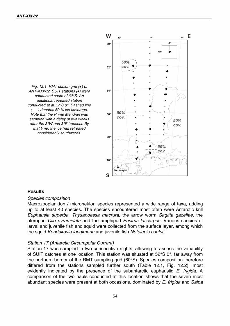
ANT-XXIV/2
54
Fig. 12.1: RMT station grid ( ) of
ANT-XXIV/2. SUIT stations ( ) were
conducted south of 62°S. An
additional repeated station
conducted at at 52°S 0°. Dashed line
(- - -) denotes 50 % ice coverage.
Note that the Prime Meridian was
sampled with a delay of two weeks
after the 3°W and 3°E transect. By
that time, the ice had retreated
considerably southwards.
Results
Species composition
Macrozooplankton / micronekton species represented a wide range of taxa, adding
up to at least 40 species. The species encountered most often were Antarctic krill
Euphausia superba, Thysanoessa macrura, the arrow worm Sagitta gazellae, the
pteropod Clio pyramidata and the amphipod Eusirus laticarpus. Various species of
larval and juvenile fish and squid were collected from the surface layer, among which
the squid Kondakovia longimana and juvenile fish Notolepis coatsi.
Station 17 (Antarctic Circumpolar Current)
Station 17 was sampled in two consecutive nights, allowing to assess the variability
of SUIT catches at one location. This station was situated at 52°S 0°, far away from
the northern border of the RMT sampling grid (60°S). Species composition therefore
differed from the stations sampled further south (Table 12.1, Fig. 12.2), most
evidently indicated by the presence of the subantarctic euphausiid E. frigida. A
comparison of the two hauls conducted at this location shows that the seven most
abundant species were present at both occasions, dominated by E. frigida and Salpa
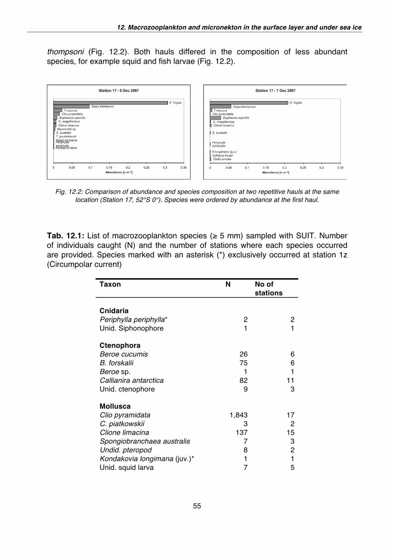
12. Macrozooplankton and micronekton in the surface layer and under sea ice
55
thompsoni (Fig. 12.2). Both hauls differed in the composition of less abundant
species, for example squid and fish larvae (Fig. 12.2).
Fig. 12.2: Comparison of abundance and species composition at two repetitive hauls at the same
location (Station 17, 52°S 0°). Species were ordered by abundance at the first haul.
Tab. 12.1: List of macrozooplankton species ( 5 mm) sampled with SUIT. Number
of individuals caught (N) and the number of stations where each species occurred
are provided. Species marked with an asterisk (*) exclusively occurred at station 1z
(Circumpolar current)
Taxon N No of stations
Cnidaria
Periphylla periphylla* 2 2
Unid. Siphonophore 1 1
Ctenophora
Beroe cucumis 26 6
B. forskalii 75 6
Beroe sp. 1 1
Callianira antarctica 82 11
Unid. ctenophore 9 3
Mollusca
Clio pyramidata 1,843 17
C. piatkowskii 3 2
Clione limacina 137 15
Spongiobranchaea australis 7 3
Undid. pteropod 8 2
Kondakovia longimana (juv.)* 1 1
Unid. squid larva 7 5
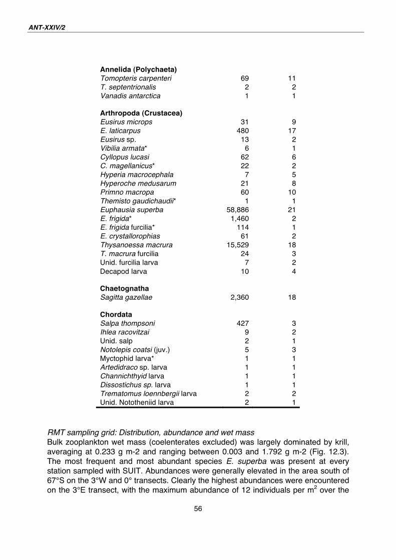
ANT-XXIV/2
56
Annelida (Polychaeta)
Tomopteris carpenteri 69 11
T. septentrionalis 2 2
Vanadis antarctica 1 1
Arthropoda (Crustacea)
Eusirus microps 31 9
E. laticarpus 480 17
Eusirus sp. 13 2
Vibilia armata* 6 1
Cyllopus lucasi 62 6
C. magellanicus* 22 2
Hyperia macrocephala 7 5
Hyperoche medusarum 21 8
Primno macropa 60 10
Themisto gaudichaudii* 1 1
Euphausia superba 58,886 21
E. frigida* 1,460 2
E. frigida furcilia* 114 1
E. crystallorophias 61 2
Thysanoessa macrura 15,529 18
T. macrura furcilia 24 3
Unid. furcilia larva 7 2
Decapod larva 10 4
Chaetognatha
Sagitta gazellae 2,360 18
Chordata
Salpa thompsoni 427 3
Ihlea racovitzai 9 2
Unid. salp 2 1
Notolepis coatsi (juv.) 5 3
Myctophid larva* 1 1
Artedidraco sp. larva 1 1
Channichthyid larva 1 1
Dissostichus sp. larva 1 1
Trematomus loennbergii larva 2 2
Unid. Nototheniid larva 2 1
RMT sampling grid: Distribution, abundance and wet mass
Bulk zooplankton wet mass (coelenterates excluded) was largely dominated by krill,
averaging at 0.233 g m-2 and ranging between 0.003 and 1.792 g m-2 (Fig. 12.3).
The most frequent and most abundant species E. superba was present at every
station sampled with SUIT. Abundances were generally elevated in the area south of
67°S on the 3°W and 0° transects. Clearly the highest abundances were encountered
on the 3°E transect, with the maximum abundance of 12 individuals per m2 over the
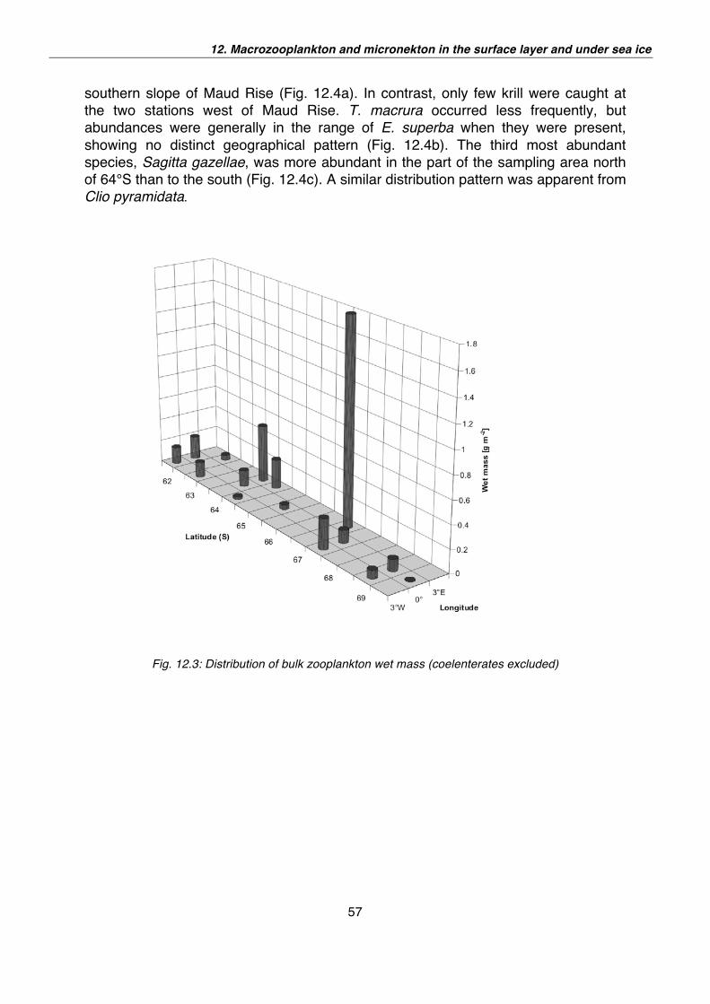
12. Macrozooplankton and micronekton in the surface layer and under sea ice
57
southern slope of Maud Rise (Fig. 12.4a). In contrast, only few krill were caught at
the two stations west of Maud Rise. T. macrura occurred less frequently, but
abundances were generally in the range of E. superba when they were present,
showing no distinct geographical pattern (Fig. 12.4b). The third most abundant
species, Sagitta gazellae, was more abundant in the part of the sampling area north
of 64°S than to the south (Fig. 12.4c). A similar distribution pattern was apparent from
Clio pyramidata.
Fig. 12.3: Distribution of bulk zooplankton wet mass (coelenterates excluded)
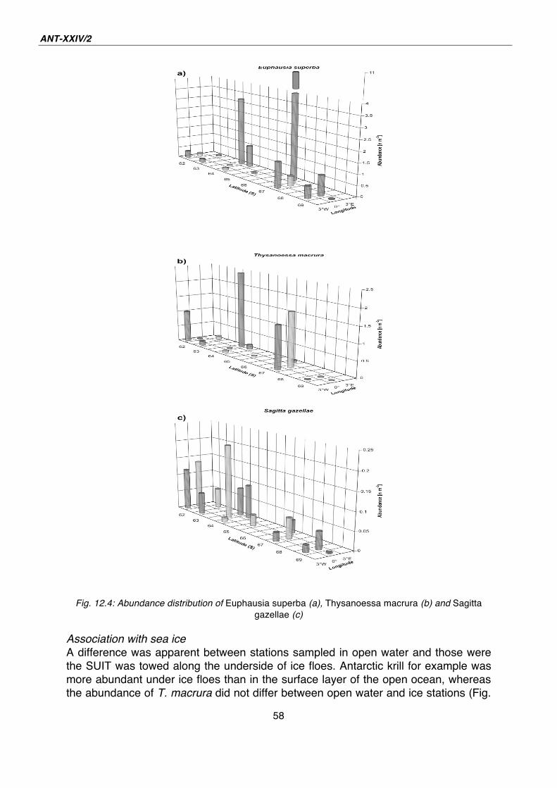
ANT-XXIV/2
58
Fig. 12.4: Abundance distribution of Euphausia superba (a), Thysanoessa macrura (b) and Sagitta
gazellae (c)
Association with sea ice
A difference was apparent between stations sampled in open water and those were
the SUIT was towed along the underside of ice floes. Antarctic krill for example was
more abundant under ice floes than in the surface layer of the open ocean, whereas
the abundance of T. macrura did not differ between open water and ice stations (Fig.
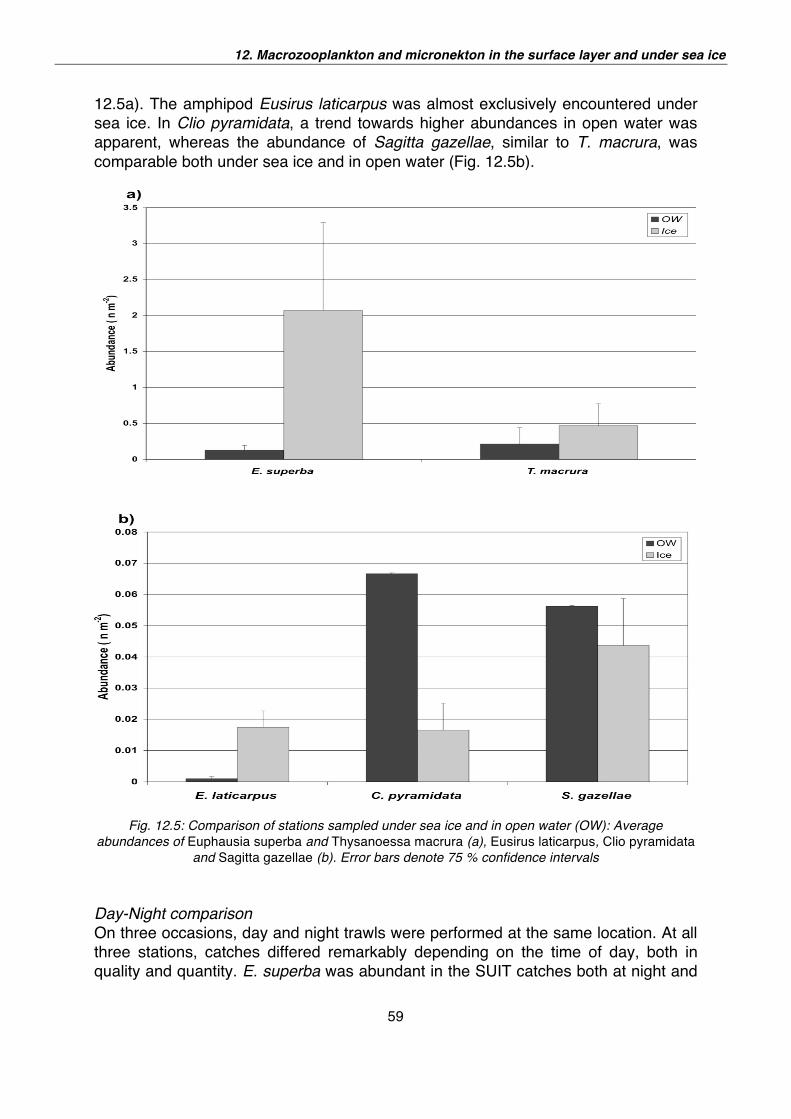
12. Macrozooplankton and micronekton in the surface layer and under sea ice
59
12.5a). The amphipod Eusirus laticarpus was almost exclusively encountered under
sea ice. In Clio pyramidata, a trend towards higher abundances in open water was
apparent, whereas the abundance of Sagitta gazellae, similar to T. macrura, was
comparable both under sea ice and in open water (Fig. 12.5b).
Fig. 12.5: Comparison of stations sampled under sea ice and in open water (OW): Average
abundances of Euphausia superba and Thysanoessa macrura (a), Eusirus laticarpus, Clio pyramidata
and Sagitta gazellae (b). Error bars denote 75 % confidence intervals
Day-Night comparison
On three occasions, day and night trawls were performed at the same location. At all
three stations, catches differed remarkably depending on the time of day, both in
quality and quantity. E. superba was abundant in the SUIT catches both at night and
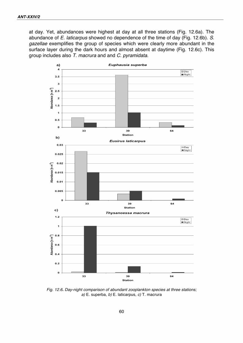
ANT-XXIV/2
60
at day. Yet, abundances were highest at day at all three stations (Fig. 12.6a). The
abundance of E. laticarpus showed no dependence of the time of day (Fig. 12.6b). S.
gazellae exemplifies the group of species which were clearly more abundant in the
surface layer during the dark hours and almost absent at daytime (Fig. 12.6c). This
group includes also T. macrura and and C. pyramidata.
Fig. 12.6. Day-night comparison of abundant zooplankton species at three stations;
a) E. superba, b) E. laticarpus, c) T. macrura
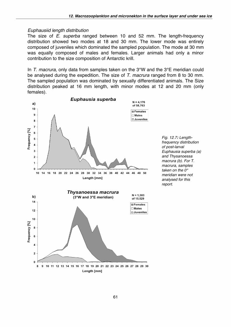
12. Macrozooplankton and micronekton in the surface layer and under sea ice
61
Euphausiid length distribution
The size of E. superba ranged between 10 and 52 mm. The length-frequency
distribution showed two modes at 18 and 30 mm. The lower mode was entirely
composed of juveniles which dominated the sampled population. The mode at 30 mm
was equally composed of males and females. Larger animals had only a minor
contribution to the size composition of Antarctic krill.
In T. macrura, only data from samples taken on the 3°W and the 3°E meridian could
be analysed during the expedition. The size of T. macrura ranged from 8 to 30 mm.
The sampled population was dominated by sexually differentiated animals. The Size
distribution peaked at 16 mm length, with minor modes at 12 and 20 mm (only
females).
Fig. 12.7: Length-
frequency distribution
of post-larval
Euphausia superba (a)
and Thysanoessa
macrura (b). For T.
macrura, samples
taken on the 0°
meridian were not
analysed for this
report.
ANT-XXIV/2
62
Discussion The data collected on the Antarctic summer expedition ANT-XXIV/2 illustrate the
significance of the surface layer to a wide range of macrozooplankton and micro-
nekton species. The presence of sea ice apparently had a strong influence on the
composition of thenear-surface community. In spite of the differences in species
composition, the surface layerwas rich in macrozooplankton / micronekton, both
under ice floes and in open water. Somespecies were concentrated under the ice,
such as Euphausia superba and Eusirus laticarpus, indicating that ice plays a major
role for these species as a habitat and foraging ground. E. superba was clearly more
abundant under ice than in the surface layer of the open ocean, especially if one
takes into account that the large confidence interval shown in Fig. 12.5a was mainly
influenced by the extra-ordinary large catch at St. 44 (67°S / 3°E; Fig. 12.4a).
Thenotion that krill often aggregated in thin layers not only under ice, but also at the
surface inopen water is further supported by the observation of surface swarms
(chapter 11). A concentration of krill under sea ice might partly explain the high
abundance of Antarctic krill encountered by the SUIT in the surface / under ice layer
compared to water column abundances sampled by the RMT in the area south of
62°S (Siegel et al., chapter 11).
In contrast to E. superba, the abundance of Thysanoessa macrura showed no
difference between stations sampled under ice floes and those fished in open water
(Fig. 12.5a). They were more efficiently caught by the RMT, indicating a more
dispersed distribution over a wide depth range (chapter 11). In spite of the
differences in euphausiid abundances, SUIT and RMT catches were related to each
other, as exemplified by the significant positive relationships between SUIT bulk wet
mass and RMT abundances of E. superba and T. macrura, respectively (Fig. 12.8 b,
c).
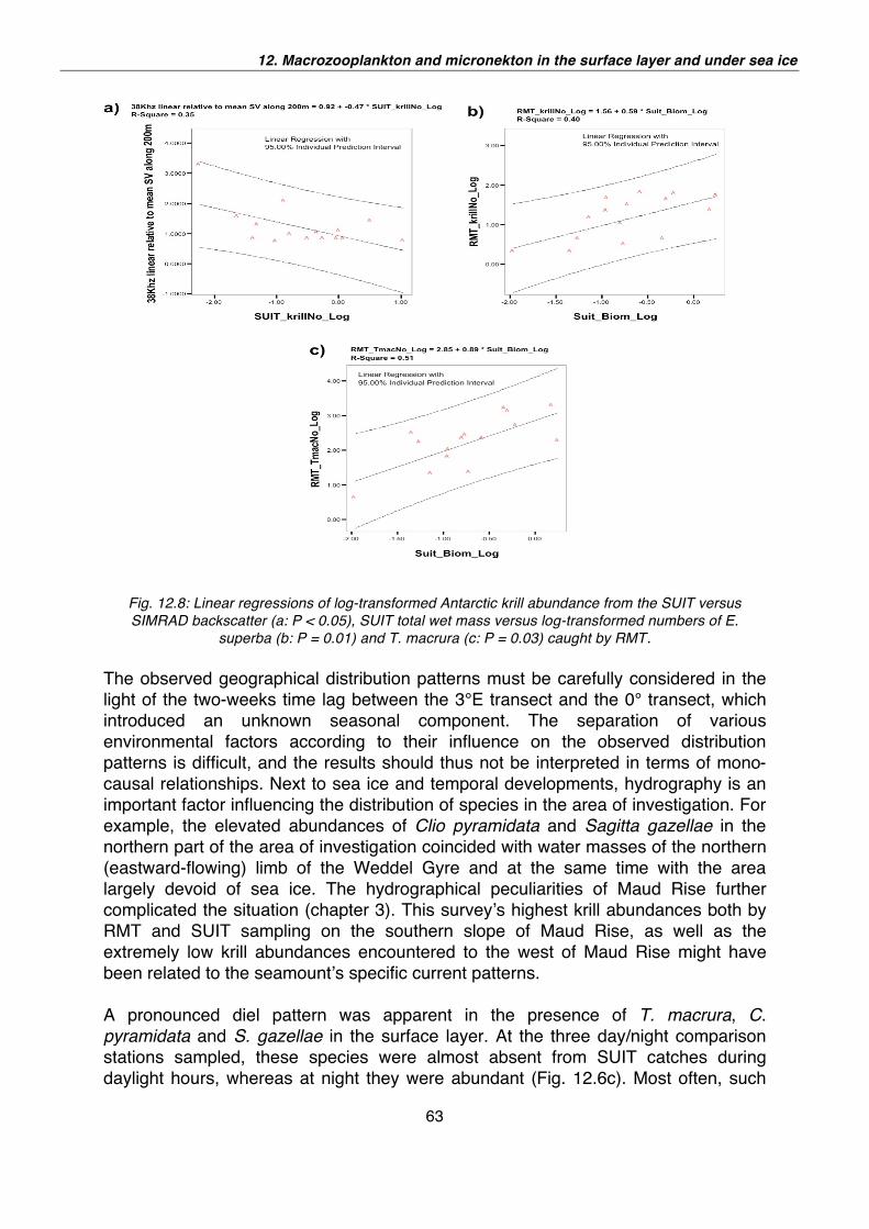
12. Macrozooplankton and micronekton in the surface layer and under sea ice
63
Fig. 12.8: Linear regressions of log-transformed Antarctic krill abundance from the SUIT versus
SIMRAD backscatter (a: P < 0.05), SUIT total wet mass versus log-transformed numbers of E.
superba (b: P = 0.01) and T. macrura (c: P = 0.03) caught by RMT.
The observed geographical distribution patterns must be carefully considered in the
light of the two-weeks time lag between the 3°E transect and the 0° transect, which
introduced an unknown seasonal component. The separation of various
environmental factors according to their influence on the observed distribution
patterns is difficult, and the results should thus not be interpreted in terms of mono-
causal relationships. Next to sea ice and temporal developments, hydrography is an
important factor influencing the distribution of species in the area of investigation. For
example, the elevated abundances of Clio pyramidata and Sagitta gazellae in the
northern part of the area of investigation coincided with water masses of the northern
(eastward-flowing) limb of the Weddel Gyre and at the same time with the area
largely devoid of sea ice. The hydrographical peculiarities of Maud Rise further
complicated the situation (chapter 3). This survey s highest krill abundances both by
RMT and SUIT sampling on the southern slope of Maud Rise, as well as the
extremely low krill abundances encountered to the west of Maud Rise might have
been related to the seamount s specific current patterns.
A pronounced diel pattern was apparent in the presence of T. macrura, C.
pyramidata and S. gazellae in the surface layer. At the three day/night comparison
stations sampled, these species were almost absent from SUIT catches during
daylight hours, whereas at night they were abundant (Fig. 12.6c). Most often, such
ANT-XXIV/2
64
diel migration behaviour is explained as the avoidance of visual predators. Yet, at
least in the two species carrying almost no pigmentation, T. macrura and S. gazellae,
avoidance of harmful UV radiation could be an alternative explanation.
In contrast, E. superba even showed a tendency to higher abundances at day (Fig.
12.6a). Apparently, the benefit of grazing under the ice and in the phytoplankton-rich
surface layer in open water was higher than the danger imposed by predation during
summer. Interestingly, the opposite behaviour was observed in winter 2006, when
krill only was abundant under the ice at night (Flores et al., in press). No diel pattern
was observed in Eusirus laticarpus, indicating that the amphipod continuously stays
in the ice habitat (Fig. 12.6b).
Initial comparisons of the abundances of surface / under ice macrozooplankton and
the food requirements of the top predator community showed no simple overall
correlation (chapter 13). Further integrated analysis of all potentially relevant
biological and physical datasets is warranted to increase our understanding of the
functioning of the high-Antarctic ecosystem.
Acknowledgements We express our deepest thanks to the crew of Polarstern ANT-XXIV/2. Martina
Vortkamp contributed a lot to the success of our work. This project was funded by the
Netherlands Ministry for Agriculture, Nature and Food Quality (LNV).
References Atkinson A, Siegel V, Pakhomov E, Rothery P (2004) Long-term decline in krill stock and
increase in salps within the southern Ocean. Nature 432:100-103
Brierly AS, Fernandez PG, Brandon MA, Armstrong F, Millard NW, McPhail SD, Stevenson
P, Pebody M, Perrett J, Squires M, Bone DG, Griffiths G (2002) Antarctic krill under sea
ice: Elevated abundance in a narrow band just south of ice edge. Science 295:1890-1892
Flores H, van Franeker JA, Fijn R, Meijboom A, van Dorssen M (in press) Fresh from the
fridge: Top predators food resources under the pack ice. BerzPolF
Van Franeker JA, Bathmann UV, Mathot S (1997) Carbon fluxes to Antarctic top predators.
Deep-Sea Res II 44:435-455
65
13. MARINE BIRDS AND MAMMALS IN THE LAZAREV SEA: THE SUMMER INFLUX Jan Andries van Franeker, Bram Feij,
Hauke Flores, Andre Meijboom, Michiel
van Dorssen
IMARES, Texel, The
Netherlands
Introduction and objectives
IMARES participates in AWI s multi-year LAKRIS study with a special focus on the role
of the surface layer on the biology and abundance of krill and other potential prey of
marine top predators. The history of this involvement is that consistent observations of
elevated densities of marine birds and mammals in the seaice zone remained largely
unexplained in terms of known food availability (e.g. van Franeker et al. 1997). The
poorly quantified under-ice habitat was thought to potentially hold missing explanations,
which led to development of the Surface and Under Ice Trawl (SUIT) research (see
Flores et al. this volume).
In the Southern Ocean, top predator abundances strongly suggest that biological
production in sea ice is a major driving force behind Antarctic animal population sizes
and biodiversity. Understanding the sea ice related foodweb is thus critical for a proper
evaluation of the potential impacts of climate change, a key issue in the research of the
International Polar Year 2007-2008. The interdisciplinary approach and seasonal
spread in Polarstern's Lakris cruises offers an excellent framework to improve such
knowledge of marine Antarctic foodwebs.
IMARES uses a top down approach in its ecosystem study which means that we start
with a quantification of food requirements of the top predator community derived from
detailed density surveys of birds, seals and whales. Results will be compared with catch
data from the SUIT (Flores et al., this volume), the Rectangular Midwater Trawl (RMT)
used in the CCAMLR krill survey (Siegel et al., this volume), acoustic surveys
(Krägefsky et al. this vol.) and ultimately all biological and physical information collected.
This report presents the preliminary results of predator surveys in terms of food
requirements of the top predator community.
Work a sea
Methods
Two platforms, the ship and helicopter, were available for making quantitative counts
of marine top predators during the Lakris expedition.
Ship-based censuses of birds and mammals were made from outdoor observation
posts installed on top of the bridge of Polarstern (± 20 m height). The wooden
observation posts have perspex windshields, a rain-hood and a small fan-heater that
ANT-XXIV/2
66
allowed usage in extreme conditions. The outdoor position gives an unobstructed
clear view to all sides, crucial to detect all animals in the band transect and also
needed to identify ship-associated birds that have to be omitted from density
calculations. Birds are counted from the moving ship, in a band transect during time
blocks of ten minutes. Ship-based bird censuses use band-transect methodology in
which birds in flight are counted according to the so-called snapshot-method (Tasker
et al. 1984) in order to avoid density bias by bird movement. Ship speed and transect
width can be used to convert observed numbers of animals to densities per unit of
surface area for each ten-minute period. The standard width of the transect band is
300 m, taken as 150 m to each side of the ship. Under average conditions, this is
considered the maximum distance to ensure detection of all individuals, even of
inconspicuous species. Depending on viewing conditions such as seastate, light level
and glare, the transect may be limited to one side of the ship and transect width may
be adapted to a distance that maximizes detection of all individuals of different
species. Special adaptation of band-width is sometimes necessary in dense and
heavy ice, where the ship often follows an erratic course searching leads or cracks in
the ice. As many predators aggregate in or around these leads, persisting in a narrow
transect band would result in a highly (upward) biased census result. Under such
conditions, the band-width of observations was widened at both sides to
approximately half the floe-size between leads, to ensure that counts represent an
adequate cross-section of the overall habitat.
Seal censuses are based on the same band records as used for bird observations.
Band-transect counts are considered adequate for seal censuses (Laws 1980), but
the Antarctic Pack Ice Seal Program (APIS) recommended line-transect methods
where possible (SCAR Group of Specialists on Seals 1994). Therefore, for ship-
based seal counts in ice areas, line transect data (Hiby and Hammond 1989) are
currently being collected in addition to band transect observations. However, current
analyses are still based on the band transect data. In the analyses hauled out seal
numbers seen from the ship were corrected for diurnal patterns in haul-out behaviour.
In ship-based observations, whale sightings are recorded following line-transect
methods, that is noting the angle and detection distance for each observation
irrespective of distance. Since the focus of the observer is on the narrow band
transect, chances for detection of whales at greater distances are reduced. Our
current data analysis for whales is based on simple estimated 'effective detection
ranges'; finer detection curves for Minke and larger whales will gradually be
developed from our dataset.
Helicopter based surveys used band-transect methods for all species groups. A
dedicated observer in the front seat focused all attention ahead on a narrow band-
transect which, depending on viewing conditions, ranged between 200 and 300 m
width. Band width was calibrated by perpendicular overflights of Polarstern (118 m
length). By overflying the ship over bow or stern at least twice at the start of each
survey, at the chosen altitude of 250 or 300 ft and standard speed of 60 knots,
reference points for transect limits could be made using interior parts of the heli.
Survey-tracks were subdivided into smaller units by making GPS waypoints
approximately every three to four minutes and recording data in between waypoints.
13. Marine birds and mammals in the Lazarev Sea: the summer influx
67
The GPS was operated by a second observer in the rear seat, at the same time
making ice-records for each subsection of the survey. Observers in the rear also
noted animal sightings outside of the transect band.
Analysis of survey data
Survey distance within each 10 min ship-survey was calculated from averaged ship-
speeds in Polarsterns PODAS database system. For helicopter surveys accurate flight
speed and distance covered were established using waypoints made. Surface surveyed
was thus established from speed and band-transect width, allowing the calculation of
densities (number of animals per km2) for each count unit. Each count unit also has a
number of environmental parameters, either noted during the counts (e.g. ice-
conditions, sea-state, visibility etc) or extracted from the PODAS system (position,
surface water-temperature, salinity etc.). Results of ice records are presented
elsewhere in this volume.
Top predator density data have been translated to daily prey requirements, expressed
as kg carbon requirement of the top predator community per km2 per day. Calculations
are based on published literature of field metabolic rates and energy contents of prey as
described in Van Franeker et al. (1997). In addition to the quantitative counts, qualitative
information was collected on the occurrence of species outside transect bands or during
oceanographical stations. Such data are not used for density estimates, but assist in
more complete distribution mapping of species.
Analyses in this paper are based on averages of all 10 minute ship-counts and the
between waypoints helicopter-counts, mostly grouped over half a degree of latitude
around station positions on each transect leg. Helicopter surveys were only conducted
where sea ice was present. Due to the speed of the observation platform, helicopter
surveys are expected to give some underestimate of especially whale densities as
diving individuals can be easily missed in fast overflight. However, seal data from heli-
counts are expected to be more complete than those from the ship because all heli-
surveys were conducted around midday, the peak haul-out period for ice seals.
Furthermore, in contrast to the ship, the helicopter follows a straight unbiased transect
line over seaice, where the ship often follows an erratic course in response to ice
conditions. In a later phase, detailed comparisons of ship and helicopter results may
lead to adaptations in data analyses.
Results and discussion
The long summer daylight periods for ship surveys plus the availability of helicopters
resulted in good coverage of top predator surveys over the full grid area. Until the 23 of
January a total of 2,094 counts was made: 1,395 ten-minute counts from the ship, and
699 between waypoint counts made during 28 flights with the helicopter. The surface
area thus covered by top predator counts amounts to 3,061 km2, of which 1,537 km2
from ship and 15,24 km2 from the helicopter. Helicopter counts were restricted to areas
with sea ice.
These sample sizes include the observations during the southward voyage from Cape
Town to Neumayer preceding the work in the study grid between 62°S-70°S and 3°W-
ANT-XXIV/2
68
3°E. Sample sizes and surface surveyed for different transects within the study-grid
area are specified in Table 13.1. Ship based counts were continued throughout the
northward voyage, and will be included in later analyses.
The overall north to south distribution of food requirements of top predators (Fig 13.1)
shows the usual pattern of relatively low values in warmer open ocean, occasionally
sharply elevated by incidental observations of large whales. In the seasonal sea ice
zone (sea ice retreated from about 60°S to 67°S) requirements are consistently higher,
largely due to regular presence of seals and whales. Birds, especially penguins were
relatively scarce during this voyage, likely because most species retreat to land for
breeding and moulting during this period, all at considerable distance from the study
grid.
Logistic commitments of Polarstern to support the delivery of building materials to
Neumayer station caused a break in the transects in the study grid. This seriously
complicates interpretation of spatial patterns of top predator distributions in the study
grid between 60° to 70°S and 3°W to 3°E. Data are presented for the somewhat wider
latitudes south of 60, as events a bit north of the grid were considered illustrative for
results obtained within the grid. The combination of ship counts and helicopter based
surveys allowed excellent coverage of all transects (Fig. 13.2A). However, in this
season of very rapid changes in ice conditions, the delay between the outer transects
(3°W and 3°E) and the central one along the 0° meridian seems to have had an
overruling effect on observed animal densities confusing a view on basic spatial
patterns (Fig. 13.2B).
As was the case during earlier winter observations, the 3°W transect showed higher
densities of predators than the 3°E transect which runs over Maud Rise (Fig. 13.3B and
C). However, food requirements during the delayed third and last transect moving north
along the zero meridian showed no matching intermediate pattern (Fig. 13.3D).
Strongly elevated food requirements from top predators were observed, largely caused
by increasing densities of crabeater seal (Lobodon carcinophagus) in the constantly
shrinking area of sea ice in the south and increased abundance of Antarctic minke
whale (Baleanoptera bonaerensis) in and around the open and broad marginal ice
zone. In winter, minke whales concentrated far south in heavy sea ice, but it appears
these animals move to the melting zones in summer, likely increased with migrating
individuals. On top of this, summer arrival of large baleen whales added to sharply
increased food requirements. In the rim of the sea ice, a rare observation of a blue
whale (Balaenoptera musculus) was documented. At the northern side of the study grid,
large numbers of migratory humpback whales (Megaptera novaeangliae) had arrived,
and flocks of thousands of moulting blue petrels (Halobaena caerulea) further indicated
rich and reliable food supply for predators. The seasonal change of seals concentrating
in residual ice and arrival of migratory whales attracted by the productivity of the
seasonal sea ice zone, is best seen by a comparison of the final transect along the zero
meridian (Fig. 13.3D) with the initial track to Neumayer (Fig. 13.3A) about five weeks
earlier which ran along 1°West until 65°S before gradually moving further southwest. In
the five weeks time gap, sea ice had retreated over seven degrees of latitude and
triggered a strong change in the composition of top predator community and a fourfold
13. Marine birds and mammals in the Lazarev Sea: the summer influx
69
increase of top predator daily food requirements in the study grid (Table 13.1), clearly
indicating the importance of the seasonal sea ice zone.
Among the remarkable observations, Ross seals (Ommatophoca rossii) need
mentioning. Throughout the cruise, but particulary in the area around the 0° meridian,
we observed unusually high numbers of this rarest among the ice seals. Where Bester
et al. (2002) reported an already relatively high percentage of 1.7 % Ross seals in the
seal populations of the Lazarev Sea, our observations add up to a more than three
times higher percentage of 5.4 % in summer 2007 - 2008.
In this early stage of data processing, no scientifically accurate evaluation of relations of
predator abundance with catches from various nets, acoustics or other biological or
physical parameters is possible. However, a quick initial survey of data was made with
preliminary SUIT data (Flores et al. this vol), RMT data (chapter 11) and echosounding
information (Krägefsky et al this vol). In many but not all cases, positive correlations
between predator abundance and prey abundance are visible. However, only few
correlations were significant in linear regressions. Three examples of correlations
between specific predator groups and krill abundance are shown in Fig. 13.4 using
logaritmic data and simple linear regressions. Food requirements of petrels were
positively related (p<0.001) to numbers of krill in the RMT net (Fig. 13.4A) and
requirements of seals were positively related (p=0.03) to mass of krill in the SUIT net.
Simrad 38 kHZ backscatter over the upper 200 m showed a near significant correlation
(p=0.052) with food requirements of the total top predator community. Further analyses
will be needed to combine prey abundance from all different indicators.
In conclusion, results of the ANT-XXIV/2 expedition confirm a major role of the seasonal
sea ice in supporting Antarctic food webs. Insight into finer scale relations and
processes is increasing, but still very incomplete because that requires integration of
results from different sampling devices over different depth ranges and needs to deal
with extremely patchy distributions and strongly variable diel migration patterns.
Additional work
Fishing by helicopter
During predator counts from from ship and heli, as in several earlier cruises, we
observed “brown spots”, i.e. discolourations in the water up to may tens of meters in
diameter. Although zooplankton swarming was suspected, this remained
unconfirmed as close subsurface swarming of zooplankton during daylight hours
would be unusual. Sampling had been impossible so far, but with the team of Heli
Transair we prepared a trial with a simple 50cm diameter plankton net on a 20 m
long rope deployed as sling load under the helicopter. We made one successful trial
lowering the net to about 15 m subsurface in a brown spot, hauling up uniformly
young krill. Learning more about the species/age composition of such patchy
swarms, their size and potential biomass contribution to the zooplankton community
is crucial to understand the functioning of the Southern Ocean ecosystem and
interpretation of catch data from conventional sampling net studies and even the
SUIT net, which will rarely hit these swarms. Given the opportunity in future
expeditions, we will look into the development of a more quantitative type of sampling
ANT-XXIV/2
70
net to be deployed under helicopter, as better knowledge of the brown spot
phenomenon fully fits our objective to assess the role of surface layer phenomena in
the functioning of the Antarctic ecosystem.
Atka Bay Emperor Penguin colony count
During the first visit of Polarstern to Neumayer Station, conditions on 14 Dec were
excellent for aerial photography of the colony of emperor penguins (Aptenodytes
forsteri) in Atka Bucht. Chicks were distributed over eight different creches that were
all photographed with telelens from distance out of the helicopter. Counts of the
photographic material shows that close to 11.000 chicks were present with about
1,200 attending adult birds.
Opportunistic diet sampling
In our research, birds accidentally landing on the ship are routinely measured and if
possible a stomach sample is taken for diet studies. As expected in a mid-summer
cruise accidental landings hardly occurred. Two Kerguelen petrels were reported on
the ship, one of which took off again by itself. The other one had regurgitated its
stomach content on the deck (krill). It was captured, measured and subsequently
released, and the stomach content was collected.
Education, Outreach and Communication
Considerable effort was made by our group to produce 12 short videos for the Dutch
IPY site (www.pooljaar.nl/poolijs) and the AWI ftp site, 9 weekly illustrated
newsletters (in Dutch and German; www.jafweb.nl ) and various other written and
photographic contributions for general usage. During the voyage we also cooperated
in a newspaper article and radio interview in the Netherlands.
Acknowledgements
We thank officers and crew of Polarstern, cruise leader Uli Bathmann and all
colleagues on board for their frequent and extensive support for our project. Martina
Vortkamp and Sören Krägefsky kindly assisted in providing preliminary RMT and
SIMRAD data. Special thanks are expressed towards the HeliTransAir pilots and
technicians. This project was funded by the Netherlands Ministry for Agriculture,
Nature and Food Quality (LNV). Last but not least we are very grateful to the Alfred
Wegener Institute for its open attitude to international cooperation through the sharing
of costly logistic facilities.
References Bester, M.N., Ferguson, M.N. & Jonker, F.C. 2002. Population densities of pack ice seals in
the Lazarev Sea, Antarctica. Antarctic Science 14: 123-127.
Hiby A.R. and Hammond P.S. 1989. Survey techniques for estimating cetaceans. In:
Donovan G.P.(ed). The comprehensive assessment of whale stocks: the early years.
Rep.Int.Whal.Comn (Special Issue II). Cambridge. pp 47-80.
Laws, R.M. (ed) 1980. Estimation of population sizes of seals. BIOMASS Handbook No. 2:
21 pp. SCAR, Cambridge.
SCAR Group of Specialists on Seals 1994. Antarctic Pack Ice Seals: indicators of
environmental change and contributors to carbon flux. APIS Program, draft
implementation plan, Aug. 1994. SCAR Group of Specialists on Seals, Seattle.7 pp.
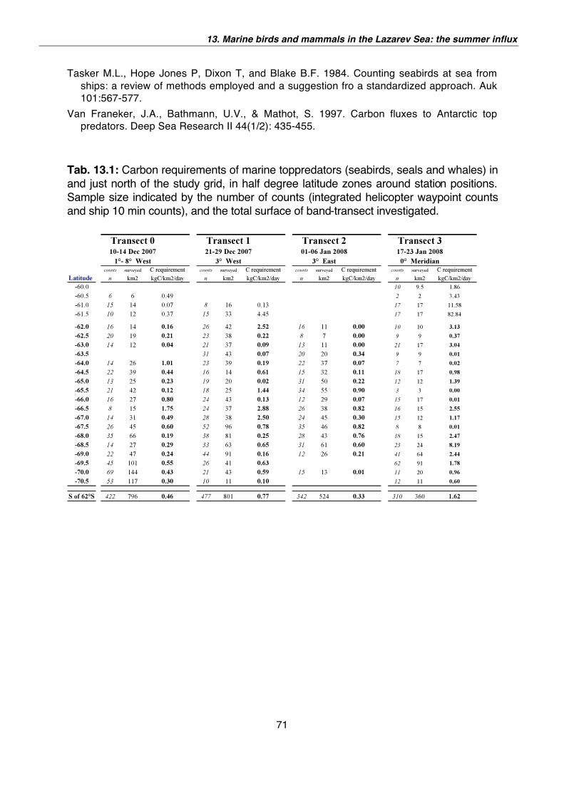
13. Marine birds and mammals in the Lazarev Sea: the summer influx
71
Tasker M.L., Hope Jones P, Dixon T, and Blake B.F. 1984. Counting seabirds at sea from
ships: a review of methods employed and a suggestion fro a standardized approach. Auk
101:567-577.
Van Franeker, J.A., Bathmann, U.V., & Mathot, S. 1997. Carbon fluxes to Antarctic top
predators. Deep Sea Research II 44(1/2): 435-455.
Tab. 13.1: Carbon requirements of marine toppredators (seabirds, seals and whales) in
and just north of the study grid, in half degree latitude zones around station positions.
Sample size indicated by the number of counts (integrated helicopter waypoint counts
and ship 10 min counts), and the total surface of band-transect investigated.
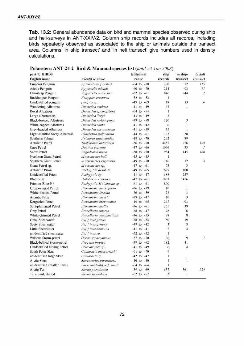
ANT-XXIV/2
72
Tab. 13.2: General abundance data on bird and mammal species observed during ship
and heli-surveys in ANT-XXIV/2. Column ship records includes all records, including
birds repeatedly observed as associated to the ship or animals outside the transect
area. Columns in ship transect and in heli transect give numbers used in density
calculations.
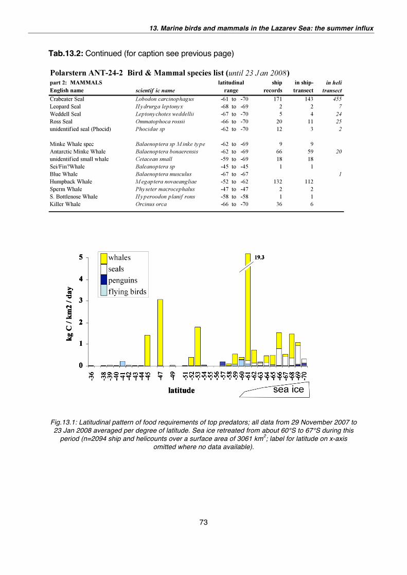
13. Marine birds and mammals in the Lazarev Sea: the summer influx
73
Tab.13.2: Continued (for caption see previous page)
Fig.13.1: Latitudinal pattern of food requirements of top predators; all data from 29 November 2007 to
23 Jan 2008 averaged per degree of latitude. Sea ice retreated from about 60°S to 67°S during this
period (n=2094 ship and helicounts over a surface area of 3061 km2; label for latitude on x-axis
omitted where no data available).
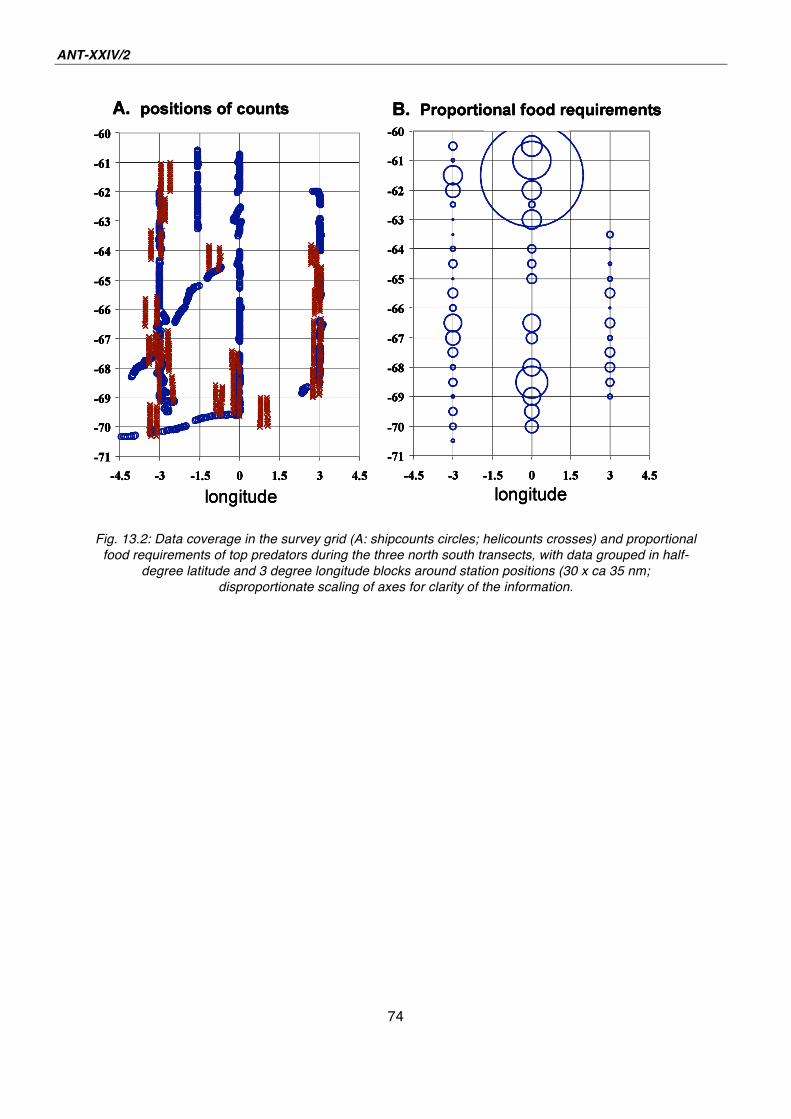
ANT-XXIV/2
74
Fig. 13.2: Data coverage in the survey grid (A: shipcounts circles; helicounts crosses) and proportional
food requirements of top predators during the three north south transects, with data grouped in half-
degree latitude and 3 degree longitude blocks around station positions (30 x ca 35 nm;
disproportionate scaling of axes for clarity of the information.
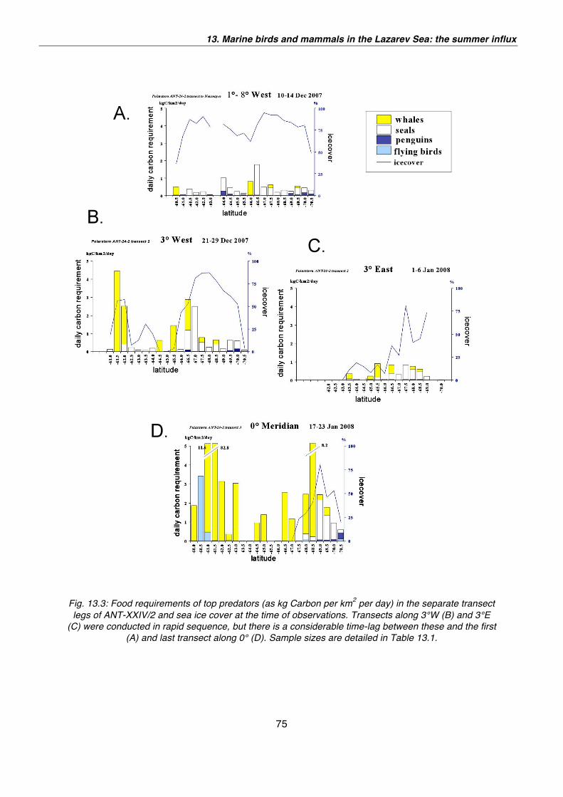
13. Marine birds and mammals in the Lazarev Sea: the summer influx
75
Fig. 13.3: Food requirements of top predators (as kg Carbon per km
2 per day) in the separate transect
legs of ANT-XXIV/2 and sea ice cover at the time of observations. Transects along 3°W (B) and 3°E
(C) were conducted in rapid sequence, but there is a considerable time-lag between these and the first
(A) and last transect along 0° (D). Sample sizes are detailed in Table 13.1.
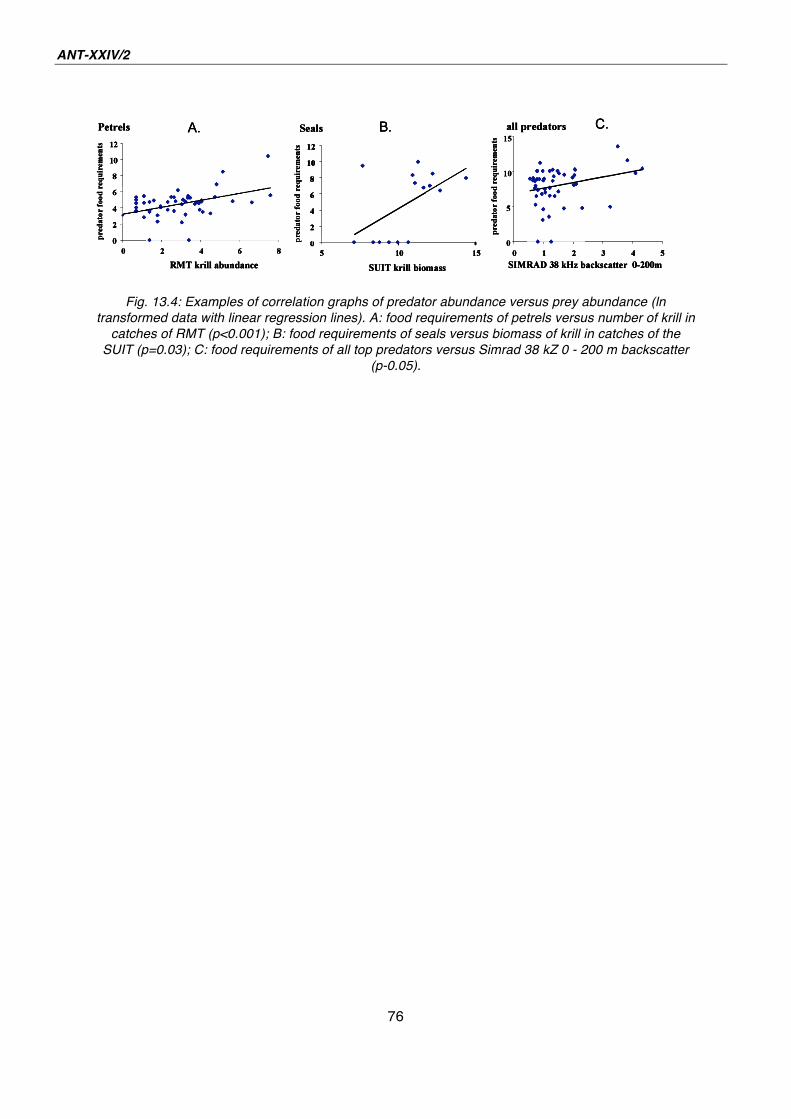
ANT-XXIV/2
76
Fig. 13.4: Examples of correlation graphs of predator abundance versus prey abundance (ln
transformed data with linear regression lines). A: food requirements of petrels versus number of krill in
catches of RMT (p<0.001); B: food requirements of seals versus biomass of krill in catches of the
SUIT (p=0.03); C: food requirements of all top predators versus Simrad 38 kZ 0 - 200 m backscatter
(p-0.05).
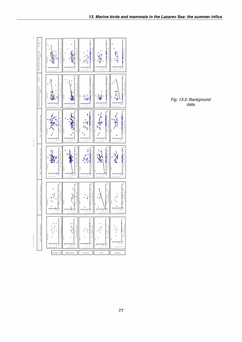
13. Marine birds and mammals in the Lazarev Sea: the summer influx
77
Fig. 13.5: Background
data
78
14. ANDEEP-SYSTCO (SYSTEM COUPLING) SYSTEM COUPLING IN THE DEEP SOUTHERN OCEAN - FROM CENSUS TO ECOSYSTEM FUNCTIONING Angelika Brandt1), Brigitte Ebbe2),
Eberhard J. Sauter3)
1) Zoological Museum Hamburg, Germany
2) German Centre of Marine Biodiversity,
Senckenberg, Germany
3) Alfred-Wegener-Institut, Bremerhaven,
Germany
The general scope and objectives
Vast areas of the Southern Ocean surrounding the Antarctic continental shelf are
deep sea. In contrast to our knowledge of the benthos in Southern Ocean shelf
areas, corresponding data from the deep sea are still scarce. However, the
pioneering investigations of ANDEEP aboard the German icebreaker Polarstern have
revealed a remarkable biodiversity in the Southern Ocean deep sea. SYSTCO builds
on the precursor programme ANDEEP which was multidisciplinary but more focused
on the status quo of the nearly unexplored ecosystem of the abyssal benthos in the
Antarctic.
We will now build on those results and try to understand the role of deep-sea key
species in the ecosystem and will try to elucidate the functioning of atmospheric,
pelagic, and benthic systems of the Southern Ocean in a process oriented context.
SYSTCO will help to understand the role of the Southern Ocean in global energy
budgets, climate change, and the functioning of atmospheric, pelagic, and benthic
systems of the Southern Ocean. The approach of exploring a new or almost
untouched frontier with regard to the geographic area will be complemented by
approaching a new frontier in linking major scientific disciplines. SYSTCO involves a
wide variety of scientists from different disciplines, such as atmospheric sciences,
planktology, physical oceanography, geology, sedimentology, and biogeochemistry
for simultaneous study of a defined area to shed light on atmospheric-pelagic-benthic
coupling processes (atmospheric, biological sciences, physical oceanography,
sedimentology, and geology) for simultaneous study of a defined area.
SYSTCO is an ambitious programme designed to study processes in different realms
of the biosphere in Antarctica and uncover how these systems are linked to each
other (atmospheric-pelagic-benthic coupling processes).
Important objectives in the different realms are as follows:
Atmosphere: SYSTCO aims to unravel surface fluxes from satellite data:
14. ANDEEP-SYSTCO in the deep Southern Ocean - From census to ecosystem functioning
79
Water column and plankton: SYSTCO aims to understand the influence of
atmospheric processes on processes in the water column, the influence of the
biogeochemistry of the surface water on primary productivity, and to describe vertical
changes in the plankton community to abyssal depths.
Benthos: SYSTCO investigates the biology of abyssal key species, the role of the
bottom-nepheloid layer for recruitment of benthic animals, the influence on abyssal
life of the quantity and quality of food sinking through the water column, feeding
ecology and trophic relationships of abyssal animals.
Seabed characteristics: SYSTCO studies the effects of topography, sedimentology
and biogeochemistry of sediment and pore water on benthic life and microhabitat
formation.
The benthic fauna depends on deep carbon export from the pelagic production and
particle sedimentation. For that reason the project aimed to revisit a station on the
way back to Cape Town in order to perform repeated measurements at the same
station for an estimate of seasonal and episodic variabilities of the particle flux.
The area investigated during SYSTCO will provide a basis for future monitoring
programmes, i.e., global change studies and could serve as a time-series-area which
could be revisited in future.
SYSTCO is the IPY lead project #66 and it is also integrated into SCAR-EBA and
CAML (Census of the Antarctic Marine Life) and CeDAMar (Census of the Diversity
of Abyssal Marine Life). Data management can be guaranteed through SCAR-
MarBIN to OBIS. Samples will be handled through the German Centre for Marine
Biodiversity (DZMB) in Wilhelmshaven, Germany, a department of the Senckenberg
Institute especially designed as a service organisation coordinating sample handling,
processing, tracking, and archiving for all projects staged from German research
vessels, as well as providing a database of taxonomic experts. As SYSTCO is an
important field project also for the global Census of Marine Life (CoML, field projects
CeDAMar and CAML), education and outreach are managed during the expedition by
Dr Victoria Wadley (CAML) and Dr Brigitte Ebbe (CeDAMar).
In order to avoid duplication of the presentation of results in this cruise report, only
the general aims of physical oceanography and planktology are outlined here, and
references to the other chapters of the report are provided.
Physical Oceanography
The physical and oceanographic measurements of the Polarstern cruise ANT-XXIV/2
will form part of the IPY-project Synoptic Circum-Antarctic Climate and Ecosystem
study (SCACE). The overarching goal of SCACE is to internationally collaborate in
the collection of a unique data set that can serve as a benchmark for comparison of
existing data for the identification and quantification of polar changes.
ANT-XXIV/2
80
SCACE (for description of the project see chapter 2) contributes to SYSTCO in
addressing questions such as:
• Which physical, biological and chemical processes regulate the Southern
Ocean system and determine its influence on the global climate development?
• How sensitive are Southern Ocean processes and systems to natural climate
change and anthropogenic perturbations?
To answer these questions a CTD was used that held additional instruments such as
a chlorophyll-sensitive fluorometer to provide an indication of the abundance of
phytoplankton and a transmissiometer to measure the attenuation of light. It will be
attached to a carousel water sampler holding 24 bottles of 12 l volume each. The
CTD water is used to measure the distributions of inorganic carbon, total alkalinity,
oxygen and nutrients in the Weddell Sea and on the Antarctic shelf. The CTD
measurements were accompanied by measurements of horizontal currents in the top
few hundred metres. This was done by continuously recording with a vessel mounted
ADCP (Acoustic Doppler Current Profiler). The ADCP is also used to detect
zooplankton abundance by evaluating the backscattered echo amplitude and
provides background information on processes in the water column (for further
descriptions of this work chapter 4).
Investigations of the upper layer of surface water and sea ice
The ocean surface layer and its link to sea ice is of critical importance to the Antarctic
food webs. A top-down survey of the food web structure is done in order to explain
high predator abundance in sea ice, which is believed to be largely triggered by ice
algae concentrating higher food web levels in the poorly studied upper layer of
surface water. Sampling of these systems was conducted using a special net to
sample fish and zooplankton residing in the upper water layer, even when directly
under sea ice. The scraping off of the under ice fauna is performed using an
especially constructed heavy-framed but floating net that can 'roll' along the
undersurface of the sea ice, the SUIT (Surface and Under-Ice Trawl) (for more details
see chapter 12).
Studies on Plankton
The physical and oceanographic measurements are complemented by a suite of
chemical and biological measurements. Data of zooplankton abundance are derived
from different net catches to provide insight into the biodiversity and distribution of
zooplankton, including euphausiid (krill) life stages for demography studies and
population dynamics (chapter 12), in the Southern Ocean surface layer of the
Circumpolar Current, as well as the pelagic realm. A Continuous Plankton Recorder
(CPR) was used to determine the patchiness and species composition of
zooplankton. The role of carnivorous zooplankton (e.g. chaetognaths) in the
mesopelagic food web of the Southern Ocean was studied on the basis of stratified
sampling by a multinet (MN) at depth intervals between 2,000 - 1,500 m, 1,500 -
1,000 m, 1,000 - 750 m, 750 - 500 m, 500 - 0 m. Further material was derived from
Rectangular Midwater Trawl (RMT) samples (chapters 6 - 9).
14. ANDEEP-SYSTCO in the deep Southern Ocean - From census to ecosystem functioning
81
Biogeochemistry at the sediment-water interface
Biogeochemistry was done to study organic carbon (Corg) fluxes reaching the seafloor
at the different SYSTCO locations. Moreover, interactions between geochemical
microgradients and benthic organisms can be discovered using a suite of gear
including Landers, microprofilers, benthic corers and sledges at the same station.
Measurements of geochemical microgradients are used to describe the geochemical
milieu around benthic organisms and help to explain faunal community structures
with their ecological and metabolic characteristics. Further details are presented in
the background of the DOMINO (Dynamics of benthic Organic Matter fluxes In polar
deep-Ocean environments) project (chapter 31). DOMINO contributes to both
SCACE and SYSTCO, as well as to the IPY programme ICED (Integrating Climate
and Ecosystem Dynamics).
Measurement of the pore-water oxygen distribution provides a suitable tool for the
determination of Corg fluxes through the sediment-water interface as an estimate of
food input to the benthic communities. So far, only few data on Corg remineralization
rates exist for high latitudes beyond 60° S and furthermore very little is known also
about the total amount of organic carbon remineralized and fixed within surface
sediments of the Southern Ocean.
In-situ microprofile measurements of small scale variabilities generated by bacteria or
benthic organisms were planned to be performed by means of an autonomously
working 3D deep-sea microprofiler mounted on a free falling Lander system. Besides
the photographs taken, the 3D reconstruction of the pore water oxygen distribution
was to be used for a geochemical habitat characterization as well as for 3D pore
water modelling. These data are of great importance for benthic biologists, especially
when measured around biogenic structures. In-situ measurements were planned to
be complemented by ex-situ measurements of microprofiles, sediment, pore water for
the determination of further geochemical parameters like Corg, C/N ratio as well as
nutrient profiles. Sediment was sampled using a MUC (multicorer).
In addition, the sea floor surrounding the sampling and measuring locations was
characterized hydroacoustically using Parasound and Hydrosweep for approximately
30 minutes before approaching a station.
Some interesting achievements of the ANDEEP-SYSTCO project are
General
• First biogeochemical in-situ measurement repeated after 7 weeks, to
investigate the effect of a phytoplankton bloom on benthos and how surface
productivity is linked to the seafloor
• First biogeochemical sampling of deep-sea stations 12 nm apart in order to
look at small-scale heterogeneity in the sediment
• Worldwide southernmost in-situ benthic flux measurement at 69°40.4 S
(Polynia station)
• First sampling through the entire water column in the Southern Ocean from
surface and ice flora and fauna down to bathyal or abyssal depths (5 stations,
partly incomplete)
ANT-XXIV/2
82
• First sediment profiles measured simultaneously with the complete benthic
community, including epibenthos and infauna
• 52° SPF is characterised by low diversity and abundance in the macrofauna,
even after a slight plankton bloom in spring (revisit of stations after 7 weeks)
• Eastern Weddell Sea and Lazarev Sea are generally poorer in species and
abundance of organisms in the deep sea
• Maud Rise (seamount) differs completely in taxon composition from the
abyssal stations, perhaps due to the unique physical oceanographic conditions
including the Taylor column influencing localised entrainment of larvae.
Brooders, on the contrary, occur only as a minor fraction in the macrobenthic
sample.
Fauna
• Discovery of the rare Monoplacophora Laevipilina antarctica close to
Neumayer (northern pier) which will help to elucidate the phylogenetic position
of this taxon
• High numbers of Bivalvia at Maud Rise (52 % of the macrofauna) possibly
indicating high particle availability for filter feeders
• High biomass of Holothuria (in total about 15 kg, with the largest holothurian
[70 cm] of 3.6 kg, possibly indicating that these mud-feeding animals have
much organic matter available
• High biodiversity of Gastropoda (higher than at northernmost stations)
providing interesting result for deep-sea latitudinal gradients!
• Sampling of a high number of small calcareous Porifera at northern pier and of
a large carnivorous sponge (70°S Lazarev Sea in 2,100 m)
• Finding symbioses; parasitic gastropods on holothurians and crinoids, many
parasitic copepods on a scale worm and on fishes
• Sampling of more than 10 specimens of Haplomunnidae, a very rare deep-sea
isopod family, at Maud Rise.
Methods
• An experimental approach to the meiobenthic food-web study in the Southern
Ocean deep sea to uncover the microbial carbon contribution to the diet of
Nematoda
• About 750 samples for biochemistry for food-web analysis (fatty acids and
stable isotopes) which is essential for the analysis of the trophic structure
• About 500 samples for isopod barcoding and 350 extractions for genetics,
important for population genetics and phylogenetic analyses of selected taxa
• Many samples for genetics of polychaetes and other taxa (same background
as isopods)
• Fixation of Laevipilina for genetics in order to solve the phylogenetic
relationship of Monoplacophora
• Five deployments (4xSYSTCO) of free-falling Lander equipped with in-situ
microprofiler for high resolution pore water oxygen profiles
• Laboratory oxygen porewater profiles measured at 5 stations ex-situ in MUC
and GKG samples. Complementing sampling for porosity, Chlorophyll a and
organic carbon content to be determined at the institute.
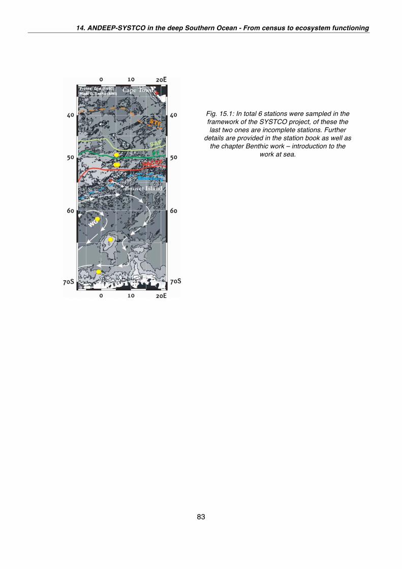
14. ANDEEP-SYSTCO in the deep Southern Ocean - From census to ecosystem functioning
83
Fig. 15.1: In total 6 stations were sampled in the
framework of the SYSTCO project, of these the
last two ones are incomplete stations. Further
details are provided in the station book as well as
the chapter Benthic work – introduction to the
work at sea.
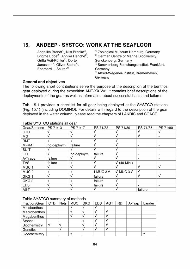
84
15. ANDEEP - SYSTCO: WORK AT THE SEAFLOOR Angelika Brandt1), Nils Brenke2),
Brigitte Ebbe2), Annika Henche2),
Gritta Veit-Köhler2), Dorte
Janussen3), Oliver Sachs4),
Eberhard J. Sauter4)
1) Zoological Museum Hamburg, Germany
2) German Centre of Marine Biodiversity,
Senckenberg, Germany
3) Senckenberg Forschungsinstitut, Frankfurt,
Germany 4) Alfred-Wegener-Institut, Bremerhaven,
Germany
General and objectives The following short contributions serve the purpose of the description of the benthos
gear deployed during the expedition ANT-XXIV/2. It contains brief descriptions of the
deployments of the gear as well as information about successful hauls and failures.
Tab. 15.1 provides a checklist for all gear being deployed at the SYSTCO stations
(Fig. 15.1) (including DOMINO). For details with regard to the description of the gear
deployed in the water column, please read the chapters of LAKRIS and SCACE.
Table SYSTCO stations all gear Gear/Stations PS 71/13 PS 71/17 PS 71/33 PS 71/39 PS 71/85 PS 71/90
CTD
MD - RMT - -
M-RMT no deploym. failure - -
SUIT - -
FFL no deploym. failure - -
A-Traps failure - -
TVS failure (40 Min.) - - MUC 1
MUC 2 f-MUC 3 MUC 3 - GKG 1 failure
GKG 2 failure - -
EBS failure - -
AGT failure
Table SYSTCO summary of methods Fraction/Gear CTD Nets MUC GKG EBS AGT RD A-Trap Lander
Meiobenthos
Macrobenthos
Megabenthos
Stones
Biochemistry
Genetics
Geochemistry
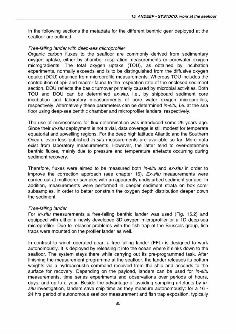
15. ANDEEP - SYSTDCO. work at the seafloor
85
In the following sections the metadata for the different benthic gear deployed at the
seafloor are outlined.
Free-falling lander with deep-sea microprofiler
Organic carbon fluxes to the seafloor are commonly derived from sedimentary
oxygen uptake, either by chamber respiration measurements or porewater oxygen
microgradients. The total oxygen uptake (TOU), as obtained by incubation
experiments, normally exceeds and is to be distinguished from the diffusive oxygen
uptake (DOU) obtained from microprofile measurements. Whereas TOU includes the
contribution of epi- and macro- fauna to the respiration rate of the enclosed sediment
section, DOU reflects the basic turnover primarily caused by microbial activities. Both
TOU and DOU can be determined ex-situ, i.e., by shipboard sediment core
incubation and laboratory measurements of pore water oxygen microprofiles,
respectively. Alternatively these parameters can be determined in-situ, i.e. at the sea
floor using deep-sea benthic chamber and microprofiler landers, respectively.
The use of microsensors for flux determination was introduced some 25 years ago.
Since their in-situ deployment is not trivial, data coverage is still modest for temperate
equatorial and upwelling regions. For the deep high latitude Atlantic and the Southern
Ocean, even less published in-situ measurements are available so far. More data
exist from laboratory measurements. However, the latter tend to over-determine
benthic fluxes, mainly due to pressure and temperature artefacts occurring during
sediment recovery.
Therefore, fluxes were aimed to be measured both in-situ and ex-situ in order to
improve the correction approach (see chapter 16). Ex-situ measurements were
carried out at multicorer samples with an apparently undisturbed sediment surface. In
addition, measurements were performed in deeper sediment strata on box corer
subsamples, in order to better constrain the oxygen depth distribution deeper down
the sediment.
Free-falling lander
For in-situ measurements a free-falling benthic lander was used (Fig. 15.2) and
equipped with either a newly developed 3D oxygen microprofiler or a 1D deep-sea
microprofiler. Due to releaser problems with the fish trap of the Brussels group, fish
traps were mounted on the profiler lander as well.
In contrast to winch-operated gear, a free-falling lander (FFL) is designed to work
autonomously. It is deployed by releasing it into the ocean where it sinks down to the
seafloor. The system stays there while carrying out its pre-programmed task. After
finishing the measurement programme at the seafloor, the lander releases its bottom
weights via a hydroacoustic command received from the ship and ascends to the
surface for recovery. Depending on the payload, landers can be used for in-situ
measurements, time series experiments and observations over periods of hours,
days, and up to a year. Beside the advantage of avoiding sampling artefacts by in-
situ investigation, landers save ship time as they measure autonomously: for a 16 -
24 hrs period of autonomous seafloor measurement and fish trap exposition, typically
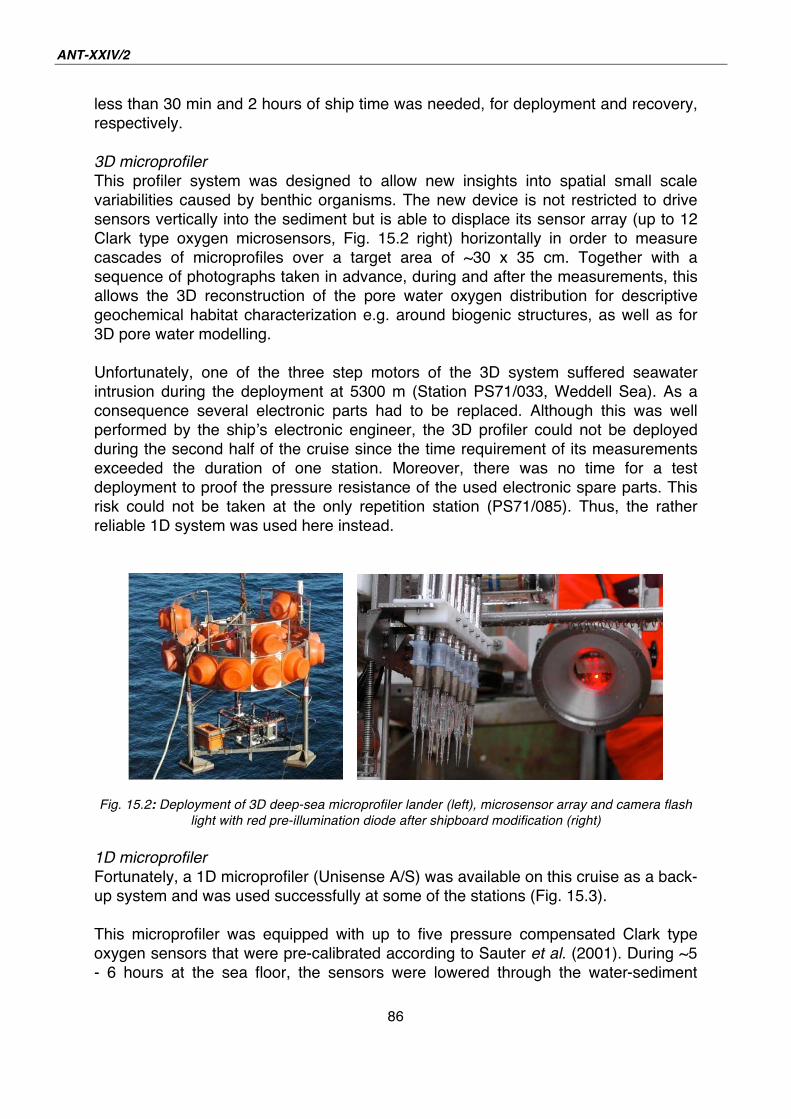
ANT-XXIV/2
86
less than 30 min and 2 hours of ship time was needed, for deployment and recovery,
respectively.
3D microprofiler
This profiler system was designed to allow new insights into spatial small scale
variabilities caused by benthic organisms. The new device is not restricted to drive
sensors vertically into the sediment but is able to displace its sensor array (up to 12
Clark type oxygen microsensors, Fig. 15.2 right) horizontally in order to measure
cascades of microprofiles over a target area of ~30 x 35 cm. Together with a
sequence of photographs taken in advance, during and after the measurements, this
allows the 3D reconstruction of the pore water oxygen distribution for descriptive
geochemical habitat characterization e.g. around biogenic structures, as well as for
3D pore water modelling.
Unfortunately, one of the three step motors of the 3D system suffered seawater
intrusion during the deployment at 5300 m (Station PS71/033, Weddell Sea). As a
consequence several electronic parts had to be replaced. Although this was well
performed by the ship s electronic engineer, the 3D profiler could not be deployed
during the second half of the cruise since the time requirement of its measurements
exceeded the duration of one station. Moreover, there was no time for a test
deployment to proof the pressure resistance of the used electronic spare parts. This
risk could not be taken at the only repetition station (PS71/085). Thus, the rather
reliable 1D system was used here instead.
Fig. 15.2: Deployment of 3D deep-sea microprofiler lander (left), microsensor array and camera flash
light with red pre-illumination diode after shipboard modification (right)
1D microprofiler
Fortunately, a 1D microprofiler (Unisense A/S) was available on this cruise as a back-
up system and was used successfully at some of the stations (Fig. 15.3).
This microprofiler was equipped with up to five pressure compensated Clark type
oxygen sensors that were pre-calibrated according to Sauter et al. (2001). During ~5
- 6 hours at the sea floor, the sensors were lowered through the water-sediment
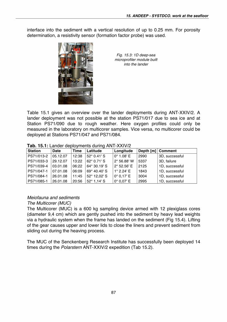
15. ANDEEP - SYSTDCO. work at the seafloor
87
interface into the sediment with a vertical resolution of up to 0.25 mm. For porosity
determination, a resistivity sensor (formation factor probe) was used.
Table 15.1 gives an overview over the lander deployments during ANT-XXIV/2. A
lander deployment was not possible at the station PS71/017 due to sea ice and at
Station PS71/090 due to rough weather. Here oxygen profiles could only be
measured in the laboratory on multicorer samples. Vice versa, no multicorer could be
deployed at Stations PS71/047 and PS71/084.
Tab. 15.1: Lander deployments during ANT-XXIV/2 Station Date Time Latitude Longitude Depth [m] Comment PS71/013-2 05.12.07 12:38 52° 0.41' S 0° 1.08' E 2990 3D, successful
PS71/033-3 29.12.07 13:22 62° 0.71' S 2° 56.88' W 5337 3D, failure
PS71/039-4 03.01.08 06:22 64° 30.19' S 2° 52.56' E 2125 1D, successful
PS71/047-1 07.01.08 06:09 69° 40.40' S 1° 2.24' E 1843 1D, successful
PS71/084-1 26.01.08 11:45 52° 12,02' S 0° 0,17' E 3004 1D, successful
PS71/085-1 26.01.08 20:56 52° 1,14' S 0° 0,07' E 2995 1D, successful
Meiofauna and sediments
The Multicorer (MUC)
The Multicorer (MUC) is a 600 kg sampling device armed with 12 plexiglass cores
(diameter 9,4 cm) which are gently pushed into the sediment by heavy lead weights
via a hydraulic system when the frame has landed on the sediment (Fig 15.4). Lifting
of the gear causes upper and lower lids to close the liners and prevent sediment from
sliding out during the heaving process.
The MUC of the Senckenberg Research Institute has successfully been deployed 14
times during the Polarstern ANT-XXIV/2 expedition (Tab 15.2).
Fig. 15.3: 1D deep-sea
microprofiler module built
into the lander
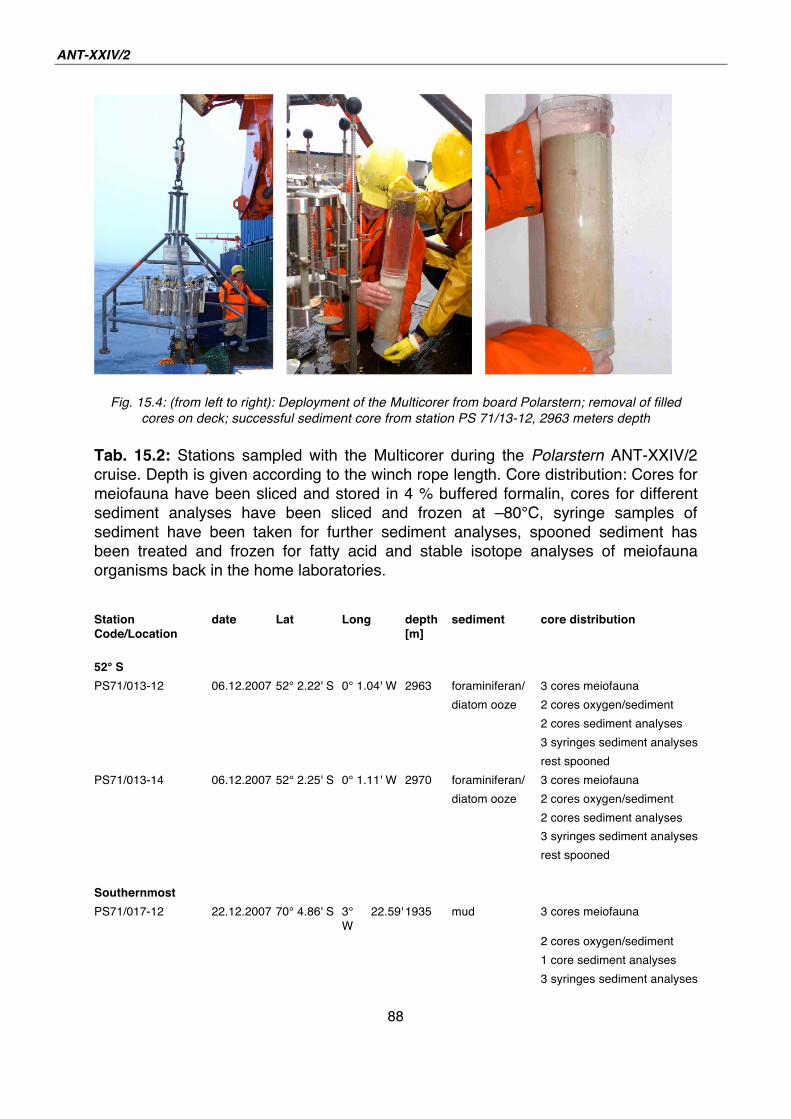
ANT-XXIV/2
88
Fig. 15.4: (from left to right): Deployment of the Multicorer from board Polarstern; removal of filled
cores on deck; successful sediment core from station PS 71/13-12, 2963 meters depth
Tab. 15.2: Stations sampled with the Multicorer during the Polarstern ANT-XXIV/2
cruise. Depth is given according to the winch rope length. Core distribution: Cores for
meiofauna have been sliced and stored in 4 % buffered formalin, cores for different
sediment analyses have been sliced and frozen at –80°C, syringe samples of
sediment have been taken for further sediment analyses, spooned sediment has
been treated and frozen for fatty acid and stable isotope analyses of meiofauna
organisms back in the home laboratories.
Station Code/Location
date Lat Long depth [m]
sediment core distribution
52° S
PS71/013-12 06.12.2007 52° 2.22' S 0° 1.04' W 2963 foraminiferan/ 3 cores meiofauna
diatom ooze 2 cores oxygen/sediment
2 cores sediment analyses
3 syringes sediment analyses
rest spooned
PS71/013-14 06.12.2007 52° 2.25' S 0° 1.11' W 2970 foraminiferan/ 3 cores meiofauna
diatom ooze 2 cores oxygen/sediment
2 cores sediment analyses
3 syringes sediment analyses
rest spooned
Southernmost
PS71/017-12 22.12.2007 70° 4.86' S 3° 22.59'
W
1935 mud 3 cores meiofauna
2 cores oxygen/sediment
1 core sediment analyses
3 syringes sediment analyses
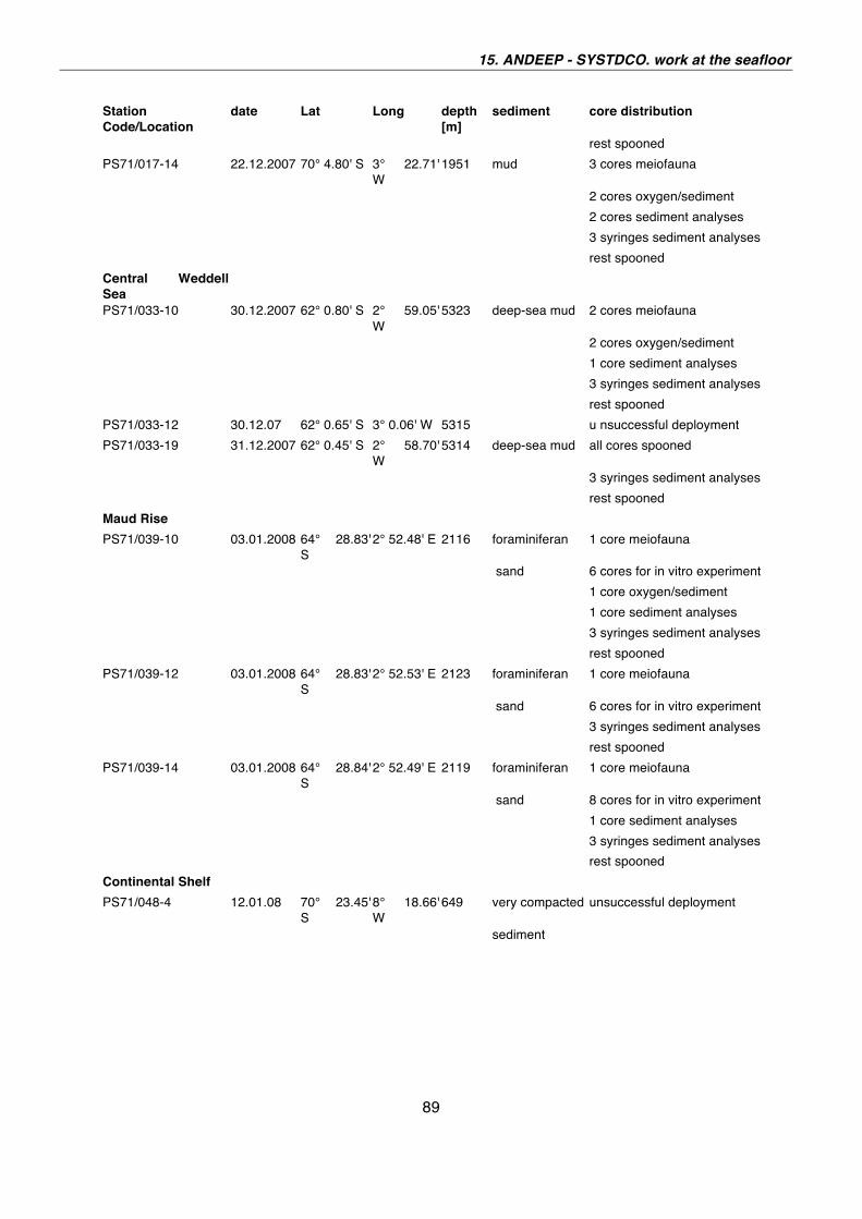
15. ANDEEP - SYSTDCO. work at the seafloor
89
Station Code/Location
date Lat Long depth [m]
sediment core distribution
rest spooned
PS71/017-14 22.12.2007 70° 4.80' S 3° 22.71'
W
1951 mud 3 cores meiofauna
2 cores oxygen/sediment
2 cores sediment analyses
3 syringes sediment analyses
rest spooned
Central Weddell Sea
PS71/033-10 30.12.2007 62° 0.80' S 2° 59.05'
W
5323 deep-sea mud 2 cores meiofauna
2 cores oxygen/sediment
1 core sediment analyses
3 syringes sediment analyses
rest spooned
PS71/033-12 30.12.07 62° 0.65' S 3° 0.06' W 5315 u nsuccessful deployment
PS71/033-19 31.12.2007 62° 0.45' S 2° 58.70'
W
5314 deep-sea mud all cores spooned
3 syringes sediment analyses
rest spooned
Maud Rise
PS71/039-10 03.01.2008 64° 28.83'
S
2° 52.48' E 2116 foraminiferan 1 core meiofauna
sand 6 cores for in vitro experiment
1 core oxygen/sediment
1 core sediment analyses
3 syringes sediment analyses
rest spooned
PS71/039-12 03.01.2008 64° 28.83'
S
2° 52.53' E 2123 foraminiferan 1 core meiofauna
sand 6 cores for in vitro experiment
3 syringes sediment analyses
rest spooned
PS71/039-14 03.01.2008 64° 28.84'
S
2° 52.49' E 2119 foraminiferan 1 core meiofauna
sand 8 cores for in vitro experiment
1 core sediment analyses
3 syringes sediment analyses
rest spooned
Continental Shelf
PS71/048-4 12.01.08 70° 23.45'
S
8° 18.66'
W
649 very compacted unsuccessful deployment
sediment
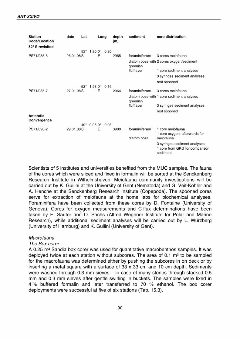
ANT-XXIV/2
90
Station Code/Location
date Lat Long depth [m]
sediment core distribution
52° S revisited
PS71/085-5 26.01.08
52° 1.20'
S
0° 0.20'
E 2965 foraminiferan/ 3 cores meiofauna
diatom ooze with 2 cores oxygen/sediment
greenish
flufflayer 1 core sediment analyses
3 syringes sediment analyses
rest spooned
PS71/085-7 27.01.08
52° 1.53'
S
0° 0.16'
E 2964 foraminiferan/ 3 cores meiofauna
diatom ooze with 1 core sediment analyses
greenish
flufflayer 3 syringes sediment analyses
rest spooned
Antarctic Convergence
PS71/090-2 29.01.08
49° 0.95'
S
0° 0.03'
E 3980 foraminiferan/ 1 core meiofauna
diatom ooze
1 core oxygen, afterwards for
meiofauna
3 syringes sediment analyses
1 core from GKG for comparison
sediment
Scientists of 5 institutes and universities benefited from the MUC samples. The fauna
of the cores which were sliced and fixed in formalin will be sorted at the Senckenberg
Research Institute in Wilhelmshaven. Meiofauna community investigations will be
carried out by K. Guilini at the University of Gent (Nematoda) and G. Veit-Köhler and
A. Henche at the Senckenberg Research Institute (Copepoda). The spooned cores
serve for extraction of meiofauna at the home labs for biochemical analyses.
Foraminifera have been collected from these cores by D. Fontaine (University of
Geneva). Cores for oxygen measurements and C-flux determinations have been
taken by E. Sauter and O. Sachs (Alfred Wegener Institute for Polar and Marine
Research), while additional sediment analyses will be carried out by L. Würzberg
(University of Hamburg) and K. Guilini (University of Gent).
Macrofauna
The Box corer
A 0.25 m Sandia box corer was used for quantitative macrobenthos samples. It was
deployed twice at each station without subcores. The area of 0.1 m to be sampled
for the macrofauna was determined either by pushing the subcores in on deck or by
inserting a metal square with a surface of 33 x 33 cm and 10 cm depth. Sediments
were washed through 0.3 mm sieves – in case of many stones through stacked 0.5
mm and 0.3 mm sieves after gentle swirling in buckets. The samples were fixed in
4 % buffered formalin and later transferred to 70 % ethanol. The box corer
deployments were successful at five of six stations (Tab. 15.3).
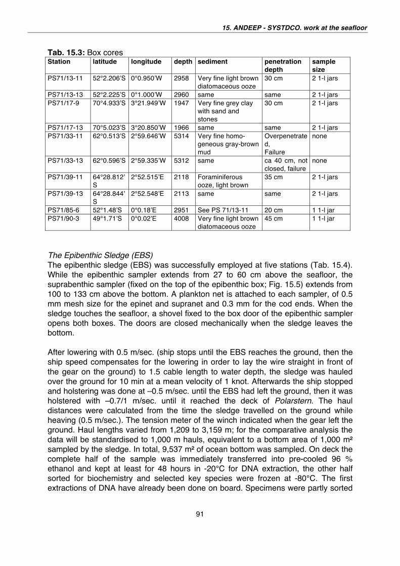
15. ANDEEP - SYSTDCO. work at the seafloor
91
Tab. 15.3: Box cores Station latitude longitude depth sediment penetration
depth
sample size
PS71/13-11 52°2.206 S 0°0.950 W 2958 Very fine light brown
diatomaceous ooze
30 cm 2 1-l jars
PS71/13-13 52°2.225 S 0°1.000 W 2960 same same 2 1-l jars
PS71/17-9 70°4.933 S 3°21.949 W 1947 Very fine grey clay
with sand and
stones
30 cm 2 1-l jars
PS71/17-13 70°5.023 S 3°20.850 W 1966 same same 2 1-l jars
PS71/33-11 62°0.513 S 2°59.646 W 5314 Very fine homo-
geneous gray-brown
mud
Overpenetrate
d,
Failure
none
PS71/33-13 62°0.596 S 2°59.335 W 5312 same ca 40 cm, not
closed, failure
none
PS71/39-11 64°28.812
S
2°52.515 E 2118 Foraminiferous
ooze, light brown
35 cm 2 1-l jars
PS71/39-13 64°28.844
S
2°52.548 E 2113 same same 2 1-l jars
PS71/85-6 52°1.48 S 0°0.18 E 2951 See PS 71/13-11 20 cm 1 1-l jar
PS71/90-3 49°1.71 S 0°0.02 E 4008 Very fine light brown
diatomaceous ooze
45 cm 1 1-l jar
The Epibenthic Sledge (EBS)
The epibenthic sledge (EBS) was successfully employed at five stations (Tab. 15.4).
While the epibenthic sampler extends from 27 to 60 cm above the seafloor, the
suprabenthic sampler (fixed on the top of the epibenthic box; Fig. 15.5) extends from
100 to 133 cm above the bottom. A plankton net is attached to each sampler, of 0.5
mm mesh size for the epinet and supranet and 0.3 mm for the cod ends. When the
sledge touches the seafloor, a shovel fixed to the box door of the epibenthic sampler
opens both boxes. The doors are closed mechanically when the sledge leaves the
bottom.
After lowering with 0.5 m/sec. (ship stops until the EBS reaches the ground, then the
ship speed compensates for the lowering in order to lay the wire straight in front of
the gear on the ground) to 1.5 cable length to water depth, the sledge was hauled
over the ground for 10 min at a mean velocity of 1 knot. Afterwards the ship stopped
and holstering was done at –0.5 m/sec. until the EBS had left the ground, then it was
holstered with –0.7/1 m/sec. until it reached the deck of Polarstern. The haul
distances were calculated from the time the sledge travelled on the ground while
heaving (0.5 m/sec.). The tension meter of the winch indicated when the gear left the
ground. Haul lengths varied from 1,209 to 3,159 m; for the comparative analysis the
data will be standardised to 1,000 m hauls, equivalent to a bottom area of 1,000 m
sampled by the sledge. In total, 9,537 m of ocean bottom was sampled. On deck the
complete half of the sample was immediately transferred into pre-cooled 96 %
ethanol and kept at least for 48 hours in -20°C for DNA extraction, the other half
sorted for biochemistry and selected key species were frozen at -80°C. The first
extractions of DNA have already been done on board. Specimens were partly sorted
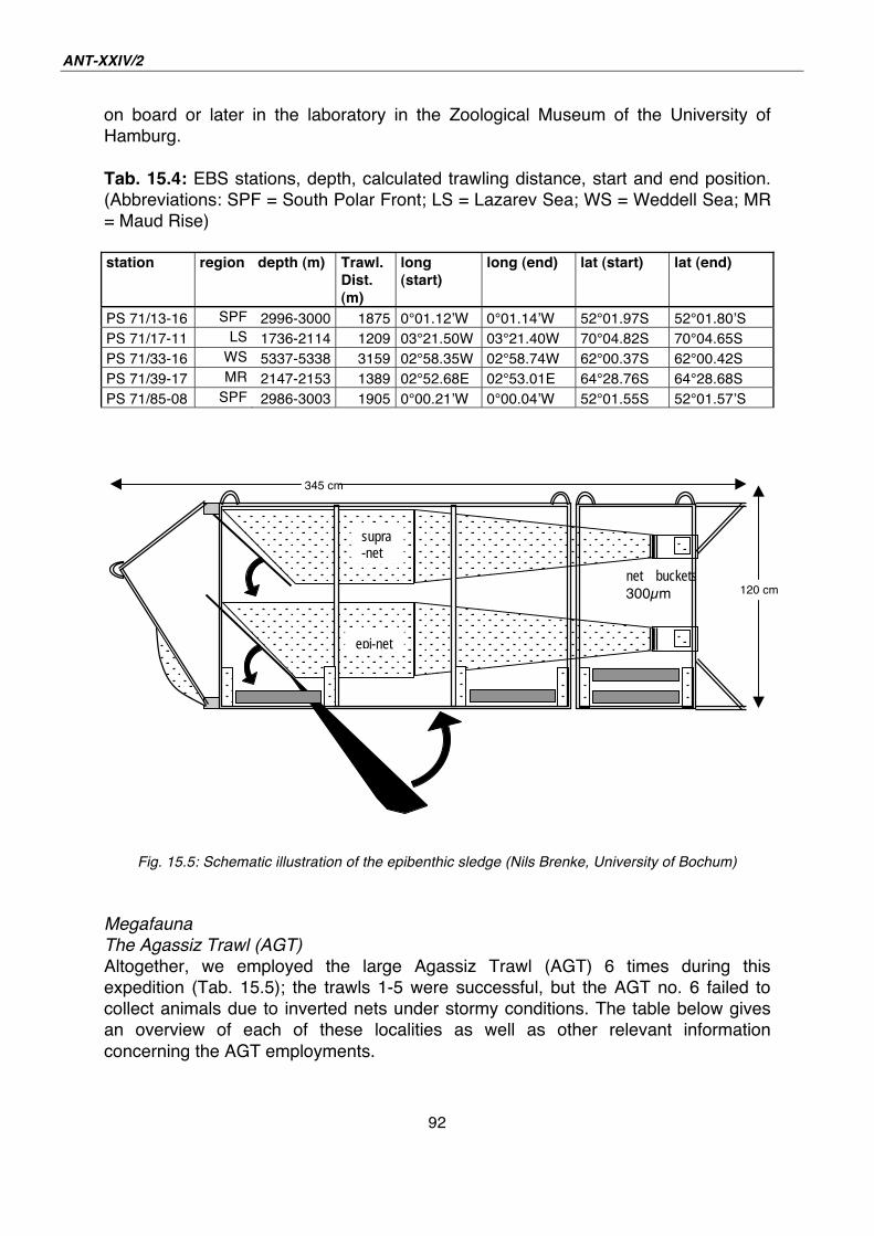
ANT-XXIV/2
92
on board or later in the laboratory in the Zoological Museum of the University of
Hamburg.
Tab. 15.4: EBS stations, depth, calculated trawling distance, start and end position.
(Abbreviations: SPF = South Polar Front; LS = Lazarev Sea; WS = Weddell Sea; MR
= Maud Rise)
station region depth (m) Trawl.
Dist. (m)
long (start)
long (end) lat (start) lat (end)
PS 71/13-16 SPF 2996-3000 1875 0°01.12 W 0°01.14 W 52°01.97S 52°01.80 S
PS 71/17-11 LS 1736-2114 1209 03°21.50W 03°21.40W 70°04.82S 70°04.65S
PS 71/33-16 WS 5337-5338 3159 02°58.35W 02°58.74W 62°00.37S 62°00.42S
PS 71/39-17 MR 2147-2153 1389 02°52.68E 02°53.01E 64°28.76S 64°28.68S
PS 71/85-08 SPF 2986-3003 1905 0°00.21 W 0°00.04 W 52°01.55S 52°01.57 S
Fig. 15.5: Schematic illustration of the epibenthic sledge (Nils Brenke, University of Bochum)
Megafauna
The Agassiz Trawl (AGT)
Altogether, we employed the large Agassiz Trawl (AGT) 6 times during this
expedition (Tab. 15.5); the trawls 1-5 were successful, but the AGT no. 6 failed to
collect animals due to inverted nets under stormy conditions. The table below gives
an overview of each of these localities as well as other relevant information
concerning the AGT employments.
net buckets
300μm
epi-net
supra
-net
345 cm
120 cm
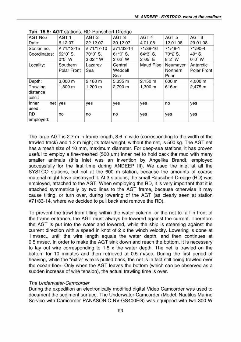
15. ANDEEP - SYSTDCO. work at the seafloor
93
Tab. 15.5: AGT stations, RD-Ranschort-Dredge AGT No./
Date:
AGT 1
6.12.07
AGT 2
22.12.07
AGT 3
30.12.07
AGT 4
4.01.08
AGT 5
12.01.08
AGT 6
29.01.08
Station no. # 71/13-15 # 71/17-10 #71/33-14 71/39-16 71/48-1 71/90-4
Coordinates: 52°0` S,
0°0` W
70°0` S,
3,02`° W
61°0` S,
3°02` W
64°3` S,
2°05` E
70°2`S,
8°2` W
49° S,
0°0` W
Locality: Southern
Polar Front
Lazarev
Sea
Central
Weddell
Sea
Maud Rise Neumayer
Northern
Pear
Antarctic
Polar Front
Depth: 3,000 m 2,180 m 5,335 m 2,150 m 600 m 4,000 m
Trawling
distance
calc.:
1,809 m 1,200 m 2,790 m 1,300 m 616 m 2,475 m
Inner net
used:
yes yes yes yes no yes
RD
employed:
no no no yes yes yes
The large AGT is 2.7 m in frame length, 3.6 m wide (corresponding to the width of the
trawled track) and 1.2 m high; its total weight, without the net, is 500 kg. The AGT net
has a mesh size of 10 mm, maximum diameter. For deep-sea stations, it has proven
useful to employ a fine-meshed (500 μm) inner net to hold back the mud with many
smaller animals (this inlet was an invention by Angelika Brandt, employed
successfully for the first time during ANDEEP III). We used the inlet at all the
SYSTCO stations, but not at the 600 m station, because the amounts of coarse
material might have destroyed it. At 3 stations, the small Rauschert Dredge (RD) was
employed, attached to the AGT. When employing the RD, it is very important that it is
attached symmetrically by two lines to the AGT frame, because otherwise it may
cause tilting, or turn over, during lowering of the AGT (as clearly seen at station
#71/33-14, where we decided to pull back and remove the RD).
To prevent the trawl from tilting within the water column, or the net to fall in front of
the frame entrance, the AGT must always be lowered against the current. Therefore
the AGT is put into the water and lowered, while the ship is steaming against the
current direction with a speed in knot of 2 x the winch velocity. Lowering is done at
1 m/sec., until the wire length equals the water depth, and then continues at
0.5 m/sec. In order to make the AGT sink down and reach the bottom, it is necessary
to lay out wire corresponding to 1.5 x the water depth. The net is trawled on the
bottom for 10 minutes and then retrieved at 0.5 m/sec. During the first period of
heaving, while the “extra” wire is pulled back, the net is in fact still being trawled over
the ocean floor. Only when the AGT leaves the bottom (which can be observed as a
sudden increase of wire tension), the actual trawling time is over.
The Underwater-Camcorder
During the expedition an electronically modified digital Video Camcorder was used to
document the sediment surface. The Underwater-Camcorder (Model: Nautilus Marine
Service with Camcorder PANASONIC NV-GS400EG) was equipped with two 300 W
ANT-XXIV/2
94
spotlights (Deep-Sea Multi-SeaLife, P/N 710041601), and all parts were installed in a
two meter high, pyramidal Lander-frame (DOCLT). Additionally two hundred
kilograms of lead were attached to the frame to increase the weight. By using a
Coax-Communication-Cable (Winch 31), the Underwater-Camcorder was powered
up using a power supply unit to provide 450 - 450V with 1.1 - 1.4 A. The Underwater-
Camcorder filmed, in a position 80 cm above the sediment surface, an area of
approximately 85 x 45 cm . The film was saved on a 6.35 mm digital videotape, in
625 lines PAL, PCM-Digital-Take record system with 16 Bit (48 kHz/2 canal) audio
quality. The tape recorded a time of 60 minutes.
The Lander-frame with the pressure chamber, including the underwater-camcorder,
was lowered to the sea bottom, with at first 0.7 m/s and later at 1.0 m/s and held
above the ground for three minutes, to allow a clear view of the sediment surface.
After 3 minutes the Lander-frame was heaved up 10 m and followed the drift of the
ship for two minutes. Then a new cycle was started, and the procedure was repeated
for one hour. At this time the underwater-camcorder returned to surface.
During the expedition ANT-XXIV/2 five locations were sampled with the underwater-
camcorder. Unfortunately, the first deployment (PS71/13-20) was not successful, due
to a misinterpretation of the conductivity of the Coax-Communication-Cable. The last
deployments (PS71/17-15, 33-17, 39-9, 48-2) were successful.
95
16. GEOCHEMICAL INVESTIGATIONS AT THE SEAFLOOR Eberhard J. Sauter, Oliver
Sachs
Alfred-Wegener-Institut, Bremerhaven,
Germany
Objectives
Biological and physical processes in the surface ocean strongly control the air-sea
carbon dioxide (CO2) balance, as a key factor of the earth s climate system
(Sarmiento & Le Quere, 1996). CO2 fixation by phytoplankton via photosynthesis
combined with the subsequent cycle of grazing, export to the deep, sedimentation,
and remineralisation, often referred to as the “biological pump” (Sarmiento & Le
Quere, 1996), represents one of the major CO2 sinks. During this cruise these
processes were investigated within the programmes SCACE and LAKRIS. In
association with the ANT-XXI/4 cruise in 2004, the geochemical investigations were
carried out within the DFG project DOMINO which is to be considered a module of
SYSTCO linking the water column work to the benthic compartment, whose results
are described in this section.
Putting the geochemical seafloor investigations into such multidisciplinary framework,
the main objectives of DOMINO were:
• to characterize the geochemical milieu of the benthic environment and
• to determine organic carbon fluxes through the water/sediment interface.
The sediments of the oligotrophic Antarctic deep-sea as well as of the shelf are
generally well oxygenated. Thus, the main focus is put on the determination of the
porewater oxygen depth distribution, i.e., the measurement of oxygen micro profiles
(as described in section 15, Lander Methods). Where possible (at stations with both
lander and MUC deployment) in-situ and ex-situ profiles were measured in order to
improve the correction function of Sachs et al. (submitted a) which permits revision of
ex-situ measured fluxes to be corrected for pressure artefacts (temperature artefacts
only play a minor role in polar regions).
Oxygen measurements are complemented by sediment investigations to obtain
pigment and carbon concentrations as well as sediment porosity. In cooperation with
the University of Hamburg, additional sedimentological parameters will be determined
from multicorer samples.
ANT-XXIV/2
96
Work at sea
Hydroacoustic seafloor survey
For about 30 - 60 minutes before reaching a SYSTCO station, the ship s
HYDROSWEEP and PARASOUND systems were switched on, in order to obtain
information about the seafloor topography and sediment stratification of the benthos
station to be sampled. It was not intended to acquire hydroacoustic data for seismic,
bathymetric or geological use. Instead, this hydroacoustic survey was performed to
support the safe use and the identification of the appropriate location for the
deployment of the benthos gear.
The data quality of the fish sounder Simrad EK60 (used for zooplankton
observations, see section 4) was considerably disturbed by HYDROSWEEP and
PARASOUND, which were therefore only switched on for minimal time periods.
Since high quality EK60 information was essential in particular during net operations,
and those, dependent on a clear water column, preceded the benthos work at the
SYSTCO stations, the hydroacoustic seafloor survey was performed during the EBS
or AGT tows at the later stations.
Geochemical investigations
According to the description given in section 15, Lander Methods, lander
deployments were prepared and carried out if ice conditions and sea state permitted.
In addition, laboratory measurements were performed at multicorer samples. All
sensors were calibrated prior to their deployment. Oxygen microprofiles were
obtained as raw data sets from both in-situ and ex-situ measurements (in-situ: mV,
ex-situ: pA values) and had to be translated to oxygen values via the following steps:
• Correction of sensor drift if necessary
• adjustment of sensor height relative to the water/sediment interface
• translation of raw signal into oxygen concentration on the basis of a two point
calibration (bottom water oxygen concentration by Winkler titration, and sensor
zero reading from oxygen-free water)
For the determination of organic carbon fluxes to the seafloor, at first the diffusive
oxygen uptake was calculated from the porewater oxygen microgradient at the
sediment surface using the software PROFILE of Berg et al. (1998). The oxygen
uptake was then transferred to the amount of carbon aerobically respired using a
modified Redfield ratio according to Anderson and Sarmiento (1994). Whereas the
organic carbon flux reflects a “snapshot” of food supply at the time of measurement,
oxygen penetration depth (OPD) changes much more slowly on a time scale of
years, in particular in the oligotrophic deep Southern Ocean. Therefore OPD was
determined as a long term measure of carbon supply to the seafloor. This was
achieved by extrapolation of oxygen profiles using exponential functions and was at
some stations supported by oxygen point measurements in deeper sediment strata
sub-sampled from the boxcorer.
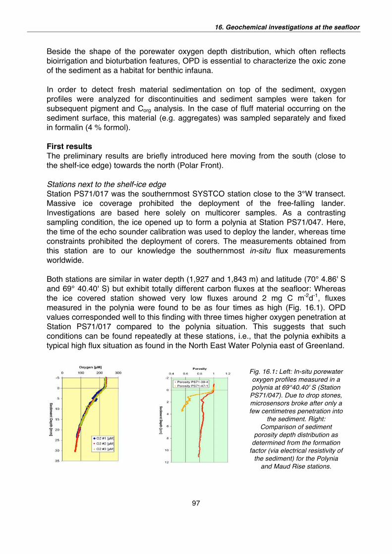
16. Geochemical investigations at the seafloor
97
Beside the shape of the porewater oxygen depth distribution, which often reflects
bioirrigation and bioturbation features, OPD is essential to characterize the oxic zone
of the sediment as a habitat for benthic infauna.
In order to detect fresh material sedimentation on top of the sediment, oxygen
profiles were analyzed for discontinuities and sediment samples were taken for
subsequent pigment and Corg analysis. In the case of fluff material occurring on the
sediment surface, this material (e.g. aggregates) was sampled separately and fixed
in formalin (4 % formol).
First results The preliminary results are briefly introduced here moving from the south (close to
the shelf-ice edge) towards the north (Polar Front).
Stations next to the shelf-ice edge
Station PS71/017 was the southernmost SYSTCO station close to the 3°W transect.
Massive ice coverage prohibited the deployment of the free-falling lander.
Investigations are based here solely on multicorer samples. As a contrasting
sampling condition, the ice opened up to form a polynia at Station PS71/047. Here,
the time of the echo sounder calibration was used to deploy the lander, whereas time
constraints prohibited the deployment of corers. The measurements obtained from
this station are to our knowledge the southernmost in-situ flux measurements
worldwide.
Both stations are similar in water depth (1,927 and 1,843 m) and latitude (70° 4.86' S
and 69° 40.40' S) but exhibit totally different carbon fluxes at the seafloor: Whereas
the ice covered station showed very low fluxes around 2 mg C m-2d-1, fluxes
measured in the polynia were found to be as four times as high (Fig. 16.1). OPD
values corresponded well to this finding with three times higher oxygen penetration at
Station PS71/017 compared to the polynia situation. This suggests that such
conditions can be found repeatedly at these stations, i.e., that the polynia exhibits a
typical high flux situation as found in the North East Water Polynia east of Greenland.
Fig. 16.1: Left: In-situ porewater
oxygen profiles measured in a
polynia at 69°40.40' S (Station
PS71/047). Due to drop stones,
microsensors broke after only a
few centimetres penetration into
the sediment. Right:
Comparison of sediment
porosity depth distribution as
determined from the formation
factor (via electrical resistivity of
the sediment) for the Polynia
and Maud Rise stations.
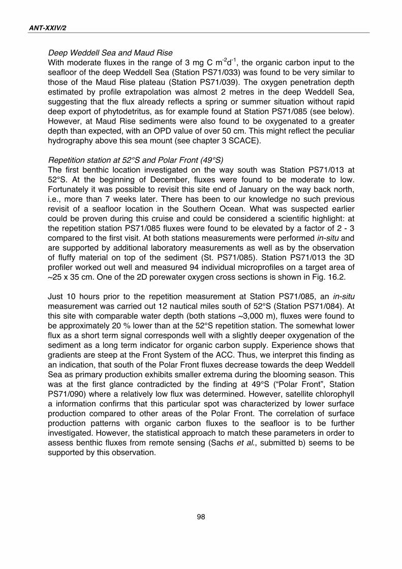
ANT-XXIV/2
98
Deep Weddell Sea and Maud Rise
With moderate fluxes in the range of 3 mg C m-2d-1, the organic carbon input to the
seafloor of the deep Weddell Sea (Station PS71/033) was found to be very similar to
those of the Maud Rise plateau (Station PS71/039). The oxygen penetration depth
estimated by profile extrapolation was almost 2 metres in the deep Weddell Sea,
suggesting that the flux already reflects a spring or summer situation without rapid
deep export of phytodetritus, as for example found at Station PS71/085 (see below).
However, at Maud Rise sediments were also found to be oxygenated to a greater
depth than expected, with an OPD value of over 50 cm. This might reflect the peculiar
hydrography above this sea mount (see chapter 3 SCACE).
Repetition station at 52°S and Polar Front (49°S)
The first benthic location investigated on the way south was Station PS71/013 at
52°S. At the beginning of December, fluxes were found to be moderate to low.
Fortunately it was possible to revisit this site end of January on the way back north,
i.e., more than 7 weeks later. There has been to our knowledge no such previous
revisit of a seafloor location in the Southern Ocean. What was suspected earlier
could be proven during this cruise and could be considered a scientific highlight: at
the repetition station PS71/085 fluxes were found to be elevated by a factor of 2 - 3
compared to the first visit. At both stations measurements were performed in-situ and
are supported by additional laboratory measurements as well as by the observation
of fluffy material on top of the sediment (St. PS71/085). Station PS71/013 the 3D
profiler worked out well and measured 94 individual microprofiles on a target area of
~25 x 35 cm. One of the 2D porewater oxygen cross sections is shown in Fig. 16.2.
Just 10 hours prior to the repetition measurement at Station PS71/085, an in-situ
measurement was carried out 12 nautical miles south of 52°S (Station PS71/084). At
this site with comparable water depth (both stations ~3,000 m), fluxes were found to
be approximately 20 % lower than at the 52°S repetition station. The somewhat lower
flux as a short term signal corresponds well with a slightly deeper oxygenation of the
sediment as a long term indicator for organic carbon supply. Experience shows that
gradients are steep at the Front System of the ACC. Thus, we interpret this finding as
an indication, that south of the Polar Front fluxes decrease towards the deep Weddell
Sea as primary production exhibits smaller extrema during the blooming season. This
was at the first glance contradicted by the finding at 49°S (“Polar Front”, Station
PS71/090) where a relatively low flux was determined. However, satellite chlorophyll
a information confirms that this particular spot was characterized by lower surface
production compared to other areas of the Polar Front. The correlation of surface
production patterns with organic carbon fluxes to the seafloor is to be further
investigated. However, the statistical approach to match these parameters in order to
assess benthic fluxes from remote sensing (Sachs et al., submitted b) seems to be
supported by this observation.
16. Geochemical investigations at the seafloor
99
Distance Y [mm]
Fig. 16.2: 2D porewater oxygen cross section measured in-situ at Station PS71/013. Oxygen
concentration decreases according to colour transition from blue-yellow-green-red whereas the border
blue-yellow indicated the sediment-water interface.
References Anderson, L. A., Sarmiento, J. L., 1994. Redfield ratios of remineralization determined by
nutrient data analysis. Global Biogeochemical Cycles 8, 65-80.
Berg, P., Risgaard-Petersen, N., Rysgaard, S., 1998. Interpretation of measured
concentration profiles in sediment pore water. Limnology and Oceanography 43, 1500-
1510.
Sachs, O., Sauter, E. J., Schlüter, M., Rutgers van der Loeff, M. M., Jerosch, K., Holby, O.
(submitted a). Benthic organic carbon flux and oxygen penetration reflect different
plankton provinces in the Southern Ocean. Deep-Sea Research I.
Sachs, O., Schwarz, J.N., Sauter, E.J., Schlüter, M., Schodlok M., (submitted b). Spatial
variability of the transfer efficiency of primary produced carbon to the seafloor of the
Southern Ocean. Global Biogeochemical Cycles.
Sarmiento, J. L. & Le Quere, C. (1996) Oceanic Carbon Dioxide Uptake in a Model of
Century-Scale Global Warming. Science 274, 1346-1350.
Acknowledgements
We are grateful for the unremitting support of Captain Uwe Pahl and his crew
throughout the entire cruise. We thank Werner Dimmler (FIELAX) for his skilled help
and repair of the 3D profiler and the camera system as well as his support with the
Parasound and Hydrosweep surveys. We appreciated the home support of Ulli Hoge,
Burkhard Sablotny and Gerd Rohardt and thank Jill Schwarz for providing remote
sensing chlorophyll information. In particular we are grateful for the excellent cruise
organisation by Uli Bathmann as well as for the mutual help amongst the scientific
party and many scientific discussions which made this voyage successful and rich in
positive experiences despite the shortage of ship time. DOMINO was funded by the
DFG under contract SA1030/2-1.
100
17. MICROBIAL COMMUNITIES WITHIN DEEP ANTARCTIC SEDIMENTS Henri Robert, Bruno
Danis, (not on board)
Institut Royal des Sciences Naturelles de
Belgique, Brussels, Belgium
Scientific background and objectives
In a previous study, carried out using samples from the ANDEEP 3 expedition, 16S
ribosomal DNA clone library analysis was performed to assess archaeal diversity
within three surficial sediment samples obtained from the bathypelagic zone (depth :
2,165 -3,406 m) of the Weddell Sea,. The nearly complete 16S rDNA gene (1,440 bp)
was obtained for 146 clones; 46 phylotypes were defined. The majority of the
sequences (> 99 %) formed three clusters within the Marine Group I Crenarchaeota.
The most important cluster, with 78.8 % of the clones, included Candidatus
Nitrosopumilus maritimus, a mesophilic archaeon able to oxidize ammonia. The most
important subgroup in that cluster was the APA4-0cm subgroup (with 62.3 % of the
clones). This subgroup might represent important Crenarchaeota in the functioning of
the bathypelagic sedimentary ecosystems of the Weddell Sea because it dominated
the clone libraries in all sampling stations, and was found in sediments separated by
very large geographic distances. Only one clone grouped within the Euryarchaeota.
This euryarchaeal clone could not be affiliated with any of the previously defined
clusters and might represent a novel Euryarchaeal lineage.
The objective of this part of the project is to further the description of Archaeal
diversity in the deep Antarctic sediments, using the same techniques, and same
collaborations.
Work at sea
Sediments for bacterial analyses were sampled during box corer (GKG) operations,
at 6 stations. Subcores (top 8 cm) of the sample were taken using 50 ml sterile
plastic syringes. Subcores were taken away from the borders of the untouched core,
in obviously undisturbed areas. Samples were processed immediately in the dry
laboratory on Polarstern, using all precautions to avoid bacteriological contamination.
Cryotubes were filled with sediment of the subcores and deep-frozen in liquid N2 (-
196°C) until the end of the cruise, when samples were transferred to the cold storage
room (-30°C) for preservation.
Preliminary results
5 samples of each subcore were collected at six different benthic stations of the
cruise (PS 71/13, PS 71/17, PS 71/33, PS 71/39, PS 71/85 and PS 71/90), bringing a
total of 30 samples.
101
18. PROTISTS - BENTHIC FORAMINIFERA OF THE DEEP SOUTHERN OCEAN: DIVERSITY AND BIOGEOGRAPHY Delia Fontaine, Jan Pawlowski
(not on board)
University of Geneva, Geneva,
Switzerland
Objectives
Foraminifera are a significant and often visually conspicuous component of the deep-
sea and high-latitude benthic fauna. In addition to the geologically important and well-
known calcareous foraminifera, deep-sea and high-latitude assemblages include
substantial numbers of soft-shelled, mostly single-chambered species, most of which
are undescribed. These organisms include the organic-walled allogromiids, finely
agglutinated saccamminids and the large, delicately agglutinated komokiaceans, of
which the phylogenetic origin remains a mystery and deserves further studies. Literature records, combined with our own studies on Antarctic fauna, suggest that
many foraminiferal morphospecies have wide geographical ranges in the deep sea.
However, it is not certain whether all of these morphospecies constitute single
taxonomic entities at the molecular level, over their entire geographical ranges.
Furthermore, the hypothesis of genetic variation rates being lower within deep-
species than the shallow ones has to be investigated. Finally, sampling of phytodedritus, mudballs, or komoki specimens will be used to
analyze whether they could represent hotspots of deep-sea micro-diversity, as
previous observations seem to indicate. Living benthic foraminiferans were collected from 52°S latitude of the Greenwich
meridian (South Polar Front), Lazarev Sea, Weddell Sea, Maud Rise and Atka Bay,
in depths from 600 to 5,000 meters. The species collected during this expedition will be compared with similar
morphospecies collected from Antarctica during previous sampling campaigns
(Weddell Sea and McMurdo Sound). The comparison will combine molecular
analyses of ribosomal RNA gene sequences with conventional morphology-based
species descriptions to determine whether or not genetic divergence has occurred
between widely separated populations of the same morphospecies. The description
of some of the many new species collected during this expedition is also an important
objective, which will improve our knowledge of benthic foraminiferal and gromiid
biodiversity. Methods The foraminifera were isolated from surface sediment samples (0 - 5 cm) collected by
multicorer (3 cores), boxcorer (20x10cm) and additionally sediment collected by
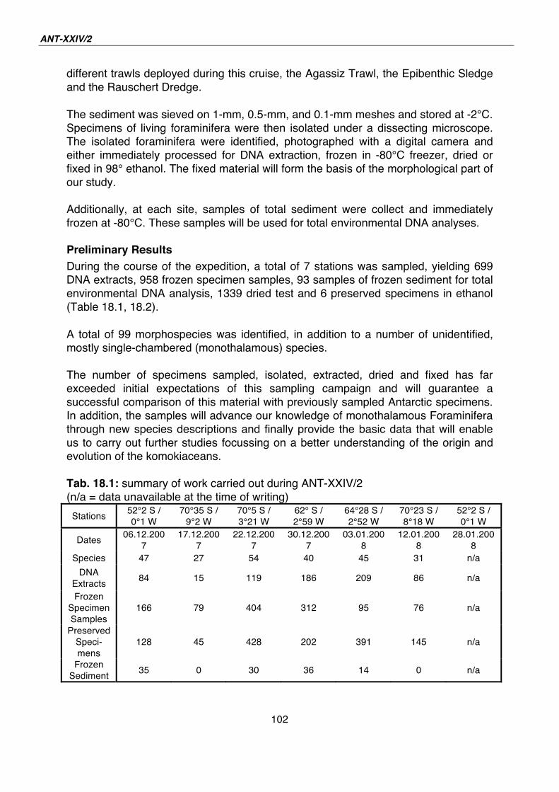
ANT-XXIV/2
102
different trawls deployed during this cruise, the Agassiz Trawl, the Epibenthic Sledge
and the Rauschert Dredge.
The sediment was sieved on 1-mm, 0.5-mm, and 0.1-mm meshes and stored at -2°C.
Specimens of living foraminifera were then isolated under a dissecting microscope.
The isolated foraminifera were identified, photographed with a digital camera and
either immediately processed for DNA extraction, frozen in -80°C freezer, dried or
fixed in 98° ethanol. The fixed material will form the basis of the morphological part of
our study.
Additionally, at each site, samples of total sediment were collect and immediately
frozen at -80°C. These samples will be used for total environmental DNA analyses.
Preliminary Results
During the course of the expedition, a total of 7 stations was sampled, yielding 699
DNA extracts, 958 frozen specimen samples, 93 samples of frozen sediment for total
environmental DNA analysis, 1339 dried test and 6 preserved specimens in ethanol
(Table 18.1, 18.2).
A total of 99 morphospecies was identified, in addition to a number of unidentified,
mostly single-chambered (monothalamous) species.
The number of specimens sampled, isolated, extracted, dried and fixed has far
exceeded initial expectations of this sampling campaign and will guarantee a
successful comparison of this material with previously sampled Antarctic specimens.
In addition, the samples will advance our knowledge of monothalamous Foraminifera
through new species descriptions and finally provide the basic data that will enable
us to carry out further studies focussing on a better understanding of the origin and
evolution of the komokiaceans.
Tab. 18.1: summary of work carried out during ANT-XXIV/2
(n/a = data unavailable at the time of writing)
Stations 52°2 S /
0°1 W
70°35 S /
9°2 W
70°5 S /
3°21 W
62° S /
2°59 W
64°28 S /
2°52 W
70°23 S /
8°18 W
52°2 S /
0°1 W
Dates 06.12.200
7
17.12.200
7
22.12.200
7
30.12.200
7
03.01.200
8
12.01.200
8
28.01.200
8
Species 47 27 54 40 45 31 n/a
DNA
Extracts 84 15 119 186 209 86 n/a
Frozen
Specimen
Samples
166 79 404 312 95 76 n/a
Preserved
Speci-
mens
128 45 428 202 391 145 n/a
Frozen
Sediment 35 0 30 36 14 0 n/a
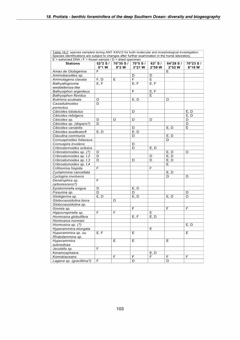
18. Protists - benthic foraminifera of the deep Southern Ocean: diversity and biogeography
103
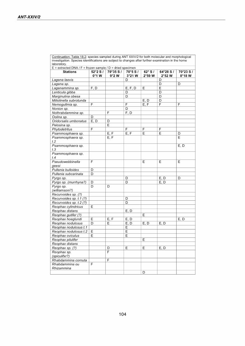
ANT-XXIV/2
104
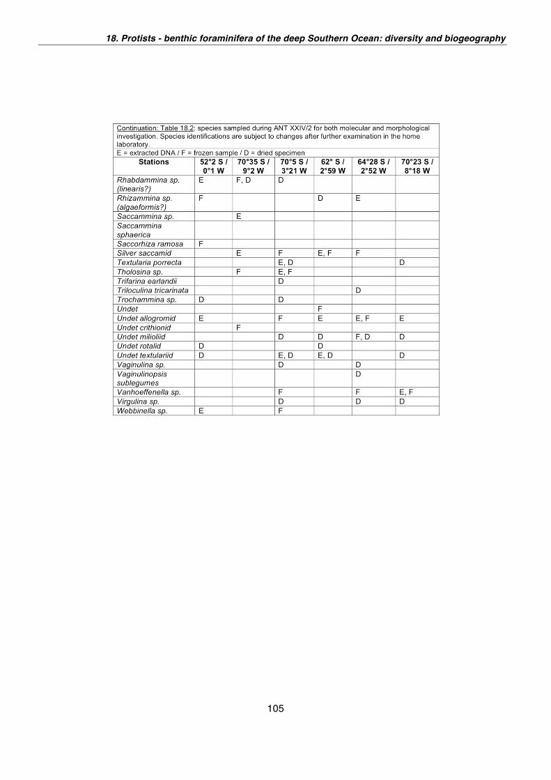
18. Protists - benthic foraminifera of the deep Southern Ocean: diversity and biogeography
105
106
19. METAZOAN MEIOFAUNA - THE LINK BETWEEN STRUCTURAL AND FUNCTIONAL BIODIVERSITY OF THE MEIOFAUNA COMMUNITIES IN THE ANTARCTIC DEEP SEA Gritta Veit-Köhler1), Annika
Henche1), Katja Guilini2), Ann
Vanreusel2) (not on board)
1) German Centre of Marine Biodiversity,
Senckenberg, Germany
2) Gent University, Gent, Belgium
Objectives
Meiofauna can significantly contribute to the regulation of benthic turnover and serve
as food for secondary consumers. The role of meiofauna in the deep Antarctic ocean
as trophic link between sedimented organic matter and higher level consumers is a
question that will be investigated in this study. The contribution of the meiofauna to
the C-flow through benthic deep-sea sediments has to be addressed in relation to
their biodiversity. In order to unravel the link between meiofaunal biodiversity and
function, it is essential to reveal the interactions in the benthic food web and the
trophic position of different meiofauna taxa and functional groups at locations with
contrasting food supply. Many studies have illustrated the high biodiversity of small
benthic taxa in the deep sea. However it remains unclear what drives this high local
biodiversity. For many systems, a relation with productivity of the system has been
hypothesized but correlation with water depth and other associated environmental
factors often hampers unravelling the link between biodiversity and food input. At the
Southern Polar Front, strong water mass and primary productivity gradients exist. A
repeated sampling on the front and sampling southwards would allow an estimate of
the variation in local biodiversity in relation to changing productivity levels.
Biomarkers such as stable isotopes and fatty acids can be traced throughout food
webs and thus are suitable for the understanding of trophic positions and food
resource selectivity of marine species. Detailed analyses of fatty acid, fatty alcohol
and wax ester compositions can elucidate similarities between taxa and reveal
indications of feeding behaviour and food sources. The advantage of applying lipid
compositions to feeding studies is that trophic lipid markers integrate longer time
periods than conventional methods. Feeding experiments verified the concept of
trophic marker lipids, using algae and copepods of known lipid composition. But
generally, benthic species have relatively low lipid contents as compared to
herbivorous zooplankton species and do not rely on depot lipids in the same way.
Often fatty acids of the available food sources dominate the fatty acid composition of
the species, masking potentially taxon-specific patterns and emphasising the intensity of the pelago-benthic coupling. Therefore stable isotope ratios 13C and 15N
19. Metazoan meiofauna
107
have to be used as an additional tool which can contribute to the determination of
food sources and selectivity in meiofauna organisms, even at species level.
This and the linking to total meiofaunal standing stocks in the Antarctic deep-sea
sediments, which are highly dependent on the degree of organic matter input and
consequently the surface primary production, will be a crucial contribution to the
generalised energy-flux model and food web study - a common objective of the
ANDEEP-SYSTCO cruise.
Work at sea
Samples were taken with the multiple corer (MUC). From every MUC deployment 1 to
3 sediment cores were sliced down to 20 cm (0 - 1 cm, 1 - 2 cm, 2 - 3 cm, 3 - 4 cm, 4
- 5 cm, 5 - 7 cm, 7 - 10 cm, 10 - 15 cm, 15 - 20 cm). The sediment slices were
preserved in 4 % buffered formaldehyde/seawater solution and stored for meiofauna
community analysis. Our sampling method enables us not only to compare different
regions but also to study the vertical distribution profile of the meiobenthos in the
sediment. From one core per deployment, syringe subsamples were taken for
granulometry, organic carbon and pigment analyses. The organic carbon and
pigment samples were stored at -30°C. Furthermore a minimum of 4 cores per
deployment were used to scoop off the upper 5 cm of sediment. This material was
immediately sieved in the lab with filtered seawater over stacked sieves (1 mm, 500
μm, 100 μm and 32 μm). We retained the 500 μm, 100 μm and 32 μm fractions and
stored them at -80°C. Back at the laboratory, the nematodes and copepods will be
extracted for biochemical analyses (fatty acids and stable isotopes).
Preliminary results
During the course of the expedition a total of 6 deep-sea stations was sampled,
yielding 25 cores which were sliced for meiofaunal community analysis, 24 samples
for biochemical analysis and 12 x 3 subsamples for additonal granulometry, organic
carbon and pigment analysis.
Back at the laboratory, the nematodes and copepods from the formalin fixed samples
will be extracted from the sediment, identified and counted for analyzing the
communities and diversity at the different locations. Stable isotope and fatty acid
analyses will be performed on the nematodes and copepods picked out from the
frozen samples and identified to the lowest taxonomic level possible, in order to
identify the relative importance of the different food sources and the potential
selectivity. Nevertheless, very high numbers of these animals are necessary for these
analyses.
Co-operation with Laura Würzberg (University of Hamburg) as well as Eberhard
Sauter and Oliver Sachs (Alfred Wegener Institute for Polar and Marine Research)
will ensure linking of our data to sediment parameters and oxygen profiles.
108
20. AN EXPERIMENTAL APPROACH TO THE MEIOBENTHIC FOOD-WEB STUDY IN THE SOUTHERN OCEAN DEEP SEA: WHAT IS THE MICROBIAL CARBON CONTRIBUTION TO THE DIET OF NEMATODA? Katja Guilini, Ann
Vanreusel (not on board)
Gent University, Gent, Belgium
Objectives
In addition to the analyses on the meiofauna community and the biochemical
background values, an experiment was planned in which the trophodynamic and
functional aspects of the dominant metazoan benthos taxon, the Nematoda, were the
main focus. Owing to their ubiquitous presence, nematodes are assumed to play an
important role in the benthic food web. However, little is known on their trophic status
and functioning in deep-sea sediments. Although previous studies showed that the
nematode standing stock in deep-sea sediments is closely linked to the degree of
organic matter input and consequently the surface primary production, their response
to seasonally varying deposition of phytodetritus seems often delayed in time.
Instead of an increase in densities at the surface of the sediments, there also seem
to be subsurface maxima in densities. Although limited to date, evidence for a
microbial related feeding activity rather than using fresh phytodetritus as food source
is growing. In order to test the uptake rate and potential preference for microbial
related food sources an ex-situ enrichment experiment with several 13C labeled
substrates was performed. Back at the laboratory, these results together with the
natural biomarker analysis (stable isotopes and fatty acids) of selected taxa will
unravel an integrated view on of the degree of selectivity and food preferences of
nematodes for particular components of the deep-sea ecosystem.
Work at sea
Methods
At the approximately 2,120 m deep Maud Rise station, 20 sediment cores were
gathered during 3 MUC deployments for the ex-situ experiment. The 100-mm
diameter cores were subsampled on deck with 67-mm diameter cores, incubated in a
cold room at in-situ temperature (0.5°C) and oxygenated. Shortly after, 13C labelled
substrates were injected in the upper 5 cm of the sediment. There were four
treatments (acetate, bicarbonate, glucose and bacteria grown on degrading diatoms)
and one control which was sampled according to a time series (day 2, day 4, day 8
and day 12). The control samples were checked for living nematodes and preserved
in 4 % buffered formaldehyde, while the treatment samples for biochemical analysis
were stored at -20°C. Additionally, DNA extractions of the bacterial communities in
the sediment were performed. This was done for the different treatments at several
20. What is the microbial carbon contribution to the diet of nematoda?
109
sampling days from the time series. Due to a collaboration with Eberhard Sauter and
Oliver Sachs (AWI) established during the campaign, oxygen profiles could be
measured in several cores over the time series.
Preliminary results
The experiment was completed on day 12. At each time step living nematodes were
found in the control samples, however, not quantified. The oxygen profiles measured
in the samples over the time series indicate different ongoing processes in the upper
layers of the sediment according to the treatment. However we will only be able to
interpret these profiles after we have performed the biochemical and DNA analyses
back in the laboratory. The experimental results will enable us to quantify the uptake
and incorporation of microbial carbon by nematodes.
110
21. MACROFAUNA – BIODIVERSITY, ECOLOGY AND ZOOGEOGRAPHY OF PERACARID CRUSTACEANS AND POLYCHAETA Angelika Brandt1), Lydia Kramer1),
Torben Riehl1), Laura Würzberg1),
Saskia Brix2),
Brigitte Ebbe2), Myriam Schüller3)
1) Zoological Museum Hamburg, Germany
2) German Centre of Marine Biodiversity,
Senckenberg, Germany
3) Ruhr Universität Bochum, Germany
Objectives
During SYSTCO, the biodiversity and ecology including feeding biology of peracarid
crustaceans (with focus on the Isopoda), and polychaetes were investigated using an
epibenthic sledge. The results will be compared with data from the ANDEEP
expeditions. Quantitative and qualitative samples were taken at five stations between
1,736 and 5,338 m in different water masses and environments with different
topographical and sedimentary conditions. These catches covered a trawled area of
9,537 m . For further details please see benthic work - introduction to work at sea.
Very little is known about the ecology and role of deep-sea fauna in the
trophodynamic coupling and nutrient cycling in oceanic ecosystems. This project
examines the trophic structure and functioning of the abyssal macrobenthic
community of the Southern Atlantic Ocean, focusing specifically on the role of the
Isopoda and Polychaeta including
1) general feeding biology,
2) bentho-pelagic coupling,
3) the reproduction of abundant species, and
4) population genetics of selected abundant species.
Epibenthic sledge samples from three previous Polarstern expeditions (ANDEEP I-III)
and new epibenthic sledge and sediment core samples taken during this expedition
will be analysed. A variety of methods will be used including gut content analysis,
functional morphology of target species as well as biochemical measurements. The
latter include analyses of lipid classes, fatty acid biomarkers, and examination of
stable isotopic signatures of epifaunal animals and surrounding sediments.
The results will be compared and combined with the findings of research groups
examining other aspects of the Southern Ocean foodweb and biogeochemistry of the
sediment. Combining the comprehensive datasets concerning diversity and
colonisation patterns available from ANDEEP I-III and this study focusing on foodweb
dynamics allows us, for the first time, to better understand the trophodynamic role of
deep-sea fauna in the ecology of the South Atlantic and Southern Ocean.
21. Macrofauna - biodiversity, ecology and zoogeography of peracarid crustaceans and polychaeta
111
The high diversity of the Southern Ocean Isopoda was shown by Brandt et al. (2007).
To this constraint, the difficulty of obtaining DNA-friendly samples from the deep sea
has to be added. Our results from previous expeditions show that DNA quality
strongly depends on the fixation method used and a stable cooling chain while taking
deep-sea samples. Successful genetic work with isopods can only be performed with
fresh material, sorted and extracted on board. To develop the most efficient analytical
procedures, we want to improve DNA quality. Thus, we started a series of
experiments as an approach for DNA quality improvement. High quality DNA is
important to gain clear genetic signals (sequences) for phylogenetic studies.
Parallel to the aim to elucidate the phylogeny of different asellote isopod families (e.g.
Desmosomatidae Sars, 1897; Macrostylidae Hansen, 1916), we are attempting DNA
barcoding on deep-sea isopods for the first time. The barcoding approach in
collaboration with the Canadian Centre of DNA Barcoding (CCDB) contributes to the
SYSTCO objectives in using barcoding alongside traditional taxonomic methods to
investigate key species and their role in the benthos of the Southern Ocean.
DNA barcoding is a standardized approach to identifying species by comparing small
sequences of DNA. Target sequence is CO I. The early goals of DNA barcoding
focus on the assembly of reference libraries of barcode sequences for known
species. Working with deep-sea material, our research focuses on unknown or
undescribed species. Molecular barcoding can hint at the existence of new taxa, but
cannot replace their formal description. Our aims are to link morphological
descriptions with barcodes and to establish a storage of the voucher specimens
together with the DNA samples.
Work at sea
We started our analyses with the ethanol fixed samples from the ANDEEP I-III
expeditions and determined abundant abyssal species as background information for
the cruise. We also did first analyses of the mouthparts and foregut (including the gut
contents) and some morphometric measurements on isopods in the laboratory before
we started with the expedition, in order to obtain some ideas on the general feeding
biology of abundant species (e.g. suspension feeders, deposit feeders, scavengers,
predators, etc.). On board we started with gut content analyses of bigger organisms
like fish and holothurians to check which of the species found fed on crustaceans or
more specifically on isopods.
During this expedition (ANT-XXIV/2) we sampled at 6 of 7 planned stations for
SYSTCO in total. Two stations were incomplete. The first station we took on our way
south from Cape Town was revisited seven weeks later on our way back to Cape
Town (see Fig. 15.1). This station at 52°S was the only station revisited, contrary to
our original intention to revisit two stations. Five of the six stations included
epibenthic sledge samples, which will serve as a basis for the above-described
biochemical and gut content analysis.
Half of the epibenthic sledge material was immediately fixed in precooled 96 %
ethanol and stored at least for 48 hours at –20°C, later at 0° C. Sorting was started
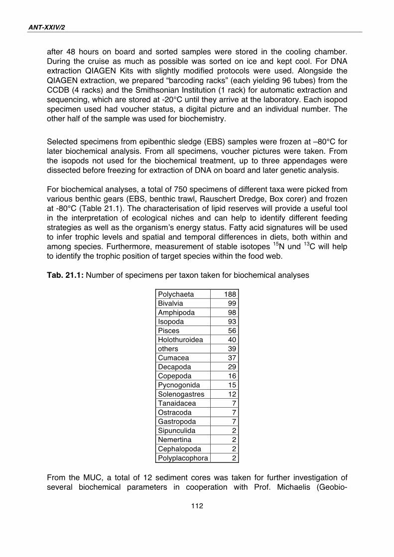
ANT-XXIV/2
112
after 48 hours on board and sorted samples were stored in the cooling chamber.
During the cruise as much as possible was sorted on ice and kept cool. For DNA
extraction QIAGEN Kits with slightly modified protocols were used. Alongside the
QIAGEN extraction, we prepared “barcoding racks” (each yielding 96 tubes) from the
CCDB (4 racks) and the Smithsonian Institution (1 rack) for automatic extraction and
sequencing, which are stored at -20°C until they arrive at the laboratory. Each isopod
specimen used had voucher status, a digital picture and an individual number. The
other half of the sample was used for biochemistry.
Selected specimens from epibenthic sledge (EBS) samples were frozen at –80°C for
later biochemical analysis. From all specimens, voucher pictures were taken. From
the isopods not used for the biochemical treatment, up to three appendages were
dissected before freezing for extraction of DNA on board and later genetic analysis.
For biochemical analyses, a total of 750 specimens of different taxa were picked from
various benthic gears (EBS, benthic trawl, Rauschert Dredge, Box corer) and frozen
at -80°C (Table 21.1). The characterisation of lipid reserves will provide a useful tool
in the interpretation of ecological niches and can help to identify different feeding
strategies as well as the organism s energy status. Fatty acid signatures will be used
to infer trophic levels and spatial and temporal differences in diets, both within and
among species. Furthermore, measurement of stable isotopes 15N und 13C will help
to identify the trophic position of target species within the food web.
Tab. 21.1: Number of specimens per taxon taken for biochemical analyses
Polychaeta 188
Bivalvia 99
Amphipoda 98
Isopoda 93
Pisces 56
Holothuroidea 40
others 39
Cumacea 37
Decapoda 29
Copepoda 16
Pycnogonida 15
Solenogastres 12
Tanaidacea 7
Ostracoda 7
Gastropoda 7
Sipunculida 2
Nemertina 2
Cephalopoda 2
Polyplacophora 2
From the MUC, a total of 12 sediment cores was taken for further investigation of
several biochemical parameters in cooperation with Prof. Michaelis (Geobio-
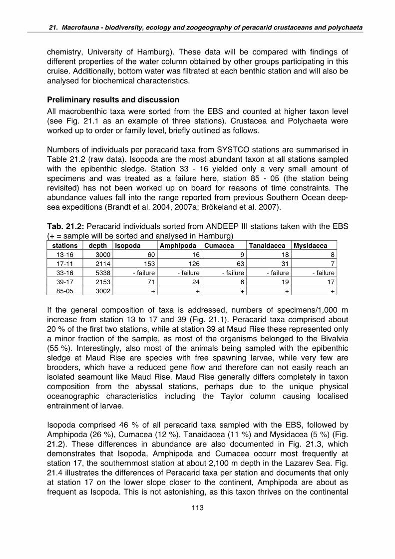
21. Macrofauna - biodiversity, ecology and zoogeography of peracarid crustaceans and polychaeta
113
chemistry, University of Hamburg). These data will be compared with findings of
different properties of the water column obtained by other groups participating in this
cruise. Additionally, bottom water was filtrated at each benthic station and will also be
analysed for biochemical characteristics.
Preliminary results and discussion
All macrobenthic taxa were sorted from the EBS and counted at higher taxon level
(see Fig. 21.1 as an example of three stations). Crustacea and Polychaeta were
worked up to order or family level, briefly outlined as follows.
Numbers of individuals per peracarid taxa from SYSTCO stations are summarised in
Table 21.2 (raw data). Isopoda are the most abundant taxon at all stations sampled
with the epibenthic sledge. Station 33 - 16 yielded only a very small amount of
specimens and was treated as a failure here, station 85 - 05 (the station being
revisited) has not been worked up on board for reasons of time constraints. The
abundance values fall into the range reported from previous Southern Ocean deep-
sea expeditions (Brandt et al. 2004, 2007a; Brökeland et al. 2007).
Tab. 21.2: Peracarid individuals sorted from ANDEEP III stations taken with the EBS
(+ = sample will be sorted and analysed in Hamburg) stations depth Isopoda Amphipoda Cumacea Tanaidacea Mysidacea
13-16 3000 60 16 9 18 8
17-11 2114 153 126 63 31 7
33-16 5338 - failure - failure - failure - failure - failure
39-17 2153 71 24 6 19 17
85-05 3002 + + + + +
If the general composition of taxa is addressed, numbers of specimens/1,000 m
increase from station 13 to 17 and 39 (Fig. 21.1). Peracarid taxa comprised about
20 % of the first two stations, while at station 39 at Maud Rise these represented only
a minor fraction of the sample, as most of the organisms belonged to the Bivalvia
(55 %). Interestingly, also most of the animals being sampled with the epibenthic
sledge at Maud Rise are species with free spawning larvae, while very few are
brooders, which have a reduced gene flow and therefore can not easily reach an
isolated seamount like Maud Rise. Maud Rise generally differs completely in taxon
composition from the abyssal stations, perhaps due to the unique physical
oceanographic characteristics including the Taylor column causing localised
entrainment of larvae.
Isopoda comprised 46 % of all peracarid taxa sampled with the EBS, followed by
Amphipoda (26 %), Cumacea (12 %), Tanaidacea (11 %) and Mysidacea (5 %) (Fig.
21.2). These differences in abundance are also documented in Fig. 21.3, which
demonstrates that Isopoda, Amphipoda and Cumacea occurr most frequently at
station 17, the southernmost station at about 2,100 m depth in the Lazarev Sea. Fig.
21.4 illustrates the differences of Peracarid taxa per station and documents that only
at station 17 on the lower slope closer to the continent, Amphipoda are about as
frequent as Isopoda. This is not astonishing, as this taxon thrives on the continental
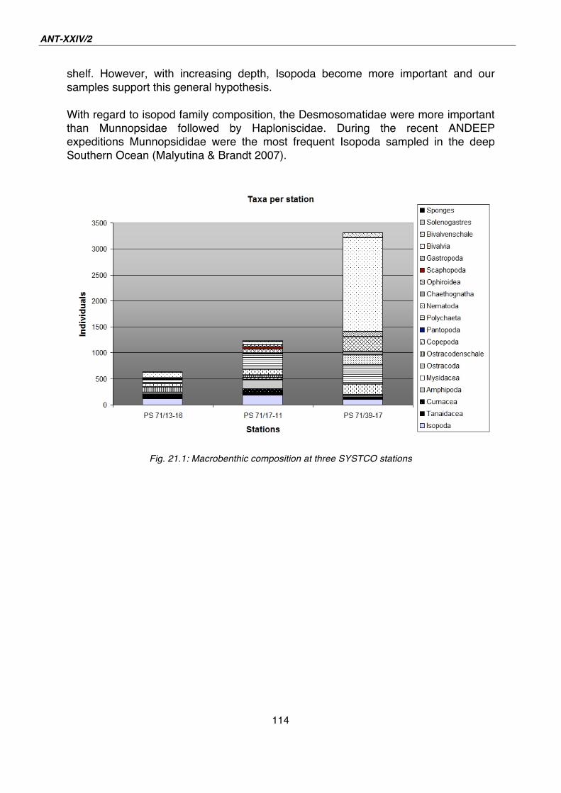
ANT-XXIV/2
114
shelf. However, with increasing depth, Isopoda become more important and our
samples support this general hypothesis.
With regard to isopod family composition, the Desmosomatidae were more important
than Munnopsidae followed by Haploniscidae. During the recent ANDEEP
expeditions Munnopsididae were the most frequent Isopoda sampled in the deep
Southern Ocean (Malyutina & Brandt 2007).
Fig. 21.1: Macrobenthic composition at three SYSTCO stations
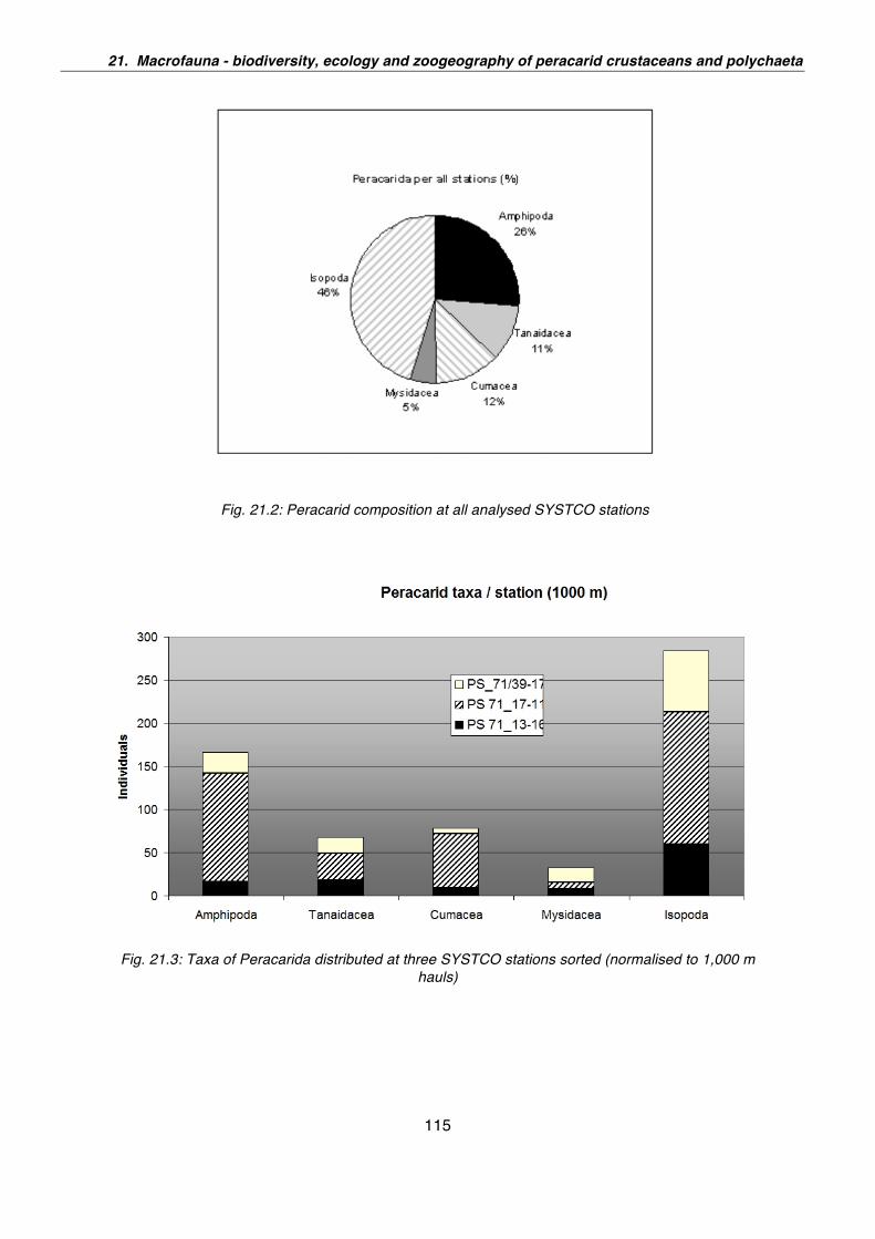
21. Macrofauna - biodiversity, ecology and zoogeography of peracarid crustaceans and polychaeta
115
Fig. 21.2: Peracarid composition at all analysed SYSTCO stations
Fig. 21.3: Taxa of Peracarida distributed at three SYSTCO stations sorted (normalised to 1,000 m
hauls)
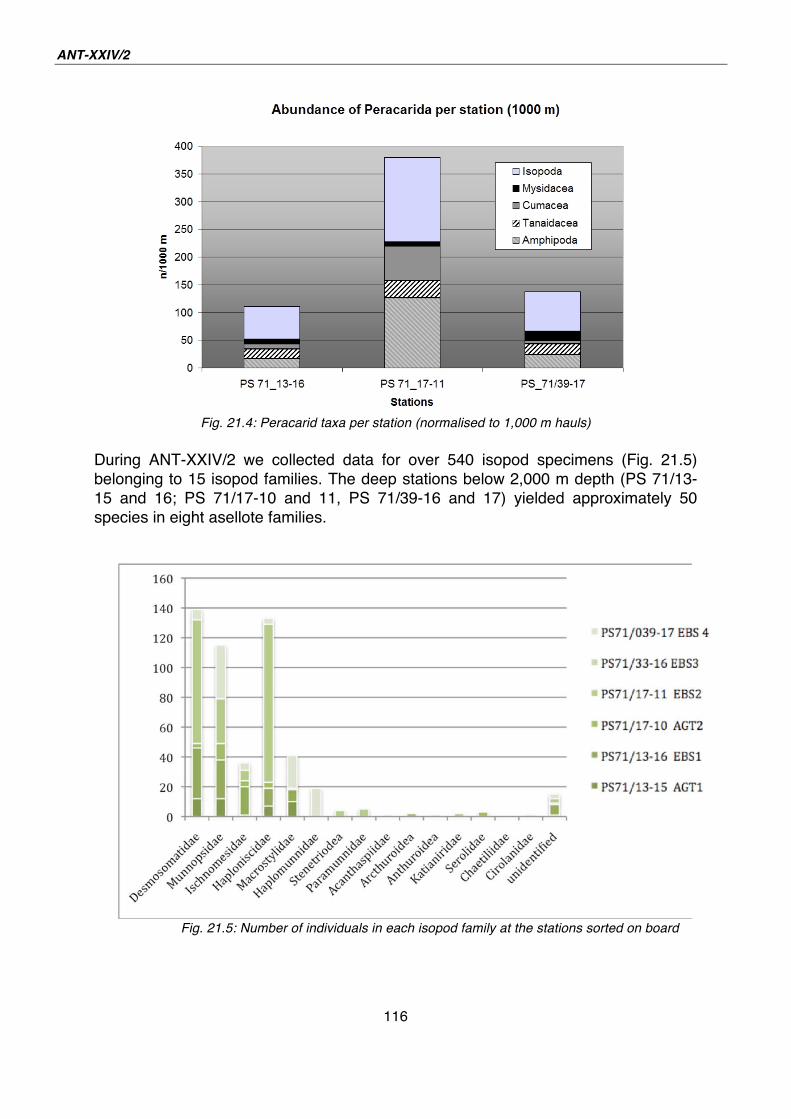
ANT-XXIV/2
116
Fig. 21.4: Peracarid taxa per station (normalised to 1,000 m hauls)
During ANT-XXIV/2 we collected data for over 540 isopod specimens (Fig. 21.5)
belonging to 15 isopod families. The deep stations below 2,000 m depth (PS 71/13-
15 and 16; PS 71/17-10 and 11, PS 71/39-16 and 17) yielded approximately 50
species in eight asellote families.
Fig. 21.5: Number of individuals in each isopod family at the stations sorted on board
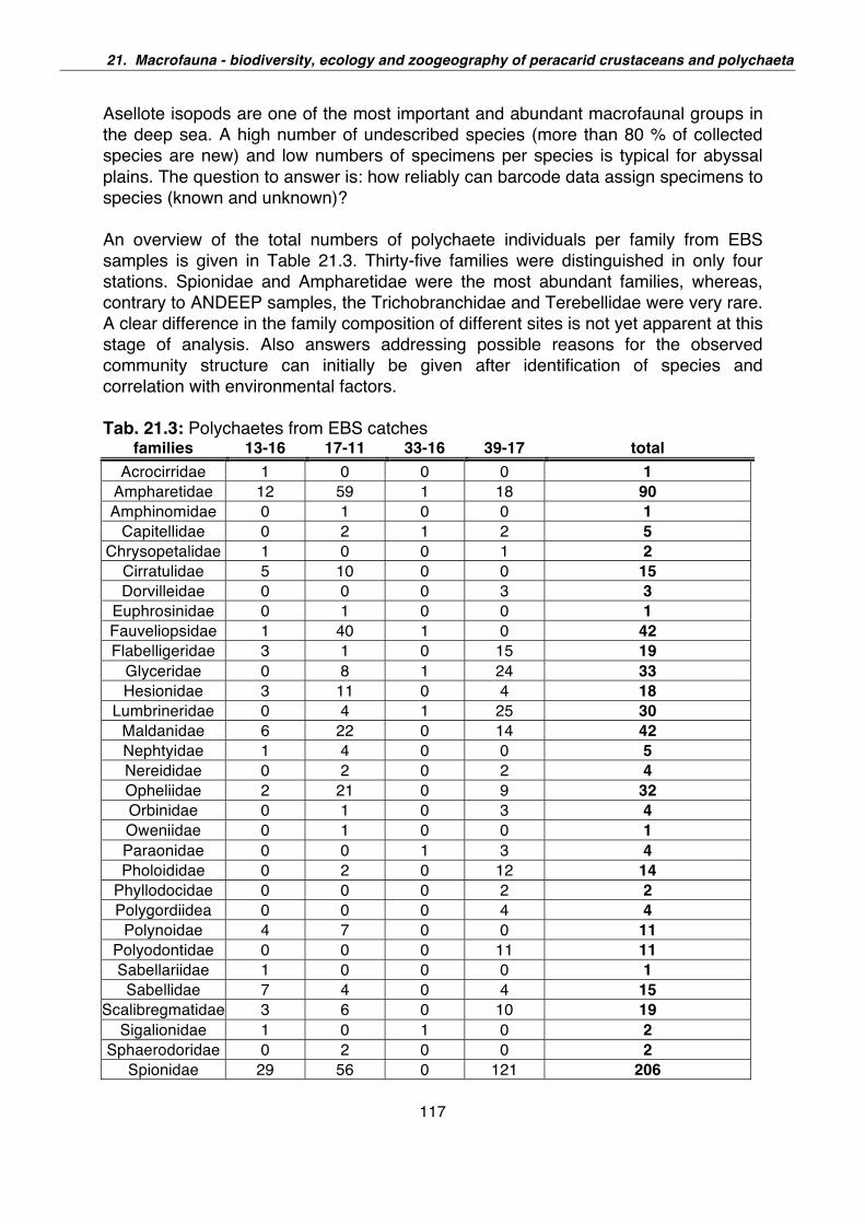
21. Macrofauna - biodiversity, ecology and zoogeography of peracarid crustaceans and polychaeta
117
Asellote isopods are one of the most important and abundant macrofaunal groups in
the deep sea. A high number of undescribed species (more than 80 % of collected
species are new) and low numbers of specimens per species is typical for abyssal
plains. The question to answer is: how reliably can barcode data assign specimens to
species (known and unknown)?
An overview of the total numbers of polychaete individuals per family from EBS
samples is given in Table 21.3. Thirty-five families were distinguished in only four
stations. Spionidae and Ampharetidae were the most abundant families, whereas,
contrary to ANDEEP samples, the Trichobranchidae and Terebellidae were very rare.
A clear difference in the family composition of different sites is not yet apparent at this
stage of analysis. Also answers addressing possible reasons for the observed
community structure can initially be given after identification of species and
correlation with environmental factors.
Tab. 21.3: Polychaetes from EBS catches families 13-16 17-11 33-16 39-17 total
Acrocirridae 1 0 0 0 1 Ampharetidae 12 59 1 18 90 Amphinomidae 0 1 0 0 1
Capitellidae 0 2 1 2 5 Chrysopetalidae 1 0 0 1 2
Cirratulidae 5 10 0 0 15 Dorvilleidae 0 0 0 3 3
Euphrosinidae 0 1 0 0 1 Fauveliopsidae 1 40 1 0 42 Flabelligeridae 3 1 0 15 19
Glyceridae 0 8 1 24 33 Hesionidae 3 11 0 4 18
Lumbrineridae 0 4 1 25 30 Maldanidae 6 22 0 14 42 Nephtyidae 1 4 0 0 5 Nereididae 0 2 0 2 4 Opheliidae 2 21 0 9 32 Orbinidae 0 1 0 3 4 Oweniidae 0 1 0 0 1 Paraonidae 0 0 1 3 4 Pholoididae 0 2 0 12 14
Phyllodocidae 0 0 0 2 2 Polygordiidea 0 0 0 4 4
Polynoidae 4 7 0 0 11 Polyodontidae 0 0 0 11 11 Sabellariidae 1 0 0 0 1
Sabellidae 7 4 0 4 15 Scalibregmatidae 3 6 0 10 19
Sigalionidae 1 0 1 0 2 Sphaerodoridae 0 2 0 0 2
Spionidae 29 56 0 121 206
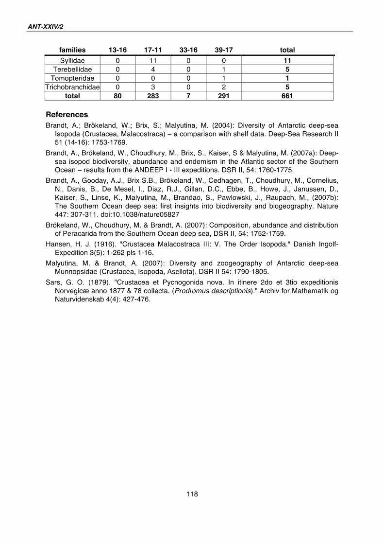
ANT-XXIV/2
118
families 13-16 17-11 33-16 39-17 total
Syllidae 0 11 0 0 11 Terebellidae 0 4 0 1 5
Tomopteridae 0 0 0 1 1 Trichobranchidae 0 3 0 2 5
total 80 283 7 291 661 References Brandt, A.; Brökeland, W.; Brix, S.; Malyutina, M. (2004): Diversity of Antarctic deep-sea
Isopoda (Crustacea, Malacostraca) – a comparison with shelf data. Deep-Sea Research II
51 (14-16): 1753-1769.
Brandt, A., Brökeland, W., Choudhury, M., Brix, S., Kaiser, S & Malyutina, M. (2007a): Deep-
sea isopod biodiversity, abundance and endemism in the Atlantic sector of the Southern
Ocean – results from the ANDEEP I - III expeditions. DSR II, 54: 1760-1775.
Brandt, A., Gooday, A.J., Brix S.B., Brökeland, W., Cedhagen, T., Choudhury, M., Cornelius,
N., Danis, B., De Mesel, I., Diaz, R.J., Gillan, D.C., Ebbe, B., Howe, J., Janussen, D.,
Kaiser, S., Linse, K., Malyutina, M., Brandao, S., Pawlowski, J., Raupach, M., (2007b):
The Southern Ocean deep sea: first insights into biodiversity and biogeography. Nature
447: 307-311. doi:10.1038/nature05827
Brökeland, W., Choudhury, M. & Brandt, A. (2007): Composition, abundance and distribution
of Peracarida from the Southern Ocean deep sea, DSR II, 54: 1752-1759.
Hansen, H. J. (1916). "Crustacea Malacostraca III: V. The Order Isopoda." Danish Ingolf-
Expedition 3(5): 1-262 pls 1-16.
Malyutina, M. & Brandt, A. (2007): Diversity and zoogeography of Antarctic deep-sea
Munnopsidae (Crustacea, Isopoda, Asellota). DSR II 54: 1790-1805.
Sars, G. O. (1879). "Crustacea et Pycnogonida nova. In itinere 2do et 3tio expeditionis
Norvegicæ anno 1877 & 78 collecta. (Prodromus descriptionis)." Archiv for Mathematik og
Naturvidenskab 4(4): 427-476.
119
22. INDICATIONS FOR CRYPTIC SPECIATION IN THE SOUTHERN OCEAN AMPHARETIDAE AND TRICHOBRANCHIDAE (ANNELIDA, POLYCHAETA) Myriam Schüller1), Brigitte
Ebbe2)
1) Ruhr Universität Bochum, Germany
2) German Centre of Marine Biodiversity,
Senckenberg, Germany
Objectives
During the former ANDEEP I-III projects, the deep Weddell Sea has proven to host a
highly diverse polychaete fauna. However, species accumulation plots have shown
that the number of species recorded for the Southern Ocean deep sea is far below
the expected level. Also, the forces that drive the composition of the polychaete
fauna at different areas are merely subject to speculation so far. The SYSTCO
programme therefore offered the chance to enlarge our knowledge about the number
of species inhabiting the deep Southern Ocean and correlate these findings to
parameters measured throughout the complete water column, giving insight into
possible coupling processes for the first time (see chapter 15).
The analysis of distribution patterns of polychaete species from the Southern Ocean
has shown that the polychaete fauna is not isolated. Rather, many species have wide
distribution ranges (Schüller & Hilbig, 2007). About 25 % of all species found during
ANDEEP I-III are considered cosmopolitan species. Additionally, eurybathy seems to
be very common among Southern Ocean polychaetes (Hilbig, 2004). In the context of
the background of the discovery of cryptic speciation among many invertebrate
species world wide (e.g., Bleidorn et al., 2006, Held, 2003, Linse et al., 2007) and
with help of molecular genetics, this apparent distribution pattern can be studied in
greater detail and may have to be revised. As model taxa to find indications for
cryptic speciation among Southern Ocean polychaetes, the families Ampharetidae
and Trichobranchidae were chosen. Both families include species with wide vertical
and global distribution ranges. Their taxonomy is poorly resolved and world-wide
records of one species might be due to misidentification. However, the Ampharetidae
especially are among the most abundant and diverse families in the deep sea. A
thorough knowledge of this group is therefore essential for biodiversity analyses in
the deep sea. The Trichobranchidae include with Terebellides stroemii probably the
best known cosmopolitan species in polychaete science. Although Williams (1984)
has already discovered two different morphological variations, further investigations
about its cosmopolitan status have not been carried out to date Work at sea
Methods
During this cruise polychaete samples from three different gears (EBS, AGT,
Rauschert dredge) were sorted to family level as preparation for later biodiversity
analyses. Part of the material was sorted alive and frozen for biochemical analyses;
ANT-XXIV/2
120
their numbers are not included in the subsequent results. While the numbers of all
remaining individuals from EBS samples were documented, the numbers of the AGT
samples only include those from the 500 μm fraction. The material of the Rauschert
dredge was only sorted for genetic analyses and not enumerated. For genetic
analyses the Ampharetidae and Trichobranchidae of all samples were identified to
species level when possible. DNA extractions using the QIAamp® DNA Mini Kit
(Qiagen) with a slightly modified standard protocol were done for three ampharetid
species (Ampharete kerguelensis, Amphicteis vestis, Amphicteis gunneri) and one
trichobranchid species (Terebellides stroemii). For the extractions only posterior body
parts were taken, still allowing a detailed morphological comparison of the specimens
in the future.
Results and outlook
During this cruise over 1,000 polychaete specimens were observed. The on-board
identification to species level for the Ampharetidae and Trichobranchidae resulted in
eight clearly distinguished ampharetid species and two trichobranchid species. All
species were only represented in low numbers, limiting the number of extractions
done during this cruise. In total DNA was extracted from 33 specimens (10 A.
kerguelensis, 18 A. vestis, 1 A. gunneri, 4 T. stroemii), two coming from AGT
samples, three from the Rauschert dredge and the remaining from the EBS. As a
next step, these extractions will be used for 16S rDNA sequencing. For comparison,
further specimens of these species from former cruises to different areas in the
Southern Ocean, and as far as available, specimens from northern hemisphere sites
will be treated likewise. The sequences will be used to conduct a combined
morphological and genetic comparison of populations of these species from different
areas and depths, to find first indications for cryptic speciation among Southern
Ocean polychaetes.
References Bleidorn, C., Kruse, I., Albrecht, S. & Bartolomaeus, T. (2006). Mitochondrial sequence data
expose the putative cosmopolitan polychaete Scolopos armiger (Annelida, Orbiniidae) as
a species complex. BMC Evolutinary Biology 6:47. 1-13.
Held, C. (2003). Molecular evidence for cryptic speciation within the widespread Antarctic
crustacean Ceratoserolis trilobitoides (Crustacea, Isopoda). In: Huiskes AHL, WWC
Gieskes, J Rozema, RML Schorno, SM van der Vies and WJ Wolff (eds) Antarctic biology
in a global context. Backhuys Publishers, Leiden. 135-139.
Hilbig, B. (2004). Polychaetes of the deep Weddell and Scotia Seas- composition and
zoogeographical links. Deep-Sea Research II 51. 1817-1825.
Linse, K., Cope, T., Lörz, A-N & Sands, C. (2007). Is the Scotia Sea a centre of Antarctic
marine diversification? Some evidence of cryptic speciation in the circum-Antarctic bivalve
Lissarca notorcadensis (Arcoidea: Philobryidae). Polar Biology 30(8). 1059-1068.
Schüller, M. & Ebbe, B. (2007): Global distributional patterns of selected deep-sea
Polychaeta (Annelida) from the Southern Ocean. Deep-Sea Research II, 54. 1737-1751.
Williams, S.J. (1984). The status of Terebellides stroemii (Polychaeta; Trichobranchidae) as
a cosmopolitan species, based on a worldwide morphological survey, including description
of new species. Proceedings of the first International Polychaete Conference, Sydney, ed.
P.A. Hutchings, publ. The Linnean Society of New South Wales. 118-142.
121
23. BIODIVERSITY, PHYLOGENY AND TROPHO-DYNAMICS OF AMPHIPOD CRUSTACEANS IN THE ANTARCTIC DEEP SEA Henri Robert, Claude De Broyer
(not on board)
Institut Royal des Sciences Naturelles de
Belgique, Brussels, Belgium
Scientific background and objectives
Peracarid crustaceans, and in particular Amphipoda, are known to be by far the most
speciose animal group in the Antarctic coastal and shelf communities, with a high
percentage of endemic species. About 600 amphipod species have been recorded so
far in the Southern Ocean s.s., mostly at shelf depths. The Antarctic deep sea
remained virtually unknown until the ANDEEP I-III cruises in 2002 and 2005 revealed
an overwhelming diversity and abundance of amphipod crustaceans in various deep-
sea basins of the Atlantic sector. In terms of abundance, the ANDEEP I-III results
showed that Amphipoda contributed up to 32 % of the large peracarid material
collected by the epibenthic sledge (EBS), just after Isopoda (38 %) which are the
usual dominant group in the deep sea. This is in sharp contrast with other deep-sea
samples, where amphipods were usually much less abundant. In terms of species
richness, the ANDEEP cruises collected about 200 species – mostly new – compared
with only 72 Antarctic species previously known below 1,000 m.
Investigations on the trophic role of the rich and diverse amphipod taxocoenosis of
the Antarctic shelf have revealed a rather large diversity of trophic types according to
the results of detailed gut content analyses, confirmed by stable isotopes and fatty
acid analyses. How far the trophic structure of the deep sea amphipod communities
is similar to the shelf communities remains to be investigated.
Pioneering molecular studies (16s rRNA, 18s rRNA and CO1 data) on polar
submergence in Antarctic isopods indicated several invasions into the deep sea from
the Antarctic shelf, all of which occurred independently and may be related to the
glaciation history in Antarctica. How far these trends may apply to amphipod
crustaceans remains to be investigated. Can phylogenetic links be established
between shelf and deep sea amphipod fauna and the origin of some World deep-sea
taxa traced in the Antarctic shelf or in the deep Weddell Sea?
The present project will contribute to the ANDEEP-SYSTCO general aim by focusing
on three main objectives:
ANT-XXIV/2
122
Patterns and processes of amphipod biodiversity
- To pursue by a combined morphological and molecular approach the
characterization of the composition of the amphipod fauna of the Antarctic deep sea
and its relations with the Antarctic shelf fauna and the world abyssal fauna.
- To contribute taxonomical material, photographic records, distribution and
ecological data to the ongoing “Synopsis of the Amphipoda of the Southern Ocean”.
Ecomorphological and trophic characterization
- To document the ecological and ecomophological traits (abundance, habitats, mode
of life, size spectrum, etc.) of the Antarctic deep sea amphipod taxocoenoses on
latitudinal and bathymetrical scales, in comparison with the Antarctic shelf fauna and
the Atlantic deep-sea fauna.
- To characterize by digestive tract and stable isotope analyses the trophodiversity
and the trophodynamic role of the Antarctic deep-sea amphipods in comparison with
the shelf communities (as far as collected material will allow).
Molecular phylogeny and phylogeography
- To investigate the phylogeny and phylogeography of selected amphipod taxa
(mostly Lysianassoidea) through parallel molecular and morphological approaches in
an attempt to understand the colonisation history of deep sea taxa.
Work at sea
Benthic amphipods were collected using different gears: Agassiz trawl (AGT),
Epibenthic sledge (EBS), autonomous baited traps (AT), and Rauschert dredge (RD.
Tab.23). About 90 % of the amphipod collected during this cruise were sorted to
species level. For each species sorted, a 50 % sample was fixed in cooled ethanol
for further molecular studies and the other fraction was fixed in 4 % formalin for
further morphological studies and proper identification.
Preliminary results
A total of 4502 individuals of amphipods were collected during this cruise.
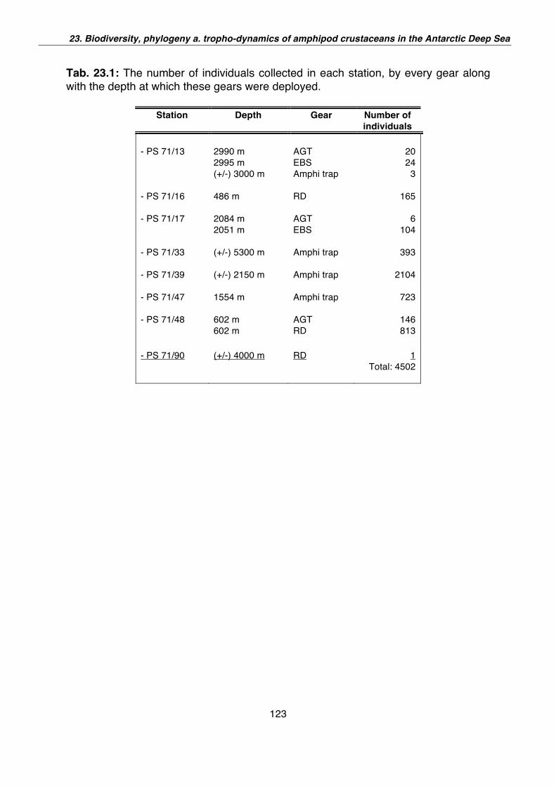
23. Biodiversity, phylogeny a. tropho-dynamics of amphipod crustaceans in the Antarctic Deep Sea
123
Tab. 23.1: The number of individuals collected in each station, by every gear along
with the depth at which these gears were deployed.
Station Depth Gear Number of individuals
- PS 71/13 2990 m AGT 20
2995 m EBS 24
(+/-) 3000 m Amphi trap 3
- PS 71/16 486 m RD 165
- PS 71/17 2084 m AGT 6
2051 m EBS 104
- PS 71/33 (+/-) 5300 m Amphi trap 393
- PS 71/39 (+/-) 2150 m Amphi trap 2104
- PS 71/47 1554 m Amphi trap 723
- PS 71/48 602 m AGT 146
602 m RD 813
- PS 71/90 (+/-) 4000 m RD 1
Total: 4502
124
24. PRELIMINARY REPORT ON AGT CATCHES DURING ANT-XXIV/2 Dorte Janussen1), Michael
Schrödl2), Enrico Schwabe2),
Brigitte Ebbe3)
Henri Robert4), Victoria
Wadley5), Laura Würzberg6),
Angelika Brandt6), Rebeca
Zapata Guardiola7)
1)Senckenberg Forschungsinstitut, Frankfurt, Germany 2)Ludwig Maximilians-Universität München,
Germany 3) German Centre of Marine Biodiversity,
Senckenberg, Germany 4)Institut Royal des Sciences Naturelles de
Belgique, Brussels, Belgium 5)Australian Antarctic Division, Australia 6) Zoological Museum Hamburg, Germany 7)Universidad de Sevilla, Spain
Objectives
The deployment of the large Agassiz trawl at the benthic deep-sea stations was an
integral part of the SYSTCO programme. Our objective was to collect data on the
diversity and distribution of mainly the megafauna and to collect, fixate and freeze
sufficient material from representative taxa for genetic and biochemical
investigations, which will be performed in our home laboratories. The purpose is to
obtain a better understanding of the ecological role of important benthic animal taxa
and the trophodynamic coupling in the deep sea (Brandt et al. 2007). Furthermore,
we aim to approach the reconstruction of the phylogenetic and geographic history of
benthic key taxa in the Southern Ocean deep sea (e. g. Conradi 2007, Janussen
2007).
Work at sea
Methods
After the trawl had been retrieved, the net was emptied into baskets and inspected
for the first obvious animals. Then the catch was washed on deck in running sea
water through sieves with mesh sizes of 5 mm, 1 mm, and 0.5 mm. For AGT 1, an
additional 0.3 mm sieve was used but then considered inefficient and not used for
subsequent trawls. While washing, animals were picked out and the residues were
kept for checking and later sorting under the binocular microscope. For each
dominant megafauna taxon in terms of biomass, the wet weight was measured
before the material was fixed or frozen for further investigations, such as molecular
biology and biochemistry. The wet weights of the 5 dominant taxa for each station
and their contributions to the total biomass are shown in the Table 24.1. In the lab,
the catches were further sorted into major taxonomic groups, and distributed among
the responsible specialists on board. During the course of this expedition, further
sorting of mainly the macrofauna from the fine sediment fractions took place; only
residue samples of AGT 5 are not yet fully sorted. Taxonomic identifications of the
different taxa were done by the specialists on board. Therefore, our preliminary data
24. Preliminary report on AGT catches
125
are of very different quality depending on whether or not a specialist of the taxon on
board was able to deliver detailed identifications of taxa. Thus, the numbers of
species and specimens are based on counting for molluscs, polychaetes, sponges,
isopods, and for other Crustacea from AGT 1 and 2, while partly on estimations for
the other groups. Fig. 24.1 shows our very preliminary evaluation of some major taxa
from the AGT catches nos. 1 - 5. A short description of each of the AGT stations and
the catches is given below.
Results and Discussion
During this expedition, 5 of 6 AGT deployments were successful in the sense that the
trawl collected animals and, in most cases, also sediment from the ocean floor. The
AGT no. 6 failed to collect animals due to an inverted net under stormy conditions.
The AGTs nos. 1 - 4 were bathyal or abyssal benthic deep-sea stations, which had
been planned for SYSTCO from the very beginning (see SYSTCO introduction). AGT
no. 5, near Neumayer Northern Pier in 600 m water depth, was chosen mainly
because of the need for the Polarstern to do logistic work for Neumayer, where we
had to stay for ten days in the beginning of January. Water depths of our AGT
stations thus ranged between 600 m and 5,335 m (Table 24.1), and correspondingly
the effective trawling distances varied between c. 616 m and 2,790 m from the
shallowest to the deepest station. Further details concerning the methods of AGT
deployment are provided in the chapter “Methods: Agassiz Trawl”.
#71/13-15, AGT 1: Depth 3,000 m, trawled distance 1,809 m, deployed with inner
net. Sediment: About 100 liters of diatom ooze to foraminiferan sand, few stones.
Megafauna: Porifera, few: 4 very small demosponges, 1 small hexactinellid (but
many isolated spicules from hexactinellid sponges). Cnidaria: a few seapens
(Umbellula), zooantharians and hexacorals. Mollusca: 1 large cephalopod (squid),
common scaphopods (54 empty shells). Tentaculata: Some Bryozoa. Crustacea: a
few large amphipods (Ischnomesidae sp., Accolathura gigantissima, Syneurycope
sp.); Echinodermata: abundant ophiurids, some large holothurians and some
asteroids. Chordata: 1 fish; 1 ascidian. Macrofauna (as identified later from the
300 μm and 500 μm residues fractions): bivalves abundant (8 spp., 227 specimens),
gastropods 16 spp., polychaetes 17 spp., Crustacea: Isopoda, 18 spp., other
Crustacea, 25 spp.
In summary, a rich macrofauna, but the megafauna was neither very diverse nor
abundant.
# PS 71/17-10, AGT 2: Depth 2,180 m, trawled distance 1,200 m, deployed with
inner net. Sediment: About 75 liters of silty clay with many stones (basalt).
Megafauna: Porifera: 2 hexactinellid spp., 2 demosponges (1 big carnivore sponge,
Chondrocladia cf. albatrossi). Cnidaria: Some scypho-medusae. Mollusca: Some
scaphopods (empty), 1 octopus, 1 big Solenogaster. Tentaculata: abundant
bryozoans (7 spp., 156 specimens). Mollusca: Abundant Nematocarcinus (2 spp.,
382 specimens). Echinodermata: Abundant holothurians (10 spp., 231 specimens, 2
of them very large ones), also common were echinoids (2 spp., 62 specimens),
crinoids (3 spp., 47 specimens) and asteroids. Chordata: Some Ascidiacea and
ANT-XXIV/2
126
fishes (3/12). Macrofauna: bivalves 5 spp., gastropods 4 spp., polychaetes (22 spp.,
104 specimens). Isopoda, 15 spp., other Crustacea, 20 spp.
In summary, at this station, the megafauna was rather diverse and abundant. The
macrofauna was similar to that of AGT 1.
#PS 71/33-14, AGT 3: Depth 5335 m, trawled distance 2790 m, deployed with inner
net. Sediment: about 650 liters of very pure and soft clay, few stones. It contained
many, but small foraminiferans. Megafauna: Porifera: 2 hexactinellid spp., 1
demosponge sp. (the carnivore Cladorhiza sp.). Cnidaria: 2 medusae, 1 sea pen.
Crustacea: Few Nematocarcinus. Echinodermata: Many Holothurians (4 spp., 229
specimens), common ophiurids and asteroids, few echinoids. Macrofauna:
Gastropoda: 12 spp., Bivalvia 3 spp. (not all determined, so far). Polychaeta, 24 spp.
130 specimens, Isopoda, 6 spp., other Crustacea, 9 spp.
In summary, apart from the holothurians, which comprise almost 90 % of the weighed
biomass, the megafauna was comparably poor at this station; especially if
considering the long trawling distance and the large amount of sediment. The
macrofauna, where Mollusca and Polychaeta are concerned, was rather rich;
Crustacea comparably poor (e. g. the Isopoda, compared with AGT 1 and 2).
However, this was the deepest station, and the sediment was extremely soft; so as
we would expect, it is mainly colonized by soft bottom dwellers and burrowing
animals.
#PS 71/39-16, AGT 4: Depth 2150 m, trawled distance 1300 m, deployed with inner
net. Sediment: About 35 liters foraminiferan sand with many stones; very clean catch,
no sieving on deck necessary, but unfortunately due to a mistake, part of the
sediment was lost before sieving. Megafauna: Porifera: Polymastiidae very common
on the stones: Tentorium and Polymastia, 4 spp. (mostly small specimens, probably
juveniles). Cnidaria: some scyphozoan medusae, hydrozoan polyps and 1 actinian.
Polychaeta: some large scale worms. Crustacea: few Nematocarcinus, 1 large
isopod. Chelicerata: some pycnogonids. Cnidaria: Abundant ophiorids (3 spp., 135
specimens), some echinoids and some large holothurians (4 spp. 30 specimens).
Chordata: fishes (3 spp., 13 specimens, 2 were washed out as the AGT was heaved
on deck). Macrofauna: bivalves common, but apparently only 3 spp., gastropods: 2
spp. Crustacea: 9 spp.
In summary, in spite of a considerable amount of hard substrate (stones), the
megafauna, including the sessile, of this station is comparably poor with low diversity.
The macrofauna is extremely poor (especially the Crustacea and Polychaeta). Of the
bivalves and poriferans, we found many specimens, but only few species. This may
point towards few colonization events, which brought a few species to Maud Rise,
where they remained fairly isolated; corresponding to the relatively isolated current
system described from this locality (for details, see chapter contribution by Volker
Strass “Physical Oceanography”, this volume).
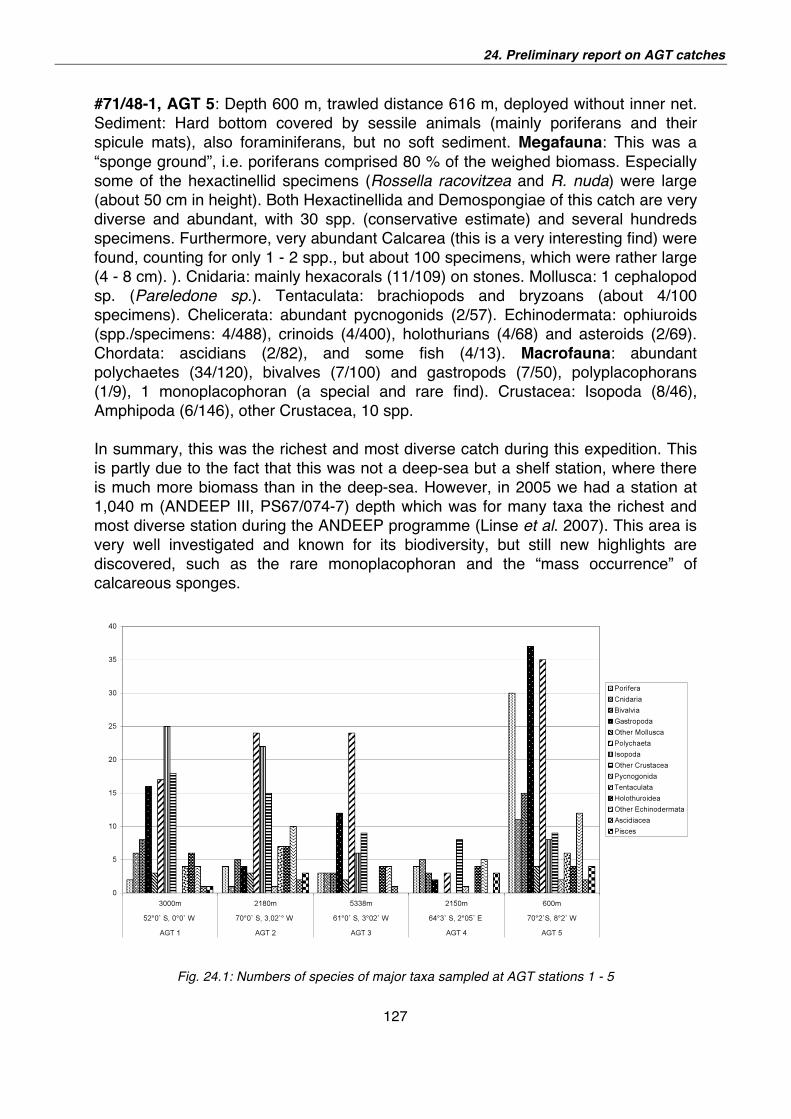
24. Preliminary report on AGT catches
127
#71/48-1, AGT 5: Depth 600 m, trawled distance 616 m, deployed without inner net.
Sediment: Hard bottom covered by sessile animals (mainly poriferans and their
spicule mats), also foraminiferans, but no soft sediment. Megafauna: This was a
“sponge ground”, i.e. poriferans comprised 80 % of the weighed biomass. Especially
some of the hexactinellid specimens (Rossella racovitzea and R. nuda) were large
(about 50 cm in height). Both Hexactinellida and Demospongiae of this catch are very
diverse and abundant, with 30 spp. (conservative estimate) and several hundreds
specimens. Furthermore, very abundant Calcarea (this is a very interesting find) were
found, counting for only 1 - 2 spp., but about 100 specimens, which were rather large
(4 - 8 cm). ). Cnidaria: mainly hexacorals (11/109) on stones. Mollusca: 1 cephalopod
sp. (Pareledone sp.). Tentaculata: brachiopods and bryzoans (about 4/100
specimens). Chelicerata: abundant pycnogonids (2/57). Echinodermata: ophiuroids
(spp./specimens: 4/488), crinoids (4/400), holothurians (4/68) and asteroids (2/69).
Chordata: ascidians (2/82), and some fish (4/13). Macrofauna: abundant
polychaetes (34/120), bivalves (7/100) and gastropods (7/50), polyplacophorans
(1/9), 1 monoplacophoran (a special and rare find). Crustacea: Isopoda (8/46),
Amphipoda (6/146), other Crustacea, 10 spp.
In summary, this was the richest and most diverse catch during this expedition. This
is partly due to the fact that this was not a deep-sea but a shelf station, where there
is much more biomass than in the deep-sea. However, in 2005 we had a station at
1,040 m (ANDEEP III, PS67/074-7) depth which was for many taxa the richest and
most diverse station during the ANDEEP programme (Linse et al. 2007). This area is
very well investigated and known for its biodiversity, but still new highlights are
discovered, such as the rare monoplacophoran and the “mass occurrence” of
calcareous sponges.
Fig. 24.1: Numbers of species of major taxa sampled at AGT stations 1 - 5
ANT-XXIV/2
128
Tab. 24.1: The contributions of the 5 dominant taxa for each AGT station to the
biomass in total wet weight, and in %.
AGT station #71/13-15, AGT # 71/17-10AGT #71/33-14, AGT #71/39-16, AGT #71/48-1, AGT
Coordinates 52°0`S, 0°0`W 70°0`S, 3°02`W 61°0`S, 3°02`W 64°3`S, 2°05`E 70°2`S,8°2`W
Depth 3000 m 2180 m 5335m 2150 m 600 m
Porifera _ _
_
_ 25570g/ 80,1%
Cnidaria 10g/ 0,4 % _
_ 240g/ 1,5%
_
Polychaeta 25g/ 0,9% _
_
_
_
Caridea _ 3700g/ 22,6 70g/ 1,2%
_
_
Pycnogonida _
_
_ 20g/ 0,1%
_
Cephalopoda 500g/ 19,3% _
_
_
_
Holothurioidea 2000g/ 77,4% 8450g/ 52,0% 5200g/ 89,8% 14613g/ 89,0% 500g/ 1,6%
Ophiuroidea 50g/ 2,0% _ 245g/ 4,2%
_
_
Echinoidea _ 1490g/ 9,0%
_ 845g/ 5,1%
_
Asteroidea _
_ 230g/ 4,0%
_
_
Crinoidea _ 200g/ 1,2%
_
_ 1180g/ 3,7%
Ascidacea _
_ 40g/ 0,8%
_ 2145g/ 6,7%
Pisces _ 2470g/ 15,2%
_ 700g/ 4,3% 2530g/ 7,9%
Sum 2585g/ 100% 16310g/ 100% 5785g/ 100% 16418g/ 100% 31925g/ 100%
References Brandt, A., Cramer, L., Riedl, T., Würzburg, L., Brix, S., Ebbe, B., Schüller, M. & Robert, H.
(2007): On the functional biodiversity and ecology of macrobenthic abyssal kay species
with focus on the Isopoda, Mollusca and Polychaetha.- In: Fahrbach E. (ed.),
Expedtionsprogramm Nr. 79 FS Polarstern, p.p. 62-63, AWI Bremerhaven.
Conradi, M. (2007): Diversity, origin and evolution of the deep-sea Antarctic anthozoan
fauna.- In: Fahrbach E. (ed.), Expedtionsprogramm Nr. 79 FS Polarstern, p.p. 67-68, AWI
Bremerhaven.
Janussen, D. (2007): The role of sponges in the benthic-pelagic coupling in biotopes of the
deep Weddell Sea and adjacent areas.-.- In: Fahrbach E. (ed.), Expedtionsprogramm Nr.
79 FS Polarstern, p.p. 66-67, AWI Bremerhaven (by mistake this contribution was
published as „N. Brenke et al.”.
Linse, K.., Brandt A., Bohn, J., Danis, B., De Broyer, C., Ebbe, B., Heterier, V., Janussen, D.,
López González, P. J., Schüller, M., Schwabe,, E., Thomson, M. R. A. (2007): Macro- and
megabenthic assemblages in the bathyal and abyssal Weddell Sea (Southern Ocean).- Deep-Sea Research, II, 54 (16/17): 1848-1863.
129
25. PRELIMINARY REPORT ON THE PORIFERA (SPONGES) CAUGHT DURING THE ANT-XXIV/2, ANDEEP-SYSTCO Dorte Janussen
Senckenberg Forschungsinstitut, Frankfurt
Objectives
For the Porifera research (the detailed work programme is described in Janussen,
2007), the main objectives, within the framework of the SYSTCO expedition, were as
follows:
1. Increase of the knowledge gained during the ANDEEP programme on the
biodiversity of sponges in the deep Southern Ocean (SO).
2. To collect and fixate fresh material from representative key taxa for genetics, in
order to investigate the phylogenetic relationships of SO deep-sea sponges in
comparison with representatives from other deep oceans and from the shelf.
3. To obtain sufficient material of representative taxa for isotope and other
biochemical analyses, in order to gain a better understanding of the functional
ecology of sponges in the deep SO food web.
Results and discussion
During ANT-XXIV/2, we collected all together about 50 Porifera species from 25
families (conservative estimates). Of these species, 30 belong to the Demospongiae,
10 to the Hexactinellida and 1 or 2 to the Calcarea. As usual, sponges were collected
mainly by the AGT, some by EBS and a few by GKG. At 3 stations, the Rauschert
dredge was successfully deployed, either by itself (RD1) or attached to the AGT
(RD2, RD3, RD4). Next to the AGT, this small dredge caught most of the sponges
during this expedition, but interestingly for the Porifera the catches of the RD are not
significantly different from those of the AGT (for other taxa, e. g. the Crustacea, the
results are different, see contribution by Henry Robert on the Amphipoda, this
volume). Obviously, the fine-meshed (500 μm) inner net, which we applied as inlet
within the normal net at most AGT stations, was equally efficient as the RD net in
holding back especially the smaller sponges. A detailed taxonomic list of the Porifera
collected during this expedition and an overview of their distribution are given below
(Table 25.1, Fig. 25.1).
Generally, the catches from the SYSTCO deep-sea stations were rather poor in
sponges, compared with those of the ANDEEP II and III expedtions (Janussen &
Tendal 2007). The richest station, both in total numbers and in diversity was AGT 5
(#71/48-1), which was not a deep-sea station and not originally planned for the
SYSTCO expedition (see Janussen et al. “AGT catches”, this volume).
ANT-XXIV/2
130
Brief description of sponge catches from the AGT stations 1 - 5:
AGT 1, #71/13, 52°S, 3000 m: the poorest station in terms of sponges: 3 tiny,
probably demosponges, and 1 hexactinellid fragment.
AGT 2, # 71/17, Lazarev Sea, 2180 m: this station was richer: 3 complete
demosponges of 3 spp. and 7 fragments from 1 or 2 hexactinellids were collected.
One of the demosponges from the AGT was a comparably large specimen of the
carnivore sponge, Chodrocladia cf. albatrossi. With its 6 cm in length, it is almost a
giant compared with most specimens of the family Cladorhizidae collected during the
ANDEEP cruises, which were mostly tiny specimens, a few mm only, and were
collected mainly by EBS. With this large specimen of Chondrocladia, we now finally
obtained sufficient biomass to fixate parts of the sponge in RNA-Later for genetics
and also freeze a good portion for analysis of the stable isotopes.
AGT 3, #1/33-14, Central Weddell Sea, 5330 m: this station was the deepest, and a
typical abyssal station, providing only few true deep-sea sponges: 4 specimens of
carnivore Cladorhiza sp. and 2 hexactinellid fragments. The Cladorhiza specimens
were rather long, 4 - 5 cm, but also very thin and did not provide much biomass;
furthermore they were penetrated by clay sediment and are probably not suitable for
biochemistry.
AGT 4, #1/39-16, Maud Rise, 2,150 m: a station rather rich in sponges, but of low
diversity: we collected 17 specimens of 4 spp. belonging to the two genera
Polymastia and Tentorium of the family Polymastiidae, all encrusting on stones.
Many of these sponges are only a few mm big, and probably juveniles. The
Polymastiidae is one of the Porifera families that show very wide distribution, both
geographically and bathymetrically. For this reason, it was chosen among the key
taxa for phylogenetic and zoogeographical comparisons of Antarctic sponges with
representatives from other oceans (Janussen & Wörheide, unpubl.). Because the
catch contained very little sediment, some of the larger specimens were suitable for
biochemistry.
AGT 5, #1/48-1, near Neumayer northern pier, 600 m: not surprisingly, the major part
of the sponges collected are from this locality, which was a shelf station.
Nevertheless, the large amounts of very pure samples, containing almost no
sediment, are very useful and necessary for our originally planned genetic and
biochemical investigations, which are well-integrated within the SYSTCO programme.
The Porifera comprise 80 % of the biomass of the weighed dominant taxa of this
station (see Janussen et al. “AGT catches”, this volume). Altogether, we collected 40
spp. of Porifera from 24 families (conservative estimate), which must be considered a
high diversity, both on species and at higher taxonomic levels. About 21 of the
families represented here belong to the class Demospongiae, 1 to the Calcarea and
apparently only 2 (Rossellidae and Farreidae) to the Hexactinellida. For the latter,
this is a normal situation, because in the Southern Ocean, the diversity of
Hexactinellida increases from the shelf down to the bathyal, where it reaches its
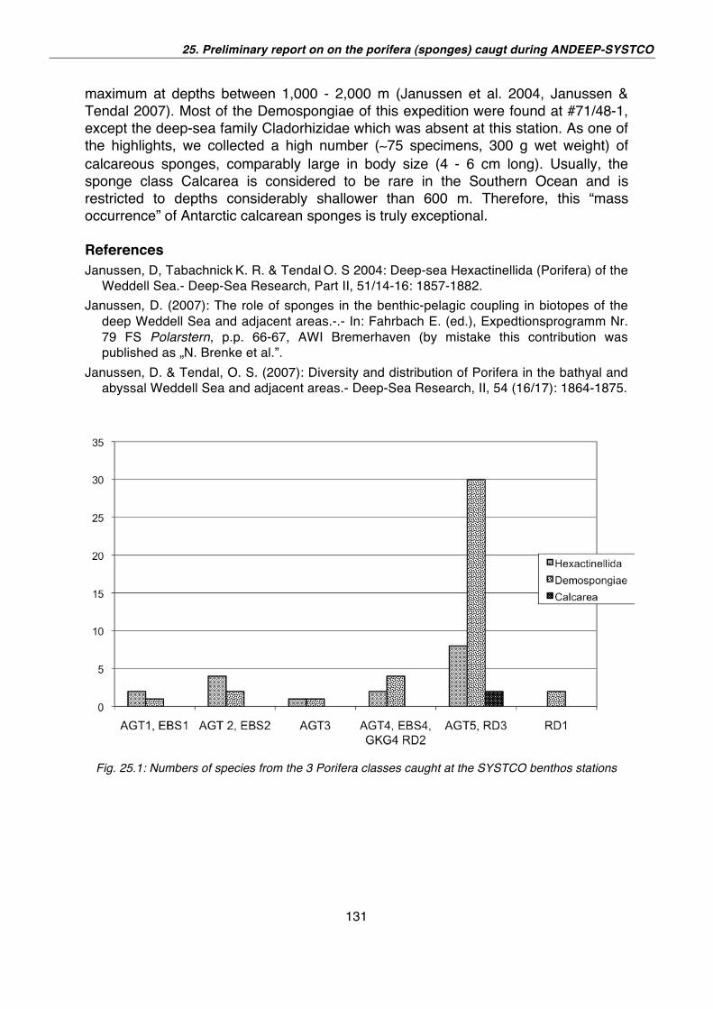
25. Preliminary report on on the porifera (sponges) caugt during ANDEEP-SYSTCO
131
maximum at depths between 1,000 - 2,000 m (Janussen et al. 2004, Janussen &
Tendal 2007). Most of the Demospongiae of this expedition were found at #71/48-1,
except the deep-sea family Cladorhizidae which was absent at this station. As one of
the highlights, we collected a high number ( 75 specimens, 300 g wet weight) of
calcareous sponges, comparably large in body size (4 - 6 cm long). Usually, the
sponge class Calcarea is considered to be rare in the Southern Ocean and is
restricted to depths considerably shallower than 600 m. Therefore, this “mass
occurrence” of Antarctic calcarean sponges is truly exceptional.
References Janussen, D, Tabachnick K. R. & Tendal O. S 2004: Deep-sea Hexactinellida (Porifera) of the
Weddell Sea.- Deep-Sea Research, Part II, 51/14-16: 1857-1882.
Janussen, D. (2007): The role of sponges in the benthic-pelagic coupling in biotopes of the
deep Weddell Sea and adjacent areas.-.- In: Fahrbach E. (ed.), Expedtionsprogramm Nr.
79 FS Polarstern, p.p. 66-67, AWI Bremerhaven (by mistake this contribution was
published as „N. Brenke et al.”.
Janussen, D. & Tendal, O. S. (2007): Diversity and distribution of Porifera in the bathyal and
abyssal Weddell Sea and adjacent areas.- Deep-Sea Research, II, 54 (16/17): 1864-1875.
Fig. 25.1: Numbers of species from the 3 Porifera classes caught at the SYSTCO benthos stations
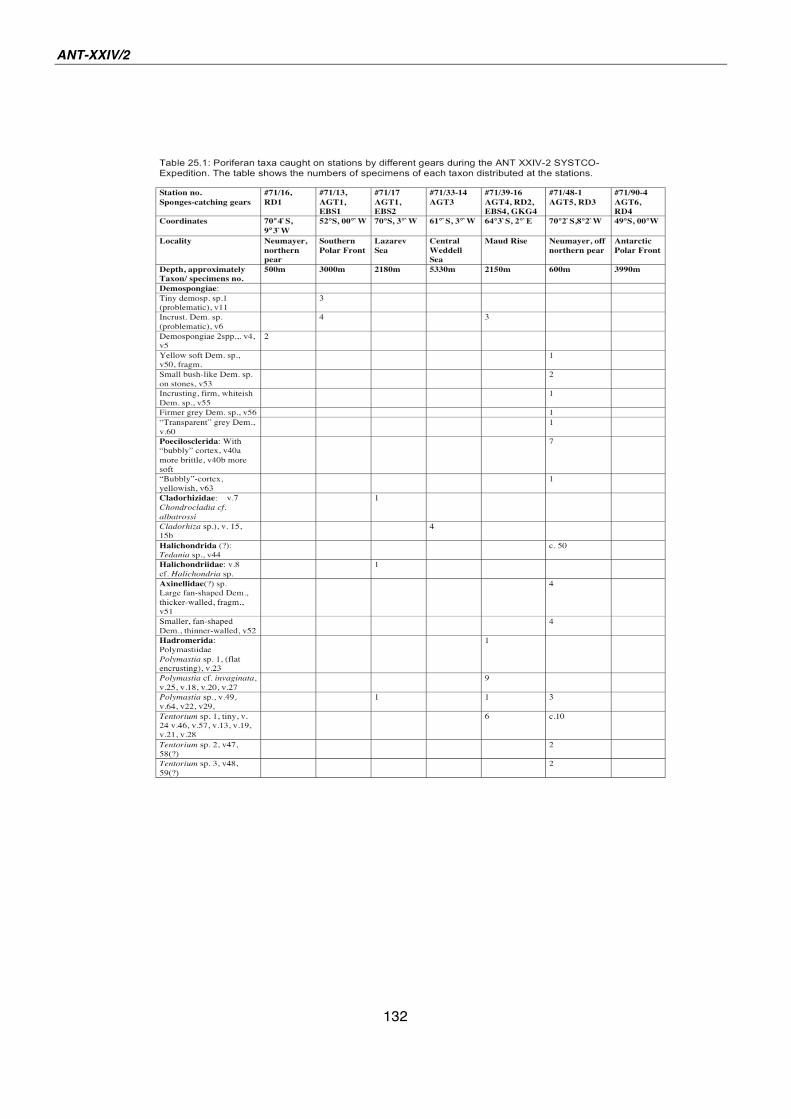
ANT-XXIV/2
132
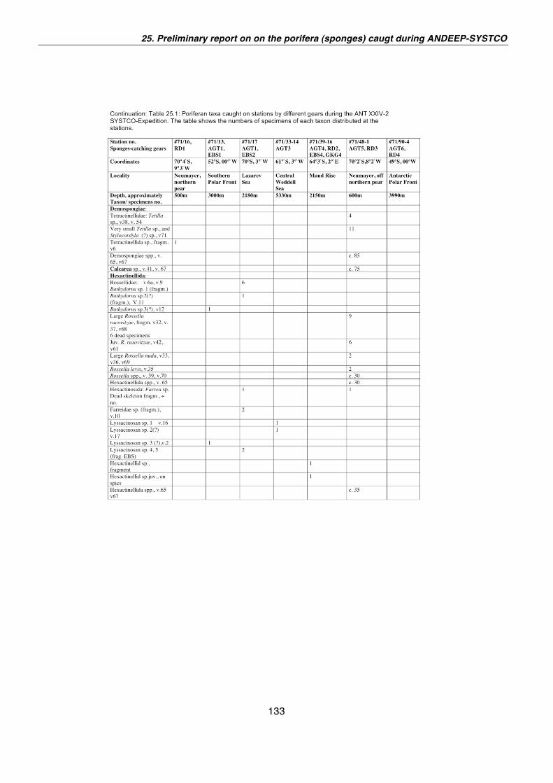
25. Preliminary report on on the porifera (sponges) caugt during ANDEEP-SYSTCO
133
134
26. DIVERSITY OF THE SOUTHERN OCEAN DEEP-SEA ANTHOZOAN FAUNA Rebeca Zapata Guardiola,
López-González (not on board)
Universidad de Sevilla, Spain
Objectives
Anthozoans are commonly one of the major components in benthic sessile
communities in terms of both abundance and diversity (Arntz 1997; Arntz et al. 1997;
Gili et al. 1999). They offer a good substrate (e.g. refuge, feeding) to many benthic
mobile animal groups such as crustaceans, polychaetes, and echinoderms. The
Antarctic fauna of anthozoans is still poorly known (Winston 1992, Clark & Johnston
2003), and most of our knowledge comes from the continental shelf. The deep-sea
fauna is much less explored and perhaps not as diverse as that living on the shelf,
but undescribed genera and species are continuously discovered (e.g. López-
González & Gili 2000, 2001; López-González et al. 2002; López-González & Williams
2002; Rodríguez & López-González 2001, 2002, 2003). Since most parts of the
Southern Ocean refer to deep waters, current estimates of the total number of
Antarctic and Subantarctic Anthozoan species are still very imprecise, no more than
50 % of all species. Furthermore, several unreliably described species and genera
should be revised, preferably using newly collected material in combination with the
type specimens deposited in museums.
Three main hypotheses have been suggested to explain the origin of recent Antarctic
benthic communities: derivation from indigenous fauna components, immigration
from the deep sea, or recent dispersal from neighbouring shallow-water areas
(Crame 1989, 1994, Clarke 1990, Clark & Crame 1989, 1992). According to
preliminary results of the anthozoan fauna from previous EASIZ, ANDEEP and
LAMPOS cruises, the Antarctic alcyonaceans apparently include elements derived
from all three hypotheses (López-González & Gili 2001), while pennatulaceans are
mainly immigrants from the deep sea of surrounding oceans (e.g. Umbellula,
Kophobelemnon) and secondarily from shallow waters (e.g. Pennatula) (López-
González & Williams 2002).
Because of this our objectives are focused on looking for the presence of possible
boundaries in the distribution of anthozoans at different taxonomic levels (family,
genus, species) in the Southern Antarctic deep sea. Likewise we attempt to evaluate
the potential origin of the Antarctic anthozoan fauna according to the known
distribution of genera and species in this and other biogeographical areas. The
finding of any undescribed species might eventually assist with a better
understanding of the relationship between Antarctica and other deep-sea bottoms
and continental shelf areas in the past and present. Finally, we aim to complete the
26. Diversity of the Southern Ocean Deep Sea anthozoan fauna
135
scarce information about anthozoan reproductive biology and to provide adequately
fixed material for the bank of tissues useful for further molecular studies, both already
initiated since the EASIZ II and III in 1998 and 2000, respectively.
Work at sea
Methods
During this cruise anthozans were searched for in all Agassiz trawl (AGT), Epibenthic
sledge (EBS) and Rauschert dredge (RD) catches (Table 26.1).
All colonies and individual specimens, including discernable fragments of them, were
sorted, labelled, and when possible photographs were taken to obtain information
about the colour patterns of the different species while still alive. A considerable
amount of ethanol-fixed residues from AGT station no. 5 still await sorting; it is
expected to contain numerous smaller anthozoans or fragments.
Anthozoans were fixed for morphological studies (histology, anatomy, etc.) in
buffered 6 % formaldehyde in sea water (pH 8 - 9), some selected specimens of
fragments were fixed in 96 % ethanol for further molecular analysis. Some
hexacorals were relaxed before fixation by adding menthol crystals on the surface of
the sea water. Depending on their size, some sea anemones were fixed also injecting
40 % formaldehyde. Once in the laboratory, all specimens will be preserved in 70 %
ethanol.
Preliminary results and discussion
The anthozoan material collected during ANT-XXIV/2 was obtained from 5 AGT, 2
RD and 1 EBS hauls. We found anthozoans almost at all geographical stations (the
last AGT was not successful due to the weather conditions) but not in all the benthic
gears used for each station.
A total of 102 individuals/colonies were identified, although some of them were only
present in a fragmentary state, (e.g. gorgonians). These specimens belong to 30
morphospecies, some of which were identified on board to species level, although
most are awaiting further morphological studies in the laboratory, (e.g., histological
sections, light and electron microscopy). Fourteen species belong to the Octocorallia,
and 16 to the Hexacorallia. The octocoral classification used here, which is
considered to be the most natural currently available, considers only three orders:
Helioporacea, Alcyonacea, and Pennatulacea; only the last two are present in the
Southern Ocean. Among the octocoral species there were 6 pennatulaceans, and 8
alcyonaceans (4 soft coral, and 4 gorgonian species). The hexacoral species
consisted of 9 actiniarians, 5 scleractiniarians and 2 zoanthideans.
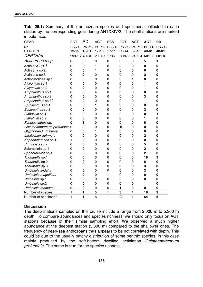
ANT-XXIV/2
136
Tab. 26.1: Summary of the anthozoan species and specimens collected in each
station by the corresponding gear during ANTXXIV/2. The shelf stations are marked
in bold face.
GEAR AGT RD AGT EBS AGT AGT AGT RD
Nº
STATION
PS 71-
13-15
PS 71- 16-01
PS 71-
17-10
PS 71-
17-11
PS 71-
33-14
PS 71-
39-16
PS 71- 48-01
PS 71- 48-01
DEPTH(m) 2997.6 486.3 2084.7 1736 5336.7 2150.4 601.8 601.8
Actinernus n.sp. 0 0 0 0 0 0 5 1
Actiniaria sp.1 0 0 1 0 0 0 0 0 Actiniaria sp.2 0 0 1 0 0 0 0 0 Actiniaria sp.3 0 0 0 0 0 0 2 0 Actinostolidae sp.1 0 0 0 0 0 1 0 0 Alcyonium sp.1 0 0 0 0 0 0 1 0 Alcyonium sp.2 0 0 0 0 0 0 1 0 Amphianthus sp.1 0 0 4 0 0 0 0 0 Amphianthus sp.2 0 0 0 0 0 0 3 0 Amphianthus sp.3? 0 0 0 0 0 0 1 0 Epizoanthus sp.1 0 0 1 0 0 0 0 0 Epizoanthus sp.2 0 0 0 0 0 0 2 0 Flabellum sp.1 0 0 0 0 0 0 0 1 Flabellum sp.2 0 0 0 0 0 0 1 0 Fungiacyathus sp. 0 1 0 0 0 0 6 0 Galatheanthemum profundale 0 0 0 0 19 0 0 0 Glyphoperidium bursa 0 0 1 0 0 0 0 0 Inflatocalyx infirmata 0 0 0 0 0 0 2 0 Kophobelemnon sp.1 1 0 0 0 0 0 0 0 Primnoisis sp.? 0 0 0 0 0 0 5 0 Scleractinia sp.1 0 0 0 0 0 0 2 0 Sphaeralcyon sp.1 0 0 0 0 0 0 2 0 Thouarella sp.1 0 0 0 0 0 0 19 3 Thouarella sp.2 0 0 0 0 0 0 6 0 Thouarella sp.3 0 0 0 0 0 0 3 0 Umbellula lindahli 0 0 0 0 0 0 2 0 Umbellula magniflora 0 0 0 1 0 0 0 0 Umbellula sp.1 0 0 0 0 2 0 0 0 Umbellula sp.2 0 0 0 0 0 0 1 0 Umbellula thomsoni 0 0 0 0 1 0 0 0 Number of species 1 1 5 1 3 1 18 3 Number of specimens 1 1 8 1 22 1 64 5
Discussion The deep stations sampled on this cruise include a range from 2,000 m to 5,300 m
depth. To compare abundances and species richness, we should only focus on AGT
stations because of their similar sampling effort. We observed a much higher
abundance at the deepest station (5,300 m) compared to the shallower ones. The
frequency of deep-sea anthozoans thus appears to be not correlated with depth. This
could be due to the usually patchy distribution of some benthic species, in this case
mainly produced by the soft-bottom dwelling actiniarian Galatheanthemum
profundale. The same is true for the species richness.
26. Diversity of the Southern Ocean Deep Sea anthozoan fauna
137
Other factors such as the availability of adequate bottom substrates or potential
latitudinal gradients need to be considered as well. The distance to the continent may
play an important role in the way of providing food into the bottom (Gili et al. 2001).
In summary, the shallowest stations show higher species richness (18 spp. in
stn. 48 - 01), while the most speciose of the deeper ones only reaches five species
(stn. 17 10).
For the actiniarian species, Galatheanthemum profundale and Glyphoperidium bursa,
the collected material should be considered as a deeper record in the Southern
Ocean and for G. bursa the deepest.
With regard to the knowledge of zoanthideans, only one genus, Parazoanthus, was
previously known from that area, and seemed to be restricted to the shelf, associated
with gorgonians. During the last deep-sea cruise, ANDEEP III in 2002, species
belonging to the genus Epizoanthus were found. Now two more specimens of the
latter genus have been collected. This genus has not been found in the different
shallow (shelf) water Antarctic research programmes. Our findings confirm the
presence of the genus Epizoanthus in the deep Southern Ocean, revealing an
immigration from the surrounding oceanic basins.
During ANDEEP I, members of the genus Thouarella were collected down to
3000 m depth. No Thouarella could be found in any of the deep stations during
this cruise, while 35 specimens were obtained from the shelf station PS71/48-01
at 600 m. We certainly need a more intensified sampling to conclude properly on
distributional patterns, but we can already suspect that Thouarella shows a
patchy distribution, not only with latitude, but also with depth. Furthermore, its
presence outside Antarctic and Subantarctic regions, as well as some anatomical
features (branching patterns, distribution of sclerites on the polyps, etc…) could
suggest that this genus is an ancient component that mainly diversifies in
Subantarctic waters.
Results from previous deep-sea cruises showed a constant anthozoan
species/group composition at depths around 4000 m and 5000 m. The only
species occurring in such depths were Galatheanthemum profundale (Actiniaria),
Antipatharia gen.1 (Antipatharia), and Umbellula thomsoni (Pennatulacea).
Interestingly, none of these species are present in Antarctic or Subantarctic shelf
areas. During this cruise we collected two of them (G. profundale and U.
thomsoni) in the deepest station at 5300 m only, confirming the presence of a
homogeneous faunal composition in abyssal depths.
References Arntz, W.E. (1997): Investigación antártica en biología marina: situación actual, proyectos
internacionales y perspectivas. Bol.R.Soc.Esp.Hist.Nat.Secc.
Biol. 93: 13-44.
Arntz, W.E., Gutt, J. And M. Klages (1997): Antarctic marine biodiversity: anoverview. In:
Battaglia B, Valencia J, Walton DWH (eds) Antarctic
ANT-XXIV/2
138
communities, species, structure and survival. Cambridge University Press, Cambridge, pp 3-
14.
Crame, J.A. (1989): Origins and evolution of the Antarctic biota. London: The Geological
Society London (Geological Society Special Publications, 47).
Crame, J. A. (1994) Evolutionary history of Antarctica. In: Hempel G (ed) Antarctic science -
global concerns. Springer, Berlin, pp 188-214.
Clarke. A. (1990): Temperature and evolution. Southern Ocean cooling the Antartic marine
fauna. In: Kerry KR, Hempel G (eds) Antarctic ecosystems. Ecological change and
conservation. Springer Berlin, pp 9-22.
Clarke, A. and J.A. Crame (1989): The origin of the Southern Ocean marine fauna. In: Crame
J.A. (ed) Origins and evolution of the Antarctic biota. The Geological Society London
(Geological Society Special Publication 47), pp 253-268.
Clarke, A. and J.A. Crame (1992): The Southern Ocean benthic fauna and climate change: a
historical perspective. Phil Trans R Soc Lond B 338: 299-309.
Clarke, A. and N.M. Johnston (2003): Antarctic marine benthic diversity. Oceanogr.
Mar.Biol.Ann.Rev. 41: 47-114.
Gili, J. M., Arntz, W.E., Filipe, P., López, P., Orejas, C., Ros, J. and N.Teixido, (1999): The
role of benthic suspension feeders in Antarctic communities. In: The Expedition
ANTARKTIS XV/3 (EASIZ II) of Polarstern in 1998. Berichte zur Polarforschung 301: 30-
83.
Gili, J.M., Coma, R., López-González, P.J., Orejas, C., Zabala, M. (2001): Are Antarctic
suspension-feeding communities different from those elsewhere in the world?. Polar Biol.
24: 473-485.
López-González, P.J. and J.M. Gili (2000): A new octocorallian genus (Cnidaria: Anthozoa)
from Antarctic waters. Polar Biol. 23: 452-458.
López-González, P.J. and J.m. Gili (2001): Rosgorgia inexspectata, new genus and species
of Subergorgiidae (Cnidaria, Octocorallia) from off the Antarctic Peninsula. Polar Biol. 24:
122-126.
López-González, P.J., Gili, J.M. and C. Orejas (2002): A new primnoid genus (Anthozoa:
Octocorallia) from the Southern Ocean. Sci.Mar. 66(4): 383-397.
López-González, P.J. and G.C. Williams (2002): A new genus and species of sea pen
(Octocorallia: Pennatulacea: Stachyptilidae) from the Antarctic.
Peninsula. Invert. Syst. 16: 919-929.
Rodríguez, E. and P.J. López-González (2001): A new species of Hormathia (Actiniaria,
Hormathiidae) from the eastern Weddell Sea, Antarctica. Helgol.Mar.Res. 55: 116-123.
Rodríguez, E. and P.J. López-González P. J. (2002): A new species of Halcampella
(Actiniaria, Halcampoididae) from the eastern Weddell Sea and Antarctic Peninsula. Sci
Mar 66(1): 43-52.
Rodríguez, E., López-González (2003): Stephanthus antarcticus, a new genus and species
of sea anemone (Actiniaria, Haloclavidade) from the South Shetland Islands, Antarctica.
Helgol.Mar.Res. 57: 54-62.
Winston, J.E. (1992): Systematics and marine conservation. In Eldredge N (ed) Systematics,
ecology and biodiversity crisis. Columbia University Press, New York, pp. 144-168.
139
27. GASTROPODA OF THE DEEP SOUTHERN OCEAN - RESULTS FROM AGT CATCHES DURING ANDEEP-SYSTCO Michael Schrödl, Enrico Schwabe
Ludwig Maximilians-Universität
München, Germany
Objectives
Molluscs generally are among the most common and diverse phyla in the deep sea.
Within the framework of ANDEEP, former expeditions allowed first insights into the
biodiversity of trenches and abyssal plains off the Antarctic Peninsula, the Scotia Arc
and across the Weddell Sea. Our previous results on gastropods showed a surprising
overall species diversity, but great heterogeneity between the areas with regard to
species numbers and abundance. In contrast to earlier assumptions, an abyssal
Antarctic gastropod fauna exists that is not just an impoverished shelf fauna but
contains a high amount of apparently unique faunal elements. Its origin and
relationships were unknown because adjacent deep-sea areas were virtually
unexplored. Also the reproductive biology and ecology of southern deep-sea
molluscs is unknown, and, thus, their role in abyssal food webs and their
dependence and influence on special deep-sea environments. During ANDEEP-
SYSTCO, we aimed to fill a gap within our inventory by collecting in several deep
water areas between South Africa and Antarctica. Besides uncovering gradients in
diversity, abundance and faunal composition we hoped to shed some light on the
biology and ecological interactions of molluscs and other organisms. The present
report gives a preliminary list of gastropods found in the AGT catches so far.
Work at sea
Methods For AGT collecting methods and a short description of the catches see Janussen et
al. (Preliminary report on AGT catches during ANT-XXIV/2; this volume). Note that at
the deep sea stations nos. 1-4 an inner net with a mesh size of 0.5 mm was used,
while at the shelf station (AGT 5) the mesh size was approx. 1 cm. Gastropods were
sorted out of the catches quantitatively, on deck by eye and then from finer fractions
down to 0.5 mm under the dissecting microscope. All AGT catches have been
completely revised, except for no. 5, of which about 20 liters of mixed biogenic
residues remain to be sorted. Most gastropods were preserved in 95 % ethanol,
while some selected specimens were deep frozen for later biochemical or stable
isotope analyses, or relaxed in an isotonic solution of MgCl2 prior to fixation in either
70 % ethanol or 4 % formalin-seawater.
ANT-XXIV/2
140
Results and Discussion
We sorted and pre-identified gastropods from five AGT-stations of ANDEEP-
SYSTCO at approximately 600 to 5335 m depth. To date we have found 324
specimens belonging to 67 species (Table 27.1). Most of the 30 families were
represented by single or just a few species. The most diverse families are the
Buccinidae (8 spp.), followed by Naticidae (5 spp.), and Turridae, Marginellidae, and
Eulimidae (4 spp. each). The most abundant species were Lissotesta strebeli (137
spms.), Melanella sp. 3 (27 spms.), and Puncturella conica (23 spms.). 55 species
were represented by 1 - 3 individuals only.
Several new biological observations have been made. Puncturella conica frequently
sits on a still unidentified ascidian, probably using it as an adequate substrate. Four
species of Eulimidae, three of them unidentified and potentially new, were found
parasitizing on holothurian hosts. Females of Melanella sp. 2 were deeply buried into
the sea cucumbers' body wall.
With 129 specimens of 37 species, the not yet fully sorted shelf station is richer than
the deep- sea stations (Fig. 27.1). Comparing the deep-sea stations, most
gastropods were found at the deepest station (AGT 3; 5,338 m) in the central
Weddell Sea. This is mainly due to Lissotesta strebeli which was very abundant
locally (109 specimens). Most species (16) were collected at the second deepest
station, in the abyssal plain of the Agulhas Basin (AGT 1; almost 3,000 m).
Standardized values (specimens and species per 1,000 m trawling distance) confirm
the shelf station to be considerably richer than deeper stations (Fig. 27.2), as it was
expected. Values of gastropod species richness in the deep stations range between
1.54 and 8.84, thus approximately one order of magnitude less than on the shelf
(60.1). Surprisingly, the bathyal stations AGT nos. 2 (Lazarev Sea) and 4 (Maud
Rise) seem to be the poorest with regards to gastropods (Fig. 27.2). Considering the
bathyal and abyssal stations only, there is no linear correlation between the number
of gastropod specimens and species collected by the AGT with depth. However, such
comparisons based on AGT catches have to be treated with great caution. Most
Southern Ocean gastropods are small sized and they are certainly underrepresented
in the shelf catch where larger mesh sizes were used; furthermore, sorting is still
ongoing. Delicate shells are easily smashed within large AGT catches containing
stones or gravel, such as in the apparently poor catches taken from the slope of the
Lazarev Sea and from Maud Rise. Also volumes of material available for sieving and
sorting differed greatly between the catches, ranging from 35 liters in AGT 4 to
approximately 650 liters in AGT 3 (see Janussen et al., chapter 25). Data from
epibenthic sledge, multicorer and box corer samples will be required for drawing
conclusions on gastropod abundances and diversity.
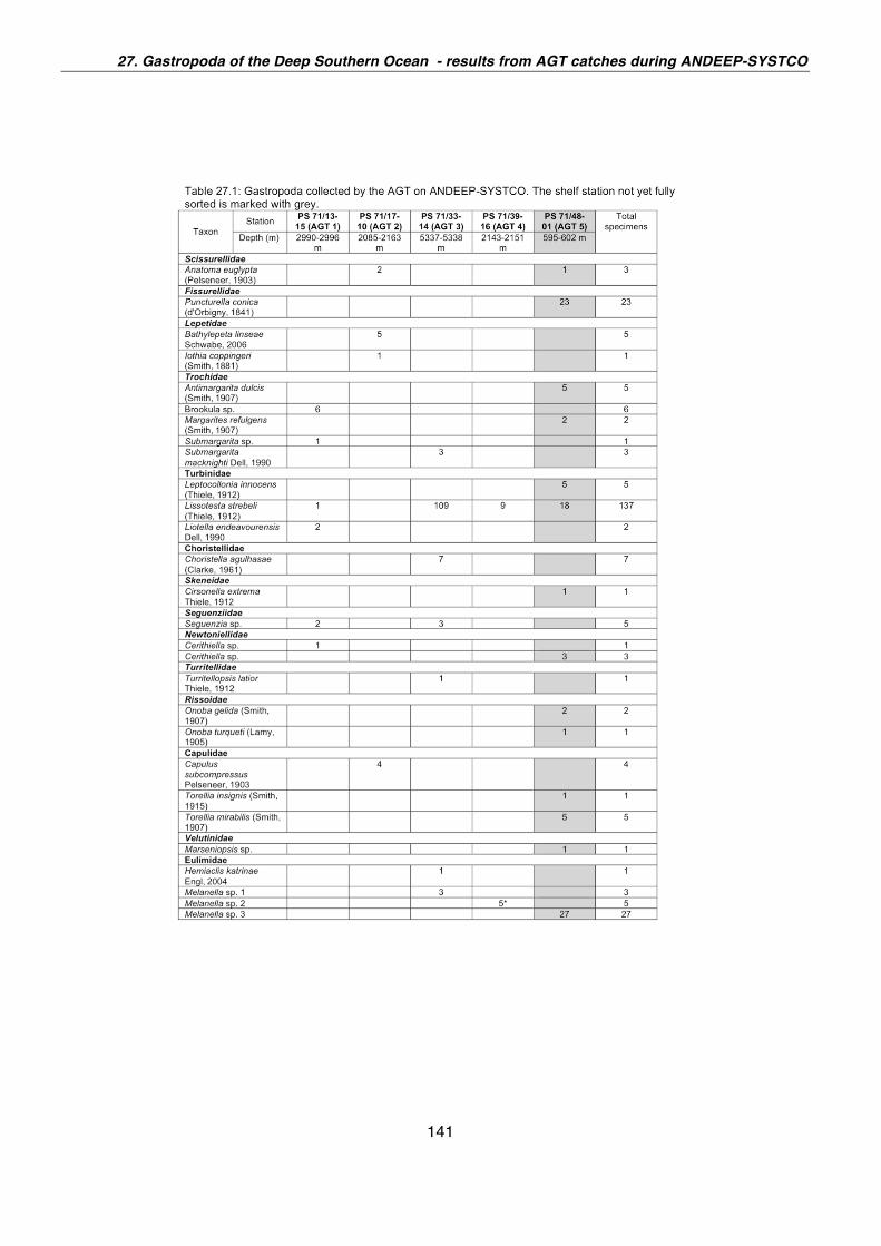
27. Gastropoda of the Deep Southern Ocean - results from AGT catches during ANDEEP-SYSTCO
141
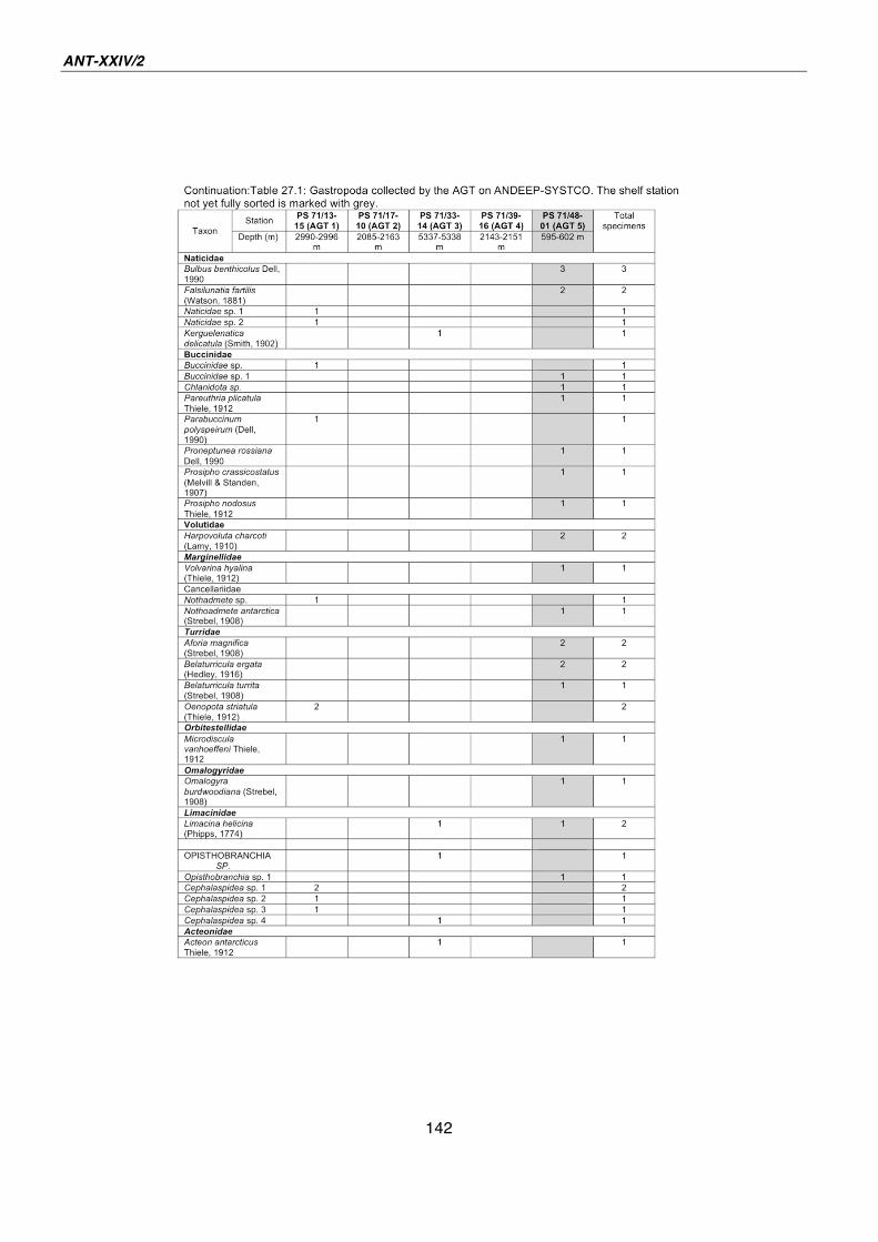
ANT-XXIV/2
142
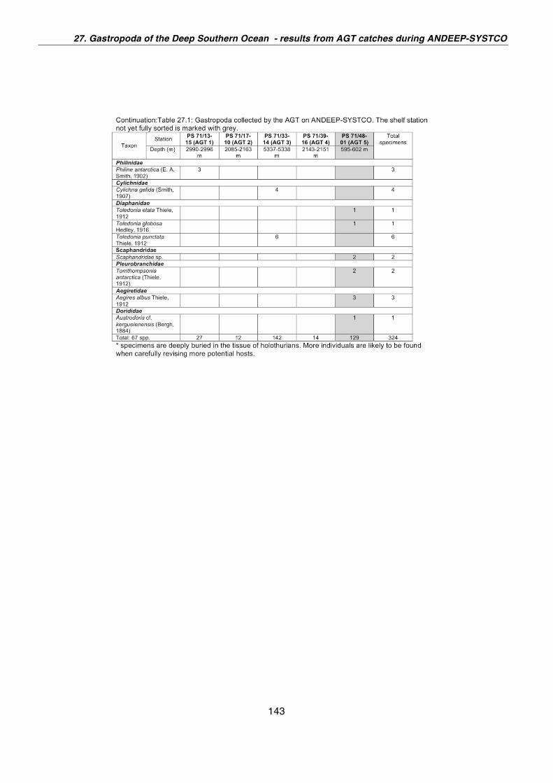
27. Gastropoda of the Deep Southern Ocean - results from AGT catches during ANDEEP-SYSTCO
143
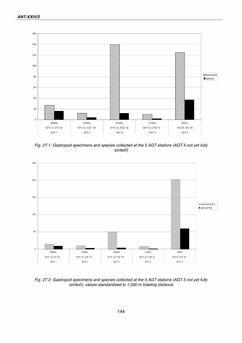
ANT-XXIV/2
144
Fig. 27.1: Gastropod specimens and species collected at the 5 AGT stations (AGT 5 not yet fully
sorted!)
Fig. 27.2: Gastropod specimens and species collected at the 5 AGT stations (AGT 5 not yet fully
sorted!), values standardized to 1,000 m trawling distance
145
28. BIOGEOGRAPHY OF ASTEROIDS Henri Robert, Bruno
Danis (not on board)
Institut Royal des Sciences Naturelles de
Belgique, Brussels, Belgium
Scientific background and objectives
The Antarctic fauna is generally described as characterized by its high level of
specific endemism, and a relatively low level of generic endemism. Since the
isolation of Antarctica, the benthic fauna of the Southern Ocean has been subject to
environmental parameters considered as extreme. As an example, glaciation cycles
and iceberg scouring largely influence diversity and distribution of the Antarctic
benthos. Antarctic asteroids are generally considered as being widely distributed
(circumpolar), having a high degree of endemism and a large bathymetric range. To
the best of our knowledge, few studies have addressed this question, although
asteroids are an ecologically successful group, being well represented in the
Antarctic.
A preliminary study has already been carried out using sea stars collected during a
previous expedition (ANDEEP III) and by integrating the data obtained with data from
other campaigns (Walter Herwig, EPOS). The objective is to aggregate the largest
quantity of data possible in order to understand interactions resulting from the actual
distribution of the Southern Ocean sea stars, using objective presence/absence data.
The preliminary study has shown that among the families considered, the Asteriidae
(Forcipulatida) displayed the richest specific biodiversity. Results have also
confirmed previous observations on eurybathy, and have refined the available
knowledge. The study of specific richness in the different sectors considered in the
study has established the east of the Weddell Sea and the southern branch of the
Scotia Arc as regions where the sea star fauna is particularly diversified.
While the general analysis has shown that there is little chance that new species are
discovered above 1,000 m depth, results have shown that most of the species
considered in the study are rarely reported. The results seem to be very different
when considering the deep sea (below 1,000 m), which has been far less sampled.
Sampling sea stars during the ANDEEP-SYSTCO will allow completion of the very
scattered picture we have on Southern Ocean sea star biodiversity, in the regions
which have been less sampled, the Southern Ocean deep sea. It is also intended to
utilize genetic tools, in order to support the biogeographic information available.
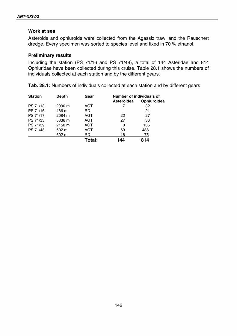
ANT-XXIV/2
146
Work at sea
Asteroids and ophiuroids were collected from the Agassiz trawl and the Rauschert
dredge. Every specimen was sorted to species level and fixed in 70 % ethanol.
Preliminary results
Including the station (PS 71/16 and PS 71/48), a total of 144 Asteridae and 814
Ophiuridae have been collected during this cruise. Table 28.1 shows the numbers of
individuals collected at each station and by the different gears.
Tab. 28.1: Numbers of individuals collected at each station and by different gears
Station Depth Gear Number of individuals of Asteroidea Ophiuroidea PS 71/13 2990 m AGT 7 32
PS 71/16 486 m RD 1 21
PS 71/17 2084 m AGT 22 27
PS 71/33 5336 m AGT 27 36
PS 71/39 2150 m AGT 0 135
PS 71/48 602 m AGT 69 488
602 m RD 18 75
Total: 144 814
147
29. BIODIVERSITY AND EVOLUTION OF ECHINOIDS Henri Robert, Bruno
Danis (not on board)
Institut Royal des Sciences Naturelles de
Belgique, Brussels, Belgium
Scientific background and objectives
A conspicuous and important component of the benthic community is the cidaroid
echinoids (colloquially known as pencil-spine sea urchins). The cidaroid assemblage
of the Southern Ocean belongs to the subfamily Ctenocidarinae and comprises
approximately 21 extant species within 5 genera. In spite of the suitability of this
taxon for studying major biological factors in the Southern Ocean, problems with the
systematics of the group require investigation. In the process, many data relating to
the evolution of benthic Antarctic fauna can be uncovered. Among the
ctenocidarines, the status of taxa at every rank is uncertain. The confusion
surrounding the systematics of this group is due in part to a lack of consistent, well-
delineated features that can be used to unequivocally identify some species.
Morphological techniques, along with advanced molecular analyses of several genes
will be used to elucidate the systematics of this group. This will provide, for the first
time, well supported data to construct a comprehensive phylogenetic tree. By
studying phylogenetic trees one can map the events that signify environmental
change, such as alterations in biogeographic and bathymetric distributions, and in
reproductive behaviour.
Although the full ranges of these species are poorly known, many have a circumpolar
distribution: a remarkable feat for species without dispersive larvae. Generally, the
production of pelagic larvae is a common mode of development for benthic
organisms of the Southern Ocean. However, there are a number of speciose clades
that protect their brood. The ctenocidarines are one such clade. Brood-protection has
been reported in 13 ctenocidarine species to date and is suspected in the remaining
species. How so many brood protecting taxa, such as these urchins, have come to
be so diverse in the Southern Ocean compared to the other areas of the world
oceans, is unknown. It has been proposed that the unique oceanographic conditions
of the Southern Ocean, afforded by the opening of Drake Passage initiating the
Antarctic Circumpolar Current (ACC), have contributed to the radiation of these
clades. Indeed, a larger number of brood-protecting benthic invertebrate species are
found in the region of the Scotia Arc than in surrounding areas. Through the analysis
of the morphological and molecular phylogenetic trees elucidated for this group, and
careful calibration for an accurate timeline, we will be able to reconstruct their
evolutionary history. Support for the theory will be gained if the majority of genera are
23 million years old or younger, i.e. if the radiation of this group occurred mainly after
the final isolation of Antarctica and the initiation of the ACC.
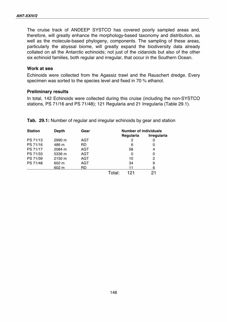
ANT-XXIV/2
148
The cruise track of ANDEEP SYSTCO has covered poorly sampled areas and,
therefore, will greatly enhance the morphology-based taxonomy and distribution, as
well as the molecule-based phylogeny, components. The sampling of these areas,
particularly the abyssal biome, will greatly expand the biodiversity data already
collated on all the Antarctic echinoids; not just of the cidaroids but also of the other
six echinoid families, both regular and irregular, that occur in the Southern Ocean.
Work at sea
Echinoids were collected from the Agassiz trawl and the Rauschert dredge. Every
specimen was sorted to the species level and fixed in 70 % ethanol.
Preliminary results
In total, 142 Echinoids were collected during this cruise (including the non-SYSTCO
stations, PS 71/16 and PS 71/48); 121 Regularia and 21 Irregularia (Table 29.1).
Tab. 29.1: Number of regular and irregular echinoids by gear and station
Station Depth Gear Number of individuals Regularia Irregularia PS 71/13 2990 m AGT 2 0
PS 71/16 486 m RD 6 0
PS 71/17 2084 m AGT 58 4
PS 71/33 5336 m AGT 0 0
PS 71/39 2150 m AGT 10 2
PS 71/48 602 m AGT 34 9
602 m RD 11 6
Total: 121 21
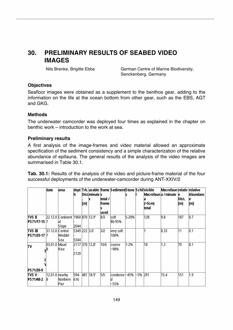
149
30. PRELIMINARY RESULTS OF SEABED VIDEO IMAGES Nils Brenke, Brigitte Ebbe
German Centre of Marine Biodiversity,
Senckenberg, Germany
Objectives
Seafloor images were obtained as a supplement to the benthos gear, adding to the
information on the life at the ocean bottom from other gear, such as the EBS, AGT
and GKG.
Methods
The underwater camcorder was deployed four times as explained in the chapter on
benthic work – introduction to the work at sea.
Preliminary results
A first analysis of the image-frames and video material allowed an approximate
specification of the sediment consistency and a simple characterization of the relative
abundance of epifauna. The general results of the analysis of the video images are
summarised in Table 30.1.
Tab. 30.1: Results of the analysis of the video and picture-frame material of the four
successful deployments of the underwater-camcorder during ANT-XXIV/2
date area dept
h Trk. Dist. [m]
usable minutes
frames total / frames used
Sediment Stones
Schill
visible Macrofauna (>5cm) total
Macrofauna / minute
relative Dist. [m]
relative Abundance [m]
TVS II PS71/17-15
22.12.0
7
Continent
al
Slope
1960
-
2044
870 12.9' 8/3 soft
80-95%
5-20% 128 9.8 187 0.7
TVS III PS71/33-17
31.12.0
7
Central
Weddel
Sea
5349
-
5344
222 3.0' 3/2 very soft
100%
1 0.33 11 0.1
TVS IV
PS71/39-9
03.01.0
8
Maud
Rise
2117
-
2120
370 12,8' 10/5 coarse
~98%
1-2% 18 1.3 79 0.1
TVS V PS71/48-2
12.01.0
8
nearby
Northern
Pier
594-
616
481 18.9' 5/5 condense
d
~55%
~45% ~5% 291 15.4 151 1.9
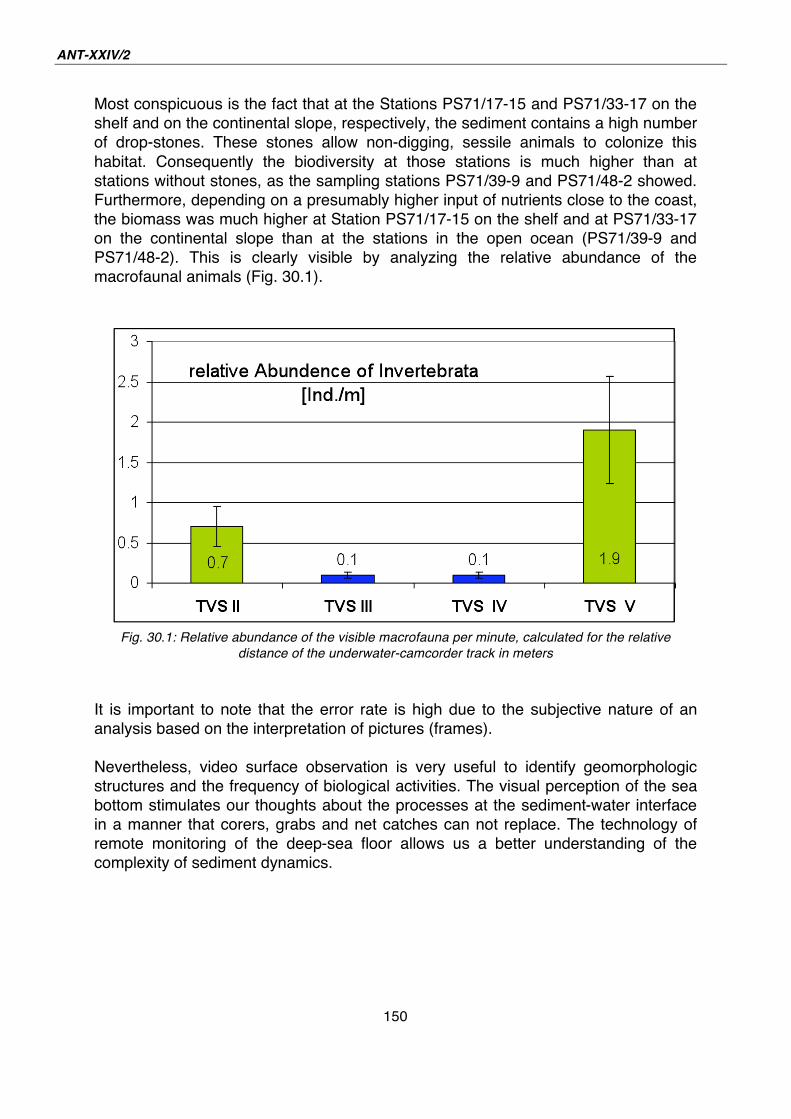
ANT-XXIV/2
150
Most conspicuous is the fact that at the Stations PS71/17-15 and PS71/33-17 on the
shelf and on the continental slope, respectively, the sediment contains a high number
of drop-stones. These stones allow non-digging, sessile animals to colonize this
habitat. Consequently the biodiversity at those stations is much higher than at
stations without stones, as the sampling stations PS71/39-9 and PS71/48-2 showed.
Furthermore, depending on a presumably higher input of nutrients close to the coast,
the biomass was much higher at Station PS71/17-15 on the shelf and at PS71/33-17
on the continental slope than at the stations in the open ocean (PS71/39-9 and
PS71/48-2). This is clearly visible by analyzing the relative abundance of the
macrofaunal animals (Fig. 30.1).
Fig. 30.1: Relative abundance of the visible macrofauna per minute, calculated for the relative
distance of the underwater-camcorder track in meters
It is important to note that the error rate is high due to the subjective nature of an
analysis based on the interpretation of pictures (frames).
Nevertheless, video surface observation is very useful to identify geomorphologic
structures and the frequency of biological activities. The visual perception of the sea
bottom stimulates our thoughts about the processes at the sediment-water interface
in a manner that corers, grabs and net catches can not replace. The technology of
remote monitoring of the deep-sea floor allows us a better understanding of the
complexity of sediment dynamics.
151
31. DOMINO - DYNAMICS OF BENTHIC ORGANIC MATTER FLUXES IN POLAR DEEP-OCEAN ENVIRONMENTS Eberhard Sauter, Oliver Sachs
Alfred-Wegener-Institut, Bremerhaven,
Germany
Being part of the ICED umbrella (Integrating Climate and Ecosystem Dynamics) and
closely associated to the IPY projects ANDEEP-SYSTCO (ANtarctic benthic DEEP-
sea biodiversity: colonization history and recent community patterns - SYSTem
COupling) and SCACE (Synoptic Circum-Antarctic Climate-processes and
Ecosystem study), DOMINO links water column processes such as particle export
and the fate of this food supply to the polar deep-sea communities at the seafloor.
The DFG-funded project (Priority Program Antarctic Research) focuses on the
determination of organic carbon fluxes onto deep-sea sediments of the Southern
Ocean, their spatial distribution as well as their temporal dynamics. Such fluxes to the
seafloor comprise a carbon sink at the lower end of the ocean s biological pump
which binds atmospheric CO2 to biomass and partly exports it to depth. Although
playing a key role in this respect, there are so far only few data available for the
Southern Ocean. DOMINO aims to improve the data coverage by high quality in-situ
measurements (for methodology, see chapter 14, 15) and will at the same time foster
the multidisciplinary linkage to planktology, oceanography, and benthos biology by
the project s close linkage to SYSTCO, SCACE and LAKRIS.
The ANT-XXIV/2 expedition ties up to the ANT-XXI/4 cruise in 2004 during which
benthic fluxes were measured on a north-south transect through the ACC front
system to the Weddell Sea. Scientific publications, discussions and workshops in the
aftermath of ANT-XXI/4 helped to coordinate the planning of the much more
multidisciplinary IPY cruise ANT-XXIV/2, and to adjust the field programmes of
SCACE, LAKRIS, DOMINO and SYSTCO. In this concert, DOMINO was to act as a
“geochemical interface” between water column and benthos investigations. Due to
time constraints, one element of the programme could not be worked out: The near-
bottom water column (bottom-next 2 metres) was planned to be sampled at the
SYSTCO stations by means of a special bottom water sampler (Sauter et al., 2005)
for the description of gradients in dissolved substances, particles and
microorganisms. This sampler was not deployed at all during the cruise.
However, despite the mentioned difficulties, a number of research highlights could be
achieved during this cruise: Amongst others, the DOMINO-related results can be
summarized as follows (for a more detailed description of preliminary results see
chapter 16):
ANT-XXIV/2
152
• Close to the shelf ice, benthic fluxes were found to be low under the
exceptionally heavy sea ice but significantly elevated after the opening of a
polynia.
• During the cruise the southernmost in-situ flux measurement was carried out
at 69°40 S.
• At least one of the originally planned repetition stations could be investigated
and allowed for new insights into the dynamics of seasonal benthic food
supply and the activities of benthic infauna. Whereas the benthic organic
carbon input was found to be 3 times higher end of January than at the begin
of December, an additional station 12 nautical miles south of this repetition
station showed a 20 % lower mean flux.
• The preliminary comparison of benthic fluxes with the development of sea
surface chlorophyll (from remote sensing data) suggests a linkage between
these parameters.
• As an overall result, this cruise revealed, that our knowledge of the pelago-
benthic coupling in the Southern Ocean is still poor. Continued efforts and an
integrated approach including water column as well as benthic investigations
is necessary to reveal the role of the benthic compartment in respect to
carbon export, reworking and fixation, respectively, and to assess the
ecological importance of the Southern Ocean s sea-floor habitats for system
functioning.
Reference Sauter, E. J., Schlüter, M., Wegner, J., Labahn, E. (2005). A routine device for high
resolution bottom water sampling. Journal of Sea Research, 54, 204-210.
153
32. EDUCATION AND OUTREACH REPORT - POLARSTERN ANT-XXIV/2 Victoria Wadley1), Brigitte
Ebbe2)
1)Australian Antarctic Division, Australia
2)German Centre of Marine Biodiversity,
Senckenberg, Germany The initial objective of the Education and Outreach (E&O) campaign on Polarstern
ANT-XXIV/2 was to publicise the scientific results of the voyage. This objective was
subsequently broadened, to include the logistic activities. Projects of the International
Polar Year (IPY), including the three on Polarstern ANT-XXIV/2, have agreed to
include the education of young scientists (“the next generation of polar researchers”)
and outreach to the general public. E&O campaigns for 18 biodiversity voyages
during the IPY, including Polarstern ANT-XXIV/2, are being coordinated by the
Census of Antarctic Marine Life (CAML) in association with the IPY. The campaign
was implemented on board by scientists with media experience and specialist
training, in addition to their research duties. All participants on the voyage contributed
to the campaign in a cooperative spirit. The E&O activities are grouped into those before the voyage, while at sea, and at the
end of the voyage. Communications at sea are limited by the high cost of emails and
lack of internet access. As a consequence, important aspects of the campaign were
planned for the weeks immediately after the voyage. The AWI Press Office provided
advice and support, including an .ftp site accessible by partner organisations to feed
their websites. Before the voyage a Memorandum of Understanding was signed by a responsible
person at each participating institution. This document outlined the objectives and
scope of the campaign and the roles of the contributors, most importantly the Voyage
Leader to approve all material. A meeting at AWI on 4 October 2007 clarified the
approach and provided connection with the successful press coverage of biodiversity
research on Polarstern ANT-XXIII/8. English was the main language used, with
translation to German, Dutch and French as appropriate. While at sea the scope of the E&O campaign was presented to all scientists at an
evening lecture early in the voyage. A daily activity report for the Census of the
Diversity of Abyssal Marine Life (CeDAMar) website was coordinated by Brigitte
Ebbe, using text (in both English and German) and photos from contributing
scientists. Victoria Wadley wrote a weekly biodiversity report for the CAML website
about the animals and sampling gear, accompanied by photos and videos. Equipe
Cousteau and Census of Marine Life (CoML) posted material from the campaign. Jan van Franeker coordinated a regular series of short videos by the Surface and
Under Ice Trawl (SUIT) team for the official Dutch IPY website, which were shared
ANT-XXIV/2
154
through the AWI ftp server, and contributed articles, photos and video material for
general usage. On a more personal level, the Dutch team produced weekly illustrated
newsletters in Dutch and German Partner websites including IPY. Through CAML, Polarstern communicated with E&O campaigns on the vessels Ivan
Papanin, Aurora Australis, G.O. Sars, L Astrolabe, Umitaku Maru and Tangaroa
which were at sea at the same time on IPY biodiversity voyages. Reports to
participating institutions were submitted as required. The IPY office and the Scientific
Committee on Antarctic Research (SCAR) were updated regularly on developments.
Standard protocols were adopted for photo metadata, including acknowledgement of
authors and their institutions. Karoline Stürmer wrote an article published in the Frankfurter Allgemeine about the
voyage s logistic support for the construction of Neumayer III. Michael Schröder
wrote for a Munich newspaper about his discovery of a rare monoplacophoran,
significant for molluscan phylogenetics. Various articles were written for local
newspapers in Germany and the Netherlands and a telephone interview was given
on Dutch national radio. A press release was prepared to announce Time magazine s
selection of a deepsea Antarctic biodiversity Nature paper in the Top Ten science
results of 2007; four of the authors were on the Polarstern voyage. During the voyage, the E&O team presented the results of the campaign and thanked
all participants. Many scientists expressed interest in continuing the activities as part
of their projects, using the freely-shared resources (text, photos, videos) collected
during the campaign. As an example, one of the daily reports was selected as the
introduction for a childrens book. The students on board increased their awareness
of how to communicate their results to a wider audience. At the end of the voyage posters, talks and video material on the voyage s
highlights were prepared for a press conference in Capetown on 5 February,
attended by Minister Schavan and 150 guests. It is hoped that these E&O products
will foster cooperation between South African and German research institutions
through messages tailored to viewpoints of politicians, media and decision makers.
Furthermore, the presentations will support in an understandable way the scientists
bid for additional shiptime to make up for the time losses due to logistic
responsibilities of Polarstern. The E&O highlights will be archived for publicity by
CoML/IPY at the end of the IPY in March 2009. The effectiveness and impact of the
campaign, including website hits, will be assessed in the weeks after the voyage. List of partner websites Alfred Wegener Institute for polar and marine research www.awi.de
Biodiversity reports for the CAML website www.caml.aq
Daily blogs to CeDAMar www.cedamar.org and www.deepsea-research.de
Equipe Cousteau coordinating 18 biodiversity voyages at www.cousteau.org
Census of Marine Life international marine biodiversity coordination www.coml.org
The Dutch IPY website is www.pooljaar.nl in which page www.pooljaar.nl/poolijs/
refers especially to the Polarstern ANT-XXIV/2 participation; Dutch/German
newsletters posted on www.jafweb.nl
155
33. WEATHER Eugen Müller, Hartmut
Sonnabend
Deutscher Wetterdienst Hamburg, Germany
The expedition ANT-XXIV/2 started in Cape Town in the evening of 28 November,
just after sunset. Frequency distributions of wave heights, wind directions and wind
forces for Dec 07 and Jan 08 are presented in Figs. 33.1, 33.2 and 33.3,
respectively. The first two days were dominated by a subtropical high pressure
system with SE-winds decreasing from 7 Bft near the coast to 4 Bft on the open sea.
During the following days Polarstern crossed the west drift and several deep
cyclones with their frontal systems passed the track causing stormy winds. The first
storm occurred on 1 December, a further one on 3 December and a third one on 7/8
December. The synoptic situation of these three storms was quite similar and was
defined by a cyclone with a well marked trough on the rear side. At each time a
maximal wind speed of 8 - 9 Bft and waves of 7 - 9 m were observed when the trough
passed. On 9/10 December a high pressure ridge extended to the south and by its
moving to the southeast the wind shifted from southwest to northwest and decreased
to 4 Bft. At the late evening of the 9 December the sea ice limit was reached at 60°S.
From 11 to 13 December the weather was dominated by a low pressure system that
moved along 60°S to the east. The winds changed their direction from northwest to
northeast with 3 - 4 Bft and light snowfall occurred when the occlusion passed
through. Behind this eastwards-moving cyclone a high pressure ridge built up and
after a passage through quite heavy ice Polarstern arrived in the early afternoon in
the Atka-Bay. The unloading had to take place on the sea ice of the Atka-Bay Due to
the fast ice it wasn t possible to go alongside the shelf ice edge. Therefore the
unloading had to take place on the sea ice of the Atka-Bay.These operations took
almost two days, and fair weather with weak southerly winds dominated till 17
December. Between the anticyclone over the Antarctic continent and a cyclone
moving along 62°S weak southerly winds persisted, sometimes even calm.
From 18 to 21 December an extensive storm cyclone moved from the South
Sandwich Islands to the southeast. With its flat trough, which reached to the eastern
Weddell Sea, it caused mainly weak winds with changing directions. The unloading of
the fuel for Neumayer was finished at midday of 19 December.
On 22 December another storm cyclone moved from Bouvet Islands to the southeast
and filled up. Polarstern was on the southern edge of this low, so the winds of 4 Bft
shifted slowly from east to southeast and later to south.
ANT-XXIV/2
156
On 24 December a ridge of high pressure built up over the Lazarev Sea and
dominated the weather until 27 December. Below a pronounced inversion there were
an extended layer of low level clouds and southwesterly winds of 3-4 Bft which
shifted to the northwest on 26 December. From 28 to 30 December Polarstern was
between an occluded low near South Sandwich Islands and a high over the Lazarev
Sea, what caused northeasterly winds 4-5 Bft. They shifted gradually to southeast
and later to southwest.
For the turn of the year cyclonic weather conditions prevailed. A low pressure system
over the Weddell Sea passed Cape Norvegia and travelled on to the Lazarev Sea.
After its coldfront went through westerly winds 6 Bft set in, shifting to southwest on
New Year. In only few or even no ice waves built up to 2 - 2,5 m.
On 2 January a secondary cyclone over the Weddell Sea moved to the Lazarev Sea
and its occlusion front brought some snowfall and freezing drizzle. The northwesterly
wind increased to 5 Bft. Already on the next day a ridge followed and the decreasing
winds shifted from southwest to east. On 4 and 5 January on the southern edge of a
low on 57°S 7°W moving to the southeast an easterly current of 5 - 6 Bft developed,
with embedded showers of snow and snow grains. A ridge of high pressure caused
on 6 and 7 January southeasterly winds of 3 - 4 Bft, shifting later to west. Extended
stratocumulus clouding prevailed. On 8 January the scientific work was stopped and
Polarstern sailed back to the Atka Bay for supporting the freighter Naja Arctica. On
the southern edge of an extended low over the Weddell Sea an easterly current
caused wind speeds of 5 - 6 Bft. On 9 and 10 January a ridge of high pressure over
the Lazarev Sea brought sunny weather and southerly winds around 4 Bft. From 11
to 13 January cyclonic weather dominated. An intense low pressure system
developed west of South Georgia and moved to the eastern Weddell Sea. On the
southern edge of this cyclone there were easterly winds of 8 Bft over the Atka Bay on
the 12/13 January. Already on the 14 January the wind shifted to southeast on the
back of the low and later decreased to 4 Bft. And it was also quite sunny due to the
dry air that was advected from the continent.
A ridge of high pressure formed over the eastern Weddell Sea and shifted very slowly
to the Lazarev Sea, where it became more and more flat. Therefore weak
southwesterly winds prevailed, temporary it was almost calm. Most of the time it was
cloudy, occasionally some showers of snow occurred.
From 20 to 22 January a small cyclone moved slowly from the eastern Weddell Sea
to the Lazarev Sea. In the moist and unstable air convective clouds formed and also
some showers of snow. The moderate winds came first from northwest, later from
southwest. From 23 to 25 January a small cyclone moved from the South Sandwich
Islands to the southeast and influenced the weather during the station work. The
highest wind speed during the passage of this low was observed on 24 January
when a northwesterly wind of 7 - 8 Bft occurred.
On 26 January a low pressure system developed over the Weddell Sea and moved,
under further intensifying to a storm, until 29 January to 63°S 10°E, where it became
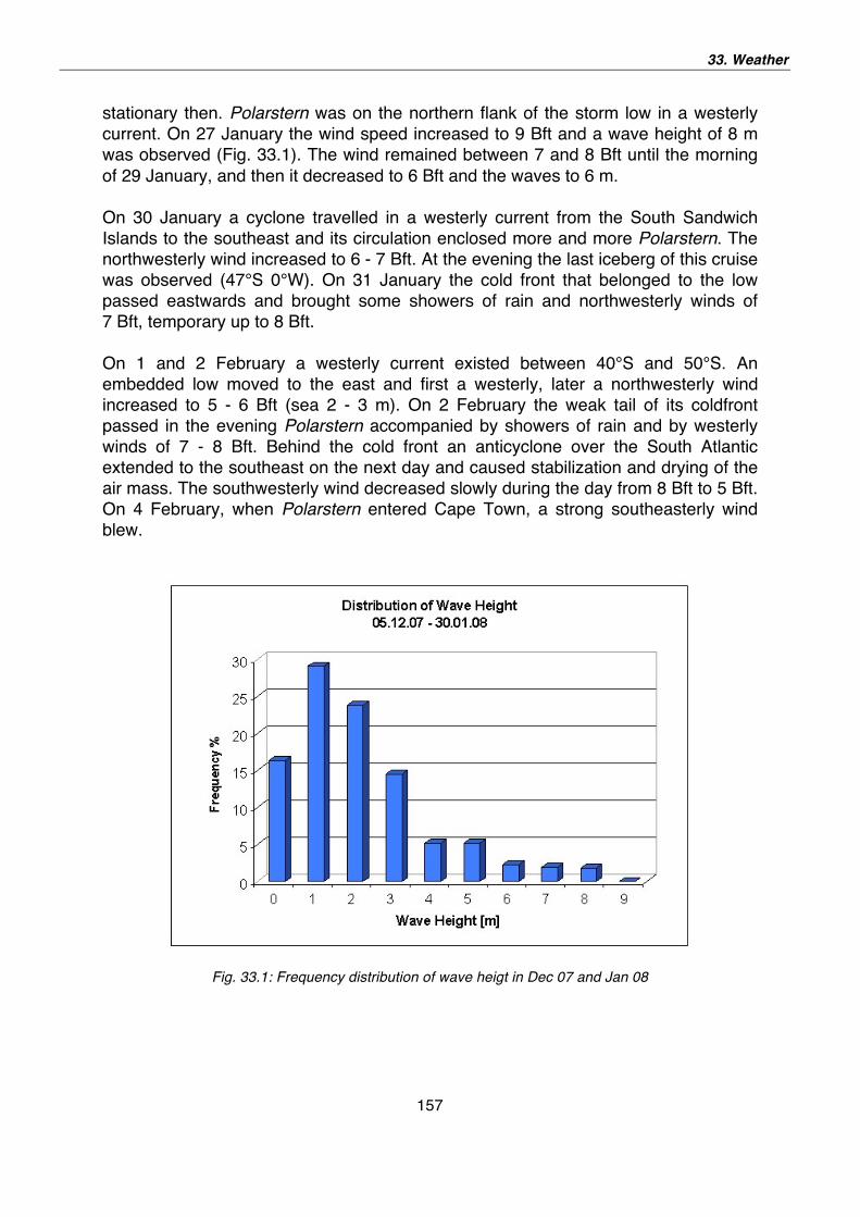
33. Weather
157
stationary then. Polarstern was on the northern flank of the storm low in a westerly
current. On 27 January the wind speed increased to 9 Bft and a wave height of 8 m
was observed (Fig. 33.1). The wind remained between 7 and 8 Bft until the morning
of 29 January, and then it decreased to 6 Bft and the waves to 6 m.
On 30 January a cyclone travelled in a westerly current from the South Sandwich
Islands to the southeast and its circulation enclosed more and more Polarstern. The
northwesterly wind increased to 6 - 7 Bft. At the evening the last iceberg of this cruise
was observed (47°S 0°W). On 31 January the cold front that belonged to the low
passed eastwards and brought some showers of rain and northwesterly winds of
7 Bft, temporary up to 8 Bft.
On 1 and 2 February a westerly current existed between 40°S and 50°S. An
embedded low moved to the east and first a westerly, later a northwesterly wind
increased to 5 - 6 Bft (sea 2 - 3 m). On 2 February the weak tail of its coldfront
passed in the evening Polarstern accompanied by showers of rain and by westerly
winds of 7 - 8 Bft. Behind the cold front an anticyclone over the South Atlantic
extended to the southeast on the next day and caused stabilization and drying of the
air mass. The southwesterly wind decreased slowly during the day from 8 Bft to 5 Bft.
On 4 February, when Polarstern entered Cape Town, a strong southeasterly wind
blew.
Fig. 33.1: Frequency distribution of wave heigt in Dec 07 and Jan 08
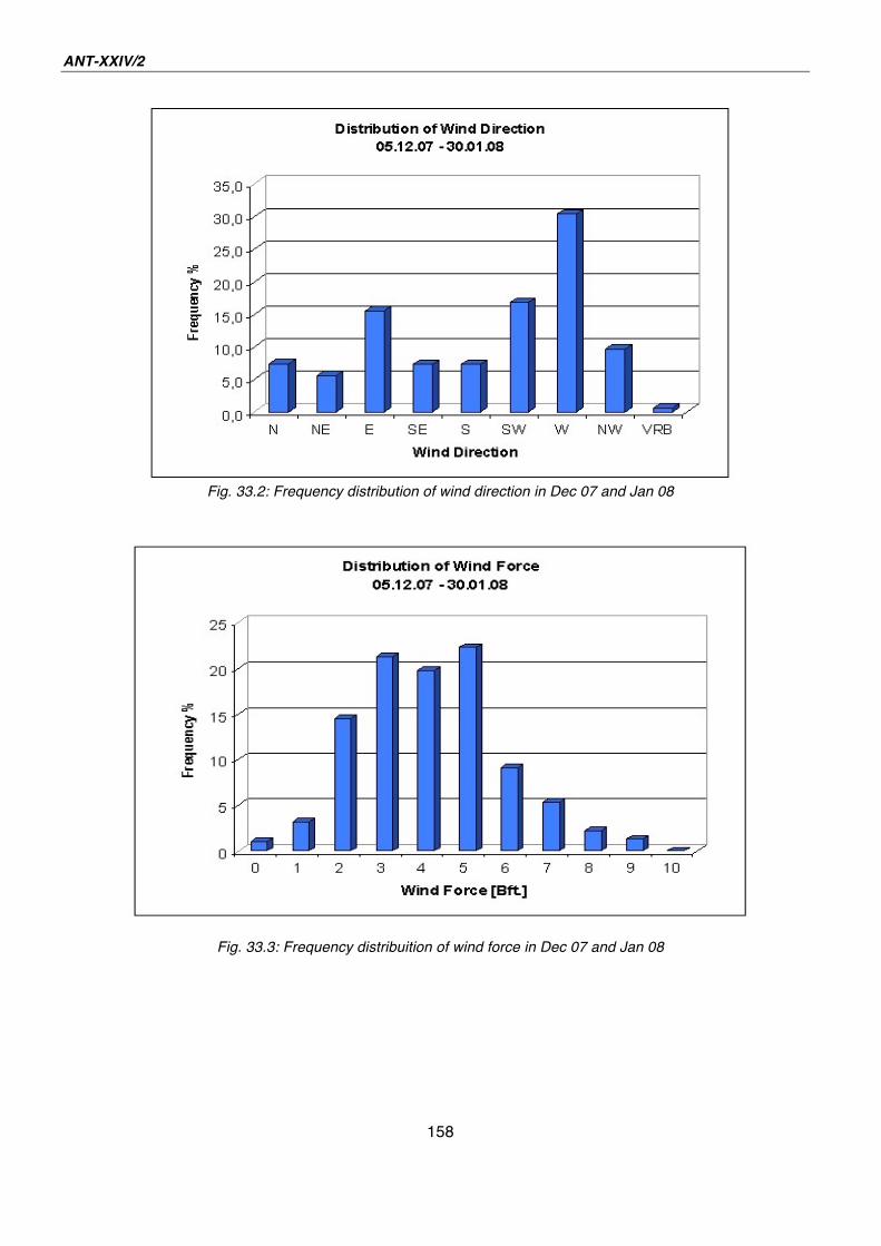
ANT-XXIV/2
158
Fig. 33.2: Frequency distribution of wind direction in Dec 07 and Jan 08
Fig. 33.3: Frequency distribuition of wind force in Dec 07 and Jan 08
159
34. SEA ICE CONDITIONS DURING POLARSTERN EXPEDITION ANT-XXIV/2, DECEMBER 2007 – JANUARY 2008 Jan Andries van Franeker1),
Bram Feij1), Andre Meijboom1),
Eugen Müller2)
1)IMARES, Texel, The Netherlands 2)Deutscher Wetterdienst Hamburg,
Germany
Introduction
Sea ice conditions are a major determinant in marine biology, physics and chemistry
and therefore of direct relevance to all studies conducted during the Polarstern
ANT-XXIV/2 expedition. Regular updates on the ice situationfrom satellite information
was provided during the daily weather forecasts on board. Summer 2007 - 2008 in the
Weddell and Lazarev Seas was characterized by unusual heavy, extended and
persistent sea ice. This made progress slow for Polarstern on its first southward
transect to Neumayer Station. Persistent fast ice also necessitated a second journey to
the station in the second week of January to break out a harbour in the fast ice to allow
unloading of the freighter Naja Arctica at the cliffs of the shelf ice.
The seasonal melting of sea ice in the Lazarev Sea is not only characterized by a north
south retreat but also by a strong east to west retreat. Melting often starts in a polynia to
the west of Maud Rise which rapidly widens. This pattern of rapid southward and
eastward retreat of the sea ice in the Lazarev Sea is clear from a comparison of the
satelite images of 21 Dec and 29 Dec 2007, starting and end date of the first research
transect moving north from 70° to 60° South along 3° West. Satellite images shown in
Fig. 34.1 are produced by Bremen University (Spreen et al., 2006) from microwave
radiometers with a spation resolution of 6 x 4 km and thus lack resolution at low ice
concentrations. Furthermore, the speed of melting complicates the assessment of
actual ice conditions around Polarstern at its station positions from satelite images.
Detailed ice records are a standard component of the predator survey programme (van
Franeker et al., this volume) and allow fine scale additional information for momentary
ice conditions around station positions
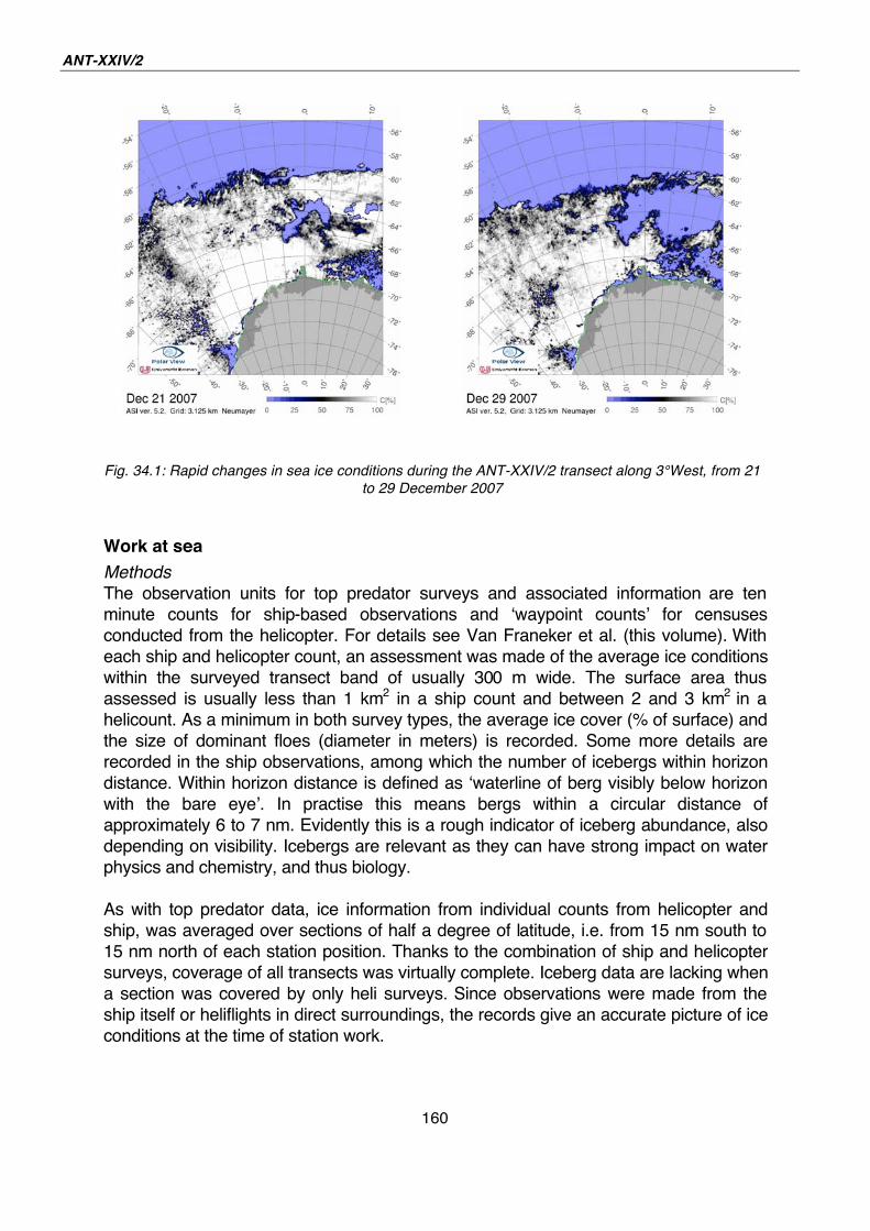
ANT-XXIV/2
160
Fig. 34.1: Rapid changes in sea ice conditions during the ANT-XXIV/2 transect along 3°West, from 21
to 29 December 2007
Work at sea
Methods
The observation units for top predator surveys and associated information are ten
minute counts for ship-based observations and waypoint counts for censuses
conducted from the helicopter. For details see Van Franeker et al. (this volume). With
each ship and helicopter count, an assessment was made of the average ice conditions
within the surveyed transect band of usually 300 m wide. The surface area thus
assessed is usually less than 1 km2 in a ship count and between 2 and 3 km2 in a
helicount. As a minimum in both survey types, the average ice cover (% of surface) and
the size of dominant floes (diameter in meters) is recorded. Some more details are
recorded in the ship observations, among which the number of icebergs within horizon
distance. Within horizon distance is defined as waterline of berg visibly below horizon
with the bare eye . In practise this means bergs within a circular distance of
approximately 6 to 7 nm. Evidently this is a rough indicator of iceberg abundance, also
depending on visibility. Icebergs are relevant as they can have strong impact on water
physics and chemistry, and thus biology.
As with top predator data, ice information from individual counts from helicopter and
ship, was averaged over sections of half a degree of latitude, i.e. from 15 nm south to
15 nm north of each station position. Thanks to the combination of ship and helicopter
surveys, coverage of all transects was virtually complete. Iceberg data are lacking when
a section was covered by only heli surveys. Since observations were made from the
ship itself or heliflights in direct surroundings, the records give an accurate picture of ice
conditions at the time of station work.
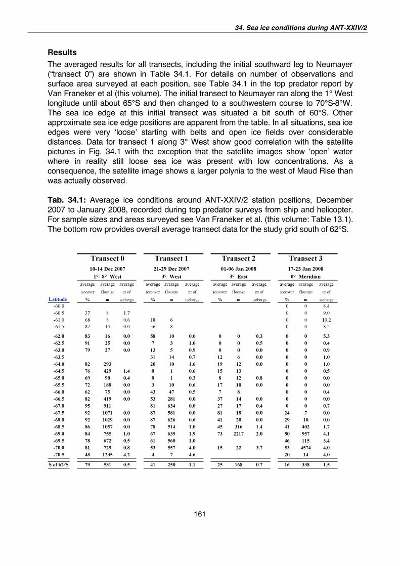
34. Sea ice conditions during ANT-XXIV/2
161
Results
The averaged results for all transects, including the initial southward leg to Neumayer
(“transect 0”) are shown in Table 34.1. For details on number of observations and
surface area surveyed at each position, see Table 34.1 in the top predator report by
Van Franeker et al (this volume). The initial transect to Neumayer ran along the 1° West
longitude until about 65°S and then changed to a southwestern course to 70°S-8°W.
The sea ice edge at this initial transect was situated a bit south of 60°S. Other
approximate sea ice edge positions are apparent from the table. In all situations, sea ice
edges were very loose starting with belts and open ice fields over considerable
distances. Data for transect 1 along 3° West show good correlation with the satellite
pictures in Fig. 34.1 with the exception that the satellite images show open water
where in reality still loose sea ice was present with low concentrations. As a
consequence, the satellite image shows a larger polynia to the west of Maud Rise than
was actually observed.
Tab. 34.1: Average ice conditions around ANT-XXIV/2 station positions, December
2007 to January 2008, recorded during top predator surveys from ship and helicopter.
For sample sizes and areas surveyed see Van Franeker et al. (this volume: Table 13.1).
The bottom row provides overall average transect data for the study grid south of 62°S.
ANT-XXIV/2
162
Acknowledgements
Officers and crew of Polarstern and pilots and technicians of Heli Transair are
gratefully acknowledged for their support to the top predator observation programme.
The research project by IMARES is funded by the Netherlands Ministry for
Agriculture, Nature and Food Quality (LNV). We thank the to the Alfred Wegener
Institute for its open attitude to international cooperation through the sharing of costly
logistic facilities.
References Spreen, G., Kaleschke, L. & Heygster, G. 2006. Sea ice remote sensing using AMSR-E 89
GHz channels. Journal of Geophysical Research DOI:10.1029.
163
35. ACOUSTIC SURVEY OF THE HORIZONTAL AND VERTICAL DISTRIBUTION OF KRILL, ZOOPLANKTON AND NEKTON Sören Krägefsky, Ulrich Bathmann
Alfred-Wegener-Institut,
Bremerhaven, Germany
Objectives
Antarctic krill, Euphausia superba, is an important species in the Antarctic food web
and plays an important role in the biochemical cycling in the Southern Ocean.
Antarctic krill provides an important food source for whales, seals, penguins, squids,
fish and birds.
There is a potential for large increase in krill fishery in the coming years due to the
development in krill-processing technology and an increasing demand (Kock et al.
2007). Today, most krill is processed to produce fish food.
The distribution of krill is highly uneven, and despite long lasting research, estimates
of the total krill biomass and production is still very uncertain (Atkinson et al., 2009).
Acoustic measurements allow to study the distributional pattern of krill in large survey
areas, and were used for survey krill abundance and distribution in the Lazarvev Sea.
The Lazerev Sea is part of the area 48.6 of the Convention of the Conservation of
Antarctic Marine Living Resources (CCAMLR), which, so far, has a small spatial and
temporal coverage with krill measurements.
Work at sea
The distribution and abundance of krill, zooplankton and nekton were surveyed
continuously with multifrequency acoustic measurements, using a Simrad EK60 at
frequencies 38, 70 120 and 200 kHz. A calibration of the system was performed on
08 - 09.01.2008 with standard target spheres. During the survey, a pulse duration of
1,024 ms was used for all frequencies. Raw data was recorded down to a depth of
1,000 m, at a ping rate of 1 ping every 2 - 3 seconds. The acoustic survey comprised
four main meridional transects across the Lazarev Sea (Fig. 35.1), with a time lag
between single transects due to logistic tasks during the expedition. The noise
content of the acoustic record varies, among others, subject to the actual ice
coverage encountered along the transects.
Preliminary results
Preliminary data exploration suggests that advection and seasonal vertical
displacement of animals may have contributed to changing backscattering signature
over the course of the survey.
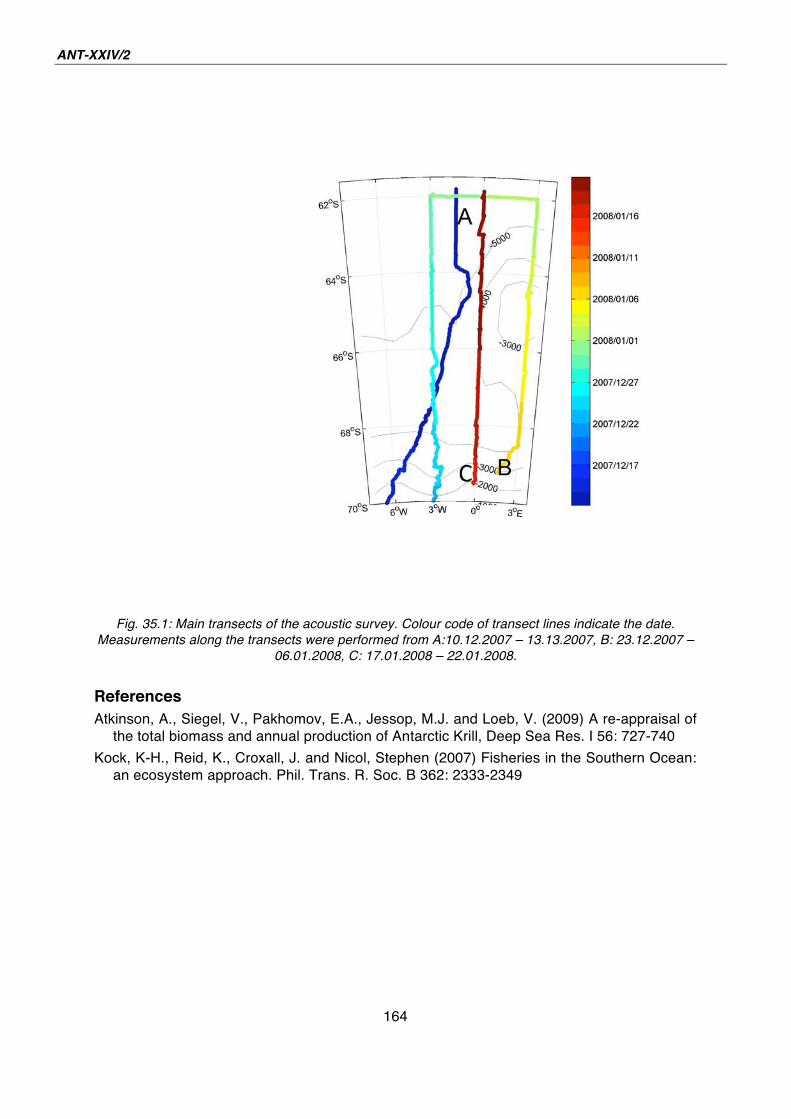
ANT-XXIV/2
164
Fig. 35.1: Main transects of the acoustic survey. Colour code of transect lines indicate the date.
Measurements along the transects were performed from A:10.12.2007 – 13.13.2007, B: 23.12.2007 –
06.01.2008, C: 17.01.2008 – 22.01.2008.
References Atkinson, A., Siegel, V., Pakhomov, E.A., Jessop, M.J. and Loeb, V. (2009) A re-appraisal of
the total biomass and annual production of Antarctic Krill, Deep Sea Res. I 56: 727-740
Kock, K-H., Reid, K., Croxall, J. and Nicol, Stephen (2007) Fisheries in the Southern Ocean:
an ecosystem approach. Phil. Trans. R. Soc. B 362: 2333-2349
165
APPENDIX
A.1 PARTICIPATING INSTITUTIONS A.2 CRUISE PARTICIPANTS A.3 SHIP'S CREW A.4 STATION LIST
166
A.1 BETEILIGTE INSTITUTE / PARTICIPATING INSTITUTES
Adresse /Address
AAD Australian Antarctic Division
Department of the Environment and
Water Resources
203 Channel Highway
7050 Kingston, Tasmania
Australia
AWI Alfred-Wegener-Institut für Polar- und
Meeresforschung
in der Helmholtz-Gemeinschaft
Postfach 12 01 61
27515 Bremerhaven
Germany
DFZ Universidad de Sevilla
Departamento Fisiologia Animal y
Zoologia
Facultad de Biologia
Avenida Reina Mecedes
Spain
DWD Deutscher Wetterdienst
Geschäftsbereich Wettervorhersage
Seeschifffahrtsberatung
Bernhard Nocht Str. 76
20359 Hamburg
Germany
DZMB German Centre of Marine Biodiversity
Senckenberg Institute
Südstrand 44
46382 Wilhelmshaven
Germany
167
Adresse /Address
FIS Senckenberg
Forschungsinstitut und Naturmuseum
Senckenberganlage 25
60325 Frankfurt
Germany
HeliTransair Heli Transair GmbH
Flugplatz
63329 Egelsbach
Germany
I.R.Sc.N.B. Institut Royal des Sciences Naturelles de
Belgique (I.R.Sc.N.B./K.B.I.N.)
Département des Invertébrés
Laboratoire de Carcinologie
Rue Vautier, 29
B-1000 Brussels / Belgium
IMARES
IMARES
Marine and Coastal Zone Research
PO Box 167
1790AD Den Burg (Texel)
The Netherlands
LAEISZ Reederei F. Laeisz GmbH
Brückenstr. 25
27568 Bremerhaven
Germany
LMU, Uni München
Ludwig Maximilians-Universität München
(LMU)
Biozentrum, Department Biologie II,
Systematische Zoologie
Großhaderner Str. 2
D-82152 Planegg-Martinsried
Germany
OPTIMARE Optimare Sensorsyteme AG
Am Luneort 15A
27572 Bremerhaven
Germany
ANT-XXVI/2
168
Adresse /Address
RUB Ruhr Universität Bochum
Zoologie
Universitätsstr. 150
44780 Bochum
Germany
UiB University of Bergen
Allégaten 55
5007 Bergen
Norway
Uni HB Marine Zoologie
Universität Bremen
Postfach 33 04 40
28334 Bremen
Germany
Uni Geneva University of Geneva
30, Quai Ernest Ansermet
Genève 4, 1211
Switzerland
U Gent Gent University
Biological Department / Marine Biology
Krijgslaan 281 – Building S8
Gent, 9000
Belgium
ZIM, Uni HH Zoological Institute and
Zoological Museum
University of Hamburg
Martin-Luther-King-Platz 3
20146 Hamburg
Germany
Uni L. University of Liverpool
Department of Earth and Ocean Sciences
4 Brownlow Street
Liverpool L69 3GP, UK
United Kingdom
169
Adresse /Address
UTC University of Cape Town
Rondebosch 7701
South Africa
v.T.I. Johann Heinrich von Thünen-Institut
Institut für Seefischerei
Herrn Dr. Gerd Kraus
Palmaille 9
22767 Hamburg
Germany
170
A.2 FAHRTTEILNEHMER / PARTICIPANTS
Fahrtleiter/Chief Scientist: Ulrich Bathmann
Cape Town – Cape Town
Name Vorname/ First Name
Institut/ Institute
Beruf/ Profession
Bathmann Ulrich AWI Biologist
chief scientist
Brandt Angelika ZIM, Uni HH Biologist
Brauer Jens HeliTransair Technician
Brenke Nils DZMB Biologist
Brix Saskia DZMB Biologist
Brown Kelly UiB Chemist
Büchner Jürgen HeliTransair Pilot
Dorssen Michiel van IMARES Biologist
Ebbe Brigitte DZMB Biologist
Edinger Jens v.T.I. Student
Ewe Daniela AWI Student
Feij Bram IMARES Ornithologist
Flores Hauke IMARES Biologist
Fontaine Delia Uni Geneva Biologist
Franeker Jan van IMARES Biologist
Friedt Wolfgang HeliTransair Pilot
Guilini Katja U Gent Biologist
Haraldsson Matilda v.T.I. Student
Hauck Judith UiB Chemist
Heckmann Markus HeliTransair Technician
Henche Annika DZMB Biologist
Herrmann Sarah AWI Biologist
Hofmann Oliver UiB Student
Janussen Dorte FIS Biologist
Kitchener John AAD Biologist
Krägefsky Sören AWI Biologist
171
Name Vorname/ First Name
Institut/ Institute
Beruf/ Profession
Kramer Lydia ZIM, Uni HH Biologist
Kruse Svenja AWI Biologist
Leach Harry Uni Liverpool Physicist
Maßmann Silvia AWI Student
Meijboom Andre IMARES Biologist
Neill Craig UiB Chemist
Müller Eugen DWD Meteorologist
Sonnabend Hartmut DWD Technician
Olischläger Mark AWI Student
Pey Frank UiB Chemist
Richter Falk AWI Student
Riehl Torben ZIM, Uni HH Biologist
Robert Henri I.R.Sc.N.B. Scientist
Sachs Oliver AWI Geologist
Sauter Eberhard AWI Geochemist
Schrödl Michael LMU, Uni München Biologist
Schüller Myriam RUB Biologist
Schwabe Enrico LMU, Uni München Biologist
Strass Volker AWI Physicist
Stürmer Karoline v.T.I. Biologist
Veith-Köhler Gritta DZMB Biologist
Vortkamp Martina v.T.I. Technician
Wadley Victoria AAD Biologist
Wend Britta AWI Biologist
Witte Timo OPTIMARE Physicist
Würzberg Laura ZIM, Uni HH Biologist
Zapata Guardiola Rebeca DFZ Biologist
172
A.3 SCHIFFSBESATZUNG / SHIP'S CREW
No. Name Rank
1. Pahl, Uwe Master
2. Grundmann, Uwe 1. Offc.
3. Ziemann, Olaf Ch. Eng.
4. Bratz, Herbert 2. Offc.
5. Fallei, Holger 2. Offc.
6. Hering, Igor 2. Offc.
7. Kapieske, Uwe Doctor
8. Koch, Georg R. Offc.
9. Kotnik, Herbert 2. Eng.
10. Schnürch, Helmut 2. Eng.
11. Westphal, Henning 2. Eng.
12. Holtz, Hartmut ElecEng.
13. Dimmler, Werner ELO
14. Feiertag, Thomas ELO
15. Fröb, Martin ELO
16. Rehe, Lars ELO
17. Clasen, Burkhard Boatsw.
18. Neisner, Winfried Carpenter
19. Burzan, Gerd-Ekkeh. A.B.
20. Hartwig-Lab. , Andreas A.B.
21. Kreis, Reinhard A.B.
22. Kretzschmar, Uwe A.B.
23. Moser, Siegfried A.B.
24. Pousada Martinez, S. A.B.
25. Schröder, Norbert A.B.
26. Schultz, Ottomar A.B.
27. Beth, Detlef Storek.
28. Dinse, Horst Mot-man
29. Fritz, Günter Mot-man
30. Kliem, Peter Mot-man
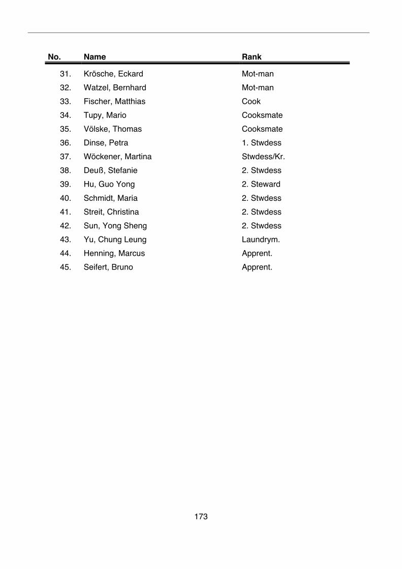
173
No. Name Rank
31. Krösche, Eckard Mot-man
32. Watzel, Bernhard Mot-man
33. Fischer, Matthias Cook
34. Tupy, Mario Cooksmate
35. Völske, Thomas Cooksmate
36. Dinse, Petra 1. Stwdess
37. Wöckener, Martina Stwdess/Kr.
38. Deuß, Stefanie 2. Stwdess
39. Hu, Guo Yong 2. Steward
40. Schmidt, Maria 2. Stwdess
41. Streit, Christina 2. Stwdess
42. Sun, Yong Sheng 2. Stwdess
43. Yu, Chung Leung Laundrym.
44. Henning, Marcus Apprent.
45. Seifert, Bruno Apprent.
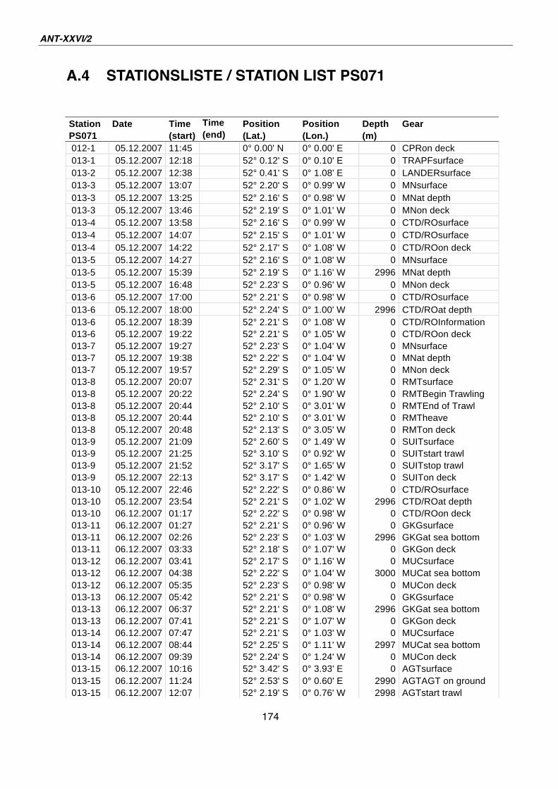
ANT-XXVI/2
174
A.4 STATIONSLISTE / STATION LIST PS071
Station Date Time Time Position Position Depth Gear
PS071 (start) (end) (Lat.) (Lon.) (m)
012-1 05.12.2007 11:45 0° 0.00' N 0° 0.00' E 0 CPRon deck
013-1 05.12.2007 12:18 52° 0.12' S 0° 0.10' E 0 TRAPFsurface
013-2 05.12.2007 12:38 52° 0.41' S 0° 1.08' E 0 LANDERsurface
013-3 05.12.2007 13:07 52° 2.20' S 0° 0.99' W 0 MNsurface
013-3 05.12.2007 13:25 52° 2.16' S 0° 0.98' W 0 MNat depth
013-3 05.12.2007 13:46 52° 2.19' S 0° 1.01' W 0 MNon deck
013-4 05.12.2007 13:58 52° 2.16' S 0° 0.99' W 0 CTD/ROsurface
013-4 05.12.2007 14:07 52° 2.15' S 0° 1.01' W 0 CTD/ROsurface
013-4 05.12.2007 14:22 52° 2.17' S 0° 1.08' W 0 CTD/ROon deck
013-5 05.12.2007 14:27 52° 2.16' S 0° 1.08' W 0 MNsurface
013-5 05.12.2007 15:39 52° 2.19' S 0° 1.16' W 2996 MNat depth
013-5 05.12.2007 16:48 52° 2.23' S 0° 0.96' W 0 MNon deck
013-6 05.12.2007 17:00 52° 2.21' S 0° 0.98' W 0 CTD/ROsurface
013-6 05.12.2007 18:00 52° 2.24' S 0° 1.00' W 2996 CTD/ROat depth
013-6 05.12.2007 18:39 52° 2.21' S 0° 1.08' W 0 CTD/ROInformation
013-6 05.12.2007 19:22 52° 2.21' S 0° 1.05' W 0 CTD/ROon deck
013-7 05.12.2007 19:27 52° 2.23' S 0° 1.04' W 0 MNsurface
013-7 05.12.2007 19:38 52° 2.22' S 0° 1.04' W 0 MNat depth
013-7 05.12.2007 19:57 52° 2.29' S 0° 1.05' W 0 MNon deck
013-8 05.12.2007 20:07 52° 2.31' S 0° 1.20' W 0 RMTsurface
013-8 05.12.2007 20:22 52° 2.24' S 0° 1.90' W 0 RMTBegin Trawling
013-8 05.12.2007 20:44 52° 2.10' S 0° 3.01' W 0 RMTEnd of Trawl
013-8 05.12.2007 20:44 52° 2.10' S 0° 3.01' W 0 RMTheave
013-8 05.12.2007 20:48 52° 2.13' S 0° 3.05' W 0 RMTon deck
013-9 05.12.2007 21:09 52° 2.60' S 0° 1.49' W 0 SUITsurface
013-9 05.12.2007 21:25 52° 3.10' S 0° 0.92' W 0 SUITstart trawl
013-9 05.12.2007 21:52 52° 3.17' S 0° 1.65' W 0 SUITstop trawl
013-9 05.12.2007 22:13 52° 3.17' S 0° 1.42' W 0 SUITon deck
013-10 05.12.2007 22:46 52° 2.22' S 0° 0.86' W 0 CTD/ROsurface
013-10 05.12.2007 23:54 52° 2.21' S 0° 1.02' W 2996 CTD/ROat depth
013-10 06.12.2007 01:17 52° 2.22' S 0° 0.98' W 0 CTD/ROon deck
013-11 06.12.2007 01:27 52° 2.21' S 0° 0.96' W 0 GKGsurface
013-11 06.12.2007 02:26 52° 2.23' S 0° 1.03' W 2996 GKGat sea bottom
013-11 06.12.2007 03:33 52° 2.18' S 0° 1.07' W 0 GKGon deck
013-12 06.12.2007 03:41 52° 2.17' S 0° 1.16' W 0 MUCsurface
013-12 06.12.2007 04:38 52° 2.22' S 0° 1.04' W 3000 MUCat sea bottom
013-12 06.12.2007 05:35 52° 2.23' S 0° 0.98' W 0 MUCon deck
013-13 06.12.2007 05:42 52° 2.21' S 0° 0.98' W 0 GKGsurface
013-13 06.12.2007 06:37 52° 2.21' S 0° 1.08' W 2996 GKGat sea bottom
013-13 06.12.2007 07:41 52° 2.21' S 0° 1.07' W 0 GKGon deck
013-14 06.12.2007 07:47 52° 2.21' S 0° 1.03' W 0 MUCsurface
013-14 06.12.2007 08:44 52° 2.25' S 0° 1.11' W 2997 MUCat sea bottom
013-14 06.12.2007 09:39 52° 2.24' S 0° 1.24' W 0 MUCon deck
013-15 06.12.2007 10:16 52° 3.42' S 0° 3.93' E 0 AGTsurface
013-15 06.12.2007 11:24 52° 2.53' S 0° 0.60' E 2990 AGTAGT on ground
013-15 06.12.2007 12:07 52° 2.19' S 0° 0.76' W 2998 AGTstart trawl
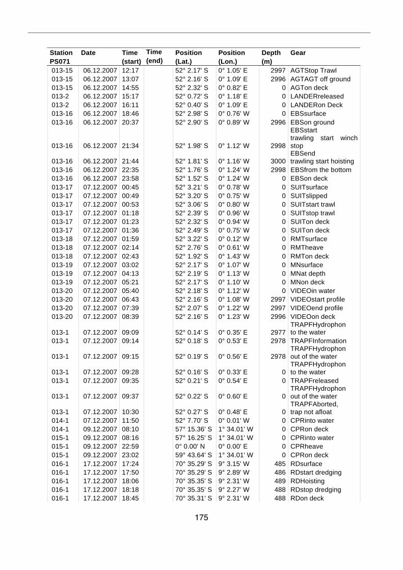
175
Station Date Time Time Position Position Depth Gear
PS071 (start) (end) (Lat.) (Lon.) (m)
013-15 06.12.2007 12:17 52° 2.17' S 0° 1.05' E 2997 AGTStop Trawl
013-15 06.12.2007 13:07 52° 2.16' S 0° 1.09' E 2996 AGTAGT off ground
013-15 06.12.2007 14:55 52° 2.32' S 0° 0.82' E 0 AGTon deck
013-2 06.12.2007 15:17 52° 0.72' S 0° 1.18' E 0 LANDERreleased
013-2 06.12.2007 16:11 52° 0.40' S 0° 1.09' E 0 LANDERon Deck
013-16 06.12.2007 18:46 52° 2.98' S 0° 0.76' W 0 EBSsurface
013-16 06.12.2007 20:37 52° 2.90' S 0° 0.89' W 2996 EBSon ground
013-16 06.12.2007 21:34
52° 1.98' S 0° 1.12' W 2998
EBSstart trawling start winch stop
013-16 06.12.2007 21:44
52° 1.81' S 0° 1.16' W 3000 EBSend trawling start hoisting
013-16 06.12.2007 22:35 52° 1.76' S 0° 1.24' W 2998 EBSfrom the bottom
013-16 06.12.2007 23:58 52° 1.52' S 0° 1.24' W 0 EBSon deck
013-17 07.12.2007 00:45 52° 3.21' S 0° 0.78' W 0 SUITsurface
013-17 07.12.2007 00:49 52° 3.20' S 0° 0.75' W 0 SUITslipped
013-17 07.12.2007 00:53 52° 3.06' S 0° 0.80' W 0 SUITstart trawl
013-17 07.12.2007 01:18 52° 2.39' S 0° 0.96' W 0 SUITstop trawl
013-17 07.12.2007 01:23 52° 2.32' S 0° 0.94' W 0 SUITon deck
013-17 07.12.2007 01:36 52° 2.49' S 0° 0.75' W 0 SUITon deck
013-18 07.12.2007 01:59 52° 3.22' S 0° 0.12' W 0 RMTsurface
013-18 07.12.2007 02:14 52° 2.76' S 0° 0.61' W 0 RMTheave
013-18 07.12.2007 02:43 52° 1.92' S 0° 1.43' W 0 RMTon deck
013-19 07.12.2007 03:02 52° 2.17' S 0° 1.07' W 0 MNsurface
013-19 07.12.2007 04:13 52° 2.19' S 0° 1.13' W 0 MNat depth
013-19 07.12.2007 05:21 52° 2.17' S 0° 1.10' W 0 MNon deck
013-20 07.12.2007 05:40 52° 2.18' S 0° 1.12' W 0 VIDEOin water
013-20 07.12.2007 06:43 52° 2.16' S 0° 1.08' W 2997 VIDEOstart profile
013-20 07.12.2007 07:39 52° 2.07' S 0° 1.22' W 2997 VIDEOend profile
013-20 07.12.2007 08:39 52° 2.16' S 0° 1.23' W 2996 VIDEOon deck
013-1 07.12.2007 09:09
52° 0.14' S 0° 0.35' E 2977 TRAPFHydrophon to the water
013-1 07.12.2007 09:14 52° 0.18' S 0° 0.53' E 2978 TRAPFInformation
013-1 07.12.2007 09:15
52° 0.19' S 0° 0.56' E 2978 TRAPFHydrophon out of the water
013-1 07.12.2007 09:28
52° 0.16' S 0° 0.33' E 0 TRAPFHydrophon to the water
013-1 07.12.2007 09:35 52° 0.21' S 0° 0.54' E 0 TRAPFreleased
013-1 07.12.2007 09:37
52° 0.22' S 0° 0.60' E 0 TRAPFHydrophon out of the water
013-1 07.12.2007 10:30
52° 0.27' S 0° 0.48' E 0 TRAPFAborted, trap not afloat
014-1 07.12.2007 11:50 52° 7.70' S 0° 0.01' W 0 CPRinto water
014-1 09.12.2007 08:10 57° 15.36' S 1° 34.01' W 0 CPRon deck
015-1 09.12.2007 08:16 57° 16.25' S 1° 34.01' W 0 CPRinto water
015-1 09.12.2007 22:59 0° 0.00' N 0° 0.00' E 0 CPRheave
015-1 09.12.2007 23:02 59° 43.64' S 1° 34.01' W 0 CPRon deck
016-1 17.12.2007 17:24 70° 35.29' S 9° 3.15' W 485 RDsurface
016-1 17.12.2007 17:50 70° 35.29' S 9° 2.89' W 486 RDstart dredging
016-1 17.12.2007 18:06 70° 35.35' S 9° 2.31' W 489 RDHoisting
016-1 17.12.2007 18:18 70° 35.35' S 9° 2.27' W 488 RDstop dredging
016-1 17.12.2007 18:45 70° 35.31' S 9° 2.31' W 488 RDon deck
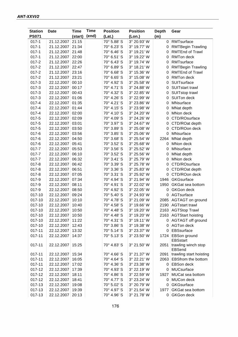
ANT-XXVI/2
176
Station Date Time Time Position Position Depth Gear
PS071 (start) (end) (Lat.) (Lon.) (m)
017-1 21.12.2007 21:15 70° 5.88' S 3° 20.93' W 0 RMTsurface
017-1 21.12.2007 21:34 70° 6.23' S 3° 19.77' W 0 RMTBegin Trawling
017-1 21.12.2007 21:48 70° 6.46' S 3° 19.21' W 0 RMTEnd of Trawl
017-1 21.12.2007 22:00 70° 6.51' S 3° 19.22' W 0 RMTon deck
017-2 21.12.2007 22:26 70° 6.43' S 3° 19.74' W 0 RMTsurface
017-2 21.12.2007 22:47 70° 6.89' S 3° 18.21' W 0 RMTBegin Trawling
017-2 21.12.2007 23:16 70° 6.68' S 3° 15.36' W 0 RMTEnd of Trawl
017-2 21.12.2007 23:21 70° 6.65' S 3° 15.08' W 0 RMTon deck
017-3 22.12.2007 00:10 70° 4.92' S 3° 25.58' W 0 SUITsurface
017-3 22.12.2007 00:17 70° 4.71' S 3° 24.88' W 0 SUITstart trawl
017-3 22.12.2007 00:43 70° 4.32' S 3° 22.85' W 0 SUITstop trawl
017-3 22.12.2007 01:06 70° 4.26' S 3° 22.99' W 0 SUITon deck
017-4 22.12.2007 01:35 70° 4.21' S 3° 23.86' W 0 MNsurface
017-4 22.12.2007 01:44 70° 4.15' S 3° 23.98' W 0 MNat depth
017-4 22.12.2007 02:00 70° 4.10' S 3° 24.20' W 0 MNon deck
017-5 22.12.2007 02:09 70° 4.09' S 3° 24.26' W 0 CTD/ROsurface
017-5 22.12.2007 03:01 70° 3.97' S 3° 24.67' W 0 CTD/ROat depth
017-5 22.12.2007 03:50 70° 3.89' S 3° 25.08' W 0 CTD/ROon deck
017-6 22.12.2007 03:56 70° 3.85' S 3° 25.06' W 0 MNsurface
017-6 22.12.2007 04:50 70° 3.68' S 3° 25.54' W 2264 MNat depth
017-6 22.12.2007 05:41 70° 3.52' S 3° 25.68' W 0 MNon deck
017-7 22.12.2007 05:53 70° 3.56' S 3° 25.52' W 0 MNsurface
017-7 22.12.2007 06:10 70° 3.52' S 3° 25.56' W 0 MNat depth
017-7 22.12.2007 06:32 70° 3.41' S 3° 25.79' W 0 MNon deck
017-8 22.12.2007 06:42 70° 3.39' S 3° 25.78' W 0 CTD/ROsurface
017-8 22.12.2007 06:51 70° 3.36' S 3° 25.83' W 0 CTD/ROat depth
017-8 22.12.2007 07:05 70° 3.31' S 3° 25.92' W 0 CTD/ROon deck
017-9 22.12.2007 07:34 70° 4.94' S 3° 21.94' W 1946 GKGsurface
017-9 22.12.2007 08:11 70° 4.91' S 3° 22.02' W 1950 GKGat sea bottom
017-9 22.12.2007 08:50 70° 4.92' S 3° 22.05' W 0 GKGon deck
017-10 22.12.2007 09:24 70° 5.40' S 3° 24.93' W 0 AGTsurface
017-10 22.12.2007 10:10 70° 4.78' S 3° 21.09' W 2085 AGTAGT on ground
017-10 22.12.2007 10:40 70° 4.58' S 3° 19.66' W 2190 AGTstart trawl
017-10 22.12.2007 10:50 70° 4.48' S 3° 19.20' W 2163 AGTStop Trawl
017-10 22.12.2007 10:50 70° 4.48' S 3° 19.20' W 2163 AGTStart hoisting
017-10 22.12.2007 11:22 70° 4.31' S 3° 19.11' W 0 AGTAGT off ground
017-10 22.12.2007 12:43 70° 3.86' S 3° 19.38' W 0 AGTon deck
017-11 22.12.2007 13:32 70° 5.14' S 3° 23.37' W 0 EBSsurface
017-11 22.12.2007 14:37 70° 5.13' S 3° 23.50' W 1724 EBSon ground
017-11 22.12.2007 15:25
70° 4.83' S 3° 21.50' W 2051 EBSstart trawling winch stop
017-11 22.12.2007 15:34
70° 4.66' S 3° 21.37' W 2091 EBSend trawling start hoisting
017-11 22.12.2007 16:05 70° 4.64' S 3° 22.21' W 2063 EBSfrom the bottom
017-11 22.12.2007 17:02 70° 4.36' S 3° 23.38' W 0 EBSon deck
017-12 22.12.2007 17:39 70° 4.93' S 3° 22.19' W 0 MUCsurface
017-12 22.12.2007 18:11 70° 4.86' S 3° 22.59' W 1927 MUCat sea bottom
017-12 22.12.2007 18:41 70° 4.77' S 3° 23.24' W 0 MUCon deck
017-13 22.12.2007 19:08 70° 5.02' S 3° 20.79' W 0 GKGsurface
017-13 22.12.2007 19:39 70° 4.97' S 3° 21.54' W 1977 GKGat sea bottom
017-13 22.12.2007 20:13 70° 4.96' S 3° 21.78' W 0 GKGon deck
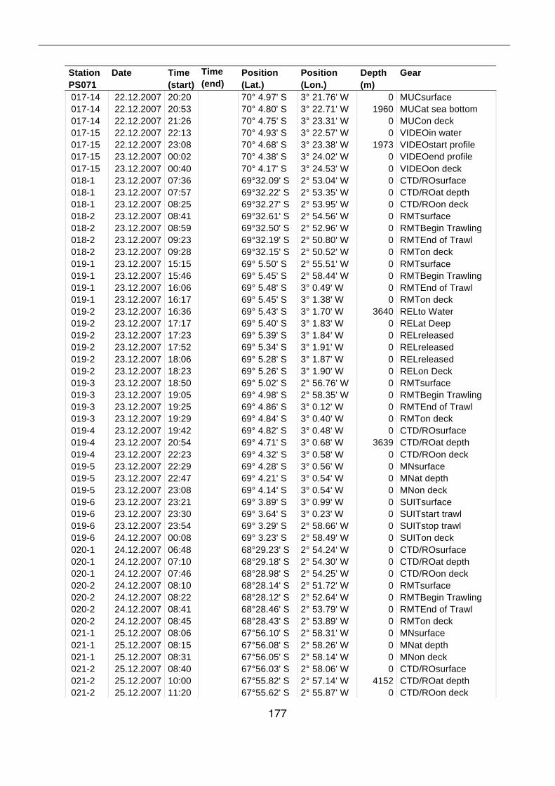
177
Station Date Time Time Position Position Depth Gear
PS071 (start) (end) (Lat.) (Lon.) (m)
017-14 22.12.2007 20:20 70° 4.97' S 3° 21.76' W 0 MUCsurface
017-14 22.12.2007 20:53 70° 4.80' S 3° 22.71' W 1960 MUCat sea bottom
017-14 22.12.2007 21:26 70° 4.75' S 3° 23.31' W 0 MUCon deck
017-15 22.12.2007 22:13 70° 4.93' S 3° 22.57' W 0 VIDEOin water
017-15 22.12.2007 23:08 70° 4.68' S 3° 23.38' W 1973 VIDEOstart profile
017-15 23.12.2007 00:02 70° 4.38' S 3° 24.02' W 0 VIDEOend profile
017-15 23.12.2007 00:40 70° 4.17' S 3° 24.53' W 0 VIDEOon deck
018-1 23.12.2007 07:36 69°32.09' S 2° 53.04' W 0 CTD/ROsurface
018-1 23.12.2007 07:57 69°32.22' S 2° 53.35' W 0 CTD/ROat depth
018-1 23.12.2007 08:25 69°32.27' S 2° 53.95' W 0 CTD/ROon deck
018-2 23.12.2007 08:41 69°32.61' S 2° 54.56' W 0 RMTsurface
018-2 23.12.2007 08:59 69°32.50' S 2° 52.96' W 0 RMTBegin Trawling
018-2 23.12.2007 09:23 69°32.19' S 2° 50.80' W 0 RMTEnd of Trawl
018-2 23.12.2007 09:28 69°32.15' S 2° 50.52' W 0 RMTon deck
019-1 23.12.2007 15:15 69° 5.50' S 2° 55.51' W 0 RMTsurface
019-1 23.12.2007 15:46 69° 5.45' S 2° 58.44' W 0 RMTBegin Trawling
019-1 23.12.2007 16:06 69° 5.48' S 3° 0.49' W 0 RMTEnd of Trawl
019-1 23.12.2007 16:17 69° 5.45' S 3° 1.38' W 0 RMTon deck
019-2 23.12.2007 16:36 69° 5.43' S 3° 1.70' W 3640 RELto Water
019-2 23.12.2007 17:17 69° 5.40' S 3° 1.83' W 0 RELat Deep
019-2 23.12.2007 17:23 69° 5.39' S 3° 1.84' W 0 RELreleased
019-2 23.12.2007 17:52 69° 5.34' S 3° 1.91' W 0 RELreleased
019-2 23.12.2007 18:06 69° 5.28' S 3° 1.87' W 0 RELreleased
019-2 23.12.2007 18:23 69° 5.26' S 3° 1.90' W 0 RELon Deck
019-3 23.12.2007 18:50 69° 5.02' S 2° 56.76' W 0 RMTsurface
019-3 23.12.2007 19:05 69° 4.98' S 2° 58.35' W 0 RMTBegin Trawling
019-3 23.12.2007 19:25 69° 4.86' S 3° 0.12' W 0 RMTEnd of Trawl
019-3 23.12.2007 19:29 69° 4.84' S 3° 0.40' W 0 RMTon deck
019-4 23.12.2007 19:42 69° 4.82' S 3° 0.48' W 0 CTD/ROsurface
019-4 23.12.2007 20:54 69° 4.71' S 3° 0.68' W 3639 CTD/ROat depth
019-4 23.12.2007 22:23 69° 4.32' S 3° 0.58' W 0 CTD/ROon deck
019-5 23.12.2007 22:29 69° 4.28' S 3° 0.56' W 0 MNsurface
019-5 23.12.2007 22:47 69° 4.21' S 3° 0.54' W 0 MNat depth
019-5 23.12.2007 23:08 69° 4.14' S 3° 0.54' W 0 MNon deck
019-6 23.12.2007 23:21 69° 3.89' S 3° 0.99' W 0 SUITsurface
019-6 23.12.2007 23:30 69° 3.64' S 3° 0.23' W 0 SUITstart trawl
019-6 23.12.2007 23:54 69° 3.29' S 2° 58.66' W 0 SUITstop trawl
019-6 24.12.2007 00:08 69° 3.23' S 2° 58.49' W 0 SUITon deck
020-1 24.12.2007 06:48 68°29.23' S 2° 54.24' W 0 CTD/ROsurface
020-1 24.12.2007 07:10 68°29.18' S 2° 54.30' W 0 CTD/ROat depth
020-1 24.12.2007 07:46 68°28.98' S 2° 54.25' W 0 CTD/ROon deck
020-2 24.12.2007 08:10 68°28.14' S 2° 51.72' W 0 RMTsurface
020-2 24.12.2007 08:22 68°28.12' S 2° 52.64' W 0 RMTBegin Trawling
020-2 24.12.2007 08:41 68°28.46' S 2° 53.79' W 0 RMTEnd of Trawl
020-2 24.12.2007 08:45 68°28.43' S 2° 53.89' W 0 RMTon deck
021-1 25.12.2007 08:06 67°56.10' S 2° 58.31' W 0 MNsurface
021-1 25.12.2007 08:15 67°56.08' S 2° 58.26' W 0 MNat depth
021-1 25.12.2007 08:31 67°56.05' S 2° 58.14' W 0 MNon deck
021-2 25.12.2007 08:40 67°56.03' S 2° 58.06' W 0 CTD/ROsurface
021-2 25.12.2007 10:00 67°55.82' S 2° 57.14' W 4152 CTD/ROat depth
021-2 25.12.2007 11:20 67°55.62' S 2° 55.87' W 0 CTD/ROon deck
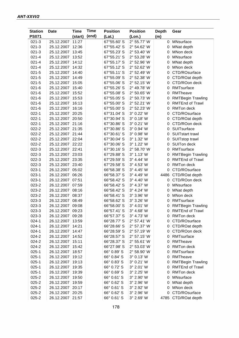
ANT-XXVI/2
178
Station Date Time Time Position Position Depth Gear
PS071 (start) (end) (Lat.) (Lon.) (m)
021-3 25.12.2007 11:27 67°55.60' S 2° 55.77' W 0 MNsurface
021-3 25.12.2007 12:36 67°55.42' S 2° 54.62' W 0 MNat depth
021-3 25.12.2007 13:45 67°55.23' S 2° 53.40' W 0 MNon deck
021-4 25.12.2007 13:52 67°55.21' S 2° 53.28' W 0 MNsurface
021-4 25.12.2007 14:12 67°55.17' S 2° 52.96' W 0 MNat depth
021-4 25.12.2007 14:32 67°55.12' S 2° 52.62' W 0 MNon deck
021-5 25.12.2007 14:40 67°55.11' S 2° 52.49' W 0 CTD/ROsurface
021-5 25.12.2007 14:49 67°55.09' S 2° 52.38' W 0 CTD/ROat depth
021-5 25.12.2007 15:05 67°55.06' S 2° 52.15' W 0 CTD/ROon deck
021-6 25.12.2007 15:40 67°55.26' S 2° 49.78' W 0 RMTsurface
021-6 25.12.2007 15:52 67°55.08' S 2° 50.65' W 0 RMTheave
021-6 25.12.2007 15:53 67°55.05' S 2° 50.73' W 0 RMTBegin Trawling
021-6 25.12.2007 16:13 67°55.00' S 2° 52.21' W 0 RMTEnd of Trawl
021-6 25.12.2007 16:16 67°55.00' S 2° 52.23' W 0 RMTon deck
022-1 25.12.2007 20:25 67°31.04' S 3° 0.22' W 0 CTD/ROsurface
022-1 25.12.2007 20:50 67°30.94' S 3° 0.18' W 0 CTD/ROat depth
022-1 25.12.2007 21:16 67°30.86' S 3° 0.21' W 0 CTD/ROon deck
022-2 25.12.2007 21:35 67°30.86' S 3° 0.94' W 0 SUITsurface
022-2 25.12.2007 21:44 67°30.61' S 3° 0.98' W 0 SUITstart trawl
022-2 25.12.2007 22:04 67°30.04' S 3° 1.32' W 0 SUITstop trawl
022-2 25.12.2007 22:22 67°30.06' S 3° 1.22' W 0 SUITon deck
022-3 25.12.2007 22:41 67°30.16' S 2° 58.70' W 0 RMTsurface
022-3 25.12.2007 23:03 67°29.88' S 3° 1.13' W 0 RMTBegin Trawling
022-3 25.12.2007 23:35 67°29.59' S 3° 4.44' W 0 RMTEnd of Trawl
022-3 25.12.2007 23:40 67°29.58' S 3° 4.53' W 0 RMTon deck
023-1 26.12.2007 05:02 66°58.38' S 3° 4.45' W 0 CTD/ROsurface
023-1 26.12.2007 06:26 66°58.37' S 3° 4.49' W 4486 CTD/ROat depth
023-1 26.12.2007 07:51 66°58.42' S 3° 4.40' W 0 CTD/ROon deck
023-2 26.12.2007 07:59 66°58.42' S 3° 4.37' W 0 MNsurface
023-2 26.12.2007 08:16 66°58.42' S 3° 4.24' W 0 MNat depth
023-2 26.12.2007 08:37 66°58.41' S 3° 3.96' W 0 MNon deck
023-3 26.12.2007 08:49 66°58.62' S 3° 3.26' W 0 RMTsurface
023-3 26.12.2007 09:08 66°58.00' S 3° 4.01' W 0 RMTBegin Trawling
023-3 26.12.2007 09:23 66°57.41' S 3° 4.68' W 0 RMTEnd of Trawl
023-3 26.12.2007 09:28 66°57.37' S 3° 4.73' W 0 RMTon deck
024-1 26.12.2007 13:59 66°28.77' S 2° 57.41' W 0 CTD/ROsurface
024-1 26.12.2007 14:21 66°28.66' S 2° 57.37' W 0 CTD/ROat depth
024-1 26.12.2007 14:47 66°28.59' S 2° 57.19' W 0 CTD/ROon deck
024-2 26.12.2007 14:52 66°28.57' S 2° 57.15' W 0 RMTsurface
024-2 26.12.2007 15:11 66°28.37' S 2° 55.61' W 0 RMTheave
024-2 26.12.2007 15:42 66°27.98' S 2° 53.03' W 0 RMTon deck
025-1 26.12.2007 18:57 66° 0.89' S 2° 58.90' W 0 RMTsurface
025-1 26.12.2007 19:12 66° 0.84' S 3° 0.13' W 0 RMTheave
025-1 26.12.2007 19:13 66° 0.83' S 3° 0.21' W 0 RMTBegin Trawling
025-1 26.12.2007 19:35 66° 0.72' S 3° 2.01' W 0 RMTEnd of Trawl
025-1 26.12.2007 19:39 66° 0.69' S 3° 2.25' W 0 RMTon deck
025-2 26.12.2007 19:50 66° 0.61' S 3° 2.90' W 0 MNsurface
025-2 26.12.2007 19:59 66° 0.62' S 3° 2.96' W 0 MNat depth
025-2 26.12.2007 20:17 66° 0.61' S 3° 2.92' W 0 MNon deck
025-2 26.12.2007 20:25 66° 0.62' S 3° 2.96' W 0 CTD/ROsurface
025-2 26.12.2007 21:57 66° 0.61' S 3° 2.69' W 4785 CTD/ROat depth
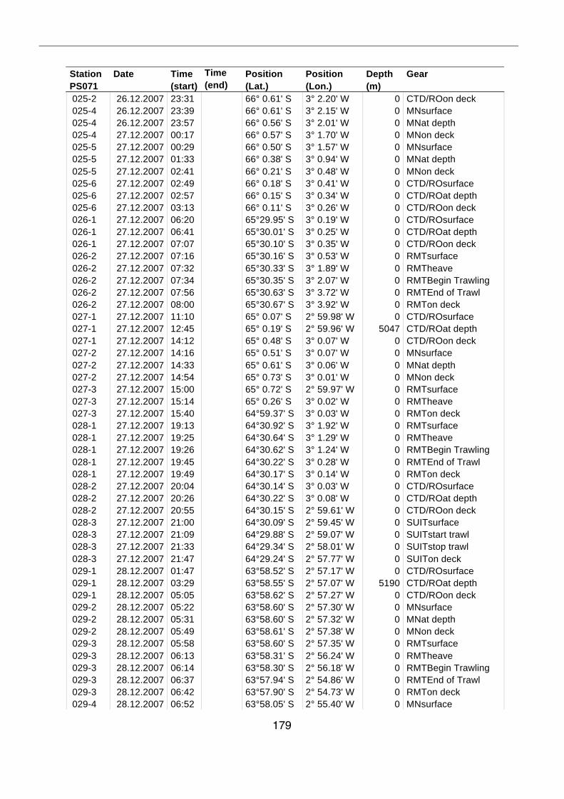
179
Station Date Time Time Position Position Depth Gear
PS071 (start) (end) (Lat.) (Lon.) (m)
025-2 26.12.2007 23:31 66° 0.61' S 3° 2.20' W 0 CTD/ROon deck
025-4 26.12.2007 23:39 66° 0.61' S 3° 2.15' W 0 MNsurface
025-4 26.12.2007 23:57 66° 0.56' S 3° 2.01' W 0 MNat depth
025-4 27.12.2007 00:17 66° 0.57' S 3° 1.70' W 0 MNon deck
025-5 27.12.2007 00:29 66° 0.50' S 3° 1.57' W 0 MNsurface
025-5 27.12.2007 01:33 66° 0.38' S 3° 0.94' W 0 MNat depth
025-5 27.12.2007 02:41 66° 0.21' S 3° 0.48' W 0 MNon deck
025-6 27.12.2007 02:49 66° 0.18' S 3° 0.41' W 0 CTD/ROsurface
025-6 27.12.2007 02:57 66° 0.15' S 3° 0.34' W 0 CTD/ROat depth
025-6 27.12.2007 03:13 66° 0.11' S 3° 0.26' W 0 CTD/ROon deck
026-1 27.12.2007 06:20 65°29.95' S 3° 0.19' W 0 CTD/ROsurface
026-1 27.12.2007 06:41 65°30.01' S 3° 0.25' W 0 CTD/ROat depth
026-1 27.12.2007 07:07 65°30.10' S 3° 0.35' W 0 CTD/ROon deck
026-2 27.12.2007 07:16 65°30.16' S 3° 0.53' W 0 RMTsurface
026-2 27.12.2007 07:32 65°30.33' S 3° 1.89' W 0 RMTheave
026-2 27.12.2007 07:34 65°30.35' S 3° 2.07' W 0 RMTBegin Trawling
026-2 27.12.2007 07:56 65°30.63' S 3° 3.72' W 0 RMTEnd of Trawl
026-2 27.12.2007 08:00 65°30.67' S 3° 3.92' W 0 RMTon deck
027-1 27.12.2007 11:10 65° 0.07' S 2° 59.98' W 0 CTD/ROsurface
027-1 27.12.2007 12:45 65° 0.19' S 2° 59.96' W 5047 CTD/ROat depth
027-1 27.12.2007 14:12 65° 0.48' S 3° 0.07' W 0 CTD/ROon deck
027-2 27.12.2007 14:16 65° 0.51' S 3° 0.07' W 0 MNsurface
027-2 27.12.2007 14:33 65° 0.61' S 3° 0.06' W 0 MNat depth
027-2 27.12.2007 14:54 65° 0.73' S 3° 0.01' W 0 MNon deck
027-3 27.12.2007 15:00 65° 0.72' S 2° 59.97' W 0 RMTsurface
027-3 27.12.2007 15:14 65° 0.26' S 3° 0.02' W 0 RMTheave
027-3 27.12.2007 15:40 64°59.37' S 3° 0.03' W 0 RMTon deck
028-1 27.12.2007 19:13 64°30.92' S 3° 1.92' W 0 RMTsurface
028-1 27.12.2007 19:25 64°30.64' S 3° 1.29' W 0 RMTheave
028-1 27.12.2007 19:26 64°30.62' S 3° 1.24' W 0 RMTBegin Trawling
028-1 27.12.2007 19:45 64°30.22' S 3° 0.28' W 0 RMTEnd of Trawl
028-1 27.12.2007 19:49 64°30.17' S 3° 0.14' W 0 RMTon deck
028-2 27.12.2007 20:04 64°30.14' S 3° 0.03' W 0 CTD/ROsurface
028-2 27.12.2007 20:26 64°30.22' S 3° 0.08' W 0 CTD/ROat depth
028-2 27.12.2007 20:55 64°30.15' S 2° 59.61' W 0 CTD/ROon deck
028-3 27.12.2007 21:00 64°30.09' S 2° 59.45' W 0 SUITsurface
028-3 27.12.2007 21:09 64°29.88' S 2° 59.07' W 0 SUITstart trawl
028-3 27.12.2007 21:33 64°29.34' S 2° 58.01' W 0 SUITstop trawl
028-3 27.12.2007 21:47 64°29.24' S 2° 57.77' W 0 SUITon deck
029-1 28.12.2007 01:47 63°58.52' S 2° 57.17' W 0 CTD/ROsurface
029-1 28.12.2007 03:29 63°58.55' S 2° 57.07' W 5190 CTD/ROat depth
029-1 28.12.2007 05:05 63°58.62' S 2° 57.27' W 0 CTD/ROon deck
029-2 28.12.2007 05:22 63°58.60' S 2° 57.30' W 0 MNsurface
029-2 28.12.2007 05:31 63°58.60' S 2° 57.32' W 0 MNat depth
029-2 28.12.2007 05:49 63°58.61' S 2° 57.38' W 0 MNon deck
029-3 28.12.2007 05:58 63°58.60' S 2° 57.35' W 0 RMTsurface
029-3 28.12.2007 06:13 63°58.31' S 2° 56.24' W 0 RMTheave
029-3 28.12.2007 06:14 63°58.30' S 2° 56.18' W 0 RMTBegin Trawling
029-3 28.12.2007 06:37 63°57.94' S 2° 54.86' W 0 RMTEnd of Trawl
029-3 28.12.2007 06:42 63°57.90' S 2° 54.73' W 0 RMTon deck
029-4 28.12.2007 06:52 63°58.05' S 2° 55.40' W 0 MNsurface
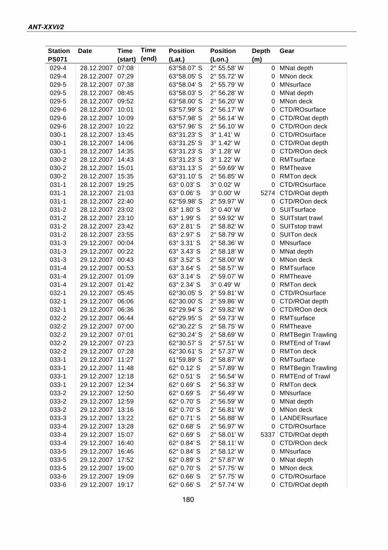
ANT-XXVI/2
180
Station Date Time Time Position Position Depth Gear
PS071 (start) (end) (Lat.) (Lon.) (m)
029-4 28.12.2007 07:08 63°58.07' S 2° 55.58' W 0 MNat depth
029-4 28.12.2007 07:29 63°58.05' S 2° 55.72' W 0 MNon deck
029-5 28.12.2007 07:38 63°58.04' S 2° 55.79' W 0 MNsurface
029-5 28.12.2007 08:45 63°58.03' S 2° 56.28' W 0 MNat depth
029-5 28.12.2007 09:52 63°58.00' S 2° 56.20' W 0 MNon deck
029-6 28.12.2007 10:01 63°57.99' S 2° 56.17' W 0 CTD/ROsurface
029-6 28.12.2007 10:09 63°57.98' S 2° 56.14' W 0 CTD/ROat depth
029-6 28.12.2007 10:22 63°57.96' S 2° 56.10' W 0 CTD/ROon deck
030-1 28.12.2007 13:45 63°31.23' S 3° 1.41' W 0 CTD/ROsurface
030-1 28.12.2007 14:06 63°31.25' S 3° 1.42' W 0 CTD/ROat depth
030-1 28.12.2007 14:35 63°31.23' S 3° 1.28' W 0 CTD/ROon deck
030-2 28.12.2007 14:43 63°31.23' S 3° 1.22' W 0 RMTsurface
030-2 28.12.2007 15:01 63°31.13' S 2° 59.69' W 0 RMTheave
030-2 28.12.2007 15:35 63°31.10' S 2° 56.85' W 0 RMTon deck
031-1 28.12.2007 19:25 63° 0.03' S 3° 0.02' W 0 CTD/ROsurface
031-1 28.12.2007 21:03 63° 0.06' S 3° 0.00' W 5274 CTD/ROat depth
031-1 28.12.2007 22:40 62°59.98' S 2° 59.97' W 0 CTD/ROon deck
031-2 28.12.2007 23:02 63° 1.80' S 3° 0.40' W 0 SUITsurface
031-2 28.12.2007 23:10 63° 1.99' S 2° 59.92' W 0 SUITstart trawl
031-2 28.12.2007 23:42 63° 2.81' S 2° 58.82' W 0 SUITstop trawl
031-2 28.12.2007 23:55 63° 2.97' S 2° 58.79' W 0 SUITon deck
031-3 29.12.2007 00:04 63° 3.31' S 2° 58.36' W 0 MNsurface
031-3 29.12.2007 00:22 63° 3.43' S 2° 58.18' W 0 MNat depth
031-3 29.12.2007 00:43 63° 3.52' S 2° 58.00' W 0 MNon deck
031-4 29.12.2007 00:53 63° 3.64' S 2° 58.57' W 0 RMTsurface
031-4 29.12.2007 01:09 63° 3.14' S 2° 59.07' W 0 RMTheave
031-4 29.12.2007 01:42 63° 2.34' S 3° 0.49' W 0 RMTon deck
032-1 29.12.2007 05:45 62°30.05' S 2° 59.81' W 0 CTD/ROsurface
032-1 29.12.2007 06:06 62°30.00' S 2° 59.86' W 0 CTD/ROat depth
032-1 29.12.2007 06:36 62°29.94' S 2° 59.82' W 0 CTD/ROon deck
032-2 29.12.2007 06:44 62°29.95' S 2° 59.73' W 0 RMTsurface
032-2 29.12.2007 07:00 62°30.22' S 2° 58.75' W 0 RMTheave
032-2 29.12.2007 07:01 62°30.24' S 2° 58.69' W 0 RMTBegin Trawling
032-2 29.12.2007 07:23 62°30.57' S 2° 57.51' W 0 RMTEnd of Trawl
032-2 29.12.2007 07:28 62°30.61' S 2° 57.37' W 0 RMTon deck
033-1 29.12.2007 11:27 61°59.89' S 2° 58.87' W 0 RMTsurface
033-1 29.12.2007 11:48 62° 0.12' S 2° 57.89' W 0 RMTBegin Trawling
033-1 29.12.2007 12:18 62° 0.51' S 2° 56.54' W 0 RMTEnd of Trawl
033-1 29.12.2007 12:34 62° 0.69' S 2° 56.33' W 0 RMTon deck
033-2 29.12.2007 12:50 62° 0.69' S 2° 56.49' W 0 MNsurface
033-2 29.12.2007 12:59 62° 0.70' S 2° 56.59' W 0 MNat depth
033-2 29.12.2007 13:16 62° 0.70' S 2° 56.81' W 0 MNon deck
033-3 29.12.2007 13:22 62° 0.71' S 2° 56.88' W 0 LANDERsurface
033-4 29.12.2007 13:28 62° 0.68' S 2° 56.97' W 0 CTD/ROsurface
033-4 29.12.2007 15:07 62° 0.69' S 2° 58.01' W 5337 CTD/ROat depth
033-4 29.12.2007 16:40 62° 0.84' S 2° 58.11' W 0 CTD/ROon deck
033-5 29.12.2007 16:46 62° 0.84' S 2° 58.12' W 0 MNsurface
033-5 29.12.2007 17:52 62° 0.89' S 2° 57.87' W 0 MNat depth
033-5 29.12.2007 19:00 62° 0.70' S 2° 57.75' W 0 MNon deck
033-6 29.12.2007 19:09 62° 0.66' S 2° 57.75' W 0 CTD/ROsurface
033-6 29.12.2007 19:17 62° 0.66' S 2° 57.74' W 0 CTD/ROat depth
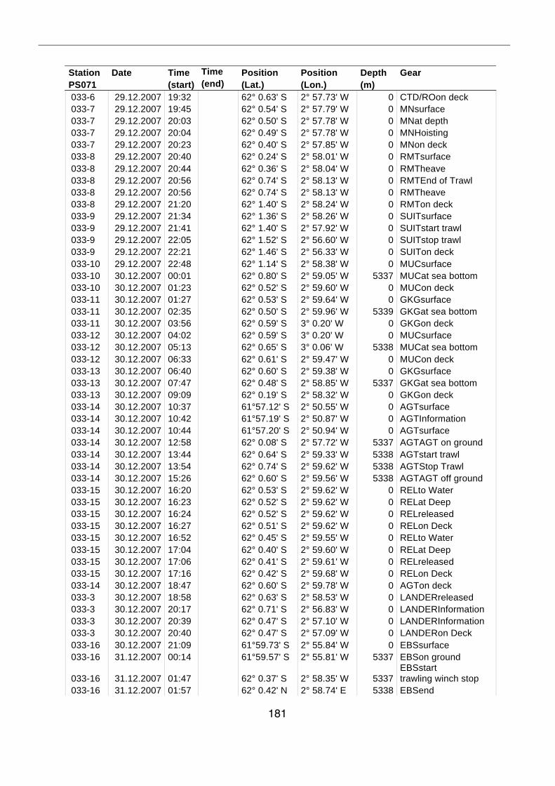
181
Station Date Time Time Position Position Depth Gear
PS071 (start) (end) (Lat.) (Lon.) (m)
033-6 29.12.2007 19:32 62° 0.63' S 2° 57.73' W 0 CTD/ROon deck
033-7 29.12.2007 19:45 62° 0.54' S 2° 57.79' W 0 MNsurface
033-7 29.12.2007 20:03 62° 0.50' S 2° 57.78' W 0 MNat depth
033-7 29.12.2007 20:04 62° 0.49' S 2° 57.78' W 0 MNHoisting
033-7 29.12.2007 20:23 62° 0.40' S 2° 57.85' W 0 MNon deck
033-8 29.12.2007 20:40 62° 0.24' S 2° 58.01' W 0 RMTsurface
033-8 29.12.2007 20:44 62° 0.36' S 2° 58.04' W 0 RMTheave
033-8 29.12.2007 20:56 62° 0.74' S 2° 58.13' W 0 RMTEnd of Trawl
033-8 29.12.2007 20:56 62° 0.74' S 2° 58.13' W 0 RMTheave
033-8 29.12.2007 21:20 62° 1.40' S 2° 58.24' W 0 RMTon deck
033-9 29.12.2007 21:34 62° 1.36' S 2° 58.26' W 0 SUITsurface
033-9 29.12.2007 21:41 62° 1.40' S 2° 57.92' W 0 SUITstart trawl
033-9 29.12.2007 22:05 62° 1.52' S 2° 56.60' W 0 SUITstop trawl
033-9 29.12.2007 22:21 62° 1.46' S 2° 56.33' W 0 SUITon deck
033-10 29.12.2007 22:48 62° 1.14' S 2° 58.38' W 0 MUCsurface
033-10 30.12.2007 00:01 62° 0.80' S 2° 59.05' W 5337 MUCat sea bottom
033-10 30.12.2007 01:23 62° 0.52' S 2° 59.60' W 0 MUCon deck
033-11 30.12.2007 01:27 62° 0.53' S 2° 59.64' W 0 GKGsurface
033-11 30.12.2007 02:35 62° 0.50' S 2° 59.96' W 5339 GKGat sea bottom
033-11 30.12.2007 03:56 62° 0.59' S 3° 0.20' W 0 GKGon deck
033-12 30.12.2007 04:02 62° 0.59' S 3° 0.20' W 0 MUCsurface
033-12 30.12.2007 05:13 62° 0.65' S 3° 0.06' W 5338 MUCat sea bottom
033-12 30.12.2007 06:33 62° 0.61' S 2° 59.47' W 0 MUCon deck
033-13 30.12.2007 06:40 62° 0.60' S 2° 59.38' W 0 GKGsurface
033-13 30.12.2007 07:47 62° 0.48' S 2° 58.85' W 5337 GKGat sea bottom
033-13 30.12.2007 09:09 62° 0.19' S 2° 58.32' W 0 GKGon deck
033-14 30.12.2007 10:37 61°57.12' S 2° 50.55' W 0 AGTsurface
033-14 30.12.2007 10:42 61°57.19' S 2° 50.87' W 0 AGTInformation
033-14 30.12.2007 10:44 61°57.20' S 2° 50.94' W 0 AGTsurface
033-14 30.12.2007 12:58 62° 0.08' S 2° 57.72' W 5337 AGTAGT on ground
033-14 30.12.2007 13:44 62° 0.64' S 2° 59.33' W 5338 AGTstart trawl
033-14 30.12.2007 13:54 62° 0.74' S 2° 59.62' W 5338 AGTStop Trawl
033-14 30.12.2007 15:26 62° 0.60' S 2° 59.56' W 5338 AGTAGT off ground
033-15 30.12.2007 16:20 62° 0.53' S 2° 59.62' W 0 RELto Water
033-15 30.12.2007 16:23 62° 0.52' S 2° 59.62' W 0 RELat Deep
033-15 30.12.2007 16:24 62° 0.52' S 2° 59.62' W 0 RELreleased
033-15 30.12.2007 16:27 62° 0.51' S 2° 59.62' W 0 RELon Deck
033-15 30.12.2007 16:52 62° 0.45' S 2° 59.55' W 0 RELto Water
033-15 30.12.2007 17:04 62° 0.40' S 2° 59.60' W 0 RELat Deep
033-15 30.12.2007 17:06 62° 0.41' S 2° 59.61' W 0 RELreleased
033-15 30.12.2007 17:16 62° 0.42' S 2° 59.68' W 0 RELon Deck
033-14 30.12.2007 18:47 62° 0.60' S 2° 59.78' W 0 AGTon deck
033-3 30.12.2007 18:58 62° 0.63' S 2° 58.53' W 0 LANDERreleased
033-3 30.12.2007 20:17 62° 0.71' S 2° 56.83' W 0 LANDERInformation
033-3 30.12.2007 20:39 62° 0.47' S 2° 57.10' W 0 LANDERInformation
033-3 30.12.2007 20:40 62° 0.47' S 2° 57.09' W 0 LANDERon Deck
033-16 30.12.2007 21:09 61°59.73' S 2° 55.84' W 0 EBSsurface
033-16 31.12.2007 00:14 61°59.57' S 2° 55.81' W 5337 EBSon ground
033-16 31.12.2007 01:47
62° 0.37' S 2° 58.35' W 5337 EBSstart trawling winch stop
033-16 31.12.2007 01:57 62° 0.42' N 2° 58.74' E 5338 EBSend
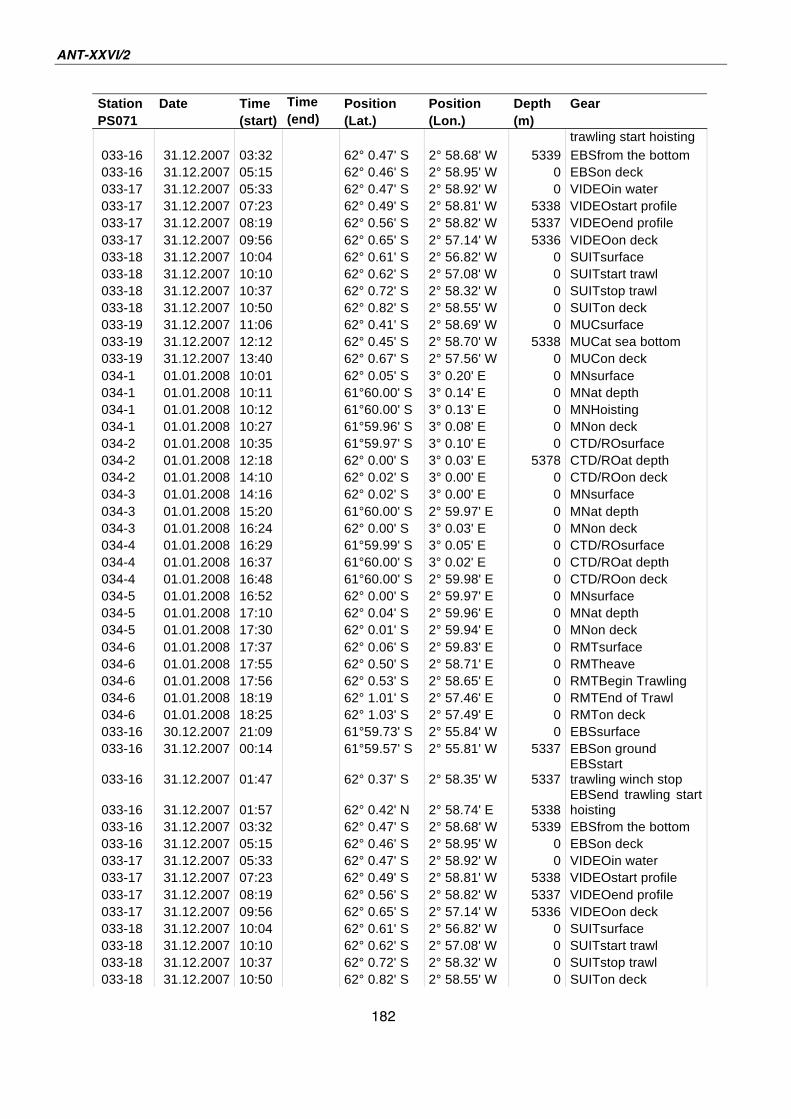
ANT-XXVI/2
182
Station Date Time Time Position Position Depth Gear
PS071 (start) (end) (Lat.) (Lon.) (m)
trawling start hoisting
033-16 31.12.2007 03:32 62° 0.47' S 2° 58.68' W 5339 EBSfrom the bottom
033-16 31.12.2007 05:15 62° 0.46' S 2° 58.95' W 0 EBSon deck
033-17 31.12.2007 05:33 62° 0.47' S 2° 58.92' W 0 VIDEOin water
033-17 31.12.2007 07:23 62° 0.49' S 2° 58.81' W 5338 VIDEOstart profile
033-17 31.12.2007 08:19 62° 0.56' S 2° 58.82' W 5337 VIDEOend profile
033-17 31.12.2007 09:56 62° 0.65' S 2° 57.14' W 5336 VIDEOon deck
033-18 31.12.2007 10:04 62° 0.61' S 2° 56.82' W 0 SUITsurface
033-18 31.12.2007 10:10 62° 0.62' S 2° 57.08' W 0 SUITstart trawl
033-18 31.12.2007 10:37 62° 0.72' S 2° 58.32' W 0 SUITstop trawl
033-18 31.12.2007 10:50 62° 0.82' S 2° 58.55' W 0 SUITon deck
033-19 31.12.2007 11:06 62° 0.41' S 2° 58.69' W 0 MUCsurface
033-19 31.12.2007 12:12 62° 0.45' S 2° 58.70' W 5338 MUCat sea bottom
033-19 31.12.2007 13:40 62° 0.67' S 2° 57.56' W 0 MUCon deck
034-1 01.01.2008 10:01 62° 0.05' S 3° 0.20' E 0 MNsurface
034-1 01.01.2008 10:11 61°60.00' S 3° 0.14' E 0 MNat depth
034-1 01.01.2008 10:12 61°60.00' S 3° 0.13' E 0 MNHoisting
034-1 01.01.2008 10:27 61°59.96' S 3° 0.08' E 0 MNon deck
034-2 01.01.2008 10:35 61°59.97' S 3° 0.10' E 0 CTD/ROsurface
034-2 01.01.2008 12:18 62° 0.00' S 3° 0.03' E 5378 CTD/ROat depth
034-2 01.01.2008 14:10 62° 0.02' S 3° 0.00' E 0 CTD/ROon deck
034-3 01.01.2008 14:16 62° 0.02' S 3° 0.00' E 0 MNsurface
034-3 01.01.2008 15:20 61°60.00' S 2° 59.97' E 0 MNat depth
034-3 01.01.2008 16:24 62° 0.00' S 3° 0.03' E 0 MNon deck
034-4 01.01.2008 16:29 61°59.99' S 3° 0.05' E 0 CTD/ROsurface
034-4 01.01.2008 16:37 61°60.00' S 3° 0.02' E 0 CTD/ROat depth
034-4 01.01.2008 16:48 61°60.00' S 2° 59.98' E 0 CTD/ROon deck
034-5 01.01.2008 16:52 62° 0.00' S 2° 59.97' E 0 MNsurface
034-5 01.01.2008 17:10 62° 0.04' S 2° 59.96' E 0 MNat depth
034-5 01.01.2008 17:30 62° 0.01' S 2° 59.94' E 0 MNon deck
034-6 01.01.2008 17:37 62° 0.06' S 2° 59.83' E 0 RMTsurface
034-6 01.01.2008 17:55 62° 0.50' S 2° 58.71' E 0 RMTheave
034-6 01.01.2008 17:56 62° 0.53' S 2° 58.65' E 0 RMTBegin Trawling
034-6 01.01.2008 18:19 62° 1.01' S 2° 57.46' E 0 RMTEnd of Trawl
034-6 01.01.2008 18:25 62° 1.03' S 2° 57.49' E 0 RMTon deck
033-16 30.12.2007 21:09 61°59.73' S 2° 55.84' W 0 EBSsurface
033-16 31.12.2007 00:14 61°59.57' S 2° 55.81' W 5337 EBSon ground
033-16 31.12.2007 01:47
62° 0.37' S 2° 58.35' W 5337 EBSstart trawling winch stop
033-16 31.12.2007 01:57
62° 0.42' N 2° 58.74' E 5338 EBSend trawling start hoisting
033-16 31.12.2007 03:32 62° 0.47' S 2° 58.68' W 5339 EBSfrom the bottom
033-16 31.12.2007 05:15 62° 0.46' S 2° 58.95' W 0 EBSon deck
033-17 31.12.2007 05:33 62° 0.47' S 2° 58.92' W 0 VIDEOin water
033-17 31.12.2007 07:23 62° 0.49' S 2° 58.81' W 5338 VIDEOstart profile
033-17 31.12.2007 08:19 62° 0.56' S 2° 58.82' W 5337 VIDEOend profile
033-17 31.12.2007 09:56 62° 0.65' S 2° 57.14' W 5336 VIDEOon deck
033-18 31.12.2007 10:04 62° 0.61' S 2° 56.82' W 0 SUITsurface
033-18 31.12.2007 10:10 62° 0.62' S 2° 57.08' W 0 SUITstart trawl
033-18 31.12.2007 10:37 62° 0.72' S 2° 58.32' W 0 SUITstop trawl
033-18 31.12.2007 10:50 62° 0.82' S 2° 58.55' W 0 SUITon deck
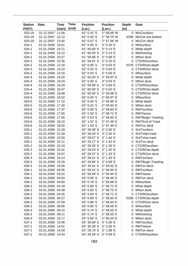
183
Station Date Time Time Position Position Depth Gear
PS071 (start) (end) (Lat.) (Lon.) (m)
033-19 31.12.2007 11:06 62° 0.41' S 2° 58.69' W 0 MUCsurface
033-19 31.12.2007 12:12 62° 0.45' S 2° 58.70' W 5338 MUCat sea bottom
033-19 31.12.2007 13:40 62° 0.67' S 2° 57.56' W 0 MUCon deck
034-1 01.01.2008 10:01 62° 0.05' S 3° 0.20' E 0 MNsurface
034-1 01.01.2008 10:11 61° 60.00' S 3° 0.14' E 0 MNat depth
034-1 01.01.2008 10:12 61° 60.00' S 3° 0.13' E 0 MNHoisting
034-1 01.01.2008 10:27 61° 59.96' S 3° 0.08' E 0 MNon deck
034-2 01.01.2008 10:35 61° 59.97' S 3° 0.10' E 0 CTD/ROsurface
034-2 01.01.2008 12:18 62° 0.00' S 3° 0.03' E 5378 CTD/ROat depth
034-2 01.01.2008 14:10 62° 0.02' S 3° 0.00' E 0 CTD/ROon deck
034-3 01.01.2008 14:16 62° 0.02' S 3° 0.00' E 0 MNsurface
034-3 01.01.2008 15:20 61° 60.00' S 2° 59.97' E 0 MNat depth
034-3 01.01.2008 16:24 62° 0.00' S 3° 0.03' E 0 MNon deck
034-4 01.01.2008 16:29 61° 59.99' S 3° 0.05' E 0 CTD/ROsurface
034-4 01.01.2008 16:37 61° 60.00' S 3° 0.02' E 0 CTD/ROat depth
034-4 01.01.2008 16:48 61° 60.00' S 2° 59.98' E 0 CTD/ROon deck
034-5 01.01.2008 16:52 62° 0.00' S 2° 59.97' E 0 MNsurface
034-5 01.01.2008 17:10 62° 0.04' S 2° 59.96' E 0 MNat depth
034-5 01.01.2008 17:30 62° 0.01' S 2° 59.94' E 0 MNon deck
034-6 01.01.2008 17:37 62° 0.06' S 2° 59.83' E 0 RMTsurface
034-6 01.01.2008 17:55 62° 0.50' S 2° 58.71' E 0 RMTheave
034-6 01.01.2008 17:56 62° 0.53' S 2° 58.65' E 0 RMTBegin Trawling
034-6 01.01.2008 18:19 62° 1.01' S 2° 57.46' E 0 RMTEnd of Trawl
034-6 01.01.2008 18:25 62° 1.03' S 2° 57.49' E 0 RMTon deck
035-1 01.01.2008 21:29 62° 28.28' S 3° 2.56' E 0 SUITsurface
035-1 01.01.2008 21:34 62° 28.44' S 3° 2.32' E 0 SUITstart trawl
035-1 01.01.2008 22:00 62° 29.07' S 3° 1.44' E 0 SUITstop trawl
035-1 01.01.2008 22:11 62° 29.17' S 3° 1.32' E 0 SUITon deck
035-2 01.01.2008 22:19 62° 29.20' S 3° 1.30' E 0 CTD/ROsurface
035-2 01.01.2008 22:41 62° 29.23' S 3° 1.32' E 0 CTD/ROat depth
035-2 01.01.2008 23:07 62° 29.37' S 3° 1.23' E 0 CTD/ROon deck
035-3 01.01.2008 23:14 62° 29.41' S 3° 1.20' E 0 RMTsurface
035-3 01.01.2008 23:29 62° 29.86' S 3° 0.58' E 0 RMTBegin Trawling
035-3 01.01.2008 23:56 62° 30.61' S 2° 59.42' E 0 RMTon deck
036-1 02.01.2008 03:05 62° 59.41' S 2° 59.94' E 0 RMTsurface
036-1 02.01.2008 03:21 62° 59.93' S 2° 59.40' E 0 RMTheave
036-1 02.01.2008 03:53 63° 0.85' S 2° 58.46' E 0 RMTon deck
036-2 02.01.2008 04:00 63° 0.76' S 2° 58.68' E 0 MNsurface
036-2 02.01.2008 04:18 63° 0.80' S 2° 58.71' E 0 MNat depth
036-2 02.01.2008 04:38 63° 0.82' S 2° 58.72' E 0 MNon deck
036-3 02.01.2008 04:45 63° 0.83' S 2° 58.71' E 0 CTD/ROsurface
036-3 02.01.2008 06:27 63° 0.89' S 2° 58.84' E 5358 CTD/ROat depth
036-3 02.01.2008 07:59 63° 0.86' S 2° 58.63' E 0 CTD/ROon deck
036-3 02.01.2008 08:06 63° 0.85' S 2° 58.66' E 0 MNsurface
036-3 02.01.2008 09:10 63° 0.74' S 2° 58.55' E 0 MNat depth
036-3 02.01.2008 09:11 63° 0.74' S 2° 58.55' E 0 MNHoisting
036-3 02.01.2008 10:17 63° 0.66' S 2° 58.34' E 0 MNon deck
037-1 02.01.2008 13:46 63° 30.68' S 3° 4.36' E 0 RMTsurface
037-1 02.01.2008 14:01 63° 30.39' S 3° 3.26' E 0 RMTheave
037-1 02.01.2008 14:28 63° 29.78' S 3° 1.68' E 0 RMTon deck
037-2 02.01.2008 14:44 63° 29.29' S 3° 0.58' E 0 CTD/ROsurface
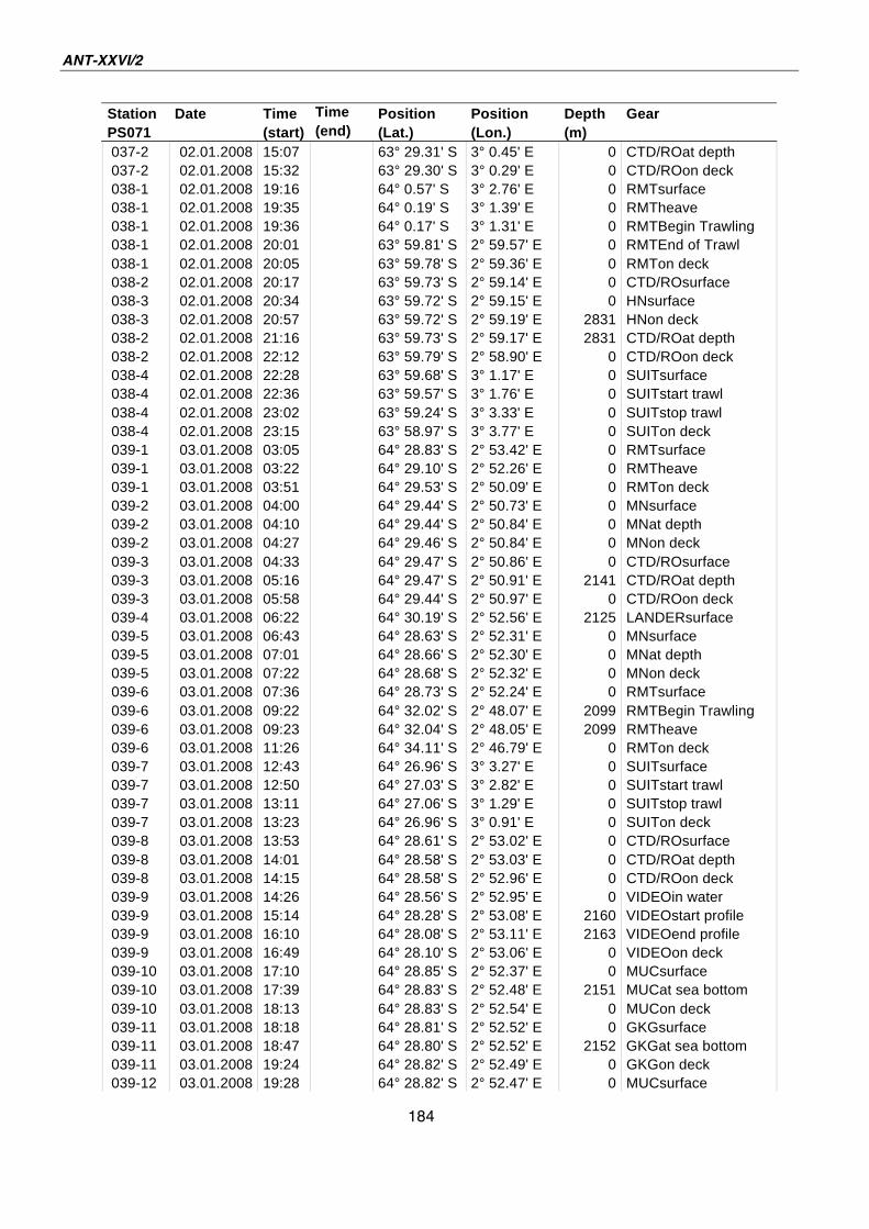
ANT-XXVI/2
184
Station Date Time Time Position Position Depth Gear
PS071 (start) (end) (Lat.) (Lon.) (m)
037-2 02.01.2008 15:07 63° 29.31' S 3° 0.45' E 0 CTD/ROat depth
037-2 02.01.2008 15:32 63° 29.30' S 3° 0.29' E 0 CTD/ROon deck
038-1 02.01.2008 19:16 64° 0.57' S 3° 2.76' E 0 RMTsurface
038-1 02.01.2008 19:35 64° 0.19' S 3° 1.39' E 0 RMTheave
038-1 02.01.2008 19:36 64° 0.17' S 3° 1.31' E 0 RMTBegin Trawling
038-1 02.01.2008 20:01 63° 59.81' S 2° 59.57' E 0 RMTEnd of Trawl
038-1 02.01.2008 20:05 63° 59.78' S 2° 59.36' E 0 RMTon deck
038-2 02.01.2008 20:17 63° 59.73' S 2° 59.14' E 0 CTD/ROsurface
038-3 02.01.2008 20:34 63° 59.72' S 2° 59.15' E 0 HNsurface
038-3 02.01.2008 20:57 63° 59.72' S 2° 59.19' E 2831 HNon deck
038-2 02.01.2008 21:16 63° 59.73' S 2° 59.17' E 2831 CTD/ROat depth
038-2 02.01.2008 22:12 63° 59.79' S 2° 58.90' E 0 CTD/ROon deck
038-4 02.01.2008 22:28 63° 59.68' S 3° 1.17' E 0 SUITsurface
038-4 02.01.2008 22:36 63° 59.57' S 3° 1.76' E 0 SUITstart trawl
038-4 02.01.2008 23:02 63° 59.24' S 3° 3.33' E 0 SUITstop trawl
038-4 02.01.2008 23:15 63° 58.97' S 3° 3.77' E 0 SUITon deck
039-1 03.01.2008 03:05 64° 28.83' S 2° 53.42' E 0 RMTsurface
039-1 03.01.2008 03:22 64° 29.10' S 2° 52.26' E 0 RMTheave
039-1 03.01.2008 03:51 64° 29.53' S 2° 50.09' E 0 RMTon deck
039-2 03.01.2008 04:00 64° 29.44' S 2° 50.73' E 0 MNsurface
039-2 03.01.2008 04:10 64° 29.44' S 2° 50.84' E 0 MNat depth
039-2 03.01.2008 04:27 64° 29.46' S 2° 50.84' E 0 MNon deck
039-3 03.01.2008 04:33 64° 29.47' S 2° 50.86' E 0 CTD/ROsurface
039-3 03.01.2008 05:16 64° 29.47' S 2° 50.91' E 2141 CTD/ROat depth
039-3 03.01.2008 05:58 64° 29.44' S 2° 50.97' E 0 CTD/ROon deck
039-4 03.01.2008 06:22 64° 30.19' S 2° 52.56' E 2125 LANDERsurface
039-5 03.01.2008 06:43 64° 28.63' S 2° 52.31' E 0 MNsurface
039-5 03.01.2008 07:01 64° 28.66' S 2° 52.30' E 0 MNat depth
039-5 03.01.2008 07:22 64° 28.68' S 2° 52.32' E 0 MNon deck
039-6 03.01.2008 07:36 64° 28.73' S 2° 52.24' E 0 RMTsurface
039-6 03.01.2008 09:22 64° 32.02' S 2° 48.07' E 2099 RMTBegin Trawling
039-6 03.01.2008 09:23 64° 32.04' S 2° 48.05' E 2099 RMTheave
039-6 03.01.2008 11:26 64° 34.11' S 2° 46.79' E 0 RMTon deck
039-7 03.01.2008 12:43 64° 26.96' S 3° 3.27' E 0 SUITsurface
039-7 03.01.2008 12:50 64° 27.03' S 3° 2.82' E 0 SUITstart trawl
039-7 03.01.2008 13:11 64° 27.06' S 3° 1.29' E 0 SUITstop trawl
039-7 03.01.2008 13:23 64° 26.96' S 3° 0.91' E 0 SUITon deck
039-8 03.01.2008 13:53 64° 28.61' S 2° 53.02' E 0 CTD/ROsurface
039-8 03.01.2008 14:01 64° 28.58' S 2° 53.03' E 0 CTD/ROat depth
039-8 03.01.2008 14:15 64° 28.58' S 2° 52.96' E 0 CTD/ROon deck
039-9 03.01.2008 14:26 64° 28.56' S 2° 52.95' E 0 VIDEOin water
039-9 03.01.2008 15:14 64° 28.28' S 2° 53.08' E 2160 VIDEOstart profile
039-9 03.01.2008 16:10 64° 28.08' S 2° 53.11' E 2163 VIDEOend profile
039-9 03.01.2008 16:49 64° 28.10' S 2° 53.06' E 0 VIDEOon deck
039-10 03.01.2008 17:10 64° 28.85' S 2° 52.37' E 0 MUCsurface
039-10 03.01.2008 17:39 64° 28.83' S 2° 52.48' E 2151 MUCat sea bottom
039-10 03.01.2008 18:13 64° 28.83' S 2° 52.54' E 0 MUCon deck
039-11 03.01.2008 18:18 64° 28.81' S 2° 52.52' E 0 GKGsurface
039-11 03.01.2008 18:47 64° 28.80' S 2° 52.52' E 2152 GKGat sea bottom
039-11 03.01.2008 19:24 64° 28.82' S 2° 52.49' E 0 GKGon deck
039-12 03.01.2008 19:28 64° 28.82' S 2° 52.47' E 0 MUCsurface
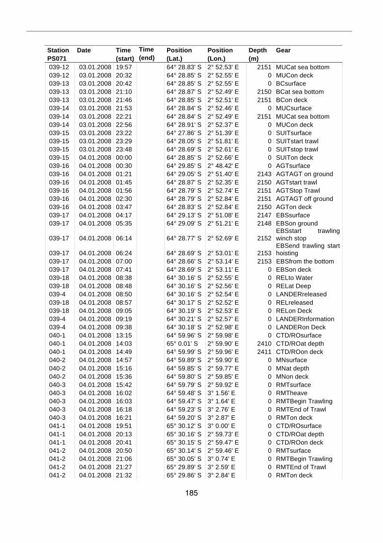
185
Station Date Time Time Position Position Depth Gear
PS071 (start) (end) (Lat.) (Lon.) (m)
039-12 03.01.2008 19:57 64° 28.83' S 2° 52.53' E 2151 MUCat sea bottom
039-12 03.01.2008 20:32 64° 28.85' S 2° 52.55' E 0 MUCon deck
039-13 03.01.2008 20:42 64° 28.85' S 2° 52.55' E 0 BCsurface
039-13 03.01.2008 21:10 64° 28.87' S 2° 52.49' E 2150 BCat sea bottom
039-13 03.01.2008 21:46 64° 28.85' S 2° 52.51' E 2151 BCon deck
039-14 03.01.2008 21:53 64° 28.84' S 2° 52.46' E 0 MUCsurface
039-14 03.01.2008 22:21 64° 28.84' S 2° 52.49' E 2151 MUCat sea bottom
039-14 03.01.2008 22:56 64° 28.91' S 2° 52.37' E 0 MUCon deck
039-15 03.01.2008 23:22 64° 27.86' S 2° 51.39' E 0 SUITsurface
039-15 03.01.2008 23:29 64° 28.05' S 2° 51.81' E 0 SUITstart trawl
039-15 03.01.2008 23:48 64° 28.69' S 2° 52.61' E 0 SUITstop trawl
039-15 04.01.2008 00:00 64° 28.85' S 2° 52.66' E 0 SUITon deck
039-16 04.01.2008 00:30 64° 29.85' S 2° 48.42' E 0 AGTsurface
039-16 04.01.2008 01:21 64° 29.05' S 2° 51.40' E 2143 AGTAGT on ground
039-16 04.01.2008 01:45 64° 28.87' S 2° 52.35' E 2150 AGTstart trawl
039-16 04.01.2008 01:56 64° 28.79' S 2° 52.74' E 2151 AGTStop Trawl
039-16 04.01.2008 02:30 64° 28.79' S 2° 52.84' E 2151 AGTAGT off ground
039-16 04.01.2008 03:47 64° 28.83' S 2° 52.84' E 2150 AGTon deck
039-17 04.01.2008 04:17 64° 29.13' S 2° 51.08' E 2147 EBSsurface
039-17 04.01.2008 05:35 64° 29.09' S 2° 51.21' E 2148 EBSon ground
039-17 04.01.2008 06:14
64° 28.77' S 2° 52.69' E 2152 EBSstart trawling winch stop
039-17 04.01.2008 06:24
64° 28.69' S 2° 53.01' E 2153 EBSend trawling start hoisting
039-17 04.01.2008 07:00 64° 28.66' S 2° 53.14' E 2153 EBSfrom the bottom
039-17 04.01.2008 07:41 64° 28.69' S 2° 53.11' E 0 EBSon deck
039-18 04.01.2008 08:38 64° 30.16' S 2° 52.55' E 0 RELto Water
039-18 04.01.2008 08:48 64° 30.16' S 2° 52.56' E 0 RELat Deep
039-4 04.01.2008 08:50 64° 30.16' S 2° 52.54' E 0 LANDERreleased
039-18 04.01.2008 08:57 64° 30.17' S 2° 52.52' E 0 RELreleased
039-18 04.01.2008 09:05 64° 30.19' S 2° 52.53' E 0 RELon Deck
039-4 04.01.2008 09:19 64° 30.21' S 2° 52.57' E 0 LANDERInformation
039-4 04.01.2008 09:38 64° 30.18' S 2° 52.98' E 0 LANDERon Deck
040-1 04.01.2008 13:15 64° 59.96' S 2° 59.98' E 0 CTD/ROsurface
040-1 04.01.2008 14:03 65° 0.01' S 2° 59.90' E 2410 CTD/ROat depth
040-1 04.01.2008 14:49 64° 59.99' S 2° 59.96' E 2411 CTD/ROon deck
040-2 04.01.2008 14:57 64° 59.89' S 2° 59.90' E 0 MNsurface
040-2 04.01.2008 15:16 64° 59.85' S 2° 59.77' E 0 MNat depth
040-2 04.01.2008 15:36 64° 59.80' S 2° 59.85' E 0 MNon deck
040-3 04.01.2008 15:42 64° 59.79' S 2° 59.92' E 0 RMTsurface
040-3 04.01.2008 16:02 64° 59.48' S 3° 1.56' E 0 RMTheave
040-3 04.01.2008 16:03 64° 59.47' S 3° 1.64' E 0 RMTBegin Trawling
040-3 04.01.2008 16:18 64° 59.23' S 3° 2.76' E 0 RMTEnd of Trawl
040-3 04.01.2008 16:21 64° 59.20' S 3° 2.87' E 0 RMTon deck
041-1 04.01.2008 19:51 65° 30.12' S 3° 0.00' E 0 CTD/ROsurface
041-1 04.01.2008 20:13 65° 30.16' S 2° 59.73' E 0 CTD/ROat depth
041-1 04.01.2008 20:41 65° 30.15' S 2° 59.47' E 0 CTD/ROon deck
041-2 04.01.2008 20:50 65° 30.14' S 2° 59.46' E 0 RMTsurface
041-2 04.01.2008 21:06 65° 30.05' S 3° 0.74' E 0 RMTBegin Trawling
041-2 04.01.2008 21:27 65° 29.89' S 3° 2.59' E 0 RMTEnd of Trawl
041-2 04.01.2008 21:32 65° 29.86' S 3° 2.84' E 0 RMTon deck
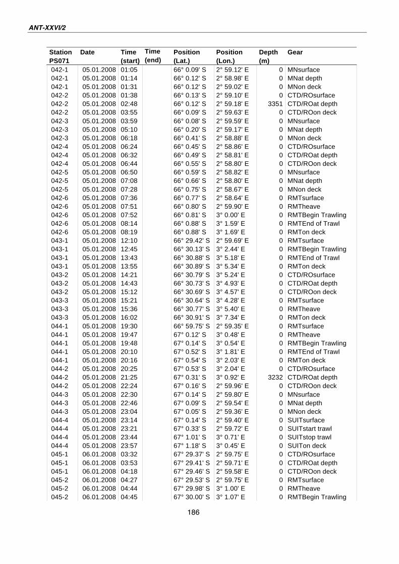
ANT-XXVI/2
186
Station Date Time Time Position Position Depth Gear
PS071 (start) (end) (Lat.) (Lon.) (m)
042-1 05.01.2008 01:05 66° 0.09' S 2° 59.12' E 0 MNsurface
042-1 05.01.2008 01:14 66° 0.12' S 2° 58.98' E 0 MNat depth
042-1 05.01.2008 01:31 66° 0.12' S 2° 59.02' E 0 MNon deck
042-2 05.01.2008 01:38 66° 0.13' S 2° 59.10' E 0 CTD/ROsurface
042-2 05.01.2008 02:48 66° 0.12' S 2° 59.18' E 3351 CTD/ROat depth
042-2 05.01.2008 03:55 66° 0.09' S 2° 59.63' E 0 CTD/ROon deck
042-3 05.01.2008 03:59 66° 0.08' S 2° 59.59' E 0 MNsurface
042-3 05.01.2008 05:10 66° 0.20' S 2° 59.17' E 0 MNat depth
042-3 05.01.2008 06:18 66° 0.41' S 2° 58.88' E 0 MNon deck
042-4 05.01.2008 06:24 66° 0.45' S 2° 58.86' E 0 CTD/ROsurface
042-4 05.01.2008 06:32 66° 0.49' S 2° 58.81' E 0 CTD/ROat depth
042-4 05.01.2008 06:44 66° 0.55' S 2° 58.80' E 0 CTD/ROon deck
042-5 05.01.2008 06:50 66° 0.59' S 2° 58.82' E 0 MNsurface
042-5 05.01.2008 07:08 66° 0.66' S 2° 58.80' E 0 MNat depth
042-5 05.01.2008 07:28 66° 0.75' S 2° 58.67' E 0 MNon deck
042-6 05.01.2008 07:36 66° 0.77' S 2° 58.64' E 0 RMTsurface
042-6 05.01.2008 07:51 66° 0.80' S 2° 59.90' E 0 RMTheave
042-6 05.01.2008 07:52 66° 0.81' S 3° 0.00' E 0 RMTBegin Trawling
042-6 05.01.2008 08:14 66° 0.88' S 3° 1.59' E 0 RMTEnd of Trawl
042-6 05.01.2008 08:19 66° 0.88' S 3° 1.69' E 0 RMTon deck
043-1 05.01.2008 12:10 66° 29.42' S 2° 59.69' E 0 RMTsurface
043-1 05.01.2008 12:45 66° 30.13' S 3° 2.44' E 0 RMTBegin Trawling
043-1 05.01.2008 13:43 66° 30.88' S 3° 5.18' E 0 RMTEnd of Trawl
043-1 05.01.2008 13:55 66° 30.89' S 3° 5.34' E 0 RMTon deck
043-2 05.01.2008 14:21 66° 30.79' S 3° 5.24' E 0 CTD/ROsurface
043-2 05.01.2008 14:43 66° 30.73' S 3° 4.93' E 0 CTD/ROat depth
043-2 05.01.2008 15:12 66° 30.69' S 3° 4.57' E 0 CTD/ROon deck
043-3 05.01.2008 15:21 66° 30.64' S 3° 4.28' E 0 RMTsurface
043-3 05.01.2008 15:36 66° 30.77' S 3° 5.40' E 0 RMTheave
043-3 05.01.2008 16:02 66° 30.91' S 3° 7.34' E 0 RMTon deck
044-1 05.01.2008 19:30 66° 59.75' S 2° 59.35' E 0 RMTsurface
044-1 05.01.2008 19:47 67° 0.12' S 3° 0.48' E 0 RMTheave
044-1 05.01.2008 19:48 67° 0.14' S 3° 0.54' E 0 RMTBegin Trawling
044-1 05.01.2008 20:10 67° 0.52' S 3° 1.81' E 0 RMTEnd of Trawl
044-1 05.01.2008 20:16 67° 0.54' S 3° 2.03' E 0 RMTon deck
044-2 05.01.2008 20:25 67° 0.53' S 3° 2.04' E 0 CTD/ROsurface
044-2 05.01.2008 21:25 67° 0.31' S 3° 0.92' E 3232 CTD/ROat depth
044-2 05.01.2008 22:24 67° 0.16' S 2° 59.96' E 0 CTD/ROon deck
044-3 05.01.2008 22:30 67° 0.14' S 2° 59.80' E 0 MNsurface
044-3 05.01.2008 22:46 67° 0.09' S 2° 59.54' E 0 MNat depth
044-3 05.01.2008 23:04 67° 0.05' S 2° 59.36' E 0 MNon deck
044-4 05.01.2008 23:14 67° 0.14' S 2° 59.40' E 0 SUITsurface
044-4 05.01.2008 23:21 67° 0.33' S 2° 59.72' E 0 SUITstart trawl
044-4 05.01.2008 23:44 67° 1.01' S 3° 0.71' E 0 SUITstop trawl
044-4 05.01.2008 23:57 67° 1.18' S 3° 0.45' E 0 SUITon deck
045-1 06.01.2008 03:32 67° 29.37' S 2° 59.75' E 0 CTD/ROsurface
045-1 06.01.2008 03:53 67° 29.41' S 2° 59.71' E 0 CTD/ROat depth
045-1 06.01.2008 04:18 67° 29.46' S 2° 59.58' E 0 CTD/ROon deck
045-2 06.01.2008 04:27 67° 29.53' S 2° 59.75' E 0 RMTsurface
045-2 06.01.2008 04:44 67° 29.98' S 3° 1.00' E 0 RMTheave
045-2 06.01.2008 04:45 67° 30.00' S 3° 1.07' E 0 RMTBegin Trawling
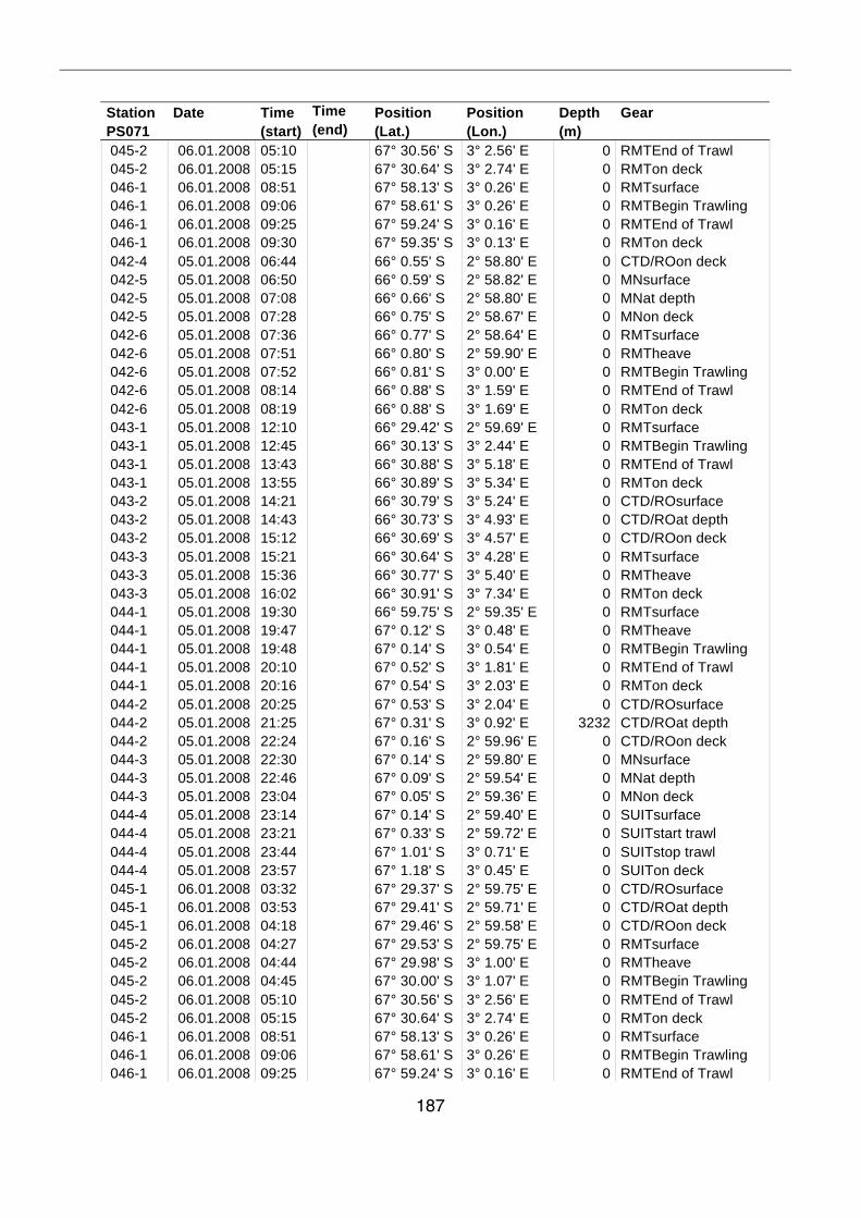
187
Station Date Time Time Position Position Depth Gear
PS071 (start) (end) (Lat.) (Lon.) (m)
045-2 06.01.2008 05:10 67° 30.56' S 3° 2.56' E 0 RMTEnd of Trawl
045-2 06.01.2008 05:15 67° 30.64' S 3° 2.74' E 0 RMTon deck
046-1 06.01.2008 08:51 67° 58.13' S 3° 0.26' E 0 RMTsurface
046-1 06.01.2008 09:06 67° 58.61' S 3° 0.26' E 0 RMTBegin Trawling
046-1 06.01.2008 09:25 67° 59.24' S 3° 0.16' E 0 RMTEnd of Trawl
046-1 06.01.2008 09:30 67° 59.35' S 3° 0.13' E 0 RMTon deck
042-4 05.01.2008 06:44 66° 0.55' S 2° 58.80' E 0 CTD/ROon deck
042-5 05.01.2008 06:50 66° 0.59' S 2° 58.82' E 0 MNsurface
042-5 05.01.2008 07:08 66° 0.66' S 2° 58.80' E 0 MNat depth
042-5 05.01.2008 07:28 66° 0.75' S 2° 58.67' E 0 MNon deck
042-6 05.01.2008 07:36 66° 0.77' S 2° 58.64' E 0 RMTsurface
042-6 05.01.2008 07:51 66° 0.80' S 2° 59.90' E 0 RMTheave
042-6 05.01.2008 07:52 66° 0.81' S 3° 0.00' E 0 RMTBegin Trawling
042-6 05.01.2008 08:14 66° 0.88' S 3° 1.59' E 0 RMTEnd of Trawl
042-6 05.01.2008 08:19 66° 0.88' S 3° 1.69' E 0 RMTon deck
043-1 05.01.2008 12:10 66° 29.42' S 2° 59.69' E 0 RMTsurface
043-1 05.01.2008 12:45 66° 30.13' S 3° 2.44' E 0 RMTBegin Trawling
043-1 05.01.2008 13:43 66° 30.88' S 3° 5.18' E 0 RMTEnd of Trawl
043-1 05.01.2008 13:55 66° 30.89' S 3° 5.34' E 0 RMTon deck
043-2 05.01.2008 14:21 66° 30.79' S 3° 5.24' E 0 CTD/ROsurface
043-2 05.01.2008 14:43 66° 30.73' S 3° 4.93' E 0 CTD/ROat depth
043-2 05.01.2008 15:12 66° 30.69' S 3° 4.57' E 0 CTD/ROon deck
043-3 05.01.2008 15:21 66° 30.64' S 3° 4.28' E 0 RMTsurface
043-3 05.01.2008 15:36 66° 30.77' S 3° 5.40' E 0 RMTheave
043-3 05.01.2008 16:02 66° 30.91' S 3° 7.34' E 0 RMTon deck
044-1 05.01.2008 19:30 66° 59.75' S 2° 59.35' E 0 RMTsurface
044-1 05.01.2008 19:47 67° 0.12' S 3° 0.48' E 0 RMTheave
044-1 05.01.2008 19:48 67° 0.14' S 3° 0.54' E 0 RMTBegin Trawling
044-1 05.01.2008 20:10 67° 0.52' S 3° 1.81' E 0 RMTEnd of Trawl
044-1 05.01.2008 20:16 67° 0.54' S 3° 2.03' E 0 RMTon deck
044-2 05.01.2008 20:25 67° 0.53' S 3° 2.04' E 0 CTD/ROsurface
044-2 05.01.2008 21:25 67° 0.31' S 3° 0.92' E 3232 CTD/ROat depth
044-2 05.01.2008 22:24 67° 0.16' S 2° 59.96' E 0 CTD/ROon deck
044-3 05.01.2008 22:30 67° 0.14' S 2° 59.80' E 0 MNsurface
044-3 05.01.2008 22:46 67° 0.09' S 2° 59.54' E 0 MNat depth
044-3 05.01.2008 23:04 67° 0.05' S 2° 59.36' E 0 MNon deck
044-4 05.01.2008 23:14 67° 0.14' S 2° 59.40' E 0 SUITsurface
044-4 05.01.2008 23:21 67° 0.33' S 2° 59.72' E 0 SUITstart trawl
044-4 05.01.2008 23:44 67° 1.01' S 3° 0.71' E 0 SUITstop trawl
044-4 05.01.2008 23:57 67° 1.18' S 3° 0.45' E 0 SUITon deck
045-1 06.01.2008 03:32 67° 29.37' S 2° 59.75' E 0 CTD/ROsurface
045-1 06.01.2008 03:53 67° 29.41' S 2° 59.71' E 0 CTD/ROat depth
045-1 06.01.2008 04:18 67° 29.46' S 2° 59.58' E 0 CTD/ROon deck
045-2 06.01.2008 04:27 67° 29.53' S 2° 59.75' E 0 RMTsurface
045-2 06.01.2008 04:44 67° 29.98' S 3° 1.00' E 0 RMTheave
045-2 06.01.2008 04:45 67° 30.00' S 3° 1.07' E 0 RMTBegin Trawling
045-2 06.01.2008 05:10 67° 30.56' S 3° 2.56' E 0 RMTEnd of Trawl
045-2 06.01.2008 05:15 67° 30.64' S 3° 2.74' E 0 RMTon deck
046-1 06.01.2008 08:51 67° 58.13' S 3° 0.26' E 0 RMTsurface
046-1 06.01.2008 09:06 67° 58.61' S 3° 0.26' E 0 RMTBegin Trawling
046-1 06.01.2008 09:25 67° 59.24' S 3° 0.16' E 0 RMTEnd of Trawl
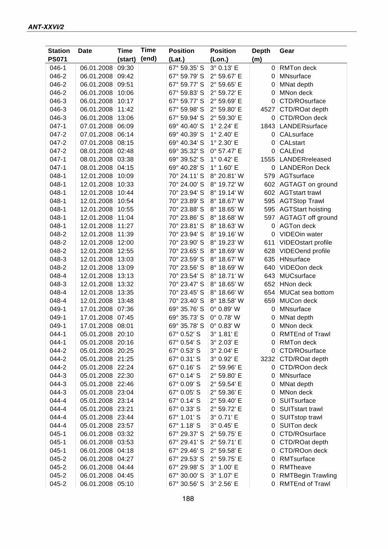
ANT-XXVI/2
188
Station Date Time Time Position Position Depth Gear
PS071 (start) (end) (Lat.) (Lon.) (m)
046-1 06.01.2008 09:30 67° 59.35' S 3° 0.13' E 0 RMTon deck
046-2 06.01.2008 09:42 67° 59.79' S 2° 59.67' E 0 MNsurface
046-2 06.01.2008 09:51 67° 59.77' S 2° 59.65' E 0 MNat depth
046-2 06.01.2008 10:06 67° 59.83' S 2° 59.72' E 0 MNon deck
046-3 06.01.2008 10:17 67° 59.77' S 2° 59.69' E 0 CTD/ROsurface
046-3 06.01.2008 11:42 67° 59.98' S 2° 59.80' E 4527 CTD/ROat depth
046-3 06.01.2008 13:06 67° 59.94' S 2° 59.30' E 0 CTD/ROon deck
047-1 07.01.2008 06:09 69° 40.40' S 1° 2.24' E 1843 LANDERsurface
047-2 07.01.2008 06:14 69° 40.39' S 1° 2.40' E 0 CALsurface
047-2 07.01.2008 08:15 69° 40.34' S 1° 2.30' E 0 CALstart
047-2 08.01.2008 02:48 69° 35.32' S 0° 57.47' E 0 CALEnd
047-1 08.01.2008 03:38 69° 39.52' S 1° 0.42' E 1555 LANDERreleased
047-1 08.01.2008 04:15 69° 40.28' S 1° 1.60' E 0 LANDERon Deck
048-1 12.01.2008 10:09 70° 24.11' S 8° 20.81' W 579 AGTsurface
048-1 12.01.2008 10:33 70° 24.00' S 8° 19.72' W 602 AGTAGT on ground
048-1 12.01.2008 10:44 70° 23.94' S 8° 19.14' W 602 AGTstart trawl
048-1 12.01.2008 10:54 70° 23.89' S 8° 18.67' W 595 AGTStop Trawl
048-1 12.01.2008 10:55 70° 23.88' S 8° 18.65' W 595 AGTStart hoisting
048-1 12.01.2008 11:04 70° 23.86' S 8° 18.68' W 597 AGTAGT off ground
048-1 12.01.2008 11:27 70° 23.81' S 8° 18.63' W 0 AGTon deck
048-2 12.01.2008 11:39 70° 23.94' S 8° 19.16' W 0 VIDEOin water
048-2 12.01.2008 12:00 70° 23.90' S 8° 19.23' W 611 VIDEOstart profile
048-2 12.01.2008 12:55 70° 23.65' S 8° 18.69' W 628 VIDEOend profile
048-3 12.01.2008 13:03 70° 23.59' S 8° 18.67' W 635 HNsurface
048-2 12.01.2008 13:09 70° 23.56' S 8° 18.69' W 640 VIDEOon deck
048-4 12.01.2008 13:13 70° 23.54' S 8° 18.71' W 643 MUCsurface
048-3 12.01.2008 13:32 70° 23.47' S 8° 18.65' W 652 HNon deck
048-4 12.01.2008 13:35 70° 23.45' S 8° 18.66' W 654 MUCat sea bottom
048-4 12.01.2008 13:48 70° 23.40' S 8° 18.58' W 659 MUCon deck
049-1 17.01.2008 07:36 69° 35.76' S 0° 0.89' W 0 MNsurface
049-1 17.01.2008 07:45 69° 35.73' S 0° 0.78' W 0 MNat depth
049-1 17.01.2008 08:01 69° 35.78' S 0° 0.83' W 0 MNon deck
044-1 05.01.2008 20:10 67° 0.52' S 3° 1.81' E 0 RMTEnd of Trawl
044-1 05.01.2008 20:16 67° 0.54' S 3° 2.03' E 0 RMTon deck
044-2 05.01.2008 20:25 67° 0.53' S 3° 2.04' E 0 CTD/ROsurface
044-2 05.01.2008 21:25 67° 0.31' S 3° 0.92' E 3232 CTD/ROat depth
044-2 05.01.2008 22:24 67° 0.16' S 2° 59.96' E 0 CTD/ROon deck
044-3 05.01.2008 22:30 67° 0.14' S 2° 59.80' E 0 MNsurface
044-3 05.01.2008 22:46 67° 0.09' S 2° 59.54' E 0 MNat depth
044-3 05.01.2008 23:04 67° 0.05' S 2° 59.36' E 0 MNon deck
044-4 05.01.2008 23:14 67° 0.14' S 2° 59.40' E 0 SUITsurface
044-4 05.01.2008 23:21 67° 0.33' S 2° 59.72' E 0 SUITstart trawl
044-4 05.01.2008 23:44 67° 1.01' S 3° 0.71' E 0 SUITstop trawl
044-4 05.01.2008 23:57 67° 1.18' S 3° 0.45' E 0 SUITon deck
045-1 06.01.2008 03:32 67° 29.37' S 2° 59.75' E 0 CTD/ROsurface
045-1 06.01.2008 03:53 67° 29.41' S 2° 59.71' E 0 CTD/ROat depth
045-1 06.01.2008 04:18 67° 29.46' S 2° 59.58' E 0 CTD/ROon deck
045-2 06.01.2008 04:27 67° 29.53' S 2° 59.75' E 0 RMTsurface
045-2 06.01.2008 04:44 67° 29.98' S 3° 1.00' E 0 RMTheave
045-2 06.01.2008 04:45 67° 30.00' S 3° 1.07' E 0 RMTBegin Trawling
045-2 06.01.2008 05:10 67° 30.56' S 3° 2.56' E 0 RMTEnd of Trawl
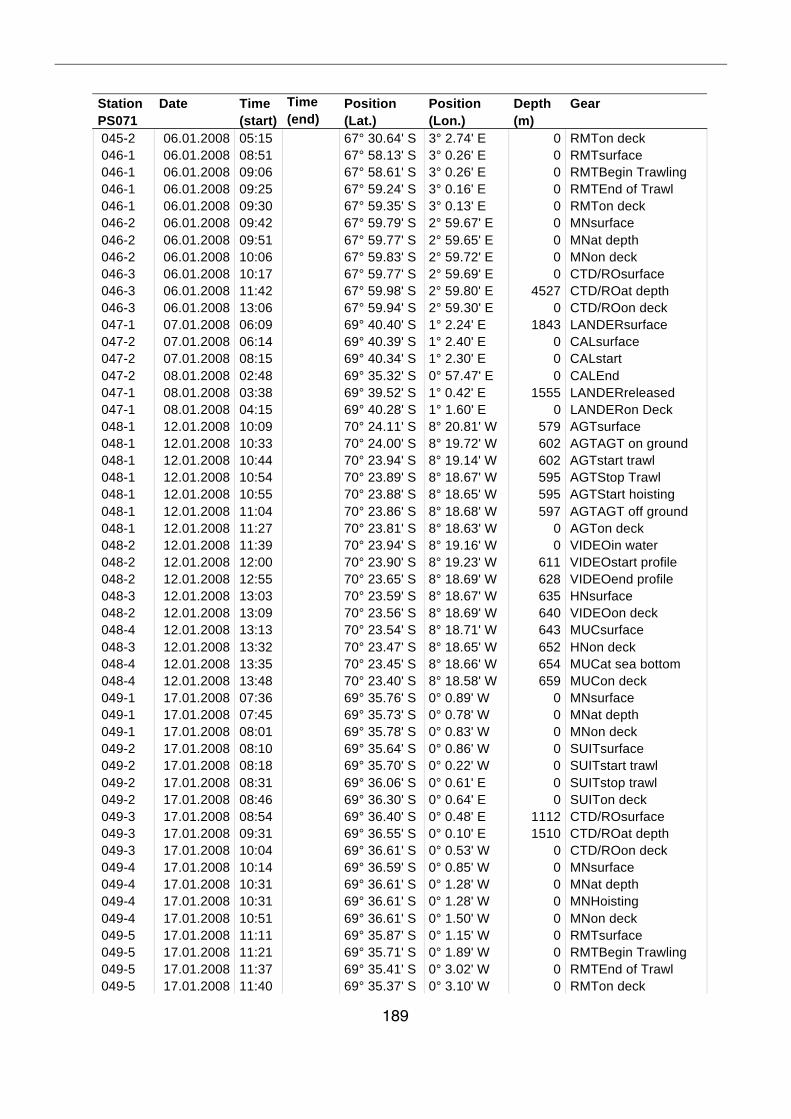
189
Station Date Time Time Position Position Depth Gear
PS071 (start) (end) (Lat.) (Lon.) (m)
045-2 06.01.2008 05:15 67° 30.64' S 3° 2.74' E 0 RMTon deck
046-1 06.01.2008 08:51 67° 58.13' S 3° 0.26' E 0 RMTsurface
046-1 06.01.2008 09:06 67° 58.61' S 3° 0.26' E 0 RMTBegin Trawling
046-1 06.01.2008 09:25 67° 59.24' S 3° 0.16' E 0 RMTEnd of Trawl
046-1 06.01.2008 09:30 67° 59.35' S 3° 0.13' E 0 RMTon deck
046-2 06.01.2008 09:42 67° 59.79' S 2° 59.67' E 0 MNsurface
046-2 06.01.2008 09:51 67° 59.77' S 2° 59.65' E 0 MNat depth
046-2 06.01.2008 10:06 67° 59.83' S 2° 59.72' E 0 MNon deck
046-3 06.01.2008 10:17 67° 59.77' S 2° 59.69' E 0 CTD/ROsurface
046-3 06.01.2008 11:42 67° 59.98' S 2° 59.80' E 4527 CTD/ROat depth
046-3 06.01.2008 13:06 67° 59.94' S 2° 59.30' E 0 CTD/ROon deck
047-1 07.01.2008 06:09 69° 40.40' S 1° 2.24' E 1843 LANDERsurface
047-2 07.01.2008 06:14 69° 40.39' S 1° 2.40' E 0 CALsurface
047-2 07.01.2008 08:15 69° 40.34' S 1° 2.30' E 0 CALstart
047-2 08.01.2008 02:48 69° 35.32' S 0° 57.47' E 0 CALEnd
047-1 08.01.2008 03:38 69° 39.52' S 1° 0.42' E 1555 LANDERreleased
047-1 08.01.2008 04:15 69° 40.28' S 1° 1.60' E 0 LANDERon Deck
048-1 12.01.2008 10:09 70° 24.11' S 8° 20.81' W 579 AGTsurface
048-1 12.01.2008 10:33 70° 24.00' S 8° 19.72' W 602 AGTAGT on ground
048-1 12.01.2008 10:44 70° 23.94' S 8° 19.14' W 602 AGTstart trawl
048-1 12.01.2008 10:54 70° 23.89' S 8° 18.67' W 595 AGTStop Trawl
048-1 12.01.2008 10:55 70° 23.88' S 8° 18.65' W 595 AGTStart hoisting
048-1 12.01.2008 11:04 70° 23.86' S 8° 18.68' W 597 AGTAGT off ground
048-1 12.01.2008 11:27 70° 23.81' S 8° 18.63' W 0 AGTon deck
048-2 12.01.2008 11:39 70° 23.94' S 8° 19.16' W 0 VIDEOin water
048-2 12.01.2008 12:00 70° 23.90' S 8° 19.23' W 611 VIDEOstart profile
048-2 12.01.2008 12:55 70° 23.65' S 8° 18.69' W 628 VIDEOend profile
048-3 12.01.2008 13:03 70° 23.59' S 8° 18.67' W 635 HNsurface
048-2 12.01.2008 13:09 70° 23.56' S 8° 18.69' W 640 VIDEOon deck
048-4 12.01.2008 13:13 70° 23.54' S 8° 18.71' W 643 MUCsurface
048-3 12.01.2008 13:32 70° 23.47' S 8° 18.65' W 652 HNon deck
048-4 12.01.2008 13:35 70° 23.45' S 8° 18.66' W 654 MUCat sea bottom
048-4 12.01.2008 13:48 70° 23.40' S 8° 18.58' W 659 MUCon deck
049-1 17.01.2008 07:36 69° 35.76' S 0° 0.89' W 0 MNsurface
049-1 17.01.2008 07:45 69° 35.73' S 0° 0.78' W 0 MNat depth
049-1 17.01.2008 08:01 69° 35.78' S 0° 0.83' W 0 MNon deck
049-2 17.01.2008 08:10 69° 35.64' S 0° 0.86' W 0 SUITsurface
049-2 17.01.2008 08:18 69° 35.70' S 0° 0.22' W 0 SUITstart trawl
049-2 17.01.2008 08:31 69° 36.06' S 0° 0.61' E 0 SUITstop trawl
049-2 17.01.2008 08:46 69° 36.30' S 0° 0.64' E 0 SUITon deck
049-3 17.01.2008 08:54 69° 36.40' S 0° 0.48' E 1112 CTD/ROsurface
049-3 17.01.2008 09:31 69° 36.55' S 0° 0.10' E 1510 CTD/ROat depth
049-3 17.01.2008 10:04 69° 36.61' S 0° 0.53' W 0 CTD/ROon deck
049-4 17.01.2008 10:14 69° 36.59' S 0° 0.85' W 0 MNsurface
049-4 17.01.2008 10:31 69° 36.61' S 0° 1.28' W 0 MNat depth
049-4 17.01.2008 10:31 69° 36.61' S 0° 1.28' W 0 MNHoisting
049-4 17.01.2008 10:51 69° 36.61' S 0° 1.50' W 0 MNon deck
049-5 17.01.2008 11:11 69° 35.87' S 0° 1.15' W 0 RMTsurface
049-5 17.01.2008 11:21 69° 35.71' S 0° 1.89' W 0 RMTBegin Trawling
049-5 17.01.2008 11:37 69° 35.41' S 0° 3.02' W 0 RMTEnd of Trawl
049-5 17.01.2008 11:40 69° 35.37' S 0° 3.10' W 0 RMTon deck
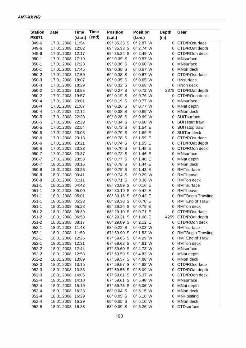
ANT-XXVI/2
190
Station Date Time Time Position Position Depth Gear
PS071 (start) (end) (Lat.) (Lon.) (m)
049-6 17.01.2008 11:54 69° 35.33' S 0° 2.87' W 0 CTD/ROsurface
049-6 17.01.2008 12:02 69° 35.33' S 0° 2.74' W 0 CTD/ROat depth
049-6 17.01.2008 12:17 69° 35.34' S 0° 2.49' W 0 CTD/ROon deck
050-1 17.01.2008 17:19 69° 0.39' S 0° 0.57' W 0 MNsurface
050-1 17.01.2008 17:28 69° 0.36' S 0° 0.60' W 0 MNsurface
050-1 17.01.2008 17:45 69° 0.38' S 0° 0.67' W 0 MNon deck
050-2 17.01.2008 17:50 69° 0.38' S 0° 0.67' W 0 CTD/ROsurface
050-3 17.01.2008 18:07 69° 0.35' S 0° 0.65' W 0 HNsurface
050-3 17.01.2008 18:29 69° 0.32' S 0° 0.68' W 0 HNon deck
050-2 17.01.2008 18:55 69° 0.27' S 0° 0.72' W 3378 CTD/ROat depth
050-2 17.01.2008 19:57 69° 0.19' S 0° 0.76' W 0 CTD/ROon deck
050-4 17.01.2008 20:01 69° 0.19' S 0° 0.77' W 0 MNsurface
050-4 17.01.2008 21:07 69° 0.26' S 0° 0.77' W 0 MNat depth
050-4 17.01.2008 22:12 69° 0.38' S 0° 0.69' W 0 MNon deck
050-5 17.01.2008 22:23 69° 0.28' S 0° 0.99' W 0 SUITsurface
050-5 17.01.2008 22:29 69° 0.34' S 0° 0.60' W 0 SUITstart trawl
050-5 17.01.2008 22:54 69° 0.73' S 0° 1.54' E 0 SUITstop trawl
050-5 17.01.2008 23:08 69° 0.79' S 0° 1.69' E 0 SUITon deck
050-6 17.01.2008 23:13 69° 0.78' S 0° 1.59' E 0 CTD/ROsurface
050-6 17.01.2008 23:21 69° 0.74' S 0° 1.55' E 0 CTD/ROat depth
050-6 17.01.2008 23:33 69° 0.70' S 0° 1.48' E 0 CTD/ROon deck
050-7 17.01.2008 23:37 69° 0.72' S 0° 1.46' E 0 MNsurface
050-7 17.01.2008 23:53 69° 0.77' S 0° 1.40' E 0 MNat depth
050-7 18.01.2008 00:15 69° 0.78' S 0° 1.44' E 0 MNon deck
050-8 18.01.2008 00:25 69° 0.75' S 0° 1.43' E 0 RMTsurface
050-8 18.01.2008 00:41 69° 0.74' S 0° 0.29' W 0 RMTheave
050-8 18.01.2008 01:11 69° 0.71' S 0° 3.38' W 0 RMTon deck
051-1 18.01.2008 04:42 68° 30.89' S 0° 0.16' E 0 RMTsurface
051-1 18.01.2008 05:00 68° 30.19' S 0° 0.42' E 0 RMTheave
051-1 18.01.2008 05:01 68° 30.15' S 0° 0.43' E 0 RMTBegin Trawling
051-1 18.01.2008 05:23 68° 29.38' S 0° 0.70' E 0 RMTEnd of Trawl
051-1 18.01.2008 05:28 68° 29.24' S 0° 0.75' E 0 RMTon deck
051-2 18.01.2008 05:39 68° 29.10' S 0° 0.71' E 0 CTD/ROsurface
051-2 18.01.2008 06:58 68° 29.21' S 0° 1.68' E 4259 CTD/ROat depth
051-2 18.01.2008 08:17 68° 29.09' S 0° 2.12' E 0 CTD/ROon deck
052-1 18.01.2008 11:43 68° 0.22' S 0° 0.03' W 0 RMTsurface
052-1 18.01.2008 11:59 67° 59.90' S 0° 1.53' W 0 RMTBegin Trawling
052-1 18.01.2008 12:26 67° 59.65' S 0° 4.29' W 0 RMTEnd of Trawl
052-1 18.01.2008 12:31 67° 59.62' S 0° 4.61' W 0 RMTon deck
052-2 18.01.2008 12:44 67° 59.60' S 0° 4.73' W 0 MNsurface
052-2 18.01.2008 12:53 67° 59.59' S 0° 4.83' W 0 MNat depth
052-2 18.01.2008 13:09 67° 59.57' S 0° 4.88' W 0 MNon deck
052-3 18.01.2008 13:15 67° 59.57' S 0° 4.88' W 0 CTD/ROsurface
052-3 18.01.2008 13:38 67° 59.55' S 0° 5.09' W 0 CTD/ROat depth
052-3 18.01.2008 14:05 67° 59.61' S 0° 5.37' W 0 CTD/ROon deck
052-4 18.01.2008 14:10 67° 59.61' S 0° 5.48' W 0 MNsurface
052-4 18.01.2008 15:19 67° 59.75' S 0° 6.06' W 0 MNat depth
052-4 18.01.2008 16:28 68° 0.04' S 0° 6.15' W 0 MNon deck
052-4 18.01.2008 16:29 68° 0.05' S 0° 6.16' W 0 MNHoisting
052-4 18.01.2008 16:29 68° 0.05' S 0° 6.16' W 0 MNon deck
052-5 18.01.2008 16:35 68° 0.09' S 0° 6.26' W 0 CTDsurface
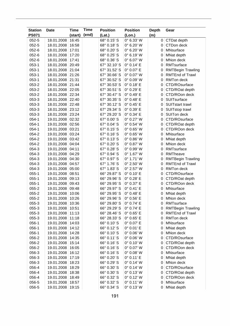
191
Station Date Time Time Position Position Depth Gear
PS071 (start) (end) (Lat.) (Lon.) (m)
052-5 18.01.2008 16:45 68° 0.15' S 0° 6.33' W 0 CTDat depth
052-5 18.01.2008 16:58 68° 0.18' S 0° 6.20' W 0 CTDon deck
052-6 18.01.2008 17:01 68° 0.20' S 0° 6.20' W 0 MNsurface
052-6 18.01.2008 17:20 68° 0.25' S 0° 6.19' W 0 MNat depth
052-6 18.01.2008 17:41 68° 0.36' S 0° 6.07' W 0 MNon deck
053-1 18.01.2008 20:49 67° 32.10' S 0° 0.14' E 0 RMTsurface
053-1 18.01.2008 21:04 67° 31.52' S 0° 0.07' E 0 RMTBegin Trawling
053-1 18.01.2008 21:26 67° 30.66' S 0° 0.07' W 0 RMTEnd of Trawl
053-1 18.01.2008 21:31 67° 30.52' S 0° 0.09' W 0 RMTon deck
053-2 18.01.2008 21:44 67° 30.53' S 0° 0.18' E 0 CTD/ROsurface
053-2 18.01.2008 22:05 67° 30.51' S 0° 0.29' E 0 CTD/ROat depth
053-2 18.01.2008 22:34 67° 30.47' S 0° 0.49' E 0 CTD/ROon deck
053-3 18.01.2008 22:40 67° 30.35' S 0° 0.48' E 0 SUITsurface
053-3 18.01.2008 22:48 67° 30.12' S 0° 0.45' E 0 SUITstart trawl
053-3 18.01.2008 23:12 67° 29.34' S 0° 0.39' E 0 SUITstop trawl
053-3 18.01.2008 23:24 67° 29.20' S 0° 0.34' E 0 SUITon deck
054-1 19.01.2008 02:32 67° 0.00' S 0° 0.27' W 0 CTD/ROsurface
054-1 19.01.2008 02:56 67° 0.04' S 0° 0.54' W 0 CTD/ROat depth
054-1 19.01.2008 03:21 67° 0.15' S 0° 0.65' W 0 CTD/ROon deck
054-2 19.01.2008 03:24 67° 0.16' S 0° 0.65' W 0 MNsurface
054-2 19.01.2008 03:42 67° 0.13' S 0° 0.86' W 0 MNat depth
054-2 19.01.2008 04:04 67° 0.20' S 0° 0.87' W 0 MNon deck
054-3 19.01.2008 04:11 67° 0.28' S 0° 0.99' W 0 RMTsurface
054-3 19.01.2008 04:29 67° 0.94' S 0° 1.67' W 0 RMTheave
054-3 19.01.2008 04:30 67° 0.97' S 0° 1.71' W 0 RMTBegin Trawling
054-3 19.01.2008 04:57 67° 1.76' S 0° 2.50' W 0 RMTEnd of Trawl
054-3 19.01.2008 05:00 67° 1.83' S 0° 2.57' W 0 RMTon deck
055-1 19.01.2008 08:51 66° 29.87' S 0° 0.10' E 0 CTD/ROsurface
055-1 19.01.2008 09:13 66° 29.96' S 0° 0.28' E 0 CTD/ROat depth
055-1 19.01.2008 09:43 66° 29.95' S 0° 0.37' E 0 CTD/ROon deck
055-2 19.01.2008 09:48 66° 29.97' S 0° 0.41' E 0 MNsurface
055-2 19.01.2008 10:06 66° 29.95' S 0° 0.48' E 0 MNat depth
055-2 19.01.2008 10:26 66° 29.96' S 0° 0.56' E 0 MNon deck
055-3 19.01.2008 10:36 66° 29.80' S 0° 0.74' E 0 RMTsurface
055-3 19.01.2008 10:51 66° 29.29' S 0° 0.74' E 0 RMTBegin Trawling
055-3 19.01.2008 11:13 66° 28.46' S 0° 0.65' E 0 RMTEnd of Trawl
055-3 19.01.2008 11:18 66° 28.33' S 0° 0.65' E 0 RMTon deck
056-1 19.01.2008 14:03 66° 0.10' S 0° 0.07' E 0 MNsurface
056-1 19.01.2008 14:12 66° 0.12' S 0° 0.01' E 0 MNat depth
056-1 19.01.2008 14:28 66° 0.10' S 0° 0.06' W 0 MNon deck
056-2 19.01.2008 14:35 66° 0.11' S 0° 0.06' W 0 CTD/ROsurface
056-2 19.01.2008 15:14 66° 0.16' S 0° 0.10' W 0 CTD/ROat depth
056-2 19.01.2008 16:05 66° 0.16' S 0° 0.07' W 0 CTD/ROon deck
056-3 19.01.2008 16:12 66° 0.16' S 0° 0.08' W 0 MNsurface
056-3 19.01.2008 17:19 66° 0.20' S 0° 0.11' E 0 MNat depth
056-3 19.01.2008 18:23 66° 0.29' S 0° 0.14' W 0 MNon deck
056-4 19.01.2008 18:29 66° 0.30' S 0° 0.14' W 0 CTD/ROsurface
056-4 19.01.2008 18:38 66° 0.30' S 0° 0.13' W 0 CTD/ROat depth
056-4 19.01.2008 18:49 66° 0.32' S 0° 0.12' W 0 CTD/ROon deck
056-5 19.01.2008 18:57 66° 0.32' S 0° 0.11' W 0 MNsurface
056-5 19.01.2008 19:15 66° 0.34' S 0° 0.13' W 0 MNat depth
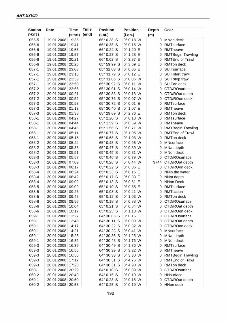
ANT-XXVI/2
192
Station Date Time Time Position Position Depth Gear
PS071 (start) (end) (Lat.) (Lon.) (m)
056-5 19.01.2008 19:35 66° 0.38' S 0° 0.18' W 0 MNon deck
056-6 19.01.2008 19:41 66° 0.38' S 0° 0.15' W 0 RMTsurface
056-6 19.01.2008 19:56 66° 0.24' S 0° 1.20' E 0 RMTheave
056-6 19.01.2008 19:57 66° 0.23' S 0° 1.28' E 0 RMTBegin Trawling
056-6 19.01.2008 20:21 66° 0.02' S 0° 3.37' E 0 RMTEnd of Trawl
056-6 19.01.2008 20:26 65° 59.99' S 0° 3.69' E 0 RMTon deck
057-1 19.01.2008 23:08 65° 32.08' S 0° 0.05' E 0 SUITsurface
057-1 19.01.2008 23:15 65° 31.79' S 0° 0.12' E 0 SUITstart trawl
057-1 19.01.2008 23:39 65° 31.06' S 0° 0.06' W 0 SUITstop trawl
057-1 19.01.2008 23:50 65° 30.92' S 0° 0.11' W 0 SUITon deck
057-2 19.01.2008 23:56 65° 30.91' S 0° 0.14' W 0 CTD/ROsurface
057-2 20.01.2008 00:21 65° 30.83' S 0° 0.13' W 0 CTD/ROat depth
057-2 20.01.2008 00:52 65° 30.76' S 0° 0.07' W 0 CTD/ROon deck
057-3 20.01.2008 00:58 65° 30.72' S 0° 0.01' E 0 RMTsurface
057-3 20.01.2008 01:13 65° 30.40' S 0° 1.07' E 0 RMTheave
057-3 20.01.2008 01:38 65° 29.69' S 0° 2.76' E 0 RMTon deck
058-1 20.01.2008 04:27 65° 2.20' S 0° 0.18' W 0 RMTsurface
058-1 20.01.2008 04:44 65° 1.59' S 0° 0.69' W 0 RMTheave
058-1 20.01.2008 04:45 65° 1.56' S 0° 0.71' W 0 RMTBegin Trawling
058-1 20.01.2008 05:11 65° 0.77' S 0° 1.05' W 0 RMTEnd of Trawl
058-1 20.01.2008 05:15 65° 0.68' S 0° 1.03' W 0 RMTon deck
058-2 20.01.2008 05:24 65° 0.48' S 0° 0.96' W 0 MNsurface
058-2 20.01.2008 05:33 65° 0.47' S 0° 0.89' W 0 MNat depth
058-2 20.01.2008 05:51 65° 0.45' S 0° 0.81' W 0 MNon deck
058-3 20.01.2008 05:57 65° 0.46' S 0° 0.79' W 0 CTD/ROsurface
058-3 20.01.2008 07:09 65° 0.26' S 0° 0.44' W 3744 CTD/ROat depth
058-3 20.01.2008 08:17 65° 0.22' S 0° 0.06' E 0 CTD/ROon deck
058-4 20.01.2008 08:24 65° 0.23' S 0° 0.16' E 0 NNin the water
058-4 20.01.2008 08:42 65° 0.17' S 0° 0.38' E 0 NNat depth
058-4 20.01.2008 09:02 65° 0.13' S 0° 0.61' E 0 NNon Deck
058-5 20.01.2008 09:09 65° 0.10' S 0° 0.55' E 0 RMTsurface
058-5 20.01.2008 09:26 65° 0.08' S 0° 0.41' W 0 RMTaction
058-5 20.01.2008 09:45 65° 0.12' S 0° 1.03' W 0 RMTon deck
058-6 20.01.2008 09:56 65° 0.18' S 0° 0.88' W 0 CTD/ROsurface
058-6 20.01.2008 10:04 65° 0.21' S 0° 0.84' W 0 CTD/ROat depth
058-6 20.01.2008 10:17 65° 0.25' S 0° 1.13' W 0 CTD/ROon deck
059-1 20.01.2008 13:27 64° 30.03' S 0° 0.16' E 0 CTD/ROsurface
059-1 20.01.2008 13:48 64° 30.11' S 0° 0.09' W 0 CTD/ROat depth
059-1 20.01.2008 14:17 64° 30.22' S 0° 0.32' W 0 CTD/ROon deck
059-1 20.01.2008 14:21 64° 30.23' S 0° 0.41' W 0 MNsurface
059-1 20.01.2008 15:25 64° 30.35' S 0° 1.25' W 0 MNat depth
059-1 20.01.2008 16:32 64° 30.48' S 0° 1.76' W 0 MNon deck
059-3 20.01.2008 16:39 64° 30.49' S 0° 1.86' W 0 RMTsurface
059-3 20.01.2008 16:55 64° 30.39' S 0° 3.22' W 0 RMTheave
059-3 20.01.2008 16:56 64° 30.38' S 0° 3.30' W 0 RMTBegin Trawling
059-3 20.01.2008 17:17 64° 30.31' S 0° 4.76' W 0 RMTEnd of Trawl
059-3 20.01.2008 17:20 64° 30.31' S 0° 4.90' W 0 RMTon deck
060-1 20.01.2008 20:29 64° 0.10' S 0° 0.09' W 0 CTD/ROsurface
060-2 20.01.2008 20:40 64° 0.15' S 0° 0.19' W 0 HNsurface
060-1 20.01.2008 20:50 64° 0.23' S 0° 0.15' W 0 CTD/ROat depth
060-2 20.01.2008 20:53 64° 0.25' S 0° 0.19' W 0 HNon deck
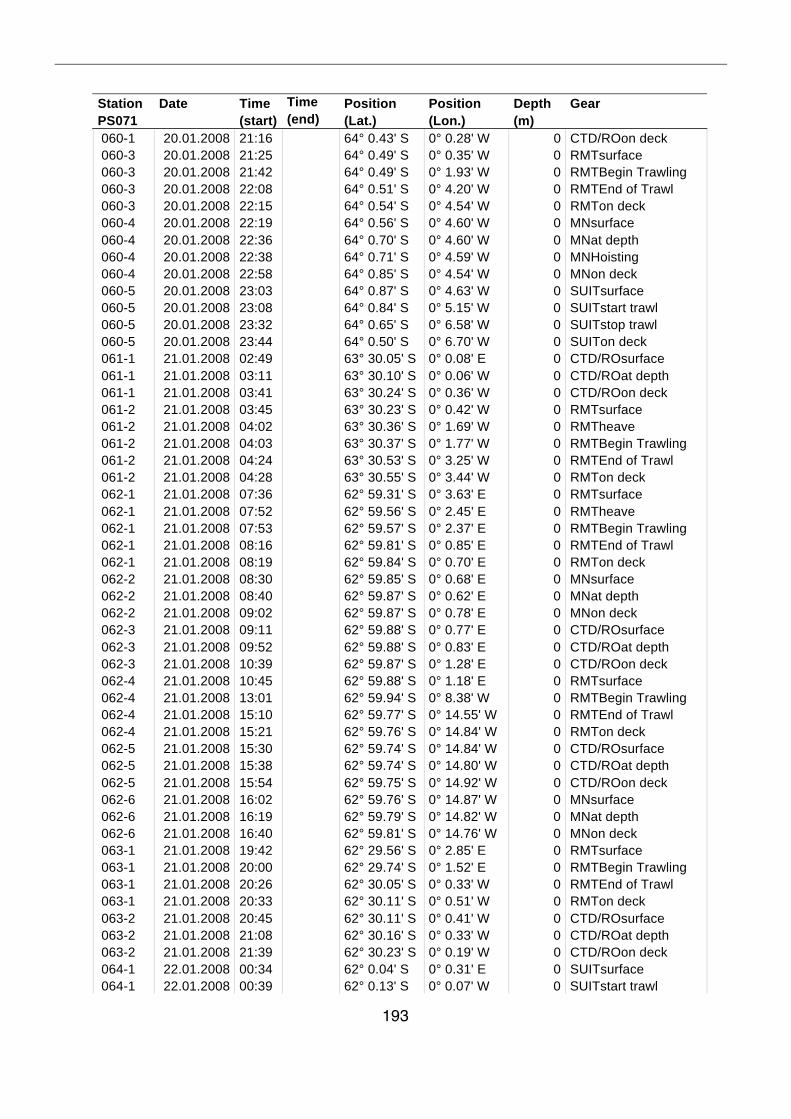
193
Station Date Time Time Position Position Depth Gear
PS071 (start) (end) (Lat.) (Lon.) (m)
060-1 20.01.2008 21:16 64° 0.43' S 0° 0.28' W 0 CTD/ROon deck
060-3 20.01.2008 21:25 64° 0.49' S 0° 0.35' W 0 RMTsurface
060-3 20.01.2008 21:42 64° 0.49' S 0° 1.93' W 0 RMTBegin Trawling
060-3 20.01.2008 22:08 64° 0.51' S 0° 4.20' W 0 RMTEnd of Trawl
060-3 20.01.2008 22:15 64° 0.54' S 0° 4.54' W 0 RMTon deck
060-4 20.01.2008 22:19 64° 0.56' S 0° 4.60' W 0 MNsurface
060-4 20.01.2008 22:36 64° 0.70' S 0° 4.60' W 0 MNat depth
060-4 20.01.2008 22:38 64° 0.71' S 0° 4.59' W 0 MNHoisting
060-4 20.01.2008 22:58 64° 0.85' S 0° 4.54' W 0 MNon deck
060-5 20.01.2008 23:03 64° 0.87' S 0° 4.63' W 0 SUITsurface
060-5 20.01.2008 23:08 64° 0.84' S 0° 5.15' W 0 SUITstart trawl
060-5 20.01.2008 23:32 64° 0.65' S 0° 6.58' W 0 SUITstop trawl
060-5 20.01.2008 23:44 64° 0.50' S 0° 6.70' W 0 SUITon deck
061-1 21.01.2008 02:49 63° 30.05' S 0° 0.08' E 0 CTD/ROsurface
061-1 21.01.2008 03:11 63° 30.10' S 0° 0.06' W 0 CTD/ROat depth
061-1 21.01.2008 03:41 63° 30.24' S 0° 0.36' W 0 CTD/ROon deck
061-2 21.01.2008 03:45 63° 30.23' S 0° 0.42' W 0 RMTsurface
061-2 21.01.2008 04:02 63° 30.36' S 0° 1.69' W 0 RMTheave
061-2 21.01.2008 04:03 63° 30.37' S 0° 1.77' W 0 RMTBegin Trawling
061-2 21.01.2008 04:24 63° 30.53' S 0° 3.25' W 0 RMTEnd of Trawl
061-2 21.01.2008 04:28 63° 30.55' S 0° 3.44' W 0 RMTon deck
062-1 21.01.2008 07:36 62° 59.31' S 0° 3.63' E 0 RMTsurface
062-1 21.01.2008 07:52 62° 59.56' S 0° 2.45' E 0 RMTheave
062-1 21.01.2008 07:53 62° 59.57' S 0° 2.37' E 0 RMTBegin Trawling
062-1 21.01.2008 08:16 62° 59.81' S 0° 0.85' E 0 RMTEnd of Trawl
062-1 21.01.2008 08:19 62° 59.84' S 0° 0.70' E 0 RMTon deck
062-2 21.01.2008 08:30 62° 59.85' S 0° 0.68' E 0 MNsurface
062-2 21.01.2008 08:40 62° 59.87' S 0° 0.62' E 0 MNat depth
062-2 21.01.2008 09:02 62° 59.87' S 0° 0.78' E 0 MNon deck
062-3 21.01.2008 09:11 62° 59.88' S 0° 0.77' E 0 CTD/ROsurface
062-3 21.01.2008 09:52 62° 59.88' S 0° 0.83' E 0 CTD/ROat depth
062-3 21.01.2008 10:39 62° 59.87' S 0° 1.28' E 0 CTD/ROon deck
062-4 21.01.2008 10:45 62° 59.88' S 0° 1.18' E 0 RMTsurface
062-4 21.01.2008 13:01 62° 59.94' S 0° 8.38' W 0 RMTBegin Trawling
062-4 21.01.2008 15:10 62° 59.77' S 0° 14.55' W 0 RMTEnd of Trawl
062-4 21.01.2008 15:21 62° 59.76' S 0° 14.84' W 0 RMTon deck
062-5 21.01.2008 15:30 62° 59.74' S 0° 14.84' W 0 CTD/ROsurface
062-5 21.01.2008 15:38 62° 59.74' S 0° 14.80' W 0 CTD/ROat depth
062-5 21.01.2008 15:54 62° 59.75' S 0° 14.92' W 0 CTD/ROon deck
062-6 21.01.2008 16:02 62° 59.76' S 0° 14.87' W 0 MNsurface
062-6 21.01.2008 16:19 62° 59.79' S 0° 14.82' W 0 MNat depth
062-6 21.01.2008 16:40 62° 59.81' S 0° 14.76' W 0 MNon deck
063-1 21.01.2008 19:42 62° 29.56' S 0° 2.85' E 0 RMTsurface
063-1 21.01.2008 20:00 62° 29.74' S 0° 1.52' E 0 RMTBegin Trawling
063-1 21.01.2008 20:26 62° 30.05' S 0° 0.33' W 0 RMTEnd of Trawl
063-1 21.01.2008 20:33 62° 30.11' S 0° 0.51' W 0 RMTon deck
063-2 21.01.2008 20:45 62° 30.11' S 0° 0.41' W 0 CTD/ROsurface
063-2 21.01.2008 21:08 62° 30.16' S 0° 0.33' W 0 CTD/ROat depth
063-2 21.01.2008 21:39 62° 30.23' S 0° 0.19' W 0 CTD/ROon deck
064-1 22.01.2008 00:34 62° 0.04' S 0° 0.31' E 0 SUITsurface
064-1 22.01.2008 00:39 62° 0.13' S 0° 0.07' W 0 SUITstart trawl
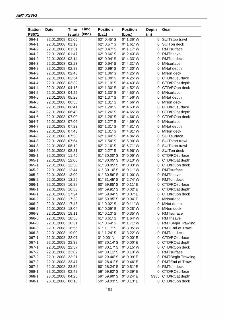
ANT-XXVI/2
194
Station Date Time Time Position Position Depth Gear
PS071 (start) (end) (Lat.) (Lon.) (m)
064-1 22.01.2008 01:05 62° 0.45' S 0° 1.36' W 0 SUITstop trawl
064-1 22.01.2008 01:13 62° 0.57' S 0° 1.61' W 0 SUITon deck
064-2 22.01.2008 01:31 62° 0.47' S 0° 1.17' W 0 RMTsurface
064-2 22.01.2008 01:47 62° 0.66' S 0° 2.43' W 0 RMTheave
064-2 22.01.2008 02:14 62° 0.94' S 0° 4.33' W 0 RMTon deck
064-3 22.01.2008 02:23 62° 0.94' S 0° 4.31' W 0 MNsurface
064-3 22.01.2008 02:33 62° 0.99' S 0° 4.30' W 0 MNat depth
064-3 22.01.2008 02:48 62° 1.06' S 0° 4.25' W 0 MNon deck
064-4 22.01.2008 02:54 62° 1.08' S 0° 4.25' W 0 CTD/ROsurface
064-4 22.01.2008 03:32 62° 1.19' S 0° 4.43' W 0 CTD/ROat depth
064-4 22.01.2008 04:16 62° 1.30' S 0° 4.52' W 0 CTD/ROon deck
064-5 22.01.2008 04:22 62° 1.30' S 0° 4.50' W 0 MNsurface
064-5 22.01.2008 05:28 62° 1.37' S 0° 4.56' W 0 MNat depth
064-5 22.01.2008 06:33 62° 1.31' S 0° 4.66' W 0 MNon deck
064-6 22.01.2008 06:41 62° 1.28' S 0° 4.63' W 0 CTD/ROsurface
064-6 22.01.2008 06:49 62° 1.26' S 0° 4.65' W 0 CTD/ROat depth
064-6 22.01.2008 07:00 62° 1.26' S 0° 4.66' W 0 CTD/ROon deck
064-7 22.01.2008 07:06 62° 1.27' S 0° 4.69' W 0 MNsurface
064-7 22.01.2008 07:23 62° 1.31' S 0° 4.81' W 0 MNat depth
064-7 22.01.2008 07:43 62° 1.31' S 0° 4.81' W 0 MNon deck
064-8 22.01.2008 07:50 62° 1.40' S 0° 4.86' W 0 SUITsurface
064-8 22.01.2008 07:54 62° 1.54' S 0° 5.00' W 0 SUITstart trawl
064-8 22.01.2008 08:19 62° 2.16' S 0° 5.71' W 0 SUITstop trawl
064-8 22.01.2008 08:31 62° 2.27' S 0° 5.96' W 0 SUITon deck
065-1 22.01.2008 11:45 61° 30.00' S 0° 0.06' W 0 CTD/ROsurface
065-1 22.01.2008 12:06 61° 30.05' S 0° 0.13' W 0 CTD/ROat depth
065-1 22.01.2008 12:38 61° 30.05' S 0° 0.03' W 0 CTD/ROon deck
065-2 22.01.2008 12:44 61° 30.10' S 0° 0.11' W 0 RMTsurface
065-2 22.01.2008 13:00 61° 30.56' S 0° 1.00' W 0 RMTheave
065-2 22.01.2008 13:29 61° 31.45' S 0° 2.74' W 0 RMTon deck
066-1 22.01.2008 16:38 60° 59.85' S 0° 0.11' E 0 CTD/ROsurface
066-1 22.01.2008 16:58 60° 59.91' S 0° 0.02' E 0 CTD/ROat depth
066-1 22.01.2008 17:24 60° 59.94' S 0° 0.07' E 0 CTD/ROon deck
066-2 22.01.2008 17:28 60° 59.95' S 0° 0.04' E 0 MNsurface
066-2 22.01.2008 17:46 61° 0.02' S 0° 0.11' W 0 MNat depth
066-2 22.01.2008 18:04 61° 0.09' S 0° 0.28' W 0 MNon deck
066-3 22.01.2008 18:11 61° 0.13' S 0° 0.35' W 0 RMTsurface
066-3 22.01.2008 18:30 61° 0.61' S 0° 1.64' W 0 RMTheave
066-3 22.01.2008 18:31 61° 0.64' S 0° 1.71' W 0 RMTBegin Trawling
066-3 22.01.2008 18:56 61° 1.17' S 0° 3.05' W 0 RMTEnd of Trawl
066-3 22.01.2008 19:00 61° 1.24' S 0° 3.22' W 0 RMTon deck
067-1 22.01.2008 22:07 0° 0.00' N 0° 0.00' E 0 CTD/ROsurface
067-1 22.01.2008 22:32 60° 30.14' S 0° 0.00' E 0 CTD/ROat depth
067-1 22.01.2008 22:57 60° 30.17' S 0° 0.15' W 0 CTD/ROon deck
067-2 22.01.2008 23:02 60° 30.11' S 0° 0.13' W 0 RMTsurface
067-2 22.01.2008 23:21 60° 29.40' S 0° 0.09' E 0 RMTBegin Trawling
067-2 22.01.2008 23:47 60° 28.41' S 0° 0.46' E 0 RMTEnd of Trawl
067-2 22.01.2008 23:52 60° 28.24' S 0° 0.51' E 0 RMTon deck
068-1 23.01.2008 02:42 59° 59.82' S 0° 0.39' E 0 CTD/ROsurface
068-1 23.01.2008 04:26 59° 59.90' S 0° 0.24' E 5355 CTD/ROat depth
068-1 23.01.2008 06:18 59° 59.93' S 0° 0.13' E 0 CTD/ROon deck
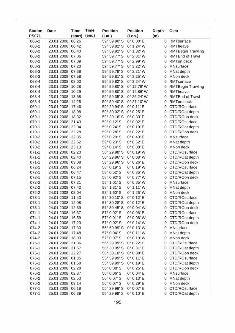
195
Station Date Time Time Position Position Depth Gear
PS071 (start) (end) (Lat.) (Lon.) (m)
068-2 23.01.2008 06:26 59° 59.90' S 0° 0.00' E 0 RMTsurface
068-2 23.01.2008 06:42 59° 59.82' S 0° 1.24' W 0 RMTheave
068-2 23.01.2008 06:43 59° 59.82' S 0° 1.32' W 0 RMTBegin Trawling
068-2 23.01.2008 07:06 59° 59.77' S 0° 2.81' W 0 RMTEnd of Trawl
068-2 23.01.2008 07:09 59° 59.77' S 0° 2.99' W 0 RMTon deck
068-3 23.01.2008 07:20 59° 59.77' S 0° 3.22' W 0 MNsurface
068-3 23.01.2008 07:38 59° 59.78' S 0° 3.21' W 0 MNat depth
068-3 23.01.2008 07:58 59° 59.81' S 0° 3.25' W 0 MNon deck
068-4 23.01.2008 08:03 59° 59.82' S 0° 3.24' W 0 RMTsurface
068-4 23.01.2008 10:28 59° 59.80' S 0° 12.79' W 0 RMTBegin Trawling
068-4 23.01.2008 10:29 59° 59.80' S 0° 12.86' W 0 RMTheave
068-4 23.01.2008 13:58 59° 59.35' S 0° 26.24' W 0 RMTEnd of Trawl
068-4 23.01.2008 14:25 59° 59.40' S 0° 27.10' W 0 RMTon deck
069-1 23.01.2008 17:46 59° 29.94' S 0° 0.11' E 0 CTD/ROsurface
069-1 23.01.2008 18:08 59° 30.02' S 0° 0.25' E 0 CTD/ROat depth
069-1 23.01.2008 18:32 59° 30.16' S 0° 0.33' E 0 CTD/ROon deck
070-1 23.01.2008 21:43 59° 0.12' S 0° 0.02' E 0 CTD/ROsurface
070-1 23.01.2008 22:04 59° 0.24' S 0° 0.10' E 0 CTD/ROat depth
070-1 23.01.2008 22:28 59° 0.28' S 0° 0.22' E 0 CTD/ROon deck
070-2 23.01.2008 22:35 59° 0.20' S 0° 0.43' E 0 MNsurface
070-2 23.01.2008 22:52 59° 0.23' S 0° 0.62' E 0 MNat depth
070-2 23.01.2008 23:13 59° 0.14' S 0° 0.88' E 0 MNon deck
071-1 24.01.2008 02:20 58° 29.98' S 0° 0.19' W 0 CTD/ROsurface
071-1 24.01.2008 02:40 58° 29.96' S 0° 0.08' W 0 CTD/ROat depth
071-1 24.01.2008 03:08 58° 29.96' S 0° 0.26' E 0 CTD/ROon deck
072-1 24.01.2008 06:24 58° 0.19' S 0° 0.19' W 0 CTD/ROsurface
072-1 24.01.2008 06:47 58° 0.52' S 0° 0.36' W 0 CTD/ROat depth
072-1 24.01.2008 07:15 58° 0.92' S 0° 0.77' W 0 CTD/ROon deck
072-2 24.01.2008 07:21 58° 1.01' S 0° 0.85' W 0 MNsurface
072-2 24.01.2008 07:42 58° 1.31' S 0° 1.11' W 0 MNat depth
072-2 24.01.2008 08:04 58° 1.60' S 0° 1.25' W 0 MNon deck
073-1 24.01.2008 11:43 57° 30.10' S 0° 0.12' E 0 CTD/ROsurface
073-1 24.01.2008 12:08 57° 30.28' S 0° 0.12' E 0 CTD/ROat depth
073-1 24.01.2008 12:39 57° 30.45' S 0° 0.04' W 0 CTD/ROon deck
074-1 24.01.2008 16:37 57° 0.02' S 0° 0.06' E 0 CTD/ROsurface
074-1 24.01.2008 16:59 57° 0.01' S 0° 0.08' W 0 CTD/ROat depth
074-1 24.01.2008 17:23 57° 0.02' S 0° 0.14' W 0 CTD/ROon deck
074-2 24.01.2008 17:30 56° 59.99' S 0° 0.13' W 0 MNsurface
074-2 24.01.2008 17:48 57° 0.04' S 0° 0.11' W 0 MNat depth
074-2 24.01.2008 18:09 57° 0.07' S 0° 0.19' W 0 MNon deck
075-1 24.01.2008 21:36 56° 29.99' S 0° 0.22' E 0 CTD/ROsurface
075-1 24.01.2008 21:57 56° 30.05' S 0° 0.31' E 0 CTD/ROat depth
075-1 24.01.2008 22:27 56° 30.10' S 0° 0.38' E 0 CTD/ROon deck
076-1 25.01.2008 01:35 55° 59.99' S 0° 0.11' E 0 CTD/ROsurface
076-1 25.01.2008 01:58 55° 59.99' S 0° 0.19' E 0 CTD/ROat depth
076-1 25.01.2008 02:28 56° 0.08' S 0° 0.25' E 0 CTD/ROon deck
076-2 25.01.2008 02:37 56° 0.06' S 0° 0.04' E 0 MNsurface
076-2 25.01.2008 02:53 56° 0.07' S 0° 0.13' E 0 MNat depth
076-2 25.01.2008 03:14 56° 0.07' S 0° 0.29' E 0 MNon deck
077-1 25.01.2008 06:18 55° 29.99' S 0° 0.07' E 0 CTD/ROsurface
077-1 25.01.2008 06:39 55° 29.98' S 0° 0.10' E 0 CTD/ROat depth
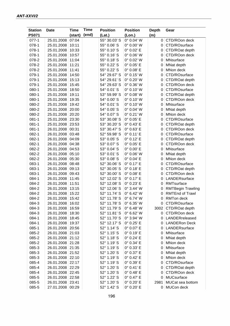
ANT-XXVI/2
196
Station Date Time Time Position Position Depth Gear
PS071 (start) (end) (Lat.) (Lon.) (m)
077-1 25.01.2008 07:04 55° 30.03' S 0° 0.04' W 0 CTD/ROon deck
078-1 25.01.2008 10:11 55° 0.06' S 0° 0.00' W 0 CTD/ROsurface
078-1 25.01.2008 10:33 55° 0.10' S 0° 0.02' E 0 CTD/ROat depth
078-1 25.01.2008 10:57 55° 0.16' S 0° 0.06' W 0 CTD/ROon deck
078-2 25.01.2008 11:04 55° 0.18' S 0° 0.02' W 0 MNsurface
078-2 25.01.2008 11:21 55° 0.22' S 0° 0.05' E 0 MNat depth
078-2 25.01.2008 11:41 55° 0.22' S 0° 0.08' E 0 MNon deck
079-1 25.01.2008 14:50 54° 29.67' S 0° 0.15' W 0 CTD/ROsurface
079-1 25.01.2008 15:13 54° 29.61' S 0° 0.20' W 0 CTD/ROat depth
079-1 25.01.2008 15:45 54° 29.63' S 0° 0.36' W 0 CTD/ROon deck
080-1 25.01.2008 18:50 54° 0.01' S 0° 0.10' W 0 CTD/ROsurface
080-1 25.01.2008 19:11 53° 59.99' S 0° 0.08' W 0 CTD/ROat depth
080-1 25.01.2008 19:35 54° 0.00' S 0° 0.10' W 0 CTD/ROon deck
080-2 25.01.2008 19:42 54° 0.01' S 0° 0.10' W 0 MNsurface
080-2 25.01.2008 20:00 54° 0.05' S 0° 0.04' W 0 MNat depth
080-2 25.01.2008 20:20 54° 0.07' S 0° 0.21' W 0 MNon deck
081-1 25.01.2008 23:30 53° 30.08' S 0° 0.05' E 0 CTD/ROsurface
081-1 25.01.2008 23:53 53° 30.20' S 0° 0.43' E 0 CTD/ROat depth
081-1 26.01.2008 00:31 53° 30.47' S 0° 0.63' E 0 CTD/ROon deck
082-1 26.01.2008 03:48 52° 59.98' S 0° 0.11' E 0 CTD/ROsurface
082-1 26.01.2008 04:09 53° 0.05' S 0° 0.12' E 0 CTD/ROat depth
082-1 26.01.2008 04:38 53° 0.07' S 0° 0.05' E 0 CTD/ROon deck
082-2 26.01.2008 04:53 53° 0.04' S 0° 0.00' E 0 MNsurface
082-2 26.01.2008 05:10 53° 0.01' S 0° 0.06' W 0 MNat depth
082-2 26.01.2008 05:30 53° 0.08' S 0° 0.04' E 0 MNon deck
083-1 26.01.2008 08:48 52° 30.06' S 0° 0.17' E 0 CTD/ROsurface
083-1 26.01.2008 09:13 52° 30.05' S 0° 0.18' E 0 CTD/ROat depth
083-1 26.01.2008 09:43 52° 30.00' S 0° 0.08' E 0 CTD/ROon deck
084-1 26.01.2008 11:45 52° 12.02' S 0° 0.17' E 0 LANDERsurface
084-2 26.01.2008 11:51 52° 12.08' S 0° 0.23' E 0 RMTsurface
084-2 26.01.2008 13:15 52° 12.06' S 0° 3.44' W 0 RMTBegin Trawling
084-2 26.01.2008 15:22 52° 11.74' S 0° 6.42' W 0 RMTEnd of Trawl
084-2 26.01.2008 15:42 52° 11.78' S 0° 6.74' W 0 RMTon deck
084-3 26.01.2008 16:02 52° 11.78' S 0° 6.35' W 0 CTD/ROsurface
084-3 26.01.2008 16:59 52° 11.79' S 0° 6.48' W 3002 CTD/ROat depth
084-3 26.01.2008 18:30 52° 11.81' S 0° 6.62' W 0 CTD/ROon deck
084-1 26.01.2008 18:45 52° 11.70' S 0° 3.94' W 0 LANDERreleased
084-1 26.01.2008 19:37 52° 12.17' S 0° 0.25' E 0 LANDERon Deck
085-1 26.01.2008 20:56 52° 1.14' S 0° 0.07' E 0 LANDERsurface
085-2 26.01.2008 21:03 52° 1.15' S 0° 0.19' E 0 MNsurface
085-2 26.01.2008 21:12 52° 1.18' S 0° 0.24' E 0 MNat depth
085-2 26.01.2008 21:28 52° 1.19' S 0° 0.34' E 0 MNon deck
085-3 26.01.2008 21:35 52° 1.19' S 0° 0.33' E 0 MNsurface
085-3 26.01.2008 21:52 52° 1.20' S 0° 0.37' E 0 MNat depth
085-3 26.01.2008 22:10 52° 1.19' S 0° 0.42' E 0 MNon deck
085-4 26.01.2008 22:17 52° 1.19' S 0° 0.39' E 0 CTD/ROsurface
085-4 26.01.2008 22:29 52° 1.20' S 0° 0.41' E 0 CTD/ROat depth
085-4 26.01.2008 22:45 52° 1.20' S 0° 0.48' E 0 CTD/ROon deck
085-5 26.01.2008 22:58 52° 1.22' S 0° 0.47' E 0 MUCsurface
085-5 26.01.2008 23:41 52° 1.20' S 0° 0.20' E 2981 MUCat sea bottom
085-5 27.01.2008 00:29 52° 1.42' S 0° 0.20' E 0 MUCon deck
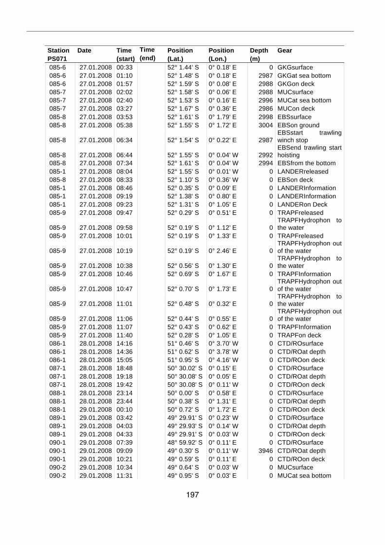
197
Station Date Time Time Position Position Depth Gear
PS071 (start) (end) (Lat.) (Lon.) (m)
085-6 27.01.2008 00:33 52° 1.44' S 0° 0.18' E 0 GKGsurface
085-6 27.01.2008 01:10 52° 1.48' S 0° 0.18' E 2987 GKGat sea bottom
085-6 27.01.2008 01:57 52° 1.59' S 0° 0.08' E 2988 GKGon deck
085-7 27.01.2008 02:02 52° 1.58' S 0° 0.06' E 2988 MUCsurface
085-7 27.01.2008 02:40 52° 1.53' S 0° 0.16' E 2996 MUCat sea bottom
085-7 27.01.2008 03:27 52° 1.67' S 0° 0.36' E 2986 MUCon deck
085-8 27.01.2008 03:53 52° 1.61' S 0° 1.79' E 2998 EBSsurface
085-8 27.01.2008 05:38 52° 1.55' S 0° 1.72' E 3004 EBSon ground
085-8 27.01.2008 06:34
52° 1.54' S 0° 0.22' E 2987 EBSstart trawling winch stop
085-8 27.01.2008 06:44
52° 1.55' S 0° 0.04' W 2992 EBSend trawling start hoisting
085-8 27.01.2008 07:34 52° 1.61' S 0° 0.04' W 2994 EBSfrom the bottom
085-1 27.01.2008 08:04 52° 1.55' S 0° 0.01' W 0 LANDERreleased
085-8 27.01.2008 08:33 52° 1.10' S 0° 0.36' W 0 EBSon deck
085-1 27.01.2008 08:46 52° 0.35' S 0° 0.09' E 0 LANDERInformation
085-1 27.01.2008 09:19 52° 1.38' S 0° 0.80' E 0 LANDERInformation
085-1 27.01.2008 09:23 52° 1.31' S 0° 1.05' E 0 LANDERon Deck
085-9 27.01.2008 09:47 52° 0.29' S 0° 0.51' E 0 TRAPFreleased
085-9 27.01.2008 09:58
52° 0.19' S 0° 1.12' E 0 TRAPFHydrophon to the water
085-9 27.01.2008 10:01 52° 0.19' S 0° 1.33' E 0 TRAPFreleased
085-9 27.01.2008 10:19
52° 0.19' S 0° 2.46' E 0 TRAPFHydrophon out of the water
085-9 27.01.2008 10:38
52° 0.56' S 0° 1.30' E 0 TRAPFHydrophon to the water
085-9 27.01.2008 10:46 52° 0.69' S 0° 1.67' E 0 TRAPFInformation
085-9 27.01.2008 10:47
52° 0.70' S 0° 1.73' E 0 TRAPFHydrophon out of the water
085-9 27.01.2008 11:01
52° 0.48' S 0° 0.32' E 0 TRAPFHydrophon to the water
085-9 27.01.2008 11:06
52° 0.44' S 0° 0.55' E 0 TRAPFHydrophon out of the water
085-9 27.01.2008 11:07 52° 0.43' S 0° 0.62' E 0 TRAPFInformation
085-9 27.01.2008 11:40 52° 0.28' S 0° 1.05' E 0 TRAPFon deck
086-1 28.01.2008 14:16 51° 0.46' S 0° 3.70' W 0 CTD/ROsurface
086-1 28.01.2008 14:36 51° 0.62' S 0° 3.78' W 0 CTD/ROat depth
086-1 28.01.2008 15:05 51° 0.95' S 0° 4.16' W 0 CTD/ROon deck
087-1 28.01.2008 18:48 50° 30.02' S 0° 0.15' E 0 CTD/ROsurface
087-1 28.01.2008 19:18 50° 30.08' S 0° 0.05' E 0 CTD/ROat depth
087-1 28.01.2008 19:42 50° 30.08' S 0° 0.11' W 0 CTD/ROon deck
088-1 28.01.2008 23:14 50° 0.00' S 0° 0.58' E 0 CTD/ROsurface
088-1 28.01.2008 23:44 50° 0.38' S 0° 1.31' E 0 CTD/ROat depth
088-1 29.01.2008 00:10 50° 0.72' S 0° 1.72' E 0 CTD/ROon deck
089-1 29.01.2008 03:42 49° 29.91' S 0° 0.23' W 0 CTD/ROsurface
089-1 29.01.2008 04:03 49° 29.93' S 0° 0.14' W 0 CTD/ROat depth
089-1 29.01.2008 04:33 49° 29.91' S 0° 0.03' W 0 CTD/ROon deck
090-1 29.01.2008 07:39 48° 59.92' S 0° 0.11' E 0 CTD/ROsurface
090-1 29.01.2008 09:09 49° 0.30' S 0° 0.11' W 3946 CTD/ROat depth
090-1 29.01.2008 10:21 49° 0.59' S 0° 0.11' E 0 CTD/ROon deck
090-2 29.01.2008 10:34 49° 0.64' S 0° 0.03' W 0 MUCsurface
090-2 29.01.2008 11:31 49° 0.95' S 0° 0.03' E 0 MUCat sea bottom
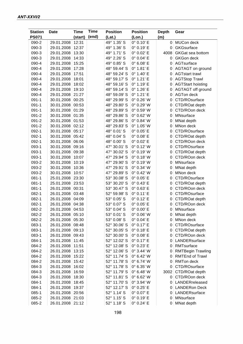
ANT-XXVI/2
198
Station Date Time Time Position Position Depth Gear
PS071 (start) (end) (Lat.) (Lon.) (m)
090-2 29.01.2008 12:31 49° 1.35' S 0° 0.10' E 0 MUCon deck
090-3 29.01.2008 12:37 49° 1.36' S 0° 0.19' E 0 GKGsurface
090-3 29.01.2008 13:30 49° 1.71' S 0° 0.02' E 4008 GKGat sea bottom
090-3 29.01.2008 14:33 49° 2.26' S 0° 0.04' E 0 GKGon deck
090-4 29.01.2008 15:25 49° 0.85' S 0° 6.08' E 0 AGTsurface
090-4 29.01.2008 17:28 48° 59.44' S 0° 1.81' E 0 AGTAGT on ground
090-4 29.01.2008 17:51 48° 59.24' S 0° 1.40' E 0 AGTstart trawl
090-4 29.01.2008 18:01 48° 59.17' S 0° 1.21' E 0 AGTStop Trawl
090-4 29.01.2008 18:02 48° 59.16' S 0° 1.19' E 0 AGTStart hoisting
090-4 29.01.2008 19:10 48° 59.14' S 0° 1.26' E 0 AGTAGT off ground
090-4 29.01.2008 21:27 48° 59.09' S 0° 1.21' E 0 AGTon deck
091-1 30.01.2008 00:25 48° 29.99' S 0° 0.26' W 0 CTD/ROsurface
091-1 30.01.2008 00:53 48° 29.80' S 0° 0.29' W 0 CTD/ROat depth
091-1 30.01.2008 01:29 48° 29.89' S 0° 0.59' W 0 CTD/ROon deck
091-2 30.01.2008 01:35 48° 29.86' S 0° 0.62' W 0 MNsurface
091-2 30.01.2008 01:53 48° 29.86' S 0° 0.84' W 0 MNat depth
091-2 30.01.2008 02:12 48° 29.83' S 0° 1.05' W 0 MNon deck
092-1 30.01.2008 05:17 48° 0.01' S 0° 0.05' E 0 CTD/ROsurface
092-1 30.01.2008 05:42 48° 0.04' S 0° 0.08' E 0 CTD/ROat depth
092-1 30.01.2008 06:06 48° 0.00' S 0° 0.02' E 0 CTD/ROon deck
093-1 30.01.2008 09:16 47° 30.01' S 0° 0.12' W 0 CTD/ROsurface
093-1 30.01.2008 09:38 47° 30.02' S 0° 0.19' W 0 CTD/ROat depth
093-1 30.01.2008 10:07 47° 29.94' S 0° 0.18' W 0 CTD/ROon deck
093-2 30.01.2008 10:19 47° 29.90' S 0° 0.19' W 0 MNsurface
093-2 30.01.2008 10:36 47° 29.91' S 0° 0.34' W 0 MNat depth
093-2 30.01.2008 10:57 47° 29.89' S 0° 0.42' W 0 MNon deck
081-1 25.01.2008 23:30 53° 30.08' S 0° 0.05' E 0 CTD/ROsurface
081-1 25.01.2008 23:53 53° 30.20' S 0° 0.43' E 0 CTD/ROat depth
081-1 26.01.2008 00:31 53° 30.47' S 0° 0.63' E 0 CTD/ROon deck
082-1 26.01.2008 03:48 52° 59.98' S 0° 0.11' E 0 CTD/ROsurface
082-1 26.01.2008 04:09 53° 0.05' S 0° 0.12' E 0 CTD/ROat depth
082-1 26.01.2008 04:38 53° 0.07' S 0° 0.05' E 0 CTD/ROon deck
082-2 26.01.2008 04:53 53° 0.04' S 0° 0.00' E 0 MNsurface
082-2 26.01.2008 05:10 53° 0.01' S 0° 0.06' W 0 MNat depth
082-2 26.01.2008 05:30 53° 0.08' S 0° 0.04' E 0 MNon deck
083-1 26.01.2008 08:48 52° 30.06' S 0° 0.17' E 0 CTD/ROsurface
083-1 26.01.2008 09:13 52° 30.05' S 0° 0.18' E 0 CTD/ROat depth
083-1 26.01.2008 09:43 52° 30.00' S 0° 0.08' E 0 CTD/ROon deck
084-1 26.01.2008 11:45 52° 12.02' S 0° 0.17' E 0 LANDERsurface
084-2 26.01.2008 11:51 52° 12.08' S 0° 0.23' E 0 RMTsurface
084-2 26.01.2008 13:15 52° 12.06' S 0° 3.44' W 0 RMTBegin Trawling
084-2 26.01.2008 15:22 52° 11.74' S 0° 6.42' W 0 RMTEnd of Trawl
084-2 26.01.2008 15:42 52° 11.78' S 0° 6.74' W 0 RMTon deck
084-3 26.01.2008 16:02 52° 11.78' S 0° 6.35' W 0 CTD/ROsurface
084-3 26.01.2008 16:59 52° 11.79' S 0° 6.48' W 3002 CTD/ROat depth
084-3 26.01.2008 18:30 52° 11.81' S 0° 6.62' W 0 CTD/ROon deck
084-1 26.01.2008 18:45 52° 11.70' S 0° 3.94' W 0 LANDERreleased
084-1 26.01.2008 19:37 52° 12.17' S 0° 0.25' E 0 LANDERon Deck
085-1 26.01.2008 20:56 52° 1.14' S 0° 0.07' E 0 LANDERsurface
085-2 26.01.2008 21:03 52° 1.15' S 0° 0.19' E 0 MNsurface
085-2 26.01.2008 21:12 52° 1.18' S 0° 0.24' E 0 MNat depth
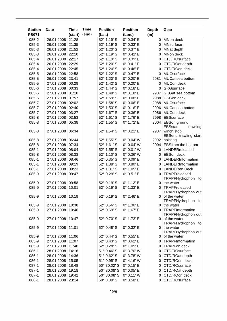
199
Station Date Time Time Position Position Depth Gear
PS071 (start) (end) (Lat.) (Lon.) (m)
085-2 26.01.2008 21:28 52° 1.19' S 0° 0.34' E 0 MNon deck
085-3 26.01.2008 21:35 52° 1.19' S 0° 0.33' E 0 MNsurface
085-3 26.01.2008 21:52 52° 1.20' S 0° 0.37' E 0 MNat depth
085-3 26.01.2008 22:10 52° 1.19' S 0° 0.42' E 0 MNon deck
085-4 26.01.2008 22:17 52° 1.19' S 0° 0.39' E 0 CTD/ROsurface
085-4 26.01.2008 22:29 52° 1.20' S 0° 0.41' E 0 CTD/ROat depth
085-4 26.01.2008 22:45 52° 1.20' S 0° 0.48' E 0 CTD/ROon deck
085-5 26.01.2008 22:58 52° 1.22' S 0° 0.47' E 0 MUCsurface
085-5 26.01.2008 23:41 52° 1.20' S 0° 0.20' E 2981 MUCat sea bottom
085-5 27.01.2008 00:29 52° 1.42' S 0° 0.20' E 0 MUCon deck
085-6 27.01.2008 00:33 52° 1.44' S 0° 0.18' E 0 GKGsurface
085-6 27.01.2008 01:10 52° 1.48' S 0° 0.18' E 2987 GKGat sea bottom
085-6 27.01.2008 01:57 52° 1.59' S 0° 0.08' E 2988 GKGon deck
085-7 27.01.2008 02:02 52° 1.58' S 0° 0.06' E 2988 MUCsurface
085-7 27.01.2008 02:40 52° 1.53' S 0° 0.16' E 2996 MUCat sea bottom
085-7 27.01.2008 03:27 52° 1.67' S 0° 0.36' E 2986 MUCon deck
085-8 27.01.2008 03:53 52° 1.61' S 0° 1.79' E 2998 EBSsurface
085-8 27.01.2008 05:38 52° 1.55' S 0° 1.72' E 3004 EBSon ground
085-8 27.01.2008 06:34
52° 1.54' S 0° 0.22' E 2987 EBSstart trawling winch stop
085-8 27.01.2008 06:44
52° 1.55' S 0° 0.04' W 2992 EBSend trawling start hoisting
085-8 27.01.2008 07:34 52° 1.61' S 0° 0.04' W 2994 EBSfrom the bottom
085-1 27.01.2008 08:04 52° 1.55' S 0° 0.01' W 0 LANDERreleased
085-8 27.01.2008 08:33 52° 1.10' S 0° 0.36' W 0 EBSon deck
085-1 27.01.2008 08:46 52° 0.35' S 0° 0.09' E 0 LANDERInformation
085-1 27.01.2008 09:19 52° 1.38' S 0° 0.80' E 0 LANDERInformation
085-1 27.01.2008 09:23 52° 1.31' S 0° 1.05' E 0 LANDERon Deck
085-9 27.01.2008 09:47 52° 0.29' S 0° 0.51' E 0 TRAPFreleased
085-9 27.01.2008 09:58
52° 0.19' S 0° 1.12' E 0 TRAPFHydrophon to the water
085-9 27.01.2008 10:01 52° 0.19' S 0° 1.33' E 0 TRAPFreleased
085-9 27.01.2008 10:19
52° 0.19' S 0° 2.46' E 0 TRAPFHydrophon out of the water
085-9 27.01.2008 10:38
52° 0.56' S 0° 1.30' E 0 TRAPFHydrophon to the water
085-9 27.01.2008 10:46 52° 0.69' S 0° 1.67' E 0 TRAPFInformation
085-9 27.01.2008 10:47
52° 0.70' S 0° 1.73' E 0 TRAPFHydrophon out of the water
085-9 27.01.2008 11:01
52° 0.48' S 0° 0.32' E 0 TRAPFHydrophon to the water
085-9 27.01.2008 11:06
52° 0.44' S 0° 0.55' E 0 TRAPFHydrophon out of the water
085-9 27.01.2008 11:07 52° 0.43' S 0° 0.62' E 0 TRAPFInformation
085-9 27.01.2008 11:40 52° 0.28' S 0° 1.05' E 0 TRAPFon deck
086-1 28.01.2008 14:16 51° 0.46' S 0° 3.70' W 0 CTD/ROsurface
086-1 28.01.2008 14:36 51° 0.62' S 0° 3.78' W 0 CTD/ROat depth
086-1 28.01.2008 15:05 51° 0.95' S 0° 4.16' W 0 CTD/ROon deck
087-1 28.01.2008 18:48 50° 30.02' S 0° 0.15' E 0 CTD/ROsurface
087-1 28.01.2008 19:18 50° 30.08' S 0° 0.05' E 0 CTD/ROat depth
087-1 28.01.2008 19:42 50° 30.08' S 0° 0.11' W 0 CTD/ROon deck
088-1 28.01.2008 23:14 50° 0.00' S 0° 0.58' E 0 CTD/ROsurface
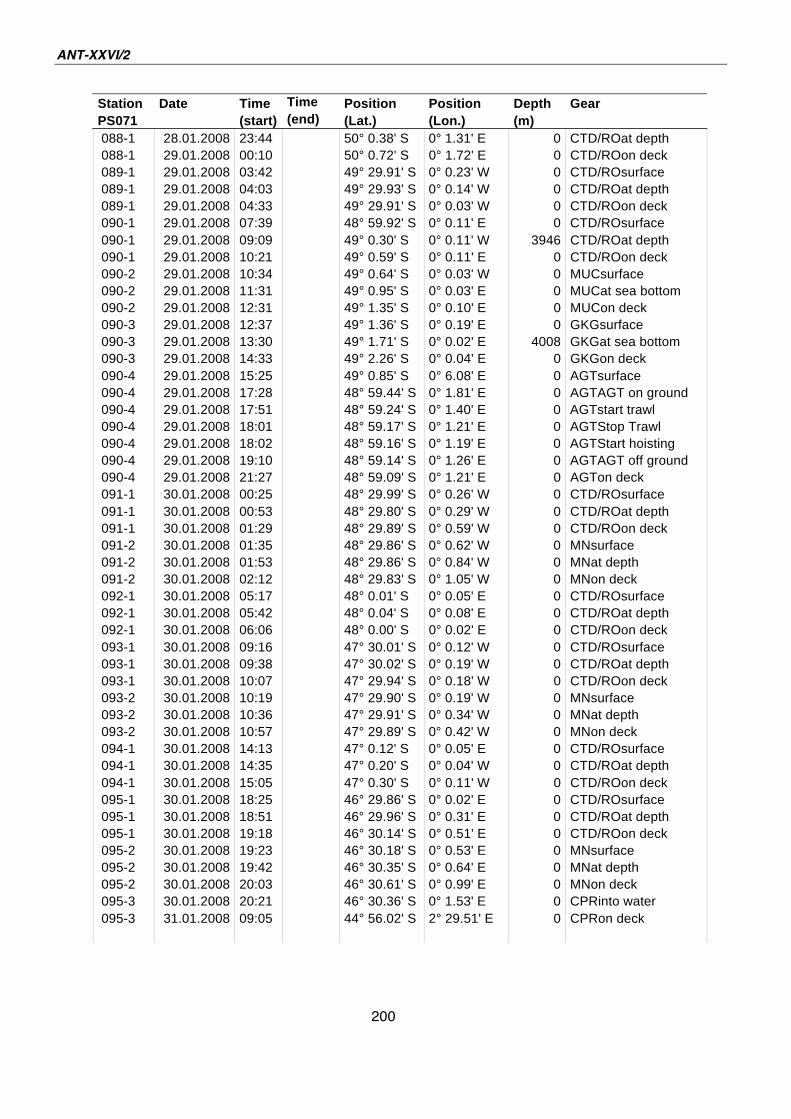
ANT-XXVI/2
200
Station Date Time Time Position Position Depth Gear
PS071 (start) (end) (Lat.) (Lon.) (m)
088-1 28.01.2008 23:44 50° 0.38' S 0° 1.31' E 0 CTD/ROat depth
088-1 29.01.2008 00:10 50° 0.72' S 0° 1.72' E 0 CTD/ROon deck
089-1 29.01.2008 03:42 49° 29.91' S 0° 0.23' W 0 CTD/ROsurface
089-1 29.01.2008 04:03 49° 29.93' S 0° 0.14' W 0 CTD/ROat depth
089-1 29.01.2008 04:33 49° 29.91' S 0° 0.03' W 0 CTD/ROon deck
090-1 29.01.2008 07:39 48° 59.92' S 0° 0.11' E 0 CTD/ROsurface
090-1 29.01.2008 09:09 49° 0.30' S 0° 0.11' W 3946 CTD/ROat depth
090-1 29.01.2008 10:21 49° 0.59' S 0° 0.11' E 0 CTD/ROon deck
090-2 29.01.2008 10:34 49° 0.64' S 0° 0.03' W 0 MUCsurface
090-2 29.01.2008 11:31 49° 0.95' S 0° 0.03' E 0 MUCat sea bottom
090-2 29.01.2008 12:31 49° 1.35' S 0° 0.10' E 0 MUCon deck
090-3 29.01.2008 12:37 49° 1.36' S 0° 0.19' E 0 GKGsurface
090-3 29.01.2008 13:30 49° 1.71' S 0° 0.02' E 4008 GKGat sea bottom
090-3 29.01.2008 14:33 49° 2.26' S 0° 0.04' E 0 GKGon deck
090-4 29.01.2008 15:25 49° 0.85' S 0° 6.08' E 0 AGTsurface
090-4 29.01.2008 17:28 48° 59.44' S 0° 1.81' E 0 AGTAGT on ground
090-4 29.01.2008 17:51 48° 59.24' S 0° 1.40' E 0 AGTstart trawl
090-4 29.01.2008 18:01 48° 59.17' S 0° 1.21' E 0 AGTStop Trawl
090-4 29.01.2008 18:02 48° 59.16' S 0° 1.19' E 0 AGTStart hoisting
090-4 29.01.2008 19:10 48° 59.14' S 0° 1.26' E 0 AGTAGT off ground
090-4 29.01.2008 21:27 48° 59.09' S 0° 1.21' E 0 AGTon deck
091-1 30.01.2008 00:25 48° 29.99' S 0° 0.26' W 0 CTD/ROsurface
091-1 30.01.2008 00:53 48° 29.80' S 0° 0.29' W 0 CTD/ROat depth
091-1 30.01.2008 01:29 48° 29.89' S 0° 0.59' W 0 CTD/ROon deck
091-2 30.01.2008 01:35 48° 29.86' S 0° 0.62' W 0 MNsurface
091-2 30.01.2008 01:53 48° 29.86' S 0° 0.84' W 0 MNat depth
091-2 30.01.2008 02:12 48° 29.83' S 0° 1.05' W 0 MNon deck
092-1 30.01.2008 05:17 48° 0.01' S 0° 0.05' E 0 CTD/ROsurface
092-1 30.01.2008 05:42 48° 0.04' S 0° 0.08' E 0 CTD/ROat depth
092-1 30.01.2008 06:06 48° 0.00' S 0° 0.02' E 0 CTD/ROon deck
093-1 30.01.2008 09:16 47° 30.01' S 0° 0.12' W 0 CTD/ROsurface
093-1 30.01.2008 09:38 47° 30.02' S 0° 0.19' W 0 CTD/ROat depth
093-1 30.01.2008 10:07 47° 29.94' S 0° 0.18' W 0 CTD/ROon deck
093-2 30.01.2008 10:19 47° 29.90' S 0° 0.19' W 0 MNsurface
093-2 30.01.2008 10:36 47° 29.91' S 0° 0.34' W 0 MNat depth
093-2 30.01.2008 10:57 47° 29.89' S 0° 0.42' W 0 MNon deck
094-1 30.01.2008 14:13 47° 0.12' S 0° 0.05' E 0 CTD/ROsurface
094-1 30.01.2008 14:35 47° 0.20' S 0° 0.04' W 0 CTD/ROat depth
094-1 30.01.2008 15:05 47° 0.30' S 0° 0.11' W 0 CTD/ROon deck
095-1 30.01.2008 18:25 46° 29.86' S 0° 0.02' E 0 CTD/ROsurface
095-1 30.01.2008 18:51 46° 29.96' S 0° 0.31' E 0 CTD/ROat depth
095-1 30.01.2008 19:18 46° 30.14' S 0° 0.51' E 0 CTD/ROon deck
095-2 30.01.2008 19:23 46° 30.18' S 0° 0.53' E 0 MNsurface
095-2 30.01.2008 19:42 46° 30.35' S 0° 0.64' E 0 MNat depth
095-2 30.01.2008 20:03 46° 30.61' S 0° 0.99' E 0 MNon deck
095-3 30.01.2008 20:21 46° 30.36' S 0° 1.53' E 0 CPRinto water
095-3 31.01.2008 09:05 44° 56.02' S 2° 29.51' E 0 CPRon deck
Die "Berichte zur Polar- und Meeresforschung" (ISSN 1866-3192) werden beginnend mit dem Heft Nr. 569 (2008) ausschließlich elektronisch als Open-Access-Publikation herausgegeben. Ein Verzeichnis aller Hefte einschließlich der Druckausgaben (Heft 377-568) sowie der früheren "Berichte zur Polarforschung (Heft 1-376, von 1982 bis 2000) befindet sich im Internet in der Ablage des electronic Information Center des AWI (ePIC) unter der URL http://epic.awi.de. Durch Auswahl "Reports on Polar- and Marine Research" auf der rechten Seite des Fensters wird eine Liste der Publikationen in alphabetischer Reihenfolge (nach Autoren) innerhalb der absteigenden chronologischen Reihenfolge der Jahrgänge erzeugt. To generate a list of all Reports past issues, use the following URL: http://epic.awi.de and select the right frame to browse "Reports on Polar and Marine Research". A chronological list in declining order, author names alphabetical, will be produced, and pdf-icons shown for open access download.
Verzeichnis der zuletzt erschienenen Hefte: Heft-Nr. 592/2009 — "The Expedition of the Research Vessel 'Polarstern' to the Antarctic in 2007 (ANT-XXIV/1)", edited by Sigrid Schiel Heft-Nr. 593/2009 — "The Campaign MELTEX with Research Aircraft 'POLAR 5' in the Arctic in 2008", edited by Gerit Birnbaum, Wolfgang Dierking, Jörg Hartmann, Christof Lüpkes, André Ehrlich, Thomas Garbrecht, and Manuel Sellmann Heft-Nr. 594/2009 — "The Expedition of the Research Vessel 'Polarstern' to the Antarctic in 2008 (ANT-XXV/1)", edited by Gerhard Kattner and Boris Koch Heft-Nr. 595/2009 — "The Expedition of the Research Vessel 'Polarstern' to the Antarctic in 2008/2009 (ANT-XXV/2)", edited by Olaf Boebel Heft-Nr. 596/2009 — "Crustal evolution of the submarine plateaux of New Zealand and their tectonic reconstruction based on crustal balancing", by Jan Werner Gerhard Grobys Heft-Nr. 597/2009 — "The Expedition of the Research Vessel 'Polarstern' to the Arctic in 2008 (ARK-XXIII/3)", edited by Wilfried Jokat Heft-Nr. 598/2009 — "The Expedition of the Research Vessel 'Pelagia' to the Natal Basin and the Mozambique Ridge in 2009 (Project AISTEK III)", edited by Wilfried Jokat Heft-Nr. 599/2009 — "The Expedition of the Research Vessel 'Maria S. Merian' to the Labrador Sea in 2009 (MSM12/2)", edited by Gabriele Uenzelmann-Neben Heft-Nr. 600/2009 — "Russian-German Cooperation SYSTEM LAPTEV SEA: The Expedition Lena 2009, edited by Julia Boike, Katya Abramova, Dmitry Yu. Bolshiyanov, Mikhail N. Grigoriev, Ulrike Herzschuh, Gerhard Kattner, Christian Knoblauch, Lars Kutzbach, Gesine Mollenhauer, Waldemar Schneider Heft-Nr. 601/2009 — "Analyse von Bathymetrie und akustischer Rückstreuung verschiedener Fächersonar- und Sedimentecholot-Systeme zur Charakterisierung und Klassifizierung des Meeresbodens am Gakkel-Rücken, Arktischer Ozean", by Jörn Hatzky Heft-Nr. 602/2009 — "Cumacea (Crustacea; Peracarida) of the Antarctic shelf – diversity, biogeography, and phylogeny", by Peter Rehm Heft-Nr. 603/2010 — "The Expedition of the Research Vessel 'Polarstern' to the Antarctic in 2009 (ANT-XXV/5)", edited by Walter Zenk and Saad El Naggar Heft-Nr. 604/2010 — "The Expedition of the Research Vessel 'Polarstern' to the Antarctic in 2007/2008 (ANT-XXIV/2)", edited by Ulrich Bathmann


