Embed Size (px)
Citation preview

The Dynamic Political Economy of Support for Barack Obama
During the 2008 Presidential Election Campaign
by
Thomas J. Scotto University of Essex [email protected]
Harold D. Clarke
University of Texas at Dallas and University of Essex [email protected]
Allan Kornberg Duke University
Jason Reifler Georgia State University [email protected]
David Sanders
University of Essex [email protected]
Marianne C. Stewart
University of Texas at Dallas [email protected]
Paul Whiteley
University of Essex [email protected]
Version: January 28, 2010

1
Abstract
The Dynamic Political Economy of Support for Barack Obama During the 2008 Presidential Election Campaign
In recent years, students of voting behavior have become increasingly interested
in valence politics models of electoral choice. These models share the core assumption
that key issues in electoral politics typically are ones upon which there is a widespread
public consensus on the goals of public policy. The present paper uses latent curve
modeling procedures and data from a six-wave national panel survey of the American
electorate to investigate the dynamic effects of voters' concerns with the worsening
economy—a valence issue par excellence—in the skein of causal forces at work in the
2008 presidential election campaign. As the campaign developed, the economy became
the dominant issue. Although the massively negative public reaction to increasingly
perilous economic conditions was not the only factor at work in 2008, dynamic
multivariate analyses show that mounting worries about the economy played an
important role in fueling Barack Obama's successful run for the presidency.

2
The Dynamic Political Economy of Support for Barack Obama During the 2008 Presidential Election Campaign
"It's getting harder and harder to make the mortgage or even keep the electricity on until the end of the month. The question isn't just whether you're better off than four years ago: it's whether you're better off than you were four weeks ago." Barack Obama “The issue of economics is not something I've understood as well as I should ....I've got Greenspan's book.” John McCain
In recent years, students of voting behavior have become increasingly interested
in valence politics models of electoral choice (e.g., Ansolabehere and Snyder, 2000;
Clarke, Kornberg and Scotto, 2009; Clarke et al., 2004, 2009; Johns et al., 2009;
Schofield, 2004, 2005). Building on pathbreaking work by Stokes (1963; see also
Stokes, 1992) these models differ in specifics, but share the core assumption that key
issues in electoral politics in contemporary mature democracies such as Great Britain and
the United States typically are ones upon which there is a widespread public consensus
on the goals of public policy. The classic example is the economy; almost everyone
endorses the goal of a vibrant economy characterized by low rates of inflation and
unemployment, and robust, sustainable, growth. But there are others—for example, vast
majorities of voters endorse the goals of having high quality, easily affordable, and
readily accessible health care and educational systems. Crime and terrorism are issues
with similarly one-sided opinion distributions; citizen demands for security from threats
posed by terrorists and common criminals are virtually ubiquitous. For these and similar
issues, political debate focuses not on ends, but rather on means. In the world of valence
politics, "who?" and "how?" are what matter when voters make their electoral choices.

3
As developed in our previous work (e.g., Clarke, Kornberg and Scotto, 2009;
Clarke et al., 2004, 2009; see also Clarke and McCutcheon, 2009), valence issues are
joined by party leader images and flexible partisan attachments as the three key variables
in a valence politics model. Although this model provides a powerful and parsimonious
explanation of voting behavior, we do not claim that other variables are irrelevant. In
particular, the locations of voters, parties and candidates on position issues emphasized in
Downsian-style spatial models of party competition (e.g., Adams, Merrill and Grofman,
2005) provide modest additional explanatory power. In previous work on voting the
2008 American presidential election (Clarke et al., 2010), we have demonstrated how
these several variables do much to account for the choices voters ultimately made in this
contest.
In the present paper, we focus on the dynamic effects of voters' concerns with the
worsening economy in the skein of causal forces at work in the 2008 election campaign.
As the campaign developed, the economy, a valence issue par excellence, became the
dominant issue. Consistent with a basic hypothesis of the voluminous literature on
"economic voting" (e.g., Lewis-Beck, 1988; Norpoth, Lewis-Beck and Lafay, 1991;
Duch and Stevenson, 2008), the consequence of the flood of bad economic news in 2008
had predictably negative effects on the fortunes of John McCain, the presidential
candidate of the incumbent Republican Party, and predictably positive ones for his
Democratic opponent, Barack Obama. The increasingly perilous state of the economy
was not the only factor at work but, as discussed below, it was a crucial factor in Obama's
successful run for the White House (see Lewis-Beck and Nadeau, 2009). He reaped

4
major political profits from an economy that was plunging into one of the deepest
recessions in American history.
Data: The data set we use was generated by a large multi-wave national internet survey
of registered voters conducted by YouGov/Polimetrix.1 This Cooperative Campaign
Analysis Project (CCAP) survey was administered six times over the course of the 2008
presidential campaign. Starting with a baseline survey in December 2007, subsequent
waves were fielded in January, March, September, October, and November 2008. For
present purposes, we utilize data gathered in the five-wave December 2007-October 2008
pre-election panel (N = 7595).2
The 2008 Context: From Guns to Butter
On the eve of the 2008 campaign season it was not inevitable that the economy
would become the issue of the general election. Unemployment was under five percent,
and the implications of President Bush’s decision to increase the number of troops
fighting in Iraq was the issue more likely to appear in the opening segment of the nightly
news. In the 2006 mid-term congressional elections the Democrats had capitalized on
Bush’s failure to quell the insurgency in Iraq. The steadily rising numbers of American
and Iraqi casualties and the escalating financial burden of the war convinced large
numbers of voters that a major redirection of policy was necessary. Discontent with the
evident lack of progress in Iraq, disgusted by the Bush administration's inept handling of
the Katrina hurricane crisis, and disillusioned by a widely publicized series of financial
and sex scandals involving Congressional Republicans, the public mood was sympathetic
to the Democrats' appeal for change. In November 2006, a disgruntled electorate gave

5
the keys of both Houses of Congress to the Democrats for the first time since 1994
(Clarke, Kornberg, and Scotto, 2009).
Although public unhappiness with the situation in Iraq had done much to help the
Democratic cause, a year later, in late 2007, the continuing conflict in that country
presented a challenge to candidates for the Democratic presidential nomination. Many of
those who had voted to give the Democrats control of Congress expected them to push
hard for withdrawal. Newly installed House Speaker Nancy Pelosi and her colleagues in
the liberal wing of the Democratic congressional caucus were happy to oblige. However,
President Bush, never one to appear swayed by public opinion, let alone liberal
Democrats, would hear nothing of withdrawal. Instead, he announced a plan to send an
additional 20,000 troops to Iraq. According to a White House press release (2007), the
troop "surge" would quell sectarian violence, isolate extremists determined to see the
United States fail, and provide the safe, stable environment needed to foster the
development of democratic governance in Iraq. Mindful of the sizable base of strident
anti-war voters in their party, Senator Obama and his main rival for the Democratic
presidential nomination, Senator Hillary Clinton, initially came out strongly against the
surge and called for a definitive timetable to draw down US troops and end US military
involvement in Iraq.
These positions became difficult to maintain because voters were increasingly
seeing the surge as a successful policy. For example, in the December 2007 wave of the
CCAP national panel survey, 44% reported that they believed the surge had improved the
situation and only 18% said that they thought it had failed. And, as the primary season
progressed, the percentage of respondents who wanted American armed forces to leave

6
Iraq immediately declined (from 30% in December 2007) to 20% (in March 2008).
Moreover, although less than one third of the CCAP respondents wanted the United
States remain in Iraq indefinitely, many more were willing to give the surge more time,
more than one year, to work. The Democrats had used public disaffection with Iraq to
their advantage in 2006, but in early 2008 advocacy of a "cut and run" strategy seemed
politically ill-advised.
Indeed, advocating a quick exit strategy as a solution to the Iraq problem might be
a liability. The eventually victorious Democratic candidate, whether Senator Obama or
Senator Clinton, would compete against Republican John McCain, whose popularity with
the electorate was fueled by his unquestioned status as a genuine war hero. McCain also
made much of his reputation as a straight talking maverick willing to oppose Republican
colleagues, regardless of possible political costs. However, on Iraq, he backed Bush.
Claiming great experience in foreign policy and proven ability to meet the challenges of
wartime leadership, McCain strongly endorsed the surge.
In the event, Obama did not have to worry greatly about positioning himself
relative to McCain on vexing issue of Iraq because another issue, the state of the
economy, quickly became the dominant public concern. As observed above, the
economy is a quintessential valence issue—virtually everyone wants a healthy economy.
Since prosperity has a vanishingly small number of political opponents, when adverse
economic conditions become a salient issue debate focuses heavily on who can get the
derailed engine of wealth production back on track. Economic mismanagement and
political success seldom go hand-in-hand and, since many voters attribute responsibility

7
to presidents for the performance the economy, recessions are typically bad news for
incumbent administrations.
In 2008, growing public concern about the economy began with signs of trouble
in the housing and commercial properties industry that had expanded rapidly in the first
two-thirds of the decade leading to a so-called “Housing Bubble” that saw many people
make large sums of money, at least on paper. When the bubble burst, a subprime
mortgage crisis ensued, and many Americans found themselves with heavily mortgaged
properties and negative equity (Akerlof and Shiller, 2009; Shiller, 2006). There were
major "knock on" effects because of a liquidity crisis (the inability/unwillingness of
banks to extend credit because of their own perilous conditions): in the banking and
investment sectors, in the insurance industry, in the automobile industry, in thousands of
other businesses, large and small. Job losses and layoffs started to make front-page news;
and the growing possibility of state and local government bankruptcies threatened
disruptions in vital public services. As Figure 1 shows, on the eve of the 2008 election
the Dow Jones industrial average, a signal to millions of Americans of the health of their
retirement portfolios and personal investments, was nearly 5,000 points down from early
2007. And, as just noted, unemployment became an increasingly serious problem,
moving upward, first gradually and then more rapidly, as 2008 wore on. The public
reacted predictably—as Figure 2 illustrates, retrospective and prospective assessments of
national economic conditions became massively negative as the bad economic news
mounted.
(Figures 1 and 2 about here)

8
Voters' worries about the economy are abundantly evident in the successive
CCAP panel surveys. The percentage of respondents who stated that the economy had
performed worse over the past year rose steadily from 68% in December 2007 to fully
93% in October 2008. Not only that, as Figure 3 shows, the economy became the
dominant issue on the public mind. In December 2007, less than one in five respondents
had designated the economy as their most important issue, but that figure grew markedly
throughout the campaign. When voters cast their ballots in November 2008 nearly 60%
stated that the economy was their foremost concern. Also important was the fact a
decreasing number of voters were concerned with any other issues, including ones such
as immigration, Iraq or terrorism that might have been Senator Obama’s Achilles Heel
had one or more of them become highly salient in a contest with an opponent such as
Senator McCain.
(Figure 3 about here)
Was Senator Obama able to convince voters he was able to handle the economy
effectively, and did this issue provide the ''political rocket fuel" that propelled him to
victory? Inspection of the CCAP data suggests that the preliminary answers to these
questions are affirmative. Figure 4 shows that Obama tended to be viewed positively
among the large and growing number of voters designating the economy as their most
important issues, with his favorability ratings increasing from 46% to 60% across the
December 2007 to October 2008 CCAP surveys. Also, and indicative of the problems he
might have faced if the economy had not weighed so heavily on voters' minds, the CCAP
data indicate that his favorability was much lower and actually declined slightly—from
42% in December 2007 to 38% in October 2008—among those collectively concerned

9
primarily with one of the non-economic issues. As the campaign drew to a close, Obama
effectively "owned" the issue—the economy—that defined the political agenda.
(Figure 4 about here)
As noted above, a host of studies have indicated that economic conditions have
significant effects on electoral choice. To date, however, the vast bulk of the work on
"economic voting" has relied on either aggregate time series data or cross-sectional
survey data. The former facilitate the analysis of dynamic relationships, but are
bedeviled by the problem of ecological inference. The latter avoid this problem, but are
necessarily unable to address questions relating to dynamic interrelationships among
variables of interest. The five-wave 2008 CCAP survey has the major advantage of
allowing one to conduct multivariate analyses of how individual voters responded to
worsening economic conditions, and the consequences those reactions had for support for
Barack Obama. That is our next task.
Methods and Models
As observed above, both retrospective economic evaluations and public support
for Democratic challenger Barack Obama exhibited substantial dynamics over the course
of the 2007-2008 election campaign. The primary topic we investigate is whether those
who grew more pessimistic about economic performance as the year wore on grew more
favorable to the Democratic challenger controlling for a variety of demographic,
ideological, and partisan forces that motivate candidate support in valence and other
models of voter choice. In addition, we consider the extent to which the growing
economic pessimism that characterized the electorate throughout the 2008 campaign hurt

10
Republican presidential candidate John McCain and widened the favorability gap
between him and his Democratic rival.
Latent Curve Modeling (LCM) (Browne, 1993; Bollen and Curran, 2006;
Duncan, Duncan and Strycker, 2006; Lackey et al. 2006) is a flexible methodology that
permits one to model individual-level variation in the dynamics of processes of interest—
here support for presidential candidates and evaluations of the performance of the
national economy. LCMs incorporate random intercepts and slopes into a broader
structural equation modeling (SEM) framework by specifying them as latent factors. As
part of the more general SEM class, the performance of LCMs can be assessed using a
wide array of model fit and adjudication statistics.3
We begin by investigating the relationship between negative economic
retrospections and support for Barack Obama. A similar model is used to analyze
support for Obama relative to his Republican opponent, Senator McCain. As discussed
above, attitudes towards the two presidential candidates are measured using five-point
ordinal scales, ranging from "very favorable" to "very unfavorable." These scales are
available in each of five pre-election waves (December, January, March, September,
October) of the CCAP 2008 national panel survey.
For unconditional models that exclude exogenous, time-invariant covariates, the
dynamics of favorability towards Obama and economic retrospections can be represented
as follows:
itretecontretieconretieconit
ObamaittiObamaiObamait
retEconObama
...... ελβαελβα++=
++=
The subscript i indicates that each individual in the sample has their own growth
trajectory giving them their own intercept, slope, and residual. The subscript t indexes

11
the five time points in our data so that each value of the variables on the left-hand side of
these equations represents the value of economic retrospections or Obama favorability
given by each individual i at each time point. The λt’s represent the paths from the latent
factors (described below) to the repeated measures that have initial and time varying
properties we wish to understand. Unconditional equations for the latent intercepts, α,
and slopes, β, are:
ireteconreteconretiEcon
reteconreteconretiEcon
iObamaretieconretieconretieconretieconObamaiObama
iObamaretieconretieconObamaiObama
i
...
...
....
..
ββ
αα
ββ
αα
ζμβ
ζμα
ζλβλαμβζλαμα
+=
+=
+++=
++=
These equations signify that the intercepts and slopes are functions of their mean
intercepts and slopes across all individuals plus random disturbances, the ζi’s. The values
of both the retieconretiecon .. λα and the retieconretiecon .. λβ parameters are noteworthy. A person’s
position on the latent intercept measuring favorability towards Senator Obama is a
function of their position on the latent intercept for economic retrospections, and their
position on the latent slope that measures favorability towards Senator Obama is a
function of their positions on the latent intercepts and slopes that capture an individual’s
starting level of and subsequent changes in economic evaluations. Model parameters
thereby indicate how voters' initial and subsequent negativity regarding the performance
of the national economy were related to initial levels of and movements in candidate
support.
The random intercepts and slopes can be thought of as factors that are linked to
observed indicators via path coefficients, here λecon.ret1t, λecon.ret2t, λObama1t, and λObama2t
where t = 1, 2, 3, 4, 5 and the first factor for each variable is the latent intercept (αObama

12
and αecon.ret) and the second factor is the latent slope (βObama and βecon.ret).4 A key
decision when estimating an LCM is how to scale the paths from the latent intercepts and
latent slopes to the time-varying observations. Typically, latent intercepts are fit to the
time-varying indicators by constraining all of the factor loadings to 1.0. Identification
also requires fixing the path from the latent slope to one of the time-varying indicators to
zero.5 Substantively, setting the path from the latent slopes to the December 2007
measurement of support for Obama and negative economic retrospections to zero
provides a straightforward interpretation of the latent intercepts: they are the initial levels
of negative attitudes towards the economy and favorability towards Obama.
Many LCMs assume a linear growth process (see Bollen and Curran, 2006), and
with five unevenly spaced surveys, we can estimate a growth model under the linearity
assumption by fixing the paths from the latent slopes to the indicators to the number of
months after the initial December 2007 measurement was taken. Thus, the fixed paths
from the latent slopes to the indicators would be: λJan = 0, λJan = 1, λMarch = 3, λSept. = 9,
and λOct = 10.
Although parsimonious, it is not necessary to assume a strictly linear process for
either economic evaluations or candidate support, and identification of an LCM with five
time-varying indicators requires only that two of the paths remain fixed (Bollen and
Curran, 2006). The 2008 race for the presidency featured a highly divisive Democratic
primary and a subsequent general election campaign that many argued was not well
fought by Obama’s opponent, John McCain. Obama's hotly contested primary battle
against Senator Hillary Clinton may have stunted his rise in support early in the year.
Further, although growth in economic pessimism is evident in the data throughout the

13
entire time period, the pace of this growth may have increased somewhat late in the
campaign after the highly publicized mid-September collapse of Lehman Brothers. To
determine whether the growth processes are non-linear, we fix λJan and λOct and freely
estimate the other λ's. Non-linearity in the growth process for economic retrospections
and Obama’s favorability will be evident if the estimated coefficients for the freed
parameters are significantly different from the time in months after December 2007 in
which a particular wave of the survey was fielded.
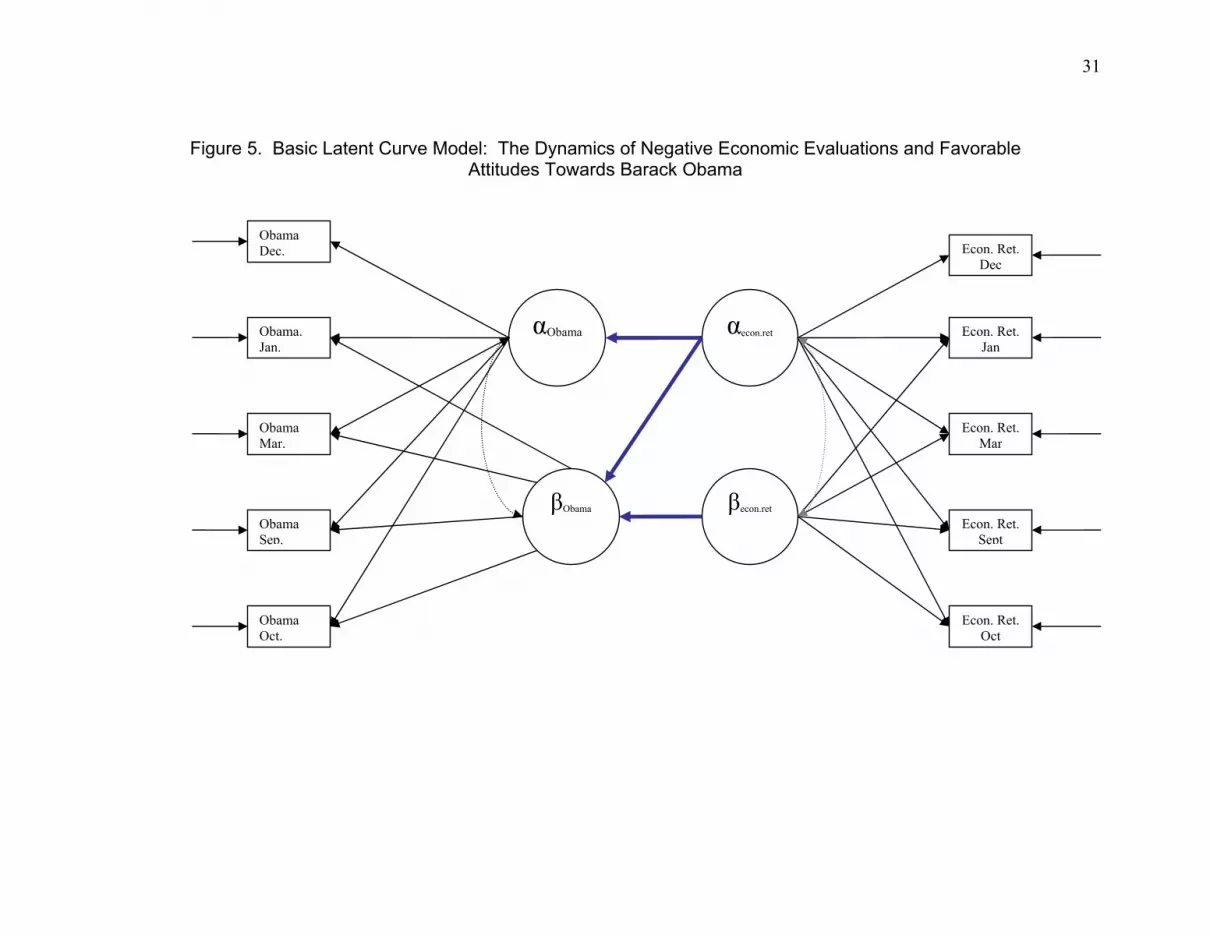
Figure 5 presents a conceptual diagram of the unconditional growth model just
described. Structural relationships of interest involve initial economic retrospections, on
the one hand, and the initial level and growth in support for Senator Obama, on the other.
The other important structural relationship involves change in negative economic
retrospections, measured by βiecon.ret and change in support for Obama, measured by
βiObama. The thick lines in Figure 5 indicate these paths.
(Figure 5 about here)
LCMs such as the one depicted in Figure 5 may be augmented to incorporate a
variety of additional factors affecting candidate support in presidential election
campaigns. Initial positions and growth in favorability towards Senator Obama and
evaluations of economic performance were not likely to be evenly distributed across
different sub-groups in the electorate, defined either in terms of political psychology or
political sociology. In 2008, discussions of forces at work in the campaign focused
heavily on whether the candidacy of Senator Obama transcended deep-seated attitudes
Americans held concerning race generally, and the status of African Americans in
particular. And, as is typical in American national elections, ideology and partisanship
14
were relevant, with Senator Obama needing both to appeal to the Democratic base after a
divisive primary, while simultaneously distancing himself from what many commentators
considered a very liberal voting record in the Senate. Socio-demographic characteristics
also may have played a role by influencing both worries about the worsening economy
and varying levels of support for the Democratic candidate and his Republican rival.
Taken, together, these considerations suggest that the growth trajectories depicted
in Figure 2 are conditional on several longer term factors. Incorporating these factors
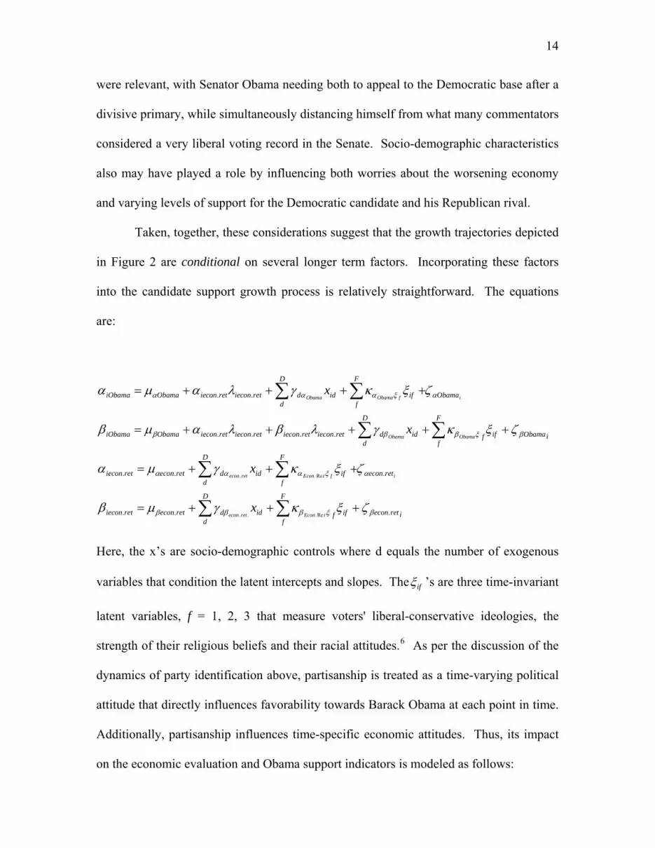
into the candidate support growth process is relatively straightforward. The equations
are:
iretecon
D
d
F
fiffiddreteconretiecon
retecon
D
d
F
fifiddreteconretiecon
iObama
D
d
F
fiffiddretieconretieconretieconretieconObamaiObama
Obama
D
d
F
fifiddretieconretieconObamaiObama
tEconretecon
iftEconretecon
ObamaObama
ifObamaObama
x
x
x
x
...
...
....
..
Re...
Re..
βξβββ
αξααα
βξβββ
αξααα
ζξκγμβ
ζξκγμα
ζξκγλβλαμβ
ζξκγλαμα
+++=
+++=
+++++=
++++=
∑ ∑
∑ ∑
∑ ∑
∑ ∑
Here, the x’s are socio-demographic controls where d equals the number of exogenous
variables that condition the latent intercepts and slopes. The ifξ ’s are three time-invariant
latent variables, f = 1, 2, 3 that measure voters' liberal-conservative ideologies, the
strength of their religious beliefs and their racial attitudes.6 As per the discussion of the
dynamics of party identification above, partisanship is treated as a time-varying political
attitude that directly influences favorability towards Barack Obama at each point in time.
Additionally, partisanship influences time-specific economic attitudes. Thus, its impact
on the economic evaluation and Obama support indicators is modeled as follows:

15
itreteconitttretieconretieconit
ObamaititttiObamaiObamait
zretEconzObama
..... εωλβαεωλβα+++=
+++=
In these equations zit is a voter's partisanship at a given point in time, and this is related to
support for Obama and economic evaluations via a time specific slope parameter, ωt.7
nt an additional set of
e first estimated an unconditional latent curve model where five-point ordinal
measures of favorability towards O time points (December 2007 and
Therefore, the interpretation of the latent intercepts and slopes shown in the conditional
model depicted in Figure 6 is that initial favorability and changes in support for Obama
are affected by the dynamics of negative economic retrospections conditional on
covariates, xd and yf, and net of an individual’s partisanship, zit, at each of the time points.
(Figure 6 about here)
In the next section, we first report results of analyses of the unconstrained and
constrained growth models for Senator Obama. Then, we prese
analyses focusing on the initial and growth in differences in support for Obama and
McCain.
Empirical Results
W
bama across the five
January, March, September, October 2008) were specified as functions of a latent
intercept (αObama) and a latent slope (βObama). Likewise, a latent intercept (αecon.ret) and a
latent slope (βecon.ret) were specified based on respondents’ evaluations of the past year’s
economic performance measured at each of the five time points. Indicator variables were
coded so that increasing values on the latent economic retrospection intercept and slope
corresponded with more negative initial retrospections and growth in negative
retrospections, respectively. Thus, a (weighted least squares) regression of βObama on
αecon.ret and βecon.ret should yield positive coefficients. Further, in accordance with the

16
literature on economic voting, we expect voters with initial negative economic
retrospections would be more positively predisposed to the Democratic challenger.
Regressing αObama onto αecon.ret should produce a positive coefficient.8
Results from the unconstrained model accorded well with these expectations. As
hypothesized in the preceding paragraph, the three relationships involving αObama and
Obama
to suspect attitudes towards him were contingent on several
β as dependent variables were positive and statistically significant (p < .05). Also,
the root mean square error of approximation (RMSEA), a statistic commonly used to
judge the goodness-of-fit of structural equation models, was only .046.9 What the
unconstrained model suggests is that, on average, those who believed the economy was
performing poorly at the outset of the campaign were likely to have higher levels of
favorability towards candidate Obama and they grew more favorable towards the
Democratic candidate as the year wore on. Furthermore, those whose negativity about
recent economic performance increased as the campaign progressed also became more
favorable to Senator Obama.
However, not all voters became more favorably inclined to the Democratic
challenger and there is reason
factors in addition to those generated by the worsening economy. The Senator from
Illinois was perceived by many to be very liberal, much was made of the fact that he was
the first African-American nominee from a major party, and attitudes toward him were
divided along socio-demographic and partisan lines. By estimating the conditional latent
curve model depicted in Figure 6, we can determine whether racial attitudes, ideology,
and religiosity were important factors driving favorability towards Senator Obama, and
whether economic effects are sustained when these factors are controlled. Although this

17
model has far more parameters than the unconditional model discussed above, the lower
RMSEA value of .02 suggests a better fit. The weighted root mean square residual
(WRMR), another measure of model fit, also has a satisfactory value.10 Table 1 reports
the parameter estimates and asymptotic standard errors for the latent portion of the
conditional LCM.
(Table 1 about here)
Inspecting the bottom half of Table 1 beginning with “latent predictors” first, we
see from the positive and signif t of 0.08 that initial economic
trosp
so were also regressed on several socio-demographics. Results show that
Obama was supported initially by a niche section of the electorate. He appealed most
icant slope coefficien
re ections (αrcon.eet) remain a significant predictor of initial attitudes towards Obama
(αObama). However, its magnitude is dwarfed by the coefficients of the race (.30),
religiosity (-.14), and "new racism" (1.60) latent variables. Latent liberalism and
progressive scores on the new racism scale in conjunction with low levels of religiosity
were more potent in predicting initial support for Obama. Standardized slope coefficients
(not shown) show that the power of the new racism scale dwarfed that of the other latent
variables combined. Before his primary victory over Senator Hillary Clinton and before
the economy became the issue of the 2008 campaign, Senator Obama appealed to those
on the ideological left and those with progressive racial attitudes. We also note that these
variables had indirect effects—liberals and those with progressive attitudes concerning
race were also more likely to view the economy as troubled in the beginning of the
campaign.
Although space prevents us from showing all of the coefficients, the latent
variables al

18
strongly to the young, the upper class, Catholics, and African-Americans. Obama’s
appeal among Hispanic voters was not greater than that among Whites, and older voters
and persons with a high school education or less initially held him in relatively low
esteem. However, Obama’s negatives presented an opportunity for his candidacy.
Voters in the demographics that did not favor his candidacy were also those most ill-
disposed about the performance of the economy and, accordingly, were potential recruits
for a candidate perceived able to restore "good times."
The regression of the latent slope for Obama’s favorability rating on other latent
variables and socio-demographic characteristics tell the story about how the economy
propelled his candidacy and secured voters beyond those in his initial base. The most
portaim nt findings is that the combined effects of αecon.ret and βecon.ret on βObama far exceed
those of other predictors. Beginning levels (.05) and growth (.66) in negative evaluations
of the performance of the economy were associated with significant increases in
favorable attitudes towards Obama. To illustrate the effects that initial economic
concerns and subsequent growth in these concerns had on initial support for Obama and
subsequent increases in that support, Figure 7 presents scatter plots and accompanying
regression lines of αObama by αecon.ret, βObama by αecon.ret, and βObama by βecon.ret for African
American and White respondents. The data displayed in this figure show that initial and
increasingly negative economic retrospections were associated with initial levels of and
growing support for Obama among both racial groups. Note that the relationships are
somewhat stronger among Whites. Since the election of Lyndon Johnston in 1964,
Democratic presidential candidates typically have struggled to win a majority of the
White vote. Although Obama was no exception, growing economic worries helped him

19
increase his level of support among Whites the campaign progressed. In this regard, a
large plurality of White respondents (46.6%) in the post-election wave of the CCAP
survey reported that they cast their ballots for Obama.11
(Figure 7 about here)
Just how important was the economy? The top portion of Table 1 reports the
mean values of the latent slopes, βObama by βecon.ret. On average, support for Obama across
the electorate rose at a modest .18 of a standardized unit (p < .10), and a sizable number
Obama
was only .39 and significantly less than 1.0 suggests that growth in his support was muted
of voters grew more negative towards him over the course of the campaign. However,
the effect of growth in negative economic retrospections was large .41 (p < .001), and
only a minuscule number of respondents grew more positive about the performance of
the economy. Among whites, positive growth in favorable attitudes towards Obama does
not occur until values of growth in negative economic retrospections surpass the
variable’s mean value. In sum, the analyses summarized in Table 1 and Figure 7 strongly
suggest that Obama's task would have been much more difficult had there not been a
substantial number of voters initially concerned about the economy and a sizable increase
in the percentage who became worried about worsening economic conditions. As Figure
3 above indicated, those worries did not occur only in the autumn in reaction to shocking
news about the failure of Lehman Bothers and other aspects of the deepening financial
crisis. Rather, economic concerns mounted over the course of the campaign.12
Although the economy was an increasingly salient issue throughout 2008, the top
half of Table 1 shows that growth in support for Obama and the incidence of negative
economic retrospections were both slightly non-linear.13 The fact that λJan for

20
during the early part of the primary season. The two remaining freed λ coefficients of
2.91 and 8.40 for the March and September waves, respectively, are not significantly
different from the values of 3 and 9 that would be expected if Obama's favorability
followed a linear growth process. However,, the fact that λSept. remains more than .5 of a
unit below its expected value suggests larger growth in the closing month of the
campaign.
The growth process for negative economic retrospections appears quite close to
linear until the end of the campaign season. The λSept. coefficient of 7.72 is significantly
lower than 9.0, and suggests that the rapid compounding of an already poor economic
outlook that accompanied the widely publicized collapse of Lehman Brothers in
eptem
ies helped to determine the trajectory of
bama'
S ber caused a late campaign surge in negative economic retrospections. Again, the
model tells a simple story, suggesting that Obama benefited from the extraordinarily bad
economic news in September and October, with people worried about the economy
swinging their support behind his candidacy.14
As noted above, Obama did not have it all his way; there were a substantial
minority of voters who did not grow warmer towards him. Conditioning the latent slope
for Obama’s favorability on the other latent variables and various other covariates
indicates that racial attitudes and political ideolog
O s favorability ratings (results not shown in tabular form). People with lower
levels of education who were initially unfavorable towards the candidate but also initially
pessimistic about the performance of the economy grew more favorable to the candidate
during the year. Quite possibly, this effect reflects the simple fact that, with the
Democratic primaries over, the only alternative to Obama was Republican John McCain.

21
It is also noteworthy that few of the covariates other than the latent variable tapping the
intensity of religious beliefs significantly predicted growth in negative economic
retrospections. This, in conjunction with the small magnitude of the variance of βecon.ret
(.02) suggests that growing negative economic retrospections became nearly ubiquitous
throughout the electorate.
Our analyses of Obama's favorability ratings also considered the effects of party
identification and attitudes toward Iraq. Recall that the conditional latent curve model
(Figure 6) examines the growth in latent favorability towards Obama after factoring out
the impact of partisan identification on his favorability indicators. As one might expect,
althoug
he results (not shown in tabular form) reveal that negative initial
h its influence was statistically significant on all five measures of favorability, the
strength of partisanship in predicting favorability towards the Democratic challenger was
stronger in September and October than earlier in the year. To study the impact of
opinions about Iraq, we estimated another conditional growth model similar to the one
discussed above. In this supplemental model, we added a measure of attitudes towards
the course of action the United States should in Iraq. This variable was measured in
September and it was used to predict support for Obama in October. The impact of initial
levels of and growth in negative economic retrospections on growth in his support
remained strong.
Did the increase of initial and increasingly negative economic retrospections also
hurt the candidacy of John McCain? To answer this question, we re-estimated the model
depicted in Figure 6 using McCain's favorability ratings in the five pre-election waves of
the CCAP panel. T

22
econom
ignificantly associated
with in
ble, a finding consistent with our
argume
ic retrospections and growth in economic pessimism was associated with both
initial and increasing disfavor towards the Republican candidate.
There are other interesting findings in the McCain model. The sign on the
coefficient for the effect of ideology on initial attitudes suggests that McCain initially
found favor among liberals. Further attesting to McCain’s early ability to appeal to a
broad section of the electorate the religiosity variable was not s
itial reactions to him, and the impact of racial attitudes was correctly signed and
significant, but quite weak. Coefficients for other predictors show that African-
Americans and Latinos were actually more favorably disposed than Whites to McCain
whose appeal, at least at the campaign's outset, seemed to have potential to transcend
narrow partisan and socio-demographic boundaries.
Regarding the dynamics of McCain's favorability ratings, voters with initially
negative economic evaluations and those who became negative about the economy as the
year progressed became less favorably disposed towards him. Standardized LCM
coefficients indicate that these effects were siza
nt that reactions to the worsening economy were a key factor driving the
dynamics of candidate support during the campaign. Model estimates also indicate that
McCain's appeal narrowed over time. African Americans and Latinos grew significantly
cooler towards his candidacy, and his appeal to ideological and racial conservatives and
religiously minded voters increased. In sum, while Obama was able to expand his
support beyond the Democratic heartland over the course of the campaign, McCain found
himself supported by fewer and fewer voters outside of the Republican base.

23
Finally, we consider a head-to-head match-up of voters’ favorability ratings of the
two candidates. This is an interesting analysis because the difference in favorability
ratings in the October CCAP survey has an extremely strong correlation (r = +.90) with
voting
publican
rival as evident in the reported slope roduced by regressing αObama-
McCain o
in the November post-election survey.15 Table 2 reports the results of a latent
curve analysis for the difference in Obama and McCain's favorability ratings.16 Similar
to the dynamics of support for Obama, the growth in the favorability gap between the two
candidates follows a slightly non-linear trajectory. The absence of growth early in the
primary season (λJan = -.01) is followed by a surge, such that the λMarch coefficient of 3.46
is significantly greater than the 3.0 value expected if the growth process was linear. And,
although not significantly different from its value under the linearity assumption, the
finding that λSept exceeds 9.0 suggests that much of the growth in the favorability gap
between the two candidates occurred before the closing month of the campaign.
(Table 2 about here)
Similar to their effects in the Obama support model, liberal racial attitudes were
the most potent factor prompting voters to favor Obama initially over his Re
coefficient of 0.70 p
nto the new racism latent variable.17 However, starting levels of and growth in
negative economic retrospections, that yielded slope coefficients of .05 and .49,
respectively, again combined to trump other forces in driving the growing gap between
Obama and McCain. Unlike the favorability models for the individual candidates, few of
the socio-demographic variables were significant predictors in the favorability gap
model. Only African-Americans demonstrated an increasing tendency to favor Obama
over McCain. Thus, although several variables help to explain support for the individual

24
candidates, voters' reactions to the worsening economy was a dominant force driving the
growing gap in support between Obama and McCain as the campaign progressed.
Conclusion: "It's the Economy and ..."
The 2008 presidential election provides a classic example of the power of valence
politics. With the American economy going into freefall over the course of the
campaign, the election real-world experiment
emons
Although McCain had attempted to portray himself as the only candidate who
constituted an important, but very painful,
d trating the ability of a quintessential valence politics issue—the state of the
national economy—to drive support for the competing presidential candidates. As the
campaign progressed, Democratic standard bearer, Barack Obama, found himself
propelled towards the White House by perilous economic conditions that were
preoccupying an increasingly worried electorate. Obama's campaign slogans "Yes We
Can!" and "Change You Can Believe In!" proved highly effective rhetorical devices that
enabled him to exploit the deepening crisis for handsome political profit. Carefully
avoiding potentially divisive policy specifics, Obama convinced many voters that he had
the "right stuff" to handle the ailing economy and other serious problems confronting the
country.
Obama's success in persuading a substantial portion of the electorate that he could
do the job on the economy and other vexing issues was facilitated by his rival, John
McCain.
had the experience needed to be an effective president, he maladroitly undercut his
message by proclaiming at the campaign's outset that he knew little, if anything, about
economics. Subsequently, his selection of untested Alaska Governor Sarah Palin as his
vice presidential running mate—a choice many commentators judged to be a bizarre,

25
even irresponsible, act of political desperation—substantially weakened his argument that
proven experience should be the sine qua non for choosing between himself and his
Democratic rival. Leader images regularly are key heuristic for voters trying to make
sensible decisions in a political world of high stakes and considerable uncertainty, and in
2008 Obama was able to portray himself as having the traits needed to be successful
president in a time of national crisis.
Obama's campaign was helped by other factors as well. After 2004, the
distribution of party identification had swung sharply in favor of the Democrats, as
sizable numbers of voters became increasingly disaffected with President Bush and his
become
handling of the Iraq War. A rising tide of lurid publicity about scandals involving
members of the Republican congressional caucus also tarnished the GOP brand, not just
among liberals, but also among many people closer to the center of the ideological
spectrum. Benefitting from this wave of dissatisfaction, Obama had strong appeal to
many groups that typically contribute heavily to the Democratic Party's electoral coalition
(see Lewis-Beck et al., 2008). African Americans, Hispanics, blue-collar workers,
women and young people all demonstrated their enthusiasm for him at the polls.
There is an important addendum to the story—analyses of the CCAP survey data
testify that Obama was not uniformly well received. Specifically, although he became
the first African-American president, this did not occur because racial biases had
irrelevant in American politics in 2008. A sizable number of voters continued to harbor
less than flattering views of African Americans, and these negative attitudes strongly
influenced their images of the candidates. Nevertheless, Obama prevailed. Benefiting
handsomely from an extremely well-organized and lavishly financed campaign, he did an

26
excellent job in combating these toxic stereotypes to the extent needed to ride the
deepening economic crisis to victory. Replaying the 2008 election without the economic
adversity that worked powerfully to make Barack Obama America's 44th president is
destined to remain a counterfactual exercise for Political Science commons rooms.

27
Figure 1. The Dynamics of Unemployment Rates and the Stock Market, November 2004-November 2008
4.0
4.5
5.0
5.5
6.0
7.0 14,000
6.5
8,000
9,000
10,000
11,000
12,000
13,000
2005 2006 2007 2008
Do
Per
cent
Une
mpl
oyed
w Jones Industrial A
verage Close
Unemployment
2008-->
Date
Source: Federal Reserve Bank of St. Louis (FRED) database; monthly data.
Dow Jones

28
Figure 2. Retrospective and Prospective National Economic Evaluations, November 2004-November 2008
0
20
40
60
80
100
120
140
2005 2006 2007 2008
Neutral
LastYear
NextYear
2008-->
Pess
imis
m<-
----
----
----
----
----
----
-->O
ptim
ism
Date
Source: Monthly Reuters/University of Michigan Surveys of Consumers.

29
Figure 3. The Dynamics of Issue Concerns—Most Important Issue December 2007-November 2008
0
10
20
30
40
50
60P
erce
nt M
entio
ning
Issu
eEconomy
TerrorismHealthIraqImmigration
Dec Jan Mar Sept OctDate
Nov
57
17
30
34
4548
Source: December 2007-November 2008 waves of CCAP panel survey.

Figure 4. The Aggregate Dynamics of Obama's Favorability Ratings and the Economy as Most Important Issue, December 2007-November 2008
30
10
20
30
40
50
60
70
Economy Most Important IssueObama Favorable if Mention EconomyObama Favorable if Mention Other Issue
DateDec Jan Mar Sept Oct
Perc
ent
Nov
46
5352
59 6063
42 4139 38 38 38
17
30
34
4548
57
Source: December 2007-November 2008 waves of CCAP panel survey.
31
Figure 5. Basic Latent Curve Model: The Dynamics of Negative Economic Evaluations and Favorable Attitudes Towards Barack Obama
Obama Dec.
Obama. Jan.
Obama Mar.
Obama Sep.
Obama Oct.
Econ. Ret. Dec
Econ. Ret. Jan
Econ. Ret. Mar
Econ. Ret. Sept
Econ. Ret. Oct
αObama
βObama
βecon.ret
αecon.ret

Party ID Dec
Obama Dec.
Party ID Jan
Obama. Jan.
Party ID Mar
Obama Mar.
Party ID Sept
Obama Sep.
Party ID Oct
Obama Oct.
Party IDDec
Econ. Ret. Dec
Econ. Ret. Jan
Party IDJan
Party IDMa
r
Econ. Ret. Mar
Econ. Ret. Sept
Party IDSe
pt
Party IDOc
t
Econ. Ret. Oct
αObama
βObama βecon.ret
αecon.ret.
New Racism, Religiosity and Ideology Factors
Exogenous Socio-Demographic Covariates
32
Figure 6. Latent Curve Model of Dynamics of Negative Economic Evaluations and Favorable Attitudes Towards Barack Obama with Covariates

33
Figure 7. Individual-Level Intercepts and Slopes in Dynamics of Obama Favorability by Individual-Level Intercepts and Slopes in
Dynamics of Economic Evaluations, African American and White CCAP Panelists
-16
-12
-8
-4
0
4
-8 -6 -4 -2 0 2 4 6
Intercept Economic Evaluations
Inte
rcep
t O
bam
a Fa
vora
bilit
y
Af rican American r = +.32 White r = +.46
<--regression l ines
-.8
-.6
-.4
-.2
.0
.2
.4
.6
.8
-8 -6 -4 -2 0 2 4 6
Intercept Economic Evaluatons
Slop
e O
bam
a Fa
vora
bilit
yAf rican American r = +.55 White r = +.67
<--regression l ines
-.8
-.6
-.4
-.2
.0
.2
.4
.6
.8
-.2 .0 .2 .4 .6 .8
Slope Economic Evaluations
Slop
e O
bam
a Fa
vora
bilit
y
Af rican American r = +.38 White r = +.37
<--regression l ines

34
Table 1. Parameter Estimates and Asymptotic Standard Errors for Conditional Multivariate Latent Curve Model of Support for Obama and Negative
Retrospective Evaluations Dependent Variables
Parameter Obama
Favorability Economic Retrospections
mu-alpha 0 0 mu-beta 0.18(.10)+ 0.41(.07)*** Lambda(Dec07) 0 0 Lambda(Jan08) 0.39(0.22)+ 0.91(0.45)* Lambda(Mar08) 2.91(0.20)*** 2.83(0.34)*** Lambda(Sept08) 8.40(0.43)*** 7.72(0.75)*** Lambda(Oct08) 10 10 psi-alpha alpha 4.52(.36)*** 3.25(.25)*** psi-beta beta 0.06(.01)*** 0.02(.004)*** psi-alpha beta -0.02(.02) -0.07(.02)*** Latent Predictor Alpha-Obama
alpha-Economic Retrospections
alpha-Econ Ret. 0.08(0.03)** --- Ideology. 0.30(0.03)*** 0.20(0.03)*** Religiosity -0.14(0.04)*** -0.01(0.03) New-Racism 1.60(0.07)*** 0.23(0.04)***
Latent Predictor Beta-Obama beta-Economic Retrospections
alpha-Econ. Ret. 0.05(0.01)*** --- beta-Econ. Ret. 0.66(0.10)*** --- Ideology 0.02(0.01)*** 0.00(0.00)
Religiosity 0.004(0.01) 0.01(0.01)+
Race 0.05(0.01)*** -0.013(0.004)** +p < .10 *p < .05 **p < .01 *** p < .001
Χ2(WLSMV) = 634.05 (p < 0.000) RMSEA = 0.02
WRMR = 0.94

35
Table 2. Parameter Estimates and Asymptotic Standard Errors for Conditional Multivariate Latent Curve Model of Support for Obama Relative to Support for
McCain and Negative Retrospective Evaluations Dependent Variables
Parameter
Obama Favorability
Minus McCain
Favorability Economic Retrospections
mu-alpha 0 0 mu-beta 0.18(.10)+ 0.41(.07)*** Lambda(Dec07) 0 0 Lambda(Jan08) -0.01(0.18) 0.88(0.46)+ Lambda(Mar08) 3.46(0.17)*** 2.92(0.34)*** Lambda(Sept08) 9.28(0.45)*** 7.70(0.77)*** Lambda(Oct08) 10 10 psi-alphaalpha 3.31(.24)*** 3.24(.25)*** psi-betabeta 0.07(.01)*** 0.02(.004)*** psi-alphabeta -0.02(.01) -0.07(.02)***
Latent Predictor
Alpha-Obama-McCain
alpha-Economic Retrospections
alpha-Econ Ret. 0.15(0.02)*** --- Ideology. 0.15(0.03)*** 0.20(0.03)*** Religiosity -0.10(0.03)*** -0.01(0.03) New-Racism 0.70(0.05)*** 0.23(0.04)***
Latent Predictor Beta-Obama-McCain
beta-Economic Retrospections
alpha-Econ. Ret. 0.05(0.04)*** --- beta-Econ. Ret. 0.49(0.07)*** --- Ideology 0.01(0.01)*** 0.00(0.00)
Religiosity -0.01(0.01) 0.01(0.01) Race 0.04(0.01)*** -0.013(0.004)** +p < .10 *p < .05 **p < .01 *** p < .001
Χ2(WLSMV) = 596.18 (p < .000) RMSEA=.02
WRMR = .92

36
References
Adams, James, Samuel Merrill and Bernard Grofman. 2005. A Unified Theory of Party Competition. New York: Cambridge University Press.
Akerlof, George A. and Robert J. Shiller. 2009. Animal Spirits: How Human Psychology
Drives the Economy and Why It Matters. Princeton: Princeton University Press. Ansolabehere, Stephen and James M. Snyder. 2000. "Valence Politics and Equilibrium in
Spatial Election Models." Public Choice 103: 327-36. Biesanz, Jeremy C., Natalia, Deeb-Sossa, Alison A. Papadakis, Kenneth A. Bollen,
Patrick J. Curran. 2004. “The Role of Time in Estimating and Interpreting Growth Curve Models.” Psychological Methods 9: 30-52
Bollen, Kenneth A. 1989. Structural Equations with Latent Variables. New York:
Wiley. Bollen, Kenneth A. and Patrick J. Curran. 2006. Latent Curve Models: A Structural
Equation Perspective. New York: Wiley Interscience. Browne, M. W. 1993. Structured Latent Curve Models. In C. M. Cuadras and C. R. Rao
eds., Multivariate Analysis: Future Directions. New York: Elsevier Science. Clarke, Harold D., Allan Kornberg, Thomas Scotto, Jason Reifler, David Sanders,
Marianne C. Stewart and Paul Whiteley. 2010. "'Yes We Can! Valence Politics and Electoral Choice in America, 2008." Richardson, Texas: University of Texas at Dallas, School of Economic, Political and Policy Sciences.
Clarke, Harold D., Allan Kornberg, and Thomas J. Scotto. 2009. Making Political
Choices: Canada and the United States. Toronto: University of Toronto Press. Clarke, Harold D., and Allan McCutcheon. 2009. The Dynamics of Party Identification
Reconsidered. Public Opinion Quarterly. 73: 704-28. Clarke, Harold D., David Sanders, Marianne C. Stewart, and Paul Whiteley. 2004.
Political Choice in Britain. Oxford: Oxford University Press. Clarke, Harold D., David Sanders, Marianne C. Stewart, and Paul Whiteley. 2009.
Performance Politics and the British Voter. Cambridge: Cambridge University Press.
Duch, Raymond M. and Randolph T. Stevenson. 2008. The Economic Vote: How
Economic Institutions Condition Election Results. New York: Cambridge University Press.

37
Duncan, Terry E., Susan C. Duncan and Lisa A. Strycker. 2006. An Introduction to Latent Variable Growth Curve Modeling: Concepts, Issues and Applications. Mahwah, NJ: Lawrence Erlbaum.
Downs, Anthony. 1957. An Economic Theory of Democracy. New York: Harper. Gomez, Brad T. and J. Matthew Wilson. 2006. "Rethinking Symbolic Racism: Evidence
of Attribution Bias." American Journal of Political Science 68:611-25. Hox, Joop. 2002. Multilevel Analysis: Techniques and Applications. New Jersey:
Lawrence Erlbaum Associates. Jackman, Simon, and Lynne Vavreck. 2009. Co-operative Campaign Analysis Project:
2007-2008. (Version 1.0) University of California, Los Angeles, Stanford University, and YouGov/Polimetrix.
Johns, Robert, James Mitchell, David Denver and Charles Pattie. 2009. "Valence Politics
in Scotland: Towards an Explanation of the 2007 Election." Political Studies 57: 207-33.
Kline, Rex B. 2005. Principles and Practices of Structural Equation modeling, 2nd ed.
New York: Guilford Press. Lackey, Gerald, Thomas J. Scotto, Thomas K. Bias, and Arian Spahiu. 2006. “Altered
Faith, Altered Party? The Relationship Between Religious Commitment and the Intensity of Party Identification.” Paper presented at the 2006 Annual Meeting of the American Political Science Association, Philadelphia, PA.
Lewis-Beck, Michael. 1988. Economics and Elections: The Major Western Democracies.
Ann Arbor: University of Michigan Press. Lewis-Beck, Michael and Richard Nadeau. 2009. “Obama and the Economy in 2008.”
PS: Political Science & Politics. 43: 479-83. Lewis-Beck, Michael, Helmut Norpoth, William Jacoby and Herbert Weisberg. 2008.
The American Voter Revisited. Ann Arbor: University of Michigan Press. Muthén, Bengt, Stephen du Toit, and Damir Spisic. 1997. “Robust Inference Using
Weighted Least Squares and Quadratic Estimating Equations in Latent Variable Modeling with Categorical and Continuous Outcomes.” Unpublished Paper.
Muthén, Linda K. and Bengt O. Muthén. 2007. Mplus User’s Guide: Statistical Analysis
With Latent Variables. Los Angeles: Muthén and Muthén.

38
Norpoth, Helmut, Michael S. Lewis-Beck and Jean-Dominique Lafay. eds. 1991. Economics and Politics: The Calculus of Support. Ann Arbor: University of Michigan Press.
Preacher, Kristopher J. et al. 2008. Latent Growth Curve Modeling. Thousand Oaks CA:
Sage Publications. Stephen W. Raudenbush and Bryk, Anthony S. 2002. Hierarchical Linear Models: Applications and Data Analysis Methods. 2nd Edition. Thousand Oaks, CA: Sage Publications. Schofield, Norman. 2004. "Equilibrium in the Spatial Valence Model of Elections." Journal of Theoretical Politics 16: 447-81. Schofield, Norman. 2005. "A Valence Politics Model of Political Competition in Britain:
1992-1997." Electoral Studies 24: 347-70. Shiller, Robert. 2006. Irrational Exuberance. 2nd edition. New York: Random House. Sniderman, Paul M. and Philip E. Tetlock. 1986. "Symbolic Racism: Problems of Motive
Attribution in Political Analysis." Journal of Social Issues. 42:129-l50 Snijders, Tom A.B., and Roel J. Bosker. 1999. Multilevel Analysis: An Introduction to
Basic and Advanced Multi-level Modeling. London: Sage Publications. Stokes, Donald E. 1963. Spatial Models of Party Competition. American Political
Science Review 57: 368-377. Stokes, Donald E. 1992. Valence Politics. In Electoral Politics, edited by D. Kavanagh.
Oxford: Clarendon Press. Tarman, Christopher and David O. Sears. 2005. "The Conceptualization and
Measurement of Symbolic Racism." Journal of Politics 67: 731-61. The White House. 2007. “Fact Sheet: The New Way Forward in Iraq” Press Release, 10
January 2007. [cited 20 December 2009] Available from: http://georgewbush-whitehouse.archives.gov/news/releases/2007/01/20070110-3.html.
Yu, Ching-Yun. 2002. Evaluating Cutoff Criteria of Model Fit Indices for Latent
Variable Models with Binary and Continuous Outcomes. Ph.D., Education, University of California, Los Angeles.

39
Endnotes 1 Lynn Vavreck, UCLA, and Simon Jackman, Stanford, served as CCAP study directors. We take this opportunity to thank them for their insightful and generous assistance. 2 The analyses employ a large number of variables in the CCAP data set. Three variables are particular crucial. Two of them measure of how favorably or unfavorably respondents were disposed towards Barack Obama and his general election opponent, John McCain. The question measuring these attitudes is: "Here is a list of candidates running for president. How favorable is your impression of each candidate or haven't you heard enough to say? Response categories were "very favorable," "somewhat unfavorable," "neutral," "somewhat unfavorable," and "very unfavorable." The list of candidates varied depending upon when a particular wave of the survey was in the field. The third crucial variable is a measure of respondents' retrospective economic evaluations ascertained by asking them for their reactions to the state of the national economy over the past year. This question is: "Would you say that over the PAST YEAR [emphasis in original] the nation's economy has gotten much better, gotten better, stayed about the same, gotten worse, gotten much worse?" Respondents also were given the opportunity to indicate that they were "not sure." Details concerning the measurement of other variables and how they were coded for analysis are available from Thomas Scotto’s website: http://privatewww.essex.ac.uk/~tscott/ 3 A hierarchical linear model (HLM) would treat a respondent's repeated evaluations of Barack Obama and the economy as level one units that are nested within respondents who are treated as the units of analysis at level two (e.g., Raudenbush and Bryk, 2002). However, HLM models can be problematic with only five units at the first level, and an HLM model designed to answer the questions we are asking would contain many cross-level interactions (Snijders and Bosker, 1994; Hox, 2002). 4 Given the ordinal and highly skewed nature of the data, particularly the observed values on economic retrospections, parameter estimates are obtained via the weighted least squares with adjusted means and variances (WLSMV) estimator with the theta parameterization available in MPLUS 5.1 (Muthén et al., 1997). Only respondents who answered all five pre-elections waves of CCAP panel are included, and the small number of respondents who failed to report their attitudes towards Obama or the economy were treated as missing at random and included in the analysis via MPLUS’s procedure for handling missing ordinal data (e.g.. Muthén and Muthén, 1999-2006). Paths between the latent variables and time-varying parameters are ordered probit coefficients. Thresholds of ordinal variables are estimated, but constrained to be equal over time, a process that allows observations across exogenous latent variables to be normally distributed with a mean of zero and a standard deviation of one (Bollen, 1989; Lackey et al., 2006). 5 There is no requirement that the first time-varying indicator act as the starting or zero point for the coding of time, but interpretations change when a different starting point is used (see Biesanz et al., 2004).

40
6 The latent variables measuring ideology and racial attitudes also are conditioned on the socio-demographics. To increase the reliability of the control for ideology, it is specified as a latent factor that motivated responses to a standard liberal-conservative ideology question asked in all five waves of the survey. A person’s latent racial attitudes drove their responses to four questions from the modern symbolic racism scale (e.g.. Tarman and Sears 2005) fielded in the March 2008 wave of the study. A person’s latent religiosity drove their responses to three questions: a) frequency of church attendance; b) belief in the authenticity of the bible, and the importance of religion in the respondent's everyday life. See the Co-operative Election Study Codebook (Jackman and Vavreck, 2009) for question wording and answer choices. Higher factor scores indicate greater religiosity, liberalism, and progressive attitudes on the symbolic racism scale. Given the strong relationship between ideology and symbolic racism (Sniderman and Tetlock 1986; see also Gomez and Wilson, 2006; Tarman and Sears, 2005), we regressed ideology onto latent religiosity in the conditional LCM for Obama. All latent factors, in addition to partisanship were regressed onto the socio-demographic variables. Full details are available from the authors.
Similar to regression analysis, E(εObamait=0) and E(εEcon.ret.it=0) and the errors of the time-varying indicators are assumed to be uncorrelated with any of the other variables on the right-hand side of the model and are also considered to be uncorrelated across time. As in Lackey et al. (2006), we designate the time-varying errors of the level 1 residuals as invariant, making the error matrix Θεε block diagonal. Elements of the level-2 covariance matrix, Ψ, are freely estimated. For the purposes of improving model fit and specification, some errors of the indicators of the ideology and racial attitudes latent variable were allowed to co-vary as were those of some of exogenous covariates. Details concerning the specification of the model and of results from parameters not included in the tables can be found at the authors' website cited in note 2 above.
7 Partisanship is a three-category variable (Republican, Independent/Other, Democrat) with higher values indicating Democratic partisanship. Each time-specific measure of partisanship is conditional on the exogenous socio-demographic variables and the latent ideology, religiosity and racial attitudes factors. Further, partisanship has an autoregressive property—party identification in March 2008, September 2008, and October 2008 is modeled as an AR(1,2) process. Given data availability limitations, party identification in January 2008 is modeled as a function of partisanship in December 2007. 8 Given the paucity respondents reporting positive economic retrospections by the end of 2008, we investigated whether the skewed responses to the question might drive the results. We replaced the economic retrospections variable with a dichotomous economy is the most important issue variable (where 1 = respondent named the economy as the most important issue and 0 = respondent named another issue as most important or did not believe any issue was important), and re-estimated the LCMs. Results were similar to those reported in the paper.

41
9 The statistically significant χ2
WLSMV value of 434.80 (26 df), p = .00 does not surprise given the large sample size of 7,595 and the propensity of this statistic to signal a poor fit because of the presence of small but significant co-variances that are fixed at zero. Rather than freeing additional co-variances in an atheoretical fashion to attain a statistically insignificant χ2, we rely chiefly on RMSEA as a measure of adequacy of fit. RMSEA is the average discrepancy between the observed and model implied co-variances weighted by the degrees of freedom in the model (Kline, 2005: 137-40). RMSEA values than less than .05 indicate a close fit. 10 WRMR is a weighted measure of the difference between sample variances and co-variances and those estimated for a population. A model with a WRMR less than 1.00 is generally judged to have close fit (Yu, 2002). 11 The 2008 ANES data tell the same story, with 44.5% of White respondents in the post-election survey reporting that they voted for Obama. McCain's vote shares in the two surveys are 51.5% in the CCAP and 53.4% in the ANES. Other presidential candidates received 1.9% and 2.1% of the vote among CCAP and ANES respondents, respectively. 12 The correlaton (r) between the percentage of CCAP respondents mentioning the economy as the most important issue and month of survey is +.95. 13We conducted χ2 difference tests (modified for the WLSMV estimator) and rejected the null hypothesis that setting the λ coefficients equal to the number of months after administration of the initial survey produced equal or superior model fit. 14 Remaining coefficients reported in the top part of Table 1 signify that even with the added covariates, there remains unexplained variance in the latent intercept and slopes for both favorability towards Obama (4.52 and .06) and negative retrospections (3.52 and .02). However, note that the magnitude of the variance of the slopes is small. Initial favorability towards Obama was not significantly associated with growth in his support (-.02), but people with initial positive economic retrospections grew more negative over time (-.07). Note that only a very small number of people (e.g., .5% of those participating in the December 2007 and October 2008 waves of the survey) were initially negative about the economy and subsequently became positive. 15 The percentage of CCAP respondents voting for Obama in November who are strongly favorable to him and strongly unfavorable to McCain in October is 99.2; the percentage of respondents voting for McCain who are strongly favorable to him and strongly unfavorable to Obama is 98.4. 16 In this analysis the lambda coefficients and variances of the latent slope and intercept for economic retrospections (reported in the top portion of Table 2) are very similar to those reported for the LCM for Obama favorability. This finding lends bolsters confidence in the specification decisions made in paramaterizing that model.

42
17 Ideological liberalism also predicted respondents to have an initial predisposition to favor Obama (.15) and negative initial economic evaluations (.20). Those with liberal positions on the new racism latent factor also tended to negatively evaluate economic performance (i.e., the regression of αEcon.Ret.on new racism yielded a coefficient of .23).


