The Distributional Impact of Fiscal Policy in Honduras

WP/08/XX

The Distributional Impact of Fiscal Policy in Honduras

Robert Gillingham, David Newhouse, and Irene Yackovlev

WP/08/168

© 2008 International Monetary Fund WP/08/168

IMF Working Paper Fiscal Affairs Department

The Distributional Impact of Fiscal Policy in Honduras

Prepared by Robert Gillingham, David Newhouse, and Irene Yackovlev1

Authorized for distribution by Rolando Ossowski

July 2008

Abstract

This Working Paper should not be reported as representing the views of the IMF. The views expressed in this Working Paper are those of the author(s) and do not necessarily represent those of the IMF or IMF policy. Working Papers describe research in progress by the author(s) and are published to elicit comments and to further debate.

This paper uses household survey data to estimate the incidence of tax and spending programs in Honduras. Any such exercise is fraught with difficulty, so our simplifying assumptions are carefully explained. Rather than look at tax and spending completely independently, we evaluate net incidence of major programs—such as health care and pensions—to get a more holistic evaluation of redistribution. Our results show that fiscal policy is, on balance, progressive, but that there is room for significant improvement. In particular, energy subsidies, university education and public pension programs provide disproportionate benefits to higher-income households. JEL Classification Numbers: D30, D60, E62, H20, I38 Keywords: Tax policy, expenditure policy, subsidies, welfare distribution, household survey data

Authors’ E-Mail Addresses: [email protected]; [email protected]; [email protected]

1 David Newhouse (World Bank). The authors would like to thank Rodrigo Cubero and Ivanna Vladkova for helpful comments and suggestions.

2

Contents Page

I. Introduction ............................................................................................................................3 II. Methodology .........................................................................................................................4

Data sources ...................................................................................................................4 Estimation of taxes and price subsidies .........................................................................4 Estimation of other government benefits .......................................................................4 Classifying variables......................................................................................................5

III. The Incidence of Direct and Indirect Taxes.........................................................................6 Direct taxes ....................................................................................................................7 Indirect taxes..................................................................................................................8

IV. Distribution of Government Spending Programs and Implicit Subsidies ...........................9 Subsidies and grants.......................................................................................................9 Government expenditure on health and education.......................................................10 Pension systems ...........................................................................................................12

V. Summary and Conclusions..................................................................................................13

Tables 1. Household Demographic Characteristics ...........................................................................5 2. Distribution of Consumption and Income ..........................................................................6 3. Tax Revenues by Type, 2004-2006 ....................................................................................7 4. Tax Rate Schedule ..............................................................................................................7 5. Distribution of Personal and Corporate Income Taxes.......................................................8 6. Distribution of Indirect Taxes.............................................................................................9 7. Distribution of Subsidies and Grants ................................................................................10 8. Distribution of MOH Health Spending.............................................................................11 9. Distribution of Education Spending .................................................................................11 10. Pension System Contribution Rates..................................................................................12 11. Distribution of Pension System Subsidies........................................................................13 12. Distributional Effects of Fiscal Policy..............................................................................14 13. Distributional Effects of Fiscal Policy (Income per Capita Quintiles).............................18

Figures 1. Income and Consumption by Income per Capita Quintile ...............................................16 2. Income and Consumption by Consumption per Capita Quintile......................................17 3. Effect of Changing Classifying Variable on Means .........................................................19 Appendix I. Effect of Classifying Households by Income per Capita .....................................................16 References................................................................................................................................20

3

I. INTRODUCTION

Government policy can affect the level and distribution of income in myriad ways. In the long run, the efficacy of government action will be paramount. A government that puts society’s resources to their highest use—whether to build human capital and infrastructure, or simply to promote private sector growth—will ensure that the economic pie is as large as possible. Recent history has demonstrated that increased reliance on market forces can be very successful in achieving this goal. At the same time, however, it is incumbent on a government to promote equity as well as efficiency. It is difficult to believe that policies that promote rapid growth can be successful in the long term if this growth leaves too many people behind, if too many people believe that whatever economic system is adopted does not work for them.

At least for the IMF, the potential tension between equity and efficiency can be avoided by promoting and engendering high-quality growth—that is, “growth that is sustainable in the face of external shocks; accompanied by adequate investment (including in human capital, to lay the basis for future growth); respectful of environmental and national concerns; and, last but not least, consistent with policies that reduce poverty and improve equity” (Camdessus, 1999). This paper focuses on this last dimension of high-quality growth—how fiscal policy can redistribute currently available resources to share the benefits of growth. As part of this exercise, we will also touch on investment in human capital and setting the stage for future growth. However, we will not systematically address the equally important issue of how government policies promote rapid, as well as equitable, growth.

Any attempt to assess the distributional impact of government policy is fraught with problems. For one thing, policy can affect the distribution of income in many ways that are indirect or difficult to measure. For instance, government regulations that set a minimum wage or labor standards can have important effects on well-being that are not evenly distributed. We will narrow our investigation further to look only at the contemporaneous effects of tax and spending policies. Moreover, even within this narrow focus, we face extremely difficult measurement issues. On the one hand, we can estimate how much tax is collected from a particular household or how much is spent to provide public education to the children of this household. However, the ultimate incidence of a tax—who ultimately bears the burden—is more problematic, as is determining the value to a household, as opposed to the cost, of public education. With the exception of the estimated incidence of the corporate income tax, our incidence estimates ignore behavioral responses. For instance, the personal income and VAT estimates ignore any possible change in factor prices as a result of the imposition (or elimination) of the tax. Consequently, they are an incomplete representation of the full distributional effects of fiscal policy, as some effects may be revealed only over time, if at all. For the corporate income tax, on the other hand, we adopt an incidence assumption based on theoretical and empirical incidence studies that include behavioral responses. We feel this is necessary because the difference between who pays and who bears the burden is much more important for the corporate income tax than it is for other taxes and benefits.

4

II. METHODOLOGY

Data sources

In order to consistently analyze the distributional impact of fiscal policy, we need a single data source that can provide the basis for estimating both who pays taxes and who receives the benefits of government spending and subsidies. Our analysis is based on the Encuesta Nacional de Condiciones de Vida (ENCOVI) survey conducted by the Institute of National Statistics (INE). This survey sample comprised 8,175 households containing a total of 39,500 people. The sample was spread among 408 villages within the two main cities of Tegucigalpa and San Pedro Sula, two smaller cities, and several rural areas. Households were interviewed between July and November of 2004. Key to this analysis, the survey collected information on (1) income by source, (2) consumer spending, and (3) access to and receipt of the benefits of government spending. The survey collected information on participation in government subsidy and grant programs and on the types of pensions and health coverages for which the households were eligible.

Estimation of taxes and price subsidies

The income data allow us to estimate the incidence of direct taxes. The consumer spending data, on the other hand, allow us to estimate the incidence of indirect taxes—the VAT, tariffs and excises—and estimate the incidence of energy subsidies, which have significant distributional consequences in Honduras. Our analysis considers both the direct effects of indirect taxes and subsidies and the indirect effects, as the taxes and subsidies are passed through to the prices of other consumer goods and services. To model the indirect effects, we use an input-output table to simulate the pass-through of a price change in one sector onto other sectors, assuming that input proportions are fixed and that price changes in upstream sectors are fully passed on to consumers in the form of price changes in the downstream sectors. We obtain the matrix of input-output coefficients for this simulation from a Social Accounting Matrix prepared by Jose Cuesta (Cuesta, 2004) and publicly available from the International Food Policy Research Institute (IFPRI).

Estimation of other government benefits

We estimate the other benefits that households receive from the government in three ways. First, we assign the benefits of any cash transfers that the government makes available to individual households based on their characteristics. In these cases, the benefits can be estimated on an individual household basis. Second, we identify which households benefit from government spending on health and education, the two major programs that build human capital. These are also in-kind benefits, but they are much harder to quantify, since spending is not household-specific. As discussed in more detail below, we have information on the total cost of a program and how many household members benefit from it. However, we have no information on the amount spent on each household or on particular household groups. That is, we have no information on how the quantity or quality of the service provided might vary among households. A related problem is that we have no direct measure of the value of the program to each household. Some households might value the service more or less than its cost of delivery. To the extent that participants must contribute to

5

become eligible for benefits—in particular, health benefits—we focus on the net benefit—that is, the cost of the benefit less the household-specific contribution. If the net benefit is positive, it represents a net subsidy. If it is negative, it represents a net tax.

Third, the government administers old-age insurance programs, to which participants pay contributions while they are working and receive benefits after they retire. If the program is in financial balance, the present value of the cash flows will be zero. To represent the net benefit of a pension plan, we assign to each contributor the difference between her or his contribution and the contribution that would be necessary to bring the pension plan into financial balance. As with health insurance, if the actual contribution is greater (smaller) than the contribution that achieves financial balance, the participant incurs a tax (receives a subsidy).

Classifying variables

We use consumption per capita of a household as our primary proxy for welfare in classifying households. The underlying consumption aggregate is identical to that used for distributional analysis in the World Bank poverty report (World Bank, 2006), and reflects actual and imputed rental values, out-of-pocket health and education expenditures, and expenditures on durable goods. This variable accounts not only for consumption of purchased goods, but also for the consumption of own-produced goods. The use of per capita consumption implicitly assumes that the demand on resources of a household member does not vary by age or sex and that there are no economies of scale in consumption for larger households. Consumption per capita is used as the classifying variable because it is viewed as a better indicator of household welfare than current income per capita (see the discussion in the appendix). Moreover, per capita consumption offers the virtue of simplicity and consistency with the World Bank poverty report. Table 1 provides demographic summary information on households by quintiles of per capita consumption. In general, households with higher per capita consumption levels have fewer household members, are more urban, and are more

Table 1. Household Demographic Characteristics

Bottom Quintile 2 3 4

Top Quintile

All HHs

RegionTegucigalpa 1.0 5.0 12.1 20.4 28.1 13.3 San Pedro de Sula 0.5 3.6 8.1 11.6 18.8 8.5 Middle-size cities 4.5 11.9 17.1 20.7 22.8 15.4 Small towns 8.1 13.8 16.6 17.1 13.6 13.8 Rural 86.0 65.7 46.0 30.3 16.8 49.0

Age of household head15 to 30 17.1 22.0 23.2 24.4 20.1 21.4 31 to 40 25.7 24.5 25.5 21.9 22.1 24.0 41 to 50 24.4 21.1 20.9 22.2 23.1 22.3 51 to 60 15.3 16.0 14.9 14.0 16.5 15.3 Over 60 17.5 16.4 15.5 17.5 18.2 17.0

SchoolingNone 2.2 1.1 0.6 0.8 0.6 1.1 Elementary 57.8 62.7 65.0 57.2 32.2 55.0 Middle school 0.6 5.3 15.4 25.8 35.9 16.6 Secondary and above 39.3 30.9 19.0 16.2 31.4 27.4

Female household head 16.2 23.9 23.8 29.2 30.2 24.7 Household size 6.3 5.4 5.0 4.4 3.7 5.0

Source: Institute of National Statistics (ENCOVI) and staff estimates.

6

likely to have a female head of household. There is little variation in average age, and a somewhat perplexing relationship between consumption level and education. A relatively high percentage of household heads in the two lowest quintiles have completed secondary school, while household heads in the third and fourth quintiles are more likely to have stopped at middle school. Only in the top quintile is the educational attainment clearly higher than in the first two quintiles.

Table 2 displays consumption and income statistics by quintiles of the distributions of both per capita consumption and per capita income. We use consumption as the primary classifying variable, for two reasons: (1) to the extent that households consume out of permanent rather than current income, consumption is a better measure of permanent income, which is arguably the best measure of welfare, and (2) even if income is not as variable as it would appear, but rather measured with great error, as long as the measurement errors are not correlated with the measurement errors in consumption, the spread for average income will not be biased by measurement error. When grouped by income, all the HHs in the bottom quintile will either be correctly classified or in the bottom quintile because of a negative error of measurement, and vice versa for the top quintile. When classified by consumption, the same overestimate of spread in consumption can also occur, but it is not as drastic.

III. THE INCIDENCE OF DIRECT AND INDIRECT TAXES

The first step in our analysis is to estimate both the direct and indirect taxes paid by each household. The ENCOVI has no direct observations on either type of tax, so we estimate them based on reported income and consumption patterns. Moreover, we assume that the tax is collected exactly as it is designed. That is, we assume that the income tax is collected exactly according to the tax rate schedule, and that the VAT and excise taxes are collected on all nonexempt items.

Table 3 displays tax revenue by type for the years 2004 to 2006. Our focus is on 2004, since that is the year in which the ENCOVI was collected. The primary sources of revenue are the

Table 2. Distribution of Consumption and Income


Top Quintile

All HHs

By consumption quintiles

Annual consumption 27,725 45,967 68,764 96,296 182,829 84,316 Own production of food 5,368 5,360 4,275 4,256 4,352 4,722 Consumption per capita 4,484 8,563 13,794 21,844 51,945 20,119

Annual income 31,557 46,681 68,755 99,047 199,205 89,049 Non-market income 9,742 9,549 8,722 11,043 12,846 10,381 Income per capita 5,166 8,744 13,887 22,418 56,432 21,321

By income quintiles

Annual consumption 40,629 51,855 73,194 94,824 161,027 84,306 Own production of food 4,434 5,217 4,667 4,108 5,187 4,723 Consumption per capita 8,521 10,406 15,395 21,578 44,707 20,119

Annual income 14,297 33,733 57,174 92,519 247,496 89,044 Non-market income 6,242 8,766 9,304 10,899 16,699 10,382 Income per capita 2,495 6,189 11,216 20,060 66,671 21,321


7

VAT (35.5 percent of total revenue) and income taxes (23.3 percent). Social insurance contributions are large (19.4 percent), but, as discussed above, these require special treatment. The other indirect taxes—excise taxes and tariffs—comprise the bulk (12.9 percent) of the remaining taxes. We exclude other direct taxes and other taxes (a total of 9.0 percent) from our analysis because we have insufficient household-specific information on the tax base, and we treat corporate income taxes only qualitatively.

Direct taxes

Personal income tax. The division of income taxes between personal and corporate is the same in each year of Table 3, and is based on an estimate of the breakdown from the Ministry of Finance which has been relatively constant over time. The personal income tax is relatively straightforward, with a large zero-bracket amount and a progressive rate schedule (Table 4). The tax applies to all income except own production of consumption goods, state transfers, income from the 13th and 14th months (additional “monthly” payments made once or twice a year), inheritance, and income for teachers, university professors, and pensioners. It is levied on an individual basis, so even if a household has an aggregate income of greater than Lp 70,000, it will not be subject to income tax unless one of its members also had income that exceeded the threshold.

Table 5 presents the distribution of direct tax liabilities by quintiles of the distribution of per capita consumption. The income tax—both with and without the exemption of income from teaching—is quite progressive: households in the top quintile of consumption per capita pay almost three quarters of the income tax, while households in the bottom two quintiles pay roughly three percent. The exemption for teachers, on the other hand, is very regressive. Almost 83 percent of the benefit goes to households in the top quintile, and only 2.2 percent goes to households in the bottom three quintiles. However, whether this can be construed as a benefit for teachers depends on whether the current pay scale results from an efficient

Table 3. Tax Revenues by Type, 2004–2006

In millions of lempira As share of total revenue

2004 2005 2006 2004 2005 2006

Direct taxes 6,259 7,668 9,607 26.7 28.7 30.6 Income taxes 5,451 6,433 8,443 23.3 24.1 26.9

Personal 1,957 2,309 3,031 8.4 8.6 9.6 Corporate 3,494 4,124 5,412 14.9 15.4 17.2

Other direct taxes 2,765 3,544 4,195 11.8 13.3 13.3 Indirect taxes 11,331 12,851 15,185 48.4 48.1 48.3

VAT 8,308 9,565 11,568 35.5 35.8 36.8 Excise taxes 1,077 1,112 1,264 4.6 4.2 4.0 Tariffs 1,946 2,174 2,353 8.3 8.1 7.5

Social insurance 4,540 4,916 5,105 19.4 18.4 16.2 Other 1,282 1,273 1,538 5.5 4.8 4.9

Total 23,412 26,708 31,435 100.0 100.0 100.0

Source: Ministry of Finance and staff estimates.

Table 4. Tax Rate Schedule

Income bracket Marginal tax rate

Less than Lp 70 thousand 0%Lp 70 to 100 thousand 10%Lp 100 to 200 thousand 15%Lp 200 to 500 thousand 20%Over Lp 500 thousand 25%

Source: Ministry of Finance and staff estimates.

8

bargain over net wages or is administratively imposed. At any rate, the estimate of the benefit of the exclusion is needed to allow appropriate comparison between the pay of teachers and other government employees.

Corporate income tax. As discussed above, the incidence of the corporate income tax is problematic, and we treat it differently than we do the incidence of other taxes. The long-run incidence will depend, inter alia, on the openness of the economy, the structure of production, and the structure and evolution of the tax (Auerbach, 2005). In a small, open economy, the long-run incidence will fall primarily on wages, but wages throughout the economy, not just in the corporate sector (Harberger, 2006). In a Harberger-type general equilibrium model calibrated to the United States, Randolph (2006) estimates that domestic labor bears slightly more than 70 percent of the corporate tax. In an empirical model estimated with worldwide firm-level data, Arulampalam, Devereux, and Maffini (2007) estimate that wages bear on the order of 60 percent of the corporate tax in the short run and more than 100 percent in the long run. Table 5 presents one possible decomposition of the corporate income tax, assigning 75 percent to labor income and 25 percent to the “income from other sources” category on the survey. This latter category presumably includes capital income and is heavily skewed—almost 80 percent—to the top two income quintiles.

Based on the 75/25 split in incidence, the corporate income tax is slightly progressive overall. The portion that falls on our proxy for capital income is a bit more progressive, and the portion that falls on labor income is roughly proportional. We emphasize that these estimates are conditional on our incidence assumption. However, it is straightforward to adjust the estimates to implement an alternative assumption, keeping in mind the range of estimates in the tax incidence literature. Note also that many analysts believe that the long-run incidence is more than 100 percent of revenue—in other words, an increase in the tax may cost taxpayers significantly more than the revenue collected.

Indirect taxes

The value-added tax comprises roughly two thirds of indirect taxes. About half of the remainder are collected on imports, with the remaining indirect taxes split between excise

Table 5. Distribution of Personal and Corporate Income Taxes


Top Quintile

All HHs

Lempira per year

Personal taxes 116 241 638 1,434 7,007 1,886 w/o teacher ex. 116 243 657 1,576 7,788 2,075 Teacher exempt. - (2) (19) (142) (781) (189)

Corporate taxes 728 1,164 1,868 2,796 5,707 2,452 On labor 619 955 1,417 2,012 4,194 1,839 On capital 109 209 452 784 1,514 613

Share of total taxes

Personal taxes 1.2 2.6 6.8 15.2 74.3 100.0 w/o teacher ex. 1.1 2.3 6.3 15.2 75.1 100.0 Teacher exempt. - 0.2 2.0 15.1 82.8 100.0

Corporate taxes 5.9 9.5 15.2 22.8 46.6 100.0 On labor 6.7 10.4 15.4 21.9 45.6 100.0 On capital 3.5 6.8 14.7 25.6 49.4 100.0


9

taxes and tariffs. Table 6 displays the estimated incidence of these indirect taxes. Because exempt items—primarily food items—are a larger share of the consumption of households in the lower quintiles, the VAT is also progressive, although less so than the income tax. Moreover, we have likely underestimated the progressivity of the VAT, because we have assumed that it is collected on all eligible items. Purchases of eligible items that are made in small outlets—turnover of less than Lp 180 thousand per year—are still exempt from the VAT, and it is likely that poorer households purchase a larger share of their consumption items in small outlets than do richer households.

On the other hand, excise taxes—applied primarily to products considered to be harmful to the user—are regressive, since these products represent a larger share of the consumption of households in the lower quintiles. Tariffs are applied to a range of products, but the bulk of the revenue is derived from a 15 percent tariff on petroleum and petroleum products, and our analysis focuses on these products. Petroleum derivatives show up not only in final consumption, but also as intermediate inputs. Consequently, it is necessary to use an input-output table to estimate the indirect effect of tariffs on consumers. Although the direct effect of fuel taxes is roughly proportional to total consumption, the indirect effect is slightly regressive, with a disproportionately low effect on the highest quintile.

IV. DISTRIBUTION OF GOVERNMENT SPENDING PROGRAMS AND IMPLICIT SUBSIDIES

Subsidies and grants

Relatively little direct social assistance is included in the budget for Honduras. In fact, the largest subsidies—those for electricity—are not included in the budget, but rather are distributed indirectly through the operations of the Empresa Nacional de Energia Electrica (ENEE). In addition, the budget includes relatively small subsidies and grants that are distributed through the school lunch program, the Programa de Asignacion Familiar (PRAF), and an assortment of smaller subsidy and grant programs. Table 7 presents the estimated distribution of subsidies and grants. Because subsidies and grants add to income, progressivity requires that the share of subsidies and grants accruing to the poorer households must be greater than their share of income. This condition is met in aggregate; however, subsidies and grants as a whole are poorly targeted, because the average benefit accruing to richer households is greater than that accruing to poorer households.

Table 6. Distribution of Indirect Taxes


Top Quintile

All HHs

Lempira per year

VAT 1,780 2,986 4,541 6,784 15,349 6,142 Excise taxes 96 427 832 998 1,096 690 Tariffs 505 858 1,299 1,880 3,362 1,581 Total 2,381 4,272 6,673 9,663 19,807 8,413

Share of total taxes

VAT 5.8 9.7 14.8 22.1 50.0 102.4 Excise taxes 2.8 12.4 24.1 28.9 31.8 100.0 Tariffs 6.4 10.9 16.4 23.8 42.5 100.0 Total 5.7 10.2 15.9 23.0 47.1 101.7


10

The targeting performance of subsidies and grants is driven almost entirely by the fact that the electricity subsidies comprise more than three quarters of the total grants, and this subsidy is especially poorly targeted, with almost one half going to the highest quintile. The remaining subsidies and grants are quite well targeted, but command very few resources. The total electricity subsidy is not only badly targeted, but it is also large, equal to roughly three percent of total consumption. Eliminating this subsidy and redirecting the resources toward well-targeted social assistance subsidies—PRAF and school lunches, for instance—would significantly improve the net impact of fiscal policy on the distribution of welfare. At the same time, it would also increase efficiency, by reducing the incentive to overconsume electricity.

Government expenditure on health and education

Health. The health sector comprises a public sector, which includes the Ministry of Health and the Honduran Social Security Institute (IHSS), and a private sector, which includes both nonprofit and for-profit institutions. The private sector accounts for more than half of all spending, and represents a much large share of spending by the top two welfare quintiles. Within the public sector, the Ministry of Health (MOH) is the primary provider of health care, accounting for three quarters of public health spending. The IHSS provides health care (and a pension system) for formal-sector workers and their families. Because of its tie to the formal sector, its activities are concentrated in Tegucigalpa and San Pedro Sula. MOH facilities are financed by the budget, grants, and user fees. The IHSS is funded by a contribution of 10.5 percent of wages up to a maximum contribution of Lp 4,800 per month.

Both the MOH and IHSS provide medical insurance. Households have the option of obtaining care without paying the full cost of the services provided. For IHSS, the ENCOVI provides information on who is enrolled in the IHSS system. Assuming that each household has access to the same services (an heroic assumption, but one for which we have no counterevidence), the insurance value of IHSS enrollment is roughly total IHSS spending divided by the number of enrollees. Offsetting this value are the member contributions and the any user fees collected. There is no formal enrollment for the MOH, so we have to infer the insurance value from actual usage of MOH services. To do this, we calculate from the ENCOVI the total out-of-pocket and covered expenses for services provided by MOH. The average covered expense is an indirect measure of the insurance value of access to MOH

Table 7. Distribution of Subsidies and Grants


Top Quintile

All HHs

Lempira per year

Electricity 242 970 2,268 3,471 5,617 2,513 School lunch 789 850 499 266 92 499 PRAF education 146 104 38 13 5 61 Other assistance 401 172 65 128 148 183 Total 1,577 2,096 2,869 3,877 5,861 3,256

Share of total benefits

Electricity 1.9 7.7 18.0 27.6 44.7 100.0 School lunch 31.6 34.1 20.0 10.7 3.7 100.0 PRAF education 47.6 34.0 12.5 4.3 1.5 100.0 Other assistance 43.9 18.8 7.1 14.0 16.2 100.0 Total 9.7 12.9 17.6 23.8 36.0 100.0


11

services. It will vary among households with the variation in utilization. Our implicit assumption is that differences in utilization reflect differences in insurance value.

At this point, IHSS health spending is largely self-financed. Although households in the top two quintiles consume 70 percent of the insurance value, they pay a slightly larger share of contributions and user charges. Consequently, it is essentially neutral with respect to the distribution of welfare. On the other hand, the primary source of funding for the MOH is the budget, supplemented by user charges. Table 8 displays the distribution of MOH health spending (gross benefits), user charges, and net benefits. The spending is not well-targeted. The top two quintiles receive roughly 60 percent of both the gross and net benefits, even though the user charges improve the targeting very slightly.

Education. The distribution of students by welfare quintile is very sensitive to the level of education (Table 9). For elementary schools, the distribution is heavily skewed toward the lower quintiles; for secondary schools, the distribution shifts toward the upper quintiles; and for universities, the enrollment is almost entirely in the top two quintiles. As a result, the distribution of education spending is also very sensitive to education level. The most striking aspect of the distribution is the average cost per student that it implies. The average cost per elementary school student is Lp 2,942 per year. For secondary school students, the cost rises to Lp 4,376. Finally, at the university level, the average cost per student is Lp 18,783. In other words, the budget supports a very large per student transfer for university students, when over 90 percent of these students

Table 8. Distribution of MOH Health Spending


Top Quintile

All HHs

Lempira per year

Gross benefits 735 1,286 1,563 1,813 3,716 1,822 User charges 44 65 155 216 411 178 Net benefitss 691 1,221 1,408 1,597 3,305 1,644


Gross benefits 8.1 14.1 17.2 19.9 40.8 100.0 User charges 4.9 7.3 17.4 24.3 46.1 100.0 Net benefitss 8.4 14.9 17.1 19.4 40.2 100.0


Table 9. Distribution of Education Spending


Top Quintile

All HHs

Number of students ('000s)

Elementary 316 277 211 143 62 1,010 Secondary 17 51 93 117 69 347 University 0 1 4 21 53 79

Lempira per year per household

Elementary 3,281 2,879 2,187 1,479 642 2,094 Secondary 267 792 1,436 1,808 1,065 1,074 University 33 70 257 1,392 3,494 1,049

Share of total benefits and students

Elementary 31.3 27.5 20.9 14.1 6.1 100.0 Secondary 5.0 14.7 26.7 33.7 19.8 100.0 University 0.6 1.3 4.9 26.5 66.6 100.0


12

come from households in the top two quintiles, and two thirds are from households in the top quintile. This distribution is inconsistent with the prevailing view that the difference between the social return and the private return on investment in education—that is, the positive externality from education—is higher at the elementary and secondary school levels than at the university level.

Pension systems

A significant share of government revenues and outlays is associated with sponsorship of retirement saving plans. Honduras sponsors five:

IHSS (Instituto Hondureño de Seguridad Social), the broad-based pension plan for workers in the formal private sector (8.9 percent of the workforce),

INJUPEMP (Instituro Nacional de Jubilaciones y Pensiones de los Empleados y Funcionarios del Poder Ejecutivo), a separate plan for civil servants (2.4 percent),

IMPREMA (Instituto Nacional de Juilaciones y Pensiones del Magisterio), covering teachers through the secondary school level (2.1 percent),

IPM (Instituto de Previsión Militar), another separate plan for members of the armed forces (0.5 percent), and

INPREUNAH (Instituto Nacional de los Empleados de la Universidad Nacional Autonoma de Honduras), which covers university employees (0.2 percent).

Despite the plethora of plans, the total coverage of the workforce is very low, especially for those workers who do not qualify for one of the narrowly targeted plans.

Two of the plans—IHSS and INPREMA—are significantly out of financial balance. To break even, IHSS would have to increase its contribution rate from 3.5 to 15 percent, and INPREMA would have to increase its rate from 18 to 30 percent (Table 10). The other three systems are at least close to actuarial balance, with IPM having a contribution rate greater than its break-even rate. The subsidy in these systems, on an accrual basis, is the difference between the break-even and the actual contribution rates. INJUPEMP, IMP, and INPREUNAH are sufficiently close to balance that we ignore them in our analysis and calculate the distribution of subsidies only for IHSS and INPREMA.

The distribution of the pension-system subsidies is heavily skewed toward households in the top two welfare quartiles (Table 11). For IHSS contributors, more than three quarters of the subsidy accrues to these quartiles. Because of the cap on income subject to contribution in this system however, the individual subsidy is also capped, at 11.5 percent of Lp 4,800, or Lp 552 per month. The share of the total benefit accruing to households in the top welfare quintiles is even higher for teachers, at more than 90 percent, with roughly 2 percent accruing

Table 10. Pension System Contribution Rates

Contribution rate

Break-even rate

Subsidy rate

IHSS 3.5% 15.0% 11.5%INJUPEMP 19.0% 20.0% 1.0%INPREMA 18.0% 30.0% 12.0%IMP 24.0% 20.0% -4.0%INPREUNAH 19.0% 20.0% 1.0%

Source: World Bank (2007)

13

to the top quintile. The average seven individual subsidy is Lp 580 per month—not much larger than that for IHSS workers, but the ENCOVI was collected before the recent large wage increases.

V. SUMMARY AND CONCLUSIONS

Table 12 summarizes the results of our analysis, distinguishing between fiscal instruments that are progressive and regressive. The income tax is by far the most progressive tax. However, the exemption from income taxation of the wages of teachers and university professors is extremely regressive. Given our incidence assumption, the corporate income tax is slightly progressive, with the portion that is assumed to fall on capital income more progressive than the part that is assumed to fall on labor income. The VAT is slightly progressive. On the spending side, social assistance instruments—school lunches, PRAF education grants and other subsidies—are all very well targeted, with at least two thirds of the benefits accruing to the bottom two welfare quintiles. Electricity subsidies, on the other hand, are so poorly targeted that they are marginally regressive. Health and education are progressive, but a disproportionate share of the benefits goes to households in the top two quintiles. For health, it is difficult to tell whether that is because poorer households do not have effective access—either because user charges are too high or the facilities are not conveniently located—or they choose not to use the system for other reasons. Education, on the other hand, is a mixed bag. Poorer households benefit disproportionately from spending on elementary education, but the situation is reversed for secondary and higher education. The distribution of spending on university education is especially skewed toward better off households. The implicit subsidies to the IHSS and INPREMA pension plans—that is, the difference between what individuals contribute and the contribution necessary to finance the system—are also heavily skewed to the top quintiles of the welfare distribution. On average, fiscal policy reduces income by roughly 5 percent. Income in the top quintile is reduced by almost 10 percent. The primary beneficiaries are those in the bottom quintile, with net benefits—benefits less taxes—equal to 7.4 percent.

Although fiscal policy is on balance progressive, there is room for improvement:

The income tax exemption for teachers accrues almost completely to relatively well-off households (Table 5).

Table 11. Distribution of Pension System Subsidies


Top Quintile

All HHs

Number of contributors ('000s)

IHSS 2.5 7.0 17.4 28.6 43.1 98.7 INPREMA 0.1 2.0 5.1 11.7 25.7 44.6

Average contribution

IHSS 19 45 144 257 389 171 INPREMA - 13 101 409 1,342 373

Average subsidy

IHSS 62 148 472 845 1,277 561 INPREMA - 9 68 273 895 249


IHSS 2.2 5.3 16.8 30.2 45.6 100.0 INPREMA - 0.7 5.4 21.9 72.0 100.0


Tab

le 1

2. D

istr

ibut

iona

l Eff

ects

of F

isca

l Pol

icy

In le

mpi

ra p

er y

ear

As s

hare

of t

otal

taxe

s or b

enef

its

Bott

om

Qui

ntile

23

4T

op

Qui

ntile

All

HH

sBo

ttom

Q

uint

ile2

34

Top

Q

uint

ileA

ll H

Hs

Dist

ribut

ion

of in

com

e be

fore

fisc

al p

olic

y

Inco

me

"bef

ore"

fisc

al p

olic

y31

,557

46

,681

68,7

5599

,047

19

9,20

589

,024

7.

1

10.5

15

.4

22.2

44.7

100.

0

Prog

ress

ive

fisca

l pol

icy

inst

rum

ents

Pers

onal

taxe

s(1

16)

(241

)

(638

)

(1,4

34)

(7

,007

)

(1,8

86)

1.

2

2.6

6.8

15.2

74.3

100.

0

Corp

orat

e ta

xes

(728

)

(1

,164

)(1

,868

)(2

,796

)

(5,7

07)

(2

,452

)

5.9

9.

5

15

.2

22.8

46.5

100.

0

VAT

(1,7

80)

(2

,986

)(4

,541

)(6

,784

)

(15,

349)

(6,1

42)

5.

7

9.5

14.4

21

.6

48

.8

10

0.0

Sc

hool

lunc

h78

9

85

0

49

9

26

6

92

49

9

31

.6

34

.1

20.0

10

.7

3.

7

100.

0

PRA

F ed

ucat

ion

146

104

38

13

5

61

47.6

34.1

12

.5

4.3

1.

5

100.

0

Oth

er a

ssist

ance

401

172

65

12

8

14

8

18

3

43

.9

18

.8

7.1

14.0

16.2

100.

0

Hea

lth69

1

1,

221

1,

408

1,

597

3,

305

1,

644

8 .

4

14.9

17

.1

19.4

40.2

100.

0

Educ

atio

n3,

582

3,

740

3,

879

4,

679

5,

201

4,

216

17

.0

17

.7

18.4

22

.2

24

.7

10

0.0

T

otal

2,98

3

1,69

5

(1,1

59)

(4,3

32)

(1

9,31

2)(3

,877

)

Tax

es(2

,625

)

(4,3

92)

(7,0

48)

(11,

015)

(28,

063)

(10,

480)

4.9

8.

3

13

.3

20.7

52.8

100.

0

Bene

fits

5,60

8

6,08

7

5,88

9

6,68

2

8,75

0

6,60

3

17.0

18.4

17

.8

20.2

26.5

100.

0

Regr

essiv

e fis

cal p

olic

y in

stru

men

ts

Exci

se ta

xes

(96)

(4

27)

(8

32)

(9

98)

(1,0

96)

(6

90)

2.8

12

.4

24.1

28

.9

31

.8

10

0.0

T

ariff

s(5

05)

(858

)

(1,2

99)

(1,8

80)

(3

,362

)

(1,5

81)

6.

4

10.9

16

.4

23.8

42.5

100.

0

Elec

. sub

sidie

s24

2

97

0

2,

268

3,

471

5,

617

2,

513

1.

9

7.7

18.0

27

.6

44

.7

10

0.0

Pe

nsio

n pl

ans

62

157

539

1,11

8

2,17

2

809

1.5

3.

9

13

.3

27.6

53.6

100.

0

Tot

al(2

98)

(157

)

676

1,71

1

3,33

0

1,05

2

(5.7

)

(3

.0)

12.8

32

.5

63

.3

10

0.0

T

axes

(601

)

(1

,285

)(2

,131

)(2

,879

)

(4,4

59)

(2

,271

)

5.3

11

.3

18.8

25

.4

39

.3

10

0.0

Be

nefit

s30

3

1,

128

2,

807

4,

589

7,

789

3,

322

1.

8

6.8

16.9

27

.6

46

.9

10

0.0

Dist

ribut

ion

of in

com

e af

ter f

iscal

pol

icy

Inco

me

"aft

er"

fisca

l pol

icy

34,2

43

48,2

1968

,272

96,4

25

183,

222

86,1

99

8.0

11

.2

15.9

22

.4

42

.6

10

0.0

D

iffer

ence

2,68

5

1,53

8

(483

)

(2

,622

)

(15,

983)

(2

,826

)

0.9

0.

7

0.4

0.

2

(2.2

)

Sour

ce: I

nstit

ute

of N

atio

nal S

tatis

tics (

ENCO

VI) a

nd st

aff e

stim

ates

.

14

15

Energy subsidies, in particular, are both poorly targeted and inefficient. Moreover, they are hidden in the operations of ENEE, rather than explicitly laid out in the budget.

Social assistance programs such as the school lunch program and PRAF are very well targeted and would benefit from a redirection of resources from energy subsidies.

Education and health need not be targeted to the poor, since they are universal programs. However, the distribution of benefits should be at least even across the welfare distribution. The distribution of benefits for university education is particularly perverse (Table 9).

There is no reason why the budget should bear the cost of subsidizing public pension plans, especially since the membership in these plans is relatively well off. Moreover, these subsidies are implicit. They are accruing, but they are not reflected in the current, cash budget.

An important feature of these suggestions is that the progressivity of fiscal policy can be increased by reducing expenditures that are poorly targeted and eliminating only one tax exemption. No increase in the size of government is necessary.

16

APPENDIX I. EFFECT OF CLASSIFYING HOUSEHOLDS BY INCOME PER CAPITA

Methodological issues

We use consumption per capita as the measure of welfare on which households are classified. We argued above that this variable is superior to income per capita as a classifying variable. To demonstrate why this is important, Figures 1 and 2 display how the relationship between income and consumption depends on the classifying variable. When income per capita is used as the classifying variable (Figure 1), average consumption is 2.8 times as large as average income in the bottom quintile and 65 percent of average income in the top quintile. We believe that this result is primarily an artifact of mismeasurement of, at least, permanent income and, more likely, current income itself (see Deaton, 1997 for an exposition of the issues in measuring income relative to consumption). With measurement error of any size, a disproportionate number of households with negative measurement errors will be assigned to the bottom quintile of income per capita. If measurement error is large relative to the level of income, a significant portion of the households assigned to the bottom income quintile will be incorrectly classified. As a result, the estimated mean level of income in the bottom quintile will be significantly biased downward.

Figure 1. Income and Consumption by Income per Capita Quintile

14,29733,733

57,174

92,519

247,496

40,62951,855

73,194

94,824

161,027

0

50,000

100,000

150,000

200,000

250,000

300,000

Bottom Quintile 2 3 4 Top Quintile

Annual income

Annual consumption


A symmetrical argument holds in reverse for the top quintile. For that reason, and because income has a significant positive skew, we have excluded the households with the 20 highest reported income levels from the analysis. These observations—ranging from an annual income of Lp 2.1 million to over Lp 24 million—appear to be outliers, given the probability of households with this level of income being included in the sample and accurately reporting their income.

17

Figure 2. Income and Consumption by Consumption per Capita Quintile

31,55746,681

68,755

99,047

199,205

27,72545,967

68,764

96,296

182,829

0

50,000

100,000

150,000

200,000

250,000

300,000


Annual income

Annual consumption


When consumption is used as the classifying variable (Figure 2), average income and consumption are roughly in balance across quintiles. With this classification, average consumption in the bottom and top quintiles is subject to the same bias as average income when income per capita is the classifying variable. However, the evidence of large measurement errors is much weaker for consumption, for which there are no zero observations and the maximum observation is “only” Lp 1.1 million per year. Finally, to the extent that the errors in measurement in income and consumption are uncorrelated, average income will be unbiased when households are ordered by consumption. This, in turn, reduces the bias in estimated tax rates by quintile when they are measured as a percentage of income.

Effect of classifying variable on estimated effect of fiscal policy

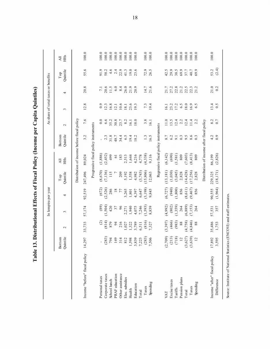
In order to determine how sensitive our results are to the choice of consumption per capita as the classifying variable, we duplicated the analysis using income per capita to classify households (Table 13). As we would expect, the range across quintiles in household income is much larger when households are classified by income per capita than it is when households are classified by consumption per capita. In Table 13, the share of income accruing to the top (bottom) quintile is 55.6 percent (3.2 percent), rather than 44.7 percent (7.1), and the Gini coefficient for income before fiscal policy is 0.69 rather than 0.64 using consumption per capita to classify households. The corollary to this result is that the range in consumption is narrower (Table 2). The share of consumption by the top (bottom) quintile is 38.2 percent (9.6 percent) with income per capita as the classifying variable, rather than 43.4 percent (6.6 percent) with consumption per capita as the classifying variable. As a result, the income tax—a fiscal policy instrument that keys off income—appears more progressive, while those instruments that key off consumption—the VAT being the most

Tab

le 1

3. D

istr

ibut

iona

l Eff

ects

of F

isca

l Pol

icy

(Inc

ome

per

Cap

ita Q

uint

iles)

In le

mpi

ra p

er y

ear

As s

hare

of t

otal

taxe

s or b

enef

its

Bott

om

Qui

ntile

23

4T

op

Qui

ntile

All

HH

sBo

ttom

Q

uint

ile2

34

Top

Q

uint

ileA

ll H

Hs

Dist

ribut

ion

of in

com

e be

fore

fisc

al p

olic

y

Inco

me

"bef

ore"

fisc

al p

olic

y14

,297

33

,733

57

,174

92

,519

24

7,49

6

89,0

24

3.2

7.

6

12.8

20.8

55

.6

100.

0

Prog

ress

ive

fisca

l pol

icy

inst

rum

ents

Pers

onal

taxe

s-

(2

)

(89)

(6

72)

(8,6

70)

(1

,886

)

-

0.0

0.

9

7.1

91

.9

100.

0

Co

rpor

ate

taxe

s(2

83)

(814

)

(1

,504

)

(2,5

26)

(7

,136

)

(2,4

52)

2.

3

6.6

12

.3

20

.6

58.2

10

0.0

Scho

ol lu

nch

794

879

420

286

11

5

499

31

.8

35

.2

16

.8

11

.5

4.6

10

0.0

PRA

F ed

ucat

ion

149

94

37

18

7

61

48

.7

30

.8

12

.1

6.

0

2.4

10

0.0

Oth

er a

ssist

ance

314

216

96

77

20

9

183

34

.4

23

.7

10

.6

8.

4

22.9

10

0.0

Elec

. sub

sidie

s81

2

1,

027

2,

271

3,

265

5,19

2

2,

513

6.5

8.

2

18.1

26.0

41

.3

100.

0

H

ealth

1,59

8

1,32

2

1,94

0

1,80

1

1,

558

1,64

4

19

.4

16

.1

23

.6

21

.9

19.0

10

0.0

Educ

atio

n3,

839

3,

789

4,

075

4,

397

4,98

2

4,

216

18.2

18.0

19.3

20.9

23

.6

100.

0

T

otal

7,22

3

6,51

1

7,24

6

6,64

7

(3

,743

)

4,77

8

T

axes

(283

)

(8

16)

(1,5

93)

(3

,198

)

(15,

806)

(4

,338

)

1.3

3.

8

7.3

14

.7

72.9

10

0.0

Spen

ding

7,50

6

7,32

7

8,83

9

9,84

5

12

,063

9,

116

16.5

16.1

19.4

21.6

26

.5

100.

0

Regr

essiv

e fis

cal p

olic

y in

stru

men

ts

VAT

(2,7

09)

(3

,397

)

(4,9

92)

(6

,727

)

(13,

181)

(6

,142

)

8.7

11

.0

16

.1

21

.7

42.5

10

0.0

Exci

se ta

xes

(213

)

(4

66)

(802

)

(9

40)

(1,0

30)

(6

90)

6.2

13

.5

23

.2

27

.2

29.9

10

0.0

Tar

iffs

(718

)

(9

83)

(1,3

59)

(1

,800

)

(3,0

45)

(1

,581

)

9.1

12

.4

17

.2

22

.8

38.5

10

0.0

Pens

ion

plan

s12

88

26

4

85

6

2,82

8

80

9

0.3

2.

2

6.5

21

.2

69.9

10

0.0

Tot

al(3

,627

)

(4,7

58)

(6

,889

)

(8,6

11)

(1

4,42

8)

(7,6

03)

9.

5

12.4

18.0

22.5

37

.7

100.

0

T

axes

(3,6

39)

(4

,846

)

(7,1

53)

(9

,467

)

(17,

256)

(8

,413

)

8.6

11

.4

16

.9

22

.3

40.7

10

0.0

Spen

ding

12

88

264

856

2,

828

809

0.

3

2.2

6.

5

21.2

69

.9

100.

0

Dist

ribut

ion

of in

com

e af

ter f

iscal

pol

icy

Inco

me

"aft

er"

fisca

l pol

icy

17,8

92

35,4

86

57,5

31

90,5

55

229,

325

86

,199

4.

2

8.2

13

.4

21

.0

53.2

10

0.0

Diff

eren

ce3,

595

1,

753

35

7

(1

,964

)

(18,

171)

(2

,826

)

0.9

0.

7

0.5

0.

2

(2.4

)

Sour

ce: I

nstit

ute

of N

atio

nal S

tatis

tics (

ENCO

VI) a

nd st

aff e

stim

ates

.

18

19

important—appear less progressive. In fact, when income per capita is used as the classifying variable, the VAT appears slightly regressive, whereas when households are classified according to consumption per capita, the VAT appears slightly progressive.

In absolute terms, fiscal policy appears slightly more progressive when households are classified according to income per capita. The average income in the bottom quintile is increased by one-third more in absolute terms, and the income in the top quintile is decreased by 12 percent less. The reduction in the Gini coefficient between income before and income after fiscal policy is also slightly larger in absolute terms (but smaller in percentage terms) when households are classified by income per capita. However, the qualitative results are identical. If we look at the effect of the classifying variable on tax and benefit rates, the effect of the shift from consumption per capita to income per capita appears much larger. However, this is largely an artifact of the effect on the denominator of the tax rate, rather than the numerator.

Figure 3. Effect of Changing Classifying Variable on Means

(75.3)

(32.2)

(18.4)

(6.8)

21.6

37.8

12.06.2

(1.5)(12.7)

-100

-80

-60

-40

-20

0

20

40

60


Percentage change in average consumption

Percentage change in average income


This point is demonstrated in Figure 3, which displays the effect of changing from consumption per capita to income per capita on the quintile estimates of average income and consumption. The percentage changes are measured relative to the average of the respective means for each classifying variable. The effects on the estimated means for income are far greater than they are for consumption. This, in turn, creates a serious bias on estimated tax and benefit rates. Although the aggregate absolute effect of fiscal policy on the bottom quintile is only one third larger when households are classified by income, the shift to income per capita from consumption per capita triples the estimated net benefit rate from 8.5 percent to 25.1 percent, because the denominator falls by 54 percent. We believe this fall in the denominator stems from two sources—measurement error and transitory reductions in income—and the denominator using income per capita as the classifying variable is a flawed measure of welfare, both absolutely and in comparison to classifying by consumption per capita.

20

REFERENCES

Arulampalam, Wiji, Michael Devereux, and Giorgia Maffini, 2007, “The Incidence of Corporate Income Tax on Wages,” mimeo.

Auerbach, Alan, 2005, “Who Bears the Corporate Tax? A Review of What We Know,” NBER Working Paper 11686, (Cambridge: National Bureau of Economic Research).

Camdessus, Michel, 1999, “Foreward,” in Economic Policy & Equity, ed. by Vito Tanzi, Ke-Young Chu and Sanjeev Gupta, (Washington: International Monetary Fund), pp. v-viii.

Deaton, Angus, 1997, The Analysis Of Household Surveys: A Microeconometric Approach To Development Policy, (Baltimore and London: Johns Hopkins University Press for the World Bank).

Harberger, Arnold, 2006, “Corporate Tax Incidence: Reflections on What is Known, Unknown and Unknowable,” mimeo, University of California, Los Angeles.

Randolph, William, 2006, “International Burdens of the Corporate Income Tax,” Working Paper 2006–09, (Washington: Congressional Budget Office).

World Bank, 2006, Honduras Poverty Assessment: Attaining Poverty Reduction, Report No. 35622-HN, (Washington: World Bank).

———, 2007, Honduras: Public Expenditure Review, Volume II, Report No. 39251-HO (Green Cover Draft), (Washington: World Bank).

Documents

The Distributional Impact of Fiscal Policy in Honduras