The crustal thickness of West Antarctica

The crustal thickness of West AntarcticaJ. Chaput,1 R. C. Aster,2,3 A. Huerta,4 X. Sun,5,6 A. Lloyd,5 D. Wiens,5 A. Nyblade,7S. Anandakrishnan,7 J. P. Winberry,4 and T. Wilson8

Received 30 August 2013; revised 25 November 2013; accepted 26 November 2013.

[1] P-to-S receiver functions (PRFs) from the Polar Earth Observing Network(POLENET) GPS and seismic leg of POLENET spanning West Antarctica and theTransantarctic Mountains deployment of seismographic stations provide new estimates ofcrustal thickness across West Antarctica, including the West Antarctic Rift System(WARS), Marie Byrd Land (MBL) dome, and the Transantarctic Mountains (TAM)margin. We show that complications arising from ice sheet multiples can be effectivelymanaged and further information concerning low-velocity subglacial sediment thicknessmay be determined, via top-down utilization of synthetic receiver function models. Wecombine shallow structure constraints with the response of deeper layers using aregularized Markov chain Monte Carlo methodology to constrain bulk crustal properties.Crustal thickness estimates range from 17.0˙ 4 km at Fishtail Point in the westernWARS to 45˙ 5 km at Lonewolf Nunataks in the TAM. Symmetric regions of crustalthinning observed in a transect deployment across the West Antarctic Ice Sheet correlatewith deep subice basins, consistent with pure shear crustal necking under past localizedextension. Subglacial sediment deposit thicknesses generally correlate with trough/domeexpectations, with the thickest inferred subice low-velocity sediment estimated as � 0.4km within the Bentley Subglacial Trench. Inverted PRFs from this study and otherpublished crustal estimates are combined with ambient noise surface wave constraints togenerate a crustal thickness map for West Antarctica south of 75ıS. Observations areconsistent with isostatic crustal compensation across the central WARS but indicatesignificant mantle compensation across the TAM, Ellsworth Block, MBL dome, andeastern and western sectors of thinnest WARS crust, consistent with low density andlikely dynamic, low-viscosity high-temperature mantle.Citation: Chaput, J., R. C. Aster, A. Huerta, X. Sun, A. Lloyd, D. Wiens, A. Nyblade, S. Anandakrishnan, J. P. Winberry, andT. Wilson (2014), The crustal thickness of West Antarctica, J. Geophys. Res. Solid Earth, 119, doi:10.1002/2013JB010642.

1. Introduction1.1. The West Antarctic Rift System

[2] The West Antarctic Rift System (WARS; Figure 1)is a broad extended region, comparable in scale to the

Additional supporting information may be found in the online versionof this article.

1ISTERRE, Université Joseph Fourier, Grenoble, France.2Department of Earth and Environmental Science, New Mexico Insti-

tute of Mining and Technology, Socorro, New Mexico, USA.3Geosciences Department, Colorado State University, Fort Collins,

Colorado, USA.4Department of Geological Sciences, Central Washington University,

Ellensburg, Washington, USA.5Department of Earth and Planetary Sciences, Washington University,

St. Louis, Missouri, USA.6State Key Laboratory of Isotope Geochemistry, Guangzhou Institute

of Geochemistry, Chinese Academy of Sciences, Guangzhou, China.7Department of Geosciences, Pennsylvania State University, University

Park, Pennsylvania, USA.8School of Earth Sciences, Ohio State University, Columbus, Ohio,

USA.

Corresponding author: J. Chaput, ISTERRE, Université Joseph Fourier,Grenoble I, BP 53, 38041 Grenoble CEDEX 9, France. ([email protected])

©2013. American Geophysical Union. All Rights Reserved.2169-9313/14/10.1002/2013JB010642

western North American Basin and Range province [e.g.,Behrendt, 1999]. The WARS is distinguished amongEarth’s continental rift systems in being associated withlow intraplate rates of deformation [Wilson et al., 2011],low seismicity [Winberry and Anandakrishnan, 2003;Reading, 2007], generally low subice elevations (e.g.,hundreds of meters above sea level after accounting forice sheet loading [Wilson and Luyendyk, 2009]), thin crust[Winberry and Anandakrishnan, 2004], low-viscosity man-tle [Wiens et al., 2012], and (at least in some regions)high heat flow in excess of 120 mW/m2 [Clow et al.,2012], all of which significantly influence West AntarcticIce Sheet (WAIS) dynamics and history [Pollard et al.,2005]. To better understand these aspects of West Antarctictectonics and their contributions to ice sheet processes,the POLENET-ANET project (the West Antarctic andTransantarctic Mountains portion of the Polar Earth Observ-ing Network), funded as part of the International PolarYear (IPY), deployed a seismographic and geodetic net-work of unprecedented duration and scale across theWAIS/Transantarctic Mountains (TAM) region. A notablefeature of the WARS is the presence of the extraordinar-ily deep ice-filled grabens of the Byrd Subglacial Basin andBentley Subglacial Trough (the lowest points on Earth’s

1

JOURNAL OF GEOPHYSICAL RESEARCH: SOLID EARTH, VOL. 119, 1–18, doi:10.1002/2013JB010642, 2014

CHAPUT ET AL.: CRUSTAL THICKNESS OF WEST ANTARCTICA

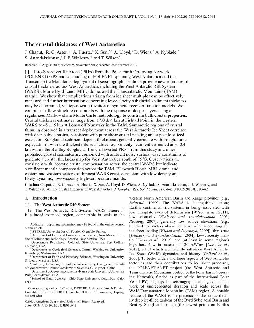
Figure 1. (a) Principal geographic features of West Antarctica, shown atop BEDMAP2 subglacialtopography [Fretwell et al., 2013], with the approximate Antarctic coast delineated. Grid easting and nor-thing coordinates are kilometers relative to South Pole. (b) POLENET-ANET station locations through2012. Fishtail Point (FISH) and Lonewolf Nunatak (LONW), as noted in the abstract, are located on eitherside of the Transantarctic Mountains. Other station name/location associations can be found in Table 1.

continental surface), with subglacial surface elevations aslow as 2500 m below sea level. This contrasts notably withthe East African and Basin and Range provinces, wherebuoyant warm mantle uplift results in mean elevations thatare 1–2 km higher. With the exception of the relativelycool Baikal rift [Liu and Gao, 2006; Tiberi et al., 2003;ten Brink and Taylor, 2002; Cooper et al., 1987, 1995], con-tinental rift provinces do not reside at such low elevationsexcept at margins characterized by much greater crustal thin-ning and/or proximity to recently emerged oceanic spreadingcenters and oceanic crust (e.g., Gulf of California or Afar;McClusky et al. [2010]). The highest elevations (aboveapproximately 2500 m) are restricted to the boundaries ofthe rift system, Transantarctic Mountains (TAM), EllsworthMountains, Whitmore Mountains, and the Marie Byrd Land(MBL) dome, including the Holocene volcanically activeExecutive Committee and Flood Ranges and outlying vol-canoes to the east. These trachytic shield volcanoes sitatop occupy an uplifted and faulted basement of alkalinebasaltic rocks and have erupted basaltic lavas similar tooceanic island basalts sampled in known mantle plumesystems [LeMasurier and Rex, 1989; LeMasurier, 2008].Multiple studies indicate that elements of this magmaticand volcanic system are presently and/or have been veryrecently active [e.g., Blankenship et al., 1992; Lough etal., 2013]. Although the nonglacial seismicity of the con-tinental interior is remarkably low, it is detectable withregional seismographs, and recent improvements in monitor-ing have identified events interpreted as both due to faulting[Winberry and Anandakrishnan, 2003] and magmatism[Lough et al., 2013]. Unraveling the tectonic structure andhistory of the WARS is complicated due to the vast WestAntarctic Ice Sheet (WAIS) that covers much of the region,obscuring direct access to underlying bedrock. The generalstability of the WAIS and linkages between the evolutionof the ice sheet and underlying rift system and adjacentTransantarctic mountains have long been recognized as

being of fundamental importance to understanding AntarcticIce Sheet evolution [e.g., Wilch et al., 1993; Wilch andMcIntosh, 2000; Pollard and DeConto, 2009].

1.2. Seismic Constraints on Crustal Thicknessin West Antarctica

[3] Much of our understanding of the WARS and its tec-tonic relationship to surrounding regions is derived fromseismological data. The Transantarctic Mountains (TAM)constitute one of Earth’s most significant intracontinen-tal tectonic transitions, broadly delineating the boundarybetween fast upper mantle and thick crust within the EastAntarctic Craton (EAC) and the slower upper mantle andthin crust of the West Antarctic Rift System (WARS)[Sieminski et al., 2003; Danesi and Morelli, 2001; Ritzwolleret al., 2001; Morelli and Danesi, 2004; Wiens et al., 2012].In association with gravity studies of the TAM, prior seismicstudies have revealed crustal thickness of as low as 20˙2 kmfor parts of the WARS [Bannister et al., 2000].

[4] The TAMSEIS (TransAntarctic Mountains SeismicExperiment) experiment [Reusch et al., 2008; Watson et al.,2006] was a pioneering network of broadband seismo-graphs in Antarctica. TAMSEIS crossed the TAM boundaryinto the EAC to characterize the WARS/EAC transitionin the vicinity of McMurdo Sound, revealing low litho-spheric and upper mantle velocity structure beneath RossIsland and extending 50–100 km beneath the TAM. Jointreceiver function, phase velocity, and gravity analysis usingTAMSEIS data [Lawrence et al., 2006] yielded crustalthickness estimates of �20 km below Ross Island to a max-imum of �40 km below the crest of the TAM, with EACcrustal thicknesses �35 km. Also identified in this studywas the presence of only a thin (�5 km) buoyant crustalTAM root, indicating that topography in this region is sub-stantially gravitationally compensated by buoyant mantle.However, while seismic studies to date have mapped outsections of the WARS crustal and upper mantle structures

2


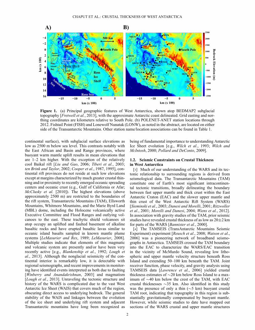
Figure 2. (a) Synthetic reflectivity forward modeled PRF waveforms showing characteristic ice sheetand sedimentary basin features. The models feature a 2.5 km thick ice sheet (Vp = 3.87 km/s; Poisson’sratio � = 0.33), a 1 km thick sedimentary basin (Vp of 0.9 km/s; � = 0.25), a 30 km thick crust, and anincident wave with a slowness 0.05 s/km. Because of the large seismic impedance contrast between theice sheet and underlying crustal structure, and low ice sheet seismic attenuation, note that reverberationswithin the ice sheet commonly completely obscure Moho-associated phases used to determine crustalthickness. (b) Top-down fitting process for inversion priors at station BYRD. Note the great improvementbrought to the fit in the later portion of the PRF by the addition of a simple crustal structure.

[Lawrence et al., 2006; Winberry and Anandakrishnan,2004; Anandakrishnan and Winberry, 2004], these studieshave necessarily focused on geographically limited targetssuch as the TAM East-West Antarctica transition, necessitat-ing a larger effort incorporating a more spatially extensivenetwork of seismographs to produce continent-scale struc-tural models that can be applied to better understand WARStectonics and to inform WAIS modeling efforts. This motiva-tion produced the POLENET-ANET project, funded as partof the International Polar Year (IPY), which has deployed aseismographic and geodetic network of unprecedented dura-tion and scale across the WAIS/TAM region [e.g., Wienset al., 2013].

1.3. Seismic Methodologies1.3.1. Receiver Functions and Forward Modeling

[5] P-to-S receiver function (PRF) and S-to-P receiverfunction (SRF) studies provide robust methodologies fordetecting seismic impedance contrasts and have been widelyand successfully used to constrain crustal and mantle dis-continuity structures. The advantage of this approach lies inits ability to enhance converted phases (P-to-S in the case ofPRFs and S-to-P in the case of SRFs) and allows for sim-ple interpretation in light of the zero phase output inherentto deconvolution process. The deconvolution step, where thevertical component of the seismogram is deconvolved fromthe radial component of the seismogram (for PRFs), is anill-posed problem that is inherently unstable and/or noisy.Because of this, a variety of time- and frequency-domainapproaches [Park and Levin, 2000; Bostock, 2004] havebeen applied to regularize the receiver function solution.

[6] Receiver function analysis for constraining crustalthickness has recently been performed for portions of theEast Antarctic craton [Reading, 2006], for the TAM throughTAMSEIS [Lawrence et al., 2006; Hansen et al., 2009], andfor the Gamburtsev region AGAP projects (composed of

GAMBIT (aerial geophysical survey) and GAMSEIS (seis-mic) with a focus on the Gamburtsev subglacial Mountains).[Hansen et al., 2010]. However, receiver functions acquiredover complex low-velocity shallow structures, such as icesheets and sedimentary basins, can be very difficult to inter-pret via the most straightforward means (i.e., the h-k stackingmethod of Zhou and Kanamori [2000] and common con-version point stacking imaging) because of strong P wavemultiples that mask P-S Moho and other key seismic phaseconversions [e.g., Wilson and Aster, 2005]. In particular, athick ice sheet generates strong and slowly attenuating Pmultiples that mask deeper P-S conversions, including con-versions from the Moho that are key to estimating crustalthickness. One potential approach is to deconvolve an icesheet response signal [Cho, 2011], but the complexity of theinteractions between the various layers limits its robustness.

[7] Receiver function studies in West Antarctica aresparse and have previously been limited to a few small-scale or very sparse deployments, notably the pioneeringANUBIS (Antarctic Network of Broadband Seismometers)array and the Ross Sea component of the TAMSEIS array.Thick ice sheet coverage, typical for most of Antarctica,can result in the complete masking of conventionally inter-preted phases in PRFs. SRFs tend to be less sensitive to theseeffects in theory but also have lower frequency content andpresent smaller data sets (due to poor signal to noise ratioson the incoming S waves and a more restrictive teleseismicdistance range). To complicate matters further, West Antarc-tica hosts a number of deep subglacial troughs [Karner et al.,2005; Bell et al., 1998], which may contain low-velocity sed-iment deposits, thus further obscuring the PRF signatures. Toextract meaningful information from PRFs over ice sheets,ANUBIS efforts focused on fitting PRF signatures with asimple grid searched forward model solution [Winberry andAnandakrishnan, 2004, 2003], thus yielding rough estimatesof both crustal thickness and, in some cases, subglacial

3


sediment characteristics. An example of this approach, aswell as the impact of ice and sediments on the PRF signature,is shown in Figure 2.

[8] For this approach to be successful, very accurate mea-surements of the ice thicknesses are required (for ANUBIS,these values were obtained through drilling and previ-ous reflection surveys). The resulting crustal models mayyield reasonable waveform fits, but due to their inherentsimplicity, uncertainty estimates will be high. The backboneportion of the POLENET-ANET deployment is composed ofstations deployed on nunataks, mountain crests, and coastallocations, and consequently, many of these stations presentchallenging local asymmetric subaerial or subice topogra-phy variations that can affect receiver functions. In suchcases, evaluating the Moho depth and Vp/Vs ratio via multi-ple fitting [Zhou and Kanamori, 2000] from a simple crustalmodel typically does not yield convergent results due to mul-tiple early peaks. It is therefore preferable to attempt to fit amore complex crustal structure to the PRFs.1.3.2. Markov Chain Monte Carlo Inversionand Surface Wave Constraints

[9] Markov chain Monte Carlo (MCMC) algorithms[Mosegaard and Tarantola, 1995; Aster et al., 2012, pp. 270]have recently gained traction in receiver function stud-ies [Bodin et al., 2012; Agostinetti and Malinverno, 2010;Seiberlich et al., 2013] and many other areas of inversegeophysics problems due to their broad applicability totractably solving Bayesian inverse problems. The MCMCapproach samples the posterior distribution of the modelspace, thus facilitating nonparametric probabilistic modelestimates. This method also offers the advantage of a linearincrease in computation time with the number of parameters,and only the forward problem must be (repeatedly) solved toproduce samples of the Bayesian posterior distribution. Thealgorithm explores the model space in a directed randomwalk fashion typical of Monte Carlo algorithms but with anadded “acceptance criterion” at every step, which allows itto accept or reject the current model iteration based on a pre-chosen probability distribution. Model iterations that resultin a reduction of data misfit are more likely to be sampled,but the acceptance criterion algorithm permits model stepsresulting in higher misfits to be included in the samplingprocess, thus allowing for exploration outside of any localminimum.

[10] One of the primary difficulties with inverting wave-forms generated from ice stations lies in fitting the ampli-tudes of the ice signature. Given the large amplitudes ofthese multiples, models may easily evolve toward unrealis-tic alternating low-/high-velocity layering. To penalize suchmodel structure, it is possible regularize the MCMC inver-sion by adding a Total Variation (TV) seminorm term tothe objective function [e.g., Aster et al., 2012, pp. 186] tofavor models with small numbers of discontinuities. Giventhe boundaries set by the prior models, large positive jumpsare less unaffected overall, thus improving the likelihood ofresolving a distinct Moho estimate. The TV regularizationmodel seminorm is

TV(m) =n–1X

i=1

|mi+1 – mi| = kLmk1 (1)

where m is the current model, L is the first-order roughen-ing matrix, and the subscript 1 indicates the one norm. The

objective function calculated at every forward model itera-tion then becomes a weighted sum of the misfit and the TVregularization seminorm

Mi = kGm – dk22 + ˛kLmk1 (2)

where ˛ is an empirically determined weighting factor that,as it increases, favors positive over negative velocity jumpsat the cost of data fit.

[11] Receiver functions tend to be sensitive to velocitydiscontinuities at layer interfaces and not to the absolutevelocities of those layers. Given that surface waves are sen-sitive to absolute velocities and not impedance contrasts, ithas been shown [Shen et al., 2012; Liu et al., 2010] thatthe joint inversion of surface waves and receiver functionscan greatly improve the accuracy of inverted model esti-mates. Alternatively, surface wave tomography models canbe combined with discrete crustal thickness measurementsto produce smoothed crustal thickness maps [Assumpcao etal., 2013]. The latter option employed here has the advan-tage of being able to appropriately weight one model or theother based on error estimates and can be smoothed accord-ing to an arbitrary regularization coefficient to optimize datafit versus functional complexity.

[12] We present the results of iterative forward model-ing as described above to obtain simple ice/sediment/crustmodels. We then apply these interim results as prior infor-mation for Bayesian MCMC inversions to determine crustalthickness. We show that this two-step process results in atighter waveform fit, as well as accounting for crustal com-plexity where necessary. We then generate and describea crustal thickness map of West Antarctica that combinesour new determinations, previously published seismic con-straints, and concurrent efforts in continent-scale ambientnoise surface wave crustal thickness modeling.

2. Crustal Structure of West AntarcticaFrom Receiver Function Methods2.1. New Seismic Data

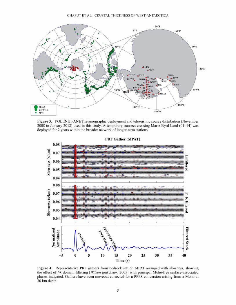
[13] Recent instrumentation development and generalsupport by the Incorporated Research Institutions for Seis-mology (IRIS) Consortium [Parker et al., 2011] has pro-duced high-reliability stations for the Antarctic environment,and only a single station (KOLR) proved to be unusablein this study due to instrumentation problems. We used alldata for the presently available POLENET-ANET data set,encompassing both its backbone (2008–2012) and tempo-rary transect (Marie Byrd Land crossing; stations 01–14;2010–2012) components. Figure 3 shows stations and thedistribution of teleseismic earthquake sources utilized inthis study. Approximately 1300 events from 30 to 90ıdistance were examined, with the transect stations record-ing approximately 50% of that number due to a shorterdeployment period.

2.2. Receiver Function Computationand Forward Modeling

[14] We compute PRFs by applying a multitaper decon-volution approach [Helffrich, 2006; Park and Levin, 2000],which provides the advantage of low spectral leakage andprecludes the necessity of searching over any regularization

4


Figure 3. POLENET-ANET seismographic deployment and teleseismic source distribution (November2008 to January 2012) used in this study. A temporary transect crossing Marie Byrd Land (01–14) wasdeployed for 2 years within the broader network of longer-term stations.

Figure 4. Representative PRF gathers from bedrock station MPAT arranged with slowness, showingthe effect of f-k domain filtering [Wilson and Aster, 2005] with principal Moho/free surface-associatedphases indicated. Gathers have been moveout corrected for a PPPS conversion arising from a Moho at30 km depth.

5


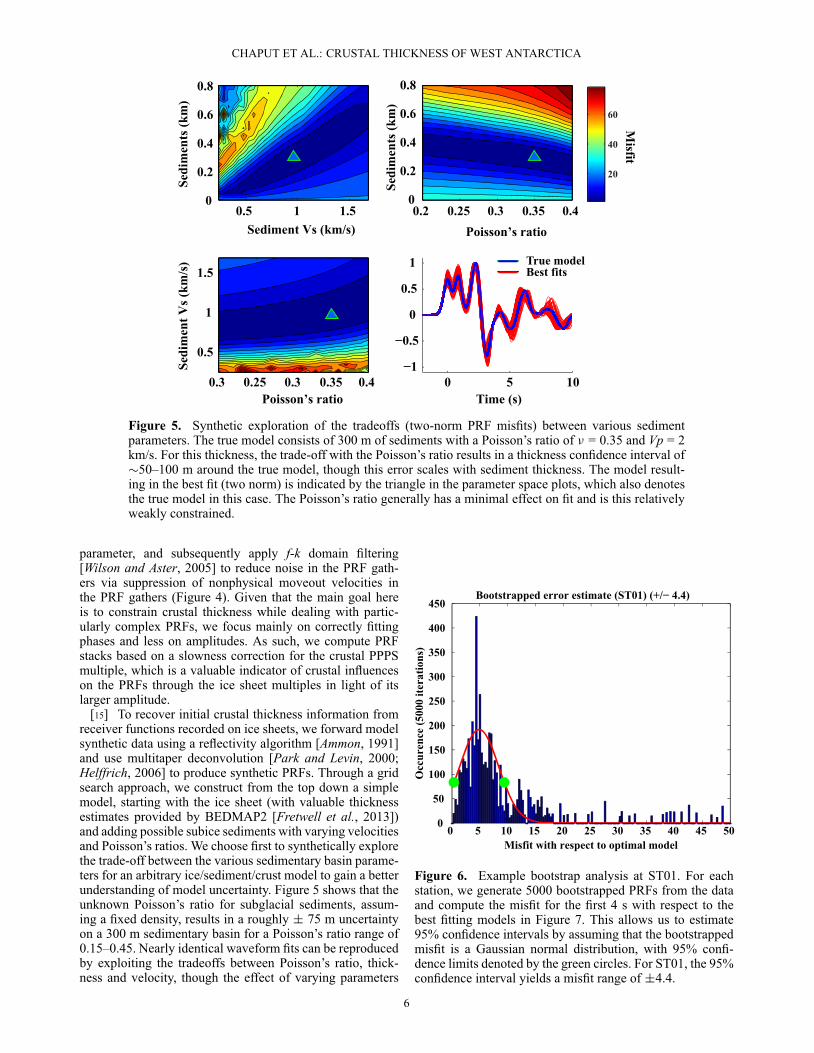
Figure 5. Synthetic exploration of the tradeoffs (two-norm PRF misfits) between various sedimentparameters. The true model consists of 300 m of sediments with a Poisson’s ratio of � = 0.35 and Vp = 2km/s. For this thickness, the trade-off with the Poisson’s ratio results in a thickness confidence interval of�50–100 m around the true model, though this error scales with sediment thickness. The model result-ing in the best fit (two norm) is indicated by the triangle in the parameter space plots, which also denotesthe true model in this case. The Poisson’s ratio generally has a minimal effect on fit and is this relativelyweakly constrained.

parameter, and subsequently apply f-k domain filtering[Wilson and Aster, 2005] to reduce noise in the PRF gath-ers via suppression of nonphysical moveout velocities inthe PRF gathers (Figure 4). Given that the main goal hereis to constrain crustal thickness while dealing with partic-ularly complex PRFs, we focus mainly on correctly fittingphases and less on amplitudes. As such, we compute PRFstacks based on a slowness correction for the crustal PPPSmultiple, which is a valuable indicator of crustal influenceson the PRFs through the ice sheet multiples in light of itslarger amplitude.

[15] To recover initial crustal thickness information fromreceiver functions recorded on ice sheets, we forward modelsynthetic data using a reflectivity algorithm [Ammon, 1991]and use multitaper deconvolution [Park and Levin, 2000;Helffrich, 2006] to produce synthetic PRFs. Through a gridsearch approach, we construct from the top down a simplemodel, starting with the ice sheet (with valuable thicknessestimates provided by BEDMAP2 [Fretwell et al., 2013])and adding possible subice sediments with varying velocitiesand Poisson’s ratios. We choose first to synthetically explorethe trade-off between the various sedimentary basin parame-ters for an arbitrary ice/sediment/crust model to gain a betterunderstanding of model uncertainty. Figure 5 shows that theunknown Poisson’s ratio for subglacial sediments, assum-ing a fixed density, results in a roughly ˙ 75 m uncertaintyon a 300 m sedimentary basin for a Poisson’s ratio range of0.15–0.45. Nearly identical waveform fits can be reproducedby exploiting the tradeoffs between Poisson’s ratio, thick-ness and velocity, though the effect of varying parameters

Figure 6. Example bootstrap analysis at ST01. For eachstation, we generate 5000 bootstrapped PRFs from the dataand compute the misfit for the first 4 s with respect to thebest fitting models in Figure 7. This allows us to estimate95% confidence intervals by assuming that the bootstrappedmisfit is a Gaussian normal distribution, with 95% confi-dence limits denoted by the green circles. For ST01, the 95%confidence interval yields a misfit range of ˙4.4.

6


scales with sediment thickness. Ultimately, the thickness,and velocity parameters are well recovered, but a variation inthe Poisson’s ratio has a minimal effect for such thin layers.

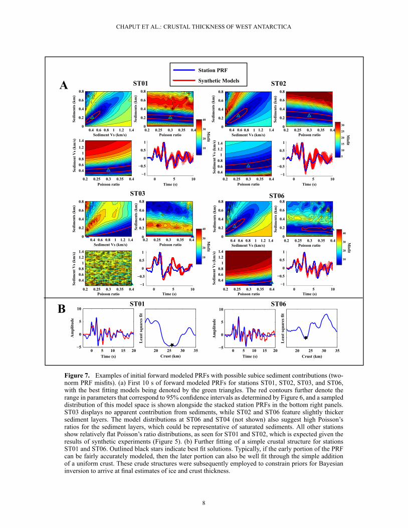
[16] Figure 7a shows examples of the grid search forwardmodeling approach, where we searched across sedimentthickness, sediment velocity, and sediment Poisson’s ratio.A distribution of the models within a 95% confidence inter-val is also shown. Given the typically lower velocity of thesediments with respect to the ice sheet, the uncertainty fromthe ice sheet will result in a comparatively smaller error onthe sedimentary basin thickness, with uncertainties in icethickness propagating into the sediment estimates roughlydivided by the ratio of inferred ice/sediment velocities.This error is (conservatively) summed along into a roughly95% confidence ellipse determined via forward model gridsearch, and we estimate the ellipse by bootstrapping theobserved station PRFs to produce a pseudo-normal distribu-tion of misfit with respect to the best fitting synthetic solutioncomputed from the PRF stacks shown in Figure 7. An exam-ple of this for station ST01 is displayed in Figure 6. Modelfitness is ultimately determined by a least squares mini-mization between synthetic and observed PRFs using thefirst 4 s.

[17] During forward modeling, we allowed Vp for subicesediments to range from 0.5 to 3 km/s, while fixingthe subice sheet sediment density to � = 2.4 g/cm3 [e.g.,Studinger et al., 2004]. We seek the simplest physically plau-sible models necessary to fit the waveforms, though varia-tions in the sediment densities are likely. Ice velocity wasfixed at 3.87 km/s with � = 0.33, based on studies of P wavevelocity in glacial ice of various temperatures [Kohnen,1974]. It should be noted that the root-mean-square velocityfor thinner ice sheets may vary due to the presence of low-velocity firn layers, which may add additional uncertainty toice and sediment estimates for shallower ice sheet sites, butis not incorporated here.

[18] After an initial fit was obtained for the shallow struc-ture, we appended a uniform crust to the model, settingcrustal Vp to a nominal value of 6.3 km/s and fixing � at 0.27,and evaluated the fit for the first 25 s of the computed PRF.Figure 7b shows examples of crustal-scale forward model-ing fits, along with curves showing the best parameter fits.Following this final forward modeling step, we next usedthese rough estimates in constraining priors in a Bayesianinversion of PRFs for structure, as described below.

2.3. Additional Modeling Considerations[19] Difficulties in modeling the delay of the P-S con-

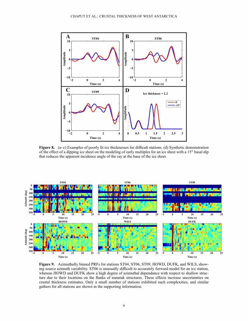
version from the base of the ice sheet relative to the laterPPPS from within the ice sheet were still encountered fora few stations within the Marie Byrd Land transect (ST04,ST06, ST09, SIPL). Possible explanations include seismicanisotropy in the ice sheet [Bentley, 1971] or variable basaldip. Basal dip can also produce substantial timing differ-ences between the predicted ice sheet multiples for a giventhickness and the computed PRFs. Failure to correctly modelthe earliest portion of the PRFs could propagate into poorcrustal fits during the subsequent grid search, and an inad-equately modeled ice sheet may furthermore force laterinversion steps to attempt to compensate for this problemby generating rough or nonphysical models (e.g., highlyoscillatory models featuring large amplitude alternating low-

and high-velocity zones). The Fresnel zone width for ateleseismic body wave at the base of a 3 km ice sheetis on the order of 4 to 10 km [e.g., Lindsay, 1989] sosmaller spatial wavelength bed gradient features not neces-sarily visible in BEDMAP2 subice topography could explainsome unusual stations. Stations deployed on nunataks alsotypically yielded less well constrained results attributableto extreme topography and possible steeply dipping com-plex shallow structure, resulting in multiple early peaksand highly oscillatory PRFs (e.g., PECA, HOWD, WILS,DUFK, MECK). This suggests that crustal to mantle-scalestructural studies in Antarctica are probably generally betterfacilitated by ice-sited stations than by stations deployed onisolated bedrock features. Such bedrock outcrops can alsofeature significantly greater wind noise and attendant sus-ceptibility to environmental damage due to their topographicprominence [Anthony, 2013]. Figure 8 displays examplesof poorly fitted early portions of PRFs and the impact onmultiples for varying degrees of basal dip. An ice sheet pre-senting a basal dip that decreases the apparent incidenceangle of the ray with respect to the ice sheet will result ina slightly delayed PS conversion from the ice sheet and amuch earlier PPPS multiple, thus potentially accounting forthe mismatch in the modeled ice sheet and masquerading as asediment layer.

[20] We can explore for consistent data features associ-ated with simple anisotropy or basal dip by examining PRFgathers arranged by event back azimuth. Figure 9 showsazimuthally binned gathers for a few stations for which asimple ice/sediment/crust model was insufficient. For exam-ple, later multiples at ST04 show substantial azimuthaldependence, suggesting some degree of geometrical com-plexity to the ice sheet, though the early multiple seemrelatively unaffected. We noted some cases (ST04, ST06where solely the first P-S conversion from the base of the icesheet is mismatched even though the general character of thelater multiples can be described fairly well through a verysimple ice/sediment/crust model).

[21] Although we do not implement a methodology hereto model dipping layer PRFs, or better yet, finite differencemodeling of the ice-rock interface, future studies utiliz-ing PRFs over ice sheets should explore basal topographyeffects. We note that a small basal dip can account for muchof the delay in the ice sheet PPPS and that there is a trade-offwith inferred low-velocity subice (e.g., sedimentary basin)structure, although the effect on the PS phase is opposite.One must therefore be cautious when simply fitting the PPPSfrom the ice sheet to infer the presence of a sedimentarybasin if the early waveform fit is poor, even if the ice thick-ness is well constrained, if there is a good deal of azimuthalvariation on the timings of the early PRFs. Where the earlyfit is very good, however, or the later multiples can easilybe matched by a simple crustal model, a sedimentary basinis more likely to be resolvable, and we can ultimately usethis information to build a more robust prior for subsequentinversion, as described below.

2.4. Implementation of Markov ChainMonte Carlo Inversion

[22] In the implementation of the MCMC inversion, weassume a Poisson’s ratio of 0.27 for the crust and allowthe velocity of internal layers to vary freely as constrained

7


Figure 7. Examples of initial forward modeled PRFs with possible subice sediment contributions (two-norm PRF misfits). (a) First 10 s of forward modeled PRFs for stations ST01, ST02, ST03, and ST06,with the best fitting models being denoted by the green triangles. The red contours further denote therange in parameters that correspond to 95% confidence intervals as determined by Figure 6, and a sampleddistribution of this model space is shown alongside the stacked station PRFs in the bottom right panels.ST03 displays no apparent contribution from sediments, while ST02 and ST06 feature slightly thickersediment layers. The model distributions at ST06 and ST04 (not shown) also suggest high Poisson’sratios for the sediment layers, which could be representative of saturated sediments. All other stationsshow relatively flat Poisson’s ratio distributions, as seen for ST01 and ST02, which is expected given theresults of synthetic experiments (Figure 5). (b) Further fitting of a simple crustal structure for stationsST01 and ST06. Outlined black stars indicate best fit solutions. Typically, if the early portion of the PRFcan be fairly accurately modeled, then the later portion can also be well fit through the simple additionof a uniform crust. These crude structures were subsequently employed to constrain priors for Bayesianinversion to arrive at final estimates of ice and crust thickness.

8


Figure 8. (a–c) Examples of poorly fit ice thicknesses for difficult stations. (d) Synthetic demonstrationof the effect of a dipping ice sheet on the modeling of early multiples for an ice sheet with a 15ı basal dipthat reduces the apparent incidence angle of the ray at the base of the ice sheet.

Figure 9. Azimuthally binned PRFs for stations ST04, ST06, ST09, HOWD, DUFK, and WILS, show-ing source azimuth variability. ST06 is unusually difficult to accurately forward model for an ice station,whereas HOWD and DUFK show a high degree of azimuthal dependance with respect to shallow struc-ture due to their locations on the flanks of nunatak structures. These effects increase uncertainties oncrustal thickness estimates. Only a small number of stations exhibited such complexities, and similargathers for all stations are shown in the supporting information.

9


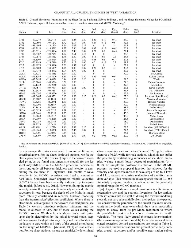
Table 1. Crustal Thickness (From Base of Ice Sheet for Ice Stations), Subice Sediment, and Ice Sheet Thickness Values for POLENET-ANET Stations (Figure 1), Determined by Receiver Function Analysis and MCMC Modelinga

Elev Ice �ice Sed �Sed Vs,Sed Moho �MohoStation Lat Lon (km) (km) (km) (km) (km) (km/s) (km) (km) Location

ST01 –83.2279 –98.7419 2.03 2.24 0.30 0.20 0.11 0.45 28.0 3 Ice sheetST02 –82.0690 –109.1243 1.72 2.14 0.09 0.27 0.12 0.61 32.1 2 Ice sheetST03 –81.4065 –113.1504 1.66 2.23 0.15 0 0 - 24.3 2 Ice sheetST04 –80.7150 –116.5782 1.52 2.96 0.09 0.35 0.12 0.62 20.8 3 Ice sheetST06 –79.3316 –121.8196 1.52 2.40 0.09 0.23 0.1 0.45 22.4 2 Ice sheetST07 –78.6387 –123.7953 1.59 2.61 0.15 0 0 - 23.6 3 Ice sheetST08 –77.9576 –125.5313 1.78 2.30 0.09 0.15 0.1 0.6 24.5 2 Ice sheetST09 –76.5309 –128.4734 2.25 2.14 0.20 0.45 0.6 0.78 29.6 2 Ice sheetST10 –75.8143 –129.7489 1.75 1.13 1.00 0.3 0.12 0.7 28.7 2 Ice sheetST12 –76.8970 –123.8160 2.20 1.92 1.00 0 0 - 22.1 2 Ice sheetST13 –77.5609 –130.5139 1.86 1.98 0.09 0.25 0.5 0.8 30.2 4 Ice sheetST14 –77.8378 –134.0802 1.64 1.73 0.09 0 0 - 27.2 2 Ice sheetCLRK –77.3231 –141.8485 1.04 0.00 - 0 0 - 30.0 2 Mt. ClarkeKOLR –76.1545 –120.7276 1.89 1.79 0.30 0.62 0.62 0.61 - - Kohler GlacierWNDY –82.3695 –119.4129 0.94 1.67 0.20 0 0 - 21.5 4 WindyFALL –85.3066 –143.6284 0.29 0.00 - 0 0 - 24.0 4 Fallone NunatakSILY –77.1332 –125.9660 2.09 0.00 - 0 0 - 32.8 2 Mt. SidleyDNTW –76.4571 –107.7804 1.04 2.11 0.09 0 0 - 23.1 2 Down ThwaitsWHIT –82.6823 –104.3867 1.29 0.00 - 0 0 - 31.5 3 Mt. WhitmoreMPAT –78.0297 –155.0220 0.54 0.00 - 0 0 - 27.5 1 Mt. PattersonSIPL –81.6405 –148.9555 0.65 1.03 0.15 0.20 0.2 0.42 27.0 10 Ice sheet (Siple Dome)MECK –75.2807 –72.1849 1.08 0.00 - 0 0 - 26.5 4 Merrick MountainsHOWD –77.5285 –86.7694 1.50 0.00 - 0 0 - 37.0 4 Howard NunatakWILS –80.0396 –80.5587 0.69 0.00 - 0 0 - 30.0 5 Wilson NunatakDUFK –82.8619 –53.2007 0.97 0.00 - 0 0 - 38.4 5 Dufek MassifPECA –85.6124 –68.5527 1.51 0.00 - 0 0 - 37.0 5 Pecora EscarpmentLONW –81.3466 152.7350 1.55 0.00 - 0 0 - 45.0 5 Lonewolf NunataksMILR –83.3063 156.2517 1.90 0.00 - 0 0 - 45.0 10 Miller RangeSURP –84.7199 –171.2018 0.41 0.00 - 0 0 - 26.5 2 Cape SurpriseDEVL –81.4757 161.9745 0.10 0.00 - 0 0 - 18.0 4 Devlin IslandFISH –78.9276 162.5652 0.27 0.00 - 0 0 - 17.0 4 Fishtail PointWAIS –79.4181 –111.7776 1.80 3.37 0.15 0 0 - 22.2 2 Ice sheet (WAIS Divide)BYRD –80.0168 –119.4730 1.52 2.45 0.09 0 0 - 24.3 2 Ice sheet (BYRD Camp)THUR –72.5301 –97.5606 0.24 0.00 - 0 0 - 24.1 3 Thurston IslandUPTW –77.5797 –109.0396 1.33 2.39 0.09 0.3 0.06 0.52 20.0 10 Up Thwaits

aIce thicknesses are from BEDMAP2 [Fretwell et al., 2013]. Error estimates are 95% confidence intervals. Station CLRK is installed on negligiblythin ice.

by station-specific priors evaluated from initial fitting asdescribed above. For ice sheet-deployed stations, we fix theelastic parameters of the first (ice) layer to the forward mod-eled prior, as we found that unrealistic models for the icesheet may still arise in the MCMC procedure because ofthe strong trade-off between thickness and velocity in gen-erating the ice sheet PRF signature. The mantle P wavevelocity in the MCMC inversions was fixed at a nominal8.04 km/s. Somewhat lower uppermost mantle velocities(7.7–7.8 km/s) have been recently indicated by tomogra-phy models [Lloyd et al., 2013]. However, fixing the mantlevelocity across this range results in nearly identical inferredstructures in tests because the depth of the Moho is muchmore robustly constrained in receiver function modelingthan the transmission/reflection coefficient. Where there isclear model convergence in the forward modeled priors (seeTable 1), we also introduce sediment thickness, and themodel is allowed to vary out of these values during theMCMC process. We then fit a ten-layer model with priorlayer depths determined by the initial forward model step,while allowing the depths to vary freely and the velocities ofthe layers to vary within ˙1 km/s of the crustal prior, basedon the range of IASPEI91 [Kennett, 1991] crustal veloci-ties. For ice sheet stations, we use an empirically determined

(from examining various trade-off curves) TV regularizationfactor ˛ of 0.25, while for rock stations, which do not sufferthe potentially destabilizing influences of ice sheet multi-ples, we use a much lower degree of regularization (˛ =0.02). To sample the posterior distribution in the MCMCprocess, we used a proposal function that allowed for thevelocity and layer thicknesses to take steps of up to 1 km/sand 1 km, respectively, using realizations of a uniform ran-dom variable. This resulted in an acceptance rate of 0.3–0.5for newly proposed models, which is within the generallyoptimal range for MCMC methods.

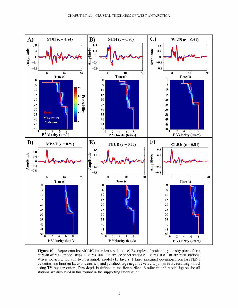
[23] Figure 10 shows example inversion results for rep-resentative rock and ice stations. Inversions for ice stationswith structures that are well fit during the forward modelingsteps do not vary substantially from their priors, as expected.We conservatively parameterize the crustal thickness uncer-tainty as the depth range over which the crustal probabilitybegins to decay from its pre-Moho maximum to wherethe post-Moho peak reaches a local maximum in mantlevelocities. The most likely crustal thickness determinations(the maximum a posteriori models) for all stations and asso-ciated posteriori-derived uncertainties are noted in Table 1.For a small number of stations that present particularly com-plex crustal structures and/or possible near-station subice

10


Figure 10. Representative MCMC inversion results. (a–e) Examples of probability density plots after aburn-in of 5000 model steps. Figures 10a–10c are ice sheet stations; Figures 10d–10f are rock stations.Where possible, we aim to fit a simple model (10 layers, 1 km/s maximal deviation from IASPEI91velocities, no limit on layer thicknesses) and penalize large negative velocity jumps in the resulting modelusing TV regularization. Zero depth is defined at the free surface. Similar fit and model figures for allstations are displayed in this format in the supporting information.

11


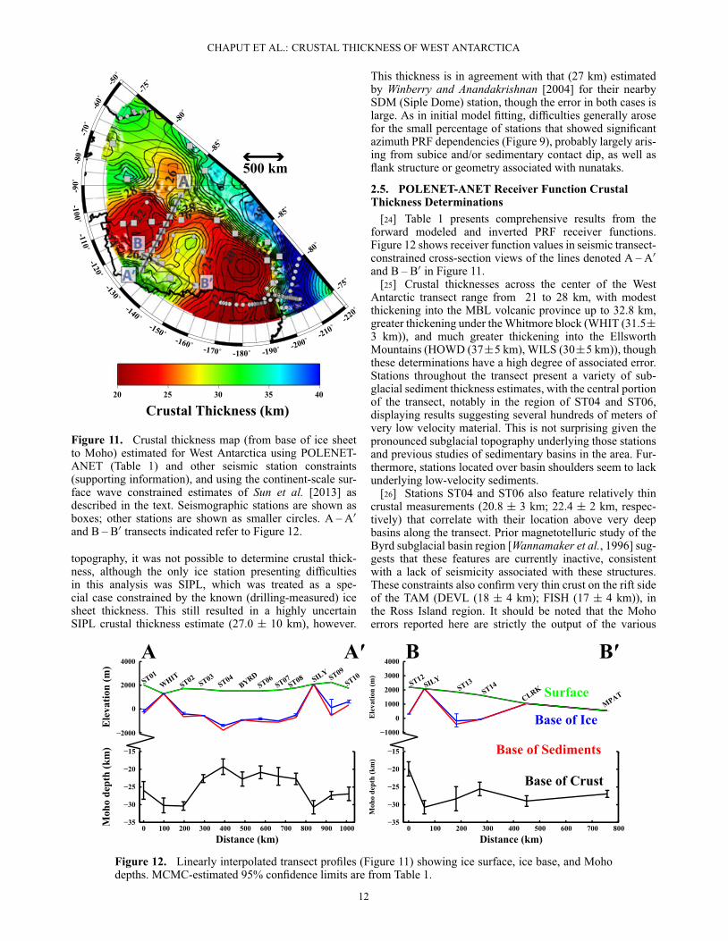
Figure 11. Crustal thickness map (from base of ice sheetto Moho) estimated for West Antarctica using POLENET-ANET (Table 1) and other seismic station constraints(supporting information), and using the continent-scale sur-face wave constrained estimates of Sun et al. [2013] asdescribed in the text. Seismographic stations are shown asboxes; other stations are shown as smaller circles. A – A0and B – B0 transects indicated refer to Figure 12.

topography, it was not possible to determine crustal thick-ness, although the only ice station presenting difficultiesin this analysis was SIPL, which was treated as a spe-cial case constrained by the known (drilling-measured) icesheet thickness. This still resulted in a highly uncertainSIPL crustal thickness estimate (27.0 ˙ 10 km), however.

This thickness is in agreement with that (27 km) estimatedby Winberry and Anandakrishnan [2004] for their nearbySDM (Siple Dome) station, though the error in both cases islarge. As in initial model fitting, difficulties generally arosefor the small percentage of stations that showed significantazimuth PRF dependencies (Figure 9), probably largely aris-ing from subice and/or sedimentary contact dip, as well asflank structure or geometry associated with nunataks.

2.5. POLENET-ANET Receiver Function CrustalThickness Determinations

[24] Table 1 presents comprehensive results from theforward modeled and inverted PRF receiver functions.Figure 12 shows receiver function values in seismic transect-constrained cross-section views of the lines denoted A – A0and B – B0 in Figure 11.

[25] Crustal thicknesses across the center of the WestAntarctic transect range from 21 to 28 km, with modestthickening into the MBL volcanic province up to 32.8 km,greater thickening under the Whitmore block (WHIT (31.5˙3 km)), and much greater thickening into the EllsworthMountains (HOWD (37˙5 km), WILS (30˙5 km)), thoughthese determinations have a high degree of associated error.Stations throughout the transect present a variety of sub-glacial sediment thickness estimates, with the central portionof the transect, notably in the region of ST04 and ST06,displaying results suggesting several hundreds of meters ofvery low velocity material. This is not surprising given thepronounced subglacial topography underlying those stationsand previous studies of sedimentary basins in the area. Fur-thermore, stations located over basin shoulders seem to lackunderlying low-velocity sediments.

[26] Stations ST04 and ST06 also feature relatively thincrustal measurements (20.8 ˙ 3 km; 22.4 ˙ 2 km, respec-tively) that correlate with their location above very deepbasins along the transect. Prior magnetotelluric study of theByrd subglacial basin region [Wannamaker et al., 1996] sug-gests that these features are currently inactive, consistentwith a lack of seismicity associated with these structures.These constraints also confirm very thin crust on the rift sideof the TAM (DEVL (18 ˙ 4 km); FISH (17 ˙ 4 km)), inthe Ross Island region. It should be noted that the Mohoerrors reported here are strictly the output of the various

Figure 12. Linearly interpolated transect profiles (Figure 11) showing ice surface, ice base, and Mohodepths. MCMC-estimated 95% confidence limits are from Table 1.

12


sources mentioned and are likely an underestimate of thetrue error. This is due to several sources of error that aredifficult to quantify, such as crustal Vp/Vs ratios and theTV regularization criterion, which further restricts the modelspace exploration and results in tighter than expected pos-terior distributions. This is, however, necessary due to theevident problems associated with fitting ice sheet multiplesvia unreasonable models.

3. West Antarctic Crustal Thickness Constrainedby Receiver Functions and Ambient Noise SurfaceWave Tomography

[27] We combined our station constraints with prior esti-mates into a West Antarctica crustal thickness map byapplying the highly smoothed but continent-scale ambi-ent noise surface wave tomography model of Sun et al.[2013] as an informed interpolant. The ambient model ishighly complementary to receiver function methods in that itproduces a very smooth crustal thickness estimate for areasthat are unsampled by the receiver function methodology buthas generally lesser localized crustal thickness resolution.This modeling incorporated results from this study and fromother seismic networks and experiments (e.g., AGAP, TAM-SEIS, ANUBIS, and the GT and GSN networks; Tables 1and S1 of the supporting information list these sources) tocreate a crustal map of Antarctica south of 75ıS with alateral discretization of 75 km. A full continent-scale mapusing this methodology is planned to be the subject of fur-ther work; we report here specifically on the results forWest Antarctica.

[28] The crustal thickness model for West Antarctica wascalculated using a least squares, second-order Tikhonov(Laplacian) regularization (with free edges) to produce aminimized second-order integrated spatial derivative acrossthe surface. Stations utilized are summarized in the sup-porting information Tables S1 and S2. We solved forcrustal thickness for 1550 seventy-five square kilometerareal patches covering Antarctica south of 75ıS. A totalof 208 seismically determined crustal thickness measure-ment using receiver functions were implemented. Standarddeviations from Table 1 and Figure S5 were applied toweight all the constraint equations in the regularized leastsquares problem (A1), with the relatively sparse receiverfunction point constraints being weighed a factor of fivegreater than the much denser but less localized surface waveconstraints. Crustal and ice thickness determinations forPOLENET-ANET station sites can be found in Table 1, andresults utilized from prior, non-POLENET, studies and sta-tions are noted in the supporting information. The surface fitis designed to obtain an optimal smooth surface with vary-ing curvature that optimally fits all data in the least squaressense without tectonic or other assumptions. The resolutionof this model is highly nonuniform due to the highly unevenspacing of seismic stations. Spectral analysis of the surfaceshows that 100–150 km wavelength information is presentin regions of the model where constraints are dense, such asthe vicinity of McMurdo Sound. Conversely, where stationcoverage is exceptionally sparse, such as the southern RossSea, only features with spatial wavelengths of greater thanapproximately 400 km are resolved. The fitting methodologyis described in detail in the Appendix.

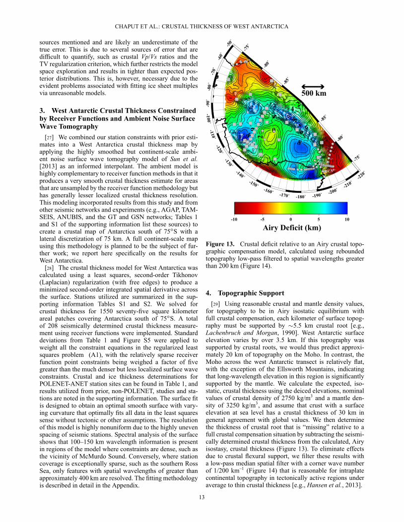
Figure 13. Crustal deficit relative to an Airy crustal topo-graphic compensation model, calculated using reboundedtopography low-pass filtered to spatial wavelengths greaterthan 200 km (Figure 14).

4. Topographic Support[29] Using reasonable crustal and mantle density values,

for topography to be in Airy isostatic equilibrium withfull crustal compensation, each kilometer of surface topog-raphy must be supported by �5.5 km crustal root [e.g.,Lachenbruch and Morgan, 1990]. West Antarctic surfaceelevation varies by over 3.5 km. If this topography wassupported by crustal roots, we would thus predict approxi-mately 20 km of topography on the Moho. In contrast, theMoho across the west Antarctic transect is relatively flat,with the exception of the Ellsworth Mountains, indicatingthat long-wavelength elevation in this region is significantlysupported by the mantle. We calculate the expected, iso-static, crustal thickness using the deiced elevations, nominalvalues of crustal density of 2750 kg/m3 and a mantle den-sity of 3250 kg/m3, and assume that crust with a surfaceelevation at sea level has a crustal thickness of 30 km ingeneral agreement with global values. We then determinethe thickness of crustal root that is “missing” relative to afull crustal compensation situation by subtracting the seismi-cally determined crustal thickness from the calculated, Airyisostasy, crustal thickness (Figure 13). To eliminate effectsdue to crustal flexural support, we filter these results witha low-pass median spatial filter with a corner wave numberof 1/200 km–1 (Figure 14) that is reasonable for intraplatecontinental topography in tectonically active regions underaverage to thin crustal thickness [e.g., Hansen et al., 2013].

13


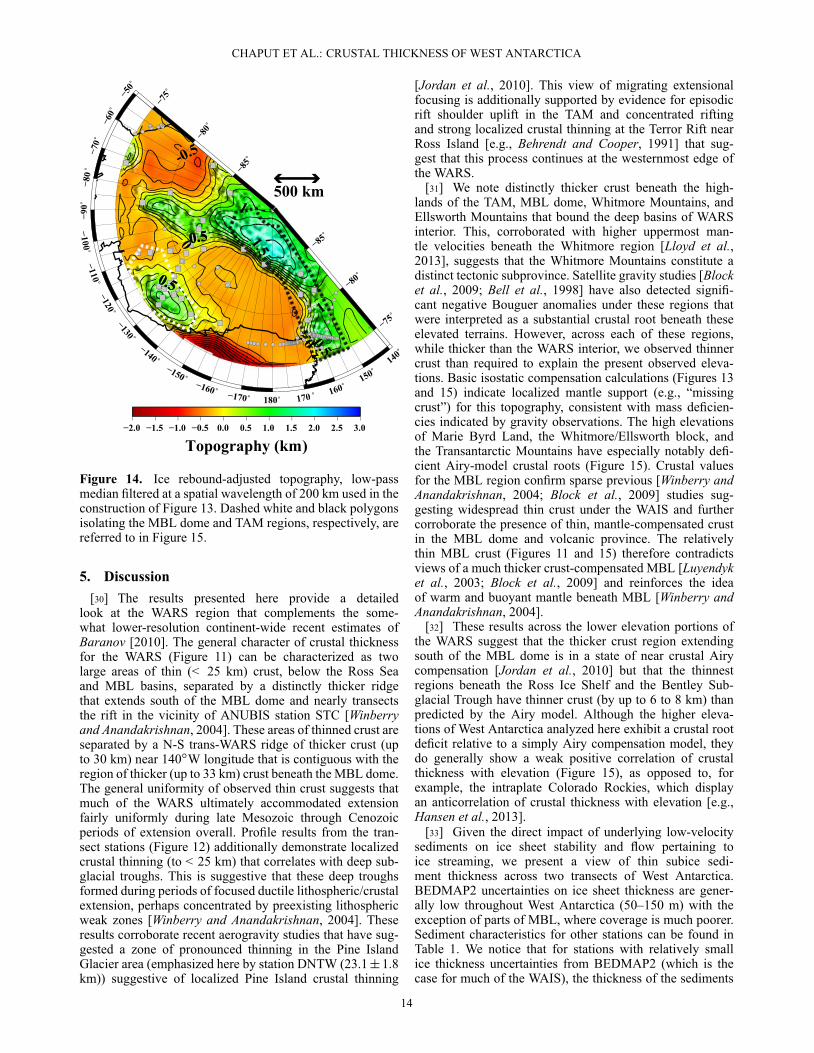
Figure 14. Ice rebound-adjusted topography, low-passmedian filtered at a spatial wavelength of 200 km used in theconstruction of Figure 13. Dashed white and black polygonsisolating the MBL dome and TAM regions, respectively, arereferred to in Figure 15.

5. Discussion[30] The results presented here provide a detailed

look at the WARS region that complements the some-what lower-resolution continent-wide recent estimates ofBaranov [2010]. The general character of crustal thicknessfor the WARS (Figure 11) can be characterized as twolarge areas of thin (< 25 km) crust, below the Ross Seaand MBL basins, separated by a distinctly thicker ridgethat extends south of the MBL dome and nearly transectsthe rift in the vicinity of ANUBIS station STC [Winberryand Anandakrishnan, 2004]. These areas of thinned crust areseparated by a N-S trans-WARS ridge of thicker crust (upto 30 km) near 140ıW longitude that is contiguous with theregion of thicker (up to 33 km) crust beneath the MBL dome.The general uniformity of observed thin crust suggests thatmuch of the WARS ultimately accommodated extensionfairly uniformly during late Mesozoic through Cenozoicperiods of extension overall. Profile results from the tran-sect stations (Figure 12) additionally demonstrate localizedcrustal thinning (to < 25 km) that correlates with deep sub-glacial troughs. This is suggestive that these deep troughsformed during periods of focused ductile lithospheric/crustalextension, perhaps concentrated by preexisting lithosphericweak zones [Winberry and Anandakrishnan, 2004]. Theseresults corroborate recent aerogravity studies that have sug-gested a zone of pronounced thinning in the Pine IslandGlacier area (emphasized here by station DNTW (23.1˙1.8km)) suggestive of localized Pine Island crustal thinning

[Jordan et al., 2010]. This view of migrating extensionalfocusing is additionally supported by evidence for episodicrift shoulder uplift in the TAM and concentrated riftingand strong localized crustal thinning at the Terror Rift nearRoss Island [e.g., Behrendt and Cooper, 1991] that sug-gest that this process continues at the westernmost edge ofthe WARS.

[31] We note distinctly thicker crust beneath the high-lands of the TAM, MBL dome, Whitmore Mountains, andEllsworth Mountains that bound the deep basins of WARSinterior. This, corroborated with higher uppermost man-tle velocities beneath the Whitmore region [Lloyd et al.,2013], suggests that the Whitmore Mountains constitute adistinct tectonic subprovince. Satellite gravity studies [Blocket al., 2009; Bell et al., 1998] have also detected signifi-cant negative Bouguer anomalies under these regions thatwere interpreted as a substantial crustal root beneath theseelevated terrains. However, across each of these regions,while thicker than the WARS interior, we observed thinnercrust than required to explain the present observed eleva-tions. Basic isostatic compensation calculations (Figures 13and 15) indicate localized mantle support (e.g., “missingcrust”) for this topography, consistent with mass deficien-cies indicated by gravity observations. The high elevationsof Marie Byrd Land, the Whitmore/Ellsworth block, andthe Transantarctic Mountains have especially notably defi-cient Airy-model crustal roots (Figure 15). Crustal valuesfor the MBL region confirm sparse previous [Winberry andAnandakrishnan, 2004; Block et al., 2009] studies sug-gesting widespread thin crust under the WAIS and furthercorroborate the presence of thin, mantle-compensated crustin the MBL dome and volcanic province. The relativelythin MBL crust (Figures 11 and 15) therefore contradictsviews of a much thicker crust-compensated MBL [Luyendyket al., 2003; Block et al., 2009] and reinforces the ideaof warm and buoyant mantle beneath MBL [Winberry andAnandakrishnan, 2004].

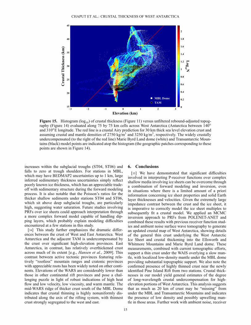
[32] These results across the lower elevation portions ofthe WARS suggest that the thicker crust region extendingsouth of the MBL dome is in a state of near crustal Airycompensation [Jordan et al., 2010] but that the thinnestregions beneath the Ross Ice Shelf and the Bentley Sub-glacial Trough have thinner crust (by up to 6 to 8 km) thanpredicted by the Airy model. Although the higher eleva-tions of West Antarctica analyzed here exhibit a crustal rootdeficit relative to a simply Airy compensation model, theydo generally show a weak positive correlation of crustalthickness with elevation (Figure 15), as opposed to, forexample, the intraplate Colorado Rockies, which displayan anticorrelation of crustal thickness with elevation [e.g.,Hansen et al., 2013].

[33] Given the direct impact of underlying low-velocitysediments on ice sheet stability and flow pertaining toice streaming, we present a view of thin subice sedi-ment thickness across two transects of West Antarctica.BEDMAP2 uncertainties on ice sheet thickness are gener-ally low throughout West Antarctica (50–150 m) with theexception of parts of MBL, where coverage is much poorer.Sediment characteristics for other stations can be found inTable 1. We notice that for stations with relatively smallice thickness uncertainties from BEDMAP2 (which is thecase for much of the WAIS), the thickness of the sediments

14


Figure 15. Histogram (log10) of crustal thickness (Figure 11) versus unfiltered rebound-adjusted topog-raphy (Figure 14) evaluated along 75 by 75 km cells across West Antarctica (Antarctica between 140ıand 310ıE longitude. The red line is a crustal Airy prediction for 30 km thick sea level elevation crust andassuming crustal and mantle densities of 2750 kg/m3 and 3250 kg/m3, respectively. The widely crustallyundercompensated (to the right of the red line) Marie Byrd Land dome (white) and Transantarctic Moun-tains (black) model points are indicated atop the histogram (the geographic patches corresponding to thesepoints are shown in Figure 14).

increases within the subglacial troughs (ST04, ST06) andfalls to zero at trough shoulders. For stations in MBL,which may have BEDMAP2 uncertainties up to 1 km, largeinferred sedimentary thickness uncertainties simply reflectpoorly known ice thickness, which has an appreciable trade-off with sedimentary structure during the forward modelingprocess. It is also notable that the Poisson’s ratios for thethicker shallow sediments under stations ST04 and ST06,which sit above deep subglacial troughs, are particularlyhigh, suggesting water saturation. Future studies involvingPRFs over ice sheets could approach interpretation througha more complex forward model capable of handling dip-ping layers, which probably explain modeling difficultiesencountered at a few stations in this study.

[34] This study further emphasizes the dramatic differ-ences between the crust of West and East Antarctica. WestAntarctica and the adjacent TAM is undercompensated bythe crust over significant high-elevation provinces. EastAntarctica, in contrast, has relatively overthickened crustacross much of its extent [e.g., Hansen et al., 2009]. Thiscontrast between active tectonic provinces featuring rela-tively “rootless” mountain ranges and cratonic provinceswith appreciable roots has been widely noted on other conti-nents. Elevations of the WARS are considerably lower thanthose in other continental rift provinces and pose a chal-lenging puzzle in light of robust indications of high heatflow and low velocity, low viscosity, and warm mantle. Themid-WARS ridge of thicker crust south of the MBL Domeindicates that crustal thinning is highly nonuniformly dis-tributed along the axis of the rifting system, with thinnestcrust strongly segregated to the west and east.

6. Conclusions[35] We have demonstrated that significant difficulties

involved in interpreting P-receiver functions over complexshallow media involving ice sheets can be overcome througha combination of forward modeling and inversion, evenin situations where there is a limited amount of a prioriinformation concerning ice sheet properties and solid Earthlayer thicknesses and velocities. Given the extremely largeimpedance contrast between the crust and the ice sheet, itis imperative to correctly model the ice sheet multiples tosubsequently fit a crustal model. We applied an MCMCinversion approach to PRFs from POLENET-ANET andcombined these results with previous receiver function stud-ies and ambient noise surface wave tomography to generatean updated crustal map of West Antarctica, showing detailsof the general thin crust underlying the West AntarcticIce Sheet and crustal thickening into the Ellsworth andWhitmore Mountains and Marie Byrd Land dome. Thesemeasurements, combined with current tomographic efforts,support a thin crust under the WAIS overlying a slow man-tle, with localized low-density mantle under the MBL domeproviding substantial topographic support. We also note theconfirmed presence of highly thinned crust near the newlyidentified Pine Island Rift from two stations. Crustal thick-nesses in our model yield general estimates of the degreeof long-wavelength crustal undercompensation for high-elevation portions of West Antarctica. This analysis suggeststhat as much as 20 km of crust may be “missing” fromunder the MBL and Transantarctic Mountains and indicatesthe presence of low density and possibly upwelling man-tle in those areas. Further work with ambient noise, receiver

15


function, and other methodologies should facilitate improv-ing the resolution of crustal thickness further across thecontinent as Antarctic seismic data continue to improve inquantity and quality.

Appendix A: Crustal Thickness Surface Estimation

A1. Methodology[36] We estimated a crustal thickness surface for West

Antarctica by fitting a second-order smoothed Tikhonov sur-face jointly to the station-specific thickness determinationsmeasured in this paper (Table 1) and in previous studies (seesupporting information). This procedure produces a mapthat reverts to the Sun et al. [2013] model where receiverfunction data were not available while allowing for smoothperturbations to incorporate regions of good receiver func-tion sampling. The associated minimization problem can beexpressed as

minkGm – dk22 + ˛2kLmk2

2 (A1)

where G is a sparse matrix that maps the model parametersm to estimates from the ambient noise surface wave and PRFestimates, d is the vector of observations, L approximatesthe discrete Laplacian operation via second differencing, andthe subscript 2 indicates the two norm. Both the elements ofd and associated rows of G were weighted by the observa-tion reciprocal standard deviation estimates in conformancewith standard (normal assumption) weighted least squaresminimization. The linear system of weighted constraints wassolved using LSQR [Paige and Saunders, 1982]. An opti-mal value for the trade-off parameter ˛ of 10–0.93 � 0.12was determined via L curve analysis of seminorm valuekLmk2 versus the weighted two-norm data misfit �2 [e.g.,Aster et al., 2012, pp. 95, Figure 22].

A2. Constraint Weighting[37] When using published PRF Moho estimates for

which uncertainties were not available, 2� standard errorswere set to 2 km. In addition to a distance-to-nearest-stationproportional term, an additional surface wave constraintdeweighting term was included to make the edges of themodel conform strongly to the smoothness constraint andthus avoid edge warping effects where constraints are excep-tionally poor or absent. The surface wave model standarddeviation for each model point i in kilometer was

� = wmin–((di–dmin)/(dmax–dmin)) � (wmin–wmax)+20( pi/pmax)2 (A2)

where pi is the distance of point i from South Pole, pmax =12, 339 km is the maximum distance from the pole in themodel space, di is the distance in km of model point i fromthe nearest seismic station (and its associated PRF Mohothickness constraint), wmax = 2 km, wmin = 18 km, dmin =4.95 km, and dmax = 90.25 km. The resultant surface waveerror surface is shown in Figure S6. Standard deviationsfrom Table 1 and Figure S5 were applied to weight all theconstraint equations in the regularized least squares problem(A1), with the relatively sparse receiver function point con-straints being weighed a factor of five greater than the muchdenser, but less localized, surface wave constraints.

[38] Acknowledgments. We thank Anya Reading for helpful reviewcomments that significantly improved this paper during revision.POLENET-ANET is supported by NSF Office of Polar Programs grants0632230, 0632239, 0652322, 0632335, 0632136, 0632209, and 0632185.Seismic instrumentation provided and supported by the IncorporatedResearch Institutions for Seismology (IRIS) through the PASSCAL Instru-ment Center at New Mexico Tech. Seismic data are available throughthe IRIS Data Management Center. The facilities of the IRIS Consor-tium are supported by the National Science Foundation under Cooperativeagreement EAR-1063471, the NSF Office of Polar Programs, and theDOE National Nuclear Security Administration. Additional informationregarding the POLENET-ANET project, sites, and data is available athttp://polenet.org.

ReferencesAgostinetti, N., and A. Malinverno (2010), Receiver function inversion by

trans-dimensional Monte Carlo sampling, Geophys. J. Int., 181, 858–872.Ammon, C. J. (1991), The isolation of receiver effects from teleseismic P

waveforms, Bull. Seismol. Soc. Am., 81, 2504–2510.Anandakrishnan, S., and J. P. Winberry (2004), Antarctic subglacial sedi-

mentary layer thickness from receiver function analysis, Global Planet.Change, 42, 167–176.

Anthony, R. (2013), Annual and seasonal seismic background noise acrossAntarctica, MS Independent Study, New Mexico Institute of Mining andTechnology.

Assumpcao, M., M. Feng, A. Tassara, and J. Julia (2013), Models of crustalthickness for South America from seismic refraction, receiver functionsand surface wave tomography, Tectonophysics, 609, 82–96.

Aster, R. C., B. Borchers, and C. Thurber (2012), Parameter Estimation andInverse Problems, 2nd ed., 360 pp., Elsevier Academic Press, Waltham,Mass.

Bannister, S., R. K. Sneider, and M. L. Passier (2000), Shear-wave veloc-ities under the Transantarctic Mountains and Terror Rift from surfacewave inversion, Geophys. Res. Lett., 27(2), 281–284.

Baranov, A. A. (2010), A new crustal model for Central and Southern Asia,Izv. Phys. Solid Earth, 46, 34–46.

Behrendt, J., and A. Cooper (1991), Evidence of rapid Cenozoic upliftof the shoulder escarpment of the Cenozoic West Antarctic rift sys-tem and a speculation on possible climate forcing, Geology, 19,315–319.

Behrendt, J. (1999), Crustal and lithospheric structure of the West AntarcticRift System from geophysical investigations — A review, Global Planet.Change, 23, 25–44.

Bell, R. E., D. Blankenship, C. Finn, D. Morse, T. Scambos, J. Brozena,and S. Hodge (1998), Influence of subglacial geology on the onset ofa West Antarctic ice stream from aerogeophysical observations, Nature,394, 58–62.

Bentley, C. R. (1971), Seismic anisotropy in the West Antarctic ice sheet,AGU Antarct. Res. Ser., 16, 131–177.

Blankenship, D. D., R. E. Bell, S. M. Hodge, J. M. Brozena, J. C. Behrendt,and C. A. Finn (1992), Active volcanism beneath the West Antarctic icesheet and implications for ice-sheet stability, Nature, 361, 526–529.

Block, A., R. Bell, and M. Studinger (2009), Antarctic crustal thicknessfrom satellite gravity: Implications for the Transantarctic and Gamburt-sev Subglacial Mountains, Earth Planet. Sci. Lett., 288, 194–203.

Bodin, T., M. Sambridge, H. Tkalcic, P. Arroucau, K. Gallagher, andN. Rawlinson (2012), Transdimensional inversion of receiver func-tions and surface wave dispersion, J. Geophys. Res., 117, B02301,doi:10.1029/2011JB008560.

Bostock, M. G. (2004), Green’s functions, source signatures, and the nor-malization of teleseismic wave fields, J. Geophys. Res., 109, B03303,doi:10.1029/2003JB002783.

Cho, T. (2011), Removing reverberation in ice sheets from receiver func-tions, Seismol. Res. Lett., 82, 207–210.

Clow, G., K. Cuffey, and E. Waddington (2012), High heat-flow beneaththe central portion of the West Antarctic ice sheet, Eos Trans. AGU, FallMeet. Suppl.

Cooper, A., F. Davey, and J. Behrendt (1987), Seismic stratigraphy andstructure of the Victoria Land Basin, western Ross Sea, Antarctica, in TheAntarctic Continental Margin: Geology and Geophysics of the WesternRoss Sea, CPCEMR Earth Sci. Ser., vol. 5B, pp. 27–76, Circum-Pac.Counc. for Energy and Miner. Resour., Houston Tex.

Cooper, A. K., and P. Barker (1995), Geology and Seismic Stratigraphyof the Antarctic Margin, Antarct. Res. Ser., vol. 68, 303 pp., AGU,Washington, D. C.

Danesi, S., and A. Morelli (2001), Structure of the upper mantle under theAntarctic Plate from surface wave tomography, Geophys. Res. Lett., 28,4395–4398.

16


Fretwell, P., et al. (2013), BEDMAP2: Improved ice bed, surface andthickness datasets for Antarctica, Cryosphere, 7, 375–393.

Hansen, S. E., J. Julià, A. A. Nyblade, M. L. Pyle, D. A. Wiens, and S.Anandakrishnan (2009), Using S wave receiver functions to estimatecrustal structure beneath ice sheets: An application to the TransantarcticMountains and East Antarctic craton, Geochem. Geophys. Geosyst., 10,Q08014, doi:10.1029/2009GC002576.

Hansen, S. E., A. A. Nyblade, D. Heeszel, D. A. Wiens, P. Shore, andM. Kanao (2010), Crustal structure of the Gamburtsev Mountains, EastAntarctica, from S-wave receiver functions and Rayleigh wave phasevelocities, Earth Planet. Sci. Lett., 300, 395–401.

Hansen, S. M., K. G. Dueker, J. C. Stachnik, R. C. Aster, andK. E. Karlstrom (2013), A rootless Rockies—Support and lithosphericstructure of the Colorado Rocky Mountains inferred from CRESTand TA seismic data, Geochem. Geophys. Geosyst., 14, 2670–2695,doi:10.1002/ggge.20143.

Helffrich, G. (2006), Extended-time multitaper frequency domain cross-correlation receiver-function estimation, Bull. Seismol. Soc. Am., 96,344–347.

Jordan, T. A., F. Ferraccioli, D. Vaughan, J. Holt, H. Corr, D. Blankenship,and T. Diehl (2010), Aerogravity evidence for major crustal thinningunder the Pine Island Glacier region (West Antarctica), Bull. Geol. Soc.Am., 122, 714–726.

Karner, G. D., M. Studinger, and R. Bell (2005), Gravity anomalies of sed-imentary basins and their mechanical implications: Application to theRoss Sea basins, West Antarctica, Earth Planet. Sci. Lett., 235, 577–596.

Kennett, B. L. N. (Compiler and Editor) (1991), IASPEI 1991 SeismologicalTables, 167 pp., Bibliotech, Canberra, Australia.

Kohnen, H. (1974), The temperature dependence of seismic waves in ice,J. Glaciol., 13, 144–147.

Lachenbruch, A. H., and P. Morgan (1990), Continental extension, magma-tism and elevation; Formal relations and rules of thumb, Tectonophysics,174, 39–62.

Lawrence, J. F., D. Wiens, A. Nyblade, S. Anandrakrishnan, P. Shore, andD. Voigt (2006), Crust and upper mantle structure of the Transantarc-tic Mountains and surrounding regions from receiver functions, surfacewaves, and gravity: Implications for uplift models, Geochem. Geophys.Geosyst., 7, Q10011, doi:10.1029/2006GC001282.

LeMasurier, W. E., and D. C. Rex (1989), Evolution of linear volcanicranges in Marie Byrd Land, West Antarctica, J. Geophys. Res., 94,7223–7236.

LeMasurier, W. (2008), Neogene extension and basin deepening in the WestAntarctic rift inferred from comparisons with the East African rift andother analogs, Geology, 36(3), 247–250.

Lindsay, J. P. (1989), The Fresnel zone and its interpretive significance,Leading Edge, 8, 33–39.

Liu, Q. Y., Y. Li, J. H. Chen, R. D. van der Hilst, B. A. Guo, J. Wang, S. H.Qi, and S. C. Li (2010), Joint inversion of receiver function and ambientnoise based on Bayesian theory, Chinese J. Geophys., 53, 2603–2612.

Liu, K. H., and S. S. Gao (2006), Mantle transition zone discontinuitiesbeneath the Baikal rift and adjacent areas, J. Geophys. Res., 111, B11301,doi:10.1029/2005JB004099.

Lloyd, A., D. Wiens, A. Nyblade, S. Anandakrishnan, R. Aster, A. Huerta,T. Wilson, P. Shore, and D. Zhao (2013), Upper mantle structure beneaththe Whitmore Mountains, Byrd Basin, and Marie Byrd Land frombody-wave tomography, Proc. International Symposium: ReconcilingObservations and Models of Elastic and Viscoelastic Deformation due toIce Mass Change.

Lough, A. C., D. A. Wiens, C. G. Barcheck, S. Anandakrishnan, R. C.Aster, D. D. Blankenship, A. D. Huerta, A. Nyblade, D. A. Young, andT. J. Wilson (2013), Seismic detection of an active subglacial magmaticcomplex in Marie Byrd Land, Antarctica, Nat. Geosci., 6, 1031–1035,doi:10.1038/ngeo1992.

Luyendyk, B. P., C. H. Smith, and G. Druivenga (2003), Gravity measure-ments on King Edward VII Peninsula, Marie Byrd Land, West Antarctica,during GANOVEX VII, Geolog. Jahrb., B, 95, 101–126.

McClusky, S., et al. (2010), Kinematics of the southern Red Sea–AfarTriple Junction and implications for plate dynamics, Geophys. Res. Lett.,37, L05301, doi:10.1029/2009GL041127.

Morelli, A., and S. Danesi (2004), Seismological imaging of the Antarcticcontinental lithosphere: A review, Global Planet. Change, 42, 155–165.

Mosegaard, K., and A. Tarantola (1995), Monte Carlo methods in geophys-ical inverse problems, Rev. Geophys., 40, 3.1–3.29.

Paige, C. C., and M. A. Saunders (1982), LSQR: An algorithm for sparselinear equations and sparse least squares, TOMS, 8(1), 43–71.

Park, J., and V. Levin (2000), Receiver functions from multiple-taperspectral correlation estimates, Bull. Seismol. Soc. Am., 90, 1507–1520.

Parker, T., B. Beaudoin, J. Gridley, and K. Anderson (2011), Next gen-eration polar seismic instrumentation challenges, Eos Trans. AGU, FallMeet. Suppl., Abstract C54B-04.

Pollard, D., R. DeConto, and A. Nyblade (2005), Sensitivity of CenozoicAntarctic ice sheet variations to geothermal heat flux, Global Planet.Change, 49(1-2), 63–74.

Pollard, D., and R. DeConto (2009), Modelling West Antarctic ice sheetgrowth and collapse through the past five million years, Nature, 458,329–332.

Reading, A. (2002), Antarctic seismicity and neotectonics, in Antarctic atthe Close of a Millennium, vol. 35, pp. 479–484, R. Soc. of N. Z. Bull.,New Zealand.

Reading, A. (2006), The seismic structure of Precambrian and early Palaeo-zoic terranes in the Lambert Glacier region, East Antarctica, EarthPlanet. Sci. Lett., 244, 44–57.

Reading, A. (2007), The seismicity of the Antarctic Plate, in Continen-tal intraplate earthquakes: Science, hazard and policy issues, editedby S. Stein and S. Mazzotti, Geol. Soc. of Am. Spec. Pap., 425,285–298.

Reusch, A. M., A. A. Nyblade, M. H. Benoit, D. A. Wiens, S.Anandakrishnan, D. Voigt, and P. J. Short (2008), Mantle transitionzone thickness beneath Ross Island, the Transantarctic Mountains,and East Antarctica, Geophys. Res. Lett., 35, L12301, doi:10.1029/2008GL033873.

Ritzwoller, M. H., N. Shapiro, A. Levshin, and G. Leahy (2001), The struc-ture of the crust and upper mantle beneath Antarctica and the surroundingoceans, J. Geophys. Res., 106(B12), 30,645–30,670.

Seiberlich, C., J. Ritter, and B. Wawerzinek (2013), Topography of thelithosphere-asthenosphere boundary below the Upper Rhine Graben Riftand the volcanic Eifel region, Central Europe, Tectonophysics, 603,222–236.

Shen, W., M. Ritzwoller, V. Schulte-Pelkum, and F.-C. Lin (2012), Jointinversion of surface wave dispersion and receiver functions: A BayesianMonte-Carlo approach, Geophys. J. Int., 192, 807–836.

Sieminski, A., E. Debayle, and J. Leveque (2003), Seismic evidencefor deep low-velocity anomalies in the transition zone beneath WestAntarctica, Earth Planet. Sci. Lett., 216, 645–661.

Studinger, M., R. E. Bell, W. R. Buck, G. D. Karner, and D. D.Blankenship (2004), Sub-ice geology inland of the Transantarctic Moun-tains in light of new aerogeophysical data, Earth Planet. Sci. Lett., 220,391–408.

Sun, X., D. Wiens, A. Nyblade, S. Anandakrishnan, R. Aster, J. Chaput, A.Huerta, and T. Wilson (2013), Three dimensional crust and upper man-tle velocity structure of Antarctica from seismic noise correlation, EosTrans. AGU, Fall Meet. Suppl.

ten Brink, U. S., and M. H. Taylor (2002), Crustal structure of central LakeBaikal: Insights into intracontinental rifting, J. Geophys. Res., 107(B7),2132, doi:10.1029/2001JB000300.

Tiberi, C., M. Diament, J. Déverchère, C. Petit-Mariani, V. Mikhailov, S.Tikhotsky, and U. Achauer (2003), Deep structure of the Baikal rift zonerevealed by joint inversion of gravity and seismology, J. Geophys. Res.,108(B3), 2133, doi:10.1029/2002JB001880.

Wannamaker, P. E., J. A. Stodt, and L. Olsen (1996), Dormant state ofrifting below the Byrd Subglacial Basin, West Antarctica, implied bymagnetotelluric (MT) profiling, Geophys. Res. Lett., 23, 2983–2986.

Watson, T., A. Nyblade, D. A. Wiens, S. Anandakrishnan, M. Benoit, P. J.Shore, D. Voigt, and J. VanDecar (2006), P and S velocity structure ofthe upper mantle beneath the Transantarctic Mountains, East Antarcticcraton, and Ross Sea from travel time tomography, Geochem. Geophys.Geosyst., 7, Q07005, doi:10.1029/2005GC001238.

Wiens, D., D. Heeszel, X. Sun, J. Chaput, R. Aster, A. Nyblade, T.Wilson, A. Huerta, and S. Anandakrishnan (2012), Lithospheric structureof Antarctica from Rayleigh wave tomography, Eos Trans. AGU, FallMeet. Suppl.

Wiens, D., D. Heeszel, X. Sun, A. Lloyd, A. Nyblade, S. Anandakrishnan,R. Aster, J. Chaput, A. Huerta, S. Hansen, and T. Wilson (2013),Lithospheric structure of Antarctica and implications for geological andcryospheric evolution, Proc. IASPEI Meeting, Gothenburg, Sweden.

Wilch, T. I., D. Lux, G. Denton, and W. C. McIntosh (1993), MinimalPliocene-Pleistocene uplift of the dry valleys sector of the TransantarcticMountains: A key parameter in ice sheet reconstructions, Geology, 21,841–844.

Wilch, T. I., and W. C. McIntosh (2000), Eocene and Oligocene volcanismat Mount Petras, Marie Byrd Land: Implications for middle Ceno-zoic ice sheet reconstructions in West Antarctica, Antarct. Sci., 12(4),477–491.

Wilson, T., et al. (2011), The POLENET Project: Data acquisition sta-tus, initial results, future modeling, 11th International Symposium onAntarctic Earth Sciences, Eos Trans. AGU, Fall Meet. Suppl., Edinburgh,Scotland, 10–16 July.

Wilson, D. S., and B. P. Luyendyk (2009), West Antarctic paleotopogra-phy estimated at the Eocene-Oligocene climate transition, Geophys. Res.Lett., 36, L16302, doi:10.1029/2009GL039297.

17


Wilson, D., and R. Aster (2005), Seismic imaging of the crust and uppermantle using regularized joint receiver functions, frequency–wave num-ber filtering, and multimode Kirchhoff migration, J. Geophys. Res., 110,B05305, doi:10.1029/2004JB003430.

Winberry, J. P., and S. Anandakrishnan (2003), Seismicity and neo-tectonics of West Antarctica, Geophys. Res. Lett., 30, 1931–1935.,doi:10.1029/2003GL018001.

Winberry, J. P., and S. Anandakrishnan (2004), Crustal structure of theWest Antarctic rift system and Marie Byrd Land hotspot, Geology, 32,977–980.

Zhou, L., and H. Kanamori (2000), Moho depth variation in southernCalifornia from teleseismic receiver functions, J. Geophys. Res., 105,2969–2980.

18

Documents

The crustal thickness of West Antarctica